Understanding GMM, HMM, DNN and LSTM

Pradeep R12th April 2019

Outline

● Introduction● K-Means Clustering● Gaussian Model● Need for GMM● Need for HMM

– Implementation

● Conclusion

Introduction

● Applications:– Hand Character Recognition

– Spoken Digit Recognition

– Weather Prediction

– Human activity detection

● Central limit theorem states that “when we add large number of independent random variables, irrespective of the original distribution of these variables, their normalized sum tends towards a Gaussian distribution.”

● For example, the distribution of total distance covered in an random walk tends towards a Gaussian probability distribution.

Why Gaussian?

● Gaussian remain as a Gaussian even after transformation– Product of two Gaussian is a Gaussian

– Sum of two independent Gaussian random variables is a Gaussian

– Convolution of Gaussian with another Gaussian is a Gaussian

– Fourier transform of Gaussian is a Gaussian

● Simpler– The entire distribution can be specified using just two

parameters- mean and variance

Variants of Gaussian

MultiVariate Gaussian

Gaussian Mixture Model

UniVariate Gaussian

K-Means Clustering - Idea1

2

3

N

. . . . . . . . . . ..

2 1 1 3 2 4 3 3 4 1 2 4 2

1 2 3 13

3 2 1 2 4 3 2 1 3 4

1 2 3 13

Centroid_init

Centroid_new

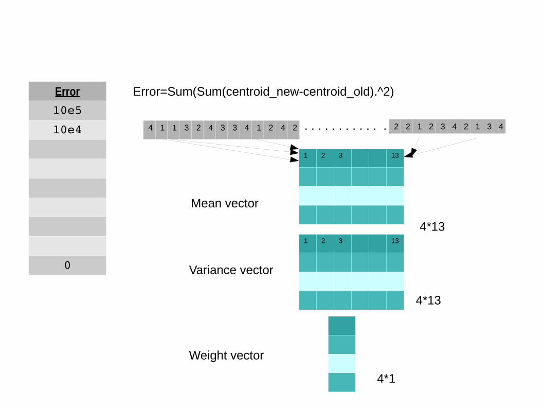
Error

10e5

10e4

0

Error=Sum(Sum(centroid_new-centroid_old).^2)

4 1 1 3 2 4 3 3 4 1 2 4 2 2 2 1 2 3 4 2 1 3 4

1 2 3 13

1 2 3 13

Mean vector

Variance vector

Weight vector

4*13

4*13

4*1

. . . . . . . . . . . .

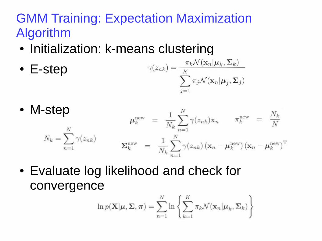
GMM Training: Expectation Maximization Algorithm● Initialization: k-means clustering● E-step

● M-step

● Evaluate log likelihood and check for convergence

Implementation-Initial Setup

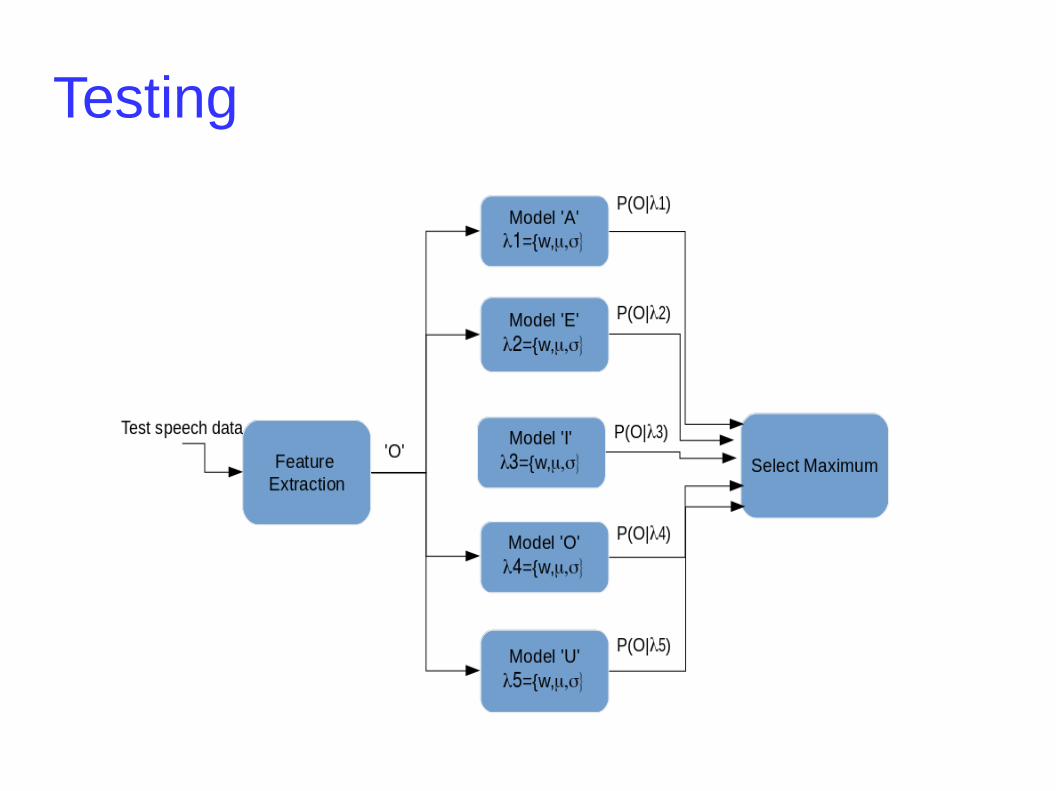
Testing

Drawbacks of GMM

● Cannot alone perform time series prediction● It is necessary to evaluate probabilities along with

time in many practical applications.– Ex 01: GMM build for word ‘Kamal’ and ‘Kalam’

gathers no sequential information

– GMM - ‘b’ and GMM - ‘d’ may have false substitutions

● Hence it is necessary to capture temporal/sequential information along with spatial information.

Hidden Markov Models

● Terminologies:– State

– State Transition

– Emission Probability

Illustration of phone level modeling

● Train utterance.wav Trancription: One

Phonetic equivalence: One -- w ah n

Expected Outcome

w nah/n/

/ah/

/w/

Start

O1... O17O18..................... O48O49...O60

1 0 0 0 1 0 0 .. 0 .. .. 0 0

0

0

0

S0

S1

S2

S3

S0 S1 S2 S3

S0

S1

S2

S3

Aij = Bjk =

O1......O20O21......O40O41......O60O0

Compute Forward probabilities: Forward Recursion The goal here is to find the probablity that the HMM is

in state 'i' at time 't' ----- αi(t)

0 ; t=0 & j!=initial state

αj(t)= 1 ; t=0 & j=initial state sum(αi(t-1)*aij)*bj(Ot)

0 ; Si(t)!=0 & t=final state

βi(t)= 1 ; Si(t)=0 & t=final state sum(αj(t+1)*aij)*bj(Ot+1)

● O4={O1,O25,O46,O0}

0 ; t=0 & j!=initial state

αj(t)= 1 ; t=0 & j=initial state sum(αi(t-1)*aij)*bj(Ot)

t: 1 2 3 4

0

0

1

0

S3

S2

S1

S0

Assumption:● Let the HMM be at state

S1 at t=0● α1(0)=1● Find P(O4|θ)

1 0 0 0

0.2 0.3 0.1 0.4

0.2 0.5 0.2 0.1

0.7 0.1 0.1 0.1

1 0 0 0 0

0 0.3 0.1 0.4 0.2

0 0.1 0.7 0.1 0.1

0 0.5 0.1 0.2 0.2

[A] [B]

S0 S1 S2 S3 O0 O1 O25 O46 O0

αj(0) αj(1) αj(2) αj(3) αj(T=4)

0

0.0057

0.0217

0.0052

0

0.2

0.01

0.09

0

0.001

0.0005

0.0052

0.0018

0

0

0

0

0

1

0

S3

S2

S1

S0

t=1α0(1)={α0(0)a00+α1(0)a10+α2(0)a20+α3(0)a30}*b0(O1)=0α1(1)={α0(0)a01+α1(0)a11+α2(0)a21+α3(0)a31}*b1(O25)=0.09α2(1)={α0(0)a02+α1(0)a12+α2(0)a22+α3(0)a32}*b2(O46)=0.02α3(1)={α0(0)a03+α1(0)a13+α2(0)a23+α3(0)a33}*b3(O0)=0.05

In matrix form [0 1 0 0]*[A]*[B(:,2)] = [0.2 0.01 0.09 0]

Use Viterbi decoding to find the hidden state sequence that generated the particular observationP(O4|θ)=α0(T)=0.0018P(O4)=βi(0)

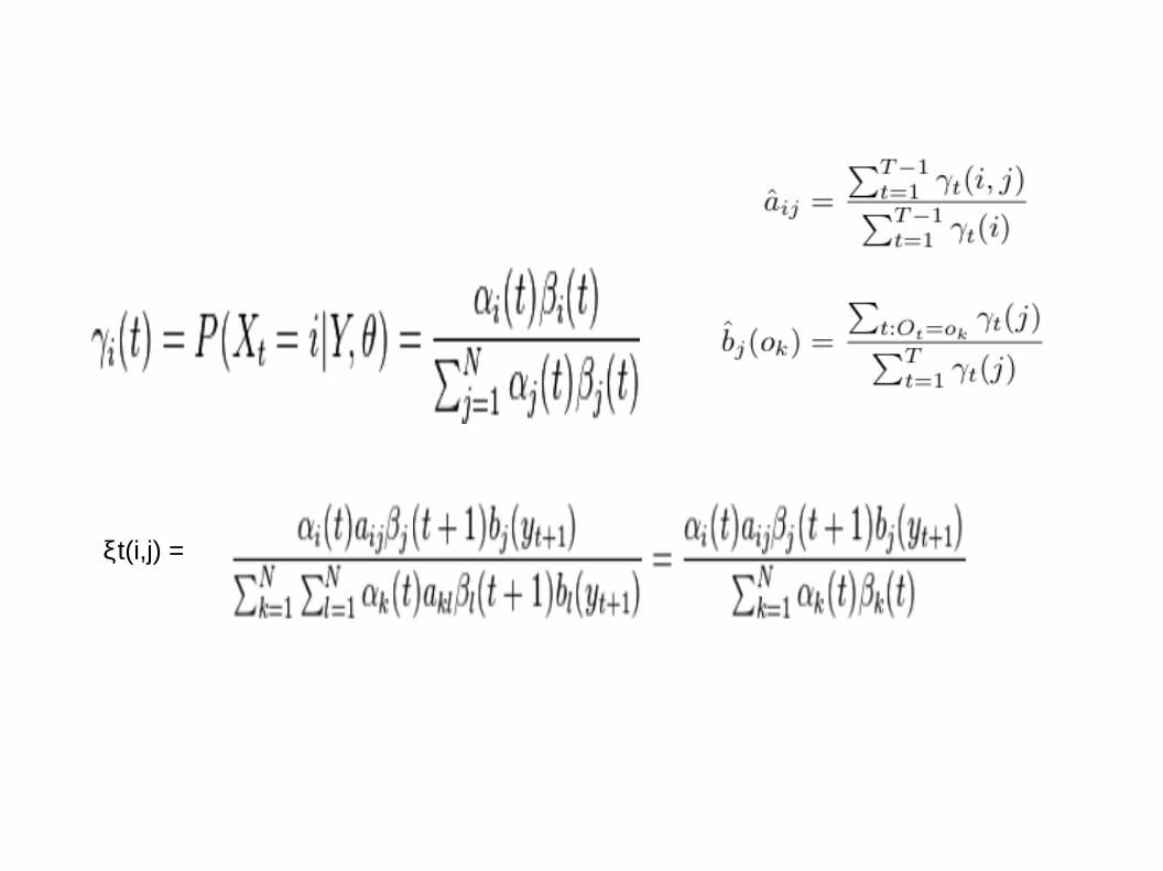
ξt(i,j) =

Illustration

● Data:– Ten words of the utterance one

– One : w ah n

● Build 3 state HMM per phone

s1 s2 s3 s4 s5 s6 s7 s8 s9

MFCC

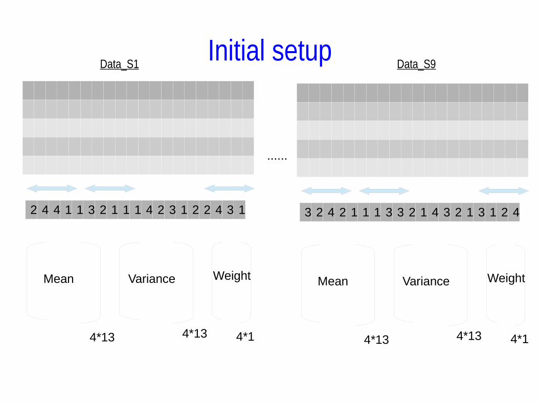
Initial setup

2 4 4 1 1 3 2 1 1 1 4 2 3 1 2 2 4 3 1

Data_S1

4*13 4*13 4*1

Mean Variance Weight

3 2 4 2 1 1 1 3 3 2 1 4 3 2 1 3 1 2 4

4*13 4*13 4*1

Mean Variance Weight

Data_S9

......

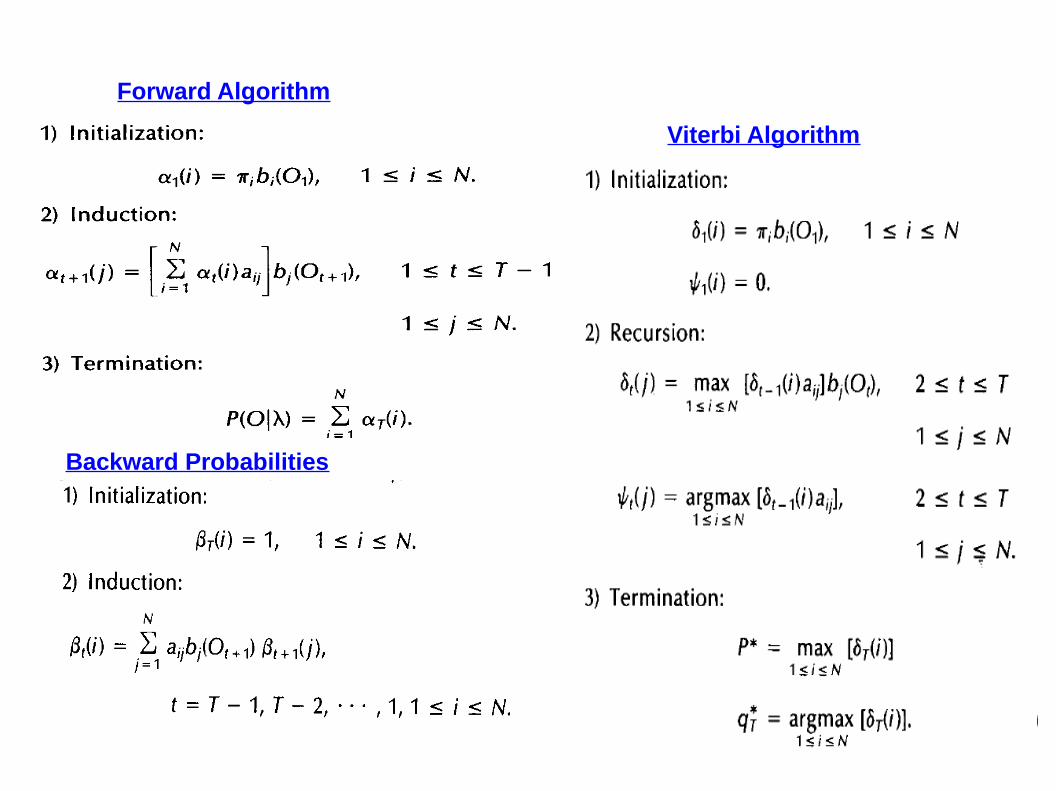
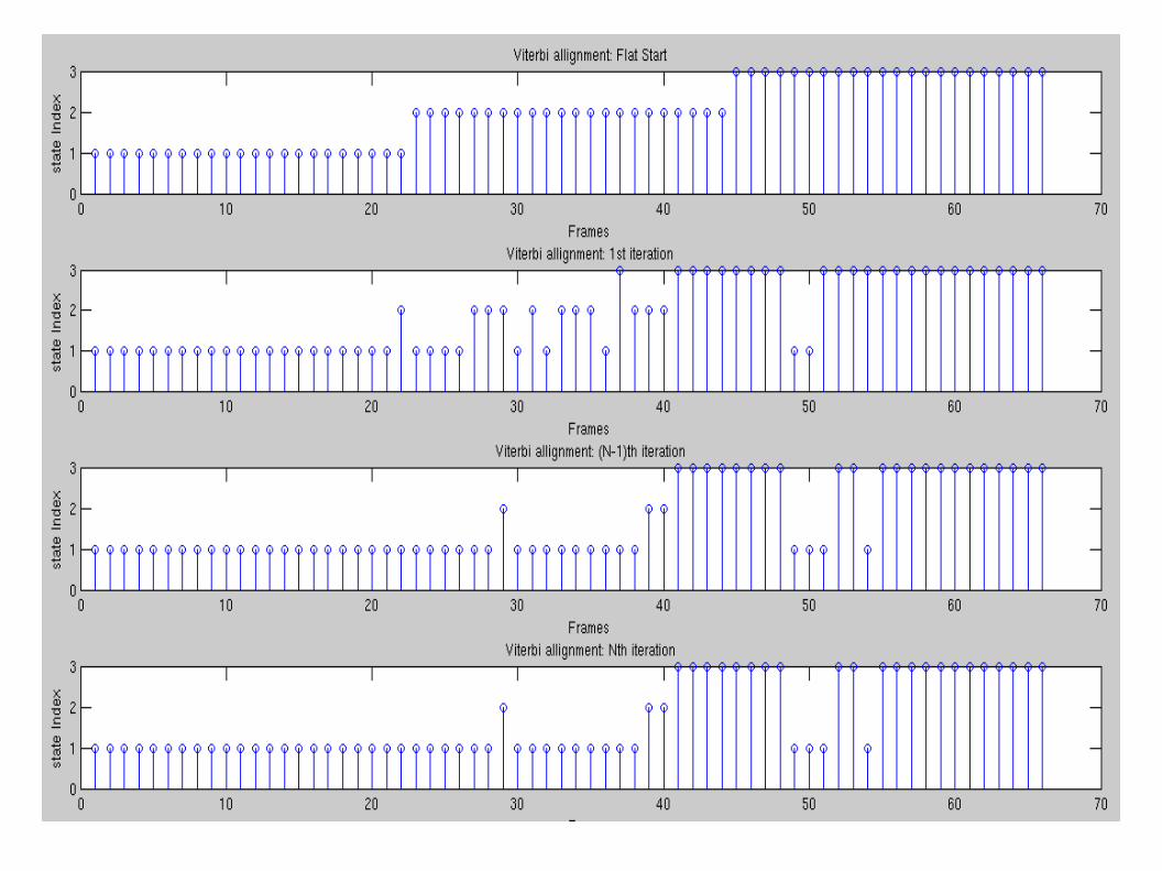
Viterbi Algorithm

Forward Algorithm

Backward Probabilities

S1

S2

s3

s1 s2 s3

ξ

Г

A(S1,:) = zeeta(S1,:)./ [S1 S1 S1]

F1 F2 ....... F30

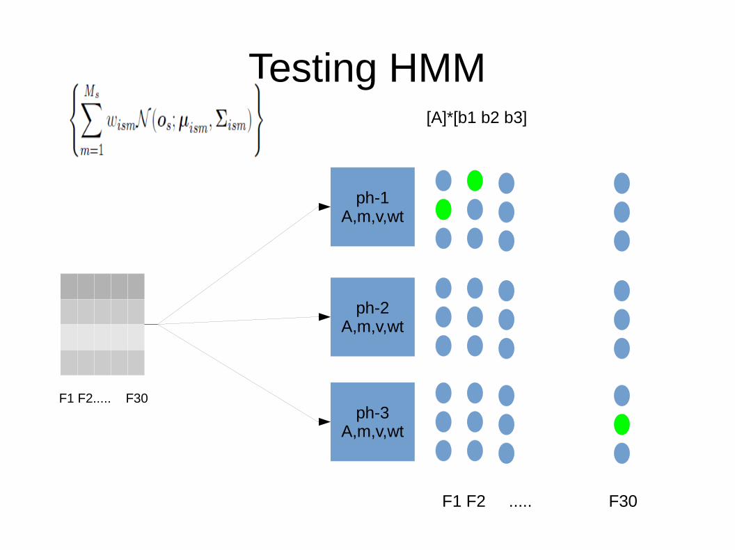
Testing HMM

ph-1A,m,v,wt

ph-2A,m,v,wt

ph-3A,m,v,wt

[A]*[b1 b2 b3]

F1 F2 ..... F30

F1 F2..... F30

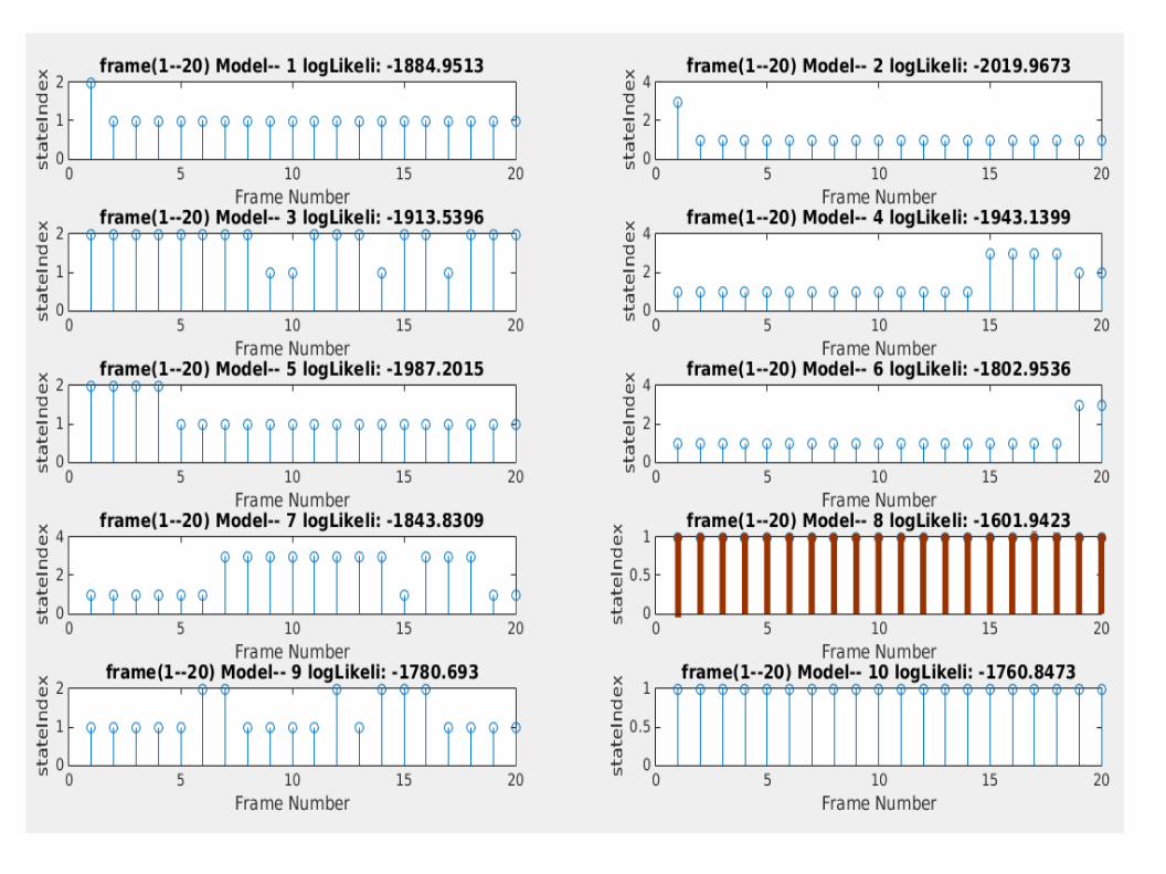
Calculating log-Likelihood from updated parameters

● Trained parameters for each state of a class:– Mean vector

– Diagonal covariance matrix

– Weighting factors for each Gaussian in a GMM

– Updated Transition matrix (N*N)

– priors

● Finding Likelihood:– α(:, t) = B(:, t) .* (A' * α(:, t – 1));

– logLikelihood = log(sum(α(:, t)));

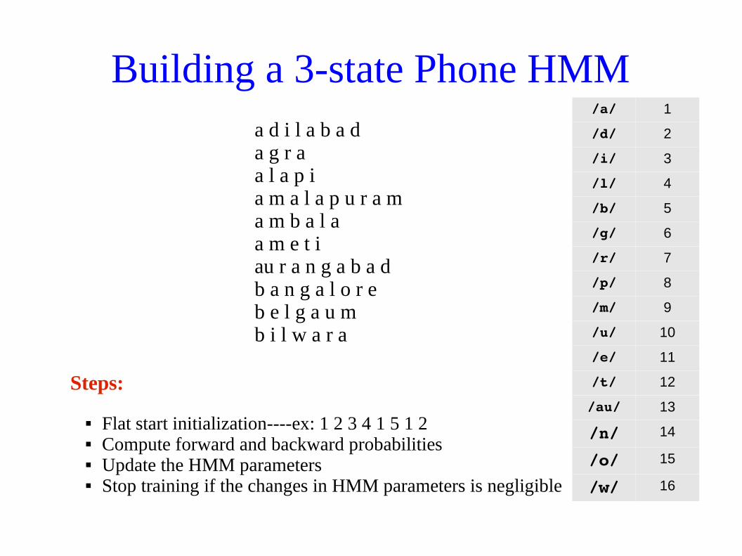
Building a 3-state Phone HMM/a/ 1

/d/ 2

/i/ 3

/l/ 4

/b/ 5

/g/ 6

/r/ 7

/p/ 8

/m/ 9

/u/ 10

/e/ 11

/t/ 12

/au/ 13

/n/ 14

/o/ 15

/w/ 16

a d i l a b a da g r aa l a p ia m a l a p u r a ma m b a l aa m e t iau r a n g a b a db a n g a l o r eb e l g a u mb i l w a r a

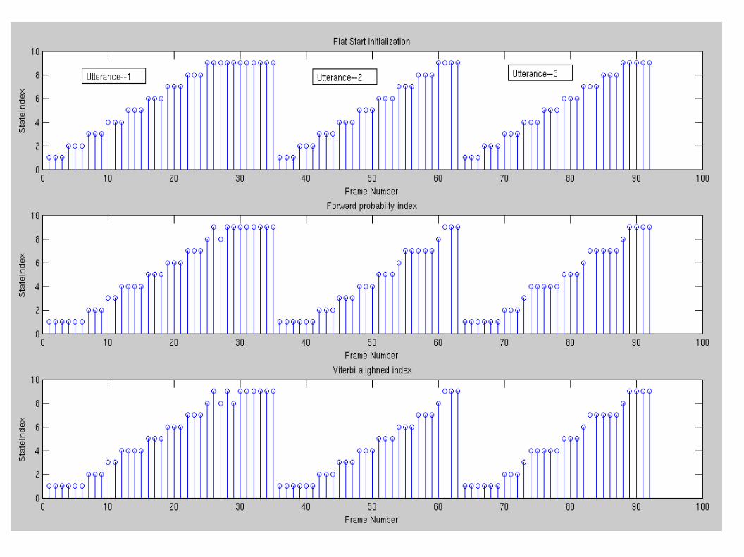
Steps:

Flat start initialization----ex: 1 2 3 4 1 5 1 2 Compute forward and backward probabilities Update the HMM parameters Stop training if the changes in HMM parameters is negligible

Analysing the break points

S2 S3 S4

S2 S3 S4

S2 S3 S4

S1 S5

/a/

/b/

/sil/

Key idea:Find the hidden state index where the final emitting state starts emitting the MFCC feature vectorsAnalyze the corresponding viterbi path and its score w.r.t all trained models

S4

S3

S2

S1

✘

✘

✘

✘

✘

✘

✘

✘

✔

✘

✘

✔

✘

✘

✔

✘

✘

-inf

-77

-78

-inf

-inf

-inf

0

-inf

-inf

-inf

● Identify the path with less significant Viterbi score

● Prune the Viterbi path by considering only the effect of maximum state sequence.

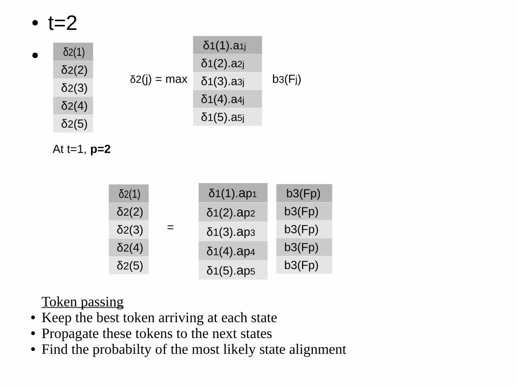
● t=2● δ2(1)

δ2(2)

δ2(3)

δ2(4)

δ2(5)

δ1(1).a1j

δ1(2).a2j

δ1(3).a3j

δ1(4).a4j

δ1(5).a5j

δ2(j) = max b3(Fj)

δ1(1).ap1

δ1(2).ap2

δ1(3).ap3

δ1(4).ap4

δ1(5).ap5

At t=1, p=2

δ2(1)

δ2(2)

δ2(3)

δ2(4)

δ2(5)

b3(Fp)

b3(Fp)

b3(Fp)

b3(Fp)

b3(Fp)

=

Token passing● Keep the best token arriving at each state● Propagate these tokens to the next states● Find the probabilty of the most likely state alignment

Practical Implementation of ANNs for Speech Applications

Introduction

X Y Z

0 0 0

0 1 1

1 0 1

1 1 1

W'I>Th

w1

w2

Z

0*w1+0*w2 < Th0*w1+1*w2 >= Th1*w1+0*w2 >=Th1*w1+1*w2 >=Th

Th > 0W2 >=ThW1 >=Thw1+w2 >=Th

Soln : Th = 0.1;W = [0.15 0.2]X Y Z

0 0 0

0 1 1

1 0 1

1 1 0

0*w1+0*w2 < Th0*w1+1*w2 >= Th1*w1+0*w2 >=Th1*w1+1*w2 >=Th

Th > 0W2 >=ThW1 >=Thw1+w2 < Th

OR-Gate

XOR-Gate

X

Y

y=mx+c//m=w2/w1;//c=Th;

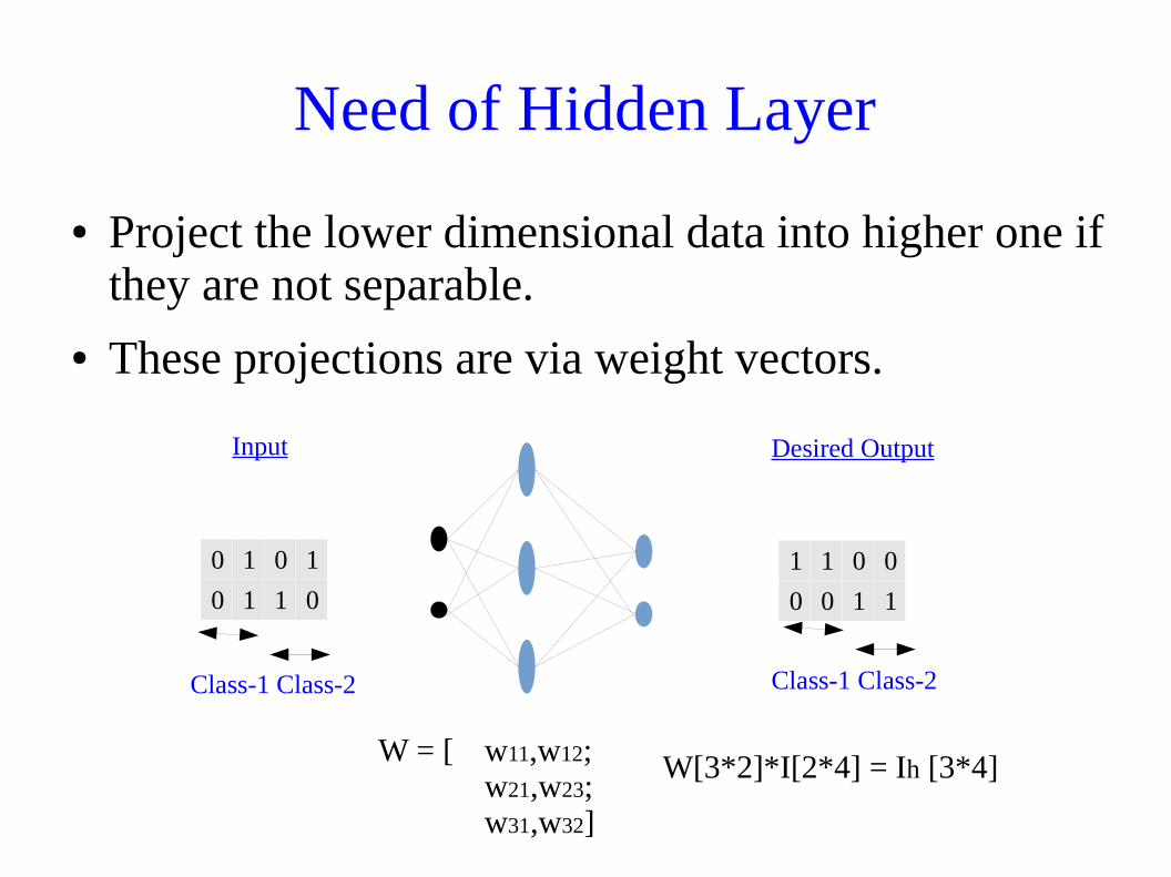
Need of Hidden Layer

● Project the lower dimensional data into higher one if they are not separable.

● These projections are via weight vectors.

W = [ w11,w12;w21,w23;w31,w32]

0 1 0 1

0 1 1 0

1 1 0 0

0 0 1 1

Class-1 Class-2 Class-1 Class-2

Input Desired Output

W[3*2]*I[2*4] = Ih [3*4]

Trained weights

W = [ w11,w12;w21,w23;w31,w32]

0 1 0 1

0 1 1 0

1 1 0 0

0 0 1 1

Class-1 Class-2 Class-1 Class-2

Input Desired Output

W[3*2]*I[2*4] = Ih [3*4]

Wih = [-6.793,12.214; 8.051,8.053; 12.208,-6.791];

Who = [-11.58, 8.4, 8.4; 11.57, -8.39, -8.39];

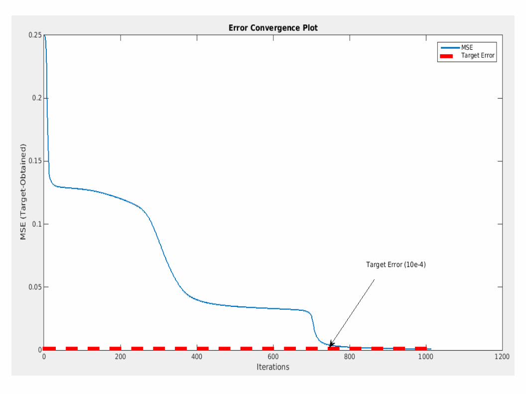
0.93 0.99 0.04 0.04

0.06 0.01 0.96 0.96Actual output (after training)

MSE = sum(Desired-Actual).^2 =9.9*10e-4

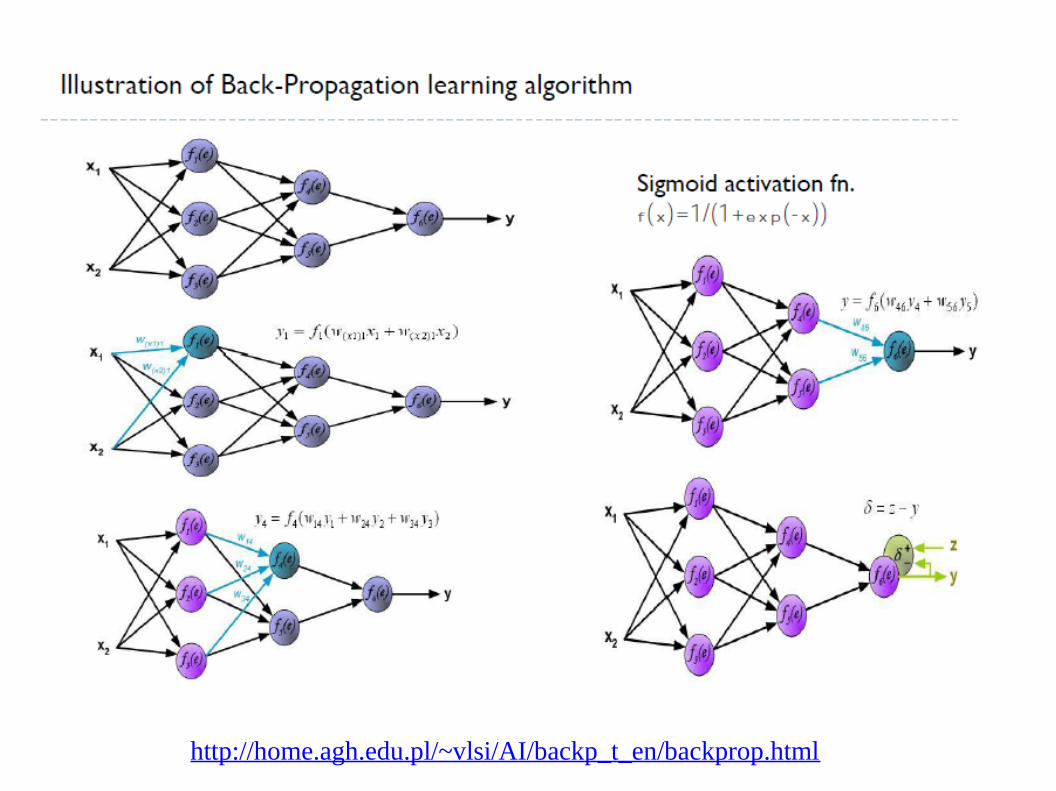
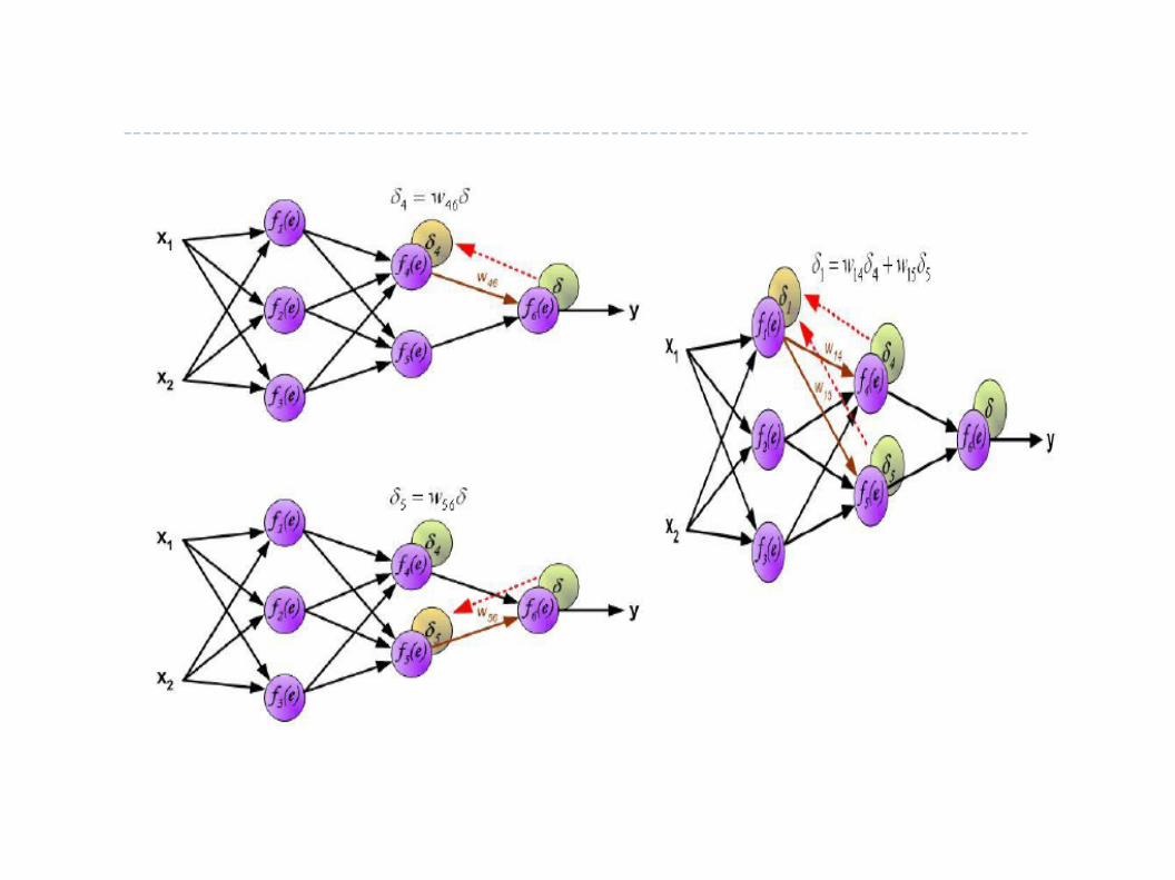
http://home.agh.edu.pl/~vlsi/AI/backp_t_en/backprop.html

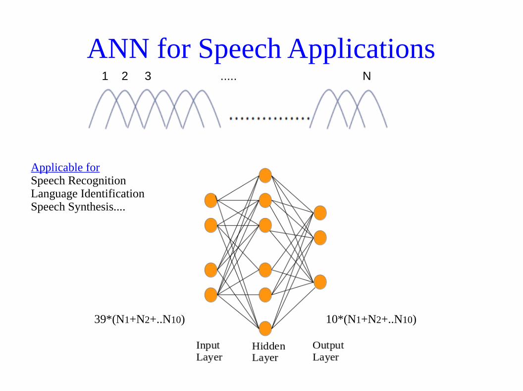
ANN for Speech Applications1 2 3 ..... N

39*(N1+N2+..N10)

Applicable forSpeech RecognitionLanguage IdentificationSpeech Synthesis....

10*(N1+N2+..N10)

39*50

10*50

Comparing GMMs and ANNsGMMs ANNs

Maximize the Likelihood score Maximize the posterior probabilitiesNeeds appropriate choice of Mixture

components

Choice of nodes and layers plays a vital

role

Future Work

To create HMM-ANN baseline HMM State Transitions

Viterbi Aligned Result

ANN posteriors HMM-ANN Baseline

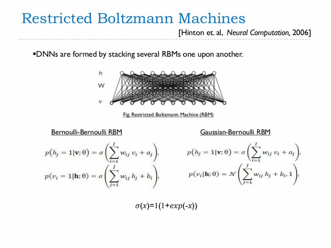
DNN

RBMTraining:● Unsupervised Pre-training● Supervised Fine tuning

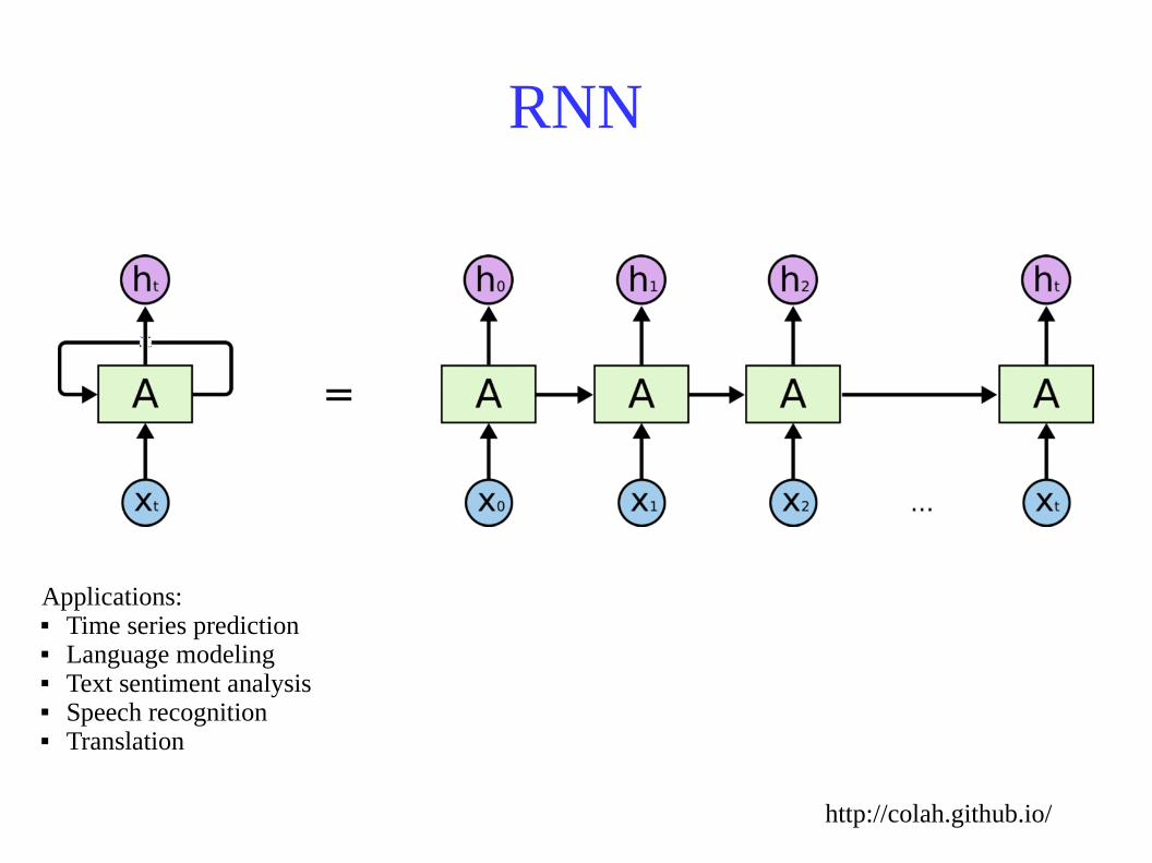
RNN

http://colah.github.io/

Applications: Time series prediction Language modeling Text sentiment analysis Speech recognition Translation

Variations of RNN

Ex: Image-to-Words

Ex: Sentence-to-Sentiment

Ex: Translation

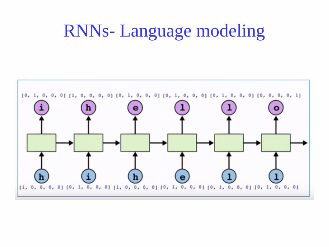
RNNs- Language modeling

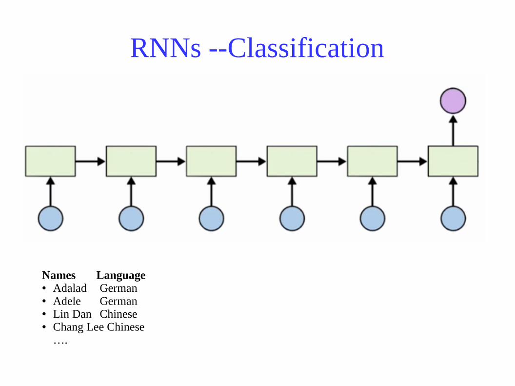
RNNs --Classification

Names Language● Adalad German● Adele German● Lin Dan Chinese● Chang Lee Chinese

….

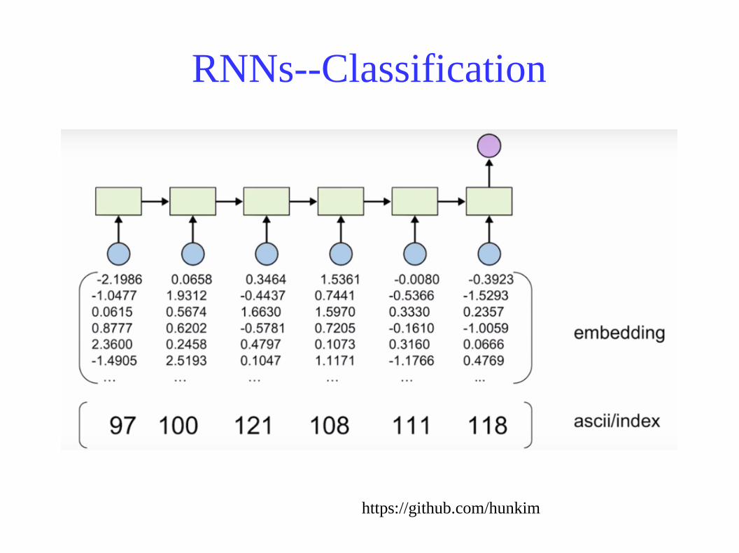
RNNs--Classification

https://github.com/hunkim

LSTM

Gates:● Forget gate: Determines whether current contents of memory will beforgotten (erased)● Input gate: Determines whether the input will be stored in the memory

cell● Output Gate: Determines if current memory contents will be output

F I O

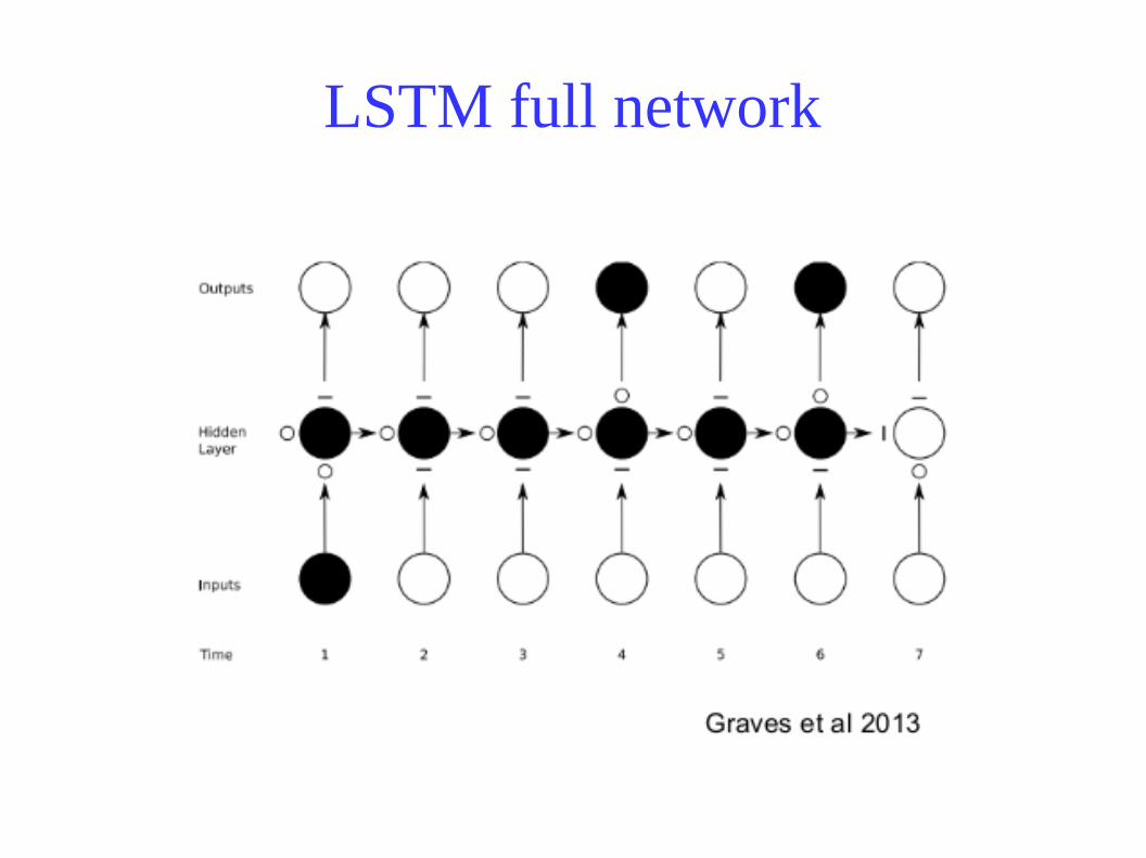
LSTM full network

Thank You