Embed Size (px)
Citation preview

Series Werner Herres and Joern Gronholz
Understanding FT·IR Data Processing
Part 1: Data Acquisition and Fourier Transformation
1 Introduction
Although Infrared spectroscopy Is one of the most powerful tools available to the analytical chemist and Is routinely used In research and application labs and for process control, the most advanced form of JR-spectroscopy, Fourier Transform infrared Spectroscopy (FT-IR), still holds some secrets for the chemist who is trained lo work with conventional grating instruments. One reason is surely that the generation of the spectral trace Is not straightforwardly controlled by setting appropriate knobs controlllng slit widths, scanning speed, etc. but involves a certain amount of mathematical manipulations such as Fourier transformation, phase correction, and apodization, which may introduce a barrier to understanding the FTIR technique. Despite this difficulty, moderately and low priced FT-IR Instruments are now entering even routine labs, because of their clear advantages compared to grating spectrometers. Even in lowerpriced FT-IR spectrometers, a laboratoryor dedicated computer Is the most Important component apart from the optics. As the quality of its software directly determines the accuracy of the spectra, It is recommended that the user be familiar with the principles of FT·IR data collection and manipulation. Unfortunately, there still seems lo be a lack of literature on FT-IR at an Introductory level. Therefore,
·this series of articles allempts to compile the essential facts in a, hopefully, lucid way without too many mathematical and technical details and thus provide an insight into the Interrelation between FT-IR hardware, the data manipulations involved, and the final spectrum.
Dr. Werner Herres and Dr. Joern Gronholz Bruker Analytlsche Messtechnlk GmbH, Wikfngerstr. 13, 7500 Karlsruhe21, West-Germany.
This Is the first of a series of three articles, describing the data acquisition and mathematics performed by the minicomputer Inside an FT-IR spectrometer. Special emphasis Is placed on operations and artifacts relating to the Fourier transformation and on methods dealing directly with the lnterferogram. Part 1 covers the measurement process and the conversion of the raw data (the lnterferogram) Into a spectrum.
s
A
B •r11 1,111 :111 ,, ''•JI 11,1 :11,1 11111 11111 1111 1:"1
c '1111 l1U1 ,·111
L A-~~-l-~-ll~/~,o¥---l> ~ . . ' . ' .. .. . ' ,
/ , , ,
I / ,, A
D
x~
Figure 1: A) Schematics of a Michelson Interferometer. S: source. D: detector. M1: fixed mirror. M2: movable mirror. X: mirror displacement. B) Signal measured by detector D. This ls the lnterferogram. C) Interference pattern of a laser source. Its zero crossings define the positions where the lnterferogram Is sampled (dashed lines).

2
2 Raw Data Generation
The essential piece of optical hardware in a FT-IR spectrometer is the interferometer. The basic scheme of an idealized Michelson interferometer is shown in Figure 1.
Infrared light emitted by a source (Globar, metal wire, Nernst bar ... ) is directed to a device called the beam splitter, because it ideally allows half of the light to pass through while it reflects the other half.
The reflected part of the beam travels to the fixed mirror M1 through a distance L, is reflected there and hits the beam splitter again after a total path length of 2 L. The same happens to the transmitted part of the beam. However, as the reflecting mirror M2 for this Interferometer arm is not fixed at the same position L but can be moved very precisely back and forth around L by a distance x, the total path length of this beam is accordingly 2 • (L + x). Thus when the two halves of the beam recombine again on the beam splitter they exhibit a path length difference or optical retardation of 2 * x, I.e. the partial beams are spatially coherent and will interfere when they recombine.
The beam leaving the interferometer is passed through the sample compartment and Is finally focused on the detector D. The quantity actually measured by the detector Is thus the Intensity I (x) of the combined IR beams.as a function of the moving mirror displacement x, the so-called interferogram (Figure 1 B).
The interference pattern as seen by the detector is shown in Figure 2A for the case of a single, sharp spectral line. The interferometer produces and recombines two wave trains with a relative phase difference, depending on the mirror displacement. These partial waves interfere constructively, yielding maximum detector signal, If their optical retardation is an exact multiple of the wavelength,\, I.e. if
2•x= n• ,\(n = 0, 1,2, ... ). (1)
Minimum detector signal and destructive Interference occur if 2 *xis an odd multiple
___ ,Series of >J2. The complete dependence of l(x)on xis g)ven by a cosine function:
l(x) = S(v) • cos(2" · v ·x) (2)
where we have introduced the wavenumber v = 1/A, which is more common In FT-IR spectroscopy, and S (v) is the Intensity of the monochromatic line located at wavenumber JI.
Equation (2) is extremely useful for practical measurements, because it allows very precise tracking of the movable mirror. In fact, all modern FT-IR spectrometers use the Interference pattern of the monochromatic light of a He-Ne laser to control the change in optical path difference. This is the reason why we included the Interference pattern of the HeNe laser in Figure 1C. This demonstrates how the IR interferogram is digitized precisely at the zero crossings of the laser interferogram. The accuracy of the sample spacing A. x between two zero crossings is solely determined by the precision of the laser wavelength Itself. As the sample spacing A. J1 in the spectrum is Inversely proportional to A. x, the error in A. v is of the same order as in A. x. Thus, FT-JR spectrometers have a built-in. wavenumber calibration of high precision (practically about O.o1 cm·'}. This advantage is known as the Cannes advantage.
3 Advantages of FT-IR
Besides its high wavenumber accuracy, FT-IA has other features which make it superior to conventional IR.
The so-called Jacquinot- or throughput advantage arises from the fact that the circu· lar apertures used in FT-IR spectrometers have a larger area than the linear slits used In grating spectrometers, thus enabling higher throughput of radiation.
In conventional spectrometers the spectrum S (v) is measured directly by recording the Intensity at different monochromator settings JI, one v after the other. In FT-IR, all frequencies emanating from the IR source Impinge stmuitaneously on the detector. This accounts for the so-called multiplex- or Fellget advantage.
The measuring lime in FT-IR is the time needed to move mirror M2 over a distance proportional to the desired resolution. As
the mirror can be moved very fast, complete spectra can be measured In fractions of a second. This is essential, e.g. in the coupling of FT-IR to capillary GC, where a time resolution of 10-20 spectra per second at a resolution of 8 cm·1 is often necessary [1].
Finally, the Feliget- and Jacquinot advantages permit construction of interferometers having much higher resolving power than dispersive instru'ments.
Further advantages can be found In the IR literature, e.g. In the book by Bell [2].
4 Fourier Transformation
Data acquisition yields the digitized interferogram l(x), which must be converted into a spectrum by means of a mathematical operation called Fourier transformation (FT). Generally, the FT determines the frequency components making up a continuous waveform. However, If the waveform (the interferogram} is sampled and consists of N discrete, equidistant points, one has to use the discrete version of the FT, I.e. discrete FT (OFT}:
N-1
S(k·Av) = "f:,l(nAx)exp(i27rnk/N) (3)
n=O
where the continuous variables x, J1 have been replaced byn · Axandk· Av, respectively. The spacing A. JI In the spectrum is related to Ax by
Av= 1/(N·AJ!) (4)
The DFT expresses a given function as a sum of sine and cosine functions. The resulting new function S (k · A v) then consist of the coefficients (called the Fourier coefficients) necessary for such a developmen,Ailernatively, If the set S (k ·A v} of FourJ~t coefficients is known, one can easlly"%reconstruct the interferogram I {n · A.xi>hy combining all cosines and sines multiplle(j\ by their Fourier coefficients s (k. A v) 'and dividing the whole sum by the number o.t points N. This is stated by the formula forthe inverse OFT (IDFT}:
/(n·AX) = \\
N-1. \
(1/N) "f:,S(k· A v)exp(.,,.i2,,-· nk!N) (5)
n=O
."Series
l t 4000 2000
WRVENUHBERS CH-1 x~
Figure 2: Examples of spectra (on the left) and their corresponding lnlerferograms (on the right). A) One monochromatic line. B) Two monochromatic lines. C) Lorentzian line. D) Broadband spectrum of polychromatic source.
The summation (5) is best illustrated In the simple case of a spectrum with one or two monochromatic lines, as shown in Figures 2A and 28. For a limited number of functions like the Lorentzian in Figure 2C1 the corresponding FT Is known analytically and can be looked up from an Integral table. However, in the general case of measured data, the DFT and IDFT must be calculated numerically by a computer.
Although the precise shape of a spectrum cannot be determined from the lnterferogram without a computer, it may nevertheless be helpful to know two simple trading rules for an approximate description of the correspondence between I (n · Ax) and S(k·Av).
From Figure 2C we can, e.g., extract the general qualitative rule that a finite spectral line width (as Is always present for real samples) is due to damping in the interferogram: The broader the line the stronger the damping.
Comparing the widths at half height (WHH) of I (n · Ax) and S (k · A v), reveals another related rule: The WHH's of a 'hump-like' function and Its FT are Inversely proportional. This rule explains why In Figure 20 the lnterferogram due to a broad band source shows a very sharp peak around the zero path difference position x = 0, while the wings of the interferogram, which contain most of the useful spectral information, have a very low
amplitude. This Illustrates the need tor ADC's of high dynamic range In FT-IR measurements. Typically, FT-IR spectrometers are equipped with 15- or 16-bit ADC's.
For n = 0, the exponential In (5) Is equal to unity. For this case, expression (5) states, that the Intensity I (0) measured at the lnterferogram centerburst is equal to the sum over alt N spectral intensities divided by N. This means the height of the center burst Is a measure of the average spectral Intensity.
In practice, eq. (3) Is seldom used directly because It Is highly redundant. Instead a number of so-called fast Fourier transforms (FTT's) are in use, the most common of which is the Cooley-Tukey algorithm. The aim of these FTT's Is to reduce the number of complex multiplications and sine- and cosine calculations appreciably, leading to a substantial saving of computer time. The (small) price paid for the speed Is that the number of lnterferogram points N cannot be chosen at will, but depends on the algorithm. Iii the case of the CooleyTukey algorithm, which Is used by most FT-IR manufacturers with slight modifications, N must be a power of two. For this reason and from relation (4) It follows that spectra taken with laser-controlled FT-IR spectrometers will show a sample spacl'll! of Av.= m * laserwavenumber/2* *N···
5 Final Transmittance Spectrum
To obtain a transmittance spectrum, the three steps shown in Figures 3 A, 8, Care necessary (this example was taken from a GC run): • an interferogram measured without
sample in the optical path Is Fourier transformed and yields the so-called single channel reference spectrum R (v) of Fig. 3A.
• an lnterferogram with a sample In the optical path Is measured and Fourier transformed. This yields the so-called single channel sample spectrum S(v) of Fig. 38. S(v) looks similar to R(v) bul has less intensity at those wavenumbers where the sample absorbs.
• The final transmittance spectrum T(v) is definedastheratioT(v) = S(v)/R(v). This is shown In Fig. 3C.
Once the transmittance spectrum has been obtained1 further data processing resembles that of digitized spectra from dispersive Instruments.
3

4
Series
0.5 0.5 105.0 A) B)
N C) ~
~ ~ ·"
~ ;; ~
z ~ z "' z w w ~
~ z
~ z ~
" ~
'·' '·' GIL 0 4000 301"Hl 2000 1000 4000 3fl0C 2000 1000 4000 3000 2000 1000
'o'RVENUHBERS CH-I VRVENUHBERS CH-I llRVENUHBERS CH-I
Figure 3: A) Single channel reference spectrum measured through an empty sample compartment. B) Single channel spectrum of absorbing sample. C) Transmittance spectrum equal to Fig. 38 divided by Fig. 3A.
VAVENUMBERS CM-I
Figure 4: Two closely spaced spectral lines at distance d (left) produce repeallve patterns at distance 1/d In the lnterferogram (right).
A)
B)
5000 4000 3000 2000 1000 llRVENUHBERS CH-1
C)
5000 4000 3000 2000 1000 llf.IVENUHBERS CH-l
Figure 5: A) First 2048 points of an lnterferogram consisting of a total of 8196 points. Signal In the wings Is amplified 100 times. B) FT of first 512 points of lnterferogram In Fig. 5a, corresponding to a resolution of 32 cm. C) FT of ali 8196 points of lnterferogram In Fig. 5a, corresponding to a resolution of 2 cm.

6 Resolution In FT-IR
Figure 4 shows the lnterterogram corresponding to two sharp lines separated by a wavenumber distance d. Due to the separation d In the spectrum, the interferogram shows periodic modulation patterns repeated after a path length difference 1/d. The closer the spectral lines are, the greater the distance between the repeated patterns. This Illustrates the socaiied Rayleigh criterion, which states that In order to resolve two spectral Jines separated by a distance done has to measure the lnterferogram up to a path length of at least 1/d.
For a practical measurement, which was done on a Bruker IFS-88 using a broad band MCT detector, the influence of increasing the interferogram path length on the resolution is shown In Figures SA, B, C. The lnterferogram in Figure SA represents the first 2048 points from a total of 8196. Figure SB was obtained by transforming only the first S12 lnterferogram points, which corresponds to a resolution of 32 cm- 1 • Figure SC exhibits the full 8196 point transform. It Is clearly seen that many more spectral features are resolved In the case of a longer optical path.
7 Zero Filling
It should be noted that DFT only approximates the continuous FT, although it is a very good approximation if used with care. Blind use of eq. (3), however, can lead to three well-known spectral artifacts: the picket-fence effect, aliasing, and leakage.
The picket-fence effect becomes evident when the interferogram contains frequencies which do not coincide with the frequency sample points k • A v. If, In the worst case, a frequency component lies exactly halfway between two sample points, an erroneous signal reduction by 36 O/o can occur: one seems to be viewing the true spectrum through a picket-fence, thereby clipping those spectral contributions lying 'behind the pickets', i.e. between the sampling positions k * .6. v. In practice, the problem is less extreme than stated above if the spectral components are broad enough to be spread over several sampling positions.
.Series '·'
-ll. 2 1600 1550 1500 1450 !400
'IAVENUHSERS CH-I
Figure 6: Picket-fence effect In bands due to water vapor. Top: no zero filling, bands look badly clipped. Bottom: spectrum zero fllled using a ZFF of 8.
The picket-fence effect can be overcome by addin!hzelQ~<to,the end ~Hhe interferogram·beforeDFT1s·pefformed, therebydncreasing the number ·01 points per wavenumber-in the spectrum. Thus, zero filling the lriferterogram has the effect of interpolating the spectrum, reducing the error. As a rule of thumb, one should always at least double the original inlerferogram size for practical measurements
by zero filling it, I.e. one should choose a zero filling factor (ZFF) of two. In those cases, however, where the expected line width Is similar to the spectral sample spacing (as e.g. in case of gas-phase spectra), a ZFFvalue of up to 8 maybe appropriate.
The Influence of zero filling on the appearance of water vapor bands ls demonstrated in Figure 6. Al the top, a · spectrum with no zero filling Is shown. The spectrum at the bottom Is zero filled using a ZFF of 8. While the lines of the upper spectrum look badly clipped, the lines are smooth In zero filled spectrum.
It should be noted, that zero filling does not introduce any errors because the instrumental line shape is not changed. It Is therefore superior to polynomial interpolation procedures working In the spectral domain.
Aliasing, leakage, apodlzation, and phase correction will be dealt with In the following installments.
References
(1] W. Herres, uCapfffary GC.fTIR Analysis of Vol· stiles: HRGC..FTIR" In Proceedings uAnalysls of Volatiles", P. Schreier (editor), Walter de Gruyter & Co., Berlin {19B4).
{2} A.J. Bell, u/nltoductory Fourier Transform Spectroscopy", Academic Press, New York (1972).
(3] G.D. Bergland, IEEE Spectrum, Vol. 6, pp. 41-52 (1969).
5

6
By Joern Gronholz and Werner Herres
UNDERSTANDING FT-IR DATA PROCESSING PART 2: DETAILS OF THE SPECTRUM CALCULATION In the first part of this series, we covered the FT-IR data acquisition and the Fourier transformation. This second part continues with the description of the mathematical operations performed by an FT-IR minicomputer to compute the spectrum from the interferogram.
1 Aliasing
In part 1 [l] it was shown that sampling the continuous interferogram and the use of the discrete version of the Fourier transformation (the DPT) may produce artifacts, such as the picket-fence effect, unless special precautions are taken. Another possible source of error due to the use of the DPT is aliasing.
To understand aliasing, we recall the basic DPT-equation
N-1
S(k· il.v) = L; exp(i27fk n!N)I(n • il.x) (I) n"'O
which describes how a spectrum sampled at wavenumbers k · !J.v can be computed from an interferogram sampled at optical path differences n · Ax. In practical calculations both n and k will run from 0 to N-1, i.e. the DPT produces N (generally complex) output points from an input interferogram of N (generally real) input points. If we expect the spectrum to be of the form shown in Figure IA, we will find that the DPT yields not just a single spectrum but rather the spectrum plus its mirror image, as given in Figure 1B: the first N/2 points represent the expected spectrum, the second part, starting with the index k = N/2 equals its mirror image. For practical computations this means
Joern Gronholz and Werner Herres, Bruker Analytische Me.fttechnik, GmbH, Wikingerstr. 13, Karlsruhe 21, FRO.
that a DPT of an N-point interferogram yields only N/2 meaningful output points. The second set of N/2 points is redundant and therefore automatically discarded. This behavior is also easily derived from Equation (1), if one substitutes index k by N-k. Using the identity
exp i27rk = (exp i27r) * * k = 1 * *k (2) = 1
one obtains the mathematical description of mirror symmetry
S([N-k]) = S(-k) (3)
about the. !c:>-c~lled 'folding' - or G!l)Jyquist' :wavenimiber ,;•, .J-P,...• (N/2)· fiv D v~ f'1 b'f
;;;·ll(2. Ax) . (4)
Furthermore, one sees that Equation (1) is not only valid for indices k from 0 to N - 1 but for all integers including negative numbers. In particular, if we replace k in Equation (I) by k + m · N, we get the equation
S([k + m · N]) = S(k) (5)
which states that the mirror-symmetrical N-point sequence of Figure 1B is endlessly and periodically replicated as indicated in Figure 1 C. I This replicat.ion ~f th~ original E~pectrum and its mtrror image on if (he wavenumber axis is termed "'-'aliasing'.
I.I Alias Overlap
From Figures 1B and IC it is clear that a unique spectrum can only be
calculated if the spectrum does not overlap with its mirror-symmetrical replicate (alias). Nl>"•overlap will occur.if·4he•spectrum·is zet<lll.bove a maximum-'-'wavenumber--i;;:n-~ -and if •max •s smaller than the folding wavenumber v,:
Pmai.;;11r.;; (N/2);/J.p (6) = 1/(2. Ax)
Here, we recall from [1] that /J.v is related to Ax by
!J.v = 1/(N ·Ax) (7)
If; ·however, the'· ~pectrum contains .. a.non·zero ·Contribution e.g. 200 ... cnF'. above the.folding wave. number·vr,this•will•be'folded back' below• Pf. and appear at the wrohg position; i,e; P['-200 cm-'1• This is the possible artifact due to aliasing.
The finer the interferogram .sample spacing Ax is, the further apart are the aliases and the lower the danger of alias overlap. However, small Ax means also an increased number of points N and therefore higher storage needs and larger computation times. For a given wavenumber range, the FT-IR software has therefore to choose the maximum sample spacing for which still no overlap occurs.
In part I we explained that in PTIR, the sampling positions are derived from the zero crossings of an He-Ne laser wave having a wavelength >.. of 1/15800\cm. As a zero crossing occurs every A./2, the minimum possible sample spacing Axmin is 1/31600 cm. With Equation (4), this corresponds to a folding wave"

n111uber 'of 15800~ cm- 1, i.e. the maximum bandwidth which can be measured without overlap has a width of 15800 cm- 1• A larger range can be covered, if the laser frequency is electronically doubled (frequency multiplication).
Very often, the investigated bandwidth is much smaller than 15800 cm-1, e.g. in mid-IR, \Vhere Vmax is generally less than 4500 cm - 1 and especially in the far-IR with wavenumbers below 200 cm - 1• In these cases, one can choose & to be an mfold multiple of dxmin· This leads to an m-fold reduction of the interferogram size.
1.2 Undersampling
An even greater reduction of the data slze is possible, if the spectrum is zero below a lower band limit Vmin
and if Vmin is not zero as- assumed above. If the spectrum bandlimits Vmin and Vmax lie bet,veen lo\ver and upper folding wavenumbers VfL and vru, which are related by
n-1 VfL = ~n- Vru (n = 1,2,3,. .. ) (8)
it will look as indicated in Figure ID for the case n = 4. The upper folding wavenumber Pru must be a natural fraction (or integer multiple) of the He-Ne laser wavenumber:
Vru = fr' 15800 (fr= .. ., 1/J, 1/2,1,2,3,. .. ).(9)
If we now further increase the sample spacing by a factor n, the aliases of Figure 1 D will overlap appreciably, thus filling the previously empty range from 0 to VfL with n - 1 further copies of the original spectrum. This is shown in Figure IE. As all copies are identical (except that their absolute wavenumber scaling and their direction on the vaxis can differ from the original), we need not calculate the spectrum at its true position by an N-point FT, but can rather calculate the alias of lowest wavenumber by an NI n-point FT and correct its wavenumber scaling afterwards. This further n-fold reduction of interferogram size compared to the conventional case,
\Vhere Vmin = 0, is termed 'undersampling'. It should be noted that undersampling enables measurements with a Vmox higher than the original laser wavenumber, because only the difference vru - VfL, and not the absolute values of the folding wavenumbers is to be considered in the sampling condition
D
0
0 v ... ll..
1 llx ,;; ~2~[ v_ru ___ v_fL~I - (10)
An advanced FT-IR software package will automatically account for proper sampling and undersampling, such that only the upper and lower limits of the desired spectral range need to be specified. The user only needs to make sure
Figure I: Effects of Sampling. A) Expected Shape of the Spectrum. B) The DPT Yields the Spectrum and Its Mirror Image. Only the First N/2 Points Contain Useful Information. The Second N/2 Points are Redundant and Discarded. C) Aliasing: Figure JB is Endlessly Replicated on the Wavenu1nber Axis. Aliasing Causes Errors, if the Spectrum is Nonzero up toa Wavenumber Vmaxand ifvmrixlsabove the Nyquist Wavenumber vf' This Happens if the Sampling Condition fil: < 11(2 · vm,,) is Violated. D) Spectrum is Zero Belolv vmin and above Vmru;" This Allows/or Undersampling. E) Undersampling Produces Spectrum Aliases. The DPT Calculates the Alias of Lolvest Wavenumber Instead of the Original. The Spectrum must be Zero outside The Bandpass Defined by the Upper and Lower Folding Limits.
7

·that the investigated spectrum is, really zero outside the range vfL to Pru J:>y il!serting either, optical , or electronic filters.
iifl For technical reasons, the sample 'ii spacing must often be increased in ~ steps of powers of two. The possible 1\ folding wavenumbers for this com'i\mon case are given in Table I.
2 Effect of the Finite Record Length: Leakage Unlike the picket-fence effect and
aliasing, leakage is not due to using
a digitized version of a continuous ,interferogram. Leakage is caused by the truncation of the interferogram at finite optical path difference. The proper mathematical term to describe the effect on the spectra of
·truncating theinterferogramis 'convoli\tilln'.
2.1 Convolution
Mathematically, an interferogram IL(x), truncated at optical path difference x = L can be obtained by multiplying an interferogram Ii (x)
Table 1: Possible Folding Wavenumbers Depending on the Sample Spacing.
Actual sample spacing is 2* • SSP • (l/31600) [cm]. Laser wavenumberis assumed to be exactly 15800 cm-I, BWis the maximum possible bandwidth, i.e. the difference between upper and lower folding limit Pn; and vfL. Undersampling occurs, if n from Equation (8) is > I. Only cases up ton= 4 are shown.
2• •SSP n BW[cm-IJ vfL[cm-I] Pru [cm-I]
I 15800.000 0.000 15800.000 I 2 15800.000 15800.000 31600.000 I 3 15800.000 31600.000 47400.000 I 4 15800.000 47400.000 63200.000
2 I 7900.000 0.000 7900.000 2 2 7900.000 7900.000 15800.000 2 3 7900.000 15800.000 23700.000 2 4 7900.000 23700.000 31600.000
4 l 3950.000 0.000 3950.000 4 2 3950.000 3950.000 7900.000 4 3 3950.000 7900.000 11850.000 4 4 3950.000 11850.000 15800.000
8 1975.000 0.000 1975.000 8 2 1975.000 1975.000 3950.000 8 3 1975.000 3950.000 5925.000 8 4 1975.000 5925.000 7900.000
16 987.500 0.000 987.500 16 2 987.500 987.500 1975.000 16 3 987.500 1975.000 2962.500 16 4 987.500 2962.500 3950.000
32 I 493.750 0.000 493.750 32 2 493.750 493.750 987.500 32 3 493.750 987.500 1481.250 32 4 493.750 1481.250 1975.000
64 I 246.875 0.000 246.875 64 2 246.875 246.875 493.750 64 3 246.875 493.750 740.625 64 4 246.875 740.625 987.500
128 l 123.437 0.000 123.437 128 2 123.437 123.437 246.875 128 3 123.437 246.875 370.312 128 4 123.437 370.312 493.750
8
\
of infinite extension by a 'boxcar' function BX (x), which is zero for x > L and unity for x ~ L, i.e.
IL (x) =Ii (x) · BX(x) . (11)
According to the convolution'' theorem of Fourier analysis, the Fourier transform of a product of two functions is given by the convolution (here indicated by the ' o' symbol of their individual Fourier transforms, i.e. if Si (v) and bx (v) are the Fourier transforms of Ii (x) and BX (x), respectively:
+oo
Si (v) = J exp(i2'1!'vX) · Ii(x)dx
+oo (12) bx (P) = J exp(i2'1!'PX) . BX(x)dx
-00
then we get the following relation for the Fourier transform SL (v) of the truncated interferogram IL (x)
+oo
SL (P) = J exp(i2'1!'PX) . IL(x)dx -00
+oo
J exp(i2'1!'vx)Ii(x)BX(x)dx -00
(13) +oo
J Si(k)bx(v-k) dk
Si(v) o bx(v) .
The computation of a convolution integral B(v) o C(v) as in Equation (13) can be visualized by the following procedure:
- Put the function B onto the k-axis with its origin at k= 0. This is B(k). Do the same for function C(k).
- Move the origin of function C(k) to another position k = v and reflect it about this position. This yields C(v-k).
- Multiply the displaced and reversed function C(v-k) by B(k) and measure the area under the product function. This is the value of the convolution integral for one position.
- Repetition of the above three steps for all positions yields the complete wavenumber dependence of the convolution integral.

1! ,,
According to Equation (13), the spectrum SL(v) of a finite interferogram can thus be obtained by convolving the spectrum Si(v) corresponding to infinite optical path difference (and hence to infinite resolution, see part 1) with the 'instrumental lineshape' (ILS) function, bx(v). This enables a clear description of a measured Iineshape in terms of a natural lineshape (NLS) due to physical line-broadening, the ILS representing solely the contribu-
of finite resolution. The analytical form of the ILS
corresponding to boxcar truncation can be easily derived from the Fourier integral of a unity operand using a finite integration range. The result is the well known sine function:
bx(v) =L ·sine (2vL) =L · sin(27rvL)/(27rvL), (14)
which is plotted in Figure 2. One sees, besides a main maximum centered about v = 0, numerous additional peaks, called side lobes or 'feet'. These side lobes cause a 'leakage' of the spectral intensity, i.e. the intensity is not strictly localized but contributes also to these side lobes. The largest side lobe amplitude is 22 OJo of the main lobe amplitude.
As the side lobes do not correspond to actually measured in-
SIHC2bU
"" - - a.s11t
Figure 2: Fourier Transfor1n of the Boxcar Cutoff. known as the Sine Function. Largest Side Lobe is 22 % of the Main LobeAmp/itude. L = Opitca/ Pathlength Difference.
forination but rather represent an artifact due to the abrupt truncation at x = L, it is desirable to reduce their amplitude~Jlll!PtOJ.'~~··~pJ!;b<
,;~~t••~i!~~~'~:a~ d!Z~!IO!J:' , (originating from the Greek,word C<1i'OO, which means 'removal of the feet').
2.2 Solution to Leakage: Apodization
lobes than the sine function. Numerous such functions exist. An extensive overview of their individual properties can be found in the review by Harris [2]. In Figures 3B- 3D, four examples of such functions and their Fourier transforms are plotted together with the boxcar cutoff in Figure 3A. The analytical forms of these apodization functions are
Triangular (TR): TR(x) = 1-n/L
(n=0,1, .. .,L) (15)
Trapezoidal or four-point (FP): FP(x) = 1 (n=0, 1, .. .,BPC)
The solution to the problem of leakage i to truncate the interferogram less abruptly than with the rectangular or 'boxcar' cutoff. This is equivalent to finding a cutoff or apodization function with a Fourier transform which shows fewer side
1- [n -BPC]l[BPD-BPC] (n =BPC, .. ., BPD) (16)
A
BOXCAR
B
TRIANGULAR
c TRAPEZOIDAL
D
H.RPP-GENZEL
E
3-TERH. BLRCKH.RN-HRRRJS
Figure 3: Several Apodization Fu"nctions (left) and the 'Instru1nental Lineshape' Produced by Them (right). The Cases A -D Are Commonly Used in FT-IR.
9

This is a boxcar function between 0 and breakpoint BPC, and a triangular function between breakpoints BPC and BPD. In Figure 3C we chooseBPD=L.
Hamming or Happ-Genzel (HG): HG(x) = 0.54 + 0.46 COS('ll"nlL)
(n=0, 1, ... ,L) (17)
This is a cosine halfwave on a boxcar pedestal. The amplitude at the boundary x = L is not zero but still 8 % of the amplitude at the origin. The parameters 0.54 and 0.46 have been chosen for optimum suppression of the first, largest side
'Johe.
Three- and four-term BlackmannHarris (BH) BH(x) =AO+ Al COS('ll"nlL)
+ A2 COS('11"2n/L) + AJ CoS('11"3n/ L)
(n=0, 1, ... ,L) (18)
This set of windows is a generalization of the Happ-Genzel function. The coefficients have been optimized numerically to trade main lobe width for sidelobe suppression (see [2]):
3-termBH 4-termBH
AO 0.42323 0.35875 Al 0.49755 0.48829 A2 0.07922 0.14128 A3 0.0 0.01168
The three-term EH-window is plotted in Figure 3E.
2.3 Apodization and Resolution
As expected, Figure 3 reveals that all apodization functions produce an ILS with a lower sidelobe level than the sine function. Ho\vever, one also sees that the main lobes of all ILS's in Figures 3B - 3E are broader than that of the sine function in Figure 3A. The width at half height (WHH) of the ILS defines the best resolution achievable with a given apodization function. This is because if two spectral lines are to appear resolved from one another, they must
10
be separated by at least the distance of their WHH, otherwise no 'dip' will occur between them. As side lobe suppression always causes main lobe broadening, leakage reduction is only possible at the cost of resolution.
The choice of a particular apodization function depends therefore on what one is aiming at. If the optimum resolution of 0.61/L is mandatory, boxcar truncation ( = no apodization) should be chosen. If a resolution loss of 50 % compared to the boxcar can be tolerated, the Happ-Genzel-, or even better, the 3-term BH-apodization is recommended. If the interferogram contains strong low-frequency components, it may show an offset at the end, which would produce 'wiggles' in the spectrum. To suppress these wiggles, one should use a function which is close to ·zero at· the boundary, such as the triangular-, trapezoidal-, or Blackman-Harriswindows. As the ILS produced by the Blackman-Harris function shows nearly the same WHH as the triangular- and Happ-Genzel function (roughly 0.9/L), but at the same time, the highest side lobe suppression and is furthermore nearly zero at the interval ends, it can be considered the top performer of these three functions.
In practice, the shape of a spectral line measured at finite resolution is always a mixture of natural and instrumental lineshape. This is demonstrated in Figures 4A-4C, where the same NLS (in our case a Lorentzian), recorded at different resolutions, is plotted. The ILS corresponds to boxcar truncation. One sees that a lineshape close to the NLS can only be observed if the width of the ILS is small compared to theNLS.
At the end of the discussion of apodization, it should be noted that an instrumental lineshape with side lobes is of course also imposed on spectra from dispersive instruments. The ILS produced by the slit of a grating spectrometer corresponds to the ILS caused by triangular apo-
dization. The difference between FT-IR- and dispersive spectroscopy concerning apodization is that an FT-IR spectroscopist can choose the optimum ILS for his specific needs, while the 'dispersive spectroscopist' cannot.
3 Phase Correction
The last mathematical operation to be performed during the conversion of an interferogram into a spectrum is phase correction.
Phase correction is necessary, because the FT of a measured interferogram generally yields a complex spectrum C(v) rather than a real spectrum S(v) as known from conventional spectrometers.
A complex spectrum C(v) can be represented by the sum
C(v) = R(v) + il(v) (19)
of a purely real part R ( v) and a purely imaginary part I(v) or, equivalently, by the product
~);-S(vJ'exfltltfi(JJ)r <20> of the true 'amplitude' spectrum S(v) and the complex exponential exp(ic/>(v)) containing the wavenumber-dependent 'phase' cf>(v).
The aim of the phase correction procedure is to extract the amplitude£• spectrum S(v) from the comple'j!•··~ output C(v) of the FT. This can bN done either by calculating the squa~ root of the 'power spectrum' P(v) c! C(v) · C*(v): '[1,
'/ S(v) = [C(v) · C*(v)J112 !~.
= [R2(v) + l2(v)] 112 (21)1
or by multiplication of C(v) by thel1, inverse of the phase exponential and~ taking the real part of the result: J; S(v) = Re[C(v) exp(-ic/>(v))] (22f
The phase c/>(v) in the exponential exp(-ic/>(v)) can be computed from the relation
cf>(v) = arctan[I(v) I R(v)] . (23)
Equations (21) and (22) are equivalent, if one deals with perfect data free of noise. However, if noise is present, as is always the case with measured data, noise contributions

computed from Equation (21) are always positive and in the worst case, a factor or ...fi larger than the correctly signed noise amplitudes ~g111-puted from Equation (22). ~!Sf&ft\~ dure'(22).·isknown.1!$dmultipll~1ttive phase ··correction' · ON·theI<«Mer'tzmethod~ t3J.
3.1 Reasons for the Non-Zero-Phase
The reason for getting a complex spectrum out cif the FT is that the in: put to the FT is not mirror-symmetrical about the point x = 0. The asymmetry of the FT input originates from three different sources:
a) None of the sampling positions coincides exactly with the proper position of zero path difference. This is generally the case and causes a phase linear in v.
b) Only a 'one-sided' interferogram is measured, i.e. only one side is recorded to its full extent, the other consists only of a few hundred points.
c) The interferogram may be 'intrinsically' asymmetric. This may be due to wavenumber-dependent phase delays of either the optics, the detector/amplifier unit, or the electronic filters.
Figure 5 shows how the phase contributions from a) and b) can be calculated from a short double-sided portion of length PIP (PIP/2 points on either side of the centerburst). This yields, after iipodization, zero filling, and FT gives a low resolution phase spectrum. As the phase is a slowly varying ful\ction of v (except in the regions of beamsplitter or filter cutoff), a low resolution phase spectrum is sufficient. During the phase correction this is expanded to the size of the full array by interpolation.
The steps in the computation of the full array are shown in Figure 6. After apodization, the short doublesided part is multiplied by a ramp to avoid counting it twice. The effect of this ramp can be understood by decomposing it into a boxcar of
height 0.5 and a ramp through the origin, as indicated in Figure 6B. Because of the symmetry properties of the FT, the even boxcar function contributes only to the real part of the FT and has the effect of multiplying all contributions from
A B
-PJP/2 to +PIP/2 by 1/2, while the odd part of the ramp contributes only to the imaginary part of the FT. The odd part of the ramp is added to avoid a step at + PIP/2, which would produce 'wiggles' in the spectrum.
c D
Figure 4: Measured Lineshape Function Corresponding to a Lorentzian Natural Lineshape (D) and Boxcar Truncation, Depending on the Resolution. Resolution IncreasesfromA toD.
A
8
' "' '" ' '
y c D
-+ lr'AVENUHBERS
Fig~re5: Phase Computation. A) The Complete 'One-Sided' Interferogram. B) PIP Poiiftsofthe Short Double-Sided Part Around the Centerburst are Used to Compute the Phase Spectrum. C) The Double-Sided Part is Apodized, Zero Filled and Fourier transformed. D) The Phase Spectn11n is Computed from the Complex Output of the FT via Equation (23). This is Later Interpolated to Full Resolution.
11

I , . ! 1,:
1,
Having multiplied the data array by the ramp and the apodization function, it is zero filled and Fourier transformed. Using Equation (22) the resulting complex array C(v) is then multiplied by the complex exponential exp( -i<f>(v)), which is computed by interpolation from the low resolution phase spectrum.
After the phase correction, the corrected real part R ' ( v)
d=
R '(v) ~ R(v)cos(<f>(v)) - J(v)sin(</>(v))
represents the final single-channel spectrum S(v) which is stored for further processing. The corrected imaginary part I' (v)
I' (v) ~ R(v)sin(<f>(v)) + I(v)cos(<f>(v))
originates from the antisymmetric contribution of the cutoff at
d=Jeven r:+,jodd
·~·~ iua an HU OU l~U HU !l!U UH
VAVfXUMBEltS Cit-I t.O.Vf!<IJllBEllS tll•I
\
·~ uu 21u Jen 1aaa
YllYHIJll!(llS Cll•J
Figure 6: Computalion of 1he Final Spec/rum. A) The One-Sided lmerferogram is Apodized to Reduce Leakage. BJ Afler Apodizalion, !he Double-Sided Par! of Lenglh PIP ls Mul1iplied by a Ramp. The Ramp can be Decomposed imo an Even and an Odd Par!. The Even Par! Prevems !he PIP-Range from Being Coun1ed 1kice. The Array is !hen Zero Filled and Iransformed. CJ Real Pan of !he D(T-Outpul before Phase Correc1ion. D) Imaginary Par! of the DFT-Outp~I before Phase Correclion. E) Final Spec/rum after Phase Correclion Usil:!g !he In1erpola1ed Phase Spec/rum of Figure 5D According to Equaiio\(22).
12
-PIP/2 and the ramp as is shown in Figure 7. I' (v) would be zero, if a double-sided interferogram had been used. The corrected imaginary part is normally skipped or not even calculated to save computer time.
The fact that I' (v) is non zero after the phase correction demonstrates that the direct calculation of S(v) from the power spectrum via Equation (21) will yield erroneous results in the case of one-sided interferograins, because this procedure corrects for all contributions to I(v), including those from the cutoff at -PJP/2. This method is only properly applicable to double-sided interferograms.
With this last topic we have now completed the discussion of the standard operations necessary to convert an interferogram into its spectrum. In the next installment, we will deal with several FT- or interferogram-based techniques which are very useful in IR- and GCIR spectroscopy. o
k =
•••n +
r "' .Figure 7: Represemation of a One-Sided Cutoff Fune/ion by 1he Sum of an Even and an Odd Par!. The Even Part Corresponds to a Double-Sided lnterferogram. The Odd Part Contribu1es Solely to !he Imaginary Part of 1he Complex Spectrun1.
References
[1] W. Herres and J. Gronholz. Con1p. App/, Lab. 2 (1984) 216.
[2] F.J, Harris, Proceedings of the IEEE, 66 (1978) 51.
13] L. Mertz, Infrared Phys. 7 (1967) 17.
l
Joern Gronholz and Werner Herres
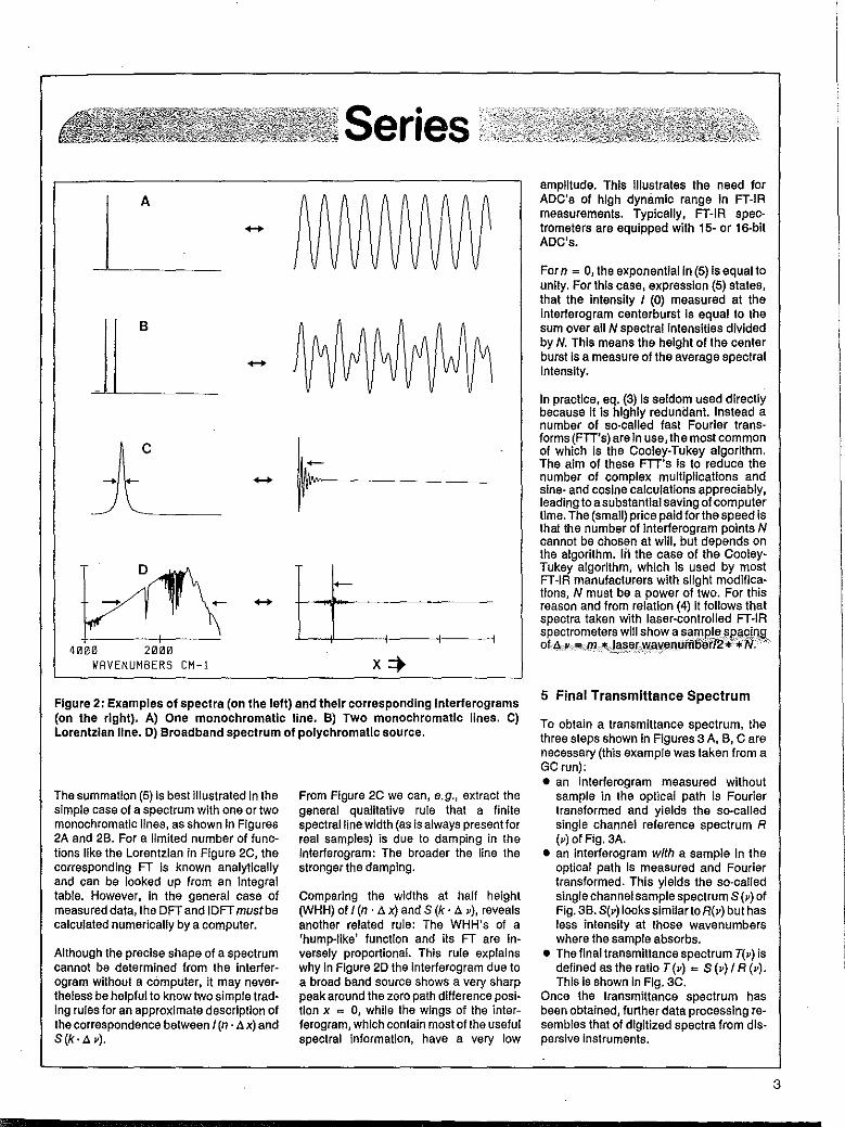
UNDERSTANDING FT-IR DATA PROCESSING PART 3: FURTHER USEFUL COMPUTATIONAL METHODS
In Parts 1 and 2 of this series lVe covered the standard operations of FT-JR, fro1n data acquisition to the final spectru111. This third and last part continues with a discussion of additional useful techniques and closes lvith a remark about the data system.
I n Parts 1 and 2 [l, 2] of this series we dealt with data acquisi
tion in a Fourier transform infrared {FT-IR) spectrometer and described the processing of the raw data to generate the final spectrum. To perform the necessary calculations in a reasonable time, the minicomputer of an FTIR spectrometer needs sufficient on-line computing power and is thus also very well suited to do more than just calculation of FFT's, phase correction, and ratioing of spectra. In fact, the considerable inherent numbercrunching capability inside an FTIR spectrometer is sometimes called the fourth advantage of FTIR. In this last part of our series we discuss some examples of such additional data processing in both domains: the frequency domain and the interferogram domain.
I The Problem of "Ghost" Interferograms or Fringes
The appearance of sinusoidal modulations, called 'fringes' on the baseline of IR-spectra is well known to spectroscopists. These
Joern Gronholz and Werner Herres, Bn1ker Analytische Messtechnik GnzbH, Wikingerstr. 13, Karlsruhe 21, West Gerrnany.
fringes or 'channel spectra' result from multireflections of the IR beam between the surfaces of a plane-parallel device in the- spectrometer's optical path, such as the plane parallel sample itself or a liquid-cell window. They can disturb the 'useful' spectral information quite seriously, as is shown for the absorbance spectrum of a silicon wafer in Figure IA. From Figure 2 in [l] it is readily concluded that fringes of constant frequency in the \vave number domain must result from a single 'spike' or a narro\v 'signature' in the corresponding interferogram. Indeed, the sample interferogram from which the absorbance spectrum in Figure lA was calculated, shows a 'ghost' interferogram or 'echo peak' ai an offset of 4206 interferogram points from the centerburst (see Figure JB). The lnterferogram was acquired at a resolution of 2 cm- 1
and thus consists of 8192 points. Fourier transformation of the full interferogram including the echo peak yields the spectrum in Figure lA, whereas reduction of the resolution to 4 cm- 1 (equivalent to an interferogram of 4096 data points) truncates the interferogram just before the echo peak yielding the 'fringe-free' spectrum of Figure JC.
This example shows that one can easily get rid of the fringes by discarding all interferogram points
from the echo peak to the end. This can be achieved either by choosing a lower optical resolution during data acquisition or by apodization with a trapezoidal function (see Figure 3 of [2]) chosen such that all points from the echo peak to the end are set to zero.
1.1 Mathematica/Description of the Fringes
The single channel spectrum S(P) of the IR-radiation transmitted through a multireflecting plate can be calculated from the empty-channel background spectrum B(v), the half-space power reflectance R(v), the refractive index n(v), the absorption coefficient a(v), the phase change ¥'(v) occurring at every internal reflection and the thickness d of the plate. The result is the well-known Airy formula [3] which we have extended to include absorptive intensity loss and cast into a form better suited for Fourier transformation:
S(P) ~So+ 2So!; {R(v)exp(-ad))k k=I
x cos(4?Tkn(v)d + 2k<0(v)) (I)
with
So(v) ~ B(v) (I-R(v))'exp(-ad) (2) I -R2(v) exp(-2ad)
Equation (1) shows nicely that the resulting spectrum can be represented by the sum of a fringefree spectrum S0 (v) and an infinite number of interference terms. Due to the factor (R(v) exp(-ad))k, the intensity of the k-th order inter-
13

'
I'
11
11
ti I
i II
Ii
14
Ii.'
0.7
A
0.35
0.0 1200 1000 800 600
WRVENUMBERS CM-1
B
x
0.5
c
0.375
0.25 1200 1000. 800 600
WRVENUMBERS CM-1
Figure 1: A) Absorbance spec/nun of a silicon lvajer calculated using the full length (BK points ~ RES 2 cm-1) of the interferogramfrom Fig. IB. B) Satnple interferogram of a silicon lVafer. Spectral resolution corresponds to 2 cm-1 (= BK points). The distance between thes1nall 'ghost' interferogra1n on the right and the centerburst is 4206 points (y-scale expanded for clarity). C) Absorbance spectrun1 of a silicon wafer calculated fro1n the interferogranz of Fig. IB using only 4K data points (resolution = 4 cin- 1).
ference term decreases 'vith ascending order k because Rk(P) is always less than l.
The interferogram corresponding to S(•) can be calculated from eq. (l) by inverse Fourier transformation. For the sake of simplicity we assume that the refractive index n (•) and the phase \O(P) within the argument of the cosine interference terms do not depend on P.
For this simplified case one gets
I(x) ~ Io(X)
+ 2 ~J,(x) o lo[x-(2nkd + 2k\O)] k=l
(3)
+ 2 ~J,(x) o lo[x+(2nkd + 2k,,)] k=l
This result shows that the cosine interference terms of the spectral domain correspond to additional ghost interferograms in the interferogram domain, appearing symmetrically on both sides of the centerburst at distances 2nkd + 2k\O. The shape of these echo peaks is given 1ly convolution of the undisturbed main interferogram J0(x) with the 'interferogram' h(x) which is the inverse FT of the k-th power of the product of the reflectance spectrum R (P) and the transmission spectrum T(P) exp(-ad). For the same reason as given above, the intensity of the kth ghost interferogram is at least smaller by a factor Rk than the main centerburst. Due to the wavenumber dependence of n(P) (i.e.: to dispersion) and of \O(v) which we explicitly neglected in the derivation of eq. (3), the echo peaks are generally additionally broadened and distorted and may be thus further reduced.
1.2 Use of Fringes for Thickness Determination
Eq. (3) shows, that the distance between the main centerburst and the echo peaks is directly proportional to the product of refractive index n and thickness d. If the average refractive index n is known, one can therefore calculate

the thickness of the fringe-producing element. This possibility is, e.g., often used in semiconductor quality control to determine the thickness of epitaxial layers deposited on doped substrates. Conversely, if both n and dare known, the offset X between main peak and first echo peak can be calculated as:
X=N·&
= 2·n·d
or in points
N= 2·n·d(&)-I (4)
with (&)-I = 15800 cm-I for mid-IR bandwidth, 0-7900cm-I,
The problem of ghost interferograms is of course not restricted to silicon wafers but can also be encountered in measuring standard alkali halide pellets or cast films on, e.g., KBr crystals. Sometimes spectra look 'noisy' at longer wavelength whereas expansion reveals fringes resulting from 'too perfect' a preparation, i.e. from plane-parallelism of the pellet.
In Table 1 the distance N between the interferogram centerburst and the first echo peak has been compiled for several thicknesses of four substrates commonly used in FT-IR. This table also sho,vs the maximum resolution which does not include the echo peak. It may be helpful in finding the proper combination of sample thickness and resolution for a given substrate.
1.3 Possibilities for Eliminating Fringes
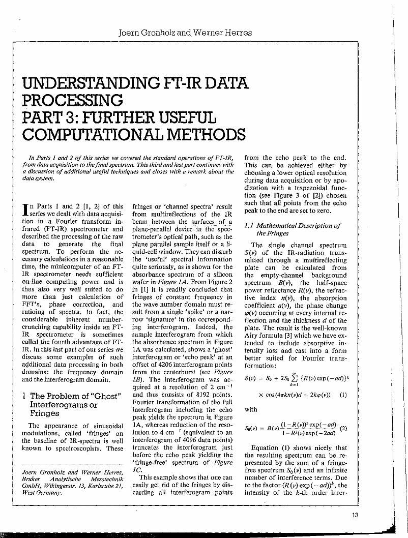
The question might arise whether there is some method of eliminating all kinds of fringes which plague the spectroscopist when measuring polymer films. Figure 2A shows the transmission spectrum of some technical polyethylene (PE)-type film. Although the modulations are very pronounced in the spectrum; the corresponding echo peak in the
Table 1: Location of the echo peak as a function of substrate thickness. Offset of the echo peak relative to the centerburst as a function of the thickness of four co1n1nonly used substrates, Last co/unzn contains the maximum possible resolution/or lYhich still no interferences occur assuming 250 points before and 2* *N~250pointsafterthecenterburstinallcases. Bandwidth= 7900cm-I throughout. Value of refractive indexn corresponds to JOOOcm-1.
Substrate Thickness
[cm]
KBr 0.05 0.1
(n = 1.53) 0.15 0.2 0.3 0.5
Ag Cl 0.05 0.1
(n= 1.98) 0.15 0.2 0.3 0.5
ZnSe 0.05 0.1
(n=2.40) 0.15 0.2 0.3 0.5
Si 0.05 0.1
(n= 3.42) 0.15 0.2 0.3 0.5
sample interferogram of Figure 2B can hardly be detected, being due to a much smaller reflectance R (v) of PE as compared to silicon and to stronger dispersion, which additionally broadens the echo peak and reduces its size. Furthermore, the echo peak is located only 267 points away from the centerburst because the film is only about fifty microns thick. For this latter reason, truncation of the interferogram ( = reduction of resolution) is here obviously no solution because the resulting resolution would be too poor.
In those cases where reduction of resolution cannot be applied, there are at least two other solutions to the fringe problem: an experimental and a numerical solution.
Offset from Maximum resolution centerburst \Vithout interferences [points] [cm-I]
2417 8 4834 4 7252 4 9669 2
14504 2 24174
3128 8 6257 4 9385 2
12514 2 18770 1 31284
3792 8 7584 4
11386 2 15168 2 22752 1 37920 0.5
5403 4 10807 2 16211 21614 32421 1 54036 0.5
1.3.J Experimental Solution of/he Fringe Problem
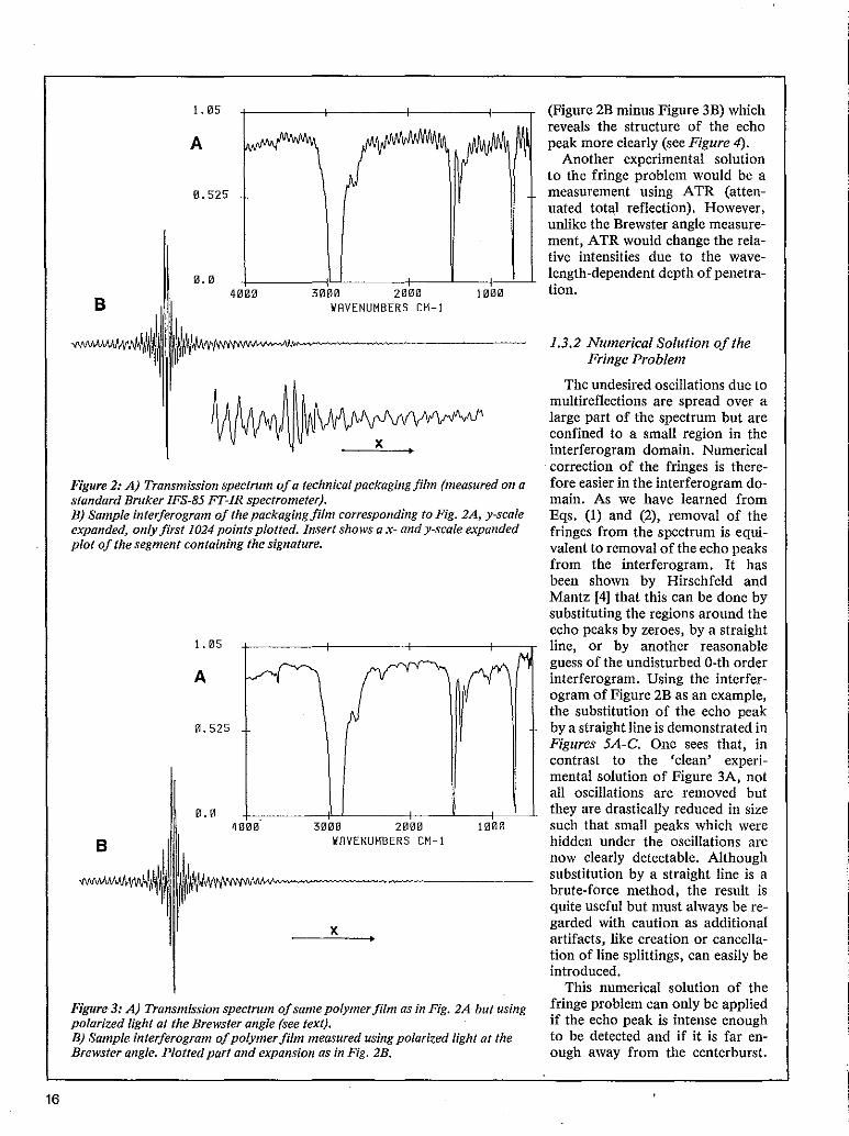
From Eq. (!) it is clear that all interference terms vanish if the reflectance R (v) of the sample can be made zero. Experimentally, this is indeed possible using polarized IR radiation, as is sho\Vn in Figure 3A, where the same polymer film was measured. A KRS-5 polarizer was used to provide an IR beam polarized parallel to the plane of incidence, while the film itself was oriented to the incident light at the Brewster angle. As the reflectance of this type of polarized radiation approaches a minimum at the Brewster angle (or is ideally zero), multireflections and thus 'channel spectra' are also minimized. This experiment makes it possible to obtain a difference interferogram
15
...............................................
16
1. 05
A
0.525
0.0 4000 3000 2000 1000
VAVENUHBERS CH-1
Figure 2: A) Transmission spectru1n of a technical packaging fihn (1neasured on a standard Bruker IFS-85 FT-JR spectrometer). B) Sample interferogram of the packaging film corresponding to Fig. 2A, y-sca/e expanded, only first 1024 points plotted. Insert shows ax- and y-scale expanded plot of the segment containing the signature.
1. 05
A
0.525
0.0 4000 3000 2000
VAYENUHBERS CH-1 B '1
~w~111 ·~~i11Mr1~~· ~-----x
Figure-3: A) Transmission spectrum of sanze poly1ner film as in Fig. 2A but using polarized light at the Brewster angle (see text). B) Sample interferograrn of po!y1ner film measured using polarized light at the Brelvster angle. Plotted part and expansion as in Fig. 2B.
(Figure 2B minus Figure 3B) which reveals the structure of the echo peak more clearly (see Figure 4).
Another experimental solution to the fringe problem would be a measurement using ATR (attenuated total reflection). However, unlike the Brewster angle measurement, ATR would change the relative intensities due to the wavelength-dependent depth of penetration.
1.3.2 Numerical Solution of the Fringe Problem
The undesired oscillations due to multireflections are spread over a large part of the spectrum but are confined to a small region in the interferogram domain. Numerical correction of the fringes is therefore easier in the interferogram domain. As we have learned from Eqs. (1) and (2), removal of the fringes from the spectrum is equivalent to removal of the echo peaks from the interferogram. It has been shown by Hirschfeld and Mantz [4] that this can be done by substituting the regions around the echo peaks by zeroes, by a straight line, or by another reasonable guess of the undisturbed 0-th order interferogram. Using the interferogram of Figure 2B as an example, the substitution of the echo peak by a straight line is demonstrated in Figures 5A-C. One sees that, in contrast to the 'clean' experimental solution of Figure 3A, not all oscillations are removed but they are drastically reduced in size such that small peaks which were hidden under the oscillations are now clearly detectable. Although substitution by a straight line is a brute-force method, the result is quite useful but must always be regarded with caution as additional artifacts, like creation or cancellation of line splittings, can easily be introduced.
This numerical solution of the fringe problem can only be applied if the echo peak is intense enough to be detected and if it is far enough away from the centerburst.

Figure 4: Difference interferograrn, Fig. 2B 111inus Fig. 3B, sho1ving the echo peak 1nore clearly. The insert sho1vs the signature x-scale expanded.
A
B
x---+
Figure 5: A) Part of the san1ple interferogra111 front Fig. 2B containing the signature. B) Sa111e part of interferogra1n as in Fig. 5A, but points 466 to 479 (14 points) are substituted by a straight line to suppress the si'gnature. C) Saine as Fig. 6B but points 466 to 514 are substituted (49 points). D) Transn1ission spec/nun calculated fro1n the interferograrn of Fig. SB. E) Trans111ission spectru1n calculated
·fro1n the interjerogra1n of Fig. SC.
1. 05
0.525
D
0.0 4000
1. 05
0.525
E
0.0 4000
While the smallness of the echo peak can be overcome by calculating its position from Eq. (5) if both n and dare known, violation of the second condition leads to severe baseline distortions and cannot be recommended.
Before leaving the interesting field of ghost interferograms, it is worthwhile noting that a 'simple' absorbancemeasurement of, say, a KBr pellet is not adequately described by the familiar formula
T(v) = exp(-a(v)d)
with transmittance T(v) and absorbance a(v)d, but must even in the simplest case of no multireflections be substituted by the numerator of Eq. (2).
T(v) = (1-R(v))'exp(-a(v)d) (5)
3000 2000 1000 WAYENUHBERS CH-1
3000 2000 1000 WRYENUHBERS CH-1
17

18
This means that one must not forget at least two reflections at both boundaries of the sample. The factor (1 - R) * * 2 causes an intensity reduction of the transmitted radiation, but may also lead to changes in position and intensity of single lines if R(v) is significantly structured. If the pellet has planeparallel surfaces, multireflection comes into play and the full Eq. (2) (divided by the empty channel background spectrum B(v}) must be used. Thus, from a transmission measurement one always gets a mixture of reflection and absorption properties unless the reflectance contributions are explicitly corrected for. This single or multireflection correction, i.e. extraction of the absorbance a(v)d from equations (5) or (2) is another task which could be routinely performed by the FT-IR spectrometer's minicomputer. It is mandantory if one is interested in precise determination of optical constants.
2 Interrelation of Smoothing and Apodization
In Part 2 of th is series we already described apodization at some length. Apodization means multiplication of the interferogram by a decaying function. Its effect on the spectrum is a suppression of side lobes at the expense of decreased resolution. We also showed that multiplication of the interferogram I(x) by a function a(x) is equivalent to convolution of the spectrum S(v} by the Fourier transform A (v) of the apodization function.
Three of the special apodization functions discussed (Happ-Genzel, 3- and 4-term Blackman-Harris) consisted of a sum of cosine functions as
N
BH(x) = AO + 2;An cos(n · "· x/L). n=l
It is instructive to calculate the Fourier transform of such a func-
tion and look at the corresponding convolution in the spectral domain in more detail. One gets
S' (n · Liv) = AO S(n · Liv)
+ Al(S((n-l)·Llv) + S((n+l)·Llv))
+ A2(S((n-2) ·Liv)+ S((n+2) ·Liv))
(6)
+ AN(S((n-N) ·Liv)+ S((n+N) ·Liv))
Hence, in order to calculate one point S' (n • .:l.v) of the spectrum corresponding to the apodized interferogram one must: - multiply the ordinate S(n · .:l.v}
of the non-apodized spectrum by AO,
- multiply the left and right next neighbors of S(n • .:l.v) by AI,
- multiply the left and right second next neighbors by A2 and so forth (up to N = 3 for 4-term BH)
- sum the intermediate results. This is S' (n · .:l.v). This shows that the points of the
spectrum S' (n · .:1.v) are a weighted mean of adjacent points of the non-apodized case S(v), the coefficients An of the apodization function being the weighting factors. As taking a weighted mean of spectral data amounts to nothing but smoothing, we conclude that apodization in the interferogram domain is equivalent to smoothing in the spectral domain. (Note that this special family of apodization functions would easily allow one to perform the apodization after the FT by summing neighboring points of the non-apodized spectrum multiplied by appropriate factors.)
Smoothing is an essential tool for reducing the noise in a spectrum. In addition to apodization, smoothing is mostly done by the famous Savitzky-Golay procedure [5], the merit of which is that (although a least-squares method and therefore data-dependent) the weighting coefficients used in the averaging process are fixed integers. This means that smoothing can be programmed in integer arithmetic leading to short computation times even on machines
without floating point hardware support. As spectral smoothing is so widespread and well known, we omit a detailed description and rather turn to the question of what happens if smoothing is done in the interferogram domain.
2.1 Smoothing in the Interferogram Domain: Digital Filtering
The effect of smoothing an interferogram on the corresponding spectrum is demonstrated in Figure 6A-C. Figure 6A shows an unmodified single channel spectrum, Figure 6B shows the spectrum corresponding to the same interferogram smoothed using a 9-point Savitzky-Golay window. Figure 6C is the ratio of Figures 6B and 6C. One sees that the effect of smoothing the interferogram is to decrease the intensity of the spectrum towards higher wavelengths, i.e. it behaves like a low-pass filter with the frequency response of Figure 6C. Accordingly, convolution in the interferogram domain is termed 'digital filtering'.
Digital filtering is closely related to apodization although the aims of both procedures are completely different. While during apodization one multiplies the interferogram by the apodization function to achieve a certain line shape (convolution), digital filtering means that one convolves the interferogram by a filter function to achieve a certain (multiplicative) frequency response. In practice, the filter function is seldom of the Savitzky-Golay type (this was simply used as an example) but is derived from the desired frequency response by inverse Fourier transformation of the desired spectral bandpass in case of non-recursive filters.
The advantage of digital - compared to analog - filtering lies in its great flexibility, because almost any conceivable frequency response can be modeled. The only problem is that, even today, where high-speed multipliers/adders are

o.z
A
'· l
' 2000 4000 6000 \l'RVENUMBERS CM-I
•• 2 +----->----+----+----
B
'· l
2000 4000 6000 liRVEtlUHBERS CM-I
l.' +-~-·+---<
c
0.5
2000 4000 60(Hl WRYENUMBERS CM-I
available, the time needed for computing the necessary convolutions is often still too long for real-time filtering in high-speed applications with data rates > 100 KHz. For slow-scanning FT-IR spectrometers, however, digital filtering can be appropriate and is then another task to be performed by the spec- . trometer's minicomputer.
3 Deconvolution Deconvolution is another inter
esting FT-based method closely·related to apodization and convolution. The aim of deconvolution is to decrease the widths of all lines in a limited spectral region or, equivalently, to enhance the apparent resolution of the spectrum.
The method is based on the assumption that the investigated spectrum S(v) may be represented by a convolution
S(v) = S' (v) O L(v) (7)
of a deconvolved spectrum S' (v) containing sharp lines and a func- · tion L(v) which is responsible for the line broadening. From the discussion of apodization in Part 2 of this series we know that convolution in the spectral domain corresponds to simple multiplication in the interferogram domain. Thus, inverse FT of Eq. (7) yields the product
I(x) = I' (x)- I (x) (8)
from which the broadening effect of L(v) can be easily cancelled by division by l(x). The deconvolved spectrum S' (v) is then obtained by another forward FT to the spectral domain. I(x), I' (x), and l(x) represent the inverse Fourier trans-
Figure 6: A) Single-channel sanzple spectru1n of the polymer Ji/Jn used for Figs. 2, 3. B) Sa111e spectru1n as in Fig. 6A but after s1noothing the interferogra111 by a 9-point Savitzky-Golay window. The intensity tolvards higher lYavenu1nbers is decreased. C) Ratio of Fig. 6B and Fig. 6A, showing the frequency response of the Savitzky-Go/ay 9-point digital filter (see text).
forms of S(v), S' (v), and L (v), respectively.
As an easy example we consider the case of an absorbance spectrum S(v) consisting of a single Lorentzian line which may be represented by convolution of an infinitely sharp line (a delta function) at v= v0
S'(v) = b(v-vo)
with a line shape function
L(v) = -3!!!_ : a2 + v2
S(v) = S'(v) o L(v)
(9)
(10)
ahr = b(v-vo) o-- (11) a2 + vi
ahr a2 + (v-vo)2
As was shown in Figures 2A, C of[!], a sharp line corresponds to a cosine function in the interfer- -ogram domain
I' (x) = cos(hvox) (12)
\vhereas a Lorentzian at \Vavenumber v0 corresponds to a cosine damped by (i.e. multiplied by) an exponential decay function
l(x) = exp ( - 2'r a fxJ) (13)
and is thus represented by the product
I(x) = I' (x) · l(x)
= cos(hvox) exp(-2" a fxf)(l4)
Deconvolution ( = removal of the damping function l(x)) is here obviously achieved by multiplication of I(x) by the inverse of l(x)
!/l(x) = exp(+ 2,,. a fxf) (15)
yielding first the Fourier representation I' (x) of the deconvolved spectrum S' (v) and -· after another forward FT - the deconvolved spectrum S' (v) itself.
Applied to experimental data, deconvolution is less trivial than it appears from the synthetic case
19

20
above because the proper form of the line shape function L(v) _is not known a priori. L(v) can only be approximated by making a more or less reasonable assumption of its form (e.g. Lorentzian or Gaussian, or a mixture of both) and by estimating its width from the narrowest line in the investigated spectral area.
Another complication arises from the noise which is always present in experimental data as it is strongly amplified by the removal of the damping function. It has been shown by Kauppinen el al. [6] that noise effects can be partly suppressed by apodization of J(x) by a triangular function which truncates I(x) at a point x = Ebefore the end at x = L. If it happens that the assumed L(v) exactly equals the true L(v), the shape of the lines in the deconvolved spectrum S' (v) will be exactly of the type
L'(v) = Esinc2 (-irvE)
due to the apodization. An example of what one typic
ally may expect from deconvolution is given in Figures 7A-E. By an inverse FT, the original spectrum of Figure 7 A is transformed to the interferogram domain (Figure 7B) and enhanced (multiplied) by the function of Figure 7C yielding Figure 7D which, after another forward FT, results in the resolutionenhanced spectrum of Figure 7E. _ On comparing Figure 7 A with Figure 7E, one sees that the original spectrum has been resolved into four components \Vith an indication of a fifth component near 1450 cm- 1• The question, whether all of the smaller three components are true or artificial is not easy to solve. Additional oscillations may easily be introduced by 'over-deconvolution', i.e. by overestimating the widths of the line shape L(v), as shown in Figure 9. In case of doubt, one should always underestimate the proper line width; this leads to lines broader than the achievable minimum but also with less artifacts.
B
>< c
D 11 FT
1460 1440 1420 1400 .VAVENUMBERS CM-1
Figure 7: Individual steps of deconvolution. A) Spectral region to be deconvolved with broad, overlapping bands. BJ Result of an inverse FT of data from Fig. JA. CJ Plot of the function 1/l(vJ used to amplify the wings of the interferogram-like quantity fron1 Fig. 7B. This function is the product of a n1onotonically increasing exponential function and a decreasing triangular apodization function (see text). DJ Result of multiplying the functions from Figs. 7B and 7C. EJ Final result of the deconvolution procedure obtained by a forward FT of the datafron1 Fig. 7D. The individual lines are clearly sharpened.
4 Spectrum Simulation Deconvolution allows one to de
termine peak positions, relative intensities, and the number of individual components contributing to a certain spectral area. It should not be confused with spectrum simulation, which works in the spectral domain and which tries to represent a given spectrum by superposition of individual lines, the parameters of which (position, height, width, type) are optimized such that the deviation between experimental and simulated curve approaches a minimum. It should be noted, however, that deconvolution is well able to provide good starting values for the parameters of a spectrum simulation. This has been documented in Figure 8 which represents the result of an automatic least-squares spectrum simulation using the example of Figure 7 A and the results from the deconvolution as starting values
1460 1440 1420 1400 \iRVEtlUHBERS CM-1
Figure 8: Result of a spectrum sitnulation using the exa1nplefrom Fig. 7A. The experimental curve is here approximated by superposition of three lines whose para1neters (height, position, width, type) have been optitnized auto111atically in the least-squares sense.

WRVEtlUMBERS CM-1
Figure 9: Exa1nple of over-deconvolution using the data of Fig. 7A (see text).
for the variation parameters. This shows that both methods complement each other nicely.
Deconvolution and spectrum simulation are mostly applied to absorbance spectra but they could equally well be used for analyzing other data like chromatograms.
6 Generation of GC-IR Chromatograms
The combination of fastscanning spectrometers with gas chromatography (GC) and especially with capillary gas chromatography (HRGC) has evolved to the powerful hyphenated tech-
steps of computation typical for FT-IR spectroscopy like apodization, FT, phase correction, and ratioing to a stored background spectrum and is therefore a demanding task for the spectrometer's minicomputer. If it is to be done in real-time, with both high time resolution and sufficient spectral resolution, it generally needs the number crunching capability of an additional FT- or array processor.
5.2 GC Traces Directly from the Interferogram
Besides window GC traces also non-frequency selective 'total' IR chromatograms similar to a GCFID trace can be calculated in various ways [7,8]. From the algorithms working directly on the interferometric data, a vector projection technique using the Gram-Schmidt orthonormalization procedure became fairly popular as 'Gram-Schmidt' technique and
shall be treated below, Extracting chromatographic information directly from the interferogram without FT is fast and thus also possible on minicomputers without dedicated FT-processor.
5.2.1 Gram-Schmidt Technique
In the Gram-Schmidt technique a reference set of M interferograms is collected directly before the GC run when only carrier gas is leaving the GC column. A segment of each reference interferogram of N points is extracted, treated as an Ndimensional vector r0 , and used to construct a set of M <N orthonormal basis vectors b •. This set of basis vectors represents the starting condition of pure carrier gas.
During the subsequent GC run the same segment from each acquired interferogram is used as a sample vectors. This sample vector is projected onto the orthonormal set of basis vectors and compared to its projection p by taking the
M
niques GC-FTIR and HRGC- { FTIR. In these techniques, the FT- ~~ IR spectrometer is used to measure complete interferograms of the gas leaving a GC-column at constant time intervals. From the acquired interferograms different kinds of chromatographic traces may be generated.
5.1 Spectral Window Chromatograms
Spectral window chromat-ograms monitor the change in absorbance in discrete spectral regions. This calculation involves all
+ 0 N
Figure 10: Visualization of the Gram-Sclunidt para1neters. 0: offsetfro111 the centerburst in points. N: n111nber of points per vector (vector dimension). M: nzunber of reference and basis vectors (see te~t).
21

r,
22
s
I I
I
I I
I
I I
t s -P
b2 Figures 11: Explanation of the Gram-Schmidt trace calculation lVifh two basis vectors. bi, b2: basis vectors. s: sample vector. p: projection ofs onto two-vector basis set. The 111agnitude of the vector differences- p is the Gratn-Schnzidt trace.
vector difference s-p. This procedure is explained in Figure 11 for the case of just two basis vectors. While p represents the part of s due to pure carrier gas, the difference s - p represents deviations therefrom, i.e. the value of s - p constitutes the actual point of the chromatogram trace.
A practical example of the Gram-Schmidt trace is shown in Figure 12 in comparison with a conventional GC-FID trace. One sees the excellent agreement between the two chromatograms and also the excellent sensitivity of the Gram-Schmidt method.
The achievable sensitivity depends on the setting of the GramSchmidt parameters, namely the number of points N per vector, their offset 0 relative to the centerburst and the number M <N of basis vectors (compare Figure JO). The optimization of these parameters is still a field of active research [9,10]. A good parameter set may be obtained as follows [9]: - The offset 0 can be found em
pirically by inspecting the interferogram on the display by selecting a start point just outside the strong features of the centerburst. Depending on the type of beam splitter and on electronic filtering, the optimum offset may be between 15 and 20 points.
- The optimum number of basis vectors depends on the spectrometer's stability and should be found between 10 and 20.
- The optimum number of points per vector N depends on the spectra of the investigated components and is expected to be between 80 and 200. As the computation time in
creases roughly proportionally to the product of Mand N, it may be advisable to use values smaller than the optimum ones if very high time resolution is necessary.
Although our short overviews of the various kinds of computations to be performed by the minicomputer of an FT-IR spectrometer is, of course, far from complete, we shall now end this series \vith some concluding remarks about the required performance of the data system.
6 Typical Data System Requirements
The development of fast scanning interferometers in connection with HRGC and the availability of extensive libraries have increased the demand for speed and storage capacity enormously in recent years.
To get an idea of the speed and storage requirements, \Ve consider a HRGC run with 10- 20 scans per second at a resolution of 8 cm - 1. Each scan consists of 2048 data points of 16 bit each. The incoming raw data are written into the computers RAM by DMA either in automatic hardware coadd mode (get current content of a computer word, add new data, write result back, advance memory address) or in simple replace mode at a rate of about I 00 KHz. If every single scan is to be stored on disk, this corresponds to an average disk transfer rate of 20-40 Kwords/second (= 60-120 Kbytes/second with 24 bits/word). A disk of 20 Mbyte capacity would be full after 5 - IO minutes of GC run. During all this DMA-activity a Gram-Schmidt and possibly several window traces must be computed and displayed. In case of \vindo\v traces a complete spectrum calculation must also be performed.
In order to meet the speed requirements, not only is sufficiently fast hardware needed but also -and even more important - an operating system with high disk throughput and real time capability. It should be noted that most commercially available operating systems for personal computers would not be suited for HRGC because their file organization is inadequate (no contiguous files), which drastically reduces the transfer rate. In connection with the necessary dedicated hardware this explains why the m1mcomputer of an FT-IR spectrometer is more than just an 'overexpensive personal computer'.
' The required disk space also seems to be ever-increasing, especially if large spectral libraries of several tens of thousand spectra are to be stored on a disk which is also used for GC-IR. Therefore, if optical disks with capacities of several gigabytes become reasonably priced in the next few years, their use might well be interesting,-

I MINUTES
Figure 12: Example of traces fron1 a capillary GC-FTJR separation of oil destillate. Bottom: Gra1n-Scl11nidt IR chro111atogran1. Top: GC-FID detector trace acquired during the san1e GC-IR run. FID (fla111e ionisation detector) n1ounted behind the entire GC-IR interface.
Modern FT-IR scanners already allow for more than 50 scans per second and new 16-bit ADC's permit sampling rates of 500 KHz, which calls for the development of faster hardware and software. The future will show where these developments will lead.
References
[1] W. Herres and J. Gronholz, Comp. Appl. Lab. 4 (1984), 216.
[2] J, Gronholz and \V. Herres, Instruments & Co1nputers 3 (1985), 10.
[3] M. Born and E. \Volf, "Principles of Optics", Pergamon, Oxford (1970).
[4) T. Hirschfeld and A.W. Mantz, Appl. Spectr. 30 (1976), 552.
[5] A. Savitzky and M.J .E. Golay, Anal. Chem. 36 (1964), 1627.
[6] J.R. Kauppinen, D.G. Moffat, H.H. Mantsch, and D.G. Cameron Appl. Spectr. 35 (1981), 35.
[7] D.A. Hanna, G. Hangac, B.A. Hohne, G.W. Small, R.C. Wieboldt, and T.I. Isenhour, J. Chromatogr. Sci. 17 (1979), 423.
[8] P.M. Owens, R.B. Lam, and T.L. Isenhour,, Anal. Chen1. 54 (1982), 2344.
[9) W. Herres, to be published. [10] D.T. Sparks, P.M. Owens, S.S.
Williams, C.P. Wang, and T.L. Isenhour, Appl. Spectr. 39 (1985), 288.
23