Embed Size (px)
Citation preview
Understanding Error Propagation in DeepLearning Neural Network (DNN) Accelerators and Applications
Guanpeng Li
University of British Columbia
Siva Kumar Sastry Hari
NVIDIA
Michael Sullivan
NVIDIA
Timothy Tsai
NVIDIA
Karthik Pattabiraman
University of British Columbia
Joel Emer
NVIDIA
Stephen W. Keckler
NVIDIA
ABSTRACT
Deep learning neural networks (DNNs) have been successful in
solving a wide range of machine learning problems. Specialized
hardware accelerators have been proposed to accelerate the execu-
tion of DNN algorithms for high-performance and energy efficiency.
Recently, they have been deployed in datacenters (potentially for
business-critical or industrial applications) and safety-critical sys-
tems such as self-driving cars. Soft errors caused by high-energy
particles have been increasing in hardware systems, and these can
lead to catastrophic failures in DNN systems. Traditional methods
for building resilient systems, e.g., Triple Modular Redundancy
(TMR), are agnostic of the DNN algorithm and the DNN acceler-
ator’s architecture. Hence, these traditional resilience approaches
incur high overheads, which makes them challenging to deploy. In
this paper, we experimentally evaluate the resilience characteris-
tics of DNN systems (i.e., DNN software running on specialized
accelerators). We find that the error resilience of a DNN system
depends on the data types, values, data reuses, and types of layers
in the design. Based on our observations, we propose two efficient
protection techniques for DNN systems.
KEYWORDS
Deep Learning, Silent Data Corruption, Soft Error, Reliability
ACM Reference Format:
Guanpeng Li, Siva Kumar Sastry Hari, Michael Sullivan, Timothy Tsai,
Karthik Pattabiraman, Joel Emer, and StephenW. Keckler. 2017. Understand-
ing Error Propagation inDeep LearningNeural Network (DNN)Accelerators
and Applications. In Proceedings of SC17. ACM, Denver, CO, USA, 12 pages.
https://doi.org/10.1145/3126908.3126964
Permission to make digital or hard copies of all or part of this work for personal or
classroom use is granted without fee provided that copies are not made or distributed
for profit or commercial advantage and that copies bear this notice and the full
citation on the first page. Copyrights for components of this work owned by others
than ACM must be honored. Abstracting with credit is permitted. To copy otherwise,
or republish, to post on servers or to redistribute to lists, requires prior specific
permission and/or a fee. Request permissions from [email protected].
SC17, November 12–17, 2017, Denver, CO, USA
© 2017 Association for Computing Machinery.
ACM ISBN 978-1-4503-5114-0/17/11. . . $15.00
https://doi.org/10.1145/3126908.3126964
1 INTRODUCTION
Deep learning neural network (DNN) applications are widely used
in high-performance computing systems and datacenters [4, 18, 47].
Researchers have proposed the use of specialized hardware accel-
erators to accelerate the inferencing process of DNNs, consisting
of thousands of parallel processing engines [12, 14, 25]. For exam-
ple, Google recently announced its DNN accelerator, the Tensor
Processing Unit (TPU), which they deploy in their datacenters for
DNN applications [58].
While the performance of DNN accelerators and applications
have been extensively studied, the reliability implications of using
them is not well understood. One of the major sources of unrelia-
bility in modern systems are soft errors, typically caused by high-
energy particles striking electronic devices and causing them to
malfunction (e.g., flip a single bit) [5, 16]. Such soft errors can cause
application failures, and they can result in violations of safety and
reliability specifications. For example, the IEC 61508 standard [28]
provides reliability specifications for a wide range of industrial
applications ranging from the oil and gas industry to nuclear power
plants. Deep neural networks have promising uses for data analyt-
ics in industrial applications [60], but they must respect the safety
and reliability standards of the industries where they are employed.
A specific and emerging example of HPC DNN systems is for
self-driving cars (i.e., autonomous vehicles), which deploy high
performance DNNs for real-time image processing and object iden-
tification. The high performance, low power, high reliability, and
real-time requirements of these applications require hardware that
rivals that of the fastest and most reliable supercomputer (albeit
with lower precision and memory requirements). For instance,
NVIDIA Xavier—a next-generation SoC with a focus on self-driving
applications—is expected to deliver 20 Tops/s at 20W in 16nm tech-
nology [51]. We focus our investigation into DNN systems1in this
emerging HPC market due to its importance, stringent reliability
requirements, and its heavy use of DNNs for image analysis. The
ISO 26262 standard for functional safety of road vehicles mandates
the overall FIT rate2of the System on Chip (SoC) carrying the DNN
1We use the term DNN systems to refer to both the software and the hardware
accelerator that implements the DNN.
2Failure-in-Time rate: 1 FIT = 1 failure per 1 billion hours
SC17, November 12–17, 2017, Denver, CO, USA G. Li et al.
inferencing hardware under soft errors to be less than 10 FIT [48].
This requires us to measure and understand the error resilience
characteristics of these high-performance DNN systems.
This paper takes a first step towards this goal by (1) charac-
terizing the propagation of soft errors from the hardware to the
application software of DNN systems, and (2) devising cost-effective
mitigation mechanisms in both software and hardware, based on
the characterization results .
Traditional methods to protect computer systems from soft errors
typically replicate the hardware components (e.g., Triple Modular
Redundancy or TMR). While these methods are useful, they often
incur large overheads in energy, performance and hardware cost.
This makes them very challenging to deploy in self-driving cars,
which need to detect objects such as pedestrians in real time [33]
and have strict cost constraints. To reduce overheads, researchers
have investigated software techniques to protect programs from soft
errors, e.g., identifying vulnerable static instructions and selectively
duplicating the instructions [20, 26, 35]. The main advantage of
these techniques is that they can be tuned based on the application
being protected. However, DNN software typically has a very differ-
ent structure compared to general-purpose software. For example,
the total number of static instruction types running on the DNN
hardware is usually very limited (less than five) as they are repeat-
edly executing the multiply-accumulate (MAC) operations. This
makes these proposed techniques very difficult to deploy as dupli-
cating even a single static instruction will result in huge overheads.
Thus, current protection techniques are DNN-agnostic in that they
consider neither the characteristics of DNN algorithms, nor the
architecture of hardware accelerators. To the best of our knowledge,
we are the first to study the propagation of soft errors in DNN systems
and devise cost-effective solutions to mitigate their impact.
We make the following major contributions in this paper:
• We modify a DNN simulator to inject faults in four widely used
neural networks (AlexNet, CaffeNet, NiN and ConvNet) for im-
age recognition, using a canonical model of the DNN accelerator
hardware.
• We perform a large-scale fault injection study using the simulator
for faults that occur in the data-path of accelerators. We classify
the error propagation behaviors based on the structure of the
neural networks, data types, positions of layers, and the types
of layers.
• We use a recently proposed DNN accelerator, Eyeriss [13], to
study the effect of soft errors in different buffers and calculate
its projected FIT rates.
• Based on our observations, we discuss the reliability implications
of designing DNN accelerators and applications and also propose
two cost-effective error protection techniques to mitigate Silent
Data Corruptions (SDCs) i.e., incorrect outcomes. The first tech-
nique, symptom-based detectors, is implemented in software and
the second technique, selective latch hardening, in hardware. We
evaluate these techniques with respect to their fault coverage
and overhead.
Our main results and implications are as follows:
• We find that different DNNs have different sensitivities to SDCs
depending on the topology of the network, the data type used,
and the bit position of the fault. In particular, we find that only
high-order bits are vulnerable to SDCs, and the vulnerability
is proportional to the dynamic value range the data type can
represent. The implications of this result are twofold: (1) When
designing DNN systems, one should choose a data type providing
just-enough dynamic value range and precision. The overall FIT
rate of the DNN system can be reduced by more than an order
of magnitude if we do so - this is in line with recent work that
has proposed the use of such data types for energy efficiency.
(2) Leveraging the asymmetry of the SDC sensitivity of bits, we
can selectively protect the vulnerable bits using our proposed
selective latch hardening technique. Our evaluation shows that
the corresponding FIT rate of the datapath can be reduced by
100x with about 20% area overhead.
• We observe that faults causing a large deviation in magnitude of
values likely lead to SDCs. Normalization layers can reduce the
impact of such faults by averaging the faulty values with adjacent
correct values, thereby mitigating SDCs. While the normalization
layers are typically used to improve performance of a DNN, they
also boost its resilience. Based on the characteristics, we propose
a symptom-based detector that provides 97.84% precision and
92.08% recall in error detection, for selected DNNs and data types.
• In our case study of Eyeriss, the sensitivity study of each hard-
ware component shows that some buffers implemented to lever-
age data locality for performance may dramatically increase the
overall FIT rate of a DNN accelerator by more than 100x. This
indicates that novel dataflows proposed in various studies should
also add protection to these buffers as they may significantly
degrade the reliability otherwise.
• Finally, we find that for the Eyeriss accelerator platform, the FIT
rates can exceed the safety standards (i.e., ISO 26262) by orders
of magnitude without any protection. However, applying the pro-
posed protection techniques can reduce the FIT rate considerably
and restore it within the safety standards.
2 BACKGROUND
2.1 Deep Learning Neural Networks
A deep learning neural network (DNN) is a directed acyclic graph
consisting of multiple computation layers [34]. A higher level ab-
straction of the input data or a feature map (fmap) is extracted to
preserve the information that are unique and important in each
layer. There is a very deep hierarchy of layers in modern DNNs,
and hence their name.
We consider convolutional neural networks of DNNs, as they
are used in a broad range of DNN applications and deployed in
self-driving cars, which are our focus. In such DNNs, the primary
computation occurs in the convolutional layers (CONV) that per-
form multi-dimensional convolution calculations. The number of
convolutional layers can range from three to a few tens of lay-
ers [27, 31]. Each convolutional layer applies a kernel (or filter) on
the input fmaps (ifmaps) to extract underlying visual characteristics
and generate the corresponding output fmaps (ofmaps).
Each computation result is saved in an activation (ACT) after
being processed by an activation function (e.g., ReLU), which is in
turn, the input of the next layer. An activation is also known as a
neuron or a synapse - in this work, we use ACT to represent an ac-
tivation. ACTs are connected based on the topology of the network.
For example, if two ACTs, A and B, are both connected to an ACT C
Understanding Error Propagation in DNN Accelerators and Applications SC17, November 12–17, 2017, Denver, CO, USA
in the next layer, thenACT C is calculated usingACTA and B as the
inputs. In convolutional layers, ACTs in each fmap are usually fully
connected to each other, whereas the connection of ACTs between
each fmap in other layers are usually sparse. In some DNNs, a small
number (usually less than 3) of fully-connected layers (FC) are
typically stacked behind the convolutional layers for classification
purposes. In between the convolutional and fully-connected layers,
additional layers can be added, such as the pooling (POOL) and
normalization (NORM) layers. POOL selects the ACT of the local
maximum in an area to be forwarded to the next layer and discards
the rest in the area, so the size of fmaps will become smaller after
each POOL. NORM averages ACT values based on the surrounding
ACTs. Thus ACT values will also be modified after the NORM layer.
Once a DNN topology is constructed, the network can be fed
with training input data, and the associated weights, abstracted
as connections between ACTs, will be learned through a back-
propagation process. This is referred to as the training phase of
the network. The training is usually done once, as it is very time-
consuming, and then the DNN is ready for image classification with
testing input data. This is referred to as the inferencing phase of
the network and is carried out many times for each input data set.
The input of the inferencing phase is often a digitized image, and
the output is a list of output candidates of possible matches such as
car, pedestrian, animal, each with a confidence score. Self-driving
cars deploy DNN applications for inferencing, and hence, we focus
on the inferencing phase of DNNs.
2.2 DNN Accelerator
Many specialized accelerators [12, 13, 25] have been proposed for
DNN inferencing, each with different features to cater to DNN al-
gorithms. However, there are two properties common to all DNN
algorithms that are used in the design of all DNN accelerators: (1)
MAC operations in each feature map have very sparse dependen-
cies, which can be computed in parallel, and (2) there are strong
temporal and spatial localities in data within and across each feature
map, which allow the data to be strategically cached and reused. To
leverage the first property, DNN accelerators adopt spatial architec-
tures [57], which consist of massively parallel processing engines
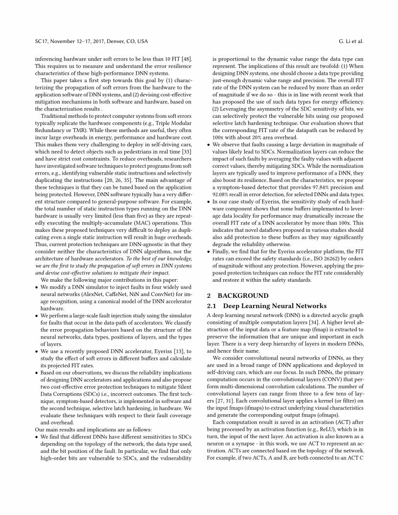
(PEs), each of which computes MACs. Figure 1 shows the architec-
ture of a general DNN accelerator. A DNN accelerator consists of
a global buffer and an array of PEs. The accelerator is connected
to DRAM where data is transferred from. A CPU is usually used to
off-load tasks to the accelerator. The overall architecture is shown
in Figure 1a. The ALU of each PE consists of a multiplier and an
adder as execution units to perform MACs — this is where the
majority of computations happen in DNNs. A general structure of
the ALU in each PE is shown in Figure 1b.
(a) Overview (b) ALU in PE
Figure 1: Architecture of general DNN accelerators
To leverage the second property of DNN algorithms, special
buffers are added on each PE as local scratchpad to cache data for
reuse. Each DNN accelerator may implement its own dataflow to
explore data localities. We classify the localities in DNNs into three
major categories:
• Weight Reuse:Weight data of each kernel can be reused in each
fmap as the convolutions involving the kernal data are used many
times on the same ifmap.
• Image Reuse: Image data of each fmap can be reused in all con-
volutions where the ifmap is involved, because different kernels
operate on the same sets of ifmap in each layer.
• Output Reuse: Computation results of MACs can be buffered
and consumed on-PE without transferring off the PEs.
Table 1 illustrates nine different DNN accelerators that have been
proposed in prior work and the corresponding data localities they
exploit in their dataflows. As can be seen, each accelerator exploits
one of more localities in its dataflow. Eyeriss [13] considers all of
the three data localities in its dataflow.
We separate faults that originate in the datapath (i.e., latches in
execution units) from those that originate in buffers (both on- and
off-PEs), because they propagate differently: faults in the datapath
will be only read once, whereas faults in buffers may be read mul-
tiple times due to reuse and hence the same fault can be spread to
multiple locations within short time windows.
Table 1: Data Reuses in DNN Accelerators
Accelerators Weight
Reuse
Image
Reuse
Output
Reuse
Zhang et al. [61], Diannao [12], Dadiannao [14] x x x
Chakradhar et al. [10], Sriram et al. [53], Sankaradas et al. [49],
nn-X [23], K-Brain [41], Origami [9]
✓ x x
Gupta et al. [24], Shidiannao [19], Peemen et al. [43] x x ✓Eyeriss [13] ✓ ✓ ✓
2.3 Consequences of Soft Errors
The consequences of soft errors that occur in DNN systems can be
catastrophic as many of them are safety-critical, and error mitiga-
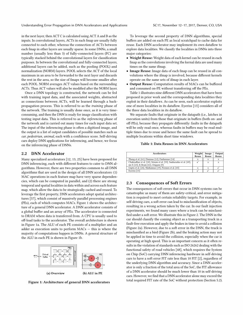
tion is required to meet certain reliability targets. For example, in
self-driving cars, a soft error can lead to misclassification of objects,
resulting in a wrong action taken by the car. In our fault injection
experiments, we found many cases where a truck can be misclassi-
fied under a soft error. We illustrate this in Figure 2. The DNN in the
car should classify the coming object as a transporting truck in a
fault-free execution and apply the brakes in time to avoid a collision
(Figure 2a). However, due to a soft error in the DNN, the truck is
misclassified as a bird (Figure 2b), and the braking action may not
be applied in time to avoid the collision, especially when the car is
operating at high speed. This is an important concern as it often re-
sults in the violation of standards such as ISO 26262 dealing with the
functional safety of road vehicles [48], which requires the System
on Chip (SoC) carrying DNN inferencing hardware in self-driving
cars to have a soft error FIT rate less than 10 FIT [2], regardless of
the underlying DNN algorithm and accuracy. Since a DNN acceler-
ator is only a fraction of the total area of the SoC, the FIT allowance
of a DNN accelerator should be much lower than 10 in self-driving
cars. However, we find that a DNN accelerator alone may exceed the
total required FIT rate of the SoC without protection (Section 5.2).
SC17, November 12–17, 2017, Denver, CO, USA G. Li et al.
(a) Fault-free execution: A truck
is identified by the DNN and
brakes are applied
(b) SDC: Truck is incorrectly
identified as bird and brakes
may be not applied
Figure 2: Example of SDC that could lead to collision in
self-driving cars due to soft errors
3 EXPLORATION OF DESIGN SPACE
We seek to understand how soft errors that occur in DNN acceler-
ators propagate in DNN applications and cause SDCs (we define
SDCs later in Section 4.6). We focus on SDCs as these are the most
insidious of failures and cannot be detected easily. There are four
parameters that impact of soft errors on DNNs:
(1) Topology and Data Type: Each DNN has its own distinct
topology which affects error propagation. Further, DNNs can also
use different data types in their implementation. We want to ex-
plore the effect of the topology and data type on the overall SDC
probability.
(2) Bit Position and Value: To further investigate the impact
of data type on error propagation, we examine the sensitivity of
each bit position in the networks using different data types. This is
because the values represented by a data type depend on the bit po-
sitions affected, as different data types interpret each bit differently
(explained in Section 4.5). Hence, we want to understand how SDC
probabilities vary based on the bit corrupted in each data type and
how the errors result in SDCs affect program values.
(3) Layers: Different DNNs have different layers - this includes
the differences in type, position, and the total number of layers. We
investigate how errors propagate in different layers and whether
the propagation is influenced by the characteristics of each layer.
(4)DataReuse:Wewant to understand how different data reuses
implemented in the dataflows of DNN accelerators affects the SDC
probability. Note that unlike other parameters, data reuse is not a
property of the DNN itself but of its hardware implementation.
4 EXPERIMENTAL SETUP
4.1 Networks
Table 2: Networks Used
Network Dataset No. of Output Candi-
dates
Topology
ConvNet [17] CIFAR-10 10 3 CONV + 2 FC
AlexNet [31] ImageNet 1,000 5 CONV(with LRN) + 3 FC
CaffeNet [8] ImageNet 1,000 5 CONV(with LRN) + 3 FC
NiN [37] ImageNet 1,000 12 CONV
We focus on convolutional neural networks in DNNs, as they
have shown great potential in solving many complex and emerging
problems and are often executed in self-driving cars. There are four
neural networks that we consider in Table 2. They range from the
relatively simple 5-layer ConvNet to the 12-layer NiN. The reasons
we chose these networks are: (1) They have different topologies and
methods implemented to cover a variety of common features used
in today’s DNNs, and the details are publicly accessible, (2) they are
often used as benchmarks in developing and testing DNN acceler-
ators [13, 30, 52], and (3) they are well known to solve challenging
problems, (4) and the official pre-trained models are freely available.
This allows us to fully reproduce the networks for benchmarking
puposes. All of the networks perform the same task, namely im-
age classification. We use the ImageNet dataset [29] for AlexNet,
CaffeNet and NiN, and the CIFAR-10 dataset [15] for ConvNet, as
they were trained and tested with these datasets. We use these
reference datasets and the pre-trained weights together with the
corresponding networks from the Berkeley Vision and Learning
Center (BVLC) [6].
We list the details of each network in Table 2. As shown, all
networks except NiN have fully-connected layers behind the convo-
lutional layers. All four networks implement ReLU as the activation
function and use the max-pooling method in their sub-sampling
layers. Both AlexNet and CaffeNet use a Local Response Normal-
ization (LRN) layer following each of the first two convolutional
layers - the only difference is the order of the ReLU and the sub-
sampling layer in each convolution layer. In AlexNet, CaffeNet and
ConvNet, there is a soft-max layer at the very end of each network
to derive the confidence score of each ranking, which is also part of
the network’s output. However, in NiN, there is no such soft-max
layer. Hence, the output of the NiN network has only the ranking
of each candidate without their confidence scores.
4.2 DNN Accelerators
We consider nine of DNN accelerators mentioned in Table 1. We
separate the faults in the datapaths of the networks from those
in the buffers. We study datapath faults based on the common ab-
straction of their execution units in Figure 1b. Thus, the results for
datapath faults apply to all nine accelerators.
For buffer faults, since the dataflow (and buffer structure) is dif-
ferent in each accelerator, we have to choose a specific design. We
chose the Eyeriss accelerator for studying buffer faults because: (1)
The dataflow of Eyeriss includes all three data localities in DNNs
listed in Table 1, which allows us to study the data reuse seen in
other DNN accelerators, and (2) the design parameters of Eyeriss
are publicly available, which allows us to conduct a comprehensive
analysis on its dataflow and overall resilience.
4.3 Fault Model
We consider transient, single-event upsets that occur in the data
path and buffers, both inside and outside the processing engines of
DNN accelerators. We do not consider faults that occur in combina-
tional logic elements as they are much less sensitive to soft errors
than storage elements shown in recent studies [22, 50]. We also do
not consider errors in control logic units. This is due to the nature
of DNN accelerators which are designed for offloaded data acceler-
ation - the scheduling is mainly done by the host (i.e., CPU). Finally,
Understanding Error Propagation in DNN Accelerators and Applications SC17, November 12–17, 2017, Denver, CO, USA
because our focus is on DNN accelerators, we do not consider faults
in the CPU, main memory, or the memory/data buses.
4.4 Fault Injection Simulation
Since we do not have access to the RTL implementations of the ac-
celerators, we use a DNN simulator for fault injection. We modified
an open-source DNN simulator framework, Tiny-CNN [56], which
accepts Caffe pre-trained weights [7] of a network for inferencing
and is written in C++. We map each line of code in the simulator to
the corresponding hardware component, so that we can pinpoint
the impact of the fault injection location in terms of the underly-
ing microarchitectural components. We randomly inject faults in
the hardware components we consider by corrupting the values in
the corresponding executions in the simulator. This fault injection
method is in line with other related work [26, 32, 35, 36, 59].
4.5 Data Types
Different data types offer different tradeoffs between energy con-
sumption and performance in DNNs. Our goal is to investigate the
sensitivity of different design parameters in data types to error prop-
agation. Therefore, we selected a wide range of data types that have
different design parameters as listed in Table 3. We classify them
into two types: floating-point data type (FP) and fixed-point data
type (FxP). For FP, we choose 64-bit double, 32-bit float, and 16-bit
half-float, all of which follow the IEEE 745 floating-point arith-
metic standard. We use the terms DOUBLE, FLOAT, and FLOAT16
respectively for these FP data types in this study. For FxPs, unfor-
tunately there is no public information about how binary points
(radix points) are chosen for specific implementations. Therefore,
we choose different binary points for each FxP.We use the following
notations to represent FxPs in this work: 16b_rb10 means a 16-bit in-
teger with 1 bit for the sign, 5 bits for the integer part, and 10 bits for
the mantissa, from the leftmost bit to the rightmost bit. We consider
three FxP types, namely 16b_rb10, 32b_rb10 and 32b_rb26. They
all implement 2’s complement for their negative arithmetic. Any
value that exceeds the maximum or minimum dynamic value range
will be saturated to the maximum or minimum value respectively.
Table 3: Data types used
Data
Type
FP or
FxP
Data
Width
Bits (From left to right)
DOUBLE FP 64-bit 1 sign bit, 11 bits for exponent, 52 bits for mantissa
FLOAT FP 32-bit 1 sign bit, 8 bits for exponent, 23 bits for mantissa
FLOAT16 FP 16-bit 1 sign bit, 5 bits for exponent, 10 bits for mantissa
32b_rb26 FxP 32-bit 1 sign bit, 5 bits for integer, 26 bits for mantissa
32b_rb10 FxP 32-bit 1 sign bit, 21 bits for integer, 10 bits for mantissa
16b_rb10 FxP 16-bit 1 sign bit, 5 bits for integer, 10 bits for mantissa
4.6 Silent Data Corruption (SDC)
We define the SDC probability as the probability of an SDC given
that the fault affects an architecturally visible state of the program
(i.e., the fault was activated). This is in line with the definition used
in other work [20, 26, 36, 59].
In a typical program, an SDCwould be a failure outcome in which
the application’s output deviates from the correct (golden) output.
This comparison is typicallymade on a bit-by-bit basis. However, for
DNNs, there is often not a single correct output, but a list of ranked
outputs each with a confidence score as described in Section 2.1, and
hence a bit-by-bit comparison would be misleading. Consequently,
we need to define new criteria to determine what constitutes an
SDC for a DNN application.We define four kinds of SDCs as follows:
• SDC-1: The top ranked element predicted by the DNN is different
from that predicted by its fault-free execution. This is the most
critical SDC because the top-ranked element is what is typically
used for downstream processing.
• SDC-5: The top ranked element is not one of the top five predicted
elements of the fault-free execution of the DNN.
• SDC-10%: The confidence score of the top ranked element varies
by more than +/-10% of its fault-free execution.
• SDC-20%: The confidence score of the top ranked element varies
by more than +/-20% of its fault-free execution.
4.7 FIT Rate Calculation
The formula of calculating the FIT rate of a hardware structure is
shown in Equation 1, where Rraw is the raw FIT rate (estimated
as 20.49 FIT/Mb by extrapolating the results of Neale et al. [39].
The original measurement for a 28nm process is 157.62 FIT/MB
in the paper. We project this for a 16nm process by applying the
trend shown in Figure 1 of the Neale paper3). Scomponent is the
size of the component, and SDCcomponent is the SDC probability of
each component. We use this formula to calculate the FIT rate of
datapath components and buffer structures of DNN accelerators, as
well as the overall FIT rate of Eyeriss in Section 5.1 and Section 5.2.
FIT =∑
componentRraw∗Scomponent∗SDCcomponent (1)
5 CHARACTERIZATION RESULTS
We organize the results based on the origins of faults (i.e., datapath
faults and buffer faults) for each parameter. We randomly injected
3,000 faults per latch, one fault for each execution of the DNN appli-
cation. The error bars for all the experimental results are calculated
based on 95% confidence intervals.
5.1 Datapath Faults
5.1.1 Data Types and Networks. Figure 3 shows the resultsof the fault injection experiments on different networks and differ-
ent data types. We make three observations based on the results.
First, SDC probabilities vary across the networks for the same
data type. For example, using the FLOAT data type, the SDC prob-
abilities for NiN are higher than for other networks using the same
data type (except ConvNet - see reason below). This is because of
the different structures of networks in terms of sub-sampling and
normalization layers which provide different levels of error mask-
ing - we further investigate this in Section 5.1.4. Further, ConvNet
has the highest SDC propagation probabilities among all the net-
works considered (we show the graph for ConvNet separately as its
SDC probabilities are significantly higher than the other networks).
This is because the structure of ConvNet is much less deep than for
other networks, and consequently there is higher error propagation
in ConvNet. For example, there are only 3 convolutional layers
3We also adjusted the original measurement by a factor of 0.65 as there is a mistake
we found in the paper. The authors of the paper have acknowledged the mistake in
private email communications with us.
SC17, November 12–17, 2017, Denver, CO, USA G. Li et al.
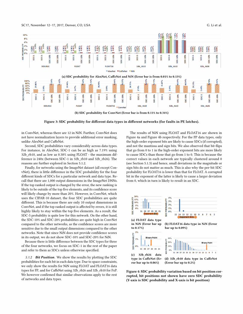
(a) SDC probability for AlexNet, CaffeNet and NiN (Error bar is from 0.01% to 0.13%)
(b) SDC probability for ConvNet (Error bar is from 0.11% to 0.34%)
Figure 3: SDC probability for different data types in different networks (for faults in PE latches).
in ConvNet, whereas there are 12 in NiN. Further, ConvNet does
not have normalization layers to provide additional error masking,
unlike AlexNet and CaffeNet.
Second, SDC probabilities vary considerably across data types.
For instance, in AlexNet, SDC-1 can be as high as 7.19% using
32b_rb10, and as low as 0.38% using FLOAT - the maximum dif-
ference is 240x (between SDC-1 in 32b_rb10 and 32b_rb26). The
reasons are further explored in Section 5.1.2.
Finally, for networks using the ImageNet dataset (all except Con-
vNet), there is little difference in the SDC probability for the four
different kinds of SDCs for a particular network and data type. Re-
call that there are 1,000 output dimensions in the ImageNet DNNs.
If the top ranked output is changed by the error, the new ranking is
likely to be outside of the top five elements, and its confidence score
will likely change by more than 20%. However, in ConvNet, which
uses the CIFAR-10 dataset, the four SDC probabilities are quite
different. This is because there are only 10 output dimensions in
ConvNet, and if the top ranked output is affected by errors, it is still
highly likely to stay within the top five elements. As a result, the
SDC-5 probability is quite low for this network. On the other hand,
the SDC-10% and SDC-20% probabilities are quite high in ConvNet
compared to the other networks, as the confidence scores are more
sensitive due to the small output dimensions compared to the other
networks. Note that since NiN does not provide confidence scores
in its output, we do not show SDC-10% and SDC-20% for NiN.
Because there is little difference between the SDC types for three
of the four networks, we focus on SDC-1 in the rest of the paper
and refer to them as SDCs unless otherwise specified.
5.1.2 Bit Position. We show the results by plotting the SDC
probabilities for each bit in each data type. Due to space constraints,
we only show the results for NiN using FLOAT and FLOAT16 data
types for FP, and for CaffeNet using 32b_rb26 and 32b_rb10 for FxP.
We however confirmed that similar observations apply to the rest
of networks and data types.
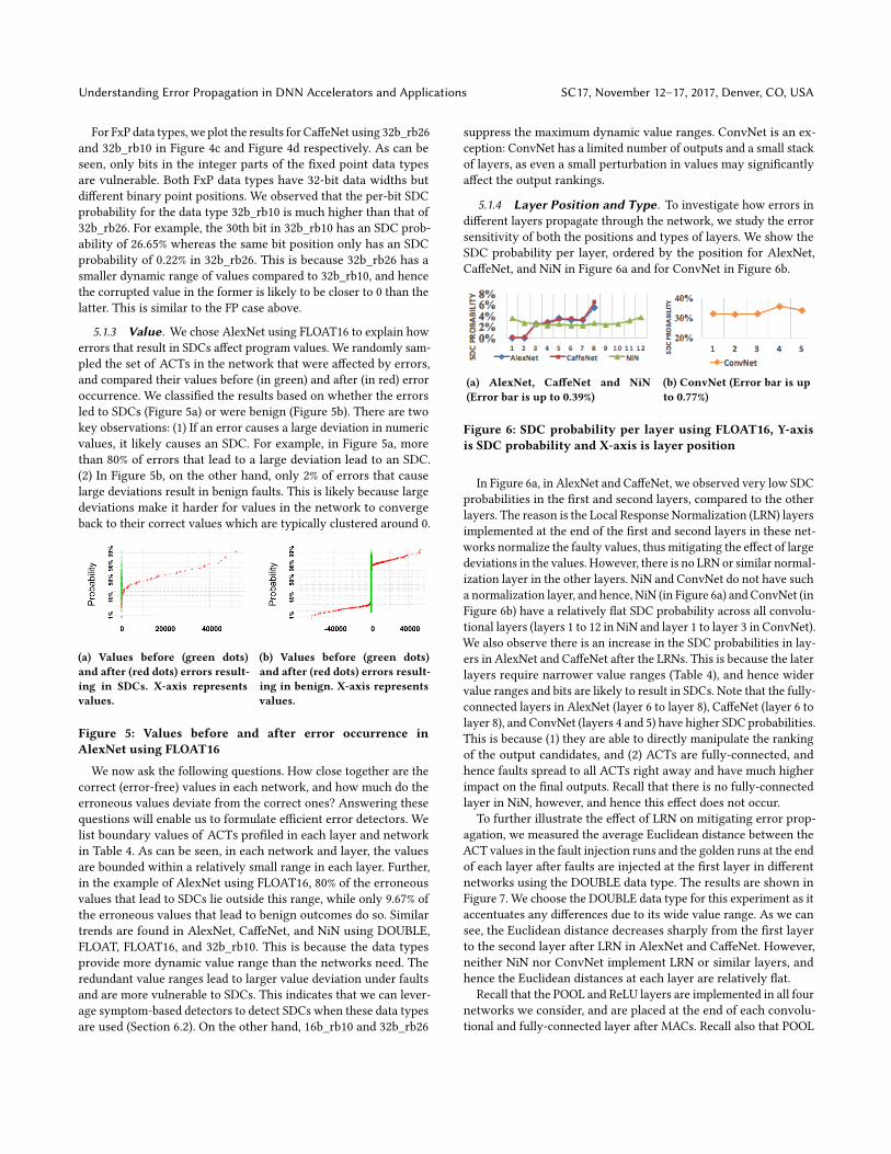
The results of NiN using FLOAT and FLOAT16 are shown in
Figure 4a and Figure 4b respectively. For the FP data types, only
the high-order exponent bits are likely to cause SDCs (if corrupted),
and not the mantissa and sign bits. We also observed that bit-flips
that go from 0 to 1 in the high-order exponent bits are more likely
to cause SDCs than those that go from 1 to 0. This is because the
correct values in each network are typically clustered around 0
(see Section 5.1.3) and hence, small deviations in the magnitude or
sign bits do not matter as much. This is also why the per-bit SDC
probability for FLOAT16 is lower than that for FLOAT. A corrupted
bit in the exponent of the latter is likely to cause a larger deviation
from 0, which in turn is likely to result in an SDC.
(a) FLOAT data type
in NiN (Error bar up
to 0.17%)
(b) FLOAT16 data type in NiN (Error
bar up to 0.09%)
(c) 32b_rb26 data
type in CaffeNet (Er-
ror bar up to 0.06%)
(d) 32b_rb10 data type in CaffeNet
(Error bar up to 0.2%)
Figure 4: SDC probability variation based on bit position cor-
rupted, bit positions not shown have zero SDC probability
(Y-axis is SDC probability and X-axis is bit position)
Understanding Error Propagation in DNN Accelerators and Applications SC17, November 12–17, 2017, Denver, CO, USA
For FxP data types, we plot the results for CaffeNet using 32b_rb26
and 32b_rb10 in Figure 4c and Figure 4d respectively. As can be
seen, only bits in the integer parts of the fixed point data types
are vulnerable. Both FxP data types have 32-bit data widths but
different binary point positions. We observed that the per-bit SDC
probability for the data type 32b_rb10 is much higher than that of
32b_rb26. For example, the 30th bit in 32b_rb10 has an SDC prob-
ability of 26.65% whereas the same bit position only has an SDC
probability of 0.22% in 32b_rb26. This is because 32b_rb26 has a
smaller dynamic range of values compared to 32b_rb10, and hence
the corrupted value in the former is likely to be closer to 0 than the
latter. This is similar to the FP case above.
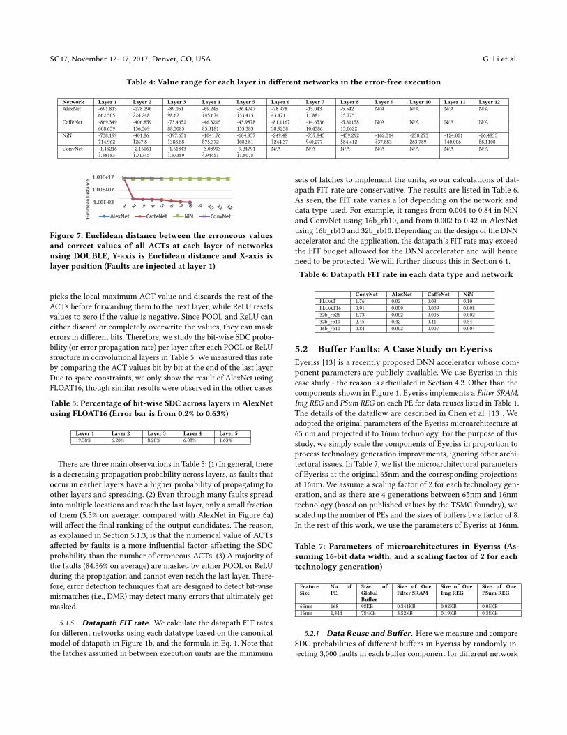
5.1.3 Value. We chose AlexNet using FLOAT16 to explain how
errors that result in SDCs affect program values. We randomly sam-
pled the set of ACTs in the network that were affected by errors,
and compared their values before (in green) and after (in red) error
occurrence. We classified the results based on whether the errors
led to SDCs (Figure 5a) or were benign (Figure 5b). There are two
key observations: (1) If an error causes a large deviation in numeric
values, it likely causes an SDC. For example, in Figure 5a, more
than 80% of errors that lead to a large deviation lead to an SDC.
(2) In Figure 5b, on the other hand, only 2% of errors that cause
large deviations result in benign faults. This is likely because large
deviations make it harder for values in the network to converge
back to their correct values which are typically clustered around 0.
(a) Values before (green dots)
and after (red dots) errors result-
ing in SDCs. X-axis represents
values.
(b) Values before (green dots)
and after (red dots) errors result-
ing in benign. X-axis represents
values.
Figure 5: Values before and after error occurrence in
AlexNet using FLOAT16
We now ask the following questions. How close together are the
correct (error-free) values in each network, and how much do the
erroneous values deviate from the correct ones? Answering these
questions will enable us to formulate efficient error detectors. We
list boundary values of ACTs profiled in each layer and network
in Table 4. As can be seen, in each network and layer, the values
are bounded within a relatively small range in each layer. Further,
in the example of AlexNet using FLOAT16, 80% of the erroneous
values that lead to SDCs lie outside this range, while only 9.67% of
the erroneous values that lead to benign outcomes do so. Similar
trends are found in AlexNet, CaffeNet, and NiN using DOUBLE,
FLOAT, FLOAT16, and 32b_rb10. This is because the data types
provide more dynamic value range than the networks need. The
redundant value ranges lead to larger value deviation under faults
and are more vulnerable to SDCs. This indicates that we can lever-
age symptom-based detectors to detect SDCs when these data types
are used (Section 6.2). On the other hand, 16b_rb10 and 32b_rb26
suppress the maximum dynamic value ranges. ConvNet is an ex-
ception: ConvNet has a limited number of outputs and a small stack
of layers, as even a small perturbation in values may significantly
affect the output rankings.
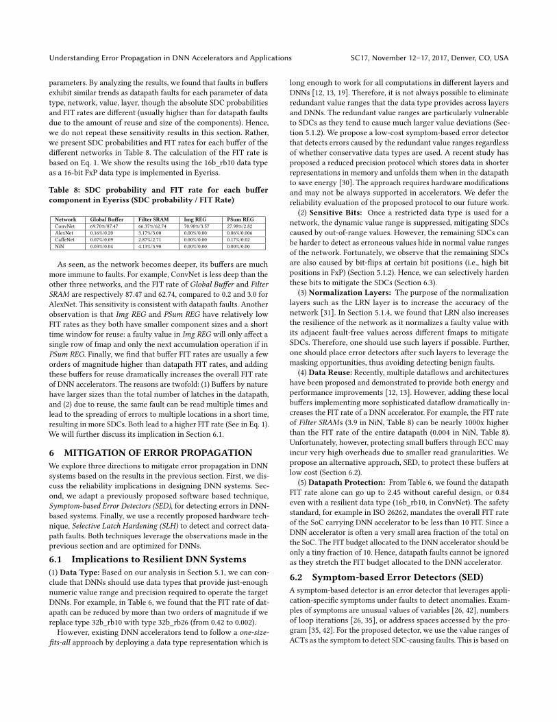
5.1.4 Layer Position and Type. To investigate how errors in
different layers propagate through the network, we study the error
sensitivity of both the positions and types of layers. We show the
SDC probability per layer, ordered by the position for AlexNet,
CaffeNet, and NiN in Figure 6a and for ConvNet in Figure 6b.
(a) AlexNet, CaffeNet and NiN
(Error bar is up to 0.39%)
(b) ConvNet (Error bar is up
to 0.77%)
Figure 6: SDC probability per layer using FLOAT16, Y-axis
is SDC probability and X-axis is layer position
In Figure 6a, in AlexNet and CaffeNet, we observed very low SDC
probabilities in the first and second layers, compared to the other
layers. The reason is the Local Response Normalization (LRN) layers
implemented at the end of the first and second layers in these net-
works normalize the faulty values, thus mitigating the effect of large
deviations in the values. However, there is no LRN or similar normal-
ization layer in the other layers. NiN and ConvNet do not have such
a normalization layer, and hence, NiN (in Figure 6a) and ConvNet (in
Figure 6b) have a relatively flat SDC probability across all convolu-
tional layers (layers 1 to 12 in NiN and layer 1 to layer 3 in ConvNet).
We also observe there is an increase in the SDC probabilities in lay-
ers in AlexNet and CaffeNet after the LRNs. This is because the later
layers require narrower value ranges (Table 4), and hence wider
value ranges and bits are likely to result in SDCs. Note that the fully-
connected layers in AlexNet (layer 6 to layer 8), CaffeNet (layer 6 to
layer 8), and ConvNet (layers 4 and 5) have higher SDC probabilities.
This is because (1) they are able to directly manipulate the ranking
of the output candidates, and (2) ACTs are fully-connected, and
hence faults spread to all ACTs right away and have much higher
impact on the final outputs. Recall that there is no fully-connected
layer in NiN, however, and hence this effect does not occur.
To further illustrate the effect of LRN on mitigating error prop-
agation, we measured the average Euclidean distance between the
ACT values in the fault injection runs and the golden runs at the end
of each layer after faults are injected at the first layer in different
networks using the DOUBLE data type. The results are shown in
Figure 7. We choose the DOUBLE data type for this experiment as it
accentuates any differences due to its wide value range. As we can
see, the Euclidean distance decreases sharply from the first layer
to the second layer after LRN in AlexNet and CaffeNet. However,
neither NiN nor ConvNet implement LRN or similar layers, and
hence the Euclidean distances at each layer are relatively flat.
Recall that the POOL and ReLU layers are implemented in all four
networks we consider, and are placed at the end of each convolu-
tional and fully-connected layer after MACs. Recall also that POOL
SC17, November 12–17, 2017, Denver, CO, USA G. Li et al.
Table 4: Value range for each layer in different networks in the error-free execution
Network Layer 1 Layer 2 Layer 3 Layer 4 Layer 5 Layer 6 Layer 7 Layer 8 Layer 9 Layer 10 Layer 11 Layer 12
AlexNet -691.813
6̃62.505
-228.296
2̃24.248
-89.051
9̃8.62
-69.245
1̃45.674
-36.4747
1̃33.413
-78.978
4̃3.471
-15.043
1̃1.881
-5.542
1̃5.775
N/A N/A N/A N/A
CaffeNet -869.349
6̃08.659
-406.859
1̃56.569
-73.4652
8̃8.5085
-46.3215
8̃5.3181
-43.9878
1̃55.383
-81.1167
3̃8.9238
-14.6536
1̃0.4386
-5.81158
1̃5.0622
N/A N/A N/A N/A
NiN -738.199
7̃14.962
-401.86
1̃267.8
-397.651
1̃388.88
-1041.76
8̃75.372
-684.957
1̃082.81
-249.48
1̃244.37
-737.845
9̃40.277
-459.292
5̃84.412
-162.314
4̃37.883
-258.273
2̃83.789
-124.001
1̃40.006
-26.4835
8̃8.1108
ConvNet -1.45216
1̃.38183
-2.16061
1̃.71745
-1.61843
1̃.37389
-3.08903
4̃.94451
-9.24791
1̃1.8078
N/A N/A N/A N/A N/A N/A N/A
Figure 7: Euclidean distance between the erroneous values
and correct values of all ACTs at each layer of networks
using DOUBLE, Y-axis is Euclidean distance and X-axis is
layer position (Faults are injected at layer 1)
picks the local maximum ACT value and discards the rest of the
ACTs before forwarding them to the next layer, while ReLU resets
values to zero if the value is negative. Since POOL and ReLU can
either discard or completely overwrite the values, they can mask
errors in different bits. Therefore, we study the bit-wise SDC proba-
bility (or error propagation rate) per layer after each POOL or ReLU
structure in convolutional layers in Table 5. We measured this rate
by comparing the ACT values bit by bit at the end of the last layer.
Due to space constraints, we only show the result of AlexNet using
FLOAT16, though similar results were observed in the other cases.
Table 5: Percentage of bit-wise SDC across layers in AlexNet
using FLOAT16 (Error bar is from 0.2% to 0.63%)
Layer 1 Layer 2 Layer 3 Layer 4 Layer 5
19.38% 6.20% 8.28% 6.08% 1.63%
There are three main observations in Table 5: (1) In general, there
is a decreasing propagation probability across layers, as faults that
occur in earlier layers have a higher probability of propagating to
other layers and spreading. (2) Even through many faults spread
into multiple locations and reach the last layer, only a small fraction
of them (5.5% on average, compared with AlexNet in Figure 6a)
will affect the final ranking of the output candidates. The reason,
as explained in Section 5.1.3, is that the numerical value of ACTs
affected by faults is a more influential factor affecting the SDC
probability than the number of erroneous ACTs. (3) A majority of
the faults (84.36% on average) are masked by either POOL or ReLU
during the propagation and cannot even reach the last layer. There-
fore, error detection techniques that are designed to detect bit-wise
mismatches (i.e., DMR) may detect many errors that ultimately get
masked.
5.1.5 Datapath FIT rate. We calculate the datapath FIT rates
for different networks using each datatype based on the canonical
model of datapath in Figure 1b, and the formula in Eq. 1. Note that
the latches assumed in between execution units are the minimum
sets of latches to implement the units, so our calculations of dat-
apath FIT rate are conservative. The results are listed in Table 6.
As seen, the FIT rate varies a lot depending on the network and
data type used. For example, it ranges from 0.004 to 0.84 in NiN
and ConvNet using 16b_rb10, and from 0.002 to 0.42 in AlexNet
using 16b_rb10 and 32b_rb10. Depending on the design of the DNN
accelerator and the application, the datapath’s FIT rate may exceed
the FIT budget allowed for the DNN accelerator and will hence
need to be protected. We will further discuss this in Section 6.1.
Table 6: Datapath FIT rate in each data type and network
ConvNet AlexNet CaffeNet NiN
FLOAT 1.76 0.02 0.03 0.10
FLOAT16 0.91 0.009 0.009 0.008
32b_rb26 1.73 0.002 0.005 0.002
32b_rb10 2.45 0.42 0.41 0.54
16b_rb10 0.84 0.002 0.007 0.004
5.2 Buffer Faults: A Case Study on Eyeriss
Eyeriss [13] is a recently proposed DNN accelerator whose com-
ponent parameters are publicly available. We use Eyeriss in this
case study - the reason is articulated in Section 4.2. Other than the
components shown in Figure 1, Eyeriss implements a Filter SRAM,
Img REG and PSum REG on each PE for data reuses listed in Table 1.
The details of the dataflow are described in Chen et al. [13]. We
adopted the original parameters of the Eyeriss microarchitecture at
65 nm and projected it to 16nm technology. For the purpose of this
study, we simply scale the components of Eyeriss in proportion to
process technology generation improvements, ignoring other archi-
tectural issues. In Table 7, we list the microarchitectural parameters
of Eyeriss at the original 65nm and the corresponding projections
at 16nm. We assume a scaling factor of 2 for each technology gen-
eration, and as there are 4 generations between 65nm and 16nm
technology (based on published values by the TSMC foundry), we
scaled up the number of PEs and the sizes of buffers by a factor of 8.
In the rest of this work, we use the parameters of Eyeriss at 16nm.
Table 7: Parameters of microarchitectures in Eyeriss (As-
suming 16-bit data width, and a scaling factor of 2 for each
technology generation)
Feature
Size
No. of
PE
Size of
Global
Buffer
Size of One
Filter SRAM
Size of One
Img REG
Size of One
PSum REG
65nm 168 98KB 0.344KB 0.02KB 0.05KB
16nm 1,344 784KB 3.52KB 0.19KB 0.38KB
5.2.1 Data Reuse and Buffer. Here we measure and compare
SDC probabilities of different buffers in Eyeriss by randomly in-
jecting 3,000 faults in each buffer component for different network
Understanding Error Propagation in DNN Accelerators and Applications SC17, November 12–17, 2017, Denver, CO, USA
parameters. By analyzing the results, we found that faults in buffers
exhibit similar trends as datapath faults for each parameter of data
type, network, value, layer, though the absolute SDC probabilities
and FIT rates are different (usually higher than for datapath faults
due to the amount of reuse and size of the components). Hence,
we do not repeat these sensitivity results in this section. Rather,
we present SDC probabilities and FIT rates for each buffer of the
different networks in Table 8. The calculation of the FIT rate is
based on Eq. 1. We show the results using the 16b_rb10 data type
as a 16-bit FxP data type is implemented in Eyeriss.
Table 8: SDC probability and FIT rate for each buffer
component in Eyeriss (SDC probability / FIT Rate)
Network Global Buffer Filter SRAM Img REG PSum REG
ConvNet 69.70%/87.47 66.37%/62.74 70.90%/3.57 27.98%/2.82
AlexNet 0.16%/0.20 3.17%/3.00 0.00%/0.00 0.06%/0.006
CaffeNet 0.07%/0.09 2.87%/2.71 0.00%/0.00 0.17%/0.02
NiN 0.03%/0.04 4.13%/3.90 0.00%/0.00 0.00%/0.00
As seen, as the network becomes deeper, its buffers are much
more immune to faults. For example, ConvNet is less deep than the
other three networks, and the FIT rate of Global Buffer and Filter
SRAM are respectively 87.47 and 62.74, compared to 0.2 and 3.0 for
AlexNet. This sensitivity is consistent with datapath faults. Another
observation is that Img REG and PSum REG have relatively low
FIT rates as they both have smaller component sizes and a short
time window for reuse: a faulty value in Img REG will only affect a
single row of fmap and only the next accumulation operation if in
PSum REG. Finally, we find that buffer FIT rates are usually a few
orders of magnitude higher than datapath FIT rates, and adding
these buffers for reuse dramatically increases the overall FIT rate
of DNN accelerators. The reasons are twofold: (1) Buffers by nature
have larger sizes than the total number of latches in the datapath,
and (2) due to reuse, the same fault can be read multiple times and
lead to the spreading of errors to multiple locations in a short time,
resulting in more SDCs. Both lead to a higher FIT rate (See in Eq. 1).
We will further discuss its implication in Section 6.1.
6 MITIGATION OF ERROR PROPAGATION
We explore three directions to mitigate error propagation in DNN
systems based on the results in the previous section. First, we dis-
cuss the reliability implications in designing DNN systems. Sec-
ond, we adapt a previously proposed software based technique,
Symptom-based Error Detectors (SED), for detecting errors in DNN-
based systems. Finally, we use a recently proposed hardware tech-
nique, Selective Latch Hardening (SLH) to detect and correct data-
path faults. Both techniques leverage the observations made in the
previous section and are optimized for DNNs.
6.1 Implications to Resilient DNN Systems
(1) Data Type: Based on our analysis in Section 5.1, we can con-
clude that DNNs should use data types that provide just-enough
numeric value range and precision required to operate the target
DNNs. For example, in Table 6, we found that the FIT rate of dat-
apath can be reduced by more than two orders of magnitude if we
replace type 32b_rb10 with type 32b_rb26 (from 0.42 to 0.002).
However, existing DNN accelerators tend to follow a one-size-
fits-all approach by deploying a data type representation which is
long enough to work for all computations in different layers and
DNNs [12, 13, 19]. Therefore, it is not always possible to eliminate
redundant value ranges that the data type provides across layers
and DNNs. The redundant value ranges are particularly vulnerable
to SDCs as they tend to cause much larger value deviations (Sec-
tion 5.1.2). We propose a low-cost symptom-based error detector
that detects errors caused by the redundant value ranges regardless
of whether conservative data types are used. A recent study has
proposed a reduced precision protocol which stores data in shorter
representations in memory and unfolds them when in the datapath
to save energy [30]. The approach requires hardware modifications
and may not be always supported in accelerators. We defer the
reliability evaluation of the proposed protocol to our future work.
(2) Sensitive Bits: Once a restricted data type is used for a
network, the dynamic value range is suppressed, mitigating SDCs
caused by out-of-range values. However, the remaining SDCs can
be harder to detect as erroneous values hide in normal value ranges
of the network. Fortunately, we observe that the remaining SDCs
are also caused by bit-flips at certain bit positions (i.e., high bit
positions in FxP) (Section 5.1.2). Hence, we can selectively harden
these bits to mitigate the SDCs (Section 6.3).
(3) Normalization Layers: The purpose of the normalization
layers such as the LRN layer is to increase the accuracy of the
network [31]. In Section 5.1.4, we found that LRN also increases
the resilience of the network as it normalizes a faulty value with
its adjacent fault-free values across different fmaps to mitigate
SDCs. Therefore, one should use such layers if possible. Further,
one should place error detectors after such layers to leverage the
masking opportunities, thus avoiding detecting benign faults.
(4) Data Reuse: Recently, multiple dataflows and architectures
have been proposed and demonstrated to provide both energy and
performance improvements [12, 13]. However, adding these local
buffers implementing more sophisticated dataflow dramatically in-
creases the FIT rate of a DNN accelerator. For example, the FIT rate
of Filter SRAMs (3.9 in NiN, Table 8) can be nearly 1000x higher
than the FIT rate of the entire datapath (0.004 in NiN, Table 8).
Unfortunately, however, protecting small buffers through ECC may
incur very high overheads due to smaller read granularities. We
propose an alternative approach, SED, to protect these buffers at
low cost (Section 6.2).
(5) Datapath Protection: From Table 6, we found the datapath
FIT rate alone can go up to 2.45 without careful design, or 0.84
even with a resilient data type (16b_rb10, in ConvNet). The safety
standard, for example in ISO 26262, mandates the overall FIT rate
of the SoC carrying DNN accelerator to be less than 10 FIT. Since a
DNN accelerator is often a very small area fraction of the total on
the SoC. The FIT budget allocated to the DNN accelerator should be
only a tiny fraction of 10. Hence, datapath faults cannot be ignored
as they stretch the FIT budget allocated to the DNN accelerator.
6.2 Symptom-based Error Detectors (SED)
A symptom-based detector is an error detector that leverages appli-
cation-specific symptoms under faults to detect anomalies. Exam-
ples of symptoms are unusual values of variables [26, 42], numbers
of loop iterations [26, 35], or address spaces accessed by the pro-
gram [35, 42]. For the proposed detector, we use the value ranges of
ACTs as the symptom to detect SDC-causing faults. This is based on
SC17, November 12–17, 2017, Denver, CO, USA G. Li et al.
the observation from Section 5.1.3: If an error makes the magnitude
of ACTs very large, it likely leads to an SDC, and if it does not, it
is likely to be benign. In the design of the error detector, there are
two questions that need to be answered: Where (which program
locations) and What (which reference value ranges) to check? The
proposed detector consists of two phases - we describe each phase
along with the answers to the two questions below:
Learning: Before deploying the detector, a DNN application
needs to be instrumented and executed with its representative test
inputs to derive the value ranges in each layer during the fault-
free execution. We can use these value ranges, say -X to Y, as the
bounds for the detector. However, to be safe, we apply an addi-
tional 10% cushion on top of the value ranges of each layer, that
is (-1.1*X) to (1.1*Y) as the reference values for each detector to
reduce false alarms. Note that the learning phase is only required
to be performed once before the deployment.
Deployment: Once the detectors are derived, they are checked
by the host which off-loads tasks to the DNN accelerator. At the end
of each layer, the data of fmaps of the current layer are calculated
and transferred to the global buffer from the PE array as the input
data of ifmaps for the next layer. These data will stay in the global
buffer during the entire execution of the next layer for reuse. This
gives us an opportunity to execute the detector asynchronously
from the host, and check the values in global buffer to detect er-
rors. We perform the detection asynchronously to keep the runtime
overheads as low as possible.
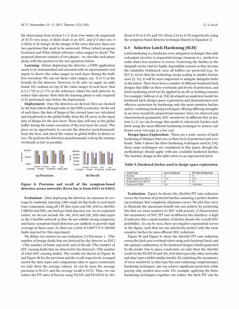
(a) Precision (b) Recall
Figure 8: Precision and recall of the symptom-based
detectors across networks (Error bar is from 0.03% to 0.04%)
Evaluation: After deploying the detector, we measure its cov-
erage by randomly injecting 3,000 single bit-flip faults in each hard-
ware component, using all 3 FP data types and 32b_rb10 in AlexNet,
CaffeNet and NiN, one fault per fault injection run. As we explained
earlier, we do not include the 16b_rb10 and 32b_rb26 data types
or the ConvNet network as they do not exhibit strong symptoms,
and hence symptom-based detectors are unlikely to provide high
coverage in these cases. So there are a total of 3,000*5*4*3=180,000
faults injected for this experiment.
We define two metrics in our evaluation: (1) Precision: 1 - (The
number of benign faults that are detected by the detector as SDC)
/ (The number of faults injected), and (2) Recall: (The number of
SDC-causing faults that are detected by the detector) / (The number
of total SDC-causing faults). The results are shown in Figure 8a
and Figure 8b for the precision and the recall respectively averaged
across the data types and components (due to space constraints,
we only show the average values). As can be seen, the average
precision is 90.21% and the average recall is 92.5%. Thus, we can
reduce the FIT rates of Eyeriss using FLOAT and FLOAT16 by 96%
(from 8.55 to 0.35) and 70% (from 2.63 to 0.79) respectively using
the symptom-based detector technique (based on Equation 1).
6.3 Selective Latch Hardening (SLH)
Latch hardening is a hardware error mitigation technique that adds
redundant circuitry to sequential storage elements (i.e., latches) to
make them less sensitive to errors. Protecting the latches in the
datapath can be vital for highly dependable systems as they become
the reliability bottleneck once all buffers are protected (e.g., by
ECCs). Given that the technology keeps scaling to smaller feature
sizes [5, 16], it will be more important to mitigate datapath faults
in the future. There have been a number of different hardened latch
designs that differ in their overheads and levels of protection, and
latch hardening need not be applied in an all-or-nothing manner.
For example, Sullivan et al. [54] developed an analytical model for
hardened latch design space exploration and demonstrated cost-
effective protection by hardening only the most sensitive latches
and by combining hardening techniques offering differing strengths
in an error-sensitivity proportional manner. Since we observed and
characterized asymmetric SDC sensitivity in different bits in Sec-
tion 5.1.2, we can leverage this model to selectively harden each
latch using the most efficient hardening technique to achieve suf-
ficient error coverage at a low cost.
Design Space Exploration: There are a wide variety of latch
hardening techniques that vary in their level of protection and over-
heads. Table 9 shows the three hardening techniques used by [54];
these same techniques are considered in this paper, though the
methodology should apply with any available hardened latches.
The baseline design in the table refers to an unprotected latch.
Table 9: Hardened latches used in design space exploration
Latch Type Area Overhead FIT Rate Reduction
Baseline 1x 1x
Strike Suppression (RCC) 1.15x 6.3x
Redundant Node (SEUT) 2x 37x
Triplicated (TMR) 3.5x 1,000,000x
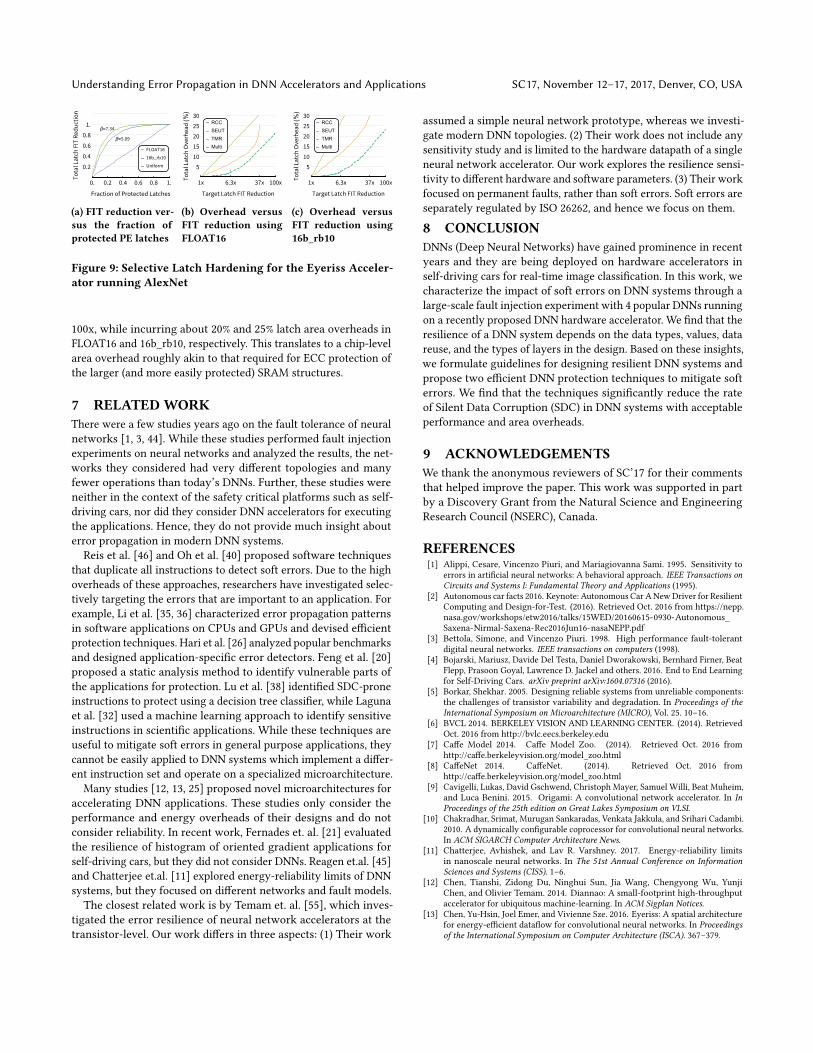
Evaluation: Figure 9a shows the AlexNet FIT rate reduction
versus the fraction of protected latches assuming a perfect harden-
ing technique that completely eliminates errors. We plot this curve
to illustrate the maximum benefit one can achieve by protecting
bits that are more sensitive to SDC with priority. β characterizes
the asymmetry of SDC FIT rate in different bits (latches)—a high
β indicates that a small number of latches dictate the overall SDC
probability. As can be seen, there are negative exponential curves
in the figure, such that we can selectively protect only the most
sensitive latches for area-efficient SDC reduction.
Figure 9b and Figure 9c show the AlexNet FIT rate reduction
versus the latch area overhead when using each hardened latch, and
the optimal combination of the hardened designs (Multi) generated
by the model. Due to space constraints, we only show the AlexNet
result for the FLOAT16 and 16b_rb10 data types (the other networks
and data types exhibit similar trends). By exploiting the asymmetry
of error sensitivity in data type bits and combining complementary
hardening techniques, one can achieve significant protection while
paying only modest area costs. For example, applying the three
hardening techniques together can reduce the latch FIT rate by
Understanding Error Propagation in DNN Accelerators and Applications SC17, November 12–17, 2017, Denver, CO, USA
FLOAT16
16b_rb10
Uniform
0. 0.2 0.4 0.6 0.8 1.
0.2
0.4
0.6
0.8
1.
Fraction of Protected Latches
Tota
lLat
chFI
TRe
duct
ion
β=7.34
β=5.09
(a) FIT reduction ver-
sus the fraction of
protected PE latches
RCC
SEUT
TMR
Multi
1x 6.3x 37x 100x
5
10
15
20
25
30
Target Latch FIT ReductionTo
talL
atch
Ove
rhea
d(%
)
(b) Overhead versus
FIT reduction using
FLOAT16
RCC
SEUT
TMR
Multi
1x 6.3x 37x 100x
5
10
15
20
25
30
Target Latch FIT Reduction
Tota
lLat
chO
verh
ead(%
)
(c) Overhead versus
FIT reduction using
16b_rb10
Figure 9: Selective Latch Hardening for the Eyeriss Acceler-
ator running AlexNet
100x, while incurring about 20% and 25% latch area overheads in
FLOAT16 and 16b_rb10, respectively. This translates to a chip-level
area overhead roughly akin to that required for ECC protection of
the larger (and more easily protected) SRAM structures.
7 RELATEDWORK
There were a few studies years ago on the fault tolerance of neural
networks [1, 3, 44]. While these studies performed fault injection
experiments on neural networks and analyzed the results, the net-
works they considered had very different topologies and many
fewer operations than today’s DNNs. Further, these studies were
neither in the context of the safety critical platforms such as self-
driving cars, nor did they consider DNN accelerators for executing
the applications. Hence, they do not provide much insight about
error propagation in modern DNN systems.
Reis et al. [46] and Oh et al. [40] proposed software techniques
that duplicate all instructions to detect soft errors. Due to the high
overheads of these approaches, researchers have investigated selec-
tively targeting the errors that are important to an application. For
example, Li et al. [35, 36] characterized error propagation patterns
in software applications on CPUs and GPUs and devised efficient
protection techniques. Hari et al. [26] analyzed popular benchmarks
and designed application-specific error detectors. Feng et al. [20]
proposed a static analysis method to identify vulnerable parts of
the applications for protection. Lu et al. [38] identified SDC-prone
instructions to protect using a decision tree classifier, while Laguna
et al. [32] used a machine learning approach to identify sensitive
instructions in scientific applications. While these techniques are
useful to mitigate soft errors in general purpose applications, they
cannot be easily applied to DNN systems which implement a differ-
ent instruction set and operate on a specialized microarchitecture.
Many studies [12, 13, 25] proposed novel microarchitectures for
accelerating DNN applications. These studies only consider the
performance and energy overheads of their designs and do not
consider reliability. In recent work, Fernades et. al. [21] evaluated
the resilience of histogram of oriented gradient applications for
self-driving cars, but they did not consider DNNs. Reagen et.al. [45]
and Chatterjee et.al. [11] explored energy-reliability limits of DNN
systems, but they focused on different networks and fault models.
The closest related work is by Temam et. al. [55], which inves-
tigated the error resilience of neural network accelerators at the
transistor-level. Our work differs in three aspects: (1) Their work
assumed a simple neural network prototype, whereas we investi-
gate modern DNN topologies. (2) Their work does not include any
sensitivity study and is limited to the hardware datapath of a single
neural network accelerator. Our work explores the resilience sensi-
tivity to different hardware and software parameters. (3) Their work
focused on permanent faults, rather than soft errors. Soft errors are
separately regulated by ISO 26262, and hence we focus on them.
8 CONCLUSION
DNNs (Deep Neural Networks) have gained prominence in recent
years and they are being deployed on hardware accelerators in
self-driving cars for real-time image classification. In this work, we
characterize the impact of soft errors on DNN systems through a
large-scale fault injection experiment with 4 popular DNNs running
on a recently proposed DNN hardware accelerator. We find that the
resilience of a DNN system depends on the data types, values, data
reuse, and the types of layers in the design. Based on these insights,
we formulate guidelines for designing resilient DNN systems and
propose two efficient DNN protection techniques to mitigate soft
errors. We find that the techniques significantly reduce the rate
of Silent Data Corruption (SDC) in DNN systems with acceptable
performance and area overheads.
9 ACKNOWLEDGEMENTS
We thank the anonymous reviewers of SC’17 for their comments
that helped improve the paper. This work was supported in part
by a Discovery Grant from the Natural Science and Engineering
Research Council (NSERC), Canada.
REFERENCES
[1] Alippi, Cesare, Vincenzo Piuri, and Mariagiovanna Sami. 1995. Sensitivity to
errors in artificial neural networks: A behavioral approach. IEEE Transactions on
Circuits and Systems I: Fundamental Theory and Applications (1995).
[2] Autonomous car facts 2016. Keynote: Autonomous Car ANewDriver for Resilient
Computing and Design-for-Test. (2016). Retrieved Oct. 2016 from https://nepp.
nasa.gov/workshops/etw2016/talks/15WED/20160615-0930-Autonomous_
Saxena-Nirmal-Saxena-Rec2016Jun16-nasaNEPP.pdf
[3] Bettola, Simone, and Vincenzo Piuri. 1998. High performance fault-tolerant
digital neural networks. IEEE transactions on computers (1998).
[4] Bojarski, Mariusz, Davide Del Testa, Daniel Dworakowski, Bernhard Firner, Beat
Flepp, Prasoon Goyal, Lawrence D. Jackel and others. 2016. End to End Learning
for Self-Driving Cars. arXiv preprint arXiv:1604.07316 (2016).
[5] Borkar, Shekhar. 2005. Designing reliable systems from unreliable components:
the challenges of transistor variability and degradation. In Proceedings of the
International Symposium on Microarchitecture (MICRO), Vol. 25. 10–16.
[6] BVCL 2014. BERKELEY VISION AND LEARNING CENTER. (2014). Retrieved
Oct. 2016 from http://bvlc.eecs.berkeley.edu
[7] Caffe Model 2014. Caffe Model Zoo. (2014). Retrieved Oct. 2016 from
http://caffe.berkeleyvision.org/model_zoo.html
[8] CaffeNet 2014. CaffeNet. (2014). Retrieved Oct. 2016 from
http://caffe.berkeleyvision.org/model_zoo.html
[9] Cavigelli, Lukas, David Gschwend, Christoph Mayer, Samuel Willi, Beat Muheim,
and Luca Benini. 2015. Origami: A convolutional network accelerator. In In
Proceedings of the 25th edition on Great Lakes Symposium on VLSI.
[10] Chakradhar, Srimat, Murugan Sankaradas, Venkata Jakkula, and Srihari Cadambi.
2010. A dynamically configurable coprocessor for convolutional neural networks.
In ACM SIGARCH Computer Architecture News.
[11] Chatterjee, Avhishek, and Lav R. Varshney. 2017. Energy-reliability limits
in nanoscale neural networks. In The 51st Annual Conference on Information
Sciences and Systems (CISS). 1–6.
[12] Chen, Tianshi, Zidong Du, Ninghui Sun, Jia Wang, Chengyong Wu, Yunji
Chen, and Olivier Temam. 2014. Diannao: A small-footprint high-throughput
accelerator for ubiquitous machine-learning. In ACM Sigplan Notices.
[13] Chen, Yu-Hsin, Joel Emer, and Vivienne Sze. 2016. Eyeriss: A spatial architecture
for energy-efficient dataflow for convolutional neural networks. In Proceedings
of the International Symposium on Computer Architecture (ISCA). 367–379.
SC17, November 12–17, 2017, Denver, CO, USA G. Li et al.
[14] Chen, Yunji, Tao Luo, Shaoli Liu, Shijin Zhang, Liqiang He, Jia Wang, Ling Li
and others. 2014. Dadiannao: A machine-learning supercomputer. In Proceedings
of the International Symposium on Microarchitecture (MICRO).
[15] CIFAR dataset 2014. CIFAR-10. (2014). Retrieved Oct. 2016 from
https://www.cs.toronto.edu/~kriz/cifar.html
[16] Constantinescu, Cristian. 2008. Intermittent faults and effects on reliability
of integrated circuits. In Proceedings of the Reliability and Maintainability
Symposium. 370.
[17] ConvNet 2014. High-performance C++/CUDA implementation of
convolutional neural networks. (2014). Retrieved Oct. 2016 from
https://code.google.com/p/cuda-convnet
[18] Dahl, George E., Dong Yu, Li Deng, and Alex Acero. 2012. Context-dependent
pre-trained deep neural networks for large-vocabulary speech recognition. IEEE
Transactions on Audio, Speech, and Language Processing 20, 1 (2012), 30–42.
[19] Du, Zidong, Robert Fasthuber, Tianshi Chen, Paolo Ienne, Ling Li, Tao Luo,
Xiaobing Feng, Yunji Chen, and Olivier Temam. 2015. ShiDianNao: shifting vision
processing closer to the sensor. In ACM SIGARCH Computer Architecture News.
[20] Feng, Shuguang and Gupta, Shantanu and Ansari, Amin and Mahlke, Scott. 2010.
Shoestring: probabilistic soft error reliability on the cheap. In ACM SIGARCH
Computer Architecture News, Vol. 38. ACM, 385–396.
[21] Fernandes, Fernando and Weigel, Lucas and Jung, Claudio and Navaux, Philippe
and Carro, Luigi and Rech, Paolo. 2016. Evaluation of histogram of oriented
gradients soft errors criticality for automotive applications. ACM Transactions
on Architecture and Code Optimization (TACO) 13, 4 (2016), 38.
[22] Gill, B., N. Seifert, and V. Zia. 2009. Comparison of alpha-particle and neutron-
induced combinational and sequential logic error rates at the 32nm technology
node. In Proceedings of the International Reliability Physics Symposium (IRPS).
[23] Gokhale, Vinayak, Jonghoon Jin, Aysegul Dundar, Berin Martini, and Eugenio
Culurciello. 2014. A 240 g-ops/s mobile coprocessor for deep neural networks. In
In Proceedings of the IEEE Conference on Computer Vision and Pattern Recognition
Workshops.
[24] Gupta, Suyog, Ankur Agrawal, Kailash Gopalakrishnan, and Pritish Narayanan.
2015. Deep learning with limited numerical precision. (2015).
[25] Han, Song, Xingyu Liu, Huizi Mao, Jing Pu, Ardavan Pedram, Mark A. Horowitz,
and William J. Dally. 2016. EIE: efficient inference engine on compressed deep
neural network. (2016).
[26] Hari, Siva Kumar Sastry and Adve, Sarita V and Naeimi, Helia. 2012. Low-cost
program-level detectors for reducing silent data corruptions. In Proceedings of
the International Conference on Dependable Systems and Networks (DSN).
[27] He, Kaiming, Xiangyu Zhang, Shaoqing Ren, and Jian Sun. 2015. Deep residual
learning for image recognition. Proceedings of the IEEE conference on computer
vision and pattern recognition (2015).
[28] IEC 61508 2016. Functional Safety and IEC 61508. (2016). Retrieved Oct. 2016
from http://www.iec.ch/functionalsafety/
[29] ImageNet 2014. ImageNet. (2014). Retrieved Oct. 2016 from http://image-net.org
[30] Judd, Patrick, Jorge Albericio, Tayler Hetherington, Tor M. Aamodt, Natalie
Enright Jerger, and Andreas Moshovos. 2016. Proteus: Exploiting Numerical
Precision Variability in Deep Neural Networks.
[31] Krizhevsky, Alex, Ilya Sutskever, and Geoffrey E. Hinton. 2012. Imagenet
classification with deep convolutional neural networks. In Advances in neural
information processing systems.
[32] Laguna, Ignacio, Martin Schulz, David F. Richards, Jon Calhoun, and Luke Olson.
2016. Ipas: Intelligent protection against silent output corruption in scientific
applications. In Preceedings of the International Symposium on Code Generation
and Optimization (CGO).
[33] Lane, Nicholas D., and Petko Georgiev. 2015. Can deep learning revolutionize
mobile sensing?. In In Proceedings of the 16th International Workshop on Mobile
Computing Systems and Applications.
[34] LeCun, Yann, Koray Kavukcuoglu, and Clément Farabet. 2010. Convolutional
networks and applications in vision.. In Proceedings of IEEE International
Symposium on Circuits and Systems.
[35] Li, Guanpeng and Lu, Qining and Pattabiraman, Karthik. 2015. Fine-Grained Char-
acterization of Faults Causing Long Latency Crashes in Programs. In Proceedings
of the International Conference on Dependable Systems and Networks (DSN).
[36] Li, Guanpeng and Pattabiraman, Karthik and Cher, Chen-Yong and Bose, Pradip.
2016. Understanding Error Propagation in GPGPU Applications. In Proceedings
of the International Conference on High Performance Computing, Networking,
Storage and Analysis (SC).
[37] Lin, Min and Chen, Qiang and Yan, Shuicheng. 2013. Network in network. arXiv
preprint arXiv:1312.4400 (2013).
[38] Lu, Qining and Li, Guanpeng and Pattabiraman, Karthik and Gupta, Meeta S and
Rivers, Jude A. 2017. Configurable detection of SDC-causing errors in programs.
ACM Transactions on Embedded Computing Systems (TECS) 16, 3 (2017), 88.
[39] Neale, Adam, and Manoj Sachdev. 2016. Neutron Radiation Induced Soft Error
Rates for an Adjacent-ECC Protected SRAM in 28 nm CMOS. (2016).
[40] Oh, Nahmsuk, Philip P. Shirvani, and Edward J. McCluskey. 2002. Error detection
by duplicated instructions in super-scalar processors. IEEE Transactions on
Reliability (2002).
[41] Park, Seongwook, Kyeongryeol Bong, Dongjoo Shin, Jinmook Lee, Sungpill Choi,
and Hoi-Jun Yoo. [n. d.]. 4.6 A1. 93TOPS/W scalable deep learning/inference
processor with tetra-parallel MIMD architecture for big-data applications. In
International Solid-State Circuits Conference.
[42] Karthik Pattabiraman, Giancinto Paolo Saggese, Daniel Chen, Zbigniew Kalbar-
czyk, and Ravishankar Iyer. 2011. Automated derivation of application-specific
error detectors using dynamic analysis. IEEE Transactions on Dependable and
Secure Computing 8, 5 (2011), 640–655.
[43] Peemen, Maurice, Arnaud AA Setio, Bart Mesman, and Henk Corporaal. 2013.
Memory-centric accelerator design for convolutional neural networks. In IEEE
31st International Conference on Computer Design (ICCD).
[44] Piuri, Vincenzo. 2001. Analysis of fault tolerance in artificial neural networks.
J. Parallel and Distrib. Comput. (2001).
[45] Reagen, Brandon and Whatmough, Paul and Adolf, Robert and Rama, Saketh and
Lee, Hyunkwang and Lee, Sae Kyu and Hernández-Lobato, José Miguel and Wei,
Gu-Yeon and Brooks, David. 2016. Minerva: Enabling low-power, highly-accurate
deep neural network accelerators. In Proceedings of the International Symposium
on Computer Architecture (ISCA). 267–278.
[46] Reis, George A., Jonathan Chang, Neil Vachharajani, Ram Rangan, and David
I. August. 2005. SWIFT: Software implemented fault tolerance. In Preceedings
of the International Symposium on Code Generation and Optimization (CGO).
[47] Russakovsky, Olga, Jia Deng, Hao Su, Jonathan Krause, Sanjeev Satheesh, Sean
Ma, Zhiheng Huang and others. 2015. Imagenet large scale visual recognition
challenge. International Journal of Computer Vision 115, 3 (2015), 211–252.
[48] Safety Standard 2016. ISO-26262: Road Vehicles Functional safety. (2016).
Retrieved Oct. 2016 from https://en.wikipedia.org/wiki/ISO_26262
[49] Sankaradas, Murugan, Venkata Jakkula, Srihari Cadambi, Srimat Chakradhar,
Igor Durdanovic, Eric Cosatto, and Hans Peter Graf. 2009. A massively parallel
coprocessor for convolutional neural networks. In IEEE International Conference
on Application-specific Systems, Architectures and Processors.
[50] Seifert, Norbert, Balkaran Gill, Shah Jahinuzzaman, Joseph Basile, Vinod
Ambrose, Quan Shi, Randy Allmon, and Arkady Bramnik. 2012. Soft error
susceptibilities of 22 nm tri-gate devices. (2012).
[51] Danny Shapiro. 2016. Introducing Xavier, the NVIDIA AI Supercomputer for
the Future of Autonomous Transportation. (2016). Retrieved Apr. 2017 from
https://blogs.nvidia.com/blog/2016/09/28/xavier/
[52] Simonyan, Karen, and Andrew Zisserman. 2014. Very deep convolutional
networks for large-scale image recognition. arXiv preprint arXiv:1409.1556 (2014).
[53] Sriram, Vinay, David Cox, Kuen Hung Tsoi, and Wayne Luk. 2010. To-
wards an embedded biologically-inspired machine vision processor. In In
Field-Programmable Technology.
[54] Sullivan, Michael and Zimmer, Brian and Hari, Siva and Tsai, Timothy and
Keckler, Stephen W. 2016. An Analytical Model for Hardened Latch Selection
and Exploration. (2016).
[55] Olivier Temam. 2012. A defect-tolerant accelerator for emerging high-
performance applications. In Proceedings of the International Symposium on
Computer Architecture (ISCA). 356–367.
[56] Tiny-CNN [n. d.]. Tiny-CNN Framework. ([n. d.]). Retrieved Oct. 2016 from
https://github.com/nyanp/tiny-cnn
[57] Tithi, Jesmin Jahan, Neal C. Crago, and Joel S. Emer. 2014. Exploiting spatial
architectures for edit distance algorithms. In Proceedings of the International
Symposium on Performance Analysis of Systems and Software (ISPASS).
[58] TPU [n. d.]. Google supercharges machine learning tasks with TPU custom chip.
([n. d.]). Retrieved Oct. 2016 from https://cloudplatform.googleblog.com/2016/
05/Google-supercharges-machine-learning-tasks-with-custom-chip.html
[59] Wei, Jiesheng and Thomas, Anna and Li, Guanpeng and Pattabiraman, Karthik.
2014. Quantifying the accuracy of high-level fault injection techniques for
hardware faults. In Proceedings of the International Conference on Dependable
Systems and Networks (DSN).
[60] Yann LeCun. 2000. Deep Learning and the Future of AI. (2000). Retrieved Apr.
2017 from https://indico.cern.ch/event/510372/
[61] Zhang, Chen, Peng Li, Guangyu Sun, Yijin Guan, Bingjun Xiao, and Jason
Cong. 2015. Optimizing FPGA-based accelerator design for deep convolutional
neural networks. In In Proceedings of ACM/SIGDA International Symposium on
Field-Programmable Gate Arrays.


![Error Sources and Error Propagation in the Levinson-Durbin Algorithmarchimedes.ece.ntua.gr/ScientificWork/[1993-J] IEEE... · 2016-10-18 · ERROR SOURCES IN THE LEVINSON-DURBIN ALGORITHM](https://img.pdfslide.us/doc/110x75/5e94a41f3d2f102ea75a0976/error-sources-and-error-propagation-in-the-levinson-durbin-1993-j-ieee-2016-10-18.jpg)