UNDERSTANDING DYNAMIC AND STATIC PRESSURE BY MEANS OF PARTICLE AND SHOCK VELOCITY STUDY IN AN AIR BLAST

Garett Renon1, Jessica McClay1

1 Defense Threat Reduction Agency 1680 Texas ST SE,

Kirtland Air Force Base, Albuquerque, New Mexico 87117

ABSTRACT Particle velocity studies are an effective way to determine pressures via the Rankine-Hugoniot relationship. A study of particle and shock velocity took place at the Large Blast Thermal Simulator (LBTS) on White Sands Missile Range (WSMR), New Mexico in September 2009. A ten foot PVC pole was suspended from the overhead. The pole was dropped approximately one half second before the simulator blast was initiated. High speed cameras were used to capture both the pole and the shock position. Time and position data were then used to determine velocity of the shock wave and pole. The shock wave velocity was used to determine static pressure. The pole did not represent the particle velocity directly. The velocity and acceleration of the pole were used to find the corresponding particle velocity of the blast. Using a Rankine-Hugoniot relationship the dynamic pressure was calculated from the particle velocity and compared to the gage data. Dynamic pressure between the gage and the pole methods yield a percent error slightly less than 8%. The static pressure found via the speed of the shock wave and gage measurement had a percent error of approximately 5%.

SUMMARY

A study of particle and shock velocity took place at the Large Blast Thermal Simulator (LBTS) on White Sands Missile Range (WSMR), New Mexico in September 2009. A ten foot PVC pole was suspended from the overhead. The pole was dropped approximately one half second before the simulator blast was initiated. High speed cameras were used to record the pole and the shock wave position. Time and position data were used to determine velocity. Velocity of the shock wave and pole was then was used to determine pressures. Knowing shock wave velocity one can calculate static pressure and knowing particle velocity one can calculate dynamic pressure. These pressures were then compared to gage data. Initially the pole was assumed to be a particle in the blast wave. The velocity of the pole was measured to be 173.9 ft/s. This yielded a calculated dynamic pressure of 0.257 psi. When compared to the measured dynamic gage pressure of 3.2 psi a 92% error was calculated. The reason for such a gross error was due to the fact that the density of the PVC pole is 500 times greater then the density of air. A large transfer of energy is required between the blast particles and the pole in order to get the pole up to the same speed as the blast wave. Reviewing the experiment, an article less dense such as a ping pong ball would be a better choice than the pole. An object such as a ping pong ball would require less time to achieve the blast speed. Also, the cameras field of view was limited since the pole was still accelerating as it went out of view. Ideally, one would see the pole accelerate, reach terminal velocity, and then decelerate.

Report Documentation Page Form ApprovedOMB No. 0704-0188

Public reporting burden for the collection of information is estimated to average 1 hour per response, including the time for reviewing instructions, searching existing data sources, gathering andmaintaining the data needed, and completing and reviewing the collection of information. Send comments regarding this burden estimate or any other aspect of this collection of information,including suggestions for reducing this burden, to Washington Headquarters Services, Directorate for Information Operations and Reports, 1215 Jefferson Davis Highway, Suite 1204, ArlingtonVA 22202-4302. Respondents should be aware that notwithstanding any other provision of law, no person shall be subject to a penalty for failing to comply with a collection of information if itdoes not display a currently valid OMB control number.

1. REPORT DATE OCT 2010

2. REPORT TYPE N/A

3. DATES COVERED -

4. TITLE AND SUBTITLE Understanding Dynamic And Static Pressure By Means Of Particle AndShock Velocity Study In An Air Blast

5a. CONTRACT NUMBER

5b. GRANT NUMBER

5c. PROGRAM ELEMENT NUMBER

6. AUTHOR(S) 5d. PROJECT NUMBER

5e. TASK NUMBER

5f. WORK UNIT NUMBER

7. PERFORMING ORGANIZATION NAME(S) AND ADDRESS(ES) Defense Threat Reduction Agency 1680 Texas ST SE, Kirtland Air ForceBase, Albuquerque, New Mexico 87117

8. PERFORMING ORGANIZATIONREPORT NUMBER

9. SPONSORING/MONITORING AGENCY NAME(S) AND ADDRESS(ES) 10. SPONSOR/MONITOR’S ACRONYM(S)

11. SPONSOR/MONITOR’S REPORT NUMBER(S)

12. DISTRIBUTION/AVAILABILITY STATEMENT Approved for public release, distribution unlimited

13. SUPPLEMENTARY NOTES See also ADA550809. Military Aspects of Blast and Shock (MABS 21) Conference proceedings held onOctober 3-8, 2010. Approved for public release; U.S. Government or Federal Purpose Rights License., Theoriginal document contains color images.

14. ABSTRACT Particle velocity studies are an effective way to determine pressures via the Rankine-Hugoniot relationship.A study of particle and shock velocity took place at the Large Blast Thermal Simulator (LBTS) on WhiteSands Missile Range (WSMR), New Mexico in September 2009. A ten foot PVC pole was suspended fromthe overhead. The pole was dropped approximately one half second before the simulator blast wasinitiated. High speed cameras were used to capture both the pole and the shock position. Time and positiondata were then used to determine velocity of the shock wave and pole. The shock wave velocity was used todetermine static pressure. The pole did not represent the particle velocity directly. The velocity andacceleration of the pole were used to find the corresponding particle velocity of the blast. Using aRankine-Hugoniot relationship the dynamic pressure was calculated from the particle velocity andcompared to the gage data. Dynamic pressure between the gage and the pole methods yield a percent errorslightly less than 8%. The static pressure found via the speed of the shock wave and gage measurement hada percent error of approximately 5%.

15. SUBJECT TERMS

16. SECURITY CLASSIFICATION OF: 17. LIMITATION OF ABSTRACT

UU

18. NUMBEROF PAGES

17

19a. NAME OFRESPONSIBLE PERSON

a. REPORT unclassified

b. ABSTRACT unclassified

c. THIS PAGE unclassified

Standard Form 298 (Rev. 8-98) Prescribed by ANSI Std Z39-18

Recognizing that the pole did not represent the particle velocity, the pole was then considered to be a piece of debris from explosive blast, opposed to a blast particle. There have been previous studies relating blast particle speed to pieces of debris. The velocity and acceleration of the pole was used to find the corresponding particle velocity which was in turn used to calculate the dynamic pressure and compared to the gage data. This yielded a calculated dynamic pressure of 2.95 psi. When compared to the measured dynamic gage pressure of 3.2 psi, a 7.67% error was calculated. While this is much closer to the measured pressure it is believed that had there been a larger camera field of view it would have allowed the camera to see the pole reach a terminal velocity and the calculated dynamic pressure would likely be much closer to the measured pressure from the gages. Another explanation for the difference between the values is the general nature of the measurement. The gage provides a point measurement where as the pole is more indicative of an average, or the total environment. The speed of the shock wave was measured by two different methods, analysis of the high speed video, and by the time of arrival measured at the pressure gages. A velocity can be calculated from arrival time of the initial pressure spike on multiple gages and the distance between them. The velocities measured from the two different methods yielded very similar speeds of 1538 ft/s and 1515 ft/s, respectively. The calculated static pressures using the two different shock wave velocities were 12.3 and 11.7 psi for the high speed video and gage time of arrival methods, respectively. Comparing the calculated static pressures to the measured gage static pressure of 12.3 psi results in a percent error of 0% for the high speed video method and 4.9% for the gage time of arrival method. The static pressures were calculated using two different methods of obtaining velocity and the results were within 5% of the gage. Since it is much easier to obtain time of arrival data from gages then trying to spot the shock wave on video, the time of arrival measurement is a very strong method to double check gage pressure measurements.

INTRODUCTION Two methods of measuring blast pressure are: reflected-pressure transducers and pencil probes. As with many measurement devices, the influence of the gage on the environment can not be disregarded. Furthermore, the information provide by these measurement tools can not always be considered accurate, and must be fully analyzed to extract meaningful data. The driving factor in the ambiguity of these pressure measurements is the variety of different pressure. In a blast environment there is side-on pressure, dynamic pressure, stagnation pressure, and reflected pressure. Measurement accuracy is improved when two fundamentally different approaches are used to determine a value. In this case pressures are measured using the standard electric, piezo resistive pressure gages. These measurements can then be compared and evaluated against the calculated pressures values of using photographed times-of-arrivals (peak static pressure) and particle velocities (dynamic pressures) obtained from the flow. Additionally a study of particle velocity in the blast environment can be employed to focus on the dynamic pressure. Particle velocity studies have been demonstrated as an effective method to determine pressures in nuclear blasts (Porzel, 19). Additionally, in the case of a visual shock front, high speed video can be used to quantitatively observe the speed of the shock and the

particles. These velocities can then be used to calculate the dynamic pressure, static pressure and overpressure.

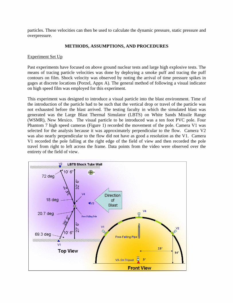
METHODS, ASSUMPTIONS, AND PROCEDURES Experiment Set Up Past experiments have focused on above ground nuclear tests and large high explosive tests. The means of tracing particle velocities was done by deploying a smoke puff and tracing the puff contours on film. Shock velocity was observed by noting the arrival of time pressure spikes in gages at discrete locations (Porzel, Appx A). The general method of following a visual indicator on high speed film was employed for this experiment. This experiment was designed to introduce a visual particle into the blast environment. Time of the introduction of the particle had to be such that the vertical drop or travel of the particle was not exhausted before the blast arrived. The testing faculty in which the simulated blast was generated was the Large Blast Thermal Simulator (LBTS) on White Sands Missile Range (WSMR), New Mexico. The visual particle to be introduced was a ten foot PVC pole. Four Phantom 7 high speed cameras (Figure 1) recorded the movement of the pole. Camera V1 was selected for the analysis because it was approximately perpendicular to the flow. Camera V2 was also nearly perpendicular to the flow did not have as good a resolution as the V1. Camera V1 recorded the pole falling at the right edge of the field of view and then recorded the pole travel from right to left across the frame. Data points from the video were observed over the entirety of the field of view.

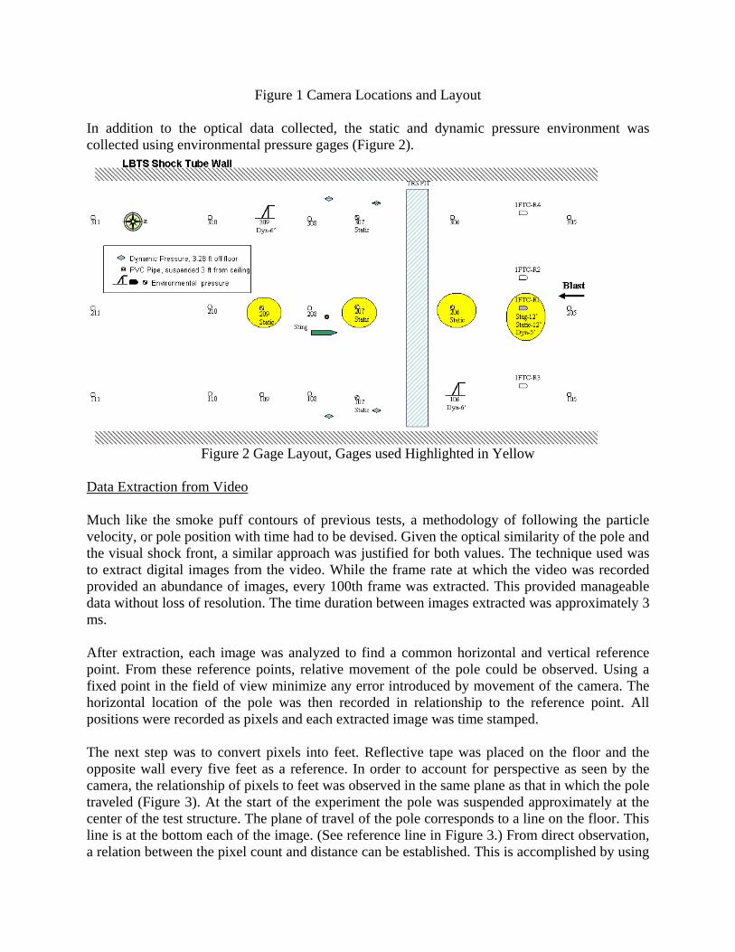
Figure 1 Camera Locations and Layout In addition to the optical data collected, the static and dynamic pressure environment was collected using environmental pressure gages (Figure 2).

Figure 2 Gage Layout, Gages used Highlighted in Yellow

Data Extraction from Video Much like the smoke puff contours of previous tests, a methodology of following the particle velocity, or pole position with time had to be devised. Given the optical similarity of the pole and the visual shock front, a similar approach was justified for both values. The technique used was to extract digital images from the video. While the frame rate at which the video was recorded provided an abundance of images, every 100th frame was extracted. This provided manageable data without loss of resolution. The time duration between images extracted was approximately 3 ms. After extraction, each image was analyzed to find a common horizontal and vertical reference point. From these reference points, relative movement of the pole could be observed. Using a fixed point in the field of view minimize any error introduced by movement of the camera. The horizontal location of the pole was then recorded in relationship to the reference point. All positions were recorded as pixels and each extracted image was time stamped. The next step was to convert pixels into feet. Reflective tape was placed on the floor and the opposite wall every five feet as a reference. In order to account for perspective as seen by the camera, the relationship of pixels to feet was observed in the same plane as that in which the pole traveled (Figure 3). At the start of the experiment the pole was suspended approximately at the center of the test structure. The plane of travel of the pole corresponds to a line on the floor. This line is at the bottom each of the image. (See reference line in Figure 3.) From direct observation, a relation between the pixel count and distance can be established. This is accomplished by using

the known distance between tape lines on the floor and relating it to pixels. Perspective from left to right was also considered, however no appreciable difference in the pixel count between lines on the far left and right of the field of view was observed from those line near center line. Therefore, a linear relationship between pixels and feet was justified for all images.

Figure 3 Pixel Reference

The approach for calculating the shock velocity was modified slightly due to the speed of the wave. The wave is first observed on the opposite wall of the tunnel as a dark band. Manually advancing frame by frame, images were extracted at the point the wave is most visible. In addition to the first appearance of the shock front, each time the wave arrives at reflective tape placed on the wall to mark distance it is evidently seen. The images are then processed the same way as the pole images—by observing a pixel count for the wave position relative to a reference point. The pixel to feet ratio for the shock velocity was observed on the opposite wall instead of the bottom of the frame. Just as with the pole, the reference was made in the plane in which the shock wave traveled. The shock is observed local to the wall; therefore, the reference must be on the wall. This method described above is ideal when the plane in which the motion is observed can be calibrated. However, the application is limited. Another, more general, approach is to use trigonometry to relate the triangle formed between the camera and the lines on the back wall to

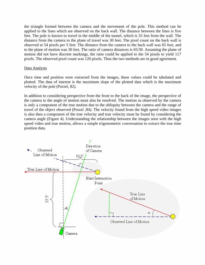
the triangle formed between the camera and the movement of the pole. This method can be applied to the lines which are observed on the back wall. The distance between the lines is five feet. The pole is known to travel in the middle of the tunnel, which is 35 feet from the wall. The distance from the camera to the plane of travel was 30 feet. The pixel count on the back wall is observed at 54 pixels per 5 feet. The distance from the camera to the back wall was 65 feet, and to the plane of motion was 30 feet. The ratio of camera distances is 65/30. Assuming the plane of motion did not have discrete markings, the ratio could be applied to the 54 pixels to yield 117 pixels. The observed pixel count was 120 pixels. Thus the two methods are in good agreement. Data Analysis Once time and position were extracted from the images, these values could be tabulated and plotted. The data of interest is the maximum slope of the plotted data which is the maximum velocity of the pole (Porzel, 82). In addition to considering perspective from the front to the back of the image, the perspective of the camera to the angle of motion must also be resolved. The motion as observed by the camera is only a component of the true motion due to the obliquity between the camera and the range of travel of the object observed (Porzel ,84). The velocity found from the high speed video images is also then a component of the true velocity and true velocity must be found by considering the camera angle (Figure 4). Understanding the relationship between the images seen with the high speed video and true motion, allows a simple trigonometric conversation to extract the true time position data.

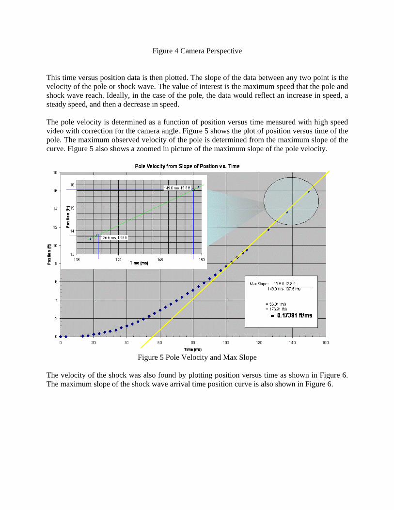
Figure 4 Camera Perspective This time versus position data is then plotted. The slope of the data between any two point is the velocity of the pole or shock wave. The value of interest is the maximum speed that the pole and shock wave reach. Ideally, in the case of the pole, the data would reflect an increase in speed, a steady speed, and then a decrease in speed. The pole velocity is determined as a function of position versus time measured with high speed video with correction for the camera angle. Figure 5 shows the plot of position versus time of the pole. The maximum observed velocity of the pole is determined from the maximum slope of the curve. Figure 5 also shows a zoomed in picture of the maximum slope of the pole velocity.

Figure 5 Pole Velocity and Max Slope

The velocity of the shock was also found by plotting position versus time as shown in Figure 6. The maximum slope of the shock wave arrival time position curve is also shown in Figure 6.

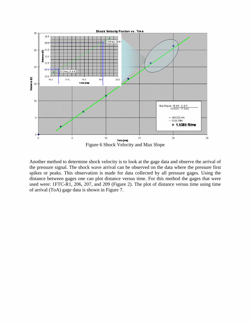
Figure 6 Shock Velocity and Max Slope

Another method to determine shock velocity is to look at the gage data and observe the arrival of the pressure signal. The shock wave arrival can be observed on the data where the pressure first spikes or peaks. This observation is made for data collected by all pressure gages. Using the distance between gages one can plot distance versus time. For this method the gages that were used were: 1FTC-R1, 206, 207, and 209 (Figure 2). The plot of distance versus time using time of arrival (ToA) gage data is shown in Figure 7.

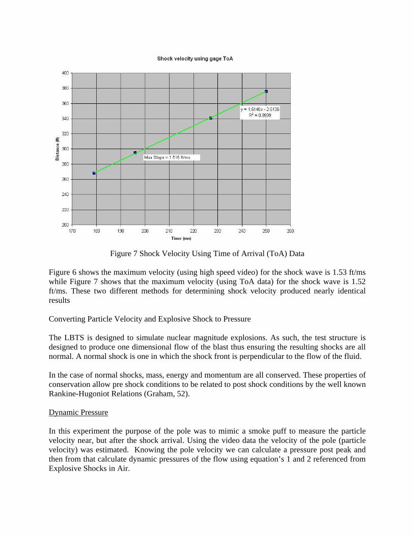
Figure 7 Shock Velocity Using Time of Arrival (ToA) Data

Figure 6 shows the maximum velocity (using high speed video) for the shock wave is 1.53 ft/ms while Figure 7 shows that the maximum velocity (using ToA data) for the shock wave is 1.52 ft/ms. These two different methods for determining shock velocity produced nearly identical results Converting Particle Velocity and Explosive Shock to Pressure The LBTS is designed to simulate nuclear magnitude explosions. As such, the test structure is designed to produce one dimensional flow of the blast thus ensuring the resulting shocks are all normal. A normal shock is one in which the shock front is perpendicular to the flow of the fluid. In the case of normal shocks, mass, energy and momentum are all conserved. These properties of conservation allow pre shock conditions to be related to post shock conditions by the well known Rankine-Hugoniot Relations (Graham, 52). Dynamic Pressure In this experiment the purpose of the pole was to mimic a smoke puff to measure the particle velocity near, but after the shock arrival. Using the video data the velocity of the pole (particle velocity) was estimated. Knowing the pole velocity we can calculate a pressure post peak and then from that calculate dynamic pressures of the flow using equation’s 1 and 2 referenced from Explosive Shocks in Air.

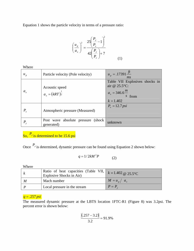
Equation 1 shows the particle velocity in terms of a pressure ratio:

742

1252

2

+⎟⎟⎠

⎞⎜⎜⎝

⎛

⎟⎟⎠

⎞⎜⎜⎝

⎛−

=⎟⎟⎠

⎞⎜⎜⎝

⎛

x

y

x

y

x

p

PPPP

au

(1) Where

pu Particle velocity (Pole velocity) msftu p 17391.=

xa Acoustic speed

( )21

kRTax =

Table VII Explosives shocks in air @ 25.5°C:

smax 6.346=

from 402.1=k

xP Atmospheric pressure (Measured) psiPx 7.12=

yP Post wave absolute pressure (shock generated) unknown

So, is determined to be 15.6 psi yP

Once is determined, dynamic pressure can be found using Equation 2 shown below: yP

PkMq 22/1= (2)

Where

k Ratio of heat capacities (Table VII, Explosive Shocks in Air)

402.1=k @ 25.5°C

M Mach number xp auM = P Local pressure in the stream yPP =

psiq 257.= The measured dynamic pressure at the LBTS location 1FTC-R1 (Figure 8) was 3.2psi. The percent error is shown below:

( )%9.91

2.32.3257.

=−

Figure 8 Measured Dynamic Pressure

In the previous calculation, the pole velocity was assumed to be the particle velocity. The pole velocity was used to directly calculate the dynamic pressure using the Rankine-Hugoniot relations. The large percent error could be attributed to the assumption that pole velocity equaled particle velocity. The assumption was incorrect for numerous reasons. First, the density of the pole was nearly 500 times that of air. A transfer of energy from the air or particles to the pole needs to occur for the pole to achieve speed. Second, the amount of time and visual space was limited both physically, and by the recorded field of view and therefore, only captured the acceleration and not the maximum speed of the visual particle. Third, any visual particle denser than air will have a vertical speed due to gravity. The visual particle must reach the blast velocity before it is pulled to the ground. An alternate approach to the data collected on the time and position of the pole needs to be applied. This approach is to consider the pole a piece of debris in the blast. There are established relationships between debris speed, shape, acceleration and surface area and the speed of the particles in the blast (Witt, 1-8). Knowing the physical parameters of the pole, or the debris, the particle velocity can be calculated. This calculated particle velocity is then applied to the Rankine-Hugoniot relations to determine dynamic pressure.

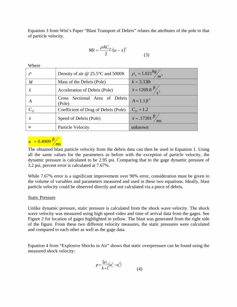
Equation 3 from Witt’s Paper “Blast Transport of Debris” relates the attributes of the pole to that of particle velocity.

( )2

2xuACxM D &&& −=

ρ

(3) Where ρ Density of air @ 25.5°C and 5000ft 3021.1 m

kgx =ρ

M Mass of the Debris (Pole) lbk 33.3= x&& Acceleration of Debris (Pole) 28.1269 s

ftx =&&

A Cross Sectional Area of Debris (Pole)

21.1 ftA =

DC Coefficient of Drag of Debris (Pole) 2.1=DC x& Speed of Debris (Pole) ms

ftx 17391.=&

u Particle Velocity unknown

msftu 4909.0=

The obtained blast particle velocity from the debris data can then be used in Equation 1. Using all the same values for the parameters as before with the exception of particle velocity, the dynamic pressure is calculated to be 2.95 psi. Comparing that to the gage dynamic pressure of 3.2 psi, percent error is calculated at 7.67%. While 7.67% error is a significant improvement over 90% error, consideration must be given to the volume of variables and parameters measured and used in these two equations. Ideally, blast particle velocity could be observed directly and not calculated via a piece of debris. Static Pressure Unlike dynamic pressure, static pressure is calculated from the shock wave velocity. The shock wave velocity was measured using high speed video and time of arrival data from the gages. See Figure 2 for location of gages highlighted in yellow. The blast was generated from the right side of the figure. From these two different velocity measures, the static pressures were calculated and compared to each other as well as the gage data. Equation 4 from “Explosive Shocks in Air” shows that static overpressure can be found using the measured shock velocity:

( )22

12

xxx au

kp −

+=

ρ

(4)

Where

xρ Density of air @ 25.5°C and 5000 ft 3021.1 mkg

x =ρ

k Ratio of heat capacities 402.1=k @ 25.5°C

xa Acoustic speed

smax 6.346=

from

xu Shock Velocity observed from video msftux 5385.1=

xu Shock Velocity observed Time of arrival data ms

ftux 52.1=

From video

psip 3.12= From time of arrival

psip 7.11= The measured static overpressure at the LBTS at floor location 206 (Figure 9) is 12.3 psi. The percent error is shown below: From video

( )%0.0

3.123.123.12

=−

From time of arrival

( )%9.4

3.127.113.12

=−

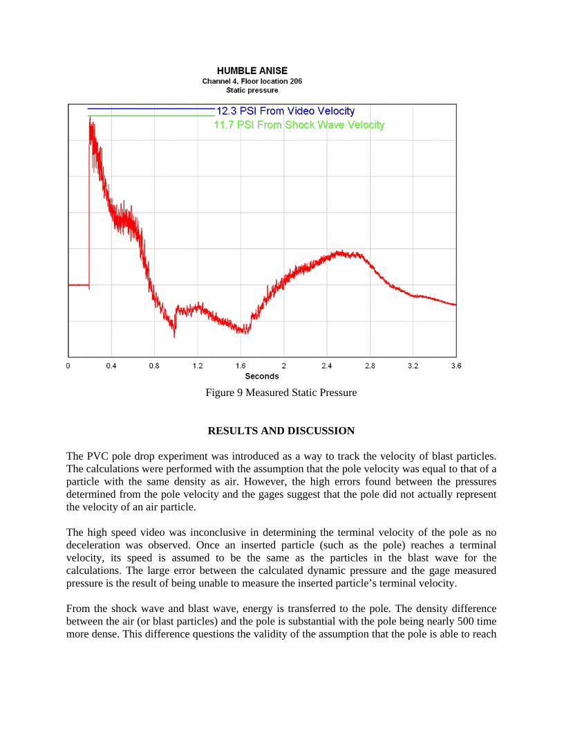
Figure 9 Measured Static Pressure

RESULTS AND DISCUSSION The PVC pole drop experiment was introduced as a way to track the velocity of blast particles. The calculations were performed with the assumption that the pole velocity was equal to that of a particle with the same density as air. However, the high errors found between the pressures determined from the pole velocity and the gages suggest that the pole did not actually represent the velocity of an air particle. The high speed video was inconclusive in determining the terminal velocity of the pole as no deceleration was observed. Once an inserted particle (such as the pole) reaches a terminal velocity, its speed is assumed to be the same as the particles in the blast wave for the calculations. The large error between the calculated dynamic pressure and the gage measured pressure is the result of being unable to measure the inserted particle’s terminal velocity. From the shock wave and blast wave, energy is transferred to the pole. The density difference between the air (or blast particles) and the pole is substantial with the pole being nearly 500 time more dense. This difference questions the validity of the assumption that the pole is able to reach

the velocity of the blast particles. The transfer of energy in a normal shock occurs over a finite period. That duration may not provide ample time for the pole to reach the desired speed. The shock wave was measured using three different methods: High speed video, ToA gage data, and directly by a pressure gage. All three methods show impressive agreement amongst themselves.

SUMMARY AND RECOMMENDATIONS The objective of the experiment was based on recording the terminal velocity of the pole which then was assumed to be the particle velocity for pressure calculations. Because uncertainty exists as to the terminal velocity of the pole and the relationship to the particle velocity, no conclusive data was derived from the speed of the pole. However, given the results from the shock velocity, there is value in studying particle velocity instead of relying solely on gage data for dynamic pressure. In future experiments, to eliminate uncertainty in the particle velocity observation, the following adjustments are suggested: First, the selection of the inserted particle; the pole was nearly 500 as dense as the air. A less dense particle that is still visible is more desirable. Ideally, the particle would have the same density as air. This makes smoke a very clear choice. However some applications, such as the one conducted in the LBTS, smoke was not permitted and therefore, not an option. Other experiments where there is a large amount of debris, smoke from the explosion, or dust and dirt may also preclude using smoke. A second suggested tractable particle would be a ping pong ball. Theses balls are small and relatively similar in density to air. Additionally, the spherical shape of the ball eliminates any twisting motion allow all the energy to be conserved normal to the shock and in line with the flow. In the experiment a PVC pole was dropped from a 60 ft high ceiling approximately ½ second before the blast wave arrived. The rational behind the drop timing was to have the pole drop to the middle of the vertical distance of the tunnel, thus giving a good field of view for the cameras. Upon reviewing the high speed camera footage, it was determined that the terminal velocity of the pole was not captured. Had more video footage been available, the terminal velocity of the pole may have been recorded on film. Upon review of the footage, two problems were indentified. First, the pole was released prior to the blast. This reduced the distance available for the pole to travel horizontally before it hit the ground. Given the pole is more dense than air, the vertical displacement, while not of interest for the assertion of particle velocity, is a concern in how much data can be collected. It is imperative that the pole reaches a terminal horizontal velocity from the blast. If the pole falls to the ground before the terminal velocity is reached, the data point is lost. To account for the affects of gravity, the inserted particle (the pole in this case), must be released at the top most part of the camera’s field of view or higher.

Second, the horizontal terminal velocity of the pole was not recorded because the pole exited the field of view of the camera. For future experiments, more cameras are needed to capture the pole’s maximum velocity. Placement of these cameras is also important as the shock and the blast wave need time, and therefore distance to transfer energy to the pole. The point at which the pole is inserted in the flow—the drop point—provides little insight as to the final velocity of the pole. Therefore, the cameras should be placed at a calculated distance after the drop point to maximize collection of data. Good agreement was seen between all the methods of determining static pressure. The nature of blast testing is to have numerous pressure measurements. Therefore, time of arrival data is nearly always available even when high speed film may not be. ToA data has proven to be just as accurate as pressure gage data. Additionally, ToA is advantageous to gage data in that it is less sensitive to ranging errors. A gage can be ranged incorrectly and miss the data; however the spikes in pressure will still be recorded. Understanding that magnitude of these spikes is not of consequence, and only the time is important for a ToA calculation, pressure data can still be obtained. Furthermore, ToA considers a series of gages. Therefore, the ToA measurement more accurately depicts the blast environment as opposed to point measurements.

REFERENCES

Graham, Kenneth J. E., and Gilbert F. Kinney. Explosive Shocks in Air. New York: Springer, 1985. Porro, A. Robert . Pressure Probe Designs for Dynamic Pressure Measurements in a Supersonic Flow Field. Cleveland, Ohio: NASA, 2001. Porzel, F. B.. Blast Measurements Operation Tumbler-Snapper. University of California: Los Alamos Scientific Laboratory , 1952. Walter, Patrick L.. "Air-Blast and the Science of Dynamic Pressure Measurements." Sound and Vibration December (2004): 10-16. Witt, Eugene F.. Blast Transport of Debris from Scale Model Buildings. Whippany, New Jersey : Bell Telephone Laboratories, Inc., 1979.