Understanding Correlation-RJ Rummel

8/7/2019 Understanding Correlation-RJ Rummel

http://slidepdf.com/reader/full/understanding-correlation-rj-rummel 1/41

Understanding

Correlation*

R.J. Rummel

Honolulu: Department of Political Science

University of Hawaii, 1976

There is an inverse correlation between the power a government has and the nation's

foreign and domestic peace and the welfare of its people.

----From this Web Site

CONTENTS

CHAPTER 1. Introduction

CHAPTER 2. Correlation Intuitively Considered

CHAPTER 3. Standard Scores and Correlation

CHAPTER 4. Characteristics of The Correlation Coefficient

y 4.1. The Range

y 4.2. The Zero

y 4.3. Interpreting The Correlation: Correlation Squared

CHAPTER 5. The Vector Approach

CHAPTER 6. The Cartesian Approach





Of course, many of our concepts may be apriori, our frameworks may be

projected onto phenomena and create order, and our understanding may be

partly intuitive. Our knowledge is a dialectical balance between that sensory

reality bearing on us, and our reaching out and imposing on this reality structure

and framework.

Whatever the framework within which we order phenomena, however, that

reality we perceive is of dependence, concomitance, covariation, coincidence,

concurrence; or of independence, disassociation, or disconnectedness. We exist in

a field of relatedness: i.e., we come to understand the world around us through

the multifold, interlaced and intersecting correlations it manifests. Sometimes we

call these relationships cause and effect, sometimes we generalize them into

assumed laws, and sometimes we simply call them natural or social uniformities

or regularities.

Reflecting this interrelatedness, our theories and ideas about phenomena usuallyare based on assumed correlations. "Birds of a feather flock together." "Time

heals all wounds." "Power kills and absolute power kills absolutely." Or at a

different level: "National cohesion increases in wartime." "Prolonged severe

inflation disorders society." "Institutional power aggrandizes until checked by

opposing institutional power."

No wonder, then, that scientists have tried to make the concept of correlation

more precise, to measure and to quantitatively compare correlations. Here I will

deal with one such measure, called the product moment correlation coefficient.

This is the most widely used technique for assessing correlations and is the basis

for techniques determining mathematical functions (such as regression analysis)

or patterns of interdependence (such as factor analysis).

Although much used, however, the correlation coefficient1

is not widely

understood by students and teachers, and even those applying the correlation in

advanced research.

Therefore, the purpose of this book is to convey an understanding of the

correlation coefficient to students that will be generally useful. I am especially

concerned with providing the student with an intuitive understanding of

correlation that will enable him to better comprehend the use of correlation

coefficients in the literature, while providing material helpful for applying the

correlation coefficient to his own work.

Conveying understanding and facilitating application are my aims. The

organization of this book and the topics included mirror these goals, as does my



emphasis on figures. A picture is worth a thousand derivations and symbols.

Correlation can be beautifully illustrated, but yet many statistical books solely

present the mathematical derivations and statistical formula for the correlation

coefficient, to the detriment of a student's learning. Here I hope to show the very

simple meaning of correlation, both in vector terms and in graphical plots. With

this meaning understood, the application of the correlation coefficient is straight

forward and intuitively reasonable, while the usual complex statistical formula is

then simply a computational tool to that end.

To convey this understanding, the first chapters look at correlation intuitively.

Given certain phenomena, what does correlation mean? What about phenomena

are we perceiving? How can we approach a measure of correlation? Chapter 5

then looks at correlation in terms of vectors. Correlated phenomena are vector

phenomena: they have direction and magnitude. To appreciate the correlation

intuitively it is helpful to visualize the geometric or spatial meaning of the

coefficient. However, there is an alternative spatial view of correlation as a

Cartesian plot. This is the usual picture of correlation presented in the statistical

books, and will also be presented in Chapter 6. From this view will be derived the

usual formulation of the correlation coefficient.

The remaining chapters move on to more advanced topics concerning the

correlation. Chapter 7 describes the partial correlation coefficient. Our ability to

portray partial correlation in simple geometric terms exemplifies the usefulness

of the geometric approach. Chapter 8 briefly defines the correlation matrix.

Chapter 9 considers significance conceptually and untangles two types of

significance often confused. Chapter 10 is a discussion of different types of

correlation coefficients and should be useful for understanding a particular

coefficient in the context of its alternatives. And Chapter 11 recapitulates the

major points and adds a few considerations in understanding correlation.

NOTES

1. Henceforth, unless otherwise specified, correlation coefficient will mean the product

moment.

CHAPTER 2:

CORRELATION INTUITIVELY CONSIDERED



When we perceive two things that covary, what do we see? When we see one

thing vary, we perceive it changing in some regard, as the sun setting, the price of

goods increasing, or the alternation of green and red lights at an intersection.

Therefore, when two things covary there are two possibilities. One is that thechange in a thing is concomitant with the change in another, as the change in a

child's age covaries with his height. The older, the taller. When higher

magnitudes on one thing occur along with higher magnitudes on another and the

lower magnitudes on both also co-occur, then the things vary together positively,

and we denote this situation as positive covariation or positive correlation.

The second possibility is that two things vary inversely or oppositely. That is, the

higher magnitudes of one thing go along with the lower magnitudes of the other

and vice versa. Then, we denote this situation as negative covariation or negative

correlation. This seems clear enough, but in order to be more systematic aboutcorrelation more definition is needed.

Perceived covariation must be covariation across some cases. A case is a

component of variation in a thing. For example, the change in the speed of traffic

with the presence or absence of a traffic policeman (a negative correlation) is a

change across time periods. Different time periods are the cases. Different levels

of GNP that go along with different amounts of energy consumption may be

perceived across nations. Nations are the cases, and

the correlation is positive, meaning that a nation

(case) with high GNP has high energyconsumption; and one with low GNP has low

energy consumption. The degree to which a regime

is democratic is inversely correlated with the

intensity of its foreign violence. The cases here are

different political regimes.

To be more specific, consider the magnitudes

shown in Table 2.1. The two things we perceive

varying together--the variables--are 1955 GNP per

capita and trade. The cases across which these varyare the fourteen nations shown. Although it is not

easy to observe because of the many different magnitudes, the correlation is

positive, since for more nations than not, high GNP per capita co-occurs with

high trade, and low GNP per capita with low trade.



We can summarize this covariation in terms of a four-fold table, as in Table 2.2.

Let us define high as above the means (averages) of $481 for GNP per capita in

Table 2.1 and $4,975 millions for trade, and low at or

below these means. Then we get the positive correlation

shown in Table 2.2. The numbers that appear in the cells

of the table are the number of nations that have the

indicated joint magnitudes. For example, there are nine

nations which have both low GNP per capita and low

trade.

From the table, we can now clearly see that the

correlation between the two variables is positive, since with only one exception

(in the upper right cell) high magnitudes are observed together, as are low

magnitudes.

If the correlation were negative, then most cases would be counted in the lowerleft and upper right cells. What if there were about an equal number of cases in

all the cells of the fourfold table? Then, there would be little correlation: the two

variables would not covary. In other words, sometimes high magnitudes on one

variable would occur as often with low as with high magnitudes on the other.

But all this is still imprecise. The four-fold table gives us a way of looking at

correlation, but just considering correlation as covarying high or low magnitudes

is quite a loss of information, since we are not measuring how high or low the

figures are. Moreover, if we are at all going to be precise about a correlation, we

should determine some coefficient of correlation--some one number that in itself

expresses the correlation between variables. To be a useful coefficient, however,

this must be more than a number unique to a pair of variables. It must be a

number com parable.between pairs of variables. We must be able to compare

correlations, so that we can determine, for example, which variables are more or

less correlated, or whether variables change correlation with change in cases.

Finally, we want a correlation that indicates whether the correlation is positive

or negative. In the next chapter we can intuitively and precisely define such a

coefficient.

CHAPTER 3:

STANDARD SCORES AND CORRELATION



Although the cases across which two variables covary usually will be the same,

1

the units in which the magnitudes are expressed for each variable may differ.

One variable may be in dollars per capita, another number of infant deaths. One

may be in percent, another in feet. One apples, the other oranges.

Clearly, we have a classic problem. How can we measure the correlation between

different things in different units? We know we perceive covariation between

things that are different. But determining common units for different things such

that their correlations can be measured and compared to other correlations

seems beyond our ability. Yet, we must make units comparable before we can

jointly measure variation. But how?

Consider the observations on ten variables in Table 3.1, which include those on

GNP per capita and trade in Table 2.1. Note the differences in units between thevarious variables, both in their nature and average magnitudes. our problem,

then, is to determine some way of making the units of such variables comparable,

so that we can determine the correlation between any two of them, as well as

compare the correlations between various pairs of variables. Is, for example, the

covariation of foreign conflict and of defense budget across the fourteen nations

greater or less than that of, say, foreign conflict and the freedom of group

opposition?

Let us consider this problem for a moment. We want a measure of covariation, of

how much two t hings change toget her or o ppositely. Clearly, then, we have nointerest in their different magnitudes. And since magnitudes are irrelevant we

can at least make the different magnitudes of the two variables comparable by

making their average magnitude the same. This we can do by subtracting the

average or mean of each variable from all its magnitudes.

To illustrate this, consider from Table 3.1 the power and defense budget

variables, two variables measured in different units and involving quite different

magnitudes. As shown in the table, the mean of power is 7.5 and that of defense

budget is $5,963.5 (millions). Table 3.2 shows the result of subtracting the mean

from each variable. Such data resulting from subtracting the mean is calledmean-deviation data, and the mean of mean-deviation data is always zero.

Now that we have made the average magnitude comparable by transforming

each variable to a mean of zero, the observations now represent pure variation.

It is as though we had taken different statistical profile shots of each variable and

overlaid them so that we could better see their covariation. But yet, as we can see



from Table 3.2, the mean-deviation data does not give us a very good view of the

degree of correlation, although it does enable us to see how the pluses and

minuses line up

The problem is that subtracting the means did not change the magnitude of

variation, and that of the defense budget is very large compared to power. Westill need a transformation to make their variation comparable.

Why not compute an average variation then? This average could be calculated

by adding up all the mean-deviations and dividing by the number of cases.

However, the summed minus magnitudes equal the summed positive magnitudes

(by virtue of the subtraction of the mean), and the average variation always will

be zero as shown in Table 3.2, regardless of the absolute magnitude of the

variation.

Then why not average t he absolute mean-deviation data? That is, eliminate thenegative signs. But if we did this, we would run into some mathematical

difficulties in eventually determining a correlation coefficient. Absolutes create

more problems than they solve.

However, we can invoke a traditional solution. If we square all the mean-

deviation data, we eliminate negative signs. Then the average of these squared

magnitudes will give us a measure of variation around the mean.

From this point on, I will have to be more precise and use some notation towards

that end. I will adopt the following definitions.

Definitions 3.1:

X = anything that varies; a variable;

X j = a specific variable j;

Xk = a specific variable k;

i = a particular case i

xij = a magnitude (datum) for case i on variable j;

n = the number of cases for a variable;

= the average or mean of variable X;X*

j = mean-deviation data (the mean has been subtracted from each

original magnitude) for variable j;

xij = the first case (i = 1 for variable j) to the last case (i = n for

variable j), that is x1j + x2j + x3j + . . . + xnj = xij.



The last definition2 is especially important, for it enables us to compress a lot of

summations into a concise equation.

Now, using this notation, we can define the mean as,

Equation 3.1:

X j = ( xi) / n

And we can also easily define mean-deviation data. Since X* j stands for the mean-

deviation data for variable X j, let x*ij be the corresponding mean-deviation

magnitude. Then

Equation 3.2:

x*

ij = xij - j

With these equations I can return to our measure of variation. Remember, we

are going to square the mean-deviation data, add, and divide the sum by n to get

an average variation. Let 2 (sigma squared) stand for our measure of variation.

Then

Equation 3.3:

2 = ( x*ij

2) / n = ( xij - j)2/n

where the last equality follows from Equation 3.2.

We can now introduce two important definitions.

Definition 3.2 :

2 j = the variance of variable X j.

j = the standard deviation of variable X j, which is the positive square

root of the variance.

We now have two measures of variation around the mean and we will find that

each of them is a useful tool for understanding correlation. At this point, we can

use the standard deviation to help resolve our original problem of making the

variation in two variables comparable, since it is expressed in the original units

(to get a measure of variation, we squared the mean-deviations; the standard

deviation is the square root of the average squared mean-deviations and thus

brings us back to the original units).









Finally from Equation 3.3 and Definition 3.2, we can rewrite the standard

deviation in terms of the raw data, and thus define the correlation entirely as a

function of the variables in their original magnitudes. That is

Equation 3.7:

r jk = ( (xij - j)(xik - k )) / n j k

= ( (xij - j)(xik - k )) / (( (xij - j)2)( (xik - k )

2))1/2

The terms on the right of the second equality give the formula most often

presented in statistical books. It is imposing, but as we have seen, its underlying

logic is intuitively reasonable.

NOTES

1. There are occasions when the cases may differ, such as in lagged correlations where the

case for one variable is a time period lagged behind the time period for the other.

2. I am leaving the range off the , which would be written as

ni=1

In this book the range will always be from i = 1 to n, and so is omitted.

3. Note that the mean of a standardized variable is always zero. Therefore simply adding

the standard scores for each case, summing the result across all the cases, and taking theaverage of that sum will always, regardless of the data, get you:

( (zij + zik )) / n = ( zij) / n + zik ) / n

= (mean of Z j) + (mean of Zk )

= 0 + 0

CHAPTER 4:

CHAR ACTERISTICS OF

THE CORRELATION COEFFICIENT

4 .1 T he Range



Given that the correlation coefficient measures the degree to which two things

vary together or oppositely, how do we interpret it? First, the maximum positive

correlation is 1.00. Since the correlation is the average product of the standard

scores for the cases on two variables, and since the standard deviation of

standardized data is 1.00, then if the two standardized variables covary positively

and perfectly, the average of their products across the cases will equal 1.00.1

On the other hand, if two things vary oppositely and perfectly, then the

correlation will equal 1.00.

We therefore have a measure which tells us at a glance whether two things

covary perfectly, or near perfectly, and whether positively or negatively. If the

coefficient is, say, .80 or .90, we know that the corresponding variables closely

vary together in the same direction; if -.80 or -.90, they vary together in opposite

directions.

4 .2 T he Zero

What then is the meaning of zero or near zero correlation? It means simply that

two things vary separately. That is, when the magnitudes of one thing are high;

the other's magnitudes are sometimes high, and sometimes low. It is through

such uncorrelated variation--such independence of things--that we can sharply

discriminate between phenomena.

I should point out that there are two ways of viewing independent variation. One

is that the more distinct and unrelated the covariation, the greater the

independence. Then, a zero correlation represents complete independence and -

1.00 or 1.00 indicates complete dependence. Independence viewed in this way is

called statistical inde pendence. Two variables are then statistically independent if

their correlation is zero.2

There is another view of independence, however, called linear inde pendence,

which sees independence or dependence as a matter of presence or absence, not

more or less. In this perspective, two things varying perfectly together are lineardependent. Thus, variables with correlation of -1.00 or 1.00 are linear dependent.

Variables with variation less than perfect are linear independent. Figure 4.1

shows how these two views of dependence overlap.



4 .3 Inter preting t he Correlation: Correlation Squared

Seldom, indeed, will a correlation be zero or perfect. Usually, the covariation

between things will be something like .43 or -.16. How are we to interpret such

correlations? Clearly .43 is positive, indicating positive covariation; -.16 is

negative, indicating some negative covariation. Moreover, we can say that thepositive correlation is greater than the negative. But, we require more than. If we

have a correlation of .56 between two variables, for example, what precisely can

we say other than the correlation is positive and .56?

From my derivation of the correlation coefficient in the last chapter, we know

that the squared correlation (Definition 3.3) describes the proportion of variance

in common between the two variables. If we multiply this by 100 we then get the

percent of variance in common between two variables. That is:

r2 jk x 100 = percent of variance in common between X j and Xk . For example, we found that the correlation between a nation's power and its

defense budget was .66. This correlation squared is .45, which means that across

the fourteen nations constituting the sample 45 percent of their variance on the

two variables is in common (or 55 percent is not in common). In thus squaring

correlations and transforming covariance to percentage terms we have an easy to

understand meaning of correlation. And we are then in a position to evaluate a

particular correlation.

As a matter of routine it is the squared correlations that should be interpreted.This is because the correlation coefficient is misleading in suggesting the

existence of more covariation than exists, and this problem gets worse as the

correlation approaches zero. Consider the following correlations and their

squares.



Note that as the correlation r decrease by tenths, the r2 decreases by much more.

A correlation of .50 only shows that 25 percent variance is in common; a

correlation of .20 shows 4 percent in common; and a correlation of .10 shows 1

percent in common (or 99 percent not in common). Thus, squaring should be a

healthy corrective to the tendency to consider low correlations, such as .20 and

.30, as indicating a meaningful or practical covariation.

NOTES

1. There are exceptions to this, as when the correlation is computed for dichotomous

variables with disparate frequencies. See Section 10.1.

2. I am talking about statistical independence in its descriptive and not inferential sense. In

its inferential sense, a nonzero correlation would represent independent variation insofar

as its variation from zero could be assumed due to chance, within some acceptable

probability of error. If it is improbable that the deviation is due to chance, then the

correlation is accepted as measuring statistically dependent variation. See Chapter 9.

CHAPTER 5:

THE VECTOR APPR OACH

The standard scores considered in Chapter 3 provide an intuitive route to

developing and understanding correlation. There are two more approaches, each

providing a different kind of insight into the nature of the correlation coefficient.

One is the vector approach, to be developed here. The other is what I will call the

Cartesian approach, to be developed in the next chapter.

Consider again the problem. Two things vary and we wish to determine in some

systematic fashion whether they vary together, oppositely, or separately. Wehave seen that one approach involves a simple averaging and common sense. But

let us say that we are the kind of people that must visualize things and draw

pictures of relationships before we understand them. How, then, can we visualize

covariation? That is, how can we geometrize it?



There are many ways this could be done. For example, we could plot the

magnitudes for different cases on each variable to get a profile. And we could

then compare the profile curves to see if they moved oppositely or together.

While intuitively appealing, however, it does not lead to a precise measure.

But what about this? Variables can be portrayed as vectors in a space. We areused to treating variables this way in visualizing physical forces. A vector is an

ordered set of magnitudes; a variable is such an ordered set (each magnitude is

for a specific case). A vector can be plotted; therefore a variable can be plotted as

a vector. Vectors pointing in the same direction have a positive relationship and

those pointing in opposite directions have a negative relationship. Could this

geometric fact also be useful in picturing correlation? Let us see.

The first problem is how to plot a variable as a vector. Now consider the variable

as located in space spanned by dimensions constituting the cases. For example,

consider the stability and freedom of group opposition variables from Table 3.1 and their magnitudes for Israel and Jordan. These two cases then define the

dimensions of the space containing these variables--vectors--that are plotted as

shown in Figure 5.1. We thus have a picture of variation representing the two

pairs of observations for these variables. T he variation of t he variables across

t hese nations is t hen indicated by t he lengt h and direction of t hese vectors in t his

s pace.

To give a different example, consider again the power and defense budget

variables (Table 3.1. There are fourteen cases--nations--for each variable. To

consider these variables as vectors, we would therefore treat these nations as

constituting the dimensions of a fourteen dimensional space. Now, if we picture

both variables as vectors in this space, their relative magnitudes and orientation

towards each other would show how they vary together, as in Figure 5.2.

To get a better handle on this, think of the vectors as forces, which is the

graphical role they have played for most of us. If the vectors are pointed in a

similar direction, they are pushing together. They are working together, which is

to say that they are varying together. Vectors oppositely directed are pushing

against each other: their efforts are inverse, their covariation is opposite. Then

we have vectors that are at right angles, such as one pushing north, another east.

These are vectors working independently: their variation is independent.

With this in mind, return again to Figure 5.2. First, the vectors are not pointing

oppositely, and therefore their variation is not negative. But they are not pointing

exactly in the same direction either, so that they do not completely covary

together. Yet, they are pointing enough in the same general direction to suggest



some variation in common. But how do we measure this common covariation for

vectors?

Again, we have the problem of units to consider. The length and direction of the

vectors is a function of the magnitudes and units involved. Thus, the defense

budget vector is much longer than the power one.

Since differing lengths are a problem, why not transform the vectors to equal

lengths? There is indeed such a transformation called normalization,1 which

divides the magnitudes of the vector by its length.

Definition 5.1:

X j = vector j or variable j

|X j| = length of vector j = ( x2ij)

1/2

That is, the length of a vector is the square root of the squared sum of its

magnitudes. Then the normalization of a vector is the division of its separate

magnitudes by the vector's length. All vectors so normalized have their lengths

transformed to 1.00.

The problem with normalization is that there can be considerable differences in

mean magnitudes on the normalized vectors, and these mean differences would

then confound the measure of correlation. After all, we want a measure of pure

covariation, and differences in average magnitude confound this.

Then, in reconsidering our original vectors, what about transforming the

magnitudes on the vectors by subtracting their averages, as we did in Chapter 3

(Equation 3.2)? If we did this we would be translating the origin of the space to

the mean for each vector: the zero point on each dimension would be the mean.

By so transforming the vectors to mean-deviation data we eliminate the affect of

mean differences, but we still have the differing vector lengths. Need this bother

us, now? After all, we are concerned with similarity or dissimilarity in vector

direction as an indication of correlation. Let us therefore work for the moment

with mean-deviation vectors and see what we get.

Recall that codirectionality for vectors is the essence of covariation. How do we

measure codirectionality, then? B y t he angle between t he vectors.

But measuring this angle creates a problem. In degrees it can vary from 0o to

360o and is always positive, where perfect positive covariation would be zero,



independent variation would be 90o or 270o and opposite variation 180o. As with

the correlation coefficient derived in Chapter 3, it would be desirable to have

some measure which would range between something like 1.00 for perfect

correlation, -1.00 for perfect negative correlation, and zero for no correlation.

And we do have such a measure given by elementary trigonometry. It is thecosine. The cosine of the angle between vectors will be +1.00 for vectors with an

angle of 0o, -1.00 for an angle of 180o (completely opposite directionality), and 0

for an angle of 90o or 270o. What is more, from linear algebra we can compute

the cosine directly from the vectors without measuring their angles. For vectors

X* j and X*

k of mean-deviation data, this is

Equation 5.1:

Cos jk = ( x*ijx

*ik ) / | X

* j||X

*k |

Let the magnitudes of power and defense budget be transformed to mean-

deviation data. Then Figure 5.3 shows the angle between the vectors given by the

cosine (Equation 5.1) and for the mean-deviation data of Table 3.2 we would find

the cosine of the angle equals .66.

Thus, the cosine between two variables transformed to mean-deviation data--to

data describing the variation around the mean--gives us a measure of

correlation. But there is a coincidence here. The .66 cosine for the angle of 49 o

between the two vectors is the same as the .66 product moment correlation we

found for the two variables using standard scores (Table 3.4). Is there in fact arelationship between these alternatives?

To see what this relationship might be, let us expand the formula for the cosine

between two mean-deviation vectors so that it is expressed in the original

magnitudes.

Equation 5.2:

Cosine jk = ( x*ijx*

ik ) / | X* j||X

*k |

= ( (xij - j)( xik - k ) / ( x *ij 2)1/2( x *ik 2)1/2 = ( (xij - j)( xik - k ) / (( (xij - j)

2) ( (xik - k )2))1/2

The lengths of the vectors have been expanded using Definition 5.1.

Now compare Equation 5.2 with Equation 3.7 for the correlation. They are the

same! Thus,



Equation 5.3:

cosine jk = r jk for mean-deviation data. And since standardized data is also mean deviation

data, Equation 5.3 holds for standard scores as well.

To sum up, we have found that we can geometrically treat the variation of things

as vectors, with the cases across which the variation occurs as dimensions of the

space containing the vector. The covariation between two things is then shown by

their angle in this space. However, we have to again transform the variation in

two things to eliminate the effects of mean-differences. The resulting mean-

deviation data reflects pure variation and the covariation between the vectors is

then the cosine of their angle. Moreover, this cosine turns out to be precisely the

product moment correlation derived from standardized data. Instead of two

alternative measures of correlation, we thus have alternative perspectives orroutes to understanding correlation: the average cross-products of standardized

data, or the cosine of the angle between mean-deviation (or standardized) data

vectors.

NOTES

1. This is not to be confused with transforming distributions to normality, an entirely

different procedure.

CHAPTER 6:

THE CARTESIAN APPR OACH

So far we have approached correlation in intuitive-conceptual and geometricfashion. But there is another approach beloved of introductory statistical tests.

This is the Cartesian approach: it relies on a Cartesian coordinate system, where

each variable represents a coordinate, and the cases are points plotted in this

two-dimensional space.



Let us again begin with trying to determine some measure of

the covariation of things. We saw that the variation of a

variable could be pictured as a vector and covariation as

codirectionality between vectors. We could have, however,

pictured variation differently. Rather than fixing the cases as

dimensions of the space, we could have treated the variables

as the dimensions. Then we could plot each case on these

dimensions in terms of their joint magnitudes, as shown in

Figure 6.1 for variables X j and Xk . The variation of the cases

in this space then represents the covariation of the variables.

What, then, would perfect covariation look like? Here, we

have a fundamental ambiguity. Perfect covariation could

look like Figure 6.2a, b, or c. That is, covariation could lie

along some curve, like the covariation between time and the

height of a ball thrown upward which can be plotted as a

parabola.Or, covariation could lie along a straight line. In

intuitively assessing covariation, we were concerned with a

measure of when magnitudes were both high and low or

when one was high, the other low. That is, we wanted to

index positive or negative correlation.

Concerning positive correlation, this desire is clearly

reflected in Figure 6.2c, for as the magnitude of a case on one

variable is high, it is high on the other; as it is low on one, it

is low on the other. And uniformly so. We can therefore

consider this figure as representing perfect positive

correlation. Perfect negative correlation would then be reflected in cases forming

a straight line slanting downwards to the right, as shown in Figure 6.3a. If the

cases appear randomly distributed as in Figure 6.3b, we have a case of no

covariation in common.

But it is our misfortune that most phenomena will have less than perfect

covariation and therefore would manifest a plot like that in Figure 6.1. Again, we

must develop some measure of all this. And again we can approach this

intuitively.

Now, we know that perfect correlation would be represented by the cases

forming a straight line and that our real data will vary from this line. Is it not

reasonable, then, to think of correlation as the degree to which the cases vary

from a straight line?



A problem, however, is determining what this perfect correlation, this straight

line amongst the cases plotted on the variables, should be. We know the line

should go through the points as in Figure 6.4a,

but we want to locate it more precisely than this

so that we can develop an exact measure of

correlation. One possibility is to locate the line

such that the deviation of cases from the line are

minimal. Let us consider such deviations as

shown in Figure 6.4b, where the deviations are

computed as the difference between the case's

magnitude xij on one variable (X j), and the

location xij of the case on the line if X j and Xk

were perfectly correlated. I will denote this

deviation by di as shown. Deviations d2 and d3 are

also shown as examples.

We could then sum these deviations for all cases

and locate the line so that the sum is as small as possible. And since deviations

above the line would always be positive, those below would be negative, we could

always locate the line such that these deviations sum to zero. Unfortunately,

however, an infinitude of lines could be fitted to the cases to yield deviations

summing to zero, and we cannot define any unique line this way.

We could sum absolute deviations, but then absolutes are again difficult to deal

with mathematically. Then why not do what we did in Chapter 3 to get rid of

sign differences? Why not square deviations and sum the squares? This in fact

provides a solution, for the minimization of di2 leads to a unique line fitting the

points. We need not go into the actual minimization. Suffice to say that the

equation of the straight line is

X j = + Xk ,

and the line minimizing the squared deviations1

is called the least squares line or

least squares regression.

Now, let us say that we have such a least squares line in Figure 6.4B, and the

squared deviations add to the smallest possible sum. What then? This sum of

squared deviations always would be zero in the case of perfect correlation, but

otherwise would depend on the original data units. Therefore, different sums of

squared deviations for different variables would not be easily comparable or

interpretable. When this type of unit-dependent variation occurs, a solution is

often to develop a ratio of some sort. For example, national government budgets



in national currencies are difficult to compare between nations, but the ratio of

national budget to GNP eliminates currency units and provides easily

comparable measures.

But to what do we compute a ratio for our sums? Consider that we have so far

computed differences from a perfect correlation line fitted to the actualmagnitudes of the variables. Could we not also introduce a hypothetical line

fitted to the cases as though they had no correlation? We would then have two

hypothetical lines, one measuring perfect correlation; the other measuring

complete statistical independence, or noncorrelation. Would not some ratio of

differences from the two lines give us what we want? Let's see.

To be consistent with the previous approach, squared deviations from the second

line would also be calculated. But, where would the line of perfect noncorrelation

be placed among the cases in Figure 6.4b?

First, the line would be horizontal, since if there is some variation in common

between two variables, the line will angle upward to the right if this correlation is

positive, or to the left if negative.

Okay, now where do we place the horizontal line? If there is no correlation

between two variables, then from a magnitude on the one variable, we cannot

predict to a magnitude in the other. Knowing one variable's variation does not

reduce uncertainty about the other's. This is an opposite situation for perfectly

correlated variables, where knowing a magnitude on one variable enables a

precise prediction as to the magnitude of the other.

When we have complete uncertainty, as in the case of perfect statistical

independence, then given the one variable, what is the best estimate of the

magnitude on the other?

This is the other variable's mean. In a situation of complete uncertainty about the

magnitude of a case on a variable, the best guess as to this magnitude is the

variable's mean. Since the line of perfect noncorrelation is a line of complete

uncertainty about where a case would lie on the vertical axis, X j, in Figure 6.4b,

given its magnitude on Xk k, the most intuitively reasonable location for the line isat the average of X j, as in Figure 6.5.

However, not only is this intuitively reasonable, but if in fact the two variables

were perfectly uncorrelated, then the line which would minimize d2i would be

this horizontal line. In other words, as the correlation approaches zero, the

perfect correlation line approaches the horizontal one shown.



Now, given this horizontal line for hypothetically perfect noncorrelation, we can

determine the deviation of each case from it. Let me denote such a deviation as gi,

which is shown in Figure 6.5, along with g1 as an example. The sum of the

squared deviations of gi is g2i , which is a minimum if the variables are

perfectly correlated.

Thus, we have two measures of deviation. One from the perfect correlation line

fitting the actual data; the other from the line of hypothetical noncorrelation.

Surely, there will be a relationship between d2i and g2

i.

Now, the less correlated the variables, the more the slanted line approaches the

horizontal one. That is, the more d2i approaches g2

i. If the variables were

perfectly correlated, d2i would be zero, since there would be no deviation from

the line of perfect correlation. And therefore the less the observations covary, the

closer d2i approaches g2

i from zero. If the observations are in fact perfectly

uncorrelated, then d2i = g2

i.

Thus, it appears that a ratio between d2i and d2

i would measure the actual

correlation between two variables. If the correlation were perfect, then the ratio

would be zero; if there were no correlation, the ratio would be one. But this is the

opposite of the way we measured correlation before. Therefore, reverse this

measurement by subtracting the ratio from 1.00, and denote the resulting

coefficient as h. Then,

Equation 6.1:

h = 1 - d2i / g2

i

To deepen our understanding of h, return to Figure 6.5 and consider again the

horizontal line. The deviations gi are from the average j. Therefore,

gi = xij - j,

g2i = (xij - j)

2,

g2

i / n = (xij - j)2

/ n =2 j.

That is, what in fact g2i measures is the total variation of X j. If we divide this by

n, as in Equation 3.3, we would have the variance ( 2 j) of X j.

The other sum of squares, d2i, measures that part of the variation in X j that

does not covary with Xk --that is independent of covariation with Xk . If X j and Xk



covaried perfectly, there would be no independent variation in X j and d2i would

equal zero.

Therefore, the ratio of d2i to g2

i measures the variance in X j independent of

Xk with respect to the total variance of X j, Thus, when we subtract this ratio from

1.00 we get

h = 1 - d2i / g2

i

= ( g2i - d2

i) / g2i

= (total variance - independent variance) / total variance

= (variance in common) / total variance.

In other words, h measures the pro portion of variance between two variables. Butthis is what the coefficient of determination r2 does (Definition 3.4).

Therefore,

Equation 6.2:

h = r2,

and our measure of correlation derived through the Cartesian approach is the

product moment correlation squared.A

nd theC

artesian approach provides anunderstanding of why the correlation squared measures the proportion of

variance of two variables in common.

NOTES

1. Through calculus we can determine the values for and that define the minimizing

equation. They are

= ( (xij - j)(xik - k )) / (xik - k )2

= j - k .

CHAPTER 7:



THE PR OBLEM OF EXTER NAL EFFECTS:

PARTIAL CORRELATION

A problem with the correlation coefficient arises from the very way thecovariation question was phrased in Chapter 2. We wanted some systematic

measure of the covariation of two things. And that is precisely what we got with

the correlation coefficient: a measure confined wholly to two things and which

treats them as an isolated system.

But few pairs of things are isolated. Most things are part of larger wholes or

complexes of interrelated and covarying parts, and these wholes in turn are still

parts of other wholes, as a cell is a part of the leaf, which is part of the tree that is

part of a forest. Things usually covary in large clusters or patterns of

interdependence and causal influences (which is the job of factor analysis touncover). To then isolate two things, compute the correlation between them, and

to interpret that correlation as measuring the relationship between the two

variables alone can be misleading.

Consider two examples. First, let us assess the correlation between illiteracy and

infant mortality. We may feel that a lack of education means poor infant care,

resulting in higher mortality. Of course, we want to be as comparative as possible

so we compute the correlation for all nations. The actual correlation for 1955 is

.61, which is to say that illiteracy and infant mortality have 37 percent of their

variance in common. Are we then to conclude that education helps prevent infantmortality? If we were unwary, we might. But these two variables are not isolated.

They are aspects of larger social systems and both subject to extraneous

influences; and in this case, these influences flow from economic development.

Many in the least developed countries have insufficient diets and inadequate

health services, and live in squalid conditions. High infant mortality follows.Also

by virtue of nonexistent or poor educational systems, many people are illiterate.

This is quite the opposite of the developed nations, which usually have good

medical services, a varied and high protein diet, and high literacy. Thus the

correlation between illiteracy and infant mortality. It has less to do with any

intrinsic relationship between them then to the joint influence on illiteracy and

infant mortality of national development.

A second example has to do with the covariation between economic growth rate

and social conflict. Let us hypothesize that they have a negative correlation due

to economic growth increasing opportunities, multiple group membership, and

cross-pressures, thus draining off conflict. Let us find, however, that the actual



correlation is near zero. Before rushing out into the streets to proclaim that

economic growth is independent of conflict, however, we might consider whether

exogenous influences are dampening the real correlation. In this case, we could

argue that the educational growth rate is the depressant. Increasing education

creates new interests, broadens expectations, and generates a consciousness of

deprivations. Thus, if education increases faster than opportunities, social

conflict would increase. To assess the correlation between economic growth rate

and conflict, therefore, we should hold constant the educational growth rate.

How do we handle these kinds of situations? There is an approach called partial

correlation, which involves calculating the correlation between two variables

holding constant the external influences of a third.

Before looking at the formula for computing the partial correlation, three

intuitive approaches to understanding what is involved may be helpful. First,

consider the first example of the correlation between illiteracy and infantmortality. How can we hold constant economic development? of course, before

we can do anything, we must have some measure of economic development, and I

will use GNP (gross national product) per capita for this purpose. Given this

measure, then, a reasonable approach would be to divide the sample of nations

into three groups: those with high, with moderate, and with low GNP per capita.

Then the correlation between illiteracy and infant mortality rate can be

calculated separately within each group. We would then have three different

correlations between illiteracy and infant mortality, at different economic levels.

We could then calculate the average of these three correlations (weighting by the

number of nations in each sample) to determine an overall correlation, holding

constant economic develo pment. The result would be the partial correlation

coefficient.

As a second intuitive approach, consider the deviations d i between the actual

magnitudes and the perfect correlation line for two variables, as shown in Figure

6.4b. This deviation measures the amount of variation in X j unrelated to Xk . It is

called the residual.

Now, consider two separate plots, one for the correlation between GNP per

capita and illiteracy; the other for the correlation between GNP per capita and

infant mortality. In each case, GNP per capita would be Xk , the horizontal axis.

For each plot there will be a perfect correlation line, from which can be

calculated the residuals for GNP per capita and illiteracy, and for GNP per

capita and infant mortality. These two sets of residuals, di, measure the

independence of illiteracy and infant mortality from GNP per capita.1



With this in mind, consider. What we are after is the correlation between the two

variables with the effect of economic development, as measured by GNP per

capita, removed. But are not these residuals exactly the two variables with these

effects taken out? Of course. Therefore, it seems reasonable to define the partial

correlation as the product moment correlation between these residuals--between

the di for illiteracy and the di for infant mortality--which would be .13. And in

fact, this is the partial correlation.

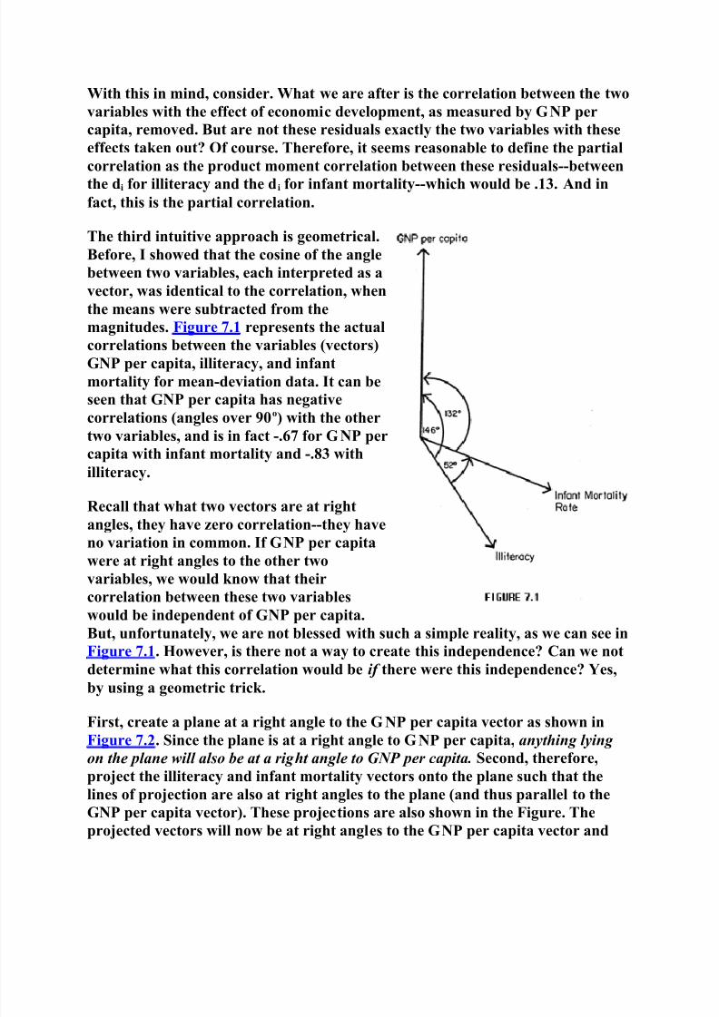
The third intuitive approach is geometrical.

Before, I showed that the cosine of the angle

between two variables, each interpreted as a

vector, was identical to the correlation, when

the means were subtracted from the

magnitudes. Figure 7.1 represents the actual

correlations between the variables (vectors)

GNP per capita, illiteracy, and infant

mortality for mean-deviation data. It can be

seen that GNP per capita has negative

correlations (angles over 90o) with the other

two variables, and is in fact -.67 for GNP per

capita with infant mortality and -.83 with

illiteracy.

Recall that what two vectors are at right

angles, they have zero correlation--they have

no variation in common. If GNP per capita

were at right angles to the other two

variables, we would know that their

correlation between these two variables

would be independent of GNP per capita.

But, unfortunately, we are not blessed with such a simple reality, as we can see in

Figure 7.1. However, is there not a way to create this independence? Can we not

determine what this correlation would be if there were this independence? Yes,

by using a geometric trick.

First, create a plane at a right angle to the GNP per capita vector as shown in

Figure 7.2. Since the plane is at a right angle to GNP per capita, anyt hing lying

on t he plane will also be at a rig ht angle to GNP per ca pita. Second, therefore,

project the illiteracy and infant mortality vectors onto the plane such that the

lines of projection are also at right angles to the plane (and thus parallel to the

GNP per capita vector). These projections are also shown in the Figure. The

projected vectors will now be at right angles to the GNP per capita vector and



thus independent of it. It follows, therefore, that the angle between these

projected vectors will also be independent of GNP per capita, and indeed, this is

the case.

Now, since we are after the correlation between illiteracy and infant mortality,

holding constant (independent of) GNP per capita, it appears intuitivelyreasonable to consider the cosine of between the projected vectors as this

correlation. Cosine is, as we know, the product moment correlation for mean-

deviation data (which we are assuming), and is the angle independent of GNP

per capita. In fact, cosine ( = 82.53o) is the partial correlation between illiteracy

and infant mortality and equals .13.2

To conclude, the three approaches--grouping, residuals, and vectors--to

understanding partial correlation provide insight into what it means to assess the

variation between two variables independent of a third. What remains is to

present the formula for doing this, which is

Equation 7.1:

r jk.m = (r jk - r jmrkm) / ((1 - r2 jm)(1 - r2

km))1/2,

where

r jk.m = partial correlation between X j and Xk , holding Xm constant;

r jk , r jm, rkm = product moment correlations between X j, Xk , and Xm.

For illiteracy and infant mortality, partialling out the influence of GNP per

capita, the formula equations of GNP per capita, the formula equals

r jk.m = (.61 - (-.67)(-.83)) / ((1 - (-.67)2)(1 - (-.83)2))1/2 = .13.

The partial correlation of .13 is quite a drop from the original correlation of .61

between illiteracy and infant mortality, a sharp decrease from 37 percent to 2

percent covariation. Thus, the hypothesis of an underlying economic

development influencing the correlation between these two variables surely has

substance.

The discussion of partial correlation has been only in terms of one externalinfluence--a third variable. Partial correlation, however, can be generalized to

any number of other variables, and formulas for their calculation are readily

available in standard statistical texts. My concern here was not to present these

extensions, but to provide a description of the underlying logic. Once this logic is

clear for a third variable, then understanding what is involved when holding

constant more than one variable is straight forward.









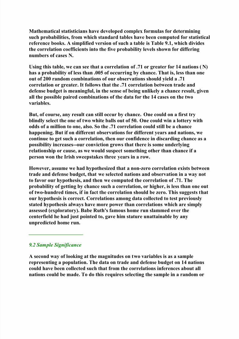
Mathematical statisticians have developed complex formulas for determining

such probabilities, from which standard tables have been computed for statistical

reference books. A simplified version of such a table is Table 9.1, which divides

the correlation coefficients into the five probability levels shown for differing

numbers of cases N.

Using this table, we can see that a correlation of .71 or greater for 14 nations (N)

has a probability of less than .005 of occurring by chance. That is, less than one

out of 200 random combinations of our observations should yield a .71

correlation or greater. It follows that the .71 correlation between trade and

defense budget is meaningful, in the sense of being unlikely a chance result, given

all the possible paired combinations of the data for the 14 cases on the two

variables.

But, of course, any result can still occur by chance. One could on a first try

blindly select the one of two white balls out of 50. One could win a lottery withodds of a million to one, also. So the .71 correlation could still be a chance

happening. But if on different observations for different years and nations, we

continue to get such a correlation, then our confidence in discarding chance as a

possibility increases--our conviction grows that there is some underlying

relationship or cause, as we would suspect something other than chance if a

person won the Irish sweepstakes three years in a row.

However, assume we had hypothesized that a non-zero correlation exists between

trade and defense budget, that we selected nations and observation in a way not

to favor our hypothesis, and then we computed the correlation of .71. The

probability of getting by chance such a correlation, or higher, is less than one out

of two-hundred times, if in fact the correlation should be zero. This suggests that

our hypothesis is correct. Correlations among data collected to test previously

stated hypothesis always have more power than correlations which are simply

assessed (exploratory). Babe Ruth's famous home run slammed over the

centerfield he had just pointed to, gave him stature unattainable by any

unpredicted home run.

9 .2 Sam ple Significance

A second way of looking at the magnitudes on two variables is as a sample

representing a population. The data on trade and defense budget on 14 nations

could have been collected such that from the correlations inferences about all

nations could be made. To do this requires selecting the sample in a random or



stratified manner so as to best reflect the population of nations. For example,

such a sample might be collected of 100 students attending the University of

Hawaii to determine the correlation between drug use and grades; of 500

Hawaiian residents to assess the correlation between ethnicity and liberalism in

Hawaii; of 1,500 national television viewers to ascertain the correlation between

programming and violence.

Now, assume the fourteen nations we have used to assess the correlation between

trade and defense budget is a good sample, i.e., well reflects all nations. Then

what inference about all nations can be made from a correlation of .71 between

the two variables?

A useful way of answering this is in terms of an alternative hypothesis.1 If in

reality there were a zero or negative correlation in fact for all nations, what

would be the probability of getting by chance at least the correlation found? That

is, what is the chance of a plus .71 or higher being found for the sample when the

correlation is zero or negative in the population?

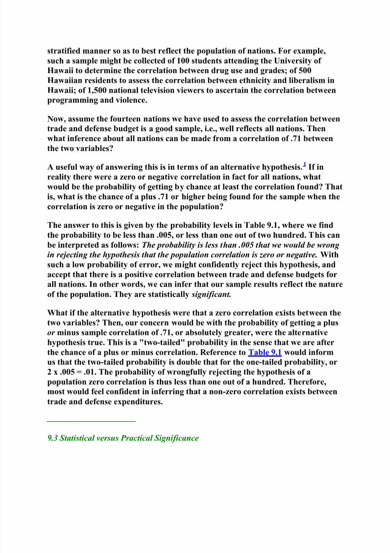
The answer to this is given by the probability levels in Table 9.1, where we find

the probability to be less than .005, or less than one out of two hundred. This can

be interpreted as follows: T he probability is less t han .005 t hat we would be wrong

in rejecting t he h y pot hesis t hat t he po pulation correlation is zero or negative. With

such a low probability of error, we might confidently reject this hypothesis, and

accept that there is a positive correlation between trade and defense budgets for

all nations. In other words, we can infer that our sample results reflect the nature

of the population. They are statistically significant.

What if the alternative hypothesis were that a zero correlation exists between the

two variables? Then, our concern would be with the probability of getting a plus

or minus sample correlation of .71, or absolutely greater, were the alternative

hypothesis true. This is a "two-tailed" probability in the sense that we are after

the chance of a plus or minus correlation. Reference to Table 9.1 would inform

us that the two-tailed probability is double that for the one-tailed probability, or

2 x .005 = .01. The probability of wrongfully rejecting the hypothesis of a

population zero correlation is thus less than one out of a hundred. Therefore,

most would feel confident in inferring that a non-zero correlation exists between

trade and defense expenditures.

9 .3 Statistical versus Practical Significance



There are, therefore, two types of statistical significance. One is the likelihood of

getting by chance the particular correlation or greater between two sets of

magnitudes; the second is the probability of getting a sample correlation by

chance from a population. In either case, the significance of a result increases--

the probability of the result being by chance decreases--as the number of cases

increases. This can be seen from Table 9.1. Simply consider the column in the

table for the probability of .05, and notice how the correlation that meets this

level decreases as N increases. For an N of 5 a correlation must be as high as .80

to be significant at .05; but for an N of 1,000, a

correlation of .05 is significant.

Therefore, very small correlations can be

significant at very low probabilities of their being

chance results, even though the variance in

common is nil. Table 9.2 compares significance

and variance in common for correlations at a

probability level of .05 for selected sample sizes.

Clearly, one can have significant results

statistically, when there is very little variation in

common. A high significance does not mean a strong relationship. Even though

for 1,000 cases, 99.75 percent of the variation between two variables is not in

common, the small covariation that does exist can significantly differ from zero.

Which should one consider, then? Significance or variance in common? This

depends on what one is testing or concerned about. If one wants results from

which to make forecasts or predictions, correlations of even .7 or .8 may not be

sufficient, no matter how significant, since there is still much unrelated variance.

If one's results are to be a base for policy decisions, only a high percent of

variance in common may be acceptable. But if one is interested in uncovering

relationships, no matter how small, then significance is of concern.

9 .4 Sam ple versus Po pulation

Can one determine the significance of a correlation for a population? Say we had

computed the correlation between trade and defense budget for all nations and

found .71. Could we ask whether this is significant?

Yes, when we keep in mind the two types of significance. Clearly, this is not a

sample correlation and sample significance is meaningless. But, we can assess the



likelihood of this being a chance correlation between the two sets of magnitudes

for all nations, as described in Section 9.1.

Fortunately, both types of significance can be assessed using the same probability

table, such as Table 9.1.

9 .5 Assum ptions

The formulas mathematical statisticians have developed for assessing

significance require certain assumptions for this derivation. As the data depart

from these assumptions, the tables of probabilities for the correlation are less

applicable.

Both types of significance described here assume a normal distribution for bothvariables, i.e., that the magnitudes approximate a bell-shaped distribution.

When sampling significance is of concern, the observations are assumed drawn

from a bivariate normal population. That is, were the frequencies of observation

plotted for both variables for the population, then they would be distributed in

the shape of a bell placed on the middle of a plane, with the lower flanges

widening out and merging into the flat surface.

By virtue of these distributive requirements, the assessment of significance also

demands that the data be interval. or ratio measurements, i.e., data like that fortrade, GNP per capita, defense budget, GNP for defense, or U.S. agreement

shown in Table 3.1 Dichotomous data, as that for stability and foreign conflict, or

rank order data, as that for power, cannot have the significance of their product

moment correlations assessed. For this, one must use a different type of

correlation coefficient, of which the next chapter will give examples.

NOTES

1. Statisticians have formulated a systematic design, called "tests of hypotheses," for

making a decision to reject or accept statistical hypotheses. Most elementary statistical text

books have a chapter or so dealing with this topic.





dichotomous variables may be less than an absolute value of 1.00. Thus, different

phi coefficients may not be comparable.

The maximum possible value of phi for given marginals can be computed and

used to form the phi-over- phi-mix correlation coefficient, which is the ratio of phi

to the maximum possible phi given the marginals. Regardless of marginal values,then, phi-over-phi-max will be plus or minus 1.00 in the case of perfect

correlation, and these coefficients will be comparable for different variables.

However, the phi-over-phi-max makes a strong assumption that the underlying

bivariate distribution in the data is rectangular. Moreover, this coefficient has an

increasingly steep approach to 1.00 as the number of cases with the two

magnitudes become increasingly disproportionate.

In addition to the phi-over-phi-max coefficient for dichotomous data, the

tetrachoric coefficient could be computed. This estimates the value of the productmoment correlation, if the dichotomous data are drawn from a normal

distribution. The basic assumption of the tetrachoric, therefore, is that the

underlying distribution of the data is bivariate normal. However, in contrast to

the phi coefficient, the tetrachoric does not have its range affected by unequal

data marginals and its significance can be assessed using appropriate tables.

10.2 Pattern-Magnitude Coefficients

The correlation and alternative coefficients measure the pattern similarity of the

magnitudes for two variables--their covariation. Sometimes, however, it may be

useful to measure both pattern and magnitude correlation.

Figure 10.1 may help to make the distinction between pattern and magnitude

clear.

A number of pattern-magnitude correlation coefficients have been developed.

One that is particularly useful is the intraclass correlation coefficient, which can

be applied to any number of variables. Just restricting it to two variables,however, the intraclass divides their variance into two parts. One is the variance

of each case on the two variables and is called the within-class variance. If the

magnitudes for each case on the two variables are the same, this variance is zero.

The second part is the variance of the variable across the cases, which is the

between-class variance. The intraclass correlation is then simply the between-



class minus the within-class variance as a ratio to the sum of the two kinds of

variance. And the significance of this ratio can be assessed.

For two variables, the intraclass will range between -1.00 and +1.00. When it is

1.00, each case has identical magnitudes for each variable--all the variation is

across cases. When it is -1.00, all the variation is due to each case having differentmagnitudes on each variable.

NOTES

1. I provide more detail with references to specific sources in my Applied Factor Analysis

(1970, Section 12.3).

2.A

ssuming a bivariate normally distributed population, the efficiency of the Spearmanand Kendall rank correlation coefficient will be 91 percent that of the product moment.

3. The margins of the fourfold table are the number of cases for each of the two values of a

variable. For example, in Table 2.2, the marginals for trade are 10 cases with a low value, 4

cases with a high; for GNP per capita there are 9 cases with low values, 5 with high.

Clearly, these marginals are unequal.

CHAPTER 11:

CONSIDER ATIONS

In this final chapter I will pull together several aspects of correlation and some

pertinent considerations, as well as add a few final comments.

Two things are correlated if they covary positively or negatively. And we have a

widely used, mathematically based, coefficient called the product moment for

determining this correlation.

This coefficient will describe the correlation between any two variables,

regardless of their type of measurement. If, however, the statistical significance

of the correlation is of concern, then to assess this significance interval or ratio

measurement and normal distributions are assumed.



Alternative correlation coefficients are available for specific purposes and types

of data. Moreover, if the data do not meet the assumptions required for assessing

the significance of the product moment, then these alternative coefficients may

enable significance to be determined.

The product moment, and indeed, most alternative coefficients, measure patterncorrelation. Alternatives, especially the intraclass, are available to also measure

both pattern at magnitude correlation, however.

Whether describing the data or regarding significance, the correlation coefficient

measures linear correlations, i.e., that along a straight line as in Figure 6.2c or

Figure 6.3a. Even were observations to fall exactly on a curve as in Figure 6.2a or

Figure 6.2b, the product moment or alternative coefficients would show a zero or

low linear correlation.

The product moment correlation is sensitive to extreme magnitudes. Extremecases can have many times the effect of other cases on the correlation coefficient.

The correlation coefficient may thus "hang" on a few cases with unusually large

or small magnitudes, and data transformation or alternative correlations might

be used to avoid this problem.

Errors in the data on two variables can make the correlation coefficient higher

or lower than it should be. However, error that is random--uncorrelated among

themselves or with the true magnitudes--only depresses the absolute correlation.

Thus the correlation coefficient for data with random error understates the real

correlation and is thus a conservative measure.1

The correlation between two variables may be influenced by other variables.

Formulas are available, fortunately, to determine these influences and remove

them from the correlation. Therefore, if outside influences are suspected, a high,

low, or zero correlation between two variables should not be accepted at face

value and partial correlations, holding constant these extraneous influences, can

be calculated.

There is a geometry of correlation in terms of vectors that provides an intuitively

and heuristically powerful picture of correlation. This is simply the cosine of theangle between two variables of mean-deviation data plotted as vectors.

Correlation between magnitudes on variables for a specific time period (such as

power and defense budget for 1955) do not indicate the correlations between

these variables over time (such as for power and defense budget by year in the

U.S., 1946-75). Similarly, over time correlations do not indicate what the



correlations would be for cases at a point in time. That is, for the same variables

cross-sectional and time series correlations are independent.2

Finally, the correlation coefficient is a useful and potentially powerful tool. It can

aid understanding reality, but it is no substitute for insight, reason, and

imagination. The correlation coefficient is a flashlight of the mind. It must beturned on and directed by our interests and knowledge; and it can help gratify

and illuminate both. But like a flashlight, it can be uselessly turned on in the

daytime, used unnecessarily beneath a lamp, employed to search for something

in the wrong room, or become a play thing.

Understanding correlations is understanding both the nature of the coefficient

and its dependence on human intelligence, intuition, and competence.

NOTES

1. The logic and details underlying this paragraph are elaborated in Rummel (1972,

Chapter 6).

2. The picture of this independence is shown in Rummel (1970, Figure 8.1, p. 201).

REFERENCES

Horst, P., Matrix Algebra for Social Scientists. New York: Holt, Rinehart, and Winston,

1963.

Rummel, R. J., Applied Factor Analysis. Evanston, Ill.: Northwestern University Press,

1970.

____________ , Dimensions of Nations. Beverly Hills: Sage, 1972.

Go to top of document

Documents

Understanding Correlation-RJ Rummel