Understanding competing risks: a simulation point of view

RESEARCH ARTICLE Open Access

Understanding competing risks: a simulationpoint of viewArthur Allignol1,2*, Martin Schumacher2, Christoph Wanner3, Christiane Drechsler3 and Jan Beyersmann1,2

Abstract

Background: Competing risks methodology allows for an event-specific analysis of the single components ofcomposite time-to-event endpoints. A key feature of competing risks is that there are as many hazards as there arecompeting risks. This is not always well accounted for in the applied literature.

Methods: We advocate a simulation point of view for understanding competing risks. The hazards are envisagedas momentary event forces. They jointly determine the event time. Their relative magnitude determines the eventtype. ‘Empirical simulations’ using data from a recent study on cardiovascular events in diabetes patients illustratesubsequent interpretation. The method avoids concerns on identifiability and plausibility known from the latentfailure time approach.

Results: The ‘empirical simulations’ served as a proof of concept. Additionally manipulating baseline hazards andtreatment effects illustrated both scenarios that require greater care for interpretation and how the simulationpoint of view aids the interpretation. The simulation algorithm applied to real data also provides for a general toolfor study planning.

Conclusions: There are as many hazards as there are competing risks. All of them should be analysed. Thisincludes estimation of baseline hazards. Study planning must equally account for these aspects.

BackgroundThe analysis of time-to-event data (’survival analysis’)has evolved into a well established application ofadvanced statistical methodology in medicine. E.g., inthe New England Journal of Medicine, survival methodshave evolved from an occasionally used technique in thelate 70s over moderate use in the late 80s into the lead-ing statistical procedure by 2005 [1]. The archetypicalapplication analyses time until death, but combined end-points are also frequently considered. E.g., a recent lit-erature review in clinical oncology [2] found a multitudeof combined endpoints including, e.g., progression-freesurvival, distant metastasis-free survival, locoregionalrelapse-free survival, etc. The medical problems at handwill, as these endpoints exemplarily suggest, usually bemore complex than can be addressed by the analysis oftime until one potentially combined event type.

Competing risks techniques allow for a more specificanalysis in that they consider time until occurrence ofthe combined endpoint and endpoint type, e.g., progres-sion in contrast to death without prior progression. Therelevance of competing risks in medical research is high-lighted by methodological papers in various medicalfields. We mention [3-5] as recent examples. A classicalstatistics textbook account has been given in the firstedition of [6] in 1980, and a definite mathematical treat-ment based on counting processes is included in [7].Excellent tutorial papers in the statistical literature are[8,9].However, despite an obvious practical relevance and a

firmly established methodological background, compet-ing risks are not always well accounted for in publishedsurvival analyses in medical journals: E.g., another recentliterature review [10] in clinical oncology found that 27out of 125 included randomised controlled trials consid-ered time to progression, but only 5 out of 125 studiesaccounted for such endpoint types being non-exclusive.A similar picture has been reported for studies on the

* Correspondence: [email protected] Center for Data Analysis and Modeling, University of Freiburg,GermanyFull list of author information is available at the end of the article

Allignol et al. BMC Medical Research Methodology 2011, 11:86http://www.biomedcentral.com/1471-2288/11/86

© 2011 Allignol et al; licensee BioMed Central Ltd. This is an Open Access article distributed under the terms of the Creative CommonsAttribution License (http://creativecommons.org/licenses/by/2.0), which permits unrestricted use, distribution, and reproduction inany medium, provided the original work is properly cited.

mailto:[email protected]

http://creativecommons.org/licenses/by/2.0

effect of implantable cardioverter defibrillator on subse-quent cardiac events [11].The key to an adequate competing risks analysis is:

There are as many hazards as there are competing risks.Unless all of these hazards, which are often calledcause-specific hazards, have been analysed, the analysiswill remain incomplete. In particular, only a completeanalysis will allow for predicting event probabilities.The aim of this paper is to suggest an algorithmic or

simulation point of view towards this key issue. The ideabehind this point of view is that it gives a clear buildingplan of how the involved hazards generate competingrisks data over the course of time. However, although thealgorithm is mathematically well established [12], it israrely used in practice [13]. We will use it as an opera-tional device for understanding competing risks.The remainder of the paper is organised as follows: The

Methods Section introduces competing risks as arisingfrom a multistate model, gives an algorithmic interpreta-tion of the involved hazards and provides a description ofthe data example from a recent study on cardiovascularevents in diabetes patients [14]. In this Section, we alsoexplain ‘empirical simulation’, where one simulates basedon the empirical study probabilities, and give an overviewon simulation scenarios that will be considered. The Sec-tion closes with a brief summary of the differencebetween the present paper and the common latent failuretime approach to competing risks. Results are reported inthe Results Section. Our simulations are ‘empirical simu-lations’, and they work as a proof of concept: Interpretinga competing risks analysis from a simulation perspectivecan be viewed as a thought experiment. The actual simu-lations show that the simulation perspective works.Finally, a discussion and a conclusion are offered, with afocus on consequences for practical competing risks ana-lyses, including graphical presentation and planning inthe presence of competing events.

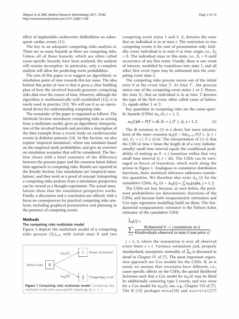
MethodsThe competing risks multistate modelFigure 1 depicts the multistate model of a competingrisks process (Xt)t≥0 with initial state 0 and two

competing event states 1 and 2. Xt denotes the statethat an individual is in at time t. The restriction to twocompeting events is for ease of presentation only. Initi-ally, every individual is in state 0 at time origin, i.e., X0

= 0. The individual stays in this state, i.e., Xt = 0 untiloccurrence of any first event. Usually, there is one eventof interest, modelled by transitions into state 1, and allother first event types may be subsumed into the com-peting event state 2.The competing risks process moves out of the initial

state 0 at the event time T. At time T , the processenters one of the competing event states 1 or 2. Hence,the state XT that an individual is in at time T denotesthe type of the first event, often called cause of failure.XT equals either 1 or 2.Key quantities in competing risks are the cause-speci-

fic hazards (CSHs) a0j (t), j = 1, 2,

α0j(t)dt = P(T ∈ dt, XT = j, |T ≥ t), j = 1, 2. (1)

The dt notation in (1) is a short, but more intuitiveform of the more common a0j(t) = limΔt↘0 P(T Î [t, t +Δt), XT = j | T ≥ t)/Δt. The interpretation of (1) is thatthe CSH at time t times the length dt of a very (infinite-simally) small time interval equals the conditional prob-ability of making an 0 ® j transition within that verysmall time interval [t, t + dt). The CSHs can be envi-saged as forces of transition, which work along thearrows in Figure 1. Analogous to cumulative distributionfunctions, basic statistical inference addresses cumula-tive quantities. We therefore also write A0j (t) for thecumulative CSHs, A0j (t) = A0j(t) =

∫ t0 α0j(u)du, j = 1, 2.

The CSHs are key, because, as seen below, the perti-nent probabilities are deterministic functions of theCSHs, and because both nonparametric estimation andCox-type regression modelling build on them. The fun-damental nonparametric estimator is the Nelson-Aalenestimator of the cumulative CSHs

A0j(t) =∑s≤t

#{observed 0 → j transitions at s}#{individuals observed in state 0 just prior s} ,

j = 1, 2, where the summation is over all observedevent times s ≤ t. Variance estimation and, properlystandardised, asymptotic normality of A0j is discussed indetail in Chapter IV of [7]. The most important regres-sion approach are Cox models for the CSHs. If, as isusual, we assume that covariates have different, i.e.,cause-specific effects on the CSHs, the partial likelihoodfactorises such that a Cox model for a01(t) may be fittedby additionally censoring type 2 events, and vice versafor a Cox model for a02(t), see, e.g., Chapter VII of [7].The R [15] packages mvna[16] and survival[17]

Figure 1 Competing risks multistate model. Competing risksmultistate model with cause-specific hazards a0j (t), j = 1, 2.


Page 2 of 13

provide for convenient computation of the Nelson-Aalenestimator and the Cox model, respectively.The a0j’s sum up to the all-cause hazard a0·(t)dt = P

(T Î dt | T ≥ t) with cumulative all-cause hazard A0·(t).The survival function of T is therefore a function ofboth a0j’s, P(T > t) = exp(− ∫ t

0 α0·(u)du). As usual, P (T>t) is estimated using the Kaplan-Meier estimator,which is a deterministic function of the cause-specificNelson-Aalen estimators.The so-called cumulative incidence functions (CIFs)

are the expected proportion of individuals experiencinga certain competing event over the course of time,

P(T ≤ t, XT = j) =∫ t

0P(T > u−)α0 j(u)du, (2)

j = 1, 2. The interpretation of the right hand side of (2) isthat the CIF at time t equals the integral over all ‘probabil-ities’ to make an 0 ® j transition precisely at time u. Forthis, an individual has to stay in state 0 until just beforetime u, which is reflected by the term P (T >u-). Condi-tional on being in state 0 just before time u, an 0 ® j tran-sition at time u is reflected by the term a0j (u) du.One consequence is that the CIFs are involved functions

of all CSHs via P (T >u-). The CIFs P (T ≤ t, XT = 1) andP (T ≤ t, XT = 2) add up to the all-cause distribution func-tion 1 - P (T >t). The Aalen-Johansen estimators of theCIFs can be obtained from (2) by substituting P (T >u-)with the Kaplan-Meier estimator and a0j (u) du with theincrement of the cause-specific Nelson-Aalen estimator. Adetailed discussion of the Aalen-Johansen estimator is inChapter IV of [7]; variance estimation is assessed in [18].In R, survival is typically used for estimating P (T >t).The Aalen-Johansen estimator may be computed usingetm[19], and prediction of the CIFs based on Cox modelsfor the CSHs is implemented in mstate[20].It is crucial to any competing risks analysis that both

cause-specific hazards completely determine the sto-chastic behaviour of the competing risks process [7,Chapter II.6]. This is mirrored above by the CIFs andthe all-cause distribution function being deterministicfunctions of all CSHs. However, these deterministic rela-tionships are involved. Therefore, we will pursue analgorithmic interpretation of the CSHs below.

Algorithmic interpretation of the cause-specific hazardsThinking of the CSHs as momentary forces of transitionwhich move along the arrows in Figure 1 suggests thatcompeting risks data are generated over the course oftime as follows:

1. The event time T is generated with distributionfunction 1 - P (T >t), i.e., with hazard a01(t) + a02(t)= a0·(t).

2. At time T , event type j occurs with probabilitya0j (T )/a0·(T ), j = 1, 2.

Using this algorithm for simulation studies in compet-ing risks has been discussed in [13]. It is important tonote, however, that the algorithm goes beyond the com-putational question of how to implement simulations.Rather, the algorithm reflects the probabilistic questionof how to build a probability measure based on theCSHs. This aspect is discussed in detail by [12] in themore general context of multistate models which arerealized as a nested series of competing risksexperiments.The algorithmic perspective of this paper then implies

that the task of statistical inference is to detect theingredients of the above algorithm. We illustrate thisapproach in the data example below. To this end, wenote that the analysis of a combined endpoint isrestricted to step 1 of the above algorithm. Here, theeffect of a treatment, say, on both CSHs determineswhether the occurrence of an event (of any type) isdelayed or accelerated. In step 2, the type of an eventagain depends on the treatment effect on both CSHs.We illustrate below that interpretation is straightforwardif the treatment effects on the CSHs work in oppositedirections or if one CSHs remains unaffected. However,interpretation will become more challenging if there areunidirectional effects on both CSHs. We will find that,in general, it is also mandatory to consider cause-speci-fic baseline hazards in the interpretation.

The 4D studyThe background of the 4D study was that statins areknown to be protective with respect to cardiovascularevents for persons with type 2 diabetes mellitus withoutkidney disease, but that a potential benefit of statins inpatients receiving hemodialysis had until then not beenassessed. Patients undergoing hemodialysis are at highrisk for cardiovascular events. The 4D study was a pro-spective randomised controlled trial evaluating the effectof lipid lowering with atorvastatin in 1255 diabeticpatients receiving hemodialysis. Patients with type 2 dia-betes mellitus, age 18-80 years, and on hemodialysis forless than 2 years were enrolled between March 1998and October 2002. Patients were randomly assigned todouble-blinded treatment with either atorvastatin (619patients) or placebo (636 patients) and were followeduntil death, loss to follow-up, or end of the study inMarch 2004.The 4D study was planned [21] and analysed [14] for

an event of interest in the presence of competing risks.The event of interest was defined as a composite ofdeath from cardiac causes, stroke and non-fatal myocar-dial infarction, whichever occurred first. The other


Page 3 of 13

competing event was death from other causes. Wanneret al. reported a CSH ratio of 0.92 (95%-confidenceinterval [0.77, 1.10]) for the event of interest. There wasessentially no effect on the competing CSH.The simulation study below will use the data of the

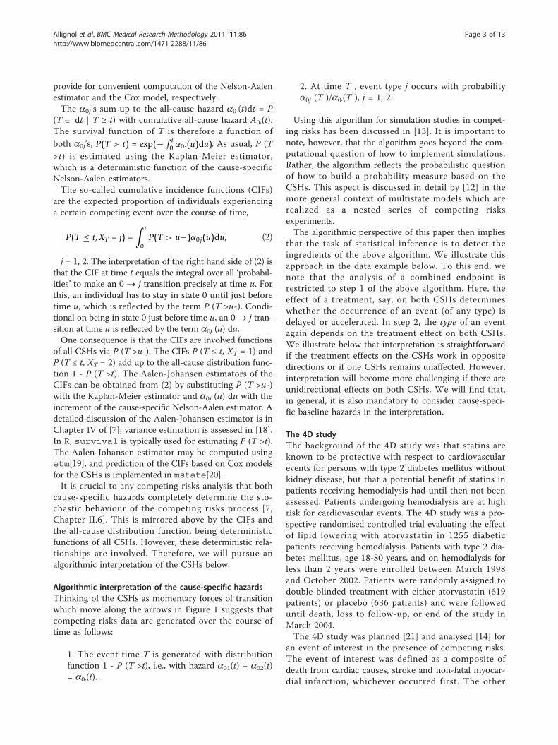
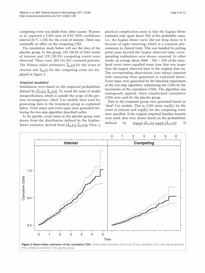
placebo group. In this group, 243 (38.2% of 636) eventsof interest and 129 (20.3%) competing events wereobserved. There were 264 (41.5%) censored patients.The Nelson-Aalen estimators A01(t) for the event of

interest and A02(t) for the competing event are dis-played in Figure 2.

’Empirical simulation’Simulations were based on the empirical probabilitiesdefined by (A01(t), A02(t)). To avoid the issue of modelmisspecification, which is outside the scope of the pre-sent investigations, ‘ideal’ Cox models were used forgenerating data in the treatment group as explainedbelow. Event times and event types were generated fol-lowing the two-step algorithm described earlier.To be specific, event times in the placebo group were

drawn from the distribution defined by the Kaplan-Meier estimator derived from (A01(t), A02(t)). Here, a

practical complication arose in that the Kaplan-Meierestimator only spent about 76% of the probability mass.I.e., the Kaplan-Meier curve did not drop down to 0because of right-censoring, which is a common phe-nomenon in clinical trials. This was handled by puttingpoint mass beyond the largest observed time; corre-sponding realisations were always censored. In otherwords, on average about 100% - 76% = 24% of the simu-lated event times equalled some time that was largerthan the largest observed time in the original data set.The corresponding observations were always censoredwith censoring times generated as explained below.Event types were generated by the binomial experimentof the two-step algorithm, substituting the CSHs by theincrements of the cumulative CSHs. The algorithm wasanalogously applied, when transformed cumulativeCSHs were used for the placebo group.Data in the treatment group were generated based on

‘ideal’ Cox models. That is, CSH ratios exp(b1) for theevent of interest and exp(b2) for the competing eventwere specified. If the original empirical baseline hazardswere used, data were drawn based on the probabilities

defined by (exp(β1)A01(t), exp(β2)A02(t)). If

Time

Cum

ulat

ive

CS

Hs

0.0

0.5

1.0

0 1 2 3 4 5 6

Interest

0 1 2 3 4 5 6

Competing

Figure 2 Nelson-Aalen estimators of the cumulative CSHs. Nelson-Aalen estimators (solid lines) of the cumulative CSHs with log-transformed95% confidence intervals in the placebo group.


Page 4 of 13

transformations of (A01(t), A02(t)) were used for gener-ating placebo data, the CSH ratios acted on the trans-formed cause-specific baseline hazards. This reflects thesituation that the true underlying baseline CSHs are a01

(t) and a02(t) (or transformations thereof) in the controlgroup, while the CSHs of the treatment group are exp(b1)a01(t) and exp(b2)a02(t) for the case of untrans-formed baseline hazards. Random censoring times weregenerated for all individuals based on the Kaplan-Meierestimator of the censoring survival function in the pla-cebo group. Note that this estimator did spend 100% ofthe probability mass.

Overview of simulation scenariosThe scenarios investigated in the next Section differedboth with respect to the choice of b1 and b2 and interms of the cumulative baseline hazards, i.e., the cumu-lative CSHs in the placebo group. The choice of the b’sbroadly falls into three categories.One category is characterised by b2 = 0, i.e., there is

no effect on the competing CSH. A prime example areimplantable cardioverter defibrillators [11], which dis-play a beneficial effect on the CSH of sudden cardiacdeath but no effect on the CSH for death from othercauses. The assumption of b2 = 0 straightforwardlyimplies the direction of the treatment effect on the CIF:If b1 < 0, the CIF of interest in the treatment group isalways less than the one in placebo group. The relation-ship is reversed, if b1 > 0. This is intuitively understoodthinking of the CSHs as momentary forces of transition,and it is reflected in step 2 of the simulation algorithm.E.g., if b1 < 0 and b2 = 0, the binomial event type 1probabilities are reduced for the treatment group.A second category is characterised by opposite treat-

ment effects on the CSHs. This category straightfor-wardly implies the direction of the treatment effect onthe CIF, too: The constellation b1 < 0 and b2 > 0 impliesa smaller CIF of interest in the treatment group but alsoa larger competing CIF. These relations are reversed forb1 > 0 and b2 < 0. This is again intuitively implied bythinking of the CSHs as momentary forces of transition,and it is also reflected in step 2 of the simulation algo-rithm. E.g., if b1 < 0 and b2 > 0, the binomial event type1 probabilities are reduced for the treatment group.Finally, unidirectional treatment effects on the CSHs

constitute the third category. Interestingly, the interpre-tation of unidirectional effects is straightforward whenboth competing events are fatal in the sense that a treat-ment with b1 < 0 and b2 < 0, say, is beneficial. But uni-directional effects also present the most challengingscenario in terms of understanding the resulting courseof the CIFs. The interpretation for step 1 of the simula-tion algorithm is straightforward. If, e.g., b1 < 0 and b2< 0, events of any type will happen later. The

interpretational challenge becomes apparent in the sec-ond step of the algorithm: If, e.g., b2 <b1 < 0, the relativemagnitude of the CSHs changes such that the binomialevent of interest probabilities are increased. The inter-pretational difficulty is the increase of this probability,although b1 is negative. This constellation may result inan (eventually) increased CIF of interest.All three categories are encountered in practice.

Examples from clinical trials in hospital epidemiologyare given in [22].

Difference to the latent failure time modelSome readers may be more familiar with competing risksas arising from risk-specific latent times, say, T(1) and T(2).The connection to our multistate framework is T = min(T(1), T(2)) with event type XT = 1, if T(1) <T(2), and XT = 2otherwise. The latent failure time model imposes an addi-tional structure, which has been heavily criticised mainlyfor three reasons. The dependence structure of T(1) and T(2) is, in general, not identifiable [23]. Since the latent timesare unobservable, there is something hypothetical aboutthem, which questions their plausibility [24]. Perhaps mostimportantly, it has been disputed whether the latent failuretime point of view constitutes a fruitful approach to answerquestions of the original subject matter [25].Despite of this critique, latent times are the predomi-

nant approach for simulating competing risks data [13].Assuming, for tractability, T(1) and T(2) to be indepen-dent with hazards equal to the cause-specific hazardsa01(t) and a02(t), respectively, is computationally correctin that simulation based on this model yields the rightdata structure.However, nothing is gained from assuming the addi-

tional latent structure, either. As a consequence, we willemphasise simulation and interpretation along the linesof the Algorithmic interpretation of the cause-specifichazards outlined earlier. This avoids the concerns onidentifiability, plausibility and usefulness.E.g., in the 4D study, the typical interpretation of the

latent times would be that T(1) is the time until death fromcardiac causes, stroke or non-fatal myocardial infarction,while T(2) is the time until death from other causes. Suchan interpretation has given rise to debating whether, say, apatient may conceptually still die from other causes afterhaving died because of a cardiac event. In contrast to this,our approach only assumes that a patient is conceptuallyat risk of experiencing any of these events, provided thatnone of these events has happened so far.

ResultsGeneralWe studied ten different scenarios, which are tabulatedin Table 1 and cover all effect categories discussed ear-lier. Scenarios 1-5 have b1 similar to the actual study


Page 5 of 13

result [14], and scenarios 6-10 have b1 similar to theplanning figures [21]. Table 1 also displays the use ofdifferent baseline hazards. For each of the scenarios,1000 simulation runs were considered with 500 indivi-duals in the placebo group and 500 individuals in thetreatment group.Table 2 presents, for each scenario and based on Cox

analyses of the CSHs, the mean log CSH ratios ¯β1

and¯β2, empirical 95% confidence intervals, the coverage

probabilities of the Wald-type confidence intervals forthe estimated regression coefficients, and the empiricalpower.For Scenarios 1-5, we also plotted the true CIFs (solid

black lines), the average of the Aalen-Johansen estima-tors (dashed black lines) and 300 randomly selectedAalen-Johansen estimators (grey lines). The reason toonly plot a random subsample was to maintain a greyshading in the plots.We collect some general observations. In the Figures,

the true CIFs are visually hardly distinguishable from

the average of the Aalen-Johansen estimators from eachsimulation study. This entails that the algorithmic pointof view is appropriate: Simulation along this line yieldsdata that are consistent with the original quantities.Similar statements hold for the average of the estimatedregression coefficients and the coverage probability oftheir confidence intervals. The Figures also show thatboth regression coefficients and baseline hazards matter.E.g., keeping both regression coefficients, but changingbaseline hazards alters the CIFs. Similarly, keeping boththe CSH ratio of interest and the baseline hazards, butchanging the competing CSH ratio alters the CIFs.We also note that recovering the true CIFs implies

that we would have also recovered the original cumula-tive hazards of Figure 2. This is so, because knowledgeof all CIFs allows to derive all CSHs and vice versa.

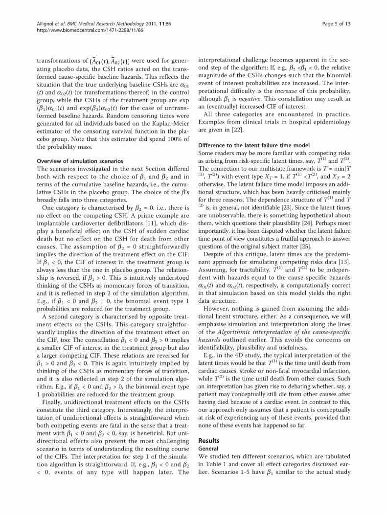
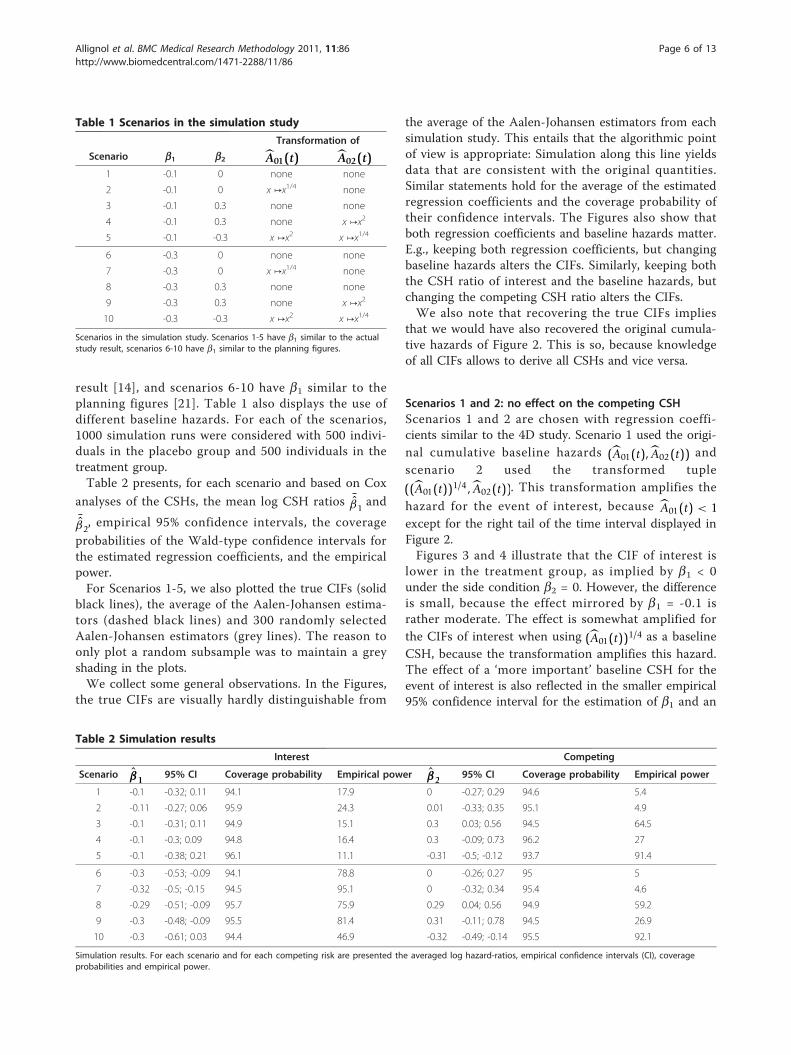
Scenarios 1 and 2: no effect on the competing CSHScenarios 1 and 2 are chosen with regression coeffi-cients similar to the 4D study. Scenario 1 used the origi-nal cumulative baseline hazards (A01(t), A02(t)) andscenario 2 used the transformed tuple

((A01(t))1/4, A02(t)). This transformation amplifies the

hazard for the event of interest, because A01(t) < 1except for the right tail of the time interval displayed inFigure 2.Figures 3 and 4 illustrate that the CIF of interest is

lower in the treatment group, as implied by b1 < 0under the side condition b2 = 0. However, the differenceis small, because the effect mirrored by b1 = -0.1 israther moderate. The effect is somewhat amplified forthe CIFs of interest when using (A01(t))1/4 as a baselineCSH, because the transformation amplifies this hazard.The effect of a ‘more important’ baseline CSH for theevent of interest is also reflected in the smaller empirical95% confidence interval for the estimation of b1 and an

Table 1 Scenarios in the simulation study

Transformation of

Scenario b1 b2 A01(t) A02(t)1 -0.1 0 none none

2 -0.1 0 x ↦x1/4 none

3 -0.1 0.3 none none

4 -0.1 0.3 none x ↦x2

5 -0.1 -0.3 x ↦x2 x ↦x1/4

6 -0.3 0 none none

7 -0.3 0 x ↦x1/4 none

8 -0.3 0.3 none none

9 -0.3 0.3 none x ↦x2

10 -0.3 -0.3 x ↦x2 x ↦x1/4

Scenarios in the simulation study. Scenarios 1-5 have b1 similar to the actualstudy result, scenarios 6-10 have b1 similar to the planning figures.

Table 2 Simulation results

Interest Competing

Scenario β1 95% CI Coverage probability Empirical power β2 95% CI Coverage probability Empirical power

1 -0.1 -0.32; 0.11 94.1 17.9 0 -0.27; 0.29 94.6 5.4

2 -0.11 -0.27; 0.06 95.9 24.3 0.01 -0.33; 0.35 95.1 4.9

3 -0.1 -0.31; 0.11 94.9 15.1 0.3 0.03; 0.56 94.5 64.5

4 -0.1 -0.3; 0.09 94.8 16.4 0.3 -0.09; 0.73 96.2 27

5 -0.1 -0.38; 0.21 96.1 11.1 -0.31 -0.5; -0.12 93.7 91.4

6 -0.3 -0.53; -0.09 94.1 78.8 0 -0.26; 0.27 95 5

7 -0.32 -0.5; -0.15 94.5 95.1 0 -0.32; 0.34 95.4 4.6

8 -0.29 -0.51; -0.09 95.7 75.9 0.29 0.04; 0.56 94.9 59.2

9 -0.3 -0.48; -0.09 95.5 81.4 0.31 -0.11; 0.78 94.5 26.9

10 -0.3 -0.61; 0.03 94.4 46.9 -0.32 -0.49; -0.14 95.5 92.1

Simulation results. For each scenario and for each competing risk are presented the averaged log hazard-ratios, empirical confidence intervals (CI), coverageprobabilities and empirical power.


Page 6 of 13

0.0

0.1

0.2

0.3

0.4

0.5

0.6

0.7

Cum

ulat

ive

Inci

denc

e F

unct

ion

Interest − Treated Interest − Untreated

0 1 2 3 4 5 6

0.0

0.1

0.2

0.3

0.4

0.5

0.6

0.7

Time

Cum

ulat

ive

Inci

denc

e F

unct

ion

Competing − Treated

0 1 2 3 4 5 6

Time

Competing − Untreated

Figure 4 Scenario 2 of Table 1. Solid black lines are the true CIFs, solid grey lines are 300 randomly selected Aalen-Johansen estimators. Theaverage of the Aalen-Johansen estimators is drawn as dashed black lines. Dotted lines in the left plots are the corresponding untreated CIFs.

0.0

0.1

0.2

0.3

0.4

0.5

0.6

0.7

Cum

ulat

ive

Inci

denc

e F

unct

ion


0 1 2 3 4 5 6

0.0

0.1

0.2

0.3

0.4

0.5

0.6

0.7

Time

Cum

ulat

ive

Inci

denc

e F

unct

ion


0 1 2 3 4 5 6

Time




Page 7 of 13

increased empirical power. This is so, because increasingthe baseline CSH of interest while not changing thecompeting baseline CSH will lead to more events ofinterest. In both scenarios, we find a slight increase ofthe competing CIF in the treatment group. Comparingboth scenarios, one also finds that the overall magnitudeof the competing CIF is reduced by amplifying the base-line CSH of interest. Finally, we note that the empiricalpower for the competing event approximately keeps thenominal level of 0.05.

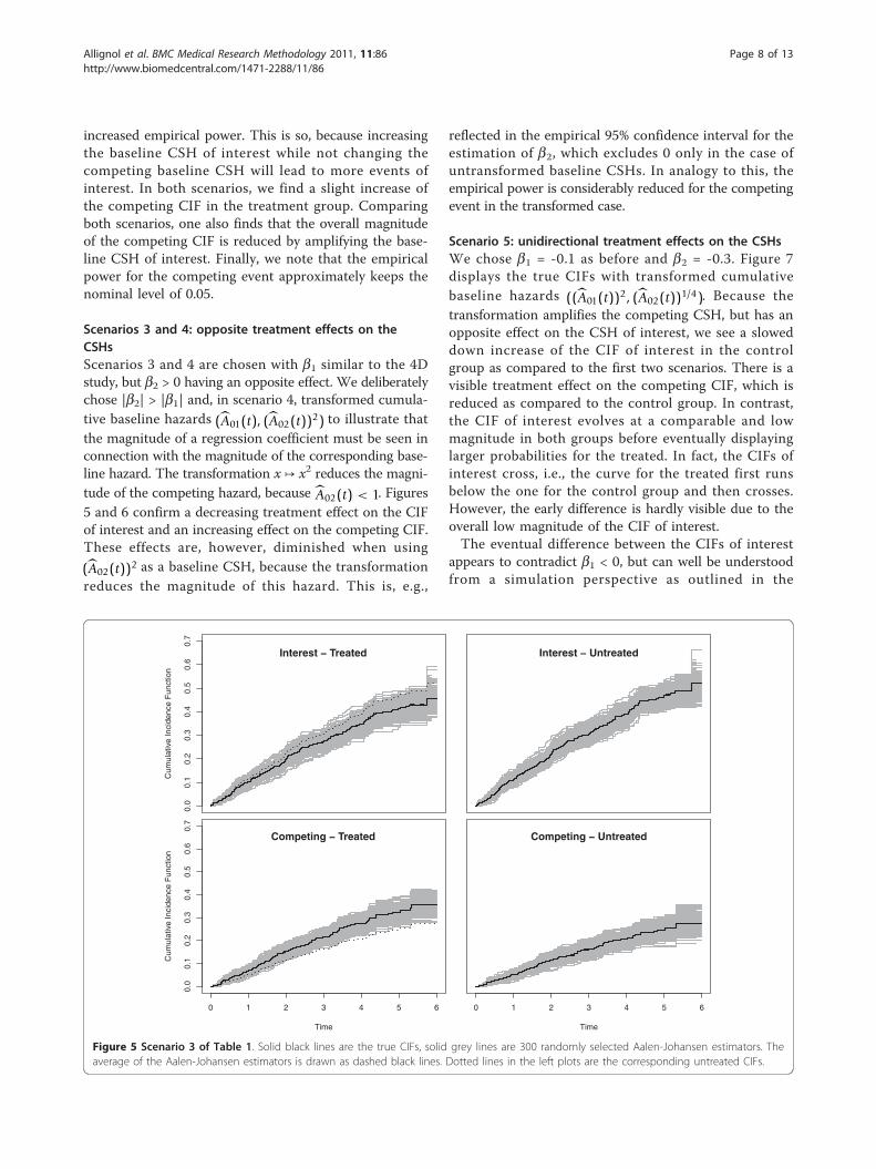
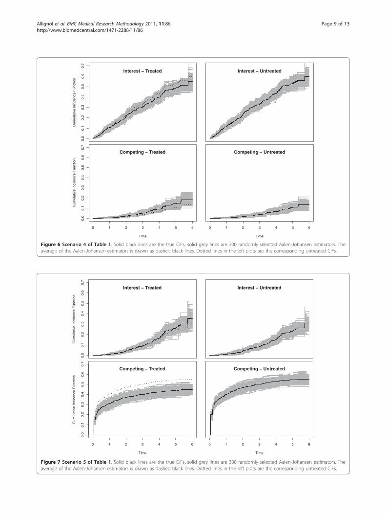
Scenarios 3 and 4: opposite treatment effects on theCSHsScenarios 3 and 4 are chosen with b1 similar to the 4Dstudy, but b2 > 0 having an opposite effect. We deliberatelychose |b2| > |b1| and, in scenario 4, transformed cumula-tive baseline hazards (A01(t), (A02(t))2) to illustrate thatthe magnitude of a regression coefficient must be seen inconnection with the magnitude of the corresponding base-line hazard. The transformation x ↦ x2 reduces the magni-tude of the competing hazard, because A02(t) < 1. Figures5 and 6 confirm a decreasing treatment effect on the CIFof interest and an increasing effect on the competing CIF.These effects are, however, diminished when using

(A02(t))2 as a baseline CSH, because the transformationreduces the magnitude of this hazard. This is, e.g.,

reflected in the empirical 95% confidence interval for theestimation of b2, which excludes 0 only in the case ofuntransformed baseline CSHs. In analogy to this, theempirical power is considerably reduced for the competingevent in the transformed case.

Scenario 5: unidirectional treatment effects on the CSHsWe chose b1 = -0.1 as before and b2 = -0.3. Figure 7displays the true CIFs with transformed cumulativebaseline hazards ((A01(t))2, (A02(t))1/4). Because thetransformation amplifies the competing CSH, but has anopposite effect on the CSH of interest, we see a sloweddown increase of the CIF of interest in the controlgroup as compared to the first two scenarios. There is avisible treatment effect on the competing CIF, which isreduced as compared to the control group. In contrast,the CIF of interest evolves at a comparable and lowmagnitude in both groups before eventually displayinglarger probabilities for the treated. In fact, the CIFs ofinterest cross, i.e., the curve for the treated first runsbelow the one for the control group and then crosses.However, the early difference is hardly visible due to theoverall low magnitude of the CIF of interest.The eventual difference between the CIFs of interest

appears to contradict b1 < 0, but can well be understoodfrom a simulation perspective as outlined in the

0.0

0.1

0.2

0.3

0.4

0.5

0.6

0.7

Cum

ulat

ive

Inci

denc

e F

unct

ion


0 1 2 3 4 5 6

0.0

0.1

0.2

0.3

0.4

0.5

0.6

0.7

Time

Cum

ulat

ive

Inci

denc

e F

unct

ion


0 1 2 3 4 5 6

Time




Page 8 of 13

0.0

0.1

0.2

0.3

0.4

0.5

0.6

0.7

Cum

ulat

ive

Inci

denc

e F

unct

ion


0 1 2 3 4 5 6

0.0

0.1

0.2

0.3

0.4

0.5

0.6

0.7

Time

Cum

ulat

ive

Inci

denc

e F

unct

ion


0 1 2 3 4 5 6

Time



0.0

0.1

0.2

0.3

0.4

0.5

0.6

0.7

Cum

ulat

ive

Inci

denc

e F

unct

ion


0 1 2 3 4 5 6

0.0

0.1

0.2

0.3

0.4

0.5

0.6

0.7

Time

Cum

ulat

ive

Inci

denc

e F

unct

ion


0 1 2 3 4 5 6

Time




Page 9 of 13

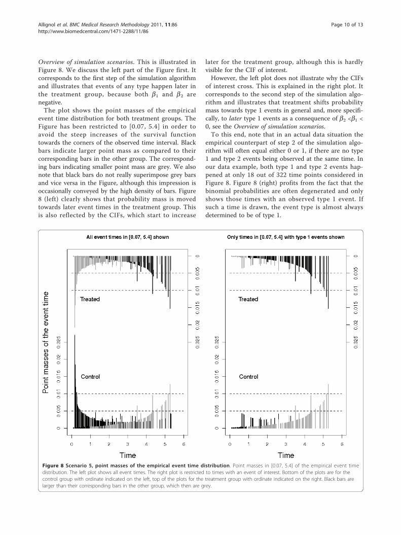
Overview of simulation scenarios. This is illustrated inFigure 8. We discuss the left part of the Figure first. Itcorresponds to the first step of the simulation algorithmand illustrates that events of any type happen later inthe treatment group, because both b1 and b2 arenegative.The plot shows the point masses of the empirical

event time distribution for both treatment groups. TheFigure has been restricted to [0.07, 5.4] in order toavoid the steep increases of the survival functiontowards the corners of the observed time interval. Blackbars indicate larger point mass as compared to theircorresponding bars in the other group. The correspond-ing bars indicating smaller point mass are grey. We alsonote that black bars do not really superimpose grey barsand vice versa in the Figure, although this impression isoccasionally conveyed by the high density of bars. Figure8 (left) clearly shows that probability mass is movedtowards later event times in the treatment group. Thisis also reflected by the CIFs, which start to increase

later for the treatment group, although this is hardlyvisible for the CIF of interest.However, the left plot does not illustrate why the CIFs

of interest cross. This is explained in the right plot. Itcorresponds to the second step of the simulation algo-rithm and illustrates that treatment shifts probabilitymass towards type 1 events in general and, more specifi-cally, to later type 1 events as a consequence of b2 <b1 <0, see the Overview of simulation scenarios.To this end, note that in an actual data situation the

empirical counterpart of step 2 of the simulation algo-rithm will often equal either 0 or 1, if there are no type1 and type 2 events being observed at the same time. Inour data example, both type 1 and type 2 events hap-pened at only 18 out of 322 time points considered inFigure 8. Figure 8 (right) profits from the fact that thebinomial probabilities are often degenerated and onlyshows those times with an observed type 1 event. Ifsuch a time is drawn, the event type is almost alwaysdetermined to be of type 1.

Figure 8 Scenario 5, point masses of the empirical event time distribution. Point masses in [0.07, 5.4] of the empirical event timedistribution. The left plot shows all event times. The right plot is restricted to times with an event of interest. Bottom of the plots are for thecontrol group with ordinate indicated on the left, top of the plots for the treatment group with ordinate indicated on the right. Black bars arelarger than their corresponding bars in the other group, which then are grey.


Page 10 of 13

The right plot illustrates two things: Firstly, blackcolour dominates the upper part of the plot, indicatingthat the event of interest is more likely to happen inthe treatment group. Secondly, the colouring movesfrom grey to black for the treatment group and fromblack to grey in the control group. The interpretationis that, initially, event type 1 times are drawn withhigher probability in the control group. The picture isbeing reversed as time proceeds, which leads to cross-ing CIFs, and eventually the cumulative proportion oftype 1 events is larger in the treatment group. Note,however, that there is overall low probability mass onearly type 1 event times, which implies that the CIFsof interest initially are hardly distinguishable andrather small.An analogous plot of Figure 8 (right) for type 2 events

shows that probability mass is almost uniformly reducedfor type 2 event times by the treatment effect (figurenot shown).

Scenarios 6-10Scenarios 6-10 repeated the previous investigations witha more pronounced treatment effect of b1 = -0.3. Resultsare reported in Table 2. The most striking difference tothe results from scenarios 1-5 is an increased empiricalpower for events of type 1. The increased empiricalpower, however, does not only depend on b1 = -0.3, buton all aspects discussed above. E.g., both scenarios 6and 7 have (b1, b2) = (-0.3, 0), but the cause-specificbaseline hazard for type 1 events is amplified in scenario7. This leads to scenario 7 having better empiricalpower than scenario 6. In contrast, power is substan-tially decreased for the situation studied in scenario 10.

DiscussionThis paper envisaged the CSHs as momentary forces oftransition, which suggests an algorithmic perspectivetowards competing risks. ‘Empirical simulations’ workedas a proof of concept. The algorithmic perspective wasused on the interplay between CSHs and CIFs.The involved relationship between CSHs and CIFs has

inspired a boost in methodological research on testingand direct modelling of the CIFs, e.g., [26-29]. Similar toour paper, a number of recent references have usedsimulation of competing risks data to investigate thesemethods. In particular, Gray’s [26] test [5,30,31] and theFine-Gray [27] model [22,32] have attracted attention.Both these exemplary references and the present paperfound a subtle interplay between different CSH constel-lations and subsequent impact on the CIFs.The difference to the present paper is that a typical

simulation study will put the simulation algorithm asideas only a computational tool, once the data have beengenerated. Thus, one will typically specify the CSHs, use

some simulation algorithm [13] for data generation andanalyse the data with the methodology at hand. Then,the CSH specifications and the results of the data ana-lyses will be compared. In contrast to this, we haveadvocated to use the simulation algorithm itself as anoperational tool for interpretation. In this context, it isworthwhile to note that the algorithm of our paper doesnot experience a number of problems which come withthe common latent failure time model. E.g., the problemof dependence of the latent times has motivated toinclude different dependence structures in some simula-tion studies. There is no such problem in our set-up,which therefore facilitates interpretation.We discuss practical consequences next. To begin, it

is interesting to revisit the results of the 4D study in thelight of the simulation algorithm. As stated earlier, theoriginal study finding was a CSH ratio of 0.92 for theevent of interest and essentially no effect on the com-peting CSH. The competing CSH ratio was, of course,not exactly equal to 1.00, but it displayed a slight reduc-tion. Because the treatment effect on the CSH of inter-est was moderate, and because the Nelson-Aalenestimators of the cumulative CSHs were not exactly pro-portional between treatment groups, the Aalen-Johansenestimators of the CIFs of interest display a somewhatsubtle relationship in the original report. (Figure threein [14], not reproduced here.) E.g., the CIFs cross beforedisplaying a moderate benefit for the treatment group.However, the difference between the CIFs is slightbefore crossing and must therefore not be overinter-preted. As a consequence, we believe that interpretationof the competing risks situation at hand is well guidedby the idealised situation of the simulation scenario 1.Next, we reiterate that it is crucial that all CSHs are

analysed. In the Backgroung Section, we noted that thisis often not the case in clinical research. We also illu-strated that a comprehensive analysis should not berestricted to hazard ratios only, but that ideally thecause-specific baseline hazards will be considered, too.The bottom line is that the interpretation of the CSHratio of interest depends both on the baseline CSH ofinterest, the competing CSH ratio and the competingbaseline CSH. In particular, a missing analysis of thecompeting CSH may have seriously misleadingconsequences.An important issue in this context is that of graphi-

cally presenting results. A popular and adequate choiceare plots of the CIFs, which should, in particular, beplotted for all event types, if all competing risks areharmful. However, it was also illustrated that the con-nection between these plots and CSH analyses is notstraightforward, such that further graphical tools wouldbe helpful. The most obvious choice is to also show theestimated cumulative CSHs as in Figure 2. This should


Page 11 of 13

be done much more often. The reason is that the CSHsregulate the stochastic behaviour of the competing risksprocess as explained in the Methods Section and as illu-strated in the Results Section.In addition, plots such as Figure 8 which highlight the

simulation perspective can be useful. The interestedreader is also referred to ‘vertical modelling’ [33] andmultistate incidence rate graphics [34]. We also note that‘vertical modelling’ aims at modelling the binomial prob-abilities in step 2 of the simulation algorithm as a smoothcurve. This approach is appropriate when taking thesimulation algorithm as a starting point to model com-peting risks data. We reiterate that our aim has been dif-ferent in that we took the simulation perspective as anoperational tool to interpret the standard CSH analyses.We return to the key fact that all CSHs should be

analysed in the presence of competing risks, and thatthis is often not accounted for in clinical research.These issues raise the question of planning competingrisks studies, see [35] for a recent review. If the aim isto compare CSHs, a typical assumption made during theplanning phase of the study is that of constant or piece-wise constant hazards, e.g., [21,36,37]. In addition, it isoften assumed that the treatment does not affect thecompeting CSH, see [35]. In practice, it may be difficultto find an adequate closed form for time-dependentCSHs. Sample size calculations may become quite for-midable, if the planned analysis is more complex thantesting the CSH of interest only. Whatever the plannedstatistical experiment is, we note that our empiricalsimulation approach provides for a general tool to studyempirical power and, hence, to decide on sample size, ifdata of a control group - or of patients similar to theanticipated control group - are available. This is alsoillustrated in Table 2. Interestingly, Figure 2 suggeststhat assuming constant CSHs might be a reasonableassumption for the present control group, but it shouldbe pointed out that the simulation approach does notrely on such an assumption. It could be applied withoutfurther ado, if the CSHs show a pronounced time-dependency. In particular, one would not need to spe-cify a closed form for the time-dependent CSHs. In clos-ing, we mention that, while we have focused on the Coxmodel as the major tool to analyse CSHs, other modelssuch as Aalen’s additive model may be used for CSHs,too; see [38] for a recent textbook treatment. The simu-lation perspective of this paper may then applied toresults from other CSH models, too.

ConclusionsThis paper suggests an algorithmic or simulation pointof view for the interpretation of competing risks ana-lyses. This point of view follows the construction ofcompeting risks data based on the CSHs, envisaging the

hazards as momentary forces of transition. Concerns onidentifiability and plausibility that are common in thelatent failure time context do not arise.Simulation studies based on the empirical probability

measure of a real data analysis served as a proof of con-cept. The simulation point of view was found to be ade-quate in that it recovered the original empirical law.Manipulating baseline hazards and treatment effectshighlighted different aspects of a competing risksanalysis.All CSHs should be analysed, including the cause-spe-

cific baseline hazards. ‘Empirical simulations’ also pro-vide a flexible tool for study planning in the presence ofcompeting risks.

AcknowledgementsThis work was supported by grant FOR 534 from the DeutscheForschungsgemeinschaft.

Author details1Freiburg Center for Data Analysis and Modeling, University of Freiburg,Germany. 2Institute of Medical Biometry and Medical Informatics, UniversityMedical Center Freiburg, Germany. 3Department of Medicine 1, Division ofNephrology, University of Wuerzburg, Germany.

Authors’ contributionsAA, MS and JB conceived the study. AA carried out the implementation. JBand AA drafted the first version of the manuscript. All authors contributed tothe writing and approved the final version.

Competing interestsThe authors declare that they have no competing interests.

Received: 19 January 2011 Accepted: 3 June 2011Published: 3 June 2011

References1. Horton N, Switzer S: Statistical methods in the journal. New England

Journal of Medicine 2005, 353(18):1977-1979.2. Le Tourneau C, Michiels S, Gan HK, Siu LL: Reporting of time-to-event end

points and tracking of failures in randomized trials of radiotherapy withor without any concomitant anticancer agent for locally advanced headand neck cancer. Journal of Clinical Oncology 2009, 27(35):5965-5971.

3. Kim H: Cumulative incidence in competing risks data and competingrisks regression analysis. Clinical Cancer Research 2007, 13(2):559-565.

4. Grunkemeier GL, Jin R, Eijkemans MJ, Takkenberg JJ: Actual and ActuarialProbabilities of Competing Risks: Apples and Lemons. The Annals ofThoracic Surgery 2007, 83(5):1586-1592.

5. Dignam JJ, Kocherginsky MN: Choice and Interpretation of StatisticalTests Used When Competing Risks Are Present. Journal of ClinicalOncology 2008, 26(24):4027-4034.

6. Kalbfleisch JD, Prentice RL: The Statistical Analysis of Failure Time Data JohnWiley & Sons; 2002.

7. Andersen PK, Borgan Ø, Gill RD, Keiding N: Statistical models based oncounting processes Springer Series in Statistics. New York, NY: Springer; 1993.

8. Andersen P, Abildstrøm S, Rosthøj S: Competing risks as a multi-statemodel. Statistical Methods in Medical Research 2002, 11(2):203-215.

9. Putter H, Fiocco M, Geskus R: Tutorial in biostatistics: competing risks andmulti-state models. Statistics in Medicine 2007, 26(11):2277-2432.

10. Mathoulin-Pelissier S, Gourgou-Bourgade S, Bonnetain F, Kramar A: Survivalend point reporting in randomized cancer clinical trials: a review ofmajor journals. Journal of Clinical Oncology 2008, 26(22):3721-3726.

11. Koller MT, Stijnen T, Steyerberg EW, Lubsen J: Meta-analyses of chronicdisease trials with competing causes of death may yield biased oddsratios. Journal of Clinical Epidemiology 2008, 61(4):365-372.


Page 12 of 13

http://www.ncbi.nlm.nih.gov/pubmed/16267336?dopt=Abstract





















12. Gill RD, Johansen S: A survey of product-integration with a view towardsapplication in survival analysis. The Annals of Statistics 1990,18(4):1501-1555.

13. Beyersmann J, Latouche A, Buchholz A, Schumacher M: Simulatingcompeting risks data in survival analysis. Statistics in Medicine 2009,28:956-971.

14. Wanner C, Krane V, März W, Olschewski M, Mann J, Ruf G, Ritz E:Atorvastatin in patients with type 2 diabetes mellitus undergoinghemodialysis. New England Journal of Medicine 2005, 353(3):238-248.

15. R Development Core Team: R: A Language and Environment for StatisticalComputing R Foundation for Statistical Computing, Vienna, Austria; 2009[http://www.R-project.org], [ISBN 3-900051-07-0].

16. Allignol A, Beyersmann J, Schumacher M: mvna: An R Package for theNelson-Aalen Estimator in Multistate Models. R News 2008, 8(2):48-50[http://www.r-project.org/doc/Rnews/].

17. Lumley T: The survival Package. R News 2004, 4:26-28[http://CRAN.R-project.org/doc/Rnews/].

18. Allignol A, Schumacher M, Beyersmann J: A Note On Variance Estimationof the Aalen-Johansen Estimator of the Cumulative Incidence Functionin Competing Risks, with a View towards Left-Truncated Data. BiometricalJournal 2010, 52:126-137.

19. Allignol A, Schumacher M, Beyersmann J: Empirical Transition Matrix ofMultistate Models: The etm Package. Journal of Statistical Software 2011,38(4):1-15.

20. de Wreede LC, Fiocco M, Putter H: The mstate package for estimationand prediction in non- and semi-parametric multi-state and competingrisks models. Computer Methods and Programs in Biomedicine 2010,99:261-274.

21. Schulgen G, Olschewski M, Krane V, Wanner C, Ruf G, Schumacher M:Sample sizes for clinical trials with time-to-event endpoints andcompeting risks. Contemporary Clinical Trials 2005, 26:386-395.

22. Grambauer N, Schumacher M, Beyersmann J: Proportional subdistributionhazards modeling offers a summary analysis, even if misspecified.Statistics in Medicine 2010, 29:875-884.

23. Tsiatis A: A nonidentifiability aspect of the problem of competing risks.Proc Natl Acad Sci USA 1975, 72:20-22.

24. Prentice R, Kalbfleisch J, Peterson A, Flournoy N, Farewell V, Breslow N: Theanalysis of failure times in the presence of competing risks. Biometrics1978, 34:541-554.

25. Aalen O: Dynamic modelling and causality. Scandinavian Actuarial Journal1987, 00000:177-190.

26. Gray RJ: A class of k-sample tests for comparing the cumulativeincidence of a competing risk. Annals of Statistics 1988, 16(3):1141-1154.

27. Fine J, Gray RJ: A proportional hazards model for the subdistribution of acompeting risk. Journal of the American Statistical Association 1999,94(446):496-509.

28. Klein J, Andersen P: Regression Modeling of Competing Risks Data Basedon Pseudovalues of the Cumulative Incidence Function. Biometrics 2005,61:223-229.

29. Scheike TH, Zhang MJ, Gerds TA: Predicting cumulative incidenceprobability by direct binomial regression. Biometrika 2008, 95:205-220.

30. Freidlin B, Korn EL: Testing treatment effects in the presence ofcompeting risks. Statistics in Medicine 2005, 24:1703-1712.

31. Bajorunaite R, Klein JP: Comparison of failure probabilities in thepresence of competing risks. Journal of Statistical Computation andSimulation 2008, 78(10):951-966.

32. Latouche A, Boisson V, Porcher R, Chevret S: Misspecified regressionmodel for the subdistribution hazard of a competing risk. Statistics inMedicine 2007, 26(5):965-974.

33. Nicolaie M, van Houwelingen H, Putter H: Vertical modeling: A patternmixture approach for competing risks modeling. Statistics in Medicine2010, 29(11):1190-1205.

34. Grambauer N, Schumacher M, Dettenkofer M, Beyersmann J: Incidencedensities in a competing events analysis. American Journal ofEpidemiology 2010, 172(9):1077-1084.

35. Latouche A, Porcher R: Sample size calculations in the presence ofcompeting risks. Statistics in Medicine 2007, 26(30):5370-5380.

36. Lakatos E: Sample Sizes Based on the Log-Rank Statistic in ComplexClinical Trials. Biometrics 1988, 44:229-241.

37. Barthel FMS, Babiker A, Royston P, Parmar MKB: Evaluation of Sample Sizeand Power for Multi-arm Survival Trials Allowing for Non-uniform

Accrual, Non-proportional Hazards, Loss to Follow-up and Cross-over.Statistics in Medicine 2006, 25(15):2521-2542.

38. Martinussen T, Scheike T: Dynamic Regression Models for Survival Data NewYork, NY: Springer; 2006.

Pre-publication historyThe pre-publication history for this paper can be accessed here:http://www.biomedcentral.com/1471-2288/11/86/prepub

doi:10.1186/1471-2288-11-86Cite this article as: Allignol et al.: Understanding competing risks: asimulation point of view. BMC Medical Research Methodology 2011 11:86.

Submit your next manuscript to BioMed Centraland take full advantage of:

• Convenient online submission

• Thorough peer review

• No space constraints or color figure charges

• Immediate publication on acceptance

• Inclusion in PubMed, CAS, Scopus and Google Scholar

• Research which is freely available for redistribution

Submit your manuscript at www.biomedcentral.com/submit


Page 13 of 13





http://www.R-project.org

http://www.r-project.org/doc/Rnews/

http://CRAN.R-project.org/doc/Rnews/

http://CRAN.R-project.org/doc/Rnews/































http://www.biomedcentral.com/1471-2288/11/86/prepub

Documents

Understanding competing risks: a simulation point of view