Understanding Catalysis A Simplified Simulation of

chemengineering

Article

Understanding Catalysis—A Simplified Simulation ofCatalytic Reactors for CO2 Reduction

Jasmin Terreni 1,2, Andreas Borgschulte 1,2,* , Magne Hillestad 3 and Bruce D. Patterson 1,4

1 Laboratory for Advanced Analytical Technologies, Empa, CH-8600 Dübendorf, Switzerland;[email protected] (J.T.); [email protected] (B.D.P.)

2 Department of Chemistry, University of Zurich, CH-8057 Zurich, Switzerland3 Department of Chemical Engineering, Norwegian University of Science and Technology (NTNU),

N-7491 Trondheim, Norway; [email protected] Department of Physics, University of Zurich, CH-8057 Zurich, Switzerland* Correspondence: [email protected]; Tel.: +41-58-765-46-39

Received: 11 August 2020; Accepted: 10 November 2020; Published: 20 November 2020��

Abstract: The realistic numerical simulation of chemical processes, such as those occurring incatalytic reactors, is a complex undertaking, requiring knowledge of chemical thermodynamics,multi-component activated rate equations, coupled flows of material and heat, etc. A standardapproach is to make use of a process simulation program package. However for a basic understanding,it may be advantageous to sacrifice some realism and to independently reproduce, in essence,the package computations. Here, we set up and numerically solve the basic equations governingthe functioning of plug-flow reactors (PFR) and continuously stirred tank reactors (CSTR), and wedemonstrate the procedure with simplified cases of the catalytic hydrogenation of carbon dioxideto form the synthetic fuels methanol and methane, each of which involves five chemical speciesundergoing three coupled chemical reactions. We show how to predict final product concentrationsas a function of the catalyst system, reactor parameters, initial reactant concentrations, temperature,and pressure. Further, we use the numerical solutions to verify the “thermodynamic limit” of a PFRand a CSTR, and, for a PFR, to demonstrate the enhanced efficiency obtainable by “looping” and“sorption-enhancement”.

Keywords: CO2 reduction; methanol; methane; thermodynamics; kinetics; reactor design

1. Introduction

Serious catalytic reactor design is a complex task involving the coupled phenomena of chemicalthermodynamics, multi-step chemical reactions, hydrodynamic flowand the generation, conduction,and dissipation of heat. Sophisticated computer software packages [1,2] are widely used to aidthe reactor designer, but it has been argued that the “black-box” results they provide may obscurefundamental relationships, which are important for a more basic understanding. Quoting Reference [3],“A potential pedagogical drawback to simulation packages such as HYSYS and ASPEN is that it mightbe possible for students to successfully construct and use models without really understanding thephysical phenomena within each unit operation. . . . . Care must be taken to insure that simulationenhances student understanding, rather than providing a crutch to allow them to solve problemswith only a surface understanding of the processes they are modeling”. Most chemical engineeringtextbooks [4–9] treat the general principles of catalytic reactor operation in terms of a set of coupleddifferential equations describing the creation and annihilation of chemical components. These equationsare generally highly non-linear, hence requiring numerical techniques for their solution. Textbooks theneither treat particularly simple reaction schemes, which do allow analytical solution, or plot numerically

ChemEngineering 2020, 4, 62; doi:10.3390/chemengineering4040062 www.mdpi.com/journal/chemengineering

http://www.mdpi.com/journal/chemengineering

http://www.mdpi.com

https://orcid.org/0000-0001-6250-4667

https://orcid.org/0000-0001-7410-5903

http://dx.doi.org/10.3390/chemengineering4040062

http://www.mdpi.com/journal/chemengineering

https://www.mdpi.com/2305-7084/4/4/62?type=check_update&version=2

ChemEngineering 2020, 4, 62 2 of 16

computed results which the average student is unable to reproduce. Only in exceptional cases does atextbook assist the student in generating a suitable computer program to solve non-linear equations [7].

In this work, we demonstrate how one may simulate the simplified operation of a catalyticreactor using basic thermodynamic data, a kinetic model for the multi-step reactions, and numericalsolutions of reactor-specific differential equations describing the evolution from reactant to productchemical species. We focus our attention on the two archetypes of continuous-flow reactors: the plugflow reactor (PFR) and the continuously stirred tank reactor (CSTR) [5]. To simplify the discussion,we assume constant and uniform reaction temperature and pressure and we neglect the issues ofheat flow and pressure drop. Furthermore, we assume that all reactant and product species behaveas ideal gases. In the main text, we explain how the relevant equations are set up to describe theevolution of chemical concentrations in the reactor and we plot and discuss their numerical solutions.Student exercises presented in the Supplementary Materials instruct the reader in the creation of acomputer program, based on a variable-step Runge–Kutta integration method [10], to solve non-lineardifferential equations.

A schematic diagram of the simulation procedure is shown in Figure 1. Once the overall relevantchemical reactions have been defined, basic thermodynamics dictates the Gibbs free energy changeand hence the equilibrium constants. From these, the temperature- (T) and pressure- (P) dependentequilibrium state is determined in the thermodynamic limit—i.e., after infinite elapsed reaction time.Dynamic reactor simulation requires knowledge of the concentration-, T-, and P-dependent productionrates of the individual chemical species. This information is typically contained in a published“kinetic model”, which depends on the catalyst used. Once the reactor type (PFR or CSTR) is defined,coupled differential equations describing the chemical component flows are set up. These equationsare then numerically solved to yield the time or position-dependent concentration of each chemicalcomponent. A useful check of the computation procedure, including the kinetic model, is to extendthe dynamic simulation to infinite elapsed time, which should reproduce the thermodynamic limitobtained earlier.

ChemEngineering 2020, 4, x FOR PEER REVIEW 2 of 17

ChemEngineering 2020, 4, x; doi: FOR PEER REVIEW www.mdpi.com/journal/chemengineering

exceptional cases does a textbook assist the student in generating a suitable computer program to solve non-linear equations [7].

In this work, we demonstrate how one may simulate the simplified operation of a catalytic reactor using basic thermodynamic data, a kinetic model for the multi-step reactions, and numerical solutions of reactor-specific differential equations describing the evolution from reactant to product chemical species. We focus our attention on the two archetypes of continuous-flow reactors: the plug flow reactor (PFR) and the continuously stirred tank reactor (CSTR) [5]. To simplify the discussion, we assume constant and uniform reaction temperature and pressure and we neglect the issues of heat flow and pressure drop. Furthermore, we assume that all reactant and product species behave as ideal gases. In the main text, we explain how the relevant equations are set up to describe the evolution of chemical concentrations in the reactor and we plot and discuss their numerical solutions. Student exercises presented in the Appendix instruct the reader in the creation of a computer program, based on a variable-step Runge–Kutta integration method [10], to solve non-linear differential equations.

A schematic diagram of the simulation procedure is shown in Figure 1. Once the overall relevant chemical reactions have been defined, basic thermodynamics dictates the Gibbs free energy change and hence the equilibrium constants. From these, the temperature- (T) and pressure- (P) dependent equilibrium state is determined in the thermodynamic limit—i.e., after infinite elapsed reaction time. Dynamic reactor simulation requires knowledge of the concentration-, T-, and P-dependent production rates of the individual chemical species. This information is typically contained in a published “kinetic model”, which depends on the catalyst used. Once the reactor type (PFR or CSTR) is defined, coupled differential equations describing the chemical component flows are set up. These equations are then numerically solved to yield the time or position-dependent concentration of each chemical component. A useful check of the computation procedure, including the kinetic model, is to extend the dynamic simulation to infinite elapsed time, which should reproduce the thermodynamic limit obtained earlier.

Figure 1. Schematic diagram illustrating the catalytic reactor simulation procedure. Orange boxes indicate the external input of information.

Figure 1. Schematic diagram illustrating the catalytic reactor simulation procedure. Orange boxesindicate the external input of information.

We demonstrate the usefulness of this approach to reactor simulation and hopefully motivatefurther exploration by the reader by examining the enhanced efficiency of two modificationsof the PFR, which effectively shift the thermodynamic equilibrium: product separation and theremoval/recycling of unreacted species in a “looped” reactor [7], and product removal by selectiveabsorption (“sorption enhancement”) [11]. As mentioned, a series of progressively more challengingstudent exercises which review and develop the concepts treated in the main text is included,with answers, as an Supplementary Materials.


2. Materials and Methods

Equilibrium constants for the chemical reactions considered were either computed fromthermodynamic data on the Gibbs free energy change [12] or taken from the literature [13,14],and the kinetic rate factors were obtained from published models of experimental data [13–15].The numerical computations were performed with Wolfram Mathematica, Version 11.3 [16].

3. Results and Discussion

3.1. CO2 Hydrogenation to Methanol and Methane

In order to demonstrate our simulation of catalytic reactors by the setup and numerical solutionof kinetic equations, we have chosen as chemical processes the reduction of carbon dioxide byhydrogenation to form the synthetic fuels methanol and methane [17,18]. Note that the production ofmethane in this fashion is also called “CO2 methanation”. Carbon-based fossil fuels remain the mostimportant energy source worldwide due to the high chemical stability of their combustion product,carbon dioxide [19]. However, carbon dioxide is a major greenhouse gas causing global warming.Therefore viable alternatives to the burning of fossil fuels have to be found, and one option is the useof synthetic carbon-based fuels, produced using renewable energy, and carbon dioxide which hasbeen recycled from natural or industrial processes [17,20]. The CO2 may then be converted to a fuelby catalytic hydrogenation [18,21,22]. The simplest carbon-based synthetic fuels are the C1 speciesformic acid (HCOOH), formaldehyde (HCHO), methanol (CH3OH), and methane (CH4) (Figure 2).We note that CO2 can also be converted to higher hydrocarbons and alcohols by Fischer–Tropschsynthesis [18,23].

From Figure 2, we can see that methanol and methane are promising candidates for syntheticcarbon-based fuels. Note that the production reactions of both methanol and methane are spontaneousunder standard conditions (∆Gred < 0) [24]. While methanol has the advantage of being a liquid atroom temperature and hence has a high volumetric energy storage density, the gas methane offers highgravimetric energy storage [25].ChemEngineering 2020, 4, x FOR PEER REVIEW 4 of 17


Figure 2. A Latimer–Frost-type diagram [26] showing, as a function of the degree of hydrogen reduction n(H2) and at standard temperature and pressure, the change in Gibbs free energy ΔGred upon production by CO2 hydrogenation and the change in enthalpy ΔHoxid upon combustion in oxygen for the C1 chemicals formic acid (HCOOH), formaldehyde (HCHO), methanol (CH3OH), and methane (CH4). The negative values of ΔGred for methanol and methane formation imply spontaneous production reactions, and the large values of ΔHoxid imply a high capacity for chemical energy storage. The thermodynamic data are from references [12,27].

The reduction of carbon dioxide to methanol is usually carried out over a copper-zinc oxide catalyst at temperatures of approximately 200–300 °C and a pressure of several tens of bars [13,14,21]. Nickel is a practical catalyst for CO2 methanation, and the reaction is carried out at a few bars of pressure and temperatures of approximately 250–450 °C [15,21,28,29].

The important overall chemical reactions [14,15] involved in the gas phase hydrogenation of CO2 to CH3OH and CH4 are shown in Figure 3. In both cases, the production can either be direct (reaction 3) or can proceed via carbon monoxide as an intermediate (reactions 2 and 1); the reverse water gas shift (RWGS) reaction 2 competes for CO2 with direct hydrogenation. From thermodynamic arguments, we can conclude the following: (1) In contrast to the CO2 and CO hydrogenation reactions, the RWGS reaction 2 is endothermic. Therefore, increasing the reaction temperature will lead to an increase in the formation of CO and will consequently hinder the direct hydrogenation of CO2 to CH3OH or CH4. (2) Since, in both cases, reaction 3 involves a reduction in the number of moles, an increase in pressure will facilitate the direct hydrogenation of CO2 to CH3OH or CH4. These predictions follow from Le Chatelier’s principle [24].

Figure 2. A Latimer–Frost-type diagram [26] showing, as a function of the degree of hydrogenreduction n(H2) and at standard temperature and pressure, the change in Gibbs free energy ∆Gred

upon production by CO2 hydrogenation and the change in enthalpy ∆Hoxid upon combustion inoxygen for the C1 chemicals formic acid (HCOOH), formaldehyde (HCHO), methanol (CH3OH),and methane (CH4). The negative values of ∆Gred for methanol and methane formation implyspontaneous production reactions, and the large values of ∆Hoxid imply a high capacity for chemicalenergy storage. The thermodynamic data are from references [12,27].


The reduction of carbon dioxide to methanol is usually carried out over a copper-zinc oxidecatalyst at temperatures of approximately 200–300 ◦C and a pressure of several tens of bars [13,14,21].Nickel is a practical catalyst for CO2 methanation, and the reaction is carried out at a few bars ofpressure and temperatures of approximately 250–450 ◦C [15,21,28,29].

The important overall chemical reactions [14,15] involved in the gas phase hydrogenation of CO2

to CH3OH and CH4 are shown in Figure 3. In both cases, the production can either be direct (reaction 3)or can proceed via carbon monoxide as an intermediate (reactions 2 and 1); the reverse water gas shift(RWGS) reaction 2 competes for CO2 with direct hydrogenation. From thermodynamic arguments,we can conclude the following: (1) In contrast to the CO2 and CO hydrogenation reactions, the RWGSreaction 2 is endothermic. Therefore, increasing the reaction temperature will lead to an increase inthe formation of CO and will consequently hinder the direct hydrogenation of CO2 to CH3OH orCH4. (2) Since, in both cases, reaction 3 involves a reduction in the number of moles, an increase inpressure will facilitate the direct hydrogenation of CO2 to CH3OH or CH4. These predictions followfrom Le Chatelier’s principle [24].ChemEngineering 2020, 4, x FOR PEER REVIEW 5 of 17


Figure 3. Gas phase CO2 reduction to methanol (a) and methane (b) [14,15]. Reaction 3, in each case is the direct hydrogenation of CO2. Reaction 2 is the reverse water gas shift (RWGS) reaction, and reaction 1 is the hydrogenation of carbon monoxide. Standard enthalpies of formation are from Swaddle [12].

The equilibrium state in the conversion of carbon dioxide to methanol or methane is defined by thermodynamics and can be determined using the temperature-dependent equilibrium constants Keq . These are, in turn, determined by the change in Gibbs free energy at a given temperature [24]. For example, for the direct conversion of CO2 to CH3OH in reaction 3 in Figure 3, we have: 𝐾 (𝑇) = exp ∆ = exp ∆ ∆ = 𝑒𝑥𝑝 ∆ ∆ ∆ ∆ ∗𝑒𝑥𝑝 ,

(1)

where T is the absolute temperature, R is the gas constant, and ΔH0 and S0 are the standard enthalpy and entropy of formation of the corresponding reactant or product species (Table 1).

Table 1. Standard enthalpy of formation and entropy of involved species for CO2 reduction to form methanol and methane [12].

ΔH0 [kJ/mol] S0 [J/mol K] CO −110.52 197.67 CO2 −393.51 213.74 H2 0 130.68

H2O −241.82 188.82 CH3OH −200.66 239.81

CH4 −74.81 186.26

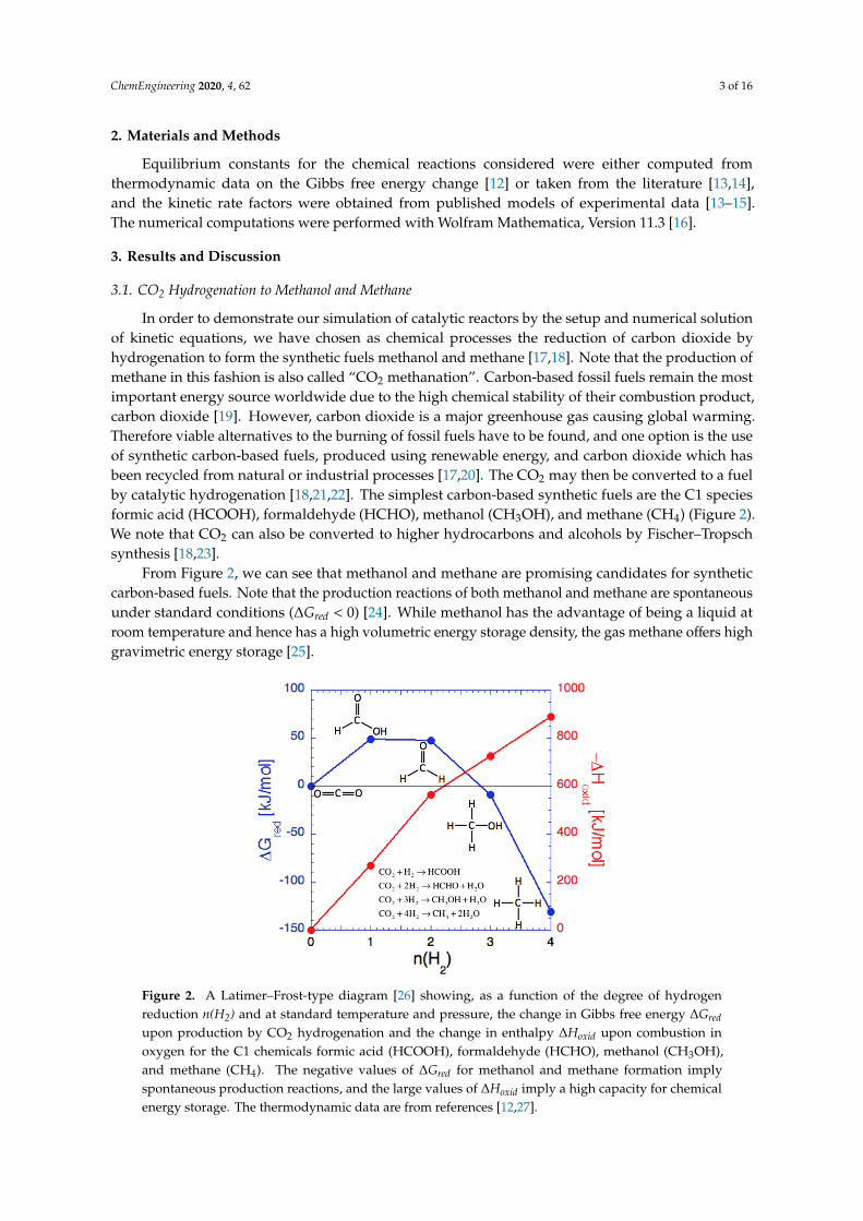
In this way, we arrive at the equilibrium constants for the reactions of Figure 3, as plotted as a function of inverse temperature in Figure 4 for methanol formation (in red) and for methane formation (in blue). The equilibrium constant for the reverse water gas shift reaction (reaction 2) is plotted in green.

Figure 3. Gas phase CO2 reduction to methanol (a) and methane (b) [14,15]. Reaction 3, in each case isthe direct hydrogenation of CO2. Reaction 2 is the reverse water gas shift (RWGS) reaction, and reaction1 is the hydrogenation of carbon monoxide. Standard enthalpies of formation are from Swaddle [12].

The equilibrium state in the conversion of carbon dioxide to methanol or methane is definedby thermodynamics and can be determined using the temperature-dependent equilibrium constantsKeq. These are, in turn, determined by the change in Gibbs free energy at a given temperature [24].For example, for the direct conversion of CO2 to CH3OH in reaction 3 in Figure 3, we have:

Keq3 (T) = exp

[−∆G0

3RT

]= exp

[−∆H0

3+T∆S03

RT

]= exp

[−∆H0

CH3OH−∆H0H2O+3∆H0

H2+∆H0

CO2RT

]∗

exp[

S0CH3OH+S0

H2O−3S0H2−S0

CO2R

],

(1)

where T is the absolute temperature, R is the gas constant, and ∆H0 and S0 are the standard enthalpyand entropy of formation of the corresponding reactant or product species (Table 1).


Table 1. Standard enthalpy of formation and entropy of involved species for CO2 reduction to formmethanol and methane [12].

∆H0 [kJ/mol] S0 [J/mol K]

CO −110.52 197.67CO2 −393.51 213.74H2 0 130.68

H2O −241.82 188.82CH3OH −200.66 239.81

CH4 −74.81 186.26

In this way, we arrive at the equilibrium constants for the reactions of Figure 3, as plotted as afunction of inverse temperature in Figure 4 for methanol formation (in red) and for methane formation(in blue). The equilibrium constant for the reverse water gas shift reaction (reaction 2) is plottedin green.



Figure 4. Equilibrium constants for methanol (red) and methane (blue) production reactions as a function of the inverse temperature. The green line shows the equilibrium constant of the reverse water gas shift reaction. Note the substantially higher values for methane production compared to those for methanol and that the endothermic RWGS reaction is enhanced with increasing temperature.

Because the three reactions in each set are coupled, only two of the three equilibrium constants are independent: 𝐾 (𝑇) ∗ 𝐾 (𝑇) = 𝐾 (𝑇). (2)

3.2. Thermodynamic Equilibrium

At a given temperature and pressure, the thermodynamic yield of a reaction is the equilibrium result that is approached after an infinite elapsed time. Because of their coupling (Equation (2)), we need only to consider two of the three reactions. The thermodynamic yield is determined by equating the equilibrium constant with the corresponding “reaction quotient” [24]. In the case of methanol synthesis, we consider reactions 2 and 3 of Figure 3 to arrive at the following expressions: 𝐾 (𝑇) = ∗∗ , (3)

𝐾 (𝑇) = ∗ ∗ ∗∗ ∗ . (4)

The reaction quotients are determined by the reduced partial pressures pj or molar concentrations Nj of the reactant and product species j, the reaction pressure P, and the atmospheric pressure P0. The molar concentrations, in turn, are related to the degrees of completion ξi of the individual reactions i. For the case of methanol synthesis, the relationships between the equilibrium molar concentrations Nj and the degrees of completion ξi are given by [30]: 𝑁 = 𝜉 ∗ 𝑁 , (5)𝑁 = (1 − 𝜉 − 𝜉 ) ∗ 𝑁 , (6)𝑁 = (𝑆𝑁 + 1 − 𝜉 − 3𝜉 ) ∗ 𝑁 , (7)

Figure 4. Equilibrium constants for methanol (red) and methane (blue) production reactions as afunction of the inverse temperature. The green line shows the equilibrium constant of the reverse watergas shift reaction. Note the substantially higher values for methane production compared to those formethanol and that the endothermic RWGS reaction is enhanced with increasing temperature.

Because the three reactions in each set are coupled, only two of the three equilibrium constantsare independent:

Keq1 (T) ∗Keq

2 (T) = Keq3 (T). (2)

3.2. Thermodynamic Equilibrium

At a given temperature and pressure, the thermodynamic yield of a reaction is the equilibriumresult that is approached after an infinite elapsed time. Because of their coupling (Equation (2)),we need only to consider two of the three reactions. The thermodynamic yield is determined byequating the equilibrium constant with the corresponding “reaction quotient” [24]. In the case ofmethanol synthesis, we consider reactions 2 and 3 of Figure 3 to arrive at the following expressions:

Keq2 (T) =

NCO ∗NH2o

NH2 ∗NCO2

, (3)


Keq3 (T) =

NCH3OH ∗NH2O ∗N2tot ∗ P2

0

N3H2∗NCO2 ∗ P2

. (4)

The reaction quotients are determined by the reduced partial pressures pj or molar concentrationsNj of the reactant and product species j, the reaction pressure P, and the atmospheric pressure P0.The molar concentrations, in turn, are related to the degrees of completion ξi of the individual reactionsi. For the case of methanol synthesis, the relationships between the equilibrium molar concentrationsNj and the degrees of completion ξi are given by [30]:

NCO = ξ2 ∗N0CO2

, (5)

NCO2 = (1− ξ2 − ξ3) ∗N0CO2

, (6)

NH2 = (SN + 1− ξ2 − 3ξ3) ∗N0CO2

, (7)

NH2O = (ξ2 + ξ3) ∗N0CO2

, (8)

NCH3OH = ξ3 ∗N0CO2

, (9)

Ntot = NCO + NCO2 + NH2 + NH2O + NCH3OH = (SN + 2− 2ξ3) ∗N0CO2

. (10)

Here, Ntot is the total molar concentration and SN is the “stoichiometric number” [31], defined asthe ratio between the difference of the initial molar concentrations of hydrogen and carbon dioxideand the sum of the initial concentrations of CO and CO2:

SN =N0

H2−N0

CO2

N0CO + N0

CO2

. (11)

In the present work, we assume no initial concentration of carbon monoxide (N0CO= 0). For ideal

conditions, SN = 2 for CO2 reduction to methanol and SN = 3 for the reduction to methane.The specification of SN, T, and P allows us to numerically solve Equations (5)–(10) for the two

unknowns, ξ2 and ξ3, where ξ3 represents the degree of conversion of CO2 to CH3OH. A similarprocedure can be applied to treat CO2 reduction to methane (see Exercises 3–5). The resultingequilibrium conversions for the CO2 reduction to methanol and methane, with the ideal SN values,are shown as a function of T and P in Figure 5.



Here, Ntot is the total molar concentration and SN is the “stoichiometric number” [31], defined as the ratio between the difference of the initial molar concentrations of hydrogen and carbon dioxide and the sum of the initial concentrations of CO and CO2: 𝑆𝑁 = . (11)

In the present work, we assume no initial concentration of carbon monoxide (𝑁 = 0). For ideal conditions, SN = 2 for CO2 reduction to methanol and SN = 3 for the reduction to methane.

The specification of SN, T, and P allows us to numerically solve Equations (5)–(10) for the two unknowns, ξ2 and ξ3, where ξ3 represents the degree of conversion of CO2 to CH3OH. A similar procedure can be applied to treat CO2 reduction to methane (see Exercises 3–5). The resulting equilibrium conversions for the CO2 reduction to methanol and methane, with the ideal SN values, are shown as a function of T and P in Figure 5.

Figure 5. Equilibrium molar conversion for the reduction of CO2 to methanol (a) and to methane (b), as a function of temperature and at different pressures.

As predicted by Le Chatelier’s principle, the equilibrium conversion of CO2 to methanol or methane increases with increasing pressure and decreases with increasing temperature. The results in Figure 5 are in good agreement with published studies for methanol [30] and methane [32,33] synthesis.

3.3. Kinetic Behavior in a Continuous Flow Catalytic Reactor

In a practical chemical reactor, a catalyst is used to selectively accelerate the desired reaction. It should be noted that the presence of a catalyst cannot by itself increase the reaction yield beyond that given by thermodynamics; by effectively lowering the pertinent potential energy barrier, it can only increase the rate at which a reaction proceeds [34,35].

A more realistic treatment of a chemical process than that provided by equilibrium thermodynamics requires the analysis of the kinetic behavior, which, besides the choice of catalyst, depends on the reactor geometry [4]. In the pharmaceutical industry, a “batch reactor” is often used to repeatedly process limited amounts of material. Here, we consider the kinetic behavior of CO2

𝑁 = (𝜉 + 𝜉 ) ∗ 𝑁 , (8)𝑁 = 𝜉 ∗ 𝑁 , (9)𝑁 = 𝑁 + 𝑁 + 𝑁 + 𝑁 + 𝑁 = (𝑆𝑁 + 2 − 2𝜉 ) ∗ 𝑁 . (10)

Figure 5. Equilibrium molar conversion for the reduction of CO2 to methanol (a) and to methane (b),as a function of temperature and at different pressures.


As predicted by Le Chatelier’s principle, the equilibrium conversion of CO2 to methanol ormethane increases with increasing pressure and decreases with increasing temperature. The results inFigure 5 are in good agreement with published studies for methanol [30] and methane [32,33] synthesis.

3.3. Kinetic Behavior in a Continuous Flow Catalytic Reactor

In a practical chemical reactor, a catalyst is used to selectively accelerate the desired reaction.It should be noted that the presence of a catalyst cannot by itself increase the reaction yield beyondthat given by thermodynamics; by effectively lowering the pertinent potential energy barrier, it canonly increase the rate at which a reaction proceeds [34,35].

A more realistic treatment of a chemical process than that provided by equilibrium thermodynamicsrequires the analysis of the kinetic behavior, which, besides the choice of catalyst, depends on the reactorgeometry [4]. In the pharmaceutical industry, a “batch reactor” is often used to repeatedly processlimited amounts of material. Here, we consider the kinetic behavior of CO2 hydrogenation in the twoarchetypical “continuous flow” reactor types: the “plug flow reactor” (PFR) and the “continuouslystirred tank reactor” (CSTR).

The kinetics of the reduction of CO2 to methanol over a Cu/ZnO/Al2O3 catalyst have beenmodeled by Graaf et al. [13,14]. By analyzing the important reaction intermediates and determining therate-limiting steps, these authors find the following expressions for ri, the rates of the three reactions inFigure 3a, and hence for R a 5-component vector giving the net production rates for the individualchemical species:

r1 = k1KCO

pCO ∗ p32H2−

pCH3OH

P12H2∗Keq

1

/denom, (12)

r2 = k2KCO2

pCO2 ∗ pH2 −pH2O ∗ pCO

Keq2

/denom, (13)

r3 = k3KCO2

pCO2 ∗ p32H2−

pCH3OH ∗ pH2O

p32H2∗Keq

3

/denom, (14)

denom =(1 + KCO ∗ pCO + Kco2 ∗ pCO2

)∗

p 12H2

+

KH2O

K12H2

∗ pH2O

, (15)

R =(RCO, RCO2 , RH2 , RH2O, RCH3OH

)= (−r1 + r2,−r2 − r3,−2r1 − r2 − 3r3, r2 + r3, r1 + r3. (16)

Like the equilibrium constants, the temperature-dependent kinetic factors in Equations (12)–(16)also have the Arrhenius form:

Kn(T) = an ∗ exp(

bn

R ∗ T

). (17)

The values presented by Graaf et al. for the Arrhenius parameters for the various factors inmethanol production are given in Table 2. The corresponding factors for methanation are given inExercise 6 of the Supplementary Materials. Instead of the thermodynamically derived expressions forthe equilibrium rate constants Keq

j, we use for methanol synthesis the expressions from Graaf et al. [13,14]in Table 2.


Table 2. Arrhenius parameters for the temperature-dependent factors in the model of the kinetics ofmethanol production of Graaf et al. [13,14].

Variable a b[ J

mol

]Keq

1 2.39× 10−13 9.84× 104

Keq2 1.07× 102

−3.91× 104

Keq3 2.56× 10−11 5.87× 104

k1 4.89× 107 molkg s −1.13× 105

k2 9.64× 1011 molkg s −1.53× 105

k3 1.09× 105 molkg s −0.875× 105

KCO 2.16 ×10−5 0.468 ×105

KCO2 7.05 ×10−7 0.617 ×105

KH2O/KH21/2 6.37 ×10−9 0.840 ×105

3.3.1. Plug Flow Reactor

We first consider the plug flow reactor, where the reactants and products flow with a constanttotal mass flow rate through one or more parallel tubes filled with loosely packed catalyst. For ourcalculations, we make the simplifying assumptions: (1) that all reactants and products are idealgases, and (2) that the temperature and pressure are constant and uniform along the reactor tubes.The working principle and the corresponding method of numerical simulation for the PFR are givenin Figure 6. The vector

.N denotes the molar flow rates (moles/s), the components of which are the x

position-dependent flows of CO, CO2, H2, H2O, and CH3OH. As the gases proceed along the reactortubes, the initial reactants CO2 and H2 are converted to the product species CO, H2O, and CH3OH.The values used for the PFR parameters in Figure 6 are shown in Table 3.



3.3.1. Plug Flow Reactor

We first consider the plug flow reactor, where the reactants and products flow with a constant total mass flow rate through one or more parallel tubes filled with loosely packed catalyst. For our calculations, we make the simplifying assumptions: (1) that all reactants and products are ideal gases, and (2) that the temperature and pressure are constant and uniform along the reactor tubes. The working principle and the corresponding method of numerical simulation for the PFR are given in Figure 6. The vector 𝐍 denotes the molar flow rates (moles/s), the components of which are the x position-dependent flows of CO, CO2, H2, H2O, and CH3OH. As the gases proceed along the reactor tubes, the initial reactants CO2 and H2 are converted to the product species CO, H2O, and CH3OH. The values used for the PFR parameters in Figure 6 are shown in Table 3.

Figure 6. Computational scheme for a plug flow reactor, defining the function PFR, which relates the input and output component molar flow rates [5]. The component molecular weights are given by mj.

Table 3. Plug flow reactor parameter values used in the present simulation of methanol and methane synthesis.

Parameter Methanol Synthesis Methane Synthesis Catalyst Cu/ZnO/Al2O3 Ni/MgAl2O4

Catalyst density ρcatalyst 1000 kg/m3 1000 kg/m3 Nr of parallel tubes ntubes 10,000 10

Tube diameter d 2 cm 2 cm Tube area Atube = ntube x πd2/4 3.14 m2 0.00314 m2

Tube length Ltube 3 m 1 m Initial flow velocity vflow 0.05 m/s 5 m/s

Stoichiometric number SN 2 3 Temperature range T 180–340 °C 100–1000 °C

Pressures P 20, 40, 60 bar 1, 10, 20 bar

The resulting temperature- and pressure-dependent degree of CO2 → CH3OH conversion is shown with solid curves in Figure 7 and is in qualitative agreement with previously published studies [36–38]. We highlight two important features: (1) at practical pressures, only a low degree of conversion to methanol (<0.25) is obtained. (2) The conversion predicted by the kinetic behavior cannot exceed the equilibrium value (dotted curves in Figures 5 and 7. We attribute the slight

Figure 6. Computational scheme for a plug flow reactor, defining the function PFR, which relates theinput and output component molar flow rates [5]. The component molecular weights are given by mj.


Table 3. Plug flow reactor parameter values used in the present simulation of methanol andmethane synthesis.

Parameter Methanol Synthesis Methane Synthesis

Catalyst Cu/ZnO/Al2O3 Ni/MgAl2O4Catalyst density ρcatalyst 1000 kg/m3 1000 kg/m3

Nr of parallel tubes ntubes 10,000 10Tube diameter d 2 cm 2 cm

Tube area Atube = ntube × πd2/4 3.14 m2 0.00314 m2

Tube length Ltube 3 m 1 mInitial flow velocity vflow 0.05 m/s 5 m/s

Stoichiometric number SN 2 3Temperature range T 180–340 ◦C 100–1000 ◦C

Pressures P 20, 40, 60 bar 1, 10, 20 bar

The resulting temperature- and pressure-dependent degree of CO2→CH3OH conversion is shownwith solid curves in Figure 7 and is in qualitative agreement with previously published studies [36–38].We highlight two important features: (1) at practical pressures, only a low degree of conversion tomethanol (<0.25) is obtained. (2) The conversion predicted by the kinetic behavior cannot exceed theequilibrium value (dotted curves in Figures 5 and 7. We attribute the slight overshoot of the kineticdata at 20 bar to slight inconsistencies in the parameter values of Graaf et al. (Table 2) [13,14].



overshoot of the kinetic data at 20 bar to slight inconsistencies in the parameter values of Graaf et al. (Table 2) [13,14].

Figure 7. Comparison of the thermodynamic (dotted curves) and kinetic (solid curves) degrees of molar conversion, as a function of temperature and pressure, (a) for the reduction of CO2 to methanol and (b) for CO2 methanation. The assumed values for the reactor parameters are given in Table 3.

We leave as an exercise for the reader the setup of a similar kinetic simulation for CO2 methanation (Exercises 6–10), using, for example, the kinetic model of Xu and Froment for a Ni/MgAl2O4 catalyst [15]. We assume an ideal stoichiometric number SN = 3, again with no initial CO. As indicated by the equilibrium constants in Figure 4, CO2 methanation is much more rapid than the reduction of CO2 to methanol. As a consequence, to obtain the results shown in Figure 7b we have modified the reactor parameter values from the methanol case (see Table 3). Again, our kinetic results are in qualitative agreement with the published data [39].

By taking the tube length Ltube to be a variable, one may use the computation scheme of Figure 6 to simulate the molar flow rates of the individual chemical components as a function of position along the reactor tubes (Figure 8). These position dependencies are comparable to those found previously [32,40].

Figure 8. Position-dependent component molar flow rates in a plug flow reactor. (a) CO2 reduction to methanol (40 bar, 230 °C, SN = 2); (b) CO2 methanation (10 bar, 400 °C, SN = 3).

In Figure 7, we observed that the molar degree of conversion achievable with a simple PFR cannot exceed the value predicted by equilibrium thermodynamics. By greatly extending the length (to impractical sizes), one should, however, approach the thermodynamic limit. In Figure 9, we show the PFR molar conversion for very long PFR tubes, and we confirm the approach to this limit.

Figure 7. Comparison of the thermodynamic (dotted curves) and kinetic (solid curves) degrees ofmolar conversion, as a function of temperature and pressure, (a) for the reduction of CO2 to methanoland (b) for CO2 methanation. The assumed values for the reactor parameters are given in Table 3.

We leave as an exercise for the reader the setup of a similar kinetic simulation for CO2 methanation(Exercises 6–10), using, for example, the kinetic model of Xu and Froment for a Ni/MgAl2O4 catalyst [15].We assume an ideal stoichiometric number SN = 3, again with no initial CO. As indicated by theequilibrium constants in Figure 4, CO2 methanation is much more rapid than the reduction of CO2 tomethanol. As a consequence, to obtain the results shown in Figure 7b we have modified the reactorparameter values from the methanol case (see Table 3). Again, our kinetic results are in qualitativeagreement with the published data [39].

By taking the tube length Ltube to be a variable, one may use the computation scheme of Figure 6 tosimulate the molar flow rates of the individual chemical components as a function of position along thereactor tubes (Figure 8). These position dependencies are comparable to those found previously [32,40].




overshoot of the kinetic data at 20 bar to slight inconsistencies in the parameter values of Graaf et al. (Table 2) [13,14].

Figure 7. Comparison of the thermodynamic (dotted curves) and kinetic (solid curves) degrees of molar conversion, as a function of temperature and pressure, (a) for the reduction of CO2 to methanol and (b) for CO2 methanation. The assumed values for the reactor parameters are given in Table 3.

We leave as an exercise for the reader the setup of a similar kinetic simulation for CO2 methanation (Exercises 6–10), using, for example, the kinetic model of Xu and Froment for a Ni/MgAl2O4 catalyst [15]. We assume an ideal stoichiometric number SN = 3, again with no initial CO. As indicated by the equilibrium constants in Figure 4, CO2 methanation is much more rapid than the reduction of CO2 to methanol. As a consequence, to obtain the results shown in Figure 7b we have modified the reactor parameter values from the methanol case (see Table 3). Again, our kinetic results are in qualitative agreement with the published data [39].

By taking the tube length Ltube to be a variable, one may use the computation scheme of Figure 6 to simulate the molar flow rates of the individual chemical components as a function of position along the reactor tubes (Figure 8). These position dependencies are comparable to those found previously [32,40].

Figure 8. Position-dependent component molar flow rates in a plug flow reactor. (a) CO2 reduction to methanol (40 bar, 230 °C, SN = 2); (b) CO2 methanation (10 bar, 400 °C, SN = 3).

In Figure 7, we observed that the molar degree of conversion achievable with a simple PFR cannot exceed the value predicted by equilibrium thermodynamics. By greatly extending the length (to impractical sizes), one should, however, approach the thermodynamic limit. In Figure 9, we show the PFR molar conversion for very long PFR tubes, and we confirm the approach to this limit.

Figure 8. Position-dependent component molar flow rates in a plug flow reactor. (a) CO2 reduction tomethanol (40 bar, 230 ◦C, SN = 2); (b) CO2 methanation (10 bar, 400 ◦C, SN = 3).

In Figure 7, we observed that the molar degree of conversion achievable with a simple PFRcannot exceed the value predicted by equilibrium thermodynamics. By greatly extending the length(to impractical sizes), one should, however, approach the thermodynamic limit. In Figure 9, we showthe PFR molar conversion for very long PFR tubes, and we confirm the approach to this limit.



Figure 9. A demonstration that extending the tube length of a plug flow reactor to impractically large sizes causes the degree of molar conversion of CO2 to CH3OH to approach the limit given by equilibrium thermodynamics (dotted curves). The pressure is taken to be 20 bar, and the initial stoichiometric number SN = 2.

3.3.2. Continuously Stirred Tank Reactor

In an ideal continuously stirred tank reactor (CSTR), the environmental conditions in the reactor are everywhere the same, since the contents (reactants, catalyst, and products) are constantly mixed—e.g., by a mechanical stirrer. The numerical simulation scheme for the CSTR reaction kinetics is given in Figure 10.

Figure 10. Computational scheme for a continuously stirred tank reactor, defining the function CSTR, which relates the input and output component molar flows [5].

The following points provide additional information regarding the computation scheme in Figure 10:

• The volume of the reactor tank is given by Vtank; • The reactants enter the tank with a flow velocity vflow through an inlet aperture, the area of which

is Ainlet;

Figure 9. A demonstration that extending the tube length of a plug flow reactor to impracticallylarge sizes causes the degree of molar conversion of CO2 to CH3OH to approach the limit givenby equilibrium thermodynamics (dotted curves). The pressure is taken to be 20 bar, and the initialstoichiometric number SN = 2.


In an ideal continuously stirred tank reactor (CSTR), the environmental conditions in thereactor are everywhere the same, since the contents (reactants, catalyst, and products) are constantlymixed—e.g., by a mechanical stirrer. The numerical simulation scheme for the CSTR reaction kineticsis given in Figure 10.




Figure 9. A demonstration that extending the tube length of a plug flow reactor to impractically large sizes causes the degree of molar conversion of CO2 to CH3OH to approach the limit given by equilibrium thermodynamics (dotted curves). The pressure is taken to be 20 bar, and the initial stoichiometric number SN = 2.


In an ideal continuously stirred tank reactor (CSTR), the environmental conditions in the reactor are everywhere the same, since the contents (reactants, catalyst, and products) are constantly mixed—e.g., by a mechanical stirrer. The numerical simulation scheme for the CSTR reaction kinetics is given in Figure 10.

Figure 10. Computational scheme for a continuously stirred tank reactor, defining the function CSTR, which relates the input and output component molar flows [5].

The following points provide additional information regarding the computation scheme in Figure 10:

• The volume of the reactor tank is given by Vtank; • The reactants enter the tank with a flow velocity vflow through an inlet aperture, the area of which

is Ainlet;

Figure 10. Computational scheme for a continuously stirred tank reactor, defining the function CSTR,which relates the input and output component molar flows [5].

The following points provide additional information regarding the computation scheme inFigure 10:

• The volume of the reactor tank is given by Vtank;• The reactants enter the tank with a flow velocity vflow through an inlet aperture, the area of which

is Ainlet;• The remaining variables have the same meaning as for the PFR described in Figure 6;• The solution of the CSTR equations is self-consistent and requires the component production rates

Rj to be evaluated at the exit of the reactor [41].

For calculating the catalytic conversion of CO2 to CH3OH in a CSTR, we again use the kineticmodel of Graaf et al. [13,14]. In Figure 11, we show the degree of conversion for CO2 to CH3OHin a CSTR as a function of temperature and tank volume (Vtank). The pressure is constant at 20 bar;the catalyst density is again 1000 kg/m3; and, as for the methanol PFR case, the initial volumetric flowis taken to be vflow × Ainlet = 3.14 × 0.05 m3/s. The red curve in Figure 11 corresponds to a CSTR tankvolume equal to that of the PFR tubes (Atubes × Ltube), with Atubes = 3.14 m2 and Ltube = 3 m. The blue,orange, and green curves correspond to larger tank volumes (Atubes × Ltube, with Atube constant butvarying Ltube = 10, 20, 50, and 100 m, respectively). In analogy with the results of an extra-long PFRreactor (Figure 9), we see from Figure 11 that, with increasing the CSTR tank volume, the degree of CO2

→ CH3OH conversion increases and approaches the thermodynamic equilibrium value (dotted curve).



• The remaining variables have the same meaning as for the PFR described in Figure 6; • The solution of the CSTR equations is self-consistent and requires the component production

rates Rj to be evaluated at the exit of the reactor [41].

For calculating the catalytic conversion of CO2 to CH3OH in a CSTR, we again use the kinetic model of Graaf et al. [13,14]. In Figure 11, we show the degree of conversion for CO2 to CH3OH in a CSTR as a function of temperature and tank volume (Vtank). The pressure is constant at 20 bar; the catalyst density is again 1000 kg/m3; and, as for the methanol PFR case, the initial volumetric flow is taken to be vflow × Ainlet = 3.14 × 0.05 m3/s. The red curve in Figure 11 corresponds to a CSTR tank volume equal to that of the PFR tubes (Atubes × Ltube), with Atubes = 3.14 m2 and Ltube = 3 m. The blue, orange, and green curves correspond to larger tank volumes (Atubes × Ltube, with Atube constant but varying Ltube = 10, 20, 50, and 100 m, respectively). In analogy with the results of an extra-long PFR reactor (Figure 9), we see from Figure 11 that, with increasing the CSTR tank volume, the degree of CO2 → CH3OH conversion increases and approaches the thermodynamic equilibrium value (dotted curve).

Figure 11. CO2 → CH3OH degree of molar conversion for a CSTR (P = 20 bar) as a function of the reactor temperature and tank volume. In analogy with the case for the extra-long PFR (Figure 9), at large values of Vtank the CSTR conversion approaches that predicted by equilibrium thermodynamics (dotted curve).

3.4. Modified Plug Flow Reactor

Figure 7 illustrates that the degree of conversion in a PFR, particularly in the case of CO2 hydrogenation to CH3OH, is severely limited by thermodynamics. In an attempt to circumvent this limitation, we now simulate two modifications of a PFR—namely, “looping” [7] and “sorption-enhancement” [11]—which have the effect of shifting the thermodynamic equilibrium to allow a more efficient reactor operation. In both cases, this shift of equilibrium is achieved by the continuous removal of reaction products, thus reducing the probability of a back-reaction.

3.4.1. Looped Plug Flow Reactor with Recycling

A well-established method for compensating for the low conversion in methanol synthesis is PFR “looping” [7]. In contrast to a single-pass PFR, a looped PFR recycles the unreacted H2, CO2, and CO, as illustrated in the corresponding computation scheme shown in Figure 12.

Figure 11. CO2 → CH3OH degree of molar conversion for a CSTR (P = 20 bar) as a function of thereactor temperature and tank volume. In analogy with the case for the extra-long PFR (Figure 9),at large values of Vtank the CSTR conversion approaches that predicted by equilibrium thermodynamics(dotted curve).


3.4. Modified Plug Flow Reactor

Figure 7 illustrates that the degree of conversion in a PFR, particularly in the case of CO2

hydrogenation to CH3OH, is severely limited by thermodynamics. In an attempt to circumventthis limitation, we now simulate two modifications of a PFR—namely, “looping” [7] and“sorption-enhancement” [11]—which have the effect of shifting the thermodynamic equilibriumto allow a more efficient reactor operation. In both cases, this shift of equilibrium is achieved by thecontinuous removal of reaction products, thus reducing the probability of a back-reaction.

3.4.1. Looped Plug Flow Reactor with Recycling

A well-established method for compensating for the low conversion in methanol synthesis is PFR“looping” [7]. In contrast to a single-pass PFR, a looped PFR recycles the unreacted H2, CO2, and CO,as illustrated in the corresponding computation scheme shown in Figure 12.ChemEngineering 2020, 4, x FOR PEER REVIEW 13 of 17


Figure 12. Computational scheme of the looped PFR. The function “PFR” refers to the operation of the previously considered single-pass plug flow reactor (Figure 6). The individual molar flows are defined in the Figure.

In the looped PFR, the input “make-up gas” (MUG), with a given initial stoichiometric number SN, is mixed with the recycled unreacted educt gases prior to entering the PFR. This requires a separation of the reactor output flow, removing the products H2O and CH3OH from the unreacted species, CO, CO2 and H2, which are then re-introduced at the PFRinput. In order to adjust the looping process, a controlled fraction bof the recycled gas, principally H2, is purged. The looping factor feffectively determines how many times the unreacted gases are recycled through the reactor. The looping causes an increase in the overall conversion efficiency compared to the single-pass PFR, as shown in Figure 13, where a MUG stoichiometric number of SN = 2.02 and a looping factor of f = 4 are used. The efficiency increase in a looped PFR comes at the expense of the “temperature swing” required to re-heat the recycled unreacted gases following product removal by condensation.

Figure 13. Simulated CO2 to CH3OH molar conversion efficiency for a looped PFR (dashed curves), compared to that for a single-pass PFR (solid curves). For the looped PFR, the stoichiometric number SN of the incoming make-up gas (MUG) is taken to be 2.02 (with no initial CO), and the looping factor f is 4.

Figure 12. Computational scheme of the looped PFR. The function “PFR” refers to the operation of thepreviously considered single-pass plug flow reactor (Figure 6). The individual molar flows are definedin the Figure.

In the looped PFR, the input “make-up gas” (MUG), with a given initial stoichiometric number SN,is mixed with the recycled unreacted educt gases prior to entering the PFR. This requires a separationof the reactor output flow, removing the products H2O and CH3OH from the unreacted species, CO,CO2 and H2, which are then re-introduced at the PFR input. In order to adjust the looping process,a controlled fraction b of the recycled gas, principally H2, is purged. The looping factor f effectivelydetermines how many times the unreacted gases are recycled through the reactor. The looping causesan increase in the overall conversion efficiency compared to the single-pass PFR, as shown in Figure 13,where a MUG stoichiometric number of SN = 2.02 and a looping factor of f = 4 are used. The efficiencyincrease in a looped PFR comes at the expense of the “temperature swing” required to re-heat therecycled unreacted gases following product removal by condensation.




Figure 12. Computational scheme of the looped PFR. The function “PFR” refers to the operation of the previously considered single-pass plug flow reactor (Figure 6). The individual molar flows are defined in the Figure.

In the looped PFR, the input “make-up gas” (MUG), with a given initial stoichiometric number SN, is mixed with the recycled unreacted educt gases prior to entering the PFR. This requires a separation of the reactor output flow, removing the products H2O and CH3OH from the unreacted species, CO, CO2 and H2, which are then re-introduced at the PFRinput. In order to adjust the looping process, a controlled fraction bof the recycled gas, principally H2, is purged. The looping factor feffectively determines how many times the unreacted gases are recycled through the reactor. The looping causes an increase in the overall conversion efficiency compared to the single-pass PFR, as shown in Figure 13, where a MUG stoichiometric number of SN = 2.02 and a looping factor of f = 4 are used. The efficiency increase in a looped PFR comes at the expense of the “temperature swing” required to re-heat the recycled unreacted gases following product removal by condensation.

Figure 13. Simulated CO2 to CH3OH molar conversion efficiency for a looped PFR (dashed curves), compared to that for a single-pass PFR (solid curves). For the looped PFR, the stoichiometric number SN of the incoming make-up gas (MUG) is taken to be 2.02 (with no initial CO), and the looping factor f is 4.

Figure 13. Simulated CO2 to CH3OH molar conversion efficiency for a looped PFR (dashed curves),compared to that for a single-pass PFR (solid curves). For the looped PFR, the stoichiometric number SNof the incoming make-up gas (MUG) is taken to be 2.02 (with no initial CO), and the looping factor f is 4.

3.4.2. Sorption-Enhanced Plug Flow Reactor

A second method of increasing the PFR conversion efficiency is by “sorption enhancement” [11].The corresponding simulation scheme is shown in Figure 14. Compared to the basic PFR scheme ofFigure 6, note the presence of an effective “sorbent channel” and the addition of H2O and CH3OH“transfer terms” in the differential PFR equations.




A second method of increasing the PFR conversion efficiency is by “sorption enhancement” [11]. The corresponding simulation scheme is shown in Figure 14. Compared to the basic PFR scheme of Figure 6, note the presence of an effective “sorbent channel” and the addition of H2O and CH3OH “transfer terms” in the differential PFR equations.

Figure 14. Computational scheme of the sorption-enhanced reactor. Note the presence of a parallel “sorbent” channel and the addition of new H2O and CH3OH “transfer” terms to the PFR equations. The symbol δjk is the “Kronecker delta”. The individual molar flows are defined in the figure.

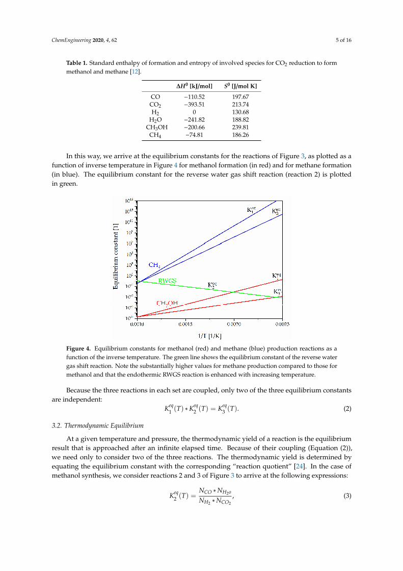
As in the case of the looped PFR, the idea of the sorption-enhanced reactor is that the product is constantly removed from the gas stream by a suitable absorber and, consequently, the equilibrium of the reaction is shifted toward the product side, in accord with Le Chatelier’s principle [11]. We can model such a reactor by introducing a second parallel channel, the “sorption channel”, and by introducing terms in the PFR equations (those proportional to the inverse transfer lengths λk), which cause a continuous transfer of the products H2O (k= 4) and/or CH3OH (k= 5) from the PFR channel to the sorption channel. We show the results, in Figure 15, for two cases respectively: (a) 𝜆 = 0—i.e., water absorption only—and (b) 𝜆 = 𝜆 —i.e., the simultaneous absorption of both water and methanol. The efficiency enhancement is particularly pronounced when both product species are absorbed. In a practical sorption enhanced PFR, the product absorptionoccurs in the catalyst system itself [42]. The sorption-enhanced PFR suffers the drawback of requiring a recurring “pressure-swing”, to first desorb from and then to re-pressurize the absorbing catalyst material.

Figure 15. Simulated sorption-enhanced PFR conversion of CO2 to CH3OH: (a) Water adsorption alone, with methanol extraction from channel 1. (b) Simultaneous adsorption of water and methanol,

Figure 14. Computational scheme of the sorption-enhanced reactor. Note the presence of a parallel“sorbent” channel and the addition of new H2O and CH3OH “transfer” terms to the PFR equations.The symbol δjk is the “Kronecker delta”. The individual molar flows are defined in the figure.

As in the case of the looped PFR, the idea of the sorption-enhanced reactor is that the product isconstantly removed from the gas stream by a suitable absorber and, consequently, the equilibriumof the reaction is shifted toward the product side, in accord with Le Chatelier’s principle [11].We can model such a reactor by introducing a second parallel channel, the “sorption channel”,and by introducing terms in the PFR equations (those proportional to the inverse transfer lengthsλk), which cause a continuous transfer of the products H2O (k = 4) and/or CH3OH (k = 5) from thePFR channel to the sorption channel. We show the results, in Figure 15, for two cases respectively:(a) λCH3OH = 0—i.e., water absorption only—and (b) λCH3OH = λH2O—i.e., the simultaneous absorptionof both water and methanol. The efficiency enhancement is particularly pronounced when bothproduct species are absorbed. In a practical sorption enhanced PFR, the product absorption occurs in


the catalyst system itself [42]. The sorption-enhanced PFR suffers the drawback of requiring a recurring“pressure-swing”, to first desorb from and then to re-pressurize the absorbing catalyst material.




A second method of increasing the PFR conversion efficiency is by “sorption enhancement” [11]. The corresponding simulation scheme is shown in Figure 14. Compared to the basic PFR scheme of Figure 6, note the presence of an effective “sorbent channel” and the addition of H2O and CH3OH “transfer terms” in the differential PFR equations.

Figure 14. Computational scheme of the sorption-enhanced reactor. Note the presence of a parallel “sorbent” channel and the addition of new H2O and CH3OH “transfer” terms to the PFR equations. The symbol δjk is the “Kronecker delta”. The individual molar flows are defined in the figure.

As in the case of the looped PFR, the idea of the sorption-enhanced reactor is that the product is constantly removed from the gas stream by a suitable absorber and, consequently, the equilibrium of the reaction is shifted toward the product side, in accord with Le Chatelier’s principle [11]. We can model such a reactor by introducing a second parallel channel, the “sorption channel”, and by introducing terms in the PFR equations (those proportional to the inverse transfer lengths λk), which cause a continuous transfer of the products H2O (k= 4) and/or CH3OH (k= 5) from the PFR channel to the sorption channel. We show the results, in Figure 15, for two cases respectively: (a) 𝜆 = 0—i.e., water absorption only—and (b) 𝜆 = 𝜆 —i.e., the simultaneous absorption of both water and methanol. The efficiency enhancement is particularly pronounced when both product species are absorbed. In a practical sorption enhanced PFR, the product absorptionoccurs in the catalyst system itself [42]. The sorption-enhanced PFR suffers the drawback of requiring a recurring “pressure-swing”, to first desorb from and then to re-pressurize the absorbing catalyst material.

Figure 15. Simulated sorption-enhanced PFR conversion of CO2 to CH3OH: (a) Water adsorption alone, with methanol extraction from channel 1. (b) Simultaneous adsorption of water and methanol,

Figure 15. Simulated sorption-enhanced PFR conversion of CO2 to CH3OH: (a) Water adsorptionalone, with methanol extraction from channel 1. (b) Simultaneous adsorption of water and methanol,with methanol extraction from channel 2. In both cases, the pressure is 40 bar, and the stoichiometricfactor SN = 2.

4. Summary and Conclusions

This work has presented, in tutorial form, recipes for the numerical simulation of catalyticreactions. The application examples chosen are the hydrogenation reduction of carbon dioxideto form the synthetic fuels methanol and methane, and it has been assumed throughout that thereactants and products are ideal gases and that the reactor temperature and pressure are constantand uniform. Based on the change in the standard Gibbs free energy, the degrees of chemicalconversion were first calculated in thermodynamic equilibrium. The results are in good agreementwith the qualitative predictions of Le Chatelier’s principle. In a practical chemical reactor, a catalystis used to selectively accelerate the reaction rate. The dynamic behaviors of the two archetypicalcontinuous-flow reactors, the plug flow reactor (PFR) and the continuously stirred tank reactor (CSTR),were simulated by incorporating published models for the catalyst-specific, multi-step chemical kineticsinto reactor-specific differential equations for the product yield. The numerical solution of theseequations quantified the effects on the reaction yield of temperature, pressure, and various reactorparameters, in reasonable agreement with previous published work. In particular, it could be shownthat, for a very long PFR or a very large volume CSTR, we regain the thermodynamic limit. It was alsoshown how the evolution from reactant to product species may be spatially followed along the length ofthe PFR tubes. The thermodynamic limit, in particular the low efficiency of methanol production, canbe influenced by shifting the chemical equilibrium—e.g., via the continuous removal of product species.Using our numerical framework, it was demonstrated how this can facilitate methanol production fortwo particular cases: PFR looping (product removal and reactant recycling—involving a continuous“temperature-swing”) and sorption-enhanced PFR (product removal via absorption, perhaps on aspecialized catalyst—involving repeated “pressure-swings”).

All of these simulations could have been performed using a commercial software package.By laying out the fundamental concepts and constructing and solving the reactor-specific differentialequations for the chemical yield, we have attempted to provide the reader with a view into the innerworkings of such a “black-box” package. The student exercises in the Supplementary Materials leadthe reader through the creation of a homemade computer program to numerically solve the differentialequations. Our hope is that our audience will gain an understanding of the basic principles governingcatalytic reactors and will be motivated to apply and adapt the presented formalism to applications ofspecific interest.


Supplementary Materials: The following are available online at http://www.mdpi.com/2305-7084/4/4/62/s1:see Supporting Information with exercises.

Author Contributions: Conceptualization: J.T. and B.D.P.; Formal analysis: J.T., A.B., M.H., B.D.P.; Investigation:J.T. and B.D.P.; Supervision: B.D.P.; Writing—original draft: J.T. and B.D.P.; Writing—review and editing: J.T., A.B.,M.H., B.D.P. All authors have read and agreed to the published version of the manuscript.

Funding: This work was partly supported by the UZH-UFSP program LightCheC. The financial support fromBFE and FOGA (SmartCat Project) and the Swiss National Science Foundation (Grant no. 200021_144120 and172662) is acknowledged.

Conflicts of Interest: The authors declare no conflict of interest.

References

1. Tripodi, A.; Compagnoni, M.; Martinazzo, R.; Ramis, G.; Rossetti, I. Process simulation for the design andscale up of heterogeneous catalytic process: Kinetic modeling issues. Catalysis 2017, 7, 159. [CrossRef]

2. Haydary, J. Chemical Process Design and Simulation: Aspen Plus and Aspen HYSYS Applications; John Wiley &Sons, Inc.: Hoboken, NJ, USA, 2019.

3. Savelski, M.J.; Hesketh, R.P. Issues encountered with students using process simulators. Age 2002, 8, 1.4. Fogler, S.H. Elements of Chemical Reaction Engineering; Pearson Education Inc.: Upper Saddle River, NJ, USA, 1987.5. Davis, M.E.; Davis, R.J. Fundamentals of Chemical Reaction Engineering; McGraw Hill: New York, NY, USA, 2003.6. Manos, G. Introduction to Chemical Reaction Engineering. In Concepts of Chemical Engineering 4 Chemists;

Simons, S., Ed.; The Royal Society of Chemistry: Cambridge, UK, 2007.7. Nauman, E.B. Chemical Reactor Design, Optimization, and Scaleup; John Wiley & Sons: Hoboken, NJ, USA, 2007.8. Hill, C.G.; Root, T.W. Introduction to Chemical Engineering Kinetics and Reactor Design; John Wiley & Sons, Inc.:

Hoboken, NJ, USA, 2014.9. Hagen, J. Industrial Catalysis; WILEY-VCH Verlag GmbH & Co. KGaA: Weinheim, Germany, 2015.10. Press, W.H.; Flannery, B.P.; Teukolsky, S.A.; Vetterling, W.T. Numerical Recipes: The Art of Scientific Computing;

Cambridge University Press: Cambridge, UK, 2007.11. Carvill, B.T.; Hufton, J.R.; Anand, M.; Sircar, S. Sorption-Enhanced Reaction Process. AIChE J. 1996, 42,

2765–2772. [CrossRef]12. Swaddle, T.W. Inorganic Chemistry—An Industrial and Environmental Perspective; Academic Press: Cambridge, MA,

USA, 1997.13. Graaf, G.H.; Stamhuis, E.J.; Beenackers, A.A.C.M. Kinetics of low-pressure Methanol Synthesis. Chem. Eng. Sci.

1988, 43, 3185–3195. [CrossRef]14. Graaf, G.H.; Scholtens, H.; Stamhuis, E.J.; Beenackers, A.A.C.M. Intra-particle Diffusion Limitations in

low-pressure Methanol Synthesis. Chem. Eng. Sci. 1990, 45, 773–783. [CrossRef]15. Xu, J.; Froment, G.F. Methane Steam Reforming, Methanation and Water-gas Shift: I. Intrinsic Kinetics.

AlChE J. 1989, 35, 88–96. [CrossRef]16. Wolfram, S. Mathematica: A System for Doing Mathematics by Computer; Addison-Wesley: Reading, MA,

USA, 1991.17. Centi, G.; Quadrelli, E.A.; Perathoner, S. Catalysis for CO2 conversion: A key technology for rapid introduction

of renewable energy in the value chain of chemical industries. Energy Environ. Sci. 2003, 6, 1711. [CrossRef]18. Wang, W.; Wang, S.; Ma, X.; Gong, J. Recent advances in catalytic hydrogenation of carbon dioxide.

Chem. Soc. Rev. 2011, 40, 3703–3727. [CrossRef]19. Abas, N.; Kalair, A.; Khan, N. Review of fossil fuels and future energy technologies. Futures 2015, 69, 31–49.

[CrossRef]20. Patterson, B.D.; Mo, F.; Borgschulte, A.; Hillestad, M.; Joos, F.; Kristiansen, T.; Sunde, S.; van Bokhoven, J.A.

Renewable CO2 recycling and synthetic fuel production in a marine environment. Proc. Natl. Acad. Sci. USA2019, 116, 12212–12219. [CrossRef]

21. Miguel, C.V.; Soria, M.A.; Mendes, A.; Madeira, L.M. Direct CO2 hydrogenation to methane or methanol frompost-combustion exhaust streams—A thermodynamic study. J. Nat. Gas Sci. Eng. 2015, 22, 1–8. [CrossRef]

22. Porosoff, M.D.; Yan, B.; Chen, J.G. Catalytic reduction of CO2 by H2 for synthesis of CO, methanol andhydrocarbons: Challenges and opportunities. Energy Environ. Sci. 2016, 9, 62. [CrossRef]

http://www.mdpi.com/2305-7084/4/4/62/s1

http://dx.doi.org/10.3390/catal7050159

http://dx.doi.org/10.1002/aic.690421008

http://dx.doi.org/10.1016/0009-2509(88)85127-3

http://dx.doi.org/10.1016/0009-2509(90)85001-T

http://dx.doi.org/10.1002/aic.690350109

http://dx.doi.org/10.1039/c3ee00056g

http://dx.doi.org/10.1039/c1cs15008a

http://dx.doi.org/10.1016/j.futures.2015.03.003

http://dx.doi.org/10.1073/pnas.1902335116

http://dx.doi.org/10.1016/j.jngse.2014.11.010

http://dx.doi.org/10.1039/c5ee02657a


23. Moioli, E.; Mutschler, R.; Züttel, A. Renewable energy storage via CO2 and H2 conversion to methane andmethanol: Assessment for small scale applications. Renew. Sustain. Energy Rev. 2019, 107, 497–506.

24. Atkins, P.W.; de Paula, J. Physikalische Chemie; Wiley-VCH Verlag GmbH & Co. KGaA: Weinheim, Germany, 2006.25. Schüth, F. Chemical Compounds for Energy Storage. Chem. Ing. Tech. 2011, 83, 1984–1993. [CrossRef]26. Koppenol, W.H.; Rush, J.D. Reduction potential of the carbon dioxide/carbon dioxide radical anion:

A comparison with other C1 radicals. J. Phys. Chem. 1987, 91, 4429–4430. [CrossRef]27. Rumble, J. CRC Handbook of Chemistry and Physics; Taylor & Francis: Abdingdon, UK, 2020.28. Aziz, M.A.A.; Jalil, A.A.; Triwahyono, S.; Ahmad, A. CO2 methanation over heterogeneous catalysts:

Recent progress and future prospects. Green Chem. 2015, 17, 2647–2663. [CrossRef]29. Kustov, A.L.; Frey, A.M.; Larsen, K.E.; Johannessen, T.; Nørskov, J.K.; Christensen, C.H. CO methanation over

supported bimetallic Ni-Fe catalysts: From computational studies towards catalyst optimization. Appl. Catal.A Gen. 2007, 320, 98–104. [CrossRef]

30. Skrzypek, J.; Lachowska, M.; Serafin, D. Methanol Synthesis from CO2 and H2: Dependence of equilibriumconversions and exit equilibrium concentrations of components on the main process variables. Chem. Eng. Sci.1990, 45, 89–96. [CrossRef]

31. Stangeland, K.; Li, H.; Yu, Z. Thermodynamic analysis of chemical and phase equilibria in CO2 hydrogenationto methanol, dimethyl ether, and higher alcohols. Ind. Eng. Chem. Res. 2018, 57, 4081–4094. [CrossRef]

32. Schlereth, D.; Hinrichsen, O. A fixed-bed reactor modeling study on the methanation of CO2. Chem. Eng.Res. Des. 2014, 92, 702–712.

33. Rönsch, S.; Schneider, J.; Matthischke, S.; Schlüter, M.; Götz, M.; Lefebvre, J.; Prabhakaran, P.; Bajohr, S.Review on methanation—From fundamentals to current projects. Fuel 2016, 166, 276–296.

34. Hanefeld, U.; Lefferts, L. Catalysis: An Integrated Textbook for Students; John Wiley & Sons: Hoboken, NJ, USA,2018.

35. Nørskov, J.K.; Studt, F.; Abild-Pedersen, F.; Bligaard, T. Fundamental Concepts in Heterogeneous Catalysis;John Wiley & Sons, Inc.: Hoboken, NJ, USA, 2014.

36. Toyir, J.; Miloua, R.; Elkadri, N.E.; Nawdali, M.; Toufik, H.; Miloua, F.; Saito, M. Sustainable process for theproduction of methanol from CO2 and H2 using Cu/ZnO-based multicomponent catalyst. Phys. Procedia2009, 2, 1075–1079. [CrossRef]

37. Gaikwad, R.; Bansode, A.; Urakawa, A. High-pressure advantages in stoichiometric hydrogenation of carbondioxide to methanol. J. Catal. 2016, 343, 127–132.

38. Slotboom, Y.; Bos, M.J.; Pieper, J.; Vrieswijk, V.; Likozar, B.; Kersten, S.R.A.; Brilman, D.W.F. Critical assessmentof steady-state kinetic models for the synthesis of methanol over an industrial Cu/ZnO/Al2O3 catalyst.Chem. Eng. J. 2020, 389, 124181.

39. Cao, H.; Wang, W.; Cui, T.; Zhu, G.; Ren, X. Enhancing CO2 hydrogenation to methane by Ni-based catalystwith V species using 3D-mesoporous KIT-6 as support. Energies 2020, 13, 2235. [CrossRef]

40. Van-Dal, E.S.; Bouallou, C. Design and simulation of a methonal production plant from CO2 hydrogenation.J. Clean. Prod. 2013, 57, 38–45.

41. Falconer, J.L. Comparing CSTR and PFR Mass Balances, LearnChemE Video Presentation, Univ. Colorado,Boulder, and Private Communication. 2019. Available online: www.youtube.com/watch?v=xrOdRKzlkcE(accessed on 15 November 2020).

42. Terreni, J.; Trottmann, M.; Franken, T.; Heel, A.; Borgschulte, A. Sorption-Enhanced Methanol Synthesis.Energy Technol. 2019, 7, 1801093. [CrossRef]

Publisher’s Note: MDPI stays neutral with regard to jurisdictional claims in published maps and institutionalaffiliations.

© 2020 by the authors. Licensee MDPI, Basel, Switzerland. This article is an open accessarticle distributed under the terms and conditions of the Creative Commons Attribution(CC BY) license (http://creativecommons.org/licenses/by/4.0/).

http://dx.doi.org/10.1002/cite.201100147

http://dx.doi.org/10.1021/j100300a045

http://dx.doi.org/10.1039/c5gc00119f

http://dx.doi.org/10.1016/j.apcata.2006.12.017

http://dx.doi.org/10.1016/0009-2509(90)87083-5

http://dx.doi.org/10.1021/acs.iecr.7b04866

http://dx.doi.org/10.1016/j.phpro.2009.11.065

http://dx.doi.org/10.3390/en13092235

www.youtube.com/watch?v=xrOdRKzlkcE

http://dx.doi.org/10.1002/ente.201801093

http://creativecommons.org/

http://creativecommons.org/licenses/by/4.0/.

Documents

Understanding Catalysis A Simplified Simulation of