TECHNICAL REPORT 1

Understanding and Tackling the Root Causes ofInstability in Wireless Mesh Networks:

(extended version)Adel Aziz, David Starobinski, and Patrick Thiran

Abstract—We investigate, both theoretically and experimen-tally, the stability of CSMA-based wireless mesh networks, wherea network is said to be stable if and only if the queue of each relaynode remains (almost surely) finite. We identify two key factorsthat impact stability: the network size and the so-called “stealingeffect”, a consequence of the hidden node problem and non-zerotransmission delays. We consider the case of a greedy source andprove, by using Foster’s theorem, that 3-hop networks are stable,but only if the stealing effect is accounted for. We also provethat 4-hop networks are, on the contrary, always unstable (evenwith the stealing effect) and show by simulations that instabilityextends to more complex linear and non-linear topologies. Totackle this instability problem, we propose and evaluate a novel,distributed flow-control mechanism, called EZ-flow. EZ-flow isfully compatible with the IEEE 802.11 standard (i.e., it does notmodify headers in packets), can be implemented using off-the-shelf hardware, and does not entail any communication overhead.EZ-flow operates by adapting the minimum congestion windowparameter at each relay node, based on an estimation of thebuffer occupancy at its successor node in the mesh. We showhow such an estimation can be conducted passively by takingadvantage of the broadcast nature of the wireless channel. Realexperiments, run on a 9-node testbed deployed over 4 differentbuildings, show that EZ-flow effectively smoothes traffic andimproves delay, throughput, and fairness performance.

I. INTRODUCTION

W IRELESS mesh networks (WMNs) promise to revolu-tionize Internet services by providing customers with

ubiquitous high-speed access at low cost. Thus, several citiesand communities have already deployed, or are about to deployWMNs [1, 2, 5]. Nevertheless, several technical obstacles mustbe surmounted to allow for the widespread adoption of thistechnology. In particular, a key challenge is to ensure a smoothand efficient traffic flow over the backhaul, i.e., the multi-hopwireless links connecting the end-users to the Internet.

The Medium Access Control (MAC) protocol, used tomanage contention and avoid packet collisions on the sharedchannel, plays a key role in determining the performance ofthe backhaul of a WMN. Most WMNs use the IEEE 802.11standard [8] as their MAC protocol for the following reasons:(i) it is based on Carrier-Sense Multiple Access (CSMA), amechanism that naturally lends itself to a distributed imple-

A. Aziz and P. Thiran are with the School of Computer and Communi-cation Sciences, EPFL, Lausanne, Switzerland; e-mail: adel.aziz@epfl.ch,patrick.thiran@epfl.ch.

D. Starobinski is with the Department of Electrical and Computer Engi-neering, Boston University, Boston, MA, USA; e-mail: staro@bu.edu

Part of the results in this paper appeared in [9] and [10].

0 300 600 900 1200 1500 18000

10

20

30

40

50

Time

Que

ue s

ize

[pac

kets

]

3−hop

Node 1Node 2

0 300 600 900 1200 1500 18000

10

20

30

40

50

Time

Que

ue s

ize

[pac

kets

]

4−hop

Node 1Node 2Node 3

Fig. 1. Experimental results for the queue evolution of each relay node in 3-and 4-hop topologies. A 3-hop network is stable, whereas a 4-hop is unstablewith the queue of its first relaying node (node 1) building up until it reachesthe buffer hardware limit of 50 packets and starts overflowing.

mentation; (ii) it has low control overhead; (iii) it is ubiquitousand (iv) it is inexpensive to deploy.

The IEEE 802.11 protocol, however, was initially designedto support single-hop, but not multi-hop, communicationwhere multiple nodes must cooperate to efficiently transportone or multiple flows. In this paper, we show how andwhy 802.11-based wireless mesh networks are susceptible toturbulence that takes the form of the following: (i) bufferbuild up and overflow at relaying nodes; (ii) major end-to-enddelay fluctuations; and (iii) reduced throughput. In Figure 1we depict the consequence of this unstable behavior by usingdata collected from measurements on a real network witha greedy access point. The figure shows the instantaneousbuffer occupancy at the relaying nodes for a (stable) 3-hopnetwork and an (unstable) 4-hop network. In this scenario,the end-to-end throughput in the 4-hop case is almost twiceas small as in the 3-hop case. The intrinsic instability ofIEEE 802.11 mesh networks that are longer than 3 hops mayexplain why current implementations use only a few hops [3].It is therefore critical to rigorously characterize the behaviorof CSMA-like protocols in multihop scenarios and proposepossible improvements when appropriate.

We prove that the network is stable or unstable, dependingon its size and a phenomenon referred to as a stealing effectthat results from the hidden node problem and non-zerotransmission delays. The likelihood of this phenomenon iscaptured by the stealing effect probability 0 ≤ p ≤ 1, aparameter explained in detail in Section III.C.

After detailing the problem and reviewing related work inSection II, we introduce a discrete Markov chain model thatcaptures the stealing effect phenomenon in Section III. Wedemonstrate in Section IV that in the case of a 3-hop network,the system is stable if and only if the stealing effect is present

TECHNICAL REPORT 2

(p > 0). However, for larger linear K-hop topologies (K > 3)the network is always unstable, as proven in Section V forK = 4, and presumably so for larger K with a formal prooffor the case p = 0. Even though multihop 802.11 networks areknown to suffer from unfairness and starvation (see [15, 20,36, 39]), to the best of our knowledge, to date the (in)stabilityof multihop 802.11 networks has not been demonstrated eitherexperimentally or analytically.

After elucidating the sources of instability, we focus on theproblem of devising distributed channel access mechanisms toensure stability in multi-hop networks. This issue has receivedmuch attention since the seminal work of Tassiulas et al. [41].Most of the solid, analytical work on this problem [13, 21, 40,44, 46] follow a “top-down” approach, i.e., they start froma theoretical algorithm that provably achieves stability andthen try to derive a distributed version. The drawback of thisapproach is the difficulty of testing the proposed solution inpractice using existing wireless cards. Indeed, despite all theprevious theoretical work, few solutions have been imple-mented and tested to date [10, 43]. To bridge this gap, weinstead resort to a bottom-up approach, i.e., we start from theexisting IEEE 802.11 protocol, identify the main causes ofturbulence and instability, and then we derive a practical anddecentralized mechanism to solve this problem.

In Section VII, we propose and analyze a new, distributedflow-control mechanism, called EZ-flow, that solves the tur-bulent behavior of IEEE 802.11 WMNs. EZ-flow requiresno modification to the IEEE 802.11 protocol and is readilyimplementable with off-the-shelf hardware. EZ-flow runs asan independent program at each relaying node. By passivelymonitoring buffer occupancy at successor nodes, it adapts aparameter of IEEE 802.11, the minimum contention windowCWmin (CWmin is inversely proportional to the channelaccess probability). The standard way to obtain the bufferoccupancy information is via message passing. Message pass-ing, however, may further exacerbate congestion and reduceresources available for sending useful data [44]. To avoid thisdrawback, EZ-flow takes advantage of the broadcast nature ofthe wireless medium to infer buffer occupancy at successornodes. Obtaining this information without message exchangesis one of the major advantages of EZ-flow as it enables the net-work to achieve stability without any communication overheadand without requiring the knowledge of the capacity (whichis time varying and hard to obtain in real implementations).

We end the paper by validating the stabilizing propertiesof EZ-flow experimentally in Section VIII and through simu-lations in Section IX. Finally, we summarize our findings inSection X.

II. BACKGROUND

A. Problem Statement

We consider the case of a wireless multi-hop topology as theone existing in the backhaul of a mesh network. The backhaulis composed of three types of nodes: (i) a Wired Access Point(WAP) that plays the role of gateway and is connected to theInternet, (ii) Access Points (APs) that ensure the access partof the WMN by having the end-users connected to them (note

that usually the backhaul and access part of a WMN run onindependent channels to avoid interferences) and (iii) TransitAccess Points (TAPs) that transport the data packets throughmultiple hops from the WAP to the AP and back.

We then focus on the stability of these multi-hop networksby analyzing the queue evolution at the relay nodes (TAPs)both analytically and experimentally.

B. Related WorkMuch effort has been put into understanding how IEEE

802.11 behaves in a multi-hop environment. Previous worksshow the inefficiency of the protocol in providing optimalperformance, as far as delay, throughput and fairness areconcerned [18]. In [34], Nandiraju et al. propose a queuemanagement mechanism to improve fairness. However, asthey mention in their conclusion, a solution to the inherentunfairness of the IEEE 802.11 MAC layer is needed for theirmechanism to work properly. In [25], Jindal et al. claimthat the performance of IEEE 802.11 in multi-hop settingsis not as bad as it could be expected. For instance, they showan example through simulation where IEEE 802.11 achievesa max-min allocation that is at least 64% of the max-minallocation obtained with a perfect scheduler. Our experiments,in Section VIII, show that the performance may actually bemuch worse. We believe that the cause of the discrepancy isthat [25] assumes that flows are rate-controlled at the source,whereas we do not make such an assumption. To tackle theinefficiency of IEEE 802.11, different approaches have beenproposed and we regroup them into five categories.

1) Throughput-Optimal Scheduling with Message Passing:A first analytical solution to the stability problem in multi-hop networks is discussed in the seminal work of Tassiulas etal. [41], which introduces a back-pressure algorithm. Theirmethodology uses a centralized scheduler that selects fortransmission the link with the greatest queue difference, i.e.the greatest difference in buffer occupancy between the MACdestination node and the MAC source node. Such a solutionworks well for a wired network, but is not adapted to amulti-hop wireless network where decentralized schedulersare needed due to the synchronization problem. Toward thisgoal, Modiano et al. introduced the first distributed schedulingframework that uses control messages to achieve throughputoptimal performances [33]. Further extensions to distributedscheduling strategies have been discussed in works suchas [13], where Chapokar et al. propose a scheduler that attainsa guaranteed ratio of the maximal throughput. Another effortto reduce the complexity of back-pressure is presented in [46],where Ying et al. propose to enhance scalability by reducingthe number of queues that need to be maintained at each node.The interaction between an end-to-end congestion controllerand a local queue-length-based scheduler is discussed byEryilmaz et al. in [16]. The tradeoff that exists in eachscheduling strategy between complexity, utility and delay isdiscussed in depth in [44]. One of the drawbacks of theseprevious methods is that they require queue information fromother nodes. The usual solution is to use message passing,which produces a costly overhead even if it is limited to thedirect neighbors.

TECHNICAL REPORT 3

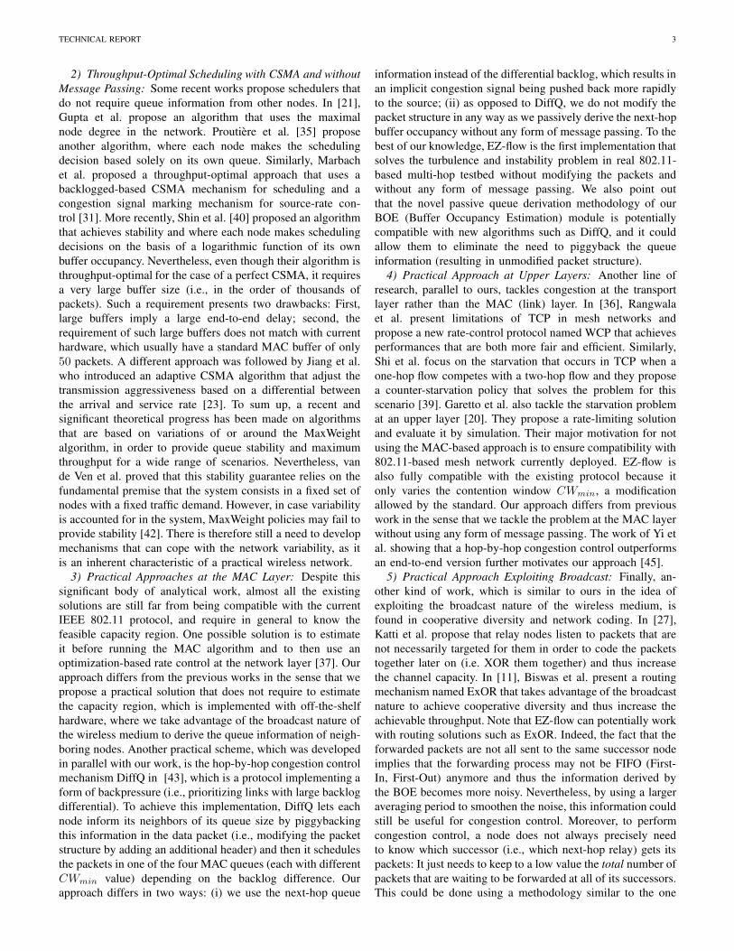
2) Throughput-Optimal Scheduling with CSMA and withoutMessage Passing: Some recent works propose schedulers thatdo not require queue information from other nodes. In [21],Gupta et al. propose an algorithm that uses the maximalnode degree in the network. Proutiere et al. [35] proposeanother algorithm, where each node makes the schedulingdecision based solely on its own queue. Similarly, Marbachet al. proposed a throughput-optimal approach that uses abacklogged-based CSMA mechanism for scheduling and acongestion signal marking mechanism for source-rate con-trol [31]. More recently, Shin et al. [40] proposed an algorithmthat achieves stability and where each node makes schedulingdecisions on the basis of a logarithmic function of its ownbuffer occupancy. Nevertheless, even though their algorithm isthroughput-optimal for the case of a perfect CSMA, it requiresa very large buffer size (i.e., in the order of thousands ofpackets). Such a requirement presents two drawbacks: First,large buffers imply a large end-to-end delay; second, therequirement of such large buffers does not match with currenthardware, which usually have a standard MAC buffer of only50 packets. A different approach was followed by Jiang et al.who introduced an adaptive CSMA algorithm that adjust thetransmission aggressiveness based on a differential betweenthe arrival and service rate [23]. To sum up, a recent andsignificant theoretical progress has been made on algorithmsthat are based on variations of or around the MaxWeightalgorithm, in order to provide queue stability and maximumthroughput for a wide range of scenarios. Nevertheless, vande Ven et al. proved that this stability guarantee relies on thefundamental premise that the system consists in a fixed set ofnodes with a fixed traffic demand. However, in case variabilityis accounted for in the system, MaxWeight policies may fail toprovide stability [42]. There is therefore still a need to developmechanisms that can cope with the network variability, as itis an inherent characteristic of a practical wireless network.

3) Practical Approaches at the MAC Layer: Despite thissignificant body of analytical work, almost all the existingsolutions are still far from being compatible with the currentIEEE 802.11 protocol, and require in general to know thefeasible capacity region. One possible solution is to estimateit before running the MAC algorithm and to then use anoptimization-based rate control at the network layer [37]. Ourapproach differs from the previous works in the sense that wepropose a practical solution that does not require to estimatethe capacity region, which is implemented with off-the-shelfhardware, where we take advantage of the broadcast nature ofthe wireless medium to derive the queue information of neigh-boring nodes. Another practical scheme, which was developedin parallel with our work, is the hop-by-hop congestion controlmechanism DiffQ in [43], which is a protocol implementing aform of backpressure (i.e., prioritizing links with large backlogdifferential). To achieve this implementation, DiffQ lets eachnode inform its neighbors of its queue size by piggybackingthis information in the data packet (i.e., modifying the packetstructure by adding an additional header) and then it schedulesthe packets in one of the four MAC queues (each with differentCWmin value) depending on the backlog difference. Ourapproach differs in two ways: (i) we use the next-hop queue

information instead of the differential backlog, which results inan implicit congestion signal being pushed back more rapidlyto the source; (ii) as opposed to DiffQ, we do not modify thepacket structure in any way as we passively derive the next-hopbuffer occupancy without any form of message passing. To thebest of our knowledge, EZ-flow is the first implementation thatsolves the turbulence and instability problem in real 802.11-based multi-hop testbed without modifying the packets andwithout any form of message passing. We also point outthat the novel passive queue derivation methodology of ourBOE (Buffer Occupancy Estimation) module is potentiallycompatible with new algorithms such as DiffQ, and it couldallow them to eliminate the need to piggyback the queueinformation (resulting in unmodified packet structure).

4) Practical Approach at Upper Layers: Another line ofresearch, parallel to ours, tackles congestion at the transportlayer rather than the MAC (link) layer. In [36], Rangwalaet al. present limitations of TCP in mesh networks andpropose a new rate-control protocol named WCP that achievesperformances that are both more fair and efficient. Similarly,Shi et al. focus on the starvation that occurs in TCP when aone-hop flow competes with a two-hop flow and they proposea counter-starvation policy that solves the problem for thisscenario [39]. Garetto et al. also tackle the starvation problemat an upper layer [20]. They propose a rate-limiting solutionand evaluate it by simulation. Their major motivation for notusing the MAC-based approach is to ensure compatibility with802.11-based mesh network currently deployed. EZ-flow isalso fully compatible with the existing protocol because itonly varies the contention window CWmin, a modificationallowed by the standard. Our approach differs from previouswork in the sense that we tackle the problem at the MAC layerwithout using any form of message passing. The work of Yi etal. showing that a hop-by-hop congestion control outperformsan end-to-end version further motivates our approach [45].

5) Practical Approach Exploiting Broadcast: Finally, an-other kind of work, which is similar to ours in the idea ofexploiting the broadcast nature of the wireless medium, isfound in cooperative diversity and network coding. In [27],Katti et al. propose that relay nodes listen to packets that arenot necessarily targeted for them in order to code the packetstogether later on (i.e. XOR them together) and thus increasethe channel capacity. In [11], Biswas et al. present a routingmechanism named ExOR that takes advantage of the broadcastnature to achieve cooperative diversity and thus increase theachievable throughput. Note that EZ-flow can potentially workwith routing solutions such as ExOR. Indeed, the fact that theforwarded packets are not all sent to the same successor nodeimplies that the forwarding process may not be FIFO (First-In, First-Out) anymore and thus the information derived bythe BOE becomes more noisy. Nevertheless, by using a largeraveraging period to smoothen the noise, this information couldstill be useful for congestion control. Moreover, to performcongestion control, a node does not always precisely needto know which successor (i.e., which next-hop relay) gets itspackets: It just needs to keep to a low value the total number ofpackets that are waiting to be forwarded at all of its successors.This could be done using a methodology similar to the one

TECHNICAL REPORT 4

presented in this paper for the unicast case. A similar extensionof a congestion-control from unicast to multicast is discussedby Scheuermann et al. in [38]. Finally, in [22] Heusse et al.also use the broadcast nature of IEEE 802.11 to improve thethroughput and fairness of single-hop WLANs by replacingthe exponential backoff with a mechanism that adapts itselfaccording to the number of slots that are sensed idle. Ourwork follows the same philosophy of taking advantage ofthe “free” information given by the broadcast nature. Apartfrom this, our approach is different, because we do not usecooperation and network coding techniques at relay nodes, butinstead in a competitive context we derive and use the next-hopbuffer occupancy information to tackle the traffic congestionoccurring in multi-hop scenarios.

III. MODELING THE SOURCES OF INSTABILITY

Figure 1 shows that a particular 3-hop networks is stable, butnot a 4-hop. In order to understand these experimental resultsshowing a drastic behavioral transition, we introduce an ana-lytical model that is inspired from the behavior of CSMA/CAprotocols (e.g., 802.11-like protocols) with some necessarysimplifications for the sake of tractability. We emphasize that,given the mathematical assumptions, our analysis is exact.

A. MAC Layer DescriptionThe first common assumption [13, 16, 30, 41, 46] is that of

a slotted discrete time axis, in other words, each transmissiontakes one time slot and all the transmissions occurring duringa given slot start and finish at the same time. We consider agreedy source model, i.e., the WAP (gateway) always has newpackets ready for transmission. Assuming a K-hop system, thepackets flow from the WAP to TAPK , via TAP1, TAP2, . . .,TAPK−1. TAPs do not generate packets of their own. EachTAP is equipped with an infinite buffer.

We assume that the system evolves according to a two-phase mechanism: a link competition phase and a transmissionphase. The link competition phase, whose length is assumedto be negligible, occurs at the beginning of each slot. Duringthis phase, all the nodes with a non-empty buffer competefor the channel and a pattern of successful transmissionsemerges, referred to as transmission pattern in this paper.Given the current state of buffers, the link competition processis assumed to be independent of competitions that happenedin previous slots. This assumption is similar to the commonlyused assumption of exponentially (memoryless) distributedbackoffs. During this phase, non-empty nodes are sequentiallychosen at random and added to the transmission patternif and only if they do not interfere with already selectedcommunications (with the notable exception of the stealingeffect described below). The final pattern is obtained when nomore nodes can be added without interfering with the others.

The second phase of the model is fairly straightforwardas it consists in applying the transmission pattern from theprevious phase in order to update the buffer status of thesystem. This buffer status information is of utmost importancefor our analysis because it is the parameter that indicateswhether the network remains stable (no buffer explodes) orsuffers congestion (one or more buffers build up).

B. Discrete Markov Chain Model

We now formalize the model previously described math-ematically. All packets are generated by the WAP (node 0),and are forwarded to the last TAP (node K) by successivetransmissions via the intermediate nodes (TAPs) 1 to K − 1.A time step n ∈ N corresponds to the successful transmissionof a packet from some node i to its neighbor i + 1, or ifK is large enough, of a set of packets from different non-interfering nodes i, j, . . . to nodes i + 1, j + 1, . . ., providedthese transmissions overlap in time (the transmitters andreceivers must therefore not interfere with each other). Weassume that node 0 always has packets to transmit (infinitequeue), and that node K consumes immediately the packets,as it is the exit point of the backbone (its queue is always0). We are interested in the evolution of the queue sizes bi ofrelaying nodes 1 ≤ i ≤ K − 1 over time, and therefore weadopt as a state variable of the system at time n the vector

~b(n) = [b1(n) b2(n) . . . bK−1(n)]T ,

with T denoting transposition. We also introduce a set of Kauxiliary binary variables zi, 0 ≤ i ≤ K − 1, representingthe ith link activity at time slot n: zi(n) = 1 if a packetwas successfully transmitted from node i to node i+1 duringthe nth time slot, and zi(n) = 0 otherwise. Observing thatbi(n+1) = bi(n)+zi−1(n)−zi(n), we can recast the dynamicsof the system as

~b(n+ 1) = ~b(n) +A ∗ ~z(n) (1)

where

~z(n) = [z0(n) z1(n) z2(n) . . . zK−1(n)]T

A =

1 −1 0 . . . 0

0 1 −1 0...

.... . .

. . .. . . 0

0 . . . 0 1 −1

.

Finally, the activity of a link zi depends on the queue sizes ofall the nodes, which we cast as zi = gi(~b) for some randomfunction gi(·) of the queue size vector, or in vector form as

~z(n) = g(~b(n)). (2)

The specification of g = [g0, . . . , gK−1]T is the less straight-forward part of the model, as it requires to enter in someadditional details of the CSMA/CA protocols, which we deferto the next sections. We will first expose it in Section IV fora K = 3 hops network, and then move to the larger networkswith K = 4 and K ≥ 5 in the subsequent section, as thespecification of g comes with some level of complexity asK gets larger. Nevertheless, we can already mention here twosimple constraints that g must verify: (i) node i cannot transmitif its buffer is empty, and therefore zi = gi(~b) = 0 if bi = 0;(ii) nodes that successfully transmit in the same time slot mustbe at least 2 hops apart, as otherwise the packet from node iwould collide at node i+ 1 with the packet from node i+ 2.Hence

zizi+k = 0 for k ∈ {−2,−1, 1, 2}. (3)

TECHNICAL REPORT 5

We observe that (1) and (2) make the model a discrete-time,irreducible Markov chain. The (in)stability of the networkcoincides with its (non-)ergodicity.

C. Stealing Effect Phenomenon

The stealing effect phenomenon is a result of the well-known hidden node problem occurring in multihop topologies.Indeed, the existence of directional multi-hop flows in thebackbone of mesh networks, from node 0 to node K mayinduce unfairness in a way that does not arise in single-hopscenarios. When node i first enters the link competition phase,node i + 2 may be unaware of this transmission attempt.Node i + 2 may therefore start a concurrent transmission tonode i+ 3 as it senses the medium to be idle. As a collisionoccurs at node i + 1 (due to the broadcast nature of thewireless medium), node i will experience an unsuccessfultransmission whereas the transmission from node i + 2 willsucceed. We refer to this unfairness artifact as the stealingeffect, which differs from the classical capture effect. Thelatter pertains to packets transmitted to the same destination.

Definition 1 (Stealing Effect): The stealing effect occurswhen a node i+ 2 successfully captures the channel from anupstream node i, even though it accesses the medium later.We define p to be the probability of the occurrence of thestealing effect.

In IEEE 802.11, the stealing effect corresponds to the eventwhere node i + 2 captures the channel, even though it hasa larger backoff value than node i. The probability of thisevent depends on the specific protocol implementation. If theoptional RTS/CTS handshake is disabled, then p → 1. IfRTS/CTS is enabled, then p is typically much smaller, butstill non-zero because RTS messages may collide [39]. Indeed,the transmission time of a control message (e.g., the RTStransmission time at the 1Mb/s basic rate is 352µs) is non-negligible compared to the duration of a backoff slot (20µs).

In our model, the stealing effect is captured by having thefunction g(·) in (2) depend on p. As revealed by our analysis,a positive and somewhat counterintuitive consequence of thestealing effect is the promotion of a laminar packet flow,namely, a smooth propagation of packets. Indeed, by favoringdownstream links over upstream ones, it creates a form ofvirtual back-pressure that prevents packets from being pushedtoo quickly into the network.

D. Stability Definition

A buffer is stable when its occupancy does not tend toincrease forever. More formally, we adopt the usual definitionsof stability (see e.g. Section 2.2 of [12]).

Definition 2 (Stability): A queue is stable when its evolu-tion is ergodic (it goes back to zero almost surely in finitetime). A network is stable when the queues of all forwardingnodes (i.e., all TAPs) are stable.

B

CD

A b1

b2

1/2 1/21

(1 − p)/2

(1 + p)/2

1/3

(1 − p)/3

(1 + p)/3

Fig. 2. Random walk in N2 modeling the 3-hop network. where the 4 regionsare: (A) {0; 0}, (B) {b1 > 0; 0}, (C) {0; b2 > 0} and (D) {b1 > 0; b2 > 0}.

IV. 3-HOP NETWORKS STABILITY

Let us first analyze the 3-hop topology, which remainsrelatively simple because only one link can be active at agiven time slot. Indeed, the only three possible transmissionpatterns ~z are [1 0 0]T , [0 1 0]T and [0 0 1]T . We can nowcomplete the description of the function g(·), before analyzingthe ergodicity of the Markov chain.

A. System Evolution

The role of the stochastic function g(·) is to map a bufferstatus ~b to a transmission pattern ~z with a certain probability.

First, in the case of an idealized CSMA/CA model withoutthe stealing effect (p = 0), all non-empty nodes have exactlythe same probability of being scheduled. That is, if only node0 and node 1 (or, respectively, node 2) have a packet to send,both patterns [1 0 0]T and [0 1 0]T (resp., [0 0 1]T ) happenwith probability 1/2. Similarly, when all three nodes have apacket to send, each of the three possible transmission patternshappens with probability 1/3.

More generally, when we include the stealing effect, wecapture the bias towards downstream links that are two hopsaway. When only node 0 and node 1 compete for the channel,nothing is changed and the probability of success remains 1/2as they are only separated by one single hop. However, whennode 0 and node 2 compete together, there is a probability pthat node 2 steals the channel.

This leads us to define function g(·) differently for eachregion of Z2 as shown in Figure 2. First, in region A ={b1(n) = 0, b2(n) = 0}, g([b1(n) b2(n)]

T ) = [1 0 0]T . Inregion B = {b1(n) > 0, b2(n) = 0} we have that

g([b1(n) b2(n)]T ) =

{

[1 0 0]T with probability 1/2[0 1 0]T with probability 1/2.

In region C = {b1(n) = 0, b2(n) > 0},

g([b1(n) b2(n)]T ) =

{

[1 0 0]T with probability (1 − p)/2[0 0 1]T with probability (1 + p)/2.

Finally, in region D = {b1(n) > 0, b2(n) > 0}, all threenodes compete, and node 2 can still steal the channel fromnode 0, hence

g([b1(n) b2(n)]T ) =

[1 0 0]T with probability (1− p)/3[0 1 0]T with probability 1/3[0 0 1]T with probability (1 + p)/3.

TECHNICAL REPORT 6

0 2 4 6 8 10

x 106

0

5

10

15

20

Time [in slot]

Que

ue s

ize

at n

ode

1Queue evolution (p=1)

0 2 4 6 8 10

x 106

0

1000

2000

3000

4000

5000

Time [in slot]

Que

ue s

ize

at n

ode

1

Queue evolution (p=0)

0 2 4 6 8 10

x 106

0

20

40

60

80

Time [in slot]

Que

ue s

ize

at n

ode

1

Queue evolution (p=0.1)

0 2 4 6 8 10

x 106

0

100

200

300

400

500

Time [in slot]

Que

ue s

ize

at n

ode

1

Queue evolution (p=0.01)

Fig. 3. Queue evolution for 3-hop with different p values.

B. Stability Analysis

The queue evolution from (1) is a random walk in N2,as depicted in Figure 2. Theorem 1 shows the stabilizinginfluence of the stealing effect.

Theorem 1: A 3-hop network is unstable for the case p = 0and it is stable for all 0 < p ≤ 1.

Proof: The instability of the case p = 0 is readily provedwith the Non-ergodicity theorem ( [17], p. 30) using theLyapunov function

h(b1, b2) = b1, (4)

and setting the constants c = d = 1 in that theorem.Next we prove the stability of the cases 0 < p ≤ 1 by using

Foster’s theorem (see Appendix) with the Lyapunov function

h(b1, b2) = b21 + b22 − b1b2,

the finite set F = {0 ≤ b1, b2 < 5/p}, the function k = 1 andthe notations

µb1,b2(n) = E[

h(~b(n+ 1)) | h(~b(n)) = h(b1, b2)]

εb1,b2(n) = µb1,b2(n)− h(b1, b2),

where εb1,b2(n) can be interpreted as the drift of the randomwalk at time n. Then we verify Foster’s theorem for all thethree regions of N2\F . After some computations, we find thatfor Region B \ F , εb1,0(n) = 2− b1(n)/2 < 0. Likewise, forregion C \ F , we get ε0,b2(n) = 1 − (3 + p)b2(n)/2 < 0.Finally, for region D \ F , we have εb1,b2(n) = 5/3 −p(b1(n) + b2(n))/3 < 0. Consequently, the two conditionsof the theorem are satisfied and stability is proved.

Finally, in Figure 3 we present the effect of p on the queueevolution through a simulation of our model. We also mention,that our theoretical results give insight into monitoring thequeue of node 1 in order to assess the stability of the system(the function of (4) only considers b1 to prove instability).

Step 0

Step 1

Step 2

(2)(1) (8)(7)(6)

(3)

(4)

(5)

(2)

(1)

(8)

(7)

(6)(3)(4)

(5)

(0)(0)

(0) (0) (0)

(1-pS12

S12+S1

3) (1-S1

3 )

(1-pS12

S12+S1

3) S1

3

pS12

S12+S1

3

1-pS13

pS13 1

S10

S10+S1

1

1-S10

S10+S1

1

δi(n)∑k δk(n)

{z0=1} {z1=1} {z2=1} {z3=1}

{ }

[1 0 0 0]T [0 1 0 0]T [0 0 1 0]T [0 0 0 1]T

[1 0 0 1]T

Fig. 4. Decision tree to obtain ~z = g(~b) for the 4-hop model.

V. 4-HOP NETWORKS INSTABILITY

The 4-hop system is relatively similar to the 3-hop, exceptthat the function g(·) becomes more complex to derive. Indeedthe five possible patterns ~z are now [1 0 0 0]T , [0 1 0 0]T ,[0 0 1 0]T , [0 0 0 1]T and [1 0 0 1]T

A. System Evolution

The drastic difference when moving to 4-hop topologies isthat nodes that can transmit concurrently will reinforce eachother and will increase their transmission probability [14, 15].

This interdependence makes the determination of g(·) lessstraightforward than in the 3-hop case. We capture this com-plexity by a decision tree, depicted in Figure 4, which mapsall the sequential events that can occur for the selection of thetransmission pattern (state in bold in Figure 4).

Before describing the exact mechanisms behind our decisiontree, we introduce some necessary notations. First, we definethe iteration step m that represents the step between twosequential events (an event corresponds to either the inclusionof a node in the transmission pattern or the removal of a nodefrom the competition). As shown in Figure 4, the decision-treeprocess ends in two iterations (m ∈ {0, 1, 2}) and this is dueto the fact that at most two links can be active concurrentlyin the transmission pattern of a 4-hop network.Secondly, we introduce the two indicator vectors ~δ(n) and ~Sm.The four entries δi(n) = 1{bi(n)>0} indicate which buffersare occupied (δi(n) = 1) or empty (δi(n) = 0). The vector~Sm = [Sm

0 . . . Sm3 ]T , which is obtained through an iterative

process, indicates the set of nodes that are still in competitionfor the channel at iteration step m. Initially, all the nodes witha non-empty buffer compete for the channel at step 0 andtherefore ~S0 = ~δ(n). Then the indicator vector at step m, ~Sm,is obtained by removing from ~Sm−1 the node that was selectedat iteration step m and its direct neighbors. For example, ifwe start from the fully-occupied case ~S0 = ~1 and follow thepath where node 1 is selected (z1 is set to 1), the nodes 0, 1and 2 are removed from the competition and the new indicatorvector becomes ~S1 = [0 0 0 1]T for this path.

The exact probabilities of each link of the decision tree aredenoted in Figure 4. The intuition behind these probabilities

TECHNICAL REPORT 7

DH

B

G

F

E

C

A b1

b2

b3

b1

b2

b3

1

1

1/21/2

(1+p)/2

(1-p)/2

(1)(2)(1)

(4)(3)

(5)(6)(7)(8) (4)

(3)

(5)

(6)(7)

(8)

(2)

b1

b2

b3(2+p)/6(4-p)/6(1-p)/3(1+2p)/61/2

(1-p)/31/3

(1+p)/3

(4)

(1)

(2)(3)

(1)(2)(3)(4)

b1

b2

b3(1-p)/4(2+p)/8(1+2p)/8(3-p)/8

Fig. 5. Random walk in N3 for a 4-hop network.

is that at step m all nodes i that are still competing for thechannel (i.e., Sm

i = 1) have an equal probability of beingselected for transmission. Furthermore, if zi−2 is already setto 1 at step m, the selected node i has a probability p ofsuccessfully stealing the channel, in which case zi−2 is set to0 and zi is set to 1 instead. Otherwise, zi is set to 0.

The computation of the different transmission pattern proba-bilities (i.e., the determination of the function g(·)) is obtainedby summing up the path probability of each of the pathsleading to one of the five possible transmission patterns (statecircled in bold in Figure 4). In other words, the probabilityof the pattern [1 0 0 0]T (resp., [0 1 0 0]T ) is the probabilityof having z0 (resp. z1) set to 1 at step 0, multiplied by theprobability of keeping this selection at step 1 (i.e., no addi-tional active link or stealing effect). Similarly, the probabilityof the pattern [0 0 1 0]T (resp., [0 0 0 1]T ) is obtained byadding: (i) the probability of having z2 (resp. z3) set to 1 atstep 0, multiplied by the probability of having this selectionmaintained at step 1 and (ii) the probability of having z0 (resp.z1) set to 1 at step 0, multiplied by the probability of having thestealing effect at step 1. Finally, the probability of the pattern[1 0 0 1]T is obtained by adding: (i) the probability of havingz0 set to 1 at step 0 multiplied by the probability of having z3set to 1 at step 1 and (ii) the probability of having z3 set to 1at step 0 multiplied by the probability of having z0 set to 1 atstep 1. As in Figure 2, Figure 5 summarizes the transmissionpatterns probability (i.e., g(·)) for each of the 8 regions of Z3:A = {0, 0, 0}, . . . , H = {b1(n) > 0, b2(n) > 0, b3(n) > 0}.

B. Stability Analysis

Similarly to the 3-hop network, we model the queueevolution by the random walk in N3 depicted in Figure 5.However, contrary to 3-hop case, the 4-hop case presents astructural factor that makes the system unstable either withor without the stealing effect as stated in Theorem 2.

Theorem 2: A 4-hop network is unstable for all 0 ≤ p ≤ 1.

Proof: Starting with p 6= 1, we introduce the function

h(b1, b2, b3) = b1 +p

1 + pb3, (5)

the constants c = 3, d = 1, ε = (1− p)/36 and

k(i) =

3 if i ∈ region B2 if i ∈ region D1 otherwise

, (6)

Furthermore we introduce the notation

µk,b1,b2,b3(n) = E[h(~b(n+ k))|h(~b(n) = h(b1, b2, b3))]εk,b1,b2,b3(n) = µk,b1,b2,b3(n)− h(b1, b2, b3),

where εk,b1,b2,b3(n) is the drift of the k-step random walk, andverifies condition 2 of the Transience theorem ( [17], p. 31)in Table I.

Region ε-valueA ∩ Sc ε1,0,0,0 = 1 ≥ εB ∩ Sc ε3,b1,0,0 = 1−p

36 ≥ εC ∩ Sc ε1,0,b2,0 = 1−p

2 + 1+p2

p1+p = 1

2 ≥ ε.

D ∩ Sc ε2,b1,b2,0 = 1−p24 + p2

12 ≥ ε for b2 > 1ε2,b1,1,0 = 1−p

18 ≥ εE ∩ Sc ε1,0,0,b3 = 1

1+p ≥ εF ∩ Sc ε1,b1,0,b3 = 1−p

6(1+p) ≥ ε

G ∩ Sc ε1,0,b2,b3 = 4+p+p2

6(1+p) ≥ ε

H ∩ Sc ε1,b1,b2,b3 = p2+18(1+p) ≥ ε

TABLE IPROOF OF CONDITION 2 OF THE TRANSIENCE THEOREM FOR p 6= 1.

Consequently, as conditions 1 and 3 are trivially satisfied,the system is unstable for p 6= 1.

In the case p = 1, we prove the instability of the networkby using the non-ergodicity theorem ( [17], p. 30) with theLyapunov function

h(b1, b2, b3) = 2b1 + b3, (7)

and setting the constants c = d = 2 in that theorem. Indeed,by computing the drift ε(~b(n)) = ε1,b1,b2,b3(n), we obtain

ε(~b(n)) =

0 if ~b(n) ∈ region B,D, F1 if ~b(n) ∈ region C,E,G2/8 if ~b(n) ∈ region H .

(8)

Therefore, as we have non-negative values for all the regionsof the space such that h(~b(n)) > c and as the drift is upper-bounded by d, we end our proof for p = 1 by applying thenon-ergodicity theorem.

These results are fundamental for real networks as theyreveal the tendency of CSMA to naturally produce instabilityfor 4-hop topologies.

C. Extension to Larger K-hop Topologies

In the case without the stealing effect (p = 0), we caneasily prove the network instability for K = 2, as we justdid in the previous sections for K = 3, 4. When p = 0, theinstability of a K-hop topology for any K > 4 follows thenfrom the following lemma.

TECHNICAL REPORT 8

Lemma 1 (K-hop Instability): If p = 0, a sufficient condi-tion for a linear K-hop network to satisfy the conditions ofthe non-ergodicity theorem and thus to be unstable is that boththe (K − 1) and (K − 3) hop networks satisfy the conditionsof the non-ergodicity theorem.

Proof: Let us denote the next step expectation of a K-hop network by µK

i (n) = E[h(~b(n + 1)) | h(~b(n)) = h(~i)].Here h(~b) = b1 and therefore we can write

µK(n) = αµK0 (n) + (1− α)µK

1 (n) (9)

where α = P(zK−1(n) = 0) and

µK0 (n) = E [b1(n+ 1) | b1(n) = b1, zK−1(n) = 0]

= µK−1(n)µK1 (n) = E [b1(n+ 1) | b1(n) = b1, zK−1(n) = 1]

= E [b1(n+ 1) | b1(n) = b1, zK−3(n) = zK−2(n) = 0]= µK−3(n)

where we have used (3) and the independence of bi(n +1) − bi(n), 1 ≤ i ≤ K − 3, from bK−2(n) and bK−1(n),conditionally to zK−3(n) = zK−2(n) = 0. Therefore (9)becomes

µK(n) = αµK−1(n) + (1− α)µK−3(n),

which implies that µK(n) verifies the inequalities of the non-ergodicity theorem if µK−1(n) and µK−3(n) do.

VI. SIMULATIONS ON MULTI-FLOWS TOPOLOGIES

Up to this point in the paper, we have focused on singleflow linear topologies as they are the building block of moregeneral mesh topologies. However, to show that the stabilityproblem also arises in more complex topologies, we present inthis section the simulation results obtained with the ns-2 sim-ulator. Moreover, we evaluate the static stabilization strategyproposed in [9] that uses a throttling factor q that reduces thechannel access probability of the source, compared to the othernodes. This factor is defined as the ratio q = cwsrc/cwrelay ,where cwsrc (cwrelay) is the CWmin contention window atthe source (relay). We note that this strategy ensures that thefirst link becomes the bottleneck of the flow and Gao et al.showed that in this situation offered load congestion controlis not needed as it does not improve performance [19].

We analyze the multi-flow topology depicted in Figure 6,where two concurrent flows compete for the medium. We setthe simulator to use the standard parameters of 802.11 ad-hoc networks (RTS/CTS disabled, Tx range: 250 m, Cs range:550 m) and let the simulations run for 100, 000 s.

The two performance metrics we focus on are: (i) the end-to-end delay (low delays means that the network is stable,whereas high delay is a symptom of saturated buffers) and(ii) the throughput. Figure 6 shows the average performanceachieved by the network as a function of the throttling factor qfor the static stabilization strategy. We compute the throughputand the delay by measuring the average on disjoint 50 secondsintervals. Then we plot the median value with the 95%-confidence intervals. We note that standard 802.11 (i.e. q = 1)performs poorly as expected, with lower throughput and high

1 2 4 8 16 32 64 128 2560

1

2

3

4

5

6

7

1/q

End

−to−

end

dela

y [s

]

Flow F1: Static strategy

Flow F2: Static strategy

Flow F1: EZ−Flow

Flow F2: EZ−Flow

1 2 4 8 16 32 64 128 25665

70

75

80

85

90

1/q

Thr

ough

put [

Kb/

s]

Flow F1: Static strategy

Flow F2: Static strategy

Flow F1: EZ−Flow

Flow F2: EZ−Flow

F1

F2

N0

N12

N11

Fig. 6. Illustration of the evolution of the median of the delay and theaveraged throughput (with confidence interval) depending on the throttlingfactor q. We note that the static value q = 1/128 stabilizes the network (i.e.low delay), while achieving a good throughput performance. As the optimalparameter q is topology dependent, we design a dynamical protocol, EZ-flow,that approaches the static performance.

end-to-end delays. Furthermore, using an appropriate throttlingfactor larger than for the single-flow case [9] (here q = 1/128),performance are significantly improved by achieving bothnegligible delay and higher global throughput due to a lowerpacket loss rate (as no buffer overflows in stable regime).

Nevertheless, the optimal throttling factor is hard to guessbeforehand as it is topology dependent. Moreover, discover-ing it at run-time requires network-wide message passing ingeneral topologies as the congestion might occur at any nodeof the network while only the source throttles itself. In orderto avoid message passing, we design EZ-flow, a dynamic hop-by-hop congestion control mechanism described in the nextsection, which automatically approaches the performance ofthe static stabilization strategy as depicted in Figure 6. EZ-flow does not require message passing, because all the nodesadapt their contention window, thus implicitly pushing backthe congestion information to the source.

VII. EZ-FLOW

A. System Requirements

In the design of our mechanism we focus on developing apractical, stabilizing solution that is compatible with currentequipments and protocols used in IEEE 802.11 wireless meshnetworks. Toward this goal, we set four main requirements:

• Network stabilization: EZ-flow is designed mainly toensure network stability, where we define a network to bestable if all the relay nodes have their queue finite whenequipped with infinite buffers. In practice, when buffersare finite, this means that no queue builds up. Further-more, as the environment changes in real networks, werequire EZ-flow to automatically adapt itself to changesin the traffic matrix.

• End-to-end delay reduction: The first implication ofnetwork stability is a reduced end-to-end delay thatshould be maintained low with EZ-flow, compared withIEEE 802.11 alone. Such a requirement of low delays is

TECHNICAL REPORT 9

of utmost importance in cases where a mesh networksupports real-time, multimedia services such as VoIP,video-on-demand or online-gaming.

• Unmodified MAC layer: We require that the IEEE802.11 MAC layer remains unmodified in order to ensurethe compatibility of our solution with the mesh networksalready deployed. To meet this objective, we propose toimplement EZ-flow as a separate program that interactswith the MAC layer solely through the contention win-dow CWmin parameter of IEEE 802.11.

• Backward compatibility: We ensure the backward com-patibility of EZ-flow by having each node derive theneeded information without message passing. This ap-proach allows for the possibility of an incremental de-ployment of EZ-flow in an already existing mesh.

B. EZ-Flow Description

First, we introduce the notion of flow, where a flow is adirected communication between a source and a destination.In the multi-hop case, the intermediate nodes act as relays totransport the packets to the final destination. A node i+ 1is the successor node of node i along a given flow if itis the next-hop relay in the multi-hop flow. We denote thebuffer occupancy of node i by bi and its minimal contentionwindow (CWmin) by cwi. In order, not to starve forwardedtraffic, each node that acts both as a source and relay shouldmaintain 2 independent queues: one for its own traffic andthe other for the forwarded traffic. Furthermore, a node thathas multiple successors should maintain 1 queue per successor(2 if it acts as source and relay). Indeed, different successorsmay encounter different congestion levels and thus EZ-flowperforms best if it can adapt the channel access probabilityper successor. Note that, this requirement is scalable as EZ-flow does not need queuing per destination, but per successorsand the number of successors is typically limited to a singledigit in the case of a WMN.

Second, we describe the two modules forming EZ-flow: (i)a Buffer Occupancy Estimator (BOE) that derives the bufferstatus of the successor node along a flow and (ii) a ChannelAccess Adaptation (CAA) that uses the information from theBOE to adapt the channel access probability through cwi.

C. Buffer Occupancy Estimation

One of the major novelties of EZ-flow lies in the BOEthat passively derives the buffer occupancy at the successornode bi+1 without requiring any type of message passing.We emphasize that our BOE works differently than estimationapproaches, such as [24], that sends probe packets to estimatethe total queue size. Instead, in our approach each node ipassively computes how many of its own packets are queuedat node i + 1. Using this information instead of the totalqueue size, EZ-flow aims to keep the number of packets ata successor’s queue small. This design choice prevents fromhaving a node starving itself due to non-cooperative neighbors(not performing congestion control).

To perform its task, the BOE keeps in memory a list L ofthe identifiers of the last 1000 packets it sent to a successor

node. In our deployment we use the 16-bit checksum of theTCP or UDP packet as an identifier so as not to incur anycomputational overhead due to processing the packet. We notethat this identifier, present in the packet header, could beused by any mesh network based on TCP/UDP and IP, andthis is clearly the standard in currently deployed networks.Nevertheless, we stress that this design choice is used withoutany loss of generality. Even if, in the future, the standardwould be to run IPsec or to use non-TCP/UDP packets, ourmechanism would just need to use a lightweight hash of thepacket payload as an identifier instead.

Then the second information needed is the identifier of thepacket that is actually forwarded by the successor node. Thispiece of information can be obtained by taking advantage ofthe broadcast nature of the wireless medium. Indeed, nodei is on the range of i+ 1 and is thus able to hear most ofthe packets that are sent by node i+ 1 to i+ 2. In the usualsettings, the MAC layer at each node transmits to the upperlayer only the messages that are targeted to it and ignores themessages targeted to other nodes. However, by setting a nodein the monitoring mode, it is possible to sniff packets thatare targeted to other nodes through a raw socket (as tcpdumpdoes [7]). Using such a methodology, it is then possible fora node to track which packets are being forwarded by itssuccessor node without it requiring any message passing.

Finally, as the standard buffering policy is ”First In, FirstOut” (FIFO), node i can accurately compute the number of itspackets stored at node i+ 1 each time it hears a packet fromnode i+ 1. Indeed, it only needs to compare the identifier ofthe packet it hears with the identifiers of the sent packets it hasin the list L. The number of packets between the correspondingmatch (the packet that node i+ 1 forwards) and the last packetthat node i sent (the last entry in the list L) corresponds tobi+1. It is important to note that the BOE module does not needto overhear all the packets forwarded by node i+ 1 in order towork. Instead, it is enough for it to be able to overhear somepackets. Each time node i overhears a forwarded packet fromnode i+ 1 (which happens most of the time, experimentally),it can precisely derive the buffer occupancy and transmit itto the CAA that will react accordingly. Obviously, the moreforwarded packets node i can overhear, the faster it can detectand react to congestion. Nevertheless, even in the hypotheticalcase where node i is unable to hear most of the forwardedpackets, it will still adapt to the congestion and eventuallyset its contention window to the right value. This robustnessof EZ-flow to forwarded packets that are not overheard is acrucial property, as some packets may be missed due to thevariability of the wireless channel or hidden node situations.

D. Channel Access AdaptationThe second module of EZ-flow is the CAA that adapts the

channel access probability according to bi+1, which is the 50samples average of the bi+1 derived by the BOE. The intuitionbehind EZ-flow is that in the case a successor node has alreadymany packets to forward, it is useless to send it more packets.Even worse, sending more packets degrades the performances.Indeed, every time node i sends a new packet to be forwarded,node i+ 1 looses a chance to transmit.

TECHNICAL REPORT 10

Algorithm 1 EZ-flow mechanism at node iBOE module:if transmission of packet p to node i+ 1 then

Store checksum of p in PktSent[] (overwrite oldestentry if needed)LastPktSent = checksum of p

else if sniffing of packet p from i+ 1 to i+ 2 thenif checksum of p ∈ PktSent[] thenbi+1 = number of packets in PktSent[] between p andLastPktSentreturn bi+1 to CAA module

end ifend if

CAA module:Require: Reception of 50 bi+1 samples from BOEbi+1 = Average of 50 bi+1 samplesif (bi+1 > bmax) thencountdown ← 0; countup ← countup + 1if (countup >= log(cwi)) thencwi ← cwi · 2; countup ← 0

end ifelse if (bi+1 < bmin) thencountup ← 0; countdown ← countdown + 1if (countdown >= 15− log(cwi)) thencwi ← cwi/2; countdown ← 0

end ifelsecountup ← 0; countdown ← 0

end if

Following this result, we propose a simple policy for theCAA that uses solely two thresholds: (i) bmin and (ii) bmax.Then it adapts the channel access of each node by changingits value of the contention window cwi. Indeed, every time thenode i needs to send a packet when the channel is not idle,it randomly chooses a backoff value that is inside the interval[0, cwi−1] and it waits for this amount of time before retryingto transmit (see [8] for more details on how the backoff exactlyworks in IEEE 802.11). Therefore, we note that the higher thecwi is, the lower the channel access probability is.

Our policy makes the decision based on a time average ofthe buffer occupancy at the successor node (bi+1). We set thetime average parameter to be of 50 samples and then one ofthree cases may occur:

• bi+1 < bmin: the average queue at node i+ 1 is belowthe lower threshold. This shows that the buffer is under-utilized. Thus node i should increase its channel accessprobability by dividing cwi by a factor of two.

• bi+1 > bmax: the average queue at node i+ 1 is abovethe upper threshold. This shows that the buffer is overuti-lized (or even overflows). Thus node i should decreaseits channel access probability, which it does by doublingcwi.

• bmin < bi+1 < bmax: it is the desired situation as thebuffer is correctly utilized by neither being empty most of

the time or being saturated. In this case, node i concludesthat it has a correct channel access probability and thuskeeps cwi unchanged.

Other policies than multiplicative-increase, multiplicative-decrease could be used to update cwi in order to have a higherrange of possible values. Yet, we chose this policy due to thehardware constraint that requires setting cwi at powers of 2.

Furthermore, we provide a better inter-flow fairness in EZ-flow by using two parameters:

• countup counts the number of successive times the con-dition (bi+1 > bmax) happens (overutilization).

• countdown counts the number of successive times thecondition (bi+1 < bmin) happens (underutilization).

These two pieces of information are then used to update thecontention window parameter according to the current cwivalue, where nodes with a high cwi react both quicker tounderutilization signals and slower to overutilization signalsthan nodes with a low cwi react.

Finally, the selection of the parameters bmin and bmax canaffect the reactivity and the speed of convergence of EZ-flow depending on the topology. Indeed, the smaller the gapbetween these two values, the higher the reactivity of EZ-flowto slight variations, whether due to variation of the traffic loador not. These parameters can thus be fine tuned depending onthe desired behavior, but fortunately the general values of bminand bmax already significantly improve the situation comparedto standard IEEE 802.11. Indeed, the most important parameterto set is bmin, which has to be very small (i.e., ∼ 10−1) inorder to avoid that the nodes too often become too aggressiveand reach unsupportable rates. The parameter bmax can thenbe set with more flexibility depending on the desired reactivity.

E. EZ-Flow Dynamical Model

Using the same notation as in Section III, the dynamics of anetwork using EZ-flow are captured by the recursive equations

cwi(n+ 1) = f(cwi(n), bi+1(n)) (10)

bi(n+ 1) = bi(n) + zi−1(n)− zi(n), (11)

where f(·, ·) is defined by

f(cwi(n), bi+1(n)) =

min(cwi(n) · 2,maxcw) if (bi+1(n) > bmax)max(cwi(n)/2,mincw) if (bi+1(n) < bmin)cwi(n) otherwise,

with bmax and bmin being, respectively, the maximal andminimal threshold values for the buffer and mincw = 2m

and maxcw = 2M being the bounds between which thecontention windows can evolve. Practical values are m = 4and M = 15, thus we always take M > m+1. This discrete-time model is a Markov chain with the tuple {~b(n), ~cw(n)}as state, where ~b(n) ∈ NK+1 and where ~cw(n) satisfies bothcwi(n) ∈ {2m, 2m+1, · · · , 2M} and

cwi(n) ≥ 2m+min(l,M−m) when bi+1(n) > bmax + l, (12)

where l > 0. The lower-bound condition (12) comes fromthe recursive application of (10) for the last l time slots

TECHNICAL REPORT 11

Region ~z P(~z)A [1, 0, 0, 0] 1B [1, 0, 0, 0] cw1/(cw0 + cw1)

[0, 1, 0, 0] cw0/(cw0 + cw1)C [0, 0, 1, 0] 1D [0, 1, 0, 0] cw0cw2∑

i=0,1,2∏

j 6=i cwj

[0, 0, 1, 0] 1− cw0cw2∑i=0,1,2

∏j 6=i cwj

E [1, 0, 0, 1] 1F [0, 0, 0, 1] cw0/(cw0 + cw1)

[1, 0, 0, 1] cw1/(cw0 + cw1)G [0, 0, 1, 0] cw3/(cw2 + cw3)

[1, 0, 0, 1] cw2/(cw2 + cw3)H [0, 0, 1, 0] cw0cw1cw3∑

i=0,1,2,3∏

j 6=i cwj

+ cw1cw2cw3∑i=0,1,2,3

∏j 6=i cwj

cw3cw2+cw3

[0, 0, 0, 1] cw0cw2cw3∑i=0,1,2,3

∏j 6=i cwj

+ cw0cw1cw2∑i=0,1,2,3

∏j 6=i cwj

cw0cw0+cw1

[1, 0, 0, 1] cw1cw2cw3∑i=0,1,2,3

∏j 6=i cwj

cw2cw2+cw3

+ cw0cw1cw2∑i=0,1,2,3

∏j 6=i cwj

cw1cw0+cw1

TABLE IIPROBABILITY OF OCCURRENCE OF THE TRANSMISSION PATTERN ~z FOR

THE DIFFERENT REGION OF THE SPACE N3 .

(bi+1(k) > bmax for n− l < k ≤ n implies that cwi(k+1) =min(cwi(k) · 2, 2M )). The state space is divided in 2K−1

regions, which differ by the entries of ~b that are zero andnon zero (i.e., the queues that are empty or not). Figure 5illustrates these 8 regions for a 4-hop network (denoted A-H).In each region, one can compute first the possible outcomesof the back-off timers that depend on the contention values~cw(n), and next the resulting transmission patterns that depend

also on the possible collisions due to hidden terminals. Theenumeration of all the possible outcomes is not included herefor lack of space, but it follows the same reasoning as inSection V. It is summarized in Table II for the 4-hop networkwith a stealing effect p = 1 (i.e. no RTS/CTS).

F. Proof of Stability

Equipped with the model described above, we now formallyprove the efficiency of EZ-flow in stabilizing the network. Wegive a proof, which holds when

bmin > M −m+ 1. (13)

This condition further reduces the state space of our model as,following a similar recursive argument than for (12), it impliesthat

cwi(n) = 2m when bi+1(n) = 0. (14)

When bmin ≤ M −m+ 1, the proof uses computer-assistedcomputations, and is given in [10].

Theorem 3: EZ-flow stabilizes a 4-hop network by main-taining the queue of all the relaying nodes almost surely finite.

Proof: We apply Foster’s theorem (see Appendix) withthe Lyapunov function

h(b1, b2, b3, cw0, cw1, cw2, cw3) = b1 + b2 + b3,

and the finite set S = {cw0, cw1, cw2, cw3 ≤ 2M ; 0 ≤b1, b2, b3 ≤ bmax + M − m + 3}. We need to verify that

[...]

[...]

E+3

E+2

E+1

E0

E−1

[b1, 0, 0] [b1, 1, 0]

[b1 + 1, 1, 0][b1 + 1, 0, 0]

[b1 + 2, 0, 0]

[b1 + 3, 0, 0]

[b1 − 1, 0, 0]

[b1 − 1, 1, 0]

[b1 − 1, 0, 1]

[b1 − 2, 2, 0]

Fig. 7. Tree representing all possible transitions at steps n+ 1, n+ 2 andn + 3 starting from b(n) ∈ B \ S. The five possible resulting events areare E+3, E+2, E+1, E0, E−1; where Ex = Ex(~b(n)) is the event thath(~b(n+ 3))− h(~b(n)) = x.

both conditions (15) and (16) of this theorem are verified forall points {~b(n), ~cw(n)} within the state space.

We note first that (15) is satisfied by the definition of h andthe non-zero transition probabilities of the random walk.

It takes some more work to verify (16). One needs tocompute εk,~b(n) = E

[

h(~b(n+ k(~b(n))))|~b(n)]

− h(~b(n)) for

all possible ~cw and with ~b(n) in each of the 7 regions B-Houtside S, similarly to the proof of Theorem 2.

First, we note that the transition probabilities from Table IIimpliy that: (i) ε1,~b(n) > 0 for ~b(n) ∈ B, (ii) ε1,~b(n) < 0 for~b(n) ∈ F ∪H , and (iii) ε1,~b(n) = 0 otherwise.

Then, we find that after some computations that for all~cw, (16) is verified with: k(~b(n)) = 1 when ~b(n) ∈ F ∪ H

(directly obtained from Table II); k(~b(n)) = 2 when ~b(n) ∈D ∪E (because there is a strictly positive probability to have~b(n+1) ∈ F ∪H and a zero probability to have~b(n+1) ∈ B);k(~b(n)) = 3 when ~b(n) ∈ G (because there is a strictlypositive probability to have ~b(n + 1) ∈ D ∪ H and a zeroprobability to have~b(n+1) ∈ B); k(~b(n)) = 4 when~b(n) ∈ C(because there is a probability 1 to have ~b(n+ 1) ∈ G).

We know that for ~b(n) ∈ B \ S, we have b1(n) > bmax +M−m+3 and b2(n) = b3(n) = 0. Thus, it follows from (12)and (14) that ~cw(n) = [2M , 2m, 2m, 2m] for ~b(n) ∈ B \ S.

Next, we obtain ε3,~b(n) by computing the probabilities forthe five possible events E+3(~b(n)), E+2(~b(n)), E+1(~b(n)),E0(~b(n)), and E−1(~b(n)), where Ex(~b(n)) is the event thath(~b(n+ 3))− h(~b(n)) = x (see Figure 7). We compute that

P(E+3) = 1/(1 + 2M−m)3

P(E+2) = 1/(1 + 2M−m)2 − 1/(1 + 2M−m)3

P(E+1) = 1/(1 + 2M−m)− 1/(1 + 2M−m)2

P(E−1) = 2M−m/(1 + 2M−m) ·(1− 2M−m/(2 · 2M−m + 1)) ·2M−m/(1 + 2M−m).

Then, we find that ε3,~b(n) = 3 · P(E+3(~b(n))) + 2 ·P(E+2(~b(n)))+P(E+1(~b(n)))−P(E−1(~b(n))) < 0, becauseM−m > 1. Thus k(~b(n)) = 3 satisfies (16) for ~b(n) ∈ B \S.

TECHNICAL REPORT 12

F1

0 19 38 57 76 95 ml0

l5l4

l3l2l1

F2 l6

N0 N1 N2 N4

N3

N0 N6N5'

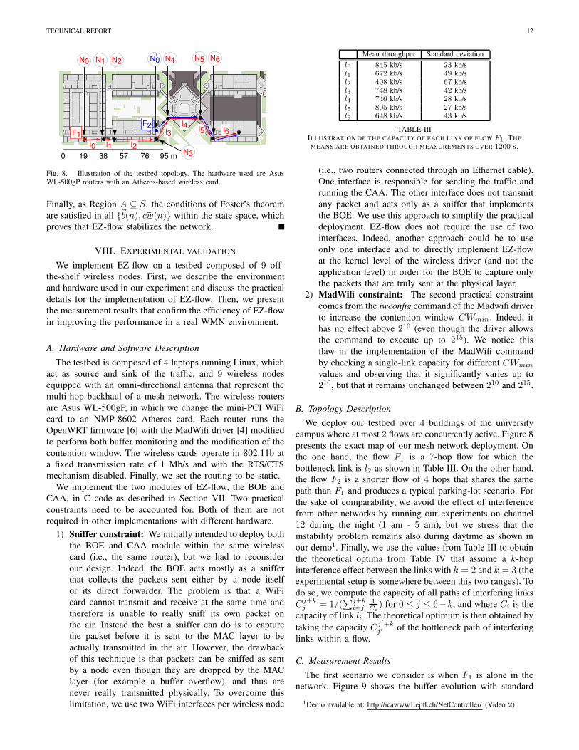
Fig. 8. Illustration of the testbed topology. The hardware used are AsusWL-500gP routers with an Atheros-based wireless card.

Finally, as Region A ⊆ S, the conditions of Foster’s theoremare satisfied in all {~b(n), ~cw(n)} within the state space, whichproves that EZ-flow stabilizes the network.

VIII. EXPERIMENTAL VALIDATION

We implement EZ-flow on a testbed composed of 9 off-the-shelf wireless nodes. First, we describe the environmentand hardware used in our experiment and discuss the practicaldetails for the implementation of EZ-flow. Then, we presentthe measurement results that confirm the efficiency of EZ-flowin improving the performance in a real WMN environment.

A. Hardware and Software Description

The testbed is composed of 4 laptops running Linux, whichact as source and sink of the traffic, and 9 wireless nodesequipped with an omni-directional antenna that represent themulti-hop backhaul of a mesh network. The wireless routersare Asus WL-500gP, in which we change the mini-PCI WiFicard to an NMP-8602 Atheros card. Each router runs theOpenWRT firmware [6] with the MadWifi driver [4] modifiedto perform both buffer monitoring and the modification of thecontention window. The wireless cards operate in 802.11b ata fixed transmission rate of 1 Mb/s and with the RTS/CTSmechanism disabled. Finally, we set the routing to be static.

We implement the two modules of EZ-flow, the BOE andCAA, in C code as described in Section VII. Two practicalconstraints need to be accounted for. Both of them are notrequired in other implementations with different hardware.

1) Sniffer constraint: We initially intended to deploy boththe BOE and CAA module within the same wirelesscard (i.e., the same router), but we had to reconsiderour design. Indeed, the BOE acts mostly as a snifferthat collects the packets sent either by a node itselfor its direct forwarder. The problem is that a WiFicard cannot transmit and receive at the same time andtherefore is unable to really sniff its own packet onthe air. Instead the best a sniffer can do is to capturethe packet before it is sent to the MAC layer to beactually transmitted in the air. However, the drawbackof this technique is that packets can be sniffed as sentby a node even though they are dropped by the MAClayer (for example a buffer overflow), and thus arenever really transmitted physically. To overcome thislimitation, we use two WiFi interfaces per wireless node

Mean throughput Standard deviationl0 845 kb/s 23 kb/sl1 672 kb/s 49 kb/sl2 408 kb/s 67 kb/sl3 748 kb/s 42 kb/sl4 746 kb/s 28 kb/sl5 805 kb/s 27 kb/sl6 648 kb/s 43 kb/s

TABLE IIIILLUSTRATION OF THE CAPACITY OF EACH LINK OF FLOW F1 . THE

MEANS ARE OBTAINED THROUGH MEASUREMENTS OVER 1200 S.

(i.e., two routers connected through an Ethernet cable).One interface is responsible for sending the traffic andrunning the CAA. The other interface does not transmitany packet and acts only as a sniffer that implementsthe BOE. We use this approach to simplify the practicaldeployment. EZ-flow does not require the use of twointerfaces. Indeed, another approach could be to useonly one interface and to directly implement EZ-flowat the kernel level of the wireless driver (and not theapplication level) in order for the BOE to capture onlythe packets that are truly sent at the physical layer.

2) MadWifi constraint: The second practical constraintcomes from the iwconfig command of the Madwifi driverto increase the contention window CWmin. Indeed, ithas no effect above 210 (even though the driver allowsthe command to execute up to 215). We notice thisflaw in the implementation of the MadWifi commandby checking a single-link capacity for different CWminvalues and observing that it significantly varies up to210, but that it remains unchanged between 210 and 215.

B. Topology DescriptionWe deploy our testbed over 4 buildings of the university

campus where at most 2 flows are concurrently active. Figure 8presents the exact map of our mesh network deployment. Onthe one hand, the flow F1 is a 7-hop flow for which thebottleneck link is l2 as shown in Table III. On the other hand,the flow F2 is a shorter flow of 4 hops that shares the samepath than F1 and produces a typical parking-lot scenario. Forthe sake of comparability, we avoid the effect of interferencefrom other networks by running our experiments on channel12 during the night (1 am - 5 am), but we stress that theinstability problem remains also during daytime as shown inour demo1. Finally, we use the values from Table III to obtainthe theoretical optima from Table IV that assume a k-hopinterference effect between the links with k = 2 and k = 3 (theexperimental setup is somewhere between this two ranges). Todo so, we compute the capacity of all paths of interfering linksCj+k

j = 1/(∑j+k

i=j1Ci

) for 0 ≤ j ≤ 6−k, and where Ci is thecapacity of link li. The theoretical optimum is then obtained bytaking the capacity Cj′+k

j′ of the bottleneck path of interferinglinks within a flow.

C. Measurement Results

The first scenario we consider is when F1 is alone in thenetwork. Figure 9 shows the buffer evolution with standard

1Demo available at: http://icawww1.epfl.ch/NetController/ (Video 2)

TECHNICAL REPORT 13

0 500 1000 1500 20000

10

20

30

40

50

Time [s]

Que

ue s

ize

[pac

kets

]Buffer occupancy of F

1 without EZ−flow

N2

N1

N3

0 500 1000 1500 20000

10

20

30

40

50

Time [s]

Que

ue s

ize

[pac

kets

]

Buffer occupancy of F1 with EZ−flow

N1

N2

N3

0 500 1000 1500 20000

10

20

30

40

50

Time [s]

Que

ue s

ize

[pac

kets

]

Buffer occupancy of F2 without EZ−flow

N4

N5

N6

0 500 1000 1500 20000

10

20

30

40

50

Time [s]

Que

ue s

ize

[pac

kets

]

Buffer occupancy of F2 with EZ−flow

N4

N5

N6

Fig. 9. Experimental results for the queue evolution of the relay nodes whenflow F1 or F2 are active. The average number of buffered packets are: (i)without EZ-flow 41.6 (N1), 43.1 (N2) and 43.7 (N4) and (ii) with EZ-flow29.5 (N1), 5.2 (N2) and 5.3 (N4). The remaining queues are very small.

IEEE 802.11 and with EZ-flow turned on. We note that forIEEE 802.11 both nodes N1 and N2 saturate and overflow,due to the bottleneck link l2 (between N2 and N3), whereas allthe other nodes have their buffer occupancy negligibly small,similarly to N3. This results in an end-to-end throughput of119 kb/s as shown in Table IV (note that a similar throughputdegradation for the backlogged case has been observed throughsimulation in [29]). In contrast, EZ-flows detects and reacts tothe bottleneck at link l2 by increasing cw1 up to 28. Thisaction stabilizes the buffer of N2 by reducing the channelaccess of link l1. Similarly, EZ-flow detects that the bufferof N1 builds up and makes N0 increase cw0 until it reachesour hardware limit of 210 (see Section 4.1). This hardwarelimitation prevents EZ-flow from reducing the buffer occu-pancy of N1 to a value as low as N2. However, we stressthat despite this hardware limitation, EZ-flow still significantlyimproves the performance by reducing the turbulence of theflow and increasing the throughput to 148 kb/s (close to the 3-hop interference range theoretical optimum and mapping to a41% reduction in the gap to the 2-hop optimum). Furthermore,

Mean throughput Theoretical optima Jain’s Fairnessk = 3 k = 2

F1 119 kb/s 151 kb/s 190 kb/sF2 157 kb/s 183 kb/s 242 kb/sF1 7 kb/s 0.55F2 143 kb/s

FEZ1 148 kb/s 151 kb/s 190 kb/s

FEZ2 185 kb/s 183 kb/s 242 kb/s

FEZ1 71 kb/s 0.96

FEZ2 110 kb/s

TABLE IVMEASUREMENTS OVER 1800 S WITH AND WITHOUT EZ-FLOW.

THEORETICAL OPTIMA ARE OBTAINED ASSUMING A 3-HOP (2-HOP)INTERFERENCE RANGE. THE SUB-DIVISION IN THE TABLE SHOWS THE

RESULTS FOR: (I) ONE SINGLE FLOW, OR (II) TWO SIMULTANEOUS FLOWS.

we show through simulation in [10] that EZ-flow completelystabilizes the network once this limitation is removed.

In the second scenario, we consider F2 alone. Similarlyto our mathematical analysis of Section V, we note that forIEEE 802.11 the buffer of the first relay node of F2 (i.e., N4)builds up and overflows, resulting in a throughput of 157 kb/s.However, EZ-flow completely stabilizes the network for all therelay nodes (no queue builds up) by making the source nodeN

′

0 increase cw′

0 up to 28. Thus EZ-flow works even better inthis scenario where it is not blocked by the hardware limitationand it achieves a throughput of 185 kb/s.

Finally the last scenario is a parking-lot scenario where bothF1 and F2 are simultaneously active. Similarly to what is alsoreported in [39] between a 1- and 2-hop flow, Table IV showsthat IEEE 802.11 performs very poorly: the long flow F1 iscompletely starved in favor of the short flow F2, because N

′

0is too aggressive (even for its own flow) and thus preventsthe packets from the longer flow F1 from being relayed bythe intermediate nodes N1, N2, N3. However, by its nature,EZ-flow solves the problem by making the two source nodes,N

′

0 and N0, become less aggressive in order to stabilize theirown flow. This approach thus solves the starvation problemand significantly increases both the aggregate throughput ofF1 and F2 and the Jain’s fairness index.

D. Effect of bi-directional traffic

EZ-flow is designed to stabilize the queues within a flowindependently of the interferences caused by other flows. Inthe previous sub-section, we investigated the effect of havingmultiple flows by looking at a setting where two separate flowsshare part of their path to reach the same destination (e.g., thegateway).

We now focus on a different scenario, where two flowsgo through exactly opposite paths (i.e., the destination of aflow is the source of the other flow). Toward this goal weuse the experimental setting depicted in Figure 11, where thetwo 4-hop flows are F1→5 (from node 1 to node 5) and F5→1(from node 5 to node 1). The measurements show a seriousthroughput asymmetry in this setting. Indeed, we set the datarate of all nodes to 2 Mb/s and when first launching each flowby itself, we obtain a throughput of: (i) 411 kb/s for flow F1→5(379 kb/s with RTS); and (ii) 206 kb/s for flow F5→1 (172 kb/swith RTS). We then launch both flows simultaneously for 600 sand our results are summarized in Figure 10 and Table V.

w/o, RTS, w/o EZ w/o RTS, EZ RTS, w/o EZ RTS, EZb2 93 37 37 2b3 40 2 2 1b4 0 0 0 0

F1→5 102 kb/s 140 kb/s 53 kb/s 62 kb/sb4′ 1 1 1 1b3′ 0 0 0 0b2′ 0 0 0 0

F5→1 26 kb/s 68 kb/s 34 kb/s 44 kb/s

TABLE VMEASUREMENTS OF THE EFFECT OF EZ-FLOW ON: (I) THE MEDIAN

QUEUE OCCUPANCY AT THE RELAY NODES AND (II) THE END-TO-ENDTHROUGHPUT OF THE 4-HOP FLOWS F1→5 AND F5→1 .

TECHNICAL REPORT 14

0 100 200 300 400 500 6000

20

40

60

80

100

Time [s]

Que

ue [p

acke

ts]

Queue b3 without EZ−flow

0 100 200 300 400 500 6000

20

40

60

80

100

Time [s]

Que

ue [p

acke

ts]

Queue b3 with EZ−flow

Fig. 10. Effect of EZ-flow on the queue evolution through time of b3.

Table V shows for each flow: (i) the median queue occu-pancy from measurements taken each second (we set the buffersize limit to 100 packets); and (ii) the average end-to-endthroughput. The results indicate that, either with or withoutRTS, the use of EZ-flow reduces the queue size and increasesthe end-to-end throughput for both flows. Moreover the resultsshow that, in our setting, the performances are better withoutthe use of RTS, and this also corresponds to the case whereEZ-flow provides the largest performance gain. We show inFigure 10 the evolution through time of the queue b3 with andwithout EZ-flow. Finally, we stress that the Madwifi constraintis the reason that the queue b2 does not reach a lower valuewith EZ-flow (i.e., the contention window of node 1 is set tothe maximal working value of 210.

E. Instability problem at higher rates

The analytical model of Section III allows to explain whya stable 3-hop network becomes unstable when a 4th hop isadded (see Figure 1). Nevertheless, the results from Figure 1are obtained with a fixed data rate of 1 Mb/s, a buffer sizelimit of 50 packets, and a small-scale testbed where the routersare used without their external antennas (better control on theexperimental environment). In order to validate our results ona different setting, we modify the MadWifi driver to unlockthe buffer size limit and to allow the modification of its valueat run time through a simple command. We then set the bufferlimit to 100 packets and repeat the experiment from Figure 1on the real-scale deployment of Figure 11, with different datarate settings.

Figure 12 and 13 show the queue evolution of a 3-hopnetwork (node 1 to 4 in Figure 11) and a 4-hop network (node1 to 5 in Figure 11) at data rates of: 1 Mb/s, 2 Mb/s, 11Mb/s and auto-rate. Additionally, Table VI presents the link

66 m

1 2

3

4

5

l2

l1

l4

l3

Fig. 11. Illustration of the deployment used in Sections 8.D and 8.E.

0 50 100 150 200 250 3000

20

40

60

80

1003−hop at 1Mb/s

Time [s]

Que

ue s

ize

[pac

kets

]

Node 1Node 2

0 50 100 150 200 250 3000

20

40

60

80

1004−hop at 1Mb/s

Time [s]

Que

ue s

ize

[pac

kets

]

Node 1Node 2Node 3

0 50 100 150 200 250 3000

20

40

60

80

1003−hop at 2Mb/s

Time [s]

Que

ue s

ize

[pac

kets

]

Node 1Node 2

0 50 100 150 200 250 3000

20

40

60

80

1004−hop at 2Mb/s

Time [s]

Que

ue s

ize

[pac

kets

]

Node 1Node 2Node 3

Fig. 12. Validation of the experimental results from Figure 1 on a differentsetup running at various data rate.

0 50 100 150 200 250 3000

20

40

60

80

1003−hop at 11Mb/s

Time [s]

Que

ue s

ize

[pac

kets

]

Node 1Node 2

0 50 100 150 200 250 3000

20

40

60

80

1004−hop at 11Mb/s

Time [s]

Que

ue s

ize

[pac

kets

]

Node 1Node 2Node 3

0 50 100 150 200 250 3000

20

40

60

80

1003−hop with auto−rate

Time [s]

Que

ue s

ize

[pac

kets

]

Node 1Node 2

0 50 100 150 200 250 3000

20

40

60

80

1004−hop with auto−rate

Time [s]

Que

ue s

ize

[pac

kets

]

Node 1Node 2Node 3

Fig. 13. Validation of the experimental results from Figure 1 on a differentsetup running at various data rate.

throughputs and the end-to-end throughputs achieved at thedifferent data rates.

Our results show that even though l3 is the bottleneck linkfor all the data rates, it does not result in network instability,due to the stealing effect described in Section III.C. Moreover,the simple addition of a 4th hop turns the network fromstable to unstable (i.e., the queue remains close to the bufferlimit). We note that the queue size variations are larger than inFigure 1 (especially at higher rates). It is because the real-scaledeployment is a less controlled environment that is more proneto changing channel conditions, and also increasing the datarate results in a reduction of the stealing effect probabilityp > 0. Despite the variations, we stress that the changein stability between a 3- and 4-hop network is seen for allthe different data rates that we tested, as predicted by ouranalytical model.

throughput\rate 1 Mb 2 Mb 11 Mb auto-ratel1 894 kb/s 1.67 Mb/s 6.71 Mb/s 5.79 Mb/sl2 858 kb/s 1.52 Mkb/s 5.82 Mb/s 2.03 Mb/sl3 754 kb/s 1.28 Mb/s 4.23 Mb/s 1.95 Mb/sl4 813 kb/s 1.6 Mkb/s 5.98 Mb/s 5.49 Mb/s

3-hop 241 kb/s 493 kb/s 1.05 Mb/s 373 kb/s4-hop 194 kb/s 354 kb/s 791 kb/s 260 kb/s

TABLE VIMEASUREMENTS OF THE LINKS THROUGHPUT AND THE END-TO-ENDTHROUGHPUT OF A 3- AND 4-HOP LINEAR TOPOLOGY FOR DIFFERENT

DATA RATES.

TECHNICAL REPORT 15

F2

F1

N0

N12

N10

N8

N6

N11

N9

N7

N5 N4 N3 N2 N1

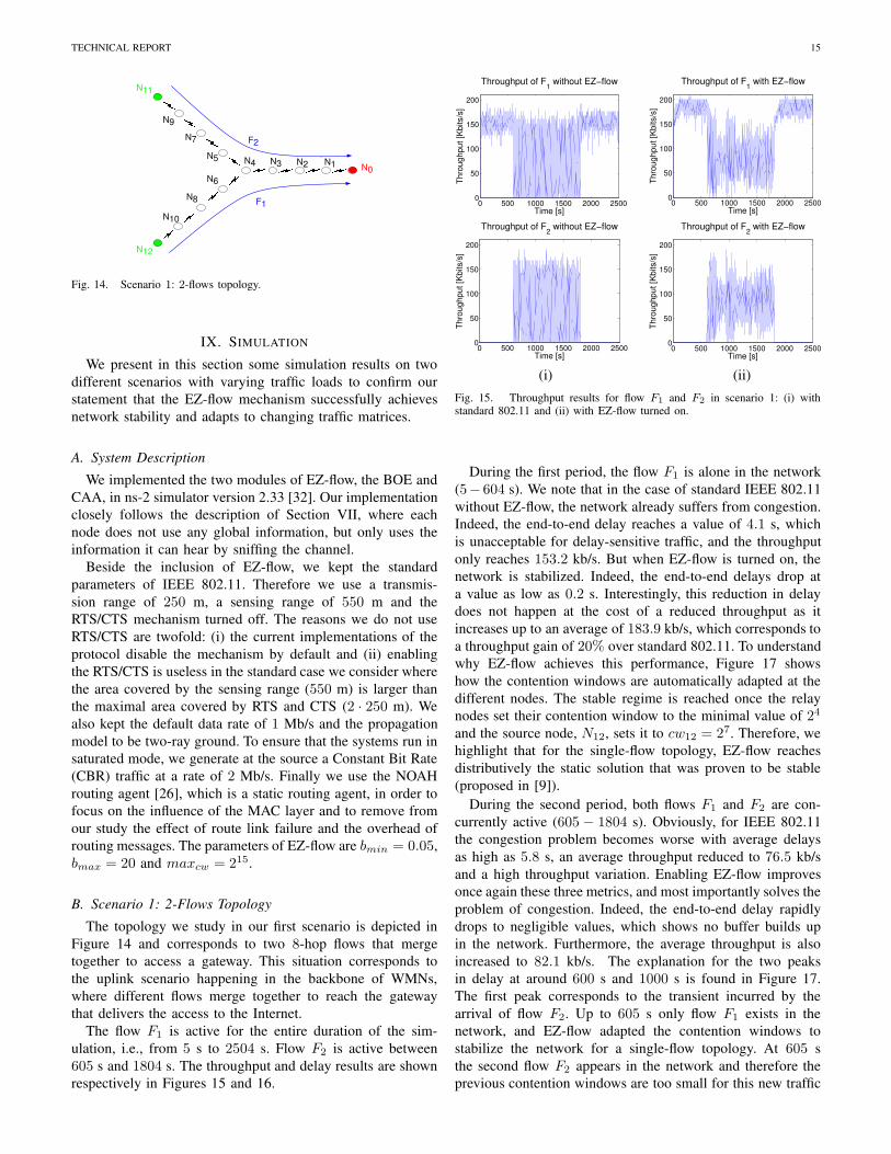
Fig. 14. Scenario 1: 2-flows topology.

IX. SIMULATION

We present in this section some simulation results on twodifferent scenarios with varying traffic loads to confirm ourstatement that the EZ-flow mechanism successfully achievesnetwork stability and adapts to changing traffic matrices.

A. System Description

We implemented the two modules of EZ-flow, the BOE andCAA, in ns-2 simulator version 2.33 [32]. Our implementationclosely follows the description of Section VII, where eachnode does not use any global information, but only uses theinformation it can hear by sniffing the channel.

Beside the inclusion of EZ-flow, we kept the standardparameters of IEEE 802.11. Therefore we use a transmis-sion range of 250 m, a sensing range of 550 m and theRTS/CTS mechanism turned off. The reasons we do not useRTS/CTS are twofold: (i) the current implementations of theprotocol disable the mechanism by default and (ii) enablingthe RTS/CTS is useless in the standard case we consider wherethe area covered by the sensing range (550 m) is larger thanthe maximal area covered by RTS and CTS (2 · 250 m). Wealso kept the default data rate of 1 Mb/s and the propagationmodel to be two-ray ground. To ensure that the systems run insaturated mode, we generate at the source a Constant Bit Rate(CBR) traffic at a rate of 2 Mb/s. Finally we use the NOAHrouting agent [26], which is a static routing agent, in order tofocus on the influence of the MAC layer and to remove fromour study the effect of route link failure and the overhead ofrouting messages. The parameters of EZ-flow are bmin = 0.05,bmax = 20 and maxcw = 215.

B. Scenario 1: 2-Flows Topology

The topology we study in our first scenario is depicted inFigure 14 and corresponds to two 8-hop flows that mergetogether to access a gateway. This situation corresponds tothe uplink scenario happening in the backbone of WMNs,where different flows merge together to reach the gatewaythat delivers the access to the Internet.

The flow F1 is active for the entire duration of the sim-ulation, i.e., from 5 s to 2504 s. Flow F2 is active between605 s and 1804 s. The throughput and delay results are shownrespectively in Figures 15 and 16.

0 500 1000 1500 2000 25000

50

100

150

200

Time [s]

Thr

ough

put [

Kbi

ts/s

]

Throughput of F1 without EZ−flow

0 500 1000 1500 2000 25000

50

100

150

200

Time [s]

Thr

ough

put [

Kbi

ts/s

]

Throughput of F1 with EZ−flow

0 500 1000 1500 2000 25000

50

100

150

200

Time [s]

Thr

ough

put [

Kbi

ts/s

]

Throughput of F2 without EZ−flow

0 500 1000 1500 2000 25000

50

100

150

200

Time [s]

Thr

ough

put [

Kbi

ts/s

]

Throughput of F2 with EZ−flow

(i) (ii)

Fig. 15. Throughput results for flow F1 and F2 in scenario 1: (i) withstandard 802.11 and (ii) with EZ-flow turned on.

During the first period, the flow F1 is alone in the network(5− 604 s). We note that in the case of standard IEEE 802.11without EZ-flow, the network already suffers from congestion.Indeed, the end-to-end delay reaches a value of 4.1 s, whichis unacceptable for delay-sensitive traffic, and the throughputonly reaches 153.2 kb/s. But when EZ-flow is turned on, thenetwork is stabilized. Indeed, the end-to-end delays drop ata value as low as 0.2 s. Interestingly, this reduction in delaydoes not happen at the cost of a reduced throughput as itincreases up to an average of 183.9 kb/s, which corresponds toa throughput gain of 20% over standard 802.11. To understandwhy EZ-flow achieves this performance, Figure 17 showshow the contention windows are automatically adapted at thedifferent nodes. The stable regime is reached once the relaynodes set their contention window to the minimal value of 24

and the source node, N12, sets it to cw12 = 27. Therefore, wehighlight that for the single-flow topology, EZ-flow reachesdistributively the static solution that was proven to be stable(proposed in [9]).

During the second period, both flows F1 and F2 are con-currently active (605 − 1804 s). Obviously, for IEEE 802.11the congestion problem becomes worse with average delaysas high as 5.8 s, an average throughput reduced to 76.5 kb/sand a high throughput variation. Enabling EZ-flow improvesonce again these three metrics, and most importantly solves theproblem of congestion. Indeed, the end-to-end delay rapidlydrops to negligible values, which shows no buffer builds upin the network. Furthermore, the average throughput is alsoincreased to 82.1 kb/s. The explanation for the two peaksin delay at around 600 s and 1000 s is found in Figure 17.The first peak corresponds to the transient incurred by thearrival of flow F2. Up to 605 s only flow F1 exists in thenetwork, and EZ-flow adapted the contention windows tostabilize the network for a single-flow topology. At 605 sthe second flow F2 appears in the network and therefore theprevious contention windows are too small for this new traffic

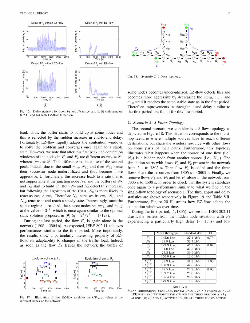
TECHNICAL REPORT 16

0 500 1000 1500 2000 25000

5

10

15

Time [s]

End

−to−

end

dela

y [s

]Delay of F

1 without EZ−flow

0 500 1000 1500 2000 25000

5

10

15

Time [s]

End

−to−

end

dela

y [s

]

Delay of F1 with EZ−flow

0 500 1000 1500 2000 25000

5

10

15

Time [s]

End

−to−

end

dela

y [s

]

Delay of F2 without EZ−flow

0 500 1000 1500 2000 25000

5

10

15

Time [s]

End

−to−

end

dela

y [s

]

Delay of F2 with EZ−flow

(i) (ii)

Fig. 16. Delay statistics for flows F1 and F2 in scenario 1: (i) with standard802.11 and (ii) with EZ-flow turned on.

load. Thus, the buffer starts to build up at some nodes andthis is reflected by the sudden increase in end-to-end delay.Fortunately, EZ-flow rapidly adapts the contention windowsto solve the problem and converges once again to a stablestate. However, we note that after this first peak, the contentionwindows of the nodes in F1 and F2 are different as cw8 = 24,whereas cw7 = 25. This difference is the cause of the secondpeak. Indeed, due to the small cw8, N10 and then N12 sensetheir successor node underutilized and thus become moreaggressive. Unfortunately, this increase leads to a rate that isnot supportable at the junction node N4, and the buffers of N5and N6 start to build up. Both N7 and N8 detect this increase,but following the algorithm of the CAA, N8 is more likely toreact as cw8 < cw7. Therefore N8 increases its cw8, N10 andN12 react to it and reach a steady state. Interestingly, once thestable regime is reached, the source nodes set cw11 and cw12at the value of 211, which is once again similar to the optimalstatic solution proposed in [9] (q = 24/211 = 1/128).

During the last period, the flow F1 is again alone in thenetwork (1805− 2504 s). As expected, IEEE 802.11 achievesperformances similar to the first period. More importantly,the results show a particularly interesting property of EZ-flow: its adaptability to changes in the traffic load. Indeed,as soon as the flow F1 leaves the network the buffer of

0 500 1000 1500 2000 25000

2

4

6

8

10

12

Time [s]

log(

cw)

Evolution of cw at F1

cw10

cw12

cw8

cw6, cw

4−cw

2

0 500 1000 1500 2000 25000

2

4

6

8

10

12

Time [s]

log(

cw)

Evolution of cw at F2

cw4,cw

3,cw

2

cw9

cw11

cw7,cw

5

Fig. 17. Illustration of how EZ-flow modifies the CWmin values at thedifferent nodes of the network.

F2

F3

N9N0 N7N5

N10

N8N6N4N3N2N1

F1

N11 N12 N13N14

N15

N16

N17 N20

N21

N22

N23N24 N25 N26

N19N18

N27

Fig. 18. Scenario 2: 3-flows topology.

some nodes becomes under-utilized. EZ-flow detects this andbecomes more aggressive by decreasing the cw12, cw10 andcw8 until it reaches the same stable state as in the first period.Therefore improvements in throughput and delay similar tothe first period are found for this last period.

C. Scenario 2: 3-Flows Topology

The second scenario we consider is a 3-flow topology asdepicted in Figure 18. This situation corresponds to the multi-hop scenario where multiple sources have to reach differentdestinations, but share the wireless resource with other flowson some parts of their paths. Furthermore, this topologyillustrates what happens when the source of one flow (i.e.,N0) is a hidden node from another source (i.e., N10). Thesimulation starts with flows F1 and F2 present in the networkfrom 5 s to 1805 s. Then flow F3 is added and the threeflows share the resources from 1805 s to 3605 s. Finally, weremove flows F2 and F3 and let F1 alone in the network from3605 s to 4500 s, in order to check that the system stabilizesonce again to a performance similar to what we find in thesingle-flow topology of scenario 1. The throughput and delaystatistics are shown respectively in Figure 19 and Table VII.Furthermore, Figure 20 illustrates how EZ-flow adapts thecontention windows over time.

During the first period, [5, 1805), we see that IEEE 802.11drastically suffers from the hidden node situation, with F2experiencing a particularly high delay (∼ 15 s) and low

Mean throughput Standard dev. FIF1 145.6 kb/s 27.4 kb/s 0.75F2 39.9 kb/s 36.7 kb/sF1 129.9 kb/s 45.3 kb/s 0.64F2 31.0 kb/s 32.5 kb/sF3 27.3 kb/s 39.9 kb/sF1 150.0 kb/s 13.0 kb/s

FEZ1 89.9 kb/s 41.3 kb/s 1.00

FEZ2 100.3 kb/s 42.6 kb/s

FEZ1 29.5 kb/s 22.9 kb/s 0.80

FEZ2 139.7 kb/s 23.0 kb/s

FEZ3 135.4 kb/s 26.9 kb/s

FEZ1 179.9 kb/s 13.5 kb/s

TABLE VIIMEAN THROUGHPUT, STANDARD DEVIATION AND JAIN’S FAIRNESS INDEX

(FI) WITH AND WITHOUT EZ-FLOW FOR THE THREE PERIODS: (I) F1ALONE, (II) F1 AND F2 ACTIVE AND (III) ALL THREE FLOWS ACTIVE.

TECHNICAL REPORT 17

0 1000 2000 3000 40000

5

10

15

Time [s]

End

−to−

end

dela

y [s

]Delay F

1 without EZ−flow

0 1000 2000 3000 40000

5

10

15

Time [s]

End

−to−

end

dela

y [s

]

Delay F1 with EZ−flow

0 1000 2000 3000 40000

5

10

15

20

25

30

Delay F2 without EZ−flow

Time [s]

End

−to−

end

dela

y [s

]

0 1000 2000 3000 40000

5

10

15

20

25

30

Time [s]

End

−to−

end

dela

y [s

]

Delay F2 with EZ−flow

0 1000 2000 3000 40000

5

10

15

20

25

30

Time [s]

End

−to−

end

dela

y [s

]

Delay F3 without EZ−flow

0 1000 2000 3000 40000

5

10

15

20

25

30

Time [s]

End

−to−

end

dela

y [s

]

Delay F3 with EZ−flow

(i) (ii)

Fig. 19. Delay statistics for flow F1, F2 and F3 in scenario 2: (i) withstandard 802.11 and (ii) with EZ-flow turned on.

throughput. The fairness index is of 0.75. On the contrary,when EZ-flow is turned on, the contention window of thesource of F2 cw10 is increased up to a value of 210 to providea smooth flow. We note that this increase delivers negligibledelays to both flows and does not penalize F2 as it has athroughput that is even slightly higher than F1. The reason F2achieves a higher throughput while having a larger contentionwindow (cw10 = 210 and cw0 = 25) is that N10 onlydirectly competes with two nodes (N11 and N12), whereasN0 competes with seven other nodes.

During the second period, [1805, 3605), we see that IEEE802.11 starves flow F2 and F3 in favor of F1 and that allflows suffer from high delays. The reason that F1 showsbetter performances than F3 is that N0 has many neighborsand it naturally reduces the source access rate and thus thebuffer building-up problem. IEEE 802.11 achieves a cumula-

0 1000 2000 3000 40000

2

4

6

8

10

12

Evolution of cw

Time [s]

log(

cw) cw

0

cw1

cw10

cw11

0 1000 2000 3000 40000

2

4

6

8

10

12

Evolution of cw

Time [s]

log(

cw)

cw20

cw0

cw1

cw19

Fig. 20. Illustration of how EZ-flow modifies the CWmin values at the twofirst node of each flow.

tive throughput of 188.2 kb/s and a fairness index of 0.64.In contrast, EZ-flow increases the cumulative throughput to304.6 kb/s (a 62% throughput gain over 802.11), increasesthe fairness index to 0.8, and drastically reduces the end-to-end delay by an order of magnitude at least. We note thatF1 has its throughput reduced even though the source of F1,N0, has cw0 that is lower than cw10 and cw19 (cw0 = 27

and cw10 = cw19 = 29). This reduction is due to the highercompetition that F1 experiences and it allows both F2 and F3to have higher throughputs and all the flows to have negligibledelays and thus, a stable network.

Finally, during the last period we see that once again EZ-flow successfully detects the variation in traffic load and adaptsthe contention windows to achieve results similar to those inthe single-flow case of scenario 1.

X. CONCLUSION

We addressed the problem of network stability in CSMA-based linear wireless mesh network and provide three maincontributions. First, we identified two key factors impact-ing the stability: the network size and an artifact that wecalled stealing effect. Second, we proved analytically andshowed experimentally that 3-hop networks are stable whenwe account for the stealing effect, but 4-hop networks (andpresumably larger topologies) are not. Third, we proposedand designed EZ-flow, a new flow control mechanism forIEEE 802.11 WMNs. EZ-flow is fully backward compatiblewith the IEEE 802.11 standard and works without any formof message passing. EZ-flow is implemented in a distributedfashion as a simple program running at each relay node. Ittakes advantage of the broadcast nature of the wireless mediumto passively estimate the buffer occupancy at a successor node.The minimum congestion window parameter is adapted at eachrelay node based on this estimation to ensure a smooth flow,specifically, each relay node adapts its contention window toavoid buffer build-up at its successor node.

We have demonstrated by experiments the attendant benefitsof EZ-flow on a testbed composed of 9 standard wireless meshrouters deployed over 4 different buildings. Our measurementresults show that EZ-flow simultaneously improves throughputand fairness performance. To our knowledge, it is the firstimplementation of an algorithm addressing instability in a realmulti-hop network. Moreover, we have derived a Lyapunovfunction with which we analytically prove the stability of an802.11-based linear K-hop topology implementing EZ-flow.

We conclude by noting that the methodology followedby EZ-flow is not limited to line topologies. One possibleapproach to dealing with more general topologies is to takeadvantage of IEEE 802.11e, which uses four different MAC-layer queues. This protocol was originally designed to supportQuality of Service (QoS) by categorizing the traffic into fourtypes of service: (i) Background (BK), (ii) Best Effort (BE),(iii) Voice (VO) and (iv) Video (VI). Yet to date, this servicedifferentiation is not commonly used and almost all traffic isclassified as BE and queued accordingly. Thus, the three otherqueues are mostly left idle. A node forwarding traffic to upto four successors could take advantage of the availability of

TECHNICAL REPORT 18

these MAC-layer queues in order to use one different queue(thus one different CWmin value) per successor. This approachsuits well the backhaul scenario this paper focuses on, as itusually follows a tree-based topology with a limited numberof neighbors. In cases where EZ-flow needs to be deployed innetworks with a higher neighbor density, a similar mechanismcould be used with a slight modification. Here, multiple queuescould be implemented at the routing layer (e.g. by usingClick [28]). The BOE would remain unchanged; and the CAAwould control the scheduling rate at which packets belongingto different routing queues are delivered to the MAC layer,instead of directly modifying the MAC contention window.

APPENDIX

Theorem 4 (Foster [17], p. 30): Let the transition proba-bility matrix P on the state space Z2 be irreducible and sup-pose that there exists a positive function h : Z2 → R such thatfor some finite set S, some ε > 0 and some positive integer-valued function k : Z2 → R where sup~b∈Z2 k(~b(n)) <∞ thefollowing conditions hold

E[

h(~b(n+ 1)) | ~b(n) =~i]

=∑

~k∈Z2

p~i~kh(~k) <∞ (15)

for all ~i ∈ S and

E[

h(~b(n+ k(~b(n)))|~b(n) =~i]

≤ h(~i)− εk(~b(n)) (16)

for all ~i /∈ S. Then the corresponding HMC is ergodic.

Theorem 5 (Transience [17], p. 31): For an irreducibleHomogeneous Markov Chain (HMC) to be transient, it sufficesthat there exist a positive function h(~i),~i ∈ Z3, a boundedinteger-valued positive function k(~i),~i ∈ Z3, and numbersε, c, d > 0, such that, setting Sc = {~i : h(~i) > c} 6= 0, thefollowing conditions hold:

1) sup~i∈Z3 k(~i) = k <∞;2) E[h(~bn+k(~i))|h(~bn) = h(~i)] − h(~i) ≥ ε, ∀n, for all ~i ∈

Sc;3) for some d > 0, the inequality |h(~i)−h(~j)| > d implies

p~i~j = 0.

Theorem 6 (Non-ergodicity [17], p. 30): For an irreducibleHomogeneous Markov Chain (HMC) to be non-ergodic, it issufficient that there exist a function h(~i),~i ∈ Z2, a constantd and c, such that the sets {~i | h(~i) > c} and {~i | h(~i) ≤ c}are non-empty, and the following conditions hold for everyn ∈ N:

E[

h(~b(n+ 1)) | h(~b(n)) = h(~i)]

− h(~i) ≥ 0

for all ~i ∈ {~i : h(~i) > c} and∣

∣

∣E[

h(~b(n+ 1)) | h(~b(n)) = h(~i)]

− h(~i)∣

∣

∣≤ d

for all ~i ∈ Z2.

ACKNOWLEDGMENT

This work is supported in part by Deutsche Telekom Labo-ratories, in the framework of the Magnets project, and by theUS National Science Foundation under grants CCF-0729158and CCF-0916892.

We are grateful to Julien Herzen for his help in implement-ing the first version of EZ-flow on the Asus routers and to SevaShneer for his valuable feedbacks on the analytical model.

REFERENCES

[1] The Cloud. http://www.thecloud.net/.[2] EarthLink. http://www.earthlink.net/.[3] LUNAR- Lightweight Underlay Network Ad hoc Routing project.

http://cn.cs.unibas.ch/projects/lunar/.[4] Madwifi/AtherosWireless Linux Driver Users Guide.[5] MIT Roofnet. http://pdos.csail.mit.edu/roofnet/.[6] OpenWRT firmware. http://openwrt.org/.[7] The Tcpdump Manual Page. http://www.tcpdump.org/.[8] IEEE 802.11, Part 11: Wireless LAN Medium Access Control (MAC)

and Physical Layer (PHY) Specifications, Aug. 1999.[9] A. Aziz, D. Starobinski, and P. Thiran. Elucidating the instability of

random access wireless mesh networks. In Proc. of SECON, Rome,Italy, June 2009.

[10] A. Aziz, D. Starobinski, P. Thiran, and A. El Fawal. Ez-flow: Removingturbulence in ieee 802.11 wireless mesh networks without messagepassing. In Proc. of CoNEXT, Rome, Italy, Dec. 2009.

[11] S. Biswas and R. Morris. Exor: opportunistic multi-hop routing forwireless networks. In Proc. of SIGCOMM, Philadelphia, PA, Aug. 2005.

[12] S. Borst, M. Jonckheere, and L. Leskela. Stability of parallel queueingsystems with coupled service rates. Discrete Event Dynamic Systems,18(4):447–472, 2008.

[13] P. Chapokar, H. Kar, X. Luo, and S. Sarkar. Throughput and fairnessguarantees through maximal scheduling in wireless networks. IEEETransactions on Information Theory, 54(2):572–594, Feb. 2008.

[14] O. Dousse. Revising buffering in CSMA/CA wireless multihop net-works. In Proc. of SECON, San Diego, CA, June 2007.

[15] M. Durvy and P. Thiran. A packing approach to compare slottedand non-slotted medium access control. In Proc. of INFOCOM’06,Barcelona, Spain, Apr. 2006.

[16] A. Eryilmaz and R. Srikant. Fair resource allocation in wireless networksusing queue-length-based scheduling and congestion control. In Proc.of INFOCOM, Miami, FL, Mar. 2005.

[17] G. Fayolle, V. A. Malyshev, and M. V. Menshikov. Topics in constructivetheory of countable Markov chains. Cambridge University Press, 1995.

[18] V. Gambiroza, B. Sadeghi, and E. Knightly. End-to-end performanceand fairness in multihop wireless backhaul networks. In Proceedings ofACM MobiCom, Philadelphia, PA, Sept. 2004.

[19] Y. Gao, D.-M. Chiu, and J. C. Lui. Determining the end-to-end through-put capacity in multi-hop networks: methodology and applications. InProc. of SIGMETRICS, 2006.

[20] M. Garetto, T. Salonidis, and E. W. Knightly. Modeling per-flowthroughput and capturing starvation in csma multi-hop wireless net-works. IEEE/ACM Transactions on Networking, 16(4):864–877, 2008.

[21] A. Gupta, X. Lin, and R. Srikant. Low-complexity distributed schedulingalgorithms for wireless networks. In Proc. of Infocom, Anchorage, 2007.

[22] M. Heusse, F. Rousseau, R. Guillier, and A. Duda. Idle sense: Anoptimal access method for high throughput and fairness in rate diversewireless lans. In Proc. of SIGCOMM, Philadelphia, PA, Aug. 2005.

[23] L. Jiang and J. Walrand. A distributed csma algorithm for throughputand utility maximization in wireless networks. to appear in IEEE/ACMTransactions on Networking.

[24] W. Jiang. Accurate queue length estimation in wireless networks. InPAM, 2007.

[25] A. Jindal and K. Psounis. The achievable rate region of 802.11-scheduled multihop networks. IEEE/ACM Trans. Netw., 17(4):1118–1131, 2009.

[26] J.Widmer. NO Ad-Hoc Routing Agent (NOAH).http://icapeople.epfl.ch/widmer/uwb/ns-2/noah/.

[27] S. Katti, H. Rahul, H. Wenjun, D.Katabi, M. Medard, and J. Crowcroft.Xors in the air: Practical wireless network coding. IEEE/ACM Trans-actions on Networking, 16(3):497–510, 2008.

TECHNICAL REPORT 19

[28] E. Kohler, R. Morris, B. Chen, J. Jannotti, and M. F. Kaashoek. Theclick modular router. ACM Trans. Comput. Syst., 18(3):263–297, Aug2000.

[29] J. Li, C. Blake, D. S. De Couto, H. I. Lee, and R. Morris. Capacity ofad hoc wireless networks. In Proc. of MobiCom, 2001.

[30] W. Luo and A. Ephremides. Stability of n interacting queues in random-access systems. IEEE Transactions on Information Theory, 45(5):1579–1587, July 1999.

[31] P. Marbach and A. Eryilmaz. A backlog-based csma mechanism toachieve fairness and throughput-optimality in multihop wireless net-works. In Proc. of Allerton, 2008.

[32] S. McCanne and S. Floyd. ns Network Simulator.http://www.isi.edu/nsnam/ns/l.

[33] E. Modiano, D. Shah, and G. Zussman. Maximizing throughput inwireless networks via gossiping. In Proc. of SIGMETRICS, 2006.

[34] N. Nandiraju, D. Nandiraju, D. Cavalcanti, and D. Agrawal. A novelqueue management mechanism for improving performance of multihopflows in ieee 802.11s based mesh networks. IPCCC, 2006.

[35] A. Proutiere, Y. Yi, and M. Chiang. Throughput of random accesswithout message passing. In Proc. of CISS, Princeton, NJ, Mar. 2008.

[36] S. Rangwala, A. Jindal, K.-Y. Jang, and K. Psounis. Understandingcongestion control in multi-hop wireless mesh networks. In Proc. ofMobiCom, San Francisco, CA, May 2008.

[37] T. Salonidis, G. Sotiropoulos, R. Guerin, and R. Govindan. Onlineoptimization of 802.11 mesh networks. In Proc. of CoNEXT, Rome,Italy, Dec. 2009.

[38] B. Scheuermann, M. Transier, C. Lochert, M. Mauve, and W. Effelsberg.Backpressure multicast congestion control in mobile ad-hoc networks.In Proc. of CoNEXT, New York, NY, USA, Dec. 2007.

[39] J. Shi, O. Gurewitz, V. Mancuso, J. Camp, and E. Knightly. Measure-ment and modeling of the origins of starvation in congestion controlledmesh networks. In Proc. of INFOCOM, Phoenix, AZ, Apr. 2008.

[40] J. Shin, D. Shah, and S. Rajagopalan. Network adiabatic theorem:An efficient randomized protocol for contention resolution. In Proc.of SIGMETRICS, Seattle, WA, June 2009.

[41] L. Tassiulas and A. Ephremides. Stability properties of constrainedqueueing systems and scheduling policies for maximum throughput inmultihop radio networks. IEEE Transactions on Automatic Control,37(12):1936–1948, Dec. 1992.

[42] P. van de Ven, S. Borst, and S. Shneer. Instability of maxweightscheduling algorithms. In Proc. of INFOCOM, Rio de Janeiro, Brazil,2009.

[43] A. Warrier, S. Janakiraman, S. Ha, and I. Rhee. Diffq: Practicaldifferential backlog congestion control for wireless networks. In Proc.of INFOCOM, Rio de Janeiro, Brazil, 2009.

[44] Y. Yi, A. Proutiere, and M. Chiang. Complexity in wireless scheduling:Impact and tradeoffs. In Proc. of MobiHoc, Hong Kong, China, 2008.

[45] Y. Yi and S. Shakkottai. Hop-by-hop congestion control over a wirelessmulti-hop network. IEEE/ACM Transactions on Networking, 15(1):133–144, 2007.

[46] L. Ying, R. Srikant, and D. Towsley. Cluster-based back-pressure routingalgorithm. In Proc. of INFOCOM, Phoenix, AZ, Apr. 2008.

PLACEPHOTOHERE

Adel Aziz received his M.Sc degree in 2006 in Com-munication Systems from EPFL, Lausanne, Switzer-land. He is currently a Ph.D candidate at EPFL inCommunication Systems on a project in collabora-tion with Deutsche Telekom Laboratories, Berlin. In2006, he was a research intern with Qualcomm, SanDiego. His research interests include the analysis anddesign of medium access control mechanisms formulti-hop wireless mesh networks

PLACEPHOTOHERE

David Starobinski received his Ph.D. in ElectricalEngineering (1999) from the Technion-Israel Insti-tute of Technology. In 1999-2000 he was a visitingpost-doctoral researcher in the EECS departmentat UC Berkeley. In 2007-2008, he was an invitedProfessor at EPFL (Switzerland). Since September2000, he has been with Boston University, wherehe is now an Associate Professor. Dr. Starobinskireceived a CAREER award from the U.S. NationalScience Foundation and an Early Career PrincipalInvestigator (ECPI) award from the U.S. Department

of Energy. His research interests are in the modeling and performanceevaluation of high-speed, wireless, and sensor networks. He is currently onthe editorial board of the IEEE/ACM Transactions on Networking

PLACEPHOTOHERE

Patrick Thiran received the electrical engineeringdegree from the Universite Catholique de Louvain,Louvain-la-Neuve, Belgium, in 1989, the M.S. de-gree in electrical engineering from the Universityof California at Berkeley, USA, in 1990, and thePh.D. degree from EPFL, in 1996. He is an As-sociate Professor at EPFL. He became an AdjunctProfessor in 1998, an Assistant Professor in 2002and an Associate Professor in 2006. From 2000to 2001, he was with Sprint Advanced Technol-ogy Labs, Burlingame, CA. His research interests

include communication networks, performance analysis, dynamical systems,and stochastic models. He is currently active in the analysis and design ofwireless multihop networks and in network monitoring. Dr. Thiran servedas an Associate Editor for the IEEE Transactions on Circuits and Systemsin 1997-1999, and he is currently an Associate Editor for the IEEE/ACMTransactions on Networking. He was the recipient of the 1996 EPFL Ph.D.award and of the 2008 Credit Suisse Teaching Award.