Under the sea ice: Exploring the relationship between sea ... · Under the sea ice: Exploring the relationship between sea ice and the foraging behaviour of southern elephant seals

Progress in Oceanography 156 (2017) 17–40

Contents lists available at ScienceDirect

Progress in Oceanography

journal homepage: www.elsevier .com/ locate /pocean

Under the sea ice: Exploring the relationship between sea ice and theforaging behaviour of southern elephant seals in East Antarctica

http://dx.doi.org/10.1016/j.pocean.2017.05.0140079-6611/� 2017 Elsevier Ltd. All rights reserved.

⇑ Corresponding author at: Sorbonne Universités, UPMC Univ., Paris 06, UMR 7159 CNRS-IRD-MNHN, LOCEAN-IPSL, 75005 Paris, France.E-mail address: [email protected] (S. Labrousse).

Sara Labrousse a,b,⇑, Jean-Baptiste Sallée a,c, Alexander D. Fraser d,e, Robert A. Massom e,f, Phillip Reid g,Michael Sumner f, Christophe Guinet h, Robert Harcourt i, Clive McMahon b,i,j, Frédéric Bailleul k,Mark A. Hindell b,e, Jean-Benoit Charrassin a

a Sorbonne Universités, UPMC Univ., Paris 06, UMR 7159 CNRS-IRD-MNHN, LOCEAN-IPSL, 75005 Paris, Franceb Institute for Marine and Antarctic Studies, University of Tasmania, Private Bag 129, Hobart, Tasmania 7001, AustraliacBritish Antarctic Survey, High Cross, Cambridge CB3 0ET, UKd Institute of Low Temperature Science, Hokkaido University, N19 W8, Kita-ku, Sapporo 060-0819, JapaneAntarctic Climate & Ecosystems Cooperative Research Centre, University of Tasmania, Private Bag 80, Hobart, Tasmania 7001, AustraliafAustralian Antarctic Division, Channel Highway, Kingston, Tasmania 7050, AustraliagAustralian Bureau of Meteorology, Centre for Australian Weather and Climate Research, Hobart, Tasmania 7001, AustraliahCentre d’Etudes Biologiques de Chizé (CEBC), UMR 7372 Université de la Rochelle-CNRS, 79360 Villiers en Bois, FranceiDepartment of Biological Sciences, Macquarie University, Sydney, New South Wales 2109, Australiaj Sydney Institute of Marine Science, 19 Chowder Bay Road, Mosman, New South Wales 2088, Australiak South Australian Research & Development Institute (SARDI), 2 Hamra Avenue, West Beach, South Australia 5024, Australia

a r t i c l e i n f o a b s t r a c t

Article history:Received 9 March 2016Received in revised form 7 April 2017Available online 31 May 2017

Investigating ecological relationships between predators and their environment is essential to under-stand the response of marine ecosystems to climate variability and change. This is particularly true inpolar regions, where sea ice (a sensitive climate variable) plays a crucial yet highly dynamic and variablerole in how it influences the whole marine ecosystem, from phytoplankton to top predators. For meso-predators such as seals, sea ice both supports a rich (under-ice) food resource, access to which dependson local to regional coverage and conditions. Here, we investigate sex-specific relationships between theforaging strategies of southern elephant seals (Mirounga leonina) in winter and spatio-temporal variabil-ity in sea ice concentration (SIC) and coverage in East Antarctica. We satellite-tracked 46 individualsundertaking post-moult trips in winter from Kerguelen Islands to the peri-Antarctic shelf between2004 and 2014. These data indicate distinct general patterns of sea ice usage: while females tended tofollow the sea ice edge as it extended northward, the males remained on the continental shelf despiteincreasing sea ice. Seal hunting time, a proxy of foraging activity inferred from the diving behaviour,was longer for females in late autumn in the outer part of the pack ice, �150–370 km south of the iceedge. Within persistent regions of compact sea ice, females had a longer foraging activity (i) in the highestsea ice concentration at their position, but (ii) their foraging activity was longer when there were morepatches of low concentration sea ice around their position (either in time or in space; 30 days & 50 km).The high spatio-temporal variability of sea ice around female positions is probably a key factor allowingthem to exploit these concentrated patches. Despite lack of information on prey availability, females mayexploit mesopelagic finfishes and squids that concentrate near the ice-water interface or within the watercolumn (from diurnal vertical migration) in the pack ice region, likely attracted by an ice algal autumnbloom that sustains an under-ice ecosystem. In contrast, male foraging effort increased when theyremained deep within the sea ice (420–960 km from the ice edge) over the shelf. Males had a longer for-aging activity (i) in the lowest sea ice concentration at their position, and (ii) when there were morepatches of low concentration sea ice around their position (either in time or in space; 30 days &50 km) presumably in polynyas or flaw leads between land fast and pack ice. This provides access tozones of enhanced resources in autumn or in early spring such as polynyas, the Antarctic shelf and slope.Our results suggest that some seals utilized a highly sea ice covered environment, which is key for theirforaging effort, sustaining or concentrating resources during winter.

� 2017 Elsevier Ltd. All rights reserved.

http://crossmark.crossref.org/dialog/?doi=10.1016/j.pocean.2017.05.014&domain=pdf

http://dx.doi.org/10.1016/j.pocean.2017.05.014

mailto:[email protected]


http://www.sciencedirect.com/science/journal/00796611

http://www.elsevier.com/locate/pocean

18 S. Labrousse et al. / Progress in Oceanography 156 (2017) 17–40

1. Introduction

In recent decades, complex regional patterns of change haveoccurred in both the seasonality and extent of sea ice aroundAntarc-tica (Parkinson and Cavalieri, 2012; Stammerjohn et al., 2012),widely affecting the dependent Antarctic marine ecosystem(Massom and Stammerjohn, 2010). For predators, recent studieshave highlighted clear relationships between population dynamicsand broad-scale changes and inter-annual variability in sea ice con-centration and extent – for both ‘‘sea ice obligate” seabird and sealspecies (e.g. Barbraud and Weimerskirch, 2001, 2006; Proffittet al., 2007; Siniff et al., 2008; Massom et al., 2009; Forcada et al.,2012; Jenouvrier et al., 2012) and ‘‘non sea ice obligate” species suchas chinstrap penguins (Pygoscelis Antarctica, Trivelpiece et al., 2011)and southern elephant seals (Mirounga leonina, Siniff et al., 2008;van denHoff et al., 2014). However, populations have not respondedin a uniform way around Antarctica, and contrasting trends areobserved that reflect regional differences in climate-inducedchanges in sea ice properties and in species ecology and biologicalrequirements (Massom and Stammerjohn, 2010; Constable et al.,2014; Southwell et al., 2015). Many studies exploring the linksbetween sea ice changes and seals focused on the Bellingshausenand Amundsen seas sectors (e.g. Siniff et al., 2008; Forcada et al.,2012) or the Ross sea sector (e.g. Proffitt et al., 2007; Ainley et al.,2015) where strongly opposing trends in the extent and the season-ality of the regional sea ice, were observed (Stammerjohn et al.,2008). However, studies in East Antarctica where patterns of seaice change and variability are quite complex, comprisingmixed sig-nals on regional scales (Massom et al., 2013), are lacking for marinemammals (Weimerskirch et al., 2003). A major current challengeinvolves establishing a better mechanistic understanding of thelinkages between climate, sea ice and lower to upper trophic levelsin the high-latitude Southern Ocean (Ducklow et al., 2007). Suchinformation is crucial to allow better prediction of the futureresponse of Antarctic predators to climate change and variability.Finally, while population demographic studies are essential whenconsidering the links between sea ice and marine predators (e.g. inEast Antarctica, Barbraud and Weimerskirch, 2001, 2006;Jenouvrier et al., 2012), they may not in themselves be sufficientto understand the precise nature of the linkages at play; inclusionof informationof at-sea foraging behaviour relative to sea ice habitatis also necessary.

For seals, the ice supports a rich (under-ice) food resourcebecause it provides both a substrate for the growth of ice algaeand a refuge for herbivorous zooplankton such as juvenile krilland other crustaceans (Marschall, 1988; Flores et al., 2011,2012b; David et al., 2016), which in turn attracts upper trophiclevels such as pelagic fish and their predators (Eicken, 1992; vanFraneker et al., 1997; Reid and Croxall, 2001; Brierley andThomas, 2002; Ainley et al., 2010b; Fraser and Hofmann, 2003).The access to under-ice food resource depends on local to regionalsea ice coverage and conditions (Ainley et al., 2010b), thus there isa fine balance between sea ice being either beneficial as it providesaccess to a rich food source or an impediment for air-breathingmarine predators, because of the physical barrier it builds betweenthe ocean and air. The marginal ice zone was also found to be bio-logically active with concentration of krill, fishes and predatorsthroughout the year (Lancraft et al., 1991; Bost et al., 2004). How-ever, it is unknown which types of sea ice habitat are most used bydeep-diving predators such as southern elephant seals, how theymight benefit from the under-ice resources, and how they mightovercome the physical constraints associated with the presenceof sea ice.

In this study, we combine animal telemetry (i.e. tracks and div-ing behaviour) and satellite-derived ice concentration dataacquired over the different years covering the telemetry study per-

iod, with statistical modelling to analyse the interaction with, andreliance on, sea ice characteristics of a ‘‘non sea ice obligate” spe-cies – the southern elephant seal (SES). Specifically, we investigatethe movements (horizontal and vertical) and foraging activity ofSESs from the Kerguelen Islands as a function of gender andintra-seasonal variability in East Antarctic sea ice habitat, definedhere by sea ice concentration, extent and spatio-temporal variabil-ity. While sea ice concentration and extent are critical to Antarcticecosystems through a possible cascading effect from krill to upperpredators (Loeb et al., 1997; Nicol et al., 2000; Brierley andThomas, 2002; Fraser and Hofmann, 2003; Atkinson et al., 2004;reviewed by Flores et al., 2012a), the spatio-temporal variabilityof sea ice concentration gives important information on the capac-ity of a sea ice environment to sustain active under-ice ecosystems(Eicken, 1992; Brierley and Thomas, 2002; Ainley et al., 2010b;Nicol, 2006; Clarke et al., 2008; Bluhm et al., 2010), and on theextent to which sea ice is a constraint for air breathing predators.

Although considered to be ‘‘non sea ice obligate”, some SESsinteract strongly with the sea ice environment during their longannual migrations from their breeding colonies on sub-Antarcticislands to their high-latitude foraging grounds (Bornemann et al.,2000; Bailleul et al., 2007; Biuw et al., 2010; Hindell et al., 2016;Labrousse et al., 2015). Importantly for this study, there are twoforaging strategies during the post-moult foraging trips of SESsfrom Kerguelen Islands; some individuals use the Kerguelen shelfor frontal regions of the Antarctic Circumpolar Current (ACC),while others travel south within sea ice covered areas to reachthe peri-Antarctic shelf (Bailleul et al., 2010). Moreover, as deep-diving, wide-ranging mesopredators (Hindell et al.,1991a, 1991b;McConnell et al., 1992) and major consumers of marine resourcesof the Southern Ocean (Guinet et al., 1996; Hindell et al., 2003),SESs depend upon an extensive set of trophic levels within themarine food web and their foraging and breeding performancesreflect ecosystem status (Trathan et al., 2007). They also utilize dif-ferent marine habitats depending on their sex (Bailleul et al., 2010;Labrousse et al., 2015) and breeding colony location (Biuw et al.,2007; Hindell et al., 2016). Among the main populations locatedin the South Atlantic, Southern Indian and South Pacific Oceans,contrasting demographic trends are observed, presumably inresponse to environmental variability (McMahon et al., 2005;Hindell et al., 2016). Studying how the environment will modulatethe availability of resources for a demographically stable popula-tion, such as the Kerguelen Islands population, is essential to useto compare with and help to understand the increasing or decreas-ing trends observed in the other populations.

This study follows on from previous work on Kerguelen SESsduring winter, showing that adult females were closely associatedwithin the marginal sea ice zone, following the northward sea iceextension, and foraging in highly concentrated sea ice close tothe sea ice edge (Bailleul et al., 2007; Hindell et al., 2016;Labrousse et al., 2015). In contrast, it was shown that sub-adultmales remained deep within the sea ice foraging mainly over theAntarctic shelf or within the Antarctic Slope Front (ASF) in seaice of intermediate concentration. The pattern of males diving inwaters with low sea ice concentration while on the Antarctic shelfcould be explained by either an early arrival in the season in theAntarctic region, movements restricted to sectors where sea iceextent is low, or potentially by use of coastal polynyas (Bailleulet al., 2007; Hindell et al., 2016; Labrousse et al., 2015). This studybuilds upon this previous work by investigating sea ice habitat useusing both sea ice concentration and for the first time the spatio-temporal variability of sea ice around the seals’ position using along (i.e. 7 years) and consistent time-series of male and femaleSESs tracking data. We investigated both the habitat encounteredalong their tracks and the foraging habitat. However, unlike previ-ous studies we took into account (in each of those linkages) the

S. Labrousse et al. / Progress in Oceanography 156 (2017) 17–40 19

seals’ relative distance from the sea ice edge in an attempt to pre-cisely define the change of sea ice conditions according to the sealmovements in the sea ice zone. Finally, we investigated the season-ality of foraging activity when males and females were in the seaice zone, which has not been previously reported in other studies.

2. Material and methods

2.1. Animal handling, deployment, data collection and filtering

In this study, we use positional and dive pressure data from atotal of 46 post-moulting SESs (23 females and 23 sub-adult males)that were captured and instrumented with CTD-SRDLs (Sea Mam-mal Research Unit, University of St Andrews) between Decemberand February in 2004, 2008–2009 and 2011–2014 on the Kergue-len Islands (49�200S, 70�200E) (details in Appendix A, Table A1).These animals were chosen from the larger dataset because theyvisited the area south of 55�S, which is equivalent to the maximumlatitude of annual sea ice extent (in September). Unusual behaviourwas observed with five animals (two females and three males)returning to the colony before heading back to sea again. For theseindividuals, the section of tracks where animals travelled againsouth within the sea ice region (one female and two males) aftertheir return to the colony were removed from analysis. Details ofthe instrumentation, seal handling and data processing for filteringARGOS positions are provided by Labrousse et al. (2015). An aver-age of 18.1 ± 8.6 tag positions were transmitted via the ARGOS sys-tem each day. Tags were programmed to record dive depth andtime every 4 s, from which start time, end time, duration andpost-dive surface interval were determined for individual dives.Four time-depth points were transmitted for each dive and weredetermined by a broken-stick algorithm that selects the largestinflection points in the fine scale trajectory of depth as monitoredby the tag every 4 s (Sea Mammal Research Unit). A zero offset sur-face correction was set to 15 m (Guinet et al., 2014). An averageweight of 307 ± 52 kg and 559 ± 244 kg, and an average length of245 ± 13 cm and 293 ± 39 cm were observed for females and malesrespectively.

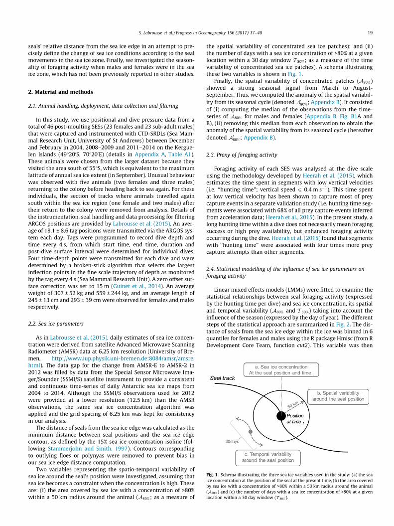
Fig. 1. Schema illustrating the three sea ice variables used in the study: (a) the seaice concentration at the position of the seal at the present time, (b) the area coveredby sea ice with a concentration of >80% within a 50 km radius around the animal(A80%) and (c) the number of days with a sea ice concentration of >80% at a givenlocation within a 30 day window (T 80%).

2.2. Sea ice parameters

As in Labrousse et al. (2015), daily estimates of sea ice concen-tration were derived from satellite Advanced Microwave ScanningRadiometer (AMSR) data at 6.25 km resolution (University of Bre-men, http://www.iup.physik.uni-bremen.de:8084/amsr/amsre.html). The data gap for the change from AMSR-E to AMSR-2 in2012 was filled by data from the Special Sensor Microwave Ima-ger/Sounder (SSMI/S) satellite instrument to provide a consistentand continuous time-series of daily Antarctic sea ice maps from2004 to 2014. Although the SSMI/S observations used for 2012were provided at a lower resolution (12.5 km) than the AMSRobservations, the same sea ice concentration algorithm wasapplied and the grid spacing of 6.25 km was kept for consistencyin our analysis.

The distance of seals from the sea ice edge was calculated as theminimum distance between seal positions and the sea ice edgecontour, as defined by the 15% sea ice concentration isoline (fol-lowing Stammerjohn and Smith, 1997). Contours correspondingto outlying floes or polynyas were removed to prevent bias inour sea ice edge distance computation.

Two variables representing the spatio-temporal variability ofsea ice around the seal’s position were investigated, assuming thatsea ice becomes a constraint when the concentration is high. Theseare: (i) the area covered by sea ice with a concentration of >80%within a 50 km radius around the animal (A80%; as a measure of

the spatial variability of concentrated sea ice patches); and (ii)the number of days with a sea ice concentration of >80% at a givenlocation within a 30 day window T 80%; as a measure of the timevariability of concentrated sea ice patches). A schema illustratingthese two variables is shown in Fig. 1.

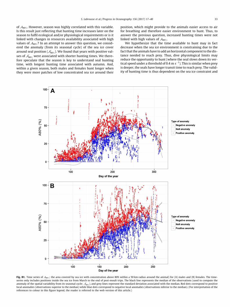
Finally, the spatial variability of concentrated patches (A80%)showed a strong seasonal signal from March to August-September. Thus, we computed the anomaly of the spatial variabil-ity from its seasonal cycle (denoted A0

80%; Appendix B). It consistedof (i) computing the median of the observations from the time-series of A80% for males and females (Appendix B, Fig. B1A andB), (ii) removing this median from each observation to obtain theanomaly of the spatial variability from its seasonal cycle (hereafterdenoted A0

80%; Appendix B).

2.3. Proxy of foraging activity

Foraging activity of each SES was analysed at the dive scaleusing the methodology developed by Heerah et al. (2015), whichestimates the time spent in segments with low vertical velocities(i.e. ‘‘hunting time”; vertical speed 6 0.4 m s�1). This time spentat low vertical velocity has been shown to capture most of preycapture events in a separate validation study (i.e. hunting time seg-ments were associated with 68% of all prey capture events inferredfrom acceleration data; Heerah et al., 2015). In the present study, along hunting time within a dive does not necessarily mean foragingsuccess or high prey availability, but enhanced foraging activityoccurring during the dive. Heerah et al. (2015) found that segmentswith ‘‘hunting time” were associated with four times more preycapture attempts than other segments.

2.4. Statistical modelling of the influence of sea ice parameters onforaging activity

Linear mixed effects models (LMMs) were fitted to examine thestatistical relationships between seal foraging activity (expressedby the hunting time per dive) and sea ice concentration, its spatialand temporal variability (A80% and T 80%) taking into account theinfluence of the season (expressed by the day of year). The differentsteps of the statistical approach are summarized in Fig. 2. The dis-tance of seals from the sea ice edge within the ice was binned in 6quantiles for females and males using the R package Hmisc (from RDevelopment Core Team, function cut2). This variable was then

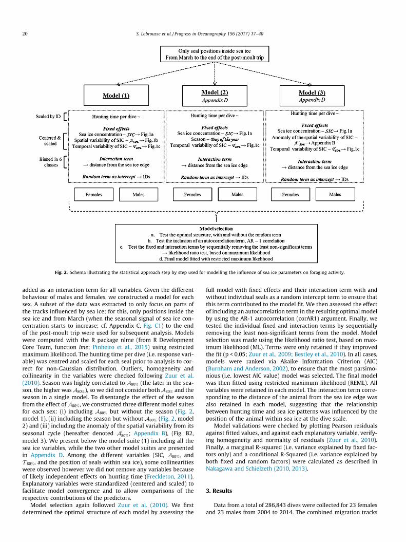
http://www.iup.physik.uni-bremen.de:8084/amsr/amsre.html

http://www.iup.physik.uni-bremen.de:8084/amsr/amsre.html

Fig. 2. Schema illustrating the statistical approach step by step used for modelling the influence of sea ice parameters on foraging activity.


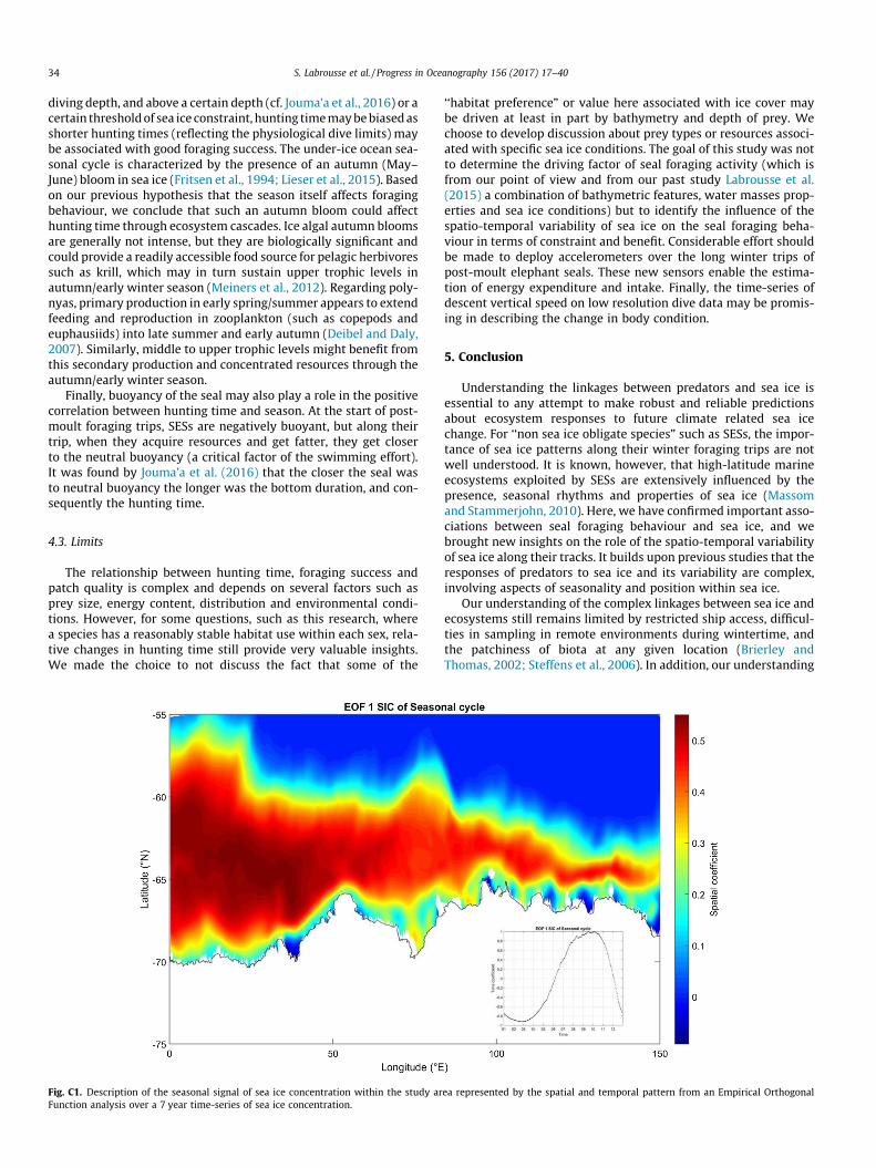
added as an interaction term for all variables. Given the differentbehaviour of males and females, we constructed a model for eachsex. A subset of the data was extracted to only focus on parts ofthe tracks influenced by sea ice; for this, only positions inside thesea ice and from March (when the seasonal signal of sea ice con-centration starts to increase; cf. Appendix C, Fig. C1) to the endof the post-moult trip were used for subsequent analysis. Modelswere computed with the R package nlme (from R DevelopmentCore Team, function lme; Pinheiro et al., 2015) using restrictedmaximum likelihood. The hunting time per dive (i.e. response vari-able) was centred and scaled for each seal prior to analysis to cor-rect for non-Gaussian distribution. Outliers, homogeneity andcollinearity in the variables were checked following Zuur et al.(2010). Season was highly correlated to A80% (the later in the sea-son, the higher wasA80%), so we did not consider bothA80% and theseason in a single model. To disentangle the effect of the seasonfrom the effect ofA80%, we constructed three different model suitesfor each sex: (i) including A80% but without the season (Fig. 2,model 1), (ii) including the season but without A80% (Fig. 2, model2) and (iii) including the anomaly of the spatial variability from itsseasonal cycle (hereafter denoted A0

80%; Appendix B), (Fig. B2,model 3). We present below the model suite (1) including all thesea ice variables, while the two other model suites are presentedin Appendix D. Among the different variables (SIC, A80%, andT 80%, and the position of seals within sea ice), some collinearitieswere observed however we did not remove any variables becauseof likely independent effects on hunting time (Freckleton, 2011).Explanatory variables were standardized (centered and scaled) tofacilitate model convergence and to allow comparisons of therespective contributions of the predictors.

Model selection again followed Zuur et al. (2010). We firstdetermined the optimal structure of each model by assessing the

full model with fixed effects and their interaction term with andwithout individual seals as a random intercept term to ensure thatthis term contributed to the model fit. We then assessed the effectof including an autocorrelation term in the resulting optimal modelby using the AR-1 autocorrelation (corAR1) argument. Finally, wetested the individual fixed and interaction terms by sequentiallyremoving the least non-significant terms from the model. Modelselection was made using the likelihood ratio test, based on max-imum likelihood (ML). Terms were only retained if they improvedthe fit (p < 0.05; Zuur et al., 2009; Bestley et al., 2010). In all cases,models were ranked via Akaike Information Criterion (AIC)(Burnham and Anderson, 2002), to ensure that the most parsimo-nious (i.e. lowest AIC value) model was selected. The final modelwas then fitted using restricted maximum likelihood (REML). Allvariables were retained in each model. The interaction term corre-sponding to the distance of the animal from the sea ice edge wasalso retained in each model, suggesting that the relationshipbetween hunting time and sea ice patterns was influenced by theposition of the animal within sea ice at the dive scale.

Model validations were checked by plotting Pearson residualsagainst fitted values, and against each explanatory variable, verify-ing homogeneity and normality of residuals (Zuur et al., 2010).Finally, a marginal R-squared (i.e. variance explained by fixed fac-tors only) and a conditional R-Squared (i.e. variance explained byboth fixed and random factors) were calculated as described inNakagawa and Schielzeth (2010, 2013).

3. Results

Data from a total of 286,843 dives were collected for 23 femalesand 23 males from 2004 to 2014. The combined migration tracks

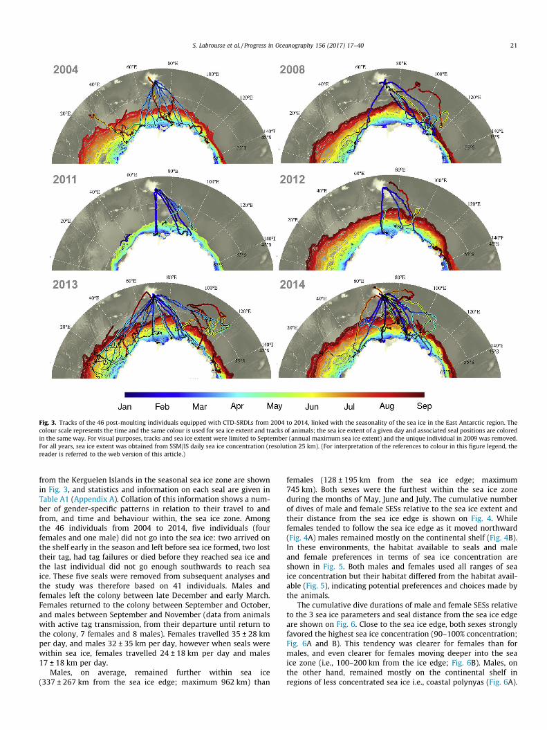
Fig. 3. Tracks of the 46 post-moulting individuals equipped with CTD-SRDLs from 2004 to 2014, linked with the seasonality of the sea ice in the East Antarctic region. Thecolour scale represents the time and the same colour is used for sea ice extent and tracks of animals; the sea ice extent of a given day and associated seal positions are coloredin the same way. For visual purposes, tracks and sea ice extent were limited to September (annual maximum sea ice extent) and the unique individual in 2009 was removed.For all years, sea ice extent was obtained from SSM/IS daily sea ice concentration (resolution 25 km). (For interpretation of the references to colour in this figure legend, thereader is referred to the web version of this article.)


from the Kerguelen Islands in the seasonal sea ice zone are shownin Fig. 3, and statistics and information on each seal are given inTable A1 (Appendix A). Collation of this information shows a num-ber of gender-specific patterns in relation to their travel to andfrom, and time and behaviour within, the sea ice zone. Amongthe 46 individuals from 2004 to 2014, five individuals (fourfemales and one male) did not go into the sea ice: two arrived onthe shelf early in the season and left before sea ice formed, two losttheir tag, had tag failures or died before they reached sea ice andthe last individual did not go enough southwards to reach seaice. These five seals were removed from subsequent analyses andthe study was therefore based on 41 individuals. Males andfemales left the colony between late December and early March.Females returned to the colony between September and October,and males between September and November (data from animalswith active tag transmission, from their departure until return tothe colony, 7 females and 8 males). Females travelled 35 ± 28 kmper day, and males 32 ± 35 km per day, however when seals werewithin sea ice, females travelled 24 ± 18 km per day and males17 ± 18 km per day.

Males, on average, remained further within sea ice(337 ± 267 km from the sea ice edge; maximum 962 km) than

females (128 ± 195 km from the sea ice edge; maximum745 km). Both sexes were the furthest within the sea ice zoneduring the months of May, June and July. The cumulative numberof dives of male and female SESs relative to the sea ice extent andtheir distance from the sea ice edge is shown on Fig. 4. Whilefemales tended to follow the sea ice edge as it moved northward(Fig. 4A) males remained mostly on the continental shelf (Fig. 4B).In these environments, the habitat available to seals and maleand female preferences in terms of sea ice concentration areshown in Fig. 5. Both males and females used all ranges of seaice concentration but their habitat differed from the habitat avail-able (Fig. 5), indicating potential preferences and choices made bythe animals.

The cumulative dive durations of male and female SESs relativeto the 3 sea ice parameters and seal distance from the sea ice edgeare shown on Fig. 6. Close to the sea ice edge, both sexes stronglyfavored the highest sea ice concentration (90–100% concentration;Fig. 6A and B). This tendency was clearer for females than formales, and even clearer for females moving deeper into the seaice zone (i.e., 100–200 km from the ice edge; Fig. 6B). Males, onthe other hand, remained mostly on the continental shelf inregions of less concentrated sea ice i.e., coastal polynyas (Fig. 6A).

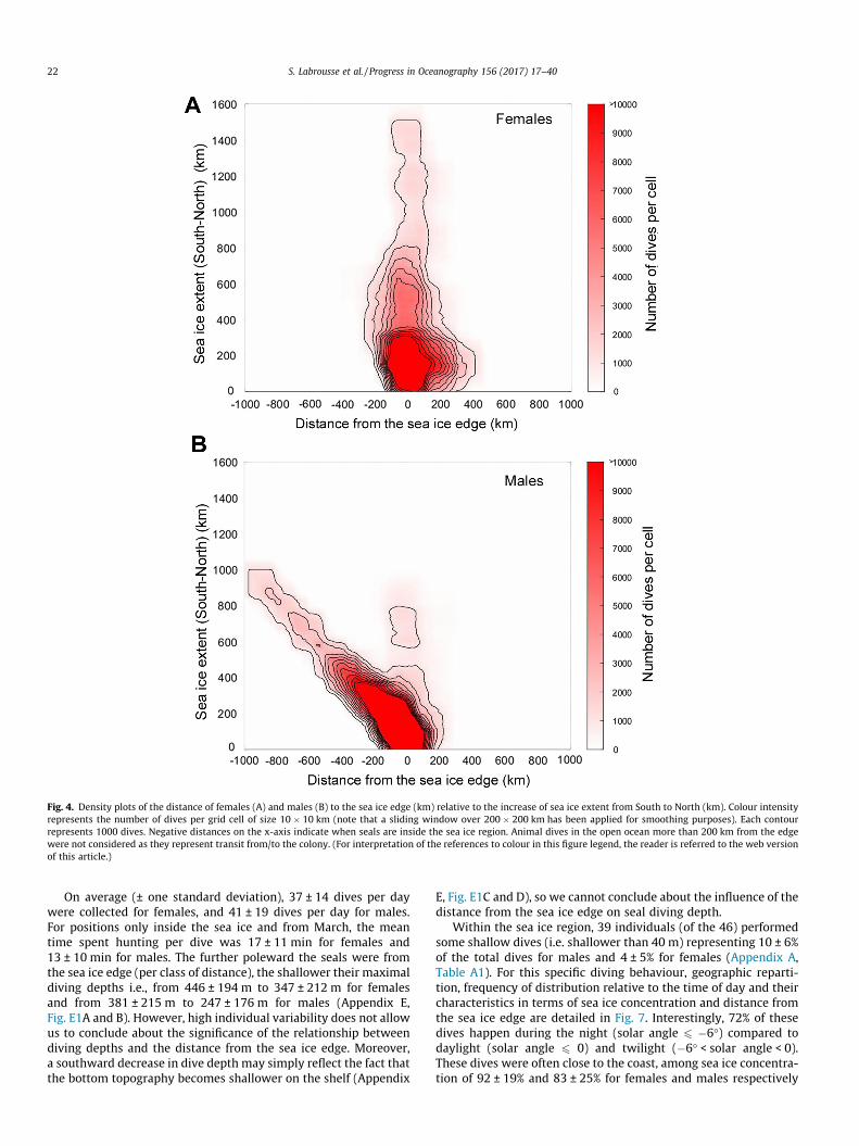
Fig. 4. Density plots of the distance of females (A) and males (B) to the sea ice edge (km) relative to the increase of sea ice extent from South to North (km). Colour intensityrepresents the number of dives per grid cell of size 10 � 10 km (note that a sliding window over 200 � 200 km has been applied for smoothing purposes). Each contourrepresents 1000 dives. Negative distances on the x-axis indicate when seals are inside the sea ice region. Animal dives in the open ocean more than 200 km from the edgewere not considered as they represent transit from/to the colony. (For interpretation of the references to colour in this figure legend, the reader is referred to the web versionof this article.)


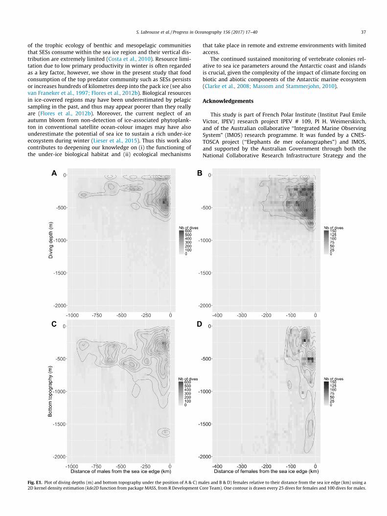
On average (± one standard deviation), 37 ± 14 dives per daywere collected for females, and 41 ± 19 dives per day for males.For positions only inside the sea ice and from March, the meantime spent hunting per dive was 17 ± 11 min for females and13 ± 10 min for males. The further poleward the seals were fromthe sea ice edge (per class of distance), the shallower their maximaldiving depths i.e., from 446 ± 194 m to 347 ± 212 m for femalesand from 381 ± 215 m to 247 ± 176 m for males (Appendix E,Fig. E1A and B). However, high individual variability does not allowus to conclude about the significance of the relationship betweendiving depths and the distance from the sea ice edge. Moreover,a southward decrease in dive depth may simply reflect the fact thatthe bottom topography becomes shallower on the shelf (Appendix

E, Fig. E1C and D), so we cannot conclude about the influence of thedistance from the sea ice edge on seal diving depth.

Within the sea ice region, 39 individuals (of the 46) performedsome shallow dives (i.e. shallower than 40 m) representing 10 ± 6%of the total dives for males and 4 ± 5% for females (Appendix A,Table A1). For this specific diving behaviour, geographic reparti-tion, frequency of distribution relative to the time of day and theircharacteristics in terms of sea ice concentration and distance fromthe sea ice edge are detailed in Fig. 7. Interestingly, 72% of thesedives happen during the night (solar angle 6 �6�) compared todaylight (solar angle 6 0) and twilight (�6� < solar angle < 0).These dives were often close to the coast, among sea ice concentra-tion of 92 ± 19% and 83 ± 25% for females and males respectively

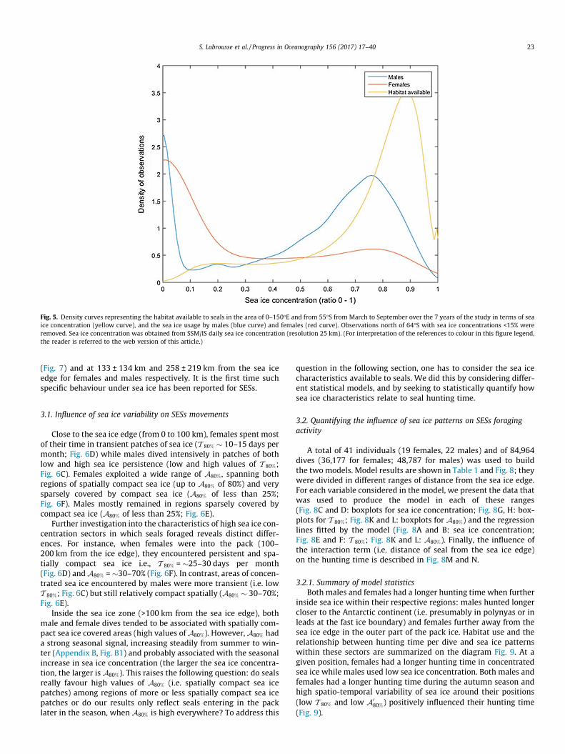
Fig. 5. Density curves representing the habitat available to seals in the area of 0–150�E and from 55�S from March to September over the 7 years of the study in terms of seaice concentration (yellow curve), and the sea ice usage by males (blue curve) and females (red curve). Observations north of 64�S with sea ice concentrations <15% wereremoved. Sea ice concentration was obtained from SSM/IS daily sea ice concentration (resolution 25 km). (For interpretation of the references to colour in this figure legend,the reader is referred to the web version of this article.)


(Fig. 7) and at 133 ± 134 km and 258 ± 219 km from the sea iceedge for females and males respectively. It is the first time suchspecific behaviour under sea ice has been reported for SESs.

3.1. Influence of sea ice variability on SESs movements

Close to the sea ice edge (from 0 to 100 km), females spent mostof their time in transient patches of sea ice (T 80% � 10–15 days permonth; Fig. 6D) while males dived intensively in patches of bothlow and high sea ice persistence (low and high values of T 80%;Fig. 6C). Females exploited a wide range of A80%, spanning bothregions of spatially compact sea ice (up to A80% of 80%) and verysparsely covered by compact sea ice (A80% of less than 25%;Fig. 6F). Males mostly remained in regions sparsely covered bycompact sea ice (A80% of less than 25%; Fig. 6E).

Further investigation into the characteristics of high sea ice con-centration sectors in which seals foraged reveals distinct differ-ences. For instance, when females were into the pack (100–200 km from the ice edge), they encountered persistent and spa-tially compact sea ice i.e., T 80% = �25–30 days per month(Fig. 6D) andA80% = �30–70% (Fig. 6F). In contrast, areas of concen-trated sea ice encountered by males were more transient (i.e. lowT 80%; Fig. 6C) but still relatively compact spatially (A80% � 30–70%;Fig. 6E).

Inside the sea ice zone (>100 km from the sea ice edge), bothmale and female dives tended to be associated with spatially com-pact sea ice covered areas (high values of A80%). However,A80% hada strong seasonal signal, increasing steadily from summer to win-ter (Appendix B, Fig. B1) and probably associated with the seasonalincrease in sea ice concentration (the larger the sea ice concentra-tion, the larger is A80%). This raises the following question: do sealsreally favour high values of A80% (i.e. spatially compact sea icepatches) among regions of more or less spatially compact sea icepatches or do our results only reflect seals entering in the packlater in the season, when A80% is high everywhere? To address this

question in the following section, one has to consider the sea icecharacteristics available to seals. We did this by considering differ-ent statistical models, and by seeking to statistically quantify howsea ice characteristics relate to seal hunting time.

3.2. Quantifying the influence of sea ice patterns on SESs foragingactivity

A total of 41 individuals (19 females, 22 males) and of 84,964dives (36,177 for females; 48,787 for males) was used to buildthe two models. Model results are shown in Table 1 and Fig. 8; theywere divided in different ranges of distance from the sea ice edge.For each variable considered in the model, we present the data thatwas used to produce the model in each of these ranges(Fig. 8C and D: boxplots for sea ice concentration; Fig. 8G, H: box-plots for T 80%; Fig. 8K and L: boxplots for A80%) and the regressionlines fitted by the model (Fig. 8A and B: sea ice concentration;Fig. 8E and F: T 80%; Fig. 8K and L: A80%). Finally, the influence ofthe interaction term (i.e. distance of seal from the sea ice edge)on the hunting time is described in Fig. 8M and N.

3.2.1. Summary of model statisticsBoth males and females had a longer hunting time when further

inside sea ice within their respective regions: males hunted longercloser to the Antarctic continent (i.e. presumably in polynyas or inleads at the fast ice boundary) and females further away from thesea ice edge in the outer part of the pack ice. Habitat use and therelationship between hunting time per dive and sea ice patternswithin these sectors are summarized on the diagram Fig. 9. At agiven position, females had a longer hunting time in concentratedsea ice while males used low sea ice concentration. Both males andfemales had a longer hunting time during the autumn season andhigh spatio-temporal variability of sea ice around their positions(low T 80% and low A0

80%) positively influenced their hunting time(Fig. 9).

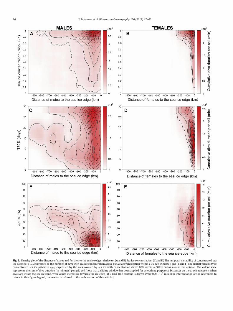
Fig. 6. Density plot of the distance of males and females to the sea ice edge relative to: (A and B) Sea ice concentration; (C and D) The temporal variability of concentrated seaice patches (T 80% , expressed as the number of days with sea ice concentration above 80% at a given location within a 30 day window); and (E and F) The spatial variability ofconcentrated sea ice patches (A80% , expressed by the area covered by sea ice with concentration above 80% within a 50 km radius around the animal). The colour scalerepresents the sum of dive duration (in minutes) per grid cell (note that a sliding window has been applied for smoothing purposes). Distances on the x-axis represent whenseals are inside the sea ice zone, with values increasing towards the ice edge (at 0 km). One contour is drawn every 0.25 � 105 min. (For interpretation of the references tocolour in this figure legend, the reader is referred to the web version of this article.)


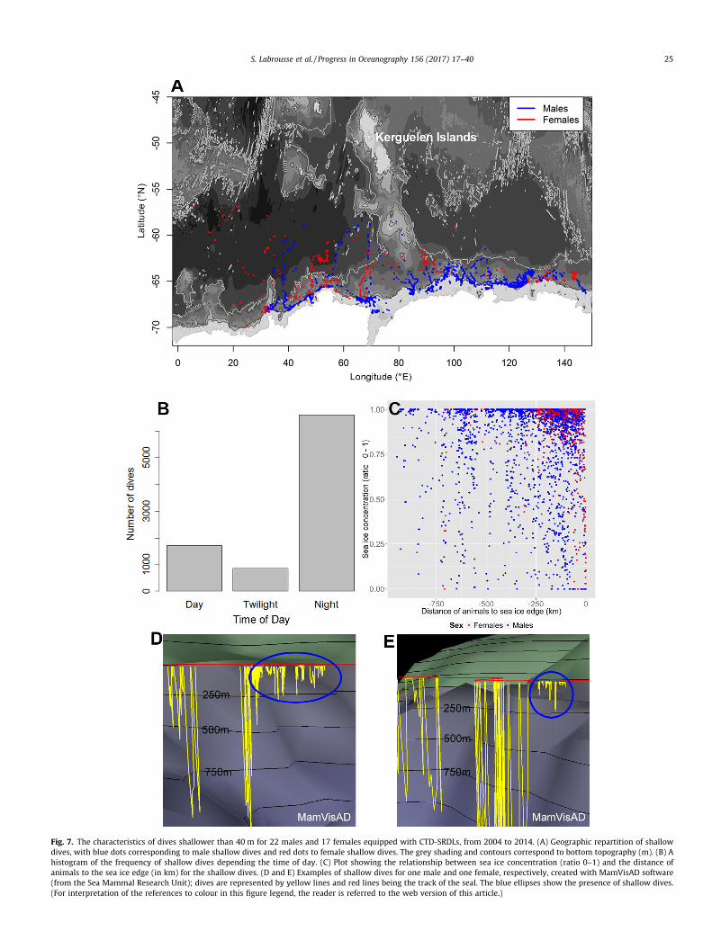
Fig. 7. The characteristics of dives shallower than 40 m for 22 males and 17 females equipped with CTD-SRDLs, from 2004 to 2014. (A) Geographic repartition of shallowdives, with blue dots corresponding to male shallow dives and red dots to female shallow dives. The grey shading and contours correspond to bottom topography (m). (B) Ahistogram of the frequency of shallow dives depending the time of day. (C) Plot showing the relationship between sea ice concentration (ratio 0–1) and the distance ofanimals to the sea ice edge (in km) for the shallow dives. (D and E) Examples of shallow dives for one male and one female, respectively, created with MamVisAD software(from the Sea Mammal Research Unit); dives are represented by yellow lines and red lines being the track of the seal. The blue ellipses show the presence of shallow dives.(For interpretation of the references to colour in this figure legend, the reader is referred to the web version of this article.)


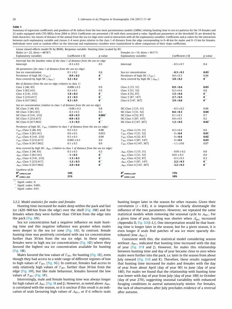
Table 1Summary of regression coefficients and goodness-of-fit indices from the two most parsimonious models (LMMs) relating hunting time to sea ice patterns for the 19 females and22 males equipped with CTD-SRDLs from 2004 to 2014. Coefficients are presented ± SE with their associated p-value. Significant parameters at the threshold 5% are denoted bybold characters. Six classes of distance of the animal from the sea ice edge were used in interaction with all the explanatory variables. Coefficients and p-values for the interactionbetween each explanatory variable and classes 2–6 were given relative to the class 1 of distance from the edge corresponding to 0–46 km for males and 0–15 km for females.Individuals were used as random effect on the intercept and explanatory variables were standardized to allow comparison of their slope coefficients.

Linear mixed-effects model fit by REML; Response variable: Hunting time (scaled by ID)Males (n = 22, dives = 48787) Females (n = 19, dives = 36177)Explanatory variables Coefficient ± SE p-value Explanatory variables Coefficient ± SE p-value

Intercept has the baseline value of the class 1 of distance from the sea ice edgeIntercept �0.3 ± 0.5 0.5 Intercept �0.5 ± 0.7 0.4

All parameters (for class 1 of distance from the sea ice edge)Sea ice concentration 0.1 ± 0.2 0.6 Sea ice concentration �0.3 ± 0.1 0.03*

Persitence of high SIC (T 80%) �0.9 ± 0.2 0*** Persitence of high SIC (T 80%) 0.6 ± 0.3 0.06Area covered by high SIC (A80%) 3.2 ± 0.2 0*** Area covered by high SIC (A80%) 3.8 ± 0.2 0***

Bin of distance from the sea ice edge (relative to class 1)Class 2 [46, 83] 0.008 ± 0.3 0.9 Class 2 [15, 31] 0.9 ± 0.4 0.03*

Class 3 [83,141] 0.2 ± 0.3 0.5 Class 3 [31, 52] 0.2 ± 0.4 0.6Class 4 [141, 233] 1.8 ± 0.3 0*** Class 4 [52, 87] 1.5 ± 0.4 0***

Class 5 [233,417] 2.1 ± 0.3 0*** Class 5 [87, 147] 2.7 ± 0.5 0***

Class 6 [417,962] 4.3 ± 0.5 0*** Class 6 [147, 367] 3.9 ± 0.6 0***

Sea ice concentration (relative to class 1 of distance from the sea ice edge)SIC:Class 2 [46, 83] �0.08 ± 0.3 0.8 SIC:Class 2 [15, 31] �0.5 ± 0.2 0.06SIC:Class 3 [83,141] �0.3 ± 0.3 0.3 SIC:Class 3 [31, 52] 0.6 ± 0.3 0.04*

SIC:Class 4 [141, 233] �0.9 ± 0.3 0.002** SIC:Class 4 [52, 87] 0.1 ± 0.3 0.7SIC:Class 5 [233,417] �0.9 ± 0.3 0*** SIC:Class 5 [87, 147] 0.6 ± 0.5 0.2SIC:Class 6 [417,962] �1.3 ± 0.3 0*** SIC:Class 6 [147, 367] 1.2 ± 0.5 0.02**

Persitence of high SIC, T 80% (relative to class 1 of distance from the sea ice edge)T 80%:Class 2 [46, 83] 0.5 ± 0.3 0.08 T 80%:Class 2 [15, 31] 0.2 ± 0.4 0.6T 80%:Class 3 [83,141] 0.6 ± 0.3 0.053 T 80%:Class 3 [31, 52] �1 ± 0.4 0.01*

T 80%:Class 4 [141, 233] 0.5 ± 0.3 0.09 T 80%:Class 4 [52, 87] �1 ± 0.4 0.02*

T 80%:Class 5 [233,417] 0.002 ± 0.3 0.9 T 80%:Class 5 [87, 147] �1 ± 0.5 0.03*

T 80%:Class 6 [417,962] 0.1 ± 0.3 0.6 T 80%:Class 6 [147, 367] �1.1 ± 0.6 0.07

Area covered by high SIC, A80% (relative to class 1 of distance from the sea ice edge)A80%:Class 2 [46, 83] 0.3 ± 0.3 0.3 A80%:Class 2 [15, 31] �0.05 ± 0.2 0.8A80%:Class 3 [83,141] �1 ± 0.3 0*** A80%:Class 3 [31, 52] 0.01 ± 0.3 0.9A80%:Class 4 [141, 233] �1.3 ± 0.3 0** A80%:Class 4 [52, 87] �0.3 ± 0.3 0.3A80%:Class 5 [233,417] �1.2 ± 0.3 0*** A80%:Class 5 [87, 147] �2.2 ± 0.3 0***

A80%:Class 6 [417,962] �2.9 ± 0.4 0*** A80%:Class 6 [147, 367] �3.2 ± 0.3 0***

Goodness-of-fitR2

LMM(m)-full 14% R2LMM(m)-full 13%

R2LMM(c)-full 21% R2

LMM(c)-full 18%

*** Signif. codes: 0.** Signif. codes: 0.001.* Signif. codes: 0.01.


3.2.2. Model statistics for males and femalesHunting time increased for males deep within the pack and fast

ice (420–960 km from the edge) over the shelf (Fig. 8M) and forfemales when they were further than 150 km from the edge intothe pack (Fig. 8N).

Sea ice concentration had a negative influence on male hunt-ing time and this negative influence was greater when maleswere deeper in the sea ice zone (Fig. 8A). In contrast, femalehunting time was positively correlated with sea ice concentrationfurther than 30 km from the sea ice edge. In these regions,females were in high sea ice concentrations (Fig. 8D) where theyfavored the highest sea ice concentration available for hunting(Fig. 8B).

Males favored the low values of T 80% for hunting (Fig. 8E), eventhough they had access to a wide range of different regimes of lowto high values of T 80% (Fig. 8G). In contrast, females had access toonly relatively high values of T 80% further than 30 km from theedge (Fig. 8H), but like male behaviour, females favored the lowvalues of T 80% (Fig. 8F).

Interestingly, male and female hunting time was always longerfor high values ofA80% (Fig. 8I and J). However, as noted aboveA80%

is correlated with the season, so it is unclear if this result is an indi-cation of seals favouring high values of A80%, or if it reflects seals

hunting longer later in the season for other reasons. Given theircorrelation (r � 0.8), it is impossible to clearly disentangle theinfluence of the two parameters. However, we repeated the samestatistical models while removing the seasonal cycle to A80%. Fora given time of year, hunting was shorter when A0

80% increased(Appendix D, Fig. D2(I–L)). One interpretation would be that hunt-ing time is longer later in the season, but for a given season, it iseven longer if seals find patches of sea ice more sparsely dis-tributed (low A80%).

Consistent with this, the statistical model considering seasonwithout A80%, indicated that hunting time increased with the dayof year (Fig. D1I and J). However, for males this relationshipbetween hunting time and day of year became close to zero whenmales were further into the pack, i.e. later in the season from aboutJuly onward (Fig. D1I and K). Therefore, these results suggestedthat hunting time increased for males and females with the dayof year from about April (day of year 90) to June (day of year180). For males we found that the relationship with hunting timewas lower with day of year from July (day of year 180) to October(day of year 270), suggesting seasonal variability with enhancedforaging conditions in austral autumn/early winter. For females,the lack of observations after July precludes evidence of a reversalafter autumn.

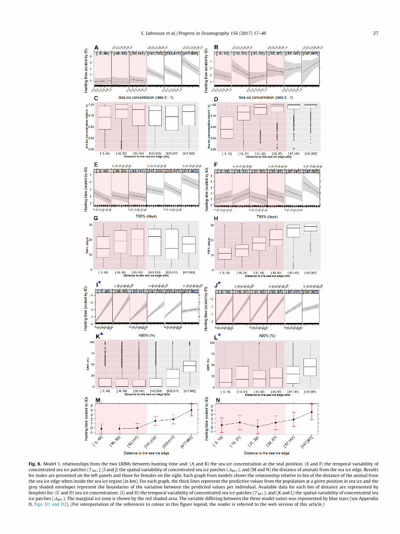
Fig. 8. Model 1, relationships from the two LMMs between hunting time and: (A and B) the sea ice concentration at the seal position; (E and F) the temporal variability ofconcentrated sea ice patches (T 80%); (I and J) the spatial variability of concentrated sea ice patches (A80%); and (M and N) the distance of animals from the sea ice edge. Resultsfor males are presented on the left panels and those for females on the right. Each graph from models shows the relationship relative to bin of the distance of the animal fromthe sea ice edge when inside the sea ice region (in km). For each graph, the thick lines represent the predictive values from the population at a given position in sea ice and thegrey shaded envelopes represent the boundaries of the variation between the predicted values per individual. Available data for each bin of distance are represented byboxplots for: (C and D) sea ice concentration; (G and H) the temporal variability of concentrated sea ice patches (T 80%); and (K and L) the spatial variability of concentrated seaice patches (A80%). The marginal ice zone is shown by the red shaded area. The variable differing between the three model suites was represented by blue stars (see AppendixD, Figs. D1 and D2). (For interpretation of the references to colour in this figure legend, the reader is referred to the web version of this article.)


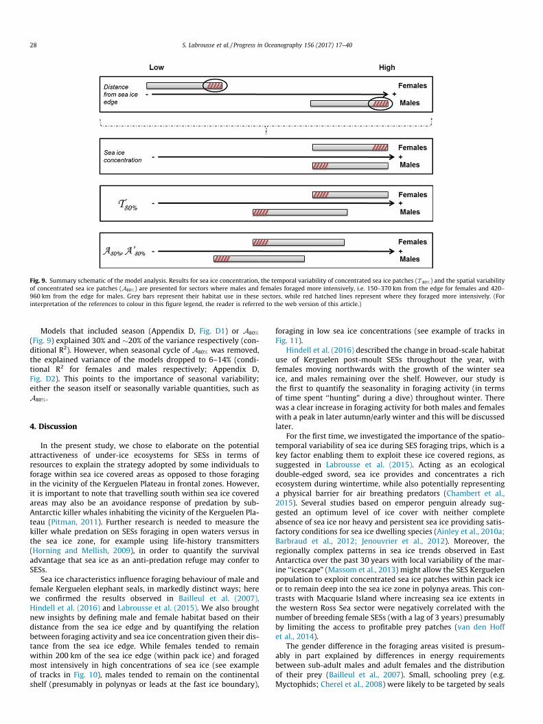
Fig. 9. Summary schematic of the model analysis. Results for sea ice concentration, the temporal variability of concentrated sea ice patches (T 80%) and the spatial variabilityof concentrated sea ice patches (A80%) are presented for sectors where males and females foraged more intensively, i.e. 150–370 km from the edge for females and 420–960 km from the edge for males. Grey bars represent their habitat use in these sectors, while red hatched lines represent where they foraged more intensively. (Forinterpretation of the references to colour in this figure legend, the reader is referred to the web version of this article.)


Models that included season (Appendix D, Fig. D1) or A80%

(Fig. 9) explained 30% and �20% of the variance respectively (con-ditional R2). However, when seasonal cycle of A80% was removed,the explained variance of the models dropped to 6–14% (condi-tional R2 for females and males respectively; Appendix D,Fig. D2). This points to the importance of seasonal variability;either the season itself or seasonally variable quantities, such asA80%.

4. Discussion

In the present study, we chose to elaborate on the potentialattractiveness of under-ice ecosystems for SESs in terms ofresources to explain the strategy adopted by some individuals toforage within sea ice covered areas as opposed to those foragingin the vicinity of the Kerguelen Plateau in frontal zones. However,it is important to note that travelling south within sea ice coveredareas may also be an avoidance response of predation by sub-Antarctic killer whales inhabiting the vicinity of the Kerguelen Pla-teau (Pitman, 2011). Further research is needed to measure thekiller whale predation on SESs foraging in open waters versus inthe sea ice zone, for example using life-history transmitters(Horning and Mellish, 2009), in order to quantify the survivaladvantage that sea ice as an anti-predation refuge may confer toSESs.

Sea ice characteristics influence foraging behaviour of male andfemale Kerguelen elephant seals, in markedly distinct ways; herewe confirmed the results observed in Bailleul et al. (2007),Hindell et al. (2016) and Labrousse et al. (2015). We also broughtnew insights by defining male and female habitat based on theirdistance from the sea ice edge and by quantifying the relationbetween foraging activity and sea ice concentration given their dis-tance from the sea ice edge. While females tended to remainwithin 200 km of the sea ice edge (within pack ice) and foragedmost intensively in high concentrations of sea ice (see exampleof tracks in Fig. 10), males tended to remain on the continentalshelf (presumably in polynyas or leads at the fast ice boundary),

foraging in low sea ice concentrations (see example of tracks inFig. 11).

Hindell et al. (2016) described the change in broad-scale habitatuse of Kerguelen post-moult SESs throughout the year, withfemales moving northwards with the growth of the winter seaice, and males remaining over the shelf. However, our study isthe first to quantify the seasonality in foraging activity (in termsof time spent ‘‘hunting” during a dive) throughout winter. Therewas a clear increase in foraging activity for both males and femaleswith a peak in later autumn/early winter and this will be discussedlater.

For the first time, we investigated the importance of the spatio-temporal variability of sea ice during SES foraging trips, which is akey factor enabling them to exploit these ice covered regions, assuggested in Labrousse et al. (2015). Acting as an ecologicaldouble-edged sword, sea ice provides and concentrates a richecosystem during wintertime, while also potentially representinga physical barrier for air breathing predators (Chambert et al.,2015). Several studies based on emperor penguin already sug-gested an optimum level of ice cover with neither completeabsence of sea ice nor heavy and persistent sea ice providing satis-factory conditions for sea ice dwelling species (Ainley et al., 2010a;Barbraud et al., 2012; Jenouvrier et al., 2012). Moreover, theregionally complex patterns in sea ice trends observed in EastAntarctica over the past 30 years with local variability of the mar-ine ‘‘icescape” (Massom et al., 2013) might allow the SES Kerguelenpopulation to exploit concentrated sea ice patches within pack iceor to remain deep into the sea ice zone in polynya areas. This con-trasts with Macquarie Island where increasing sea ice extents inthe western Ross Sea sector were negatively correlated with thenumber of breeding female SESs (with a lag of 3 years) presumablyby limiting the access to profitable prey patches (van den Hoffet al., 2014).

The gender difference in the foraging areas visited is presum-ably in part explained by differences in energy requirementsbetween sub-adult males and adult females and the distributionof their prey (Bailleul et al., 2007). Small, schooling prey (e.g.Myctophids; Cherel et al., 2008) were likely to be targeted by seals

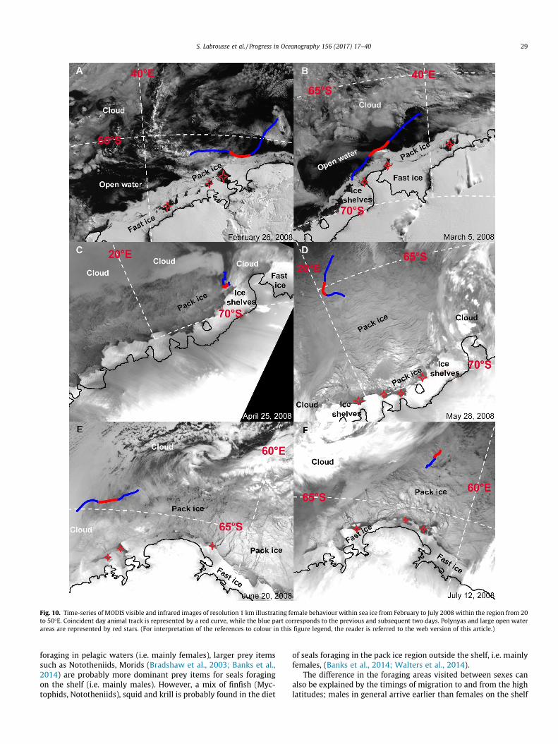
Fig. 10. Time-series of MODIS visible and infrared images of resolution 1 km illustrating female behaviour within sea ice from February to July 2008 within the region from 20to 50�E. Coincident day animal track is represented by a red curve, while the blue part corresponds to the previous and subsequent two days. Polynyas and large open waterareas are represented by red stars. (For interpretation of the references to colour in this figure legend, the reader is referred to the web version of this article.)


foraging in pelagic waters (i.e. mainly females), larger prey itemssuch as Nototheniids, Morids (Bradshaw et al., 2003; Banks et al.,2014) are probably more dominant prey items for seals foragingon the shelf (i.e. mainly males). However, a mix of finfish (Myc-tophids, Nototheniids), squid and krill is probably found in the diet

of seals foraging in the pack ice region outside the shelf, i.e. mainlyfemales, (Banks et al., 2014; Walters et al., 2014).

The difference in the foraging areas visited between sexes canalso be explained by the timings of migration to and from the highlatitudes; males in general arrive earlier than females on the shelf

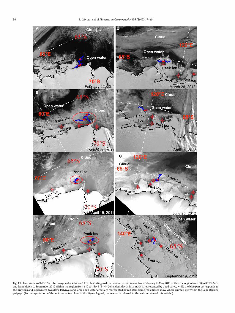
Fig. 11. Time-series of MODIS visible images of resolution 1 km illustrating male behaviour within sea ice from February to May 2011 within the region from 60 to 80�E (A–D)and from March to September 2012 within the region from 110 to 150�E (E–H). Coincident day animal track is represented by a red curve, while the blue part corresponds tothe previous and subsequent two days. Polynyas and large open water areas are represented by red stars while red ellipses show where animals are within the Cape Darnleypolynya. (For interpretation of the references to colour in this figure legend, the reader is referred to the web version of this article.)



before sea ice forms probably allowing them to reach these remoteareas without being constrained by sea ice. Moreover, because themales studied were sub-adult males, they may not prioritizereturning to the colony for breeding because they were not sexu-ally mature and thus they were able to stay longer within thesea ice region. In contrast females arrive later when sea ice isalready formed and leave earlier as they may prioritize returningto the colony to give birth. Thus females might avoid being trappedby sea ice by foraging in the pack but by following the sea ice edge(Bailleul et al., 2007; Hindell et al., 2016; Labrousse et al., 2015).

Understanding these patterns requires also consideration of theresources available to the animals. We do this below in the contextof different sea ice zones, which might aggregate specificresources, as well as in the framework of the seasonal cycle inice and primary production.

4.1. Sea ice zones and associated resources

In East Antarctica, the sea ice cover is made up of three zoneswith distinct characteristics (Massom and Stammerjohn, 2010).These are (from north to south): (i) the highly-dynamic ‘‘marginalice zone” (MIZ), which typically extends 100 km or so south fromthe ice edge, and is generally made up of small floes and diffuseice conditions (depending on wind direction); (ii) the ‘‘inner packice” zone (PIZ) comprising larger floes separated by leads; and(iii) a coastal zone comprising the band of compact ‘‘landfast (fast)ice” (FIZ) and persistent and recurrent areas of low-concentrationsea ice in the form of polynyas and flaw leads. Females in our studymostly remained and foraged in the MIZ and the outer part of thepack ice, while males used all three sea ice zones. Below, we sum-marise female and male foraging behaviour in each of these zonesin more detail.

4.1.1. Male and female foraging behaviour in the MIZWithin the MIZ, both females and males encountered regions

characterized by (i) relatively low to intermediate sea ice concen-tration; (ii) low T 80%; and (iii) low to high A80%. The MIZ is charac-terized by high sea ice variability in time and space and enhancedbiological activity due to sea ice melt and breakdown releasing animportant quantity of food resources (i.e. ice algae) under a stronginfluence of wind action and ocean wave-ice interaction processes(Wadhams, 2000; Massom et al., 2006; Karnovsky et al., 2007;Squire, 2007; Massom and Stammerjohn, 2010). However, it isnot in this region that seals had the longest hunting times per dive.

4.1.2. Female foraging behaviour in the PIZWithin the PIZ, females mostly remained in the outer part of the

pack (150–370 km away from the edge) and had their longesthunting times there compared to the MIZ. Within this region, gen-erally characterized by persistent and compact sea ice, females for-aged most intensively (i.e. longer hunting times) (i) in the highestsea ice concentration at their position, but (ii) their hunting timewas longer in areas of low concentration sea ice around their posi-tion (either in time or in space; 30 days & 50 km). The spatio-temporal variability of sea ice around female positions probablyallowed them to exploit concentrated patches of prey withoutbeing trapped by the ice (Raymond et al., 2015). Heerah et al.(2017) observed similar results with Weddell seals hunting longerin more concentrated sea ice in regions with variable sea ice (e.g.Davis station) compared with areas where sea ice conditions werepersistent and less variable (e.g. Dumont d’Urville), where the con-trary was observed.

Despite a lack of information on prey, females are known tohave a multi-species diet, (i.e. mix of finfish and squid) in thepack-ice habitat compared with shelf and pelagic habitats wherefemales have a higher proportion of finfish (Banks et al., 2014).

The study of Flores et al. (2008) provided evidence of a secondmajor trophic pathway from phytoplankton to mesopredators inthe pack ice region during autumn, via copepods and myctophids,comprising intermediate trophic steps via cephalopods and largefinfishes. In high Antarctic pelagic waters, about 24–70% of the bio-mass of the myctophid Electrona antarctica from 0–1000 m depth,was found to occur in the upper 200 m at night (Lancraft et al.,1989; Donnelly et al., 2006) and it was reported by Kaufmannet al. (1995) that mesopelagic organisms migrate closer to the sur-face beneath pack ice than in open water. Thus, concentration and/or availability of resources in the pack ice region near the ice-waterinterface or within the water column (from diurnal vertical migra-tion) possibly makes it physiologically more rewarding to forageunder-ice compared to the deep dives necessary to catch Myc-tophids in open waters or compared to the risk of being trappedby sea ice by foraging on Nototheniids (Bradshaw et al., 2003) indensely sea ice covered shelf regions. Unfortunately, there is sofar only anecdotal evidence that important prey species of SESsare found in the ice-water interface layer, such as squid and finfish(Ainley et al., 1986; Kaufmann et al., 1995; Flores et al., 2011;David et al., 2016).

4.1.3. Male foraging behaviour in the PIZ and FIZThepack ice region formales represents both a transit and a feed-

ing area. However, male hunting timewas longer in regions close tothe Antarctic coast, in the southern part of the pack and fast ice(420–960 km away from the edge). Within this environment, theyforagedmost intensively (i.e. longer hunting times) (i) in the lowestsea ice concentration at their position, and (ii) when there weremore patches of low concentrated sea ice around their position(either in time or in space; 30 days & 50 km) likely to be associatedwith polynyas, or recurrent flaw leads separating persistent fast icefrom moving pack ice (Massom and Stammerjohn, 2010). In addi-tion to relieving the sea ice constraint, these open water areas cansustain high biological activity in spring, persisting in time andmaintaining rich ecosystems thatmay support populations ofmam-mals being able to breathe and feed throughout the ice season(Ainley et al., 2010b; Arrigo and van Dijken, 2003; Karnovskyet al., 2007; Tremblay and Smith, 2007; Arrigo et al., 2015). Polynyasalso support rich benthic communities through enhanced verticalcarbon flux (Grebmeier and Barry, 2007). Sub-adult male SESsmay also benefit from this by feeding on the shelf or slope regionswithout being constrained by sea ice. They likely feed on the mostabundant pelagic finfish in Antarctic shelf water, the Antarctic sil-verfish (Pleuragramma antarcticum), from surface to �900 m(Daneri and Carlini, 2002; La Mesa et al., 2010) or on epibenthicAntarctic toothfish (Dissostichus mawsoni) (Bradshaw et al., 2003;Smith et al., 2007)with juvenile finfishprincipally foundon the shelfwhile adults are found along the slope (Ashford et al., 2012) some-times shallower than though within �1000 m of the water column(Watwood et al., 2006) or under fast ice in mid-depths (12–180 m;Fuiman et al., 2002). Shallow dives observed in high sea ice concen-tration close to the Antarctic coast (10 ± 6% of the total dives formales) could correspond to specific foraging activity associatedwiththe rich under-ice community of fish and invertebrates (Ainley et al.,1991). Moreover, these dives were mostly performed at night,where the diurnal verticalmigration of adult krill (Euphausia crystal-lorophias), more pronounced in winter than summer (Siegel, 2012;Flores et al., 2012b; Cisewski and Strass, 2016)might attract variouspreys, such as Pleuragramma antarcticum (Fuiman et al., 2002).

4.2. Seasonality in foraging activity

Our analysis highlights the importance of the seasonal cycle tothe seal hunting time. For both males and females, we found thathunting time per dive increased from April to June. This is not


surprising given that sea ice characteristics are intrinsically relatedto seasons, but whether the season itself (i.e. productivity of theecosystem at a certain period) or seasonal changes in along-tracksea ice habitat (i.e. access to favorable zones with prey availability

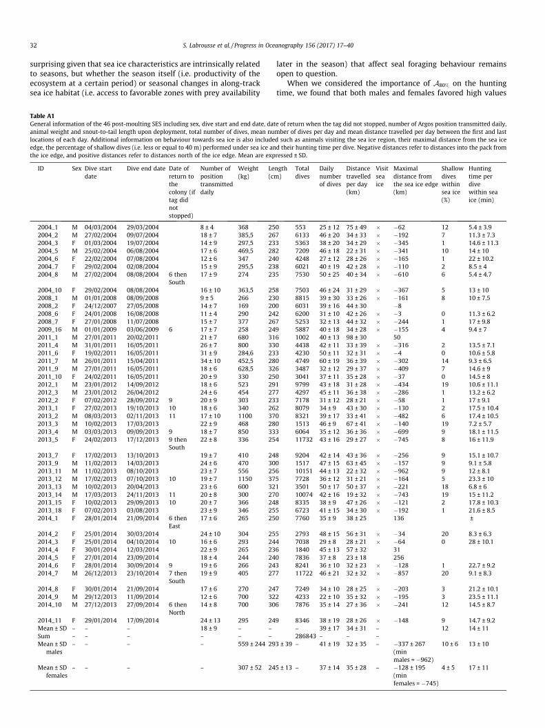
Table A1General information of the 46 post-moulting SES including sex, dive start and end date, datanimal weight and snout-to-tail length upon deployment, total number of dives, mean nulocations of each day. Additional information on behaviour towards sea ice is also includeedge, the percentage of shallow dives (i.e. less or equal to 40 m) performed under sea ice anthe ice edge, and positive distances refer to distances north of the ice edge. Mean are exp

ID Sex Dive startdate

Dive end date Date ofreturn tothecolony (iftag didnotstopped)

Number ofpositiontransmitteddaily

Weight(kg)

Le(cm

2004_1 M 04/03/2004 29/03/2004 8 ± 4 368 252004_2 M 27/02/2004 09/07/2004 18 ± 7 385,5 262004_3 F 01/03/2004 19/07/2004 14 ± 9 297,5 232004_5 M 25/02/2004 06/08/2004 17 ± 6 469,5 282004_6 F 22/02/2004 07/08/2004 12 ± 6 347 242004_7 F 29/02/2004 02/08/2004 15 ± 9 295,5 232004_8 M 27/02/2004 08/08/2004 6 then

South17 ± 9 274 23

2004_10 F 29/02/2004 08/08/2004 16 ± 10 363,5 252008_1 M 01/01/2008 08/09/2008 9 ± 5 266 232008_2 F 24/12/2007 27/05/2008 14 ± 7 169 202008_6 F 24/01/2008 16/08/2008 11 ± 4 290 242008_7 F 27/01/2008 11/07/2008 15 ± 7 377 262009_16 M 01/01/2009 03/06/2009 6 17 ± 7 258 242011_1 M 27/01/2011 20/02/2011 21 ± 7 680 312011_4 M 31/01/2011 16/05/2011 26 ± 7 800 332011_6 F 19/02/2011 16/05/2011 31 ± 9 284,6 232011_7 M 26/01/2011 15/04/2011 34 ± 10 452,5 282011_9 M 27/01/2011 16/05/2011 18 ± 6 628,5 322011_10 F 24/02/2011 16/05/2011 20 ± 9 330 252012_1 M 23/01/2012 14/09/2012 18 ± 6 523 292012_3 M 23/01/2012 26/04/2012 24 ± 6 454 272012_2 F 07/02/2012 28/09/2012 9 20 ± 9 303 232013_1 F 27/02/2013 19/10/2013 10 18 ± 6 340 262013_2 M 08/03/2013 02/11/2013 11 17 ± 10 1100 372013_3 M 10/02/2013 17/03/2013 22 ± 9 468 282013_4 M 03/03/2013 09/09/2013 9 18 ± 7 850 332013_5 F 24/02/2013 17/12/2013 9 then

South22 ± 8 336 25

2013_7 F 17/02/2013 13/10/2013 19 ± 7 410 242013_9 M 11/02/2013 14/03/2013 24 ± 6 470 302013_11 M 11/02/2013 08/10/2013 23 ± 7 556 252013_12 M 17/02/2013 07/10/2013 10 19 ± 7 1150 372013_13 M 10/02/2013 20/04/2013 23 ± 6 600 322013_14 M 17/03/2013 24/11/2013 11 20 ± 8 300 272013_15 F 10/02/2013 29/09/2013 10 20 ± 7 366 242013_18 F 07/02/2013 03/08/2013 23 ± 9 346 252014_1 F 28/01/2014 21/09/2014 6 then

East17 ± 6 265 25

2014_2 F 25/01/2014 30/03/2014 24 ± 10 304 252014_3 F 25/01/2014 04/10/2014 10 16 ± 6 293 242014_4 F 30/01/2014 12/03/2014 22 ± 9 265 232014_5 F 27/01/2014 23/09/2014 18 ± 4 244 242014_6 F 28/01/2014 30/09/2014 9 19 ± 6 266 242014_7 M 26/12/2013 23/10/2014 7 then

South19 ± 9 405 27

2014_8 F 30/01/2014 21/09/2014 17 ± 6 270 242014_9 M 29/12/2013 11/09/2014 12 ± 6 700 322014_10 M 27/12/2013 27/09/2014 6 then

North14 ± 8 700 30

2014_11 F 29/01/2014 17/09/2014 24 ± 13 295 24Mean ± SD – – – 18 ± 9 – –Sum – – – – – –Mean ± SD

males– – – – 559 ± 244 29

Mean ± SDfemales

– – – – 307 ± 52 24

later in the season) that affect seal foraging behaviour remainsopen to question.

When we considered the importance of A80% on the huntingtime, we found that both males and females favored high values

e of return when the tag did not stopped, number of Argos position transmitted daily,mber of dives per day and mean distance travelled per day between the first and lastd such as animals visiting the sea ice region, their maximal distance from the sea iced their hunting time per dive. Negative distances refer to distances into the pack fromressed ± SD.

ngth)

Totaldives

Dailynumberof dives

Distancetravelledper day(km)

Visitseaice

Maximaldistance fromthe sea ice edge(km)

Shallowdiveswithinsea ice(%)

Huntingtime perdivewithin seaice (min)

0 553 25 ± 12 75 ± 49 � �62 12 5.4 ± 3.97 6133 46 ± 20 34 ± 33 � �192 7 11.3 ± 7.33 5363 38 ± 20 34 ± 29 � �345 1 14.6 ± 11.32 7209 46 ± 18 22 ± 31 � �341 10 14 ± 100 4248 27 ± 12 28 ± 26 � �165 1 22 ± 10.28 6021 40 ± 19 42 ± 28 � �110 2 8.5 ± 45 7530 50 ± 25 40 ± 34 � �610 6 5.4 ± 4.7

8 7503 46 ± 24 31 ± 29 � �367 5 13 ± 100 8815 39 ± 30 33 ± 26 � �161 8 10 ± 7.50 6031 39 ± 16 44 ± 30 �82 6200 31 ± 10 42 ± 26 � �3 0 11.3 ± 6.27 5253 32 ± 13 44 ± 32 � �244 1 17 ± 9.89 5887 40 ± 18 34 ± 28 � �155 4 9.4 ± 76 1002 40 ± 13 98 ± 30 500 4438 42 ± 11 33 ± 39 � �316 2 13.5 ± 7.13 4230 50 ± 11 32 ± 31 � �4 0 10.6 ± 5.80 4749 60 ± 19 36 ± 39 � �302 14 9.3 ± 6.56 3487 32 ± 12 29 ± 37 � �409 7 14.6 ± 90 3041 37 ± 11 35 ± 28 � �37 0 14.5 ± 81 9799 43 ± 18 31 ± 28 � �434 19 10.6 ± 11.17 4297 45 ± 11 36 ± 38 � �286 1 13.2 ± 6.23 7178 31 ± 12 28 ± 21 � �58 1 17 ± 9.12 8079 34 ± 9 43 ± 30 � �130 2 17.5 ± 10.40 8321 39 ± 17 33 ± 41 � �482 6 17.4 ± 10.50 1513 46 ± 9 67 ± 41 � �140 19 7.2 ± 5.73 6064 35 ± 12 36 ± 36 � �699 9 18.1 ± 11.54 11732 43 ± 16 29 ± 27 � �745 8 16 ± 11.9

8 9204 42 ± 14 43 ± 36 � �256 9 15.1 ± 10.70 1517 47 ± 15 63 ± 45 � �157 9 9.1 ± 5.86 10151 44 ± 13 22 ± 32 � �962 9 12 ± 8.15 7728 36 ± 12 31 ± 21 � �164 5 23.3 ± 101 3501 50 ± 17 50 ± 37 � �221 18 6.8 ± 60 10074 42 ± 16 19 ± 32 � �743 19 15 ± 11.28 8335 38 ± 9 47 ± 26 � �121 2 17.8 ± 10.35 6723 41 ± 15 34 ± 30 � �192 1 21.6 ± 8.50 7760 35 ± 9 38 ± 25 136 ±

5 2793 48 ± 15 56 ± 31 � �34 20 8.3 ± 6.34 7038 29 ± 8 28 ± 21 � �64 0 28 ± 10.16 1840 45 ± 13 57 ± 32 310 7836 37 ± 8 23 ± 18 2563 8241 36 ± 10 32 ± 23 � �128 1 22.7 ± 9.27 11722 46 ± 21 32 ± 32 � �857 20 9.1 ± 8.3

7 7249 34 ± 10 28 ± 25 � �203 3 21.2 ± 10.12 4233 22 ± 10 35 ± 32 � �195 3 23.5 ± 11.16 7876 35 ± 14 27 ± 36 � �241 12 14.5 ± 8.7

9 8346 38 ± 19 28 ± 26 � �148 9 14.7 ± 9.2– 39 ± 17 34 ± 31 – 12 14 ± 11286843 – – –

3 ± 39 – 41 ± 19 32 ± 35 – �337 ± 267(minmales = �962)

10 ± 6 13 ± 10

5 ± 13 – 37 ± 14 35 ± 28 – �128 ± 195(minfemales = �745)

4 ± 5 17 ± 11


of A80%. However, season was highly correlated with this variable.Is this result just reflecting that hunting time increases later on theseason to fulfil ecological and/or physiological requirements or is itlinked with changes in resources availability associated with highvalues of A80%? In an attempt to answer this question, we consid-ered the anomaly (from its seasonal cycle) of the sea ice coveraround seal position (A0

80%). We found that years with positive val-ues of A0

80% were associated with shorter hunting times. We there-fore speculate that the season is key to understand seal huntingtime, with longest hunting time associated with autumn. And,within a given season, both males and females hunt longer whenthey were more patches of low concentrated sea ice around their

Fig. B1. Time series of A80%; the area covered by sea ice with concentration above 80%series only includes positions inside the sea ice from March to the end of post-moult tranomaly of the spatial variability from its seasonal cycle; A0

80%), and grey lines representlocal anomalies (observations superior to the median) while blue dots correspond to negareferences to colour in this figure legend, the reader is referred to the web version of th

position, which might provide to the animals easier access to airfor breathing and therefore easier environment to hunt. Thus, toanswer the previous question, increased hunting times were notlinked with high values of A80%.

We hypothesize that the time available to hunt may in factdecrease when the sea ice environment is constraining due to thefact that the animalshave to addanhorizontal component to thedis-tance needed to reach prey. Thus, dive physiological limits mayreduce the opportunity to hunt (where the seal slows down its ver-tical speed under a threshold of 0.4 m s�1). This is similarwhen preyis deeper, the seals have longer transit time to reach prey. The valid-ity of hunting time is thus dependent on the sea ice constraint and

within a 50 km radius around the animal) for (A) males and (B) females. The time-ips. The black line represents the median of the observations (used to compute thethe standard deviation associated with the median. Red dots correspond to positivetive local anomalies (observations inferior to the median). (For interpretation of theis article.)


diving depth, and above a certain depth (cf. Jouma’a et al., 2016) or acertain thresholdof sea ice constraint, hunting timemaybebiasedasshorter hunting times (reflecting the physiological dive limits) maybe associated with good foraging success. The under-ice ocean sea-sonal cycle is characterized by the presence of an autumn (May–June) bloom in sea ice (Fritsen et al., 1994; Lieser et al., 2015). Basedon our previous hypothesis that the season itself affects foragingbehaviour, we conclude that such an autumn bloom could affecthunting time through ecosystem cascades. Ice algal autumn bloomsare generally not intense, but they are biologically significant andcould provide a readily accessible food source for pelagic herbivoressuch as krill, which may in turn sustain upper trophic levels inautumn/early winter season (Meiners et al., 2012). Regarding poly-nyas, primary production in early spring/summer appears to extendfeeding and reproduction in zooplankton (such as copepods andeuphausiids) into late summer and early autumn (Deibel and Daly,2007). Similarly, middle to upper trophic levels might benefit fromthis secondary production and concentrated resources through theautumn/early winter season.

Finally, buoyancy of the seal may also play a role in the positivecorrelation between hunting time and season. At the start of post-moult foraging trips, SESs are negatively buoyant, but along theirtrip, when they acquire resources and get fatter, they get closerto the neutral buoyancy (a critical factor of the swimming effort).It was found by Jouma’a et al. (2016) that the closer the seal wasto neutral buoyancy the longer was the bottom duration, and con-sequently the hunting time.

4.3. Limits

The relationship between hunting time, foraging success andpatch quality is complex and depends on several factors such asprey size, energy content, distribution and environmental condi-tions. However, for some questions, such as this research, wherea species has a reasonably stable habitat use within each sex, rela-tive changes in hunting time still provide very valuable insights.We made the choice to not discuss the fact that some of the

Fig. C1. Description of the seasonal signal of sea ice concentration within the study arFunction analysis over a 7 year time-series of sea ice concentration.

‘‘habitat preference” or value here associated with ice cover maybe driven at least in part by bathymetry and depth of prey. Wechoose to develop discussion about prey types or resources associ-ated with specific sea ice conditions. The goal of this study was notto determine the driving factor of seal foraging activity (which isfrom our point of view and from our past study Labrousse et al.(2015) a combination of bathymetric features, water masses prop-erties and sea ice conditions) but to identify the influence of thespatio-temporal variability of sea ice on the seal foraging beha-viour in terms of constraint and benefit. Considerable effort shouldbe made to deploy accelerometers over the long winter trips ofpost-moult elephant seals. These new sensors enable the estima-tion of energy expenditure and intake. Finally, the time-series ofdescent vertical speed on low resolution dive data may be promis-ing in describing the change in body condition.

5. Conclusion

Understanding the linkages between predators and sea ice isessential to any attempt to make robust and reliable predictionsabout ecosystem responses to future climate related sea icechange. For ‘‘non sea ice obligate species” such as SESs, the impor-tance of sea ice patterns along their winter foraging trips are notwell understood. It is known, however, that high-latitude marineecosystems exploited by SESs are extensively influenced by thepresence, seasonal rhythms and properties of sea ice (Massomand Stammerjohn, 2010). Here, we have confirmed important asso-ciations between seal foraging behaviour and sea ice, and webrought new insights on the role of the spatio-temporal variabilityof sea ice along their tracks. It builds upon previous studies that theresponses of predators to sea ice and its variability are complex,involving aspects of seasonality and position within sea ice.

Our understanding of the complex linkages between sea ice andecosystems still remains limited by restricted ship access, difficul-ties in sampling in remote environments during wintertime, andthe patchiness of biota at any given location (Brierley andThomas, 2002; Steffens et al., 2006). In addition, our understanding

ea represented by the spatial and temporal pattern from an Empirical Orthogonal

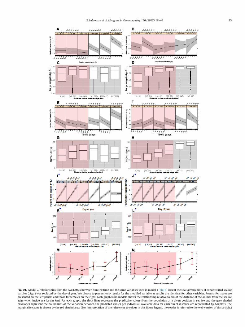
Fig. D1. Model 2, relationships from the two LMMs between hunting time and the same variables used in model 1 (Fig. 8) except the spatial variability of concentrated sea icepatches (A80%) was replaced by the day of year. We choose to present only results for the modified variable as results are identical for other variables. Results for males arepresented on the left panels and those for females on the right. Each graph from models shows the relationship relative to bin of the distance of the animal from the sea iceedge when inside sea ice (in km). For each graph, the thick lines represent the predictive values from the population at a given position in sea ice and the grey shadedenvelopes represent the boundaries of the variation between the predicted values per individual. Available data for each bin of distance are represented by boxplots. Themarginal ice zone is shown by the red shaded area. (For interpretation of the references to colour in this figure legend, the reader is referred to the web version of this article.)


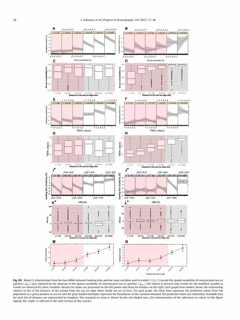
Fig. D2. Model 3, relationships from the two LMMs between hunting time and the same variables used in model 1 (Fig. 8) except the spatial variability of concentrated sea icepatches (A80%) was replaced by the anomaly of the spatial variability of concentrated sea ice patches (A0

80%). We choose to present only results for the modified variable asresults are identical for other variables. Results for males are presented on the left panels and those for females on the right. Each graph from models shows the relationshiprelative to bin of the distance of the animal from the sea ice edge when inside sea ice (in km). For each graph, the thick lines represent the predictive values from thepopulation at a given position in sea ice and the grey shaded envelopes represent the boundaries of the variation between the predicted values per individual. Available datafor each bin of distance are represented by boxplots. The marginal ice zone is shown by the red shaded area. (For interpretation of the references to colour in this figurelegend, the reader is referred to the web version of this article.)



of the trophic ecology of benthic and mesopelagic communitiesthat SESs consume within the sea ice region and their vertical dis-tribution are extremely limited (Costa et al., 2010). Resource limi-tation due to low primary productivity in winter is often regardedas a key factor, however, we show in the present study that foodconsumption of the top predator community such as SESs persistsor increases hundreds of kilometres deep into the pack ice (see alsovan Franeker et al., 1997; Flores et al., 2012b). Biological resourcesin ice-covered regions may have been underestimated by pelagicsampling in the past, and thus may appear poorer than they reallyare (Flores et al., 2012b). Moreover, the current neglect of anautumn bloom from non-detection of ice-associated phytoplank-ton in conventional satellite ocean-colour images may have alsounderestimate the potential of sea ice to sustain a rich under-iceecosystem during winter (Lieser et al., 2015). Thus this work alsocontributes to deepening our knowledge on (i) the functioning ofthe under-ice biological habitat and (ii) ecological mechanisms

Fig. E1. Plot of diving depths (m) and bottom topography under the position of A & C) m2D kernel density estimation (kde2D function from package MASS, from R Development C

that take place in remote and extreme environments with limitedaccess.

The continued sustained monitoring of vertebrate colonies rel-ative to sea ice parameters around the Antarctic coast and islandsis crucial, given the complexity of the impact of climate forcing onbiotic and abiotic components of the Antarctic marine ecosystem(Clarke et al., 2008; Massom and Stammerjohn, 2010).

Acknowledgements

This study is part of French Polar Institute (Institut Paul EmileVictor, IPEV) research project IPEV # 109, PI H. Weimerskirch,and of the Australian collaborative ‘‘Integrated Marine ObservingSystem” (IMOS) research programme. It was funded by a CNES-TOSCA project (‘‘Elephants de mer océanographes”) and IMOS,and supported by the Australian Government through both theNational Collaborative Research Infrastructure Strategy and the

ales and B & D) females relative to their distance from the sea ice edge (km) using aore Team). One contour is drawn every 25 dives for females and 100 dives for males.


Super Science Initiative and the Cooperative Research Centre pro-gramme through the Antarctic Climate & Ecosystems CooperativeResearch Centre. This work was also supported by the Japan Soci-ety for the Promotion of Science Grant-in-Aid for ScientificResearch (KAKENHI) number 25.03748. J.B. Sallée received supportfrom the ERC under the European Union’s Horizon 2020 researchand innovation program (grant agreement 637770). For R. Massom,A. Fraser and P. Reid, the work contributes to AAS Project 4116.MODIS data were obtained from the NASA Atmosphere Archiveand Distribution System (http://ladsweb.nascom.nasa.gov). Passivemicrowave sea ice concentration data were obtained from theUniversity of Bremen (http://www.iup.uni-bremen.de/seaice/amsr/) for AMSR-E, AMSR-2, and from the NASA Earth ObservingSystem Distributed Active Archive Center (DAAC) at the U.S.National Snow and Ice Data Center, University of Colorado(http://www.nsidc.org) for SSMI/S. Special thanks go to J.O. Irisson,S. Bestley, S. Wotherspoon, M. Authier, B. Picard, A. Bosse, M.O’Toole and Y. David for very useful comments. Finally, we wouldlike to thank N. El Skaby and all colleagues and volunteers involvedin the research on southern elephant seals in Kerguelen. All ani-mals in this study were treated in accordance with the IPEV ethicaland Polar Environment Committees guidelines.

Appendix A

See Table A1.

Appendix B

Computation of the anomaly of the spatial variability, A080%:

From March to August-September, an increase of A80% with timewas observed for males and females (Fig. B1A and B); we definedA0

80% by (i) computing the median of the observations from thetime-series of A80% for males and females (black lines, Fig. B1Aand B), (ii) removing this median from each observation to obtainthe anomaly of the spatial variability from its seasonal cycle (here-after denoted A0

80%).

Appendix C

See Fig. C1.

Appendix D

See Figs. D1 and D2.

Appendix E

See Fig. E1.

References

Ainley, D.G., Larue, M.A., Stirling, I., Stammerjohn, S., Siniff, D.B., 2015. An apparentpopulation decrease, or change in distribution, of Weddell seals along theVictoria Land coast. Mar. Mammal Sci. 31, 1338–1361. http://dx.doi.org/10.1111/mms.12220.

Ainley, D., Russell, J., Jenouvrier, S., Woehler, E., Lyver, P.O., Fraser, W.R., Kooyman,G.L., 2010a. Antarctic penguin response to habitat change as Earth’s tropospherereaches 2 C above preindustrial levels. Ecol. Monogr. 80, 49–66.

Ainley, D.G., Fraser, W.R., Smith Jr., W.O., Hopkins, T.L., Torres, J.J., 1991. Thestructure of upper level pelagic food webs in the Antarctic: effect ofphytoplankton distribution. J. Mar. Syst. 2, 111–122.

Ainley, D.G., Fraser, W.R., Sullivan, C.W., Torres, J.J., Hopkins, T.L., Smith, W.O., 1986.Antarctic mesopelagic micronekton: evidence from seabirds that pack iceaffects community structure. Science 232, 847–849.

Ainley, D.G., Tynan, C.T., Stirling, I., 2010b. Sea ice: a critical habitat for polar marinemammals and birds. In: Thomas, D.N., Dieckmann, G.S. (Eds.), Sea Ice 2.Blackwell Science, London, UK, pp. 395–424.

Arrigo, K.R., van Dijken, G.L., 2003. Phytoplankton dynamics within 37 Antarcticcoastal polynya systems. J. Geophys. Res. 108. http://dx.doi.org/10.1029/2002JC001739.

Arrigo, K.R., van Dijken, G.L., Strong, A., 2015. Environmental controls of marineproductivity hot spots around Antarctica. J. Geophys. Res. Oceans 120, 5545–5565. http://dx.doi.org/10.1002/2015JC010888.

Ashford, J., Dinniman, M., Brooks, C., Andrews, A.H., Hofmann, E., Cailliet, G., Jones,C., Ramanna, N., Gillanders, B., 2012. Does large-scale ocean circulationstructure life history connectivity in Antarctic toothfish (Dissostichusmawsoni)? Can. J. Fish. Aquat. Sci. 69, 1903–1919. http://dx.doi.org/10.1139/f2012-111.

Atkinson, A., Siegel, V., Pakhomov, E., Rothery, P., 2004. Long-term decline in krillstock and increase in salps within the Southern Ocean. Nature 432, 100–103.http://dx.doi.org/10.1038/nature02996.

Bailleul, F., Authier, M., Ducatez, S., Roquet, F., Charrassin, J.-B., Cherel, Y., Guinet, C.,2010. Looking at the unseen: combining animal bio-logging and stable isotopesto reveal a shift in the ecological niche of a deep diving predator. Ecography 33,709–719. http://dx.doi.org/10.1111/j.1600-0587.2009.06034.x.

Bailleul, F., Charrassin, J.-B., Ezraty, R., Girard-Ardhuin, F., McMahon, C.R., Field, I.C.,Guinet, C., 2007. Southern elephant seals from Kerguelen Islands confronted byAntarctic Sea ice. Changes in movements and in diving behaviour. Deep Sea Res.Part II 54, 343–355. http://dx.doi.org/10.1016/j.dsr2.2006.11.005.

Banks, J., Lea, M.-A., Wall, S., McMahon, C.R., Hindell, M.A., 2014. Combining bio-logging and fatty acid signature analysis indicates spatio-temporal variation inthe diet of the southern elephant seal, Mirounga leonina. J. Exp. Mar. Biol. Ecol.450, 79–90. http://dx.doi.org/10.1016/j.jembe.2013.10.024.

Barbraud, C., Rolland, V., Jenouvrier, S., Nevoux, M., Delord, K., Weimerskirch, H.,2012. Effects of climate change and fisheries bycatch on Southern Oceanseabirds: a review. Mar. Ecol. Prog. Ser. 454, 285–307. http://dx.doi.org/10.3354/meps09616.

Barbraud, C., Weimerskirch, H., 2006. Antarctic birds breed later in response toclimate change. Proc. Natl. Acad. Sci. 103, 6248–6251.

Barbraud, C., Weimerskirch, H., 2001. Emperor penguins and climate change. Nature411, 183–186.

Bestley, S., Patterson, T.A., Hindell, M.A., Gunn, J.S., 2010. Predicting feeding successin a migratory predator: integrating telemetry, environment, and modelingtechniques. Ecology 91, 2373–2384. http://dx.doi.org/10.1890/08-2019.1.

Biuw, M., Boehme, L., Guinet, C., Hindell, M., Costa, D., Charrassin, J.-B., Roquet, F.,Bailleul, F., Meredith, M., Thorpe, S., 2007. Variations in behaviour and conditionof a Southern Ocean top predator in relation to in situ oceanographicconditions. Proc. Natl. Acad. Sci. 104, 13705–13710.

Biuw, M., Nøst, O.A., Stien, A., Zhou, Q., Lydersen, C., Kovacs, K.M., 2010. Effects ofhydrographic variability on the spatial, seasonal and diel diving patterns ofsouthern elephant seals in the eastern Weddell Sea. PLoS ONE 5, e13816. http://dx.doi.org/10.1371/journal.pone.0013816.

Bluhm, B.A., Gradinger, R.R., Schnack-Schiel, S.B., 2010. Sea ice meio- andmacrofauna. In: Thomas, D.N., Dieckmann, G.S. (Eds.), Sea Ice 2. BlackwellScience, London, UK, pp. 357–394.

Bornemann, H., Kreyscher, M., Ramdohr, S., Martin, T., Carlini, A., Sellmann, L., Plötz,J., 2000. Southern elephant seal movements and Antarctic sea ice. Antarct. Sci.12, 3–15.

Bost, C.-A., Charrassin, J.-B., Clerquin, Y., Ropert-Coudert, Y., Le Maho, Y.others, 2004.Exploitation of distant marginal ice zones by king penguins during winter. Mar.Ecol. Prog. Ser. 283, 293–297.

Bradshaw, C.J.A., Hindell, M.A., Best, N.J., Phillips, K.L., Wilson, G., Nichols, P.D., 2003.You are what you eat: describing the foraging ecology of southern elephantseals (Mirounga leonina) using blubber fatty acids. Proc. R. Soc. B: Biol. Sci. 270,1283–1292. http://dx.doi.org/10.1098/rspb.2003.2371.

Brierley, A.N., Thomas, D.N., 2002. Ecology of Southern Ocean pack ice. Adv. Mar.Biol. 43, 171–276.

Burnham, K.P., Anderson, D.R., 2002. Model Selection and Multi-Model Inference: APractical Information-Theoretic Approach. Springer, New York, USA.

Chambert, T., Rotella, J.J., Garrott, R.A., 2015. Female Weddell seals show flexiblestrategies of colony attendance related to varying environmental conditions.Ecology 96, 479–488. http://dx.doi.org/10.1890/14-0911.1.

Cherel, Y., Ducatez, S., Fontaine, C., Richard, P., Guinet, C., 2008. Stable isotopesreveal the trophic position and mesopelagic fish diet of female southernelephant seals breeding on the Kerguelen Islands. Mar. Ecol. Prog. Ser. 370, 239–247. http://dx.doi.org/10.3354/meps07673.

Cisewski, B., Strass, V.H., 2016. Acoustic insights into the zooplankton dynamics ofthe eastern Weddell Sea. Prog. Oceanogr. 144, 62–92.

Clarke, A., Brierley, A.S., Harris, C.M., Lubin, D., Smith, R.C., 2008. Polar and ice-edgemarine systems. In: Polunin, N.V.C. (Ed.), Aquatic Ecosystems: Trends andGlobal Prospects. Cambridge University Press, Cambridge, UK, pp. 319–333.

Constable, A.J., Melbourne-Thomas, J., Corney, S.P., Arrigo, K.R., Barbraud, C., Barnes,D.K.A., Bindoff, N.L., Boyd, P.W., Brandt, A., Costa, D.P., Davidson, A.T., Ducklow,H.W., Emmerson, L., Fukuchi, M., Gutt, J., Hindell, M.A., Hofmann, E.E., Hosie, G.W., Iida, T., Jacob, S., Johnston, N.M., Kawaguchi, S., Kokubun, N., Koubbi, P., Lea,M.-A., Makhado, A., Massom, R.A., Meiners, K., Meredith, M.P., Murphy, E.J.,Nicol, S., Reid, K., Richerson, K., Riddle, M.J., Rintoul, S.R., Smith, W.O., Southwell,C., Stark, J.S., Sumner, M., Swadling, K.M., Takahashi, K.T., Trathan, P.N.,Welsford, D.C., Weimerskirch, H., Westwood, K.J., Wienecke, B.C., Wolf-Gladrow, D., Wright, S.W., Xavier, J.C., Ziegler, P., 2014. Climate change andSouthern Ocean ecosystems I: how changes in physical habitats directly affectmarine biota. Glob. Change Biol. 20, 3004–3025. http://dx.doi.org/10.1111/gcb.12623.

http://ladsweb.nascom.nasa.gov

http://www.iup.uni-bremen.de/seaice/amsr/

http://www.iup.uni-bremen.de/seaice/amsr/

http://www.nsidc.org

http://dx.doi.org/10.1111/mms.12220

http://dx.doi.org/10.1111/mms.12220

http://refhub.elsevier.com/S0079-6611(16)30044-1/h0010












http://dx.doi.org/10.1029/2002JC001739

http://dx.doi.org/10.1029/2002JC001739

http://dx.doi.org/10.1002/2015JC010888

http://dx.doi.org/10.1139/f2012-111

http://dx.doi.org/10.1139/f2012-111

http://dx.doi.org/10.1038/nature02996

http://dx.doi.org/10.1111/j.1600-0587.2009.06034.x

http://dx.doi.org/10.1016/j.dsr2.2006.11.005

http://dx.doi.org/10.1016/j.jembe.2013.10.024

http://dx.doi.org/10.3354/meps09616






http://dx.doi.org/10.1890/08-2019.1





http://dx.doi.org/10.1371/journal.pone.0013816











http://dx.doi.org/10.1098/rspb.2003.2371





http://dx.doi.org/10.1890/14-0911.1







http://dx.doi.org/10.1111/gcb.12623

http://dx.doi.org/10.1111/gcb.12623


Costa, D.P., Huckstadt, L.A., Crocker, D.E., McDonald, B.I., Goebel, M.E., Fedak, M.A.,2010. Approaches to studying climatic change and its role on the habitatselection of Antarctic Pinnipeds. Integr. Comp. Biol. 50, 1018–1030. http://dx.doi.org/10.1093/icb/icq054.

Daneri, G., Carlini, A., 2002. Fish prey of southern elephant seals, Mirounga leonina,at King George Island. Polar Biol. 25, 739–743.

David, C., Schaafsma, F.L., van Franeker, J.A., Lange, B., Brandt, A., Flores, H., 2016.Community structure of under-ice fauna in relation to winter sea-ice habitatproperties from the Weddell Sea. Polar Biol. http://dx.doi.org/10.1007/s00300-016-1948-4.

Deibel, D., Daly, K.L., 2007. Zooplankton Processes in Arctic and Antarctic Polynyas.In: Smith, W.O., Barber, D.G. (Eds), Polynyas: Windows to the World. ElsevierOceanography Series, vol. 74. Elsevier, pp. 271–322. doi: http://dx.doi.org/10.1016/S0422-9894(06)74009-0.

Donnelly, J., Sutton, T.T., Torres, J.J., 2006. Distribution and abundance ofmicronekton and macrozooplankton in the NW Weddell Sea: relation to aspring ice-edge bloom. Polar Biol. 29, 280–293. http://dx.doi.org/10.1007/s00300-005-0051-z.

Ducklow, H.W., Baker, K., Martinson, D.G., Quetin, L.B., Ross, R.M., Smith, R.C.,Stammerjohn, S.E., Vernet, M., Fraser, W., 2007. Marine pelagic ecosystems: theWest Antarctic Peninsula. Philos. Trans. R. Soc. B: Biol. Sci. 362, 67–94. http://dx.doi.org/10.1098/rstb.2006.1955.

Eicken, H., 1992. The role of sea ice in structuring Antarctic ecosystems. Polar Biol.12, 3–13.

Flores, H., Van de Putte, A., Siegel, V., Pakhomov, E., van Franeker, J., Meesters, H.,Volckaert, F., 2008. Distribution, abundance and ecological relevance of pelagicfishes in the Lazarev Sea, Southern Ocean. Mar. Ecol. Prog. Ser. 367, 271–282.http://dx.doi.org/10.3354/meps07530.

Flores, H., van Franeker, J.-A., Cisewski, B., Leach, H., Van de Putte, A.P., Meesters, E.H.W.G., Bathmann, U., Wolff, W.J., 2011. Macrofauna under sea ice and in theopen surface layer of the Lazarev Sea, Southern Ocean. Deep Sea Res. Part II 58,1948–1961. http://dx.doi.org/10.1016/j.dsr2.2011.01.010.

Flores, H., Atkinson, A., Kawaguchi, S., Krafft, B., Milinevsky, G., Nicol, S., Reiss, C.,Tarling, G., Werner, R., Bravo Rebolledo, E., Cirelli, V., Cuzin-Roudy, J., Fielding,S., van Franeker, J., Groeneveld, J., Haraldsson, M., Lombana, A., Marschoff, E.,Meyer, B., Pakhomov, E., Van de Putte, A., Rombolá, E., Schmidt, K., Siegel, V.,Teschke, M., Tonkes, H., Toullec, J., Trathan, P., Tremblay, N., Werner, T., 2012a.Impact of climate change on Antarctic krill. Mar. Ecol. Prog. Ser. 458, 1–19.http://dx.doi.org/10.3354/meps09831.

Flores, H., van Franeker, J.A., Siegel, V., Haraldsson, M., Strass, V., Meesters, E.H.,Bathmann, U., Wolff, W.J., 2012b. The association of Antarctic krill Euphausiasuperba with the under-ice habitat. PLoS ONE 7, e31775. http://dx.doi.org/10.1371/journal.pone.0031775.

Forcada, J., Trathan, P.N., Boveng, P.L., Boyd, I.L., Burns, J.M., Costa, D.P., Fedak, M.,Rogers, T.L., Southwell, C.J., 2012. Responses of Antarctic pack-ice seals toenvironmental change and increasing krill fishing. Biol. Cons. 149, 40–50.http://dx.doi.org/10.1016/j.biocon.2012.02.002.

Fraser, W.R., Hofmann, E.E., 2003. A predator’s perspective on causal links betweenclimate change, physical forcing and ecosystem. Mar. Ecol. Progr. Series 265, 1–15.

Freckleton, R.P., 2011. Dealing with collinearity in behavioural and ecological data:model averaging and the problems of measurement error. Behav. Ecol.Sociobiol. 65, 91–101. http://dx.doi.org/10.1007/s00265-010-1045-6.

Fritsen, C.H., Lytle, V.I., Ackley, S.F., Sullivan, C.W., 1994. Autumn Bloom of AntarcticPack-Ice Algae. Science 266, 782–784. http://dx.doi.org/10.1126/science.266.5186.782.

Fuiman, L., Davis, R., Williams, T., 2002. Behaviour of midwater fishes under theAntarctic ice: observations by a predator. Mar. Biol. 140, 815–822. http://dx.doi.org/10.1007/s00227-001-0752-y.

Grebmeier, J.M., Barry, J.P., 2007. Benthic Processes in Polynyas. In: Smith, W.O.,Barber, D.G. (Eds.), Polynyas: Windows to the World. Elsevier OceanographySeries, vol. 74. Elsevier, pp. 363–390. doi: http://dx.doi.org/10.1016/S0422-9894(06)74011-9.

Guinet, C., Cherel, Y., Ridoux, V., Jouventin, P., 1996. Consumption of marineresources by seabirds and seals in Crozet and Kerguelen waters: changes inrelation to consumer biomass 1962–85. Antarct. Sci. 8, 23–30.

Guinet, C., Vacquié-Garcia, J., Picard, B., Bessigneul, G., Lebras, Y., Dragon, A., Viviant,M., Arnould, J., Bailleul, F., 2014. Southern elephant seal foraging success inrelation to temperature and light conditions: insight into prey distribution. Mar.Ecol. Prog. Ser. 499, 285–301. http://dx.doi.org/10.3354/meps10660.

Heerah, K., Hindell, M., Andrew-Goff, V., Field, I., McMahon, C.R., Charrassin, J.-B.,2017. Contrasting behavior between two populations of an ice-obligatepredator in East Antarctica. Ecol. Evol. 7, 606–618. http://dx.doi.org/10.1002/ece3.2652.

Heerah, K., Hindell, M., Guinet, C., Charrassin, J.-B., 2015. From high-resolution tolow-resolution dive datasets: a new index to quantify the foraging effort ofmarine predators. Anim. Biotelemetry 3. http://dx.doi.org/10.1186/s40317-015-0074-3.

Hindell, M.A., McMahon, C.R., Bester, M.N., Boehme, L., Costa, D., Fedak, M.A.,Guinet, C., Herraiz-Borreguero, L., Harcourt, R.G., Huckstadt, L., Kovacs, K.M.,Lydersen, C., McIntyre, T., Muelbert, M.M.C., Patterson, T., Roquet, F., Williams,G., Charrassin, J.B., 2016. Circumpolar habitat use in the southern elephant seal:implications for foraging success and population trajectories. Ecosphere 7.

Hindell, M.A., Bradshaw, C.J., Sumner, M.D., Michael, K.J., Burton, H.R., 2003.Dispersal of female southern elephant seals and their prey consumption during

the austral summer: relevance to management and oceanographic zones. J.Appl. Ecol. 40, 703–715.

Hindell, M.A., Burton, H.R., Slip, D.J., 1991a. Foraging areas of southern elephantseals, Mirounga leonina, as inferred from water temperature data. Mar. Freshw.Res. 42, 115–128.

Hindell, M.A., Slip, D.J., Burton, H.R., 1991b. The diving behaviour of adult male andfemale Southern Elephant Seals, Mirounga Leonina (Pinnipedia, Phocidae).Austral. J. Zool. 39, 595–619.

Horning, M., Mellish, J., 2009. Spatially explicit detection of predation on individualpinnipeds from implanted post-mortem satellite data transmitters. EndangeredSpecies Res. 10, 135–143. http://dx.doi.org/10.3354/esr00220.

Jenouvrier, S., Holland, M., Stroeve, J., Barbraud, C., Weimerskirch, H., Serreze, M.,Caswell, H., 2012. Effects of climate change on an emperor penguin population:analysis of coupled demographic and climate models. Glob. Change Biol. 18,2756–2770. http://dx.doi.org/10.1111/j.1365-2486.2012.02744.x.

Jouma’a, J., Le Bras, Y., Richard, G., Vacquié-Garcia, J., Picard, B., El Ksabi, N., Guinet,C., 2016. Adjustment of diving behaviour with prey encounters and bodycondition in a deep diving predator: the Southern Elephant Seal. Funct. Ecol. 30,636–648. http://dx.doi.org/10.1111/1365-2435.12514.

Karnovsky, N., Ainley, D.G., Lee, P., 2007. The Impact and Importance of Productionin Polynyas to Top-Trophic Predators: Three Case Histories. In: Smith, W.O.,Barber, D.G. (Eds.), Polynyas: Windows to the World. Elsevier OceanographySeries, vol. 74. Elsevier, pp. 391–410. doi: http://dx.doi.org/10.1016/S0422-9894(06)74012-0.

Kaufmann, R.S., Smith Jr, K.L., Baldwin, R.J., Glatts, R.C., Robison, B.H., Reisenbichler,K.R., 1995. Effects of seasonal pack ice on the distribution of macrozooplanktonand micronekton in the northwestern Weddell Sea. Mar. Biol. 124, 387–397.

Labrousse, S., Vacquié-Garcia, J., Heerah, K., Guinet, C., Sallée, J.-B., Authier, M.,Picard, B., Roquet, F., Bailleul, F., Hindell, M., Charrassin, J.-B., 2015. Winter useof sea ice and ocean water mass habitat by southern elephant seals: the lengthand breadth of the mystery. Prog. Oceanogr. 137, 52–68. http://dx.doi.org/10.1016/j.pocean.2015.05.023.

La Mesa, M., Catalano, B., Russo, A., Greco, S., Vacchi, M., Azzali, M., 2010. Influenceof environmental conditions on spatial distribution and abundance of early lifestages of Antarctic silverfish, Pleuragramma antarcticum (Nototheniidae), in theRoss Sea. Antarct. Sci. 22, 243–254. http://dx.doi.org/10.1017/S0954102009990721.

Lancraft, T.M., Hopkins, T.L., Torres, J.J., Donnelly, J., 1991. Oceanicmicronektonic/macrozooplanktonic community structure and feeding in icecovered Antarctic waters during the winter (AMERIEZ 1988). Polar Biol. 11,157–167.

Lancraft, T.M., Torres, J.J., Hopkins, T.L., 1989. Micronekton and macrozooplanktonin the open waters near Antarctic ice edge zones (AMERIEZ 1983 and 1986).Polar Biol. 9, 225–233.

Lieser, J.L., Curran, M.A.J., Bowie, A.R., Davidson, A.T., Doust, S.J., Fraser, A.D., Galton-Fenzi, B.K., Massom, R.A., Meiners, K.M., Melbourne-Thomas, J., Reid, P.A.,Strutton, P.G., Vance, T.R., Vancoppenolle, M., Westwood, K.J., Wright, S.W.,2015. Antarctic slush-ice algal accumulation not quantified throughconventional satellite imagery: beware the ice of March. Cryosphere Discuss.9, 6187–6222. http://dx.doi.org/10.5194/tcd-9-6187-2015, unpublished.

Loeb, V., Siegel, V., Holm-Hansen, O., Hewitt, R., Fraser, W., Trivelpiece, W.,Trivelpiece, S., 1997. Effects of sea-ice extent and krill or salp dominance on theAntarctic foodweb. Nature 387, 897–900.

Marschall, H.-P., 1988. The overwintering strategy of Antarctic krill under the pack-ice of the Weddell Sea. Polar Biol. 9, 129–135.

Massom, R.A., Stammerjohn, S.E., 2010. Antarctic sea ice change and variability –physical and ecological implications. Polar Sci. 4, 149–186. http://dx.doi.org/10.1016/j.polar.2010.05.001.

Massom, R.A., Stammerjohn, S.E., Smith, R.C., Pook, M.J., Iannuzzi, R.A., Adams, N.,Martinson, D.G., Vernet, M., Fraser, W.R., Quetin, L.B.others, 2006. ExtremeAnomalous Atmospheric Circulation in the West Antarctic Peninsula Region inAustral Spring and Summer 2001/02, and Its Profound Impact on Sea Ice andBiota. J. Clim. 19, 3544–3571.

Massom, R., Hill, K., Barbraud, C., Adams, N., Ancel, A., Emmerson, L., Pook, M., 2009.Fast ice distribution in Adélie Land, East Antarctica: interannual variability andimplications for emperor penguins Aptenodytes forsteri. Mar. Ecol. Prog. Ser. 374,243–257. http://dx.doi.org/10.3354/meps07734.

Massom, R., Reid, P., Stammerjohn, S., Raymond, B., Fraser, A., Ushio, S., 2013.Change and variability in East Antarctic sea ice seasonality, 1979/80–2009/10.PLoS ONE 8, e64756. http://dx.doi.org/10.1371/journal.pone.0064756.

McConnell, B.J., Chambers, C., Fedak, M.A., 1992. Foraging ecology of southernelephant seals in relation to the bathymetry and productivity of the SouthernOcean. Antarct. Sci. 4, 393–398.

McMahon, C.R., Bester, M.N., Burton, H.R., Hindell, M.A., Bradshaw, C.J., 2005.Population status, trends and a re-examination of the hypotheses explainingthe recent declines of the southern elephant seal Mirounga leonina. MammalRev. 35, 82–100.

Meiners, K.M., Vancoppenolle, M., Thanassekos, S., Dieckmann, G.S., Thomas, D.N.,Tison, J.-L., Arrigo, K.R., Garrison, D.L., McMinn, A., Lannuzel, D., van der Merwe,P., Swadling, K.M., Smith, W.O., Melnikov, I., Raymond, B., 2012. Chlorophyll a inAntarctic sea ice from historical ice core data. Geophys. Res. Lett. 39, L21602.http://dx.doi.org/10.1029/2012GL053478.

Nakagawa, S., Schielzeth, H., 2013. A general and simple method for obtaining R2

from generalized linear mixed-effects models. Methods Ecol. Evol. 4, 133–142.http://dx.doi.org/10.1111/j.2041-210x.2012.00261.x.

http://dx.doi.org/10.1093/icb/icq054

http://dx.doi.org/10.1093/icb/icq054



http://dx.doi.org/10.1007/s00300-016-1948-4

http://dx.doi.org/10.1007/s00300-016-1948-4

http://dx.doi.org/10.1016/S0422-9894(06)74009-0

http://dx.doi.org/10.1016/S0422-9894(06)74009-0

http://dx.doi.org/10.1007/s00300-005-0051-z

http://dx.doi.org/10.1007/s00300-005-0051-z

http://dx.doi.org/10.1098/rstb.2006.1955





http://dx.doi.org/10.1016/j.dsr2.2011.01.010




http://dx.doi.org/10.1016/j.biocon.2012.02.002




http://dx.doi.org/10.1007/s00265-010-1045-6

http://dx.doi.org/10.1126/science.266.5186.782

http://dx.doi.org/10.1126/science.266.5186.782

http://dx.doi.org/10.1007/s00227-001-0752-y

http://dx.doi.org/10.1007/s00227-001-0752-y

http://dx.doi.org/10.1016/S0422-9894(06)74011-9

http://dx.doi.org/10.1016/S0422-9894(06)74011-9





http://dx.doi.org/10.1002/ece3.2652

http://dx.doi.org/10.1002/ece3.2652

http://dx.doi.org/10.1186/s40317-015-0074-3

http://dx.doi.org/10.1186/s40317-015-0074-3
















http://dx.doi.org/10.3354/esr00220

http://dx.doi.org/10.1111/j.1365-2486.2012.02744.x

http://dx.doi.org/10.1111/1365-2435.12514

http://dx.doi.org/10.1016/S0422-9894(06)74012-0

http://dx.doi.org/10.1016/S0422-9894(06)74012-0






http://dx.doi.org/10.1017/S0954102009990721

http://dx.doi.org/10.1017/S0954102009990721








http://dx.doi.org/10.5194/tcd-9-6187-2015,unpublished






http://dx.doi.org/10.1016/j.polar.2010.05.001

http://dx.doi.org/10.1016/j.polar.2010.05.001















http://dx.doi.org/10.1029/2012GL053478

http://dx.doi.org/10.1111/j.2041-210x.2012.00261.x


Nakagawa, S., Schielzeth, H., 2010. Repeatability for Gaussian and non-Gaussiandata: a practical guide for biologists. Biol. Rev. 85, 935–956. http://dx.doi.org/10.1111/j.1469-185X.2010.00141.x.

Nicol, S., 2006. Krill, currents, and sea ice: Euphausia superba and its changingenvironment. Bioscience 56, 111–120.

Nicol, S., Pauly, T., Bindoff, N.L., Wright, S., 2000. Ocean circulation off eastAntarctica affects ecosystem structure and sea-ice extent. Science 260, 1617–1623.

Parkinson, C.L., Cavalieri, D.J., 2012. Antarctic sea ice variability and trends, 1979–2010. The Cryosphere 6, 871–880. http://dx.doi.org/10.5194/tc-6-871-2012.

Pinheiro, J., Bates, D., DebRoy, S., Sarkar D., R Core Team, 2015. nlme: Linear andNonlinear Mixed Effects Models. R package version 3.1-122, <http://CRAN.R-project.org/package=nlme>.

Pitman, R., 2011. Antarctic killer whales: top of the food chain at the bottom of theworld. J. Am. Cetacean Soc. 40, 39–45.

Proffitt, K.M., Garrott, R.A., Rotella, J.J., Siniff, D.B., Testa, J.W., 2007. Exploringlinkages between abiotic oceanographic processes and a top-trophic predator inan Antarctic ecosystem. Ecosystems 10, 120–127. http://dx.doi.org/10.1007/s10021-006-9003-x.

Raymond, B., Lea, M.-A., Patterson, T., Andrews-Goff, V., Sharples, R., Charrassin, J.-B., Cottin, M., Emmerson, L., Gales, N., Gales, R., Goldsworthy, S.D., Harcourt, R.,Kato, A., Kirkwood, R., Lawton, K., Ropert-Coudert, Y., Southwell, C., van denHoff, J., Wienecke, B., Woehler, E.J., Wotherspoon, S., Hindell, M.A., 2015.Important marine habitat off east Antarctica revealed by two decades of multi-species predator tracking. Ecography 38, 121–129. http://dx.doi.org/10.1111/ecog.01021.

Reid, K., Croxall, J.P., 2001. Environmental response of upper trophic-level predatorsreveals a system change in an Antarctic marine ecosystem. Proc. R. Soc. B: Biol.Sci. 268, 377–384. http://dx.doi.org/10.1098/rspb.2000.1371.

Siegel, V., 2012. Krill stocks in high latitudes of the Antarctic Lazarev Sea: seasonaland interannual variation in distribution, abundance and demography. PolarBiol. 35, 1151–1177. http://dx.doi.org/10.1007/s00300-012-1162-y.

Siniff, D.B., Garrott, R.A., Rotella, J.J., Fraser, W.R., Ainley, D.G., 2008. Opinion:projecting the effects of environmental change on Antarctic seals. Antarct. Sci.20, 425–435. http://dx.doi.org/10.1017/S0954102008001351.

Smith, W.O., Ainley, D.G., Cattaneo-Vietti, R., 2007. Trophic interactions within theRoss Sea continental shelf ecosystem. Philos. Trans. R. Soc. B: Biol. Sci. 362, 95–111. http://dx.doi.org/10.1098/rstb.2006.1956.

Southwell, C., Emmerson, L., McKinlay, J., Newbery, K., Takahashi, A., Kato, A.,Barbraud, C., DeLord, K., Weimerskirch, H., 2015. Spatially extensivestandardized surveys reveal widespread, multi-decadal increase in EastAntarctic Adélie penguin populations. PLoS ONE 10, e0139877. http://dx.doi.org/10.1371/journal.pone.0139877.

Squire, V.A., 2007. Of ocean waves and sea-ice revisited. Cold Reg. Sci. Technol. 49,110–133. http://dx.doi.org/10.1016/j.coldregions.2007.04.007.

Stammerjohn, S.E., Martinson, D.G., Smith, R.C., Yuan, X., Rind, D., 2008. Trends inAntarctic annual sea ice retreat and advance and their relation to El Niño-

Southern Oscillation and Southern Annular Mode variability. J. Geophys. Res.113. http://dx.doi.org/10.1029/2007JC004269.

Stammerjohn, S.E., Smith, R.C., 1997. Opposing Southern Ocean climate patterns asrevealed by trends in regional sea ice coverage. Clim. Change 37, 617–639.

Stammerjohn, S., Massom, R., Rind, D., Martinson, D., 2012. Regions of rapid sea icechange: an inter-hemispheric seasonal comparison:regions of rapid sea icechange. Geophys. Res. Lett. 39. http://dx.doi.org/10.1029/2012GL050874.

Steffens, M., Piepenburg, D., Schmid, M.K., 2006. Distribution and structure ofmacrobenthic fauna in the eastern Laptev Sea in relation to environmentalfactors. Polar Biol. 29, 837–848. http://dx.doi.org/10.1007/s00300-006-0122-9.

Trathan, P., Forcada, J., Murphy, E., 2007. Environmental forcing and Southern Oceanmarine predator populations: effects of climate change and variability. Philos.Trans. R. Soc. B: Biol. Sci. 362, 2351–2365. http://dx.doi.org/10.1098/rstb.2006.1953.

Tremblay, J.-E., Smith, W.O., 2007. Primary Production and Nutrient Dynamics inPolynyas. In: Smith, W.O., Barber, D.G. (Eds.), Polynyas: Windows to the World.Elsevier Oceanography Series, vol. 74. Elsevier, pp. 239–269. doi: http://dx.doi.org/10.1016/S0422-9894(06)74008-9.

Trivelpiece, W.Z., Hinke, J.T., Miller, A.K., Reiss, C.S., Trivelpiece, S.G., Watters, G.M.,2011. Variability in krill biomass links harvesting and climate warming topenguin population changes in Antarctica. Proc. Natl. Acad. Sci. 108, 7625–7628. http://dx.doi.org/10.1073/pnas.1016560108.

van den Hoff, J., McMahon, C.R., Simpkins, G.R., Hindell, M.A., Alderman, R., Burton,H.R., 2014. Bottom-up regulation of a pole-ward migratory predator population.Proc. R. Soc. B: Biol. Sci. 281. http://dx.doi.org/10.1098/rspb.2013.2842.20132842–20132842.

van Franeker, J.A., Bathmann, U.V., Mathot, S., 1997. Carbon fluxes to antarctic toppredators. Deep Sea Res. Part II 44, 435–455. http://dx.doi.org/10.1016/S0967-0645(96)00078-1.

Wadhams, P., 2000. Ice in the Ocean. Gordon and Breach, Australia.Walters, A., Lea, M.-A., van den Hoff, J., Field, I.C., Virtue, P., Sokolov, S., Pinkerton, M.

H., Hindell, M.A., 2014. Spatially explicit estimates of prey consumption reveal anew krill predator in the Southern Ocean. PLoS ONE 9, e86452. http://dx.doi.org/10.1371/journal.pone.0086452.

Watwood, S.L., Miller, P.J.O., Johnson, M., Madsen, P.T., Tyack, P.L., 2006. Deep-diving foraging behaviour of sperm whales (Physeter macrocephalus). J. Anim.Ecol. 75, 814–825. http://dx.doi.org/10.1111/j.13652656.2006.01101.x.

Weimerskirch, H., Inchausti, P., Guinet, C., Barbraud, C., 2003. Trends in bird andseal populations as indicators of a system shift in the Southern Ocean. Antarct.Sci. 15, 249–256. http://dx.doi.org/10.1017/S0954102003001202.

Zuur, A.F., Ieno, E.N., Elphick, C.S., 2010. A protocol for data exploration to avoidcommon statistical problems: data exploration. Methods Ecol. Evol. 1, 3–14.http://dx.doi.org/10.1111/j.2041-210X.2009.00001.x.

Zuur, A., Ieno, E.N., Walker, N.J., Saheliev, A.A., Smith, G.N., 2009. Mixed EffectsModels and Extensions in Ecology With R. Springer, New York, USA.

http://dx.doi.org/10.1111/j.1469-185X.2010.00141.x







http://dx.doi.org/10.5194/tc-6-871-2012

http://CRAN.R-project.org/package=nlme

http://CRAN.R-project.org/package=nlme



http://dx.doi.org/10.1007/s10021-006-9003-x

http://dx.doi.org/10.1007/s10021-006-9003-x

http://dx.doi.org/10.1111/ecog.01021

http://dx.doi.org/10.1111/ecog.01021


http://dx.doi.org/10.1007/s00300-012-1162-y

http://dx.doi.org/10.1017/S0954102008001351




http://dx.doi.org/10.1016/j.coldregions.2007.04.007

http://dx.doi.org/10.1029/2007JC004269



http://dx.doi.org/10.1029/2012GL050874

http://dx.doi.org/10.1007/s00300-006-0122-9



http://dx.doi.org/10.1016/S0422-9894(06)74008-9

http://dx.doi.org/10.1016/S0422-9894(06)74008-9

http://dx.doi.org/10.1073/pnas.1016560108


http://dx.doi.org/10.1016/S0967-0645(96)00078-1

http://dx.doi.org/10.1016/S0967-0645(96)00078-1




http://dx.doi.org/10.1111/j.13652656.2006.01101.x

http://dx.doi.org/10.1017/S0954102003001202




Documents

Under the sea ice: Exploring the relationship between sea ... · Under the sea ice: Exploring the relationship between sea ice and the foraging behaviour of southern elephant seals