Josh ReissCentre for Digital MusicQueen Mary, University of London

www.elec.qmul.ac.uk/digitalmusic/audioengineering/

UNDER THE HOOD OF A DYNAMIC RANGE COMPRESSOR

With thanks to Michael Massberg and Dimitrios GiannoulisWith thanks to Michael Massberg and imitrios Giannoulis

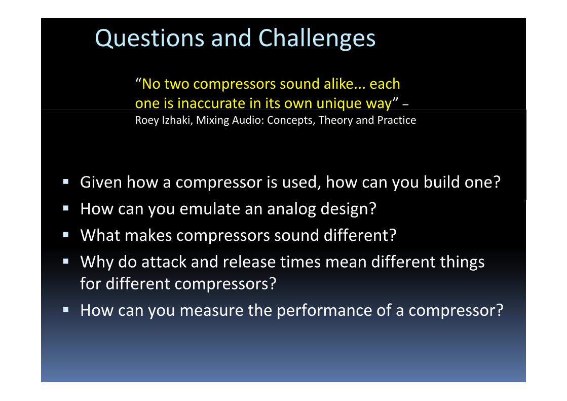
Questions and Challenges

“No two compressors sound alike... each one is inaccurate in its own unique way” –q yRoey Izhaki, Mixing Audio: Concepts, Theory and Practice

Given how a compressor is used, how can you build one?

How can you emulate an analog design?

What makes compressors sound different?

Why do attack and release times mean different things for different compressors?p

How can you measure the performance of a compressor?

What we’re not going to talk aboutHow to use a dynamic range compressorPreferred parameter settings for different tasksPreferred parameter settings for different tasks

How not to use a dynamic range compressor (Loudness war)(Loudness war)But will show how better design helps prevent misuse

Hearing aidsStill applicable, but we’re concerned with compressors for pp pmusic production, mastering and broadcast

Sidechaining and parallel compressionSidechaining and parallel compression

Multiband compressiondd lAdditional parametersLook‐ahead, hold...

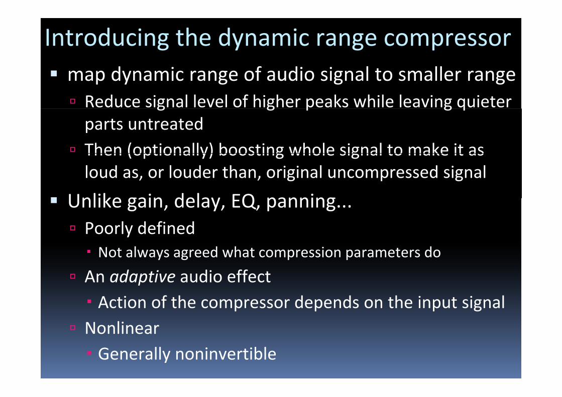
Introducing the dynamic range compressormap dynamic range of audio signal to smaller range Reduce signal level of higher peaks while leaving quieter g g p g qparts untreatedThen (optionally) boosting whole signal to make it asThen (optionally) boosting whole signal to make it as loud as, or louder than, original uncompressed signal

Unlike gain delay EQ panningUnlike gain, delay, EQ, panning... Poorly definedNot always agreed what compression parameters do

An adaptive audio effectAction of the compressor depends on the input signal

NonlinearNonlinearGenerally noninvertible

Compressor ControlsThreshold‐ T

level above which compression starts

Ratio‐ Rdetermines the amount of compression applied.p pp

Knee Width‐ WControls transition in the ratio around the thresholdControls transition in the ratio around the threshold

Make‐up Gain‐ MU d t t h th t t i l’ ll l d t th i i lUsed to match the output signal’s overall loudness to the original

Attack Time‐ τATime to decrease gain once signal overshoots threshold

Release Time‐ τRRTime to bring gain back to normal once signal falls below threshold

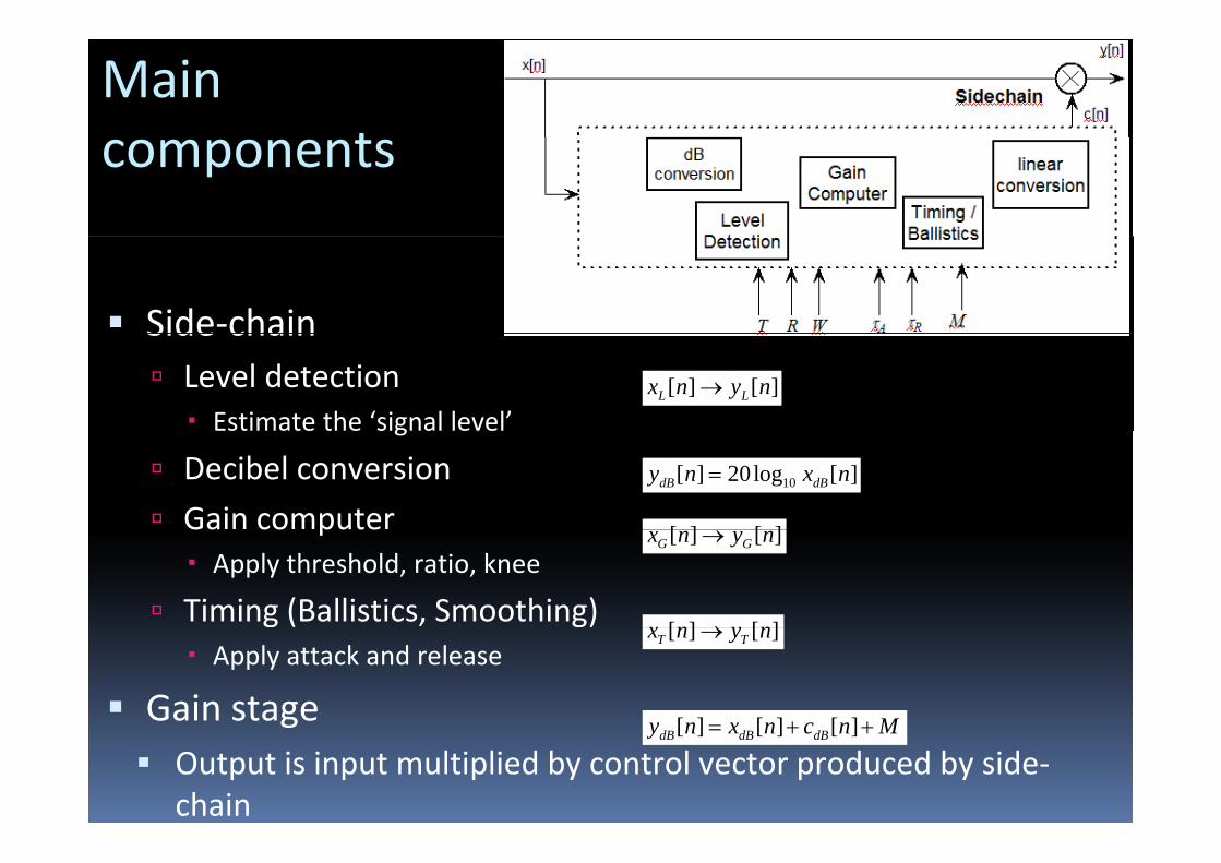
Main tcomponents

Side‐chainSide chainLevel detectionEstimate the ‘signal level’

[ ] [ ]L Lx n y n→

g

Decibel conversion

Gain computer [ ] [ ]

10[ ] 20log [ ]dB dBy n x n=

Ga co puteApply threshold, ratio, knee

Timing (Ballistics, Smoothing)

[ ] [ ]G Gx n y n→

[ ] [ ]x n y n→Apply attack and release

Gain stage [ ] [ ] [ ]y n x n c n M= + +

[ ] [ ]T Tx n y n→

gOutput is input multiplied by control vector produced by side‐chain

[ ] [ ] [ ]dB dB dBy n x n c n M= + +

Level Detection – the options

Peak vs RMSPeak detection Based on absolute value of the signalPeak detection ‐ Based on absolute value of the signal

RMS B d f th i l

[ ] | [ ] |L Ly n x n=

RMS ‐ Based on square of the signalSquare of the level is average of square of the input

/ 2 11 M

Or Square of the level is smoothed estimate of square of the input

/ 2 12 2

/2

1[ ] [ ]M

L Lm M

y n x n mM

−

=−

= −∑

q q p2 2 2[ ] (1 ) [ 1] [ ]L L Ly n y n x nα α= − − +

Exponential Moving Average Filter

Also known as smoothing filter one pole low pass filter

[ ] [ 1] (1 ) [ ]y n y n x nα α= − + −

Also known as smoothing filter, one pole low pass filter...

Step response[ ] 1 for [ ] 1, 1ny n x n nα= − = ≥

Time constant ‐ time it takes a system to reach 1‐1/e= 63% 

y

y /of its final value 1[ ] 1 1sf

sy f eττ α −= − = −→

1/ sfe τα −=

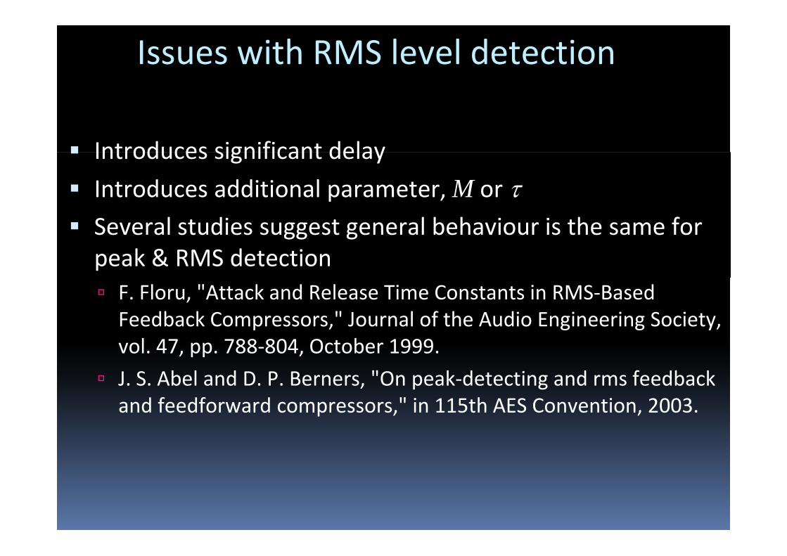
Issues with RMS level detection

Introduces significant delayIntroduces significant delay

Introduces additional parameter, M or τSeveral studies suggest general behaviour is the same for peak & RMS detection

F. Floru, "Attack and Release Time Constants in RMS‐Based Feedback Compressors," Journal of the Audio Engineering Society, l 47 788 804 O t b 1999vol. 47, pp. 788‐804, October 1999.

J. S. Abel and D. P. Berners, "On peak‐detecting and rms feedback and feedforward compressors " in 115th AES Convention 2003and feedforward compressors,  in 115th AES Convention, 2003.

The Gain Computer

Static Compression Curve

0

10

-5

0

dB)

Knee Width

-20

-15

-10

y G (

-30

-25

20

GainMake-up No compression

5:1 compression, hard knee5 1 i ft k

-40

-35

5:1 compression, soft knee

-45-45 -40 -35 -30 -25 -20 -15 -10 -5 0

xG (dB)

Threshold

The Gain Computer-15

-10

-5

0

y G (d

B)

Knee Width

Compression ratio-30

-25

-20

-15

GainMake-up No compression

5:1 compression, hard knee 5:1 compression, soft kneeCompression ratio

Hard knee GG

x TR for x T

y T−

= > -45

-40

-35

-45 -40 -35 -30 -25 -20 -15 -10 -5 0x (dB)

Threshold

Gy T−

( ) /G G

GG G

x x Ty

T x T R x T≤⎧

= ⎨ + − >⎩

xG (dB)

Soft kneeLinear interpolation (bad)

2( )/ 2 ( / 2)(1 1/ ) / 2 2 | ( ) |

( ) / 2( )

G G

G G G

G G

x x T Wy T W x T W R x T W

T x T R x T W

− < −⎧⎪= − + − + + − ≤⎨⎪ + − − >⎩

Second order interpolation (good)

2

2( )G Gx x T W− < −⎧⎪ 2(1/ 1)( / 2) / (2 ) 2 | ( ) |

( ) / 2( )G G G G

G G

y x R x T W W x T WT x T R x T W

⎪= + − − + − ≤⎨⎪ + − − >⎩

Time constantsFrom the smoothing filter

Officially, time it takes a system to reach 1‐1/e= 63% of y, y / %its final valueτ – level starts at 0 goes to 1 Attack time is the time itτA – level starts at 0, goes to 1. Attack time is the time it takes for level to reach 0.63.

τ – level starts at 1 goes to 0 Release time is the time itτR – level starts at 1, goes to 0. Release time is the time it takes for level to reach 1‐0.63=0.37.

But some compressorsBut some compressors,Miscalculate it

Define it as time to go from 90% of initial value to 10% of final value

Define it as time to change level by so many dBs

...

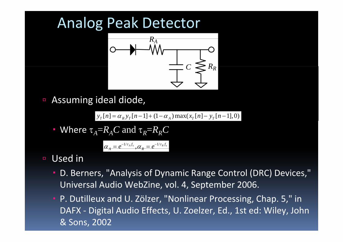
Analog Peak DetectorRRA

RC RRC

Assuming ideal diode,[ ] [ 1] (1 ) max( [ ] [ 1],0)T R T A T Ty n y n x n y nα α= − + − − −

Where τA=RAC and τR=RRC1/ 1/,A s R sf f

A Re eτ τα α− −= =

Used inD. Berners, "Analysis of Dynamic Range Control (DRC) Devices," 

,A R

D. Berners,  Analysis of Dynamic Range Control (DRC) Devices,  Universal Audio WebZine, vol. 4, September 2006.

P. Dutilleux and U. Zölzer, "Nonlinear Processing, Chap. 5," in g pDAFX ‐ Digital Audio Effects, U. Zoelzer, Ed., 1st ed: Wiley, John & Sons, 2002

Analog Peak Detector 1.0

Input signalP k d t t 50 l ti0.9

0.8

0.7

0.6e

Peak detector, 50ms release time Peak detector, 200ms release time Peak detector, 500ms release time

0.6

0.5

0.4

0.3

Volta

g

0.2

0.1

0.01.00.90.80.70.60.50.40.30.20.10.0

Time (sec)Time (sec)

Step response1

0

1[ ] (1 ) ( 1)

2

nm A R

A R Am R A R A

y nα τ

α α αα α τ τ

−

=

−= − + − → ≈

− − +∑

correct peak estimate only when release time is considerably longer than attack timeattack time gets slightly scaled by release timefaster attack time than expected when we use a fast releasefaster attack time than expected when we use a fast release time

Decoupled Peak Detector_

+

RA

CARRCR

CA

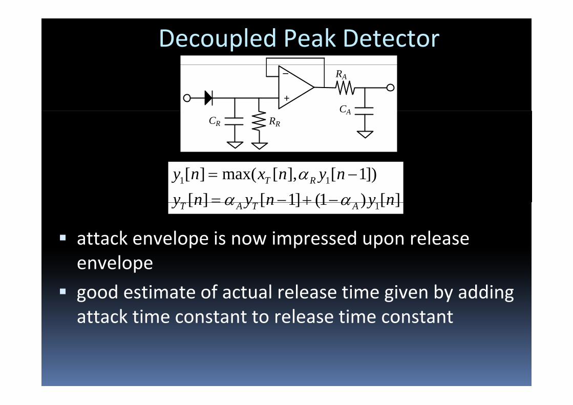
1 1[ ] max( [ ], [ 1])[ ] [ 1] (1 ) [ ]

T Ry n x n y ny n y n y n

αα α

= −= − + − 1[ ] [ 1] (1 ) [ ]T A T Ay n y n y nα α+

attack envelope is now impressed upon release envelope

good estimate of actual release time given by addinggood estimate of actual release time given by adding attack time constant to release time constant

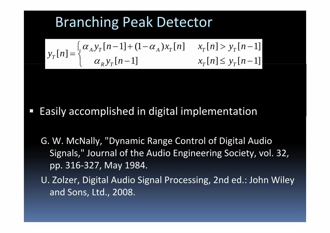
Branching Peak Detector[ 1] (1 ) [ ] [ ] [ 1]

[ ][ 1] [ ] [ 1]

A T A T T TT

R T T T

y n x n x n y ny n

y n x n y nα α

α− + − > −⎧

= ⎨ − ≤ −⎩ [ 1] [ ] [ 1]R T T Ty n x n y nα ≤⎩

Easily accomplished in digital implementationy p g p

G. W. McNally, "Dynamic Range Control of Digital AudioG. W. McNally,  Dynamic Range Control of Digital Audio Signals," Journal of the Audio Engineering Society, vol. 32, pp. 316‐327, May 1984.pp , y

U. Zolzer, Digital Audio Signal Processing, 2nd ed.: John Wiley and Sons, Ltd., 2008., ,

Time constants in decoupled & branching peak detectors1.0

0.9

0.8

Input Signal Decoupled, τA=100ms, τR=200ms Branching, τA=100ms, τR=300ms Decoupled, τA=100ms, τR=100ms

0.7

0.6

0 5nal L

evel

Branching, τA=100ms, τR=200ms

0.5

0.4

0.3

Sign

0.2

0.1

0.01.00.90.80.70.60.50.40.30.20.10.0

Time (sec)

Output of decoupled and branching peak detector circuitsOutput of decoupled and branching peak detector circuits for different release time constantsbranching peak detector produces intended release time constantbranching peak detector produces intended release time constantdecoupled peak detector produces measured  time constant ~ τA+τR.

Smooth, level corrected peak detector

[ ] max( [ ] [ 1] (1 ) [ ])y n x n y n x nα α= − + −

Smooth decoupled peak detector

1 1

1

[ ] max( [ ], [ 1] (1 ) [ ])[ ] [ 1] (1 ) [ ]

T R R T

T A T A

y n x n y n x ny n y n y n

α αα α

= += − + −

S h b hi k dSmooth branching peak detector[ 1] (1 ) [ ] [ ] [ 1]

[ ] A T A T T Ty n x n x n y ny n

α α− + − > −⎧⎨[ ]

[ 1] (1 ) [ ] [ ] [ 1]LR T R T T T

y ny n x n x n y nα α

= ⎨ − + − ≤ −⎩

Used inUsed inP. Dutilleux, et al., "Nonlinear Processing, Chap. 4," in Dafx:Digital Audio Effects, 2nd ed: Wiley, 2011, p. 554.Dafx:Digital Audio Effects, 2nd ed: Wiley, 2011, p. 554.

U. Zolzer, Digital Audio Signal Processing, 2nd ed.: John Wiley and Sons, Ltd., 2008., ,

Comparison of Digital Peak DetectorsAll envelopes reach maximum peak value and feature similar attack trajectoriesRelease envelopes too short for decoupled and branching peak detectors

smoothed versions make full use of release time

Discontinuity for smooth, branching peak detector

1.0

y g pabrupt switch from attack to releaserelease envelope is continuous for smoothed, decoupled peak detector

0.9

0.8

1.0

0 9

Inset

0.7

0.6

l Lev

el

0.9

0.80.350.300.25

0.5

0.4

0 3

Sign

al

Input Decoupled Branching Decoupled, smoothB hi S th0.3

0.2

0.1

Branching, Smooth

0.1

0.01.00.90.80.70.60.50.40.30.20.10.0

Time (ms)

Feedforward or feedback design

Feedforward

( ) /dB dB dB

dB dB

y c xy T x T R

= +

= + −

→(1/ 1)( )dB dBc R x T

→= − −

Feedback

( ) /dB dB dB

dB dB

y c xy T x T R

= +

= + −

→

Limiter (ratio of∞: 1) needs infinite negative amplification

(1 )( )dB dBc R y T= − −

Limiter (ratio of  : 1) needs infinite negative amplification

Not designed for look‐ahead 

Sidechain configuration

[ ] [ ]L Lx n y n→

10[ ] 20 log [ ]dB dBy n x n=

Level detection

Decibel conversion[ ] [ ]G Gx n y n→

[ ] [ ]x n y n→

Decibel conversion

Gain computer

Timing (Ballistics Smoothing) [ ] [ ]T Tx n y n→Timing (Ballistics, Smoothing)

Timing Placement‐ linear domain

[ ] [ ]T Lx n y n=

10[ ] 20log [ ][ ] [ ] [ ]

G L

dB G G

x n y nc n y n x n M

=

= − +

R. J. Cassidy, "Level Detection Tunings and Techniques for the Dynamic Range Compression of Audio Signals," in 117th AES Convention, 2004.

J S Ab l d D P B "O k d t ti d f db k dJ. S. Abel and D. P. Berners, "On peak‐detecting and rms feedback and feedforward compressors," in 115th AES Convention, 2003.

U. Zolzer, Digital Audio Signal Processing, 2nd ed.: John Wiley and Sons, Ltd., 2008., g g g, y , ,

P. Hämäläinen, "Smoothing of the Control Signal Without Clipped Output in Digital Peak Limiters," in International Conference on Digital Audio Effects (DAFx), Hamburg Germany 2002 pp 195 198Hamburg, Germany, 2002, pp. 195‐198.

S. J. Orfanidis, Introduction to Signal Processing Orfanidis (prev. Prentice Hall), 2010.

Timing Placement‐ biased linear domain

/ 20[ ] | [ ] | 10TT Lx n x n= −

/ 2010[ ] 20 log ( [ ] 10 )

[ ] [ ] [ ]

T LT

G T

dB G G

x n y nc n y n x n M

= +

= − +dB G G

Attack and release now depend on threshold, not zero

Envelope smoothly fades out once signal falls below threshold

Timing Placement‐ linear domain, post‐gain

10( [ ] [ ] )/ 20

[ ] 20log [ ]

[ ] 10 G G

G Ly n x n M

x n x n

x n − +

=

= ( [ ] [ ] )[ ] 10[ ] [ ]

G GyT

T

x nc n y n

==

J Bit d D S h idt "P t E ti ti f D iJ. Bitzer and D. Schmidt, "Parameter Estimation of Dynamic Range Compressors: Models, Procedures and Test Signals," presented at the 120th AES Convention 2006presented at the 120th AES Convention, 2006

L. Lu, "A digital realization of audio dynamic range control," in Fourth International Conference on Signal Processing g gProceedings (IEEE ICSP), 1998, pp. 1424 ‐ 1427.

Timing Placement‐ log (dB) domain

10[ ] 20log [ ]G Lx n x n=

S W i d W X "FPGA i l t ti f i l l ti i

[ ] [ ] [ ][ ] [ ]

T G G

dB T

x n x n y nc n M y n

= −

= −

S. Wei and W. Xu, "FPGA implementation of gain calculation using a polynomial expression for audio signal level dynamic compression," J Acoust Soc Jpn (E) vol 29 pp 372‐377 2008J. Acoust. Soc. Jpn. (E), vol. 29, pp. 372 377, 2008.

S. Wei and K. Shimizu, "Dynamic Range Compression Characteristics Using an Interpolating Polynomial for Digital Audio Systems," IEICE g p g y g y ,Trans. Fundamentals, vol. E88‐A, pp. 586‐589, 2005.

Performance – sidechain configuration0.0

-0.2B)

Linear domain Biased, linear domain Log domain

-0.4Gai

n (d

B

-0.6

1.00.80.60.40.20.0Time (sec)

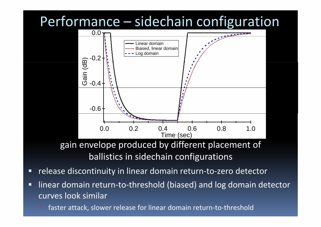
gain envelope produced by different placement of ballistics in sidechain configurations

release discontinuity in linear domain return‐to‐zero detector

linear domain return‐to‐threshold (biased) and log domain detector curves look similar

faster attack, slower release for linear domain return‐to‐threshold 

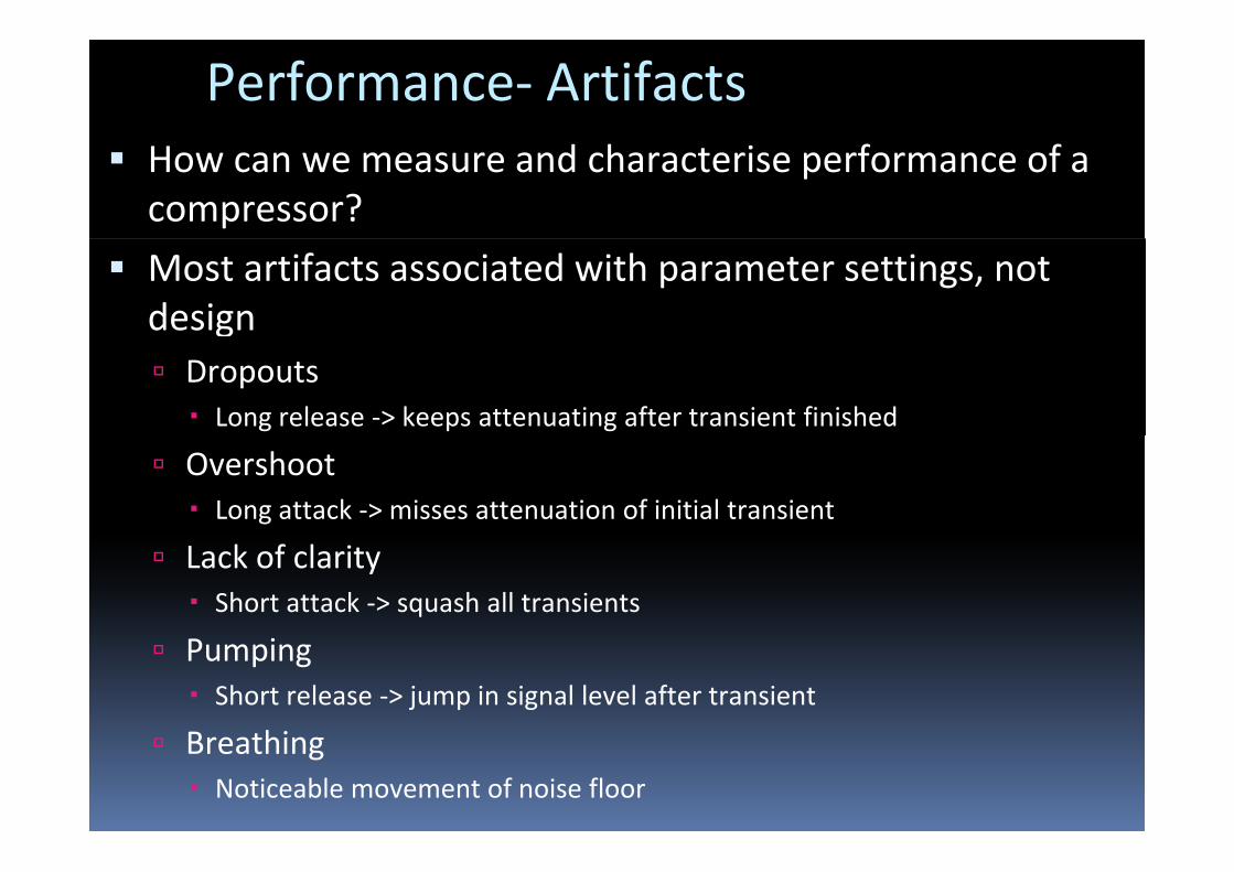
Performance‐ ArtifactsHow can we measure and characterise performance of a compressor?

Most artifacts associated with parameter settings, not designg

DropoutsLong release ‐> keeps attenuating after transient finished

OvershootLong attack ‐> misses attenuation of initial transient

Lack of clarityShort attack ‐> squash all transients

PumpingShort release ‐> jump in signal level after transient

B hiBreathingNoticeable movement of noise floor

Performance‐ Noise and DistortionSignal to Noise RatioSignal to Noise RatioNot useful

Total Harmonic DistortionMeasures strength of harmonics (introduced by 

28

g ( ycompression) in relation to original frequency

24

20

(%)

Compressor Design

16

12

THD

( g Branching Decoupled Branching Smooth Decoupled Smooth

8

4

0

102 103 104

Frequency (Hz)

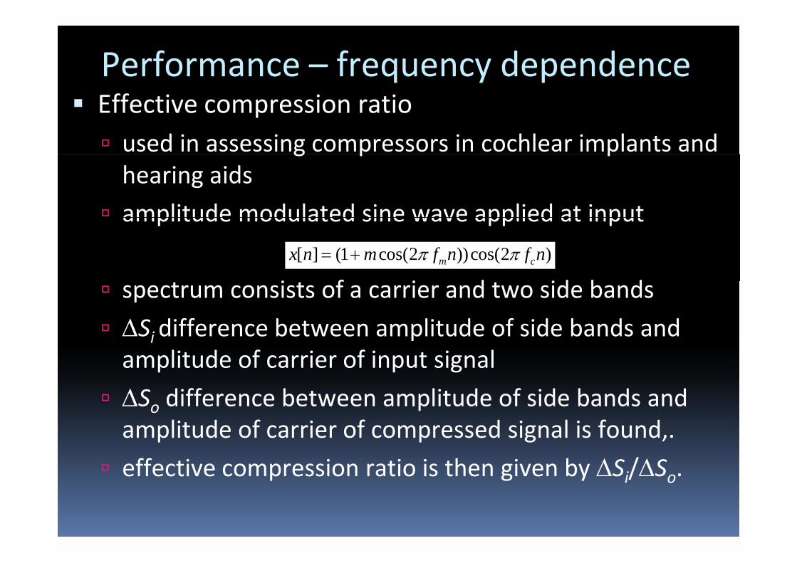
Performance – frequency dependenceEffective compression ratioused in assessing compressors in cochlear implants and g p phearing aids

amplitude modulated sine wave applied at inputamplitude modulated sine wave applied at input

i f i d id b d[ ] (1 cos(2 ))cos(2 )m cx n m f n f nπ π= +

spectrum consists of a carrier and two side bands

ΔSi difference between amplitude of side bands and amplitude of carrier of input signal

ΔSo difference between amplitude of side bands and o pamplitude of carrier of compressed signal is found,. 

effective compression ratio is then given by ΔSi/ΔS .effective compression ratio is then given by ΔSi/ΔSo.

Performance – effective compression ratio66.5

6.0

5 5Rat

io Compressor Design Branching

5.5

5.0

4 5pres

sion

Decoupled Branching Smooth Decoupled Smooth

4.5

4.0

3.5ve C

omp

3.0

2.5Effe

ctiv

2.0

3632282420161284

Interpretation?

3632282420161284Modulation Frequency (Hz)

Performance‐ Ballistics and sidechain configurationDetector Fidelity of Envelope Shape (FES)Detector

Placement Detector Typey p p ( )

Guitar Bass Drums Vocals

Branching 0.884 0.945 0.766 0.952

Decoupled 0.899 0.932 0.755 0.941

Fid lit f th Logdomain Branching Smooth 0.852 0.927 0.640 0.941

Decoupled Smooth 0 859 0 911 0 648 0 936

Fidelity of the envelope shape

Decoupled Smooth 0.859 0.911 0.648 0.936

Branching 0.836 0.879 0.517 0.932

Decoupled 0.790 0.831 0.537 0.930

Lineardomain Branching Smooth 0.825 0.856 0.456 0.932

Decoupled Smooth 0 775 0 805 0 461 0 934Decoupled Smooth 0.775 0.805 0.461 0.934

Measures correlation between envelopes of compressed and uncompressed signalsuncompressed signals

Nonsmooth designs do well since they often apply no compression

Pl i b lli ti ( tt k d l ) i l d i t fPlacing ballistics (attack and release) in log domain outperforms placing them in linear domain

Pseudocode% Smoothed branching digital dynamic range compressor.

% Parameters

% x: input signal

% fs: sample rate (kHz)

% tauAttack: attack time constant (ms)

% tauRelease: release time constant (ms)

% T l ith i th h ld% T: logarithmic threshold

% R: compression ratio

% W: decibel width of the knee transistion% W: decibel width of the knee transistion

% M: decibel Make-up Gain

% Returns

% y: output (compressed) signal

%LEVEL DETECTION

y_L = max(abs(x), 1e-6);

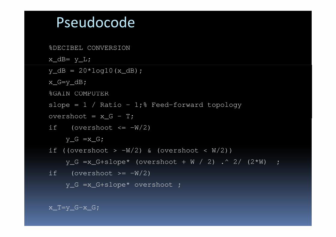
Pseudocode%DECIBEL CONVERSION

x_dB= y_L;

y_dB = 20*log10(x_dB);

x_G=y_dB;

%GAIN COMPUTER%GAIN COMPUTER

slope = 1 / Ratio - 1;% Feed-forward topology

overshoot = x G - T;_ ;

if (overshoot <= -W/2)

y_G =x_G;

if ((overshoot > -W/2) & (overshoot < W/2))

y_G =x_G+slope* (overshoot + W / 2) .^ 2/ (2*W) ;

if (overshoot > W/2)if (overshoot >= -W/2)

y_G =x_G+slope* overshoot ;

x_T=y_G-x_G;

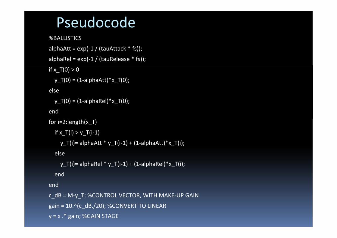
Pseudocode%BALLISTICS%BALLISTICS

alphaAtt = exp(‐1 / (tauAttack * fs));

alphaRel = exp(‐1 / (tauRelease * fs));

if x_T(0) > 0

y_T(0) = (1‐alphaAtt)*x_T(0);

elseelse

y_T(0) = (1‐alphaRel)*x_T(0);

end

for i=2:length(x_T)

if x_T(i) > y_T(i‐1)

y_T(i)= alphaAtt * y_T(i‐1) + (1‐alphaAtt)*x_T(i);

else

y_T(i)= alphaRel * y_T(i‐1) + (1‐alphaRel)*x_T(i);

dend

end

c_dB = M‐y_T; %CONTROL VECTOR, WITH MAKE‐UP GAIN

gain = 10.^(c_dB./20); %CONVERT TO LINEAR

y = x .* gain; %GAIN STAGE

The big unknown – psychoacousticsCompressor designs in the literature: >20in the literature: >20

Commercial designs: >40

Studies of parameter settingsStudies of parameter settings for hearing aids: >10

for music production and broadcast: 0 ?Anecdotal recommendations : 10? 

Studies of compressor designs for hearing aids: <5?for hearing aids: <5?

for music production and broadcast: 0 !

Recommendations

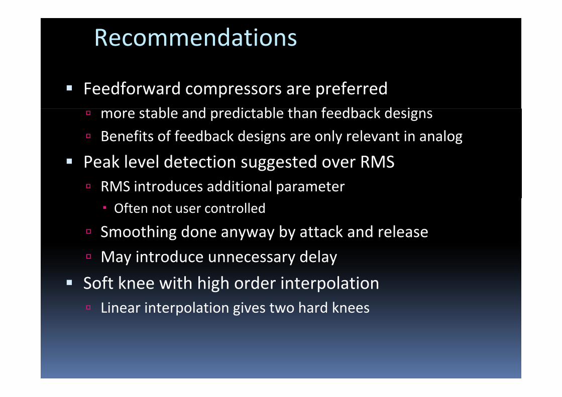
Feedforward compressors are preferred bl d di bl h f db k d imore stable and predictable than feedback designs

Benefits of feedback designs are only relevant in analog

Peak level detection suggested over RMSRMS introduces additional parameterOften not user controlled

Smoothing done anyway by attack and release

May introduce unnecessary delay

Soft knee with high order interpolationSoft knee with high order interpolationLinear interpolation gives two hard knees

RecommendationsBallistics in the log domain after the gain computerBallistics in the log domain after the gain computer

Maintain envelope shape

tt k lno attack lag

easy implementation of variable knee width

Smooth, peak detector for attack and releaseDecoupled Low harmonic distortion

Prevent discontinuities

Branchingdetailed knowledge of the effect of the time constants

d h l f hMinor discontinuities in the slope of the gain curve

Make‐up gain at end of side‐chainAgrees with expected use

Not intended or needed to be smoothed

ThanksMichael Massberg

See his talk this afternoon, at 2:30pm

“Digital Low‐Pass Filter Design with Analog Matched Magnitude Response”

Dimitrios Giannoulis