Under-determined reverberant audio source separation … domain as a zero-mean Gaussian random variable whose covari-ance encodes the spatial characteristics of the source. We then

HAL Id: inria-00435807https://hal.inria.fr/inria-00435807v2

Submitted on 14 Dec 2009

HAL is a multi-disciplinary open accessarchive for the deposit and dissemination of sci-entific research documents, whether they are pub-lished or not. The documents may come fromteaching and research institutions in France orabroad, or from public or private research centers.

L’archive ouverte pluridisciplinaire HAL, estdestinée au dépôt et à la diffusion de documentsscientifiques de niveau recherche, publiés ou non,émanant des établissements d’enseignement et derecherche français ou étrangers, des laboratoirespublics ou privés.

Under-determined reverberant audio source separationusing a full-rank spatial covariance model

Ngoc Duong, Emmanuel Vincent, Rémi Gribonval

To cite this version:Ngoc Duong, Emmanuel Vincent, Rémi Gribonval. Under-determined reverberant audio sourceseparation using a full-rank spatial covariance model. [Research Report] INRIA. 2010. <inria-00435807v2>

https://hal.inria.fr/inria-00435807v2

https://hal.archives-ouvertes.fr

appor t de r ech er ch e

ISS

N02

49-6

399

ISR

NIN

RIA

/RR

--71

16--

FR

+E

NG

Thème COM

INSTITUT NATIONAL DE RECHERCHE EN INFORMATIQUE ET EN AUTOMATIQUE

Under-determined reverberant audio sourceseparation using a full-rank spatial covariance model

Ngoc Q.K. Duong — Emmanuel Vincent — Rémi Gribonval

N° 7116

December 2009

Centre de recherche INRIA Rennes – Bretagne AtlantiqueIRISA, Campus universitaire de Beaulieu, 35042 Rennes Cedex

Téléphone : +33 2 99 84 71 00 — Télécopie : +33 2 99 84 71 71

Under-determined reverberant audio source

separation using a full-rank spatial covariance

model

Ngoc Q.K. Duong∗, Emmanuel Vincent†, Remi Gribonval‡

Theme COM — Systemes communicantsEquipe-Projet METISS

Rapport de recherche n° 7116 — December 2009 — 19 pages

Abstract: This article addresses the modeling of reverberant recording envi-ronments in the context of under-determined convolutive blind source separa-tion. We model the contribution of each source to all mixture channels in thetime-frequency domain as a zero-mean Gaussian random variable whose covari-ance encodes the spatial characteristics of the source. We then consider fourspecific covariance models, including a full-rank unconstrained model. We de-rive a family of iterative expectation-maximization (EM) algorithms to estimatethe parameters of each model and propose suitable procedures to initialize theparameters and to align the order of the estimated sources across all frequencybins based on their estimated directions of arrival (DOA). Experimental resultsover reverberant synthetic mixtures and live recordings of speech data show theeffectiveness of the proposed approach.

Key-words: Convolutive blind source separation, under-determined mixtures,spatial covariance models, EM algorithm, permutation problem.

∗ [email protected]† [email protected]‡ [email protected]

Separation de melanges audio reverberants

sous-determins l’aide d’un modele de covariance

spatiale de rang plein

Resume : Cet article traite de la modelisation d’environnements d’enregistrementreverberants dans le contexte de la separation de sources sous-determinee. Nousmodelisons la contribution de chaque source l’ensemble des canaux du melangedans le domaine temps-frequence comme une variable aleatoire vectorielle gaus-sienne de moyenne nulle dont la covariance code les caracteristiques spatiales dela source. Nous considerons quatre modeles specifiques de covariance, dont unmodele de rang plein non contraint. Nous explicitons une famille d’algorithmesExpectation-Maximization (EM) pour l’estimation des parametres de chaquemodele et nous proposons des procedures adequates d’initialisation des pa-rametres et d’appariement de l’ordre des sources travers les frequences partirde leurs directions d’arrivee. Les resultats experimentaux sur des melangesreverberants synthetiques et enregistres montrent la pertinence de l’approcheproposee.

Mots-cles : Separation de sources convolutive, melanges sous-determines,modeles de covariance spatiale, algorithme EM, probleme de permutation.

Under-determined reverberant audio source separation 3

1 Introduction

In blind source separation (BSS), audio signals are generally mixtures of sev-eral sound sources such as speech, music, and background noise. The recordedmultichannel signal x(t) is therefore expressed as

x(t) =

J∑

j=1

cj(t) (1)

where cj(t) is the spatial image of the jth source, that is the contribution of thissource to all mixture channels. For a point source in a reverberant environment,cj(t) can be expressed via the convolutive mixing process

cj(t) =∑

τ

hj(τ)sj(t− τ) (2)

where sj(t) is the jth source signal and hj(τ) the vector of filter coefficients mod-eling the acoustic path from this source to all microphones. Source separationconsists in recovering either the J original source signals or their spatial imagesgiven the I mixture channels. In the following, we focus on the separation ofunder-determined mixtures, i.e. such that I < J .

Most existing approaches operate in the time-frequency domain using theshort-time Fourier transform (STFT) and rely on narrowband approximation ofthe convolutive mixture (2) by complex-valued multiplication in each frequencybin f and time frame n as

cj(n, f) ≈ hj(f)sj(n, f) (3)

where the mixing vector hj(f) is the Fourier transform of hj(τ), sj(n, f) arethe STFT coefficients of the sources sj(t) and cj(n, f) the STFT coefficientsof their spatial images cj(t). The sources are typically estimated under theassumption that they are sparse in the STFT domain. For instance, the de-generate unmixing estimation technique (DUET) [1] uses binary masking toextract the predominant source in each time-frequency bin. Another populartechnique known as ℓ1-norm minimization extracts on the order of I sourcesper time-frequency bin by solving a constrained ℓ1-minimization problem [2, 3].The separation performance achievable by these techniques remains limited inreverberant environments [4], due in particular to the fact that the narrowbandapproximation does not hold because the mixing filters are much longer thanthe window length of the STFT.

Recently, a distinct framework has emerged whereby the STFT coefficientsof the source images cj(n, f) are modeled by a phase-invariant multivariatedistribution whose parameters are functions of (n, f) [5]. One instance of thisframework consists in modeling cj(n, f) as a zero-mean Gaussian random vari-able with covariance matrix

Rcj(n, f) = vj(n, f)Rj(f) (4)

where vj(n, f) are scalar time-varying variances encoding the spectro-temporalpower of the sources and Rj(f) are time-invariant spatial covariance matricesencoding their spatial position and spatial spread [6]. The model parameters

RR n° 7116

4 Duong, Vincent, and Gribonval

can then be estimated in the maximum likelihood (ML) sense and used estimatethe spatial images of all sources by Wiener filtering.

This framework was first applied to the separation of instantaneous audiomixtures in [7, 8] and shown to provide better separation performance than ℓ1-norm minimization. The instantaneous mixing process then translated into arank-1 spatial covariance matrix for each source. In our preliminary paper [6],we extended this approach to convolutive mixtures and proposed to considerfull-rank spatial covariance matrices modeling the spatial spread of the sourcesand circumventing the narrowband approximation. This approach was shownto improve separation performance of reverberant mixtures in both an oraclecontext, where all model parameters are known, and in a semi-blind context,where the spatial covariance matrices of all sources are known but their variancesare blindly estimated from the mixture.

In this article we extend this work to blind estimation of the model param-eters for BSS application. While the general expectation-maximization (EM)algorithm is well-known as an appropriate choice for parameter estimation ofGaussian models [9, 10, 11, 12], it is very sensitive to the initialization [13],so that an effective parameter initialization scheme is necessary. Moreover,the well-known source permutation problem arises when the model parametersare independently estimated at different frequencies [14]. In the following, weaddress these two issues for the proposed models and evaluate these models to-gether with state-of-the-art techniques on a considerably larger set of mixtures.

The structure of the rest of the article is as follows. We introduce thegeneral framework under study as well as four specific spatial covariance modelsin Section 2. We then address the blind estimation of all model parametersfrom the observed mixture in Section 3. We compare the source separationperformance achieved by each model to that of state-of-the-art techniques invarious experimental settings in Section 4. Finally we conclude and discussfurther research directions in Section 5.

2 General framework and spatial covariance mod-

els

We start by describing the general probabilistic modeling framework adoptedfrom now on. We then define four models with different degrees of flexibilityresulting in rank-1 or full-rank spatial covariance matrices.

2.1 General framework

Let us assume that the vector cj(n, f) of STFT coefficients of the spatial imageof the jth source follows a zero-mean Gaussian distribution whose covariancematrix factors as in (4). Under the classical assumption that the sources areuncorrelated, the vector x(n, f) of STFT coefficients of the mixture signal isalso zero-mean Gaussian with covariance matrix

Rx(n, f) =J∑

j=1

vj(n, f)Rj(f). (5)

INRIA


In other words, the likelihood of the set of observed mixture STFT coefficientsx = {x(n, f)}n,f given the set of variance parameters v = {vj(n, f)}j,n,f andthat of spatial covariance matrices R = {Rj(f)}j,f is given by

P (x|v,R) =∏

n,f

1

det (πRx(n, f))e−x

H(n,f)R−1

x(n,f)x(n,f) (6)

where H denotes matrix conjugate transposition and Rx(n, f) implicitly de-pends on v and R according to (5). The covariance matrices are typicallymodeled by higher-level spatial parameters, as we shall see in the following.

Under this model, source separation can be achieved in two steps. The vari-ance parameters v and the spatial parameters underlying R are first estimatedin the ML sense. The spatial images of all sources are then obtained in theminimum mean square error (MMSE) sense by multichannel Wiener filtering

cj(n, f) = vj(n, f)Rj(f)R−1x (n, f)x(n, f). (7)

2.2 Rank-1 convolutive model

Most existing approaches to audio source separation rely on narrowband ap-proximation of the convolutive mixing process (2) by the complex-valued mul-tiplication (3). The covariance matrix of cj(n, f) is then given by (4) wherevj(n, f) is the variance of sj(n, f) and Rj(f) is equal to the rank-1 matrix

Rj(f) = hj(f)hHj (f) (8)

with hj(f) denoting the Fourier transform of the mixing filters hj(τ). Thisrank-1 convolutive model of the spatial covariance matrices has recently beenexploited in [13] together with a different model of the source variances.

2.3 Rank-1 anechoic model

In an anechoic recording environment without reverberation, each mixing filterboils down to the combination of a delay τij and a gain κij specified by thedistance rij from the jth source to the ith microphone [15]

τij =rij

cand κij =

1√4πrij

(9)

where c is sound velocity. The spatial covariance matrix of the jth source ishence given by the rank-1 anechoic model

Rj(f) = aj(f)aHj (f) (10)

where the Fourier transform aj(f) of the mixing filters is now parameterized as

aj(f) =

κ1,je

−2iπfτ1,j

...κI,je

−2iπfτI,j

. (11)

RR n° 7116


2.4 Full-rank direct+diffuse model

One possible interpretation of the narrowband approximation is that the soundof each source as recorded on the microphones comes from a single spatial posi-tion at each frequency f , as specified by hj(f) or aj(f). This approximation isnot valid in a reverberant environment, since reverberation induces some spatialspread of each source, due to echoes at many different positions on the wallsof the recording room. This spread translates into full-rank spatial covariancematrices.

The theory of statistical room acoustics assumes that the spatial image ofeach source is composed of two uncorrelated parts: a direct part modeled byaj(f) in (11) and a reverberant part. The spatial covariance Rj(f) of eachsource is then a full-rank matrix defined as the sum of the covariance of itsdirect part and the covariance of its reverberant part such that

Rj(f) = aj(f)aHj (f) + σ2

revΨ(f) (12)

where σ2rev is the variance of the reverberant part and Ψil(f) is a function of

the distance dil between the ith and the lth microphone such that Ψii(f) = 1.This model assumes that the reverberation recorded at all microphones has thesame power but is correlated as characterized by Ψ(dil, f). This model has beenemployed for single source localization in [15] but not for source separation yet.

Assuming that the reverberant part is diffuse, i.e. its intensity is uniformlydistributed over all possible directions, its normalized cross-correlation can beshown to be real-valued and equal to [16]

Ψil(f) =sin(2πfdil/c)

2πfdil/c. (13)

Moreover, the power of the reverberant part within a parallelepipedic room withdimensions Lx, Ly, Lz is given by

σ2rev =

4β2

A(1 − β2)(14)

where A is the total wall area and β the wall reflection coefficient computedfrom the room reverberation time T60 via Eyring’s formula [15]

β = exp

{− 13.82

( 1Lx

+ 1Ly

+ 1Lz

)cT60

}. (15)

2.5 Full-rank unconstrained model

In practice, the assumption that the reverberant part is diffuse is rarely satisfied.Indeed, early echoes containing more energy are not uniformly distributed on thewalls of the recording room, but at certain positions depending on the positionof the source and the microphones. When performing some simulations in arectangular room, we observed that (13) is valid on average when considering alarge number of sources at different positions, but generally not valid for eachsource considered independently.

Therefore, we also investigate the modeling of each source via an uncon-strained spatial covariance matrix Rj(f) whose coefficients are not related a

INRIA


priori. Since this model is more general than (8) and (12), it allows more flex-ible modeling of the mixing process and hence potentially improves separationperformance of real-world convolutive mixtures.

3 Blind estimation of the model parameters

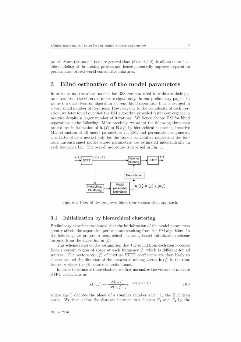
In order to use the above models for BSS, we now need to estimate their pa-rameters from the observed mixture signal only. In our preliminary paper [6],we used a quasi-Newton algorithm for semi-blind separation that converged ina very small number of iterations. However, due to the complexity of each iter-ation, we later found out that the EM algorithm provided faster convergence inpractice despite a larger number of iterations. We hence choose EM for blindseparation in the following. More precisely, we adopt the following three-stepprocedure: initialization of hj(f) or Rj(f) by hierarchical clustering, iterativeML estimation of all model parameters via EM, and permutation alignment.The latter step is needed only for the rank-1 convolutive model and the full-rank unconstrained model whose parameters are estimated independently ineach frequency bin. The overall procedure is depicted in Fig. 1.

Figure 1: Flow of the proposed blind source separation approach.

3.1 Initialization by hierarchical clustering

Preliminary experiments showed that the initialization of the model parametersgreatly affects the separation performance resulting from the EM algorithm. Inthe following, we propose a hierarchical clustering-based initialization schemeinspired from the algorithm in [2].

This scheme relies on the assumption that the sound from each source comesfrom a certain region of space at each frequency f , which is different for allsources. The vectors x(n, f) of mixture STFT coefficients are then likely tocluster around the direction of the associated mixing vector hj(f) in the timeframes n where the jth source is predominant.

In order to estimate these clusters, we first normalize the vectors of mixtureSTFT coefficients as

x(n, f)← x(n, f)

‖x(n, f)‖2e−i arg(x1(n,f)) (16)

where arg(.) denotes the phase of a complex number and ‖.‖2 the Euclideannorm. We then define the distance between two clusters C1 and C2 by the

RR n° 7116


average distance between the associated normalized mixture STFT coefficients

d(C1, C2) =1

|C1||C2|∑

x1∈C1

∑

x2∈C2

‖x1 − x2‖2 (17)

In a given frequency bin, the vectors of mixture STFT coefficients on all timeframes are first considered as clusters containing a single item. The distancebetween each pair of clusters is computed and the two clusters with the smallestdistance are merged. This ”bottom up” process called linking is repeated untilthe number of clusters is smaller than a predetermined threshold K. Thisthreshold is usually much larger than the number of sources J [2], so as toeliminate outliers. We finally choose the J clusters with the largest number ofsamples. The initial mixing vector and spatial covariance matrix for each sourceare then computed as

hinitj (f) =

1

|Cj |∑

x(n,f)∈Cj

x(n, f) (18)

Rinitj (f) =

1

|Cj |∑

x(n,f)∈Cj

x(n, f)x(n, f)H (19)

where x(n, f) = x(n, f)e−i arg(x1(n,f)). Note that, contrary to the algorithmin [2], we define the distance between clusters as the average distance betweenthe normalized mixture STFT coefficients instead of the minimum distance be-tween them. Besides, the mixing vector hinit

j (f) is computed from the phase-normalized mixture STFT coefficients x(n, f) instead of both phase and ampli-tute normalized coefficients x(n, f). These modifications were found to providebetter initial approximation of the mixing parameters in our experiments. Wealso tested random initialization and direction-of-arrival (DOA) based initial-ization, i.e. where the mixing vectors hinit

j (f) are derived from known sourceand microphone positions assuming no reverberation. Both schemes were foundto result in slower convergence and poorer separation performance than theproposed scheme.

3.2 EM updates for the rank-1 convolutive model

The derivation of the EM parameter estimation algorithm for the rank-1 con-volutive model is strongly inspired from the study in [13], which relies on thesame model of spatial covariance matrices but on a distinct model of source vari-ances. Similarly to [13], EM cannot be directly applied to the mixture model(1) since the estimated mixing vectors remain fixed to their initial value. Thisissue can be addressed by considering the noisy mixture model

x(n, f) = H(f)s(n, f) + b(n, f) (20)

where H(f) is the mixing matrix whose jth column is the mixing vector hj(f),s(n, f) is the vector of source STFT coefficients sj(n, f) and b(n, f) some addi-tive zero-mean Gaussian noise. We denote by Rs(n, f) the diagonal covariancematrix of s(n, f). Following [13], we assume that b(n, f) is stationary and spa-tially uncorrelated and denote by Rb(f) its time-invariant diagonal covariancematrix. This matrix is initialized to a small value related to the average accuracyof the mixing vector initialization procedure.

INRIA


EM is separately derived for each frequency bin f for the complete data{x(n, f), sj(n, f)}j,n that is the set of mixture and source STFT coefficients ofall time frames. The details of one iteration are as follows. In the E-step, theWiener filter W(n, f) and the conditional mean s(n, f) and covariance Rss(n, f)of the sources are computed as

Rs(n, f) = diag(v1(n, f), ..., vJ(n, f)) (21)

Rx(n, f) = H(f)Rs(n, f)HH(f) + Rb(f) (22)

W(n, f) = Rs(n, f)HH(f)R−1x (n, f) (23)

s(n, f) = W(n, f)x(n, f) (24)

Rss(n, f) = s(n, f)sH(n, f) + (I−W(n, f)H(f))Rs(n, f) (25)

where I is the I×I identity matrix and diag(.) the diagonal matrix whose entriesare given by its arguments. Conditional expectations of multichannel statisticsare also computed by averaging over all N time frames as

Rss(f) =1

N

N∑

n=1

Rss(n, f) (26)

Rxs(f) =1

N

N∑

n=1

x(n, f)sH(n, f) (27)

Rxx(f) =1

N

N∑

n=1

x(n, f)xH(n, f). (28)

In the M-step, the source variances, the mixing matrix and the noise covarianceare updated via

vj(n, f) =Rss jj(n, f) (29)

H(f) =Rxs(f)R−1ss

(f) (30)

Rb(f) =Diag(Rxx(f)−H(f)RHxs

(f)

− RxsHH(f) + H(f)Rss(n, f)HH(f)) (31)

where Diag(.) projects a matrix onto its diagonal.

3.3 EM updates for the full-rank unconstrained model

The derivation of EM for the full-rank unconstrained model is much easier sincethe above issue does not arise. We hence stick with the exact mixture model(1), which can be seen as an advantage of full-rank vs. rank-1 models. EMis again separately derived for each frequency bin f . Since the mixture canbe recovered from the spatial images of all sources, the complete data reducesto {cj(n, f)}n,f , that is the set of STFT coefficients of the spatial images ofall sources on all time frames. The details of one iteration are as follows. Inthe E-step, the Wiener filter Wj(n, f) and the conditional mean cj(n, f) and

RR n° 7116


covariance Rcj(n, f) of the spatial image of the jth source are computed as

Wj(n, f) = Rcj(n, f)R−1

x(n, f) (32)

cj(n, f) = Wj(n, f)x(n, f) (33)

Rcj(n, f) = cj(n, f)cH

j (n, f) + (I−Wj(n, f))Rcj(n, f) (34)

where Rcj(n, f) is defined in (4) and Rx(n, f) in (5). In the M-step, the variance

and the spatial covariance of the jth source are updated via

vj(n, f) =1

Itr(R−1

j (f)Rcj(n, f)) (35)

Rj(f) =1

N

N∑

n=1

1

vj(n, f)Rcj

(n, f) (36)

where tr(.) denotes the trace of a square matrix. Note that, strictly speaking,this algorithm is a generalized form of EM [17], since the M-step increases butdoes not maximize the likelihood of the complete data due to the interleavingof (35) and (36).

3.4 EM updates for the rank-1 anechoic model and the

full-rank direct+diffuse model

The derivation of EM for the two remaining models is more complex since the M-step cannot be expressed in closed form. The complete data and the E-step forthe rank-1 anechoic model and the full-rank direct+diffuse model are identical tothose for the rank-1 convolutive model and the full-rank unconstrained model,respectively. The M-step, which consists of maximizing the likelihood of thecomplete data given their natural statistics computed in the E-step, could beaddressed e.g. via a quasi-Newton technique or by sampling possible parametervalues from a grid [12]. In the following, we do not attempt to derive the detailsof these algorithms since these two models appear to provide lower performancethan the rank-1 convolutive model and the full-rank unconstrained model in asemi-blind context, as discussed in Section 4.2.

3.5 Permutation alignment

Since the parameters of the rank-1 convolutive model and the full-rank uncon-strained model are estimated independently in each frequency bin f , they shouldbe ordered so as to correspond to the same source across all frequency bins. Inorder to solve this so-called permutation problem, we apply the DOA-basedalgorithm described in [18] for the rank-1 model. Given the geometry of themicrophone array, this algorithm computes the DOAs of all sources and per-mutes the model parameters by clustering the estimated mixing vectors hj(f)normalized as in (16).

Regarding the full-rank model, we first apply principal component analy-sis (PCA) to summarize the spatial covariance matrix Rj(f) of each source ineach frequency bin by its first principal component wj(f) that points to thedirection of maximum variance. This vector is conceptually equivalent to themixing vector hj(f) of the rank-1 model. Thus, we can apply the same proce-dure to solve the permutation problem. Fig. 2 depicts the phase of the second

INRIA


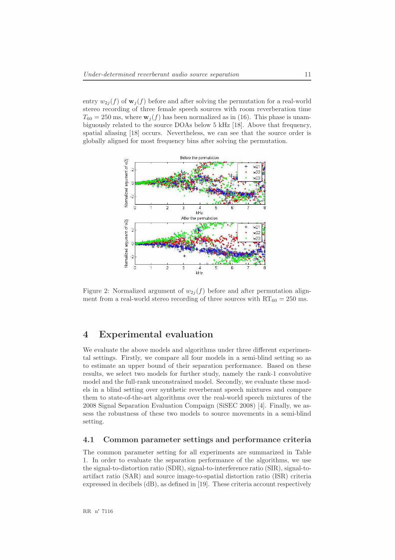
entry w2j(f) of wj(f) before and after solving the permutation for a real-worldstereo recording of three female speech sources with room reverberation timeT60 = 250 ms, where wj(f) has been normalized as in (16). This phase is unam-biguously related to the source DOAs below 5 kHz [18]. Above that frequency,spatial aliasing [18] occurs. Nevertheless, we can see that the source order isglobally aligned for most frequency bins after solving the permutation.

Figure 2: Normalized argument of w2j(f) before and after permutation align-ment from a real-world stereo recording of three sources with RT60 = 250 ms.

4 Experimental evaluation

We evaluate the above models and algorithms under three different experimen-tal settings. Firstly, we compare all four models in a semi-blind setting so asto estimate an upper bound of their separation performance. Based on theseresults, we select two models for further study, namely the rank-1 convolutivemodel and the full-rank unconstrained model. Secondly, we evaluate these mod-els in a blind setting over synthetic reverberant speech mixtures and comparethem to state-of-the-art algorithms over the real-world speech mixtures of the2008 Signal Separation Evaluation Compaign (SiSEC 2008) [4]. Finally, we as-sess the robustness of these two models to source movements in a semi-blindsetting.

4.1 Common parameter settings and performance criteria

The common parameter setting for all experiments are summarized in Table1. In order to evaluate the separation performance of the algorithms, we usethe signal-to-distortion ratio (SDR), signal-to-interference ratio (SIR), signal-to-artifact ratio (SAR) and source image-to-spatial distortion ratio (ISR) criteriaexpressed in decibels (dB), as defined in [19]. These criteria account respectively

RR n° 7116


for overall distortion of the target source, residual crosstalk from other sources,musical noise and spatial or filtering distortion of the target.

Signal duration 10 secondsNumber of channels I = 2

Sampling rate 16 kHzWindow type sine window

STFT frame size 2048STFT frame shift 1024

Propagation velocity 334 m/sNumber of EM iterations 10

Cluster threshold K = 30

Table 1: common experimental parameter setting

4.2 Potential source separation performance of all models

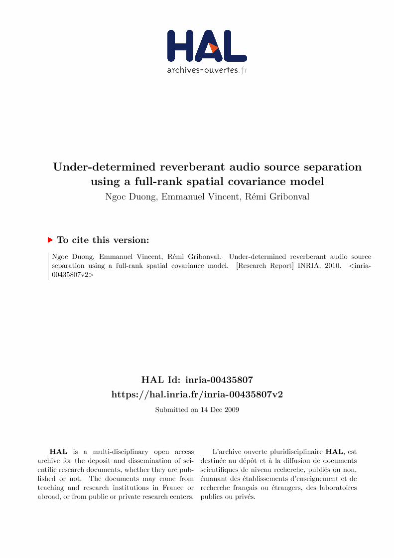
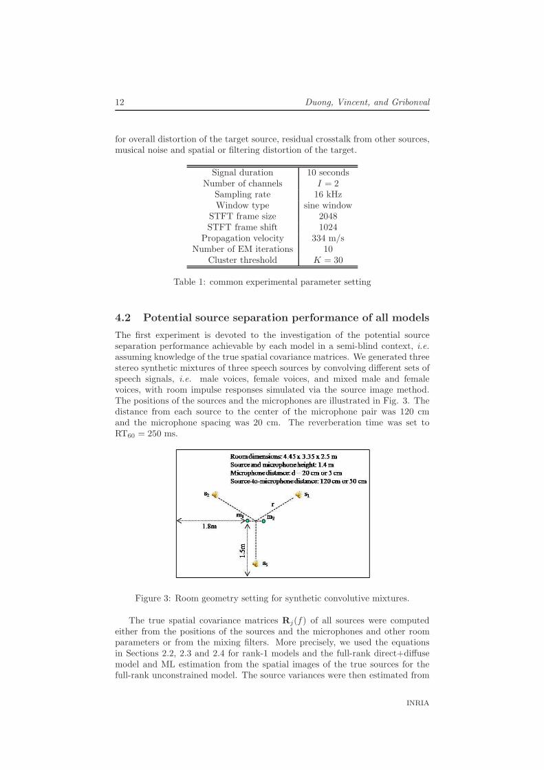
The first experiment is devoted to the investigation of the potential sourceseparation performance achievable by each model in a semi-blind context, i.e.assuming knowledge of the true spatial covariance matrices. We generated threestereo synthetic mixtures of three speech sources by convolving different sets ofspeech signals, i.e. male voices, female voices, and mixed male and femalevoices, with room impulse responses simulated via the source image method.The positions of the sources and the microphones are illustrated in Fig. 3. Thedistance from each source to the center of the microphone pair was 120 cmand the microphone spacing was 20 cm. The reverberation time was set toRT60 = 250 ms.

Figure 3: Room geometry setting for synthetic convolutive mixtures.

The true spatial covariance matrices Rj(f) of all sources were computedeither from the positions of the sources and the microphones and other roomparameters or from the mixing filters. More precisely, we used the equationsin Sections 2.2, 2.3 and 2.4 for rank-1 models and the full-rank direct+diffusemodel and ML estimation from the spatial images of the true sources for thefull-rank unconstrained model. The source variances were then estimated from

INRIA


the mixture using the quasi-Newton technique in [6], for which an efficient ini-tialization exists when the spatial covariance matrices are fixed. Binary maskingand ℓ1-norm minimization were also evaluated for comparison using the samemixing vectors as the rank-1 convolutive model with the reference software in[4]. The results are averaged over all sources and all set of mixtures and shownin Table 2.

Covariancemodels

Numberof

spatialparame-

ters

SDR SIR SAR ISR

Rank-1 anechoic 6 0.8 2.4 7.9 5.0Rank-1 convolutive 3078 3.8 7.5 5.3 9.3

Full-rank direct+diffuse 8 3.2 6.9 5.4 7.9Full-rank unconstrained 6156 5.6 10.7 7.3 11.0

Binary masking 3078 3.3 11.1 2.4 8.4ℓ1-norm minimization 3078 2.7 7.7 3.4 8.6

Table 2: Average potential source separation performance in a semi-blind settingover stereo mixtures of three sources with RT60 = 250 ms.

The rank-1 anechoic model has lowest performance because it only accountsfor the direct path. By contrast, the full-rank unconstrained model has high-est performance and improves the SDR by 1.8 dB, 2.3 dB, and 2.9 dB whencompared to the rank-1 convolutive model, binary masking, and ℓ1-norm min-imization respectively. The full-rank direct+diffuse model results in a SDRdecrease of 0.6 dB compared to the rank-1 convolutive model. This decreaseappears surprisingly small when considering the fact that the former involvesonly 8 spatial parameters (6 distances rij , plus σ2

rev and d) instead of 3078 pa-rameters (6 mixing coefficients per frequency bin) for the latter. Nevertheless,we focus on the two best models, namely the rank-1 convolutive model and thefull-rank unconstrained model in subsequent experiments.

4.3 Blind source separation performance as a function of

the reverberation time

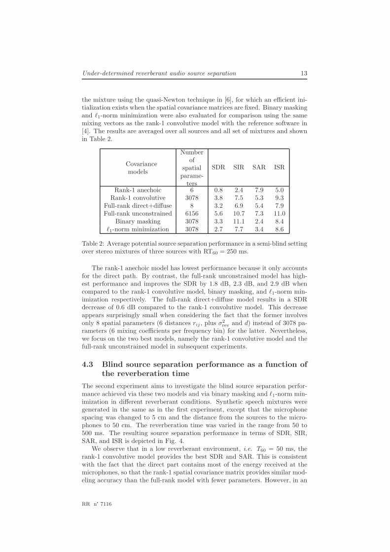
The second experiment aims to investigate the blind source separation perfor-mance achieved via these two models and via binary masking and ℓ1-norm min-imization in different reverberant conditions. Synthetic speech mixtures weregenerated in the same as in the first experiment, except that the microphonespacing was changed to 5 cm and the distance from the sources to the micro-phones to 50 cm. The reverberation time was varied in the range from 50 to500 ms. The resulting source separation performance in terms of SDR, SIR,SAR, and ISR is depicted in Fig. 4.

We observe that in a low reverberant environment, i.e. T60 = 50 ms, therank-1 convolutive model provides the best SDR and SAR. This is consistentwith the fact that the direct part contains most of the energy received at themicrophones, so that the rank-1 spatial covariance matrix provides similar mod-eling accuracy than the full-rank model with fewer parameters. However, in an

RR n° 7116


Figure 4: Average blind source separation performance over stereo mixtures ofthree sources as a function of the reverberation time.

environment with realistic reverberation time, i.e. T60 ≥ 130 ms, the full-rankunconstrained model outperforms both the rank-1 model and binary maskingin terms of SDR and SAR and results in a SIR very close to that of binarymasking. For instance, with T60 = 500 ms, the SDR achieved via the full-rankunconstrained model is 2.0 dB, 1.2 dB and 2.3 dB larger than that of the rank-1 convolutive model, binary masking, and ℓ1-norm minimization respectively.These results confirm the effectiveness of our proposed model parameter esti-mation scheme and also show that full-rank spatial covariance matrices betterapproximate the mixing process in a reverberant room.

4.4 Blind source separation with the SiSEC 2008 test data

We conducted a third experiment to compare the proposed full-rank uncon-strained model-based algorithm with state-of-the-art BSS algorithms submittedfor evaluation to SiSEC 2008 over real-world mixtures of 3 or 4 speech sources.Two mixtures were recorded for each given number of sources, using either maleor female speech signals. The room reverberation time was 250 ms and the mi-crophone spacing 5 cm [4]. The average SDR achieved by each algorithm is

INRIA


listed in Table 3. The SDR figures of all algorithms except yours were takenfrom the website of SiSEC 20081.

Algorithms 3 source mixtures 4 source mixturesfull-rank unconstrained 3.8 2.0

M. Cobos [20] 2.2 1.0M. Mandel [21] 0.8 1.0R. Weiss [22] 2.3 1.5S. Araki [23] 3.7 -

Z. El Chami [24] 3.1 1.4

Table 3: Average SDR over the real-world test data of SiSEC 2008 with T60 =250 ms and 5 cm microphone spacing.

For three-source mixtures, our algorithm provides 0.1 dB SDR improvementcompared to the best current result given by Araki’s algorithm [23] . For four-source mixtures, it provides even higher SDR improvement of 0.5 dB comparedto the best current result given by Weiss’s algorithm [22].

4.5 Investigation of the robustness to small source move-

ments

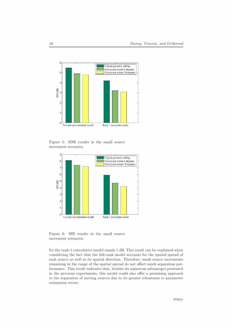
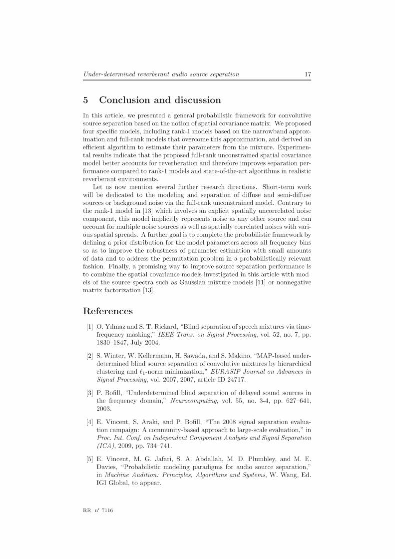
Our last experiment aims to to examine the robustness of the rank-1 convolutivemodel and the full-rank unconstrained model to small source movements. Wemade several recordings of three speech sources s1, s2, s3 in a meeting roomwith 250 ms reverberation time using omnidirectional microphones spaced by5 cm. The distance from the sources to the microphones was 50 cm. For eachrecording, the spatial images of all sources were separately recorded and thenadded together to obtain a test mixture. After the first recording, we keptthe same positions for s1 and s2 and successively moved s3 by 5 and 10◦ bothclock-wise and counter clock-wise resulting in 4 new positions of s3. We thenapplied the same procedure to s2 while the positions of s1 and s3 remainedidentical to those in the first recording. Overall, we collected nine mixtures:one from the first recording, four mixtures with 5◦ movement of either s2 or s3,and four mixtures with 10◦ movement of either s2 or s3. We performed sourceseparation in a semi-blind setting: the source spatial covariance matrices wereestimated from the spatial images of all sources recorded in the first recordingwhile the source variances were estimated from the nine mixtures using the samealgorithm as in Section 4.2. The average SDR and SIR obtained for the firstmixture and for the mixtures with 5◦ and 10◦ source movement are depicted inFig. 5 and Fig. 6, respectively. This procedure simulates errors encountered byon-line source separation algorithms in moving source environments, where thesource separation parameters learnt at a given time are not applicable anymoreat a later time.

The separation performance of the rank-1 convolutive model degrades morethan that of the full-rank unconstrained model both with 5◦ and 10◦ sourcerotation. For instance, the SDR drops by 0.6 dB for the full-rank unconstrainedmodel based algorithm when a source moves by 5◦ while the corresponding drop

1http://sisec2008.wiki.irisa.fr/tiki-index.php?page=Under-determined+speech+and+music+mixtures

RR n° 7116


Figure 5: SDR results in the small sourcemovement scenarios.

Figure 6: SIR results in the small sourcemovement scenarios.

for the rank-1 convolutive model equals 1 dB. This result can be explained whenconsidering the fact that the full-rank model accounts for the spatial spread ofeach source as well as its spatial direction. Therefore, small source movementsremaining in the range of the spatial spread do not affect much separation per-formance. This result indicates that, besides its numerous advantages presentedin the previous experiments, this model could also offer a promising approachto the separation of moving sources due to its greater robustness to parameterestimation errors.

INRIA


5 Conclusion and discussion

In this article, we presented a general probabilistic framework for convolutivesource separation based on the notion of spatial covariance matrix. We proposedfour specific models, including rank-1 models based on the narrowband approx-imation and full-rank models that overcome this approximation, and derived anefficient algorithm to estimate their parameters from the mixture. Experimen-tal results indicate that the proposed full-rank unconstrained spatial covariancemodel better accounts for reverberation and therefore improves separation per-formance compared to rank-1 models and state-of-the-art algorithms in realisticreverberant environments.

Let us now mention several further research directions. Short-term workwill be dedicated to the modeling and separation of diffuse and semi-diffusesources or background noise via the full-rank unconstrained model. Contrary tothe rank-1 model in [13] which involves an explicit spatially uncorrelated noisecomponent, this model implicitly represents noise as any other source and canaccount for multiple noise sources as well as spatially correlated noises with vari-ous spatial spreads. A further goal is to complete the probabilistic framework bydefining a prior distribution for the model parameters across all frequency binsso as to improve the robustness of parameter estimation with small amountsof data and to address the permutation problem in a probabilistically relevantfashion. Finally, a promising way to improve source separation performance isto combine the spatial covariance models investigated in this article with mod-els of the source spectra such as Gaussian mixture models [11] or nonnegativematrix factorization [13].

References

[1] O. Yılmaz and S. T. Rickard, “Blind separation of speech mixtures via time-frequency masking,” IEEE Trans. on Signal Processing, vol. 52, no. 7, pp.1830–1847, July 2004.

[2] S. Winter, W. Kellermann, H. Sawada, and S. Makino, “MAP-based under-determined blind source separation of convolutive mixtures by hierarchicalclustering and ℓ1-norm minimization,” EURASIP Journal on Advances inSignal Processing, vol. 2007, 2007, article ID 24717.

[3] P. Bofill, “Underdetermined blind separation of delayed sound sources inthe frequency domain,” Neurocomputing, vol. 55, no. 3-4, pp. 627–641,2003.

[4] E. Vincent, S. Araki, and P. Bofill, “The 2008 signal separation evalua-tion campaign: A community-based approach to large-scale evaluation,” inProc. Int. Conf. on Independent Component Analysis and Signal Separation(ICA), 2009, pp. 734–741.

[5] E. Vincent, M. G. Jafari, S. A. Abdallah, M. D. Plumbley, and M. E.Davies, “Probabilistic modeling paradigms for audio source separation,”in Machine Audition: Principles, Algorithms and Systems, W. Wang, Ed.IGI Global, to appear.

RR n° 7116


[6] N. Q. K. Duong, E. Vincent, and R. Gribonval, “Spatial covariance modelsfor under-determined reverberant audio source separation,” in Proc. 2009IEEE Workshop on Applications of Signal Processing to Audio and Acous-tics (WASPAA), 2009, pp. 129–132.

[7] C. Fevotte and J.-F. Cardoso, “Maximum likelihood approach for blindaudio source separation using time-frequency Gaussian models,” in Proc.2005 IEEE Workshop on Applications of Signal Processing to Audio andAcoustics (WASPAA), 2005, pp. 78–81.

[8] E. Vincent, S. Arberet, and R. Gribonval, “Underdetermined instantaneousaudio source separation via local Gaussian modeling,” in Proc. Int. Conf.on Independent Component Analysis and Signal Separation (ICA), 2009,pp. 775–782.

[9] A. P. Dempster, N. M. Laird, and B. D. Rubin, “Maximum likelihood fromincomplete data via the EM algorithm,” Journal of the Royal StatisticalSociety. Series B, vol. 39, pp. 1–38, 1977.

[10] J.-F. Cardoso, H. Snoussi, J. Delabrouille, and G. Patanchon, “Blind sep-aration of noisy Gaussian stationary sources. Application to cosmic mi-crowave background imaging,” in Proc. European Signal Processing Con-ference (EUSIPCO), vol. 1, 2002, pp. 561–564.

[11] S. Arberet, A. Ozerov, R. Gribonval, and F. Bimbot, “Blind spectral-GMMestimation for underdetermined instantaneous audio source separation,” inProc. Int. Conf. on Independent Component Analysis and Signal Separation(ICA), 2009, pp. 751–758.

[12] Y. Izumi, N. Ono, and S. Sagayama, “Sparseness-based 2CH BSS using theEM algorithm in reverberant environment,” in Proc. 2007 IEEE Workshopon Applications of Signal Processing to Audio and Acoustics (WASPAA),2007, pp. 147–150.

[13] A. Ozerov and C. Fevotte, “Multichannel nonnegative matrix factoriza-tion in convolutive mixtures for audio source separation,” IEEE Trans. onAudio, Speech and Language Processing, to appear.

[14] H. Sawada, S. Araki, R. Mukai, and S. Makino, “Grouping separatedfrequency components by estimating propagation model parameters infrequency-domain blind source separation,” IEEE Trans. on Audio, Speech,and Language Processing, vol. 15, no. 5, pp. 1592–1604, July 2007.

[15] T. Gustafsson, B. D. Rao, and M. Trivedi, “Source localization in rever-berant environments: Modeling and statistical analysis,” IEEE Trans. onSpeech and Audio Processing, vol. 11, pp. 791–803, Nov 2003.

[16] H. Kuttruff, Room Acoustics, 4th ed. New York: Spon Press, 2000.

[17] G. McLachlan and T. Krishnan, The EM algorithm and extensions. NewYork, NY: Wiley, 1997.

INRIA


[18] H. Sawada, S. Araki, R. Mukai, and S. Makino, “Solving the permutationproblem of frequency-domain bss when spatial aliasing occurs with widesensor spacing,” in Proc. 2006 IEEE Int. Conf. on Acoustics, Speech andSignal Processing (ICASSP), 2006, pp. 77–80.

[19] E. Vincent, H. Sawada, P. Bofill, S. Makino, and J. Rosca, “First stereo au-dio source separation evaluation campaign: data, algorithms and results,”in Proc. Int. Conf. on Independent Component Analysis and Signal Sepa-ration (ICA), 2007, pp. 552–559.

[20] M. Cobos and J. Lopez, “Blind separation of underdetermined speech mix-tures based on DOA segmentation,” IEEE Trans. on Audio, Speech, andLanguage Processing, submitted.

[21] M. Mandel and D. Ellis, “EM localization and separation using interaurallevel and phase cues,” in Proc. 2007 IEEE Workshop on Applications ofSignal Processing to Audio and Acoustics (WASPAA), 2007, pp. 275–278.

[22] R. Weiss and D. Ellis, “Speech separation using speaker-adapted eigenvoicespeech models,” Computer Speech and Language, vol. 24, no. 1, pp. 16–20,Jan 2010.

[23] S. Araki, T. Nakatani, H. Sawada, and S. Makino, “Stereo source separationand source counting with MAP estimation with Dirichlet prior consideringspatial aliasing problem,” in Proc. Int. Conf. on Independent ComponentAnalysis and Signal Separation (ICA), 2009, pp. 742–750.

[24] Z. El Chami, D. T. Pham, C. Serviere, and A. Guerin, “A new model basedunderdetermined source separation,” in Proc. Int. Workshop on AcousticEcho and Noise Control (IWAENC), 2008.

RR n° 7116

Centre de recherche INRIA Rennes – Bretagne AtlantiqueIRISA, Campus universitaire de Beaulieu - 35042 Rennes Cedex (France)

Centre de recherche INRIA Bordeaux – Sud Ouest : Domaine Universitaire - 351, cours de la Libération - 33405 Talence CedexCentre de recherche INRIA Grenoble – Rhône-Alpes : 655, avenue de l’Europe - 38334 Montbonnot Saint-Ismier

Centre de recherche INRIA Lille – Nord Europe : Parc Scientifique de la Haute Borne - 40, avenue Halley - 59650 Villeneuve d’AscqCentre de recherche INRIA Nancy – Grand Est : LORIA, Technopôle de Nancy-Brabois - Campus scientifique

615, rue du Jardin Botanique - BP 101 - 54602 Villers-lès-Nancy CedexCentre de recherche INRIA Paris – Rocquencourt : Domaine de Voluceau - Rocquencourt - BP 105 - 78153 Le Chesnay Cedex

Centre de recherche INRIA Saclay – Île-de-France : Parc Orsay Université - ZAC des Vignes : 4, rue Jacques Monod - 91893 Orsay CedexCentre de recherche INRIA Sophia Antipolis – Méditerranée :2004, route des Lucioles - BP 93 - 06902 Sophia Antipolis Cedex

ÉditeurINRIA - Domaine de Voluceau - Rocquencourt, BP 105 - 78153 Le Chesnay Cedex (France)http://www.inria.fr

ISSN 0249-6399

Documents

Under-determined reverberant audio source separation … domain as a zero-mean Gaussian random variable whose covari-ance encodes the spatial characteristics of the source. We then