Harmonic Functions and Collision Probabilities

Christopher I. Connolly, EK 266 �y

Arti�cial Intelligence Center

SRI International, Inc.

333 Ravenswood Ave.

Menlo Park CA, 94025 USA

Tel. (415) 859-5022, FAX (415) 859-3735

email: connolly@ai.sri.com

Abstract

There is a close relationship between harmonic functions { which have recently been

proposed for path planning { and hitting probabilities for random processes. The hitting

probabilities for random walks can be cast as a Dirichlet problem for harmonic func-

tions, in much the same way as in path planning. This equivalence has implications

both for uncertainty in motion planning and in the application of machine learning

techniques to some robot problems. In particular, Erdmann's method can directly in-

corporate such hitting probabilities. In addition, the value functions obtained by re-

inforcement learning algorithms can be rapidly reconstructed by relaxation or resistive

networks, once the extrema for such functions are known.

1 Introduction

Some recent research in robotics has focussed on the use of harmonic potential functions forpath planning (Connolly et al. 1990, Akishita et al. 1990, Keymeulen and Decuyper 1991,Tarassenko and Blake 1991, Kim and Khosla 1992, Connolly and Burns 1993, Connolly and

Grupen 1993, Singh et al. 1994, Connolly et al. 1995). This approach resembles other

potential �eld approaches, except that the �eld is usually computed in a \global" manner,that is, over the entire region of interest. In particular, the method as described in (Connolly

and Grupen 1993) uses a grid-based relaxation technique. This results in a potential such

that, at each point, the potential function is the average of the potentials at neighboring

points.

�Most of this work was performed while the author was at the Department of Computer Science at theUniversity of Massachusetts, under NSF grants IRI-9116297 and IRI-9208920.

yInternational Journal of Robotics Research, 16(4):497-507.

1

Obstacle and goal points provide the boundary conditions for this potential, and are

held �xed at high and low potential values, respectively. Because they are harmonic, such

functions have extrema only at designated points (the boundary conditions), and do not

su�er from the oft-cited \local-minima problem". These functions can be computed easily

either by relaxation (Connolly and Grupen 1993) or resistive grids (Tarassenko and Blake

1991). Implementation details and experimental results for harmonic function path planning

are described in (Connolly and Grupen 1993) and (Grupen et al. 1994). Such functions can

also be used in conjunction with dynamic e�ects to plan and control repetitive manipulatormovements (Connolly et al. 1995).

This paper discusses the relationship between harmonic function planning, its probabilis-

tic interpretation, and recent work on uncertainty and learning in robotics. The probabilistic

interpretation of harmonic functions is described in more detail in (Doyle and Snell 1984,

Kemeny et al. 1976). Doyle and Snell's usage of the term \harmonic" will be adopted here:

A function will be considered harmonic if it is the equilibrium voltage found in a resistivenetwork. In the following discussion, the equivalence between probabilities and potentials isdescribed in terms of lattices1, since this is a representation compatible with grid-based ap-proaches. Harmonic potential functions can be directly interpreted as collision probabilities.

They can be used to introduce an appropriate drift in randomization, and their propertiescan be used to guarantee some useful properties for reinforcement learning systems. It maybe of some use to consider these potentials as the stable equilibria for di�usion processes.That is, the potentials represent the asymptotic, steady-state values (e.g., concentrations orvoltages) for some kind of di�usion (e.g., chemical or electronic).

2 Laplace's Equation

A harmonic function � on a domain � Rn is a function which satis�es Laplace's equation:

r2� =

nXi=1

@2�

@x2i

= 0 (1)

where x 2 Rn, and each xi is a con�guration space variable.

In the case of robot path planning, the boundary of (denoted by @) consists of

the boundaries of all obstacles and goals in a cspace2 representation. Note that in thisdiscussion, goals may be sets and not merely points. Moreover, there may be more thanone goal set in the freespace domain. Harmonic functions satisfy the min-max principle:

spontaneous creation of local mimima within the solution region is impossible (Weinstock

1974, Zachmanoglou and Thoe 1986). In the continuous case, this can be shown using

the Gauss Integral Theorem (Courant and Hilbert 1989). This theorem states that for a

harmonic function �, the following integral holds:3

Z@�

@�

@ndS = 0 (2)

1It should be emphasized that the equivalence extends to the continuous case as well.2Con�guration space.3This equation can be derived by applying Green's Formula to a function � which is harmonic.

2

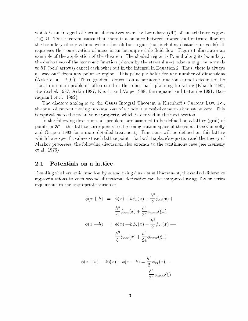
which is an integral of normal derivatives over the boundary (@�) of an arbitrary region

� � . This theorem states that there is a balance between inward and outward ow on

the boundary of any volume within the solution region (not including obstacles or goals). It

expresses the conservation of mass in an incompressible uid ow. Figure 1 illustrates an

example of the application of the theorem. The shaded region is �, and along its boundary,

the derivatives of the harmonic function (shown by the streamlines) taken along the normals

to @� (bold arrows) cancel each other out in the integral in Equation 2. Thus, there is always

a \way out" from any point or region. This principle holds for any number of dimensions(Axler et al. 1991). Thus, gradient descent on a harmonic function cannot encounter the\local minimum problem" often cited in the robot path planning literature (Khatib 1985,

Koditschek 1987, Arkin 1987, Khosla and Volpe 1988, Barraquand and Latombe 1991, Bar-

raquand et al. 1992).

The discrete analogue to the Gauss Integral Theorem is Kirchho�'s Current Law, i.e.,

the sum of current owing into and out of a node in a resistive network must be zero. Thisis equivalent to the mean value property, which is derived in the next section.

In the following discussion, all problems are assumed to be de�ned on a lattice (grid) ofpoints in Zn { this lattice corresponds to the con�guration space of the robot (see Connolly

and Grupen 1993 for a more detailed treatment). Functions will be de�ned on this latticewhich have speci�c values at each lattice point. For both Laplace's equation and the theory ofMarkov processes, the following discussion also extends to the continuous case (see Kemenyet al. 1976).

2.1 Potentials on a lattice

Denoting the harmonic function by �, and using h as a small increment, the central di�erenceapproximations to each second directional derivative can be computed using Taylor seriesexpansions in the appropriate variable:

�(x+ h) = �(x) + h�x(x) +h2

2�xx(x) +

h3

6�xxx(x) +

h4

24�xxxx(�+)

�(x� h) = �(x)� h�x(x) +h2

2�xx(x)�

h3

6�xxx(x) +

h4

24�xxxx(��)

�(x+ h)� 2�(x) + �(x� h) =h2

2�xx(x) +

h4

24�xxxx(�)

3

Since h = 1 on the lattice, we have in two dimensions:

�(x+ 1; y) + �(x� 1; y) + �(x; y + 1) + �(x; y � 1) � 4�(x) � r2� = 0 (3)

Therefore, up to truncation error, the value of � at a point in the lattice is the averageof the values at the points in the (manhattan) neighborhood. This is known as the mean-

value property, and applies in both the discrete and continuous cases (Axler et al. 1991).Although the above derivation pertains to two dimensions, the mean-value property holds

for any number of dimensions (Axler et al. 1991). To compute harmonic functions on a

lattice, one solves the system of equations de�ned by Equation 3 using iterative methods

such as successive overrelaxation (SOR) (Burden et al. 1978). In a 4-dof path planner for a

P-50 welding robot, using roughly 16,000 nodes, SOR converges in approximately 300ms on

a Sparc 10 processor (see Grupen et al. 1994). One can also employ resistive, inductive, or

capacitive circuits (Tarassenko and Blake 1991, McCann and Wilts 1949).

For the purposes of this paper, the de�nition of the term harmonic will be loosenedsomewhat (after Doyle and Snell 1984) to the case where the mean shown in Equation 3 isactually a weighted mean. This corresponds to a spatially distorted Laplacian, or to the case

of a resistive network whose resistances are not necessarily uniform. Most of the interestingproperties of harmonic functions, in particular the min-max and smoothness properties, stillapply in this case.4

2.2 Potentials in Markov Processes

Consider a Markov chain on the lattice, and let A denote the absorbing set. Divide A intotwo disjoint subsets O and G. Let p(x) at any state x be the probability that the process,

starting from x, will be absorbed in O before reaching any state in G. Then p(x) is knownas a hitting probability. Assume for the moment that the probabilities of transition from the

current state to any neighbor state are all equal ( 1

2n, where n is the number of dimensions

in the lattice). The probability p(x) can then be de�ned in two dimensions as:

p(x) =1

4( p(N jx! N) + p(Ejx! E)

+p(W jx! W ) + p(Sjx! S))

where N;E;W;S are the 4 nearest neighboring states and x! N denotes a transition fromx to N . This sum follows from the fact that transitions are exclusive, but the probability

of a transition is 1. Since the process is Markov, probabilities do not depend on prior time

steps, so that p(N jx! N) = p(N), and likewise for the other neighbors. Thus, the hittingprobability at any lattice point is the average of the hitting probabilities at the (manhattan)

neighbors. This is the mean-value property, which can be expressed as:

p(x) =1

n

nXi=1

p(xi) (4)

4Smoothness holds in the continuous case. In the discrete case, one may enforce a desired degree ofsmoothness by interpolation, using the harmonic polynomials in Rn as a basis set.

4

where the xi are the n neighbors of state x. This can also be seen by considering the transition

matrix P for a Markov chain. One can think of P as a smoothing or averaging operator

(Kemeny et al. 1976). For a general Markov chain, where the transition probabilities are

not necessarily equal, Equation 4 becomes

p(i) =mXj=1

Pijp(j) (5)

where i and j are states in the m-state Markov chain whose transition matrix is P . The sum

of transition probabilities out of a state i must be no greater than 1, so that:

mXj=1

Pij � 1 (6)

but note that whenmXj=1

Pij < 1 (7)

an equivalent Markov chain P 0 can be constructed by adding a new \disappearing" statem+ 1 to the chain (see Kemeny et al. 1976), such that:

m+1Xj=1

P 0

ij= 1 (8)

Equation 5, appropriately modi�ed, thus describes a true weighted mean. Clearly, the prob-ability function p still obeys the min-max principle, and cannot exhibit any \local" extrema.

The (weighted) mean-value property is unique up to boundary conditions. To see this,consider a harmonic function �(x) with respect to a particular Markov chain (hence it is

known to satisfy the mean-value property), and suppose that there is another function p(x)

which also satis�es the mean-value property with respect to the same chain. Let

�(x) = p(x)� �(x) (9)

at any state x, and by hypothesis, �(x) = 0 at the boundaries (absorbing states, in the

Markov chain). Using the mean-value property for p(x) and �(x),

�(x) =1

n

nXi=1

(p(xi)� �(xi))

=1

n

nXi=1

�(xi)

so that �(x) also satis�es the mean-value property. Since �(x) = 0 at the boundaries, � must

be constant over all x (i.e., �(x) = 0 everywhere). Hence, p(x) � �(x). Hitting probabilities

are therefore uniquely harmonic up to their boundary conditions.

5

There is a simple interpretation of this equivalence in the context of harmonic function

path planning. Let O be the set of states which are occupied by obstacles, and let G be the

set of goal states. The Dirichlet form for obstacles is assumed, where obstacle boundaries

are �xed at �(x) = 1, and goal regions are �xed at �(x) = 0. In this case, �(x) is simply

the collision probability for a random walk starting at x. Therefore, gradient descent of

a harmonic function so constructed will always minimize the probability of collisions with

obstacles during a randommotion (or perturbation). So if the actual trajectory of the e�ector

has a random component (e.g., control error or external forces), its probability of accidentalcollision with obstacles is minimized by using a gradient descent on the harmonic function�.

3 Uncertainty in Motion

Several authors have examined robot task execution in the presence of uncertainty in envi-ronmental modeling, robot motion, and obstacle motion (e.g., Donald 1990, Griswold and

Eem 1990, Oommen et al. 1991, Erdmann 1992, Simmons and Koenig 1995). This discus-sion centers around Erdmann's work. Erdmann argues for the utility of randomization inrobotic tasks as a way of overcoming uncertainty. The approach used by Erdmann relies ona randomization step in cases where uncertainty prevents a reliable measurement of e�ectorposition. Bounds can be computed on the expected time-to-completion for the randomiza-

tion process. The approach can take estimated obstacle positions into account through theuse of an arbitrary label function `. An appropriate choice for ` is the hitting probability forthe process.

Let pc(x) be the probability that a random walk starting at x collides with an obstaclebefore reaching the goal. As noted in (Erdmann 1992), a prerequisite to any randomizing

step is that pc(x) < 1 (i.e., that there is a nonzero probability of reaching the goal beforehitting an obstacle). IfO denotes the obstacle set, and G the goal set, then these probabilitiescan be computed directly by setting the following boundary conditions:

pc(x) = 1 x 2 O

pc(x) = 0 x 2 G

and then computing the harmonic function which satis�es these constraints (see section 2).

If pc(x) = 1, then the goal is blocked, and some other strategy must be employed.In (Erdmann 1992), the randomization process is modeled as a stochastic di�usion (Karlin

and Taylor 1981), with drift �� and variance �. The label function ` is used to analyze

expected velocity of the process. If L is the Brownian motion operator with drift:

v(x) = (L`)(x) (10)

=1

2�2r2` + ��r` (11)

Letting `(x) = pc(x) (a harmonic function), a drift velocity can be computed which biases

the randomization toward the goal. Since pc(x) is harmonic, the �rst term of Equation 11

6

vanishes:

v(x) = ��rpc(x)

By allowing � to be a function of con�guration, and then adopting Erdmann's conventionthat the expected in�nitesimal velocity v(x) = �1 (with respect to the label function pc),

��(x) must be a vector in the opposite half-plane with respect to rpc(x). In other words,

the process drift should be in the direction of decreasing collision probabilities. Thus, the

same framework which is used for coarse motion planning in (Connolly and Grupen 1993)

can also be used for determining the drift in randomization. This allows randomization to

take into account the estimated locations of obstacles in the workspace.

3.1 Examples

To illustrate the use of label functions in motion planning under uncertainty, a simple simu-

lation of a 2-dof robot arm has been programmed. The simulator uses the gradient of a labelfunction to command the arm, subject to a random perturbation of the motion of the armby up to 5 times the commanded motion step. In the examples shown here, a randomization

of 1.66 times the step size was used. Figure 2 shows the initial con�guration used in the

examples. The goal (denoted by the open circle and open square) is a speci�c con�guration.Obstacles are drawn as a mesh, with the outermost layer removed so the paths (a sequenceof points) can be easily seen.

Figure 3 shows a path obtained using a euclidean distance function as the label function.This function was computed using a wavefront propagation starting from the goal point (see,

e.g. Barraquand et al. 1992 ). This path took 252 steps to reach the goal. Figure 4 showsthe same scenario, but with a harmonic label function. The resulting path took 156 steps tocomplete. The di�erence in the number of steps arises in part because gradient descent of adistance function does not minimize hitting probabilities. In fact, in certain cases, distancefunctions obtained from the l1 or l2 norm will guarantee that many paths pass through

certain isolated points. This is illustrated in Figure 5. Notice that any path originating tothe right of the wedge must pass through one point at the tip of the wedge. If the e�ector'smotion has a random component here, or if there is error in the estimation of the obstacle's

location, then there will be a signi�cant probability that the e�ector will hit the obstacle.Such collisions occur in Figure 3, resulting in many more steps required to reach the goal

con�guration. In contrast, the motion produced by the harmonic label function (Figure 4)

is guided to regions of minimum hitting probability. In this case, no collisions occur.

4 Learning and Robotics

Robot navigation and planning serves as a convenient application domain for reinforcementlearning techniques (Dayan 1991, Bachrach 1992, Thrun and M�oller 1992, Mahadevan andConnell 1992, Singh et al. 1994, Moore 1994, Fagg et al. 1994). In this context, robot control

is often treated as a Markovian decision problem, solved using a variant of either temporal

di�erencing (TD) (Sutton 1988) or Q-learning (Watkins 1989). In these cases, the problem

7

is one of �nding the correct expected value function for the underlying Markov chain which

represents the decision problem. Convergence proofs for these methods (Dayan 1994, Sutton

1988) rely in part on the fact that the expected value function E[zjx] for a Markov chain (or

martingale)5 is de�ned by

E[zjx] = P1z (12)

where P is the transition matrix for the Markov chain, and z are the expected values at

absorbing states. Typically, z represents the reward or penalty for entering any particular

member of the set of absorbing states in the chain.

A regular function for the Markov chain de�ned by P is a function f such that (Kemeny

et al. 1976):f = Pf (13)

That is, f is invariant under the operator de�ned by the transition matrix. As seen inSection 2.2, such functions are expected value functions for the Markov chain, subject to

appropriate boundary conditions. Moreover, every regular function for a Markov chain is

harmonic in the sense that such functions satisfy the weighted mean-value property de�nedby the transition probabilities of the Markov chain. For the purposes of this discussion, theterms \hitting probability" and \expected value function" are equivalent, since they refer to

the probability of a process reaching set G before being absorbed by set O.Thus, there is a common mathematical foundation for both harmonic function path

planning and techniques in reinforcement learning. Because they are harmonic, expected

value functions must obey certain properties that do not appear to have been explicitlyrecognized in the robot learning literature. For example, the min-max property implies thatexpected value functions cannot exhibit local minima. The presence of such minima (asobserved in Bachrach 1992) can be used as an indication that a learning process has notconverged su�ciently for the desired task.

To illustrate this equivalence, harmonic functions were computed using random walkstatistics, temporal di�erencing (TD(0)), and SOR on a simple environment. Figure 6 showsa sample path for each estimate of the environment's expected value function. The smallopen squares in the lower and upper left are goals. The large square in the middle andthe outermost margin are obstacles. The small open circles represent the paths obtained

by steepest descent, hence minimization of hitting probability. Equivalently, this maximizes

goal-reaching probability, since if p(x) is the hitting probability, 1 � p(x) is the probability

that the process reaches the goal before hitting an obstacle.Figure 7 shows the estimates of the expected value function produced by each method.

The random walk statistics (leftmost surface) were generated by computing the ratio of

obstacle hits (when such hits occurred before the goal was reached) to the total number

of random walks for a given starting state. The TD(0) value function (center surface) wascomputed using TD(0) as described in (Sutton 1988), applied to random walks from a given

starting state. In the TD case, the expected value was set to 1 at obstacle points and 0 at goal

points. The random-walk and TD-based results were obtained by using 50 random walksstarting at each state. For the SOR computation (rightmost surface), 53 iterations (over

5That is, the expected absorbing state value for a process starting at state x.

8

the entire grid) were used, where the boundary conditions were de�ned as in the TD case.

Uniform transition probabilities were assumed in each case. Note the similarity between the

surfaces. An intuitive sense of the probabilistic interpretation of such functions can be had

by observing the behavior of the surface near obstacles and away from the goals, where the

hitting probability is near 1, as one would expect.

Systems which use expected value functions should be able to take advantage of smooth-

ness and the min-max principle by preserving the harmonic nature of these functions in

subsequent processing steps. The following operations preserve the harmonic properties ofa function � (where c is a constant):

� dilation �0(x) = �(cx)

� translation �0(x) = �(x+ c)

� scaling �0(x) = c�(x)

� bias �0(x) = c+ �(x)

These properties can all be veri�ed by applying the Laplacian to �0. Clearly, any linear

combination of harmonic functions is also harmonic. Thus, when collision probabilities(expected values) can be isolated, their properties can be preserved by using the aboveoperations (see also Axler et al. 1991).

When applied to navigation in its simplest form, each expected value function will onlybe valid for a particular obstacle/goal con�guration. As soon as this con�guration changes, a

new function must be computed (by uniqueness for mean-value functions). Changing the ab-sorbing set necessarily changes the expected value function, requiring recomputation. Thus,if any aspect of the environment changes, the expected value function must be recomputed,regardless of the method chosen. It follows that robot navigation or planning methods whichrequire extensive training will not work well in nonstationary environments. This suggests

that, in addition to the tradeo�s enforced by dimensionality and state space size, the rate ofchange of absorbing states must also be considered when computing expected value functions.

This discussion describes a basic equivalence between methods such as TD (Sutton 1988),Monte-Carlo solution (Barto and Du� 1994), and direct methods such as SOR or resistive

networks, all of which compute harmonic functions in some form. Typically, methods such as

temporal di�erencing can also involve a transformation X which maps observations to states.In cases where X and z, and the state space (including transition probabilities) are fully

determined and/or small enough, the expected value for each state can be computed directly(e.g., with a resisitive network). In many cases though, the state observation matrixX is not

fully determined. In other cases, the state space will be too large to allow direct computation.Finally, the TD method can rely on the process itself to update the expected value function,

and for this reason does not require any knowledge of transition probabilities. In the caseof a direct computation using, e.g., SOR or resistive networks, transition probabilities must

be determined or assumed beforehand (if they are not available). Thus, the following are

prerequisites for direct computation:

� knowledge of the observation matrix X.

9

� process transition probabilities.

� boundary conditions.

� \small" state spaces.

If these conditions do not hold, direct computation may be infeasible, and a scheme such as

TD is an appropriate choice for computing the value function.

More generally, the intent of this discussion is to show that the fundamental properties

of Markov chains provide a common framework for connectionist learning techniques and

harmonic function path planning. This in turn suggests that the choice of method is depen-

dent on the characteristics of the problem to be solved. The relationship of TD to harmonic

functions also suggests ways in which the special properties of harmonic functions (e.g.,

min-max property, smoothness) can be used to advantage in learning-based systems. Note

also that when su�cient information is available, direct methods (e.g., resistive networks)can be used to reconstruct expected value functions from their boundary conditions. By themin-max property, the boundary conditions can easily be distinguished as the extrema of

the value function. If transition probabilities are known or can be assumed, this allows thecompression of learned (stationary) expected value functions after convergence, since onlythe boundary conditions are needed.

The relationship between Laplace's equation and Markov chains can be generalized when

a reward or penalty is associated with each transition in the Markov chain. In this case,

Laplace's equation can be replaced with Poisson's equation:

r2�(x) = f(x) (14)

where f is the reward/penalty as a function of state. This equivalence is explored in moredetail in (Hordijk 1974).

5 Conclusion

In this paper, some properties of harmonic functions have been discussed in the context of re-lated work in path planning, control under uncertainty, and machine learning. In particular,

the equivalence of harmonic functions and collision probabilities has been illustrated. This

connection is applied to motion uncertainty, and in particular to Erdmann's randomization

method. The result is an explicit incorporation of obstacle information into the randomiza-

tion process, and an interpretation of harmonic functions in terms of goal-reaching probabil-ities and in terms of drift in the random motion. This also illustrates the interpretation of

harmonic functions as an extrapolation of obstacle geometry (Connolly and Grupen 1993).Collision probabilities are often utilized in robot-learning systems, in one form or another.

Because these probabilities are harmonic, local minima can be eliminated to enforce smooth

behavior of the system. In particular, temporal di�erencing (and in fact, any scheme based

on absorbing Markov chains) is in some sense equivalent to the computation of a speci�c

harmonic function. The TD weights are related to the corresponding harmonic function by

10

the matrixX of state observation vectors. It is important to note that this function can only

be fully determined if the transition probabilities for the Markov chain are known or assumed

a priori. In temporal di�erencing, the observed process itself obeys these probabilities,

whereas in a resistive grid (or other direct computation), they must be speci�ed in advance.

In any event, harmonic functions exhibit formal properties which are of use in applications

based on the theory of Markov decision problems.

References

[1] Akishita S , Kawamura S , and Hayashi K 1990. Laplace potential for moving obstacle

avoidance and approach of a mobile robot. In 1990 Japan-USA Symposium on Flexible

Automation, A Paci�c Rim Conference, pages 139{142.

[2] Arkin R. C 1987. Towards Cosmopolitan Robots: Intelligent Navigation in Extended

Man-Made Environments. PhD thesis, University of Massachusetts.

[3] Axler S , Bourdon P , and Ramey W 1991. Harmonic Function Theory, volume 137 ofGraduate Texts in Mathematics. Springer-Verlag, New York.

[4] Bachrach J. R 1992. Connectionist Modeling and Control of Finite State Environments.PhD thesis, University of Massachusetts.

[5] Barraquand J , Langlois B , and Latombe J.-C 1992. Numerical potential �eld tech-niques for robot path planning. IEEE Transactions on Systems, Man, and Cybernetics,22(2):224{241.

[6] Barraquand J and Latombe J.-C 1991. Robot motion planning: A distributed repre-

sentation approach. International Journal of Robotics Research, 10(6):628{649.

[7] Barto A and Du� M 1994. Monte Carlo matrix inversion and reinforcement learning.

In Cowan J. D , Tesauro G , and Alspector J , editors, Neural Information Processing

Systems 6, pages 687{694. Morgan Kaufmann Publishers.

[8] Burden R. L , Faires J. D , and Reynolds A. C 1978. Numerical Analysis. Prindle,

Weber and Schmidt, Boston.

[9] Connolly C. I and Burns J. B 1993. A model for the functioning of the striatum.

Biological Cybernetics, 68(6):535{544.

[10] Connolly C. I , Burns J. B , and Weiss R 1990. Path planning using Laplace's Equation.In Proceedings of the 1990 IEEE International Conference on Robotics and Automation,

pages 2102{2106. IEEE.

[11] Connolly C. I and Grupen R. A 1993. The applications of harmonic functions to robotics.

Journal of Robotic Systems, 10(7):931{946.

11

[12] Connolly C. I , Grupen R. A , and Souccar K. X 1995. A hamiltonian approach to

kinodynamic planning. In Proceedings of the 1995 IEEE International Conference on

Robotics and Automation, page to appear. IEEE.

[13] Courant R and Hilbert D 1989. Methods of Mathematical Physics, volume 2. John

Wiley and Sons, New York.

[14] Dayan P 1991. Navigating through temporal di�erence. In Lippmann R. P , Moody

J. E , and Touretzky D. S , editors, Advances in Neural Information Processing Systems

3, pages 464{470. Morgan Kaufmann Publishers.

[15] Dayan P 1994. The convergence of TD(�) for general �. Machine Learning, 8:341{362.

[16] Decuyper J and Keymeulen D 1991. A reactive robot navigation system based on a

uid dynamics metaphor. In Parallel Problem Solving from Nature, Lecture Notes in

Computer Science, pages 348{355. Springer Verlag.

[17] Donald B. R 1990. Planning multi-step error detection and recovery strategies. Inter-national Journal of Robotics Research, 9(1):3{60.

[18] Doyle P and Snell J. L 1984. Random Walks and Electric Networks. Carus Monographsin Mathematics. American Mathematical Society.

[19] Erdmann M 1992. Randomization in robot tasks. International Journal of Robotics

Research, 11(5):399{436.

[20] Fagg A. H , Lotspeich D , and Bekey G. A 1994. A reinforcement-learning approach toreactive control policy design for autonomous robots. In Proceedings of the 1994 IEEE

International Conference on Robotics and Automation, pages 39{44. IEEE.

[21] Griswold N. C and Eem J 1990. Control for mobile robots in the presence of movingobstacles. IEEE Transactions on Robotics and Automation, 6(2):263{268.

[22] Grupen R. A , Coelho J. A , Connolly C. I , Gullapalli V , Huber M , and Souccar

K 1994. Toward physical interaction and manipulation: Screwing in a light bulb. InAAAI 1994 Spring Symposium on Physical Interaction and Manipulation.

[23] Hordijk A 1974. Dynamic programming and Markov potential theory. Mathematisch

Centrum, Amsterdam.

[24] Karlin S and Taylor H. M 1981. A Second Course in Stochastic Processes. AcademicPress, New York.

[25] Kemeny J. G , Snell J. L , and Knapp A. W 1976. Denumerable Markov Chains,volume 40 of Graduate Texts in Mathematics. Springer-Verlag, New York.

[26] Khatib O 1985. Real-time obstacle avoidance for manipulators and mobile robots. In

Proceedings of the 1985 IEEE International Conference on Robotics and Automation,

pages 500{505. IEEE.

12

[27] Khosla P and Volpe R 1988. Superquadric arti�cial potentials for obstacle avoidance

and approach. In Proceedings of the 1988 IEEE International Conference on Robotics

and Automation, pages 1778{1784. IEEE.

[28] Kim J.-O and Khosla P 1991. Real-time obstacle avoidance using harmonic potential

functions. In Proceedings of the 1991 IEEE International Conference on Robotics and

Automation, pages 790{796. IEEE.

[29] Koditschek D. E 1987. Exact robot navigation by means of potential functions: Some

topological considerations. In Proceedings of the 1987 IEEE International Conference

on Robotics and Automation, pages 1{6. IEEE.

[30] Mahavedan S and Connell J 1992. Automatic programming of behavior-based robots

using reinforcement learning. Arti�cial Intelligence, 55:311{365.

[31] McCann G. D and Wilts C. H 1949. Application of electric-analog computers to heat-transfer and uid- ow problems. Journal of Applied Mechanics, 16(3):247{258.

[32] Moore A. W 1994. The parti-game algorithm for variable resolution reinforcementlearning in multidimensional state-spaces. In Cowan J. D , Tesauro G , and AlspectorJ , editors, Neural Information Processing Systems 6, pages 711{718. Morgan Kaufmann

Publishers.

[33] Oommen B. J , Andrade N , and Iyengar S. S 1991. Trajectory planning of robotmanipulators in noisy work spaces using stochastic automata. International Journal ofRobotics Research, 10(2):135{148.

[34] Simmons R and Koenig S 1995. Probabilistic navigation in partially observable envi-ronments. In IJCAI '95, pages 1080{1087.

[35] Singh S. P , Barto A. G , Grupen R , and Connolly C 1994. Robust reinforcementlearning in motion planning. In Cowan J. D , Tesauro G , and Alspector J , editors, Ad-vances in Neural Information Processing Systems 6, pages 655{662. Morgan Kaufmann

Publishers.

[36] Sutton R. S 1988. Learning to predict by the methods of temporal di�erences. Machine

Learning, 3(1):9{44.

[37] Tarassenko L and Blake A 1991. Analogue computation of collision-free paths. In

Proceedings of the 1991 IEEE International Conference on Robotics and Automation,

pages 540{545. IEEE.

[38] Thrun S. B and M�oller K 1992. Active exploration in dynamic environments. In Moody

J. E , Hanson S. J , and Lippmann R. P , editors, Advances in Neural Information

Processing Systems 4. Morgan Kaufmann Publishers.

[39] Watkins C. J. C. H 1989. Learning from Delayed Rewards. PhD thesis, Cambridge

University.

13

[40] Weinstock R 1974. Calculus of Variations with Applications to Physics and Engineering.

Dover Publications, Inc.

[41] Zachmanoglou E. C and Thoe D. W 1986. Introduction to Partial Di�erential Equations

with Applications. Dover Publications, Inc., New York.

14

List of Figures

1 An illustration of the Gauss Integral Theorem: bold arrows are normals, lightarrows are streamlines. . . . . . . . . . . . . . . . . . . . . . . . . . . . . . . 16

2 2-DOF arm example, initial con�guration: right pane is cartesian space, left

pane is con�guration space. Open circle (right) and open square (left) repre-

sent goal con�gurations. The mesh designates obstacles, including joint limits. 17

3 2-DOF arm example, path and �nal con�guration using an l2 distance map

as the label function. . . . . . . . . . . . . . . . . . . . . . . . . . . . . . . . 18

4 2-DOF arm example, path and �nal con�guration using a harmonic function

as the label function. . . . . . . . . . . . . . . . . . . . . . . . . . . . . . . . 19

5 Shadow e�ect created by a euclidean distance function. The black wedge

represents an obstacle. . . . . . . . . . . . . . . . . . . . . . . . . . . . . . . 20

6 Environment with paths generated by random walk statistics (left), TD(0)(middle) and an SOR-generated harmonic function (right). . . . . . . . . . . 21

7 Harmonic functions computed using random walk statistics (left), TD(0) (mid-

dle) and SOR (right). . . . . . . . . . . . . . . . . . . . . . . . . . . . . . . . 22

15

Streamline

Surface Normal

Γ

Figure 1: An illustration of the Gauss Integral Theorem: bold arrows are normals, lightarrows are streamlines.

16

Figure 2: 2-DOF arm example, initial con�guration: right pane is cartesian space, left pane iscon�guration space. Open circle (right) and open square (left) represent goal con�gurations.

The mesh designates obstacles, including joint limits.

17

Figure 3: 2-DOF arm example, path and �nal con�guration using an l2 distance map as the

label function.

18

Figure 4: 2-DOF arm example, path and �nal con�guration using a harmonic function as

the label function.

19

Goal

A

B

C

D

All paths in this region passthrough point A.

Figure 5: Shadow e�ect created by a euclidean distance function. The black wedge represents

an obstacle.

20

Figure 6: Environment with paths generated by random walk statistics (left), TD(0) (middle)

and an SOR-generated harmonic function (right).

21

1020

30

10

20

30

0

0.2

0.4

0.6

0.8

1

1020

30

10

20

30

0

0.2

0.4

0.6

0.8

1

1020

30

10

20

30

0

0.2

0.4

0.6

0.8

1

1020

30

10

20

30

0

0.2

0.4

0.6

0.8

1

1020

30

10

20

30

0

0.2

0.4

0.6

0.8

1

1020

30

10

20

30

0

0.2

0.4

0.6

0.8

1

Figure 7: Harmonic functions computed using random walk statistics (left), TD(0) (middle)

and SOR (right).

22