Embed Size (px)
Citation preview

Uncovering predictability of individual and teamsuccess: Signi�cant Hot Hand Effect inInternational CricketSumit Kumar Ram ( [email protected] )
ETH ZürichShyam Nandan
ETH ZürichDidier Sornette
ETH Zürich
Research Article
Keywords:
Posted Date: December 6th, 2021
DOI: https://doi.org/10.21203/rs.3.rs-1003454/v2
License: This work is licensed under a Creative Commons Attribution 4.0 International License. Read Full License

1
Uncovering predictability of individual and team success:
Significant Hot Hand Effect in International Cricket
Sumit Kumar Ram1,2*, Shyam Nandan3 and Didier Sornette2,4*
1Connection Science, Massachusetts Institute of Technology, Cambridge, USA
2Department of Management, Technology and Economics, ETH Zürich,
Scheuchzerstrasse 7, 8092, Zürich, Switzerland
3Swiss Seismological Service, ETH Zürich, Sonneggstrasse 5, 8092, Zürich, Switzerland
4Institute of Risk Analysis, Prediction and Management (Risks-X), Academy for Advanced Interdisciplinary Studies,
Southern University of Science and Technology (SUSTech), Shenzhen, China
*e-mail address: [email protected], [email protected]
We investigate the predictability and persistence (hot-hand effect) of individual and team performance by
analyzing the complete recorded history of international cricket. We introduce an original temporal
representation of performance streaks, which is suitable to be modelled as a self-exciting point process. We
confirm the presence of predictability and hot-hands across the individual performance and the absence of
the same in team performance and game outcome. Thus, Cricket is a game of skill for individuals and a game
of chance for the teams. Our study contributes to recent historiographical debates concerning the presence of
persistence in individual and collective productivity and success. The introduction of several metrics and
methods can be useful to test and exploit clustering of performance in the study of human behavior and design
of algorithms for predicting success.
1. Introduction 1
The study of what bring success or failure in battles and wars, in politics, in business, in sports, even in our personal lives, has a 2
very long history, being part of the DNA of human evolution that has tended to promote the genes of the “successful ones” (1). The 3
‘science of success’ has received a boost in recent years with the growing availability of large datasets describing individual’s 4
careers from which much can be learned and importantly predicted (2–10). The increasing shift towards collaborative and team-5
based effort (performance) in recent decades has made it more important to quantify and predict teamwork (11–15). However, the 6
translation of the predictability in individual performance to team performance is still missing. 7
In this study, we develop novel statistical tools to uncover the temporal features that are characteristic of a set of performances. 8
We explore the complete history of International cricket (16, 17) to quantify individual and team performances. We study the 9
sequence of consecutive performances of each player and team. By investigating the scores of individual players against the index 10
of the games, we note that success breeds success in individual career (also supported by ARIMA model in SM). We further 11
document that the best performances in a given player’s career are clustered in time (see figure 3), contrary to previous findings 12
(18, 19). However, we cannot say the same for teams. We uncover the presence of hot hands in individual careers in both formats 13

2
of the game but the absence of the same in team performances. Our proposed Hawkes model applied to the performance time not 14
only outperforms the traditional techniques like ARIMA (see SM) but is successful in capturing the ingredients of self-excitation 15
in the patterns of consecutive superior performances. These findings raise intriguing questions regarding the nature and extent of 16
predictability of one’s success and team success in a team game. This is particularly interesting, since these findings not only refute 17
the well-established narratives of the absence of hot hands in team games (18–21) where performances are usually driven by 18
stochastic events. Our findings suggest that the hot hand effect is not just a psychological bias (18, 19). A part of results corroborate 19
previous works on hot-hands (8, 9, 22–24). To the best of our knowledge, this is the first time a detailed quantitative analysis has 20
been done to quantify the well-known concept of ‘in form’ or ‘out of form’ present in the cricketing vocabulary. One of the possible 21
explanations for the observation of such a peculiar behavior in the game of cricket may be the relatively larger importance of skill 22
in the outcomes of a player’s game and luck in the outcomes of a teams’ game (10, 25). 23
The rest of the article is structured as follows. In section 2, we present a short literature review to motivate our study and put it 24
in the right context. Section 3 describes the dataset that has been used in the study and the data acquisition methodology. Section 4 25
summarizes the empirical observations. Section 5 presents our proposed clustering point process representation in the form of a 26
self-excited point process model to quantify and predict the hot hands in the sequences of performances. Section 6 presents our 27
main results. We conclude the results of the study in section 7. 28
29
30
2. Literature review 31
A much-debated question is whether or not a string of successes of an individual or entity is more likely to cause continued 32
success. This is called The Hot Hand effect. The belief in it is called the hot-hand fallacy, whereas the belief in the opposite, i.e., 33
success is less likely after a streak of success is called Gambler’s fallacy (26). The question of whether the Hot Hand effect 34
genuinely exists is important, as its positive answer has far-reaching consequences in several research fields, including finance 35
and econometrics (10, 24, 27–29), psychology (18, 19, 30, 31) and sociology (2, 8, 9, 32, 33). The debate on the “Hot Hand fallacy” 36
vs. the “Gambler’s Fallacy” revolves around the deeper question: ‘to what extent, human beings are capable of dealing with 37
inherent systemic stochasticity’ (10, 25). In their seminal paper, Gilovich et al. refute the validity of “the hot hand” and 38
“streak shooting” in the game of basketball (18). Their analyses of the shooting records of the Philadelphia 76ers, Boston Celtics, 39
and a controlled shooting experiment with the men and women of Cornell’s varsity teams provided no evidence for a positive 40
correlation between the outcomes of successive shots. They further showed that the belief in the hot hand and the detection of 41
streaks in random sequences is nothing but an expression of the general misconception of chance (18), according to which even 42
short random sequences are thought to be highly representative of their generating process. There has been very strong support for 43
this reasoning in the literature, especially in the field of finance and economics (21, 28–30, 34). These studies support the idea that 44
the hot-hand effect is a fallacy, stating that the hot hand does not exist and is nothing, but a psychological bias based on the “law 45
of small numbers”. Moreover, these studies warn that this fallacy may often lead people to take costly and risky decisions. 46
On the other side of the debate, Miller and Sanjurjo (22) have recently challenged the original findings in (18), with contrasting 47
conclusions revealing significant evidence for streak shooting. Miller and Sanjurjo showed that the method used in (18) introduced 48
a sampling bias because they start counting after a series of hits/misses. They further showed that the method of (18) is biased 49
towards more misses, thus claiming that an equal rate of hits to misses after a streak presented in (18) is, in fact, a sign of a hot 50
hand. The debate about successful streaks has gained fresh prominence in many other fields, with many arguing for the presence 51
of such streaks in large scale data sets of scientific careers, artistic career and acting careers (8, 9, 31, 35, 36). 52
3
The above debates revolve around the investigation of presence or absence of the hot-hand effect in individual performances. 53
However, they fail to show how these effects can be exploited for better prediction or how the aggregated individual performances 54
drive the evolution of team performance. In this study, we present a novel methodology to better understand and predict individual 55
and team performances. We derive our methodology from the self-excited conditional Hawkes point process (37), which has been 56
applied in a variety of fields particularly the description of social diffusion processes (38–40), financial systems (41–43), and 57
seismological predictions (44–46). To the best of our knowledge, this is the first use of Hawkes processes in the domain of ‘science 58
of success’. We apply our methodology for studying the presence (or absence) of the hot hand effect within the performance 59
sequences in individual performance in the game of cricket. Our methodology would be useful in predicting and quantifying hot-60
hand effect in performance sequences in many other domains. 61
62
3. Dataset 63
The dataset we use in this study includes 4,178 One Day International (ODI) games starting from January 5, 1971, till July 1, 64
2019 (48 years) and 2,351 international Test games spanning March 1877 to March 2019 (142 years) (see SM for data acquisition 65
and preparation). We record 51,699 batting performances of 2,959 Test batsmen and 51,088 bowling performances of 2,874 Test 66
bowlers, 90,166 batting performances of 2,500 ODI batsmen and 90,754 bowling performances of 2,505 ODI bowlers (in total 67
283,707 records) (see figure 1). The dataset further contains the information about the performance of the teams and the outcomes 68
of the games. To have meaningful calibration results, we only analyze the performances of those batsmen who have played at least 69
30 games (see goodness of fit in SM). 70
71
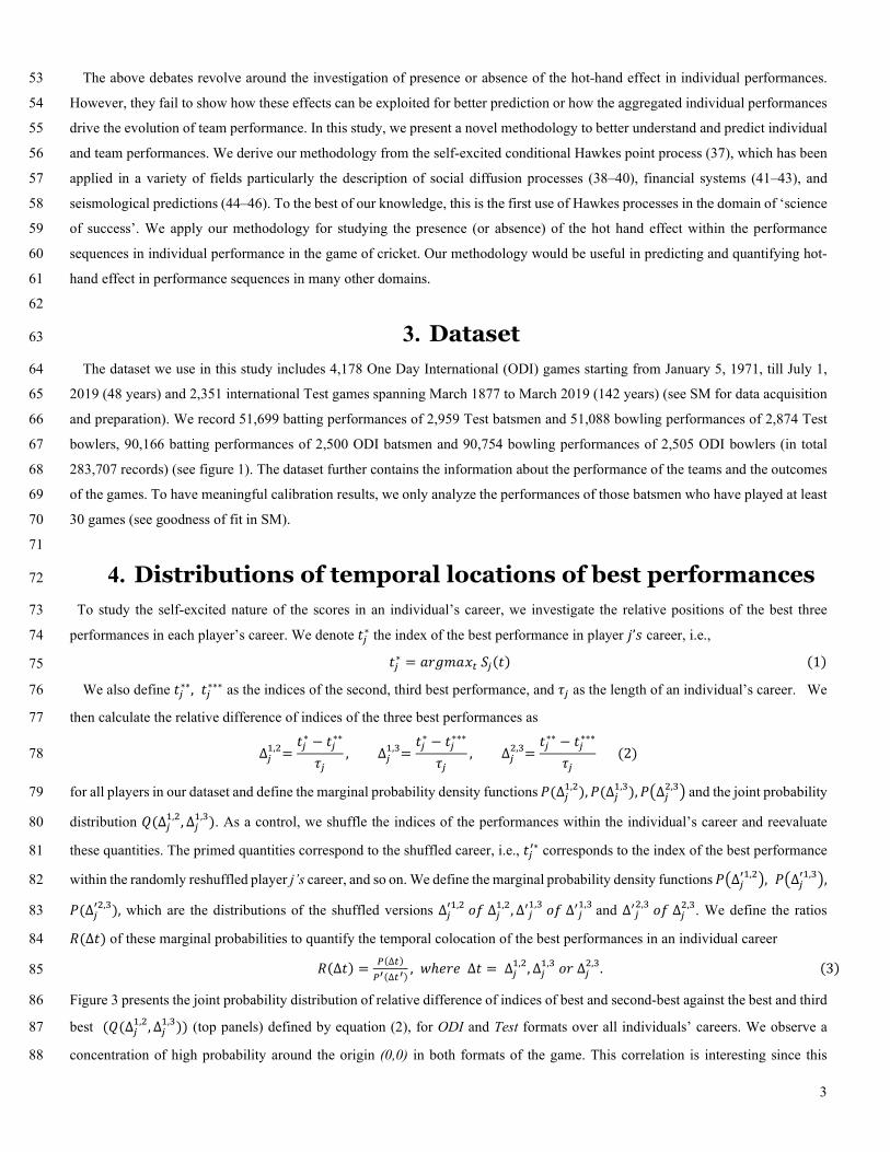
4. Distributions of temporal locations of best performances 72
To study the self-excited nature of the scores in an individual’s career, we investigate the relative positions of the best three 73
performances in each player’s career. We denote 𝑡𝑡𝑗𝑗∗ the index of the best performance in player 𝑗𝑗’𝑠𝑠 career, i.e., 74
𝑡𝑡𝑗𝑗∗ = 𝑎𝑎𝑎𝑎𝑎𝑎𝑎𝑎𝑎𝑎𝑥𝑥𝑡𝑡 𝑆𝑆𝑗𝑗(𝑡𝑡) (1) 75
We also define 𝑡𝑡𝑗𝑗∗∗, 𝑡𝑡𝑗𝑗∗∗∗ as the indices of the second, third best performance, and 𝜏𝜏𝑗𝑗 as the length of an individual’s career. We 76
then calculate the relative difference of indices of the three best performances as 77 ∆𝑗𝑗1,2=𝑡𝑡𝑗𝑗∗ − 𝑡𝑡𝑗𝑗∗∗𝜏𝜏𝑗𝑗 , ∆𝑗𝑗1,3
=𝑡𝑡𝑗𝑗∗ − 𝑡𝑡𝑗𝑗∗∗∗𝜏𝜏𝑗𝑗 , ∆𝑗𝑗2,3
=𝑡𝑡𝑗𝑗∗∗ − 𝑡𝑡𝑗𝑗∗∗∗𝜏𝜏𝑗𝑗 (2) 78
for all players in our dataset and define the marginal probability density functions 𝑃𝑃(∆𝑗𝑗1,2),𝑃𝑃(∆𝑗𝑗1,3
),𝑃𝑃�∆𝑗𝑗2,3� and the joint probability 79
distribution 𝑄𝑄(∆𝑗𝑗1,2,∆𝑗𝑗1,3
). As a control, we shuffle the indices of the performances within the individual’s career and reevaluate 80
these quantities. The primed quantities correspond to the shuffled career, i.e., 𝑡𝑡𝑗𝑗′∗ corresponds to the index of the best performance 81
within the randomly reshuffled player j’s career, and so on. We define the marginal probability density functions 𝑃𝑃�∆𝑗𝑗′1,2�, 𝑃𝑃�∆𝑗𝑗′1,3�,82 𝑃𝑃(∆𝑗𝑗′2,3), which are the distributions of the shuffled versions ∆𝑗𝑗′1,2
𝑜𝑜𝑜𝑜 ∆𝑗𝑗1,2,∆′𝑗𝑗1,3
𝑜𝑜𝑜𝑜 ∆′𝑗𝑗1,3 and ∆′𝑗𝑗2,3
𝑜𝑜𝑜𝑜 ∆𝑗𝑗2,3. We define the ratios 83 𝑅𝑅(∆𝑡𝑡) of these marginal probabilities to quantify the temporal colocation of the best performances in an individual career 84 𝑅𝑅(∆𝑡𝑡) =𝑃𝑃(∆𝑡𝑡)𝑃𝑃′(∆𝑡𝑡′) , 𝑤𝑤ℎ𝑒𝑒𝑎𝑎𝑒𝑒 ∆𝑡𝑡 = ∆𝑗𝑗1,2
,∆𝑗𝑗1,3 𝑜𝑜𝑎𝑎 ∆𝑗𝑗2,3
. (3) 85
Figure 3 presents the joint probability distribution of relative difference of indices of best and second-best against the best and third 86
best (𝑄𝑄(∆𝑗𝑗1,2,∆𝑗𝑗1,3
)) (top panels) defined by equation (2), for ODI and Test formats over all individuals’ careers. We observe a 87
concentration of high probability around the origin (0,0) in both formats of the game. This correlation is interesting since this 88
4
characteristic is a feature of the self-excited process and is not expected in a pure memoryless Poissonian process. We further 89
compare the joint probability distribution (𝑄𝑄(∆𝑗𝑗1,2,∆𝑗𝑗1,3
)) with the corresponding reshuffled joint probability distribution 90
(𝑄𝑄(∆𝑗𝑗′1,2,∆𝑗𝑗′1,3
)) and present in figure S2. The p-values from 2D Kolmogorov-Smirnov two sample tests in figure S2 signifies the 91
significant clustering around origin. This finding constitutes a first line of evidence for the existence of temporal clustering in the 92
performances across players’ careers. 93
94
95
96
The bottom panels of figure 3 shows the ratio 𝑅𝑅(∆𝑡𝑡) (eq. (3)), which compares the marginal probability distribution of the 97
relative difference of the indices in the real careers against the indices obtained from shuffled careers. The distinctive peak around 98
0 in the plots provides additional support for clustering of performance within careers. 𝑅𝑅(∆𝑡𝑡) is approximately symmetric around 99
the origin, indicating that the highest performances are equally likely to arrive before or after the second highest and third-highest 100
scores. This pattern is expected from a self-excited process with approximately equal propensity for performance persistence 101
among the best performance streaks1 (47, 48). 102
103
5. Clustering point process representation 104
Definition of the “performance time” 105
We call 𝑆𝑆𝑗𝑗(𝑡𝑡) the performance (see SM for more details about the game of cricket) of the player 𝑗𝑗 at his 𝑡𝑡𝑡𝑡ℎ attempt within his 106
career. We define the subordinate time process 𝐻𝐻𝑗𝑗(𝑡𝑡) of the stochastic process 𝑆𝑆𝑗𝑗(𝑡𝑡) (49) as 107 𝐻𝐻𝑗𝑗(𝑡𝑡) = ∑ 1𝑆𝑆𝑗𝑗(𝑡𝑡𝑖𝑖)𝑡𝑡𝑡𝑡𝑖𝑖=1 (4) 108
The 𝑡𝑡 → 𝐻𝐻𝑗𝑗(𝑡𝑡) map represents a nonlinear transformation from the calendar time 𝑡𝑡 onto an effective “performance time” of player 109 𝑗𝑗. 𝐻𝐻𝑗𝑗(𝑡𝑡) denotes a transformed time-stamp at which the 𝑡𝑡𝑡𝑡ℎ event takes place for player j. This defines a point process along 110
“performance time” with the time stamps {𝐻𝐻𝑗𝑗(𝑡𝑡1),𝐻𝐻𝑗𝑗(𝑡𝑡2), . . . ,𝐻𝐻𝑗𝑗(𝑡𝑡𝑛𝑛), . . . }. The intuition behind definition (4) is that a series of 111
strong performance values {𝑆𝑆𝑗𝑗(𝑡𝑡𝑖𝑖), 𝑆𝑆𝑗𝑗(𝑡𝑡𝑖𝑖+1), . . . } are transformed into closely clustered points in “performance time”. This allows 112
us to analyze the relationship between performances in time using simple one-dimensional techniques. In other words, by 113
transforming 𝑆𝑆𝑗𝑗(𝑡𝑡), into 𝐻𝐻𝑗𝑗(𝑡𝑡), we project the stochastic process described by the sequence {𝑆𝑆𝑗𝑗(𝑡𝑡), 𝑡𝑡 = 1, . . . } onto an one-114
dimensional point process with time stamps {𝐻𝐻𝑗𝑗(𝑡𝑡1),𝐻𝐻𝑗𝑗(𝑡𝑡2), . . . ,𝐻𝐻𝑗𝑗(𝑡𝑡𝑛𝑛), . . . }. By construction, the 𝑡𝑡 → 𝐻𝐻𝑗𝑗(𝑡𝑡) transformation 115
preserves the self-excited component of performance scores described by the stochastic process �𝑆𝑆𝑗𝑗(𝑡𝑡)� and amplifies it by the 116
magnitude of the performance values. 117
118
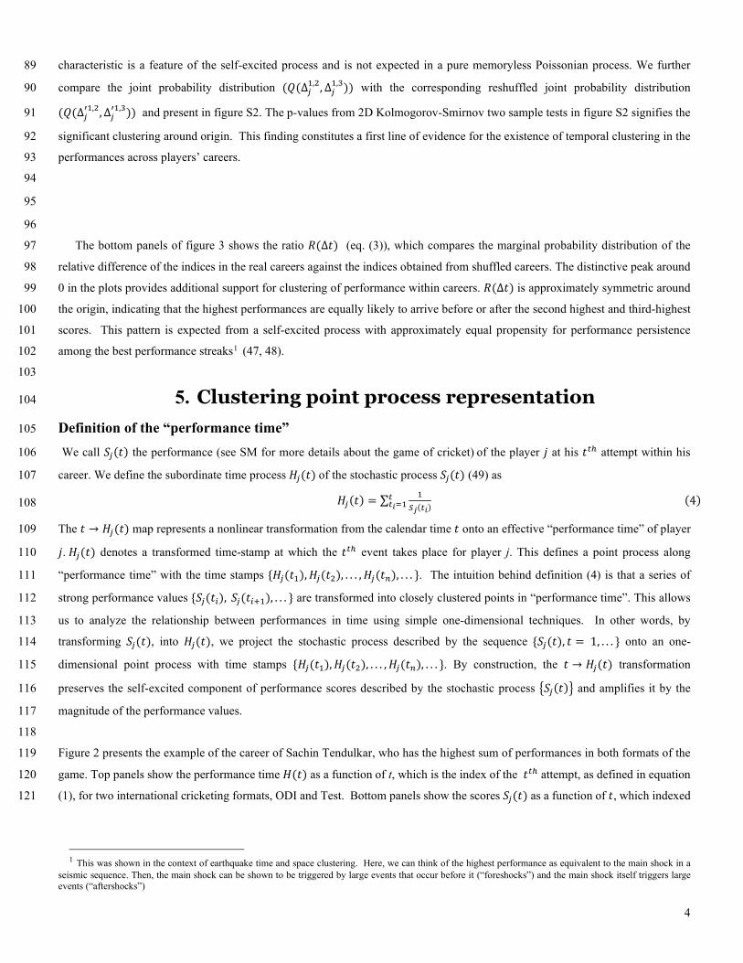
Figure 2 presents the example of the career of Sachin Tendulkar, who has the highest sum of performances in both formats of the 119
game. Top panels show the performance time 𝐻𝐻(𝑡𝑡) as a function of t, which is the index of the 𝑡𝑡𝑡𝑡ℎ attempt, as defined in equation 120
(1), for two international cricketing formats, ODI and Test. Bottom panels show the scores 𝑆𝑆𝑗𝑗(𝑡𝑡) as a function of 𝑡𝑡, which indexed 121
1 This was shown in the context of earthquake time and space clustering. Here, we can think of the highest performance as equivalent to the main shock in a
seismic sequence. Then, the main shock can be shown to be triggered by large events that occur before it (“foreshocks”) and the main shock itself triggers large events (“aftershocks”)

5
the 𝑡𝑡𝑡𝑡ℎ attempt, for the same two international cricketing formats, ODI and Test. The presence of local temporal clustering around 122
the high and low performances is clearly visible in both representations of 𝐻𝐻(𝑡𝑡) and 𝑆𝑆(𝑡𝑡) for this player. 123
124
Hawkes point process along the “performance time” 125
The performance time 𝐻𝐻𝑗𝑗(𝑡𝑡) of player j defined by expression (1) allows us to introduce a point process by the performance times 126
{𝐻𝐻𝑗𝑗(𝑡𝑡1),𝐻𝐻𝑗𝑗(𝑡𝑡2), . . . ,𝐻𝐻𝑗𝑗(𝑡𝑡𝑛𝑛), . . . } along the 𝐻𝐻 axis. In other words, we consider the “performance time” axis 𝐻𝐻𝑗𝑗(𝑡𝑡) and, along this 127
new time axis, we identify “points” at the locations {𝐻𝐻𝑗𝑗(𝑡𝑡1),𝐻𝐻𝑗𝑗(𝑡𝑡2), . . . ,𝐻𝐻𝑗𝑗(𝑡𝑡𝑛𝑛), . . . }. When player 𝑗𝑗 has a series of large scores, this 128
is expressed as a cluster of closely spaced points along the 𝐻𝐻 axis as shown in figure 2. 129
Inspired by the analyses of (38, 43, 50) using generalized non-homogeneous Poisson processes, we propose to model the 130
clustering of the points along the H axis of each player by using the self-excited stochastic Hawkes point process model (37, 42), 131
augmented by some necessary ingredients for constructing a prediction model (19). In other words, we visualize the points for a 132
given player j along the performance time axis 𝐻𝐻𝑗𝑗(𝑡𝑡) as being generated by a Hawkes model with intensity 𝜆𝜆(𝑡𝑡) given by 133 𝜆𝜆(𝑡𝑡) = 𝜇𝜇 + ∑ 𝜑𝜑(𝑡𝑡 − 𝑡𝑡𝑖𝑖)𝑡𝑡𝑖𝑖<𝑡𝑡 (5)134
In expression (5), the first term μ in the right-hand-side is the background intensity, which quantifies the “intrinsic” performance 135
level of a player, uninfluenced by his/her past performances. The second term describes how past points can trigger future points 136
along the H axis. This is a convenient and elegant way to account for the possibility of a hot-hand effect, since each next point is 137
function of the whole history, with a weight quantified by the memory or kernel function 𝜑𝜑(𝑡𝑡 − 𝑡𝑡𝑖𝑖) > 0, which is decaying as a 138
function of its argument (points further in the past have a weaker influence). Thus, the sum ∑ 𝜑𝜑(𝑡𝑡 − 𝑡𝑡𝑖𝑖)𝑡𝑡𝑖𝑖<𝑡𝑡 quantifies the influence 139
of the history of past performances on a player’s present performance. 140
Depending on the problem, previous researchers have used different parametric forms for , e.g. (38, 45, 46) use a power law 141
kernel, whereas (51) use an exponential kernel. In the present case, as there is no reason to favor any parametric form, we decide 142
to use a non-parametric kernel function for φ (42, 52). Thus, shortly after a large performance amplitude, model (2) describes the 143
possibility that the excess intensity of observing a similar performance is boosted and then decays to the baseline average 144
performance level 𝜇𝜇 at long times. 145
The self-excited Hawkes conditional point process is one of the simplest models to account for how the past can influence the 146
future, while keeping a very convenient linear dependence of the past onto the future. The most important parameter of the Hawkes 147
model is its branching ratio defined by 148 𝑛𝑛 = � 𝜑𝜑(𝑡𝑡)𝑑𝑑𝑡𝑡∞0 . (6) 149
The branching ratio n is the average number of points (or events) of first generation triggered by a given point. It is also the fraction 150
of points (events) that have been triggered by past events (53). A value of n close to the critical value 1 thus qualifies a large level 151
of triggering (strong hot hand effect) and endogeneity. Please see figure S4 for details about the used method. 152
We use the expectation maximization algorithm as described (42) to calibrate the model. 153
6. Results 154
Hot individual hands 155
We partition the career of a player j into training set and validation set. We take the first 80% of the performances as the training 156
set and the next 20% as the validation set. We transform the performance sequence in training and validation set to performance 157
time representation (4) as discussed in methods section. We calibrate the performance time in training set to determine background 158
6
intensity 𝜇𝜇 and the memory kernel 𝜑𝜑. We then use the calibrated 𝜇𝜇 and 𝜑𝜑 to evaluate the prediction performance in validation set 159
using the log-likelihood score and call the median value ℒ𝑗𝑗𝑚𝑚𝑚𝑚𝑚𝑚𝑚𝑚𝑚𝑚 . 160
161
Similarly, we prepare a controlled set of log-likelihood estimation for the same player. Keeping the validation set unaltered, we 162
shuffle the sequence of the performance in the training set 100 times and use this to train the model. We evaluate the trained model 163
on the unaltered validation set to determine the corresponding median log-likelihood estimation ℒ𝑗𝑗𝑐𝑐𝑚𝑚𝑛𝑛𝑡𝑡𝑐𝑐𝑚𝑚𝑚𝑚. With the above 164
constructions, we define the relative differences 𝛿𝛿 �ℒ𝑗𝑗𝑚𝑚𝑚𝑚𝑚𝑚𝑚𝑚𝑚𝑚 ,ℒ𝑗𝑗𝑐𝑐𝑚𝑚𝑛𝑛𝑡𝑡𝑐𝑐𝑚𝑚𝑚𝑚� by 165
166 𝛿𝛿 �ℒ𝑗𝑗𝑚𝑚𝑚𝑚𝑚𝑚𝑚𝑚𝑚𝑚 ,ℒ𝑗𝑗𝑐𝑐𝑚𝑚𝑛𝑛𝑡𝑡𝑐𝑐𝑚𝑚𝑚𝑚� =ℒ𝑗𝑗𝑚𝑚𝑚𝑚𝑚𝑚𝑚𝑚𝑚𝑚 − ℒ𝑗𝑗𝑐𝑐𝑚𝑚𝑛𝑛𝑡𝑡𝑐𝑐𝑚𝑚𝑚𝑚ℒ𝑗𝑗𝑐𝑐𝑚𝑚𝑛𝑛𝑡𝑡𝑐𝑐𝑚𝑚𝑚𝑚 (7) 167
168
Additionally, we estimate the branching ratios (see equation (6)) (38, 41, 45) of the performance time for all players over the 169
duration of their entire career. For comparison, we construct null estimations by randomly shuffling the performance time times 170
and reevaluating the 100 null branching ratios for each of the players. 171
172
The relative difference of log-likelihood prediction scores in equation (7) is shown in the bottom panels of figure 4, for both 173
formats of the games. The insets present the fraction of time control performing better and the fraction of time the model performing 174
better. The results show a significant improvement in prediction score in model experiments compared to the control experiments. 175
We plot the distribution of the branching ratios obtained from the data and the null branching ratios and compare them in the top 176
panels of figure 4. In the plots, the shaded region marks the fraction of players’ branching ratios that are never found in the null 177
models. This behavior is robust against the number of simulated null models, i.e., the fraction of players’ branching ratios that are 178
never found in the null model remains the same even if we consider 500 and 1000 null models. 179
180
We then compare the log-likelihood score from 100 control estimates with the log-likelihood score obtained from the data for 181
each of the player. We evaluate the statistical significance of having a better log-likelihood score in the model experiments 182
compared to the control experiments. We perform the Wilcoxon signed-rank test in each career to determine the statistical 183
significance. Considering a confidence level of 0.05, we observe that, in 49.6% of Test careers and in 46.8% of the ODI careers, 184
the log-likelihood prediction score in original sequences is significantly higher than the median log-likelihood prediction score in 185
control experiments. This leads us to conclude that the probability of falsely accepting the null hypotheses -- the control experiments 186
perform equally good – is < 10−6 (using a binomial probability distribution with success rate 0.05 of false test result) for both the 187
cases. This result is sufficient to support the predictive power of our model. Furthermore, our model performs better than the 188
standard techniques like ARIMA (please refer SM). 189
190
We then compare the branching ratios (see equation (6)) of the performance time obtained from data and null shuffling for each 191
player to quantify the Hot-Hand effect. We perform the Wilcoxon signed-rank test to determine the statistical significance. We 192
observe that in 56.8% of Test careers and in 53.7% of the ODI careers, the branching ratio of original performance time is 193
significantly higher than the median branching ratio in null performance time (confidence level = 0.05). These results suggest a 194
significant presence of Hot Hands in the players career, as the probability for the absence of Hot Hands is < 10−6 (using a binomial 195
probability distribution with success rate 0.05 of false test result) 196
197
7
Hot team hands 198
199
We repeat the above analysis to predict and quantify the team performances (sum of all individual performances in a game) 200
(please see SM for more details). We take the first 80% of the team performances as the training set and validate the model on the 201
next 20%. Using the Wilcoxon signed-rank test with confidence level 0.05, we observe that, only in 30% and 20% of ODI and Test 202
teams, the log likelihood scores in model experiments is significantly better than the control experiments. These results suggest a 203
significant reduction in prediction (~50% reduction) compared to predictability of individual performances (please see SM for more 204
details). Further the probability of falsely accepting the null hypotheses – the control experiments perform better – increases to 205
~10−2 and ~10−1 respectively (using a binomial probability distribution with success rate 0.05 of false test result). The absence 206
of reliable prediction in the above results suggest the absence of exploitable self-excited patterns in team performance. 207
208
Hot winning hands 209
210
We investigate the presence of hot hands in the team performances by going through the complete history of games played by 211
each team and analyze the winning streaks (i.e., the number of continuous wins without losing a single game in between). We note 212
down the length of winning streaks and the corresponding frequencies of occurrences of such streaks in each team playing history. 213
214
Then, we construct a statistical ensemble of possible performance trajectories. We randomly shuffle the original performance 215
sequences to generate 1000 synthetic performance trajectories. Using this statistical ensemble, we evaluate the null probability 216
distribution for the joint occurrence of streaks of length n and of corresponding frequency f. We use this probability distribution 217
for estimating the p-values for the observed events. we define the p-values 𝑝𝑝(𝑛𝑛) and 𝑝𝑝(𝑛𝑛𝑓𝑓) according to 218 𝑝𝑝(𝑛𝑛) = 𝑃𝑃(𝑛𝑛𝑖𝑖 ≥ 𝑛𝑛), 𝑝𝑝�𝑛𝑛𝑓𝑓� = 𝑃𝑃(𝑛𝑛𝑖𝑖 ≥ 𝑛𝑛|𝑜𝑜) (8) 219
220
which respectively represent the p-value for observation of streaks with length n and streaks with length n conditional on frequency 221
f. To avoid the problem of multiple hypothesis testing (54), because of simultaneous consideration of the multiple individual tests, 222
we correct the error rates of individual tests using multiple hypothesis testing methods (55–59). We note down the results 223
from the methods (55–59) and identify the extreme events (see supporting tables for multiple hypothesis testing in SM). 224
225
Figure 5 presents the position of the realized winning streaks, along with the null distribution of the winning streaks for the 10 226
teams in the ODI format (top panel) and in the Test format (bottom panel). The red stars in figure reveal several highly improbable 227
i.e., one or both of 𝑝𝑝(𝑛𝑛) and 𝑝𝑝(𝑛𝑛𝑓𝑓) is significant with confidence level 0.05, after multiple testing. A large number of white stars 228
indicate probable events i.e., none of 𝑝𝑝(𝑛𝑛) and 𝑝𝑝(𝑛𝑛𝑓𝑓) is significant. We present the 𝑝𝑝(𝑛𝑛) and 𝑝𝑝(𝑛𝑛𝑓𝑓) values for the events that pass 229
the multiple hypothesis tests in figure. 230
231
We observe 5 out of 98 (5.1%) streaks in ODI cricket are significantly long, considering both their length (n) and frequency (). 232
In Test cricket, 6 out of 73 (8%) considering the length and 5 out of 73 (7%) considering the frequency are statistically significant. 233
Because of the considered significance level, we expect an error rate of 0.05 in individual verification. In total we verified 98 234
possible streaks in ODI cricket and 73 streaks in Test cricket. The binomial probability for the observation of 5 hot hands in ODI 235
cricket is 0.18 and more than 5 hot hands is 0.36. However, for the Test format, the probability of observing 5 and 6 hot hands are 236
8
0.14 and 0.08 and more than 5 and 6 are 0.15 and 0.07 respectively. This allows us to conclude that we don’t observe any Hot Hand 237
effect in winning streaks of teams both in ODI and Test cricket. 238
7. Concluding remarks 239
240
In this study, we have quantified the predictability and persistence of individual and collective performances of the teams in a 241
team game. We introduced a number of novel statistical tools to study the hot hand effect in a new dataset on game of Cricket. We 242
quantified and exploited the self-excited patterns in individual and team performances to better predict the future compared to 243
traditional methods like ARIMA. 244
245
Our investigation has confirmed the presence of significant hot-hands in individual performance. This is supported by the fact 246
that the three highest performances in individual career cluster in time, particularly when players partake in hundreds of games. 247
Further, the shaded branching ratios in figure 4A and 4B are very rarely found in simulated null data, confirming the strength of 248
the self-excitation that qualifies the presence of the hot-hand effect. The major finding of our work is that these self-excitation 249
patterns can indeed be exploited for predicting future performances. The findings of this investigation complement those of earlier 250
studies supporting the presence of hot hands in individual careers, while raising questions about the validity of those refuting the 251
same. 252
253
Additionally, we have showed a significant reduction in prediction of team performances compared with single players’ 254
performance, suggesting the dominance of stochasticity in the determinant of teams’ performance. While there is still some 255
predictability to a certain extent, the outcome of the game cannot be predicted, nor do they cluster in time. This leads us to suggest 256
the somewhat paradoxical conclusion that ‘Cricket is a game of skill for individuals and a game of chance for the teams.’ 257
258
Our study showed that, while an individual can consistently deal with the environmental systemic stochasticity, it is difficult for 259
the team to perform equally well. Thus, these results open door for future research in the direction of the impact of group size in 260
predictability and consistency of performance. 261
262
Furthermore, the present study established a quantitative framework for detecting and predicting the performances in individual 263
careers. This approach will prove useful in expanding our understanding of the predictability of success in individual careers. This 264
paper contributes to recent historiographical debates concerning the presence of hot hands in the sequence of successes in individual 265
performances. Further work needs to be done to establish whether the presented methodology for predicting the performances can 266
be improved for commercial usage and for financial gains, exploiting the presence of self-excited patterns in individual careers. 267
The findings of this study have a number of important implications for future research in the field of quantifying self-excited 268
performance patterns involved in the study of human behavior and design of algorithms for predicting success. 269
270
Acknowledgment 271
272

9
We thank Ananya Acharya, Ali Ayoub, Giuseppe-Maria Ferro, Jan-Christian Gerlach and Devendra Shintre for many 273
enlightening discussions during the preparation of the manuscript. Competing interests: The authors declare no competing interests. 274
Data and materials availability: All data, codes, and materials used in the analysis would be made available. 275
Datasets: the dataset used in this study is publicly available at https://www.espncricinfo.com , http://howstat.com/. All 276 methods were carried out in accordance with relevant guidelines and regulations. 277
278
279
280
281
282
290
291
292

10
293
Figure 2: Sequence of performances in the individual career of Sachin Tendulkar. (A) Performance time 𝐻𝐻(𝑡𝑡) as a function 294
of 𝑡𝑡, as defined in equation (1), for the highest performer in ODI cricket. (B) Performance time (1) for the highest run scorer in 295
Test cricket. (C) The performance score 𝑆𝑆(𝑡𝑡) of the player in ODI corresponding to panel (A). (D) The performance score 𝑆𝑆(𝑡𝑡) of 296
the player in Test cricket corresponding to panel (B). The large yellow stars represent the top 3 performances. The top insets in (A) 297
and (B) give the point process representation of 𝐻𝐻(𝑡𝑡), in which each dot corresponds to an instant of time along the 𝐻𝐻(𝑡𝑡) time axis. 298
We have added noise along the y-direction for better visualization. 299
300
301
306
307
308

11
Figure 4: Analysis of clustering in the time series of performance time with the self-excited point process model. (A) and 309
(B) represent the distribution of branching ratios over the set of players and of the branching ratios obtained from synthetic shuffled 310
careers. (A) represents the distribution for ODI cricket and (B) is for Test cricket. Shaded regions in the plot represent the domain 311
of branching ratios obtained from the real data that cannot be explained by the null models. (C) and (D) show the distribution of 312 𝛿𝛿(ℒ𝑗𝑗𝑚𝑚𝑚𝑚𝑚𝑚𝑚𝑚𝑚𝑚 ,ℒ𝑗𝑗𝑐𝑐𝑚𝑚𝑛𝑛𝑡𝑡𝑐𝑐𝑚𝑚𝑚𝑚) (see equation (7)). (C) represents the distribution for ODI cricket, and (D) is for the Test format. The fraction 313
of the times model experiments achieves a better log-likelihood score compared to the control experiments is colored green, 314
otherwise the color is red. The insets show the fraction of control and model outperforming their counterparts. In ODI games, the 315
fraction of times model experiment performs better than the control experiment is: 0.62; for Test cricket, this fraction is 0.60. 316
Figure 5: Hot hands in cricket teams. (top panel) ODI: Each of the 10 subplots in the figure shows the null distribution (obtained
through randomly shuffling the performance sequence) of joint occurrence of winning streak length and of the corresponding
frequency of occurrence. The title of each subplot provides the country of the team. Marked points on the plots represent the realized
events. The white points represent the probable events, and the red points represent the extreme/unlikely events (determined through
multiple testing methods). The p-values (𝑝𝑝(𝑛𝑛) and 𝑝𝑝(𝑛𝑛𝑓𝑓)) (see equation (8) for definitions) for the unlikely events are provided
along with the points. (Bottom panel) Test: Same as top figure for the performances in the Test format.

12
1. M. Favre, D. Sornette, Strong gender differences in reproductive success variance, and the times to the most recent
common ancestors. J. Theor. Biol. 310, 43–54 (2012).
2. S. P. Fraiberger, R. Sinatra, M. Resch, C. Riedl, A. L. Barabási, Quantifying reputation and success in art. Science (80-
. ). 362, 825–829 (2018).
3. R. Sinatra, D. Wang, P. Deville, C. Song, A. L. Barabási, Quantifying the evolution of individual scientific impact.
Science (80-. ). 354 (2016).
4. P. Deville, et al., Career on the move: Geography, stratification, and scientific impact. Sci. Rep. 4, 4770 (2014).
5. J. Berger, D. Pope, Can losing lead to winning? Manage. Sci. 57, 817–827 (2011).
6. S. F. Way, A. C. Morgan, A. Clauset, D. B. Larremore, The misleading narrative of the canonical faculty productivity
trajectory. Proc. Natl. Acad. Sci. 114, E9216--E9223 (2017).
7. A. Clauset, S. Arbesman, D. B. Larremore, Systematic inequality and hierarchy in faculty hiring networks. Sci. Adv. 1,
e1400005 (2015).
8. L. Liu, et al., Hot streaks in artistic, cultural, and scientific careers. Nature 559, 396–399 (2018).
9. O. E. Williams, L. Lacasa, V. Latora, Quantifying and predicting success in show business. Nat. Commun. 10, 2256
(2019).
10. M. J. Mauboussin, The success equation: Untangling skill and luck in business, sports, and investing (Harvard Business
Press, 2012).
11. A. V Carron, S. R. Bray, M. A. Eys, Team cohesion and team success in sport. J. Sports Sci. 20, 119–126 (2002).
12. S. Wuchty, B. F. Jones, B. Uzzi, The increasing dominance of teams in production of knowledge. Science (80-. ). 316,
1036–1039 (2007).
13. N. J. Cooke, M. L. Hilton, others, Enhancing the effectiveness of team science (National Academies Press Washington,
DC, 2015).
14. L. Wu, D. Wang, J. A. Evans, Large teams develop and small teams disrupt science and technology. Nature 566, 378–
382 (2019).
15. V. Larivière, Y. Gingras, C. R. Sugimoto, A. Tsou, Team size matters: Collaboration and scientific impact since 1900.
J. Assoc. Inf. Sci. Technol. 66, 1323–1332 (2015).
16. S. Mukherjee, Quantifying individual performance in Cricket—A network analysis of Batsmen and Bowlers. Phys. A
Stat. Mech. its Appl. 393, 624–637 (2014).
17. S. Mukherjee, Identifying the greatest team and captain—A complex network approach to cricket matches. Phys. A
Stat. Mech. its Appl. 391, 6066–6076 (2012).
18. T. Gilovich, R. Vallone, A. Tversky, The hot hand in basketball: On the misperception of random sequences. Cogn.
Psychol. 17, 295–314 (1985).
19. D. Kahneman, A. Tversky, On the psychology of prediction. Psychol. Rev. 80, 237 (1973).
20. A. Tversky, D. Kahneman, S. Kahneman, Tversky, Belief in the law of small numbers. A Handb. Data Anal. Behav.
Sci. 1, 341 (2014).
21. D. Kahneman, M. W. Riepe, Aspects of investor psychology. J. Portf. Manag. 24, 52--+ (1998).
22. J. B. Miller, A. Sanjurjo, Surprised by the hot hand fallacy? A truth in the law of small numbers. Econometrica 86,
13
2019–2047 (2018).
23. J. J. Koehler, C. A. Conley, The “hot hand” myth in professional basketball. J. Sport Exerc. Psychol. 25, 253–259
(2003).
24. D. Hendricks, J. Patel, R. Zeckhauser, Hot hands in mutual funds: Short-run persistence of relative performance, 1974-
-1988. J. Finance 48, 93–130 (1993).
25. D. Sornette, S. Wheatley, P. Cauwels, The fair reward problem: the illusion of success and how to solve it. Adv.
Complex Syst. 22, 1950005 (52 pages) (2019).
26. C. J. R. Roney, L. M. Trick, Sympathetic magic and perceptions of randomness: The hot hand versus the gambler’s
fallacy. Think. \& Reason. 15, 197–210 (2009).
27. E. F. Fama, K. R. French, Luck versus skill in the cross-section of mutual fund returns. J. Finance 65, 1915–1947
(2010).
28. D. Hirshleifer, Investor psychology and asset pricing. J. Finance 56, 1533–1597 (2001).
29. M. M. Carhart, On persistence in mutual fund performance. J. Finance 52, 57–82 (1997).
30. G. Gigerenzer, H. Brighton, Homo heuristicus: Why biased minds make better inferences. Top. Cogn. Sci. 1, 107–143
(2009).
31. R. K. Merton, The matthew effect in science. Science (80-. ). 159, 56–62 (1968).
32. D. Lazer, et al., Computational social science. Science (80-. ). 323, 721–723 (2009).
33. I. Iacopini, S. Milojević, V. Latora, Network dynamics of innovation processes. Phys. Rev. Lett. 120, 48301 (2018).
34. T. Heatherton, D. M. Tice, others, Losing control: How and why people fail at self-regulation (San Diego, CA:
Academic Press, Inc, 1994).
35. A. Clauset, D. B. Larremore, R. Sinatra, Data-driven predictions in the science of science. Science (80-. ). 355, 477–
480 (2017).
36. T. Bol, M. de Vaan, A. van de Rijt, The Matthew effect in science funding. Proc. Natl. Acad. Sci. 115, 4887–4890
(2018).
37. A. G. Hawkes, Spectra of some self-exciting and mutually exciting point processes. Biometrika 58, 83–90 (1971).
38. R. Crane, D. Sornette, Robust dynamic classes revealed by measuring the response function of a social system. Proc.
Natl. Acad. Sci. U. S. A. 105, 15649–15653 (2008).
39. J. D. O’Brien, A. Aleta, Y. Moreno, J. P. Gleeson, Quantifying uncertainty in a predictive model for popularity
dynamics. Phys. Rev. E 101, 62311 (2020).
40. A. N. Medvedev, J.-C. Delvenne, R. Lambiotte, Modelling structure and predicting dynamics of discussion threads in
online boards. J. Complex Networks 7, 67–82 (2019).
41. V. Filimonov, D. Sornette, Quantifying reflexivity in financial markets: Toward a prediction of flash crashes. Phys.
Rev. E 85, 56108 (2012).
42. E. Lewis, G. Mohler, A nonparametric EM algorithm for multiscale Hawkes processes. J. Nonparametr. Stat. 1, 1–20
(2011).
43. V. Filimonov, D. Sornette, Apparent criticality and calibration issues in the {H}awkes self-excited point process model:
application to high-frequency financial data. Quant. Financ. 15, 1293–1314 (2015).
14
44. R. Shcherbakov, J. Zhuang, G. Zöller, Y. Ogata, Forecasting the magnitude of the largest expected earthquake. Nat.
Commun. 10, 1–11 (2019).
45. S. Nandan, G. Ouillon, S. Wiemer, D. Sornette, Objective estimation of spatially variable parameters of epidemic type
aftershock sequence model: Application to California. J. Geophys. Res. Solid Earth 122, 5118–5143 (2017).
46. S. Nandan, G. Ouillon, D. Sornette, S. Wiemer, Forecasting the rates of future aftershocks of all generations is essential
to develop better earthquake forecast models. J. Geophys. Res. Solid Earth 124, 8404–8425 (2019).
47. D. Sornette, A. Helmstetter, Endogenous versus exogenous shocks in systems with memory. Phys. A Stat. Mech. its
Appl. 318, 577–591 (2003).
48. A. Helmstetter, D. Sornette, J.-R. Grasso, Mainshocks are Aftershocks of Conditional Foreshocks: How do foreshock
statistical properties emerge from aftershock laws. J. Geophys. Res. (Solid Earth) 108, 2046,
doi:10.1029/2002JB001991 (2003).
49. M. Jagielski, R. Kutner, D. Sornette, Theory of earthquakes interevent times applied to financial markets. Phys. A Stat.
Mech. its Appl. 483, 68–73 (2017).
50. V. Filimonov, D. Sornette, Quantifying reflexivity in financial markets: Toward a prediction of flash crashes. Phys.
Rev. E 85, 56108 (2012).
51. V. Filimonov, D. Sornette, Spurious trend switching phenomena in financial markets. Eur. Phys. J. B 85, 155 (2012).
52. D. Sornette, S. Utkin, Limits of declustering methods for disentangling exogenous from endogenous events in time
series with foreshocks, main shocks, and aftershocks. Phys. Rev. E 79, 61110 (2009).
53. A. Helmstetter, D. Sornette, Importance of direct and indirect triggered seismicity in the ETAS model of seismicity.
Geophys. Res. Lett. 30, doi:10.1029/2003GL017670 (2003).
54. L. Fiévet, D. Sornette, Decision trees unearth return sign predictability in the S\&P 500. Quant. Financ. 18, 1797–1814
(2018).
55. Y. Benjamini, Y. Hochberg, Controlling the false discovery rate: a practical and powerful approach to multiple testing.
J. R. Stat. Soc. Ser. B 57, 289–300 (1995).
56. Y. Hochberg, A sharper Bonferroni procedure for multiple tests of significance. Biometrika 75, 800–802 (1988).
57. S. Holm, A simple sequentially rejective multiple test procedure. Scand. J. Stat., 65–70 (1979).
58. Z. Šidák, Rectangular confidence regions for the means of multivariate normal distributions. J. Am. Stat. Assoc. 62,
626–633 (1967).
59. J. D. Storey, R. Tibshirani, Statistical significance for genomewide studies. Proc. Natl. Acad. Sci. 100, 9440–9445
(2003).

Supplementary Files
This is a list of supplementary �les associated with this preprint. Click to download.
supmat.pdf