1

Paper 1910-2015

Unconventional Data-Driven Methodologies Forecast Performance

In Unconventional Oil and Gas Reservoirs

Keith R. Holdaway, Louis Fabbi, and Dan Lozie, SAS Institute Inc.

ABSTRACT

How do historical production data relate a story about subsurface oil and gas reservoirs? Business and domain experts must perform accurate analysis of reservoir behavior using only rate and pressure data as a function of time. This paper introduces innovative data-driven methodologies to forecast oil and gas production in unconventional reservoirs that, owing to the nature of the tightness of the rocks, render the empirical functions less effective and accurate. You learn how implementations of the SAS® MODEL procedure provide functional algorithms that generate data-driven type curves on historical production data. Reservoir engineers can now gain more insight to the future performance of the wells across their assets. SAS enables a more robust forecast of the hydrocarbons in both an ad hoc individual well interaction and in an automated batch mode across the entire portfolio of wells. Examples of the MODEL procedure arising in subsurface production data analysis are discussed, including the Duong data model and the Stretched-Exponential-Decline Model. In addressing these examples, techniques for pattern recognition and for implementing TREE, CLUSTER, and DISTANCE procedures in SAS/STAT® are highlighted to emphasize the importance of oil and gas well profiling to characterize the reservoir. The MODEL procedure analyzes models in which the relationships among the variables comprise a system of one or more nonlinear equations. Primary uses of the MODEL procedure are estimation, simulation, and forecasting of nonlinear simultaneous equation models, and generating type curves that fit the historical rate production data. You will walk through several advanced analytical methodologies that implement the SEMMA process to enable hypotheses testing as well as directed and undirected data mining techniques. SAS® Visual Analytics Explorer drives the exploratory data analysis to surface trends and relationships, and the data QC workflows ensure a robust input space for the performance forecasting methodologies that are visualized in a web-based thin client for interactive interpretation by reservoir engineers.

INTRODUCTION

"I have seen the future and it is very much like the present, only longer."

Kehlog Albran, “The Profit”

Estimating reserves and predicting production in reservoirs has always been a challenge. The complexity of data, combined with limited analytical insights, means some upstream companies do not fully understand the integrity of wells under management. In addition, it can take weeks or months to establish and model alternative scenarios, potentially resulting in missed opportunities to capitalize on market conditions. Performing accurate analysis and interpretation of reservoir behavior is fundamental to assessing extant reserves and potential forecasts for production. Decline Curve Analysis (DCA) is traditionally used to provide deterministic estimates for future performance and remaining reserves. But unfortunately, deterministic estimates contain significant uncertainty. As a result, the deterministic prediction of future decline is often far from the actual future production trend; making the single deterministic value of reserves nowhere close to reality. Probabilistic approaches, on the other hand, quantify the uncertainty and improve Estimated Ultimate Recovery (EUR).

The literature in the early years of the twentieth century immersed itself in the study of percentage decline curves or empirical rate-time curves that found credence in expression of production rates across successive units of time, framed as percentages of production over the first unit of time. W.W. Cutler suggested that a more robust methodology defining a straight-line relationship was achievable when using log-log paper. The implication being that decline curves that reflected such characteristics were of a hyperbolic geometric type as opposed to an exponential.

2

Engineers determine Estimated Ultimate Recovery (EUR) of reserves in existing reservoirs and forecast production trends implementing the equations in Table 1.

We use the decline curve equations to estimate future asset production (Arps, 1945):

Exponential Hyperbolic Harmonic

b=0 0<b<1 b=1

D¹ ln(q¹q²) / t

D¹(q¹/q²)^1/b D¹(q¹/q²)

q¹ q¹exp(-D¹t) q¹/(1 + btD¹)^1/b q¹/(1 + btD¹)

Qp q¹ - q²/D¹ q¹/D¹(1 – b)(1 - q²/q¹)^1-b q¹/D¹ln(1 + D¹t)

t ln(q¹q²)/D¹ (q¹/q²)^b – 1/bD¹ q¹ - q²/D¹q²

Table 1: Decline Curve Analysis using Arps empirical algorithms

D¹ Initial rate of decline

q¹ Initial rate of production

q² Rate of production

Qp Cumulative production

t Time

Hyperbolic decline

q = q (1+ D bt) −1/b

Exponential decline

q = qi exp (−Dt)

In the equations b and D are empirical constants that are determined based on historical production data. When b = 1, it is a harmonic model and when b=0, it yields an exponential decline model.

There are a number of assumptions and restrictions applicable to conventional DCA using these equations. Theoretically, DCA is applicable to a stabilized flow in wells producing at constant flowing Bottom-Hole Pressure (BHP). Thus data from the transient flow period should be excluded from DCA. In addition, use of the equation implies that there are no changes in completion or stimulation, no changes in operating conditions, and that the well produces from a constant drainage area.

The hyperbolic decline exponent, b, has physical meaning in reservoir engineering, falling between 0 and 1. In general, we think of decline exponent, b, as a constant. But for a gas well, b varies with time. Instantaneous b decreases as the reservoir depletes at constant BHP condition and can be larger than 1 under some conditions. The average b over the depletion stage is indeed less than 1.

It is also critical to surface the statistical properties of a time-series that are stationary or immutable from a temporal perspective: correlations, autocorrelations, levels, trends and seasonal patterns. Then we can predict the future from these descriptive properties.

Thus, the implementation of data-driven models and automated and semi-automated workflows that feed into a data mining methodology are crucial in order to determine a probabilistic suite of forecasts and estimates for well performance.

Reliably estimating recoverable reserves from low-permeability shale-gas formations is a problematic exercise owing to the nature of the unconventional reservoir and inherent geomechanical and rock properties. Employing the Arps’ hyperbolic model, for example, invariably results in an over-optimistic forecast and estimation. Alternative DCA models based on empirical considerations have been positioned:

3

The Duong power-law model

The Stretched-Exponential-Decline Model (SEDM)

Weibull Growth Curve

Projecting production-decline curves is ostensibly the most commonplace method to forecast well performance in tight gas and shale-gas assets. The potential production and EUR are determined by fitting an empirical model of the well’s production-decline trend and then projecting this trend to the well’s economic limit or an acceptable cut-off time. Forcing Arps’ hyperbolic model to fit production data from shale-gas wells has invariably resulted in over-optimistic results of EUR, stemming from physically unrealistically high values of the decline exponent to force the fit. There have been a few alternatives proposed for the analysis of decline curves in tight gas wells. One preference constrains the tardy decline rate to a more realistic value on the basis of analogs. Another methodology determines empirical decline curve models that impose physically relevant parameter definitions and finite EUR values on model predictions. A key issue associated with the use of multiple models is how to discriminate between them with limited production periods, and how to combine the model results to yield an assessment of uncertainty in reserves estimates.

Production decline analysis of tight gas and shale-gas wells with this method typically results in a best-fit value of greater than unity for the decline exponent parameter. The result often is physically unrealistic in that cumulative production becomes unbounded as time increases.

The Duong model is based on a long-term flow regime approximating a linear flow. We adopted a modified Duong model that implements a switch of 5% followed by an Arps curve where the b factor is set to 0.4.

The SEDM model is a more plausible physical explanation than the assumption of boundary-dominated flow that is inordinately long to develop in tight and shale-gas reservoirs. Unlike the hyperbolic model, the SEDM yields a finite value for ultimate recovery. The SEDM appears to fit field data from various shale plays reasonably well and provides an effective alternative to Arps’ hyperbolic model.

Because tight gas and shale-gas reservoirs generally are produced after massive hydraulic fracturing, it is reasonable to assume that flow toward wells in such systems will exhibit fracture-dominated characteristics. For finite-conductivity fractures, the flow will be bilinear, which manifests as a quarter-slope line on a log-log graph of production rate, q, vs. time, whereas flow in infinite-conductivity fractures will be linear and be characterized by a half-slope line on the same graph. Under both conditions, it has been shown that a log-log graph of q/Gp vs. time should have a slope of −1.

However, analysis of field data from several shale-gas plays has shown that the relationship between these variables is described better by an empirical model that also appears to fit field data from various shale plays very well, providing an effective alternative to Arps’ hyperbolic model.

Many mathematical algorithms have been implemented to describe population growth (or decline) effectively under an expansive range of conditions. The Weibull growth curve is a generalization of the widely used Weibull distribution for modeling time to failure in applied-engineering problems. A three-parameter Weibull model can be reduced to two unknowns if the q/Gp ratio is taken as the dependent variable. Nonlinear-regression analysis can estimate the observed ratio against time.

4

Figure 1: Process diagram implementing key components

The three important composite engines, as depicted in Figure 1, are data mining, cluster analysis and bootstrapping:

1. The bootstrapping module will help engineers to build reliable confidence intervals for production rate forecast and reserves and lifetime estimates.

2. The clustering module will help engineers to deal with large numbers of wells, by providing a means for grouping wells and finding similar wells.

3. The data mining module enables the development of advanced analytical workflows. Via Exploratory Data Analysis it is feasible to identify hidden patterns and correlations that facilitate the evolution of the data-driven predictive models.

BOOTSTRAPPING MODULE

The purpose of the bootstrapping module is to automate the temporal data selection process to build reliable confidence intervals for rate-time and rate-cumulative models prediction. It is done by means of multiple scenarios optimization and Monte-Carlo simulation for block residuals resampling. Historical production data invariably possess significant amounts of noise. Thus, the empirical postulates that underpin the traditional DCA workflow introduce much uncertainty as regards the reserves estimates and performance forecasts. Probabilistic approaches regularly provide three confidence levels (P10, P50 and P90) with an analogous 80% confidence interval. How reliable is the 80% confidence interval? To put it another way: does the estimate of reserves fall within the interval 80% of the time? Investigative studies have shown that it is not uncommon for true values of reserves to be located outside the 80% confidence interval much more than 20% of the time when implementing the traditional methodology. Uncertainty is thus significantly underestimated.

The majority of engineers are ingrained with the philosophy that quantifying uncertainty of estimates is primarily a subjective task. This perspective has taken the oil and gas industry along the perpetual road that bypasses effective probabilistic workflows to assess reserves estimation and quantify uncertainty of those estimates. It seems that prior distributions of drainage area, net pay, porosity, formation volume factor, recovery factor and saturation are pre-requisites to perform Monte Carlo simulations. And invariably we impose several distribution types such as log-normal, triangular or uniform from an

Bootstrapping Module

• Confidence Intervals

• Monte Carlo Simulation

• Statistical methodology

Clustering Module

• Classify wells across

• Similarity

• Dissimilarity

• Field segmentation

Data Mining Workflow

• Key production indicators

• Statistical factors

• Good/Bad Well performance profiles

5

experienced or subjective position. To preclude any assumptions derived from adopting prior distributions of parameters, let us investigate the value inherent in the bootstrap methodology.

The first adventure into application of the bootstrap method for DCA adopted ordinary bootstrap to resample the original production data. This enabled the generation of multiple pseudo data sets appropriate for probabilistic analysis. However, there are inherent assumptions that are deemed improper for temporal data such as production data, since the ordinary bootstrap method takes for granted the original production time-series data as independent and identically distributed. And there are often correlations between data points in a time-series data structure.

To avoid assuming prior distributions of parameters, the bootstrap method has been used to directly construct probabilistic estimates with specified confidence intervals from real data sets. It is a statistical approach and is able to assess uncertainty of estimates objectively. To the best of our knowledge, Jochen and Spivey first applied the bootstrap method to decline curve analysis for reserves estimation. They used ordinary bootstrap to resample the original production data set so as to generate multiple pseudo data sets for probabilistic analysis. The ordinary bootstrap method assumes that the original production data are independent and identically distributed, so the data will be independent of time.

However, this assumption is usually improper for time-series data, such as production data, because the time-series data structure often contains correlation between data points.

The purpose of the bootstrapping module is to automate the time-series selection process to build reliable confidence intervals for rate-time and rate-cumulative predictive models. It is done by means of multiple scenarios optimization and Monte-Carlo simulation for block residuals resampling.

Bootstrapping statistically reflects a method for assigning measurements or metrics of accuracy to sample estimates. Conventional bootstrap algorithms assume independent points of reference that are identically distributed. The modified bootstrap method essentially generates a plethora of independent bootstrap realizations or synthetic data sets from the original production data; each pseudo data set being of equal dimension as the original data set. A nonlinear regression model is fit to each synthetic data set to ascertain decline equation parameters and subsequently extrapolated to estimate future production and ultimate recovery. The complete suite of synthetic data sets is used to determine objectively the distribution of the reserves.

To bypass the assumptions that production data contain points that are independent and identically distributed, the modified bootstrap methodology adopts a more rigorous algorithm to preserve time series data structure:

1. It implements the hyperbolic and exponential equations to fit the production data for a given time period and determines residuals from the fitted models and observations.

2. The workflow generates multiple synthetic data realizations using block resampling with modified model-based bootstrap, and to determine the size of the blocks the autocorrelation plot of residuals is used to surface any randomness or potential correlations within the residual data.

3. Further we implement a backward analysis methodology using a more recent sample of production data to address issues of forecasting owing to periods of transient flow and variable operational conditions.

4. Calculate Confidence Intervals for production and reserves.

Iterations of steps 1 through 4 provide a scheme to determine automatically the “Best Forecast” based on analysis of recent historical data during specific time periods.

Thus, the purpose of the bootstrapping module is to automate the intervals selection process to build reliable confidence intervals for rate-time and rate-cumulative models prediction. It is done by means of multiple scenarios optimization and Monte-Carlo simulation for block residuals resampling.

Reservoir engineers are faced with an expanding portfolio of wells to analyze in order to establish EUR and identify candidates for stimulation and/or shut-in. Owing to the data volumes collated from each well, solutions invariably limit the number of wells that may be included in the analysis, thus requiring a

6

deterministic sampling process that increases the uncertainty of forecasts. Data errors and outliers also have to be flagged manually, which is a time intensive task for engineers.

It is ideal to work with a targeted web-based solution that helps an oil and gas company to:

Aggregate, analyze, and forecast production from wells and reservoirs

Automatically detect and cleanse bad data

Publish and share results of analysis throughout the company

The bootstrapping code implements an estimate for well performance rate against both time and cumulative production, generating multiple models or simulations of the input monthly production time-series data. The intent is to identify the optimum temporal window that will fit the most reliable type curve to generate accurate and robust forecasts constrained by acceptable confidence intervals. The sigma values are calculated for estimations and are used for confidence interval generation. The following code is replicated for each model expressed by both Rate-Time and Rate-Cumulative perspectives:

/*****RATE-TIME EXPONENTIAL *****/

function rt_exp_T(cutoff, qi, a);

if a <= 0 then

return(.);

return((1 / a) * log(qi / cutoff));

endsub;

function rt_exp_T_sigma(cutoff, qi, a, var_qi, var_a, cov_qi_a);

if a <= 0 then

return(.);

der1 = 1 / (a * qi);

der2 = - (1 / (a ** 2)) * log(qi / cutoff);

return(calc_sigma(der1, der2, var_qi, var_a, cov_qi_a));

endsub;

function rt_exp_rate(time, qi, a);

if a <= 0 then

return(.);

return(qi * exp(-a * time));

endsub;

function rt_exp_sigma(time, qi, a, var_qi, var_a, cov_qi_a);

if a <= 0 then

return(.);

der1 = exp(-a * time);

der2 = qi * (-time) * exp(-a * time);

return(calc_sigma(der1, der2, var_qi, var_a, cov_qi_a));

endsub;

The models are coded so as to accommodate varying implementations of the Arps equations and any innovative models developed to address the unique geological and geophysical environments typical of the unconventional reservoirs.

* Fit the actual DCA Models */

proc model

data=WORK.TMP0TempTableInput

outparms=work.hypparms;

/* Arps Hyperbolic Algorithm: q=qi/ (1+bait) ** (1/b) */

measure = q0 / ((1 - D*b*t) ** (1/b));

restrict b>0;

7

fit measure start=(q0=&Lin_Hyp_crate., D=&Lin_Hyp_Di.,

b=&Lin_Hyp_n.);

run;

Data hypparms;

set hypparms;

model = "hyp";

if missing(Q0) then q0=&Lin_Hyp_crate.;

if missing(D) then D=&Lin_Hyp_Di.;

if missing(b) then b=&Lin_Hyp_n.;

run;

proc model

data=work.forecast_input

outparms=work.duongparms;

measure = q0*t** (-b)*exp((D/(1-b))*(t** (1-b)-1));

restrict b>0;

fit measure start=(q0=&NLin_Hyp_crate., D=&NLin_Hyp_Di.,

b=&NLin_Hyp_n.);

run;

Data duongparms;

set duongparms;

Model = "duong";

if missing(Q0) then q0=&NLin_Hyp_crate.;

if missing(D) then D=&NLin_Hyp_Di.;

if missing(b) then b=&NLin_Hyp_n.;

The reservoir engineer inputs the well production history and constructs confidence intervals for production rate prediction. The following steps are implemented:

The user selects wells and properties for bootstrapping and runs the bootstrapping code

The input data are the rate and cumulative production

The user examines the bootstrapping results

The output parameters include bias information, multiple backward scenarios that trend as either linear, exponential, harmonic or hyperbolic.

We can also investigate a combined production rate confidence set of intervals based on percentile bootstrap methods: P10, P50 and P90.

CLUSTERING MODULE

The purpose of the clustering module, Figure 2, is to develop a methodology that enables engineers to easily classify wells into groups (called clusters) so that the wells in the same cluster are more similar (based on selected properties) to each other than to those in other clusters.

Cluster analysis can improve engineering convenience in analyzing wells by separating them into groups based on decline curve shapes (patterns) and other properties.

Clustering is an undirected data-mining tool for categorizing and analyzing groups of data dimensions having similar attribute characteristics or properties. For analyzing well profiles this methodology consists of classifying wells by dividing the field into areas.

8

Figure 2: Clustering the wells by profiling characteristics for each well type

This method determines the most similar wells and generates a first set of clusters; then it compares the average of the clusters to the remaining wells to form a second set of clusters, and so on. There are several ways to aggregate wells but the hierarchical method is more stable than the K-means procedure and provides more detailed results. Moreover, a displayed dendrogram, see Figure 3, is useful for results interpretation or to select the number of clusters appropriate for a subsequent directed data-mining technique such as a neural network.

Figure 3: Dendrogram enables a visual discrimination of the cluster methodology

The following properties for wells could be used as parameters for clustering:

• Cumulative liquid production

• Cumulative oil or gas production

• Water cut (Percentage determined by water production/liquid production)

9

• B exponent (Decline type curve)

• Initial rate of decline

• Initial rate of production

• Average liquid production

Leveraging nonlinear multivariate regressions, interpolation and smoothing procedures, principal component analysis, cluster analysis and discrimination analysis, it is feasible to divide a field into discrete regions for field re-engineering tactics and strategies. The methodology classifies the wells according to the production indicators, and divides the field into areas.

Figure 3 also depicts the importance of visualization by quickly identifying the evolutionary changes of profiling the important properties for the producing wells.

The statistical results can be mapped to identify the production mechanisms; e.g., best producers, depletion, and pressure maintenance, ultimately to identify and locate poorly-drained zones potentially containing remaining reserves. Field re-engineering can also be optimized by identifying those wells where the productivity can be improved.

DATA MINING MODULE

These workflows are based on a SEMMA process, see Figure 4, that systematically and logically walks through a suite of analytical nodes that Sample the data to capture a population applicable to the objective function and thus enables Exploration to uncover trends and surface hidden patterns. Subsequent nodes initiate a Modify workflow on the selected data to ensure a robust and cleansed version that has been transformed and imputed to preclude the adage “Garbage in, garbage out”, followed by Modeling from a predictive perspective implementing soft computing workflows based on regression, neural networks, decision trees, genetic algorithms and fuzzy logic. Finally, an Assessment node focuses on the relative merits of the implemented models, resulting in the statistically sound analysis that identifies the optimized model or range of probabilistically valid models given a range of acceptable confidence intervals. The SEMMA workflows are constrained by prior knowledge provided by subject matter or domain experts to ensure valid interpretations throughout the process. A robust data input space with reduced dimensionality is also paramount to ensure valid results. The data analyst evolves the analytic solution that is underpinned by the SEMMA process for delivery of a solution that can be operationalized against real-time data feeds from sensors in intelligent wells.

Turning increasing amounts of raw data into useful information remains a challenge for most oil companies because the relationships and answers that identify key opportunities often lie buried in mountains of data. The SEMMA process streamlines the data mining methodology to create highly accurate predictive and descriptive models based on analysis of vast amounts of upstream data gathered

10

from across an enterprise.

Figure 4: SEMMA process underpins the data mining analytical workflows to build models

RESERVOIR PRODUCTION MANAGEMENT

RESERVOIR LIFE-CYCLE

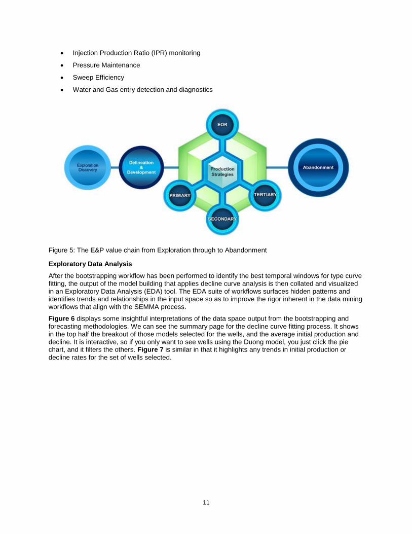
A reservoir's life begins with exploration, leading to discovery; reservoir delineation and field development; production by primary, secondary and tertiary means; and inexorably the final phase of abandonment.

Sound reservoir management necessitates constant monitoring and surveillance of the reservoir performance from a holistic perspective as depicted in Figure 5. Is the reservoir performance conforming to management expectations? The important areas that add value across the E&P value chain as regards monitoring and surveillance involve data acquisition and management from the following geoscientific silos:

Oil, Water and Gas Rates and Cumulative production

Gas and Water injection

Static and flowing bottom-hole pressures

Production and injection well tests

Well injection and production profiles

Fluid analyses

4D Seismic surveys

Determine a suite of reservoir performance and field planning workflows:

o Reservoir surveillance

Well management

Well reliability and optimization

Field management

Reservoir modeling

o Reservoir Performance

11

Injection Production Ratio (IPR) monitoring

Pressure Maintenance

Sweep Efficiency

Water and Gas entry detection and diagnostics

Figure 5: The E&P value chain from Exploration through to Abandonment

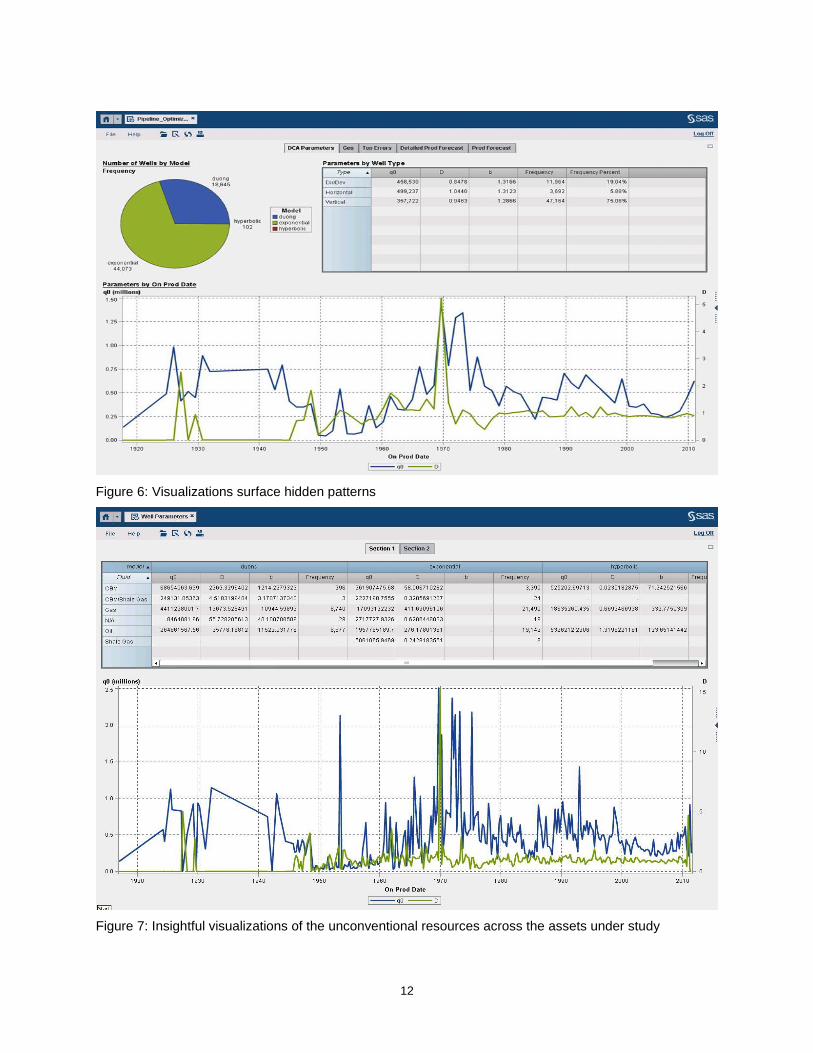
Exploratory Data Analysis

After the bootstrapping workflow has been performed to identify the best temporal windows for type curve fitting, the output of the model building that applies decline curve analysis is then collated and visualized in an Exploratory Data Analysis (EDA) tool. The EDA suite of workflows surfaces hidden patterns and identifies trends and relationships in the input space so as to improve the rigor inherent in the data mining workflows that align with the SEMMA process.

Figure 6 displays some insightful interpretations of the data space output from the bootstrapping and forecasting methodologies. We can see the summary page for the decline curve fitting process. It shows in the top half the breakout of those models selected for the wells, and the average initial production and decline. It is interactive, so if you only want to see wells using the Duong model, you just click the pie chart, and it filters the others. Figure 7 is similar in that it highlights any trends in initial production or decline rates for the set of wells selected.

12

Figure 6: Visualizations surface hidden patterns

Figure 7: Insightful visualizations of the unconventional resources across the assets under study

13

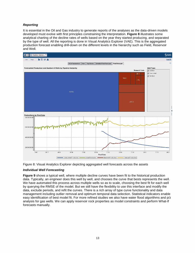
Reporting

It is essential in the Oil and Gas industry to generate reports of the analyses as the data-driven models developed must evolve with first principles constraining the interpretation. Figure 8 illustrates some analytical charting of the decline rates of wells based on the year they started producing, and separated by the type of well. All the reporting is done in Visual Analytics Explorer (VAE). This is the aggregated production forecast enabling drill-down on the different levels in the hierarchy such as Field, Reservoir and Well.

Figure 8: Visual Analytics Explorer depicting aggregated well forecasts across the assets

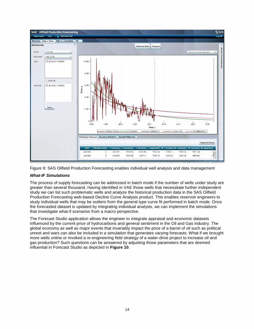
Individual Well Forecasting

Figure 9 shows a typical well, where multiple decline curves have been fit to the historical production data. Typically, an engineer does this well by well, and chooses the curve that bests represents the well. We have automated this process across multiple wells so as to scale, choosing the best fit for each well by querying the RMSE of the model. But we still have the flexibility to use this interface and modify the data, exclude periods, and refit the curves. There is a rich array of type curve functionality and data management including outlier removal and optimum temporal data selection. Statistical indicators enable easy identification of best model fit. For more refined studies we also have water flood algorithms and p/z analysis for gas wells. We can apply reservoir rock properties as model constraints and perform What-If forecasts manually.

14

Figure 9: SAS Oilfield Production Forecasting enables individual well analysis and data management

What-IF Simulations

The process of supply forecasting can be addressed in batch mode if the number of wells under study are greater than several thousand. Having identified in VAE those wells that necessitate further independent study we can list such problematic wells and analyze the historical production data in the SAS Oilfield Production Forecasting web-based Decline Curve Analysis product. This enables reservoir engineers to study individual wells that may be outliers from the general type curve fit performed in batch mode. Once the forecasted dataset is updated by integrating individual analysis, we can implement the simulations that investigate what-if scenarios from a macro perspective.

The Forecast Studio application allows the engineer to integrate appraisal and economic datasets influenced by the current price of hydrocarbons and general sentiment in the Oil and Gas industry. The global economy as well as major events that invariably impact the price of a barrel of oil such as political unrest and wars can also be included in a simulation that generates varying forecasts. What if we brought more wells online or invoked a re-engineering field strategy of a water-drive project to increase oil and gas production? Such questions can be answered by adjusting those parameters that are deemed influential in Forecast Studio as depicted in Figure 10.

15

Figure 10: Forecast Studio enables What-If scenarios to be studied

Data-Driven Models

Data-driven models are the result of adopting data mining techniques. Data mining is a way of learning from the past in order to make better decisions in the future. We strive to avoid:

Learning things that are not true

Learning things that are true but not useful

What are the burning issues to be addressed across E&P and downstream? Mining data to transform them into actionable information is key to successfully making business sense of the data. Data comes from multiple sources in many formats: real-time and in batch mode as well as structured and unstructured in nature.

Soft computing concepts incorporate heuristic information. What does that mean? We can adopt hybrid analytical workflows to address some of the most challenging upstream problems. Couple expert knowledge that is readily retiring from the petroleum industry with data-driven models that explore and predict events resulting in negative impacts on CAPEX and OPEX. The age of the Digital Oilfield littered with intelligent wells generate a plethora of data that when mined surface hidden patterns to enhance the conventional studies. Marrying first principles with data-driven modeling is becoming more popular among the earth scientists and engineers.

Clustering is one data-mining tool for categorizing and analyzing groups of data dimensions having similar attribute characteristics or properties. For analyzing well profiles this methodology consists of classifying wells by dividing the field into areas. We adopted the clustering approach to study the results of applying the different DCA models across the various reservoirs and wells, identifying the most common models across the hierarchy of wells.

16

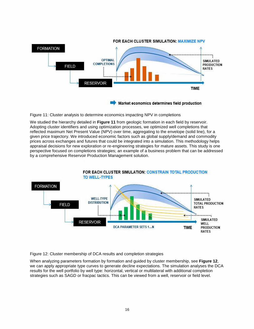
Figure 11: Cluster analysis to determine economics impacting NPV in completions

We studied the hierarchy detailed in Figure 11 from geologic formation in each field by reservoir. Adopting cluster identifiers and using optimization processes, we optimized well completions that reflected maximum Net Present Value (NPV) over time, aggregating to the envelope (solid line), for a given price trajectory. We introduced economic factors such as global supply/demand and commodity prices across exchanges and futures that could be integrated into a simulation. This methodology helps appraisal decisions for new exploration or re-engineering strategies for mature assets. This study is one perspective focused on completions strategies; an example of a business problem that can be addressed by a comprehensive Reservoir Production Management solution.

Figure 12: Cluster membership of DCA results and completion strategies

When analyzing parameters formation by formation and guided by cluster membership, see Figure 12, we can apply appropriate type curves to generate decline expectations. The simulation analyses the DCA results for the well portfolio by well type: horizontal, vertical or multilateral with additional completion strategies such as SAGD or fracpac tactics. This can be viewed from a well, reservoir or field level.

17

Figure 13: Cluster methodology to optimize DCA model for existing and new wells

The forecasting results across the existing portfolio of wells can be clustered by an empirical model that represents the optimum fit for all production data; thus if a new well is drilled in a particular location/pool we can devise the best potential model to use a type curve. Along with the initial rate of production and the initial decline rate, a robust forecast can be determined.

These data points can enrich subsequent cluster analyses when additional reservoir data are aggregated to the workflow to enable insights into reservoir management as seen in Figure 13.

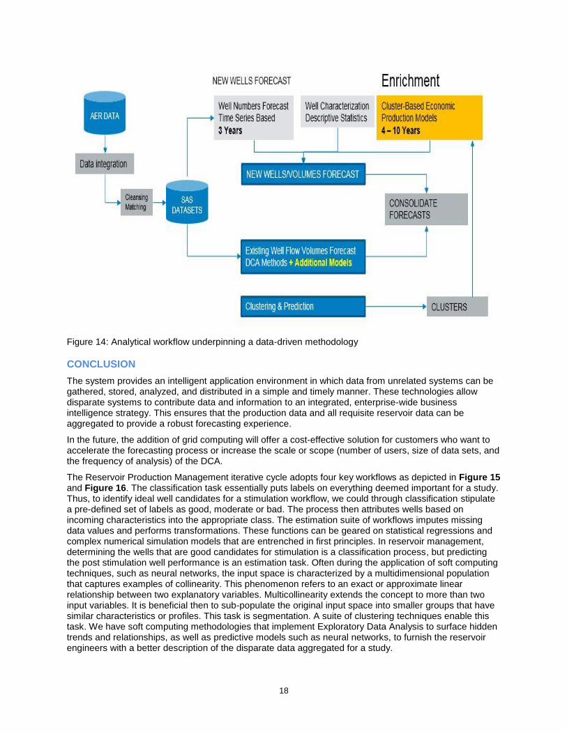
Having generated the Analytical Data Warehouse (ADW) from accumulated datasets across the E&P engineering silos, we can generate accurate forecasts (P10, P50 and P90) for each well in the asset portfolio adopting a data-driven suite of processes as shown in Figure 14. It is then feasible to aggregate forecasts with other reservoir management datasets housed in the ADW (Business Case dependent). With clusters in hand we can segregate the field into good/bad wells from the target variable or objective function perspective and enrich the reservoir characterization steps and ascertain, under defined confidence limits, a good guess forecast for new wells.

Integrating economic data, we can enable the appraisal stages of new field development work: either brownfield or via analogs in green-fields.

The reserve categories are totaled up by the measures 1P, 2P, and 3P, which are inclusive, so include the previous safer measures as:

"1P reserves" = proven reserves (both proved developed reserves + proved undeveloped reserves).

"2P reserves" = 1P (proven reserves) + probable reserves, hence "proved AND probable."

"3P reserves" = the sum of 2P (proven reserves + probable reserves) + possible reserves, all 3Ps "proven AND probable AND possible."

18

Figure 14: Analytical workflow underpinning a data-driven methodology

CONCLUSION

The system provides an intelligent application environment in which data from unrelated systems can be gathered, stored, analyzed, and distributed in a simple and timely manner. These technologies allow disparate systems to contribute data and information to an integrated, enterprise-wide business intelligence strategy. This ensures that the production data and all requisite reservoir data can be aggregated to provide a robust forecasting experience.

In the future, the addition of grid computing will offer a cost-effective solution for customers who want to accelerate the forecasting process or increase the scale or scope (number of users, size of data sets, and the frequency of analysis) of the DCA.

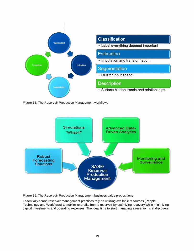
The Reservoir Production Management iterative cycle adopts four key workflows as depicted in Figure 15 and Figure 16. The classification task essentially puts labels on everything deemed important for a study. Thus, to identify ideal well candidates for a stimulation workflow, we could through classification stipulate a pre-defined set of labels as good, moderate or bad. The process then attributes wells based on incoming characteristics into the appropriate class. The estimation suite of workflows imputes missing data values and performs transformations. These functions can be geared on statistical regressions and complex numerical simulation models that are entrenched in first principles. In reservoir management, determining the wells that are good candidates for stimulation is a classification process, but predicting the post stimulation well performance is an estimation task. Often during the application of soft computing techniques, such as neural networks, the input space is characterized by a multidimensional population that captures examples of collinearity. This phenomenon refers to an exact or approximate linear relationship between two explanatory variables. Multicollinearity extends the concept to more than two input variables. It is beneficial then to sub-populate the original input space into smaller groups that have similar characteristics or profiles. This task is segmentation. A suite of clustering techniques enable this task. We have soft computing methodologies that implement Exploratory Data Analysis to surface hidden trends and relationships, as well as predictive models such as neural networks, to furnish the reservoir engineers with a better description of the disparate data aggregated for a study.

19

Figure 15: The Reservoir Production Management workflows

Figure 16: The Reservoir Production Management business value propositions

Essentially sound reservoir management practices rely on utilizing available resources (People, Technology and Workflows) to maximize profits from a reservoir by optimizing recovery while minimizing capital investments and operating expenses. The ideal time to start managing a reservoir is at discovery.

20

REFERENCES

Holdaway, K.R. 2014. Harness Oil and Gas Big Data with Analytics. 1st ed. Hoboken, NJ: John Wiley & Sons.

Yuhong Wang. 2006. “Determination of Uncertainty in Reserves Estimate from Analysis of Production Decline Data.” Master of Science Thesis, Texas A&M.

ACKNOWLEDGMENTS

The authors wish to acknowledge the research and contributions of Gary M. Williamson, Dennis Seemann, and Husameddin Madani, Saudi ARAMCO.

RECOMMENDED READING

Base SAS® Procedures Guide

Harness Oil and Gas Big Data with Analytics

Bayesian Analysis of Item Response Theory Models using SAS

Applied Data Mining for Forecasting using SAS

Decision Trees for Analytics using SAS Enterprise Miner

Data Visualization, Big Data and the Quest for Better Decisions

CONTACT INFORMATION

Your comments and questions are valued and encouraged. Contact the author at:

Keith R. Holdaway SAS Institute Inc. C5188 SAS Campus Drive Cary NC 27513 Work Telephone: +1 919 531 2034 E-mail: keith.holdaway@sas.com

SAS and all other SAS Institute Inc. product or service names are registered trademarks or trademarks of SAS Institute Inc. in the USA and other countries. ® indicates USA registration.

Other brand and product names are trademarks of their respective companies.