UNCLASSIFIED AD 4 10 2i9 - DTIChaust for torpedo-control purposes and the use of base-vented hydrofoils as propeller blades. ... tion, China Lake, Calif., Attn: Code 7506. This work

UNCLASSIFIED

AD 4 10 2i9

DEFENSE DOCUMENTATION CENTERFOR

SCIENTIFIC AND TECHNICAL INFORMATION

CAMERON STATION, ALEXANDRIA. VIRGINIA

UNCLASSIFIED

NOTICE: When government or other dravings, speci-fications or other data are used for any purposeother than in connection with a definitely relatedgovernment procurement operation, the U. S.Government thereby incurs no responsibility, nor anyobligation whatsoever; and the fact that the Govern-ment may have formalated, furnished, or in any wvysupplied the said drawingso specifications, or otherdata is not to be regarded by implication or other-

wise as in any manner licensing the holder or anyother person or corporation, or conveying any rightsor permission to manufacture, use or sell anypatented invention that may in any way be relatedthereto.

NAVWEPS REPORT 7941Part I

NOTS TP 2977

cOPY 60

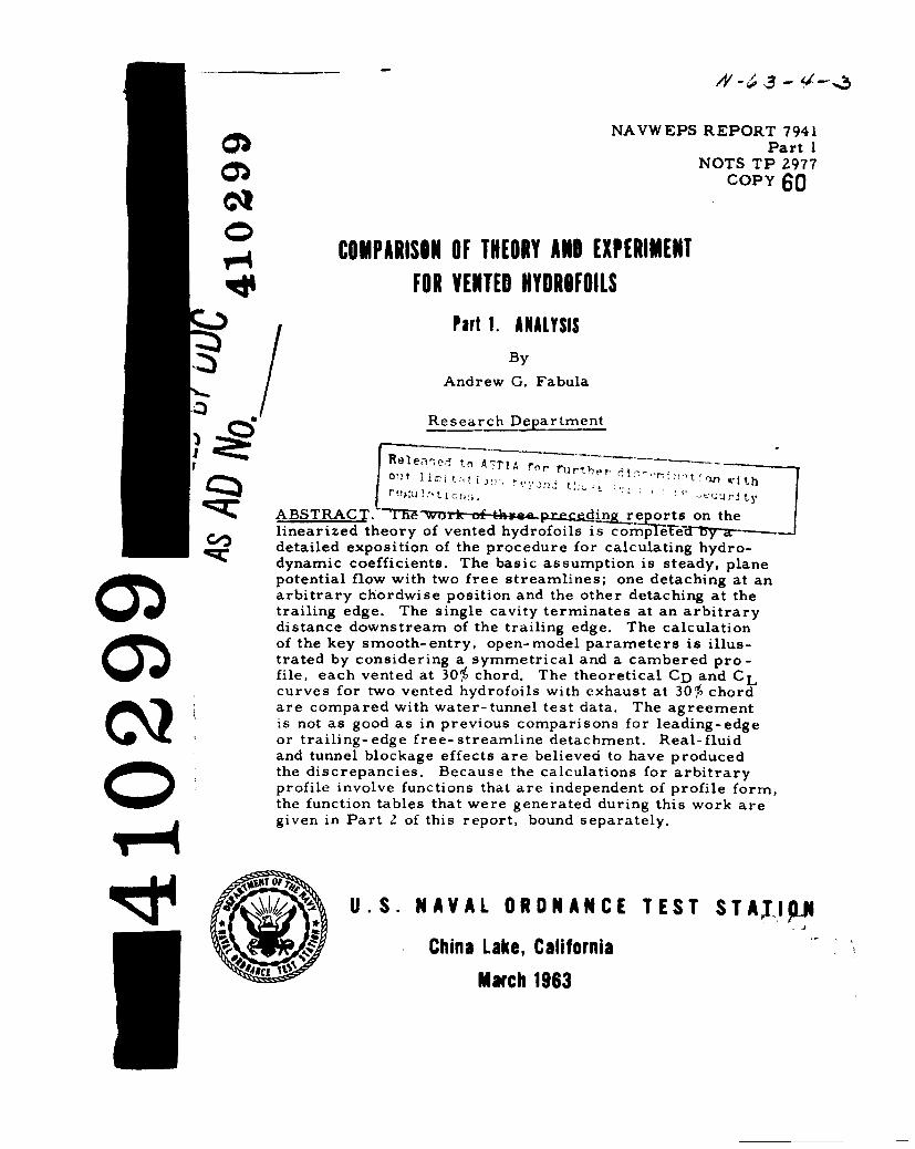
0, COMPARISON OF THEORY AND EXPERIMENT

FOR VENTED HYDROFOILSPart 1. ANALYSIS

By

Andrew G. Fabula

CS Research Department

[Ra len t A~I A .... n. A' 771 thF O~e ,Ut tn t'i~ yttys

ABSTRACT. -TI orepo..orts on thelinearized theory of vented hydrofoils is compTeTh

G detailed exposition of the procedure for calculating hydro-dynamic coefficients. The basic assumption is steady, planepotential flow with two free streamlines; one detaching at anarbitrary chordwise position and the other detaching at thetrailing edge. The single cavity terminates at an arbitrarydistance downstream of the trailing edge. The calculation

of the key smooth-entry, open-model parameters is illus-trated by considering a symmetrical and a cambered pro -file, each vented at 30% chord. The theoretical CD and CLcurves for two vented hydrofoils with exhaust at 30% chordare compared with water- tunnel test data. The agreementis not as good as in previous comparisons for leading-edge

Cor trailing-edge free-streamline detachment. Real-fluidand tunnel blockage effects are believed to have producedthe discrepancies. Because the calculations for arbitraryprofile involve functions that are independent of profile form,the function tables that were generated during this work aregiven in Part 2 of this report, bound separately.

4 , U.S. NAVAL ORDNANCE TEST STA).,

China Lake, CaliforniaEMarch 1963

U. S. NAVAL ORDNANCE TEST STATION

AN ACTIvir y OF THE BUREAU OF NAVAL WEAPONS

C BLINM&AI JR., CAPT., USM Wm. B. MCLEAN. PiL.cmftmmond., Technical Director

CONTENTS

Foreword...................... . .. ...... . . .. .. .. . ...

Notation...............................v

Introduction..................... .. . . ... . .. .. .. .. ... 1

Infinite Cavity Length........................................NACA 0010 Thickness Distribution.............................5Polynomial and Uniform- Load Camber Lines. .......... 6Hydrofoil B..........................10

The Smooth-Entry, Op~en-Model Parameters ............ 10NACA 0010 Thickness Distribution ............... 16Uniform- Load Camb~zer Line..................22

The Flat-Plate Parameters .................... 24Open Model..........................24Closed Model.........................26

Discussion. ... ........................ 27

Examples of Theoretic.al1 CL and CD Versus K and Two Com-Vparisons of Theor-y and Experiment. ............. 30

Hydrofoil A.........................30Hydrofoil B.........................35Discussion............................35

Sum m ary . . . . . . . . . . . . . . . . . . . . . . . . . .1

Appendixes:A. Corrigenda........................41B. Vented Wedge. ...................................... 42C. Partly Closed Miodel Solutions for Vented Flat Plate . . . . 48

References...........................52

NO'S Technical Publication 2977NAVWEPS Report 794 1, Part I

Published by.............Research DepartmentManuscript...................P5006/MS-7Collation..........Cove r, 30 leaves, abstract cardsFirst printing..............255 numbered copiesSecurity classification. .......... UNCLASSIFIED

ii

FOREWORD

As one of a series on vented hydrofoils, this report,consisting of two parts, completes the application oflinearized theory for steady, plane, unbounded flow. Thegeneral study is motivated by the possible use of gas ex-haust for torpedo-control purposes and the use of base-vented hydrofoils as propeller blades.

The theoretical calculations are illustrated by treatingtwo vented hydrofoils for which experimental results weregiven in Water- Tunnel Tests of Hydrofoils With Forced Ven-tilation, by T. G. Lng, D. A. Daybell, and K. E. Smith(= URD Report 7008, 10 November 1959).

The comparison of theory with experiment leads tonew insight into the nature of the experimental flows.

Because the calculations for arbitrary profile involvefunctions that are independent of profile form, the func-tion tables that were generated during this work are givenin Part 2 of this report, bound separately. Thus other re-searchers may consider further hydrofoil profiles withminimal labor. However, since the tables are of restrictedinterest, Part 2 is being sent only to a small number ofthose receiving Part 1. Others who wish to receive Part 2may write to Commander, U. S. Naval Ordnance Test Sta-tion, China Lake, Calif., Attn: Code 7506.

This work was done under Bureau of Naval WeaponsTask Assignments RUAW-4E401/216 1/R009-01-003 andRUTO-3E-000/216 1/R009-01-003, problem assign-ment 401. The report was reviewed for technical adequacyby Dr. Blaine R. Parkin of the RAND Corp.

Released by Under authority ofT. E. PHIPPS, Head, Win. B. McLEANResearch Department 'rechnical Director'0 March 1961

iii

NAVWEPS REPORT 7941Part 1

NOTATION

/ - 4, lea

4--+ %(1 -I)e

b (I + a)4%7T

a, + ib1 , a 2 + ... Coefficients in expansion of w(z) for z-.Qoo

C + id o = '.i

c n cn =- H(O) co n dO n 1,2...

C' Closure coefficient

Cz z-plane closure singularity coefficient

CD, CL, CM Drag, lift, and moment coefficients for unit chordlength and unit span (Fig. 1)

CQ Gas-supply coefficients, taken from Ref. 11

dn cn + 2(Q - a.) cos ne'

e Exhaust location measured from leading edge forunit chord length

F, G Functions of c, d, and coso0 (page 12)

F 1 , F7, F 3 , F4 Functions of c, d, and cos 0 (page 12)

h Hydrofoil contour height above x axis

h', h" Parameters in polynomial approximation ofuniform-load camber line

H Contour slope, dh*/dx

iTf 10,cos - coso 0n

InI dOJO 1+ cose, 1

iv

f


Im. Imaginary part of

I {;I T (Cos0 C~os, )fn dO

K Cavity number, 2(p,, - PC)/PU~

I Distance from leading edge to cavity- termination point,called cavity length

Mn in Jn

Ne iv ( U ib) c -a + i(d -b)

P Vented flat-plate solution for unit angle of attack and open-cavity model

Pn In+_iQ Vented flat- plate solution for unit angle of attack and

closed- cavity model

R1. Real part of

tw Wakc thickness for unit chord

11, v x and y components of velocity perturbation divided by U"

w Conjugate complex perturbation velocity, u - iv, andanalytic function of z, and

N, y Cartesian coordinates in physical plane with free streamin positive x direction and (0, 0) at leading edge

A X -iy

(I Angle of' attack

ji Flat- plate solution parameter

NO Y1 ... Parameters in polynomnial approximation of uniforin-loadcamber line

SVented wedge full apex angle

V

NAVWEPS REPORT 7941P art I

6.i/2, 60, 6 I ... Parameters in expression for NACA 0010 profile

slope distribution

Circle-plane complex coordinate, 1 +i42

8 Circle-plane polar angle

8' Value of 0 at leading- edge point on unit circlex, A zo Ae i X

Y, N (a + ib) = Neiv

p Water density

T Tunnel height divided by hydrofoil chord

-() Arctan[d+(-) -a2 ]/(c - a)

Subscriptsc Cavity value

cl Closed model

cw Cavity-wall- speed linearizationfs Free- stream- speed linearization

o Open model

P Open-model flat-plate solution for unit angle ofattack

* Closed-model flat-plate solvion for unit angleof attack

s Smooth-entry condition for open model

* Respectively upper and lower sides of singularityslit or hydrofoil

o Condition or value at z = o

Superscripts+ Cusp closure

0 Zero angle of attack

- Thickness profile and its parameters after re-moval of leading-edge singularity

Open-model point-drag profile and its parameters

vi


INTRODUCTION

Theoretical analyses of vented hydrofoils using the linearized

"thin- airfoil" theory of steady, plane, ideal flow are presented in

Ref. 1 and 2. This third report presents sample theoretical results,comparison with experiment, and function tables with which hydrody-namic coefficients can be calculated according to the formulas devel-oped in Ref. 1 and 2.

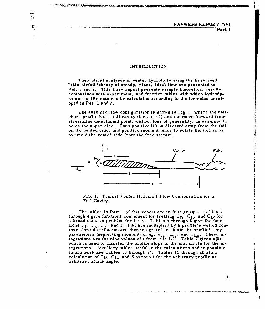
The assumed flow configuration is shown in Fig. 1, where the unit-chord profile has a full cavity (i. e., I > 1) and the more forward free-streamline detachment point, without loss of generality, is assumed tobe on the upper side. Thus positive lift is directed away from the foilon the vented side, and positive moment tends to rotate the foil so asto shield the vented side from the free stream.

IL Cavity Wake

Uo

FIG. 1. Typical Vented Hydrofoil Flow Configuration for aFull Cavity.

The tables in Part Z of this report are in four groups. Tables 1through 4 give functions convenient for treating CD, CL, and C fora broad class of profiles for I = 'r. Tables 5 through 8 give the !unc-tions F 1 , F,, F 3 , and F 4 that are multiplied by a profile's wetted con-tour slope distribution and then integrated to obtain the profile's keyparameters (neglecting moment) of as , uc , tw , and CLs. These in-tegrations are for nine values of I from ,o 1..s Table 9 gives x(e)which is used to transfer the profile slope to the unit circle for the in-tegrations. Auxiliary tables useful in the calculations and in possiblefuture work are Tables 10 through 14. Tables 15 through 20 allowcalculation of CD, CL, and K versus I for the arbitrary profile atarbitrary attack angle.

1


In this work, the exhaust point location, e, is in effect assumed tobe in the range 0 :S e < I, since for trailing-edge venting, e = 1, thework in Ref. 3 is complete in itself. However, for various reasons,particularly the arrangement of tables, the case of e = I is also in-cluded here at several points.

INFINITE CAVITY LENGTH

In Ref. 2 the relations for hydrodynamic coefficients for I = wo areapplied mainly to profiles of simple form. The function tables givenhere allow ready treatment of a fairly broad class of profiles.

The relations for I = oo are

_ _ _ _ + %r- 2 1_+ ___

D d1 CL (2dl cos 0' - d2)

(1)

CM -- d 4 -6 coo 0, d3 + 2(1 + 6 cos 2 0')d24 2

-2 coos0 '(3 + 4 cos 0 )dl

The dn coefficients are determined by the contour slope and the angleof attack a, with

dn=cn+ 2(- asl)cosn0', cn=- cos nHd0 (n= 1,2...)

(2)

s =.- [ H dO. cos 0' a

It is to be noted that as, the smooth-entry attack angle, is denoted byao in Ref. 2, but in this report the subscript o is reserved for the open-model condition. H(O) is the wetted-surface contour slope distribution,dh*/dx, specified over the upper half of the -plane unit circle. Theupper surface (+) corresponds to 0 < 0 < 0', and the lower surface (-)corresponds to 0' < 0 < wi, according to the wetted-surface mapping for

(3= (Cose0- cosO') = (coo 0-ooe) (co.o..-a)

2 + coo e' + a

* See Item 1, Appendix A.

2


It will be seen later that these uses of as and a for I = Qo are con-sistent with the definitions of the same symbols for finite I. For eachprofile and 1, a - as is important to the character of the pressure dis-tribution near the leading edge, and thus as is a useful parameter.Therefore, for continuity between the results for infinite and finite 1,the formulas of Eq. 1 are put in the form

C_D= + (a- as) %r[ 2 CL = CLs + 2(a - as) 2

(4) 2zCm -- Cms - (aas 1+ 4 %l

The smooth-entry-angle parameters are seen to be

(5) CDs = _ - cos 0 H de

(6) CLs = 2 f (2 cos 0' cos 0 - cos 20) HdO

(7) CM s= 2 2[cos 40 -6 cos 0' cos 30 + 2(l + 6 cos 2 lcos 28

-2 cos 0'(3 + 4 cos4 0')cos 0] H dO

When only the results for I = oo are of interest, the natural formula-tion in terms of zero angle of attack is

I(L -f)]j2 2CD ( CL = CL )2 -

C M .= G M - - a- 1+ 4(

Noting that dn = cn for a = as , and using the relations

See Item 3, Appendix A.

3


cos 20- cos 20' =4a (cos 0- a) + 2 (cos 0 a)2

coB 30 - cos 30' = (12a 2 - 3)(cos 0 - a) + 12a (cos 0 - a)2 + 4(cos 0 - a)3

cos 40 - cos 40' = (32a 3 - 16a)(cos 0 - a) + (48a 2 - 8)(cos 0 - a) 2

+ 32a (cos 0- a) + 8(cos 0 - a)4

obtain

v'~='' fowco;a)-da(9) =L4 )s ( + ) H dO

(10) CL 4 O+Hd

1 a -1+ a I+a

[ co ) cos-CM =- ----- H dO . H dO

(1 + a)3 a (+a) + a°-' H dO + 2 o H. d-o,1 +a f I +a+ a

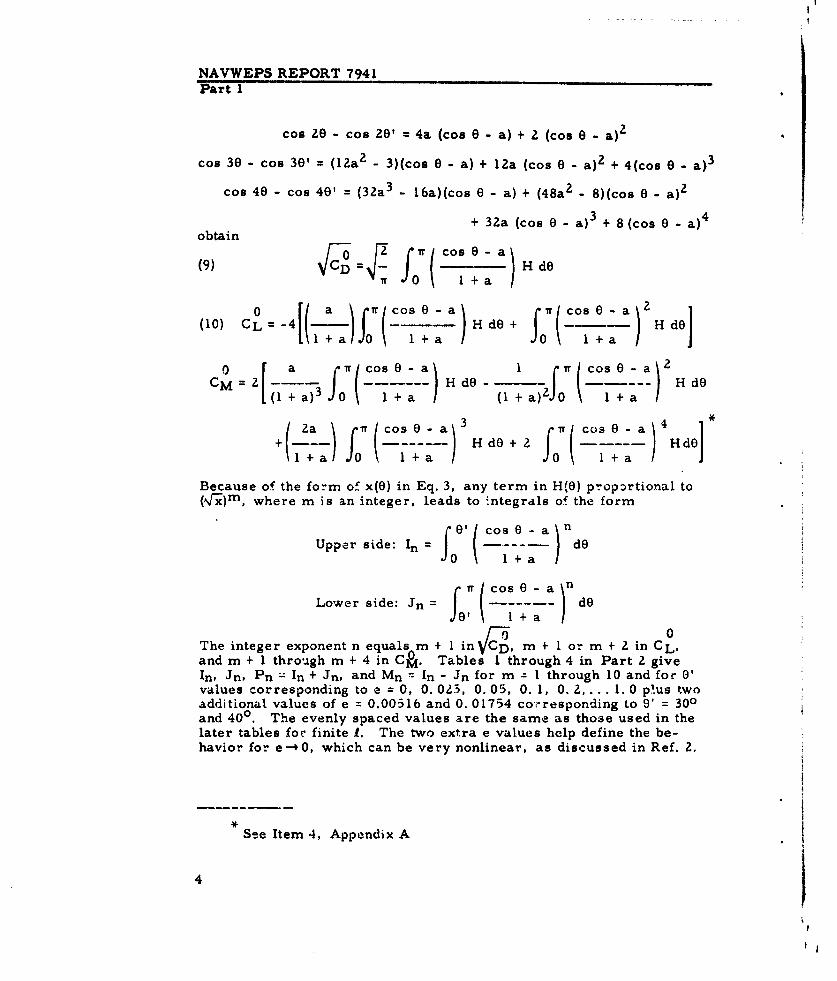
Because of the form of x(O) in Eq. 3, any term in H(O) proportional to(-)m, where m is an integer, leads to integrals of the form

Upper side: In : -(dO(c

Lower side: Jn f 1r ( 0a dO

0The integer exponent n equals m + 1 in ,CD m + 1 or m + 2 in CL,and m + 1 through m + 4 in C&1 . Tables 1 through 4 in Part 2 giveIn, Jn, Pn - In + Jn, and Mn = In - Jn for m = 1 through 10 and for 0'values corresponding to e = 0, 0. 0.3, 0.05, 0. 1, 0. 2.... 1. 0 plus twoadditional values of e = 0.00516 and 0. 01754 co -responding to 9' = 300and 400. The evenly spaced values are the same as those used in thelater tables for finite 1. The two extra e values help define the be-havior for e--40, which can be very nonlinear, as discussed in Ref. 2.

See Item .4, Appendix A

4


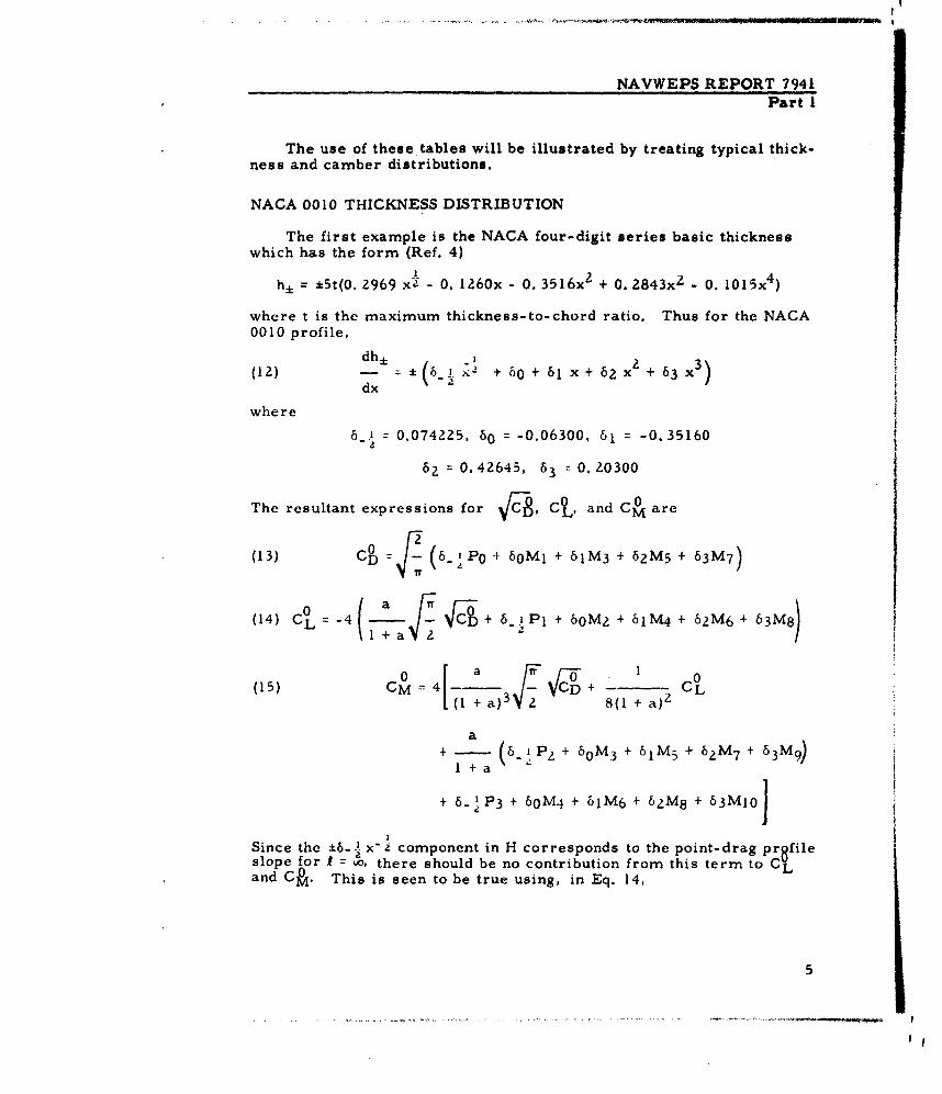
The use of these tables will be illustrated by treating typical thick-ness and camber distributions.

NACA 0010 THICKNESS DISTRIBUTIONThe first example is the NACA four-digit series basic thickness

which has the form (Ref. 4)

h± = ±5t(0. 2969 xz - 0. 1260x - 0. 3516x2 + 0. 2843x 2 - 0. 1015x4 )

where t is the maximum thickness-to-chord ratio. Thus for the NACA0010 profile,

(12) ( h + 60 + 61 x + 62 x + 3x 3 )dx

where

6_ -- 0.074225, 60 = -0.06300, 61 = -0.35160

6z = 0.42645, 63 0. 20300

0 0The resultant expressions for CC CL , and CM are

(13 c -~ (6-1P0 4 60MI + 61M3 + 62M5 + 63M7 )

(14) C L -4 ( A + 6.)PI + 60M2 + 61 M4 + 62M6 + 63M 8

(15) C° - 4 --- - VC t CLI( +a) 3 8(1 + a) 2

( iP 2 + 60 M3 + 6iM 5 + 62 M7 + 63 M9 )S+a

+ 6. P3 + 60M4 + 61M6 + 62M 8 + 63MI0

Since the ±6- x-a component in H corresponds to the point-drag profileslope for I = w, there should be no contribution from this term to CLand CA. This is seen to be true using, in Eq. 14,

5

I j


a air aP1 + P0 = - + - - (W) = 0

1+a 1+a 1+a

and in Eq. 15,

a a a a [(12- a2 )1 aw(3/2+a )P 0 +-P 2 +P 3 = - w+- I - a 0

(1 + a)3 I+4a (1 + a)3 1+a t (1+a) 2 (14-a)3

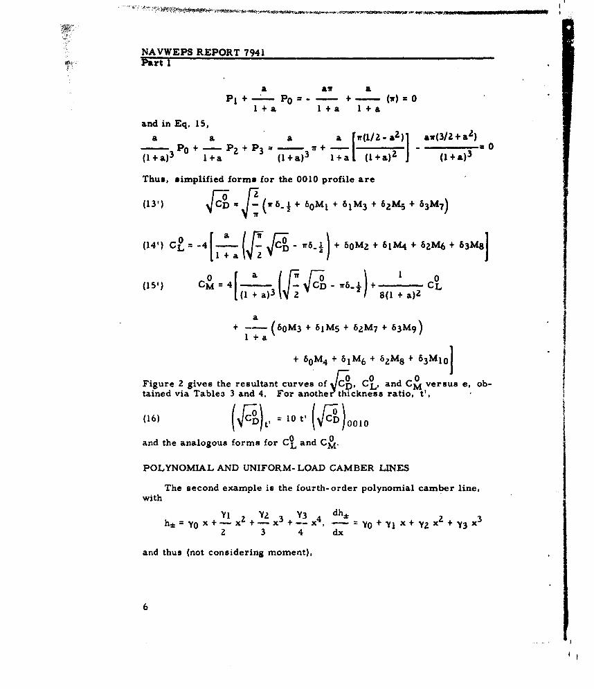
Thus, simplified forms for the 0010 profile are

(13') W= (i6._1+ 60M 1 + 6 1M3 + 62 M5 + 63 M7)

(15')A C 0M 4 - Il 2VD1r~(14,) C° - -4 a - 1. + 6oM2 + 61M4 + 62M6 + 63M8

(15,) M(4 + a)3 18(l + a)2

+ -~ 60M3 + 61MS + 62 M7 + 63M 9 )

+ 60 M 4 + 61 M6 + 6ZM 8 + 63 MIo

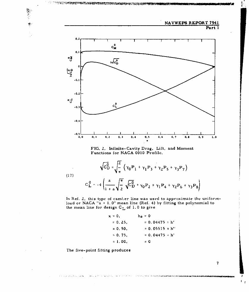
Figure 2 gives the resultant curves of -CD, C L, and CO versus e, ob-tained via Table3 3 and 4. For another thickness ratio, t',

(16) (F~ CD%)t = 10 t' FD 01

and the analogous forms for CO and CO

POLYNOMIAL AND UNIFORM- LOAD CAMBER LINES

The second example is the fourth-order polynomial camber line,with

y1 z Y 3 3 dh.* 3h* = y 0 x+ -x + L +--- -- 0 + yl x+ Y2 x

4- + Y3x2 3 4 dx

and thus (not considering moment),

6


0.1

0

-O0.1 -

-0.2 -

U0-0.3 CL

-0.4 -

0.0 0.1 o.z 0.3 0.4 0.5 0.6 0.7 0.8 0.9 1.0

FIG. 2. Infinite-Cavity Drag, Lift, and MomentFunctions for NACA 0010 Profile.

PC z (ji7 I~P + YIP 3 +* Y2 P5 + *Y.3P7)

(17)

VC7 .i J + y0 P 2 + YiP 4 + y2 P 6 + Y3 P 8

In Ref. 2, this type of camber line was used to approximate the uniform-load or NACA "a = 1. 0" mean line (Ref. 4) by fitting the polynomial tothe mean line for design CL of 1. 0 to give

x 0, h±=0

-0. 25, =0. 04475 h'

-0. 50, 0. 05515 h"

* 0. 75, = 0. 04475 h'

-1.00, =0

The five-point fitting produces

7


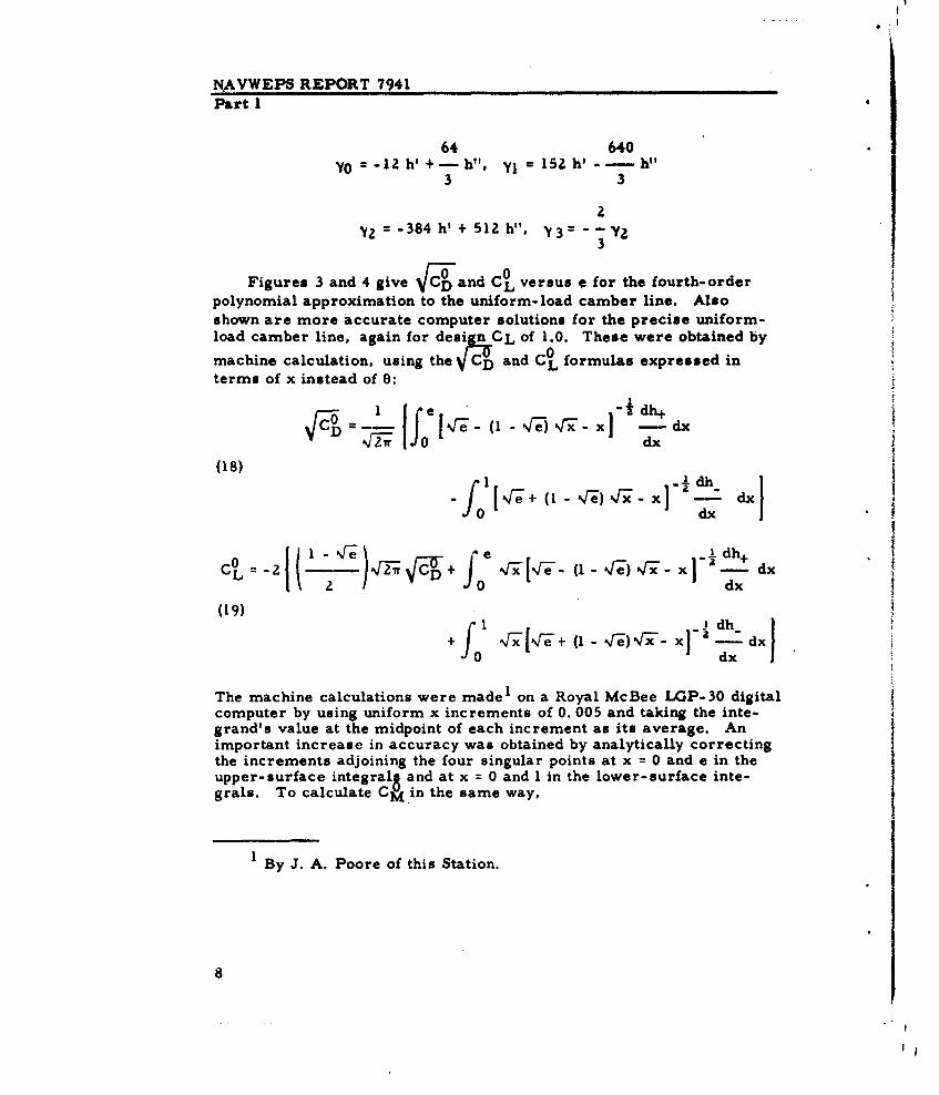
64 640YO 12 h' +- h", YI = 152 h' -- h"

3 3

2

Y2 -384 h' + 512 h", y= - 3y 2

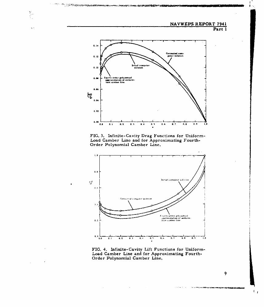
Figures 3 and 4 give D and Co versus e for the fourth-orderpolynomial approximation to the uniform-load camber line. Alsoshown are more accurate computer solutions for the precise uniform-load camber line, again for desiJnCL of 1.0. These were obtained by

machine calculation, using the C and CL formulas expressed interms of x instead of 0:

D i 0"re " (" -) '"x'dh+d

- edx dx

_1 dh

cO=-2~I-e + N-l re-) -F 'r- x]' dxf- dx

_____ e Idh+

CO 2( f; +: 41A4- 1- %je) ,fx- xl --+ dx

(19)' 1 dh

+101 r_ ,I (1- +( %r)AJT x dxdx

The machine calculations were made1 on a Royal McBee LGP-30 digitalcomputer by using uniform x increments of 0. 005 and taking the inte-grand's value at the midpoint of each increment as its average. Animportant increase in accuracy was obtained by analytically correctingthe increments adjoining the four singular points at x = 0 and e in theupper-surface integrall and at x = 0 and I in the lower-surface inte-grals. To calculate CI in the same way,

1 By J. A. Poore of this Station.

8


0. 14

Corrcted corn

0. 12 puter saoution

Inititl computer0. 0 solution

0. 0i Fourth-order polynomialapproxtmatiot of uniform.load Camber line

0.06

0.04

0.02

0.00

0.0 0.1 0.2 0.3 0.4 0.S 0.6 0.7 0.8 0.9 1.00

FIG. 3. Infinite-Cavity Drag Functions for Uniform-Load Camber Line and for Approximating Fourth-Order Polynomial Camber Line.

.0

0.8

F,,,*rtIh-order pnlsnominl,.pprox-mAtion of ,lorr- I

0.2 " ,,.,cI .. rnbrr lint. I1

0.0 I .0.0 0.1 0.2 0. 0.4 0.S Ot 0.7 0.1 0,9 1.0

FIG. 4. Infinite-Cavity Lift Functions for Uniform-Load Camber Line and for Approximating Fourth-Order Polynomial Camber Line.

9


- Idh+f x (-I a+z r,- G( ) 4 x x -dx

dx

HYDROFOIL B

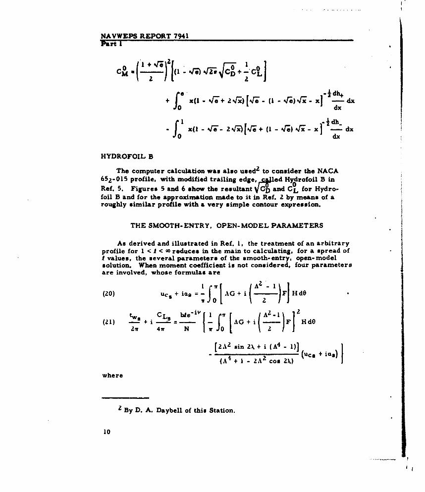
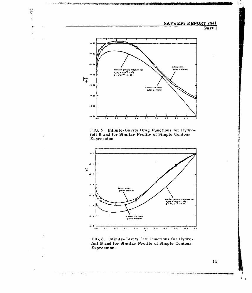
The computer calculation was also usedZ to consider the NACA652-05 profile, with modified trailing edge, ed Hydrofoil B in

0Ref. 5. Figures S and 6 show the resultant VD and CL for Hydro-foil B and for the approximation made to it in Ref. 2 by means of aroughly similar profile with a very simple contour expression.

THE SMOOTH-ENTRY, OPEN-MODEL PARAMETERS

As derived and illustrated in Ref. 1, the treatment of an arbitraryprofile for I < I <0 reduces in the main to calculating, for a spread ofI values, the several parameters of the smooth-entry, open-modelsolution. When moment coefficient is not considered, four parametersare involved, whose formulas are

(20) Ucs + ias f wAG + i )F Hd0 2

(21) - + i - -- AG+i - F HdO2W' 4wr N V w 2

[2AZ2 sin 2\ + i (A4 - 1)] uc, + ia)

(A4 + 1 - ZA2 cos 2 )s

where

2 By D. A. Daybell of this Station.

10

NAVWEPS REPORT 7941

Part 1

0. 00 _ez=

-0.0OZ

-0.04

folB nfrSimilar roffile ofuto Simper Cotour

Expression.o

.0. 10

-0. Il

foi Ban fr imla PofleofSimler Crloltonfur

.0

.0.7 2

0.0 ~ 0. .1. . . . . . .

FIG. 6. Infinite- Cavity Lift Functions for Hydro-

foil B and for Similar Profile of Simple ContourExpres sion.


1 1

+A2 + 1- 2Acos () + 0) A2 + I- 2Acos ( - 0)

2(A 2 + 1) - 4A cos X coso

(A 2 - 1)2 - 4(A 2 + 1)A coo X coso 0 + 4AZ(cosZX + cooz 0)and

sin (X + 0) sin ( - 0)G= +A2 + I - 2AcosQ.+( ) A2 + I - 2Acoso(X- 0)

sinX [2(A 2 + 1) coso - 4Acos

(A2 - 1)2 - 4(A 2 + l)Acos X coo 0 + 4AZ (cos 2 ). + cosZO)

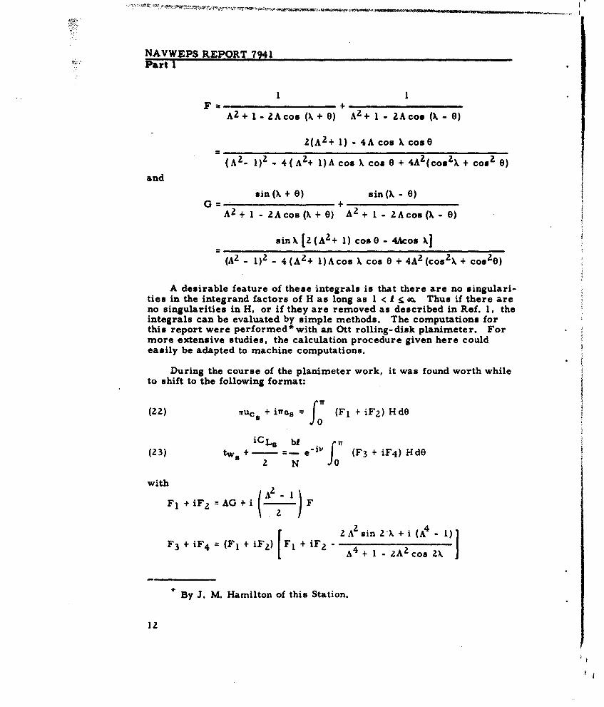
A desirable feature of these integrals is that there are no singulari-ties in the integrand factors of H as long as 1 < I K 0. Thus if there areno singularities in H, or if they are removed as described in Ref. 1, theintegrals can be evaluated by simple methods. The computations forthis report were performed*with an Ott rolling-disk planimeter. Formore extensive studies, the calculation procedure given here couldeasily be adapted to machine computations.

During the course of the planimeter work, it was found worth whileto shift to the following format:

(2) iruc + irTc1 s = Tf (F1 + iF 2 ) HdO

iCLs h . r(23) tw + - =- e-'j (F3 + iF4) HdO

2 N JO

with

Fl + iF2 = AG + iF( ) F

F3+F4(i~F 2 )Fi~F Z 2A2 sin 2A+ i (A4 -1)

A4 + I- A2 co2)X

* By J. M. Hamilton of this Station.

12

NAVWEPS REPORT 7941~Part I

(A 4 - 1)F? - ZA sin 2XF,SF Z F +A4 + I -2A 2 cos 2X

2A2 sin 2X F2 -(A 4 - )F 1 1+ i I F + A4 + I _ A2 cos 2X

The use of F 3 + iF 4 avoids some unnecessary compounding of errors,caused by subtracting nearly equal, relatively large terms, particularlyfor large 1.

The planimeter work has considered the following spread of I

values:

go, 8, 4, 2.5, 2, 1.5, 1.25, 1.125, and 1.1

It will be seen that the absence of 1.0 from this list is regrettable,since the s-parameter curves, when plotted versus reciprocal cavitylength, often show increasing curvature for 1--+1, The mapping usedcaused the forms of the s-parameter integrals to be indeterminate atI = 1, but it can be seen that the s-parameters are finite there unlessthe profile has a trailing-edge singularity. A case in which the solu-tion for I = I has been obtained is the vented wedge discussed in Ap-pendix B. For more extensive work, it would be useful to specificallytreat I - 1 and to routinely obtain the smooth-entry, open-model rela-tions for that limit. The I value of 1.125 could be dropped, keeping thenumber of cases to nine.

At the other limit, I uo, simplified relations are already availablefrom the previous work. However, it is necessary to confirm thatthose previous results are recovered with the more general forms.Using the notation

AeiX c + id - (a + N cos v) + i (b + N sin v)

and the definitions

f -e - /(- l)e-ar ___ , b =( + a) WI- 1

4T--e +-le

which lead to

)4 C 1 % % IN :( + a) T c V =-- - .

it can be seen that, for -- ,~,

13


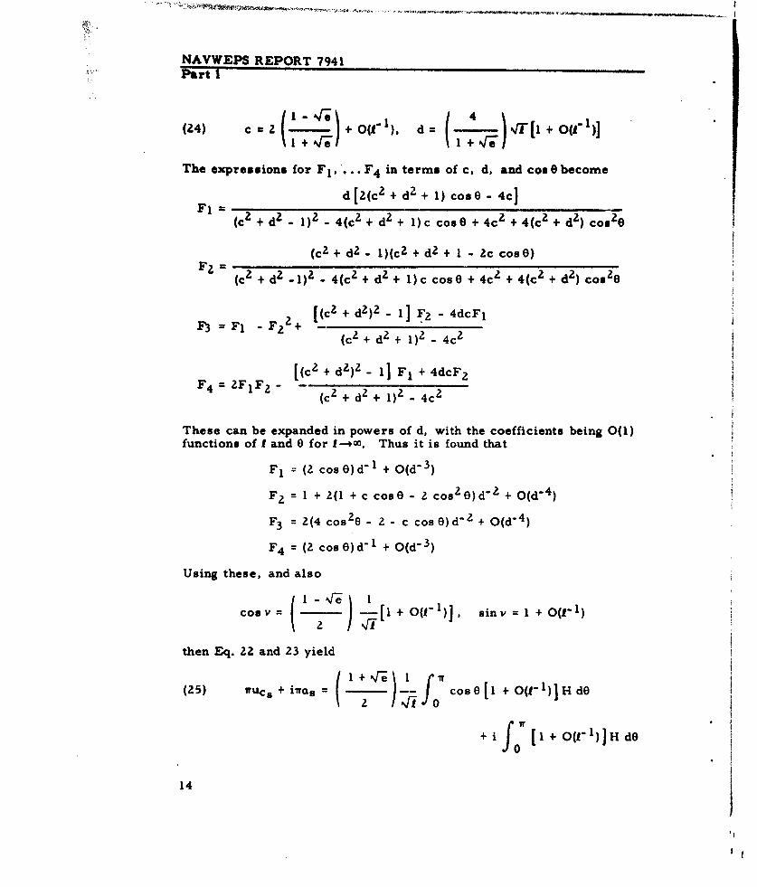
(24) c + d= -1)[. dO('1)

The expressions for Fl, ... F 4 in terms of c, d, and con0 become

Fd[2(c2 + d2 + 1) coso 0- 4c]

(c 2 + d 2 - 1)2 - 4(c 2 + d2 + 1)c cos0 + 4c 2 + 4(c 2 + d 2 ) cos2o

(c 2 + d2 - 1)(c 2 + + I - 2c coso0)

(c2 + d2 -1)2 - 4(c 2 + d2 + 1)c coso0 + 4c 2 + 4(c 2 + d2 ) coo20

[(c 2 + d2)2 - 1] F2 - 4dcF 1F3 =Fl -F 2 + (c 2 + d2 + 1)2 - 4c 2

[(c 2 + d2 )2 - I] FI + 4dcF 2F 4 = FIF 2 (c 2 + d2 + 1) 2 - 4c 2

These can be expanded in powers of d, with the coefficients being 0(l)functions of I and 0 for 1-.. . Thus it is found that

F I (2 cos0)d - I + O(d"3)

F2 = 1 + 2(1 + c coso0 - 2 cosz0)d- 2 + O(d- 4 )

F3 = 2(4 cos20 - 2 - c cos0)d- 2 + 0(d "4 )

F 4 = (2 cos0)d 1 + O(d "3 )

Using these, and also

coy = I + 0(1 1)], sinv = I + 0(1- 1)

then Eq. 22 and 23 yield

Irm + 4- f co'se[ I + 01 1)(25) WUcs + iT1s H dO

+ i [I + O(1')]H dOJo,

14

______NAVWEPS REPORT 7941Part I

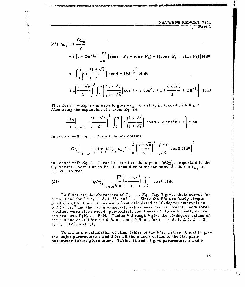
CL s(z6) tWs + i --

2

-- [i + oci-l)] f: [(cos v F3 + Sifl F4) + i~cos ' F4 - sinvF 3 )]HdO

- TJ('+ T cos 0 + O(W2) H dO

1~ - zo +Ic Cos 0+ T cos0 - 2 cos 2 0 + 1+- + HdO

Thus for I = u Eq. 25 is seen to give Ucs = 0 and as in accord with Eq. 2.Also using the expansion of c from Eq. 24,

.( . [2( cose - 2 cos 2 0 + I Hdo

in accord with Eq. 6. Similarly one obtains

C D -- r ( 2 + ( f Tr c o s 0 H d OC s 0 1 -- +m X2U s t s) Tr 2

in accord with Eq. 5. It can be seen that the sign of "CDs, important to the

CD versus a variation in Eq. 4, should be taken the same as that of tWs inEq. 26, so that

(27) Vi-6 s I " f cosO HdO

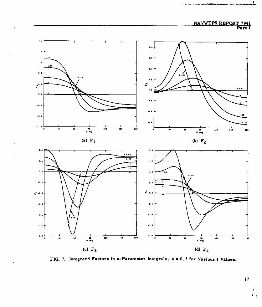
To illustrate the characters of F l, ... F 4 , Fig. 7 gives their curves fore = 0. 3 and for f = -, 4, 2, 1.Z5, and 1.1. Since the F's are fairly simplefunctions of 0, their values were first calculated at 10-degree intervals in0 < 0 < 1800 and then at intermediate values near critical points. Additional0 values were also needed, particularly for 0 near 0', to sufficiently definethe products FIH , ... F 4 H. Tables 5 through 9 give the 10-degree values ofthe F's and of x(0) for e r 0. 3, 0.4, and 0. 5 and for 1 -O, 8, 4, 2. 5, 2, 1.5,1. 25, 1. 125, and 1.1.

To aid in the calculation of other tables of the F's, Tables 10 and I I givethe major parameters c and d for all the e and I values of the flat-plateparameter tables given later. Tables 12 and 13 give parameters a and b

15


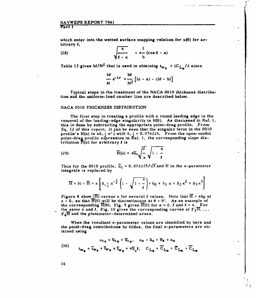
which enter into the wetted surface mapping relation for x(O) for ar-bitrary 1,

(28) - ±- (cos 0 - a)F7_x b

Table 13 gives b1/N 2 that is used in obtaining tws + iCLs/2 since

bi b- er i v - [(c - a) -i(d- b)]N N2

Typical steps in the treatment of the NACA 0010 thickness distribu-tion and the uniform-load camber line are described below.

NACA 0010 THICKNESS DISTRIBUTION

The first step in treating a profile with a round leading edge is theremoval of the leading-edge singularity in H(O). As discussed in Ref. 1,this is done by subtracting the appropriate point-drag profile. FromEq. 12 of this report, it Fan be seen that the singular term in the 0010profile's H(x) is *6. x-i with 6.. = 0.074225. From the open-modelpoint-dra& profile expression in lef. 1, the corresponding slope dis-tribution R(x) for arbitrary I is

(29) H(x) = +kucV-§ -

Thus for the 0010 profile, uc = 0. 074225/0-and H in the s-parameterintegrals is replaced by

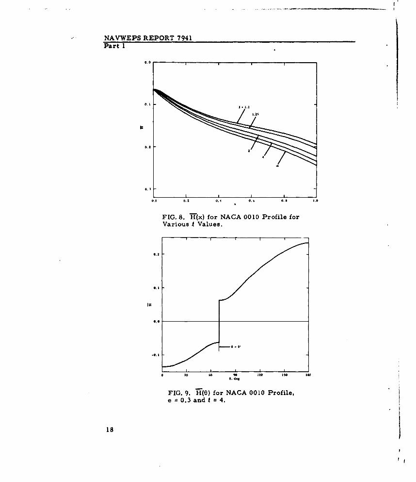
=Ho H=[ x_ (I - 1 . +60 + 61 x+ 62 x2 + 63 x3

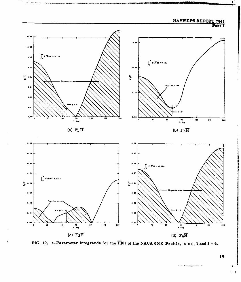
Figure 8 show ITI versus x for several I values. Note that it *60 atx = 0, so that 11(0) will be discontinuous at 0 = 0'. As an example ofthe corresponding 11(0), Fig. 9 gives 11(0) for e = 0. 3 and I = 4. Forthe same e and 1, Fig. 10 gives the corresponding curves of FIRT,F4 "and the planimeter- determined areas.

When the resultant s-parameter values are identified by bars andthe point-drag contributions by tildes, the final s-parameters are ob-tained using

Ucs =Mcs + _UCs, as = 'as + Is = as

(30) twS = ts+w -s + C CLs=CLs+Ls CaL

16

NAVWEPS REPORT 7941Pairt1

2.0 I

1.6 I

3.20 1.4

0.8

4-3.S0.4 6:

0.0.

4

0.8

.0.4 4

0.6

0.4 3 .3

0 30 60 90 320 .30 300 a t0 120 IS ISO3430. d~ 0. d"

(a) F1 (b) F2

0.8 Z. 01 11

0.4 3.0 ..

0.0 3.0 1.20

-0.4 0.0

.~ 1. 0.0

.2.4 ..0 30O 60O IN30 30 0 30 4090 320 330 to0

0. d"

(c) F3 (d) F4

FIG. 7. Integrand Factors in s-Parameter Integrals, e =0. 3 for Various I Values.

17


0.0 I

0. &

0. 8

0. 3

0.0 0.10. 0.3z 0.8 1.0

FIG. 8. Hf(x) for NACA 0010 Profile for

Various I Values.

0.12

0.0

-0.I

0 30 60 Ito ISO ISO0, dog

FIG. 9. -(0) for NACA 0010 Profile,e =0.3 and I =4.

18


0.08 I I I

0.0

0.07

0.06 J f? 1 dO "0AZZ

fO 1 'Wd. 0.16?0.0

0 .0 5 . 15

I" 0.04 Ik

Negative l r.0.03 Negative area

0.03

0. 30

0.02

0.01

60

0.00 1O0 ISO ISO0 00 0 30 60 90 120 IS0 ISO

0. dot 0. deg

(a) F1 I (b) F21T

0.09 0.08

0, 0 0.07

0.07 0.06 0 F4 1dO - .1 6

f+ F4 WdO .0.01220.04 0.0_

O. OdO 0.00 +--

IC 0.04 -0.04

I.IN

Negative area0.01 0.00

0.02 - Ngtvara0.02

0 *

0.01 S.0.01

0.00 0. 0010 IS0 10 60 90 120 IS0 1 0 0 30 60 0 120 100 1000, deg 0 de

(c) F31T (d) F41TFIG. 10. a-Parameter Integrands for the H(0) of the NACA 0010 Profile, e = 0. 3 and I = 4.

19


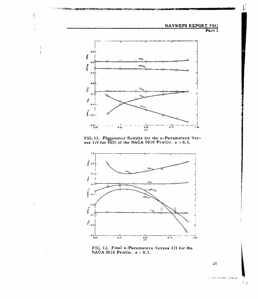
Figures I I and 12 give the curves of the s-parameters correspondiugto~and H, showing how important are the tilde contributions to Ucsand tw . C'D, and CD _ have been evaluated for I = 00 using Eq. 27to chec&c continuity wit the values for finite I.

One check on the accuracy of the calculations can be made as fol-lows. For e = 0. 3 and I =, the analytically determined values for the0010 profile, from Fig. 2, are

FCD= -0. 0059, CO = -0. 306

The planimeter results are

= 0. 0414, CDs = (0. 0 1 6 1 )Z, CL = -0. 163

which imply0 4e-- = -0. 0068

CL = CLs- ZT(ra s ) -0.319

The effect of the errors in FGD and CL can be seen to be small,

as follows. CD and CL from Eq. 8 can be put in the forms

CD=2'r (Qa +) 2 (- Fe) a+ F=

2 0 r+ %r= O

CL = 2r( - (1o)( alo=Zn (l +.Aq)22

where alo is a for CL = 0. Thus a+ is in error by about +0.09 degreeand a10 by about +0.18 degree. Thus the error due to the planimetercalculation inaccuracy will be small away from the zero drag and zerolift angles.

20

I

awf


-0A ~ 1~ -) 0 0. 0

IOD0 =

0.

CL

IIIIFIG. 11. Planimeter Results for the s-Parameters Ver-sus 1/1 for H(0) of the NACA 0010 Profile, e =0.3.

- 00

-0. It

U -0,40.00 0.2" 0.50 0.75 1.00

FIG. 12. Final s-Parameters Versus 1/1 for theNACA 0010 Profile, e -7 0.3.


UNIFORM- LOAD CAMBER LINE

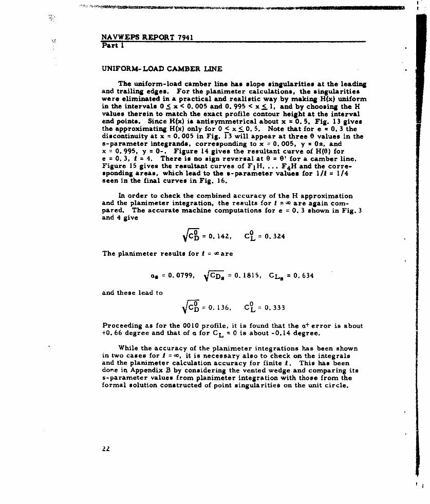
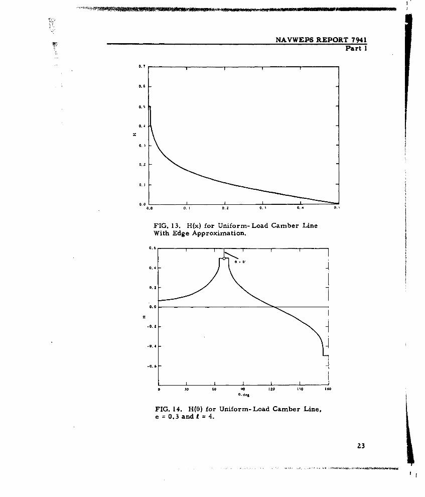
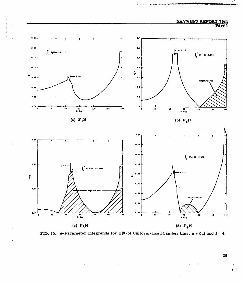
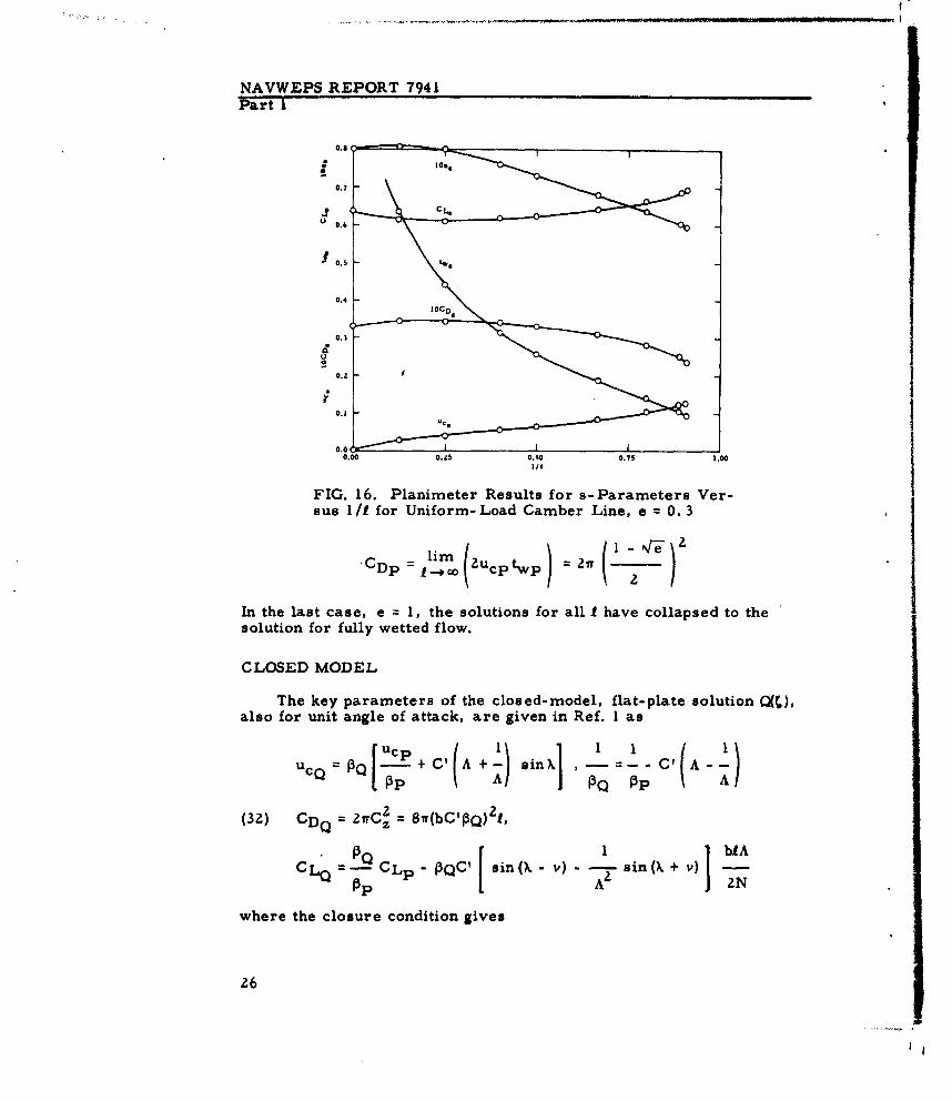
The uniform-load camber line has slope singularities at the leadingand trailing edges. For the planimeter calculations, the singularitieswere eliminated in a practical and realistic way by making H(x) uniformin the intervals 0 <5 x < 0. 005 and 0. 995 < x 1, and by choosing the Hvalues therein to match the exact profile contour height at the intervalend points. Since H(x) is antisymmetrical about x = 0. 5, Fig. 13 givesthe approximating H(x) only for 0 < x < 0.5. Note that for e = 0. 3 thediscontinuity at x = 0. 005 in Fig. 13 will appear at three 0 values in thes-parameter integrands, corresponding to x = 0. 005, y = 0*, andx = 0. 995, y = 0-. Figure 14 gives the resultant curve of H(0) fore = 0. 3. A = 4. There is no sign reversal at 0 = 0' for a camber line.Figure 15 gives the resultant curves of FIH, ... F 4 H and the corre-sponding areas, which lead to the s-parameter values for 1/1 = 1/4seen in the final curves in Fig. 16.

In order to check the combined accuracy of the H approximationand the planimeter integration, the results for I = '0 are again com-pared. The accurate machine computations for e = 0. 3 shown in Fig. 3and 4 give

CD=0.142, CO= 0.324

The planimeter results for I = a0are

= 0.0799, V = 0. 1815, CLs = 0.634

and these lead to

rD = 0.136, CO=0.333

Proceeding as for the 0010 profile, it is found that the a+ error is about+0.66 degree and that of a for CL = 0 is about -0.14 degree.

While the accuracy of the planimeter integrations has been shownin two cases for I = oo, it is necessary also to check on the integralsand the planimeter calculation accuracy for finite 1. This has beendone in Appendix B by considering the vented wedge and comparing itss-parameter values from planimeter integration with those from theformal solution constructed of point singularities on the unit circle.

22


0.7

0.6

0.5

0.4

0.1

0.1

0. 1

0.0 0 1 O. 0.! 0. 0.

FIG. 13. H(x) for Uniform- Load Camber LineWith Edge Approximation.

0.00.,4 -

.0.20.0

-0.4

-0.6 -

SI I I I ,

0 30 60 90 120 ISO ISO0, deg

FIG. 14. H(O) for Uniform-Load Camber Line,e 0.3 and = 4.

23


THE FLAT-PLATE PARAMETERS

OPEN MODEL

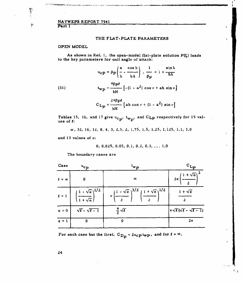
As shown in Ref. 1, the open-model flat-plate solution P(4) leadsto the key parameters for unit angle of attack:

a cosX) 1 sin XUcp =p1-+--,--

Ub bA I p

(31) twp = bN [-(I - a 2 ) cos v + ab sinv]bN

2 1TpfCLP = bN ab cos v + (1 - a 2) sin v

Tables 15, 16, and 17 give Ucp, and CLp respectively for 15 val-

ues of 1:

go, 32, 16, 12, 8, 4, 3, 2.5, 2, 1.75, 1.5, 1.25, 1.125, 1.1, 1.0

and 13 values of e:

0, 0.025, 0.05, 0.1, 0.2, 0.3, ... 1.0

The boundary cases are

Case Ucp twp CLp

I + e'I"+2 2

1e0l 0 0 21rNr l- 1 2 1Ni 3 /2(1 + 4e-/ ~

2 - 2

e =0 %rT - Ni -- I %rT 1T~rI(1T 0I--1)

e =1 0 0 21T

For each case but the first, CDP 2 ucptwp, and for I =go

24

!

NAvWEPS REPORT 7241Part I

0.24 0.?

0.20 0.6

0.1 0,5FJ FH d 0. 122 *

0. 12 - 0.4 -

0.08 -0.0 0. e

0.04 0.2

0.00 0.1

.0.04 1 0 JA0 o0 40 ISO 150 10 0 . 0..0 010 IS Igo

0. d.g 0, des

(a) FIH (b) FZH

0.16 I

0.14

0. 14

0 F 4 HdO 0. 130

0I 0.10

loF3H dO - - 0. 0680

0 0 8 t 0 0 '

0 .06

0 0'04

Nallve e rre

N.Bati- ae

000 0.000o0 Is* ISO 0 30 60 00 I0 IS0 t0

0, de 0. deg

(c) F 3H (d) F 4 H

FIG. 15. s-Parameter Integrands for H(O)of Uniform- Load Camber Line, e, 0.3 and 1 = 4.

25

I'


0.7

I CLL)0.6

0.

0.2

0.1.

0.0.00 0.&S 0.S0 0.71 1.001/t

FIG. 16. Planimeter Results for s-Parameters Ver-Isus 1 /1 for Uniform- Load Camber Line, e = 0.3

CDP=1 lim (ucp twP) 1 Ijs[

In the last case, e = 1, the solutions for all I1 have collapsed to thesolution for fully wetted flow.

CLOSED MODEL

The key parameters of the closed-model, flat-plate solution )also for unit angle of attack, are given in Ref. 1 as

PQ0 = - + C1(A +_11 n -I=_ .C,(A l[QPP A/ PQ PP A

z2 i~CP)1(32) CDQ 21rC. wbCP)

CLQ -CLp P 2N

where the closure condition gives

26


r 1 IbN~ 1

(33) Co Cos (k -) + 1 CosP + v) :tw bN1

IL A. j wp bi A

Tables 18, 19, and 20 give ucQ. CDQ, and CLQ for the same e and Ivalues as the P-parameters.

For two of the four boundary cases, the closed and open modelsare identical, because the closure singularity is unimportant for I = 0and is zero for e = 1. For 1-- 1., the closure singularity increaseswithout limit and ucQ and CL 0 -40 0 . The CDQ behavior for F--1 ismore complicated, with CDQ-- 0 for e 0, and CD-.0 for e > 0 dueto the leading-edge singularity. For e 0, the closed model has

I irl - -ucQ CD LQ C Q . -_ (T- Of-1)

The general character of these P- and Q-parameters as functionsof e and I can be seen in Fig. 6 and 7 of Ref. 1, where they are pre-sented in terms of the flat plate's hydrodynamic coefficients for thetwo models, using

CD 0 / 2 CD, CDcl/a2 = CDQI CLo/a = CLp, and CLcI/a =CL.

DISCUSSION

It is interesting to see the character of the differences between theforce coefficients for the two models, by comparing their forms fore - 0. The open-model relations for e 0 given above lead to

CD CL T

while the corresponding closed-model relations produce

C L + K Ja2 C (K)K,(

Thus the closed model for e - 0 and K/Za -40 has

CD CL I LK +.()Z+ Kf)4 ]Q2 a 2 4 2

27

! I


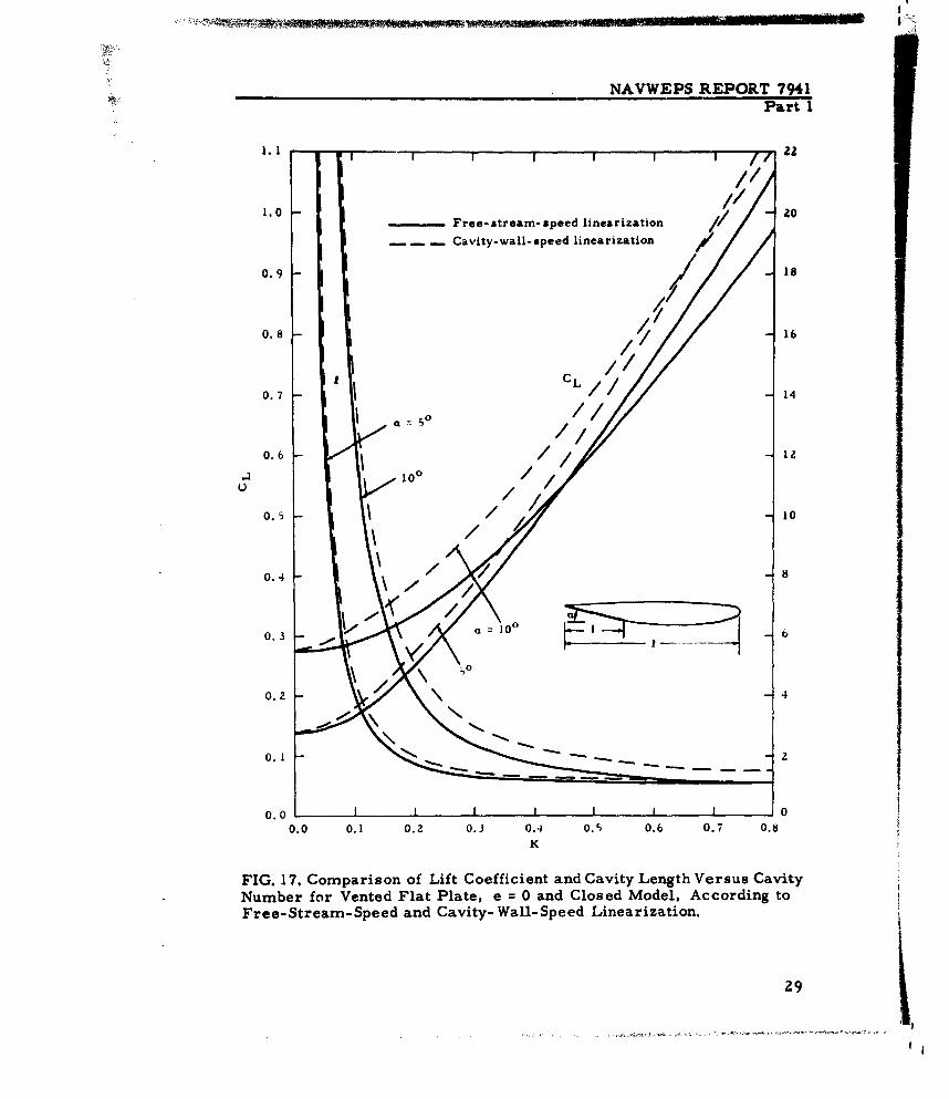
In contrast to these. results for free-stream speed linearization,the well-known cavity-wall-speed linearization always gives linearvariation with K (not K/a) of the hydrodynamic coefficients for K--0.The conversion from the free-stream- speed linearization to the otheris quite simple, as discussed in Appendix A of Ref. 3. It is easy to seethat the CD conversion given there for e = I applies for all e and forboth the closed and open models. Thus for a given profile, cavitylength, and particular cavity termination within the open, partly closed,and closed model family,

(34) CDCW = (1 + Kcw) CDfs, CLcw= (I + Kcw) CLf , CMcw = (I + Kcw) CMfs

where1 Kfs

(35) 1- ---4/I + Kgcw

Thus, for example, for the vented flat plate with e = 0, the closed-model result is

CDcw CLcw I_____ +r(l +Kcw) (.7-- 4T-i), I -

2 a 1 il+Kcw NJT T

Figure 17 shows that the consequent differences in the curves of CD/l -

and CL/ versus K are not important for the small angles of attacktypical of vented hydrofoil applications.

Applications of the six flat-plate parameters are illustrated nextby generation of the CD and CL versus K curves for two hydrofoil pro-files that have been tested in fully vented flow (Ref. 5). As discussedin Ref. 1, the P-parameters are used in two ways: (1) to shift fromthe open-model, smooth-entry condition to the cusp-closure condition,and (2) to obtain the open-model results for arbitrary attack angle ofan arbitrary profile, starting with its cusp-closure parameters. TheQ-parameters are used to obtain the closed-model results for arbitraryattack angle of an arbitrary profile, starting with its cusp-closureparameters.

28

! I


1.0 _______Free- stream- speed linearization 2

--- Cavity- wall- speed linearization

0.9 / 18

0.8 /1- 16

Al CL /0.7 - -/ 14

50/

.0.6 -/1/ 12

0.5/ 10

0.4 - /0" 8

0. 3 -l / ' ii i 6

-o

0.2 4

0. 12

0.0 IIII 00.0 0.1 0.2 0.3 0.4 0.1 0.6 0.7 0.8

K

FIG. 17. Comparison of Lift Coefficient and Cavity Length Versus CavityNumber for Vented Flat Plate, e = 0 and Closed Model, According toFree- Stream- Speed and Cavity- Wall- Speed Linearization.

29


EXAMPLES OF THEORETICAL CL AND CDVERSUS K AND TWO COMPARISONS

OF THEORY AND EXPERIMENT

HYDROFOIL A

The profile of Hydrofoil A has the NACA 0010 thickness distribu-tion and the uniform-load camber line for design CL of 0. 2. Thus thes-parameters for Hydrofoil A, e = 0. 3, are simply obtained fromprevious results, using, in obvious notation,

Ucs (ucs) 0010 .2ucsa=.0

and corresponding forms for as, tws, and CL.. All other combinationsof the NACA four-digit thickness distribution and the uniform-loadcamber line for e = 0. 3 can also be considered with the theoretical re-sults in this report because the thickness and camber distributions weretreated separately. If Hydrofoil A had been treated from the start, onlyother thickness ratios each for design CL of twice the thickness ratiocould be considered.

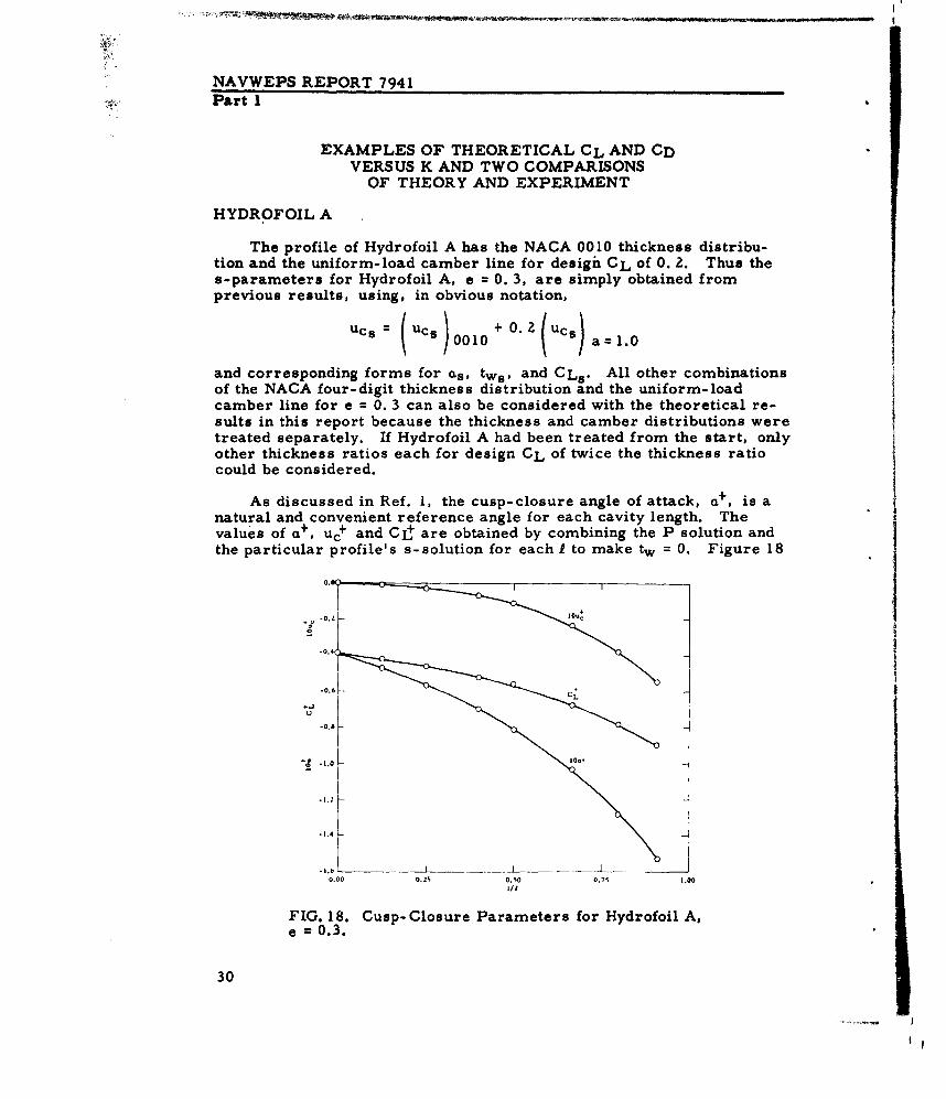
As discussed in Ref. 1, the cusp-closure angle of attack, a+ , is anatural and convenient reference angle for each cavity length. Thevalues of a+ , uc+ and CIt are obtained by combining the P solution andthe particular profile's s-solution for each I to make tw = 0. Figure 18

* 0. Z1u

~ -10

-0.4

-0.6

g.0.8 -

, 0 0 Z 0.- 1 0, 1

-1.4

1/I

FIG. 18. Cusp-Closure Parameters for Hydrofoil A,e a 0.3.

30

I I-


gives the cusp-closure parameters for Hydrofoil A, e 0. 3, obtainedwith

0 = tws + (a+ - as)twp

Uc+ = Ucs - w Ucp, = - --ns CLp

twp tWP

Having K+ = 2u+ and a+ for each 1, then as discussed in Ref. 1, alla values for a> a+ correspond to proper cavity solutions in the re-stricted sense that the closure singularity has proper sign. Thismerely means that cases of definite free-streamline crossing have beeneliminated, and of course it is likely that experimental cavity conditionswill not extend down to the negative K region typically included in theproper solution domain, as seen below. A more detailed discussionof solution domains is given in Appendix B.

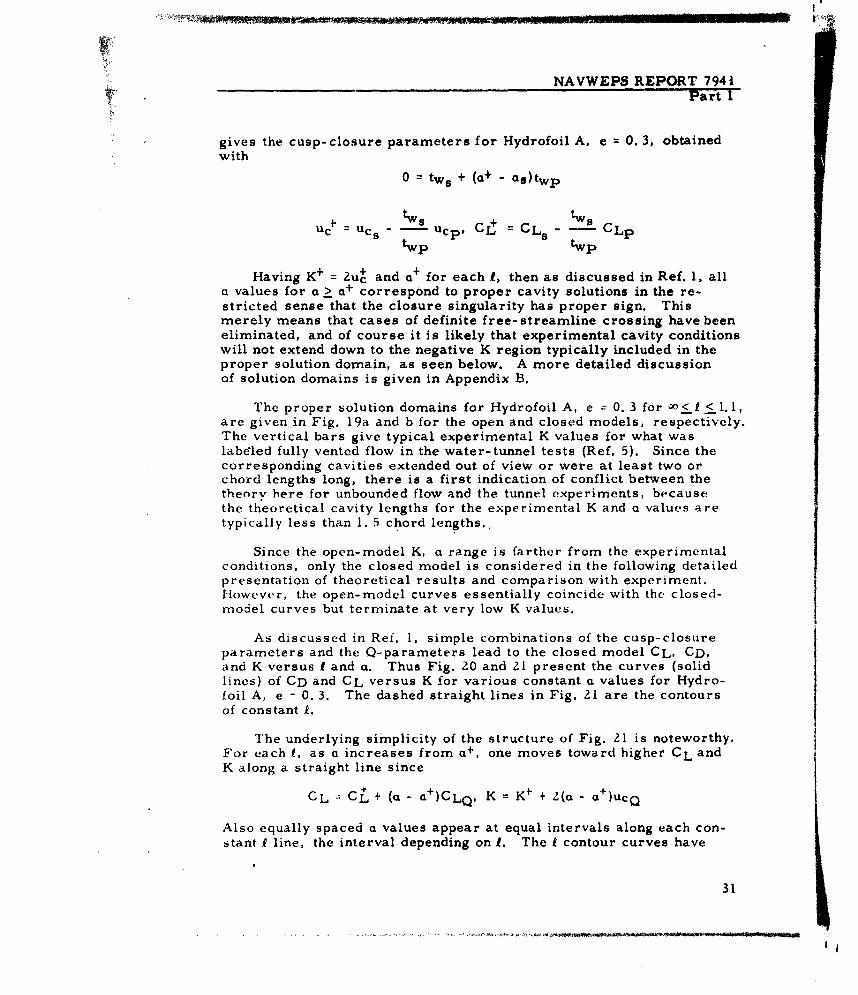
The proper solution domains for Hydrofoil A, e = 0. 3 for J0< I < 1.1,are given in Fig. 19a and b for the open and closed models, respectively.The vertical bars give typical experimental K values for what waslabcrled fully vented flow in the water-tunnel tests (Ref. 5). Since thecorresponding cavities extended out of view or were at least two orchord lengths long, there is a first indication of conflict between thetheory here for unbounded flow and the tunnel experiments, becausethe theoretical cavity lengths for the experimental K and a values aretypically less than 1. 5 chord lengths..

Since the open-model K, a range is farther from the experimentalconditions, only the closed model is considered in the following detailedpresentation of theoretical results and comparison with experiment.However, the open-model curves essentially coincide with the closed-model curves but terminate at very low K values.

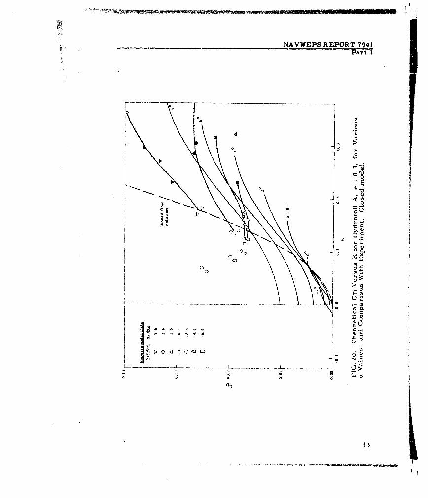
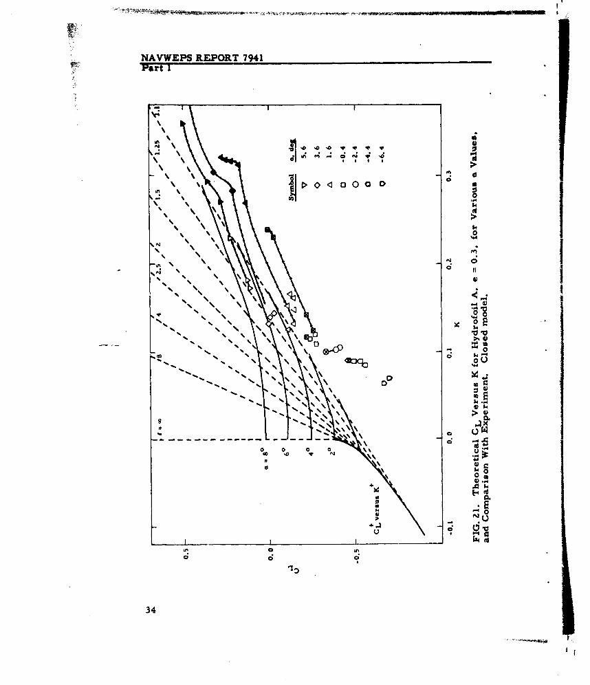
As discussed in Ref. 1, simple combinations of the cusp-closureparameters and the Q-parameters lead to the closed model CL, CD,and K versus I and a. Thus Fig. 20 and 21 present the curves (solidlines) of CD and CL versus K for various constant a values for Hydro-foil A, e - 0. 3. The dashed straight lines in Fig. 21 are the contoursof constant f.

The underlying simplicity of the structure of Fig. 21 is noteworthy.For each 1, as a increases from a+ , one moves toward higher CL andK along a straight line since

CL z CL + (a - a+)CLQ, K = K " + 2(a - a+)ucQ

Also equally spaced a values appear at equal intervals along each con-stant I line, the interval depending on 1. The I contour curves have

31

NAYWIPS 1LZT 7941Pr~t I

I- -

:0W, 0 I- I~ I 0 .0

0.1S

(a) Open model

0.3. 1.1 LAS

J lo , lo

(b) Close model

Souin o yrfi ,e=0.3, an Com-

paio Wit Exeimna -es Codtos

32, / ~ .-


0 I T

0

0

o co

0

CIC]4

L)u

0a

1' II

a.a

331. .

± i L Lcv

0,,

N 33


-. i.",W. 1 1

- - -4

J> 0 0 00

, 0

if\ 'lb

o! U

0b 00

' CID

lb. ~ lb

lb.~E- c 'd0

*%lb%~ ~ m

'l0

l o

34\'~\I

$

NAVWEPS REPORT 7941Part T

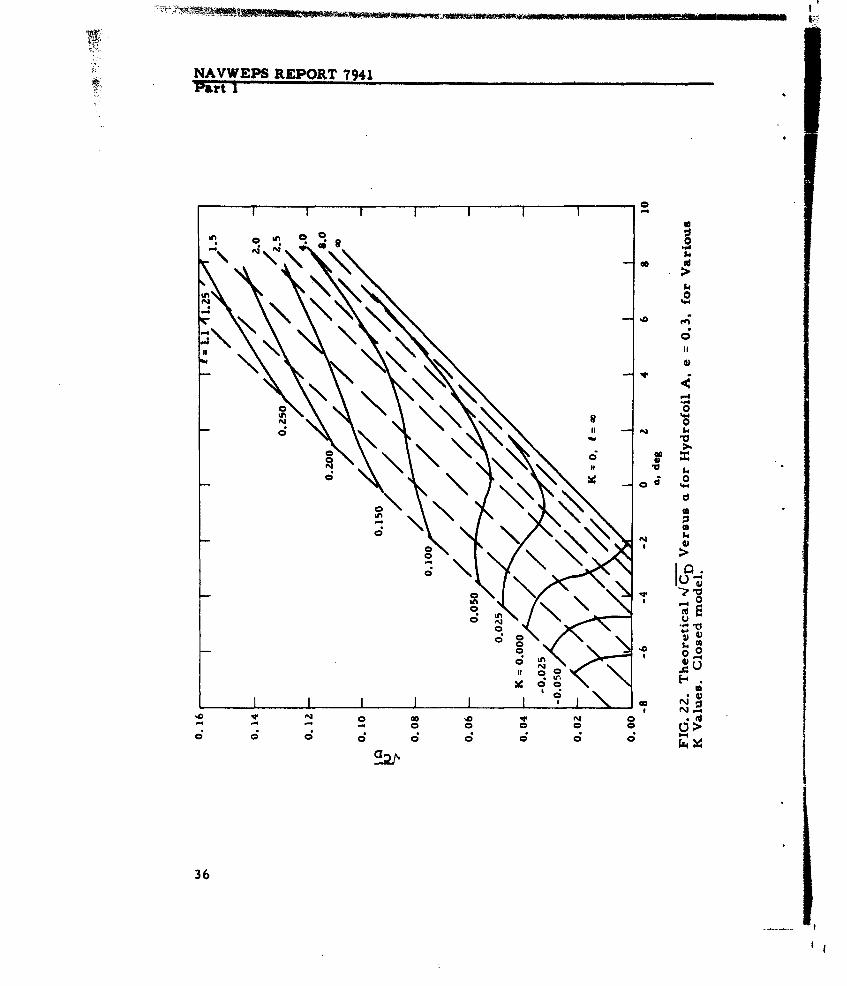
been omitted from Fig. 20 to avoid crowding , but it can be seen thatthese would have parabolic shape, and if %Cn were plotted versus K,the I contours would be straight lines.

However, greater insight into the complicated structure of Fig. 20can be obtained more easily by plotting q7CD versus a as in Fig. 22.The I contours are again straight lines and the intersections with theK contours are spaced along each I contour at intervals proportionalto the K increments. Note that there are two contours for K = 0 in theproper solution domain (NI" > 0). The first is that for I =00, witha.> a. The second, for finite -, is similar to the type of solution forfinite I and K = 0 which was discussed in Appendix B of Ref. 2. Sincethe defining equation is

K = 0 = 2 + (a - a+)ucQ]so that

OCDz(a - a+) '\JBrQ - - (u+C/ucQ) NTD_

the intersection of the two contours is at I and

S ( )--- Vlim (-uc+/ucQ)

This intersection has been estimated by extrapolation in Fig. 22.

The various types of experimental data points in Fig. 20 and'21and the choked-flow curve in Fig. 20 are discussed later.

HYDROFOIL B

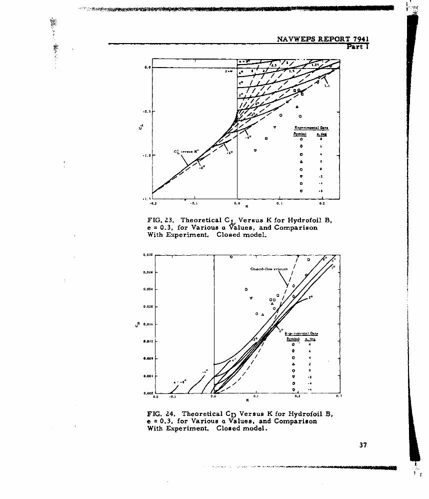
Because this modified NACA 652-015 profile is uncambered, thetheoretical treatment for Hydrofoil B, e - 0. 3 is similar to that forthe NACA 0010 profile. Thus only the final closed-model curves ofCD and CL versus K and a are given in Fig. 23 and 24, along with thecorresponding experimental fully vented data from Ref. 5.

DISCUSSION

The agreement between theory and experiment seen in Fig. 20 to24 is poorer than has been found in previous cases of both cavitatingprofiles for e " 0, 0.5, and 1.0 and of vented profiles for e r. 0 and 1.It is believed that any major errors in the theoretical calculationswould have been detected by the various checks described earlier.While the accuracy of the planimeter integrations decreases for smallI due to the greater complexity of F 1 , ... F4, the major causes of thedifferences between the theory for unbounded flow and the experimentsare thought to be r,iJ.-rl i66 ant tunnel blockage effects, as discussedbelow.

35

NAYWEPS REPORT 7941Part I

0

IA* o~. C 0

Go.

Ct Ct\C; Z \; C c

364

NAVWEPS REPORT 7941Part1

0.0 -, e o 00.125

-0.I 1.d

0 6

oo 0

v -2

0 -4

-0.2-0. 0.00.10.2K

FIG. 23. Theoretical CL Versus K for Hydrofoil B,e = 0.3, for Various a Values, and ComparisonWith Experiment. Closed model.

0.032 0

0.028 - Choked-flo%% relation t

0.024 0

002

0.020 -0

0 E,-itn,,I.1 Dat..

0.12-Synmbo a, deg

/ 0

0.004 / 0

0.00 . -el: .K

FI.24. Theoretical CD Versus K for Hydrofoil B,e =0.3, for Various a Values, and ComparisonWith Experiment. Closed model.

37


Consider first the dashed curves in Fig. 20 and 23. These give theexact theoretical choked-flow relation between CD, K, and tunnel height-to-chord ratio, T, from Ref. 6:

(36) CD = (' + K- 1).

For the tests of Ref. 5, - = 14/4 = 3. 5. Since the open data points inthe figures are apparently for choked or nearly choked flow, as dis-cussed later, the large departure of those experimental CD values fromthe dashed curves shows that important discrepancies are present be-tween the real and the ideal flow conditions. Boundary-layer separa-tion on the unvented lower side appears to be a major cause of the in-crease of CD as a decreases from zero. This explanation is suggestedby the similar increase of CD for fully wetted flow, seen in Fig. 12 ofRef. 5, where, for example, CD for a = -6. 4 degrees is higher by about0.0084 than it is for a = 0. Furthermore, with venting it seems rea-sonable to expect more forward boundary-layer separation on the lowerside, and comparison of the lower-surface pressure distributions withand without venting in Fig. 30 of Ref. 5 seems to stupport this idea.Finally, if the experimental CD values are reduced by 0.0059 to allowfor skin friction, as suggested in Ref. 5, page 106, the remainingseparation of the CD values for large a from the choked-flow curvemay be due to the effect of blockage on the experimental K determina-tion, as discussed in Ref. 5 (page 104).

There are several reasons for describing the fully vented condi-tions in the tests of Ref. 5 as being apparently choked flow. Firstthere is the characteristic behavior of K versus gas supply (Fig. 28 ofRef. 5). More conclusive, however, is the notably linear variation ofK, CL and CM versus a (or a, CL and CM versus K) as seen in Fig. 56,7, and 13, respectively of Ref. 5. That this behavior is precisely thatof choked flow can be seen as follows. As long as cavity length isconstant--as it is of course in choked flow when I = o0--then as a isvaried by adding the flat plate solution for aa, K, CL and CM will varylinearly with a.

A third possible cause of discrepancy between theory and experi-ment is as follows. A key difference between the experiments of Ref. 5and previous vented-flow tests is the exhausting of gas at an arbitrarychordwise position on the profile without any sharp edge from which thefree streamline springs clear of the profile. Thus the theoretical gas-water interference is often actually a layer of individual bubbles nearthe exhaust point, as seen in Fig. 21 of Ref. 5. In other words, par-ticularly for negative a and exhaust ahead of the maximum thickness,some differences are to be expected as the result of the free-streamlineseparation being delayed till some point aft of the exhaust point.

The last items of experimental data to be discussed are the datapoints with x inside and the "tracks" joining the clear and the x data

38


points in Fig. 20 and 21. In Ref. 5, the x data identify partially ventedflow based on visual observation, and the "tracks" indicate unsteadyforces. A definite question about the visual classification of cavitylength is implied by the agreement of the slopes of the full-cavity theoryand the "track" data up to K = 0. 3, where corresponding jogs in the ex-perimental CL curves and slope changes in the CD curves seem tooccur. This suggests that the lower K portions of the "track" data,including some of the x data points, correspond to full-cavity flow.

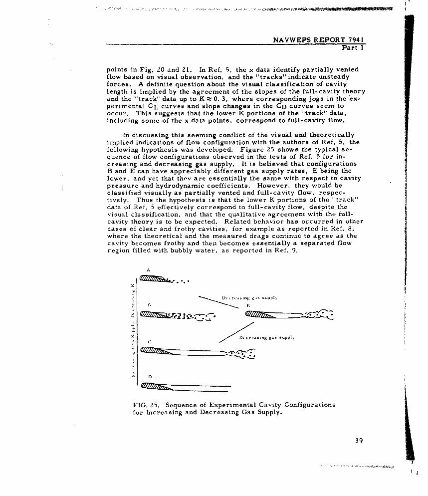
In discussing this seeming conflict of the visual and theoreticallyimplied indications of flow configuration with the authors of Ref. 5, thefollowing hypothesis was developed. Figure 25 shows the typical se-quence of flow configurations observed in the tests of Ref. 5 for in-creasing and decreasing gas supply. It is believed that configurationsB and E can have appreciably different gas supply rates, E being thelower, and yet that thev are essentially the same with respect to cavitypressure and hydrodynamic coefficients. However, they would beclassified visually as partially vented and full-cavity flow, respec-tively. Thus the hypothesis is that the lower K portions of the "track"data of Ref. 5 effectively correspond to full-cavity flow, despite thevisual classification, and that the qualitative agreement with the full-cavity theory is to be expected. Related behavior has occurred in othercases of clear and frothy cavities, for example as reported in Ref. 8,where the theoretical and the measured drags continue to agree as thecavity becomes frothy and then becomes essentially a separated flowregion filled with bubbly water, as reported in Ref. 9.

A

rea s'ng g, . supp .

C

-

FIG. 25. Sequence of Experimental Cavity Configurationsfor Increasing and Decreasing Gas Supply.

39


SUMMARY

The example calculations, comparisons of theory with experiment,and function tables in this report are the culmination of a study of thelinearized theory of vented hydrofoils in two-dimensional flow.

The tables simplify the lift and drag calculations for nearly arbi-trary hydrofoil profiles and typical exhaust locations for infinite orfinite cavity length of full cavity flow. Moment coefficient, because ofits greater calculation complexity, is treated only for infinite cavitylength.

Two experimental hydrofoils have been treated with the theory toillustrate the calculation procedure and the nature of the theoretical Icurves of CL and CD versus K and a for e = 0. 3. The resultant agree-ment of theory and experiment is poorer than expected from previouscomparisons. However, the main discrepancies are reasonably at-tributed to hitherto less important real-fluid and tunnel-choking effects.In particular, boundary-layer separation on the lower, unvented side

seems to have been appreciable for negative attack angles, possiblyaggravated by the upper side venting.

While no definite statement about the importance of the choked-floweffects upon the present comparisons can be made until choked-flow-theory calculations are completed, the experimental data displayqualitative features of choked flow. The indication of greater effectsof choking than noticed before seems reasonable in view of the lowertunnel height-to-chord ratio and the lower theoretical cavity lengths forunbounded flow for the experimental choked flow cavity numbers.

An unexpected result of the comparison for Hydrofoil A is a newinterpretation of the visual classification of the experimental flows asfully vented or partially vented, following from the qualitative agree-ment of portions of the data for so-called partially vented flow with fullcavity theory.

40


Appendix A

CORRIGENDA

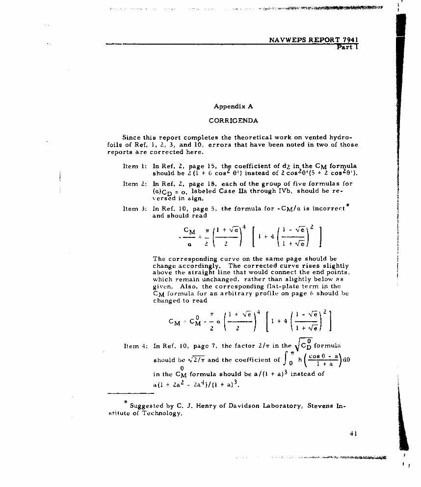
Since this report completes the theoretical work on vented hydro-foils of Ref. 1, 2, 3, and 10, errors that have been noted in two of thosereports are corrected here.

Item 1: In Ref. 2, page 15, the coefficient of d2 in the CM formulashould be 2 (1 + 6 cos 2 0') instead of 2 cos 2 0'(5 + 2 cost0').

Item 2: In Ref. 2, page 18, each of the group of five formulas for(a)CD = o, labeled Case Ha through IVb, should be re-v ersed in sign.

Item 3: In Ref. 10, page 5, the formula for -CM/a is incorrectand should read

C . 1+4 -1

a 2 2 I+ NI-e

The corresponding curve on the same page should bechange accordingly. The corrected curve rises slightlyabove the straight line that would connect the end points,which remain unchanged, rather than slightly below asgiven. Also, the corresponding flat-plate term in theCM formula for an arbitrary profile on page 6 should bechanged to read

0 TT (+ ~4 [i \i 2

CM CM -- a I + 42 \2 L l+ 4.f;l

Item 4: In Ref. 10, page 7, the factor 2/1w in the 4 formula

should be N'2/rr and the coefficient of .1 h(c°s0 - a d00

in the CM formula should be a/(I + a) 3 instead of

a(1 + 2a 2 - -a 4 )/(I + a) 3 .

Suggested by C. J. Henry of Davidson Laboratory, Stevens In-stitute of Technology.

41

---------------- f


Appendix B

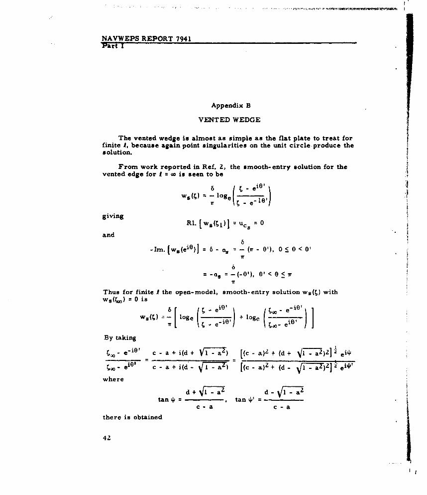
VENTED WEDGE

The vented wedge is almost as simple as the flat plate to treat forfinite 1, because again point singularities on the unit circle-produce thesolution.

From work reported in Ref. 2, the smooth-entry solution for thevented edge for I wo is seen to be

6 ,-eie '

wsm - loge -

givingRl. [w,(t 1 )] ucs = 0

and

6-Ima. [Ws(eie)] = 6 - ,-- -(ir - 0'), 0 < 8 < 0'

=-% : -(-0'), e' < e <IT

Thus for finite I the open-model, smooth-entry solution ws(t) withWs(6 o ) = 0 is

Ws( M- loge +io log e ---7r - e- ' - eiO

By taking

e-iO' c - a + i(d + ayz7) [(c - a)? + (d + V- a2)2]1 ei4'

po"eiO0 c- a + i(d'- I - - [(c- a)2 + (d- 71- e4]

where

d+i .l- az d I - aZtan= , tan

c- a c- a

there is obtained

4Z


In. w s(e io ) 6- as 6

= - s - (-0' + - 0), e' < 0I.

and6 1 + (tan, 2

R.[w.(;)]= u 8 - log e '1w l+(tan v')2J

Proceeding as usual, with o - (a + ib) = Ne i ', it is found that

tWs + i Zi- -- - - - (sin v + i cos V)2 d {,dZ 0 N

Though the mapping for I > 1 is singular for 1-41, the s-parametersare not. Ordinary procedures show that the limit values for I = 1 are

rI i+ kI _21+1 +

7rucs 1 e l -

= - )o6 2

tan-l +e + -- tan- _

6e

62 2 2

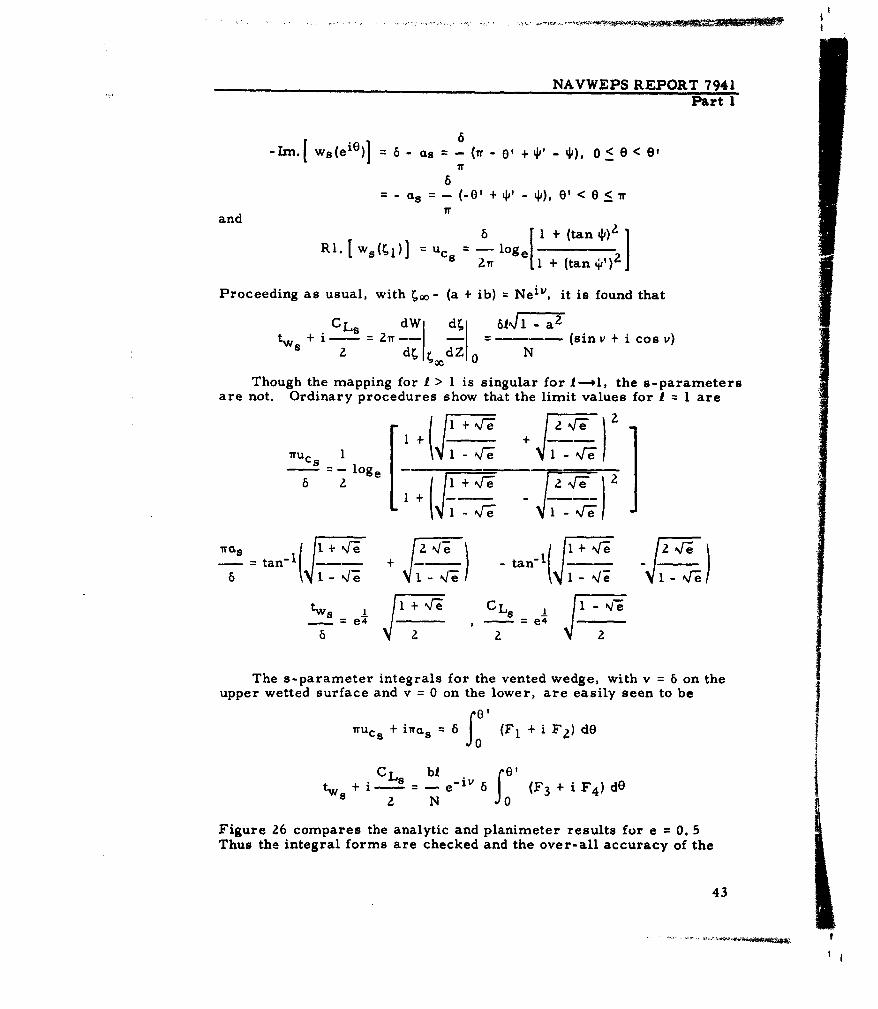
The s-parameter integrals for the vented wedge, with v = 6 on theupper wetted surface and v = 0 on the lower, are easily seen to be

TrUcs + iTras = 6 J' (FI + i F2) dO

C L bi . Itws+i'= - e " v 6 (F 3 + iF)d

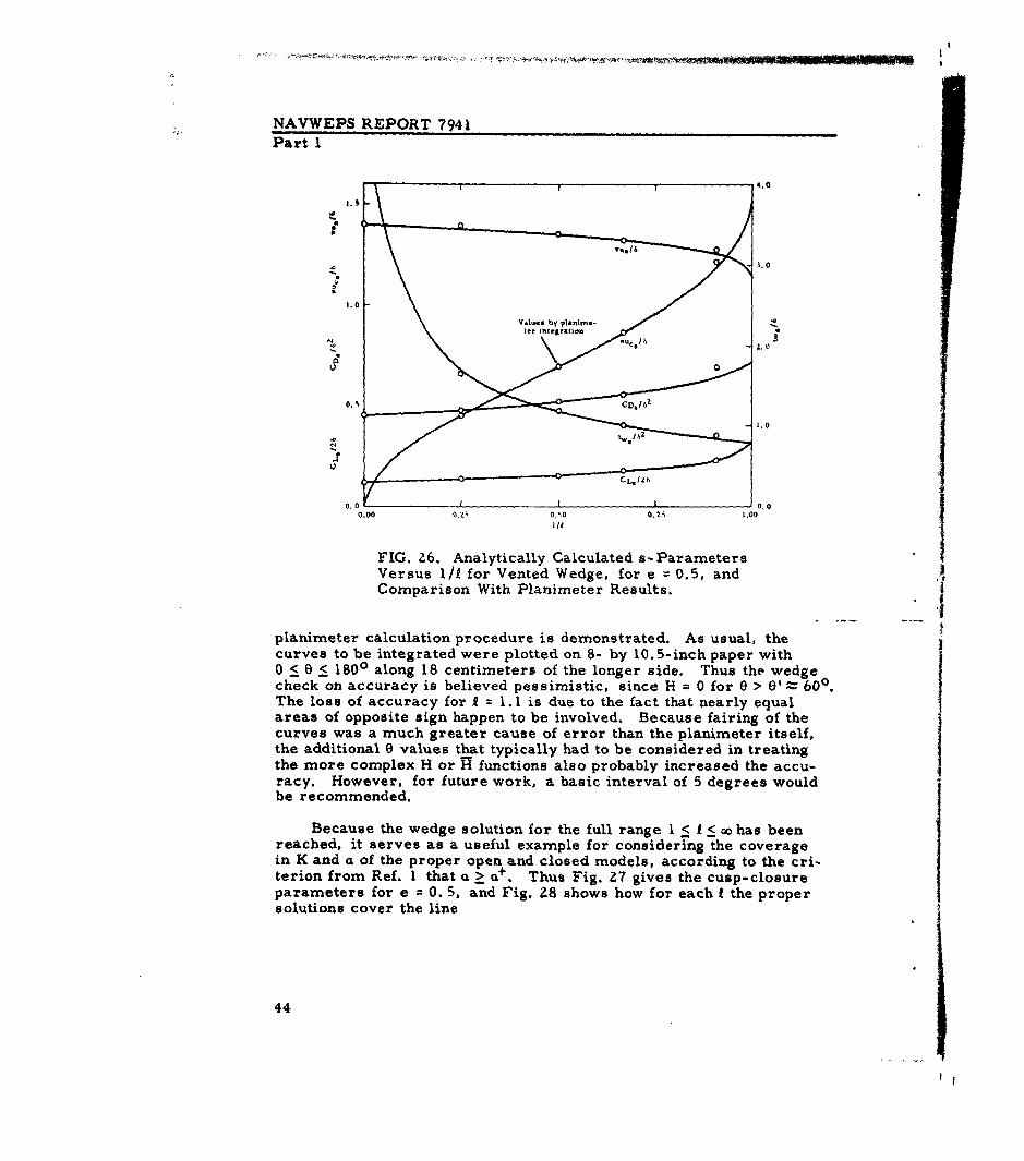
2 N OFigure 26 compares the analytic and planimeter results for e = 0. 5Thus the integral forms are checked and the over-all accuracy of the

43


i4.0

I. S

13.0

Vah... by planime.

ter inerto

1.0

CL./Zh

0. 0 1- .. .0A~

0.00 0.zn 01 ,0 0. 7A 1,00

FIG. Z6. Analytically Calculated s-ParametersVersus l/1 for Vented Wedge, for e = 0.5, andComparison With Planimeter Results.

planirneter calculation procedure is demonstrated. As usual, thecurves to be integrated were plotted on 8- by 10.5-inch paper with0 < 0 < 1800 along 18 centimeters of the longer side. Thus the wedgecheck on accuracy is believed pessimistic, since H = 0 for 0 > 0' - 600.The loss of accuracy for I = 1.1 is due to the fact that nearly equalareas of opposite sign happen to be involved. Because fairing of thecurves was a much greater cause of error than the planimeter itself,the additional 0 values that typically had to be considered in treatingthe more complex H or R functions also probably increased the accu-racy. However, for future work, a basic interval of 5 degrees wouldbe recommended.

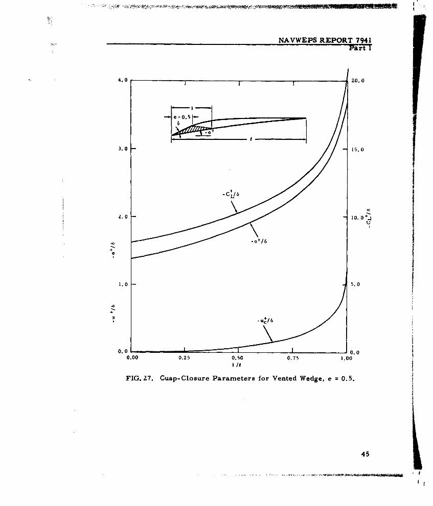
Because the wedge solution for the full range I < I < Go has beenreached, it serves as a useful example for considering the coverage

in K and a of the proper open and closed models, according to the cri-terion from Ref. I that a a a+. Thus Fig. Z7 gives the cusp-closureparameters for e = 0. 5, and Fig. Z8 shows how for each I the propersolutions cover the line

44


4.0 Io20.0

3.0 15.0

I

2. 0 10.0+4

U

1.0 5.0

c+/

0.0 0.00.00 o.z5 0.50 0.75 1.00

FIG. 27. Cusp-Closure Parameters for Vented Wedge, e = 0.5.

45

NAVWEPS REPORT 7941- Part 1

4 - -~

4 -- _/ o = - -e --"

I !- ---

//-- - t

(a) Open model

I / /

- K I- 6'/

i / ""F Z8. K,! a a r p l

6/

6 / I/;

I /

41 --

FIG.78. , a omai for roeSlion

or Vente Weg, -- = .


K ~K + +a -= + Ucp ' Q

o, cl 6 6 (

The open-model's multivaluedness for the typically unimportant areaof a near a + means that a given K and a can be obtained with more thanone value of 1, for which the hydrodynamic coefficients will also differsomewhat. Actually the criterion for solution admissibility of a 2: a+

is not a clear-cut condition since the implied free streamlines shouldbe calculated and any cases where the free streamlines cross even fora slightly greater than a+ should be excluded. That such cases occuris suggested by considering the shape of the free streamlines for cusp- Iclosure, as follows. Since the profile-plus-cavity obstacle keeps thesame pressure distribution if the free stream is considered reversed,it would appear that for ut positive, as sometimes occurs, the freestreamlines should initially diverge from the cusp in a crossingmanner. However, such details have not been found important in thepractical application of the theory.

In a more practical respect, only solutions for K > 0 are of interestfor cavitating flows and even then only if pressure coefficient on the foilnowhere falls below -K. For vented flows, for which cases of negativeK can be conjectured, it remains to be seen whether real fluid effectswill not prevent such cases from occurring, even if both the linearized Itheory and corresponding nonlinearized potential-flow solutions arespatially reasonable, as in the case of some cusp-closure cavities.

I

I


Appendix C

PARTLY CLOSED MODEL SOLUTIONS FORVENTED FLAT PLATE

As discussed in Ref. 1, for each vented hydrofoil profile thereexists a family of partly closed cavity model solutions for given cavitylength, with wake thickness t, lying between the zero of the closedmodel and two of the open model The particular case of the ventedflat plate with e = 0 is considered here in order to compare the theo-retical ranges of cavity length and wake thickness with certain experi-mental results given in Ref. 11.

The partly closed model solution for unit angle of attack for each

particular cavity length is constructed by superposing the open- andclosed-model solutions wp and wQ with

w = T wpand (I - T)wQ

tw = Ttwp, Uc = T Ucp+ (I - T) ucQ

and with the z-plane closure-singularity strength

C z = (1 - T) 4/7D 2 w

Consideration of the implied cavity and wake geometry and the dragintegral shows that the drag coefficient for the partly closed model is

CD = tw Zuc + 2r(Cz) 2

= T twp 2 [T ucp+ (1- T)uc Q + (l - T)2 CDQThe lift superposition is simply

CL = T CLp + ( - T) CLQand since CD/Q 2 = CL/a for the flat plate with e = 0, it must also be I(as was found for e = I in Ref. 3 and was stated for all e in Ref. I) that

CD = T CDp+ (I - T) CDQ

This is confirmed by application of the formulas given earlier for theopen- and closed-model solutions for e = 0.

48


It is not clear from the resultant partly closed model relations,which give K and tw as functions of I and T, and which imply tw as afunction of T and K, that maximum wake thickness for given K cor-responds to the open-model limit. However, manipulation of therelations yields

~tw T7( +;K2 2""1 T

T I (1KT

-"'(1- T) -T + (1- T)2 (1- 1 TTI / -I

From this it can be seen that tw monontonically increases with T forconstant K, reaching a maximum and critical point for T = 1.

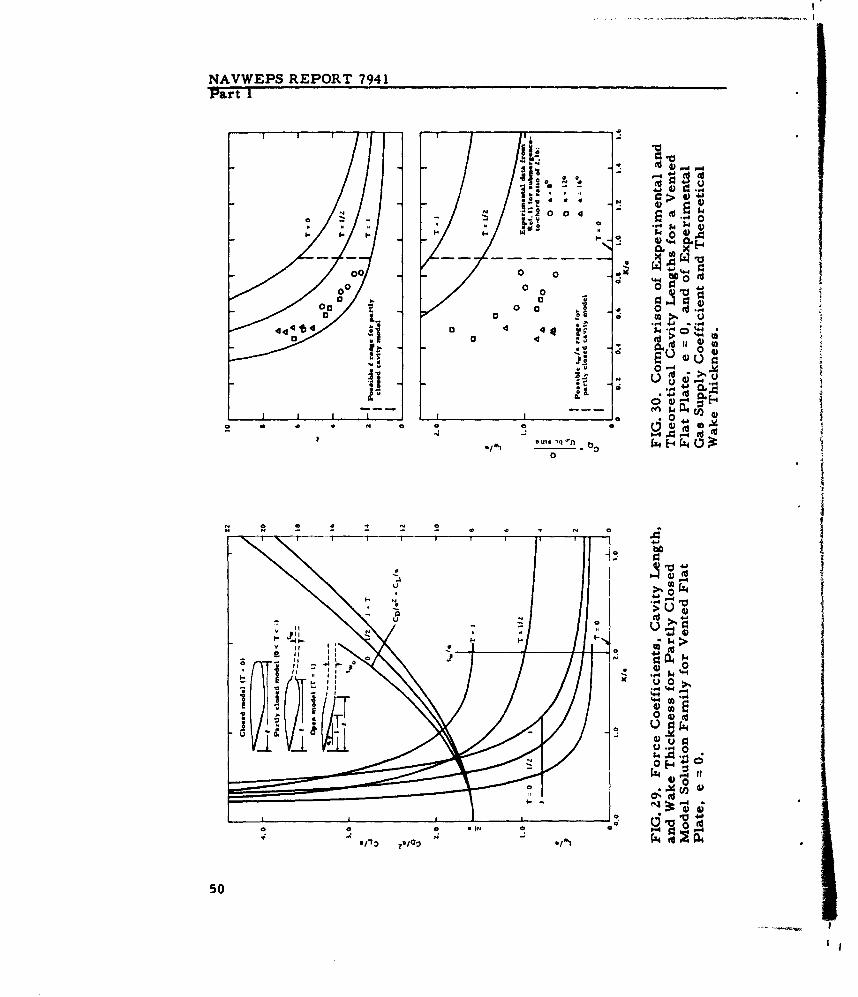
To illustrate the partly closed model results, Fig. 29 gives thecurses of force coefficient, cavity length, and wake thickness versuscavity number for T = 0, 1/2, and 1. In Fig. 30 some portions of thesame cavity-length and wake-thickness curves are compared with someexperimental results of T. E. Dawson, who tested a flat plate for e = 0(Ref. 11). The upper portion of Fig. 30 shows that the experimentalcavity lengths correspond to T = 3/4. If the shortness of the cavitiesis due to the wake produced by the required gas supply, rather than tothe effects of gravity, the free surface, or the bottom of the tunnel,then the experimental gas supply rates should be compatible, at leastroughly, with the wake thicknesses corresponding to T = 3/4. Thelower half of Fig. 30 shows the experimentally required gas-supply co-efficients, CQ, which are apparently from the same tests as for the Imeasurements. The definition of CQ in Ref. 11 makes it correspondto tw/a, since

CQ-Uo bc sin a

where

Q = volume of gas supplied to test hydrofoil per unit time (referencepressure and temperature assumed very nearly equal to free-stream pressure at hydrofoil depth and water temperature)

b = hydrofoil span

c = hydrofoil chord

In the lower half of Fig. 30, the experimental CQ values are seen tocorrespond more nearly to T = 1/4 than to 3/4, but in view of the crude-ness of the wake model, the order-of-magnitude agreement seemssignificant. Also, since the real wake near the cavity is a mixture ofgas and water moving downstream relative to the foil at a speed less

49

NAVWEPS REPORT 7941 ________

Part I

f IL

>U 0

-~ i~O4 0o 0

00 0 0 t

00 0000 0 . 0

00 0 0 1~ .

0 .1 0

N04 0

q On 4 ' W .4

vo 0

0 4 )

____ 0

N 0 C 4 4 4 't

soI


than Uoo, it is to be expected that the wake thickness implied by gassupply would be smaller than that implied by the hydrodynamic effectof the wake.

It will be interesting to see whether future experiments show othercases of peculiarly short cavities coupled with gas-supply coefficientsof the order of two/4 - CD/4K, in accord with the partly closed cavitymodel interpretation of Dawson's results.

REFERENCES

1. Fabula, A. G. "Thin-Airfoil Theory Applied to Hydrofoils With aSingle Finite Cavity and Arbitrary Free-Streamline Detachment. ',J FLUID MECH, Vol. 12, Part 2 (1962), pp. 227-40.

2. U. S. Naval Ordnance Test Station. Theoretical Lift and Drag onVented Hydrofoils for Zero Cavity Number and Steady Two-Dimensional Flow, by A. G. Fabula. China Lake, Calif., NOTS,4 November 1959. (NAVORD Report 7005, NOTS TP 2360. )

3. Application of Thin-Airfoil Theory to Hydrofoils WithCut-Off Ventilated Trailing Edge, by A. G. Fabula. China Lake,Calif., NOTS, 13 September 1960. (NAVWEPS Report 7571,NOTS TP 2547.)

4. Abbott, I. H., and A. E. Von Doenhoff. Theory of Wing Sections.New York, Dover, 1959.

5. U. S. Naval Ordnance Test Station. Water- Tunnel Tests of Hydro-foils With Forced Ventilation, by T. G. Lang, D. A. Daybell, andK. E. Smith. China Lake, Calif., NOTS, 10 November 1959.(NAVORD Report 7008, NOTS TP 2363.)

6. Birkhoff, G., M. Plesset, and N. Simmons. "Wall Effects in CavityFlow - I." QUART APPL MATH, Vol. VIII, No. 2 (July 1950), pp.151 - 168.

7. The RAND Corporation. Linearized Theory of Cavity Flow in Two-Dimensions, by B. R. Parkin. Santa Monica, Calif., RAND,15 July 1959. (P-1745.)

8. California Institute of Technology. Water Tunnel Investigation ofTwo-Dimensional Cavities, by R. L. Waid. Pasadena, Calif., CIT,September 1957. (CIT Hydrodynamics Laboratory Report E-73. 6.)

51


9. California Institute of Technology. Incipient Cavitation and WakeFlow Behind Sharp-E dged Disks, by R. W. Kermeen and B. R.Parkin. Pasadena, Calif., CIT, August 1957. (CIT EngineeringDivision Report 85. 4.)

10. U. S. Naval Ordnance Test Station. Linearized Theory of VentedHydrofoils, by A. G. Fabula. China Lake, Calif., NOTS,7 March 1961. (NAVWEPS Report 7637, NOTS TP 2650.) Also in:Office of Naval Research. Washington, ONR, 18 - 20 April 1961.(ONR-9, Vol. 3.)

11. California Institute of Technology. An Experimental Investigationof a Fully Cavitating Two-Dimensional Flat Plate Near a FreeSurface, by T. E. Dawson. Pasadena, Calif., CIT, 1959. (Gug-genheim Aeronautical Laboratory, Aeronautical Engineer Thesis.)

I

I

52


INITIAL-DISTRIBUTION

10 Chief, Bureau of Naval WeaponsDLI- 31 (2)R-12 (1)RAAD- 3 (1)RRRE (1)RRRE- 4 (1)RU (1)RUTO (1)RUTO-32 (2)

6 Chief, Bureau of Ships

Code 106 (1)Code 335 (1)Code 421 (2)Code 442 (1)Code 664 (1)

1 Chief of Naval Operations3 Chief of Naval Research

Code 429 (1)Code 438 (1)Code 466 (1)

5 David W. Taylor Model BasinCode 142 (1)Code 500 (1)Code 513 (1)Code 526 (1)Code 580 (1)

I Naval Academy, Annapolis (Librarian)1 Naval Air Development Center, Johnsville1 Naval Aircraft Torpedo Unit, Quonset PointI Naval Civil Engineering Laboratory, Port Hueneme (Code L54)I Naval Engineering Experiment Station, Annapolis1 Naval Ordnance Laboratory, White Oak (Library Division, Desk HL)I Naval Postgraduate School, Monterey (Library, Technical Reports

Section)I Naval Research Laboratory1 Naval Torpedo Station, Keyport (Quality Evaluation Laboratory,

Technical Library)I Naval Underwater Ordnance Station, NewportI Naval War College, Newport (Institute of Naval Studies)I Naval Weapons Laboratory, Dahlgren2 Naval Weapons Services Office

53


I Navy Electronics Laboratory, San Diego1 Navy Mine Defense Laboratory, Panama CityI Navy Underwater Sound Laboratory, Fort TrumbullI Office of Naval Research Branch Office, PasadenaI Army Research Office, Durham1 Air Force Office of Scientific Research (Mechanics Division)

10 Armed Services Technical Information Agency (TIPCR)1 Director of Defense (R&E) (Office of Fuels, Materials and Ordnance,

Byard Belyea)I Committee on Undersea Warfare1 Maritime Administration (Coordinator for Research)1 Merchant Marine Academy, Kings Point, N. Y. (Head, Depart.-aent

of Engineering)6 National Aeronautics and Space AdministrationI National Bureau of Standards (Fluid Mechanics Section, Dr. G.Schubauer)

2 National Science FoundationDirector (I) IDirector, Engineering Sciences Division (1)

5 British Joint Services Mission (Navy Staff), via BuWeps (DSC)2 Defence Research Member, Canadian Joint Staff (W), via BuWeps

(DSC)2 Aerojet-General Corporation, Azusa, Calif., via BuWepsRepJ. Ley(1)

Library (1)1 Aeronutronic, Newport Beach, Calif. (Library)1 Airesearch Manufacturing Company, Los Angeles (Dr. B. R. Parkin)I Alden Hydraulic Laboratory, Worcester Polytechnic Institute,

Worcester, Mass.1 American Mathematical Society, Providence, R.I. (Editor, Mathe-

matical Review)1 Applied Physics Laboratory, University of Washington, SeattleI AVCO Research Laboratory, Everett, Mass. (Technical Library)I Baker Manufacturing Company, Evansville, Wisc.1 Bell Aerosystems Company, Buffalo (Technical Library)1 Brown University, Providence, R. I. (Division of Engineering)1 Bulova Research and Development Laboratories, Inc., Wood-

side, N.Y.3 California Institute of Technology, Pasadena (Engineering Division)

Prof. C. B. Millikan (1)Prof. M. S. Plesset (I)Prof. V. A. Vanoni (1)

I Case Institute of Technology, Cleveland (Department of MechanicalEngineering)

1 Clevite Ordnance, Cleveland (Library)I Colorado State University, Fort Collins (Department of CivilEngineering)

1 Convair, San Diego (Engineering Library)1 Convair Hydrodynamics Laboratory, San Diego

54


1 Convair Scientific Research Laboratory, San Diego1 Cornell Aeronautical Laboratory, Inc., Buffalo (Department 410)1 Cornell University, Graduate School of Aeronautical Engineering,

Ithaca (Library)2 Davidson Laboratory, Stevens Institute of Technology, Hoboken, N. J.

A. Suarez (1)Dr. J. Breslin (1)

1 Douglas Aircraft Company, Inc., Long Beach (Aerodynamics Section)1 Eastern Research Group, New York CityI EDO Corporation, College Point, N. Y. (Library)I Electric Boat Division, General Dynamics Corporation, Groton, Conn.

(Library)

1 Engineering Societies Library, New York City1 General Electric Company, Defense Electronics Division, Pittsfield,

Mass. (Engineering Librarian)1 General Electric Company, Schenectady (Librarian, LMEE Depart-

ment)2 Gibbs and Cox, Inc., New York City

Dr. S. Hoerner (1)Library (1)

1 Grumman Aircraft Engineering Corporation, Bethpage, N. Y. (Library)1 Harvard University, Cambridge, Mass. (Department of Engineering

Sciences)1 Hughes Aircraft Company, Culver City, Calif. (Library)5 Hydrodynamics Laboratory, CIT, Pasadena

Prof. A. J. Acosta (1)Prof. A. T. Ellis (1)Prof. T. Y. Wu (I)T. Kiceniuk (1)Library (1)

1 Hydronautics, Inc., Rockville, Md.I Illinois Institute of Technology, Chicago (Head, Department of

Mechanical Engineering)1 Institute of Aerospace Sciences, Inc., New York City (Librarian)1 Johns Hopkins University, Baltimore (Head, Department of Mechani-

cal Engineering)1 Lehigh University, Bethlehem, Pa. (Civil Engineering Department)1 Lockheed Aircraft Corporation, Burbank, Calif. (Library)I Lockheed Aircraft Corporation, Missiles and Space Division, Palo

Alto, Calif. (R. W. Kermeen)2 Massachusetts Institute of Technology, Cambridge

Department of Civil Engineering (1)Department of Naval Architecture and Marine Engineering (I)

I McDonnell Aircraft Corporation, St. Louis (Library)1 Mississippi State University, State College (Aerophysics Department)I New York State Maritime College, Fort Schuyler (Librarian)I New York University, Institute of Mathematical Science, New York

CityI North American Aviation, Inc., Los Angeles (Technical Library,

Department 56)

55


I Oceanics Incorporated, New York CityI Operations Research, Inc., Los Angeles2 Ordnance Research Laboratory, Pennsylvania State University,

University Park (Garfield Thomas Water Tunnel)I Pacific Aeronautical Library of the IAS, Los AngelesI Reed Research, Inc.I Rensselaer Polytechnic Institute, Troy, N. Y. (Department of Mathe-

matics)1 Republic Aviation Corporation, Farmingdale, N. Y.I Rocketdyne, Canoga Park, Calif. (Library, Department 596-6)1 Rose Polytechnic Institute, Terre Haute, Ind. (Library)1 Society of Naval Architects and Marine Engineers, New York City2 Southwest Research Institute, San Antonio

Director, Department of Applied Mechanics (1)Editor, Applied Mechanics Review (I)

1 Stanford University, Stanford, Calif. (Department of Civil Engineer-ing, Prof. B. Perry)

1 Technical Research Group, Syosset, N. Y.I The Boeing Company, Seattle (Library, Organization No. 2-5190)2 The Martin Company, Baltimore (Science Technical Library)

1 The Rand Corporation, Santa Monica, Calif. (Technical Library)4 The University of Michigan, Ann Arbor

Department of Civil Engineering (1)Department of Engineering Mechanics (1)Department of Naval Architecture and Marine Engineering (2)

1 The University of Southern California, Los Angeles (EngineeringCenter)

I Thompson Ramo Wooldridge, Inc., Cleveland (Chief EngineeringScience Group)

1 United Technology Corporation, Sunnyvale, Calif. (Technical Library)2 University of California, College of Engineering, Berkeley

Prof. J. V. Wehausen (1)Library (1)

1 University of Illinois, Urbana (College of Engineering)2 University of Iowa, Iowa Institute of Hydraulic Research, Iowa City

Prof. H. Rouse (1)Prof. L. Landweber (1)

1 University of Kansas, School of Architecture and Engineering,Lawrence

I University of Maryland, Institute of Fluid Dynamics and AppliedMathematics, College Park

1 University of Minnesota, St. Anthony Falls Hydraulic Laboratory,Minneapolis

I University of Nebraska, Lincoln (Department of EngineeringMechanics)

I University of Notre Dame (Department of Engineering Mechanics)I University of Wisconsin, Mathematics Research Center, Madison

(Prof. L. M. Milne-Thomson)I Vitro Corporation of America, Silver Spring Laboratory (Librarian)

56

0 40) 0 >

4.1-S 6'Wt- , IV'*E-4 A S

0 4 0 0

d d U> ~

4-b, 0~4 (N14K

s. 04 UU4m 0

.4a0 k'.+ c

91 to i . A : )o 0

U 14o 0 1 4 . 4 , 1- 0 J .4 .

go 00 0 C.o a .1'd U LI

og o-8 $4 C d1 1

::,4 .0 0 r ..

*14

4444

.00

1S4

030

4-A~0 410 4J$C444

4

.,4 '4 -

-4

4- 0 0

M0304

4),.4 v

0~.

.0 04

43

OW 435

-4 0-144

Z 4.d5 0 414

04 0.4

*4 %).o(,,

0 0 *

M4-

*~f 0~ 0 .

0 U 0 0d) d 4) 04

CL S : I zt-

z .0 ; .0 t-

a." aC4W.0 4 e4W.0 44

A- Z

144

-41.1 4 It.4.4

0 4 CN a4 4 N

4,. k~ 4, .

0. 0doL ..04 4) 0

u A .P-4

a 40 C4 (nH t

4 0

(d.0).

0~ Q 0.UM V 4 W

)pQ.Cl Im a

5.4 4) 1~*: 4 ed 8400 to -. a

0. 0 U a -. >

-4 4o 4) V- (d 4 0 0

4A40' &), $3 4) 0 01.4 01.441 4 44 4 41 g30 0 :1

4.) 0

~4.454 4)I. 4 .,j 4)5.>. 4.45. 414

0 r 0 :- 00 4)0C 1 0 B 0.) 0 CL 41

ISi, 0 4 ) 5 4 ' U00)> )4

ZO4 w 100

)1 4) I)-C 4)1C3 w , 41 1..4-

0 4 4.d 0 004 -4 0~ 4 4 004 Q b

> 4,. 0 r.0U '9d~4 41 '1 '4)

41 F401u

0 o E 10.0 O~4 U 5.1)

0 414~ 4104"4) 0 Id 41 04 . 0 4 4) -4 o 4) a.*;!

I)V4 w )>- ) 0 -0 ( 4)0 bo -d 0d o 0 o0 .go

41 E 0044 ~~ 41o 4) Q - = . ' > j -4 ),.> kw".o*4 400414 p

co 0 c d 0~ 0 -z04 4 ( E4 Ez0 a 1c

ft 4) U (0-0 4)4

S 0 0U 4 ) q~ be%4 U) 40*U) 4 . u W 4 ' V-,... U)a Z). (

'4 4 - a)~ 4

411 rd-M(

I Vought Aeronautics, Dallas (Engineering Library)I Webb Institute of Naval Architecture, Glen Cove, N. Y. (Technical

Library)I Westinghouse Electric Corporation. Baltimore (Engineering

Librarian)t Westinghouse Electric Corporation, Sunnyvale, Calif. (Library)I Westinghouse Research Laboratories, Pittsburgh (Library)

i I '

Documents

UNCLASSIFIED AD 4 10 2i9 - DTIChaust for torpedo-control purposes and the use of base-vented hydrofoils as propeller blades. ... tion, China Lake, Calif., Attn: Code 7506. This work