Uncertainty Quantification, Lecture 1

Philip B. Stark

Department of Statistics, University of California, Berkeley

5–8 February 2017, Les Diablerets, Switzerland

1

2

Reading list

– Evans, S.N. and P.B. Stark, 2002. Inverse Problems asStatistics, Inverse Problems, 18, R55–R97.http://iopscience.iop.org/0266-5611/18/4/201/pdf/0266-5611 18 4 201.pdf

– Evans, S.N., B. Hansen and P.B. Stark, 2005. MinimaxExpected Measure Confidence Sets for RestrictedLocation Parameters, Bernoulli, 11, 571–590.

– Freedman, D.A., 1997. Some Issues in the Foundations ofStatistics, Foundations of Science, 1, 19–39.http://link.springer.com/chapter/10.1007%2F978-94-015-8816-4 4#page-1

– Hengartner, N.W., and P.B. Stark, 1992. Finite-SampleConfidence Envelopes for Shape-Restricted Densities,Ann. Statist., 23, 525–550.

3

– Ioannidis, J.P.A., 2005. Why Most Published ResearchFindings Are False, PLoS Medicine, 2, e124.http://dx.doi.org/10.1371/journal.pmed.0020124

– Kennedy, M.C., and A. O’Hagan, 2001. Bayesiancalibration of computer models, JRSS B, 63, 425–464.DOI:10.1111/1467-9868.00294

– Kuusela, M., and P.B. Stark, 2016. Shape-constraineduncertainty quantification in unfolding steeply fallingelementary particle spectra. Submitted to Annals ofApplied Statistics. http://arxiv.org/abs/1512.00905

– Mulargia, F., P.B. Stark, and R.J. Geller, 2017. Why isProbabilistic Seismic Hazard Analysis (PSHA) still used?Phys. Earth Planet. Inter.,http://dx.doi.org/10.1016/j.pepi.2016.12.002

– Regier, J.C. and P.B. Stark, 2015. Uncertaintyquantification for emulators. SIAM/ASA Journal onUncertainty Quantification, 3, 686–708.doi:10.1137/130917909,http://epubs.siam.org/doi/10.1137/130917909

4

– Russi, T., A. Packard, and M. Frenklach, 2010.Uncertainty quantification: Making predictions of complexreaction systems reliable Chemical Physics Letters, 499,1–8. http://dx.doi.org/10.1016/j.cplett.2010.09.009

– Sacks, J., W.J. Welch, T.J. Mitchell, and H.P. Wynn,1989. Design and Analysis of Computer Experiments,Statistical Science, 4, 409–423.http://www.jstor.org/stable/2245858

– Saltelli, A., T.H. Andres, and T. Homma, 1993.Sensitivity analysis of model output: An investigation ofnew techniques, Computational Statistics & DataAnalysis, 15, 211–238.http://dx.doi.org/10.1016/0167-9473(93)90193-W“,

– Saltelli, A., and Funtowicz, S., 2014. When all Modelsare Wrong, Issues in Science and Technology, 30,http://issues.org/30-2/andrea/

5

– Saltelli, A., P.B. Stark, W. Becker, and P. Stano, 2015.Climate Models as Economic Guides: Scientific Challengeor Quixotic Quest?,Issues in Science and Technology, Spring 2015.http://issues.org/31-3/climate-models-as-economic-guides-scientific-challenge-or-quixotic-quest/

– Schafer, C.M. and P.B. Stark, 2009. ConstructingConfidence Sets of Optimal Expected Size, J. Am. Stat.Assoc., 104, 1080–1089.http://dx.doi.org/10.1198/jasa.2009.tm07420

– Smith, R.C., 2013. Uncertainty Quantification: Theory,Implementation, and Applications, SIAM, 383pp.

– Soergel, D.A.W., 2015. Rampant software errors mayundermine scientific results. F1000Research, 3:303. doi:10.12688/f1000research.5930.2

6

– Stark, P.B., 1992. Inference in infinite-dimensional inverseproblems: Discretization and duality, Journal ofGeophysical Research, 97, 14,055–14,082.http://onlinelibrary.wiley.com/doi/10.1029/92JB00739/epdf

– Stark, P.B. and D.A. Freedman, 2003. What is theChance of an Earthquake? in Earthquake Science andSeismic Risk Reduction, F. Mulargia and R.J. Geller, eds.,NATO Science Series IV: Earth and EnvironmentalSciences, v. 32, Kluwer, Dordrecht, The Netherlands,201–213. Preprint:http://www.stat.berkeley.edu/˜stark/Preprints/611.pdf

– Stark, P.B., 2008. Generalizing resolution, InverseProblems, 24, 034014. Reprint:http://www.stat.berkeley.edu/˜stark/Preprints/resolution07.pdf

7

– Stark, P.B. and L. Tenorio, 2010. A Primer of Frequentistand Bayesian Inference in Inverse Problems. In LargeScale Inverse Problems and Quantification of Uncertainty,Biegler, L., G. Biros, O. Ghattas, M. Heinkenschloss, D.Keyes, B. Mallick, L. Tenorio, B. van Bloemen Waandersand K. Willcox, eds. John Wiley and Sons, NY. Preprint:http://www.stat.berkeley.edu/˜stark/Preprints/freqBayes09.pdf

– Stark, P.B., 2015. Constraints versus priors. SIAM/ASAJournal of Uncertainty Quantification, 3(1), 586–598.http://epubs.siam.org/doi/10.1137/130920721

– Stark, P.B., 2016. Pay no attention to the model behindthe curtain.http://www.stat.berkeley.edu/˜stark/Preprints/eucCurtain15.pdf

– Urban, M.C., 2015. Accelerating extinction risk fromclimate change, Science, 348, 571–573. DOI:10.1126/science.aaa4984

8

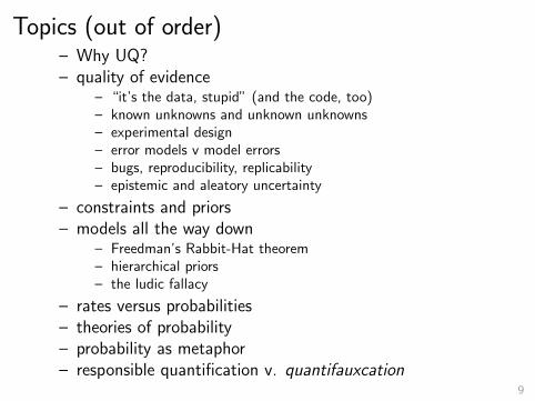
Topics (out of order)– Why UQ?– quality of evidence

– “it’s the data, stupid” (and the code, too)– known unknowns and unknown unknowns– experimental design– error models v model errors– bugs, reproducibility, replicability– epistemic and aleatory uncertainty

– constraints and priors– models all the way down

– Freedman’s Rabbit-Hat theorem– hierarchical priors– the ludic fallacy

– rates versus probabilities– theories of probability– probability as metaphor– responsible quantification v. quantifauxcation

9

– how big is your model space?

– bias/variance tradeoffs– is the bias bounded?– regularization for inference vs estimation– assuming the problem away

– lampposting and hypocognition– how bad can it be?

– lower bounds on minimax uncertainties for emulators– uncertainty quantification for the HEP unfolding problem– curse of dimensionality– bugs, bugs, bugs– reproducibility and replicability; verification and validation

10

Abstract

UQ tries to appraise and quantify the uncertainty of models ofphysical systems calibrated to noisy data (and of predictionsfrom those models), including contributions from ignorance;systematic and stochastic measurement error; limitations oftheoretical models; limitations of numerical representations ofthose models; limitations of the accuracy and reliability ofcomputations, approximations, and algorithms; and humanerror (including software bugs).Much UQ research focuses on developing efficient numericalapproximations (emulators) of computationally expensivenumerical models.In some circles, UQ is nearly synonymous with the study ofemulators and Bayesian models.

11

What sources of uncertainty does a UQ analysis take intoaccount? What does it ignore? How ignorable are the ignoredsources? What assumptions were made? What evidencesupports those assumptions? Are the assumptions testable?What happens if the assumptions are false?I will sketch an embedding of UQ within the theory ofstatistical estimation and inverse problems.I will point to a few examples of work that quantifiesuncertainty from systematic measurement error anddiscretization error.Bad examples will be drawn from the 2009 NAS report,“Evaluation of Quantication of Margins and UncertaintiesMethodology for Assessing and Certifying the Reliability of theNuclear Stockpile,” the Climate Prospectus, and probabilisticseismic hazard analysis (PSHA).

12

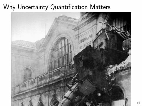
Why Uncertainty Quantification Matters

Figure: Montparnasse

13

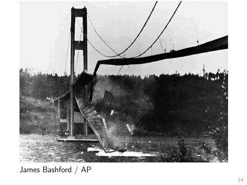
James Bashford / AP14

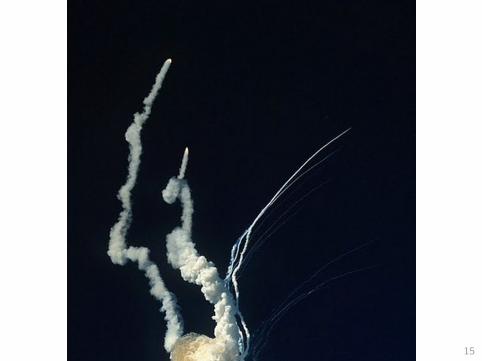
NASA

15

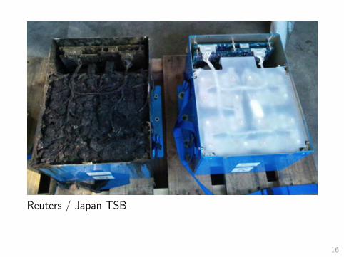
Reuters / Japan TSB

16

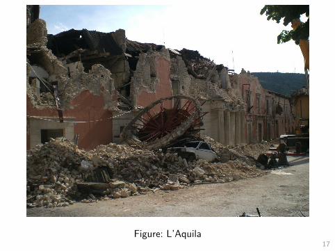
Figure: L’Aquila17

What is UQ?

UQ is typically more specific than just quantifying uncertainty:

UQ = inverse problems + approximate forward model.

18

What are inverse problems?

statistics

19

What is the effect of an approximate forward

model, discretization, etc.?

additional systematic measurement error

20

How can we deal with systematic measurement

error?

statistics

21

So,

UQ = statistics

22

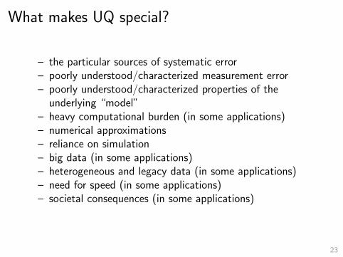
What makes UQ special?

– the particular sources of systematic error– poorly understood/characterized measurement error– poorly understood/characterized properties of the

underlying “model”– heavy computational burden (in some applications)– numerical approximations– reliance on simulation– big data (in some applications)– heterogeneous and legacy data (in some applications)– need for speed (in some applications)– societal consequences (in some applications)

23

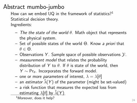
Abstract mumbo-jumboHow can we embed UQ in the framework of statistics?1

Statistical decision theory.Ingredients:

– The the state of the world θ. Math object that representsthe physical system.

– Set of possible states of the world Θ. Know a priori thatθ ∈ Θ.

– Observations Y . Sample space of possible observations Y .– measurement model that relates the probability

distribution of Y to θ. If θ is state of the world, thenY ∼ Prθ. Incorporates the forward model.

– one or more parameters of interest, λ = λ[θ]– an estimator λ̂(Y ) of the parameter (might be set-valued)– a risk function that measures the expected loss from

estimating λ[θ] by λ̂(Y )1Moreover, does it help?

24

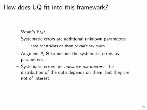
How does UQ fit into this framework?

– What’s Prθ?

– Systematic errors are additional unknown parameters.

– need constraints on them or can’t say much

– Augment θ, Θ to include the systematic errors asparameters.

– Systematic errors are nuisance parameters: thedistribution of the data depends on them, but they arenot of interest.

25

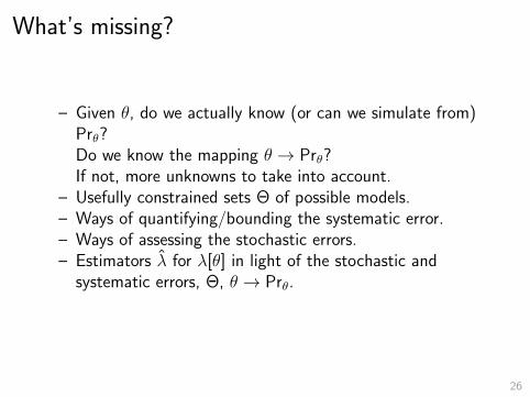
What’s missing?

– Given θ, do we actually know (or can we simulate from)Prθ?Do we know the mapping θ → Prθ?If not, more unknowns to take into account.

– Usefully constrained sets Θ of possible models.– Ways of quantifying/bounding the systematic error.– Ways of assessing the stochastic errors.– Estimators λ̂ for λ[θ] in light of the stochastic and

systematic errors, Θ, θ → Prθ.

26

What can we do with the framework?

– Bayes or frequentist analysis?

– Nature of the assumptions.

– Where does the prior come from?

27

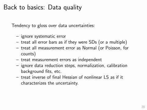
Back to basics: Data quality

Tendency to gloss over data uncertainties:

– ignore systematic error– treat all error bars as if they were SDs (or a multiple)– treat all measurement error as Normal (or Poisson, for

counts)– treat measurement errors as independent– ignore data reduction steps, normalization, calibration

background fits, etc.– treat inverse of final Hessian of nonlinear LS as if it

characterizes the uncertainty.

28

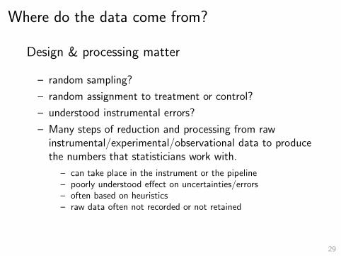
Where do the data come from?

Design & processing matter

– random sampling?

– random assignment to treatment or control?

– understood instrumental errors?

– Many steps of reduction and processing from rawinstrumental/experimental/observational data to producethe numbers that statisticians work with.

– can take place in the instrument or the pipeline– poorly understood effect on uncertainties/errors– often based on heuristics– raw data often not recorded or not retained

29

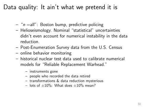
Data quality: It ain’t what we pretend it is

– “n =all”: Boston bump, predictive policing– Helioseismology. Nominal “statistical” uncertainties

didn’t even account for numerical instability in the datareduction.

– Post-Enumeration Survey data from the U.S. Census– online behavior monitoring– historical nuclear test data used to calibrate numerical

models for “Reliable Replacement Warhead.”

– instruments gone– people who recorded the data retired– transformations & data reduction mysterious– lots of ±10%: What does ±10% mean?

30

Can’t get off the ground

How can you know how well the model should fit the data, ifyou don’t understand the nature and probable / possible /plausible size of systematic and stochastic errors in the data?

31

Theory and Practice

– In theory, there’s no difference between theory andpractice. But in practice, there is.–Jan L.A. van de Snepscheut

– The difference between theory and practice is smaller intheory than it is in practice.–unknown UQ master

32

Bad incentives:

Grappling with Data Quality ain’t Sexy

– Academic statisticians rewarded for proving hardtheorems, doing heroic numerical work (speed or size),making splashy images that get on the cover of Nature,being “first.”

– We fall in love with technology, models, technique, tools.

– Digging into data quality, systematic errors, etc., iscrucial, unglamorous, and unrewarded—but crucial.

– Can’t Q U without understanding limitations of the data.

33

The society which scorns excellence in plumbing as a humbleactivity and tolerates shoddiness in philosophy because it is anexalted activity will have neither good plumbing nor goodphilosophy: neither its pipes nor its theories will hold water.–John W. Gardner

34

What does the analysis tell us?

– If UQ gives neither an upper bound nor a lower bound ona sensibly defined measure of uncertainty, what have welearned?

– At the very least, should list what we have and have nottaken into account.

35

Examples with uncertain forward models and

discretization error

– Stark (1992) treats a problem in helioseismology in whichthe forward model is known only approximately; boundsthe systematic error that introduces and takes it intoaccount to find confidence sets for a fullyinfinite-dimensional model; also gives a generalframework.

– Evans & Stark (2002) give a more general framework.

– Stark (2008) discusses generalizing “resolution” tononlinear problems and problems with systematic errors.

– Gagnon-Bartsch & Stark (2012) treat a problem ingravimetry with discretized domain; bound systematicerror from discretization and take it into account to findconfidence sets for a fully infinite-dimensional model.

36

Generic approach: Strict Bounds

– Find sup and inf of parameter λ[θ] of interest over aconfidence set for the model θ, including stochastic andsystematic error included in Prθ.

– Leads to infinite-dimensional optimization problems

– can be exactly reduced to finite-dimensional problems in somecases

– prior constraints usually essential– functionals that can be estimated w finite uncertainty are

limited– convexity and other properties help– often solvable using Fenchel duality

37

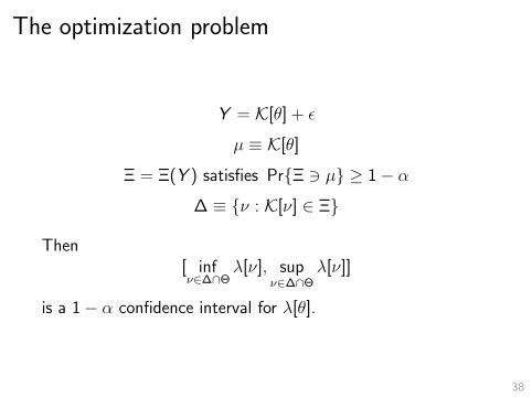
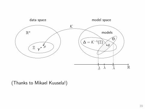
The optimization problem

Y = K[θ] + ε

µ ≡ K[θ]

Ξ = Ξ(Y ) satisfies Pr{Ξ 3 µ} ≥ 1− α

∆ ≡ {ν : K[ν] ∈ Ξ}

Then[ infν∈∆∩Θ

λ[ν], supν∈∆∩Θ

λ[ν]]

is a 1− α confidence interval for λ[θ].

38

Rn

data space

models

model space

YΞ

∆ = K−1(Ξ)Θ

θ

K

µ

Rλ λλ

(Thanks to Mikael Kuusela!)

39

Evaluation of Quantification of Margins andUncertainties Methodology for Assessing andCertifying the Reliability of the Nuclear Stockpile(EQMU)

Committee on the Evaluation of Quantification of Margins andUncertainties Methodology for Assessing and Certifying theReliability of the Nuclear Stockpile, 2009.http://www.nap.edu/openbook.php?record id=12531&page=R1

40

Fundamental Theorem of Physics

Axiom: Anything that comes up in a physics problem isphysics.

Lemma: Nobody knows more about physics than physicists.2

Theorem: There’s no reason for physicists to talk to anybodyelse to solve physics problems.

2Follows from the axiom: Nobody knows more about anything thanphysicists.

41

Practical consequence

Physicists often re-invent the wheel. It is not always as goodas the wheel a mechanic would build.

Some “unsolved” problems–according to EQMU—are solved.But not by physicists.

NAS panel included physicists, nuclear engineer, seniormanager, probabilistic risk assessor, and one statistician

42

Cream of EQMU (p25)Assessment of the accuracy of a computational predictiondepends on assessment of model error, which is the differencebetween the laws of nature and the mathematical equationsthat are used to model them. Comparison against experimentis the only way to quantify model error and is the onlyconnection between a simulation and reality. . . .

Even if model error can be quantified for a given set ofexperimental measurements, it is difficult to draw justifiablebroad conclusions from the comparison of a finite set ofsimulations and measurements. . . . it is not clear how toestimate the accuracy of a simulated quantity of interest foran experiment that has not yet been done. . . .

In the end there are inherent limits [which] might arise fromthe paucity of underground nuclear data and the circularity ofdoing sensitivity studies using the same codes that are to beimproved in ways guided by the sensitivity studies. 43

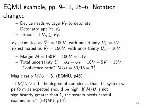
EQMU example, pp. 9–11, 25–6. Notation

changed– Device needs voltage VT to detonate.– Detonator applies VA.– “Boom” if VA ≥ VT .

VT estimated as V̂T = 100V , with uncertainty UT = 5V .VA estimated as V̂A = 150V , with uncertainty UA = 10V .

– Margin M = 150V − 100V = 50V .– Total uncertainty U = UA + UT = 10V + 5V = 15V .– “Confidence ratio” M/U = 50/15 = 3 1

3.

Magic ratio M/U = 3. (EQMU, p46)

“If M/U >> 1, the degree of confidence that the system willperform as expected should be high. If M/U is notsignificantly greater than 1, the system needs carefulexamination.” (EQMU, p14)

44

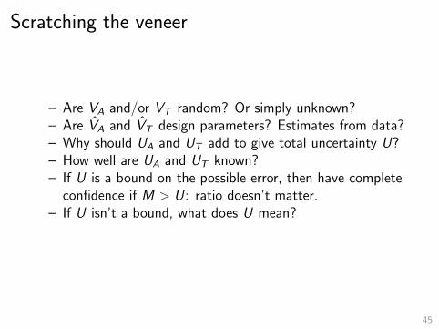
Scratching the veneer

– Are VA and/or VT random? Or simply unknown?– Are V̂A and V̂T design parameters? Estimates from data?– Why should UA and UT add to give total uncertainty U?– How well are UA and UT known?– If U is a bound on the possible error, then have complete

confidence if M > U : ratio doesn’t matter.– If U isn’t a bound, what does U mean?

45

EQMU says:

– “Generally [uncertainties] are described by probabilitydistribution functions, not by a simple band of values.”(EQMU, p13)

– “An important aspect of [UQ] is to calculate the (output)probability distribution of a given metric and from thatdistribution to estimate the uncertainty of that metric.The meaning of the confidence ratio (M/U) dependssignificantly on this definition . . . ” (EQMU, p15)

46

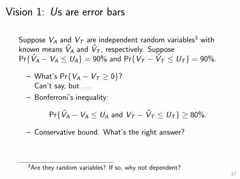
Vision 1: Us are error bars

Suppose VA and VT are independent random variables3 withknown means V̂A and V̂T , respectively. SupposePr{V̂A − VA ≤ UA} = 90% and Pr{VT − V̂T ≤ UT} = 90%.

– What’s Pr{VA − VT ≥ 0}?Can’t say, but . . .

– Bonferroni’s inequality:

Pr{V̂A − VA ≤ UA and VT − V̂T ≤ UT} ≥ 80%.

– Conservative bound. What’s the right answer?

3Are they random variables? If so, why not dependent?47

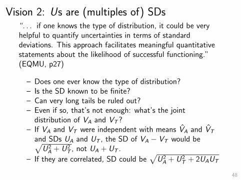
Vision 2: Us are (multiples of) SDs“. . . if one knows the type of distribution, it could be veryhelpful to quantify uncertainties in terms of standarddeviations. This approach facilitates meaningful quantitativestatements about the likelihood of successful functioning.”(EQMU, p27)

– Does one ever know the type of distribution?– Is the SD known to be finite?– Can very long tails be ruled out?– Even if so, that’s not enough: what’s the joint

distribution of VA and VT?– If VA and VT were independent with means V̂A and V̂T

and SDs UA and UT , the SD of VA − VT would be√U2A + U2

T , not UA + UT .

– If they are correlated, SD could be√U2

A + U2T + 2UAUT

48

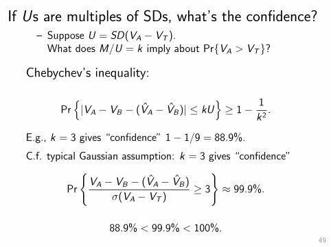
If Us are multiples of SDs, what’s the confidence?– Suppose U = SD(VA − VT ).

What does M/U = k imply about Pr{VA > VT}?

Chebychev’s inequality:

Pr{|VA − VB − (V̂A − V̂B)| ≤ kU

}≥ 1− 1

k2.

E.g., k = 3 gives “confidence” 1− 1/9 = 88.9%.

C.f. typical Gaussian assumption: k = 3 gives “confidence”

Pr

{VA − VB − (V̂A − V̂B)

σ(VA − VT )≥ 3

}≈ 99.9%.

88.9% < 99.9% < 100%.49

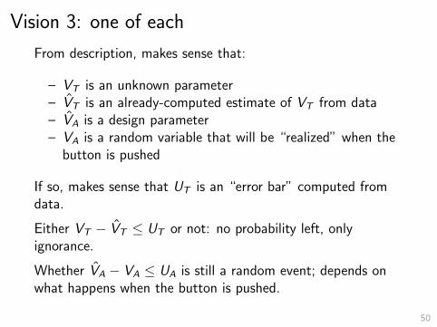
Vision 3: one of each

From description, makes sense that:

– VT is an unknown parameter– V̂T is an already-computed estimate of VT from data– V̂A is a design parameter– VA is a random variable that will be “realized” when the

button is pushed

If so, makes sense that UT is an “error bar” computed fromdata.

Either VT − V̂T ≤ UT or not: no probability left, onlyignorance.

Whether V̂A − VA ≤ UA is still a random event; depends onwhat happens when the button is pushed.

50

– EQMU is careless about

– what is known– what is estimated– what is uncertain– what is random– etc.

– The “toy” lead example is problematic.

51

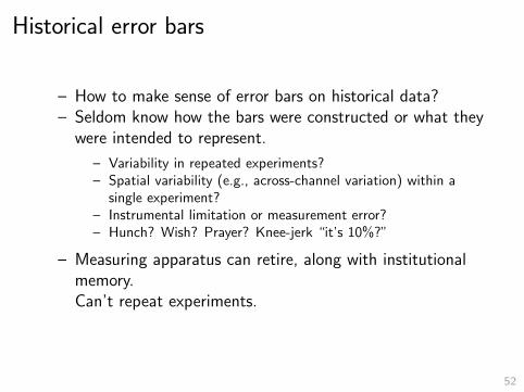
Historical error bars

– How to make sense of error bars on historical data?– Seldom know how the bars were constructed or what they

were intended to represent.

– Variability in repeated experiments?– Spatial variability (e.g., across-channel variation) within a

single experiment?– Instrumental limitation or measurement error?– Hunch? Wish? Prayer? Knee-jerk “it’s 10%?”

– Measuring apparatus can retire, along with institutionalmemory.Can’t repeat experiments.

52

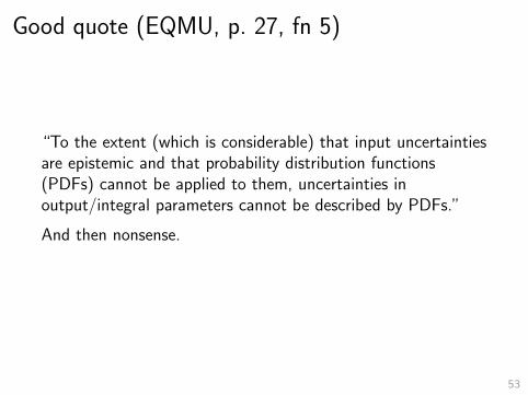
Good quote (EQMU, p. 27, fn 5)

“To the extent (which is considerable) that input uncertaintiesare epistemic and that probability distribution functions(PDFs) cannot be applied to them, uncertainties inoutput/integral parameters cannot be described by PDFs.”

And then nonsense.

53

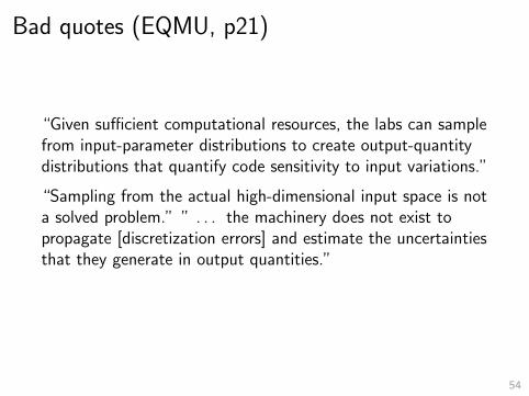
Bad quotes (EQMU, p21)

“Given sufficient computational resources, the labs can samplefrom input-parameter distributions to create output-quantitydistributions that quantify code sensitivity to input variations.”

“Sampling from the actual high-dimensional input space is nota solved problem.” ” . . . the machinery does not exist topropagate [discretization errors] and estimate the uncertaintiesthat they generate in output quantities.”

54

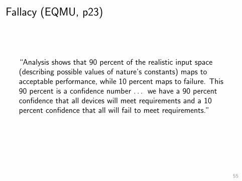
Fallacy (EQMU, p23)

“Analysis shows that 90 percent of the realistic input space(describing possible values of nature’s constants) maps toacceptable performance, while 10 percent maps to failure. This90 percent is a confidence number . . . we have a 90 percentconfidence that all devices will meet requirements and a 10percent confidence that all will fail to meet requirements.”

55

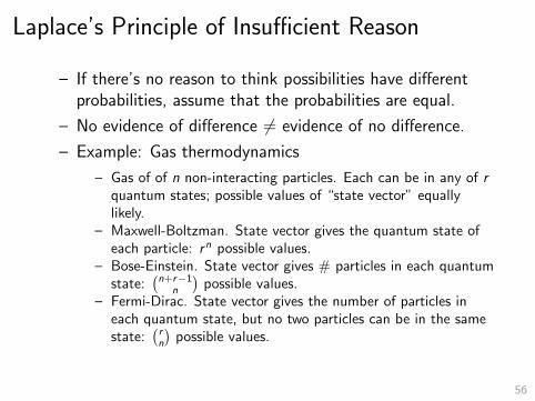
Laplace’s Principle of Insufficient Reason

– If there’s no reason to think possibilities have differentprobabilities, assume that the probabilities are equal.

– No evidence of difference 6= evidence of no difference.

– Example: Gas thermodynamics

– Gas of of n non-interacting particles. Each can be in any of rquantum states; possible values of “state vector” equallylikely.

– Maxwell-Boltzman. State vector gives the quantum state ofeach particle: rn possible values.

– Bose-Einstein. State vector gives # particles in each quantumstate:

(n+r−1

n

)possible values.

– Fermi-Dirac. State vector gives the number of particles ineach quantum state, but no two particles can be in the samestate:

(rn

)possible values.

56

– Maxwell-Boltzman common in probability theory, but butdescribes no known gas.

– Bose-Einstein describes bosons, e.g., photons and He4

atoms.

– Fermi-Dirac describes fermions, e.g., electrons and He3

atoms.

Outcomes can be defined or parametrized in many ways.Not clear which–if any–give equal probabilities.

57

Constraints versus prior probabilities

Bayesian machinery is appealing but can be misleading.

– Capturing constraints using priors adds “information” notpresent in the constraints.

– Why a particular form?– Why particular values of the parameters?– What’s the relation between the “error bars” the prior

represents and specific choices?– Distributions on states of nature Bayes’ Rule:

Pr(B|A) = Pr(A|B) Pr(B)/Pr(A). “Just math.”– To have posterior Pr(B|A), need prior Pr(B).– The prior matters. Where does it come from?

58

Conservation of Rabbits

The Rabbit Axioms

1. For the number of rabbits in a closed system to increase,the system must contain at least two rabbits.

2. No negative rabbits.

59

Freedman’s Rabbit-Hat Theorem

You cannot pull a rabbit from a hat unless at leastone rabbit has previously been placed in the hat.

60

– The prior puts the rabbit in the hat– PRA puts many rabbits in the hat– Hierarchical priors put many rabbits in the hat– Bayes/minimax duality: minimax uncertainty is Bayes

uncertainty for least favorable prior.4

4Least favorable 6= “uninformative.”61

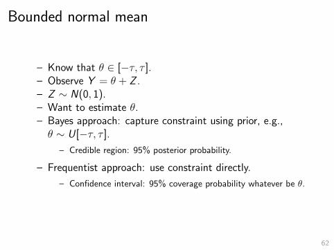
Bounded normal mean

– Know that θ ∈ [−τ, τ ].– Observe Y = θ + Z .– Z ∼ N(0, 1).– Want to estimate θ.– Bayes approach: capture constraint using prior, e.g.,θ ∼ U[−τ, τ ].

– Credible region: 95% posterior probability.

– Frequentist approach: use constraint directly.

– Confidence interval: 95% coverage probability whatever be θ.

62

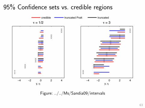
95% Confidence sets vs. credible regions

−4 −2 0 2 4y, !

" = 1/2

−4 −2 0 2 4

" = 3

y, !

credible truncated Pratt truncated

Figure: ../../Ms/Sandia09/intervals

63

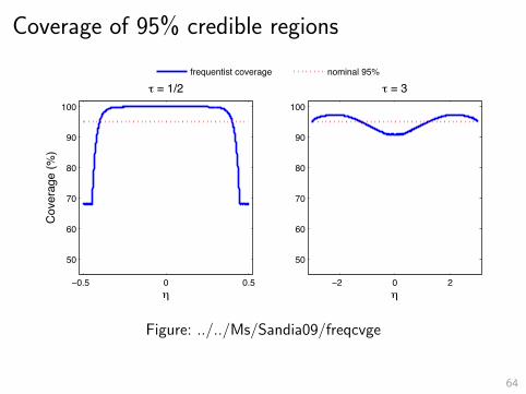
Coverage of 95% credible regions

−0.5 0 0.5

50

60

70

80

90

100

! = 1/2

"

Cov

erag

e (%

)

−2 0 2

50

60

70

80

90

100

! = 3

"

frequentist coverage nominal 95%

Figure: ../../Ms/Sandia09/freqcvge

64

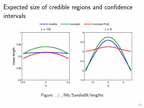
Expected size of credible regions and confidence

intervals

−0.5 0 0.50.8

0.85

0.9

0.95

1

!

mea

n le

ngth

" = 1/2

−2 0 21.5

2

2.5

3

3.5

4" = 3

!

credible truncated truncated Pratt

Figure: ../../Ms/Sandia09/lengths

65

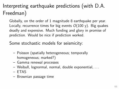
Interpreting earthquake predictions (with D.A.

Freedman)

Globally, on the order of 1 magnitude 8 earthquake per year.Locally, recurrence times for big events O(100 y). Big quakesdeadly and expensive. Much funding and glory in promise ofprediction. Would be nice if prediction worked.

Some stochastic models for seismicity:

– Poisson (spatially heterogeneous; temporallyhomogeneous; marked?)

– Gamma renewal processes– Weibull, lognormal, normal, double exponential, . . .– ETAS– Brownian passage time

66

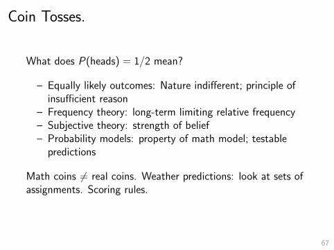
Coin Tosses.

What does P(heads) = 1/2 mean?

– Equally likely outcomes: Nature indifferent; principle ofinsufficient reason

– Frequency theory: long-term limiting relative frequency– Subjective theory: strength of belief– Probability models: property of math model; testable

predictions

Math coins 6= real coins. Weather predictions: look at sets ofassignments. Scoring rules.

67

USGS 1999 Forecast

P(M≥6.7 event by 2030) = 0.7± 0.1

– What does this mean?– Where does the number come from?

Two big stages.

68

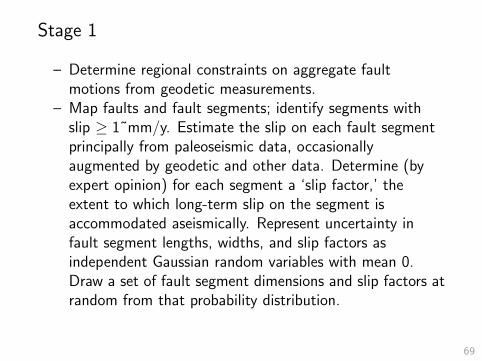
Stage 1

– Determine regional constraints on aggregate faultmotions from geodetic measurements.

– Map faults and fault segments; identify segments withslip ≥ 1˜mm/y. Estimate the slip on each fault segmentprincipally from paleoseismic data, occasionallyaugmented by geodetic and other data. Determine (byexpert opinion) for each segment a ‘slip factor,’ theextent to which long-term slip on the segment isaccommodated aseismically. Represent uncertainty infault segment lengths, widths, and slip factors asindependent Gaussian random variables with mean 0.Draw a set of fault segment dimensions and slip factors atrandom from that probability distribution.

69

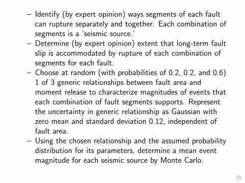
– Identify (by expert opinion) ways segments of each faultcan rupture separately and together. Each combination ofsegments is a ‘seismic source.’

– Determine (by expert opinion) extent that long-term faultslip is accommodated by rupture of each combination ofsegments for each fault.

– Choose at random (with probabilities of 0.2, 0.2, and 0.6)1 of 3 generic relationships between fault area andmoment release to characterize magnitudes of events thateach combination of fault segments supports. Representthe uncertainty in generic relationship as Gaussian withzero mean and standard deviation 0.12, independent offault area.

– Using the chosen relationship and the assumed probabilitydistribution for its parameters, determine a mean eventmagnitude for each seismic source by Monte Carlo.

70

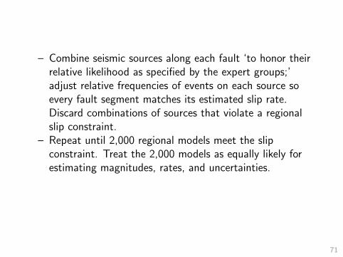
– Combine seismic sources along each fault ‘to honor theirrelative likelihood as specified by the expert groups;’adjust relative frequencies of events on each source soevery fault segment matches its estimated slip rate.Discard combinations of sources that violate a regionalslip constraint.

– Repeat until 2,000 regional models meet the slipconstraint. Treat the 2,000 models as equally likely forestimating magnitudes, rates, and uncertainties.

71

– Estimate background rate of seismicity:

– Use an (unspecified) Bayesian procedure to categorizehistorical events from three catalogs either as associated ornot associated with the seven fault systems.

– Fit generic Gutenberg-Richter magnitude-frequency relationN(M) = 10a−bM to events deemed not to be associated withthe seven fault systems.

– Model background seismicity as a marked Poisson process.Extrapolate Poisson model to M ≥ 6.7, which gives aprobability of 0.09 of at least one event.

– Generate 2,000 models; estimate long-term seismicityrates as a function of magnitude for each seismic source.

72

Stage 2:

– Fit 3 stochastic models for earthquakerecurrence—Poisson, Brownian passage time and“time-predictable”—to long-term seismicity ratesestimated in stage 1.

– Combine stochastic models to estimate chance of a largeearthquake:

– Use Poisson and Brownian passage time models to estimatethe probability an earthquake will rupture each fault segment.

– Some parameters fitted to data; some set more arbitrarily.– Aperiodicity (standard deviation of recurrence time, divided by

expected recurrence time) set to three different values, 0.3,0.5, and 0.7.

– Method needs estimated date of last rupture of each segment.Model redistribution of stress by earthquakes; predictionsmade w/ & w/o adjustments for stress redistribution.

73

– contd.

– Predictions for segments combined into predictions for eachfault using expert opinion about the relative likelihoods ofdifferent rupture sources.

– ‘Time-predictable model’ (stress from tectonic loading needsto reach the level at which the segment ruptured in theprevious event for the segment to initiate a new event) usedto estimate the probability that an earthquake will originateon each fault segment.

– Estimating the state of stress before the last event requiresdate of the last event and slip during the last event. Thosedata are available only for the 1906 earthquake on the SanAndreas Fault and the 1868 earthquake on the southernsegment of the Hayward Fault.

74

– contd.

– Time-predictable model could not be used for many Bay Areafault segments. Need to know loading of the fault over time;relies on viscoelastic models of regional geological structure.Stress drops and loading rates modeled probabilistically; theform of the probability models not given.

– Loading of San Andreas fault by the 1989 Loma Prietaearthquake and the loading of Hayward fault by the 1906earthquake were modeled.

– Probabilities estimated using time-predictable model wereconverted into forecasts using expert opinion for relativelikelihoods that an event initiating on one segment will stop orwill propagate to other segments.

– outputs of the 3˜types of stochastic models for each segmentweighted using opinions of a panel of 15 experts.

– When results from the time-predictable model were notavailable, the weights on its output were 0.

75

So, what does it mean?– No standard interpretation of probability applies.– Aspects of Fisher’s fiducial inference, frequency theory,

probability models, subjective probability.– Frequencies equated to probabilities; outcomes assumed

to be equally likely; subjective probabilities used in waysthat violate Bayes’ Rule.

– Calibrated using incommensurable data–global,extrapolated across magnitude ranges using “empirical”scaling laws.

– PRA is very similar—made-up models for various risks,hand enumeration of possibilities. Lots of “expertjudgment” turned into the appearance of precisequantification: quantifauxcation

– UQ for RRW similar to EQ prediction: can’t do relevantexperiments to calibrate the models, lots of judgmentneeded.

76

More uncertainty: failures of reproducibility

– attempts to replicate experiments or data analyses oftenfail to support the original claims.5

– P-hacking, ignoring multiplicity, small effects, file-drawereffect, bugs, etc.

– Failures contribute to uncertainty: hard to quantify

– Journals generally uninterested in publishing negativeresults or replications of positive results: emphasis is on“discoveries.”

– Thermo ML found ˜20% of papers that otherwise wouldhave been accepted had serious errors, discovered b/crequired sharing data

5E.g., http://science.sciencemag.org/content/349/6251/aac4716.fullhttp://www.newyorker.com/magazine/2010/12/13/the-truth-wears-off

77

– Selecting data, hypotheses, data analyses, and results, toproduce (apparently) positive results inflates the apparentsignal-to-noise ratio and overstates statistical significance.

– Automation of data analysis, including feature selectionand model selection, combined with the large number ofvariables measured in many modern studies andexperiments, including “omics,” high-energy physics, andsensor networks: inevitable that many “discoveries” willbe wrong.

78

Most software has bugs

– 2014 study by Coverity, based on code-scanningalgorithms, found 0.61 errors per 1,000 lines of sourcecode in open-source projects and 0.76 errors per 1,000lines of source code in commercial software6

– Few scientists use sound software engineering practices,such as rigorous testing—or even version control.7

6http://go.coverity.com/rs/157-LQW-289/images/2014-Coverity-Scan-Report.pdf

7See, e.g.: Merali, Z., 2010. Computational science: . . . Error . . .why scientific programming does not compute. Nature, 467, 775–777doi:10.1038/467775ahttp://www.nature.com/news/2010/101013/full/467775a.html; Soergel,D.A.W., 2015. Rampant software errors may undermine scientific results.F1000Research, 3, 303. doi:10.12688/f1000research.5930.2http://f1000research.com/articles/3-303/v2

79

“Rampant software errors undermine scientific

results”

Soergel, 2015

Errors in scientific results due to software bugs arenot limited to a few high-profile cases that lead toretractions and are widely reported. Here I estimatethat in fact most scientific results are probably wrongif data have passed through a computer, and thatthese errors may remain largely undetected. Theopportunities for both subtle and profound errors insoftware and data management are boundless, yetthey remain surprisingly underappreciated.

80

How can we do better?

– Scripted analyses: no point-and-click tools, especiallyspreadsheet calculations

– Revision control systems

– Documentation, documentation, documentation

– Coding standards/conventions

– Pair programming

– Issue trackers

– Code reviews (and in teaching, grade code, not justoutput)

– Code tests: unit, integration, coverage, regression

81

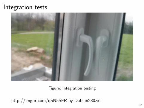
Integration tests

Figure: Integration testing

http://imgur.com/qSN5SFR by Datsun280zxt82

Spreadsheets especially bad– Easier to commit errors and harder to find them.– 2010 work of Reinhart and Rogoff8 used to justify

austerity measures in southern Europe. Errors in theirExcel spreadsheet lead to the wrong conclusion9

– Spreadsheets might be OK for data entry, but not forcalculations.

– Conflate input, output, code, presentation; facilitate &obscure error

– According to KPMG and PWC, over 90% of corporatespreadsheets have errors

– Not just errors: bugs in Excel too: +, *, randomnumbers, statistical routines

– “Stress tests” of international banking system use Excelsimulations!

8Reinhart, C. and K. Rogoff, 2010. Growth in a Time of Debt,Working Paper no. 15639,National Bureau of Economic Research,http://www.nber.org/papers/w15639; Reinhart, C. and K. Rogoff, 2010.Growth in a Time of Debt, American Economic Review, 100, 573–578.

9Herndon, T., M. Ash, and R. Pollin, 2014. Does high public debtconsistently stifle economic growth? A critique of Reinhart and Rogoff,Cambridge Journal of Economics, 38 257–279. doi:10.1093/cje/bet075

83

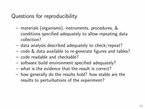
Questions for reproducibility

– materials (organisms), instruments, procedures, &conditions specified adequately to allow repeating datacollection?

– data analysis described adequately to check/repeat?– code & data available to re-generate figures and tables?– code readable and checkable?– software build environment specified adequately?– what is the evidence that the result is correct?– how generally do the results hold? how stable are the

results to perturbations of the experiment?

84

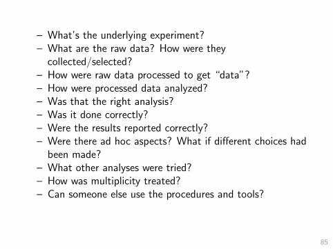
– What’s the underlying experiment?– What are the raw data? How were they

collected/selected?– How were raw data processed to get “data”?– How were processed data analyzed?– Was that the right analysis?– Was it done correctly?– Were the results reported correctly?– Were there ad hoc aspects? What if different choices had

been made?– What other analyses were tried?– How was multiplicity treated?– Can someone else use the procedures and tools?

85

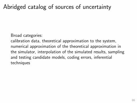
Abridged catalog of sources of uncertainty

Broad categories:calibration data, theoretical approximation to the system,numerical approximation of the theoretical approximation inthe simulator, interpolation of the simulated results, samplingand testing candidate models, coding errors, inferentialtechniques

86

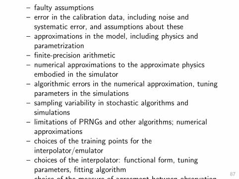
– faulty assumptions– error in the calibration data, including noise and

systematic error, and assumptions about these– approximations in the model, including physics and

parametrization– finite-precision arithmetic– numerical approximations to the approximate physics

embodied in the simulator– algorithmic errors in the numerical approximation, tuning

parameters in the simulations– sampling variability in stochastic algorithms and

simulations– limitations of PRNGs and other algorithms; numerical

approximations– choices of the training points for the

interpolator/emulator– choices of the interpolator: functional form, tuning

parameters, fitting algorithm– choice of the measure of agreement between observation

and prediction– choices in the sampler, including the probability

distribution used and the number of samples drawn.– technique actually used to draw conclusions from the

emulated output– bugs, data transcription errors, faulty proofs, . . .

87

Conclusions

– UQ is hard to do well.– Most attempts ignore sources of uncertainty that could

contribute more than the sources they include:lampposting.

– Some of those sources can be appraised.– Errors and error bars for the original measurements are

poorly understood: insurmountable?– Bayesian methods make very strong assumptions about

the probability distribution of data errors, models andoutput; reduce apparent but not real uncertainty.

– Extrapolating complex simulations requires refusing tocontemplate violations of assumptions that cannot betested using calibration data.

– Numerical experiments are not an adequate substitute forreal experiments.

88