Uncertainty quantiﬁ cation for evaluating impacts of caprock and ...lin491/pub/GLIN-13-GHG.pdf · 12 other parameters describing hydrogeological properties of subsurface formations,

338 © 2013 Society of Chemical Industry and John Wiley & Sons, Ltd | Greenhouse Gas Sci Technol. 3:338–358 (2013); DOI: 10.1002/ghg

Correspondence to: Jie Bao, Fluid and Computational Engineering Group, Energy and Environment Directorate, Pacifi c Northwest National

Laboratory, Richland, WA 99352, USA. E-mail: [email protected]

Received May 29, 2013; revised and accepted July 3, 2013

Published online at Wiley Online Library (wileyonlinelibrary.com). DOI: 10.1002/ghg.1362

Modeling and Analysis

Uncertainty quantifi cation for evaluating impacts of caprock and reservoir properties on pressure buildup and ground surface displacement during geological CO2 sequestrationJie Bao, Zhangshuan Hou, Yilin Fang, Huiying Ren, and Guang Lin, Pacifi c Northwest National Laboratory, Richland, WA, USA

Abstract: A series of numerical test cases refl ecting broad and realistic ranges of geological formation properties was developed to systematically evaluate and compare the impacts of those properties on pressure build-up and ground surface displacement and therefore risks of induced seismicity during CO2 injection. A coupled hydro-geomechanical subsurface transport simulator, STOMP (Subsurface Transport over Multiple Phases), was adopted to simulate the migration of injected CO2 and geome-chanical behaviors of the surrounding geological formations. A quasi-Monte Carlo sampling method was applied to effi ciently sample a high-dimensional parameter space consisting of injection rate and 12 other parameters describing hydrogeological properties of subsurface formations, including poros-ity, permeability, entry pressure, pore-size index, Young’s modulus, and Poisson’s ratio for both reser-voir and caprock. Generalized cross-validation and analysis of variance methods were used to quanti-tatively measure the signifi cance of the 13 input parameters. For the investigated two-dimensional cases, reservoir porosity, permeability, and injection rate were found to be among the most signifi cant factors affecting the geomechanical responses to the CO2 injection, such as injection pressure and ground surface uplift. We used a quadrature generalized linear model to build a reduced-order model that can estimate the geomechanical response instantly instead of running computationally expensive numerical simulations. © 2013 Society of Chemical Industry and John Wiley & Sons, Ltd

Keywords: CO2 geological sequestration; uncertainty quantifi cation; sensitivity analysis; reduced-order model

Modeling and Analysis: Uncertainty quantifi cation for CO2 sequestration J Bao et al.

339© 2013 Society of Chemical Industry and John Wiley & Sons, Ltd | Greenhouse Gas Sci Technol. 3:338–358 (2013); DOI: 10.1002/ghg

Introduction

Emissions of greenhouse gases (GHGs) have been implicated as a primary contributor to global warming and accelerated climate change.1 It was

estimated that energy-related CO2 production ac-counted for 81.5% of the GHG emissions in the United States.2 Injecting fl uid into confi ned aquifers has been a widely accepted strategy for enhanced oil recovery (EOR), gas storage, and waste disposal.3 It is well known that CO2 sequestration in deep saline aquifers could be a promising mitigation method for the reduction of CO2 emitted to the atmosphere.4 Th e storage of CO2 in deep saline aquifers is potentially an excellent solution for large parts of northwestern Europe and the Midwestern United States, where large-scale CO2 storage will be required in order to make a signifi cant contribution to reduce CO2 emis-sions.5 Geological storage of CO2 involves fairly complex physical and chemical processes such as multiphase fl ow, multicomponent miscible transport, and geochemical,6 geomechanical, and non-isother-mal eff ects.7 Mathematical models and numerical simulation tools play an important role in evaluating the feasibility of CO2 storage in subsurface reservoirs, designing and analyzing fi eld tests, and designing and operating geological CO2 disposal systems.8 One of the processes that we need to understand regarding the feasibility and risks associated with carbon sequestration is the geomechanical responses of the target injection formations. It is therefore essential to identify and understand the importance of diff erent factors that aff ect geomechanical responses during injection of substantial supercritical CO2 into a deep geological formation.

Geomechanical responses, such as induced seismic-ity, fracturing, and pre-existing fault reactivation upon CO2 injection and sequestration, indicate the safety and sustainability of the injection activities. Top surface/ground surface displacements can partially refl ect underground geomechanical activities, and therefore provide critical information that can be used to infer potential hazard caused by CO2 sequestration activities. Even if there is no noticeable induced seismic activity or fracturing, the ground surface displacement can still pose safety issues for buildings and facilities on the surface. Colesanti and Wasowski9 showed that about 10 mm year–1 ground surface movement velocity can induce severe damage to buildings with high probability. In practice, the

ground surface displacements can be detected and monitored using the global positioning system (GPS)10,11 or satellite-borne synthetic aperture radar (SAR).9

Because of the complexity of CO2 geological seques-tration processes, many factors aff ect the safety and sustainability of a CO2 injection practice to a greater or lesser degree. In recent years, uncertainty quantifi -cation techniques have proven to be necessary for quantitative evaluations of the contribution of each factor. Sensitivity analysis of input parameters can reduce a complex system to a ‘smaller’ or ‘simpler’ system but still provide reasonable descriptions of major aspects of the system or process. Such a simplifi ed model is oft en called a reduced-order model (ROM).12 Hence, ROMs usually are thought of as computationally inexpensive models that have the potential for real-time analysis.13 A suitable ROM that closely approximates the geomechanical re-sponse to CO2 sequestration will be a valuable tool for effi ciently estimating and evaluating the risk of the injection activities. However, ROM construction oft en is considered computationally expensive because it requires accumulating a large number of system responses to input excitations.14 ROMs can be based on many diff erent regression methods, such as generalized linear method (GLM),15–18 multivariate adaptive regression splines (MARS) method,19–24 support vector regression (SVR),25–27 Gaussian process,28 artifi cial neural networks (ANN),29 and so on. Generally, GLM is oft en recommended for monotonic system,27 and can off er an explicit equa-tion to present the relationship between input and output parameters, which is favorable for engineering applications. MARS theoretically can off er better interpolation than GLM for non-monotonic non-linear system, but the ROM based on MARS oft en cannot be expressed as an explicit equation. SVR, Gaussian process, and ANN might be more suitable for very complicated systems, such as high-level non-monotonic and highly non-linear system, but they require large amount of observations as training set, and the constructed ROMs cannot be expressed as explicit equations, and the accuracy of these regression methods is case-dependent. Both GLM and MARS approaches are accurate enough for simple response system, and are easy to be imple-mented. For complicated system, Gaussian process and ANN may off er more reliable results. Th erefore, effi cient sampling methods, reliable data from previous exploratory sensitivity analyses of input

J Bao et al. Modeling and Analysis: Uncertainty quantifi cation for CO2 sequestration


factors, and appropriate regression methods, are critical to the effi ciency and accuracy of the ROM.

Th e geological sequestration of CO2 involves a number of complicated physical and chemical pro-cesses that occur within a large spatial domain and span a long period of time. Considering the high dimensionality of the input parameter space and the number of numerical model evaluations required to achieve reliable relationships between input param-eters/factors and various observed responses, an effi cient numerical simulator is essential to provide eff ective predicted responses to diff erent input param-eters set-ups. In our study, a scalable simulator STOMP (Subsurface Transport over Multiple Phases30), with fully coupled hydro-geomechanics, was adopted for the simulations of geological CO2 sequestration. A rigid-body-spring model (RBSM)31 was coupled and integrated with STOMP’s hydrogeo-logical fl ow transport simulator. Porous media properties, such as porosity and permeability, are geomechanical-stress dependent.

In the next section we introduce and discuss the STOMP simulator and describe the CO2 sequestration test case set-up. Information on input parameter characteristics collected prior to our study is then presented; the sampling method and sensitivity analysis framework are also introduced. Results of the sensitivity analysis are later described and the ROM and the response surface are also shown.

A hydro-geomechanical model for CO2 geological sequestrationTh e sensitivity analysis of geomechanical responses to the input parameters during CO2 injection was based on the simulation results of the engineering simulator STOMP. Th e STOMP simulator was designed to solve a wide variety of nonlinear, single- or multi-phase, fl ow and transport problems for variably-saturated geologic media.30 Partial diff erential conservation equations for component mass, energy, and solute mass comprise the fundamental equations for the simulator. In STOMP, the partial diff erential equa-tions are discretized spatially on structured orthogo-nal grids using the integral fi nite diff erence approach and temporally using fi rst-order backward Euler diff erencing.

For coupled hydro-geomechanical simulation, RBSM was integrated into STOMP using sequential coupled approach, that is, multiphase fl ow equations

and stress equation are solved separately for each time increment. RBSM was fi rst proposed by Kawai31 to model discontinuous rock systems. In RBSM, the physical model is divided into polyhedron rigid blocks in contact with each other through continuously distributed zero-size normal and shear springs. Th e unknowns are at the center of each grid block. If the physical model is divided into structured orthogonal grid that STOMP uses, then each RBSM grid block represents a STOMP grid element. All the unknowns, such as displacement, pressure, and saturation, are at the center of each grid element. Th is feature makes it convenient to have RBSM to share the same numeri-cal grid with STOMP, and therefore there is no need to convert results between diff erent grid settings. Conversion between grids are oft en required by coupling a fl ow solver using fi nite volume method (unknowns located at cell centers) with a geomechan-ics solver using fi nite element method (unknowns located at vertices).

RBSM solves the mechanical equilibrium equation for quasi-static state conditions. A general constitu-tive theory of linear thermoporoelasticity is used to describe the coupled processes of hydraulic, me-chanical and thermal in porous media. We have considered the Poisson’s eff ect in RBSM to improve the accuracy of the method. Details of the develop-ment of the coupled STOMP-RBSM are in Fang’s work.32

Our coupled hydro-mechanical model accounts for the changes in porosity and absolute permeabil-ity due to the change in eff ective stress computed from the geomechanics model. In our sequential coupled approach, Darcy fl uxes at the contact face and pressures (both water and CO2) at the cell center simulated from the fl ow solver are used to calculate the water and CO2 pressure on the contact surface during each time increment. Saturations of water and CO2 on the contact surface are linearly interpolated from the cell center of the elements connected by the surface. Pore pressure on the contact is then calculated as the sum of the water and CO2 pressure on the contact weighted by their corresponding saturations. Geomechanics solver takes these pore pressure changes on the contact to update stresses and strains. Th e updated strains and stresses are then passed back to the fl ow solver and used to compute coupled parameters, such as porosity and permeability, to update the secondary variables for the next time step. Note that these



calculations are in a single code without read/write from the disk.

Th e injection induced porosity change can be modeled by either empirical functions fi tted to laboratory data or fi eld observation,33 or theoretical relationship, such as the model in Liu and Rutqvist’s work.34 We adopted the method used in Rutqvist and Tsang’s work:35

θ θ( )θ θ−θ ( )σ +)θθ ( σ r (1)

k k expxpxk expx⎛⎝⎝⎝

⎞⎠⎟⎞⎞⎠⎠

⎡

⎣⎢⎡⎡

⎣⎣

⎤

⎦⎥⎤⎤

⎦⎦0

0

22 2 1−⎛⎝⎜⎛⎛⎝⎝

. θθ

(2)

where θ is porosity, θ0 is porosity at zero stress, θr is residual porosity at high stress, and σMʹ is the mean eff ective stress (in Pa). In Eqn (2), k is permeability, and k0 is the zero stress permeability.

To eff ectively predict the geomechanical responses to various geological CO2 sequestration conditions, numerous exploratory numerical experiments were performed on a two-dimensional (2D) domain shown in Fig. 1. Th e investigated region was 700 km wide in the horizontal direction, and from 0 to 3000 m below ground surface (bgs) in the vertical direction. Th e caprock layer was between 1200 m and 1300 m bgs, and the reservoir was between 1300 m and 1500 m bgs. Th e injection point was at 1500 m bgs and at the center of the domain in horizontal directions.5, 35–37 Compressed CO2 was injected continuously at a constant rate with a unit of kg s–1 per meter (per meter normal to the 2D model), and the well was set

as 7 km long, equivalent to a 1-km-diameter well fi eld.35 Th e ground surface vertical displacement (x = 0 m, z = 0 m) and the pressure at the injection point (x = 0 m, z = −1500 m) were selected as the output responses to variation in the input parameters.

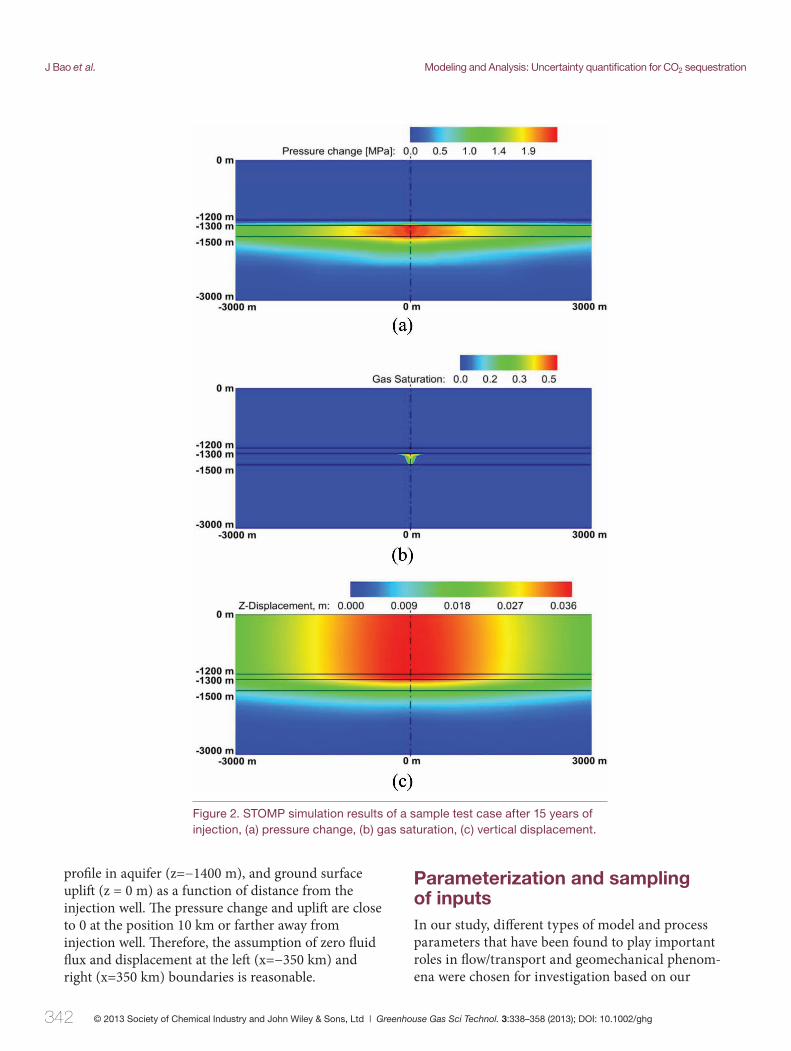
A vertical hydrostatic pressure gradient of 9.79 × 10–3 MPa m–1 was assumed along the z direction. Because the left and right boundaries are 350 km away from the injection well, it is assumed that there is no fl ow and displacement at these boundaries. Th e upper boundary was no fl ow for the liquid phase but had a constant pressure boundary of 0.101325 MPa (atmo-spheric pressure) for the gas phase. Approximately 2300 structured rectangular meshes with refi nement near the injection well, reservoir, and caprock were applied for the numerical simulator. Figure 2 shows the simulation results of pressure change, gas satura-tion, and vertical displacement for a sample test case aft er 15 years of injection. Th e parameter values of this particular test case are: initial reservoir porosity = 0.175, Log10 initial reservoir permeability = −13.5 log10(m2), initial reservoir entry pressure = 1.05 m–1, reservoir van Genuchten parameter (n) = 5.55, initial caprock porosity = 0.05, log10 initial caprock permeability = −18 log10(m2), initial caprock entry pressure = 0.265 m–1, caprock van Genuchten parameter (n) = 5.55, injection rate = 0.75 MMT year–1

(0.0034 kg s–1), reservoir Young’s modulus = 25 GPa, reservoir Poisson ratio=0.225, caprock Young’s modu-lus = 27 GPa, and caprock Poisson ratio=0.185. Figure 3(a) shows that both the injection point pres-sure and ground surface uplift increase with time of injection. Figure 3(b) shows the pressure change

Figure 1. Simulation domain for CO2 sequestration.



profi le in aquifer (z=−1400 m), and ground surface uplift (z = 0 m) as a function of distance from the injection well. Th e pressure change and uplift are close to 0 at the position 10 km or farther away from injection well. Th erefore, the assumption of zero fl uid fl ux and displacement at the left (x=−350 km) and right (x=350 km) boundaries is reasonable.

Parameterization and sampling of inputsIn our study, diff erent types of model and process parameters that have been found to play important roles in fl ow/transport and geomechanical phenom-ena were chosen for investigation based on our

Figure 2. STOMP simulation results of a sample test case after 15 years of injection, (a) pressure change, (b) gas saturation, (c) vertical displacement.



extreme cases in which the geomechanical deforma-tions were in unreasonable ranges during the injec-tion period.

Samples should be generated to consider all possi-bilities within the parametric space without introduc-ing undesired bias. However, as the model’s parameter dimensionality increases, the number of samples required for a systematic approach to adequately cover the parametric space becomes unreasonable without effi cient sampling methods. Quasi-Monte Carlo methods have become increasingly popular over the last two decades because of their faster convergence

previous studies.38–40 Th ese include 13 hydrological, mechanical, and elastic parameters that possibly aff ect the geomechanical responses. Th e parameters and their sampling ranges are listed in Table 1.39,41–47 Because STOMP calculates the changes of rock porosity, and permeability during geomechanical stress changes, we treated only the initial value of each property as an input parameter that represents the property prior to CO2 injection. Some previous studies indicate wider ranges of the aquifer porosity and permeability for diff erent geological formations39, but we considered slightly narrower ranges to avoid

Figure 3. Simulation results of sample test case, (a) injection point pressure and ground surface uplift at injection well evolution as a function of time of injection, (b) pressure in aquifer and ground surface uplift as a function of distance from injection well.



and eff ective sampling of high-dimensional paramet-ric space without clumping and gaps.39, 48 In our study, the quasi-Monte Carlo samples were generated from an existing scrambled Sobol sequences49 ranged from 0 to 1, which were scaled to the actual input parameter ranges as listed in Table 1. In QMC sam-pling we are able to get a series of samples with

controlled deterministic inputs instead of random ones, and thus alleviate the clumping issue of the Monte Carlo methods. Th e well-dispersed QMC samples enable more effi cient exploration of multidi-mensional parameter spaces than regular Monte Carlo and Latin hypercube sampling. Figure 4 shows the comparison of pseudorandom (regular Monte Carlo) sampling versus quasi-random sampling (quasi-Monte Carlo) for two fi ctitious variables from a multivariate uniform distribution. In Fig. 4, pseudo-random method causes clumping and gap of samples, but the quasi-random method alleviates these prob-lems, and the samples are well dispersed. Th e number of quasi-Monte Carlo samples is normally a power of 2 (and a new set of samples are designed to be supple-mentary to the existing ones) and is usually chosen as a trade-off between computational time and numeri-cal accuracy. Because STOMP is a parallel computa-tion simulator, each test case was run on 8 cores/threads, and the simulation can be completed in 10 to 30 min. For developing reliable responses between output and input parameters, 512, 1024, and 2048 samplings were used for response surface convergence tests. Th e coeffi cients of response surface that calcu-lated from the fi rst 512 or 1024 simulation cases results are very close to the coeffi cients generated from the whole 2048 simulation cases results. Th ere-fore, we assumed that for the 13-dimensional param-eter space, 2048 samples were adequate to yield a

Table 1. 13 input parameters and their sampling ranges.

Initial reservoir porosity 0.05–0.3039

Log10 initial reservoir permeability –15 to –12 (log10(m2))39

Initial reservoir entry pressure 0.1–2.0 (m–1)41

Reservoir van Genuchten parameter (n)

1.1–1041

Initial caprock porosity 0.0–0.139

Log10 initial caprock permeability –20 to –16 (m2)39

Initial caprock entry pressure 0.003–0.05 (m–1)43

Caprock van Genuchten parameter (n)

1.1–1041

Injection rate 0.01–1.5(MMT yr–1) or 4.5 × 10–5–0.0068 (kg s–1)

Reservoir Young’s modulus 10–40 (GPa)44, 45

Reservoir Poisson ratio 0.05–0.446

Caprock Young’s modulus 4–50 (GPa)47

Caprock Poisson ratio 0.05–0.3246

Figure 4. Comparison of pseudorandom (regular Monte Carlo) sampling (left) versus quasi-random sampling (right).



reliable analysis. Th e paired scatter plot of the 13 independent parameters can be used to show the sampling points, in which the sampling points in the 13-dimensional parameter space are projected onto a paired two-dimensional plane. Among the scatter plots between the 13 input parameters, we show a subset of the paired scatter plots for selected input parameters, including initial reservoir porosity, log10 initial reservoir permeability, injection rate, and reservoir Young’s modulus in Fig. 5. Th ere is no replicated value for any input parameters among the 2048 samplings, and the sampling points are uni-formly scattered in the parameter space.

Regarding the output response variables, we focused on the maximum pressure (pressure increase at the

injection well) and the vertical ground surface dis-placement (uplift ) at the injection well. Th e maximum pressure is an important indicator of the safety and sustainability of the injection. Top surface/ground surface displacements are critical information that can be used to infer the potential hazard caused by CO2 sequestration activities and can be measured and monitored in the actual site using the GPS or SAR.

Sensitivity analysisTo identify the sensitivity of each input variable, we employed generalized cross-validation (GCV) based on the MARS, the analysis of variance (ANOVA) method, which uses the value of the residual of

Figure 5. Paired scatterplot of quasi-Monte Carlo sampling points of input parameters.



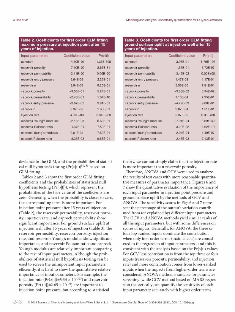
deviance in the GLM, and the probabilities of statisti-cal null hypothesis testing (Pr(>|t|))50, 51 based on GLM fi tting.

Tables 2 and 3 show the fi rst order GLM fi tting coeffi cients and the probabilities of statistical null hypothesis testing (Pr(>|t|)), which represent the probabilities of the true value of the coeffi cients are zero. Generally, when the probability is closer to zero, the corresponding term is more important. For injection point pressure aft er 15 years of injection (Table 2), the reservoir permeability, reservoir poros-ity, injection rate, and caprock permeability show signifi cant importance. For ground surface uplift at injection well aft er 15 years of injection (Table 3), the reservoir permeability, reservoir porosity, injection rate, and reservoir Young’s modulus show signifi cant importance, and reservoir Poisson ratio and caprock Young’s modulus are relatively important comparing to the rest of input parameters. Although the prob-abilities of statistical null hypothesis testing can be used to screen the unimportant input parameters effi ciently, it is hard to show the quantitative relative importance of input parameters. For example, the injection rate (Pr(>|t|)=5.34 × 10–263) and reservoir porosity (Pr(>|t|)=2.65 × 10–31) are important to injection point pressure, but according to statistical

theory, we cannot simply claim that the injection rate is more important than reservoir porosity.

Th erefore, ANOVA and GCV were used to analyze the results of test cases with more reasonable quantita-tive measures of parameter importance. Figures 6 and 7 show the quantitative evaluation of the importance of each input parameter in injection point pressure and ground surface uplift by the methods of GCV and ANOVA. Th e sensitivity scores in Figs 6 and 7 repre-sent the percentage of the output’s variation contrib-uted from (or explained by) diff erent input parameters. Th e GCV and ANOVA methods yield similar ranks of all the input parameters, but with some diff erences on scores of inputs. Generally, for ANOVA, the three or four top-ranked inputs dominate the contribution when only fi rst-order terms (main eff ects) are consid-ered in the regression of input parameters , and this is consistent with the analysis based on the Pr(>|t|) values. For GCV, less contribution is from the top three or four inputs (reservoir porosity, permeability, and injection rate) and more contribution comes from lower-ranked inputs when the impacts from higher-order terms are considered. ANOVA method is suitable for parameter screening, while GCV method based on MARS regres-sion theoretically can quantify the sensitivity of each input parameter accurately with higher order terms

Table 2. Coeffi cients for fi rst order GLM fi tting maximum pressure at injection point after 15 years of injection.

Input parameters Coeffi cient value Pr(>|t|)

constant –4.50E+01 1.36E-305

reservoir porosity –7.10E+00 2.65E-31

reservoir permeability –3.11E+00 0.00E+00

reservoir entry pressure 9.64E-02 2.22E-01

reservoir n 3.84E-03 8.20E-01

caprock porosity –9.56E-01 5.24E-01

caprock permeability –2.40E-01 1.84E-10

caprock entry pressure –3.67E-02 9.91E-01

caprock n 2.37E-02 1.60E-01

injection rate 4.07E+00 5.34E-263

reservoir Young’s modulus –2.18E-03 6.63E-01

reservoir Poisson ratio –1.37E-01 7.50E-01

caprock Young’s modulus 9.01E-04 7.82E-01

caprock Poisson ratio –8.33E-03 9.88E-01

Table 3. Coeffi cients for fi rst order GLM fi tting ground surface uplift at injection well after 15 years of injection.

Input parameters Coeffi cient value Pr(>|t|)

constant –3.98E-01 8.79E-195

reservoir porosity –1.57E-01 6.72E-97

reservoir permeability –3.42E-02 0.00E+00

reservoir entry pressure 1.47E-03 1.17E-01

reservoir n 5.56E-05 7.81E-01

caprock porosity –3.36E-02 5.94E-02

caprock permeability 1.16E-04 7.95E-01

caprock entry pressure –4.79E-03 9.00E-01

caprock n 2.87E-04 1.51E-01

injection rate 5.97E-02 0.00E+00

reservoir Young’s modulus –7.94E-04 3.69E-39

reservoir Poisson ratio –3.22E-02 3.02E-10

caprock Young’s modulus –2.04E-04 1.49E-07

caprock Poisson ratio –2.43E-03 7.13E-01



and interaction eff ects of input parameters considered. However, because the diff erence of sensitivity between input parameters are narrowed with the interaction terms of input parameters in MARS regression, it is not straightforward to use GCV for parameter screening.

Figure 8 shows the boxplots52–54 between the injec-tion point pressure and the top four important input parameters aft er 15 years of injection. Th e pressure

decreases with increase of reservoir permeability, and increases with injection rate, which is expected. Th e 3rd and 4th rank input parameters (reservoir porosity or caprock permeability) do not seem to have obvious relationships with pressure. Th e sensitivity score from ANOVA based on fi rst order GLM is consistent with such a qualitative observation from Fig. 8. Figure 9 shows the boxplots between the ground surface uplift

Figure 6. Sensitivity score of input parameters for injection point pressure after 15 years of injection.

Figure 7. Sensitivity score of the input parameters for ground surface uplift after 15 years of injection.



and the top four important input parameters aft er 15 years of injection. Similar to the pressure, the uplift decreases with increase of reservoir permeability, and increases with injection rate. Th e relationships be-tween uplift and reservoir porosity or reservoir Young’s modulus are weak if we focus on the medium value in the boxplot, which is more consistent with the sensitivity score from ANOVA based on fi rst order GLM. However, if we considering the 3rd quarter

value (the value at the upper edge of rectangular box in the boxplot), maximum value (the value at the upper horizontal bar in the boxplot), or the outliers (the value at the points higher than the upper hori-zontal bar in the boxplot), the relationships between the uplift and the 3rd and 4th rank input parameters are clearer from qualitative observations from the boxplots, which corresponds better to the sensitivity score from GCV analysis based on MARS regression.

Figure 8. Boxplots between injection point pressure and top four important input parameters after 15 years of injection.



Th erefore, in this study, both ANOVA and GCV analysis can off er reasonable sensitivity analysis.

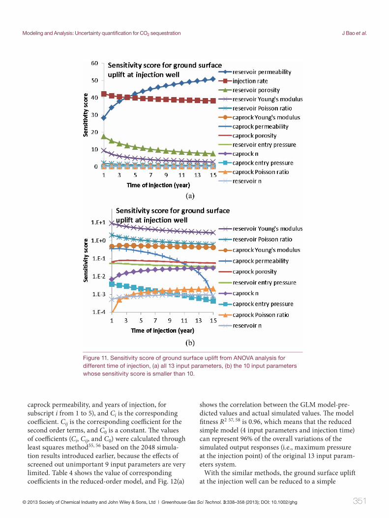
Additionally, the sensitivities of input parameters change with time of injection. Figures 10(a) and 11(a) show the sensitivity scores from ANOVA as a func-tion of time of injection for all the 13 input param-eters. Figures 10(b) and 11(b) shows the sensitivity scores of the input parameters whose sensitivity score

is smaller than 10, and the vertical axis (sensitivity score) is plotted in logarithmic scale for clear view. For injection point pressure, the importance of reservoir permeability decrease with time of injection, while the importance of injection rate increases. For ground surface uplift , the importance of reservoir permeability increases with time of injection, while the importance of injection rate decreases with time.

Figure 9. Boxplots between ground surface vertical displacement and top four important input parameters after 15 years of injection.



Near the beginning of injection, the injection rate is more important than permeability; aft er four years of injection, the importance of permeability gradually exceeds injection rate.

Reduced-order model and response surfaceWith the sensitivity analysis explained earlier, the top four important input parameters were selected to build the reduced-order model. Because the reduced-

order model was designed to be able to predict the output response at diff erent time of injection, time was treated as the 5th input parameter in the reduced-order model. For injection point pressure, the second order GLM regression model can be expressed as:

pressure C I I Ci ij

ij i jI= ∑ ∑C I Ci iI +C IiI 0

(3)

In Eqn (3), Ii is the input parameter (reservoir permeability, injection rate, reservoir porosity,

Figure 10. Sensitivity score of injection point pressure from ANOVA analysis for different time of injection, (a) all 13 input parameters, (b) the 11 input parameters whose sensitivity score is smaller than 10.



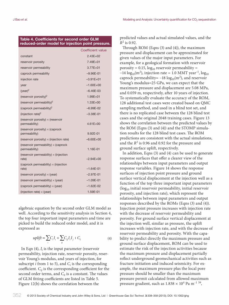
caprock permeability, and years of injection, for subscript i from 1 to 5), and Ci is the corresponding coeffi cient. Cij is the corresponding coeffi cient for the second order terms, and C0 is a constant. Th e values of coeffi cients (Ci, Cij, and C0) were calculated through least squares method55, 56 based on the 2048 simula-tion results introduced earlier, because the eff ects of screened out unimportant 9 input parameters are very limited. Table 4 shows the value of corresponding coeffi cients in the reduced-order model, and Fig. 12(a)

shows the correlation between the GLM model-pre-dicted values and actual simulated values. Th e model fi tness R2 57, 58 is 0.96, which means that the reduced simple model (4 input parameters and injection time) can represent 96% of the overall variations of the simulated output responses (i.e., maximum pressure at the injection point) of the original 13 input param-eters system.

With the similar methods, the ground surface uplift at the injection well can be reduced to a simple

Figure 11. Sensitivity score of ground surface uplift from ANOVA analysis for different time of injection, (a) all 13 input parameters, (b) the 10 input parameters whose sensitivity score is smaller than 10.



algebraic equation by the second order GLM model as well. According to the sensitivity analysis in Section 4, the top four important input parameters and time are picked to build the reduced order model, and it is expressed as

uplifti C I I Ci ij

ij i jI= ∑ ∑C I Ci iI +C IiI 0 (4)

In Eqn (4), Ii is the input parameter (reservoir permeability, injection rate, reservoir porosity, reser-voir Young’s modulus, and years of injection, for subscript i from 1 to 5), and Ci is the corresponding coeffi cient. Cij is the corresponding coeffi cient for the second order terms, and C0 is a constant. Th e values of GLM fi tting coeffi cients are listed in Table 5. Figure 12(b) shows the correlation between the

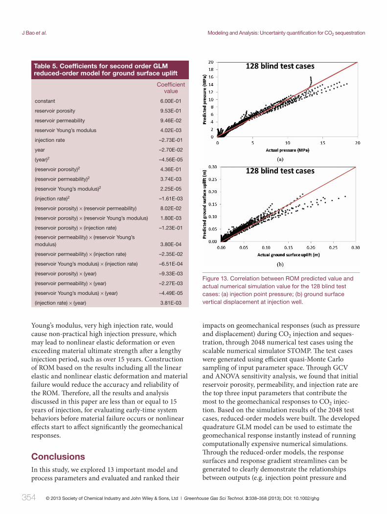
predicted values and actual simulated values, and the R2 is 0.92.

Th rough ROM (Eqns (3) and (4)), the maximum pressure and displacement can be approximated for given values of the major input parameters. For example, for a geological formation with reservoir porosity = 0.15, log10 reservoir permeability = −14 log10(m2), injection rate = 1.0 MMT year–1, log10 caprock permeability= −18 log10(m2), and reservoir Young’s modulus=25 GPa, we can expect that the maximum pressure and displacement are 5.08 MPa, and 0.059 m, respectively, aft er 10 years of injection. To systematically evaluate the accuracy of the ROM, 128 additional test cases were created based on QMC sampling method, and used in a blind test set, and there is no replicated case between the 128 blind test cases and the original 2048 training cases. Figure 13 shows the correlation between the predicted values by the ROM (Eqns (3) and (4)) and the STOMP simula-tion results for the 128 blind test cases. Th e ROM predictions are consistent with the actual simulations, and the R2 is 0.96 and 0.92 for the pressure and ground surface uplift , respectively.

In addition, Eqns (3) and (4) can be used to generate response surfaces that off er a clearer view of the relationships between input parameters and output response variables. Figure 14 shows the response surfaces of injection point pressure and ground surface vertical displacement at the injection well as a function of the top three important input parameters (log10 initial reservoir permeability, initial reservoir porosity, and injection rate), which represent the relationships between input parameters and output responses described by the ROMs (Eqns (3) and (4)). Injection point pressure increases with injection rate with the decrease of reservoir permeability and porosity. For ground surface vertical displacement at the injection well, similar as pressure, the uplift increases with injection rate, and with the decrease of reservoir permeability and porosity. With the capa-bility to predict directly the maximum pressure and ground surface displacement, ROM can be used to estimate the risk of the injection activities because the maximum pressure and displacement partially refl ect underground geomechanical activities such as fracture initiation and induced seismicity. For ex-ample, the maximum pressure plus the local pore pressure should be smaller than the maximum pressure permit calculated from allowed maximum pressure gradient, such as 1.838 × 104 Pa m–1 59,

Table 4. Coeffi cients for second order GLM reduced-order model for injection point pressure.

Coeffi cient value

constant 2.43E+02

reservoir porosity 7.49E+01

reservoir permeability 3.77E+01

caprock permeability –9.96E-01

injection rate –3.91E+01

year –1.60E+00

(year)2 –6.46E-03

(reservoir porosity)2 1.99E+01

(reservoir permeability)2 1.33E+00

(caprock permeability)2 –6.99E-02

(injection rate)2 –3.38E-01

(reservoir porosity) × (reservoir permeability) 4.61E+00

(reservoir porosity) × (caprock permeability) 9.92E-01

(reservoir porosity) × (injection rate) –6.60E+00

(reservoir permeability) × (caprock permeability) 1.16E-01

(reservoir permeability) × (injection rate) –2.94E+00

(caprock permeability) × (injection rate) –1.64E-01

(reservoir porosity) × (year) –2.97E-01

(reservoir permeability) × (year) –1.09E-01

(caprock permeability) × (year) –1.62E-02

(injection rate) × (year) 1.59E-01



2.298 × 104 Pa m–1 60, or 1.562 × 104 Pa m–1 61; otherwise, the risk of initiation of fracture or seismic activity would increase signifi cantly.

Figure 15 shows the streamline of gradient of the pressure and displacement. Th e direction of the streamline represents the sensitivity of outputs to inputs. When the streamline is more parallel to the axis (input), the output is more sensitive to the input. Th e color of the streamline is the magnitude of the gradient, which represents how much output can be varied per unit of input changes. For the injection point pressure, the reservoir permeability plays an important role, which is consistent with the ANOVA

and GCV evaluation results in Section 4. For ground surface vertical displacement at the injection well, reservoir permeability dominates the contribution, which is consistent with our earlier analysis.

Th e ROM (Eqns and ) can be used only in the range of the input parameters’ designed ranges as listed in Table 1. To make the ROM usable in a variety of situations, the ranges of input parameters are oft en chosen as wide as possible to cover all the possible values of subsurface environment properties. How-ever, some combination of the input parameters, such as very low reservoir permeability, porosity and

Figure 12. Correlation between ROM predicted value and actual numerical simulation value for the 2048 training cases: (a) injection point pressure; (b) ground surface vertical displacement at injection well.



Young’s modulus, very high injection rate, would cause non-practical high injection pressure, which may lead to nonlinear elastic deformation or even exceeding material ultimate strength aft er a lengthy injection period, such as over 15 years. Construction of ROM based on the results including all the linear elastic and nonlinear elastic deformation and material failure would reduce the accuracy and reliability of the ROM. Th erefore, all the results and analysis discussed in this paper are less than or equal to 15 years of injection, for evaluating early-time system behaviors before material failure occurs or nonlinear eff ects start to aff ect signifi cantly the geomechanical responses.

ConclusionsIn this study, we explored 13 important model and process parameters and evaluated and ranked their

impacts on geomechanical responses (such as pressure and displacement) during CO2 injection and seques-tration, through 2048 numerical test cases using the scalable numerical simulator STOMP. Th e test cases were generated using effi cient quasi-Monte Carlo sampling of input parameter space. Th rough GCV and ANOVA sensitivity analysis, we found that initial reservoir porosity, permeability, and injection rate are the top three input parameters that contribute the most to the geomechanical responses to CO2 injec-tion. Based on the simulation results of the 2048 test cases, reduced-order models were built. Th e developed quadrature GLM model can be used to estimate the geomechanical response instantly instead of running computationally expensive numerical simulations. Th rough the reduced-order models, the response surfaces and response gradient streamlines can be generated to clearly demonstrate the relationships between outputs (e.g. injection point pressure and

Figure 13. Correlation between ROM predicted value and actual numerical simulation value for the 128 blind test cases: (a) injection point pressure; (b) ground surface vertical displacement at injection well.

Table 5. Coeffi cients for second order GLM reduced-order model for ground surface uplift

Coeffi cient value

constant 6.00E-01

reservoir porosity 9.53E-01

reservoir permeability 9.46E-02

reservoir Young’s modulus 4.02E-03

injection rate –2.73E-01

year –2.70E-02

(year)2 –4.56E-05

(reservoir porosity)2 4.36E-01

(reservoir permeability)2 3.74E-03

(reservoir Young’s modulus)2 2.25E-05

(injection rate)2 –1.61E-03

(reservoir porosity) × (reservoir permeability) 8.02E-02

(reservoir porosity) × (reservoir Young’s modulus) 1.80E-03

(reservoir porosity) × (injection rate) –1.23E-01

(reservoir permeability) × (reservoir Young’s modulus) 3.80E-04

(reservoir permeability) × (injection rate) –2.35E-02

(reservoir Young’s modulus) × (injection rate) –6.51E-04

(reservoir porosity) × (year) –9.33E-03

(reservoir permeability) × (year) –2.27E-03

(reservoir Young’s modulus) × (year) –4.49E-05

(injection rate) × (year) 3.81E-03



ground surface vertical displacement at the injection well) and input parameters, such as the initial reser-voir porosity, permeability, and injection rate.

AcknowledgementsTh is research has been accomplished and funded through the Pacifi c Northwest National Laboratory (PNNL) Carbon Sequestration Initiative, which is part of the Laboratory Directed Research and Develop-ment Program. A portion of this research was per-formed using the resources of the PNNL Institutional

Figure 14. Response surfaces: (a) injection point pressure after 5 years of injection; (b) ground surface displacement at injection well after 5 years of injection.

Figure 15. Streamline of response surface gradient: (a) injection point pressure after 5 years of injection; (b) ground surface displacement at injection well after 5 years of injection.

Computing program. PNNL is operated by Battelle for the US Department of Energy under Contract DE-AC05-76RL01830.

References 1. Intergovernmental Panel on Climate Change (IPCC), Special

Report on Carbon Dioxide Capture and Storage, Technical



Report prepared by Working Group III. Cambridge University Press, New York (2005).

2. EIA, Emission of Greenhouse Gases in the United States: 2009, Brochure No. DOE/EIA-0573. Energy Information Administration, US Department of Energy, Washington, DC (2011).

3. Nordbotten JM and Celia MA, Similarity solutions for fl uid injection into confi ned aquifers. J Fluid Mech 561:307–327 (2006).

4. Vilarrasa V, Olivella S and Carrera J, Geomechanical stability of the caprock during CO2 sequestration in deep saline aquifers. Energ Procedia 4:5306–5313 (2011).

5. Rutqvist J, Vasco DW and Myer L, Coupled reservoir-geome-chanical analysis of CO2 injection at In Salah, Algeria. Energ Procedia 1(1):1847–1854 (2009).

6. Spycher N, Pruess K and Ennis-King J, CO2-H2O mixtures in the geological sequestration of CO2. I. Assessment and calculation of mutual solubilities from 12 to 100°C and up to 600 bar. Geochim Cosmochim Ac 67:3015–3031 (2003).

7. Celia MA and Nordbotten JM, How simple can we make models for CO2 injection, migration, and leakage? Energ Procedia 4:3857–3864 (2010).

8. Pruess K, Garcia J, Kovscek T, Oldenburg C, Rutqvist J, Steefel C et al., Code intercomparison builds confi dence in numerical simulation models for geologic disposal of CO2. Energy 29:1431–1444 (2004).

9. Colesanti C and Wasowski J, Satellite sar interferometry for wide-area slope hazard detection and site-specifi c monitoring of slow landslides. International Landslid Symposium, Rio de Janeiro, Brazil, pp. 1–6 (2004).

10. Ma F, Zhao H, Zhang Y, Guo J, Wei A, Wu Z et al., GPS monitoring and analysis of ground movement and deforma-tion induced by transition from open-pit to underground mining. J Rock Mech Geotech Eng 4(1):82–87 (2012).

11. Nikolaidis RM, Bock Y, Jonge PJd, Shearer P, Agnew DC and Domselaar MV, Seismic wave observations with the global positioning system. J Geophys Res 106:21897–21916 (2001).

12. Pan W, Bao J, Lo C, Lai K, Agarwal K, Koeppel BJ et al., A general approach to develop reduced order models for simulation of solid oxide fuel cell stacks. J Power Sources 232:139–151 (2013).

13. Burkardt J, Du Q, Gunzburger M and Lee HC (eds), Reduced Order Modeling of Complex Systems. NA03, Dundee (2003).

14. Amsallem D and Farhat C, Interpolation method for the adaptation of reduced-order models to parameter changes and its application to aeroelasticity. AIAA J 46:1803–1813 (2008).

15. Box GEP, Some theorems on quadratic forms applied in the study of analysis of variance problems, I. Effect of inequality of variance in the one-way classifi cation. Ann Math Stat 25(2):290–302 (1954).

16. Anscombe FJ, The validity of comparative experiments. J Roy Statist Soc Series A 111:181–211 (1948).

17. McCullagh P and Nelder J, Generalized Linear Models, 2nd Edn. Chapman and Hall/CRC, Boca Raton, FL (1989).

18. Chambers JM and Hastie TJ, Statistical Models in S. Chapman and Hall/CRC, Boca Raton, FL (1992).

19. Friedman JH, Fitting functions to noisy data in high dimen-sions. Twentieth Symposium on the Interface, ed. by Wegman EJ, Gantz DT and Miller JJ. American Statistical Association, Alexandria (1988).

20. Friedman JH, Multivariate Adaptive Regression Splines. Ann Stat 19:140–141 (1991).

21. Friedman JH, Multivariate Adaptive Regression Splines. Ann Stat 19:1–67 (1991).

22. Friedman JH, Fast MARS, Technical Report LCS110. Stanford University, Stanford, CA (1993).

23. Friedman JH and Silverman BW, Flexible parsimonious smoothing and additive modeling, CA Report SLAC-PUB-4390. Stanford Linear Accelerator, Stanford University, Stanford, CA (1987).

24. Friedman JH, Estimating functions of mixed ordinal and categorical variables using adaptive splines, Tech. Report LCS108. Department of Statistics, Stanford University, Stanford, CA (1991).

25. Drucker H, Burges CJC, Kaufman L, Smola AJ and Vapnik VN, Advances in Neural Information Processing Systems 9 (NIPS). MIT Press, Cambridge, MA, pp. 155–161 (1996).

26. Smola AJ and Scholkopf B, A tutorial on support vector regression. Stat Comput 14:199–222 (2004).

27. Tong C, PSUADE User’s Manual. Lawrence Livermore National Laboratory, Livermore, CA (2009).

28. Williams CKI, Prediction With Gaussian Processes: From Linear Regression to Linear Prediction and Beyond, in Learning and Inference in Graphical Models, ed. by Jordan, MI. Kluwer, UK, pp. 599–621 (1997).

29. Mehrotra K, Mohan CK and Ranka S, Elements of Artifi cial Neural Networks. Institute of Technology, Massachusetts (2000).

30. White MD and Oostrom M, STOMP Subsurface Transport over Multiple Phases Version 4.0, PNNL-15782. Pacifi c Northwest National Laboratory, Richland, Washington (2006).

31. Kawai T, New element models in discrete structural analysis. Japan Soc Naval Arch 141:174–180 (1977).

32. Fang Y, Nguyen BN, Carroll K, Xu Z, Yabusaki SB, Scheibe TD et al., Development of a coupled thermo-hydro-mechani-cal model in discontinuous media for carbon sequestration. Int J Rock Mech Mining Sci 62:138–147 (2013).

33. Davies JP and Davies DK, Stress-dependent permeability: Characterization and modeling. Soc Petrol Eng J 6(2):224–235 (2001).

34. Liu H and Rutqvist J, A new coal permeability model: Internal swelling stress and fracture-matrix interaction. Transport Porous Med 82:157–171 (2010).

35. Rutqvist J and Tsang C-F, A study of caprock hydromechani-cal changes associated with CO2 injection into a brine formation. Environ Geol 42:296–305 (2002).

36. Rutqvist J, The geomechanics of CO2 storage in deep sedimentry formations. Geotech Geol Eng 30:525–551 (2012).

37. Rutqvist J, Vasco DW and LMyer L, Coupled reservoir-geo-mechanical analysis of CO2 injection and ground deforma-tions at In Salah, Algeria. Int J Greenhouse Gas Control 4:225–230 (2010).

38. Bao J, Xu Z, Lin G and Fang Y, Evaluating the impact of aquifer layer properties on geo-mechanical response during CO2 geological sequestration. Comput Geosci 54:28–37 (2013).

39. Hou Z, Rockhold ML and Murray CJ, Evaluating the impact of caprock and reservoir properties on potential risk of CO2 leakage after injection. Environ Earth Sci 66(8):2403–2415 (2012).

40. Hou Z, Engel D, Lin G, Fang Y and Fang Z, An uncertainty quantifi cation framework for studying the effect of spatial



heterogeneity in reservoir permeability on CO2 sequestration. Math Geosci MAY:1–19 (2013).

41. van Genuchten MT, A closed-form equation for redicting the hydraulic conductivity of unsaturated soils. Soil Sci Soc Am J 44(5):892–898 (1980).

42. Wilson GV, Jardine PM, Luxmoore RJ, Zelazny LW, Todd DE and Lietzke DA, Hydrogeochemical processes controlling subsurface transport from an upper subcatchment of Walker Branch Watershe during storm events, 2, Solute transport processes. J Hydol 123(3/4):317–336 (1991).

43. Zhou Q, Birkholzer JT, Tsang C-F and Rutqvist J, A method for quick assessment of CO2 storage capacity in closed and semi-closed saline formations. Int J Greenhouse Gas Cont 2:626–639 (2008).

44. Hart DJ and Wang HF, Laboratory measurements of a complete set of poroelastic moduli for Berea sandstone and Indiana limestone. J Geophys Res 100:17741–17751 (1995).

45. Palmstrom A and Singh R, The deformation modulus of rock masses - comparisons between in situtests and indirect estimates. Tunn Undergr Sp Tech 16(3):115–131 (2001).

46. Gercek H, Poisson’s ratio values for rocks. Int J Rock Mech Min 44:1–13 (2007).

47. Eseme E, Littke R, Krooss BM and Schwartzbauer J, Experimental investigation of the compositional variation of petroleum during primary migration. Org Geochem 38(8):1373–1397 (2007).

48. Tarantola A, Inverse Problem Theory and Model Parameter Estimation. Society for Industrial and Applied Mathematics, Philadelpia, PA (2005).

49. Bratley P and Fox BL, Algorithm 659: Implementing sobol’s quasirandom sequence generator. ACM T Math Software 14:88–100 (1988).

50. Berger RL and Casella G, Statistical Inference. Duxbury Press, Pacifi c Grove, CA (2001).

51. Fisher RA, Statistical Methods for Research Workers. Oliver and Boyd, Edinburgh (1925).

52. Tukey JW, Exploratory Data Analysis. Addison-Wesley, Boston, Mass. (1977).

53. Benjamini Y, Opening the box of a boxplot. Am Stat 42:257–262 (1988).

54. Rousseeuw PJ, Ruts I and Tukey JW, The Bagplot: A Bivariate Boxplot. Am Stat 53:382–387 (1999).

55. Rao CR, Toutenburg H, Fieger A, Heumann C, Nittner T and Scheid S, Linear Models: Least Squares and Alternatives. Springer Series in Statistics: Springer, New York, NY (1999).

56. Björck Å, Numerical Methods for Least Squares Problems. Society for Industrial and Applied Mathematics, Philadelphia, PA (1996).

57. Steel RGD and Torrie JH, Principles and Procedures of Statistics. McGraw-Hill, New York (1960).

58. Cameron AC and Windmeijer FAG, An R-squared measure of goodness of fi t for some common nonlinear regression models. J Econometrics 77:329–342 (1997).

59. EPA, Determination of maximum injection pressure for Class I wells, in Underground Injection Control Section Regional Guidance #7. [Online]. Water Division USEPAR, Chicago, IL (1994). Available at: http://www.epa.gov/r5water/uic/r5guid/r5_07.htm. [29 March 2011]

60. Leetaru HE, Morse DG, Bauer R, Frailey S, Keefer D, Kolata D et al., Saline reservoirs as a sequestration target, in An Assessment of Geological Carbon Sequestration Options in

the Illinois Basin, Final Report for U.S. DOE Contract: DE-FC26-03NT41994, Principal Investigator: Robert Finley, pp. 253–324 (2005).

61. FutureGen, Project Final Environmental Impact Statement (DOE/EIS-0394) [Online]. Washington, DC (2006). Available at: http://www.netl.doe.gov/technologies/coalpower/futuregen/eis/ [30 July 2013].

Dr Guang Lin

Dr Guang Lin is a staff scientist in Computational Mathematics Group at Pacifi c Northwest National Laboratory. His research focuses on uncertainty quantifi cation and multiscale modeling of complex systems. He holds a PhD from the Division of Applied Math-ematics at Brown University (2007).

Ms Huiying Ren

Ms Huiying Ren is a research associ-ate at Hydrology Group, Earth Systems Science Division, Pacifi c Northwest National Laboratory (PNNL). Her research fi elds at PNNL are analysis of acoustic, marine mammal passive acoustic system and Uncertainty Quantifi cation (UQ) of

CO2 sequestration. She received her BEng and BA from Dalian University of Technology, Dalian, China in 2008. She joined Wright State University since then and received her MSc in Mechanical and Materials Depart-ment from Wright State University in 2010. Her master study was fl uid dynamic that focused on experimental study of turbulent fl ow and macro air vehicles (MAV) using particle image velocimetry (PIV) devices.

Dr Jie Bao

Dr Jie Bao is an engineer in Experi-mental and Computational Engineer-ing Group at Pacifi c Northwest National Laboratory. He has expertise in numerical simulation for turbulent fl ow, multiphase fl ow, and porous media fl ow. His research focuses on lattice Boltzmann method, fi nite

element method, massive parallel computation, GPU computing, UQ, and solving problems related to waste tank management, carbon sequestration, and fl ow battery. He holds a PhD from the Mechanical Engineer-ing and Materials Science Department at University of Pittsburgh (2010).



Dr Yilin Fang

Dr Yilin Fang is a staff scientist in Hydrology Group at Pacifi c Northwest National Laboratory. Her research focuses on subsurface multiphase fl ow and reactive transport, geome-chanics, high performance parallel computing, carbon sequestration, and biogeochemistry in land surface

model. She holds a PhD from the Civil and Environmen-tal Engineering Department at the Pennsylvania State University (2003).

Dr Zhangshuan Hou

Dr Zhangshuan Hou has expertise in Applied Statistics, Hydrogeology, Geophysics, and Atmospheric Sciences. His research focuses on EDA, UQ, and inversion approaches, solving problems related to carbon sequestration, oil/gas exploration, environmental remediation, climate

change, and power systems.

Documents

Uncertainty quantiﬁ cation for evaluating impacts of caprock and ...lin491/pub/GLIN-13-GHG.pdf · 12 other parameters describing hydrogeological properties of subsurface formations,