Uncertainty in the Movie Industry:Does Star Power Reduce the Terror of the Box Office?∗

Arthur De VanyDepartment of Economics

Institute for Mathematical Behavioral SciencesUniversity of California

Irvine, CA 92697USA

W. David WallsSchool of Economics and Finance

The University of Hong KongPokfulam Road

Hong Kong

Abstract

Everyone knows that the movie business is risky. But how riskyis it? Do strategies exist that reduce risk? We investigate these ques-tions using a sample of over 2000 motion pictures. We discover thatthe movies are very risky indeed. Box-office revenue dynamics are aLe’vy stable process and are asymptotically Pareto-distributed withinfinite variance. The mean is dominated by rare blockbuster moviesthat are located in the far right tail. There is no typical movie be-cause box office revenue outcomes do not converge to an average, theydiverge over all scales. Movies with stars in them have higher revenue

∗This paper was presented at the annual meeting of the American Economic Associa-tion, New York, January 1999. Walls received support from the Committee on Researchand Conference Grants of the University of Hong Kong. De Vany received support fromthe Private Enterprise Research Center of Texas A&M University.

1

expectations, but infinite variance. Only 19 stars have a positive cor-relation with the probability that a movie will be a hit. No star is“bankable” if bankers want sure things; they all carry significant risk.The highest grossing movies enjoy long runs and their total revenue isonly weakly associated with their opening revenue. Contrary to con-ventional wisdom in Hollywood, the top stars are female and a star ismore important in extending a movie’s run than in making it open.

We conclude: (1) The studio model of risk management lacks afoundation in theory or evidence and revenue forecasts have zero pre-cision. In other words, “Anything can happen.” (2) Movies are com-plex products and the cascade of information among film-goers duringthe course of a film’s run can evolve along so many paths that it isimpossible to attribute the success of a movie to individual causal fac-tors. In other words, “No one knows anything.” (3) The audiencemakes a movie a hit and no amount of “star power” or marketing canalter that. In other words, the real star is the movie.

2

“No one knows anything.” Screenwriter William Goldman (1983).

1 Introduction

Everyone knows that motion pictures are uncertain products. In this paper

we show that film makers must operate under such vague and uncertain

knowledge of the probabilities of outcomes that “no one knows anything.”

The essence of the movie business is this: The mean of box-office revenue is

dominated by a few “blockbuster” movies and the probability distribution

of box-office outcomes has infinite variance! The distribution of box-office

revenues is a member of the class of probability distributions known as Levy

stable distributions. These distributions are the limiting distributions of

sums of random variables and are appropriate for modeling the box-office

revenues that motion pictures earn during their theatrical runs.

Levy stable distributions have a “heavy” upper tail and may not have

a finite variance. Our parameter estimates of the asymptotic upper tail

index reveal that the variance of box-office revenue is in fact infinite: Motion

pictures are among the most risky of products. Theoretically, the skewed

shape of the Levy distribution means there is no natural scale or average

to which movie revenues converge. Movie revenues diverge over all possible

values of outcomes. One can forecast the mean of box-office revenue since

it exists and is finite, but the confidence interval of the forecast is without

bounds. The far-from-normal shape of the Levy probability distribution of

box-office revenue and its infinite variance are the sources of Hollywood’s

“terror of the box office.”

Our results explain heretofore puzzling aspects of the movie business.

The average of motion picture box office revenues depends almost entirely

on a few extreme revenue outcomes in the upper tail whose chances are ex-

tremely small. Success is tied to the extremal events, not the average; the

average is driven by the rare, extremal events. The mean and variance of

the distribution drift over time and do not converge or settle to an attractor.

3

Movie projects are, in reality, probability distributions and a proper assess-

ment of their prospects requires one to do a risk analysis of the probabilities

of extreme outcomes. The normal distribution is completely unsuited for

this kind of analysis because when outcomes are normally distributed, the

probability of extreme outcomes is vanishingly small. The movie business is

not “normal” because outcomes do not follow a normal probability distribu-

tion. The probability distribution is highly skewed with a “heavy” upper tail

with a theoretical variance far beyond the sample variance. Our estimates

of the theoretical Levy distribution permit calculation of the probability of

box-office revenues that have never before been realized.

There are no formulas for success in Hollywood. We find that much

conventional Hollywood wisdom is not valid. By making strategic choices

in booking screens, budgeting, and hiring producers, directors and actors

with marquee value, a studio can position a movie to improve its chances of

success. But, after a movie opens, the audience decides its fate. The exchange

of information among a large number of individuals interacting personally

unleashes a dynamic that is complex and unpredictable.1 Even a carefully

managed and expensive marketing program cannot direct the information

cascade; it is a complex stochastic process that can go anywhere.2

We conclude that the studio model of risk management lacks a foundation

in theory or evidence. Revenue forecasts have zero precision, which is just

a formal way of saying that “anything can happen.” Movies are complex

products and the cascade of information among film-goers during the course

of a film’s theatrical exhibition can evolve along so many paths that it is

impossible to attribute the success of a movie to individual causal factors.

In other words, as Goldman said, “No one knows anything.” The audience

makes a movie a hit and no amount of “star power” or marketing hype can

1See De Vany and Walls (1996) and De Vany (1997) for analyses of information dy-namics in the context of the motion picture industry.

2It may be possible to “steer” the information cascade, i.e. to affect the conditionalprobabilities of branching to different paths. This is a subject of ongoing research.

4

alter that.3 The real star is the movie.

2 Related Literature

Three strands of literature are relevant to our topic: one dealing with motion

pictures and uncertainty, one dealing with stars, and another dealing with

power law probability distributions.

2.1 Motion Picture Uncertainty

De Vany and Walls (1996) modeled the motion picture information cascade

as a Bose-Einstein statistical process and they argued that it converged on

a Pareto distribution; Walls (1997) and Lee (1998) replicated these findings

for another market and time period, respectively. In a rank tournament

model of the motion picture market, De Vany and Walls (1997) modeled

a film’s theatrical run as a stochastic survival process with a rising hazard

rate; Walls (1998) replicated these results for another market. De Vany and

Eckert (1991) portray motion pictures as a market organized to deal with

the problem that film makers “don’t know anything” and showed that the

studio system and block booking were adaptations to uncertainty.4 In a

related context, where outcomes are uncertain, Chisholm (1996, 1997) and

Weinstein (1998) examine the use of share contracts versus a fixed payment

contract for compensating stars.

2.2 Stars

Wallace, Seigerman, and Holbrook (1993) estimate regression models of the

relationship of actors and actresses to film rentals and associate stars with

3Industry analyst Art Murphy states this bluntly, “Films succeed or fail on their ownmerits. . . . Also, films of mass appeal are relatively impervious to ‘critics’. Films that aregoing to be popular are popular” (Dale, 1997, p. 4).

4Kenney and Klein (1983) and Blumenthal (1988) also examine block booking andblind bidding for motion pictures.

5

positive or negative residuals. Prag and Casavant (1994) also estimate film

rentals as a function of production cost, a measure of quality, and an index of

star power and find that these variables are significant only when advertising

costs are omitted. Ravid (1998) examines a signaling model of the role of

stars and estimates rental and profit equations, concluding that stars play

no role in the financial success of a film.

2.3 Pareto and Levy Distributions

Pareto (1897) found that income was distributed according to a power law

that was subsequently named after him. Atkinson and Harrison (1978) found

wealth to be Pareto distributed. Ijiri and Simon (1977) found the size distri-

bution of firms in the United States and in Britain to be Pareto distributed.

Levy showed that there is a class of distribution functions which follow the

asymptotic form of the law of Pareto which Mandelbrot defined as

1− FX(x) ∼ (x

k)−α x→∞ (1)

Such distributions are characterized by the fact that 0 < α < 2 and they

have infinite variance. The Levy is a generalization of the normal distribution

when the variance is infinite. Mandelbrot (1963) found that the distribution

of cotton price changes is approximated by the Levy distribution. Fama

(1963) described an information process (similar to Bose-Einstein informa-

tion updating) that could lead to a Levy stable distribution. Both S&P 500

stock index and NYSE composite index returns are well-fitted by a Levy

distribution (Mantegna and Stanly, 1995, and Soloman and Levy, 1998, re-

spectively). This paper adds motion pictures to the list of processes that

follow a Levy distribution.

3 Modeling Star Power

One has to be humble in approaching this subject—the movie business is

complicated and hard to understand. There are many reasons for this diffi-

6

culty: motion pictures are complex products that are difficult to make well;

no one knows they like a movie until they see it; movies are “one-off” unique

products; their “shelf life” is only a few weeks; movies enter and exit the

market on a continuing basis; movies compete against a changing cast of

competitors as they play out their theatrical “runs”; most movies have but

a week or two to capture the audience’s imagination; a rare handful have

“legs” and enjoy long runs; weekly box-office revenues are concentrated on

only three or four top ranking films; most movies lose money.

These characteristics of the business led us to model movies as stochastic

dynamic processes in our earlier work (De Vany and Walls, 1996 and 1997).

This work has convinced us that a fruitful way to model the movies is to treat

them as probability distributions. We model the distribution of probability

mass of movie outcomes on the outcome space and strive to uncover how

the mass is shifted when certain conditioning variables are changed.5 Among

the variables that we consider as potential probability-altering variables are

sequels, genres, ratings, stars, budgets, and opening screens. We also consider

individual stars and how much power they have to move the movie box-office

revenue probability distribution toward more favorable outcomes.

3.1 Modeling Probability Mass

Formally our strategy is to characterize the unconditional probability distri-

bution of movies, without qualification as to genre, stars or other variables

that may condition the distribution. Then we characterize the distribution

conditional on a list of choice variables that potentially alter the location of

the distribution’s probability mass. We consider the cumulative density func-

tion and the probability density functions in continuous and discrete form.

5We focus on the domestic North American theatrical market because revenues in thismarket are an important determinant of revenues in foreign markets, video, pay televisionand non-pay television as well as ancillary revenues from soundtracks, books, video games,theme parks, and other consumer products (Dale, 1997, p. 22; Cones, 1997, pp. 143–44).

7

Symbolically, we examine the conditional cumulative density function

F (x | ~Z) (2)

where x is a random variable, and ~Z is a vector of conditioning variables

on which F depends. We seek to find the form of F and the conditional

distribution of F with respect to ~Z. The random variable x will be box-office

revenue, profits, or some other variable of interest and the components of

the vector ~Z will be budgets, stars, sequels, ratings, and other variables that

might alter F . We follow a similar modeling strategy for the probability den-

sity function. We also rely on a discrete version of this model by estimating

the effects of changes in the conditioning variables on the quantiles of the

distribution or the probability of a specific event.

In our other work, we found that the dynamics of audiences and box-office

revenues follow a Bose-Einstein statistical process. It is known that the Bose-

Einstein allocation process has as its limit a power law and this holds for the

rank order statistics (Hill, 1975) and for the density function (Ijiri and Simon,

1977). Based on these considerations, we expect the probability distribution

of motion picture outcomes for extreme outcomes to follow a power law. The

Bose-Einstein information process is a stable process (see Fama (1963) on

stable information processes and De Vany (1997) on the stability of the Bose-

Einstein process), so we expect the distribution generated by a Bose-Einstein

process to be in the Levy stable class. In this class of distributions, only the

normal distribution has finite variance. Probability mass in the tail decays

as a power of x, x−α, in the power law but exponentially, e−x in the normal

distribution. Second and higher moments, therefore, may not converge for a

power distribution: Var(x) =∫x2f(x)dx =

∫x2x−αdx. If α < 2, the product

x2x−α diverges as x→∞.Analysis of the data further sharpens our expectation that a Levy stable

process is at work. As we show below, the mean is dominated by extreme

outcomes, which is characteristic of Levy stable processes. The sample vari-

ance is unstable and less than the theoretical variance, also indicators of a

8

Levy stable process. A further indicator of a stable process is our discovery

that the rank and frequency distributions are self-similar.

3.2 Risk and Survival Analysis

If, as we expect, the variance of the probability distribution of movie out-

comes is infinite, then it is not useful or even well-defined to rely on the

second moment to make probability-based judgments about movies. One

can, however, do risk and survival analyses. In a risk analysis, we consider

the probabilities that are attached to certain outcomes in the upper tail. This

is a well-defined exercise, even when the variance is infinite. In a survival

analysis, we consider the conditional probability that a movie will continue

to earn more, given that it already has earned a certain amount. This also

is well defined for the Levy distribution and the conditional probability of

continuation of a movie’s run can be calculated from the distribution func-

tion. These kinds of analyses require that we model quantiles, extremals, and

probability mass over motion picture outcomes rather than rely on traditional

measures like mean and variance.

The question then becomes this: How do stars, genre, release patterns, et

cetera, alter the quantiles, extremals, probability mass, and survival functions

of motion pictures? These are well-defined questions even for infinite variance

distributions, where mean-variance analysis fails. An example will make

this clear. Consider the cumulative distribution function and its associated

continuation function6 shown in Figures 1 and 2. In the first figure, the X

axis—the outcome space—corresponds to motion picture revenue outcomes

and the Y axis corresponds to the cumulative probability of all outcomes up

to each point in the outcome space. Once we identify the functional form

and parameters of the cumulative probability function, we can calculate the

probability of an outcome or set of outcomes. If, in addition, we are successful

in identifying how this function is shifted when movies have stars or different

6The continuation function is defined as f(x)/(1− F (x)).

9

release patterns and so on, then we can calculate how these decision variables

alter the probabilities of specific outcomes.

In fact, we do identify the conditional probability density functions of

movies with stars and without stars. These distributions are shown as the

solid and dashed lines in Figure 1. It is a simple matter to calculate the prob-

ability that a movie will earn box-office revenues equal to or greater than $50

million and then to further calculate how stars alter those probabilities. Using

the continuation function, we can also calculate the probability that a movie

will continue its run, given that it already has earned $50 million or $300

million, or any amount. The continuation function shown in Figure 2 is what

we find for movies with stars. The curve shows for every revenue outcome

the probability that the movie will continue to go forward to higher revenues,

conditional on it having earned some amount. Note that the continuation

probability declines very slowly, an indication of the infinite variance and

the power law decay in the upper tail. Using risk and continuation analyses

we can predict the probability of events never before experienced. The slow

decay of the continuation probability predicts unheard of successes like The

Full Monty or Titanic and shows that the probability of even more striking

successes does not vanish.

4 The Movie Data

4.1 Data Sources and Definitions

The data include 2,015 movies that were released in the closed interval 1984–

1996. Information on each movie’s box-office revenue, production cost, screen

counts by week, genre, rating, and artists were obtained from Entertainment

Data International’s historical database. The box-office revenue data include

weekly and weekend box-office revenues for the United States and Canada

compiled from distributor-reported figures. These data are the standard

industry source for published information on the motion pictures and are used

by such publications as Daily Variety and Weekly Variety , The Los Angeles

10

Times , The Hollywood Reporter , Screen International , and numerous other

newspapers, magazines, and electronic media.

Each actor, producer, or director appearing on Premier ’s annual listing

of the hundred most powerful people in Hollywood or on James Ulmer’s list

of A and A+ people is considered to be a “star” in our analysis.7 In our

sample, 1689 movies do not have a star, meaning they do not feature an

actor, director, writer, or producer whose name appears on the lists of stars

. 326 movies feature a star, about 20 to 40 movies a year. Sources list fifteen

genres—action, adventure, animated, black comedy, comedy, documentary,

drama, fantasy, horror, musical, romantic comedy, science fiction, sequel,

suspense and western. There are four ratings: G, PG, PG-13, and R. The

most common genre is drama, followed by comedy. R is by far the most

common rating—accounting for more than half—followed by PG-13. The

least frequent rating is G.

4.2 A Film’s Theatrical Run

Dynamics are an essential feature of motion pictures. Movies open, play out

their run over the course of a few weeks, and then are gone. Demand and

supply are dynamic and adaptive processes. Initially, a movie is booked on

theaters screens for its opening. The contract will usually call for a minimum

run of from 4 to 8 weeks. During the run demand is revealed and the supply of

theatrical engagements is adjusted. On a widely released movie, the number

of screens on which it is shown will typically decline during the run. But,

that is far from certain; some widely released movies become so popular that

the number of screens may not decline and might even increase during the

run.

Motion picture runs are highly variable. Figure 3 plots the temporal

pattern of screen counts for several films that were widely released. The

7Cassey Lee provided the list of stars. We also constructed an alternative star variableindicating if an actor had been in more than five films. This variable gave qualitativelysimilar results to Premier ’s and James Ulmer’s lists.

11

upper panel shows the run profile of Waterworld , a highly promoted film

(starring Kevin Costner) with a production budget of $175 million: it opened

on over 2000 screens and had fallen to 500 screens by the tenth week of its

run. In contrast to Waterworld is Home Alone, a film with a much smaller

budget and which featured no stars: it opened on just over 1000 screens and

grew to peak at over 2000 screens in the eighth week before starting a slow

decline. The box-office gross for Home Alone was nearly four times as large

as the box-office gross for Waterworld . The lower panel of Figure 3 shows

the run profiles for the series of Batman films: Batman, Batman Forever ,

and Batman Returns . Successive Batman films cost more to make, opened

more widely, played out more rapidly, and earned less at the box office.

Figure 4 shows the run profiles for smaller budget films. The top panel

of the figure shows the run profiles for four films that opened on about 500

screens. Excessive Force fell rapidly from the first week, while Nixon rose to

peak at 977 screens in the third weak and then fell rapidly. Serial Mom’s

run profile was flat to the fifth week and then it fell, while House Party

had “legs” and was still playing on 430 screens at the tenth week of its run.

Excessive Force, Serial Mom, Nixon, and House Party grossed about 0.8,

5, 9, and 20 million dollars, respectively, at the box office. The lower panel

of Figure 4 shows the run profiles of three highly successful micro-budget

films. Sex, Lies, and Videotape and The Brothers McMullen went through

tremendous growth after their initial releases. El Mariachi got “legs” even

though it opened on only 66 screens; it was still showing on 35 screens ten

weeks after its release.

About 65–70 percent of all motion pictures earn their maximum box-

office revenue in the first week of release; the exceptions are those that gain

positive word-of-mouth and enjoy long runs. The point of widest release

for most movies is the second week, but the maximum revenue is in the

first week. However, if a movie had good revenues in the first week, other

exhibitors may choose to play it in the following week, or exhibitors currently

showing it could add screens. This is an attempt to accommodate growth in

12

demand after the film’s initial exhibition.8

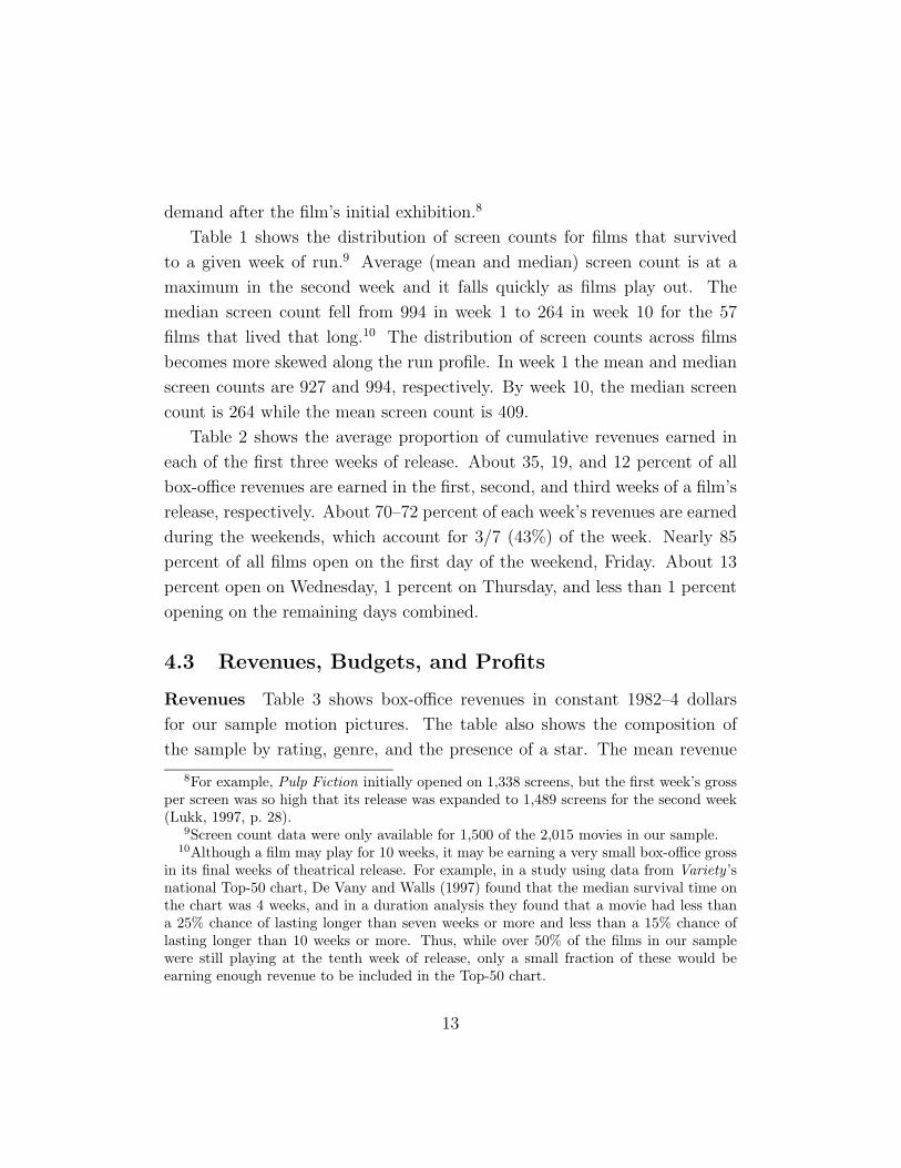
Table 1 shows the distribution of screen counts for films that survived

to a given week of run.9 Average (mean and median) screen count is at a

maximum in the second week and it falls quickly as films play out. The

median screen count fell from 994 in week 1 to 264 in week 10 for the 57

films that lived that long.10 The distribution of screen counts across films

becomes more skewed along the run profile. In week 1 the mean and median

screen counts are 927 and 994, respectively. By week 10, the median screen

count is 264 while the mean screen count is 409.

Table 2 shows the average proportion of cumulative revenues earned in

each of the first three weeks of release. About 35, 19, and 12 percent of all

box-office revenues are earned in the first, second, and third weeks of a film’s

release, respectively. About 70–72 percent of each week’s revenues are earned

during the weekends, which account for 3/7 (43%) of the week. Nearly 85

percent of all films open on the first day of the weekend, Friday. About 13

percent open on Wednesday, 1 percent on Thursday, and less than 1 percent

opening on the remaining days combined.

4.3 Revenues, Budgets, and Profits

Revenues Table 3 shows box-office revenues in constant 1982–4 dollars

for our sample motion pictures. The table also shows the composition of

the sample by rating, genre, and the presence of a star. The mean revenue

8For example, Pulp Fiction initially opened on 1,338 screens, but the first week’s grossper screen was so high that its release was expanded to 1,489 screens for the second week(Lukk, 1997, p. 28).

9Screen count data were only available for 1,500 of the 2,015 movies in our sample.10Although a film may play for 10 weeks, it may be earning a very small box-office gross

in its final weeks of theatrical release. For example, in a study using data from Variety ’snational Top-50 chart, De Vany and Walls (1997) found that the median survival time onthe chart was 4 weeks, and in a duration analysis they found that a movie had less thana 25% chance of lasting longer than seven weeks or more and less than a 15% chance oflasting longer than 10 weeks or more. Thus, while over 50% of the films in our samplewere still playing at the tenth week of release, only a small fraction of these would beearning enough revenue to be included in the Top-50 chart.

13

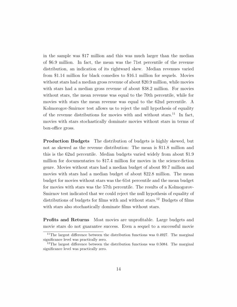
in the sample was $17 million and this was much larger than the median

of $6.9 million. In fact, the mean was the 71st percentile of the revenue

distribution, an indication of its rightward skew. Median revenues varied

from $1.14 million for black comedies to $16.1 million for sequels. Movies

without stars had a median gross revenue of about $20.9 million, while movies

with stars had a median gross revenue of about $38.2 million. For movies

without stars, the mean revenue was equal to the 70th percentile, while for

movies with stars the mean revenue was equal to the 62nd percentile. A

Kolmorogov-Smirnov test allows us to reject the null hypothesis of equality

of the revenue distributions for movies with and without stars.11 In fact,

movies with stars stochastically dominate movies without stars in terms of

box-office gross.

Production Budgets The distribution of budgets is highly skewed, but

not as skewed as the revenue distribution: The mean is $11.8 million and

this is the 62nd percentile. Median budgets varied widely from about $1.9

million for documentaries to $17.4 million for movies in the science-fiction

genre. Movies without stars had a median budget of about $9.7 million and

movies with stars had a median budget of about $22.8 million. The mean

budget for movies without stars was the 61st percentile and the mean budget

for movies with stars was the 57th percentile. The results of a Kolmogorov-

Smirnov test indicated that we could reject the null hypothesis of equality of

distributions of budgets for films with and without stars.12 Budgets of films

with stars also stochastically dominate films without stars.

Profits and Returns Most movies are unprofitable. Large budgets and

movie stars do not guarantee success. Even a sequel to a successful movie

11The largest difference between the distribution functions was 0.4927. The marginalsignificance level was practically zero.

12The largest difference between the distribution functions was 0.5084. The marginalsignificance level was practically zero.

14

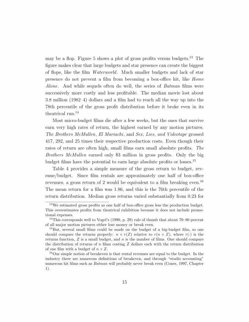
may be a flop. Figure 5 shows a plot of gross profits versus budgets.13 The

figure makes clear that large budgets and star presence can create the biggest

of flops, like the film Waterworld . Much smaller budgets and lack of star

presence do not prevent a film from becoming a box-office hit, like Home

Alone. And while sequels often do well, the series of Batman films were

successively more costly and less profitable. The median movie lost about

3.8 million (1982–4) dollars and a film had to reach all the way up into the

78th percentile of the gross profit distribution before it broke even in its

theatrical run.14

Most micro-budget films die after a few weeks, but the ones that survive

earn very high rates of return, the highest earned by any motion pictures.

The Brothers McMullen, El Mariachi , and Sex, Lies, and Videotape grossed

417, 292, and 25 times their respective production costs. Even though their

rates of return are often high, small films earn small absolute profits. The

Brothers McMullen earned only $3 million in gross profits. Only the big

budget films have the potential to earn large absolute profits or losses.15

Table 4 provides a simple measure of the gross return to budget, rev-

enue/budget. Since film rentals are approximately one half of box-office

revenues, a gross return of 2 would be equivalent to a film breaking even.16

The mean return for a film was 1.86, and this is the 76th percentile of the

return distribution. Median gross returns varied substantially from 0.23 for

13We estimated gross profits as one half of box-office gross less the production budget.This overestimates profits from theatrical exhibition because it does not include promo-tional expenses.

14This corresponds well to Vogel’s (1990, p. 29) rule of thumb that about 70–80 percentof all major motion pictures either lose money or break even.

15But, several small films could be made on the budget of a big-budget film, so oneshould compare the returns properly: n × r(Z) relative to r(n × Z), where r(·) is thereturns function, Z is a small budget, and n is the number of films. One should comparethe distribution of returns of n films costing Z dollars each with the return distributionof one film with a budget of n× Z.

16Our simple notion of breakeven is that rental revenues are equal to the budget. In theindustry there are numerous definitions of breakeven, and through “studio accounting”numerous hit films such as Batman will probably never break even (Cones, 1997, Chapter1).

15

black comedies to 1.6 for sequels. For movies without stars, the median gross

return was about 0.6; assuming that film rentals are half of box-office gross

this translates into a net rate of return of about −70%. For movies with

stars, the median gross return was about 1.37, and this corresponds to a net

rate of return of about −32%.

Stars increase the median of the returns distribution much more than

the mean; they make the distribution less skewed. The mean return with no

stars is at the 78th percentile, while the mean return with stars is at the 67th

percentile. We performed a Kolmogorov-Smirnov test for equality of distribu-

tions and could reject the null hypothesis that the returns distributions were

equal for movies with and without stars at a marginal significance level of

practically zero. However, movies with stars do not stochastically dominate

movies without stars in terms of gross return to budget. The largest gross re-

turn to a movie with a star was 16.7 times production cost for (Beverly Hills

Cop); this movie also had a large box-office revenue. However, most movies

with very large gross returns did not have stars, had low revenues, and tiny

budgets.17 The successful micro-budget non-star movies have tremendous

returns on budget, but they earn a less absolute profit than a big-budget

production with a gross return of 3 times production cost.

5 Estimation Results

5.1 The Size Distribution of Box Office Revenue

One of the ways star power might work is in moving a movie up in the

money rankings by getting it booked on many screens at the opening. Once

there, more viewers might be drawn to it if the ranking is taken by movie-

goers to be an indicator of entertainment value. Figure 6 plots the box-

office revenue and rank for each year in our sample. It is clear that the

size distribution of revenue is uneven and highly convex in rank. This is

17For example, El Mariachi and The Brothers McMullen had gross returns to budgetof 292 and 417, respectively. But their absolute profits were small.

16

consistent with the distribution of box-office revenues following the Pareto

rank law: SRβ2 = β1, where S is the size of box-office revenues, R is the rank

(1=highest), and β1 and β2 are parameters. The exponent β2 is an indication

of the degree of concentration of revenues on movies because it indicates the

relative frequency of large grossing movies to small grossing movies.18

The Pareto rank law can be written as

log Revenue = log β1 + β2 log Rank + β3Star + β4[log Rank× Star] + µ (3)

This is the form we estimate. Table 5 shows our estimates of the Pareto

rank law regressions. Column 1 shows the results restricting the Pareto

parameters to be equal for all movies, with and without stars. In this case,

we get a value of β2 = −1.825 indicating a very high degree of inequality. In

column 2 the estimates allow the Pareto rank parameters to differ for movies

with and without stars. The estimates indicate that the intercept term is a

little smaller and that the slope is much flatter among movies with a star:

β2 = −0.996 for movies with stars versus −2.149 for movies without stars.

As we have seen, star movies have larger budgets, wider releases, and quite

likely better scripts, so these differences in distributions cannot be solely

attributed to stars.

Table 6 shows estimates of the Pareto rank law regressions for 6 two-year

intervals. With the exception of 1985–6, the Pareto rank parameters show

little change. The Pareto rank law has remained quite stable over the years

in spite of escalating production and advertising budgets. Independence of

form on the time scale of the data is a feature of power law distributions that

describe processes that are self-similar on all scales; this is revealed in the

similarity of the rank-revenue curves plotted in Figure 6. The Pareto rank

distribution is a remarkably good fit for all movies, with or without stars.

Hence, the distinguishing factor that causes movies to be strongly ranked in

terms of revenue cannot be traced to stars. It is a natural order, durable

18Ijiri and Simon (1971) model the firm size distribution using this form of the Paretolaw.

17

over time and place.19 The steep decline in box office revenue share with

declining rank has remained stable during a decade of change in advertising

and production budgets, the use of stars, and changes in opening release

patterns.20

5.2 Opening and Staying Power

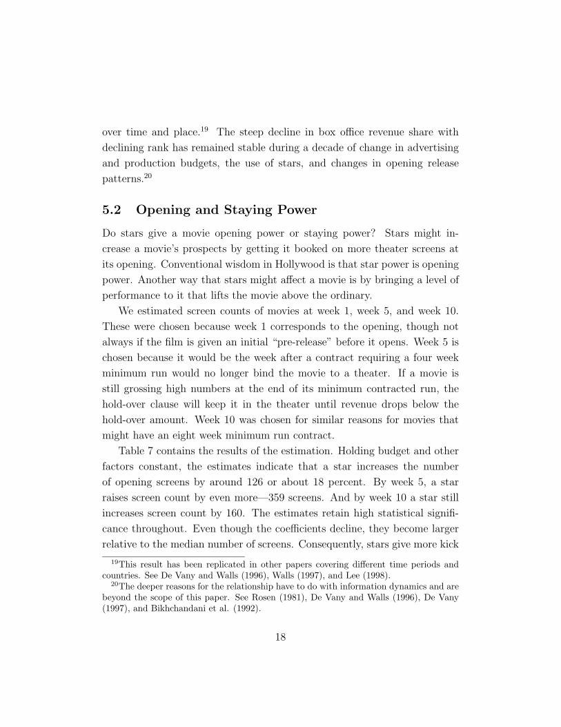
Do stars give a movie opening power or staying power? Stars might in-

crease a movie’s prospects by getting it booked on more theater screens at

its opening. Conventional wisdom in Hollywood is that star power is opening

power. Another way that stars might affect a movie is by bringing a level of

performance to it that lifts the movie above the ordinary.

We estimated screen counts of movies at week 1, week 5, and week 10.

These were chosen because week 1 corresponds to the opening, though not

always if the film is given an initial “pre-release” before it opens. Week 5 is

chosen because it would be the week after a contract requiring a four week

minimum run would no longer bind the movie to a theater. If a movie is

still grossing high numbers at the end of its minimum contracted run, the

hold-over clause will keep it in the theater until revenue drops below the

hold-over amount. Week 10 was chosen for similar reasons for movies that

might have an eight week minimum run contract.

Table 7 contains the results of the estimation. Holding budget and other

factors constant, the estimates indicate that a star increases the number

of opening screens by around 126 or about 18 percent. By week 5, a star

raises screen count by even more—359 screens. And by week 10 a star still

increases screen count by 160. The estimates retain high statistical signifi-

cance throughout. Even though the coefficients decline, they become larger

relative to the median number of screens. Consequently, stars give more kick

19This result has been replicated in other papers covering different time periods andcountries. See De Vany and Walls (1996), Walls (1997), and Lee (1998).

20The deeper reasons for the relationship have to do with information dynamics and arebeyond the scope of this paper. See Rosen (1981), De Vany and Walls (1996), De Vany(1997), and Bikhchandani et al. (1992).

18

to screen counts later than at the opening of a movie’s run. In its first week,

a movie with a star will have about twenty percent more screens than a movie

without a star. By its fifth week a movie with a star will have nearly twice

as many theaters as a movie without a star. And by the tenth week nearly

three times as many. The effect becomes more pronounced later in the run.

The estimates also show that bigger budgets produce more opening screens:

an increase in the budget of one million dollars corresponds to an increase of

36 screens in the opening week. Given that the median production budget

for a film was less than 10 million dollars and the mean was $32 million, the

effect of a big budget on opening screens does not rise to economic signif-

icance. In terms of opening screen counts, a star is worth as much as an

extra six million dollars in the production budget. By week 10 the size of

the budget has a small effect on the number of screens; a million dollars of

production cost only buys seven more screens in the tenth week.

Sequels open on nearly twice as many screens as the average movie. How-

ever, during the remainder of the run the sequel advantage declines. By week

10, the sequel advantage is statistically not different from zero.

In modeling screens in week 1 we are primarily modeling the behavior of

theater bookers who select films to exhibit. By week 5 we are closer to seeing

what the audience likes and not what the booking agents think. And, by

week 10 we have a pretty clear vision of what counts with the audience. By

then, sequels and budgets become unimportant which suggests that booking

agents do not always share the tastes or perceptions of the audience.21 Star

movies have more staying power than opening power.

5.3 The Asymptotic Pareto Distribution

The Pareto rank distribution estimated above is an excellent model of the

inequality of motion picture revenues, but it tells us little about the probabil-

ity distribution of revenues. In order to fix probabilities so that we are able

to assess the box-office expectations of a movie before it is released, we must

21The glare from the concession stand may blind their vision.

19

estimate probability distributions. As we discussed in Section 2, the Levy

stable process converges asymptotically to a Pareto distribution as x → ∞.

To estimate the asymptotic Pareto law of equation (2), we set the minimum

revenue at k = $40 million. We fit the Pareto distribution for all movies

whose box-office revenues equaled or exceeded $40 million and obtained an

estimate of the tail coefficient α of 1.91. Since 1 < α < 2 the mean is finite

and the variance is infinite. A Kolmogorov-Smirnov test of equality of the

empirical distribution and the theoretical Pareto law F (x) = 1− (x/40)−1.91

does not reject the Pareto distribution at the 5% significance level. Figure 7

is a plot of the empirical cumulative distribution against the fitted Pareto

distribution. The fit is extraordinary over a wide range of values running

from $40 to $250 million in box-office revenues.

We proceeded to estimated α separately for movies with and without stars

with k fixed at $40 million. For movies with stars α = 1.72 implying a finite

mean and infinite variance. For movies without stars α = 2.26 implying that

both mean and variance are finite. The small value of α and infinite variance

of star movies indicates they have more probability mass in the upper tail

than movies without stars.

Note how different the Pareto distribution looks relative to the normal

distribution that most people unconsciously draw on when they think about

movies. The probability density of the Pareto is “piled up” on the small box-

office revenues because most movies earn small revenues. Unlike the normal

distribution, where there is a piling up of density in the center around the

mean, there is no central tendency in the Pareto distribution. The probability

slopes away to the right, where the rare and big grossing films are. The Pareto

distribution for values of α < 2 (the star movies) has more upper tail mass

than the normal distribution.

The Levy distribution implies that forecasts of box-office revenues for

movies lack a foundation. The expectation of the distribution for movies

without stars is 7.17 × 107 but the variance is 8.76 × 1015. The variance is

122 million times as large as the expectation. The expectation of the star

20

movie distribution is 9.55×107 but its variance is infinite. In practical terms,

forecasting revenue is futile because the magnitude of the forecast variance

completely overwhelms the value of the forecast.

5.4 The Probability of a Hit

Because forecasting expected revenue is imprecise and lacking in foundation,

we examine another approach. How are stars, budgets, genre, rating, and

opening screens associated with the probability that a movie will be a hit?

These are all variables that can be chosen; if their impact on the probabilities

of certain outcomes can be predicted, then better choices might be possible.

The problem is that the subtle shifts in probability distributions are difficult

to measure and we still face the infinite or nearly infinite variance.

Our attack on this problem is to examine the probabilities of extreme out-

comes. We examine the probability that a movie will be a hit, which we define

as earning a box office revenue of fifty million or more. Even with a Pareto

distribution of unbounded variance, this exercise is meaningful because we

are discretizing the distribution and can easily calculate the probability that

revenue will equal or exceed $50 million. We carry this exercise out by mod-

eling the conditional hit probability as a function of the film’s budget, star

presence, genre, rating, year of release, survival time, and number of opening

screens.

Column (1) of Table 8 contains the parameter estimates and the asso-

ciated marginal probabilities—the change in the probability that a movie

becomes a hit for a unit change in the corresponding independent variable.

The individual parameters are all statistically significant. The estimates in-

dicate that a higher budget is associated with a higher hit probability. The

star variable has a higher marginal probability than the sequel variable. The

same pattern is observed in the results shown in column (2) where we have

estimated on the subset of 1,500 observations for which we have screen count

and life-length data. These data show that our estimates are not sensitive

to the sample selection.

21

In column (3) of the table two additional variables appear that indicate

whether or not the movie survived for at least ten weeks and whether or

not the movie was released on not less than 2,000 screens. Now the highest

marginal probability is on a run of at least ten weeks, followed by the number

of opening screens, then by star, and sequel in that order. That a long run

is the most important factor associated with a movie becoming a hit is clear

evidence that the audience decides a movie’s fate at the box office and no

amount of star power, screen counts, or promotional hype is as important as

the public’s acceptance of the film. Controlling for screens and life length,

a star has the same effect on the average movie’s chances of grossing at

least $50 million in theaters as an additional $40 million on production cost.

Heavy spending on special effects or “production value” is the most risky

strategy for making a movie a hit. Making a movie the audience loves is the

surest way to making a hit, but that takes talents that are more rare than

the ability to spend money. Next in importance to making a good movie in

achieving a box-office hit is to have the movie booked on a large number of

opening screens. But this is no simple task either as booking managers are

no doubt influenced by their highly profitable concession sales.

A big opening is a double-edged sword (De Vany and Walls, 1997). Open-

ing on many screens preempts screens from other movies and gives a film a

shot at a high rank. High rank movies are more likely to engage the infor-

mation cascade and draw positive or negative attention. But, if the critical

judgments of the viewers are predominately negative, the flow of negative

information can kill a film and more swiftly if it is on many screens. On the

other hand, a broad opening may bring large screen revenues in the early

weeks of a run. Later, the number of screens is adjusted to fit demand and

the initial number becomes less important.

5.5 Stars and Hits

To more closely identify the association of individual stars with hit movies,

we re-estimated column 1 of Table 8 using binary variables for individual

22

stars in place of the single variable indicating the presence of any star in the

movie. The coefficients on most of the individual star dummy variables were

insignificantly different from zero at the 5% marginal significance level: Most

stars do not have a statistically significant association with the probability

that a movie will be a hit. Only a few stars have a non-negligible correlation

with hit movies.

Who are the stars with real impact on a movie’s chances of becoming

a hit? Table 9 lists the individual stars whose coefficients are statistically

significant and the associated marginal probabilities. Only nineteen stars

had a statistically significant impact on the hit probability. The names on

the list are familiar ones. But some stars thought to have box-office power

do not make the list; for example, neither Sylvester Stallone nor Robert De

Niro were statistically significant. All the male stars that are thought to be

“bankable” are there, along with behind-the-camera talents Steven Spielberg

and Oliver Stone.

The real surprise, given conventional Hollywood wisdom about star power,

is the power of the female stars.22 Four of the top nineteen stars are female.

The top two stars are females and three of the top five stars are females.

No star is a “sure thing” however. They all face the infinite variance of the

Levy distribution, so they each bring a measure of risk with them. They also

have sizable standard errors of their estimated hit coefficients. Jodie Foster,

Michelle Pfeiffer, and Sandra Bullock have high standard errors, implying

that their positive impact is more variable. Tom Cruise has a small standard

error; not only does he have a big impact but his impact is more certain

than the impact of all the stars but Tom Hanks. The smallest standard error

goes to Tom Hanks, though he has a smaller hit impact than Cruise, Pfeiffer,

Foster, Carrey, and Bullock. Steven Spielberg is the top behind-the-camera

star, with a marginal impact that is slightly higher but more variable than

22Bill Mechanic, Chairman of Twentieth Century Fox, lists no females among his topstars. His list: Tom Cruise, Harrison Ford, Mel Gibson, Tom Hanks, Arnold Schwarzeneg-ger and John Travolta. Quoted in John Cassidy, “Chaos in Hollywood,” The New Yorker ,March 31, 1997.

23

for Oliver Stone.

Of course, none of these estimates guarantee that a particular star will

make a movie successful. In fact, they assure that no star can guarantee any

outcome because there is infinite variance in the distribution—every star has

a sizable probability of making a bomb. Moreover, it would be an error to

attribute causality to what is only an association between stars and movie

outcome probabilities. Causality could even go in the other direction—a star

might just be someone who is lucky enough to give a fine performance in

a terrific movie. Once someone is blessed with the mantle of stardom, it is

clear that better projects and bigger budgets come his or her way. Hence,

their chances of appearing in high grossing movies go up and their chances

of being regarded as stars remain higher than average.

5.6 Stars and Profits

To investigate profits we estimate a simple equation of the form

Profit = f(star, sequel, genre, rating, year) (4)

where Profit = (0.5× revenue− budget) is measured in millions of dollars.23

We have reported least squares and robust regression estimates in Table 10.24

We estimated the equation in levels (and not logs) because Profit is negative

for a large proportion of the sample. The equation is a very poor fit, with

an R-squared value of just 0.118. That is as it should be, for were profits

predictable, everyone would make them. The lack of structure of the profit

23Recall that profits are calculated for the theatrical market only and do not includeforeign and other revenues. Cost is the estimated budget reported in the EDI data. The0.5 figure is a rough estimate of the average rental rate. A high grossing film typicallywill earn a higher than average rental rate although a poor performing film on whichguarantees were paid may also earn a high rate. Consequently, this equation is a crudeapproximation to profits in the North American theatrical market.

24We do not report quantile regressions because the mean absolute deviation estimatorwould not converge for the profit regressions. We are tackling this problem in anotherpaper.

24

equation is a confirmation of the rule that “nobody knows anything” when

it comes to predicting profits.

To investigate how stars may add structure to this featureless pattern,

we re-estimated the equation with binary variables representing the individ-

ual stars. The twenty-five stars with statistically significant coefficients are

reported in Table 11. Jodie Foster tops the list, followed by Tom Cruise,

and now Steven Spielberg moves into the third position on the profit list.

Sandra Bullock and Jim Carrey are about tied for fourth, with Brad Pitt

and Kevin Costner just behind. A few new names appear that did not show

up before such as Warren Beatty, Steve Martin, Francis Ford Coppola and

Robert Redford. De Niro, Nicholson, and Willis appear with statistically

significant negative coefficients.

Given all we have said about the nature of the probability distribution,

it is difficult to place an interpretation on these estimates. They primarily

reflect the success that movies with these stars had in the past and do not

imply that these successes will be repeated in the future. Those successes

may reflect their performances or their judgment in choosing movies. It may

just be luck in the matching of actor and movie. A deeper problem is that if

the box-office revenue distribution has infinite or near infinite variance, then

no formula will be able to forecast revenue or profit. Since profit equals some

fraction of revenue minus cost, the variance of profit will be infinite if the

variance of revenue is infinite. Thus, theory indicates that profits should be

asymptotically Pareto-distributed. We find that this prediction is confirmed

and that profits in excess of $10 million are Pareto-distributed with an infinite

variance.

The estimated Pareto exponent for all movies is α = 1.357. For movies

without stars, α = 1.505. For movies with stars, α = 1.261. All the estimates

of α are greater than 1 and less than 2, implying that the mean of each

distribution exists but the variance is infinite. Kolmogorov-Smirnov tests

indicated that we could not reject the null hypothesis of equality of distri-

butions between the fitted Pareto and the empirical cumulative distribution

25

functions. Figure 8 plots the fitted Pareto distribution function against the

empirical distribution function for all movies. The fit is excellent and this is

compelling evidence that profits are Levy distributed as are revenues.

Stars shift probability mass to higher outcomes. The theoretical mean

profits are $38 million for all movies, $48.3 million for star movies, and $29.8

million for no-star movies. The variance of profits for movies that earn

high profits (≥ $10 million) is infinite for all movies as a group, for movies

with stars, and for movies without stars. A few non-star movies achieve

extraordinary profits (Home Alone) and some star-movies lose extraordinary

amounts of money (Waterworld). Both these effects contribute to the heavy

tails in the profit distribution. Profits are more risky and less predictable

than box-office revenues.

6 Choosing Among Movie Projects

The movie industry is a small sample business. Studios only get so many

chances. If only the very best survive and the competition is intense, then

studios need to draw a movie project out of the many that are around that

will have an extreme positive result. That is, with just a few draws from

the hat the studio has to pull out an unlikely movie to succeed against its

competitors. Finishing first in a large field requires doing something far from

the average and being lucky enough to have it pay off (Levinthal and March,

1993).

In such highly competitive situations, experience and learning, which are

predictors of success on average, are not closely related to outcomes because

success depends on doing something different—getting an extreme draw in a

small sample. Experience may be a poor teacher in the movies. Effectiveness

or success in the short run and in the neighborhood of recent experience

(sequels) interferes with learning and experimentation in the long run. Since

success comes from an unlikely event in a small sample, it is not reliable to

extrapolate success into the future. This is why it is hard to learn in the

26

movie business.

The movie business encourages selective learning based on extreme events.

Ignoring failures and focusing on successes is built into the process. This is

so because the statistics of the movies are dominated by a few extreme out-

comes. There are a lot of failures and a few rare and unpredictable successes.

Individuals tend to attribute causality improperly. They tend to attribute

their successes to ability and their failures to bad luck. This error affects

how they approach risk in the movie business. If executives attribute poor

outcomes to bad luck, then they will overestimate risk. They will be inclined

to demand a “bankable” star in a movie before they will make it. If they

attribute good outcomes to their ability, then they will be inclined to take

too much risk. Hence, one or two successes can lead to too much risk taking

and a few failures to too little. Probably, most studio executives overesti-

mate their ability to beat the odds. Of course, not all of them can.25 In the

long run, none of them can beat the odds. The odds are that only about 8

percent of all movies made gross more than $40 million at the domestic box

office. Many of these are not profitable in spite of their high revenues.

Experience may not be helpful because it cannot produce a rare event.

Most rare events, like the movie Titanic, lie outside the sample and are

beyond experience. If aspirations are based on highly successful movies, then

performance is bound not to match. Even if successful, tying aspirations to

successes in the past deters exploration and innovation that are essential to

success in the future; too many sequels and copies are made and too few

genuinely new movies are produced.

Past successes give executives an illusion of control (Langer, 1975; Presson

and Benassi, 1996). They become confident in their ability to manage risk

and handle future events. They have difficulty recognizing the role of luck

in their achievements. Studio executives and producers have little control

in this business. It is a high-skill business because good movies are hard

25In our current research we use probability models to estimate the “half lives” of starsand movie studios based on their movie portfolios of the past decade.

27

to make. But that very fact fosters an illusion of control. It is such an

uncertain business that the distinction between causal factors, luck, or the

sheer sweep of events is blurred. In a complex system, where there are many

interacting parts and complicated stochastic dynamics, there is no simple

form of causality. Everything depends, in some way, on almost everything

else and it will usually be impossible to attribute an outcome to a cause or

complex of causes.

Managerial errors in judgment are fostered by the very nature of uncer-

tainty in the motion picture industry that is documented in this paper. 26

The uniqueness of individual movies comes from the underlying probability

distribution: because it is a power law, there is no characteristic scale, no

central tendency, and events on all scales happen. 27 Thus, there is no typical

movie. The hold that last year’s blockbuster has on the imagination comes

also from the power law, a distribution so highly skewed that blockbusters

dominate the mean. Only risk and hazard analyses are well-defined for this

business. The probability that a movie will reach an extreme outcome in

the upper tail, which is required for it to be profitable, is small. But, the

outcomes associated with extremums dominate total and average revenues

and profits. So, risk not only is unavoidable, it is desirable. One wants to

choose movies that have a large upside variance. We have only hinted at

how it might be done here by investigating a few strategies.28 Star movies

have that kind of variance, but by virtue of that fact they also have un-

predictable outcomes. No star is “bankable” if bankers or studio executives

want sure things. Stars only increase the odds of favorable events that are

highly improbable.

26De Vany (1997) deals with this issue in more detail. We analyze how productiondecisions are related to past events in our current research.

27Earthquakes also follow a power law. Trying to predict the next blockbuster is liketrying to predict the next big earthquake.

28Given the risk at the box office, it is not surprising that many movies are made onthe basis of pre-committed foreign distribution funds and tie-ins to games and fast foodpromotions.

28

7 Conclusions

The movie industry is a profoundly uncertain business. The probability

distributions of movie box-office revenues and profits are characterized by

heavy tails and infinite variance! It is hard to imagine making choices in more

difficult circumstances. Past success does not predict future success because

a movie’s box office possibilities are Levy-distributed. Forecasts of expected

revenues are meaningless because the possibilities do not converge on a mean;

they diverge over the entire outcome space with an infinite variance. This

explains precisely why “no one knows anything” in the movie business.

A proper assessment of a movie’s prospects requires a risk analysis of

extreme outcomes. We have demonstrated that estimates of the Levy distri-

bution parameters permit calculation of the probability of box-office revenues

that have not before been realized. Film makers can position a movie to im-

prove its chances of success, but after a movie opens the audience decides its

fate: There are no formulas for success in Hollywood. The complex dynam-

ics of personal interaction between viewers and potential viewers overwhelm

the initial conditions. The difficulties of predicting outcomes for individ-

ual movies are so severe that a strategy of choosing portfolios of movies is

more sensible than the current practice of “greenlighting” individual movie

projects.

29

References

Atkinson, A. B. and Harrison, A. J. (1978). Distribution of Total Wealth in

Britain. Cambridge University Press, Cambridge.

Bikhchandani, S., Hirshleifer, D., and Welch, I. (1992). A theory of fads,

fashion, custom, and cultural change as informational cascades. Journal

of Political Economy, 100(5):992–1026.

Blumenthal, M. A. (1988). Auctions with constrained information: Blind bid-

ding for motion pictures. Review of Economics and Statistics, 70(2):191–

198.

Chisholm, D. C. (1996). Continuous degrees of residual claimancy: Some

contractual evidence. Applied Economics Letters, 3(11):739–41.

Chisholm, D. C. (1997). Profit-sharing versus fixed-payment contracts: Evi-

dence fom the motion pictures industry. Journal of Law, Economics and

Organization, 13(1):169–201.

Cones, J. W. (1997). The Feature Film Distribution Deal. Southern Illinois

University Press, Carbondale.

Dale, M. (1997). The Movie Game: The Film Business in Britain, Europe

and America. Cassell, London.

De Vany, A. S. (1997). Complexity in the movies. Forthcoming in Complexity:

The Journal of the Santa Fe Institute.

De Vany, A. S. and Eckert, R. (1991). Motion picture antitrust: The

Paramount cases revisited. Research in Law and Economics, 14:51–112.

De Vany, A. S. and Walls, W. D. (1996). Bose-Einstein dynamics and adap-

tive contracting in the motion picture industry. The Economic Journal,

439(106):1493–1514.

30

De Vany, A. S. and Walls, W. D. (1997). The market for motion pictures:

Rank, revenue and survival. Economic Inquiry, 4(35):783–797.

Fama, E. (1963). Mandelbrot and the stable Paretian hypothesis. Journal

of Business, 36(4):420–429.

Goldman, W. (1983). Adventures in the Film Trade. Warner Books, New

York.

Hamilton, L. C. (1991). How robust is robust regression? Stata Technical

Bulletin, 2:21–26.

Hill, B. and Woodrofe, M. (1975). Stronger forms of Zipf’s law. Journal of

the American Statistical Association, 70(349):212–219.

Ijiri, Y. and Simon, H. A. (1971). Effects of mergers and acquisitions on

business firm concentration. Journal of Political Economy, 79(2):314–

322.

Ijiri, Y. and Simon, H. A. (1977). Skew Distributions and the Sizes of Busi-

ness Firms. North-Holland, New York.

Kenney, R. W. and Klein, B. (1983). The economics of block booking. Journal

of Law and Economics, 26:497–540.

Langer, E. J. (1975). The illusion of control. Journal of Personality and

Social Psychology, 32:311–338.

Lee, C. (1998). Bose-Einstein dynamics in the motion picture industry re-

visited. Mimeo, Economics Deptartment, University of California at

Irvine.

Levinthal, D. A. and March, J. G. (1993). The myopia of learning. Strategic

Management Journal, 14:95–112.

Levy, M. and Soloman, S. (1998). Of wealth power and law: the origin of

scaling in economics. Racah Institute of Physics, Hebrew University.

31

Lukk, T. (1997). Movie Marketing: Opening the Picture and Giving it Legs.

Silman-James Press, Los Angeles.

Mandelbrot, B. (1963). The variation of certain speculative prices. Journal

of Business, 36:394–419.

Mantegna, R. N. and Stanley, H. E. (1995). Scaling in financial markets.

Nature, 376:46–49.

Pareto, V. (1897). Cours d’Economique Politique.

Prag, J. and Cassavant, J. (1994). An empirical study of determinants of

revenues and marketing expenditures in the motion picture industry.

Journal of Cultural Economics, 18(3):217–35.

Presson, P. K. and Benassi, V. A. (1996). Illusion of control: A meta-analytic

review. Journal of Social Behavior and Personality, 11(3):493–510.

Ravid, S. A. (1998). Information, blockbusters and stars: A study of the film

industry. Working paper, New York University.

Rosen, S. (1981). The economics of superstars. American Economic Review,

71:167–183.

Vogel, H. L. (1990). Entertainment Industry Economics: A Guide for Finan-

cial Analysis. Cambridge University Press, New York, second edition.

Wallace, W. T., Seigerman, A., and Holbrook, M. B. (1993). The role of

actors and actresses in the success of films: How much is a movie star

worth? Journal of Cultural Economics, 17(1):1–24.

Walls, W. D. (1997). Increasing returns to information: Evidence from the

Hong Kong movie market. Applied Economics Letters, 4(5):187–190.

Walls, W. D. (1998). Product survival at the cinema: Evidence from Hong

Kong. Applied Economics Letters, 5(4):215–219.

32

Weinstein, M. (1998). Profit-sharing contracts in Hollywood: Evolution and

analysis. Journal of Legal Studies, 27(1):67–112.

33

Figure 1: Cumulative Probability for Movies with and without Stars

Figure 2: The Continuation Function for Movies with Stars

Figure 3: Wide Releases: Hits, Bombs, and Sequels

Figure 4: Narrow Releases: Growth, Death, and Legs

Figure 5: Gross Profit versus Budget

Figure 6: Pareto Rank Distribution by Year

Figure 7: Asymptotic Pareto Law for Box-Office Gross

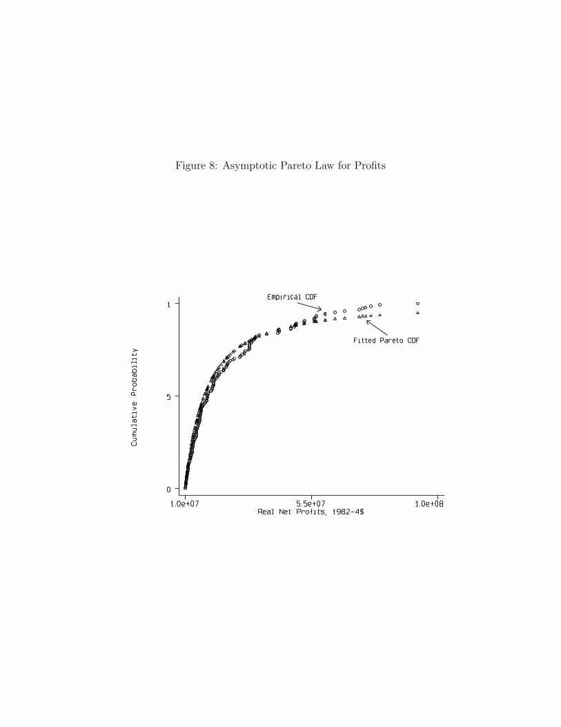
Figure 8: Asymptotic Pareto Law for Profits

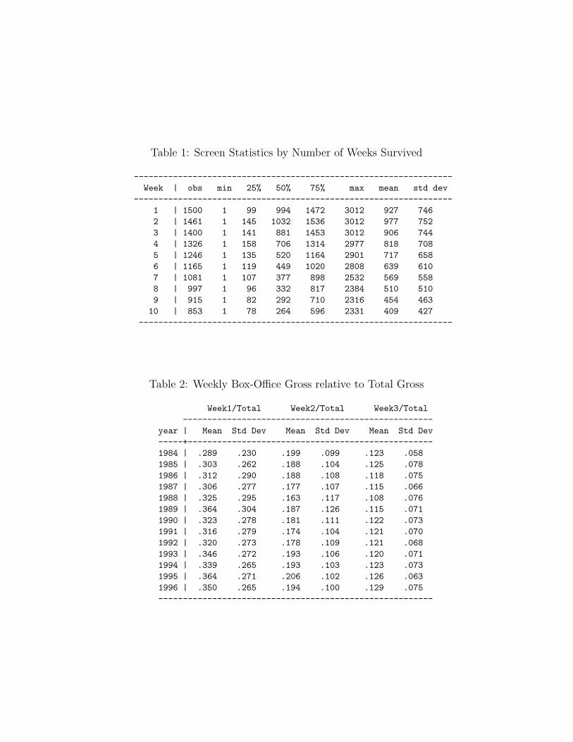
Table 1: Screen Statistics by Number of Weeks Survived

-----------------------------------------------------------------Week | obs min 25% 50% 75% max mean std dev

-----------------------------------------------------------------1 | 1500 1 99 994 1472 3012 927 7462 | 1461 1 145 1032 1536 3012 977 7523 | 1400 1 141 881 1453 3012 906 7444 | 1326 1 158 706 1314 2977 818 7085 | 1246 1 135 520 1164 2901 717 6586 | 1165 1 119 449 1020 2808 639 6107 | 1081 1 107 377 898 2532 569 5588 | 997 1 96 332 817 2384 510 5109 | 915 1 82 292 710 2316 454 46310 | 853 1 78 264 596 2331 409 427

----------------------------------------------------------------

Table 2: Weekly Box-Office Gross relative to Total Gross

Week1/Total Week2/Total Week3/Total---------------------------------------------------

year | Mean Std Dev Mean Std Dev Mean Std Dev-----+--------------------------------------------------1984 | .289 .230 .199 .099 .123 .0581985 | .303 .262 .188 .104 .125 .0781986 | .312 .290 .188 .108 .118 .0751987 | .306 .277 .177 .107 .115 .0661988 | .325 .295 .163 .117 .108 .0761989 | .364 .304 .187 .126 .115 .0711990 | .323 .278 .181 .111 .122 .0731991 | .316 .279 .174 .104 .121 .0701992 | .320 .273 .178 .109 .121 .0681993 | .346 .272 .193 .106 .120 .0711994 | .339 .265 .193 .103 .123 .0731995 | .364 .271 .206 .102 .126 .0631996 | .350 .265 .194 .100 .129 .075--------------------------------------------------------

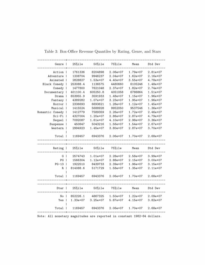
Table 3: Box-Office Revenue Quantiles by Rating, Genre, and Stars

----------------+--------------------------------------------------------Genre | 25%ile 50%ile 75%ile Mean Std Dev

----------------+--------------------------------------------------------Action | 1761336 8204898 2.06e+07 1.79e+07 2.81e+07

Adventure | 1208704 9946237 2.04e+07 1.62e+07 2.16e+07Animated | 2828827 1.53e+07 4.40e+07 3.55e+07 4.78e+07

Black Comedy | 253088.4 1136575 4480660 6105246 1.48e+07Comedy | 1477800 7621048 2.37e+07 1.82e+07 2.74e+07

Documentary | 401100.4 605250.8 4051058 6786864 1.51e+07Drama | 653955.9 3591933 1.48e+07 1.15e+07 1.96e+07

Fantasy | 4389282 1.07e+07 3.23e+07 1.95e+07 1.96e+07Horror | 2336693 6693621 1.28e+07 1.12e+07 1.45e+07Musical | 1415524 5688928 9952050 9537546 1.36e+07

Romantic Comedy | 1412779 7589359 2.26e+07 1.72e+07 2.46e+07Sci-Fi | 4327004 1.20e+07 2.86e+07 2.87e+07 4.79e+07Sequel | 7092087 1.61e+07 4.10e+07 2.98e+07 3.36e+07

Suspense | 450647 5043216 1.56e+07 1.54e+07 2.67e+07Western | 2994923 1.45e+07 3.80e+07 2.87e+07 3.70e+07

|Total | 1169457 6943376 2.06e+07 1.70e+07 2.68e+07

----------------+------------------------------------------------------------------------+--------------------------------------------------------

Rating | 25%ile 50%ile 75%ile Mean Std Dev----------------+--------------------------------------------------------

G | 2574743 1.01e+07 2.28e+07 2.58e+07 3.99e+07PG | 1566304 1.12e+07 2.88e+07 2.15e+07 3.00e+07

PG-13 | 1922510 8439733 2.39e+07 1.96e+07 3.15e+07R | 814088.6 5171729 1.58e+07 1.35e+07 2.11e+07

|Total | 1169457 6943376 2.06e+07 1.70e+07 2.68e+07

----------------+------------------------------------------------------------------------+--------------------------------------------------------

Star | 25%ile 50%ile 75%ile Mean Std Dev----------------+--------------------------------------------------------

No | 852226.1 4867325 1.50e+07 1.22e+07 2.09e+07Yes | 1.33e+07 3.25e+07 5.87e+07 4.15e+07 3.82e+07

|Total | 1169457 6943376 2.06e+07 1.70e+07 2.68e+07

----------------+--------------------------------------------------------Note: All monetary magnitudes are reported in constant 1982-84 dollars.

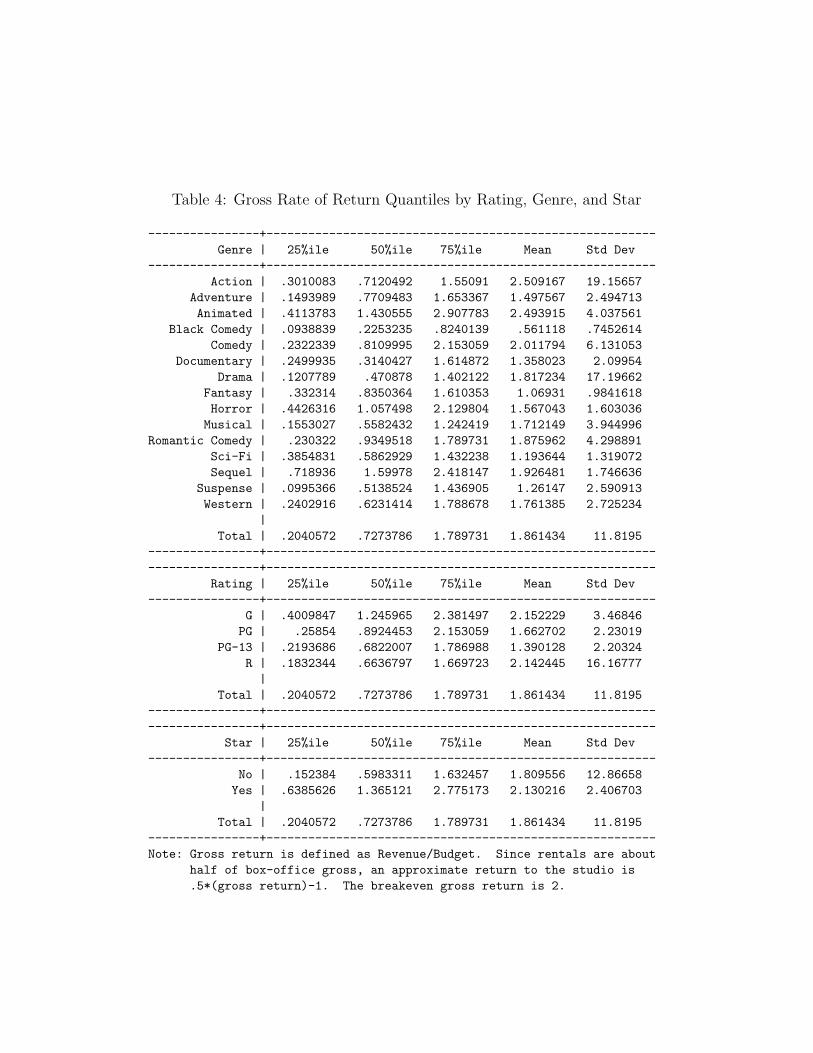
Table 4: Gross Rate of Return Quantiles by Rating, Genre, and Star

----------------+--------------------------------------------------------Genre | 25%ile 50%ile 75%ile Mean Std Dev

----------------+--------------------------------------------------------Action | .3010083 .7120492 1.55091 2.509167 19.15657

Adventure | .1493989 .7709483 1.653367 1.497567 2.494713Animated | .4113783 1.430555 2.907783 2.493915 4.037561

Black Comedy | .0938839 .2253235 .8240139 .561118 .7452614Comedy | .2322339 .8109995 2.153059 2.011794 6.131053

Documentary | .2499935 .3140427 1.614872 1.358023 2.09954Drama | .1207789 .470878 1.402122 1.817234 17.19662

Fantasy | .332314 .8350364 1.610353 1.06931 .9841618Horror | .4426316 1.057498 2.129804 1.567043 1.603036Musical | .1553027 .5582432 1.242419 1.712149 3.944996

Romantic Comedy | .230322 .9349518 1.789731 1.875962 4.298891Sci-Fi | .3854831 .5862929 1.432238 1.193644 1.319072Sequel | .718936 1.59978 2.418147 1.926481 1.746636

Suspense | .0995366 .5138524 1.436905 1.26147 2.590913Western | .2402916 .6231414 1.788678 1.761385 2.725234

|Total | .2040572 .7273786 1.789731 1.861434 11.8195

----------------+------------------------------------------------------------------------+--------------------------------------------------------

Rating | 25%ile 50%ile 75%ile Mean Std Dev----------------+--------------------------------------------------------

G | .4009847 1.245965 2.381497 2.152229 3.46846PG | .25854 .8924453 2.153059 1.662702 2.23019

PG-13 | .2193686 .6822007 1.786988 1.390128 2.20324R | .1832344 .6636797 1.669723 2.142445 16.16777

|Total | .2040572 .7273786 1.789731 1.861434 11.8195

----------------+------------------------------------------------------------------------+--------------------------------------------------------

Star | 25%ile 50%ile 75%ile Mean Std Dev----------------+--------------------------------------------------------

No | .152384 .5983311 1.632457 1.809556 12.86658Yes | .6385626 1.365121 2.775173 2.130216 2.406703

|Total | .2040572 .7273786 1.789731 1.861434 11.8195

----------------+--------------------------------------------------------Note: Gross return is defined as Revenue/Budget. Since rentals are about

half of box-office gross, an approximate return to the studio is.5*(gross return)-1. The breakeven gross return is 2.

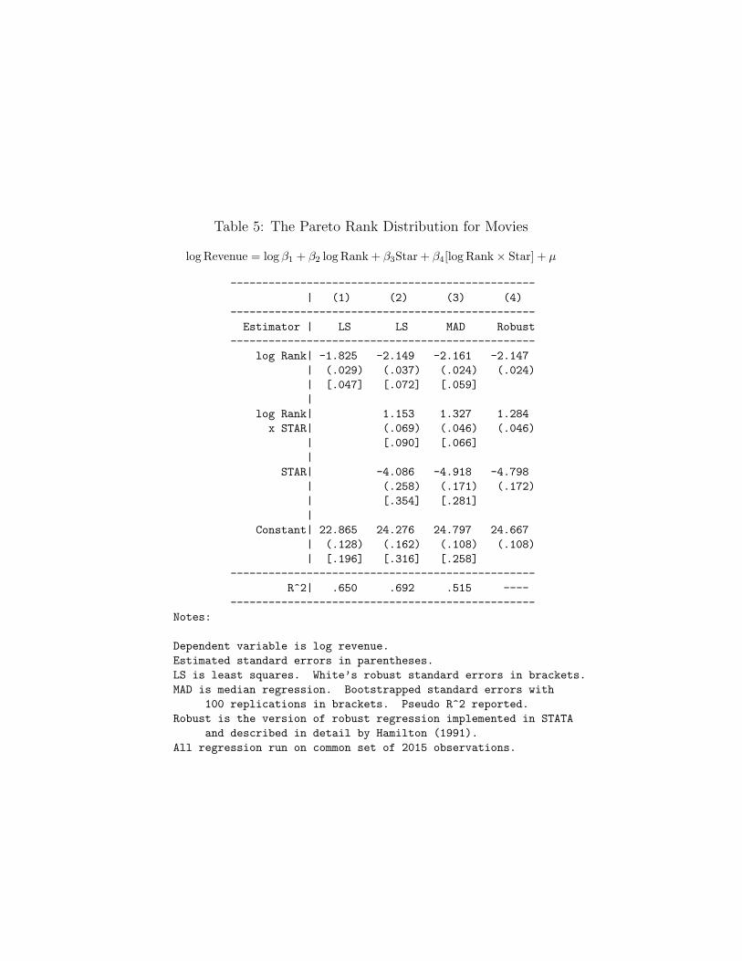
Table 5: The Pareto Rank Distribution for Movies

log Revenue = log β1 + β2 log Rank + β3Star + β4[log Rank× Star] + µ

------------------------------------------------| (1) (2) (3) (4)

------------------------------------------------Estimator | LS LS MAD Robust

------------------------------------------------log Rank| -1.825 -2.149 -2.161 -2.147

| (.029) (.037) (.024) (.024)| [.047] [.072] [.059]|

log Rank| 1.153 1.327 1.284x STAR| (.069) (.046) (.046)

| [.090] [.066]|

STAR| -4.086 -4.918 -4.798| (.258) (.171) (.172)| [.354] [.281]|

Constant| 22.865 24.276 24.797 24.667| (.128) (.162) (.108) (.108)| [.196] [.316] [.258]

------------------------------------------------R^2| .650 .692 .515 ----

------------------------------------------------Notes:

Dependent variable is log revenue.Estimated standard errors in parentheses.LS is least squares. White’s robust standard errors in brackets.MAD is median regression. Bootstrapped standard errors with

100 replications in brackets. Pseudo R^2 reported.Robust is the version of robust regression implemented in STATA

and described in detail by Hamilton (1991).All regression run on common set of 2015 observations.

Table 6: The Pareto Rank Distribution of Movies by Year

log Revenue = log β1 + β2 log Rank + β3Star + β4[log Rank× Star] + µ

------------------------------------------------------------------| (1) (2) (3) (4) (5) (6)

------------------------------------------------------------------Year| 85-86 87-88 89-90 91-92 93-94 95-96

------------------------------------------------------------------log Rank| -1.649 -2.189 -2.487 -2.058 -2.247 -2.130

| (.075) (.085) (.086) (.078) (.109) (.107)| [.113] [.180] [.199] [.153] [.198] [.227]|

log Rank| .810 1.181 1.204 1.115 1.333 1.145x STAR| (.165) (.168) (.188) (.136) (.170) (.175)

| [.138] [.286] [.242] [.185] [.211] [.253]|

STAR| -2.441 -4.392 -4.492 -4.043 -4.729 -4.095| (.570) (.611) (.719) (.521) (.623) (.680)| [.494] [.984] [1.028] [.762] [.847] [1.057]|

Constant| 22.024 24.519 25.647 24.135 24.634 24.333| (.305) (.380) (.378) (.348) (.460) (.474)| [.442] [.804] [.930] [.685] [.824] [.996]

------------------------------------------------------------------R^2| .724 .698 .708 .730 .686 .635

------------------------------------------------------------------Observations| 231 369 447 361 278 329------------------------------------------------------------------

Notes:

Dependent variable is log revenue.Estimated standard errors in parentheses.White’s robust standard errors are in brackets.

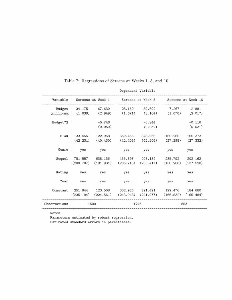
Table 7: Regressions of Screens at Weeks 1, 5, and 10

Dependent Variable--------------+--------------------------------------------------------------------

Variable | Screens at Week 1 Screens at Week 5 Screens at Week 10--------------+--------------------- --------------------- ----------------------

Budget | 34.175 67.630 28.160 39.692 7.267 12.881(millions)| (1.639) (2.949) (1.671) (3.164) (1.070) (2.017)

|Budget^2 | -0.746 -0.244 -0.116

| (0.050) (0.052) (0.031)|

STAR | 133.455 122.958 359.456 348.966 160.265 155.373| (42.231) (40.430) (42.405) (42.206) (27.298) (27.332)|

Genre | yes yes yes yes yes yes|

Sequel | 781.557 638.136 455.897 408.134 235.792 202.162|(200.707) (191.931) (206.715) (205.417) (138.200) (137.520)|

Rating | yes yes yes yes yes yes|

Year | yes yes yes yes yes yes|

Constant | 251.844 123.508 332.926 291.491 199.476 184.680|(235.194) (224.561) (243.948) (241.977) (166.832) (165.484)

--------------+--------------------------------------------------------------------Observations | 1500 1246 853--------------+--------------------------------------------------------------------

Notes:Parameters estimated by robust regression.Estimated standard errors in parentheses.

Table 8: Estimating the Probability of a Hit

(1) (2) (3)------------------- ------------------- -------------------

Variable | Coeff Marg Prob Coeff Marg Prob Coeff Marg Prob----------------------------------------------------------------------------------

Budget | 4.82e-08 4.05e-09 4.45e-08 4.09e-09 3.19e-08 8.10e-10|(5.06e-09) (4.98e-10) (5.50e-09) (5.84e-10) (6.58e-09) (4.03e-10)|

STAR | .92979 .13440 .98622 .15379 .84640 .04306| (.11414) (.02380) (.12896) (.02809) (.14556) (.01995)|

Sequel | .62257 .08146 .64563 .09126 .47506 .01920| (.20406) (.03753) (.22433) (.04404) (.26592) (.01757)|

Genre | yes yes yes|

Rating | yes yes yes|

Year | yes yes yes|

Life>=10 weeks | 2.16755 .07339| (.47415) (.01118)|

Wide Release | .90980 .05519(>=2000 screens)| (.19715) (.02974)

|Constant |-2.24740 -2.20408 -3.59036

| (.44974) (.51816) (.73964)----------------------------------------------------------------------------------

Pseudo R^2 | 0.306 0.303 0.428----------------------------------------------------------------------------------log Likelihood |-414.221 -326.052 -267.306----------------------------------------------------------------------------------

Observations | 2015 1500 1500----------------------------------------------------------------------------------

Notes:

Dependent variable =1 if (revenue>=50 million), 0 otherwise.Marginal probability is for discrete 0 to 1 change for dummy variables.Estimated standard errors in parentheses.

Table 9: Stars with Statistically Significant Impact on the Hit Probability

------------------------------------------------------Star Name | Coeff Std Err Marg Prob

------------------------------------------------------Cher | 1.283 0.751 0.264Bullock, Sandra | 2.076 0.646 0.569Carrey, Jim | 1.882 0.590 0.493Costner, Kevin | 1.380 0.417 0.297Cruise, Tom | 2.011 0.470 0.542Douglas, Michael | 1.173 0.412 0.226Eastwood, Clint | 1.091 0.520 0.200Ford, Harrison | 1.268 0.433 0.258Foster, Jodie | 1.820 0.952 0.469Gibson, Mel | 1.091 0.421 0.200Hanks, Tom | 1.378 0.357 0.296Murphy, Eddie | 0.997 0.429 0.172Pfeiffer, Michelle | 2.385 0.909 0.682Pitt, Brad | 1.637 0.792 0.396Schwarzenegger, Arnold | 0.813 0.405 0.124Spielberg, Steven | 1.625 0.534 0.391Stone, Oliver | 1.585 0.484 0.375Travolta, John | 1.380 0.385 0.297Williams, Robin | 1.143 0.379 0.216------------------------------------------------------

Notes:

Stars with significant coefficients (10% level, two-sided)in probit regression of the form of column 1 of Table 8.Marginal probabilities are the change in the probabilityof a movie being a hit with the presence of the given stars.

Table 10: Profit Regressions

Profit = β1 + β2Star + Γ[Sequel,Genre,Rating,Year] + µ

----------------------------| (1) (2)

----------------------------Estimator | LS Robust----------------------------

STAR| 17.144 2.391| (1.349) (0.567)| [2.054]|

Sequel| 10.633 4.818| (2.270) (0.953)| [2.510]|

Genre| yes yes|

Rating| yes yes|

Year| yes yes|

Constant| 10.394 1.786| (4.759) (1.999)| [5.058]

----------------------------R^2| .118 ---

----------------------------Notes:

Dependent variable is profit=(0.5*revenue-budget) in millions.All regressions run on common set of 2015 observations.LS is least squares regression.Robust is the robust regression implemented in STATA.Estimated standard errors in parentheses.Robust standard errors are in brackets (White’s estimator for LS).

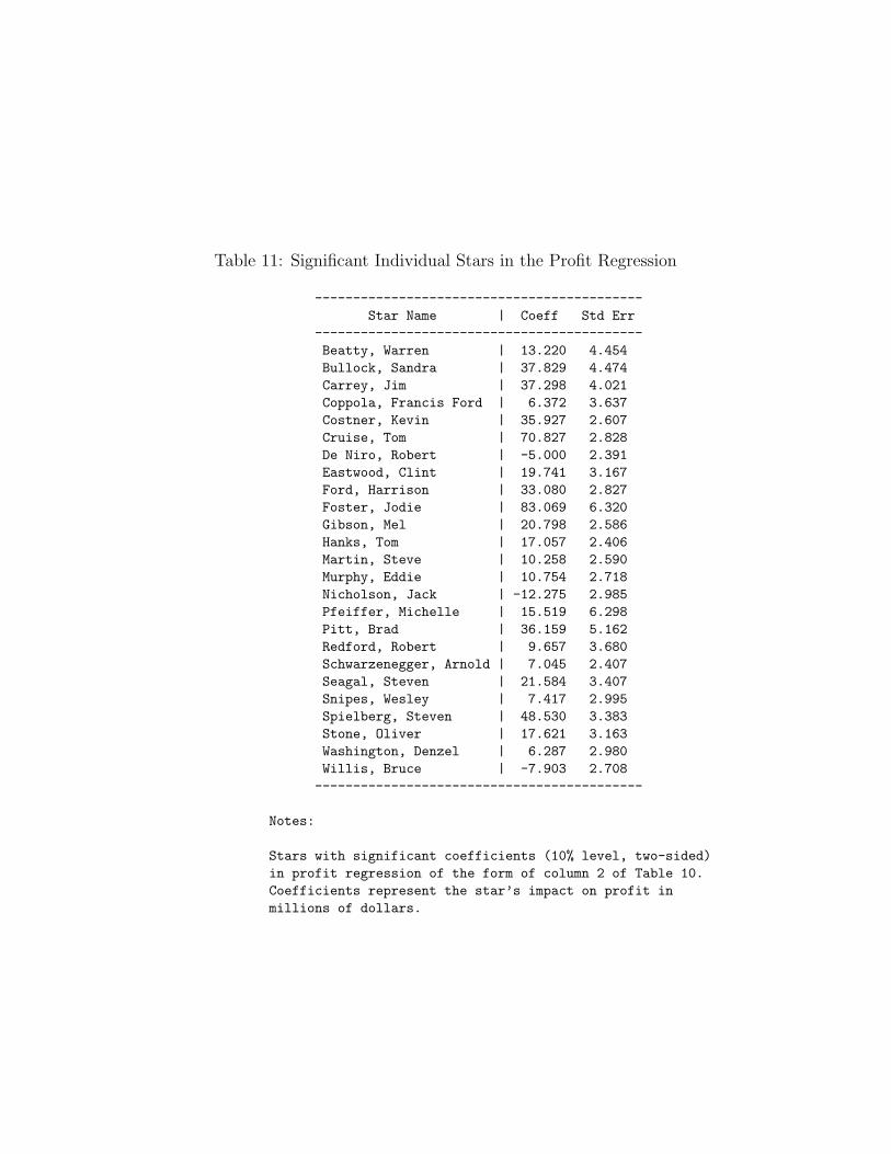
Table 11: Significant Individual Stars in the Profit Regression

-------------------------------------------Star Name | Coeff Std Err

-------------------------------------------Beatty, Warren | 13.220 4.454Bullock, Sandra | 37.829 4.474Carrey, Jim | 37.298 4.021Coppola, Francis Ford | 6.372 3.637Costner, Kevin | 35.927 2.607Cruise, Tom | 70.827 2.828De Niro, Robert | -5.000 2.391Eastwood, Clint | 19.741 3.167Ford, Harrison | 33.080 2.827Foster, Jodie | 83.069 6.320Gibson, Mel | 20.798 2.586Hanks, Tom | 17.057 2.406Martin, Steve | 10.258 2.590Murphy, Eddie | 10.754 2.718Nicholson, Jack | -12.275 2.985Pfeiffer, Michelle | 15.519 6.298Pitt, Brad | 36.159 5.162Redford, Robert | 9.657 3.680Schwarzenegger, Arnold | 7.045 2.407Seagal, Steven | 21.584 3.407Snipes, Wesley | 7.417 2.995Spielberg, Steven | 48.530 3.383Stone, Oliver | 17.621 3.163Washington, Denzel | 6.287 2.980Willis, Bruce | -7.903 2.708-------------------------------------------

Notes:

Stars with significant coefficients (10% level, two-sided)in profit regression of the form of column 2 of Table 10.Coefficients represent the star’s impact on profit inmillions of dollars.