UNCERTAINTY IN THE HOT HAND FALLACY:

DETECTING STREAKY ALTERNATIVES IN RANDOM BERNOULLI SEQUENCES

By

David M. Ritzwoller Joseph P. Romano

Technical Report No. 2019-05 August 2019

Department of Statistics STANFORD UNIVERSITY

Stanford, California 94305-4065

UNCERTAINTY IN THE HOT HAND FALLACY:

DETECTING STREAKY ALTERNATIVES IN RANDOM BERNOULLI SEQUENCES

By

David M. Ritzwoller Joseph P. Romano Stanford University

Technical Report No. 2019-05 August 2019

Department of Statistics STANFORD UNIVERSITY

Stanford, California 94305-4065

http://statistics.stanford.edu

Uncertainty in the Hot Hand Fallacy:Detecting Streaky Alternatives in Random

Bernoulli Sequences

David M. Ritzwoller, Stanford University∗

Joseph P. Romano, Stanford University

August 22, 2019

Abstract

We study a class of tests of the randomness of Bernoulli sequences and their applicationto analyses of the human tendency to perceive streaks as overly representative of positivedependence—the hot hand fallacy. In particular, we study tests of randomness (i.e., that tri-als are i.i.d.) based on test statistics that compare the proportion of successes that directlyfollow k consecutive successes with either the overall proportion of successes or the pro-portion of successes that directly follow k consecutive failures. We derive the asymptoticdistributions of these test statistics and their permutation distributions under randomnessand under general models of streakiness, which allows us to evaluate their local asymp-totic power. The results are applied to revisit tests of the hot hand fallacy implemented ondata from a basketball shooting experiment, whose conclusions are disputed by Gilovich,Vallone, and Tversky (1985) and Miller and Sanjurjo (2018a). We establish that the testsare insufficiently powered to distinguish randomness from alternatives consistent with thevariation in NBA shooting percentages. While multiple testing procedures reveal that oneshooter can be inferred to exhibit shooting significantly inconsistent with randomness, wefind that participants in a survey of basketball fans over-estimate an average player’s streak-iness, corroborating the empirical support for the hot hand fallacy.

∗E-mail: ritzwoll@stanford.edu, romano@stanford.edu. DR acknowledges funding from the Stanford Institutefor Economic Policy Research (SIEPR). We thank Tom DiCiccio, Matthew Gentzkow, Tom Gilovich, Zong Huang,Victoria Jalowitzki de Quadros, Joshua Miller, Linda Ouyang, Adam Sanjurjo, Azeem Shaikh, Jesse Shapiro, ShunYang, Molly Wharton, and Michael Wolf for helpful comments and conversations.

1

1 Introduction

Suppose that, for each i in 1, . . . ,N, we observe n consecutive Bernoulli trials Xi ={

Xi j}n

j=1,

with Xi j = 1 denoting a success and Xi j = 0 denoting a failure. We are interested in testing

either the individual hypotheses

H i0 : Xi is i.i.d. ,

the multiple hypothesis problem that tests the H i0 simultaneously, or the joint hypothesis

H0 : Xi is i.i.d. for all i in 1, . . . ,N

against alternatives in which the probabilities of success and failure immediately following

streaks of consecutive successes or consecutive failures are greater than their unconditional

probabilities.

The interpretation of the results of tests of this form have been pivotal in the development

of behavioral economics, and in particular, theories of human misperception of randomness. In

a formative paper, Tversky and Kahneman (1971) hypothesize that people erroneously believe

that small samples are highly representative of the “essential characteristics” of the population

from which they are drawn. For example, investors who observe a period of increasing returns

to an asset will perceive the increase to be representative of the dynamics of the asset and

expect the increases in returns to persist (Greenwood and Shleifer 2014, Barberis et. al 2015).

Similarly, people perceive streaks of ones in Bernoulli sequences to be overly representative of

a deviation from randomness, and thereby underestimate their probability when randomness is

true (Bar-Hillel and Wagenaar 1991, Rabin 2002).

Gilovich, Vallone, and Tversky (1985), henceforth GVT, test this hypothesis, that people

significantly under-estimate the probability of streaks in random processes, by analyzing bas-

ketball shooting data collected from the men and women of Cornell University’s varsity and

junior varsity basketball teams. They are unable to reject the hypothesis that the sequences

of shots they observe are i.i.d. and conclude that the belief in the “hot hand,” that basketball

players experience periods with elevated rates of success or failure, is a pervasive cognitive illu-

sion or fallacy. This conclusion became the academic consensus for the following three decades

(Kahneman 2011) and provided a central empirical support for many economic models in which

agents are overconfident in conclusions drawn from small samples (Rabin and Vayanos 2009).

2

The GVT results were challenged by Miller and Sanjurjo (2018a), henceforth MS, who note

that there is a significant small-sample bias in estimates of the probability of success following

streaks of successes or failures. They argue that when the GVT analysis is corrected to account

for this small-sample bias, they are able to reject the null hypothesis that shots are i.i.d. in favor

of a positive dependence consistent with expectations of streakiness in basketball.1

Miller and Sanjurjo (2018b) argue that their work “uncovered critical flaws ... sufficient to

not only invalidate the most compelling evidence against the hot hand, but even to vindicate

the belief in streakiness.” In fact, their conclusions resulted in persisting uncertainty in the

empirical support for the human tendency to perceive streaks as overly representative of positive

dependence (Rinott and Bar-Hillel 2015). Benjamin (2018) indicates that MS “re-opens–but

does not answer–the key question of whether there is a hot hand bias ... a belief in a stronger

hot hand than there really is.”

The objective of this paper is to clarify and quantify this uncertainty by developing the

asymptotic properties of the tests considered by GVT and MS, measuring the tests’ finite-

sample power with a set of local asymptotic approximations and simulations, and providing

a comprehensive presentation and interpretation of the results of these tests implemented on the

GVT shooting data. We find that the tests considered are insufficiently powered to detect devi-

ations from randomness consistent with the variation in NBA shooting percentages. Although

there is evidence that some basketball shooters are significantly non-i.i.d, average predictions of

the streakiness of basketball players in a survey of basketball fans are larger than the observed

streakiness, supporting the existence of the hot hand fallacy.

We focus our empirical analysis on the data from the GVT shooting experiment, because the

conclusions reached in GVT and MS are starkly different and have resulted in both the former

consensus and current uncertainty concerning the empirical support for the hot hand fallacy.

It is worth noting that Miller and Sanjurjo (2014) administer their own controlled shooting

experiment and reach similar conclusion to their analysis of the GVT shooting experiment.

The hypothesis tests studied in this paper are applicable to a wider class of questions. Tests

of the randomness of stochastic processes against nonrandom, persistent, or streaky alternatives

have been studied extensively within finance, economics, and psychology, including the large

1The MS results earned extensive coverage in the popular press, garnering expository articles in the New YorkTimes (Johnson 2015 and Appelbaum 2015), the New Yorker (Remnick 2015), the Wall Street Journal (Cohen2015), and on ESPN (Haberstroh 2017) among many other media outlets. MS was the 10th most downloaded pa-per on SSRN in 2015. Statistics sourced from http://ssrnblog.com/2015/12/29/ssrn-top-papers-of-2015/ accessedon July 21st, 2019.

3

literatures developing tests of the efficient market hypothesis (see Fama 1965, Malkiel and Fama

1970, and Malkiel 2003) or tests designed to detect whether mutual funds consistently outper-

form their benchmarks (see Jensen 1968, Hendricks et. al 1993, Carhart 1997, and Romano

and Wolf 2005).2 More broadly, our paper contributes to the literature on inference in Markov

Chains (see Billingsley 1961, Chapter 5 of Bhat and Miller 2000, and references therein).

Following MS and GVT, we study the test statistics Pn,k(Xi), Qn,k (Xi), and Dn,k (Xi). Each

Xi j has probability of success pi, which may depend on i. Let each individual’s observed prob-

ability of success be given by pn,i =1n ∑

nj=1 Xi j and let Pn,k(Xi) denote the proportion of suc-

cesses following k consecutive successes. That is, letting Yi jk = ∏j+km= j Xim and Vik = ∑

n−kj=1Yi jk,

then Pn,k(Xi) is given by

Pn,k(Xi) =Vik/

Vi(k−1). (1.1)

Likewise, let Qn,k (Xi) denote the proportion of failures following k consecutive failures. Letting

Zi jk = ∏j+km= j (1−Xim) and Wik = ∑

n−kj=1 Zi jk, then Qn,k(Xi) is given by

Qn,k(Xi) =Wik/

Wi(k−1). (1.2)

Let Dn,k (Xi) denote the difference between the proportion of successes following k consecutive

successes and k consecutive failures, given by

Dn,k (Xi) = Pn,k(Xi)−(1− Qn,k(Xi)

). (1.3)

Section 2 derives the asymptotic distributions of Pn,k(Xi), Qn,k(Xi), and Dn,k(Xi) and their

permutation distributions under H0. We give analytical expressions for the normal asymptotic

distributions of these test statistics, showing that tests relying on a normal approximation, ap-

plied by both GVT and MS, control type 1 error asymptotically. Additionally, we show that the

permutation distributions of these statistics converge to the statistics’ normal asymptotic distri-

butions, implying that the permutation tests applied by MS behave similarly to tests relying on

normal approximations.

Section 3 analyzes the asymptotics of the test statistics and their permutation distributions

under a set of general stationary processes. First, we characterize the normal asymptotic dis-

2Hendricks et. al (1993), titled “Hot Hands in Mutual Funds: Short-Run Persistence of Relative Performance,1974-1988”, argue that mutual fund performance is substantially streaky.

4

tributions of the test statistics under general α-mixing processes (see Bradley 2005). We use

these results to study the asymptotic distributions of the test statistics under a Markov model

of streakiness, in which the probability of a success or a failure is increased directly following

m consecutive successes or failures, respectively. We give expressions for the local asymptotic

power of the hypothesis tests under consideration against these streaky alternatives.

We show that the test rejecting for large values of Dn,1 (Xi) is asymptotically equivalent

to the Wald Wolfowitz (1940) runs test, which is known to be the uniformly most powerful

unbiased statistic against first-order Markov Chains and is the standard test statistic used to test

randomness in Bernoulli sequences (Lehmann 1998). As a byproduct of our analysis, we derive

the limiting local power function for the Wald Wolfowitz (1940) runs test, which appears to

be new. In turn, we show that Dn,k (Xi) has the maximum power, within the hypothesis tests

that we consider, against alternatives in which streakiness begins after k consecutive successes

or failures. Simulation evidence indicates that our asymptotic approximations to the power

against streaky alternatives perform remarkably well in the sample sizes considered in GVT

and MS.

Section 4 presents several methods for testing the joint null hypothesis H0 with a single test

statistic and by combining the results of several tests using different test statistics. We imple-

ment a set of simulations that measure the finite-sample power of these tests against alternatives

in which individuals follow the streaky model developed in Section 3 with probability θ and H i0

with probability 1−θ .

Having established the asymptotic properties of Dn,k (Xi) under the null and under alterna-

tive models of streakiness, Section 5 revisits the GVT and MS analysis, delineating individual,

simultaneous, and joint testing environments. When testing the hypotheses H i0 simultaneously,

we find that we are able to reject H i0 for only one shooter consistently. This shooter’s shot se-

quence is strikingly streaky. He makes 16 shots in a row directly following a period in which

he misses 15 out of 18 shots. Tests of the joint null hypothesis at the 5% level are not robust to

the exclusion of this shooter from the sample.

We find that the tests considered by GVT and MS do not have adequate power to detect

hot hand shooting effect sizes consistent with the observed variation in NBA field goal and

three point shooting percentage. However, the tests are able to detect the average effect sizes

predicted by the survey of basketball fans presented in GVT with probability close to one.

Therefore, while there is strong evidence that non-random shooting is present for some shooters,

a contribution of MS, weak evidence against H0 over most shooters indicates that people over-

5

estimate an average player’s streakiness, the central thesis of GVT.

Section 6 concludes. Online Appendix A and Online Appendix B include supplemental

tables and figures relevant to our analysis, respectively. Proofs of all mathematical results pre-

sented in the main body of this paper are given in Online Appendix C.

2 Asymptotics Under I.I.D. Processes

In this section, we derive the asymptotic unconditional sampling distributions of Pn,k(Xi),

Pn,k(Xi)− pi, and Dn,k(Xi) under H i0. We also derive the limiting behavior of the corresponding

permutation distributions of these test statistics.

For ease of notation, we drop the dependence on the individual i. Note that the asymptotic

distribution of Qn,k(X) can be obtained by replacing p with 1− p in the expressions for the

asymptotic distributions of Pn,k(X). Note, Pn,k(X), Qn,k(X), and Dn,k(X) are not defined for

every sequence X, that is they are not defined for sequences without instances of k consecu-

tive successes or failures. However, the statistics are defined with probability approaching one

exponentially quickly as n grows to infinity.

2.1 Asymptotic Behavior of the Test Statistics

First, we evaluate the asymptotic distributions of Pn,k(X), Pn,k(X)− p, and Dn,k(X) under H0.

Despite the long history of this problem, such distributions have not been provided to date.

Miller and Sanjurjo (2014) claim that Pn,k(X) is asymptotically normal, referencing Mood

(1940), but are unable to provide explicit formulae for the asymptotic variances. Note that,

even in the null i.i.d. case, the test statistics are functions of overlapping subsequences of ob-

servations, and so central limit theorems for dependent data are required. In order to analyze

the asymptotic behavior of the permutation distributions, we are aided by an appropriate central

limit theorem using Stein’s method (see Rinot 1994 and Stein 1986).

Theorem 2.1. Under the assumption that X = {Xi}ni=1 is a sequence of i.i.d. Bernoulli(p)

random variables,

(i) Pn,k (X), given by (1.1), is asymptotically normal with limiting distribution given by

√n(Pn,k (X)− p

) d→ N(0,σ2

P (p,k)), (2.1)

where σ2P (p,k) = p1−k (1− p) and d→ denotes convergence in distribution,

6

(ii) Pn,k (X)− p, where p= n−1∑

ni=1 Xi, is asymptotically normal with limiting distribution given

by√

n(Pn,k (X)− p

) d→ N(0,σ2

P (p,k)), (2.2)

where σ2P (p,k) = p1−k (1− p)

(1− pk),

(iii) and Dn,k (X), given by (1.3), is asymptotically normal with limiting distribution given by√

nDn,k (X)d→ N

(0,σ2

D (p,k)), (2.3)

where σ2D (p,k) = (p(1− p))1−k

((1− p)k + pk

).

Note that σ2D(1

2 ,k)= 2k−1 increases quite rapidly with k, stemming from an effectively

reduced sample size when considering successes, or failures, following only streaks of length k.

Remark 2.1. Theorem 2.1 can be generalized to a triangular array Xn ={

Xn, j}n

j=1 of i.i.d.

Bernoulli trials with probability of success pn converging to p. Specifically, we have that,

n1/2 (Pk (Xn)− pn) d→ N

(0,σ2

P (p,k)),

n1/2 (Pk (Xn)− pn) d→ N

(0,σ2

P (p,k)), and

n1/2Dk (Xn)d→ N

(0,σ2

D (p,k)).

This result implies that we can consistently approximate the quantiles of the distributions of

Pn,k (Xn) and Dn,k (Xn) with the parametric bootstrap, which approximates the distribution of√

nDn,k (X) under p by that of√

nDn,k (X) under pn.

Remark 2.2. MS show that, under H i0, the expectations of Pn,k (X)− p and Dn,k (X) under the

null are significantly less than 0 in small samples. While exact expressions for the expectations

of these statistics appear to be unknown for k > 1, in Online Appendix D we obtain the second

order approximations

E[Pn,k(X)− p

]= n−1 p

(1− p−k

)+O

(n−2) and

E[Dn,k(X)

]= n−1

(1− (1− p)1−k− p1−k

)+O

(n−2) .

Remark 2.3. Note that the asymptotic variance of Dn,k (X) is equal to the sum of the asymptotic

variances of Pn,k (X) and Qn,k (X), suggesting that

nCov(Pn,k (X) , Qn,k (X)

)→ 0. (2.4)

7

In fact, in Online Appendix D, we show that Cov(Pn,k (X) , Qn,k (X)

)= O

(n−2) . GVT and MS

approximate the variance of Dn,k (X) with estimators that implicitly assume (2.4). MS cite a

simulation exercise supporting their assumption. Our results justify this assumption mathemat-

ically. Additionally, the asymptotic variance of Pn,k (X)− p is equal to the sum of the asymptotic

variance of Pn,k (X)− p and p(1− p), which implies Pn,k (X)− p and p are asymptotically in-

dependent.

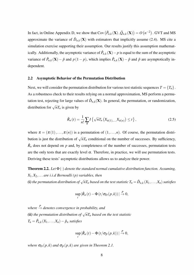
2.2 Asymptotic Behavior of the Permutation Distribution

Next, we will consider the permutation distribution for various test statistic sequences T = {Tn} .As a robustness check to their results relying on a normal approximation, MS perform a permu-

tation test, rejecting for large values of Dn,k(X). In general, the permutation, or randomization,

distribution for√

nTn is given by

Rn (t) =1n! ∑

π

I{√

nTn(Xπ(1),...,Xπ(n)

)≤ t}, (2.5)

where π = (π (1) , . . . ,π (n)) is a permutation of (1, . . . ,n). Of course, the permutation distri-

bution is just the distribution of√

nTn conditional on the number of successes. By sufficiency,

Rn does not depend on p and, by completeness of the number of successes, permutation tests

are the only tests that are exactly level α . Therefore, in practice, we will use permutation tests.

Deriving these tests’ asymptotic distributions allows us to analyze their power.

Theorem 2.2. Let Φ(·) denote the standard normal cumulative distribution function. Assuming,

X1,X2, . . . are i.i.d Bernoulli (p) variables, then

(i) the permutation distribution of√

nTn based on the test statistic Tn = Dn,k (X1, . . . ,Xn) satisfies

supt|Rn (t)−Φ(t/σD (p,k)) | P→ 0,

where P→ denotes convergence in probability, and

(ii) the permutation distribution of√

nTn based on the test statistic

Tn = Pn,k (X1, . . . ,Xn)− pn satisfies

supt|Rn (t)−Φ(t/σP (p,k)) | P→ 0,

where σD (p,k) and σP (p,k) are given in Theorem 2.1.

8

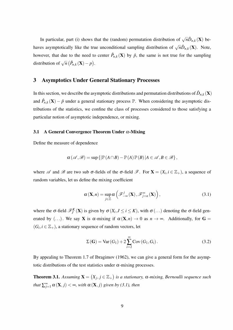
In particular, part (i) shows that the (random) permutation distribution of√

nDn,k (X) be-

haves asymptotically like the true unconditional sampling distribution of√

nDn,k (X). Note,

however, that due to the need to center Pn,k (X) by p, the same is not true for the sampling

distribution of√

n(Pn,k (X)− p

).

3 Asymptotics Under General Stationary Processes

In this section, we describe the asymptotic distributions and permutation distributions of Dn,k (X)

and Pn,k (X)− p under a general stationary process P. When considering the asymptotic dis-

tributions of the statistics, we confine the class of processes considered to those satisfying a

particular notion of asymptotic independence, or mixing.

3.1 A General Convergence Theorem Under α-Mixing

Define the measure of dependence

α (A ,B) = sup{|P(A∩B)−P(A)P(B) |A ∈A ,B ∈B} ,

where A and B are two sub σ -fields of the σ -field F . For X = (Xi, i ∈ Z+), a sequence of

random variables, let us define the mixing coefficient

α (X,n) = supj∈Z

α

(F j−∞ (X) ,F ∞

j+n (X)), (3.1)

where the σ -field F KJ (X) is given by σ (Xi,J ≤ i≤ K), with σ (. . .) denoting the σ -field gen-

erated by (. . .) . We say X is α-mixing if α (X,n) → 0 as n → ∞. Additionally, for G =

(Gi, i ∈ Z+), a stationary sequence of random vectors, let

Σ(G) = Var(G1)+2∞

∑i=2

Cov(G1,Gi) . (3.2)

By appealing to Theorem 1.7 of Ibragimov (1962), we can give a general form for the asymp-

totic distributions of the test statistics under α-mixing processes.

Theorem 3.1. Assuming X =(X j, j ∈ Z+

)is a stationary, α-mixing, Bernoulli sequence such

that ∑∞j=1 α (X, j)< ∞, with α (X, j) given by (3.1), then

9

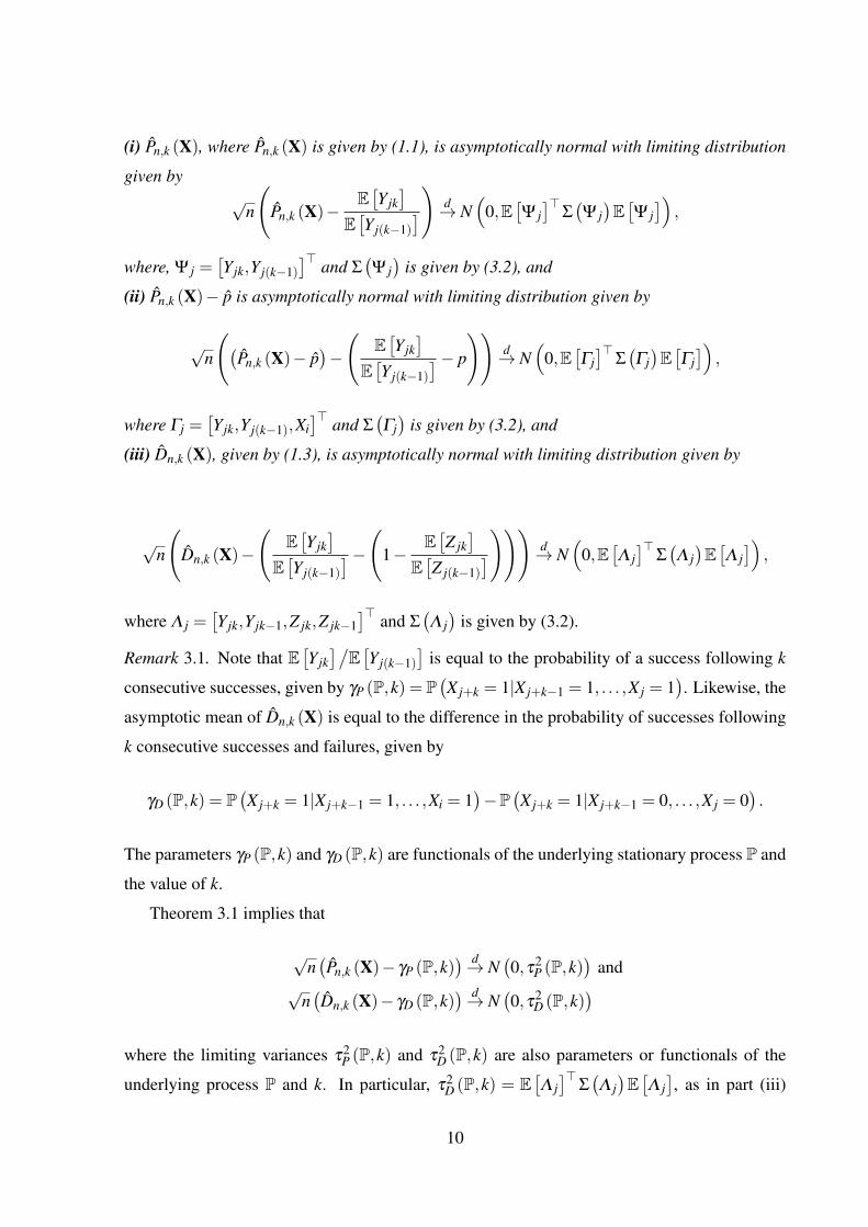
(i) Pn,k (X), where Pn,k (X) is given by (1.1), is asymptotically normal with limiting distribution

given by√

n

(Pn,k (X)−

E[Yjk]

E[Yj(k−1)

]) d→ N(

0,E[Ψ j]>

Σ(Ψ j)E[Ψ j])

,

where, Ψ j =[Yjk,Yj(k−1)

]> and Σ(Ψ j)

is given by (3.2), and

(ii) Pn,k (X)− p is asymptotically normal with limiting distribution given by

√n

((Pn,k (X)− p

)−

(E[Yjk]

E[Yj(k−1)

] − p

))d→ N

(0,E

[Γj]>

Σ(Γj)E[Γj])

,

where Γj =[Yjk,Y j(k−1),Xi

]> and Σ(Γj)

is given by (3.2), and

(iii) Dn,k (X), given by (1.3), is asymptotically normal with limiting distribution given by

√n

(Dn,k (X)−

(E[Yjk]

E[Yj(k−1)

] −(1−E[Z jk]

E[Z j(k−1)

]))) d→ N(

0,E[Λ j]>

Σ(Λ j)E[Λ j])

,

where Λ j =[Y jk,Yjk−1,Z jk,Z jk−1

]> and Σ(Λ j)

is given by (3.2).

Remark 3.1. Note that E[Yjk]/

E[Yj(k−1)

]is equal to the probability of a success following k

consecutive successes, given by γP (P,k) = P(X j+k = 1|X j+k−1 = 1, . . . ,X j = 1

). Likewise, the

asymptotic mean of Dn,k (X) is equal to the difference in the probability of successes following

k consecutive successes and failures, given by

γD (P,k) = P(X j+k = 1|X j+k−1 = 1, . . . ,Xi = 1

)−P

(X j+k = 1|X j+k−1 = 0, . . . ,X j = 0

).

The parameters γP (P,k) and γD (P,k) are functionals of the underlying stationary process P and

the value of k.

Theorem 3.1 implies that

√n(Pn,k (X)− γP (P,k)

) d→ N(0,τ2

P (P,k))

and√

n(Dn,k (X)− γD (P,k)

) d→ N(0,τ2

D (P,k))

where the limiting variances τ2P (P,k) and τ2

D (P,k) are also parameters or functionals of the

underlying process P and k. In particular, τ2D (P,k) = E

[Λ j]>

Σ(Λ j)E[Λ j], as in part (iii)

10

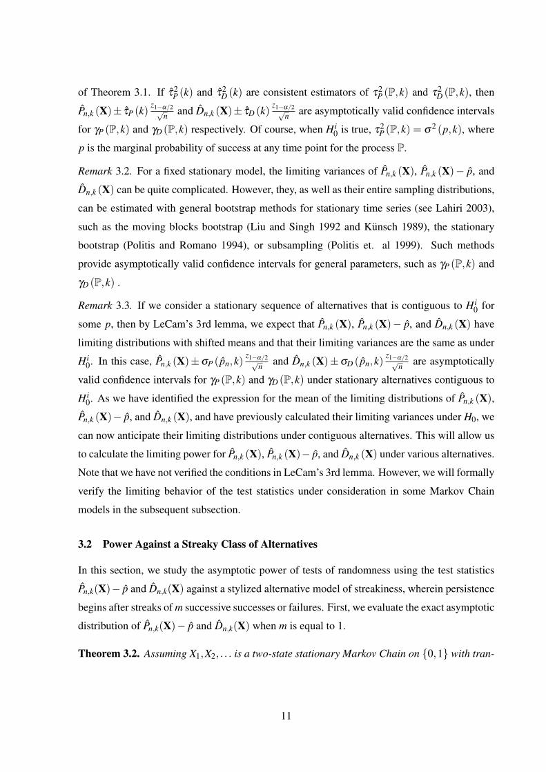
of Theorem 3.1. If τ2P (k) and τ2

D (k) are consistent estimators of τ2P (P,k) and τ2

D (P,k), then

Pn,k (X)± τP (k)z1−α/2√

n and Dn,k (X)± τD (k)z1−α/2√

n are asymptotically valid confidence intervals

for γP (P,k) and γD (P,k) respectively. Of course, when H i0 is true, τ2

P (P,k) = σ2 (p,k), where

p is the marginal probability of success at any time point for the process P.

Remark 3.2. For a fixed stationary model, the limiting variances of Pn,k (X), Pn,k (X)− p, and

Dn,k (X) can be quite complicated. However, they, as well as their entire sampling distributions,

can be estimated with general bootstrap methods for stationary time series (see Lahiri 2003),

such as the moving blocks bootstrap (Liu and Singh 1992 and Kunsch 1989), the stationary

bootstrap (Politis and Romano 1994), or subsampling (Politis et. al 1999). Such methods

provide asymptotically valid confidence intervals for general parameters, such as γP (P,k) and

γD (P,k) .

Remark 3.3. If we consider a stationary sequence of alternatives that is contiguous to H i0 for

some p, then by LeCam’s 3rd lemma, we expect that Pn,k (X), Pn,k (X)− p, and Dn,k (X) have

limiting distributions with shifted means and that their limiting variances are the same as under

H i0. In this case, Pn,k (X)±σP (pn,k)

z1−α/2√n and Dn,k (X)±σD (pn,k)

z1−α/2√n are asymptotically

valid confidence intervals for γP (P,k) and γD (P,k) under stationary alternatives contiguous to

H i0. As we have identified the expression for the mean of the limiting distributions of Pn,k (X),

Pn,k (X)− p, and Dn,k (X), and have previously calculated their limiting variances under H0, we

can now anticipate their limiting distributions under contiguous alternatives. This will allow us

to calculate the limiting power for Pn,k (X), Pn,k (X)− p, and Dn,k (X) under various alternatives.

Note that we have not verified the conditions in LeCam’s 3rd lemma. However, we will formally

verify the limiting behavior of the test statistics under consideration in some Markov Chain

models in the subsequent subsection.

3.2 Power Against a Streaky Class of Alternatives

In this section, we study the asymptotic power of tests of randomness using the test statistics

Pn,k(X)− p and Dn,k(X) against a stylized alternative model of streakiness, wherein persistence

begins after streaks of m successive successes or failures. First, we evaluate the exact asymptotic

distribution of Pn,k(X)− p and Dn,k(X) when m is equal to 1.

Theorem 3.2. Assuming X1,X2, . . . is a two-state stationary Markov Chain on {0,1} with tran-

11

sition matrix given by

P =

12 + ε

12 − ε

12 − ε

12 + ε

, (3.3)

where 0≤ ε < 12 , then

(i) Dn,1 (X), given by (1.3) with k equal to 1, is asymptotically normal with limiting distribution

given by√

n(Dn,1 (X)−2ε

) d→ N(0,1−4ε

2) . (3.4)

(ii) Pn,1 (X), given by (1.1) with k equal to 1, is asymptotically normal with limiting distribution

given by√

n(

Pn,1 (X)− 12− ε

)d→ N

(0,

12−2ε

2). (3.5)

(ii) Pn,1 (X)− p, given by (1.1) with k equal to 1, is asymptotically normal with limiting distri-

bution given by√

n(Pn,1 (X)− p− ε

) d→ N(

0,1−2ε +16ε2

4−8ε

). (3.6)

Remark 3.4. The argument for Theorem 3.2 holds if we let ε vary with n such that εn = ε +

O(

n−1/2)

. If we take εn =h√n , then

√n(

Dn,1 (X)− 2h√n

)d→ N (0,1) and therefore the power

of the test that rejects when√

nDn,1 (X)> z1−α is given by

P(√

nDn,1 (X)> z1−α

)= P

(√n(

Dn,1 (X)− 2h√n

)> z1−α −2h

)→ 1−Φ(z1−α −2h) .

The same limiting power results if z1−α is replaced by the permutation quantile.

Next, we verify the asymptotic normality of Pn,k(X)− p and Dn,k(X) for deviations from

independence occurring at general m.

Theorem 3.3. Let 0 ≤ ε < 12 . Assume X1,X2, . . . is a two-state stationary Markov chain of

order m on {0,1} such that the probability of transitioning from 1 to 1 (0 to 0) is 12 + ε after m

successive 1’s (0′s) and 12 after any other sequence of m states with at least one 1 and one 0,

then

12

√n(Pn,k (X)−µP (k,m,ε)

) d→ N(0,σ2

P (k,m,ε)),

√n(Pn,k (X)− p−µP (k,m,ε)

) d→N(0,σ2

P (k,m,ε)), and

√n(Dn,k (X)−µD (k,m,ε)

) d→ N(0,σ2

D (k,m,ε))

where µP (k,m,ε), µP (k,m,ε), and µD (k,m,ε) are given explicitly in the proof and σ2P (k,m,ε),

σ2P (k,m,ε), and σ2

D (k,m,ε) are functions of k, m, and ε .

The functions σ2 (k,m,ε) are continuous in ε , so if we take εn = h√n then we expect that

σ2P (k,m,ε), σ2

P (k,m,ε) , and σ2D (k,m,ε) would converge to the asymptotic variances of Pn,k (X),

Pn,k (X)− p, and Dn,k (X) under H0, respectively. This is verified formally for the case of m = 1

in Remark 3.4 and can be shown more generally by tracing the proof of Theorem 3.2, though

the details are omitted. Therefore, if εn =h√n , then

√n(Dn,k (X)−µD (k,m,εn)

) d→ N(

0,2k−1),

where 2k−1 is the asymptotic variance of Dn,k (X) under H0, given by Theorem 2.1. Let

φD (k,m,h) denote the limit of√

nµD (k,m,εn)√2k−1 and z1−α be the 1− α quantile of the standard

normal distribution. The power of the test that rejects when√

nDn,k(X)√2k−1 > z1−α where under the

Markov Chain model considered in Theorem 3.3 is given by

P(√

nDn,k (X)√2k−1

> z1−α

)= P

(√n(

Dn,k (X)√2k−1

− µD(k,m,εn)√2k−1

)> z1−α −

√nµD(k,m,εn)√

2k−1

)→ 1−Φ(z1−α −φD (k,m,h)) . (3.7)

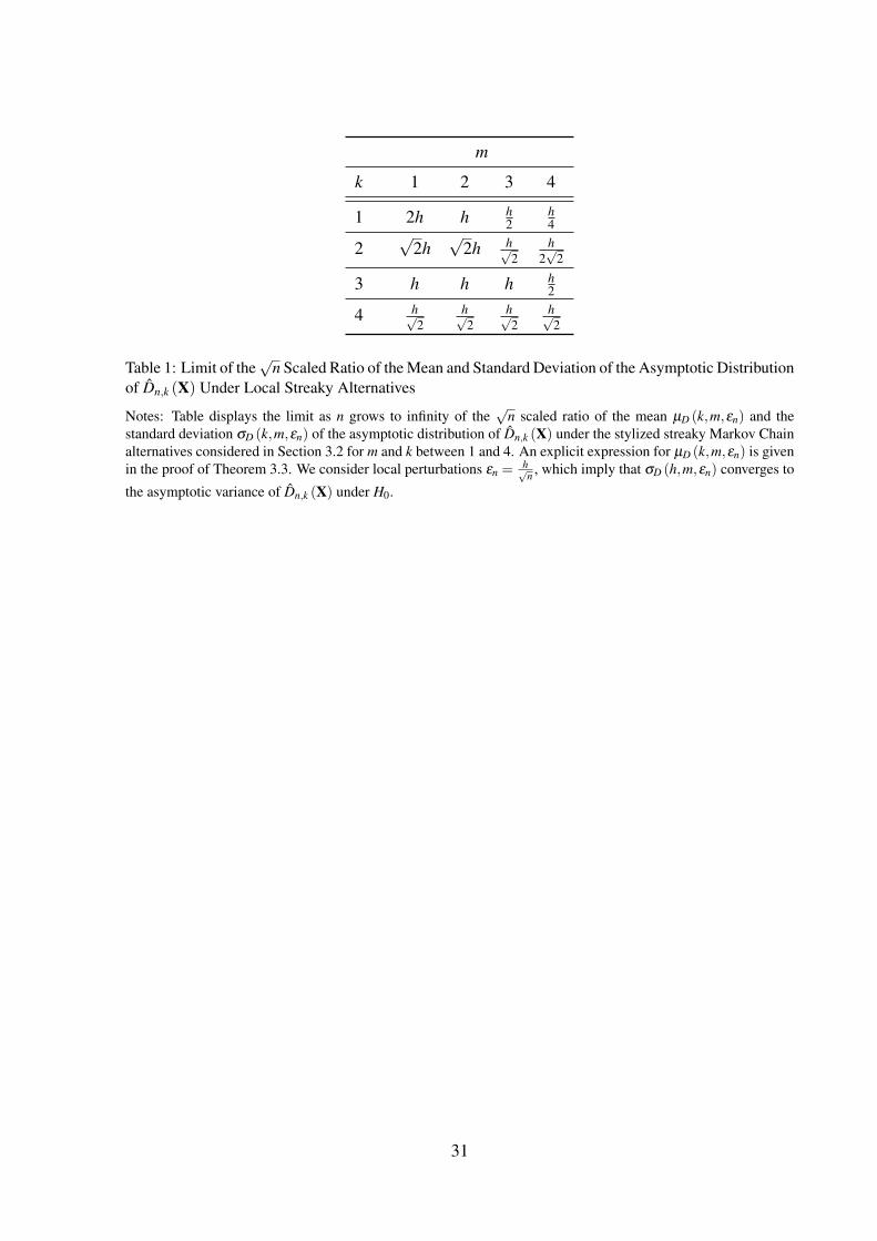
Table 1 displays the values of φD (k,m,h) for m and k between 1 and 4. The tests that reject

for large values of Dn,k (X) for k = m have the largest power against the alternative where

streakiness begins after m consecutive successes or failures. The test that rejects for large values

Dn,k (X) for k = 1 against the alternative with m = 1 has the largest power over any combination

of test statistics and alternatives. Thus, when we present results measuring the finite-sample

power, the power of the test using Dn,k (Xi) for k = 1 against the alternative with m = 1 gives an

upper bound to the power of any of the hypothesis tests against any models of streakiness we

consider.

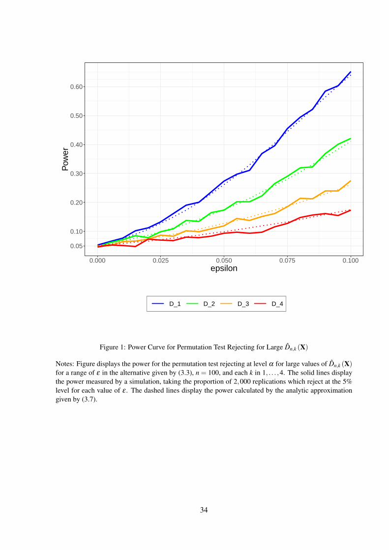
Figure 1 displays the power for the permutation test rejecting at level 0.05 for large values

of Dn,k (X) for k between 1 and 4 and n = 100 against the model considered in Theorem 3.3

13

with m = 1 over a grid of ε .3 The solid lines display the power of each test measured with a

simulation, drawing and implementing the tests on 2,000 replicates of sequences for each value

of ε . The dashed lines display the power approximated with the asymptotic expression derived

in equation (3.7).

The finite-sample simulation and asymptotic-approximation results are remarkably close.

The permutation test rejecting for large values of Dn,1 (X) has the largest power, and in fact, in

the following section we show that it is asymptotically equivalent to the uniformly most power-

ful unbiased test. The power of the test rejecting for large values of Dn,1 (X) is approximately

0.5 for ε = 0.08 and n = 100.

3.3 Asymptotic Equivalence between the Wald-Wolfowitz Runs Test and the Test Based

on Dn,1 (X)

The Wald-Wolfowitz Runs Test (Wald and Wolfowitz 1940) rejects for small values of the

number of runs R, or equivalently, for large values of

Zn =

(−R2n + p(1− p)

p(1− p)

).

As shown in Wald and Wolfowitz (1940), under i.i.d. Bernoulli trials,√

nZnd→ N (0,1), so

the runs test may use either z1−α or a critical value determined exactly from the permutation

distribution. Note that the runs test is known to be the uniformly most powerful unbiased test

against the Markov Chain alternatives considered in Section 3.2; see Lehmann and Romano

(2005), Problems 4.29–4.31. The following Theorem shows the runs test is asymptotically

equivalent to the test based on Dn,1 (X).

Theorem 3.4. The Wald Wolfowitz Runs Test and the test based on Dn,1 (X) are asymptotically

equivalent in the sense that they reach the same conclusion with probability tending to one,

both under the null hypothesis and under contiguous alternatives. In particular, we show the

following:

(i) Under i.i.d Bernoulli trials,

√n(Dn,1 (X)−Zn

) P→ 0. (3.8)

3Most shooters take 100 shots in the experiment considered in GVT and MS. Three shooters take 90, 75, and 50shots, respectively.

14

Therefore, if both statistics are applied using z1−α as a critical value, they both lead to the same

decision with probability tending to one.

(ii) Since (3.8) implies the same is true under contiguous alternatives to Bernoulli sampling (for

some p), the same conclusion holds.

(iii) The same conclusion holds if z1−α is replaced by critical values obtained by the permuta-

tion distribution.

(iv) Both tests have the same local limiting power functions under some sequence of contiguous

alternatives, and in particular, under the Markov Chain model considered in Section 3.2, where

the limiting local power function is given in Remark 3.4.

Remark 3.5. The permutation test based on the standardized first sample autocorrelation di-

vided by the sample variance, which is not known to have any optimality properties for binary

data, is equivalent to the permutation test based on ∑nj=1 XiXi+1 by the invariance of the sample

mean and variance under permutations. In turn, the permutation test based on ∑nj=1 XiXi+1 is

asymptotically equivalent to the permutation test based on Pn,1 (X); See Wald and Wolfowitz

(1943). It also follows from (C.5) in the Online Appendix that the test based on Pn,1 (X)− p and

Dn,1 (X) are asymptotically equivalent. Therefore, the permutation tests based on Zn, Dn,1 (X),

Pn,1 (X)− p, and the first sample autocorrelation are asymptotically equivalent and Theorem 3.4

can be applied to any of the four tests. Miller and Sanjurjo (2014) note this approximate equiv-

alence. Their results are not asymptotic and are based on an approximate algebraic equivalence

supported by simulation of correlations between the various test statistics.

3.4 Asymptotic Behavior of the Permutation Distribution in Non I.I.D. Settings

Previously, we considered the permutation distribution for various test statistic sequences T =

{Tn}. The permutation distribution itself is random, but depends only on the number of suc-

cesses in the data set. Under i.i.d. Bernoulli trials, the number of successes is binomial. We now

wish to study the behavior of the permutation distribution in possibly non i.i.d. settings (such

as the Markov Chain models considered in Section 3.2). But first, we will study the behavior of

the permutation distribution for fixed (nonrandom) sequences of number of successes, in which

case the permutation distribution is not random, but its limiting distribution is nontrivial.

In order to do this, the following notation is useful. Let Ln (h) be the permutation distribution

15

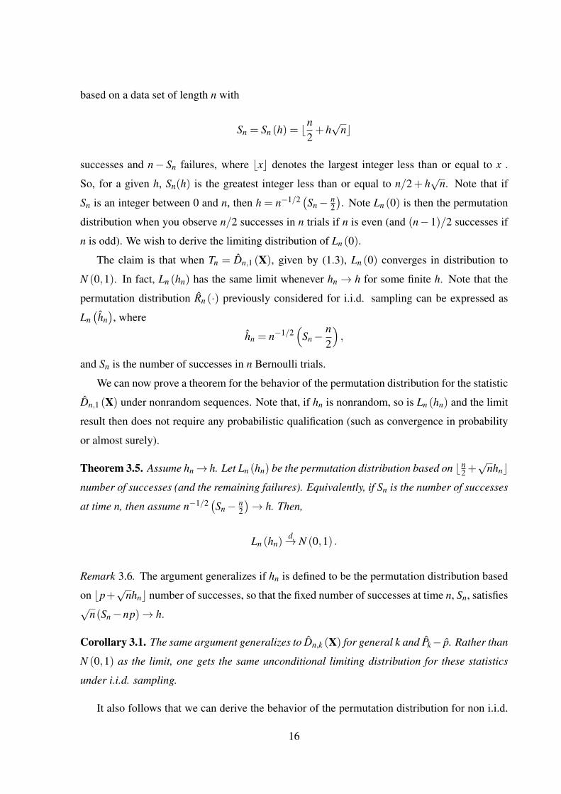
based on a data set of length n with

Sn = Sn (h) = bn2+h√

nc

successes and n− Sn failures, where bxc denotes the largest integer less than or equal to x .

So, for a given h, Sn(h) is the greatest integer less than or equal to n/2+ h√

n. Note that if

Sn is an integer between 0 and n, then h = n−1/2 (Sn− n2

). Note Ln (0) is then the permutation

distribution when you observe n/2 successes in n trials if n is even (and (n−1)/2 successes if

n is odd). We wish to derive the limiting distribution of Ln (0).

The claim is that when Tn = Dn,1 (X), given by (1.3), Ln (0) converges in distribution to

N (0,1). In fact, Ln (hn) has the same limit whenever hn→ h for some finite h. Note that the

permutation distribution Rn (·) previously considered for i.i.d. sampling can be expressed as

Ln(hn), where

hn = n−1/2(

Sn−n2

),

and Sn is the number of successes in n Bernoulli trials.

We can now prove a theorem for the behavior of the permutation distribution for the statistic

Dn,1 (X) under nonrandom sequences. Note that, if hn is nonrandom, so is Ln (hn) and the limit

result then does not require any probabilistic qualification (such as convergence in probability

or almost surely).

Theorem 3.5. Assume hn→ h. Let Ln (hn) be the permutation distribution based on bn2 +√

nhncnumber of successes (and the remaining failures). Equivalently, if Sn is the number of successes

at time n, then assume n−1/2 (Sn− n2

)→ h. Then,

Ln (hn)d→ N (0,1) .

Remark 3.6. The argument generalizes if hn is defined to be the permutation distribution based

on bp+√

nhnc number of successes, so that the fixed number of successes at time n, Sn, satisfies√

n(Sn−np)→ h.

Corollary 3.1. The same argument generalizes to Dn,k (X) for general k and Pk− p. Rather than

N (0,1) as the limit, one gets the same unconditional limiting distribution for these statistics

under i.i.d. sampling.

It also follows that we can derive the behavior of the permutation distribution for non i.i.d.

16

processes, such as the Markov Chains considered in Section 3.2.

Theorem 3.6. Suppose that X1,X2, . . . is a possibly dependent stationary Bernoulli sequence.

Let Sn denote the number of successes in n trials. Assume, for some p ∈ (0,1),√

n(Sn−np

)converges in distribution to some limiting distribution. Then, the permutation distribution for

Dn,1 (X) converges to N (0,1) in probability; that is

supt|Rn (t)−Φ(t) | P→ 0. (3.9)

Remark 3.7. In the Markov Chain model considered in Section 3.2. we know from the proof of

Theorem 3.2 that√

n(Sn−n/2

) d→ N(

0,14+

ε

1−2ε

),

and so Theorem 3.6 applies. More generally, the assumption that√

n(Sn−np

)converges in

distribution can be weakened to the assumption that X is an α-mixing process, as the former

condition follows from the latter assumption by Theorem 1.7 of Ibragimov (1962).

4 Tests of the Joint Null

The previous sections dealt with the statistical properties of the statistics Gn,k (Xi), applied to an

individual i, given a choice of G ∈ {D,P,Q}. In order to consider the joint null hypothesis that

no individual deviates from randomness, we first consider methods that combine these statistics,

or corresponding p-values, over all individuals to provide an overall test for deviation from the

joint null. We will consider four well-known approaches to this below. Since it is not clear that

there is a universally optimal choice of test statistic, we will also combine these results over

many choices of test statistics to get one global test of H0.

We simulate the finite-sample power of these joint hypothesis testing procedures against

alternatives in which each of the N individuals has probability θ of being drawn from the streaky

alternative considered in Section 3.2 under a specified ε .

4.1 Methods Considered

We outline four procedures for testing the joint hypothesis H0 using a single statistic Gn,k (Xi),

given a choice of G ∈ {D,P,Q} and a value of k. We then present two methods for testing H0

which combine individual tests of H0 using various test statistics into one overall test statistic.

17

The four procedures that test the joint hypothesis H0 using a single statistic Gn,k (Xi) com-

bined across individuals are as follows:

• Average Value of Gn,k (Xi): The first procedure rejects for large values of the average

of the appropriately centered mean of the test statistic over individuals Gk. Specifically,

Dk = ∑Ni=1 Dn,k (Xi), Pk = ∑

Ni=1 Pn,k (Xi)− pi, and Qk = ∑

Ni=1 Qn,k (Xi)− (1− pi). MS

implement this procedure and approximate the critical values of the test rejecting for

large Tk with a normal approximation and with a stratified permutation procedure wherein

each individual’s observed sequence of trials is permuted separately. We will refer to the

distribution of a statistic computed on each of the permuted replicates of each individual’s

sequence of trials as the stratified permutation distribution. In each stratified permutation,

Gk is computed over all individuals with Gn,k (Xi) defined.

• Minimum p-value: Let ρG (k, i) denote the p-value for individual i for a test of the

hypothesis H i0 which rejects for extreme values of Gn,k (Xi). The minimum p-value joint

hypothesis testing procedure rejects for small values of ψT,k = min1≤i≤N (ρG (k, i)). The

critical values of the test rejecting for small value of ψG,k can be approximated by the

stratified permutation distribution of ψG,k .

• Fisher’s Method: The Fisher joint hypothesis test statistic (Fisher 1925) is given by

fG,k = −2∑ log(ρG (k, i)). If ρG (k, i) are p-values for independent tests, then fG,k has

a chi-squared distribution with 2 ·N degrees of freedom. However, we need to account

for the fact that Dn,k(Xi), Pn,k(Xi), and Qn,k (Xi) are undefined for some sequences. By

assigning a p-value of 1 to these sequences, the critical values of the test rejecting for

large values of fG,k can be approximated with the stratified permutation distribution of

fG,k .

• Tukey’s Higher Criticism: The Tukey Higher Criticism test statistic is given by

TG,k = max0<δ<δ0

[Tδ ] = max0<δ<δ0

[√N (ξδ −δ )√δ (1−δ )

],

where ξδ is the fraction of individuals that are significant at level δ for a given test of

H i0 rejecting for large values of Gn,k (Xi) and δ0 is a tuning parameter. Again, critical

values of the test rejecting for large values of GS,k can be approximated with the stratified

permutation distribution of GS,k. The fraction ξδ is computed over the set of individuals

18

for which ξδ is defined; see Donoho and Jin (2004) for further discussion. MS implement

binomial tests (Clopper and Pearson 1934) that reject for large proportions of significant

individuals. A binomial test chooses a threshold of significance δ , and rejects H0 at level

α if the number of individuals significant at level δ exceeds the 1−α quantile of the

distribution of a binomial variable with parameters N and δ . Tukey’s Higher Criticism is a

refinement of this testing procedure that allows for a data-driven choice of the significance

threshold δ .

The results of any of the procedures that test the joint hypothesis for a single test statistic can

be combined with the results from tests using different test statistics with Fisher’s method or

the minimum p-value procedure. Specifically, let ρG (k) be the p-value of a test of the joint null

using the test statistic Gn,k(Xi) for G ∈ {D,P,Q}. The Fisher test statistic is given by

F =−2log ∑G∈{D,P,Q}

4

∑k=1

ρG (k) (4.1)

and the minimum p-value test statistic is given by Ψ = min{ρG (k) |G ∈ {D,P,Q} ,1≤ k ≤ 4}.The critical values for the tests rejecting for large values of F and small values of Ψ can be

approximated with the stratified permutation distribution of F and Ψ, respectively.

4.2 Power Against a Class of Streaky Alternatives

In this section, we implement a series of simulations that measure the power of the joint hy-

pothesis testing methods presented in the Section 4.1 against alternatives in which each of the

N individuals independently follow the streaky alternative with m = 1, studied in Section 3.2,

with probability θ and H i0 with probability 1−θ .

For all simulations, we simulate 1,000 draws of N = 26 individuals, each with n = 100

observed trials, under specified values of ε and θ .4 For each simulated individual, we compute

the p-value for each permutation test rejecting for large values of Gn,k(Xi) for G ∈ {D,P,Q}and k in 1, . . . ,4. We then compute each of Gk, ψG,k, fG,k, and TG,k as well as their permutation

distributions.

Figure 2 displays the proportion of replicates that reject H0 at the 5% level over a grid of

ε between 0 and 0.15 and θ = 1. The test rejecting for large values of D1 has the largest

4There are 26 shooters that participate in the shooting experiment in GVT and MS.

19

power, followed by the tests rejecting for large fD,1, TD,1, and small ψD,1, respectively. The test

rejecting for large values of D1 has power near 1 for ε = 0.05 and near 0.5 for ε = 0.0175.

Figure 3 displays the proportion of replicates that reject H0 at the 5% level over a grid of θ

between 0 and 1 and ε = 0.05. The rank ordering of the power of the test statistics is consistent

with the previous figure. The test rejecting for large values of D1 has power around 0.5 for

θ = 0.33.

5 Application to the Hot Hand Fallacy

GVT and MS use data from a controlled and incentivized shooting experiment, implemented

by GVT, to test the null hypothesis that basketball shooting is an i.i.d. process. To test the

individual shooter hypotheses H i0, GVT and MS choose the test statistic Dn,k (Xi). MS show

formally that, while Dn,k (Xi) converges to 0 in probability as n increases, the expectation of

Dn,k (Xi) for finite n is strictly less than 0 and argue numerically that this difference can be

substantial for the sample sizes considered in the GVT shooting data. MS argue that if the GVT

analysis is corrected to account for the small-sample bias, the results are reversed and there is

evidence for significant deviations from randomness.

In this section, we replicate and extend the results of GVT and MS, delineating single,

multiple, and joint testing environments and applying a suite of appropriate methods in each

setting. We find that, while respecting the multiple testing environment, we are only able to

reject H i0 for one shooter consistently. Tests of the joint null H0 at the 5% level are not robust to

the removal of this shooter from the sample. We conclude this section with a discussion of the

interpretation of these results in light of the power analysis developed in Sections 3.2 and 4.2.

We observe shooting sequences for 26 members of the Cornell University men’s and women’s

varsity and junior varsity basketball teams.5 14 of the players are men and 12 of the players are

women. For all but 3 players we observe 100 shots. We observe 90, 75, and 50 shots for three

of the men.

5.1 Tests of Individual Shooter Hypotheses H i0

We begin by testing the individual hypotheses H i0 with permutation tests. MS give the results

of permutation tests as a robustness check. Permutation tests have the advantage of accounting

5We obtained the data from https://www.econometricsociety.org/sites/default/files/14943 Data and Programs.zipon April 19, 2019.

20

for finite-sample bias automatically. We remarked in Section 2.2 that permutation tests are

the only tests that are exactly level α . In the Appendix, we study individual tests relying on

normal approximation confidence intervals, applied by both GVT and MS. Note that Theorem

2.1 justifies this approximation.

GVT present results for tests using Dn,k(Xi) for k in 1, . . . ,3 and MS present results using

Dn,k(Xi) for k = 3 and note that the results for k = 2 and 4 are consistent. We display results

for all tests using Dn,k(Xi), Pn,k(Xi), and Qn,k (Xi) for k between 1 and 4, as these tests all have

maximal power within the class of statistics we consider against different plausible models of

hot hand shooting.

Figure 4 overlays the estimates for Dn,k(Xi) onto the estimated permutation distributions

for each shooter and streak length k = 1, . . . ,4. Each panel displays the density of the statis-

tics of interest for each shooter over the permutation replications in a white-to-black gradient.

The 97.5th and 2.5th quantiles of the estimated permutation distributions are denoted by black

horizontal line segments. The observed estimates for Dn,k(Xi) are denoted by grey horizontal

line segments. Online Appendix Figures 4 and 5 show equivalent plots for the tests statistics

Pn,k(Xi)− pi, and Qn,k (Xi)− (1− pi), respectively. The observed values of Dn,k(Xi) are above

the 97.5th quantile of the permutation distribution for 1 shooter for k equal to 1, 3 shooters for

k equal to 2 and 4, and 4 shooters for k equal to 3.

Online Appendix Figures 6, 7, and 8 display the p-values of the one-sided permutation tests

using Dn,k(Xi), Pn,k(Xi), and Qn,k (Xi) for each k in 1, . . . ,4. Under H0 we would expect the

p-values to vary about the black line drawn on the diagonal. Almost all p-values are below the

diagonal line. However, relatively few p-values are below the canonical thresholds of 0.05 and

0.1. Roughly, the separation between the p-values and the diagonal line increases with k.

5.2 Multiple Hypothesis Testing Procedures

In this section, we apply a set of multiple hypothesis testing procedures to test the individual hy-

potheses H i0 simultaneously. These procedures allow us to infer which shooters can be detected

as deviating from randomness.

The collection of individual p-values across the 26 players and 12 test statistics offers a

valuable summary of the results of the 312 tests of the individual hypotheses H i0. However,

conclusions drawn from these p-values must be taken with caution, as the probability of a Type

1 error increases with the number of tests. For example, consider 26 independent tests based on

21

the test statistic Dn,1 (Xi), each tested at level α = 0.05. If all the null hypotheses are true, then

the chance of at least one false rejection (i.e., the familywise error rate) is 1− 0.9526 ≈ 0.74.

Thus, we implement multiple testing procedures that control the familywise error rate at level

α , allowing for greater confidence in decisions made over the hypotheses H i0 simultaneously.

Let ρi denote the p-value for the test of H i0. Let the p-values ordered from lowest to

highest be ρ(1), . . . ,ρ(N) with associated hypotheses H(1)0 , . . . ,H(N)

0 . First, we implement two

variants of the Bonferroni procedure, the canonical Bonferroni procedure and the Bonferroni-

Sidak procedure. The canonical Bonferroni procedure rejects H i0 for each i such that ρi ≤ α/N.

The Bonferroni-Sidak procedure rejects H i0 for each i such that ρi ≤

(1− (1−α)1/N

). The

Bonferroni-Sidak procedure is marginally more powerful than the canonical Bonferroni proce-

dure, but can fail to control the familywise error rate if there is negative dependence between

tests. In our setting, the tests are independent, so the Bonferroni-Sidak procedure is justified.

Second, we implement two algorithmic multiple testing procedures, the Holm (1979) step-

down procedure and the Hochberg (1988) step-up procedure. Let j be the minimal index such

that

ρ( j) >α

m+1− j

and l be the maximal index such that

ρ(l) ≤α

m+1− l.

The Holm step-down procedure rejects all H(i)0 with (i)< ( j) and the Hochberg step-up proce-

dure rejects all H(i)0 with (i)< (l). The Hochberg step-up procedure is more powerful than the

Holm step-down procedure, but can fail to control the familywise error rate if there is negative

dependence between tests. Again, as the tests in our setting are independent, the Hochberg

step-up procedure is justified.

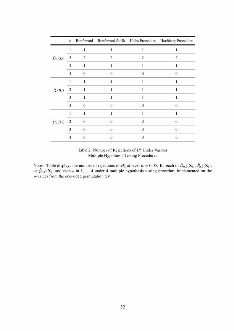
Table 2 displays the number of rejections of H i0 at level α = 0.05 when the p-values from

the one-sided individual shooter permutation tests are corrected with a suite of multiple testing

procedures.6 On the whole, each procedure consistently rejects H i0 for only one shooter, shooter

109, over the set of test statistics considered. The procedures reject H i0 for two shooters when

using Pn,2(Xi). No procedure rejects H i0 for any statistic with k = 4 or when using Qn,k(Xi) with

k ≥ 2.

6The results are identical if we take α = 0.1.

22

5.3 Tests of the Joint Hypothesis H0

In this section, we implement the procedures outlined in Section 4 that test the joint null H0 and

enable us to infer whether any shooters deviate from randomness.

The primary evidence MS provide in support of significant hot hand shooting effects are

rejections of two tests of the joint null H0. First, they reject H0 for the test using Dk with

k = 3, and note that the results for k = 2 and 4 are consistent. Second, they perform a set

of binomial tests, rejecting for large proportions of individuals significant at the 5% and 50%

levels. The binomial tests are sensitive to the choice of the significance thresholds 5% and

50% and Online Appendix Figure 6 Panel C indicates that these choices were fortuitous, in the

sense that H0 is rejected for these choices and not for others. Additionally, when the individual

hypotheses H i0 are tested simultaneously by applying the 5% binomial test, the 50% binomial

test, or Tukey’s Higher Criticism with the closed testing procedure of Markus et. al. (1976), no

individual hypotheses are rejected at the 5% level, including Shooter 109.7

Figure 5 overlays the estimates for Dk, Pk, and Qk onto the estimated permutation distri-

butions for each streak length k = 1, . . . ,4. Each panel displays the density of the statistics of

interest over the permutation replications in a white-to-black gradient. The 97.5th and 2.5th

quantiles of the computed permutation distributions are denoted by dark black horizontal line

segments. The observed estimates for Dk, Pk, and Qk are indicated by grey horizontal line seg-

ments. Although each of the observed values of Dk, Pk, and Qk are above the means of the

respective permutation distributions, only the observed values of Dk and Qk for k equals 3 are

above the 97.5th quantile of their permutation distributions.

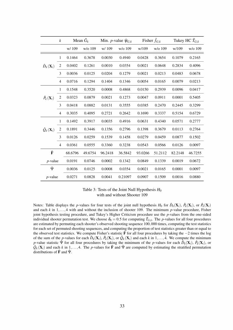
Table 3 presents the p-values for the four tests of H0 outlined in Section 4 implemented with

each test statistic Dn,k(Xi), Pn,k(Xi), and Qn,k (Xi) for each k between 1 and 4. The majority of

tests using individual test statistics reject H0 at the 5% level. The Fisher test statistic F, specified

in (4.1), is highly significant for the test using the means of the test statistics, for Tukey’s Higher

Criticism, and for the test using the minimum p-value. F is significant at the 10% level for the

the test using the Fisher test statistic. The minimum p-value test statistic Ψ is highly significant

for all four tests.

However, the rejection of H0 at the 5% level is not robust to the exclusion of shooter 109

7The closed testing procedure rejects an individual hypotheses H i0 at level α if all possible intersection hypotheses

containing H i0 are rejected by a joint testing procedure at level α . Note that any coherent multiple testing procedure

that controls the familywise error rate must arise from a closed testing procedure; see Theorem 2.1 of Romano et.al (2011).

23

from the sample. Table 3 displays the p-values for the tests of H0 implemented without the

inclusion of shooter 109 in the sample. Now, at most 3 of the p-values for tests of H0 using a

single test statistic for each method of testing the joint null are significant at the 5% level. F and

Ψ are no longer significant at the 5% level for tests using the means of the test statistics over

shooters and Tukey’s Higher Criticism and are no longer significant at the 10% level for tests

using the minimum p-value and Fisher’s test statistic.

5.4 Discussion

In order to evaluate the implications for the hot hand fallacy conveyed by the outcomes of the

GVT shooting experiment, we consider three distinct questions. First, does basketball shooting

deviate from an i.i.d. process? Second, how streaky is basketball shooting and how much

variation is there in this streakiness between shooters? Finally and fundamentally, do people

over-estimate the positive dependence in basketball shooting?

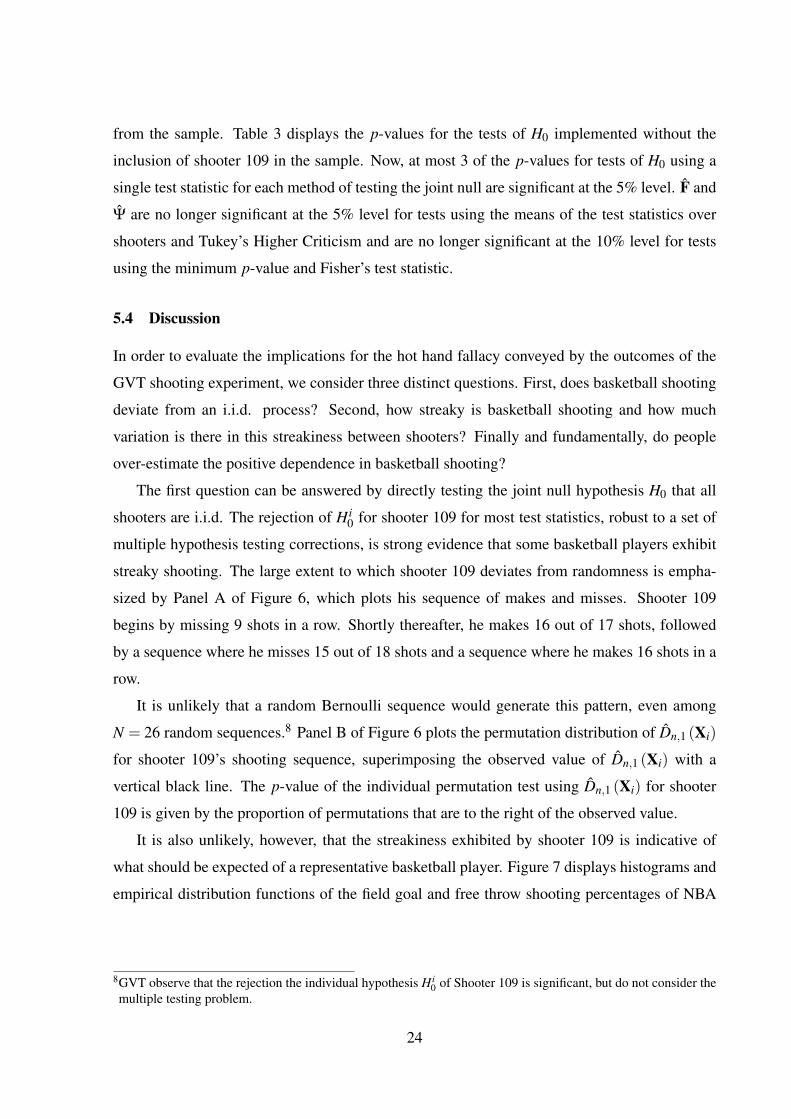
The first question can be answered by directly testing the joint null hypothesis H0 that all

shooters are i.i.d. The rejection of H i0 for shooter 109 for most test statistics, robust to a set of

multiple hypothesis testing corrections, is strong evidence that some basketball players exhibit

streaky shooting. The large extent to which shooter 109 deviates from randomness is empha-

sized by Panel A of Figure 6, which plots his sequence of makes and misses. Shooter 109

begins by missing 9 shots in a row. Shortly thereafter, he makes 16 out of 17 shots, followed

by a sequence where he misses 15 out of 18 shots and a sequence where he makes 16 shots in a

row.

It is unlikely that a random Bernoulli sequence would generate this pattern, even among

N = 26 random sequences.8 Panel B of Figure 6 plots the permutation distribution of Dn,1 (Xi)

for shooter 109’s shooting sequence, superimposing the observed value of Dn,1 (Xi) with a

vertical black line. The p-value of the individual permutation test using Dn,1 (Xi) for shooter

109 is given by the proportion of permutations that are to the right of the observed value.

It is also unlikely, however, that the streakiness exhibited by shooter 109 is indicative of

what should be expected of a representative basketball player. Figure 7 displays histograms and

empirical distribution functions of the field goal and free throw shooting percentages of NBA

8GVT observe that the rejection the individual hypothesis H i0 of Shooter 109 is significant, but do not consider the

multiple testing problem.

24

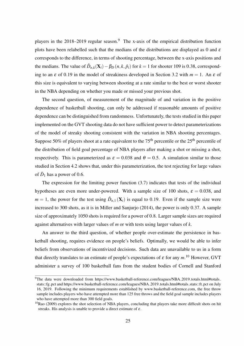
players in the 2018–2019 regular season.9 The x-axis of the empirical distribution function

plots have been relabelled such that the medians of the distributions are displayed as 0 and ε

corresponds to the difference, in terms of shooting percentage, between the x-axis positions and

the medians. The value of Dn,k(Xi)−βD (n,k, pi) for k = 1 for shooter 109 is 0.38, correspond-

ing to an ε of 0.19 in the model of streakiness developed in Section 3.2 with m = 1. An ε of

this size is equivalent to varying between shooting at a rate similar to the best or worst shooter

in the NBA depending on whether you made or missed your previous shot.

The second question, of measurement of the magnitude of and variation in the positive

dependence of basketball shooting, can only be addressed if reasonable amounts of positive

dependence can be distinguished from randomness. Unfortunately, the tests studied in this paper

implemented on the GVT shooting data do not have sufficient power to detect parameterizations

of the model of streaky shooting consistent with the variation in NBA shooting percentages.

Suppose 50% of players shoot at a rate equivalent to the 75th percentile or the 25th percentile of

the distribution of field goal percentage of NBA players after making a shot or missing a shot,

respectively. This is parameterized as ε = 0.038 and θ = 0.5. A simulation similar to those

studied in Section 4.2 shows that, under this parameterization, the test rejecting for large values

of D1 has a power of 0.6.

The expression for the limiting power function (3.7) indicates that tests of the individual

hypotheses are even more under-powered. With a sample size of 100 shots, ε = 0.038, and

m = 1, the power for the test using Dn,1 (Xi) is equal to 0.19. Even if the sample size were

increased to 300 shots, as it is in Miller and Sanjurjo (2014), the power is only 0.37. A sample

size of approximately 1050 shots is required for a power of 0.8. Larger sample sizes are required

against alternatives with larger values of m or with tests using larger values of k.

An answer to the third question, of whether people over-estimate the persistence in bas-

ketball shooting, requires evidence on people’s beliefs. Optimally, we would be able to infer

beliefs from observations of incentivized decisions. Such data are unavailable to us in a form

that directly translates to an estimate of people’s expectations of ε for any m.10 However, GVT

administer a survey of 100 basketball fans from the student bodies of Cornell and Stanford

9The data were downloaded from https://www.basketball-reference.com/leagues/NBA 2019 totals.html#totalsstats::fg pct and https://www.basketball-reference.com/leagues/NBA 2019 totals.html#totals stats::ft pct on July16, 2019. Following the minimum requirements established by www.basketball-reference.com, the free throwsample includes players who have attempted more than 125 free throws and the field goal sample includes playerswho have attempted more than 300 field goals.

10Rao (2009) explores the shot selection of NBA players, concluding that players take more difficult shots on hitstreaks. His analysis is unable to provide a direct estimate of ε .

25

that directly elicits expectations of ε when m = 1. Although survey evidence is suboptimal

for this context and subject to the criticism that responses may be driven by framing or lan-

guage, similar surveys of probabilistic expectations have found robust application in finance

and macroeconomics (see Manski 2004 and Greenwood and Shleifer 2014).

The tests considered in this paper are able to detect the average hot hand shooting effect

size predicted by the survey of fans presented in GVT with probability close to 1. GVT report

that “The fans were asked to consider a hypothetical player who shoots 50% from the field.

Their average estimate of his field goal percentage was 61% after having just made a shot and

42% after having just missed a shot.” This is roughly equivalent to an NBA player with the

median field goal percentage shooting at the 91st percentile after making a shot and the 1st

percentile after missing a shot. This variation corresponds to an ε ≈ 0.1, which can be detected

with a probability close to 1 for all four methods of testing the joint null and reasonably large

proportions of streaky shooters.11

If the participants in the GVT shooting experiment were similarly streaky to what was pre-

dicted by the participants in the GVT survey, we would expect a strong rejection of H0.12 In

fact, we would expect a strong rejection of H0 under a model consistent with a substantial at-

tenuation of the estimates of beliefs. Indeed, the power of the test based on D1 is approximately

0.94 against the model with m = 1, θ = 0.5, and ε = 0.07. However, certainty in the detection

of a deviation from randomness is localized to shooter 109 and evidence against randomness for

the remainder of the sample is tenuous. We find that the participants in the GVT survey over-

estimate streakiness in basketball shooting, the central thesis of GVT, but maintain the rejection

of H0, a core contribution of MS. This result tempers the MS conclusion of the reversal of the

GVT results. The existence of streakiness in basketball shooting does not necessarily equate to

the invalidation of the cognitive bias.

6 Conclusion

The purpose of this paper is to clarify and quantify the uncertainty in the empirical support for

the human tendency to perceive streaks as overly representative of positive dependence–the hot

11The results of this calculation are similar for the difference between the average expected shooting percentagefor making second free throws after having made or missed the first free throw, reported by GVT.

12Moreover, we would expect to reject H i0 for more than one individual at the 5% level after applying the

Bonferroni-Sidak multiple testing correction. If ε = 0.1 and θ = 1, then we would expect the minimum p-value test to reject at least one individual with probability 0.995 and at least two individuals with probability0.965. The expected number of rejections for the minimum p-value test would be 4.78.

26

hand fallacy. Following Gilovich, Vallone, and Tversky (1985), the results of a class of tests

of randomness implemented on data from a basketball shooting experiment have provided a

central empirical support for the existence of the hot hand fallacy. The results and conclusions

of these tests were drawn into question by Miller and Sanjurjo (2018), raising doubts about

the validity of the hot hand fallacy as an accurate representation of human misperception of

randomness. We evaluate the implications and interpretation of these tests by establishing their

validity, approximating their power, and revisiting their application to the Gilovich, Vallone,

and Tversky (1985) shooting experiment.

Our theoretical and simulation analyses show that the tests considered are insufficiently

powered to detect effect sizes consistent with the observed variation in NBA shooting percent-

ages with high probability. However, the tests are able to detect effect sizes consistent with

those predicted by a survey of basketball fans with probability close to one. The results of these

tests confirm that the shooting sequences of some basketball players deviate from randomness,

but indicate that people over-estimate the magnitude of this deviation, providing support for

the existence of the hot hand fallacy. More broadly, our findings support models of human

misperception of randomness that incorporate over-confidence in inferences drawn from small

samples.

Future research should measure and test the hot hand fallacy in new experimental and obser-

vational settings. We provide a mathematical and statistical theory to serve as a foundation for

these future analyses. Additionally, we contribute an emphasis on the differentiation of individ-

ual, simultaneous, and joint hypothesis testing that can more clearly delineate the conclusions

and limitations of inferences on deviations from randomness.

There are many potential models of streakiness in Bernoulli sequences. We explore only

one in detail. Tests of the hot hand fallacy would optimally directly test the accuracy of peo-

ple’s predictions of streakiness in stochastic processes and should be implemented in settings

with reasonable power against sensible alternatives. Future research should study the construc-

tion of confidence intervals for the magnitude of streakiness in stochastic processes, optimal

experimental design and choice of test statistic, and more rigorous elicitation of beliefs.

27

References

Appelbaum, Binyamin. Streaks Like Daniel Murphy’s Aren’t Necessarily Random. The New

York Times, The New York Times, 27 Oct. 2015, www.nytimes.com/2015/10/27/upshot/trust-your-eyes-a-hot-streak-is-not-a-myth.html.

Bar-Hillel, M. and Wagenaar, W.A., 1991. The perception of randomness. Advances in Applied

Mathematics, 12(4), pp.428-454.Barberis, N., Greenwood, R., Jin, L. and Shleifer, A., 2015. X-CAPM: An extrapolative capital

asset pricing model. Journal of Financial Economics, 115(1), pp.1-24.Benjamin, D.J., 2018. Errors in probabilistic reasoning and judgment biases (No. w25200).

National Bureau of Economic Research.Bhat, U.N. and Miller, G.K., 2002. Elements of applied stochastic processes (Vol. 3). Hoboken,

NJ: Wiley-Interscience.Bradley, R.C., 2005. Basic properties of strong mixing conditions. A survey and some open

questions. Probability Surveys, 2, pp.107-144.Carhart, M.M., 1997. On persistence in mutual fund performance. The Journal of Finance,

52(1), pp.57-82.Clopper, C.J. and Pearson, E.S., 1934. The use of confidence or fiducial limits illustrated in the

case of the binomial. Biometrika, 26(4), pp.404-413.Cohen, Ben. The ’Hot Hand’ Debate Gets Flipped on Its Head. The Wall Street Journal, Dow

Jones & Company, 1 Oct. 2015, www.wsj.com/articles/the-hot-hand-debate-gets-flipped-on-its-head-1443465711.

Fama, E.F., 1965. The behavior of stock-market prices. The Journal of Business, 38(1), pp.34-105.

Gilovich, T., Vallone, R. and Tversky, A., 1985. The hot hand in basketball: On the mispercep-tion of random sequences. Cognitive Psychology, 17(3), pp.295-314.

Greenwood, R. and Shleifer, A., 2014. Expectations of returns and expected returns. The

Review of Financial Studies, 27(3), pp.714-746.Haberstroh, Tom. He’s Heating up, He’s on Fire! Klay Thompson and the Truth about the Hot

Hand. ESPN, ESPN Internet Ventures, 12 June 2017, www.espn.com/nba/story/ /page/presents-19573519/heating-fire-klay-thompson-truth-hot-hand-nba.

Hendricks, D., Patel, J. and Zeckhauser, R., 1993. Hot hands in mutual funds: Short-run persis-tence of relative performance, 1974–1988. The Journal of Finance, 48(1), pp.93-130.

Hochberg, Y., 1988. A sharper Bonferroni procedure for multiple tests of significance. Biometrika,75(4), pp.800-802.

Holm, S., 1979. A simple sequentially rejective multiple test procedure. Scandinavian journal

of statistics, pp.65-70.

28

Ibragimov, I.A., 1962. Some limit Theorems for stationary processes. Theory of Probability &

Its Applications, 7(4), pp.349-382.Jensen, M.C., 1968. The performance of mutual funds in the period 1945–1964. The Journal

of Finance, 23(2), pp.389-416.Johnson, George. Gamblers, Scientists and the Mysterious Hot Hand. The New York Times, The

New York Times, 17 Oct. 2015, www.nytimes.com/2015/10/18/sunday-review/gamblers-scientists-and-the-mysterious-hot-hand.html.

Kahneman, Daniel. Thinking, Fast and Slow. Macmillan, 2011.Kunsch, H.R., 1989. The jackknife and the bootstrap for general stationary observations. The

Annals of Statistics, pp.1217-1241.Lahiri, S.N., 2013. Resampling methods for dependent data. Springer Science & Business

Media.Lehmann, Erich L., Nonparametrics; Statistical Methods Based on Ranks. 1998, Prentice Hall.Lehmann, Erich L., and Joseph P. Romano. Testing Statistical Hypotheses. 2006, Springer

Science & Business Media.Liu, R.Y. and Singh, K., 1992. Moving blocks jackknife and bootstrap capture weak depen-

dence. Exploring the Limits of Bootstrap, 225, p.248.Malkiel, B.G., 2003. The efficient market hypothesis and its critics. Journal of Economic

Perspectives, 17(1), pp.59-82.Malkiel, B.G. and Fama, E.F., 1970. Efficient capital markets: A review of theory and empirical

work. The Journal of Finance, 25(2), pp.383-417.Manski, C.F., 2004. Measuring expectations. Econometrica, 72(5), pp.1329-1376.Marcus, R., Eric, P. and Gabriel, K.R., 1976. On closed testing procedures with special refer-

ence to ordered analysis of variance. Biometrika, 63(3), pp.655-660.Miller, J.B. and Sanjurjo, A., 2018. Surprised by the hot hand fallacy? A truth in the law of

small numbers. Econometrica, 86(6), pp.2019-2047.Miller, Joshua, and Adam Sanjurjo. Momentum Isn’t Magic--Vindicating the Hot Hand with the

Mathematics of Streaks. Scientific American, 28 Mar. 2018b, www.scientificamerican.com/article/momentum-isnt-magic-vindicating-the-hot-hand-with-the-mathematics-of-streaks/.

Miller, J.B. and Sanjurjo, A., 2014. A cold shower for the hot hand fallacy. University ofAlicante mimeo.

Mood, A.M., 1940. The distribution theory of runs. The Annals of Mathematical Statistics,11(4), pp.367-392.

Politis, D.N. and Romano, J.P., 1994. The stationary bootstrap. Journal of the American Statis-

tical Association, 89(428), pp.1303-1313.Politis, D.N., Romano, J.P. and Wolf, M., 1999. Subsampling. Springer-Verlag, NY.

29

Rabin, M., 2002. Inference by believers in the law of small numbers. The Quarterly Journal of

Economics, 117(3), pp.775-816.Rabin, M. and Vayanos, D., 2010. The gambler’s and hot-hand fallacies: Theory and applica-

tions. The Review of Economic Studies, 77(2), pp.730-778.Rao, J.M., 2009. Experts’ perceptions of autocorrelation: The hot hand fallacy among profes-

sional basketball players. Unpublished technical manuscript. San Diego, CA.Remnick, David. Bob Dylan and the ‘Hot Hand.’ The New Yorker, The New Yorker, 19 June

2017, www.newyorker.com/culture/cultural-comment/bob-dylan-and-the-hot-hand.Rinott, Y., 1994. On normal approximation rates for certain sums of dependent random vari-

ables. Journal of Computational and Applied Mathematics, 55(2), pp.135-143.Rinott, Y. and Bar-Hillel, M., 2015. Comments on a ’Hot Hand’ Paper by Miller and Sanjurjo

(2015). Available at SSRN 2642450.Stein, C., 1986. Approximate computation of expectations. IMS. Hayward, CA.Romano, J.P., Shaikh, A. and Wolf, M., 2011. Consonance and the closure method in multiple

testing. The International Journal of Biostatistics, 7(1), pp.1-25.Romano, J.P. and Wolf, M., 2005. Stepwise multiple testing as formalized data snooping.

Econometrica, 73(4), pp.1237-1282.Tversky, A. and Kahneman, D., 1971. Belief in the law of small numbers. Psychological

Bulletin, 76(2), p.105.Wald, A. and Wolfowitz, J., 1940. On a test whether two samples are from the same population.

The Annals of Mathematical Statistics, 11(2), pp.147-162.Wald, A. and Wolfowitz, J., 1943. An exact test for randomness in the non-parametric case

based on serial correlation. The Annals of Mathematical Statistics, 14(4), pp.378-388.

30

m

k 1 2 3 4

1 2h h h2

h4

2√

2h√

2h h√2

h2√

2

3 h h h h2

4 h√2

h√2

h√2

h√2

Table 1: Limit of the√

n Scaled Ratio of the Mean and Standard Deviation of the Asymptotic Distributionof Dn,k (X) Under Local Streaky Alternatives

Notes: Table displays the limit as n grows to infinity of the√

n scaled ratio of the mean µD (k,m,εn) and thestandard deviation σD (k,m,εn) of the asymptotic distribution of Dn,k (X) under the stylized streaky Markov Chainalternatives considered in Section 3.2 for m and k between 1 and 4. An explicit expression for µD (k,m,εn) is givenin the proof of Theorem 3.3. We consider local perturbations εn =

h√n , which imply that σD (h,m,εn) converges to

the asymptotic variance of Dn,k (X) under H0.

31

k Bonferroni Bonferroni-Sidak Holm Procedure Hochberg Procedure

Dk (Xi)

1 1 1 1 1

2 2 2 2 2

3 1 1 1 1

4 0 0 0 0

Pk (Xi)

1 1 1 1 1

2 1 1 1 1

3 1 1 1 1

4 0 0 0 0

Qk (Xi)

1 1 1 1 1

2 0 0 0 0

3 0 0 0 0

4 0 0 0 0

Table 2: Number of Rejections of H i0 Under Various

Multiple Hypothesis Testing Procedures

Notes: Table displays the number of rejections of H i0 at level α = 0.05. for each of Dn,k(Xi), Pn,k(Xi),

or Qn,k (Xi) and each k in 1, . . . ,4 under 4 multiple hypothesis testing procedure implemented on thep-values from the one-sided permutation test.

32

k Mean Gk Min. p-value ψG,k Fisher fG,k Tukey HC TG,k

w/ 109 w/o 109 w/ 109 w/o 109 w/109 w/o 109 w/109 w/o 109

Dk (Xi)

1 0.1464 0.3678 0.0030 0.4940 0.0428 0.3654 0.1079 0.2165

2 0.0402 0.1261 0.0010 0.0354 0.0021 0.0648 0.2834 0.4096

3 0.0036 0.0125 0.0204 0.1279 0.0021 0.0213 0.0483 0.0678

4 0.0716 0.1294 0.1404 0.1346 0.0054 0.0165 0.0079 0.0213

Pk (Xi)

1 0.1548 0.3520 0.0008 0.4868 0.0150 0.2939 0.0096 0.0417

2 0.0323 0.0879 0.0021 0.1273 0.0047 0.0911 0.0001 0.5405

3 0.0418 0.0882 0.0131 0.3555 0.0385 0.2470 0.2445 0.3299

4 0.3035 0.4095 0.2721 0.2642 0.1690 0.3337 0.5154 0.6729

Qk (Xi)

1 0.1492 0.3917 0.0035 0.4916 0.0631 0.4340 0.0571 0.2777

2 0.1891 0.3446 0.1356 0.2796 0.1398 0.3679 0.0113 0.2764

3 0.0126 0.0259 0.1539 0.1458 0.0279 0.0459 0.0877 0.1502

4 0.0361 0.0555 0.3360 0.3238 0.0543 0.0566 0.0126 0.0097

F 68.6796 49.6754 96.2418 36.5842 93.0266 51.2112 82.2148 46.7255

p-value 0.0191 0.0746 0.0002 0.1342 0.0849 0.1339 0.0019 0.0672

Ψ 0.0036 0.0125 0.0008 0.0354 0.0021 0.0165 0.0001 0.0097

p-value 0.0271 0.0828 0.0041 0.21097 0.0907 0.1509 0.0016 0.0880

Table 3: Tests of the Joint Null Hypothesis H0with and without Shooter 109

Notes: Table displays the p-values for four tests of the joint null hypothesis H0 for Dk(Xi), Pk(Xi), or Pk(Xi)and each k in 1, . . . ,4 with and without the inclusion of shooter 109. The minimum p-value procedure, Fisherjoint hypothesis testing procedure, and Tukey’s Higher Criticism procedure use the p-values from the one-sidedindividual shooter permutation test. We choose δ0 = 0.5 for computing TG,k. The p-values for all four proceduresare estimated by permuting each shooter’s observed shooting sequence 100,000 times, computing the test statisticsfor each set of permuted shooting sequences, and computing the proportion of test statistics greater than or equal tothe observed test statistics. We compute Fisher’s statistic F for all four procedures by taking the −2 times the logof the sum of the p-values for each Dk(Xi), Pk(Xi), or Qk (Xi) and each k in 1, . . . ,4. We compute the minimump-value statistic Ψ for all four procedures by taking the minimum of the p-values for each Dk(Xi), Pk(Xi), orQk (Xi) and each k in 1, . . . ,4. The p-values for F and Ψ are computed by estimating the stratified permutationdistributions of F and Ψ.

33

0.05

0.10

0.20

0.30

0.40

0.50

0.60

0.000 0.025 0.050 0.075 0.100epsilon

Pow

er

D_1 D_2 D_3 D_4

Figure 1: Power Curve for Permutation Test Rejecting for Large Dn,k (X)

Notes: Figure displays the power for the permutation test rejecting at level α for large values of Dn,k (X)for a range of ε in the alternative given by (3.3), n = 100, and each k in 1, . . . ,4. The solid lines displaythe power measured by a simulation, taking the proportion of 2,000 replications which reject at the 5%level for each value of ε . The dashed lines display the power calculated by the analytic approximationgiven by (3.7).

34

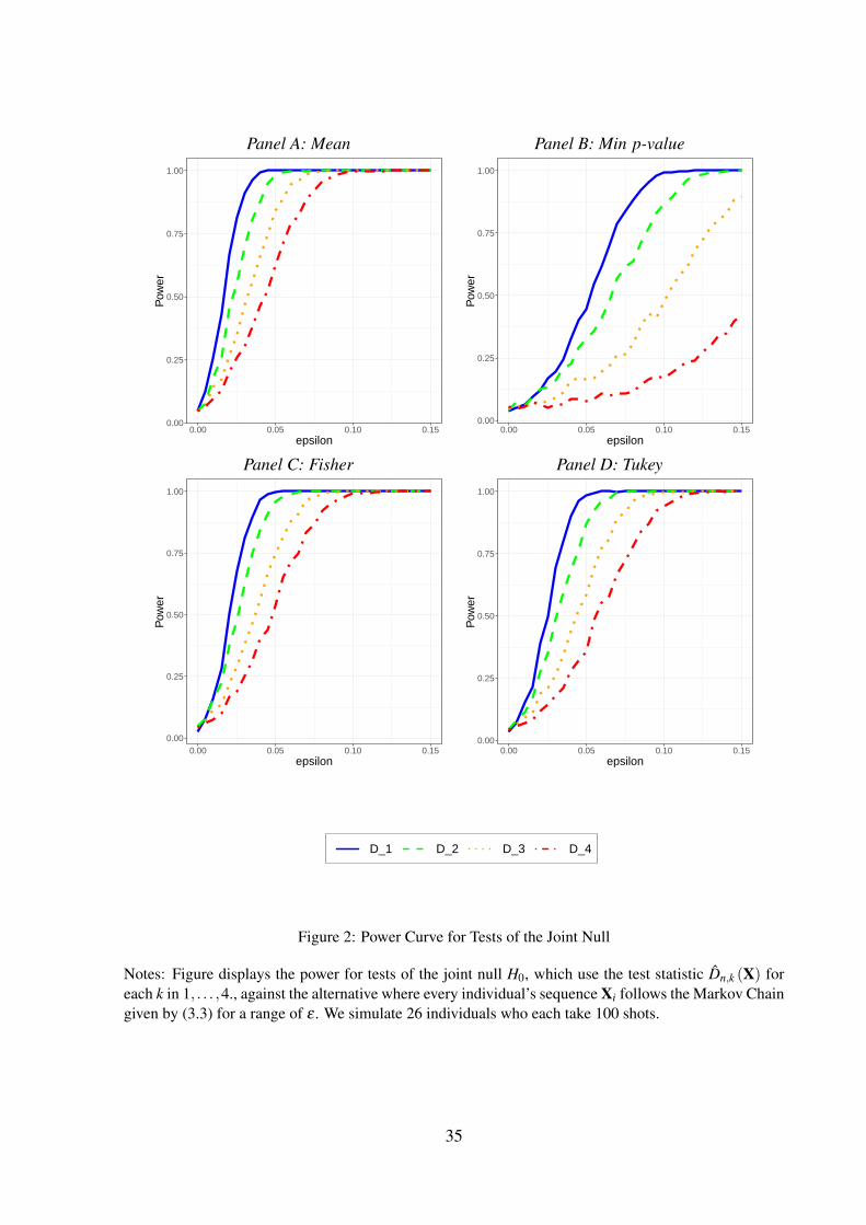
Panel A: Mean Panel B: Min p-value

0.00

0.25

0.50

0.75

1.00

0.00 0.05 0.10 0.15epsilon

Pow

er

0.00

0.25

0.50

0.75

1.00

0.00 0.05 0.10 0.15epsilon

Pow

erPanel C: Fisher Panel D: Tukey

0.00

0.25

0.50

0.75

1.00

0.00 0.05 0.10 0.15epsilon

Pow

er

0.00

0.25

0.50

0.75

1.00

0.00 0.05 0.10 0.15epsilon

Pow

er

D_1 D_2 D_3 D_4

Figure 2: Power Curve for Tests of the Joint Null

Notes: Figure displays the power for tests of the joint null H0, which use the test statistic Dn,k (X) foreach k in 1, . . . ,4., against the alternative where every individual’s sequence Xi follows the Markov Chaingiven by (3.3) for a range of ε . We simulate 26 individuals who each take 100 shots.

35

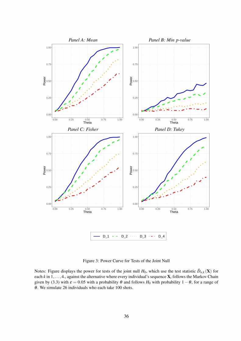
Panel A: Mean Panel B: Min p-value

0.00

0.25

0.50

0.75

1.00

0.00 0.25 0.50 0.75 1.00Theta

Pow

er

0.00

0.25

0.50

0.75

1.00

0.00 0.25 0.50 0.75 1.00Theta

Pow

erPanel C: Fisher Panel D: Tukey

0.00

0.25

0.50

0.75

1.00

0.00 0.25 0.50 0.75 1.00Theta

Pow

er

0.00

0.25

0.50

0.75

1.00

0.00 0.25 0.50 0.75 1.00Theta

Pow

er

D_1 D_2 D_3 D_4

Figure 3: Power Curve for Tests of the Joint Null

Notes: Figure displays the power for tests of the joint null H0, which use the test statistic Dn,k (X) foreach k in 1, . . . ,4., against the alternative where every individual’s sequence Xi follows the Markov Chaingiven by (3.3) with ε = 0.05 with a probability θ and follows H0 with probability 1−θ , for a range ofθ . We simulate 26 individuals who each take 100 shots.

36

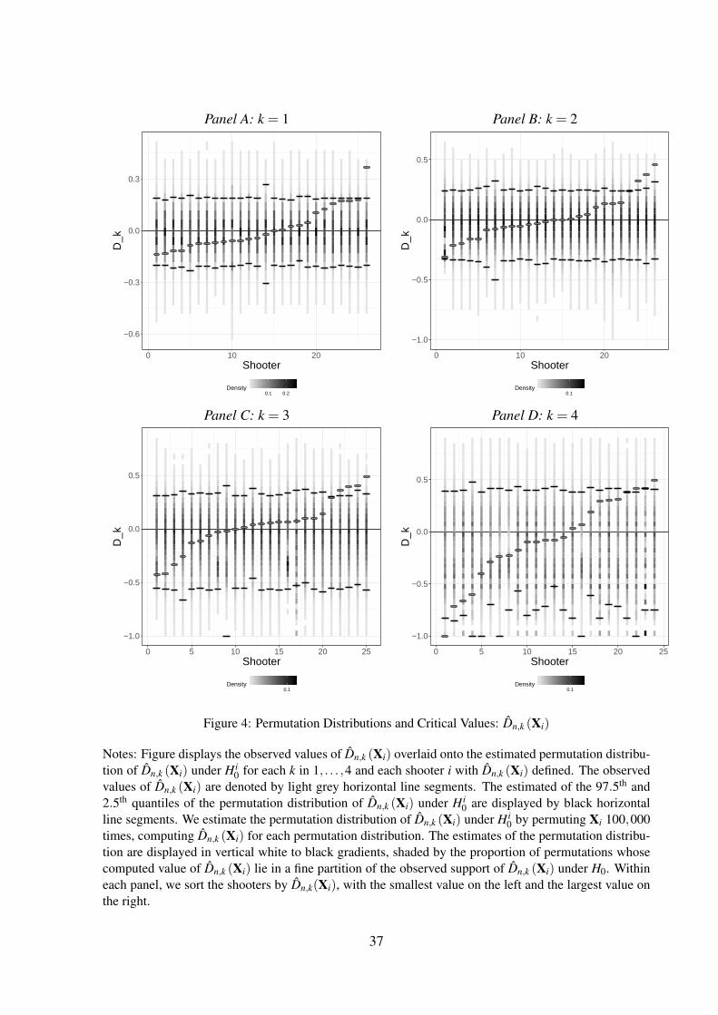
Panel A: k = 1 Panel B: k = 2

−0.6

−0.3

0.0

0.3

0 10 20Shooter

D_k

0.1 0.2Density

−1.0

−0.5

0.0

0.5

0 10 20Shooter

D_k

0.1Density

Panel C: k = 3 Panel D: k = 4

−1.0

−0.5

0.0

0.5

0 5 10 15 20 25Shooter

D_k

0.1Density

−1.0

−0.5

0.0

0.5

0 5 10 15 20 25Shooter

D_k

0.1Density

Figure 4: Permutation Distributions and Critical Values: Dn,k (Xi)

Notes: Figure displays the observed values of Dn,k (Xi) overlaid onto the estimated permutation distribu-tion of Dn,k (Xi) under H i

0 for each k in 1, . . . ,4 and each shooter i with Dn,k (Xi) defined. The observedvalues of Dn,k (Xi) are denoted by light grey horizontal line segments. The estimated of the 97.5th and2.5th quantiles of the permutation distribution of Dn,k (Xi) under H i

0 are displayed by black horizontalline segments. We estimate the permutation distribution of Dn,k (Xi) under H i

0 by permuting Xi 100,000times, computing Dn,k (Xi) for each permutation distribution. The estimates of the permutation distribu-tion are displayed in vertical white to black gradients, shaded by the proportion of permutations whosecomputed value of Dn,k (Xi) lie in a fine partition of the observed support of Dn,k (Xi) under H0. Withineach panel, we sort the shooters by Dn,k(Xi), with the smallest value on the left and the largest value onthe right.

37

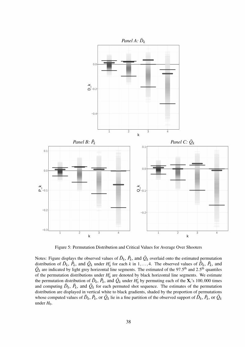
Panel A: Dk

−0.4

−0.2

0.0

1 2 3 4k

D_k

Panel B: Pk Panel C: Qk

−0.3

−0.2

−0.1

0.0

0.1

1 2 3 4k

P_k

−0.2

−0.1

0.0

0.1

1 2 3 4k

Q_k

Figure 5: Permutation Distribution and Critical Values for Average Over Shooters

Notes: Figure displays the observed values of Dk, Pk, and Qk overlaid onto the estimated permutationdistribution of Dk, Pk, and Qk under H i

0 for each k in 1, . . . ,4. The observed values of Dk, Pk, andQk are indicated by light grey horizontal line segments. The estimated of the 97.5th and 2.5th quantilesof the permutation distributions under H i

0 are denoted by black horizontal line segments. We estimatethe permutation distribution of Dk, Pk, and Qk under H i

0 by permuting each of the Xi’s 100,000 timesand computing Dk, Pk, and Qk for each permuted shot sequence. The estimates of the permutationdistribution are displayed in vertical white to black gradients, shaded by the proportion of permutationswhose computed values of Dk, Pk, or Qk lie in a fine partition of the observed support of Dk, Pk, or Qkunder H0.

38

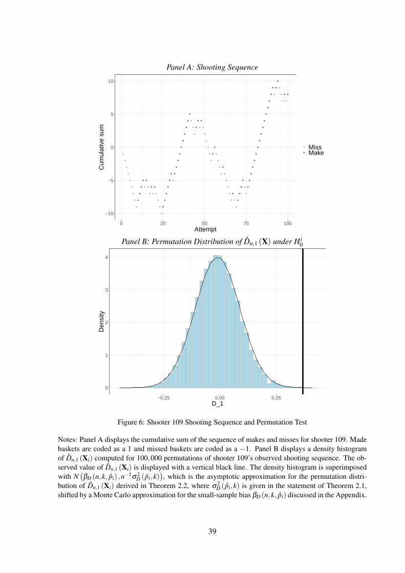
Panel A: Shooting Sequence

●

●

●

●

●

●

●

●

●

● ●

● ● ●

●

●

●

●

●

●

●

● ●

●

●

●

●

●

●

●

●

● ●

●

●

●

● ●

●

●

●

●

●

●

● ●

−10

−5

0

5

10

0 25 50 75 100Attempt

Cum

ulat

ive

sum

● MissMake

Panel B: Permutation Distribution of Dn,1 (X) under H i0

0

1

2

3

4

−0.25 0.00 0.25D_1

Den

sity

Figure 6: Shooter 109 Shooting Sequence and Permutation Test

Notes: Panel A displays the cumulative sum of the sequence of makes and misses for shooter 109. Madebaskets are coded as a 1 and missed baskets are coded as a −1. Panel B displays a density histogramof Dn,1 (Xi) computed for 100,000 permutations of shooter 109’s observed shooting sequence. The ob-served value of Dn,1 (Xi) is displayed with a vertical black line. The density histogram is superimposedwith N

(βD (n,k, pi) ,n−1σ2

D (pi,k)), which is the asymptotic approximation for the permutation distri-

bution of Dn,1 (Xi) derived in Theorem 2.2, where σ2D (pi,k) is given in the statement of Theorem 2.1,

shifted by a Monte Carlo approximation for the small-sample bias βD (n,k, pi) discussed in the Appendix.

39

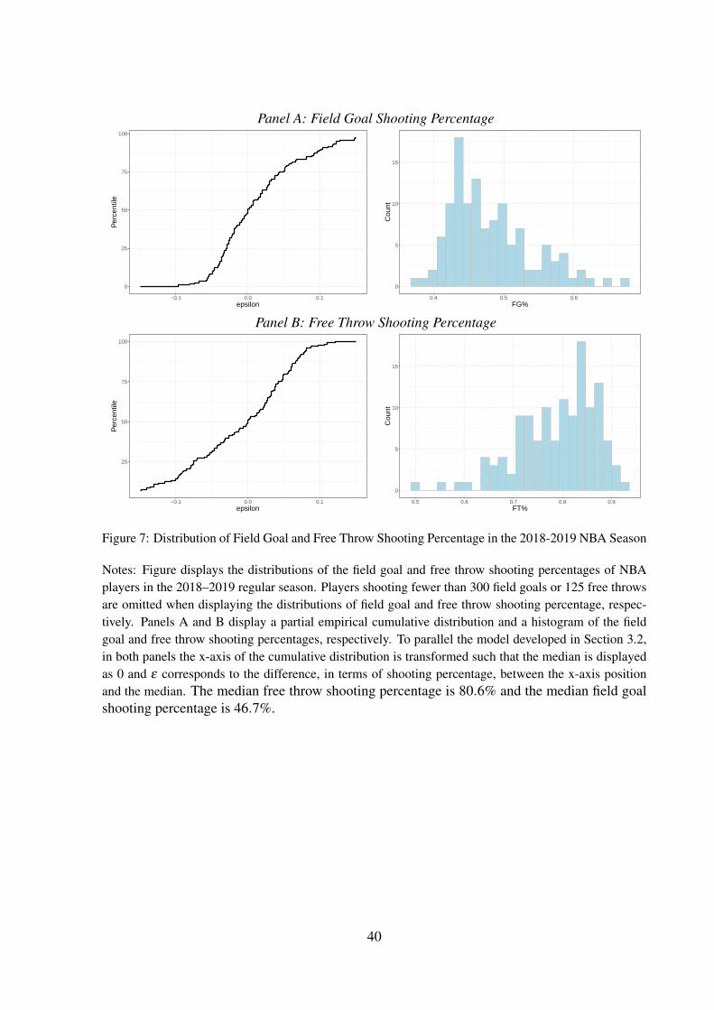
Panel A: Field Goal Shooting Percentage

0

25

50

75

100

−0.1 0.0 0.1epsilon

Per

cent

ile

0

5

10

15

0.4 0.5 0.6FG%

Cou

nt

Panel B: Free Throw Shooting Percentage

25

50

75

100

−0.1 0.0 0.1epsilon

Per

cent

ile

0

5

10

15

0.5 0.6 0.7 0.8 0.9FT%

Cou

nt

Figure 7: Distribution of Field Goal and Free Throw Shooting Percentage in the 2018-2019 NBA Season

Notes: Figure displays the distributions of the field goal and free throw shooting percentages of NBAplayers in the 2018–2019 regular season. Players shooting fewer than 300 field goals or 125 free throwsare omitted when displaying the distributions of field goal and free throw shooting percentage, respec-tively. Panels A and B display a partial empirical cumulative distribution and a histogram of the fieldgoal and free throw shooting percentages, respectively. To parallel the model developed in Section 3.2,in both panels the x-axis of the cumulative distribution is transformed such that the median is displayedas 0 and ε corresponds to the difference, in terms of shooting percentage, between the x-axis positionand the median. The median free throw shooting percentage is 80.6% and the median field goalshooting percentage is 46.7%.

40

A Appendix: Normal Approximation Confidence Intervals

For their main analyses, GVT and MS use tests that rely on normal approximations to thedistributions of Dn,k(Xi), Pn,k(Xi), and Qn,k (Xi). We have shown in Section 2 that these testscontrol the probability of a type 1 error asymptotically.

We are interested in giving confidence intervals for γP (P,k), γQ (P,k), and γD (P,k), where

γP (P,k) = P(X j+k = 1|X j+k−1 = 1, . . . ,X j = 1

)−P

(X j = 1

),

γQ (P,k) = P(X j+k = 0|X j+k−1 = 0, . . . ,X j = 0

)−P

(X j = 0

), and

γD (P,k) = P(X j+k = 1|X j+k−1 = 1, . . . ,X j = 1

)−P

(X j+k = 1|X j+k−1 = 0, . . . ,Xi = 0

).

Recall from Remark 3.3 that Pn,k (Xi)− pi±σp (pi,k)z1−α/2√

n , Qn,k (Xi)−(1− pi)±σQ (pi,k)z1−α/2√

n ,

and Dn,k (Xi)±σD (pi,k)z1−α/2√

n are asymptotically valid confidence intervals for γP (P,k), γQ (P,k),and γD (P,k) under stationary alternatives contiguous to H i

0, respectively.MS depart from GVT by correcting for finite-sample bias. Specifically, let βP (n,k, pi) de-

note EH i0

[Pn,k(Xi)− pi

]. Then, Pn,k (Xi)− pi−βP (n,k, pi) is an unbiased estimator for γP (P,k)

and has asymptotic variance equal to σ2P (p,k) under H i

0. Therefore, Pn,k (Xi)− pi−βP (n,k, pi)±σ2

P (p,k)z1−α/2√

n is an asymptotically valid confidence interval for γP (P,k) that likely has im-proved coverage in finite samples under H i

0. Likewise, let βQ (n,k, pi) and βD (n,k, pi) denoteEH i

0

[Qn,k(Xi)− (1− pi)

], and EH i

0

[Dn,k(Xi)

]. Bias corrected confidence intervals for γQ (P,k),

and γQ (P,k) are formed similarly. Note that these parameters are all 0 under the null hypothesisH i

0.MS approximate βP (n,k, pi), βQ (n,k, pi), and βD (n,k, pi) using the parametric bootstrap,

computing the means of Dn,k(Xi), Pn,k(Xi)− pi, and Qn,k (Xi)− (1− pi) over the many repli-cates of Xi drawn as i.i.d. Bernoulli sequences with probability of success pi. We denotethese estimates βD (n,k, pi), βP (n,k, pi), and βQ (n,k, pi) for each choice of streak length k andshooter i.13

Online Appendix Figures 1, 2, and 3 replicate the GVT and MS results, displaying 95%confidence intervals for γP (P,k), γQ (P,k), and γD (P,k) for each shooter and streak lengthk = 1, . . . ,4. We estimate the variance of Pn,k(Xi)− pi, Qn,k (Xi)− (1− pi), and Dn,k (Xi) byplugging in each shooter’s observed shooting percentage pi into the respective formulae of the

13The expectations of the permutation distributions of Pk(Xi)− pi, Qk(Xi)− (1− pi), and Dk (Xi) are also con-sistent estimates ofγP (P,k), γQ (P,k), and γD (P,k) . In Online Appendix D, we provide second order approxi-mations to γP (P,k), γQ (P,k), and γD (P,k) and demonstrate that they perform accurately in small samples. Thesecond order approximations may be computationally advantageous for problems of a large sample size.

41

asymptotic variances.14 The 100 · (1−α)% confidence intervals for γP (P,k), γQ (P,k), andγD (P,k) are given by

Pn,k (Xi)− pi−βP (n,k, pi) ± tn,1−α/2

(n−1/2

σP (pi,k)),

Qn,k (Xi)− (1− pi )−βQ (n,k, pi) ± tn,1−α/2

(n−1/2

σQ (1− pi,k)), and

Dn,k (Xi)−βD (n,k, pi) ± tn,1−α/2

(n−1/2

σD (pi,k)),

respectively, where tn,1−α/2 denotes the 1−α/2 quantile of the t distribution with n degrees offreedom.15

These confidence interval constructions are valid for parameters where the underlying pro-cess P is i.i.d. or nearly so (i.e., a sequence contiguous to i.i.d.). However, our main applicationis to determine whether the confidence intervals include 0, corresponding to the true parametersfor an i.i.d. process. As mentioned before, for general and potentially non-contiguous station-ary sequences one could apply block resampling methods as a means of confidence intervalconstruction. Given the relatively small sample sizes of the data in the study under considera-tion, we do not pursue the more general problem of confidence interval construction using thebootstrap. Under the null, the asymptotic variances of the test statistics only depend on the un-derlying success rate, which is much easier to estimate consistently than the limiting variancesin Theorem 3.1.

The 95% confidence intervals for γP (P,k), γQ (P,k), and γD (P,k) are above 0 for at most1 shooter for k = 1, 3 shooters for k = 2, 4 shooters for k = 3, and 2 shooters for k = 4. Foreach statistic and for k equal to 1 and 2, the bias-corrected estimates of γP (P,k), γQ (P,k), andγD (P,k) are approximately evenly split above and below 0. For k equals 3 and 4, approximately60% of the shooters have bias-corrected estimates of γP (P,k), γQ (P,k), and γD (P,k) greater

14Any consistent estimate of pi can be plugged into the asymptotic variances of Pn,k(Xi), Qn,k(Xi), and Dn,k (Xi)to produce a set of consistent estimators. This includes Pn,k (Xi) for all k. Additionally, the variances canbe estimated consistently with the permutation distribution or with the bootstrap. In Online Appendix E, weshow that Pn,k (Xi)

(1− Pn,k (Xi)

)/Vik is also a consistent estimator for the asymptotic variance of Pn,k (Xi). MS

estimate the variance of Dn,k (Xi) with((Vik−1)s2

p,i +(Wik−1)s2q,i

Vik +Wik−2

)(1

Vik+

1Wik

)(A.1)

where s2p,i =

(Vik

Vik−1

)Pn,k(Xi)

(1− Pn,k(Xi)

)and s2

q,i =(

WikWik−1

)Qn,k(Xi)

(1− Qn,k(Xi)

). This estimator is typi-

cally employed when Pn,k(Xi) and Qn,k(Xi) are the sample means of i.i.d. populations assumed to have equalvariances. This is not the case in our setting, where the variances of Pn,k(Xi) and Qn,k(Xi) are not equal and thecovariance of Pn,k(Xi) and Qn,k(Xi) is not equal to 0. However, in Online Appendix E, we show that the ratio of(A.1) and the asymptotic variance of Dn,k (Xi) converges to 1 in probability.

15We use the t quantiles to be consistent with MS, though they are no more justified asymptotically than the normalquantiles.

42

than 0. MS approximate the variance of Dn,k (Xi) differently. For their approximation, the 95%confidence intervals for γD (P,k) with k = 3 are above 0 for 5 shooters.

43