Uncertainty in 1D Heat-Flow Analysis to Estimate Groundwater Discharge to a Stream

Uncertainty in 1D Heat-Flow Analysis toEstimate Groundwater Discharge to a Streamby Grant Ferguson1 and Victor Bense2

AbstractTemperature measurements have been used by a variety of researchers to gain insight into groundwater

discharge patterns. However, much of this research has reduced the problem to heat and fluid flow in onedimension for ease of analysis. This approach is seemingly at odds with the goal of determining spatial variabilityin specific discharge, which implies that the temperature field will vary in more than one dimension. However,it is unclear how important the resulting discrepancies are in the context of determining groundwater dischargeto surface water bodies. In this study, the importance of these variations is examined by testing two popularone-dimensional analytical solutions with stochastic models of heat and fluid flow in a two-dimensional porousmedium. For cases with low degrees of heterogeneity in hydraulic conductivity, acceptable results are possible forspecific discharges between 10−7 and 10−5 m/s. However, conduction into areas with specific discharges less than10−7 m/s from adjacent areas can lead to significant errors. In some of these cases, the one-dimensional solutionsproduced estimates of specific discharge of nearly 10−6 m/s. This phenomenon is more likely in situations withgreater degrees of heterogeneity.

IntroductionTemperature surveys have become quite popular as a

hydrogeological characterization tool over the past twodecades (Anderson 2005). This is particularly true ingroundwater-surface water interaction studies (Constantz2008), where temperature anomalies are generally largerthan in the deeper subsurface and fewer accessibilityissues exist. These techniques have also become quitepopular in submarine groundwater discharge (SGD)investigations (Burnett et al. 2006). One of the advantagesof temperature-based methods is the ability to collect a

1Corresponding author: Department of Earth Sciences,St. Francis Xavier University, P.O. Box 5000, Antigonish, NovaScotia, Canada B2G 2W5; (902) 867 3614; fax: (902) 867 2414;[email protected]

2University of East Anglia, School of Environmental Sciences,Norwich, NR4 7TJ, UK; +44 (0)1603 591297; fax: +44 (0)1603591327; [email protected]

Received January 2010, accepted June 2010.Copyright © 2010 The Author(s)Journal compilation © 2010 National Ground Water Association.doi: 10.1111/j.1745-6584.2010.00735.x

large number of data in a short period of time, leadingto detailed spatial coverage. Temperature measurementsare instantaneous, generally do not require drilling orstreambed installations and require no laboratory analysisfollowing the field investigation. Infrared thermal imaging(Loheide and Gorelick 2006) and fiber optic technology(Selker et al. 2006) are also promoting these techniquesby facilitating the collection of an even greater number ofdata and increasing the temporal and spatial resolution.

Conant (2004) produced one of the first detailedmaps of groundwater discharge through a streambedusing a temperature survey. In that study, temperatureswere related to slug test and vertical hydraulic gradientmeasurements using an empirical relationship. In a followup study, Schmidt et al. (2007) analyzed temperature,piezometric, and seepage meter data from the same studysite using an analytical solution by Turcotte and Schubert(1982) based on a one-dimensional treatment of theadvective-conductive heat transport equation for porousmedia:

qfz = −(κfs/ρfcfz) ln([T (z) − TL]/[To − TL]) (1)

336 Vol. 49, No. 3–GROUND WATER–May-June 2011 (pages 336–347) NGWA.org

where qfz is vertical specific discharge, ρf is fluid density,cf is fluid heat capacity, z is depth, κfs is the effectivethermal conductivity of the saturated porous medium,T (z) is temperature at depth z, TL is temperature atthe lower boundary, To is the temperature at the upperboundary. Note that because this solution uses a semi-infinite half–space, the lower boundary is technically atan infinite distance. However, during application of thissolution, this boundary is normally applied at a depthwhere seasonal temperature variations are negligible.Specific discharge estimates from the few publishedstudies that used this analytical equation (e.g., Schmidtet al. 2007) were generally in good agreement withmeasurements from seepage meters. Schmidt et al. (2007)provide an equation for determining the upper limit ofspecific discharge (qmax

z ) that can be determined uniquelyfrom Equation 1:

qmaxz = −[κfs/ρf cfz] ln[(−1)aTAC/(To − TL)] (2)

where a is 1 for To < TL and 2 for To > TL and TAC is theaccuracy of the temperature measurement equipment. Fortypical environments and measurement accuracy (0.1 to0.2 ◦C for most commercially available instrumentationcurrently used in groundwater discharge studies), thisgives an upper limit of approximately 10−5 m/s.

However, the use of such an equation to mapspecific discharge known to be variable in space bringsinto question the validity of this method in generalbecause of the potential for lateral heat flow betweenareas of high and low specific discharge (Figure 1).Reiter (2001) suggests that it is difficult to uniquelydetermine vertical specific discharge when there aresignificant components of horizontal heat flow, either dueto advection or conduction. These horizontal gradientsexist in the data collected by Conant (2004) wherehorizontal temperature gradients of approximately 1 ◦C/mwere present in some locations. The presence of lateralheat flow in that environment suggests that either there isconsiderable uncertainty in the estimated fluxes from thatstudy or that one-dimensional treatment of temperaturedata can produce acceptable results over a greater range

of conditions than those suggested by Reiter (2001).Similar questions exist in other studies that have usedtemperature measurements in conjunction with one-dimensional solutions to characterize the variability inspecific discharge. A study of groundwater discharge inan estuary by Land and Paull (2001) used the analyticalsolution developed by Bredehoeft and Papadopulos (1965)to examine variations in specific discharge.

T (z) = To + [TL−T o]

[exp(NPe(z/L)) − 1]/[exp(NPe) − 1] (3)

where

NPe = ρfcfqfz L/κfs (4)

and NPe is the Peclet number for porous media and L isthe length of the profile. This approach was also usedby Schmidt et al. (2006) to examine the variability ofspecific discharge through a streambed along a transectof a stream. Schornberg et al. (in press) examined theaccuracy of specific discharge estimates from Equation 3in an environment influenced by bedrock heterogeneities.They concluded that significant errors were possible wherestrong contrasts in hydraulic conductivity were present.

As noted by Taniguchi et al. (2003), treatment ofsubsurface temperatures in one dimension should onlybe used as a first-order approximation. In this study, weexamine the importance of discrepancies that may arisefrom the use of one-dimensional solutions to estimatespatially variable specific discharge with the help ofboth stochastic and vertical column numerical models ofdominantly vertical specific discharge in two dimensionsillustrating the type of variability exhibited in previousstudies (e.g., Conant 2004; Kalbus et al. 2009). This studyfocuses on the effect of heterogeneities in streambedsediments, which along with the results of Schornberget al. (in press) for heat flow in environments sharpgeological contacts, provides insight into the implicationsof assuming that heat and fluid flow are strictly verticalin groundwater discharge studies.

Figure 1. Conceptual models of heat flow through a heterogeneous streambed by a one-dimensional analytical solution andfield conditions. Thicker lines indicate larger fluxes. Note that a small horizontal component of advection is likely also present.

NGWA.org G. Ferguson, V. Bense GROUND WATER 49, no. 3: 336–347 337

Stochastic Numerical Modeling

MethodologyTo investigate the effect of heterogeneity on the

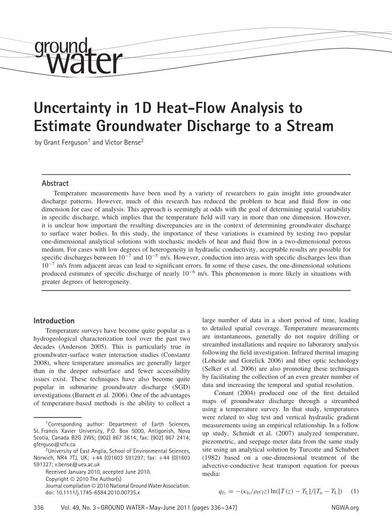
accuracy of the solutions of Turcotte and Schubert (1982)and Bredehoeft and Papadopulos (1965) in estimatingspecific discharge a series of numerical models werecreated using the METRA module within MULTIFLO(Painter and Seth 2003). METRA is an integrated finitedifference code capable of simulating heat transport andvariable density groundwater flow using a pressure andenthalpy based formulation. This code has been appliedsuccessfully in a variety of situations (e.g., Painter et al.2003; Illman and Hughson 2005; Ferguson and Woodbury2006). These models measured 50 m wide by 10 mhigh and consisted of 50,000 grid elements. Verticalspacing ranged from 0.02 m in the upper 2 to 0.2 min the lower 8 m of the domain. All the elements were0.1 m wide. The thermal boundary conditions consistedof fixed temperatures of 20 and 10 ◦C at the top andbottom of the model respectively and zero-heat fluxboundaries on both sides (Figure 2). These temperatureswould be typical of many temperate areas during summer.Hydraulic boundary conditions consisted of fixed pressureboundaries of 9800 and 117,600 Pa at the top and bottomof the model respectively, which translates to a headdifference between the top and bottom of the modelof 0.74 m. This gradient creates an average specificdischarge of 7.4 × 10−7 m/s in a homogeneous basemodel and was chosen because it falls near the centerof the range of values where temperatures measurementsare useful for groundwater discharge estimation. Lapham(1989) states that temperature measurements are notsensitive to changes in advection at specific dischargesbelow 4 × 10−7 m/s or above 4 × 10−5 m/s. Otherresearchers have suggested that at specific discharges aslow as 8 × 10−8 m/s (Silliman and Booth 1993) oreven 10−8 m/s (Niswonger 2005) advection can havenoticeable effect on temperatures. The lateral boundarieswere assigned fluid fluxes of zero. These models were rununtil they approached equilibrium, which was defined byconvergence of the temperature field to a change of lessthan 10−5 ◦C between time steps. Seasonal variations intemperature were not considered in this study.

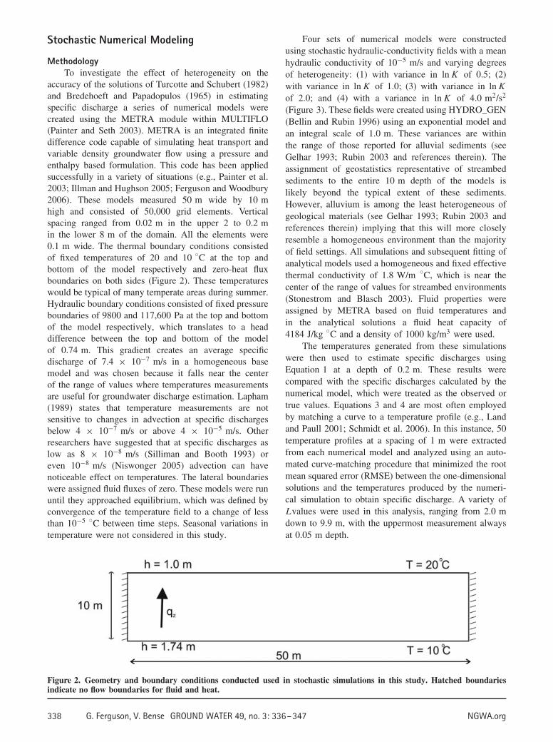
Four sets of numerical models were constructedusing stochastic hydraulic-conductivity fields with a meanhydraulic conductivity of 10−5 m/s and varying degreesof heterogeneity: (1) with variance in ln K of 0.5; (2)with variance in ln K of 1.0; (3) with variance in ln K

of 2.0; and (4) with a variance in ln K of 4.0 m2/s2

(Figure 3). These fields were created using HYDRO_GEN(Bellin and Rubin 1996) using an exponential model andan integral scale of 1.0 m. These variances are withinthe range of those reported for alluvial sediments (seeGelhar 1993; Rubin 2003 and references therein). Theassignment of geostatistics representative of streambedsediments to the entire 10 m depth of the models islikely beyond the typical extent of these sediments.However, alluvium is among the least heterogeneous ofgeological materials (see Gelhar 1993; Rubin 2003 andreferences therein) implying that this will more closelyresemble a homogeneous environment than the majorityof field settings. All simulations and subsequent fitting ofanalytical models used a homogeneous and fixed effectivethermal conductivity of 1.8 W/m ◦C, which is near thecenter of the range of values for streambed environments(Stonestrom and Blasch 2003). Fluid properties wereassigned by METRA based on fluid temperatures andin the analytical solutions a fluid heat capacity of4184 J/kg ◦C and a density of 1000 kg/m3 were used.

The temperatures generated from these simulationswere then used to estimate specific discharges usingEquation 1 at a depth of 0.2 m. These results werecompared with the specific discharges calculated by thenumerical model, which were treated as the observed ortrue values. Equations 3 and 4 are most often employedby matching a curve to a temperature profile (e.g., Landand Paull 2001; Schmidt et al. 2006). In this instance, 50temperature profiles at a spacing of 1 m were extractedfrom each numerical model and analyzed using an auto-mated curve-matching procedure that minimized the rootmean squared error (RMSE) between the one-dimensionalsolutions and the temperatures produced by the numeri-cal simulation to obtain specific discharge. A variety ofLvalues were used in this analysis, ranging from 2.0 mdown to 9.9 m, with the uppermost measurement alwaysat 0.05 m depth.

Figure 2. Geometry and boundary conditions conducted used in stochastic simulations in this study. Hatched boundariesindicate no flow boundaries for fluid and heat.

338 G. Ferguson, V. Bense GROUND WATER 49, no. 3: 336–347 NGWA.org

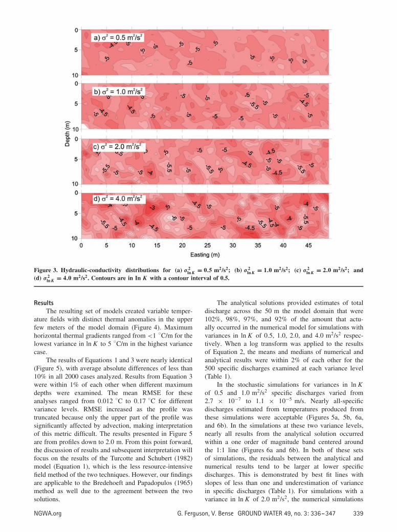
Figure 3. Hydraulic-conductivity distributions for (a) σ 2ln K = 0.5 m2/s2; (b) σ 2

ln K = 1.0 m2/s2; (c) σ 2ln K = 2.0 m2/s2; and

(d) σ 2ln K = 4.0 m2/s2. Contours are in In K with a contour interval of 0.5.

ResultsThe resulting set of models created variable temper-

ature fields with distinct thermal anomalies in the upperfew meters of the model domain (Figure 4). Maximumhorizontal thermal gradients ranged from <1 ◦C/m for thelowest variance in ln K to 5 ◦C/m in the highest variancecase.

The results of Equations 1 and 3 were nearly identical(Figure 5), with average absolute differences of less than10% in all 2000 cases analyzed. Results from Equation 3were within 1% of each other when different maximumdepths were examined. The mean RMSE for theseanalyses ranged from 0.012 ◦C to 0.17 ◦C for differentvariance levels. RMSE increased as the profile wastruncated because only the upper part of the profile wassignificantly affected by advection, making interpretationof this metric difficult. The results presented in Figure 5are from profiles down to 2.0 m. From this point forward,the discussion of results and subsequent interpretation willfocus on the results of the Turcotte and Schubert (1982)model (Equation 1), which is the less resource-intensivefield method of the two techniques. However, our findingsare applicable to the Bredehoeft and Papadopulos (1965)method as well due to the agreement between the twosolutions.

The analytical solutions provided estimates of totaldischarge across the 50 m the model domain that were102%, 98%, 97%, and 92% of the amount that actu-ally occurred in the numerical model for simulations withvariances in ln K of 0.5, 1.0, 2.0, and 4.0 m2/s2 respec-tively. When a log transform was applied to the resultsof Equation 2, the means and medians of numerical andanalytical results were within 2% of each other for the500 specific discharges examined at each variance level(Table 1).

In the stochastic simulations for variances in ln K

of 0.5 and 1.0 m2/s2 specific discharges varied from2.7 × 10−7 to 1.1 × 10−5 m/s. Nearly all-specificdischarges estimated from temperatures produced fromthese simulations were acceptable (Figures 5a, 5b, 6a,and 6b). In the simulations at these two variance levels,nearly all results from the analytical solution occurredwithin a one order of magnitude band centered aroundthe 1:1 line (Figures 6a and 6b). In both of these setsof simulations, the residuals between the analytical andnumerical results tend to be larger at lower specificdischarges. This is demonstrated by best fit lines withslopes of less than one and underestimation of variancein specific discharges (Table 1). For simulations with avariance in ln K of 2.0 m2/s2, the numerical simulations


Figure 4. Temperature distributions in upper 2 m for selected simulations with (a) σ 2ln K = 0.5 m2/s2; (b) σ 2

ln K = 1.0 m2/s2;(c) σ 2

ln K = 2.0 m2/s2; and (d) σ 2ln K = 4.0 m2/s2.

produced specific discharges between 4.4 × 10−8 and1.2 × 10−5 m/s. The analytical model overpredicted someof these specific discharges by more than factor of 50beyond a numerical model specific discharge of 10−6 m/s(Figures 5c and 6c). At a variance in ln K of 4.0 m2/s2, thenumerical models produced specific discharges between1.3 × 10−8 and 3.1 × 10−5 m/s. In this case, a fewspecific discharges were overpredicted by more than anorder of magnitude below a numerical model specificdischarge of 10−6 m/s (Figures 5d and 6d). Results at thehigher specific discharges were generally in agreementand fall within a few percent of the 1:1 line (Figure 6d).However, it should be noted that these specific dischargesare beyond the upper range where these one-dimensional

solutions should be used according to previous studies(e.g., Lapham 1989; Schmidt et al. 2007).

Vertical Column Sensitivity Modeling

MethodologyAn additional set of models was produced to examine

an extreme interpretation of the application of one-dimensional analytical models to map specific dischargeinto a surface water body. In section, one can envisionzones of uniform specific discharge bordering each otherwith a sharp interface (Figure 7). If we accept constanthydraulic and thermal boundary conditions at the upper


Figure 5. Specific discharges for selected simulations with variances in In K of: (a) 0.5; (b) 1.0; (c) 2.0; and (d) 4.0 m2/s2.


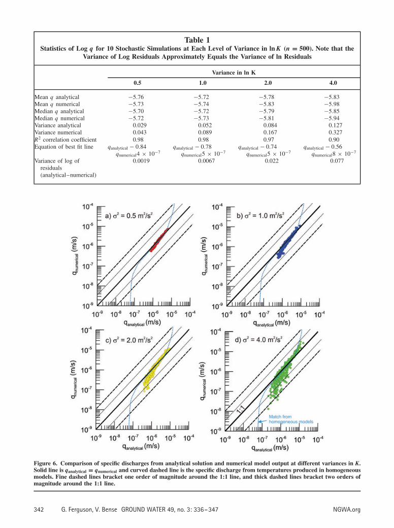
Table 1Statistics of Log q for 10 Stochastic Simulations at Each Level of Variance in ln K (n = 500). Note that the

Variance of Log Residuals Approximately Equals the Variance of ln Residuals

Variance in ln K

0.5 1.0 2.0 4.0

Mean q analytical −5.76 −5.72 −5.78 −5.83Mean q numerical −5.73 −5.74 −5.83 −5.98Median q analytical −5.70 −5.72 −5.79 −5.85Median q numerical −5.72 −5.73 −5.81 −5.94Variance analytical 0.029 0.052 0.084 0.127Variance numerical 0.043 0.089 0.167 0.327R2 correlation coefficient 0.98 0.98 0.97 0.90Equation of best fit line qanalytical − 0.84

qnumerical4 × 10−7qanalytical − 0.78



qnumerical8 × 10−7

Variance of log ofresiduals(analytical–numerical)

0.0019 0.0067 0.022 0.077

Figure 6. Comparison of specific discharges from analytical solution and numerical model output at different variances in K.Solid line is qanalytical = qnumerical and curved dashed line is the specific discharge from temperatures produced in homogeneousmodels. Fine dashed lines bracket one order of magnitude around the 1:1 line, and thick dashed lines bracket two orders ofmagnitude around the 1:1 line.


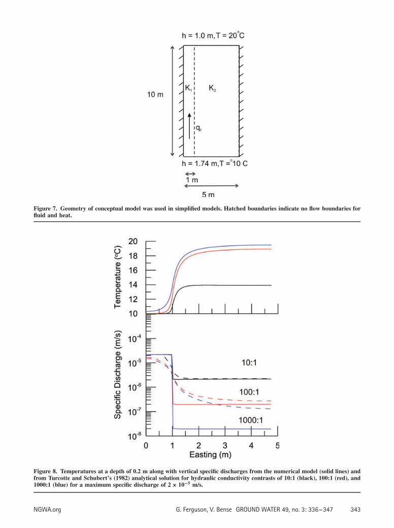
Figure 7. Geometry of conceptual model was used in simplified models. Hatched boundaries indicate no flow boundaries forfluid and heat.

Figure 8. Temperatures at a depth of 0.2 m along with vertical specific discharges from the numerical model (solid lines) andfrom Turcotte and Schubert’s (1982) analytical solution for hydraulic conductivity contrasts of 10:1 (black), 100:1 (red), and1000:1 (blue) for a maximum specific discharge of 2 × 10−5 m/s.


and lower bounds of the model, each column can beinterpreted in terms of an effective vertical hydraulicconductivity or harmonic mean. This is at odds withthe conventional characterization of hydrostratigraphicunits in most environments, which tend to be defined byhorizontal bedding, but might be appropriate in cases ofdominantly vertical groundwater flow with horizontallyvariable hydraulic conductivity within individual beds.Kalbus et al. (2009) came to the similar conclusion ina study of stream discharge, where they found that inmany cases the hydraulic conductivity of the underlyingbedrock exerted a greater control on discharge than thestream sediments.

The numerical models consisted of a 1-m-wide zoneof high hydraulic conductivity bordered by a 4-m-widezone of low hydraulic conductivity. This enables us toinvestigate the “halo” effect around high discharge areassuggested by Schmidt el al. (2007). Boundary conditionsused in these models were identical to those used in theprevious section.

ResultsTemperatures produced by these models were exam-

ined at a depth of 0.2 m (Figure 8, 9, and 10). Thehorizontal distribution of specific discharge took on an

Figure 9. Temperatures at a depth of 0.2 m along withvertical specific discharges from the numerical model (solidlines) and from Turcotte and Schubert’s (1982) analyticalsolution for hydraulic conductivity contrasts of 10:1 (black),100:1 (red), and 1000:1 (blue) for a maximum specificdischarge of 2 × 10−6 m/s.

exponential shape across the interface of the two zonesin the simulations. Resulting temperature gradients wereas great as 24.6 ◦C/m across the model grid cells adja-cent to the boundary of the two zones. Average hori-zontal thermal gradients in the 1 m centered around theboundary ranged from 0.12 ◦C/m up to 7.9 ◦C/m in thedifferent models, with the highest gradients occurring inthe simulations with a maximum specific discharge of2 × 10−6 m/s. Horizontal specific discharges were gen-erally low and flow was toward the high hydraulic-conductivity zone. These horizontal specific dischargesonly exceeded 10−7 m/s in the simulations where verti-cal specific discharge was 2 × 10−5 m/s. In each of thesecases, horizontal specific discharge was less than 1% ofvertical specific discharge.

Equation 1 was used to estimate specific dischargesfrom temperatures at a depth of 0.2 m in the numericalmodels (Figure 8, 9, and 10). The analytical solution per-formed well for all hydraulic conductivity contrasts andspecific discharges examined in the high hydraulic con-ductivity zone. Specific discharge estimates were under-estimated by less than a factor of two throughout thiszone in the majority of cases. The results for thelower hydraulic conductivity zone were generally goodwhen hydraulic conductivity contrasts were less than twoorders of magnitude different for a specific discharge of2 × 10−5 m/s in the high hydraulic-conductivity zone(Figure 8). When the contrast was three orders of mag-nitude different, specific discharge in the low hydraulic-conductivity zone was overestimated by over an order ofmagnitude within 1.5 m of the interface and was over-estimated by at least a factor of seven through out thedomain.

For the case with a specific discharge of2 × 10−6 m/s, performance of the analytical solutionin the low hydraulic-conductivity zone was poor forhydraulic conductivity contrasts greater than two orders ofmagnitude (Figure 9). Estimated specific discharges weretoo large by an order of magnitude or more within 1 m ofthe interface for the 1:100 contrast case and were overes-timated by nearly two orders of magnitude over the entiredomain for the 1:1000 case.

When the specific discharge in the high hydraulic-conductivity zone was reduced to 2 × 10−7 m/s, resultsfor the low hydraulic-conductivity zone were generallypoor (Figure 10). For a contrast of 1:10, the best estimateswere too large by a factor of four. At permeabilitycontrasts of 1:100 and 1:1000, the best estimates wereat least 35 times too large.

DiscussionIn the stochastic simulations, the mean specific

discharge was reproduced suggesting that the analysis ofstreambed temperature could be used to estimate totaldischarge to a stream. This is theoretically possible butwould require a sufficient density and spatial coverage ofmeasurements. This distribution of measurements woulddepend on the integral scale, which was quite small in


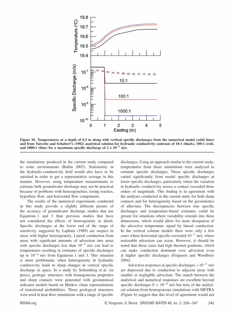
Figure 10. Temperatures at a depth of 0.2 m along with vertical specific discharges from the numerical model (solid lines)and from Turcotte and Schubert’s (1982) analytical solution for hydraulic conductivity contrasts of 10:1 (black), 100:1 (red),and 1000:1 (blue) for a maximum specific discharge of 2 × 10−7 m/s.

the simulations produced in the current study comparedto some environments (Rubin 2003). Stationarity inthe hydraulic-conductivity field would also have to besatisfied in order to get a representative average in thismanner. However, using temperature measurements toestimate bulk groundwater discharge may not be practicalbecause of problems with heterogeneities, losing reaches,hyporheic flow, and horizontal flow components.

The results of the numerical experiments conductedin this study provide a slightly different picture ofthe accuracy of groundwater discharge studies that useEquations 1 and 3 than previous studies that havenot considered the effects of heterogeneity in detail.Specific discharges at the lower end of the range ofsensitivity suggested by Lapham (1989) are suspect inareas with higher heterogeneity. Lateral conduction fromareas with significant amounts of advection into areaswith specific discharges less than 10−7 m/s can lead totemperatures resulting in estimates of specific dischargesup to 10−6 m/s from Equations 1 and 3. This situationis more problematic when heterogeneity in hydraulicconductivity leads to sharp changes in vertical specificdischarge in space. In a study by Schornberg et al. (inpress), geologic structures with homogeneous propertiesand sharp contacts were generated with geostatisticalindicator models based on Markov chain representationsof transitional probabilities. Those geological structureswere used in heat-flow simulations with a range of specific

discharges. Using an approach similar to the current study,temperatures from those simulations were analyzed toestimate specific discharges. Those specific dischargesvaried significantly from model specific discharges atlower specific discharges, particularly where the variationin hydraulic conductivity across a contact exceeded threeorders of magnitude. This finding is in agreement withthe analyses conducted in the current study for both sharpcontacts and for heterogeneity based on the geostatisticsof alluvium. The discrepancies between true specificdischarges and temperature-based estimates could begreater for situations where variability extends into threedimensions, which would allow for more dissipation ofthe advective temperature signal by lateral conduction.In the vertical column models there were only a fewcases where horizontal specific exceeded 10−7 m/s, wherenoticeable advection can occur. However, it should benoted that these cases had high thermal gradients, whichcan make conduction dominant over advection evenat higher specific discharges (Ferguson and Woodbury2004).

Advective responses at specific discharges >10−5 m/sare depressed due to conduction to adjacent areas withsmaller or negligible advection. The match between theanalytical and numerical responses are excellent beyondspecific discharges 8 × 10−6 m/s but tests of the analyti-cal solution from homogeneous simulations with METRA(Figure 6) suggest that this level of agreement would not


occur at these higher specific discharges. However, usingEquation 2 with a measurement accuracy of 0.2 ◦C givesan upper limit at a specific discharge of 9 × 10−6 m/sfor the parameters examined in this study. This indi-cates that lateral heat flow at specific discharges >10−5

is of minimal importance unless unusually accuratetemperature measurements are made.

The dampening of estimated specific discharge byheat flow into or out of surrounding areas suggests that thecalculation of specific discharge from point measurementsof temperature reflect conditions over several hundredsquare centimeters to a few square meters, rather thanthe actual point of measurement as suggested by Kalbuset al. (2006). The dimensions of this radius of influencewill be determined by the variability in specific discharge,and the radius varies from tens of centimeters to severalmeters in the vertical column simulations was conductedin this study, where conduction created temperatures thatgave apparent discharges much higher than those actuallypresent. The area affected by the lateral conduction ofheat can be larger than the area sampled by a seepagemeter in many cases. The influence of horizontal heattransport will become noticeable when vertical specificdischarges differ by more than an order of magnitudebecause of the resulting horizontal temperature gradients.Lateral heat transport is particularly problematic whereapparent advective signals occur in areas with specificdischarges below the threshold of noticeable advectionoutlined in past studies such as that by Lapham (1989).The presence of high horizontal thermal gradients willprovide some evidence of these issues but there areno simple correlations between these gradients and thedifferences between the analytical and numerical modelresults. Further studies with different integral scalesand three dimensions are needed to quantify the radiusof temperature anomalies associated with variations invertical specific discharge in a range of environments.

Many studies have attributed uncertainty in specificdischarge estimates from temperature-based methods touncertainty in thermal properties (Anderson 2005; Van-denbohede and Lebbe 2010). Uncertainty is generallyquite low for thermal conductivity, which varies betweenapproximately 1.4 and 2.2 W/m ◦C for streambed sedi-ments (Stonestrom and Blasch 2003). Moderate levels ofheterogeneity in hydraulic conductivity are likely to pro-duce greater uncertainty in temperature-based estimates ofdischarge. However, the variance of the residuals is lowerthan that associated with uncertainty in Darcy’s law-basedestimates. The relation between the variance in ln K usedin the stochastic simulations, which represents the major-ity of uncertainty in Darcy’s law-based estimates, and thevariance in the ln of the residuals between the analyticaland numerical results (ln res) is described by:

σ 2(ln res) = 0.0077σ 2(ln K)1.78 (5)

Note that in this case the residuals of the logtransform of specific discharges are approximately equalto the residuals of the ln transform of the specific

discharges. Equation 5 had an R2 correlation coefficientof 0.9999. However, this fit is probably not applicable ifthe mean specific discharge does not occur near the centerof the range of sensitivity or in highly heterogeneousareas. Further uncertainty is related to the possibilityof horizontal flow components (Constantz 2008; Lautz2010), greater degrees of heterogeneity in hydraulicproperties, either within the streambed sediments or inthe underlying or adjacent hydrostratigraphic units (Gelhar1993; Schornberg et al. in press), and transient effects(Arrigoni et al. 2008; Anibas et al. 2009; Lautz 2010).

ConclusionsOne-dimensional analytical solutions can provide

good estimates of specific discharge into streams for spe-cific discharges between 1 × 10−7 m/s and 1 × 10−5 m/sif variance in ln K is less than 1.0 m2/s2. However, forvariances in ln K greater than 2.0 m2/s2 or as specificdischarges decrease toward 10−7 m/s, lateral conductioncan cause temperatures that result in estimation of spe-cific discharges of up to 10−6 m/s by Equations 1 and3. The geostatistics of hydraulic conductivity are rarelyknown a priori, suggesting that specific discharge esti-mates less than 10−6 m/s be interpreted with caution. Theuncertainty arising from lateral heat flow suggests thatthere is more uncertainty in these estimates than previ-ous studies which suggested that uncertainty is primarilyassociated with the thermal conductivity term (e.g., Van-denbohede and Lebbe 2010). The reliability of these esti-mates is inversely proportional to the level of heterogene-ity in hydraulic conductivity but the level of uncertaintyshould be low compared with other techniques where themean specific discharge is near the center of the rangeof applicability. These temperature-based estimates alsooffer the benefit of knowing the likely sign of the errordue to the systematic nature of the errors, with specificdischarges underestimated in high discharge areas andoverestimated in low discharge areas. This investigationconfirms that temperature-based estimates of specific dis-charge have enormous potential. However, results shouldbe confirmed through the use of other field techniques ortested by more complex numerical models.

AcknowledgmentsThe authors are grateful to John Selker for a

review of a preliminary version of this manuscript andother insightful reviews from Jim Constantz and threeanonymous reviewers. This research was supported byfunding from the Natural Sciences and EngineeringResearch Council of Canada and Manitoba Hydro.

ReferencesAnderson, M. 2005. Heat as a ground water tracer. Ground Water

43, 951–968.


Anibas, C., J.H. Fleckenstein, N. Volze, K. Buis, R. Verhoeven,P. Meire, and O. Batelaan. 2009. Transient or steady-state? Using vertical temperature profiles to quantifygroundwater surface water-exchange. Hydrologic Processes23, 2165–2177.

Arrigoni, A.S., G.C. Poole, L.A.K. Mertes, S.J. O’Daniel, W.W.Woessner, and S.A. Thomas. 2008. Buffered, lagged, orcooled? Disentangling hyporheic influences on temperaturecycles in stream channels. Water Resources Research 44,W09418. DOI: 10.1029/2007WR006480.

Bellin, A., and Y. Rubin. 1996. HYDRO_GEN: A spatiallydistributed random field generator for correlated randomproperties. Stochastic Environmental Research and RiskAssessment 10, 253–278.

Bredehoeft, J.D., and I.S. Papadopulos. 1965. Rates of verticalgroundwater movement estimated from the Earth’s thermalprofiles. Water Resources Research 1, 325–328.

Burnett, W.C., P.K. Aggarwal, A. Aureli, H. Bokuniewicz, J.E.Cable, M.A. Charette, E. Kontar, S. Krupa, K.M. Kulkarni,A. Loveless, W.S. Moore, J.A. Oberdorfer, J. Oliveria,N. Ozyurt, P. Povinec, A.M.G. Privitera, R. Rajar, R.T.Ramessur, J. Scholten, T. Stiglitz, M. Taniguchi, andJ.V. Turner. 2006. Quantifying submarine groundwaterdischarge in the coastal zone via multiple methods. Scienceof the Total Environment 367, 498–543.

Conant, B. 2004. Delineating and quantifying ground waterdischarge zones using streambed temperatures. GroundWater 42, 243–257.

Constantz, J. 2008. Heat as a tracer to determine streambed waterexchanges. Water Resources Research 44, W00D10.

Ferguson, G., and A.D. Woodbury. 2006. Observed ther-mal pollution and post-development simulations of low-temperature geothermal systems in Winnipeg, Canada.Hydrogeology Journal 14, 1206–1215. DOI: 10.1007/s10040-006-0047-y.

Gelhar, L.W. 1993. Stochastic Subsurface Hydrology. Engle-wood Cliffs, New Jersey: Prentice Hall.

Illman, W.A., and D.L. Hughson. 2005. Stochastic simulationsof steady state unsaturated flow in a three-layer, heteroge-neous, dual continuum model of fractured rock. Journal ofHydrology 307, 17–37.

Kalbus, E., C. Schmidt, J.W. Molson, F. Reinstorf, andM. Schirmer. 2009. Influence of aquifer and streambedheterogeneity on the distribution of groundwater discharge.Hydrology and Earth System Sciences 13, 69–77.

Kalbus, E., F. Reinstorf, and M. Schirmer. 2006. Measur-ing methods for groundwater-surface water interactions:A review. Hydrology and Earth System Sciences 10,873–887.

Land, L.A., and C.K. Paull. 2001. Thermal gradients as a tool forestimating groundwater discharge rates in a coastal estuary:White Oak River, North Carolina. Journal of Hydrology248, 198–215.

Lapham, W.W. 1989. Use of temperature profiles beneathstreams to determine rates of vertical ground-water flowand vertical hydraulic conductivity. USGS Water SupplyPaper 2337.

Lautz, L.K. 2010. Impacts of nonideal field conditions on verti-cal water velocity estimates from streambed temperature

time series. Water Resources Research 46, W01509.DOI:10.1029/2009WR007917.

Loheide, S.P., and S.M. Gorelick. 2006. Quantifying stream-aquifer interactions through the analysis of remotely sensedthermographic profiles and in situ temperature histories.Environmental Science and Technology 40,3336–3341.

Niswonger, R.G. 2005. The hydroecological significance ofperched groundwater beneath streams. Ph.D. thesis, Uni-versity of California, Davis, Califiornia, 160.

Painter, S., and M.S. Seth. 2003. MULTIFLO User’s Manual;MULTIFLO Version 2.0, San Antonio, Texas, SouthwestResearch Institute.

Painter, S., J. Winterle, and A. Armstrong. 2003. Using temper-atures to test models of flow near Yucca Mountain, Nevada.Ground Water 41, 657–666.

Reiter, M. 2001. Using precision temperature logs to estimatehorizontal and vertical groundwater flow components.Water Resources Research 37, 663–674.

Rubin, Y. 2003. Applied Stochastic Hydrogeology. New York,NY: Oxford University Press.

Schmidt, C., B. Conant, M. Bayer-Raich, and M. Schirmer.2007. Evaluation and field–scale application of an ana-lytical method to quantify groundwater discharge usingmapped streambed temperatures. Journal of Hydrology 347,292–307.

Schmidt, C., M. Bayer-Raich, and M. Schirmer. 2006. Charac-terization of spatial heterogeneity of groundwater-streaminteractions using multiple depth streambed temperaturemeasurements at the reach scale. Hydrology and Earth Sys-tem Sciences 10, 849–859.

Schornberg, C., C. Schmidt, E. Kalbus, and J.H. Fleckenstein.Simulating the effects of geologic heterogeneity andtransient boundary conditions on streambed temperaturesfor temperature-based water flux calculations. Advances inWater Resources . In press.

Selker, J., N. van de Giesen, M. Westhoff, W. Luxemburg, andM.B. Parlange. 2006. Fiber optics opens window on streamdynamics. Geophysical Research Letters 33, L24401.

Silliman, S.E., and D.F. Booth. 1993. Analysis of time-seriesmeasurements of sediment temperature for identification ofgaining vs. losing portions of Judy Creek, Indiana. Journalof Hydrology 146, 131–148.

Stonestrom, D.A., and K.W. Blasch. 2003. Determining tem-perature and thermal properties for heat-based studies ofsurface-water ground-water interactions. In Heat as a Toolfor Studying the Movement of Ground Water Near Streams,D.A. Stonestrom, and J. Constantz, 73–80. USGS Circular1260.

Taniguchi, M., J.V. Turner, and A.J. Smith. 2003. Evaluations ofgroundwater discharge rates from subsurface temperature inCockburn Sound, Western Australia. Biogeochemistry 66,111–124.

Turcotte, D., and G. Schubert. 1982. Geodynamics: Applicationof Continuum Physics to Geological Problems. New York:Wiley.

Vandenbohede, A., and L. Lebbe. 2010. Parameter estimationbased on vertical heat transport in the surficial zone.Hydrogeology Journal 18, 931–943.


Documents

Uncertainty in 1D Heat-Flow Analysis to Estimate Groundwater Discharge to a Stream