Uncertainty, Hiring, and Subsequent Performance: The NFL Draft Law... · The NFL Draft CHECKED 3 Monday Aug 11 2003 04:07 PM JOLE v21n4 210405 BBS candidate’s training (their “nature”)

Proof 1

[ Journal of Labor Economics, 2003, vol. 21, no. 4]� 2003 by The University of Chicago. All rights reserved.0734-306X/2003/2104-0005$10.00

Monday Aug 11 2003 04:07 PM JOLE v21n4 210405 BBS

Uncertainty, Hiring, and SubsequentPerformance: The NFL Draft

Wallace Hendricks, University of Illinois

Lawrence DeBrock, University of Illinois

Roger Koenker, University of Illinois

In this article, we analyze the impact of uncertainty on the hiringprocess. We show the connection between models of statistical dis-crimination where uncertainty can work against groups that have lessreliable indicators of future productivity and models of option valuewhere uncertainty about future productivity can be beneficial forthese groups. These models generate hypotheses about the relation-ship between ex ante hiring patterns and ex post productivity. Thisis applied to the market for NFL football players. We provide variousestimates of NFL success, which suggest that statistical discriminationand option value influence choices in this market.

I. Introduction

Information problems are fundamentally important to the outcomes ofmost markets. This is perhaps most obvious in labor markets. Uncertaintyabout the true qualities and effort levels of workers and candidates hasattracted much attention from economists. When information is somehowlimited, employers are unable to acquire perfect information about workerproductivity. Given such uncertainty, it is common to turn to group iden-tification as a signal of underlying productivity.

Firms use a variety of sources to gather information to predict futureproductivity. Interviews, prejob test scores, and letters of recommenda-tion, for example, provide both objective and subjective information, and

CHECKED 2 Hendricks et al.


they vary widely in total cost. Given the nature of information, it is notpossible for the firm to discover the true ability of each worker prior toactual employment. Firms will therefore look to information gatheredfrom signals that have proven effective in prediction of worker perform-ance. One such signal is group identification. The battery of tests that thefirm uses will result in “scores,” but these scores may be noisier for somegroups than for other groups.

Previous literature in this area has focused on the relationship betweenthe formulation of the signal and the resulting outcomes for groups. Thesignal itself could be biased due to prejudice (Becker 1957), or the signalcould be inefficient. There are two basic approaches to this inefficiencyproblem. In the first approach, a highly inefficient signal for one groupcan put that group at a disadvantage (Phelps 1972; Arrow 1973; Akerlof1976; Aigner and Cain 1977; Borjas and Goldberg 1978; Bloch and Rao1993; Coate and Loury 1993; Cornell and Welch 1996). This is calledstatistical discrimination. Job opportunities are different across groups,even though productivity might be the same. In the second approach,selection between applicants is not viewed as a one-shot choice. Instead,firms are allowed to observe new employees over some probationaryperiod and determine their true productivity. In this case, Lazear (1995)shows that applicants from high-risk groups are more valuable to the firmif the firm has some way of capturing rents associated with knowing thisvalue. Thus, uncertainty improves the job prospects of members of thesegroups. This is called option value.

In this article, our concern is somewhat different. Rather than focuson the outcome of this formation of expectations, we consider the rela-tionship between ex ante expectations and ex post realizations. That is,our concern is the relationship between prior beliefs and realized out-comes. This allows us to generate empirical predictions from both thestatistical discrimination and option value models.

As an example of our approach, consider the case of economics de-partments. This is an attractive market to consider as ex post productivityis clearly observable. However, to explore this issue further, we wouldneed to determine the ex ante rankings of the candidates. Then we couldcompare these preemployment ratings with the ex post realization ofproductivity, the career results of these economists. Unfortunately, sucha methodology is flawed by the critical “nature versus nurture” problem.By definition, overvalued candidates will be placed in higher-level de-partments through sorting in the market. These departments will haveenvironments that are necessary to produce high-quality research. Thesuccess of undervalued candidates, on the other hand, may be retardedby their placement in schools with less attractive research environments.Thus, it is not easy to determine how much career success is due to the

q1

The NFL Draft CHECKED 3


candidate’s training (their “nature”) and how much is due to professionalgrowth on the job (their “nurture”).

Most occupations that lend themselves to such postemployment ob-servability of productivity are subject to this nature versus nurture prob-lem.1 If we are to investigate what the ex ante–ex post relationship shouldlook like, we need an industry where the higher-valued candidates arenot systematically sorted into the better nurturing environments.

Our response to this problem is to examine employment practices inthe National Football League (NFL). We chose the NFL to considerscreening for several reasons. First, a particularly rich data set is available.All prospective employees in the NFL are hired after successful collegefootball careers. The individual teams spend a large amount of money inscouting players, analyzing the records of their college performance, andadministering additional physical and mental examinations. Once eachteam has processed this information on all players, it is able to determinea complete ranking of the talent available.

Second, the NFL does not allow potential players to choose amongthe teams. Instead, a regimented system of “player rights” is exercised inthe annual draft. Each team selects a player in a predetermined sequence.These draft positions are allocated according to a formula based on theorder of finish in the previous NFL season. Therefore, there is much lesslikelihood that talented players will be matched with teams that providegreater opportunity for a successful career.

In Section II, we present a simple model of uncertainty and employmentscreening. This allows us to make empirical predictions about the rela-tionship between preemployment evaluation and observed success. InSection III, we provide institutional detail about the NFL as an empiricaltest of our predictions. Section IV presents the results of our empiricaltests. In Section V, we conclude with some observations and extensions.

II. Statistical Discrimination, Employer Risk Aversion,and Option Value

As in the Aigner and Cain model (1977), suppose that there are twogroups of potential job applicants. Employers observe the group affiliationof each applicant, and they observe a signal of individual ability, say atest score, because of preemployment screening. We will assume, for thesake of simplicity, that the joint distribution of the signal, x, and the

1 This problem is specific to that small subset of industries where we have“good” data on productivity, such as our example of academic economists. Inmost cases, our measures of preemployment quality and postemployment pro-ductivity amount to nothing more than the observations “Did they hire them?”followed by “Did they stay at the firm?”



(eventually) observed productivity, y, is bivariate normal for each group,with mean vector and covariance matrix,′m p (a, a)

1 r2 iQ p j , i p 1, 2.i ( )r 1i

As in the Aigner and Cain formulation, unconditional mean produc-tivity is the same for both groups; only the covariance parameters differ.Conditional mean productivity, given the signal, can then be written as

( ) ( )m y d x p a�r x � a , i p 1, 2.i i

With , applicants from group 1 are preferred when the signal, x,r 1 r1 2

is above the unconditional mean, a, and applicants from group 2 arepreferred when the signal falls below a. This occurs because the signalallows better differentiation of applicants from group 1 than applicantsfrom group 2. This is a disadvantage for high-signal group 2 members,but it is an advantage for low-signal group 2 members. In the absence ofrisk aversion, employers simply choose in order of the signal value fromthe two groups as long as the respective signals indicate that expectedproductivity exceeds some designated cutoff.

A. Risk Aversion

With risk aversion, the situation is somewhat more complicated. Therewill be a penalty paid by members of a group where it is more difficultto evaluate their ability based on the signal. The size of this penalty,however, may not be constant because of systematic differences in theefficiency of the forecasted productivity. We continue to assume that

, that is, that group 1’s signal is more strongly correlated withr 1 r1 2

productivity than is group 2’s signal. In addition, we will assume that. The conditional variance of productivity, given the signal under2 2j 1 j2 1

our assumptions, is independent of the signal, that is,

2 2( ) ( )V y d x pj 1 � r .i i

However, this presumes that employers know the parameters of the (x,y) process. If, more realistically, we adopt the view that employers mustbase their decisions on an estimated version of , we may writem (y d x)i

for applicant j from group i

( )y p a � r x � a �u ,ij i j ij

where Employing standard least squares fore-2 2 2V (u ) p q p j (1 � r ) .ij i i i

casting, we have

ˆ ˆˆ ˆ( )y p a � r x � a ,ij i j



and

2( )x � aj2ˆ( )V y pq 1 � .ij i [ ]l

For example, if the employer’s estimates of (a, ri) had been based on asample (xi, yi, ), then n 2¯i p 1, … , n l p � (x � x) .iip1

Of course, there are many other possible sources of heterogeneity inpredicted performance as a function of the observed signal; our simpleleast squares forecasting model is among the simplest of these possibilities.The model illustrates that, even with homogeneous underlying uncer-tainty, decision makers may face heterogeneity. It is perhaps worth em-phasizing that the precise form of the heterogeneity produced by themodel is not really crucial to the subsequent empirical interpretation ofthe model. However, the general characteristic that there is more uncer-tainty for extreme values of the signal will be an inherent feature of anymodel in which predictions at these extremes are based on smaller samplesizes than those found at more moderate values of the signal.

Now, if we assume that employers compare prospects using the Pratt(1964) approximation of the “certainty equivalent” prospect, with a co-efficient of absolute risk aversion g,

1( ) ( ) ( )CE y d x p E y d x � gV y � x ,

2

then we have

2( )x � a12( ) ( )CE y d x pa�r x � a � gq 1 � .i i ( )2 l

In figure 1, we plot the risk-adjusted certainty equivalent productivitycurves for group 1 and group 2 under the assumption that group 2 hasa larger “risk premium.”2 The plot is drawn to illustrate a situation wherethe risk premium may be in effect. The solid line is the group 1 certaintyequivalent line. In this group, productivity is quite accurately predictablefrom the signal, and, consequently, the curve is almost linear. For group2, productivity is much more difficult to predict, and the resulting cer-tainty equivalent curve, shown by the dotted line, is less linear. At themean signal, the two curves coincide. Group 1 candidates are alwayspreferred when signals are above the mean. Conditional on a “good”

2 The statement that group 2 has a larger risk premium means that the confidenceband for conditional mean productivity is wider for group 2, especially at theextremes of the distribution. For exposition, groups 1 and 2 are plotted by as-suming arbitrary values of ; ; ; .r p .8 r p .6 q p 2 q p 201 2 1 2



Fig. 1.—Pratt certainty equivalents conditional on preemployment signals for two groups

signal, group 1 applicants have both a higher mean and less risk thangroup 2 applicants with the same signal. For signals below the mean, thelarger risk premium associated with group 2 attenuates their risk neutral(conditional mean) advantage. While we are left with an interval of signalsin which group 2 applicants are preferred, for sufficiently poor signals,the risk effect dominates the mean advantage of group 2 and group 1 isagain preferred. Therefore, it is possible that the risk aversion discountcould cause employers with high risk aversion to again prefer group 1applicants at low values of the signal. This differs from the predictionwithout risk aversion. This depends on actual values of the parameters inthe market.

If risk aversion by employers exists, we should anticipate that group1 individuals would dominate choices when a high signal is achieved.Now suppose that the employer ranks applicants from high to low. Forscores above the mean, equivalent ranks for group 1 and group 2 indi-viduals would indicate that group 2 individuals are expected to performbetter than group 1 individuals since the group 2 individuals pay a riskaversion penalty due to the poor performance of their predictor. Thisdifference in actual job performance should be greatest at high signals.For a given ex ante evaluation of performance, we should expect group1 individuals to underperform ex post relative to individuals from group2. For scores below the mean, we will again observe that group 1 indi-



viduals will underperform relative to group 2 individuals for a given lowex ante ranking. There is an area in between, however, where the reversecan occur.

B. Option Value

While the above analysis shows that uncertainty about future produc-tivity can work against the choice of individuals from a group where theproductivity signal is noisy, as Lazear (1995) shows, uncertainty can alsobe of benefit for a group. This occurs when the employer can take ad-vantage of information about the worker’s productivity that is gatheredduring an evaluation period.

In the foregoing analysis we presumed that the hiring decision was aone-shot affair. There was no subsequent stage in which productivity wasevaluated and a decision to retain or dismiss the employee made. Theintroduction of such a probationary period, or tenure process, complicatesthe situation in quite interesting and important ways, which we will nowaddress. In effect, we shall see that the retention decision introduces anoption value element into the analysis and that statistical discriminationcan be directly incorporated into this model.

The high variance of the group 2 candidates offers a potentially at-tractive opportunity to the employer who is willing and able to hirecandidates from this group and retain them only if they turn out to besuccessful. While the upper tail of the group 2 productivity distributionis obviously attractive, the employer presumably bears some cost in theprobationary period for unsuccessful hires.3 Suppose that this “tenurereview” cost is K. Then the firm can evaluate the expected value of anemployee with signal x as

( ) ( ) ( )W x pp x E(y d x, y 1 y ) � [1 � p x ]K,0 0

where is the probability of success given the signal.p (x) p P (y 1 y d x)0 0

In an environment in which employers encounter potential hires fromboth groups, we can easily compute, for any specified K, the expected

3 The firm would need to balance the cost of low productivity during theevaluation period plus the replacement cost of these poor workers against thegain it can achieve by paying a salary below the market value of the worker inthe event that the worker becomes a “star.” Of course, the firm must have someopportunity to capture rent from star performers. Lazear (1995) argues that thisrequires the employee to have some value that is specific to the firm. However,as he shows in his paper on offer matching (Lazear 1986), if the employing firmcan gather information about the employee’s productivity that is not readilyobserved by other firms, then any firm that attempts to raid the employee willface the winner’s curse. Thus, high-risk workers can have option value if otherfirms cannot easily monitor their performance (or there are constraints on theirmobility) and if replacement costs are not large. In some circumstances, high costsassociated with incorrect hires will negate this option advantage.

q2



Fig. 2.—Expected productivity conditional on the observed signal with a cutoff y p 600

for group 1 applicants and group 2 applicants.

values for the two groups and compare them to the expected productivityof successful applicants from each group.

Suppose that the firm imposes a simple rule: only employees achievingproductivity level y0 will be retained. In figure 2, we plot the expectedproductivity of the two groups, as well as the computed conditional ex-pectation of productivity given both the signal and that observed pro-ductivity exceeds the threshold . We use the same parameter valuesy p 600

as for figure 1. The dotted line is the conditional expectation for group2, and the solid line indicates this conditional expectation for group 1.Again, for sufficiently good signals, group 1 is preferred. But for low andmoderate signals there is a clear advantage in group 2. This is due to thefact that the employer is able to truncate the left tail of the productivitydistribution.

Both figure 1 and figure 2 plot the relationship between the preem-ployment signal (x) and the preemployment evaluation of the candidate(y). Qualitatively, above the mean they look quite similar. There is a riskdiscount that works against group 2 workers with high signal values. Forhigh-signal applicants, the ability to truncate the productivity distributionat the bottom has little effect. However, below the mean in figure 2, thereis a clear advantage in the choice of applicants from group 2 workers,while in figure 1, group 1 workers are favored for some of the region



Fig. 3.—Expected productivity by successful applicants against expected value for the twogroups’ ex ante productivity. Cost of .evaluation p K p 20

below the mean. Why is there a difference? Risk aversion is only rea-sonable when downside errors generate much more disutility than thebenefits gained when value is underestimated. If the downside errors canbe truncated at a reasonable cost, then risk aversion can be avoided. There-fore, we can model risk aversion simply as an increase in the fixed costK of the probationary process. With K extremely high, we expect riskavoidance to be a plausible hiring strategy. We can therefore use the optionvalue model to make predictions about the relationship between expectedproductivity conditional on meeting some minimum cutoff and actual(realized) productivity on the job. These predictions can be modified forrisk aversion by changing the value for the cost of identifying poorworkers.

In figure 3, we plot expected productivity by successful applicants (expost productivity) against expected value (ex ante productivity) for thetwo groups. The solid line corresponds to group 1 applicants, who havelow variability, and the dotted line indicates group 2 applicants, who havehigher variability. Here the cost of an unsuccessful applicant is set at

. Note that, for high ex ante productivity applicants, the twoK p 20groups have essentially identical ex post performance, but for lower exante applicants, the group 2 applicants have better ex post performancethan group 1 applicants. The larger number of failures among group 2



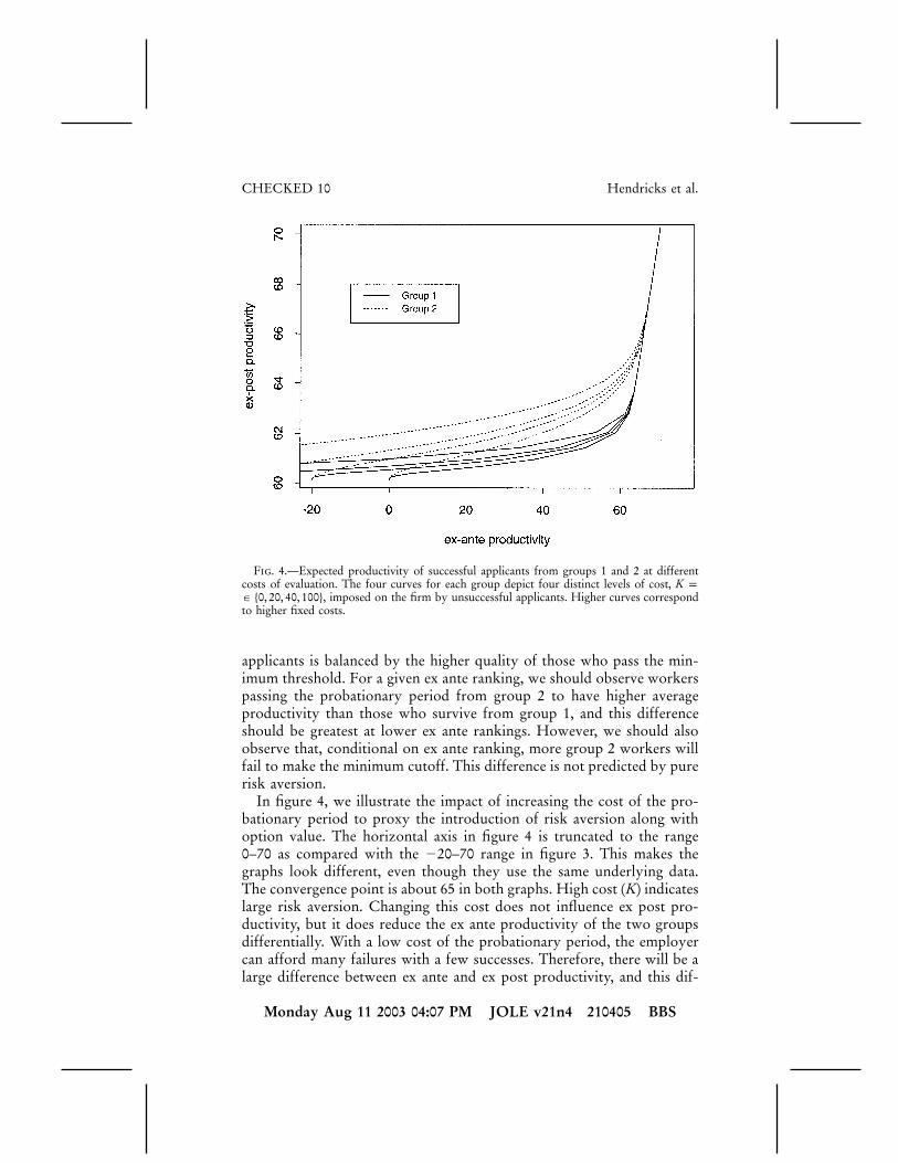
Fig. 4.—Expected productivity of successful applicants from groups 1 and 2 at differentcosts of evaluation. The four curves for each group depict four distinct levels of cost, K p

imposed on the firm by unsuccessful applicants. Higher curves correspond� {0, 20, 40, 100},to higher fixed costs.

applicants is balanced by the higher quality of those who pass the min-imum threshold. For a given ex ante ranking, we should observe workerspassing the probationary period from group 2 to have higher averageproductivity than those who survive from group 1, and this differenceshould be greatest at lower ex ante rankings. However, we should alsoobserve that, conditional on ex ante ranking, more group 2 workers willfail to make the minimum cutoff. This difference is not predicted by purerisk aversion.

In figure 4, we illustrate the impact of increasing the cost of the pro-bationary period to proxy the introduction of risk aversion along withoption value. The horizontal axis in figure 4 is truncated to the range0–70 as compared with the �20–70 range in figure 3. This makes thegraphs look different, even though they use the same underlying data.The convergence point is about 65 in both graphs. High cost (K) indicateslarge risk aversion. Changing this cost does not influence ex post pro-ductivity, but it does reduce the ex ante productivity of the two groupsdifferentially. With a low cost of the probationary period, the employercan afford many failures with a few successes. Therefore, there will be alarge difference between ex ante and ex post productivity, and this dif-



ference will be most evident for a group with high uncertainty (like group2). This is reflected by the small difference of changing probation costsfor group 1 as compared with group 2.

These models predict that the impact of uncertainty will depend on thecost of an incorrect hire. If a mistake in hiring leads to large costs, statisticaldiscrimination is likely to result. If a mistake can be made with low cost,option value will likely favor the group with the most uncertainty. Whenarraying on mistake costs, we expect to observe hiring differences in thetails of the distribution of productivity that are in opposite directions.Our empirical specification will require measures of productivity at bothtails of the distribution.

III. The NFL Draft

Each year, all potential NFL entry-level players must participate in theNFL draft. This is a procedure wherein each team selects a player in apredetermined sequence. The sequence is arranged in reverse order ofstandings for the previous NFL season in an attempt to improve parity.4

For the time period of our analysis, there were 12 rounds of the draft.With 28 NFL teams, this meant that 336 players were drafted each year.5

All NFL teams have access to an overwhelming array of individualplayer data compiled during the college career of each player. In addition,the teams jointly operate a common camp where a large number of newlyeligible NFL hopefuls gather prior to the draft. This camp is a thoroughphysical examination of the players’ health as well as of their relativeabilities.6 Using all of this combined information about each player, eachteam must make an estimate of that player’s value. It is this estimate andits relationship to the ultimate productivity of the player that form thebasis for our analysis.

4 Of course, since drafted players can be and are traded freely, the impositionof the draft per se has little impact on the final allocation of talent. Teams withhigher values will get the player via interteam transactions rather than via theinitial allocation.

5 In fact, more than that number are actually drafted, on average. This is becausethe NFL holds supplementary drafts at unscheduled times. These drafts handlethe allocation of players entering NFL eligibility under extremely special circum-stances, such as sudden and unexpected loss of college eligibility. In the caseswhere NFL rules required teams to give up first-round draft picks to select inthe supplemental draft, we assigned first-round draft numbers to the players. Inthe special case of the U.S. Football League supplemental draft, which occurredwhen the rival USFL disbanded, we include a dummy variable for all playersselected in this draft.

6 Some players acquire injuries in the period after their college experience butbefore the draft. Other players may have had unannounced injuries. Finally, somecolleges are notoriously inaccurate in their physical descriptions of the players.The physical examinations at this camp reconcile these problems.



To test for statistical discrimination against one group based on the useof a noisy signal of future productivity or for option value in favor ofone group based on similar uncertainty, we first need to identify the twogroups. For the first group, the preemployment predictor should performbetter than for the second group. This translates to the evaluator beingable to distinguish the performances of group 1 members from the averagefor the group better than he can for members of group 2. In the limit,the evaluator would simply predict the mean of group 2 if there were noway to distinguish its members. This will generate a larger variance inthe predicted values for the first group. Cornell and Welch (1996) showthat the larger variance in predicted outcomes can be expected to lead toa larger selection from this group since there will be more members inthe right tail of the distribution. This should be distinguished from largeruncertainty about the predicted values. Thus there should be more var-iance in the scores for one group, but the uncertainty associated with anyindividual score should be less.

In our model of Section II, we have assumed for convenience that bothgroups have identical mean productivity; only the variability of predictedproductivity differs between the two groups. In many situations, therecan be both mean and variance effects. For example, individuals with lessexperience are likely to have both lower means and higher variance ofoutcomes. Mean effects are accounted for in the empirical specificationby the presence of several predictors of individual performance availableex ante to the teams and by the inclusion of the group indicator variable.Departures from the conditional mean determined by these predictorsfound in the interaction effects between the group indicators and the exante observables are then attributed to variance effect.

We have selected individuals from the schools that play Division IAfootball as group 1, with individuals from the remaining schools as group2. The Division IA schools consist of the major football universities inthe NCAA, and they have much higher profile programs than otherschools. These Division IA schools can be assumed to attract and trainfootball players better than the other schools.7

7 We have some support for this assumption. In preparation for the 1996 NFLdraft, a league reporting service called the NFL Combine did evaluations on ap-proximately 770 players producing Combine ratings which range from 7.40 to 9.89( ), with 7 indicating a player who probably will not make the NFLmean p 7.76and 10 indicating a player who almost surely will start in his first year. These ratingsrepresent the expected value of players as predicted from the Combine tests. Athletesfrom Division IA schools ( ) score higher (7.83 vs. 7.59; ) thann p 542 t p 5.49non–Division IA athletes ( ) and have a larger standard error (.62 vs. .40;n p 231

) for their rating. For these data to be consistent with the model, the ratingsF p 73.9for non–Division IA athletes should also be more difficult to predict. We haveperformed regressions that indicate the Combine rating is more predictable forschools that have had traditionally stronger football programs. Scouts make larger



Table 1Players on 1996 Opening Roster by Draft Round

Round On Roster Not on Roster Total

1 30 0 302 31 0 313 31 3 344 36 1 375 24 11 356 26 16 427 24 21 45Undrafted 69 464 533

It is possible that option value and risk aversion will dominate in dif-ferent segments of the draft. If all drafted players in a round far exceedthe minimum cutoff, option value is likely to be small. Conversely, if allplayers are unlikely to meet the minimum, then option value might bequite important while risk aversion is relatively unimportant. To inves-tigate this possibility, table 1 tabulates players on the basis of their draftround and whether or not they made the opening roster of any team inthe NFL. A total of 271 new players made NFL rosters in 1996. Everyplayer in the first two rounds of the draft and 67 of 71 players in thenext two rounds made opening rosters. On the other hand, only 50 of87 players in the last two rounds made teams, and only 69 players of 533additional players, who were evaluated but not drafted, made the rosters.These results suggest that option value may be quite important in thelater rounds of the draft and for nondrafted players. Very few candidateswill meet the minimum acceptable standards, so that choosing from thehigher variance group might be more attractive. A discount for uncertaintyabout the player’ s future performance, if it is important, is likely to occurduring the first few rounds, where players receive higher salaries and long-term contracts.

In addition to the 1996 data, we have gathered data on all college playerswho were drafted into the NFL between 1979 and 1992 (4,765 players)and all NFL players who began their careers in the NFL during the sameperiod but who were not drafted (“free agents,” 958 players).8 For 1989

distinctions in ability for the Division IA athletes than they do for the non–DivisionIA athletes, based on measured criteria. We also estimated models with interactionsbetween position and weight, height, and time in the 40-yard dash. These modelsgave the same results as the more parsimonious representation without interactions.The difference in fit for the Division IA and non–Division IA players was evenmore dramatic since the interactions as a group were significant for the DivisionIA players but not significant for the non–Division IA players. They thereforeincreased the adjusted R2 for the Division IA athletes and reduced the R2 for thenon–Division IA athletes. These results are available from the first author.

8 See table 5 for details on the sources of our data.



only, we have data on salary for all NFL players. We do not have infor-mation on the pool of potential NFL players. These players could comefrom the senior classes of colleges that play football. They could alsocome from underclassmen, seniors from the previous years, participantsin the Canadian Football League, or players who never attended college.We also have no information on players who were not drafted and whowere unsuccessful in their attempt to be employed with an NFL teamfor these time-series data.

Of the players who were drafted by the NFL, approximately 67%(3,171) actually were employed for at least one game by an NFL team.Of the NFL players who began their careers after 1978, 77% were drafted,with the remaining being free agents. Of the 4,129 NFL players, overthese 14 years, approximately 9% were judged to be talented enough toplay in at least one Pro Bowl event (the all-star game for the NFL).

In 1992, there were 106 universities that had Division IA football teams.There were approximately 9,000 men playing football at these schools.We estimate that approximately 31,500 men participated in Division IAfootball over the time period of our data. Of these players, the NFLdrafted approximately 12%. The percentage of potential players from allpossible sources who are actually drafted in any year is, therefore, likelyto be less than 12%. Of the nondrafted players, only 2% were employedby an NFL team, as compared with 69% of the drafted players.

If differences in uncertainty about future performance influence theteams’ ex ante evaluation of the players, as given by their draft position,then we should observe differences in career performance between Di-vision IA and non–Division IA players when we condition on draft round.We have gathered several proxies for performance to test this prediction.

Table 2 provides information about career length for NFL players.Although the average career is longer for athletes who come from DivisionIA schools (4.75 vs. 4.5 years for non–Division IA players), when wehold constant the position where the players where drafted, Division IAplayers have shorter careers in nine of the 12 rounds and also among freeagents. Over the full sample, Division IA players’ careers are longer be-cause they are drafted higher. Thus, if we use career length as a measureof productivity, there is some indication that non–Division IA playersmight be better than Division IA players for the same ex ante evaluation.This could indicate statistical discrimination or option-value effects.

The NFL Pro Bowl is the all-star game that is played once per year.Table 3 shows the probability of appearance in the Pro Bowl during aplayer’s career and the percentage of years in the league when the playerappeared in the Pro Bowl. Both statistics show a similar pattern. In eightor nine of the rounds, the non–Division IA athletes have a higher prob-ability of appearing in the Pro Bowl. However, the largest differencesappear in the early draft rounds, supporting a risk aversion interpretation



Table 2Average Years Played for NFL Players by Round of Draft andCollege Division, 1979–92

Round Non–Division IA Division IA Difference

1 7.78 7.18 .602 6.26 5.95 .313 5.87 5.12 .754 5.00 4.79 .215 4.24 4.42 �.186 4.79 4.10 .697 3.79 3.96 �.178 4.88 4.55 .339 4.32 4.36 �.0410 4.90 4.46 .4411 4.25 3.92 .3312 3.94 3.75 .19Free agent 3.80 3.48 .32Average 4.50 4.75 �.26

Note.—The table includes only players who appeared in at least one NFL season. Averagesinclude players with incomplete careers.

Table 3Pro Bowl Appearances by Round and Division

Round

Percentage of Players in Pro Bowl Percentage of Career in Pro Bowl

Non–Division

IADivision

IA Difference

Non–Division

IADivision

IA Difference

1 34.5 29.1 5.4 13.1 10.9 2.22 20.0 15.6 4.4 6.2 4.8 1.43 11.7 8.9 2.8 3.4 2.5 1.04 6.6 4.2 2.4 2.5 1.1 1.45 5.6 4.5 1.0 2.0 1.3 .76 5.5 3.2 2.3 2.1 1.1 1.07 3.3 3.9 �.6 2.4 1.1 1.38 3.1 1.6 1.6 1.4 .7 .69 1.9 2.4 �.6 .6 .9 �.310 1.0 2.7 �1.8 .3 1.1 �.811 1.7 .4 1.4 1.1 .2 .912 1.0 1.4 �.4 .8 .9 �.1Free agent 4.7 3.6 1.0 1.1 .9 .1Average 5.4 7.0 �1.6 2.1 2.7 �.7

Note.—The table includes players with incomplete careers.

but not an option value interpretation if we assume option value is notimportant in the early rounds. Again, non–Division IA players have prod-uctivities that exceed the Division IA players for a given ex ante evaluation.

Table 4 provides information for all players drafted between 1979 and1992. These data provide a different picture from the results for careerlength and all-star quality. In eight of the 12 rounds, non–Division IAplayers were less likely to actually ever play. This indicates that teamswere willing to take chances on marginal non–Division IA athletes more



Table 4Percentage of Draftees Who Actually Played by Round andDivision

Round Non–Division IA Division IA Difference

1 92.3 98.9 �6.62 91.3 95.9 �4.63 89.2 91.2 �2.04 89.0 87.1 2.05 76.0 80.1 �4.16 72.9 69.0 3.97 55.9 67.3 �11.48 50.0 60.7 �10.79 41.5 48.3 �6.710 39.6 37.8 1.811 38.3 34.1 4.212 32.3 37.1 �4.8Average 70.0 75.1 �5.0

often than they were on Division IA athletes. The evidence from tables3 and 4 is consistent with the existence of more uncertainty over theexpected productivity of non–Division IA players. The table 4 results areconsistent with the option value model.

Position in the draft provides significant information about the pre-employment evaluations of the player by the teams in the NFL. Furtherinformation is provided by the failure of the teams to draft a player. Inthis case, the player must have been valued lower than all players in thedraft. More players fail among those who are drafted than succeed amongfree agents. Thus, all free agents are “mistakes” in the sense that theycould have been selected in the draft. For the years 1979–92, 34% of freeagents came from non–Division IA schools, while players from theseschools made up only 17.7% of the drafted players.

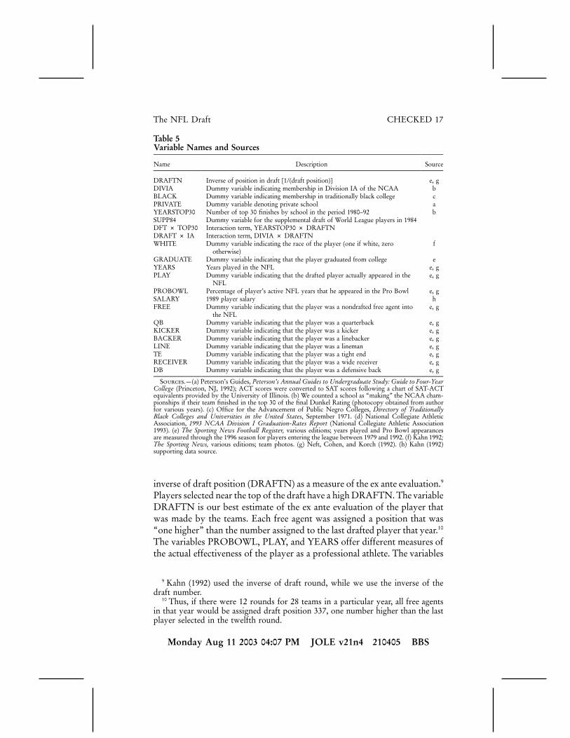
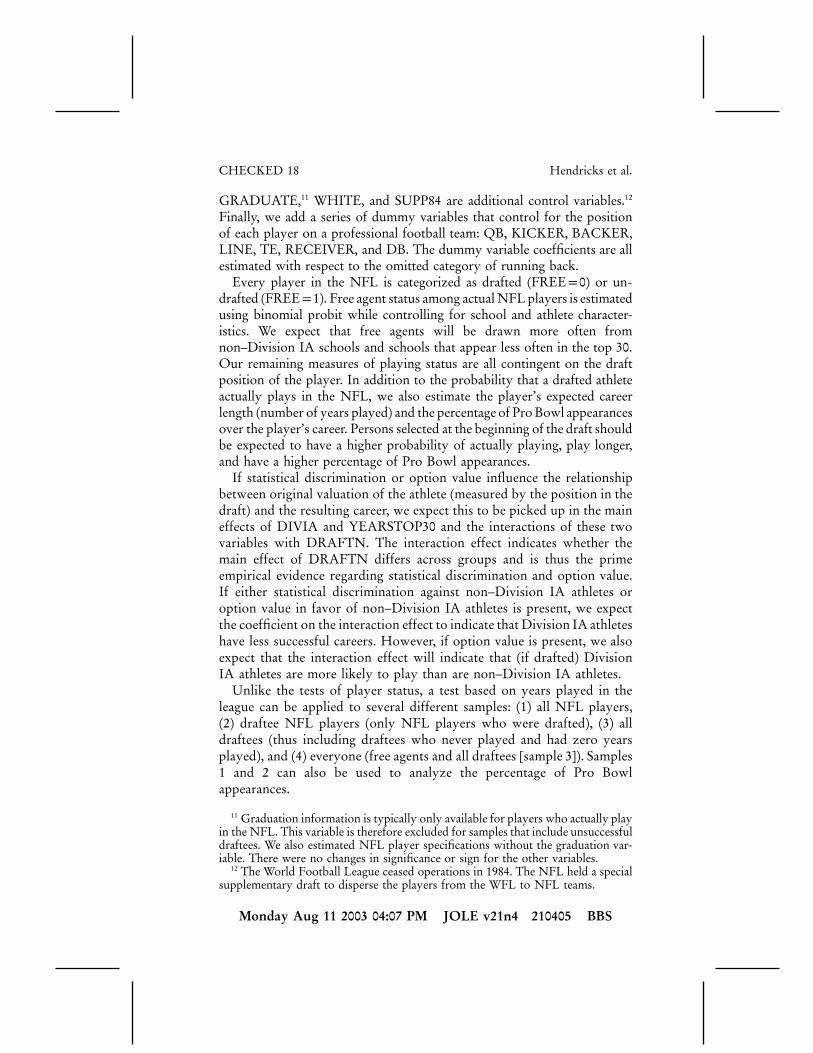
These results provide a prima facie case for different evaluations of playerswho come from schools where the talent of the players is probably harderto evaluate. These results are tested more formally in tables 6–8, where wecontrol for characteristics of the school and the athletes. Table 5 lists thevariables that we use to analyze the NFL screening problem. The datainclude characteristics of the school and the athletes. There are four variablesthat characterize the athlete’s college choice: DIVIA is a measure of thelevel of competition that the player experienced, YEARSTOP30 is the actualcompetitiveness of the player’s college over the period 1980–92, andBLACK and PRIVATE are dummy variables to capture other character-istics of the school. We have 15 variables that measure the salient charac-teristics of each athlete in the data set. The variable FREE is a dummyvariable representing players who played in the NFL but who were over-looked during the draft (“free agents”). Following Kahn (1992) we use the



Table 5Variable Names and Sources

Name Description Source

DRAFTN Inverse of position in draft [1/(draft position)] e, gDIVIA Dummy variable indicating membership in Division IA of the NCAA bBLACK Dummy variable indicating membership in traditionally black college cPRIVATE Dummy variable denoting private school aYEARSTOP30 Number of top 30 finishes by school in the period 1980–92 bSUPP84 Dummy variable for the supplemental draft of World League players in 1984DFT # TOP30 Interaction term, YEARSTOP30 # DRAFTNDRAFT # IA Interaction term, DIVIA # DRAFTNWHITE Dummy variable indicating the race of the player (one if white, zero

otherwise)f

GRADUATE Dummy variable indicating that the player graduated from college eYEARS Years played in the NFL e, gPLAY Dummy variable indicating that the drafted player actually appeared in the

NFLe, g

PROBOWL Percentage of player’s active NFL years that he appeared in the Pro Bowl e, gSALARY 1989 player salary hFREE Dummy variable indicating that the player was a nondrafted free agent into

the NFLe, g

QB Dummy variable indicating that the player was a quarterback e, gKICKER Dummy variable indicating that the player was a kicker e, gBACKER Dummy variable indicating that the player was a linebacker e, gLINE Dummy variable indicating that the player was a lineman e, gTE Dummy variable indicating that the player was a tight end e, gRECEIVER Dummy variable indicating that the player was a wide receiver e, gDB Dummy variable indicating that the player was a defensive back e, g

Sources.—(a) Peterson’s Guides, Peterson’s Annual Guides to Undergraduate Study: Guide to Four-YearCollege (Princeton, NJ, 1992); ACT scores were converted to SAT scores following a chart of SAT-ACTequivalents provided by the University of Illinois. (b) We counted a school as “making” the NCAA cham-pionships if their team finished in the top 30 of the final Dunkel Rating (photocopy obtained from authorfor various years). (c) Office for the Advancement of Public Negro Colleges, Directory of TraditionallyBlack Colleges and Universities in the United States, September 1971. (d) National Collegiate AthleticAssociation, 1993 NCAA Division I Graduation-Rates Report (National Collegiate Athletic Association1993). (e) The Sporting News Football Register, various editions; years played and Pro Bowl appearancesare measured through the 1996 season for players entering the league between 1979 and 1992. (f) Kahn 1992;The Sporting News, various editions; team photos. (g) Neft, Cohen, and Korch (1992). (h) Kahn (1992)supporting data source.

inverse of draft position (DRAFTN) as a measure of the ex ante evaluation.9

Players selected near the top of the draft have a high DRAFTN. The variableDRAFTN is our best estimate of the ex ante evaluation of the player thatwas made by the teams. Each free agent was assigned a position that was“one higher” than the number assigned to the last drafted player that year.10

The variables PROBOWL, PLAY, and YEARS offer different measures ofthe actual effectiveness of the player as a professional athlete. The variables

9 Kahn (1992) used the inverse of draft round, while we use the inverse of thedraft number.

10 Thus, if there were 12 rounds for 28 teams in a particular year, all free agentsin that year would be assigned draft position 337, one number higher than the lastplayer selected in the twelfth round.



GRADUATE,11 WHITE, and SUPP84 are additional control variables.12

Finally, we add a series of dummy variables that control for the positionof each player on a professional football team: QB, KICKER, BACKER,LINE, TE, RECEIVER, and DB. The dummy variable coefficients are allestimated with respect to the omitted category of running back.

Every player in the NFL is categorized as drafted (FREEp0) or un-drafted (FREEp1). Free agent status among actual NFL players is estimatedusing binomial probit while controlling for school and athlete character-istics. We expect that free agents will be drawn more often fromnon–Division IA schools and schools that appear less often in the top 30.Our remaining measures of playing status are all contingent on the draftposition of the player. In addition to the probability that a drafted athleteactually plays in the NFL, we also estimate the player’s expected careerlength (number of years played) and the percentage of Pro Bowl appearancesover the player’s career. Persons selected at the beginning of the draft shouldbe expected to have a higher probability of actually playing, play longer,and have a higher percentage of Pro Bowl appearances.

If statistical discrimination or option value influence the relationshipbetween original valuation of the athlete (measured by the position in thedraft) and the resulting career, we expect this to be picked up in the maineffects of DIVIA and YEARSTOP30 and the interactions of these twovariables with DRAFTN. The interaction effect indicates whether themain effect of DRAFTN differs across groups and is thus the primeempirical evidence regarding statistical discrimination and option value.If either statistical discrimination against non–Division IA athletes oroption value in favor of non–Division IA athletes is present, we expectthe coefficient on the interaction effect to indicate that Division IA athleteshave less successful careers. However, if option value is present, we alsoexpect that the interaction effect will indicate that (if drafted) DivisionIA athletes are more likely to play than are non–Division IA athletes.

Unlike the tests of player status, a test based on years played in theleague can be applied to several different samples: (1) all NFL players,(2) draftee NFL players (only NFL players who were drafted), (3) alldraftees (thus including draftees who never played and had zero yearsplayed), and (4) everyone (free agents and all draftees [sample 3]). Samples1 and 2 can also be used to analyze the percentage of Pro Bowlappearances.

11 Graduation information is typically only available for players who actually playin the NFL. This variable is therefore excluded for samples that include unsuccessfuldraftees. We also estimated NFL player specifications without the graduation var-iable. There were no changes in significance or sign for the other variables.

12 The World Football League ceased operations in 1984. The NFL held a specialsupplementary draft to disperse the players from the WFL to NFL teams.



IV. Estimation and Results

Our model requires us to measure productivity at various positions inthe distribution of player talent. To capture this, our dependent variablesconsist of data on salary of the player in 1989, free agent status or not,whether the player made the team or not, years played, and percentageof years in the Pro Bowl. Whether the player made the team or not andpercentage of years in the Pro Bowl are taken from tails of the productivitydistribution. Recall the discussion at the end of Section II regarding figure4. Given the differences in costs incurred from “mistakes” in hiring, weexpect to observe differences in the tails of the probability distribution.“Making the team” allows us to distinguish statistical discrimination (SD)from option value (OV) predictions, since the two are different in thiscase. Probability of a Pro Bowl appearance allows us to focus on pro-duction of “stars,” although predictions of both SD and OV are the same.Salary and years in the league are better measures of central tendenciesof productivity effects, although results at the mean do allow distinctionbetween OV and SD. If salary is a good measure of productivity, weshould be able to capture these effects best with our salary measure.Unfortunately, as we detail below, salary data are the least likely to showresults. We have therefore used as many measures as possible to give thebest picture of total effects.

“Percentage of years in the Pro Bowl” and “years played” exhibit bothleft censoring and right censoring. The data are left censored because thelowest value of zero years has considerable heterogeneity in the qualityof the players. The data are right censored because they include playerswhose career is incomplete. Because of the discreteness of the data, aswell as the problems of left and right censoring, there is no “ideal” es-timation scheme. Thus, we report several alternative methods of esti-mation on different subsets of the data.

The first results in table 6 (those reported in col. 1) are for the di-chotomous dependent variable FREE, which indicates that the player wasnot drafted out of college but ultimately played in the NFL. Players whoplayed outside Division IA or who played for weaker Division IA teamswhile in college tend to be overrepresented among free agents. Both theDIVIA coefficient and the YEARSTOP30 coefficient are negative andsignificant. White players are also overrepresented among free agents.

The second set of results in table 6 (those in col. 2) concern the dummyvariable PLAY, which indicates whether a player chosen in the draft ul-timately played for any NFL team. The specification (and all our sub-sequent estimations) includes the draft variable (high values of DRAFTNindicate high ex ante evaluation) and interactions between the draft var-iable and DIVIA and YEARSTOP30. If the impact of uncertainty doesnot vary with position in the draft, then the dummy variables for DIVIA



Table 6Probability of Choice as Free Agent, Probability of Draftees Playing in theNFL, and Probability of Choice for Pro Bowl

Dependent Variable

FREE PLAY PROBOWL PROBOWL

Sample NFL players Draftees Drafted NFL players NFL playersEstimation method Binomial probit Binomial probit Weighted probit Weighted probitN 3,838 4,515 3,020 3,838Log-likelihood �1,851 �2,349 �3,700 �4,189Variable:

QB .03015 �.19158 .12832 .21006 *(.1269) (.107) (.07976) .07289

KICKER .93210 * .00371 .32171 * .30837 *(.1217) (.1295) (.09581) .07866

BACKER .06994 .15042 �.19293 * �.23261 *(.08774) (.07891) (.05818) .05437

LINE .16976 * �.16967 * .18258 * .20804 *(.08249) (.07086) (.05178) .04871

TE .15780 .12254 .00677 .01165(.1095) (.09875) (.0802) .07491

RECEIVER .18390 * �.13332 .08864 .05375(.08303) (.07224) (.05498) .05303

DB .31644 * �.03373 �.01943 �.01426(.07316) (.06752) (.05009) .04708

WHITE .13999 * �.12635 * �.33293 * �.32661 *(.05778) (.05104) (.04188) .03887

PRIVATE .05413 .07752 .03622 .04779(.05804) (.05123) (.03291) .03156

GRADUATE �.08536 .10272 * .07770 *(.05353) (.03427) .03210

BLACK .05403 �.16001 �.02029 �.02079(.1028) (.1016) (.08772) .07650

SUPP84 �2.36850 * .36009 * .37759 *(.1953) (.09563) .09563

DRAFTN 76.84700 * 7.21700 7.62080 *(7.642) (1.501) 1.43200

YEARSTOP30 �.06506 * .05777 * .01157 * .01670 *(.007749) (.009907) (.005326) .00496

DIVIA �.27426 * �.34487 * .05663 .03906(.06934) (.0982) (.0636) .05491

DRAFT # IA 50.61200 * �4.77220 * �5.09370 *(11.07) (1.514) 1.44600

DFT # TOP30 �7.66080 * �.10389 * �.11399 *(1.098) (.0316) .03132

Constant �.61190 �.06204 * �1.74560 * �1.77720 *(.07265) (.08447) (.0623) .05430

Note.—NFL players are players with at least 1 year in the NFL. They include both drafted NFL playersand free agents. Draftees are all athletes chosen in the draft from 1979 to 1992. FREE is a dummy variablefor free agent status; PLAY is a dummy variable for playing in at least one game in 1 year in the NFL.PROBOWL is the proportion of a player’s career when he was chosen for the Pro Bowl game.

* Significant at the .05 level or better (two-tailed test).

and YEARSTOP30 should be significant but the interactions should notbe significant.

The coefficient for DRAFTN is strongly positive, as expected. Thosewith good draft positions are much more likely to actually play in theNFL. Among draftees, white athletes are less likely to play. This mightreflect the fact that white players have a much higher probability of grad-uation than black players. Thus, their employment alternatives are greater,and their effort to make the team could be less than the effort given by



black players. However, white players are also overrepresented amongfree agents. This seems counter to the effort explanation.

If athletes from lesser-regarded football schools have more option value,the teams will take a chance on them. This chance could result in fewerof them actually surviving their first probationary period. In this case,their probability of making the team should be less. If teams are reluctantto take a chance on players with noisy predraft information due to riskaversion, then the players from lesser-regarded football schools shouldactually have a higher probability of surviving the probationary period.The results for school characteristics present a mixed relationship. Theeffects of DIVIA and YEARSTOP30 are exactly opposite. The main effectof DIVIA is negative and the interaction effect is positive, while the maineffect of YEARSTOP30 is positive and the interaction effect is negative.

The combined effects of Division (DIVIA) and quality within division(YEARSTOP30) are evaluated in table 7. This table shows the predictedZ-scores (and their corresponding probabilities for draftees playing in theNFL) from the probit estimation for the probability of a draftee actuallyplaying (see col. 2 of table 6). These are evaluated at three points in thedraft distribution for three different school levels. We selected the mid-points of the first draft round (drafting position p 15), the third round(drafting position p 75), and the tenth round (drafting position p 285).13

The pattern of the Z-scores and their probabilities is consistent withboth option value and statistical discrimination explanations. The strongerDIVIA school athletes have the lowest Z-scores at the top of the draft(compare 3.434 to 4.935 and 7.511) but the highest at the bottom (compare.223 to .081 and �.055). The smaller probabilities of playing at the topof the draft are consistent with statistical discrimination against athletesfrom weaker, less visible programs. Since all athletes at the top of thedraft are likely to play (all predicted probabilities are essentially 1.0), theactual effect of this is very small even though the differences are significant.The larger probabilities of playing near the bottom of the draft are con-sistent with oversampling of non–Division IA athletes and Division IAathletes from weaker programs due to their option value. Thus, the PLAYresults provide support for both option value and statistical discriminationfor this comparison.

13 The predictions assume that the control variables (all dummies) take the valueof the omitted category, which are specified in the footnote to the table. Based onWald tests for linear combinations of the coefficients in this probit, all differencesin the Z-scores going down rows are significant. All differences across the columnsare also significant, with the exception of the difference between very strong DivisionIA schools (DIVIAp1 and YEARSTOP30p10) and non–Division IA schools inthe 75th and 285th draft position and the difference between weaker Division IAschools (YEARSTOP30p1) and non–Division IA schools in the 285th draftposition.



Table 7Predicted Probability of Draftees Playing (Table 6, Col. 2) Evaluated forDifferent Draft Rounds and Different Player’s School Characteristics

Round Drafted(Drafting Position)

Player’s School’s Characteristics

Non–Division IA(0 Years Top 30)

Division IA(1 Year Top 30)

Division IA(10 Years Top 30)

Round 1 (15):Z-score predicted 4.935 7.511 3.434Predicted probability 1.000 1.000 1.000

Round 3 (75):Z-score predicted .836 1.122 .722Predicted probability .798 .869 .765

Round 10 (285):Z-score predicted .081 �.055 .223Predicted probability .532 .478 .588

Predicted Z-scores are computed for the two divisions, years in the top 30, and the different draft numberswith all control dummies set to the omitted categories (black running back from a public [non–traditionallyblack] institution and not chosen in the supplemental 1984 draft).

While it is natural to equate the outcome we call “making the team”with the probationary period, this is not exactly correct. NFL teams oftenkeep players who are not expected to help their teams in the near futurebut who are expected to help later. These players might get the oppor-tunity to play several times before the team releases them. Their proba-tionary period thus includes not only their preseason tryout but also asmall amount of playing time with the team. Therefore, it is necessary toevaluate other measures of career success that might better capture thequality of the player’s career.

The last two specifications in table 6 (cols. 3 and 4) provide results forthe quality of a player’s career when “quality” is measured by the per-centage of a player’s career where he is elected to the “Pro Bowl.” Eachyear, the players in the NFL vote to determine which of their colleagueswill play in the Pro Bowl. Election to the Pro Bowl is a sign of dominanceat the player’s particular position on the field.

Since players’ career length ranges from 1 to 14 years, this percentageis based on from 1 to 14 actual observations for each player on whetheror not he was selected for the Pro Bowl. If the proportion is used withoutweighting, the underlying assumption is that we are making a single drawfrom a distribution with variance , where in fact we are makingp(1 � p)multiple draws, which have unconditional variance of . To ac-p(1 � p)/Ncount for the more precise estimate of the variance and to treat the het-eroskedasticity that is introduced by having varying career length, wetreat each proportion as a replication of N draws of size one. Therefore,we use probit as our estimation procedure. We label this “weighted” probitto indicate that career length is used as the weight to replicate observa-



tions.14 We perform this weighted probit on two subsamples of the data.The first limits the data to just those NFL players who were drafted outof college: 3,020 observations. The second subset represents all playersthat appeared in the NFL: 3,838 observations on successful draftees aswell as free agents. In both cases, DRAFTN is once again strongly pos-itive. The effects of both Division IA membership and strength of program(YEARSTOP30) and their interactions with DRAFTN are in the samedirection for both samples. All coefficients except the main effect of DI-VIA are significant.

We again find a negative coefficient on WHITE in the PROBOWLestimations. Throughout this period, white players represented a minorityof the sample (about 38%). Thus, this might be explained by a votingeffect. However, it is again consistent with the results for PLAY esti-mations. Controlling for their playing position, their position in the draft,and the characteristics of their school, white players tend to have lessdistinguished careers.15

The results for the predicted Z-scores and probabilities of playing inthe Pro Bowl are evaluated at different draft positions and school cate-gories in table 8.16 Athletes from non–Division IA schools are much morelikely to be chosen for the Pro Bowl when they are drafted in the firstround. This result supports both statistical discrimination and optionvalue. However, option value is not supported at the bottom of the draft,since we should observe more distinguished careers among those whoactually survive the probationary period. Again, we are constrained bynot having a specific probationary period that would provide the besttest of option value.

Our next estimate uses the length of a player’s tenure in the NFL asthe measure of success. Those players with high YEARS should representvery successful careers. They should have been identified as valuable se-lections in the draft.

The dependent variable is YEARS, a series of integers representing thelength of career. This data series is truncated on the right for those playerswhose career was not complete at the time our data set was compiled,and it is truncated on the left (in principle) for players who are not goodenough to even play “zero” years. In addition, the data are not really

14 See Greene (1995, p. 413) for a discussion of the use of probit with groupeddata.

15 Kahn and Sherer (1988) find evidence consistent with discrimination againstblack players in the National Basketball Association that is similar to this result.In analyzing draft position, however, they do not find evidence that white playersare drafted before black players, ceteris paribus.

16 All the differences across rows and columns are significant, with the exceptionof the comparison of athletes from weaker Division IA schools and non–DivisionIA athletes in the 75th and 285th draft positions.



Table 8Predicted Probability of NFL Players Playing in the Pro Bowl (Table 6, Col.4) Evaluated for Different Draft Rounds and Different School Characteristics

Round Drafted (Draft-ing Position)

Player’s School Characteristics

Non–Division IA(0 Years Top 30)

Division IA(1 Year Top 30)

Division IA(10 Years Top 30)

Round 1 (15):Z-score predicted �1.596 �1.887 �1.805Predicted probability .055 .030 .036



Note.—Predicted Z-scores computed for the two divisions, years in the top 30, and the different draftnumbers, with all control dummies set to the omitted categories (black running back from a public(non–traditionally black) institution and not chosen in the supplemental 1984 draft).

continuous. Thus both ordered probit and survival techniques have somedrawbacks in the estimation of career length. Finally, we used four dif-ferent subsets of the data. The first included those players, draftees andfree agents, who had played at least one game in the NFL. The nextestimation used the entire data set, which included all players drafted(regardless of tenure in the NFL) and free agents. Our next set used thesubset of NFL players who were drafted, and it therefore excluded freeagents. Finally, our last cut included all drafted players, regardless of theirpotential success.

In all four samples, DRAFTN had the expected sign: higher-draftedplayers have longer careers. The main effects of DRAFTN and YEAR-STOP30 were all positive and significant in six of the eight estimations.The interaction terms DRAFT # IA and DFT # TOP30 were all negativeand significant. In contrast to our other results, white athletes did nothave significantly different career lengths than black athletes.

Figure 5 illustrates the estimated probabilities of specific career lengthsfor Division IA and non–Division IA players selected in different draftrounds.17 This is not like a survival function. It is like a density function.For example, non–Division IA athletes have an expected probability ofabout 2% of leaving the league after 1 year if they are drafted in position15. The same value for Division IA athletes from strong schools is about4%. We present the probabilities of career lengths in years for two groups:

17 These estimations are based on the results of estimates for all players anddraftees. The differences in expected years in the league for the two groups wereevaluated for significance for each round. All four tests yielded significant differ-ences. The full coefficient estimates are available in Hendricks et al. (2001), whichis available from the first author.



Fig. 5.—Predicted probabilities of career length

strong Division IA school athletes (DIVIAp1 and YEARSTOP30p10)and non–Division IA school athletes (DIVIAp0 and YEARSTOP30).For each group, we present the pattern for those chosen in round 1 (draftposition p 15) and those chosen in round 10 (draft position p 285).There is a quite striking difference in career lengths for athletes fromstrong Division IA schools and athletes from other schools who are bothchosen in round 1 of the draft. Non–Division IA athletes chosen in thefirst round show a much larger probability of having a long career lengthand a much lower probability of having a short career as compared withDivision IA athletes chosen in the first round. The reverse pattern occursat the end of the draft. Although the differences are not so striking, athletesfrom strong Division IA schools have higher probabilities of longer ca-reers than non–Division IA athletes when both are drafted near the bot-tom (in our example, the tenth round). These results are again consistentwith option value and statistical discrimination. Non–Division IA athletesare drafted more often at the bottom of the draft and less often at thetop than one would expect based on their realized career lengths.

We had salary data for only one point in the player’s careers, the year1989. The explanatory variables used in our salary regression were drawnfrom Kahn (1992).18 We simply added DIVIA and YEARSTOP30 to his

18 See Kahn (1992) for a full description of these variables.



data and included interactions of these two variables with his draft variable.19

Altonji and Pierret (2001) show that, under statistical discrimination, theimpact of easily observed signals of ability (such as school football program)should fall over time, while the impact of hard-to-observe correlates ofproductivity should increase through time. Therefore, we should expect theeffect of original draft position to decline as the player’s career is extended.In Kahn’s original study, he found that the interactions of draft positionand experience and experience squared with draft position were negative.This is consistent with Altonji and Pierret’s (2001) conjecture. The first-year salary of most players is almost entirely based on the team’ s ex anteestimate of their value. As the player’s tenure in the league lengthens, histrue productivity becomes more evident, and the impact of his draft positionbecomes less important. This is reflected in the negative interaction of draftwith experience.

Unfortunately, this makes the interpretation of salary as a measure oftrue ability problematical. Salary will be a good measure of true abilityonly after recontracting based on revealed productivity. However, manyplayers sign multiple-year contracts. Since the average career span is only3–4 years, it will be difficult to find the impact of statistical discriminationor option value using salary data. The relationship between the decreasein the effect of the draft and time in the league should be moderated bythe school variables if either influence is associated with ex ante evaluation.This requires interacting the experience interaction terms with DIVIAand YEARSTOP30 to allow a difference in this moderating influence oftime for schools with different characteristics. To be consistent with pre-vious results, these new interaction terms should be negative. Players frommore visible schools should see their salaries increase less quickly as com-pared with those of players from less visible schools if either statisticaldiscrimination or option value is influencing ex ante choices.

The full results are available in our longer working paper (Hendrickset al. 2001). While an F-test of the joint effect of DIVIA and YEAR-STOP30 and their interactions indicates that these variables are significantat the .003 level, many of the individual double and triple interactionswere insignificant. This could be expected given the short panel for mostplayers and the collinearity between the main effects and interactions. Thepredictions suggest that there is approximately a 5% beginning positiveincrement for players coming from highly rated Division IA schools. Thiseffect is eliminated after about 2 years.

19 In the Kahn study, the draft variable was measured as 1/(draft round) ratherthan 1/(draft number) as we used in our study. We have maintained this formerdefinition in our salary analysis.

q3



V. Conclusion

In this article, we have argued that the literature on statistical discrim-ination in the labor market and the literature on option value are linkedby their connection with uncertainty about future productivity. The lit-erature on statistical discrimination suggests that groups may be at adisadvantage when the reliability of the test instrument used to predicttheir performance is less than the reliability of this instrument when it isused to predict a competing group’s performance. As Cornell and Welch(1996) show, this can result in selection primarily from the majority groupwhen there are many applicants for a few slots. Thus, the effect of un-certainty is to provide fewer opportunities for minority individuals com-peting for highly competitive positions. They, like Aigner and Cain (1977),also show that this also implies that there should be a spot in the queuewhere the employer will begin to value minority applicants more highlythan majority applicants. This latter prediction has raised some questionbecause researchers have not cited situations where this observation ap-pears to hold. On the other hand, the labor literature on option value(Lazear 1986, 1995) suggests that uncertainty can be of positive benefitto risky groups. As long as the employer can eliminate poor performerswithout other employers taking advantage of the sorting information, itwill pay employers to take members of minority groups. Viewed in thismanner, it seems quite possible that employers take chances on riskyworkers in the hope of finding “stars.”

The National Football League provides a good test case for both ideas.First, we do not run into the nature-nurture problem in attempting toevaluate future performance. Second, employees are bound to the em-ployer for a fixed period because league rules do not allow other teamsto bid for the player until after a number of years have passed. This allowsthe employer to earn rents from keeping a risky worker.

Our empirical work used a variety of outcome measures in our tests.One measure, PLAY, indicated that the athlete was good enough to ac-tually play in the league. Another (PROBOWL) indicated that the playerwas actually very talented relative to his peers. Finally, salary regressionsoffer more traditional measures of outcomes as rewards. We find broadsupport for both statistical discrimination and option value effects. Con-ditional on selection in one of the early rounds of the draft, athletes fromless visible programs seem to have better careers. Their salaries are lesslikely to fall with experience, although they do pay an initial salary penaltyfor not being from a visible school. It is possible that this reflects optionvalue, but it is more likely the result of statistical discrimination. Whenteams are choosing between two star athletes at the top of the draft, theyseem to act in a risk adverse manner and select the athlete from the morevisible football program. In the last rounds of the draft, the reverse appears



to be true. Division IA athletes from top programs are undervalued. Thissupports the option value explanation, but we should see the results for“survivors” of the probationary period reversed. Athletes in this groupshould have stronger careers. We do not find evidence of this.

This conclusion is also consistent with our results for free agents. How-ever, in contrast to the university tenure process, it is not always clearwhen the probationary period ceases for football players. In an article inUSA Today (Bell 1997), one NFL owner was quoted in regard to thereduction in the length of time each team holds exclusive rights to draftees.The owner noted that hastening the time when a draftee is allowed tonegotiate with other teams has forced teams to draft players who arelikely to play immediately. This could potentially reduce the demand forathletes with more uncertain futures, that is, those with higher optionvalue.

Even though the NFL has an enormous array of information sourcesat its disposal, we see evidence of systematic effects in the selection ofplayers in their annual draft. Recalling the special nature of our data setonly strengthens the significance of these findings. Our goal was to con-sider the existence of systematic “error” in labor market decisions. Cer-tainly, one would expect such “errors” to be more likely in markets withless information. The greater the uncertainty, the more likely it is toobserve such a pattern of choice. We have shown evidence for the existenceof such effects in a market with excellent preemployment information.Very few markets have comparable information regarding preemploymentperformance. The print and electronic media devote tremendous attentionto college athletics, in general, and to potential professional talent, inparticular. In addition to their own predictions, each team has access toa variety of pundits’ predictions. The fact that we are still able to documenta systematic group effect is even more striking in such an environmentof copious information.

If a test score (or any other characteristic that is used to differentiatecandidates) is more unreliable for one group than another (even thoughit is unbiased), it is likely that few candidates from the less reliable groupwill be chosen when there is a large number of candidates for a few slots.One remedy for this statistical discrimination is to oversample from thegroup with the less reliable indicator. This might serve as one basis foraffirmative action efforts. The impact of these efforts should be similarto the effect of option value. The employer will be able to choose moreaccurately from the group with less uncertainty. As a result, their ex antepredicted performance should be higher. However, if we allow the em-ployer to eliminate the weakest performers, the ex post mean of the groupwith the unreliable indicator can be higher than the mean for the othergroup. We should expect more failures in the group with large uncertainty.However, these failures will be balanced off with successes that were not



anticipated. The option value message is to not focus exclusively on thefailures.

References

Aigner, Dennis, and Cain, Glen. “Statistical Theories of Discriminationin the Labor Market.” Industrial and Labor Relations Review 30 (Jan-uary 1977): 175–87.

Akerlof, George. “The Economics of Caste and of the Rat Race and OtherWoeful Tales.” Quarterly Journal of Economics 90 (November 1976):599–617.

Altonji, Joseph G., and Pierret, Charles R. “Employer Learning and Sta-tistical Discrimination.” Quarterly Journal of Economics 116 (February2001): 313–50.

Arrow, Kenneth. “The Theory of Discrimination.” In Discrimination inLabor Markets, edited by Orley Ashenfelter and Albert Rees, pp. 3–33.Princeton, NJ: Princeton University Press, 1973.

Becker, Gary. The Economics of Discrimination. 2d ed. Chicago: Univer-sity of Chicago Press, 1957.

Bell, Jarrett. “Early Returns: NFL Caught in Rookie Blitz as Quick Stud-ies Hit Pay Dirt.” USA Today (September 17, 1997), p. C1.

Bloch, Francis, and Rao, Vijayendra. “Statistical Discrimination, IdentitySelection, and the Social Transformation of Caste and Race.” ResearchReport no. 93-276. Ann Arbor: University of Michigan, PopulationStudies Center, 1993.

Borjas, George J., and Goldberg, Matthew S. “Biased Screening and Dis-crimination in the Labor Market.” American Economic Review 68, no.5 (1978): 918–22.

Coate, Stephan, and Loury, Glenn. “Will Affirmative-Action PoliciesEliminate Negative Stereotypes?” American Economic Review 83 (De-cember 1993): 1220–40.

Cornell, Bradford, and Welch, Ivo. “Culture, Information, and ScreeningDiscrimination.” Journal of Political Economy 104, no. 3 (1996): 542–71.

Greene, William. Limdep, Version 7.0. New York: Econometric Software,1995.

Hendricks, Wallace; DeBrock, Lawrence; and Koenker, Roger. “Uncer-tainty, Hiring, and Subsequent Performance: The NFL Draft.” Workingpaper. Urbana: University of Illinois, Institute of Labor and IndustrialRelations, 2001.

Kahn, Lawrence M. “The Effects of Race on Professional Football Players’Compensation.” Industrial and Labor Relations Review 45, no. 1(1992): 295–310.

Kahn, Lawrence M., and Sherer, Peter D. “Racial Differences in Profes-



sional Basketball Players’ Compensation.” Journal of Labor Economics6 (January 1988): 40–61.

Lazear, Edward P. “Raids and Offer-Matching.” In Research in LaborEconomics, vol. 8, pt. A, edited by Ronald Ehrenberg, pp. 141–65.Greenwich, CT: JAI, 1986.

———. 1993 NCAA Division I Graduation-Rates Report. Overland Park,KS: National Collegiate Athletic Association, 1993.

———. “Hiring Risky Workers.” Working Paper no. 5334. Cambridge,MA: National Bureau of Economic Research, 1995.

Neft, D.; Cohen, R.; and Korch, R. The Sports Encyclopedia: Pro Football,10th ed. New York: St. Martin’s, 1992.

Office for Advancement of Public Negro Colleges. Directory of Tradi-tionally Black Colleges and Universities in the United States. Atlanta:Office for Advancement of Public Negro Colleges, 1971.

Peterson’s Guides, Peterson’s Annual Guides to Undergraduate Study:Guide to Four-Year Colleges. Princeton, NJ: Peterson’s Guides, 1992.

Phelps, Edmund. “The Statistical Theory of Racism and Sexism.” Amer-ican Economic Review 62 (September 1972): 659–61.

Pratt, J. “Risk Aversion in the Small and in the Large.” Econometrica 32(January 1964): 122–36.

Sporting News. St. Louis, MO: Sporting News, various editions.Sporting News Football Register. St. Louis, MO: Sporting News, various

editions.



QUERIES TO THE AUTHOR

1 AU: This journal’s style does not italicize foreign phrases that appearas a regular entry in Webster’s 11th edition dictionary. Therefore, ex postand ex ante have been changed to roman font. There are also nothyphenated.

2 AU: In the last term of the equation above, is the x being multipliedby 1 - pi or only by pi?

3 AU: The original sentence was grammatically awkward. Is the rewriteOK?

��

�� !�"�#$�%�%&'

��

�� !"��#�$%�&��'

�� (��))))))�*��)))))�+��))))))))))))))))))))))))

,��-�./�)))))))))))))))))))))))))))))))))))))))))))))))))))))))))))))))))))))��*��!��))))))))))��0��,��/��))))))))))))))))))))))))))))))))))))))))))))))))))))))))))))))))))))))))))))))))))))))))))))))

��!�(��!�(��"(��'��!��1�� *��21��2 ��,�� 3�4��!��!��

�� )�� *� ��+� �,�� -��.

��!�+� /0 100 1/0 �00 /0*

523 6%3�� 6'%�� 6�7�� 6�� 6�� )))))))�8��9 6��)))))))))))�

�2� '�� 7�� 5%�� 7�� 6��)))))))))))

72�5 ''�� &7�� %�� 5�� :�� 6��)))))))))))

�&2�% �%�� 5&�� %�� &3�� 0�-'4�� 9. 6��)))))))))))

�'25� 7�� 3%�� 7�� 5&3�� 33�� *��21��;��2 ��3�4��:��6��)))))))))))

5�253 �� %�� 5�3�� 5%�� &��

�<��3��!� �5�� 53�� 35�� %�� %��

�2�� 7&�� 5&�� 3�� 7�� $"��%��,%��3. 3�44444444444

�

��+�(� �� +�(� �� ,(� �� .

*� ��))))))))))))))))))))))))))))))))))))))))))))))))))))) #��)))))))))))))))))))))))))))))))))))))))))))))))

��=�))))))))))))))))))))))))))��>�))))))))))))))))))))) ��))))))))))))))))))))))))))))))))))))))))))))))))))

?��))))))))))))))))))))))))))))))))))))))�� )))))))))) ��9�))))))))))))))))))))))))��)))))�@��))))))))))))))

#��))))))))))))))))))))))))))))))))))))))))))))))))) ��9��))))))))))))))))))))))))))))))))))))))))))))))))�

��))))))))))))))))))))))))))))))))))))))))))))))))))))) ��))))))))))))))))))))))))))))))))))))))))))))))))))

��9�))))))))))))))))))))))))))��)))))�@��))))))))))))))) � ��)))))))))))))))))))))))))))))))))))))))))))))))))))

��9�))))))))))))))))))))))))))))))))))))))))))))))))))) �=�� :��A��9��:��9��

$5��&��5��$��!%��&$��!$#$�"��'��%��2�� +�!�� :��!��B��,�� :�� :9��9 ��/��"��C; ��9��"��(��;+�� 1��9��, ��:��C��0�� &��9��523�A��C��:��B��

1.�#��*��)))))))))))))))))))))))))))))))))))� ��

��

�.�� C��+��9��!�� 6.� ��!��/��(#�,��+,�0�� ,�?

�� :�� -��9.��))))))))))))))))))))))))))))))))))))))))))))))))))))))))))))))))))

��*� :��))))))))))))))))))))))))))))))))))))))))))))))))))))� �>��?��)))))))))))))))))))))))))))))))))))))))

��!��)))))))))))))))))))))))))))))))))))))))))))))))))))))))��)))))))))))))))))))))))))))))))))))))))))))))�

��;5';�&

Documents

Uncertainty, Hiring, and Subsequent Performance: The NFL Draft Law... · The NFL Draft CHECKED 3 Monday Aug 11 2003 04:07 PM JOLE v21n4 210405 BBS candidate’s training (their “nature”)