Uncertainty Determinantsof Corporate Liquidity∗

Christopher F BaumBoston College

Mustafa Caglayan

University of Glasgow

Andreas Stephan

European University Viadrina, DIW Berlin

Oleksandr Talavera

DIW Berlin

18th January 2006

∗We gratefully acknowledge comments and helpful suggestions by Fabio Schiantarelliand Yuriy Gorodnichenko. An earlier version of this paper appears as Chapter 3 of Ta-lavera’s Ph.D. dissertation at European University Viadrina. The standard disclaimerapplies. Corresponding author: Oleksandr Talavera, tel. (+49) (0)30 89789 407, fax.(+49) (0)30 89789 104, e-mail: otalavera@diw.de, mailing address: Konigin-Luise-Str. 5,14195 Berlin, Germany.

1

Uncertainty Determinants of Corporate Liquidity

Abstract

This paper investigates the link between the optimal level of non-

financial firms’ liquid assets and uncertainty. We develop a partial

equilibrium model of precautionary demand for liquid assets showing

that firms change their liquidity ratio in response to changes in either

macroeconomic or idiosyncratic uncertainty. We test this proposition

using a panel of non-financial US firms drawn from the COMPUSTAT

quarterly database covering the period 1993–2002. The results in-

dicate that firms increase their liquidity ratios when macroeconomic

uncertainty or idiosyncratic uncertainty increases.

Keywords: liquidity, uncertainty, non-financial firms, dynamic panel data.

JEL classification: C23, D8, D92, G32.

2

1 Introduction

“As a result of the foregoing, Honda’s consolidated cash and cash

equivalents amounted to ¥547.4 billion as of March 31, 2003,

a net decrease of ¥62.0 billion from a year ago. ... Honda’s

general policy is to provide amounts necessary for future capital

expenditures from funds generated from operations. With the

current levels of cash and cash equivalents and other liquid assets,

as well as credit lines with banks, Honda believes that it maintains

a sufficient level of liquidity.”1

“Standard & Poor’s said those reserves have declined severely

over the last year and blamed the drain, in part, on Schrempp’s

massive spending spree, which included taking a 34 percent stake

in debt-ridden Japanese automaker Mitsubishi Motors. Accord-

ing to an article in Newsweek magazine, DaimlerChrysler’s cash

reserves – a cushion against any economic turndown — will dwin-

dle to $ 2 billion by the end of the year, down 78 percent from two

years ago. That compares with cash reserves of more than $13

billion at rivals General Motors and Ford, the magazine said.”2

Why should a company maintain considerable amounts of cash, as in

Honda’s case? Why is a decline in cash reserves problematic as in Daimler-

Chrysler’s case? What determines the optimal level of non-financial firms’

1Citation. http://world.honda.com/investors/annualreport/2003/17.html

2Citation. http://www.detnews.com/2000/autos/0012/04/-157334.htm

3

liquidity? In the seminal paper of Modigliani and Miller (1958) cash is

considered as a zero net present value investment. There are no benefits

from holding cash in a world of perfect capital markets lacking information

asymmetries, transaction costs or taxes. Firms undertake all positive NPV

projects regardless of their level of liquidity.3

However, due to the presence of market frictions, we generally observe

that there is great variation in liquidity ratios among different types of firms

according to their size, industry and degree of financial leverage. For instance,

several studies suggest that for liquidity constrained firms, liquid asset hold-

ings are positively correlated with proxies for the severity of agency problems.

Myers and Majluf (1984) argue that firms facing information asymmetry-

induced financial constraints are likely to accumulate cash holdings. Kim

and Sherman (1998) indicate that firms increase investment in liquid assets

in response to increase in the cost of external financing, the variance of fu-

ture cash flows or the return on future investment opportunities.4 Harford

(1999) argues that corporations with excessive cash holdings are less likely

to be takeover targets. Almeida, Campello, and Weisbach (2004) develop a

liquidity demand model where firms have access to investment opportunities

but cannot finance them.

3Keynes (1936) suggests that firms hold liquid assets to reduce transaction costs and

to meet unexpected contingencies as a buffer. This cash buffer allows the company to

maintain the ability to invest when the company does not have sufficient current cash

flows to meet investment demands.

4See also Opler, Pinkowitz, Stulz, and Williamson (1999), Mills, Morling, and Tease

(1994) and Bruinshoofd (2003).

4

We aim to contribute to the literature on corporate liquidity by consid-

ering an additional factor which may have important effects on firms’ cash

management behavior: the uncertainty they face in terms of both macroeco-

nomic conditions and idiosyncratic risks. In explaining the role of macroeco-

nomic uncertainty on cash holding behavior, Baum, Caglayan, Ozkan, and

Talavera (2006) develop a static model of cash management under uncer-

tainty with a signal extraction mechanism. In their empirical investigation,

they find that firms behave more homogeneously in response to increases in

macroeconomic uncertainty.5 However, their model implies predictable vari-

ations in the cross-sectional distribution of corporate cash holdings and does

not make predictions about the individual firm’s optimal level of liquidity.

Furthermore, they do not consider the impact of idiosyncratic uncertainty

on the firm’s cash holdings.

In this paper, we complement Baum, Caglayan, Ozkan, and Talavera

(2006) by investigating the impact of macroeconomic uncertainty as well as

idiosyncratic uncertainty on the cash holding behavior of non-financial firms.

We provide a theoretical and empirical investigation of the firm’s decision to

hold liquid assets. Our theoretical model formalizes the individual firm’s pre-

cautionary demand for cash and assumes that the firm maximizes its value

by investing in capital goods and holding cash to offset an adverse cash flow

shock. The optimal level of cash holdings is derived as a function of expected

return on investment, the expected interest rate on loans, the finite bounds

of their cash flow distribution, the probability of getting a loan and their ini-

5In a recent paper Bo and Lensink (2005) suggests that presence of uncertainty factors

changes the structural parameters of the Q-model of investment.

5

tial resources. We then parameterize optimal cash holdings and turn to the

data to see if there is empirical support for the predictions of the model that

managers change levels of liquidity in response to changes in both macroeco-

nomic and idiosyncratic uncertainty. To do that, we match firm-specific data

with information on the state of the macroeconomic environment, filling the

gap in existing research by investigating the roles of both macroeconomic

and idiosyncratic measures of uncertainty on firms’ cash holdings.

To test the model’s predictions, we apply the System GMM estimator

(Blundell and Bond, 1998) to a panel of US non-financial firms obtained

from the quarterly COMPUSTAT database over the 1993–2002 period. Af-

ter screening procedures our data include more than 30,000 manufacturing

firm-quarter observations, with 700 firms per quarter. Since the impact of

uncertainty may differ across categories of firms, we also consider five sample

splits. Our main findings can be summarized as follows. We find strong

evidence of a positive association between the optimal level of liquidity and

macroeconomic uncertainty as proxied by the conditional variance of infla-

tion. US companies also increase their liquidity ratios when idiosyncratic

uncertainty increases. Results obtained from sample splits confirm findings

from earlier research that firm-specific characteristics are important determi-

nants of cash-holding policy.6

The remainder of the paper is organized as follows. Section 2 discusses

the theoretical model of non-financial firms’ precautionary demand for liquid

assets. Section 3 describes our data and empirical results. Finally, Section 4

6For instance, see Ozkan and Ozkan (2004) and the references therein.

6

concludes.

2 Theoretical Model

2.1 Model Setup

We develop a two period cash buffer-stock model which describes how the

firm’s manager should vary the optimal level of liquid assets in response

to macroeconomic and/or idiosyncratic uncertainty. We assume that the

manager maximizes the expected value of the firm.

At time t the firm has initial resources Wt−1 to be distributed between

capital investment (It) and cash holdings (Ct). Cash holdings may include

not only cash itself but also low-yield highly liquid assets such as Treasury

bills. For simplicity, the firm does not finance any other activities. Invest-

ment is expected to earn a gross return in time t + 1, denoted E[R]t+1.7

Liquid asset holdings, Ct, are required to guard against a negative cash-flow

shock.8 Prior to period t + 1 the firm faces a random cash-flow shock ψt,

distributed according to a symmetric triangular distribution with mean zero

where ψt ∈ [−Ht, Ht].9 Here Ht can be interpreted as a measure of uncer-

7For simplicity we assume that distribution of returns is independent from all other

variables’ distributions.

8The model ignores the transaction motive for holding cash, and the optimal amount

of liquid assets is zero in the absence of costly external financing.

9The triangular distribution is chosen as an approximation to the normal distribution,

which does not have a closed-form solution.

7

tainty faced by the firm’s managers.

There are three possible cases to consider, distinguished by a second sub-

script on each variable. They are graphically depicted in Appendix B. First,

the firm can experience a positive cash-flow shock that occurs with proba-

bility p1 and has conditional expectation ψt,1. This corresponds to the right

half of the figure.

p1 = Pr(ψt > 0) = 1/2

ψt,1 = E(ψt|ψt > 0) = Ht

(1−

√2

2

)

The firm’s value in this case is

Wt+1,1 = ItE[R]t+1 + Ct + ψt,1 = ItE[R]t+1 + Ct +Ht

(1−

√2

2

)(1)

Second, the firm could be exposed to a negative cash-flow shock yet may

have enough liquid assets to meet it. In the figure, this corresponds to a cash

flow shock between −C and 0. This shock occurs with probability p2 and

has conditional expectation ψt,2:

p2 = Pr(0 > ψt > −Ct) =1

2

Ct(2Ht − Ct)

H2t

ψt,2 = E(ψt|0 > ψt > −Ct) = −Ct

(1−

√2

2

)

The value of the firm in the case when −Ct < ψt < 0 is equal to

Wt+1,2 = ItE[R]t+1 + Ct + ψt,2 = ItE[R]t+1 + Ct

√2

2(2)

Finally, the size of the negative shock could exceed the available liquid as-

sets of the firm. This event occurs with probability p3 and has conditional

8

expectation ψt,3:

p3 = Pr(−Ct > ψt) =H2

t − 2HtCt + C2t

2H2t

ψt,3 = E(ψt| − Ct > ψt) = −Ht +

√2

2(Ht − Ct)

In this case the firm must seek external finance and borrow −(ψt +Ct) at the

gross rate Xt. However, there is a probability st ∈ [0, 1] that the firm will be

extended sufficient credit to prevent negative net worth. This implies that

with probability (1− st) the firm declares bankruptcy and its value at time

t + 1 is zero.10 In the figure, this corresponds to a cash-flow shock between

−H and −C. For simplicity we assume that the probability of being granted

sufficient credit is independent of the distribution of cash-flow shocks. The

value of the firm in the last case is equal to

Wt+1,3 = st (ItE[R]t+1 + Ct + ψt,3 +Xt(ψt,3 + Ct)) (3)

= st

[ItE[R]t+1 − (1 +Xt)(Ht − Ct)

(1−

√2

2

)]

Given the three possible cases, the manager’s objective is to maximize the

expected value of the firm in period t + 1. Defining investment as It =

Wt−1 − Ct, the manager’s problem can be written as

maxCt

(E(Wt+1)) = maxCt

(p1Wt+1,1 + p2Wt+1,2 + p3Wt+1,3

)(4)

= maxCt

(1

2

((Wt−1 − Ct)E[R]t+1 + Ct +Ht

(1−

√2

2

))

+1

2

Ct(2Ht − Ct)

H2t

((Wt−1 − Ct)E[R]t+1 + Ct

√2

2

)

10We ignore the liquidation value of the firm’s real assets, which can be assumed seized

by creditors.

9

+(Ht − Ct)

2st

2H2t

((Wt−1 − Ct)E[R]t+1 − (1 +Xt)(Ht − Ct)

(1−

√2

2

)))

where Ct is the only choice variable. Hence, maximizing equation (4) with

respect to Ct, the optimal level of cash can be expressed as11,12

Ct =1

3

2.83Ht − 2.00(1− st)(Wt−1 + 2Ht)E[R]t+1 − 1.76stHt(Xt + 1) +√D

1.41− 2.0E[R]t+1(1− st)− 0.59st(Xt + 1)(5)

Note that equation (5) is non-linear. Hence, to test if the model will receive

support from the data, we linearize it around the steady state equilibrium:

Ct = α1Wt−1 + α2Rt+1 + α3Ht + α4Xt + α5st (6)

where the coefficients α1 − α5 are functions of the model’s parameters. The

expected signs of the coefficients are discussed in the following subsection.

2.2 Model solution

The analytical solution for the firm’s optimal cash holdings is a nonlinear

function of initial resources, Wt−1; the expected gross return on investment,

E[R]t+1; the gross interest rate for borrowing, Xt; the bounds of the tri-

angular distribution of cash shocks, Ht and st, the probability of acquiring

11Given its quadratic structure, there are two possible solutions to the optimization

problem. We work with the solution that implies non-negative cash holdings, as the other

solution has no economic meaning.

12D is a function f(E[R]t+1, Xt, st,Ht,Wt−1) : D = 33.17stH2t E[R]t+1 − 6stXtH

2t +

5.66Wt−1HtE[R]t+1 + 8st(2− st)Wt−1HtE[R]2t+1 + (7.03stXt + 28)H2t E[R]t+1 + (16.49−

6st)H2t + 28E[R]2t+1H

2t + 4E[R]2t+1W

2t−1 − 43.11E[R]t+1H

2t + 4s2tE[R]2t+1W

2t−1 −

8stE[R]2t+1W2t−1 + 4st

2E[R]2t+1H2t − 32stE[R]2t+1Ht

2 − 8E[R]2t+1HtWt−1 −

5.66stE[R]t+1Wt−1Ht.

10

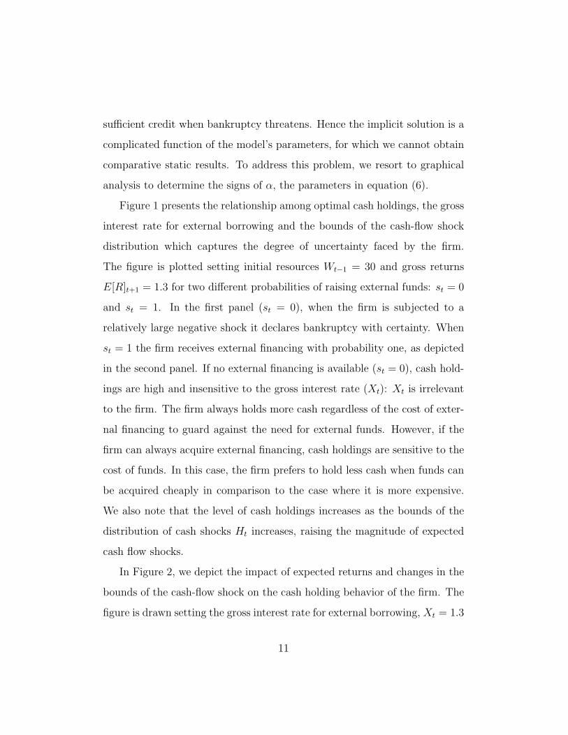
sufficient credit when bankruptcy threatens. Hence the implicit solution is a

complicated function of the model’s parameters, for which we cannot obtain

comparative static results. To address this problem, we resort to graphical

analysis to determine the signs of α, the parameters in equation (6).

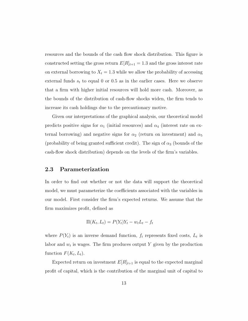
Figure 1 presents the relationship among optimal cash holdings, the gross

interest rate for external borrowing and the bounds of the cash-flow shock

distribution which captures the degree of uncertainty faced by the firm.

The figure is plotted setting initial resources Wt−1 = 30 and gross returns

E[R]t+1 = 1.3 for two different probabilities of raising external funds: st = 0

and st = 1. In the first panel (st = 0), when the firm is subjected to a

relatively large negative shock it declares bankruptcy with certainty. When

st = 1 the firm receives external financing with probability one, as depicted

in the second panel. If no external financing is available (st = 0), cash hold-

ings are high and insensitive to the gross interest rate (Xt): Xt is irrelevant

to the firm. The firm always holds more cash regardless of the cost of exter-

nal financing to guard against the need for external funds. However, if the

firm can always acquire external financing, cash holdings are sensitive to the

cost of funds. In this case, the firm prefers to hold less cash when funds can

be acquired cheaply in comparison to the case where it is more expensive.

We also note that the level of cash holdings increases as the bounds of the

distribution of cash shocks Ht increases, raising the magnitude of expected

cash flow shocks.

In Figure 2, we depict the impact of expected returns and changes in the

bounds of the cash-flow shock on the cash holding behavior of the firm. The

figure is drawn setting the gross interest rate for external borrowing, Xt = 1.3

11

and initial resources Wt−1 = 30 while allowing the probability of raising funds

to take the values st = 0 and st = 0.5. In this case the optimal level of

cash holdings decreases as the expected return on investment E[R]t+1—the

opportunity cost of holding liquid assets—increases. An increase in expected

returns induces the manager to channel funds towards profitable investment

opportunities, ceteris paribus. Furthermore, cash holdings are more sensitive

to changes in expected returns when st = 0.5 compared to st = 0. However,

the impact of a change in the bounds of the cash flow shock distribution is

more complicated. When expected returns are low cash holdings increase

as the bounds of the cash-flow shock distribution widen. However, when

expected return on investment is much higher optimal cash holdings first

increase in response to an increase of the bounds of the cash-flow shock

distribution and then decrease. Thus, cash holdings exhibit a complex non-

linear relationship to uncertainty in the face of changes in expected returns.

In Figure 3, we present the relationship among cash holdings, Ct, the

bounds of the cash-flow shock distributionHt and the probability of acquiring

sufficient credit when threatened with bankruptcy, st. We plot the figure

setting initial resources Wt−1 = 30 and the gross returns to Rt+1 = 1.3 while

the gross interest rate for external loans is set to Xt = 1.3 or Xt = 1.6. Notice

that cash holdings decrease in response to an increase in the probability of

getting a loan (a higher st). With better odds of external financing, firms

are likely to hold less cash, ceteris paribus. However, when the costs of

external financing are high, cash holdings are less sensitive to the probability

of acquiring external financing.

Finally, Figure 4 describes the relationship among cash holdings, initial

12

resources and the bounds of the cash flow shock distribution. This figure is

constructed setting the gross return E[R]t+1 = 1.3 and the gross interest rate

on external borrowing to Xt = 1.3 while we allow the probability of accessing

external funds st to equal 0 or 0.5 as in the earlier cases. Here we observe

that a firm with higher initial resources will hold more cash. Moreover, as

the bounds of the distribution of cash-flow shocks widen, the firm tends to

increase its cash holdings due to the precautionary motive.

Given our interpretations of the graphical analysis, our theoretical model

predicts positive signs for α1 (initial resources) and α4 (interest rate on ex-

ternal borrowing) and negative signs for α2 (return on investment) and α5

(probability of being granted sufficient credit). The sign of α3 (bounds of the

cash-flow shock distribution) depends on the levels of the firm’s variables.

2.3 Parameterization

In order to find out whether or not the data will support the theoretical

model, we must parameterize the coefficients associated with the variables in

our model. First consider the firm’s expected returns. We assume that the

firm maximizes profit, defined as

Π(Kt, Lt) = P (Yt)Yt − wtLt − ft

where P (Yt) is an inverse demand function, ft represents fixed costs, Lt is

labor and wt is wages. The firm produces output Y given by the production

function F (Kt, Lt).

Expected return on investment E[R]t+1 is equal to the expected marginal

profit of capital, which is the contribution of the marginal unit of capital to

13

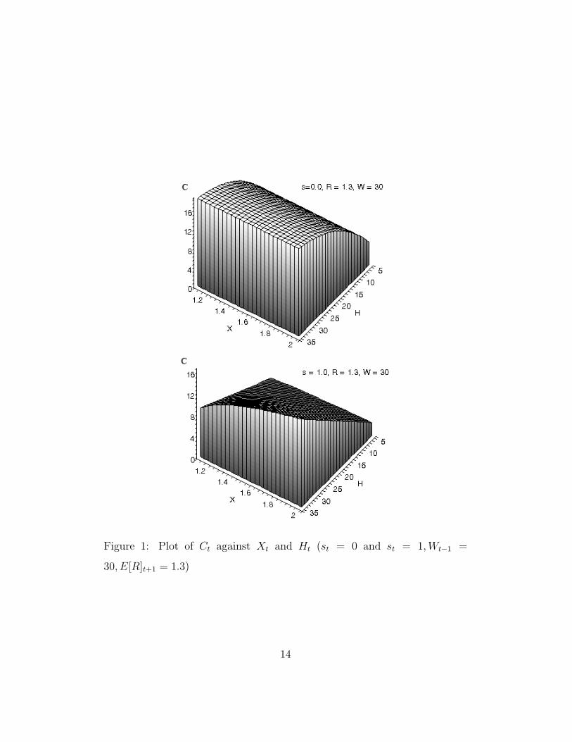
Figure 1: Plot of Ct against Xt and Ht (st = 0 and st = 1,Wt−1 =

30, E[R]t+1 = 1.3)

14

Figure 2: Plot of Ct against E[R]t+1 and Ht (st = 0 and st = 0.5,Wt−1 = 30,

Xt = 1.3)

15

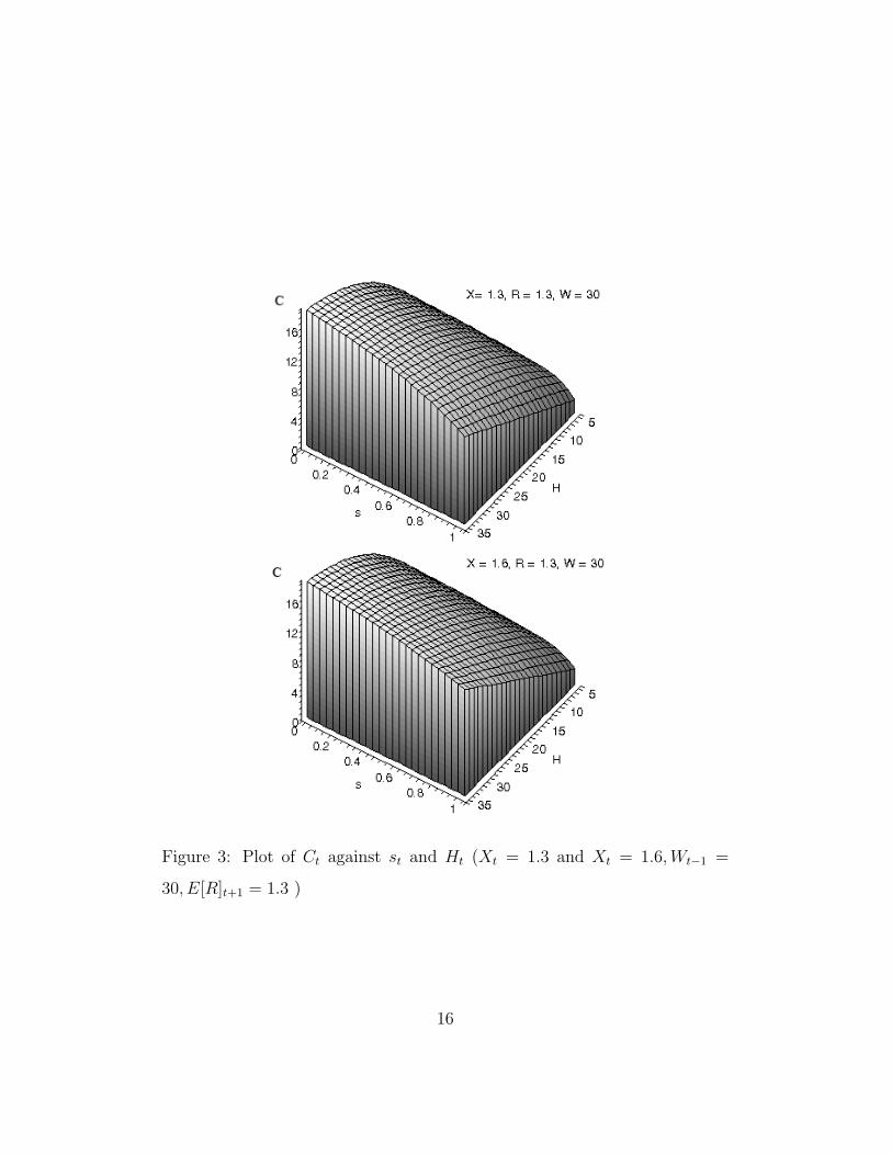
Figure 3: Plot of Ct against st and Ht (Xt = 1.3 and Xt = 1.6,Wt−1 =

30, E[R]t+1 = 1.3 )

16

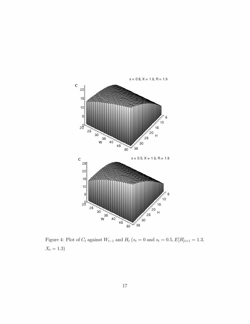
Figure 4: Plot of Ct against Wt−1 and Ht (st = 0 and st = 0.5, E[R]t+1 = 1.3,

Xt = 1.3)

17

profit:

E[R]t+1 = E

[∂Π

∂K

]=E[P ]t+1

µ

∂Y

∂K

where µ = 1/(1 + 1/η) and η is the price elasticity of demand, η = ∂Y∂P

Pt+1

Yt+1.

Assuming a Cobb–Douglas production function Yt+1 = At+1Kαkt+1L

αlt+1 we

express the marginal product of capital ∂Y∂K

as

E[R]t+1 =E[P ]t+1

µ

αkYt+1

K=αk

µ

E[S]t+1

Kt+1

=αk

µ

(E[S]t+1

Kt+1

)(7)

where E[S] denotes expected sales in period t + 1. We assume rational

expectations and replace expected sales at time t + 1 with actual sales at

time t+1 plus a firm-specific expectation error term, νt, which is orthogonal

to the information set available at the time when optimal cash holdings are

chosen. Moreover, we allow for different profitability of capital across firms

and industries, adding an industry specific term, κ, and a firm specific term,

ω. In linearized form we have13

E [R]t+1 = θ(St+1

TAt+1

)+ κ+ ω + νt (8)

The firm’s initial resources are Wt−1 = Ct−1 +RtIt−1 +ψt−1, where It−1 is

investment in period t−1, Ct−1 is cash in the previous period, Rt is the gross

return on investment in period t and ψt−1 is the level of the cash flow shock

most recently experienced by the firm. Hence, linearized initial resources are

equal to

Wt−1 = ζ1Ct−1 + ζ2It−1 + ζ3ψt−1 (9)

13We proxy the firm’s capital stock K with total assets, TA.

18

The interest rate on borrowing in the case when the firm does not have

enough cash to cover a negative cash flow shock is taken to be proportional

to the risk-free interest rate, TBt:

Xt = δ TBt (10)

We employ macroeconomic uncertainty and idiosyncratic uncertainty as

determinants of the bounds of the distribution of cash-flow shocks:

Ht = β21τ

2t + β2

2ε2t + β1β2cov(τt, εt) (11)

where τ 2t denotes a proxy for the degree of macroeconomic uncertainty while

ε2t is a measure of idiosyncratic uncertainty. Normalizing the covariance term

(a second-order magnitude) to zero, the expression takes the form

Ht = β21 τ

2t + β2

2 ε2t . (12)

Finally, the probability of being able to acquire sufficient credit when threat-

ened with bankruptcy, st, is parameterized as

st = γ1LIt + γ2E[R]t+1 (13)

where LIt is the index of leading indicators: a measure of overall economic

health. E[R]t+1 is the firm’s expected return on investment. Both a stronger

economic environment and a higher expected return on investment increase

the firm’s probability of acquiring sufficient credit if threatened with bankruptcy

(see Altman (1968), Liu (2004)).

Substituting the parameterized expressions into equation (6) yields

C = α1ζ1Ct−1 + α1ζ2It−1 + ζ3ψt−1 + (α2 + α5γ2)θ( S

TA

)t+1

+ α3β21 τ

2t

+ α3β22 ε

2t + α4δTBt + α5γ1LIt + (α2 + α5γ2)(κ+ ω + ν).

19

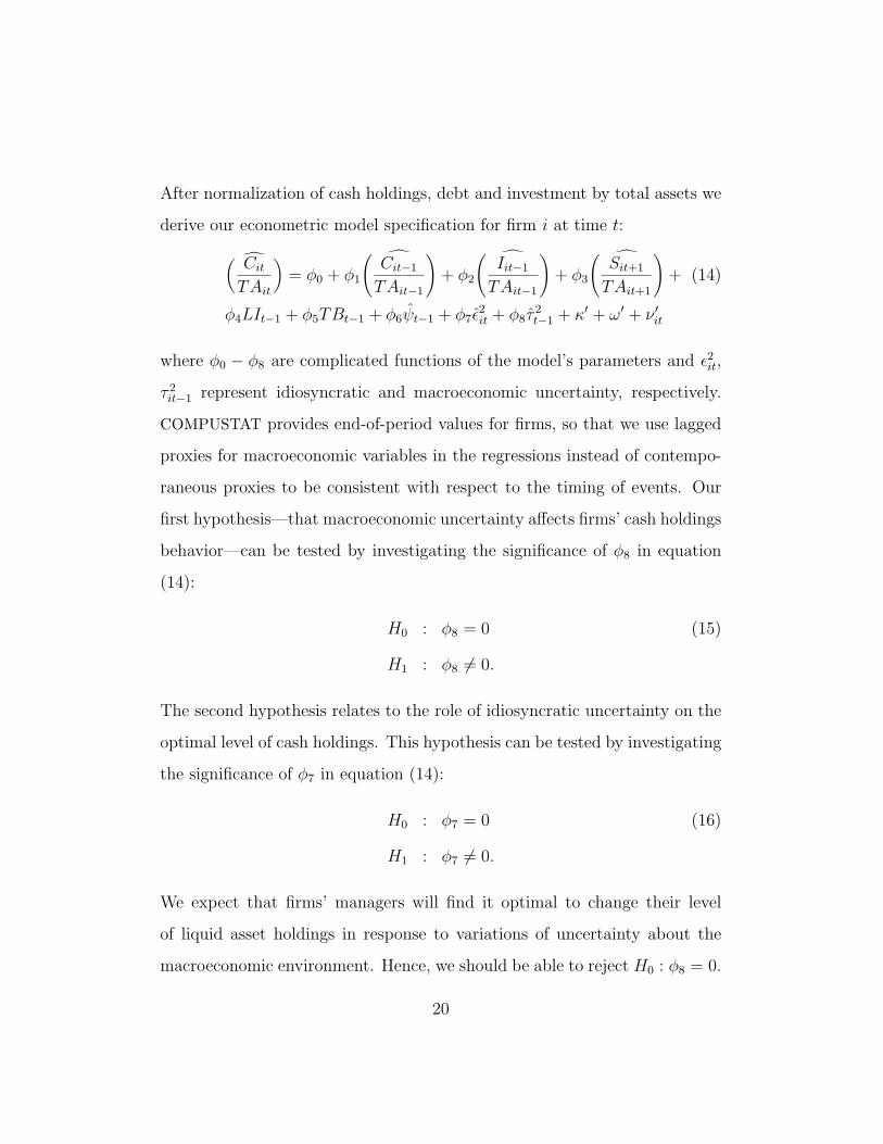
After normalization of cash holdings, debt and investment by total assets we

derive our econometric model specification for firm i at time t:

(Cit

TAit

)= φ0 + φ1

(Cit−1

TAit−1

)+ φ2

(Iit−1

TAit−1

)+ φ3

(Sit+1

TAit+1

)+ (14)

φ4LIt−1 + φ5TBt−1 + φ6ψt−1 + φ7ε2it + φ8τ

2t−1 + κ′ + ω′ + ν ′it

where φ0 − φ8 are complicated functions of the model’s parameters and ε2it,

τ 2it−1 represent idiosyncratic and macroeconomic uncertainty, respectively.

COMPUSTAT provides end-of-period values for firms, so that we use lagged

proxies for macroeconomic variables in the regressions instead of contempo-

raneous proxies to be consistent with respect to the timing of events. Our

first hypothesis—that macroeconomic uncertainty affects firms’ cash holdings

behavior—can be tested by investigating the significance of φ8 in equation

(14):

H0 : φ8 = 0 (15)

H1 : φ8 6= 0.

The second hypothesis relates to the role of idiosyncratic uncertainty on the

optimal level of cash holdings. This hypothesis can be tested by investigating

the significance of φ7 in equation (14):

H0 : φ7 = 0 (16)

H1 : φ7 6= 0.

We expect that firms’ managers will find it optimal to change their level

of liquid asset holdings in response to variations of uncertainty about the

macroeconomic environment. Hence, we should be able to reject H0 : φ8 = 0.

20

Similarly, if an increase in idiosyncratic uncertainty causes an increase in cash

holdings, the second hypothesis may be rejected as well.

2.4 Identification of macroeconomic uncertainty

The literature suggests various methods to obtain a proxy for macroeco-

nomic uncertainty. In our investigation, as in Driver, Temple, and Urga

(2005) and Byrne and Davis (2002), we use a GARCH model to proxy for

macroeconomic uncertainty. We believe that this approach is more appropri-

ate compared to alternatives such as proxies obtained from moving standard

deviations of the macroeconomic series (e.g., Ghosal and Loungani (2000))

or survey-based measures based on the dispersion of forecasts (e.g., Graham

and Harvey (2001), Schmukler, Mehrez, and Kaufmann (1999)). While the

former approach suffers from substantial serial correlation problems in the

constructed series the latter potentially contains sizable measurement errors.

In an environment of sticky wages and prices, unanticipated volatility

of inflation will impose real costs on firms and their workers. In this con-

text, we consider a volatility measure derived from changes in the consumer

price index (CPI) as a proxy for the macro-level uncertainty that firms face

in their financial and production decisions. We build a generalized ARCH

(GARCH(1,1)) model for the series, where the mean equation is an autore-

gression, as described in Table 1. We find significant ARCH and GARCH

coefficients. The conditional variances derived from this GARCH model are

averaged to the quarterly frequency and then employed in the analysis as a

measure of macroeconomic uncertainty, τ 2t .

21

2.5 Identification of idiosyncratic uncertainty

One can employ different proxies to capture firm-specific risk. For instance,

Bo and Lensink (2005) use three measures: stock price volatility, estimated

as the difference between the highest and the lowest stock price normalized by

the lowest price; volatility of sales measured by the coefficient of variation of

sales over a seven–year window; and the volatility of number of employees es-

timated similarly to volatility of sales. Bo (2002) employs a slightly different

approach, setting up the forecasting AR(1) equation for the underlying un-

certainty variable driven by sales and interest rates. The unpredictable part

of the fluctuations, the estimated residuals, are obtained from that equation

and their three-year moving average standard deviation is computed. Kalck-

reuth (2000) uses cost and sales uncertainty measures, regressing operating

costs on sales. The three-month aggregated orthogonal residuals from that

regression are used as uncertainty measures.

Different from the studies cited above, we proxy the idiosyncratic uncer-

tainty by computing the the standard deviation of the closing price for the

firm’s shares over the last nine months.14 This measure is calculated using

COMPUSTAT items data12, 1st month of quarter close price; data13, 2nd

month of quarter close price; data14, 3rd month of quarter close price and

their first and second lags. We believe that volatility of stock prices reflect

not only sales or cost uncertainty but also captures other idiosyncratic risks.

14To check the robustness of our results to the period considered, we also used the

standard deviation of closing price over the last six months; we receive quantitatively

similar results.

22

To ascertain that the measure captured by this method is different from

that used to proxy macroeconomic uncertainty described in Section 2.4, we

compute the correlation between the two measures. We find a very low cor-

relation (-0.001) between idiosyncratic uncertainty and the macroeconomic

uncertainty measure.

3 Empirical Implementation

3.1 Data construction

For the empirical investigation we work with Standard & Poor’s Quarterly

Industrial COMPUSTAT database of U.S. firms. The initial database includes

201,552 firm-quarter characteristics over 1993–2002. We restrict our analysis

to manufacturing companies for which COMPUSTAT provides information.

The firms are classified by two-digit Standard Industrial Classification (SIC).

The main advantage of the dataset is that it contains detailed balance sheet

information.

In order to construct firm-specific variables we utilize COMPUSTAT data

items Cash and Short-term Investment (data1 item) and Total Assets (data6

item), Capital Expenditures (data90 item), Sales (data2 item) for liquidity

ratio (Cash/TA), Investment-to-Asset ratio (I/TA) and Sales-to-Asset ratio

(S/TA). A measure of cash-flow shocks, ψ, is calculated as the first difference

of the cash flow/total assets ratio.15

15Cash flow is defined as sum of depreciation (data5) and income before extraordinary

items (data8).

23

We apply several sample selection criteria to the original sample. The

following observations are set as missing values in our estimation sample: (a)

negative values for cash-to-assets, leverage, sales-to-assets and investment-to-

assets ratios; (b) the values of ratio variables lower than the first percentile

or higher than the 99th percentile; (c) those from firms that have fewer

than ten observations over the time span. We employ the screened data to

reduce the potential impact of outliers upon the parameter estimates. After

the screening and including only manufacturing sector firms we obtain on

average 700 firms’ quarterly characteristics.16

Descriptive statistics for the quarterly means of cash-to-asset ratios along

with investment and sales to asset ratios and ψ are presented in Table 2. From

the means of the sample we see that firms hold about 10 percent of their total

assets in cash. This amount is sizable and similar to that reported in Baum,

Caglayan, Ozkan, and Talavera (2006).

The empirical literature investigating firms’ cash-holding behavior has

identified that firm-specific characteristics play an important role.17 We

might expect that a group of firms with similar characteristics (e.g., those

firms with high levels of leverage) might behave similarly, and quite differ-

ently from those with differing characteristics. Consequently, we split the

sample into subsamples of firms to investigate if the model’s predictions

would receive support in each subsample. We consider five different sam-

ple splits in the interest of identifying groups of firms that may have similar

16We also use winsorized versions of balance sheet measures and receive similar quanti-

tative results.

17See Ozkan and Ozkan (2004).

24

characteristics relevant to their choice of liquidity. The splits are based on

firm size, durable-goods vs. non-durable goods producers, growth rate, in-

vestment rate, and leverage ratio. The durable/non-durable classifications

only apply to firms in the manufacturing sector (one-digit SIC 2 or 3). A firm

is considered durable if its primary SIC is 24, 25, 32–39.18 SIC classifications

for non-durable industries are 20–23 or 26–31.19 All other sample splits are

based on firms’ average values of the characteristic lying in the first or fourth

quartile of the sample. For instance, a firm with average total assets above

the 75%th percentile of the distribution will be classed as large, while a firm

with average total assets below the 25%th percentile will be classed as small.

As such, the classifications are not mutually exhaustive.

The detrended index of leading indicators (LIt) is computed from DRI–

McGraw Hill Basic Economics series DLEAD. The interest rate, TBt is the

three-month secondary market Treasury bill rate obtained from the same

database (item FY GM3).20

18These industries include lumber and wood products, furniture, stone, clay, and glass

products, primary and fabricated metal products, industrial machinery, electronic equip-

ment, transportation equipment, instruments, and miscellaneous manufacturing indus-

tries.

19These industries include food, tobacco, textiles, apparel, paper products, printing

and publishing, chemicals, petroleum and coal products, rubber and plastics, and leather

products makers.

20Further details on the data used are presented in Appendix A.

25

3.2 Empirical results

Estimates of optimal corporate behavior often suffer from endogeneity prob-

lems, and the use of instrumental variables may be considered as a possible

solution. We estimate our econometric models using the system dynamic

panel data (DPD) estimator. DPD combines equations in differences of the

variables with equations in levels of the variables. In this “system GMM” ap-

proach (see Blundell and Bond (1998)), lagged levels are used as instruments

for differenced equations and lagged differences are used as instruments for

level equations. The models are estimated using a first difference transfor-

mation to remove the individual firm effect.

The reliability of our econometric methodology depends crucially on the

validity of instruments. We check it with Sargan’s test of overidentifying

restrictions, which is asymptotically distributed as χ2 in the number of re-

strictions. The consistency of estimates also depends on the serial correlation

in the error terms. We present test statistics for first-order and second-order

serial correlation in Tables 3–5, which lay out our results on the links between

macroeconomic uncertainty, idiosyncratic uncertainty and the liquidity ratio.

For the “all firms” sample, we also present the full set of coefficients corre-

sponding to the α parameters of equation (14). In the interest of brevity, we

only present the coefficients on the uncertainty variables, corresponding to

equations (15) and (16) for the subsample splits.21

Table 3 displays results the Blundell–Bond one-step system GMM esti-

mator with the conditional variance of CPI inflation as a proxy for macroe-

21Full results are available on request.

26

conomic uncertainty. An increase in macroeconomic uncertainty leads to an

increase in firms’ cash holdings, with a highly significant effect. Idiosyncratic

uncertainty is also important, with a significant positive coefficient estimate.

Hence, our findings support the hypotheses that heightened levels of macroe-

conomic and idiosyncratic uncertainty lead to a rise in the firm’s liquidity

ratio. The results also suggest significant positive persistence in the liquidity

ratio with a coefficient of 0.7846. A negative and significant effect of the

expected sales-to-assets ratio is also in accordance with our expectations.

This ratio may be considered as a proxy for the firm’s expected return on

investment. When the expected opportunity cost of holding cash increases,

firms are likely to decrease their liquidity ratio. Improvements in the state of

the macroeconomy (proxied by the index of leading indicators) or increases

in the cost of funds (via the Treasury bill rate) will reduce the firm’s de-

mand for cash.22 Overall the data for this broadest sample support the basic

predictions of the model that we laid out in section 2.

3.3 Results for subsamples of firms

Having established the presence of a positive role for macroeconomic un-

certainty on firm’s cash holdings, we next investigate if the strength of the

association varies across groups of firms with differing characteristics. It is

important to consider that the average cash-to-asset ratios of firms with dif-

22Although the analytical model predicts that the Treasury blll rate should be positively

related to the liquidity ratio, the model assumes that the firm cannot lend, thus ignoring

the opportunity cost of cash holdings.

27

ferent characteristics vary widely. The last lines of Tables 4 and 5 present

the sample average liquidity ratios (µC/TA) for each subsample. On average,

small firms hold twice as much cash as do their large counterparts, perhaps

reflecting that they have constrained access to external funds. Durable-goods

makers hold slightly more cash, on average than do non-durable goods mak-

ers. High-growth firms hold significantly more cash than low-growth coun-

terparts, perhaps reflecting their greater cash flow needs. High-investment

firms, who perhaps economize on cash holdings in order to finance capital

expenditures, hold less cash on average than firms in the lowest quartile of

the investment rate distribution. High-leverage firms also economize on cash,

holding only about one-quarter as much as than low-leverage counterparts.

The variations in subsample average liquidity ratios will naturally influence

those firms’ sensitivity to macroeconomic and idiosyncratic uncertainty.

The first two columns of Table 4 reports results for small and large firms.

Based on the point estimates, the former firms are highly sensitive to the

changes in volatility of CPI inflation, with large firms display a considerably

smaller sensitivity. Small firms also have a much larger coefficient for idiosyn-

cratic uncertainty. The greater sensitivity of small firms could be explained

by the fact that smaller firms are more likely to be financially constrained. As

Almeida, Campello, and Weisbach (2004) indicate, financially unconstrained

firms have no precautionary motive to hold cash; their cash holding policies

are indeterminate. In contrast, for financially constrained firms, any change

in the level of uncertainty that affects managers’ ability to predict cash flows

should cause them to alter their demand for liquidity. We see that small

firms are much more sensitive to both forms of uncertainty, and hold much

28

more cash on average than do large firms.

We find an interesting contrast in the results for durable goods makers

and non-durable goods makers, reported in columns 3 and 4. While both

categories of firms exhibit positive and significant effects for macroeconomic

uncertainty, durable goods makers also exhibit sensitivity to idiosyncratic

uncertainty, which appears to have no significant effect on non-durable goods

firms. Durable goods makers’ production involves greater time lags and larger

inventories of work-in-progress, which may imply a greater need for cash as

well as a greater sensitivity to uncertainty.

The last two columns report results for high-growth and low-growth firms,

respectively. Here again, high-growth firms display sensitivity to idiosyn-

cratic uncertainty, unlike their low-growth counterparts. Both types of firms

display significant sensitivity to macroeconomic uncertainty, with larger ef-

fects for the low-growth category. This may reflect the smaller levels of cash

held by those firms.

The first two columns of Table 5 present results for high-investment

firms: those in the top quartile of investment-to-assets ratios versus their

low-investment counterparts. Idiosyncratic uncertainty has no effect on low-

investment firms, while these firms display considerably greater sensitivity to

macroeconomic uncertainty than their high-investment counterparts. Firms

in the latter group are meaningfully affected by both types of uncertainty.

The last two columns of Table 5 present results for firms with high lever-

age versus low leverage, respectively. Both types of firms are significantly

affected by both macroeconomic uncertainty and idiosyncratic uncertainty.

The effects of macroeconomic uncertainty are considerably stronger for the

29

low-leverage firms, who as noted hold almost four times as much cash, on

average, as do highly-levered firms. Both types of firms are sensitive to id-

iosyncratic uncertainty, with high-leverage firms displaying almost twice as

much sensitivity.

In summary, we may draw several conclusions from the analysis of these

five subsamples. Variations in idiosyncratic uncertainty have a strong ef-

fect on the liquidity ratios of small firms, durable-goods makers, and firms

experiencing high growth, high investment or high leverage. Variations in

macroeconomic uncertainty have significant effects on liquidity of all ten

subsamples, but those effects differ considerably in strength across subsam-

ples. The subsample evidence buttresses our findings from the “all firms”

full sample and further strengthens support for the hypotheses generated by

our analytical model.

4 Conclusions

We set out in this paper to shed light on the link between the level of liquidity

of manufacturing firms and uncertainty measures. Based on the theoretical

predictions obtained from a simple optimization problem, we first show that

firms will increase their level of cash holdings when macroeconomic or id-

iosyncratic uncertainty increases. This result confirms the existence of a pre-

cautionary motive for holding liquid assets among non-financial firms. Next

we empirically investigate if our model receives support from a large firm-

level dataset of U.S. non-financial firms from Quarterly COMPUSTAT over

the 1993–2002 period using dynamic panel data methodology. The results

30

suggest positive and significant effects of both macroeconomic and idiosyn-

cratic uncertainty on firms’ cash holding behavior, supporting the hypotheses

of equations (15) and (16). We find that firms unambiguously increase their

liquidity ratio in more uncertain times. The strength of their response differs

meaningfully across subsamples of firms with similar characteristics. When

the macroeconomic environment is less predictable, or when idiosyncratic

risk is higher, companies become more cautious and increase their liquidity

ratio.

Our results should be considered in conjunction with those of Baum,

Caglayan, Ozkan, and Talavera (2006) who predict that during periods of

higher uncertainty firms behave more similarly in terms of their cash-to-

asset ratios. Taken together, these studies allow us to conjecture that as ei-

ther macroeconomic or idiosyncratic uncertainty increases the total amount

of cash held by non-financial firms will increase significantly, with negative

effects on the economy. The idea behind this proposition is that cash hoarded

but not applied to potential investment projects can keep the economy linger-

ing in a recessionary phase. Since during recessionary periods firms generally

are more sensitive to asymmetric information problems, cash hoarding will

exacerbate these problems and delay an economic recovery.

31

References

Almeida, Heitor, Murillo Campello, and Michael Weisbach, 2004, The cash

flow sensitivity of cash, Journal of Finance 59, 1777–1804.

Altman, E., 1968, Financial ratios discriminant analysis and prediciton of

corporate bankruptcy, Journal of Finance pp. 261–280.

Baum, Christopher F., Mustafa Caglayan, Neslihan Ozkan, and Oleksandr

Talavera, 2006, The impact of macroeconomic uncertainty on non-financial

firms’ demand for liquidity, Review of Financial Economics.

Blundell, Richard, and Stephen Bond, 1998, Initial conditions and moment

restrictions in dynamic panel data models, Journal of Econometrics 87,

115–143.

Bo, Hong, 2002, Idiosyncratic uncertainty and firm investment, Australian

Economic Papers 41, 1–14.

, and Robert Lensink, 2005, Is the investment-uncertainty relation-

ship nonlinear? an empirical analysis for the Netherlands, Economica 72,

307–331.

Bruinshoofd, W.A., 2003, Corporate investment and financing constraints:

Connections with cash management, WO Research Memoranda (discon-

tinued) 734 Netherlands Central Bank, Research Department.

Byrne, Joseph P., and E. Philip Davis, 2002, Investment and uncertainty

in the G7, Discussion papers National Institute of Economic Research,

London.

32

Driver, Ciaran, Paul Temple, and Giovanni Urga, 2005, Profitability, capac-

ity, and uncertainty: a model of UK manufacturing investment, Oxford

Economic Papers 57, 120–141.

Ghosal, Vivek, and Prakash Loungani, 2000, The differential impact of uncer-

tainty on investment in small and large business, The Review of Economics

and Statistics 82, 338–349.

Graham, John R., and Campbell R. Harvey, 2001, Expectations of equity risk

premia, volatility and asymmetry from a corporate finance perspective,

NBER Working Papers 8678 National Bureau of Economic Research, Inc.

Harford, J., 1999, Corporate cash reserves and acquisitions, Journal of Fi-

nance 54, 1967–1997.

Kalckreuth, Ulf, 2000, Exploring the role of uncertainty for corporate invest-

ment decisions in Germany, Discussion Papers 5/00 Deutsche Bundesbank

- Economic Research Centre.

Keynes, John Maynard, 1936, The general theory of employment, interest

and money (London: Harcourt Brace).

Kim, Chang-Soo, David C. Mauer, and Ann E. Sherman, 1998, The deter-

minants of corporate liquidity: Theory and evidence, Journal of Financial

and Quantitative Analysis 33, 335–359.

Liu, Jia, 2004, Macroeconomic determinants of corporate failures: evidence

from the UK, Applied Economics 36, 939–945.

33

Mills, Karen, Steven Morling, and Warren Tease, 1994, The influence of fi-

nancial factors on corporate investment, RBA Research Discussion Papers

rdp9402 Reserve Bank of Australia.

Modigliani, F., and M. Miller, 1958, The cost of capital, corporate finance,

and the theory of investment, American Economic Review 48, 261–297.

Myers, Stewart C., and Nicholas S. Majluf, 1984, Corporate financing and

investment decisions when firms have information that investors do not

have, Journal of Financial Economics 13, 187–221.

Opler, Tim, Lee Pinkowitz, Rene Stulz, and Rohan Williamson, 1999, The

determinants and implications of cash holdings, Journal of Financial Eco-

nomics 52, 3–46.

Ozkan, Aydin, and Neslihan Ozkan, 2004, Corporate cash holdings: An em-

pirical investigation of UK companies, Journal of Banking and Finance

28, 2103–2134.

Schmukler, Sergio, Gil Mehrez, and Daniel Kaufmann, 1999, Predicting cur-

rency fluctuations and crises - do resident firms have an informational

advantage?, Policy Research Working Paper Series 2259 The World Bank.

34

Appendix A. Construction of macroeconomic and firm spe-

cific measures

The following variables are used in the empirical study.

From the Quarterly Industrial COMPUSTAT database:

DATA1: Cash and Short-Term Investments

DATA2: Sales

DATA5: Depreciation

DATA6: Total Assets

DATA8: Income before extraordinary items

DATA12: 1st month of quarter close price

DATA13: 2nd month of quarter close price

DATA14: 3rd month of quarter close price

DATA90: Capital Expenditures

From International Financial Statistics:

64IZF: Industrial Production monthly

From the DRI–McGraw Hill Basic Economics database:

DLEAD: index of leading indicators

FYGM3: Three-month U.S. Treasury bill interest rate

35

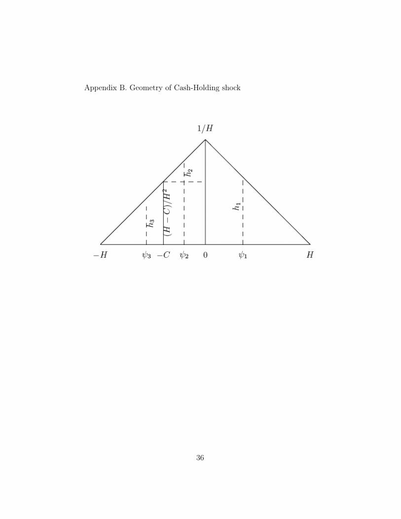
Appendix B. Geometry of Cash-Holding shock

36

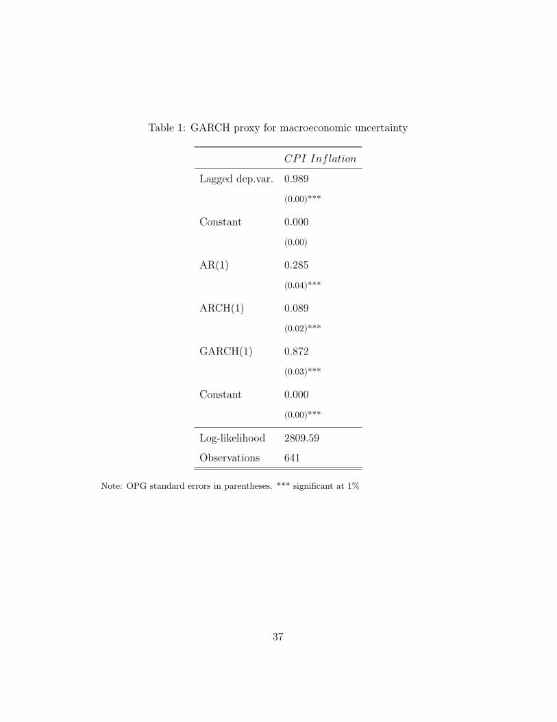
Table 1: GARCH proxy for macroeconomic uncertainty

CPI Inflation

Lagged dep.var. 0.989

(0.00)***

Constant 0.000

(0.00)

AR(1) 0.285

(0.04)***

ARCH(1) 0.089

(0.02)***

GARCH(1) 0.872

(0.03)***

Constant 0.000

(0.00)***

Log-likelihood 2809.59

Observations 641

Note: OPG standard errors in parentheses. *** significant at 1%

37

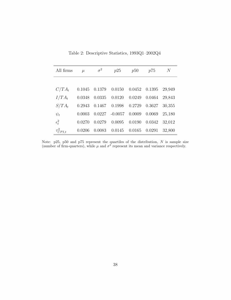
Table 2: Descriptive Statistics, 1993Q1–2002Q4

All firms µ σ2 p25 p50 p75 N

C/TAt 0.1045 0.1379 0.0150 0.0452 0.1395 29,949

I/TAt 0.0348 0.0335 0.0120 0.0249 0.0464 29,843

S/TAt 0.2943 0.1467 0.1998 0.2729 0.3627 30,355

ψt 0.0003 0.0227 -0.0057 0.0009 0.0069 25,180

ε2t 0.0270 0.0279 0.0095 0.0190 0.0342 32,012

τ 2CPI,t 0.0206 0.0083 0.0145 0.0165 0.0291 32,800

Note: p25, p50 and p75 represent the quartiles of the distribution, N is sample size(number of firm-quarters), while µ and σ2 represent its mean and variance respectively.

38

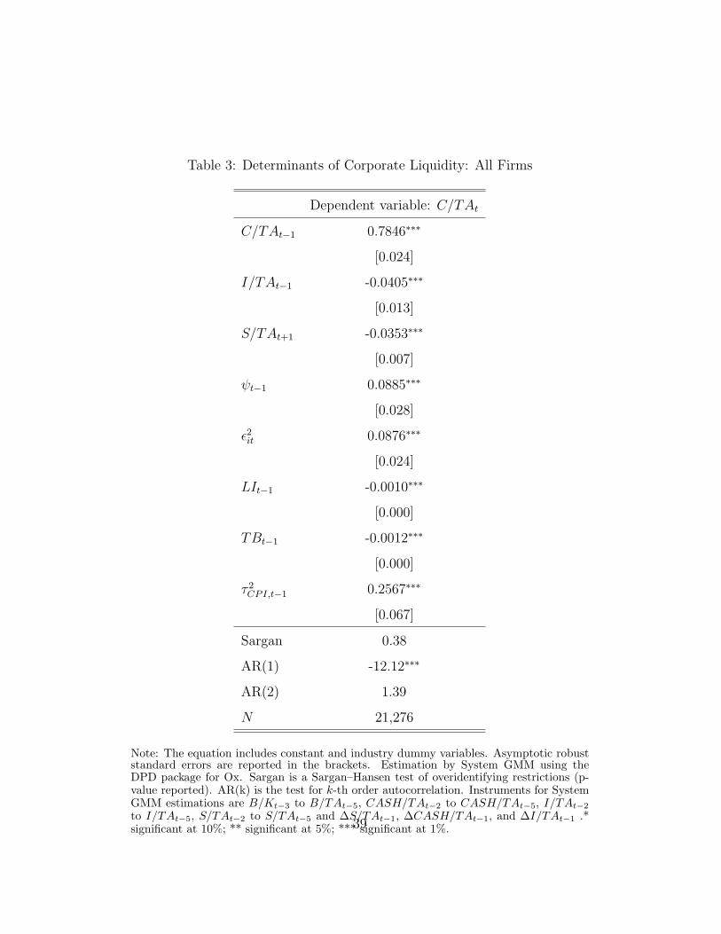
Table 3: Determinants of Corporate Liquidity: All Firms

Dependent variable: C/TAt

C/TAt−1 0.7846∗∗∗

[0.024]

I/TAt−1 -0.0405∗∗∗

[0.013]

S/TAt+1 -0.0353∗∗∗

[0.007]

ψt−1 0.0885∗∗∗

[0.028]

ε2it 0.0876∗∗∗

[0.024]

LIt−1 -0.0010∗∗∗

[0.000]

TBt−1 -0.0012∗∗∗

[0.000]

τ 2CPI,t−1 0.2567∗∗∗

[0.067]

Sargan 0.38

AR(1) -12.12∗∗∗

AR(2) 1.39

N 21,276

Note: The equation includes constant and industry dummy variables. Asymptotic robuststandard errors are reported in the brackets. Estimation by System GMM using theDPD package for Ox. Sargan is a Sargan–Hansen test of overidentifying restrictions (p-value reported). AR(k) is the test for k-th order autocorrelation. Instruments for SystemGMM estimations are B/Kt−3 to B/TAt−5, CASH/TAt−2 to CASH/TAt−5, I/TAt−2

to I/TAt−5, S/TAt−2 to S/TAt−5 and ∆S/TAt−1, ∆CASH/TAt−1, and ∆I/TAt−1 .*significant at 10%; ** significant at 5%; *** significant at 1%.39

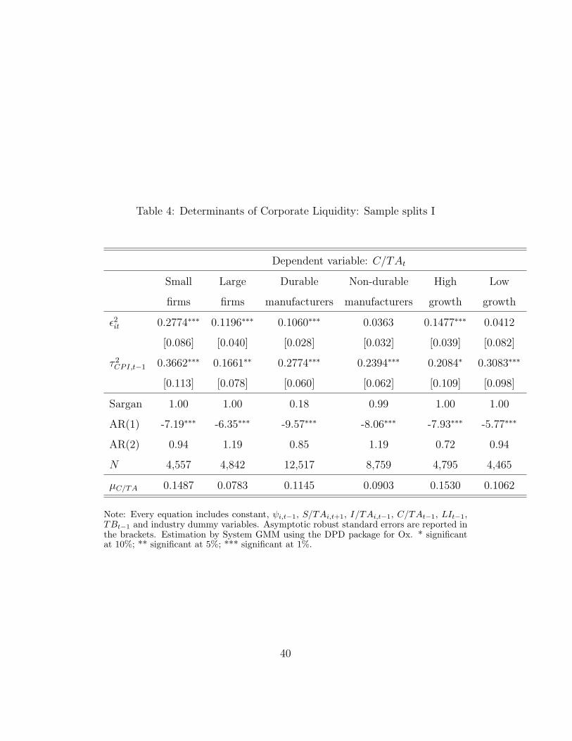
Table 4: Determinants of Corporate Liquidity: Sample splits I

Dependent variable: C/TAt

Small Large Durable Non-durable High Low

firms firms manufacturers manufacturers growth growth

ε2it 0.2774∗∗∗ 0.1196∗∗∗ 0.1060∗∗∗ 0.0363 0.1477∗∗∗ 0.0412

[0.086] [0.040] [0.028] [0.032] [0.039] [0.082]

τ 2CPI,t−1 0.3662∗∗∗ 0.1661∗∗ 0.2774∗∗∗ 0.2394∗∗∗ 0.2084∗ 0.3083∗∗∗

[0.113] [0.078] [0.060] [0.062] [0.109] [0.098]

Sargan 1.00 1.00 0.18 0.99 1.00 1.00

AR(1) -7.19∗∗∗ -6.35∗∗∗ -9.57∗∗∗ -8.06∗∗∗ -7.93∗∗∗ -5.77∗∗∗

AR(2) 0.94 1.19 0.85 1.19 0.72 0.94

N 4,557 4,842 12,517 8,759 4,795 4,465

µC/TA 0.1487 0.0783 0.1145 0.0903 0.1530 0.1062

Note: Every equation includes constant, ψi,t−1, S/TAi,t+1, I/TAi,t−1, C/TAt−1, LIt−1,TBt−1 and industry dummy variables. Asymptotic robust standard errors are reported inthe brackets. Estimation by System GMM using the DPD package for Ox. * significantat 10%; ** significant at 5%; *** significant at 1%.

40

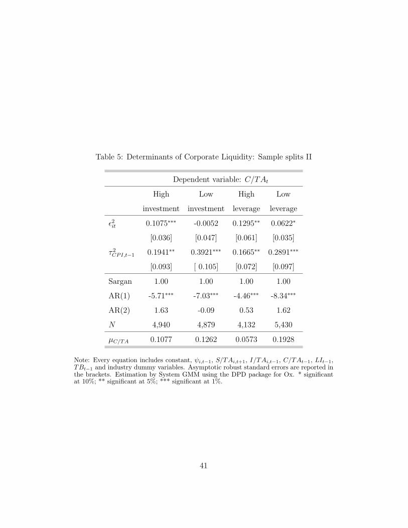
Table 5: Determinants of Corporate Liquidity: Sample splits II

Dependent variable: C/TAt

High Low High Low

investment investment leverage leverage

ε2it 0.1075∗∗∗ -0.0052 0.1295∗∗ 0.0622∗

[0.036] [0.047] [0.061] [0.035]

τ 2CPI,t−1 0.1941∗∗ 0.3921∗∗∗ 0.1665∗∗ 0.2891∗∗∗

[0.093] [ 0.105] [0.072] [0.097]

Sargan 1.00 1.00 1.00 1.00

AR(1) -5.71∗∗∗ -7.03∗∗∗ -4.46∗∗∗ -8.34∗∗∗

AR(2) 1.63 -0.09 0.53 1.62

N 4,940 4,879 4,132 5,430

µC/TA 0.1077 0.1262 0.0573 0.1928

Note: Every equation includes constant, ψi,t−1, S/TAi,t+1, I/TAi,t−1, C/TAt−1, LIt−1,TBt−1 and industry dummy variables. Asymptotic robust standard errors are reported inthe brackets. Estimation by System GMM using the DPD package for Ox. * significantat 10%; ** significant at 5%; *** significant at 1%.

41