Embed Size (px)
Citation preview

Banco de México
Documentos de Investigación
Banco de México
Working Papers
N° 2019-12
Uncertainty and Exchange Rate Volat i l i ty: the Case ofMexico
August 2019
La serie de Documentos de Investigación del Banco de México divulga resultados preliminares detrabajos de investigación económica realizados en el Banco de México con la finalidad de propiciar elintercambio y debate de ideas. El contenido de los Documentos de Investigación, así como lasconclusiones que de ellos se derivan, son responsabilidad exclusiva de los autores y no reflejannecesariamente las del Banco de México.
The Working Papers series of Banco de México disseminates preliminary results of economicresearch conducted at Banco de México in order to promote the exchange and debate of ideas. Theviews and conclusions presented in the Working Papers are exclusively the responsibility of the authorsand do not necessarily reflect those of Banco de México.
Gabrie la López Nor iaBanco de México
Georgia Bush Banco de México

Uncertainty and Exchange Rate Volat i l i ty: the Case ofMexico*
Abstract: This paper investigates the effect of uncertainty on the volatility of the Mexican peso U.S. dollar exchange rate for the period 1999 - 2018. The empirical analysis consists on estimating a model by OLS and System GMM that includes measures of economic, political, and financial uncertainty, both domestic and international, as explicative variables. The main results show that greater uncertainty leads to higher exchange rate volatility; measures of international uncertainty are found to dominate domestic uncertainty measures, although the domestic uncertainty has also an important effect on the exchange rate volatility; and there is evidence of an amplifying effect of domestic economic uncertainty on exchange rate volatility, especially during periods of recession. These results are shown to be robust to different exchange rate volatility measures, different specifications, and different economic policy uncertainty indices.Keywords: Exchange Rate Volatility, Uncertainty, ExpectationsJEL Classification: F31, D80, D84
Resumen: Este documento investiga el efecto de la incertidumbre sobre la volatilidad del tipo de cambio peso mexicano dólar estadounidense durante el periodo 1999 - 2018. El análisis empírico consiste en estimar un modelo por MCO y MGM en Sistema que incluye como variables explicativas medidas de incertidumbre económica, política y financiera, tanto doméstica como internacional. Los resultados principales muestran que una mayor incertidumbre induce una mayor volatilidad del tipo de cambio; la incertidumbre internacional domina sobre la doméstica, si bien la incertidumbre interna también tiene un efecto importante; y hay evidencia de un efecto amplificador de la incertidumbre sobre la situación económica interna en la volatilidad del tipo de cambio, especialmente en periodo de recesión. Los hallazgos son robustos a diferentes medidas de volatilidad del tipo de cambio, diferentes especificaciones y diferentes índices de incertidumbre económica política.Palabras Clave: Volatilidad del Tipo de Cambio, Incertidumbre, Expectativas
Documento de Investigación2019-12
Working Paper2019-12
Gabr ie la López Nor ia †
Banco de MéxicoGeorg ia Bush ‡
Banco de México
*We are grateful to Aldo Heffner, Guillermo Benavides, and Raúl Ibarra for their helpful comments andsuggestions. We thank Ángel García-Lascurain Fernández y Luz Stephanie Ramos for their excellent researchassistance.
† Dirección General de Investigación Económica, Banco de México. Email: [email protected]. ‡ Dirección General de Estabilidad Financiera. Email: [email protected].

1 Introduction
For Mexico, the exchange rate and its volatility are key economic variables that have
the potential to be influenced by a myriad of factors. Mexico is a small open economy
that has experienced a rapid rate of international integration since the implementation
of the North American Free Trade Agreement (NAFTA) in 1994. The trade agreement
included commitments to free capital mobility as well as trade liberalization. Akin to
other emerging market economies, Mexico has suffered currency crises, one of which
began in December 1994. Since that crisis, Mexico has maintained a floating exchange
rate regime and as of the most recent Bank for International Settlements Triannual
Central Bank survey, the Mexican peso is the most traded emerging market currency
after the Chinese renminbi.
In general, the exchange rate is the key financial variable that connects the domestic
economy with the rest of the world. A floating exchange rate regime and high levels
of capital flows will result in higher volatility of the exchange rate reflecting the role
of the exchange rate as an adjustment mechanism and buffer to external shocks. The
exchange rate affects a country’s net international investment position depending on the
scale of the country’s international balance sheet and on the currency composition of its
foreign assets and liabilities. In the case of emerging markets, the tendency to rely on
foreign-currency debt can generate adverse effects during bouts of currency volatility,
particularly depreciations (Lane and Shambaugh (2009) and Asis and Chari (2018)).
Exchange rate volatility is an important issue also because of its documented effect
on economic decision making. As noted in Balcilar et al. (2016b), economic agents
base their investment and consumption decisions on the value of the domestic currency
and on its volatility. Greater exchange rate volatility can have a negative impact via a
number of channels. For firms, financing investments–whether through retained profits
or external funding–becomes more difficult with higher levels of financial volatility in
particular because of increased unpredictability of foreign earned revenues.1 Firms may
delay investment, impeding productivity and GDP growth, if exchange rate shifts lead
to uncertain business profits and net worth (Krol (2014)). Also, exchange rate volatility
has been linked to firm defaults in emerging economies (Asis and Chari (2018)). For
households and portfolio investors, higher volatility can dampen risk appetite. Further-
more, to the extent that the exchange rate influences domestic prices, volatility can lead
to inflation uncertainty, possibly inducing tighter monetary policies and lower levels of
consumption (Grier et al. (2004) and Grier and Grier (2006)).2 Thus, exchange rate
volatility is an important matter and can represent a challenge to the performance of
1See Domınguez and Tesar (2001) and Lane and Shambaugh (2009) on the magnitude and sectoralelements of exchange rate exposure.
2For a further literature review on implications of exchange rate volatility see Krol (2014).
1

any economy.
Predicting the volatility of the exchange rate remains puzzling. Debate contin-
ues about the process of expectation formation and the role of fundamental macro
variables. Models using macro fundamentals have had limited success in predicting ex-
change rates, particularly at time horizons shorter than 5 to 10 years. An often quoted
study is Meese and Rogoff (1983), which showed that exchange rate models based on
macro variables such as money supply, interest rates and output, did not outperform
a random walk in explaining nominal exchange rate movements. In the survey Frankel
and Rose (1995), the authors reiterate that basic monetary macro models have not
been shown to perform satisfactorily. In addition, Rogoff (1999) makes the case that it
is challenging to firmly demonstrate a systematic relationship between exchange rates
and macroeconomic fundamentals.
In Engel et al. (2008), the authors argue that exchange rate models should take a
financial market perspective, emphasizing the role of uncertainty.3 In Engel (2006), the
exchange rate is modeled under rational expectations as the expected present discounted
value of current and future fundamentals. Thus current news announcements that affect
expectations about future macro fundamentals are determinants of exchange rates. As
discussed further in for example Engle (1982) and Grier and Grier (2006), this literature
argues surprises about macroeconomic data or policy are the key drivers of exchange
rate adjustments. Using expectation surveys and data announcements, researchers have
identified volatility caused by the surprise component of these announcements. For a
discussion of the empirical literature, see Neely (2011). Generally, the evidence suggests
surprises are associated with higher exchange rate volatility.
Building on this literature, in this paper we analyze potential drivers of the Mexican
peso (MXN) US dollar (USD) exchange rate volatility focusing on a range of uncertainty
measures, not just macroeconomic surprises.4 To construct our uncertainty measures,
we exploit the data from Banco de Mexico’s Survey of Professional Forecasters (SPF).5
Our survey-based measures have the advantage of being direct, model-free measures
that also have enough granularity to distinguish between macroeconomic versus political
uncertainty.6 In addition to our survey-based measures, we also consider the impact
3See Jurado et al. (2015) for an analysis of economic uncertainty, and its measurement, in macromodels more generally.
4In the empirical literature on uncertainty, three main approaches have been used to proxy uncer-tainty: 1) volatility of asset prices 2) ARCH or GARCH estimates of the conditional variance of pricesand/or other type of aggregates, 3) statistics characterizing the distribution of survey data, specificallysurveys on entrepreneurs’ expectations about the future demand for their firms’ products or outputprices changes and/or individual forecasters’ expectations about the economic climate for investmentdecisions. We build our measures based on this last approach, although we also use other uncertaintymeasures.
5Since the SPF began in January 1999, our sample period covers January 1999 - December 2018.6Section 2 of the paper explains the construction of these uncertainty variables in more detail.
2

of other measures of uncertainty that have commonly been used by researchers as
uncertainty proxies such as the VIX, and including media-based indices such as the
Economic Policy Uncertainty (EPU) index from Baker et al. (2016).
Our hypothesis is that uncertainty has an observable impact on exchange rate
volatility, and that our survey-based measures will contain information not captured in
other uncertainty measures.7 Nested within this will be tests of the relative importance
of different types of uncertainty, in particular international versus domestic, political,
economic and financial. Mexico provides an illustrative case of an economy affected
by uncertainty along these multiple dimensions. Mexico’s banking sector includes sub-
sidiaries of several large global banks that were affected by the global financial crisis.
The US renegotiation of NAFTA under the Trump administration has been cited as a
key driver of exchange rate volatility. Others have pointed to domestic political uncer-
tainty surrounding Mexican presidential elections as an explanation to such exchange
rate volatility. We will also test for evidence of interaction effects between uncertainty
and the domestic business cycle and the political cycle.
We test our uncertainty hypotheses using regression analysis. The analysis is per-
formed in two stages. In the first stage, we estimate a univariate GARCH (1, 1) model
to derive the MXN/USD exchange rate volatility measure.8 In the second stage, we
regress the estimated exchange rate volatility on different uncertainty measures, includ-
ing the surprise component of macroeconomic data announcements for gross domestic
product (GDP) and inflation, and the controls. Finally, in order to investigate if the
effect of uncertainty on exchange rate volatility is amplified during election and/or re-
cession periods we introduce some interaction terms: a measure of domestic political
uncertainty (DPU) interacted with an election dummy, DPU interacted with a recession
dummy, and a measure of domestic economic uncertainty (DEU) interacted as well with
a recession dummy.9 The sample period covers January 1999 (when the SPF survey
began) to December 2018.
Our emphasis on uncertainty draws on a literature that has proliferated since the
2008 global financial crisis. Policymakers and researchers have focused on uncertainty
as a key determinant of macroeconomic aggregates such as output, employment, in-
vestment and productivity growth, as well as financial variables such as stock market
volatility (Liu and Zhang (2015) and Antonakakis et al. (2013)) and asset prices gen-
7Future work can exploit the time variation of individual respondents to the same questions, aswell as characteristics of the cross-sectional distribution of the responses other than those used in thispaper.
8Similar to Benavides and Capistran (2012), this model was chosen from the ARCH family sinceHansen and Lunde (2005) found no evidence in their analysis of exchange rates that the GARCH (1,1)model was outperformed by more sophisticated models when they compared 330 ARCH-type models.
9See Garfinkel et al. (1999) and Krol (2014) for election and recession analysis, respectively.
3

erally (Brogaard and Detzel (2015)).10
There is also research specifically analyzing the impact of uncertainty on exchange
rates, most papers using one or two measures of uncertainty. Several papers use news-
based economic policy uncertainty measures and find evidence of uncertainty effects.11
Kurasawa (2016) finds that during several periods the EPU index from Baker et al.
(2016) for the US and for Japan have been correlated with the level of US dollar
Japanese yen exchange rate. Balcilar et al. (2016a) uses a nonparametric causality-in-
quantiles test on 16 currency pairs and find that the differential between the US and
domestic EPU measures has explanatory power for the variance of the Mexican peso US
dollar exchange rate returns, but not the level. For other references on exchange rates,
see Kido (2016), Liu and Pauwels (2012) and Beckmann and Czudaj (2017). We include
these indices in our model in addition to our survey-based uncertainty measures.
Two papers are most similar to our approach of using multiple uncertainty measures.
In Krol (2014), the author uses data from 1990-2010 for a sample of ten developed and
emerging economies, and focuses on the role of general economic versus economic pol-
icy uncertainty using the indices from Baker et al. (2016) and Brogaard and Detzel
(2015). The author finds evidence that both domestic and international (US) economic
policy uncertainty directly increase exchange rate volatility, and that for developed
economies this effect is stronger during recessionary periods. General economic uncer-
tainty increases exchange rate volatility, but the effect is smaller. Mavee et al. (2016)
analyze the drivers of volatility of the South African rand after the global financial
crisis, 2009-2015. They find that rand volatility is mainly driven by global factors, such
as commodity price volatility and the VIX. Domestic political uncertainty is positively
associated with exchange rate volatility, but domestic macroeconomic surprises are not
statistically important.12
Our paper’s main results show that the survey-based DPU measure, as well as the
VIX and the EPU from Baker et al. (2016), are the main drivers of the MXN/USD
exchange rate volatility. Furthermore, and in contrast to the DPU result, there is no
evidence that DEU on its own is a driver of the MXN/USD exchange rate volatility,
10For example, Bloom (2009) simulate the impact of macro uncertainty shocks on employment, out-put and productivity growth. Baker and Bloom (2013) assess the effect of disaster shocks on growth.Jones and Olson (2013) analyze the relationships between uncertainty and output and inflation. Bal-cilar et al. (2014) study the role of uncertainty as a determinant of US inflation. Karnizova and Li(2014) and Balcilar et al. (2016b) use uncertainty measures to predict economic recessions in the UnitedStates. Lopez-Noria and Zamudio-Fernandez (2018) and Cebreros et al. (2019) explore the effect ofuncertainty on foreign direct investment in Mexico.
11To construct the news-based measures, text searches are applied to newspapers to quantify thefrequency of words such as uncertainty in the news. An example is the group of uncertainty measuresconstructed by Baker et al. (2016).
12Relative to the domestic macroeconomic conditions, it may be that surprises were external onesduring this sample period. However, in our longer time period we also find that in the Mexico casedomestic macro surprises add little explanatory power.
4

it only has an impact during recession periods. In line with Mavee et al. (2016),
we also find that neither the domestic macro surprises nor the EMBI+ index have
a distinct impact on the MXN/USD exchange rate volatility.13 Comparing the effect
of international versus domestic uncertainty, simulations and standardized coefficient
estimates show that both have had a similar effect on the MXN/USD exchange rate
volatility, although the EPU index’s effect seems to dominate.
The results are robust to different MXN/USD exchange rate volatility measures
(i.e. we also estimate our main specification using a realized exchange rate volatility
obtained from Bloomberg), different specifications, different econometric techniques (we
estimate our main specification by Ordinary Least Squares (OLS) and the Generalized
Method of Moments (GMM)), and different global EPU indexes (one that includes data
on Mexico’s EPU index and one that excludes it).
The contributions of this paper to the empirical literature are three-fold. First, we
analyze the impact of different dimensions of uncertainty. We consider measures of
political and economic uncertainty, as well as of financial instability and trade policy
uncertainty, rather than just focusing on economic or economic policy uncertainty as
in Balcilar et al. (2016a), Krol (2014), Sin (2015) and Kurasawa (2016). In addition,
we include both domestic and international uncertainty.
Second, we use Banco de Mexico’s SPF to build our domestic and international
uncertainty measures.14 In particular, we use the surveyed analysts’ perceptions about
factors that they consider will most limit economic growth in the following six months.15
To our knowledge, this is the first paper that exploits these data from the SPF.16
Empirical analyses such as Balcilar et al. (2014), Balcilar et al. (2016a), Krol (2014)
and Sin (2015), proxy uncertainty with the news-based EPU index from Baker et al.
(2016) or Brogaard and Detzel (2015).
Third, this paper adds another case study of an emerging economy currency, however
over a long time period, and one that is highly liquid and heavily traded. See Table 1.
In the most recent BIS triennial survey, the Mexican peso was the emerging economy
currency with the second highest average daily turnover, after the Chinese renminbi,
and has consistently been in the top 15 global currencies since 2001.17
The paper proceeds as follows. Section 2 describes the empirical model and the
data. Section 3 presents the results, while Section 4, robustness tests. The analysis on
the relative contribution of each independent variable to the MXN/USD exchange rate
13See for JP Morgan Emerging Markets Bond Index (EMBI).14In Jurado et al. (2015), the authors argue that survey based measures are preferred.15Section 2 explains the construction of these uncertainty variables in more detail.16Lopez-Noria and Zamudio-Fernandez (2018) also derive their uncertainty measures based on Banco
de Mexico’s SPF, but they concentrate on the analysts’ perceptions regarding the economic climatefor investment decisions.
17See Bank for International Settlements (2016).
5

Table 1: Mexican peso vs. major currencies(ranked by average daily turnover)
OTC Foreign Exchange Daily Turnover Domestic Currency Gov. Bonds(USD bn) % nominal GDP (USD bn) % nominal GDP
USD 4,438 23.82 17,252 88.97EUR 1,591 13.32 9,431 74.80JPY 1,096 22.14 9,427 193.49GBP 649 24.39 2,669 101.69AUD 348 27.51 647 46.90MXN 97 9.00 362 31.5
Daily turnover includes cash and derivatives markets. USD, GBP, EUR general government
total debt securities reported, issuance is primarily in domestic currency.
For the rest of the countries, general government domestic debt securities are reported.
Source: Triennial Central Bank Survey, IMF, BIS.
volatility is presented in Section 5 and the conclusions in Section 6.
2 Empirical Model and Data
In order to analyze the uncertainty-exchange rate link, we estimate an econometric
model where the MXN/USD exchange rate volatility is the dependent variable and,
its lag, uncertainty measures and other control variables are the independent variables.
The estimated specification can be written as follows:
σ2t = β0 + β1σ
2t−1 + β2DPUt + β3DEUt + β4IPUt + β5IFIt + β6Xt + β7Zt + εt (1)
Where:
Exchange rate volatility
σ2t is the monthly MXN/USD exchange rate volatility. This volatility was estimated
using a univariate Generalized Autoregressive Conditional Heteroskedasticity GARCH
(1,1) model and daily data from Banco de Mexico on the FIX MXN/ USD exchange
rate.18 This model takes the form (Engle (1982) and Bollerslev (1986)):19
18The FIX MXN/USD exchange rate is determined by Banco de Mexico based on the average of thewholesale exchange rate market returns. It is published by the Diario Oficial de la Federacion (DOFin Spanish) one day after Banco de Mexico has determined it. The FIX MXN/USD exchange rate isused to pay bills denominated in dollars in Mexico one day after the DOF has published it.
19We conducted ARCH-LM tests to verify if the series being analyzed presents ARCH effects. Theresults show that the series rejected the null in favor of ARCH effects. As in Benavides and Capistran(2012), the tests were carried out using up to seven lags.
6

Yt = c+ ϕYt−1 + εt + θεt−1 (2)
σ2t = α0 + α1ε
2t−1 + βσ2
t−1 (3)
Similar to Benavides and Capistran (2012), this model was chosen from the ARCH
family since Hansen and Lunde (2005) found no evidence in their analysis of exchange
rates that the GARCH (1,1) model was outperformed by more sophisticated models
when they compared 330 ARCH-type models. Once we obtained the estimated daily
MXN/USD exchange rate volatility, we calculate the monthly average of this variable.
σ2t−1 is the lagged dependent variable and it is also included in the main specification
in order to control for the persistence of the series. Its inclusion indicates we are
estimating a dynamic model.
Survey based uncertainty measures
DPUt, DEUt, IPUt and IFIt stand for domestic political uncertainty, domestic eco-
nomic uncertainty, international political uncertainty, and international financial in-
stability, respectively. These variables are constructed using Banco de Mexico’s SPF,
which is a survey of macroeconomic forecasts for the rates of inflation, real GDP growth,
exchange rates, interest rates, labour indicators, public finances indicators, trade bal-
ance, current account, foreign direct investment, factors affecting growth, among others.
Since January 1999, Banco de Mexico’s SPF has been conducted monthly and comprises
the responses of an average of 35 economic analysts from the private sector, both na-
tional and foreign. About one third of the surveyed analysts work at banks and one
third at consultancies. Figure 1 shows the distribution of the analysts participating in
the SPF per sector.
In order to build our uncertainty measures we focus on the following question from
the SPF:
Which are the three factors that you consider will most limit growth in eco-
nomic activity in the following six months?
The respondents of the survey choose three options out of a list of 32 factors related
to inflation and monetary policy in Mexico; external conditions (foreign trade policy,
international political instability, monetary policy in the US, fiscal policy in the US, oil
price, international financial instability, the level of foreign interest rates, among others);
domestic economic conditions (firms’ level of debt, families’ level of debt, platform of oil
production, uncertainty about the domestic economic situation, among others); public
finances; governance (domestic political uncertainty, corruption, impunity, lack of rule
of law, security issues); and other. We then calculate the percentage distribution of the
7

Figure 1: Surveyed professional forecasters by sector
Source: Banco de Mexico’s Survey of Professional Forecasters.
responses and we derive our uncertainty measures as the percentage each uncertainty
response obtained (i.e. domestic political uncertainty, domestic economic uncertainty,
international political uncertainty, and international financial instability). Figure 2
plots our four survey based uncertainty measures, which vary considerably over time.
We can also see that DPUt picks up election uncertainty but does not spike with every
election cycle. This is graphical evidence that the survey measure of DPUt captures
more information than just election activity. In particular, the result of the 2012 election
was much less uncertain than in other cycles. Since the SPF began in January 1999, the
empirical analysis conducted in this paper covers the period January 1999 to December
2018.
Other uncertainty measures
Xt stands for other uncertainty measures that may also affect the MXN/USD exchange
rate volatility. The following paragraphs describe these measures.
The global EPUt index is a GDP-weighted average of 19 national economic policy
uncertainty indices (Australia, Brazil, Canada, Chile, China, France, Germany, India,
Ireland, Italy, Japan, Mexico, the Netherlands, Russia, South Korea, Spain, Sweden,
the United Kingdom, and the United States).20 Each of these national indices reflects
20Mexico is included in this global EPU index, but according to Steven J.Davis this is not a problemsince Mexico’s weight in it is small, around 2%. Nonetheless, as a robustness check, we also estimateregressions using an earlier version of the global EPU index, which excludes Mexico and covers the
8

Figure 2: Banco de Mexico survey uncertainty measures, monthly data
Source: Uncertainty measures derived by the authors with data from Banco de Mexico’sSurvey Professional Forecasters.
the relative frequency of own-country newspaper articles that contain terms related to
the economy and policies that have been implemented or proposed.
We also incorporate a trade policy uncertainty index in specification (1) in order
to analyze if uncertainty regarding NAFTA and Mexico’s trade liberalization policies
has had an impact on the MXN/USD exchange rate volatility. This index was built
by Banco de Mexico using the standardized results from Google Trends regarding in-
ternet searches for the terms: NAFTA, TLCAN (NAFTA in Spanish), Renegociacion
(Renegotitation in Spanish), Renegociacion TLC (NAFTA’s renegotiation in Spanish),
Aranceles (tariff in Spanish), Trump NAFTA, TLCAN Trump Mexico, libre comercio
(free trade in Spanish), and que es NAFTA (what is NAFTA in Spanish). For more
details see Cebreros et al. (2019). Figure 3 shows the development of this trade policy
uncertainty index from 2004 to 2018.21
We also include the Chicago Board Options Exchange Volatility Index (VIX). The
V IXt is constructed using the implied volatilities of the S&P 500 index options and it is
considered a measure of global financial market volatility, and has been used as a proxy
for global uncertainty.22 The V IXt differs from our surveyed-based measure of IFIt in
that it measures the sentiment of a large and diverse set of investors based around the
period January 2001-December 2016. See Section 4 for more details.21Data derived from Google Trends is available from January 2004 onwards, so this trade policy
uncertainty index starts in that date.22See for Chicago Board Options Exchange Volatility Index (VIX).
9

Figure 3: Trade uncertainty index based on Google Trends
Note: The trade uncertainty index was built using the standardized results from GoogleTrends regarding internet searches for different terms related with trade.Source: Banco de Mexico and Google Trends.
world, while IFIt reflects the market sentiment of an average of 35 economic analysts
focused on Mexico.
We also include uncertainty measures for GDP and inflation in equation (1) that
capture the surprise component of macroeconomic data announcements. We use Banco
de Mexico’s SPF to build these surprises as the deviation between the observed data of
the economic indicator (i.e. GDP or inflation) and the mean of the surveyed forecasters’
expectations on that same economic indicator.
Computing the GDP surprise poses challenges because of the quarterly frequency of
the observed data (the SPF is conducted monthly), and the fact that the data are first
released 2 months after the end of the quarter. Consequently, from the monthly SPF
data we have three expected values for each quarter, 1 for each of the 3 monthly surveys
before the GDP value is published. For example, the surveys for November, December
and January ask for the forecasters’ expected value for Q4 GDP. Then Q4 GDP is
published in February, and surveys from February onward do not ask for expected
values for Q4. Therefore, to compute the monthly GDP surprise for each of those 3
months, we subtract each of the Q4 expected values derived from Banco de Mexico’s
SPF from the Q4 GDP value published in February. Table 2 shows how was the GDP
surprise constructed. The unit of measurement is basis points. Figure 4 shows the
evolution of the GDP and inflation surprises across time. The biggest GDP surprise
(negative) coincides with the global financial crisis.
10

Table 2: GDP surprises calculation
survey forecast published data GDP surpriseJan E[Q4] Q4 - E[Q4]Feb E[Q1] Q4 Q1 - E[Q1]Mar E[Q1] Q1 - E[Q1]
Apr E[Q1] Q1 - E[Q1]May E[Q2] Q1 Q2 - E[Q2]Jun E[Q2] Q2 - E[Q2]
Jul E[Q2] Q2 - E[Q2]Aug E[Q3] Q2 Q3 - E[Q3]Sep E[Q3] Q3 - E[Q3]
Oct E[Q3] Q3 - E[Q3]Nov E[Q4] Q3 Q4 - E[Q4]Dec E[Q4] Q4 - E[Q4]
Note: This table shows how the GDP surprises are computed since the SPFis conducted every month and the GDP is published every quarter.Source: From authors’ own calculations.
Figure 4: Mexico macro surprises for the GDP and the Inflation, basis points
Note: The macro surprises are built as the deviation between the observed data of the economicindicator (i.e. GDP or inflation) and the mean of the surveyed forecasters expectations on thatsame economic indicator.Source: From authors’ own calculations.
11
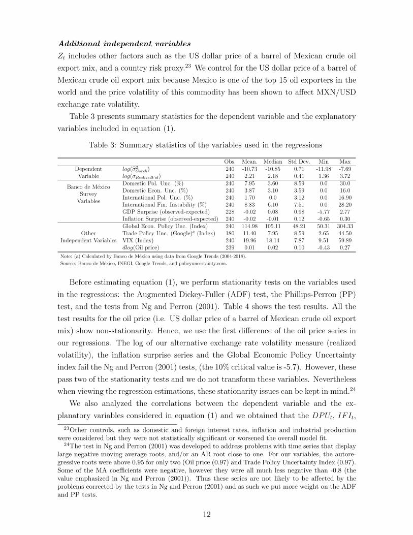
Additional independent variables
Zt includes other factors such as the US dollar price of a barrel of Mexican crude oil
export mix, and a country risk proxy.23 We control for the US dollar price of a barrel of
Mexican crude oil export mix because Mexico is one of the top 15 oil exporters in the
world and the price volatility of this commodity has been shown to affect MXN/USD
exchange rate volatility.
Table 3 presents summary statistics for the dependent variable and the explanatory
variables included in equation (1).
Table 3: Summary statistics of the variables used in the regressions
Obs. Mean. Median Std Dev. Min MaxDependent log(σ2
Garch) 240 -10.73 -10.85 0.71 -11.98 -7.69Variable log(σRealizedV ol) 240 2.21 2.18 0.41 1.36 3.72
Banco de MexicoDomestic Pol. Unc. (%) 240 7.95 3.60 8.59 0.0 30.0
SurveyDomestic Econ. Unc. (%) 240 3.87 3.10 3.59 0.0 16.0
VariablesInternational Pol. Unc. (%) 240 1.70 0.0 3.12 0.0 16.90International Fin. Instability (%) 240 8.83 6.10 7.51 0.0 28.20GDP Surprise (observed-expected) 228 -0.02 0.08 0.98 -5.77 2.77Inflation Surprise (observed-expected) 240 -0.02 -0.01 0.12 -0.65 0.30
OtherGlobal Econ. Policy Unc. (Index) 240 114.98 105.11 48.21 50.31 304.33
Independent VariablesTrade Policy Unc. (Google)a (Index) 180 11.40 7.95 8.59 2.65 44.50VIX (Index) 240 19.96 18.14 7.87 9.51 59.89dlog(Oil price) 239 0.01 0.02 0.10 -0.43 0.27
Note: (a) Calculated by Banco de Mexico using data from Google Trends (2004-2018).
Source: Banco de Mexico, INEGI, Google Trends, and policyuncertainty.com.
Before estimating equation (1), we perform stationarity tests on the variables used
in the regressions: the Augmented Dickey-Fuller (ADF) test, the Phillips-Perron (PP)
test, and the tests from Ng and Perron (2001). Table 4 shows the test results. All the
test results for the oil price (i.e. US dollar price of a barrel of Mexican crude oil export
mix) show non-stationarity. Hence, we use the first difference of the oil price series in
our regressions. The log of our alternative exchange rate volatility measure (realized
volatility), the inflation surprise series and the Global Economic Policy Uncertainty
index fail the Ng and Perron (2001) tests, (the 10% critical value is -5.7). However, these
pass two of the stationarity tests and we do not transform these variables. Nevertheless
when viewing the regression estimations, these stationarity issues can be kept in mind.24
We also analyzed the correlations between the dependent variable and the ex-
planatory variables considered in equation (1) and we obtained that the DPUt, IFIt,
23Other controls, such as domestic and foreign interest rates, inflation and industrial productionwere considered but they were not statistically significant or worsened the overall model fit.
24The test in Ng and Perron (2001) was developed to address problems with time series that displaylarge negative moving average roots, and/or an AR root close to one. For our variables, the autore-gressive roots were above 0.95 for only two (Oil price (0.97) and Trade Policy Uncertainty Index (0.97).Some of the MA coefficients were negative, however they were all much less negative than -0.8 (thevalue emphasized in Ng and Perron (2001)). Thus these series are not likely to be affected by theproblems corrected by the tests in Ng and Perron (2001) and as such we put more weight on the ADFand PP tests.
12

the V IXt, and the EPUt are some of the variables that correlate the most with the
MXN/USD exchange rate volatility.25
Table 4: Stationarity tests for variables used in the regressions
Aug. Dickey- Phillips- Ng and Stationary Transf.Fuller Perron Perron ADF/PP/NP
log(σ2Garch) 0.0000 0.0000 -7.4136 Y/Y/Y
log(σRealizedV ol) 0.0000 0.0000 -4.1745+ Y/Y/NDomestic Political Unc. (DPU) (%) 0.0743 0.0808 -6.0563 Y/Y/YDomestic Economic Unc. (DEU) (%) 0.0008 0.0000 -12.1466 Y/Y/YInternational Political Unc. (IPU) (%) 0.0000 0.0000 -10.4958 Y/Y/YInternational Financial Inst. (IFI) (%) 0.0022 0.0042 -6.4491 Y/Y/YGDP surprise (observed-expected) 0.0000 0.0000 -25.2139 Y/Y/YInflation Surprise (observed-expected) 0.0000 0.0000 -1.3537+ Y/Y/NGlobal Econ. Policy Unc. (EPU Index) 0.0132 0.0475 -5.4413+, Y/Y/NTrade Policy Uncertainty (Google)a (Index) 0.0230 0.0000 -6.4832 Y/Y/YVIX (Index) 0.0004 0.0003 -7.1925 Y/Y/YOil price ($, dollar) 0.1294+ 0.2277+ -3.4116+ N/N/N Log first diff.
Note: The Trade Uncertainty Index is calculated using data from Google Trends.
Inflation and GDP surprises are calculated as the deviation between the observed figure and the surveyed forecasters’ expectations.+ Cannot reject the null hypothesis of a unit root. Reject unit root using Ng and Perron MSB statistic.
For more detail see Table 15 in the Appendix.
Source: The authors performed the stationarity tests.
2.1 Interaction Terms
Following Krol (2014), we also investigate whether the impact of uncertainty on the
MXN/USD exchange rate volatility is amplified during election or recessionary periods.
In order to analyze whether elections amplify the effect of uncertainty, we introduce
an interaction term between DPUt and an election dummy. The election dummy is
equal to 1 for the three months before and one month after an election has taken place
in Mexico and, zero otherwise.26 During our sample period, Mexico had four elections
(see Table 5).
Furthermore, in order to study the influence of recessions, we interact a recession
dummy with our measures of DPUt and DEUt.
25For details see Table 16 in the Appendix.26We also performed sensitivity checks using election periods of 6 months and 9 months, and the
results were robust.
13

Table 5: Twentieth and twenty first century election cycles for Mexico
Name of winner YearErnesto Zedillo Ponce de Leon 1994
Vicente Fox Quesada 2000
Felipe de Jesus Calderon Hinojosa 2006
Enrique Pena Nieto 2012
Andres Manuel Lopez Obrador 2018
Note: Every election is held on July 1st (or 2nd), except for the election of Ernesto
Zedillo who was elected on August 21, 1994. The election period comprises 4 months,
April-July. Our sample includes four election periods.
Source: The authors built this table.
The recession dummy is equal to 1 if there is a recession period, the shaded areas in
Figure 5, and equal to 0 if there is an expansionary period.27
Figure 5: Mexico’s GDP
Source: The GDP data was obtained from INEGI, while the data used by the authorsto build the recession dummy was obtained from Banco de Mexico.
27In order to determine the peaks and troughs of the business cycle (i.e. booms and recessions), theBry and Boschan (1971) algorithm is applied to the ”Global Indicator of Economic Activity” series(IGAE in Spanish), which is monthly and published by INEGI. A recession is defined as a decline inthe IGAE for two consecutive quarters (6 months).
14

3 Results
Tables 6 and 7 report the OLS results of estimating equation (1), considering the
global EPU index that includes Mexico. Table 6 includes, apart from the uncertainty
measures and the additional independent variables (V IXt and the US dollar price
of a barrel of Mexican crude oil export mix) mentioned in Section 2, the GDP and
inflation surprises, while Table 7 additionally includes the interaction term between
DPUt and the election dummy and the interaction terms between DPUt and DEUt
and the recession dummy. We mainly find that of the two domestic surveyed-based
uncertainty measures (DPUt and DEUt) considered, only DPUt has a positive and a
consistently statistically significant effect (except for some columns) on the MXN/USD
exchange rate volatility. The results also show that the V IXt and the EPUt indices,
two of the international and non-surveyed based uncertainty measures considered in
the specification, have a positive and a consistently statistically significant effect on the
MXN/USD exchange rate volatility as well, which suggests that greater global financial
and economic policy uncertainty tends to lead to higher exchange rate volatility in the
Mexican economy.
Regarding the trade policy uncertainty index, we find that it does not have a sta-
tistically significant effect on the MXN/USD exchange rate volatility in any of the
estimated specifications. It may be the case that the effect of trade policy uncertainty
on the MXN/USD exchange rate volatility has been captured by the international un-
certainty measures such as the V IXt and the EPUt indices.
In line with Mavee et al. (2016), which study the case of the South African rand,
we also find that none of the macro surprises included in the estimated specification
are statistically significant.28 This suggests that other measures of uncertainty may be
more important for emerging economies, although further research is required to assess
to what degree the Mexico and South Africa cases can be generalized.
The oil price variable is negative and statistically significant in some of the estimated
specifications. A possible explanation for this result is the following: Mexico is an oil
producer and exporter, so if the international oil price increases, Mexico’s government
oil revenue increases as well. This effect reduces uncertainty regarding the government’s
revenues and so it is translated into lower MXN/USD exchange rate volatility.
Similar to Krol (2014), the results show that during recession periods, an increase
in DEUt leads to higher MXN/USD exchange rate volatility, which is evidence of an
amplifying effect during recessions. In contrast, DPUt does not seem to have a statis-
tically significant effect on the MXN/USD exchange rate volatility during election or
recession periods. The election period result is robust to using longer election periods,
28This was also true for specifications that included the absolute values of the macro surprises.
15

for example 6 and 9 month periods.
Finally, our main findings regarding DPUt, the V IXt and the EPUt remain and are
robust to inclusion of JP Morgan’s Emerging Markets Bond Index (EMBI+ (Mexico)),
a measure of bond spreads for Mexico, higher levels are associated with higher country
risk.
In order to control for possible cases of endogeneity (some regressors might be a
function of exchange rate volatility, rather than a determinant of it), we estimate equa-
tion (1) by GMM, an instrumental variables econometric technique. The results are
presented in Tables 8 and 9. Similar to Tables 6 and 7, we mainly find that DPUt has
a positive and a statistically significant effect (except for column 4 in Table 8) on the
MXN/USD exchange rate volatility. We also find that an increase in the V IXt and the
EPUt indices leads to higher MXN/USD exchange rate volatility. However, in contrast
to Tables 6 and 7 which present some unexplained negative and statistically significant
effects of the IPUt, the recession dummy and the interaction between DPUt and the
recession dummy on the MXN/USD exchange rate volatility, Tables 8 and 9 show that
these effects are no longer statistically significant.
It should be mentioned that in order to control for general forms of heteroskedasticity
and serial correlation in the error term of equation (1), HAC robust standard errors
are presented both in the OLS and the GMM estimated specifications. In the case of
the GMM results we additionally include Hansen’s J test for the exogeneity of the set
of instruments considered in the estimated specifications. The results on this test show
that the null hypothesis E{ziui(β)} = 0 is not rejected, which suggest that the models
are correctly specified.
16

Tab
le6:
Est
imat
ion
Res
ult
sbyOLS
;in
cludes
mar
cro
surp
rise
s
Dep
end
ent
Vari
ab
le:log(σ
2 Garch)
log(σ
2 Garch)
(1)
(2)
(3)
(4)
(5)
(6)
(7)
log(σ
2 Garcht−
1)
0.7
619∗
∗∗0.6
447∗
∗∗0.6
332∗
∗∗0.7
329∗
∗∗0.6
381∗
∗∗0.6
508∗
∗∗0.6
430∗
∗∗
(0.0
335)
(0.0
441)
(0.0
600)
(0.0
541)
(0.0
464)
(0.0
434)
(0.0
463)
Dom
esti
cP
olit
ical
Un
cert
ainty
(DP
U)
0.0
044
0.0
068∗
0.0
074
0.0
078
0.0
083∗
∗0.0
074∗
0.0
088∗
∗
(0.0
027)
(0.0
030)
(0.0
054)
(0.0
051)
(0.0
030)
(0.0
029)
(0.0
029)
Dom
esti
cE
con
omic
Un
cert
ainty
(DE
U)
0.0
145+
0.0
084
0.0
072
0.0
087
0.0
105
0.0
090
0.0
106
(0.0
077)
(0.0
068)
(0.0
089)
(0.0
091)
(0.0
069)
(0.0
068)
(0.0
069)
Inte
rnat
ion
alP
olit
ical
Un
cert
ainty
(IP
U)
-0.0
005
-0.0
145+
-0.0
031
0.0
181
-0.0
203∗
-0.0
135
-0.0
194∗
(0.0
072)
(0.0
085)
(0.0
117)
(0.0
113)
(0.0
084)
(0.0
085)
(0.0
084)
Inte
rnat
ion
alF
inan
cial
Inst
abil
ity
(IF
I)0.0
192∗
∗∗0.0
079+
0.0
049
0.0
116∗
∗0.0
062
0.0
085∗
0.0
067
(0.0
049)
(0.0
043)
(0.0
050)
(0.0
044)
(0.0
044)
(0.0
043)
(0.0
044)
Glo
bal
Eco
n.
Pol
icy
Un
c.(W
ith
Mexico
)a0.0
035∗
∗∗0.0
034∗
∗0.0
043∗
∗∗0.0
035∗
∗∗0.0
042∗
∗∗
(0.0
010)
(0.0
011)
(0.0
011)
(0.0
010)
(0.0
011)
Tra
de
Pol
icy
Unce
rtai
nty
(Goog
le)b
-0.0
008
-0.0
005
(0.0
056)
(0.0
061)
VIX
0.0
125∗
0.0
193∗
0.0
188∗
0.0
138∗
0.0
120∗
0.0
133∗
(0.0
057)
(0.0
082)
(0.0
089)
(0.0
057)
(0.0
058)
(0.0
059)
dlog(O
ilp
rice
)-0
.5093+
-0.5
191
-0.7
541+
-0.4
548
-0.5
434+
-0.4
848
(0.2
773)
(0.3
390)
(0.4
019)
(0.2
955)
(0.2
785)
(0.2
955)
GD
PS
urp
rise
0.0
150
0.0
099
(0.0
245)
(0.0
246)
Infl
atio
nS
urp
rise
-0.2
714
-0.2
057
(0.2
263)
(0.2
280)
Con
stan
t-2
.8182∗
∗∗-4
.5936∗∗
∗-4
.7944∗∗
∗-3
.4218∗∗
∗-4
.7680∗∗
∗-4
.5375∗∗
∗-4
.7185∗∗
∗
(0.3
865)
(0.6
176)
(0.8
279)
(0.7
098)
(0.6
488)
(0.6
121)
(0.6
501)
Ad
jR
-Squ
ared
0.6
948
0.7
466
0.7
837
0.7
589
0.7
582
0.7
474
0.7
582
Aka
ike
234.5
062
192.9
292
151.0
433
169.6
381
180.1
478
193.1
474
181.1
536
F-s
tat
151.3
957
108.6
547
80.5
365
65.8
174
96.1
942
103.9
468
89.8
551
No.
ofO
bs.
239
239
180
180
228
239
228
Not
e:H
AC
rob
ust
stan
dar
der
rors
inp
aren
thes
es.
+p<.1
,∗p<.0
5,∗∗p<.0
1,∗∗
∗p<.0
01.
log(σ
2 Garch)
isth
ees
tim
ated
vari
ance
extr
acte
dfr
om
Garc
h(1
,1)
model
of
log
diff
eren
ces
of
the
exch
an
ge
rate
.(a
)T
his
ind
exis
aG
DP
wei
ghte
dav
erag
eof
19
nati
on
al
econ
om
icp
oli
cyu
nce
rtain
tyin
dic
es,
incl
ud
ing
Mex
ico,
and
cove
rsth
ep
erio
dJan
uar
y19
99-
Dec
emb
er2018.
(b)
Cal
cula
ted
by
Ban
cod
eM
exic
ou
sin
gd
ata
from
Tre
nd
s,w
hic
hst
art
sin
Janu
ary
2004.
17

Tab
le7:
Est
imat
ion
Res
ult
sbyOLS
;in
cludes
rece
ssio
ndum
mie
s,el
ecti
ondum
mie
s,an
dE
MB
I+in
dex
Dep
end
ent
Vari
ab
le:log(σ
2 Garch)
log(σ
2 Garch)
(1)
(2)
(3)
(4)
(5)
(6)
log(σ
2 Garcht−
1)
0.6
378∗
∗∗0.6
244∗
∗∗0.6
292∗
∗∗0.6
337∗
∗∗0.6
100∗
∗∗0.6
404∗
∗∗
(0.0
431)
(0.0
595)
(0.0
465)
(0.0
439)
(0.0
612)
(0.0
434)
Dom
esti
cP
olit
ical
Un
cert
ainty
(DP
U)
0.0
032
0.0
031
0.0
060+
0.0
058+
0.0
072
0.0
066∗
(0.0
034)
(0.0
059)
(0.0
031)
(0.0
031)
(0.0
053)
(0.0
032)
Dom
esti
cE
con
omic
Un
cert
ainty
(DE
U)
0.0
088
0.0
068
0.0
082
0.0
024
-0.0
012
0.0
089
(0.0
066)
(0.0
089)
(0.0
068)
(0.0
066)
(0.0
080)
(0.0
069)
Inte
rnat
ion
alP
olit
ical
Un
cert
ainty
(IP
U)
-0.0
118
-0.0
004
-0.0
153+
-0.0
152+
-0.0
043
-0.0
147+
(0.0
085)
(0.0
120)
(0.0
084)
(0.0
087)
(0.0
113)
(0.0
085)
Inte
rnat
ion
alF
inan
cial
Inst
abil
ity
(IF
I)0.0
055
0.0
025
0.0
066
0.0
059
0.0
041
0.0
083+
(0.0
044)
(0.0
051)
(0.0
046)
(0.0
045)
(0.0
051)
(0.0
044)
Glo
bal
Eco
n.
Pol
icy
Un
c.(W
ith
Mexico
)a0.0
034∗
∗∗0.0
033∗
∗0.0
036∗
∗∗0.0
036∗
∗∗0.0
037∗
∗0.0
035∗
∗∗
(0.0
010)
(0.0
011)
(0.0
010)
(0.0
010)
(0.0
011)
(0.0
010)
Tra
de
Pol
icy
Unce
rtai
nty
(Goog
le)b
-0.0
003
-0.0
013
(0.0
056)
(0.0
057)
VIX
0.0
132∗
0.0
199∗
0.0
114∗
0.0
139∗
0.0
153∗
0.0
117+
(0.0
058)
(0.0
082)
(0.0
057)
(0.0
061)
(0.0
074)
(0.0
068)
dlog(O
ilp
rice
)-0
.5029+
-0.5
597
-0.4
846+
-0.6
053∗
-0.6
637∗
-0.5
130+
(0.2
760)
(0.3
400)
(0.2
707)
(0.2
742)
(0.3
284)
(0.2
769)
Ele
ctio
nD
um
my
0.2
741+
0.1
748+
(0.1
449)
(0.0
969)
DP
U*E
lect
ion
Du
mm
y0.0
006
0.0
059
(0.0
060)
(0.0
049)
Rec
essi
onD
um
my
0.1
408
-0.3
575∗∗
-0.2
050
(0.1
393)
(0.1
186)
(0.2
783)
DP
U*R
eces
sion
Du
mm
y-0
.0873+
-0.1
633
(0.0
449)
(0.2
655)
DE
U*R
eces
sion
Du
mm
y0.0
609∗
0.0
900∗
∗
(0.0
239)
(0.0
301)
EM
BI+
(Mex
ico)
0.0
001
(0.0
003)
Con
stan
t-4
.6441∗
∗∗-4
.8594∗∗
∗-4
.7300∗∗
∗-4
.6962∗∗
∗-4
.9750∗∗
∗-4
.6507∗∗
∗
(0.6
024)
(0.8
179)
(0.6
365)
(0.6
198)
(0.8
234)
(0.6
018)
Ad
jR
-Squ
ared
0.7
533
0.7
879
0.7
497
0.7
523
0.7
916
0.7
456
Aka
ike
188.4
829
149.3
245
191.8
696
189.4
544
147.1
127
194.7
996
F-s
tat
93.4
136
88.2
386
89.2
794
105.9
004
73.8
263
96.6
363
No.
ofO
bs.
239
180
239
239
180
239
Not
e:H
AC
rob
ust
stan
dar
der
rors
inp
are
nth
eses
.+p<.1
,∗p<.0
5,∗∗p<.0
1,∗∗
∗p<.0
01.
log(σ
2 Garch)
isth
ees
tim
ated
vari
ance
extr
act
edfr
om
Garc
h(1
,1)
model
of
log
diff
eren
ces
of
the
exch
an
ge
rate
.(a
)T
his
ind
exis
aG
DP
wei
ghte
dav
erage
of
19
nati
on
al
econ
om
icp
oli
cyu
nce
rtain
tyin
dic
es,
incl
ud
ing
Mex
ico,
and
cove
rsth
ep
erio
dJan
uar
y19
99-
Dec
emb
er2018.
(b)
Cal
cula
ted
by
Ban
cod
eM
exic
ou
sin
gd
ata
from
Tre
nd
s,w
hic
hst
art
sin
Janu
ary
2004.
18

Tab
le8:
Est
imat
ion
Res
ult
sbyGM
M;
incl
udes
mac
rosu
rpri
ses
Dep
end
ent
Vari
ab
le:log(σ
2 Garch)
log(σ
2 Garch)
(1)
(2)
(3)
(4)
(5)
(6)
(7)
log(σ
2 Garcht−
1)
0.6
634∗∗
∗0.6
757∗
∗∗0.4
373∗
∗0.7
591∗
∗∗0.7
062∗
∗∗0.6
232∗
∗∗0.6
183∗
∗∗
(0.0
700)
(0.0
695)
(0.1
482)
(0.0
973)
(0.0
531)
(0.0
646)
(0.0
645)
Dom
esti
cP
olit
ical
Un
cert
ainty
(DP
U)
0.0
364∗
∗0.0
077∗
0.0
149+
0.0
104
0.0
073∗
0.0
092∗
0.0
101∗
(0.0
121)
(0.0
037)
(0.0
086)
(0.0
080)
(0.0
036)
(0.0
041)
(0.0
045)
Dom
esti
cE
con
omic
Un
cert
ainty
(DE
U)
0.0
633∗
∗0.0
065
0.0
092
-0.0
054
-0.0
038
0.0
051
0.0
110
(0.0
238)
(0.0
131)
(0.0
129)
(0.0
247)
(0.0
104)
(0.0
145)
(0.0
143)
Inte
rnat
ion
alP
olit
ical
Un
cert
ainty
(IP
U)
0.0
263
0.0
040
-0.0
437
0.0
402∗
-0.0
083
-0.0
108
-0.0
109
(0.0
265)
(0.0
167)
(0.0
368)
(0.0
171)
(0.0
112)
(0.0
169)
(0.0
149)
Inte
rnat
ion
alF
inan
cial
Inst
abil
ity
(IF
I)0.0
826∗
∗∗0.0
082
-0.0
110
0.0
034
0.0
074
0.0
024
0.0
036
(0.0
242)
(0.0
072)
(0.0
124)
(0.0
089)
(0.0
074)
(0.0
084)
(0.0
086)
Glo
bal
Eco
n.
Pol
icy
Un
c.(W
ith
Mexico
)a0.0
021
0.0
105∗
0.0
025
0.0
044∗
∗∗0.0
044∗
∗∗
(0.0
017)
(0.0
050)
(0.0
018)
(0.0
013)
(0.0
013)
Tra
de
Pol
icy
Unce
rtai
nty
(Goog
le)b
-0.0
086
-0.0
067
(0.0
054)
(0.0
073)
VIX
0.0
186∗
0.0
231∗
∗0.0
249∗∗
0.0
123∗
0.0
198∗
0.0
197∗
∗
(0.0
088)
(0.0
071)
(0.0
080)
(0.0
053)
(0.0
084)
(0.0
074)
dlog(O
ilp
rice
)-0
.5766
-0.3
734
-0.7
285+
-0.5
263
-0.6
047
-0.6
120
(0.3
988)
(0.4
486)
(0.4
267)
(0.3
350)
(0.5
009)
(0.4
155)
GD
PS
urp
rise
0.0
070
-0.0
022
(0.0
270)
(0.0
362)
Infl
atio
nS
urp
rise
-0.3
145
-0.3
427
(0.3
028)
(0.3
077)
Con
stan
t-4
.9304∗∗
∗-4
.2213∗∗
∗-7
.5533∗
∗∗-3
.1045∗
-3.7
635∗∗
∗-5
.0036∗∗
∗-5
.0979∗∗
∗
(1.0
366)
(0.9
489)
(2.0
573)
(1.2
779)
(0.7
100)
(0.8
647)
(0.8
436)
Han
sen
’sJ-T
est:
(p-v
alu
e)(0
.3105)
(0.5
462)
(0.9
458)
(0.7
069)
(0.7
167)
(0.9
226)
(0.9
614)
No.
ofO
bs.
180
180
178
180
228
178
178
Not
e:H
AC
rob
ust
stan
dar
der
rors
inp
are
nth
eses
.+p<.1
,∗p<.0
5,∗∗p<.0
1,∗∗
∗p<.0
01.log(σ
2 Garch)
isth
ees
tim
ated
vari
ance
extr
acte
dfr
omG
arch
(1,1
)m
od
elof
log
diff
eren
ces
of
the
exch
an
ge
rate
.(a
)T
his
ind
exis
aG
DP
wei
ghte
dav
erag
eof
19
nati
on
al
econom
icp
oli
cyu
nce
rtain
tyin
dic
es,
incl
ud
ing
Mex
ico,
and
cove
rsth
ep
erio
dJan
uar
y19
99-
Dec
emb
er2018.
(b)
Cal
cula
ted
by
Ban
cod
eM
exic
ou
sin
gd
ata
from
Tre
nd
s,w
hic
hst
art
sin
Janu
ary
2004.
19

Tab
le9:
Est
imat
ion
Res
ult
sbyGM
M;
incl
udes
rece
ssio
ndum
mie
s,el
ecti
ondum
mie
s,an
dE
MB
I+in
dex
Dep
end
ent
Vari
ab
le:log(σ
2 Garch)
log(σ
2 Garch)
(1)
(2)
(3)
(4)
(5)
(6)
log(σ
2 Garcht−
1)
0.6
687∗∗
∗0.6
544∗
∗∗0.6
235∗
∗∗0.5
755∗
∗∗0.5
877∗
∗∗0.5
890∗
∗∗
(0.0
763)
(0.0
764)
(0.0
617)
(0.0
557)
(0.0
718)
(0.0
825)
Dom
esti
cP
olit
ical
Un
cert
ainty
(DP
U)
0.0
202∗
0.0
253+
0.0
076∗
0.0
084∗
0.0
120+
0.0
072+
(0.0
095)
(0.0
146)
(0.0
036)
(0.0
038)
(0.0
066)
(0.0
040)
Dom
esti
cE
con
omic
Un
cert
ainty
(DE
U)
0.0
024
-0.0
073
0.0
106
0.0
093
-0.0
012
-0.0
014
(0.0
122)
(0.0
132)
(0.0
153)
(0.0
151)
(0.0
131)
(0.0
131)
Inte
rnat
ion
alP
olit
ical
Un
cert
ainty
(IP
U)
-0.0
054
0.0
073
-0.0
057
-0.0
108
-0.0
077
-0.0
105
(0.0
233)
(0.0
462)
(0.0
117)
(0.0
128)
(0.0
124)
(0.0
159)
Inte
rnat
ion
alF
inan
cial
Inst
abil
ity
(IF
I)0.0
125
-0.0
017
0.0
071
0.0
062
0.0
009
0.0
035
(0.0
144)
(0.0
160)
(0.0
091)
(0.0
088)
(0.0
061)
(0.0
100)
Glo
bal
Eco
n.
Pol
icy
Un
c.(W
ith
Mexico
)a0.0
048∗
0.0
057∗
0.0
035∗∗
0.0
047∗
∗0.0
049∗
∗∗0.0
033+
(0.0
019)
(0.0
023)
(0.0
012)
(0.0
015)
(0.0
012)
(0.0
018)
Tra
de
Pol
icy
Un
cert
ainty
(Goog
le)b
-0.0
085
-0.0
057
(0.0
108)
(0.0
065)
VIX
0.0
165+
0.0
226∗
∗0.0
140+
0.0
154+
0.0
172∗
∗0.0
159
(0.0
085)
(0.0
088)
(0.0
078)
(0.0
083)
(0.0
065)
(0.0
112)
dlog(O
ilp
rice
)-0
.6798
-0.6
616
-0.4
958
-0.5
401
-0.7
230∗
-0.5
319
(0.4
820)
(0.4
031)
(0.4
471)
(0.4
957)
(0.3
175)
(0.5
737)
Ele
ctio
nD
um
my
-1.2
830
-0.8
573
(1.3
233)
(1.2
213)
DP
U*E
lect
ion
Du
mm
y0.0
216
-0.0
049
(0.0
587)
(0.0
682)
Rec
essi
onD
um
my
0.2
753
-0.2
724
-0.2
136
(0.2
779)
(0.2
105)
(0.2
653)
DP
U*R
eces
sion
Du
mm
y-0
.1939
-0.1
762
(0.3
109)
(0.2
380)
DE
U*R
eces
sion
Du
mm
y0.0
860∗
0.0
925∗
∗
(0.0
336)
(0.0
337)
EM
BI+
(Mex
ico)
0.0
013
(0.0
016)
Con
stan
t-4
.6047∗∗
∗-4
.7483∗∗
∗-4
.8593∗∗
∗-5
.5291∗∗
∗-5
.3225∗∗
∗-5
.4099∗∗
∗
(0.9
981)
(0.8
615)
(0.8
143)
(0.7
769)
(0.8
999)
(1.0
666)
Han
sen
’sJ-T
est:
(p-v
alu
e)(0
.8356)
(0.6
925)
(0.7
148)
(0.7
484)
(0.7
428)
(0.9
219)
No.
ofO
bs.
156
180
180
180
178
178
Not
e:H
AC
rob
ust
stan
dar
der
rors
inp
are
nth
eses
.+p<.1
,∗p<.0
5,∗∗p<.0
1,∗∗
∗p<.0
01.log(σ
2 Garch)
isth
ees
tim
ated
vari
ance
extr
acte
dfr
omG
arc
h(1
,1)
model
of
log
diff
eren
ces
of
the
exch
an
ge
rate
.(a
)T
his
ind
exis
aG
DP
wei
ghte
dav
erage
of
19
nati
on
al
econ
om
icp
oli
cyu
nce
rtain
tyin
dic
es,
incl
ud
ing
Mex
ico,
and
cover
sth
ep
erio
dJan
uar
y19
99
-D
ecem
ber
2018.
(b)
Cal
cula
ted
by
Ban
cod
eM
exic
ou
sin
gd
ata
from
Tre
nd
s,w
hic
hst
art
sin
January
2004.
20

4 Robustness Tests
We perform some additional exercises in order to test for the robustness of the results.
4.1 Alternative Exchange Rate Volatility Measure
First, we re-estimate equation (1) by OLS using a measure of realized MXN/USD
exchange rate volatility as a dependent variable, rather than the MXN/USD exchange
rate volatility we obtained from the estimated GARCH (1,1) model. The realized
exchange rate volatility is based on daily observed data from Bloomberg on the spot
MXN/USD exchange rate. It is calculated by annualizing the standard deviation (σ) of
periodic logarithmic returns over the sample period.29 Figure 6 plots our two exchange
rate volatility measures for the sample period. Both measures of exchange rate volatility
are converted into monthly time series.
The results of this first exercise are presented in Table 10.
Figure 6: Monthly averages on daily data, Jan. 1999=100
Source: The GARCH(1,1) model was estimated by the authors using daily data from Bancode Mexico on the FIX Mexican peso (MXN) US dollar (USD) exchange rate.The realized volatility was obtained from Bloomberg.
4.2 Alternative Global EPU Index (it excludes Mexico)
Second, we re-estimate equation (1) by OLS and GMM using as a dependent variable
the MXN/USD exchange rate volatility derived from the GARCH (1,1) model and,
29For more details see Bloomberg.
21

as one of the explanatory variables, the EPUt index that excludes Mexico. As we
mentioned in Section 2, the EPUt index that excludes Mexico is an earlier version of
the index and it only covers the period January 2001 - December 2016. The results are
presented in Tables 11 and 12.
Our main findings from both exercises show that regardless of the EPUt index
we include as an explanatory variable (with or without including Mexico) and the
econometric technique we employed to estimate equation (1), DPUt, as well as the
V IXt and the EPUt indexes continue to have a positive and a statistically significant
effect on the MXN/USD exchange rate volatility. We also confirm that the effect of
DEUt on the MXN/USD exchange rate volatility is amplified in recession periods.
4.3 Simulations
Sections 3 and 4 show that higher international and domestic uncertainty may lead to
higher MXN/USD exchange rate volatility. In order to investigate the size of this effect,
we perform simulations using specification (2) in Table 8. We choose this specification
for three reasons. First, it includes the survey-based uncertainty measures we derived
from Banco de Mexico’s SPF, as well as international indicators such as the V IXt, the
EPUt and the price of a barrel of Mexican crude oil export mix. This is important since
this set of regressors includes the variables that we found had a statistically significant
effect on the MXN/USD exchange rate volatility. Second, this particular specification
was estimated by GMM, which is robust to the possibility of endogeneity. Finally, this
regression includes as an independent variable the most recent EPUt index published
by Bloom, Baker and Davis, so it covers the complete sample period (January 1999 –
December 2018).
We conduct the simulations fixing the uncertainty measures for each and every
month during the period 2007 – 2018 equal to the lowest level they reached during the
sample period. Since all uncertainty measures were at their sample minimum level in
2007, just before the eruption of the global financial crisis, the simulations start in that
year. We build counterfactual scenarios for the MXN/USD exchange rate volatility
from 2007 to 2018 under the assumption of minimum uncertainty, and compare them
with the base scenario where MXN/USD exchange rate volatility is that derived from
the estimated GARCH (1,1) model. Figure 7 plots several counterfactual scenarios for
MXN/USD exchange rate volatility, as well as the base scenario.
The results show that if uncertainty (proxied, for example, by the domestic political
uncertainty (DPUt in equation (1)) for each and every month during the period 2007-
2018 had been equal to 1% (the sample period minimum), then MXN/USD exchange
rate volatility would have been that depicted with the triangle pattern, a lower exchange
22

Tab
le10
:E
stim
atio
nR
esult
sbyOLS
;in
cludes
mac
roSurp
rise
s,re
cess
ion
dum
mie
s,el
ecti
ondum
mie
san
dE
MB
I+in
dex
Dep
end
ent
Vari
ab
le:log(σ
RealizedVol)
log(σ
RealizedVol)
(1)
(2)
(3)
(4)
(5)
(6)
(7)
log(σ
RealizedVolt−1)
0.6
138∗∗
∗0.5
756∗∗
∗0.6
244∗∗
∗0.6
050∗∗
∗0.5
612∗∗
∗0.5
489∗∗
∗0.6
177∗∗
∗
(0.0
525)
(0.0
689)
(0.0
535)
(0.0
513)
(0.0
677)
(0.0
656)
(0.0
517)
Dom
esti
cP
oliti
cal
Un
cert
ain
ty(D
PU
)0.0
025
0.0
028
0.0
041∗
-0.0
004
-0.0
007
0.0
026
0.0
027
(0.0
023)
(0.0
039)
(0.0
021)
(0.0
025)
(0.0
041)
(0.0
038)
(0.0
024)
Dom
esti
cE
con
om
icU
nce
rtain
ty(D
EU
)0.0
035
0.0
031
0.0
049
0.0
037
0.0
028
-0.0
026
0.0
030
(0.0
048)
(0.0
065)
(0.0
049)
(0.0
047)
(0.0
065)
(0.0
062)
(0.0
048)
Inte
rnati
on
al
Politi
cal
Un
cert
ain
ty(I
PU
)-0
.0051
0.0
031
-0.0
084+
-0.0
032
0.0
052
0.0
022
-0.0
049
(0.0
058)
(0.0
074)
(0.0
050)
(0.0
058)
(0.0
073)
(0.0
071)
(0.0
058)
Inte
rnati
on
al
Fin
an
cial
Inst
ab
ilit
y(I
FI)
0.0
032
0.0
014
0.0
023
0.0
016
-0.0
003
0.0
007
0.0
029
(0.0
028)
(0.0
033)
(0.0
027)
(0.0
028)
(0.0
033)
(0.0
034)
(0.0
029)
Glo
bal
Eco
n.
Policy
Un
c.(W
ith
Mexico
)a
0.0
021∗∗
0.0
021∗
0.0
026∗∗
∗0.0
020∗∗
0.0
020∗∗
0.0
023∗∗
0.0
021∗∗
(0.0
007)
(0.0
008)
(0.0
006)
(0.0
007)
(0.0
008)
(0.0
008)
(0.0
007)
Tra
de
Policy
Un
cert
ain
ty(G
oogle
)b-0
.0001
0.0
003
-0.0
007
(0.0
036)
(0.0
034)
(0.0
036)
VIX
0.0
065∗
0.0
120∗∗
0.0
073∗
0.0
069∗
0.0
124∗∗
0.0
090+
0.0
073+
(0.0
030)
(0.0
043)
(0.0
030)
(0.0
030)
(0.0
042)
(0.0
046)
(0.0
037)
dlog(O
ilp
rice
)-0
.2221
-0.1
778
-0.1
661
-0.2
255
-0.2
145
-0.2
734
-0.2
171
(0.1
717)
(0.1
853)
(0.1
742)
(0.1
718)
(0.1
842)
(0.1
719)
(0.1
687)
GD
PS
urp
rise
0.0
050
(0.0
153)
Infl
ati
on
Su
rpri
se-0
.1761
(0.1
413)
Ele
ctio
nD
um
my
0.1
229
0.0
777
(0.0
759)
(0.0
579)
DP
U*E
lect
ion
Du
mm
y0.0
045
0.0
079∗
(0.0
038)
(0.0
036)
Rec
essi
on
-0.0
968
(0.1
570)
DP
U*R
eces
sion
Du
mm
y-0
.1752
(0.1
327)
DE
U*R
eces
sion
Du
mm
y0.0
598∗∗
(0.0
182)
EM
BI+
(Mex
ico)
-0.0
001
(0.0
002)
Con
stant
0.4
286∗∗
∗0.4
364∗∗
∗0.3
314∗∗
∗0.4
683∗∗
∗0.4
908∗∗
∗0.5
544∗∗
∗0.4
273∗∗
∗
(0.0
992)
(0.1
018)
(0.0
944)
(0.0
993)
(0.1
041)
(0.1
055)
(0.0
995)
Ad
jR
-Squ
are
d0.6
797
0.7
191
0.7
072
0.6
901
0.7
292
0.7
320
0.6
786
Akaik
e-9
.3595
-6.6
467
-25.4
800
-15.3
722
-11.3
287
-12.3
028
-7.6
294
F-s
tat
68.7
550
52.8
652
56.2
210
61.9
349
57.6
689
47.7
637
60.8
406
No.
of
Ob
s.239
180
228
239
180
180
239
Note
:H
AC
rob
ust
stan
dard
erro
rsin
pare
nth
eses
.+p<.1
,∗p<.0
5,∗∗p<.0
1,∗∗
∗p<.0
01.
Blo
om
ber
gre
alize
dvola
tili
tyis
calc
ula
ted
by
an
nu
alizi
ng
the
stan
dard
dev
iati
on
of
per
iod
iclo
gre
turn
sover
the
his
tori
cti
me
hori
zon
.(a
)T
his
ind
exis
aG
DP
wei
ghte
daver
age
of
19
nati
on
al
econ
om
icp
olicy
un
cert
ain
tyin
dic
es,
incl
ud
ing
Mex
ico,
an
dco
ver
sth
ep
erio
dJanu
ary
1999
-D
ecem
ber
2018.
(b)
Calc
ula
ted
by
Ban
cod
eM
exic
ou
sin
gd
ata
from
Tre
nds,
wh
ich
start
sin
Janu
ary
2004.
23
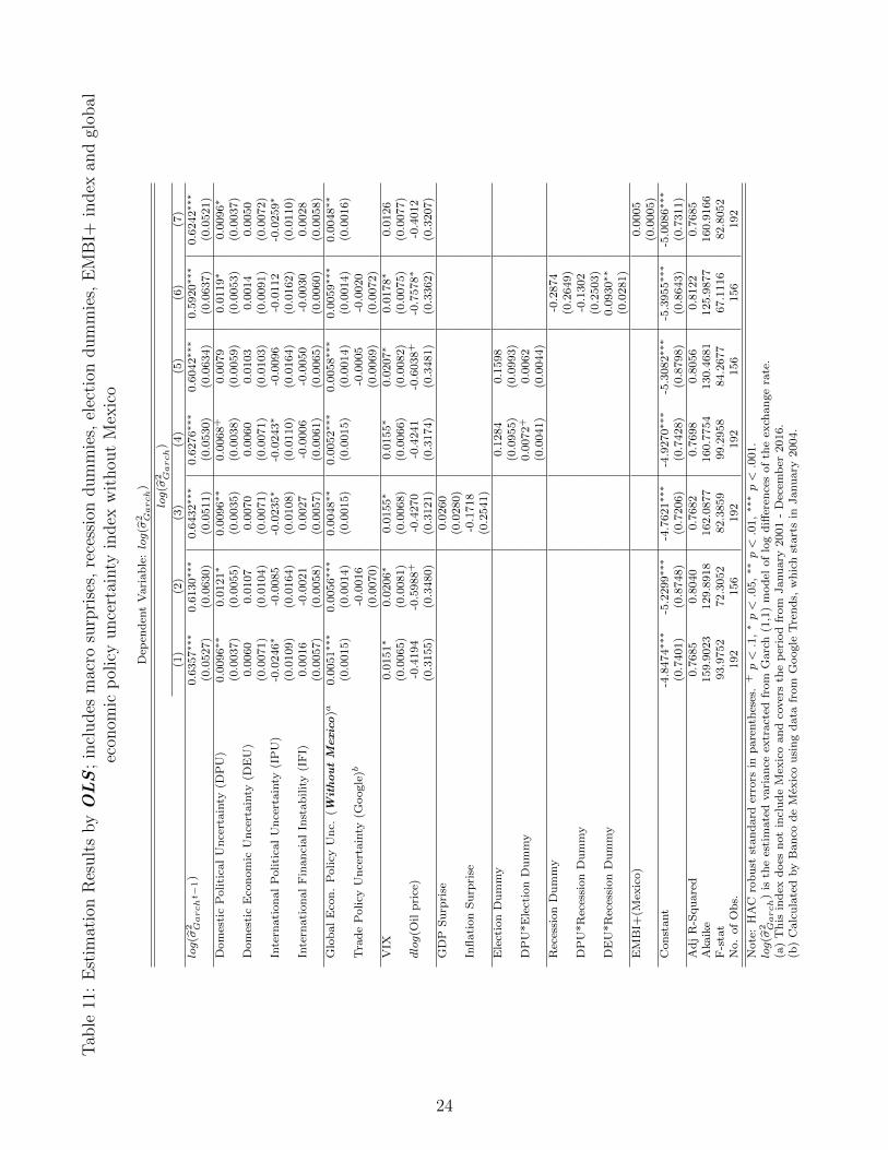
Tab
le11
:E
stim
atio
nR
esult
sbyOLS
;in
cludes
mac
rosu
rpri
ses,
rece
ssio
ndum
mie
s,el
ecti
ondum
mie
s,E
MB
I+in
dex
and
glob
alec
onom
icp
olic
yunce
rtai
nty
index
wit
hou
tM
exic
o
Dep
end
ent
Vari
ab
le:log(σ
2 Garch
)
log(σ
2 Garch
)
(1)
(2)
(3)
(4)
(5)
(6)
(7)
log(σ
2 Garcht−
1)
0.6
357∗∗
∗0.6
130∗∗
∗0.6
432∗∗
∗0.6
276∗∗
∗0.6
042∗∗
∗0.5
920∗∗
∗0.6
242∗∗
∗
(0.0
527)
(0.0
630)
(0.0
511)
(0.0
530)
(0.0
634)
(0.0
637)
(0.0
521)
Dom
esti
cP
oliti
cal
Un
cert
ain
ty(D
PU
)0.0
096∗∗
0.0
121∗
0.0
096∗∗
0.0
068+
0.0
079
0.0
119∗
0.0
096∗
(0.0
037)
(0.0
055)
(0.0
035)
(0.0
038)
(0.0
059)
(0.0
053)
(0.0
037)
Dom
esti
cE
con
om
icU
nce
rtain
ty(D
EU
)0.0
060
0.0
107
0.0
070
0.0
060
0.0
103
0.0
014
0.0
050
(0.0
071)
(0.0
104)
(0.0
071)
(0.0
071)
(0.0
103)
(0.0
091)
(0.0
072)
Inte
rnati
on
al
Politi
cal
Un
cert
ain
ty(I
PU
)-0
.0246∗
-0.0
085
-0.0
235∗
-0.0
243∗
-0.0
096
-0.0
112
-0.0
259∗
(0.0
109)
(0.0
164)
(0.0
108)
(0.0
110)
(0.0
164)
(0.0
162)
(0.0
110)
Inte
rnati
on
al
Fin
an
cial
Inst
ab
ilit
y(I
FI)
0.0
016
-0.0
021
0.0
027
-0.0
006
-0.0
050
-0.0
030
0.0
028
(0.0
057)
(0.0
058)
(0.0
057)
(0.0
061)
(0.0
065)
(0.0
060)
(0.0
058)
Glo
bal
Eco
n.
Policy
Un
c.(W
ithoutM
exico
)a0.0
051∗∗
∗0.0
056∗∗
∗0.0
048∗∗
0.0
052∗∗
∗0.0
058∗∗
∗0.0
059∗∗
∗0.0
048∗∗
(0.0
015)
(0.0
014)
(0.0
015)
(0.0
015)
(0.0
014)
(0.0
014)
(0.0
016)
Tra
de
Policy
Un
cert
ain
ty(G
oogle
)b-0
.0016
-0.0
005
-0.0
020
(0.0
070)
(0.0
069)
(0.0
072)
VIX
0.0
151∗
0.0
206∗
0.0
155∗
0.0
155∗
0.0
207∗
0.0
178∗
0.0
126
(0.0
065)
(0.0
081)
(0.0
068)
(0.0
066)
(0.0
082)
(0.0
075)
(0.0
077)
dlog(O
ilp
rice
)-0
.4194
-0.5
988+
-0.4
270
-0.4
241
-0.6
038+
-0.7
578∗
-0.4
012
(0.3
155)
(0.3
480)
(0.3
121)
(0.3
174)
(0.3
481)
(0.3
362)
(0.3
207)
GD
PS
urp
rise
0.0
260
(0.0
280)
Infl
ati
on
Su
rpri
se-0
.1718
(0.2
541)
Ele
ctio
nD
um
my
0.1
284
0.1
598
(0.0
955)
(0.0
993)
DP
U*E
lect
ion
Du
mm
y0.0
072+
0.0
062
(0.0
041)
(0.0
044)
Rec
essi
on
Du
mm
y-0
.2874
(0.2
649)
DP
U*R
eces
sion
Du
mm
y-0
.1302
(0.2
503)
DE
U*R
eces
sion
Du
mm
y0.0
930∗∗
(0.0
281)
EM
BI+
(Mex
ico)
0.0
005
(0.0
005)
Con
stant
-4.8
474∗∗
∗-5
.2299∗∗
∗-4
.7621∗∗
∗-4
.9270∗∗
∗-5
.3082∗∗
∗-5
.3955∗∗
∗-5
.0086∗∗
∗
(0.7
401)
(0.8
748)
(0.7
206)
(0.7
428)
(0.8
798)
(0.8
643)
(0.7
311)
Ad
jR
-Squ
are
d0.7
685
0.8
040
0.7
682
0.7
698
0.8
056
0.8
122
0.7
685
Akaik
e159.9
023
129.8
918
162.0
877
160.7
754
130.4
681
125.9
877
160.9
166
F-s
tat
93.9
752
72.3
052
82.3
859
99.2
958
84.2
677
67.1
116
82.8
052
No.
of
Ob
s.192
156
192
192
156
156
192
Note
:H
AC
rob
ust
stan
dard
erro
rsin
pare
nth
eses
.+p<.1
,∗p<.0
5,∗∗p<.0
1,∗∗
∗p<.0
01.
log(σ
2 Garch
)is
the
esti
mate
dvari
an
ceex
tract
edfr
om
Garc
h(1
,1)
mod
elof
log
diff
eren
ces
of
the
exch
an
ge
rate
.(a
)T
his
ind
exd
oes
not
incl
ud
eM
exic
oan
dco
ver
sth
ep
erio
dfr
om
Janu
ary
2001
-D
ecem
ber
2016.
(b)
Calc
ula
ted
by
Ban
cod
eM
exic
ou
sin
gd
ata
from
Tre
nds,
wh
ich
start
sin
Janu
ary
2004.
24

Tab
le12
:E
stim
atio
nR
esult
sbyGM
M;
incl
udes
mac
rosu
rpri
ses,
rece
ssio
ndum
mie
s,el
ecti
ondum
mie
s,E
MB
I+in
dex
and
glob
alec
onom
icp
olic
yunce
rtai
nty
index
wit
hou
tM
exic
o
Dep
end
ent
Vari
ab
le:log(σ
2 Garch
)
log(σ
2 Garch
)
(1)
(2)
(3)
(4)
(5)
(6)
(7)
log(σ
2 Garcht−
1)
0.5
726∗∗
∗0.5
408∗∗
∗0.5
908∗∗
∗0.5
266∗∗
∗0.5
886∗∗
∗0.4
748∗∗
∗0.6
030∗∗
∗
(0.0
748)
(0.0
848)
(0.0
679)
(0.0
887)
(0.1
075)
(0.0
845)
(0.0
750)
Dom
esti
cP
oliti
cal
Un
cert
ain
ty(D
PU
)0.0
128∗∗
0.0
169∗
0.0
123∗∗
0.0
124+
0.0
260+
0.0
209∗∗
0.0
078+
(0.0
049)
(0.0
069)
(0.0
044)
(0.0
072)
(0.0
142)
(0.0
076)
(0.0
040)
Dom
esti
cE
con
om
icU
nce
rtain
ty(D
EU
)0.0
057
0.0
119
0.0
062
0.0
110
-0.0
050
0.0
050
-0.0
048
(0.0
164)
(0.0
144)
(0.0
140)
(0.0
136)
(0.0
138)
(0.0
154)
(0.0
133)
Inte
rnati
on
al
Politi
cal
Un
cert
ain
ty(I
PU
)-0
.0269
-0.0
280
-0.0
228
-0.0
376
-0.0
299
-0.0
422
-0.0
090
(0.0
265)
(0.0
365)
(0.0
252)
(0.0
248)
(0.0
485)
(0.0
320)
(0.0
201)
Inte
rnati
on
al
Fin
an
cial
Inst
ab
ilit
y(I
FI)
-0.0
093
-0.0
119
-0.0
071
-0.0
112
-0.0
143
-0.0
170
-0.0
009
(0.0
108)
(0.0
112)
(0.0
102)
(0.0
135)
(0.0
161)
(0.0
121)
(0.0
110)
Glo
bal
Eco
n.
Policy
Un
c.(W
ithoutM
exico
)a0.0
082∗∗
0.0
093∗∗
0.0
073∗∗
∗0.0
103∗∗
∗0.0
085∗
0.0
116∗∗
∗0.0
040+
(0.0
027)
(0.0
034)
(0.0
020)
(0.0
029)
(0.0
038)
(0.0
032)
(0.0
022)
Tra
de
Policy
Un
cert
ain
ty(G
oogle
)b-0
.0044
-0.0
111
-0.0
076
(0.0
074)
(0.0
096)
(0.0
080)
VIX
0.0
201∗∗
0.0
217∗∗
0.0
199∗
0.0
188∗
0.0
242∗∗
0.0
166∗
0.0
162+
(0.0
068)
(0.0
071)
(0.0
080)
(0.0
074)
(0.0
083)
(0.0
069)
(0.0
086)
dlog(O
ilp
rice
)-0
.5001
-0.4
717
-0.5
483
-0.5
008
-0.4
913
-0.5
388+
-0.5
608
(0.3
778)
(0.4
134)
(0.3
856)
(0.3
534)
(0.3
852)
(0.3
253)
(0.4
942)
GD
PS
urp
rise
-0.0
083
(0.0
354)
Infl
ati
on
Su
rpri
se-0
.2903
(0.3
438)
Ele
ctio
nD
um
my
-0.5
987
-0.1
386
(0.9
609)
(0.9
181)
DP
U*E
lect
ion
Du
mm
y0.0
365
-0.0
222
(0.0
382)
(0.0
593)
Rec
essi
on
Du
mm
y-0
.1305
(0.2
693)
DP
U*R
eces
sion
Du
mm
y-0
.2665
(0.2
299)
DE
U*R
eces
sion
Du
mm
y0.0
967∗∗
(0.0
310)
EM
BI+
(Mex
ico)
0.0
012
(0.0
010)
Con
stant
-5.8
465∗∗
∗-6
.3140∗∗
∗-5
.5862∗∗
∗-6
.5313∗∗
∗-5
.6436∗∗
∗-7
.1073∗∗
∗-5
.2720∗∗
∗
(1.0
609)
(1.2
092)
(0.9
372)
(1.2
412)
(1.4
893)
(1.1
481)
(1.0
027)
Han
sen
’sJ-T
est:
(p-v
alu
e)(0
.8870)
(0.9
740)
(0.9
303)
(0.7
436)
(0.8
436)
(0.8
436)
(0.9
339)
No.
of
Ob
s.156
156
156
156
156
156
156
Note
:H
AC
rob
ust
stan
dard
erro
rsin
pare
nth
eses
.+p<.1
,∗p<.0
5,∗∗p<.0
1,∗
∗∗p<.0
01.
log(σ
2 Garch
)is
the
esti
mate
dvari
an
ceex
tract
edfr
om
Garc
h(1
,1)
mod
elof
log
diff
eren
ces
of
the
exch
an
ge
rate
.(a
)T
his
ind
exd
oes
not
incl
ud
eM
exic
oan
dco
ver
sth
ep
erio
dfr
om
Janu
ary
2001
-D
ecem
ber
2016
(b)
Calc
ula
ted
by
Ban
cod
eM
exic
ou
sin
gd
ata
from
Tre
nds,
wh
ich
start
sin
Janu
ary
2004.
25

rate volatility compared to the base scenario. This same interpretation can be given to
the rest of the counterfactual scenarios.
Figure 7: Simulation exercises, exchange rate volatility derived from the GARCH(1,1)model (log)
Note: This simulation was performed using specification (2) in Table 8.Source: From authors’ own calculations.
Furthermore, in order to assess whether international uncertainty, measured by the
V IXt and the EPUt indices, is having a bigger or a smaller effect on the MXN/USD
exchange rate volatility than the domestic uncertainty, measured by DPUt, we build
two additional counterfactual scenarios. The first one (depicted with a square pattern)
is built under the assumption that the V IXt and the EPUt indices are equal to 10.42%
and 50.07%, respectively, from 2007 onwards; while the second one (depicted with the
triangle pattern), under the assumption that DPUt is equal to 1%, from 2007 onwards.
Figure 8 presents both counterfactual scenarios and the base scenario.
26

Figure 8: Simulation exercises, exchange rate volatility derived from the GARCH(1,1)model (log)
Comparing the effect of domestic vs. international uncertainty
Note: This simulation was performed using specification (2) in Table 8.Source: From authors’ own calculations.
We additionally calculate the yearly average standard deviation of both the coun-
terfactual and the base scenarios of the MXN/USD exchange rate volatility, depicted
in Figures 7 and 8, as a proportion of the yearly average standard deviation of the
base scenario. Table 13 shows the results. These proportions show that both interna-
tional and domestic uncertainty have had a similar effect on the MXN/USD exchange
rate volatility during the sample period, although the EPUt’s effect seems to be the
predominant.
Table 13: A comparison between the effect of the international and the domesticuncertainty measures on the MXN/USD exchange rate volatility
Base Scenario DPU VIX EPU VIX&EPU1.0000 0.8902 0.9591 0.8851 0.9612
Source: From authors’ own calculations.
27

5 Relative Contribution of Explanatory Variables
to the MXN/USD Exchange Rate Volatility
Based on specification (2) from Table 12,30 we also analyze the relative contribution
of each independent variable to the MXN/USD exchange rate volatility. Hence, we
calculate beta coefficients from that particular specification according to the formula:
βcoefficient =βx ∗ σx
σGARCH(1,1)
(4)
where βx stands for the estimated coefficient of the independent variable, σx stands
for the regressor’s standard deviation, and σGARCH(1,1), for the standard deviation of the
MXN/USD exchange rate volatility derived from the estimated GARCH (1,1) model.
The calculated beta coefficients from that specification are presented in Table 14.
The results show that EPUt is the variable that contributes the most to the MXN/USD
exchange rate volatility, followed by the V IXt and the DPUt, in that order, respectively.
Therefore, we conclude that the main drivers of the MXN/USD exchange rate volatility
during the sample period are both the international and domestic uncertainty.
Table 14: Beta coefficients
Variable Beta coefficientDomestic Political Uncertainty (DPU) 0.1764*
(0.07165)Domestic Economic Uncertainty (DEU) 0.0463
(0.0562)International Political Uncertainty (IPU) -0.0662
(0.0862)International Financial Instability (IFI) -0.1191
(-0.1187)Global Econ. Policy Unc. (Without Mexico) 0.5313**
(0.1948)Trade Uncertainty (Google) -0.0414
(0.0696)VIX 0.2280**
(0.0750)dlog(Oil price) -0.0611
(0.0536)
Note: Standard errors in parenthesis.
+ p < .1, * p < .05, ** p < .01,*** p < .001.
Source: From authors’ own calculations.
30We choose this specification since the dependent variable was derived from a GARCH (1,1) model,and it was estimated by GMM in order to control for possible endogeneity problems.
28

6 Conclusion
We investigate the impact of uncertainty on the MXN/USD exchange rate volatility
over the period 1999-2018. The analysis is conducted in two stages: in the first one,
we estimate a univariate GARCH (1,1) model to derive a MXN/USD exchange rate
volatility measure; while in the second one, we regress the estimated exchange rate
volatility on different uncertainty measures, both domestic and international, and on
the US dollar price of a barrel of Mexican crude oil mix. We also consider GDP and
inflation surprises in the estimated specification to account for the surprise component
of macroeconomic data announcements. Finally, in order to investigate if the effect
of uncertainty on the MXN/USD exchange rate volatility is amplified during election
and/or recession periods, we include interaction terms between some of the uncertainty
measures and an election dummy and, those same uncertainty measures and a recession
dummy.
The main results show that the domestic political uncertainty measure, as well as
the VIX and the EPU indices, have a positive and a statistically significant effect on
the MXN/USD exchange rate volatility. We additionally find that the effect of the
domestic economic uncertainty measure on the MXN/USD exchange rate volatility is
amplified during recession periods. These results are robust to different MXN/USD
exchange rate volatility measures (we alternatively use a realized MXN/USD exchange
rate volatility measure that we obtained from Bloomberg); different specifications; dif-
ferent econometric techniques (we use both OLS and GMM); and different global EPU
indexes (one that includes data on Mexico’s EPU index and one that excludes it).
We also conduct some simulations in order to analyze the size of the uncertainty
effect on the MXN/USD exchange rate volatility. The findings suggest that if the
international and/or domestic uncertainty had adopted, from 2007 onwards, their lowest
level during the sample period, the MXN/USD exchange rate volatility would have been
reduced. In addition, when we compare the effect of the international uncertainty to
that of the domestic uncertainty, the simulations and some calculations show that both
have had a similar effect on the MXN/USD exchange rate volatility, although the EPU
index’s effect seems to be the predominant.
Overall, the results suggest that the MXN/USD exchange rate volatility is affected
by both domestic and international uncertainty and that a stable macroeconomic envi-
ronment should be procured in order to contain exchange rate volatility.
29

A Supplemental Material
Table 15: Stationarity tests lag selection
Aug. Dickey-Fuller Phillips-Perron Ng and Perronlog(σ2
Garch) 1 1 3log(σRealizedV ol) 1 1 11Domestic Political Unc. (DPU) (%) 1 1 2Domestic Economic Unc. (DEU) (%) 1, D1 1 6International Political Unc. (IPU) (%) 1 1 14International Financial Inst. (IFI) (%) 1 1 3GDP surprise (observed-expected) 1 1 5Inflation Surprise (observed-expected) 1 1 14Global Econ. Policy Unc. (Index) 1 1 3Trade Policy Uncertainty (Google)a (Index) 1, D2 1 13VIX (Index) 1 1 9Oil price ($) 1, D1 1 1
Note: Results for models specified with an intercept and no trend.
Lag selection criteria for ADF: Schwarz Information Criterion, PP: Barlett kernel, NP: Modified Akaike Information Criterion.+ Cannot reject the null hypothesis of a Unit Root.
Source: The authors performed the stationarity tests.
Table 16: Correlations for variables used in the regressions
log(σ2Garch) log(σRealizedV ol)
Banco de MexicoDomestic Pol. Unc. (%) -0.24 -0.26
SurveyDomestic Econ. Unc. (%) 0.11 0.13
VariablesInternational Pol. Unc. (%) 0.10 0.12International Fin. Instability (%) 0.38 0.35GDP Surprise (observed-expected) -0.07 -0.06Inflation Surprise (observed-expected) 0.08 0.06
OtherGlobal Econ. Policy Unc. (Index) 0.59 0.60
Independent VariablesTrade Policy Unc. (Google)a (Index) -0.12 -0.12VIX (Index) 0.39 0.34dlog(Oil price) -0.19 -0.18
Note: (a) Calculated by Banco de Mexico using data from Google Trends (2004-2018).
Source: Calculated by the authors using data from Banco de Mexico, INEGI, Google Trends, and policyuncertainty.com.
30

References
Antonakakis, N., Chatziantoniou, I., and Filis, G. (2013). Dynamic Co-Movements ofStock Market Returns, Implied Volatility and Policy Uncertainty. Economics Letters,120(1):87–92.
Asis, G. and Chari, A. (2018). In Search of Distress Risk in Emerging Markets. HKIMRWorking Paper No. 10/2018.
Baker, S. and Bloom, N. (2013). Does Uncertainty Reduce Growth? Using Disasters asNatural Experiments. NBER Working Papers 19475, National Bureau of EconomicResearch, Inc.
Baker, S., Bloom, N., and Davis, S. (2016). Measuring Economic Policy Uncertainty.The Quarterly Journal of Economics, 131(4):1593–1636.
Balcilar, M., Gupta, R., Clement, K., and Wohar, M. (2016a). Does Economic PolicyUncertainty Predict Exchange Rate Returns and Volatility? Evidence from a Non-parametric Causality-in-Quantiles Test. Open Economies Review, 27(2):229–250.
Balcilar, M., Gupta, R., and Jooste, C. (2014). The Role of Economic Policy Uncer-tainty in Forecasting US Inflation Using a VARFIMA Model. Working Papers 15-12;Eastern Mediterranean University, Department of Economics.
Balcilar, M., Gupta, R., and Segnon, M. (2016b). The Role of Economic Policy Un-certainty in Predicting US Recessions: A Mixed-Frequency Markov-Switching Vec-tor Autoregressive Approach. Economics: The Open-Access, Open-Assessment E-Journal, Kiel Institute for the World Economy (IfW), 10:1–20.
Bank for International Settlements (2016). Triennial Central Bank Survey, ForeignExchange Turnover April 2016. Monetary and Economic Department.
Beckmann, J. and Czudaj, R. (2017). Exchange Rate Expectations and EconomicPolicy Uncertainty. European Journal of Political Economy, 47 (March):148–162.
Benavides, G. and Capistran, C. (2012). Forecasting Exchange Rate Volatility: The Su-perior Performance of Conditional Combinations of Time Series and Option ImpliedForecasts. Journal of Empirical Finance, 19(5):627–639.
Bloom, N. (2009). The Impact of Uncertainty Shocks. Econometrica, 77(3):623–685.
Bollerslev, T. (1986). Generalized Autoregressive Conditional Heteroskedasticity. Jour-nal of Econometrics, 31(3):307–327.
Brogaard, J. and Detzel, A. (2015). The Asset-Pricing Implications of GovernmentEconomic Policy Uncertainty. Management Science, 61(1):3–18.
Bry, G. and Boschan, C. (1971). Programmed Selection of Cyclical Turning Points.NBER Chapters, in Cyclical Analysis of Time Series: Selected Procedures and Com-puter Programs, pages 7–63.
31

Cebreros, A., Chiquiar, D., Heffner, A., and Salcedo, A. (2019). Trade Policy Uncer-tainty and its Effect on Foreign Direct Investment and Export Participation: Evi-dence from Mexico. Mimeo, Banco de Mexico.
Chicago Board Options Exchange Volatility Index (VIX).https://www.finance.yahoo.com/quote/%5EVIX/.
Domınguez, K. and Tesar, L. (2001). A Reexamination of Exchange-Rate Exposure.The American Economic Review, 91(2):396–399.
Engel, C. (2006). Exchange Rate Models. NBER Reporter: Research Summary, Fall.
Engel, C., Mark, N., and West, K. (2008). Exchange Rate Models Are Not As Bad AsYou Think. NBER Chapters, in NBER Macroeconomics Annual 2007, 22:381–441.
Engle, R. (1982). Autoregressive Conditional Heteroscedasticity with Estimates of theVariance of United Kingdom Inflation. Econometrica, 50(4):987–1007.
Frankel, J. and Rose, A. (1995). Empirical Research on Nominal Exchange Rates.Handbook of International Economics, 3:1689–1729.
Garfinkel, M., Glazer, A., and Lee, J. (1999). Election Surprises and Exchange RateUncertainty. Economics and Politics, 11:255–274.
Grier, K., Henry, O., Olekalns, N., and Shields, K. (2004). The Asymmetric Effectsof Uncertainty on Inflation and Output Growth. Journal of Applied Econometrics,19(5):551–565.
Grier, R. and Grier, K. (2006). On the Real Effects of Inflation and Inflation Uncertaintyin Mexico. Journal of Development Economics, 80(2):478–500.
Hansen, P. R. and Lunde, A. (2005). A Forecast Comparison of Volatility Models: DoesAnything Beat a GARCH(1,1)? Journal of Applied Econometrics, 20:873–889.
Jones, P. and Olson, E. (2013). The Time-Varying Correlation Between Uncertainty,Output, and Inflation: Evidence from a DCC-GARCH Model. Economics Letters,118(1):33–37.
JP Morgan Emerging Markets Bond Index (EMBI). https://www.jpmorgan.com.
Jurado, K., Ludvigson, S., and Ng, S. (2015). Measuring Uncertainty. The AmericanEconomic Review, 105(3):1177–1216.
Karnizova, L. and Li, J. C. (2014). Economic Policy Uncertainty, Financial Marketsand Probability of US Recessions. Economics Letters, 125(2):261–265.
Kido, Y. (2016). On The Link Between the US Economic Policy Uncertainty andExchange Rates. Economics Letters, 144:49–52.
Krol, R. (2014). Economic Policy Uncertainty and Exchange Rate Volatility. Interna-tional Finance, 17(2):241–255.
32

Kurasawa, K. (2016). Policy Uncertainty and Foreign Exchange Rates: The DCC-GARCH Model of the US/Japanese Foreign Exchange Rate. International Journalof Economic Sciences, 5(4):1–19.
Lane, P. and Shambaugh, J. (2009). Financial Exchange Rates and International Cur-rency Exposures. The American Economic Review, 99(1):1–30.
Liu, L. and Pauwels, L. (2012). Do External Political Pressures Affect the RenminbiExchange Rate. Journal of International Money and Finance, 31(6):1800–1818.
Liu, L. and Zhang, T. (2015). Economic Policy Uncertainty and Stock Market Volatility.Finance Research Letters, 15:99–105.
Lopez-Noria, G. and Zamudio-Fernandez, J. (2018). The Effect of Uncertainty onForeign Direct Investment: the Case of Mexico. Estudios Economicos, 33(1):117–149.
Mavee, N., Perrelli, R., and Schimmelpfennig, A. (2016). Surprise, Surprise : WhatDrives the Rand / U.S. Dollar Exchange Rate Volatility? IMF Working Papers,16/205:1–36.
Meese, R. and Rogoff, K. (1983). Empirical Exchange Rate Models of the Seventies:Do They Fit Out of Sample? Journal of International Economics, 14(1-2):3–24.
Neely, C. (2011). A Survey of Announcement Effects on Foreign Exchange Volatilityand Jumps. Federal Reserve Bank of St. Louis Review, 93(Sep.):361–385.
Ng, S. and Perron, P. (2001). Lag Length Selection and the Construction of Unit RootTests with Good Size and Power. Econometrica, 69(6):1519–1554.
Rogoff, K. (1999). Monetary Models of Dollar/Yen/Euro Nominal Exchange Rates:Dead or Undead? The Economic Journal, 109(Nov):F655–F659.
Sin, C. (2015). The Economic Fundamental and Economic Policy Uncertainty of Main-land China and Their Impacts on Taiwan and Hong Kong. International Review ofEconomics & Finance, 40(Nov):298–311.
33