Embed Size (px)
Citation preview
UNBURNED HYDROCARBON EMISSION MECHANISMS IN
SMALL ENGINES
By
Victor M. Salazar
A disertation submitted in partial fulfillment of the requirements for the degree of
Doctor of Philosophy
(Mechanical Engineering)
at the
UNIVERSITY OF WISCONSIN-MADISON
2008

i
ABSTRACT
The effect of the liquid fuel in the intake manifold, the ring pack crevices and the oil film
on the unburned hydrocarbon (HC) emissions of a spark-ignited, carbureted, air-cooled
V-twin engine was studied. Tests were performed for a range of engine load, two engine
speeds, various air-fuel ratio and with a fixed ignition timing. To isolate liquid fuel
effects due to the poor atomization and vaporization of the fuel when using a carburetor,
a specially conditioned homogeneous, pre-vaporized mixture system (HMS) was
developed. The results from carburetor and HMS are compared. To verify the existence
of liquid fuel in the manifold, and to obtain an estimate of its mass, a carburetor-mounted
liquid fuel injection (CMLFI) system was also implemented. Stop-injection tests
performed with the CMFLI system show that 60-80 cycles worth of liquid fuel is held in
the intake manifold depending on operating condition. The results of the comparison
show that the liquid fuel in the intake manifold does not have a statistically significant
influence on the averaged HC emissions. In addition, the cycle-resolved HC emissions
for both systems follow the same trends and are comparable in magnitude. Heat release
analysis showed little difference between fuel mixture delivery system. These results
suggest that under steady state operation the HC emissions for this engine are not
sensitive to the presence of liquid fuel in the intake manifold.
The ring pack contribution to the engine-out HC emissions was estimated using a
simplified ring pack gas flow model; the model was tested against the experimentally
ii
measured blowby. The tests were performed using the homogeneous fuel mixture system.
The integrated mass of HC leaving the crevices from the end of combustion (the crank
angle that the cumulative burn fraction reached 90%) to exhaust valve closing was taken
to represent the potential contribution of the ring pack to the overall HC emissions; post-
oxidation in the cylinder will consume some of this mass. Time-resolved exhaust HC
concentration measurements were also performed, and the instantaneous HC mass flow
rate was determined using the measured exhaust and cylinder pressure. At high load the
model predicts that the ring pack returns approximately three times as much HC mass to
the cylinder as is measured in the exhaust, indicating that the HC emissions are
dominated by the ring pack contribution. At the lightest load condition tested, the ring
pack model predicts less mass returning to the cylinder from the ring pack than is
observed in the exhaust, clearly indicating that another HC mechanism is significantly
contributing to the exhaust HC emissions. The integrated exhaust HC mass from the
time-resolved HC measurement was found to correlate inversely with the IMEP on a
cycle-by-cycle basis, which strongly suggest that incomplete combustion is materially
contributing to the exhaust HC emissions. A statistical analysis showed that the
correlation was significant. The intermediate load condition represents a combination of
these two extremes. The ensemble-average ring pack model results indicate that the mass
returned to the cylinder from the ring pack is slightly higher than the amount measured in
the exhaust. But, a conditional sampling analysis indicates that there are sub-groups, i.e.
late-burning cycles, for which this is not true. There is expected to be some in-cylinder
post-oxidation of the ring pack HC mass at this condition, and the late burning cycles
iii
were not found to excessively contribute to the HC emissions, which both strongly
suggests that there are other mechanisms besides the ring pack that are significantly
contributing to the HC emissions at this condition. The most likely mechanism is
incomplete combustion.
The contribution of fuel adsorption in engine oil and its subsequent desorption following
combustion to the engine-out hydrocarbon (HC) emissions was studied by comparing
steady state and cycle-resolved HC emission measurements from operation with a
standard full-blend gasoline, and with propane, which has a low solubility in oil.
Experiments were performed at two speeds and three loads, and for different mean
crankcase pressures. The crankcase pressure was found to impact the HC emissions,
presumably through the ringpack mechanism, which was largely unaltered by the
different fuels. The average and cycle-resolved HC emissions were found to be in good
agreement, both qualitatively and quantitatively, for the two fuels. Further, the two fuels
showed the same response to changes in the crankcase pressure. The experiments were
supported by a numerical analysis. The simulation of the liquid-gas phase equilibrium of
the fuel-oil system showed the solubility of propane in the oil was approximately an order
of magnitude lower than for gasoline. Further the numerical analysis of the adsorption-
desorption of the fuel in the oil along the cycle showed that the oil layer contribution is
very small compared with the ring pack contribution. This suggests that the effect of fuel
adsorption in the oil is not significant for small air-cooled utility-type engines.

iv
Dedicated to the memory of my father
Alfredo Salazar

v
ACKNOWLEDGEMENTS
I would like to acknowledge to all who directly or indirectly help me out while I was at
the Engine Research Center (ERC). In special, I want to acknowledge my advisor
Professor Jaal B. Ghandhi, for his guidance and valuable support along my studies. Jaal is
a real advisor.
I also would like to acknowledge the Wisconsin Small Engine Consortium (WSEC) for
providing the project funding. The feedback and technical support from its members was
extremely helpful. Thus, I would like to express thanks to Eric Hudak from Kohler,
Chuck Eichinger from Mercury Marine, and Blake Suhre from MotoTron for providing
component for the test cell.
At the ERC, thanks to Ralph Braun for helping me in the machine shop and for sorting
out several mechanical problems during the implementation of the test cell.
I would like to express my appreciation as well to my officemates Ben Petersen, Nate
Huagle, John Brossman and Doug Heim for being such nice guys.
Finally, I want to acknowledge the support of all my family and specially of my wife
Janette for her comprehension and love along my PhD endeavor.
vi
CONTENTS
ABSTRACT......................................................................................................................... i
ACKNOWLEDGEMENTS.................................................................................................v
CONTENTS....................................................................................................................... vi
TABLES .......................................................................................................................... xiv
FIGURES…..……………………………………………………………………………xvi
NOMENCLATURE…………………………………………………………………...xxix
1 INTRODUCTION…………………………………………………………………..1
1.1 OVERVIEW ....................................................................................................... 1
1.2 LEGISLATION .................................................................................................. 1
1.3 MOTIVATION................................................................................................... 2
1.4 OBJECTIVES..................................................................................................... 5
2 LITERATURE REVIEW ............................................................................................7
2.1 PREVIOUS STUDIES OF EMISSIONS FROM SMALL ENGINES .............. 8
2.2 LIQUID FUEL FILMS..................................................................................... 10
2.3 RING PACK CREVICES................................................................................. 13
2.4 CYLINDER HEAD GASKET CREVICE ....................................................... 19
2.5 SPARK PLUG CREVICES.............................................................................. 20
2.6 TRANSPORT MECHANISMS OF HC CREVICE GASES AND POST
OXIDATION................................................................................................................ 20
2.7 FUEL ADSORPTION-DESORPTION IN THE OIL FILM............................ 26
vii
2.8 FLAME QUENCHING AT THE CYLINDER WALL ................................... 30
2.9 DEPOSITS........................................................................................................ 31
3 EXPERIMENTAL SET-UP, DATA ANALYSIS, MATERIALS AND TEST
METHODOLOGY ............................................................................................................32
3.1 INTRODUCTION ............................................................................................ 32
3.2 ENGINE TEST CELL ...................................................................................... 32
3.2.1 ENGINE.................................................................................................... 32
3.2.2 FUEL SYSTEMS...................................................................................... 34
3.2.2.1 CARBURETOR FUEL SYSTEM........................................................ 35
3.2.2.2 HOMOGENEOUS MIXTURE SYSTEM (HMS) ............................... 36
3.2.2.3 CARBURETOR-MOUNTED FUEL INJECTOR SYSTEM (CMFIS)39
3.2.2.4 PROPANE FUEL SYSTEM................................................................. 40
3.2.3 AIR SUPPLY SYSTEM........................................................................... 41
3.2.4 CONTROL SYSTEM............................................................................... 42
3.2.5 DYNAMOMETER................................................................................... 45
3.2.6 EMISSIONS BENCH............................................................................... 46
3.2.7 FAST FLAME IONIZATION DETECTOR............................................ 48
3.2.8 BLOWBY MEASUREMENT AND CRANKCASE AND EXHAUST
PRESSURE CONTROL SETUP.............................................................................. 49
3.2.9 CYCLE-RESOLVED PRESSURE MEASUREMENT........................... 51
3.3 DATA ACQUISITION..................................................................................... 52
3.3.1 AVERAGE DATA ACQUISITION......................................................... 52
viii
3.3.2 CYCLE-RESOLVED DATA ACQUISITION ........................................ 53
3.4 MATERIALS.................................................................................................... 54
3.4.1 EMISSIONS BENCH AND FAST FID GASES ..................................... 54
3.4.2 FUELS ...................................................................................................... 55
3.4.3 ENGINE OIL............................................................................................ 55
3.5 EXPERIMENTAL METHODOLOGY............................................................ 56
3.5.1 GASOLINE TESTS.................................................................................. 56
3.5.1.1 CARBURETOR TESTS....................................................................... 56
3.5.1.2 HOMOGENEOUS MIXTURE SYSTEM TESTS............................... 58
3.5.1.3 STOP FUEL INJECTION TESTS........................................................ 58
3.5.2 PROPANE TESTS.................................................................................... 59
3.6 DATA ANALYSIS........................................................................................... 59
3.6.1 PRESSURE CODE................................................................................... 60
3.6.2 AIR FUEL RATIO ................................................................................... 60
3.6.3 EMISSIONS INDICES............................................................................. 61
3.6.4 COMBUSTION EFFICIENCY................................................................ 62
3.6.5 HEAT RELEASE ANALYSIS................................................................. 62
4 STUDY OF THE LIQUID FUEL EFFECTS ON THE HC EMISSIONS................65
4.1 INTRODUCTION ............................................................................................ 65
4.2 STOP-FUEL-INJECTION TESTS................................................................... 66
4.2.1 INTAKE PORT LIQUID FUEL MASS ESTIMATION ......................... 67
ix
4.2.2 FUEL CONCENTRATION HISTORY OF THE TRANSITION FIRING-
MOTORING DURING THE STOP-INJECTION TEST......................................... 68
4.2.3 FUEL CONCENTRATION HISTORY ................................................... 71
4.2.4 INJECTION PRESSURE SENSITIVITY................................................ 71
4.2.5 STOP FUEL INJECTION TESTS REPEATABILITY ........................... 73
4.2.6 CUMULATIVE MASS OF FUEL RESULTS......................................... 75
4.3 LIQUID FUEL EFFECT ON THE AVERAGE EMISSIONS......................... 76
4.3.1 AVERAGE HC EMISSIONS................................................................... 77
4.3.2 AVERAGE CO AND NOx EMISSIONS ................................................ 83
4.4 CYCLE-RESOLVED HC EMISSIONS........................................................... 86
4.5 HEAT RELEASE ANALYSIS......................................................................... 88
4.6 SUMMARY...................................................................................................... 90
5 ESTIMATION OF THE RING PACK CONTRIBUTION TO THE HC
EMISSIONS ......................................................................................................................93
5.1 INTRODUCTION ............................................................................................ 93
5.2 RING PACK CONTRIBUTION TO THE HC EMISSIONS .......................... 94
5.2.1 RING PACK GAS FLOW MODEL EQUATIONS................................. 94
5.2.2 FORCES ACTING ON THE RING......................................................... 96
5.2.3 RING PACK GEOMETRICAL DIMENSIONS.................................... 103
5.2.4 SAMPLE OF PREDICTED RESULTS FROM THE RING PACK
MODEL…………………………………………………………………...………104
5.2.5 VALIDATION OF THE RING PACK MODEL ................................... 113
x
5.2.6 SENSITIVITY ANALYSIS ................................................................... 114
5.3 TRANSPORT OF MASS RETURNING TO THE CYLINDER AND ITS
CONTRIBUTION TO THE HC EMISSIONS........................................................... 120
5.4 RESULTS ....................................................................................................... 124
5.4.1 ENSEMBLE-AVERAGE RESULTS..................................................... 124
5.4.1.1 RING PACK CONTRIBUTION TO THE HC EMISSIONS ............ 126
5.4.1.2 HEAT RELEASE ANALYSIS........................................................... 132
5.4.1.3 CYCLIC VARIABILITY ................................................................... 137
5.4.2 SINGLE-CYCLE RESULTS.................................................................. 139
5.4.2.1 SINGLE-CYCLE RING PACK CONTRIBUTION TO THE HC
EMISSIONS ....................................................................................................... 139
5.4.2.2 SINGLE-CYCLE HEAT RELEASE.................................................. 143
5.4.2.3 INCOMPLETE COMBUSTION QUANTIFICATION..................... 150
5.4.2.3.1 CONCENTRATION-BASED CORRELATION......................... 153
5.4.2.3.2 STATISTICAL ANALYSIS ........................................................ 158
5.4.2.3.3 MASS-BASED CORRELATION................................................ 160
5.4.2.3.3.1 INSTANTANEOUS HC MASS FLOW…………….....……161
5.4.2.3.3.2 COMBUSTION PHASING AND MASS OF HC AT THE
EXHAUST…………………………………………………………………171
5.4.2.3.3.3 IMEP AND INTEGRATED EXHAUST HC
MASS………………………………………………………...……………176
5.4.2.3.3.4 IMEP AND COMBUSTION PHASING (CA90)…...………181
xi
5.4.3 CONDITIONAL SAMPLING ANALYSIS........................................... 184
5.4.3.1 HEAT RELEASE - CONDITIONAL SAMPLING ANALYSIS ...... 184
5.4.3.2 RING PACK CONTRIBUTION-CONDITIONAL SAMPLING
ANALYSIS......................................................................................................... 188
5.4.3.3 CYCLE RESOLVED HC EMISSIONS - CONDITIONAL
SAMPLING ANALYSIS ................................................................................... 192
5.5 SUMMARY.................................................................................................... 196
6 FUEL ADSORPTION-DESORPTION IN THE CYLINDER OIL LAYER..........198
6.1 INTRODUCTION .......................................................................................... 198
6.2 TEST CONDITIONS...................................................................................... 199
6.3 RESULTS AND DISCUSSION..................................................................... 200
6.3.1 AVERAGE HC EMISSIONS................................................................. 200
6.3.2 CRANKCASE PRESSURE EFFECT ON THE AVERAGE HC
EMISSIONS ........................................................................................................... 201
6.3.3 OIL-FUEL ADSORPTION-DESORPTION EFFECT ON THE HC
EMISSIONS ........................................................................................................... 205
6.3.3.1 AVERAGE HC EMISSIONS............................................................. 205
6.3.3.2 HEAT RELEASE ANALYSIS........................................................... 206
6.3.3.3 CYCLE-RESOLVED HC EMISSIONS............................................. 209
6.3.3.4 THE ROLE OF THE EQUIVALENCE RATIO AND
TEMPERATURE IN THE FUEL-OIL DIFFUSION – NUMERICAL
SIMULATION.................................................................................................... 212
xii
6.3.3.4.1 PHASE EQUILIBRIUM SIMULATION..................................... 213
6.3.3.4.2 CYCLE SIMULATION OF THE FUEL-OIL ADSORPTION-
DESORPTION................................................................................................ 218
6.3.3.4.2.1 ASSUMPTIONS……………………… ………………….…218
6.3.3.4.2.2 TRANSIENT MASS DIFFUSION EQUATION AND
BOUNDARY CONDITIONS……………………….………………….…220
6.3.3.4.2.3 NUMERICAL ANALYSIS RESULTS …………………….223
6.4 SUMMARY.................................................................................................... 231
7 CONCLUSIONS AND RECOMMENDATIONS ..................................................232
7.1 CONCLUSIONS............................................................................................. 232
7.1.1 LIQUID FUEL EFFECTS ...................................................................... 232
7.1.2 RING PACK CREVICES....................................................................... 234
7.1.3 OIL FILM ADSORPTION-DESORPTION........................................... 237
7.2 RECOMMENDATIONS................................................................................ 239
REFERENCES ................................................................................................................242
APPENDIX I - MICROMOTION FLOWMETER CALIBRATION.............................251
APPENDIX II - CALIBRATION OF THE ORIFICES PLATES ..................................252
APPENDIX III - CYLINDER PRESSURE TRANSDUCER CALIBRATION.............254
APPENDIX IV - CORRECTION OF THE MAP PRESSURE TRACES......................255
APPENDIX V - LABVIEW EQUATIONS FOR EMISSIONS CALCULATIONS......258
APPENDIX VI - AIR-FUEL RATIO CALCULATION ................................................262
APPENDIX VII - FUEL SPECIFICATIONS………………………………………….269
xiii
APPENDIX VIII - STOP FUEL INJECTION TESTS....................................................271
APPENDIX IX - HITECHNIQUES PRESSURE CODE ...............................................279
APPENDIX X - EMISSIONS INDEX CALCULATION...............................................298
APPENDIX XI - COMBUSTION EFFICIENCY...........................................................301
APPENDIX XII - HEAT RELEASE ANALYSIS..........................................................303
APPENDIX XIII - RING PACK PROGRAM ................................................................314
APPENDIX XIV - RING PACK-HEAT RELEASE PROGRAM..................................320
APPENDIX XV - SINGLE CYCLE RING PACK CONTRIBUTION..........................327
APPENDIX XVI - SINGLE CYCLE RESOLVED HC EMISSIONS ...........................331
APPENDIX XVII – MASS BALANCE AT THE EXHUAST.......................................332
APPENDIX XVIII – OIL-FUEL DIFFUSION ...............................................................340
xiv
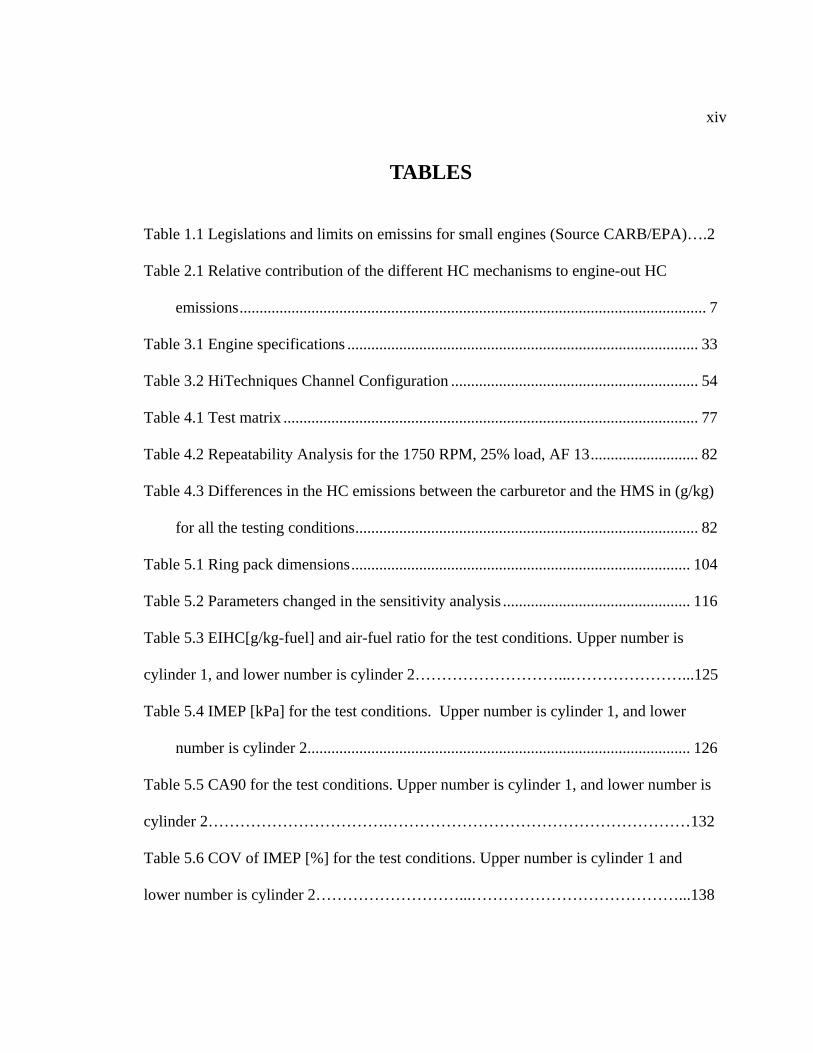
TABLES
Table 1.1 Legislations and limits on emissins for small engines (Source CARB/EPA)….2
Table 2.1 Relative contribution of the different HC mechanisms to engine-out HC
emissions..................................................................................................................... 7
Table 3.1 Engine specifications ........................................................................................ 33
Table 3.2 HiTechniques Channel Configuration .............................................................. 54
Table 4.1 Test matrix ........................................................................................................ 77
Table 4.2 Repeatability Analysis for the 1750 RPM, 25% load, AF 13........................... 82
Table 4.3 Differences in the HC emissions between the carburetor and the HMS in (g/kg)
for all the testing conditions...................................................................................... 82
Table 5.1 Ring pack dimensions..................................................................................... 104
Table 5.2 Parameters changed in the sensitivity analysis ............................................... 116
Table 5.3 EIHC[g/kg-fuel] and air-fuel ratio for the test conditions. Upper number is
cylinder 1, and lower number is cylinder 2………………………...…………………...125
Table 5.4 IMEP [kPa] for the test conditions. Upper number is cylinder 1, and lower
number is cylinder 2................................................................................................ 126
Table 5.5 CA90 for the test conditions. Upper number is cylinder 1, and lower number is
cylinder 2…………………………….…………………………………………………132
Table 5.6 COV of IMEP [%] for the test conditions. Upper number is cylinder 1 and
lower number is cylinder 2………………………...…………………………………...138
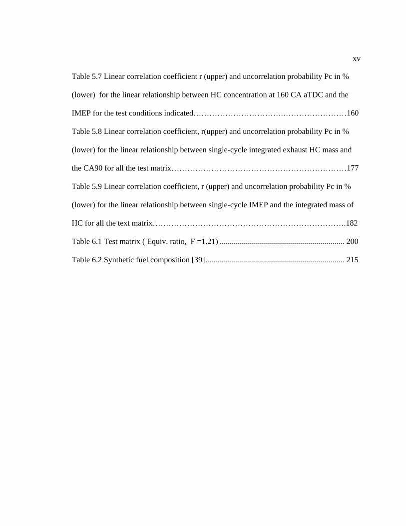
xv
Table 5.7 Linear correlation coefficient r (upper) and uncorrelation probability Pc in %
(lower) for the linear relationship between HC concentration at 160 CA aTDC and the
IMEP for the test conditions indicated…………………………….……………………160
Table 5.8 Linear correlation coefficient, r(upper) and uncorrelation probability Pc in %
(lower) for the linear relationship between single-cycle integrated exhaust HC mass and
the CA90 for all the test matrix…………………………………………………………177
Table 5.9 Linear correlation coefficient, r (upper) and uncorrelation probability Pc in %
(lower) for the linear relationship between single-cycle IMEP and the integrated mass of
HC for all the text matrix……………………………………………………………….182
Table 6.1 Test matrix ( Equiv. ratio, F =1.21) ............................................................... 200
Table 6.2 Synthetic fuel composition [39]...................................................................... 215
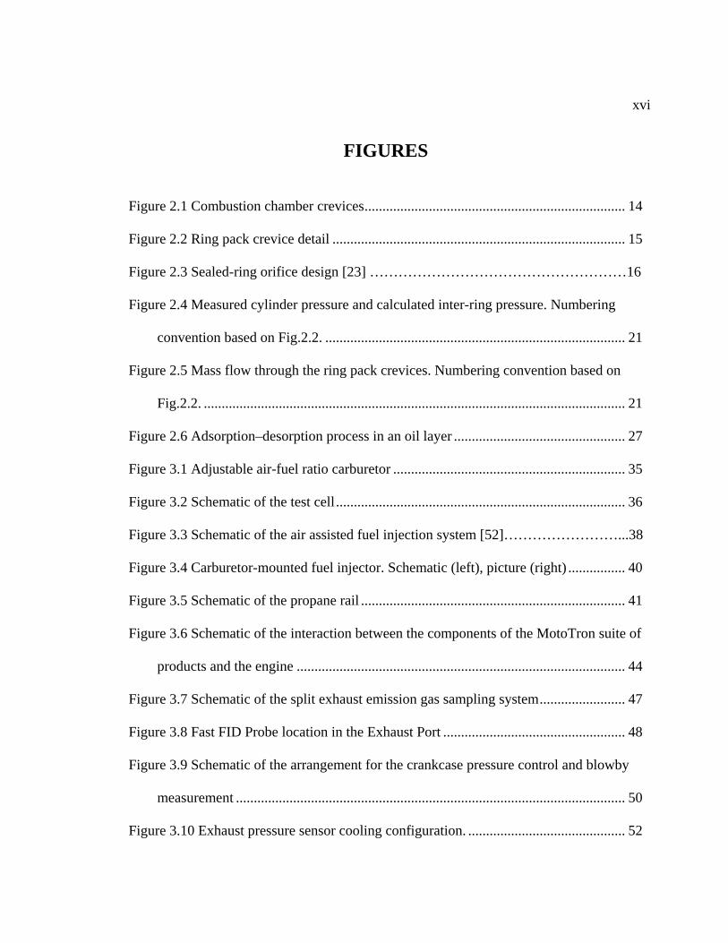
xvi
FIGURES
Figure 2.1 Combustion chamber crevices......................................................................... 14
Figure 2.2 Ring pack crevice detail .................................................................................. 15
Figure 2.3 Sealed-ring orifice design [23] ………………………………………………16
Figure 2.4 Measured cylinder pressure and calculated inter-ring pressure. Numbering
convention based on Fig.2.2. .................................................................................... 21
Figure 2.5 Mass flow through the ring pack crevices. Numbering convention based on
Fig.2.2. ...................................................................................................................... 21
Figure 2.6 Adsorption–desorption process in an oil layer ................................................ 27
Figure 3.1 Adjustable air-fuel ratio carburetor ................................................................. 35
Figure 3.2 Schematic of the test cell................................................................................. 36
Figure 3.3 Schematic of the air assisted fuel injection system [52]……………………...38
Figure 3.4 Carburetor-mounted fuel injector. Schematic (left), picture (right) ................ 40
Figure 3.5 Schematic of the propane rail .......................................................................... 41
Figure 3.6 Schematic of the interaction between the components of the MotoTron suite of
products and the engine ............................................................................................ 44
Figure 3.7 Schematic of the split exhaust emission gas sampling system........................ 47
Figure 3.8 Fast FID Probe location in the Exhaust Port ................................................... 48
Figure 3.9 Schematic of the arrangement for the crankcase pressure control and blowby
measurement ............................................................................................................. 50
Figure 3.10 Exhaust pressure sensor cooling configuration. ............................................ 52
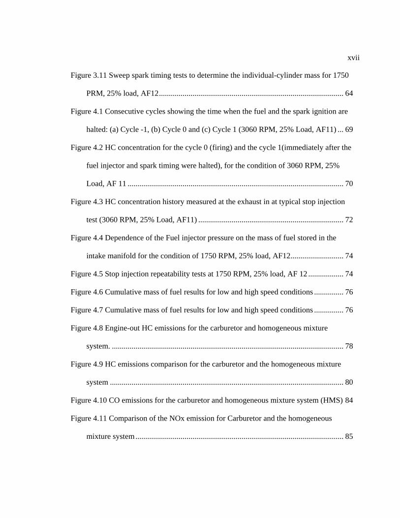
xvii
Figure 3.11 Sweep spark timing tests to determine the individual-cylinder mass for 1750
PRM, 25% load, AF12.............................................................................................. 64
Figure 4.1 Consecutive cycles showing the time when the fuel and the spark ignition are
halted: (a) Cycle -1, (b) Cycle 0 and (c) Cycle 1 (3060 RPM, 25% Load, AF11) ... 69
Figure 4.2 HC concentration for the cycle 0 (firing) and the cycle 1(immediately after the
fuel injector and spark timing were halted), for the condition of 3060 RPM, 25%
Load, AF 11 .............................................................................................................. 70
Figure 4.3 HC concentration history measured at the exhaust in at typical stop injection
test (3060 RPM, 25% Load, AF11) .......................................................................... 72
Figure 4.4 Dependence of the Fuel injector pressure on the mass of fuel stored in the
intake manifold for the condition of 1750 RPM, 25% load, AF12........................... 74
Figure 4.5 Stop injection repeatability tests at 1750 RPM, 25% load, AF 12 .................. 74
Figure 4.6 Cumulative mass of fuel results for low and high speed conditions ............... 76
Figure 4.7 Cumulative mass of fuel results for low and high speed conditions ............... 76
Figure 4.8 Engine-out HC emissions for the carburetor and homogeneous mixture
system. ...................................................................................................................... 78
Figure 4.9 HC emissions comparison for the carburetor and the homogeneous mixture
system ....................................................................................................................... 80
Figure 4.10 CO emissions for the carburetor and homogeneous mixture system (HMS) 84
Figure 4.11 Comparison of the NOx emission for Carburetor and the homogeneous
mixture system.......................................................................................................... 85
xviii
Figure 4.12 Cycle-resolved HC measurements for (a) 1750 RPM and 10% load, (b) 1750
RPM and 25% load, (c) 3060 RPM and 25% load, (d) 3060 RPM and 50% load, (e)
3060 RPM and 100% load. ....................................................................................... 89
Figure 4.13 Heat release analysis for (a) 1750 RPM and 10% load, (b) 1750 RPM and
25% load, (c) 3060 RPM and 25% load, (d) 3060 RPM and 50% load, (e) 3060
RPM and 100% load. ................................................................................................ 91
Figure 5.1 Ring pack geometry......................................................................................... 95
Figure 5.2 Piston Ring Geometry ..................................................................................... 96
Figure 5.3 Forces acting on the ring [27].......................................................................... 97
Figure 5.4 Ring pack crevices (left) and its representation as a system of interconnected
volumes (right).......................................................................................................... 99
Figure 5.5 Pressure in the combustion chamber (top land crevice) P1, in the inter-ring
volume P2 and in the crankcase P3, for the 3060RPM, 50% Load, AF 12............. 105
Figure 5.6 Relative position of the ring within the piston groove for the 3060RPM, 50%
Load, AF 12 ............................................................................................................ 106
Figure 5.7 Mass flow rates crossing the entrance of the top land crevice (m1), the first
ring end gap (m2), and the second ring end gap (m3), for the 3060RPM, 50% Load,
AF 12. ..................................................................................................................... 108
Figure 5.8 Percent of the total mass of mixture (a) and fuel (b) trapped in the cylinder that
crosses the entrance of the top land crevice (m1), the first ring end gap (m2), and the
second ring end gap (m3) that goes into the volumes V1, V2, and V3 respectively for
3060RPM, 50% Load, AF12. ................................................................................. 109
xix
Figure 5.9 Percent of the total mass of mixture (a) and fuel (b) trapped in the cylinder that
crosses the entrance of the top land crevice (m1), the first ring end gap (m2), and the
second ring end gap (m3) that leaves the volumes V1, V2, and V3 respectively for
3060RPM, 50% Load, AF12. ................................................................................. 111
Figure 5.10 Percent of the total mass of mixture (a) and fuel (b) trapped in the cylinder
that crosses the second ring end gap (m3) that goes to the crankcase as blowby for
3060RPM, 50% Load, AF12. ................................................................................. 112
Figure 5.11 Blowby mass flow comparison between experimental and ring pack model
results. The different symbol shape represents a given speed-load condition from
Table 5.2. ................................................................................................................ 114
Figure 5.12 (a) Sensitivity of the blowby to several parameters, and (b) definition of the
geometric parameters. EG-RI, and EG-RII stand for end gap of first and second ring
respectively. Cd is the discharge coefficient, Twall the cylinder temperature wall in
the model, and Pcrk_offset the offset in crankcase pressure. ................................. 117
Figure 5.13 Sensitivity of the mass that returns to the cylinder to several parameters. EG-
RI, and EG-RII stand for end gap of first and second ring respectively. Cd is the
discharge coefficient, Twall the cylinder temperature wall in the model, and
Pcrk_offset the offset of the crankcase pressure..................................................... 119
Figure 5.14 Illustration of the two metrics used to estimate the ring pack contribution to
the HC emissions. (a) Mass flow rate, and (b) cumulative mass for the 3060 RPM,
50% load, AF12. ..................................................................................................... 122
xx
Figure 5.15 Rate of heat release and cumulative heat release diagram showing the
convention to characterize the combustion phasing for the 3060 RPM, 50% load,
AF12. ...................................................................................................................... 123
Figure 5.16 Ring pack model results for all the tested conditions, (a) 1750 RPM, 10%
load, (b) 1750 RPM, 25% load, (c) 3060 RPM, 25% load , (d), 3060RPM, 50% load,
(e) 3060 RPM, 100% load. ..................................................................................... 128
Figure 5.17 Rate of heat release for 1750 RPM and 10% load as a function of the air fuel
ratio. ........................................................................................................................ 134
Figure 5.18 Rate of heat release for 1750 RPM and 25% load as a function of the air-fuel
ratio. ........................................................................................................................ 135
Figure 5.19 Rate of heat release for 3060 RPM and 25% load as a function of the air-fuel
ratio. ........................................................................................................................ 135
Figure 5.20 Rate of heat release for 3060 RPM and 50% load as a function of the air fuel
ratio. ........................................................................................................................ 136
Figure 5.21 Rate of heat release for 3060 RPM and 100% load as a function of the air
fuel ratio. ................................................................................................................. 136
Figure 5.22 EIHC predicted by the ring pack model from single cycle analysis for 1750
RPM, 10% load, AF12............................................................................................ 140
Figure 5.23 EIHC predicted by the ring pack model from single cycle analysis for 1750
RPM, 25% load, AF12............................................................................................ 141
Figure 5.24 EIHC predicted by the ring pack model from single cycle analysis for 3060
RPM, 25% load, AF12............................................................................................ 141
xxi
Figure 5.25 EIHC predicted by the ring pack model from single cycle analysis for 3060
RPM, 50% load, AF12............................................................................................ 142
Figure 5.26 EIHC predicted by the ring pack model from single cycle analysis for 3060
RPM, 100% load, AF12.......................................................................................... 142
Figure 5.27 Single cycle rate of heat release for 1750 RPM, 10% load, at different air-fuel
ratios (a) AF 12:1, (b) AF 13:1, (c) AF 14:1. ......................................................... 146
Figure 5.28 Single cycle rate of heat release for 1750 RPM, 25% load, at different air-fuel
ratios (a) AF 12:1, (b) AF 13:1, (c) AF 14:1. ......................................................... 147
Figure 5.29 Single cycle rate of heat release for 3060 RPM, 25% load, at different air-fuel
ratios (a) AF 11:1, (b) AF 12:1. .............................................................................. 148
Figure 5.30 Single cycle rate of heat release for 3060 RPM, 50% load, at different air-fuel
ratios (a) AF 11:1, (b) AF 12:1. .............................................................................. 149
Figure 5.31 Single cycle rate of heat release for 3060 RPM, 100% load, at different air-
fuel ratios (a) AF 11:1, (b) AF 12:1........................................................................ 150
Figure 5.32 Single-cycle resolved HC measurements for cylinder 1 (a) 1750 RPM, 10%
load, AF12, (b) 1750 RPM, 25% load, AF 12, (c) 3060 RPM, 25% load, AF12, (d)
3060 RPM, 50% load, AF12, and 3060 RPM, 100% load, AF12. ......................... 152
Figure 5.33 HC concentration at 160 CA aTDC vs. IMEP of same cycle for 1750 RPM,
10% load, at different air-fuel ratios (a) AF 12:1, (b) AF 13:1, (c) AF 14:1.......... 154
Figure 5.34 HC concentration at 160 CA aTDC vs. IMEP of same cycle for 1750 RPM,
25% load, at different air-fuel ratios (a) AF 12:1, (b) AF 13:1, (c) AF 14:1.......... 155
xxii
Figure 5.35 HC concentration at 160 CA aTDC vs. IMEP of same cycle for 3060 RPM,
25% load, at different air-fuel ratios (a) AF 11:1, (b) AF 12:1. ............................. 156
Figure 5.36 HC concentration at 160 CA aTDC vs. IMEP of same cycle for 3060 RPM,
50% load, at different air-fuel ratios (a) AF 11:1, (b) AF 12:1. ............................. 157
Figure 5.37 HC concentration at 160 CA aTDC vs. IMEP of same cycle for 3060 RPM,
100% load, at different air-fuel ratios (a) AF 11:1, (b) AF 12:1. ........................... 158
Figure 5.38 Discharge coefficient as a function of the valve lift.................................... 162
Figure 5.39 Schematic of the exhaust valve at is geometrical parameters. .................... 162
Figure 5.40 Cylinder, exhaust, and exhaust shifted pressures during the period when the
exhaust valve is open for (a) 1750 RPM, 10% load, AF 12 and (b) 3060 RPM, 100%
load, AF12............................................................................................................... 164
Figure 5.41 Exhaust gas mass flow rate and exhaust HC mass flow rate for (a) 1750
RPM, 10% load, AF12 and (b) 1750 RPM, 25% load, AF12................................. 166
Figure 5.42 Exhaust gas mass flow rate and exhaust HC mass flow rate for (a) 3060
RPM, 25% load, AF12, (b) 3060 RPM, 50% load, AF12 and (c) 3060 RPM, 100%
load, AF12............................................................................................................... 167
Figure 5.43 Calculated mass of HC vs. the measured HC at the exhaust for the average
data fro all the test matrix. ...................................................................................... 168
Figure 5.44 Calculated mass of HC vs. the measured HC at the exhaust for the single
cycle data for (a) 1750 RPM, 10% load, AF12, and (b) 1750 RPM, 25% load, AF12.
................................................................................................................................. 169
xxiii
Figure 5.45 Calculated mass of HC vs. the measured HC at the exhaust for the single
cycle data for (a) 3060 RPM, 25% load, AF12, (b) 3060 RPM, 50% load, AF12, and
(c) 3060 RPM, 100% load, AF12. .......................................................................... 170
Figure 5.46 Calculated mass of HC vs. CA90 for (a) 1750 RPM, 10% load, AF12, (b)
1750 RPM, 10% load, AF13, and (c) 1750 RPM, 10% load, AF14....................... 173
Figure 5.47 Calculated mass of HC vs. CA90 for (a) 1750 RPM, 25% load, AF12, (b)
1750 RPM, 25% load, AF13, and (c) 1750 RPM, 25% load, AF14....................... 174
Figure 5.48 Calculated mass of HC vs. CA90 for (a) 3060 RPM, 25% load, AF11, and
(b) 3060 RPM, 25% load, AF12. ............................................................................ 175
Figure 5.49 Calculated mass of HC vs. CA90 for (a) 3060 RPM, 50% load, AF11, and
(b) 3060 RPM, 50% load, AF12. ............................................................................ 175
Figure 5.50 Calculated mass of HC vs. CA90 for (a) 3060 RPM, 100% load, AF11, and
(b) 3060 RPM, 100% load, AF12. .......................................................................... 176
Figure 5.51 IMEP vs. calculated mass of HC for (a) 1750 RPM, 10% load, AF12, (b)
1750 RPM, 10% load, AF13, and (c) 1750 RPM, 10% load, AF14....................... 178
Figure 5.52 IMEP vs. calculated mass of HC for (a) 1750 RPM, 25% load, AF12, (b)
1750 RPM, 25% load, AF13, and (c) 1750 RPM, 25% load, AF14....................... 179
Figure 5.53 IMEP vs. calculated mass of HC for (a) 3060 RPM, 25% load, AF11, and (b)
3060 RPM, 25% load, AF12................................................................................... 180
Figure 5.54 IMEP vs. calculated mass of HC for (a) 3060 RPM, 50% load, AF11, and (b)
3060 RPM, 50% load, AF12................................................................................... 180
xxiv
Figure 5.55 IMEP vs. calculated mass of HC for (a) 3060 RPM, 100% load, AF11, and
(b) 3060 RPM, 100% load, AF12. .......................................................................... 181
Figure 5.56 CA90 vs. IMEP for (a) 1750 RPM, 10% load, AF12, (b) 1750 RPM, 25%
load, AF12, (c) 3060 RPM, 25% load, AF12, (d) 3060 RPM, 50% load, AF12 and
(e) 3060 RPM, 100% load, AF12. .......................................................................... 183
Figure 5.57 Conditional Sampling of the heat release for (a) 1750 RPM, 10% load, AF12,
and (b) 1750 RPM, 25% load, AF12. ..................................................................... 186
Figure 5.58 Conditional sampling of the heat release for (a) 3060 RPM, 25% load, AF12,
(b) 3060 RPM, 50% load, AF12, and (c) 3060 RPM, 100% load, AF12, showing the
averages of the intervals under study...................................................................... 187
Figure 5.59 Ring pack HC estimation vs. the HC mass at the exhaust for the (a) 1750
RPM, 10% load, AF 12, and (b) 1750 RPM, 25% load, AF12............................... 190
Figure 5.60 Ring pack HC estimation vs. the HC mass at the exhaust for the (a)
3060RPM, 25% load, AF 12, (b) 3060 RPM, 50% load, AF12, and (c) 3060 RPM,
100% load, AF12. ................................................................................................... 191
Figure 5.61 Fast FID average traces for the different CA90 sections for (a) 1750 RPM,
10% load, AF12, and (b) 1750 RPM, 25% load, AF12. ......................................... 194
Figure 5.62 Fast FID average traces for the different CA90 sections for (a) 3060 RPM,
25% load, AF12, (b) 3060 RPM, 50% load, AF12, and (b) 3060 RPM, 100% load,
AF12. ...................................................................................................................... 195
Figure 6.1 Average HC emissions comparison between propane and gasoline for: (case
1), 1750 RPM, 10% load, (case 2) 1750 RPM, 25% load, (case 3) 3060 RPM, 25%

xxv
load, and (case 4) 3060 RPM, 50% load,. The crankcase pressure for all cases was
101.85 kPa and Φ =1.21. ........................................................................................ 201
Figure 6.2 Average HC emissions vs. crankcase pressure (a) 1750 RPM, 10% load, (b)
1750 RPM, 25% load, (c) 3060 RPM, 25% load, and (d) 3060 RPM, 50% load.. 204
Figure 6.3 Average HC emissions vs. crankcase for gasoline at 3060 RPM, 100% load,
and Φ =1.21. .......................................................................................................... 205
Figure 6.4 Rate of heat release for three different conditions, (a) 1750 RPM, 10% load,
and (b) 1750 RPM, 25% load ................................................................................. 208
Figure 6.5 Rate of heat release for three different conditions, (a) 3060 RPM, 25% load,
and (b) 3060 RPM, 50% load……………………………………………………..209
Figure 6.6 Comparison of the cycle-resolved HC emissions for gasoline and propane at:
(a) 1750 RPM, 10% load, and (b) 1750 RPM 25% load………………………….211
Figure 6.7 Comparison of the cycle-resolved HC emissions for gasoline and propane at:
(a) 3060 RPM, 25% load, and (b) 3600 RPM 50% load………………………….212
Figure 6.8 Schematic of the system for the static fuel-oil diffusion simulation….…….214
Figure 6.9 Percentage of initial fuel mass adsorbed by the oil (n-hexatriacontane) at
equilibrium as a function of the temperature and equivalence ratio Φ….………...217
Figure 6.10 Schematic of the fuel concentration in the oil film and in the combustion
chamber gas, along with the coordinate system used for the simulation….………219
Figure 6.11 Schematic of the oil segments used in the simulation….………………….223
xxvi
Figure 6.12 Percent of the trapped mass of fuel that is absorbed and desorbed from the oil
film for (a) 1750 RMP, 10% load, AF 12, and (b) 1750 RPM, 25% load, AF12. The
oil layer thickness was 2 µm and the wall temperature 380 K….………………...224
Figure 6.13 Percent of the trapped mass of fuel that is absorbed and desorbed from the oil
film for (a) 3060 RMP, 25% load, AF 12, (b) 3060 RPM, 50% load, AF12, and (c)
3060 RMP, 100% load, AF12. The oil layer thickness was 2 µm and the wall
temperature 380 K….……….……………………………………………………..226
Figure 6.14 Percent of the trapped mass of fuel that is absorbed and desorbed from the oil
film for (a) 3060 RMP, 50% load, AF 12. The fuel is propane, the oil layer thickness
was 2 µm and the wall temperature 380 K….……….……………………………228
Figure 6.15 Effect of the temperature on the percent of the trapped mass of fuel that is
absorbed and desorbed from the oil film for 3060 RMP, 25% load at (a)380K, (b)
440K, and (c) 500K. The oil layer thickness was 2 µm….……….……………….230
Figure A1. 1 Volumetric flow vs Voltage output of the transmitter of the Micromotion
flowmeter. ............................................................................................................... 251
Figure A2. 1 Schematic for the calibration process of the orifice plates to measure the air
mass flow rate ..................................................................................................... 252
Figure A2. 2 Calibration curves of the orifice plates used to measure the air mass flow.
................................................................................................................................. 253
Figure A3. 1 Calibration curves of the piezoelectric pressure transducers for the cylinder
pressure measurements. ...................................................................................... 254
xxvii
Figure A4. 1 Schematic of the Pressure configuration to correct the slow MAP sensor
response............................................................................................................... 256
Figure A4. 2 Signals from the piezoelectric and MAP (strain gage) sensors for 1000
RPM, 25% load, motored........................................................................................ 257
Figure A4. 3 Traces from the piezoelectric and corrected MAP sensors for 1000 RPM,
25% load, motored. ................................................................................................. 257
Figure A15. 1 EIHC predicted by the ring pack model from single cycle analysis for 1750
RPM, 10% load, AF13........................................................................................ 327
Figure A15. 2 EIHC predicted by the ring pack model from single cycle analysis for 1750
RPM, 10% load, AF14............................................................................................ 328
Figure A15. 3 EIHC predicted by the ring pack model from single cycle analysis for 1750
RPM, 25% load, AF13............................................................................................ 328
Figure A15. 4 EIHC predicted by the ring pack model from single cycle analysis for 1750
RPM, 25% load, AF14............................................................................................ 329
Figure A15. 5 EIHC predicted by the ring pack model from single cycle analysis for 3060
RPM, 25% load, AF11............................................................................................ 329
Figure A15. 6 EIHC predicted by the ring pack model from single cycle analysis for 3060
RPM, 50% load, AF11............................................................................................ 330
Figure A15. 7 EIHC predicted by the ring pack model from single cycle analysis for 3060
RPM,100% load, AF11........................................................................................... 330
xxviii
Figure A16. 1 Single-cycle resolved HC measurements for cylinder 2 at (a) 1750 RPM,
10% load, AF13, (b) 1750 RPM, 25% load, AF13, (c) 3060 RPM, 25% load, AF13,
(d) 3060 RPM, 50% load, AF13, and 3060 RPM, 100% load, AF13..................... 331
xxix
NOMENCLATURE A Area
AF mixture air-fuel ratio
ap piston acceleration
aTDC after top dead center
B bore
bTDC before top dead center
C constant, concentration
c speed of the sound in the gas
CA crank angle
CA50 crank angle at the mass fraction burned of 50%
CA90 crank angle at the mass fraction burned of 90%
CA90-EVO time interval from CA90 to EVO
DC discharge coefficient
CO carbon monoxide
CO2 carbon dioxide
COV coefficient of variance
CMFIS carburetor mounted fuel injection system
cv specific heat at constant volume
D diffusivity
d diameter
d1L diameter of the bottom edge of the first piston groove
d1U diameter of the upper edge of the first piston groove
d3L diameter of the bottom edge of the second piston groove
d3U diameter of the upper edge of the second piston groove
di2 internal diameter of the first piston groove
di4 internal diameter of the second piston groove
Dv exhaust valve diameter
Ea activation energy
xxx
ECU electronic control unit
EG-RI first ring end gap
EG-RII second ring end gap
EIi emission index of species i
EVO exhaust valve opening
EVC exhaust valve closing
EIHCM,EXH HC emission index measured at the exhaust
EIHCC,RP HC emission index calculated using the ring pack model
EIHCC,MB HC emission index calculated from the mass balance at the exhaust
F force
FID flame ionization detector
FFID fast-flame ionization detector
h relative position of the ring in the grove
H2 hydrogen
H2O water
h1 first piston groove height
h2 second piston groove height
h3 top inter-grove height
h4 bottom inter-grove height
hc heat transfer coefficient
HC hydrocarbon
hR ring height
hRI height of the first ring
hRII height of the second ring
HMS homogeneous mixture system
IMEP indicated mean pressure
IVC intake valve closing
IVO intake valve opening
K static sensitivity, constant equilibrium
k specific heat ratio
Lv lift exhaust valve
xxxi
LHV lower heating value
m mass
m& mass flow rate
MAP manifold absolute pressure
MW molecular weight
N mole
N& molar flow rate
N2 nitrogen
NOx oxides of nitrogen
O2 oxygen
P pressure
Pc unprobability correlation
ppm parts per million
R gas constant
Q heat
RPM revolutions per minute
RSS root-sum-squares
S stroke
Sp mean piston speed
t time
T temperature
TDC top dead center
up piston velocity
U internal energy
V volume, volts
VA molar volume of solute A at its normal boiling temperature
Vc critical volume
wRI width of the first ring
wRII width of the second ring
x ring pack parameter, distance
X molar fraction

xxxii
y hydrogen to carbon ratio
yres in cylinder residual mass fraction
Y mass fraction
# number
[i] concentration of species i
∝ infinity
GREEK SYMBOLS
δ oil layer thickness ∆ increment η compressibility factor, efficiency γ specific heat ratio of the gas
Bµ viscosity of the solvent B ρ density of the gas φ angle θ angle Φ equivalence ratio τ time constant
SUB- AND SUPER-SCRIPTS
act actual air air C carbon c combustion C1 1 carbon basis C3 3 carbon basis carb carburetor corr corrected cr crankcase crev crevice crk_offset crankcase offset cyl cylinder d downstream disp displaced evo exhaust valve opening exh exhaust fuel fuel f friction

xxxiii
fuel/cycle fuel per cycle fuel-engine/cycle fuel injected per cycle fuel-cum.-norm normalized cumulative mass of fuel hr heat release H hydrogen HV heating value i index, species in-cum in cumulative m motoring max maximum mix mixture n potytropic exponent out-cum out cumulative p products ref reference s stick, system u upstream uncer uncertainty w wall
1
CHAPTER I
INTRODUCTION
1.1 OVERVIEW
Small engines are identified as a major source of air pollution by the California
Air Resources Board (CARB) and the Environmental Protection Agency (EPA). Every
year approximately 100 million of small engines are produced worldwide [1]. From this
total about 35 million are sold in the US. This is very significant compared with the
approximately 17 million of cars sold in the US [2]. Small engines usually run for
shorter periods of time than the automotive engines however their emissions levels are
significantly higher accounting as much as 13% of the total hydrocarbon emissions in
some regions of the US [3]. Therefore there is a considerable pressure on the
manufacturers to reduce the emissions levels by way of new, lower emission standards.
1.2 LEGISLATION
The CARB is the leading regulatory agency regarding emissions from small
engines followed by the EPA. Table 1.1 shows the general status of the CARB and EPA
legislations for the handheld and non-handheld small engines. The CARB 3 emission
regulations have been already implemented and the CARB Blue Skies have been
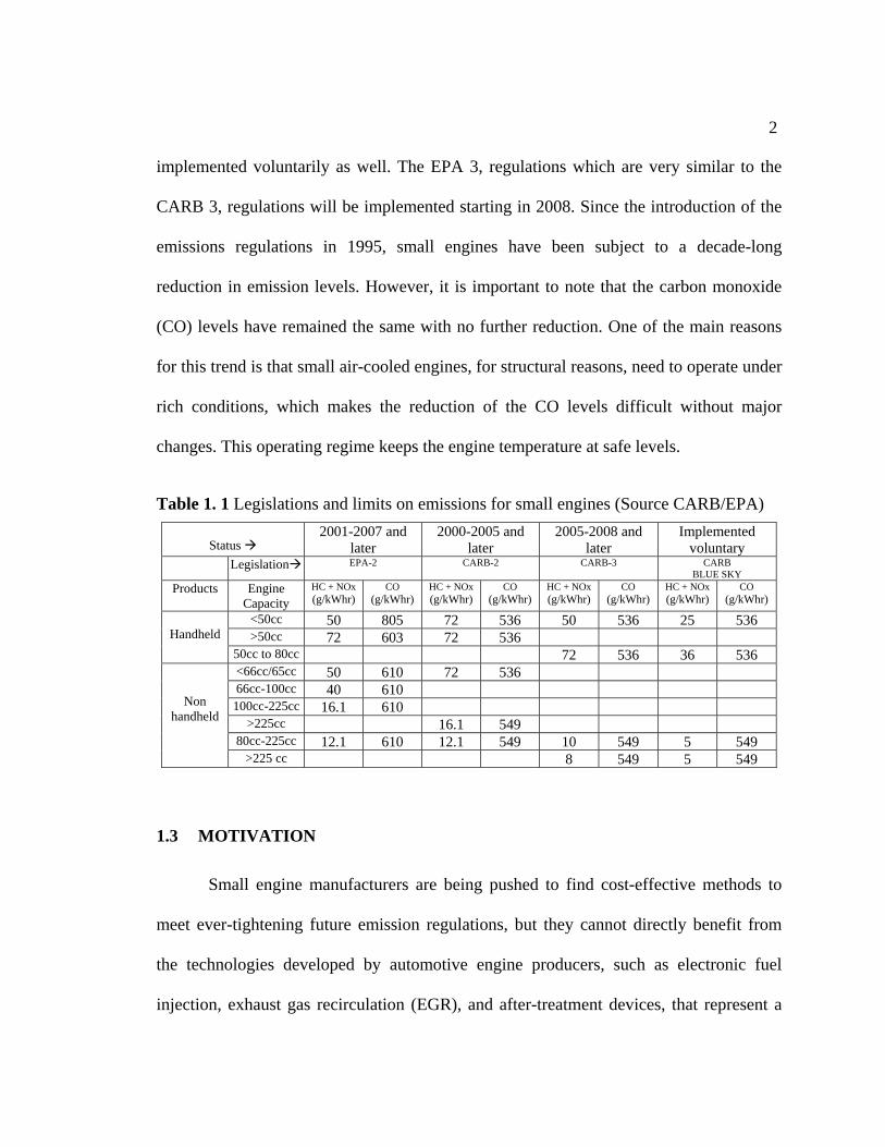
2
implemented voluntarily as well. The EPA 3, regulations which are very similar to the
CARB 3, regulations will be implemented starting in 2008. Since the introduction of the
emissions regulations in 1995, small engines have been subject to a decade-long
reduction in emission levels. However, it is important to note that the carbon monoxide
(CO) levels have remained the same with no further reduction. One of the main reasons
for this trend is that small air-cooled engines, for structural reasons, need to operate under
rich conditions, which makes the reduction of the CO levels difficult without major
changes. This operating regime keeps the engine temperature at safe levels.
Table 1. 1 Legislations and limits on emissions for small engines (Source CARB/EPA)
Status 2001-2007 and
later 2000-2005 and
later 2005-2008 and
later Implemented
voluntary Legislation EPA-2 CARB-2 CARB-3 CARB
BLUE SKY Products Engine
Capacity HC + NOx (g/kWhr)
CO (g/kWhr)
HC + NOx (g/kWhr)
CO (g/kWhr)
HC + NOx (g/kWhr)
CO (g/kWhr)
HC + NOx (g/kWhr)
CO (g/kWhr)
<50cc 50 805 72 536 50 536 25 536 >50cc 72 603 72 536
Handheld
50cc to 80cc 72 536 36 536 <66cc/65cc 50 610 72 536 66cc-100cc 40 610 100cc-225cc 16.1 610
>225cc 16.1 549 80cc-225cc 12.1 610 12.1 549 10 549 5 549
Non handheld
>225 cc 8 549 5 549
1.3 MOTIVATION
Small engine manufacturers are being pushed to find cost-effective methods to
meet ever-tightening future emission regulations, but they cannot directly benefit from
the technologies developed by automotive engine producers, such as electronic fuel
injection, exhaust gas recirculation (EGR), and after-treatment devices, that represent a
3
significant increase in production costs. Therefore, small engines will still use simple,
reliable and low-cost devices like the carburetor, and the study of engines using such
accessories is still important.
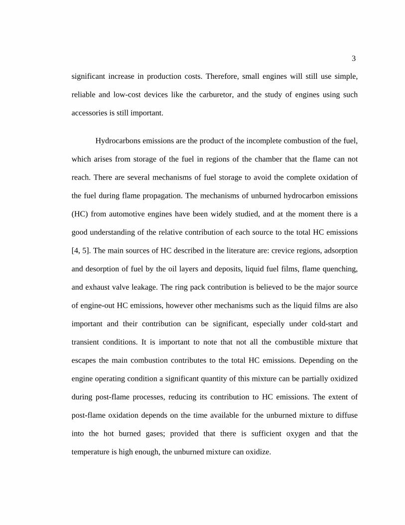
Hydrocarbons emissions are the product of the incomplete combustion of the fuel,
which arises from storage of the fuel in regions of the chamber that the flame can not
reach. There are several mechanisms of fuel storage to avoid the complete oxidation of
the fuel during flame propagation. The mechanisms of unburned hydrocarbon emissions
(HC) from automotive engines have been widely studied, and at the moment there is a
good understanding of the relative contribution of each source to the total HC emissions
[4, 5]. The main sources of HC described in the literature are: crevice regions, adsorption
and desorption of fuel by the oil layers and deposits, liquid fuel films, flame quenching,
and exhaust valve leakage. The ring pack contribution is believed to be the major source
of engine-out HC emissions, however other mechanisms such as the liquid films are also
important and their contribution can be significant, especially under cold-start and
transient conditions. It is important to note that not all the combustible mixture that
escapes the main combustion contributes to the total HC emissions. Depending on the
engine operating condition a significant quantity of this mixture can be partially oxidized
during post-flame processes, reducing its contribution to HC emissions. The extent of
post-flame oxidation depends on the time available for the unburned mixture to diffuse
into the hot burned gases; provided that there is sufficient oxygen and that the
temperature is high enough, the unburned mixture can oxidize.
4
Small engines, however, operate under different conditions than the automotive
engines. Small engines: use carburetors as a fuel delivery system; are air cooled, and
therefore have high operating temperature, which can give significant, uneven bore
distortion; and run with rich air-fuel ratios.
The atomization and subsequent vaporization of the fuel by the carburetor is
poor. Consequently, liquid fuel films in the intake manifold are formed and can adversely
impact the HC emissions. Another important aspect in small engines is that the residence
time in the intake manifold can be very short because in many cases the carburetor is
directly mounted to the head. Under such conditions, the fuel may not have enough time
to vaporize, producing a poorly vaporized and inhomogeneous air-fuel mixture.
Air cooling of small engines using external fins and an integral fan does not
provide a uniform cooling pattern, causing the engine to run hot in locations away from
the fan. This generates significant and uneven bore distortion. The bore distortion could
directly affect the mass flow through the ring pack crevices and the blowby, consequently
creating an impact on the HC emissions. In addition the adsorption-desorption
mechanism of the fuel in the oil could also be affected by the high operating temperature.
The rich operation in small engines has the advantage of higher output power
levels at cooler operating temperatures, which reduces thermal problems, and increases
the lifetime of the engine. Running under such conditions also gives good transient
response without the use special compensation systems in the carburetor. However part
5
of the fuel is not oxidized completely mainly due to the lack of oxygen, which generates
higher HC and CO emissions.
Hydrocarbon emissions have a negative impact on the environment and human
health, and represent a fraction of fuel that does not produce useful work, and therefore, a
reduction in the engine efficiency. In small engines for partial load conditions, mainly
because of the rich operation, the HC emissions dominate over the NOx in the legislated
HC+NOx emissions. Therefore, the HC mechanisms under the particular conditions of
small engine operation need to be studied
1.4 OBJECTIVES
The purpose of the present work is to study the relative contribution of each of the
unburned hydrocarbons mechanisms of a spark-ignited, carbureted, air-cooled V-twin
engine.
The HC mechanisms that were studied in depth were: the liquid fuel in the
cylinder, the ring pack crevices, and oil adsorption-desorption. The individual
contribution of each source on the total HC emissions will be studied for a wide range of
load, speed and spark timing conditions. Other HC sources that are known contributors
will be discussed and shown to be of lesser importance.
The remainder of the thesis will be presented as follows. In Chapter 2 a literature
review of the hydrocarbon emission mechanisms is provided. The majority of the
literature review comes from previous studies carried out in automotive engines. In

6
Chapter 3 the test cell and experimental apparatus are described. Chapter 4 details the
study of the liquid fuel mechanism and its impact on the hydrocarbon emissions. Chapter
5 discusses the estimation of the ring pack contribution on the HC emissions. The
findings of the effect of the fuel-oil adsorption-desorption on the HC are provided in
Chapter 6. Finally Chapter 7 covers the conclusions regarding to the main findings and
the recommendations for future work.
7
CHAPTER II
2 LITERATURE REVIEW
Hydrocarbon emission mechanisms for automotive engines have been studied
extensively. Detailed information about each possible mechanism and their relative
contribution to engine-out emissions has been obtained by using both experimental and
computational techniques. However, little small-engine-specific work been done;
therefore, the major source of information available in the literature is pertinent to
automotive engines.
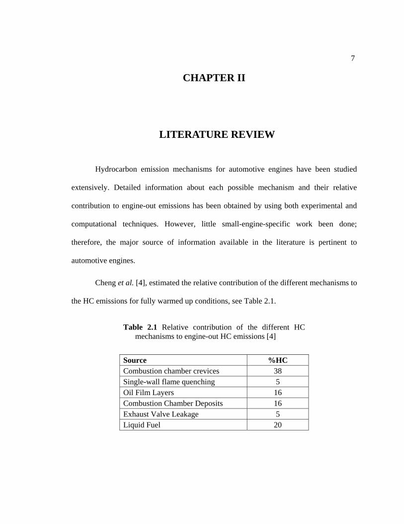
Cheng et al. [4], estimated the relative contribution of the different mechanisms to
the HC emissions for fully warmed up conditions, see Table 2.1.
Table 2.1 Relative contribution of the different HC mechanisms to engine-out HC emissions [4]
Source %HC Combustion chamber crevices 38 Single-wall flame quenching 5 Oil Film Layers 16 Combustion Chamber Deposits 16 Exhaust Valve Leakage 5 Liquid Fuel 20
8
The main contributors of the total output HC emissions are: the crevices, liquid
fuel, oil films and the combustion chamber deposits [5].
In §2.1 a literature review of the previous studies related to small engine
emissions is given, and is followed by a literature review of the different HC mechanism
for automotive engines in §2.2-2.9
2.1 PREVIOUS STUDIES OF EMISSIONS FROM SMALL ENGINES
There are no specific studies focused solely on HC emission mechanisms from
small engines. However, there are some studies reporting the general CO, HC and NOx
emission trends of small engines [6]. Thus, it is well known that the output power
requirement of small engines has a direct effect on the amount of HC, CO and NOx
emitted [6-11]. Hydrocarbon and CO emissions decrease as the load increase. In addition,
small engines, due to their particular design, run with rich air-fuel mixtures, producing
low levels of NOx and high levels of CO. It has been reported, that the air-fuel ratio has a
direct effect on the HC, CO and NOx emissions [8]. Swanson [10] implemented an
electronic port fuel injection system (EFI) on a small engine and showed that the air-fuel
mixture preparation had a significant impact on the emissions levels. Using the EFI
system, the brake specific CO (BSCO) and brake specific hydrocarbon plus oxides of
nitrogen (BSHC + NOx) were reduced 14.2% and 16.6% respectively.
Currently small engines still use carburetors as a fuel system, and the resulting
fuel atomization and subsequent vaporization of the fuel is poor and inefficient. Thus, a
significant amount of the fuel can enter the cylinder in the liquid phase. In addition, some
9
of the fuel impinges on the intake manifold and intake port walls, generating liquid fuel
films. The liquid fuel films can adversely affect the HC emissions [4]. Another important
aspect in small engines is that the residence time of the fuel in the intake manifold is very
short because in many engines the carburetor is directly mounted to the cylinder head.
Therefore, under steady-state operation the fuel may not have enough time to vaporize,
producing a poorly vaporized and inhomogeneous air-fuel mixture.
Itano et al. [12], studied the exit flow of several common carburetors. The idea
was to characterize the quality of the air-fuel mixture preparation by the carburetor. To
that end the air-fuel ratio was measured, and the exit flow was visualized with high speed
movies. The main findings of these tests were that there was a significant amount of
liquid fuel film formation on the wall of the manifold. In addition, the air-fuel ratio
measurements at the exit plane, revealed that the mixture was not uniform, having higher
air-fuel ratio close to the liquid fuel film. The problem of poor mixture preparation is
exacerbated under transient conditions [13].
It is known that the transient operation of the engine generates excursions in the
air-fuel ratio which are responsible for an increase in the HC, CO, and NOx emissions. In
the same way, transient conditions increase the formation of liquid fuel films in the intake
manifold, which act as a sink or source of fuel, causing a fluctuation in the air fuel ratio.
The transient behavior of the liquid films in the intake manifold of a four-stroke small
engine has been characterized by Jehlik et al. [13], who modified the stock engine
carburetor by incorporating a fuel injector. This setup allowed total control of the
10
injection process on a single-cycle basis. Transient tests like: step-fueling changes with
constant air flow, step-throttle changes with constant fuel flow, skip-injection and stop-
injection were performed. The idea was to characterize the liquid fuel films dynamics
under transient conditions. The engine was fueled with indolene, iso-octane, and propane
to isolate the vaporization effect. The main findings of this work were: the film dynamics
are dominated by the airflow in the intake manifold, and that the vaporization from the
fuel film in the intake walls contributed approximately 30% of the fuel inducted per cycle
regardless of load.
Bonneau [14] compared the operation of a small engine using two different fuel
systems at 10% and 50% load. In this study, the engine was first operated with the
carburetor, and then with a homogeneous pre-vaporized fuel mixture system. The results
showed that for a range of air-fuel ratios from 11.5 to 16 the carburetor did not have a
significant impact on the HC emissions; the behavior of both systems was remarkably
similar. However, for leaner air-fuel ratios the carburetor fuel system showed increased
levels of HC emissions.
2.2 LIQUID FUEL FILMS
In port-injected (PFI) engines the fuel spray usually impinges on the back side of
the intake valve and the surrounding intake port surfaces. Depending of the operating
condition of the engine, part of the fuel evaporates and part of the fuel forms a liquid film
on the back side of the valve, intake manifold and intake port. As a consequence, part of
the fuel enters to the cylinder as liquid films, droplets and ligaments. In the automotive
11
industry most of the engine-out HC emissions are oxidized using a catalyst. However,
due to the stringent emission regulations, the HC emissions are still being investigated
especially during the cold start transient, which accounts for 80-90% of the total tailpipe
HC emissions. Another area of recent interest is the formation of fuel films on the piston
surface in a direct-injection engine. It is believed that under such conditions there is also
a fuel film contribution to the particulate matter formation.
The reduction of HC emissions in a port-injected (PFI) engine using a pre-
vaporized fuel system during the cold star and warm up periods was studied by Boyle and
Boam [15]. They compared the HC emissions when different engines were fueled with
liquid gasoline, and with pre-vaporized gasoline, which eliminated the liquid fuel film
effect. The results showed a reduction of 15 to 40% in the HC emissions when operating
the engine in the pre-vaporized fuel mode. This finding highlights the importance of the
liquid fuel in the HC emissions.
The phenomena that determine the inflow process of the liquid fuel past the
intake valve in a PFI engine was addressed experimentally by Meyer et al. [16]. The
study simulated a cold-start process in a transparent engine. Detailed characterization of
the fuel droplets entering the cylinder was made using a Phase Doppler Particle Analyzer
(PDPA). In addition, Planar Laser-Induced Fluorescence (PLIF) visualization of the fuel
spray was carried out. Based on the droplet measurements and the qualitative geometrical
information of the PLIF measurements, a method to determine the amount of fuel mass
going into the cylinder was estimated for both closed-valve and open-valve injection
12
cases. The tests identified four transports mechanisms of liquid fuel into the cylinder:
forward flow atomization, spray contribution, high-speed intake flow transport, and fuel
film squeezing. The evolution in time of the liquid fuel going to the cylinder showed a
different behavior for both the closed-valve and open-valve injection cases. The
estimated fraction of liquid fuel entering the cylinder was 40 % and 25% of the injected
fuel 15 seconds after the start for closed-valve and open-valve cases respectively. Meyer
and Heywood [17], continuing the work of Meyer et al. [16], qualitatively studied the
influence of several engine and injector design parameters, and fuel parameters, on the
characteristics of the liquid fuel droplets entering the cylinder. Using a PDPA,
measurements of fuel droplet size distributions in the vicinity of the intake valve were
performed. The effect of the fuel volatility, injection timing, intake valve warming,
injector type, spray geometry, and spray targeting in the intake port were studied for both
closed-valve and open-valve injection cases. The results showed that there is a
significant dependence of the above-mentioned parameters on the liquid fuel in the
cylinder, both during the cold starting and the fully warmed up conditions. It was found
that the influence of the studied parameters on the amount of liquid fuel in the cylinder is
enough to be reflected on the HC output emissions. However no HC emissions
measurements were reported.
Takahashi and Nakase [18], using a non-intrusive optical technique, measured the
liquid fuel thickness in the intake port, the combustion chamber, and cylinder liner of a
port fuel injected engine. The measurements showed the evolution in time of the liquid
fuel film in the walls of the intake port, combustion chamber, and cylinder liner, during a
13
cold start. They found that the fuel film thickness in the intake port reaches its peak value
after 6 cycles of the start, and that the liquid fuel stored in the intake port started to enter
the cylinder three cycles after starting. Increasing the engine speed, load, coolant
temperature, and valve overlap resulted in thinner liquid fuel films.
As can be seen from the different sources above, liquid fuel films are considered
an important source of HC emissions, but their relative contribution is not clear.
2.3 RING PACK CREVICES
Combustion chamber crevices are an important source of HC emissions from
engines. As seen from Table 2.1, the crevices are the greatest contributors under fully
warmed up steady-state operation. However, for other particular conditions of engine
operation such as cold start, other sources are considered to be equally important. Several
studies regarding the HC crevices have been performed mainly focused on the impact of
reducing crevices volumes and on understanding the post flame oxidation. At the present,
it appears that there is a very good understanding of the crevice mechanism.
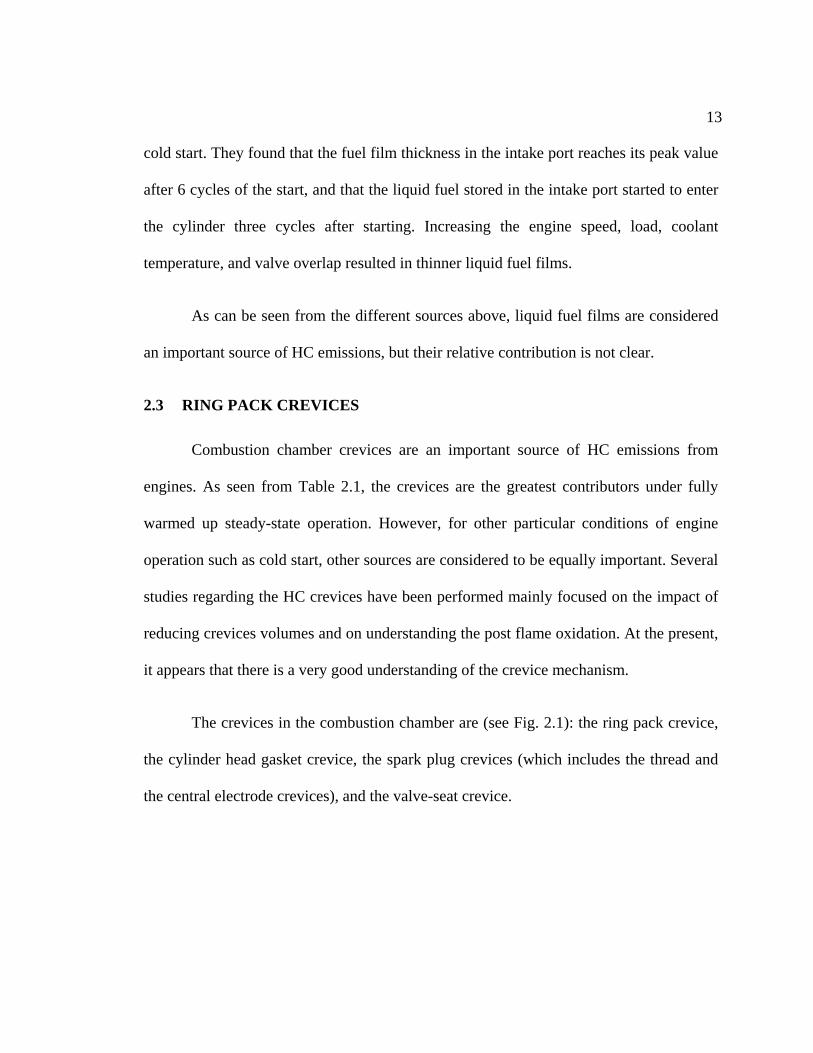
The crevices in the combustion chamber are (see Fig. 2.1): the ring pack crevice,
the cylinder head gasket crevice, the spark plug crevices (which includes the thread and
the central electrode crevices), and the valve-seat crevice.
14
Ring Pack
SparkPlugTread
CylinderHeadGasket
ValveSeat
Figure 2.1 Combustion chamber crevices
A crevice in the SI engine field is defined as a small space surrounded by walls
that is directly connected to the combustion chamber. The characteristic of a crevice is
that the small size of the passageway that connects the crevice with the main chamber
prevents the flame propagation, and thus, prevents oxidation of the combustible mixture
stored in the crevice. An easy way to characterize the ability of a flame to propagate into
a narrow passageway is the two wall quenching distance [19]. This distance is the critical
distance between two parallel plates below which the flame will not propagate. The
concept has been very useful to explain why the mixture stored in the crevices escapes
the main combustion. Several expressions that correlate the quench distance with other
parameters have been developed for internal combustion engines [20, 21]. The quench
distance depends on the equivalence ratio and the amount of charge dilution. Off-
stoichiometric air-fuel ratios and high dilution increases the quench distance [22].
15
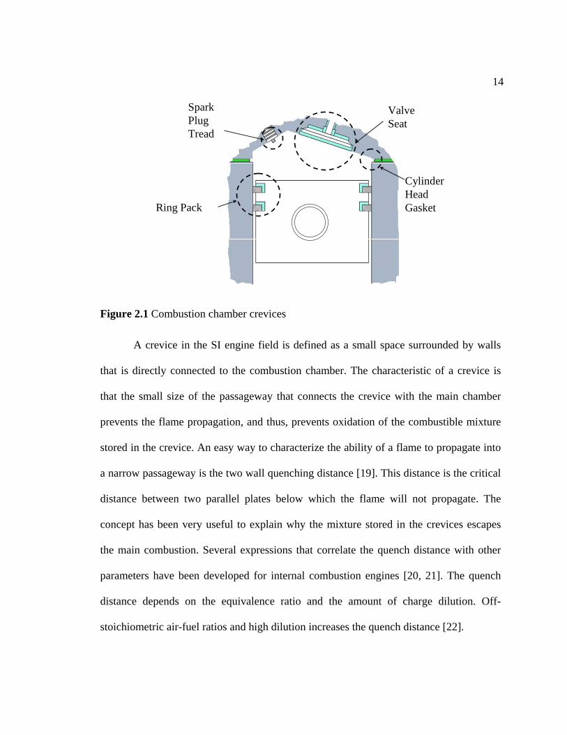
A detailed view of the ring pack is presented in Fig. 2.2. The ring pack crevices
consist of the piston upper crevices and the piston lower crevices. The piston upper
crevice (V1) is the space that is formed by the walls of the top piston land, the first ring,
and the cylinder wall. The lower piston crevice is the space formed between the two rings
(V2).
V1
V2
V3
1st Ring
2nd Ring
Oil Ring
Sideclearance
Land Height
Ring sideclearance
Figure 2.2 Ring pack crevice detail
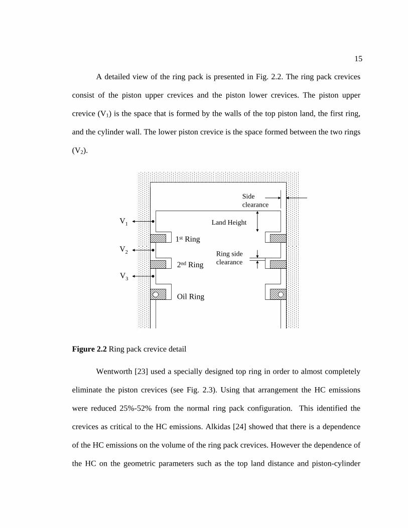
Wentworth [23] used a specially designed top ring in order to almost completely
eliminate the piston crevices (see Fig. 2.3). Using that arrangement the HC emissions
were reduced 25%-52% from the normal ring pack configuration. This identified the
crevices as critical to the HC emissions. Alkidas [24] showed that there is a dependence
of the HC emissions on the volume of the ring pack crevices. However the dependence of
the HC on the geometric parameters such as the top land distance and piston-cylinder
16
radial clearance shows a complicated relationship that involves not only the quench
distance but also other factors such as flame propagation.
Figure 2.3 Sealed-ring orifice design [23]
The change in HC emissions in response to changes in the top land height has
been studied by Alkidas [24]. Using a production engine, the HC emissions were reduced
22% when the top land height was reduced from 6 to 3 mm, which represented a 47%
reduction in the top land crevice volume.
Later, taking a different approach Bigninon and Spicher [25], tested six pistons
with different top land crevice geometry. Each piston had a different chamfer
configuration, ranging from 2 to 4 mm at 45°, and being either only half or continuous
around the top land. The observation of the flame intrusion into the top land crevice was
performed with the implementation of an optical fiber technique. The relation between
the top land crevices, output HC emissions and the flame penetration frequency in the
crevice were studied. An HC emissions reduction of 30% was obtained for the case
17
where the piston had the largest top land crevice. For this case the optical tests showed an
increase in the frequency of intrusion of the flame in the crevice.
The top land radial clearance, combined with the quench distance is an important
design parameter. Alkidas [24], observed that there is a critical radial clearance beyond
which the HC emissions are not affected by further increases in the radial clearance.
Below the critical value, the reduction in radial clearance results in a reduction on the HC
emissions, which was explained using the wall quench distance phenomena. When the
distance between the piston and the cylinder wall is large enough, the flame can
propagate into the crevice and oxidizes the stored mixture. However, when the distance is
too small the flame cannot propagate into the crevice, resulting in an increase in HC
emissions. Reitz and Kuo [26], develop a multidimensional model to assess the effects of
the flow through the ring pack on the HC emissions, and combustion. Several operating
conditions were simulated for different top land crevice designs. No significant effect on
the combustion was found. However HC emissions were increased when the top radial
clearance was increased. The authors also found that HC emissions were more sensitive
to top land radial clearance than to the top land height.
When analyzing engine-out HC emissions, it is important to also consider the
characteristics of the stored gas mixture. The main factor is the amount of unburned
gases, or the mass fraction of fresh combustible mixture. The composition of the crevice
mixture is highly dependent on the location of the spark plug in the combustion chamber
[22]. With a spark plug located at the center of the combustion chamber, the greatest HC
18
emissions are obtained. This is because the flame propagation takes more time to get the
cylinder walls, and therefore, more fresh combustible mixture can be stored in the ring
pack crevices. On the other hand as the spark plug is moved from the center towards the
cylinder wall, the amount of HC emissions are reduced, because part of the mixture
stored in the crevices are burned gases.
Another parameter that appears to affect the amount of HC emissions is the
relative location of the ring end gap with respect to the spark plug location in the
combustion chamber. Wentworth [23] fixed the ring gap position by pinning the top ring.
Several angular positions of the end gap relative to the spark plug were tested. The
minimum HC emissions were found to occur with a ring gap orientation of 60 degrees,
which was near to the exhaust valve. The total variation with respect to the average was
of about 27% of the average. Thus, this study shows the complexity of the HC emission
coming from the ring pack.
Blowby, which is the gas that flows from the combustion chamber to the
crankcase through the ring pack, affects the HC emissions. The magnitude of the blowby
is affected by the ring end gap of the two compression rings. Wentworth [23], and later
Namazian and Heywood [27], found that the blowby flow rate is controlled by the
smallest of the two compression ring gaps. However, Alkidas [22] showed that the
reduction of the top ring end gap by a factor of two only produces a small reduction of
the HC emissions. Namazian and Heywood [27] showed that reducing the crevice
19
volume between the first and second ring by 75% reduced HC emissions by
approximately 20%.
As it can be observed from this brief review the ring pack crevices have been
extensively studied, and represent the major source of the HC emissions.
2.4 CYLINDER HEAD GASKET CREVICE
The cylinder head gasket crevice [4, 22] is an important contributor to the HC
emissions. However, its relative contribution depends on the thickness of the gasket. If
the gasket thickness is relatively large (1-1.5 mm) [22], which make it greater than the
two-wall quench distance, the flame can propagate within the crevice and there is no
contribution of this crevice to the HC emissions. Experiments carried out at GM [22],
showed that when the gasket thickness was reduced from 2 to 1.3 mm the HC emissions
for low EGR levels were not affected. However, for high EGR levels there was a small
difference between the two gasket thicknesses. The difference observed at higher dilution
level can be explained by the fact that the two wall quench distance increases as the
dilution level increases. The effects of using multilayer steel and composite gaskets were
evaluated by Alkidas [28]. Thicknesses of 0.43 to 1.5 mm were tested. The lowest HC
emissions were obtained with a thickness of around 1mm. By reducing the thickness to
0.4 mm the HC emissions were significantly increased. The maximum amount of HC
reduction for the range of gasket thicknesses studied was of about 15%.
20
2.5 SPARK PLUG CREVICES
The crevices related with the spark plug are the thread and the space between the
electrode and the body of the spark plug. The relative contribution to the output HC
emissions has been reported by Alkidas [22], who found that the reduction of the thread
crevice does not have a significant impact on the HC emissions. However a four-fold
reduction in the central electrode crevice can result in a 5-11% reduction in engine-out
HC emissions.
2.6 TRANSPORT MECHANISMS OF HC CREVICE GASES AND POST
OXIDATION
As explained above, the crevices prevent the oxidation of the stored combustible
mixture from taking place during the main combustion. However, some of the mixture
that escapes the main combustion can totally or partially oxidize in the combustion
chamber during the expansion and exhaust strokes.
The measured cylinder pressure and the calculated inter-ring pressure using a
simplified ring pack model are shown in Fig. 2.4, and the history of the mass flow rate of
crevice gases as a function of the crank angle is shown in Fig. 2.5. It can be observed
from Fig. 2.5 that the outflow from the crevices into the combustion chamber starts as
soon as the cylinder pressure starts to drop. The speed at which the gases leave the
crevices is small when compared with the piston during the expansion stroke [22].
Therefore, a thin layer of crevice gas is developed near the cylinder wall during the
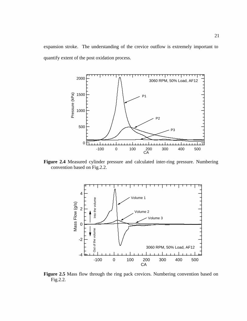
21
expansion stroke. The understanding of the crevice outflow is extremely important to
quantify extent of the post oxidation process.
2000
1500
1000
500
0
Pres
sure
(kPa
)
5004003002001000-100CA
P1
P2
P3
3060 RPM, 50% Load, AF12
Figure 2.4 Measured cylinder pressure and calculated inter-ring pressure. Numbering
convention based on Fig.2.2.
4
2
0
-2
-4
Mas
s Fl
ow (g
/s)
5004003002001000-100CA
Out
of t
he v
olum
eIn
to th
e vo
lum
e Volume 1
Volume 2
Volume 3
3060 RPM, 50% Load, AF12
Figure 2.5 Mass flow through the ring pack crevices. Numbering convention based on
Fig.2.2.
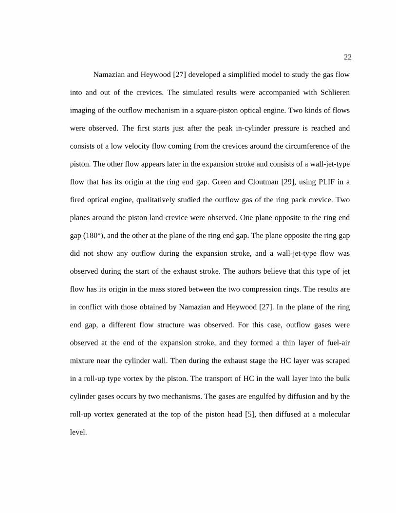
22
Namazian and Heywood [27] developed a simplified model to study the gas flow
into and out of the crevices. The simulated results were accompanied with Schlieren
imaging of the outflow mechanism in a square-piston optical engine. Two kinds of flows
were observed. The first starts just after the peak in-cylinder pressure is reached and
consists of a low velocity flow coming from the crevices around the circumference of the
piston. The other flow appears later in the expansion stroke and consists of a wall-jet-type
flow that has its origin at the ring end gap. Green and Cloutman [29], using PLIF in a
fired optical engine, qualitatively studied the outflow gas of the ring pack crevice. Two
planes around the piston land crevice were observed. One plane opposite to the ring end
gap (180°), and the other at the plane of the ring end gap. The plane opposite the ring gap
did not show any outflow during the expansion stroke, and a wall-jet-type flow was
observed during the start of the exhaust stroke. The authors believe that this type of jet
flow has its origin in the mass stored between the two compression rings. The results are
in conflict with those obtained by Namazian and Heywood [27]. In the plane of the ring
end gap, a different flow structure was observed. For this case, outflow gases were
observed at the end of the expansion stroke, and they formed a thin layer of fuel-air
mixture near the cylinder wall. Then during the exhaust stage the HC layer was scraped
in a roll-up type vortex by the piston. The transport of HC in the wall layer into the bulk
cylinder gases occurs by two mechanisms. The gases are engulfed by diffusion and by the
roll-up vortex generated at the top of the piston head [5], then diffused at a molecular
level.
23
Not all the combustible mixture that escapes the main combustion stored in the
ring pack crevices contributes to the engine-out HC emissions. Under fully warmed up
conditions, there can be significant post-flame oxidation in the cylinder during the
expansion and exhaust stroke. The amount of HC post oxidation depends of the operating
condition of the engine, however some experimental [30] and computational [31] results
show that about 50-90% of the trapped HC are oxidized within the cylinder before the
exhaust valve opening. It has been found that the critical cut-off temperature for the HC
oxidation is approximately 1500 K [32]. Therefore, the rate of HC consumption is limited
by the diffusion of the relatively cold HC from the boundary layer to the bulk of the high
temperature burned gas. This fact has been verified by Eng et al. [30], who
experimentally found that the HC emissions for neat paraffinic fuels scales inversely with
the diffusion coefficient.
Eng et al. [30] developed a global hydrocarbon consumption correlation based on
the hydrocarbons stored in the ring pack crevices. The HC consumption was defined as
the complete conversion of the fuel to CO, CO2 and H2O. On the other hand HC
conversion was defined as decomposition of the parent fuel to intermediate HC species.
The correlation developed was able to accurately predict the amount of engine-out HC
emissions based on the amount of HC stored in the ring pack crevices calculated using a
simplified ring pack flow model [27]. The correlation was able to capture the
particularities of different loads, speeds, air-fuel ratio, amount of dilution, and spark
timing. Also, the sensitivity of the correlation to different fuels was tested. Initially
experiments with n-butane were carried out because its diffusivity in the oil layer is very
24
small and the HC output emission should not be affected by the oil adsorption and
desorption mechanism. Later iso-octane was used as a fuel. Iso-octane has a higher
solubility in oil than the iso-butene, therefore some oil film adsorption effect was
expected. However when the results of both fuels were compared, no significant
difference was observed. Thus it was concluded that the oil adsorption and desorption
mechanism under fully warmed up conditions does not play a significant role in the HC
emissions.
Since the hydrocarbon global consumption correlation was heuristic in nature, it
was subject to several refinements to account for different factors affecting the HC
consumption. The integration of scaling factors like engine speed (to account for the
increased turbulence and diffusion rates), and fuel-air binary diffusivity were necessary.
The final correlation obtained was:
Global Consumption Rateτb
Oba
pc
evoexh
crevres
XRTPSDPEIHCPEIHCy
2)/(
)1(ln
maxmax
max⎥⎦
⎤⎢⎣
⎡−
= (2.1)
Global Consumption Rate )/exp( maxRTEC a−= (2.2)
In equation (2.1) and (2.2), C is a pre-exponential constant, Ea the activation
energy, R the gas constant, Tmax the in cylinder maximum temperature, yres is the in-
cylinder residual mass fraction, EIHCcrev the emission index of the maximum HC mass
stored in the ring pack and calculated with the simplified ring pack model. EIHCexh is the
measured output HC engine emissions, D is the diffusivity of the fuel, S, the mean piston
25
speed, Pmax the maximum in-cylinder pressure, Pevo the in-cylinder pressure at the time
that exhaust valve opens (EVO), 2OX is the oxygen molar fraction in the exhaust gases,
d an τ is the time period from when the cylinder reaches the peak pressure to EVO. It is
important to note that the difference between EIHCcrev and EIHCexh, represents the
amount of fuel that has been oxidized after the main combustion process. The fact that
the experimental results were fit very well by this correlation suggests that the correlation
is catching all the factors that affect the HC consumption. At the same time, it is
important to appreciate the significance of the ring pack crevices on the engine-out HC
emissions under warmed up conditions. The experimental results also allowed the
calculation of the global consumption rate against the maximum temperature in the
cylinder. Using this available information, an extrapolation of the maximum in-cylinder
temperature for a global consumption rate of zero was performed, and the extrapolated
temperature was found to be around 1500 K. This means that the minimum in-cylinder
temperature must be 1500 K in order to have post-flame oxidation. This critical value of
1500 K is in agreement with values found by other authors [32, 33].
More recently Eng [34] studied the effect of spark retard on the HC emissions
using heat release analysis and a simple model of the HC flow through the ring pack
crevices. A conceptual HC mechanism model was outlined to explain the storage and
post-flame oxidation. The ring pack crevice model was the same as the one used in [30],
and the influence of the spark retard for both lean and rich mixtures was studied. The end
of the main combustion was defined as the crank angle (CA) where the cumulative heat
release reached 90% (CA90). It was found that with significant retard of the spark timing,
26
a greater amount of HC was released from the crevices before the flame reached the
cylinder walls (as defined by CA90). As a consequence, the amount of HC initially stored
in crevices that is consumed by the flame increased, resulting in lower HC emission. For
all the conditions tested there was sufficient HC mixture in the crevices after CA90 (end
of the main combustion) to account for the engine-out HC emissions, and therefore, post
oxidation took place if the following conditions were present: 1) The temperature of the
bulk burned gases was greater than 1500 °K, 2) there was enough oxygen present to
oxidize the unburned HC, and 3) the residence time of the HC in the hot burned gases
was sufficient for the gases to diffuse and mix with the hot gases. For the conditions
tested, the majority of the HC consumption takes place inside the cylinder before exhaust
valve opening.
2.7 FUEL ADSORPTION-DESORPTION IN THE OIL FILM
Early experimental studies carried out in a closed vessel [35], in an engine [36]
and through simulation [37] showed that the fuel-oil adsorption-desorption problem could
be a significant contributor to the HC emissions despite the short exposure time of the oil
to the fuel during the engine cycle. The lubricanting oil on the cylinder liner adsorbs
unburned fuel mixture during the compression stroke [4, 5]. Therefore, part of the fuel is
hidden from the flame during the main combustion and escapes oxidation. Later during
the expansion and exhaust strokes the stored fuel desorbs, releasing unburned fuel into
the cylinder and contributing to the HC emissions. Figure 2.6 schematically shows the
adsorption-desorption process. The magnitude of this phenomenon depends on the
solubility of the fuel in the oil layer. Currently, together with the crevices, the oil films
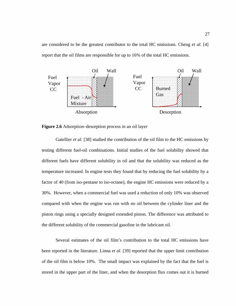
27
are considered to be the greatest contributor to the total HC emissions. Cheng et al. [4]
report that the oil films are responsible for up to 16% of the total HC emissions.
Oil WallFuel VaporCC
WallFuel
CC
Oil
BurnedVapor
Fuel - AirMixture
Gas
Absorption Desorption
Figure 2.6 Adsorption–desorption process in an oil layer
Gatellier et al. [38] studied the contribution of the oil film to the HC emissions by
testing different fuel-oil combinations. Initial studies of the fuel solubility showed that
different fuels have different solubility in oil and that the solubility was reduced as the
temperature increased. In engine tests they found that by reducing the fuel solubility by a
factor of 40 (from iso-pentane to iso-octane), the engine HC emissions were reduced by a
30%. However, when a commercial fuel was used a reduction of only 10% was observed
compared with when the engine was run with no oil between the cylinder liner and the
piston rings using a specially designed extended piston. The difference was attributed to
the different solubility of the commercial gasoline in the lubricant oil.
hen the desorption flux comes out it is burned
Several estimates of the oil film’s contribution to the total HC emissions have
been reported in the literature. Linna et al. [39] reported that the upper limit contribution
of the oil film is below 10%. The small impact was explained by the fact that the fuel is
stored in the upper part of the liner, and w
28
by the
Kaiser et al. [40] studied the effect of the fuel stored in the crankcase oil using a
single cylinder spark ignited engine. The oil sump was saturated with fuel through
exposure to the blowby gases, while the engine was fired using a certification gasoline.
After approximately 200 hours of operation motored tests were performed. During the
motored tests a relatively high concentration of HC was measured in the exhaust. Gas
chromatography analysis showed that most of HC species were from the low volatility
components of the diffused fuel. When the engine was fired using iso-octane as a fuel,
the obs
The post-flame oxidation of desorbed fuel in the cylinder was studied by Norris
and Hochgreb [41]. The oil of an SI engine was doped with a known fuel, and the engine
was fired using hydrogen as fuel. This kind of arrangement isolated the HC emissions
from th
hot bulk gases of the main combustion. Testing different oil film thicknesses with
a synthetic multi-component fuel they found that the oil thickness did not contribute
significantly to the HC emissions, and that if there was some contribution of the oil films
this it was being masked by other factors.
erved species in the motored case reduced drastically. The authors explained the
reduction by the fact that under fully warmed up condition up to 80% of the desorbed fuel
can be oxidized in the cylinder as it mixes with the hot cylinder gases. Thus the total
contribution of the crankcase-derived emissions was of approximately 1.5+-0.5%.
e fuel, so the only HC source could be the desorbed fuel from the oil film. The
studies showed that a large amount of the desorbed fuel was burned during the post-flame
29
period. The amount of post-flame oxidation was strongly affected by the engine load, air-
fuel ratio, and fuel chemical reactivity.
Kaiser et al. [42] studied the effect of fuel composition on the oil-film-related HC
emissio
Recently, the effect of the adsorption of fuel in the oil film under cold conditions
was studied by Parks et al. [43], who experimentally measured the amount of fuel
adsorbed into the oil during cold start engine operation. The amount of fuel stored was
compar
The magnitude of the fuel-oil contribution to the HC has been also addressed
numerically [44-46]. The results show that the Henry’s constant, which is related to the
fuel solubility in oil, is the most dominant parameter in the adsorption-desorption
mechanism. The Henry’s constant of the components of a typical gasoline in several
commercial oils has been experimentally measured [47] and it has been very useful for
ns. The base gasoline was doped with n-alkanes of wide range of solubility levels.
The effect of the different fuels on the engine-out HC emission was studied for two
coolant temperatures (339 and 380 K). The HC emissions were not changed significantly
over the range of fuels tested, suggesting that the oil adsorption-desorption mechanism
does not contribute significantly to the HC emissions above the temperatures tested.
atively higher than in a normal steady state warmed up condition, because the
solubility of the fuel is increased as the lower temperature. The results showed that the
fuel concentration in the oil film reached a maximum of 50% in volume. This large
increase of fuel concentration in oil could contribute significantly to the HC emissions
during the cold start period.
30
experim
As can be seen from the literature review, the impact of oil film adsorption on HC
emissions is less well understood. The diversity of results can be due to the fact that the
s it difficult to compare
the dif
The flame quenching at the cylinder wall has been identified as a HC emissions
contributor [4, 20, 21], and initially it was considered to be a major contributor. However,
experimental measurements and detailed modeling of the flame quench phenomenon
showed that the majority of the fuel layer that was not oxidized during the main
combustion diffuses into the hot gases and burns up during the expansion [50, 51]. On
diluted mixtures the flame quench phenomenon can be the greatest
contrib
entalists and for modelers as well [43]. In addition due to the complexity of the
composition of commercial oils and the lack of experimental data, surrogates such as
Squalane (C30 H62) [48, 49], which has similar characteristics than some engine oil are
used to assess the severity of the fuel-oil diffusion problem [46].
researchers use different fuel and oil formulations, which make
ferent results. However, in spite of those differences it is believed that the
contribution of oil film adsorption to the total HC emissions is small and it should
decrease at elevated temperature.
2.8 FLAME QUENCHING AT THE CYLINDER WALL
the other hand, for
utor to the HC emissions [4, 30]. The estimate of wall quenching contribution to
the HC emissions at steady state conditions for a stoichiometric air-fuel ratio is less than
3%.
31
2.9 DEPOSITS
Deposits in the combustion chamber are formed in proportion to the engine
operation time. The effects of the deposits on the HC emissions are well known [4], and
the mechanism of contribution to the HC emissions is similar to the adsorption and
desorption process of the fuel in oil. Deposits are porous organic compounds that adsorb
and des
HC emissions for both steady and transient conditions. Currently there is not detailed
information about the effect of the deposits on the HC emissions. However, some
estimates show that the deposits are responsible for up to 16% of the total engine-out HC
emissions. It is important clarify that the deposit size is highly dependent on the age of
the engine and those reported values must be used very cautiously.
orb the fuel in the same way as the oil film. In the case of port-fueled engines, the
deposits on the intake valve contribute to the HC emissions during transient conditions.
The deposits make the engine operation leaner during the acceleration and richer during
the deceleration. However, it is known that under steady state conditions the intake valve
deposits do not contribute significantly to the HC emissions [4].
On the other hand, the combustion chamber deposits are known to increase the
32
CHAPTER III
3 EXPERIMENTAL SET-UP, DATA ANALYSIS,
MATERIALS AND TEST METHODOLOGY
3.1 INTRODUCTION
Chapter III describes the main components of the test cell, the data acquisition
system, the materials, the experimental methodology for taking the data, and the data
analysis used along this investigation. Some specific schematics and programs used to
analyze the data are provided in Appendices of the thesis.
3.2 ENGINE TEST CELL
The test cell consisted of the engine, the air and fuel supply systems, the engine
control system, the dynamometer, the emissions sampling systems, and the data
acquisition systems. A detailed description of each of these systems is given below.
3.2.1 ENGINE
The engine chosen for this study was the four stroke V-twin Kohler model CH23
engine. This is a spark-ignited air-cooled engine with overhead valves (OHV) and a
horizontal shaft. It comes equipped with a carburetor and has fixed spark timing. The
engine is representative of the small engine group. In part, this two-cylinder engine was
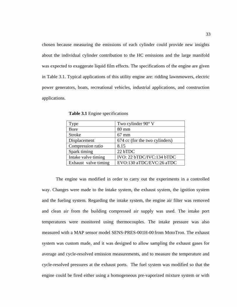
33
chosen because measuring the emissions of each cylinder could provide new insights
about the individual cylinder contribution to the HC emissions and the large manifold
was expected to exaggerate liquid film effects. The specifications of the engine are given
in Table 3.1. Typical applications of this utility engine are: ridding lawnmowers, electric
power generators, boats, recreational vehicles, industrial applications, and construction
applications.
Table 3.1 Engine specifications
Type Two cylinder 90° V Bore 80 mm Stroke 67 mm Displacement 674 cc (for the two cylinders) Compression ratio 8.15 Spark timing 22 bTDC Intake valve timing IVO: 22 bTDC/IVC:134 bTDC Exhaust valve timing EVO:130 aTDC/EVC:26 aTDC
The engine was modified in order to carry out the experiments in a controlled
way. Changes were made to the intake system, the exhaust system, the ignition system
and the fueling system. Regarding the intake system, the engine air filter was removed
and clean air from the building compressed air supply was used. The intake port
temperatures were monitored using thermocouples. The intake pressure was also
measured with a MAP sensor model SENS-PRES-001H-00 from MotoTron. The exhaust
system was custom made, and it was designed to allow sampling the exhaust gases for
average and cycle-resolved emission measurements, and to measure the temperature and
cycle-resolved pressures at the exhaust ports. The fuel system was modified so that the
engine could be fired either using a homogeneous pre-vaporized mixture system or with
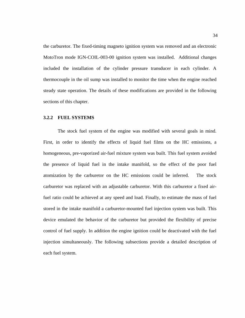
34
the carburetor. The fixed-timing magneto ignition system was removed and an electronic
MotoTron mode IGN-COIL-003-00 ignition system was installed. Additional changes
included the installation of the cylinder pressure transducer in each cylinder. A
thermocouple in the oil sump was installed to monitor the time when the engine reached
steady state operation. The details of these modifications are provided in the following
sections of this chapter.
3.2.2 FUEL SYSTEMS
The stock fuel system of the engine was modified with several goals in mind.
First, in order to identify the effects of liquid fuel films on the HC emissions, a
homogeneous, pre-vaporized air-fuel mixture system was built. This fuel system avoided
the presence of liquid fuel in the intake manifold, so the effect of the poor fuel
atomization by the carburetor on the HC emissions could be inferred. The stock
carburetor was replaced with an adjustable carburetor. With this carburetor a fixed air-
fuel ratio could be achieved at any speed and load. Finally, to estimate the mass of fuel
stored in the intake manifold a carburetor-mounted fuel injection system was built. This
device emulated the behavior of the carburetor but provided the flexibility of precise
control of fuel supply. In addition the engine ignition could be deactivated with the fuel
injection simultaneously. The following subsections provide a detailed description of
each fuel system.
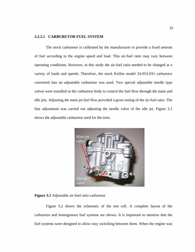
35
3.2.2.1 CARBURETOR FUEL SYSTEM
The stock carburetor is calibrated by the manufacturer to provide a fixed amount
of fuel according to the engine speed and load. This air-fuel ratio may vary between
operating conditions. However, in this study the air-fuel ratio needed to be changed at a
variety of loads and speeds. Therefore, the stock Keihin model 24-053-031 carburetor
converted into an adjustable carburetor was used. Two special adjustable needle type
valves were installed in the carburetor body to control the fuel flow through the main and
idle jets. Adjusting the main jet fuel flow provided a gross tuning of the air-fuel ratio. The
fine adjustment was carried out adjusting the needle valve of the idle jet. Figure 3.1
shows the adjustable carburetor used for the tests.
Main jetvalve
Idle jetvalve
Figure 3.1 Adjustable air-fuel ratio carburetor
Figure 3.2 shows the schematic of the test cell. A complete layout of the
carburetor and homogenous fuel systems are shown. It is important to mention that the
fuel systems were designed to allow easy switching between them. When the engine was
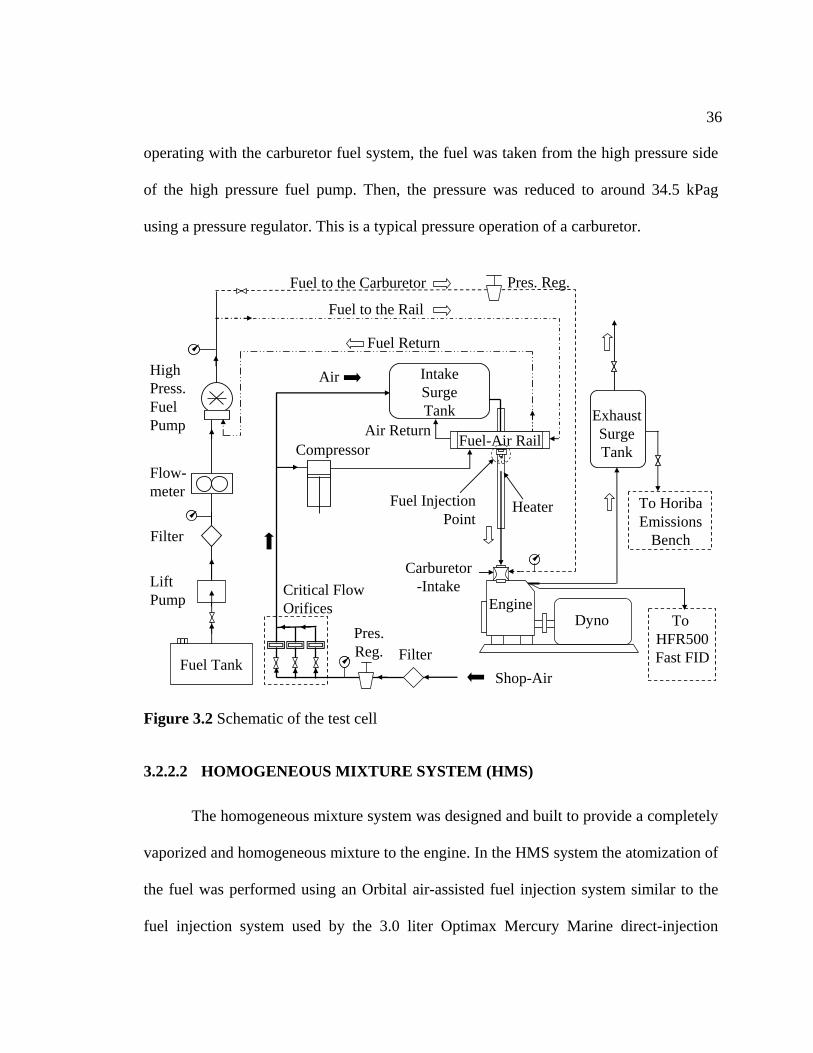
36
operating with the carburetor fuel system, the fuel was taken from the high pressure side
of the high pressure fuel pump. Then, the pressure was reduced to around 34.5 kPag
using a pressure regulator. This is a typical pressure operation of a carburetor.
Shop-Air
Pres.
Compressor
Reg.
Fuel Return
Fuel to the Carburetor
e Rail
Air Return
Fuel Injection
Fuel to th
Point
Exhaust
TankSurge
Dyno
Critical FlowOrificesPump
To Horiba
Bench
Heater
Lift
Filter
Carburetor-Intake
Emissions
Fuel Tank
Filter
Flow-meter
HighPress.Fuel Pump
IntakeSurgeTank
EngineTo
HFR500Fast FID
Fuel-Air Rail
Air
Pres. Reg.
Figure
The homogeneous mixture system was designed and built to provide a completely
vaporized and homogeneous mixture to the engine. In the HMS system the atomization of
the fuel was performed using an Orbital air-assisted fuel injection system similar to the
fuel injection system used by the 3.0 liter Optimax Mercury Marine direct-injection
3.2 Schematic of the test cell
3.2.2.2 HOMOGENEOUS MIXTURE SYSTEM (HMS)
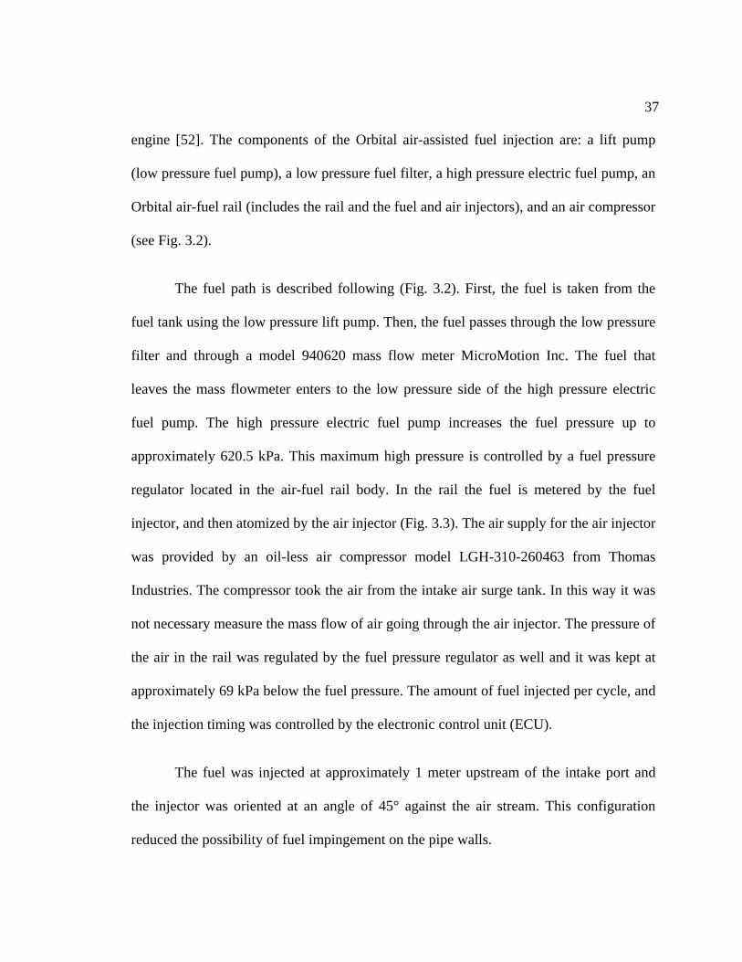
37
engine [52]. The components of the Orbital air-assisted fuel injection are: a lift pump
(low pressure fuel pump), a low pressure fuel filter, a high pressure electric fuel pump, an
Orbital air-fuel rail (includes the rail and the fuel and air injectors), and an air compressor
(see Fig. 3.2).
The fuel path is described following (Fig. 3.2). First, the fuel is taken from the
fuel tank using the low pressure lift pump. Then, the fuel passes through the low pressure
filter and through a model 940620 mass flow meter MicroMotion Inc. The fuel that
leaves
trolled by a fuel pressure
regulator located in the air-fuel rail body. In the rail the fuel is metered by the fuel
injector, and then atomized by the air injector (Fig. 3.3). The air supply for the air injector
was provided by an oil-less air compressor model LGH-310-260463 from Thomas
Industries. The compressor took the air from the intake air surge tank. In this way it was
not necessary measure the mass flow of air going through the air injector. The pressure of
the air in the rail was regulated by the fuel pressure regulator as well and it was kept at
approximately 69 kPa below the fuel pressure. The amount of fuel injected per cycle, and
the injection timing was controlled by the electronic control unit (ECU).
The fuel was injected at approximately 1 meter upstream of the intake port and
the injector was oriented at an angle of 45° against the air stream. This configuration
the mass flowmeter enters to the low pressure side of the high pressure electric
fuel pump. The high pressure electric fuel pump increases the fuel pressure up to
approximately 620.5 kPa. This maximum high pressure is con
reduced the possibility of fuel impingement on the pipe walls.
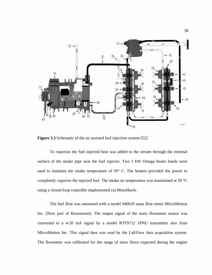
38
Figure 3.3 Schematic of the air assisted fuel injection system [52]
To vaporize the fuel injected heat was added to the stream through the external
surface of the intake pipe near the fuel injector. Two 1 kW Omega heater bands were
used to maintain the intake temperature of 50° C. The heaters provided the power to
50 °C
using a closed-loop controller implemented via MotoHawk.
completely vaporize the injected fuel. The intake air temperature was maintained at
The fuel flow was measured with a model 940620 mass flow meter MicroMotion
Inc. (Now part of Rosemount). The output signal of the mass flowmeter sensor was
converted to a 4-20 mA signal by a model RTF9712 1PNU transmitter also from
MicroMotion Inc. This signal then was read by the LabView data acquisition system.
The flowmeter was calibrated for the range of mass flows expected during the engine
39
operation (see Appendix I). It is important to mention that there was significant
variability in the data, and for some conditions the reading of the flowmeter was not
accurate. Despite the inaccuracies, the mass flow meter was used to double check the air-
fuel ratio obtained from the emissions analysis. In general they were in good agreement.
As mentioned above, due to poor fuel atomization by the carburetor, part of the
3.2.2.3 CARBURETOR-MOUNTED FUEL INJECTOR SYSTEM (CMFIS)
fuel is stored in the intake manifold as liquid films. To understand the extent of their
contribution to the engine-out HC emissions, a quantification of the mass of fuel stored
was necessary. This was accomplished by carrying out stop-fuel-injection tests. To that
end, a carburetor mounted fuel injection system was built. This device consisted of a
carburetor body and an Orbital fuel injector that delivered the fuel directly to the
carburetor main jet (Fig. 3.4). The CMFIS emulated the carburetor behavior (poor
atomization) while providing accurate control of the delivered mass of fuel and the ability
to precisely stop fuel injection. The fuel injector was controlled with the ECU and the
fuel supplied to this system came from the same low pressure line that provided fuel to
injector was simultaneously deactivated with the
ignition
the carburetor. However, the fuel pressure for this system was regulated to 58.5 kPa.
During the stop injection tests the fuel
to avoid combustion of fuel vaporized in the intake and ingested by the engine.
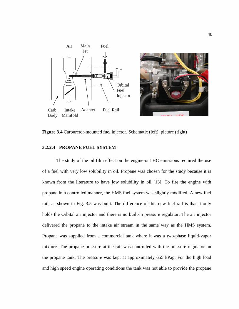
40
- +
OrbitalFuelInjector
Air
Intake Fuel RailAdapterCarb.ManifoldBody
FuelMain Jet
Figure 3.4 Carburetor-mounted fuel injector. Schematic (left), picture (right)
The study of the
3.2.2.4 PROPANE FUEL SYSTEM
oil film effect on the engine-out HC emissions required the use
of a fuel with very low solubility in oil. Propane was chosen for the study because it is
known from the literature to have low solubility in oil [13]. To fire the engine with
fuel system was slightly modified. A new fuel
ilt. The difference of this new fuel rail is that it only
holds the O
propane in a controlled manner, the HMS
rail, as shown in Fig. 3.5 was bu
rbital air injector and there is no built-in pressure regulator. The air injector
delivered the propane to the intake air stream in the same way as the HMS system.
Propane was supplied from a commercial tank where it was a two-phase liquid-vapor
mixture. The propane pressure at the rail was controlled with the pressure regulator on
the propane tank. The pressure was kept at approximately 655 kPag. For the high load
and high speed engine operating conditions the tank was not able to provide the propane
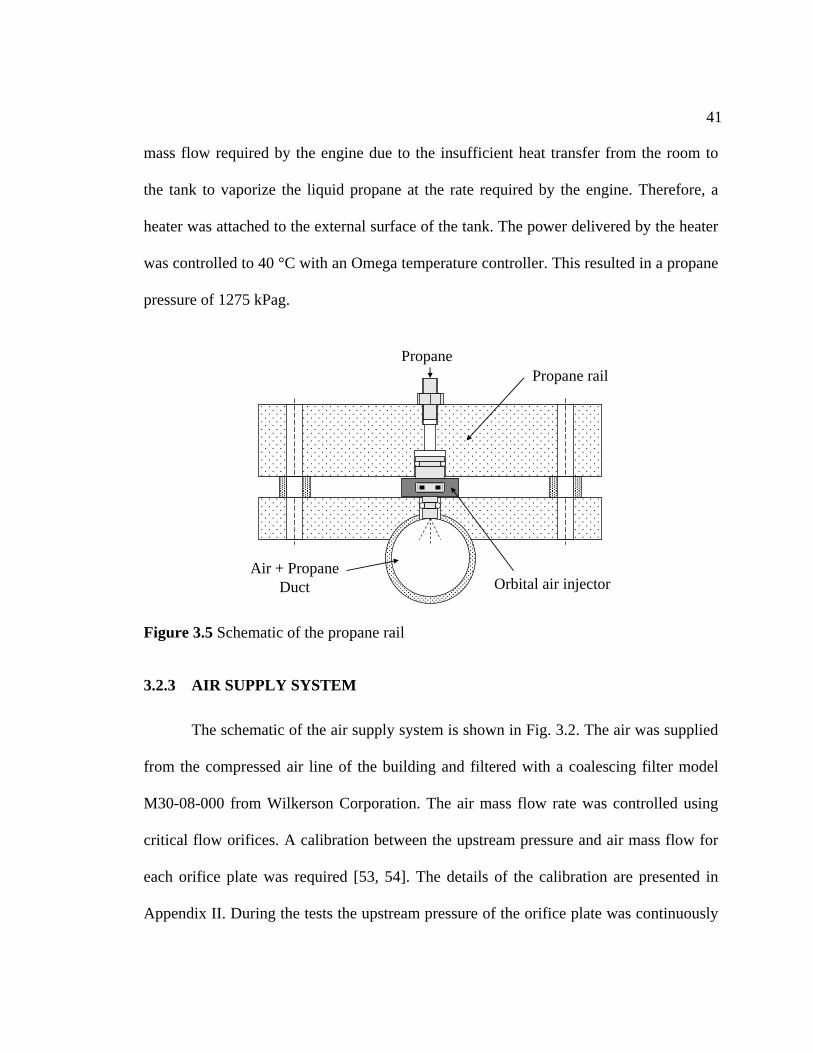
41
mass flow required by the engine due to the insufficient heat transfer from the room to
the tank to vaporize the liquid propane at the rate required by the engine. Therefore, a
heater was attached to the external surface of the tank. The power delivered by the heater
was controlled to 40 °C with an Omega temperature controller. This resulted in a propane
pressure of 1275 kPag.
Orbital air injector
PropanePropane rail
Air + PropaneDuct
Figure 3.5 Schematic of the propane rail
The schematic of the air supply system is shown in Fig. 3.2. The air was supplied
from the compressed air line of the building and filtered with a coalescing filter model
critical flow orifices. A calibration between
3.2.3 AIR SUPPLY SYSTEM
M30-08-000 from Wilkerson Corporation. The air mass flow rate was controlled using
the upstream pressure and air mass flow for
each orifice plate was required [53, 54]. The details of the calibration are presented in
Appendix II. During the tests the upstream pressure of the orifice plate was continuously
42
adjusted to match required engine air mass flow rate. The air supplied to the rail of the
air-assisted fuel injection was taken from the intake surge tank and there was no need to
individually measure the mass flow through the air injector (see Fig. 3.2). The air-fuel
mixture was heated and delivered to the engine at a constant temperature of 50 °C,
measured at approximately 10 cm above the carburetor body.
3.2.4 CONTROL SYSTEM
with a wide variety of engine control
applications. The model created in MotoHawk can be simulated and verified for errors
before
MotoTune is a calibration development tool that establishes communication
between the ECU and the command computer during the engine operation. This software
The engine was controlled using the MotoTron suite of products [55]. This
consists of three main software components MotoHawk, MotoTune and MotoServer, and
the hardware engine control unit (ECU).
MotoHawk is software that is used to develop, test, and validate control
applications using Simulink from MathWorks [56]. The program that controls the engine
operation was created in MotoHawk. The MotoHawk-Simulink integration helps to
reduce the time and complexity of working
it is transferred to the ECU hardware. However, an intermediate step to transfer
the model into the ECU is required. The Simulink-based model has to be translated into
the ECU language. The Multi2000 compiler from Green Hills Software Inc. was used for
that purpose [57]. The files generated with the Multi2000 compiler (.srz and .dll type
files) are the ones used to program the ECU.
43
has an interactive spreadsheet-type interface, in which the calibration parameters stored
in the ECU can be modified and adjusted at any time during the engine operation.
MotoTune is also for flash programming of the ECU. Other important features of
MotoTune include: activation and deactivation of specific engine systems (fuel injector,
spark coils, throttle, etc gement of the calibration files, parameter display, override
and logging capabilities.
MotoServer is the licensing software and it allows the configuration of the
communication ports. Figure 3.6 shows a schematic of the interaction of the several
components of the MotoTron suite of products. MotoHawk, MotoTune and MotoServer
were continuously being updated, however, during this work the following versions were
used: MotoHawk version 0.8.3 beta 14, MotoTune version 8.10, and MotoServer version
8.10. The Matlab version plays an important role during the installation of MotoHawk,
and it m
The engine was equipped with a Motorola model ECM-0565-128 [58]. This ECU
uses the Motorola MPC565 microprocessor at 56 MHz. The main features of the ECU
include the availability of 34 analog inputs, 8 digital inputs, 2 inputs for 2 wide band
oxygen sensors (Bosch LSU4.2), outputs for injector drivers, TTL signals for ignition
systems, PWM outputs, and 2 CAN 2.0B channels, within other resources.
), mana
ust be compatible with the MotoHawk version being installed. The ECU program
was written using Matlab version 2006b.
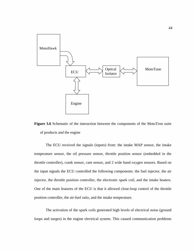
44
o, and the intake temperature.
The activation of the spark coils generated high levels of electrical noise (ground
loops and surges) in the engine electrical system. This caused communication problems
Figure 3.6 Schematic of the interaction between the components of the MotoTron suite
of products and the engine
The ECU received the signals (inputs) from: the intake MAP sensor, the intake
temperature sensor, the oil pressure sensor, throttle position sensor (embedded in the
throttle controller), crank sensor, cam sensor, and 2 wide band oxygen sensors. Based on
the input signals the ECU controlled the following components: the fuel injector, the air
injector, the throttle position controller, the electronic spark coil, and the intake heaters.
One of the main features of the ECU is that it allowed close-loop control of the throttle
position controller, the air-fuel rati
ECU Optical Isolator
MotoTune
MotoHawk
Engine
45
between the ECU and the command computer (MotoTune). The problem was eliminated
using a
The dynamometer consisted of a direct current motor and a controller. The motor
was a G
The engine was coupled to the dynamometer with a TB Wood’s SureFlex
coupling of Size 7 with a neoprene insert [61]. A considerable amount of time was spent
in finding the right size and type of coupling that matched the engine-dynamometer
dynam
n USB optical isolator model UISOHUB4 from B&B Electronics Manufacturing
Company [59], which was installed between the ECU and the command computer (Fig.
3.6).
3.2.5 DYNAMOMETER
eneral Electric model 5CY977E1 direct current motor, with a rated power of 25
HP and maximum speed of 3600 RPM. The dynamometer was controlled with the Dyn-
Loc digital dynamometer controller [60]. This controller allowed control of either the
speed or the torque. However, during the tests only the speed was controlled. The torque
was controlled adjusting the engine throttle position via MotoTune.
ic behavior. Several types of couplings were tested. Some couplings were very
stiff (Falk Wrapflex coupling from Rexnord) [62] producing intolerable levels of
vibration. Other couplings were very soft and failed after a very short time of operation
(TB Wood’s DuraFlex) [61].
46
3.2.6
ns bench. This bench had the following analyzers: Horiba AIA-23 non-
dispersive infrared analyzer for the CO and CO2, Horiba MPA-21A paramagnetic
oxygen analyzer, Horiba CLA-22A chemiluminescence analyzer for the NOx, and the
flame ionization detector (FID) FIA-23A for the total HC.
cylinder exhaust surge tanks of a
special
red the emissions bench. The cold FID can cause some
oxygenated species present in the exhaust gases to not be measured [30]. In the emission
bench the gases were passed through a chiller to further condense water. The readings of
the gas analyzers were recorded using a LabView-based data acquisition system.
EMISSIONS BENCH
The average engine-out emissions were measured with a standard 5 gas analyzer
Horiba emissio
The emissions were sampled from individual-
ly designed separated exhaust system (Fig. 3.7). With this arrangement the
individual cylinder contribution to the total emissions was estimated. The surge tanks
were designed to damp the pressure fluctuations and to promote mixing of the exhaust
gases. The tanks were made from steel with capacity of 7570.8 cm3 (2 gal) and they
satisfied the ASME pressure vessel code. The gas diffuser and the sampling probe were
built following the SAE norms [63]. The sampling probe was located at approximately 80
cm from the exhaust port.
The hot exhaust gases leaving the sampling probe were passed through a chiller to
remove the water before they ente
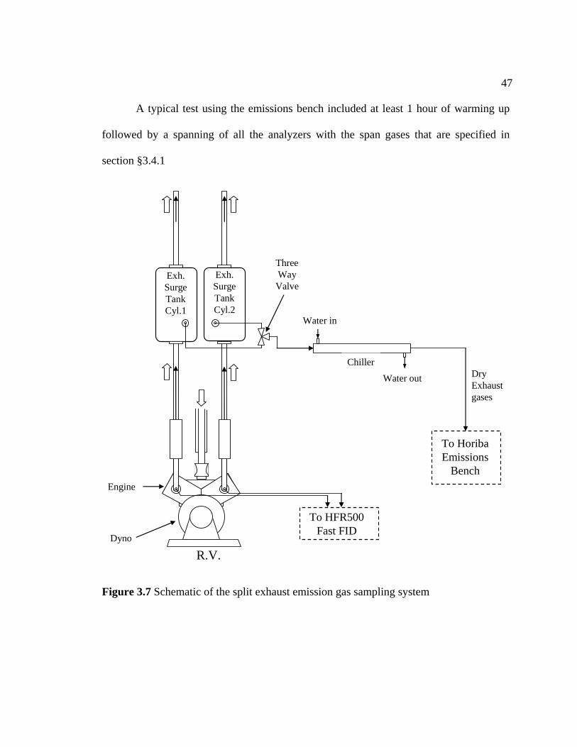
47
A typical test using the emissions bench included at least 1 hour of warming up
followed by a spanning of all the analyzers with the span gases that are specified in
section §3.4.1
To HoribaEmissions
Bench
To HFR500Fast FID
Exh.Surge TankCyl.2
R.V.
ThreeWayValve
Exh.Surge TankCyl.1
Water in
Chiller
Water out
Dyno
Engine
DryExhaust
sesga
Figure 3.7 Schematic of the split exhaust emission gas sampling system
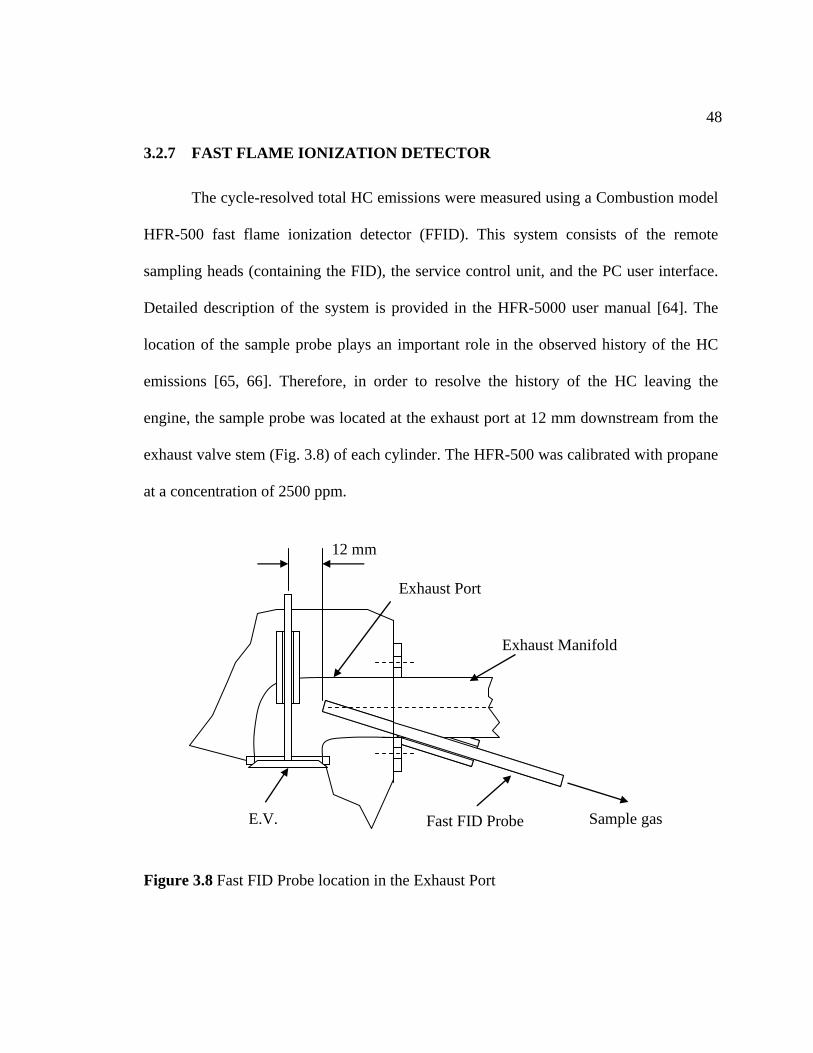
48
3.2.7 FAST FLAME IONIZATION DETECTOR
The cycle-resolved total HC emissions were measured using a Combustion model
HFR-5
emissions [65, 66]. Therefore, in order to resolve the history of the HC leaving the
engine, the sam
00 fast flame ionization detector (FFID). This system consists of the remote
sampling heads (containing the FID), the service control unit, and the PC user interface.
Detailed description of the system is provided in the HFR-5000 user manual [64]. The
location of the sample probe plays an important role in the observed history of the HC
ple probe was located at the exhaust port at 12 mm downstream from the
exhaust valve stem (Fig. 3.8) of each cylinder. The HFR-500 was calibrated with propane
at a concentration of 2500 ppm.
12 mm
Fast FID Probe
Exhaust Port
Exhaust Manifold
E.V. Sample gas
Figure 3.8 Fast FID Probe location in the Exhaust Port
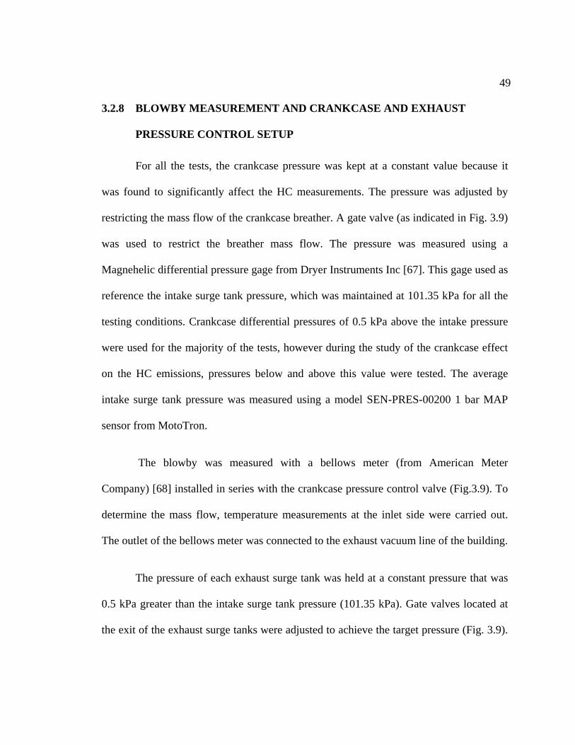
49
3.2.8 BLOWBY MEASUREMENT AND CRANKCASE AND EXHAUST
PRESSURE CONTROL SETUP
ith the crankcase pressure control valve (Fig.3.9). To
determine the mass flow, temperature measurements at the inlet side were carried out.
The outlet of the bellows meter was connected to the exhaust vacuum line of the building.
The pressure of each exhaust surge tank was held at a constant pressure that was
0.5 kPa greater than the intake surge tank pressure (101.35 kPa). Gate valves located at
the exit of the exhaust surge tanks were adjusted to achieve the target pressure (Fig. 3.9).
For all the tests, the crankcase pressure was kept at a constant value because it
was found to significantly affect the HC measurements. The pressure was adjusted by
restricting the mass flow of the crankcase breather. A gate valve (as indicated in Fig. 3.9)
was used to restrict the breather mass flow. The pressure was measured using a
Magnehelic differential pressure gage from Dryer Instruments Inc [67]. This gage used as
reference the intake surge tank pressure, which was maintained at 101.35 kPa for all the
testing conditions. Crankcase differential pressures of 0.5 kPa above the intake pressure
were used for the majority of the tests, however during the study of the crankcase effect
on the HC emissions, pressures below and above this value were tested. The average
intake surge tank pressure was measured using a model SEN-PRES-00200 1 bar MAP
sensor from MotoTron.
The blowby was measured with a bellows meter (from American Meter
Company) [68] installed in series w
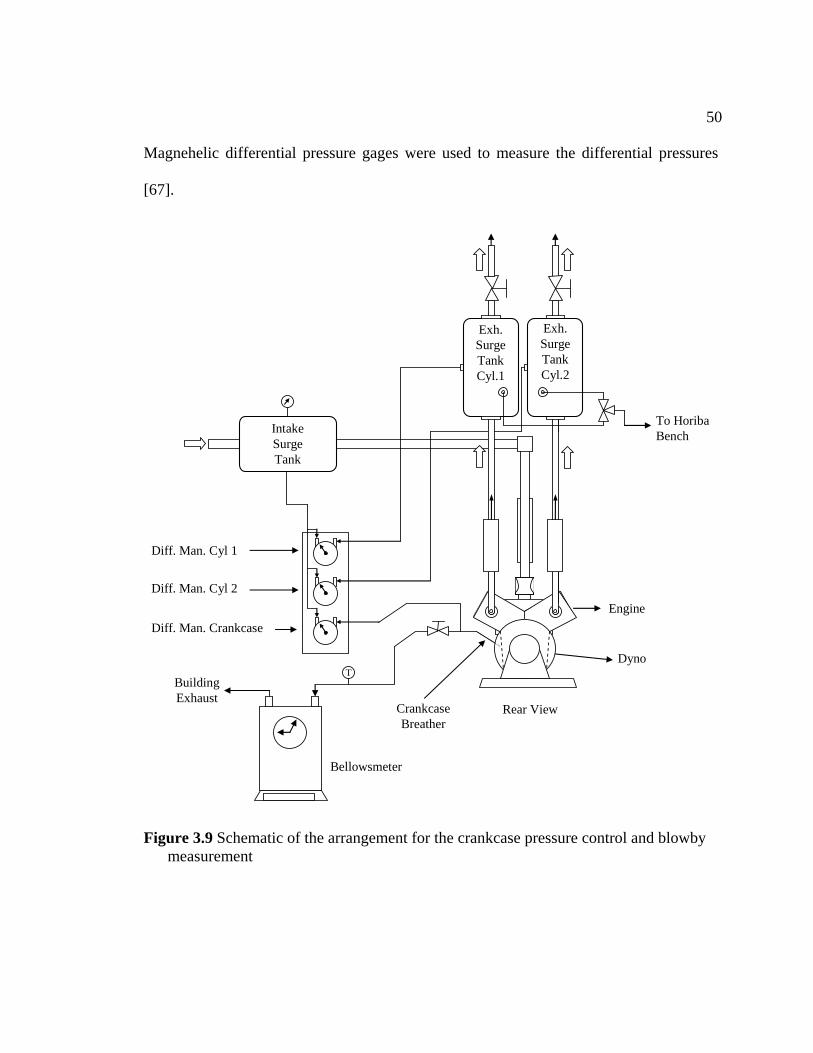
50
Magnehelic differential pressure gages were used to measure the differential pressures
[67].
Exh.Surge TankCyl.2
Rear View
Exh.Surge TankCyl.1
Dyno
Engine
IntakeSurge Tank
T
Bellowsmeter
BuildingExhaust
To HoribaBench
Diff. Man. Cyl 1
Diff. Man. Cyl 2
Diff. Man. Crankcase
CrankcaseBreather
Figure 3.9 Schematic of the arrangement for the crankcase pressure control and blowby measurement
51
3.2.9 CYCLE-RESOLVED PRESSURE MEASUREMENT
rder correction was performed on the pressure traces.
A detailed explanation of the correction process is presented in Appendix IV. The
corrected pressure traces showed satisfactory agreement with a piezoelectric sensor,
showing that a low cost sensor could be used to measure accurately the cycle-resolved
exhaust and intake pressure traces.
Cycle-resolved measurements of the in-cylinder, exhaust manifold, and intake
manifold pressures were performed.
The in-cylinder pressure was measured with water-cooled Kistler 7061 and
7063A pressure transducers [69] for cylinder 1 and cylinder 2, respectively. A special
threaded hole was made in the cylinder head to accept the pressure transducer. The
pressure transducers were calibrated using a weight dead tester, and the calibration curves
are shown in Appendix III.
The exhaust and intake manifold pressures were measured with a 2 bar MAP
pressure sensor, model SEN-PRES-0001H from MotoTron. The sensors located in the
exhaust required a special cooling system to avoid the high temperatures of the exhaust
gases. The cooling system is shown in Fig. 3.10. Typical operating temperatures of these
sensors were around 30-40 °C. The intake side sensor did not require cooling, and
temperatures at the intake location ranged from 50-70 °C. The intake and exhaust
pressure transducers described above have relatively slow time response (approximately
1 kHz) and do not accurately follow the dynamics of the intake and exhaust manifold
pressure waves. Therefore, a first-o
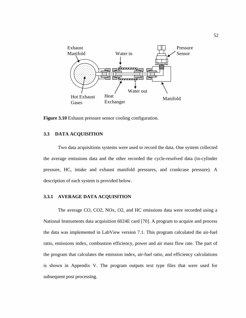
52
Water in
Water outHeatExchanger
Manifold
PressureSensor
EMa
Hot Ex Gases
xhaust nifold
haust
Figure 3.10 Exhaus ressure uration.
3.3 DATA ACQUISITION
isitions systems were used to record the data. One system collected
ycle-resolved data (in-cylinder
pressur
3.3.1 AVERAGE DATA ACQUISITION
The average CO, CO2, NOx, O2, and HC emissions data were recorded using a
National Instruments data acquisition 6024E card [70]. A program to acquire and process
the data was implemented in LabView version 7.1. This program calculated the air-fuel
ratio, emissions index, combustion efficiency, power and air mass flow rate. The part of
the program that calculates the emission index, air-fuel ratio, and efficiency calculations
is shown in Appendix V. The program outputs text type files that were used for
subsequent post processing.
t p sensor cooling config
Two data acqu
the average emissions data and the other recorded the c
e, HC, intake and exhaust manifold pressures, and crankcase pressure). A
description of each system is provided below.
53
The air-fuel ratio was calculated using several methods available in the literature
and were implemented in the program: carbon-based, oxygen-based, Bartesville, Spindt
and one locally developed. The details of the calculations are given in section §3.6 and in
Appendix VI
3.3.2 CYCLE-RESOLVED DATA ACQUISITION
o phase the data with the corresponding stages of the engine
combustion cycle. The A and Z signals were provided by a model H25D-SS-720-ABZC-
BEI Electronics Inc. [72]. This encoder has 0.5
crank a
nt to mention that the configuration does not
affect the acquisition process. The data acquisition recorded the data in binary format.
The cycle-resolved data were acquired using a HiTechniques [71] data acquisition
system. This system has capabilities to record up to 8 cycle-resolved input signals
(channels) at a sampling rate up to 1 MHz. The Win600 software, also from
HiTechniques, was used to configure the acquisition of the in cylinder pressure and all
the cycle resolved-traces. The data acquisition required the signal A, and Z of an
incremental rotary encoder t
5406R-SM18-S optical encoder from
ngle (CA) resolution providing 1440 data points per cycle per trace. The system
memory allowed recording 8 channels of data for 200 cycles. The data traces were
recorded in phase with either the first or second cylinder of the engine. However, the first
channel was reserved for the in-cylinder pressure of cylinder 1, and the other channels
could be configured in any order. The channel configuration for the present research is
show in Table 3.2. However, it is importa
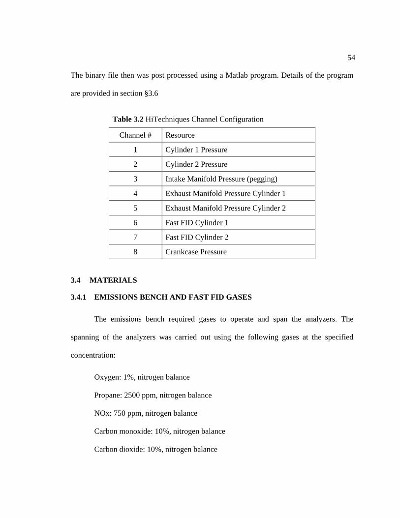
54
The binary file then was post processed using a Matlab program. Details of the program
are pro
3.4 MATERIALS
AST FID GASES
vided in section §3.6
Table 3.2 HiTechniques Channel Configuration
Channel # Resource
1 Cylinder 1 Pressure
2 Cylinder 2 Pressure
3 Intake Manifold Pressure (pegging)
4 Exhaust Manifold Pressure Cylinder 1
5 Exhaust Manifold Pressure Cylinder 2
6 Fast FID Cylinder 1
7 Fast FID Cylinder 2
8 Crankcase Pressure
3.4.1 EMISSIONS BENCH AND F
The emissions bench required gases to operate and span the analyzers. The
spanning of the analyzers was carried out using the following gases at the specified
concentration:
Oxygen: 1%, nitrogen balance
Propane: 2500 ppm, nitrogen balance
NOx: 750 ppm, nitrogen balance
Carbon monoxide: 10%, nitrogen balance
Carbon dioxide: 10%, nitrogen balance
55
Nitrogen zero, <0.5 ppm HC
Hydrogen 40%, nitrogen balance, <0.5 ppm total HC
Zero air (Oxygen 21.5%, <1.0 ppm total HC)
3.4.2 FUELS
3.4.3 ENGINE OIL
The engine lubricant oil used along all the tests was the Delo general-use SAE 30
oil from Chevron. The engine oil and filter were changed as specified by the engine
manufacturer. It is important to mention that before firing the engine with propane, the oil
was changed and the engine was fired for about 5 hours before taken emissions data. This
avoided any possible biasing on the measured HC emissions due to the vaporization of
some light HC fractions from the new oil.
In addition to the calibration gases, the FID of the emissions bench and the fast-
FID required the following two gases:
The engine was fueled with two fuels: gasoline and propane. The majority of the
tests were carried out using a fully blended US EPA TIER II EEE certification fuel
provided by Halterman Products [73]. However, to study the impact of the oil layer on
the HC emissions the engine was fueled with propane. The propane was industrial grade
99% purity, and it was purchased from Airgas Inc. The specifications of the EEE are
presented in Appendix VII.
56
3.5 EXPERIMENTAL METHODOLOGY
The contribution of the different HC mechanisms to the engine-out HC emissions
general the experimental
methodology for all the tests was similar. However, some studies required very specific
procedures. The details of the experimental procedure for the different sets of
experiments is provided below.
These tests were performed to study the effect of the liquid fuel on the HC
emissions. The following is an explanation of the carburetor tests. Before the engine was
run, the
was estimated by carrying out various types of tests. In
3.5.1 GASOLINE TESTS
The majority of the tests were carried out fueling the engine with gasoline. There
were three types of tests were the engine was fired with gasoline. These used the
adjustable carburetor, the homogeneous mixture system and the carburetor mounted fuel
injector.
3.5.1.1 CARBURETOR TESTS
emissions bench, fast FID and dynamometer were turn on for at least 30 minutes.
This provided enough time to warm up the instruments and to make sure they were fully
stabilized. In the case of the emissions bench of the gas analyzers were spanned previous
to runing the engine. However, a recalibration to verify any possible drift respect to the
initial calibration was performed. This could be done usually with the engine firing. The
fast FID required a more diligent calibration process before spinning the engine because
this instrument can not be calibrated when the engine is motoring or firing. The
57
instrument is very sensitive to pressure fluctuations. A common practice was to calibrate
the dynamometer prior to every run, thus, the zero and span values were adjusted as
required. Then, the engine was spun at the required speed with the throttle opened to a
position near to the target load. Next, the intake heaters were activated and the engine
was motored until the intake air reached the temperature of 50°C. After this the engine
was fired and the air-fuel ratio was adjusted to the required value. The engine was
warmed up in that condition until steady state operation was achieved. The engine
reached the steady state when no change in the oil temperature was observed. The time to
reach the steady state o
as reference this pressure the exhaust
sted to 101.85 kPa (a differential pressure of 0.5 kPa). At the
same tim
uel ratio was required. A
change in one of these parameters compromised the other two. A good advantage of the
test cell was that the dynamometer maintained an accurate control of the speed. Once the
desired air-fuel ratio, torque and speed were reached the engine was fired for
peration depended of the load, speed and air-fuel ratio; for the
majority of the conditions it was around 45 minutes. Typical steady-state oil
temperatures between 85-135 °C were observed. When the engine was approximately
half of the way to reach steady state, the engine was supplied with air coming from the
orifice plates. The pressure upstream of the orifice plate was adjusted to obtain an intake
surge tank pressure of 101.35±0.1 kPa. Taking
manifold pressure was adju
e the torque and air-fuel ratio were adjusted to the required values. This was
carried out by changing the throttle position, and the needle valves of the adjustable
carburetor. It is important to mention that in order to reach a run condition an iterative
adjustment of the intake air pressure, throttle position and air-f
58
approximately 15 minutes. Subsequently, all the pressures, temperatures, and emissions
were re
The homogeneous mixture system was used for the study of the liquid fuel, ring
pack and oil film HC mechanisms. The majority of the tests were carried out using this
fuel system. The methodology followed during the tests using the HMS system is very
similar to the procedure followed for the carburetor tests. However, in this case the fuel
was delivered with the Orbital air-assisted fuel injection system. An advantage of this
system was that the air-fuel ratio was close-loop controlled via MotoHawk. The air fuel
ratio was read with a wide band oxygen sensor installed at 40 cm from the exhaust port of
cylinder 1 (right cylinder). It is important to mention that the low and high pressure fuel
pumps were turned on before or at the same time that the intake heaters to avoid
formation of vapor bubbles in the high pressure fuel line.
3.5.1.3 STOP FUEL INJECTION TESTS
The methodology for the stop fuel injection tests was a little bit different from the
other tests, although the warming up process was the same. The main difference was that
data from i.e. the cylinder pressure, the signal
indicating that the spark and the fuel injector were disabled, and the fast FID data. For
these tests, the program that controlled the engine was modified so the spark and fuel
injector were disabled simultaneously. Once the engine was fully warmed up and the
desired operating steady operating condition was reached, data from 2000 consecutive
corded.
3.5.1.2 HOMOGENEOUS MIXTURE SYSTEM TESTS
only three channels were recorded,
59
cycles were recorded. The recording was started 4 to 5 seconds before the spark and fuel
injection were halted. The timing of the fast FID with the stop fuel injection was carried
out by recording fuel injector electrical pulse using a current probe. A Matlab program
was written to perform the post processing (Appendix VIII). Average emissions of the
steady state operation were also recorded with the National Instruments data acquisition
system.
3.5.2
as not used in these types
adjusted by changing the start of injection so the air
injector was open for a shorter or longer time.
Several codes were implemented to process and analyze the emissions and
pressure data. These codes calculated the air-fuel ratio, emissions indexes, heat release,
ring pack contribution to the HC emissions, and mass of HC leaving the engine. A brief
description of each of these calculations is given below.
PROPANE TESTS
The experimental procedure for the propane tests was similar to the one followed
for the HMS tests. The main difference was that the vapor phase propane was injected
only using the air injector. To control the mass of fuel delivered per cycle the program for
the HMS tests was used. The closed-loop air-fuel ratio control w
of tests. The air-fuel ratio was
3.6 DATA ANALYSIS
60
3.6.1 PRESSURE CODE
This code was implemented in Matlab to extract and process the HiTechniques
data which was recorded in binary format. The program carried out the pegging process
of the in-cylinder pressure and calculated the average and single-cycle IMEP and CA of
as pegged at 180 CA bTDC with the dynamic
intake manifold pressure. The program also performed the first order correction of the
intake and exhaust pressure transducers. Correction of the fast FID traces for transit time
and time response was also carried out by the program. It is important to mention that all
the traces were filtered using the built-in csaps smoothing function in Matlab before
any processing. Additional options of the code included plotting capabilities and output
files with the average data of all the traces. Single-cycle pressure and fast-FID output
data fi
3.6.2 AIR FUEL RATIO
In engines the mixture air-fuel ratio is an important parameter to characterize the
peak pressure. The in-cylinder pressure w
les were also available for further post-processing. The main section of the
program is shown in the Appendix IX
engine operation and it is defined as:
fuel
air
mAF
&= (3.1)
where AF is the mixture air-fuel ratio and airm& and fuelm& are the mass flow rate of air and
fuel respectively. During the tests the air-fuel ratio was calculated from the exhaust
m&
61
measured emissions using several methods. The methods used were: carbon balance,
oxygen balance [5, 74], Bartlesville [75], Spindt [76], and one ERC method [77]. No
significant differences were observed between methods, however, the oxygen-balance
method was used as a reference. The equations used to calculate the AF using these
methods are shown in the Appendix VI. These equations, as mentioned before, were
implemented in a LabView program that allowed the air-fuel ratio to be continuously
monitored and recorded.
d as reference.
3.6.3 EMISSIONS INDICES
The emissions index for species i, is defined as the ratio of the mass flow of the
specie i at the exhaust gases to the mass flow of fuel delivered to the engine i.e. [19, 74]:
The air-fuel ratio was also monitored using the wide band oxygen sensor (Bosch
LSU4.2) which was installed in exhaust manifold of cylinder 1. This sensor provided
direct information of the air-fuel ratio, and it was used by MotoTron to automatically
adjust the air-fuel ratio to the desired value. The sensor was calibrated for a wide range of
air-fuel ratios taking the oxygen-balance metho
fuel
exhaustii
mEI
& ,= (3.2)
where the EI
m&
ss flow respectively. The emission
indices have some advantages over the other emissions units used in engines. The
i is the emission index of species i, and mi,exhaust and mfuel are the mass flow
of measured species i at he exhaust and the fuel ma
62
emission index provides an indication of the amount of pollutant formed per mass of fuel
independently of the efficiency of the combustion process. The former is particularly
useful when comparing emissions from different applications. Therefore, all the emission
analysis was carried out using emission indices. The equations used for its calculation are
described in Appendix X
3.6.4 COMBUSTION EFFICIENCY
The combustion efficiency indicates the fraction of fuel supplied that is released
as energy in the combustion process. It is a useful parameter to monitor the engine
per estimated from the exhaust gas composition [5, 74]. In this
work the combustion efficiency was calculated using the combustion inefficiency concept
[5], and the details of the calculation are presented in Appendix XI.
The estimation of the combustion efficiency is extremely useful because it give an
indication of the extent of completeness of the combustion process. Additionally it is
useful parameter in the estimation of other performance parameters such as the rate of
heat release.
3.6.5 HEAT RELEASE ANALYSIS
A single-zone heat release analysis was performed to characterize the combustion
event. In the analysis the heat transfer between the cylinder wall and the gases was
modeled using the Woschni [78] correlation. An overall energy balance was employed to
correctly scale the heat transfer based on the fuel energy released correcting for the
formance, and it can be
63
combustion efficiency. The resid s calculated from the Yun and
Mirsky [79] correlation, which assumes that the gases remaining at EVO undergo a
polytropic expansion during the exhaus stroke. The combustion phasing was
c
burned reached the 10% (CA10), 5 0% (CA90). The heat release
analysis was carried out for the average pressure traces and for single-cycle pressure
traces. The details of the equations and the Matlab program are shown in Appendix XII
The heat release analysis requires the knowledge of the mass trapped in each
cylinder. T
at constant throttle position were carried
out. Th
ual mass fraction wa
t
haracterized by calculating the cumulative heat release where the mixture mass fraction
0% (CA50), and 9
his was estimated by considering that the charging of each cylinder was
proportional to the IMEP in each cylinder. To avoid the influence of incomplete
combustion and other factors, spark sweep tests
e mass trapped in each cylinder was considered to be proportional to the
maximum IMEP in each cylinder as follows:
2,2 −−
=cylmaccyl IMEP
IMEPmm
(3.3)
where 1−cylm , 2−cylm are the mass per cycle trapped in cylinder 1 and cylinder 2,
respectively; totalm is the mass of fuel and air that is delivered to the engine per cycle
(both cylinders), and is measured experimentally; and 1max, −cylIMEP and 2max, −cylIMEP are
1max,1 −− cylcyl
(3.4) totalcylcyl mmm =+ −− 21
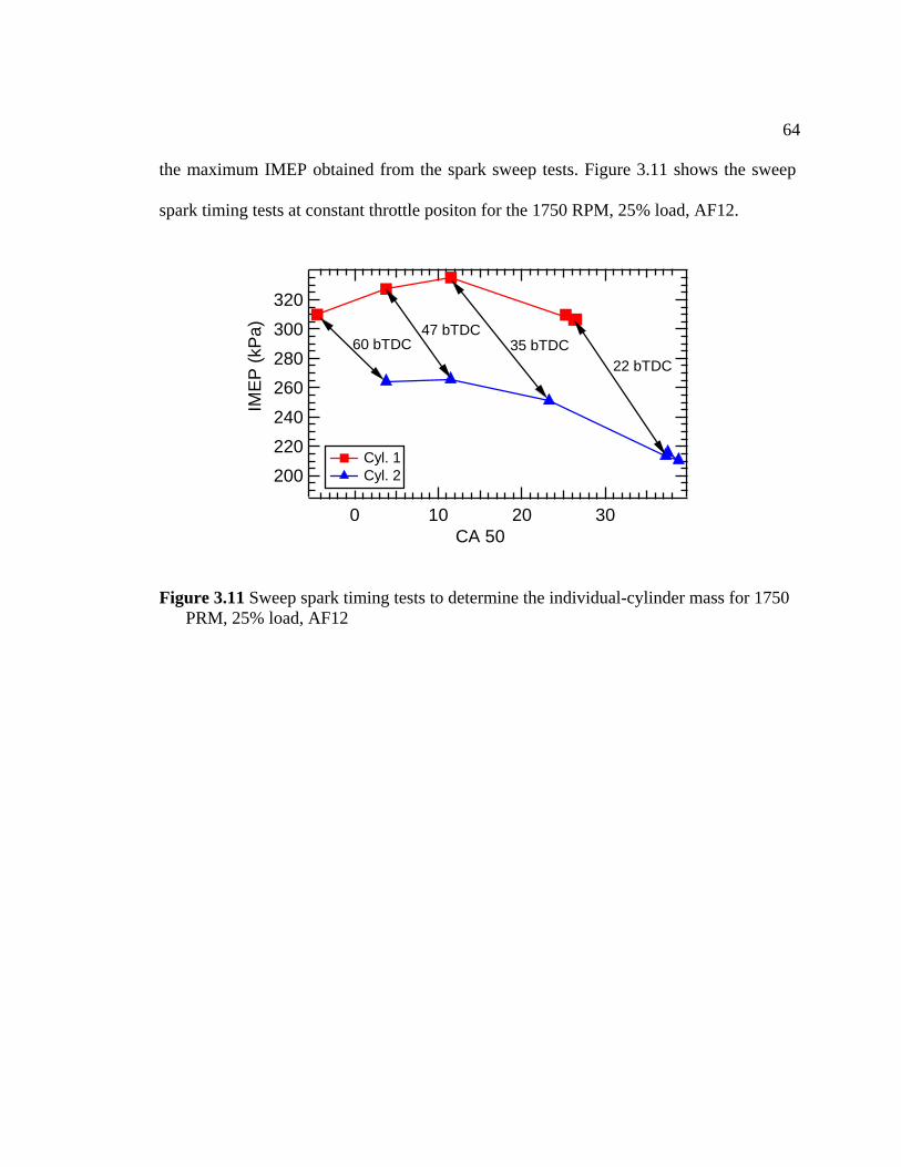
64
the maximum IMEP obtained from the spark sweep tests. Figure 3.11 shows the sweep
spark timing tests at constant throttle positon for the 1750 RPM, 25% load, AF12.
320300280260240220200
IME
P (k
Pa)
3020100CA 50
60 bTDC 35 bTDC22 bTDC
47 bTDC
Cyl. 1 Cyl. 2
Figure 3.11 Sweep spark timing tests to determine the individual-cylinder mass for 1750 PRM, 25% load, AF12
65
CHAPTER IV
TION
The liquid fuel film effects were easily isolated, and the results obtained from this
study were necessary to setup the required experimental conditions for the following
Two main goals were pursued in the liquid fuel study: the estimation of the stored
mass of fuel in the intake manifold and the characterization of its effects on the HC
emissio
s. The effect of the liquid fuel on the hydrocarbon
emissions was inferred from the comparison of two sets of engine-out HC emissions. The
first set was obtained fueling the en as
acquired fueling the engine with the homogeneous mixture systems (Both fueling system
4 STUDY OF THE LIQUID FUEL EFFECTS ON THE HC EMISSIONS
4.1 INTRODUC
studies of the other HC mechanisms.
ns. The estimation of the mass of fuel in the intake manifold was performed by
carrying out stop-fuel-injection test
gine with the carburetor, while the second set w
were described in detail in §3.2.2). For both fueling strategies, the engine was run over a
wide range of loads, speeds and air-fuel ratios. Cycle-resolved HC measurements and
heat release analysis were carried out to elucidate the implications of the liquid fuel on
the engine performance.
66
4.2 STOP-FUEL-INJECTION TESTS
As mentioned above, the stop-fuel-injections tests provided an estimation of the
mass o
In order to perform the stop-fuel-injection tests the carburetor-mounted fuel
injector system was used. As described in section §3.2.2.3, this system consists of a stock
carbure
During a typical stop-fuel-injection test, the engine was fired until the steady
state condition was reached (desired load, speed and air-fuel ratio). This condition was
attained when the engine oil temperature reached a constant value. Depending of the
engine operating condition this usually took around 30-45 minutes. Then, the injection
and the ignition were suddenly halted. After this sudden cut, the engine was kept
motoring at the same engine speed and air mass flow rate. Thus, only air was supplied to
the engine, which continued the vaporization of the liquid fuel stored in the intake
manifold. At the exhaust port, the post-stop-injection fuel concentration history was
recorded with the fast FID for about 2000 cycles.
f fuel stored in the intake manifold. Knowing the quantity of the liquid fuel present
was necessary to fully characterize its contribution on the HC engine-out emissions.
tor modified so that the fuel was supplied directly through the carburetor main jet
with a fuel injector (Fig. 3.4). This device emulates the carburetor fuel atomization, but
allows very accurate control of the fuel injection timing, the mass of fuel delivered per
cycle, and the simultaneous deactivation of the fuel injector and the ignition of the
engine.
67
4.2.1 INTAKE PORT LIQUID FUEL MASS ESTIMATION
The HC concentration in the exhaust following cessation of fuel injection is the
result of vaporization of liquid fuel in the intake system. The fast FID measures the HC
concentration, or mole fraction, XHC. In order to convert this concentration to a mass of
fuel exhausted per cycle, the fuel mole fraction was recast as the mass fraction and the
mixture in the exhaust was considered to consist of just fuel and air. The air mass flow
is measured independently, and the compilation of these effects gives the mass of
rate
fuel per cycle as:
airfuelcycleaircyclefuel MWX
MWX)1(// −
The fuel mass per cycle can be integrated, and then normalized by the mass of
fuel delivered per cycle as follows:
fuelfuelmm .= (4.1)
where, mfuel/cycle is the mass of fuel per cycle, mair/cycle is the measured amount of air per
cycle, Xfuel is the mean HC mole fraction for the cycle on a C1 basis (3XHC), MWfuel the
molecular weight of the fuel per C1, and MWair the molecular weight of the air.
cycleenginefuel
cyclesnormcumfuel m
m #..−− = (4.2)
where m
cyclefuelm
/
/
−
∑
cumulative mass of fuel, and mfuel-engine/cycle
is the mass of fuel delivered to the cylinder under steady state firing conditions for that
fuel-cum.-norm. represents the normalized
68
operating condition. Since this measurement was made in just one exhaust runner, mfuel-
cum.-norm corresponds to only one half of the total in the intake port.
4.2.2 FUEL CONCENTRATION HISTORY OF THE TRANSITION FIRING-
MOTORING DURING THE STOP-INJECTION TEST
During a stop injection test the HiTechniques data acquisition started to record
data approximately five seconds before the fuel injection and ignition were stopped. This
the me of the fuel concentration at the exhaust.
As mentioned before the program that controls the ECU was modified to
deactivate the fuel injection and the spark ignition simultaneously. To identify the cycle
in whi
allowed the observation of the transition from the firing mode to the motoring mode, and
evolution in ti
ch the stop fuel injection happened the fuel injector coil signal current was
recorded in phase with the fast-FID data. The electrical current was converted to voltage
using a Tektronic model A622 current probe. Figure 4.1 shows the sequence of the HC
concentration and the fuel injector coil current for three consecutive cycles, including the
cycle where the fuel injection is halted. In Fig. 4.1a, the injector is still energized,
however in the next two consecutive cycles Figs. 4.1b-c, the fuel injector has been
deactivated. The cycle where the fuel injector current signal disappeared indicated the
starting point where the mass of fuel leaving the engine was integrated and was
accounted as coming from the vaporization from the intake manifold.
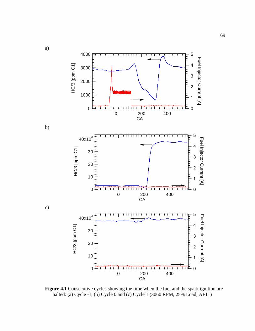
69
a) 4000 5
3000
2000
1000
0
HC
/3 [p
pm C
1]
4002000CA
4
3
2
1
0
ector Crr
]Fuel Inj
uent [A
b)
40x103
30
20
10
0
HC
/3pp
m1]
[ C
5
4002000CA
4
3
2
1
0
Fuele
nt [A]
Injctor C
urre
c)
40x103
30
20
10
0
HC
/3 [p
pm C
1]
4002000
5
4
3
2
1
0
Fuel Injector Current [A
]
CA
Figure 4.1 Consecutive cycles showing the time when the fuel and the spark ignition are halted: (a) Cycle -1, (b) Cycle 0 and (c) Cycle 1 (3060 RPM, 25% Load, AF11)
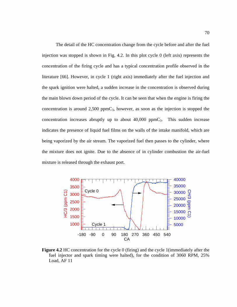
70
The detail of the HC concentration change from the cycle before and after the fuel
injection was stopped is shown in Fig. 4.2. In this plot cycle 0 (left axis) represents the
concentration of the firing cycle and has a typical concentration profile observed in the
literature [66]. However, in cycle 1 (right axis) immediately after the fuel injection and
the spark ignition were halted, a sudden increase in the concentration is observed during
the main blown down period of the cycle. It can be seen that when the engine is firing the
concentration is around 2,500 ppmC3, however, as soon as the injection is stopped the
concentration increases abruptly up to about 40,000 ppmC3. This sudden increase
indicates the presence of liquid fuel films on the walls of the intake manifold, which are
being vaporized by the air stream. The vaporized fuel then passes to the cylinder, where
the mixture does not ignite. Due to the absence of in cylinder combustion the air-fuel
mixture is released through the exhaust port.
400003500030000250002000015000100005000
CH
/3 (ppm C
1)
540450360270180900-90-180CA
4000
3500
3000
2500
2000
1500
1000
HC
C1)
/3 (p
pm
Cycle 0
Cycle 1
Figure 4.2 HC concentration for the cycle 0 (firing) and the cycle 1(immediately after the
fuel injector and spark timing were halted), for the condition of 3060 RPM, 25% Load, AF 11
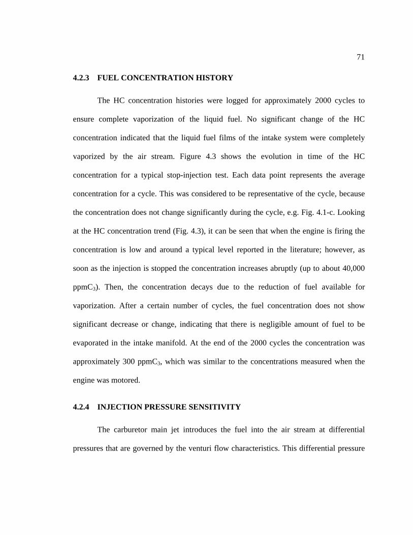
71
4.2.3 FUEL CONCENTRATION HISTORY
The HC concentration histories were logged for approximately 2000 cycles to
ensure complete vaporization of the liquid fuel. No significant change of the HC
concentration indicated that the liquid fuel films of the intake system were completely
vaporized by the air stream. Figure 4.3 shows the evolution in time of the HC
concentration for a typical stop-injection test. Each data point represents the average
concentration for a cycle. This was considered to be representative of the cycle, because
at t engine is firing the
soon as
he concentrations measured when the
engine was motored.
4.2.4 INJECTION PRESSURE SENSITIVITY
The carburetor main jet introduces the fuel into the air stream at differential
pressures that are governed by the venturi flow characteristics. This differential pressure
the concentration does not change significantly during the cycle, e.g. Fig. 4.1-c. Looking
he HC concentration trend (Fig. 4.3), it can be seen that when the
concentration is low and around a typical level reported in the literature; however, as
the injection is stopped the concentration increases abruptly (up to about 40,000
ppmC3). Then, the concentration decays due to the reduction of fuel available for
vaporization. After a certain number of cycles, the fuel concentration does not show
significant decrease or change, indicating that there is negligible amount of fuel to be
evaporated in the intake manifold. At the end of the 2000 cycles the concentration was
approximately 300 ppmC3, which was similar to t
72
40x103
30
20
10
0
/3 (p
pm C
1)H
C
2000160012008004000Cycle #
test (3060 RPM, 25% Load, AF11) Figure 4.3 HC concentration history measured at the exhaust in at typical stop injection
depends of the engine operating condition, and can be no more than ~ 50kPa
(corresponding to choked flow at the throat).
In the case of the carburetor-mounted fuel injector the fuel was pressurized using
a high pressure electrical fuel pump. Then, the pressure was reduced to typical carburetor
fuel supply pressures (around 58.5 kPag). It is very important to note that the injection of
fuel in the carburetor-mounted fuel injector is pulsating. Therefore, the fuel injection
pressure could impact the atomization, and consequently the HC emissions. In addition,
high injection pressures could promote high levels of fuel impingement on the carburetor
walls affecting the stored mass of fuel. Hence, the effect of the injection pressure on the
wall wetting was assessed. Several tests at different injection pressures were carried out
under static conditions i.e. with no air stream through the carburetor. The pseudo encoder
option of MotoTron was used to simulate the engine speed and the mass of fuel injected
per cycle. During the tests, the fuel pressure was increased until the point that the fuel
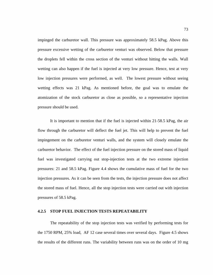
73
impinged the carburetor wall. This pressure was approximately 58.5 kPag. Above this
pressure excessive wetting of the carburetor venturi was observed. Below that pressure
the droplets fell within the cross section of the venturi without hitting the walls. Wall
wetting can also happen if the fuel is injected at very low pressure. Hence, test at very
low injection pressures were performed, as well. The lowest pressure without seeing
wetting effects was 21 kPag. As mentioned before, the goal was to emulate the
atomization of the stock carburetor as close as possible, so a representative injection
It is important to mention that if the fuel is injected within 21-58.5 kPag, the air
nt the fuel
impingement on the carburetor venturi walls, and the system will closely emulate the
carburetor behavior. The effect of the fuel injection pressure on the stored mass of liquid
fuel was investig
4.2.5 STOP ESTS REPEATABILITY
The repeat ility of the stop injection as verified by performing tests for
the 1750 RPM d, A case severa es over se l day igure 4.5 shows
the results of the different runs. The variab mg
pressure should be used.
flow through the carburetor will deflect the fuel jet. This will help to preve
ated carrying out stop-injection tests at the two extreme injection
pressures: 21 and 58.5 kPag. Figure 4.4 shows the cumulative mass of fuel for the two
injection pressures. As it can be seen from the tests, the injection pressure does not affect
the stored mass of fuel. Hence, all the stop injection tests were carried out with injection
pressures of 58.5 kPag.
FUEL INJECTION T
ab tests w
, 25% loa F 12 l tim vera s. F
ility between runs was on the order of 10
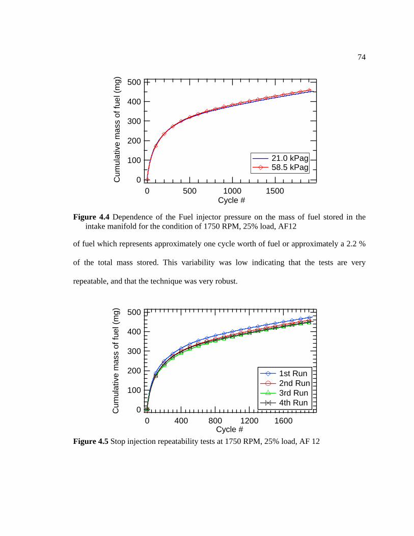
74
500
400
300
200
100
0Cm
ulat
ive
mas
s of
fue
ul (
mg)
150010005000Cycle #
21.0 kPag 58.5 kPag
Figure 4.4 Dependence of the Fuel injectorintake manifold for the condition of 1750 RPM, 25% load, A
pressure on the mass of fuel stored in the
F12
of fuel which represents approximately one cycle worth of fuel or approximately a 2.2 %
of the total mass stored. This variability was low indicating that the tests are very
repeatable, and that the technique was very robust.
500
400
300
200
100
0Cm
ulat
ive
ma
fm
uss
o fu
el (
g)
160012008004000Cycle #
1st Run 2nd Run 3rd Run 4th Run
Figure 4.5 Stop injection repeatability tests at 1750 RPM, 25% load, AF 12
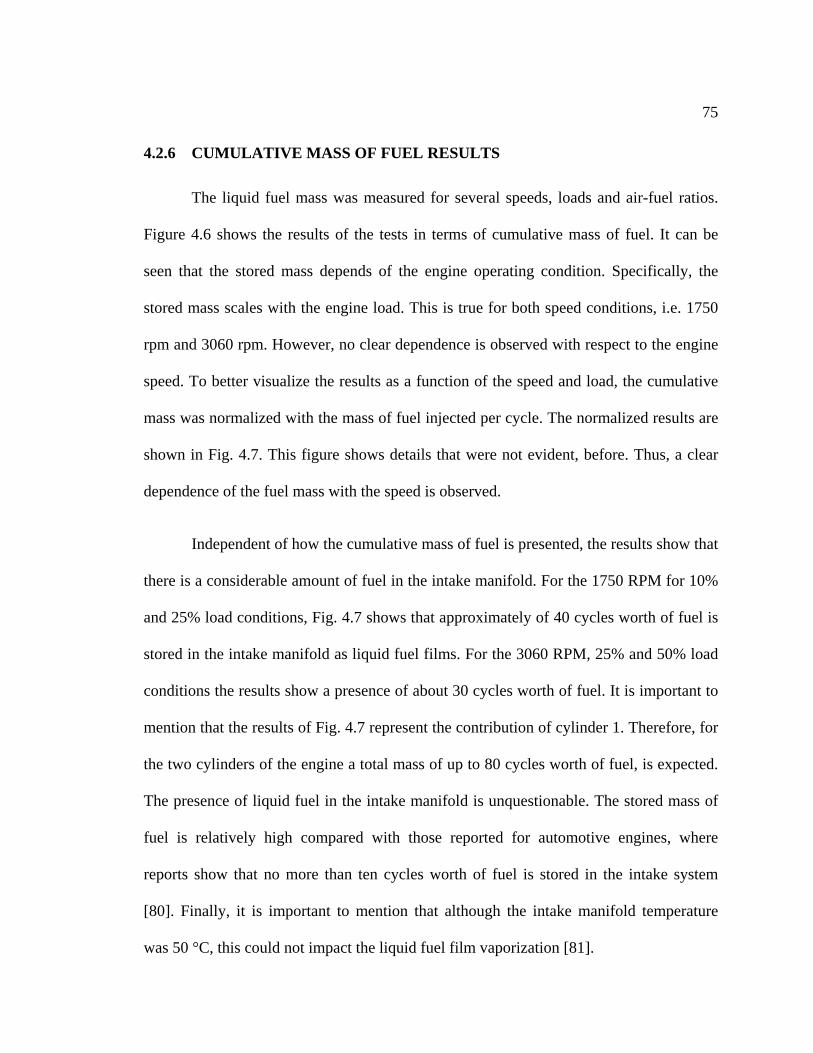
75
4.2.6 CUMULATIVE MASS OF FUEL RESULTS
iquid fuel mass was measured for several speeds, loads and air-fuel ratios.
f the te
ad. This is true for both speed conditions, i.e. 1750
rpm and 3060 rpm. However, no clear dependence is observed with respect to the engine
speed.
Independent of how the cumulative mass of fuel is presented, the results show that
there is
n that although the intake manifold temperature
was 50 °C, this could not impact the liquid fuel film vaporization [81].
The l
Figure 4.6 shows the results o sts in terms of cumulative mass of fuel. It can be
seen that the stored mass depends of the engine operating condition. Specifically, the
stored mass scales with the engine lo
To better visualize the results as a function of the speed and load, the cumulative
mass was normalized with the mass of fuel injected per cycle. The normalized results are
shown in Fig. 4.7. This figure shows details that were not evident, before. Thus, a clear
dependence of the fuel mass with the speed is observed.
a considerable amount of fuel in the intake manifold. For the 1750 RPM for 10%
and 25% load conditions, Fig. 4.7 shows that approximately of 40 cycles worth of fuel is
stored in the intake manifold as liquid fuel films. For the 3060 RPM, 25% and 50% load
conditions the results show a presence of about 30 cycles worth of fuel. It is important to
mention that the results of Fig. 4.7 represent the contribution of cylinder 1. Therefore, for
the two cylinders of the engine a total mass of up to 80 cycles worth of fuel, is expected.
The presence of liquid fuel in the intake manifold is unquestionable. The stored mass of
fuel is relatively high compared with those reported for automotive engines, where
reports show that no more than ten cycles worth of fuel is stored in the intake system
[80]. Finally, it is important to mentio
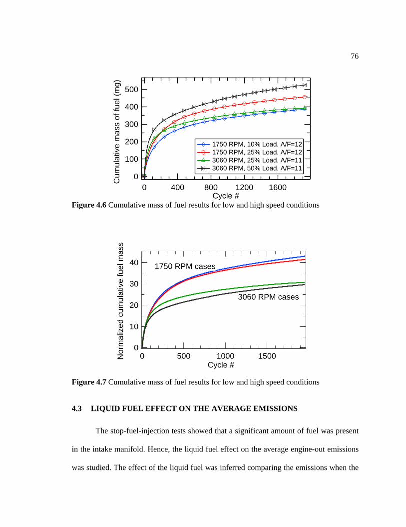
76
500
400
300
200
100
0ua
g)C
mul
tive
mas
s of
fuel
(m
160012008004000Cycle #
1750 RPM, 10% Load, A/F=12 1750 RPM, 25% Load, A/F=12 3060 RPM, 25% Load, A/F=11 3060 RPM, 50% Load, A/F=11
Figure 4.6 Cumulative mass of fuel results for low and high speed conditions
40
30
20
10
0orm
Nal
ized
cum
lave
fuel
mu
tias
s
150010005000Cycle #
3060 RPM cases
1750 RPM cases
Figure 4.7 Cumulative mass of fuel results for low and high speed conditions
4.3 LIQUID FUEL EFFECT ON THE AVERAGE EMISSIONS
The stop-fuel-injection tests showed that a significant amount of fuel was present
in the intake manifold. Hence, the liquid fuel effect on the average engine-out emissions
was studied. The effect of the liquid fuel was inferred comparing the emissions when the
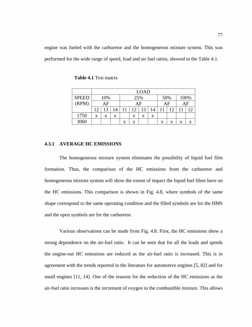
77
engine was fueled with the carburetor and the homogeneous mixture system. This was
performed for the wide range of speed, load and air fuel ratios, showed in the Table 4.1.
Table 4.1 Test matrix
LOAD
10% 25% 50% 100% AF AF AF AF
SPEED (RPM)
12 13 14 11 12 13 14 11 12 11 12 1750 x x x x x x 3060 x x x x x x
4.3.1 AVERAGE HC EMISSIONS
The homogeneous mixture system eliminates the possibility of liquid fuel film
formation. Thus, the comparison of the HC emissions from the carburetor and
the HC emissions. This comparison is shown in Fig. 4.8, where symbols of the same
shape c
Various observations can be made from Fig. 4.8. First, the HC emissions show a
strong
homogeneous mixture system will show the extent of impact the liquid fuel films have on
orrespond to the same operating condition and the filled symbols are for the HMS
and the open symbols are for the carburetor.
dependence on the air-fuel ratio. It can be seen that for all the loads and speeds
the engine-out HC emissions are reduced as the air-fuel ratio is increased. This is in
agreement with the trends reported in the literature for automotive engines [5, 82] and for
small engines [11, 14]. One of the reasons for the reduction of the HC emissions as the
air-fuel ratio increases is the increment of oxygen in the combustible mixture. This allows
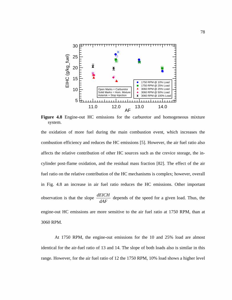
78
30
25
20
15
the oxidation of more fuel during the main combustion event, which increases the
combustion efficiency and reduces the HC emissions [5]. However, the air fuel ratio also
affects the relative contribution of other HC sources such as the crevice storage, the in-
cylinder post-flame oxidation, and the residual mass fraction [82]. The effect of the air
fuel ratio on the relative contribution of the HC mechanisms is complex; however, overall
in Fig. 4.8 an increase in air fuel ratio reduces the HC emissions. Other important
observation is that the slope dAF
dEICH depends of the speed for a given load. Thus, the
engine-out HC emissions are more sensitive to the air fuel ratio at 1750 RPM, than at
3060 RPM.
At 1750 RPM, the engine-out emissions for the 10 and 25% load are almost
identical for the air-fuel ratio of 13 and 14. The slope of both loads also is similar in this
nge. However, for the air fuel ratio of 12 the 1750 RPM, 10% load shows a higher level ra
10
514.013.012.011.0
AF
EIH
C (g
/kg_
fuel
)
1750 RPM @ 10% Load 1750 RPM @ 25% Load 3060 RPM @ 25% Load 3060 RPM @ 50% Load 3060 RPM @ 100% Load
Open Marks = CarburetorSolid Marks = Hom. MixtureAsterisk = Stop Injection
Figure 4.8 Engine-out HC emissions for the carburetor and homogeneous mixture
system.
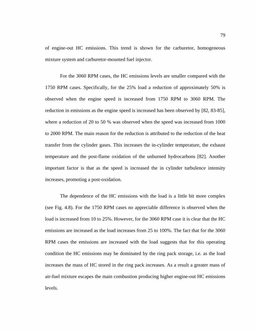
79
of eng
For the 3060 RPM cases, the HC emissions levels are smaller compared with the
1750 RPM cases. Specifically, for the 25% load a reduction of approximately 50% is
ob
reduction in emissions as the engine speed is increased has been observed by [82, 83-85],
w uction o 50 % was obser hen the speed creased 000
to 2000 RPM e m re fo re tion attr ed e r ctio f th at
transfer from the cylinder gases. This increases the in-cylinder tem r st
mperature and the post-flame oxidation of the unburned hydrocarbons [82]. Another
importa
The dependence of the HC emissions with the load is a little bit more complex
(see Fig. 4.8). For the 1750 RPM cases no appreciable difference is observed when the
load is
ted by the ring pack storage, i.e. as the load
creases. As a result a greater mass of
air-fuel mixture escapes the main combustion producing higher engine-out HC emissions
levels.
ine-out HC emissions. This trend is shown for the carburetor, homogeneous
mixture system and carburetor-mounted fuel injector.
served when the engine speed is increased from 1750 RPM to 3060 RPM. The
here a red of 20 t ved w was in from 1
. Th ain ason r the duc is ibut to th edu n o e he
peratu e, the exhau
te
nt factor is that as the speed is increased the in cylinder turbulence intensity
increases, promoting a post-oxidation.
increased from 10 to 25%. However, for the 3060 RPM case it is clear that the HC
emissions are increased as the load increases from 25 to 100%. The fact that for the 3060
RPM cases the emissions are increased with the load suggests that for this operating
condition the HC emissions may be domina
increases the mass of HC stored in the ring pack in
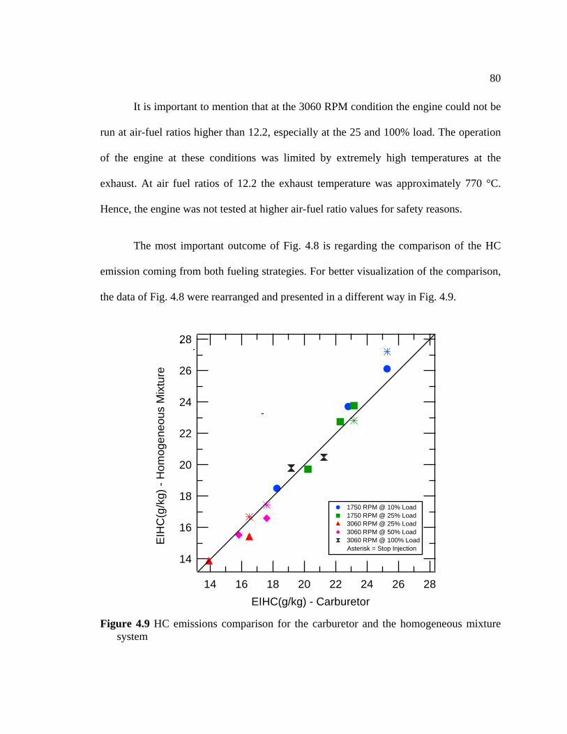
80
It is important to mention that at the 3060 RPM condition the engine could not be
n at air-fuel ratios higher than 12.2, especially at the 25 and 100% load. The operation
values for safety reasons.
ru
of the engine at these conditions was limited by extremely high temperatures at the
exhaust. At air fuel ratios of 12.2 the exhaust temperature was approximately 770 °C.
Hence, the engine was not tested at higher air-fuel ratio
The most important outcome of Fig. 4.8 is regarding the comparison of the HC
emission coming from both fueling strategies. For better visualization of the comparison,
the data of Fig. 4.8 were rearranged and presented in a different way in Fig. 4.9.
28
26
24
22
20
18
16
14
EIH
C(g
/kg)
- H
mog
eneo
us M
oix
ture
2826242220181614
1750 RPM @ 10% Load 1750 RPM @ 25% Load 3060 RPM @ 25% Load 3060 RPM @ 50% Load 3060 RPM @ 100% Load
EIHC(g/kg) - Carburetor
Asterisk = Stop Injection
system
Figure 4.9 HC emissions comparison for the carburetor and the homogeneous mixture
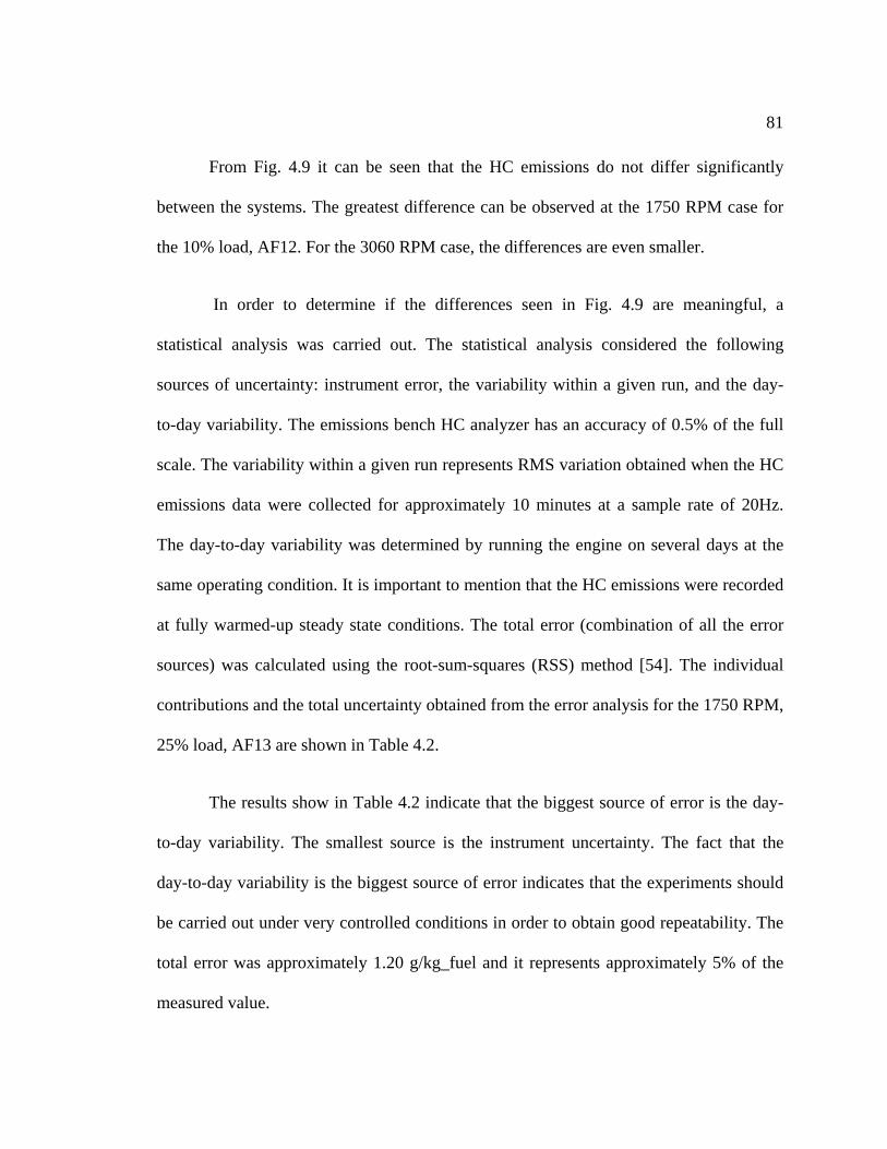
81
From Fig. 4.9 it can be seen that the HC emissions do not differ significantly
between the systems. The greatest difference can be observed at the 1750 RPM case for
the 10% load, AF12. For the 3060 RPM case, the differences are even smaller.
In order to determine if the differences seen in Fig. 4.9 are meaningful, a
statistical analysis was carried out. The statistical analysis considered the following
sources of uncertainty: instrument error, the variability within a given run, and the day-
to-day variability. The emissions bench HC analyzer has an accuracy of 0.5% of the full
scale. The variability within a given run represents RMS variation obtained when the HC
emissions data were collected for approximately 10 minutes at a sample rate of 20Hz.
The day-to-day variability was determined by running the engine on several days at the
same operating condition. It is important to mention that the HC emissions were recorded
at fully warmed-up steady state conditions. The total error (combination of all the error
sources) was calculated using the root-sum-squares (RSS) method [54]. The individual
contributions and the total uncertainty obtained from the error analysis for the 1750 RPM,
25% load, AF13 are shown in Table 4.2.
The results show in Table 4.2 indicate that the biggest source of error is the day-
to-day variability. The smallest source is the instrument uncertainty. The fact that the
day-to-day variability is the biggest source of error indicates that the experiments should
be carried out under very controlled conditions in order to obtain good repeatability. The
total error was approximately 1.20 g/kg_fuel and it represents approximately 5% of the
measured value.
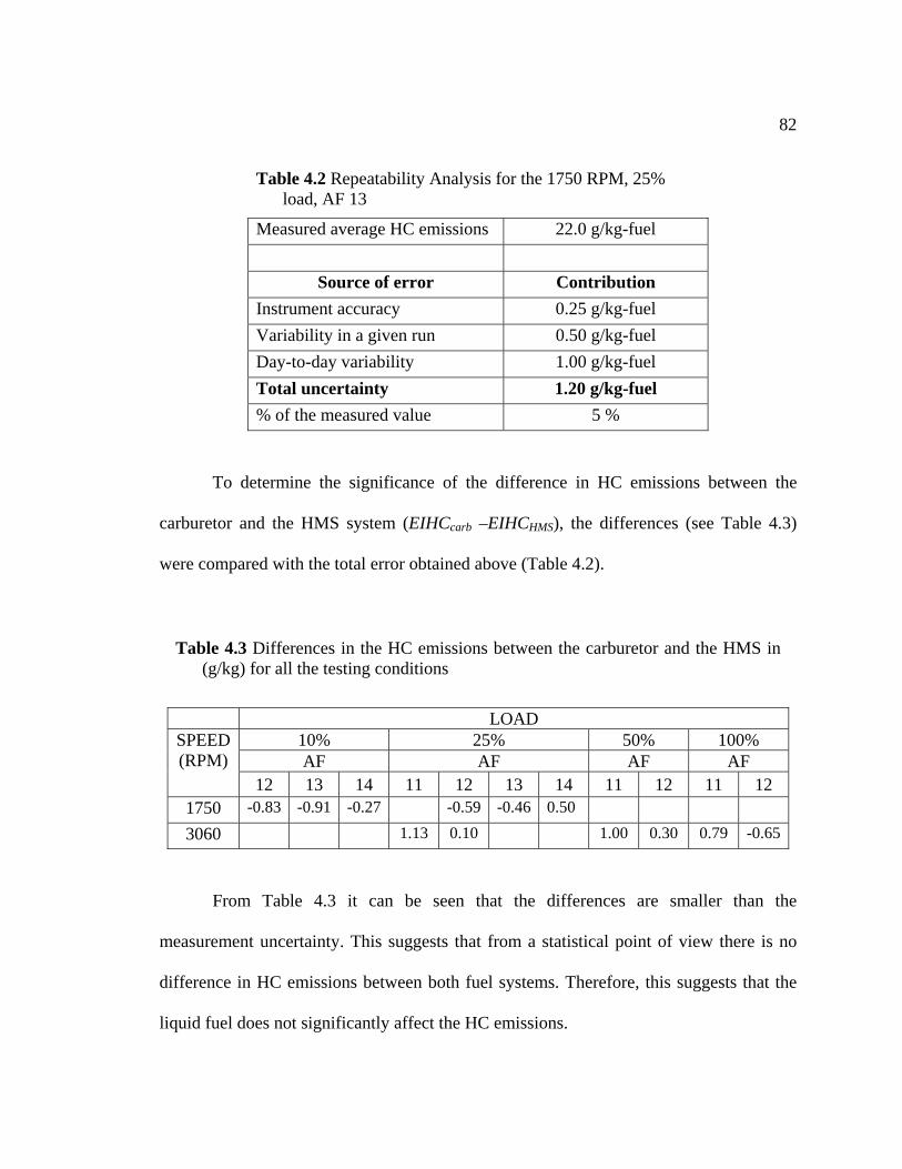
82
Table 4.2 Repeatability Analysis for the 1750 RPM, 25% load, AF 13
Measured average HC emissions 22.0 g/kg-fuel
Source of error Contribution Instrument accuracy 0.25 g/kg-fuel Variability in a given run 0.50 g/kg-fuel Day-to-day variability 1.00 g/kg-fuel Total uncertainty 1.20 g/kg-fuel % of the measured value 5 %
To determine the significance of the difference in HC emissions between the
carburetor and the HMS system (EIHCcarb –EIHCHMS), the differences (see Table 4.3)
were compared with the total error obtained above (Table 4.2).
LOAD
Table 4.3 Differences in the HC emissions between the carburetor and the HMS in (g/kg) for all the testing conditions
10% 25% 50% 100% AF AF AF AF
SPEED (RPM)
12 13 14 11 12 13 14 11 12 11 12 1750 -0.83 -0.91 -0.27 -0.59 -0.46 0.50
3060 1.13 0.10 1.00 0.30 0.79 -0.65
From Table 4.3 it can be seen that the differences are smaller than the
measurement uncertainty. This suggests that from a statistical point of view there is no
difference in HC emissions between both fuel systems. Therefore, this suggests that the
liquid fuel does not significantly affect the HC emissions.
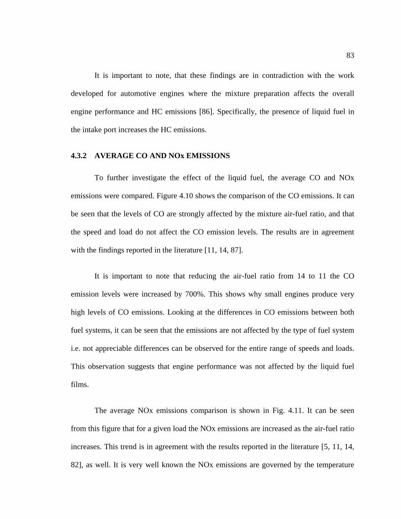
83
It is important to note, that these findings are in contradiction with the work
developed for automotive engines where the mixture preparation affects the overall
engine performance and HC emissions [86]. Specifically, the presence of liquid fuel in
the intake port increases the HC emissions.
To further investigate the effect of the liquid fuel, the average CO and NOx
emissions were com
4.3.2 AVERAGE CO AND NOx EMISSIONS
pared. Figure 4.10 shows the comparison of the CO emissions. It can
be seen that the levels of CO are strongly affected by the mixture air-fuel ratio, and that
on levels. The results are in agreement
with th
It is important to note that reducing the air-fuel ratio from 14 to 11 the CO
emission levels were increased by 700%. This shows why small engines produce very
high levels of CO emissions. Looking at the differences in CO emissions between both
fuel systems, it can be seen that the emissions are not affected by the type of fuel system
i.e. not appreciable differences can be observed for the entire range of speeds and loads.
This observation suggests that engine performance was not affected by the liquid fuel
films.
The average NOx emissions comparison is shown in Fig. 4.11. It can be seen
from this figure that for a given load the NOx emissions are increased as the air-fuel ratio
increases. This trend is in agreement with the results reported in the literature [5, 11, 14,
82], as well. It is very well known the NOx emissions are governed by the temperature
the speed and load do not affect the CO emissi
e findings reported in the literature [11, 14, 87].
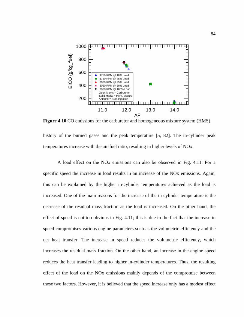
84
1000
800
600
400
200
EIC
O (
)g/
kg_f
uel
14.013.012.011.0AF
1750 RPM @ 10% Load 1750 RPM @ 25% Load 3060 RPM @ 25% Load 3060 RPM @ 50% Load 3060 RPM @ 100% Load
Open Marks = Carburetor
Asterisk = Stop Injection
Figure 4.10 CO emissions for the carburetor and homogeneous mixture system (HMS).
Solid Marks = Hom. Mixture
history of the burned gases and the peak temperature [5, 82]. The in-cylinder peak
temperatures increase with the air-fuel ratio, resulting in higher levels of NOx.
A load effect on the NOx emissions can also be observed in Fig. 4.11. For a
specific speed the increase in load results in an increase of the NOx emissions. Again,
this can be explained by the higher in-cylinder temperatures achieved as the load is
increas
gine speed
reduces the heat transfer leading to higher in-cylinder temperatures. Thus, the resulting
effect of the load on the NOx emissions mainly depends of the compromise between
these two factors. However, it is believed that the speed increase only has a modest effect
ed. One of the main reasons for the increase of the in-cylinder temperature is the
decrease of the residual mass fraction as the load is increased. On the other hand, the
effect of speed is not too obvious in Fig. 4.11; this is due to the fact that the increase in
speed compromises various engine parameters such as the volumetric efficiency and the
net heat transfer. The increase in speed reduces the volumetric efficiency, which
increases the residual mass fraction. On the other hand, an increase in the en
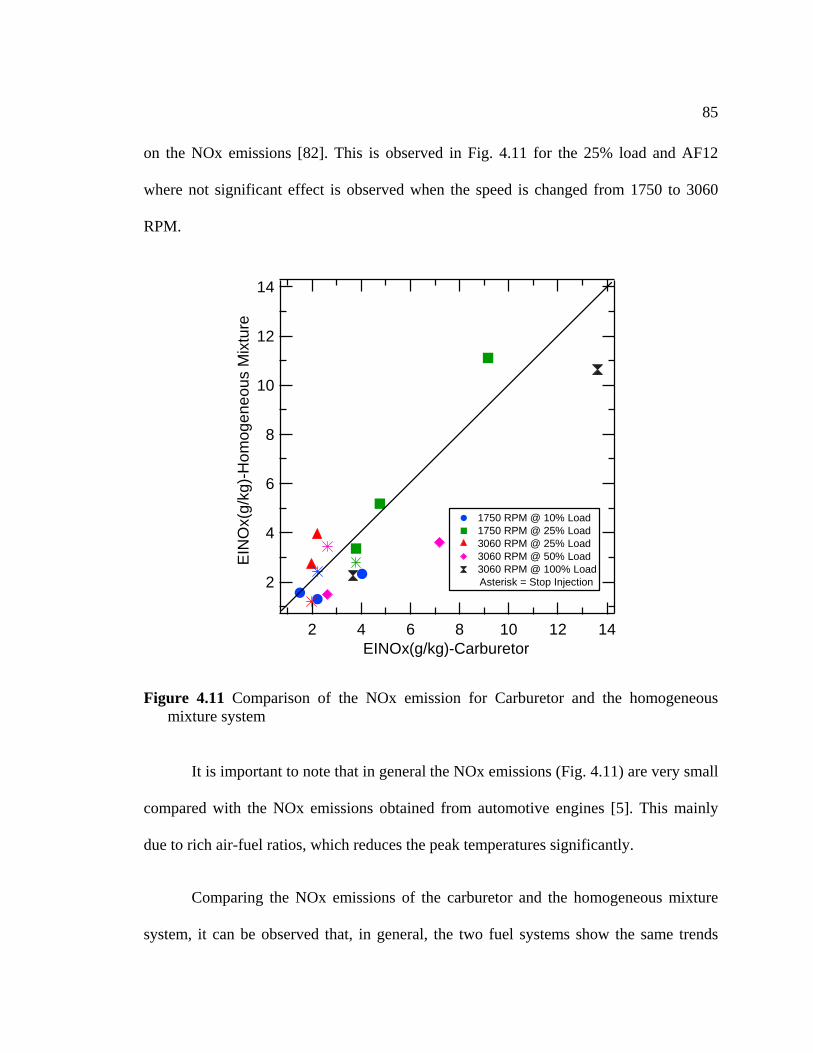
85
on the NOx emissions [82]. This is observed in Fig. 4.11 for the 25% load and AF12
where not significant effect is observed when the speed is changed from 1750 to 3060
RPM.
14
12
10
8
6
4
2
EIN
Ox(
g/kg
)-Hom
ogen
eous
Mxt
uri
e
1412108642EINOx(g/kg)-Carburetor
1750 RPM @ 10% Load 1750 RPM @ 25% Load 3060 RPM @ 25% Load 3060 RPM @ 50% Load 3060 RPM @ 100% Load
Asterisk = Stop Injection
Figure
all
compar
homogeneous mixture
system, it can be observed that, in general, the two fuel systems show the same trends
4.11 Comparison of the NOx emission for Carburetor and the homogeneous mixture system
It is important to note that in general the NOx emissions (Fig. 4.11) are very sm
ed with the NOx emissions obtained from automotive engines [5]. This mainly
due to rich air-fuel ratios, which reduces the peak temperatures significantly.
Comparing the NOx emissions of the carburetor and the
86
with no significant differences except the cases of 3060 RPM, AF12, 50 and 100% load.
However, the differences are small and can be attributed to the variability rather than to a
physical difference between the NOx emissions. The results are in agreement with the
work of Bonneau [14], who found negligible differences between fuel systems for rich
air-fuel ratios. The differences for the 3060 RPM case could be attributed to the error of
the NOx analyzer. The NOx analyzer exhibited a decay in the reading with time for a
constant gas composition. Although, the sensor was calibrated before every run the level
of signal decay was unknown in the intermediate stages of the measurement process.
Finally, in spite of the small differences observed for some cases in Fig. 4.11, it can be
concluded that the liquid fuel effect does not have a significant effect on the NOx
emissions.
4.4 CYCLE-RESOLVED HC EMISSIONS
articularities of the effect of the liquid fuel on the HC emissions. Studies carried out by
Stache and
Cycle-resolved HC emissions measurements were performed to help elucidate the
p
Alkidas [88] in a port-fuel injected automotive engine showed that the
presence of the liquid fuel in the cylinder affected the cycle-resolved HC history.
Specifically, the effect of the liquid fuel was observed during the exhaust stroke when the
piston was near TDC. Thus, similar effects should be expected in the case of a small
engine when fueled with the carburetor. Therefore, to further investigate the differences
in HC emissions for the mixture preparation systems, time-resolved HC concentration
measurements were performed using the fast FID.
87
The fast-FID results for all of the conditions tested are shown in Fig. 4.12. All of
the cases investigated follow the same general shape, which agrees with literature reports
[65, 66, 88]. During the time that both the intake and exhaust valves are closed, there is a
relatively high, steady HC concentration in the exhaust port, however since the mass flow
rate is zero it is not a significant effect. The effect of exhaust valve leakage, which would
cause an in
at 130
released increasing the relative amount of HC at the exhaust port. During the blow-down
period, the HC concentration is reduced because it contains the bulk gases that were
burned during the main combustion event. The majority of the exhaust stroke
corresponds to a relatively low HC concentration. At the end of the exhaust stroke, as the
piston approaches the TDC, the HC stored in the ring pack that escaped after the
combustion process are released. These HC-rich gases are located near the piston crown
to the low mixing rates, and are expel by the piston motion at the end of the
exhaust stroke.
The magnitude of the cycle-resolved HC concentrations measured at the exhaust
port were comparable to the corresponding values for the averaged results, but a direct
comparison is complicated by the instantaneous mass flow rate, which varies
considerably during the exhaust-valve-open period. The cycle-resolved HC
concentrations do, however, clearly show the expected trend with AF; for a fixed
condition the cycle-resolved HC concentration decreases with increasing AF.
crease in the concentration during the high pressure part of the cycle, i.e.
starting at IVC, does not appear to be significant. When the exhaust valve starts to open
°ATDC, the HC stored in the crevices of the spark plug and exhaust valve are
due led
88
A comparison of the cycle-resolved HC emissions for the two different mixture
systems shows that there is very little difference between the carburetor and the
homogeneous system. The magnitudes of the HC emissions are not exactly the same for
both systems, but the values are within 5% of the average value. Some of the differences
in the magnitude of the HC concentration can be attributed to the fact that the air-fuel
ratio was found to fluctuate in time with the carburetor. The nuances of the HC
centration history are, however, rep ed very well between the two mixture
systems. For example, the low load conditions all exhibit a decrease in HC concentration
at 250 ATDC, and the phasing and magnitude of this decrease are well matched for the
two mixture preparation systems. The increased HC concentration due to the fuel films
observed by Stache and Alkidas [88] near TDC is not observed in Fig. 4.12 for all the
cases. Overall, in accord with the average emission measurements, the cycle-resolved HC
measurements show that the emissions appear to be insensitive to the air-fuel mixture
pre
4.5 H
con licat
paration system, and the carburetor is not contributing to the HC emissions under
these conditions.
EAT RELEASE ANALYSIS
The characterization of the combustion event was carried out by performing a
single-zone heat release analysis (see Appendix XII) in order to further identify
differences in the mixture preparation system, and the results are shown in Fig. 4.13.
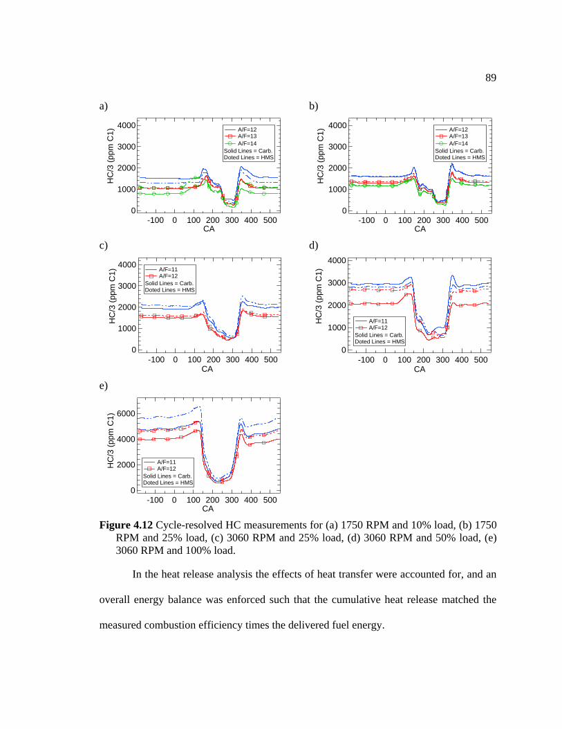
89
a)
In the heat release analysis the effects of heat transfer were accounted for, and an
overall energy balance was enforced such that the cumulative heat release matched the
measured combustion efficiency times the delivered fuel energy.
4000
3000
2000
1000
0
HC
/3 (p
pm C
1)
5004003002001000-100CA
A/F=12 A/F=13 A/F=14
Solid Lines = Carb.Doted Lines = HMS
b)
4000
3000
2000
1000
0
pH
C/3
(pm
C1)
5004003002001000-100CA
A/F=12 A/F=13 A/F=14
c)
Solid Lines = Carb.Doted Lines = HMS
d)
40004000
3000
2000
1000
5004003002001000-100
3000
2000
0
HC
/3 (p
1)pm
C
CA
A/F=11 A/F=12
Solid Lines = Carb.Doted Lines = HMS
1000
0
HC
/3 (p
pm C
1)
5004003002001000-100CA
A/F=11 A/F=12
Doted Lines = HMS
Solid Lines = Carb.
e)
6000
4000
2000
0
HC
/3 (p
pm C
1)
5004003002001000-100CA
A/F=11 A/F=12
Solid Lines = Carb.Doted Lines = HMS
Figure 4.12 Cycle-resolved HC measurements for (a) 1750 RPM and 10% load, (b) 1750 RPM and 25% load, (c) 3060 RPM and 25% load, (d) 3060 RPM and 50% load, (e) 3060 RPM and 100% load.
90
The heat release rate comparison sh
system does not have a significant effect on the energy release rate. This result further
su t
release data for the differen nt variation, which is
largely because the tests were performed at fixed spark timing. The full load data show a
-p ofile that has duration typical of spark-ignition engines. The
lower load cases, however, have a prolonged
ows that, for a given load and speed the fuel
pports the negligible difference observed in the emissions measurements. The hea
t operating conditions show a significa
well hased heat release pr
combustion event, with the heat release
continuing late into the expansion stroke. At the low load there is an indication that the
heat release is extending beyond the exhaust valve opening. This, suggests that
incomplete combustion could be a source of HC emissions. This will be discussed in
detail in the following chapter.
4.6 SUMMARY
In the present chapter the effect of the liquid fuel on the HC emissions was
studied. The study was divided in two parts. The first part was focused on the
quantification of the mass of liquid fuel stored in the intake system. This was carried out
performing stop-fuel-injection tests using a carburetor-mounted fuel injector. The results
showed that a significant amount of liquid fuel was stored in the intake manifold and that
it was highly dominated by the engine speed. For the 1750 RPM conditions the results
showed that up to 80 cycles worth of fuel was stored in the intake manifold. For the 3060
RPM about 60 cycles worth of fuel was stored in the intake system. This stored mass of
fuel is high, relative to port-fuel injected automotive engines [80].
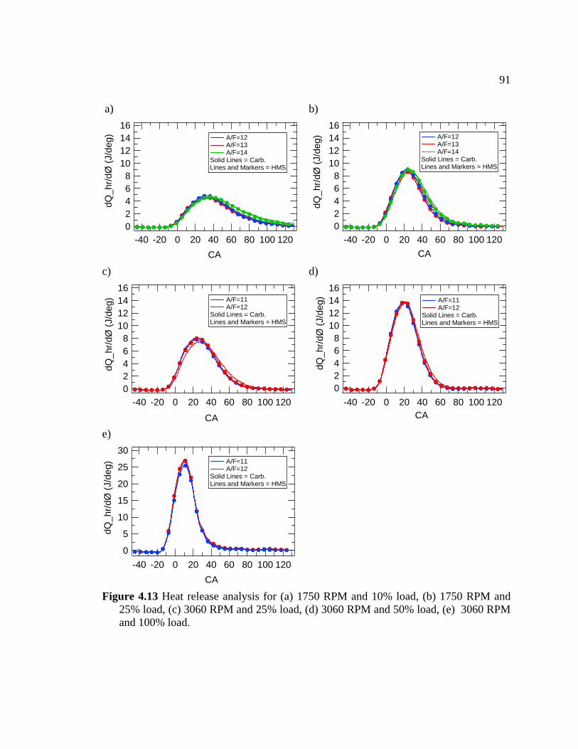
91
a) b) 16 1614121086420
/dØ
/deg
)
120100806040200-20-40CA
dQ_h
r (J
A/F=12 A/F=13 A/F=14
Solid Lines = Carb.Lines and Markers = HMS
14121086420
dQ_h
r/dØ
(J/d
eg)
120100806040200-20-40CA
A/F=12 A/F=13 A/F=14
Solid Lines = Carb.Lines and Markers = HMS
c)
16141210
86420
dQ_h
/dØ
(/d
eg)
rJ
120100806040200-20-40
CA
A/F=11 A/F=12
Solid Lines = Carb.Lines and Markers = HMS
d) 1614121086420
dQ_h
/dØ
(/d
eg)
rJ
120100806040200-20-40CA
A/F=11 A/F=12
Solid Lines = Carb.Lines and Markers = HMS
e)
30
25
20
15
10
5
0
dQ_h
r/dØ
(J/d
eg)
120100806040200-20-40CA
A/F=11 A/F=12
Figure 4.13 Heat release analysis for (a) 1750 RPM and 10% load, (b) 1750 RPM and
Solid Lines = Carb.Lines and Markers = HMS
25% load, (c) 3060 RPM and 25% load, (d) 3060 RPM and 50% load, (e) 3060 RPM and 100% load.
92
In the second part of the study, the effect of the liquid fuel on the HC emissions
was investigated. This was accomplished by comparing the engine-out HC emissions
from the carburetor and the homogeneous mixture system. The HC emissions comparison
showed only small differences. A statistical analysis was carried out to verify if the
observed small differences were significant. The total error calculated from the statistical
both fu
lved HC
emissions. In addition the average CO and NOx emissions and the heat release were not
affected by the presence of liquid fuel.
analysis was of 1.25 g/kg-fuel, and this was higher than the observed differences between
el systems. This suggested that the liquid fuel does not affect the engine out HC
emissions. It is important to mention that these tests were at steady state, fully warmed up
conditions with rich air-fuel ratios. The findings of the HC emissions comparison were
supported by the insignificant differences in CO and NOx emissions and the heat release.
Additional evidence that the liquid fuel does not affect the HC emission was provided by
cycle-resolved HC measurements. The HC concentration traces for both fuel systems
showed the same trend along the cycle with not significant differences, especially during
the last part of the exhaust process when the piston is near TDC where the liquid fuel
effect is expected to show its signature [88].
In conclusion, the results show that there is significant amount of fuel in the
intake manifold, however this does not affect either the average or cycle-reso
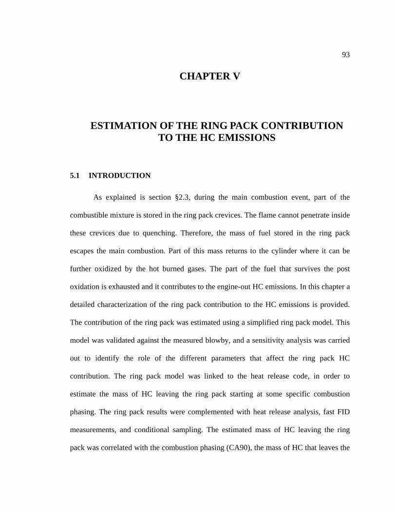
93
CHAPTER V
5 ESTIMATION OF THE RING PACK CONTRIBUTION TO THE HC EMISSIONS
5.1 INTRODUCTION
As explained is section §2.3, during the main combustion event, part of the
combustible mixture is stored in the ring pack crevices. The flame cannot penetrate inside
these crevices due to quenching. Therefore, the mass of fuel stored in the ring pack
escapes the main combustion. Part of this mass returns to the cylinder where it can be
further oxidized by the hot burned gases. The part of the fuel that survives the post
oxidation is exhausted and it contributes to the engine-out HC emissions. In this chapter a
ribution to the HC emissions is provided.
The contribution of the ring pack was estimated using a simplified ring pack model. This
model was validated against the measured blowby, and a sensitivity analysis was carried
out to identify the role of the different parameters that affect the ring pack HC
contribution. The ring pack model was linked to the heat release code, in order to
estimate the mass of HC leaving the ring pack starting at some specific combustion
phasing. The ring pack results were comple ented with heat release analysis, fast FID
The estimated mass of HC leaving the ring
pack was correlated with the combustion phasing (CA90), the mass of HC that leaves the
detailed characterization of the ring pack cont
m
measurements, and conditional sampling.
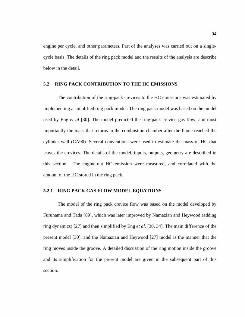
94
engine
. The details of the ring pack model and the results of the analysis are describe
below in the detail.
5.2 RING PACK CONTRIBUTION TO THE HC EMISSIONS
The contribution of the ring-pack crevices to the HC emissions was estimated by
implementing a simplified ring pack model. The ring pack model was based on the model
used by Eng et al [30]. The model predicted the ring-pack crevice gas flow, and most
importantly the mass that returns to the combustion chamber after the flame reached the
cylinder wall (CA90). Several conventions were used to estimate the mass of HC that
leaves
5.2.1 RING PACK GAS FLOW MODEL EQUATIONS
per cycle, and other parameters. Part of the analyses was carried out on a single-
cycle basis
the crevices. The details of the model, inputs, outputs, geometry are described in
this section. The engine-out HC emission were measured, and correlated with the
amount of the HC stored in the ring pack.
The model of the ring pack crevice flow was based on the model developed by
Furuhama and Tada [89], which was later improved by Namazian and Heywood (adding
ring dynamics) [27] and then simplified by Eng et al. [30, 34]. The main difference of the
present model [30], and the Namazian and Heywood [27] model is the manner that the
ring moves inside the groove. A detailed discussion of the ring motion inside the groove
and its simplification for the present model are given in the subsequent part of this
section.
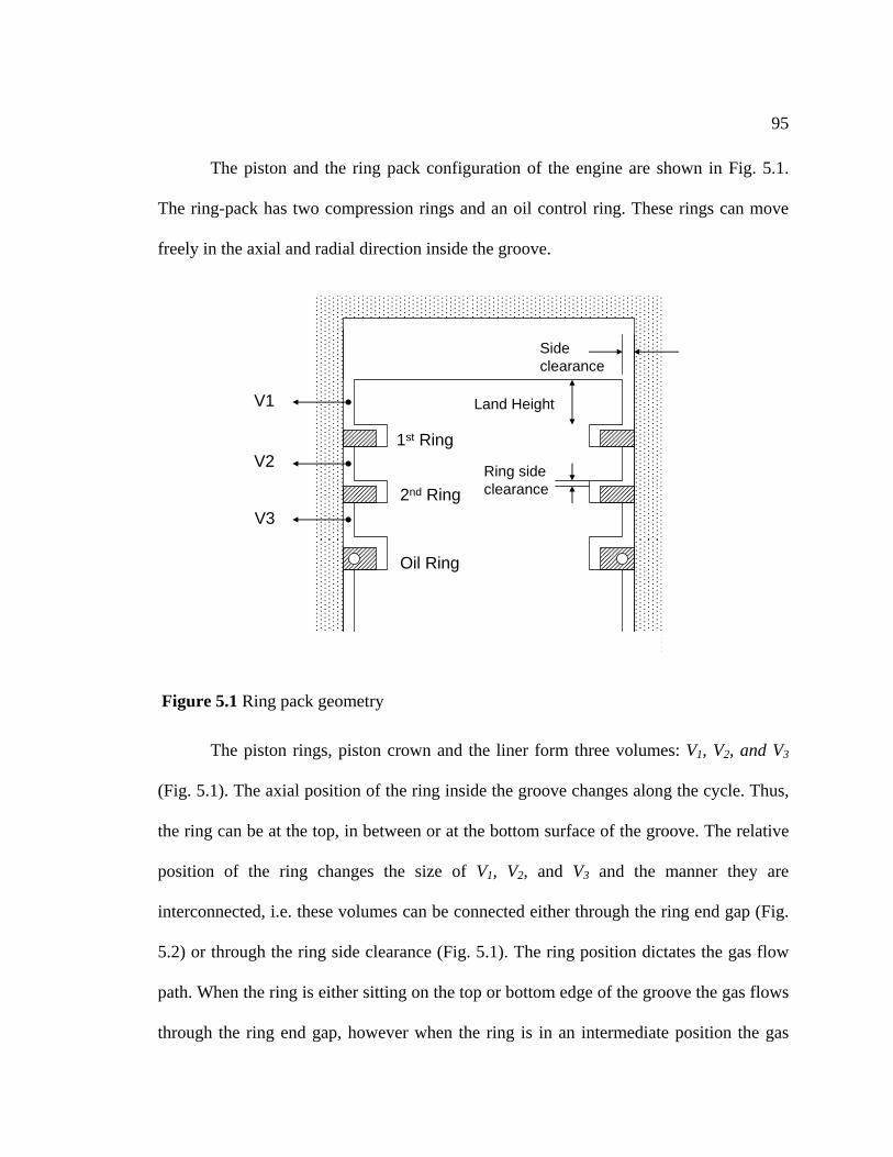
95
The piston and the ring pack configuration of the engine are shown in Fig. 5.1.
The ring-pack has two compression rings and an oil control ring. These rings can move
freely in the axial and radial direction inside the groove.
V1
V21st Ring
V32nd Ring
Oil Ring
Sideclearance
Land Height
Ring sideclearance
Figure
ring position dictates the gas flow
path. W
5.1 Ring pack geometry
The piston rings, piston crown and the liner form three volumes: V1, V2, and V3
(Fig. 5.1). The axial position of the ring inside the groove changes along the cycle. Thus,
the ring can be at the top, in between or at the bottom surface of the groove. The relative
position of the ring changes the size of V1, V2, and V3 and the manner they are
interconnected, i.e. these volumes can be connected either through the ring end gap (Fig.
5.2) or through the ring side clearance (Fig. 5.1). The
hen the ring is either sitting on the top or bottom edge of the groove the gas flows
through the ring end gap, however when the ring is in an intermediate position the gas
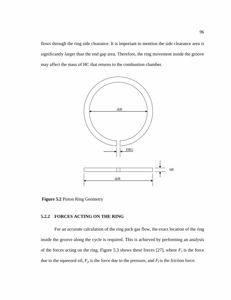
96
flows through the ring side clearance. It is important to mention the side clearance area is
significantly larger than the end gap area. Therefore, the ring movement inside the groove
may affect the mass of HC that returns to the combustion chamber.
deR
ERG
diR
hR
Figure 5.2 Piston Ring Geometry
5.3 shows these forces [27], where Fs is the force
due to the squeezed oil, Fp is the force due to the pressure, and Ff is the friction force.
5.2.2 FORCES ACTING ON THE RING
For an accurate calculation of the ring pack gas flow, the exact location of the ring
inside the groove along the cycle is required. This is achieved by performing an analysis
of the forces acting on the ring. Figure
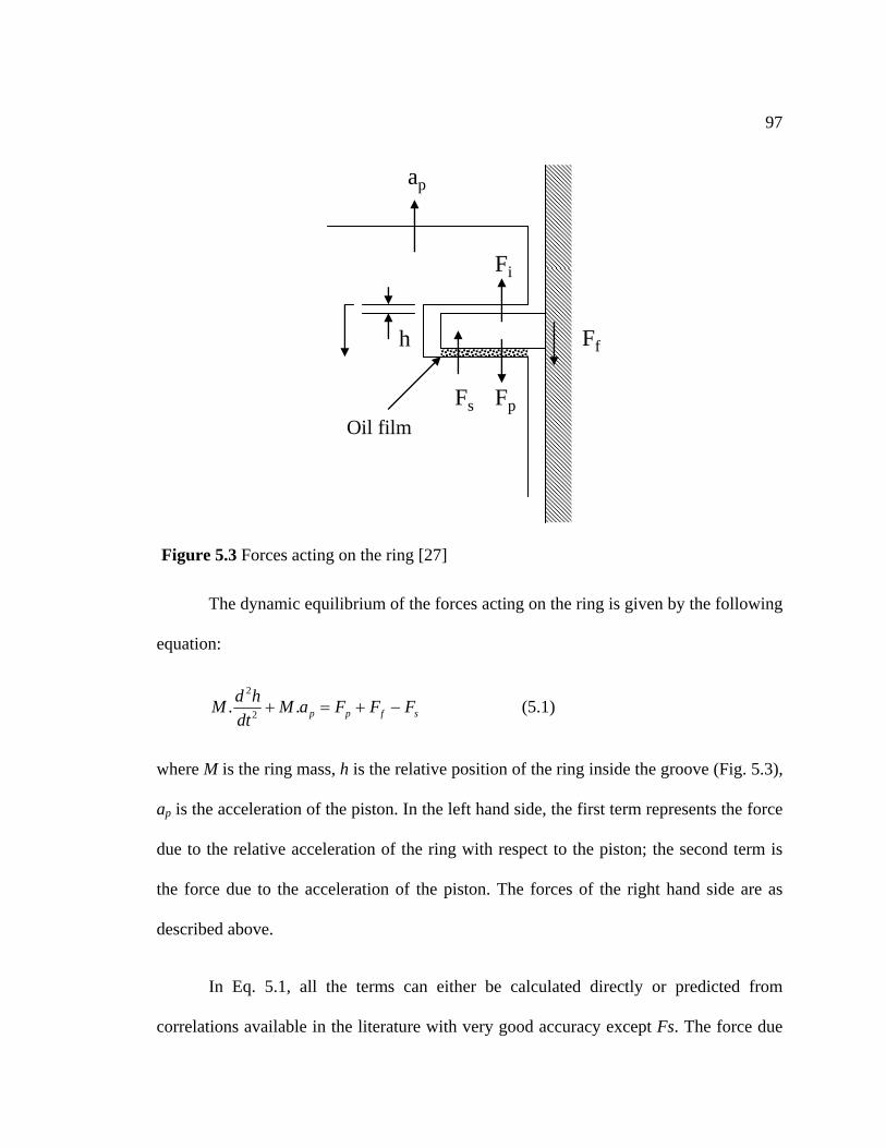
97
ap
Fi
Ffh
Fs FpOil film
Figure 5.3 Fo ]
T dy the forces acting on the ring is given by the following
equation:
rces acting on the ring [27
he namic equilibrium of
sfpp FFFaM −+=+ .. dt
hdM 2
2
(5.1)
where M is the ring mass, h is the relative position of the ring inside the groove (Fig. 5.3),
ap is the acceleration of the piston. In the left hand side, the first term represents the force
due to the relative acceleration of the ring with respect to the piston; the second term is
the force due to the acceleration of the piston. The forces of the right hand side are as
described above.
In Eq. 5.1, all the terms can either be calculated directly or predicted from
ons available in the literature with very good accuracy except Fs. The force due correlati
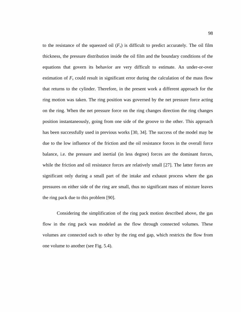
98
to the resistan ifficult to predict accurately. The oil film
thickness, the pressure distribution inside the oil film and the boundary conditions of the
equations that govern its behavior are very difficult to estimate. An under-or-over
estimation of Fs could result in significant error during the calculation of the mass flow
that ret er e
et pressure force acting
on the ring. When the net pressure force on the ring changes direction the ring changes
position instantaneously
has been successfully used in previous works [30, 34]. The success of the model may be
due to the low influence of th orce
minant forces,
while the
significant only during a small part of the intake and exhaust process where the gas
pressures on either side of the ring are small, thus no significant mass of mixture leaves
the ring p k d
C nsid the ring pack motion described above, the gas
flow in e ri s the flow through connected volumes. These
volumes are connected each to other by the ring end gap, which restricts the flow from
one volume to another (see Fig. 5.4).
ce of the squeezed oil (Fs) is d
urns to the cylind . Th refore, in the present work a different approach for the
ring motion was taken. The ring position was governed by the n
, going from one side of the groove to the other. This approach
e friction and the oil resistance forces in the overall f
balance, i.e. the pressure and inertial (in less degree) forces are the do
friction and oil resistance forces are relatively small [27]. The latter forces are
ac ue to this problem [90].
o ering the simplification of
th ng pack was modeled a
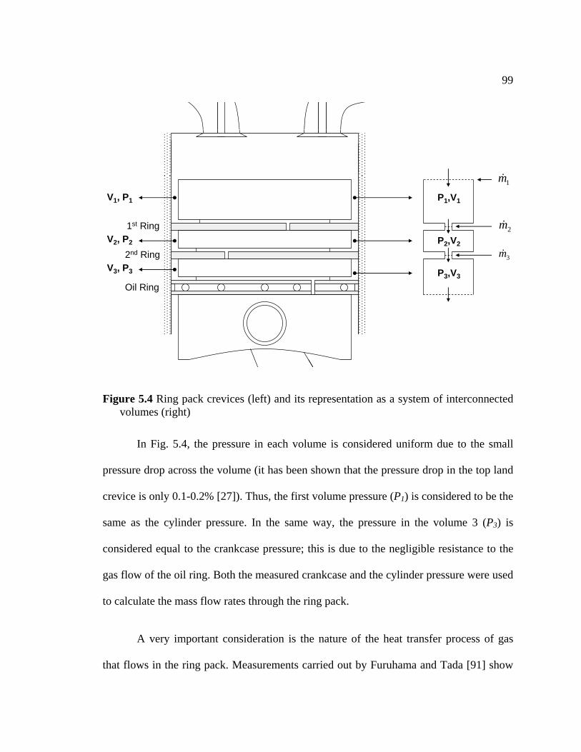
99
V1, P1
V2, P2
V3, P3
1 Ring
2nd Ring
st
Oil Ring
P1,V1
3 3
m&
2m&P2,V2
P ,V
1m&
3
Figure 5.4 Ring pack crevices (left) and its representation as a system of interconnected vol
e oil ring. Both the measured crankcase and the cylinder pressure were used
to calculate the mass flow rates through the ring pack.
A very i re of the heat transfer process of gas
that flows in the ring pack. Measurements carried out by Furuhama and Tada [91] show
umes (right)
In Fig. 5.4, the pressure in each volume is considered uniform due to the small
pressure drop across the volume (it has been shown that the pressure drop in the top land
crevice is only 0.1-0.2% [27]). Thus, the first volume pressure (P1) is considered to be the
same as the cylinder pressure. In the same way, the pressure in the volume 3 (P3) is
considered equal to the crankcase pressure; this is due to the negligible resistance to the
gas flow of th
mportant consideration is the natu
100
that the gas temperature in e top l ce r e the top land
piston temperatu The exp n of e er coefficient
e, and at it is co tively hig an the ient haracterized the
investigation of the ring pack crevice flow [27], studied the nature of the flow in a
stationary crevice of adjustable volume inserted in the cylinder head of an engine. The
crevice volume was similar to the ring pack crevice and it was connected to the
combustion chamber through a small orifice with dimensions of the order of the ring end
gap. The flow through this crevice was simulated considering the flow as adiabatic and
then isothermal. The results of this simulation were compared with the measured
pressure. It was observed that the isothermal flow predicted very accurately the measured
crevice pressure along the cycle. The authors estimated that the gas mixture takes
approximately 2 CA degrees to reach the wall temperature [27]. Therefore, based on
these results in the present model an isothermal flow was considered.
side th and crevi eaches v ry quickly
he sfre. lanatio their results was that th at tran
is very larg th mpara her th coeffic that c
heat transfer between the combustion gases and the cylinder wall. A more recent
As indicated above, the gas temperature inside the crevices are similar to the
piston wall temperature. However, the piston temperature is difficult to measure;
therefore it has been approximated to the cylinder wall temperature as in previous works
[26, 27, 92, 93]. This assumption provides accurate results because the piston and
cylinder wall temperature do not differ significantly [91]. For all the simulations a
temperature of 385 K was considered.
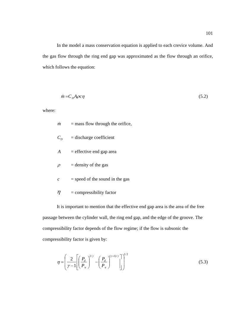
101
In the model a mass conservation equation is applied to each crevice volume. And
the gas flow through the ring end gap was approximated as the flow through an orifice,
which follows the equation:
ηρcACm D=& (5.2)
where:
= mass flow through the orifice,
= discharge coefficient
m&
D
A = effective end gap area
C
ρ = density of the gas
c = speed of the sound in the gas
η = compressibility factor
It is important to mention that the effective end gap area is the area of the free
passage between the cylinder wall, the ring end gap, and the edge of the groove. The
compressibility factor depends of the flow regime; if the flow is subsonic the
compressibility factor is given by:
2/1/)1(/22 ⎟
⎠
⎞⎜
⎝
⎛
⎥⎥⎦
⎤
⎢⎢⎣
⎡⎟⎠
⎞⎜⎝
⎛−⎟
⎠
⎞⎜⎝
⎛=
+ γγγ
ηu
d
u
d PP (5.3) 1 ⎟⎜ ⎟⎜⎟⎜−γ PP
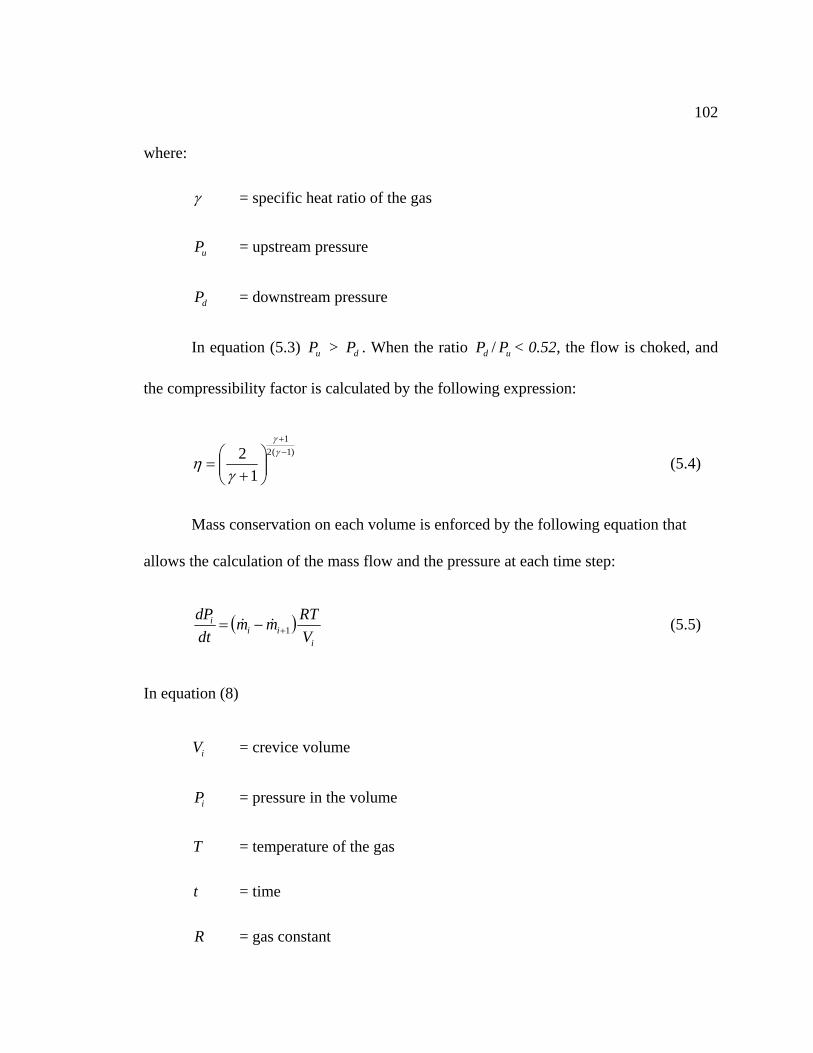
102
where:
γ = specific heat ratio of the gas
= upstream pressure uP
dP = downstream pressure
In equation (5.3) uP > dP . When the ratio dP / uP < 0.52, the flow is choked, and
the compressibility factor is calculated by the following expression:
)1(21
12 −
+
⎟⎠
⎞⎜⎝
⎛+
=γγ
γη (5.4)
Mass conservation on each volume is enforced by the following equation that
allows the calculation of the mass flow and the pressure at each time step:
⎟⎜
( )i
ii Vmm
dt 1+−= && (5.5)
iV = crevice volume
i RTdP
In equation (8)
= pressure in the volume iP
T = temperature of the gas
t = time
R = gas constant
103
im& = mass flow into the volume i
In Eq. 5.2, a representative value for the discharge coefficient is necessary. Early
temperatures and upstream pressures determined that the discharge coefficient does not
change significantly with pressure, temperature and ring gap. The fluctuation of the
0.86 should be used. In the present work a value of 0.85 was used to be consistent with
using the first order Euler method. An initial guess for the pressure P was given and the
equations were iterated until the difference P (CA=-180)- P (CA=540) was below 10-5.
5.2.3 RING PACK GEOMETRICAL DIMENSIONS
experiments [91] performed under static conditions for several effective ring gap areas,
discharge coefficient was between 0.8-0.9. They recommended that the average value of
the value used in previous works [30, 34]. The Equations (5.2) and (5.5) were integrated
2
2 2
The model was implemented in Matlab and the script is given in Appendix XIII.
The dimensions of the cylinder, piston and rings were obtained from the
manufacturer and are proprietary information, therefore they cannot be disclosed.
However, typical dimensions of the ring pack geometry of small engines described in the
schematics in Fig. 5.1, 5.2 and 5.3 are given in the Table 5.1. The geometrical dimensions
allowed the calculation of the different volumes and the ring gap effective areas. The
effect of the temperature on the deformation of these parameters was not considered in
the analysis.
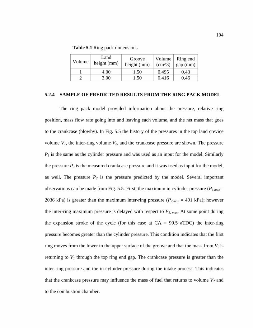
104
Table 5.1 Ring pack dimensions
Volume Land
height (mm) Groove
height (mm) Volume(cm^3)
Ring end gap (mm)
1 4.00 1.50 0.495 0.43 2 3.00 1.50 0.416 0.46
5.2.4 SAMPLE OF PREDICTED RESULTS FROM THE RING PACK MODEL
The ring pack model provided information about the pressure, relative ring
position, mass flow rate going into and leaving each volume, and the net mass that goes
to the crankcase (blowby). In Fig. 5.5 the history of the pressures in the top land crevice
volume V1, the inter-ring volume V2, and the crankcase pressure are shown. The pressure
P1 is the same as the cylinder pressure and was used as an input for the model. Simi rly
as well. The pressure P2 is the pressure predicted by the model. Several important
observations can be made from Fig. 5.5. First, the maximum in cylinder pressure (P1,max =
2036 kPa) is greater than the maximum inter-ring pressure (P2,max = 491 kPa); however
the inter-ring maximum pressure is delayed with respect to P1, max. At some point during
the expansion stroke of the cycle (for this case at CA = 90.5 aTDC) the inter-ring
pressure becomes greater than the cylinder pressure. This condition indicates that the first
ring moves from the lower to the upper surface of the groove and that the mass from V2 is
returning to V1 through the top ring end gap. The crankcase pressure is greater than the
inter-ring pressure and the in-cylinder pressure during the intake process. This indicates
that the crankcase pressure may influence the mass of fuel that returns to volume V2 and
to the combustion chamber.
la
the pressure P3 is the measured crankcase pressure and it was used as input for the model,
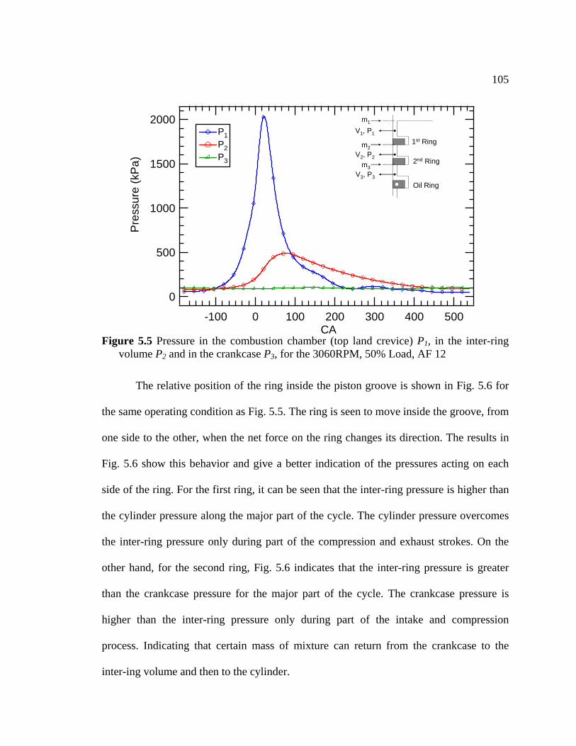
105
2000
1500
1000
500
0
Pre
ssur
e (k
Pa)
5004003002001000-100CA
V1, P1
V2, P2
V3, P3
1st Ring
2nd Ring
Oil Ring
m1
m2
m3
P1P2P3
Figure 5.5 Pressure in the combustion chamber (top land crevice) P1, in the inter-ring
volume P2 and in the crankcase P3, for the 3060RPM, 50% Load, AF 12
the
one side to the other, when the net force on the ring changes its direction. The results in
Fig. 5.6 show this behavior and give a better indication of the pressures acting on each
side of the ring. For the first ring, it can be seen that the inter-ring pressure is higher than
the cylinder pressure along the major part of the cycle. The cylinder pressure overcomes
the inter-ring pressure only during part of the compression and exhaust strokes. On the
other hand, for the second ring, Fig. 5.6 indicates that the inter-ring pressure is greater
than the crankcase pressure for the major part of the cycle. The crankcase pressure is
higher than the inter-ring pressure only during part of the intake and compression
process. Indicating that certain mass of mixture can return from the crankcase to the
inter-ing volume and then to the cylinder.
The relative position of the ring inside the piston groove is shown in Fig. 5.6 for
same operating condition as Fig. 5.5. The ring is seen to move inside the groove, from
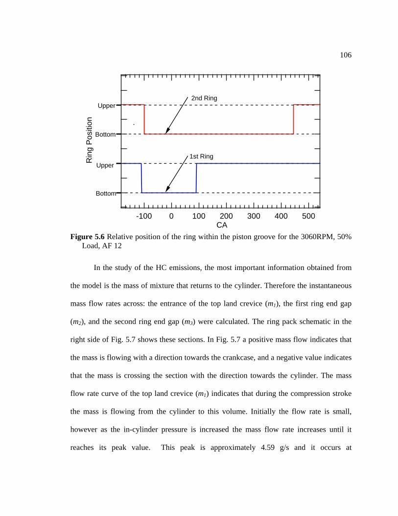
106
4.0
3.5
3.0
2.5
In the study of the HC emissions, the most important information obtained from
the model is the mass of mixture that returns to the cylinder. Therefore the instantaneous
mass flow rates across: the entrance of the top land crevice (m ), the first ring1 end gap
(m2), and the second ring end gap (m3) were calculated. The ring pack schematic in the
right side of Fig. 5.7 shows these sections. In Fig. 5.7 a positive mass flow indicates that
the mass is flowing with a direction towards the crankcase, and a negative value indicates
that the mass is crossing the section with the direction towards the cylinder. The mass
flow rate curve of the top land crevice (m1) indicates that during the compression stroke
the mass is flowing from the cylinder to this volume. Initially the flow rate is small,
however as the in-cylinder pressure is increased the mass flow rate increases until it
reaches its peak value. This peak is approximately 4.59 g/s and it occurs at
2.0
1.5
1.0
0.5
0.0
-0.5
inn
5004003002001000-100
Bottom
1st RingUpper
Bottom
Upper2nd Ring
Rg
Pos
itio
CA
Load, AF 12 Figure 5.6 Relative position of the ring within the piston groove for the 3060RPM, 50%
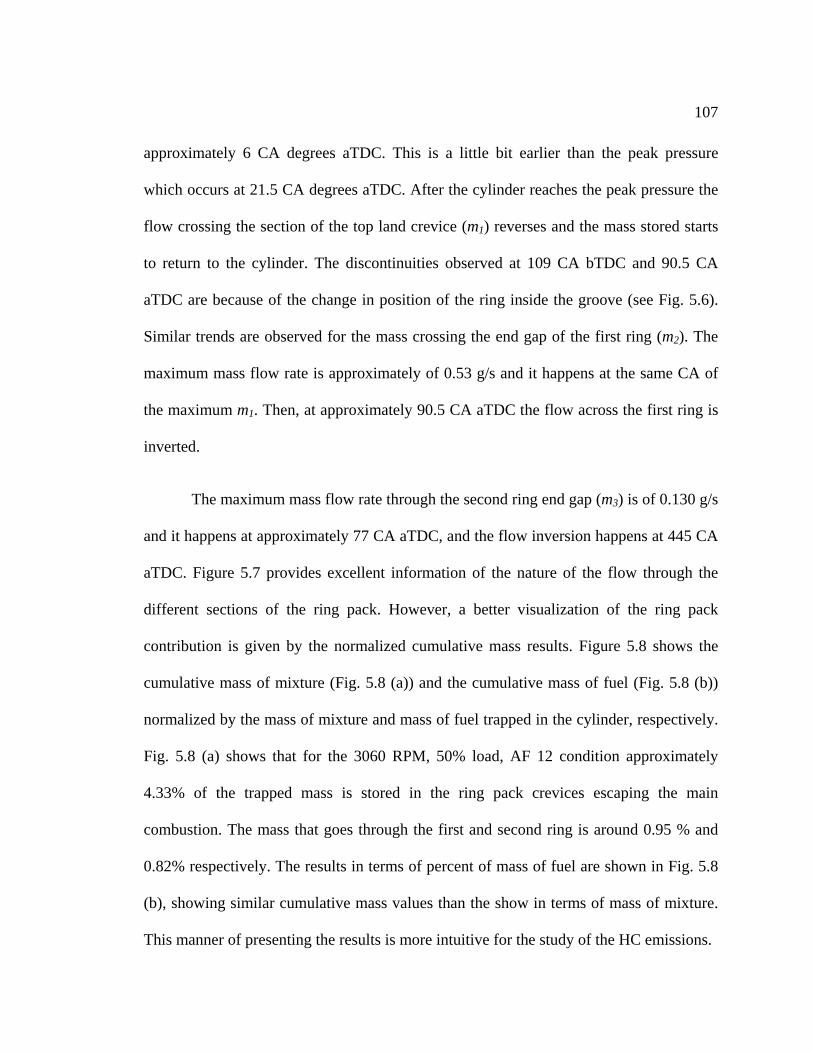
107
approximately 6 CA degrees aTDC. This is a little bit earlier than the peak pressure
ch occurs at 21.5 CA degrees aTDC. After the cylinder reaches the peak pressure the
flow crossing the section of the top land crevice (m1) reverses and the mass stored starts
to return to the cylinder. The discontinuities observed at 109 CA bTDC and 90.5 CA
aTDC are because of the change in position of the ring inside the groove (see Fig. 5.6).
Similar trends are observed for the mass crossing the end gap of the first ring (m2). The
maximum mass flow rate is approximately of 0.53 g/s and it happens at the same CA of
the maximum m1. Then, at approximately 90.5 CA aTDC the flow across the first ring is
inverted.
The maximum mass flow rate through the second ring end gap (m3) is of 0.130 g/s
and it happens at approximately 77 CA aTDC, and the flow inversion happens at 445 CA
aTD
diff ck. However, a better visualization of the ring pack
contribution is given by the normalized cum lative mass results. Figure 5.8 shows the
cumulative mass of mixture (Fig. 5.8 (a)) and the cumulative mass of fuel (Fig. 5.8 (b))
normalized by the mass of mixture and mass of fuel trapped in the cylinder, respectively.
Fig. 5.8 (a) shows that for the 3060 RPM, 50% load, AF 12 condition approximately
4.33% of the trapped mass is stored in the ring pack crevices escaping the main
combustion. The mass that goes through the first and second ring is around 0.95 % and
0.82% respectively. The results in terms of percent of mass of fuel are shown in Fig. 5.8
(b), showing similar cumulative mass values than the show in terms of mass of mixture.
This manner of presenting the results is more intuitive for the study of the HC emissions.
whi
C. Figure 5.7 provides excellent information of the nature of the flow through the
erent sections of the ring pa
u
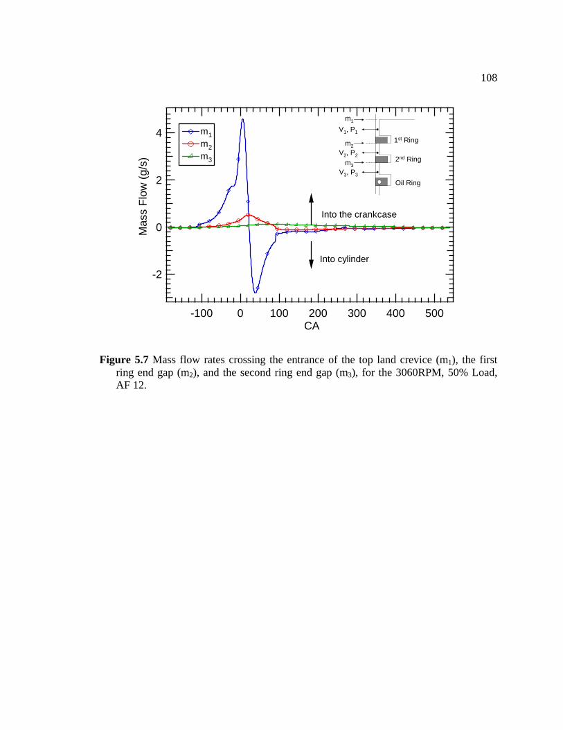
108
4
2
0
-2
Mas
s Fl
ow (g
/s)
5004003002001000-100CA
V1, P1
V2, P2
V3, P3
1st Ring
2nd Ring
Oil Ring
m1
m2
m3
Into cylinder
Into the crankcase
m1m2m3
Figure 5.7 Mass flow rates crossing the entrance of the top land crevice (m1), the first ring end gap (m2), and the second ring end gap (m3), for the 3060RPM, 50% Load, AF 12.
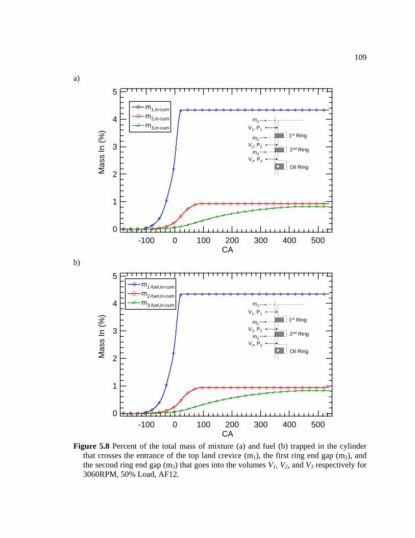
109
a)
5
4
3
2
1
0
Mas
s In
%)
(
5004003002001000-100CA
V1, P1
2 2
V , P
1st Ring
2nd Ring
Oil Ring
V , P
3 3
m1
m2
m3
m1,in-cumm2,in-cumm
3,in-cum
b)
5
4
3
2
1
0
(%)
5004003002001000-100CA
V1, P1
V2, P2
1st Ring
2nd Ring
Mas
s In
V3, P3
Oil Ring
m1
m2
m3
m1-fuel,in-cumm2-fuel,in-cumm3-fuel,in-cum
Figure 5.8 Percent of the total mass of mixture (a) and fuel (b) trapped in the cylinder
that crosses the entrance of the top land crevice (m1), the first ring end gap (m2), and the second ring end gap (m3) that goes into the volumes V1, V2, and V3 respectively for 3060RPM, 50% Load, AF12.
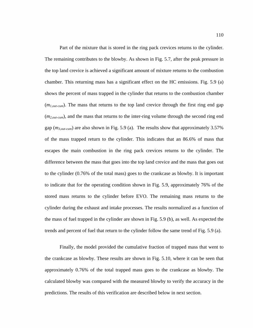
110
Part of the mixture that is stored in the ring pack crevices returns to the cylinder.
The remaining contributes to the blowby. As shown in Fig. 5.7, after the peak pressure in
the top land crevice is achieved a significant amount of mixture returns to the combustion
chamber. This returning mass has a significant effect on the HC emissions. Fig. 5.9 (a)
shows the percent of mass trapped in the cylinder that returns to the combustion chamber
(m ). The mass that returns to the top land crevice through the first ring end gap
(m ), and the mass that returns to the inter-ring volume through the second ring end
gap (m ) are also shown in Fig. 5.9 (a). The results show that approximately 3.57%
of the mass trapped return to the cylinder. This indicates that an 86.6% of mass that
escape the ring pack c e
difference between the mass that goes into the top land crevice and the mass that goes out
is im
xhaust and intake processes. The results normalized as a function of
the mass of fuel trapped in the cylinder are shown in Fig. 5.9 (b), as well. As expected the
trends ylinder fol .
Finally, the model provided the cumulative fraction of trapped mass that went to
the crankcase as blowby. These results are shown in Fig. 5.10, where it can be seen that
approximately 0.76% of the total trapped mass goes to the crankcase as blowby. The
calculated blowby was compared with the measured blowby to verify the accuracy in the
predictions. The results of this verification are described below in next section.
1,out-cum
2,out-cum
3,out-cum
s the main combustion in revices returns to the cylinder. Th
to the cylinder (0.76% of the total mass) goes to the crankcase as blowby. It portant
to indicate that for the operating condition shown in Fig. 5.9, approximately 76% of the
stored mass returns to the cylinder before EVO. The remaining mass returns to the
cylinder during the e
and percent of fuel that return to the c low the same trend of Fig. 5.9 (a)
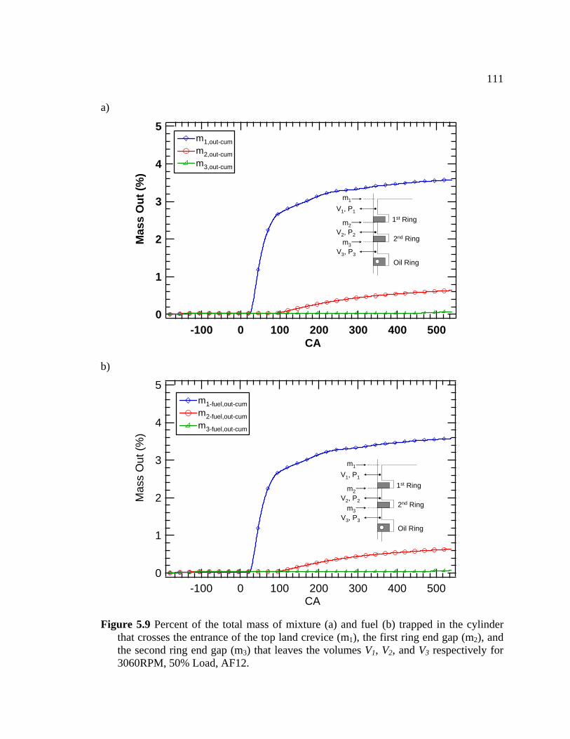
111
a)
5
4
3
2
1
0
Mas
s O
ut (%
)
5004003002001000-100CA
V1, P
V2, P2
V3, P3
st Ring
Ring
ng
1
1
2nd
Oil Ri
m1
m2
m3
m1,out-cumm2,out-cumm
b)
3,out-cum
5
4
3
2
1
0
Mas
s O
ut (%
)
5004003002001000-100CA
V1, P1
V2, P2
V3, P3
1st Ring
2nd Ring
Oil Ring
m1
m2
m3
m1-fuel,out-cumm2-fuel,out-cumm3-fuel,out-cum
ring end gap (m2), and 3 1 2 V3 respectively for
3060RPM, 50% Load, AF12.
Figure 5.9 Percent of the total mass of mixture (a) and fuel (b) trapped in the cylinder
that crosses the entrance of the top land crevice (m1), the first the second ring end gap (m ) that leaves the volumes V , V , and
112
0.8
0.6
0.4
0.2
0.0
Mas
s to
Cra
nkca
se (%
)
5004003002001000-100CA
V1, P1
V2, P2
V3, P3
1st Ring
2nd Ring
Oil Ring
m1
m2
m3
m3,net-cum
0.8
0.6
0.4
0.2
0.0
Mas
s to
Cra
nkca
se (%
)
5004003002001000-100CA
m3-fuel,net-cum
Figure 5.10 Percent of the total mass of mixture (a) and fuel (b) trapped in the cylinder that crosses the second ring end gap (m ) that goes to the crankcase as blowby for 3060RPM, 50% Load, AF12.
3
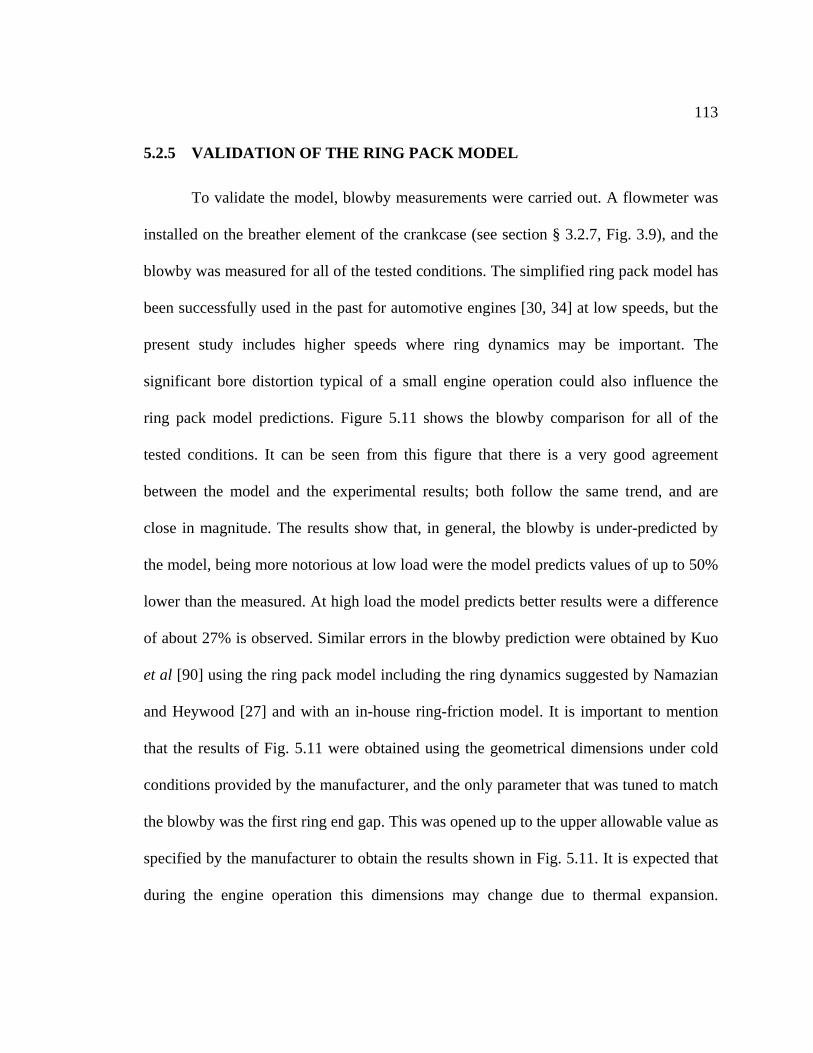
113
5.2.5 VALIDATION OF THE RING PACK MODEL
st e (see section § 3.2.7, Fig. 3.9), and the
cted that
is dimensions may change due to thermal expansion.
To validate the model, blowby measurements were carried out. A flowmeter was
alled on the breather element of the crankcasin
blowby was measured for all of the tested conditions. The simplified ring pack model has
been successfully used in the past for automotive engines [30, 34] at low speeds, but the
present study includes higher speeds where ring dynamics may be important. The
significant bore distortion typical of a small engine operation could also influence the
ring pack model predictions. Figure 5.11 shows the blowby comparison for all of the
tested conditions. It can be seen from this figure that there is a very good agreement
between the model and the experimental results; both follow the same trend, and are
close in magnitude. The results show that, in general, the blowby is under-predicted by
the model, being more notorious at low load were the model predicts values of up to 50%
lower than the measured. At high load the model predicts better results were a difference
of about 27% is observed. Similar errors in the blowby prediction were obtained by Kuo
et al [90] using the ring pack model including the ring dynamics suggested by Namazian
and Heywood [27] and with an in-house ring-friction model. It is important to mention
that the results of Fig. 5.11 were obtained using the geometrical dimensions under cold
conditions provided by the manufacturer, and the only parameter that was tuned to match
the blowby was the first ring end gap. This was opened up to the upper allowable value as
specified by the manufacturer to obtain the results shown in Fig. 5.11. It is expe
during the engine operation th
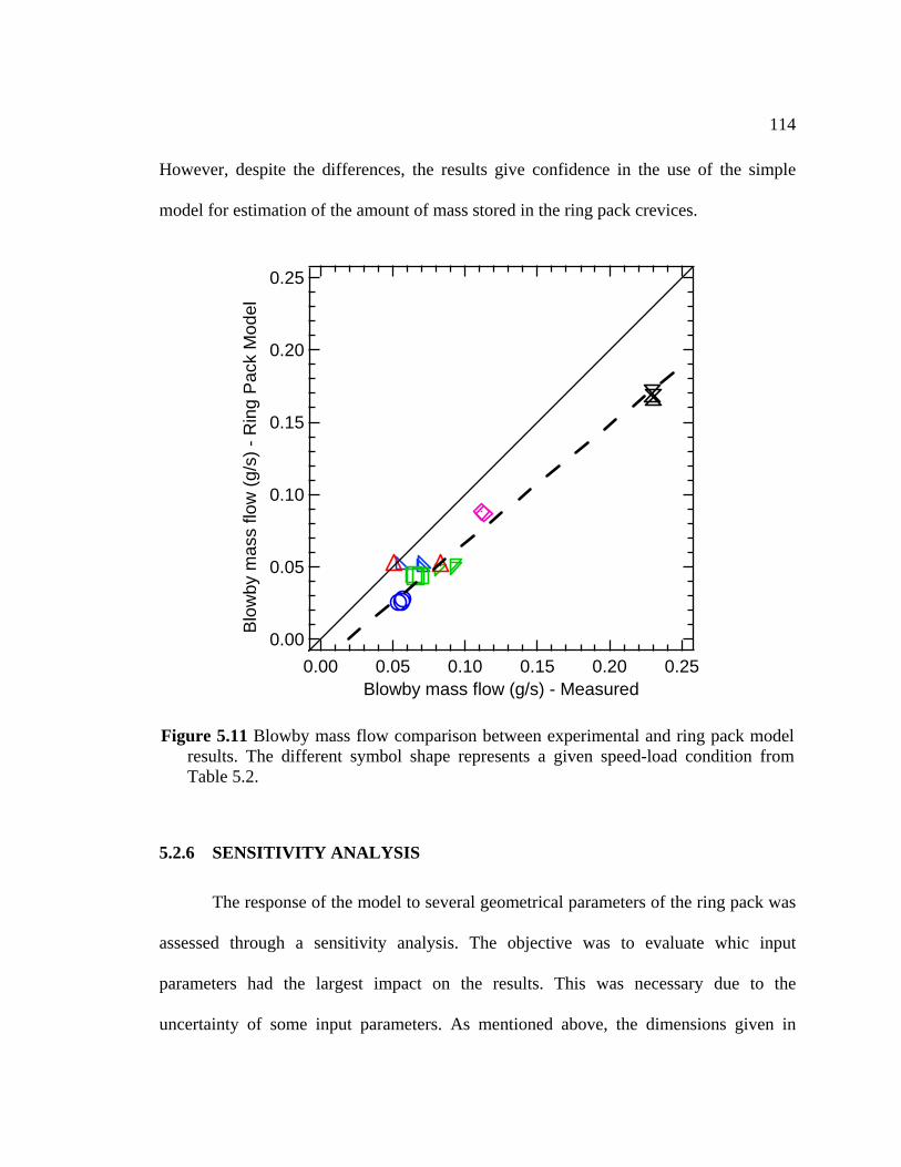
114
However, despite the differences, the results give confidence in the use of the si
l for estimation of the amount of mass stored in the
mple
mode ring pack crevices.
0.25
0.20
0.15
0.10
0.05
0.00
Bl
ow (g
/s)
Rin
g P
ack
Mod
elow
by m
ass
fl -
0.250.200.150.100.050.00Blowby mass flow (g/s) - Measured
Figure 5.11 Blowby mass flow comparison between experimental and riresults. The different symbol shape represents a given speed-load c
ng pack model ondition from
Table 5.2.
5.2.6 SENSITIVITY ANALYSIS
The response of the model to several geometrical parameters of the ring pack was
assessed through a sensitivity analysis. The objective was to evaluate whic input
parameters had the largest impact on the results. This was necessary due to the
uncertainty of some input parameters. As mentioned above, the dimensions given in
115
Table 5.1 correspond to the cold conditions. It is expected that these dimensions will
change during the engine operation due to thermal expansion. In addition there was not
accurate information about the piston wall temperature or discharge coefficient.
The model was tested against the measured blowby. All the changes in the
considered variables were with respect to the baseline values given in Table 5.1. The
change
Relative Sensitivity (% ) =
s were taken as the uncertainty in the variable’s value and they are shown in Table
5.2. These values are typical for the type of engine under study. The relative sensitivity
was calculated as follows:
100.ref
uncer
mx
dxmd
&
& ∆⎟⎠⎞
⎜⎝⎛ (5.6)
where dx
is the rate of change of the blowby with respect to the parameter x. uncerxmd &∆
d refm& are the uncertainty in the parameter x and the reference blowby respectively.
This is a different definition of the conventional definition of relative sensitivity [94],
which is defined as follows:
an
Conventional Relative Sensitivity = .ref
ref
mx
dxmd
&
&⎟⎠⎞
⎜⎝⎛ (5.7)
where xref is the value of the ref ter. Eq. (5.7) provides an insight about how
parameters that affect the blowby; however, in the present application some parameters,
value is known with
erence parame
such as the cylinder diameter, do not change significantly i.e. the
116
good accuracy. Therefore, a more fair comparison of the effect of the parameters on the
wby is provided by Eq. 5.6.
Table 5.2 Parameters changed in the sensitivity analysis
Parameter x
Units Uncertainty ∆xuncer
blo
EG-RI mm 0.25 EG-RII mm 0.21 dcyl mm 0.025 h1 mm 0.2 d1L mm 0.014 d1U mm 0.03 h2 mm 0.02 di2 mm 0.2 wRI mm 0.52 hRI mm 0.026 h3 mm 0.1 d3L mm 0.014 d3U mm 0.014 h4 mm 0.02 di4 mm 0.2 wRII mm 0.52 hRII mm 0.033 CD - 0.1 Twall K 165 Pcrk_offset kPa 60
Figure 5.12 shows the relative sensitivity of the model to all of the variables of
interest. As it can be seen in Fig. 5.12 the most sensitive parameters controlling the
blowby are the ring end gaps (EG-RI and EG-RII), the diameter of the cylinder (dcyl),
the width of the first and second ring (wRI and wRII), the discharge coefficient (CD), the
wall temperature (Twall); and the crankcase offset (Pcrk_offset).
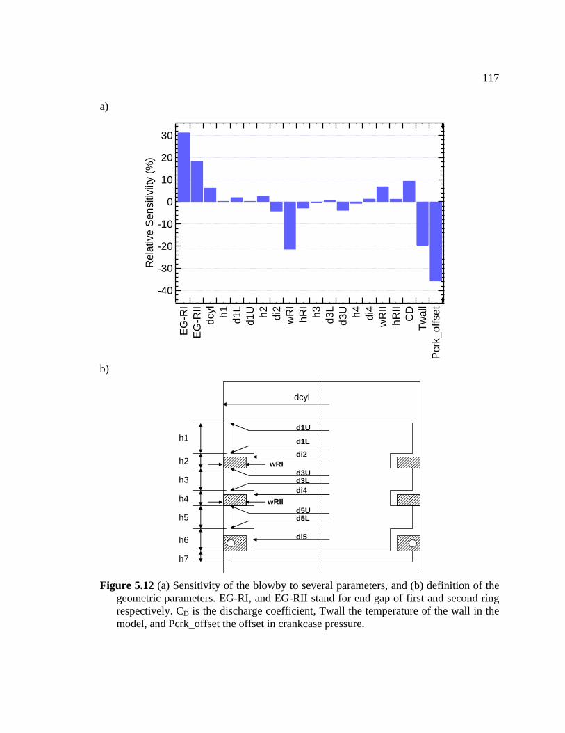
117
a)
-40
-30
-20
-10
0
10
20
30
EG
-RI
EG
-RII
dcyl h1 d1L
d1U h2 di2
wR
IhR
Ih3 d3
Ld3
U h4 di4
wR
IIhR
IIC
DTw
all
Prk
_offs
t
Rel
ativ
e S
ensi
tivit
y (%
)i
ce
b)
h1
h2
dcyl
d1U
di2
d3U
di4
d1L
h3
h4
h5
h6
h7
di5
d3L
d5Ud5L
wRII
wRI
Figure 5.12 (a) Sensitivity of the blowby to several parameters, and (b) definition of the geometric parameters. EG-RI, and EG-RII stand for end gap of first and second ring respectively. CD is the discharge coefficient, Twall the temperature of the wall in the model, and Pcrk_offset the offset in crankcase pressure.
118
The relative change in the ring gap does significantly change the blowby (up to
30% increase for the first ring). In a fully warmed-up engine, the ring gap could change,
impacting significantly the blowby. The parameter that makes the greatest impact in the
model is the crankcase pressure (up to 35% change). This is because the mass flow
towards the crankcase is restricted by the crankcase pressure, especially during the period
when the inter-ring pressure (P2) is small. It is important to mention that no geometrical
changes in the hardware were made to verify the dependence of the geometrical
parameters on the measured blowby. The results of Figs. 5.11 and 5.12 were very useful
to see how accurately the model predicts the blowby, and to have an idea of the degree of
sensitivity of the model predictions. However, the estimation of the mass that returns to
the cylinder is m ly affects the
engine-out HC emissions. Therefore, a sensitivity analysis for the mass that returns to the
cylinder was pe d considering the c
The results are own in .13 s im t to that th e changes represent
increments in the independent variable a e the mass returning to the
combustion chamber. The results show tha ass returning to linder is affected
in a different way than the blowby. T eters that
dominate their behaviors ffe The par that he mass flow out
of the top land crevice are: the ring end g G-RI and EG-RII), the diameter of the
cylinder (dcyl), the top land height (h1), th gro rnal dia eter (di2), the width
of the first ring (wRI), th ht o fir (hRI), he wall t ture (Twall), and
the crankcase offset (Pcrk_offset). As it ca e geometric eters that have
ore important in the present analysis, because it direct
rforme hanges shown in Table 5.2 and using Eq. 5.6.
sh Fig. 5 . It i portan clarify es
nd the results ar
t the m the cy
his is expected because the param
are di rent. main ameters affect t
aps (E
e first ove inte m
e heig f the st ring t empera
n be seen th al param
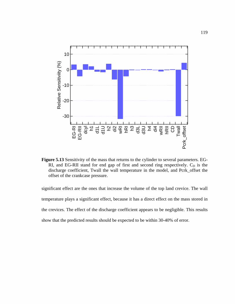
119
-30
-20
-10
0
10R
elat
ive
Sen
sitiv
iity
(%)
EG
-RI
EG
-RII
dcyl h1 d1L
d1U h2 di2
wR
IhR
Ih3 d3
Ld3
U
significant effect are the ones that increas olume the to revice. The wall
temperature plays a sign ff ec as a direct effect on the mass stored in
the crevices. The effect of the discharge c ent app ars to b ible. This results
show that the predicted results should be expected to be within 30-40% of error.
e the v of p land c
ificant e ect, b ause it h
oeffici e e neglig
h4 di4
wR
IIhR
IIC
DTw
all
Pcr
k_of
fset
Figure 5.13 Sensitivity of the mass that re th er to several parameters. EG-
RI, and EG-RII stand for end gap of nd ring re pectively. CD is the discharge coefficient, Twall the wall ature in the model, and Pcrk_offset the offset of the crankcas sur
turns to e cylind first a second stemper
e pres e.

120
5.3 TRANSPORT OF MASS RETURNING TO THE CYLINDER AND ITS
CONTRIBUTION TO THE HC EMISSIONS
T
tinues until the exhaust valve is closed (see Fig.
5.7). Depending of the combustion phasing, a fraction of the mixture returns to the
cylinde
the engine operating condition a significant quantity of this mixture can be partially
he transport process of the mixture stored in the ring pack crevices back into the
cylinder is very complex and plays an important role in the extent to which the mixture
will contribute to the engine-out HC emissions. Experimental observations [27, 29] show
that as the piston moves downward during the expansion stroke a thin layer of
hydrocarbons is formed along the wall due to the outflow of the HC stored in the ring
pack. This begins immediately following the time that the cylinder has reached peak
pressure and the out-gassing process con
r before the flame arrival to the cylinder wall. This mass is oxidized during the
main combustion when the flame reaches and quenches on the cylinder wall. After the
flame arrival, the crevice mass continues returning to the cylinder forming a layer on the
cylinder wall. The transport of this HC mass to the bulk mass of the cylinder is an
important process because it influences the post-flame oxidation process.
Two main transport mechanisms of the crevice outflow were described
schematically by Lavoie et al. [83]. The first one consists in an entrainment into the bulk
gases as they leave the crevices during the blowdown process mainly due to the diffusion
process. The second mechanism is the roll-up vortex produced by the piston when it
scrapes the HC layer off the cylinder wall. Not all of the combustible mixture that
escapes the main combustion contributes to the engine-out HC emissions. Depending on
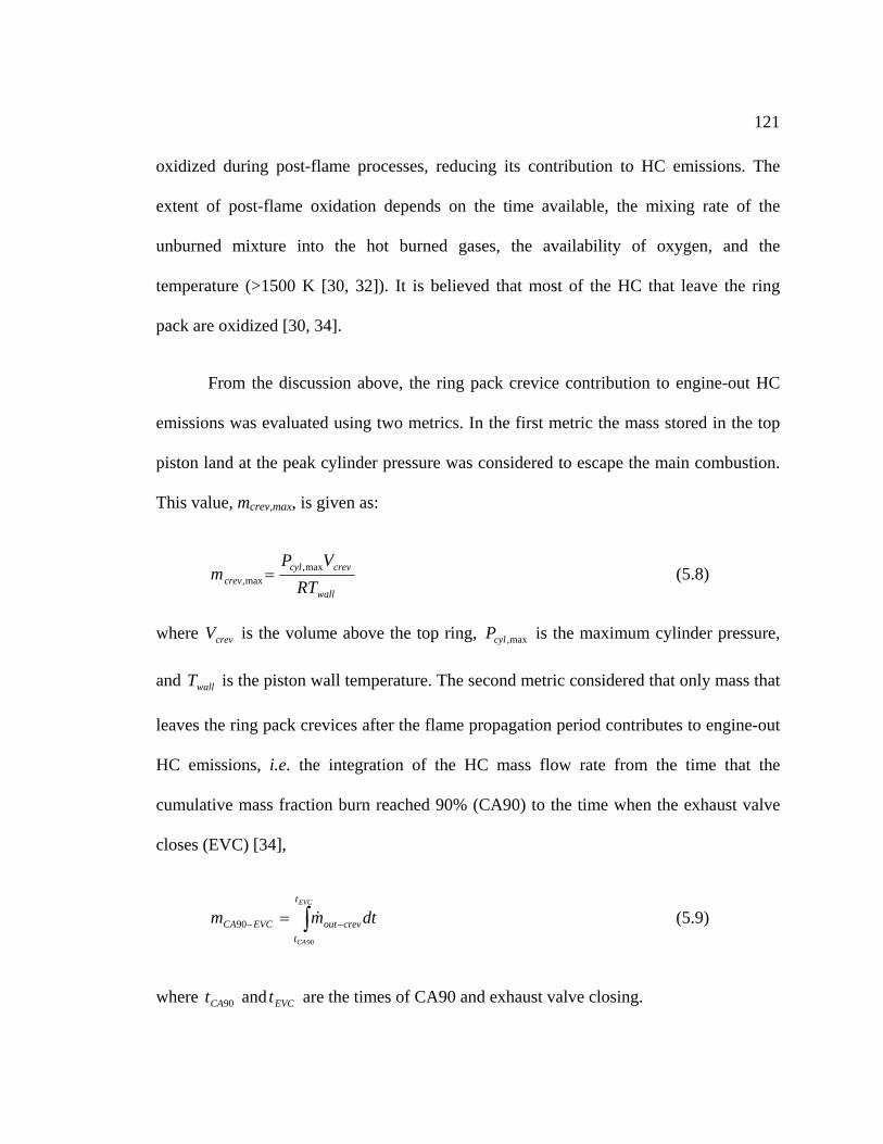
121
oxidized during post-flame processes, reducing its contribution to HC emissions. The
extent of post-flame oxidation depends on the time available, the mixing rate of the
unburned mixture into the hot burned gases, the availability of oxygen, and the
temperature (>1500 K [30, 32]). It is believed that most of the HC that leave the ring
pack are oxidized [30, 34].
From the discussion above, the ring pack crevice contribution to engine-out HC
emissions was evaluated using two metrics. In the first metric the mass stored in the top
piston land at the peak cylinder pressure was considered to escape the main combustion.
This value, mcrev,max, is given as:
wall
crevcylcrev RT
VPm max,
max, = (5.8)
where is the volume above the top ring, is the maximum cylinder pressure,
and is the piston wall temperature. The second metric considered that only mass that
leaves the ring pack crevices after the flame propagation period contributes to engine-out
HC emissions, i.e. the integration of the HC mass flow rate from the time that the
cumulative mass fraction burn reached 90% (CA90) to the time when the exhaust valve
closes (EVC) [34],
(5.9)
where and are the times of CA90 and exhaust valve closing.
crevV max,cylP
wallT
∫ −− =EVC
CA
t
tcrevoutEVCCA dtmm
90
90 &
90CAt EVCt
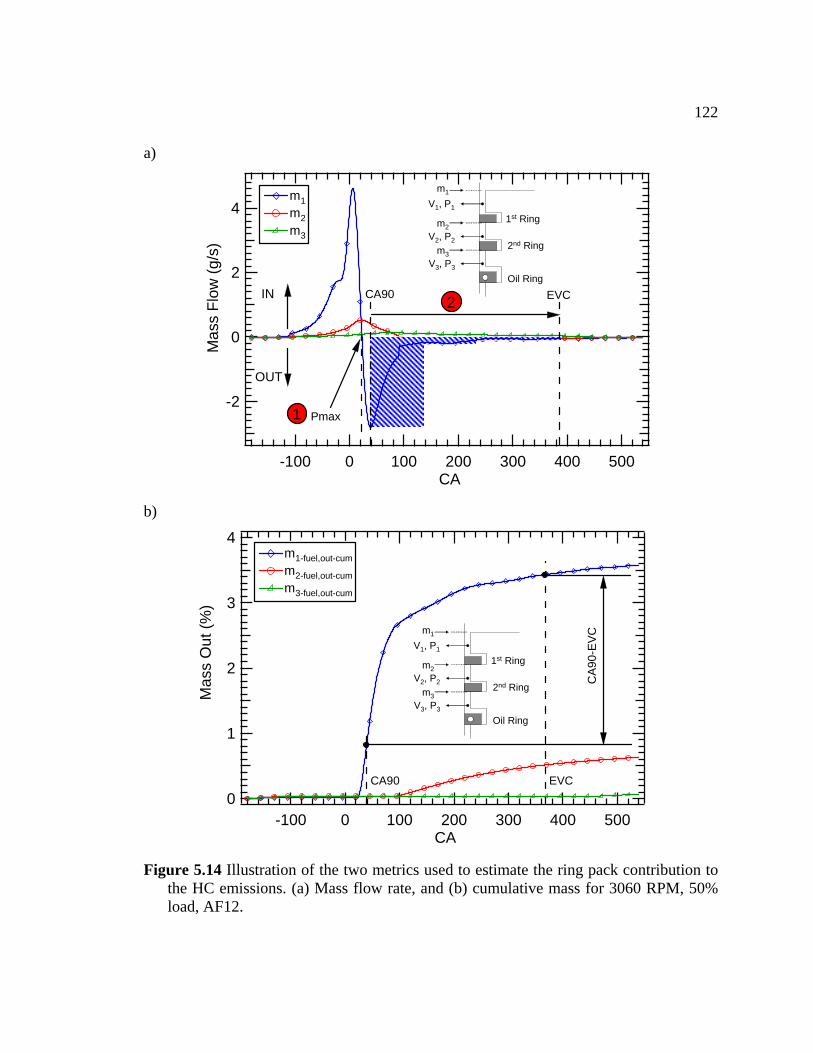
122
a)
4
2
0
-2
Mas
s Fl
ow (g
/s)
5004003002001000-100CA
V1, P1
V2, P2
V3, P3
1st Ring
2nd Ring
Oil Ring
m1
m2
m3
OUT
IN CA90 EVC
Pmax1
2
m1m2m3
b)
4
3
2
1
0
Mas
s O
ut (%
)
5004003002001000-100CA
V1, P
V2, P2
V3, P3
1st Ring
2nd Ring
Oil Ring
1
m1
m2
m3
CA90 EVC
CA9
0-EV
C
m1-fuel,out-cumm2-fuel,out-cumm3-fuel,out-cum
Figure 5.14 Illustration of the two metrics used to estimate the ring pack contribution to
the HC emissions. (a) Mass flow rate, and (b) cumulative mass for 3060 RPM, 50% load, AF12.
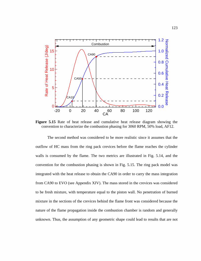
123
15
10
5
0
Rat
e of
Hea
t Rle
J/de
g)e
ase
(
120100806040200-20CA
1.2
1.0
0.8
0.6
0.4
0.2
0.0
Nor
alim
ulm
zed Cu
ative Heat R
elease
CA10
CA50
CA90
Combustion
Figure 5.15 Rate of heat release and cumulative heat release diagram showing the
convention to characterize the combustion phasing for 3060 RPM, 50% load, AF12.
The second method was considered to be more realistic since it assumes that the
outflow of HC mass from the ring pack crevices before the flame reaches the cylinder
walls is consumed by the flame. The two metrics are illustrated in Fig. 5.14, and the
convention for the combustion phasing is shown in Fig. 5.15. The ring pack model was
integrated with the heat release to obtain the CA90 in order to carry the mass integration
from CA90 to EVO (see Appendix XIV). The mass stored in the crevices was considered
to be fresh mixture, with temperature equal to the piston wall. No penetration of burned
mixture in the sections of the crevices behind the flame front was considered because the
nature of the flame propagation inside the combustion chamber is random and generally
unknown. Thus, the assumption of any geometric shape could lead to results that are not
124
realisti
5.4 RESULTS
emission bench will be denoted as M,EXH. The calculated mass of HC returned to the
C,RP
another calculated HC emission index will be developed (§5.4.2.3.3.1) from the cycle-
C,MB
separately for each cylinder of the engine, referred to hereafter as cylinder 1 and cylinder
mixture system. The use of the HMS system eliminated the possible influence of any
5.4.1 ENSEMBLE-AVERAGE RESULTS
An analysis using the emsemble-average pressure data is presented in this section.
The results of this section provided information about the general trends of the ring pack
contribution to the engine-out HC emissions. However, the discussion will start with a
brief description of the average HC emissions and IMEP for all the engine operating
conditions. The HC emissions and their respective single-cylinder air-fuel ratio are
provided in Table 5.3. From this table, it can be seen that each cylinder has a different
c. This results in over-prediction of the total ring-pack crevice HC contribution by
the model.
In the following discussion, the results will be reported as the fuel-specific
emission index of HC (EIHC). The HC measured in the exhaust using the steady state
EIHC
combustion chamber using the ring pack model will be denoted as EIHC . Later,
resolved HC measurements and an estimate of the instantaneous exhaust mass flow rate,
and this will be denoted EIHC . All of these measures have been performed
2. It is important to mention that all these tests were carried out using the homogeneous
liquid fuel in the ring pack, and did not affect the HC emissions, see chapter 4.
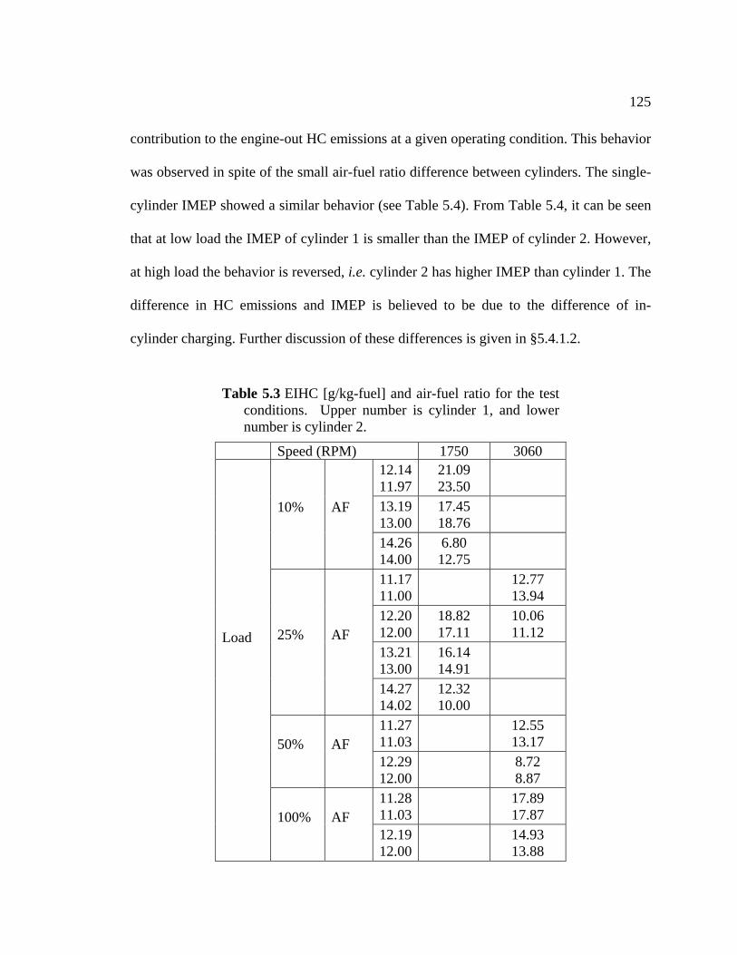
125
contribution to the engine-out HC emissions at a given operating condition. This behavior
was observed in spite of the small air-fuel ratio difference between cylinders. The single-
cylinder IMEP showed a similar behavior (see Table 5.4). From Table 5.4, it can be seen
that at low load the IMEP of cylinder 1 is smaller than the IMEP of cylinder 2. However,
at high load the behavior is reversed, i.e. cylinder 2 has higher IMEP than cylinder 1. The
difference in HC emissions and IMEP is believed to be due to the difference of in-
cylinder charging. Further discussion of these differences is given in §5.4.1.2.
Table 5.3 EIHC [g/kg-fuel] and air-fuel ratio for the test conditions. Upper number is cylinder 1, and lower number is cylinder 2.
Speed (RPM) 1750 3060 12.14 21.09 11.97 23.50
13.19 17.45 13.00 18.76 10% AF
14.2614.00
6.80 12.75
11.1711.00 12.77
13.94 12.2012.00
18.82 17.11
10.06 11.12
13.2113.00
16.14 14.91
25% AF
14.2714.02
12.32 10.00
11.2711.03 12.55
13.17 50% AF 12.2912.00 8.72
8.87 11.2811.03 17.89
17.87
Load
100% AF 12.1912.00 14.93
13.88
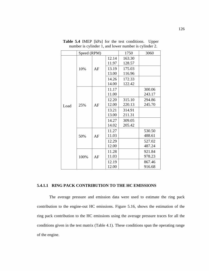
126
Table 5.4 IMEP [kPa] for the test conditions. Upper number is cylinder 1, and lower number is cylinder 2.
Speed (RPM) 1750 3060 12.111.97
4 163.30 128.57
13.113.00
9 175.03 116.96 10% AF
14.214.00
6
172.33122.42
11.111.00
7 300.06 243.17
12.212.00
0 315.10 220.13
294.86 245.70
13.213.00
1 314.91 211.31
25% AF
14.214.02
7 309.05 205.42
11.211.03
7 530.50 488.61
50% AF 12.212.00
9 527.02 487.24
11.211.03
8 921.84 978.23
Load
100% AF 12.112.00
9 867.46 916.68
O THE HC EMISSIONS
The average pressure and emission data were used to estimate the ring pack
conditions given in the test matrix (Table 4.1). These conditions span the operating range
5.4.1.1 RING PACK CONTRIBUTION T
contribution to the engine-out HC emissions. Figure 5.16, shows the estimation of the
ring pack contribution to the HC emissions using the average pressure traces for all the
of the engine.
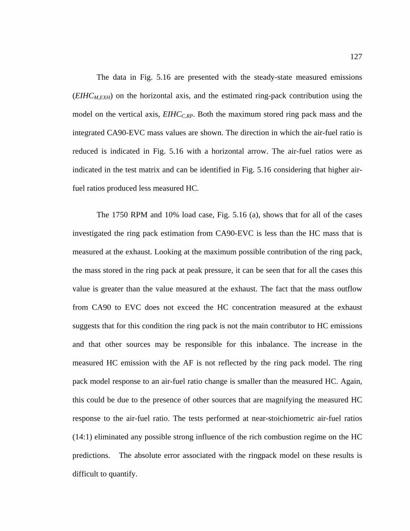
127
The data in Fig. 5.16 are presented with the steady-state measured emissions
(EIHCM,EXH) on the horizontal axis, and the estimated ring-pack contribution using the
model on the vertical axis, EIHCC,RP. Both the maximum stored ring pack mass and the
integrated CA90-EVC mass values are shown. The direction in which the air-fuel ratio is
reduced is indicated in Fig. 5.16 with a horizontal arrow. The air-fuel ratios were as
indicated in the test matrix and can be identified in Fig. 5.16 considering that higher air-
fuel ratios produced less measured HC.
The 1750 RPM and 10% load case, Fig. 5.16 (a), shows that for all of the cases
investig
ssible strong influence of the rich combustion regime on the HC
predictions. The absolute error associated with the ringpack model on these results is
difficult to quantify.
ated the ring pack estimation from CA90-EVC is less than the HC mass that is
measured at the exhaust. Looking at the maximum possible contribution of the ring pack,
the mass stored in the ring pack at peak pressure, it can be seen that for all the cases this
value is greater than the value measured at the exhaust. The fact that the mass outflow
from CA90 to EVC does not exceed the HC concentration measured at the exhaust
suggests that for this condition the ring pack is not the main contributor to HC emissions
and that other sources may be responsible for this inbalance. The increase in the
measured HC emission with the AF is not reflected by the ring pack model. The ring
pack model response to an air-fuel ratio change is smaller than the measured HC. Again,
this could be due to the presence of other sources that are magnifying the measured HC
response to the air-fuel ratio. The tests performed at near-stoichiometric air-fuel ratios
(14:1) eliminated any po
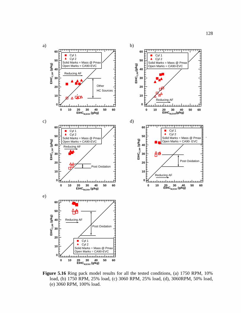
128
a) 60
50
40
30
20
10
0
EIR
PH
CC
, (g
/kg)
6050403020100EIHCM,EXH (g/kg)
OtherHC Sources
Reducing AF
Cyl 1 Cyl 2
Open Marks = CA90-EVC
b) 60
50Solid Marks = Mass @ Pmax
40
30
20
10
0
RP
EIH
CC
,(g
/kg)
6050403020100EIHCM,EXH(g/kg)
Reducing AF
Cyl 1 Cyl 2
Open Marks = CA90-EVC
c)
Solid Marks = Mass @ Pmax
60
50
40
30
20
10
0
C,R
P (g
/kg)
6050403020100EIHCM,EXH (g/kg)
Post Oxidation
Reducing AF
Cyl 1 Cyl 2
d) 60
50
40
30
20
10
0
EIH
C
Solid Marks = Mass @ PmaxOpen Marks = CA90-EVC
EIH
CC
,RP
(g/k
g)
6050403020100EIHCM,EXH (g/kg)
Post Oxidation
Reducing AF
Cyl 1 Cyl 2
Solid Marks = Mass @ PmaxOpen Marks = CA90- EVC
e)
60
50
40
30
20
10
0
EIH
CC
,RP
(g/k
g)
6050403020100EIHCM,EXH (g/kg)
Post Oxidation
Reducing AF
Cyl 1 Cyl 2
Solid Marks = Mass @ PmaxOpen Marks = CA90-EVC
b) 1750 RPM, 25% load, (c) 3060 RPM, 25% load, (d), 3060RPM, 50% load, (e) 3060 RPM, 100% load.
Figure 5.16 Ring pack model results for all the tested conditions, (a) 1750 RPM, 10% load, (
129
Increasing the load from 10 to 25% while keeping the engine speed at 1750 RPM,
as indicated in Fig. 5.16 (b), produces an in es the ring pack
fro 90 to EVC. At this condition the ring pack contribution roughly matches the
measured HC at the exhaust. The mass of HC stored at maximum pressure has also been
increased. This is expected because the increase of the load produces higher cylinder
pressures, which increases the loading of the ring pack, increasing the stored mass of HC.
The fact that at this operating condition the mass returning to the cylinder from CA90 to
EVO matches the measured HC suggests that this is a limiting condition where the ring
pack starts to become a significant contributor to the HC emissions. This also indicates
that for this condition little or negligible post-oxidation may be taking place. Regarding
the effect of the air-fuel ratio, it can be seen that for this operating condition the model
shows a steeper slope than for the 1750 RPM, 10% load case. The slope appears to be of
ed the ring pack contribution is increased. Thus, for the
3060 RPM, 25% load case, Fig. 5.16 (c), the mass leaving the ring pack from CA90 to
EVC exceeds the value measured at the exhaust. The mass stored at peak pressure has
also in
crease of the mass that leav
m CA
the same magnitude than of the measured HC.
As the speed is increas
creased and is significantly greater than the HC measured at the exhaust. This
suggests that the unburned HC mass leaving the ring pack crevice is a significant and
possibly major contributor to the HC emissions. The small difference between the
predicted and the measured HC can be accounted by post-oxidation. The results show
that the predicted HC by the ring pack model responds in the same manner than the
measured HC to the change in air-fuel ratio.
130
Increasing the load to 50% at the 3060 RPM engine speed (Fig. 5.16 (d)) a
significant increase of the ring pack contribution is observed, for both metrics i.e. the ring
pack mass stored at maximum pressure and the mass leaving the ring pack from CA90 to
EVC. It can clearly be seen that the mass returning to the cylinder from CA90 to EVC is
significantly higher than that measured at the exhaust. These results clearly indicate that
at this condition the ring pack is the major contributor to the engine-out HC emissions.
The air-fuel ratio effect on the model prediction is smaller than for the 3060RPM, 25%
load case. However, the predicted HC is increased as the air-fuel ratio is decreased. It is
important to note that the emissions index of the mass stored at maximum pressure is
slightly reduced as the air-fuel ratio is reduced. This trend is different than the previous
cases (F
index at maximum pressure with the reduction of the air-fuel ratio is also observed here,
ig. 5.16 (a-c). The justification of this trend is due to the normalization of the
mass stored with the mass of fuel per cycle. At this load there is a significant difference
in mass injected per cycle when the air-fuel ratio is increased from 12:1 (left side cases in
Fig. 5.16 (d)) to 11:1 (right side cases in Fig. 5.16(d)) , while the maximum pressure is
almost identical for both cases.
If the load is further increased, as in the 3060 RPM, 100% load case, Fig. 5.16 (e),
the two metrics used to evaluate the ring pack contribution to the HC show further
increases. At this condition it is irrefutable that the ring pack storage prevents the
oxidation of a considerable amount of fuel and there is little doubt that it is the major HC
contributor. The dependence of both ring pack prediction metrics with the air-fuel ratio
shows the same trend as for the 3060 RPM, 50% case. The reduction in the HC emission
131
and it can be also justified due to the normalization of the maximum mass stored with the
mass of fuel injected per cycle.
The inc the load is
increased is the res henomena. First, the loading of the ring pack crevices is
increased, and second the th linder walls earlier, therefore, the majority
of the mass stored will contribute to the engine-out H issions (mass that leaves from
CA90-EVC). This observation is in very good agre with the combustion phasing
obtained from the heat release analysis (Table 5.5). The difference observed between the
mass that leaves from CA90 to EVC will also be affected by the post-oxidation. Table 5.5
also shows that the air-fuel ratio affects the combustion phasing, slowing the combustion
as it increases. This affects the mass return to the ustion ch mber from CA90 to
EVC, and together with the reduced mass fuel in i uces a
decrease of the CA90 to EVC contribution
rease in the ring pack contribution to HC emissions as
ult of two p
flame reaches e cy
C em
ement
ing comb a
of the leaner m xture case prod
.
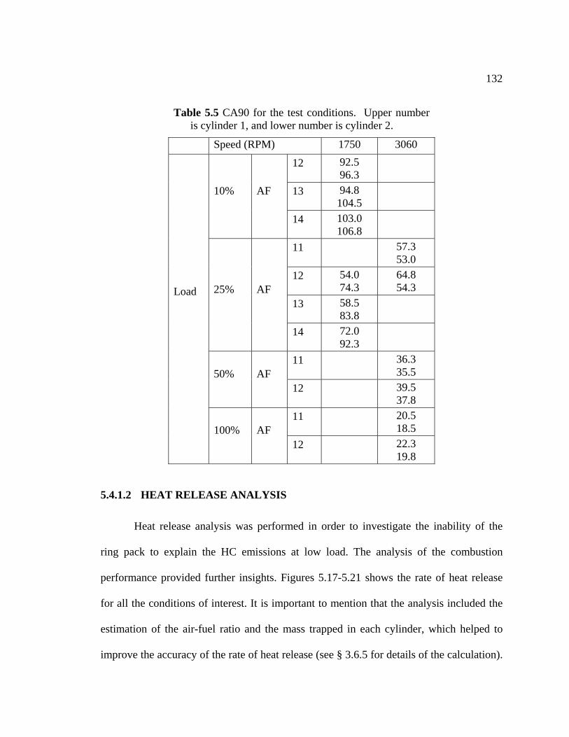
132
Table 5.5 CA90 for the test conditions. Upper number is cylinder 1, and lower number is cylinder 2.
Speed (RPM) 1750 3060
12 92.5 96.3
13 94.8 104.5 10% AF
14 103.0 106.8
11 57.3 53.0
12 54.0 64.8 74.3 54.3
13 58.5 83.8
25% AF
92.3 14 72.0
11 36.3 35.5
50% AF 12 39.5
37.8
11 20.5 18.5
Load
12 22.3 100% AF
19.8
5.4.1.2 HEAT RELEASE ANALYSIS
for all the conditions of interest. It is important to mention that the analysis included the
estimation of the air-fuel ratio and the mass trapped in each cylinder, which helped to
improve the accuracy of the rate of heat release (see § 3.6.5 for details of the calculation).
Heat release analysis was performed in order to investigate the inability of the
ring pack to explain the HC emissions at low load. The analysis of the combustion
performance provided further insights. Figures 5.17-5.21 shows the rate of heat release
133
At the low load, low speed condition, Fig. 5.17, it can be seen that neither of the cylinders
complete combustion prior to EVO. For the 1750 RPM, 25% load, Fig. 5.18, the same
behavior is observed; however, the degree of incomplete combustion has been decreased
in comparison with the 1750 RPM, 10% load case. As expected, the air-fuel ratio affects
the tail of the heat release rate. As the air-fuel ratio increases the tail of the heat release
goes up, resulting in a higher level of incomplete combustion. For both loads (10 and
25%) at 1750 PRM, cylinder 2 shows more incomplete combustion prior to EVO than
cylinder 1.
From Fig. 5.19, for the 3060 RPM, 25% case, the heat release analysis shows that
mit where incomplete combustion is not observed. In addition, the differences in heat
release between cylinders have been reduce
rele inder, although the difference is very small. If the load is
further increased as for the 50% and 100% load cases, Figs. 5.20 and 5.21, the
combustion event is clearly finished prior to EVO. For these two conditions there is no
doubt that all the combustion takes place prior EVO. For the 50% load case, the heat
release profile is not affected significantly by the air-fuel ratio, and both cylinders show
the same heat release profile. However, for the 100% load case, cylinder 1 and cylinder 2
show different heat release profiles. At this load the air-fuel ratio does not affect the heat
release profile, as well.
the combustion event is finished prior EVO. This operating condition appears to be the
li
d. Still the first cylinder shows higher heat
ase than the second cyl
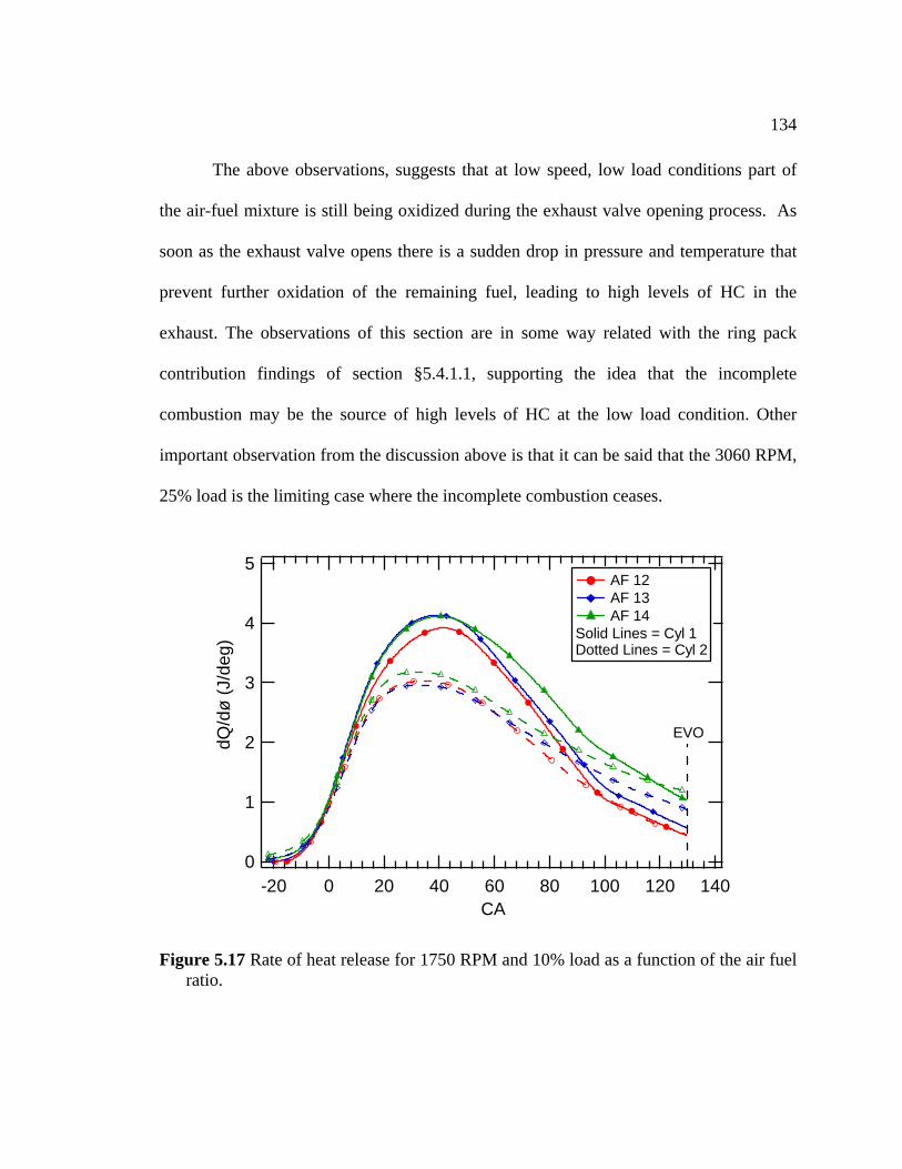
134
The above observations, suggests that at low speed, low load conditions part of
the air-fuel mixture is still being oxidized during the exhaust valve opening process. As
soon as the exhaust valve opens there is a sudden drop in pressure and temperature that
prevent further oxidation of the remaining fuel, leading to high levels of HC in the
exhaust. The observations of this section are in some way related with the ring pack
contribution findings of section §5.4.1.1, supporting the idea that the incomplete
combustion may be the source of high levels of HC at the low load condition. Other
important observation from the discussion above is that it can be said that the 3060 RPM,
25% load is the limiting case where the incomplete combustion ceases.
5
4
3
2
1
0
dQ/d
ø (J
/deg
)
140120100806040200-20CA
EVO
AF 12 AF 13 AF 14
Solid Lines = Cyl 1Dotted Lines = Cyl 2
Figure 5.17 Rate of heat release for 1750 RPM and 10% load as a function of the air fuel ratio.
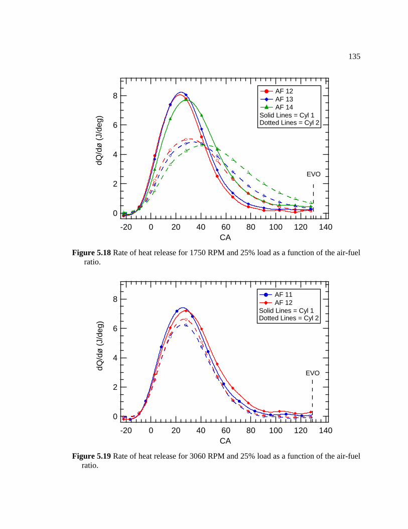
135
8
6
4
2
0
dQ/d
ø (J
/deg
)
140120100806040200-20CA
EVO
AF 12 AF 13 AF 14
Solid Lines = Cyl 1Dotted Lines = Cyl 2
Figure 5.18 Rate of heat release for 1750 RPM and 25% load as a function of the air-fuel
ratio.
8
6
4
2
0
dQ/d
ø (J
/deg
)
140120100806040200-20CA
EVO
AF 11 AF 12
Dotted Lines = Cyl 2Solid Lines = Cyl 1
Figure 5.19 Rate of heat release for 3060 RPM and 25% load as a function of the air-fuel
ratio.
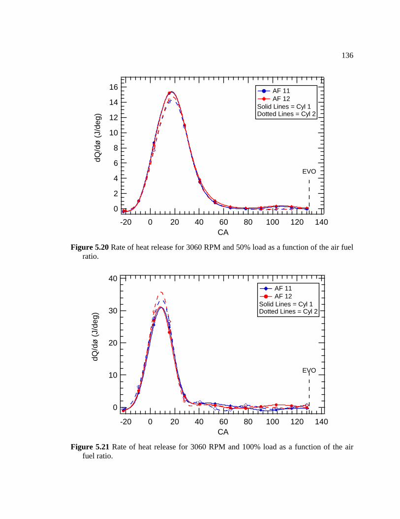
136
16
14
12
10
8
6
4
2
0
/deg
)dQ
/dø
(J
140120100806040200-20CA
EVO
AF 11 AF 12
Solid Lines = Cyl 1Dotted Lines = Cyl 2
ratio. Figure 5.20 Rate of heat release for 3060 RPM and 50% load as a function of the air fuel
40
30
20
10
0
dQ/d
ø (J
/deg
)
140120100806040200-20CA
EVO
AF 11 AF 12
Solid Lines = Cyl 1Dotted Lines = Cyl 2
Figure 5.21 Rate of heat release for 3060 RPM and 100% load as a function of the air
fuel ratio.
137
One important conclusion of sections §5.4.1.1 and §5.4.1.2 is that cylinder 1 and
cylinder 2 behave differently and produce different amount of work for all the operating
conditions except for the 3060 RPM, 50% load where both cylinders show similar rate of
heat release profiles (and similar ring pack contribution). Note that cylinder 1 produces
more work than cylinder 2 up to the 3060 RPM, 25% load, however for the 3060 RPM,
100% load cylinder 2 produces more work than cylinder 1, i.e. the behavior is inverted.
This behavior was verified several times, and it is believed that the main cause of this
behavior is the difference in charging between the cylinders. This was verified comparing
the pressure traces, the IMEP (see §5.4.1), and by carrying out sweep spark timing tests
at constant throttle position (see §3.6.5). The main reason for the difference in charging is
the design of the engine, and especially of the intake system. Despite of the differences
observ
5.4.1.3 CYCLIC VARIABILITY
w load cases. At
low load conditions there are other factors associated with the combustion process that
may affect HC e
ed, the study of the engine under these conditions provided insights of the behavior
that are particular of the small engines that are currently in production. Therefore, the
analysis was carried out for both cylinders of the engine.
The indication that the ring pack was not the major contributor to the HC
emissions at low load suggested the presence of other sources that could overwhelm the
effect of the ring pack crevices. Incomplete combustion due to a slow burn rate is the
likely cause [5]; cyclic variability is high and misfire can occur at the lo
missions. Very slow burn rate is typical because of the fixed (somewhat
retarded) ignition timing. This can lead to the tail of the heat release curve extending to
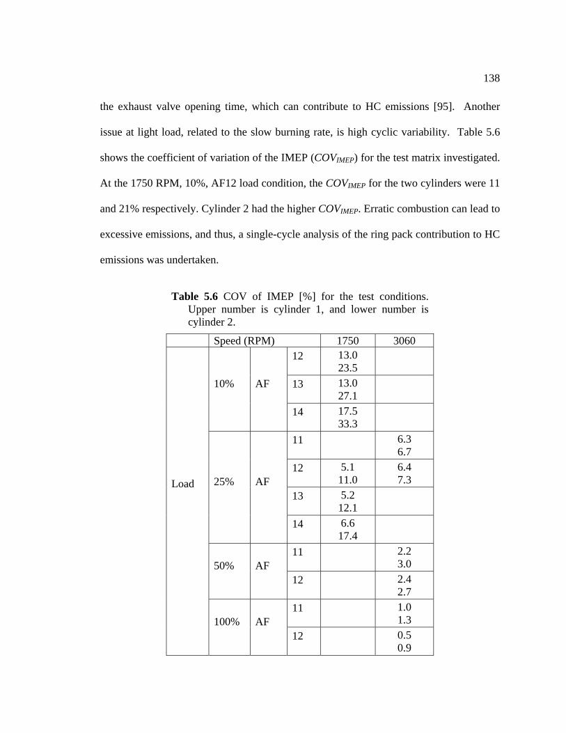
138
the exhaust valve opening time, which can contribute to HC emissions [95]. Another
issue at light load, related to the slow burning rate, is high cyclic variability. Table 5.6
shows the coefficient of variation of the IMEP (COVIMEP) for the test matrix investigated.
At the 1750 RPM, 10%, AF12 load condition, the COV
Table 5.6 COV of IMEP [%] for the test conditions. umber is cylinder 1, and lower number is
cylinder 2.
Speed (RPM) 1750 3060
IMEP for the two cylinders were 11
and 21% respectively. Cylinder 2 had the higher COVIMEP. Erratic combustion can lead to
excessive emissions, and thus, a single-cycle analysis of the ring pack contribution to HC
emissions was undertaken.
Upper n
12 13.0 23.5
13 13.0 27.1 10% AF
14 17.5 33.3
11 6.3 6.7
12 5.1 11.0
6.4 7.3
13 5.2 12.1
25% AF
14 6.6 17.4
11 2.2 3.0 50% AF
12 2.4 2.7
11 1.0 1.3
Load
100% AF 12 0.5
0.9
139
5.4.2 SINGLE-CYCLE RESULTS
The single-cycle HC analysis followed the same process as described above. The
codes were modified to perform the heat release and calculate the ring pack contribution
on a single-cycle basis. For the heat release analysis the average heat transfer multiplier
was used (see Appendix XII). It was considered to be more representative than that
the single-cycle analysis, because the heat transfer was expected to be
approximately constant along the 200 cycles of the data set. The heat release and ring
pack filling and discharging were calculated for each cycle assuming that there was a
constant cylinder charging mass, i.e. the value calculated from the spark timing sweep at
constant throttle position. The mass of HC leaving the ring pack was integrated from
CA90 to EVC on a cycle-by-cycle basis.
The results of the single-cycle analysis are shown in Figs. 5.22-5.26 for the
ifferent loads and speeds. For clarity, only e air-fuel ratio of 12:1 data is shown. The
results at other air-fuel ratios are shown in the Appendix XV. It can be clearly seen that
while there is considerable cyclic variation in the ring pack contribution to HC, there are
not isolated events that are well outside the normal range. Further, comparing the mean
ring-pack EIHC of the individual cycles to the ring-pack EIHC determined from the
mean cylinder pressure (horizontal lines in Figs. 5.22-5.26), there is good agreement.
Over the range of operating conditions in Table 4.1, the maximum deviation between the
obtained from
5.4.2.1 SINGLE-CYCLE RING PACK CONTRIBUTION TO THE HC
EMISSIONS
d th
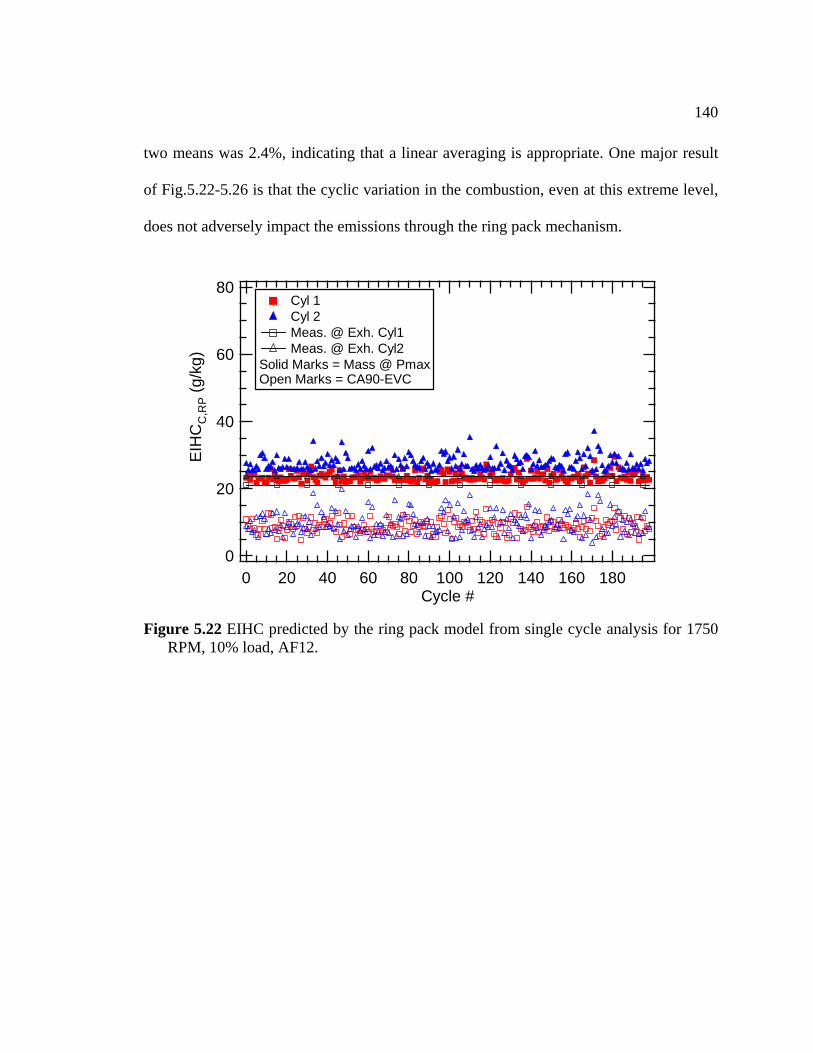
140
two means was 2.4%, indicating that a linear averaging is appropriate. One major result
of Fig.5.22-5.26 is that the cyclic variation in the combustion, even at this extreme level,
does not adversely impact the emissions through the ring pack mechanism.
80
60
40
20
0
EIH
CC
,RP (g
/kg)
180160140120100806040200Cycle #
Cyl 1 Cyl 2 Meas. @ Exh. Cyl1 Meas. @ Exh. Cyl2
Solid Marks = Mass @ PmaxOpen Marks = CA90-EVC
igure 5.22 EIHC predicted by the ring pack model from single cycle analysis for 1750
RPM, 10% load, AF12. F
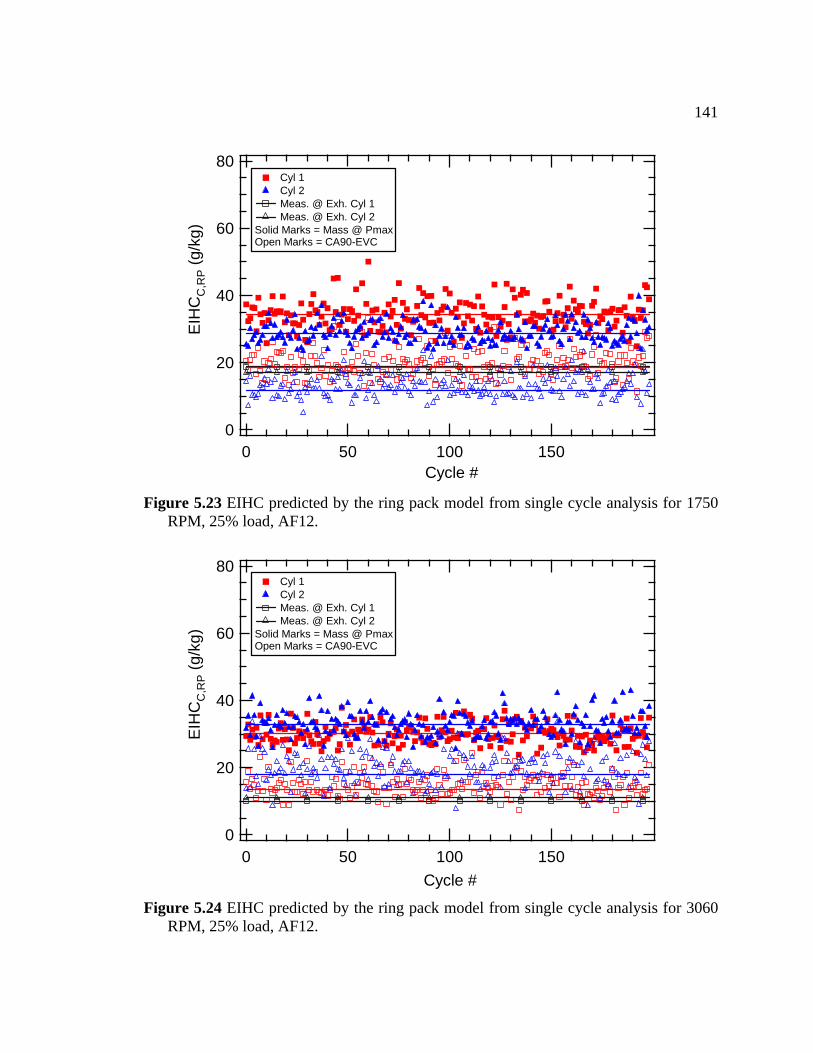
141
80
60
40
20
0
EIH
CC
,RP (g
/kg)
150100500Cycle #
Cyl 1 Cyl 2 Meas. @ Exh. Cyl 1 Meas. @ Exh. Cyl 2
Solid Marks = Mass @ PmaxOpen Marks = CA90-EVC
Figure 5.23 EIHC predicted by the ring pack model from single cycle analysis for 1750
RPM, 25% load, AF12.
80
60
40
20
0
EIH
CC
,RP (g
/kg)
150100500Cycle #
Cyl 1 Cyl 2 Meas. @ Exh. Cyl 1 Meas. @ Exh. Cyl 2
Solid Marks = Mass @ PmaxOpen Marks = CA90-EVC
Figure 5.24 EIHC predicted by the ring pack model from single cycle analysis for 3060
RPM, 25% load, AF12.
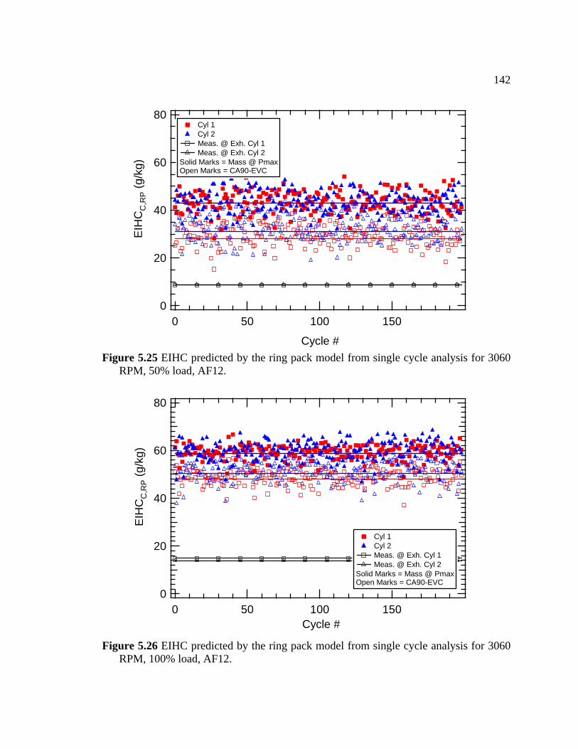
142
80
60
40
20
0
EIH
CC
,RP (g
/kg)
150100500
Cycle #
Cyl 1 Cyl 2 Meas. @ Exh. Cyl 1 Meas. @ Exh. Cyl 2
Solid Marks = Mass @ PmaxOpen Marks = CA90-EVC
Figure 5.25 EIHC predicted by the ring pack model from single cycle analysis for 3060
RPM, 50% load, AF12.
80
60
40
20
0
EIH
CC
,RP (g
/kg)
150100500Cycle #
Cyl 1 Cyl 2 Meas. @ Exh. Cyl 1 Meas. @ Exh. Cyl 2
Solid Marks = Mass @ PmaxOpen Marks = CA90-EVC
Figure 5.26 EIHC predicted by the ring pack model from single cycle analysis for 3060
RPM, 100% load, AF12.
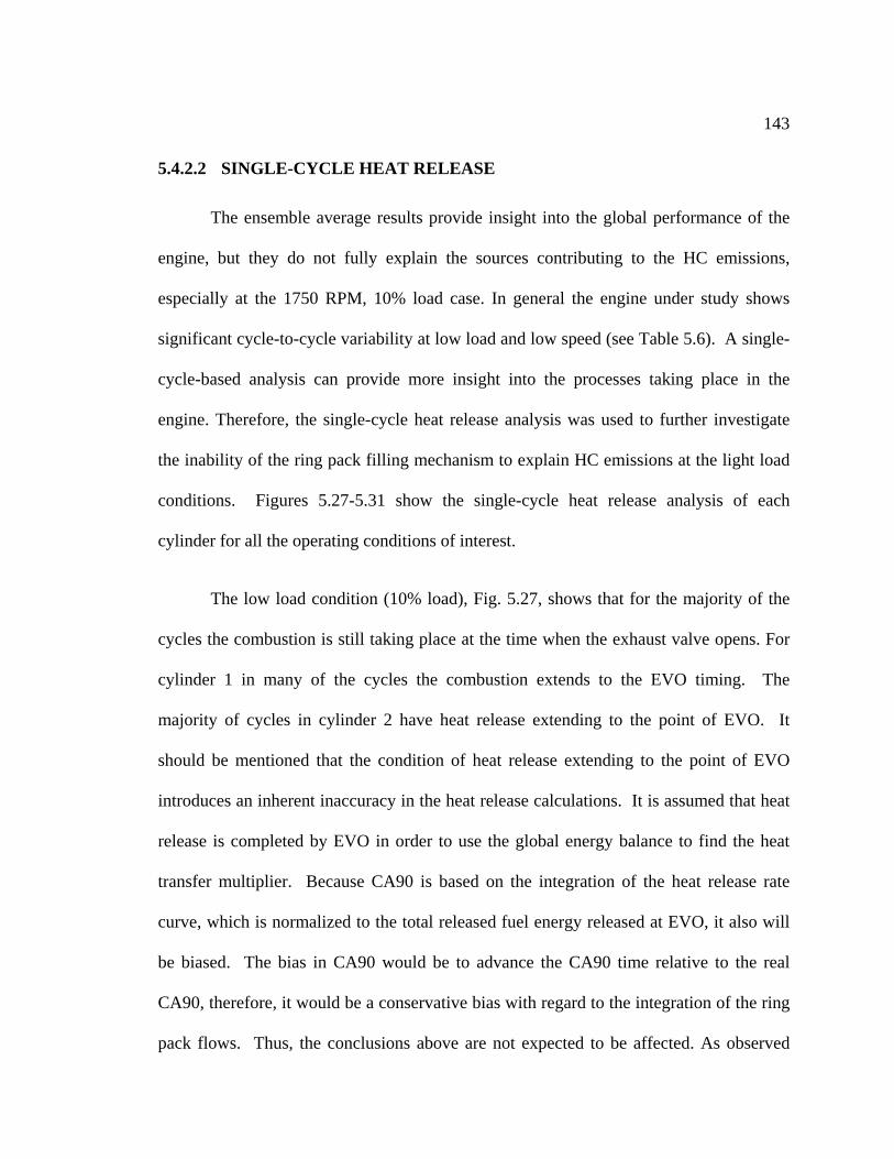
143
5.4.2.2 SINGLE-CYCLE HEAT RELEASE
The ensemble average results provide insight into the global performance of the
engine, but they do not fully explain the sources contributing to the HC emissions,
especially at the 1750 RPM, 10% load case. In general the engine under study shows
significant cycle-to-cycle variability at low load and low speed (see Table 5.6). A single-
de more insight into the processes taking place in the
engine. Therefore, the single-cycle heat release analysis was used to further investigate
the inability of the ring pack filling mechanism to explain HC emissions at the light load
conditions. Figures 5.27-5.31 show the single-cycle heat release analysis of each
cylinder for all the operating conditions of interest.
The low load condition (10% load), Fig. 5.27, shows that for the majority of the
r
bustion extends to the EVO timing. The
majority of cycles in cylinder 2 have heat release extending to the point of EVO. It
to the point of EVO
introdu
pack flows. Thus, the conclusions above are not expected to be affected. As observed
cycle-based analysis can provi
cycles the combustion is still taking place at the time when the exhaust valve opens. Fo
any of the cycles the comcylinder 1 in m
should be mentioned that the condition of heat release extending
ces an inherent inaccuracy in the heat release calculations. It is assumed that heat
release is completed by EVO in order to use the global energy balance to find the heat
transfer multiplier. Because CA90 is based on the integration of the heat release rate
curve, which is normalized to the total released fuel energy released at EVO, it also will
be biased. The bias in CA90 would be to advance the CA90 time relative to the real
CA90, therefore, it would be a conservative bias with regard to the integration of the ring
144
before, the air-fuel ratio affects the extent of the incomplete combustion, and it can
clearly be seen in Fig. 5.27. At the air-fuel ratio of 12:1, Fig. 5.27 (a), there is a small
fraction of cycles that finish combustion prior EVO. As the air fuel ratio is increased, the
fraction of cycles that complete combustion prior EVO is reduced (13:1), and then for the
air-fuel ratio of 14:1, Fig. 5.27 (c), shows that none of the cycles finish combustion prior
to EVO. This trend is consistent with the increased COV of IMEP observed at this
operating condition.
that the fraction of cycles that finish heat release prior EVO has been increased
indications of incomplete combustion. Cylinder 2 shows a higher degree of incomplete
As the load is increased to 25%, Fig. 5.28, the single-cycle heat release reveals
considerably with respect to the 10% load (Fig. 5.27). However, there are still some
ombustion than cylinder 1. This difference is more pronounced for the air-fuel ratio of
4:1, where a significant fraction of the cycles do not complete combustion prior to EVO.
At the intermediate load and high speed case (3060 RPM, 25% load), Fig. 5.29, it
can be seen that for the majority of the cycles the combustion is finished before EVO, but
bustion. The number of cycles that complete combustion
with respect to the same load at 1750 RPM (Fig. 5.28).
eed helps to increase the number of cycles
plete combustion prior EVO. No strong effect of the air-fuel ratio is observed,
and both cylinders show roughly the same heat release profile.
c
1
a few cycles exhibit late com
prior EVO has been increased
This observation suggests that the engine sp
that com
145
For the 50 and 100% load 3060 RPM case, Fig. 5.30-5.31 respectively, all the
energy is released significantly before EVO for all of the cycles. This is in full agreement
with the observations of the heat release analysis using average pressure, indicating that
for these two operating conditions there are not cycles that have incomplete combustion.
Thus, for example at the 3060 RPM, 100% load condition, Fig. 5.31, a relatively rapid
heat release rate is observed; the CA10 – CA90 duration was on average 27 crank angle
rees. At this operating condition cylinder 2 has a higher peak burning rate. For these
two conditions (Fig. 5.30-5.31), it was observed in Fig. 5.16 that the ring pack
mechanism was able to fully explain the HC emissions from the engine.
The fact that for the 1750 RPM and 10% load (and in less degree for the 1750
RPM, 25%) load case the majority of the cycles do not complete heat release prior to
bustion coul the HC emissions. It
as been previously shown by Haugle and G andhi [95] that there was a correlation
betw
MEP cycles when the heat release – calculated based on the mean cylinder pressure –
xtended beyond EVO. Therefore, based on the low load data in Fig. 5.27 it is possible
at incomplete combustion is contributing to the HC emissions, which would explain the
shortfall in the ring-pack contribution. Also, the isolated slow burn cycles at the 3060
also contribute to the HC
emissio
deg
EVO suggests that incomplete com d be contributing to
h h
een the observances of higher hydrocarbon concentrations in the exhaust with low-
I
e
th
RPM, 25% load case suggests that incomplete combustion may
ns at this condition.
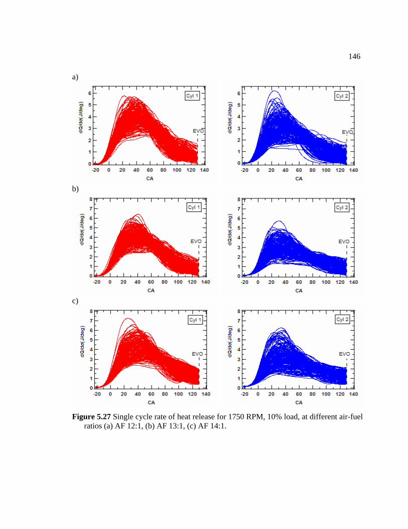
146
a)
b)
c)
Figure 5.27 Single cycle rate of heat release for 1750 RPM, 10% load, at different air-fuel ratios (a) AF 12:1, (b) AF 13:1, (c) AF 14:1.
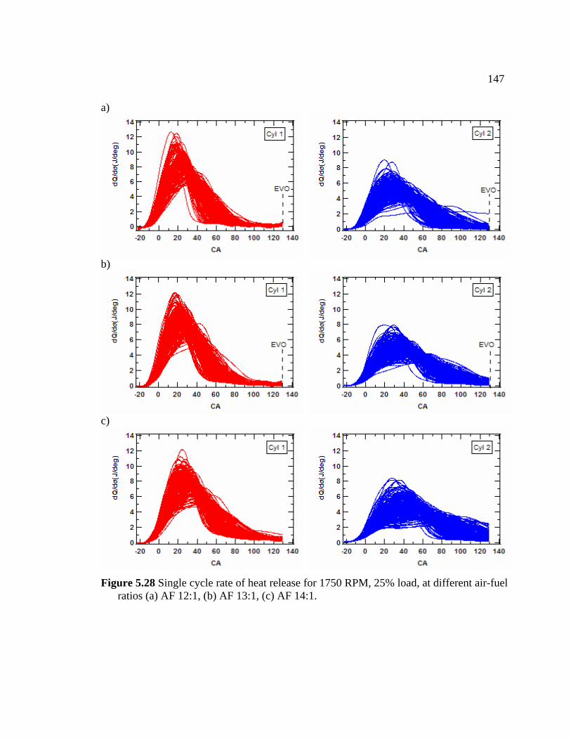
147
a)
b)
c)
Fratios (a) AF 12:1, (b) A
igure 5.28 Single cycle rate of heat release for 1750 RPM, 25% load, at different air-fuel F 13:1, (c) AF 14:1.
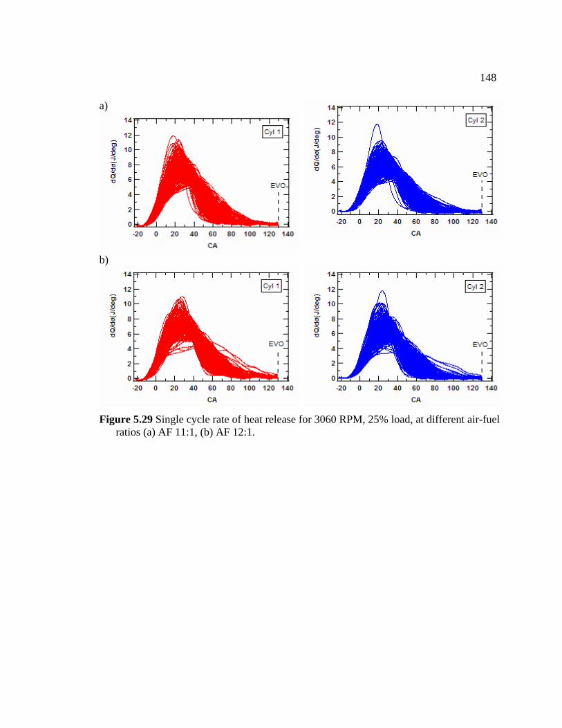
148
a)
b)
Figure 5.29 Single cycle rate of heat release for 3060 RPM, 25% load, at different air-fuel ratios (a) AF 11:1, (b) AF 12:1.
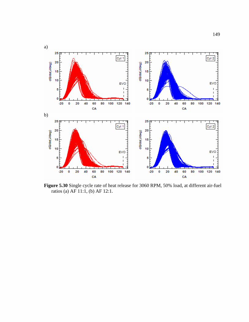
149
a)
b)
Figure 5.30 Single cycle rate of heat release for 3060 RPM, 50% load, at different air-fuel ratios (a) AF 11:1, (b) AF 12:1.
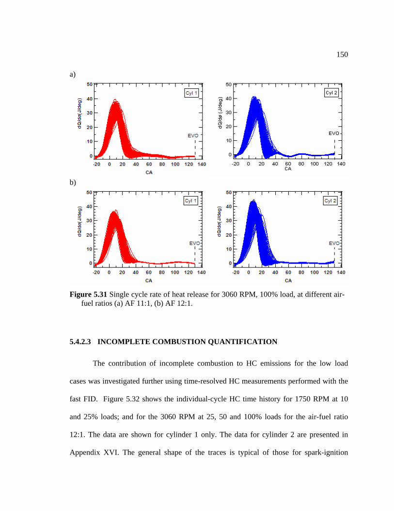
150
a)
b)
Figure 5.31 Single cycle rate of heat release for 3060 RPM, 100% load, at different air-fuel ratios (a) AF 11:1, (b) AF 12:1.
5.4.2.3 INCOMPLETE COMBUSTION QUANTIFICATION
The contribution of incomplete combustion to HC emissions for the low load
ases was investigated further using time-resolved HC measurements performed with the
st FID. Figure 5.32 shows the individual-cycle HC time history for 1750 RPM at 10
nd 25% loads; and for the 3060 RPM at 25, 50 and 100% loads for the air-fuel ratio
2:1. The data are shown for cylinder 1 only. The data for cylinder 2 are presented in
ppendix XVI. The general shape of the traces is typical of those for spark-ignition
c
fa
a
1
A
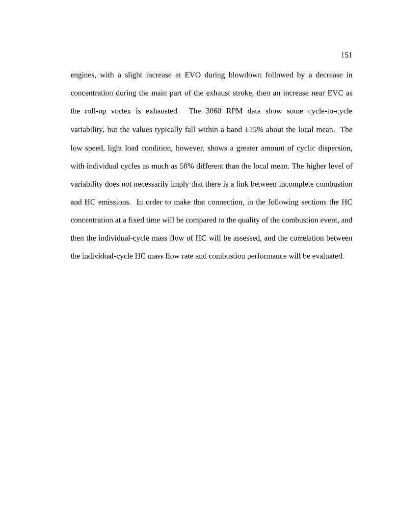
151
engines, with a slight increase at EVO during blowdown followed by a decrease in
concentration during the main part of the exhaust stroke, then an increase near EVC as
the roll-up vortex is exhausted. The 3060 RPM data show some cycle-to-cycle
variability, but the values typically fall within a band ±15% about the local mean. The
low speed, light load condition, however, shows a greater amount of cyclic dispersion,
with individual cycles as much as 50% different than the local mean. The higher level of
iability does not necessarily imply that there is a link between incomplete combustion
and HC emissions. In order to make that connection, in the following sections the HC
concentration at a fixed time will be compared to the quality of the combustion event, and
then the individual-cycle mass flow of HC will be assessed, and the correlation between
the individual-cycle HC mass flow rate and combustion performance will be evaluated.
var
152
b) a)
c) d)
e)
Figure 5.32 Single-cycle resolved HC measurements for cylinder 1 (a) 1750 RPM, 10% load, AF12, (b) 1750 RPM, 25% load, AF 12, (c) 3060 RPM, 25% load, AF12, (d) 3060 RPM, 50% load, AF12, and 3060 RPM, 100% load, AF12.
153
5. 2.3.1
The ns was
assessed by relating the HC data from the fast FID with the corresponding IMEP. The HC
concentration at a given CA timing in the cycle was compared against the IMEP of the
same cycle. Hydrocarbon concentration [HC] s a CA aTDC were chosen
because this CA represents the local peak in HC concentration during the blowdown
process (see Fig. 5.32). The results of this comp ig. 5.33-5.38
The data at 1750 RPM, 10% load, Fig. 5.33, indicate a correlation between HC
concentration at 160 CA aTDC and IMEP. C with IM se have a
higher [HC] as would be expected from a partial combustion event. This dependence is
more pronounced for cylinder 2, which at the s im s higher variability in the
HC concentration. A linear trend line is shown and appears to adequately represent the
data, but does not conclusively suggest a
Fig.5.34, a very weak dependence can be seen for all the air fuel ratios except for
cylinder 1 at the a ati 12: d 13:1 where the dep i er. The
3060 RPM cases (loads 25, 50 and 100 % load), Figs. 5.35-5.37, however, show a nearly
random relationship between [HC] at 160 CA aTDC with cycle IMEP. The linear curve
fit. The statistical nature of the fits will be
discuss
4. CONCENTRATION-BASED CORRELATION
role of cyclic variations in combustion performance on HC emissio
value t 160
arison are presented in F
ycles low EP are en to
ame t e show
linear correlation. For the 1750 RPM, 25% load,
ir-fuel r os of 1 an endence s clear
fit to the data shown, has a poor quality of the
ed further in the following section.
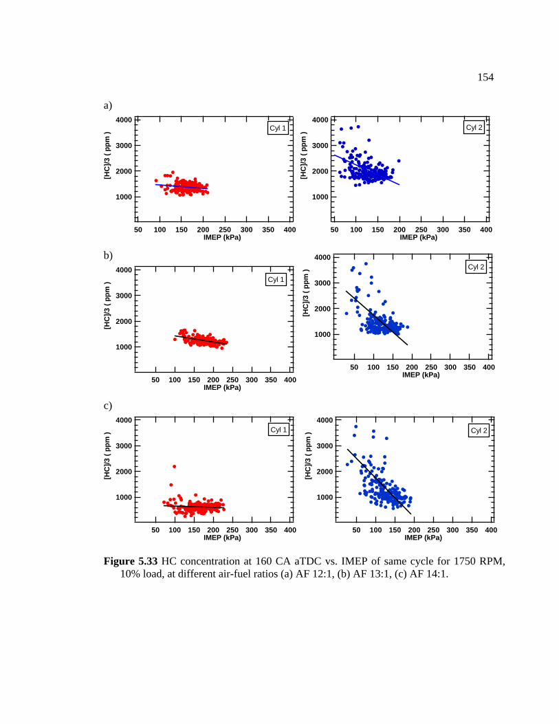
154
a) 4000
3000
2000
1000
40035030025020015010050
[HC
]p
/3 (
pm
)
IMEP (kPa)
Cyl 1
4000
3000
2000
1000
[HC
]p
40035030025020015010050IMEP (kPa)
Cyl 2
/3 (
pm
)
b) 4000
3000
2000
1000
[H
40035020015 300250
4000
3000
2000
1000
[HC
] (
ppm
/3 )
40035030025020015010050IMEP (kPa)
Cyl 1
C]/3
( pp
m )
010050IMEP (kPa)
Cyl 2
c) 4000
3000
2000
1000
[HC
3 ( p
p]/
m )
40035030025020015010050IMEP (kPa)
Cyl 1
4000
3000
2000
1000
[HC
3 ( p
p]/
m )
40035030025020015010050IMEP (kPa)
Cyl 2
Figure 5.33 HC concentration at 160 CA aTDC vs. IMEP of same cycle for 1750 RPM, 10% load, at different air-fuel ratios (a) AF 12:1, (b) AF 13:1, (c) AF 14:1.
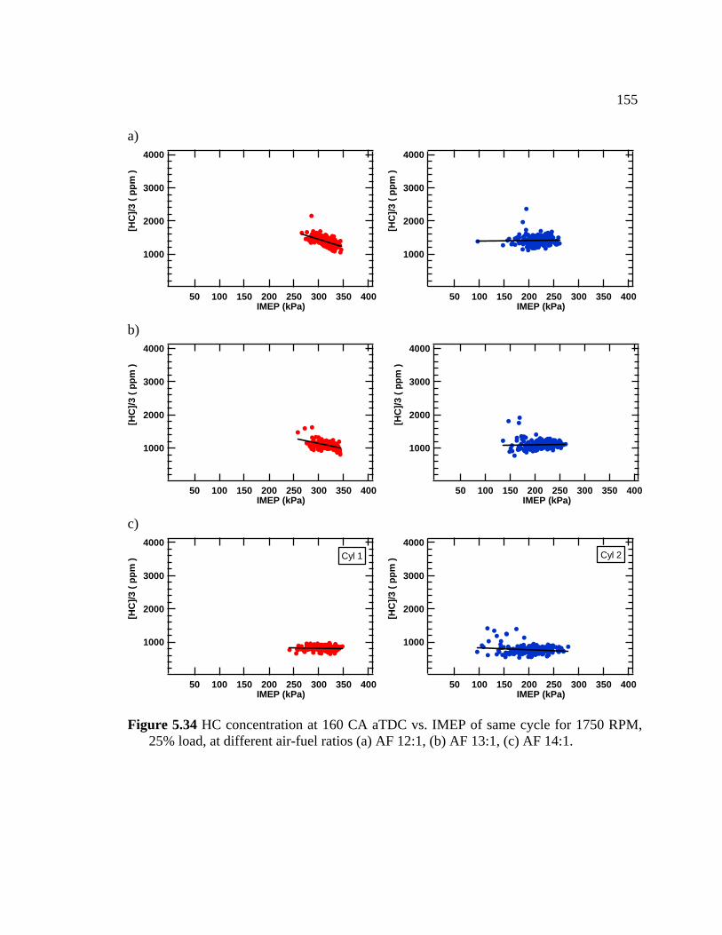
155
a)
4000
40035030025020015010050IMEP (kPa)
4000
3000
2000
1000
[HC
]/3 (
p)
pm
3000
2000
1000
[HC
]/3 (
ppm
)
40035030025020015010050IMEP (kPa)
b) 4000
3000
2000
1000
[HC
]/3 (
ppm
)
40035030025020015010050IMEP (kPa)
4000
3000
2000
1000
[HC
]/3 (
ppm
)
40035030025020015010050IMEP (kPa)
c) 4000
3000
2000
1000
[HC
]/3 (
ppm
)
40035030025020015010050IMEP (kPa)
Cyl 1
4000
3000
2000
1000
[HC
]/3pm
) (
p
40035030025020015010050IMEP (kPa)
Cyl 2
Figure25% load, at different air-fuel ratios (a) AF 12:1, (b) AF 13:1, (c) AF 14:1.
5.34 HC concentration at 160 CA aTDC vs. IMEP of same cycle for 1750 RPM,
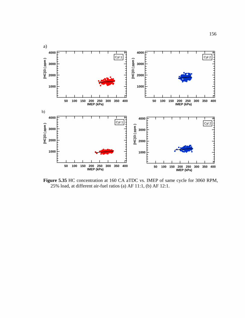
156
a)
4000
3000
2000
1000
35
[HC
/3 (
pm
)]
p
400030025020015010050IMEP (kPa)
Cyl 1
4000
3000
2000
1000
[HC
/3 (
pm
)]
p
40035030025020015010050IMEP (kPa)
Cyl 2
b) 4000
3000
2000
1000
[HC
]/3 (
ppm
)
40035030025020015010050IMEP (kPa)
4000
3000
2000
1000
[HC
]
Cyl 1
/3 (
ppm
)
40035030025020015010050IMEP (kPa)
Cyl 2
igure 5.35 HC concentration at 160 CA aTDC vs. IMEP of same cycle for 3060 RPM, 25% load, at different air-fuel ratios (a) AF 11:1, (b) AF 12:1.
F
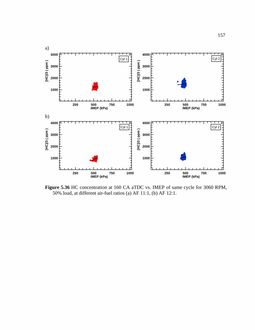
157
a) 4000
3000
2000
1000
[HC
]/3 (
ppm
)
1000750500250IMEP (kPa)
Cyl 1
4000
3000
2000
1000
[HC
]/3 (
ppm
)
1000750500250IMEP (kPa)
Cyl 2
b) 4000
3000
2000
1000
[HC
]/3 (
ppm
)
10750500 00250IMEP (kPa)
Cyl 1
4000
3000
2000
1000
[HC
]/3 (
ppm
)
1000750500250IMEP (kPa)
Cyl 2
Figure50% load, at different air-fuel ratios (a) AF 11:1, (b) AF 12:1.
5.36 HC concentration at 160 CA aTDC vs. IMEP of same cycle for 3060 RPM,
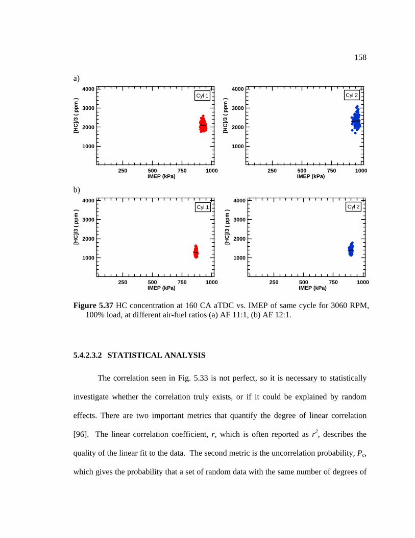
158
a)
5.4.2.3.2 STATISTICAL ANALYSIS
The correlation seen in Fig. 5.33 is not perfect, so it is necessary to statistically
investigate whether the correlation truly exists it could be explained by random
eff There are two important metrics that quantify the degree of linear correlation
[96 he linear correlation coefficient, r, which is often reported as r2, describes the
quality of the linear fit to the data. The second metric is the uncorrelation probability, Pc,
which gives the probability that a set of random data with the same number of degrees of
, or if
ects.
]. T
4000
3000
2000
1000
1000750500250IMEP (kPa)
Cyl 1
4000
3000
2000
1000
[HC
]p
1000750500250IMEP (kPa)
Cyl 2
[HC
/3 (
pm
)
/3 (
pm
)
]p
b) 4000
3000
2000
1000
[HC
]/3 (
ppm
)
1000750500250IMEP (kPa)
Cyl 1
4000
3000
2000
1000
[HC
]/3 (
ppm
)
1000750500250IMEP (kPa)
Cyl 2
Figure 5.37 HC concentration at 160 CA aTDC vs. IMEP of same cycle for 3060 RPM, load, at different air-fuel ratios (a) AF 11:1, (b) AF 12:1. 100%
159
freedom could give the same value of r. Only data that concurrently have a large r and a
P can be considered to display a true linear correlationlow c .
Tables 5.7 show the value of r and Pc for the linear correlation between the
hydrocarbon concentration and IMEP. For the 1750 RPM, 10% load data the correlation
between the [HC] with the IMEP is unambiguous. The values of Pc are universally low.
This indicates that the observed value of r is statistically meaningful, even though for
some conditions r is itself relatively low, e.g. at AF of 14. Further, the 3060 RPM, 100%
data show low values of r with high values of Pc, indicating that no statistically
meaningful correlation is observed. There are isolated cases at the other loads that
suggest that a statistically significant correlation exists.
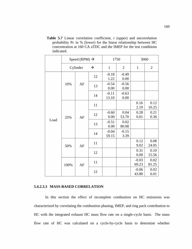
160
5.4.2.3.3 MASS-BASED CORRELATION
In this section the effect of incomplete combustion on HC emissions was
characterized by correlating the combustion phasing, IMEP, and ring pack contribution to
HC with the integrated exhaust HC mass flow rate on a single-cycle basis. The mass
flow rate of HC was calculated on a cycle-by-cycle basis to determine whether
Table 5.7 Linear correlation coefficient, r (upper) and uncorrelation probability Pc in % (lower) for th r relationship between HC concentration at 160 CA aTDC and the IMEP for the test conditions indicated.
Speed (RPM) 1750 3060
e linea
Cylinder 1 2 1 2
12 -0.18 1.22
-0.490.00
13 0.54 0.00
-0.560.00 -10% AF
14 -0.11 13.10
-0.630.00
11 0.16 2.19
0.1210.25
12 -0.600.00
0.0453.70
0.28 0.01
0.210.36
13 -0.510.00
0.0280.08
25% AF
14 -0.0459.15
-0.153.39
11 0.12 9.02
0.0824.0550% AF
12 0.31 0.00
0.1015.56
11 69.23 81.25-0.03 0.02
Load
43.80 6.01
100% AF
12 -0.06 0.02
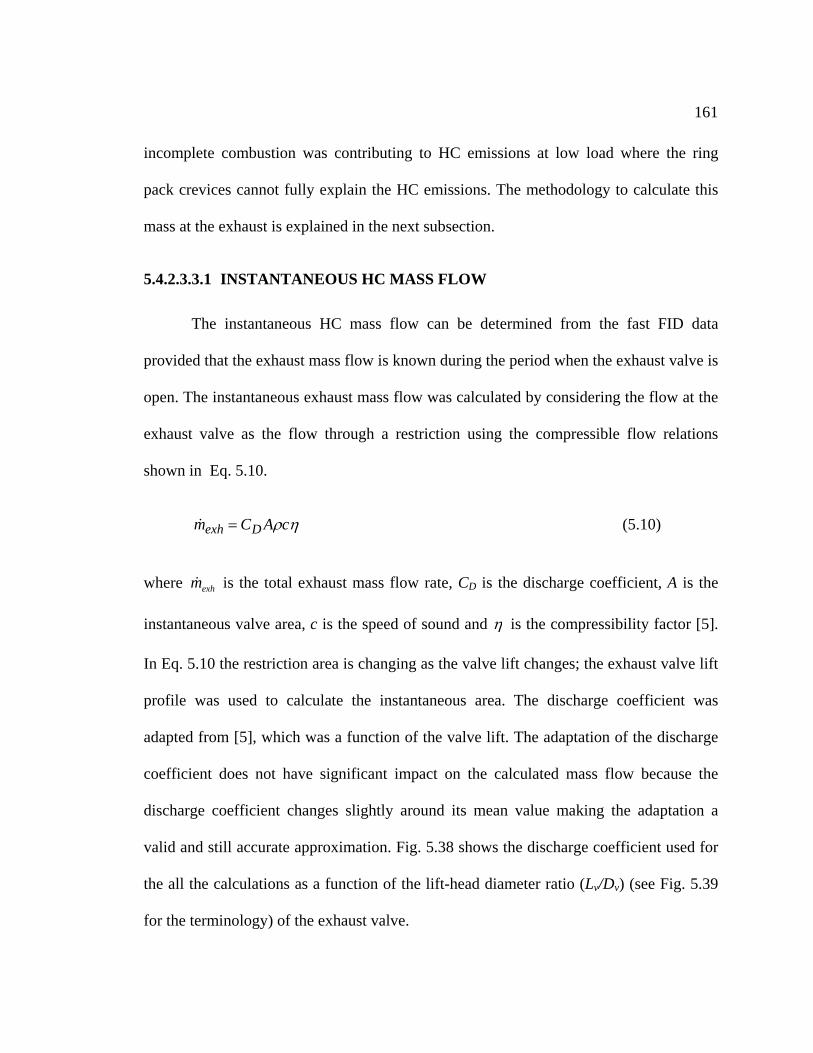
161
incomplete combustion was contributing to HC emissions at low load where the ring
pack crevices cannot fully explain the HC emissions. The methodology to calculate this
mass at the exhaust is explained in the next subsection.
5.4.2.3.3.1 INSTANTANEOUS HC MASS FLOW
The instantaneous HC mass flow can be determined from the fast FID data
provided that the exhaust mass flow is known during the period when the exhaust valve is
open. The instantaneous exhaust mass flow was calculated by considering the flow at the
exhaust valve as the flow through a restriction using the compressible flow relations
shown in Eq. 5.10.
ηρcACm Dexh =& (5.10)
here is the total exhaust mass flow rate, CD is the discharge coefficient, A is the
stantaneous valve area, c is the speed of sound and
exhm&w
in η is the compressibility factor [5].
Eq. 5.10 the restriction area is changing as the valve lift changes; the exhaust valve lift
rofile was used to calculate the instantaneous area. The discharge coefficient was
dapted from [5], which was a function of the valve lift. The adaptation of the discharge
oefficient does not have significant impact on the calculated mass flow because the
ischarge coefficient changes slightly around its mean value making the adaptation a
alid and still accurate approximation. Fig. 5.38 shows the discharge coefficient used for
e all the calculations as a function of the lift-head diameter ratio (Lv/Dv) (see Fig. 5.39
r the terminology) of the exhaust valve.
In
p
a
c
d
v
th
fo
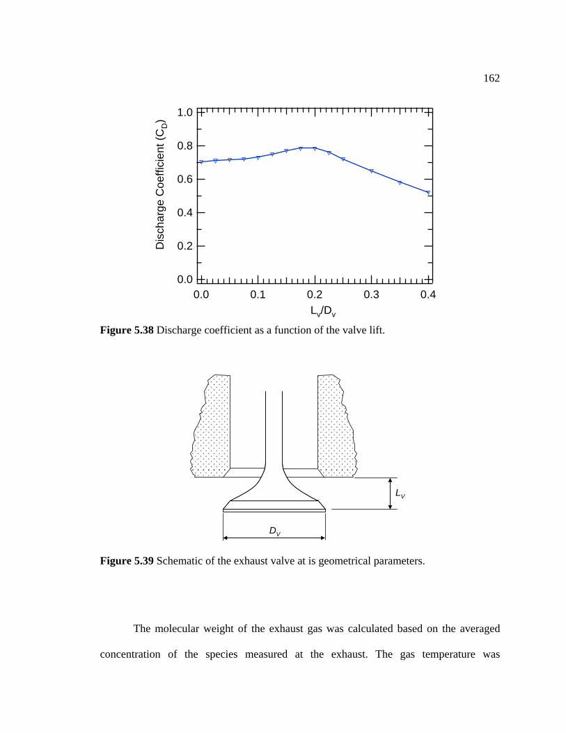
162
1.0
0.8
0.6
0.4
0.2
0.0
Dis
char
ge C
oeffi
cien
t (C
D)
0.40.30.20.10.0L /Dv v
igure 5.38 Discharge coefficient as a function of the valve lift. F
DV
LV
Figure 5.39 Schematic of the exhaust valve at is geometrical parameters.
The molecular weight of the exhaust gas was calculated based on the averaged
concentration of the species measured at the exhaust. The gas temperature was
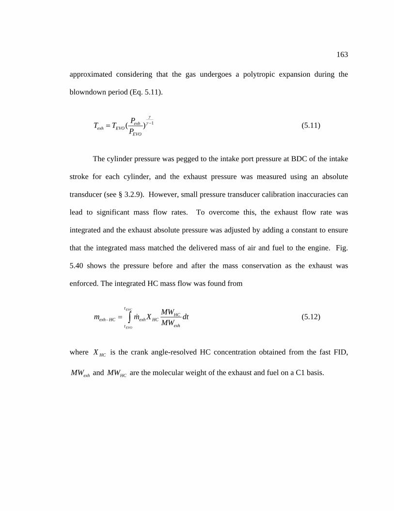
163
approximated considering that the gas undergoes a polytropic expansion during the
blowndown period (Eq. 5.11).
1)( −= γγ
EVO
exhEVOexh P
PTT (5.11)
The cylinder pressure was pegged to the intake port pressure at BDC of the intake
ke for each cylinder, and the exhaust pressure was measured using an absolute
lea To overcome this, the exhaust flow rate was
tegrated and the exhaust absolute pressure was adjusted by adding a constant to ensure
at the integrated mass matched the delivered mass of air and fuel to the engine. Fig.
as
enforce
stro
transducer (see § 3.2.9). However, small pressure transducer calibration inaccuracies can
d to significant mass flow rates.
in
th
5.40 shows the pressure before and after the mass conservation as the exhaust w
d. The integrated HC mass flow was found from
∫=−
EVC
EVO
t
t exh
HCHCexhHCexh dt
MWXmm & (5.12)
where HCX is the crank angle-resolved HC concentration obtained from the fast FID,
exhMW and HCMW are the molecular weight of the exhaust and fuel on a C1 basis.
MW
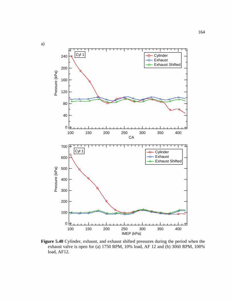
164
a)
240
200
160
120
80
40
0
Prss
ure
(kPa
)e
400350300250200150100CA
Cylinder Exhaust Exhaust Shifted
Cyl 1
700
600
500
400
300
200
100
0
Pres
sue
(kr
Pa)
400350300250200150100IMEP (kPa)
Cylinder Exhaust Exhaust Shifted
Cyl 1
exhaust valve is open for (a) 1750 RPM, 10% load, AF 12 and (b) 3060 RPM, 100%
Figure 5.40 Cylinder, exhaust, and exhaust shifted pressures during the period when the
load, AF12.
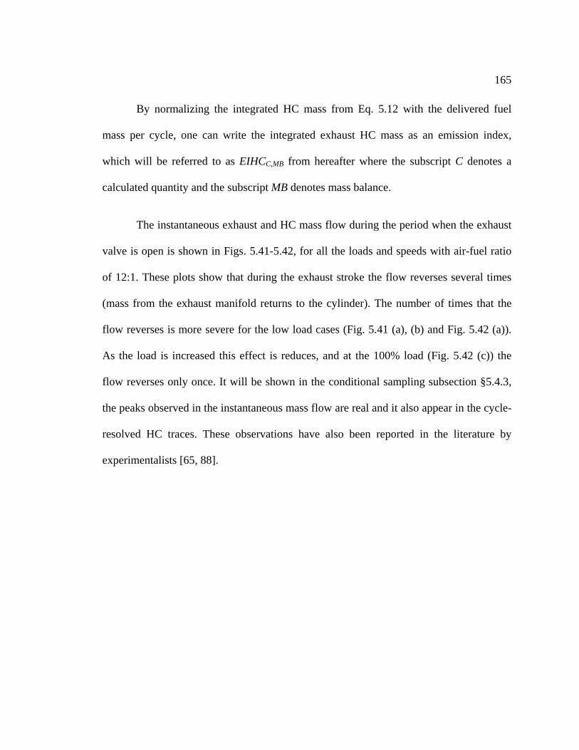
165
By normalizing the integrated HC mass from Eq. 5.12 with the delivered fuel
mass per cycle, one can write the integrated exhaust HC mass as an emission index,
which will be referred to as EIHCC,MB from hereafter where the subscript C denotes a
calculated quantity and the subscript MB denotes mass balance.
The instantaneous exhaust and HC mass flow during the period when the exhaust
valve is open is shown in Figs. 5.41-5.42, for all the loads and speeds with air-fuel ratio
of 12:1. These plots show that during the exhaust stroke the flow reverses several times
(mass f the exhaust manifold returns to the cylinder). The number of times that the
flow reverses is more severe for the low load cases (Fig. 5.41 (a), (b) and Fig. 5.42 (a)).
As the load is increased this effect is reduces, and at the 100% load (Fig. 5.42 (c)) the
reverses only once. It will be shown in the conditional sampling subsection §5.4.3,
the peaks observed in the instantaneous mass flow are real and it also appear in the cycle-
resolved HC traces. These observations have also been reported in the literature by
experimentalists [65, 88].
rom
flow
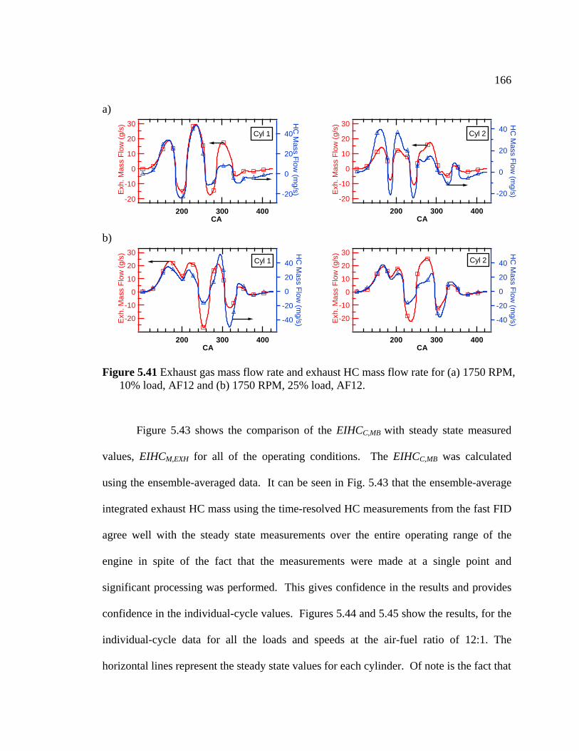
166
a) 30
20
10
0
-10
-20
Exh.
Mas
s Fl
ow (g
/s)
400300200CA
40
20
0
-20
HC
Mass Flow
(mg/s)
Cyl 1
30
20
10
0
-10
-20
Exh.
Mas
s Fl
ow (g
/s)
400300200CA
40
20
0
-20
HC
Mass Flow
(mg/s)
Cyl 2
b) 30
20
10
0
-10
-20Exh
. Mas
s Fl
ow (g
/
400300200CA
30s)
40
20
0
-20
-40
low (m
g/s)H
C M
ass F
Cyl 1 20
10
0
-10
-20Exh
. Mas
s Fl
ow (g
/400300200
CAs)
40
20
0
-20
-40
Mass Flow
(mg/s)
HCCyl 2
Figure 5.41 Exhaust gas mass flow rate and exhaust HC mass flow rate for (a) 1750 RPM, 10% load, AF12 and (b) 1750 RPM, 25% load, AF12.
Figure 5.43 shows the comparison of the EIHCC,MB with steady state measured
alues, EIHCM,EXH for all of the operating conditions. The EIHCC,MB was calculated
sing the ensemble-averaged data. It can be seen in Fig. 5.43 that the ensemble-average
grated exhaust HC mass using the time-re ed HC measurements from the fast FID
agree well with the steady state measurements over the entire operating range of the
engine in spite of the fact that the measurements were made at a single point and
significant processing was performed. This gives confidence in the results and provides
confidence in the individual-cycle values. Figures 5.44 and 5.45 show the results, for the
individual-cycle data for all the loads and speeds at the air-fuel ratio of 12:1. The
izontal lines represent the steady state values for each cylinder. Of note is the fact that
v
u
inte solv
hor
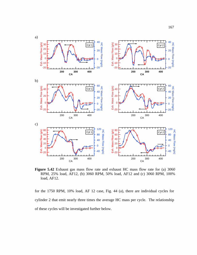
167
for 2 case, Fig. 44 (a), there are individual cycles for
inder 2 that emit nearly three times the av e HC mass per cycle. The relationship
of these cycles will be investigated further belo .
a)
the 1750 RPM, 10% load, AF 1
cyl erag
w
30
20
10
0
-10
-20
Exh.
Mas
s Fl
ow (
400300200CA
g/s) 40
20
0
-20
low (m
g/s)H
C M
ass F
Cyl 1 30
20
10
0
-10
-20
Exh.
Mas
s Fl
400300200CA
40
ow (g
/s)
20
0
-20
Mass Flow
(mg/s)
HC
Cyl 2
b)
40
20
0
-20Exh
. Mas
s Fl
ow (g
/s)
400300200CA
60
40
20
0
-20
HC
Mass Flow
(mg/s)
Cyl 1
40
20
0
-20Exh
. Mas
s Fl
ow (g
/s)
400300200CA
60
40
20
0
-20
HC
Mass Flow
(mg/s)
Cyl 2
c) 80
60
40
20
0
-20Exh
. Mas
s Fl
ow (g
/s)
400300200CA
120
80
40
0
-40
HC
Mass Flow
(mg/s)
Cyl 180
60
40
20
0
-20Exh
. Mas
s Fl
ow (g
/s)
400300200CA
120
80
40
0
-40
HC
Mass Flow
(mg/s)
Cyl 2
Figure 5.42 Exhaust gas mass flow rate and exhaust HC mass flow rate for (a) 3060 RPM, 25% load, AF12, (b) 3060 RPM, 50% load, AF12 and (c) 3060 RPM, 100% load, AF12.
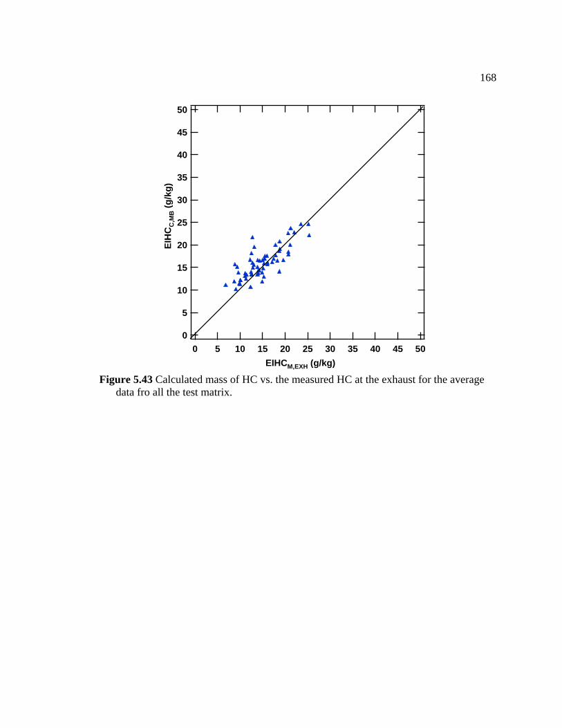
168
50
45
40
35
30
25
20
15
10
5
0
EIH
CC
,MB (g
/kg)
50454035302520151050EIHCM,EXH (g/kg)
igure 5.43 Calculated mass of HC vs. the measured HC at the exhaust for the average data fro all the test matrix.
F
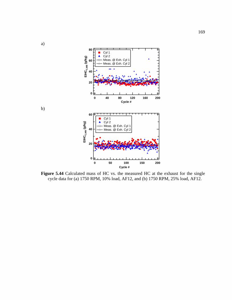
169
a) 80
60
40
20
0
EIH
CM
B (g
g)C
,/k
20016012080400Cycle #
Cyl 1 Cyl 2 Meas. @ Exh. Cyl 1 Meas. @ Exh. Cyl 2
b)
60
40
20
0
Cg/
kEI
HC
,MB (
g)
200150100500Cycle #
Cyl 1 Cyl 2 Meas. @ Exh. Cyl 1 Meas. @ Exh. Cyl 2
Figure 5.44 Calculated mass of HC vs. the measured HC at the exhaust for the single
cycle data for (a) 1750 RPM, 10% load, AF12, and (b) 1750 RPM, 25% load, AF12.
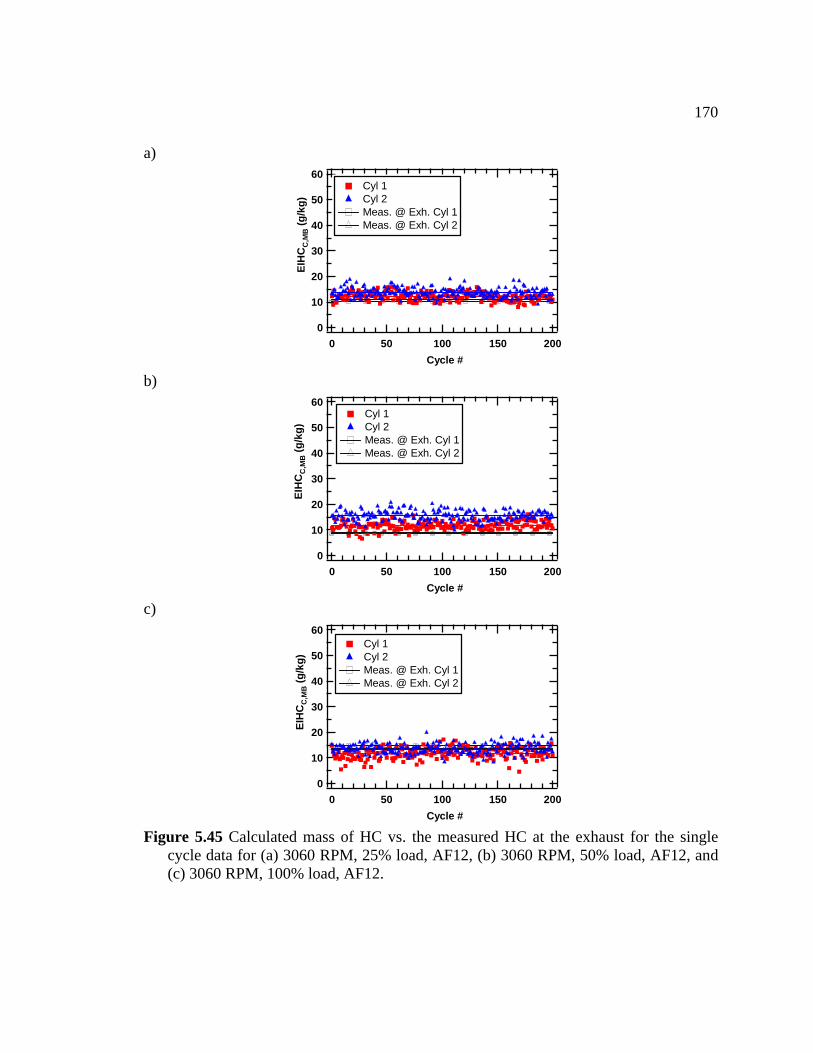
170
a) 60
50
40
30
20
10
0
EIH
CC
,MB (g
/kg)
200150100500Cycle #
Cyl 1 Cyl 2 Meas. h. Cyl 1@ Ex Meas. @ Exh. Cyl
b)
2
60
50
40
30
20
10
0
EIH
CC
,MB (g
/kg)
200150100500Cycle #
Cyl 1 Cyl 2 Meas. h. Cyl 1 @ Ex Meas. h. Cyl 2
)
@ Ex
c60
50
40
30
20
10
0
EIH
CC
,MB (g
/kg)
200150100500Cycle #
Cyl 1 Cyl 2 Meas. @ Exh. Cyl 1 Meas. @ Exh. Cyl 2
Figure 5.45 Calculated mass of HC vs. the measured HC at the exhaust for the single
cycle data for (a) 3060 RPM, 25% load, AF12, (b) 3060 RPM, 50% load, AF12, and (c) 3060 RPM, 100% load, AF12.
171
5.4.2.3.3.2 COMBUSTION PHASING AND MASS OF HC AT THE EXHAUST
Combustion phasing, usually CA50, is a good indicator the combustion
performance. In the present discussion of incomplete combustion, however, the timing of
the end of combustion, e.g. CA90, is a more appropriate metric. Figures 5.46 to 5.50
show the comparison of the integrate exhaust HC mass with CA90 on a cycle-by-cycle
basis. For the 1750 RPM, 10% load case, Fig. 5.46, there is a correlation between CA90
ore visible. The correlation is relatively weak, but still exists, for cycles with early
A90, i.e. cycles with late heat release tend to have higher levels of EIHCC,MB. It is
portant to note that there is a direct correlation between highly emitting cycles and
ery late heat release – all cycles having more than twice the integrated exhaust HC mass
ave CA90 effectively at EVO. This effect is stronger for the air-fuel ratio 14:1 (Fig. 5.46
)) and for cylinder 2, which is in agreement with the concentration results of Fig. 5.33,
ut because these data take into accounts the mass flow rate variations they are a better
dicator that incomplete combustion is a significant contributor to HC emissions. As the
d is increased (Fig. 5.47) the combustion phasing is advanced. Thus, for the 1750
RPM, 25% load, AF12 and AF13 (Fig. 5.47 (a)-(b)) all the cycles finish combustion prior
EVO. However, for the 1750 RPM, 25% load, AF14 (Fig. 5.47 (c)) there are few cycles
that do not complete heat release prior EVO. At this load the correlation between
EIHCC,MB and CA90 is weaker than for the 10% load case but still exists. Cylinder 2 still
shows more contribution to incomplete combustion.
and the integrated exhaust HC mass. As the air fuel ratio is increased this correlation is
m
C
im
v
h
(c
b
in
loa
172
If the speed is increased as for the 3060 RPM, 25% load case, Fig. 5.48, all the
IHCC,MB and CA90 is still observed, more pronounced in the case of cylinder 2. A
rther increase in load at this speed, Fig. 5.49 and 5.50, shows that all the cycles
omplete energy release relatively early, prior to EVO. For these conditions, there is not a
lear correlation between CA90 and the integrated exhaust HC mass and there are not
ycles with excessive HC emissions levels.
Overall, the observations above are in agreement with both the single-cycle heat
lease and the concentration-based results. This suggests that at low load the incomplete
ombustion could be the source of the high HC levels. To support the weak observations
the statistical analysis described in §5.4.2.3.2 was applied, and the results are shown in
Table 5.8. Again, the two statistical metrics support the observations that at low load the
high levels of HC emissions correlate well with the combustion phasing suggesting that
at these conditions the incomplete combustion is the main source of HC emissions.
cycles complete combustion prior EVO. Nevertheless, a slight correlation between
E
fu
c
c
c
re
c
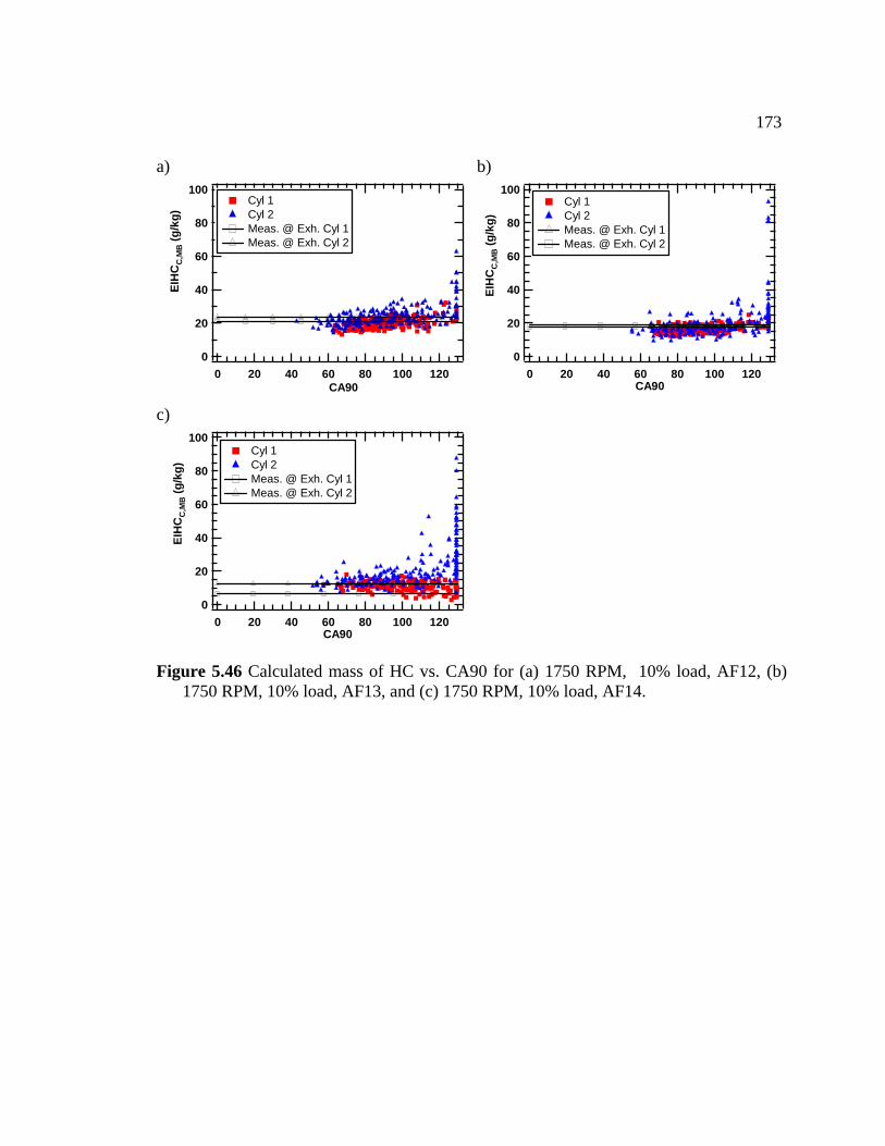
173
a) 100
80
60
40
20
0
EIH
CC
,MB (g
/kg)
120100806040200CA90
Cyl 1 Cyl 2 Meas. @ Exh. Cyl 1 Meas. @ Exh. Cyl 2
b) 100
80
60
40
20
0
EIH
CC
,MB (g
/kg)
120100806040200CA90
Cyl 1 Cyl 2 Meas. @ Exh. Cyl 1 Meas. @ Exh. Cyl 2
c) 100
80
60
40
20
0
EIH
CC
,MB (g
/kg)
120100806040200CA90
Cyl 1 Cyl 2 Meas. @ Exh. Cyl 1 Meas. @ Exh. Cyl 2
Figure 5.46 Calculated mass of HC vs. CA90 for (a) 1750 RPM, 10% load, AF12, (b) 1750 RPM, 10% load, AF13, and (c) 1750 RPM, 10% load, AF14.
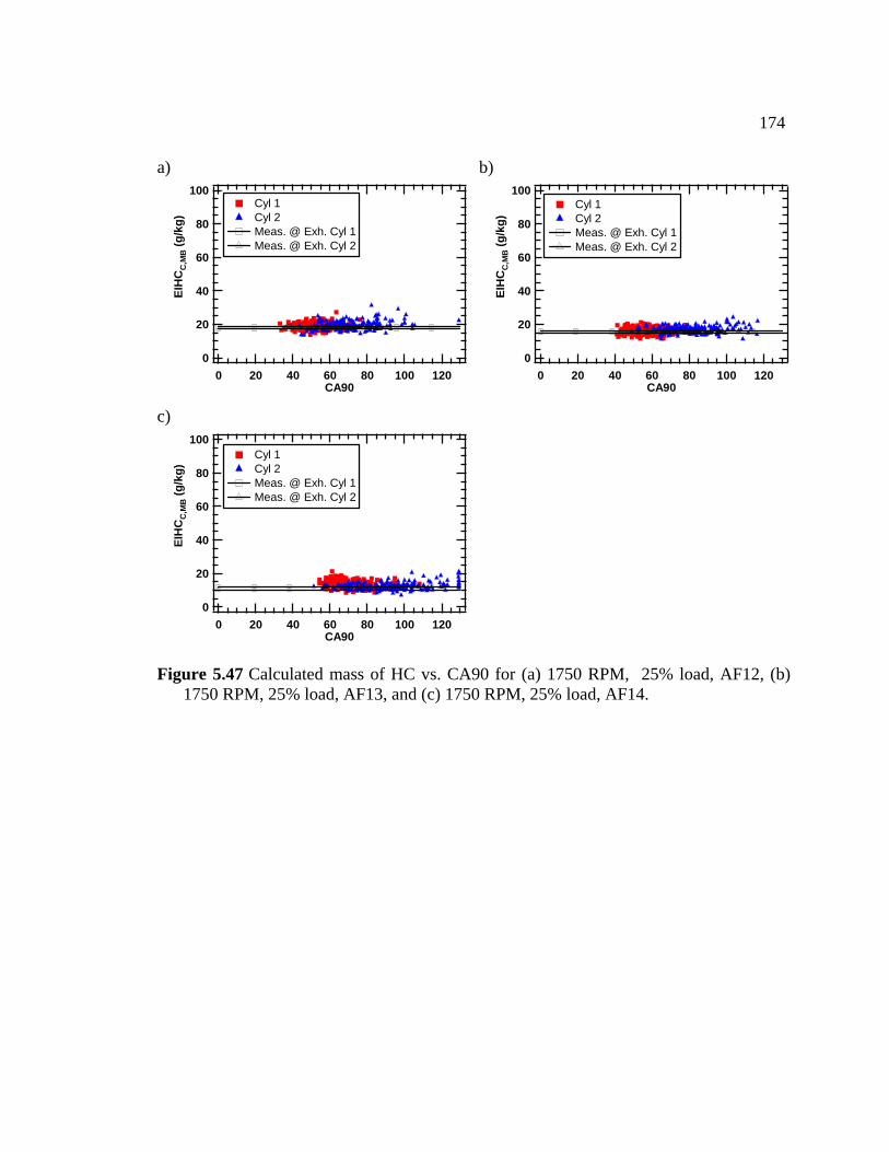
174
a) 100
80
60
40
20
0
EIH
CM
B (g
g)C
,/k
120100806040200CA90
Cyl 1 Cyl 2 Meas. @ Exh. Cyl 1 Meas. @ Exh. Cyl 2
b) 100
80
60
40
20
0
EIH
CM
B (g
g)C
,/k
120100806040200CA90
Cyl 1 Cyl 2 Meas. @ Exh. Cyl 1 Meas. @ Exh. Cyl 2
c) 100
80
60
40
20
0
MB
)
120100806040200CA90
Cyl 1 Cyl 2 Meas. @ Exh. Cyl 1 Meas. @ Exh. Cyl 2
EIH
CC
, (g
/kg
Figure 12, (b) 1750 RP
5.47 Calculated mass of HC vs. CA90 for (a) 1750 RPM, 25% load, AFM, 25% load, AF13, and (c) 1750 RPM, 25% load, AF14.
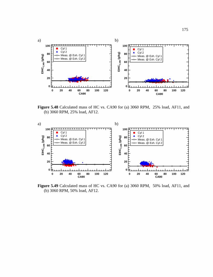
175
a) 100
80
60
40
20
0
EIH
CC
,MB (g
/kg)
120100806040200CA90
Cyl 1 Cyl 2 Meas. @ Exh. Cyl 1 Meas. @ Exh. Cyl 2
b) 100
80
60
40
20
0
EIH
CC
,MB (g
/kg)
120100806040200CA90
Cyl 1 Cyl 2 Meas. @ Exh. C 1yl Meas. @ E 2
Calculated mass of HC vs. CA90 for (a) 3060 RPM, 25% load, AF11, and (b) 3060 RPM, 25% load, AF12.
a)
xh. Cyl
Figure 5.48
100
80
60
40
20
0
EIH
CC
,MB (g
/kg)
120100806040200CA90
Cyl 1 Cyl 2 Meas. @ Exh. Cyl 1 Meas. @ Exh. Cyl 2
b) 100
80
60
40
20
0
EIH
CC
,MB (g
/kg)
120100806040200CA90
Cyl 1 Cyl 2 Meas. @ Exh. Cyl 1 Meas. @ Exh. Cyl 2
Figure 5.49 Calculated mass of HC vs. CA90 for (a) 3060 RPM, 50% load, AF11, and (b) 3060 RPM, 50% load, AF12.
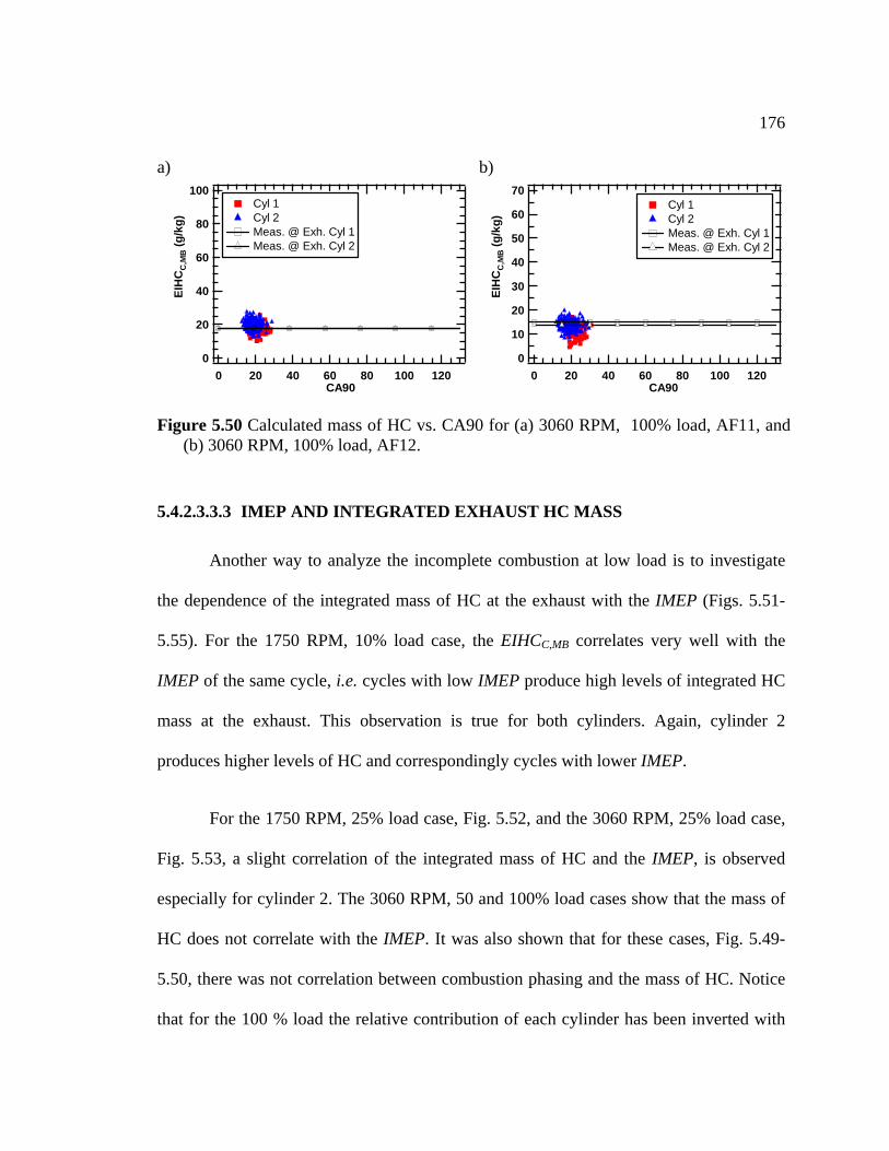
176
a) 100
80
60
40
20
0
EIH
CC
,MB (g
/kg)
120100806040200CA90
Cyl 1 Cyl 2 Meas. @ Exh. Cyl 1 Meas. @ Exh. Cyl 2
b) 70
60
50
40
30
20
10
0
EIH
CC
,MB (g
/kg)
120100806040200CA90
Cyl 1 Cyl 2 Meas. @ Exh. Cyl 1 Meas. @ Exh. Cyl 2
Figure 5.50 Calculated mass of HC vs. CA90 for (a) 3060 RPM, 100% load, AF11, and (b) 3060 RPM, 100% load, AF12.
5.4.2.3.3.3 IMEP AND INTEGRATED EXHAUST HC MASS
Another way to analyze the incomplete combustion at low load is to investigate
the dependence of the integrated mass of HC at the exhaust with the IMEP (Figs. 5.51-
5.55). For the 1750 RPM, 10% load case, the EIHCC,MB correlates very well with the
mas ation is true for both cylinders. Again, cylinder 2
produces higher levels of HC and correspondingly cycles with lower IMEP.
For the 1750 RPM, 25% load case, Fig. 5.52, and the 3060 RPM, 25% load case,
Fig. 5.5
IMEP of the same cycle, i.e. cycles with low IMEP produce high levels of integrated HC
s at the exhaust. This observ
3, a slight correlation of the integrated mass of HC and the IMEP, is observed
especially for cylinder 2. The 3060 RPM, 50 and 100% load cases show that the mass of
HC does not correlate with the IMEP. It was also shown that for these cases, Fig. 5.49-
5.50, there was not correlation between combustion phasing and the mass of HC. Notice
that for the 100 % load the relative contribution of each cylinder has been inverted with
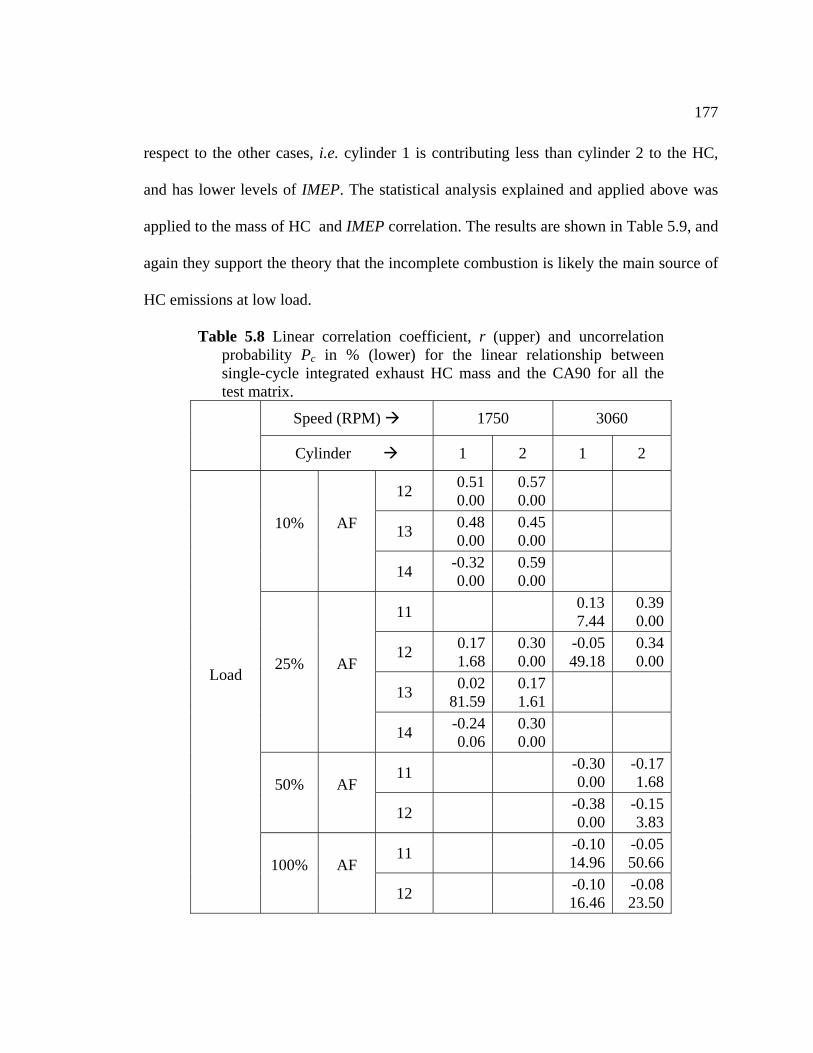
177
respect to the other cases, i.e. cylinder 1 is contributing less than cylinder 2 to the HC,
and has lower levels of IMEP. The statistical analysis explained and applied above was
applied to the mass of HC and IMEP correlation. The results are shown in Table 5.9, and
again they support the theory that the incomplete combustion is likely the main source of
HC emissions at low load.
Speed (RPM) 1750 3060
Table 5.8 Linear correlation coefficient, r (upper) and uncorrelation probability Pc in % (lower) for the linear relationship between single-cycle integrated exhaust HC mass and the CA90 for all the test matrix.
Cylinder 1 2 1 2
12 0.51 0.00
0.570.00
13 0.00 0.00 0.48 0.4510% AF
-0.32 0.5914 0.00 0.00
11 7.44 0.000.13 0.39
12 0.171.68
0.300.00
-0.05 49.18
0.340.00
13 0.0281.59
0.171.61
25% AF
14 -0.24 0.30 0.06 0.00
11 -0.30 -0.170.00 1.6850% AF
0.00 3.8312 -0.38 -0.15
11 -0.10 14.96
-0.0550.66
Load
12
100% AF -0.10 16.46
-0.0823.50
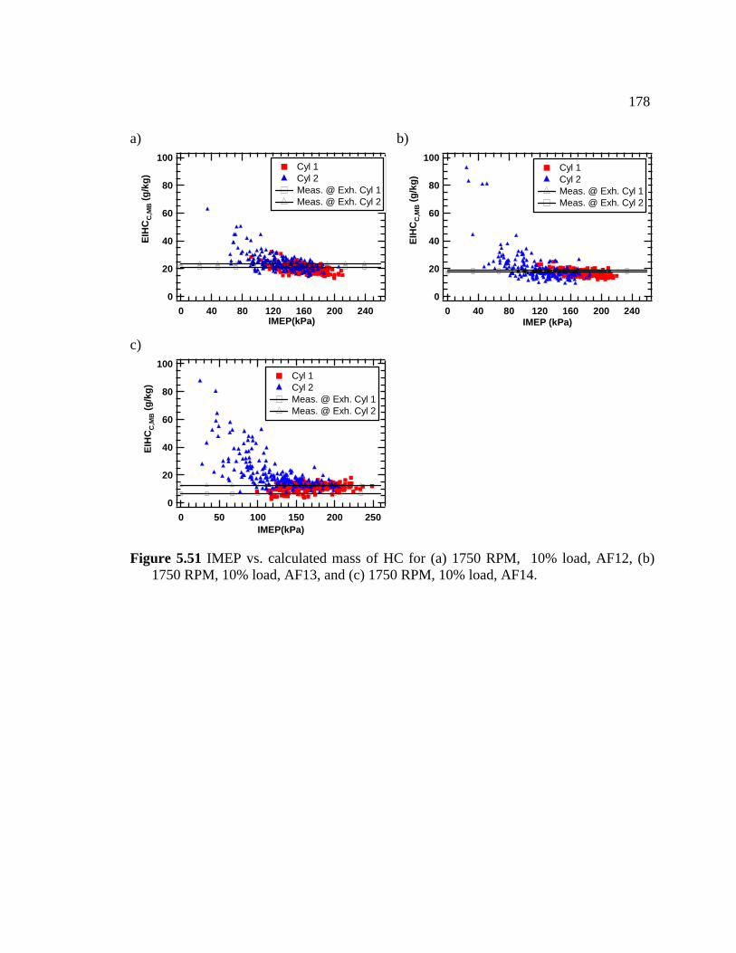
178
a) 100
80
60
40
20
0
EIH
MB (g
g)C
C,
/k
24020016012080400IMEP(kPa)
Cyl 1 Cyl 2 Meas. @ Exh. Cyl 1 Meas. @ Exh. Cyl 2
b) 100
80
60
40
20
0
EIH
CM
B (g
)C
,/k
g
24020016012080400IMEP (kPa)
Cyl 1 Cyl 2 Meas. @ Exh. Cyl 1 Meas. @ Exh. Cyl 2
c) 100
80
60
40
20
0
MB
g)
250200150100500IMEP(kPa)
Cyl 1 Cyl 2 Meas. @ Exh. Cyl 1 Meas. @ Exh. Cyl 2
EIH
CC
, (g
/k
Figure 5.51 IMEP vs. calculated mass of HC for (a) 1750 RPM, 10% load, AF12, (b) 1750 RPM, 10% load, AF13, and (c) 1750 RPM, 10% load, AF14.
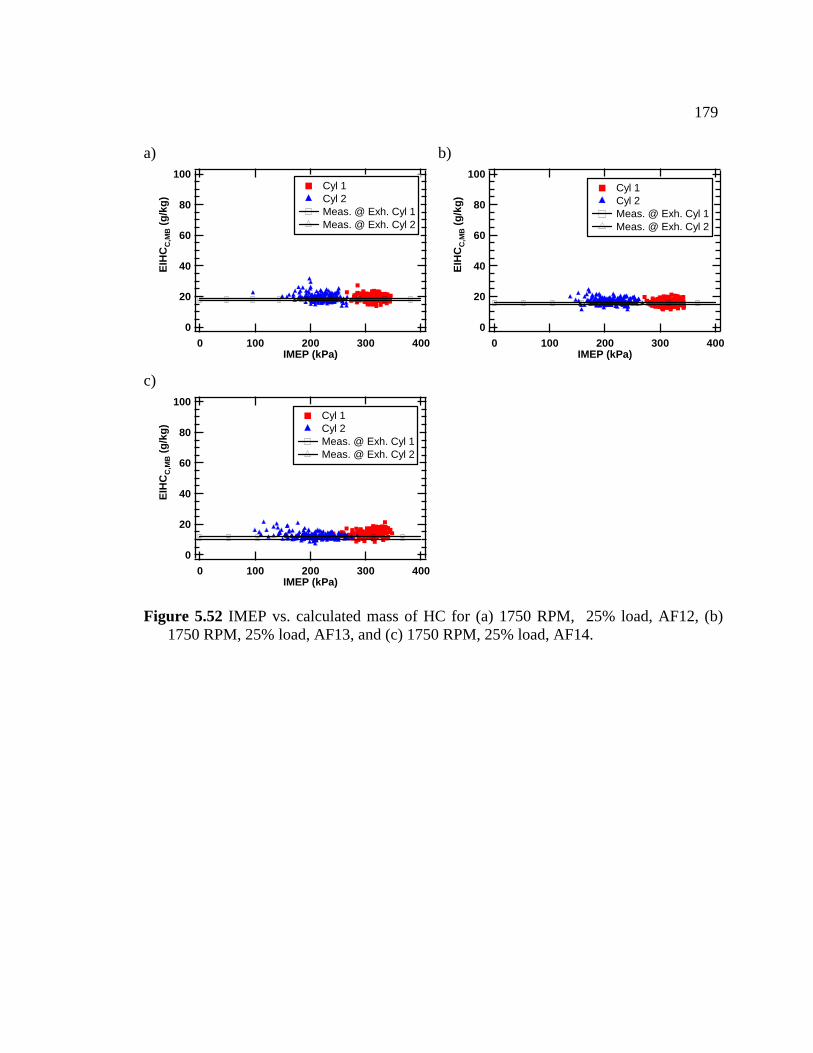
179
a) 100
80
60
40
20
0
EIH
CC
,MB (g
/kg)
4003002001000IMEP (kPa)
Cyl 1 Cyl 2 Meas. @ Exh. Cyl 1 Meas. @ Exh. Cyl 2
b) 100
80
60
40
20
0
EIH
CC
,MB (g
/kg)
4003002001000IMEP (kPa)
Cyl 1 Cyl 2 Meas. @ Exh. Cyl 1 Meas. @ Exh. Cyl 2
c) 100
80
60
40
20
0
EIH
CC
,MB (g
/kg)
4003002001000IMEP (kPa)
Cyl 1 Cyl 2 Meas. @ Exh. Cyl 1 Meas. @ Exh. Cyl 2
Figure 5.52 IMEP vs. calculated mass of HC for (a) 1750 RPM, 25% load, AF12, (b) 1750 RPM, 25% load, AF13, and (c) 1750 RPM, 25% load, AF14.
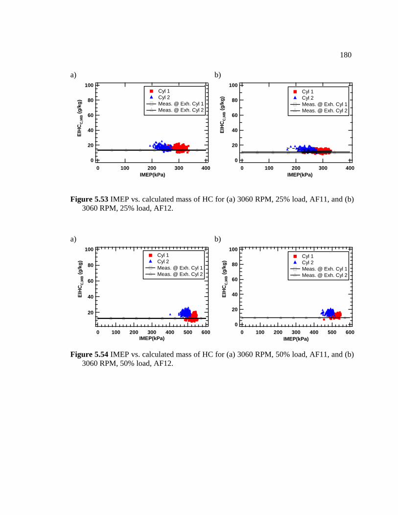
180
a) 100
80
60
40
20
0
EIH
CC
,MB (g
/kg)
4003002001000IMEP(kPa)
Cyl 1 Cyl 2 Meas. @ Exh. Cyl 1 Meas. @ Exh. Cyl 2
b) 100
80
60
40
20
0
EIH
CC
,MB (g
/kg)
4003002001000IMEP(kPa)
Cyl 1 Cyl 2 Meas. @ Exh. Cyl 1 Meas. @ Exh. Cyl 2
Figure 5.53 IMEP vs. calculated mass of HC for (a) 3060 RPM, 25% load, AF11, and (b) 3060 RPM, 25% load, AF12.
a)
100
80
60
40
20
EIH
CC
,MB (g
/kg)
6005004003002001000IMEP(kPa)
Cyl 1 Cyl 2 Meas. @ Exh. Cyl 1 Meas. @ Exh. Cyl 2
b) 100
80
60
40
20
0
C,M
B (g
/kg)
EIH
C
6005004003002001000IMEP(kPa)
Cyl 1 Cyl 2 Meas. @ Exh. Cyl 1 Meas. @ Exh. Cyl 2
F11, and (b) 3060 RPM, 50% load, AF12.
Figure 5.54 IMEP vs. calculated mass of HC for (a) 3060 RPM, 50% load, A
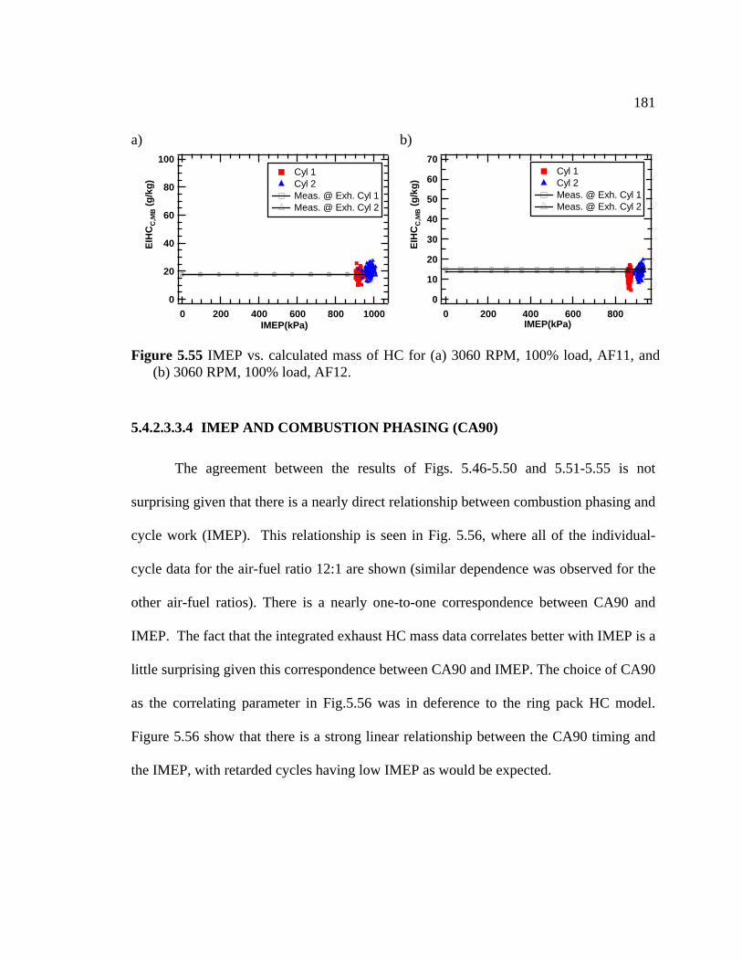
181
a) 100
80
60
40
20
0
EIH
CC
,MB (g
/g)k
10008006004002000IMEP(kPa)
Cyl 1 Cyl 2 Meas. @ Exh. Cyl 1 Meas. @ Exh. Cyl 2
b) 70
60
50
40
30
20
10
0
EIH
CC
,MB (g
/g)k
8006004002000IMEP(kPa)
Cyl 1 Cyl 2 Meas. @ Exh. Cyl 1 Meas. @ Exh. Cyl 2
Figure 5.55 IMEP vs. calculated mass of HC for (a) 3060 RPM, 100% load, AF11, and (b) 3060 RPM, 100% load, AF12.
5.4.2.3.3.4 IMEP AND COMBUSTION PHASING (CA90)
The agreement between the results of Figs. 5.46-5.50 and 5.51-5.55 is not
surprising given that there is a nearly direct relationship between combustion phasing and
cycle work (IMEP). This relationship is seen in Fig. 5.56, where all of the individual-
cycle data for the air-fuel ratio 12:1 are shown (similar dependence was observed for the
other air-fuel ratios). There is a nearly one-to-one correspondence between CA90 and
IMEP. The fact that the integrated exhaust HC mass data correlates better with IMEP is a
little surprising given this correspondence between CA90 and IMEP. The choice of CA90
as the correlating parameter in Fig.5.56 was in deference to the ring pack HC model.
Figure 5.56 show that there is a strong linear relationship between the CA90 timing and
the IMEP, with retarded cycles having low IMEP as would be expected.
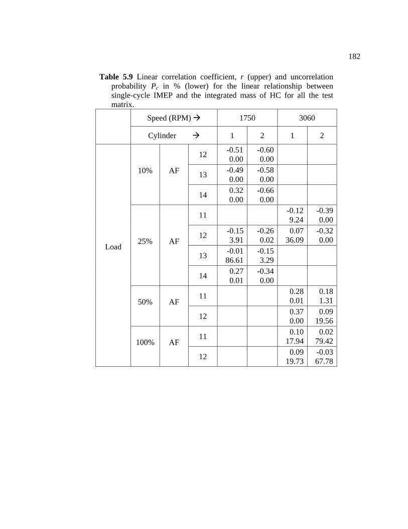
182
Table 5.9 Linear correlation coefficient, r (upper) and uncorrelation
single-cycle IMEP and the integrated mass of HC for all the test
Speed (RPM)
probability Pc in % (lower) for the linear relationship between
matrix.
1750 3060 Cylinder 1 2 1 2
12 0.00 0.00 -0.51 -0.60
13 -0.49 0.00
-0.580.00 10% AF
14 0.32 0.00
-0.660.00
11 -0.12 9.24
-0.390.00
12 -0.15 -0.26 0.07 -0.323.91 0.02 36.09 0.00
13 -0.01 -0.15 86.61 3.29
25% AF
0.01 0.0014 0.27 -0.34
11 0.28 0.01
0.181.3150% AF
0.37 0.00
0.0919.5612
11 17.94 79.420.10 0.02
Load
100% AF
12 0.09 19.73
-0.0367.78
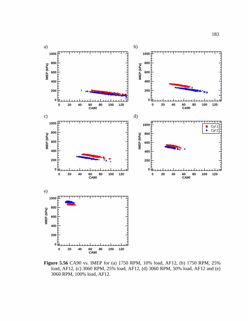
183
a) 1000
800
600
400
200
0
IMEP
(kPa
)
120100806040200CA90
b) 1000
800
600
400
200
0
IMEP
(kPa
)
120100806040200CA90
c) d) 1000
800
600
400
200
0
IMEP
(kPa
)
120100806040200CA90
1000
800
600
400
200
0
IMEP
(kPa
)
120100806040200CA90
Cyl 1 Cyl 2
e) 1000
800
600
400
200
0
MPa
)
120100806040200CA90
EP (k
I
Figure 5.56 CA90 vs. IMEP for (a) 1750 RPM, 10% load, AF12, (b) 1750 RPM, 25% load, AF12, (c) 3060 RPM, 25% load, AF12, (d) 3060 RPM, 50% load, AF12 and (e) 3060 RPM, 100% load, AF12.
184
5.4.3 CONDITIONAL SAMPLING ANALYSIS
In order to further investigate the role of the ring pack on HC emissions,
conditional sampling was performed by dividing the cycles into five groups (0-20%, 20-
40%, 40-60%, 60-80% and 80-100%) according to their combustion phasing. The
combustion phasing investigated was the CA90 time, and the assignment into groups was
made based on where an individual cycle fell in the CA90max - CA90min range; it was
based on an ordina ranking. Thus, the 0- % group represents the fastest cycles and
those in the 80-100% group are the cycles having the most retarded combustion phasing.
It is not a requirement to have the same number of cycles in all groups.
5.4.3.1 HEAT RELEASE - CONDITIONAL SAMPLING ANALYSIS
Figure 5.57 shows the average heat release of each of the five groups for all the
conditions of the test matrix with air-fuel ratio of 12:1. For the 1750 RPM, 10% load
57 (a), the cycles in the 0-20% group release all their energy before EVO; the
cycles in the 20-40% range of CA90 also show that on average combustion completes
before EVO (This group represents the largest percentage of the analyzed cycles). The
remaining sets of cycles (40-60%, 60-80%, and 80-100%) exhibit heat release that
extends beyond EVO. For these cycles, incomplete combustion is expected to contribute
to the HC emissions, while the 0-20% and 20-40% cycles may not have an HC
contribution from incomplete combustion. As the load is increased to 25%, Fig. 5.57 (b),
in t
r cylinder 2 there are still some groups that show incomplete combustion. The number
not l 20
case, Fig. 5.
he case of cylinder 1 all the groups show complete combustion prior EVO. However,
fo
185
of groups contributing to in complete combustion has been reduced, thus the 40-60%
group which finished combustion after EVO at 10% load, for the 25% load shows that
comple
omplete
combus
tes combustion prior EVO. However, the remaining groups, 60-80% and 80-
100%, show incomplete combustion. The 80-100% fraction shows similar profile of heat
release than the same group for the 10% load (Fig. 5.57 (a)). This indicates that at this
condition there are some cycles that may be contributing to the HC emissions due to
incomplete combustion.
At the 3060 RPM, 25% load condition, Fig. 5.58 (a), the majority of the cycles
complete combustion before EVO (0-20%, 20-40%, 40-60%, and 60-80%). However, the
80-100% group of cycles shows late combustion, suggesting that for this condition this
subgroup of cycles may have incomplete combustion. This shows that although on
average the ring pack is the main contributor to the HC emissions, there may be some
cycles where the incomplete combustion is present and adversely affecting HC emissions.
As the load is increased, as for the 50 and 100% load conditions, Fig. 5.58(b)-(c), none of
the groups shows late combustion phasing. For these conditions it is clear that inc
tion is not a significant contributor to the engine-out HC emissions, suggesting
that the ring pack crevices are the major source of engine-out HC emissions. Similar
results were observed for the other air-fuel ratios of the test matrix.
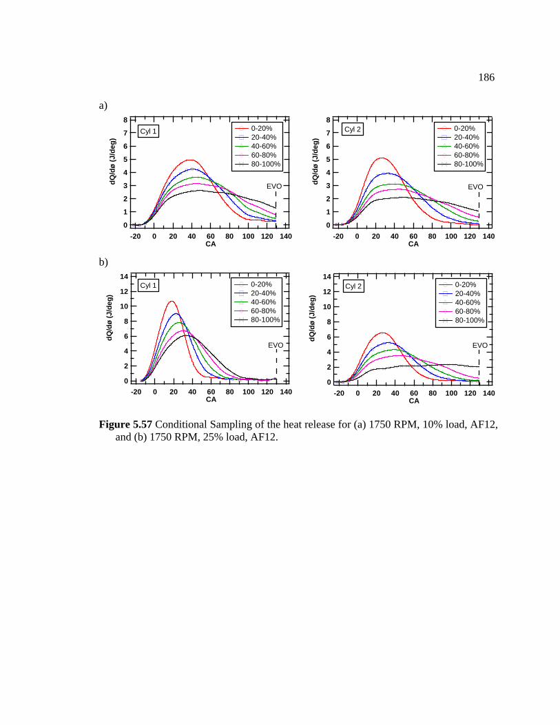
186
a) 8
7
6
5
4
3
2
1
0
/dø
(g
dQJ/
de)
140120100806040200-20CA
EVO
Cyl 1 0-20% 20-40% 40-60% 60-80% 80-100%
8
7
6
5
4
3
2
1
0
dQ/d
ø (
gJ/
de)
140120100806040200-20CA
EVO
Cyl 2 0-20% 20-40% 40-60% 60-80% 80-100%
b) 14
12
10
8
6
4
2
0
/e
dQdø
(J/d
g)
140120100806040200-20CA
EVO
Cyl 1 0-20% 20-40% 40-60% 60-80% 80-100%
14
12
10
8
6
4
2
0
/de
dQ/d
ø (J
g)
140120100806040200-20CA
EVO
Cyl 2 0-20% 20-40% 40-60% 60-80% 80-100%
Figure 5.57 Conditional Sampling of the heat release for (a) 1750 RPM, 10% load, AF12, and (b) 1750 RPM, 25% load, AF12.
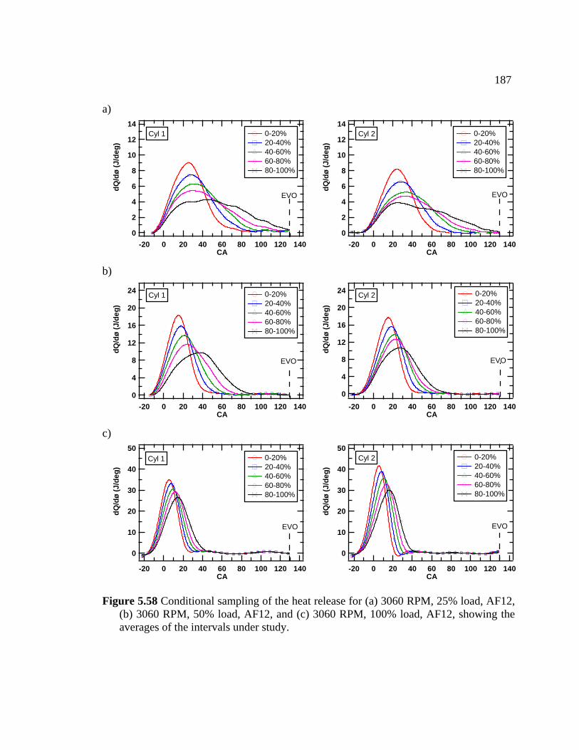
187
a) 14
12
10
8
6
4
2
0
dQ/d
eg
140120100806040200-20CA
EVO
14/d
ø (J
)
Cyl 1 0-20% 20-40% 40-60% 60-80% 80-100%
12
10
8
6
4
2
0
dQ/d
ø (J
/deg
140120100806040200-20CA
EVO
Cyl 2
)
0-20% 20-40% 40-60% 60-80% 80-100%
b) 24
20
16
12
8
4
0
dQ/d
ø (J
/deg
)
140120100806040200-20CA
EVO
Cyl 1 0-20% 20-40% 40-60% 60-80% 80-100%
24
20
16
12
8
4
0
dQ/d
ø (J
/deg
)
140120100806040200-20CA
EVO
Cyl 2 0-20% 20-40% 40-60% 60-80% 80-100%
c) 50
40
30
20
10
0
(J/d
eg)
140120100806040200-20CA
EVO
0-20% 20-40% 40-60% 60-80%
Cyl 1
50
40
30
dQ/d
ø 80-100%
20
10
0
(J/d
eg)
140120100806040200-20CA
EVO
0-20% 20-40% 40-60% 60-80% 80-100%
dQ/d
ø
Cyl 2
Figure 5.58 Conditional sampling of the heat release for (a) 3060 RPM, 25% load, AF12, (b) 3060 RPM, 50% load, AF12, and (c) 3060 RPM, 100% load, AF12, showing the averages of the intervals under study.
188
5.4.3.2 RING PACK CONTRIBUTION-CONDITIONAL SAMPLING
ANALYSIS
The use of conditional sampling has identified sub-groups within the ensemble of
cycles that may fall into different emission regimes. This is further investigated using
single-cycle results from the ring pack model and the integrated exhaust HC mass.
Figures 5.59-5.60 shows the conditionally sampled results of the EIHCC,RP on the vertical
and the EIHCC,MB on the horizontal axis, where the symbol color identifies the sub-
group. The circular symbol on the 45° line that has vertical and horizontal cross-hairs
through it represents the steady state emission value. Cycles above the horizontal cross-
hair are expected to have HC emissions largely dominated by the ring pack mechanism.
Beginning with the 3060 RPM, 100% load condition, Fig. 5.60 (c), one can see that all of
the cycles from each of the sub-groups greatly exceed both the steady state emission
ue as well as the corresponding single- cle integrated exhaust HC mass. This
confirms that for all of these cycles the previous result that the ring pack dominates the
HC emissions remains valid. Similar behavior is observed for the 3060 RPM, 50% load
case, Fig. 5.60 (b).
The 1750 RPM, 10% load case, Fig. 5.59 (a), also gives results that are consistent
with the previous discussion (§5.4.3.1). Consider the EIHCC,RP using the CA90-EVC
EIH C,RP
the EIHCC,MB for almost all of the cycles. Both of these results strongly suggest that the
axis
val cy
integration period. For all of the cycles in all of the subgroups for both cylinders, the
CC,RP is less than the steady-state emission value. Further, the EIHC is less than
189
ring pack, while contributing to the HC emissions, does not dominate the HC emissions
t this condition. The wide spread in the EIHCC,MB for the 80-100% group indicates that
there a
The 3060 RPM, 25% load condition conditionally sampled results, Fig. 5.60 (a),
give indication that the different sub-groups may fall into different emission regimes.
Consider again the EIHCC,RP results using the CA90-EVC integration period. For both
cylinders, the late combustion cycles – 60-80% and 80-100% – have EIHCC,RP less than
the steady state emission level. It is likely that some level of post-oxidation does occur
for these conditions, so the fact that these cycles emit an amount of HC that is even close
sources of HC contributing to the exhaust measurement. These late-burning cycles also
have an EIHCC,MB that is higher than the EIHCC,RP, which supports the notion that there
are other sources of HC besides the ring pack that are contributing significantly to the HC
emissions. As seen in Fig. 5.60 (a), the 80-100% group has a heat release that extends to
a
re individual cycles that are contributing excess HC. As seen in Figs. 5.46 and
5.51, these cycles are correlated with late-burning, low work-producing cycles, and thus,
incomplete combustion in the cylinder. For the 1750 RPM, 25% load case, Fig. 5.59 (b),
shows that for cylinder 1 about half of the total number of cycles do not exhibit emissions
that are ring-pack dominated. However, for cylinder 2, the majority of the cycles show
that EIHCC,RP is less than the EIHCC,MB, although the horizontal spreading for the group
of cycles with very late combustion (60-80% and 80-100%) has been reduced. The results
suggest that for this condition the HC emissions may be highly dominated by the
incomplete combustion, especially for cylinder 2.
to, let alone less than, the steady state exhaust value strongly suggests that there are other
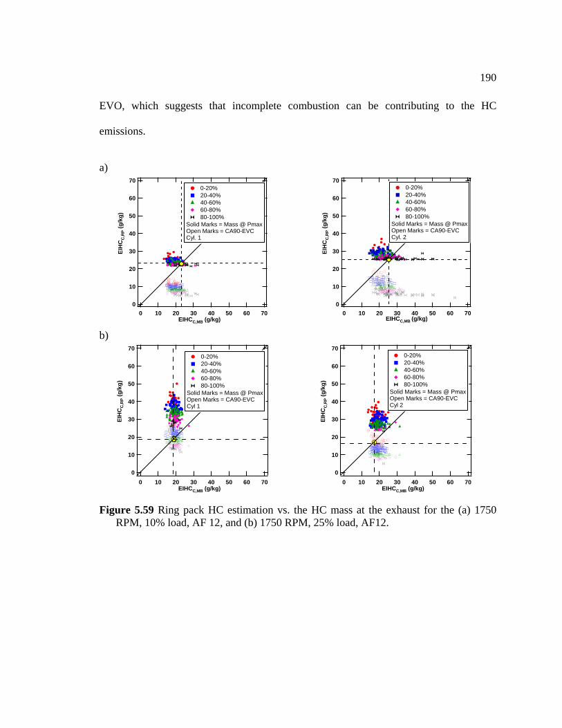
190
EVO, which suggests that incomplete combustion can be contributing to the HC
emissions.
a) 70
60
50
40
30
20
10
0
EIC
,RP
(gg)
HC
/k
706050403020100EIHCC,MB (g/kg)
0-20% 20-40% 40-60% 60-80% 80-100%
70
60
50
40
30
Solid Marks = Mass @ PmaxOpen Marks = CA90-EVCCyl. 1
20
10
0
EIC
,RP
(gg)
HC
/k
706050403020100EIHCC,MB (g/kg)
0-20% 20-40% 40-60% 60-80% 80-100%
Solid Marks = Mass @ PmaxOpen Marks = CA90-EVCCyl. 2
b)
70
60
50
40
30
20
10
0
EIH
CC
,RP
(
706050403020100EIHCC,MB (g/kg)
g/kg
)
0-20% 20-40% 40-60% 60-80% 80-100%
Solid Marks = Mass @ Pmax
70
60
50
Open Marks = CA90-EVCCyl 1
40
30
20
10
0
EIH
CC
,RP
(
706050403020100EIHCC,MB (g/kg)
0-20% 20-40%
g/kg
)
40-60% 60-80% 80-100%
Solid Marks = Mass @ PmaxOpen Marks = CA90-EVCCyl 2
Figure 5.59 Ring pack HC estimation vs. the HC mass at the exhaust for the (a) 1750
RPM, 10% load, AF 12, and (b) 1750 RPM, 25% load, AF12.
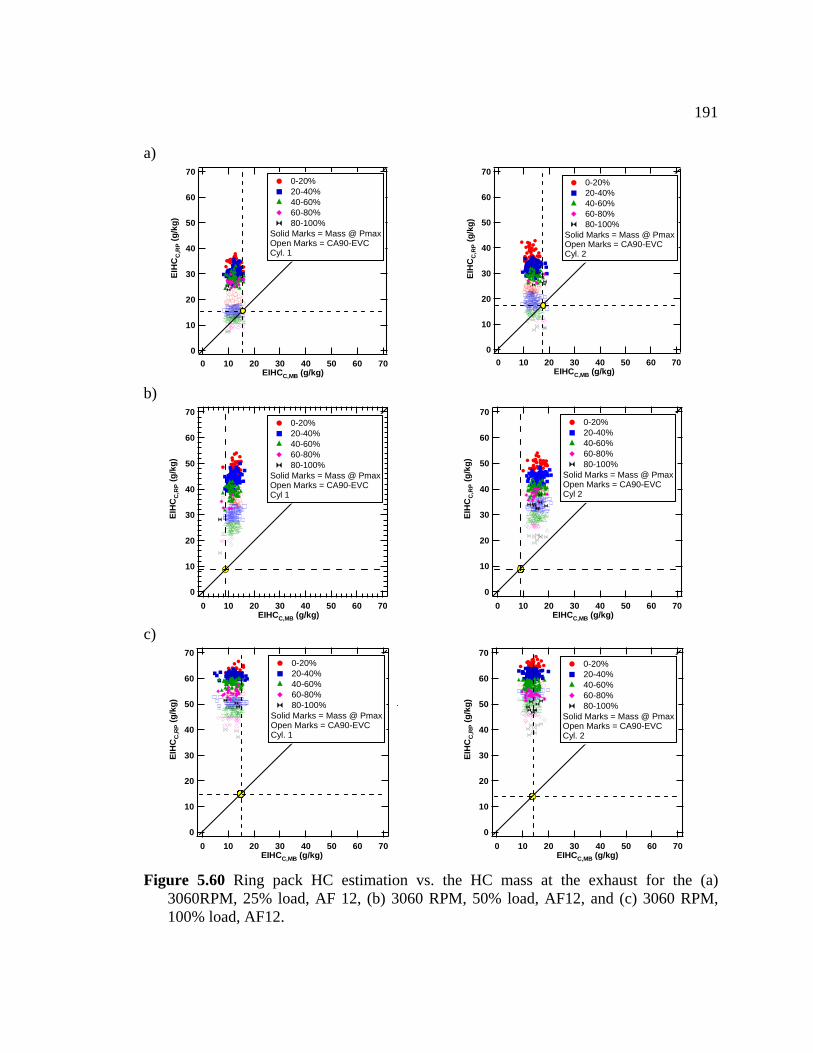
191
a) 70
60
50
40
30
20
10
0
EIH
CC
,RP
(g/k
g)
706050403020100EIHCC,MB (g/k
70
60
50
40
g)
0-20% 20-40% 40-60% 60-80% 80-100%
Solid Marks = Mass @ PmaxOpen Marks = CA90-EVC
Cyl. 1
30
20
10
0
P (g
/kg)
EIH
CC
,R
706050403020100EIHCC,MB (g/kg)
0-20% 20-40% 40-60% 60-80% 80-100%
Solid Marks = Mass @ PmaxOpen Marks = CA90-EVC
b)
Cyl. 2
70
60
50
40
30
20
10
0
EIC
C,R
P (g
g)H
/k
706050403020100EIHCC,MB (g/kg)
0-20% 20-40% 40-60% 60-80% 80-100%
Open Marks = CA90-EVCCyl 1
Solid Marks = Mass @ Pmax
70
60
50
40
30
20
10
0
EIC
C,R
P (g
g)H
/k
706050403020100EIHCC,MB (g/kg)
0-20% 20-40% 40-60% 60-80% 80-100%
Open Marks = CA90-EVCCyl 2
c)
Solid Marks = Mass @ Pmax
70
60
50
40
30
20
10
0
EIH
CC
, (g
/kg)
RP
706050403020100EIHCC,MB (g/kg)
0-20% 20-40% 40-60% 60-80% 80-100%
Solid Marks = Mass @ Pmax
Cyl. 1
70
60
50
Open Marks = CA90-EVC 40
30
20
10
0
EIH
CC
, (g
/kg)
RP
706050403020100EIHCC,MB (g/kg)
0-20% 20-40% 40-60% 60-80% 80-100%
Solid Marks = Mass @ Pmax
Cyl. 2
3060RPM, 25% load, AF 12, (b) 3060 RPM, 50% load, AF12, and (c) 3060 RPM, 100% load, AF12.
Open Marks = CA90-EVC
Figure 5.60 Ring pack HC estimation vs. the HC mass at the exhaust for the (a)
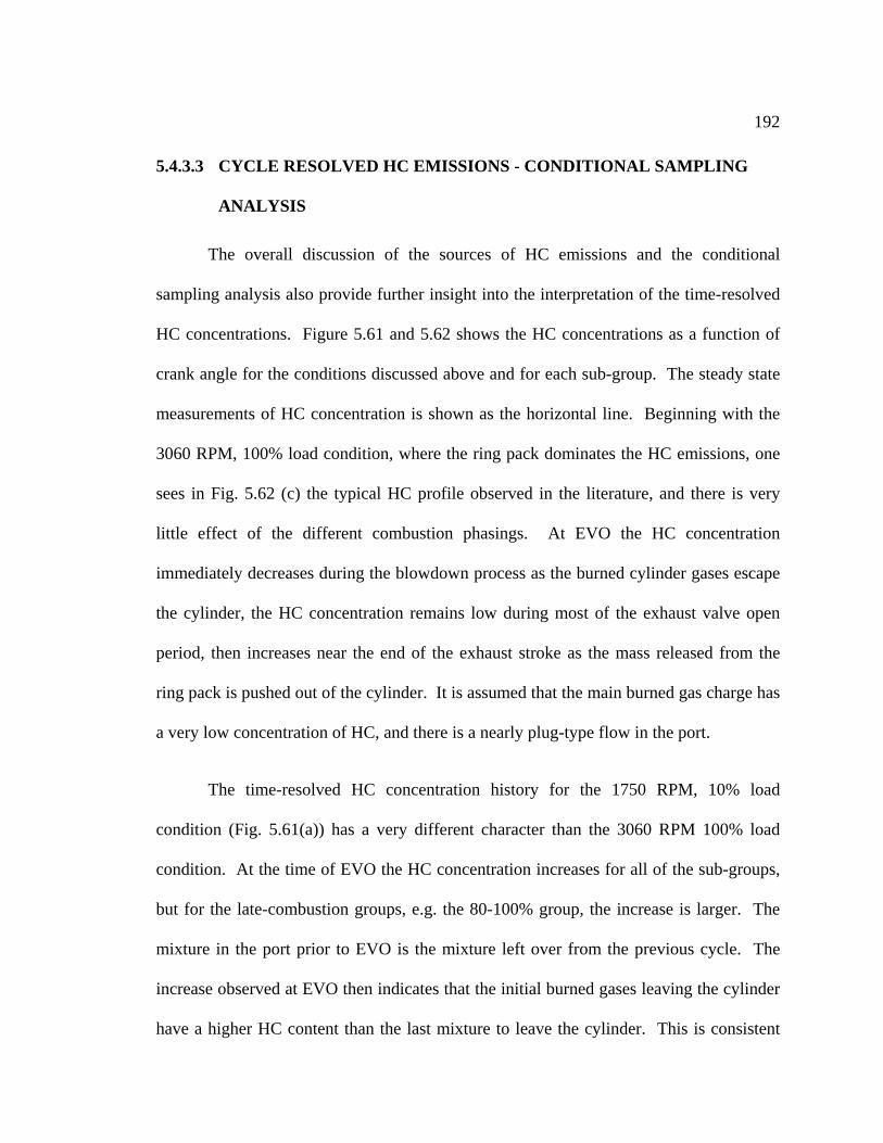
192
5.4.3.3
e typical HC profile observed in the literature, and there is very
combustion phasings. At EVO the HC concentration
immediately decreases during the blowdown process as the burned cylinder gases escape
the cylinder, the HC concentration remains low during most of the exhaust valve open
period, then increases near the end of the exhaust stroke as the mass released from the
ring pack is pushed out of the cylinder. It is assumed that the main burned gas charge has
a very low concentration of HC, and there is a nearly plug-type flow in the port.
e in the port prior to EVO is the mixture left over from the previous cycle. The
increase observed at EVO then indicates that the initial burned gases leaving the cylinder
have a higher HC content than the last mixture to leave the cylinder. This is consistent
CYCLE RESOLVED HC EMISSIONS - CONDITIONAL SAMPLING
ANALYSIS
The overall discussion of the sources of HC emissions and the conditional
sampling analysis also provide further insight into the interpretation of the time-resolved
HC concentrations. Figure 5.61 and 5.62 shows the HC concentrations as a function of
crank angle for the conditions discussed above and for each sub-group. The steady state
measurements of HC concentration is shown as the horizontal line. Beginning with the
3060 RPM, 100% load condition, where the ring pack dominates the HC emissions, one
sees in Fig. 5.62 (c) th
little effect of the different
The time-resolved HC concentration history for the 1750 RPM, 10% load
condition (Fig. 5.61(a)) has a very different character than the 3060 RPM 100% load
condition. At the time of EVO the HC concentration increases for all of the sub-groups,
but for the late-combustion groups, e.g. the 80-100% group, the increase is larger. The
mixtur
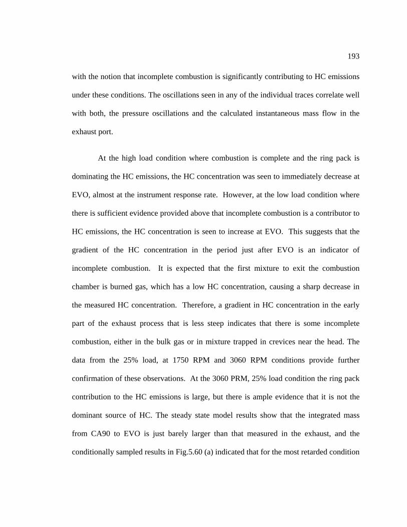
193
with the notion tha uting to HC emissions
under these conditions. The oscillations seen in any of the individual traces correlate well
with both, the pressure o ions and the calculated instantaneous mass flow in the
xhaust port.
re combustion is complete and the ring pack is
oncentration was seen to immediately decrease at
EVO, almost at the instrument response rate. However, at the low load condition where
there is sufficient evidence provided above that incomplete combustion is a contributor to
HC emissions, the HC concentration is seen to increase at EVO. This suggests that the
gradient of the HC concentration in the period just after EVO is an indicator of
incomplete combustion. It is expected that the first mixture to exit the combustion
chamber is burned gas, which has a low HC concentration, causing a sharp decrease in
the measured HC concentration. Therefore, a gradient in HC concentration in the early
part of the exhaust process that is less steep indicates that there is some incomplete
combustion, either in the bulk gas or in mixture trapped in crevices near the head. The
data from the 25% load, at 1750 RPM and 3060 RPM conditions provide further
confirmation of these observations. At the 3060 PRM, 25% load condition the ring pack
contribution to the HC emissions is large, but there is ample evidence that it is not the
dominant source of HC. The steady state model results show that the integrated mass
om CA90 to EVO is just barely larger than that measured in the exhaust, and the
onditionally sampled results in Fig.5.60 (a) indicated that for the most retarded condition
t incomplete combustion is significantly contrib
scillat
e
At the high load condition whe
dominating the HC emissions, the HC c
fr
c
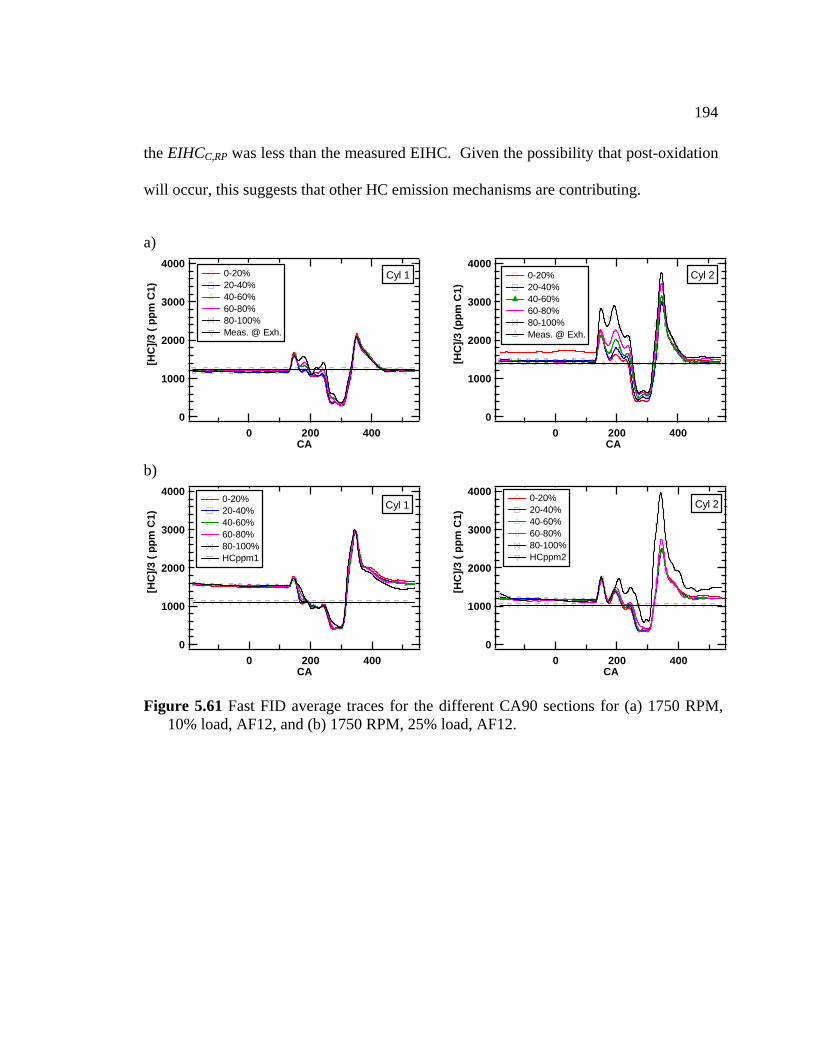
194
the EIHCC,RP was less than the measured EIHC. Given the possibility that post-oxidation
a)
will occur, this suggests that other HC emission mechanisms are contributing.
4000
3000
2000
1000
0
[HC
]/3 (
pC
1)pm
4002000CA
0-20% 20-40% 40-60% 60-80% 80-100% Meas. @ Exh.
Cyl 1
4000
3000
2000
1000
0
[HC
]/3 (
1)pp
m C
4002000CA
0-20% 20-40% 40-60% 60-80% 80-100% Meas. @ Exh.
Cyl 2
b) 4000
3000
2000
1000
0
[HC
]/3pm
( p
C1)
4002000CA
0-20% 20-40% 40-60% 60-80% 80-100% HCppm1
Cyl 1
4000
3000
2000
1000
0
[HC
]/3pm
( p
C1)
4002000CA
0-20% 20-40% 40-60% 60-80% 80-100% HCppm2
Cyl 2
Figure 5.61 Fast FID average traces for the different CA90 sections for (a) 1750 RPM, 10% load, AF12, and (b) 1750 RPM, 25% load, AF12.
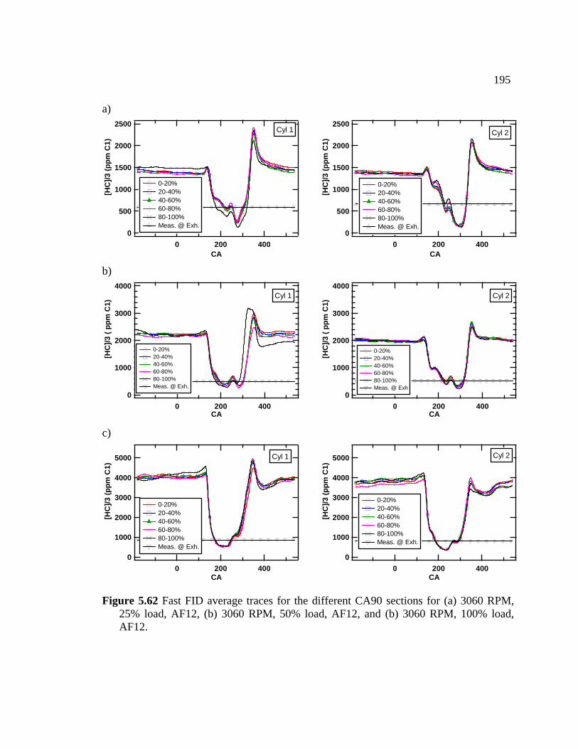
195
a) 2500
2000
1500
1000
500
0
/3 (
C[H
C]
ppm
1)
4002000CA
0-20% 20-40% 40-60% 60-80% 80-100% Meas. @ Exh.
Cyl 1
2500
2000
1500
1000
500
0
/3 (
C[H
C]
ppm
1)
4002000CA
0-20% 20-40% 40-60% 60-80% 80-100% Meas. @ Exh.
Cyl 2
b) 4000
3000
2000
1000
0
m[H
C]/3
( pp
C1)
4002000CA
0-20% 20-40% 40-60% 60-80% 80-100% Meas. @ Exh.
Cyl 1
4000
3000
2000
1000
0
m[H
C]/3
( pp
C1)
4002000CA
0-20% 20-40% 40-60% 60-80% 80-100% Meas. @ Exh
Cyl 2
c)
5000
4000
3000
2000
1000
0
[HC
] (p
pm1)
/3 C
4002000CA
0-20% 20-40% 40-60% 60-80% 80-100% Meas. @ Exh.
Cyl 1
5000
4000
3000
2000
1000
0
[HC
] (p
pm1)
/3 C
4002000CA
0-20% 20-40% 40-60% 60-80% 80-100% Meas. @ Exh.
Cyl 2
Figure 5.62 Fast FID average traces for the different CA90 sections for (a) 3060 RPM, 25% load, AF12, (b) 3060 RPM, 50% load, AF12, AF12.
and (b) 3060 RPM, 100% load,
196
5.5 SUMMARY
that at high load the
ring pack is the major contributor to the engine-out HC emissions. However at low load
the mass that returns from the ring pack to the cylinder from CA90 to EVC does not
account for the measured HC emission at the exhaust, indicating that the ring pack is not
the major contributor and that other sources are contributing to the HC emissions. Further
analysis on a single-cycle basis showed that at low load incomplete combustion was a
likely contributor to the high levels of HC emissions observed. Incomplete combustion
was characterized using both concentration- and mass-based correlations. For the
concentration-based correlation the cycle-resolved HC concentration at 160 aTDC was
correlated with the IMEP. At low load the results show a good correlation between the
HC concentration and the IMEP; cycles with low IMEP produce high levels of HC. At
high load the results show no correlation. For the HC mass-based correlation, the mass of
The relative contribution of the ring pack crevices to the HC emissions from a
small utility engine was investigated under steady, fully warmed up conditions. The ring
pack crevice contribution to HC emissions was evaluated using a simple ring pack filling
and discharging model. The model results compared quite favorably to the measured
blowby over the full range of conditions tested. The model was used on both an average
and single-cycle basis. Two metrics to characterize the emissions were implemented: the
mass stored at maximum pressure, and the mass that returns to the combustion chamber
from the time when the cumulative burn mass fraction reaches 90 percent to the time
when the exhaust valve closes (CA90-EVC). The predictions show

197
HC per cycle leaving the engine was correlated with the combustion phasing and with the
IMEP. At low load the correlation was significant, however at high load no correlation
was observed. A statistical analysis verified that at low load the correlations were
meaningful. The results also showed that there is an intermediate load condition where
incomplete combustion vanishes and the ring pack starts to be the main HC contributor.
For this intermediate condition, although the ensemble-average ring pack model results
showed that the mass that returns to the combustion chamber from the top land is slightly
higher than the measured HC at the exhaust, the conditional sampling analysis showed
that there are some sub-groups of cycles with late combustion where the ring pack
contribution is smaller than the measured at the exhaust. It is expected that at this
condition there is some in-cylinder post oxidation and the late burning cycles do not
contribute excessively to the engine-out HC emission.
198
CHAPTER VI
6 FUEL ADSORPTION-DESORPTION IN THE CYLINDER OIL LAYER
6.1 INTRODUCTION
sorption and desorption by the oil film mechanism is thought to be one
ll known
that the unburned fuel adsorbs into lubricating oil on the cylinder liner during the intake
p the fuel is hidden from the flame during
the mai
desorption mechanism does contribute in some degree to the HC emissions.
The fuel ad
of the main contributors to the engine-out HC emissions [4]. Currently, it is we
and com ression strokes. Consequently, part of
n combustion, escaping oxidation. Later, during the expansion and exhaust strokes
this stored fuel desorbs, releasing unburned fuel to the cylinder and contributing to the
HC emissions. It is important to note that part of the released fuel may be oxidized in the
cylinder during the post-flame period [30, 41]. One of the main difficulties in the study of
the relative oil film contribution to the HC emission is that it is coupled with the ring
pack mechanism. Both HC mechanisms release the fuel to the combustion chamber after
the flame arrival for approximately the same period of time. As mentioned before in §2.7,
the studies of the oil film relative contribution to the engine-out HC emission are diverse
and conflicting, i.e. some believe that is a significant contributor [38] and other authors
do not [39]. In spite of these differences, it is believed that the oil-fuel adsorption-
199
In the present chapter the effect of the oil-fuel adsorption-desorption problem is
studied for a small air-cooled utility engine. The effect of the oil layer on the HC
emissio
The engine was tested at various loads, for low and high speeds, and several spark
1.2 (Table 6.1). The equivalence ratio of 1.2
corresponds to an air-fuel ratio of 12:1 for gasoline and 12.9:1 for propane. The engine
operates at all loads and speeds at this equivalence-ratio; therefore, it was chosen to
compare the engine behavior under the two fuels. It is important to mention that the
setup for this study was implemented with an arrangement of valves and gages to control
the crankcase pressure (see §3.2.7), which allowed the study of the influence of the
crankcase pressure on the HC emissions. To estimate the trapped mass in each cylinder
spark sweep tests at constant throttle position were performed for the propane tests, as
well.
ns was investigated by running the engine with two different fuels that had
different solubility in oil: a research-grade gasoline and propane. Comparison of the
steady state HC emissions, cycle-resolved HC emissions, estimation of the ring pack
contribution to the HC emissions and the effect of the crankcase pressure were carried out
to understand the role of the oil film on the engine-out HC emissions. In addition, the
experimental findings were supported with a numerical simulation of the fuel-oil
diffusion mechanism.
6.2 TEST CONDITIONS
timings at a constant equivalence ratio of
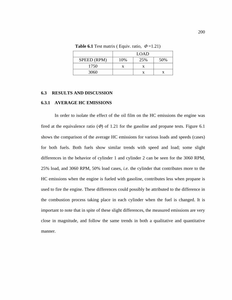
200
Table 6.1 Test matrix ( Equiv. ratio, Φ =1.21)
LOAD SPEED (RPM) 10% 25% 50%
1750 x x 3060 x x
6.3 RESULTS AND DISCUSSION
6.3.1 AVERAGE HC EMISSIONS
In order to isolate the effect of the oil film on the HC emissions the engine was
fired at the equivalence ratio (Φ) of 1.21 for the gasoline and propane tests. Figure 6.1
shows the comparison of the average HC emissions for various loads and speeds (cases)
for both fuels. Both fuels show similar trends with speed and load; some slight
differences in the behavior of cylinder 1 and cylinder 2 can be seen for the 3060 RPM,
25% load, and 3060 RPM, 50% load cases, i.e. the cylinder that contributes more to the
HC emissions when the engine is fueled with gasoline, contributes less when propane is
used to fire the engine. These differences could possibly be attributed to the difference in
the combustion process taking place in each cylinder when the fuel is changed. It is
important to note that in spite of these slight differences, the measured emissions are very
close in magnitude, and follow the same trends in both a qualitative and quantitative
manner.
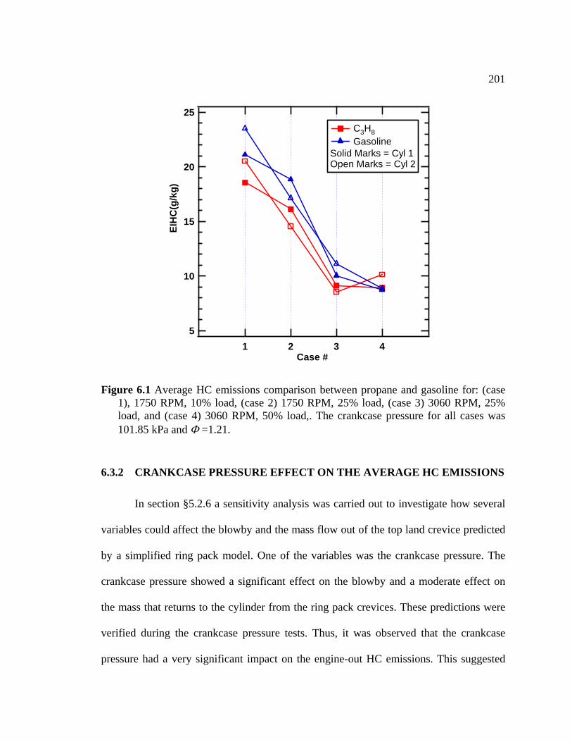
201
25
20
15
10
5
EIH
C(g
/kg)
4321Case #
C3H8 Gasoline
Solid Marks = Cyl 1Open Marks = Cyl 2
Figure 6.1 Average HC emissions comparison between propane and gasoline for: (case 1), 1750 RPM, 10% load, (case 2) 1750 RPM, 25% load, (case 3) 3060 RPM, 25% load, and (case 4) 3060 RPM, 50% load,. The crankcase pressure for all cases was 101.85 kPa and Φ =1.21.
In section §5.2.6 a sensitivity analysis was carried out to investigate how several
ariables could affect the blowby and the mass flow out of the top land crevice predicted
y a simplified ring pack model. One of the variables was the crankcase pressure. The
rankcase pressure showed a significant effect on the blowby and a moderate effect on
e mass that returns to the cylinder from the ring pack crevices. These predictions were
erified during the crankcase pressure tests. Thus, it was observed that the crankcase
ressure had a very significant impact on the engine-out HC emissions. This suggested
6.3.2 CRANKCASE PRESSURE EFFECT ON THE AVERAGE HC EMISSIONS
v
b
c
th
v
p
202
that controlling the crankcase pressure was ecessary to have repeatable HC emission
measurements. In addition, a change in the crankcase pressure is expected to affect the
ring-pack crevices HC emissions, but not the oil film contribution to the HC emissions.
Therefore, fuels of different solubility were expected to yield different trends of the
engine-out HC emissions as a function of the crankcase pressure if the fuel-oil
adsorption-desorption mechanism is important.
Figure 6.2 shows the change in the engine-out HC emissions when the crankcase
pressure was changed from 100.35 kPa to 111.35 kPa for all conditions of interest: 1750
RPM, 10% load, 1750 RPM, 25% load, 3060 RPM, 25% load, and 3060 RPM, 50% load.
These correspond to modest load engine running conditions. The atmospheric pressure
was approximately 101.35 kPa. From Fig. 6.2 (a), it can be seen that for the 1750 RPM,
10% case a clear increase in the HC emissions is observed as the crankcase pressure is
e same level of increase. It is interesting to note that the slope
n
increased. The gasoline and propane tests show the same trend and have approximately
crdPdEIHCth is not the same
ws a high rate of increase at low
crankca
along the crankcase pressure range. The HC sho
se pressures. This increase is observed up to around 106 kPa. Further increases in
pressure do not produce a significant increase in the HC emissions. This trend is observed
for both cylinders and for the propane tests as well. Increasing the load to 25% for the
1750 RPM speed, a similar trend is observed. However, for the gasoline case the
difference in HC contribution between the two cylinders has been reduced. For the
propane case the HC contribution of each cylinder has been inverted, i.e. cylinder 1 is
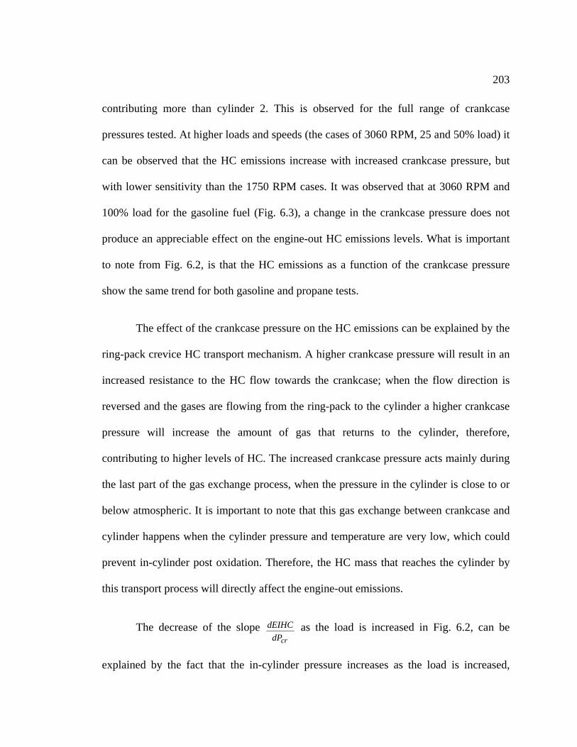
203
contributing more than cylinder 2. This is observed for the full range of crankcase
pressures tested. At higher loads and speeds (the cases of 3060 RPM, 25 and 50% load) it
can be observed that the HC emissions increase with increased crankcase pressure, but
with lower sensitivity than the 1750 RPM cases. It was observed that at 3060 RPM and
100% load for the gasoline fuel (Fig. 6.3), a change in the crankcase pressure does not
produce an appreciable effect on the engine-out HC emissions levels. What is important
to note from Fig. 6.2, is that the HC emissions as a function of the crankcase pressure
show the same trend for both gasoline and propane tests.
flow towards the crankcase; when the flow direction is
reversed and the gases are flowing from the ring-pack to the cylinder a higher crankcase
pressure will increase the amount of gas that returns to the cylinder, therefore,
contributing to higher levels of HC. The increased crankcase pressure acts mainly during
the last part of the gas exchange process, when the pressure in the cylinder is close to or
below atmospheric. It is important to note that this gas exchange between crankcase and
cylinder happens when the cylinder pressure and temperature are very low, which could
prevent in-cylinder post oxidation. Therefore, the HC mass that reaches the cylinder by
this tra
The decrease of the slope
The effect of the crankcase pressure on the HC emissions can be explained by the
ring-pack crevice HC transport mechanism. A higher crankcase pressure will result in an
increased resistance to the HC
nsport process will directly affect the engine-out emissions.
crdP
explained by the fact that the in-cylinder pressure increases as the load is increased,
dEIHC as the load is increased in Fig. 6.2, can be
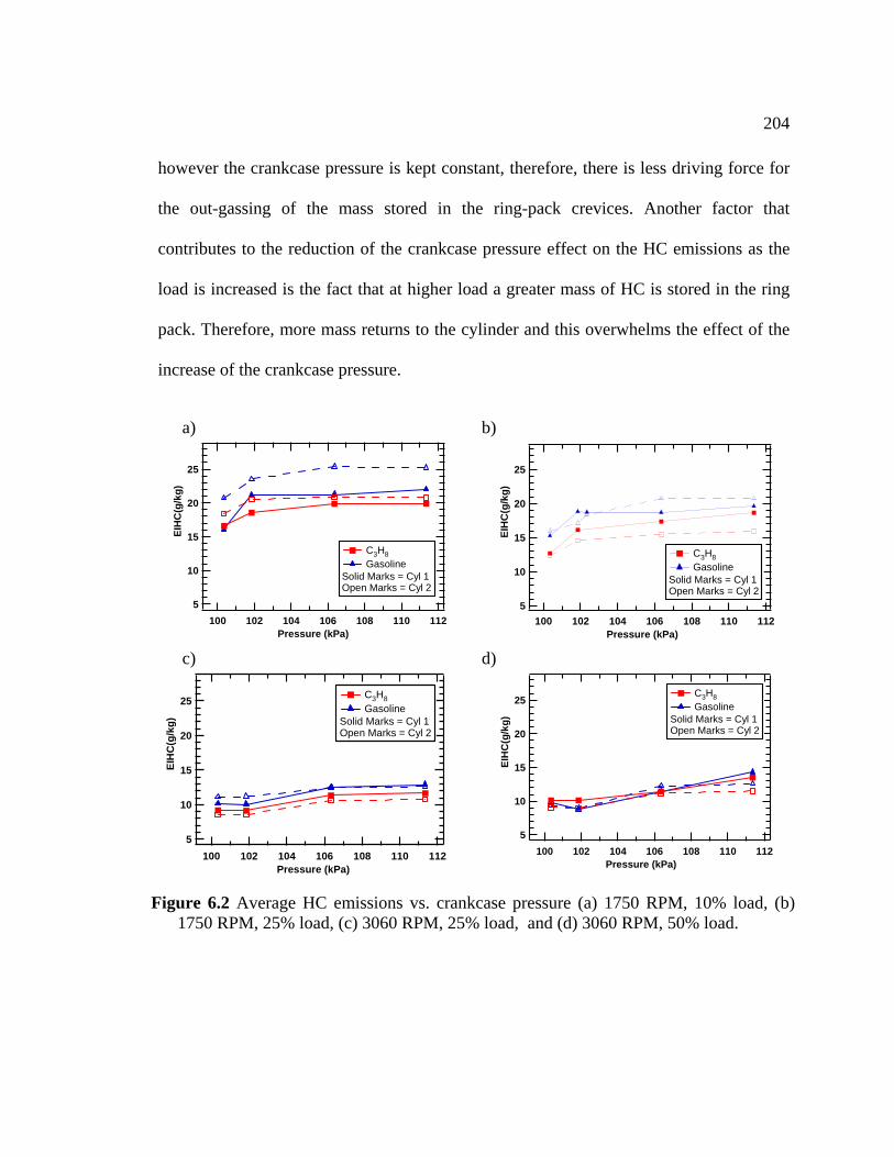
204
however the crankcase pressure is kept constant, therefore, there is less driving force for
the out-gassing of the mass stored in the ring-pack crevices. Another factor that
contributes to the reduction of the crankcase pressure effect on the HC emissions as the
load is increased is the fact that at higher load a greater mass of HC is stored in the ring
pack. Therefore, more mass returns to the cylinder and this overwhelms the effect of the
increase of the crankcase pressure.
a)
25
20
15
10
5
EIH
C(g
/kg)
112110108106104102100Pressure (kPa)
C3H8 Gasoline
Solid Marks = Cyl 1Open Marks = Cyl 2
b)
25
20
15
10
5
EIH
C(g
/kg)
112110108106104102100Pressure (kPa)
C3H8 Gasoline
Solid Marks = Cyl 1Open Marks = Cyl 2
c)
25
20
15
10
5
EIH
C(g
/kg)
112110108106104102100
C3H8 Gasoline
Solid Marks = Cyl 1Open Marks = Cyl 2
d)
25
20
15
10
5
EIH
C(g
/kg)
112110108106104102100Pressure (kPa)Pressure (kPa)
C3H8 Gasoline
Solid Marks = Cyl 1Open Marks = Cyl 2
F e (a) 1750 RPM, 10% load, (b) 1750 RPM, 25% load, (c) 3060 RPM, 25% load, and (d) 3060 RPM, 50% load.
igure 6.2 Average HC emissions vs. crankcase pressur
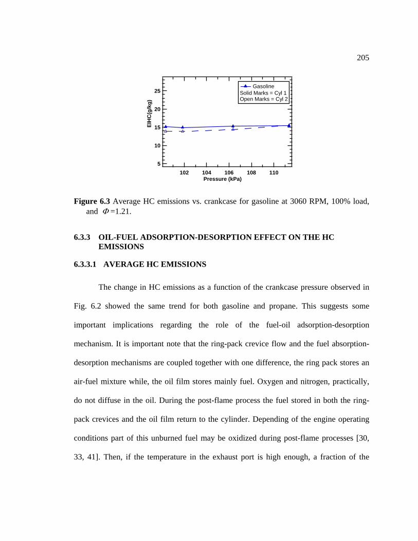
205
25
20
15
10
5
EIH
C(g
/kg)
110108106104102Pressure (kPa)
GasolineSolid Marks = Cyl 1Open Marks = Cyl 2
Figure 6.3 Average HC emissions vs. crankcase for gasoline at 3060 RPM, 100% load, and Φ =1.21.
6.3.3 OIL-FUEL ADSORPTION-DESORPTION EFFECT ON THE HC EMISSIONS
6.3.3.1 AVERAGE HC EMISSIONS
The change in HC emissions as a function of the crankcase pressure observed in
portant implications regarding the role of the fuel-oil adsorption-desorption
mechanism. It is important note that the ring-pack crevice flow and the fuel absorption-
desorption mechanisms are coupled together with one difference, the ring pack stores an
air-fuel mixture while, the oil film stores mainly fuel. Oxygen and nitrogen, practically,
do not
Fig. 6.2 showed the same trend for both gasoline and propane. This suggests some
im
diffuse in the oil. During the post-flame process the fuel stored in both the ring-
pack crevices and the oil film return to the cylinder. Depending of the engine operating
conditions part of this unburned fuel may be oxidized during post-flame processes [30,
33, 41]. Then, if the temperature in the exhaust port is high enough, a fraction of the
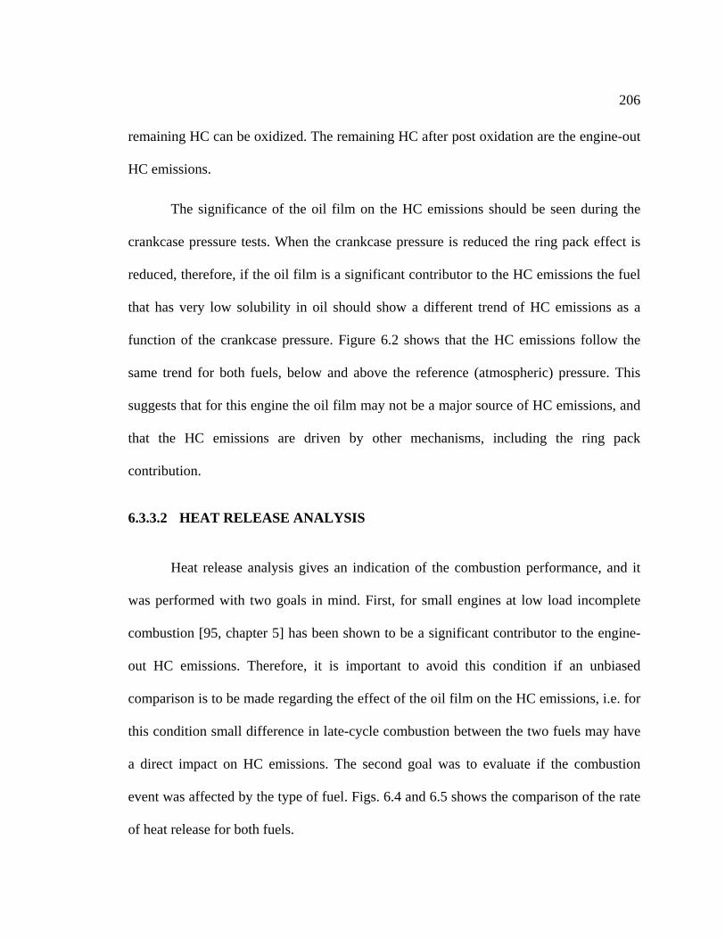
206
remaining HC can be oxidized. The remaining HC after post oxidation are the engine-out
HC emissions.
The significance of the oil film on the HC emissions should be seen during the
crankcase pressure tests. When the crankcase pressure is reduced the ring pack effect is
reduced, therefore, if the oil film is a significant contributor to the HC emissions the fuel
that has very low solubility in oil should show a different trend of HC emissions as a
function of the crankcase pressure. Figure 6.2 shows that the HC emissions follow the
same trend for both fuels, below and above the reference (atmospheric) pressure. This
suggests that for this engine the oil film may not be a major source of HC emissions, and
that the HC emissions are driven by other mechanisms, including the ring pack
contribution.
6.3.3.2 HEAT RELEASE ANALYSIS
Heat release analysis gives an indication of the combustion performance, and it
was performed with two goals in mind. First, for small engines at low load incomplete
combustion [95, chapter 5] has been shown to be a significant contributor to the engine-
out HC emissions. Therefore, it is important to avoid this condition if an unbiased
comparison is to be made regarding the effect of the oil film on the HC emissions, i.e. for
this condition small difference in late-cycle combustion between the two fuels may have
a direct impact on HC emissions. The second goal was to evaluate if the combustion
event was affected by the type of fuel. Figs. 6.4 and 6.5 shows the comparison of the rate
of heat release for both fuels.
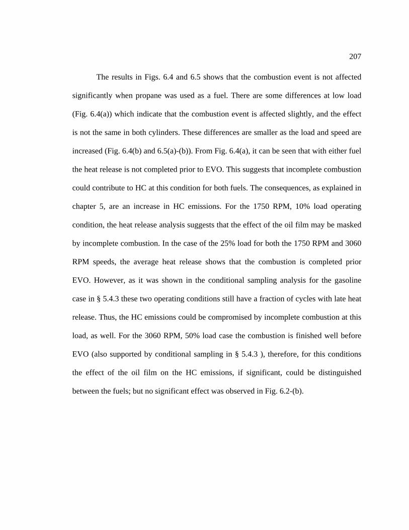
207
The results in Figs. 6.4 and 6.5 shows that the combustion event is not affected
significantly when propane was used as a fuel. There are some differences at low load
(Fig. 6.4(a)) which indicate that the combustion event is affected slightly, and the effect
is not the same in both cylinders. These differences are smaller as the load and speed are
increased (Fig. 6.4(b) and 6.5(a)-(b)). From Fig. 6.4(a), it can be seen that with either fuel
the heat release is not completed prior to EVO. This suggests that incomplete combustion
could contribute to HC at this condition for both fuels. The consequences, as explained in
chapter 5, are an increase in HC emissions. For the 1750 RPM, 10% load operating
condition, the heat release analysis suggests that the effect of the oil film may be masked
by incomplete combustion. In the case of the 25% load for both the 1750 RPM and 3060
RPM speeds, the average heat release shows that the combustion is completed prior
EVO. However, as it was shown in the conditional sampling analysis for the gasoline
case in § 5.4.3 these two operating conditions still have a fraction of cycles with late heat
release. Thus, the HC emissions could be compromised by incomplete combustion at this
load, as well. For the 3060 RPM, 50% load case the combustion is finished well before
EVO (also supported by conditional sampling in § 5.4.3 ), therefore, for this conditions
the effect of the oil film on the HC emissions, if significant, could be distinguished
between the fuels; but no significant effect was observed in Fig. 6.2-(b).
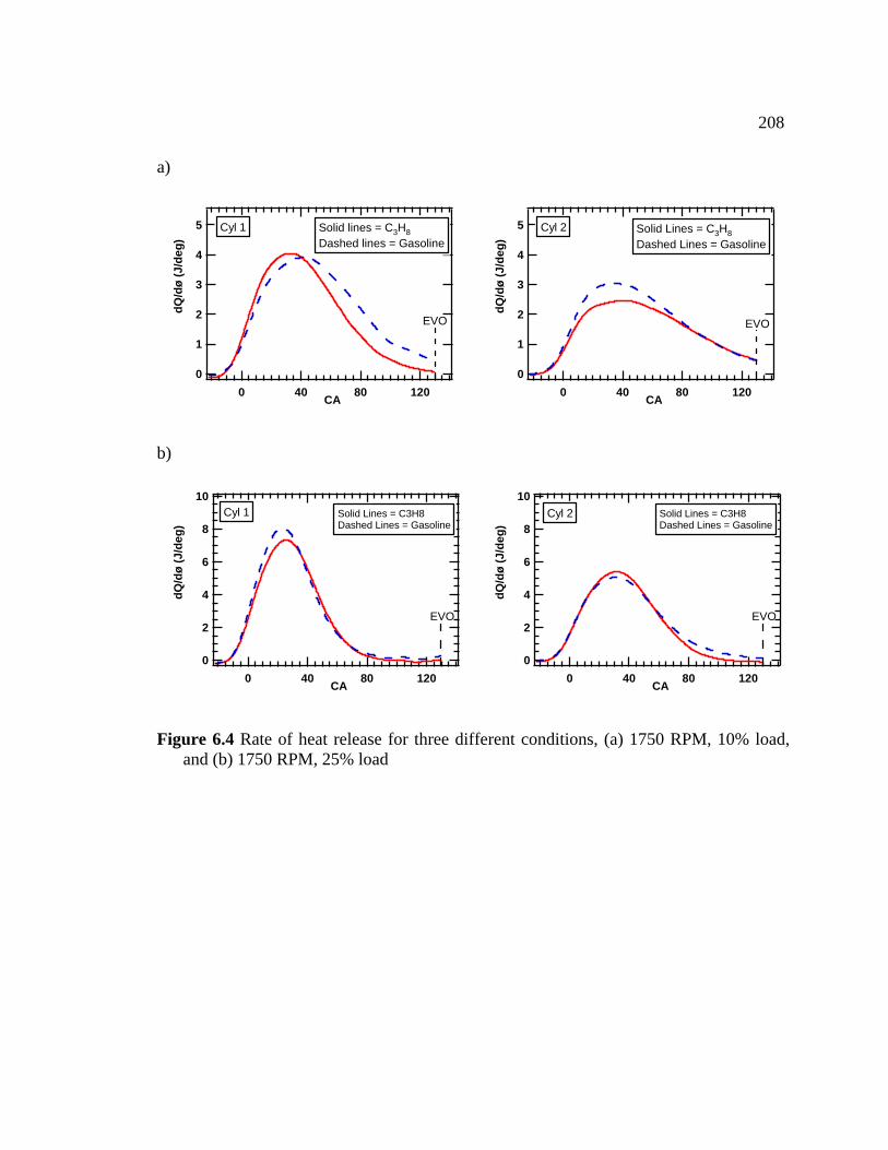
208
a)
5
4
3
2
1
0
dQ/d
ø (J
/deg
)
12080400 CA
EVO
Solid lines = Cshed lines = G
3H8asolineDa
Cyl 1 5
4
3
2
1
0
dQ/d
ø (J
/deg
)
12080400 CA
EVO
Solid Lines = C3H8Dashed Lines = Gasoline
Cy
b)
l 2
10
8
10
8
6
4
2
0
dQ/d
ø (J
/de
)g
12080400 CA
6
4
2
0
dQ/d
ø (J
/de
)g
12080400 CA
EVO
Solid Lines = C3H8Dashed Lines = Gasoline
Cyl 1
EVO
Cyl 2 Solid Lines = C3H8Dashed Lines = Gasoline
and (b) 1750 RPM, 25% load Figure 6.4 Rate of heat release for three different conditions, (a) 1750 RPM, 10% load,
209
a) 10
8
6
4
2
0
dQ/d
ø (J
/deg
)
12080400 CA
EVO
Solid Lines = C3H8Dashed Lines = Gasoline
Cyl 1
10
8
6
4
2
12080400 CA
EVO
Solid Lines = C3H8Dashed Lines = Gasoline
Cyl 2
0
/dø
(JdQ
/deg
)
b)
15
10
5
0
dQ/d
ø (J
/de
)g
12080400 CA
EVO
Solid Lines = C3 8Dashed Lines = Gasoline 15
10
5
0
dQJ/
de/d
ø (
g)
12080400 CA
EVO
Solid Lines = C3H8Dashed Lines = Gasoline
HCyl 1 Cyl 2
s is shown
in Fig.
oil film is expected it should be seen during the period when the piston scrapes the HC
Figure 6.5 Rate of heat release for three different conditions, (a) 3060 RPM, 25% load, and (b) 3060 RPM, 50% load.
6.3.3.3 CYCLE-RESOLVED HC EMISSIONS
Cycle-resolved HC emissions can help to elucidate the HC emissions difference
between the two fuels. A comparison of the averaged cycle-resolved FID trace
6.6 and 6.7. As mentioned in § 2.7 [41], the oil layer shows its effect on the fast
FID traces during the latter part of the exhaust process, when the piston moves up and
scrapes the HC wall layer. Therefore, if some influence on the HC emissions due to the
210
wall layer at the end of the exhaust stroke; specifically the difference on the fast-FID
traces should be observed when the piston is near TDC. During the main blowdown
process both the effects of the ring pack and the oil film are overwhelmed by the exhaust
of the hot core gases, which have very low HC concentration.
Under low load conditions (Fig. 6.6 (a)-(b)) the comparison can be affected by
incomplete combustion [95, chapter 5], but one can note that the propane and gasoline for
these conditions show essentially the same basic HC history, although the values are
different. This supports the heat release analysis that indicated that incomplete
combustion is also present with the propane. Single-cycle analysis of the ring pack
contribution and of the heat release for the propane case (not presented here)
corroborated this observation.
is § 5.4.3 that for
this condition there are some cycles that have a relatively slow burn rate, however, the
significant
differences are observed when the engine is fired with gasoline and propane again
suggest
The most definitive comparison can be made for the 3060 RPM, 50% load case
(Fig. 6.7(b)), where all the cycles finish heat release prior EVO. In this case the oil film
mechanism should show an influence on the fast FID traces toward the end of the exhaust
process when the cylinder approaches TDC. Fig. 6.7(b) shows no appreciable difference
For the 3060 RPM, 25% load case, Fig. 6.7 (a), no appreciable differences in HC
tory during the exhaust stage are observed, as well. It was shown in h
majority of the cycles finish combustion before EVO. The fact that no
s that the oil film is not a significant contributor to the engine-out HC emissions.
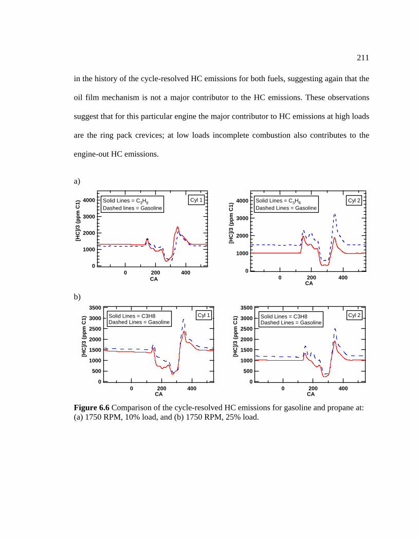
211
in the history of the cycle-resolved HC emissions for both fuels, suggesting again that the
oil film mechanism is not a major contributor to the HC emissions. These observations
suggest that for this particular engine the major contributor to HC emissions at high loads
are the ring pack crevices; at low loads incomplete combustion also contributes to the
engine-out HC emissions.
a)
4000
3000
2000
1000
0
[HC
]/3 (p
pm C
1)
4002000CA
Solid Lines = C3H8Dashed lines = Gasoline
Cyl 1
4000
3000
2000
1000
0
] C
1)[H
C/3
(ppm
4002000CA
Solid Lines = C3H8Dashed Lines = Gasoline
Cyl 2
b) 3500
3000
3500
3000
2500
2000
1500
1000
500
0
[HC
]/3 (p
pm C
1)
4002000CA
Solid Lines = C3H8Dashed Lines = Gasoline
Cyl 1
2500
2000
1500
1000
500
4002000
[HC
]/3 (p
pm C
1)
0CA
Solid Lines = C3H8solineDashed Lines = Ga
Cyl 2
igure 6.6 Comparison of the cycle-resolved HC emissions for gasoline and propane at: (a)
F1750 RPM, 10% load, and (b) 1750 RPM, 25% load.
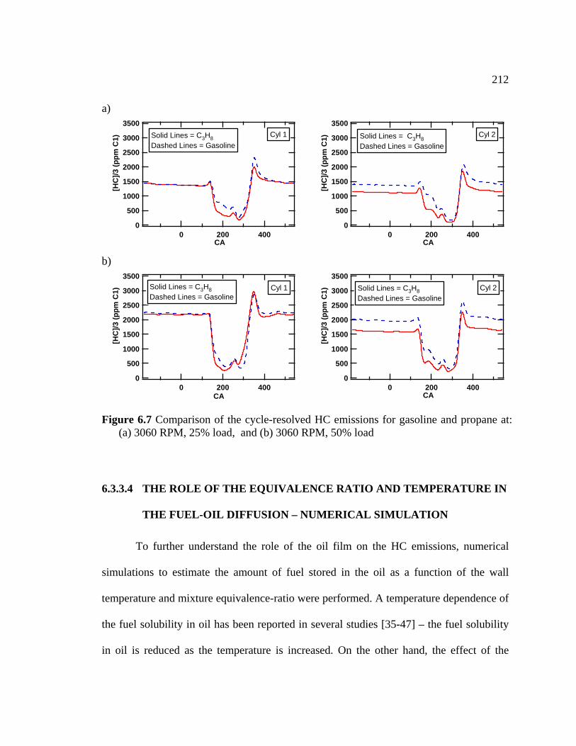
212
a) 3500
3000
2500
2000
1500
1000
500
0
[HC
]/3 (p
pm C
1)
4002000CA
Solid Lines = C3H8Dashed Lines = Gasoline
Cyl 1
3500
3000
2500
2000
1500
1000
500
0
3pm
C1)
4002000
[HC
]/ (p
CA
Solid Lines = C3H8Dashed Lines = Gasoline
Cyl 2
b) 3500
3000
2500
2000
1500
1000
500
0
pm C
1)[H
C]/3
(p
4002000
Cyl 1Solid Lines = C3H8Dashed Lines = Gasoline
3500
3000
CA
2500
2000
1500
1000
500
0
C1)
[HC
]/3 (p
pm
4002000CA
Cyl 2Solid Lines = C3H8
Figure 6.7 Comparison of the cycle-resolved HC emissions for gasoline and propane at: (a) 3060 RPM, 25% load, and (b) 3060 RPM, 50% load
6.3.3.4 THE ROLE OF THE EQUIVALENCE RATIO AND TEMPERATURE IN
THE FUEL-OIL DIFFUSION – NUMERICAL SIMULATION
T umerical
simulations to estimate th ll
temperature and mixture equivalence-ratio were performed. A temperature dependence of
s been reported in several studies [35-47] – the fuel solubility
in oil is ct of the
Dashed Lines = Gasoline
o further understand the role of the oil film on the HC emissions, n
e amount of fuel stored in the oil as a function of the wa
the fuel solubility in oil ha
reduced as the temperature is increased. On the other hand, the effe
213
equival
6.3.3.4.1 PHASE EQUILIBRIUM SIMULATION
simulation consisted of calculating the thermodynamic
equilibrium composition of the gas-liquid mixture of oil, fuel and air trapped in the
cylinde
s) and thermophysical properties of all the phases and the
feed (initial components). In the analysis, gasoline was substituted by a mixture of
ence ratio of the mixture on the fuel-oil solubility is not well documented. As
mentioned before there are two particularities of small engines that make the fuel-oil
diffusion process different than automotive engines. First, small engines run with rich air-
fuel ratio mixtures, and second, small engines are air cooled which makes them operate at
higher temperatures. It is, thus, expected that the high operating temperature of a small
engine would cause a reduction in the amount of fuel stored in the oil film and reduce its
contribution on the HC emissions. The fuel desorption process is directly proportional to
the amount of fuel adsorbed in the oil layer. In order to estimate the extent that
temperature and air-fuel ratio affects the amount of fuel diffused into the oil film, a
simplified analysis was carried out. The details of the simulations are shown in the
following subsection.
The phase equilibrium
r of the engine. In this simulation the piston was static and all trapped components
(air-fuel mixture and oil) were allowed to reach equilibrium as show in Fig. 6.8. The
dashed line represents the boundary of the closed system under study. The liquid-gas
phase equilibria composition was estimated at different temperatures for gasoline and
propane with oil using the NIST SUPERTRAPP v3.2 software, which performs phase
equilibria calculations of multi-component, multi-phase mixtures and provides as output
the composition (mass fraction
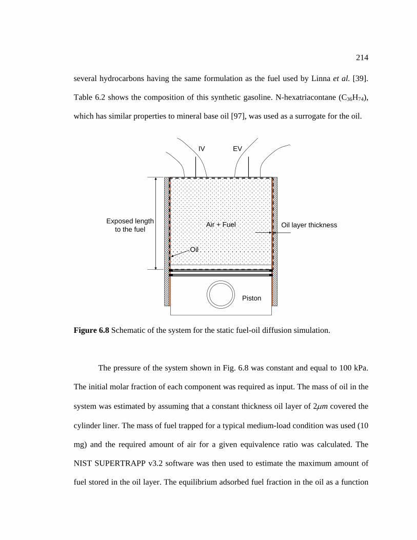
214
several hydrocarbons having the same formulation as the fuel used by Linna et al. [39].
Table 6.2 shows the composition of this synthetic gasoline. N-hexatriacontane (C36H74),
which has similar properties to mineral base oil [97], was used as a surrogate for the oil.
IV EV
Air + Fuel Oil layer thickness
Piston
Exposed lengthto the fuel
O li
Figure 6.8 Schematic of the system for the static fuel-oil diffusion simulation.
The pressure of a.
The initial molar fraction of each component was required as input. The mass of oil in the
system was estimated by assuming that a constant thickness oil layer of 2µm covered the
cylinder liner. The mass of fuel trapped for a typical medium-load condition was used (10
mg) an
he oil as a function
the system shown in Fig. 6.8 was constant and equal to 100 kP
d the required amount of air for a given equivalence ratio was calculated. The
NIST SUPERTRAPP v3.2 software was then used to estimate the maximum amount of
fuel stored in the oil layer. The equilibrium adsorbed fuel fraction in t
215
of the temperature and Φ is shown in Fig. 6.9. The software predicts a lower solubility of
propane in oil than the gasoline, which is in very good agreement with the literature. At
times greater than for
ropane for the maximum and minimum temperatures studied. It is important to note that
the oil is significantly reduced with
elevate
Table 6.2 Synthetic fuel composition [39]
Formula
Φ =1.2 the adsorbed gasoline fraction is approximately 10-35
p
for both fuels the amount of fuel diffused into
d temperature for a given equivalence ratio. Figure 6.9 also shows that the mass of
propane diffused in oil is less sensitive to temperature than the gasoline.
Compound Chemical Class
Chemical % wt
I-Pentane Saturates C5H12 20 3-Methylpentane Saturates C6H14 10 Benzene Aromatics C6H6 3 n-Heptane Saturates C H 5 7 16Toluene Aromatics C7H8 20 I-Octane Saturates C8H18 15 M,P-Xylene Aromatics C8H10 17 1,2,4-Trimethylbenzene Aromatics C9H12 5 n-Decane Saturates C10H22 3.5 I-Dodecane Saturates C12H26 1.5
The reduction in the equilibrium adsorbed fuel fraction seen in Fig. 6.9 suggests
that the oil film mechanism of HC emissions should contribute less in small engines than
in automotive engines. For automotive engines the maximum operating temperature is
limited to some extent by the coolant temperature, which is around 90 °C. The
temperature of the combustion chamber side of the liner depends on load and speed;
typical values for automotive engines at medium loads are as high as 120 °C [39] and at
216
full load the temperature can be as high as 220 °C near TDC region [98]. In small air-
cooled engines the liner temperature is typically higher; for this particular engine at full
load the liner can reach temperatures up to approximately 240 °C, and at low and medium
loads the maximum temperatures are around 200 °C. Also, small engines are operated at
wide open throttle more than automotive engines. Therefore, based on this simplified
equilibrium analysis it is expected that the amount of fuel diffused into the oil in small
ines should be smaller than the automotive engines. For automotive engines Linna et
m xpected a smaller
contrib
Figure 6.9, also shows the effect of the equivalence ratio on the fuel solubility in
the oil. As the fuel concentration is increased (Φ increases), an approximately
exponential increase in the amount of fuel diffused in the oil is observed. This is true for
all the
(240°C, Φ = 1.2) is negligible. This is due to the
competition of the higher temperature and relatively high air-fuel ratio in small engines,
eng
al. [39] estimate that the maximum contribution of the oil film to the engine-out HC
issions was less than 10%, consequently for small engines it is ee
ution due to the effect of the high operating temperature.
temperatures under study. Automotive engines operate at close to stoichiometric
while small engines operate with rich equivalence ratios. Typical equivalence ratios for
the engine under study are around Φ =1.20, and thus one would expect a larger effect in a
small engine than an automotive engine. The contribution of the oil film to the engine-out
HC emissions will be result of the competition between the equivalence ratio and
temperature effects. Using the results of Fig. 6.9 as a guide, it can be inferred that at full
load the difference in the fraction of fuel that diffuses in oil for automotive engines (220
°C, Φ = 1) and for a small engine
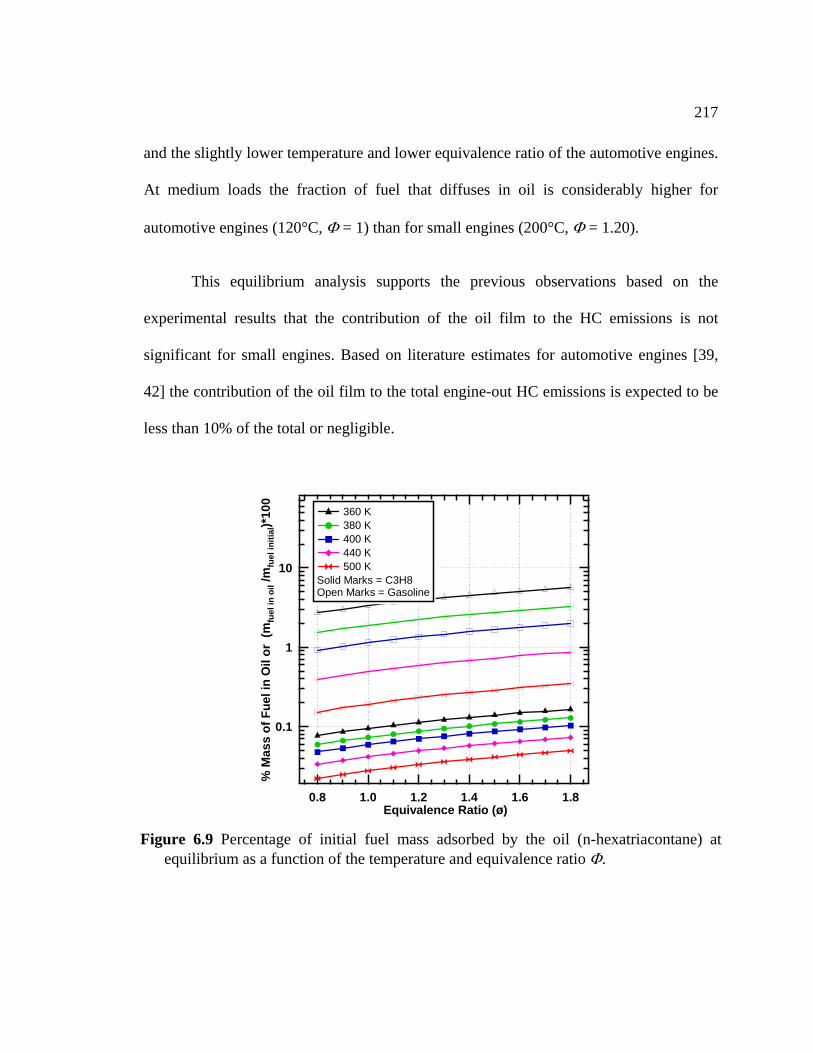
217
and the
This equilibrium analysis supports the previous observations based on the
experimental results that the contribution of the oil film to the HC emissions is not
significant for small engines. Based on literature estimates for automotive engines [39,
42] the contribution of the oil film to the total engine-out HC emissions is expected to be
less than 10% of the total or negligible.
slightly lower temperature and lower equivalence ratio of the automotive engines.
At medium loads the fraction of fuel that diffuses in oil is considerably higher for
automotive engines (120°C, Φ = 1) than for small engines (200°C, Φ = 1.20).
0.1
1
10
% M
ass
of F
uel i
n O
il or
(m
fuel
in o
il /m
fuel
inia
l)*10
it0
1.81.61.41.21.00.8Equivalence Ratio (ø)
360 K 380 K 400 K 440 K 500 K
Solid Marks = C3H8Open Marks = Gasoline
Figure 6.9 Percentage of initial fuel mass adsorbed by the oil (n-hexatriacontane) at
equilibrium as a function of the temperature and equivalence ratio Φ.
218
6.3.3.4.2 CYCLE SIMULATION OF THE FUEL-OIL ADSORPTION-
DESORPTION
To supplement the investigation of the role of the fuel-oil diffusion on the engine-
out HC emissions a time-resolved numerical simulation of the fuel-oil diffusion process
along the cylinder liner was carried out. This simulation provided an estimation of the
percent of trapped mass of fuel that returns to the combustion chamber from the oil film
r the main combustion. This made possible a comparison between the relative
tributions of the oil film and the ring pack. The model assumes a one-dimensional
transient diffusion in the radial direction of the oil film as show in the schematic of Fig.
6.10. In Fig. 6.10 the oil thickness is represented by δ, the radial coordinate by x, and the
fuel concentration by C.
6.3.3.4.2.1 ASSUMPTIONS
The main assumption in the model is that the diffusion of the fuel components in the
oil is t
assump usivity of the fuel in the oil is of the order 10 smaller than in
the gas phase [99]. In addition, no information about the flow inside of the combustion
chamber is available for this engine. Other assumptions for the calculations include:
gligible
b. The temperature of the liner is constant, and the oil temperature is equal to the
liner temperature
c. There is no interaction between individual fuel components
afte
con
he limiting factor in the adsorption-desorption mechanism. This is a reasonable
tion because the diff 4
a. The fuel flow in the axial direction of the oil film is ne
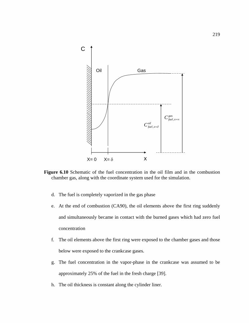
219
X= 0 X= δ x
C
Oil Gas
d. The fuel is completely vaporized in the gas phase
e. At the end of combustion (CA90), the oil elements above the first ring suddenly
and simultaneously became in contact with the b
oilxfuel δ=,
gasxfuelC ∞=,
Figure 6.10 Schematic of the fuel concentration in the oil film and in the combustion chamber gas, along with the coordinate system used for the simulation.
C
urned gases which had zero fuel
concentration
g. The fuel concentration in the vapor-phase in the crankcase was assumed to be
approximately 25% of the fuel in the fresh charge [39].
h. The oil thickness is constant along the cylinder liner.
f. The oil elements above the first ring were exposed to the chamber gases and those
below were exposed to the crankcase gases.
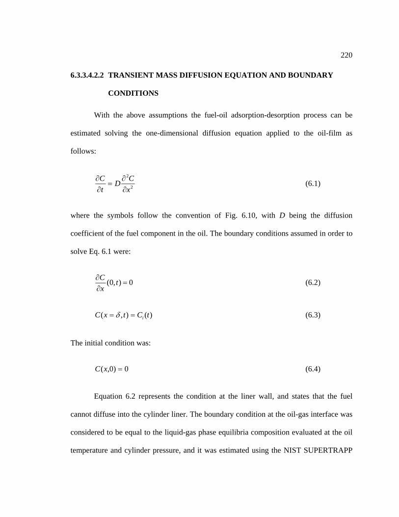
220
6.3.3.4.2.2 TRANSIENT MASS DIFFUSION EQUATION AND BOUNDARY
CONDITIONS
With the above assumptions the fuel-oil adsorption-desorption process can be
estimated solving the one-dimensional diffusion equation applied to the oil-film as
follows:
2
2
xC
tC
∂∂
∂∂
where the symbols follow the convention of Fig. 6.10, with D being the diffusion
coefficient of the fuel co
D= (6.1)
mponent in the oil. The boundary conditions assumed in order to
solve Eq. 6.1 were:
0),0( =∂∂ t
xC (6.2)
)(),( tCtxC i== δ (6.3)
(6.4)
The initial condition was:
Equation 6.2 represents the condition at the liner wall, and states that the fuel
cannot diffuse into the cylinder liner. The boundary condition at the oil-gas interface was
considered to be equal to the liquid-gas phase equilibria composition evaluated at the oil
temperature and cylinder pressure, and it was estimated using the NIST SUPERTRAPP
0)0,( =xC
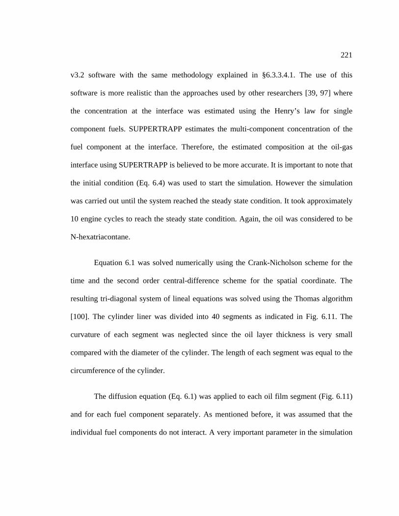
221
v3.2 software with the same methodology explained in §6.3.3.4.1. The use of this
software is more realistic than the approaches used by other researchers [39, 97] where
the concentration at the interface was estimated using the Henry’s law for single
component fuels. SUPPERTRAPP estimates the multi-component concentration of the
fuel component at the interface. Therefore, the estimated composition at the oil-gas
interface using SUPERTRAPP is believed to be more accurate. It is important to note that
the initial condition (Eq. 6.4) was used to start the simulation. However the simulation
was carried out until the system reached the steady state condition. It took approximately
10 engine cycles to reach the steady state condition. Again, the oil was considered to be
N-hexatriacontane.
quation 6.1 was solved numerically using the Crank-Nicholson scheme for the
time and the second order central-difference scheme for the spatial coordinate. The
resulting tri-diagonal system of lineal equations was solved using the Thomas algorithm
[100]. The cylinder liner was divided into 40 segments as indicated in Fig. 6.11. The
curvature of each segment was neglected since the oil layer thickness is very small
compared with the diameter of the cylinder. The length of each segment was equal to the
circumference of the cylinder.
The diffusion equation (Eq. 6.1) was applied to each oil film egment (Fig. 6.11)
and for each fuel component separately. As was assumed that the
individual fuel components do not interact. A very important parameter in the simulation
E
s
mentioned before, it
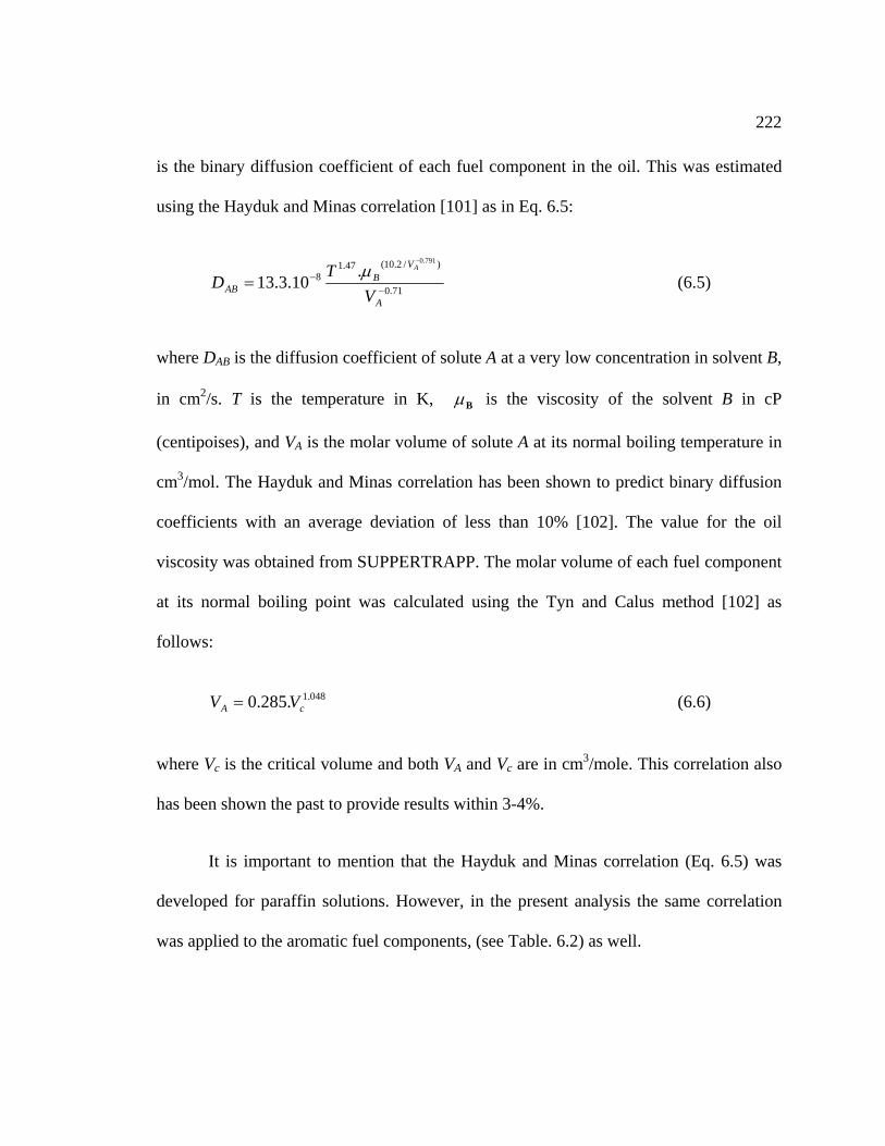
222
is the binary diffusion coefficient of each fuel component in the oil. This was estimated
using the Hayduk and Minas correlation [101] as in Eq. 6.5:
71.0
)/2.10(47.18
791.0
.10.3.13 −−
−
=A
VB
AB VTD
Aµ (6.5)
where DAB is the diffusion coefficient of solute A at a very low concentration in solvent B,
in cm2/s. T is the temperature in K, Bµ is the viscosity of the solvent B in cP
ntipoises), and V(ce normal boiling temperature in
cm3/mol. The Hayduk and Minas correlation has been shown to predict binary diffusion
fi average deviation of less than 10% [102]. The value for the oil
viscosi
VV = (6.6)
It is important to mention that the Hayduk and Minas correlation (Eq. 6.5) was
developed for paraffin solutions. However, in the present analysis the same correlation
was applied to the aromatic fuel components, (see Table. 6.2) as well.
A is the molar volume of solute A at its
coef cients with an
ty was obtained from SUPPERTRAPP. The molar volume of each fuel component
at its normal boiling point was calculated using the Tyn and Calus method [102] as
follows:
cA
where V
048.1.285.0
c is the critical volume and both VA and Vc are in cm3/mole. This correlation also
has been shown the past to provide results within 3-4%.
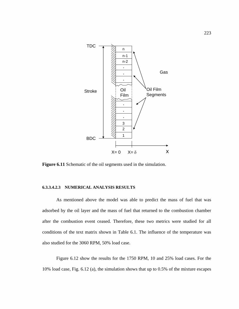
223
X= 0 X= δ x
Stroke
BDC
TDC
OilFilm
Gas
1
23
n
n-2
.
.
.
.
.
Oil FilmSegments
n-1
.
Figure 6.11 Schematic of the oil segments used in the simulation.
6.3.3.4.2.3 NUMERICAL ANALYSIS RESULTS
As mentioned above the model was able to predict the mass of fuel that was
adsorbed by the oil layer and the mass of fuel that returned to the combustion chamber
after the combustion event ceased. Therefore, these two metrics were studied for all
conditions of the text matrix shown in Table 6.1. The influence of the temperature was
also studied for the 3060 RPM, 50% load case.
Figure 6.12 show the results for the 1750 RPM, 10 and 25% load cases. For the
10% load case, Fig. 6.12 (a), the simulation shows that up to 0.5% of the mixture escapes
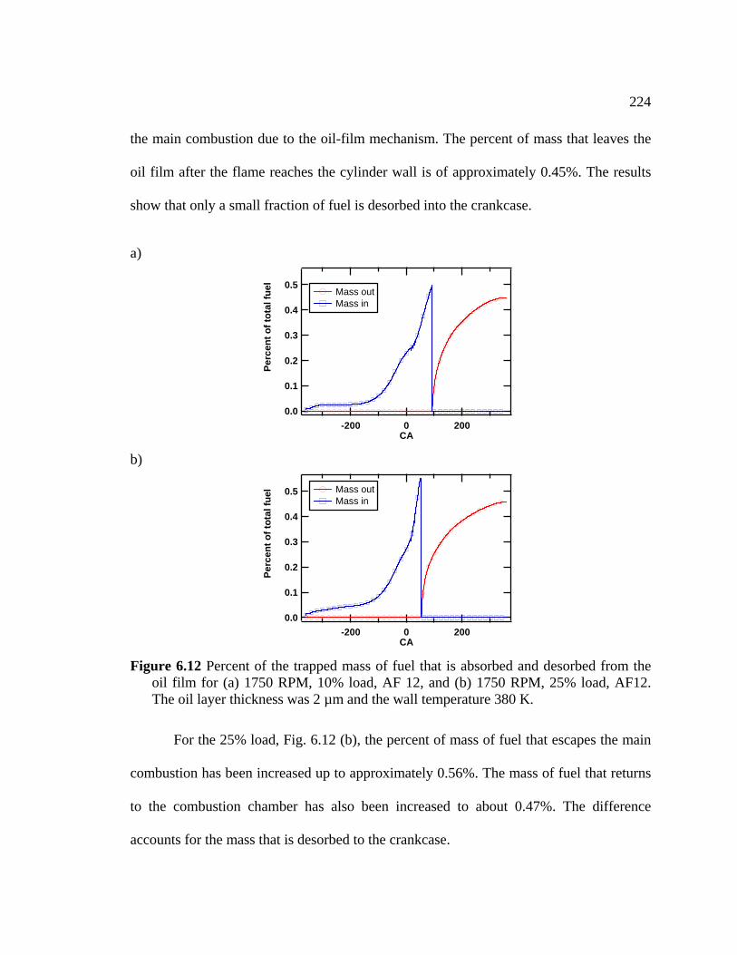
224
the main combustion due to the o percent of mass that leaves the
oil film after the flame reaches the cylinder wall is of approximately 0.45%. The results
show that only a small fraction of fuel is desorbed into the crankcase.
a)
il-film mechanism. The
0.5
0.4
0.3
0.2
0.1
0.0
t o fu
elPe
rcen
f tot
al
-200 0 200CA
Mass out Mass in
b)
0.5
0.4
0.3
0.2
0.1
0.0
fta
l fu
Perc
ent o
toel
-200 0 200CA
Mass out Mass in
Figure 6.12 Percent of the trapped m
oil film for (a) 1750 RPM, ass of fuel that is absorbed and desorbed from the
10% load, AF 12, and (b) 1750 RPM, 25% load, AF12. The oil layer thickness was 2 µm and the wall temperature 380 K.
For the 25% load, Fig. 6.12 (b), the percent of mass of fuel that escapes the main
combustion has been increased up to approximately 0.56%. The mass of fuel that returns
to the combustion chamber has also been increased to about 0.47%. The difference
accounts for the mass that is desorbed to the crankcase.
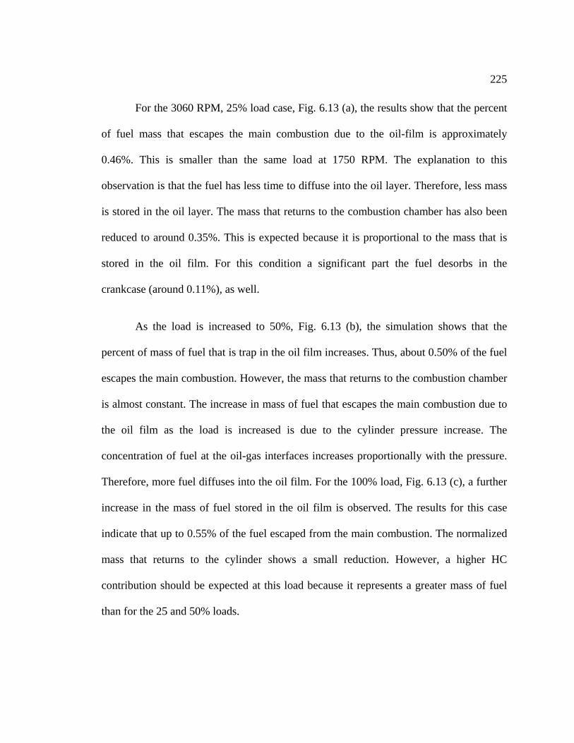
225
For the 3060 RPM, 25% load case, Fig. 6.13 (a), the results show that the percent
mass that escapes the main combustion due to the oil-film is approximately
This is smaller than the same load at 1750 RPM. The explanation to this
tion is that the fuel has less time to diffuse into the oil layer. Therefore, less mass
d in the oil layer. The mass that returns to the combustion cham
of fuel
0.46%.
observa
is store ber has also been
reduced to around 0.35%. This is expected because it is proportional to the mass that is
stored in the oil film. For this condition a significant part the fuel desorbs in the
crankcase (around 0.11%), as well.
d to 50%, Fig. 6.13 (b), the simulation shows that the
percent of mass of fuel that is trap in the oil film increases. Thus, about 0.50% of the fuel
escapes the main combustion. However, the mass that returns to the combustion chamber
is almost constant. The increase in mass of fuel that escapes the main combustion due to
the oil film as the load is increased is due to the cylinder pressure increase. The
con
Therefo
increas
indicate
mass t
contribution should be expected at this load because it represents a greater mass of fuel
than for the 25 and 50% loads.
As the load is increase
centration of fuel at the oil-gas interfaces increases proportionally with the pressure.
re, more fuel diffuses into the oil film. For the 100% load, Fig. 6.13 (c), a further
e in the mass of fuel stored in the oil film is observed. The results for this case
that up to 0.55% of the fuel escaped from the main combustion. The normalized
hat returns to the cylinder shows a small reduction. However, a higher HC
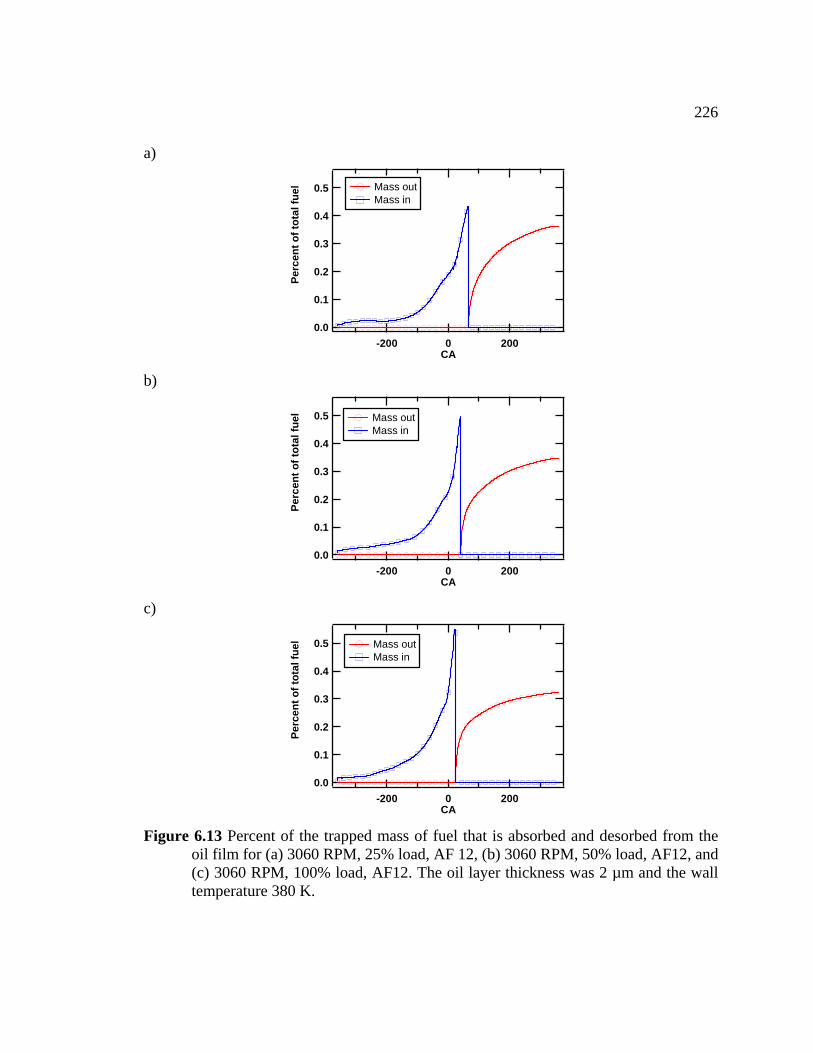
226
a)
0.5
0.4
0.3
0.2
0.1
0.0
taPe
rcen
t of t
ol f
uel
-200 0 200CA
Mass out Mass in
b)
0.5
0.4
0.3
0.2
0.1
0.0
Perc
enf t
otal
fuel
t o
-200 0 200CA
Mass out Mass in
c)
0.5
0.4
0.3
0.2
0.1
0.0
Perc
ent o
tota
lel
f fu
-200 0 200CA
Mass out
Mass in
Figure 6.13 Percent of the trapped mass of fuel that is absorbed and desorbed from the oil film for (a) 3060 RPM, 25% load, AF 12, (b) 3060 RPM, 50% load, AF12, and
temperature 380 K.
(c) 3060 RPM, 100% load, AF12. The oil layer thickness was 2 µm and the wall
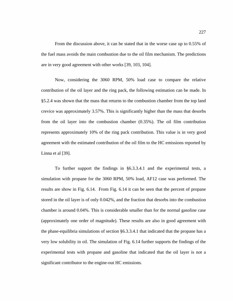
227
From the discussion above, it can be stated that in the worse case up to 0.55% of
l mass avoids the main combustion due to the oil film mechanism. The predictions
ery good agreement with other works [39, 103, 104].
the fue
are in v
Now, considering the 3060 RPM, 50% load case to compare the relative
con
§5.2.4
crevice
from th he oil film contribution
represents approximately 10% of the ring pack contribution. This value is in very good
agreement with the estimated contribution of the oil film to the HC emissions reported by
Linna et al [39].
port the findings in §6.3.3.4.1 and the experimental tests, a
simulation with propane for the 3060 RPM, 50% load, AF12 case was performed. The
results are show in Fig. 6.14. From Fig. 6.14 it can be seen that the percent of propane
stored in the oil layer is of only 0.042%, and the fraction that desorbs into the combustion
chamber is around 0.04%. This is considerable smaller than for the normal gasoline case
(approximately one order of magnitude). These results are also in good agreement with
the
very lo
experim layer is not a
significant contributor to the engine-out HC emissions.
tribution of the oil layer and the ring pack, the following estimation can be made. In
was shown that the mass that returns to the combustion chamber from the top land
was approximately 3.57%. This is significantly higher than the mass that desorbs
e oil layer into the combustion chamber (0.35%). T
To further sup
phase-equilibria simulations of section §6.3.3.4.1 that indicated that the propane has a
w solubility in oil. The simulation of Fig. 6.14 further supports the findings of the
ental tests with propane and gasoline that indicated that the oil
228
0.04
0.03
0.02
0.01
0.00f
tal f
uPe
rcen
t o to
el
-200 0 200CA
6.14 Percent of the trapped mass of fuel that is absorbed and desorbed from the film at 3060 RPM, 50% load, AF 12. The fuel is propane, the oil layer thickness
and the wall tem
Figureoil was 2 µm perature 380 K.
As was stated before, small engines run under hot conditions therefore a smaller
contribution should be expected for small engines. In order to understand the temperature
effect on the oil film contribution, simulations at different cylinder wall temperatures
were performed for the 3060 RPM, 50% load case. The results are show in Fig. 6.15.
that is t
chambe
change
small e
that for
is below
the combustion chamber
will contribute to the engine-out HC emissions. Part of this fuel will diffuse in the hot
From Fig. 6.15, it can be seen that as the temperature is increased the mass of fuel
rapped in the oil layer decreases. The mass of fuel that returns to the combustion
r has also been reduced by approximately 30% when the temperature was
d from 380K to 500K. As mentioned before at full load typical temperatures in a
ngine are of the order of 240°C (513 K). Therefore from Fig. 6.15 it is expected
the 50% load at 3060 RPM, the mass of fuel that contributes to the HC emissions
0.1%.
As mentioned before, not all the fuel mass that returns to
229
bulk burned gases, and may be oxidized during the post-flame period. The remaining
mass w
.5 g/kg-fuel. This is within the error of the
measurement of the HC emissions (see §4.3.1). This supports the equilibrium simulation
and
emissio
ill be scraped by the piston during the exhaust stroke and released to the exhaust
port where a further post-oxidation may take place. In the cylinder the degree of post
oxidation depends mainly of the temperature and on the oxygen availability [30, 41]. The
extent of the oxidation of several single-component fuels desorbing from the oil layer has
been studied experimentally by Norris and Hochgreb [41]. The results of this work
showed that between 50-80% of the desorbed mass is oxidized in the cylinder. Therefore,
based on the above results the relative contribution for the 3060 RPM, 50% load case to
the engine-out HC emissions could be at most of 0.05% of the total mass trapped in the
cylinder, or in emission index notation 0
discussion that the oil layer may not be a significant contributor to the engine-out HC
ns in small engines.
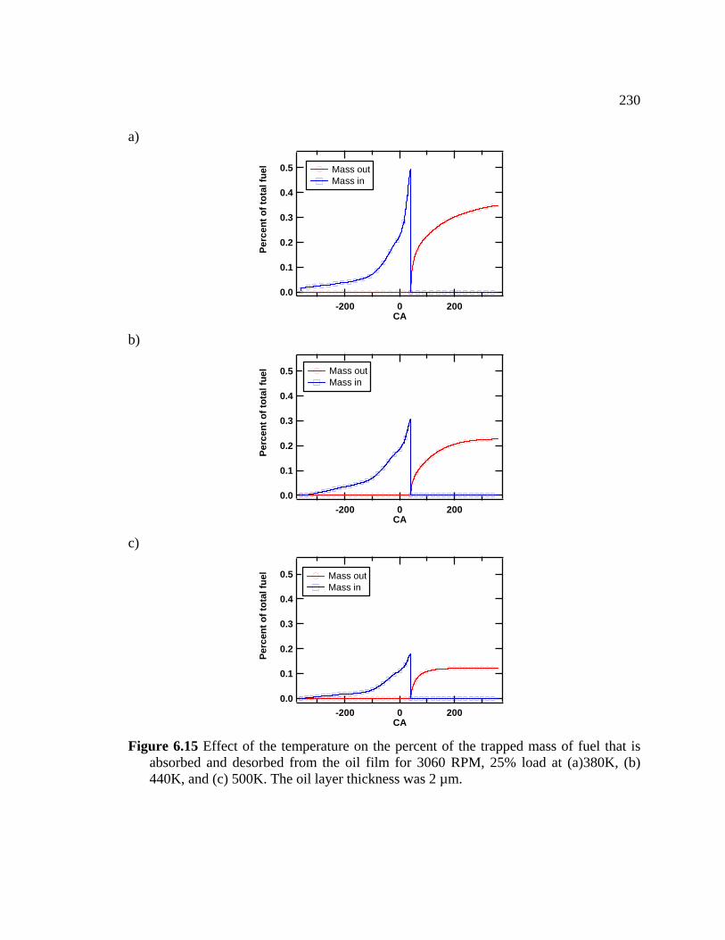
230
a)
0.5
0.4
0.3
0.2
0.1
-200 0 200CA
Mass out Mass in
ent o
f tot
al fu
el
0.0
Perc
b)
0.5
0.4
0.3
0.2
0.1
0.0
taPe
rcen
t of t
ol f
uel
-200 0 200CA
Mass out Mass in
c)
0.5
0.4
0.3
0.2
0.1
0.0
Perc
ent o
f tot
al fu
el
-200 0 200CA
Mass out Mass in
6.15 Effect of the temperature on the percent of the trapped mass of fuel that is orbed and desorbed from the oil film for 3060 RPM, 25% load at (a)380K, (b) K, and (c) 500K. The oil layer thickness w
Figureabs440 as 2 µm.
231
6.4 SUMMARY
The role of the oil film on the HC emissions from a small utility engine has been
studied experimentally and numerically. The experimental results of the crankcase
pressure tests, heat release analysis and cycle-resolved HC emissions show that the oil
layer is not a significant contributor to the engine-out HC emissions. Numerical
simulations of the fuel absorption supported the experimental findings. The phase
equilibrium simulations showed that small engines are favored with respect to the oil-film
HC emission contribution due to their high operating temperature. The results of this
simulation suggests that a smaller contribution than observed in automotive engines
should be expected (less than 10% of the total HC emissions) in small engines. Further
analysis of the fuel-oil adsorption-desorption process along the engine cycle showed that
at m
compar
contrib
experim
signific ut HC emissions.
ost a contribution of up to 0.05% of the injected mass of fuel could be expected. A
ison with the relative contribution of the ring pack crevice showed that the oil film
ution represents 10% of the ring pack contribution. In conclusion, the
ental and numerical results show that the oil layer mechanism does not contribute
antly to the engine-o
232
CHAPTER VII
7 CONCLUSIONS AND RECOMMENDATIONS
7.1 CONCLUSIONS
subsect
7.1.1 LIQUID FUEL EFFECTS
The effect of fuel mixture preparation system on the combustion and emissions
from
homogeneous, pre-vaporized m
carburetor. Em
exhaust surge tank, were performed with a fast
FID
can be
a.
The main findings of the HC mechanisms study are summarized in the following
ions.
a small, air-cooled, two-cylinder utility engine was studied. The results from a
ixture were compared to the mixture resulting from a
issions measurements were performed in the standard fashion from an
and cycle-resolved HC measurements
. The main findings of the liquid fuel effects on the engine-out HC emissions study
summarized as follows:
Stop-injection measurements with a carburetor-mounted low pressure liquid fuel
injection system that emulated the carburetor showed that in excess of 60 cycles
worth of liquid fuel was held in the intake manifold under the conditions tested.
233
b. Under steady state operation, the type of fuel system (homogeneous mixture,
carburetor or carburetor mounted low pressure liquid fuel injection) did not have a
significant effect on the average unburned HC emissions for all the operating
conditions and air-fuel ratios tested. Similarly, the CO and NOx emissions were
not affected by the fuel mixture preparation system.
c. The cycle-resolved HC emissions showed very small differences between the
carburetor and homogeneous mixture system, further suggesting that the air-fuel
mixture preparation system does not significantly affect the HC emissions under
steady state conditions.
d. The heat release analysis showed that under steady state conditions the
combustion event was not affected by the liquid fuel effects for all the tested
conditions.
e. The HC emissions results presented, suggest that the presence of the liquid-phase
fuel in the intake manifold does not ydrocarbon emissions
either in their overall level, or their evolution history. This is in spite of the fact
that the engine studied requires the flow to undergo a sharp turn just downstream
of the carburetor, which is expected to incur a significant liquid-phase fuel
impingement.
adversely impact the h
234
7.1.2 RING PACK CREVICES
A comprehensive characterization of the contribution of the ring pack storage
mec
has been carried out using a phenomenological, simplified ring pack model. The
integra the crevices from CA90 to EVC was taken to represent the
pot
cyli
measur
determ
HC mass was found to, on average, agree well with the steady state measurements, and
ther
the
the calculated mass of HC at the exhaust and with the HC concentration at a given CA
during s was verified carrying
out
contribution of sub-groups of cycles to the HC emissions based on their combustion
phasing , varied air-
fue
mixture study are:
a. ated by the ring
three times as much HC mass to the cylinder as is measured in the exhaust.
hanism to the HC emissions of both cylinders of a V-twin air-cooled utility engine
ted mass leaving
ential contribution of the ring pack to the overall HC emissions; post-oxidation in the
nder will consume a fraction of this mass. Time-resolved exhaust HC concentration
ements were also performed, and the instantaneous HC mass flow rate was
ined using the measured exhaust and cylinder pressure. The integrated exhaust
efore could be used to provide an indication of an individual cycle’s contribution to
overall HC emissions. Several engine performance parameters were correlated with
the exhaust process. The significance of these correlation
a statistical analysis. Conditional sampling of the data was performed to isolate the
. Tests were performed for a range of engine load, two engine speeds
l ratio and with a fixed ignition timing using a homogeneous, pre-vaporized fuel
system. The major conclusions that can be drawn from this
At high load the results indicate that the HC emissions are domin
pack contribution. The model predicts that the ring pack returns approximately
235
Under these conditions the combustion is robust, and isolated late-burning cycles
do not behave significantly different than the mean. In addition, for these
conditions the temperatures were high enough at the end of combustion to support
n.
b. predicts
d in the exhaust, clearly indicating that another HC mechanism is
hat including
bustion constraints put on utility-class
e were a fraction of the cycles that did not
e. At low load the integrated exhaust HC mass was shown to correlate inversely
combustion is materially contributing to the exhaust HC emissions.
significant post oxidation, but the chemistry is frozen during exhaust blowdow
At low load conditions (1750 RPM, 10 % load) the ring pack model
significantly less mass returning to the cylinder (CA90 – EVC) from the ring pack
than is observe
significantly contributing to the exhaust HC emissions.
c. A single-cycle analysis performed at the low load condition showed t
cyclic dispersion in the ring pack model did not allow the shortfall of the ring
pack contribution, with respect to the measured HC at the exhaust, to be
accounted for.
d. Single-cycle heat release analysis together with conditional sampling indicated
that at light load conditions, due to the com
engines from manufacturing costs, ther
complete heat release prior to EVO.
with the IMEP on a cycle-by-cycle basis, which strongly suggest that incomplete
236
f. A direct analysis was performed using time-resolved HC measurements, and it
was shown that cycles with late heat release correlated with high levels of HC
g. tion represents the borderline condition between
ble-average ring pack model results indicate that the
there are sub-groups, i.e. late-burning cycles, for which this is not true, and the
lower than the exhaust value. Combined with the fact that there is
s besides the ring
ikely mechanism is incomplete combustion.
mass emissions as well as high levels of HC concentration. The linear correlation
coefficients at light load were modest, ~0.18 and 0.49 for cylinder 1 and cylinder
2 respectively, but the probability that an equivalent sample of random data would
provide the same level of correlation was effectively zero. Thus, incomplete
combustion is a significant contributor to HC emissions at light load in small
utility engines.
The 3060 RPM, 25% load condi
the competition of the incomplete combustion and the ring pack contribution on
the HC emissions. The ensem
mass returned to the cylinder from the ring pack is slightly higher than the amount
measured in the exhaust. But, the conditional sampling analysis indicates that
integrated exhaust HC mass, EIHCC,MB, for this sub-group of cycles was not
considerably
expected to be some in-cylinder post-oxidation of the ring pack HC mass at this
condition, this strongly suggests that there are other mechanism
pack that are significantly contributing to the HC emissions at this condition. The
most l
237
7.1
adsorption into the oil layer
and
varying the crankcase pressure and fuel composition. Results using a standard full-blend
gaso
magnitude lower solubility in the oil. Tests were performed for multiple engine speeds
and loa
experimental study was supported with a numerical analysis of the liquid-gas phase
equilib
conclusions can be draw
a. The steady state emissions for the two fuels were qualitatively and quantitatively
st stroke where the influence
ss so at the higher
storage. The fact that the relative change in the HC with changes in crankcase
pressure was the same for the two fuels, and the lack of a difference in the cycle-
.3 OIL FILM ADSORPTION-DESORPTION
The influence on engine-out HC emissions of fuel
its subsequent desorption late in the cycle following combustion was studied by
line were compared to those using propane, which has approximately one order of
ds, with a fixed equivalence ratio of Φ = 1.21 and a fixed spark timing. The
rium and of the adsorption-desorption process of the fuel in the oil. The following
n from the study:
in good agreement for all of the operating conditions investigated.
b. The cycle-resolved HC emissions were also in good agreement between the two
fuels, most notably during the latter part of the exhau
of the fuel desorption from the oil is expected to be prominent.
c. The HC emissions were found to be significantly affected by the crankcase
pressure at the low speed light load operating condition, but le
speeds and loads. The cause for the different HC emissions observed with
varying crankcase pressure is believed to be the difference in the ring-pack
238
resolved HC emissions strongly suggests that the fuel desorption from the oil film
does not have a significant role in the overall HC emissions from small utility
d. A simulation of the liquid-gas phase equilibria of the oil-fuel system indicated the
due to their high operating
vious observations based on the
e oil film to the HC emissions is not
ates for automotive engines
be less than 10% of the total or negligible.
rption-desorption process along the
that the highest contribution to the
sm should be below 0.05% of the
er is not a significant contributor in small engines. The
engines.
contribution of the oil film to the HC emissions in small engines should be
smaller than in automotive engines. This is mainly
temperature, in spite of the relatively high equivalence-ratio operation of the small
engines. The analysis supported the pre
experimental results that the contribution of th
significant for small engines. Based on literature estim
the contribution of the oil film to the total engine-out HC emissions is expected to
e. A numerical analysis of the unsteady adso
cycle under steady state conditions predicted
HC emissions due to the oil film mechani
injected mass of fuel. This is lower than the relative contribution of the ring pack
(less than 10%). A further reduction due to post oxidation is expected. Therefore,
the effect of the oil lay
effect of the oil layer is expected to be overwhelmed either by the incomplete
combustion or the ring pack contribution.
239
7.2
r future work regarding the HC
emission in sm
le-cylinder heat release analysis, a
le-cylinder trapped mass is required. The rate
under-estimation could affect the analysis of the extent of incomplete combustion
linder trapped mass should be measured
linder engine
. This could help to improve the accuracy of the predicted contribution of
cant effect on the mass that returns from the top land crevice after the main
d.
RECOMMENDATIONS
The following recommendations are considered fo
all engines.
a. For a more accurate calculation of the sing
more rigorous estimation of the sing
of heat release is affected significantly by the trapped mass of fuel. An over- or
contribution. Therefore, the single-cy
experimentally with enough accuracy. Otherwise, either a single cy
should be used or an even charging should be provided to each cylinder.
b. The piston wall temperature should be measured or predicted with enough
accuracy
the ring pack. As was mentioned in the sensitivity analysis this parameter has a
signifi
combustion event.
c. A full characterization of the temperature profile of the cylinder wall should be
obtained. The temperature profile will help to improve the prediction of the
relative contribution of the oil film to the HC emissions.
An estimation of the extent of the in-cylinder and exhaust port oxidation should
be performed to characterize the extent of the contribution of the ring pack and oil

240
film to the engine-out HC emissions. This could help to improve the
understanding and the extent of the contribution of each HC mechanism to the
e mechanisms such as the liquid fuel could be important.
g.
he building exhaust vacuum system, the crankcase pressure was
at low load. Therefore, crankcase pressure tests with significant vacuum levels are
engine-out HC emissions. This could be done with a fully threedimensional
simulation with chemistry, correlating the measured HC with the mass that
escapes combustion due to the ring pack and oil film, as well with experimental
tests.
e. Another possible mechanism that could contribute to the engine-out HC emission
is the flame quench on the combustion chamber walls. This mechanism was not
studied in this thesis. Although, it is expected that its contribution is very small a
studied is recommended for the particular operating conditions of small engines.
f. The present study was carried out under steady state conditions. However, under
transient conditions som
Therefore, the study should be complemented with a transient characterization of
the relative contribution of the HC mechanisms.
During the ring pack study it was found that the crankcase pressure has a
significant effect on the engine out HC emissions. In the present work due to the
limitation of t
reduced only up to 100.35 kPa. It is expected that a further reduction in the
crankcase pressure could help to reduce the engine-out HC emissions, especially
suggested.

241
h. A study to increase the burn rate at the low load condition should be performed. If
the combustion is fast at this condition the high levels of HC due to the
on could be avoided. It was shown for this engine that by
incomplete combusti
placing flaps in the intake port, the burn rate was increased.
242
8 R
1. Douglas, R., and Glover, S., “The Feasibility of Meeting CARB/EPA 3 Emission Regulations for Small Engines,” SAE Paper 2007-32-0059, 2007
2. EPA Nonroad Engine and Vehicle Emission Study-Report, EPA 460/3-91-02, November 1991
3. US National Transportation Statistics, 2006. US Department of Transportation Report
4. Cheng, W. K., Hamrin, D., Heywood, J. B., Hochgreb, S., Min, K., and, Norris, M., “An Overview of Hydrocarbon Emissions Mechanisms in Spark-Ignition Engines,” SAE Paper 932708, 1993
5. Heywood, J. B., “Internal Combustion Engine Fundamentals,” McGraw-Hill, 1988
6. O’Sullivan, J. B., Russell, J. A., and Summerson, W. A., “Emission Characteristics of Small Industrial Engines,’ SAE Paper 730857, 1973
7. Burrahm, R. W., Carroll, J. N., and White, J. J., “Small Utility Engine Emissions Reduction Using Automotive Technology,” SAE Paper 911805, 1991
8. Eccleston, B. H., and Hurn, R. W., “Exhaust Emission from Small, Utility, Internal Combustion Engines,” SAE Paper 720197, 1972
9. Hare, C. T., Houtman, W. H., Oliver W. R., and Springer, K. J., “Small Engine Emissions and Their Impact,” SAE Paper 730859, 1973
10. Swanson, M., “An Emission Comparison Between a Carburetor and an Electronic Fuel Injection System for Utility Engines,” SAE Paper 911806, 1991
11. Angelo, T. G., Borman, G. L., and Martin, J. K., “Emissions and Performance of a Small L-Head Utility Engine Fueled with Homogeneous Propane/Air and Propane/Air/Nitrogen Mixture,” SAE Paper 932444, 1993
12. Itano, E., “Characterization of Carburetor Exit Flow,” M.S. Thesis, Mechanical Engineering Deparment, University of Wisconsin-Madison, 1996
13. Jehlik, F. A., and Ghandhi, J. B., “Investigation of Intake Port Fuel Films in a Small Engine,” SAE Paper 2001-01-1788, 2001
EFERENCES
243
14. and M.S.
Thesis, Mechanical Engineering Department, University of Wisconsin-Madison, 1994
. J., Boam, D. J., and Finlay, I. C., “Cold Start Performance of an Automotive Engine Using Prevaporized Gasoline,” SAE Paper 930710, 1993
16. Meyer, R., Yilmaz, E., and Heywood, J. B., “Liquid Fuel Flow in the Vicinity of the Intake Valve of a Port-Injected SI Engine,” SAE paper 982471, 1998
17. Meyer, R., and Heywood, J. B., “Effect of Engine and Fuel Variables on Liquid Fuel Transport into the Cylinder in Port-Injected SI Engines,” SAE paper 1999-0l-0563, 1999
18. Takahashi, Y., and Nakase, Y., “Analysis of the Fuel Liquid Film Thickness of a Port Fuel Injection Engine,” SAE paper 2006-01-1051, 2006
19. Turns, S. R., “An Introduction to Combustion,” McGraw-Hill, 2001
20. Goolsby, A. D., and Haskell, W. W., “Flame-Quench Distance Measurements in a CFR Engine,” Combustion and Flame, 26, 105-114, 1976
21. Ishizawa, S., “An Experimental Study on Quenching Crevice Widths in the Combustion Chamber of a Spark-Ignition Engine,” Twenty-Sixth Symposium on Combustion, The Combustion Institute, pp. 2605-2611, 1996
22. Alkidas, A.,“Combustion Chamber Crevices: The Major Source of Engine-Out Hydrocarbon Emissions Under Fully Warmed Conditions,” Prog. In Energy and Comb. Sci. Vol. 25, pp. 253-273, 1999
23. Wentworth, J. T. “Piston and Ring Variable Affect Exhaust Hydrocarbon Emissions,” SAE Paper 680109, 1968
24. Alkidas, A. C., Drews, R. J., Miller, W. F., “Effects of Piston Crevice Geometry on the Steady State Engine Out Hydrocarbon Emissions from an SI Engine,” SAE Paper 952537, 1995
25. Bignion, E. and Spicher, U. “Investigation of the Influence of Top Land Crevice Geometry on Hydrocarbon Emissions from SI Engines,” SAE Paper 982560, 1998
26. Reitz, R. D. and Kuo, T. “Modeling of HC Emissions Due to Crevice Flows in Premixed-Charge Engines,” SAE Paper 892085, 1989
Bonneau, B. J., “Development of a Homogeneous Mixture SystemComparison with Carbureted Utility Engine Emissions and Performance,”
15. Boyle, R
244
27. Namazian, M. and Heywood, J. B. “Flow in the Piston-Cylinder-Ring Crevices of a y and Power,” SAE Paper 820088, 1982
on Crevice HC Emissions: Model Results and Comparison with Experiments,”
Nitric Oxide and Hydrocarbon Oxidation Chemistry in a Spark Ignition Engine,”
reb, S. “Numerical Simulation of Post-Flame Oxidation of Hydrocarbons in Spark Ignition Engines,” SAE Paper 970886, 1997
34. Eng, J. A. “The Effect of Spark Retard on Engine-out Hydrocarbon Emissions,” SAE Paper 2005-01-3867, 2005
35. Kaiser, E. W., Adamczyk, A. A., and Lavoie G. A., “The Effect of Oil Layers on the Hydrocarbon Emissions Generated During Closed Vessel Combustion,” Eighteenth Symposium on Combustion, The Combustion Institute, pp. 1881-1892, 1981
36. Kaiser, E. W., Lorusso, J. A., Lavoie, G. A., and Adamczyk, A. A., “ The Effect of Oil Layers on the Hydrocarbon Emissions from Spark-Ignited Engines,” Combustion Science and Technology, Vol. 28, pp. 69-73, 1982
37. Carrier, G., Fendell, F., and Feldman, P., “Cyclic Absorption/Desorption of Gas
38. Gatellier, B., Trapy, J., Herrier D., Quelin, J. M. and Galliot, F. “Hydrocarbon Emissions of SI Engines as Influenced by Fuel Absorption-Desorption in Oil Films,” SAE Paper 920095, 1992
Spark-Ignition Engine: Effect on Hydrocarbon Emissions, Efficienc
28. Alkidas, A. C. “The Effects of Head Gasket Geometry on Engine-Out HC Emissions from S.I. Engines,” SAE Paper 1999-01-3580, 1999
29. Green, R. M. and Cloutman, L. D. “Planar LIF Observations of Unburned Fuel Escaping the Upper Ring-Land Crevice in an SI Engine,” SAE Paper 970823, 1997
30. Eng, J. A., Leppard, W. R., Najt, P. M. and Dryer, F. L. “Experimental Hydrocarbon Consumption Rate Correlations From a Spark Ignition Engine,” SAE Paper 972888, 1997
31. Oliveira, I. B. and Hochgreb, S. “Effect of Operating Conditions and Fuel Type
SAE Paper 1999-01-3578, 1999
32. Eng, J. A., Leppard, W. R., Najt, P. M. and Dryer, F. L. “The Interaction Between
SAE Paper 972889, 1997
33. Kuo-Chun, W. and Hochg
in a Liquid Wall Film,” Combustion Science and Technology, Vol. 25, pp. 9-19, 1981
245
39. Linna, J., Malberg, H., Bennett, P. J., Palmer, P. J., Tian, T. and Cheng, W. K. “Contribution of Oil Layer Mechanism the Hydrocarbon Emissions from Spark-Ignition Engines,” SAE Paper 972892, 1997
40. Kaiser, E. W., Siegl, W. O. and Russ, S. G. “Effect of Fuel Dissolved in Crankcase Oil on Engine-Out Hydrocarbon Emissions from a Spark-Ignited Engine,” SAE Paper 972891, 1997
41. Norris, M. G. and Hochgreb, S. “Extent of Oxidation of Hydrocarbons Desorbing from the Lubricant Oil Layer in Spark-Ignition Engines,” SAE Paper 960069, 1996
42. Kaiser, E. W., Siegl, W. O. and Russ, G. “Fuel Composition Effects on Hydrocarbon Emissions from a Spark-Ign uel Absorption in Oil Significant?,” SAE Paper 952542, 1995
43. Parks, J., Armfield J., Storey, J., Barber, T. and Wachter, E. “In Situ Measurement of Fuel Absorption into the Cylinder Wall Oil Film During Engine Cold Start,” SAE Paper 981054, 1998
44. Min, K., and Cheng, W. K., “ Oil Layer as Source of Hydrocarbon Emissions In SI Engine,” ICE-Vol. 27-4, 1996, Fall Technical Conference, pp. 85-96
45. Yu, S., and Min, K., “Effects of the Oil and Liquid Fuel Film on Hydrocarbon Emissions in Spark Ignition Engines,” Proc. Inst. Mech. Engrs. Vol. 216 Part D: Journal of Automotive Engineering, 2002
Fuel Vapor by Cylinder Lubricating Oil Films and Its Contribution to Hydrocarbon Emissions,” SAE Paper 830652, 1983
47. Schramm, J., and Sorenson, S. C., “Solubility of Gasoline Components in Different Lubricants for Combustion Engines Determined by Gas-Liquid Partition Chromatography,” Journal of Chromatography, 538, pp. 241-248, 1991
48. Chappelow, C. C., and Prausnitz, J. M., “Solubilities of Gases in High-Boiling Hydrocarbon Solvents,” AIChE Journal, Vol. 20, No. 6, 1974
49. Sugiyama, T., Takeuchi, T., and Suzuki, Y., “Thermodynamic Properties of Solute Molecules at Infinite Dilution Determined by Gas-Liquid Chromatography: I. Intermolecular Energies of n-Alkane Solutes in C28-C36 n-Alkane Solvents,” Journal of Chromatography, 105, pp. 265-272, 1975
to
S.ited Engine – Is F
46. Dent J. C., and Lakshminarayanan, “A model for Absorption and Desorption of
246
50. LoRusso, J. A., Kaiser, E. W., and Lavoie, G. A., “In-Cylinder Measurements of
Technology, Vol. 22, pp. 75-112, 1983
52. Mercury Service Manual, 200/225 Optimax, Direct Fuel Injection, August 2003
53. Miller, R. W., “Flow Measurement Engineering Handbook,” McGraw Hill Publishing Company, 2nd Edition, New York, 1989.
54. Figliola, R. S., and Beasley, D. E., “ Theory and Design for Mechanical Measurements,” John Wiley & Sons, Inc., Third Edition, New York, 2000
55. MotoTron Corporation, www.mototron.com
56. The MathWorks Inc., www.mathworks.com
57. Green Hills Software Inc., www.ghs.com
58. Electronic Control Unit Data Sheet, ECM model ECM-0565-128-0503, MotoTron Corporation, 2006
59. B&B Electronics Manufacturing Company, www.bb-elec.com
ted, www.tbwoods.com
62. Rexnord Industries LCC, www.rexno .com
63. Test Procedure for the Measurement of Gaseous Exhaust Emissions from Small
64. HRF-500 Fast FID Hydrocarbon Measurement System User Manual version 2.1,
. 89-124, 1998
Wall Layer Hydrocarbons in a Spark Ignited Engine,” Combustion Science and
51. Westbrook, C. K., Adamczyk A. A., and Lavoie, G. A., “ A Numerical Study of Laminar Flame Wall Quenching,” Combustion and Flame, Vol. 40, pp. 81-99, 1981
60. Dyne Systems Inc., www.dynesystem .com
61. TB Woods Incorpora
s
rd
Utility Engines, SAE J1088, SAE Recommended Practice, February 1993
Cambustion Inc. 2001.
65. Finlay, I. C., Boam, D. J., Bingham, J. F., and Clark, T. A., “Fast Response FID Measurement of Unburned Hydrocarbons in the Exhaust Port of a Firing Gasoline Engine,” SAE paper 902165, 1990
66. Cheng, W. K., Summers, T., and Collings, N., “The Fast-Response Flame Ionization Detector,” Progress in Energy and Combustion Science, Vol. 24, pp
247
67. Dryer Instruments Inc, www.dr
68. Elster American Meter, www.americanmeter.com
K I
71. HI-Techniques Inc, www.hi-techniques.com
74. Stivender, D. L., “Development of a Fuel-Based Mass Emission Measurement
restville Energy Research Center Report, BERC/CP-77/47, 1977
76. Spindt, R. S., “Air-Fuel Ratios from Exhaust Gas Analysis,” SAE Paper 650507,
Exhaust Concentration Measurements,” Engine Research Center, Technical
aneous Heat Transfer Coefficient in the Internal Combustion Engine,” SAE Paper 670931, 1967
, a
991
82. Sher, E. (ed)., “Handbook of Air Pollution from Internal Combustion Engines: Pollutant Formation and Control,” Academic Press, Boston, Massachusetts, 1998
yer.com
69. istler nstrumetn Corporation, www.kistler.com
70. National Instruments, www.ni.com
72. BEI Electronics Inc., www.bei.com
73. Johann Haltermann Ltd., a subsidiary of the Dow Chemical Company, www.dow.com
Procedure,” SAE Paper 710604, 1971
75. Bar
1965
77. Ghandhi, B. J., “Calculation of Engine Mass Emissions and Air-Fuel Ratio from
Report
78. Woschni, G. “ A Universally Applicable Equation for the Instant
79. Yun, H. J., and Mirsky, W., “Schlieren-Streak Measurements of Instantaneous Exhaust Gas Velocities from a Spark-Ignition Engine,” SAE Paper 741015, 1974
80. Brown C.N., Ladommatos N. “The Effects of Mixture Preparation and Trapped Residuals on the Perform nce of a Spark-Ignition Engine with Air-Shrouded Port Injectors, at low load and low speed,” Proceeding of Mechanical Engineers, Part D, Journal of Automobile Engineering, Vol. 205 (D1), pp. 17-30 , 1991
81. Brown C.N., Ladommatos N., “A Numerical Study of Fuel Evaporation and Transportation in the Intake Manifold of a Port-Injected SI Engine,” Proceeding of Mechanical Engineers, Journal of Automobile Engineering, Vol. 205 (D3), pp. 161-175, 1
248
83. Lavoie, G. A., Lorusso, J. A., and Adamczyk, A. A., “Hydrocarbon Emission Modelling for Spark Ignition Engines,” Combustion Modeling in Reciprocating Engines, pp. 409-445, 1978.
84. Trinker, F. H., Cheng, J., and Davis, G. C., “A Feedgas HC Emission Model for a n
ompson, N. D., and Wallace, J. S., “Effect of Engine Operating Variables and Piston and Ring Parameters on Crevice Hydrocarbon Emissions,” SAE Paper 940480, 1994
86. Daniels, C. H., and Evers, L. W., “The Influence of Mixture Preparation on a
87. Harrington, J. A., and Shisu, R. C., “A Single-Cylinder Engine Study of the ydrogen-to-Carbon Ratio and
CO, NO, and HC Exhaust Emissions,” SAE Paper 730476, 1973
88. Stache, I. and Alkidas, A. C., “The Influence of Mixture Preparation on the HC
r 972981, 1997
89. uhama, S. and Tada, T., “On the Flow of the Gas through the Piston-Rings,” (2nd Report, The Character of Gas Leakage) Bulletin of the JSME, Vol. 4., No. 16, pp. 691-698, 1961
90. Kuo, T.W., Sellnau, M. C., Theobald, M. A., and Jones, J. D., “Calculation of the w in the Piston-Cylinder-Ring Crevices of a Homogeneous-Charge Engine and
Comparison with Experiment,” SAE Paper 890838, 1989
. Furuhama, S. and Tada, T., “On the Flow of the Gas through the Piston-Rings,” (1st Report, The Discharge Coefficient and Temperature of Leakage) Bulletin of the JSME, Vol. 4., No. 16, pp. 684-690, 1961
92. Roberts, C. E., and Matthews, R. D., “Development and Application of an odel for Hydrocarbon Emissions Studies,” SAE Paper
961966, 1996
93. , C. G., Bae, C. S., and Choi, S. M., “Importance of the Inter-Ring Crevice Volume as a Source of Unburned Hydrocarbon Emissions-Numerical Considerations,” Proceedings of the Institute of Mechanical Engineers, Vol 214,
rinciples of Combustion,” John Wiley & Sons, Inc., Second Edition, New Jersey, 2005
SI Engines Including Parti l Bur Effects,” SAE Paper 932705, 1993
85. Th
Warm 1.9L Ford Engine,” SAE Paper 940444, 1994
Effects of Fuel Type, Fuel Stoichiometry, and H
Concentration Histories from a S.I. Engine Running Under Steady-State Conditions,” SAE Pape
Fur
Flo
91
Improved Ring Pack M
Kim
part D, pp 395-403, 2000
94. Kuo, K. K., “P
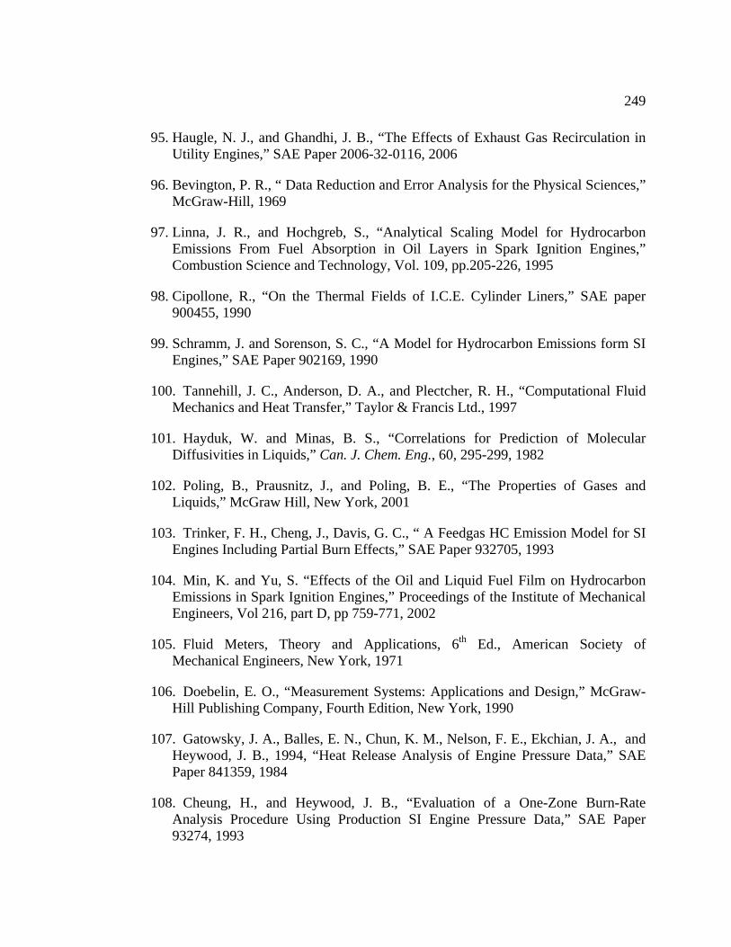
249
95. H lation in Ut
96. Bevington, P. R., “ Data Reduction and Error Analysis for the Physical Sciences,”
tical Scaling Model for Hydrocarbon m Fuel Absorption in Oil Layers in Spark Ignition Engines,”
Combustion Science and Technology, Vol. 109, pp.205-226, 1995
er 00455, 1990
ational Fluid Mechanics and Heat Transfer,” Taylor & Francis Ltd., 1997
101. Hayduk, W. and Minas, B. S., “Correlations for Prediction of Molecular hem. Eng., 60, 295-299, 1982
ling, B. E., “The Properties of Gases and 01
. C., “ A Feedgas HC Emission Model for SI ts,” SAE Paper 932705, 1993
uid Fuel Film on Hydrocarbon s of the Institute of Mechanical
th
esign,” McGraw-Hill Publishing Company, Fourth Edition, New York, 1990
107. Gatowsky, J. A., Balles, E. N., Chun, K. M., Nelson, F. E., Ekchian, J. A., and “Heat Release Analysis of Engine Pressure Data,” SAE
84
e-Zone Burn-Rate E Paper
augle, N. J., and Ghandhi, J. B., “The Effects of Exhaust Gas Recircuility Engines,” SAE Paper 2006-32-0116, 2006
McGraw-Hill, 1969
97. Linna, J. R., and Hochgreb, S., “AnalyEmissions Fro
98. Cipollone, R., “On the Thermal Fields of I.C.E. Cylinder Liners,” SAE pap9
99. Schramm, J. and Sorenson, S. C., “A Model for Hydrocarbon Emissions form SIEngines,” SAE Paper 902169, 1990
100. Tannehill, J. C., Anderson, D. A., and Plectcher, R. H., “Comput
Diffusivities in Liquids,” Can. J. C
102. Poling, B., Prausnitz, J., and PoLiquids,” McGraw Hill, New York, 20
103. Trinker, F. H., Cheng, J., Davis, GEngines Including Partial Burn Effec
104. Min, K. and Yu, S. “Effects of the Oil and LiqEmissions in Spark Ignition Engines,” Proceeding
771, 2002 Engineers, Vol 216, part D, pp 759-
105. Fluid Meters, Theory and Applications, 6 Ed., American Society ofMechanical Engineers, New York, 1971
106. Doebelin, E. O., “Measurement Systems: Applications and D
Heywood, J. B., 1994,Paper 841359, 19
108. Cheung, H., and Heywood, J. B., “Evaluation of a OnAnalysis Procedure Using Production SI Engine Pressure Data,” SA93274, 1993

250
109. Lanzafame, R., and Messina, M., “ICE Gross Heat Release Strongly Influenced of Automotive Technology,
Vol. 4, No. 3, pp. 125-13, 2003 by Specific Heat Ratio Values,” International Journal
9
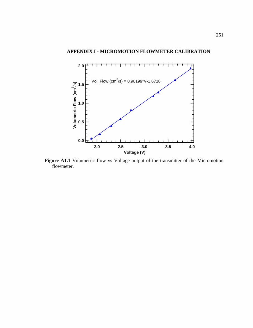
251
10 APPENDIX I - MICROMOTION FLOWMETER CALIBRATION
2.0
1.5
1.0
0.5
4.03.53.02.52.0
Vm
e3 /s
) (c
mtr
ic F
low
olu
0.0
Voltage (V)
Vol. Flow (cm3/s) = 0.90199*V-1.6718
n
flowmeter. Figure A1.1 Volumetric flow vs Voltage output of the transmitter of the Micromotio
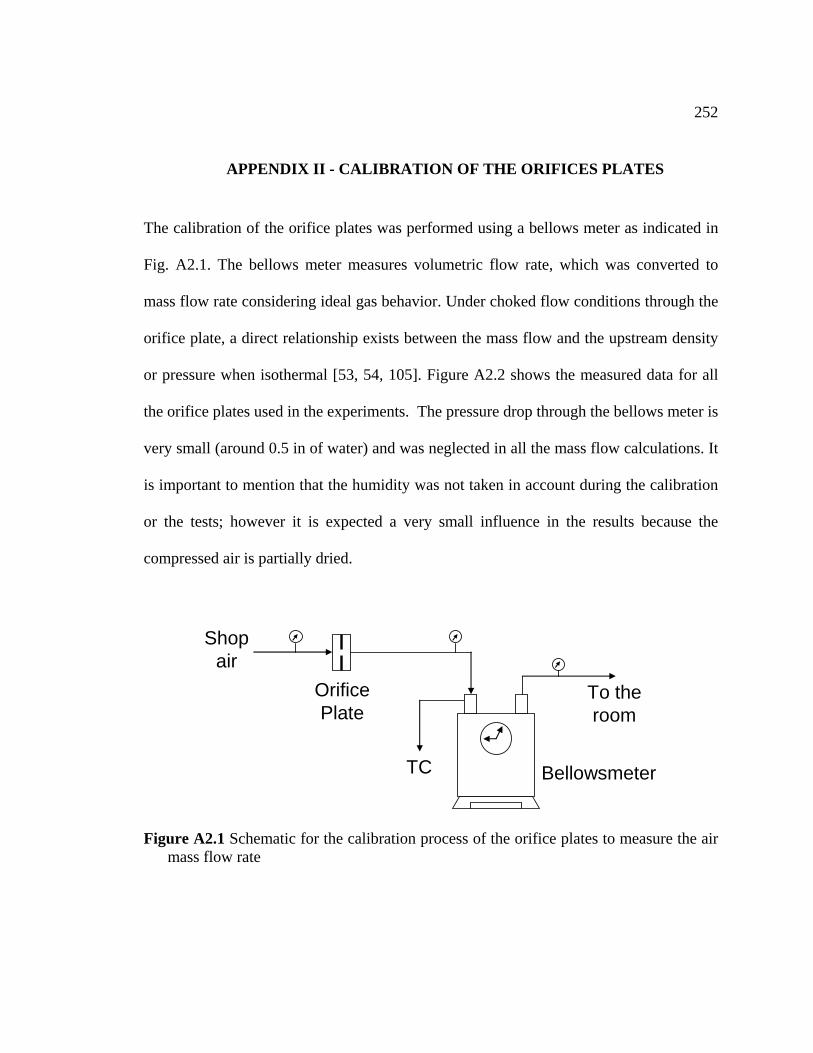
252
11 APPENDIX II - CALIBRATION OF THE ORIFICES PLATES
ifice plates was performed using a bellows meter as indicated in
s converted to
tions through the
orifice plate, a direct relationship exists between the mass flow and the upstream density
or pressure when isothermal [53, 54, 105]. Figure A2.2 shows the measured data for all
the orifice plates used in the experiments. The pressure drop through the bellows meter is
very small (around 0.5 in of water) and was neglected in all the mass flow calculations. It
is important to mention that the humidity was not taken in account during the calibration
or the tests; however it is expected a very small influence in the results because the
compressed air is partially dried.
The calibration of the or
Fig. A2.1. The bellows meter measures volumetric flow rate, which wa
mass flow rate considering ideal gas behavior. Under choked flow condi
OrificePlate
Bellowsmeter
To theroom
Shopair
TC
Figure A2.1 Schematic for the calibration process of the orifice plates to measure the air mass flow rate
253
a) b)
1.6
1.4
1.2
1.0
0.8
0.6
Aas
s F
g/s)
9080706050403020
3.6
3.2
ir M
low
(
Pressure (psig)
y 01602643x + 0.23 = 0. 448726
diam. = 0.044in
2.8
2.4
2.0
1.6
9080706050403020
Air
Mas
s F
g/s)
low
(
1.2
Pressure (psig)
y = 0.03559035x + 0.50548677
diam. = 0.065in
c)
7.0
6.0
5.0
4.0
3.0
Air
Mas
s Fl
ow (g
/s)
20 807060504030
y = 0.07259802x + 1.04373117
diam. = 0.095in
d)
14
90Pressure (psig)
12
10
8
6
Air
Ma
s Fl
ow
s(g
/s)
9080706050403020Pressure (psig)
y = 0.14918867x + 2.33092997
diam. = 0.139in
e) 32
28
24
20
16
12
Air
Mas
s Fl
ow (g
/s)
20 90807060504030
y = 0.30096650x + 5.60762889
diam 200in
Pressure (psig)
. = 0.
Figure A2.2 Calibration curves of the orifice plates used to measure the air mass flow.
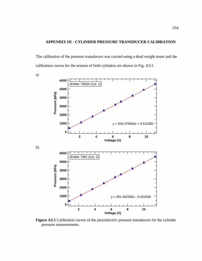
254
12 APPENDIX III - CYLINDER PRESSURE TRANSDUCER CALIBRATION
The calibration of the pressure transducers was carried using a dead weight tester and the
he sensors of both cylinders are shown in Fig. A3.1.
a)
calibration curves for t
6000
5000
4000
3000
2000
1000
0
Pres
sure
(kPa
)
108642Voltage (V)
Kistler 7063A (Cyl. 1)
y = 504.275053x + 9.512382
b)
6000
5000
4000
3000
2000
1000
108642
Kistler 7061 (Cyl. 2)
0
Pres
sure
(kPa
)
y = 491.362292x - 9.431848
Voltage (V)
Figure A3.1 Calibration curves of the piezoelectric pressure transducers for the cylinder
pressure measurements.
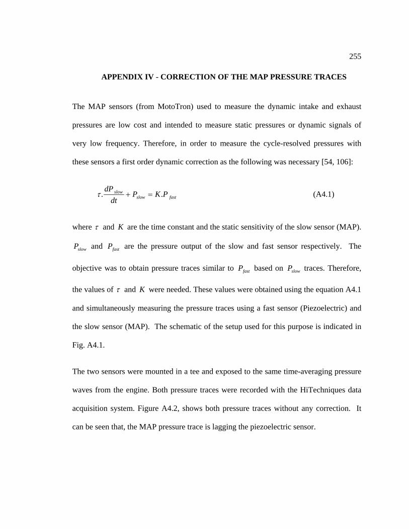
255
13
re the dynamic intake and exhaust
pressur
very low frequency. Therefore, in order to measure the cycle-resolved pressures with
ic correction as the following was necessary [54, 106]:
APPENDIX IV - CORRECTION OF THE MAP PRESSURE TRACES
The MAP sensors (from MotoTron) used to measu
es are low cost and intended to measure static pressures or dynamic signals of
these sensors a first order dynam
fastslowslow PKP
dtdP
.. =+τ (A4.1)
where τ and K are the time constant and the static sensitivity of the slow sensor (M
slowP and fastP are the pressure output of the slow
AP).
and fast sensor respectively. The
objective w s to obtain pressure traces similar to based on traces. Therefore,
f
a fastP slowP
the values o τ and K were needed. These values were obtained using the equation A4.1
and sim easuring the pressure traces using a fast sensor (Piezoelectric) and
the slow sensor (MAP). The schematic of the setup used for this purpose is indicated in
Fig. A4.1.
xposed to the same time-averaging pressure
waves from the engine. Both pressure traces were recorded with the HiTechniques data
acquisition system. Figure A4.2, sho
can be seen that, the MAP pressure trace is lagging the piezoelectric sensor.
ultaneously m
The two sensors were mounted in a tee and e
ws both pressure traces without any correction. It
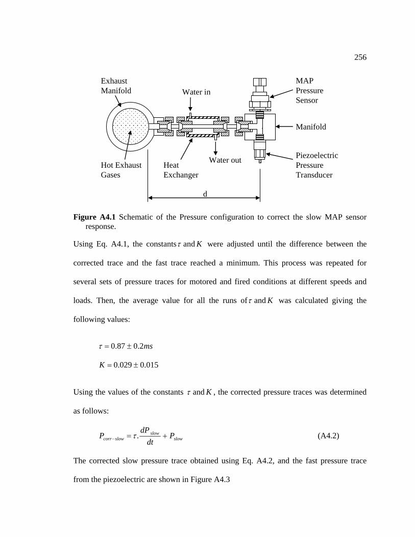
256
Water in
Water outHeatExchanger
Manifold
MAPPressureSensor
Exhaust anifoldM
Hot Exhaust Piezoelectric
GasesPressureTransducer
d
Figure A4.1 Schematic of the Pressure configuration to correct the slow MAP sensor response.
Using Eq. A4.1, the constantsτ and K were adjusted until the difference between the
corrected trace and the fast inimum. This process was repeated for
several sets of pressure traces for motored and fired conditions at different speeds and
ads. Then, the average value for all the runs of
trace reached a m
τ and K was calculated giving the lo
following values:
ms2.087.0 ±=τ
015.0029.0 ±=K
Using the values of the constants τ and K , the corrected pressure traces was determined
as follows:
slowslow
slowcorr Pdt
dPP +=− .τ (A4.2)
The corrected slow pressure trace obtained using Eq. A4.2, and the fast pressure trace
from the piezoelectric are shown in Figure A4.3
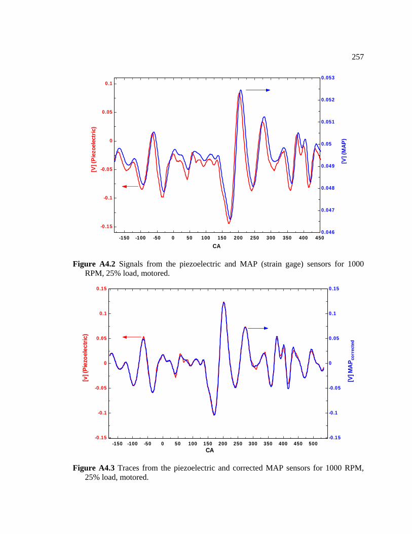
257
-150 -100 -50 0 50 100 150 200 250 300 350 400 450
-0.15
0.
-0.1
-0.05
0
0.05
1
0.046
0.047
0.048
0.049
0.05
0.051
0.052
0.053
] (Pi
ezoe
lect
ric)
[V] (
MAP
)
[V
CA
Signals from the piezoelectric and MAP (strain gage) sensors for 1000 RPM, 25% load, motored.
Figure A4.2
-150 -100 -50 0 50 100 150 200 250 300 350 400 450 500-0.15
-0.1
-0.05
0
0.05
0.1
0.15
-0.15
-0.1
-0.05
0
0.05
0.1
0.15
CA
[v] (
Piez
oele
ctric
)
[V] M
Aec
ted
Figure A r 1000 RPM, 25% load, m
P cor
r
4.3 Traces from the piezoelectric and corrected MAP sensors footored.
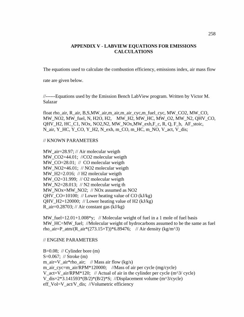
258
14 APPENDIX V - LABVIEW EQUCALCULA
ombustion efficiency, emissions index, air mass flow
//------Eq ns used by the Emission Bench LabView program. Written by Victor M. Salazar float rho_air, R_air, B,S,MW_air,m_air,m_air_cyc,m_fuel_cyc, MW_CO2, MW_CO, MW_NO2, MW_fuel, N, H2O, H2, MW_H2, MW_HC, MW_O2, MW_N2, QHV_CO, QHV_H2, HC_C1, NOx, NO2,N2, MW_NOx,MW_exh,F_c, R, Q, F_b, AF_stoic, N_air, Y_HC, Y_CO, Y_H2, N_exh, m_CO, m_HC, m_NO, V_act, V_dis;
// KNOWN PARAMETERS
MW_air=28.97; // Air molecular weigth MW_CO2=44.01; //CO2 molecular weigth MW_COMW_NO2=46.01; // NO2 molecular weigth
eigth 2 molecular weigth
QHV_CO=10100; // Lower heating value of CO (kJ/kg) QHV_H2=120000; // Lower heating value of H2 (kJ/kg) R_air=0.28703; // Air constant gas (kJ/kg) MW_fuel=12.01+1.008*y; // Molecular weight of fuel in a 1 mole of fuel basis MW_HC=MW_fuel; //Molecular weight of hydrocarbons assumed to be the same as fuel
P_atm/(R_air*(273.15+T))*6.89476; // Air density (kg/m^3) // ENGINE PARAMETERS B=0.08; // Cylinder bore (m) S=0.067; // Stroke (m) m_air=V_air*rho_air; // Mass air flow (kg/s) m_air_cyc=m_air/RPM*120000; //Mass of air per cycle (mg/cycle) V_act=V_air/RPM*120; // Actual of air in the cylinder per cycle (m^3/ cycle) V_dis=2*3.141593*(B ycle) eff_Vol=V_act/V_dis; //Volumetric efficiency
ATIONS FOR EMISSIONS TIONS
The equations used to calculate the c
rate are given below.
uatio
=28.01; // CO molecular weigth
MW_H2=2.016; // H2 molecular wMW_O2=31.999; // OMW_N2=28.013; // N2 molecular weig th MW_NOx=MW_NO2; // NOx assumed as NO2
rho_air=
/2)*(B/2)*S; //Displacement volume (m^3/c
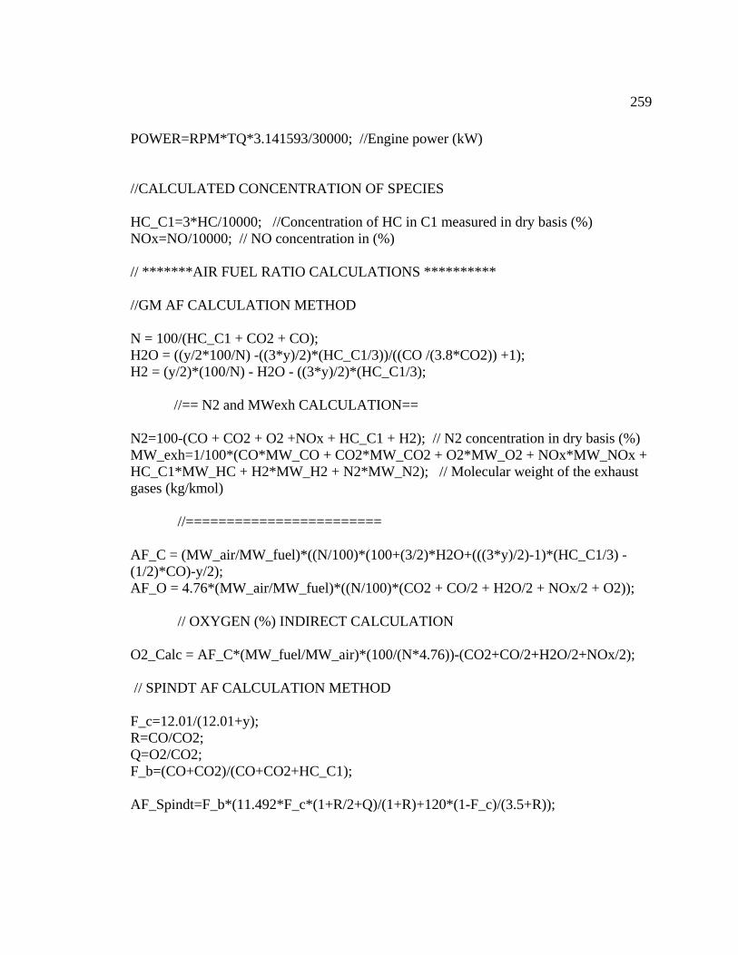
259
POWER=RPM*TQ* //CALCULATED CONCENTRATION OF SPECIES HC_C1=3*HC/10000; //Concentration of HC in C1 measured in dry basis (%) NOx=NO/10000; // NO concentration in (%) // *******AIR FUEL RATIO CALCULATIONS ********** //GM AF CALCULATION METHOD N = 100/(HC_C1 + CO2 + CO); H2O = ((y/2*100/N) -((3*y)/2)*(HC_C1/3))/((CO /(3.8*CO2)) +1); H2 = (y/2)*(100/N) - H2O - ((3*y)/2)*(HC_C1/3);
//== N2 and MWexh CALCULATION== N2=100-(CO + CO2 + O2 +NOx + HC_C1 + H2); // N2 concentration in dry basis (%) MW_exh=1/100*(CO*MW_CO + CO2*MW_CO2 + O2*MW_O2 + NOx*MW_NOx + HC_C1*MW_HC + H2*MW_H2 + N2*MW_N2); // Molecular weight of the exhaust gases (kg/kmol) //======================== AF_C = (MW_air/MW_fuel)*((N/100)*(100+(3/2)*H2O+(((3*y)/2)-1)*(HC_C1/3) - (1/2)*CO)-y/2); AF_O = 4.76*(MW_air/MW_fuel)*((N/100)*(CO2 + CO/2 + H2O/2 + NOx/2 + O2)); // OXYGEN (%) INDIRECT CALCULATION O2_Calc = AF_C*(MW_fuel/MW_air)*(100/(N*4.76))-(CO2+CO/2+H2O/2+NOx/2); // SPINDT AF CALCULATION METHOD F_c=12.01/(12.01+y); R=CO/CO2; Q=O2/CO2; F_b=(CO+CO2)/(CO+CO2+HC_C1); AF_Spindt=F_b*(11.492*F_c*(1+R/2+Q)/(1+R)+120*(1-F_c)/(3.5+R));
3.141593/30000; //Engine power (kW)
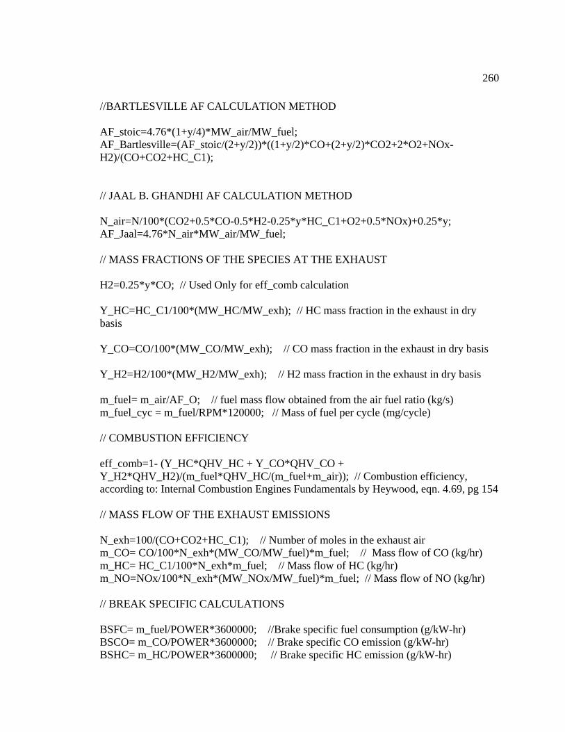
260
//BARTLESVILLE AF CALCULATION METHOD AF_stoic=4.76*(1+y/4)*MW_air/MW_fuel; AF_Bartlesville=(AF_stoic/(2+y/2))*((1+y/2)*CO+(2+y/2)*CO2+2*O2+NOx-H2)/(CO+CO2+HC_C1); // JAAL B. GHANDHI AF CALCULATION METHOD N_air=N/100*(CO2+0.5*CO-0.5*H2-0.25*y*HC_C1+O2+0.5*NOx)+0.25*y; AF_Jaal=4.76*N_air*MW_air/MW_fuel; // MASS FRACTIONS OF THE SPECIES AT THE EXHAUST H2=0.25*y*CO; // Used Only for eff_comb calculation Y_HC=HC_C1/100*(MW_HC/MW_exh); // HC mass fraction in the exhaust in dry basis Y_CO=CO/100*(MW_CO/MW_exh); // CO mass fraction in the exhaust in dry basis Y_H2=H2/100*(MW_H2/MW_exh); // H2 mass fraction in the exhaust in dry basis m_fuel= m_air/AF_O; // fuel mass flow obtained from the air fuel ratio (kg/s) m_fuel_cyc = m_fuel/RPM*120000; // Mass of fuel per cycle (mg/cycle) // COMBUSTION EFFICIENCY eff_comb=1- (Y_HC*QHV_HC + Y_CO*QHV_CO + Y_H2*QHV_H2)/(m_fuel*QHV_HC/(m_fuel+m_air)); // Combustion efficiency, according to: Internal Combustion Engines Fundamentals by Heywood, eqn. 4.69, pg 154 // MASS FLOW OF THE EXHAUST EMISSIONS N_exh=100/(CO+CO2+HC_C1); // Number of moles in the exhaust air m_CO= CO/100*N_exh*(MW_CO/MW_fuel)*m_fuel; // Mass flow of CO (kg/hr) m_HC= HC_C1/100*N_exh*m_fuel; // Mass flow of HC (kg/hr) m_NO=NOx/100*N_exh*(MW_NOx/MW_fuel)*m_fuel; // Mass flow of NO (kg/hr) // BREAK SPECIFIC CALCULATIONS BSFC= m_fuel/POWER*3600000; //Brake specific fuel consumption (g/kW-hr) BSCO= m_CO/POWER*3600000; // Brake specific CO emission (g/kW-hr) BSHC= m_HC/POWER*3600000; // Brake specific HC emission (g/kW-hr)
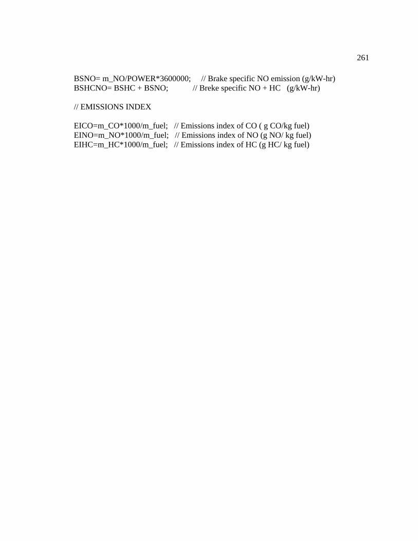
261
BSNO= m_NO/POWER*3600000; // Brake specific NO emission (g/kW-hr) BSHCNO= B
X
EICO=m_CO*1000/m_fuel; // Emissions index of CO ( g CO/kg fuel)
EIHC=m_HC*1000/m_fuel; // Emissions index of HC (g HC/ kg fuel)
SHC + BSNO; // Breke specific NO + HC (g/kW-hr) // EMISSIONS INDE
EINO=m_NO*1000/m_fuel; // Emissions index of NO (g NO/ kg fuel)
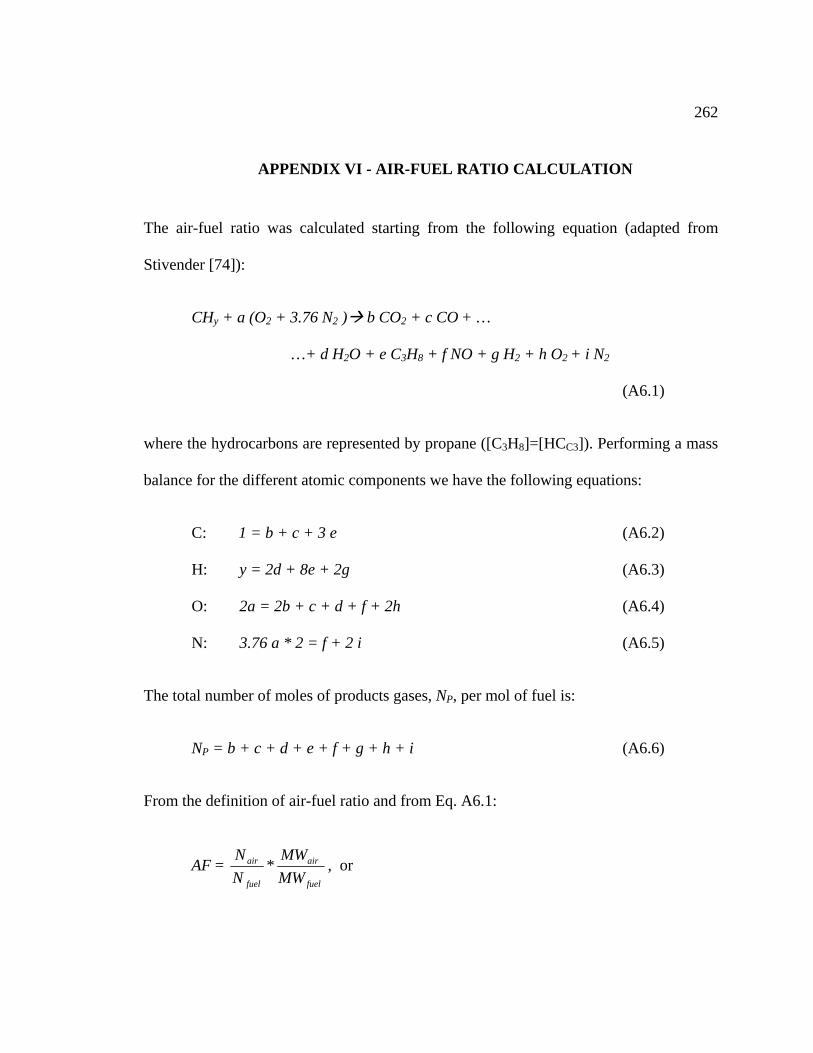
262
15 NDIX VI - AIR-FUEL RATIO CALCULATION
APPE
The air-fuel ratio was calculated starting from the following equation (adapted from
Stivender [74]):
CHy + a (O2 + 3.76 N2 ) b CO2 + c CO + …
…+
(A6.1)
where the hydrocarbons are represented by propane ([C3H8]=[HCC3]). Performing a mass
balance f
(A6.2)
H: y = 2d + 8e + 2g (A6.3)
O: 2a = 2b + c + d + f + 2h (A6.4)
(A6.5)
The total number of m
(A6.6)
From the definition of air-fuel ratio and from Eq. A6.1:
AF =
d H2O + e C3H8 + f NO + g H2 + h O2 + i N2
or the different atomic components we have the following equations:
C: 1 = b + c + 3 e
N: 3.76 a * 2 = f + 2 i
oles of products gases, NP, per mol of fuel is:
NP = b + c + d + e + f + g + h + i
fuelfuel
airair
MWMW
NN
* , or
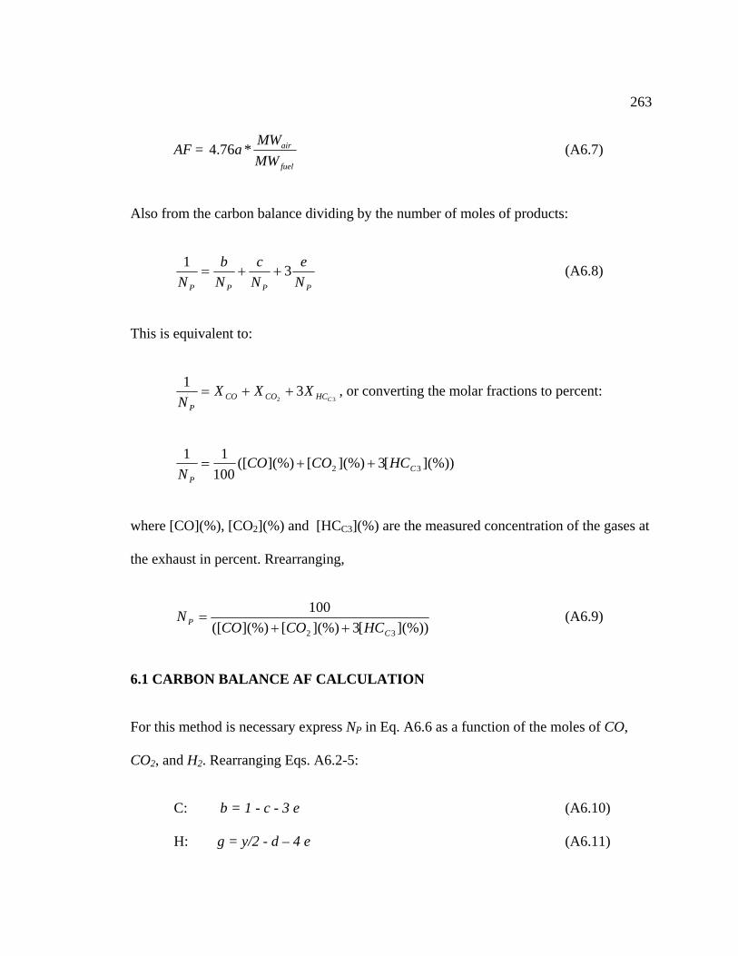
263
AF = fuel
air
MWMW
a *76.4 (A6.7)
Also from the carbon balance dividing by the number of moles of products:
PPPPN Ne
Nc
Nb 31
++= (A6.8)
This is equivalent to:
3231
CHCCOCO XXX ++= , or converting the molarPN
fractions to percent:
](%))[3](%)[](%)([100
1132 C
P
HCCOCON
++=
where [CO](%), [CO2](%) and [HCC3](%) are the measured concentration of the gases at
the exhaust in percent. Rrearranging,
](%))[3](%)[](%)([P HCCOCON
++= (A6.9) 100
32 C
6.1 CARBON BALANCE AF CALCULATION
P in Eq. A6.6 as a function of the moles of CO,
CO2, and H2. Rearranging Eqs. A6.2-5:
C: b = 1 - c - 3 e (A6.10)
H: g = y/2 - d – 4 e (A6.11)
For this method is necessary express N
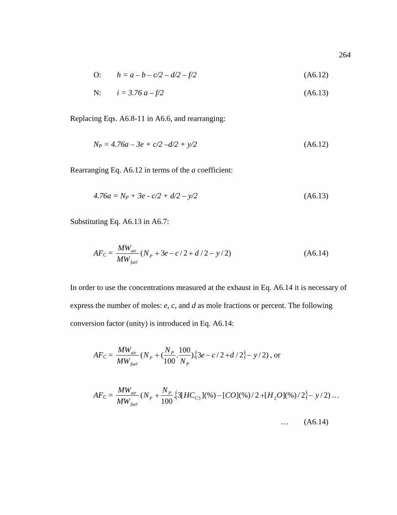
264
O d/2 – /2 6.12)
N: i = 3.76 a – f/2 (A6.13)
NP = 4.76a – 3e + c/2 –d/2 + y/2 (A6.12)
Rearranging Eq. A6.12 in term
ting Eq. A6.13 in A6.7:
AFC =
: h = a – b – c/2 – f (A
Replacing Eqs. A6.8-11 in A6.6, and rearranging:
s of the a coefficient:
4.76a = NP + 3e - c/2 + d/2 – y/2 (A6.13)
Substitu
)2/2/2/3( ydceNMWMW
Pfuel
air −+−+ (A6.14)
In order to use the concentrations measured at the exhaust in Eq. A6.14 it is necessary of
express the number of moles: e, c, and d as mole fractions or percent. The following
conversion factor (unity) is introduced in Eq. A6.14:
AFC = { } )2/2/2/3).100.100
(( ydceN
NNMWMW
P
PP
fuel
air −+−+ , or
AFC = { } )2/2/(%)][2/](%)[](%)[3.100
( 23 yOHCOHCNNMWMW
CP
Pfuel
air −+−+ …
… (A6.14)
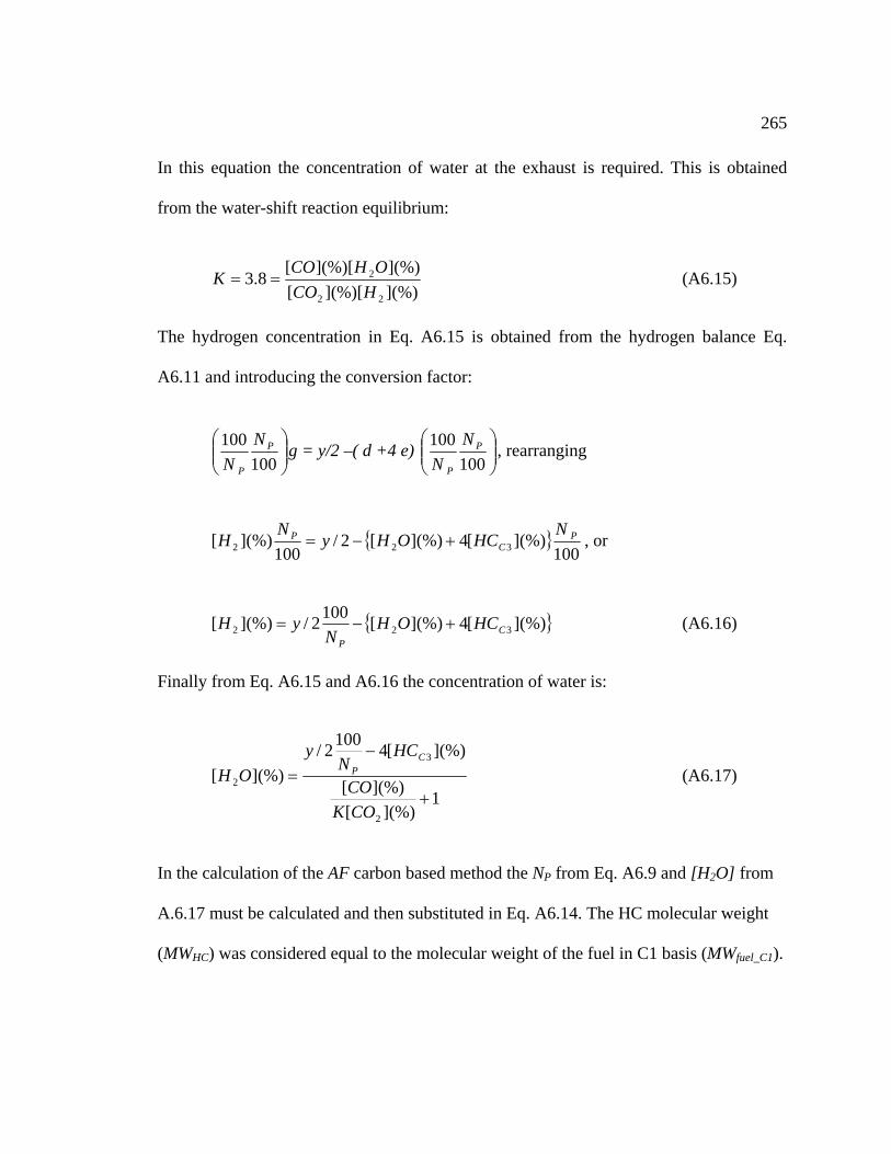
265
In this equation the concentration of water at the exhaust is required. This is obtained
from the water-shift reaction equilibrium:
](%)](%)[[](%)](%)[[8.3 2OHCOK == (A6.15
22 HCO)
rogen concentration in Eq. A6.15 is obtained from the hydrogen balance Eq. The hyd
A6.11 and introducing the conversion factor:
⎟⎟⎞⎛ 00 PN g = y/2 –( d +4 e) ⎠100P
⎜⎜⎝
1N ⎟⎟
⎞⎜⎛100 PN , rearranging
⎠⎜⎝ 100PN
{ }100
](%)[4](%)[2/100
](%)[ 2PH N
32P
CNHCOHy +−= , or
{ }](%)[4](%)[1002/](%)[ HCOHyH +−= (A6.16) 322 CN P
Finally from Eq. A6.15 and A6.16 the concentration of water is:
1](%)[2 CO
](%)[42/ 3− HCN
y CP
100
](%)[ =OH (A6.17)
[H2O] from
lar weight
MWfuel_C1).
](%)[ 2
+COK
In the calculation of the AF carbon based method the NP from Eq. A6.9 and
A.6.17 must be calculated and then substituted in Eq. A6.14. The HC molecu
(MWHC) was consi red equal to the molecular weight of the fuel in C1 basis (de
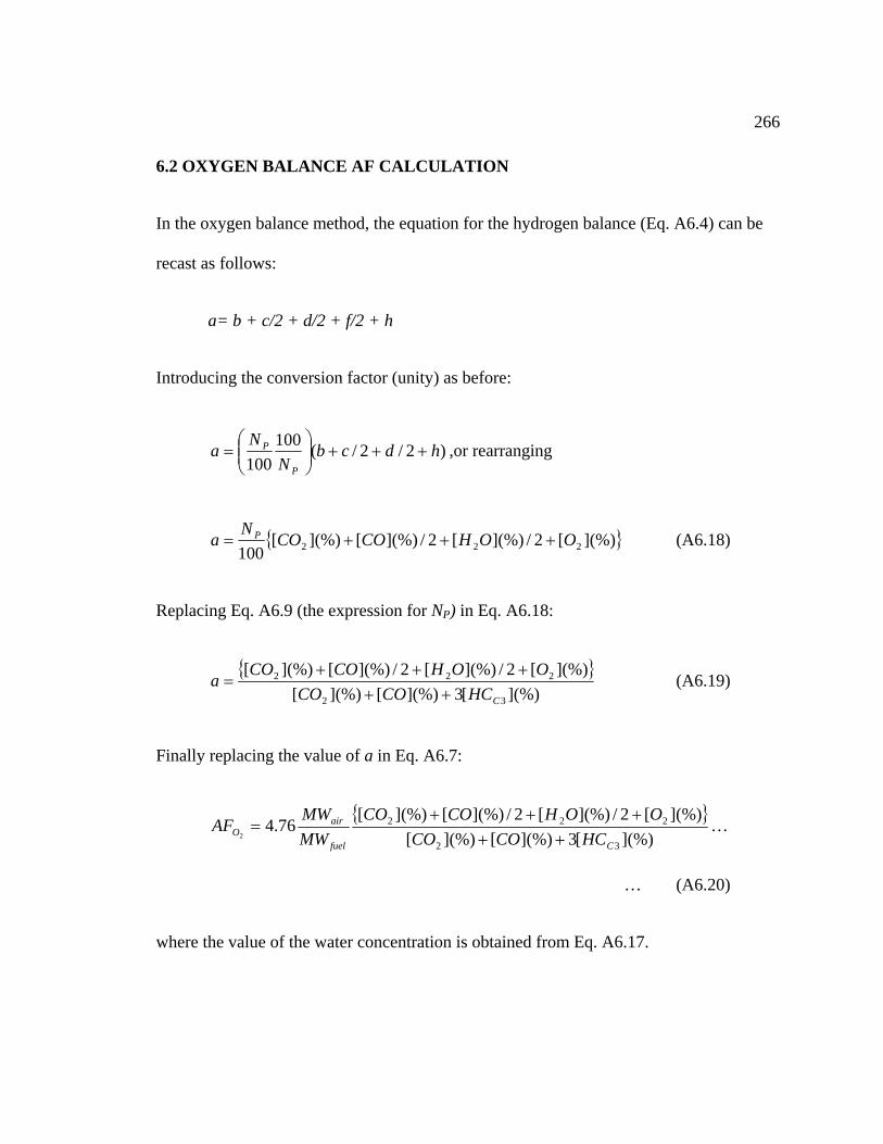
266
6.2 OXYGEN BALANCE AF CALCULATION
In the oxygen balance method, the equation for the hydrogen balance (Eq. A6.4) can be
) as before:
recast as follows:
a= b + c/2 + d/2 + f/2 + h
Introducing the conversion factor (unity
)2/2/( hdcba +++⎟⎟⎜⎜= ,or rearranging 100N P ⎞⎛100 N P ⎠⎝
{ }](%)[2/](%)[2/](%)[](%)[ 22 OOHCOCONa P +++= (A6.18)
pression for NP) in Eq. A6.18:
100 2
Replacing E . A6.9 (the exq
{ }](%)[3](%)[](%)[
](%)[2/](%)[2/](%)[](%)[ OOHCOCO +++=a
32
222
CHCCOCO ++ (A6.19)
.7: Finally replacing the value of a in Eq. A6
{ }](%)[3](%)[](%)[
76.432
2C
O HCCOCOMWAF
++=
](%)[2/](%) 2O+ …
… (A6.20)
[2/](%)[](%)[ 22air OHCOCOMW ++
fuel
where the value of the water concentration is obtained from Eq. A6.17.
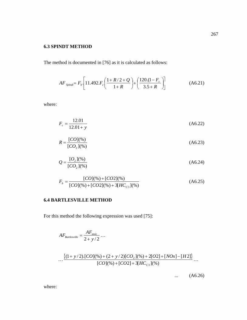
267
6.3 SPINDT METHOD
The method is documented in [76] as it is calculated as follows:
⎥⎦
⎢⎣ ⎠⎝ +⎠⎝ + RRcbSpindt 5.31
⎤⎡ ⎞⎛ −⎞⎛ ++ FQRFF c1.(1202/1 (A6.21) =AF ⎟⎜+⎟⎜.492.11.
where:
yc +01.12F = (A6.22) 01.12
](%)[CO ](%)[COR = (A6.23)
2
](%)[COQ = ](%)[ 2O (A6.24)
2
](%)[3](%)2[](%)[ 3CHCCOCO ++](%)2[](%)[
bCOCOF +
= (A6.25)
6.4 BARTLESVILLE METHOD
For this method the following expression was used [75]:
2/2 yAAF+Fstoic … leBartlesvil =
{ }… ]2[][]2[2](%))[2/2(](%)).[2/1( HNOxOCOyCOy −+++++
](%)[3]2[](%)[ 3CHCCOCO ++2 …
... (A6.26)
where:
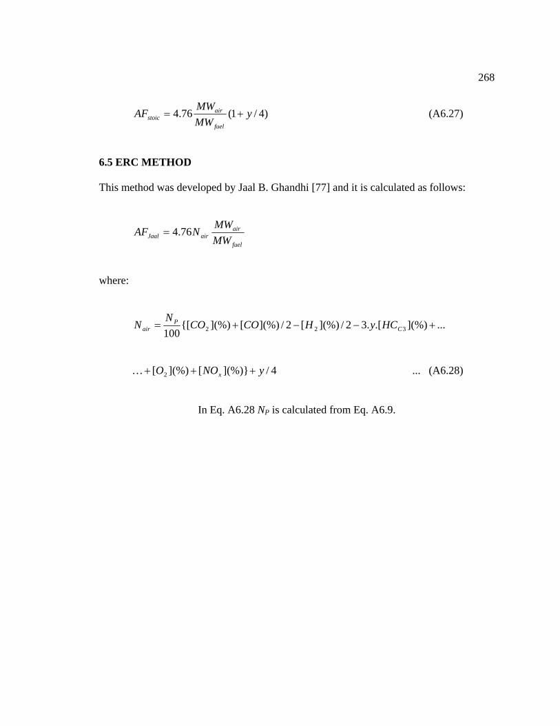
268
)4/1(76.4 yMW
AF air += (A6.27) MW fuel
This method was developed by Jaal B. Ghandhi [77] and it is calculated as follows:
stoic
6.5 ERC METHOD
fuel
airairJaal MW
MWNAF 76.4=
where:
...](%).[.32/](%)[2/](%)[](%){[100 322 +−−+= C
Pair HCyHCOCONN
… 4/](%)}[](%)[ 2 yNOO x +++ ... (A6.28)
In Eq. A6.28 NP is calculated from Eq. A6.9.
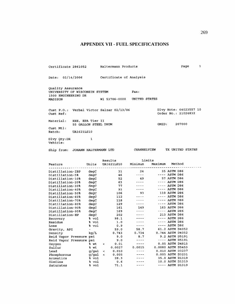
269
APPENDIX VII - FUEL SPECIFICATIONS
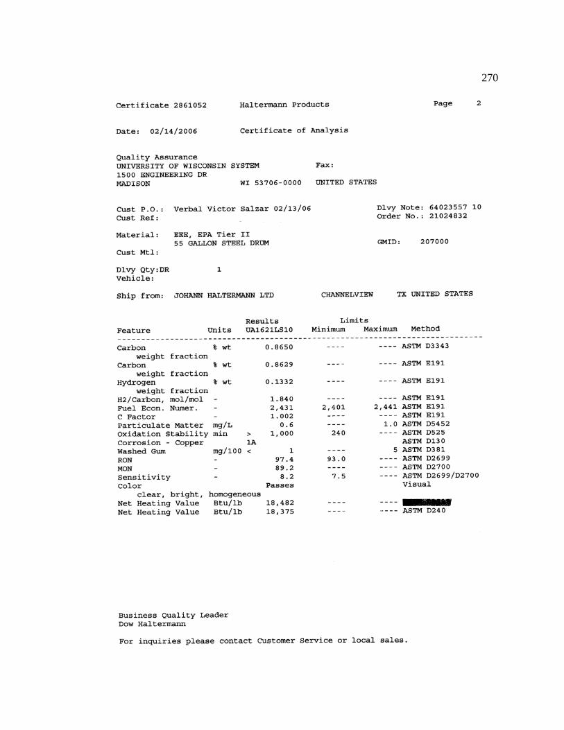
270
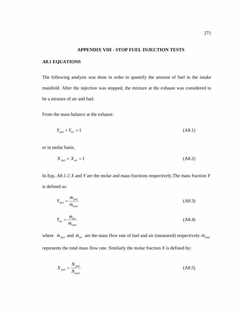
271
16 APPENDIX VIII - STOP FUEL INJECTION TESTS
e
(A8.1)
A8.1 EQUATIONS
The following analysis was done in order to quantify the amount of fuel in the intak
manifold. After the injection was stopped, the mixture at the exhaust was considered to
be a mixture of air and fuel.
From the mass balance at the exhaust:
1=+ airfuel YY
or in molar basis,
1=+ airfuel XX (A8.2)
In Eqs. A8.1-2 X and Y are the molar and mass fractions respectively.The mass fraction Y
is defined as:
fuelmY
&= (A8.3)
totalfuel m&
totalair m
Y&
= (A8.4) airm&
where m& and fuel airm& are the mass flow rate of fuel and air (measured) respectively
ed by:
. totalm&
represents the total mass flow rate. Similarly the molar fraction X is defin
total
fuel
N& (A8.5) fuel
NX
&=
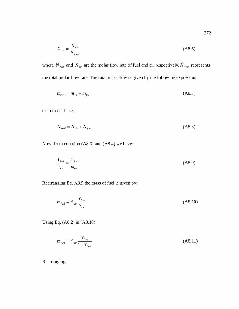
272
totalair N&
airX = N&
(A8.6)
spectively represents . totalN&where fuelN& and airN& are the molar flow rate of fuel and air re
the total molar flow rate. The total mass flow is given by the following expression:
fuelair mmm &&& += (A8.7) total
or in molar basis,
fuelairtotal NNN &&& += (A8.8)
Now, from equation (A8.3) and (A8.4) we have:
airair mY &fuelfuel = (A8.9)
mY &
Rearranging Eq. A8.9 the mass of fuel is given by:
airYfuel
airfuel
Ymm && = (A8.10)
Using Eq. (A8.2) in (A8.10)
fuelairfuel Y
mm−
=1
&& (A8.11) Yfuel
Rearranging,
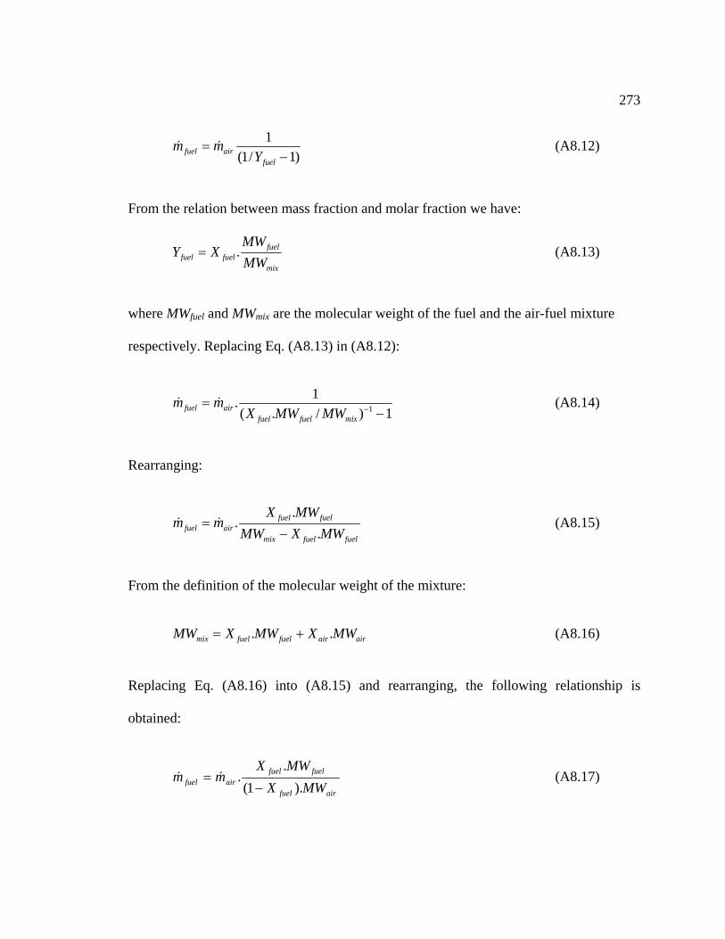
273
)1/1( −fuelY1
= airfuel mm && (A8.12)
From the relation between mass fraction and molar fraction we have:
mixMWfuel
fuelfuel
MWXY .= (A8.13)
where MW MW ture fuel and mix are the molecular weight of the fuel and the air-fuel mix
respectively. Replacing Eq. (A8.13) in (A8.12):
1)/.( 1 −−mixfuelfuel MWMWX
1.= airfuel mm && (A8.14)
Rearranging:
fuelfuelmix MWXMW .−fuelfuel
airfuel
MWXmm
..= && (A8.15)
From the definition of the molecular weight of the mixture:
fuelfuelmix airair MWXMWXMW .. += (A8.16)
Replacing Eq. (A8.16) into (A8.15) and rearranging, the following relationship is
obtained:
airfuel MWX ).1( −fuelfuel
airfuel mm .= && (A8.17MWX .
)
274
which is the equation that allows conversion of the mass fraction, Xfuel, (measured by the
FFID) into mass of fuel in mg per cycle.
In equation (A8.17) the molecular weight of the fuel is the molecular weight on a C1
(A8.18)
basis, and it is calculated as follows:
HCfuel MWyMWMW .+=
where 0011.12=MW is atomic weight of the carbon, 0079.1C =H
o of the fuel per mol
MW is the atomic
of C1:
(A8.19)
weight of the hydrogen and y is the hydrogen to carbon rati
CHy /= ratio of the fuel
The fuel molar concentration must be provided in molar fraction. Therefore the
concentration of the fuel being read by the FFID in ppm must be converted to molar
fraction by using the following conversion:
63 10/.3 fuelCfuel XX = (A8.20)
where X C3fuelC3 is the concentration of the fuel in a base (because propane was used to
calibrate the fast-FID).
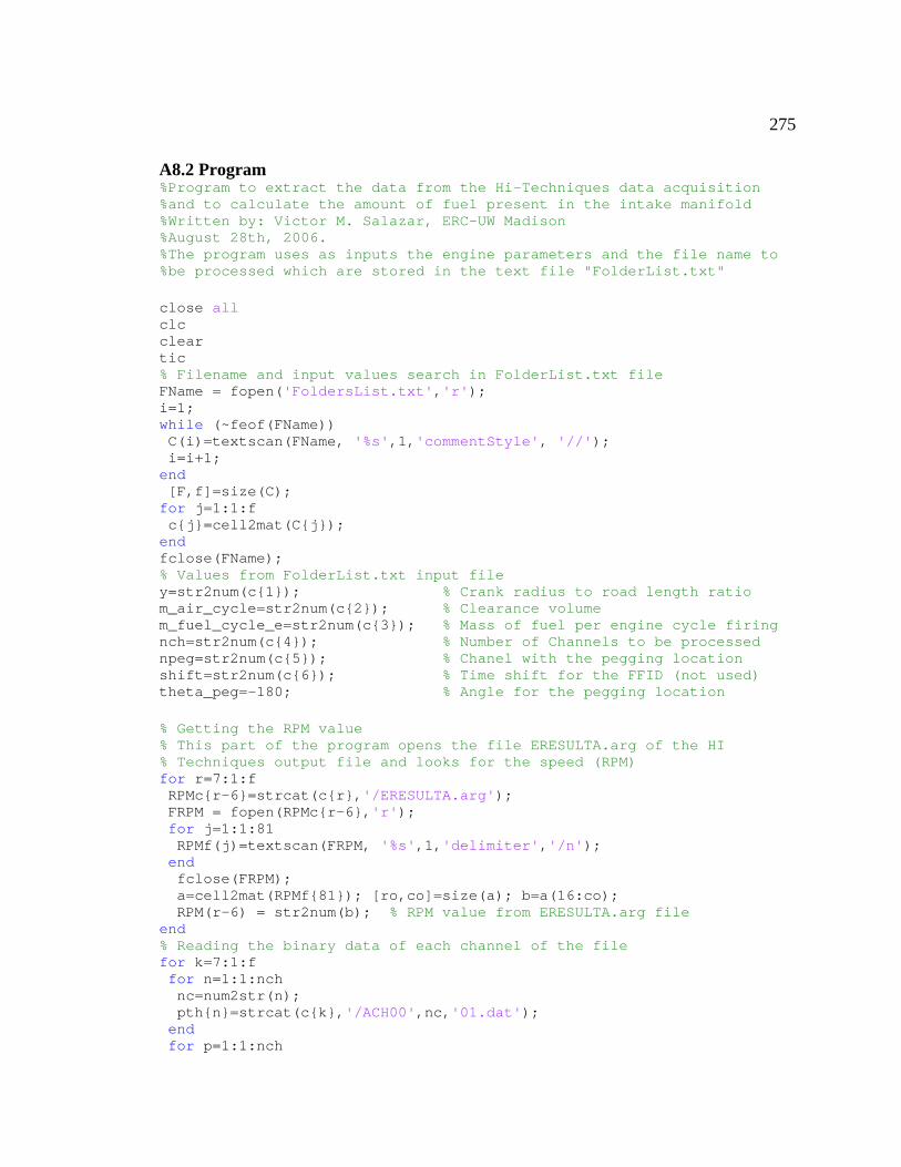
275
A8.2 Program %Program to extract the data from the Hi-Techniques data acquisition %and to calculate the amount of fuel present in the intake manifold %Written by: Victor M. Salazar, ERC-UW Madison %August 28th, 2006. %The program uses as inputs the engine parameters and the file name to
% Crank radius to road length ratio
ng
FID (not used) for the pegging location
%be processed which are stored in the text file "FolderList.txt" close all clc clear tic % Filename and input values search in FolderList.txt file FName = fopen('FoldersList.txt','r'); i=1; while (~feof(FName)) C(i)=textscan(FName, '%s',1,'commentStyle', '//'); i=i+1; end [F,f]=size(C); for j=1:1:f c{j}=cell2mat(C{j}); end fclose(FName);
rList.txt input file % Values from Folde y=str2num(c{1});
m_air_cycle=str2num(c{2}); % Clearance volume m_fuel_cycle_e=str2num(c{3}); % Mass of fuel per engine cycle firinch=str2num(c{4}); % Number of Channels to be processed npeg=str2num(c{5}); % Chanel with the pegging location
me shift for the Fshift=str2num(c{6}); % Titheta_peg=-180; % Angle % Getting the RPM value
rg of the HI % This part of the program opens the file ERESULTA.a% Techniques output file and looks for the speed (RPM) for r=7:1:f RPMc{r-6}=strcat(c{r},'/ERESULTA.arg'); FRPM = fopen(RPMc{r-6},'r'); for j=1:1:81 RPMf(j)=textscan(FRPM, '%s',1,'delimiter','/n'); end fclose(FRPM); a=cell2mat(RPMf{81}); [ro,co]=size(a); b=a(16:co);
A.arg file RPM(r-6) = str2num(b); % RPM value from ERESULTend % Reading the binary data of each channel of the file for k=7:1:f for n=1:1:nch nc=num2str(n); pth{n}=strcat(c{k},'/ACH00',nc,'01.dat'); end for p=1:1:nch
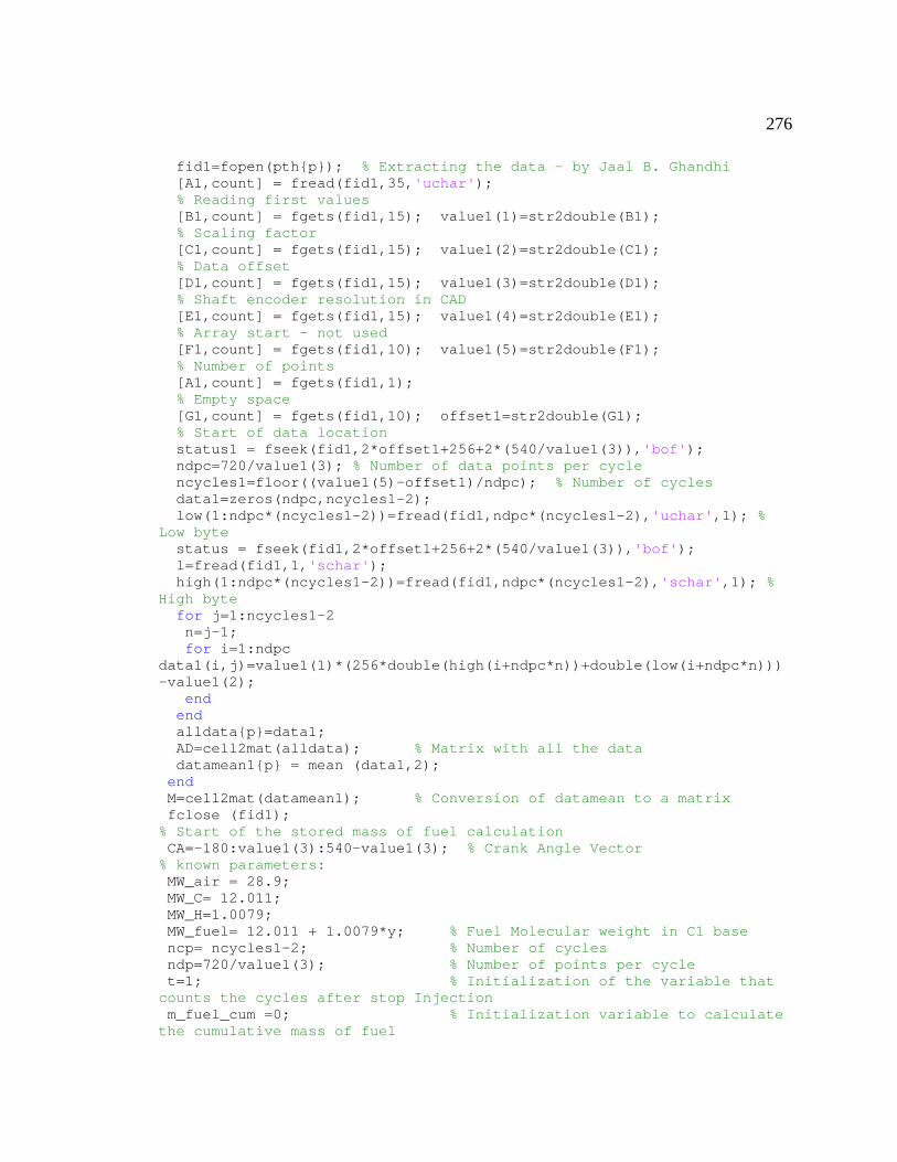
276
fid1=fopen(pth{p}); % Extracting the data - by Jaal B. Ghandhi
,15); value1(2)=str2double(C1);
et1+256+2*(540/value1(3)),'bof');
1)/ndpc); % Number of cyclespc,ncycles1-2);
,1,'schar');
1:ndpc
l the data
after stop Injection % Initialization variable to calculate
[A1,count] = fread(fid1,35,'uchar'); % Reading first values [B1,count] = fgets(fid1,15); value1(1)=str2double(B1); % Scaling factor [C1,count] = fgets(fid1 % Data offset [D1,count] = fgets(fid1,15); value1(3)=str2double(D1); % Shaft encoder resolution in CAD [E1,count] = fgets(fid1,15); value1(4)=str2double(E1); % Array start - not used [F1,count] = fgets(fid1,10); value1(5)=str2double(F1); % Number of points [A1,count] = fgets(fid1,1); % Empty space [G1,count] = fgets(fid1,10); offset1=str2double(G1); % Start of data location status1 = fseek(fid1,2*offs ndpc=720/value1(3); % Number of data points per cycle ncycles1=floor((value1(5)-offset data1=zeros(nd low(1:ndpc*(ncycles1-2))=fread(fid1,ndpc*(ncycles1-2),'uchar',1); % Low byte status = fseek(fid1,2*offset1+256+2*(540/value1(3)),'bof'); l=fread(fid1 high(1:ndpc*(ncycles1-2))=fread(fid1,ndpc*(ncycles1-2),'schar',1); % High byte for j=1:ncycles1-2 n=j-1; for i=data1(i,j)=value1(1)*(256*double(high(i+ndpc*n))+double(low(i+ndpc*n)))-value1(2); end end alldata{p}=data1; AD=cell2mat(alldata); % Matrix with al datamean1{p} = mean (data1,2); end M=cell2mat(datamean1); % Conversion of datamean to a matrix fclose (fid1); % Start of the stored mass of fuel calculation CA=-180:value1(3):540-value1(3); % Crank Angle Vector % known parameters: MW_air = 28.9; MW_C= 12.011; MW_H=1.0079;
1.0079*y; % Fuel Molecular weight in C1 base MW_fuel= 12.011 + ncp= ncycles1-2; % Number of cycles ndp=720/value1(3); % Number of points per cycle
le that t=1; % Initialization of the variab counts the cycles
m_fuel_cum =0; the cumulative mass of fuel
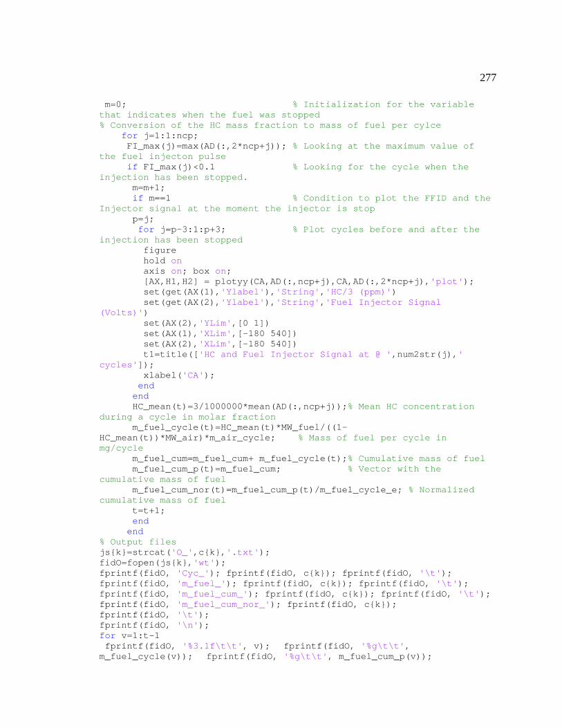
277
m=0; % Initialization for the variable
the HC mass fraction to mass of fuel per cylce
dition to plot the FFID and the
% Plot cycles before and after the
),'
ycle in
l_cycle_e; % Normalized
'Cyc_'); fprintf(fidO, c{k}); fprintf(fidO, '\t');
(fidO, c{k}); fprintf(fidO, '\t');
m_p(v));
that indicates when the fuel was stopped % Conversion of for j=1:1:ncp; FI_max(j)=max(AD(:,2*ncp+j)); % Looking at the maximum value of the fuel injecton pulse if FI_max(j)<0.1 % Looking for the cycle when the injection has been stopped. m=m+1; if m==1 % ConInjector signal at the moment the injector is stop p=j; for j=p-3:1:p+3; injection has been stopped figure hold on axis on; box on; [AX,H1,H2] = plotyy(CA,AD(:,ncp+j),CA,AD(:,2*ncp+j),'plot'); set(get(AX(1),'Ylabel'),'String','HC/3 (ppm)') set(get(AX(2),'Ylabel'),'String','Fuel Injector Signal (Volts)') set(AX(2),'YLim',[0 1])
set(AX(1),'XLim',[-180 540]) set(AX(2),'XLim',[-180 540]) t1=title(['HC and Fuel Injector Signal at @ ',num2str(jcycles']); xlabel('CA'); end end HC_mean(t)=3/1000000*mean(AD(:,ncp+j));% Mean HC concentration during a cycle in molar fraction m_fuel_cycle(t)=HC_mean(t)*MW_fuel/((1-HC_mean(t))*MW_air)*m_air_cycle; % Mass of fuel per cmg/cycle m_fuel_cum=m_fuel_cum+ m_fuel_cycle(t);% Cumulative mass of fuel m_fuel_cum_p(t)=m_fuel_cum; % Vector with the cumulative mass of fuel
t)/m_fue m_fuel_cum_nor(t)=m_fuel_cum_p(cumulative mass of fuel t=t+1; end end % Output files
k},'.txt'); js{k}=strcat('O_',c{fidO=fopen(js{k},'wt'); fprintf(fidO,fprintf(fidO, 'm_fuel_'); fprintf(fidO, c{k}); fprintf(fidO, '\t'); fprintf(fidO, 'm_fuel_cum_'); fprintf fprintf(fidO, 'm_fuel_cum_nor_'); fprintf(fidO, c{k}); fprintf(fidO, '\t'); fprintf(fidO, '\n'); for v=1:t-1 fprintf(fidO, '%3.1f\t\t', v); fprintf(fidO, '%g\t\t', m_fuel_cycle(v)); fprintf(fidO, '%g\t\t', m_fuel_cu
278
fprintf(fidO, '%g\t\t', m_fuel_cum_nor(v)); fprintf(fidO, '\n'); end fclose(fidO);
disp(toc/60);
end toc % time that takes to run the program disp(['Elapsed time in minutes:']);
279
17 APPENDIX IX - HITECHNIQUES PRESSURE CODE
% Displacement volume
r the pegging
nders he cyl 2
; % Angle between cyls in CA
% Pegg. Cyl. 1, if manual: = 1, if MAP(or Ch.): peg1Option = 2
2
s
ift
els for Phase Shift
on r
%Program to extract the binary data from the HiTechniques data
%acquisition and to correct the time delay of the MAP sensors and the%FFID traces. The inputs and file names were provided through a GUI. %Beginning of Main Code - Pressure Data Processing %Getting the Engine Parameters R = handles.metricdata.lrdata ; % Crank radius to road length ratio
% Clearance volume Vc = handles.metricdata.Vcdata ; data ; Vdisp = handles.metricdata.Vd
theta_peg = - 180 ; % Angle folocation ncyl = numofcylinders_index ; % Number of cyli
ue')+1; % Channel with tchcyl2 = get(handles.chancyl2, 'Valta.anglecylphacyl = handles.metricda
% End Getting the Engine Parameters rConst ; fc = handles.metricdata.Filte
%Getting the Engine Filter Constant = manualpegging_index; peg1Option
on peg1Optipeg2Option = manualpch2_index; % Pegg. Cyl. 1, if manual: peg2Option = 1, if MAP(or Ch.): peg2Option = 2 P_m_peg1 = ppegging1; % Pressure for the manual pegging Cyl.1, in kPa P_m_peg2 = ppegging2; % Pressure for the manual pegging Cyl.2, in kPa nch_peg1 = channel1MAP; % Channel with pressure data for pegging Cyl. 1 nch_peg2 = channel2MAP; % Channel with pressure data for pegging Cyl. 2 % Phase Shift for MAP Sensors-Mototron SENSPRESS001H00 if correction1_index == 1 % MAP Cyl. 1 cpeg1 = 1; % Phase Shift, MAP Cyl 1 else
yl 1 cpeg1 = 0; % No Phase Shift, MAP Cend if correction2_index == 1 %---MAP Cyl. 2--- cpeg2 = 1 ; % Phase Shift, MAP Cylelse cpeg2 = 0 ; % No Phase Shift, MAP Cyl 2 end % Other Channels with MAP data for Phase Shift (Maximum of 2 chnlif othercorrection_index == 1
for Phase Sh omapch = 1 ; % There are more channels elseif othercorrection_index == 2
% No more chann omapch = 0 ; end nomapch = numchannels4map ; % Number of other channels for correctichomap1 = chomap1_index ; % Channel for the first other MAP sensorchomap2 = chomap2_index ; % Channel for the second other MAP senso
280
% End of Phase Shift for MAP Sensors-Mototron SENSPRESS001H00 nchfid = ffidchannchfid1 = chffid1_in
els_index-1 ; % Channels for fast FID dex ; % 1st Channel with FFID Data
a fid1v ; % Time shift for the fid1 id2v ; % Time shift for the fid2
A.arg file
rcat( bdata( r ) , '/ERESULTA.arg' ) ; n( RPMc{r}, 'r' ) ; -1
s table or file
1 : 81 = textscan( FRPM, '%s', 1, 'delimiter' , '/n'); % he lines of:... /ERESULTA.arg
; % Row with the RPM value size
ue e from ERESULTA.arg file
'CA_Pmax1'); fprintf(fida, '\t'); 'Pmax1(kPa)'); fprintf(fida, '\t');
'IMEP1 (kPa)'); fprintf(fida, '\t'); 'Ppeg1 (kPa)'); fprintf(fida, '\t');
'\t');
'Ppeg2 (kPa)'); fprintf(fida, '\t'); 'COV_2'); fprintf(fida, '\t');
hannel Reading
binary file
'Error');
chfid2 = chffid2_index ; % 2nd Channel with FFID Datshfid1 = handles.metricdata.timefshfid2 = handles.metricdata.timeff% Getting the Engine Speed (RPM) from the ERESULTer = 0; err = 0; for r = 1 : 1 : sbdata RPMc{r} = st FRPM = fope if FRPM == errordlg('File ERESULTA.arg could not be found or accessed under specified folder. Check Folder Nameavailability.','Error'); er = 1; else for j = 1 : RPMf( j )Storage of t end fclose(FRPM); a = cell2mat( RPMf{ 81 } ) [ ro, co] = size( a ) ; % RPM line b = a( 16: co ) ; % RPM val RPM(r) = str2num(b); % RPM valu end end if er==0 if outfiles_index == 1
O.txt','wt') ; fida = fopen('HT_ADD_AVG_INF fprintf(fida, 'FileName'); fprintf(fida, '\t'); fprintf(fida, fprintf(fida, fprintf(fida, fprintf(fida, fprintf(fida, 'COV_1'); fprintf(fida, fprintf(fida, 'CA_Pmax2'); fprintf(fida, '\t'); fprintf(fida, 'Pmax2(kPa)'); fprintf(fida, '\t');
MEP2 (kPa)'); fprintf(fida, '\t'); fprintf(fida, 'I fprintf(fida, fprintf(fida, fprintf(fida, '\n'); end % Start Data File and C f = sbdata ; % Number of Pressure Data Files or Folders nump = 1 ; for k = 1 : 1 : f for p = 1 : 1 : numofchannels_index fid1 = fopen( folderpath{nump} ) ; % Reading of if fid1 == -1 errordlg('File ACH00x01.dat could not be found or accessed',
281
err=1; else [A1,count] = fread(fid1,35,'uchar'); [B1,count] = fgets(fid1,15); value1(1)=str2double(B1); % data scaling factor [C1,count] = fgets(fid1,15); value1(2)=str2double(C1); % data
); value1(3)=str2double(D1); % shaft
; value1(4)=str2double(E1); % array
=str2double(F1); % number
% empty
); offset1=str2double(G1); % start
the data start in the file are 2 bytes in
header ression alue1 ( 3
( 3 ) ; % Number of data points per cycle % Number
, 2 * offset1 + 256 + 2 * ( 540 / value1( 3 ) ack to the bof ' ) ; % Move pointer 1 byte for
d( fid1 , ndpc * ( byte that includes sign
: ndpc
e1( 1 ) * (256 * double( high( i + ndpc * n ndpc * n ) )) - value1( 2 ) ;
x with All data n of datamean to matrix
offset [D1,count] = fgets(fid1,15encoder resolution in CAD [E1,count] = fgets(fid1,15)start - not used [F1,count] = fgets(fid1,10); value1(5)of points [A1,count] = fgets(fid1,1); space [G1,count] = fgets(fid1,10of data location % Move pointer to where % the factor of 2 arises from the fact that the datalength % the factor of 256 accounts the file% the 540/value(3) is necessary to get the data at BDC of comp status1 = fseek( fid1 , 2 * offset1 + 256 + 2 * ( 540 / v) ) , 'bof' ) ; ndpc = 720 / value1 ncycles1 = floor( ( value1( 5 ) - offset1 ) / ndpc ) ; of cycles data1 = zeros( ndpc , ncycles1 - 2 ) ; % Data initialization low( 1 : ndpc * ( ncycles1 - 2 ) ) = fread( fid1 , ndpc * (ncycles1 - 2 ) , 'uchar' , 1 ) ; % Low byte status = fseek( fid1) , 'bof' ) ; % Moving pointer b l = fread( fid1 , 1 , 'scharoptimization purpose
a high( 1 : ndpc * ( ncycles1 - 2 ) ) = frencycles1 - 2 ) , 'schar' , 1 ) ; % High% Data Storing in the "data1" matrix for j = 1 : ncycles1 - 2 n = j - 1; for i = 1 data1( i , j ) = valu) ) + double( low( i + end end alldata{ p } = data1 ; datamean1{ p } = mean ( data1 , 2 ); nump = nump + 1 ; end end if err==1 err=0; else AD = cell2mat( alldata ) ; % Main Matri M = cell2mat( datamean1 ) ; % Conversio
282
fclose (fid1); end chcount = zeros (1,numofchannels_index);
lculation (Only once per file% Parameters Ca )
e1(3) ;
i ) * pi / 180 ) ;
( CA ( i ) * pi / 180 ) + ( sin
ored
value1( 3 ) ) ; alue1( 3 ) ) ; -------------------------
ing, 2= Pegging from
= AD(:, ncp * ( nch_peg1 -1 ) + 1 : ncp * ( nch_peg1 -1
ncp * ndp )'; ict ) ;
* RPM( k ) ) ; % Time
1 * ( AllMAP1D( 1 ) + tau1 * ( ( dt ) ) ) ;
u1 * ((
_CORR( ncp*ndp - 1 ) = 1 / K1 * ( AllMAP1D( ncp*ndp ) + llMAP1D( ncp*ndp - 2 ) ) / ( 2 * dt )
p) = 1 / K1 * ( AllMAP1D( 1 ) + tau1 * ( ( ncp*ndp - 1 ) ) / ( 2 * dt ) ) ) ;
tau1 * ( ( ) ;
, ndp , ncp);
% Cyl. 1 CA = -180 : value1(3) : 540-valu for i = 1 : 720 / value1(3) Vol ( i ) = Vc + (Vdisp / 2) * ( R + 1 - cos ( CA () - sqrt ( R * R - ( sin ( CA ( i ) * pi / 180 ) ) ^ 2 ) dV_dtetha ( i ) = Vdisp / 2 * ( sin( CA ( i ) * pi / 180 ) * cos ( CA ( i ) * pi / 180 ) ) / ( sqrt ( R ^ 2 - ( sin ( CA ( i ) * pi / 180 ) ) ^ 2 ) ) ) ; end % IMEP Calculation ncp = ncycles1 - 2 ; % Number of cycles st ndp = 720 / value1( 3 ) ; % Number of data points per cycle P_1_sumi = zeros( 1 , 720 / P_2_sumi = zeros( 1 , 720 / v%------------------------Cylinder 1- chcount(1) = 1 ; for j = 1 : ncycles1 - 2 Pmax1( j ) = 0 ; if peg1Option == 1 % 1=Manual Pegging, 2= Pegging from pressure trace-channel P_MAP_peg1 = P_m_peg1 ; elseif peg1Option == 2 % 1=Manual Peggpressure trace-channel chcount(nch_peg1) = 1 ; if j == 1 % Asigning all the data to a matrix AllMAP) + ncp ); AllMAP1D = AllMAP( : ) ; CAfict = ( 1 : 1 : AllMAP1D = csaps ( CAfict , AllMAP1D , fc , CAf% MAP Correction for all the cycles in Cylinder 1 dt = 1000 * value1( 3 ) / ( 6 step calculation if cpeg1 == 1 % phase shift of pegging pressure MAP_R_CORR( 1 ) = 1 / KAllMAP1D( 2 ) - AllMAP1D( ncp*ndp ) ) / ( 2 * MAP_R_CORR( 2 ) = 1 / K1 * ( AllMAP1D( 2 ) + taAllMAP1D( 3 ) - AllMAP1D( 1 )) / ( 2 * dt ) ) ) ; MAP_Rtau1 * ( ( AllMAP1D( ncp*ndp ) - A) ) ; MAP_R_CORR(ncp*nd
1D( AllMAP1D( 1 ) - AllMAP for i = 3 : 1 : ncp*ndp-2 MAP_R_CORR( i ) = 1 / K1 * ( AllMAP1D( i ) +
/ ( 2 * dt ) ) AllMAP1D( i + 1 ) - AllMAP1D( i - 1 ) ) end end % Conversion of Vector to Matrix AllfMAP_R_CORR = reshape(MAP_R_CORR
283
end % MAP Pressure Corrrected for cycle j fMAP_R_CORR = AllfMAP_R_CORR ( : , j ) ;
e 5 CA degrees - MAP pegging pressure Cyl. 1 % Average over th nwp = floor ( 2.5 / value1 ( 3 ) ) ; % Number of points in the
fMAP_R_CORR ( ( theta_peg + 180 ) / value1 (
) - ( ( + 1 : 720 / value1 ( 3 ) ) ) ;
yl 1 Press
value1 ( 3 ) - ( ( theta_peg + 180 value1 ( 3 ),j) );
2 ; % Raw pressure of the
j ( j ) ) ; %Location of Max.
% Cell with all
) * dV_dtetha ( i ) + P_1 ( i
% IMEP of the single
sum / ( ncycles1 - 2 ) ; % Averaged Cylinder ax ( P_1 ) ; % Max. Pressure Avg.
) ; % Location of Avg. 1
imep1 ) ; % Mean IMEP . IMEP Cyl. 1
x with all the data
5 CA window meanMAP1r = mean ( 3 ) + 1 : nwp ) ) ; meanMAP1l = mean ( fMAP_R_CORR ( 720 / value1 ( 3theta_peg + 180 ) / value1 ( 3 ) + nwp ) P_MAP_peg1 = ( meanMAP1r + meanMAP1l ) / 2 ; % Pressure of the MAP sensor for pegging in Cyl. 1 end % Average over the 5 CA degrees Pegging Process for the C nwp = floor ( 2.5 / value1 ( 3 ) ) ; meanP1r = mean ( AD ( ( theta_peg + 180 ) / value1 ( 3 ) + 1 : nwp , j ) ) ; meanP1l = mean ( AD ( 720 / ) / value1 ( 3 ) + nwp ) + 1 : 720 / P_1peg = ( meanP1r + meanP1l ) / Cyl. 1 for pegging in Cyl. 1 % Pegging of Cylinder Pressure 1 for i = 1 : 720 / value1 ( 3 ) P_1 ( i ) = P_MAP_peg1 + ( AD (i , j) - P_1peg) ; P_1_sum ( i ) = P_1_sumi ( i ) + P_1 ( i ) ; end % Cylinder 1 Parameters P_1_sumi = P_1_sum; [ Pmax1( j ) , i1max( j ) ] = max ( P_1 ) ; %Max. Pressure of the single cycle tetha1max ( j ) = CA ( i1maxPressure of the single cycle j allP_1{j} = P_1' ; the Cylinder 1 Pressure Data for i = 1 : 720 / value1 ( 3 ) - 1 dw1 ( i ) = pi / 180 * (P_1 ( i+ 1 ) * dV_dtetha ( i + 1 ) ) / 2 * value1 ( 3 ) ; % Work for the main cylinder end imep1 ( j ) = sum ( dw1 ) / Vdisp ; cycle j end P_1 = P_1_1 Pressure (main cylinder) [ Pmax1_avg , i1max_avg ] = mCyl. 1 tetha1max_avg = CA ( i1max_avg Peak Pressure Cyl. mimep1 = mean ( cov1 = std ( imep1 ) / mimep1 ; % COV of Avg% All Pressure Cylinder 1 AP_1 = cell2mat ( allP_1 ) ; % Matriof the Cyl. 1 Pressure AllP1D1 = AP_1( : ); % Vector with all the Pcyl2 data
284
CAfictP1 = ( 1 : 1 : ncp*ndp )'; % Fictituous CA for filteting
) ; %
-D
g, 2= Pegging from MAP_R_CORR, 2) ; meanAllfMAP_R_CORR , fc ,
ylinder) 'MAP Cyl.1 Pres.(kPa)' ;
lineder Pressure datamean ( CA , P_1 , fc , CA ) ; % Cyl 1 Pressure-
signing the Cyl.1 all the data
-1 )
% Vector with all the Pcyl2 data
+ 1 ,1) = AllP2D1 ( 2 : ncp*ndp , 1 ) = AllP2D1
ncp*ndp )'; % Fictituous CA for rposes
csaps ( CAfictP2 , AllP2D1_s , fc , CAfictP2 ) process
;
) + 1 : ncp * ( chcyl2 -1 ) + ncp )
from
Cycle in Cylinder 2 1 ;
gning all data to a matrix ) + 1 : ncp * (
pourposes AllP1D1_f = csaps ( CAfictP1 , AllP1D1 , fc , CAfictP1 Filtering process AP_1 = reshape( AllP1D1_f , ndp , ncp ) ; % Conversion of 1to 2-D if peg1Option == 2 % 1=Manual Pegginpressure trace-channel meanAllfMAP_R_CORR = mean ( Allf OCH( : , nch_peg1 ) = csaps ( CA ,CA ) ; % Averaged MAP1 Corrected Pressure ( main c channelnfig{nch_peg1}= end % De-noising of the Cy fP_1 = csaps filtered OCH( : , 1 ) = fP_1 ; % Aspressure to the OCH matrix that has channelnfig{1}= 'Cyl.1 Pres.(kPa)' ; % This version puts in phase Cyl.2 with Cyl.1 if ncyl == 2 ; chcount(chcyl2) = 1 ; % Second cylinder data shifting by phacyl = 270 CA ns_phcyl2 = phacyl / value1 ( 3 ) ; AllP2 = AD( : , ncp * ( chcyl2 -1 ) + 1 : ncp * ( chcyl2 + ncp ); % Matrix with all the Pcyl2 data AllP2D1 = AllP2( : );% Shifting of the data
2 AllP2D1_s ( 1: ncp*ndp - ns_phcylns_phcyl2 : ncp*ndp , 1 ); AllP2D1_s ( ncp*ndp - ns_phcyl2 + ( 1 : ns_phcyl2 -1 , 1 ); CAfictP2 = ( 1 : 1 : filteting pou AllP2D1_sf = ; % Filtering AllP2_s = reshape( AllP2D1_sf , ndp , ncp )% Conversion of 1-D to 2-D AD( : , ncp * ( chcyl2 -1= AllP2_s ; % End of Second cylinder data shifting for j = 1 : ncycles1 - 2 Pmax2(j) = 0 ; if peg2Option == 1 % 1=Manual Pegging, 2= Pegging pressure trace-channel P_MAP_peg2 = P_m_peg2 ; elseif peg2Option == 2 % 1=Manual Pegging, 2= Pegging from pressure trace-channel % MAP Correction for each chcount(nch_peg2) = if j == 1 % Asi AllMAP2 = AD( : , ncp * ( nch_peg2 -1nch_peg2 -1 ) + ncp ); AllMAP1D2 = AllMAP2( : );
285
% Shifting of the MAP2 data by phacyl 270CA s ( 1: ncp*ndp - ns_phcyl2 + 1 ,1) = AllMAP1D2 ( ); s ( ncp*ndp - ns_phcyl2 + 2 : ncp*ndp , 1 ) =
ndp )';
AllMAP1D2_s , fc , CAfict2
es in Cylinder 1 step
( (
( 2 ) = 1 / K2 * ( AllMAP1D2( 2 ) + tau2 * (( / ( 2 * dt ) ) ) ;
*ndp - 1 ) = 1 / K2 * ( AllMAP1D2( 1D2( ncp*ndp - 2 )
D2( 1 ) + tau2 *ndp - 1 ) ) / ( 2 * dt ) ) ) ;
R2( i ) = 1 / K2 * ( AllMAP1D2( i ) + tau2 * ( i + 1 ) - AllMAP1D2( i - 1 ) ) / ( 2 * dt ) ) ) ;
MAP_R_CORR2f = csaps ( CAfict2 , MAP_R_CORR2 , fc ,
CORR2 = reshape( MAP_R_CORR2f , ndp , ncp ) ;
( : , j ) ; ng pressure Cyl. 2 ) ) ; ( ( theta_peg + 180 ) /
0 / value1 ( 3 ) - ( : 720 / value1 ( 3 ) )
l ) / 2 ; 2
s Pegging Process for the Cyl 2 Pressure nwp2 = floor ( 2.5 / value1 ( 3 ) ) ;
AD ( ( theta_peg + 180 ) / value1 ( 3 ) + chcyl2 -1 ) + j ) ) ;
( 3 ) - ( ( theta_peg + e1 ( 3 ) , ncp * (
meanP2l ) / 2 ; % Raw pressure of
AllMAP1D2_ns_phcyl2 : ncp*ndp , 1
2_ AllMAP1DAllMAP1D2 ( 1 : ns_phcyl2 -1 , 1 ); CAfict2 = ( 1 : 1 : ncp*% Fictituous CA for smoothing AllMAP1D2 = csaps ( CAfict2 , ) ; % Smoothing of data % MAP Correction for all the cycl dt = 1000 * value1( 3 ) / ( 6 * RPM( k ) ) ; % Timecalculation if cpeg1 == 1 % phase shift of pegging pressure MAP_R_CORR2( 1 ) = 1 / K2 * ( AllMAP1D2( 1 ) + tau2 *AllMAP1D2( 2 ) - AllMAP1D2( ncp*ndp ) ) / ( 2 * dt ) ) ) ; MAP_R_CORR2AllMAP1D2( 3 ) - AllMAP1D2( 1 )) MAP_R_CORR2( ncpncp*ndp ) + tau2 * ( ( AllMAP1D2( ncp*ndp ) - AllMAP) / ( 2 * dt ) ) ) ; MAP_R_CORR2(ncp*ndp) = 1 / K2 * ( AllMAP1* ( ( AllMAP1D2( 1 ) - AllMAP1D2( ncp for i = 3 : 1 : ncp*ndp-2 MAP_R_COR( AllMAP1D2( end end CAfict2 ) ; AllfMAP_R_% Conversion of Vector to Matrix
end % MAP Pressure Corrrected for cycle j fMAP_R_CORR2 = AllfMAP_R_CORR2
gi% Average over the 5 CA degrees -MAP peg nwp2 = floor ( 2.5 / value1 ( 3 meanMAP2r = mean ( fMAP_R_CORR2 value1 ( 3 ) + 1 : nwp2 ) ) ; meanMAP2l = mean ( fMAP_R_CORR2 ( ( 72( theta_peg + 180 ) / value1 ( 3 ) + nwp2 ) + 1)) ; P_MAP_peg2 = ( meanMAP2r + meanMAP2% Pressure of the MAP sensor for pegging in Cyl.
end% Average over the 5 CA degree meanP2r = mean (1 : nwp2 , ncp * ( meanP2l = mean ( AD ( 720 / value1
p2 ) + 1 : 720 / valu180 ) / value1 ( 3 ) + nwchcyl2 -1 ) + j ) ) ; P_2peg = ( meanP2r + the Cyl. 2 for pegging in Cyl. 2 % Pegging of Cylinder Pressure 2
286
for i = 1 : 720 / value1 ( 3 )
( i ) + P_2 ( i );
] = max ( P_2 ) ; % Max.
i2max ( j ) ) ; %Location of
% Cell with
V_dtetha ( i ) + P_2
dw2 ) / Vdisp ; % IMEP of the
2 ) ; % Averaged second
max_avg ) ; %Location of Avg.
2 ) ; % Mean IMEP
AP_2 = cell2mat ( allP_2 ) ; % Matrix with all
); % Vector with all
: ncp*ndp )'; % Fictituous CA
, CAfict_P2
shape( AllP_1D2_f , ndp , ncp ) ; % Conversion of
nel mean ( AllfMAP_R_CORR2, 2) ; eg1
yl.1 Pres.(kPa)' ;
OCH( : , nch_peg2 ) = csaps ( CA , meanAllfMAP_R_CORR2 , in cylinder)
; end end g of the Cylineder Pressure datamean
P_2 ( i ) = P_MAP_peg2 + ( AD ( i , ncp * ( chcyl2 -1 ) + j ) - P_2peg ) ;
P_2_sum ( i ) = P_2_sumi end % Cylinder 2 Parameters P_2_sumi = P_2_sum ; [ Pmax2( j ) , i2max( j )Pressure of the single cycle j tetha2max ( j ) = CA (Max. Pressure of the single cycle j allP_2{j} = P_2' ; all the Cylinder 1 Pressure Data for i = 1 : 720 / value1 ( 3 ) - 1 dw2 ( i ) = pi / 180 * ( P_2 ( i ) * d( i + 1 ) * dV_dtetha ( i + 1 ) ) / 2 * value1 ( 3 ) ; % Work for the second cylinder end imep2 ( j ) = sum ( single cycle j end P_2 = P_2_sum / ( ncycles1 - Cylinder Pressure [ Pmax2_avg , i2max_avg ] = max ( P_2 ) ;%Max. Pressure Avg. Cyl. 2 tetha2max_avg = CA ( i2Peak Pressure Cyl. 2 mimep2 = mean ( imep cov2 = std ( imep2 ) / mimep2 ; % COV of Avg. IMEP Cyl. 2 the data of the Cyl. 2 Pressure AllP_1D2 = AP_2( : the Pcyl2 data CAfict_P2 = ( 1 : 1 for filteting pourposes AllP_1D2_f = csaps ( CAfict_P2 , AllP_1D2 , fc
% Filtering process ) ; AP_2 = re1-D to 2-D
% 1=Manual Pegging, if peg2Option == 2 2= Pegging from pressure trace-chan meanAllfMAP_R_CORR2 =
p if nch_peg2 == nch_ OCH( : , nch_peg2 ) = OCH( : , nch_peg1 ) ; channelnfig{nch_peg2}= 'MAP C
else fc , CA ) ; % Averaged MAP2 Corrected Pressure ( ma
channelnfig{nch_peg2}= 'MAP Cyl.2 Pres.(kPa)' % De-noisin fP_2 = csaps ( CA , P_2 , fc , CA ) ;
287
OCH( : , chcyl2 ) = fP_2 ; ;
Two channels) first additional channel
chcount(chomap1) = 1 ; AllMAP3 = AD( : , ncp * ( chomap1 -1 ) + 1 : ncp * ( chomap1 -1 ) + ncp ); % Asigning all data to a matrix AllMAP1D3 = AllMAP3( : ) ; CAfict3 = ( 1 : 1 : ncp*ndp )'; AllMAP1D3 = csaps (CAfict3 , AllMAP1D3 , fc , CAfict3); dt = 1000 * value1( 3 ) / ( 6 * RPM( k ) ) ; % Time step calc. % Start of phase shift MAP_R_CORR3( 1 ) = 1 / K3 * ( AllMAP1D3( 1 ) + tau3 * ( ( AllMAP1D3( 2 ) - AllMAP1D3( ncp*ndp ) ) / ( 2 * dt ) ) ) ; MAP_R_CORR3( 2 ) = 1 / K3 * ( AllMAP1D3( 2 ) + tau3 * (( AllMAP1D3( 3 ) - AllMAP1D3( 1 )) / ( 2 * dt ) ) ) ; MAP_R_CORR3( ncp*ndp - 1 ) = 1 / K3 * ( AllMAP1D3( ncp*ndp ) + tau3 * ( ( AllMAP1D3( ncp*ndp ) - AllMAP1D3( ncp*ndp - 2 ) ) / ( 2 * dt ) ) ) ; MAP_R_CORR3(ncp*ndp) = 1 / K3 * ( AllMAP1D3( 1 ) + tau3 * ( ( AllMAP1D3( 1 ) - AllMAP1D3( ncp*ndp - 1 ) ) / ( 2 * dt ) ) ) ; for i = 3 : 1 : ncp*ndp - 2 MAP_R_CORR3( i ) = 1 / K3 * ( AllMAP1D3( i ) + tau3 * ( ( AllMAP1D3( i + 1 ) - AllMAP1D3( i - 1 ) ) / ( 2 * dt ) ) ) ; end % Conversion of shifted Vector to Matrix AllfMAP_R_CORR3 = reshape(MAP_R_CORR3 , ndp , ncp) ; % Average of all the shifted traces meanAllfMAP_R_CORR3 = mean ( AllfMAP_R_CORR3, 2) ; % Filtering of the Corrected Exhaust MAP pressure OCH( : , chomap1 ) = meanAllfMAP_R_CORR3 ; channelnfig{chomap1}= 'Other MAP1 Pres.(kPa)' ; if nomapch==2 % Phase shift of the second additional channel chcount(chomap2) = 1 ; AllMAP4 = AD( : , ncp * ( chomap2 -1 ) + 1 : ncp * ( chomap2 -1 ) + ncp ) ; % Asigning all data to a matrix AllMAP1D4 = AllMAP4( : ) ; % Shifting of the MAP2 data by phacyl 270CA AllMAP4D2_s ( 1: ncp*ndp - ns_phcyl2 + 1 ,1) = AllMAP1D4 ( ns_phcyl2 : ncp*ndp , 1 ); AllMAP4D2_s ( ncp*ndp - ns_phcyl2 + 2 : ncp*ndp , 1 ) = AllMAP1D4 ( 1 : ns_phcyl2 -1 , 1 ); % End of Shifting CAfict4 = ( 1 : 1 : ncp*ndp )'; % Fictituous CA for smoothing AllMAP1D4 = csaps ( CAfict2 , AllMAP4D2_s , fc , CAfict4 ) ; % Smoothing of data dt = 1000 * value1( 3 ) / ( 6 * RPM( k ) ) ;% Time step % Start of phase shift MAP_R_CORR4( 1 ) = 1 / K3 * ( AllMAP1D4( 1 ) + tau3 * ( ( AllMAP1D4( 2 ) - AllMAP1D4( ncp*ndp ) ) / ( 2 * dt ) ) ) ; MAP_R_CORR4( 2 ) = 1 / K3 * ( AllMAP1D4( 2 ) + tau3 * (( AllMAP1D4( 3 ) - AllMAP1D4( 1 )) / ( 2 * dt ) ) ) ;
channelnfig{chcyl2}= 'Cyl.2 Pres.(kPa)' end
ximum of % Other MAP Channels for Phase Shift (Ma if omapch==1; % Phase shift of the
288
MAP_R_CORR4( ncp*ndp - 1 ) = 1 / K3 * ( AllMAP1D4( ncp*ndp ) + tau3 * ( ( AllMAP1D4( ncp*ndp ) - AllMAP1D4( ncp*ndp - 2 ) ) / ( 2 * dt
MAP_R_CORR4(ncp*ndp) = 1 / K3 * ( AllMAP1D4( 1 ) + tau3 * ( ( AllMAP1D4( 1 ) - AllMAP1D4( ncp*ndp - 1 ) ) / ( 2 * dt ) ) ) ;
3 * ( ( AllMAP1D4( i + 1 ) - AllMAP1D4( i - 1 ) ) / ( 2 * dt ) ) ) ; % Conv AllfMAP_R_CORR4 = reshape( MAP_R_CORR4 , ndp , ncp ) ;
% Filtering of the Corrected Exhaust MAP pressure OCH( : , chomap2 ) = meanAllfMAP_R_CORR4 ; channelnfig{chomap2}= 'Other MAP2 Pres.(kPa)' ; end
1e3) * shfid1); % Number
of data points to be shifted Allfid1 = AD( : , ncp * ( chfid1 -1 ) + 1 : ncp * ( chfid1 -1 ) + ncp ); ata Allfid1D1 = Allfid1( : ); CAfictfid1 = ( 1 : 1 : ncp*ndp )'; % Fictitouos CA for filtering
Allfid1D1_s ( 1: ncp*ndp - ns1( k ) + 1 ,1) = Allfid1D1 ( ns1( k ): ncp*ndp , 1 ); Allfid1D1_s ( ncp*ndp - ns1( k ) + 2 : ncp*ndp , 1 ) = Allfid1D1 ( 1 : ns1( k ) -1 , 1 ); % End of Shifting Allfid1D1_sf = csaps ( CAfictfid1 , Allfid1D1_s , fc , CAfictfid1 ) ; % Filtering of all the data
OCH( : , chfid1 ) = FFID_s1 ; % Data for writing and
channelnfig{chfid1}= 'Fast FID1 HC (ppm/3)' ; if nchfid==2 % if there is a second channel with FFID data chcount ( chfid2 ) = 1 ; ns2( k ) = floor( 6 * RPM( k ) / (value1( 3 ) * 1e3 ) * shfid2); % Number of data points to be shifted Allfid2 = AD( : , ncp * ( chfid2 -1 ) + 1 : ncp * ( chfid2 -1 )
l the FFID2 data Allfid1D2 = Allfid2( : ); % Vector with all FFID2 data CAfictfid2 = ( 1 : 1 : ncp*ndp )'; % Fictituous CA for filtet ng purp% Shif ing Pro Allfid1D2_s ( 1: ncp*ndp - ns2( k ) - ns_phcyl2 + 1 ,1) = Allfid1D2 ( ns2( k ) + ns_phcyl2 : ncp*ndp , 1 );
) ) ) ;
for i = 3 : 1 : ncp*ndp-2 MAP_R_CORR4( i ) = 1 / K3 * ( AllMAP1D4( i ) + tau
end ersion of shifted Vector to Matrix
% Average of all the shifted traces meanAllfMAP_R_CORR4 = mean ( AllfMAP_R_CORR4 , 2) ;
end if nchfid >=1 % FFID Channels Shifting chcount( chfid1 )= 1 ; ns1(k) = floor(6*RPM(k) / (value1(3) *
% Matrix with FFID1 d% Vector with all the FFID1 data
purposes % Shifting Process
Allfid1_s = reshape( Allfid1D1_sf , ndp , ncp ) ; % Conversion of 1-D to 2-D FFID_s1 = mean ( Allfid1_s , 2 ) ; % Averaging of the traces for all the cycles
ploting
+ ncp ); % Matrix with al
i oses t cess
289
Allfid1D2_s ( ncp*ndp - ns2( k ) - ns_phcyl2 + 2 : ncp*ndp ,
% End of Al
1 ) = Allfid1D2 ( 1 : ns2( k ) + ns_phcyl2 -1 , 1 );
Shifting lfid1D2_sf = csaps ( CAfictfid2 , Allfid1D2_s , fc ,
CAfictfid2 ) ; % Filtering process Allfid2_s = reshape( Allfid1D2_sf , ndp , ncp ) ; % Conversion of 1-D to 2-D FFID_s2 = mean ( Allfidof the traces for all the cycles OCH( : , chfid2 ) = FFID_s2 (:,1) ; % Data for writing and ploting
figure plot(CA, FFID_s1,CA, FFID_s2) end% Looking for other Channels to be in the output file for i = 1: numofchannels_index
end
chPcr = 8 ; % Channel with the crankcase pressure data ns_phcyl2 = phacyl / value1 ( 3 ) ; % Number of points to shift for the second cyl. (270 CA) AllPcr = AD( : , ncp * ( chPcr -1 ) + 1 : ncp * ( chPcr -1 ) + ncp ); % Matrix with all the Pcr data AllPcrD1 = AllPcr( : ); % Vector with all the Pcr data CAfictPcr = ( 1 : 1 : ncp*ndp )';
reshape( AllPcrD1_f , ndp , ncp ) ; % Conversion of 1-D to 2-D, this is used for the exhuast % Second cylinder Crankcase Pressure data shifting by phacyl = 270 CA- AllPcr2D1_s ( 1: ncp*ndp - ns_phcyl2 + 1 ,1) = AllPcrD1 ( ns_phcyl2 : ncp*ndp , 1 ); AllPcr2D1_s ( ncp*ndp - ns_phcyl2 + 2 : ncp*ndp , 1 ) = AllPcrD1 ( 1 : ns_phcyl2 -1 , 1 ); AllPcr2D1_fs = csaps ( CAfictPcr , AllPcCAfictPcr ) ; AllPcr2_fs = reshape( AllPcr2D1_fs , ndp , ncp ) ; % Conversion of 1-D to 2-D, crankcase pressure cyl.2 %---------------------------Output files--------------------------
js{k}=strcat('O_',foldname{k},'.txt');
ldname{k}); fprintf(fidO, '\t\t');
2_s , 2 ) ; % Averaging
channelnfig{chfid2}= 'Fast FID2 HC (ppm/3)' ; end
if chcount(i) == 0 FData = csaps ( CA , M( : , i ) , fc , CA ) ; OCH( : , i ) = FData; channelnfig{i}= channeln{i};
end %---------------- Filtering Crankcase Pressure data -------------------
% Fictituous CA for filteting purposes AllPcrD1_f = csaps ( CAfictPcr , AllPcrD1 , fc , CAfictPcr ) ; % Filtering process AllPcr_f =
r2D1_s , fc , % Filtering process
if outfiles_index == 1 % Header of Main Output File
fidO=fopen(js{k},'wt'); fprintf(fidO, 'CA_'); fprintf(fidO,foldname{k}); fprintf(fidO, '\t\t'); fprintf(fidO, 'Vol_'); fprintf(fidO,fo
290
fprintf(fidO, 'P1_'); fprintf(fidO,foldname{k}); fprintf(fidO, '\t\t'); if ncyl==2; fprintf(fidO, 'P2_'); fprintf(fidO,foldname{k}); fprintf(fidO, '\t\t'); if numofchannels_index > 2 for namch = 2 : 1 : numofchannels_index if namch ~= chcyl2 fprintf(fidO, channeln{namch}); fprintf(fidO,'_'); fprintf(fidO,foldname{k}); fprintf(fidO, '\t\t'); end end end else if numofchannels_index > 2 for namch = 2:1: numofchannels_index fprintf(fidO, channeln{namch}); fprintf(fidO,'_');fprintf(fidO,foldname{k}); fprintf(fidO, '\t\t'); end end end fprintf(fidO, '\n'); %------------------Data-Main Output File------------------- for v=1:720/value1(3) fprintf(fidO, '%3.1f\t\t', CA(v)); fprintf(fidO, '%g\t\t', Vol(v)); fprintf(fidO, '%g\t\t', fP_1(v)); if ncyl==2; fprintf(fidO, '%g\t\t', fP_2(v)); if numofchannels_index > 2 for namch = 2 : 1 : numofchannels_index if namch ~= chcyl2 fprintf(fidO, '%g\t\t', OCH( v , namch )); end end end else if numofchannels_index > 2 for namch = 2 : 1 : numofchannels_index fprintf(fidO, '%g\t\t', OCH( v , namch )); end end end fprintf(fidO, '\n'); end fclose(fidO); %-----Output Files for Exhaust HC mass flow Calculation Avg. ------ demhc = 1 ; % Indicator if output file for the AVG exhaust hc mass calc. if demhc == 1 % Output File for Cyl. 1 , P_1 om{k}=strcat('O1_', foldname{k}, '.txt'); fidm=fopen(om{k}, 'wt'); fprintf(fidm, 'CA_'); fprintf(fidm,foldname{k}); fprintf(fidm, '\t\t');
291
fprintf(fidm, 'Vol_'); fprintf(fidm,foldname{k}); fprintf(fidm, '\t\t'); fprin intf(fidm, '\t\t'); fprintf(fidm, 'ExMAP1_'); fprintf(fidm,foldname{k});
); for m1=1:720/value1(3) fprintf(fidm, '%3.1f\t\t', CA(m1)); fprintf(fidm, '%g\t\t', OCH( m1 , chomap1 ) ) ;
end
om1{k}=strcat('O2_', foldname{k}, '.txt'); open m 'wt'
'); fprintf(fidm1, '\t\t');
); fprintf(fidm1,foldname{k});
fprintf(fidm1, 'ExMAP2_'); fprintf(fidm1,foldname{k}); fprintf(fidm1, '\t\t');
)
fprintf(fidm1, '%3.1f\t\t', CA(m1)); fprintf(fidm1, '%g\t\t', Vol(m1)); fprintf(fi fprintf(fi fprintf(fidm1, '%g\t\t', OCH( m1 , chfid2 ) ) ; fprintf(fidm1, '\n');
end % Output Files for Single Cycle Ring Pack and Exhaust Mass Calculation dallscyc = 1 ; % Indicator if output files for single cylce calc if dallscyc == 1
ntf(fidup1, '\t');
fprintf(fidup1, 'A_P1 [kPa]'); fprintf(fidup1, '\n'); for v=1:720/value1(3) fprintf(fidup1, '%3.1f\t', CA(v)); fprintf(fidup1, '%g\t', Vol(v));
tf(fidm, 'P1_'); fprintf(fidm,foldname{k}); fpr
fprintf(fidm, '\t\t'); fprintf(fidm, 'HCFFID1_'); fprintf(fidm,foldname{k}); fprintf(fidm, '\t\t'); fprintf(fidm, '\n'
fprintf(fidm, '%g\t\t', Vol(m1)); fprintf(fidm, '%g\t\t', fP_1(m1));
fprintf(fidm, '%g\t\t', OCH( m1 , chfid1 ) ) ; fprintf(fidm, '\n');
fclose(fidm); if ncyl==2; % Output File for Cyl. 2 , P_2
fidm1=f (o 1{k}, ); fprintf(fidm1, 'CA2_ fprintf(fidm1,foldname{k});
fprintf(fidm1, 'Vol2_'); fprintf(fidm1,foldname{k}); fprintf(fidm1, '\t\t'); fprintf(fidm1, 'P2_'fprintf(fidm1, '\t\t');
fprintf(fidm1, 'HCFFID2_'); fprintf(fidm1,foldname{k}); fprintf(fidm1, '\t\t' ; fprintf(fidm1, '\n'); for m1=1:720/value1(3)
dm1, '%g\t\t', fP_2(m1)); dm1, '%g\t\t', OCH( m1 , chomap2 ) ) ;
end fclose(fidm1);
end
% LookUp File for All pressure cylinder 1, A_P1 up1{k}=strcat('A_P1_', foldname{k}, '.txt'); fidup1=fopen(up1{k}, 'wt'); fprintf(fidup1, 'CA'); fpri
292
for r=1: ncycles1 - 2 fprintf(fidup1, '%g\t', AP_1(v,r)); % Cylinder Pressure end
fp p1, '\n'); end fclose(fidup1); LookUp File for All pressure cylinder 1, A_EP1 up3{k}=strcat('A_EP1_', foldname{k}, '.txt'); fidup3=fopen(up3{k}, 'wt'); fprintf(fidup3, 'CA'); fprintf(fidup3, '\t'); fprintf(fidup3, 'ExhP_1 [kPa]'); fprintf(fidup3, '\n'); for v=1:720/value1(3) fprintf(fidup3, '%3.1f\t', CA(v)); for r=1: ncycles1 - 2 fprintf(fidup3, '%g\t', AllfMAP_R_CORR3(v,r)); end fprintf(fidup3, '\n'); end fclose(fidup3); % LookUp File for all FFID Data up4{k}=strcat('A_HC1_', foldname{k}, '.txt'); fidup4=fopen(up4{k}, 'wt'); fprintf(fidup4, 'CA'); fprintf(fidup4, '\t'); fprintf(fidup4, 'AHC_1 [ppm/3]'); fprintf(fidup4, '\n'); for v=1:720/value1(3) fprintf(fidup4, '%3.1f\t', CA(v)); for r=1: ncycles1 - 2 fprintf(fidup4, '%g\t', Allfid1_s (v,r)); end fprintf(fidup4, '\n'); end fclose(fidup4); % LookUp File for all Crankcase Pressure Data up2{k}=strcat('A_Pcr1_', foldname{k}, '.txt'); fidup2=fopen(up2{k}, 'wt'); fprintf(fidup2, 'CA'); fprintf(fidup2, '\t'); fprintf(fidup2, 'Pcr_1 [kPa]'); fprintf(fidup2, '\n'); for v=1:720/value1(3) fprintf(fidup2, '%3.1f\t', CA(v)); for r=1: ncycles1 - 2 fprintf(fidup2, '%g\t', AllPcr_f (v,r)); end fprintf(fidup2, '\n'); end fclose(fidup2); if ncyl==2; % LookUp File for All pressure cylinder 1, A_P1 up5{k}=strcat('A_P2_', foldname{k}, '.txt'); fidup5=fopen(up5{k}, 'wt'); fprintf(fidup5, 'CA'); fprintf(fidup5, '\t'); fprintf(fidup5, 'A_P2 [kPa]'); fprintf(fidup5, '\n'); for v=1:720/value1(3) fprintf(fidup5, '%3.1f\t', CA(v));
rintf(fidu
%
293
fprintf(fidup5, '%g\t', Vol(v)); fo f ressure end fprintf(fidup5, '\n');
% LookUp File for All pressure cylinder 1, A_EP1 '.txt');
fprintf(fidup6, 'CA'); fprintf(fidup6, '\t'); fprintf(fidup6, 'ExhP_2 [kPa]'); fprintf(fidup6, '\n');
end
up7{k}=strcat('A_HC2_', foldname{k}, '.txt'); fidup7=fopen(up7{k}, 'wt'); fprintf(fi fprintf(fidup7, for v=1:720/value1(3) fprintf(fidup7, '%3.1f\t', CA(v));
fprintf(fidup7, '%g\t', Allfid2_s (v,r));
end
for all Crankcase Pressure Data up8{k}=strcat('A_Pcr2_', foldname{k}, '.txt'); fidup8=fopen(up8{k}, 'wt');
fprintf(fidup8, '\t'); [kPa]'); fprintf(fidup8, '\n');
for v=1:720/value1(3)
fprintf(fidup8, '%g\t', AllPcr2_fs (v,r)); end
fclose(fidup8);
% Lookup File for P_1 ln{k}=strcat('lu1_', foldname{k}, '.txt');
'); fprintf(fidl, '-'); fprintf(fidl, '5'); fprintf(fidl, '\n');
r r=1: ncycles1 - 2 printf(fidup5, '%g\t', AP_2(v,r)); % Cylinder P
end fclose(fidup5);
up6{k}=strcat('A_EP2_', foldname{k}, fidup6=fopen(up6{k}, 'wt');
for v=1:720/value1(3) fprintf(fidup6, '%3.1f\t', CA(v)); for r=1: ncycles1 - 2 fprintf(fidup6, '%g\t', AllfMAP_R_CORR4(v,r));
fprintf(fidup6, '\n'); end fclose(fidup6); % LookUp File for all FFID Data
dup7, 'CA'); fprintf(fidup7, '\t'); 'AHC_2 [ppm/3]'); fprintf(fidup7, '\n');
for r=1: ncycles1 - 2
end fprintf(fidup7, '\n');
fclose(fidup7); % LookUp File
fprintf(fidup8, 'CA'); fprintf(fidup8, 'Pcr_2
fprintf(fidup8, '%3.1f\t', CA(v)); for r=1: ncycles1 - 2
fprintf(fidup8, '\n'); end
end end
fidl=fopen(ln{k}, 'wt'); fprintf(fidl, '720'); fprintf(fidl, '\t
294
fprintf(fidl, fprintf(fidl, 'F3 pressure [kPa]'); fprintf(fidl, '\n');
fprintf(fidl, 'F3 fCr_pressure [kPa]'); fprintf(fidl, '\n');
fprintf(fidl, '%g\t\t', fP_1(v)); fprintf fprintf(fidl, end
if ncyl==2;
'lu2_', foldname{k}, '.txt'); fidn=fopen(ln1{k}, 'wt');
,720/value1(3)); fprintf(fidn, '\t'); ); fprintf(fidn,'5');
fprintf(fidn, '\n'); fprintf(fidn, 'F1 theta'); fprintf(fidn, '\n');
'\n'); ntf(fidn, '\n');
for v=1:720/value1(3) fprintf(fidn, '%3.1f\t\t', CA(v)); fprintf(fid fprintf(fid fprintf(fidn, '%g\t\t', fP_2(v)); fprintf(fidn, '%g\t\t', OCH( v , 8 ) ) ;
%---------------------SP Files-------------------- sp1{k}=strcat('sp1_', foldname{k}, '.txt'); fids1=fopen(sp1{k}, 'wt') fprintf(fids1, '\t');
fprintf(fids1, '%g\t\t', mimep1); fprintf(fids1, '%g\t\t', cov1);
fprintf(fids1, '\t\t');
fprintf(fids1, '%g\t\t', imep1(s1));
fprintf(fids1, '%g\t\t', tetha1max(s1));
'F1 theta'); fprintf(fidl, '\n');
fprintf(fidl, 'F8 volume [m^3]'); fprintf(fidl, '\n'); fprintf(fidl, 'F3 fpressure [kPa]'); fprintf(fidl, '\n');
for v=1:720/value1(3) fprintf(fidl, '%3.1f\t\t', CA(v)); fprintf(fidl, '%g\t\t', P_1(v)); fprintf(fidl, '%g\t\t', Vol(v));
(fidl, '%g\t\t', OCH( v , 8 ) ) ; '\n');
fclose(fidl);
% LookUp File for P_2 ln1{k}=strcat(
fprintf(fidn, '%g\t\t' fprintf(fidn, '-'
fprintf(fidn, 'F3 pressure [kPa]'); fprintf(fidn, '\n'); fprintf(fidn, 'F8 volume [m^3]'); fprintf(fidn, '\n'); fprintf(fidn, 'F3 fpressure [kPa]'); fprintf(fidn, fprintf(fidn, 'F3 fCr_pressure [kPa]'); fpri
n, '%g\t\t', P_2(v)); n, '%g\t\t', Vol(v));
fprintf(fidn, '\n'); end fclose(fidn); end
;
fprintf(fids1, '\n'); fprintf(fids1, 'imep1'); fprintf(fids1, foldname{k}); fprintf(fids1, '\t\t'); fprintf(fids1, 'Pmax1'); fprintf(fids1, foldname{k});
fprintf(fids1, 'theta1max'); fprintf(fids1, foldname{k}); fprintf(fids1, '\t\t'); fprintf(fids1, '\n'); for s1=1:ncycles1-2
fprintf(fids1, '%g\t\t', Pmax1(s1));
295
fprintf(fids1, '\n');
fclose(fids1); if ncyl==2;
end
sp2{k}=strcat( '.txt'); fprintf(fids2, '\t'); fprintf(fids2, '%g\t\t', mimep2);
fprintf(fids2, 'Pmax2'); fprintf(fids2, foldname{k});
fids2, '\t\t'); fprintf(fids2, '\n');
for s2=1:ncycles1-2 fprintf(fids2, '%g\t\t', imep2(s2)); fprintf(fids2, '%g\t\t', Pmax2(s2)); fprin fprintf(fids2, end fclose(fids2);
output='No output files generated at this time';
itional Info file data if outfiles_index == 1 fprintf(fida,foldname{k}); fprintf(fida, '%g\t', tetha1max_avg); fprintf(fida, '%g\t', Pmax1_avg);
fprintf(fida, '%g\t', tetha2max_avg); intf(fida, '%g\t', Pmax2_avg);
'%g\t', mimep2); fprintf(fida, '%g\t', P_MAP_peg2);
fprintf(fida, '\n');
%----------Plots---------- if plot_index==1 % Plot of the two cylinder pressure traces if ncyl == 2 figure('Name', foldname{k}); axis on; grid on; box on; plot(CA, OCH( : , 1 ),'r', CA, OCH( : , chcyl2 ),'b'); legend('Pre. Right Cyl.1','Pre. Left Cyl.2');
'sp2_', foldname{k}, fids2=fopen(sp2{k}, 'wt');
fprintf(fids2, '%g\t\t', cov2); fprintf(fids2, '\n'); fprintf(fids2, 'imep2'); fprintf(fids2, foldname{k}); fprintf(fids2, '\t\t');
fprintf(fids2, '\t\t'); fprintf(fids2, 'theta2max'); fprintf(fids2, foldname{k}); fprintf(
tf(fids2, '%g\t\t', tetha2max(s2)); '\n');
end else
end % HT Add
fprintf(fida, '\t');
fprintf(fida, '%g\t', mimep1); fprintf(fida, '%g\t', P_MAP_peg1); fprintf(fida, '%g\t', cov1); if ncyl==2;
fpr fprintf(fida,
fprintf(fida, '%g\t', cov2); end
end
% Cylinder Pressure
296
set(gca,'fontsize',14); t1=title([' Right and Left Cylinders Pressure at ',foldname{k}]); xlabel('CA');ylabel('P (kPa)'); end % Plots for every channel for pin = 1 : 1 : numofchannels_index figure('Name', foldname{k}); % Cylinder Pressure axis on; grid on; box on;
'fontsize',14); t1=title([channelnfig{pin}, '@', foldname{k}]);
xlabel('CA');ylabel(channelnfig{pin}); end
legend('Pmax-Rigth Cyl.'); set(gca,'fontsize',14);
ldname{k}]);
if ncyl == 2 figure('Name', foldname{k}); %Pmax Left Cylinder axis on; grid on; box on; plot(tetha2max,Pmax2,'b*'); legend('Pmax-Left Cyl.'); set(gca,'fontsize',14); t1=title([' Left Cyl. Maximum Pressure vs. CA @ ',foldname{k}]);
figure('Name', foldname{k}); %imep Rigth Cylinder
plot(tetha1max,imep1,'r*');
if ncyl == 2
set(gca,'fontsize',14); t1=title([' Left Cyl. IMEP vs. CA @ ',foldname{k}]); x end else result='No Plots generated at this time';
errordlg('Folder Names table must be filled correctly','Error');
plot(CA, OCH( : , pin ),'b'); legend(channelnfig{pin}); set(gca,
% Plots of the IMEP, Pmax as a function of the CA figure('Name', foldname{k}); % Pmax Rigth Cylinder axis on; grid on; box on; plot(tetha1max,Pmax1,'r*');
t1=title([' Rigth Cyl. Maximum Pressure vs. CA @ ',fo xlabel('CA');ylabel('Pmax(kPa)');
xlabel('CA');ylabel('Pmax (kPa)'); end
axis on; grid on; box on;
legend('IMEP-Rigth Cyl.'); set(gca,'fontsize',14); t1=title([' Rigth Cyl. IMEP vs. CA @ ',foldname{k}]); xlabel('CA');ylabel('IMEP(kPa)');
figure('Name', foldname{k}); %imep Left Cylinder axis on; grid on; box on; plot(tetha2max,imep2,'b*'); legend('IMEP-Left Cyl.');
label('CA');ylabel('IMEP (kPa)');
end end end else

297
end
set(handles.processingtime, 'String', toc-0.029); set(handles.calculate, 'Enable', 'on'); %========END OF DATA PROCESSING========
toc
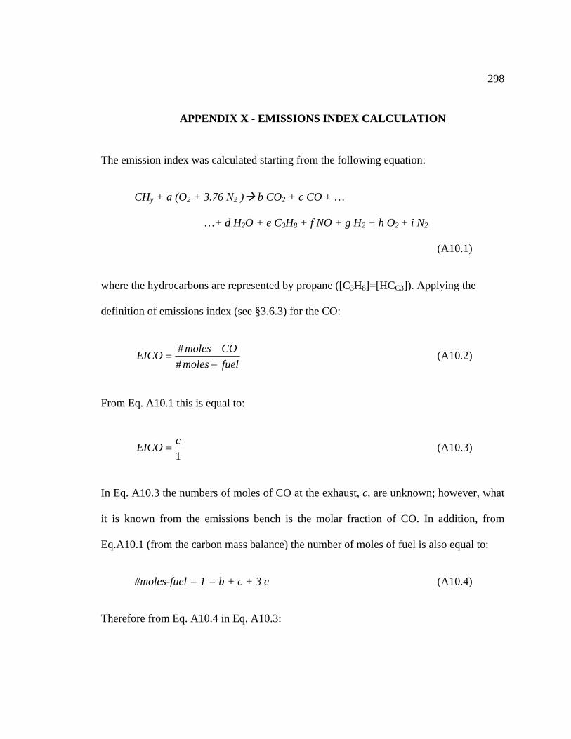
298
18 APPENDIX X - EMISSIONS INDEX CALCULATION
calculated starting from the following equation:
(A10.1)
plying the
The emission index was
CHy + a (O2 + 3.76 N2 ) b CO2 + c CO + …
…+ d H2O + e C3H8 + f NO + g H2 + h O2 + i N2
where the hydrocarbons are represented by propane ([C3H8]=[HCC3]). Ap
definition of emissions index (see §3.6.3) for the CO:
fuelmoles −#COmolesEICO −
=# (A10.2)
From Eq. A10.1 this is equal to:
c1
EICO = (A10.3)
C t the exhaust, c, are unknown; however, what
CO. In addition, from
In Eq. A10.3 the numbers of moles of O a
it is known from the emissions bench is the molar fraction of
Eq.A10.1 (from the carbon mass balance) the number of moles of fuel is also equal to:
#moles-fuel = 1 = b + c + 3 e (A10.4)
Therefore from Eq. A10.4 in Eq. A10.3:
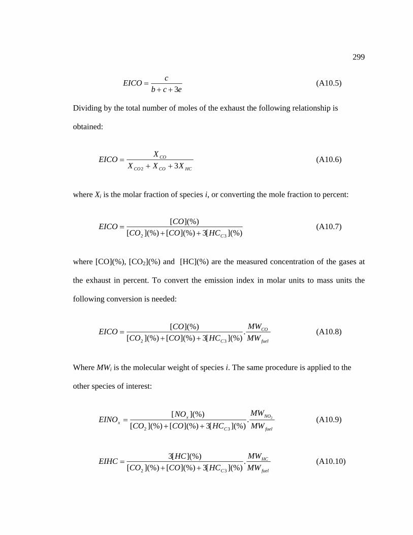
299
ecb 3++
cEICO = (A10.5)
Dividing by the total number of moles of the exhaust the following relationship is
obtained:
HCCOCO XXX 32 ++COEICO =
X (A10.6)
ng the mole fraction to percent: where Xi is the molar fraction of species i, or converti
](%)[3](%)[][ 2CO (%](%)[COEICO = (A10.7)
) 3CHCCO ++
asured concentration of the gases awhere [CO](%), [CO ](%) and [HC](%) are the me2 t
the exhaust in percent. To convert the emission index in molar units to mass units the
following conversion is needed:
COMWCOEICO .](%)[= (A10.8)
fuelC32 MWHCCOCO ](%)[3](%)[](%)[ ++
Where MWi is the molecular weight of species i. The same procedure is applied to the
other species of interest:
fuelC MWHCCOCO ](%)[3](%)[](%)[ 32 ++NOx
xEINO 2.= (A10.9) MWNO ](%)[
HCMWHCEIHC .](%)[3=
fuelC32 MWHCCOCO ](%)[3](%)[](%)[ ++(A10.10)

300
It is important to mention that in Eq. A10.6-10.10, the concentration of hydrocarbons is
in C3 basis ([C3H8]), and the HC molecular weight (MWHC) was considered equal to the
molecular weight of the fuel in C1 basis (MWfuel_C1).
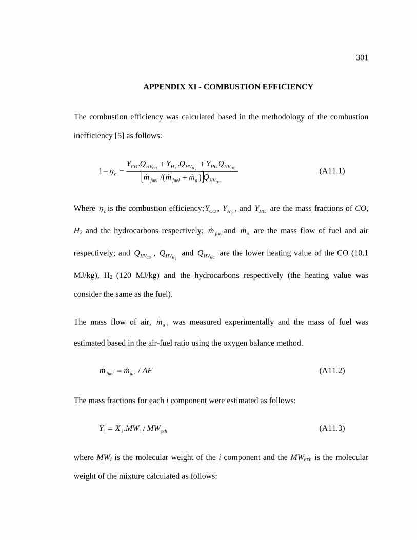
301
19 APPENDIX XI - COMBUSTION EFFICIENCY
The combustion efficiency was calculated based in the methodology of the combustion
inefficiency [5] as follows:
[ ]HCHVafuelfuel
c Qmmm )/( &&& +HCHCO HVHCHVHHVCO QYQYQY ..
1 22++
=−η (A11.1)
Where cη is the combustion efficiency; COY , HY , and HCY are the mass fractions of CO,
s
l was
nce method.
ows:
ular
2
H2 and the hydrocarbons respectively; m& and m& are the mass flow of fuel and air fuel a
respectively; and COHVQ ,
HHVQ and Q are the lower heating value of the CO (10.12 HC
MJ/kg), H
HV
2 (120 MJ/kg) and the hydrocarbons respectively (the heating value wa
consider the same as the fuel).
The mass flow of air, am& , was measured experimentally and the mass of fue
estimated based in the air-fuel ratio using the oxygen bala
AFmm aifuel /&& = (A11.2) r
The mass fractions for each i component were estimated as foll
exhiii MWMWXY /.= (A11.3)
where MWi is the molecular weight of the i component and the MWexh is the molec
weight of the mixture calculated as follows:

302
...](%).[].[](%).[](%).([12 ++++= COexh MWNOMWOMWCOMWCOMW
100 222 2 NOxOCO
… ])](%).[](%).[](%).[221 221 NHHCC MWNMWHMWHC
C+++ (A11.4)
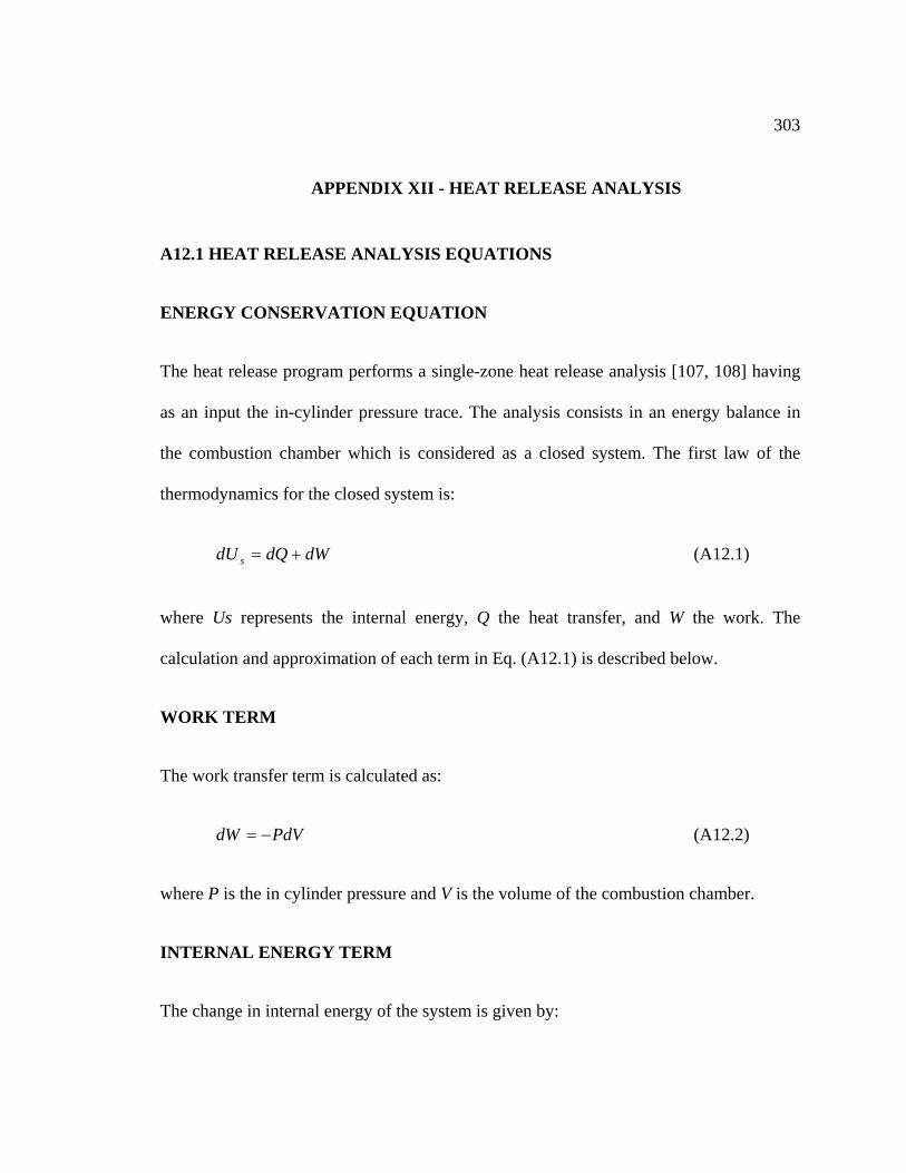
303
20 APPENDIX XII - HEAT RELEASE ANALYSIS
A12.1 HEAT RELEASE ANALYSIS EQUATIONS
ENERGY CONSERVATION EQUATION
The heat release program performs a single-zone heat release analysis [107, 108] having
as an input the in-cylinder pressure trace. The analysis consists in an energy balance in
the combustion chamber which is considered as a closed system. The first law of the
thermodynamics for the closed system is:
(A12.1)
where Us represents the internal energy, Q the heat transfer, and W the work. The
calculation and approximation of each term in Eq. (A12.1) is described below.
WORK TERM
The work transfer term is calculated as:
(A12.2)
where P is the in cylinder pressure and V is the volume of the combustion chamber.
INTERNAL ENERGY TERM
The change in internal energy of the system is given by:
dWdQdU s +=
PdVdW −=
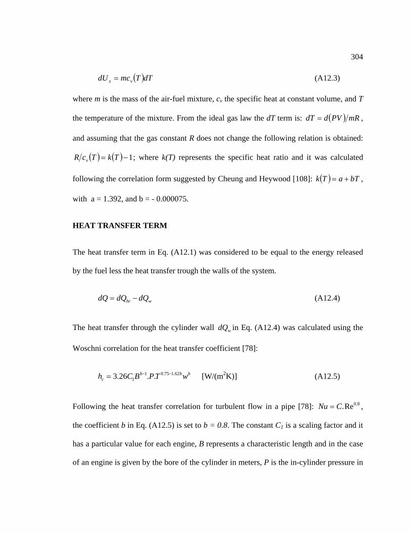
304
( )dTTmcdU vs = (A12.3)
where m is the mass of the air-fuel mixture, cv the specific heat at constant volume, and T
the temperature of the mixture. From the ideal gas law the dT term is: ( ) mRPVddT = ,
and assuming that the gas constant R does not change the following relation is obtained:
( ) ( ) 1−= TkTcR v
following the correlation form
; where k(T) represents the specific heat ratio and it was calculated
suggested by Cheung and Heywood [108]: ( ) bTaTk += ,
with a = 1.392, and b = - 0.000075.
HEAT TRANSFER TERM
The heat transfer term in Eq. (A12.1) was considered to be equal to the energy released
by the fuel less the heat transfer trough the walls of the system.
(A12.4)
The heat transfer through the cylinder wall in Eq. (A12.4) was calculated using the
Woschni correlation for the heat transfer coefficient [78]:
[W/(m2K)] (A12.5)
Following the heat transfer correlation for turbulent flow in a pipe [78]: ,
the coefficient b in Eq. (A12.5) is set to b = 0.8. The constant C1 is a scaling factor and it
has a particular value for each engine, B represents a characteristic length and in the case
of an engine is given by the bore of the cylinder in meters, P is the in-cylinder pressure in
whr dQdQdQ −=
wdQ
bbbc wTPBCh 62.175.01
1 ..26.3 −−=
8.0Re.CNu =
305
kPa, T is the temperature in K, and w represents the parameter that accounts for the gas
movement in the cylinder due to piston motion and due to the velocity assumed to result
from expansion of the gases during the combustion stage, having the following form:
( ) ivcmivcivc
dispp TPP
VpV
Cuw −×+= −2
31024.328.2 (A12.6)
In Eq. (A12.6) up is the piston mean velocity in m/s, Vdisp is the displacement volume. The
subscript ivc stands for intake valve closing. The term Pm is the pressure that the engine
could have if it were being motored at the same crank angle. This term is calculated as
follows:
nivc
ivcm VV
PP ⎟⎠
⎞⎜⎝
⎛= (A12.7)
The value of the polytropic exponent in Eq. (A12.7) was calculated from the pressure
data as:
(A12.8)
The constant C2 has a particular value for each engine. Its value is usually chosen so that
negative heat release is avoided, i.e. to have a normalized cumulative heat release greater
than 1 [107-109].
Finally rearranging Eq. (A12.1) and substituting the assumptions for each term the final
energy balance equation is obtained:
)/ln(/)/ln( ,3055,30 bTDCCAivcivcbTDCCA VVPPn ++=
306
( )( ) ( ) whr dQVdP
TkPdV
TkTkdQ +
−+
−=
11
1 (A12.9)
or in the friendly form:
( )( ) ( ) θθθθ d
dQddPV
TkddVP
TkTk
ddQ whr +
−+
−=
11
1 (A12.10)
The equation (A12.10) was integrated along the period where the heat release was taking
place.
CALCULATION OF THE CONSTANT C1 OR HEAT TRANSFER MULTIPLIER
HT IN THE HEAT RELEASE PROGRAM (C1 = HT)
The integration of the equation (A12.10) gives the following equation:
( )( ) ( ) whr Qd
ddPV
Tkd
ddVP
TkTkQ
end
start
end
start
+−
+−
= ∫∫ θθ
θθ
θ
θ
θ
θ 11
1 (A12.11)
In Eq. (A12.8) the first two terms of the right hand side can be calculated from the
pressure traces. The total heat release (left hand side term) can be calculated as well
from: cfuelhr LHVmQ η..=
heating value of the fuel, and
ured em
heat transfer to the walls
; where mfuel is the mass of fuel, LHV represents the lower
ηc is the combustion efficiency calculated from the
meas issions concentration [5, Appendix XI]. Thus, from Eq. (A12.11) the total
can be calculated, which at the same time must match the
following integral:
wQ
307
θθ
θ
dTwTAhQend
start
cw ∫ −= ).(. (A12.12)
In this equation A represents the instantaneous heat transfer area, T the in cylinder bulk
temperature, Tw is the wall temperature, and hc a scaling heat transfer coefficient to
satisfy Eq. (A12.12). The only unknown in Eq. (A12.12) is the constant C1 of the heat
transfer coefficient (hc). The value of C1 must be one such that Eq. (A12.9) is satisfied.
The value of C1 can be determined doing the following substitution:
(A12.13)
where :
[W/(m2K)] (A12.14)
Thus:
'1 cc hCh =
bbbc wTPBh 62.175.01' ..26.3 −−=
θθ
θ
dTwTAh
QCend
start
w
∫ −=
).(.'1 (A12.15)
With this constant at hand the instantaneous heat release and the instantaneous heat
transfer to the wall can be calculated. As it can be notice the choice of the wall
temperature is not relevant, because the constant C1 will take care of it when balancing
the total heat released through the wall.
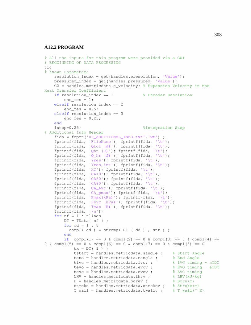
308
A12.2 PROGRAM
% All the inputs for this program were provided via a GUI % BEGGINNING OF DATA PROCESSING tic % Known Parameters resolution_index = get(handles.eresolution, 'Value'); pressured_index = get(handles.pressured, 'Value'); C2 = handles.metricdata.e_velocity; % Expansion Velocity in the Heat Transfer Coefficient if resolution_index == 1 % Encoder Resolution enc_res = 1; elseif resolution_index == 2 enc_res = 0.5; elseif resolution_index == 3 enc_res = 0.25; end istep=0.25; %Integration Step % Additional Info Header fida = fopen('HR_ADDITIONAL_INFO.txt','wt') ; fprintf(fida, 'FileName'); fprintf(fida, '\t'); fprintf(fida, 'Qtot (J)'); fprintf(fida, '\t'); fprintf(fida, 'Qht (J)'); fprintf(fida, '\t'); fprintf(fida, 'Q_hr (J)'); fprintf(fida, '\t'); fprintf(fida, 'Yres'); fprintf(fida, '\t'); fprintf(fida, 'Yres,int'); fprintf(fida, '\t'); fprintf(fida, 'HT'); fprintf(fida, '\t'); fprintf(fida, 'CA10'); fprintf(fida, '\t'); fprintf(fida, 'CA50'); fprintf(fida, '\t'); fprintf(fida, 'CA90'); fprintf(fida, '\t'); fprintf(fida, 'CA_evc'); fprintf(fida, '\t'); fprintf(fida, 'CA_pmax'); fprintf(fida, '\t'); fprintf(fida, 'Pmax(kPa)'); fprintf(fida, '\t'); fprintf(fida, 'Pevc (kPa)'); fprintf(fida, '\t'); fprintf(fida, 'Tmax (K)'); fprintf(fida, '\t'); fprintf(fida, '\n'); for nf = 1 : nlines DT = TData{ nf } ; for dd = 1 : 8 comp1( dd ) = strcmp( DT ( dd ) , str ) ; end if comp1(1) == 0 & comp1(2) == 0 & comp1(3) == 0 & comp1(4) == 0 & comp1(5) == 0 & comp1(6) == 0 & comp1(7) == 0 & comp1(8) == 0 tx = DT( 1 ) ; tstart = handles.metricdata.sangle ; % Start Angle tend = handles.metricdata.eangle ; % End Angle tivc = handles.metricdata.ivcv ; % IVC timing - aTDC tevo = handles.metricdata.evov ; % EVO timing - aTDC tevc = handles.metricdata.evcv ; % EVC timing LHV = handles.metricdata.lhvv ; % LHV(kJ/kg) D = handles.metricdata.borev ; % Bore(m) stroke = handles.metricdata.strokev ; % Stroke(m) T_wall = handles.metricdata.twallv ; % T_wall(° K)
309
tn_2 = -30 ; % CA of the second point to calcualte the polytropic index n % Cylinder two @ tcyl2 = 270 if tx(3)=='2' tcyl2 = 270 ; % timing second cylinder, this is very particular for the CH23 Kohler Engine. tstart = tcyl2 + tstart ; % Start Angle tend = tcyl2 + tend ; % End Angle tivc = tcyl2 + tivc ; % IVC timing - aTDC tevo = tcyl2 + tevo ; % EVO timing - aTDC tevc = tcyl2 + tevc ; % EVC timing if tevc > 540 tevc = ( tevc - 540 ) -180 ; end tn_2 = tcyl2 - 30 ; % CA of the second point to calcualte the polytropic index n end fid = fopen( tx ) ; % Data Table files if fid == -1 errordlg('File name entered could not be found or accessed','Error'); else line = ''; while isempty( findstr( line , 'F3 fpressure [kPa]' ) ) line = fgetl( fid ) ; end d = fscanf( fid , '%f' , [ 4 , inf ] )' ; % Extracting the data of the look Up file [ Nd , f ] = size( d ) ; fclose( fid ) ; eta = str2num( DT( 2 ) ) ; % eff._comb m_air = str2num( DT( 3 ) ) ; % mass_air(kg/cycle) m_fuel = str2num( DT( 4 ) ) ; % mass_fuel(kg/cycle) RPM = str2num( DT( 5 ) ) ; % RPM T_exh = str2num( DT( 6 ) ) ; % T_exhaust (°K) T_int = str2num( DT( 7 ) ) ; % T_intake( °K) EGR = str2num( DT( 8 ) ) ; % EGR % Checking the GUI table inputs ee = isempty( eta ); mm = isempty( m_air ); mf = isempty( m_fuel ); tin = isempty( T_int ); rpp = isempty( RPM ); tex = isempty( T_exh ); egr1 = isempty( EGR); if ee == 0 & mm == 0 & mf == 0 & tin == 0 &rpp == 0 & tex == 0 & egr1 == 0 % Constants Ru=8.314; % Universal Gas Constant MW_air=28.90; % Air molar mass R=Ru/MW_air; % Air constant % Vectors with data from the Look UP file CA=d(:,1); % Crank angle vector P=d(:,2); % Cylinder Pressure V=d(:,3); % Volume data fP=d(:,4); % Filtered Pressure
310
enc_res = d(2,1)-d(1,1); % Encoder resolution from the input data file % Selection between filtered (1) or not filtered (2) pressure if pressured_index == 2 fP = P; end Vdisp= interp1(CA,V,-180,'spline')-interp1(CA,V,0,'spline'); % Displacement Volume V_ivc=interp1(CA,V,tivc,'spline'); V_evo=interp1(CA,V,tevo,'spline'); V_evc=interp1(CA,V,tevc,'spline'); P_evo=interp1(CA,fP,tevo,'spline'); P_ivc=interp1(CA,fP,tivc,'spline'); P_evc=interp1(CA,fP,tevc,'spline'); % Pressures and Volumes to calculate the compression politropic coefficient P_1=interp1(CA,fP,tivc+5,'spline'); P_2=interp1(CA,fP,tn_2,'spline'); V_1=interp1(CA,V,tivc+5,'spline'); V_2=interp1(CA,V,tn_2,'spline'); n_comp=log(P_2/P_1)/log(V_1/V_2); % Residual Mass Calculation y_res_int=(V_evc/V_evo)*(P_evc/P_evo)^(1/n_comp); % Calcualtion of the mass trapped m_trapped = (m_air + m_fuel)*(1+(EGR/100)/(1-EGR/100))/(1-y_res_int); m_res_int = y_res_int*m_trapped; m_res_ext = m_trapped - m_res_int - (m_air + m_fuel); m_res = m_res_int + m_res_ext; y_res = m_res/m_trapped; T_ivc=P_ivc*((V_ivc/R)/(m_air + m_fuel + m_res)); Q=m_fuel*LHV*eta; speed=60/(RPM*360); time=60/RPM; Vp=2*stroke/time; % Setting the CA, P, and V according to the integration step CAi = ( tstart : istep : tend ) ; [ ri , Ni ] = size ( CAi ) ; for i = 1 : 1 : Ni Vi(i) = interp1(CA , V , CAi( i ) , 'spline'); Pi(i) = interp1(CA , fP , CAi( i ) , 'spline'); end % Pressure and Volume Derivatives for i = 1 : 1 : Ni-1 ; dP( i ) = ( Pi( i + 1 ) - Pi( i ) ) / istep ; dV( i ) = ( Vi( i + 1 ) - Vi( i ) ) / istep ; end for i = 1 : 1 : Ni - 1 T( i ) = Pi( i ) * ( Vi( i ) / R ) / ( m_air + m_fuel + m_res ) ; gamma( i ) = 1.392 - 0.000075 * T( i ) ; W( i ) = 2.28 *( Vp + C2 * 0.0136 * Vdisp / V_ivc * ( Pi( i ) /P_ivc -( V_ivc / Vi( i ) ) ^ n_comp ) * T_ivc ) ;
311
h1( i ) = 0.131 * D ^ 0.2 * ( Pi( i ) / 101.3 ) ^ 0.8 / ( T( i ) ^ 0.53 ) * W( i ) ^ 0.8 ; AREA( i ) = 2 * pi * D ^ 2 / 4 + pi * D * Vi( i ) / ( pi * D ^ 2 / 4 ) ; dI_ht( i ) = h1( i ) * AREA( i ) * ( T( i ) - T_wall ) * speed ; dI_hr( i ) = ( Vi( i ) / ( gamma( i ) -1 ) ) * dP( i ) + gamma( i ) / ( gamma( i ) - 1 ) * Pi( i ) * dV( i ) ; end % Integration to find I_tot_ht, I_tot_hr, and HT for i=1:1:Ni-2 I_hr ( i ) = 1 / 2 * ( dI_hr ( i ) + dI_hr ( i + 1 ) ) * istep ; I_ht ( i ) = 1 / 2 * ( dI_ht ( i ) + dI_ht ( i + 1 ) ) * istep ; end I_tot_ht = sum ( I_ht ) ; I_tot_hr = sum ( I_hr ) ; HT = ( Q - I_tot_hr ) / ( I_tot_ht ) ; % Calculation of dQ_ht,dQ_hr, and Q_hr_cum using the calculated scaling factor HT for i = 1 : 1 : Ni-1 dQ_ht ( i ) = HT * h1 ( i ) * AREA ( i ) * ( T ( i ) - T_wall ) * speed ; dQ_hr ( i ) = dQ_ht ( i ) + ( Vi ( i ) / ( gamma ( i ) - 1 ) ) * dP ( i ) + gamma ( i ) / ( gamma ( i ) - 1) * Pi ( i ) * dV ( i ); end % Filtering of the Heat release filter = get( handles.filteronoff , 'Value' ); % 0 = OFF 1 = ON if filter == 1 dQ_hr = csaps ( CAi(1:Ni-1),dQ_hr(1:Ni-1) , 0.005 , CAi(1:Ni-1)) ; end cum = 0 ; for i = 1 : 1 : Ni - 2 Q_hr( i ) = 1 / 2 * ( dQ_hr( i ) + dQ_hr( i + 1 ) ) * istep ; Q_ht( i ) = 1 / 2 * ( dQ_ht( i ) + dQ_ht( i + 1 ) ) * istep ; cum = cum + Q_hr( i ) ; Q_hr_cum( i ) = cum / Q ; end % Conversion to J (1000 factor) dQ_hr = 1000 * dQ_hr ; % Heat release dQ_ht = 1000 * dQ_ht ; % Heat transfer Q_tot_ht = 1000 * sum( Q_ht ) ; % Total heat transfer Q_tot_hr = 1000 * sum( Q_hr ) ; % Total heat release Diff =( Q * 1000 - Q_tot_hr ) ; % Heat Release at 10%, 50%, 90% for i = 1 : 1 : Ni - 3
312
if Q_hr_cum( i ) <= 0.1 && Q_hr_cum( i + 1 ) > 0.1 CA_10 = CAi( i ) Q_hr_cum_10 = Q_hr_cum( i ) elseif Q_hr_cum( i ) <= 0.5 && Q_hr_cum( i + 1 ) > 0.5 CA_50 = CAi( i ) Q_hr_cum_50 = Q_hr_cum( i ) elseif Q_hr_cum( i ) <= 0.9 && Q_hr_cum( i + 1 ) > 0.9 CA_90 = CAi( i ) Q_hr_cum_90 = Q_hr_cum( i ) end end [ P_max , imax ] = max ( P ) ; %Peak Pressure CA_pmax = CA ( imax ) ; %Location of Peak Pressure CA_evc = tevc ; % CA of exhaust valve closing CA_evo = tevo ; % CA of exhaust valve opening % In Cylinder Temperature Calculation R_b = R ; % Burned gases constant equal to the air constant in kJ/kg-K for i = 1 : Nd Tm ( i ) = P ( i ) * V ( i ) / ( R_b * ( m_air + m_fuel + m_res ) ) ; % Pressure in kPa end T_max = max ( Tm ) % Maximun temperature in the cyl. in K %--------------------------Output files ------------------------ % Output File Heat Release OHR{nf}=strcat('hr_',tx); fidO=fopen(OHR{nf},'wt'); [qlr,qlc]=size(tx); TX=tx(3:(qlc-4)); fprintf(fidO, 'CA_hr_'); fprintf(fidO, TX); fprintf(fidO, '\t\t'); fprintf(fidO, 'dQ_hr_'); fprintf(fidO, TX); fprintf(fidO, '\t\t\t'); fprintf(fidO, 'dQ_ht_'); fprintf(fidO, TX); fprintf(fidO, '\t\t\t'); fprintf(fidO, 'Q_hr_cum_'); fprintf(fidO, TX); fprintf(fidO, '\n'); for v=1:Ni-2 fprintf(fidO, '%3.3f\t\t\t', CAi(v)); fprintf(fidO, '%g\t\t\t', dQ_hr(v)); fprintf(fidO, '%g\t\t\t', dQ_ht(v)); fprintf(fidO, '%g\t\t\t', Q_hr_cum(v)); fprintf(fidO, '\n'); end fclose(fidO); % HR_ADDITIONAL_INFO.txt fprintf(fida, tx); fprintf(fida, '\t'); fprintf(fida, '%g\t', Q*1000); fprintf(fida, '%g\t', Q_tot_ht); fprintf(fida, '%g\t', Q_tot_hr); fprintf(fida, '%g\t', y_res); fprintf(fida, '%g\t', y_res_int); fprintf(fida, '%g\t', HT);
313
fprintf(fida, '%g\t', CA_10); fprintf(fida, '%g\t', CA_50); fprintf(fida, '%g\t', CA_90); fprintf(fida, '%g\t', CA_evc); fprintf(fida, '%g\t', CA_pmax); fprintf(fida, '%g\t', P_max); fprintf(fida, '%g\t', P_evc); fprintf(fida, '%g\t', T_max); fprintf(fida, '\n'); %---------------------- Plots -------------------------------- figure % Heat Release,Cum. Heat Release,Heat Transfer hold on axis on; grid on; box on; % Axis image; [AX,H1,H2] = plotyy(CAi(1:Ni-1),dQ_hr(1:Ni-1),CAi(1:Ni-2),Q_hr_cum(1:Ni-2),'plot'); set(get(AX(1),'Ylabel'),'String','dQ-hr') set(get(AX(2),'Ylabel'),'String','Q-hr-cum (J/J/deg)') t1=title(['Heat Release and Heat Transfer @ ',TX]); xlabel('CA');ylabel('dQ-ht , dQ-ht (J/deg)'); hold on plot(CAi(1:Ni-1),dQ_ht(1:Ni-1),'Color',[0 0.5 0]); plot(CAi(1:Ni-1),dQ_ht(1:Ni-1),'r'); legend('dQ-hr','Q-hr-cum','dQ-ht'); else errordlg('Parameters must be numeric','Error'); end end else errordlg('Table should be filled correcty','Error'); end end fclose(fida); else errordlg('Table should be filled','Error'); end toc set(handles.text36, 'String', toc); set(handles.calculate, 'Enable', 'on'); set(handles.reset, 'Enable', 'on'); %==========END OF DATA PROCESSING==========
314
21 APPENDIX XIII - RING PACK PROGRAM %The ring pack program was a function called by the Ring-Pack-Heat-%Release program (see next appendix). The dimensions of the ring pack %were provided by the function RPVol, shown at the bottom of this appendix. %RING PACK MODEL function %This program models the flow in the ring pack crevices and provides %as output their contribution to the HC emissions function [ m1out_CA90_to_CA_evc , m1out_CA90_to_CA_evo , m1stored_CA_pmax , m1out , m1in , m_s_blowby ] = RP2CR_GCR ( CA_90 , CA_evc , CA_evo, CA_pmax , d , tx , RPM ) % Known Parameters Cd = 0.85; % Discharge Coefficient gamma = 1.4; % Specific Heat Ratio T = 385; % Wall Temperature in °K R = 287; % Air constant J/kg-K [Vi , Vii , Viii , Viv , A1L , A1U , A2L , A2U ] = RPvol; % from the RPvol function - Ring Pack Volumes and Ring End Gap Areas [ Nd , f ] = size ( d ) ; CA = d ( : , 1 ); % CA vector from the reading vector P1 = 1000 * d ( : , 4 ) ; % Cylinder pressure data vector, Pa Pc = 1000 * d ( : , 5 ) ; % Crankcase pressure vector, Pa [ r , c ] = size ( P1 ) ; % Size of the cylinder pressure vector dCA=CA(2,1)-CA(1,1); % CA step integration, in Crank Angle units dt=dCA/(6*RPM); % Integration time step in sec for each file changes with the velocity Ps = csaps(CA,P1,0.005,CA); % Smoothing of the Cylinder Pressure data P1 = Ps ; % Pressure 1 equal to the smooth cyl. press % Differentiation of the Pressure data: dP/dt for i=1:1:r-1; dP(i)=(Ps(i+1)-Ps(i))/dt; end dP(1440)=(Ps(1)-Ps(r))/dt; % Derivative of the last point % Initial Pressure in the Ring Pack Crevices Volumes P2(1)=53; % Initial Pressure in the Volume 2, a guess % WHILE LOOP for the convergency of P2(1)= P2(r)=last point press differ = 1; % Criteria to stop the while loop N = 0; while abs(differ) >10e-5 for i=1:r-1 % Integration of the eq around the cyc P3(i)=Pc(i); % Cranckcase Pressure if P1(i)>=P2(i) % Mass balance in the first volume if P2(i)/P1(i) < 0.52 eta1=(2/(gamma+1))^((gamma+1)/(2*(gamma-1))); else eta1=(2/(gamma-1)*((P2(i)/P1(i))^(2/gamma)-(P2(i)/P1(i))^((gamma+1)/gamma)))^0.5; end A1 = A1L ; % Ring seating at the bottom part of the groove
315
m2(i)=Cd*A1*(sqrt(gamma/(R*T))*P1(i))*eta1; V1 ( i ) = Vi + Vii ;% Crevice volume over the first ring else if P1(i)/P2(i) < 0.52 eta2i=(2/(gamma+1))^((gamma+1)/(2*(gamma-1))); else eta2i=(2/(gamma-1)*((P1(i)/P2(i))^(2/gamma)-(P1(i)/P2(i))^((gamma+1)/gamma)))^0.5; end A1 = A1U ; % Ring seating at the upper partof the groove m2(i)=-Cd*A1*(sqrt(gamma/(R*T))*P2(i))*eta2i; V1 ( i ) = Vi ; % Crevice volume over the first ring end m1 ( i ) = m2 ( i ) + V1 ( i ) / ( R * T ) * dP ( i ) ; m1stored ( i ) = P1 ( i ) * V1 ( i ) / ( R * T ) ; V1stored ( i ) = V1 ( i ) ; if P2(i)>=P3(i) % Mass balance in the second volume if P3(i)/P2(i) < 0.52 eta2=(2/(gamma+1))^((gamma+1)/(2*(gamma-1))); else eta2=(2/(gamma-1)*((P3(i)/P2(i))^(2/gamma)-(P3(i)/P2(i))^((gamma+1)/gamma)))^0.5; end A2 = A2L; % Second ring seating on the bottom part of the groove m3(i)=Cd*A2*(sqrt(gamma/(R*T))*P2(i))*eta2; elseif P2(i)/P3(i) < 0.52 eta3i=(2/(gamma+1))^((gamma+1)/(2*(gamma-1))); else eta3i=(2/(gamma-1)*((P2(i)/P3(i))^(2/gamma)-(P2(i)/P3(i))^((gamma+1)/gamma)))^0.5; end A2 = A2U ; % Second ring seating at the upper part of the groove m3(i)=-Cd*A2*(sqrt(gamma/(R*T))*P3(i))*eta3i; end if P1(i)>=P2(i) && P2(i)>=P3(i) % Crevice Vol. between 1st and 2nd ring V2 ( i ) = Viii + Viv; elseif P1(i)>=P2(i) && P2(i)<P3(i) V2 ( i ) = Viii; elseif P1(i)<P2(i) && P2(i)<P3(i) V2 ( i ) = Vii + Viii; elseif P1(i)<P2(i) && P2(i)>P3(i) V2 ( i ) = Vii + Viii + Viv; end P2 ( i + 1 ) = P2 ( i ) + ( ( m2 ( i ) - m3 ( i ) ) * R * T / V2 ( i ) ) * dt ; % Pressure in the volume V2 m2stored ( i ) = P2 ( i ) * V2 ( i ) / ( R * T ) ; V2stored ( i ) = V2 ( i ) ; end % Difference in Pressure at the end and the start of the cycle deltaP2(N+1)=P2(1)-P2(r); differ = deltaP2(N+1); N = N + 1; P2(1)=P2(r); % Reasigment of the inital press in the crevices volume
316
end % Blowby Calculation for i=1:r-2 dm3(i)=(m3(i)+m3(i+1))/2*dt; end m3total=sum(dm3); % Total mass due to blowby m_blowby_cyc = m3total; % Blowby mass per cycle m1ini = 0 ; % Cummulative Mass In and Out Calculation m1outi = 0 ; m2ini = 0 ; m2outi = 0 ; m3ini = 0 ; m3outi = 0 ; for i = 1 : r - 2 ; if m1 ( i ) >= 0 % For Volume 1 dm1in ( i ) = ( m1 ( i ) + m1 ( i + 1 ) ) / 2 * dt ; m1in ( i ) = m1ini + dm1in ( i ) ; m1ini = m1in ( i ) ; m1out ( i ) = m1outi + 0 ; else dm1out ( i ) = ( m1 ( i ) + m1 ( i + 1 ) ) / 2 * dt ; m1out ( i ) = m1outi + dm1out ( i ) ; m1outi = m1out ( i ) ; m1in ( i ) = m1ini + 0 ; end if m2 ( i ) >= 0 % For Volume 2 dm2in ( i ) = ( m2 ( i ) + m2 ( i + 1 ) ) / 2 * dt ; m2in ( i ) = m2ini + dm2in ( i ) ; m2ini = m2in ( i ) ; m2out ( i ) = m2outi + 0 ; else dm2out ( i ) = ( m2 ( i ) + m2 ( i + 1 ) ) / 2 * dt ; m2out ( i ) = m2outi + dm2out ( i ) ; m2outi = m2out ( i ) ; m2in ( i ) = m2ini + 0 ; end if m3 ( i ) >= 0 % For Volume 3 dm3in ( i ) = ( m3 ( i ) + m3 ( i + 1 ) ) / 2 * dt ; m3in ( i ) = m3ini + dm3in ( i ) ; m3ini = m3in ( i ) ; m3out ( i ) = m3outi + 0 ; else dm3out ( i ) = ( m3 ( i ) + m3 ( i + 1 ) ) / 2 * dt ; m3out ( i ) = m3outi + dm3out ( i ) ; m3outi = m3out ( i ) ; m3in ( i ) = m3ini + 0 ; end end P3(1440)=Pc(1440); % Last point crankcase pressure m1out = - m1out ; % Mass out with possitive sign in kg m2out = - m2out ; % Mass out with possitive sign in kg m3out = - m3out ; % Mass out with possitive sign in kg m3blowby = m3in - m3out ; % Blowby cummulative mass in kg m1outi = m1out ; % Mass for integration
317
m1out_CA90_to_CA_evc = 0 ; % Mass Out from CA_90 to EVC m1out_CA90 = 0 ; m1out_CA_evc = 0 ; m1out_CA_evo = 0; for i = 1 : r - 2 if CA ( i ) >= CA_90 && CA ( i ) < ( CA_90 + dCA ) m1out_CA90 = m1outi(i); end if CA ( i ) >= CA_evc && CA ( i ) < ( CA_evc + dCA ) m1out_CA_evc = m1outi(i); end if CA ( i ) >= CA_evo && CA ( i ) < ( CA_evo + dCA ) m1out_CA_evo = m1outi(i); end if CA ( i ) >= CA_pmax && CA ( i ) < ( CA_pmax + dCA ) m1stored_CA_pmax = m1stored(i); end end m1out_CA90_to_CA_evc = ( m1out_CA_evc - m1out_CA90 ) ; % in kg m1out_CA90_to_CA_evo = ( m1out_CA_evo - m1out_CA90 ) ; % in kg m1stored_CA_pmax = ( 0 + m1stored_CA_pmax ) ; % in kg %-------------------------Unit Conversion------------------------- P1 = P1 / 1000 ; % kPa P2 = P2 / 1000 ; % kPa P3 = P3 / 1000 ; % kPa Pc = Pc / 1000 ; % kPa m1 = m1 * 1000 ; % grams/sec m2 = m2 * 1000 ; % grams/sec m3 = m3 * 1000 ; % grams/sec m1stored = m1stored * 1000 ; % grams m2stored = m2stored * 1000 ; % grams m_blowby_cyc = m_blowby_cyc * 1000 ; % grams/cycle m1in = 1000 * m1in ; % Mass 1 in with possitive sign in g m2in = 1000 * m2in ; % Mass 2 in with possitive sign in g m3in = 1000 * m3in ; % Mass 3 in with possitive sign in g m1out = 1000 * m1out ; % Mass 1 out with possitive sign in g m2out = 1000 * m2out ; % Mass 2 out with possitive sign in g m3out = 1000 * m3out ; % Mass 3 out with possitive sign in g m3blowby = 1000 * m3blowby ; % Blowby cummulative mass in g %-------------Steady State Blowby Mass Flow---------------------------- % (to be compared with the measured by the bells meter) m_s_blowby = m_blowby_cyc * RPM / 120 ; % (g/s) %-----------------------------Plots------------------------------------ figure plot(CA,P1,CA,P2, CA, P3) legend('P1','P2','Pc') xlabel('CA');ylabel('Pressure(kPa)'); figure plot(CA(1:r-1),m1,CA(1:r-1),m2,CA(1:r-1),m3) legend('m1','m2','m3') xlabel('CA');ylabel('Mass Flow (g/s)'); figure plot(CA(1:r-2),m1in,CA(1:r-2),m2in,CA(1:r-2),m3in) legend('m1in','m2in','m3in')
318
xlabel('CA');ylabel('Mass In of the Crevices (g)'); figure plot(CA(1:r-2),m1out,CA(1:r-2),m2out,CA(1:r-2),m3out) legend('m1out','m2out','m3out') xlabel('CA');ylabel('Mass Out of the Crevices (g)'); figure plot(CA(1:r-2),m3blowby) legend('Mass Blowby') xlabel('CA');ylabel('Total mass to the crankcase (g)'); %---------------------------Output files------------------------------- js=strcat('ORPap_',tx) ; fidO=fopen(js,'wt'); [qlr,qlc]=size(tx); tx1=tx(3:(qlc-4)); fprintf(fidO,'CA'); fprintf(fidO, tx1); fprintf(fidO, '\t'); fprintf(fidO,'P1(kPa)'); fprintf(fidO, tx1); fprintf(fidO, '\t'); fprintf(fidO,'P2(kPa)'); fprintf(fidO, tx1); fprintf(fidO, '\t'); fprintf(fidO,'m1(g/s)'); fprintf(fidO, tx1); fprintf(fidO, '\t'); fprintf(fidO,'m2(g/s)'); fprintf(fidO, tx1); fprintf(fidO, '\t'); fprintf(fidO,'m3(g/s)'); fprintf(fidO, tx1); fprintf(fidO, '\t'); fprintf(fidO,'m_c_cum(g)');fprintf(fidO, tx1); fprintf(fidO, '\t'); fprintf(fidO,'m1_in(g)'); fprintf(fidO, tx1); fprintf(fidO, '\t'); fprintf(fidO,'m2_in(g)'); fprintf(fidO, tx1); fprintf(fidO, '\t'); fprintf(fidO,'m3_in(g)'); fprintf(fidO, tx1); fprintf(fidO, '\t'); fprintf(fidO,'m1_out(g)');fprintf(fidO, tx1); fprintf(fidO, '\t'); fprintf(fidO,'m2_out(g)');fprintf(fidO, tx1); fprintf(fidO, '\t'); fprintf(fidO,'m3_out(g)');fprintf(fidO, tx1); fprintf(fidO, '\t\t'); fprintf(fidO, '\n'); for v=1:r-2 fprintf(fidO, '%3.1f\t', CA(v)); fprintf(fidO, '%g\t', P1(v)); fprintf(fidO, '%g\t', P2(v)); fprintf(fidO, '%g\t', m1(v)); fprintf(fidO, '%g\t', m2(v)); fprintf(fidO, '%g\t', m3(v)); fprintf(fidO, '%g\t', m3blowby(v)); fprintf(fidO, '%g\t', m1in(v)); fprintf(fidO, '%g\t', m2in(v)); fprintf(fidO, '%g\t', m3in(v)); fprintf(fidO, '%g\t', m1out(v)); fprintf(fidO, '%g\t', m2out(v)); fprintf(fidO, '%g\t', m3out(v)); fprintf(fidO, '\n'); end fclose(fidO); % RING PACK VOLUMES (GEOMETRY) CALCULATION function % Dimension provided below are not real dimensions they are used only % for illustration purposes function [V1,V2,V3,V4,A1L,A1U,A2L,A2U] = RPvol ; % All dimensions are in millimeters (mm) % Written by Victor M. Salazar % Engine Research Center % University of Wisconsin - Madison % February 24th, 2007 version %--------------------Volume V1------------------------
319
dcyl = 82; h1 = 5.2 ; d1L = 78.5; d1U = 79.0; r1L = d1L/2; r1U = d1U/2; Ve1 = pi / 4 * dcyl ^ 2 * h1; % External Volume Ve1 Vi1 = 1 / 3 * pi * h1 * ( r1L ^ 2 + r1U ^ 2 + r1L * r1U ); % Internal Volume V1 = Ve1 - Vi1; h2 = 1.7 + 0.01; di2 = 72.0 ; diRI = 75 ; hRI = 1.7 ; Ve2 = pi / 4 * dcyl ^ 2 * h2 ; % External Volume Vi2 = pi / 4 * di2 ^ 2 * h2 ; % Internal Volume VRI = pi / 4 * ( dcyl ^ 2 - diRI ^ 2) * hRI ; % Ring Volume V2 = Ve2 - Vi2 - VRI; h3 = 4.0 ; d3L = 80.01 ; d3U = 79.01 ; r3L = d3L / 2 ; r3U = d3U / 2 ; Ve3 = pi / 4 * dcyl ^ 2 * h3 ; % External Volume Vi3 = 1 / 3 * pi * h3 * ( r3L ^ 2 + r3U ^ 2 + r3L * r3U ) ; % Internal Volume V3 = Ve3 - Vi3; h4 = 1.7 ; di4 = 72 ; diRII = 72.48 ; hRII = 1.8 ; Ve4 = pi / 4 * dcyl ^ 2 * h4 ; % External Volume Vi4 = pi / 4 * di4 ^ 2 * h4 ; % Internal Volume VRII = pi / 4 * ( dcyl ^ 2 - diRII ^ 2 ) * hRII ; % Ring Volume V4 = Ve4 - Vi4 - VRII; % Units conversion from mm^3 to m^3 V1 = V1 * 1e-9; % m^3 V2 = V2 * 1e-9; % m^3 V3 = V3 * 1e-9; % m^3 V4 = V4 * 1e-9; % m^3 % End Gap Ring I Area EGRI = 0.60; A1L = EGRI * ( dcyl - d3U ) ; A1U = EGRI * ( dcyl - d1L ) ; % End Gap Ring II Area EGRII = 0.80; d5U = 79.682 ; A2L = EGRII * ( dcyl - d5U ) ; A2U = EGRII * ( dcyl - d3L ) ; % Units conversion from mm^2 to m^2 A1L = A1L * 1e-6 ; A1U = A1U * 1e-6 ; A2L = A2L * 1e-6 ; A2U = A2U * 1e-6 ;
320
22 APPENDIX XIV - RING PACK-HEAT RELEASE PROGRAM % All the inputs to this program were provided by a GUI % BEGGINNING OF DATA PROCESSING tic resolution_index = get(handles.eresolution, 'Value'); pressured_index = get(handles.pressured, 'Value'); C2 = handles.metricdata.e_velocity; % Expansion Velocity in the Heat Transfer Coefficient if resolution_index == 1 % Encoder Resolution enc_res = 1; elseif resolution_index == 2 enc_res = 0.5; elseif resolution_index == 3 enc_res = 0.25; end istep=0.25; % Integration Step fida = fopen('RINGPACK_AVG_PH_ADD_INFO.txt','wt') ; fprintf(fida, 'FileName'); fprintf(fida, '\t'); fprintf(fida, 'Qtot (J)'); fprintf(fida, '\t'); fprintf(fida, 'Qht (J)'); fprintf(fida, '\t'); fprintf(fida, 'Q_hr (J)'); fprintf(fida, '\t'); fprintf(fida, 'Yres'); fprintf(fida, '\t'); fprintf(fida, 'Yres,int'); fprintf(fida, '\t'); fprintf(fida, 'HT'); fprintf(fida, '\t'); fprintf(fida, 'CA10'); fprintf(fida, '\t'); fprintf(fida, 'CA50'); fprintf(fida, '\t'); fprintf(fida, 'CA90'); fprintf(fida, '\t'); fprintf(fida, 'CA_evc'); fprintf(fida, '\t'); fprintf(fida, 'CA_pmax'); fprintf(fida, '\t'); fprintf(fida, 'EIHC_exh (g/kg)'); fprintf(fida, '\t'); fprintf(fida, 'EIHC_crev_CA90_evc (g/kg)'); fprintf(fida, '\t'); fprintf(fida, 'EIHC_crev_CA90_evo (g/kg)'); fprintf(fida, '\t'); fprintf(fida, 'EIHC_crev_sto_pmax (g/kg)'); fprintf(fida, '\t'); fprintf(fida, 'Pmax(kPa)'); fprintf(fida, '\t'); fprintf(fida, 'Pevc (kPa)'); fprintf(fida, '\t'); fprintf(fida, 'Tmax (K)'); fprintf(fida, '\t'); fprintf(fida, 'Tau_CA90_evc (s)'); fprintf(fida, '\t'); fprintf(fida, 'Tau_CA90_evo (s)'); fprintf(fida, '\t'); fprintf(fida, 'Tau_pmax_evo (s)'); fprintf(fida, '\t'); fprintf(fida, 'X_02'); fprintf(fida, '\t'); fprintf(fida, 'X_02_calc'); fprintf(fida, '\t'); fprintf(fida, 'm_blowby (g/s)'); fprintf(fida, '\t'); fprintf(fida, '\n'); for nf = 1 : nlines DT = TData{ nf } ; for dd = 1 : 13 comp1( dd ) = strcmp( DT ( dd ) , str ) ; end if comp1(1) == 0 & comp1(2) == 0 & comp1(3) == 0 & comp1(4) == 0 & comp1(5) == 0 & comp1(6) == 0 & comp1(7) == 0 & comp1(8) == 0 &
321
comp1(9) == 0 & comp1(10) == 0 & comp1(11) == 0 & comp1(12) == 0& comp1(13) == 0 tx = DT( 1 ) ; tstart = handles.metricdata.sangle ; % Start Angle tend = handles.metricdata.eangle ; % End Angle tivc = handles.metricdata.ivcv ; % IVC timing - aTDC tevo = handles.metricdata.evov ; % EVO timing - aTDC tevc = handles.metricdata.evcv ; % EVC timing LHV = handles.metricdata.lhvv ; % LHV(kJ/kg) D = handles.metricdata.borev ; % Bore(m) stroke = handles.metricdata.strokev ; % Stroke(m) T_wall = handles.metricdata.twallv ; % T_wall(° K) tn_2 = -30 ; % CA of the second point to calcualte the polytropic index n tevc_tau = tevc ; % Tau fid = fopen( tx ) ; % Data Table files open if fid == -1 errordlg('File name entered could not be found or accessed','Error'); else line = ''; while isempty(findstr(line , 'F3 fCr_pressure [kPa]')) line = fgetl( fid ) ; end d = fscanf( fid , '%f' , [ 5 , inf ] )' ; % Extracting data of the look Up file [ Nd , f ] = size( d ) ; fclose( fid ) ; eta = str2num( DT( 2 ) ) ; % eff._comb m_air = str2num( DT( 3 ) ) ; % mass_air(kg/cycle) m_fuel = str2num( DT( 4 ) ) ; % mass_fuel(kg/cycle) RPM = str2num( DT( 5 ) ) ; % RPM T_exh = str2num( DT( 6 ) ) ; % T_exhaust (°K) T_int = str2num( DT( 7 ) ) ; % T_intake( °K) X_O2_calc = str2num( DT( 8 )); % Molar fraction O2 calc EIHC_exh = str2num(DT( 9 )); % Emissions index HC (g/kg) MW_exh = str2num( DT( 10 ) ) ; % Molecular weight AF = str2num(DT(11)); % Air fuel ratio (kg air / kg fuel) X_O2 = str2num( DT( 12 ) ) ; % Oxygen mole fraction EGR = str2num( DT( 13 ) ) ; % EGR concentration % Checking the GUI table inputs ee = isempty( eta ); mm = isempty( m_air ); mf = isempty( m_fuel ); tin = isempty( T_int ); rpp = isempty( RPM ); tex = isempty( T_exh ); mfocalc = isempty( X_O2_calc ); eihcex = isempty( EIHC_exh ); mwex = isempty( MW_exh ); afm = isempty( AF ); mfo = isempty( X_O2 ); egr1 = isempty( EGR);
322
if ee == 0 & mm == 0 & mf == 0 &rpp == 0 & tex == 0 & mfocalc == 0 & eihcex == 0 & tin == 0 & mwex == 0 & afm == 0 & mfo == 0 & egr1 == 0 % Constants Ru=8.314; % Universal Gas Constant MW_air=28.90; % Air molar mass R=Ru/MW_air; % Air constant % Vectors with data from the Look UP file CA=d(:,1); % Crank angle vector P=d(:,2); % Cylinder Pressure V=d(:,3); % Volume data fP=d(:,4); % Filtered Pressure enc_res = d(2,1)-d(1,1); % Encoder resolution % Selection between filtered (1) or not filtered (2) pressure if pressured_index == 2 fP = P; end Vdisp= interp1(CA,V,-180,'spline')-interp1(CA,V,0,'spline'); % Displacement Volume V_ivc=interp1(CA,V,tivc,'spline'); V_evo=interp1(CA,V,tevo,'spline'); V_evc=interp1(CA,V,tevc,'spline'); P_evo=interp1(CA,fP,tevo,'spline'); P_ivc=interp1(CA,fP,tivc,'spline'); P_evc=interp1(CA,fP,tevc,'spline'); % Pressures and Volumes to calculate the compression politropic coefficient P_1=interp1(CA,fP,tivc+5,'spline'); P_2=interp1(CA,fP,tn_2,'spline'); V_1=interp1(CA,V,tivc+5,'spline'); V_2=interp1(CA,V,tn_2,'spline'); n_comp=log(P_2/P_1)/log(V_1/V_2); % Residual Mass Calculation y_res_int=(V_evc/V_evo)*(P_evc/P_evo)^(1/n_comp); m_trapped = (m_air + m_fuel)*(1+(EGR/100)/(1-EGR/100))/(1-y_res_int); % Calcualtion of the mass trapped m_res_int = y_res_int*m_trapped; m_res_ext = m_trapped - m_res_int - (m_air + m_fuel); m_res = m_res_int + m_res_ext; y_res = m_res/m_trapped; T_ivc=P_ivc*((V_ivc/R)/(m_air + m_fuel + m_res)); Q=m_fuel*LHV*eta; speed=60/(RPM*360); time=60/RPM; Vp=2*stroke/time; % Setting the CA, P, and V according to the integration step CAi = ( tstart : istep : tend ) ; [ ri , Ni ] = size ( CAi ) ; for i = 1 : 1 : Ni Vi(i) = interp1( CA , V , CAi( i ), 'spline'); Pi(i) = interp1( CA , fP , CAi( i ), 'spline'); end
323
% Pressure and Volume Derivatives for i = 1 : 1 : Ni-1 ; dP( i ) = ( Pi( i + 1 ) - Pi( i ) ) / istep ; dV( i ) = ( Vi( i + 1 ) - Vi( i ) ) / istep ; end for i = 1 : 1 : Ni - 1 T(i) = Pi(i)*(Vi(i)/R)/(m_air+m_fuel+m_res); gamma( i ) = 1.392 - 0.000075 * T( i ) ; W( i ) = 2.28 *( Vp + C2 * 0.0136 * Vdisp / V_ivc * ( Pi( i ) /P_ivc -( V_ivc / Vi( i ) ) ^ n_comp ) * T_ivc ) ; h1( i ) = 0.131 * D ^ 0.2 * ( Pi( i ) / 101.3 ) ^ 0.8 / ( T( i ) ^ 0.53 ) * W( i ) ^ 0.8 ; AREA( i ) = 2 * pi * D ^ 2 / 4 + pi * D * Vi( i ) / ( pi * D ^ 2 / 4 ) ; dI_ht( i ) = h1( i ) * AREA( i ) * ( T( i ) - T_wall ) * speed ; dI_hr( i ) = ( Vi( i ) / ( gamma( i ) -1 ) ) * dP( i ) + gamma( i ) / ( gamma( i ) - 1 ) * Pi( i ) * dV( i ) ; end % Integration to find I_tot_ht, I_tot_hr, and HT for i=1:1:Ni-2 I_hr ( i ) = 1 / 2 * ( dI_hr ( i ) + dI_hr ( i + 1 ) ) * istep ; I_ht ( i ) = 1 / 2 * ( dI_ht ( i ) + dI_ht ( i + 1 ) ) * istep ; end I_tot_ht = sum ( I_ht ) ; I_tot_hr = sum ( I_hr ) ; HT = ( Q - I_tot_hr ) / ( I_tot_ht ) ; % Calculation of dQ_ht,dQ_hr, and Q_hr_cum using the calculated scaling factor HT for i = 1 : 1 : Ni-1 dQ_ht ( i ) = HT * h1 ( i ) * AREA ( i ) * ( T ( i ) - T_wall ) * speed ; dQ_hr ( i ) = dQ_ht ( i ) + ( Vi ( i ) / ( gamma ( i ) - 1 ) ) * dP ( i ) + gamma ( i ) / ( gamma ( i ) - 1) * Pi ( i ) * dV ( i ); end filter = get( handles.filteronoff , 'Value' ); % 0 = OFF 1 = ON if filter == 1 dQ_hr = csaps ( CAi(1:Ni-1),dQ_hr(1:Ni-1) , 0.005 , CAi(1:Ni-1)) ; end cum = 0 ; for i = 1 : 1 : Ni - 2 Q_hr( i ) = 1 / 2 * ( dQ_hr( i ) + dQ_hr( i + 1 ) ) * istep ; Q_ht( i ) = 1 / 2 * ( dQ_ht( i ) + dQ_ht( i + 1 ) ) * istep ; cum = cum + Q_hr( i ) ; Q_hr_cum( i ) = cum / Q ; End % Conversion to J (1000 factor) dQ_hr = 1000 * dQ_hr ; % Heat release
324
dQ_ht = 1000 * dQ_ht ; % Heat transfer Q_tot_ht = 1000*sum( Q_ht ); % Total heat transfer Q_tot_hr = 1000 * sum( Q_hr );% Total heat release Diff =( Q * 1000 - Q_tot_hr ) ; % Heat Release at 10%, 50%, %90 for i = 1 : 1 : Ni - 3 if Q_hr_cum(i) <= 0.1 && Q_hr_cum(i + 1) > 0.1 CA_10 = CAi( i ) ; Q_hr_cum_10 = Q_hr_cum( i ) ; elseif Q_hr_cum(i)<= 0.5 && Q_hr_cum(i + 1)>0.5 CA_50 = CAi( i ) ; Q_hr_cum_50 = Q_hr_cum( i ) ; elseif Q_hr_cum(i)<=0.9 && Q_hr_cum(i + 1)>0.9 CA_90 = CAi( i ) ; Q_hr_cum_90 = Q_hr_cum( i ) ; end end % EIHCcrev CALCULATION % Mass stored in the top land ring pack crevices [ P_max , imax ] = max ( P );% Peak Pressure CA_pmax = CA ( imax ) ; % Location of Peak Pressure CA_evc = tevc ; % CA of exhaust valve closing CA_evo = tevo ; % CA of exhaust valve opening % Calling the RP2CR_GCR function [ m_out_CA90_evc , m_out_CA90_evo , m_stored_pmax , m_out , m_in , m_blowby ] = RP2CR_GCR ( CA_90 , CA_evc , CA_evo, CA_pmax , d , tx , RPM ); % Calling the RP2CR_GCR function % Crevice emission index for each method of Calc. EIHC_crev_CA90_evc = m_out_CA90_evc / ( ( 1 + AF ) * m_fuel ) * 1000 ; % in g/kg EIHC_crev_CA90_evo = m_out_CA90_evo / ( ( 1 + AF ) * m_fuel ) * 1000 ; % in g/kg EIHC_crev_sto_pmax = m_stored_pmax / ( ( 1 + AF ) * m_fuel ) * 1000 ; % in g/kg % Time constant Tau for each method of Calc CA_tau_CA90_evc=tevc_tau-CA_90;% in degrees CA_evc=tevc_tau CA_tau_CA90_evo = tevo - CA_90;% in degrees CA_evo = tevc CA_tau_sto_pmax = tevo-CA_pmax;% in degrees CA_evo = tevo Tau_CA90_evc = CA_tau_CA90_evc / ( 6 * RPM ) ; % in seconds Tau_CA90_evo = CA_tau_CA90_evo / ( 6 * RPM ) ; % in seconds Tau_sto_pmax_evo = CA_tau_sto_pmax / ( 6 * RPM ) ; % in sec % Maximun Temperature Calculation R_b = Ru / MW_exh ; % Burned gases constant in kJ/kg-K for i = 1 : Nd Tm ( i ) = P ( i ) * V ( i ) / ( R_b * ( m_air + m_fuel + m_res ) ) ; % Pressure in kPa end T_max = max(Tm); % Maximun temperature in the cylinder in K % Piston mean speed Sp = 2 * stroke * RPM / 60 ; % m/s % Oxigen concentration at the exhaust calculated X_O2_calc = X_O2_calc ;
325
%------------------------------Output files ------------------------ OHR{nf}=strcat('hr_',tx); fidO=fopen(OHR{nf},'wt'); [qlr,qlc]=size(tx); TX=tx(3:(qlc-4)); fprintf(fidO, 'CA_hr_'); fprintf(fidO, TX); fprintf(fidO, '\t\t'); fprintf(fidO, 'dQ_hr_'); fprintf(fidO, TX); fprintf(fidO, '\t\t\t'); fprintf(fidO, 'dQ_ht_'); fprintf(fidO, TX); fprintf(fidO, '\t\t\t'); fprintf(fidO, 'Q_hr_cum_'); fprintf(fidO, TX); fprintf(fidO, '\n'); for v=1:Ni-2 fprintf(fidO, '%3.3f\t\t\t', CAi(v)); fprintf(fidO, '%g\t\t\t', dQ_hr(v)); fprintf(fidO, '%g\t\t\t', dQ_ht(v)); fprintf(fidO, '%g\t\t\t', Q_hr_cum(v)); fprintf(fidO, '\n'); end fclose(fidO); fprintf(fida, tx); fprintf(fida, '\t'); fprintf(fida, '%g\t', Q*1000); fprintf(fida, '%g\t', Q_tot_ht); fprintf(fida, '%g\t', Q_tot_hr); fprintf(fida, '%g\t', y_res); fprintf(fida, '%g\t', y_res_int); fprintf(fida, '%g\t', HT); fprintf(fida, '%g\t', CA_10); fprintf(fida, '%g\t', CA_50); fprintf(fida, '%g\t', CA_90); fprintf(fida, '%g\t', CA_evc); fprintf(fida, '%g\t', CA_pmax); fprintf(fida, '%g\t', EIHC_exh); fprintf(fida, '%g\t', EIHC_crev_CA90_evc); fprintf(fida, '%g\t', EIHC_crev_CA90_evo); fprintf(fida, '%g\t', EIHC_crev_sto_pmax); fprintf(fida, '%g\t', P_max); fprintf(fida, '%g\t', P_evc); fprintf(fida, '%g\t', T_max); fprintf(fida, '%g\t', Tau_CA90_evc); fprintf(fida, '%g\t', Tau_CA90_evo); fprintf(fida, '%g\t', Tau_sto_pmax_evo); fprintf(fida, '%g\t', X_O2); fprintf(fida, '%g\t', X_O2_calc); fprintf(fida, '%g\t', m_blowby); fprintf(fida, '\n'); %---------------------- Plots --------------------- figure % Heat Release,Cum. Heat Release,Heat Transfer hold on; axis on; grid on; box on; [AX,H1,H2] = plotyy(CAi(1:Ni-1),dQ_hr(1:Ni-1),CAi(1:Ni-2),Q_hr_cum(1:Ni-2),'plot'); set(get(AX(1),'Ylabel'),'String','dQ-hr') set(get(AX(2),'Ylabel'),'String','Q-hr-cum (J/J/deg)')
326
t1=title(['Heat Release and Heat Transfer @ ',TX]); xlabel('CA');ylabel('dQ-ht , dQ-ht (J/deg)'); hold on plot(CAi(1:Ni-1),dQ_ht(1:Ni-1),'Color',[0 0.5 0]); plot(CAi(1:Ni-1),dQ_ht(1:Ni-1),'r'); legend('dQ-hr','Q-hr-cum','dQ-ht'); else errordlg('Parameters must be numeric','Error'); end end else errordlg('Table should be filled correcty','Error'); end end fclose(fida); else errordlg('Table should be filled','Error'); end toc set(handles.text36, 'String', toc); set(handles.calculate, 'Enable', 'on'); set(handles.reset, 'Enable', 'on'); %========END OF DATA PROCESSING========
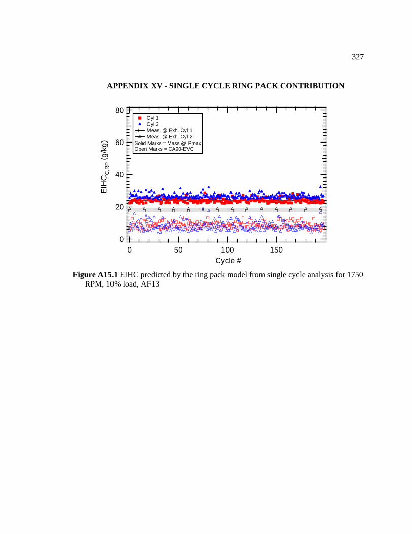
327
23 APPENDIX XV - SINGLE CYCLE RING PACK CONTRIBUTION
80
60
40
20
0
EIH
CC
,RP (g
/kg)
150100500Cycle #
Cyl 1 Cyl 2 Meas. @ Exh. Cyl 1 Meas. @ Exh. Cyl 2
Solid Marks = Mass @ PmaxOpen Marks = CA90-EVC
Figure A15.1 EIHC predicted by the ring pack model from single cycle analysis for 1750
RPM, 10% load, AF13
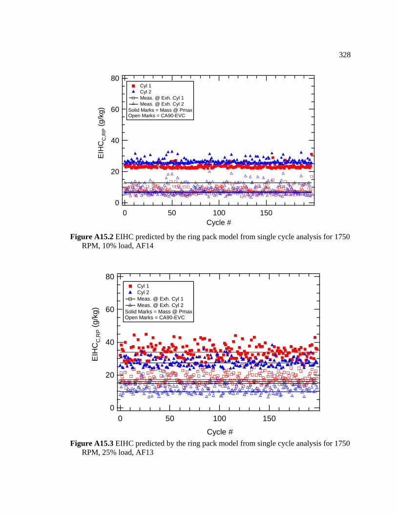
328
80
60
40
20
0
EIH
CC
,RP (g
/kg)
150100500Cycle #
Cyl 1 Cyl 2 Meas. @ Exh. Cyl 1 Meas. @ Exh. Cyl 2
Solid Marks = Mass @ PmaxOpen Marks = CA90-EVC
Figure A15.2 EIHC predicted by the ring pack model from single cycle analysis for 1750
RPM, 10% load, AF14
80
60
40
20
150100500
EIH
CC
,RP (g
/kg)
0
Cycle #
Cyl 1 Cyl 2 Meas. @ Exh. Cyl 1 Meas. @ Exh. Cyl 2
ysis for 1750
Solid Marks = Mass @ PmaxOpen Marks = CA90-EVC
Figure A15.3 EIHC predicted by the ring pack model from single cycle analRPM, 25% load, AF13
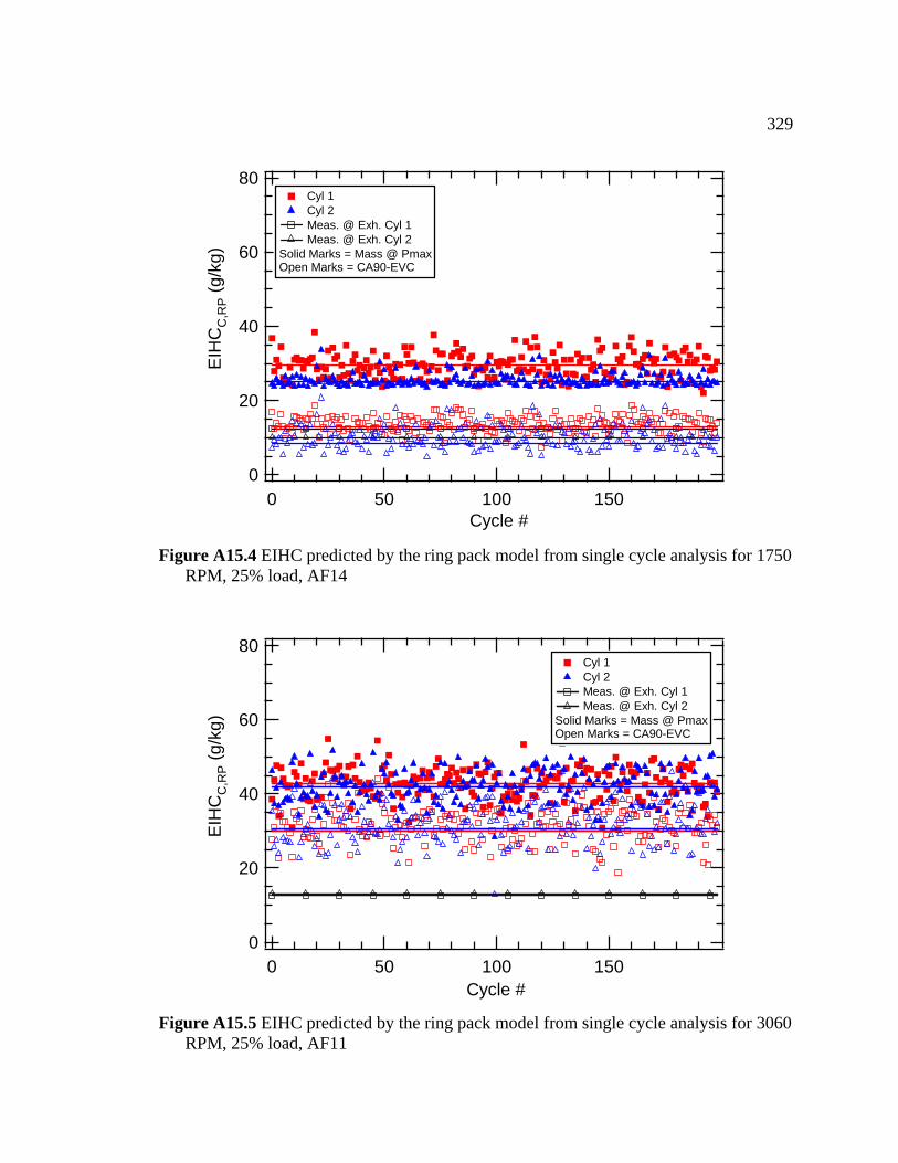
329
80
60
40
20
150100500Cycle #
Cyl 1 Cyl 2 Meas. @ Exh. Cyl 1 Meas. @ Exh. Cyl 2)
/kg
(gE
IHC
C,R
P
0
Solid Marks = Mass @ PmaxOpen Marks = CA90-EVC
Figure A15.4 EIHC predicted by the ring pack model from single cycle analysis for 1750
RPM, 25% load, AF14
80
60
40
20
0
EIH
CC
,RP (g
/kg)
150100500Cycle #
Cyl 1 Cyl 2 Meas. @ Exh. Cyl 1 Meas. @ Exh. Cyl 2
Solid Marks = Mass @ PmaxOpen Marks = CA90-EVC
Figure A15.5 EIHC predicted by the ring pack model from single cycle analysis for 3060
RPM, 25% load, AF11
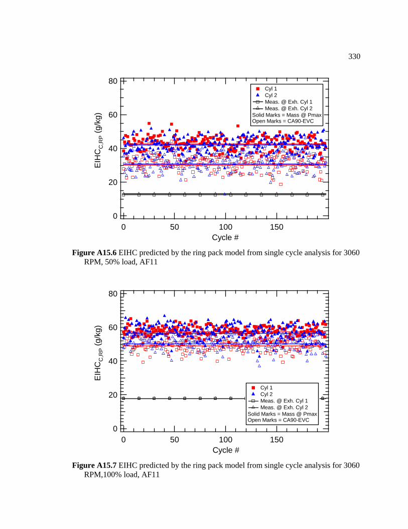
330
80
60
40
20
150100500
Cyl 1 Cyl 2 Meas. @ Exh. Cyl 1 Meas. @ Exh. Cyl 2
0
EIH
CC
,RP (g
/kg)
Cycle #
Solid Marks = Mass @ PmaxOpen Marks = CA90-EVC
g pack model from single cycle analysis for 3060
Figure A15.6 EIHC predicted by the rinRPM, 50% load, AF11
80
60
40
20
150100500
)E
IHC
(g/k
gC
,RP
Cyl 1 Cyl 2 Meas. @ Exh. Cyl 1 Meas. @ Exh. Cyl 2
Solid Marks = Mass @ Pmax
0
Open Marks = CA90-EVC
0
Cycle #
Figure A15.7 EIHC predicted by the ring pack model from single cycle analysis for 306RPM,100% load, AF11
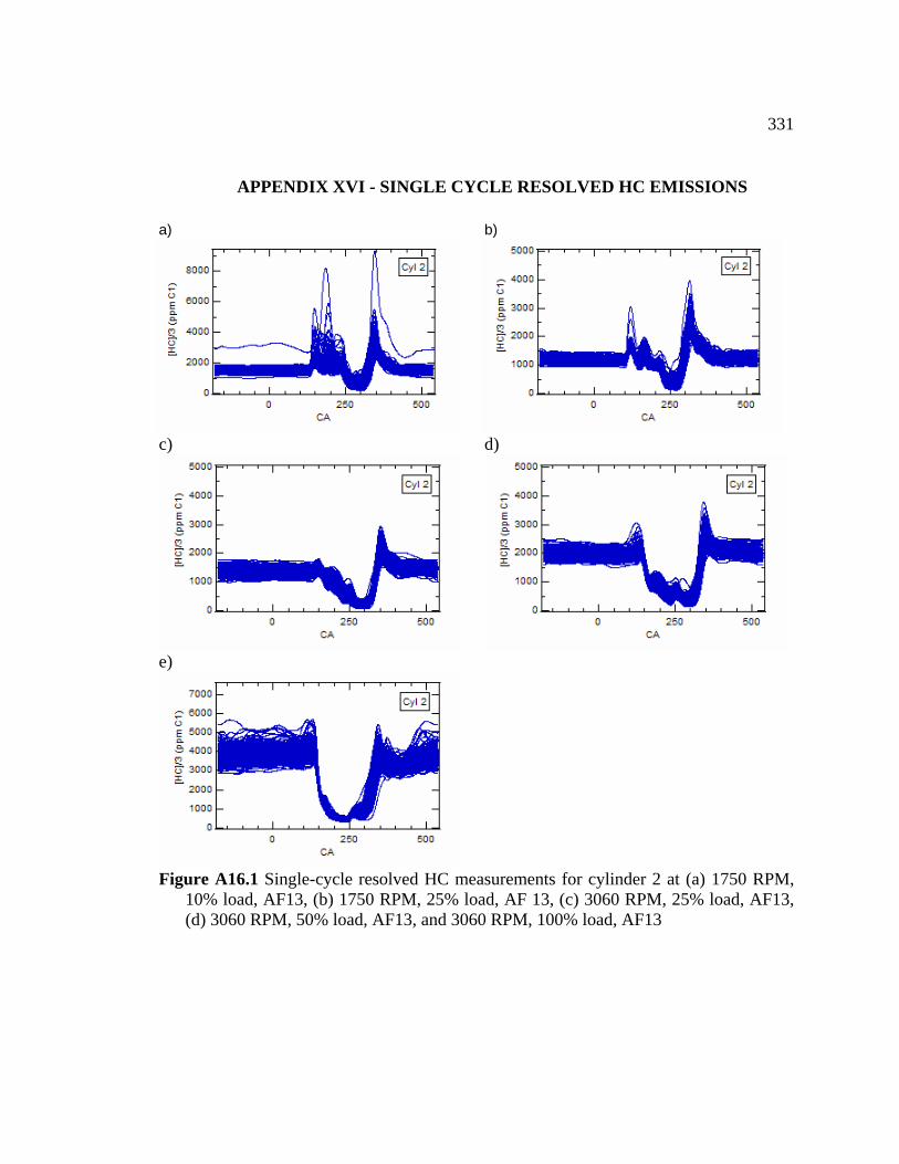
331
24 APPENDIX XVI - SI NGLE CYCLE RESOLVED HC EMISSIONS a) b)
d) c)
e)
Figure A16.1 Single-cycle resolved HC measurements for cylinder 2 at (a) 1750 RPM,
25% load, AF13, RPM, 50% load, AF13, and 3060 RPM, 100% load, AF1
10% load, AF13, (b) 1750 RPM, 25% load, AF 13, (c) 3060 RPM,3 (d) 3060
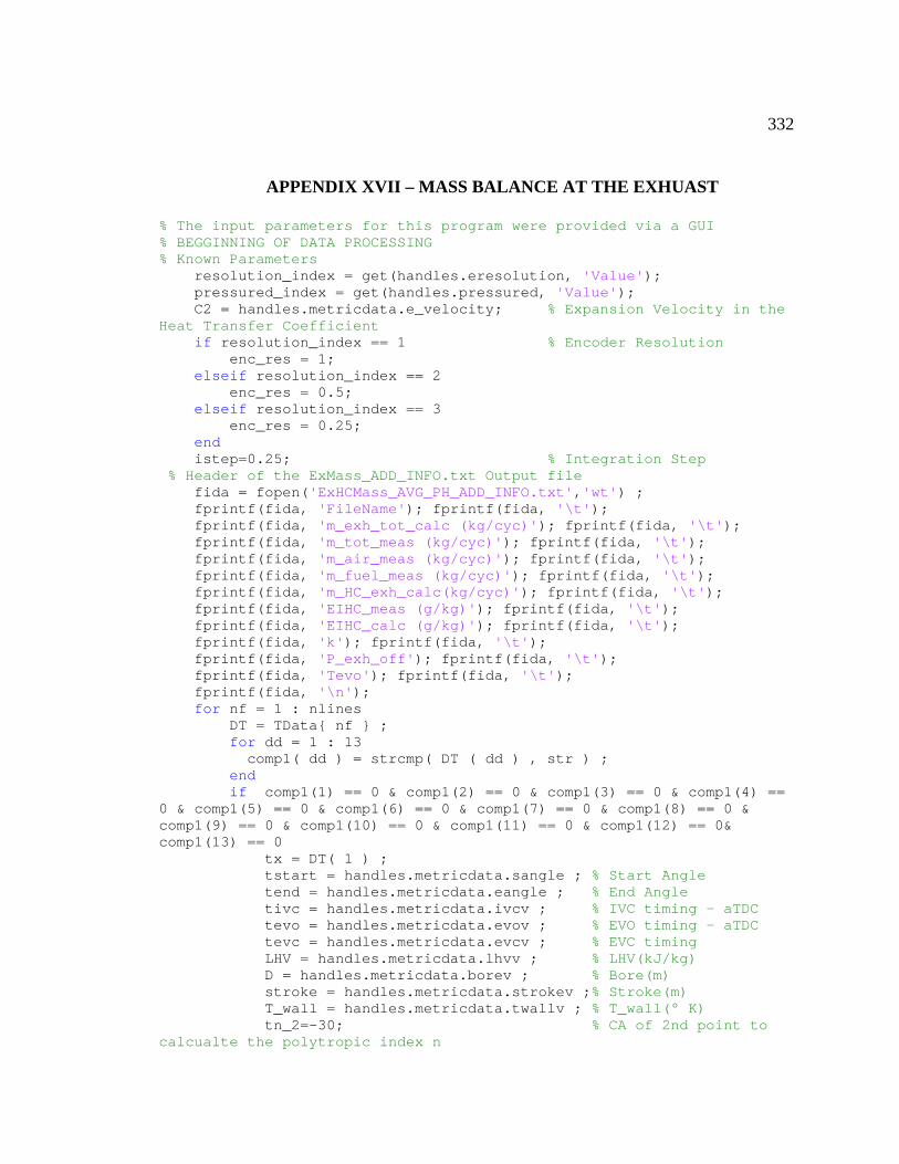
332
25 NDIX XVII – MASS BALANCAPPE E AT THE EXHUAST
% The input parameters for this program were provided via a GUI
on
p
rin (fida, '\t'); , '\t'
intf(fida, 'k'); fprintf(fida, '\t');
(4) == &
10) == 0 & comp1(11) == 0 & comp1(12) == 0& == 0
ndles.metricdata.eangle ; % End Angle
etricdata.twallv ; % T_wall(° K) % CA of 2nd point to
ndex n
% BEGGINNING OF DATA PROCESSING rameters % Known Pa
resolution_index = get(handles.eresolution, 'Value'); red_index = get(handles.pressured, 'Value'); pressu
C2 = handles.metricdata.e_velocity; % Expansion Velocity in the Heat Transfer Coefficient if resolution_index == 1 % Encoder Resoluti enc_res = 1; elseif resolution_index == 2 enc_res = 0.5; elseif resolution_index == 3 enc_res = 0.25; end istep=0.25; % Integration Ste % Header of the ExMass_ADD_INFO.txt Output file fida = fopen('ExHCMass_AVG_PH_ADD_INFO.txt','wt') ; fprintf(fida, 'FileName'); fprintf(fida, '\t'); fprintf(fida, 'm_exh_tot_calc (kg/cyc)'); fprintf(fida, '\t'); fprintf(fida, 'm_tot_meas (kg/cyc)'); fprintf(fida, '\t'); fprintf(fida, 'm_air_meas (kg/cyc)'); fprintf(fida, '\t'); fprintf(fida, 'm_fuel_meas (kg/cyc)'); fprintf(fida, '\t'); fprintf(fida, 'm_HC_exh_calc(kg/cyc)'); fp tf fprintf(fida, 'EIHC_meas (g/kg)'); fprintf(fida ); fprintf(fida, 'EIHC_calc (g/kg)'); fprintf(fida, '\t'); fpr fprintf(fida, 'P_exh_off'); fprintf(fida, '\t');
intf(fida, 'Tevo'); fprintf(fida, '\t'); fpr fprintf(fida, '\n'); for nf = 1 : nlines DT = TData{ nf } ; for dd = 1 : 13 comp1( dd ) = strcmp( DT ( dd ) , str ) ; end if comp1(1) == 0 & comp1(2) == 0 & comp1(3) == 0 & comp10 & comp1(5) == 0 & comp1(6) == 0 & comp1(7) == 0 & comp1(8) == 0
= 0 & comp1(comp1(9) =3) comp1(1
tx = DT( 1 ) ; tstart = handles.metricdata.sangle ; % Start Angle tend = ha tivc = handles.metricdata.ivcv ; % IVC timing - aTDC tevo = handles.metricdata.evov ; % EVO timing - aTDC tevc = handles.metricdata.evcv ; % EVC timing LHV = handles.metricdata.lhvv ; % LHV(kJ/kg) D = handles.metricdata.borev ; % Bore(m)
etricdata.strokev ;% Stroke(m) stroke = handles.m T_wall = handles.m
tn_2=-30; calcualte the polytropic i
333
tevc_tau = tevc ; % Tau name concatenation
ut Filename with
cle)
str2num( DT( 8 ) ) ; % Molar fraction O2
action % EGR concentration
pty(
lc ); eihcex = isempty( EIHC_exh );
ex = isempty( MW_exh ); afm = i mpty( AF ); mfo =
stants
/kmol-_air = 28.90 ; % Air molar mass
) ; % Exhaust Pressure Cyl
% File [ nrtx , nctx ] = size ( tx ) ; % Filename string size TX1 = tx ; rtx = tx ( 5 : nctx ); % Root Filename if tx(3)=='2'
; % Outp tx = strcat('O2_',rtx)all data else tx = strcat('O1_',rtx); end % Reading the main file with the Pressures and FFID info [hdrOfile, d] = hdrload(tx); % Reading file % Reading the Parameters of the table for each file from the table eta = str2num( DT( 2 ) ) ; % eff._comb m_air = str2num( DT( 3 ) ) ; % mass_air(kg/cy m_fuel = str2num( DT( 4 ) ) ; % mass_fuel(kg/cycle) RPM = str2num( DT( 5 ) ) ; % RPM
T_exh = str2num( DT( 6 ) ) ; % T_exhaust (°K) nt = str2num( DT( 7 ) ) ; % T_intake( °K) T_i
X_O2_calc = calc
EIHC_exh = str2num(DT(9)); % Emissions index HC (g/kg) MW_exh = str2num( DT( 10 ) ) ; % Molecular weight AF = str2num(DT(11)); % Air fuel ratio (kg air / kg fuel) X_O2 = str2num( DT( 12 ) ) ; % Oxygen mole fr
EGR = str2num( DT( 13 ) ) ; % Checking the GUI table inputs
ee = isempty( eta ); mm = isempty( m_air ); mf = isem m_fuel ); tin = isempty( T_int ); rpp = isempty( RPM ); tex = isempty( T_exh ); mfocalc =isempty( X_O ca2_ mw seisempty( X_O2 ); egr1 = isempty( EGR); if ee == 0 & mm == 0 & mf == 0 &rpp == 0 & tex == 0 & mfocalc == 0 & eihcex == 0 & tin == 0 & mwex == 0 & afm == 0 & mfo == 0& egr1 == 0 % Con Ru = 8314 ; % Universal Gas Constant J K MWkg/kmol R= Ru / MW_air ; % Air constant, J/kg-K gamma = 1.4; % Specific Heat Ratio for exhaust gases % Vectors with data from the Output file CA = d ( : , 1 ) ; % Crank angle vector V = d ( : , 2 ) ; % Cyl.1 volume m^3 P = 1000 * d ( : , 3 ) ; % Pressure Cylinder 1 in Pa EP = 1000 * d ( : , 4 1, and with correction for cyl 2
334
HCFFID=d(:,5); % Fast FID data ppm/3 of CH, or ppm C3
[ Nd , f ] = size( d ) ; % Data matrix size
EV] = hdrload('EVL.txt'); % File with lift
] = size( LEV) ; % Data matrix size
e coefficient file CD_ev.txt
[hdrCD Cdm]=hdrload('CD_ev.txt'); % File with the
arge coef. exhaust valve ol. of Cd
alve diameter in mm / enc_res + 1
res ; evlift , CAi ( i ) ,
Dv * LEVi ( i ) * 1e-6 ; % Area in
, Cd , Lv_Dv ( i ),
enc_res
egration time step in sec for
yl1 and Cyl2
p1(CA,V,tevc,'spline'); % m^3 P_evo=interp1(CA,P,tevo,'spline'); % Pa
enc_res=d(2,1)-d(1,1); % Encoder res from the input data file % Reading of the Valve Profile file EVL.txt [hdrEVL, Lin mm [ revl , cevl CAl = LEV ( : , 1 ); % Crank angle exhaust valve lift, deg evlift = LEV ( : , 2 ) ; % Exhaust valve lift,mm% Reading of the discharg
, Cd=Cd(Lv/Dv) [ rCd , cCd ] = size( Cdm ) ; % Data matrix size LvDv = Cdm ( : , 1 ); % Lv/Dv for the valve Cd = Cdm ( : , 2 ); % Disch
terp% Calc.of the curtain area Ac, Lv/Dv and in Dv = 29.5 ; % V
* 2 for i = 1 : (revl - 1 ) CAi ( i ) = ( i -1 ) * enc_
CAl, LEVi ( i ) = interp1 ('linear' ) ; % Lift in mm Lv_Dv ( i ) = LEVi(i)/Dv ; % mm Ac ( i ) = pi * m^2 Cdi ( i ) = interp1 ( LvDv'spline') ;
end % Pegging CA to the evo event CAshift=27; % Based in the 0.008 in criteria for open and close valve % Cylinder and Exhaust Pressures in the integration window for i = 1 : (revl - 1 )* 2 / enc_res + 1 CAint ( i ) = CA ( ( 180 + tevo - CAshift ) / enc_res + i ) ; Pi ( i ) = P ( ( 180 + tevo - CAshift ) / + i ) ; EPi ( i ) = EP ( ( 180 + tevo - CAshift ) / enc_res + i ) ;
) = HCFFID ( ( 180 + tevo - CAshift ) HCFFIDi ( i / enc_res + i ) ; end % Calculation of Additional Parameters dCAint=CAint(1,2)-CAint(1,1); % CA step integration, in Crank Angle dt=dCAint/(6*RPM); % Inteach file changes with the velocity
; % Size of the integration vectorvpsize=(revl-1)* 2 / enc_res + 1% Volume and Pressure at evo and evc conditions CV_ivc=interp1(CA,V,tivc,'spline'); % m^3 V_evo=interp1(CA,V,tevo,'spline'); % m^3 V_evc=inter
335
P_ivc=interp1(CA,P,tivc,'spline'); % Pa P_evc=interp1(CA,P,tevc,'spline'); % Parameters at evo for the integration
% Pa
) , 'spline'); % m^3 sion politrop coefficient
_evo ) * ( P_evc / P_evo ) ^ ( 1 / n_comp ) ;
( m_air + m_fuel ) * ( 1 + ( EGR / 100 ) / 1 - EGR / 100
m_trapped1 ; _res_int1 - (m_air + m_fuel )
m es_ext1 ;
Ru / MW_exh ; % Burned gases constant in J/kg-K m_air + m_fuel + m_res1 ) ) ; %
d
)); % Choke flow criteria diff = 1 ; % Mass difference = abs (
% Number of iteration required to
l decrease in pressure to
>= EPi( i ) ) / Pi( i ) < 0.52
mma + 1 )
) / EPi( i ) / Pi( i ) ) ^( ( gamma + 1 ) /
P_evoi=interp1 (CA , P , CAint(1) , 'spline'); % in kPa V_evoi=interp1 (CA , V , CAint( 1% Pres. and Vol. to calc. compres icP_1 = interp1( CA , P , tivc + 5 , 'spline') ; P_2 = interp1( CA , P , tn_2 , 'spline') ; V_1 = interp1( CA , V , tivc + 5 , 'spline') ; V_2 = interp1( CA , V , tn_2 , 'spline') ; n_comp = log( P_2 / P_1 ) / log( V_1 / V_2 ) ; % Residual Mass Calculation y_res_int1 = ( V_evc / V% Calcualtion of the mass trapped m_trapped1 = () ) / ( 1 - y_res_int1 ); m_res_int1 = y_res_int1 *m_res_ext1 = m_trapped1-m
_rm_res1 = m_res_int1 + y_res1 = m_res1 / m_trapped1 ; % Blowdown Temperature Approximation R_b = Tevo1 = P_evoi * V_evoi / ( R * (_bTevo in K, Cyl. 1 for i = 1 : (revl - 1 )* 2 / enc_res + 1 Tbd ( i ) = Tevo1 * ( Pi ( i ) / P_evoi ) ^ ( ( gamma - 1 ) / gamma ); % Blow.Temp. Cyl. 1 en% Mass Flow through the exhaust valve PRc=(2/(gamma+1))^(gamma/(gamma-1
calculated - measured), used for stop criteria dPexh = 0.01 * 1e3 ; % Increse in exhaust pressure to match the mass per cycle k = 0 ; match the mass of the cylinder dPup = 0 ; % Total increse in pressure to match the meas. mass, in kPa dPdown = 0 ; % Totamatch the meas. mass, in kPa while abs(diff) > 1e-6 && k < 5000 % Criteria to stop the loop Cyl. 1 % Mass calculation - Cyl. 1 for i = 1 : (revl - 1 )* 2 / enc_res + 1 if Pi( i ) if EPi( i eta1 = ( 2 / ( gamma + 1 ) ) ^ ( ( ga/ ( 2 * ( gamma - 1 ) ) ); else et = ( 2 / ( gamma - 1 ) * ( ( EPi( ia1Pi( i ) ) ^ ( 2 / gamma ) - (gamma ) ) ) ^ 0.5 ; end
336
me ( i ) = Cdi ( i ) * Ac ( i ) * ( sqrt ( gamma / ( R_b * Tbd ( i ) ) ) * Pi ( i ) ) * eta1 ; else if Pi( i ) / EPi( i ) < 0.52 eta2i = ( 2 /( gamma + 1 ) ) ^ ( ( gamma + 1 / ( 2 * ( gamma
) - 1 ) ) ) ;
/ ( gamma - 1 ) * ( ( Pi( i ) / Pi ) / EPi( i ) ) ^ ( ( gamma + 1 ) /
Cdi ( i ) * ( i *
l mass cycle in kg, Cyl. 1
le1_calc ;
Pi = EPi - dPexh ; + dPexh ;
ff ) ; ) = k ;
% Carbon Molecular Weigth % Hydrogen Molecular Weigth
9 * y ; % Fuel Molecular weight C1 based 2 / enc_res + 1 % Calculation of the fuel
l. 1 ) = 3 / 1000000 * HCFFIDi ( i ) ; % HC molar haust
mf ( i ) * ( MW_fuel ) / ( MW_exh ) * me ( i % Fuel mass flow
- 1 )* 2 / enc_res = ( mfuel ( i ) + mfuel ( i + 1 ) ) / 2 * dt ;
l_calc = sum ( dm_fuel1 ) ; % Total fuel per cycle in
else eta2 = ( 2
ii
EPi( i ) ) ^ ( 2 / gamma ) - ( ( gamma ) ) ) ^ 0.5 ; end
) me ( i ) = - Ac(sqrt ( gamma /( R_b * Tbd ( i ) ) )* EPi( i ) )* eta2i ; end end % Exh. mass per cycle Calc. Cyl. 1 for i = 1 : (revl - 1 )* 2 / enc_res dme1( i ) = ( me ( i ) + me ( i + 1 ) ) / 2 * dt ; % Differetial of mass end m_exh_cycle1_calc = sum ( dme1 ) ; % Totaper% if condition to match the measured mass flow
m_air + m_fuel ) - m_exh_cyc diff = ( if diff < 0 EPi = EPi + dPexh ; dPup = dPup + dPexh ;
if diff > 0 else E
dPdown = dPdown end k = k + 1 ;
( k ) = abs ( di Diff K ( k
end % Calculation of Mass Fuel
y = 1.804 ; MW_C = 12.011 ;
; MW_H = 1.0079 MW_fuel = 12.011 + 1.007
: (revl - 1 )*for i = 1mass flow Cy HCFFID_mf ( i
e exfraction at th mfuel ( i ) = HCFFID_
) ; end for i = 1 : (revl
i ) dm_fuel1( % Fuel mass differentialend m_fuel1_totaKg, Cyl. 1
337
EIHC_calc = m_fuel1_tot _calc / m_fuel * 1000 ; % Emission index in
EIHC_exh ; % EIHC measured n ---------------------
= 1000* me ; % Exhaust mass flow in g/s Cyl. 1 asured
-------------
cat('EHCM2_',rtx); ');
;
O, '\t'); dO, '\t');
ntf(fidO, TX); fprintf(fidO, '\t'); ; fprintf(fidO, TX);
'%g\t', Tbd(v)); Pi(v));
);
);
nf},'wt');
tf(fidO, TX); fprintf(fidO, '\t'); O, 'Pe1_'); fprintf(fidO, TX); fprintf(fidO, '\t');
fprintf(fidO, '%3.3f\t', CAint(v));
fprintf(fidO, '%g\t', me(v)); uel(v));
);
fprintf(fida, '\t');
alg/kg_fuel
EIHC_meas = %-------------------End of fue mass calculatiome m_total_measured=(m_air + m_fuel); % Total exh. mass meEP1i_offset = dPup -dPdown ;
--Output files ---------%-----------------if tx(2)=='2'
str OHR{nf}= fidO=fopen(OHR{nf},'wt TX = rtx; fprintf(fidO, 'CA2_'); fprintf(fidO, TX); fprintf(fidO, '\t');
fprintf(fidO, 'Tbd2_'); fprintf(fidO, TX); fprintf(fidO, '\t') fprintf(fidO, 'P2_'); fprintf(fidO, TX); fprintf(fid
intf(fidO, TX); fprintf(fi fprintf(fidO, 'Pe2_'); fpri fprintf(fidO, 'm2_'); fpr
fprintf(fidO, 'm_HCexh2_') fprintf(fidO, '\n'); for v = 1 : (revl - 1 )* 2 / enc_res + 1
, '%3.3f\t', CAint(v)); fprintf(fidO fprintf(fidO, fprintf(fidO, '%g\t', fprintf(fidO, '%g\t', EPi(v) fprintf(fidO, '%g\t', me(v));
(v) fprintf(fidO, '%g\t', mfuelrintf(fidO, '\n'); fp
end fclose(fidO); else OHR{nf}=strcat('EHCM1_',rtx);
O=fopen(OHR{ fid TX = rtx; fprintf(fidO, 'CA1_'); fprintf(fidO, TX); fprintf(fidO, '\t'); fprintf(fidO, 'Tbd1_'); fprintf(fidO, TX); fprintf(fidO, '\t');
O, 'P1_'); fprin fprintf(fid(fid fprintf
fprintf(fidO, 'm1_'); fprintf(fidO, TX); fprintf(fidO, '\t'); fprintf(fidO, 'm_HCexh1_'); fprintf(fidO, TX); fprintf(fidO, '\n'); for v = 1 : (revl - 1 )* 2 / enc_res + 1 fprintf(fidO, '%g\t', Tbd(v)); fprintf(fidO, '%g\t', Pi(v)); fprintf(fidO, '%g\t', EPi(v)); fprintf(fidO, '%g\t', mf fprintf(fidO, '\n' end
; fclose(fidO)end % ExHCMass_AVG_PH_ADD_INFO.txt fprintf(fida, TX1 );
338
fprintf(fida, '%g\t', m_exh_cycle1_calc); fprintf(fida, '%g\t', m_total_measured); fprintf(fida, '%g\t', m_air); fprintf(fida, '%g\t', m_fuel); fprintf(fida, '%g\t', m_fuel1_total_calc); fprintf(fida, '%g\t', EIHC_meas);
if tx(2)=='2'
legend ( 'Error Cyl 2')
lot(CAint,Pi,CAint,EPi)
ure
gure plot(CAint,Tbd)
( Diff)
l ('k'); ylabel('Error-Cyl. 1');
el('CA');ylabel('Pressure(kPa)');
xh-1')
fprintf(fida, '%g\t', EIHC_calc); fprintf(fida, '%g\t', k); fprintf(fida, '%g\t', EP1i_offset); fprintf(fida, '%g\t', Tevo1); fprintf(fida, '\n'); oplots = 1 ; if oplots == 1 ; figure plot ( Diff)
xlabel ('k'); ylabel('Error-Cyl. 2'); figure
p legend('P2','P_exh2') xlabel('CA');ylabel('Pressure(kPa)');
fig plot(CAint,mfuel) legend('Fuel mass flow Cyl. 2') xlabel('CA');ylabel('fuel mass flow');
figure plot(CAint,me,CAint,HCFFIDi ) legend('mexh-2', 'FFID2') xlabel('CA');ylabel('Exhaust Mass Flow Cyl. 2 (g/s)'); fi legend('Texh-2') xlabel('CA');ylabel('Exhaust Temperature Cyl.2 (K)'); else figure plot legend ( 'Error cyl 1') xlabe figure plot(CAint,Pi,CAint,EPi) legend('P1','P_exh1') xlab figure plot(CAint,mfuel) legend('Fuel mass flow Cyl. 1') xlabel('CA');ylabel('fuel mass flow'); figure plot(CAint,me,CAint,HCFFIDi ) legend('mexh-1','FFID1') xlabel('CA');ylabel('Exhaust Mass Flow Cyl. 1 (g/s)'); figure plot(CAint,Tbd) legend('Te
339
xlabel('CA');ylabel('Exhaust Temperature Cyl.1 (K)'); end end else errordlg('Parameters must be numeric','Error'); end else errordlg('Table should be filled correcty','Error'); end end fclose(fida); else errordlg('Table should be filled','Error'); end toc set(handles.text36, 'String', toc);
'Enable', 'on'); set(handles.calculate, 'Enable', 'on'); set(handles.reset,%========END OF DATA PROCESSING========
340
26 APPENDIX XVIII – OIL-FUEL DIFFUSION
culation------
n of the liquid molar volume at the normal boi ng
4.33,
ORTLIB
)
ol. @ NBP
P
_C6H14 ^ 1.048 ; % Liq. molar vol. @ NBP
BP enzene"
%-----Oil Film -Cycle Simulation-Multicomponent Main Cal% Written by: Victor M. Salazar % ERC-UW Madison % June 12, 2008 clc tic %Known Parameters Tw = 380 ; % Cylinder Wall Temperature in K
yer thickness in m th = 2e-6 ; Oil laRPM = 3060 ; % Engien Speed in RPM %------Diffusivity Calculation--------- %---- Estimatio lipoint----
the Tyn and Calus Method (1975), pg. %This was performed usign%Eq. (4-10.2) from " The Properties of Gases and Liquids " by %Poling, B., Prausnitz, J. M., and O'connell, J.P., 5th Editi .on% Critical Volumes (cm^3/g-mol) extracted from the SUPERTRAPP P% file, 1st row, second column Vc_C3H8 = 200 ; % critical volume (cm^3/mol) of Propane" Vc_C5H12 = 306 ; % critical volume (cm^3/mol) of "I-Pentane" Vc_C6H14 = 367 ; % critical volume (cm^3/mol) of "3-Methylpentane" Vc_C6H6 = 259 ; % critical volume (cm^3/mol) of "Benzene" Vc_C7H16 = 431.97 ; % critical volume (cm^3/mol) of "N-Heptane" Vc_C7H8 = 316 ; % critical volume (cm^3/mol) of "Toluene" Vc_C8H18 = 468 ; % critical volume (cm^3/mol) of "I-Octane" Vc_C8H10m = 376 ; % critical volume (cm^3/mol) of "m-Xylene" Vc_C8H10p = 379 ; % critical volume (cm^3/mol) of p-Xylene [kg/kmol] Vc_C9H12 = 427.35 ; % critical volume (cm^3/mol) of 1,2,4 Trimethylbenzene [kg/kmol] Vc_C10H22 = 600 ; % critical volume (cm^3/mol) of N-Decane [kg/kmol] Vc_C12H26 = 719.7 ; % critical volume (cm^3/mol) of N-Dodecane [kg/kmol] %--Liquid molar volume at the normal boiling point (cm^/mol
Liq. molar v VA_C3H8 = 0.258 * Vc_C3H8 ^ 1.048 ; % (cm^3/mol) of Propane"
B VA ( 1,1 ) = 0.258 * Vc_C5H12 ^ 1.048 ; % Liq. molar vol. @ N(cm^3/mol) of "I-Pentane" VA ( 2,1 ) = 0.258 * Vc(cm^3/mol) of "3-Methylpentane" VA ( 3,1 ) = 0.258 * Vc_C6H6 ^ 1.048 ; % Liq. molar vol. @ N(cm^3/mol) of "B
341
VA ( 4,1 ) = 0.258 * Vc_C7H16 ^ 1.048 ; % Liq. molar vol. @ NBP
1 ) = 0.258 * c_C7H8 ^ 1.048 ; % Liq. molar vol. @ NBP
NBP of "I-Octane"
_C8H10m ^ 1.048 ; % Liq. molar vol. @ NBP
1 ) = 0.258 * c_C8H10p ^ 1.048 ; % Liq. molar vol. @ NBP /kmol]
P ) of 1,2,4 Trime ylbenzene [kg/kmol]
c_C10H22 ^ 1.048 ; % Liq. molar vol. @ NBP
11,1 ) = 0.258 * V C12H26 ^ 1.048 ; % Liq. molar vol. @ NBP kmol]
%[K]
-
ne = ''; 'F3 fCr_pressure [kPa]' ) ) %
line = fgetl( fid ) ;
; %Extracting the
f file reading cto
ector solution
ace -------------
(cm^3/mol) of "N-Heptane" VA ( 5, V(cm^3/mol) of "Toluene" VA ( 6,1 ) = 0.258 * Vc_C8H18 ^ 1.048 ; % Liq. molar vol. @ (cm^3/mol) VA ( 7,1 ) = 0.258 * Vc(cm^3/mol) of "m-Xylene" VA ( 8, V(cm^3/mol) of p-Xylene [kg VA ( 9,1 ) = 0.258 * Vc_C9H12 ^ 1.048 ; % Liq. molar vol. @ NB(cm^3/mol th VA ( 10,1 ) = 0.258 * V(cm^3/mol) of N-Decane [kg/kmol] VA ( c_(cm^3/mol) of N-Dodecane [kg/ [ncr, ncc ] = size (VA) ; %------Input parameters to calculate the Concentration at the interface (B.C.)--------- phi = 1.2; %"Equivalence Ratio" T = Tw ; %380 ; m_fuelcyc = 15.902e-6 ; %"Mass of fuel per cycle"[kg] %------Reading the Pressure File (Experimental data)----------- tx = 'lu1_RP-3060-50-AF12-L.txt' ; % File name fid = fopen( tx ) ; % To open the data file li while isempty( findstr( line , looking for the line with the data end
d = fscanf( fid , '%f' , [ 5 , inf ] )'data of the look Up file
%Size of the file [ nr , nc ] = size( d ) ; fclose( fid ) ; % End o CA = d( :, 1 ) ; % CA ve r P = d( :, 4 ) ; % Pressure v
e dCA = d(2,1) - d(1,1); % Encoder r %--------- Shifiting of the pressure CAi =( -360:0.5:359.5) ;
tr
CAs = 180 ; nps = CAs / 0.5 ;
for i = 1: nps Ps ( i ) = P ( nr - nps + i ) ;
end
342
for i = ( nps + 1 ):nr Ps ( i ) =
end P ( - nps + i ) ;
End of shifting pressure trace-------------
ertical Position -------------
% Crankshaft radius in m necting rod length in m
( CA ( i ) / 180 * pi ) + ( l^2 - a^2* ( 2 )^(1/2) - ( l - a ) ;
-
% CA of end of combustion
ivided -----------
% Number of segments that the s being divided vertic ly
r the oil-film
c ( i ) = dL + ( i ) dL ;
ation of the matrix wiht the concentration
th the concentration
% Counter of number of plots
r,ns);
P = Ps ; CA = CAi ; %----------------- %-------- Piston v a = 33.5*1e-3 ; l = 114 * 1e-3 ; % Con for i = 1 : nr s( i ) = a * cossin (CA( i ) / 180 * pi ) )^ end
---- %----------------------- Time simulation -------------------- ncyc = 20; % Number of cycles for simulation nt = ncyc * nr ; % Number of time steps for the simulation nx = 200 ; % Number of space steps along the oil film dt = dCA * 60 / (RPM * 360) ; % time step in the simulation j = 1 ; % Index counting the number of cycles of simulation t1 = 1 ; % On or off of the concentration in the combustion chamber dx = th / (nx-1) ; % space step
% space dimension x = ( 0:dx:th); CAeoc = 39.50 ;
be d %------ Number of Segments to
ns = 40 ;
alcyinder i L = max ( s ) - min ( s ) ; % Total height of the cylindecovered by dL = L / ns ; % height of the vertical segment for i = 1 : ns
* L % heigth of each of the vertical segements end %------- Initializ
accross %the oil layer phio = zeros ( nx , ns*ncr ); % Matrix with the concentration
profile for all vertical segment phis = zeros ( nx , 1 ); % Matrix wiprofile for only one segment coun = 0 ; mic = zeros (nr,ns*ncr); moc = zeros (nr,ns*ncr); mi = zeros (nc
343
mo = zeros (ncr,ns); %---------Initial Concentration of the mixture in the cylinder ----
rix
----------------------- f
ation
ime
% Reasigment the considering the flame arrival % Boundary
cosity in centipoise cP (1/100 poise).
ion Equation--------------
% for loop for each
--- he Hayduk and Minnas correlation, pg.
ses and Liquids "
791 ;
* ( mu ^ E ) / ( VA ( ic ) ^0.71 in m2/s
r k = 1 : ns % for loop for the
---- [A1, Y1 ] = Xim( phi, m_fuelcyc, T, 100, th) ; %
Mat with all the equil info from SUPERTRAPP 4:14, 1 ) ; r1blowby = Y1(
%- ----- ----- - -------------------------
or i = 1 : nt + 1440; %1000 %nt % main loop for * ( j - 1 ) ; % time index modific i = i - 1440
as the number of cycles is increased [A, Y ] = Xim( phi, m_fuelcyc, T, P ( i ), th ) ; % Matrix with all the equil info from SUPERTRAPP
; % X (:, i) = Y( 4:14, 1 )Concentration of propane at the interface
>= CAeoc && CA ( i ) <= 360 % T if CA ( i )when combustion reaches the cylinder wall, the fuel conc. goes to zero t1 = 0 ; else t1 = 1 ; end X (:, i) = t1 * X (:, i);
e cyl.of concentration inside th r1 = X (:, i) ;
Condition with the concentration mu = A( 11, 3 ) / 10000 ; % oil
vis %--------Solution of the Diffus for ic = 1 : ncr fuel component %-----Diffusivity Estimation------- % This was done using t.25 11
% Eq. (11-9.8) from " The Properties of Gaby
% Poling, B., Prausnitz, J. M., and O'connell, J.P., 5th Edition. E = ( 10.2 / VA ( ic ) ) - 0.% Factor used in the Diff. eval. D= 13.3 * 1e-8 * ( T ^ 1.47 )
iffusivity of fuel in oil) * 1e-4; % D focylinder segments r1 = X (:, i) ; % Boundary Condition with the concentration if s( i ) > Lc ( k )
344
r1 ( ic ) = r1blowby (ic)/4 ;% 0.25*1e-3 ; %
ix at each time stepth, D, nx, dt, r1 (ic) ) ; %
f. Eq. phio ( : , k + ns * ( ic -1 )) = C ;
reas f the new value d % end of for loop
ents % end of for loop
different times cyc % Loop for
if i == npi
%-----------Cummulative mass
components
< Lc (nim) : , nim he film
if CA(i)>CAeoc && CA(i)<360 if s(i) < Lc( nim )
x, phio( of the
end mo (ic,nim) = 0; end
%------------------ mo
Blowby concentration end phis = phio ( :, k + ns * ( ic -1 ) ) ; %
In lization of the citia oncetratin matr C = OilDiff1DEq( phis, Solution of the Dif % igmetn o enfor the cylinder segem end for each fuel component %-------Pictures at if j > nthe last cycle for npi = 750 :50:1000 for ic = 1 : ncr
figure
for nsi = 1:ns
hold on plot(phio( : , nsi + ns * ( ic -1 )
) ) ; end end coun = coun + 1 ; end end
in each element for all %the fuel for ic = 1 : ncr % for for each
fuel component for nim = 1 : ns % forcummulative mass at each segment
if s( i ) mo (ic,nim ) = trapz( x, phio(
+ ns * ( ic -1 ) ) ) ; % mass out of the cylinder, in t
end
mi (ic,nim ) = trapz( : , nim + ns * ( ic -1 ) ) ) ; %mass in the cylinder, out film
moc( i, nim + ns * ( ic -1 ) ) =
(ic,nim);
345
mic( i, nim + ns * ( ic -1 ) ) = mi
if CA ( i ) >=360 mic( i, nim + ns * ( ic -1 ) ) = 0*
end %-----------------
% end for ment
end % end for of each
----------------------------------------------
% End of loop for
-----------------------------------
--- -------------------------
mocr = zeros(nr,ns*ncr); for ic = 1 : ncr % for throught each fuel component for j = 1 : ns % for through each cylinder segment for i = 1 : nr % for through each of the 1440 points of the cycle if mic ( i, j + ns * ( ic -1 ) ) >0 micr ( i, j + ns * ( ic -1 )) = max( mic( :, j + ns * ( ic -1 ) ) ) - mic( i, j + ns * ( ic -1 ) ) ; % mass in cylinder cummulative end if moc ( i, j + ns * ( ic -1 ) ) >0 dmocr ( i, j + ns * ( ic -1 ) ) = max( moc( :, j + ns * ( ic -1 ) ) ) - moc( i, j + ns * ( ic -1 ) ); % difference between the maximum and minimum end end % for through each of the 1440 points of the cycle min_mocr = max( moc(:, j + ns * ( ic -1 ) ) ) - max(dmocr(:, j + ns * ( ic -1 ) ) ); % Minimum value of the mass in each element for i = 1 : nr if moc ( i, j + ns * ( ic -1 ) ) >0 mocr (i, j + ns * ( ic -1 ) ) = moc(i, j + ns * ( ic -1 ) ) - min_mocr; % mass out of the cylinder cummulative end end mcumi ( ic, j ) = max( micr( :, j + ns * ( ic -1 ) ) ) ;
(ic,nim) ; mi (ic,nim); endcummulative mass at each seg fuel component %-------- end last cycle %---- if i == 1440 ; j = j + 1 ; end end % main loop end for%-- -------------------------------------------- micr = zeros(nr,ns*ncr);
346
mcumo ( ic, j ) = max( mocr( :, j + ns * ( ic -1 ) ) ) ; end % Enf of for through each segment end % End of for through each component mci_totc = sum(mcumi,2); mco_totc = sum(mcumo,2); mci_tot = sum(mci_totc); mco_tot = sum(mco_totc); rho = (A ( 2, 3 ) * A( 4, 3 )) ; % Mixture density Dc = 0.08; % cylinder diameter m LC = pi * Dc ; % cylinder circunference length mass_total = rho * dL * LC * mci_tot; masso_total = rho * dL * LC * mco_tot; pcti_fuel = mass_total/ m_fuelcyc * 100 pcto_fuel = masso_total/ m_fuelcyc * 100 hist_micr = rho * dL * ( LC / m_fuelcyc * 100 )* sum ( micr, 2 ) ; hist_mocr = rho * dL * ( LC / m_fuelcyc * 100 )* sum ( mocr, 2 ) ; %------------------------------------------------------ %-----------------------Output File----------------------- OLPH{1}=strcat('CumMass_','N-Hexatriacontane-Multi'); fid=fopen(OLPH{1},'wt'); fprintf(fid, 'CA'); fprintf(fid, '\t'); fprintf(fid, 'Cumm_mass_in'); fprintf(fid, '\t'); fprintf(fid, 'Cumm_mass_out'); fprintf(fid, '\t'); fprintf(fid, '\n'); for v=1:nr fprintf(fid, '%3.3f\t',CA(v)); fprintf(fid, '%g\t', hist_micr(v)); fprintf(fid, '%g\t', hist_mocr(v)); fprintf(fid, '\n'); end fclose(fid); %---------------- Plots ---------------------------- figure for i = 1:ns hold on plot(CA,mic(:,i)) end figure for i = 1:ns hold on plot(CA,micr(:,i)) end figure for i = 1:ns hold on plot(CA,moc(:,i)) end figure for i = 1:ns
347
hold on plot(CA,mocr(:,i)) end toc % Time of end of calculation function [phi] = OilDiff1DEq (phio, th, D, nx, dt, r1) ; %Crank Nicholson, 1-D Diffusion Equation %Know Parameters phi = phio ; Lx = th ; dx = Lx / ( nx - 1 ) ; Dbar = D * dt / ( dx ^ 2 ) ; %--------- Coefficients of a, b, c, crwk of the thomas algoritm %------ Initialization of the coefficients ------ a = zeros ( nx , 1 ) ; b = zeros ( nx , 1 ) ; c = zeros ( nx , 1 ) ; cwrk = zeros ( nx , 1 ) ; %----- Definition of the coefficients --------- b ( 1 ) = 1 ; r ( 1 ) = r1 ; for i = 2 : nx - 1 a ( i ) = - 1/2 * Dbar ; b ( i ) = 1 + Dbar ; c ( i ) = - 1/2 * Dbar ; end a ( nx ) = - Dbar ; b ( nx ) = 1 + Dbar ; r ( nx ) = phi ( nx ) + 1/2 * Dbar * ( - 2 * phi ( nx ) + 2 * phi ( nx - 1 ) ) ; for i = 2 : nx - 1 r ( i ) = phi ( i ) + 1/2 * Dbar * ( phi ( i + 1 ) - 2 * phi ( i ) + phi ( i - 1)) ; end r ( nx ) = phi ( nx ) + 1/2 * Dbar * ( -2 * phi ( nx ) + 2 * phi ( nx - 1 ) ) ; phi = thomas ( a, b, c, cwrk, r, nx ) ; function [A, Y] = Xim(phi, m_fuelcyc, T, P, th ) ; %Multicomponent equilibrium simulation %Written by Victor M. Salazar %Engine Research Center %University of Wisconsin-Madison %April 06,2008 P = P / 100 ; %[bar] method = 1 ; % method= 1, for PR and method = 2 for CS
348
%-------------------------------------------------------------------------- Ai = NISTSUPPMATLB (P, T, method, 1,'C36'); %Properties of the N-hexatriacontane rho_oil = (Ai ( 2, 3 ) * Ai( 4, 3 )); %Density of the N-hexatriacontane in Kg/m^3 %---------Oil mass, mass fraction, molar fraction Calc.----------- L_Oil = 0.067 ; %"Stroke" [m] D_cyl = 0.08 ; %"Cylinder diameter" [m] Area_Oil = pi*L_Oil*D_cyl ; %"Area of oil exposed to the fuel" [m^2] m_fuel = m_fuelcyc ; %"Mass of fuel per cycle"[kg] m_oil = rho_oil*Area_Oil*th ; %"Mass of oil" [kg] %-------------------Mixture molar fraction estimation---------------------- %"=========================================================================" % For lean or stoic. mix. phi <=1, and for rich mix. phi>=1, Turns, Pg. 19" %"The general equation has the following form, for the stoichiometric case" %"CxHy + a ( O2 + 3.76N2) =====> b CO2 + d H2O + f O2 + 3.76a N2" %"The general equation has the following form, for the rich case" %"CxHy + a ( O2 + 3.76N2) =====> b CO2 + d H2O + e H2 + 3.76a N2 + ..." %------------Molecular weight of C, O2, H, N2-------------- MW_C = 12.00 ; %Carbon melecular weight [kg/kmol] MW_H = 1.007825 ; %Hydrogen Molecular weight [kg/kmol] MW_O2 = 31.9988 ; %O2 melecular weight [kg/kmol] MW_N2 = 28.0134 ; %O2 melecular weight [kg/kmol] %-------------------------------------------------------------------------- MW_oil =MW_C *36 + MW_H*74 ; %"Oil molecular weigth, N-HEXATRIACONTANE, C36H74, equ. name: C36" N_oil = m_oil/MW_oil ; %"Number of moles of oil" %------- Sintetic fuel composition from Linna et at SAE Paper 972892------- Y_f_C5H12 = 0.2 ; % mass fraction of "I-Pentante" MW_C5H12 = 5 * MW_C + 12 * MW_H ; % Molecular weight of I-Pentane [kg/kmol] Y_f_C6H14 = 0.1 ; % mass fraction of "3-Methylpentane"
349
MW_C6H14 = 6 * MW_C + 14 * MW_H ; % Molecular weight of 3-Methylpentane [kg/kmol] Y_f_C6H6 = 0.03 ; % mass fraction of "Benzene" MW_C6H6 = 6 * MW_C + 6 * MW_H ; % Molecular weight of Benzene [kg/kmol] Y_f_C7H16 = 0.05 ; % mass fraction of "N-Heptane" MW_C7H16 = 7 * MW_C + 16 * MW_H ; % Molecular weight of N-Heptane [kg/kmol] Y_f_C7H8 = 0.2 ; % mass fraction of "Toluene" MW_C7H8 = 7 * MW_C + 8 * MW_H ; % Molecular weight of Toluene [kg/kmol] Y_f_C8H18 = 0.15 ; % mass fraction of "I-Octane" MW_C8H18 = 8 * MW_C + 18 * MW_H ; % Molecular weight of I-Octane [kg/kmol] Y_f_C8H10m = 0.085 ; % mass fraction of "m-Xylene" MW_C8H10m = 8 * MW_C + 10 * MW_H ; % Molecular weight of m-Xylene [kg/kmol] Y_f_C8H10p = 0.085 ; % mass fraction of "p-Xylene" MW_C8H10p = 8 * MW_C + 10 * MW_H ; % Molecular weight of p-Xylene [kg/kmol] Y_f_C9H12 = 0.05 ; % mass fraction of "1,2,4 Trimethylbenzene" MW_C9H12 = 9 * MW_C + 12 * MW_H ; % Molecular weight of 1,2,4 Trimethylbenzene [kg/kmol] Y_f_C10H22 = 0.035 ; % mass fraction of "N-Decane" MW_C10H22 = 10 * MW_C + 22 * MW_H ; % Molecular weight of N-Decane [kg/kmol] Y_f_C12H26 = 0.015 ; % mass fraction of "N-Dodecane" MW_C12H26 = 12 * MW_C + 26 * MW_H ; % Molecular weight of N-Dodecane [kg/kmol] %----Molecular weight of the syntetic Fuel (mixture of theircomponents)---- MW_fuel_syn = 1 / ( Y_f_C5H12/MW_C5H12 + Y_f_C6H14/MW_C6H14 + Y_f_C6H6/MW_C6H6... + Y_f_C7H16/MW_C7H16 + Y_f_C7H8/MW_C7H8 + Y_f_C8H18/MW_C8H18 ... + Y_f_C8H10m/MW_C8H10m + Y_f_C8H10p/MW_C8H10p + Y_f_C9H12/MW_C9H12... + Y_f_C10H22/MW_C10H22 + Y_f_C12H26/MW_C12H26 ); %----------Molar fractions of each fuel-componet in the fuel--------- X_f_C5H12 = Y_f_C5H12/MW_C5H12 * MW_fuel_syn ; X_f_C6H14 = Y_f_C6H14/MW_C6H14 * MW_fuel_syn ; X_f_C6H6 = Y_f_C6H6/MW_C6H6 * MW_fuel_syn ; X_f_C7H16 = Y_f_C7H16/MW_C7H16 * MW_fuel_syn ; X_f_C7H8 = Y_f_C7H8/MW_C7H8 * MW_fuel_syn ;
350
X_f_C8H18 = Y_f_C8H18/MW_C8H18 * MW_fuel_syn ; X_f_C8H10m = Y_f_C8H10m/MW_C8H10m * MW_fuel_syn ; X_f_C8H10p = Y_f_C8H10p/MW_C8H10p * MW_fuel_syn ; X_f_C9H12 = Y_f_C9H12/MW_C9H12 * MW_fuel_syn ; X_f_C10H22 = Y_f_C10H22/MW_C10H22 * MW_fuel_syn ; X_f_C12H26 = Y_f_C12H26/MW_C12H26 * MW_fuel_syn ; X_Total_fuel = X_f_C5H12 + X_f_C6H14 + X_f_C6H6 + X_f_C7H16 +X_f_C7H8 ... + X_f_C8H18 + X_f_C8H10m + X_f_C8H10p + X_f_C9H12 + X_f_C10H22 + X_f_C12H26 ; %" x1 and y1 values of the syntetic fuel: Cx1Hy1, x1 = number of carbon atoms, y1= number of hydrogen atoms " %----"Carbon"---- x1 = 5 * X_f_C5H12 + 6 * X_f_C6H14 + 6 * X_f_C6H6 + 7 * X_f_C7H16 ... + 7 * X_f_C7H8 + 8* X_f_C8H18 + 8 * X_f_C8H10m + 8 * X_f_C8H10p... + 9 * X_f_C9H12 + 10 * X_f_C10H22 + 12 * X_f_C12H26 ; %----"Hydrogen"---- y1 = 12 * X_f_C5H12 + 14 * X_f_C6H14 + 6 * X_f_C6H6 + 16 * X_f_C7H16... + 8 * X_f_C7H8 + 18 * X_f_C8H18 + 10 * X_f_C8H10m ... + 10 * X_f_C8H10p + 12 * X_f_C9H12 + 22 * X_f_C10H22 + 26 * X_f_C12H26; N_ffuel = m_fuel/MW_fuel_syn ; %"Number of moles of fuel" a= ((x1 + y1/4)/phi ) ; %"Number of moles of air" N_T_R =( 1 + a*4.76)*N_ffuel ; %"Total number of moles of the reactants air+fuel" N_T = N_T_R + N_oil ; %"Total number of moles including oil" X_fuel=N_ffuel/N_T ; %"Fuel molar fraction" X_O2 = a*N_ffuel/N_T ; %"Oxygen molar fraction" feed(1,1) = X_O2 ; X_N2 = 3.76*a*N_ffuel/N_T ; %"Nitrogen molar fraction" feed(2,1) = X_N2 ; X_oil = N_oil/N_T ; %"Oil molar fraction" feed(3,1) = X_oil ; X_T_v = X_oil + X_N2 + X_O2 + X_fuel ; %"Total number of moles verification" %----" Mass of the air components O2 and N2 in the mixture "---- m_O2 = ( a*N_ffuel ) * MW_O2 ; %"Mass of O2 per cycle"[kg] m_N2 = ( 3.76*a*N_ffuel ) * MW_N2 ; %"Mass of N2 per cycle"[kg] %------------Total mass of the system--------------- m_total = m_fuel + m_oil + m_O2 + m_N2 ; %---------" Moles of fuel in the Oil-Air-Fuel system"--------- X_C5H12 = X_f_C5H12*N_ffuel/N_T ; % mass fraction of "I-Pentante" feed(4,1) = X_C5H12 ; X_C6H14 = X_f_C6H14*N_ffuel/N_T ; %mass fraction of "3-Methylpentane"
351
feed(5,1) = X_C6H14 ; X_C6H6 = X_f_C6H6*N_ffuel/N_T ; %mass fraction of "Benzene" feed(6,1) = X_C6H6 ; X_C7H16 = X_f_C7H16*N_ffuel/N_T ; %mass fraction of "N-Heptane" feed(7,1) = X_C7H16 ; X_C7H8 = X_f_C7H8 *N_ffuel/N_T ; %% mass fraction of "Toluene" feed(8,1) = X_C7H8 ; X_C8H18 = X_f_C8H18*N_ffuel/N_T ; % mass fraction of "I-Octane" feed(9,1) = X_C8H18 ; X_C8H10m = X_f_C8H10m*N_ffuel/N_T ; % mass fraction of "m-Xylene" feed(10,1) = X_C8H10m ; X_C8H10p = X_f_C8H10p*N_ffuel/N_T ; % mass fraction of "p-Xylene" feed(11,1) = X_C8H10p ; X_C9H12 = X_f_C9H12*N_ffuel/N_T ; % mass fraction of "1,2,4 Trimethylbenzene" feed(12,1) = X_C9H12 ; X_C10H22 = X_f_C10H22*N_ffuel /N_T ; % mass fraction of "N-Decane" feed(13,1) = X_C10H22 ; X_C12H26 = X_f_C12H26*N_ffuel/N_T ; % mass fraction of "N-Dodecane" feed(14,1) = X_C12H26 ; X_Total_mix = X_C5H12 + X_C6H14 + X_C6H6 + X_C7H16 +X_C7H8 + X_C8H18 + X_C8H10m... + X_C8H10p + X_C9H12 + X_C10H22 + X_C12H26 + X_oil + X_N2 + X_O2 ; %--------------- Array with the components of the mixture------------------ commix = 'O2+N2+C36+IC5+3MP+BNZ+C7+TOL+224TMP+MXYL+PXYl+124TMBNZ+C10+C12'; feed ; A = NISTSUPPMATLB (P, T, method, feed,commix); %------- "Percentage of fuel in oil " ------- %---"Mass fractions of the fuel components in the LIQUID phase"--- Y_l_O2 = A(1,1) *MW_O2 / A(2,3) ; Y_l_N2 = A(2,1) *MW_N2 / A(2,3) ; Y_l_oil = A(3,1) *MW_oil/ A(2,3) ; Y_l_C5H12 = A(4,1) *MW_C5H12 / A(2,3) ; Y_l_C6H14 = A(5,1) *MW_C6H14 / A(2,3) ; Y_l_C6H6 = A(6,1) *MW_C6H6 / A(2,3) ; Y_l_C7H16 = A(7,1) *MW_C7H16 / A(2,3) ; Y_l_C7H8 = A(8,1) *MW_C7H8 / A(2,3) ; Y_l_C8H18 = A(9,1) *MW_C8H18 / A(2,3) ; Y_l_C8H10m = A(10,1) *MW_C8H10m / A(2,3) ; Y_l_C8H10p = A(11,1) *MW_C8H10p / A(2,3) ; Y_l_C9H12 = A(12,1) *MW_C9H12 / A(2,3) ; Y_l_C10H22 = A(13,1) *MW_C10H22 / A(2,3) ; Y_l_C12H26 = A(14,1) *MW_C12H26 / A(2,3) ;
352
%---- Mass Fraction of especies-------------- Y(1,1) = Y_l_O2 ; Y(2,1) = Y_l_N2 ; Y(3,1) = Y_l_oil ; Y(4,1) = Y_l_C5H12 ; Y(5,1) = Y_l_C6H14 ; Y(6,1) = Y_l_C6H6 ; Y(7,1) = Y_l_C7H16 ; Y(8,1) = Y_l_C7H8 ; Y(9,1) = Y_l_C8H18 ; Y(10,1) = Y_l_C8H10m ; Y(11,1) = Y_l_C8H10p ; Y(12,1) = Y_l_C9H12 ; Y(13,1) = Y_l_C10H22 ; Y(14,1) = Y_l_C12H26 ; %-------------Mass fraction of the fuel in oil ---------------- Y_fuel_l = Y_l_C5H12 + Y_l_C6H14 + Y_l_C6H6 + Y_l_C7H16 ... + Y_l_C7H8 + Y_l_C8H18 + Y_l_C8H10m + Y_l_C8H10p + Y_l_C9H12 + Y_l_C10H22 + Y_l_C12H26; Y_fuel_total_liquid_phase = Y_fuel_l + Y_l_O2 + Y_l_N2 + Y_l_oil ; % Check m_liq_ph = m_total / ( A(1,4)* A(2,4) / ( A(1,3) * A(2,3) ) + 1 ) ; % Mass of the liquid phase m_fuel_l = m_liq_ph * Y_fuel_l ; % mass of fuel in the liquid pashe (Oil) Per_fuel_oil = m_liq_ph * Y_fuel_l / m_fuel * 100 ; % Percent of mass of fuel stored in oil PF = Per_fuel_oil; function [x] = thomas(a,b,c,cwrk,r,n) % written by Prof. Chris Rutland % solve tridiagonal system with thomas algorithm. tri(a,b,c)*x = r. % solution returned in r array. % input % a,b,c arrays containing the tridiag matrix (these are not changed) % r array containing the right hand side (destroyed in call) % n size of the system % output % x solution returned in x array % cwrk work array so that original matrix is not destroyed % forward elimination fac = 1.0/b(1); cwrk(1) = c(1) * fac; r(1) = r(1) * fac; for i = 2:n fac = 1.d0/( b(i) - a(i)*cwrk(i-1) ); cwrk(i) = c(i) * fac; r(i) = ( r(i) - r(i-1) * a(i) ) * fac; end % back substitution % put solution into x array, r(n) already has solution x(n) = r(n); for i = n-1:-1:1
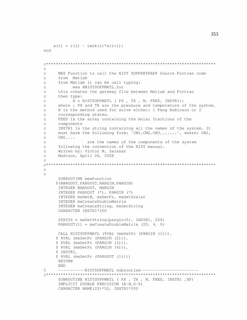
353
x(i) = r(i) - cwrk(i)*x(i+1); end c********************************************************************** c c MEX Function to call the NIST SUPPERTRAPP Source Fortran code c from Matlab c from Matlab it can be call typing: c mex HNISTSUPPMATL.for c this creates the gateway file between Matlab and Fortran c then type: c A = NISTSUPPMATL ( PX , TX , N, FEED, INSTR1); c where : PX and TX are the pressure and temperature of the system, c N is the method used for solve either: 1 Peng Robinson or 2 c corresponding states, c FEED is the array containing the molar fractions of the c components c INSTR1 is the string containing all the names of the system. It c must have the following form: 'CM1,CM2,CM3,......', where: CM1, c CM2,... c are the names of the components of the system c following the convention of the NIST manual. c Writen by: Victor M. Salazar c Madison, April 06, 2008 c c********************************************************************** c c SUBROUTINE mexFunction $(NARGOUT,PARGOUT,NARGIN,PARGIN) INTEGER NARGOUT, NARGIN INTEGER PARGOUT (*), PARGIN (*) INTEGER mxGetN, mxGetPr, mxGetScalar INTEGER mxCreateDoubleMatrix INTEGER mxCreateString, mxGetString CHARACTER INSTR1*200 STATUS = mxGetString(pargin(5), INSTR1, 200) PARGOUT(1) = mxCreateDoubleMatrix (20, 4, 0) CALL NISTSUPPMATL (%VAL (mxGetPr (PARGIN (1))), $ %VAL (mxGetPr (PARGIN (2))), $ %VAL (mxGetPr (PARGIN (3))), $ %VAL (mxGetPr (PARGIN (4))), $ INSTR1, $ %VAL (mxGetPr (PARGOUT (1)))) RETURN END C -----------NISTSUPPMATL subroutine------------------------ c********************************************************************** SUBROUTINE NISTSUPPMATL ( PX , TX , N, FEED, INSTR1 ,XP) IMPLICIT DOUBLE PRECISION (A-H,O-Z) CHARACTER NAME(20)*50, INSTR1*200
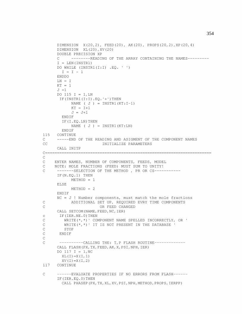
354
DIMENSION X(20,2), FEED(20), AK(20), PROPS(20,2),XP(20,4) DIMENSION XL(20),XV(20) DOUBLE PRECISION XP C --------READING OF THE ARRAY CONTAINING THE NAMES--------- I = LEN(INSTR1) DO WHILE (INSTR1(I:I) .EQ. ' ') I = I - 1 ENDDO LN = I KT = 1 J =1 DO 115 I = 1,LN IF(INSTR1(I:I).EQ.'+')THEN NAME ( J ) = INSTR1(KT:I-1) KT = I+1 J = J+1 ENDIF IF(I.EQ.LN)THEN NAME ( J ) = INSTR1(KT:LN) ENDIF 115 CONTINUE C -----END OF THE READING AND ASIGMENT OF THE COMPONENT NAMES CC INITIALIZE PARAMETERS CALL INITP C====================================================================== C C ENTER NAMES, NUMBER OF COMPONENTS, FEEDS, MODEL C NOTE: MOLE FRACTIONS (FEED) MUST SUM TO UNITY! C -------SELECTION OF THE METHOD , PR OR CS----------- IF(N.EQ.1) THEN METHOD = 1 ELSE METHOD = 2 ENDIF NC = J ! Number components, must match the mole fractions C ADDITIONAL SET UP, REQUIRED EVRY TIME COMPONENTS C OR FEED CHANGED CALL SETCOM(NAME,FEED,NC,IER) c IF(IER.NE.0)THEN C WRITE(*,*)' COMPONENT NAME SPELLED INCORRECTLY, OR ' C WRITE(*,*)' IT IS NOT PRESENT IN THE DATABASE ' C STOP C ENDIF C C ----------CALLING THE: T,P FLASH ROUTINE------------- CALL FLASH(PX,TX,FEED,AK,X,PSI,NPH,IER) DO 117 I = 1,NC XL(I)=X(I,1) XV(I)=X(I,2) 117 CONTINUE C ------EVALUATE PROPERTIES IF NO ERRORS FROM FLASH------ IF(IER.EQ.0)THEN CALL PHASEP(PX,TX,XL,XV,PSI,NPH,METHOD,PROPS,IERPP)
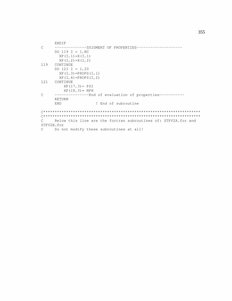
355
ENDIF C --------------SSIGMENT OF PROPERTIES-------------------- DO 119 I = 1,NC XP(I,1)=X(I,1) XP(I,2)=X(I,2) 119 CONTINUE DO 121 I = 1,20 XP(I,3)=PROPS(I,1) XP(I,4)=PROPS(I,2) 121 CONTINUE XP(17,3)= PSI XP(18,3)= NPH C ---------------End of evaluation of properties----------- RETURN END ! End of subroutine C********************************************************************* C********************************************************************* C Below this line are the fortran subroutines of: STPV2A.for and STPV2B.for C Do not modify these subroutines at all!