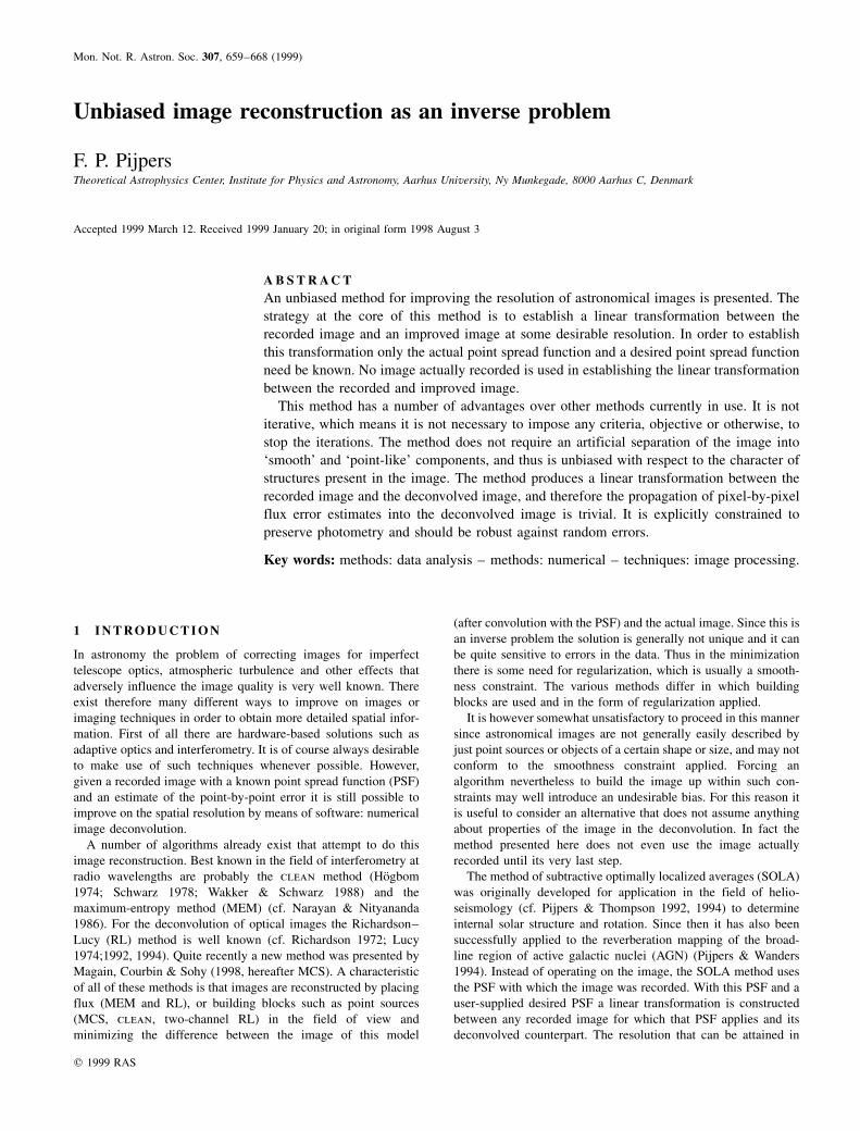
Mon. Not. R. Astron. Soc. 307, 659±668 (1999)

Unbiased image reconstruction as an inverse problem

F. P. PijpersTheoretical Astrophysics Center, Institute for Physics and Astronomy, Aarhus University, Ny Munkegade, 8000 Aarhus C, Denmark

Accepted 1999 March 12. Received 1999 January 20; in original form 1998 August 3

A B S T R A C T

An unbiased method for improving the resolution of astronomical images is presented. The

strategy at the core of this method is to establish a linear transformation between the

recorded image and an improved image at some desirable resolution. In order to establish

this transformation only the actual point spread function and a desired point spread function

need be known. No image actually recorded is used in establishing the linear transformation

between the recorded and improved image.

This method has a number of advantages over other methods currently in use. It is not

iterative, which means it is not necessary to impose any criteria, objective or otherwise, to

stop the iterations. The method does not require an artificial separation of the image into

`smooth' and `point-like' components, and thus is unbiased with respect to the character of

structures present in the image. The method produces a linear transformation between the

recorded image and the deconvolved image, and therefore the propagation of pixel-by-pixel

flux error estimates into the deconvolved image is trivial. It is explicitly constrained to

preserve photometry and should be robust against random errors.

Key words: methods: data analysis ± methods: numerical ± techniques: image processing.

1 I N T R O D U C T I O N

In astronomy the problem of correcting images for imperfect

telescope optics, atmospheric turbulence and other effects that

adversely influence the image quality is very well known. There

exist therefore many different ways to improve on images or

imaging techniques in order to obtain more detailed spatial infor-

mation. First of all there are hardware-based solutions such as

adaptive optics and interferometry. It is of course always desirable

to make use of such techniques whenever possible. However,

given a recorded image with a known point spread function (PSF)

and an estimate of the point-by-point error it is still possible to

improve on the spatial resolution by means of software: numerical

image deconvolution.

A number of algorithms already exist that attempt to do this

image reconstruction. Best known in the field of interferometry at

radio wavelengths are probably the clean method (HoÈgbom

1974; Schwarz 1978; Wakker & Schwarz 1988) and the

maximum-entropy method (MEM) (cf. Narayan & Nityananda

1986). For the deconvolution of optical images the Richardson±

Lucy (RL) method is well known (cf. Richardson 1972; Lucy

1974;1992, 1994). Quite recently a new method was presented by

Magain, Courbin & Sohy (1998, hereafter MCS). A characteristic

of all of these methods is that images are reconstructed by placing

flux (MEM and RL), or building blocks such as point sources

(MCS, clean, two-channel RL) in the field of view and

minimizing the difference between the image of this model

(after convolution with the PSF) and the actual image. Since this is

an inverse problem the solution is generally not unique and it can

be quite sensitive to errors in the data. Thus in the minimization

there is some need for regularization, which is usually a smooth-

ness constraint. The various methods differ in which building

blocks are used and in the form of regularization applied.

It is however somewhat unsatisfactory to proceed in this manner

since astronomical images are not generally easily described by

just point sources or objects of a certain shape or size, and may not

conform to the smoothness constraint applied. Forcing an

algorithm nevertheless to build the image up within such con-

straints may well introduce an undesirable bias. For this reason it

is useful to consider an alternative that does not assume anything

about properties of the image in the deconvolution. In fact the

method presented here does not even use the image actually

recorded until its very last step.

The method of subtractive optimally localized averages (SOLA)

was originally developed for application in the field of helio-

seismology (cf. Pijpers & Thompson 1992, 1994) to determine

internal solar structure and rotation. Since then it has also been

successfully applied to the reverberation mapping of the broad-

line region of active galactic nuclei (AGN) (Pijpers & Wanders

1994). Instead of operating on the image, the SOLA method uses

the PSF with which the image was recorded. With this PSF and a

user-supplied desired PSF a linear transformation is constructed

between any recorded image for which that PSF applies and its

deconvolved counterpart. The resolution that can be attained in

q 1999 RAS

660 F. P. Pijpers

this way is only limited by the sampling of the recording device

[the pixel size of the charge-coupled device (CCD)] and by the

level of the flux errors in the recorded image. Since the

transformation is linear, it is quite straightforward to impose

photometric accuracy. Astrometric accuracy at the pixel scale is

similarly guaranteed since there is no `positioning of sources' in

the image by the algorithm. Subpixel accuracy, claimed for some

deconvolution methods, implies subdividing each pixel into

subpixels. It requires knowledge of the PSF at very high accuracy

and very small errors in the data in order to deconvolve down to a

subpixel scale. If such information is available the SOLA method

can easily accommodate subpixel scale deconvolution, without

substantial modifications. In what follows however, it is assumed

that a single pixel is the smallest scale required.

In Section 2 the SOLA method is presented. In Section 3 the

method is applied to an example image to demonstrate the workings

of SOLA. In Section 4 the method is applied to some astronomical

images. Some conclusions are presented in Section 5.

2 T H E S O L A M E T H O D

2.1 Arbitrary PSFs

The strategy of the SOLA method in general is to find a set of

linear coefficients c which, when combined with the data, produce

a weighted average of the unknown convolved function under the

integral sign, where the weighting function is sharply peaked. In

the application at hand this means finding the linear transforma-

tion between an image recorded at a given resolution and an image

appropriate to a different (better) resolution.

The relation between a recorded image D and the actual

distribution of flux over the field of view I is:

D�x; y� ��

dx 0 dy 0K�x 0; y 0; x; y�I�x 0; y 0� �1�

where K is the PSF. If one assumes that the PSF is constant over

the field of view then:

K�x 0; y 0; x; y� ; K�x 2 x 0; y 2 y 0� �2�Of course generally D is not known as a continuous function of

(x, y), but instead it is sampled discretely as for instance an image

recorded on a CCD. Thus one has as available data the recorded

pixel-by-pixel values of flux D(xi, yj). These measured fluxes will

usually be corrupted by noise and thus the discretized version of

equation (1) is:

Dij ��

dx 0 dy 0Kij�x 0; y 0�I�x 0; y 0� � nij �3�

where now Kij refers to the PSF appropriate for the pixel at (xi, yj)

and Dij is the flux value recorded in that pixel. In the vocabulary

usual for the SOLA method the Kij are referred to as integration

kernels.

In the SOLA technique a set of linear coefficients cl is sought

which, when combined with the data, produces a value for the flux

R in any given pixel that would correspond to an image recorded

with a much narrower PSF. Writing this out explicitly and using

equation (3) yields:

R ;X

clDl ��

dx 0 dy 0X

clKl�x 0; y 0�n o

I�x 0; y 0� �X

clnl

�4�

in which the double subscript ij has been replaced by a single one l

for convenience. Thus one would construct the cl such that the

averaging kernel K defined by:

K�x 0; y 0� ;X

clKl�x 0; y 0� �5�is as sharply peaked as possible. If one does this for all locations

on the CCD the collected values Rm are then the fluxes

corresponding to the image at this (better) resolution with an

(improved) `point spread function' K. The so-called propagated

error, the error in the flux R is:

s2R ;

X XclcmNlm �6�

Here the Nlm is the error variance±covariance matrix of the

recorded CCD images where both l and m run over all (i, j)

combinations of the pixel coordinates. If the errors are

uncorrelated between pixels then equation (6) reduces to:

s2R �

Xc2

l s2l �7�

which is trivially computed once the coefficients cl are known.

Ideally one would wish to construct an image corresponding to

an infinitely narrow PSF: a Dirac delta function. In practice this

cannot be achieved with a finite amount of recorded data. As has

already been pointed out by Magain et al. (1998) one must in the

deconvolved image still satisfy the sampling theorem. A further

restriction arises because of the noise term in equation (3). As is

well known in helioseismology the linear combination of data

corresponding to a very highly resolved measurement usually

bears with it a very large propagated error. In order to obtain a flux

value for each pixel in the deconvolved image that does not have

an excessively large error estimate associated with it, one needs to

remain modest in the resolution sought for in the deconvolved

image.

Finding the optimal set of coefficients taking these limitations

into account can be expressed mathematically in the following

minimization problem. One needs to minimize for the coefficients

cl the following:�dx dy�K 2 T�2 � m

X XclcmNlm �8�

Here m is a free parameter which is used to adjust the relative

weight given to minimizing the errors in the deconvolved image

and to producing a more sharply peaked kernel K. The higher the

value of m the lower this error but the less successful one will be

in producing a narrow PSF. In SOLA one is free to choose the

function T. A common choice in SOLA applications is a

Gaussian:

T � 1

fD2exp 2

�x 2 x0�2 � �y 2 y0�2D2

� �� ��9�

Here (x0, y0) is the location for which one wishes to know the flux

at the resolution corresponding to the width D; and f is a

normalization factor chosen such that:�dx dyT ; 1 �10�

Although any set of locations (x0, y0) can be chosen, a natural

choice in the application at hand is to take all original pixel

locations (xi, yj). If one wishes to deconvolve to subpixel scales

this can be done by an appropriate choice of the (x0, y0) and D.

q 1999 RAS, MNRAS 307, 659±668

Unbiased image reconstruction 661

In terms of an algorithm the problem of minimizing the

function (8) leads to a set of linear equations:

Almcl � bm �11�

The elements of the matrix A are given by:

Alm ;�

dx dyKl�x; y�Km�x; y� � mNlm �12�

The elements of the vector b are given by:

bm ;�

dx dyT�x; y�Km�x; y� �13�

Writing out the dependences on the free parameters explicitly,

determining the coefficients cl results from a straightforward

matrix inversion:

cl�x0; y0;D;m� � A21lm �m�bm�x0; y0;D� �14�

It is clear that for each point (x0, y0) there is a separate set of

coefficients cl which will depend on the resolution width Drequired and on the error weighting m . Note that it is not

necessary to invert a matrix for every location (x0, y0), which

would certainly be prohibitive if one wishes to calculate the

entire deconvolved image. For a given error weighting m one

needs to invert A only once. Only the elements of the vector bneed be recomputed for different locations or different

resolutions.

In order to ensure that at every point in the reconstructed image

the summed weight of all measurements is equal and thus a true

(weighted) average it is necessary to impose the additional

condition:Xcl ; 1 �15�

It is this condition that imposes photometric accuracy on the

reconstructed image. Using the method of Lagrange multipliers

this condition is easily incorporated into the matrix equation (11)

by augmenting the matrix A with a row and column of `1's, and a

corner element equal to 0. The vector b gains one extra element

equal to 1 as well. The details of this procedure can be found in

Pijpers & Thompson 1992, 1994).

2.2 Translationally invariant PSFs

Although the method described above can work in principle

with general PSFs K, the matrix inversion becomes intractable

very quickly as the number of pixels increases. For an image

of M �M pixels the number of elements in the matrix A is

M2 �M2. The matrix A is symmetric but even so a naive

matrix inversion routine would require a number of operations

scaling as M6.

However the entire procedure for obtaining the transforma-

tion coefficients for all locations of the CCD can be speeded

up considerably if one accepts some restrictions for the

properties of the PSF K and of the expected errors Nlm. The

first restriction is to assume that the PSF is constant over the

field of view, that is to say that equation (2) is valid. When

condition (2) is met one can easily demonstrate that in

equation (12) the integrals of the cross-products of the PSFs

are a convolution:�dx dyKl�x; y�Km�x; y�

;�

dx dyK�x 2 xil ; y 2 yjl�K�x 2 xim ; y 2 yjm

�

��

dx 0 dy 0K�x 0; y 0�K 0�Dximil 2 x 0;Dyjmjl2 y 0� �16�

in which:

K 0�x 2 x 0; y 2 y 0� ; K�x 0 2 x; y 0 2 y�Dximil

; xim 2 xil

Dyjmjl; yjm

2 yjl�17�

Evaluating all the M4 elements of the matrix A is much simplified

by doing this two-dimensional convolution as a multiplication in

the Fourier domain. This calculation is then dominated by the fast

Fourier transform (FFT) calculation, which requires O(M2 log M)

operations. Similarly the vectors b in (13) can be evaluated for all

locations (xi, yj) with a single two-dimensional convolution of K

and T, again dominated by the FFT.

If the CCD pixels are assumed to be equally spaced the matrix

A for m � 0 can be constructed in such a way that it becomes of a

special type known as symmetric block circulant with circulant

blocks (BCCB), for which very fast inversion algorithms exist.

Circulant matrices have the property that every row is identical to

the previous row, but shifted to the right by one element. The

shifting is `wrapped around' so that the first element on each row

is equal to the last element of the previous row. Thus the main

diagonal elements are all equal and on every diagonal parallel to

the main diagonal of the matrix all elements are equal as well. A

BCCB matrix is a matrix that can be partitioned into blocks in

such a way that each row of blocks is repeated by shifting (and

wrapping around) by one block in the subsequent row of blocks

and each individual block is circulant. It can be shown that

circulant matrices can be multiplied and inverted using Fourier

transforms, and by extension BCCB matrices can be multiplied

and inverted using two-dimensional Fourier transforms. The

detailed steps of the algorithm are worked out in the Appendix.

The restriction on the matrix Nlm is that it must also be a

symmetric BCCB matrix for the fast inversion algorithm to work.

It is evident that fully optimal results can only be obtained if the

full N2 � N2 covariance matrix of the errors is used. However, the

error correlation function for the pixels is expected to behave

similarly to the point spread function in the sense that it is large (in

absolute value) for small pixel separations and small for large

pixel separations, independently of where on the CCD the pixel is

located. It is therefore likely that the error covariance matrix will

already be BCCB or be very nearly so. Since its role in the

minimization of function (8) is to regularize the inversion it is in

practice not essential that the exact variance±covariance matrix be

used. Experience in using SOLA in other fields has shown that the

results of linear inversions are robust to inaccuracies in the error

matrix, as long as those are not orders of magnitude large: if for

instance substantial amounts of data (fluxes in pixels) are to be

given small weight in the resulting linear combination, because of

large errors associated with them, this can give rise to large

departures from BCCB behaviour of the error covariance matrix.

This would then cause problems for the fast version of the SOLA

q 1999 RAS, MNRAS 307, 659±668

662 F. P. Pijpers

method presented here. Thus if Nlm is not circulant it should in

most cases be sufficient to use a BCCB matrix that is close to the

original: one could think of using a modified matrix NÅ lm on the

diagonals of which are the average values over those diagonals of

the true Nlm. Of course once the coefficients have been

determined, when calculating the propagated errors one should

use equation (6) with the proper variance±covariance matrix Nlm.

As is shown in the Appendix the matrix corresponding to the

collection of all vectors of coefficients c, which results from the

multiplication of A with the matrix corresponding to the collection

of all vectors b (one for every pixel), is also a BCCB matrix. The

process of combining these coefficients cl with the recorded fluxes

on the CCD to form the improved image is:

Rij �X

k

Xl

CklDi�k21j�l21 �18�

Since the matrix C is a BCCB matrix and therefore its transpose

CT is as well, the following holds:

Rij �X

k;l

CklDi�k21j�l21

�X

k;l

CTlkDi�k21j�l21

�X

k;l

CT22k22lDi�k21j�l21

�Xk 0 ;l

CTk 0l 0Di�12k 0j�12l 0 �19�

From the final equality in (19) it is clear that the process of

combining the matrix of coefficients with the image is a

convolution, and hence can also be done using FFTs.

From the above it is clear that limiting the algorithm to the case

of a PSF that is constant over the CCD implies a profound

q 1999 RAS, MNRAS 307, 659±668

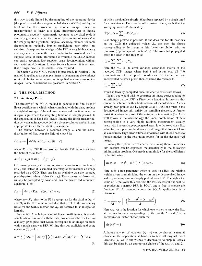
Figure 1. The 128 � 128 pixels image used in testing the algorithm. Top left panel: the original image. Top right panel: the original convolved with the target

PSF, a Gaussian with D � 1:5 pixels. Bottom left panel: the original convolved with a PSF, which is the sum of a Gaussian with D � 10 pixels and an 0.1 per

cent contribution from a Gaussian with D � 1 pixel. Bottom right panel: the image after SOLA deconvolution of the bottom left image. In all images the grey-

scale is linear. In the bottom left image noise is added before deconvolution. In the bottom right image the noise propagated in the deconvolution has an

expectation value of ,0:5 in arbitrary flux units and the signal-to-noise ratio for the brightest pixel is ,1000.

Unbiased image reconstruction 663

reduction of the computing time. If the PSFs K satisfy the

condition (2) the vectors b collected together for all �x0; y0� ��xi; yj� form a BCCB matrix, and therefore the matrix inversion of

A and its subsequent multiplication with all vectors b, shown in

equation (14), can be done in O(M2 log M) operations. The entire

deconvolved image is thus produced in O(M2 log M) operations.

This acceleration of the algorithm over the version described in

the previous section is so substantial that even when the PSF is not

constant over the CCD it is worth while subdividing the image

into subsections in which the PSF can be closely approximated by

a single function K. The error introduced in this way can be

estimated in a way similar to what is done in the application of

SOLA to the reverberation mapping of AGN (Pijpers & Wanders

1994), and should generally be much smaller than the propagated

error from equation (6). If such a subdivision is undesirable, there

is the possibility of reverting to the more general algorithm of

Section 2.1. For a single peaked PSF the matrix A should have a

banded structure to which fast sparse matrix solvers can be

applied. In this case one could use the inverse of the matrix A for

an approximated PSF that is translationally invariant as a

preconditioner to speed up the matrix inversion for the case of

the true PSF.

3 A P P L I C AT I O N T O A T E S T I M AG E

3.1 Constructing a narrow PSF

In the first instance it is useful to test the algorithm on a test image

for which the result and the errors are known. To this end an

artificial image of a cluster of stars is convolved with two different

PSFs. One PSF is a sum of two Gaussians; one with a width

D � 10 pixels in which 99.9 per cent of the flux is collected, and a

second one with a width D � 1 pixel which collects the other

0.1 per cent of the flux. Poisson-distributed noise is added to every

pixel and this `dirty' image serves as the image to be deconvolved.

The other PSF is a Gaussian with a width D � 1:5 pixels which is

also the target chosen for the SOLA algorithm. Thus the

deconvolved image can be compared directly with the image

obtained from direct convolution of the original with the narrow

target PSF. The results are shown in Fig. 1. In order to get an

optimal reproduction of the target PSF, the error weighting

parameter m is chosen to be equal to 0.

It is clear that the bottom and top right panels are very similar

and thus the image appears to be recovered quite well. To illustrate

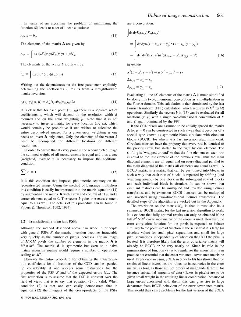
this further the two images can be subtracted. Fig. 2 shows the

SOLA deconvolved image minus the image convolved with the

target PSF, with an adjusted grey-scale to bring out the

differences, which in the central portion of the image are all

, 1 per cent. Although there is no strong evidence for it in this

image, the deconvolution can suffer from edge effects because

part of the original image can `leak away' in the convolution with

the broad PSF. When deconvolving, the region outside the image

is assumed to be empty and so a spurious negative signature is

then introduced in the image. The magnitude of such edge effects

must clearly depend both on the image and on the PSF of the

`dirty' image, since they are determined by the information that

has been lost at the edges of the CCD. Of course it is desirable to

demonstrate this method on a more realistic suite of images than

just the simple one used here, which is work currently in progress.

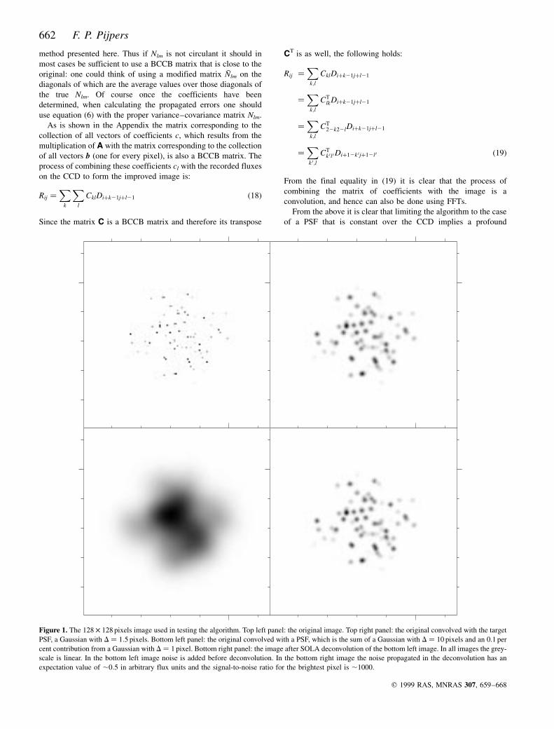
The averaging kernel that is constructed cannot in general

match perfectly the target form, even in the absence of errors. In

general any function can be completely reconstructed only out of a

complete set of base functions. Since function space is infinite-

dimensional this would require an infinite number of base

functions. In this test image there are no more available than the

1282 PSFs corresponding to each of the pixels and so there can

never be a perfect matching of K with T. In Fig. 3 a section

through the maximum of both T and K is shown. It is clear that

at the 10 ppm level, the constructed averaging kernel starts getting

wider than the target. If the ratio of the widths of the target form

and actual PSF is even smaller than for this image, alternating

negative and positive sidelobes can show up in the averaging

kernel, which cause ringing. The amplitude of the sidelobes, and

the width D below which ringing starts occurring, will in general

depend on the weighting of the errors m , as has been demonstrated

from the application of SOLA to helioseismology (Pijpers &

Thompson 1994).

As it stands the SOLA algorithm does not impose positivity on

q 1999 RAS, MNRAS 307, 659±668

Figure 2. The difference between the image that is SOLA deconvolved

and the original image convolved to the target PSF. The grey-scale is

adjusted so that the full scale is 0.01� the scale in the right-hand side

images of Fig. 1, which corresponds to 10s of the noise in the

deconvolved image.

Figure 3. A slice through the peak of the target PSF specified in the SOLA

algorithm (solid line) and the averaging kernel K (dashed) constructed

from the linear combination of the pixel PSFs.

664 F. P. Pijpers

the image. One could attempt to use a positivity constraint to

extrapolate the image beyond the recorded edges in such a way

that it eradicates any negative fluxes in the image, which would in

principle also remove associated positive artefacts around the

edges. However, in the presence of errors this might be somewhat

hazardous. Furthermore, in the presence of errors any edge effects

might well disappear into the noise.

If one assumes that the covariance of errors between pixels is

equal to 0 and the flux error in each pixel is equal to s2, or

N ; s2I, then it is particularly simple to calculate the flux error

for each pixel in the deconvolved image from equation (7) since it

is

s2R � s2

Xc2

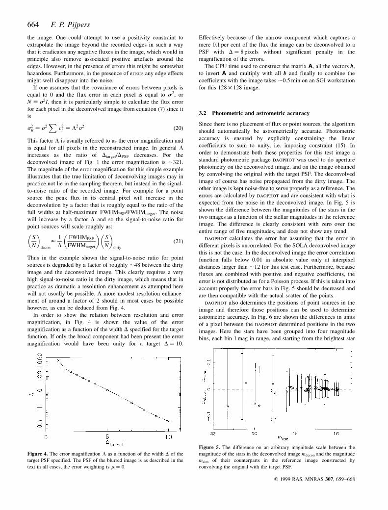
l ; L2s2 �20�This factor L is usually referred to as the error magnification and

is equal for all pixels in the reconstructed image. In general Lincreases as the ratio of Dtarget/DPSF decreases. For the

deconvolved image of Fig. 1 the error magnification is ,321.

The magnitude of the error magnification for this simple example

illustrates that the true limitation of deconvolving images may in

practice not lie in the sampling theorem, but instead in the signal-

to-noise ratio of the recorded image. For example for a point

source the peak flux in its central pixel will increase in the

deconvolution by a factor that is roughly equal to the ratio of the

full widths at half-maximum FWHMPSF/FWHMtarget. The noise

will increase by a factor L and so the signal-to-noise ratio for

point sources will scale roughly as:

S

N

� �decon

<1

L

FWHMPSF

FWHMtarget

� �S

N

� �dirty

�21�

Thus in the example shown the signal-to-noise ratio for point

sources is degraded by a factor of roughly ,48 between the dirty

image and the deconvolved image. This clearly requires a very

high signal-to-noise ratio in the dirty image, which means that in

practice as dramatic a resolution enhancement as attempted here

will not usually be possible. A more modest resolution enhance-

ment of around a factor of 2 should in most cases be possible

however, as can be deduced from Fig. 4.

In order to show the relation between resolution and error

magnification, in Fig. 4 is shown the value of the error

magnification as a function of the width D specified for the target

function. If only the broad component had been present the error

magnification would have been unity for a target D � 10.

Effectively because of the narrow component which captures a

mere 0.1 per cent of the flux the image can be deconvolved to a

PSF with D � 8 pixels without significant penalty in the

magnification of the errors.

The CPU time used to construct the matrix A, all the vectors b,

to invert A and multiply with all b and finally to combine the

coefficients with the image takes ,0:5 min on an SGI workstation

for this 128 � 128 image.

3.2 Photometric and astrometric accuracy

Since there is no placement of flux or point sources, the algorithm

should automatically be astrometrically accurate. Photometric

accuracy is ensured by explicitly constraining the linear

coefficients to sum to unity, i.e. imposing constraint (15). In

order to demonstrate both these properties for this test image a

standard photometric package daophot was used to do aperture

photometry on the deconvolved image, and on the image obtained

by convolving the original with the target PSF. The deconvolved

image of course has noise propagated from the dirty image. The

other image is kept noise-free to serve properly as a reference. The

errors are calculated by daophot and are consistent with what is

expected from the noise in the deconvolved image. In Fig. 5 is

shown the difference between the magnitudes of the stars in the

two images as a function of the stellar magnitudes in the reference

image. The difference is clearly consistent with zero over the

entire range of five magnitudes, and does not show any trend.

daophot calculates the error bar assuming that the error in

different pixels is uncorrelated. For the SOLA deconvolved image

this is not the case. In the deconvolved image the error correlation

function falls below 0.01 in absolute value only at interpixel

distances larger than ,12 for this test case. Furthermore, because

fluxes are combined with positive and negative coefficients, the

error is not distributed as for a Poisson process. If this is taken into

account properly the error bars in Fig. 5 should be decreased and

are then compatible with the actual scatter of the points.

daophot also determines the positions of point sources in the

image and therefore those positions can be used to determine

astrometric accuracy. In Fig. 6 are shown the differences in units

of a pixel between the daophot determined positions in the two

images. Here the stars have been grouped into four magnitude

bins, each bin 1 mag in range, and starting from the brightest star

q 1999 RAS, MNRAS 307, 659±668

Figure 4. The error magnification L as a function of the width D of the

target PSF specified. The PSF of the blurred image is as described in the

text in all cases, the error weighting is m � 0.

Figure 5. The difference on an arbitrary magnitude scale between the

magnitude of the stars in the deconvolved image mdecon and the magnitude

maim of their counterparts in the reference image constructed by

convolving the original with the target PSF.

Unbiased image reconstruction 665

with magnitude 15.9. The right-hand panel is a blow-up of the

central portion of the left-hand panel. Fig. 4 shows that there is a

trend in that the fainter stars show a greater scatter in position, the

largest position difference being of the order of ,0:2 pixel. In the

right-hand panel it can be seen that for stars brighter than

magnitude 19 the difference in positions is smaller than 0.03 pixel.

These uncertainties are entirely consistent with the accuracy with

which daophot can determine stellar positions.

From Figs 5 and 6 it is clear that if any errors in photometry or

in position are introduced by the deconvolution process, they are

much smaller than the errors caused by the random noise.

4 A P P L I C AT I O N T O A S T R O N O M I C A L

I M AG E S

4.1 UGC 5041

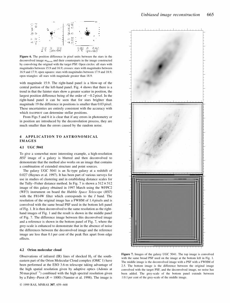
To give a somewhat more interesting example, a high-resolution

HST image of a galaxy is blurred and then deconvolved to

demonstrate that the method also works on an image that contains

a combination of extended structure and point sources.

The galaxy UGC 5041 is an Sc-type galaxy at a redshift of

0.027 (Haynes et al. 1997). It has been part of various surveys for

use in studies of clustering and in establishing distance scales for

the Tully±Fisher distance method. In Fig. 7 is shown a 512 � 512

image of this galaxy obtained in 1997 March using the WFPC2

(WF3) instrument on board the Hubble Space Telescope (HST)

with the F814W filter which corresponds to the I band. The

resolution of the original image has a FWHM of 1.4 pixels and is

convolved with the same broad PSF used in the bottom left panel

of Fig. 1. It is then deconvolved to the same resolution as the right-

hand images of Fig. 1 and the result is shown in the middle panel

of Fig. 7. The difference image between this deconvolved image

and a reference is shown in the bottom panel of Fig. 7, where the

grey-scale is enhanced to demonstrate that in the absence of noise

the differences between the deconvolved image and the reference

image are less than 0.1 per cent of the peak flux apart from edge

effects.

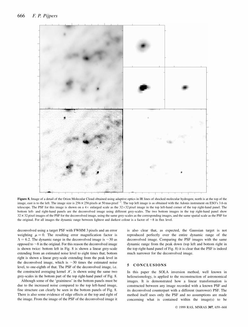
4.2 Orion molecular cloud

Observations of infrared (IR) lines of shocked H2 of the south-

eastern part of the Orion Molecular Cloud complex (OMC 1) have

been performed at the ESO 3.6-m telescope taking advantage of

the high spatial resolution given by adaptive optics (Adonis at

50 mas pixel21) combined with the high spectral resolution given

by a Fabry±Perot (R � 1000) (Vannier et al. 1998). The image is

q 1999 RAS, MNRAS 307, 659±668

Figure 6. The position difference in pixel units between the stars in the

deconvolved image mdecon and their counterparts in the image constructed

by convolving the original with the target PSF. Open circles: all stars with

magnitudes between 15.9 and 16.9; crosses: stars with magnitudes between

16.9 and 17.9; open squares: stars with magnitudes between 17.9 and 18.9;

open triangles: all stars with magnitude greater than 18.9.

Figure 7. Images of the galaxy UGC 5041. The top image is convolved

with the same broad PSF used on the image at the bottom left in Fig. 1.

The middle image is the deconvolved image with a PSF with a FWHM of

2.5. The bottom image is the difference between the original image

convolved with the target PSF, and the deconvolved image, no noise has

been added. The grey-scale of the bottom panel extends between

^0:1 per cent of the grey-scale of the middle image.

666 F. P. Pijpers

deconvolved using a target PSF with FWHM 3 pixels and an error

weighting m � 0. The resulting error magnification factor is

L � 6:2. The dynamic range in the deconvolved image is ,30 as

opposed to ,8 in the original. For this reason the deconvolved image

is shown twice: bottom left in Fig. 8 is shown a linear grey-scale

extending from an estimated noise level to eight times that; bottom

right is shown a linear grey-scale extending from the peak level in

the deconvolved image, which is ,30 times the estimated noise

level, to one-eighth of that. The PSF of the deconvolved image, i.e.

the constructed averaging kernel K, is shown using the same two

grey-scales in the bottom part of the top right-hand panel of Fig. 8.

Although some of the `graininess' in the bottom panels must be

due to the increased noise compared to the top left-hand image,

fine structure can clearly be seen in the bottom panels of Fig. 8.

There is also some evidence of edge effects at the top and right of

the image. From the image of the PSF of the deconvolved image it

is also clear that, as expected, the Gaussian target is not

reproduced perfectly over the entire dynamic range of the

deconvolved image. Comparing the PSF images with the same

dynamic range from the peak down (top left and bottom right in

the top right-hand panel of Fig. 8) it is clear that the PSF is indeed

much narrower for the deconvolved image.

5 C O N C L U S I O N S

In this paper the SOLA inversion method, well known in

helioseismology, is applied to the reconstruction of astronomical

images. It is demonstrated how a linear transformation is

constructed between any image recorded with a known PSF and

its deconvolved counterpart with a different (narrower) PSF. The

method itself uses only the PSF and no assumptions are made

concerning what is contained within the image(s) to be

q 1999 RAS, MNRAS 307, 659±668

Figure 8. Image of a detail of the Orion Molecular Cloud obtained using adaptive optics in IR lines of shocked molecular hydrogen; north is at the top of the

image, east is to the left. The image size is 256 � 256 pixels at 50 mas pixel21. The top left image is as obtained with the Adonis instrument on ESO's 3.6-m

telescope. The PSF for this image is shown on a 4� enlarged scale as the 32�32 pixel image in the top left-hand corner of the top right-hand panel. The

bottom left- and right-hand panels are the deconvolved image using different grey-scales. The two bottom images in the top right-hand panel show

32 � 32 pixel images of the PSF for the deconvolved image, using the same grey-scales as the corresponding images, and the same spatial scale as the PSF for

the original. For all images the dynamic range between lightest and darkest colour is a factor of ,8 in flux level.

Unbiased image reconstruction 667

deconvolved. It is furthermore shown that in the case of

translationally invariant PSFs, a fast algorithm, using O(N log N)

operations where N is the total number of pixels in the image, can

be constructed, which allows deconvolution of even 1024 � 1024

images within half an hour on medium-sized workstations.

AC K N OW L E D G M E N T S

Steve Holland is thanked for a number of helpful discussions.

D. Rouan, J.-L. Lemaire, D. Field and L. Vannier are thanked for

making available their data prior to publication. The observations

of UGC 5041 were made with the NASA/ESA Hubble Space

Telescope, obtained from the data archive at the Space Telescope

Science Institute. STScI is operated by the Association of

Universities for Research in Astronomy, Inc. under NASA

contract NAS 5-26555. The Theoretical Astrophysics Center is a

collaboration between Copenhagen University and Aarhus Uni-

versity and is funded by Danmarks Grundforskningsfonden.

R E F E R E N C E S

Haynes M. P., Giovanelli R., Herter T., Vogt N. P., Freudling W., Maia M.

A. G., Salzer J. J., Wegner G., 1997, AJ, 113, 1197

HoÈgbom J. A., 1974, A&AS, 15, 417

Lucy L. B., 1974, AJ, 79, 745

Lucy L. B., 1992, AJ, 104, 1260

Lucy L. B., 1994, A&A, 289, 983

Magain P., Courbin F., Sohy S., 1998, ApJ, 494, 472

Narayan R., Nityananda R., 1986, ARA&A, 24, 127

Pijpers F. P., Thompson M. J., 1992, A&A, 262, L33

Pijpers F. P., Thompson M. J., 1994, A&A, 281, 231

Pijpers F. P., Wanders I., 1994, MNRAS, 271, 183

Press W. H., Teukolsky S. A., Vetterling W. T., Flannery B. P., 1992,

Numerical Recipes, the Art of Scientific Computing, 2nd edn.

Cambridge Univ. Press, p. 70

Richardson W. H., 1972, J. Opt. Soc. Am., 62, 55

Schwarz U. J., 1978, A&A, 65, 345

Vannier L., Lemaire J.-L., Field D., Rouan D., Pijpers F. P., Pineau des

ForeÃts G., Gerin M., Falgarone E., 1999, in Bonaccini D. ed., ESO/

OSA Conf. and Workshop Proc. 56, p. 687

Wakker B. P., Schwarz U. J., 1988, A&A, 200, 312

A P P E N D I X A : T H E I N V E R S I O N A N D

M U LT I P L I C AT I O N O F C I R C U L A N T

M AT R I C E S

As it stands the matrix described in equation (16) does not

conform to the criteria for a block circulant with circulant blocks

(BCCB) matrix. Instead it is a block Toeplitz matrix with Toeplitz

blocks. For the latter type of matrix the elements are also identical

on diagonals but there is no `wrapping around' from row to row: the

final element of each row is not (necessarily) equal to the first

element of the subsequent row. In order to produce a matrix that is a

BCCB matrix it is useful to envisage a `virtual CCD' that is twice as

big in both dimensions as the actual CCD, which for convenience is

assumed to be square. This `virtual CCD' has the property that it

has a periodic point spread function in both directions: the CCD is

shaped like a torus. The actual CCD then occupies a quarter of this

virtual CCD and the other three quarters are `empty sky'.

For this virtual CCD the matrix constructed by equation (16) is

a �2M�2 � �2M�2 BCCB matrix. The first quadrant of this matrix,

�M�2 � �M�2 in size, is identical to the matrix for the actual CCD.

Unless explicitly stated otherwise the matrices for this torus-shaped

virtual CCD are the ones that the algorithm works on. In what

follows the indices `wrap around', which is to say that the values

of the indices are to be evaluated modulo the matrix dimension.

First consider a matrix that is fully circulant rather than block

circulant with circulant blocks. Such a matrix A satisfies:

Ai�nj�n � Aij ;n; �i� n�mod�MA�;� j� n�mod�MA� �A1�

in which the matrix A has dimensions MA �MA. An ordinary

matrix multiplication of two circulant matrices A and B satisfies:

Cij �X

k

AikBkj

�X

k

Ai�nk�nBk�nj�n

�X

l

Ai�nlBlj�n with l ; k � n

� Ci�nj�n ;n �A2�Thus C is circulant if A and B are circulant. It is also

straightforward to demonstrate that if A and C are circulant, Bmust be circulant as well:

0 � Ci�nj�n 2 Cij

�X

l

Ai�nlBlj�n 2 AilBlj

�X

k

Aik�Bk�nj�n 2 Bkj� k ; l 2 n �A3�

Since A is an arbitrary circulant matrix the final equality can only

lead to 0 (and thus consistency) if B is indeed circulant.

Since the identity matrix is itself a circulant matrix, a direct

consequence is that the inverse of any circulant matrix A21 is also

circulant, which is trivially demonstrated by substituting I for C.

If the matrix C is circulant then it is fully determined by its first

row, as can be demonstrated by taking n � 1 2 i in (A2), for

which the following holds:

C1n �X

l

A1lBln

�X

l

A1lB1n�12l �A4�

A one-dimensional convolution of two functions is defined by the

following integral:

C�x� ��

dx 0A�x�B�x 2 x 0� �A5�

which in discretized form is:

Ci �X

l

vlAlBi�12l �A6�

where the vl are integration weights. The vl can always be

arranged to be unity and so it is clear that (A6) and (A4) are

identical summations. This means that the multiplication of two

circulant matrices can be regarded as a convolution. The product

of two circulant matrices can therefore be determined by

multiplying the Fourier transform (FT) of the first row of each

of the two matrices, and then taking the inverse FT of this product.

q 1999 RAS, MNRAS 307, 659±668

668 F. P. Pijpers

This yields only the first row of that product but since it is known

to be a circulant matrix the other rows are then trivially found by

shifting and wrapping around. Similarly the inverse of a circulant

matrix can be found by dividing the FT of the first row of the

identity matrix by the FT of first row of the circulant matrix to be

inverted, and taking the inverse FT.

If one has a BCCB matrix with dimensions M2A �M2

A in which

the blocks have dimensions MA �MA it is fully determined by its

first row of blocks. In equations (A2)±(A6) it is nowhere used that

the individual matrix elements must be scalars. Thus two block

circulant matrices can be multiplied by a one-dimensional

convolution of the first row of blocks of each matrix, i.e. doing

the same operation of convolution on every element of each block.

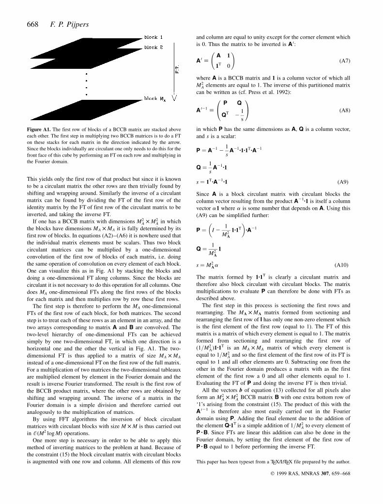
One can visualize this as in Fig. A1 by stacking the blocks and

doing a one-dimensional FT along columns. Since the blocks are

circulant it is not necessary to do this operation for all columns. One

does MA one-dimensional FTs along the first rows of the blocks

for each matrix and then multiplies row by row these first rows.

The first step is therefore to perform the MA one-dimensional

FTs of the first row of each block, for both matrices. The second

step is to treat each of these rows as an element in an array, and the

two arrays corresponding to matrix A and B are convolved. The

two-level hierarchy of one-dimensional FTs can be achieved

simply by one two-dimensional FT, in which one direction is a

horizontal one and the other the vertical in Fig. A1. The two-

dimensional FT is thus applied to a matrix of size MA �MA

instead of a one-dimensional FT on the first row of the full matrix.

For a multiplication of two matrices the two-dimensional tableaux

are multiplied element by element in the Fourier domain and the

result is inverse Fourier transformed. The result is the first row of

the BCCB product matrix, where the other rows are obtained by

shifting and wrapping around. The inverse of a matrix in the

Fourier domain is a simple division and therefore carried out

analogously to the multiplication of matrices.

By using FFT algorithms the inversion of block circulant

matrices with circulant blocks with size M �M is thus carried out

in O(M2 log M) operations.

One more step is necessary in order to be able to apply this

method of inverting matrices to the problem at hand. Because of

the constraint (15) the block circulant matrix with circulant blocks

is augmented with one row and column. All elements of this row

and column are equal to unity except for the corner element which

is 0. Thus the matrix to be inverted is A 0:

A 0 ;A 1

1T 0

!�A7�

where A is a BCCB matrix and 1 is a column vector of which all

M2A elements are equal to 1. The inverse of this partitioned matrix

can be written as (cf. Press et al. 1992):

A 021 ;P Q

QT 21

s

0@ 1A �A8�

in which P has the same dimensions as A, Q is a column vector,

and s is a scalar:

P � A21 21

sA21´1´1T´A21

Q � 1

sA21´1

s � 1T´A21´1 �A9�Since A is a block circulant matrix with circulant blocks the

column vector resulting from the product A21´1 is itself a column

vector a1 where a is some number that depends on A. Using this

(A9) can be simplified further:

P � I 21

M2A

1´1T

� �´A21

Q � 1

M2A

1

s � M2Aa �A10�

The matrix formed by 1´1T is clearly a circulant matrix and

therefore also block circulant with circulant blocks. The matrix

multiplications to evaluate P can therefore be done with FTs as

described above.

The first step in this process is sectioning the first rows and

rearranging. The MA �MA matrix formed from sectioning and

rearranging the first row of I has only one non-zero element which

is the first element of the first row (equal to 1). The FT of this

matrix is a matrix of which every element is equal to 1. The matrix

formed from sectioning and rearranging the first row of

�1=M2A�1´1T is an MA �MA matrix of which every element is

equal to 1=M2A and so the first element of the first row of its FT is

equal to 1 and all other elements are 0. Subtracting one from the

other in the Fourier domain produces a matrix with as the first

element of the first row a 0 and all other elements equal to 1.

Evaluating the FT of P and doing the inverse FT is then trivial.

All the vectors b of equation (13) collected for all pixels also

form an M2A �M2

A BCCB matrix B with one extra bottom row of

`1's arising from the constraint (15). The product of this with the

A 021 is therefore also most easily carried out in the Fourier

domain using P. Adding the final element due to the addition of

the element Q´1T is a simple addition of 1=M2A to every element of

P ´ B. Since FTs are linear this addition can also be done in the

Fourier domain, by setting the first element of the first row of

P ´ B equal to 1 before performing the inverse FT.

This paper has been typeset from a TEX/LATEX file prepared by the author.

q 1999 RAS, MNRAS 307, 659±668

Figure A1. The first row of blocks of a BCCB matrix are stacked above

each other. The first step in multiplying two BCCB matrices is to do a FT

on these stacks for each matrix in the direction indicated by the arrow.

Since the blocks individually are circulant one only needs to do this for the

front face of this cube by performing an FT on each row and multiplying in

the Fourier domain.