Embed Size (px)
Citation preview

Un metodo de elementos finitos adaptativo paraproblemas de optimizacion de forma
Pedro Morin
Instituto de Matematica Aplicadadel Litoral
Universidad Nacional del LitoralSanta Fe, Argentina
En colaboracion con
R.H. Nochetto (Maryland)M.S. Pauletti (Maryland-Texas)
M. Verani (Milan)
IMAL — 29 de octubre de 2010

Layout Introduction: Shape Optimization Problem Shape Calculus AFEM for Shape Optimization Numerical Results
Layout
Introduction: Shape Optimization Problem
Shape Calculus
AFEM for Shape Optimization
Numerical Results
MEF Adaptativos para Optimizacion de Forma Pedro Morin

Layout Introduction: Shape Optimization Problem Shape Calculus AFEM for Shape Optimization Numerical Results
Layout
Introduction: Shape Optimization Problem
Shape Calculus
AFEM for Shape Optimization
Numerical Results
MEF Adaptativos para Optimizacion de Forma Pedro Morin
Layout Introduction: Shape Optimization Problem Shape Calculus AFEM for Shape Optimization Numerical Results
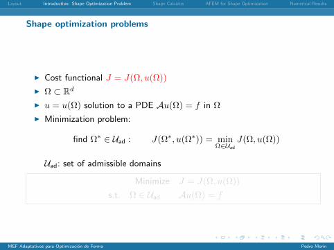
Shape optimization problems
I Cost functional J = J(Ω, u(Ω))
I Ω ⊂ Rd
I u = u(Ω) solution to a PDE Au(Ω) = f in Ω
I Minimization problem:
find Ω∗ ∈ Uad : J(Ω∗, u(Ω∗)) = minΩ∈Uad
J(Ω, u(Ω))
Uad: set of admissible domains
Minimize J = J(Ω, u(Ω))
s.t. Ω ∈ Uad Au(Ω) = f
MEF Adaptativos para Optimizacion de Forma Pedro Morin
Layout Introduction: Shape Optimization Problem Shape Calculus AFEM for Shape Optimization Numerical Results
Shape optimization problems
I Cost functional J = J(Ω, u(Ω))
I Ω ⊂ Rd
I u = u(Ω) solution to a PDE Au(Ω) = f in Ω
I Minimization problem:
find Ω∗ ∈ Uad : J(Ω∗, u(Ω∗)) = minΩ∈Uad
J(Ω, u(Ω))
Uad: set of admissible domains
Minimize J = J(Ω, u(Ω))
s.t. Ω ∈ Uad Au(Ω) = f
MEF Adaptativos para Optimizacion de Forma Pedro Morin

Layout Introduction: Shape Optimization Problem Shape Calculus AFEM for Shape Optimization Numerical Results
Example: Minimization of an obstacle drag
−∇ · T (u, p) = 0 in Ω
∇ · u = 0 in Ω
u = ud on Γin ∪ Γs ∪ Γw
T (u, p) · n = 0 on Γout
T (u, p) = 2νε(u)−pI, ε(u) =∇u+∇uT
2, ud =
V∞i on Γin
0 on Γw ∪ Γs
Drag Functional: J(Ω, [u, p]) = −∫
Γs
(T (u, p)n
)· i dΓ
Ω∗ ←− minΩ∈Uad
J(Ω, u(Ω)),
Uad = Ω : |Ω| = V, with Γin,Γout,Γw fixed
MEF Adaptativos para Optimizacion de Forma Pedro Morin

Layout Introduction: Shape Optimization Problem Shape Calculus AFEM for Shape Optimization Numerical Results
Layout
Introduction: Shape Optimization Problem
Shape Calculus
AFEM for Shape Optimization
Numerical Results
MEF Adaptativos para Optimizacion de Forma Pedro Morin

Layout Introduction: Shape Optimization Problem Shape Calculus AFEM for Shape Optimization Numerical Results
Shape Calculus
We can define the shape derivative of a cost functional J(Ω) at Ω, in thedirection of a vector field v: dJ(Ω;v).
The velocity method: Let v be a smooth vector field. Define
d
dtX(t;x) = v(X(t;x)) t > 0
X(0, x) = xx ∈ Rd.
Let Ωt be the image under X(t; ·) of Ω
Ωt :=
X(t;x) : x ∈ Ω
We then define the shape derivative of J(Ω) in the direction v as
dJ(Ω;v) = limt→0
J(Ωt)− J(Ω)
t.
MEF Adaptativos para Optimizacion de Forma Pedro Morin

Layout Introduction: Shape Optimization Problem Shape Calculus AFEM for Shape Optimization Numerical Results
Shape Calculus
Hadamard-Zolesio Theorem: There exists a function g(Ω) defined on ∂Ω
dJ(Ω;v) =
∫∂Ω
g(Ω)(v · n) dΓ
The shape derivative depends only on the normal component of v on ∂Ω.
Volume
J(Ω) =
∫Ω
dx
dJ(Ω;v) =
∫Ω
∇ · v dx =
∫Γ
1(v · n) dΓ
J(Ω) =
∫Ω
φdx (φ : Rd → R)
dJ(Ω;v) =
∫Ω
∇ · (φv) dx =
∫Γ
φ(v · n) dΓ
MEF Adaptativos para Optimizacion de Forma Pedro Morin

Layout Introduction: Shape Optimization Problem Shape Calculus AFEM for Shape Optimization Numerical Results
Shape Calculus
Hadamard-Zolesio Theorem: There exists a function g(Ω) defined on ∂Ω
dJ(Ω;v) =
∫∂Ω
g(Ω)(v · n) dΓ
The shape derivative depends only on the normal component of v on ∂Ω.
Area/Perimeter
J(Ω) =
∫∂Ω
dΓ
dJ(Ω;v) =
∫∂Ω
κ(v · n)dΓ
J(Ω) =
∫∂Ω
φdΓ (φ : Rd → R)
dJ(Ω;v) =
∫∂Ω
( ∂φ∂n
+ φκ)(v · n) dΓ
MEF Adaptativos para Optimizacion de Forma Pedro Morin

Layout Introduction: Shape Optimization Problem Shape Calculus AFEM for Shape Optimization Numerical Results
Shape Calculus
Hadamard-Zolesio Theorem: There exists a function g(Ω) defined on ∂Ω
dJ(Ω;v) =
∫∂Ω
g(Ω)(v · n) dΓ
The shape derivative depends only on the normal component of v on ∂Ω.
Obstacle Drag
dJ(Ω;v) = −2ν
∫Γs
[ε(u) : ε(z)](v · n) dΓ
With z solution to the adjoint problem
−∇ · T (z, q) = 0 in Ω
∇ · z = 0 in Ω
z = −i on Γs
z = 0 on Γw ∪ Γin
T (z, q) · n = 0 on Γout
MEF Adaptativos para Optimizacion de Forma Pedro Morin

Layout Introduction: Shape Optimization Problem Shape Calculus AFEM for Shape Optimization Numerical Results
Layout
Introduction: Shape Optimization Problem
Shape Calculus
AFEM for Shape Optimization
Numerical Results
MEF Adaptativos para Optimizacion de Forma Pedro Morin

Layout Introduction: Shape Optimization Problem Shape Calculus AFEM for Shape Optimization Numerical Results
Shape Optimization through Adaptive SQP
Goal: Design an algorithm to adaptively build Ωkk≥0 converging to alocal minimizer Ω∗ of J(Ω, u(Ω)). Use low resolution at initial stages andimprove accuracy upon convergence.
First Step: Design ∞-SQP. An ideal Sequential Quadratic Programmingalgorithm assuming the PDE’s can be solved exactly.
Second Step: Design a discrete counterpart of ∞-SQP, using adaptivityto improve approximation upon convergence
Adaptive Sequential Quadratic Programming (ASQP)
MEF Adaptativos para Optimizacion de Forma Pedro Morin

Layout Introduction: Shape Optimization Problem Shape Calculus AFEM for Shape Optimization Numerical Results
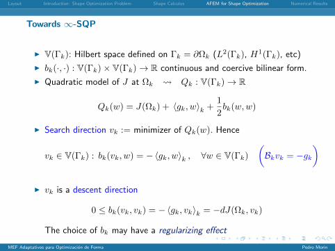
Towards ∞-SQP
I V(Γk): Hilbert space defined on Γk = ∂Ωk (L2(Γk), H1(Γk), etc)
I bk(·, ·) : V(Γk)× V(Γk)→ R continuous and coercive bilinear form.
I Quadratic model of J at Ωk Qk : V(Γk)→ R
Qk(w) = J(Ωk) + dJ(Ωk, w) +1
2bk(w,w)
I Search direction vk := minimizer of Qk(w). Hence
vk ∈ V(Γk) : bk(vk, w) = −〈gk, w〉k , ∀w ∈ V(Γk)
(Bkvk = −gk
)
I vk is a descent direction
0 ≤ bk(vk, vk) = −〈gk, vk〉k = −dJ(Ωk, vk)
The choice of bk may have a regularizing effect
MEF Adaptativos para Optimizacion de Forma Pedro Morin

Layout Introduction: Shape Optimization Problem Shape Calculus AFEM for Shape Optimization Numerical Results
Towards ∞-SQP
I V(Γk): Hilbert space defined on Γk = ∂Ωk (L2(Γk), H1(Γk), etc)
I bk(·, ·) : V(Γk)× V(Γk)→ R continuous and coercive bilinear form.
I Quadratic model of J at Ωk Qk : V(Γk)→ R
Qk(w) = J(Ωk) + 〈gk, w〉k +1
2bk(w,w)
I Search direction vk := minimizer of Qk(w). Hence
vk ∈ V(Γk) : bk(vk, w) = −〈gk, w〉k , ∀w ∈ V(Γk)
(Bkvk = −gk
)
I vk is a descent direction
0 ≤ bk(vk, vk) = −〈gk, vk〉k = −dJ(Ωk, vk)
The choice of bk may have a regularizing effect
MEF Adaptativos para Optimizacion de Forma Pedro Morin

Layout Introduction: Shape Optimization Problem Shape Calculus AFEM for Shape Optimization Numerical Results
∞-SQP Algorithm
Given an initial domain Ω0, set k = 0 and iterate:
(a) Compute uk = u(Ωk) by solving Auk = f
(b) Compute the Riesz representation gk = g(Ωk) of the
shape derivative dJ(Ωk, ·) (solve dual problem)
(c) Compute the search direction vk by solving
vk ∈ Vk : bk(vk, w) = −〈gk, w〉, ∀w ∈ Vk
(d) Determine an admissible stepsize µk satisfying
J(Ωk + µkvk) << J(Ωk) (line search)
(e) Update Ωk+1 ← Ωk + µkvk (vk = vkn); k ← k + 1.
NOT REALISTIC ∞-dimensional problems
MEF Adaptativos para Optimizacion de Forma Pedro Morin

Layout Introduction: Shape Optimization Problem Shape Calculus AFEM for Shape Optimization Numerical Results
Towards a realistic adaptive algorithm
Replace non-computable operations by adaptive finite approximations.
two main sources of error:
Adaptive approximation of PDE (PDE Error) uk, J, dJ (gk)
Adaptive approximation of domain (Geometric Error) vk
Goals:
I distribute the computational effort between the two sources of errorand adjust the accuracies along the iteration it is wasteful to impose PDE Error finer than Geometric Error
I sort out whether geometric singularities are genuine to the problemor due to lack of resolution correct the effects of early (no longer necessary) mesh refinements
MEF Adaptativos para Optimizacion de Forma Pedro Morin

Layout Introduction: Shape Optimization Problem Shape Calculus AFEM for Shape Optimization Numerical Results
ASQP algorithm
I Tk: triangulation of ΩkI Sk = Sk(Ωk): finite element space defined on ΩkI Vk = Vk(Γk): finite element space defined on ΓkI Ek = (Ωk,Sk,Vk)
The ASQP algorithm is an iteration of the form:
Ek → APPROXJ → DIRECTION → LINESEARCH → UPDATE → Ek+1
Adaptivity is carried out in APPROXJ and DIRECTION
I APPROXJ acts on PDE Error
I DIRECTION acts on Geometric Error
I LINESEARCH enforces a substantial reduction of cost functional.
I UPDATE Ωk+1 ← Ωk + µkVk
MEF Adaptativos para Optimizacion de Forma Pedro Morin

Layout Introduction: Shape Optimization Problem Shape Calculus AFEM for Shape Optimization Numerical Results
ASQP (Module APPROXJ)
APPROXJ enriches/coarsens PDE space Sk to control the error inthe approximate functional value Jk(Ωk + µkVk) to the prescribedtolerance ε (Goal oriented adaptivity / DWR method)
We choose ε := γµk‖Vk‖2Γk, γ > 0
APPROXJ ⇒∣∣J(Ωk + µkV k)− Jk(Ωk + µkV k))
∣∣ ≤ γµk‖Vk‖2Γk
I The value of ε is not very demanding coarse meshes at thebeginning and a combination of refinement and coarsening later on.
I DWR detects geometric singularities, such as corners, andrefines/coarsen what is necessary for computing J accurately
Dual Weighted Residual method (DWR) [Becker, Rannacher ’96 & ’01]
MEF Adaptativos para Optimizacion de Forma Pedro Morin

Layout Introduction: Shape Optimization Problem Shape Calculus AFEM for Shape Optimization Numerical Results
ASQP (Module APPROXJ)
APPROXJ enriches/coarsens PDE space Sk to control the error inthe approximate functional value Jk(Ωk + µkVk) to the prescribedtolerance ε (Goal oriented adaptivity / DWR method)
We choose ε := γµk‖Vk‖2Γk, γ > 0
APPROXJ ⇒∣∣J(Ωk + µkV k)− Jk(Ωk + µkV k))
∣∣ ≤ γµk‖Vk‖2Γk
I The value of ε is not very demanding coarse meshes at thebeginning and a combination of refinement and coarsening later on.
I DWR detects geometric singularities, such as corners, andrefines/coarsen what is necessary for computing J accurately
MEF Adaptativos para Optimizacion de Forma Pedro Morin

Layout Introduction: Shape Optimization Problem Shape Calculus AFEM for Shape Optimization Numerical Results
ASQP (Module DIRECTION)
I Gk approximation to shape derivative g(Ωk)
I vk ∈ V(Γk) exact solution of Bkvk = −GkI Vk ∈ V(Γk) finite element approximation to vk.
DIRECTION adapts Geometric space Vk(refine/coarsen approx. to Γk) s.t.
‖Vk − vk‖Γk≤ θ‖Vk‖Γk
(θ ≤ 1/2)
Example: Bk = −∆Γk⇒ Adaptivity for Laplace-Beltrami
[Demlow, Dziuk ’07], [Mekchay, M., Nochetto ’09]
⇓
∣∣J(Ωk + µkV k)− J(Ωk + µkvk)∣∣ ' µk∣∣dJ(Ωk;V k − vk)|
= µk∣∣bk(vk, Vk − vk)
∣∣≤ δµk‖Vk‖2Γk
(δ = M θ (1 + θ))
MEF Adaptativos para Optimizacion de Forma Pedro Morin

Layout Introduction: Shape Optimization Problem Shape Calculus AFEM for Shape Optimization Numerical Results
ASQP
I APPROXJ ⇒∣∣J(Ωk + µkV k)− Jk(Ωk + µkV k))
∣∣ ≤ γµk‖Vk‖2Γk
I DIRECTION ⇒∣∣J(Ωk + µkV k)− J(Ωk + µkvk)
∣∣ ≤ δµk‖Vk‖2Γk
I APPROXJ + DIRECTION ⇒ bound on local error at iteration k∣∣Jk(Ωk + µkV k)− J(Ωk + µkvk)∣∣ ≤ (γ + δ
)µk‖Vk‖2Γk
(choose γ ' δ → balance computational loads)
Consistency check of ASQPIf ASQP converges to a stationary point (µk‖Vk‖2Γk
→ 0)
I DIRECTION and APPROXJ approximate the descent direction vkand functional J(Ωk) increasingly better
I PDE and Geometric Error progressively decrease as k →∞
MEF Adaptativos para Optimizacion de Forma Pedro Morin

Layout Introduction: Shape Optimization Problem Shape Calculus AFEM for Shape Optimization Numerical Results
Layout
Introduction: Shape Optimization Problem
Shape Calculus
AFEM for Shape Optimization
Numerical Results
MEF Adaptativos para Optimizacion de Forma Pedro Morin

Layout Introduction: Shape Optimization Problem Shape Calculus AFEM for Shape Optimization Numerical Results
Minimization of an obstacle drag
−∇ · T (u, p) = 0 in Ω
∇ · u = 0 in Ω
u = ud on Γin ∪ Γs ∪ Γw
T (u, p) · n = 0 on Γout
T (u, p) = 2νε(u)−pI, ε(u) =∇u+∇uT
2, ud =
V∞i on Γin
0 on Γw ∪ Γs
Drag Functional: J(Ω, [u, p]) = −∫
Γs
(T (u, p)n
)· i dΓ
Ω∗ ←− minΩ∈Uad
J(Ω, u(Ω)),
Uad = Ω : |Ω| = V, with Γin,Γout,Γw fixedMEF Adaptativos para Optimizacion de Forma Pedro Morin

Layout Introduction: Shape Optimization Problem Shape Calculus AFEM for Shape Optimization Numerical Results
Initial and Final Shape (DRAG minimization)
Numerical simulations toolbox ALBERTA www.alberta-fem.deMEF Adaptativos para Optimizacion de Forma Pedro Morin

Layout Introduction: Shape Optimization Problem Shape Calculus AFEM for Shape Optimization Numerical Results
Further Ingredients
I Mesh quality: is maintained through an optimization routine thatworks locally. We try to avoid remeshing, but sometimes it isnecessary.
I Timestep: is controlled to ensure proper reduction and to avoid nodecrossing. Remeshing helps to allow bigger timesteps.
I Volume or perimeter constraints: are handled with Lagrangemultipliers and maintained up to machine precision.
I Refinement on the moving boundary: is done in a geometricallyconsistent way, to avoid overrefinement around fake corners and badapproximation of curvature.
MEF Adaptativos para Optimizacion de Forma Pedro Morin

Layout Introduction: Shape Optimization Problem Shape Calculus AFEM for Shape Optimization Numerical Results
Conclusions
I We developed an adaptive finite element method for shapeoptimization, based on an adaptive finite dimensional version of an∞-dimensional SQP algorithm ASQP
I The adaptive refinement acts on two different sources of error:I PDE error due to discretizationI Geometric Error due to boundary approximation
I A dynamically varying accuracy balances the computational effortbetween the two sources of error
I The algorithm is able to sort out whether geometric singularities aregenuine to the problem or due to lack of numerical resolution, andto correct the effects of early (and no longer necessary) meshrefinements
MEF Adaptativos para Optimizacion de Forma Pedro Morin

Layout Introduction: Shape Optimization Problem Shape Calculus AFEM for Shape Optimization Numerical Results
The Module APPROXJ
[T∗, U∗, Z∗, J∗, G∗] = APPROXJ(Ω, T , ε)Ω∗ = Ω
do
[U∗, Z∗] = SOLVE(Ω, T∗)η∗(T )T∈T∗ = ESTIMATE(U∗, Z∗, S∗)[R∗, C∗] = MARK(T∗, η∗(T )T∈T∗ )if (η∗(T∗) > ε)
[T∗, C∗] = REFINE(T∗,R∗)elseif (η∗(C∗) < δε)
T∗ = COARSEN(T∗, C∗)endif
while (η∗(T∗) > ε)
J∗ = EVALJ(Ω, T∗, U∗)G∗ = RIESZ(Ω, T∗, U∗, Z∗)
SOLVE: solve the discrete system for the primal and dual variables U∗, Z∗.
MEF Adaptativos para Optimizacion de Forma Pedro Morin

Layout Introduction: Shape Optimization Problem Shape Calculus AFEM for Shape Optimization Numerical Results
The Module APPROXJ
[T∗, U∗, Z∗, J∗, G∗] = APPROXJ(Ω, T , ε)Ω∗ = Ω
do
[U∗, Z∗] = SOLVE(Ω, T∗)η∗(T )T∈T∗ = ESTIMATE(U∗, Z∗, S∗)[R∗, C∗] = MARK(T∗, η∗(T )T∈T∗ )if (η∗(T∗) > ε)
[T∗, C∗] = REFINE(T∗,R∗)elseif (η∗(C∗) < δε)
T∗ = COARSEN(T∗, C∗)endif
while (η∗(T∗) > ε)
J∗ = EVALJ(Ω, T∗, U∗)G∗ = RIESZ(Ω, T∗, U∗, Z∗)
ESTIMATE: use DWR method to compute a posteriori error estimators taylored to ap-proximate the functional J .
MEF Adaptativos para Optimizacion de Forma Pedro Morin

Layout Introduction: Shape Optimization Problem Shape Calculus AFEM for Shape Optimization Numerical Results
The Module APPROXJ
[T∗, U∗, Z∗, J∗, G∗] = APPROXJ(Ω, T , ε)Ω∗ = Ω
do
[U∗, Z∗] = SOLVE(Ω, T∗)η∗(T )T∈T∗ = ESTIMATE(U∗, Z∗, S∗)[R∗, C∗] = MARK(T∗, η∗(T )T∈T∗ )if (η∗(T∗) > ε)
[T∗, C∗] = REFINE(T∗,R∗)elseif (η∗(C∗) < δε)
T∗ = COARSEN(T∗, C∗)endif
while (η∗(T∗) > ε)
J∗ = EVALJ(Ω, T∗, U∗)G∗ = RIESZ(Ω, T∗, U∗, Z∗)
MARK: use maximum strategy. Given 0 < δ− δ+ < 1, let η∗ = maxT∈T∗ η∗(T ) and
η∗(T ) > δ+η∗ ⇒ T ∈ R∗, η∗(T ) < δ−η∗ ⇒ T ∈ C∗.
MEF Adaptativos para Optimizacion de Forma Pedro Morin

Layout Introduction: Shape Optimization Problem Shape Calculus AFEM for Shape Optimization Numerical Results
The Module APPROXJ
[T∗, U∗, Z∗, J∗, G∗] = APPROXJ(Ω, T , ε)Ω∗ = Ω
do
[U∗, Z∗] = SOLVE(Ω, T∗)η∗(T )T∈T∗ = ESTIMATE(U∗, Z∗, S∗)[R∗, C∗] = MARK(T∗, η∗(T )T∈T∗ )if (η∗(T∗) > ε)
[T∗, C∗] = REFINE(T∗,R∗)elseif (η∗(C∗) < δε)
T∗ = COARSEN(T∗, C∗)endif
while (η∗(T∗) > ε)
J∗ = EVALJ(Ω, T∗, U∗)G∗ = RIESZ(Ω, T∗, U∗, Z∗)
REFINE/COARSEN: Refine the marked elements (in R∗) using a Geometrically ConsistentRefinement algorithm on the boundary; coarsen the elements in C∗.
MEF Adaptativos para Optimizacion de Forma Pedro Morin

Layout Introduction: Shape Optimization Problem Shape Calculus AFEM for Shape Optimization Numerical Results
DWR for Drag functional
The following DWR error estimate holds
|J(u, p)− J(U , P )| ≤∑T
‖r(U , P )‖T ‖z −Z‖T + ‖j(U , P )‖∂T ‖z −Z‖∂T
+∑T
‖R(U)‖T ‖q −Q‖T ,
with
r(U)|T := −∇ · (2νε(U)− P I) R|T := ∇ ·U ,
j(U)|e =
12
[2νε(U) · n− Pn] e ∩ ∂Ω = ∅2νε(U) · n− Pn e ⊂ Γout
0 otherwise,
MEF Adaptativos para Optimizacion de Forma Pedro Morin

Layout Introduction: Shape Optimization Problem Shape Calculus AFEM for Shape Optimization Numerical Results
SQP with constraint
I Quadratic model Q(w) := J(Ω) + 〈g, w〉+ 12bΓ(w,w)
I Volume C(Ω) =∫
Ωdx dC(Ω;w) = 〈1, w〉
I Lagrangian
L(w, λ) = Q(w) + λ(C(Ω + w)− V OL) ' Q(w) + λ(dC(Ω, w))
I Find (v, λ) such that
∇wQ(v) + λ = 0
C(Ω + vn)− V OL = 0
I v = v0 + λv1, with Bv0 = −g and Bv1 = −1
I Apply Newton’s method to c(λ) :=∫
Ω+µ(v0n+λv1)dx− V OL = 0
MEF Adaptativos para Optimizacion de Forma Pedro Morin
Layout Introduction: Shape Optimization Problem Shape Calculus AFEM for Shape Optimization Numerical Results
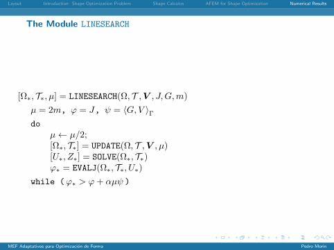
The Module LINESEARCH
[Ω∗, T∗, µ] = LINESEARCH(Ω, T ,V , J,G,m)
µ = 2m, ϕ = J, ψ = 〈G,V 〉Γdo
µ← µ/2;[Ω∗, T∗] = UPDATE(Ω, T ,V , µ)[U∗, Z∗] = SOLVE(Ω∗, T∗)ϕ∗ = EVALJ(Ω∗, T∗, U∗)
while (ϕ∗ > ϕ+ αµψ )
MEF Adaptativos para Optimizacion de Forma Pedro Morin

Layout Introduction: Shape Optimization Problem Shape Calculus AFEM for Shape Optimization Numerical Results
Evolution of meshes (DRAG minimization)
go back
Initial Mesh
MEF Adaptativos para Optimizacion de Forma Pedro Morin

Layout Introduction: Shape Optimization Problem Shape Calculus AFEM for Shape Optimization Numerical Results
Evolution of meshes (DRAG minimization)
go back
Mesh after 1 iteration
MEF Adaptativos para Optimizacion de Forma Pedro Morin

Layout Introduction: Shape Optimization Problem Shape Calculus AFEM for Shape Optimization Numerical Results
Evolution of meshes (DRAG minimization)
go back
Mesh after 2 iterations
MEF Adaptativos para Optimizacion de Forma Pedro Morin

Layout Introduction: Shape Optimization Problem Shape Calculus AFEM for Shape Optimization Numerical Results
Evolution of meshes (DRAG minimization)
go back
Mesh after 3 iterations
MEF Adaptativos para Optimizacion de Forma Pedro Morin

Layout Introduction: Shape Optimization Problem Shape Calculus AFEM for Shape Optimization Numerical Results
Evolution of meshes (DRAG minimization)
go back
Mesh after 4 iterations
MEF Adaptativos para Optimizacion de Forma Pedro Morin

Layout Introduction: Shape Optimization Problem Shape Calculus AFEM for Shape Optimization Numerical Results
Evolution of meshes (DRAG minimization)
go back
Mesh after 5 iterations
MEF Adaptativos para Optimizacion de Forma Pedro Morin

Layout Introduction: Shape Optimization Problem Shape Calculus AFEM for Shape Optimization Numerical Results
Evolution of meshes (DRAG minimization)
go back
Mesh after 6 iterations
MEF Adaptativos para Optimizacion de Forma Pedro Morin

Layout Introduction: Shape Optimization Problem Shape Calculus AFEM for Shape Optimization Numerical Results
Evolution of meshes (DRAG minimization)
go back
Mesh after 9 iterations
MEF Adaptativos para Optimizacion de Forma Pedro Morin

Layout Introduction: Shape Optimization Problem Shape Calculus AFEM for Shape Optimization Numerical Results
Evolution of meshes (DRAG minimization)
go back
Mesh after 10 iterations
MEF Adaptativos para Optimizacion de Forma Pedro Morin

Layout Introduction: Shape Optimization Problem Shape Calculus AFEM for Shape Optimization Numerical Results
Evolution of meshes (DRAG minimization)
go back
Mesh after 15 iterations
MEF Adaptativos para Optimizacion de Forma Pedro Morin

Layout Introduction: Shape Optimization Problem Shape Calculus AFEM for Shape Optimization Numerical Results
Evolution of meshes (DRAG minimization)
go back
Mesh after 16 iterations
MEF Adaptativos para Optimizacion de Forma Pedro Morin

Layout Introduction: Shape Optimization Problem Shape Calculus AFEM for Shape Optimization Numerical Results
Evolution of meshes (DRAG minimization)
go back
Mesh after 17 iterations
MEF Adaptativos para Optimizacion de Forma Pedro Morin

Layout Introduction: Shape Optimization Problem Shape Calculus AFEM for Shape Optimization Numerical Results
Evolution of meshes (DRAG minimization)
go back
Mesh after 20 iterations
MEF Adaptativos para Optimizacion de Forma Pedro Morin

Layout Introduction: Shape Optimization Problem Shape Calculus AFEM for Shape Optimization Numerical Results
Evolution of meshes (DRAG minimization)
go back
Mesh after 22 iterations
MEF Adaptativos para Optimizacion de Forma Pedro Morin

Layout Introduction: Shape Optimization Problem Shape Calculus AFEM for Shape Optimization Numerical Results
Evolution of meshes (DRAG minimization)
go back
Mesh after 25 iterations
MEF Adaptativos para Optimizacion de Forma Pedro Morin

Layout Introduction: Shape Optimization Problem Shape Calculus AFEM for Shape Optimization Numerical Results
Evolution of meshes (DRAG minimization)
go back
Mesh after 27 iterations
MEF Adaptativos para Optimizacion de Forma Pedro Morin

Layout Introduction: Shape Optimization Problem Shape Calculus AFEM for Shape Optimization Numerical Results
Evolution of meshes (DRAG minimization)
go back
Mesh after 28 iterations
MEF Adaptativos para Optimizacion de Forma Pedro Morin

Layout Introduction: Shape Optimization Problem Shape Calculus AFEM for Shape Optimization Numerical Results
Evolution of meshes (DRAG minimization)
go back
Mesh after 30 iterations
MEF Adaptativos para Optimizacion de Forma Pedro Morin

Layout Introduction: Shape Optimization Problem Shape Calculus AFEM for Shape Optimization Numerical Results
Evolution of meshes (DRAG minimization)
go back
Mesh after 32 iterations
MEF Adaptativos para Optimizacion de Forma Pedro Morin

Layout Introduction: Shape Optimization Problem Shape Calculus AFEM for Shape Optimization Numerical Results
Evolution of meshes (DRAG minimization)
go back
Mesh after 34 iterations
MEF Adaptativos para Optimizacion de Forma Pedro Morin

Layout Introduction: Shape Optimization Problem Shape Calculus AFEM for Shape Optimization Numerical Results
Evolution of meshes (DRAG minimization)
go back
Mesh after 40 iterations
MEF Adaptativos para Optimizacion de Forma Pedro Morin

Layout Introduction: Shape Optimization Problem Shape Calculus AFEM for Shape Optimization Numerical Results
Evolution of meshes (DRAG minimization)
go back
Mesh after 42 iterations
MEF Adaptativos para Optimizacion de Forma Pedro Morin

Layout Introduction: Shape Optimization Problem Shape Calculus AFEM for Shape Optimization Numerical Results
Evolution of meshes (DRAG minimization)
go back
Mesh after 45 iterations
MEF Adaptativos para Optimizacion de Forma Pedro Morin

Layout Introduction: Shape Optimization Problem Shape Calculus AFEM for Shape Optimization Numerical Results
Evolution of meshes (DRAG minimization)
go back
Mesh after 47 iterations
MEF Adaptativos para Optimizacion de Forma Pedro Morin

Layout Introduction: Shape Optimization Problem Shape Calculus AFEM for Shape Optimization Numerical Results
Evolution of meshes (DRAG minimization)
go back
Mesh after 49 iterations
MEF Adaptativos para Optimizacion de Forma Pedro Morin

Layout Introduction: Shape Optimization Problem Shape Calculus AFEM for Shape Optimization Numerical Results
Evolution of meshes (DRAG minimization)
go back
Mesh after 52 iterations
MEF Adaptativos para Optimizacion de Forma Pedro Morin

Layout Introduction: Shape Optimization Problem Shape Calculus AFEM for Shape Optimization Numerical Results
Zoom of final mesh (DRAG minimization)
go back
MEF Adaptativos para Optimizacion de Forma Pedro Morin

Layout Introduction: Shape Optimization Problem Shape Calculus AFEM for Shape Optimization Numerical Results
Zoom of final mesh (DRAG minimization)
go back
MEF Adaptativos para Optimizacion de Forma Pedro Morin

Layout Introduction: Shape Optimization Problem Shape Calculus AFEM for Shape Optimization Numerical Results
Zoom of final mesh (DRAG minimization)
go back
MEF Adaptativos para Optimizacion de Forma Pedro Morin

Layout Introduction: Shape Optimization Problem Shape Calculus AFEM for Shape Optimization Numerical Results
Zoom of final mesh (DRAG minimization)
go back
MEF Adaptativos para Optimizacion de Forma Pedro Morin

Layout Introduction: Shape Optimization Problem Shape Calculus AFEM for Shape Optimization Numerical Results
Zoom of final mesh (DRAG minimization)
go back
MEF Adaptativos para Optimizacion de Forma Pedro Morin

Layout Introduction: Shape Optimization Problem Shape Calculus AFEM for Shape Optimization Numerical Results
Zoom of final mesh (DRAG minimization)
go back
MEF Adaptativos para Optimizacion de Forma Pedro Morin

Layout Introduction: Shape Optimization Problem Shape Calculus AFEM for Shape Optimization Numerical Results
Zoom of final mesh (DRAG minimization)
go back
MEF Adaptativos para Optimizacion de Forma Pedro Morin

Layout Introduction: Shape Optimization Problem Shape Calculus AFEM for Shape Optimization Numerical Results
Evolution of meshes (BYPASS: energy minimization)
go back
Initial Mesh
MEF Adaptativos para Optimizacion de Forma Pedro Morin

Layout Introduction: Shape Optimization Problem Shape Calculus AFEM for Shape Optimization Numerical Results
Evolution of meshes (BYPASS: energy minimization)
go back
Mesh after 1 iteration
MEF Adaptativos para Optimizacion de Forma Pedro Morin

Layout Introduction: Shape Optimization Problem Shape Calculus AFEM for Shape Optimization Numerical Results
Evolution of meshes (BYPASS: energy minimization)
go back
Mesh after 2 iterations
MEF Adaptativos para Optimizacion de Forma Pedro Morin
Layout Introduction: Shape Optimization Problem Shape Calculus AFEM for Shape Optimization Numerical Results
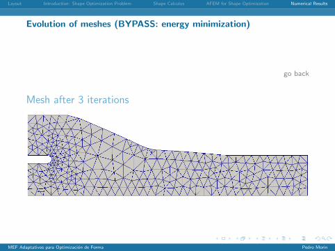
Evolution of meshes (BYPASS: energy minimization)
go back
Mesh after 3 iterations
MEF Adaptativos para Optimizacion de Forma Pedro Morin

Layout Introduction: Shape Optimization Problem Shape Calculus AFEM for Shape Optimization Numerical Results
Evolution of meshes (BYPASS: energy minimization)
go back
Mesh after 4 iterations
MEF Adaptativos para Optimizacion de Forma Pedro Morin

Layout Introduction: Shape Optimization Problem Shape Calculus AFEM for Shape Optimization Numerical Results
Evolution of meshes (BYPASS: energy minimization)
go back
Mesh after 5 iterations
MEF Adaptativos para Optimizacion de Forma Pedro Morin

Layout Introduction: Shape Optimization Problem Shape Calculus AFEM for Shape Optimization Numerical Results
Evolution of meshes (BYPASS: energy minimization)
go back
Mesh after 6 iterations
MEF Adaptativos para Optimizacion de Forma Pedro Morin

Layout Introduction: Shape Optimization Problem Shape Calculus AFEM for Shape Optimization Numerical Results
Evolution of meshes (BYPASS: energy minimization)
go back
Mesh after 7 iterations
MEF Adaptativos para Optimizacion de Forma Pedro Morin

Layout Introduction: Shape Optimization Problem Shape Calculus AFEM for Shape Optimization Numerical Results
Evolution of meshes (BYPASS: energy minimization)
go back
Mesh after 8 iterations
MEF Adaptativos para Optimizacion de Forma Pedro Morin

Layout Introduction: Shape Optimization Problem Shape Calculus AFEM for Shape Optimization Numerical Results
Evolution of meshes (BYPASS: energy minimization)
go back
Mesh after 9 iterations
MEF Adaptativos para Optimizacion de Forma Pedro Morin

Layout Introduction: Shape Optimization Problem Shape Calculus AFEM for Shape Optimization Numerical Results
Evolution of meshes (BYPASS: energy minimization)
go back
Mesh after 10 iterations
MEF Adaptativos para Optimizacion de Forma Pedro Morin

Layout Introduction: Shape Optimization Problem Shape Calculus AFEM for Shape Optimization Numerical Results
Evolution of meshes (BYPASS: energy minimization)
go back
Mesh after 11 iterations
MEF Adaptativos para Optimizacion de Forma Pedro Morin

Layout Introduction: Shape Optimization Problem Shape Calculus AFEM for Shape Optimization Numerical Results
Evolution of meshes (BYPASS: energy minimization)
go back
Mesh after 12 iterations
MEF Adaptativos para Optimizacion de Forma Pedro Morin

Layout Introduction: Shape Optimization Problem Shape Calculus AFEM for Shape Optimization Numerical Results
Evolution of meshes (BYPASS: energy minimization)
go back
Mesh after 13 iterations
MEF Adaptativos para Optimizacion de Forma Pedro Morin
Layout Introduction: Shape Optimization Problem Shape Calculus AFEM for Shape Optimization Numerical Results
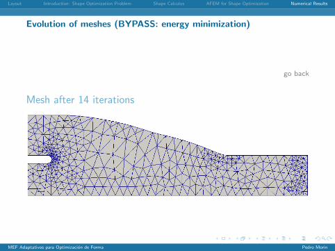
Evolution of meshes (BYPASS: energy minimization)
go back
Mesh after 14 iterations
MEF Adaptativos para Optimizacion de Forma Pedro Morin

Layout Introduction: Shape Optimization Problem Shape Calculus AFEM for Shape Optimization Numerical Results
Evolution of meshes (BYPASS: energy minimization)
go back
Mesh after 15 iterations
MEF Adaptativos para Optimizacion de Forma Pedro Morin

Layout Introduction: Shape Optimization Problem Shape Calculus AFEM for Shape Optimization Numerical Results
Evolution of meshes (BYPASS: energy minimization)
go back
Mesh after 16 iterations
MEF Adaptativos para Optimizacion de Forma Pedro Morin

Layout Introduction: Shape Optimization Problem Shape Calculus AFEM for Shape Optimization Numerical Results
Evolution of meshes (BYPASS: energy minimization)
go back
Mesh after 17 iterations
MEF Adaptativos para Optimizacion de Forma Pedro Morin

Layout Introduction: Shape Optimization Problem Shape Calculus AFEM for Shape Optimization Numerical Results
Evolution of meshes (BYPASS: energy minimization)
go back
Mesh after 18 iterations
MEF Adaptativos para Optimizacion de Forma Pedro Morin

Layout Introduction: Shape Optimization Problem Shape Calculus AFEM for Shape Optimization Numerical Results
Evolution of meshes (BYPASS: energy minimization)
go back
Mesh after 19 iterations
MEF Adaptativos para Optimizacion de Forma Pedro Morin