UMR UNIVERSITY OF MISSOURI ROLLA

Center of Excellence for Aerospace Particulate Emissions Reduction Research

Final Report

The Development of Exhaust Speciation Profiles for Commercial Jet Engines

Prepared by

Prem Lobo, Philip D. Whitefield and Donald E. Hagen Center of Excellence for Aerospace Particulate Emissions Reduction Research

G-7 Norwood Hall, University of Missouri – Rolla, Rolla, MO 65409 Contact: plobo@umr.edu or pwhite@umr.edu

Scott C. Herndon, John T. Jayne, Ezra C. Wood, W. Berk Knighton, Megan J. Northway and Richard C. Miake-Lye Aerodyne Research Inc.,

45 Manning Road, Billerica, MA 01821 Contact: herndon@aerodyne.com or rick@aerodyne.com

David Cocker, Aniket Sawant, Harshit Agrawal and J. Wayne Miller University of California - Riverside

Room 105, Administrative Bldg., 1084 Columbia Ave., Riverside, CA 92507 Contact: wayne.miller@ucr.edu or dcocker@engr.ucr.edu

Contract number: 04-344

Principal Investigator: Philip D. Whitefield

Contractor Organization: University of Missouri - Rolla

Date: October 31, 2007

Prepared for the California Air Resources Board and the California Environmental Protection Agency

i

Disclaimer

The statements and conclusions in this Report are those of the contractor and not necessarily those of the California Air Resources Board. The mention of commercial products, their source, or their use in connection with material reported herein is not to be construed as actual or implied endorsement of such products.

ii

Acknowledgments

The JETS APEX2 research team would like to acknowledge the following organizations and individuals for substantial contributions to the successful execution of this study.

Renee Dowlin, Wayne Bryant and staff at The Port of Oakland; Barry Brown, Mark Babb, Kevin Wiecek at Southwest Airlines; Chowen Wey, Changlie Wey, and Bruce Anderson at NASA; Robert Howard at AEDC; John Kinsey at EPA; Will Dodds at GEAE; Gregg Fleming at VOLPE; Lourdes Maurice and Carl Ma at FAA; Roger Wayson at UCF; Steve Baughcum at Boeing; Gary Kendall, Jim Hesson and staff at Bay Area Air Quality Management District; Judy Chow and Steve Kohl at Desert Research Institute; Dan Vickers at Frontier Analytical Laboratories; Steve Church, Steve Francis, and staff at ARB; and the UMRCOE.

This Report was submitted in fulfillment of ARB contract number 04-344: The Development of Exhaust Speciation Profiles for Commercial Jet Engines by the University of Missouri - Rolla under the partial sponsorship of the California Air Resources Board.

iii

Table of Contents

Section Title Page

Disclaimer .......................................................................................................................... ii Acknowledgments ............................................................................................................ iii Abstract............................................................................................................................ xii Executive Summary ....................................................................................................... xiii 1.0 Background ................................................................................................................. 1

1.1 Introduction............................................................................................................. 1 1.1.1 Regulated Emissions from Commercial Jet Engines ......................................... 1 1.1.2 Non-Regulated Emissions from Jet Engines...................................................... 2 1.1.3 Effects of Unburned Jet Fuel ............................................................................. 5

1.2 Recent NASA Missions ........................................................................................... 5 1.2.1 Experiment to Characterize Aircraft Volatile Aerosol and Trace Species Emissions (EXCAVATE- 1999)................................................................................. 5 1.2.2 Aircraft Particle Emissions eXperiment (APEX1-2004)................................... 6

1.3 JETS APEX2 ........................................................................................................... 8 2.0 Materials and Methods............................................................................................. 11

2.1 Aircraft Engines .................................................................................................... 11 2.2 Location for On-wing Sampling .......................................................................... 12 2.3 Equipment for On-wing Sampling ...................................................................... 15 2.4 Test Cycle............................................................................................................... 18 2.5 Fuel ......................................................................................................................... 19 2.6 ARI Methodology.................................................................................................. 19

2.6.1 Gas Phase Instrumentation............................................................................... 21 2.6.1.1 Tunable Infrared Laser Differential Absorption spectrometers (TILDAS) ............................................................................................................................... 21 2.6.1.2 Chemiluminescent NO sensor................................................................... 21 2.6.1.3 Proton transfer reaction - mass spectrometer (PTR-MS).......................... 21

2.6.2 Particle measurements ..................................................................................... 23 2.6.2.1 Aerosol Mass Spectrometer ...................................................................... 23 2.6.2.2 Multi-Angle Aerosol Photometer ............................................................. 23 2.6.2.3 Particle Counting Instrument .................................................................... 24

2.6.3 Emission Indices .............................................................................................. 24 2.7 UMR Methodology................................................................................................ 25

2.7.1 DMS500........................................................................................................... 27 2.7.2 PM parameters ................................................................................................. 28 2.7.3 Line loss characterization ................................................................................ 29 2.7.4 Soluble Mass Fraction...................................................................................... 30

2.8 UCR Methodology ................................................................................................ 30 2.8.1 UCR Design and Fabrication of Sampler for JETS APEX2............................ 31 2.8.2 Measurement of Mass, Metals and Ions .......................................................... 34 2.8.3 Measurement of Elemental and Organic Carbon (EC-OC) ............................. 34 2.8.4 Speciation of C1 to C30 Hydrocarbons.............................................................. 35

iv

2.8.5 Speciation of C1 to C12 Hydrocarbons, including BTEX & Carbonyls ........... 35 2.8.6 Speciation C 10 to C30 Hydrocarbons, including Naphthalene and PAHs........ 36 2.8.7 Detection Limits for the Organic Compounds................................................. 36

2.8.7.1 Calculating the Emissions Index............................................................... 36 2.8.7.2 Lower Detection Limits ............................................................................ 36

2.8.8 Exploratory Measurements for hexavalent chromium and dioxin................... 38 3.0 Results ........................................................................................................................ 40

3.1 Real-time Chemical Speciation (ARI) ................................................................. 40 3.1.1 Gas Phase Speciation ....................................................................................... 40 3.1.2 Particle Speciation ........................................................................................... 47

3.2 Physical characterization (UMR) ........................................................................ 50 3.2.1 PM Emission (Total Aerosol) Parameters at 1m Downstream of Exhaust Nozzle ....................................................................................................................... 51 3.2.2 PM Emission (Total Aerosol) Parameters at 50m Downstream of Exhaust Nozzle ....................................................................................................................... 55 3.2.3 PM Emission (Non-volatile Aerosol) Parameters at 1m Downstream of Exhaust Nozzle ......................................................................................................... 59 3.2.4 Deliquescence Results ..................................................................................... 62

3.3 Total organic gases and aerosol chemical speciation (UCR) ............................ 63 3.3.1 UCR Results for Mass Flow ............................................................................ 63 3.3.2 Internal Consistency Checks............................................................................ 64 3.3.3 Particulate matter ............................................................................................. 67 3.3.4 Elemental and organic carbon.......................................................................... 69 3.3.5 Polycyclic Aromatic Hydrocarbons (PAHs) and n-alkanes (C12+) ................. 70 3.3.6 Chromium Analysis ......................................................................................... 82 3.3.7 Dioxin Analysis ............................................................................................... 83 3.3.8 Metals............................................................................................................... 84 3.3.9 Ions................................................................................................................... 94 3.3.10 Mass Concentration Data............................................................................... 94

3.3.10.1 Gas-phase Carbonyls .............................................................................. 94 3.3.10.2 Light Hydrocarbons from Thermal Desorption Tubes ........................... 97 3.3.10.3 C1-C8 SUMMA Canister Analyses ......................................................... 97

3.3.11 Estimation of EIs for VOCs......................................................................... 114 3.3.11.1 Post Analysis of the Sampler ................................................................ 114 3.3.11.2 Implications for Carbonyl Analysis ...................................................... 116 3.3.11.3 Implications for Light Hydrocarbon Analysis ...................................... 117

3.3.12 UCR QA/QC Protocol ................................................................................. 119 4.0 Discussion................................................................................................................. 122

4.1 Gaseous Emissions .............................................................................................. 122 4.2 Particulate Emissions.......................................................................................... 122 4.3 PM Physical characterization ............................................................................ 123

4.3.1 Engine Warm-up Effect ................................................................................. 127 4.3.2 Discussion of aerosol volatility at 1m............................................................ 128 4.3.3 Comparison of 1m Total and Non-volatile Aerosol Data.............................. 132 4.3.4 Effect of plume processing (difference between 1m and 50m) ..................... 134

4.4 Organic gases and aerosol chemical speciation................................................ 135

v

5.0 Summary and Conclusions .................................................................................... 136 6.0 Recommendations ................................................................................................... 138 References ...................................................................................................................... 139 Glossary of terms, abbreviations and symbols........................................................... 146 APPENDIX A Oakland International Airport Diagram ......................................... 148 APPENDIX B Wind Roses (all times in Pacific Standard Time) ............................ 149 APPENDIX C Ambient DNPH cartridge sample results......................................... 152 APPENDIX D Ambient canister sample results ....................................................... 153 APPENDIX E Spatial arrangement of sampling probes.......................................... 154 APPENDIX F Willard Dodds’ (GEAE) Reports on Representativeness of Engine Performance and Emissions......................................................................................... 155 APPENDIX G Fuel Aromatic and Sulfur Content Analysis Results ...................... 162 APPENDIX H Fuel Carbon-Hydrogen Content Analysis Results .......................... 163 APPENDIX I Summary Tables ................................................................................ 164

vi

List of Figures

Figure 1a: Aerodynamic Size Distributions (nm) for Organic and Sulfate Particles in Aircraft Exhaust at 25 Meters. Figure 1b: Particulate Emission Indices Measured as a Function of Distance Behind the Engine. ........................................................................... 6

Figure 6a: Starboard sampling probe stand (left). Figure 6b: Probe rake with different

Figure 2: Picture of NASA Aircraft and Multiple Test Labs with Supporting Equipment7 : View of the GRE ............................................................................................... 13Figure 3

Figure 4: Wind-rose diagram giving prevailing wind orientation with respect to Runway and GRE facility ............................................................................................................... 13 Figure 5: Layout within the GRE...................................................................................... 14

probes (right)..................................................................................................................... 15 Figure 7: Particulate Sampling Probe ............................................................................... 16 Figure 8: Aerosol sample manifold................................................................................... 16 Figure 9: Aerosol probe plumbing.................................................................................... 17 Figure 10: Schematic diagram of the Landing and Take-Off cycle.................................. 18

: Test Matrix used at JETS APEX2................................................................... 19Figure 11Figure 12: Schematic of the Aerodyne Mobile Laboratory .............................................. 20 Figure 13: Schematic of the UMR Mobile Diagnostic Facility........................................ 25 Figure 14: Modified EPA Landing Take-Off (LTO) Sequence Used for Testing............ 31 Figure 15: Schematic of UCR's Sampling System for APEX1 ........................................ 31 Figure 16: Schematic of sampling setup. “S” setup represents DNPH, TDS, quartz, PUF/quartz, and PTFE (see below for details). Solid lines represent physical flow; dotted lines represent logical control. .......................................................................................... 33 Figure 17: Figure Showing UCR Sampler Constructed for JETS APEX2...................... 34 Figure 18: The logarithm of carbon monoxide (CO) emission index (EI) is plotted against the nominal thrust setting for the seven engines measured. The ICAO data points for the three engine types are plotted as diamond symbols.......................................................... 41 Figure 19: NOx EIs in g NO2/kg fuel, plotted versus nominal engine trust setting for the three engine types (seven engines total) that were tested. ................................................ 42 Figure 20: Formaldehyde (HCHO) is plotted versus the logarithm of the nominal engine thrust setting for all engines tested. The engine variability due to fluctuations in ambient conditions is greater than the engine-to-engine differences or to variations due to the downstream measurement locations. ................................................................................ 43 Figure 21: Acetaldehyde (CH3CHO, lower panel) EI is plotted versus the logarithm of engine power, displaying the same trend as HCHO (upper panel)................................... 44 Figure 22: Ethylene (C2H2, upper panel) and Propene (C3H6, lower panel) are plotted versus the logarithm of engine power, displaying the same trend as HCHO. .................. 44 Figure 23: Formic acid (HCOOH, upper panel) and acetic acid (CH3COOH, lower panel) are plotted versus the logarithm of engine power setting. ................................................ 46 Figure 24: Black Carbon mass EIs measured with the Multi-Angle Absorption Photometer. The mass EIs are reported in mg/ kg fuel (versus g/kg fuel for the gaseous species measurements)...................................................................................................... 48

vii

Figure 25: The condensed mass of sulfate (upper panel) and organic (lower panel) are plotted versus engine power setting. APEX1 data is also included with the bowtie symbol............................................................................................................................... 49 Figure 26: Number-based geometric mean diameter for total aerosol at 1m as a function of power ............................................................................................................................ 51 Figure 27: Geometric standard deviation for total aerosol at 1m as a function of power. 52 Figure 28: Mass-based geometric mean diameter for total aerosol at 1m as a function of power................................................................................................................................. 52 Figure 29: Number-based emission index for total aerosol at 1m as a function of power 53 Figure 30: Mass-based emission index for total aerosol at 1m as a function of power.... 54 Figure 31: Number-based geometric mean diameter for total aerosol at 50m as a function of power ............................................................................................................................ 55 Figure 32: Geometric standard deviation for total aerosol at 50m as a function of power56 Figure 33: Mass-based geometric mean diameter for total aerosol at 50m as a function of power................................................................................................................................. 56 Figure 34: Number-based emission index for total aerosol at 50m as a function of power ........................................................................................................................................... 57 Figure 35: Mass-based emission index for total aerosol at 50m as a function of power.. 58 Figure 36: Dgeom for the non-volatile aerosol at 1m as a function of power .................. 59 Figure 37: Sigma for the non-volatile aerosol at 1m as a function of power.................... 60 Figure 38: DgeomM for the non-volatile aerosol at 1m as a function of power .............. 60 Figure 39: EIn for the non-volatile aerosol at 1m as a function of power ........................ 61 Figure 40: EIm for the non-volatile aerosol at 1m as a function of power....................... 62 Figure 41: Results of the deliquescence experiment......................................................... 62 Figure 42: Correlation of total carbon concentration measured between parallel sample trains. One train was designed for high flow through the quartz to ensure sufficient sample for EC-OC analyses while the other train is the quartz-PUF combination for semi-volatile analysis................................................................................................................. 65 Figure 43: Comparison of PM mass concentration (measured on Teflo) vs. TC mass concentration measured on high flow quartz. ................................................................... 66 Figure 44: Comparison of sulfur concentration (measured sulfate as sulfur by IC) to sulfur mass concentration measured by XRF. .................................................................. 67

: PM emission indices........................................................................................ 68Figure 45: PM mass concentrations.................................................................................. 68Figure 46: Relative EC and OC emission rates for each aircraft as a function of mode .. 70Figure 47

Figure 48: Comparison of the relative contribution of naphthalenic compounds ............ 71 Figure 49: Comparison of relative contributions of non-naphthalenic PAH compounds 71 Figure 50: Comparison of n-alkane distribution (C12-C30) ............................................... 72 Figure 51: Emission Indices for significant Poly Aromatic Hydrocarbons as a function of different modes for different aircraft ................................................................................ 81

: Distribution of Metals ..................................................................................... 84Figure 52Figure 53: Relative Carbonyl Emission Indices (mg/kg-fuel).......................................... 95 Figure 54: Schematic of Flow Patterns in the Sampling System.................................... 115 Figure 55: Comparison of Light Hydrocarbons Measured with TDS in APEX1 and JETS APEX2. ........................................................................................................................... 118

viii

Figure 56a: Dgeom as a function of power for -300 and -700 series. Figure 56b: Comparison with APEX1 data........................................................................................ 124 Figure 57a: Sigma as a function of power for -300 and -700 series. Figure 57b:

Figure 58a: DgeomM as a function of power for -300 and -700 series. Figure 58b:

Figure 59a: EIn as a function of power for -300 and -700 series. Figure 59b:

Figure 60a: EIm as a function of power for -300 and -700 series. Figure 60b:

Comparison with APEX1 data........................................................................................ 125

Comparison with APEX1 data........................................................................................ 125

Comparison with APEX1 data........................................................................................ 126

Comparison with APEX1 data........................................................................................ 127 Figure 61: Example of the warm up effect observed on a -700 series engine when the exhaust was sampled at 50m........................................................................................... 128 Figure 62: Comparison of Dgeom for the non-volatile aerosol at 1m as a function of power for the -300 and -700 series ................................................................................. 129 Figure 63: Comparison of Sigma for the non-volatile aerosol at 1m as a function of power for the -300 and -700 series ............................................................................................ 130 Figure 64: Comparison of DgeomM for the non-volatile aerosol at 1m as a function of power for the -300 and -700 series ................................................................................. 130 Figure 65: Comparison of EIn for the non-volatile aerosol at 1m as a function of power for the -300 and -700 series ............................................................................................ 131 Figure 66: Comparison of EIm for the non-volatile aerosol at 1m as a function of power for the -300 and -700 series ............................................................................................ 132 Figure 67: Comparison of total and non-volatile aerosol parameters – Dgeom, Sigma and DgeomM for the -300 and -700 series ............................................................................ 133 Figure 68: Comparison of total and non-volatile number and mass-based emission indices for the -300 and -700 series ............................................................................................ 134

ix

List of Tables

Table 1: Example of Volatile Organic Compounds in Jet Engine and Diesel Engine Emissions—Aromatic Hydrocarbons (see references in Tesseraux).................................. 4 Table 2: Roles of Various Team Members ......................................................................... 9 Table 3: List of Instruments/Media to be Deployed for the Chemical and Physical Characterization of the Non-regulated Emissions in the Engine Exhaust ........................ 10 Table 4: CFM56 Fleet Statistics (through October 2006) ................................................ 11 Table 5: List of engines tested and associated airframes.................................................. 12 Table 6: EPA’s LTO Thrust Settings &Time-in-Mode .................................................... 18 Table 7: Design of the Modal Cycles for the UCR Sampler for JETS APEX2................ 32 Table 8: Hydrocarbon Speciation: Sampling and Analyses Methods .............................. 35 Table 9: Lower Detection limits for Organic Compounds analyzed ............................... 37 Table 10 : Lower Detection Limit for PM, EC, OC and Naphthalene ............................. 37 Table 11: HCHO Ratios.................................................................................................... 45 Table 12: Flow rate in LPM for Different Lines & Plane as a Function of Mode............ 64 Table 13: mass concentrations of PM, EC, OC and TC ................................................... 69 Table 14: EI (g kg-1 fuel) .................................................................................................. 69 Table 15: Mass concentration of PAH and n-alkanes (C12-C30) – N435WN ................... 73 Table 16: Mass concentration of PAH and n-alkanes (C12-C30) – N353SW .................... 74 Table 17: Mass concentration of PAH and n-alkanes (C12-C30) – N695SW .................... 75 Table 18: Mass concentration of PAH and n-alkanes (C12-C30) – N429WN ................... 76 Table 19: Emission Indices for PAH and n-alkanes (C12-C30) – N435WN...................... 77 Table 20: Emission Indices for PAH and n-alkanes (C12-C30) – N353SW....................... 78 Table 21: Emission Indices for PAH and n-alkanes (C12-C30) – N695SW....................... 79 Table 22: Emission Indices for PAH and n-alkanes (C12-C30) – N429WN...................... 80 Table 23: Chromium (VI) analyses................................................................................... 82 Table 24: Detection Limits for Dioxin.............................................................................. 83 Table 25: Metal mass concentrations – N435WN ............................................................ 85 Table 26: Metal mass concentrations – N353SW............................................................. 86 Table 27: Metal mass concentrations – N695SW............................................................. 87 Table 28: Metal mass concentrations – N429WN ............................................................ 88 Table 29: Metal Emission Indices – N435WN................................................................. 89 Table 30: Metal Emission Indices – N353SW.................................................................. 90 Table 31: Metal Emission Indices – N695SW.................................................................. 91 Table 32: Metal Emission Indices – N429WN................................................................. 92 Table 33: Limits of Detection for Metals by X-ray Fluorescence .................................... 93 Table 34: Lower Detection Limit for Sulfur..................................................................... 93 Table 35: Sulfate mass concentration (µg/m3).................................................................. 94 Table 36: Sulfate (as Sulfur) Emission Indices................................................................. 94 Table 37: Mass concentration of carbonyl species measured in sampler ......................... 96 Table 38: Alkene mass concentrations – N435WN.......................................................... 98 Table 39: Alkene mass concentrations – N353SW......................................................... 100 Table 40: Alkene mass concentrations – N695SW......................................................... 102 Table 41: Alkene mass concentrations – N429WN........................................................ 104

x

Table 42: Alkane mass concentrations – N435WN........................................................ 106 Table 43: Alkane mass concentrations – N353SW......................................................... 107 Table 44: Alkane mass concentrations – N695SW......................................................... 108 Table 45: Alkane mass concentrations – N429WN........................................................ 109 Table 46: Aromatic mass concentrations – N435WN .................................................... 110 Table 47: Aromatic mass concentrations – N353SW..................................................... 111 Table 48: Aromatic mass concentrations – N695SW..................................................... 112 Table 49: Aromatic mass concentrations - N429WN..................................................... 113 Table 50: Comparison of UCR and ARI Data for Carbonyls......................................... 116 Table 51: Benzene and Toluene concentration data from JETS APEX2 ....................... 117 Table 52: Species measured by UCR and ARI............................................................... 120

xi

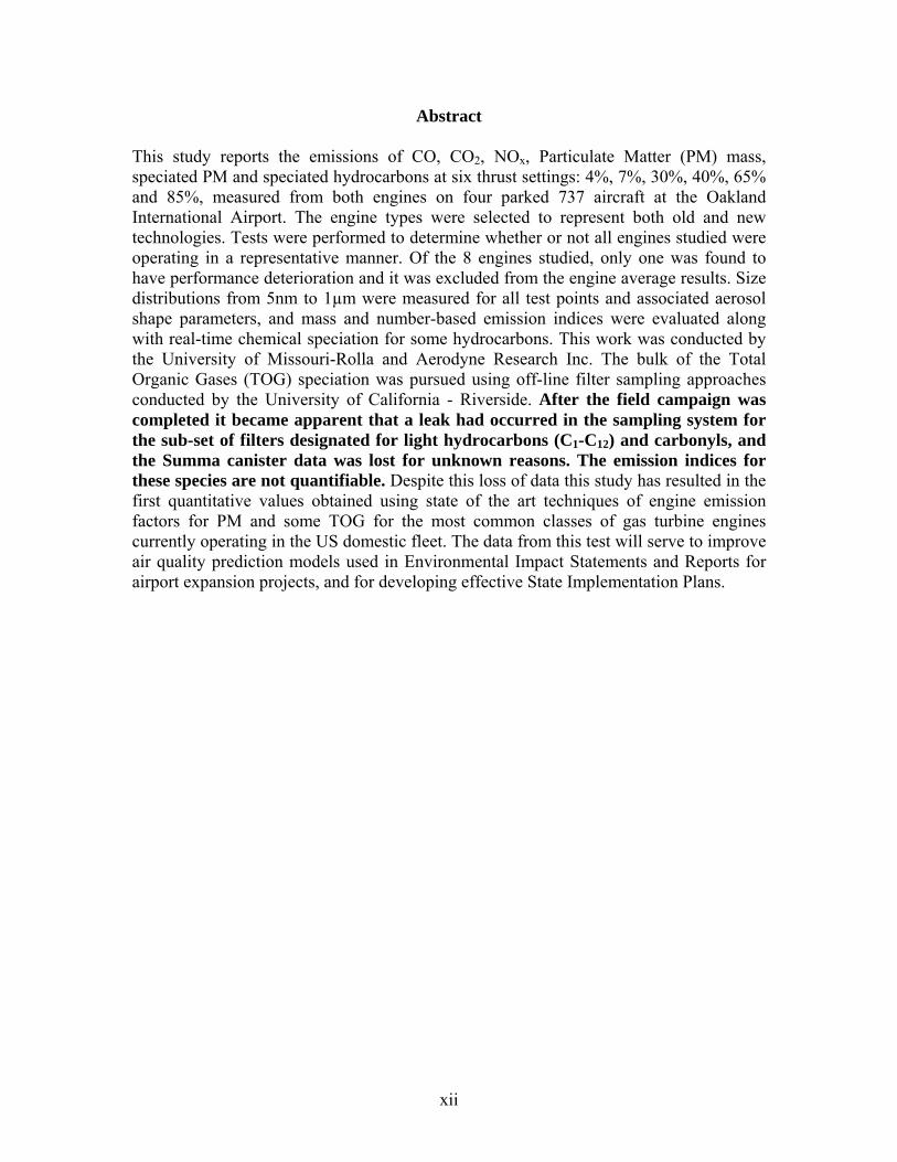
Abstract

This study reports the emissions of CO, CO2, NOx, Particulate Matter (PM) mass, speciated PM and speciated hydrocarbons at six thrust settings: 4%, 7%, 30%, 40%, 65% and 85%, measured from both engines on four parked 737 aircraft at the Oakland International Airport. The engine types were selected to represent both old and new technologies. Tests were performed to determine whether or not all engines studied were operating in a representative manner. Of the 8 engines studied, only one was found to have performance deterioration and it was excluded from the engine average results. Size distributions from 5nm to 1µm were measured for all test points and associated aerosol shape parameters, and mass and number-based emission indices were evaluated along with real-time chemical speciation for some hydrocarbons. This work was conducted by the University of Missouri-Rolla and Aerodyne Research Inc. The bulk of the Total Organic Gases (TOG) speciation was pursued using off-line filter sampling approaches conducted by the University of California - Riverside. After the field campaign was completed it became apparent that a leak had occurred in the sampling system for the sub-set of filters designated for light hydrocarbons (C1-C12) and carbonyls, and the Summa canister data was lost for unknown reasons. The emission indices for these species are not quantifiable. Despite this loss of data this study has resulted in the first quantitative values obtained using state of the art techniques of engine emission factors for PM and some TOG for the most common classes of gas turbine engines currently operating in the US domestic fleet. The data from this test will serve to improve air quality prediction models used in Environmental Impact Statements and Reports for airport expansion projects, and for developing effective State Implementation Plans.

xii

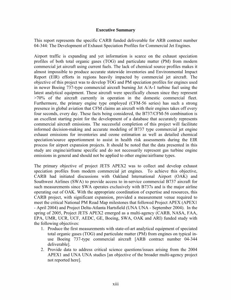
Executive Summary

This report represents the specific CARB funded deliverable for ARB contract number 04-344: The Development of Exhaust Speciation Profiles for Commercial Jet Engines.

Airport traffic is expanding and yet information is scarce on the exhaust speciation profiles of both total organic gases (TOG) and particulate matter (PM) from modern commercial jet aircraft using current fuels. The lack of chemical source profiles makes it almost impossible to produce accurate statewide inventories and Environmental Impact Report (EIR) efforts in regions heavily impacted by commercial jet aircraft. The objective of this project was to develop TOG and PM speciation profiles for engines used in newer Boeing 737-type commercial aircraft burning Jet A/A-1 turbine fuel using the latest analytical equipment. These aircraft were specifically chosen since they represent >70% of the aircraft currently in operation in the domestic commercial fleet. Furthermore, the primary engine type employed (CFM-56 series) has such a strong presence in global aviation that CFM claims an aircraft with their engines takes off every four seconds, every day. These facts being considered, the B737/CFM-56 combination is an excellent starting point for the development of a database that accurately represents commercial aircraft emissions. The successful completion of this project will facilitate informed decision-making and accurate modeling of B737 type commercial jet engine exhaust emissions for inventories and ozone estimation as well as detailed chemical speciation/source apportionment to assist in health risk assessments during the EIR process for airport expansion projects. It should be noted that the data presented in this study are engine/airframe specific and do not necessarily represent gas turbine engine emissions in general and should not be applied to other engine/airframe types.

The primary objective of project JETS APEX2 was to collect and develop exhaust speciation profiles from modern commercial jet engines. To achieve this objective, CARB had initiated discussions with Oakland International Airport (OAK) and Southwest Airlines (SWA) to provide access to in-service commercial B737 aircraft for such measurements since SWA operates exclusively with B737s and is the major airline operating out of OAK. With the appropriate coordination of expertise and resources, this CARB project, with significant expansion, provided a measurement venue required to meet the critical National PM Road Map milestones that followed Project APEX (APEX1 - April 2004) and Project Delta-Atlanta Hartsfield (UNA UNA - September 2004). In the spring of 2005, Project JETS APEX2 emerged as a multi-agency (CARB, NASA, FAA, EPA, UMR, UCR, UCF, AEDC, GE, Boeing, SWA, OAK and ARI) funded study with the following objectives:

1. Produce the first measurements with state-of-art analytical equipment of speciated total organic gases (TOG) and particulate matter (PM) from engines on typical in-use Boeing 737-type commercial aircraft [ARB contract number 04-344 deliverable].

2. Provide data to address critical science questions/issues arising from the 2004 APEX1 and UNA UNA studies [an objective of the broader multi-agency project not reported here].

xiii

These data will also be used, where possible, to develop chemical source profiles needed to make informed decisions during the Environmental Impact Report (EIR) process for airport expansions.

Custom-designed probes and extensive support equipment were used to sample jet exhaust in the on-wing position and were analyzed with state-of-the-art instrumentation. Emissions of CO, CO2, NOx, PM mass, speciated PM and speciated hydrocarbons at six thrust settings: 4%, 7%, 30%, 40%, 65% and 85% were measured from both engines on four parked 737 aircraft.

Particle-laden exhaust was extracted directly from the combustor/engine exhaust flow through the probe, transported through a sophisticated sample train, distributed to the different research groups, and analyzed in each group’s suite of instrumentation. Sampling probes were located at different positions downstream of the engine exit plane: 1m, 30m and 50m on the starboard side and at 1m on the port side of the aircraft. In this report the 1 and 50m data are presented. These aircraft engine emissions measurements were performed at the Ground Runup Enclosure (GRE) at OAK during August 2005. The engine types were selected to represent both old (-300 series) and new (-700 series) technologies. Realtime PM physical characterization was conducted by UMR. Size distributions from 5nm to 1µm were measured for all test points and associated aerosol parameters e.g. geometric mean diameter, geometric standard deviation, total concentration, and mass and number-based emission indices were evaluated are presented below.

Realtime measurements of gaseous emissions were made by ARI using 1) Tunable Infrared Laser Differential Absorption Spectroscopy (TILDAS) based on both lead-salt diode and quantum cascade laser sources for several important trace species emissions and 2) Proton-Transfer Reaction Mass Spectroscopy (PTR-MS) for hydrocarbons, and 3) chemiluminescence measurement (NO). These measurements were converted to Emission Indices using CO2 measured with a non-dispersive infrared absorption of that major combustion product. Chemical composition of the particle emissions was quantified using an Aerosol Mass Spectrometer (AMS) in concert with a Multi-Angle Absorption Photometer (MAAP, for Black Carbon mass) and particle size and number measurements.

Measurement of TOG, PM mass, metals and ion concentrations were conducted on the exhaust products collected on filter membranes by the University of California - Riverside Center for Environmental Research and Technology. The analytical methods employed are considered standard methods for such measurements and are described in detail in the methodology sections to follow. After the field campaign was completed, analysis of the DNPH cartridges and SUMMA canisters revealed anomalous CO2 concentrations which were attributed to a leak in a sub-system of the sampler. Also, C4-C12 hydrocarbon values based on the concentrations measured from the Thermal Desorption Tubes (TDS) were much lower than expected from APEX1 and other research. Since this leak introduced an unquantifiable dilution in these sub-systems, the emission factors for the light hydrocarbons and carbonyls could not be calculated.

xiv

The results of these measurements represent the heart of this final report and are presented in the results section as a series of speciation profiles by mode for each of the eight engines studied. Details of experimental methods and limits of detection are also provided in the tables.

The major conclusions from this study are as follows. Size distributions for engine exit plane were generally lognormal. Strong and sometimes non-linear dependencies were observed on engine power settings. The onset of gas-to-particle conversion was apparent at 50m for low to medium powers. In this data non-lognormal size distributions were often observed, where the mean sizes decreased and EIn increased relative to the 1m size distributions. Consistently, the aerosol Soluble Mass Fraction was found to increase with distance from the engine exit plane implying that as a result of processes such as gas to particle conversion soluble material present in the gas phase at the engine exhaust exit is being taken up by non-volatile soot as the exhaust plume expands. Its value was negligible at the engine exit plane and was ~10% at 50m. It should be noted that the aerosol properties in this study were calculated for the entire aerosol size distribution and not individual modes.

Measurement of NOx indicated that the general emissions performance of the engines was in keeping with certification measurements for the subject engine models. Measurements of individual hydrocarbon species suggest that most of the major species decrease with increasing engine power in proportion to each other and, in specific, with formaldehyde, which is one of the most plentiful emitted hydrocarbons and can be measured accurately. The particle composition includes both sulfate and organic volatile fractions at downstream distances, adding to the carbonaceous aerosol that is present already at the engine exit plane. The sulfate contribution has little dependence on engine power, while the organic contribution is greatest at low engine powers.

With respect to the TOG for which samples were obtained and analyzed, the relative distributions of the substituted naphthalenes to non-substituted naphthalenes for the idle modes are in general agreement with previous work. Chromium (VI) results for all but one of the engines studied were as expected. From DNPH analysis, the major three contributors to the carbonyl emissions are formaldehyde, acetaldehyde, and acetone. Formaldehyde and acetaldehyde are most dominant carbonyl species in the aircraft exhaust emissions.

At this time, the implications of this work for the CARBs relevant regulatory programs are limited. The State of California has no authority to regulate aircraft engine emissions or ground operations, so this project has few direct implications in those areas. However, the resulting improvements in inventory accuracy and detail will carry into other areas. Included would be improvements in air quality prediction used in Environmental Impact Statements and Reports (EIS and EIR) for airport expansion projects, and for developing effective State Implementation Plans (SIP). Of course, health effects impacts, such as those on airport neighbors, will need health risk factors to be developed. But climate change work would benefit from the improved quantification of such greenhouse emissions as NOx, CO2, and particulate matter.

xv

Upon the completion of this study, the Principal Investigators make the following recommendations for future work concerning aircraft emission characterization:

• The results of this study proved that accurate emission factors can be acquired in a cost effective manner. Since the data is clearly engine/airframe specific, studies of this nature should now be performed on other important engine/airframe combinations e.g. B747/CF6-80.

• The ideal testing conditions afforded by the GRE at Oakland leads to the recommendation that it should be considered a high priority venue for any future engine tests.

• Since the mix of transports routinely operating in and out of Oakland will limit the range of engines/airframes that can be studied, for future studies where B747, B757, B767, and B777 and the larger Airbus transports A320, A340 etc. are anticipated test vehicles, it will be necessary to consider attracting other aircraft to the Oakland test site or using GREs located at other airports, provided appropriate weather conditions prevail.

• In future tests it is recommended that high frequency data acquisition be employed for engine operating conditions such N1, N2, EGT and Fuel flow rate. This may be difficult for older airframes but straight forward for newer additions to the commercial fleet that digitally record engine operating conditions.

• Much of the data was gathered and initially analyzed in real-time. However, this was not the case for the UCR VOC samples that were analyzed off-site post test. For future studies efforts should be expended to assure that the analysis could be undertaken for these samples on-site. This would provide quasi-real-time feedback on the integrity of such samples.

• Engine to engine variability is difficult to estimate when the engine sample size is small (in this study ≤ 4 engines per model). The value of accurately estimating this parameter warrants the consideration of a longer period of study.

• Valid measurements for TOG and multiple significant speciated VOCs were not obtained because of sampling and laboratory issues for the light hydrocarbon and carbonyl analyses. These measurements should be repeated at a future engine test, when the opportunity arises, to get better estimates of TOG and speciated VOCs.

The objectives of the JETS APEX2 study were to produce a comprehensive data set of emission factors for total organic gases and PM for old and new technology CFM56 class engines operating out of a medium size hub airport in the State of California (i.e. Port of Oakland). This study was successful in producing the first state of the art measurements for PM physical characterization of in-service CFM56 type engines. Unfortunately, as a

xvi

result of the failure of some of the off-line sampling systems the TOG analysis was limited and from that perspective not all of the objectives set out in the proposed effort were accomplished. However, even with the limited TOG data this study represents the first extensive physico-chemical analysis of a series of in-service commercial engines and as such is an extremely valuable dataset. This study is part of a greater multi-agency effort that includes emissions measurements downwind of an active runway at Oakland during normal airport operations, and the results presented here are essential for the interpretation of the downwind measurements. The downwind studies were publicly released at the APEX Conference held in Cleveland, OH, November 29- December 01, 2006.

xvii

1.0 Background

1.1 Introduction

The growth of commercial air traffic over the last decade has led to an increased contribution to the local inventory of gaseous and particle emissions from the operations associated with airports, e.g. ground support equipment (GSEs) and aircraft engines. Recent studies have shown an increasing number of environmental effects from aviation related activities such as impact on climate (Penner et al., 1999) and local air quality (Waitz et al., 2004). An additional concern, primarily in the vicinity of airports, is the contribution of aircraft emissions to the formation of photochemical smog and the delivery (through inhalation) of highly concentrated irritants into human beings (Samet et al., 2000; Dutton, 2002).

The lack of EPA aircraft engine standards for PM and speciated hydrocarbons and the scarcity of information about the emissions associated with airport operations have heightened the concerns of communities living around airports. Furthermore, Federal statutory and regulatory framework prohibit states, like California, from setting emission standards for aircraft engines, regulating the number of takeoffs or landings at airports, limiting flight procedures or controlling types of planes used at airports. As a consequence, airports find it increasingly difficult to evaluate the potential contribution and health effects of all airport-related emissions during the environmental review process.

1.1.1 Regulated Emissions from Commercial Jet Engines

Lister (2003) published a comprehensive review of the background, history and development of the current aircraft engine emissions certification regime, up to the publication of Annex 16, Volume II, 1st Edition in 1981 and a brief overview of the main developments. His review is based on historic archive records of the development of the current certification methodology, which were available to the NEPAIR partnership (New Emissions Parameter covering all flight phases of AIRcraft operation).

In the United States, the United States Environmental Protection Agency (US EPA) is required by Section 231 of the Clean Air Act Amendments of 1990 to regulate aircraft engine emissions and has adopted aircraft engine emission standards recommended by the International Civil Aviation Organization (ICAO) as the applicable federal standards. The ICAO and its Committee on Aviation and Environmental Protection (CAEP) continue to coordinate development of consistent international standards for aircraft engines worldwide that “encourage the development of less polluting, more efficient aircraft engines and more aerodynamic aircraft bodies will result in aircraft that pollute substantially less, operate more quietly, and consume less fuel than today’s airplanes."

The US EPA issued its current rule in 1997 on the control of aircraft air pollution, including standards for exhaust emissions for carbon monoxide (CO), nitric oxides

1

(NOx), and smoke number (SN). The EPA regulation also incorporated the emission test and measurement procedures from the U.N. International Civil Aviation Organization (ICAO), bringing the U.S. aircraft standards into alignment with international standards. Quantification of the regulated emissions - carbon monoxide (CO), oxides of nitrogen (NOX), total hydrocarbons (THC) and smoke number (SN) - can be found in the ICAO database (ICAO 2006). It should be noted that usually only one engine is tested in triplicate in order to represent an engine family and that very few multiple engines from the same family are tested.

While most investigators use the standard SAE methods to measure the emissions, several researchers have explored other methods, especially applied to in-use emissions from aircraft operating on the ground. For example, Popp (1999) tested remote sensing at London’s Heathrow Airport and in two days made 122 measurements of 90 different aircraft in a mix of idle, taxi-out, and takeoff modes. The work found aircraft at idle exhibited little nitric oxide emissions and at higher thrust levels were somewhat consistent with values from the ICAO Databank. Heland (1998) applied FTIR spectroscopy to the determination of major combustion products such as CO2, H2O, CO, NO, and N2O in aircraft exhausts and compared them with values published in the literature. He reported the measured CO emission index at idle power of a CFM56-3 engine was about 27% lower than the value given by Spicer and about 27–48% higher than the ICAO data for the whole span of CFM56-3 engines. The CO emission index (EI) measured at idle power of a CFM56-5C2 engine of an Airbus A340 was about 30% less than the ICAO value. One observation from Heland’s work is the magnitude of the variation found when different investigators make the measurements.

Herndon (2004) measured the NO and NO2 emission ratios from 30 individual in-use commercial aircraft during taxi and takeoff at JFK Airport in New York City. NO and NO2 concentrations were measured with one-second time resolution using a dual tunable infrared laser differential absorption spectroscopy instrument. The authors reported that the field-measured emission ratio to the ICAO EIs for three aircraft engines agreed within the expected engine-to-engine variability, aging effects, and experimental uncertainty for three somewhat different engine types.

1.1.2 Non-Regulated Emissions from Jet Engines

As previously discussed, the people living near airports are concerned about their exposure to the combustion products from jet engines and a number of groups are interested in learning more about how much aircraft emissions contribute to the inventory of a basin. Combustion of jet fuel results in CO2, H2O, CO, SOx, NOx, particulate matter (PM) and hundreds of organic compounds. Most data are on the regulated emissions and information is lacking on the speciation of the hundreds of hydrocarbon compounds and PM necessary to inventory the contribution of aircraft operations to the total area loading. In order to inventory aircraft operations emissions, a detailed emissions database with speciation is required, and historically, tests to obtain speciated engine emissions data are very expensive and involve many hours of engine operation. These tests are quite rare

2

and almost non-existent. Current efforts to model commercial jet exhaust, as well as EIR's, are relying on results from testing of military aircraft performed in the 1980’s or earlier. Data, which are available, such as in EPA’s AP-42 Emission Factor report, come from measurements made around 1980.

Spicer (1992) is usually credited with being the first person to have developed comprehensive speciation profiles of the hydrocarbons in jet exhaust. His first paper reported on emissions for the F-101 and F-110 military engines using JP-4 while operating from idle to intermediate power. His primary focus was the detailed organic speciation and his methodology for sampling and analysis of the hydrocarbon species is similar to that carried out in the work reported here. However, current analytical equipment is far more sensitive and allows lower detection limits. In a second paper, Spicer (1994) reported on the chemical composition and photochemical reactivity of exhaust from two engines. One was an older TF-39 engine that was not designed with emissions in mind, and the other was the newer technology, low-emission CFM56-3 engine. Both engines were tested at three power settings using fuels meeting the JP-4, JP-5 and JP-8 specifications. Results with kerosene-based JP-5 showed the hydrocarbon emission index of the CFM56 engine was about half that of the TF-39 engine. Spicer points out that the core engine of the CFM56 is essentially the same as the F-101 used and reported on in his earlier tests.

Petzold (1999) reported a comparison of the characteristic parameters of black carbon aerosol (BC) emitted from jet engine during ground tests and in-flight behind the same aircraft. They found that the total BC number concentration at the engine exit was in good agreement with the in-flight measured number concentrations of non-volatile particles. A comparison between total number concentration of BC particles and the non-volatile fraction of the total aerosol at the exit plane suggested that the non-volatile fraction of jet engine exhaust aerosol consists almost completely of BC. BC size distribution features included a primary modal diameter at D~0.045 µm and an agglomeration mode at D<0.2 µm.

In 2000, Dewers described AERONET, “Identification of aircraft Emissions relevant for Reduction Technologies, as a cooperative network set up within the European Communities 4th Famework Programme of Research.” AERONET Thematic Network was created as a platform where stakeholders meet and exchange information, views and experiences gathered in different European projects. The complexity of the issues can be witnessed by the size of the stakeholder group: including aircraft and engine manufacturers, operators, fuel suppliers, airports, and air navigation providers. Each stakeholder has a keen interest to ensure that its products, aircraft and air transport, are environmentally acceptable.

As part of the AERONET effort, Petzold (2001) provided a comparison of the various analytical measurement methods for monitoring various emissions from aircraft engines either airborne or on the ground. The measurement of particulates is the most interesting section of his review. He points out that the smoke number method is not able to accurately reflect the presence of emitted particles in terms of their size. He concludes: “there is an urgent necessity to establish standard methods for engine exhaust aerosol

3

characterization which correspond better to present knowledge on the atmospheric impact of aircraft emitted particles.”

Wilson (2004) presented an overview of the goals and achievements of another AERONET effort: the European PartEmis project (Measurement and prediction of emissions of aerosols and gaseous precursors from gas turbine engines). PartEmis focused on the characterization and quantification of exhaust emissions from a gas turbine engine. His summary table reviews current knowledge about measurement techniques and gaseous and aerosol parameters. Of interest is their quest to measure non-methane hydrocarbons (NMVOCs -C2–C10) and partially oxidized hydrocarbons, specifically carbonyl compounds and organic acids. More than 100 NMVOCs (aliphatic and aromatic hydrocarbons, carbonyls and acids) were found and quantified but not yet published. For example, they report the emission indices of organic acids were about 10 times higher than for carbonyl compounds. Review of the aerosol phase revealed that the formation of volatile particles in jet engine emissions was the result of cooling and dilution of exhaust gases.

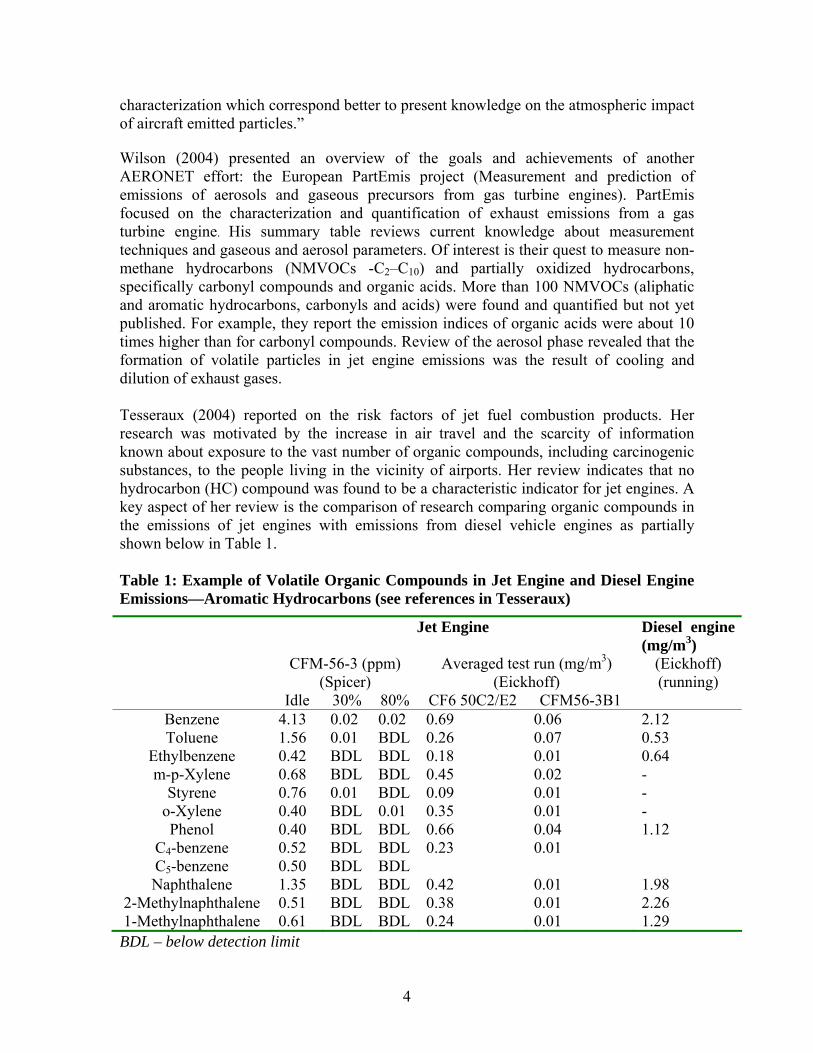
Tesseraux (2004) reported on the risk factors of jet fuel combustion products. Her research was motivated by the increase in air travel and the scarcity of information known about exposure to the vast number of organic compounds, including carcinogenic substances, to the people living in the vicinity of airports. Her review indicates that no hydrocarbon (HC) compound was found to be a characteristic indicator for jet engines. A key aspect of her review is the comparison of research comparing organic compounds in the emissions of jet engines with emissions from diesel vehicle engines as partially shown below in Table 1.

Table 1: Example of Volatile Organic Compounds in Jet Engine and Diesel Engine Emissions—Aromatic Hydrocarbons (see references in Tesseraux)

CFM-56-3 (ppm)

Jet Engine

Averaged test run (mg/m3)

Diesel engine (mg/m3)

(Eickhoff) (Spicer) (Eickhoff) (running)

Idle 30% 80% CF6 50C2/E2 CFM56-3B1 Benzene 4.13 0.02 0.02 0.69 0.06 2.12 Toluene 1.56 0.01 BDL 0.26 0.07 0.53

Ethylbenzene 0.42 BDL BDL 0.18 0.01 0.64 m-p-Xylene 0.68 BDL BDL 0.45 0.02 -

Styrene 0.76 0.01 BDL 0.09 0.01 -o-Xylene 0.40 BDL 0.01 0.35 0.01 -Phenol 0.40 BDL BDL 0.66 0.04 1.12

C4-benzene 0.52 BDL BDL 0.23 0.01 C5-benzene 0.50 BDL BDL Naphthalene 1.35 BDL BDL 0.42 0.01 1.98

2-Methylnaphthalene 0.51 BDL BDL 0.38 0.01 2.26 1-Methylnaphthalene 0.61 BDL BDL 0.24 0.01 1.29

BDL – below detection limit

4

Recently, Gerstle (2002) published a series of internal reports as the product of a 5-year series of emissions testing of seventeen military aircraft engines, two helicopter engines and two auxiliary power units (APUs), all burning military fuel, JP-8. Testing included regulated emissions and selected non-regulated emissions, such as the carbonyls and Volatile Organic Compounds (VOCs). Their data for the carbonyls and VOCs might be useful references.

1.1.3 Effects of Unburned Jet Fuel

A growing body of information is available about the physical properties and chemical composition of unburned jet fuel. These references are germane given the interest of some staff at ARB on the speciation and health effects of unburned jet fuel and its fumes. An excellent reference is the 2003 report of the National Research Council entitled: “Toxicological Assessment of Jet-Propulsion Fuel 8.” The NRC report and numerous references within dealt with the health effects of fuel vapors and liquid fuel.

1.2 Recent NASA Missions

1.2.1 Experiment to Characterize Aircraft Volatile Aerosol and Trace Species Emissions (EXCAVATE- 1999)

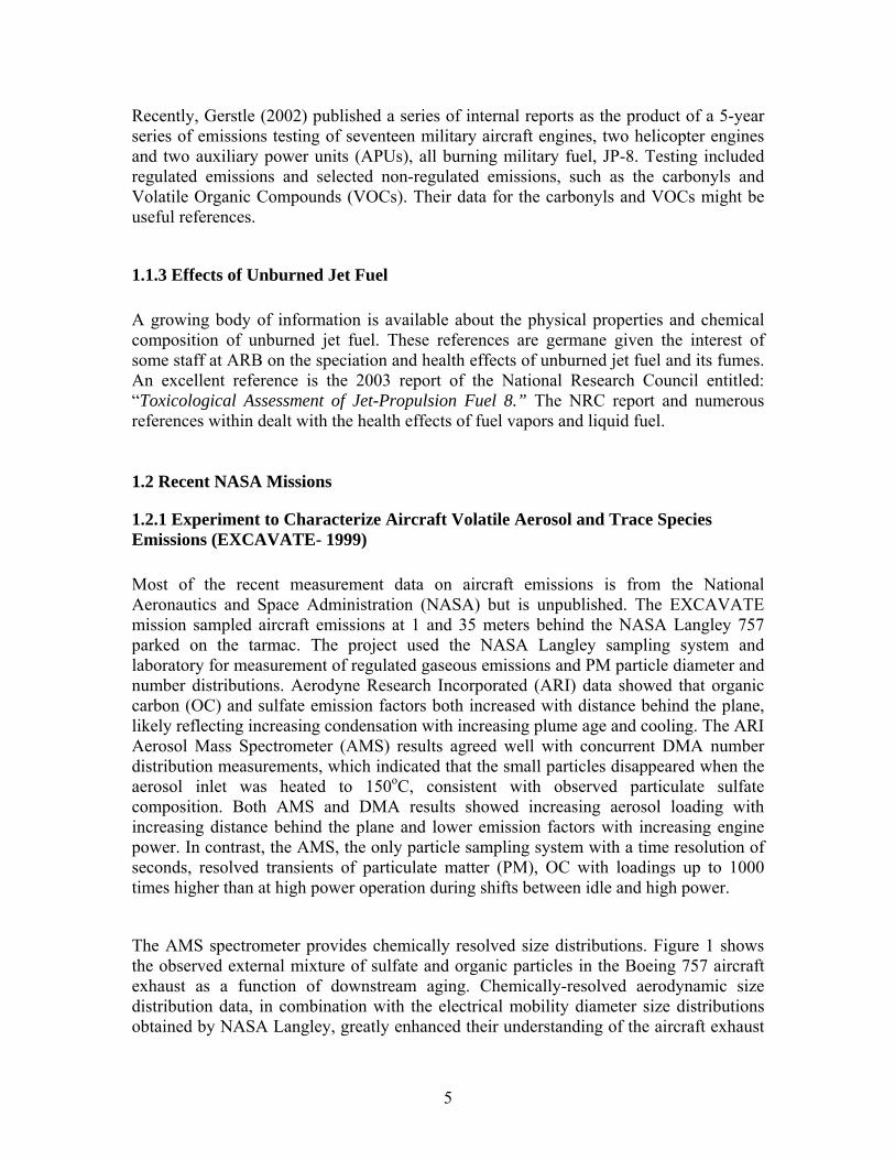
Most of the recent measurement data on aircraft emissions is from the National Aeronautics and Space Administration (NASA) but is unpublished. The EXCAVATE mission sampled aircraft emissions at 1 and 35 meters behind the NASA Langley 757 parked on the tarmac. The project used the NASA Langley sampling system and laboratory for measurement of regulated gaseous emissions and PM particle diameter and number distributions. Aerodyne Research Incorporated (ARI) data showed that organic carbon (OC) and sulfate emission factors both increased with distance behind the plane, likely reflecting increasing condensation with increasing plume age and cooling. The ARI Aerosol Mass Spectrometer (AMS) results agreed well with concurrent DMA number distribution measurements, which indicated that the small particles disappeared when the aerosol inlet was heated to 150oC, consistent with observed particulate sulfate composition. Both AMS and DMA results showed increasing aerosol loading with increasing distance behind the plane and lower emission factors with increasing engine power. In contrast, the AMS, the only particle sampling system with a time resolution of seconds, resolved transients of particulate matter (PM), OC with loadings up to 1000 times higher than at high power operation during shifts between idle and high power.

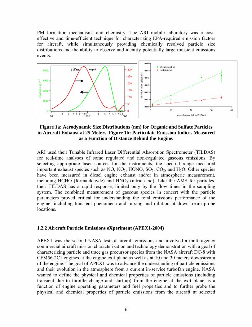
The AMS spectrometer provides chemically resolved size distributions. Figure 1 shows the observed external mixture of sulfate and organic particles in the Boeing 757 aircraft exhaust as a function of downstream aging. Chemically-resolved aerodynamic size distribution data, in combination with the electrical mobility diameter size distributions obtained by NASA Langley, greatly enhanced their understanding of the aircraft exhaust

5

• •

PM formation mechanisms and chemistry. The ARI mobile laboratory was a cost-effective and time-efficient technique for characterizing EPA-required emission factors for aircraft, while simultaneously providing chemically resolved particle size distributions and the ability to observe and identify potentially large transient emissions events.

4000

3000

2000

1000

0

Org

anic

s µg

m-3

10 2 3 4 5 6 7 8 9

100 2 3 4 5 6 7 8 9

1000

300

250

200

150

100

50

0

Sulfate Organic

0.06

0.05

0.04

0.03

0.02

0.01

0.00

Emiss

ion

Inde

x (g

/kg

fuel

)

403020100

probe distance behind 757 (m)

Organic carbon Sulfate (×5)

Figure 1a: Aerodynamic Size Distributions (nm) for Organic and Sulfate Particles in Aircraft Exhaust at 25 Meters. Figure 1b: Particulate Emission Indices Measured

as a Function of Distance Behind the Engine.

ARI used their Tunable Infrared Laser Differential Absorption Spectrometer (TILDAS) for real-time analyses of some regulated and non-regulated gaseous emissions. By selecting appropriate laser sources for the instruments, the spectral range measured important exhaust species such as NO, NO2, HONO, SO2, CO2, and H2O. Other species have been measured in diesel engine exhaust and/or in atmospheric measurement, including HCHO (formaldehyde) and HNO3 (nitric acid). Like the AMS for particles, their TILDAS has a rapid response, limited only by the flow times in the sampling system. The combined measurement of gaseous species in concert with the particle parameters proved critical for understanding the total emissions performance of the engine, including transient phenomena and mixing and dilution at downstream probe locations.

1.2.2 Aircraft Particle Emissions eXperiment (APEX1-2004)

APEX1 was the second NASA test of aircraft emissions and involved a multi-agency commercial aircraft mission characterization and technology demonstration with a goal of characterizing particle and trace gas precursor species from the NASA aircraft DC-8 with CFM56-2C1 engines at the engine exit plane as well as at 10 and 30 meters downstream of the engine. The goal of APEX1 was to advance the understanding of particle emissions and their evolution in the atmosphere from a current in-service turbofan engine. NASA wanted to define the physical and chemical properties of particle emissions (including transient due to throttle change and start-up) from the engine at the exit plane as a function of engine operating parameters and fuel properties and to further probe the physical and chemical properties of particle emissions from the aircraft at selected

6

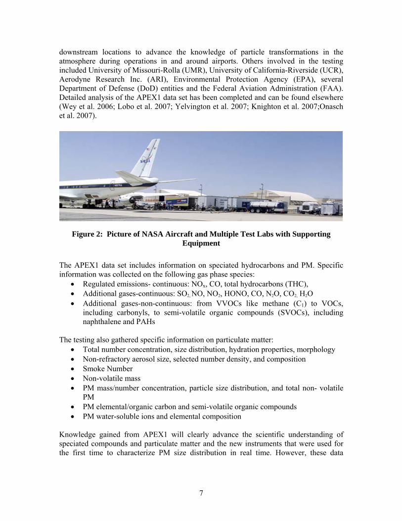
downstream locations to advance the knowledge of particle transformations in the atmosphere during operations in and around airports. Others involved in the testing included University of Missouri-Rolla (UMR), University of California-Riverside (UCR), Aerodyne Research Inc. (ARI), Environmental Protection Agency (EPA), several Department of Defense (DoD) entities and the Federal Aviation Administration (FAA). Detailed analysis of the APEX1 data set has been completed and can be found elsewhere (Wey et al. 2006; Lobo et al. 2007; Yelvington et al. 2007; Knighton et al. 2007;Onasch et al. 2007).

Figure 2: Picture of NASA Aircraft and Multiple Test Labs with Supporting Equipment

The APEX1 data set includes information on speciated hydrocarbons and PM. Specific information was collected on the following gas phase species:

• Regulated emissions- continuous: NOx, CO, total hydrocarbons (THC), • Additional gases-continuous: SO2, NO, NO2, HONO, CO, N2O, CO2, H2O • Additional gases-non-continuous: from VVOCs like methane (C1) to VOCs,

including carbonyls, to semi-volatile organic compounds (SVOCs), including naphthalene and PAHs

The testing also gathered specific information on particulate matter: • Total number concentration, size distribution, hydration properties, morphology • Non-refractory aerosol size, selected number density, and composition • Smoke Number • Non-volatile mass • PM mass/number concentration, particle size distribution, and total non- volatile

PM • PM elemental/organic carbon and semi-volatile organic compounds • PM water-soluble ions and elemental composition

Knowledge gained from APEX1 will clearly advance the scientific understanding of speciated compounds and particulate matter and the new instruments that were used for the first time to characterize PM size distribution in real time. However, these data

7

recorded were for one engine, and much more research is needed in areas related to modern engines as found on the Boeing 737 aircraft. Such data is reported here.

1.3 JETS APEX2

Put in perspective, past and recent work, including the latest NASA missions, have directed most effort towards advancing the understanding and expanding the database related to regulated emissions and some new scientific approaches for measuring PM. None of these data are included in the current ARB profiles. Instead, ARB’s current profiles were developed using older fuels and engine technology, mainly based on older military use fuels and engines from the 1980’s. Accordingly, significant uncertainties exist in ARB’s projects when quantifying speciated hydrocarbons and speciated PM emissions from current airport sources. ARB’s uncertainties exist because:

• The currently employed emissions data were collected for limited and outdated military aircraft engines with military fuels and other operations from the 1980s,

• The measured compounds, overall methodologies, and test equipment used, limit the usefulness when applied to current commercial jet engine speciation profiles, and

• Very few emissions tests have been conducted since the 1980s for speciated hydrocarbons and PM on actual commercial aircraft engines, so there was no opportunity to update the ARB database.

Obtaining data on aircraft emissions is complicated and no single entity has all the resources and expertise needed to meet ARB’s multiple goals. Accordingly, the approach was to use multiple teams, consisting of executive and technical members. The executive team consisted of the ARB, Federal Aviation Administration (FAA), the UMRCOE, Southwest Airlines (SWA) and the Port of Oakland (OAK).

The technical team consisted of researchers from the University of Missouri-Rolla (UMR), the University of California-Riverside (UCR), and Aerodyne Research Inc. (ARI). This team had the resources necessary to carry out a complex project of this nature in order to deliver the desired information to ARB. The field-ready, proven equipment included instrumentation for sampling and measuring CO, CO2, NOx, PM, and detailed chemical species emissions data from engines on modern commercial aircraft. Additionally, the South Coast Air Quality Management District analyzed the very volatile organic carbon gases (VVOCs, like methane) and the metals with their ICP-MS. As on past projects, representatives from Boeing and GE participated as advisors in the project. Roles of the various team members are shown below in Table 2 and the list of instrumentation and data acquired are reported in Table 3.

8

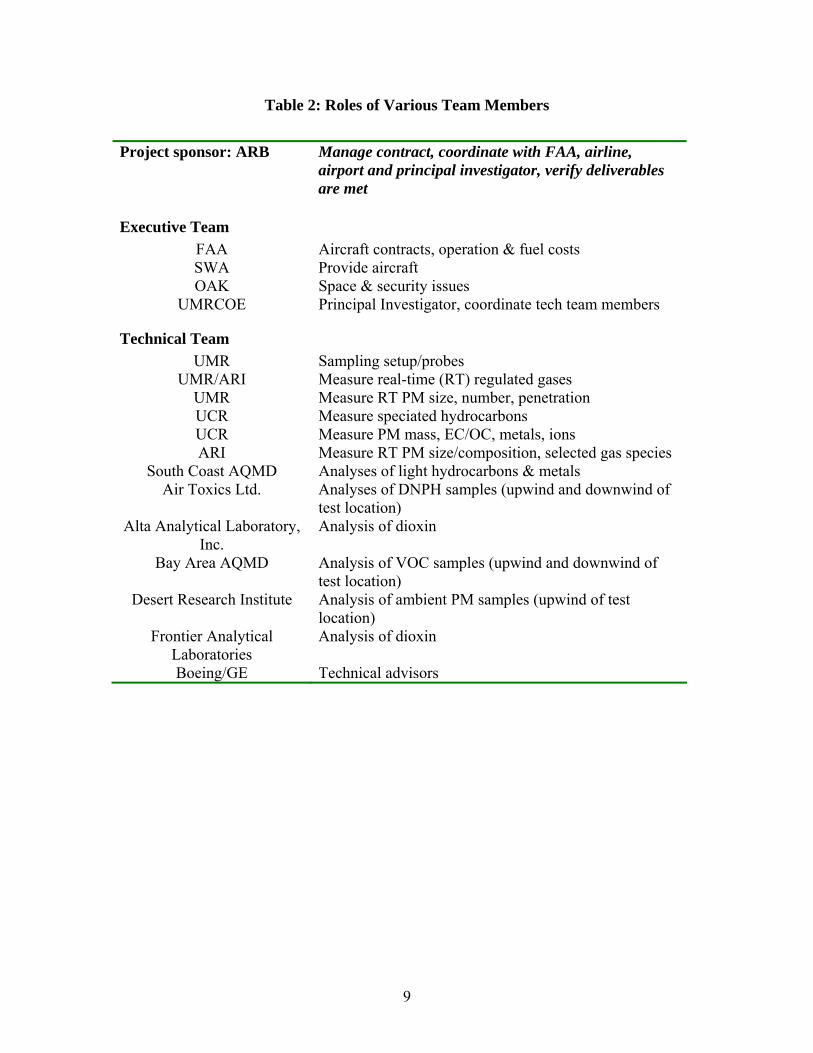
Table 2: Roles of Various Team Members

Project sponsor: ARB Manage contract, coordinate with FAA, airline, airport and principal investigator, verify deliverables are met

Executive Team FAA Aircraft contracts, operation & fuel costs SWA Provide aircraft OAK Space & security issues

UMRCOE Principal Investigator, coordinate tech team members

Technical Team UMR Sampling setup/probes

UMR/ARI Measure real-time (RT) regulated gases UMR Measure RT PM size, number, penetration UCR Measure speciated hydrocarbons UCR Measure PM mass, EC/OC, metals, ions ARI Measure RT PM size/composition, selected gas species

South Coast AQMD Analyses of light hydrocarbons & metals Air Toxics Ltd. Analyses of DNPH samples (upwind and downwind of

test location) Alta Analytical Laboratory, Analysis of dioxin

Inc. Bay Area AQMD Analysis of VOC samples (upwind and downwind of

test location) Desert Research Institute Analysis of ambient PM samples (upwind of test

location) Frontier Analytical Analysis of dioxin

Laboratories Boeing/GE Technical advisors

9

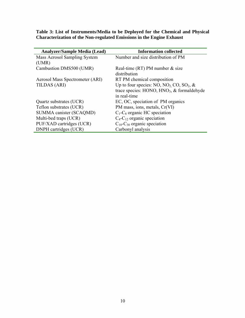
Table 3: List of Instruments/Media to be Deployed for the Chemical and Physical Characterization of the Non-regulated Emissions in the Engine Exhaust

Analyzer/Sample Media (Lead) Information collected Mass Aerosol Sampling System Number and size distribution of PM (UMR) Cambustion DMS500 (UMR) Real-time (RT) PM number & size

distribution Aerosol Mass Spectrometer (ARI) RT PM chemical composition TILDAS (ARI) Up to four species: NO, NO2, CO, SO2, &

trace species: HONO, HNO3, & formaldehyde in real-time

Quartz substrates (UCR) EC, OC, speciation of PM organics Teflon substrates (UCR) PM mass, ions, metals, Cr(VI) SUMMA canister (SCAQMD) C1-C8 organic HC speciation Multi-bed traps (UCR) C4-C12 organic speciation PUF/XAD cartridges (UCR) C10-C30 organic speciation DNPH cartridges (UCR) Carbonyl analysis

10

2.0 Materials and Methods

2.1 Aircraft Engines

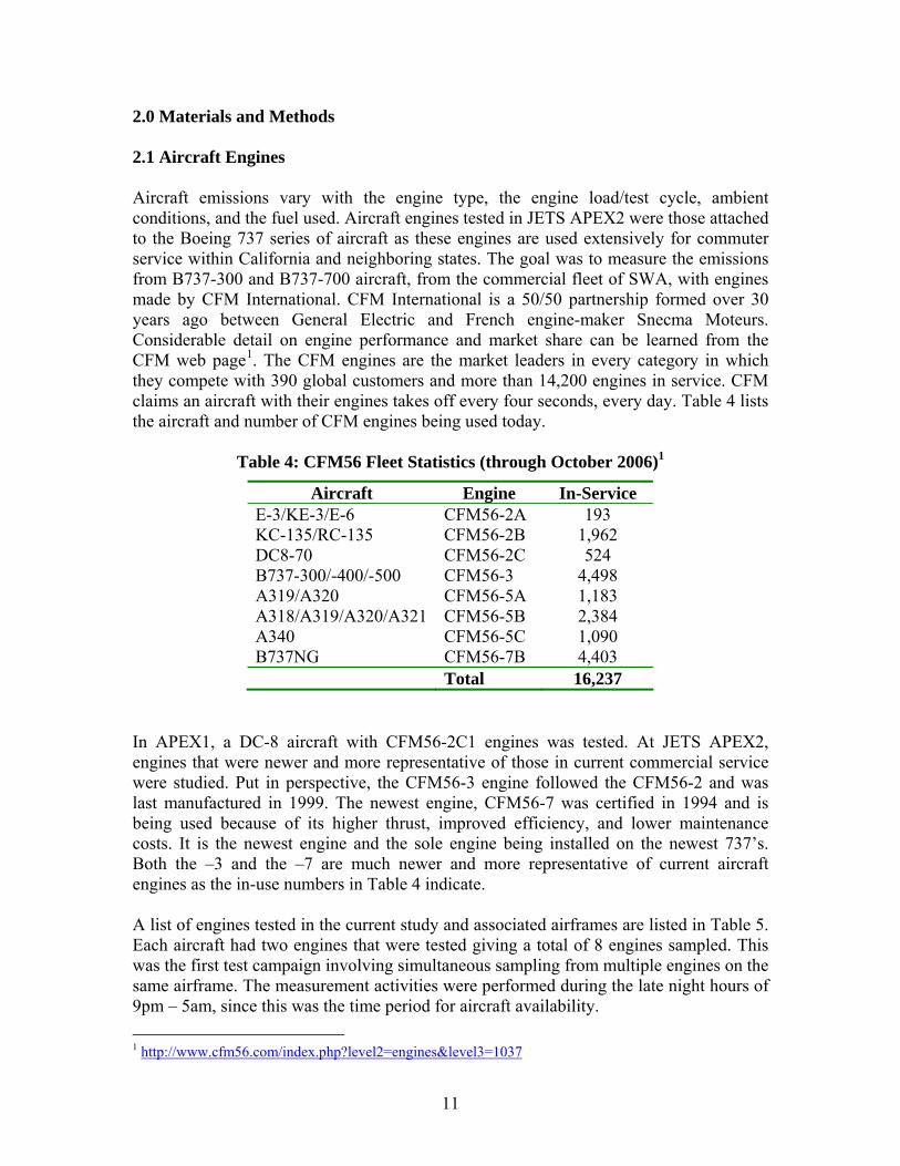
Aircraft emissions vary with the engine type, the engine load/test cycle, ambient conditions, and the fuel used. Aircraft engines tested in JETS APEX2 were those attached to the Boeing 737 series of aircraft as these engines are used extensively for commuter service within California and neighboring states. The goal was to measure the emissions from B737-300 and B737-700 aircraft, from the commercial fleet of SWA, with engines made by CFM International. CFM International is a 50/50 partnership formed over 30 years ago between General Electric and French engine-maker Snecma Moteurs. Considerable detail on engine performance and market share can be learned from the CFM web page1. The CFM engines are the market leaders in every category in which they compete with 390 global customers and more than 14,200 engines in service. CFM claims an aircraft with their engines takes off every four seconds, every day. Table 4 lists the aircraft and number of CFM engines being used today.

Table 4: CFM56 Fleet Statistics (through October 2006)1

Aircraft Engine In-Service E-3/KE-3/E-6 CFM56-2A 193 KC-135/RC-135 CFM56-2B 1,962 DC8-70 CFM56-2C 524 B737-300/-400/-500 CFM56-3 4,498 A319/A320 CFM56-5A 1,183 A318/A319/A320/A321 CFM56-5B 2,384 A340 CFM56-5C 1,090 B737NG CFM56-7B 4,403

Total 16,237

In APEX1, a DC-8 aircraft with CFM56-2C1 engines was tested. At JETS APEX2, engines that were newer and more representative of those in current commercial service were studied. Put in perspective, the CFM56-3 engine followed the CFM56-2 and was last manufactured in 1999. The newest engine, CFM56-7 was certified in 1994 and is being used because of its higher thrust, improved efficiency, and lower maintenance costs. It is the newest engine and the sole engine being installed on the newest 737’s. Both the –3 and the –7 are much newer and more representative of current aircraft engines as the in-use numbers in Table 4 indicate.

A list of engines tested in the current study and associated airframes are listed in Table 5. Each aircraft had two engines that were tested giving a total of 8 engines sampled. This was the first test campaign involving simultaneous sampling from multiple engines on the same airframe. The measurement activities were performed during the late night hours of 9pm – 5am, since this was the time period for aircraft availability.

1 http://www.cfm56.com/index.php?level2=engines&level3=1037

11

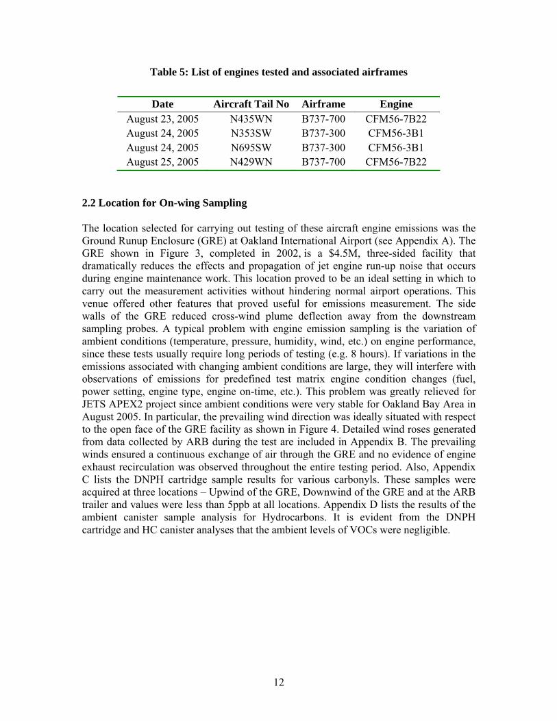
Table 5: List of engines tested and associated airframes

Date Aircraft Tail No Airframe Engine August 23, 2005 N435WN B737-700 CFM56-7B22 August 24, 2005 N353SW B737-300 CFM56-3B1 August 24, 2005 N695SW B737-300 CFM56-3B1 August 25, 2005 N429WN B737-700 CFM56-7B22

2.2 Location for On-wing Sampling

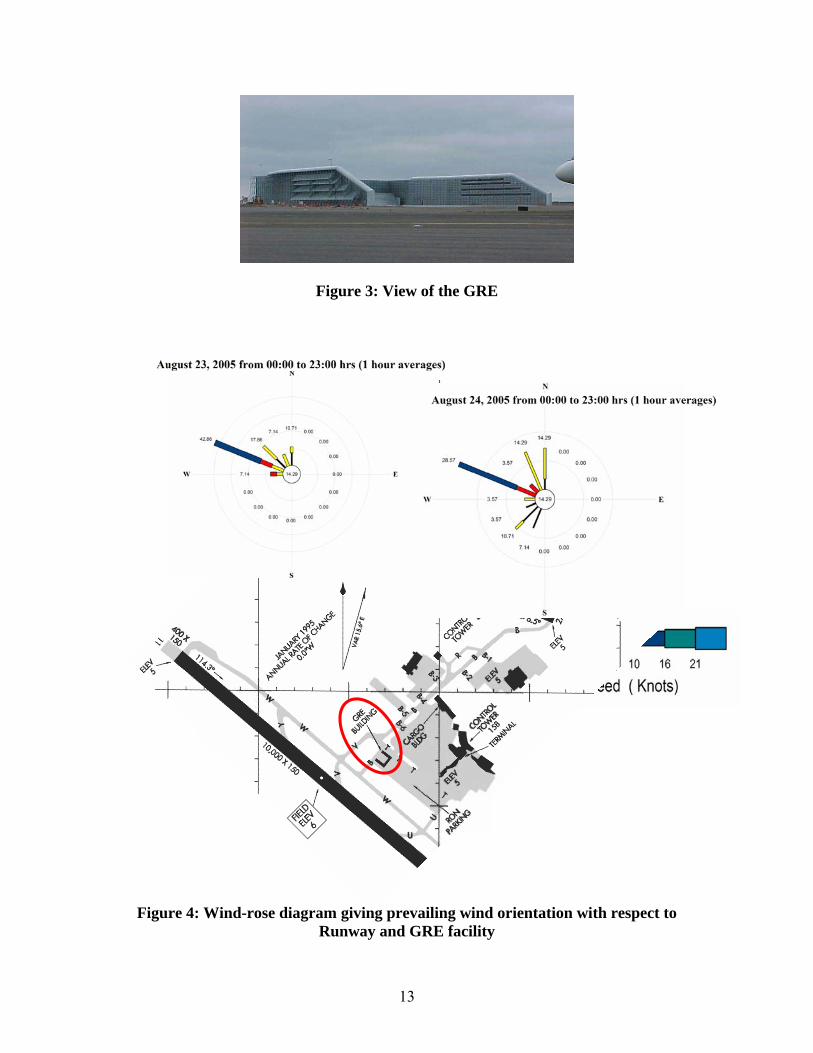
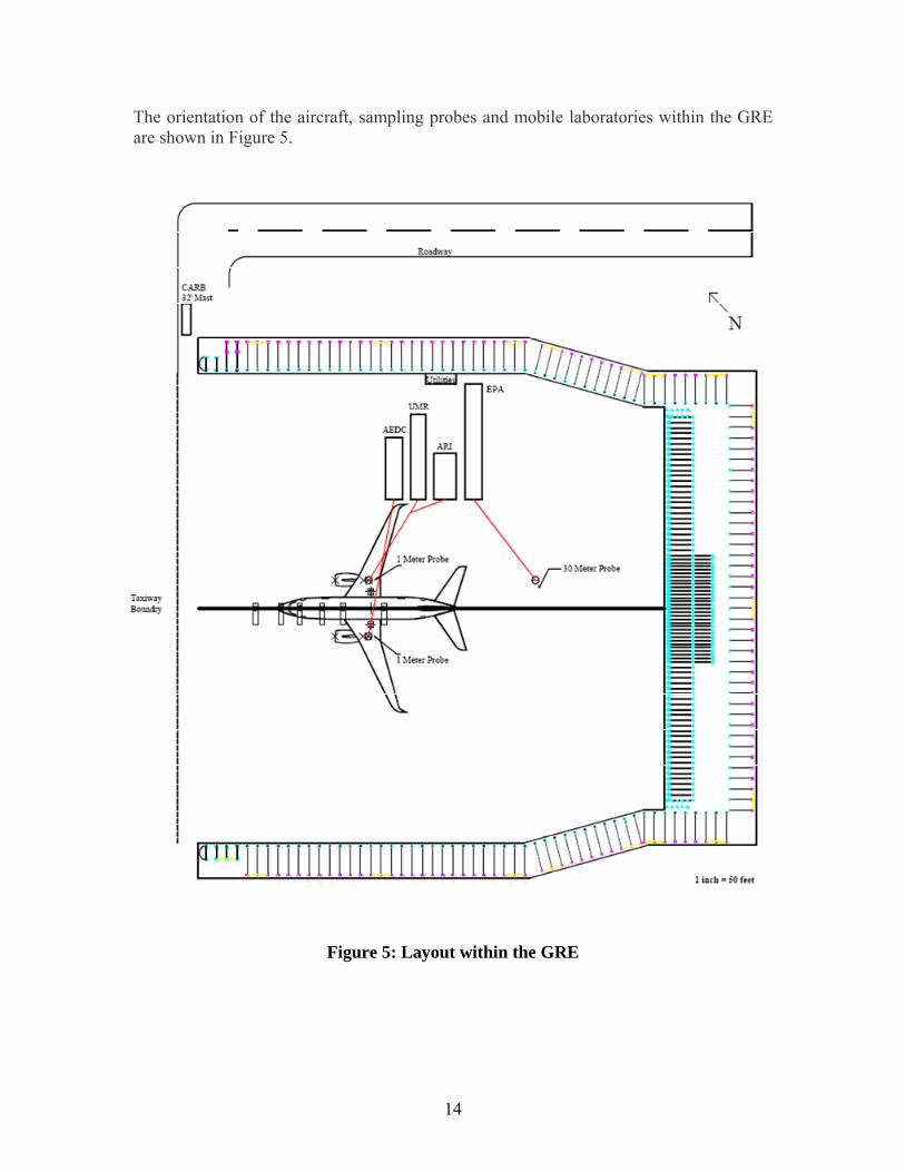
The location selected for carrying out testing of these aircraft engine emissions was the Ground Runup Enclosure (GRE) at Oakland International Airport (see Appendix A). The GRE shown in Figure 3, completed in 2002, is a $4.5M, three-sided facility that dramatically reduces the effects and propagation of jet engine run-up noise that occurs during engine maintenance work. This location proved to be an ideal setting in which to carry out the measurement activities without hindering normal airport operations. This venue offered other features that proved useful for emissions measurement. The side walls of the GRE reduced cross-wind plume deflection away from the downstream sampling probes. A typical problem with engine emission sampling is the variation of ambient conditions (temperature, pressure, humidity, wind, etc.) on engine performance, since these tests usually require long periods of testing (e.g. 8 hours). If variations in the emissions associated with changing ambient conditions are large, they will interfere with observations of emissions for predefined test matrix engine condition changes (fuel, power setting, engine type, engine on-time, etc.). This problem was greatly relieved for JETS APEX2 project since ambient conditions were very stable for Oakland Bay Area in August 2005. In particular, the prevailing wind direction was ideally situated with respect to the open face of the GRE facility as shown in Figure 4. Detailed wind roses generated from data collected by ARB during the test are included in Appendix B. The prevailing winds ensured a continuous exchange of air through the GRE and no evidence of engine exhaust recirculation was observed throughout the entire testing period. Also, Appendix C lists the DNPH cartridge sample results for various carbonyls. These samples were acquired at three locations – Upwind of the GRE, Downwind of the GRE and at the ARB trailer and values were less than 5ppb at all locations. Appendix D lists the results of the ambient canister sample analysis for Hydrocarbons. It is evident from the DNPH cartridge and HC canister analyses that the ambient levels of VOCs were negligible.

12

August 23, 2005 from 00:00 to 23:00 hrs (1 hour averages) - N

N

Augu t 24, 2005 from 00:00 to 23:00 hr (1 hour average )

"' 1071 ...

--~ ... '"'" , ...

0.00 000 ,..,

0.00

"' 1,... 14..29 ... r. 0.00

0.00 000

w 0.00 E 000 ... ...

0.00 . .. 000

1071 0.00 ,,,

000 000

s

0 3 6 10 16 21

Wind Speed ( Knots)

Figure 3: View of the GRE

Figure 4: Wind-rose diagram giving prevailing wind orientation with respect to Runway and GRE facility

13

dil l IIIIII III l I I !Tl

:=J ------­,____

,____

11 1 LU Ill I [ I [ 111 11 [ I I I I Ill [ I [ I [ · \ \ \ \ \ \ \ \IJjfi I LI ,::::i

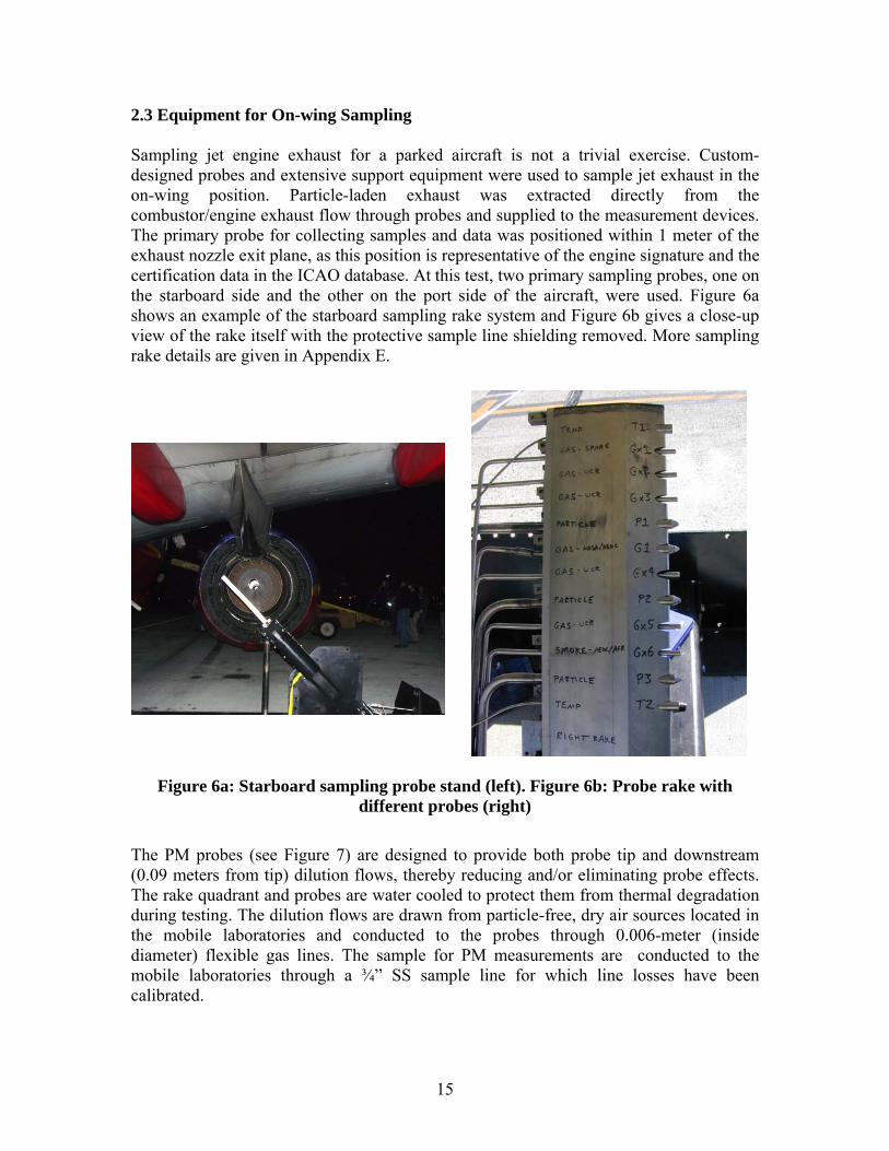
The orientation of the aircraft, sampling probes and mobile laboratories within the GRE are shown in Figure 5.

50 Meter probe

Figure 5: Layout within the GRE

14

2.3 Equipment for On-wing Sampling

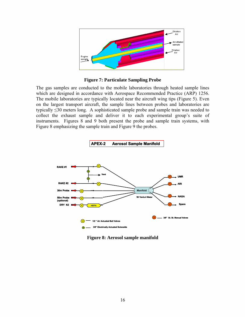
Sampling jet engine exhaust for a parked aircraft is not a trivial exercise. Custom-designed probes and extensive support equipment were used to sample jet exhaust in the on-wing position. Particle-laden exhaust was extracted directly from the combustor/engine exhaust flow through probes and supplied to the measurement devices. The primary probe for collecting samples and data was positioned within 1 meter of the exhaust nozzle exit plane, as this position is representative of the engine signature and the certification data in the ICAO database. At this test, two primary sampling probes, one on the starboard side and the other on the port side of the aircraft, were used. Figure 6a shows an example of the starboard sampling rake system and Figure 6b gives a close-up view of the rake itself with the protective sample line shielding removed. More sampling rake details are given in Appendix E.

Figure 6a: Starboard sampling probe stand (left). Figure 6b: Probe rake with different probes (right)

The PM probes (see Figure 7) are designed to provide both probe tip and downstream (0.09 meters from tip) dilution flows, thereby reducing and/or eliminating probe effects. The rake quadrant and probes are water cooled to protect them from thermal degradation during testing. The dilution flows are drawn from particle-free, dry air sources located in the mobile laboratories and conducted to the probes through 0.006-meter (inside diameter) flexible gas lines. The sample for PM measurements are conducted to the mobile laboratories through a ¾” SS sample line for which line losses have been calibrated.

15

... ---Di lution ...-- Air

Engine

~

®-

HEPA

Manifold

APEX-2 Aerosol Sample Manifold

3/8” St. St. Manual Valves1/2 “ Air Actuated Ball Valves

3/8” Electrically Actuated Solenoids

Figure 7: Particulate Sampling Probe The gas samples are conducted to the mobile laboratories through heated sample lines which are designed in accordance with Aerospace Recommended Practice (ARP) 1256. The mobile laboratories are typically located near the aircraft wing tips (Figure 5). Even on the largest transport aircraft, the sample lines between probes and laboratories are typically ≤30 meters long. A sophisticated sample probe and sample train was needed to collect the exhaust sample and deliver it to each experimental group’s suite of instruments. Figures 8 and 9 both present the probe and sample train systems, with Figure 8 emphasizing the sample train and Figure 9 the probes.

APEX-2 Aerosol Sample Manifold

UMR

ARI

NASA

Spare

W/ Venturi Meter

Vent

RAKE #1

RAKE #2

30m Probe

50m Probe(optional)

DRY N2

UMR

ARI

NASA

SpareHEPA

Manifold

W/ Venturi Meter

Vent

RAKE #1

RAKE #2

30m Probe

50m Probe (optional)

DRY N2

3/8” St. St. Manual Valves 1/2 “ Air Actuated Ball Valves

3/8” Electrically Actuated Solenoids

Figure 8: Aerosol sample manifold

16

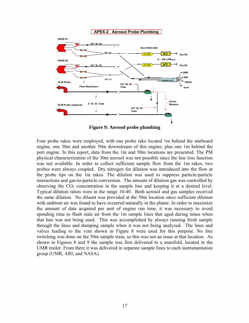
APEX-2 Aerosol Probe Plumbing RAKE #1

RAKE #2

30 M Probe

50 M Probe (optional) Hi-Vol Blowers

MANIFOLD

2” St. St. Tube

3/4” St. St. Tube

3/4” St. St. Tube

MFC

MFC

Dry N2

Dry N2

0 – 100 LPM (ea)

FILTER

FILTER

YY

Y

“Y”

“Y” 3/4” St. St.

3/4” St. St.

Flow Restrictors

3/8” Cu

3/8” Cu

DILUTION GAS

UMR

ARI

NASA

Spare

Figure 9: Aerosol probe plumbing

Four probe rakes were employed, with one probe rake located 1m behind the starboard engine, one 30m and another 50m downstream of this engine, plus one 1m behind the port engine. In this report, data from the 1m and 50m locations are presented. The PM physical characterization of the 30m aerosol was not possible since the line loss function was not available. In order to collect sufficient sample flow from the 1m rakes, two probes were always coupled. Dry nitrogen for dilution was introduced into the flow at the probe tips on the 1m rakes. The dilution was used to suppress particle-particle interactions and gas-to-particle conversion. The amount of dilution gas was controlled by observing the CO2 concentration in the sample line and keeping it at a desired level. Typical dilution ratios were in the range 10-40. Both aerosol and gas samples received the same dilution. No diluent was provided at the 50m location since sufficient dilution with ambient air was found to have occurred naturally in the plume. In order to maximize the amount of data acquired per unit of engine run time, it was necessary to avoid spending time to flush stale air from the 1m sample lines that aged during times when that line was not being used. This was accomplished by always running fresh sample through the lines and dumping sample when it was not being analyzed. The lines and valves leading to the vent shown in Figure 8 were used for this purpose. No line switching was done on the 50m sample train, so this was not an issue at that location. As shown in Figures 8 and 9 the sample was first delivered to a manifold, located in the UMR trailer. From there it was delivered in separate sample lines to each instrumentation group (UMR, ARI, and NASA).

17

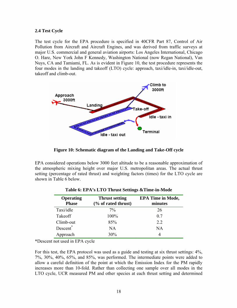
Id le - taxii o,ut

.I Termiinal

2.4 Test Cycle

The test cycle for the EPA procedure is specified in 40CFR Part 87, Control of Air Pollution from Aircraft and Aircraft Engines, and was derived from traffic surveys at major U.S. commercial and general aviation airports: Los Angeles International, Chicago O. Hare, New York John F Kennedy, Washington National (now Regan National), Van Nuys, CA and Tamiami, FL. As is evident in Figure 10, the test procedure represents the four modes in the landing and takeoff (LTO) cycle: approach, taxi/idle-in, taxi/idle-out, takeoff and climb-out.

Figure 10: Schematic diagram of the Landing and Take-Off cycle

EPA considered operations below 3000 feet altitude to be a reasonable approximation of the atmospheric mixing height over major U.S. metropolitan areas. The actual thrust setting (percentage of rated thrust) and weighting factors (times) for the LTO cycle are shown in Table 6 below.

Table 6: EPA’s LTO Thrust Settings &Time-in-Mode

Operating Phase

Taxi/idle Takeoff

Thrust setting (% of rated thrust)

7% 100%

EPA Time in Mode, minutes

26 0.7

Climb-out 85% 2.2 Descent* NA NA Approach 30% 4

*Descent not used in EPA cycle

For this test, the EPA protocol was used as a guide and testing at six thrust settings: 4%, 7%, 30%, 40%, 65%, and 85%, was performed. The intermediate points were added to allow a careful definition of the point at which the Emission Index for the PM rapidly increases more than 10-fold. Rather than collecting one sample over all modes in the LTO cycle, UCR measured PM and other species at each thrust setting and determined

18

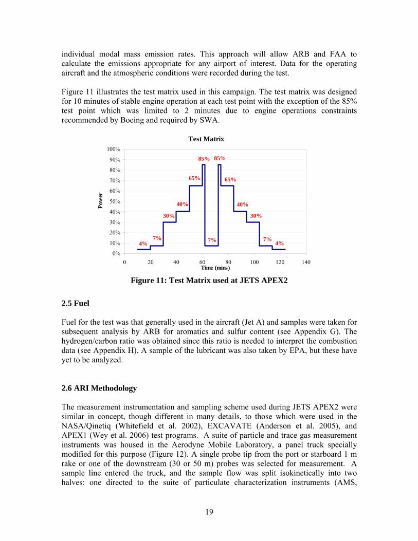
individual modal mass emission rates. This approach will allow ARB and FAA to calculate the emissions appropriate for any airport of interest. Data for the operating aircraft and the atmospheric conditions were recorded during the test.

Figure 11 illustrates the test matrix used in this campaign. The test matrix was designed for 10 minutes of stable engine operation at each test point with the exception of the 85% test point which was limited to 2 minutes due to engine operations constraints recommended by Boeing and required by SWA.

Test Matrix

Pow

er

100%

90%

80%

70%

60%

50%

40%

30%

20%

10%

0%

30%

40%

65%

85% 85%

65%

40%

30%

4% 7% 7%

4%7%

0 20 40 60 80 100 120 140 Time (mins)

Figure 11: Test Matrix used at JETS APEX2

2.5 Fuel

Fuel for the test was that generally used in the aircraft (Jet A) and samples were taken for subsequent analysis by ARB for aromatics and sulfur content (see Appendix G). The hydrogen/carbon ratio was obtained since this ratio is needed to interpret the combustion data (see Appendix H). A sample of the lubricant was also taken by EPA, but these have yet to be analyzed.

2.6 ARI Methodology

The measurement instrumentation and sampling scheme used during JETS APEX2 were similar in concept, though different in many details, to those which were used in the NASA/Qinetiq (Whitefield et al. 2002), EXCAVATE (Anderson et al. 2005), and APEX1 (Wey et al. 2006) test programs. A suite of particle and trace gas measurement instruments was housed in the Aerodyne Mobile Laboratory, a panel truck specially modified for this purpose (Figure 12). A single probe tip from the port or starboard 1 m rake or one of the downstream (30 or 50 m) probes was selected for measurement. A sample line entered the truck, and the sample flow was split isokinetically into two halves: one directed to the suite of particulate characterization instruments (AMS,

19

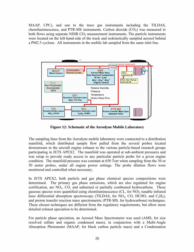
Cyclone isokinetic sample splits "

I ~ I < 2.SlJm I Ur MAAP Condensation AMS

L__

I Black Carbon 11 Particle/",-., nt<>r Aerosol Mass Spec 1co2 ,I Size Resolved Composition Licor N.O. IR

30 nm-2 µm I NO3·, SO4=, NH4 + f;02 High Range I

Roof Organic Carbon corN.O. IR

Sun Photometer Anemometer Relative Humidity

GPS Pressure

QCL Temperature Quantum Cascade Laser Venturi Mass Flow

NzO, COCO2 r, I ■

TDL - QCL PTR-MS [D Tunable Diode Lasen1 Quantum Cascade Laser Proton-Transfer Mass Spec NO2, HCHO C2H4, HONO Selected voes

~

MAAP, CPC), and one to the trace gas instruments including the TILDAS, chemiluminescence, and PTR-MS instruments. Carbon dioxide (CO2) was measured in both flows using separate NDIR CO2 measurement instruments. The particle instruments were located on the left-hand-side of the truck and isokinetically sampled aerosol behind a PM2.5 cyclone. All instruments in the mobile lab sampled from the same inlet line.

Figure 12: Schematic of the Aerodyne Mobile Laboratory

The sampling lines from the Aerodyne mobile laboratory were connected to a distribution manifold, which distributed sample flow pulled from the several probes located downstream in the aircraft engine exhaust to the various particle-based research groups participating in JETS APEX2. The manifold was operated at sub-ambient pressures and was setup to provide ready access to any particular particle probe for a given engine condition. The manifold pressure was constant at 650 Torr when sampling from the 30 or 50 meter probes, under all engine power settings. The probe dilution flows were monitored and controlled when necessary.

In JETS APEX2, both particle and gas phase chemical species compositions were determined. The primary gas phase emissions, which are also regulated for engine certification, are NOx, CO, and unburned or partially combusted hydrocarbons. These gaseous species were quantified using chemiluminescence (CL, for NO), tunable infrared laser differential absorption spectroscopy (TILDAS, for NO2, CO, HCHO, and C2H4), and proton transfer reaction mass spectrometric (PTR-MS, for hydrocarbons) techniques. These chosen techniques are different from the regulatory requirements, but allow more detailed exhaust speciation to be determined.

For particle phase speciation, an Aerosol Mass Spectrometer was used (AMS, for size resolved sulfate and organic condensed mass), in conjunction with a Multi-Angle Absorption Photometer (MAAP, for black carbon particle mass) and a Condensation

20

Particle Counter (CPC, for particle number count). These measurements provided the concentration and size resolved composition of particles ranging from about 30 nm to 1000 nm vacuum aerodynamic diameter.

2.6.1 Gas Phase Instrumentation

2.6.1.1 Tunable Infrared Laser Differential Absorption spectrometers (TILDAS) Two different types of lasers were used in the TILDAS instruments: tunable lead-salt diode lasers, which operate in a continuous mode and at near liquid nitrogen temperatures, and quantum cascade lasers, which operate in a pulsed mode and at temperatures allowing thermoelectric cooling rather than cryogenic cooling (Nelson et al. 2004). Quantum Cascade -TILDAS systems were used to measure NO2 in the spectral region of 1606 cm-1, C2H4 in the spectral region of 968 cm-1, CO in the spectral region of 2183 cm-1, and acrolein in the spectral region of 959 cm-1. A lead-salt TILDAS system was used to measure HCHO in the spectral region of 1725 cm-1.

2.6.1.2 Chemiluminescent NO sensor A Thermo-Electron model 42c chemiluminescent detector was used for the NO measurements. The detection method is based on the detection of chemiluminescence stemming from electronically excited NO2 molecules produced by the reaction of NO with a small flow of ozone added to the sample flow (Heard, 2006).

2.6.1.3 Proton transfer reaction - mass spectrometer (PTR-MS) Hydrocarbons were measured using a PTR-MS operated by Berk Knighton, Montana State University. The PTR-MS (Ionicon Analytic GMBH) is a chemical ionization based mass spectrometry method that utilizes H3O+ as a reagent ion. This instrument has been described elsewhere (de Gouw et al. 2003), so that only a brief description of the relevant details is provided here. The instrument consists of an ion source, a drift tube reaction region and a quadrupole mass spectrometer. H3O+ reagent ions formed in the hollow cathode discharge ion source are electrostatically injected into the drift tube through which the sampled air stream is continuously passed at reduced pressure, 1.9 mbar. These H3O+ reagent ions are pulled through the air sample by an electric field where they can react via proton transfer reactions with those components in the sample having proton affinities greater than that of water. The reagent ions and the resulting proton transfer reaction products are mass selected and detected using the mass spectrometer.

The PTR-MS sampled the exhaust stream from the main sample inlet through a short length of 1/8” O.D. Teflon tubing. A fraction of the sampled exhaust enters the drift tube reaction region where those components of the sample having proton affinities greater than that of water undergo proton transfer reactions with H3O+ reagent ions. The mass spectrometer monitored a selected set of 32 ions at 0.2 seconds per mass, along with the drift tube pressure and temperature, which yielded a cycle measurement time of approximately 8 seconds. The ions monitored included the reagent ions H3O+ (m/z 21 O-

21

--------------------------------------

18 isotope) and H3O+(H2O) (m/z 39 O-18 isotope), the diagnostic ions NO+ (m/z 31) and O2

+ (m/z 32) and the sample ions as presented below.

The sampled exhaust flow stream was periodically diverted through a heated Pt catalyst (400oC) to provide a VOC free gas stream for determining the instrumental background. In many cases the Pt catalyst did not efficiently remove the VOCs from the exhaust sample stream, and this reduced efficiency has been attributed to poisoning of the catalyst due to the sulfur content of the fuel. Under circumstances where the catalyst appeared to be compromised, instrumental background measurements were determined when the main inlet was purged with N2 blow off from a liquid N2 dewar. The instrumental background is non-zero for most masses and the reported concentrations reflect the difference between the sample and background signals. The concentration of a HC emission component (R) can be deduced from the measured ion signals using relationships derived either from simple reaction kinetics or from calibrated response factors (Knighton et al., 2007). For compounds where calibration gas standards were not available, the concentrations were calculated by assuming that simple reaction kinetics were applicable (Knighton et al., 2007).

Trace gas levels are reported as emission indices, expressed in units of grams of trace gas emitted per kg of fuel consumed. The fuel consumption and CO2 emission are proportional, so trace gas emission indices can be derived from the trace gas concentration and CO2 concentration observed in the exhaust sample. The CO2 concentration used must have the contribution due to ambient CO2 subtracted out, and if the sample has been diluted, that dilution factor must be known before the subtraction of the ambient CO2 can be carried out. The formula used to convert trace gas concentrations in parts per million by volume (ppmv) is

____3160 MWt (trace gas concentration, ppm) ________ (Eq. 1) EI (trace gas) = 44.01((CO2 concentration, ppmv) – (ambient CO2, ppmv)/dilution)

where 3160 is the CO2 emission index, g CO2 per kg of fuel, MW is the molecular weight (g/mole) of the trace gas, and 44.01 is the molecular weight of CO2. For the emission index of nitrogen oxides, NO and NO2, MW is taken to be 46.01, that is, the NO emission indices are reported as equivalent g NO2 per kg of fuel. In cases where the sample was not diluted we subtracted an ambient CO2 concentration of 380 ppmv, while for samples that were diluted by a factor of 2 we subtracted 190 ppmv, and so on. For the 30 m and 50 m sampling data, where fluctuations in observed concentrations were large, a different procedure was used, in which a regression of trace gas concentration against CO2 concentration was used to simultaneously derive the emission index (from the slope) and the term “(ambient CO2, ppmv)/dilution” (from the intercept). For time histories in which the relative variance of the trace gas concentration is large this is the preferred method, while when the relative variance is small it is preferable to average the records of trace gas and CO2 concentrations over the time for a given engine condition and use the averages in the above formula.

22

2.6.2 Particle measurements

The particle measurements were conducted using the Aerodyne Aerosol Mass Spectrometer (AMS) to characterize the volatile chemical compositions and chemically-speciated size distributions, a Condensation Particle Counter to measure the total particle concentration, and a modified Multiangle Aerosol Photometer (MAAP; Thermo Electron) to measure the aerosol absorption and derive black carbon mass concentrations. The particle instruments were operated downstream of a PM2.5 (UGI) cyclone to remove large particles.

2.6.2.1 Aerosol Mass Spectrometer The Aerodyne Aerosol Mass Spectrometer (AMS) has been described in detail in the literature (Jayne et al. 2000). The AMS sampled aerosols into a high vacuum and focused the particles into a tight beam using an aerodynamic lens. The focused particle beam exiting the lens was directed through a particle-sizing chamber and impacted on a 3.8 mm circular vaporizer held at 600oC. By mechanically modulating the particle beam with a chopper and using the time-of-flight (TOF) of particles between the chopper and the detector, the particle velocity and the vacuum aerodynamic diameter were obtained. The particle detection scheme consisted of a vaporizer that was coupled into the ionizing cage of a time-of flight mass spectrometer (MS). When the particles struck the vaporizer surface, the nonrefractory (volatile and semi-volatile) components of particles flash vaporized. The vaporization plume was ionized using standard 70 eV electron impact ionization techniques and extracted into the mass spectrometer, spanning a range of 1-300 atomic mass units. The AMS was operated during this study with a time-resolution of 30 seconds, alternating every 15 seconds between a TOF mode (particle mass distributions as a function of size) and a MS mode (particle chemical speciation and quantitative mass loadings) (Jimenez et al. 2003).

Quantitative mass calibration of the instrument was performed by using a pure ammonium nitrate aerosol source. Particles were generated with an atomizer (TSI, model 3076, USA), dried using silica gel, size-selected using a differential mobility analyzer (TSI, model DMA 3071) and sampled simultaneously by the AMS and a CPC (TSI, model 3022a). Multiply charged particles were eliminated using an impactor upstream of the DMA and the AMS isokinetically sampled from the CPC aerosol flow to ensure identical size distributions. The well-characterized aerosol sample calibrated the electron multiplier signals at m/z 30 and 46 for nitrate (NO3

+) and 15, 16, and 17 for ammonium (NH4

+). The AMS analysis uses relative ionization efficiencies measured in previous laboratory studies to calibrate for the chemical species present in aircraft exhaust (sulfates and organics). During this experiment, the AMS had a nitrate ionization efficiency of 6.9x10-6 ions/molecule and detection limits (three times the standard deviation) of 0.024 and 0.26 μg/m3, respectively for sulfates and organics.

2.6.2.2 Multi-Angle Aerosol Photometer Aerosol black carbon concentrations were derived with a Thermo Electron Multi-Angle Aerosol Photometer (MAAP). A detailed description is provided in the literature

23

(Petzold et al. 2002; Petzold and Schonlinner 2004). The MAAP is a filter-based photometer that deposits aerosol onto a 2 cm2 spot on a quartz fiber filter tape. A 630 nm wavelength LED shines on the spot and multiple photodetectors measure the transmission and scattering/reflection of the light from the depositing aerosol layer and the underlying filter. A two stream radiation transfer calculation is used to separate the absorption of the light by the aerosol layer from the scattering of light by the particles and filter matrix (Petzold and Schonlinner 2004). A narrow range of values of σabs (~6.4-6.6 m2 g-1) is reported to provide a decent fit for commercially-produced black carbon particles and urban particles containing black carbon collected at several sites (Petzold and Schonlinner 2004). A value of σabs = 6.6 m2 g-1 is currently used to calculate the instantaneous black carbon mass loading on the filter at a rate of 1 Hz. The MAAP was operated with a flow rate of 8 lpm using custom plumbing. The precision of the MAAP for deriving black carbon mass loadings under these operating conditions is ± 2.4 μg/m3.

2.6.2.3 Particle Counting Instrument The total aerosol concentration was measured with several Condensation Particle Counters (CPC; TSI model 3022a and 7061). The CPC supersaturates a sample flow with butanol vapor, causing submicron particles to grow in size into the supermicron size range where the particles are detected via individual light scattering pulses at low concentrations and via ensemble particle scattering at high concentrations. The 3022a CPC has a 50% cut size of 7 nm at atmospheric pressure, a response time of < 10 seconds for 90% step change, and can sample particle concentrations up to 107 cm-3.

2.6.3 Emission Indices

LiCor infrared absorption instruments were used to measure the gas phase CO2 concentration in the sampled plume. The gas phase CO2 concentration was used to relate the measured particulate mass loading to fuel-based particulate mass emission indices (EI’s), with units of milligrams of PM per kilogram of fuel burned (mg per kg fuel). Following the methodology described in Herndon et al. (Herndon et al. 2005), for a given exhaust component concentration, X, the EI(X) is calculated by

EI(x) = (ΔX/ΔCO2) × EI(CO2) × Mair /MCO2 × (1/ρair ) (Eq. 2)

where ΔX/ΔCO2 is the emission ratio for the exhaust component, Mair is the molar mass of air, MCO2 is the molar mass of CO2, and ρair is the density of air at ambient conditions. This expression is based on 100% conversion of the carbon in the fuel to CO2. Corrections for incomplete combustion can be made, based on measurements of CO and hydrocarbon emissions, but these corrections are within experimental uncertainties for the measurements reported here. EI (CO2) equals 3160 g CO2 (kg fuel)-1 for most available Jet A fuel, within a few percent. This value can be replaced with that appropriate for a given fuel where the mass fraction of hydrogen in the fuel is known (or equivalently if the C/H ratio is known). EI’s are also calculated for particle number concentrations (number per kg fuel) using a slightly modified version of this formula.

24

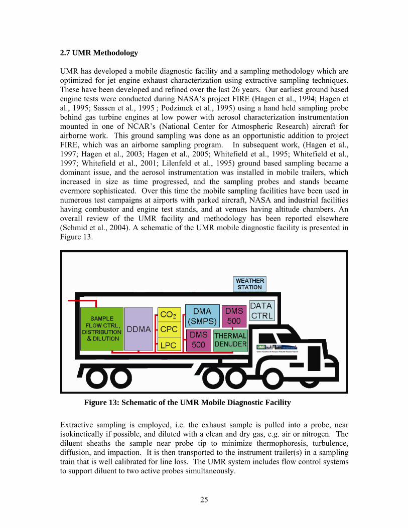
FLOWCTRL DISTRIBUTION

&DILUTION

CO2

DDMA CPC

LPC

WEATHER STATION

2.7 UMR Methodology

UMR has developed a mobile diagnostic facility and a sampling methodology which are optimized for jet engine exhaust characterization using extractive sampling techniques. These have been developed and refined over the last 26 years. Our earliest ground based engine tests were conducted during NASA’s project FIRE (Hagen et al., 1994; Hagen et al., 1995; Sassen et al., 1995 ; Podzimek et al., 1995) using a hand held sampling probe behind gas turbine engines at low power with aerosol characterization instrumentation mounted in one of NCAR’s (National Center for Atmospheric Research) aircraft for airborne work. This ground sampling was done as an opportunistic addition to project FIRE, which was an airborne sampling program. In subsequent work, (Hagen et al., 1997; Hagen et al., 2003; Hagen et al., 2005; Whitefield et al., 1995; Whitefield et al., 1997; Whitefield et al., 2001; Lilenfeld et al., 1995) ground based sampling became a dominant issue, and the aerosol instrumentation was installed in mobile trailers, which increased in size as time progressed, and the sampling probes and stands became evermore sophisticated. Over this time the mobile sampling facilities have been used in numerous test campaigns at airports with parked aircraft, NASA and industrial facilities having combustor and engine test stands, and at venues having altitude chambers. An overall review of the UMR facility and methodology has been reported elsewhere (Schmid et al., 2004). A schematic of the UMR mobile diagnostic facility is presented in Figure 13.

Figure 13: Schematic of the UMR Mobile Diagnostic Facility

Extractive sampling is employed, i.e. the exhaust sample is pulled into a probe, near isokinetically if possible, and diluted with a clean and dry gas, e.g. air or nitrogen. The diluent sheaths the sample near probe tip to minimize thermophoresis, turbulence, diffusion, and impaction. It is then transported to the instrument trailer(s) in a sampling train that is well calibrated for line loss. The UMR system includes flow control systems to support diluent to two active probes simultaneously.

25

The instrumentation suite in the UMR trailer is flexible and varies from test to test. The following instrumentation is usually included in most test campaigns. A pressure reduction system consisting of a selection of calibrated orifices is available to reduce the sample line pressure to near ambient where most of instrumentation needs to work. This is designed to handle only the small ram pressures associated with sampling at high power conditions, not those expected from sampling directly from combustors. Normally the sample line flow is allowed to increase so that the pressure can be dropped across the probe tip orifice. In cases where this is not practical, our pressure reduction system can be employed.

Condensation Particle Counters (CPC) (TSI 3022 and 3025) are used to measure total particle concentration. Particle size distributions are measured with Differential Mobility Spectrometers (DMS) (Cambustion DMS500) and Differential Mobility Analyzers (DMA) (TSI 3071). The DMA uses a single channel which is swept through different sizes over time, and the newer multi-channel electrometer-based instrument, DMS500, measures a full set of sizes simultaneously. We employ two of the new and fast instruments which run in parallel, one being downstream of a thermal denuder. This allows both the total and non-volatile components of the aerosol to be measured simultaneously. This combination of information can be used to characterize the aerosol’s volatility, assess the sampling train for anomalous particle generation and to characterize plume processing of the emission aerosol size distribution. The new fast response instruments allow for much shorter engine run times in order to complete the measurements, and the characterization of transients in the emissions, e.g. those during throttle changes. The older, slower sizing instrument is normally run in parallel with the faster ones in order to accomplish a quality check on the data, and to allow measurements to be made in the case of very clean engines where the signal (particle concentration) is insufficient for the newer instruments. These fast mobility instruments also yield total particle concentration measurements which complements those from the CPC. The DMS500 instruments cover a broad size range, from 5 nm up to 1 μm. A laser particle counter (LPC) is used for size distribution measurements in the large size regime, diameter > 0.5 μm. Hence there is a region of overlap between the DMS500 and LPC. Typically gas turbine engines produce little emissions in the LPC’s size range.

The exhaust aerosol’s hydration behavior is characterized using the deliquescence technique with a Deliquescence DMA (DDMA). The aerosol is subjected to a high relative humidity, below but near 100%, and its size distribution is re-measured using the DMA technique. Their change in size due to humidity change can be used to determine their critical supersaturation and their soluble mass fraction, i.e. their response to water vapor. This is an important parameter which strongly influences their behavior in the atmosphere. Normally if their soluble mass fraction is zero at engine exit, it is too hot for soluble material to form. However at only 30 to 50m of plume processing, soluble material can be detected. An electrostatic precipitator is used to collect aerosol samples on an electron microscope grid for subsequent off-line single particle analysis. This can be used for morphological information using TEM (Transmission Electronic Microscopy). CO2 concentration is measured in an undiluted sample line and also in the

26

diluted sample line, which is used for particle characterization. CO2 is chemically inert and its emission index for jet fuel is well known. The CO2 measurement allows an accurate measure of the dilution of the sample, which is necessary for corrections of the data to probe tip concentration values, and can be used to evaluate emission index values for the particle data. A weather station is used to get ambient wind, temperature, and pressure data near the test site. These parameters can influence engine performance and the probability that the exhaust plume reaches downstream sampling probes.

Two other features of the UMR mobile laboratory greatly facilitate successfully accomplishing emissions testing at the diverse range of available venues. A diesel powered electrical generator (60 kW) is available to provide electricity for instruments, lights, air conditioning, etc. In many situations ground supplied electric power is not available, or would be prohibitively expensive. An elaborate communications system is available to handle voice communications between instrument operators within our trailer, test directors in our trailer or external, and colleagues in other instrumented trailers and vans from other institutions. Data acquisition and running the test engine must be coordinated, and this is actually a complicated problem requiring a sophisticated communications system. The trailers and instrumentation need to be relatively close to the engine under test, and engines are very noisy. The communications system must handle both voice communications and noise suppression. Hardware was acquired and software developed to allow digital communications between the large number of computers involved the test campaign. This includes UMR computers and those of colleagues and test managers collaborating in a test campaign. In many cases a few real-time plots can communicate more than many minutes of voice information.

2.7.1 DMS500

The DMS500 instrument is a new device which depends on electrical mobility for particle sizing (Biskos et al. 2005), and has been used primarily for investigation of fast changing spectra such as diesel engine emissions, drug delivery systems such as inhalers, and roadside ambient aerosol sampling. In this instrument the aerosol sample is passed through a cyclone separator to remove particles larger than 1 μm. It is then given a known charge distribution using a corona charger. The aerosol is then charged, inserted into a clean laminar flow air stream, and subjected to an electric field which deflects (in a size dependent manner) the particles’ trajectories toward electrometer rings. The currents resulting from the charge transported to the electrometer rings by the particles are measured and the current-electrometer data matrix is converted into particle number and size classification. Since the various electrometer currents are measured simultaneously rather than sequentially, the measurement is fast, up to 10 Hz.

27

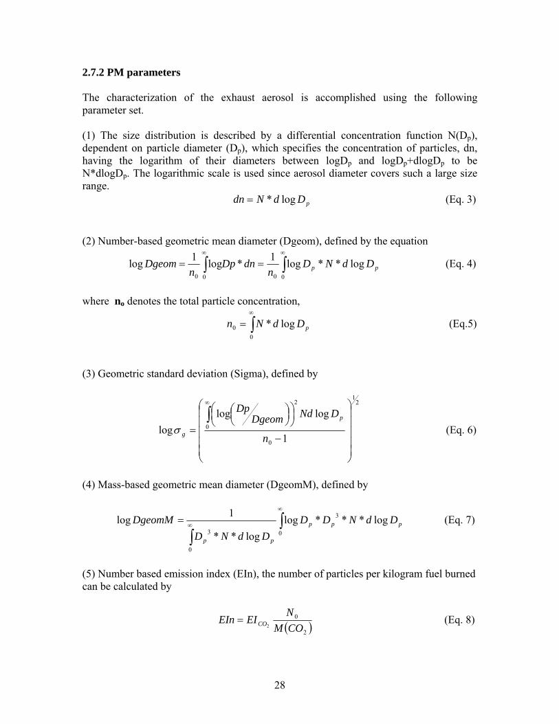
I I

2.7.2 PM parameters

The characterization of the exhaust aerosol is accomplished using the following parameter set.

(1) The size distribution is described by a differential concentration function N(Dp), dependent on particle diameter (Dp), which specifies the concentration of particles, dn, having the logarithm of their diameters between logDp and logDp+dlogDp to be N*dlogDp. The logarithmic scale is used since aerosol diameter covers such a large size range.

dn = N * d log Dp (Eq. 3)

(2) Number-based geometric mean diameter (Dgeom), defined by the equation ∞ ∞1 1logDp * dn

n0 0 0

where no denotes the total particle concentration,

∫ 0 ∫Dgeom D N d Dlog log * * log p (Eq. 4)= = pn

n0

∞

∫= N * d log Dp (Eq.5) 0

(3) Geometric standard deviation (Sigma), defined by

2 1

2 ⎞⎟⎠

⎛⎜⎝

∞

∫ pDgeom0

(4) Mass-based geometric mean diameter (DgeomM), defined by

⎛ ⎞⎟⎟ ⎟ ⎟⎟

Dp⎛⎜⎝

⎞⎟⎠

Nd Dlog log σlog (Eq. 6)

⎜⎜ ⎜ ⎜⎜⎝

= g n0 −1

⎠

1 ∞

∫ 3 *log DgeomM ∞

∫ = D D N d Dlog * * log (Eq. 7)p p p

Dp 3 * N * d log Dp

0

(

0

(5) Number based emission index (EIn), the number of particles per kilogram fuel burned can be calculated by

N M CO

0EIn EI (Eq. 8) 2 )

= CO2

28

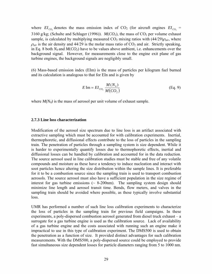
where EICO2 denotes the mass emission index of CO2 (for aircraft engines EICO2

= 3160 g/kg; (Schulte and Schlager (1996)). M(CO2), the mass of CO2 per volume exhaust sample, is calculated by multiplying measured CO2 mixing ratios with (44/29)ρair, where ρair is the air density and 44/29 is the molar mass ratio of CO2 and air. Strictly speaking, in Eq. 8 both N0 and M(CO2) have to be values above ambient, i.e. enhancements over the background signal. However, for measurements close to the engine exit plane of gas turbine engines, the background signals are negligibly small.

(6) Mass-based emission index (EIm) is the mass of particles per kilogram fuel burned and its calculation is analogous to that for EIn and is given by

M (N 0 )E Im = EICO (Eq. 9)

2 M (CO2 )

where M(N0) is the mass of aerosol per unit volume of exhaust sample.

2.7.3 Line loss characterization

Modification of the aerosol size spectrum due to line loss is an artifact associated with extractive sampling which must be accounted for with calibration experiments. Inertial, thermophoretic, and diffusional effects contribute to the loss of particles in the sampling train. The penetration of particles through a sampling system is size dependent. While it is harder to experimentally quantify losses due to thermophoretic effects, inertial and diffusional losses can be handled by calibration and accounted for in the data reduction. The source aerosol used in line calibration studies must be stable and free of any volatile compounds and moisture as these have a tendency to induce nucleation and interact with soot particles hence altering the size distribution within the sample lines. It is preferable for it to be a combustion source since the sampling train is used to transport combustion aerosols. The source aerosol must also have a sufficient population in the size regime of interest for gas turbine emissions (~ 8-200nm). The sampling system design should minimize line length and aerosol transit time. Bends, flow meters, and valves in the sampling train should be avoided where possible, as these typically involve substantial loss.

UMR has performed a number of such line loss calibration experiments to characterize the loss of particles in the sampling train for previous field campaigns. In these experiments, a poly-dispersed combustion aerosol generated from diesel truck exhaust – a surrogate for a gas turbine engine is used as the calibration source. Lack of availability of a gas turbine engine and the costs associated with running such an engine make it impractical to use in this type of calibration experiment. The DMS500 is used to obtain the penetration as a function of size. It provided distinct advantages for such calibration measurements. With the DMS500, a poly-dispersed source could be employed to provide fast simultaneous size dependent losses for particle diameters ranging from 5 to 1000 nm.

29

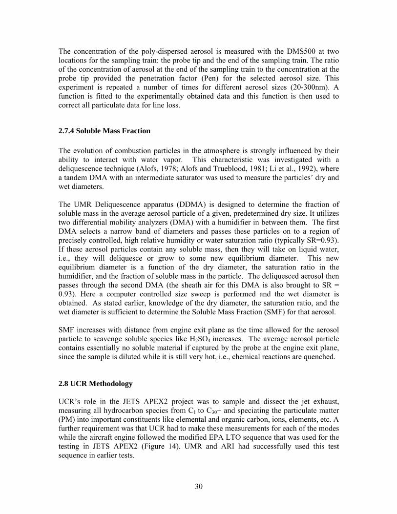
The concentration of the poly-dispersed aerosol is measured with the DMS500 at two locations for the sampling train: the probe tip and the end of the sampling train. The ratio of the concentration of aerosol at the end of the sampling train to the concentration at the probe tip provided the penetration factor (Pen) for the selected aerosol size. This experiment is repeated a number of times for different aerosol sizes (20-300nm). A function is fitted to the experimentally obtained data and this function is then used to correct all particulate data for line loss.

2.7.4 Soluble Mass Fraction

The evolution of combustion particles in the atmosphere is strongly influenced by their ability to interact with water vapor. This characteristic was investigated with a deliquescence technique (Alofs, 1978; Alofs and Trueblood, 1981; Li et al., 1992), where a tandem DMA with an intermediate saturator was used to measure the particles’ dry and wet diameters.

The UMR Deliquescence apparatus (DDMA) is designed to determine the fraction of soluble mass in the average aerosol particle of a given, predetermined dry size. It utilizes two differential mobility analyzers (DMA) with a humidifier in between them. The first DMA selects a narrow band of diameters and passes these particles on to a region of precisely controlled, high relative humidity or water saturation ratio (typically SR=0.93). If these aerosol particles contain any soluble mass, then they will take on liquid water, i.e., they will deliquesce or grow to some new equilibrium diameter. This new equilibrium diameter is a function of the dry diameter, the saturation ratio in the humidifier, and the fraction of soluble mass in the particle. The deliquesced aerosol then passes through the second DMA (the sheath air for this DMA is also brought to SR = 0.93). Here a computer controlled size sweep is performed and the wet diameter is obtained. As stated earlier, knowledge of the dry diameter, the saturation ratio, and the wet diameter is sufficient to determine the Soluble Mass Fraction (SMF) for that aerosol.

SMF increases with distance from engine exit plane as the time allowed for the aerosol particle to scavenge soluble species like H2SO4 increases. The average aerosol particle contains essentially no soluble material if captured by the probe at the engine exit plane, since the sample is diluted while it is still very hot, i.e., chemical reactions are quenched.

2.8 UCR Methodology

UCR’s role in the JETS APEX2 project was to sample and dissect the jet exhaust, measuring all hydrocarbon species from C1 to C30+ and speciating the particulate matter (PM) into important constituents like elemental and organic carbon, ions, elements, etc. A further requirement was that UCR had to make these measurements for each of the modes while the aircraft engine followed the modified EPA LTO sequence that was used for the testing in JETS APEX2 (Figure 14). UMR and ARI had successfully used this test sequence in earlier tests.

30

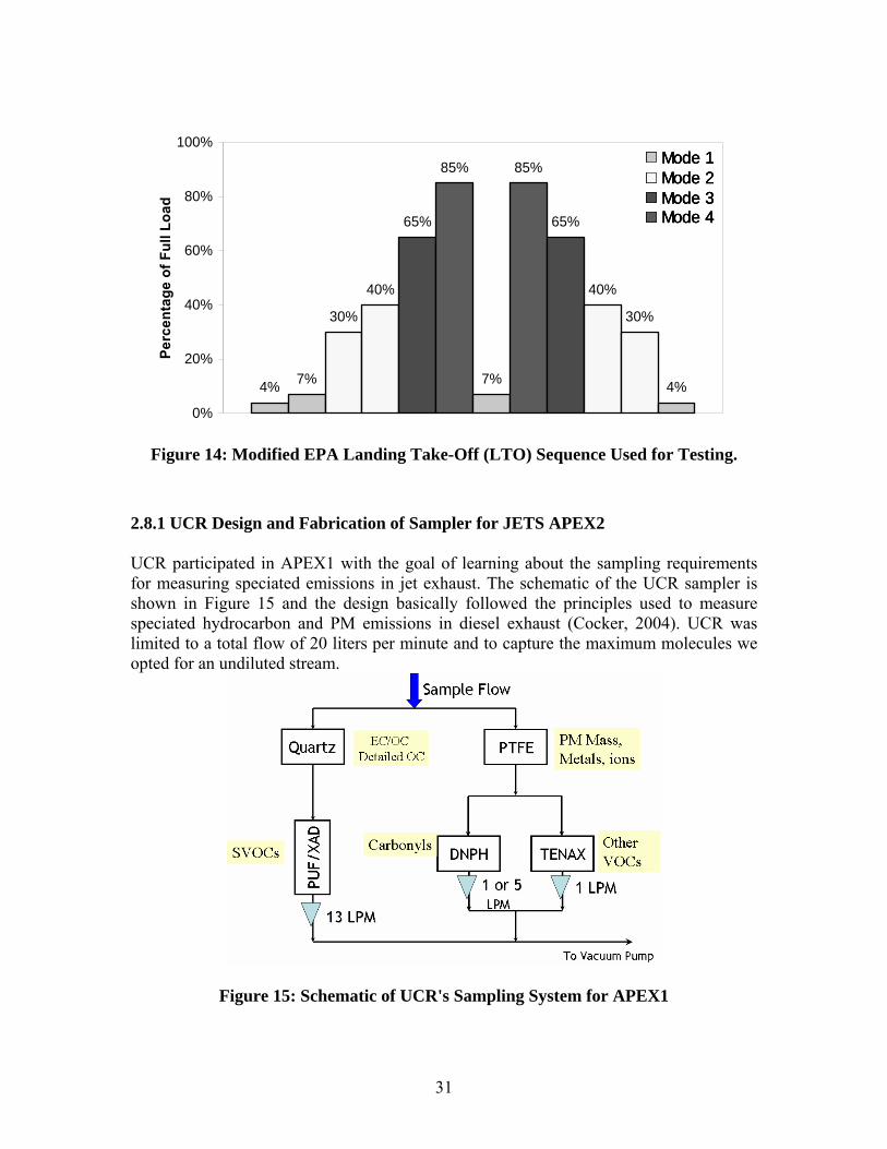
SVOCs

Quartz

0

~ -LL :::> a..

Sample Flow

EC/OC Detailed OC

Carbonyls

1 or 5 LPM

13 LPM

PM Mass, Metals, ions

Other voes

1 LPM

□ □ ■ ■

To Vacuum Pump

4% 7%

30%

40%

65%

85%

7%

85%

65%

40%

30%

4%

0%

20%

40%

60%

80%

100%Pe

rcen

tage

of F

ull L

oad

Mode 1Mode 2Mode 3Mode 4

4% 7%

30%

40%

65%

85%

7%

85%

65%

40%

30%

4%

0%

20%

40%

60%

80%

100% Pe

rcen

tage

of F

ull L

oad

Mode 1Mode 2Mode 3Mode 4

Mode 1Mode 1 Mode 2Mode 2 Mode 3Mode 3 Mode 4Mode 4

Figure 14: Modified EPA Landing Take-Off (LTO) Sequence Used for Testing.

2.8.1 UCR Design and Fabrication of Sampler for JETS APEX2

UCR participated in APEX1 with the goal of learning about the sampling requirements for measuring speciated emissions in jet exhaust. The schematic of the UCR sampler is shown in Figure 15 and the design basically followed the principles used to measure speciated hydrocarbon and PM emissions in diesel exhaust (Cocker, 2004). UCR was limited to a total flow of 20 liters per minute and to capture the maximum molecules we opted for an undiluted stream.

Figure 15: Schematic of UCR's Sampling System for APEX1

31

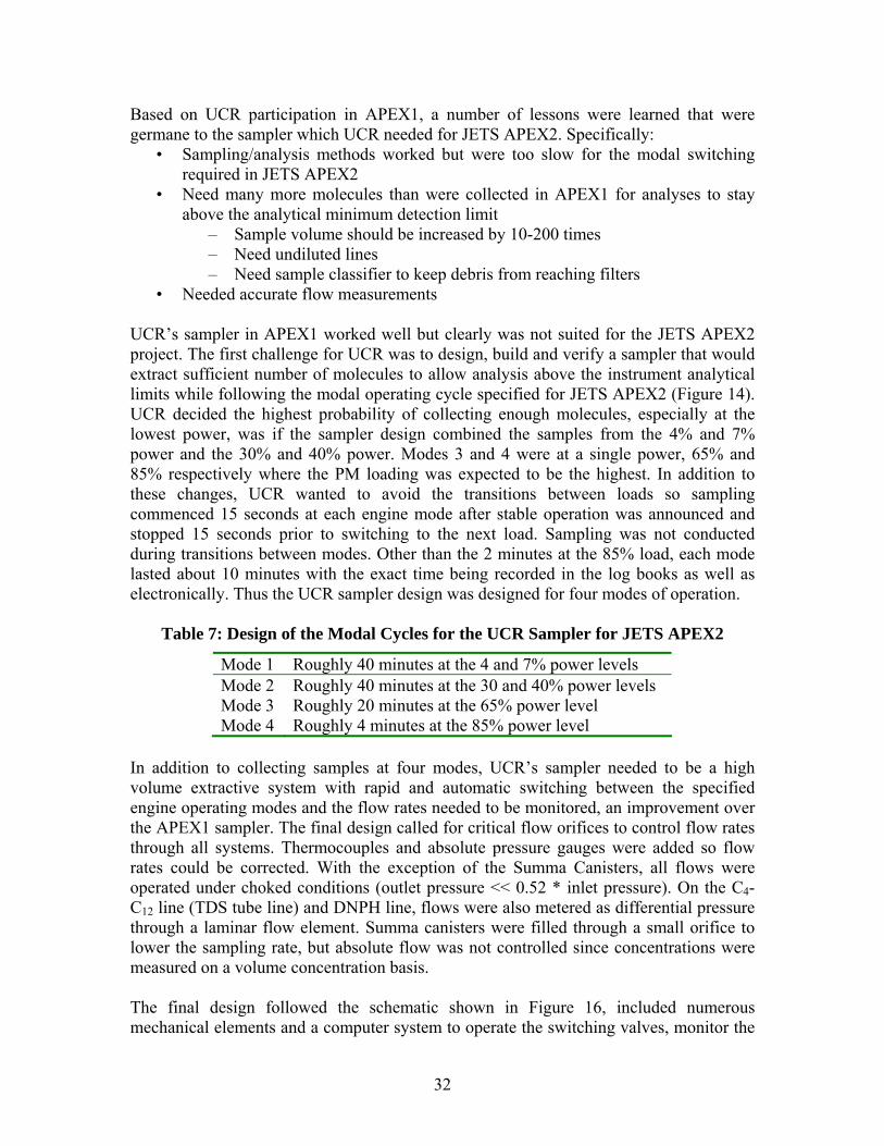
Based on UCR participation in APEX1, a number of lessons were learned that were germane to the sampler which UCR needed for JETS APEX2. Specifically:

• Sampling/analysis methods worked but were too slow for the modal switching required in JETS APEX2

• Need many more molecules than were collected in APEX1 for analyses to stay above the analytical minimum detection limit

– Sample volume should be increased by 10-200 times – Need undiluted lines – Need sample classifier to keep debris from reaching filters

• Needed accurate flow measurements

UCR’s sampler in APEX1 worked well but clearly was not suited for the JETS APEX2 project. The first challenge for UCR was to design, build and verify a sampler that would extract sufficient number of molecules to allow analysis above the instrument analytical limits while following the modal operating cycle specified for JETS APEX2 (Figure 14). UCR decided the highest probability of collecting enough molecules, especially at the lowest power, was if the sampler design combined the samples from the 4% and 7% power and the 30% and 40% power. Modes 3 and 4 were at a single power, 65% and 85% respectively where the PM loading was expected to be the highest. In addition to these changes, UCR wanted to avoid the transitions between loads so sampling commenced 15 seconds at each engine mode after stable operation was announced and stopped 15 seconds prior to switching to the next load. Sampling was not conducted during transitions between modes. Other than the 2 minutes at the 85% load, each mode lasted about 10 minutes with the exact time being recorded in the log books as well as electronically. Thus the UCR sampler design was designed for four modes of operation.

Table 7: Design of the Modal Cycles for the UCR Sampler for JETS APEX2

Mode 1 Roughly 40 minutes at the 4 and 7% power levels Mode 2 Roughly 40 minutes at the 30 and 40% power levels Mode 3 Roughly 20 minutes at the 65% power level Mode 4 Roughly 4 minutes at the 85% power level

In addition to collecting samples at four modes, UCR’s sampler needed to be a high volume extractive system with rapid and automatic switching between the specified engine operating modes and the flow rates needed to be monitored, an improvement over the APEX1 sampler. The final design called for critical flow orifices to control flow rates through all systems. Thermocouples and absolute pressure gauges were added so flow rates could be corrected. With the exception of the Summa Canisters, all flows were operated under choked conditions (outlet pressure << 0.52 * inlet pressure). On the C4-C12 line (TDS tube line) and DNPH line, flows were also metered as differential pressure through a laminar flow element. Summa canisters were filled through a small orifice to lower the sampling rate, but absolute flow was not controlled since concentrations were measured on a volume concentration basis.

The final design followed the schematic shown in Figure 16, included numerous mechanical elements and a computer system to operate the switching valves, monitor the

32

........... ·­. . . . .

··························-

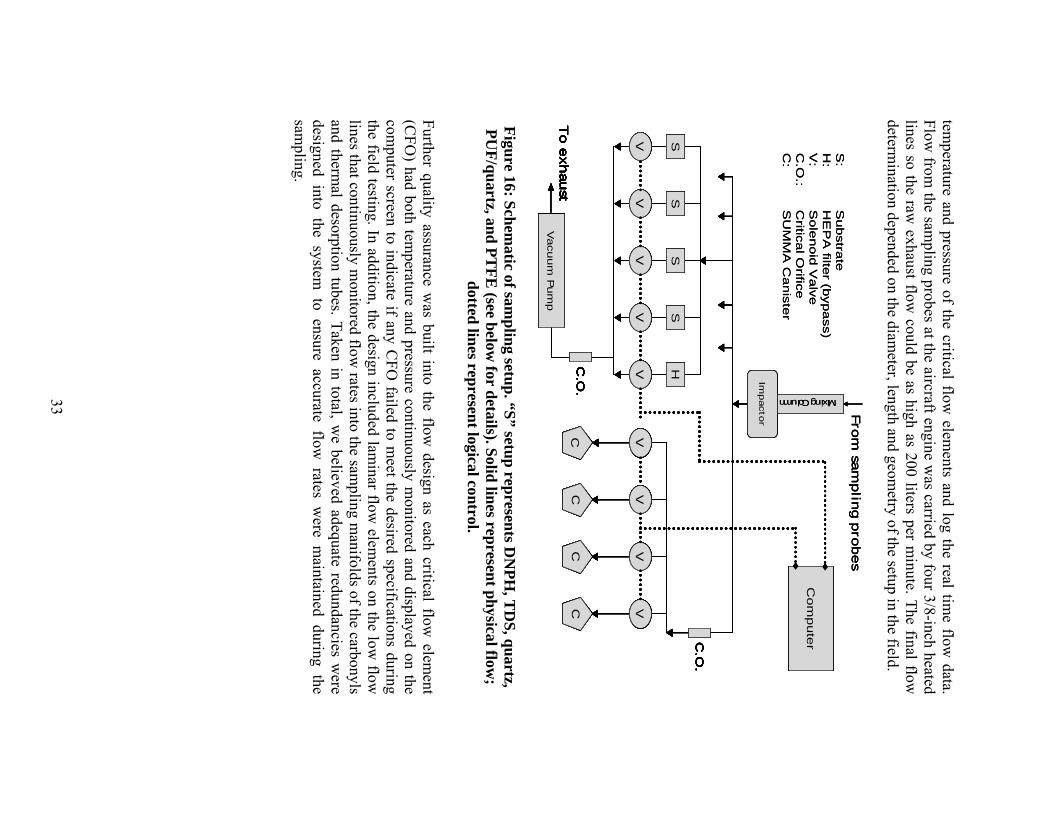
Mixing Column

Impacto

r

HS

VV

VV

V

SS

S

CC

C VV

VV

Vacuum

Pum

p

Co

mp

ute

r

Mixing Column

Impacto

r

HS

VV

VV

V

SS

S

CC

C VV

VV

Vacuum

Pum

p

Co

mp

ute

r

Mixing Column

Impacto

r

HS

VV

VV

V

SS

S

CC

C VV

VV

Vacuum

Pum

p

Co

mp

ute

r

Impacto

r

HS

VV

VV

V

SS

S

CC

C VV

VV

Vacuum

Pum

p

Co

mp

ute

r

HS

VV

VV

V

SS

S

CC

C VV

VV

Vacuum

Pum

p

Co

mp

ute

r

HS

VV

VV

V

SS

S

CC

C VV

VV

Vacuum

Pum

p

HS

VV

VV

V

SS

S

CC

C VV

VV

HS

VV

VV

V

SS

S

CC

C VV

VV

CC

C VV

VV

VV

VV

temperature and pressure of the critical flow

elements and log the real tim

e flow data.

Flow from

the sampling probes at the aircraft engine w

as carried by four 3/8-inch heatedlines so the raw

exhaust flow could be as high as 200 liters per m

inute. The final flowdeterm

ination depended on the diameter, length and geom

etry of the setup in the field.

Fro

m sa

mplin

g p

robes

C.O

.To e

xhaust

C

C.O

.

S:

Su

bstra

teH

:H

EP

A filte

r (byp

ass)

V:

So

len

oid

Va

lveC

.O.:

Critica

lOrifice

C:

SU

MM

AC

aniste

r

Fro

m sa

mplin

g p

robes

C.O

.To e

xhaust

C

C.O

.

Fro

m sa

mplin

g p

robes

C.O

.To e

xhaust

C

C.O

.

Mixing Column

C.O

.To e

xhaust

C

C.O

.

Mixing Column

Impacto

r

C.O

.To e

xhaust

C

C.O

.

C.O

.To e

xhaust

C

C.O

.

C.O

.To e

xhaust

C

C.O

.

C.O

.C

.O.

To e

xhaust

HS

V

VV

V

V

S

S

S

CCC

C

C

C VV

VV

C.O

.C

.O.

Vacuum

Pum

p

Co

mp

ute

r

S:

Su

bstra

teH

: H

EP

A filte

r (byp

ass)

V:

So

len

oid

Va

lve

C.O

.: C

ritical O

rifice

C:

SU

MM

A C

aniste

r

Figure 16: Schematic of sam

pling setup. “S” setup represents DN

PH, T

DS, quartz,

PUF/quartz, and PT

FE (see below

for details). Solid lines represent physical flow;

dotted lines represent logical control.

Further quality assurance was built into the flow

design as each critical flow elem

ent (C

FO) had both tem

perature and pressure continuously monitored and displayed on the

computer screen to indicate if any C

FO failed to m

eet the desired specifications duringthe field testing. In addition, the design included lam

inar flow elem

ents on the low flow

lines that continuously m

onitored flow rates into the sam

pling manifolds of the carbonyls

and thermal desorption tubes. Taken in total, w

e believed adequate redundancies were

designed into the system to ensure accurate flow

rates were m

aintained during the sam

pling.

33

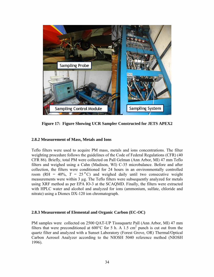
Figure 17: Figure Showing UCR Sampler Constructed for JETS APEX2

2.8.2 Measurement of Mass, Metals and Ions

Teflo filters were used to acquire PM mass, metals and ions concentrations. The filter weighting procedure follows the guidelines of the Code of Federal Regulations (CFR) (40 CFR 86). Briefly, total PM were collected on Pall Gelman (Ann Arbor, MI) 47 mm Teflo filters and weighed using a Cahn (Madison, WI) C-35 microbalance. Before and after collection, the filters were conditioned for 24 hours in an environmentally controlled room (RH = 40%, T = 25 C) and weighed daily until two consecutive weight measurements were within 3 µg. The Teflo filters were subsequently analyzed for metals using XRF method as per EPA IO-3 at the SCAQMD. Finally, the filters were extracted with HPLC water and alcohol and analyzed for ions (ammonium, sulfate, chloride and nitrate) using a Dionex DX-120 ion chromatograph.

2.8.3 Measurement of Elemental and Organic Carbon (EC-OC)

PM samples were collected on 2500 QAT-UP Tissuquartz Pall (Ann Arbor, MI) 47 mm filters that were preconditioned at 600°C for 5 h. A 1.5 cm2 punch is cut out from the quartz filter and analyzed with a Sunset Laboratory (Forest Grove, OR) Thermal/Optical Carbon Aerosol Analyzer according to the NIOSH 5040 reference method (NIOSH 1996).

34

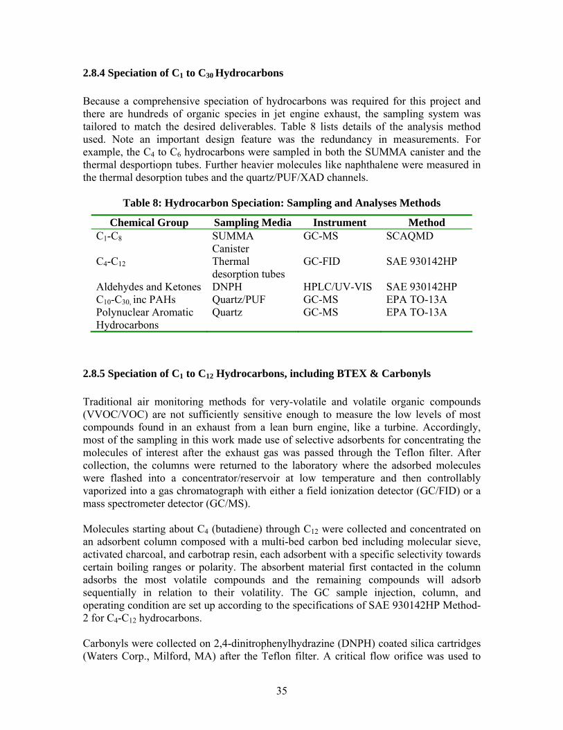
2.8.4 Speciation of C1 to C30 Hydrocarbons

Because a comprehensive speciation of hydrocarbons was required for this project and there are hundreds of organic species in jet engine exhaust, the sampling system was tailored to match the desired deliverables. Table 8 lists details of the analysis method used. Note an important design feature was the redundancy in measurements. For example, the C4 to C6 hydrocarbons were sampled in both the SUMMA canister and the thermal desportiopn tubes. Further heavier molecules like naphthalene were measured in the thermal desorption tubes and the quartz/PUF/XAD channels.

Table 8: Hydrocarbon Speciation: Sampling and Analyses Methods

Chemical Group Sampling Media Instrument Method C1-C8 SUMMA GC-MS SCAQMD

Canister C4-C12 Thermal GC-FID SAE 930142HP

desorption tubes Aldehydes and Ketones DNPH HPLC/UV-VIS SAE 930142HP C10-C30, inc PAHs Quartz/PUF GC-MS EPA TO-13A Polynuclear Aromatic Quartz GC-MS EPA TO-13A Hydrocarbons

2.8.5 Speciation of C1 to C12 Hydrocarbons, including BTEX & Carbonyls

Traditional air monitoring methods for very-volatile and volatile organic compounds (VVOC/VOC) are not sufficiently sensitive enough to measure the low levels of most compounds found in an exhaust from a lean burn engine, like a turbine. Accordingly, most of the sampling in this work made use of selective adsorbents for concentrating the molecules of interest after the exhaust gas was passed through the Teflon filter. After collection, the columns were returned to the laboratory where the adsorbed molecules were flashed into a concentrator/reservoir at low temperature and then controllably vaporized into a gas chromatograph with either a field ionization detector (GC/FID) or a mass spectrometer detector (GC/MS).

Molecules starting about C4 (butadiene) through C12 were collected and concentrated on an adsorbent column composed with a multi-bed carbon bed including molecular sieve, activated charcoal, and carbotrap resin, each adsorbent with a specific selectivity towards certain boiling ranges or polarity. The absorbent material first contacted in the column adsorbs the most volatile compounds and the remaining compounds will adsorb sequentially in relation to their volatility. The GC sample injection, column, and operating condition are set up according to the specifications of SAE 930142HP Method-2 for C4-C12 hydrocarbons.

Carbonyls were collected on 2,4-dinitrophenylhydrazine (DNPH) coated silica cartridges (Waters Corp., Milford, MA) after the Teflon filter. A critical flow orifice was used to

35

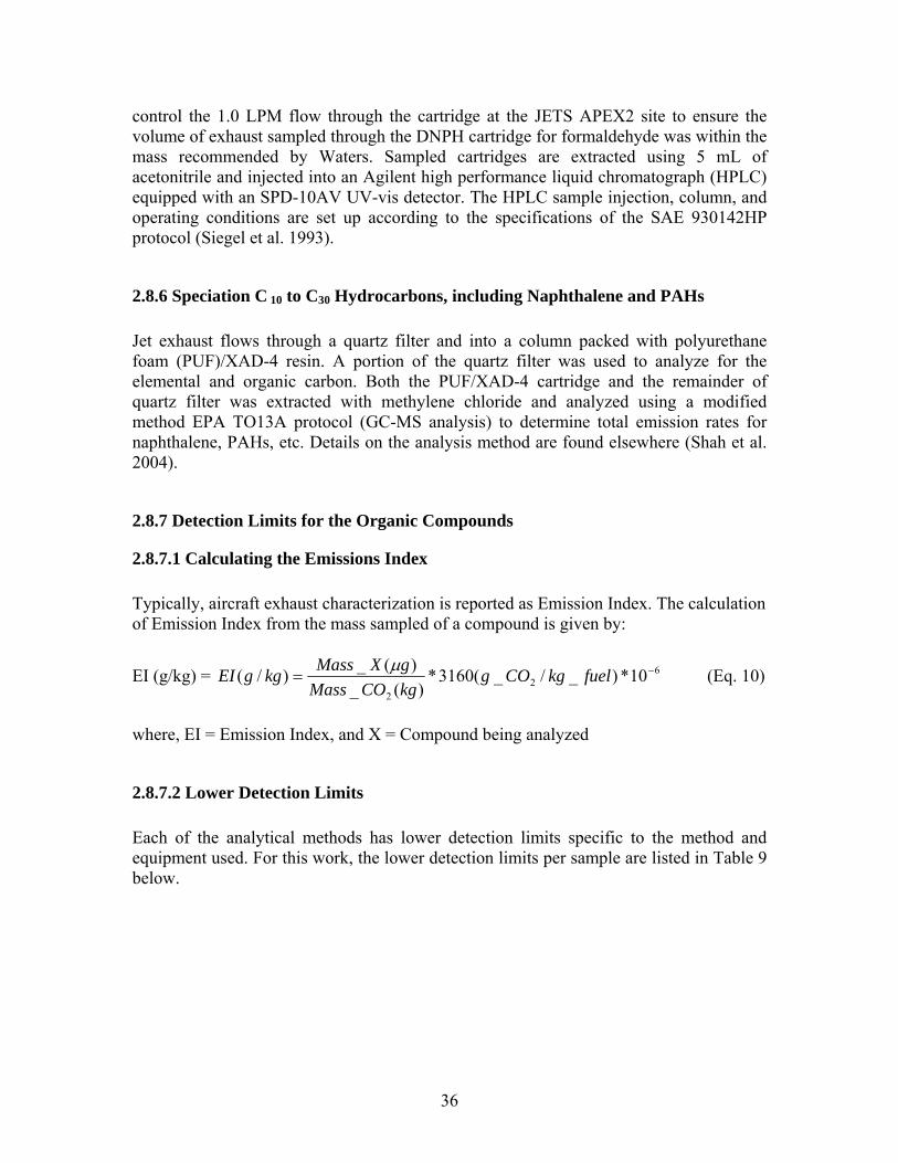
control the 1.0 LPM flow through the cartridge at the JETS APEX2 site to ensure the volume of exhaust sampled through the DNPH cartridge for formaldehyde was within the mass recommended by Waters. Sampled cartridges are extracted using 5 mL of acetonitrile and injected into an Agilent high performance liquid chromatograph (HPLC) equipped with an SPD-10AV UV-vis detector. The HPLC sample injection, column, and operating conditions are set up according to the specifications of the SAE 930142HP protocol (Siegel et al. 1993).

2.8.6 Speciation C 10 to C30 Hydrocarbons, including Naphthalene and PAHs

Jet exhaust flows through a quartz filter and into a column packed with polyurethane foam (PUF)/XAD-4 resin. A portion of the quartz filter was used to analyze for the elemental and organic carbon. Both the PUF/XAD-4 cartridge and the remainder of quartz filter was extracted with methylene chloride and analyzed using a modified method EPA TO13A protocol (GC-MS analysis) to determine total emission rates for naphthalene, PAHs, etc. Details on the analysis method are found elsewhere (Shah et al. 2004).

2.8.7 Detection Limits for the Organic Compounds

2.8.7.1 Calculating the Emissions Index

Typically, aircraft exhaust characterization is reported as Emission Index. The calculation of Emission Index from the mass sampled of a compound is given by:

Mass _ X (μg) −6EI (g/kg) = EI (g / kg) = *3160(g _ CO2 / kg _ fuel) *10 (Eq. 10)Mass _ CO2 (kg)

where, EI = Emission Index, and X = Compound being analyzed

2.8.7.2 Lower Detection Limits

Each of the analytical methods has lower detection limits specific to the method and equipment used. For this work, the lower detection limits per sample are listed in Table 9 below.

36

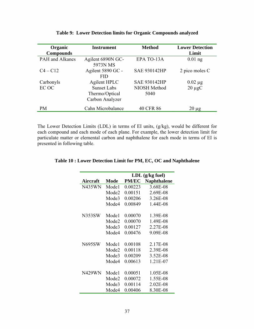
Table 9: Lower Detection limits for Organic Compounds analyzed

Organic Instrument Method Lower Detection Compounds Limit

PAH and Alkanes Agilent 6890N GC- EPA TO-13A 0.01 ng 5973N MS

C4 – C12 Agilent 5890 GC - SAE 930142HP 2 pico moles C FID

Carbonyls Agilent HPLC SAE 930142HP 0.02 µg EC OC Sunset Labs NIOSH Method 20 µgC

Thermo/Optical 5040 Carbon Analyzer

PM Cahn Microbalance 40 CFR 86 20 µg

The Lower Detection Limits (LDL) in terms of EI units, (g/kg), would be different for each compound and each mode of each plane. For example, the lower detection limit for particulate matter or elemental carbon and naphthalene for each mode in terms of EI is presented in following table.

Table 10 : Lower Detection Limit for PM, EC, OC and Naphthalene

Aircraft N435WN

Mode Mode1 Mode2 Mode3 Mode4

LDL (g/kg fuel) PM/EC Naphthalene 0.00223 3.68E-08 0.00151 2.69E-08 0.00206 3.26E-08 0.00849 1.44E-08

N353SW Mode1 Mode2 Mode3 Mode4

0.00070 0.00070 0.00127 0.00476

1.39E-08 1.49E-08 2.27E-08 9.09E-08

N695SW Mode1 Mode2 Mode3 Mode4

0.00108 0.00118 0.00209 0.00613

2.17E-08 2.39E-08 3.52E-08 1.21E-07

N429WN Mode1 Mode2 Mode3 Mode4

0.00051 0.00072 0.00114 0.00406

1.05E-08 1.55E-08 2.02E-08 8.30E-08

37

2.8.8 Exploratory Measurements for hexavalent chromium and dioxin

As a last minute inclusion in the final test matrix, we added the sampling of exhaust onto appropriate media for the measurement of hexavalent chromium and dioxin. The rationale was there were no known measurements reported in the literature. Further, the alloys used for the combustor section in the turbine often have high amounts of nickel and chromium contents. For example, GE reported that some of the materials used for the combustor section in the turbine might include: HastelloyX, MAR-M-509, HS188 and Rene' N5.

• HastelloyX is about 47% Ni, 22% Cr, 19% Fe, 9% Mo and ~1% Co, C, Mn, Si, and W.

• HS188 is about 22% Ni, 22% Cr, and 39% Co and 3% Fe. • MarM509 is mostly Co with about 20% Cr, and N5 is mostly Ni with about 7%

Cr As noted above, these alloys are high in chromium and nickel. In any case, these measurements were regarded as exploratory in nature and designed to provide insight as to whether further investigations were warranted for these compounds.

A sample of raw exhaust was extracted from the portside of the subject aircraft and conveyed through a 75 foot by 3/8-inch stainless line to the filter heated to 300ºF. Once the extracted sample reached the measurement bench, it was divided into two streams with a “tee.” The sample portion that flowed directly through the “tee” was dedicated for the analysis of the hexavalent chromium and the sample portion at right angles to this flow was for the dioxin analysis. Each leg had a vacuum pump and critical flow orifice rated at 30 liters per minute. In addition, we included a condensing section before the pump so condensing water would not reach the operating pump.

The measurement for hexavalent chromium in the jet exhaust followed a method in which exhaust gases flowed through a pretreated cellulose fiber filter that was subsequently analyzed using an ion chromatography method of the South Coast Air Quality Management District Method for chrome-VI.

The 47mm treated filters were mounted in Gelman holders and the times recorded for the period of sampling at the 30 liters per minute. A number of preliminary trials were undertaken of the hexavalent chromium system in addition to the sampling of the aircraft exhaust. The test matrix included collecting two samples of ambient air drawn throught he sampling system for one and eight hours. These samples served as verification that the system could measure values normally found for ambient air. Collection of samples with jet engine exhaust were started before the aircraft was in place and continued until the engines were shut down and we could go outside and turn the power off the pumps. The filter was removed and returned to the Petri dish, sealed with Teflon tape and stored with the quartz filters in a refrigerator until sent for analysis.

Dioxin sampling followed a modified EPA Method 23. This method is applicable to the determination of emissions of polychlorinated dibenzo-p-dioxins (PCDD's) and polychlorinated dibenzofurans (PCDF's) from stationary sources. In principle, a sample is

38

withdrawn from the gas stream, transferred in a heated line, cooled and collected on a packed column of adsorbent material. The sample cannot be separated into a particle and vapor fraction. The PCDD's and PCDF's are extracted from the sample, separated by high resolution gas chromatography (HRGC), and measured by high resolution mass spectrometry (HRMS).

Glassware with the spiked XAD resin was prepared and analyzed by Frontier Analytical Laboratory and Alta Analytical Laboratory, Inc. (Sacramento). Each firm provided two sample trains in appropriate sealed and chilled containers for a total of four sampling trains. Since the plan called for two different aircraft engines to be tested twice, the sample trains were split so that each firm tested one different engine rather than run duplicate samples. With only four sample trains, we decided to check each engine rather than be concerned with the repeatability of the measurements.

39

3.0 Results

It is a basic premise of this study and other similar studies to argue that if the engine gas phase combustion emissions and performance parameters were representative, then it would be assumed that likewise, the PM emissions were also representative. To address this issue, the engine manufacturer, GEAE, provided on-site and post-test analyses of the gas phase combustion emissions and performance parameters for all engines studied. The details of these analyses are summarized in Appendix F. Based on the results presented in Appendix F, the following conclusion pertaining to representativeness was provided by GEAE: “Trends in engine core speed, EGT and fuel flow data are generally consistent with expectations. The only apparent indication of performance deterioration was on the left engine of N695SW.”

3.1 Real-time Chemical Speciation (ARI)

3.1.1 Gas Phase Speciation

The gas phase pollutant species produced by aircraft gas turbine engines fall into two classes: oxides of nitrogen and products of incomplete combustion. The oxides of nitrogen are produced, not by reactions central to fuel hydrocarbon combustion, but primarily through interaction of combustion radical species with nitrogen in the combustion air. These nitrogen oxides are dominated by NO and NO2, although small amounts of HONO have been quantified and bounds determined in previous aviation emission campaigns (Wormhoudt et al., 2007).

The products of incomplete combustion include carbon monoxide (CO) and unburned/partially combusted hydrocarbons (UHCs). While the regulatory requirement specifies that a flame ionization detector (FID) be used to quantify the total UHCs in sum, a more detailed measurement approach was taken in JETS APEX2. Based on prior measurements of hydrocarbon speciation of aviation gas turbine exhausts (Spicer et al. 1994), individual hydrocarbon species were selected for measurement with the TILDAS and PTR-MS instruments. This allowed for a more detailed determination of the emitted hydrocarbons, but direct comparison to the regulatory FID is complicated by both 1) potentially significant contributions from individual species omitted from the selected TILDAS and PTR-MS species and 2) for the non-uniform response of the FID to individual hydrocarbon species. However, based on previous measurements and intercomparisons (Yelvington et al. 2007), a majority of the gaseous hydrocarbons emitted are accounted for by the combination of TILDAS and PTR-MS measurements reported here.

Carbon monoxide emissions are presented in Figure 18. The emissions data are presented as emission index (EI) in grams of CO emitted per kilogram of fuel burned. As discussed above, the analysis procedure uses the measured CO2 and the known fuel composition to calculate the CO EI. The CO EIs are highest at the lowest power settings, and decrease

40

♦

♦

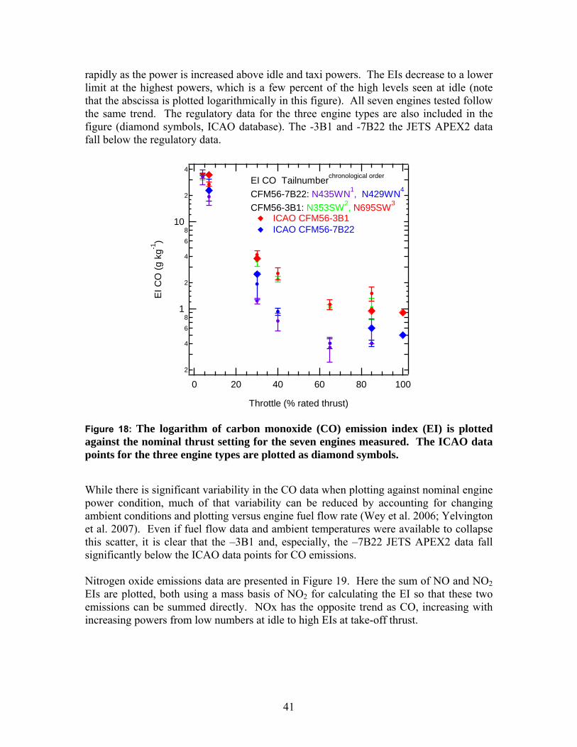
rapidly as the power is increased above idle and taxi powers. The EIs decrease to a lower limit at the highest powers, which is a few percent of the high levels seen at idle (note that the abscissa is plotted logarithmically in this figure). All seven engines tested follow the same trend. The regulatory data for the three engine types are also included in the figure (diamond symbols, ICAO database). The -3B1 and -7B22 the JETS APEX2 data fall below the regulatory data.

2

4

6 8

1

2

4

6 8

10

2

4 EI

CO

(g k

g-1 )

EI CO Tailnumberchronological order

CFM56-7B22: N435WN1 , N429WN4

CFM56-3B1: N353SW2 , N695SW3

ICAO CFM56-3B1 ICAO CFM56-7B22

0 20 40 60 80 100

Throttle (% rated thrust)

Figure 18: The logarithm of carbon monoxide (CO) emission index (EI) is plotted against the nominal thrust setting for the seven engines measured. The ICAO data points for the three engine types are plotted as diamond symbols.

While there is significant variability in the CO data when plotting against nominal engine power condition, much of that variability can be reduced by accounting for changing ambient conditions and plotting versus engine fuel flow rate (Wey et al. 2006; Yelvington et al. 2007). Even if fuel flow data and ambient temperatures were available to collapse this scatter, it is clear that the –3B1 and, especially, the –7B22 JETS APEX2 data fall significantly below the ICAO data points for CO emissions.

Nitrogen oxide emissions data are presented in Figure 19. Here the sum of NO and NO2 EIs are plotted, both using a mass basis of NO2 for calculating the EI so that these two emissions can be summed directly. NOx has the opposite trend as CO, increasing with increasing powers from low numbers at idle to high EIs at take-off thrust.

41

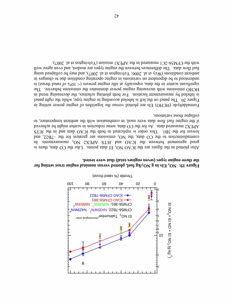
-+--+- I!

2

3

4

5

6 7 8 9

10

2

3

EI N

OX

= EI NO

+ EI NO

2 (g kg -1 )

EI NOX T ailnum berchronological order

CF M56-7B22: N435W N1 , N429W N

4

CF M56-3B1: N353SW2 , N695SW

3

ICAO CF M56-3B1 ICAO CF M56-7B22

0 20 40 60 80 100

Throttle (% rated thrust)

Figure 19: NOx EIs in g NO2/kg fuel, plotted versus nominal engine trust setting for the three engine types (seven engines total) that were tested.

Also plotted in the figure are the ICAO NOx EI data points. Like the CO data, there is good agreement between the ICAO and JETS APEX2 NOx measurements. In contradistinction to the CO data, the NOx emissions are greatest for the –7B22, and lowest for the 3B1. This order is replicated in both the ICAO data and in the JETS APEX2 measured data. As for the CO data, some reduction in scatter might be achieved if the engine fuel flow data were used, in combination with the ambient temperature, to collapse those variations.

Formaldehyde (HCHO) EIs are plotted versus the logarithm of engine power setting in Figure 20. The panel on the left is labeled according to engine type, while the right panel is labeled by measurement location. For both plotting schemes, the decreasing trend in HCHO emissions with increasing engine power dominates the emissions behavior. The significant scatter in the data, especially at idle engine powers (< 10% of rated thrust) is understood to be dependent on variations in engine operating condition due to changes in ambient conditions (Wey et al. 2006; Yelvington et al. 2007), and may be collapsed using fuel flow data. The differences between the engine types are modest, and even agree well with the CFM56-2C1 measured in the APEX1 mission (Yelvington et al. 2007).

42

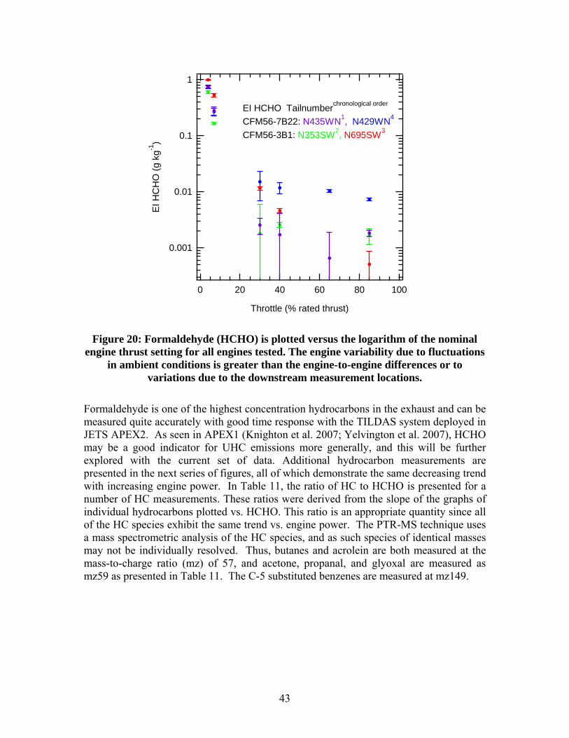
0.001

0.01

0.1

1

EI H

CH

O (g

kg-1

)

EI HCHO Tailnumberchronological order

CFM56-7B22: N435WN1 , N429WN4

CFM56-3B1: N353SW2 , N695SW3

0 20 40 60 80 100

Throttle (% rated thrust)

Figure 20: Formaldehyde (HCHO) is plotted versus the logarithm of the nominal engine thrust setting for all engines tested. The engine variability due to fluctuations

in ambient conditions is greater than the engine-to-engine differences or to variations due to the downstream measurement locations.

Formaldehyde is one of the highest concentration hydrocarbons in the exhaust and can be measured quite accurately with good time response with the TILDAS system deployed in JETS APEX2. As seen in APEX1 (Knighton et al. 2007; Yelvington et al. 2007), HCHO may be a good indicator for UHC emissions more generally, and this will be further explored with the current set of data. Additional hydrocarbon measurements are presented in the next series of figures, all of which demonstrate the same decreasing trend with increasing engine power. In Table 11, the ratio of HC to HCHO is presented for a number of HC measurements. These ratios were derived from the slope of the graphs of individual hydrocarbons plotted vs. HCHO. This ratio is an appropriate quantity since all of the HC species exhibit the same trend vs. engine power. The PTR-MS technique uses a mass spectrometric analysis of the HC species, and as such species of identical masses may not be individually resolved. Thus, butanes and acrolein are both measured at the mass-to-charge ratio (mz) of 57, and acetone, propanal, and glyoxal are measured as mz59 as presented in Table 11. The C-5 substituted benzenes are measured at mz149.

43

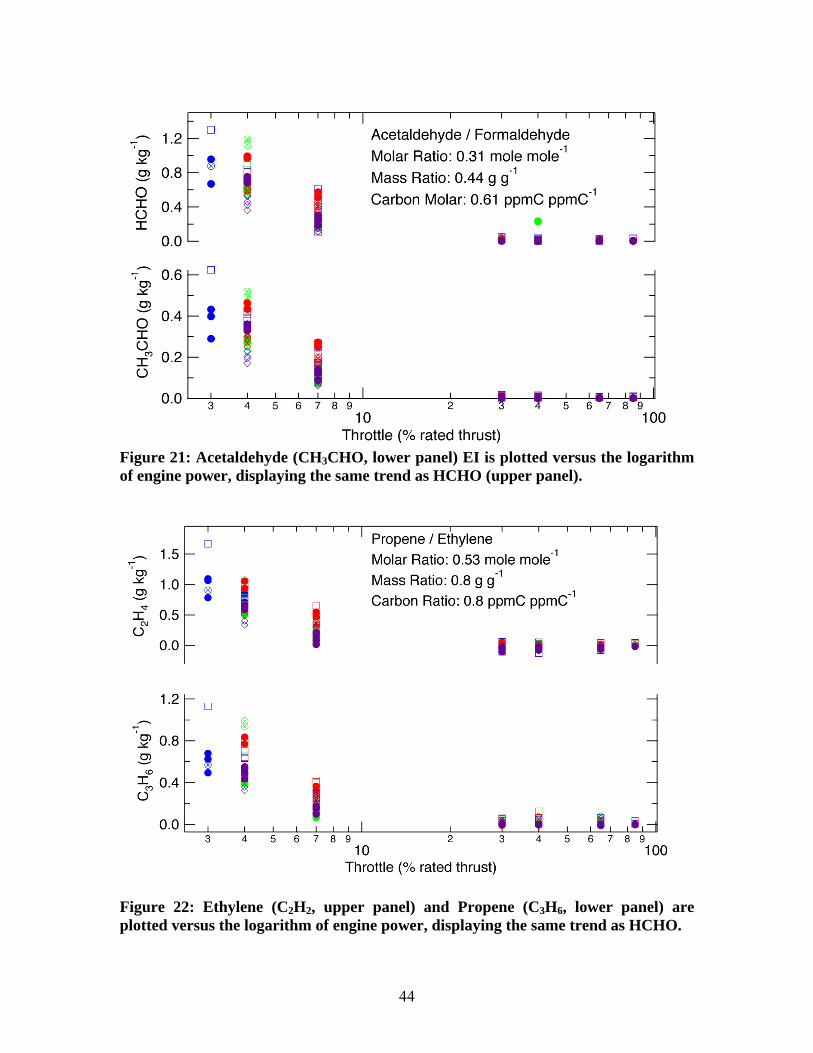
1.2 D Acetaldehyde I Formaldehyde - @

' -1 0)

I I Molar Ratio: 0.31 mole mole ~

9 0.8 Mass Ratio: 0.44 g g -1

•

I 0 -1 I 0.4 Carbon Molar: 0.61 ppmC ppmC 0 I •

0.0 I I ■ i

- 0.6 D ~

0)

I ~

9 0.4 I

0 I • 0 I (') 0.2 I 0

0.0 3 4 5 6 7 8 9 2

10 Throttle {% rated thrust)

□ Propene / Ethylene - 1.5 -1 Molar Ratio: 0.53 mole mole

en • I Mass Ratio : 0.8 g g

-1 ..lo::: 1.0 9 i -1

..;-

I Carbon Ratio: 0.8 ppmC ppmC

I 0.5 C\J

0 0.0 I I I I

1.2 □

"7 @

~ 0.8 I 9 ! CD • I I (") 0.4 I (_)

0.0 • Ii 3 4 5 6 7 8 9 2 3 4 5 6 7 8 9

10 100 Throttle (% rated thrust)

Figure 21: Acetaldehyde (CH3CHO, lower panel) EI is plotted versus the logarithm of engine power, displaying the same trend as HCHO (upper panel).

Figure 22: Ethylene (C2H2, upper panel) and Propene (C3H6, lower panel) are plotted versus the logarithm of engine power, displaying the same trend as HCHO.

44

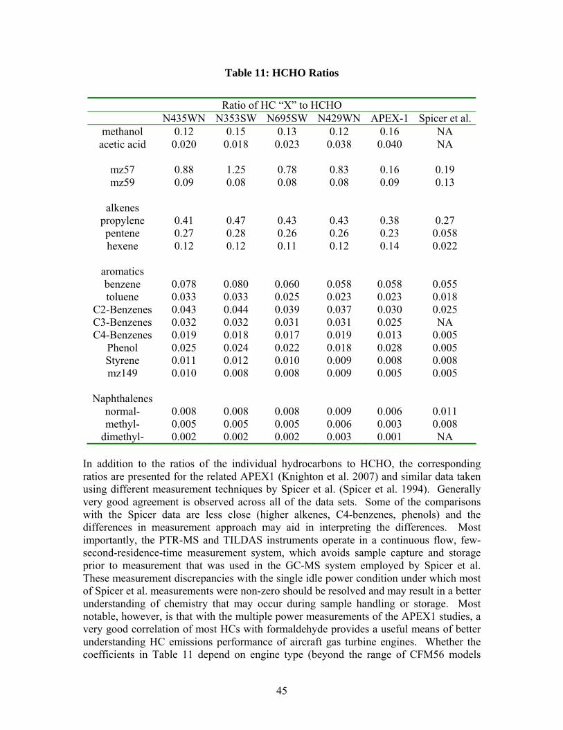
Table 11: HCHO Ratios

Ratio of HC “X” to HCHO

methanol acetic acid

N435WN 0.12 0.020

N353SW 0.15 0.018

N695SW 0.13 0.023

N429WN 0.12 0.038

APEX-1 0.16 0.040

Spicer et al. NA NA

mz57 mz59

0.88 0.09

1.25 0.08

0.78 0.08

0.83 0.08

0.16 0.09

0.19 0.13

alkenes propylene pentene hexene

0.41 0.27 0.12

0.47 0.28 0.12

0.43 0.26 0.11

0.43 0.26 0.12

0.38 0.23 0.14

0.27 0.058 0.022

aromatics benzene toluene

C2-Benzenes C3-Benzenes C4-Benzenes

Phenol Styrene mz149

0.078 0.033 0.043 0.032 0.019 0.025 0.011 0.010

0.080 0.033 0.044 0.032 0.018 0.024 0.012 0.008

0.060 0.025 0.039 0.031 0.017 0.022 0.010 0.008

0.058 0.023 0.037 0.031 0.019 0.018 0.009 0.009

0.058 0.023 0.030 0.025 0.013 0.028 0.008 0.005

0.055 0.018 0.025 NA

0.005 0.005 0.008 0.005

Naphthalenes normal- methyl-

dimethyl-

0.008 0.005 0.002

0.008 0.005 0.002

0.008 0.005 0.002

0.009 0.006 0.003

0.006 0.003 0.001

0.011 0.008 NA

In addition to the ratios of the individual hydrocarbons to HCHO, the corresponding ratios are presented for the related APEX1 (Knighton et al. 2007) and similar data taken using different measurement techniques by Spicer et al. (Spicer et al. 1994). Generally very good agreement is observed across all of the data sets. Some of the comparisons with the Spicer data are less close (higher alkenes, C4-benzenes, phenols) and the differences in measurement approach may aid in interpreting the differences. Most importantly, the PTR-MS and TILDAS instruments operate in a continuous flow, few-second-residence-time measurement system, which avoids sample capture and storage prior to measurement that was used in the GC-MS system employed by Spicer et al. These measurement discrepancies with the single idle power condition under which most of Spicer et al. measurements were non-zero should be resolved and may result in a better understanding of chemistry that may occur during sample handling or storage. Most notable, however, is that with the multiple power measurements of the APEX1 studies, a very good correlation of most HCs with formaldehyde provides a useful means of better understanding HC emissions performance of aircraft gas turbine engines. Whether the coefficients in Table 11 depend on engine type (beyond the range of CFM56 models

45

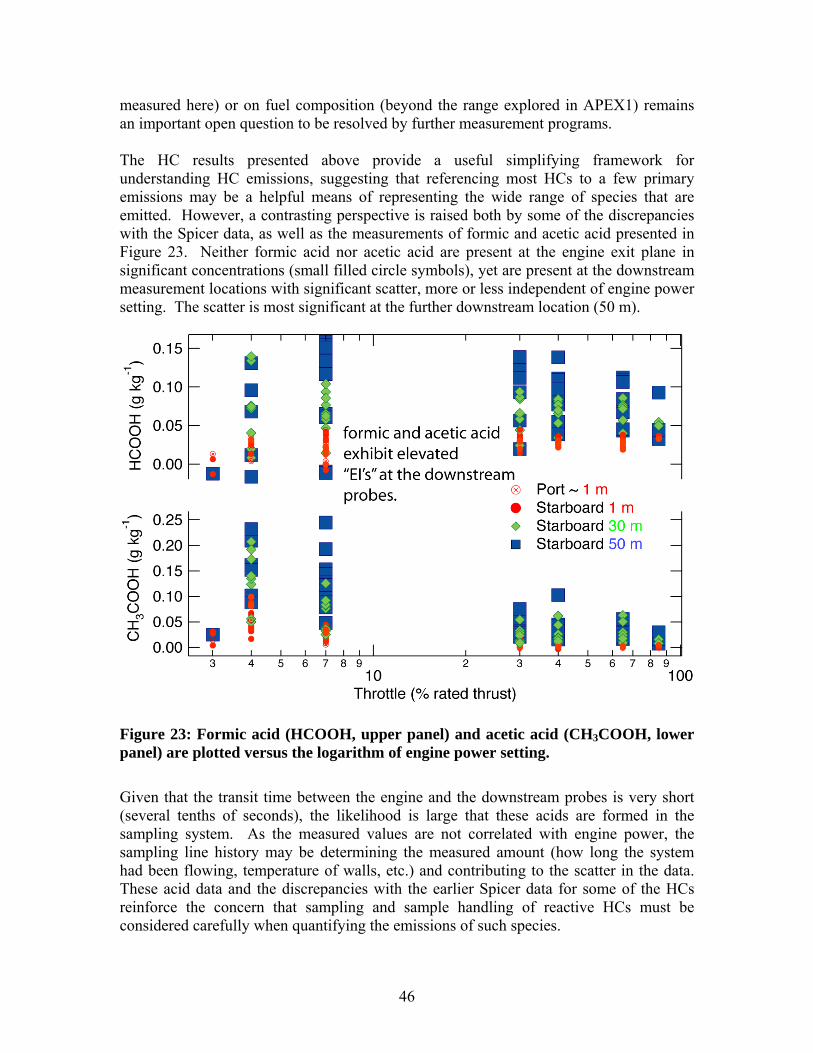
0.15

Ol -I o 0.05 0 (_) I 0.00

"-;- 0.25 Ol

~ 0.20 -I 0.15 0 0 0.10 (_)

IC') 0.05 (_)

i

■

' 3

■

t •

■ ■

I '

formic and acetic acid exhibit elevated

I ■

I I

"El's" at the downstream probes. ® Port ~ 1 m

• Starboard 1 m ♦ Starboard 30 m ■ Starboard 50 m

■

4 5 6 7 8 9 10

Throttle (% rated thrust)

■

II 8 9

100

measured here) or on fuel composition (beyond the range explored in APEX1) remains an important open question to be resolved by further measurement programs.

The HC results presented above provide a useful simplifying framework for understanding HC emissions, suggesting that referencing most HCs to a few primary emissions may be a helpful means of representing the wide range of species that are emitted. However, a contrasting perspective is raised both by some of the discrepancies with the Spicer data, as well as the measurements of formic and acetic acid presented in Figure 23. Neither formic acid nor acetic acid are present at the engine exit plane in significant concentrations (small filled circle symbols), yet are present at the downstream measurement locations with significant scatter, more or less independent of engine power setting. The scatter is most significant at the further downstream location (50 m).

Figure 23: Formic acid (HCOOH, upper panel) and acetic acid (CH3COOH, lower panel) are plotted versus the logarithm of engine power setting.

Given that the transit time between the engine and the downstream probes is very short (several tenths of seconds), the likelihood is large that these acids are formed in the sampling system. As the measured values are not correlated with engine power, the sampling line history may be determining the measured amount (how long the system had been flowing, temperature of walls, etc.) and contributing to the scatter in the data. These acid data and the discrepancies with the earlier Spicer data for some of the HCs reinforce the concern that sampling and sample handling of reactive HCs must be considered carefully when quantifying the emissions of such species.

46

3.1.2 Particle Speciation

The composition of the particles emitted by aviation gas turbine engines is a complex issue that involves difficult measurement and data interpretation issues. In fact, the nature and composition of the emitted particles are continually evolving and there is not a single physical situation that can be used to uniquely characterize them. There are several states at which the particles are evolving less quickly that can be used as nominal reference points, but even those depend on the precise definition of those conditions and the measurement of those states requires careful sampling and sample handling so that the physical state of the particles is accurately captured.

The initial particle formation occurs in the engine combustor as a byproduct of the combustion process. The carbonaceous soot particles formed in the high temperatures of the combustor are subject to little change themselves after they leave the combustor, pass out of the engine, and mix with the atmosphere. However, condensable gases also are emitted with the soot particles, and these condensable gases contribute both to condensed material on the soot surfaces and to the formation of new volatile particles composed of the condensed species.

The measurement approach taken in JETS APEX2 was to quantify the composition of the particles centers around the Aerosol Mass Spectrometer (AMS), which measures the size resolved composition of volatile species measured by heating the particles to 600o C on a filament. For aviation gas turbine engines, the volatile components consist of sulfate (sulfuric acid) and organics, as will be discussed and quantified below. Notably, no significant nitrate volatile component is evident, even though this is typically a constituent of background aerosol and nitrogen oxides are emitted in the exhaust. Apparently there is insufficient time or oxidative potential for nitrate to condense into the particle phase under the conditions at JETS APEX2.

The AMS only measures the volatile (600oC) components of the particles, so the AMS is complemented by a MAAP instrument to measure the refractory black carbon mass. While the AMS is size resolved, the MAAP is not, so that coordination with particle size distribution measurements is useful for fully characterizing the non-volatile mass contributions. To aid in making comparisons with the other particle measurements, a CPC is also operated in parallel with the AMS and MAAP instruments in the Aerodyne mobile laboratory. All of these data are presented in the following figures.

The black carbon mass measurement quantified by the MAAP is presented in Figure 24. For all the engine types, the black carbon begins at a low value at low powers and increases at higher powers. While generally increasing with power, there is a modest increase in black carbon at the very lowest idle settings for all engines. After the modest decrease from idle, the black carbon continually increases with engine power, with the most rapid increase between 60 and 80% power. This matches the power dependence of the APEX1 data as well. There is some variation among the various engine types, with the -3B1 > -7B22 even though all engines have the same qualitative trends with engine

47

,....._

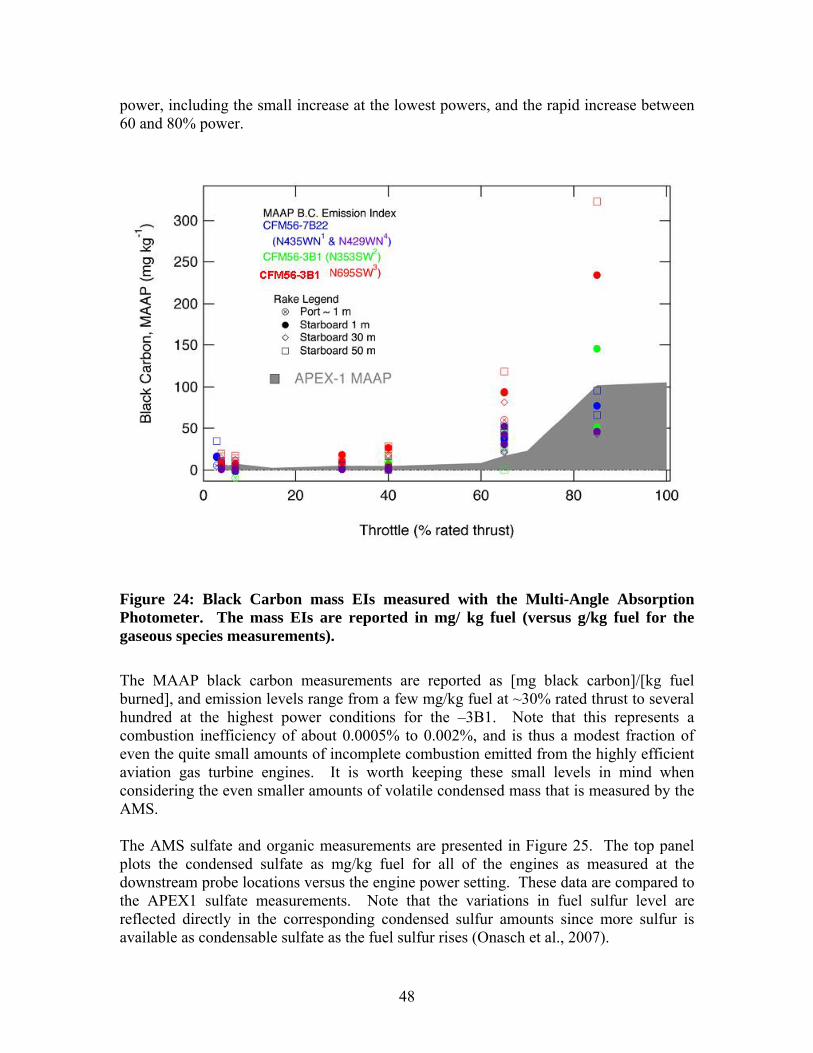
C: 0 ..c ..... ctl C) ~ () ctl co

300

250

200

150

100

50 D

MAAP B.C. Emission Index CFM56-7B22

(N435WN 1

& N429WN4

)

CFM56-3B1 (N353SWI

CFM56-3B1 N695Sw'}

Rake Legend © Port- 1 m • Starboard 1 m ◊ Starboard 30 m o Starboard 50 m

□ APEX-1 MAAP

D

•

• D

0 '-• -------11--1~--==::::::;~-------ll 0 20 40 60 80 100

Throttle (% rated thrust)

power, including the small increase at the lowest powers, and the rapid increase between 60 and 80% power.

Figure 24: Black Carbon mass EIs measured with the Multi-Angle Absorption Photometer. The mass EIs are reported in mg/ kg fuel (versus g/kg fuel for the gaseous species measurements).

The MAAP black carbon measurements are reported as [mg black carbon]/[kg fuel burned], and emission levels range from a few mg/kg fuel at ~30% rated thrust to several hundred at the highest power conditions for the –3B1. Note that this represents a combustion inefficiency of about 0.0005% to 0.002%, and is thus a modest fraction of even the quite small amounts of incomplete combustion emitted from the highly efficient aviation gas turbine engines. It is worth keeping these small levels in mind when considering the even smaller amounts of volatile condensed mass that is measured by the AMS.

The AMS sulfate and organic measurements are presented in Figure 25. The top panel plots the condensed sulfate as mg/kg fuel for all of the engines as measured at the downstream probe locations versus the engine power setting. These data are compared to the APEX1 sulfate measurements. Note that the variations in fuel sulfur level are reflected directly in the corresponding condensed sulfur amounts since more sulfur is available as condensable sulfate as the fuel sulfur rises (Onasch et al., 2007).

48

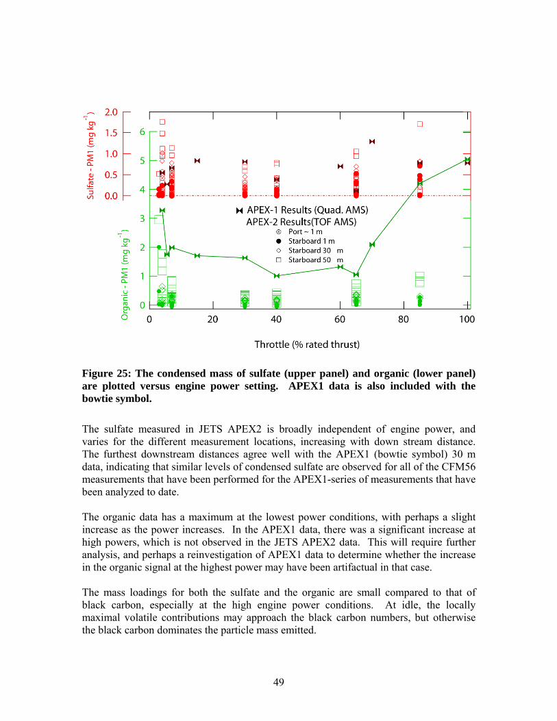
~ 2.0 ";"

□ Ol □ ..>£ 1.5 6 Ol □

5 H

~ 1.0 5 ~B El

a.. H

N § N I i '

................ _J .. J. . . ... . ..... ... . ... . .... -----....... QJ 0.5 .... ~ 4 :::J 0.0 V)

3 ~ APEX-1 Results (Quad. AMS)

APEX-2 Results(TOF AMS) ® Port - 1 m

Ol • Starboard 1 m ..>£ 2 Ol ◊ Starboard 30 m

5 D Starboard 50 m

~ B a..

I I

-~

' C l1l 0 2' 0 0 20 40 60 80 100

Throttle (% rated thrust)

Figure 25: The condensed mass of sulfate (upper panel) and organic (lower panel) are plotted versus engine power setting. APEX1 data is also included with the bowtie symbol.

The sulfate measured in JETS APEX2 is broadly independent of engine power, and varies for the different measurement locations, increasing with down stream distance. The furthest downstream distances agree well with the APEX1 (bowtie symbol) 30 m data, indicating that similar levels of condensed sulfate are observed for all of the CFM56 measurements that have been performed for the APEX1-series of measurements that have been analyzed to date.

The organic data has a maximum at the lowest power conditions, with perhaps a slight increase as the power increases. In the APEX1 data, there was a significant increase at high powers, which is not observed in the JETS APEX2 data. This will require further analysis, and perhaps a reinvestigation of APEX1 data to determine whether the increase in the organic signal at the highest power may have been artifactual in that case.

The mass loadings for both the sulfate and the organic are small compared to that of black carbon, especially at the high engine power conditions. At idle, the locally maximal volatile contributions may approach the black carbon numbers, but otherwise the black carbon dominates the particle mass emitted.

49

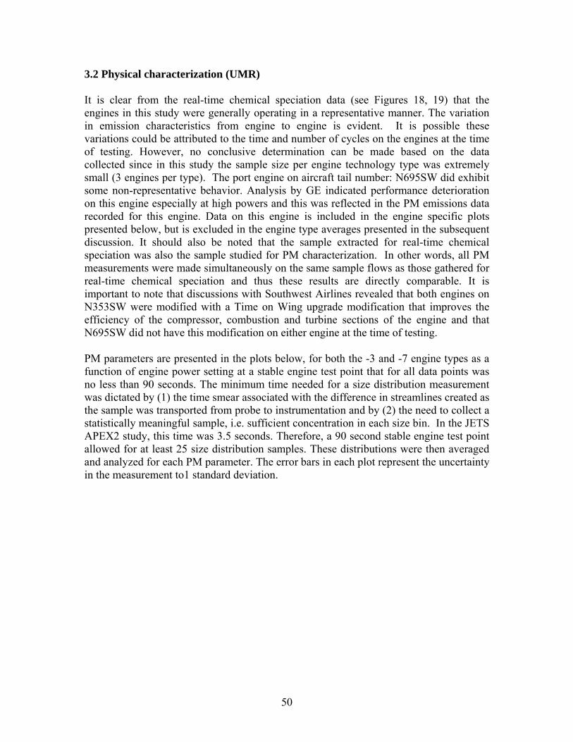
3.2 Physical characterization (UMR)

It is clear from the real-time chemical speciation data (see Figures 18, 19) that the engines in this study were generally operating in a representative manner. The variation in emission characteristics from engine to engine is evident. It is possible these variations could be attributed to the time and number of cycles on the engines at the time of testing. However, no conclusive determination can be made based on the data collected since in this study the sample size per engine technology type was extremely small (3 engines per type). The port engine on aircraft tail number: N695SW did exhibit some non-representative behavior. Analysis by GE indicated performance deterioration on this engine especially at high powers and this was reflected in the PM emissions data recorded for this engine. Data on this engine is included in the engine specific plots presented below, but is excluded in the engine type averages presented in the subsequent discussion. It should also be noted that the sample extracted for real-time chemical speciation was also the sample studied for PM characterization. In other words, all PM measurements were made simultaneously on the same sample flows as those gathered for real-time chemical speciation and thus these results are directly comparable. It is important to note that discussions with Southwest Airlines revealed that both engines on N353SW were modified with a Time on Wing upgrade modification that improves the efficiency of the compressor, combustion and turbine sections of the engine and that N695SW did not have this modification on either engine at the time of testing.

PM parameters are presented in the plots below, for both the -3 and -7 engine types as a function of engine power setting at a stable engine test point that for all data points was no less than 90 seconds. The minimum time needed for a size distribution measurement was dictated by (1) the time smear associated with the difference in streamlines created as the sample was transported from probe to instrumentation and by (2) the need to collect a statistically meaningful sample, i.e. sufficient concentration in each size bin. In the JETS APEX2 study, this time was 3.5 seconds. Therefore, a 90 second stable engine test point allowed for at least 25 size distribution samples. These distributions were then averaged and analyzed for each PM parameter. The error bars in each plot represent the uncertainty in the measurement to1 standard deviation.

50

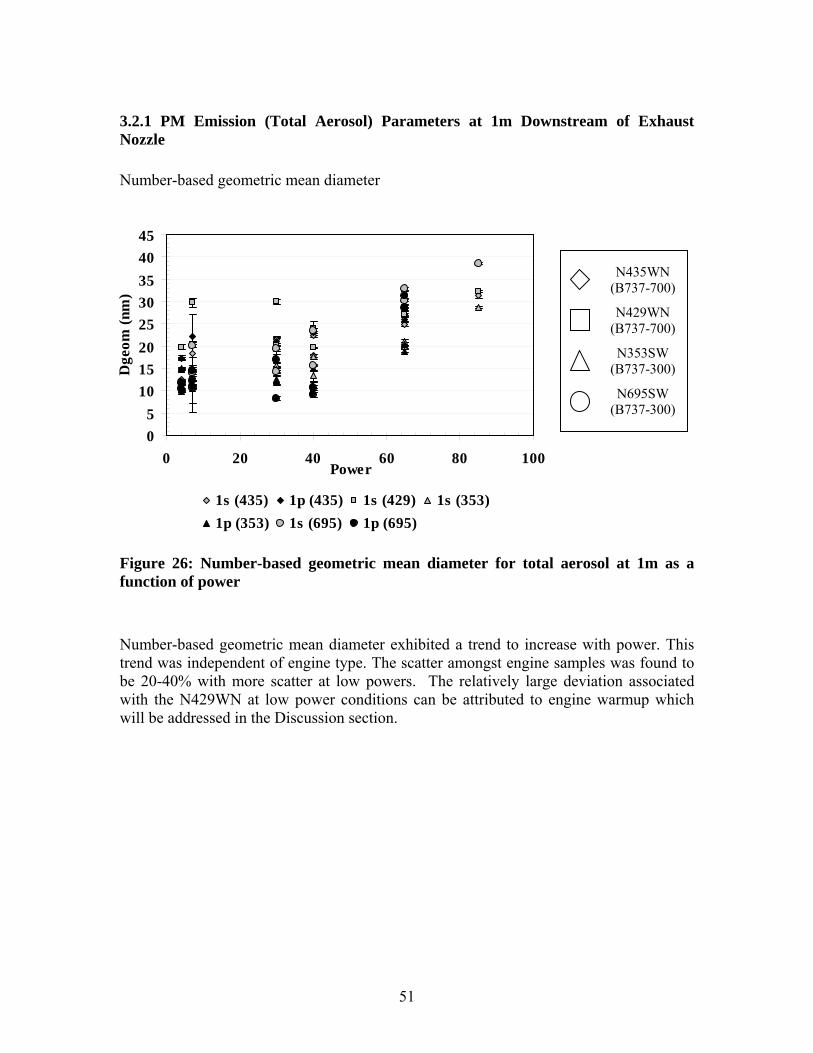
0

- !l I ◊

-r:t

e

Q -ts

- a1 l i □

•• D I - . ~

- ., I D •

- . 0 I I I I 7 -

◊ • □

A 0 •

3.2.1 PM Emission (Total Aerosol) Parameters at 1m Downstream of Exhaust Nozzle

Number-based geometric mean diameter

45 40 35 30 25 20 15 10

5 0

0 20 40 60 80 100 Power

Dge

om (n

m)

1s (435) 1p (435) 1s (429) 1s (353) 1p (353) 1s (695) 1p (695)

N435WN (B737-700)

N429WN (B737-700)

N353SW (B737-300)

N695SW (B737-300)

Figure 26: Number-based geometric mean diameter for total aerosol at 1m as a function of power

Number-based geometric mean diameter exhibited a trend to increase with power. This trend was independent of engine type. The scatter amongst engine samples was found to be 20-40% with more scatter at low powers. The relatively large deviation associated with the N429WN at low power conditions can be attributed to engine warmup which will be addressed in the Discussion section.

51

◊

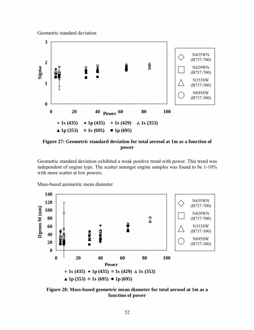
J! i i I • • □

D 0

◊ • □

• 0 •

◊

0 □ ~

•

i i D

• 0

◊ • □

• 0 •

Geometric standard deviation

3

N435WN (B737-700)2

Sigm

a

0 20 40 60 80 100 Power

N429WN (B737-700)

N353SW 1 (B737-300)

N695SW (B737-300)

0

1s (435) 1p (435) 1s (429) 1s (353) 1p (353) 1s (695) 1p (695)

Figure 27: Geometric standard deviation for total aerosol at 1m as a function of power

Geometric standard deviation exhibited a weak positive trend with power. This trend was independent of engine type. The scatter amongst engine samples was found to be 1-10% with more scatter at low powers.

Mass-based geometric mean diameter

140 120

0 20 40 60 80 100 Power

N435WN (B737-700)

N429WN (B737-700)

N353SW (B737-300)

N695SW (B737-300)

Dge

om M

(nm

)

100 80 60 40 20

0

1s (435) 1p (435) 1s (429) 1s (353) 1p (353) 1s (695) 1p (695)

Figure 28: Mass-based geometric mean diameter for total aerosol at 1m as a function of power

52

•

◊ ♦

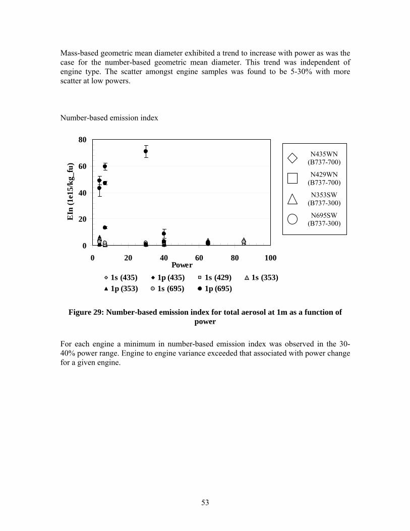
0

□

•

◊

□ D 0

Mass-based geometric mean diameter exhibited a trend to increase with power as was the case for the number-based geometric mean diameter. This trend was independent of engine type. The scatter amongst engine samples was found to be 5-30% with more scatter at low powers.

Number-based emission index

80

60

40

20

0 0 20 40 60 80 100

Power

EIn

(1e1

5/kg

_fu)

N435WN (B737-700)

N429WN (B737-700)

N353SW (B737-300)

N695SW (B737-300)

1s (435) 1p (435) 1s (429) 1s (353) 1p (353) 1s (695) 1p (695)

Figure 29: Number-based emission index for total aerosol at 1m as a function of power

For each engine a minimum in number-based emission index was observed in the 30-40% power range. Engine to engine variance exceeded that associated with power change for a given engine.

53

•• -·• -

◊ ♦

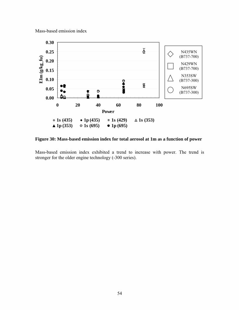
0

• 0

□

•

~ I

◊

□ D

C: ~

0

Mass-based emission index

EIm

(g/k

g_fu

) 0.30

0.25

0.20

0.15

0.10

0.05

0.00

N435WN (B737-700)

N429WN (B737-700)

N353SW (B737-300)

N695SW (B737-300)

0 20 40 60 80 100 Power

1s (435) 1p (435) 1s (429) 1s (353) 1p (353) 1s (695) 1p (695)

Figure 30: Mass-based emission index for total aerosol at 1m as a function of power

Mass-based emission index exhibited a trend to increase with power. The trend is stronger for the older engine technology (-300 series).

54

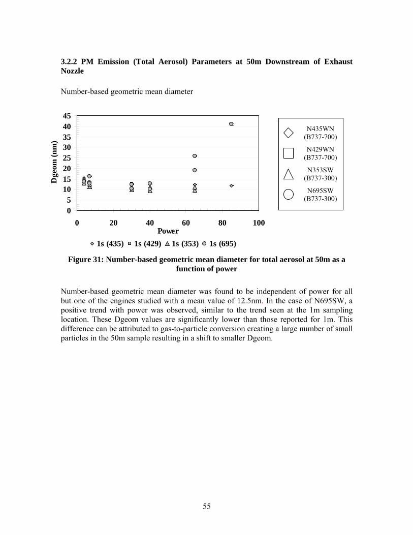
0

◊

0 □ 0 D 0

§ <> - ~Q a 6 0 I I I I

◊ □ 0

Dge

om (n

m)

3.2.2 PM Emission (Total Aerosol) Parameters at 50m Downstream of Exhaust Nozzle

Number-based geometric mean diameter

45 40 N435WN

(B737-700)35 30 N429WN

(B737-700)25 20 N353SW

(B737-300)15 10 N695SW

(B737-300)5 0

0 20 40 60 80 100 Power

1s (435) 1s (429) 1s (353) 1s (695)

Figure 31: Number-based geometric mean diameter for total aerosol at 50m as a function of power

Number-based geometric mean diameter was found to be independent of power for all but one of the engines studied with a mean value of 12.5nm. In the case of N695SW, a positive trend with power was observed, similar to the trend seen at the 1m sampling location. These Dgeom values are significantly lower than those reported for 1m. This difference can be attributed to gas-to-particle conversion creating a large number of small particles in the 50m sample resulting in a shift to smaller Dgeom.

55

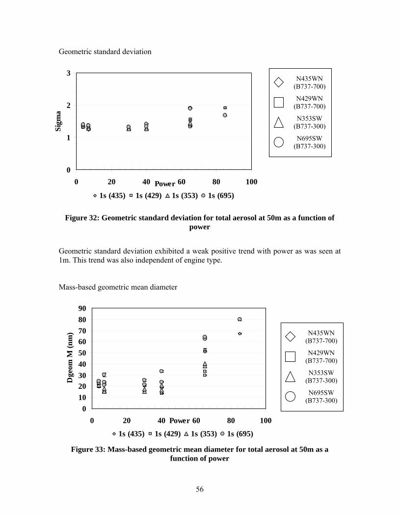
0

-Bij

◊ □

- Q 0

-8~ Q

B ~

◊ □

0

9 ij

A ct Cs

CE

0

0

Q

<>

◊

□ D 0

◊

□ D 0

Geometric standard deviation Si

gma

3 N435WN

(B737-700)

N429WN 2 (B737-700)

N353SW (B737-300)

1 N695SW (B737-300)

0 0 20 40 60 80 100 Power

1s (435) 1s (429) 1s (353) 1s (695)

Figure 32: Geometric standard deviation for total aerosol at 50m as a function of power

Geometric standard deviation exhibited a weak positive trend with power as was seen at 1m. This trend was also independent of engine type.

Mass-based geometric mean diameter

90 80

Dge

om M

(nm

) 70 60 50 40 30 20 10

0 0 20 40 Power 60 80 100

1s (435) 1s (429) 1s (353) 1s (695)

N435WN (B737-700)

N429WN (B737-700)

N353SW (B737-300)

N695SW (B737-300)

Figure 33: Mass-based geometric mean diameter for total aerosol at 50m as a function of power

56

~~ ! ~ ◊

~

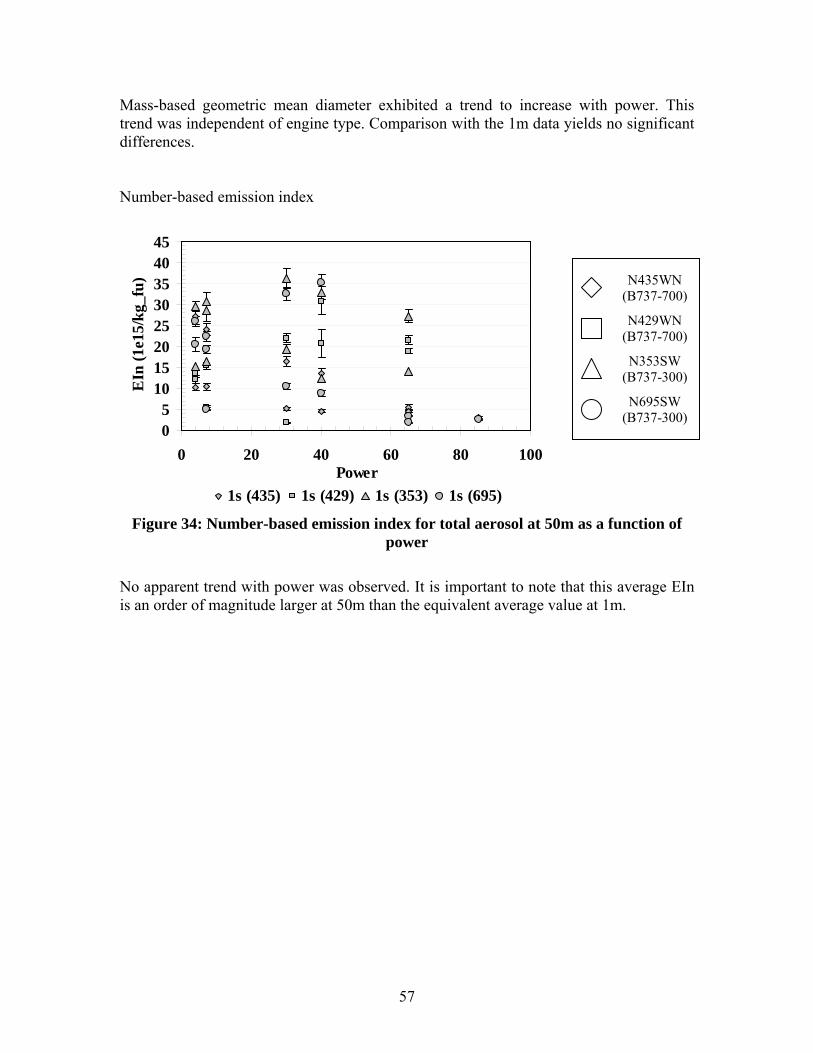
2~ ~ f ~ □ E.

g: ~ er

8 lS. D Q

Q

0 ~ ~

' ~ 0 D 0 7 I I I I : I I I I

I I I I I

I

◊ □ 0

Mass-based geometric mean diameter exhibited a trend to increase with power. This trend was independent of engine type. Comparison with the 1m data yields no significant differences.

Number-based emission index

45 40 35 30 25 20 15 10

5 0

0 20 40 60 80 100 Power

EIn

(1e1

5/kg

_fu)

1s (435) 1s (429) 1s (353) 1s (695)

N435WN (B737-700)

N429WN (B737-700)

N353SW (B737-300)

N695SW (B737-300)

Figure 34: Number-based emission index for total aerosol at 50m as a function of power

No apparent trend with power was observed. It is important to note that this average EIn is an order of magnitude larger at 50m than the equivalent average value at 1m.

57

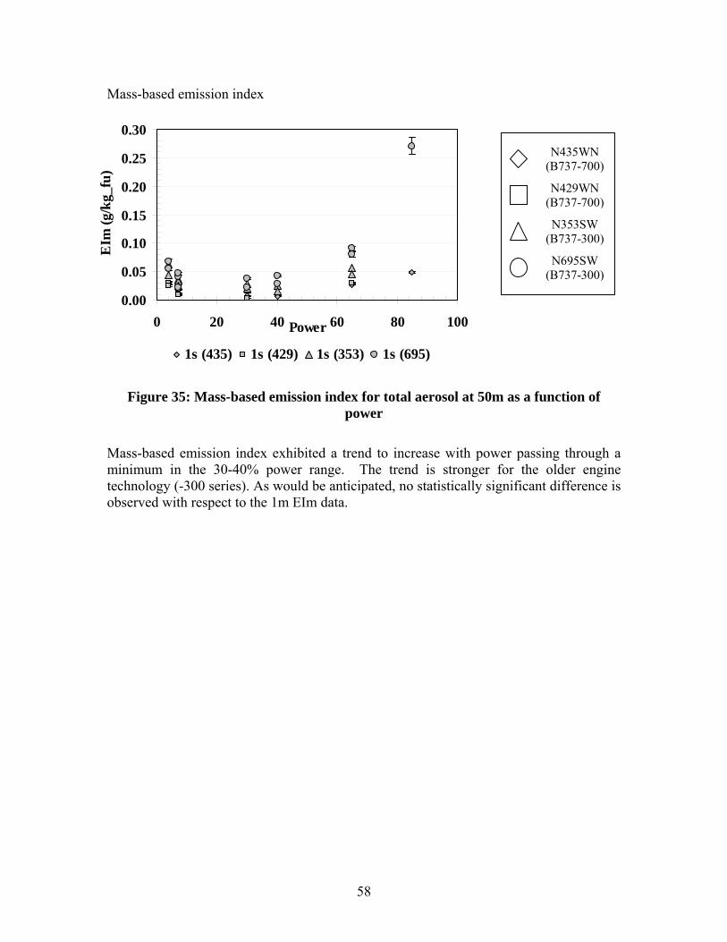
a~ I I I I I I

◊ □

8 8 g,

0

<>

◊

□ D 0

Mass-based emission index E

Im (g

/kg_

fu)

0.30

0.25

0.20

0.15

0.10

0.05

0.00 0 20 40 60 80 100 Power

N435WN (B737-700)

N429WN (B737-700)

N353SW (B737-300)

N695SW (B737-300)

1s (435) 1s (429) 1s (353) 1s (695)

Figure 35: Mass-based emission index for total aerosol at 50m as a function of power

Mass-based emission index exhibited a trend to increase with power passing through a minimum in the 30-40% power range. The trend is stronger for the older engine technology (-300 series). As would be anticipated, no statistically significant difference is observed with respect to the 1m EIm data.

58

◊ ♦

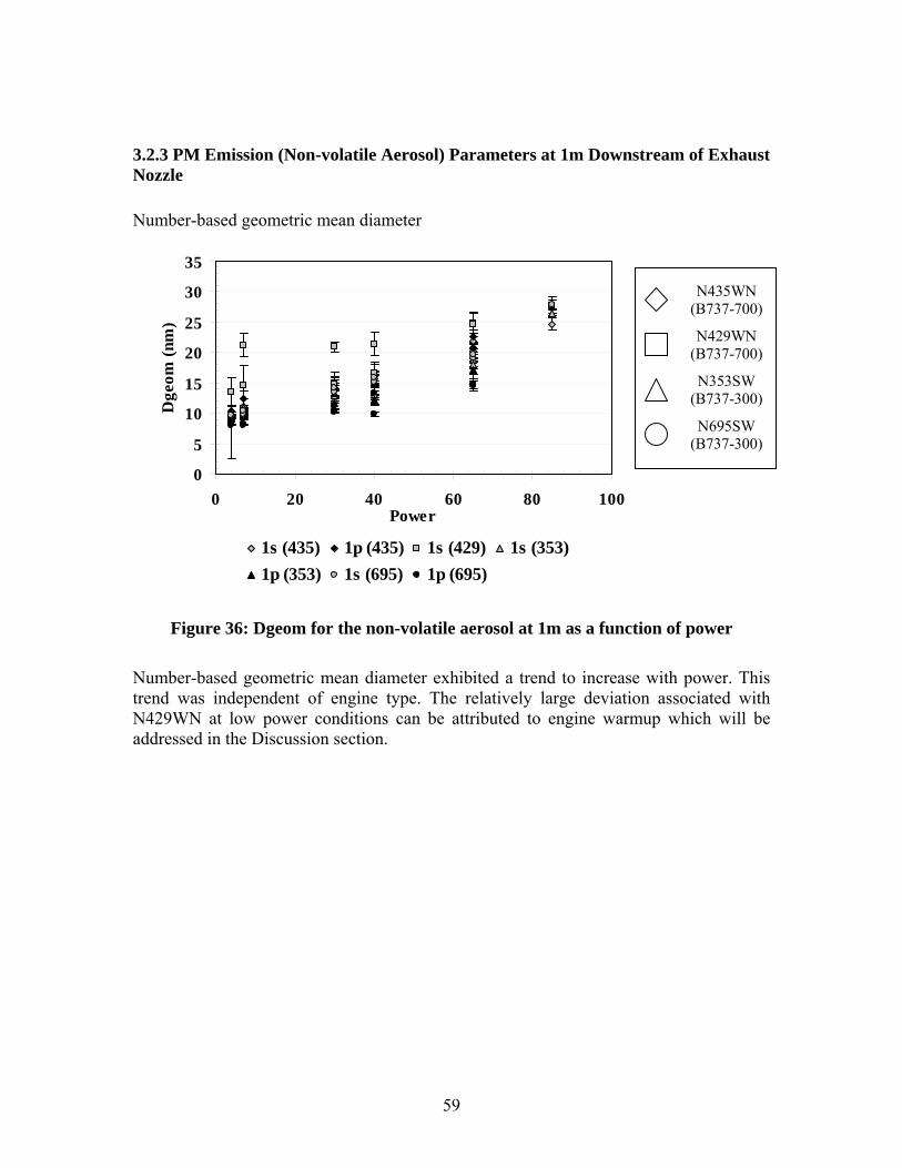
0

□

•

3.2.3 PM Emission (Non-volatile Aerosol) Parameters at 1m Downstream of Exhaust Nozzle

Number-based geometric mean diameter

Dge

om (n

m)

35

30

25

20

15

10

5

0 0 20 40 60 80 100

Power

N435WN (B737-700)

N429WN (B737-700)

N353SW (B737-300)

N695SW (B737-300)

1s (435) 1p (435) 1s (429) 1s (353) 1p (353) 1s (695) 1p (695)

Figure 36: Dgeom for the non-volatile aerosol at 1m as a function of power

Number-based geometric mean diameter exhibited a trend to increase with power. This trend was independent of engine type. The relatively large deviation associated with N429WN at low power conditions can be attributed to engine warmup which will be addressed in the Discussion section.

59

◊

♦

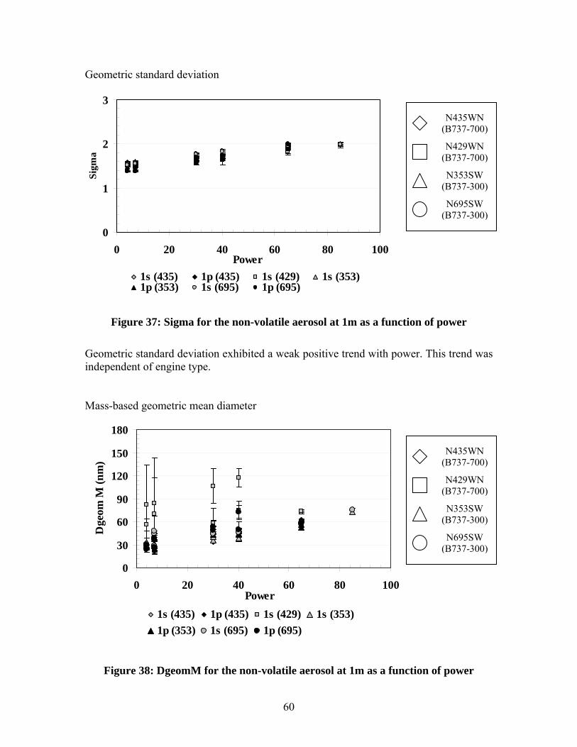
0

♦

0

□

•

□

•

g

I

Geometric standard deviation

3 N435WN

(B737-700) 2 N429WN

Sigm

a

0 20 40 60 80 100 Power

(B737-700)

N353SW (B737-300)1 N695SW

(B737-300)

0

1s (435) 1p (435) 1s (429) 1s (353) 1p (353) 1s (695) 1p (695)

Figure 37: Sigma for the non-volatile aerosol at 1m as a function of power

Geometric standard deviation exhibited a weak positive trend with power. This trend was independent of engine type.

Mass-based geometric mean diameter

180

N435WN 150

Dge

om M

(nm

) (B737-700) 120 N429WN

(B737-700)90

N353SW (B737-300)60 N695SW

30 (B737-300)

0

1s (435) 1p (435) 1s (429) 1s (353) 1p (353) 1s (695) 1p (695)

0 20 40 60 80 100 Power

Figure 38: DgeomM for the non-volatile aerosol at 1m as a function of power

60

◊ ♦

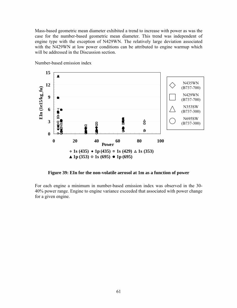
0

a

•

0. 0

◊

□ D 0

Mass-based geometric mean diameter exhibited a trend to increase with power as was the case for the number-based geometric mean diameter. This trend was independent of engine type with the exception of N429WN. The relatively large deviation associated with the N429WN at low power conditions can be attributed to engine warmup which will be addressed in the Discussion section.

Number-based emission index

15

N435WN 12 (B737-700)

N429WN 9 (B737-700)

N353SW 6 (B737-300)

N695SW 3 (B737-300)

0

EIn

(1e1

5/kg

_fu)

0 20 40 60 80 100 Power

1s (435) 1p (435) 1s (429) 1s (353) 1p (353) 1s (695) 1p (695)

Figure 39: EIn for the non-volatile aerosol at 1m as a function of power

For each engine a minimum in number-based emission index was observed in the 30-40% power range. Engine to engine variance exceeded that associated with power change for a given engine.

61

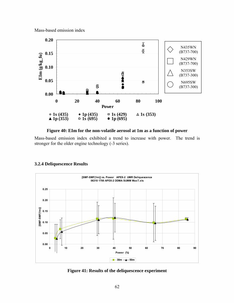
I) I /

' ~

L.---

V

♦

0

~

i B I

I I I I

r -=

---------- l

----

□

•

1---- --½-

~ Q ◊

□ D 0

I I I I

S7T =

Mass-based emission index

0.20 N435WN

EIm

(g/k

g_fu

) (B737-700)0.15 N429WN

(B737-700)0.10

N353SW (B737-300)

0.05 N695SW (B737-300)

0.00

1s (435) 1p (435) 1s (429) 1s (353) 1p (353) 1s (695) 1p (695)

Figure 40: EIm for the non-volatile aerosol at 1m as a function of power

0 20 40 60 80 100 Power

Mass-based emission index exhibited a trend to increase with power. The trend is stronger for the older engine technology (-3 series).

3.2.4 Deliquescence Results

[SMF-SMF(1m)] vs. Power APEX-2 UMR Deliquescence 06310 1700 APEX-2 DDMA SUMM MaxT.xls

0.00

0.05

0.10

0.15

0.20

0.25

0 10 20 30 40 50 60 70 80 90

Power (%)

[SM

F-SM

F(1m

)]

30m 50m

Figure 41: Results of the deliquescence experiment

62

At the 1m location, the Soluble Mass Fraction (SMF) of the aerosol sample was found to be negligible. This result is expected since the exit plane temperature (at 1m) greatly exceeds that of any anticipated soluble material e.g. sulfuric acid. The SMF was found to increase with distance from the engine exit plane reaching ~10% at 50m. No statistically significant variation is observed with engine power.

3.3 Total organic gases and aerosol chemical speciation (UCR)

3.3.1 UCR Results for Mass Flow

As discussed in the methodology section, UCR’s role was to deliver a special sampler and the measurement of speciated hydrocarbons and particulate matter for jet exhaust at each mode. A new sampler was needed for the JETS APEX 2 project since the sampler from APEX1 was not suitable for the test cycle designed for the JETS APEX2 project. Therefore UCR designed, constructed and planned to verify the performance of a custom high volume sampler before the tests at the Oakland Airport. However, ARB funding for the Oakland test was approved on August 9th and because the deployment to the field took place on August 20th, the approximate two week period after funding was spent purchasing parts, assembly, packaging, troubleshooting, and deploying the instrument. As a consequence of the late contracting and a policy of no pre-awards, neither the flow measurements nor the planned verification of the JETS APEX2 sampling unit against another sampling system, as is usually carried out for a new sampler before a field campaign, were carried out.

Much of the programming for the electronic controls and final leak checks and repairs to the sampler were made at the Oakland airport the day before testing started. As discussed earlier, UCR used a number of methods to ensure that the flows rates in the final sampler matched the planned values. The process started in the field by extensive leak checking of the system under pressure. Identifiable leaks were repaired. For example, the large pipe threads near the impactor required epoxy to seal the leak with subsequent vacuum checks indicating the system was leak tight. Finally, flow in the low flow channels (thermal desorption tube and carbonyl trap line) was verified with a primary flow calibration unit. The high flow rates were only verified when the unit was returned to UCR as there was no standard gauge available in the field.

Table 12 summarizes the calibrated flow rates through the sampling media and for the system. Each flow rate was pressure and temperature corrected for sampling conditions encountered for each engine. Critical flow orifices were used to control flow rates through all systems. With the exception of the Summa Canisters, all flows were operated under choked conditions (outlet pressure << 0.52 * inlet pressure). Thermocouples and absolute pressure gauges were used to correct for pressure and temperature fluctuations in the system. On the C4-C12 line (TDS tube line) and DNPH line, flows were also metered as differential pressure through a laminar flow element. Summa canisters were filled

63

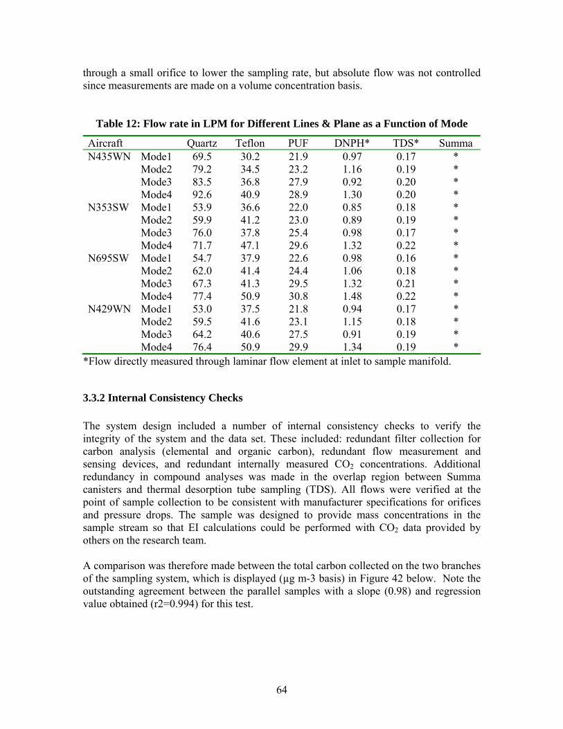
through a small orifice to lower the sampling rate, but absolute flow was not controlled since measurements are made on a volume concentration basis.

Table 12: Flow rate in LPM for Different Lines & Plane as a Function of Mode

Aircraft Quartz Teflon PUF DNPH* TDS* Summa N435WN Mode1 69.5 30.2 21.9 0.97 0.17 *

Mode2 79.2 34.5 23.2 1.16 0.19 * Mode3 83.5 36.8 27.9 0.92 0.20 * Mode4 92.6 40.9 28.9 1.30 0.20 *

N353SW Mode1 53.9 36.6 22.0 0.85 0.18 * Mode2 59.9 41.2 23.0 0.89 0.19 * Mode3 76.0 37.8 25.4 0.98 0.17 * Mode4 71.7 47.1 29.6 1.32 0.22 *

N695SW Mode1 54.7 37.9 22.6 0.98 0.16 * Mode2 62.0 41.4 24.4 1.06 0.18 * Mode3 67.3 41.3 29.5 1.32 0.21 * Mode4 77.4 50.9 30.8 1.48 0.22 *

N429WN Mode1 53.0 37.5 21.8 0.94 0.17 * Mode2 59.5 41.6 23.1 1.15 0.18 * Mode3 64.2 40.6 27.5 0.91 0.19 * Mode4 76.4 50.9 29.9 1.34 0.19 *

*Flow directly measured through laminar flow element at inlet to sample manifold.

3.3.2 Internal Consistency Checks

The system design included a number of internal consistency checks to verify the integrity of the system and the data set. These included: redundant filter collection for carbon analysis (elemental and organic carbon), redundant flow measurement and sensing devices, and redundant internally measured CO2 concentrations. Additional redundancy in compound analyses was made in the overlap region between Summa canisters and thermal desorption tube sampling (TDS). All flows were verified at the point of sample collection to be consistent with manufacturer specifications for orifices and pressure drops. The sample was designed to provide mass concentrations in the sample stream so that EI calculations could be performed with CO2 data provided by others on the research team.

A comparison was therefore made between the total carbon collected on the two branches of the sampling system, which is displayed (µg m-3 basis) in Figure 42 below. Note the outstanding agreement between the parallel samples with a slope (0.98) and regression value obtained (r2=0.994) for this test.

64

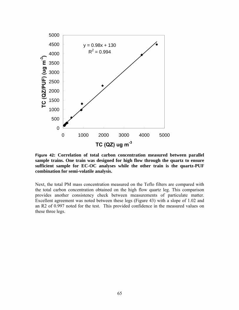
y = 0.98x + 130 R2 = 0.994

0

500

1000

1500

2000

2500

3000

3500

4000

4500

5000

TC (Q

Z/PU

F) (u

g m

-3 )

0 1000 2000 3000 4000 5000

TC (QZ) ug m-3

Figure 42: Correlation of total carbon concentration measured between parallel sample trains. One train was designed for high flow through the quartz to ensure sufficient sample for EC-OC analyses while the other train is the quartz-PUF combination for semi-volatile analysis.

Next, the total PM mass concentration measured on the Teflo filters are compared with the total carbon concentration obtained on the high flow quartz leg. This comparison provides another consistency check between measurements of particulate matter. Excellent agreement was noted between these legs (Figure 43) with a slope of 1.02 and an R2 of 0.997 noted for the test. This provided confidence in the measured values on these three legs.

65

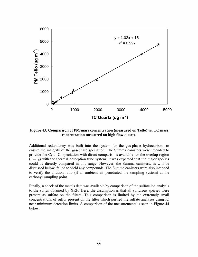
y = 1.02x + 15 R2 = 0.997

0

1000

2000

3000

4000

5000

6000

PM T

eflo

(ug

m-3

)

0 1000 2000 3000 4000 5000

TC Quartz (ug m-3)

Figure 43: Comparison of PM mass concentration (measured on Teflo) vs. TC mass concentration measured on high flow quartz.

Additional redundancy was built into the system for the gas-phase hydrocarbons to ensure the integrity of the gas-phase speciation. The Summa canisters were intended to provide the C1 to C8 speciation with direct comparisons available for the overlap region (C4-C8) with the thermal desorption tube system. It was expected that the major species could be directly compared in this range. However, the Summa canisters, as will be discussed below, failed to yield any compounds. The Summa canisters were also intended to verify the dilution ratio (if an ambient air penetrated the sampling system) at the carbonyl sampling point.

Finally, a check of the metals data was available by comparison of the sulfate ion analysis to the sulfur obtained by XRF. Here, the assumption is that all sulfurous species were present as sulfate on the filters. This comparison is limited by the extremely small concentrations of sulfur present on the filter which pushed the sulfate analyses using IC near minimum detection limits. A comparison of the measurements is seen in Figure 44 below.

66

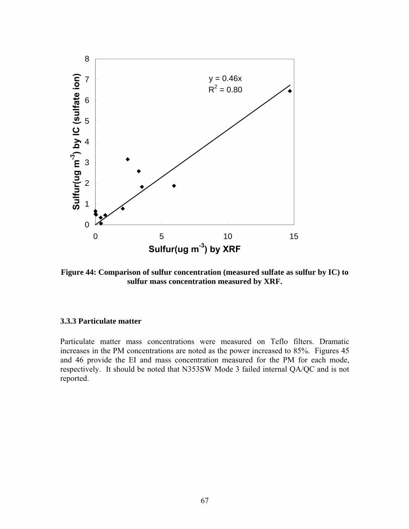
y = 0.46x R2 = 0.80

0

1

2

3

4

5

6

7

8

Sulfu

r(ug

m-3

) by

IC (s

ulfa

te io

n)

0 5 10 15 Sulfur(ug m-3) by XRF

Figure 44: Comparison of sulfur concentration (measured sulfate as sulfur by IC) to sulfur mass concentration measured by XRF.

3.3.3 Particulate matter

Particulate matter mass concentrations were measured on Teflo filters. Dramatic increases in the PM concentrations are noted as the power increased to 85%. Figures 45 and 46 provide the EI and mass concentration measured for the PM for each mode, respectively. It should be noted that N353SW Mode 3 failed internal QA/QC and is not reported.

67

~ -

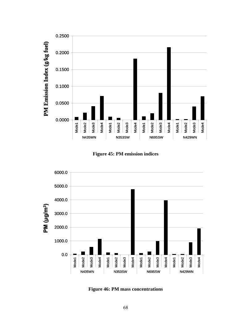
La_ -- • - -- - ~- -- -

- -

- - - - -- -- -- -

PM (μ

g/m

3 )PM

Em

issi

on In

dex

(g/k

g fu

el)

0.2500

0.2000

0.1500

0.1000

0.0500

0.0000

PM (μ

g/m

3 ) PM

Em

issi

on In

dex

(g/k

g fu

el)

0.2500

0.2000

0.1500

0.1000

0.0500

0.0000

Mod

e1

Mod

e2

Mod

e3

Mod

e4

Mod

e1

Mod

e2

Mod

e3

Mod

e4

Mod

e1

Mod

e2

Mod

e3

Mod

e4

Mod

e1

Mod

e2

Mod

e3

Mod

e4

N435WN N353SW N695SW N429WN

Mod

e1

Mod

e2

Mod

e3

Mod

e4

Mod

e1

Mod

e2

Mod

e3

Mod

e4

Mod

e1

Mod

e2

Mod

e3

Mod

e4

Mod

e1

Mod

e2

Mod

e3

Mod

e4

N435WN N353SW N695SW N429WN

Figure 45: PM emission indices

0.0

1000.0

2000.0

3000.0

4000.0

5000.0

6000.0

Mod

e1

Mod

e2

Mod

e3

Mod

e4

Mod

e1

Mod

e2

Mod

e3

Mod

e4

Mod

e1

Mod

e2

Mod

e3

Mod

e4

Mod

e1

Mod

e2

Mod

e3

Mod

e4

N435WN N353SW N695SW N429WN

0.0

1000.0

2000.0

3000.0

4000.0

5000.0

6000.0

Mod

e1

Mod

e2

Mod

e3

Mod

e4

Mod

e1

Mod

e2

Mod

e3

Mod

e4

Mod

e1

Mod

e2

Mod

e3

Mod

e4

Mod

e1

Mod

e2

Mod

e3

Mod

e4

N435WN N353SW N695SW N429WN

Figure 46: PM mass concentrations

68

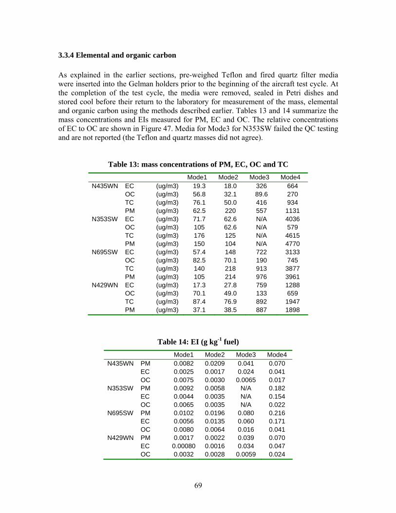
3.3.4 Elemental and organic carbon

As explained in the earlier sections, pre-weighed Teflon and fired quartz filter media were inserted into the Gelman holders prior to the beginning of the aircraft test cycle. At the completion of the test cycle, the media were removed, sealed in Petri dishes and stored cool before their return to the laboratory for measurement of the mass, elemental and organic carbon using the methods described earlier. Tables 13 and 14 summarize the mass concentrations and EIs measured for PM, EC and OC. The relative concentrations of EC to OC are shown in Figure 47. Media for Mode3 for N353SW failed the QC testing and are not reported (the Teflon and quartz masses did not agree).

Table 13: mass concentrations of PM, EC, OC and TC Mode1 Mode2 Mode3 Mode4

N435WN EC (ug/m3) 19.3 18.0 326 664 OC (ug/m3) 56.8 32.1 89.6 270 TC (ug/m3) 76.1 50.0 416 934 PM (ug/m3) 62.5 220 557 1131

N353SW EC (ug/m3) 71.7 62.6 N/A 4036 OC (ug/m3) 105 62.6 N/A 579 TC (ug/m3) 176 125 N/A 4615 PM (ug/m3) 150 104 N/A 4770

N695SW EC (ug/m3) 57.4 148 722 3133 OC (ug/m3) 82.5 70.1 190 745 TC (ug/m3) 140 218 913 3877 PM (ug/m3) 105 214 976 3961

N429WN EC (ug/m3) 17.3 27.8 759 1288 OC (ug/m3) 70.1 49.0 133 659 TC (ug/m3) 87.4 76.9 892 1947 PM (ug/m3) 37.1 38.5 887 1898

Table 14: EI (g kg-1 fuel) Mode1 Mode2 Mode3 Mode4

N435WN PM 0.0082 0.0209 0.041 0.070 EC 0.0025 0.0017 0.024 0.041 OC 0.0075 0.0030 0.0065 0.017

N353SW PM 0.0092 0.0058 N/A 0.182 EC 0.0044 0.0035 N/A 0.154 OC 0.0065 0.0035 N/A 0.022

N695SW PM 0.0102 0.0196 0.080 0.216 EC 0.0056 0.0135 0.060 0.171 OC 0.0080 0.0064 0.016 0.041

N429WN PM 0.0017 0.0022 0.039 0.070 EC 0.00080 0.0016 0.034 0.047 OC 0.0032 0.0028 0.0059 0.024

69

■ ■

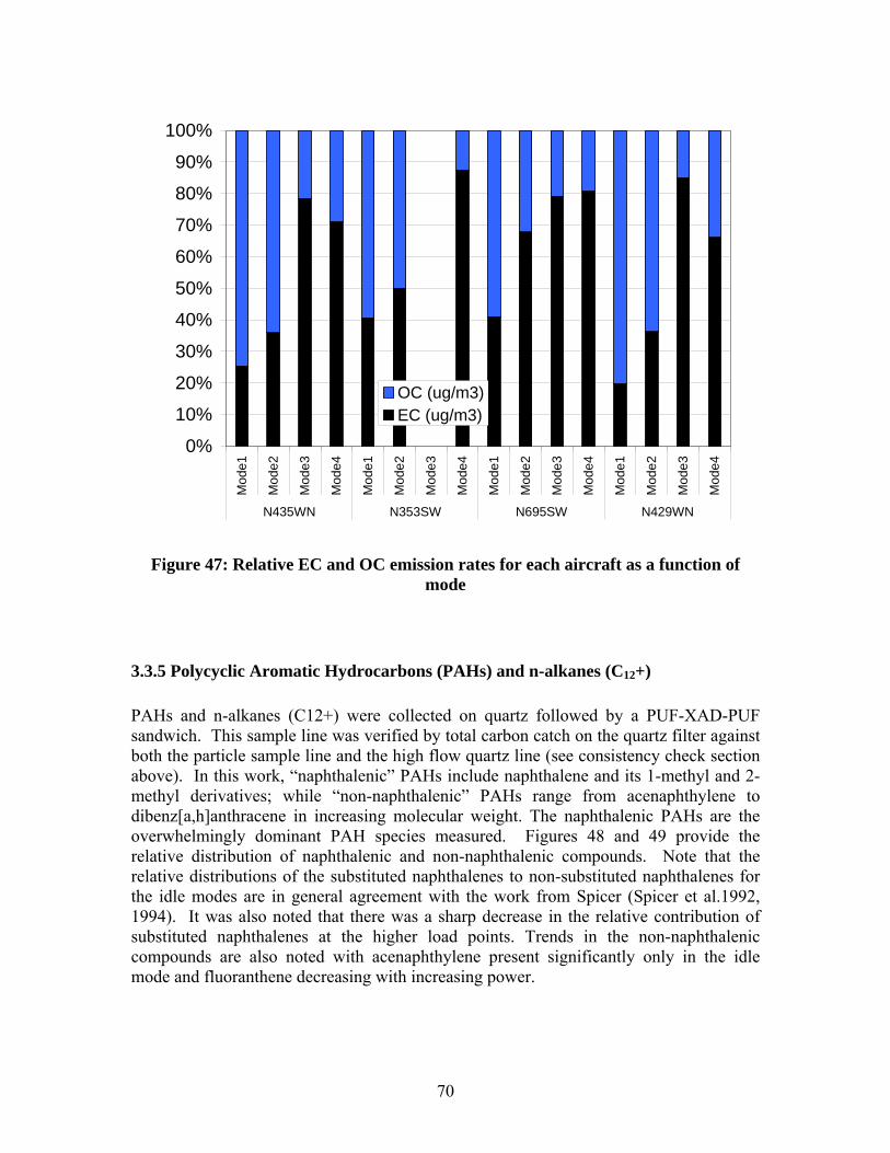
100%

90%

80%

70%

60%

50%

40%

30%

20%

10%

0%

Mod

e1

Mod

e2

Mod

e3

Mod

e4

Mod

e1

Mod

e2

Mod

e3

Mod

e4

Mod

e1

Mod

e2

Mod

e3

Mod

e4

Mod

e1

Mod

e2

Mod

e3

Mod

e4

OC (ug/m3) EC (ug/m3)

N435WN N353SW N695SW N429WN

Figure 47: Relative EC and OC emission rates for each aircraft as a function of mode

3.3.5 Polycyclic Aromatic Hydrocarbons (PAHs) and n-alkanes (C12+)

PAHs and n-alkanes (C12+) were collected on quartz followed by a PUF-XAD-PUF sandwich. This sample line was verified by total carbon catch on the quartz filter against both the particle sample line and the high flow quartz line (see consistency check section above). In this work, “naphthalenic” PAHs include naphthalene and its 1-methyl and 2-methyl derivatives; while “non-naphthalenic” PAHs range from acenaphthylene to dibenz[a,h]anthracene in increasing molecular weight. The naphthalenic PAHs are the overwhelmingly dominant PAH species measured. Figures 48 and 49 provide the relative distribution of naphthalenic and non-naphthalenic compounds. Note that the relative distributions of the substituted naphthalenes to non-substituted naphthalenes for the idle modes are in general agreement with the work from Spicer (Spicer et al.1992, 1994). It was also noted that there was a sharp decrease in the relative contribution of substituted naphthalenes at the higher load points. Trends in the non-naphthalenic compounds are also noted with acenaphthylene present significantly only in the idle mode and fluoranthene decreasing with increasing power.

70

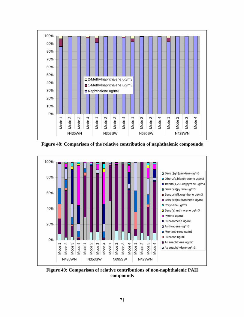
• I - -...

-

I

- -

I I !

-

□

■

□

-I

I

... i

- • I

11111 - ... - - -... ,-

I □

□

■

■ -

I ■

■

□

□

■

■

□

I I ■

□

■

□

0%

10%

20%

30%

40%

50%

60%

70%

80%

90%

100%

Mod

e 1

Mod

e 2

Mod

e 3

Mod

e 4

Mod

e 1

Mod

e 2

Mod

e 3

Mod

e 4

Mod

e 1

Mod

e 2

Mod

e 3

Mod

e 4

Mod

e 1

Mod

e 2

Mod

e 3

Mod

e 4

N435WN N353SW N695SW N429WN

2-Methylnaphthalene ug/m3 1-Methylnaphthalene ug/m3 Naphthalene ug/m3

Figure 48: Comparison of the relative contribution of naphthalenic compounds

0%

20%

40%

60%

80%

100%

Mod

e 1

Mod

e 2

Mod

e 3

Mod

e 4

Mod

e 1

Mod

e 2

Mod

e 3

Mod

e 4

Mod

e 1

Mod

e 2

Mod

e 3

Mod

e 4

Mod

e 1

Mod

e 2

Mod

e 3

Mod

e 4

N435WN N353SW N695SW N429WN

Benzo[ghi]perylene ug/m3

Dibenz[a,h]anthracene ug/m3

Indeno[1,2,3-cd]pyrene ug/m3

Benzo(a)pyrene ug/m3

Benzo(k)f luoranthene ug/m3

Benzo(b)fluoranthene ug/m3

Chrysene ug/m3

Benz(a)anthracene ug/m3

Pyrene ug/m3

Fluoranthene ug/m3

Anthracene ug/m3

Phenanthrene ug/m3

Fluorene ug/m3

Acenaphthene ug/m3

Acenaphthylene ug/m3

Figure 49: Comparison of relative contributions of non-naphthalenic PAH compounds

71

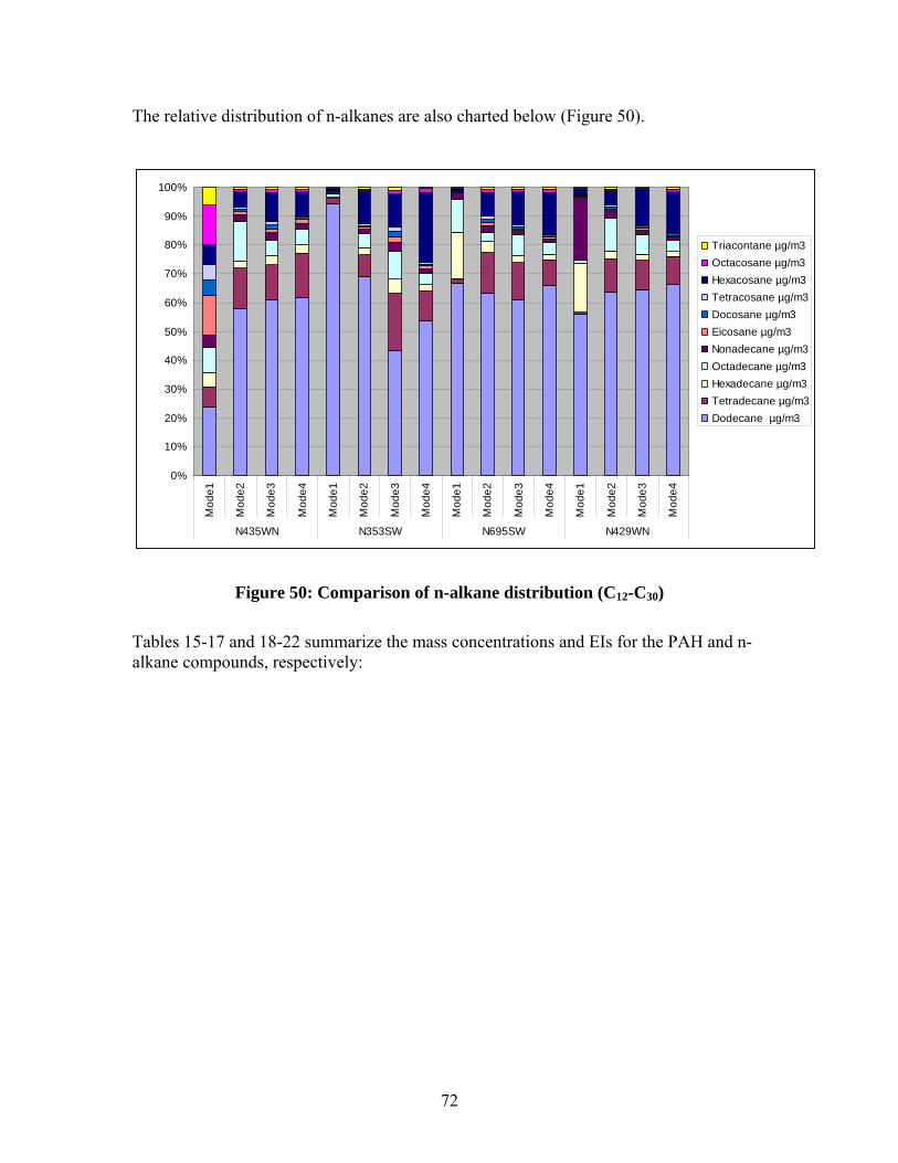
The relative distribution of n-alkanes are also charted below (Figure 50).

0%

10%

20%

30%

40%

50%

60%

70%

80%

90%

100%

Mod

e1

Mod

e2

Mod

e3

Mod

e4

Mod

e1

Mod

e2

Mod

e3

Mod

e4

Mod

e1

Mod

e2

Mod

e3

Mod

e4

Mod

e1

Mod

e2

Mod

e3

Mod

e4

N435WN N353SW N695SW N429WN

Triacontane µg/m3 Octacosane µg/m3 Hexacosane µg/m3 Tetracosane µg/m3 Docosane µg/m3 Eicosane µg/m3 Nonadecane µg/m3 Octadecane µg/m3 Hexadecane µg/m3 Tetradecane µg/m3 Dodecane µg/m3

Figure 50: Comparison of n-alkane distribution (C12-C30)

Tables 15-17 and 18-22 summarize the mass concentrations and EIs for the PAH and n-alkane compounds, respectively:

72

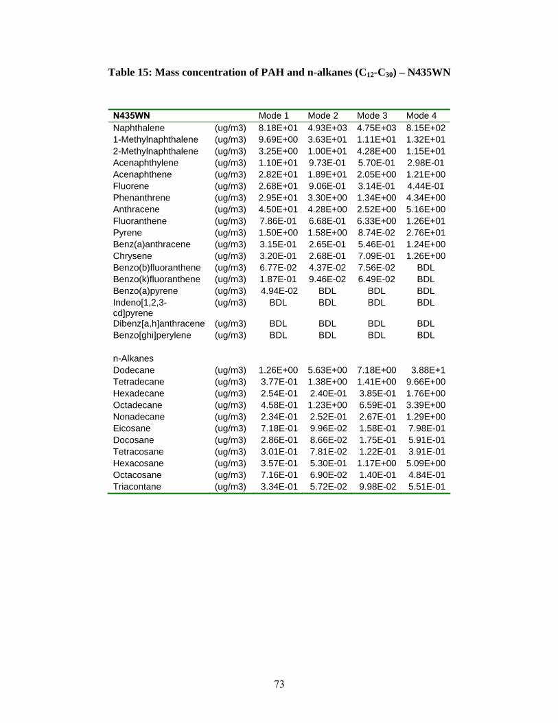
Table 15: Mass concentration of PAH and n-alkanes (C12-C30) – N435WN

N435WN Mode 1 Mode 2 Mode 3 Mode 4 Naphthalene (ug/m3) 8.18E+01 4.93E+03 4.75E+03 8.15E+02 1-Methylnaphthalene (ug/m3) 9.69E+00 3.63E+01 1.11E+01 1.32E+01 2-Methylnaphthalene (ug/m3) 3.25E+00 1.00E+01 4.28E+00 1.15E+01 Acenaphthylene (ug/m3) 1.10E+01 9.73E-01 5.70E-01 2.98E-01 Acenaphthene (ug/m3) 2.82E+01 1.89E+01 2.05E+00 1.21E+00 Fluorene (ug/m3) 2.68E+01 9.06E-01 3.14E-01 4.44E-01 Phenanthrene (ug/m3) 2.95E+01 3.30E+00 1.34E+00 4.34E+00 Anthracene (ug/m3) 4.50E+01 4.28E+00 2.52E+00 5.16E+00 Fluoranthene (ug/m3) 7.86E-01 6.68E-01 6.33E+00 1.26E+01 Pyrene (ug/m3) 1.50E+00 1.58E+00 8.74E-02 2.76E+01 Benz(a)anthracene (ug/m3) 3.15E-01 2.65E-01 5.46E-01 1.24E+00 Chrysene (ug/m3) 3.20E-01 2.68E-01 7.09E-01 1.26E+00 Benzo(b)fluoranthene (ug/m3) 6.77E-02 4.37E-02 7.56E-02 BDL Benzo(k)fluoranthene (ug/m3) 1.87E-01 9.46E-02 6.49E-02 BDL Benzo(a)pyrene (ug/m3) 4.94E-02 BDL BDL BDL Indeno[1,2,3- (ug/m3) BDL BDL BDL BDL cd]pyrene Dibenz[a,h]anthracene (ug/m3) BDL BDL BDL BDL Benzo[ghi]perylene (ug/m3) BDL BDL BDL BDL

n-Alkanes Dodecane (ug/m3) 1.26E+00 5.63E+00 7.18E+00 3.88E+1 Tetradecane (ug/m3) 3.77E-01 1.38E+00 1.41E+00 9.66E+00 Hexadecane (ug/m3) 2.54E-01 2.40E-01 3.85E-01 1.76E+00 Octadecane (ug/m3) 4.58E-01 1.23E+00 6.59E-01 3.39E+00 Nonadecane (ug/m3) 2.34E-01 2.52E-01 2.67E-01 1.29E+00 Eicosane (ug/m3) 7.18E-01 9.96E-02 1.58E-01 7.98E-01 Docosane (ug/m3) 2.86E-01 8.66E-02 1.75E-01 5.91E-01 Tetracosane (ug/m3) 3.01E-01 7.81E-02 1.22E-01 3.91E-01 Hexacosane (ug/m3) 3.57E-01 5.30E-01 1.17E+00 5.09E+00 Octacosane (ug/m3) 7.16E-01 6.90E-02 1.40E-01 4.84E-01 Triacontane (ug/m3) 3.34E-01 5.72E-02 9.98E-02 5.51E-01

73

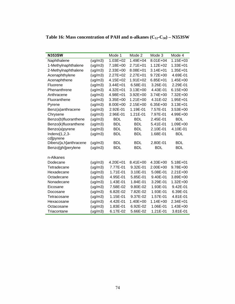
Table 16: Mass concentration of PAH and n-alkanes (C12-C30) – N353SW

N353SW Mode 1 Mode 2 Mode 3 Mode 4 Naphthalene (ug/m3) 1.03E+02 1.49E+04 8.01E+04 1.15E+03 1-Methylnaphthalene (ug/m3) 7.18E+00 2.71E+01 1.12E+02 1.33E+01 2-Methylnaphthalene (ug/m3) 2.33E+00 8.08E+01 3.14E+01 1.35E+01 Acenaphthylene (ug/m3) 2.27E+02 2.27E+01 9.72E+00 4.69E-01 Acenaphthene (ug/m3) 4.15E+02 1.91E+02 6.85E+01 1.45E+00 Fluorene (ug/m3) 3.44E+01 6.58E-01 3.26E-01 2.29E-01 Phenanthrene (ug/m3) 4.32E+01 3.13E+00 4.43E-01 6.15E+00 Anthracene (ug/m3) 4.98E+01 3.92E+00 3.74E+00 7.32E+00 Fluoranthene (ug/m3) 3.35E+00 1.21E+00 4.31E-02 1.95E+01 Pyrene (ug/m3) 8.00E+00 2.15E+00 6.35E+00 3.13E+01 Benz(a)anthracene (ug/m3) 2.92E-01 1.19E-01 7.57E-01 3.53E+00 Chrysene (ug/m3) 2.96E-01 1.21E-01 7.97E-01 4.99E+00 Benzo(b)fluoranthene (ug/m3) BDL BDL 2.45E-01 BDL Benzo(k)fluoranthene (ug/m3) BDL BDL 5.41E-01 1.09E+00 Benzo(a)pyrene (ug/m3) BDL BDL 2.10E-01 4.10E-01 Indeno[1,2,3- (ug/m3) BDL BDL 1.68E-01 BDL cd]pyrene Dibenz[a,h]anthracene (ug/m3) BDL BDL 2.80E-01 BDL Benzo[ghi]perylene (ug/m3) BDL BDL BDL BDL

n-Alkanes Dodecane (ug/m3) 4.20E+01 8.41E+00 4.33E+00 5.18E+01 Tetradecane (ug/m3) 7.77E-01 9.32E-01 2.00E+00 9.78E+00 Hexadecane (ug/m3) 1.71E-01 3.10E-01 5.08E-01 2.21E+00 Octadecane (ug/m3) 4.95E-01 5.85E-01 9.40E-01 3.89E+00 Nonadecane (ug/m3) 1.43E-01 1.84E-01 3.29E-01 1.32E+00 Eicosane (ug/m3) 7.58E-02 9.80E-02 1.93E-01 9.42E-01 Docosane (ug/m3) 6.82E-02 7.82E-02 1.93E-01 6.39E-01 Tetracosane (ug/m3) 1.15E-01 9.37E-02 1.57E-01 4.81E-01 Hexacosane (ug/m3) 4.42E-01 1.40E+00 1.14E+00 2.34E+01 Octacosane (ug/m3) 1.83E-01 6.92E-02 1.06E-01 1.43E+00 Triacontane (ug/m3) 6.17E-02 5.66E-02 1.21E-01 3.81E-01

74

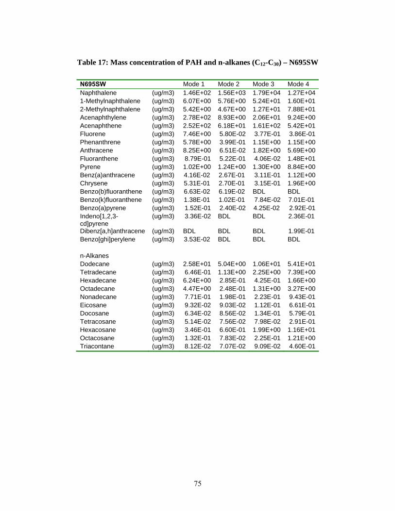
Table 17: Mass concentration of PAH and n-alkanes (C12-C30) – N695SW

N695SW Mode 1 Mode 2 Mode 3 Mode 4 Naphthalene (ug/m3) 1.46E+02 1.56E+03 1.79E+04 1.27E+04 1-Methylnaphthalene (ug/m3) 6.07E+00 5.76E+00 5.24E+01 1.60E+01 2-Methylnaphthalene (ug/m3) 5.42E+00 4.67E+00 1.27E+01 7.88E+01 Acenaphthylene (ug/m3) 2.78E+02 8.93E+00 2.06E+01 9.24E+00 Acenaphthene (ug/m3) 2.52E+02 6.18E+01 1.61E+02 5.42E+01 Fluorene (ug/m3) 7.46E+00 5.80E-02 3.77E-01 3.86E-01 Phenanthrene (ug/m3) 5.78E+00 3.99E-01 1.15E+00 1.15E+00 Anthracene (ug/m3) 8.25E+00 6.51E-02 1.82E+00 5.69E+00 Fluoranthene (ug/m3) 8.79E-01 5.22E-01 4.06E-02 1.48E+01 Pyrene (ug/m3) 1.02E+00 1.24E+00 1.30E+00 8.84E+00 Benz(a)anthracene (ug/m3) 4.16E-02 2.67E-01 3.11E-01 1.12E+00 Chrysene (ug/m3) 5.31E-01 2.70E-01 3.15E-01 1.96E+00 Benzo(b)fluoranthene (ug/m3) 6.63E-02 6.19E-02 BDL BDL Benzo(k)fluoranthene (ug/m3) 1.38E-01 1.02E-01 7.84E-02 7.01E-01 Benzo(a)pyrene (ug/m3) 1.52E-01 2.40E-02 4.25E-02 2.92E-01 Indeno[1,2,3- (ug/m3) 3.36E-02 BDL BDL 2.36E-01 cd]pyrene Dibenz[a,h]anthracene (ug/m3) BDL BDL BDL 1.99E-01 Benzo[ghi]perylene (ug/m3) 3.53E-02 BDL BDL BDL

n-Alkanes Dodecane (ug/m3) 2.58E+01 5.04E+00 1.06E+01 5.41E+01 Tetradecane (ug/m3) 6.46E-01 1.13E+00 2.25E+00 7.39E+00 Hexadecane (ug/m3) 6.24E+00 2.85E-01 4.25E-01 1.66E+00 Octadecane (ug/m3) 4.47E+00 2.48E-01 1.31E+00 3.27E+00 Nonadecane (ug/m3) 7.71E-01 1.98E-01 2.23E-01 9.43E-01 Eicosane (ug/m3) 9.32E-02 9.03E-02 1.12E-01 6.61E-01 Docosane (ug/m3) 6.34E-02 8.56E-02 1.34E-01 5.79E-01 Tetracosane (ug/m3) 5.14E-02 7.56E-02 7.98E-02 2.91E-01 Hexacosane (ug/m3) 3.46E-01 6.60E-01 1.99E+00 1.16E+01 Octacosane (ug/m3) 1.32E-01 7.83E-02 2.25E-01 1.21E+00 Triacontane (ug/m3) 8.12E-02 7.07E-02 9.09E-02 4.60E-01

75

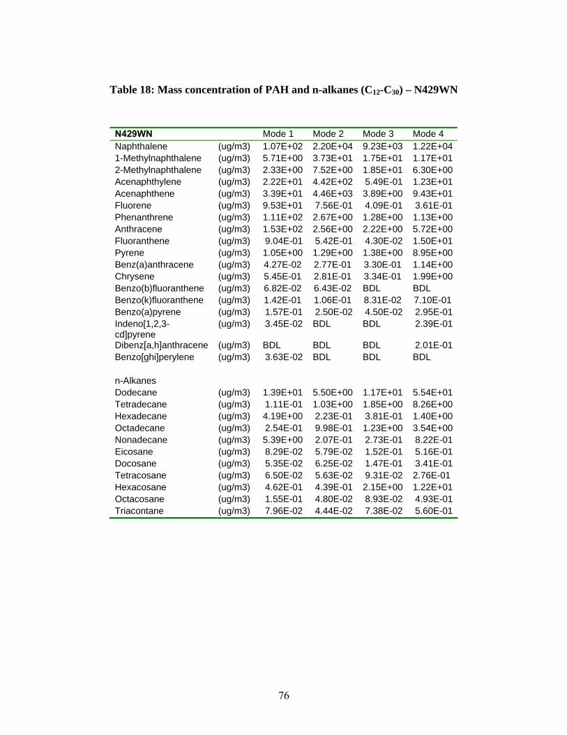
Table 18: Mass concentration of PAH and n-alkanes (C12-C30) – N429WN

N429WN Mode 1 Mode 2 Mode 3 Mode 4 Naphthalene (ug/m3) 1.07E+02 2.20E+04 9.23E+03 1.22E+04 1-Methylnaphthalene (ug/m3) 5.71E+00 3.73E+01 1.75E+01 1.17E+01 2-Methylnaphthalene (ug/m3) 2.33E+00 7.52E+00 1.85E+01 6.30E+00 Acenaphthylene (ug/m3) 2.22E+01 4.42E+02 5.49E-01 1.23E+01 Acenaphthene (ug/m3) 3.39E+01 4.46E+03 3.89E+00 9.43E+01 Fluorene (ug/m3) 9.53E+01 7.56E-01 4.09E-01 3.61E-01 Phenanthrene (ug/m3) 1.11E+02 2.67E+00 1.28E+00 1.13E+00 Anthracene (ug/m3) 1.53E+02 2.56E+00 2.22E+00 5.72E+00 Fluoranthene (ug/m3) 9.04E-01 5.42E-01 4.30E-02 1.50E+01 Pyrene (ug/m3) 1.05E+00 1.29E+00 1.38E+00 8.95E+00 Benz(a)anthracene (ug/m3) 4.27E-02 2.77E-01 3.30E-01 1.14E+00 Chrysene (ug/m3) 5.45E-01 2.81E-01 3.34E-01 1.99E+00 Benzo(b)fluoranthene (ug/m3) 6.82E-02 6.43E-02 BDL BDL Benzo(k)fluoranthene (ug/m3) 1.42E-01 1.06E-01 8.31E-02 7.10E-01 Benzo(a)pyrene (ug/m3) 1.57E-01 2.50E-02 4.50E-02 2.95E-01 Indeno[1,2,3- (ug/m3) 3.45E-02 BDL BDL 2.39E-01 cd]pyrene Dibenz[a,h]anthracene (ug/m3) BDL BDL BDL 2.01E-01 Benzo[ghi]perylene (ug/m3) 3.63E-02 BDL BDL BDL

n-Alkanes Dodecane (ug/m3) 1.39E+01 5.50E+00 1.17E+01 5.54E+01 Tetradecane (ug/m3) 1.11E-01 1.03E+00 1.85E+00 8.26E+00 Hexadecane (ug/m3) 4.19E+00 2.23E-01 3.81E-01 1.40E+00 Octadecane (ug/m3) 2.54E-01 9.98E-01 1.23E+00 3.54E+00 Nonadecane (ug/m3) 5.39E+00 2.07E-01 2.73E-01 8.22E-01 Eicosane (ug/m3) 8.29E-02 5.79E-02 1.52E-01 5.16E-01 Docosane (ug/m3) 5.35E-02 6.25E-02 1.47E-01 3.41E-01 Tetracosane (ug/m3) 6.50E-02 5.63E-02 9.31E-02 2.76E-01 Hexacosane (ug/m3) 4.62E-01 4.39E-01 2.15E+00 1.22E+01 Octacosane (ug/m3) 1.55E-01 4.80E-02 8.93E-02 4.93E-01 Triacontane (ug/m3) 7.96E-02 4.44E-02 7.38E-02 5.60E-01

76

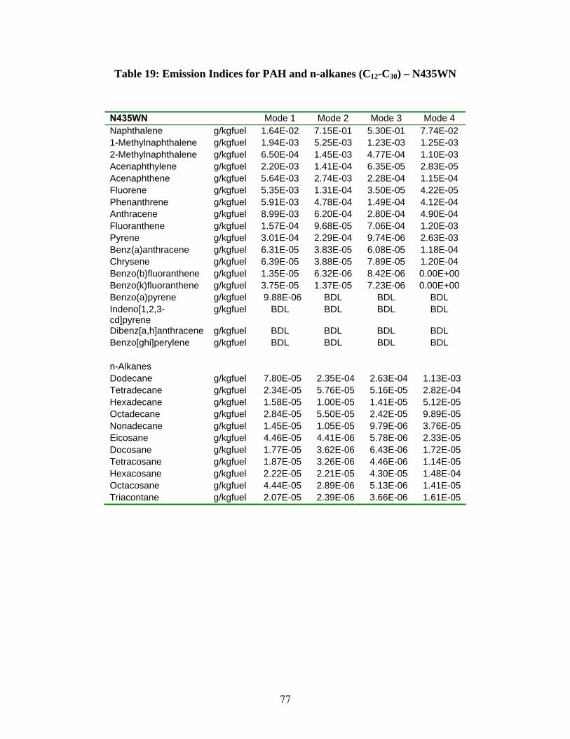
Table 19: Emission Indices for PAH and n-alkanes (C12-C30) – N435WN

N435WN Mode 1 Mode 2 Mode 3 Mode 4 Naphthalene g/kgfuel 1.64E-02 7.15E-01 5.30E-01 7.74E-02 1-Methylnaphthalene g/kgfuel 1.94E-03 5.25E-03 1.23E-03 1.25E-03 2-Methylnaphthalene g/kgfuel 6.50E-04 1.45E-03 4.77E-04 1.10E-03 Acenaphthylene g/kgfuel 2.20E-03 1.41E-04 6.35E-05 2.83E-05 Acenaphthene g/kgfuel 5.64E-03 2.74E-03 2.28E-04 1.15E-04 Fluorene g/kgfuel 5.35E-03 1.31E-04 3.50E-05 4.22E-05 Phenanthrene g/kgfuel 5.91E-03 4.78E-04 1.49E-04 4.12E-04 Anthracene g/kgfuel 8.99E-03 6.20E-04 2.80E-04 4.90E-04 Fluoranthene g/kgfuel 1.57E-04 9.68E-05 7.06E-04 1.20E-03 Pyrene g/kgfuel 3.01E-04 2.29E-04 9.74E-06 2.63E-03 Benz(a)anthracene g/kgfuel 6.31E-05 3.83E-05 6.08E-05 1.18E-04 Chrysene g/kgfuel 6.39E-05 3.88E-05 7.89E-05 1.20E-04 Benzo(b)fluoranthene g/kgfuel 1.35E-05 6.32E-06 8.42E-06 0.00E+00 Benzo(k)fluoranthene g/kgfuel 3.75E-05 1.37E-05 7.23E-06 0.00E+00 Benzo(a)pyrene g/kgfuel 9.88E-06 BDL BDL BDL Indeno[1,2,3- g/kgfuel BDL BDL BDL BDL cd]pyrene Dibenz[a,h]anthracene g/kgfuel BDL BDL BDL BDL Benzo[ghi]perylene g/kgfuel BDL BDL BDL BDL

n-Alkanes Dodecane g/kgfuel 7.80E-05 2.35E-04 2.63E-04 1.13E-03 Tetradecane g/kgfuel 2.34E-05 5.76E-05 5.16E-05 2.82E-04 Hexadecane g/kgfuel 1.58E-05 1.00E-05 1.41E-05 5.12E-05 Octadecane g/kgfuel 2.84E-05 5.50E-05 2.42E-05 9.89E-05 Nonadecane g/kgfuel 1.45E-05 1.05E-05 9.79E-06 3.76E-05 Eicosane g/kgfuel 4.46E-05 4.41E-06 5.78E-06 2.33E-05 Docosane g/kgfuel 1.77E-05 3.62E-06 6.43E-06 1.72E-05 Tetracosane g/kgfuel 1.87E-05 3.26E-06 4.46E-06 1.14E-05 Hexacosane g/kgfuel 2.22E-05 2.21E-05 4.30E-05 1.48E-04 Octacosane g/kgfuel 4.44E-05 2.89E-06 5.13E-06 1.41E-05 Triacontane g/kgfuel 2.07E-05 2.39E-06 3.66E-06 1.61E-05

77

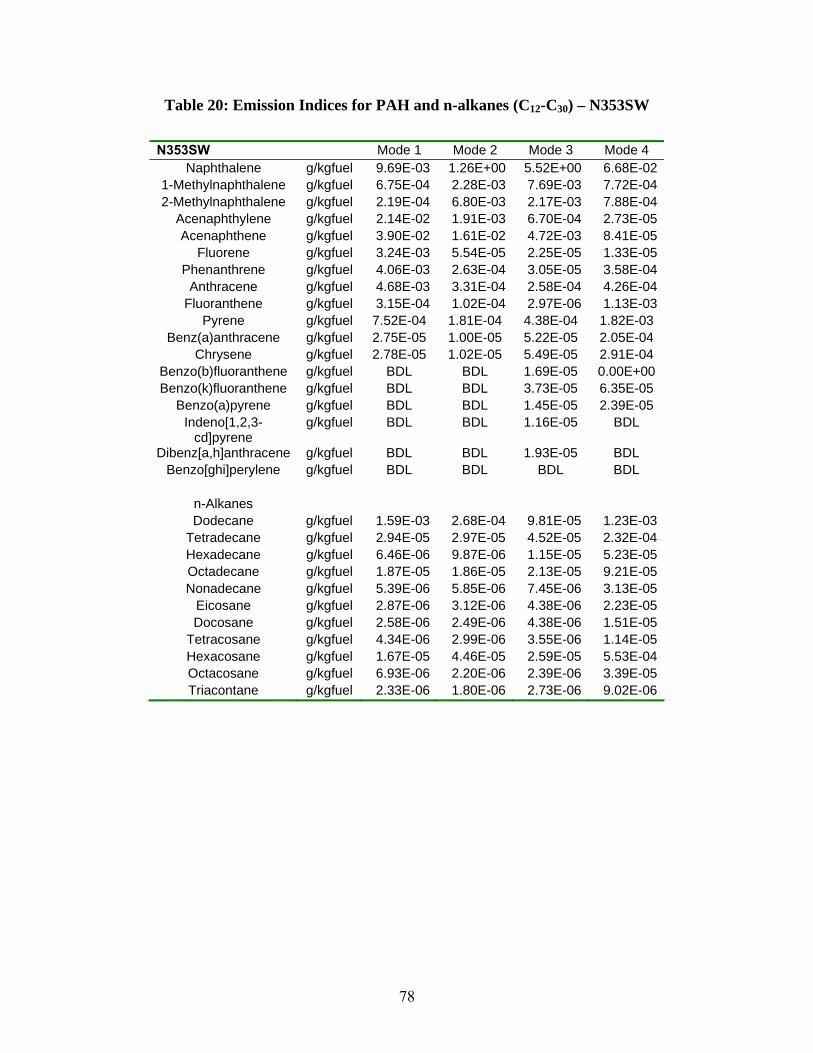
Table 20: Emission Indices for PAH and n-alkanes (C12-C30) – N353SW

N353SW Mode 1 Mode 2 Mode 3 Mode 4 Naphthalene g/kgfuel 9.69E-03 1.26E+00 5.52E+00 6.68E-02

1-Methylnaphthalene g/kgfuel 6.75E-04 2.28E-03 7.69E-03 7.72E-04 2-Methylnaphthalene g/kgfuel 2.19E-04 6.80E-03 2.17E-03 7.88E-04

Acenaphthylene g/kgfuel 2.14E-02 1.91E-03 6.70E-04 2.73E-05 Acenaphthene g/kgfuel 3.90E-02 1.61E-02 4.72E-03 8.41E-05

Fluorene g/kgfuel 3.24E-03 5.54E-05 2.25E-05 1.33E-05 Phenanthrene g/kgfuel 4.06E-03 2.63E-04 3.05E-05 3.58E-04

Anthracene g/kgfuel 4.68E-03 3.31E-04 2.58E-04 4.26E-04 Fluoranthene g/kgfuel 3.15E-04 1.02E-04 2.97E-06 1.13E-03

Pyrene g/kgfuel 7.52E-04 1.81E-04 4.38E-04 1.82E-03 Benz(a)anthracene g/kgfuel 2.75E-05 1.00E-05 5.22E-05 2.05E-04

Chrysene g/kgfuel 2.78E-05 1.02E-05 5.49E-05 2.91E-04 Benzo(b)fluoranthene g/kgfuel BDL BDL 1.69E-05 0.00E+00 Benzo(k)fluoranthene g/kgfuel BDL BDL 3.73E-05 6.35E-05

Benzo(a)pyrene g/kgfuel BDL BDL 1.45E-05 2.39E-05 Indeno[1,2,3- g/kgfuel BDL BDL 1.16E-05 BDL

cd]pyrene Dibenz[a,h]anthracene g/kgfuel BDL BDL 1.93E-05 BDL

Benzo[ghi]perylene g/kgfuel BDL BDL BDL BDL

n-Alkanes Dodecane g/kgfuel 1.59E-03 2.68E-04 9.81E-05 1.23E-03

Tetradecane g/kgfuel 2.94E-05 2.97E-05 4.52E-05 2.32E-04 Hexadecane g/kgfuel 6.46E-06 9.87E-06 1.15E-05 5.23E-05 Octadecane g/kgfuel 1.87E-05 1.86E-05 2.13E-05 9.21E-05 Nonadecane g/kgfuel 5.39E-06 5.85E-06 7.45E-06 3.13E-05

Eicosane g/kgfuel 2.87E-06 3.12E-06 4.38E-06 2.23E-05 Docosane g/kgfuel 2.58E-06 2.49E-06 4.38E-06 1.51E-05

Tetracosane g/kgfuel 4.34E-06 2.99E-06 3.55E-06 1.14E-05 Hexacosane g/kgfuel 1.67E-05 4.46E-05 2.59E-05 5.53E-04 Octacosane g/kgfuel 6.93E-06 2.20E-06 2.39E-06 3.39E-05 Triacontane g/kgfuel 2.33E-06 1.80E-06 2.73E-06 9.02E-06

78

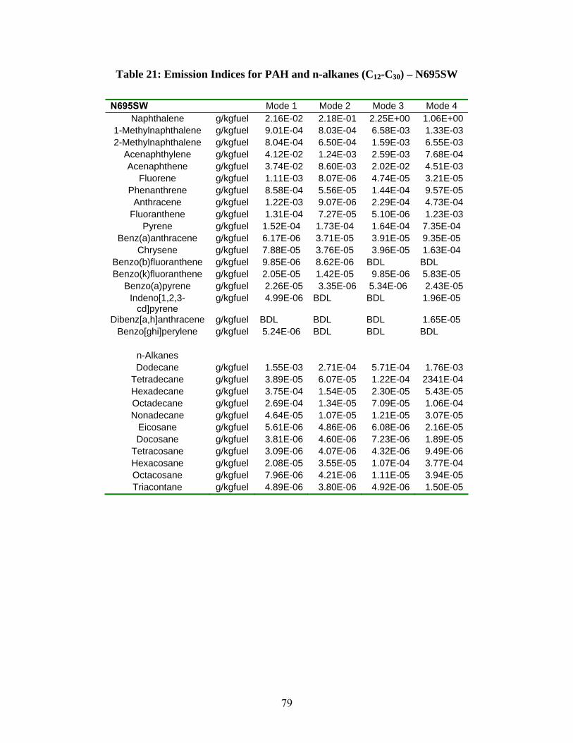
Table 21: Emission Indices for PAH and n-alkanes (C12-C30) – N695SW

N695SW Mode 1 Mode 2 Mode 3 Mode 4 Naphthalene g/kgfuel 2.16E-02 2.18E-01 2.25E+00 1.06E+00

1-Methylnaphthalene g/kgfuel 9.01E-04 8.03E-04 6.58E-03 1.33E-03 2-Methylnaphthalene g/kgfuel 8.04E-04 6.50E-04 1.59E-03 6.55E-03

Acenaphthylene g/kgfuel 4.12E-02 1.24E-03 2.59E-03 7.68E-04 Acenaphthene g/kgfuel 3.74E-02 8.60E-03 2.02E-02 4.51E-03

Fluorene g/kgfuel 1.11E-03 8.07E-06 4.74E-05 3.21E-05 Phenanthrene g/kgfuel 8.58E-04 5.56E-05 1.44E-04 9.57E-05

Anthracene g/kgfuel 1.22E-03 9.07E-06 2.29E-04 4.73E-04 Fluoranthene g/kgfuel 1.31E-04 7.27E-05 5.10E-06 1.23E-03

Pyrene g/kgfuel 1.52E-04 1.73E-04 1.64E-04 7.35E-04 Benz(a)anthracene g/kgfuel 6.17E-06 3.71E-05 3.91E-05 9.35E-05

Chrysene g/kgfuel 7.88E-05 3.76E-05 3.96E-05 1.63E-04 Benzo(b)fluoranthene g/kgfuel 9.85E-06 8.62E-06 BDL BDL Benzo(k)fluoranthene g/kgfuel 2.05E-05 1.42E-05 9.85E-06 5.83E-05

Benzo(a)pyrene g/kgfuel 2.26E-05 3.35E-06 5.34E-06 2.43E-05 Indeno[1,2,3- g/kgfuel 4.99E-06 BDL BDL 1.96E-05

cd]pyrene Dibenz[a,h]anthracene g/kgfuel BDL BDL BDL 1.65E-05

Benzo[ghi]perylene g/kgfuel 5.24E-06 BDL BDL BDL

n-Alkanes Dodecane g/kgfuel 1.55E-03 2.71E-04 5.71E-04 1.76E-03

Tetradecane g/kgfuel 3.89E-05 6.07E-05 1.22E-04 2341E-04 Hexadecane g/kgfuel 3.75E-04 1.54E-05 2.30E-05 5.43E-05 Octadecane g/kgfuel 2.69E-04 1.34E-05 7.09E-05 1.06E-04 Nonadecane g/kgfuel 4.64E-05 1.07E-05 1.21E-05 3.07E-05

Eicosane g/kgfuel 5.61E-06 4.86E-06 6.08E-06 2.16E-05 Docosane g/kgfuel 3.81E-06 4.60E-06 7.23E-06 1.89E-05

Tetracosane g/kgfuel 3.09E-06 4.07E-06 4.32E-06 9.49E-06 Hexacosane g/kgfuel 2.08E-05 3.55E-05 1.07E-04 3.77E-04 Octacosane g/kgfuel 7.96E-06 4.21E-06 1.11E-05 3.94E-05 Triacontane g/kgfuel 4.89E-06 3.80E-06 4.92E-06 1.50E-05

79

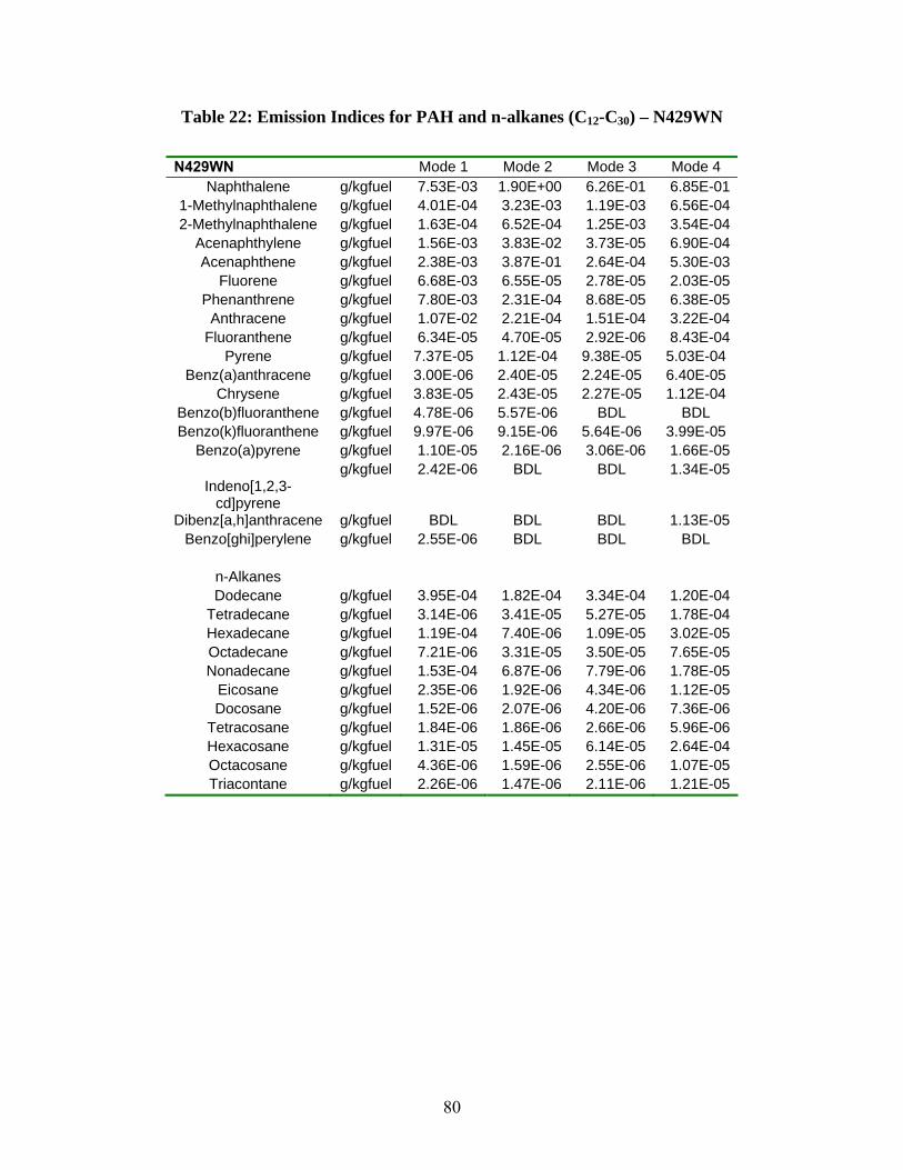
Table 22: Emission Indices for PAH and n-alkanes (C12-C30) – N429WN

N429WN Mode 1 Mode 2 Mode 3 Mode 4 Naphthalene g/kgfuel 7.53E-03 1.90E+00 6.26E-01 6.85E-01

1-Methylnaphthalene g/kgfuel 4.01E-04 3.23E-03 1.19E-03 6.56E-04 2-Methylnaphthalene g/kgfuel 1.63E-04 6.52E-04 1.25E-03 3.54E-04

Acenaphthylene g/kgfuel 1.56E-03 3.83E-02 3.73E-05 6.90E-04 Acenaphthene g/kgfuel 2.38E-03 3.87E-01 2.64E-04 5.30E-03

Fluorene g/kgfuel 6.68E-03 6.55E-05 2.78E-05 2.03E-05 Phenanthrene g/kgfuel 7.80E-03 2.31E-04 8.68E-05 6.38E-05

Anthracene g/kgfuel 1.07E-02 2.21E-04 1.51E-04 3.22E-04 Fluoranthene g/kgfuel 6.34E-05 4.70E-05 2.92E-06 8.43E-04

Pyrene g/kgfuel 7.37E-05 1.12E-04 9.38E-05 5.03E-04 Benz(a)anthracene g/kgfuel 3.00E-06 2.40E-05 2.24E-05 6.40E-05

Chrysene g/kgfuel 3.83E-05 2.43E-05 2.27E-05 1.12E-04 Benzo(b)fluoranthene g/kgfuel 4.78E-06 5.57E-06 BDL BDL Benzo(k)fluoranthene g/kgfuel 9.97E-06 9.15E-06 5.64E-06 3.99E-05

Benzo(a)pyrene g/kgfuel 1.10E-05 2.16E-06 3.06E-06 1.66E-05 g/kgfuel 2.42E-06 BDL BDL 1.34E-05

Indeno[1,2,3-cd]pyrene

Dibenz[a,h]anthracene g/kgfuel BDL BDL BDL 1.13E-05 Benzo[ghi]perylene g/kgfuel 2.55E-06 BDL BDL BDL

n-Alkanes Dodecane g/kgfuel 3.95E-04 1.82E-04 3.34E-04 1.20E-04

Tetradecane g/kgfuel 3.14E-06 3.41E-05 5.27E-05 1.78E-04 Hexadecane g/kgfuel 1.19E-04 7.40E-06 1.09E-05 3.02E-05 Octadecane g/kgfuel 7.21E-06 3.31E-05 3.50E-05 7.65E-05 Nonadecane g/kgfuel 1.53E-04 6.87E-06 7.79E-06 1.78E-05

Eicosane g/kgfuel 2.35E-06 1.92E-06 4.34E-06 1.12E-05 Docosane g/kgfuel 1.52E-06 2.07E-06 4.20E-06 7.36E-06

Tetracosane g/kgfuel 1.84E-06 1.86E-06 2.66E-06 5.96E-06 Hexacosane g/kgfuel 1.31E-05 1.45E-05 6.14E-05 2.64E-04 Octacosane g/kgfuel 4.36E-06 1.59E-06 2.55E-06 1.07E-05 Triacontane g/kgfuel 2.26E-06 1.47E-06 2.11E-06 1.21E-05

80

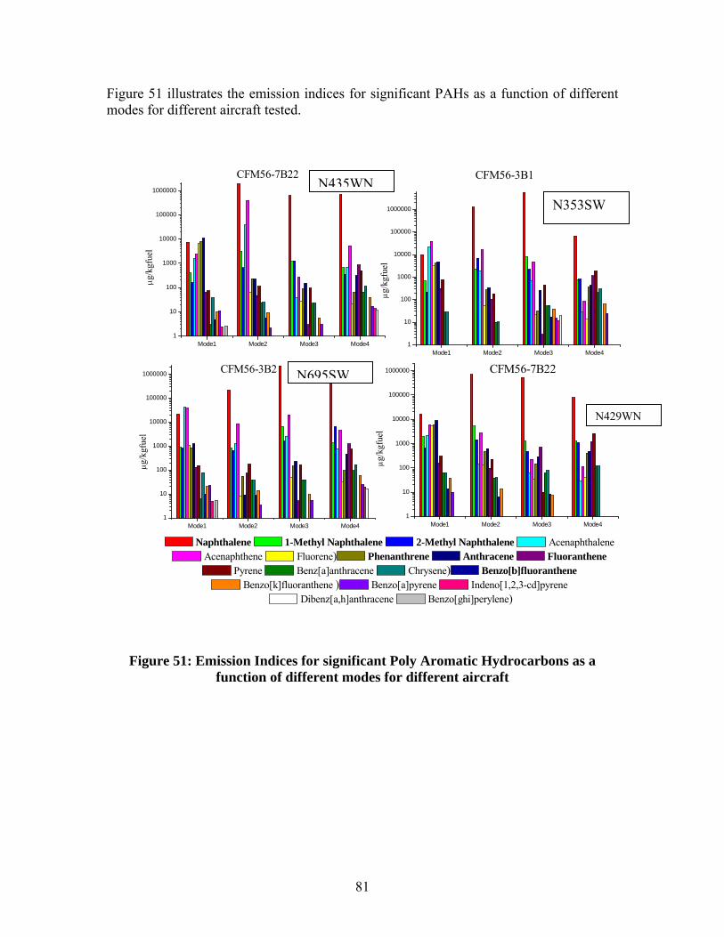
---~ C:J ~ -~

-- - -- --~

Figure 51 illustrates the emission indices for significant PAHs as a function of different modes for different aircraft tested.

Mode1 Mode2 Mode3 Mode4 1

10

100

1000

10000

100000

1000000

μg/k

gfue

l

CFM56-3B1

CFM56-3B2

Mode1 Mode2 Mode3 Mode4 1

10

100

1000

10000

100000

1000000

μg/k

gfue

l

CFM56-7B22

1

10

100

1000

10000

100000

1000000 μg

/kgf

uel

CFM56-7B22

N435WN N353SW

N695SW

N429WN

1000000

100000

10000

μg/k

gfue

l

1000

100

10

1 Mode1 Mode2 Mode3 Mode4 Mode1 Mode2 Mode3 Mode4

Naphthalene 1-Methyl Naphthalene 2-Methyl Naphthalene Acenaphthalene Acenaphthene Fluorene) Phenanthrene Anthracene Fluoranthene

Pyrene Benz[a]anthracene Chrysene) Benzo[b]fluoranthene Benzo[k]fluoranthene ) Benzo[a]pyrene Indeno[1,2,3-cd]pyrene

Dibenz[a,h]anthracene Benzo[ghi]perylene)

Figure 51: Emission Indices for significant Poly Aromatic Hydrocarbons as a function of different modes for different aircraft

81

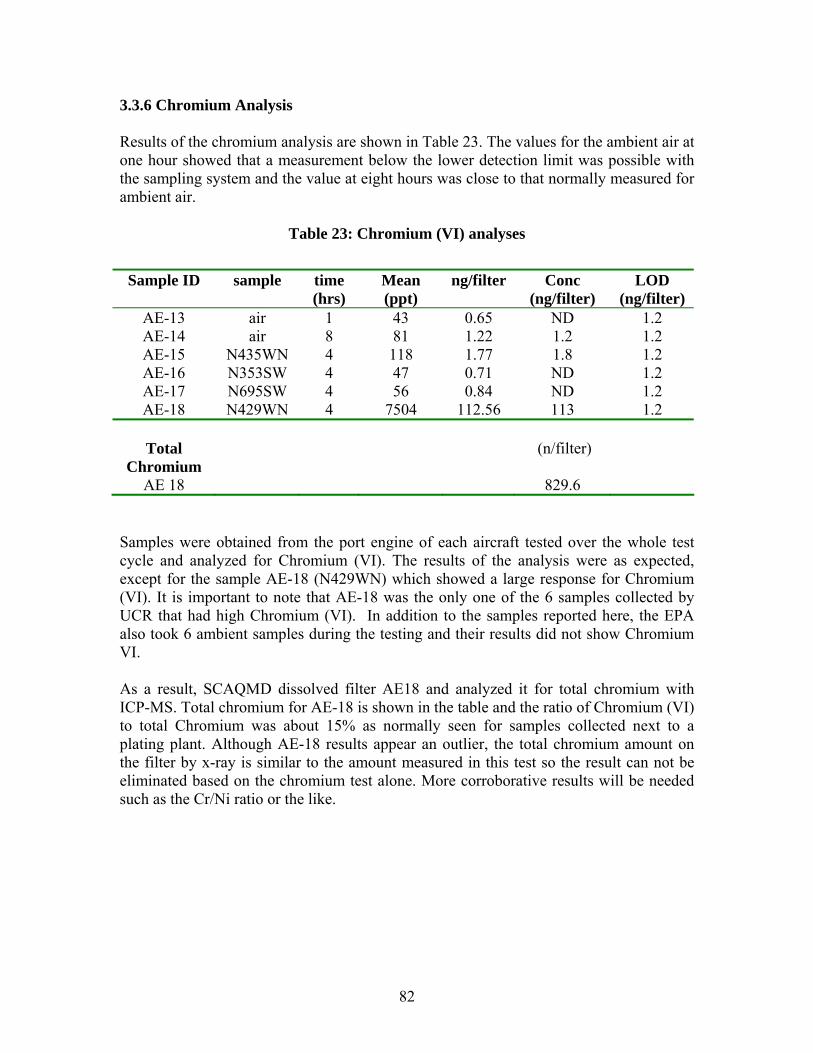
3.3.6 Chromium Analysis

Results of the chromium analysis are shown in Table 23. The values for the ambient air at one hour showed that a measurement below the lower detection limit was possible with the sampling system and the value at eight hours was close to that normally measured for ambient air.

Table 23: Chromium (VI) analyses

Sample ID sample time Mean ng/filter Conc LOD (hrs) (ppt) (ng/filter) (ng/filter)

AE-13 air 1 43 0.65 ND 1.2 AE-14 air 8 81 1.22 1.2 1.2 AE-15 N435WN 4 118 1.77 1.8 1.2 AE-16 N353SW 4 47 0.71 ND 1.2 AE-17 N695SW 4 56 0.84 ND 1.2 AE-18 N429WN 4 7504 112.56 113 1.2

Total (n/filter) Chromium

AE 18 829.6

Samples were obtained from the port engine of each aircraft tested over the whole test cycle and analyzed for Chromium (VI). The results of the analysis were as expected, except for the sample AE-18 (N429WN) which showed a large response for Chromium (VI). It is important to note that AE-18 was the only one of the 6 samples collected by UCR that had high Chromium (VI). In addition to the samples reported here, the EPA also took 6 ambient samples during the testing and their results did not show Chromium VI.

As a result, SCAQMD dissolved filter AE18 and analyzed it for total chromium with ICP-MS. Total chromium for AE-18 is shown in the table and the ratio of Chromium (VI) to total Chromium was about 15% as normally seen for samples collected next to a plating plant. Although AE-18 results appear an outlier, the total chromium amount on the filter by x-ray is similar to the amount measured in this test so the result can not be eliminated based on the chromium test alone. More corroborative results will be needed such as the Cr/Ni ratio or the like.

82

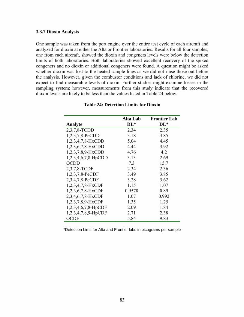
3.3.7 Dioxin Analysis

One sample was taken from the port engine over the entire test cycle of each aircraft and analyzed for dioxin at either the Alta or Frontier laboratories. Results for all four samples, one from each aircraft, showed the dioxin and congeners levels were below the detection limits of both laboratories. Both laboratories showed excellent recovery of the spiked congeners and no dioxin or additional congeners were found. A question might be asked whether dioxin was lost to the heated sample lines as we did not rinse those out before the analysis. However, given the combustor conditions and lack of chlorine, we did not expect to find measurable levels of dioxin. Further studies might examine losses in the sampling system; however, measurements from this study indicate that the recovered dioxin levels are likely to be less than the values listed in Table 24 below.

Table 24: Detection Limits for Dioxin

Alta Lab Frontier Lab Analyte DL* DL* 2,3,7,8-TCDD 2.34 2.35 1,2,3,7,8-PeCDD 3.18 3.85 1,2,3,4,7,8-HxCDD 5.04 4.45 1,2,3,6,7,8-HxCDD 4.44 3.92 1,2,3,7,8,9-HxCDD 4.76 4.2 1,2,3,4,6,7,8-HpCDD 3.13 2.69 OCDD 7.3 15.7 2,3,7,8-TCDF 2.34 2.36 1,2,3,7,8-PeCDF 3.49 3.85 2,3,4,7,8-PeCDF 3.28 3.62 1,2,3,4,7,8-HxCDF 1.15 1.07 1,2,3,6,7,8-HxCDF 0.9578 0.89 2,3,4,6,7,8-HxCDF 1.07 0.992 1,2,3,7,8,9-HxCDF 1.35 1.25 1,2,3,4,6,7,8-HpCDF 2.09 1.84 1,2,3,4,7,8,9-HpCDF 2.71 2.38 OCDF 5.84 9.83

*Detection Limit for Alta and Frontier labs in picograms per sample

83

- ,-

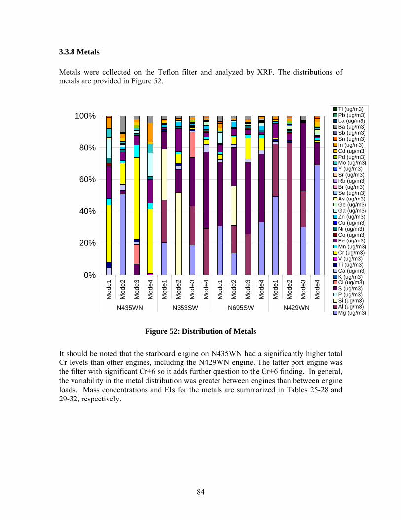
~ ;;;; iiii = ,- - : ,- -- ,-

! -"" I t::: ,-

~ = --- - i~ ~ - ~ - -

- -,-,- -

-- ~ ~ ~ ~ ~ ~ ~ -• >-

,--- - ~ ~ ~ - - -

--- ~ ~ ~ - -,-

I I ,-

ii = = i - I = -

I - - -

-- -

- - - -

- - - -

- - - -

~ - -ii

I -- --

- -

- -

- -

- -

- -

- -

- -

--s i -

-

-

-

-

■ ■ ■ □ ■ □ □ □ □ □ ■ □ □ □ □ □ □ □ □ ■ ■ ■ ■ □ □ ■ ■ □ ■ □ ■ □ □ ■ □

3.3.8 Metals

Metals were collected on the Teflon filter and analyzed by XRF. The distributions of metals are provided in Figure 52.

100%

80%

60%

40%

20%

0%

Mod

e1

Mod

e2

Mod

e3

Mod

e4

Mod

e1

Mod

e2

Mod

e3

Mod

e4

Mod

e1

Mod

e2

Mod

e3

Mod

e4

Mod

e1

Mod

e2

Mod

e3

Mod

e4

N435WN N353SW N695SW N429WN

Figure 52: Distribution of Metals

Tl (ug/m3) Pb (ug/m3)La (ug/m3) Ba (ug/m3) Sb (ug/m3) Sn (ug/m3)In (ug/m3) Cd (ug/m3) Pd (ug/m3) Mo (ug/m3)Y (ug/m3) Sr (ug/m3) Rb (ug/m3) Br (ug/m3)Se (ug/m3) As (ug/m3) Ge (ug/m3) Ga (ug/m3)Zn (ug/m3) Cu (ug/m3) Ni (ug/m3)Co (ug/m3) Fe (ug/m3) Mn (ug/m3) Cr (ug/m3)V (ug/m3) Ti (ug/m3) Ca (ug/m3) K (ug/m3)Cl (ug/m3) S (ug/m3) P (ug/m3) Si (ug/m3)Al (ug/m3) Mg (ug/m3)

It should be noted that the starboard engine on N435WN had a significantly higher total Cr levels than other engines, including the N429WN engine. The latter port engine was the filter with significant Cr+6 so it adds further question to the Cr+6 finding. In general, the variability in the metal distribution was greater between engines than between engine loads. Mass concentrations and EIs for the metals are summarized in Tables 25-28 and 29-32, respectively.

84

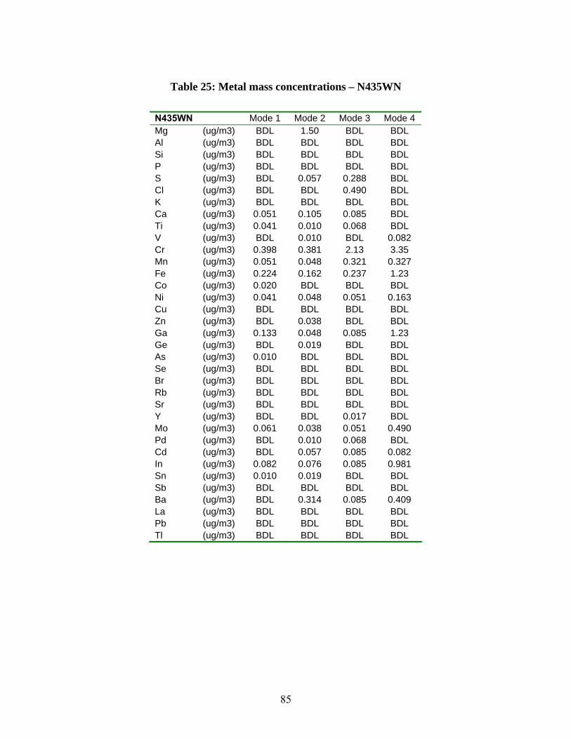
Table 25: Metal mass concentrations – N435WN

N435WN Mode 1 Mode 2 Mode 3 Mode 4 Mg (ug/m3) BDL 1.50 BDL BDL Al (ug/m3) BDL BDL BDL BDL Si (ug/m3) BDL BDL BDL BDL P (ug/m3) BDL BDL BDL BDL S (ug/m3) BDL 0.057 0.288 BDL Cl (ug/m3) BDL BDL 0.490 BDL K (ug/m3) BDL BDL BDL BDL Ca (ug/m3) 0.051 0.105 0.085 BDL Ti (ug/m3) 0.041 0.010 0.068 BDL V (ug/m3) BDL 0.010 BDL 0.082 Cr (ug/m3) 0.398 0.381 2.13 3.35 Mn (ug/m3) 0.051 0.048 0.321 0.327 Fe (ug/m3) 0.224 0.162 0.237 1.23 Co (ug/m3) 0.020 BDL BDL BDL Ni (ug/m3) 0.041 0.048 0.051 0.163 Cu (ug/m3) BDL BDL BDL BDL Zn (ug/m3) BDL 0.038 BDL BDL Ga (ug/m3) 0.133 0.048 0.085 1.23 Ge (ug/m3) BDL 0.019 BDL BDL As (ug/m3) 0.010 BDL BDL BDL Se (ug/m3) BDL BDL BDL BDL Br (ug/m3) BDL BDL BDL BDL Rb (ug/m3) BDL BDL BDL BDL Sr (ug/m3) BDL BDL BDL BDL Y (ug/m3) BDL BDL 0.017 BDL Mo (ug/m3) 0.061 0.038 0.051 0.490 Pd (ug/m3) BDL 0.010 0.068 BDL Cd (ug/m3) BDL 0.057 0.085 0.082 In (ug/m3) 0.082 0.076 0.085 0.981 Sn (ug/m3) 0.010 0.019 BDL BDL Sb (ug/m3) BDL BDL BDL BDL Ba (ug/m3) BDL 0.314 0.085 0.409 La (ug/m3) BDL BDL BDL BDL Pb (ug/m3) BDL BDL BDL BDL Tl (ug/m3) BDL BDL BDL BDL

85

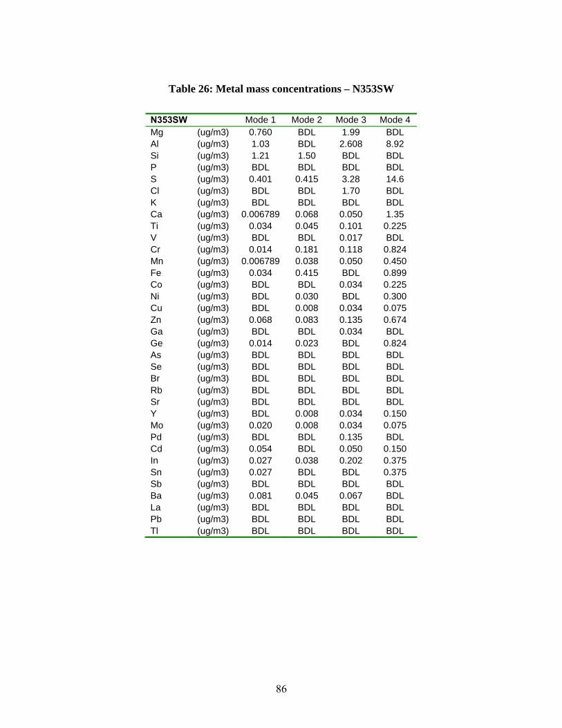
Table 26: Metal mass concentrations – N353SW

N353SW Mode 1 Mode 2 Mode 3 Mode 4 Mg (ug/m3) 0.760 BDL 1.99 BDL Al (ug/m3) 1.03 BDL 2.608 8.92 Si (ug/m3) 1.21 1.50 BDL BDL P (ug/m3) BDL BDL BDL BDL S (ug/m3) 0.401 0.415 3.28 14.6 Cl (ug/m3) BDL BDL 1.70 BDL K (ug/m3) BDL BDL BDL BDL Ca (ug/m3) 0.006789 0.068 0.050 1.35 Ti (ug/m3) 0.034 0.045 0.101 0.225 V (ug/m3) BDL BDL 0.017 BDL Cr (ug/m3) 0.014 0.181 0.118 0.824 Mn (ug/m3) 0.006789 0.038 0.050 0.450 Fe (ug/m3) 0.034 0.415 BDL 0.899 Co (ug/m3) BDL BDL 0.034 0.225 Ni (ug/m3) BDL 0.030 BDL 0.300 Cu (ug/m3) BDL 0.008 0.034 0.075 Zn (ug/m3) 0.068 0.083 0.135 0.674 Ga (ug/m3) BDL BDL 0.034 BDL Ge (ug/m3) 0.014 0.023 BDL 0.824 As (ug/m3) BDL BDL BDL BDL Se (ug/m3) BDL BDL BDL BDL Br (ug/m3) BDL BDL BDL BDL Rb (ug/m3) BDL BDL BDL BDL Sr (ug/m3) BDL BDL BDL BDL Y (ug/m3) BDL 0.008 0.034 0.150 Mo (ug/m3) 0.020 0.008 0.034 0.075 Pd (ug/m3) BDL BDL 0.135 BDL Cd (ug/m3) 0.054 BDL 0.050 0.150 In (ug/m3) 0.027 0.038 0.202 0.375 Sn (ug/m3) 0.027 BDL BDL 0.375 Sb (ug/m3) BDL BDL BDL BDL Ba (ug/m3) 0.081 0.045 0.067 BDL La (ug/m3) BDL BDL BDL BDL Pb (ug/m3) BDL BDL BDL BDL Tl (ug/m3) BDL BDL BDL BDL

86

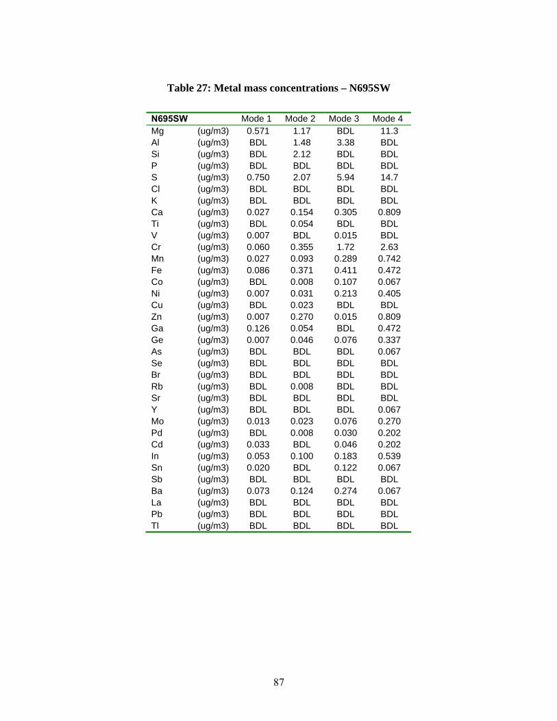
Table 27: Metal mass concentrations – N695SW

N695SW Mode 1 Mode 2 Mode 3 Mode 4 Mg (ug/m3) 0.571 1.17 BDL 11.3 Al (ug/m3) BDL 1.48 3.38 BDL Si (ug/m3) BDL 2.12 BDL BDL P (ug/m3) BDL BDL BDL BDL S (ug/m3) 0.750 2.07 5.94 14.7 Cl (ug/m3) BDL BDL BDL BDL K (ug/m3) BDL BDL BDL BDL Ca (ug/m3) 0.027 0.154 0.305 0.809 Ti (ug/m3) BDL 0.054 BDL BDL V (ug/m3) 0.007 BDL 0.015 BDL Cr (ug/m3) 0.060 0.355 1.72 2.63 Mn (ug/m3) 0.027 0.093 0.289 0.742 Fe (ug/m3) 0.086 0.371 0.411 0.472 Co (ug/m3) BDL 0.008 0.107 0.067 Ni (ug/m3) 0.007 0.031 0.213 0.405 Cu (ug/m3) BDL 0.023 BDL BDL Zn (ug/m3) 0.007 0.270 0.015 0.809 Ga (ug/m3) 0.126 0.054 BDL 0.472 Ge (ug/m3) 0.007 0.046 0.076 0.337 As (ug/m3) BDL BDL BDL 0.067 Se (ug/m3) BDL BDL BDL BDL Br (ug/m3) BDL BDL BDL BDL Rb (ug/m3) BDL 0.008 BDL BDL Sr (ug/m3) BDL BDL BDL BDL Y (ug/m3) BDL BDL BDL 0.067 Mo (ug/m3) 0.013 0.023 0.076 0.270 Pd (ug/m3) BDL 0.008 0.030 0.202 Cd (ug/m3) 0.033 BDL 0.046 0.202 In (ug/m3) 0.053 0.100 0.183 0.539 Sn (ug/m3) 0.020 BDL 0.122 0.067 Sb (ug/m3) BDL BDL BDL BDL Ba (ug/m3) 0.073 0.124 0.274 0.067 La (ug/m3) BDL BDL BDL BDL Pb (ug/m3) BDL BDL BDL BDL Tl (ug/m3) BDL BDL BDL BDL

87

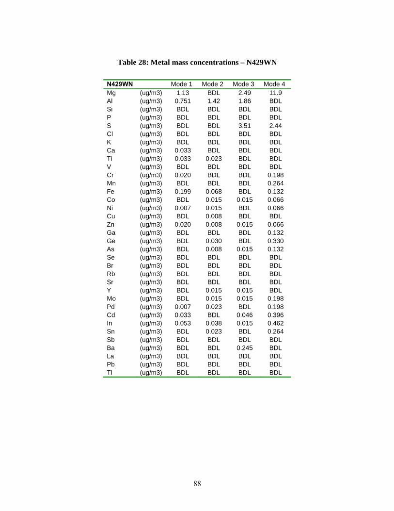
Table 28: Metal mass concentrations – N429WN

N429WN Mode 1 Mode 2 Mode 3 Mode 4 Mg (ug/m3) 1.13 BDL 2.49 11.9 Al (ug/m3) 0.751 1.42 1.86 BDL Si (ug/m3) BDL BDL BDL BDL P (ug/m3) BDL BDL BDL BDL S (ug/m3) BDL BDL 3.51 2.44 Cl (ug/m3) BDL BDL BDL BDL K (ug/m3) BDL BDL BDL BDL Ca (ug/m3) 0.033 BDL BDL BDL Ti (ug/m3) 0.033 0.023 BDL BDL V (ug/m3) BDL BDL BDL BDL Cr (ug/m3) 0.020 BDL BDL 0.198 Mn (ug/m3) BDL BDL BDL 0.264 Fe (ug/m3) 0.199 0.068 BDL 0.132 Co (ug/m3) BDL 0.015 0.015 0.066 Ni (ug/m3) 0.007 0.015 BDL 0.066 Cu (ug/m3) BDL 0.008 BDL BDL Zn (ug/m3) 0.020 0.008 0.015 0.066 Ga (ug/m3) BDL BDL BDL 0.132 Ge (ug/m3) BDL 0.030 BDL 0.330 As (ug/m3) BDL 0.008 0.015 0.132 Se (ug/m3) BDL BDL BDL BDL Br (ug/m3) BDL BDL BDL BDL Rb (ug/m3) BDL BDL BDL BDL Sr (ug/m3) BDL BDL BDL BDL Y (ug/m3) BDL 0.015 0.015 BDL Mo (ug/m3) BDL 0.015 0.015 0.198 Pd (ug/m3) 0.007 0.023 BDL 0.198 Cd (ug/m3) 0.033 BDL 0.046 0.396 In (ug/m3) 0.053 0.038 0.015 0.462 Sn (ug/m3) BDL 0.023 BDL 0.264 Sb (ug/m3) BDL BDL BDL BDL Ba (ug/m3) BDL BDL 0.245 BDL La (ug/m3) BDL BDL BDL BDL Pb (ug/m3) BDL BDL BDL BDL Tl (ug/m3) BDL BDL BDL BDL

88

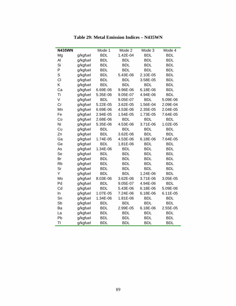
Table 29: Metal Emission Indices – N435WN

N435WN Mode 1 Mode 2 Mode 3 Mode 4 Mg g/kgfuel BDL 1.42E-04 BDL BDL Al g/kgfuel BDL BDL BDL BDL Si g/kgfuel BDL BDL BDL BDL P g/kgfuel BDL BDL BDL BDL S g/kgfuel BDL 5.43E-06 2.10E-05 BDL Cl g/kgfuel BDL BDL 3.58E-05 BDL K g/kgfuel BDL BDL BDL BDL Ca g/kgfuel 6.69E-06 9.96E-06 6.18E-06 BDL Ti g/kgfuel 5.35E-06 9.05E-07 4.94E-06 BDL V g/kgfuel BDL 9.05E-07 BDL 5.09E-06 Cr g/kgfuel 5.22E-05 3.62E-05 1.56E-04 2.09E-04 Mn g/kgfuel 6.69E-06 4.53E-06 2.35E-05 2.04E-05 Fe g/kgfuel 2.94E-05 1.54E-05 1.73E-05 7.64E-05 Co g/kgfuel 2.68E-06 BDL BDL BDL Ni g/kgfuel 5.35E-06 4.53E-06 3.71E-06 1.02E-05 Cu g/kgfuel BDL BDL BDL BDL Zn g/kgfuel BDL 3.62E-06 BDL BDL Ga g/kgfuel 1.74E-05 4.53E-06 6.18E-06 7.64E-05 Ge g/kgfuel BDL 1.81E-06 BDL BDL As g/kgfuel 1.34E-06 BDL BDL BDL Se g/kgfuel BDL BDL BDL BDL Br g/kgfuel BDL BDL BDL BDL Rb g/kgfuel BDL BDL BDL BDL Sr g/kgfuel BDL BDL BDL BDL Y g/kgfuel BDL BDL 1.24E-06 BDL Mo g/kgfuel 8.03E-06 3.62E-06 3.71E-06 3.05E-05 Pd g/kgfuel BDL 9.05E-07 4.94E-06 BDL Cd g/kgfuel BDL 5.43E-06 6.18E-06 5.09E-06 In g/kgfuel 1.07E-05 7.24E-06 6.18E-06 6.11E-05 Sn g/kgfuel 1.34E-06 1.81E-06 BDL BDL Sb g/kgfuel BDL BDL BDL BDL Ba g/kgfuel BDL 2.99E-05 6.18E-06 2.55E-05 La g/kgfuel BDL BDL BDL BDL Pb g/kgfuel BDL BDL BDL BDL Tl g/kgfuel BDL BDL BDL BDL

89

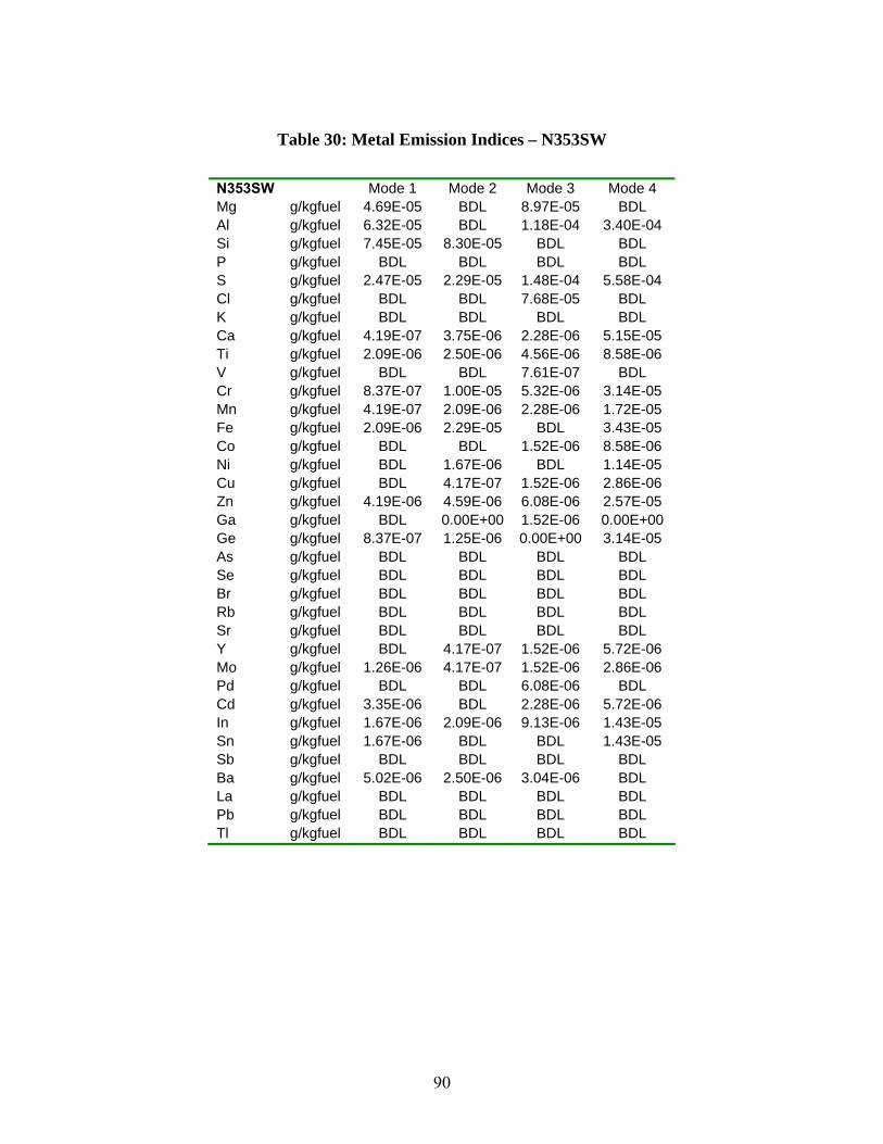
Table 30: Metal Emission Indices – N353SW

N353SW Mode 1 Mode 2 Mode 3 Mode 4 Mg g/kgfuel 4.69E-05 BDL 8.97E-05 BDL Al g/kgfuel 6.32E-05 BDL 1.18E-04 3.40E-04 Si g/kgfuel 7.45E-05 8.30E-05 BDL BDL P g/kgfuel BDL BDL BDL BDL S g/kgfuel 2.47E-05 2.29E-05 1.48E-04 5.58E-04 Cl g/kgfuel BDL BDL 7.68E-05 BDL K g/kgfuel BDL BDL BDL BDL Ca g/kgfuel 4.19E-07 3.75E-06 2.28E-06 5.15E-05 Ti g/kgfuel 2.09E-06 2.50E-06 4.56E-06 8.58E-06 V g/kgfuel BDL BDL 7.61E-07 BDL Cr g/kgfuel 8.37E-07 1.00E-05 5.32E-06 3.14E-05 Mn g/kgfuel 4.19E-07 2.09E-06 2.28E-06 1.72E-05 Fe g/kgfuel 2.09E-06 2.29E-05 BDL 3.43E-05 Co g/kgfuel BDL BDL 1.52E-06 8.58E-06 Ni g/kgfuel BDL 1.67E-06 BDL 1.14E-05 Cu g/kgfuel BDL 4.17E-07 1.52E-06 2.86E-06 Zn g/kgfuel 4.19E-06 4.59E-06 6.08E-06 2.57E-05 Ga g/kgfuel BDL 0.00E+00 1.52E-06 0.00E+00 Ge g/kgfuel 8.37E-07 1.25E-06 0.00E+00 3.14E-05 As g/kgfuel BDL BDL BDL BDL Se g/kgfuel BDL BDL BDL BDL Br g/kgfuel BDL BDL BDL BDL Rb g/kgfuel BDL BDL BDL BDL Sr g/kgfuel BDL BDL BDL BDL Y g/kgfuel BDL 4.17E-07 1.52E-06 5.72E-06 Mo g/kgfuel 1.26E-06 4.17E-07 1.52E-06 2.86E-06 Pd g/kgfuel BDL BDL 6.08E-06 BDL Cd g/kgfuel 3.35E-06 BDL 2.28E-06 5.72E-06 In g/kgfuel 1.67E-06 2.09E-06 9.13E-06 1.43E-05 Sn g/kgfuel 1.67E-06 BDL BDL 1.43E-05 Sb g/kgfuel BDL BDL BDL BDL Ba g/kgfuel 5.02E-06 2.50E-06 3.04E-06 BDL La g/kgfuel BDL BDL BDL BDL Pb g/kgfuel BDL BDL BDL BDL Tl g/kgfuel BDL BDL BDL BDL

90

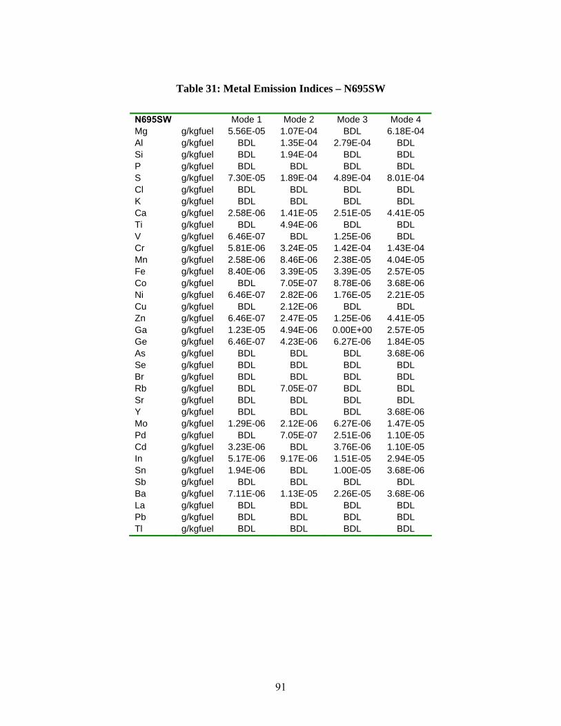
Table 31: Metal Emission Indices – N695SW

N695SW Mode 1 Mode 2 Mode 3 Mode 4 Mg g/kgfuel 5.56E-05 1.07E-04 BDL 6.18E-04 Al g/kgfuel BDL 1.35E-04 2.79E-04 BDL Si g/kgfuel BDL 1.94E-04 BDL BDL P g/kgfuel BDL BDL BDL BDL S g/kgfuel 7.30E-05 1.89E-04 4.89E-04 8.01E-04 Cl g/kgfuel BDL BDL BDL BDL K g/kgfuel BDL BDL BDL BDL Ca g/kgfuel 2.58E-06 1.41E-05 2.51E-05 4.41E-05 Ti g/kgfuel BDL 4.94E-06 BDL BDL V g/kgfuel 6.46E-07 BDL 1.25E-06 BDL Cr g/kgfuel 5.81E-06 3.24E-05 1.42E-04 1.43E-04 Mn g/kgfuel 2.58E-06 8.46E-06 2.38E-05 4.04E-05 Fe g/kgfuel 8.40E-06 3.39E-05 3.39E-05 2.57E-05 Co g/kgfuel BDL 7.05E-07 8.78E-06 3.68E-06 Ni g/kgfuel 6.46E-07 2.82E-06 1.76E-05 2.21E-05 Cu g/kgfuel BDL 2.12E-06 BDL BDL Zn g/kgfuel 6.46E-07 2.47E-05 1.25E-06 4.41E-05 Ga g/kgfuel 1.23E-05 4.94E-06 0.00E+00 2.57E-05 Ge g/kgfuel 6.46E-07 4.23E-06 6.27E-06 1.84E-05 As g/kgfuel BDL BDL BDL 3.68E-06 Se g/kgfuel BDL BDL BDL BDL Br g/kgfuel BDL BDL BDL BDL Rb g/kgfuel BDL 7.05E-07 BDL BDL Sr g/kgfuel BDL BDL BDL BDL Y g/kgfuel BDL BDL BDL 3.68E-06 Mo g/kgfuel 1.29E-06 2.12E-06 6.27E-06 1.47E-05 Pd g/kgfuel BDL 7.05E-07 2.51E-06 1.10E-05 Cd g/kgfuel 3.23E-06 BDL 3.76E-06 1.10E-05 In g/kgfuel 5.17E-06 9.17E-06 1.51E-05 2.94E-05 Sn g/kgfuel 1.94E-06 BDL 1.00E-05 3.68E-06 Sb g/kgfuel BDL BDL BDL BDL Ba g/kgfuel 7.11E-06 1.13E-05 2.26E-05 3.68E-06 La g/kgfuel BDL BDL BDL BDL Pb g/kgfuel BDL BDL BDL BDL Tl g/kgfuel BDL BDL BDL BDL

91

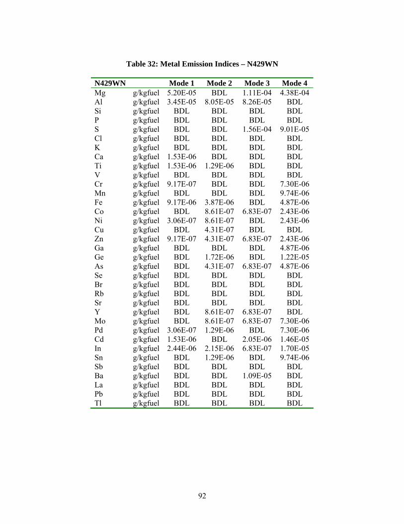
Table 32: Metal Emission Indices – N429WN

N429WN Mode 1 Mode 2 Mode 3 Mode 4 Mg g/kgfuel 5.20E-05 BDL 1.11E-04 4.38E-04 Al g/kgfuel 3.45E-05 8.05E-05 8.26E-05 BDL Si g/kgfuel BDL BDL BDL BDL P g/kgfuel BDL BDL BDL BDL S g/kgfuel BDL BDL 1.56E-04 9.01E-05 Cl g/kgfuel BDL BDL BDL BDL K g/kgfuel BDL BDL BDL BDL Ca g/kgfuel 1.53E-06 BDL BDL BDL Ti g/kgfuel 1.53E-06 1.29E-06 BDL BDL V g/kgfuel BDL BDL BDL BDL Cr g/kgfuel 9.17E-07 BDL BDL 7.30E-06 Mn g/kgfuel BDL BDL BDL 9.74E-06 Fe g/kgfuel 9.17E-06 3.87E-06 BDL 4.87E-06 Co g/kgfuel BDL 8.61E-07 6.83E-07 2.43E-06 Ni g/kgfuel 3.06E-07 8.61E-07 BDL 2.43E-06 Cu g/kgfuel BDL 4.31E-07 BDL BDL Zn g/kgfuel 9.17E-07 4.31E-07 6.83E-07 2.43E-06 Ga g/kgfuel BDL BDL BDL 4.87E-06 Ge g/kgfuel BDL 1.72E-06 BDL 1.22E-05 As g/kgfuel BDL 4.31E-07 6.83E-07 4.87E-06 Se g/kgfuel BDL BDL BDL BDL Br g/kgfuel BDL BDL BDL BDL Rb g/kgfuel BDL BDL BDL BDL Sr g/kgfuel BDL BDL BDL BDL Y g/kgfuel BDL 8.61E-07 6.83E-07 BDL Mo g/kgfuel BDL 8.61E-07 6.83E-07 7.30E-06 Pd g/kgfuel 3.06E-07 1.29E-06 BDL 7.30E-06 Cd g/kgfuel 1.53E-06 BDL 2.05E-06 1.46E-05 In g/kgfuel 2.44E-06 2.15E-06 6.83E-07 1.70E-05 Sn g/kgfuel BDL 1.29E-06 BDL 9.74E-06 Sb g/kgfuel BDL BDL BDL BDL Ba g/kgfuel BDL BDL 1.09E-05 BDL La g/kgfuel BDL BDL BDL BDL Pb g/kgfuel BDL BDL BDL BDL Tl g/kgfuel BDL BDL BDL BDL

92

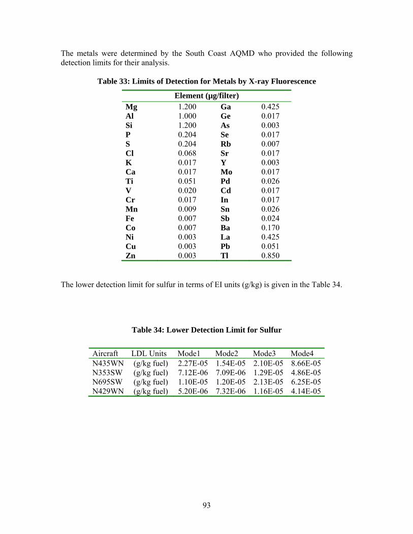
The metals were determined by the South Coast AQMD who provided the following detection limits for their analysis.

Table 33: Limits of Detection for Metals by X-ray Fluorescence

Element (µg/filter) Mg 1.200 Ga 0.425 Al 1.000 Ge 0.017 Si 1.200 As 0.003 P 0.204 Se 0.017 S 0.204 Rb 0.007 Cl 0.068 Sr 0.017 K 0.017 Y 0.003 Ca 0.017 Mo 0.017 Ti 0.051 Pd 0.026 V 0.020 Cd 0.017 Cr 0.017 In 0.017 Mn 0.009 Sn 0.026 Fe 0.007 Sb 0.024 Co 0.007 Ba 0.170 Ni 0.003 La 0.425 Cu 0.003 Pb 0.051 Zn 0.003 Tl 0.850

The lower detection limit for sulfur in terms of EI units (g/kg) is given in the Table 34.

Table 34: Lower Detection Limit for Sulfur

Aircraft LDL Units Mode1 Mode2 Mode3 Mode4 N435WN N353SWN695SWN429WN

(g/kg fuel) (g/kg fuel) (g/kg fuel)

(g/kg fuel)

2.27E-05 7.12E-06 1.10E-05 5.20E-06

1.54E-05 7.09E-06 1.20E-05 7.32E-06

2.10E-05 1.29E-05 2.13E-05 1.16E-05

8.66E-05 4.86E-05 6.25E-05 4.14E-05

93

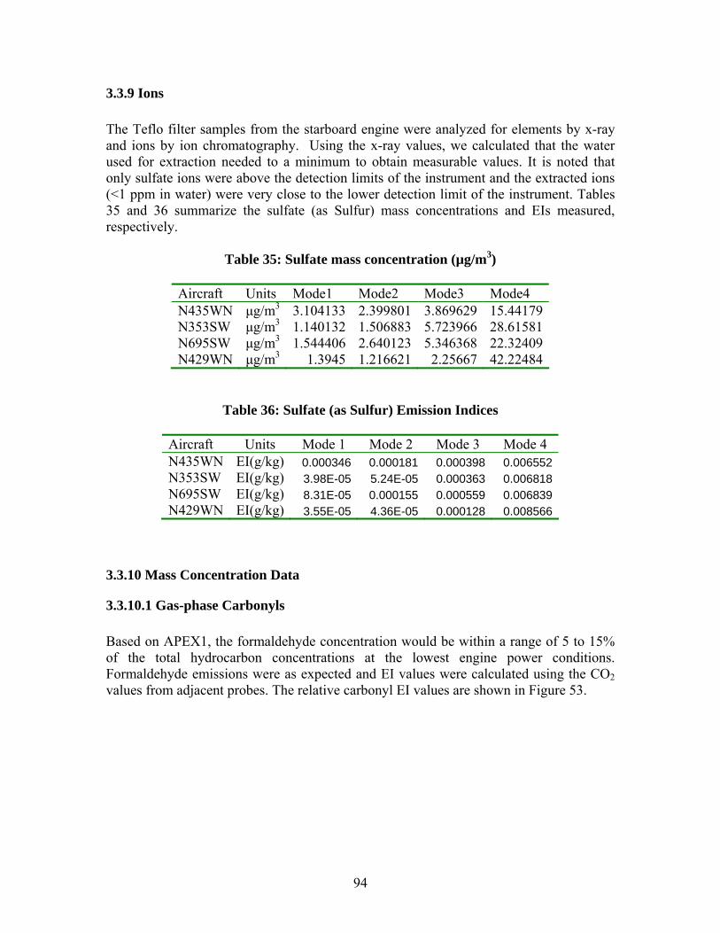
3.3.9 Ions

The Teflo filter samples from the starboard engine were analyzed for elements by x-ray and ions by ion chromatography. Using the x-ray values, we calculated that the water used for extraction needed to a minimum to obtain measurable values. It is noted that only sulfate ions were above the detection limits of the instrument and the extracted ions (<1 ppm in water) were very close to the lower detection limit of the instrument. Tables 35 and 36 summarize the sulfate (as Sulfur) mass concentrations and EIs measured, respectively.

Table 35: Sulfate mass concentration (µg/m3)

Aircraft Units Mode1 Mode2 Mode3 Mode4 N435WN μg/m3 3.104133 2.399801 3.869629 15.44179 N353SW μg/m3 1.140132 1.506883 5.723966 28.61581 N695SW μg/m3 1.544406 2.640123 5.346368 22.32409 N429WN μg/m3 1.3945 1.216621 2.25667 42.22484

Table 36: Sulfate (as Sulfur) Emission Indices

Aircraft Units Mode 1 Mode 2 Mode 3 Mode 4 N435WN EI(g/kg) 0.000346 0.000181 0.000398 0.006552 N353SW EI(g/kg) 3.98E-05 5.24E-05 0.000363 0.006818 N695SW EI(g/kg) 8.31E-05 0.000155 0.000559 0.006839 N429WN EI(g/kg) 3.55E-05 4.36E-05 0.000128 0.008566

3.3.10 Mass Concentration Data

3.3.10.1 Gas-phase Carbonyls

Based on APEX1, the formaldehyde concentration would be within a range of 5 to 15% of the total hydrocarbon concentrations at the lowest engine power conditions. Formaldehyde emissions were as expected and EI values were calculated using the CO2 values from adjacent probes. The relative carbonyl EI values are shown in Figure 53.

94

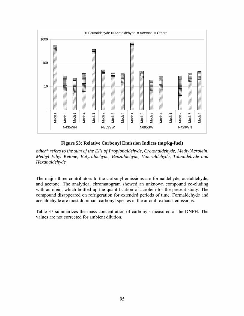
~ Ell Ill

~ - ~ - -

?,; 0. ;::;::; 0 1

10

100

1000

Mod

e1

Mod

e2

Mod

e3

Mod

e4

Mod

e1

Mod

e2

Mod

e3

Mod

e4

Mod

e1

Mod

e2

Mod

e3

Mod

e4

Mod

e1

Mod

e2

Mod

e3

Mod

e4

N435WN N353SW N695SW N429WN

Formaldehyde Acetaldehyde Acetone Other*

Figure 53: Relative Carbonyl Emission Indices (mg/kg-fuel)

other* refers to the sum of the EI's of Propionaldehyde, Crotonaldehyde, MethylAcrolein, Methyl Ethyl Ketone, Butyraldehyde, Benzaldehyde, Valeraldehyde, Tolualdehyde and Hexanaldehyde

The major three contributors to the carbonyl emissions are formaldehyde, acetaldehyde, and acetone. The analytical chromatogram showed an unknown compound co-eluding with acrolein, which bottled up the quantification of acrolein for the present study. The compound disappeared on refrigeration for extended periods of time. Formaldehyde and acetaldehyde are most dominant carbonyl species in the aircraft exhaust emissions.

Table 37 summarizes the mass concentration of carbonyls measured at the DNPH. The values are not corrected for ambient dilution.

95

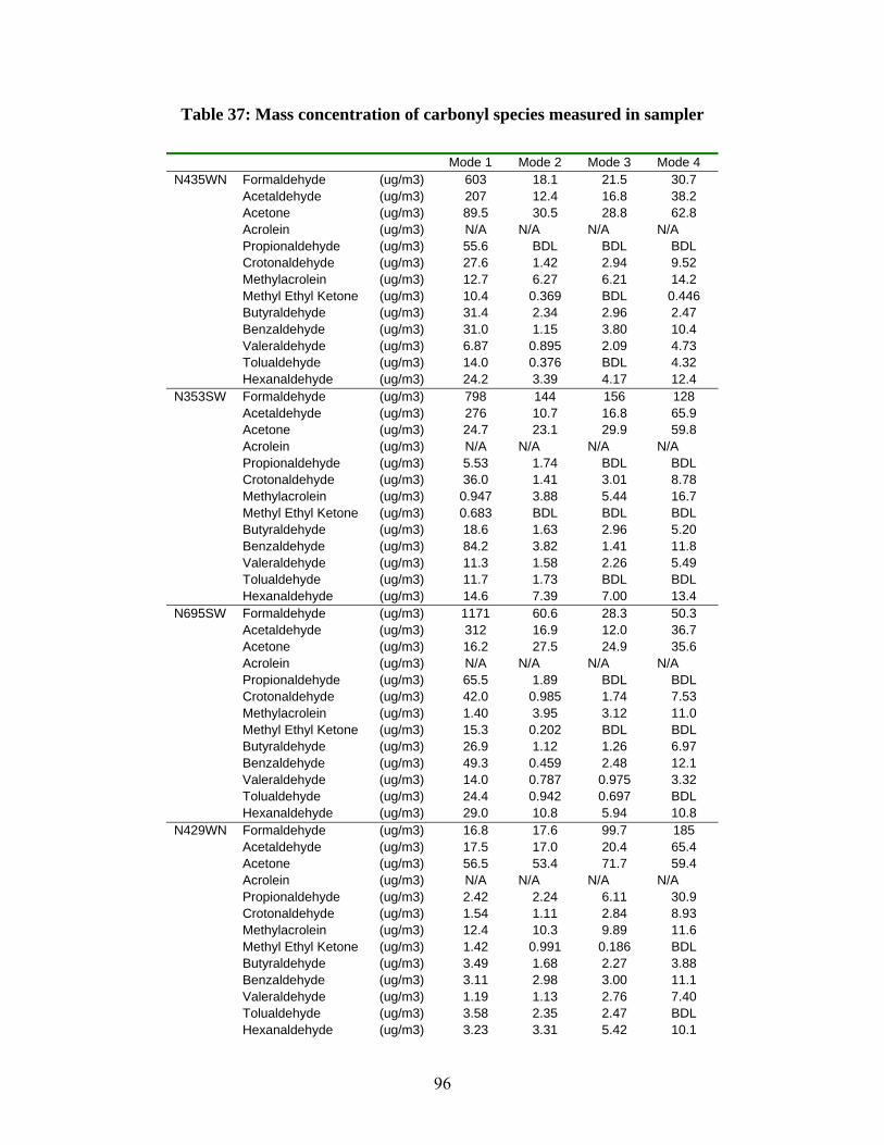
Table 37: Mass concentration of carbonyl species measured in sampler

Mode 1 Mode 2 Mode 3 Mode 4 N435WN

N353SW

Formaldehyde Acetaldehyde

Acetone Acrolein Propionaldehyde

Crotonaldehyde Methylacrolein

Methyl Ethyl Ketone Butyraldehyde Benzaldehyde Valeraldehyde Tolualdehyde Hexanaldehyde

Formaldehyde Acetaldehyde

Acetone Acrolein Propionaldehyde

Crotonaldehyde Methylacrolein

Methyl Ethyl Ketone Butyraldehyde Benzaldehyde Valeraldehyde

Tolualdehyde Hexanaldehyde

(ug/m3) (ug/m3) (ug/m3) (ug/m3) (ug/m3) (ug/m3) (ug/m3) (ug/m3) (ug/m3) (ug/m3) (ug/m3) (ug/m3) (ug/m3) (ug/m3) (ug/m3) (ug/m3) (ug/m3) (ug/m3) (ug/m3) (ug/m3) (ug/m3) (ug/m3) (ug/m3) (ug/m3) (ug/m3) (ug/m3)

603 207 89.5 N/A 55.6 27.6 12.7 10.4 31.4 31.0 6.87 14.0 24.2 798 276 24.7 N/A 5.53 36.0 0.947 0.683 18.6 84.2 11.3 11.7 14.6

18.1 12.4 30.5

N/A BDL 1.42 6.27 0.369 2.34 1.15 0.895 0.376 3.39 144 10.7 23.1

N/A 1.74 1.41 3.88 BDL 1.63 3.82 1.58 1.73 7.39

21.5 16.8 28.8

N/A BDL 2.94 6.21 BDL 2.96 3.80 2.09 BDL 4.17 156 16.8 29.9

N/A BDL 3.01 5.44 BDL 2.96 1.41 2.26 BDL 7.00

30.7 38.2 62.8

N/A BDL 9.52 14.2 0.446 2.47 10.4 4.73 4.32 12.4 128 65.9 59.8

N/A BDL 8.78 16.7 BDL 5.20 11.8 5.49 BDL 13.4

N695SW

N429WN

Formaldehyde Acetaldehyde

Acetone Acrolein Propionaldehyde

Crotonaldehyde Methylacrolein

Methyl Ethyl Ketone Butyraldehyde Benzaldehyde Valeraldehyde Tolualdehyde Hexanaldehyde

Formaldehyde Acetaldehyde

Acetone Acrolein

Propionaldehyde Crotonaldehyde Methylacrolein

Methyl Ethyl Ketone Butyraldehyde Benzaldehyde Valeraldehyde

Tolualdehyde Hexanaldehyde

(ug/m3) (ug/m3) (ug/m3) (ug/m3) (ug/m3) (ug/m3) (ug/m3) (ug/m3) (ug/m3) (ug/m3) (ug/m3) (ug/m3) (ug/m3) (ug/m3) (ug/m3) (ug/m3) (ug/m3) (ug/m3) (ug/m3) (ug/m3) (ug/m3) (ug/m3) (ug/m3) (ug/m3) (ug/m3) (ug/m3)

1171 312 16.2 N/A 65.5 42.0 1.40 15.3 26.9 49.3 14.0 24.4 29.0 16.8 17.5 56.5 N/A 2.42 1.54 12.4 1.42 3.49 3.11 1.19 3.58 3.23

60.6 16.9 27.5

N/A 1.89 0.985 3.95 0.202 1.12 0.459 0.787 0.942 10.8 17.6 17.0 53.4

N/A 2.24 1.11 10.3 0.991 1.68 2.98 1.13 2.35 3.31

28.3 12.0 24.9

N/A BDL 1.74 3.12 BDL 1.26 2.48 0.975 0.697 5.94 99.7 20.4 71.7

N/A 6.11 2.84 9.89 0.186 2.27 3.00 2.76 2.47 5.42

50.3 36.7 35.6

N/A BDL 7.53 11.0 BDL 6.97 12.1 3.32 BDL 10.8 185 65.4 59.4

N/A30.9 8.93 11.6 BDL 3.88 11.1 7.40 BDL 10.1

96

3.3.10.2 Light Hydrocarbons from Thermal Desorption Tubes

C4-C12 hydrocarbon values were explored based on the concentrations measured from the Thermal Desorption Tubes (TDS) but the values were much lower than expected from APEX1 and other research. Tables 38-41, 42-45, and 46-49, summarize the mass concentration of alkenes, alkanes and aromatics, respectively, in the C4-C12 range measured from the thermal desorption tubes. The mass concentrations in these tables were not corrected for ambient dilution since we could not determine the dilution ratio. Based on the measured concentrations being near typical ambient values, there is no appropriate method to scale these values to develop suitable emission factors.

C4-C12 hydrocarbon mass concentrations were measured using TDS (Tables 38 – 49) which were located on the low flow side of the sampling system. The data presented are not reliable as the mass concentrations do not significantly exceed ambient levels. In the absence of a leak these concentrations would be expected to be higher and may have significantly exceeded ambient levels thereby enhancing their reliability.

3.3.10.3 C1-C8 SUMMA Canister Analyses

SUMMA canisters were collected at the light hydrocarbon manifold to provide the sole measurement of the C1-C4 analyses, redundancy for measuring the C4-C8 analyses including 1, 3-Butadiene and BTEX, and provide CO2 concentrations to provide a confirming measurement of the values used in the dilution calculation. As with other samples, four samples were extracted for each aircraft test for a total of sixteen canister samples. These samples were forwarded to the outside laboratory for analysis of CO2 and light hydrocarbon species. The plan was to determine the concentration of CO2 in a first test and hydrocarbon species in a second test. The external laboratory measured CO2 concentrations in eleven of the sixteen canisters at about the same value as used in the dilution calculations, and CO2 less than detection limit for the remaining five analyses. For example, the CO2 levels were below detection for the samples collected at the idle modes and for Mode 2 for N435WN and N353SW. For the second test of the hydrocarbons species in the SUMMA canisters, the laboratory reported that all hydrocarbon species were below detection limits. It is unclear as to what happened on the second test of the SUMMA canisters.

97

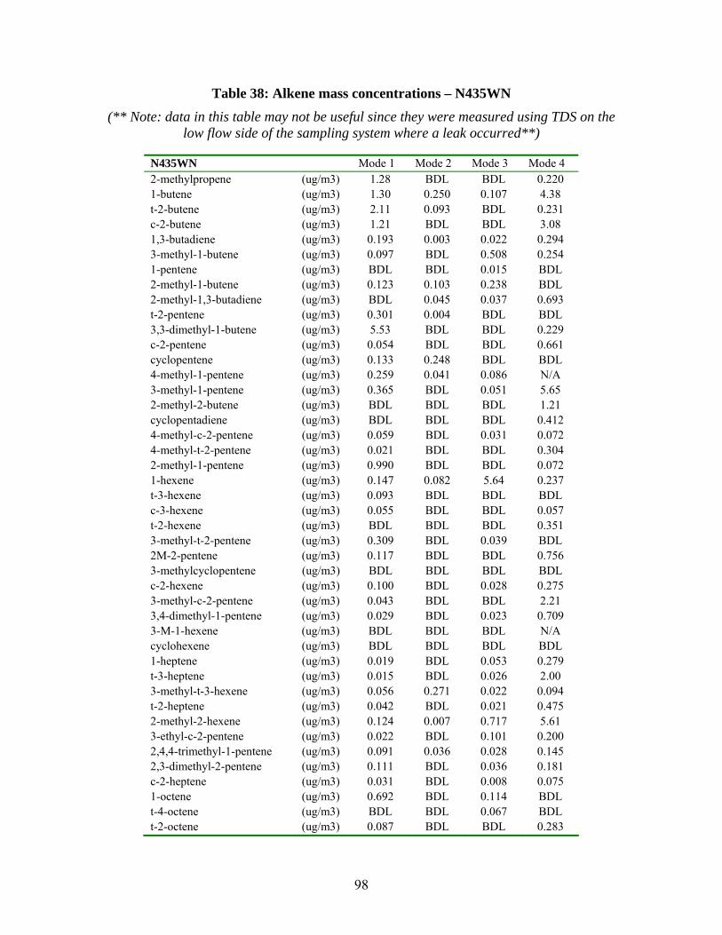
Table 38: Alkene mass concentrations – N435WN

(** Note: data in this table may not be useful since they were measured using TDS on the low flow side of the sampling system where a leak occurred**)

N435WN Mode 1 Mode 2 Mode 3 Mode 4 2-methylpropene (ug/m3) 1.28 BDL BDL 0.220 1-butene (ug/m3) 1.30 0.250 0.107 4.38 t-2-butene (ug/m3) 2.11 0.093 BDL 0.231 c-2-butene (ug/m3) 1.21 BDL BDL 3.08 1,3-butadiene (ug/m3) 0.193 0.003 0.022 0.294 3-methyl-1-butene (ug/m3) 0.097 BDL 0.508 0.254 1-pentene (ug/m3) BDL BDL 0.015 BDL 2-methyl-1-butene (ug/m3) 0.123 0.103 0.238 BDL 2-methyl-1,3-butadiene (ug/m3) BDL 0.045 0.037 0.693 t-2-pentene (ug/m3) 0.301 0.004 BDL BDL 3,3-dimethyl-1-butene (ug/m3) 5.53 BDL BDL 0.229 c-2-pentene (ug/m3) 0.054 BDL BDL 0.661 cyclopentene (ug/m3) 0.133 0.248 BDL BDL 4-methyl-1-pentene (ug/m3) 0.259 0.041 0.086 N/A 3-methyl-1-pentene (ug/m3) 0.365 BDL 0.051 5.65 2-methyl-2-butene (ug/m3) BDL BDL BDL 1.21 cyclopentadiene (ug/m3) BDL BDL BDL 0.412 4-methyl-c-2-pentene (ug/m3) 0.059 BDL 0.031 0.072 4-methyl-t-2-pentene (ug/m3) 0.021 BDL BDL 0.304 2-methyl-1-pentene (ug/m3) 0.990 BDL BDL 0.072 1-hexene (ug/m3) 0.147 0.082 5.64 0.237 t-3-hexene (ug/m3) 0.093 BDL BDL BDL c-3-hexene (ug/m3) 0.055 BDL BDL 0.057 t-2-hexene (ug/m3) BDL BDL BDL 0.351 3-methyl-t-2-pentene (ug/m3) 0.309 BDL 0.039 BDL 2M-2-pentene (ug/m3) 0.117 BDL BDL 0.756 3-methylcyclopentene (ug/m3) BDL BDL BDL BDL c-2-hexene (ug/m3) 0.100 BDL 0.028 0.275 3-methyl-c-2-pentene (ug/m3) 0.043 BDL BDL 2.21 3,4-dimethyl-1-pentene (ug/m3) 0.029 BDL 0.023 0.709 3-M-1-hexene (ug/m3) BDL BDL BDL N/A cyclohexene (ug/m3) BDL BDL BDL BDL 1-heptene (ug/m3) 0.019 BDL 0.053 0.279 t-3-heptene (ug/m3) 0.015 BDL 0.026 2.00 3-methyl-t-3-hexene (ug/m3) 0.056 0.271 0.022 0.094 t-2-heptene (ug/m3) 0.042 BDL 0.021 0.475 2-methyl-2-hexene (ug/m3) 0.124 0.007 0.717 5.61 3-ethyl-c-2-pentene (ug/m3) 0.022 BDL 0.101 0.200 2,4,4-trimethyl-1-pentene (ug/m3) 0.091 0.036 0.028 0.145 2,3-dimethyl-2-pentene (ug/m3) 0.111 BDL 0.036 0.181 c-2-heptene (ug/m3) 0.031 BDL 0.008 0.075 1-octene (ug/m3) 0.692 BDL 0.114 BDL t-4-octene (ug/m3) BDL BDL 0.067 BDL t-2-octene (ug/m3) 0.087 BDL BDL 0.283

98

c-2-octene (ug/m3) 0.134 BDL BDL 0.058 1-nonene (ug/m3) 0.159 BDL 0.042 5.09 1-butyne (ug/m3) 1.94 BDL BDL BDL 2-butyne (ug/m3) BDL 0.085 0.012 BDL

99

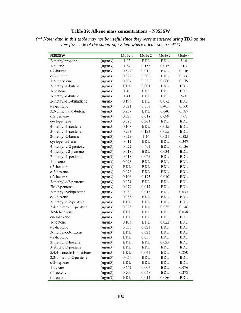
Table 39: Alkene mass concentrations – N353SW

(** Note: data in this table may not be useful since they were measured using TDS on the low flow side of the sampling system where a leak occurred**)

N353SW Mode 1 Mode 2 Mode 3 Mode 4 2-methylpropene (ug/m3) 1.03 BDL BDL 7.10 1-butene (ug/m3) 1.84 0.156 0.015 1.03 t-2-butene (ug/m3) 0.829 0.010 BDL 0.116 c-2-butene (ug/m3) 0.329 0.006 BDL 0.166 1,3-butadiene (ug/m3) 0.307 0.026 0.088 0.119 3-methyl-1-butene (ug/m3) BDL 0.004 BDL BDL 1-pentene (ug/m3) 1.46 BDL BDL BDL 2-methyl-1-butene (ug/m3) 1.41 BDL BDL N/A 2-methyl-1,3-butadiene (ug/m3) 0.195 BDL 0.072 BDL t-2-pentene (ug/m3) 0.021 0.058 0.405 0.160 3,3-dimethyl-1-butene (ug/m3) 0.257 BDL 0.040 0.187 c-2-pentene (ug/m3) 0.025 0.018 0.099 N/A cyclopentene (ug/m3) 0.080 0.264 BDL BDL 4-methyl-1-pentene (ug/m3) 0.168 BDL 0.015 BDL 3-methyl-1-pentene (ug/m3) 0.233 0.123 0.055 BDL 2-methyl-2-butene (ug/m3) 0.029 1.24 0.021 0.825 cyclopentadiene (ug/m3) 0.011 BDL BDL 0.347 4-methyl-c-2-pentene (ug/m3) 0.022 0.491 BDL 0.136 4-methyl-t-2-pentene (ug/m3) 0.018 BDL 0.034 BDL 2-methyl-1-pentene (ug/m3) 0.418 0.027 BDL BDL 1-hexene (ug/m3) 0.098 BDL BDL BDL t-3-hexene (ug/m3) BDL BDL BDL BDL c-3-hexene (ug/m3) 0.078 BDL BDL BDL t-2-hexene (ug/m3) 0.108 0.175 0.040 BDL 3-methyl-t-2-pentene (ug/m3) 0.024 BDL BDL BDL 2M-2-pentene (ug/m3) 0.079 0.017 BDL BDL 3-methylcyclopentene (ug/m3) 0.032 0.018 BDL 0.073 c-2-hexene (ug/m3) 0.038 BDL BDL BDL 3-methyl-c-2-pentene (ug/m3) BDL BDL BDL BDL 3,4-dimethyl-1-pentene (ug/m3) 0.023 BDL 0.035 0.146 3-M-1-hexene (ug/m3) BDL BDL BDL 0.078 cyclohexene (ug/m3) BDL BDL BDL BDL 1-heptene (ug/m3) 0.105 BDL 0.022 BDL t-3-heptene (ug/m3) 0.030 0.021 BDL BDL 3-methyl-t-3-hexene (ug/m3) BDL 0.022 BDL BDL t-2-heptene (ug/m3) BDL 0.055 BDL BDL 2-methyl-2-hexene (ug/m3) BDL BDL 0.025 BDL 3-ethyl-c-2-pentene (ug/m3) BDL BDL BDL BDL 2,4,4-trimethyl-1-pentene (ug/m3) BDL 0.041 BDL 0.280 2,3-dimethyl-2-pentene (ug/m3) 0.056 BDL BDL BDL c-2-heptene (ug/m3) BDL BDL BDL BDL 1-octene (ug/m3) 0.642 0.007 BDL 0.076 t-4-octene (ug/m3) 0.209 0.048 BDL 0.278 t-2-octene (ug/m3) BDL 0.014 0.086 BDL

100

c-2-octene (ug/m3) BDL 0.277 0.037 BDL 1-nonene (ug/m3) 0.129 0.149 BDL 0.201 1-butyne (ug/m3) 0.067 BDL BDL BDL 2-butyne (ug/m3) 0.121 BDL 0.081 BDL

101

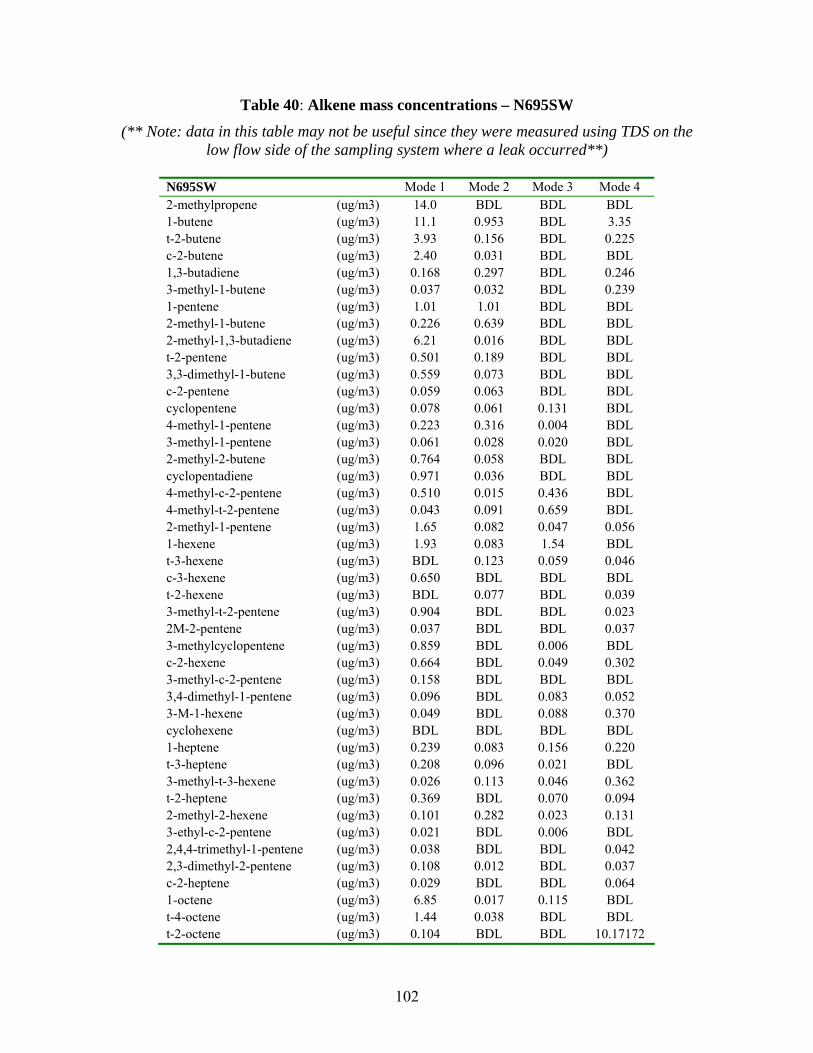
Table 40: Alkene mass concentrations – N695SW

(** Note: data in this table may not be useful since they were measured using TDS on the low flow side of the sampling system where a leak occurred**)

N695SW Mode 1 Mode 2 Mode 3 Mode 4 2-methylpropene (ug/m3) 14.0 BDL BDL BDL 1-butene (ug/m3) 11.1 0.953 BDL 3.35 t-2-butene (ug/m3) 3.93 0.156 BDL 0.225 c-2-butene (ug/m3) 2.40 0.031 BDL BDL 1,3-butadiene (ug/m3) 0.168 0.297 BDL 0.246 3-methyl-1-butene (ug/m3) 0.037 0.032 BDL 0.239 1-pentene (ug/m3) 1.01 1.01 BDL BDL 2-methyl-1-butene (ug/m3) 0.226 0.639 BDL BDL 2-methyl-1,3-butadiene (ug/m3) 6.21 0.016 BDL BDL t-2-pentene (ug/m3) 0.501 0.189 BDL BDL 3,3-dimethyl-1-butene (ug/m3) 0.559 0.073 BDL BDL c-2-pentene (ug/m3) 0.059 0.063 BDL BDL cyclopentene (ug/m3) 0.078 0.061 0.131 BDL 4-methyl-1-pentene (ug/m3) 0.223 0.316 0.004 BDL 3-methyl-1-pentene (ug/m3) 0.061 0.028 0.020 BDL 2-methyl-2-butene (ug/m3) 0.764 0.058 BDL BDL cyclopentadiene (ug/m3) 0.971 0.036 BDL BDL 4-methyl-c-2-pentene (ug/m3) 0.510 0.015 0.436 BDL 4-methyl-t-2-pentene (ug/m3) 0.043 0.091 0.659 BDL 2-methyl-1-pentene (ug/m3) 1.65 0.082 0.047 0.056 1-hexene (ug/m3) 1.93 0.083 1.54 BDL t-3-hexene (ug/m3) BDL 0.123 0.059 0.046 c-3-hexene (ug/m3) 0.650 BDL BDL BDL t-2-hexene (ug/m3) BDL 0.077 BDL 0.039 3-methyl-t-2-pentene (ug/m3) 0.904 BDL BDL 0.023 2M-2-pentene (ug/m3) 0.037 BDL BDL 0.037 3-methylcyclopentene (ug/m3) 0.859 BDL 0.006 BDL c-2-hexene (ug/m3) 0.664 BDL 0.049 0.302 3-methyl-c-2-pentene (ug/m3) 0.158 BDL BDL BDL 3,4-dimethyl-1-pentene (ug/m3) 0.096 BDL 0.083 0.052 3-M-1-hexene (ug/m3) 0.049 BDL 0.088 0.370 cyclohexene (ug/m3) BDL BDL BDL BDL 1-heptene (ug/m3) 0.239 0.083 0.156 0.220 t-3-heptene (ug/m3) 0.208 0.096 0.021 BDL 3-methyl-t-3-hexene (ug/m3) 0.026 0.113 0.046 0.362 t-2-heptene (ug/m3) 0.369 BDL 0.070 0.094 2-methyl-2-hexene (ug/m3) 0.101 0.282 0.023 0.131 3-ethyl-c-2-pentene (ug/m3) 0.021 BDL 0.006 BDL 2,4,4-trimethyl-1-pentene (ug/m3) 0.038 BDL BDL 0.042 2,3-dimethyl-2-pentene (ug/m3) 0.108 0.012 BDL 0.037 c-2-heptene (ug/m3) 0.029 BDL BDL 0.064 1-octene (ug/m3) 6.85 0.017 0.115 BDL t-4-octene (ug/m3) 1.44 0.038 BDL BDL t-2-octene (ug/m3) 0.104 BDL BDL 10.17172

102

c-2-octene (ug/m3) 1.07 BDL BDL 0.035 1-nonene (ug/m3) 2.67 0.015 BDL 0.322 1-butyne (ug/m3) 0.633 0.141 N/A 1.660732 2-butyne (ug/m3) BDL 0.315 BDL BDL

103

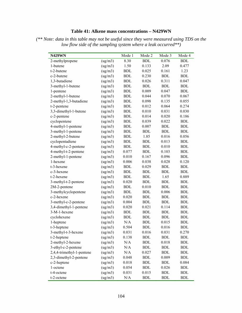
Table 41: Alkene mass concentrations – N429WN

(** Note: data in this table may not be useful since they were measured using TDS on the low flow side of the sampling system where a leak occurred**)

N429WN Mode 1 Mode 2 Mode 3 Mode 4 2-methylpropene (ug/m3) 8.30 BDL 0.076 BDL 1-butene (ug/m3) 1.50 0.133 2.09 0.477 t-2-butene (ug/m3) BDL 0.025 0.161 1.23 c-2-butene (ug/m3) BDL 0.230 BDL BDL 1,3-butadiene (ug/m3) BDL 0.026 0.311 0.047 3-methyl-1-butene (ug/m3) BDL BDL BDL BDL 1-pentene (ug/m3) BDL 0.009 0.047 BDL 2-methyl-1-butene (ug/m3) BDL 0.044 0.070 0.067 2-methyl-1,3-butadiene (ug/m3) BDL 0.098 0.135 0.055 t-2-pentene (ug/m3) BDL 0.012 0.064 0.274 3,3-dimethyl-1-butene (ug/m3) BDL 0.010 0.031 0.030 c-2-pentene (ug/m3) BDL 0.014 0.020 0.186 cyclopentene (ug/m3) BDL 0.039 0.022 BDL 4-methyl-1-pentene (ug/m3) BDL 0.007 BDL BDL 3-methyl-1-pentene (ug/m3) BDL BDL BDL BDL 2-methyl-2-butene (ug/m3) BDL 1.85 0.016 0.056 cyclopentadiene (ug/m3) BDL BDL 0.013 BDL 4-methyl-c-2-pentene (ug/m3) BDL BDL 0.010 BDL 4-methyl-t-2-pentene (ug/m3) 0.077 BDL 0.103 BDL 2-methyl-1-pentene (ug/m3) 0.010 0.167 0.096 BDL 1-hexene (ug/m3) 0.006 0.038 0.028 0.120 t-3-hexene (ug/m3) BDL 0.029 BDL BDL c-3-hexene (ug/m3) BDL BDL BDL BDL t-2-hexene (ug/m3) BDL BDL 1.65 0.889 3-methyl-t-2-pentene (ug/m3) 0.020 BDL BDL BDL 2M-2-pentene (ug/m3) BDL 0.010 BDL BDL 3-methylcyclopentene (ug/m3) BDL BDL 0.006 BDL c-2-hexene (ug/m3) 0.020 BDL BDL BDL 3-methyl-c-2-pentene (ug/m3) 0.004 BDL BDL BDL 3,4-dimethyl-1-pentene (ug/m3) 0.020 0.021 0.114 BDL 3-M-1-hexene (ug/m3) BDL BDL BDL BDL cyclohexene (ug/m3) BDL BDL BDL BDL 1-heptene (ug/m3) N/A BDL 0.015 BDL t-3-heptene (ug/m3) 0.504 BDL 0.016 BDL 3-methyl-t-3-hexene (ug/m3) 0.031 0.016 0.031 0.270 t-2-heptene (ug/m3) 0.138 BDL BDL BDL 2-methyl-2-hexene (ug/m3) N/A BDL 0.018 BDL 3-ethyl-c-2-pentene (ug/m3) N/A BDL BDL BDL 2,4,4-trimethyl-1-pentene (ug/m3) N/A 0.027 BDL BDL 2,3-dimethyl-2-pentene (ug/m3) 0.048 BDL 0.009 BDL c-2-heptene (ug/m3) 0.018 BDL BDL 0.084 1-octene (ug/m3) 0.054 BDL 0.026 BDL t-4-octene (ug/m3) 0.031 0.015 BDL BDL t-2-octene (ug/m3) N/A BDL BDL BDL

104

c-2-octene (ug/m3) 0.086 BDL 0.044 0.444 1-nonene (ug/m3) 0.127 BDL BDL BDL 1-butyne (ug/m3) BDL 0.023 BDL BDL 2-butyne (ug/m3) BDL 0.019 BDL BDL

105

Table 42: Alkane mass concentrations – N435WN

(** Note: data in this table may not be useful since they were measured using TDS on the low flow side of the sampling system where a leak occurred**)

N435WN Mode 1 Mode 2 Mode 3 Mode 4 octane (ug/m3) 0.057 BDL BDL 0.081 2-methylpropane (ug/m3) 2.28 BDL BDL BDL butane (ug/m3) 0.162 0.026 0.039 0.405 2,2-dimethylpropane (ug/m3) 0.075 0.105 0.043 0.669 2-methylbutane (ug/m3) 0.031 0.116 0.045 BDL pentane (ug/m3) 0.411 0.030 0.140 BDL 2,2-dimethylbutane (ug/m3) 0.074 0.524 BDL 0.223 cyclopentane (ug/m3) 1.79 BDL 0.085 BDL 2,3-dimethylbutane (ug/m3) 0.204 0.027 0.076 BDL 2-methylpentane (ug/m3) 0.026 BDL 0.021 0.076 3-methylpentane (ug/m3) 0.088 0.044 BDL 0.920 hexane (ug/m3) 0.241 BDL BDL 0.489 methylcyclopentane (ug/m3) BDL 0.009 BDL BDL 2,2-dimethylpentane (ug/m3) 0.028 BDL BDL 0.111 2,4-dimethylpentane (ug/m3) BDL BDL 0.054 0.116 2,2,3-trimethylbutane (ug/m3) BDL BDL BDL 0.063 3,3-dimethylpentane (ug/m3) 0.101 BDL BDL 0.113 cyclohexane (ug/m3) BDL BDL BDL 0.248 2-methylhexane (ug/m3) BDL 0.051 0.043 0.679 2,3-dimethylpentane (ug/m3) 0.025 0.005 0.038 0.246 3-methylhexane (ug/m3) BDL 0.007 0.097 N/A c-1,3-dimethylcyclopentane (ug/m3) 0.187 BDL 0.141 0.082 3-ethylpentane (ug/m3) BDL 0.004 0.019 0.553 t-1,2-dimethylcyclopentane (ug/m3) BDL 0.004 0.012 0.191 2,2,4-trimethylpentane (i-octane) (ug/m3) 0.497 0.020 0.040 0.085 heptane (ug/m3) 0.018 BDL 0.074 0.125 methylcyclohexane (ug/m3) 0.038 BDL 0.013 N/A 2,4,4-trimethyl-2-pentene (ug/m3) 0.035 0.006 0.028 BDL 2,2-dimethylhexane (ug/m3) 0.078 BDL 0.069 BDL 2,5-dimethylhexane (ug/m3) 0.128 BDL 0.164 BDL 2,4-dimethylhexane (ug/m3) 0.137 BDL BDL 0.078 3,3-dimethylhexane (ug/m3) 0.303 BDL 0.022 0.134 2,3,4-trimethylpentane (ug/m3) 0.348 BDL 0.026 0.228 2,3-dimethylhexane (ug/m3) 0.138 BDL 0.020 BDL 2-methylheptane (ug/m3) 0.083 BDL BDL 0.280 4-methylheptane (ug/m3) BDL BDL 0.010 0.233 3-methylheptane (ug/m3) 0.039 BDL 0.018 1.22 1c,2t,3-trimethylcyclopentane (ug/m3) 0.437 BDL 0.012 0.110 c-1,3-dimethylcyclohexane (ug/m3) 0.044 BDL BDL 0.129 t-1,4-dimethylcyclohexane (ug/m3) 0.035 0.014 0.033 0.115 2,2,5-TM-hexane (ug/m3) BDL BDL BDL 0.330 t-1,3-dimethylcyclohexane (ug/m3) 0.066 0.019 BDL N/A 2,3,5-trimethylhexane (ug/m3) 0.014 BDL 0.294 0.123 2,4-dimethylheptane (ug/m3) 0.079 BDL BDL 0.177 NN-DM- (ug/m3) 0.007 BDL BDL 0.027 c-1,2-dimethylcyclohexane (ug/m3) 0.247 BDL BDL 0.644 ethylcyclohexane (ug/m3) 0.169 BDL 0.026 0.114 3,5-dimethylheptane (ug/m3) 0.632 BDL 0.063 0.148 2,3-dimethylheptane (ug/m3) 1.27 BDL 0.027 0.177 2-methyloctane (ug/m3) 1.78 BDL 0.027 BDL 3-methyloctane (ug/m3) 0.118 BDL 0.036 0.291 nonane (ug/m3) 0.099 BDL 0.073 0.204 2,2-dimethyloctane (ug/m3) 0.010 BDL 0.031 0.268 2,4-dimethyloctane (ug/m3) 0.011 BDL 0.023 0.393 decane (ug/m3) 0.385 0.024 0.435 0.971 undecane (ug/m3) 0.234 BDL 0.079 N/A

106

Table 43: Alkane mass concentrations – N353SW

(** Note: data in this table may not be useful since they were measured using TDS on the low flow side of the sampling system where a leak occurred**)

N353SW Mode 1 Mode 2 Mode 3 Mode 4 octane (ug/m3) BDL BDL BDL BDL 2-methylpropane (ug/m3) 0.863 BDL BDL BDL butane (ug/m3) 0.311 0.023 0.011 0.157 2,2-dimethylpropane (ug/m3) 0.013 0.018 BDL 0.089 2-methylbutane (ug/m3) 1.00 BDL 0.050 BDL pentane (ug/m3) 0.204 BDL BDL 4.02 2,2-dimethylbutane (ug/m3) 0.023 0.731 BDL BDL cyclopentane (ug/m3) 0.052 BDL BDL BDL 2,3-dimethylbutane (ug/m3) 0.016 BDL BDL BDL 2-methylpentane (ug/m3) 0.073 BDL BDL BDL 3-methylpentane (ug/m3) 0.122 BDL BDL BDL hexane (ug/m3) BDL BDL BDL BDL methylcyclopentane (ug/m3) BDL BDL BDL BDL 2,2-dimethylpentane (ug/m3) BDL BDL 0.069 BDL 2,4-dimethylpentane (ug/m3) BDL 0.545 BDL BDL 2,2,3-trimethylbutane (ug/m3) BDL 0.014 BDL 0.786 3,3-dimethylpentane (ug/m3) 0.042 0.018 BDL BDL cyclohexane (ug/m3) BDL BDL BDL BDL 2-methylhexane (ug/m3) BDL BDL BDL BDL 2,3-dimethylpentane (ug/m3) 0.029 BDL BDL BDL 3-methylhexane (ug/m3) 0.045 0.327 BDL BDL c-1,3-dimethylcyclopentane (ug/m3) 0.094 0.020 BDL BDL 3-ethylpentane (ug/m3) 0.327 BDL BDL BDL t-1,2-dimethylcyclopentane (ug/m3) BDL BDL BDL BDL 2,2,4-trimethylpentane (i-octane) (ug/m3) BDL BDL 0.022 BDL heptane (ug/m3) 0.094 BDL 0.023 0.082 methylcyclohexane (ug/m3) BDL BDL BDL BDL 2,4,4-trimethyl-2-pentene (ug/m3) BDL BDL BDL BDL 2,2-dimethylhexane (ug/m3) BDL BDL BDL BDL 2,5-dimethylhexane (ug/m3) 0.072 BDL BDL BDL 2,4-dimethylhexane (ug/m3) 1.52 BDL BDL BDL 3,3-dimethylhexane (ug/m3) 0.030 BDL 0.056 BDL 2,3,4-trimethylpentane (ug/m3) 0.100 BDL BDL BDL 2,3-dimethylhexane (ug/m3) 0.063 BDL BDL BDL 2-methylheptane (ug/m3) 0.143 0.017 BDL BDL 4-methylheptane (ug/m3) 0.038 0.009 BDL BDL 3-methylheptane (ug/m3) 0.155 BDL BDL BDL 1c,2t,3-trimethylcyclopentane (ug/m3) 0.290 BDL 0.217 BDL c-1,3-dimethylcyclohexane (ug/m3) BDL BDL BDL BDL t-1,4-dimethylcyclohexane (ug/m3) BDL 0.049 BDL BDL 2,2,5-TM-hexane (ug/m3) 0.007 0.000 BDL BDL t-1,3-dimethylcyclohexane (ug/m3) 0.125 0.129 BDL BDL 2,3,5-trimethylhexane (ug/m3) 0.025 0.014 0.014 BDL 2,4-dimethylheptane (ug/m3) 0.121 BDL 0.014 BDL NN-DM- (ug/m3) 0.003 BDL 0.002 0.008 c-1,2-dimethylcyclohexane (ug/m3) 0.045 0.006 BDL BDL ethylcyclohexane (ug/m3) 0.078 0.014 BDL 0.243 3,5-dimethylheptane (ug/m3) 0.223 0.010 BDL 0.137 2,3-dimethylheptane (ug/m3) 1.14 BDL BDL 0.194 2-methyloctane (ug/m3) 0.025 BDL BDL BDL 3-methyloctane (ug/m3) 0.128 BDL BDL 0.398 nonane (ug/m3) 0.058 BDL BDL 0.178 2,2-dimethyloctane (ug/m3) 0.100 0.012 BDL BDL 2,4-dimethyloctane (ug/m3) 0.050 0.008 BDL BDL decane (ug/m3) 0.274 0.190 0.015 BDL undecane (ug/m3) 0.084 0.023 BDL BDL

107

Table 44: Alkane mass concentrations – N695SW

(** Note: data in this table may not be useful since they were measured using TDS on the low flow side of the sampling system where a leak occurred**)

N695SW Mode 1 Mode 2 Mode 3 Mode 4 octane (ug/m3) 0.135 0.037 BDL BDL 2-methylpropane (ug/m3) 0.630 BDL BDL BDL butane (ug/m3) 0.301 0.165 BDL 0.205 2,2-dimethylpropane (ug/m3) 0.125 0.264 #N/A 1.58 2-methylbutane (ug/m3) 0.137 0.755 BDL BDL pentane (ug/m3) 1.50 0.040 BDL BDL 2,2-dimethylbutane (ug/m3) 0.010 0.037 0.109 BDL cyclopentane (ug/m3) 0.678 0.020 0.035 BDL 2,3-dimethylbutane (ug/m3) BDL 0.258 0.302 BDL 2-methylpentane (ug/m3) N/A 0.038 0.066 BDL 3-methylpentane (ug/m3) 0.524 0.146 0.075 BDL hexane (ug/m3) 4.46 0.125 0.030 0.417 methylcyclopentane (ug/m3) 0.108 0.135 0.063 0.068 2,2-dimethylpentane (ug/m3) 0.455 BDL 0.115 0.233 2,4-dimethylpentane (ug/m3) 0.061 BDL BDL 0.117 2,2,3-trimethylbutane (ug/m3) 0.012 0.108 0.021 0.026 3,3-dimethylpentane (ug/m3) 0.022 BDL 0.261 BDL cyclohexane (ug/m3) 0.389 BDL 0.010 BDL 2-methylhexane (ug/m3) 0.041 N/A 0.013 N/A 2,3-dimethylpentane (ug/m3) 0.123 0.261 0.009 0.103 3-methylhexane (ug/m3) 0.069 0.083 0.254 0.144 c-1,3-dimethylcyclopentane (ug/m3) 0.145 BDL 0.143 0.106 3-ethylpentane (ug/m3) N/A BDL 0.008 BDL t-1,2-dimethylcyclopentane (ug/m3) 0.280 BDL 0.040 0.215 2,2,4-trimethylpentane (i-octane) (ug/m3) 0.021 0.089 0.268 N/A heptane (ug/m3) 0.012 0.113 0.082 0.022 methylcyclohexane (ug/m3) 0.161 0.026 0.026 BDL 2,4,4-trimethyl-2-pentene (ug/m3) 0.250 0.023 BDL 0.056 2,2-dimethylhexane (ug/m3) 0.029 0.007 BDL 0.049 2,5-dimethylhexane (ug/m3) 0.131 BDL 0.006 N/A 2,4-dimethylhexane (ug/m3) 6.92 BDL 0.024 0.071 3,3-dimethylhexane (ug/m3) 0.091 0.053 0.010 0.113 2,3,4-trimethylpentane (ug/m3) 1.19 0.012 0.013 0.040 2,3-dimethylhexane (ug/m3) BDL 0.038 0.015 BDL 2-methylheptane (ug/m3) 0.189 0.007 BDL BDL 4-methylheptane (ug/m3) 0.375 0.007 BDL 0.034 3-methylheptane (ug/m3) 0.166 0.057 BDL BDL 1c,2t,3-trimethylcyclopentane (ug/m3) 0.189 0.035 BDL BDL c-1,3-dimethylcyclohexane (ug/m3) 0.327 0.022 BDL 0.158 t-1,4-dimethylcyclohexane (ug/m3) N/A 0.010 0.032 BDL 2,2,5-TM-hexane (ug/m3) 0.030 0.006 BDL BDL t-1,3-dimethylcyclohexane (ug/m3) 0.156 BDL BDL BDL 2,3,5-trimethylhexane (ug/m3) 0.127 0.309 0.077 0.519 2,4-dimethylheptane (ug/m3) 0.456 0.011 BDL 0.076 NN-DM- (ug/m3) 0.046 0.002 BDL BDL c-1,2-dimethylcyclohexane (ug/m3) 0.055 0.015 BDL BDL ethylcyclohexane (ug/m3) 1.03 0.024 BDL BDL 3,5-dimethylheptane (ug/m3) 1.46 BDL 0.037 BDL 2,3-dimethylheptane (ug/m3) 0.347 BDL BDL BDL 2-methyloctane (ug/m3) 1.42 BDL BDL BDL 3-methyloctane (ug/m3) BDL 0.040 BDL BDL nonane (ug/m3) 0.180 0.177 BDL BDL 2,2-dimethyloctane (ug/m3) 0.060 0.055 BDL 0.046 2,4-dimethyloctane (ug/m3) 0.251 0.044 BDL BDL decane (ug/m3) 0.223 0.267 BDL 0.438 undecane (ug/m3) 0.109 0.394 BDL BDL

108

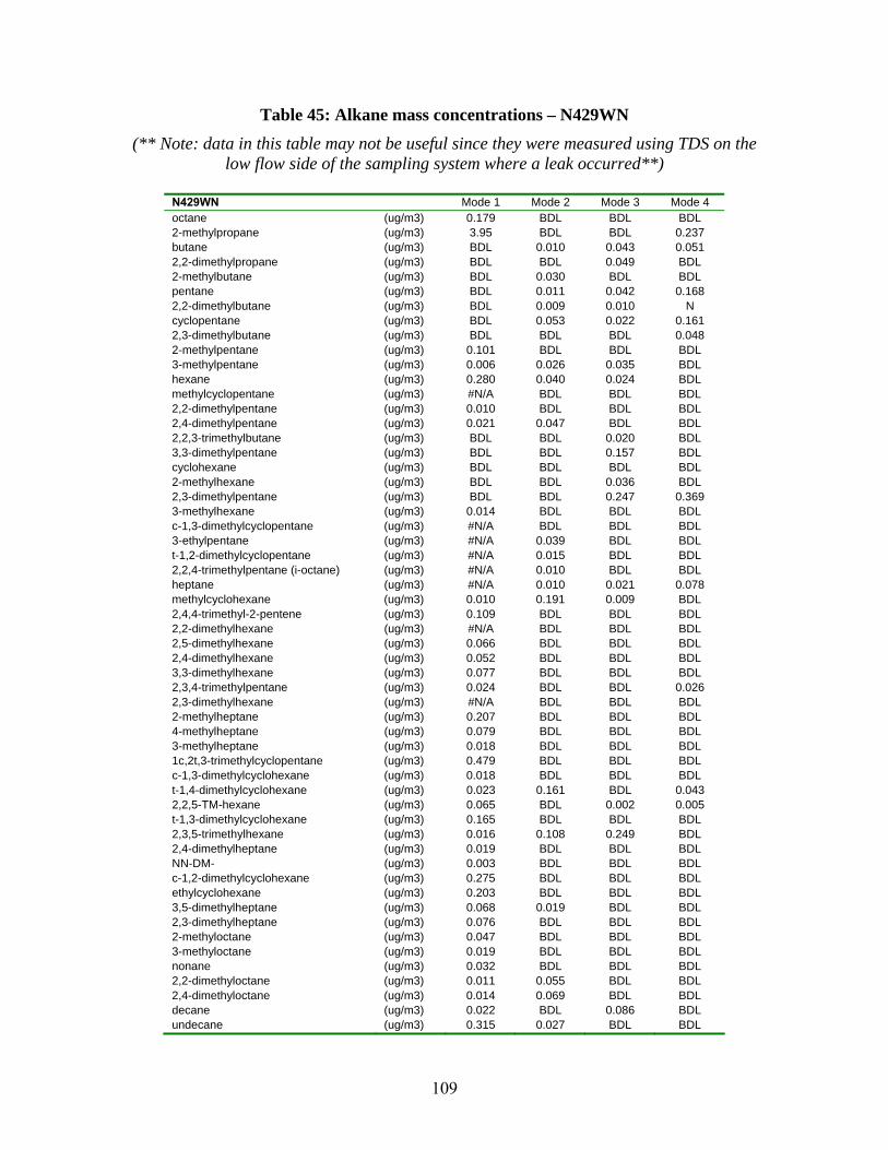
Table 45: Alkane mass concentrations – N429WN

(** Note: data in this table may not be useful since they were measured using TDS on the low flow side of the sampling system where a leak occurred**)

N429WN Mode 1 Mode 2 Mode 3 Mode 4 octane (ug/m3) 0.179 BDL BDL BDL 2-methylpropane (ug/m3) 3.95 BDL BDL 0.237 butane (ug/m3) BDL 0.010 0.043 0.051 2,2-dimethylpropane (ug/m3) BDL BDL 0.049 BDL 2-methylbutane (ug/m3) BDL 0.030 BDL BDL pentane (ug/m3) BDL 0.011 0.042 0.168 2,2-dimethylbutane (ug/m3) BDL 0.009 0.010 N cyclopentane (ug/m3) BDL 0.053 0.022 0.161 2,3-dimethylbutane (ug/m3) BDL BDL BDL 0.048 2-methylpentane (ug/m3) 0.101 BDL BDL BDL 3-methylpentane (ug/m3) 0.006 0.026 0.035 BDL hexane (ug/m3) 0.280 0.040 0.024 BDL methylcyclopentane (ug/m3) #N/A BDL BDL BDL 2,2-dimethylpentane (ug/m3) 0.010 BDL BDL BDL 2,4-dimethylpentane (ug/m3) 0.021 0.047 BDL BDL 2,2,3-trimethylbutane (ug/m3) BDL BDL 0.020 BDL 3,3-dimethylpentane (ug/m3) BDL BDL 0.157 BDL cyclohexane (ug/m3) BDL BDL BDL BDL 2-methylhexane (ug/m3) BDL BDL 0.036 BDL 2,3-dimethylpentane (ug/m3) BDL BDL 0.247 0.369 3-methylhexane (ug/m3) 0.014 BDL BDL BDL c-1,3-dimethylcyclopentane (ug/m3) #N/A BDL BDL BDL 3-ethylpentane (ug/m3) #N/A 0.039 BDL BDL t-1,2-dimethylcyclopentane (ug/m3) #N/A 0.015 BDL BDL 2,2,4-trimethylpentane (i-octane) (ug/m3) #N/A 0.010 BDL BDL heptane (ug/m3) #N/A 0.010 0.021 0.078 methylcyclohexane (ug/m3) 0.010 0.191 0.009 BDL 2,4,4-trimethyl-2-pentene (ug/m3) 0.109 BDL BDL BDL 2,2-dimethylhexane (ug/m3) #N/A BDL BDL BDL 2,5-dimethylhexane (ug/m3) 0.066 BDL BDL BDL 2,4-dimethylhexane (ug/m3) 0.052 BDL BDL BDL 3,3-dimethylhexane (ug/m3) 0.077 BDL BDL BDL 2,3,4-trimethylpentane (ug/m3) 0.024 BDL BDL 0.026 2,3-dimethylhexane (ug/m3) #N/A BDL BDL BDL 2-methylheptane (ug/m3) 0.207 BDL BDL BDL 4-methylheptane (ug/m3) 0.079 BDL BDL BDL 3-methylheptane (ug/m3) 0.018 BDL BDL BDL 1c,2t,3-trimethylcyclopentane (ug/m3) 0.479 BDL BDL BDL c-1,3-dimethylcyclohexane (ug/m3) 0.018 BDL BDL BDL t-1,4-dimethylcyclohexane (ug/m3) 0.023 0.161 BDL 0.043 2,2,5-TM-hexane (ug/m3) 0.065 BDL 0.002 0.005 t-1,3-dimethylcyclohexane (ug/m3) 0.165 BDL BDL BDL 2,3,5-trimethylhexane (ug/m3) 0.016 0.108 0.249 BDL 2,4-dimethylheptane (ug/m3) 0.019 BDL BDL BDL NN-DM- (ug/m3) 0.003 BDL BDL BDL c-1,2-dimethylcyclohexane (ug/m3) 0.275 BDL BDL BDL ethylcyclohexane (ug/m3) 0.203 BDL BDL BDL 3,5-dimethylheptane (ug/m3) 0.068 0.019 BDL BDL 2,3-dimethylheptane (ug/m3) 0.076 BDL BDL BDL 2-methyloctane (ug/m3) 0.047 BDL BDL BDL 3-methyloctane (ug/m3) 0.019 BDL BDL BDL nonane (ug/m3) 0.032 BDL BDL BDL 2,2-dimethyloctane (ug/m3) 0.011 0.055 BDL BDL 2,4-dimethyloctane (ug/m3) 0.014 0.069 BDL BDL decane (ug/m3) 0.022 BDL 0.086 BDL undecane (ug/m3) 0.315 0.027 BDL BDL

109

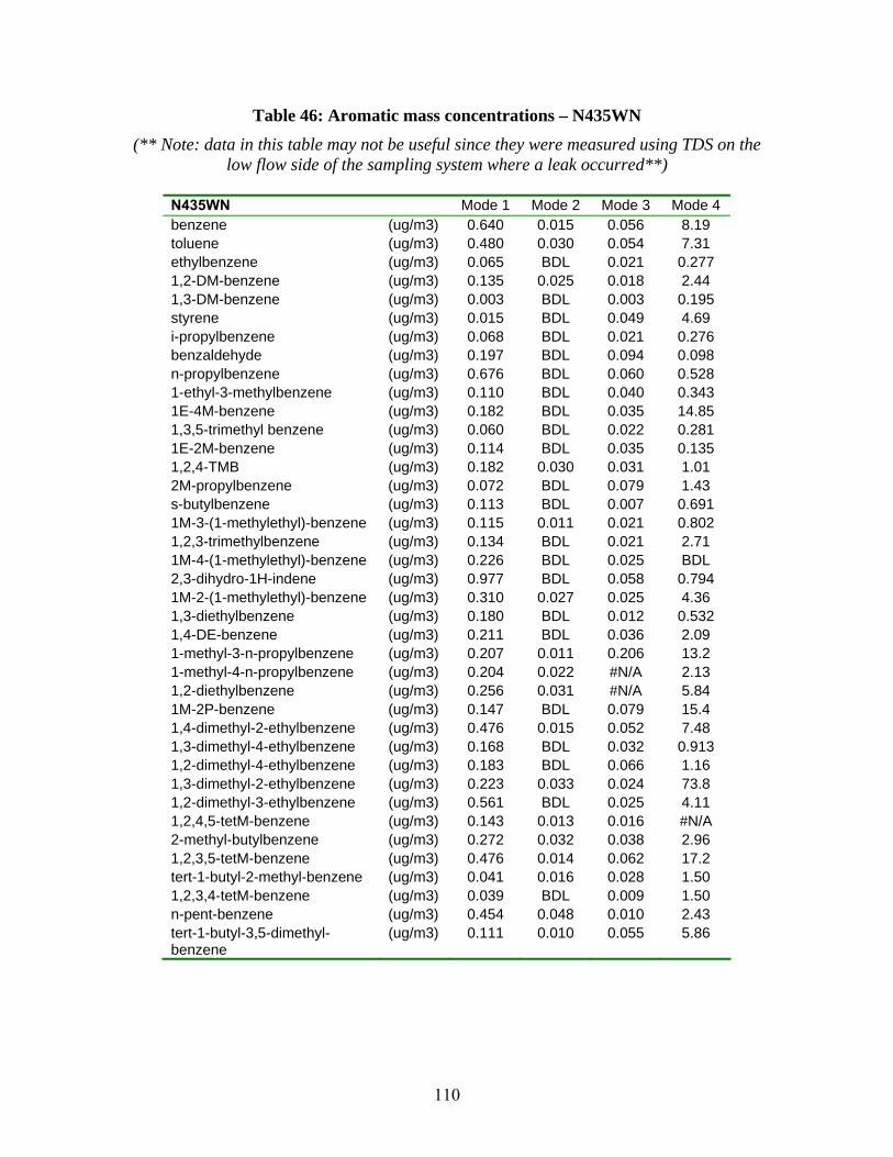
Table 46: Aromatic mass concentrations – N435WN

(** Note: data in this table may not be useful since they were measured using TDS on the low flow side of the sampling system where a leak occurred**)

N435WN Mode 1 Mode 2 Mode 3 Mode 4 benzene (ug/m3) 0.640 0.015 0.056 8.19 toluene (ug/m3) 0.480 0.030 0.054 7.31 ethylbenzene (ug/m3) 0.065 BDL 0.021 0.277 1,2-DM-benzene (ug/m3) 0.135 0.025 0.018 2.44 1,3-DM-benzene (ug/m3) 0.003 BDL 0.003 0.195 styrene (ug/m3) 0.015 BDL 0.049 4.69 i-propylbenzene (ug/m3) 0.068 BDL 0.021 0.276 benzaldehyde (ug/m3) 0.197 BDL 0.094 0.098 n-propylbenzene (ug/m3) 0.676 BDL 0.060 0.528 1-ethyl-3-methylbenzene (ug/m3) 0.110 BDL 0.040 0.343 1E-4M-benzene (ug/m3) 0.182 BDL 0.035 14.85 1,3,5-trimethyl benzene (ug/m3) 0.060 BDL 0.022 0.281 1E-2M-benzene (ug/m3) 0.114 BDL 0.035 0.135 1,2,4-TMB (ug/m3) 0.182 0.030 0.031 1.01 2M-propylbenzene (ug/m3) 0.072 BDL 0.079 1.43 s-butylbenzene (ug/m3) 0.113 BDL 0.007 0.691 1M-3-(1-methylethyl)-benzene (ug/m3) 0.115 0.011 0.021 0.802 1,2,3-trimethylbenzene (ug/m3) 0.134 BDL 0.021 2.71 1M-4-(1-methylethyl)-benzene (ug/m3) 0.226 BDL 0.025 BDL 2,3-dihydro-1H-indene (ug/m3) 0.977 BDL 0.058 0.794 1M-2-(1-methylethyl)-benzene (ug/m3) 0.310 0.027 0.025 4.36 1,3-diethylbenzene (ug/m3) 0.180 BDL 0.012 0.532 1,4-DE-benzene (ug/m3) 0.211 BDL 0.036 2.09 1-methyl-3-n-propylbenzene (ug/m3) 0.207 0.011 0.206 13.2 1-methyl-4-n-propylbenzene (ug/m3) 0.204 0.022 #N/A 2.13 1,2-diethylbenzene (ug/m3) 0.256 0.031 #N/A 5.84 1M-2P-benzene (ug/m3) 0.147 BDL 0.079 15.4 1,4-dimethyl-2-ethylbenzene (ug/m3) 0.476 0.015 0.052 7.48 1,3-dimethyl-4-ethylbenzene (ug/m3) 0.168 BDL 0.032 0.913 1,2-dimethyl-4-ethylbenzene (ug/m3) 0.183 BDL 0.066 1.16 1,3-dimethyl-2-ethylbenzene (ug/m3) 0.223 0.033 0.024 73.8 1,2-dimethyl-3-ethylbenzene (ug/m3) 0.561 BDL 0.025 4.11 1,2,4,5-tetM-benzene (ug/m3) 0.143 0.013 0.016 #N/A 2-methyl-butylbenzene (ug/m3) 0.272 0.032 0.038 2.96 1,2,3,5-tetM-benzene (ug/m3) 0.476 0.014 0.062 17.2 tert-1-butyl-2-methyl-benzene (ug/m3) 0.041 0.016 0.028 1.50 1,2,3,4-tetM-benzene (ug/m3) 0.039 BDL 0.009 1.50 n-pent-benzene (ug/m3) 0.454 0.048 0.010 2.43 tert-1-butyl-3,5-dimethyl- (ug/m3) 0.111 0.010 0.055 5.86 benzene

110

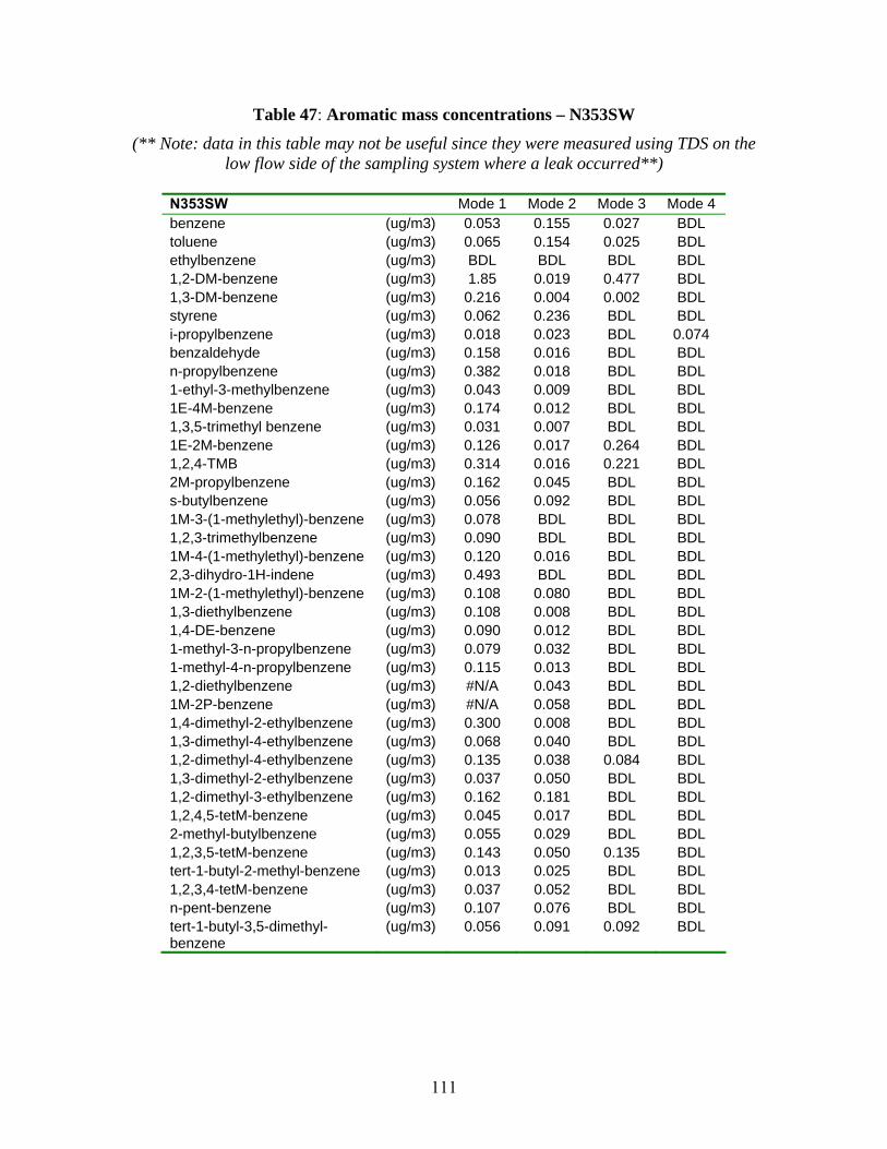
Table 47: Aromatic mass concentrations – N353SW

(** Note: data in this table may not be useful since they were measured using TDS on the low flow side of the sampling system where a leak occurred**)

N353SW Mode 1 Mode 2 Mode 3 Mode 4 benzene (ug/m3) 0.053 0.155 0.027 BDL toluene (ug/m3) 0.065 0.154 0.025 BDL ethylbenzene (ug/m3) BDL BDL BDL BDL 1,2-DM-benzene (ug/m3) 1.85 0.019 0.477 BDL 1,3-DM-benzene (ug/m3) 0.216 0.004 0.002 BDL styrene (ug/m3) 0.062 0.236 BDL BDL i-propylbenzene (ug/m3) 0.018 0.023 BDL 0.074 benzaldehyde (ug/m3) 0.158 0.016 BDL BDL n-propylbenzene (ug/m3) 0.382 0.018 BDL BDL 1-ethyl-3-methylbenzene (ug/m3) 0.043 0.009 BDL BDL 1E-4M-benzene (ug/m3) 0.174 0.012 BDL BDL 1,3,5-trimethyl benzene (ug/m3) 0.031 0.007 BDL BDL 1E-2M-benzene (ug/m3) 0.126 0.017 0.264 BDL 1,2,4-TMB (ug/m3) 0.314 0.016 0.221 BDL 2M-propylbenzene (ug/m3) 0.162 0.045 BDL BDL s-butylbenzene (ug/m3) 0.056 0.092 BDL BDL 1M-3-(1-methylethyl)-benzene (ug/m3) 0.078 BDL BDL BDL 1,2,3-trimethylbenzene (ug/m3) 0.090 BDL BDL BDL 1M-4-(1-methylethyl)-benzene (ug/m3) 0.120 0.016 BDL BDL 2,3-dihydro-1H-indene (ug/m3) 0.493 BDL BDL BDL 1M-2-(1-methylethyl)-benzene (ug/m3) 0.108 0.080 BDL BDL 1,3-diethylbenzene (ug/m3) 0.108 0.008 BDL BDL 1,4-DE-benzene (ug/m3) 0.090 0.012 BDL BDL 1-methyl-3-n-propylbenzene (ug/m3) 0.079 0.032 BDL BDL 1-methyl-4-n-propylbenzene (ug/m3) 0.115 0.013 BDL BDL 1,2-diethylbenzene (ug/m3) #N/A 0.043 BDL BDL 1M-2P-benzene (ug/m3) #N/A 0.058 BDL BDL 1,4-dimethyl-2-ethylbenzene (ug/m3) 0.300 0.008 BDL BDL 1,3-dimethyl-4-ethylbenzene (ug/m3) 0.068 0.040 BDL BDL 1,2-dimethyl-4-ethylbenzene (ug/m3) 0.135 0.038 0.084 BDL 1,3-dimethyl-2-ethylbenzene (ug/m3) 0.037 0.050 BDL BDL 1,2-dimethyl-3-ethylbenzene (ug/m3) 0.162 0.181 BDL BDL 1,2,4,5-tetM-benzene (ug/m3) 0.045 0.017 BDL BDL 2-methyl-butylbenzene (ug/m3) 0.055 0.029 BDL BDL 1,2,3,5-tetM-benzene (ug/m3) 0.143 0.050 0.135 BDL tert-1-butyl-2-methyl-benzene (ug/m3) 0.013 0.025 BDL BDL 1,2,3,4-tetM-benzene (ug/m3) 0.037 0.052 BDL BDL n-pent-benzene (ug/m3) 0.107 0.076 BDL BDL tert-1-butyl-3,5-dimethyl- (ug/m3) 0.056 0.091 0.092 BDL benzene

111

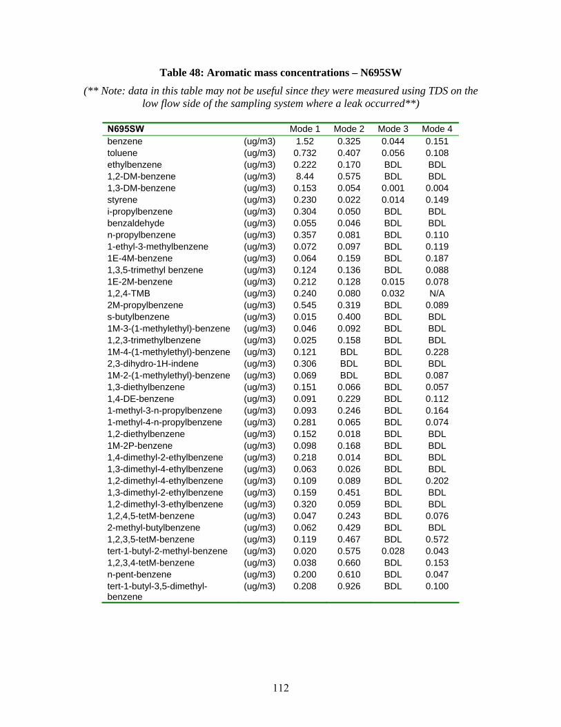
Table 48: Aromatic mass concentrations – N695SW

(** Note: data in this table may not be useful since they were measured using TDS on the low flow side of the sampling system where a leak occurred**)

N695SW Mode 1 Mode 2 Mode 3 Mode 4 benzene (ug/m3) 1.52 0.325 0.044 0.151 toluene (ug/m3) 0.732 0.407 0.056 0.108 ethylbenzene (ug/m3) 0.222 0.170 BDL BDL 1,2-DM-benzene (ug/m3) 8.44 0.575 BDL BDL 1,3-DM-benzene (ug/m3) 0.153 0.054 0.001 0.004 styrene (ug/m3) 0.230 0.022 0.014 0.149 i-propylbenzene (ug/m3) 0.304 0.050 BDL BDL benzaldehyde (ug/m3) 0.055 0.046 BDL BDL n-propylbenzene (ug/m3) 0.357 0.081 BDL 0.110 1-ethyl-3-methylbenzene (ug/m3) 0.072 0.097 BDL 0.119 1E-4M-benzene (ug/m3) 0.064 0.159 BDL 0.187 1,3,5-trimethyl benzene (ug/m3) 0.124 0.136 BDL 0.088 1E-2M-benzene (ug/m3) 0.212 0.128 0.015 0.078 1,2,4-TMB (ug/m3) 0.240 0.080 0.032 N/A 2M-propylbenzene (ug/m3) 0.545 0.319 BDL 0.089 s-butylbenzene (ug/m3) 0.015 0.400 BDL BDL 1M-3-(1-methylethyl)-benzene (ug/m3) 0.046 0.092 BDL BDL 1,2,3-trimethylbenzene (ug/m3) 0.025 0.158 BDL BDL 1M-4-(1-methylethyl)-benzene (ug/m3) 0.121 BDL BDL 0.228 2,3-dihydro-1H-indene (ug/m3) 0.306 BDL BDL BDL 1M-2-(1-methylethyl)-benzene (ug/m3) 0.069 BDL BDL 0.087 1,3-diethylbenzene (ug/m3) 0.151 0.066 BDL 0.057 1,4-DE-benzene (ug/m3) 0.091 0.229 BDL 0.112 1-methyl-3-n-propylbenzene (ug/m3) 0.093 0.246 BDL 0.164 1-methyl-4-n-propylbenzene (ug/m3) 0.281 0.065 BDL 0.074 1,2-diethylbenzene (ug/m3) 0.152 0.018 BDL BDL 1M-2P-benzene (ug/m3) 0.098 0.168 BDL BDL 1,4-dimethyl-2-ethylbenzene (ug/m3) 0.218 0.014 BDL BDL 1,3-dimethyl-4-ethylbenzene (ug/m3) 0.063 0.026 BDL BDL 1,2-dimethyl-4-ethylbenzene (ug/m3) 0.109 0.089 BDL 0.202 1,3-dimethyl-2-ethylbenzene (ug/m3) 0.159 0.451 BDL BDL 1,2-dimethyl-3-ethylbenzene (ug/m3) 0.320 0.059 BDL BDL 1,2,4,5-tetM-benzene (ug/m3) 0.047 0.243 BDL 0.076 2-methyl-butylbenzene (ug/m3) 0.062 0.429 BDL BDL 1,2,3,5-tetM-benzene (ug/m3) 0.119 0.467 BDL 0.572 tert-1-butyl-2-methyl-benzene (ug/m3) 0.020 0.575 0.028 0.043 1,2,3,4-tetM-benzene (ug/m3) 0.038 0.660 BDL 0.153 n-pent-benzene (ug/m3) 0.200 0.610 BDL 0.047 tert-1-butyl-3,5-dimethyl- (ug/m3) 0.208 0.926 BDL 0.100 benzene

112

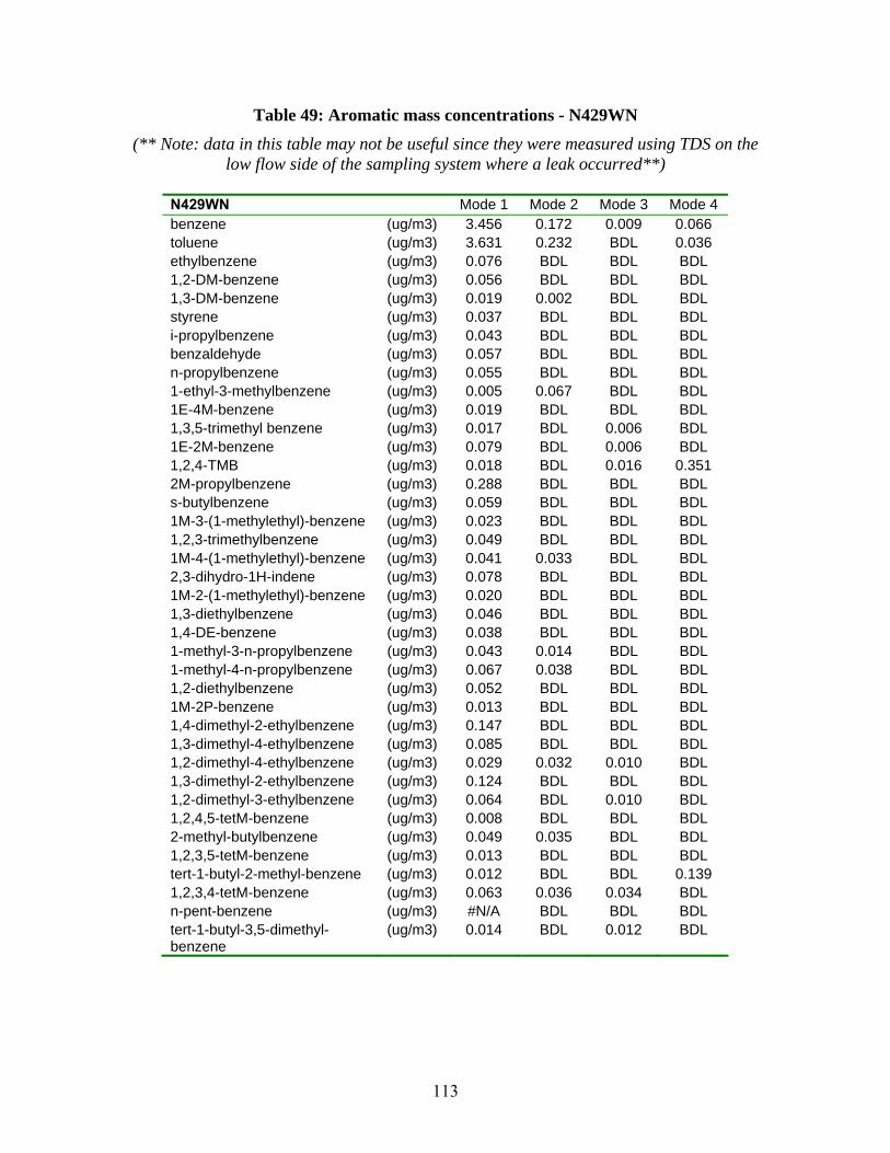
Table 49: Aromatic mass concentrations - N429WN

(** Note: data in this table may not be useful since they were measured using TDS on the low flow side of the sampling system where a leak occurred**)

N429WN Mode 1 Mode 2 Mode 3 Mode 4 benzene (ug/m3) 3.456 0.172 0.009 0.066 toluene (ug/m3) 3.631 0.232 BDL 0.036 ethylbenzene (ug/m3) 0.076 BDL BDL BDL 1,2-DM-benzene (ug/m3) 0.056 BDL BDL BDL 1,3-DM-benzene (ug/m3) 0.019 0.002 BDL BDL styrene (ug/m3) 0.037 BDL BDL BDL i-propylbenzene (ug/m3) 0.043 BDL BDL BDL benzaldehyde (ug/m3) 0.057 BDL BDL BDL n-propylbenzene (ug/m3) 0.055 BDL BDL BDL 1-ethyl-3-methylbenzene (ug/m3) 0.005 0.067 BDL BDL 1E-4M-benzene (ug/m3) 0.019 BDL BDL BDL 1,3,5-trimethyl benzene (ug/m3) 0.017 BDL 0.006 BDL 1E-2M-benzene (ug/m3) 0.079 BDL 0.006 BDL 1,2,4-TMB (ug/m3) 0.018 BDL 0.016 0.351 2M-propylbenzene (ug/m3) 0.288 BDL BDL BDL s-butylbenzene (ug/m3) 0.059 BDL BDL BDL 1M-3-(1-methylethyl)-benzene (ug/m3) 0.023 BDL BDL BDL 1,2,3-trimethylbenzene (ug/m3) 0.049 BDL BDL BDL 1M-4-(1-methylethyl)-benzene (ug/m3) 0.041 0.033 BDL BDL 2,3-dihydro-1H-indene (ug/m3) 0.078 BDL BDL BDL 1M-2-(1-methylethyl)-benzene (ug/m3) 0.020 BDL BDL BDL 1,3-diethylbenzene (ug/m3) 0.046 BDL BDL BDL 1,4-DE-benzene (ug/m3) 0.038 BDL BDL BDL 1-methyl-3-n-propylbenzene (ug/m3) 0.043 0.014 BDL BDL 1-methyl-4-n-propylbenzene (ug/m3) 0.067 0.038 BDL BDL 1,2-diethylbenzene (ug/m3) 0.052 BDL BDL BDL 1M-2P-benzene (ug/m3) 0.013 BDL BDL BDL 1,4-dimethyl-2-ethylbenzene (ug/m3) 0.147 BDL BDL BDL 1,3-dimethyl-4-ethylbenzene (ug/m3) 0.085 BDL BDL BDL 1,2-dimethyl-4-ethylbenzene (ug/m3) 0.029 0.032 0.010 BDL 1,3-dimethyl-2-ethylbenzene (ug/m3) 0.124 BDL BDL BDL 1,2-dimethyl-3-ethylbenzene (ug/m3) 0.064 BDL 0.010 BDL 1,2,4,5-tetM-benzene (ug/m3) 0.008 BDL BDL BDL 2-methyl-butylbenzene (ug/m3) 0.049 0.035 BDL BDL 1,2,3,5-tetM-benzene (ug/m3) 0.013 BDL BDL BDL tert-1-butyl-2-methyl-benzene (ug/m3) 0.012 BDL BDL 0.139 1,2,3,4-tetM-benzene (ug/m3) 0.063 0.036 0.034 BDL n-pent-benzene (ug/m3) #N/A BDL BDL BDL tert-1-butyl-3,5-dimethyl- (ug/m3) 0.014 BDL 0.012 BDL benzene

113

3.3.11 Estimation of EIs for VOCs

After the field campaign was completed and analysis of the DNPH cartridges, thermal desorption tubes and SUMMA canisters was undertaken, the EIs were calculated using the earlier described protocol. However, calculated EIs were much lower when compared with other investigators in this project or literature. It appeared that a leak had occurred in the subsystem designated for light hydrocarbon and carbonyl analysis. The sampling system, under vacuum, had allowed ambient air to enter at a leak and dilute the samples by an unknown amount.

3.3.11.1 Post Analysis of the Sampler C4-C12 hydrocarbon values were explored based on the concentrations measured from the Thermal Desorption Tubes (TDS) tubes but the values were much lower than expected from APEX1 and other research. This finding lead to an extensive evaluation of the UCR sampling system, especially given that in-field and post test calibrations indicated accurate flow through the sample media. Given that the samples collected on Teflon and quartz media matched expected values and that the carbonyl was close to the expected EI value than the sorption tubes, it was presumed that a small leak must have occurred near the split point for the thermal desorption system. The leak would have resulted in significant dilution with ambient air without affecting the PM, quartz, and quartz-PUF sample trains. This conclusion is easily reached by looking at the design flows in Figure 54. Note that the approximate flows in the quartz (qz) line was 80 liter per minute (LPM), for PTFE about 35LPM, for (QZ+PUF) about 25LPM, for DNPH about 1LPM and for thermal desorption tubes about 0.2LPM. Thus since the system was pressure and vacuum checked for leaks, it became clear that a small leak in the vicinity of the TDS collection tube would be consistent with the findings for the TDS tubes.

The design included a redundancy on the emission rates for the trace hydrocarbon gases; namely collection of gas phase samples in SUMMA canisters for subsequent analyses. The SUMMA canisters also allowed an internal check of the dilution ratio since CO2 was also measured. Unfortunately, all Summa canisters analyzed by the external lab reported no measurable hydrocarbons but the CO2 values matched the value measured from sampling ports adjacent to UCR’s ports. With no trace hydrocarbons reported from the TDS tubes or the SUMMA canisters, meant that the data collected for C1-C8 analyses are not available for this study. All data on C1-C12 speciated hydrocarbons provided in the report is thus given as measured µg m-3 as opposed to EI data.

114

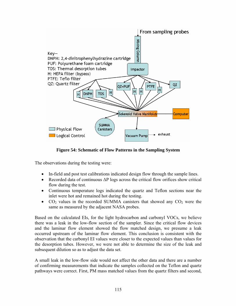
Key-DNPH: 2,4-dinitrophenylhyd razine cartridge PUF: Polyurethane foam cartridge TDS: Thermal desorption tubes H: HEPA filter (bypass) PTFE: Teflo filter

From sampling probes

Impactor

as-----,Computer '----~----'

D Physical Flow

D Logical Control Vacuum Pump exhaust

Figure 54: Schematic of Flow Patterns in the Sampling System

The observations during the testing were:

• In-field and post test calibrations indicated design flow through the sample lines. • Recorded data of continuous ΔP logs across the critical flow orifices show critical

flow during the test. • Continuous temperature logs indicated the quartz and Teflon sections near the

inlet were hot and remained hot during the testing. • CO2 values in the recorded SUMMA canisters that showed any CO2 were the

same as measured by the adjacent NASA probes.

Based on the calculated EIs, for the light hydrocarbon and carbonyl VOCs, we believe there was a leak in the low-flow section of the sampler. Since the critical flow devices and the laminar flow element showed the flow matched design, we presume a leak occurred upstream of the laminar flow element. This conclusion is consistent with the observation that the carbonyl EI values were closer to the expected values than values for the desorption tubes. However, we were not able to determine the size of the leak and subsequent dilution so as to adjust the data set.

A small leak in the low-flow side would not affect the other data and there are a number of confirming measurements that indicate the samples collected on the Teflon and quartz pathways were correct. First, PM mass matched values from the quartz filters and second,

115

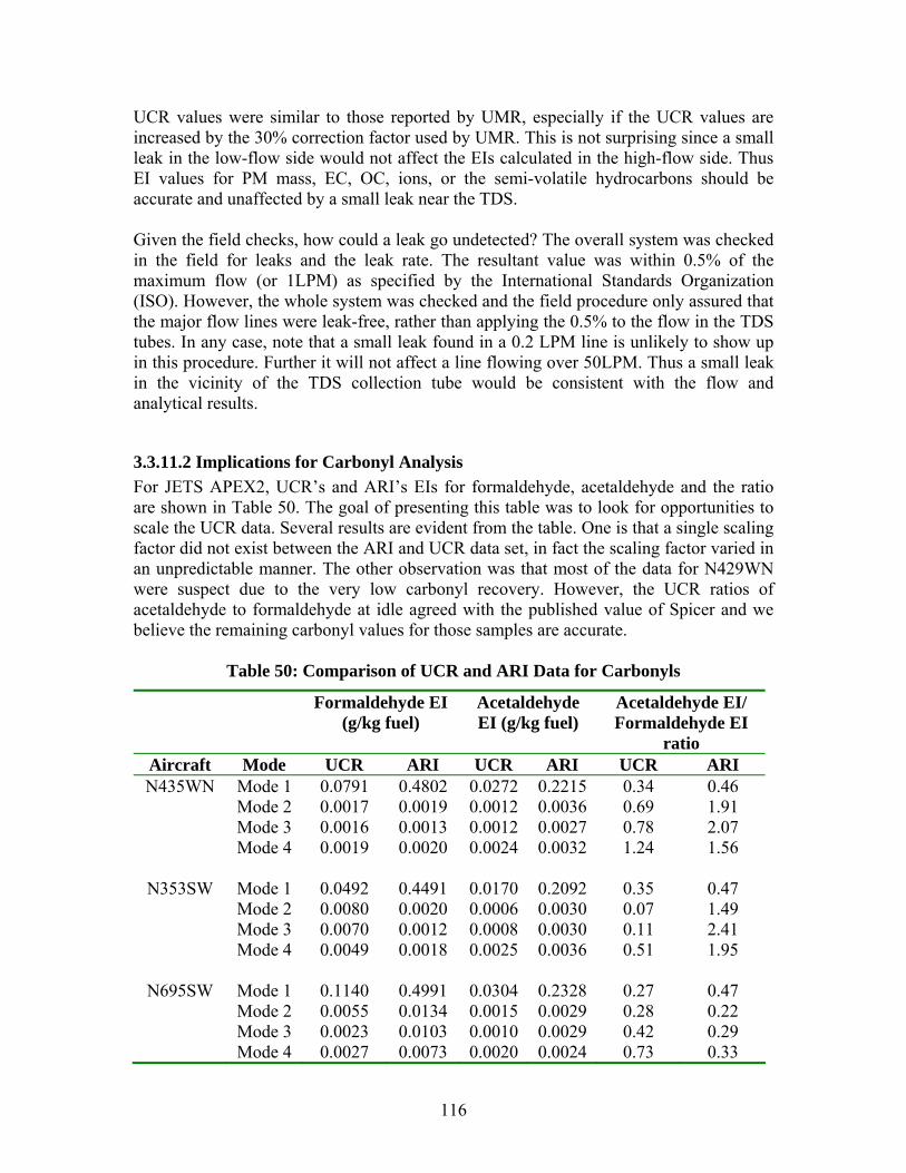
UCR values were similar to those reported by UMR, especially if the UCR values are increased by the 30% correction factor used by UMR. This is not surprising since a small leak in the low-flow side would not affect the EIs calculated in the high-flow side. Thus EI values for PM mass, EC, OC, ions, or the semi-volatile hydrocarbons should be accurate and unaffected by a small leak near the TDS.

Given the field checks, how could a leak go undetected? The overall system was checked in the field for leaks and the leak rate. The resultant value was within 0.5% of the maximum flow (or 1LPM) as specified by the International Standards Organization (ISO). However, the whole system was checked and the field procedure only assured that the major flow lines were leak-free, rather than applying the 0.5% to the flow in the TDS tubes. In any case, note that a small leak found in a 0.2 LPM line is unlikely to show up in this procedure. Further it will not affect a line flowing over 50LPM. Thus a small leak in the vicinity of the TDS collection tube would be consistent with the flow and analytical results.

3.3.11.2 Implications for Carbonyl Analysis For JETS APEX2, UCR’s and ARI’s EIs for formaldehyde, acetaldehyde and the ratio are shown in Table 50. The goal of presenting this table was to look for opportunities to scale the UCR data. Several results are evident from the table. One is that a single scaling factor did not exist between the ARI and UCR data set, in fact the scaling factor varied in an unpredictable manner. The other observation was that most of the data for N429WN were suspect due to the very low carbonyl recovery. However, the UCR ratios of acetaldehyde to formaldehyde at idle agreed with the published value of Spicer and we believe the remaining carbonyl values for those samples are accurate.

Table 50: Comparison of UCR and ARI Data for Carbonyls

Formaldehyde EI Acetaldehyde Acetaldehyde EI/ (g/kg fuel) EI (g/kg fuel) Formaldehyde EI

ratio Aircraft Mode UCR ARI UCR ARI UCR ARI N435WN Mode 1 0.0791 0.4802 0.0272 0.2215 0.34 0.46

Mode 2 0.0017 0.0019 0.0012 0.0036 0.69 1.91 Mode 3 0.0016 0.0013 0.0012 0.0027 0.78 2.07 Mode 4 0.0019 0.0020 0.0024 0.0032 1.24 1.56

N353SW Mode 1 0.0492 0.4491 0.0170 0.2092 0.35 0.47 Mode 2 0.0080 0.0020 0.0006 0.0030 0.07 1.49 Mode 3 0.0070 0.0012 0.0008 0.0030 0.11 2.41 Mode 4 0.0049 0.0018 0.0025 0.0036 0.51 1.95

N695SW Mode 1 0.1140 0.4991 0.0304 0.2328 0.27 0.47 Mode 2 0.0055 0.0134 0.0015 0.0029 0.28 0.22 Mode 3 0.0023 0.0103 0.0010 0.0029 0.42 0.29 Mode 4 0.0027 0.0073 0.0020 0.0024 0.73 0.33

116

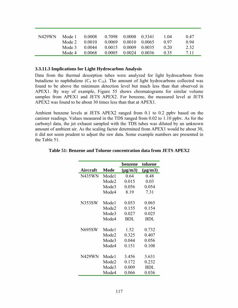
N429WN Mode 1 0.0008 0.7098 0.0008 0.3341 1.04 0.47 Mode 2 0.0010 0.0069 0.0010 0.0065 0.97 0.94 Mode 3 0.0044 0.0015 0.0009 0.0035 0.20 2.32 Mode 4 0.0068 0.0005 0.0024 0.0036 0.35 7.11

3.3.11.3 Implications for Light Hydrocarbon Analysis Data from the thermal desorption tubes were analyzed for light hydrocarbons from butadiene to naphthalene (C4 to C10). The amount of light hydrocarbons collected was found to be above the minimum detection level but much less than that observed in APEX1. By way of example, Figure 55 shows chromatograms for similar volume samples from APEX1 and JETS APEX2. For benzene, the measured level at JETS APEX2 was found to be about 30 times less than that at APEX1.

Ambient benzene levels at JETS APEX2 ranged from 0.1 to 0.2 ppbv based on the canister readings. Values measured in the TDS ranged from 0.02 to 1.10 ppbv. As for the carbonyl data, the jet exhaust sampled with the TDS tubes was diluted by an unknown amount of ambient air. As the scaling factor determined from APEX1 would be about 30, it did not seem prudent to adjust the raw data. Some example numbers are presented in the Table 51.

Table 51: Benzene and Toluene concentration data from JETS APEX2

Aircraft N435WN

Mode Mode1 Mode2 Mode3 Mode4

benzene (µg/m3)

0.64 0.015 0.056 8.19

toluene (µg/m3)

0.48 0.03 0.054 7.31

N353SW Mode1 Mode2 Mode3 Mode4

0.053 0.155 0.027 BDL

0.065 0.154 0.025 BDL

N695SW Mode1 Mode2 Mode3 Mode4

1.52 0.325 0.044 0.151

0.732 0.407 0.056 0.108

N429WN Mode1 Mode2 Mode3 Mode4

3.456 0.172 0.009 0.066

3.631 0.232 BDL 0.036

117

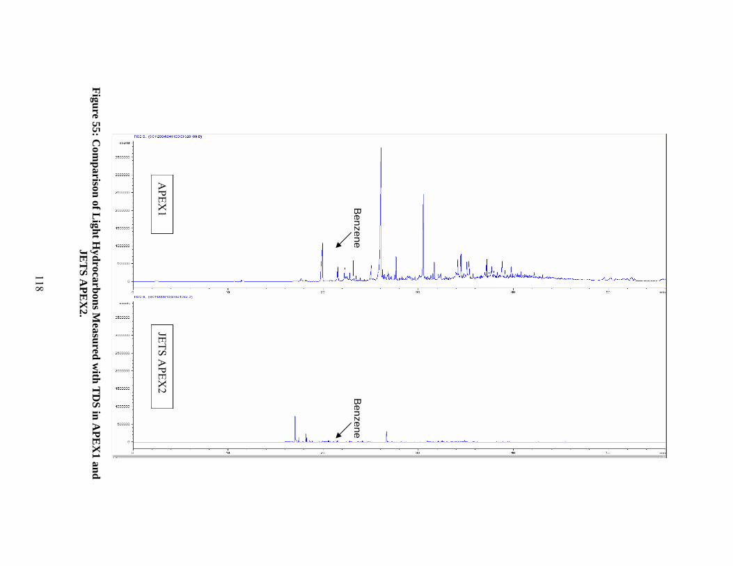
FID2 8, (GC1\2004\JJ41103\SIG20109.D)

counts

3!500000

3000000

2!500000

2000000

1!500000

·-1 /

~ W-JlliJ !500000

0

1~ 20 30 .:, !5~ FID2 8, (GC1\JJ6081!5\SIG21082.D)

counts

3!500000

3000000

2!500000

2000000

1!500000

1000000

500,J I / ~

,0 20 30 40 50

Benzene

Benzene

APEX

1 JETS A

PEX2

Figure 55: Com

parison of Light H

ydrocarbons Measured w

ith TD

S in APE

X1 and

JET

S APE

X2.

118

3.3.12 UCR QA/QC Protocol

The contributions of UCR were focused in two areas. One was the development of the sampling system to match the engine test cycle (see Figure 11) and the other contribution was the sampling and off-line analysis of the speciated hydrocarbons and speciated PM. Both areas were given considerable thought on the QA/QC.

Sampling System The original plan for the quality control and quality assurance of the sampling system was designed at two levels, since the sampler was a complex assembly of mechanical and electronic equipment with a computer precisely controlling all the equipment to fit within the sampling window allowed by the selected test cycle. Because this sampler was quite complex and the first-of-a-kind design, quality control runs at UCR were planned to compare the measured values with those measured in UCR’s recognized mobile emissions laboratory. Quality assurance in the field was to follow the protocol outlined in ISO 8178-1 Chapter 8-4 “Leakage Test”. This planned quality check could not be implemented because construction of the complex sampling system was completed at the Oakland airport the day before testing began.

However, once the sampling equipment was assembled, UCR did perform the second level of quality assurance testing as specified in ISO: “The maximum allowable leakage rate on the vacuum side shall be 0.5 % of the in-use flow rate for the portion of the system being checked.” Early trials indicated the leakage rate exceeded the allowed value and the sampling system was made leak tight by sealing leaks on the pipe threads with epoxy resins. Other components in the sampling system were leak tight. The system easily passed the ISO leakage rate specification after the repairs. The leakage rate was checked against the whole system flow of 200 LPM and not against the smallest flow component of 0.25 LPM where the Thermal Desorption Tubes were located. Other reports in the literature with similar sampling systems apply the QA test in the same manner as UCR did but the test should have been applied to the lowest flow element in the system.

Chemical Collection and Analysis A key element in the quality plan was to build a number of redundancies in the collection and analyses of the exhaust since the samples were quite difficult to collect and so few data existed in the literature. Some of the redundancies are illustrated in the Table 52 below. ARI was collecting selected hydrocarbons from the mixtures collected and analyzed by UCR.

All data, except for the VOCs, was successfully collected and collaborated against the redundant measurement. For example, Teflon mass was matched with the combination of EC plus OC from the quartz filter and also by the values calculated from the UMR instruments. However, for the VOCs, both the SUMMA canisters and the thermal desorption tubes failed to provide the expected results.

119

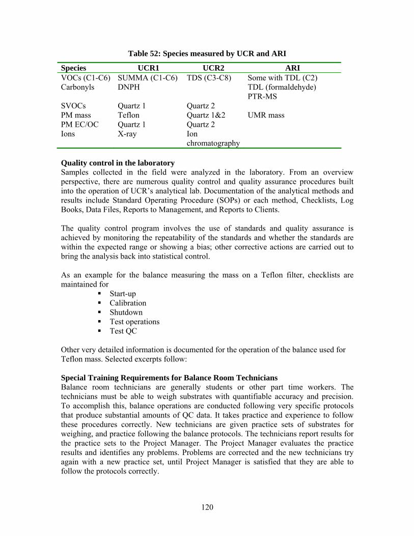
Table 52: Species measured by UCR and ARI

Species UCR1 UCR2 ARI VOCs (C1-C6) SUMMA (C1-C6) TDS (C3-C8) Some with TDL (C2) Carbonyls DNPH TDL (formaldehyde)

PTR-MS SVOCs Quartz 1 Quartz 2 PM mass Teflon Quartz 1&2 UMR mass PM EC/OC Quartz 1 Quartz 2 Ions X-ray Ion

chromatography

Quality control in the laboratory Samples collected in the field were analyzed in the laboratory. From an overview perspective, there are numerous quality control and quality assurance procedures built into the operation of UCR’s analytical lab. Documentation of the analytical methods and results include Standard Operating Procedure (SOPs) or each method, Checklists, Log Books, Data Files, Reports to Management, and Reports to Clients.

The quality control program involves the use of standards and quality assurance is achieved by monitoring the repeatability of the standards and whether the standards are within the expected range or showing a bias; other corrective actions are carried out to bring the analysis back into statistical control.

As an example for the balance measuring the mass on a Teflon filter, checklists are maintained for

Start-up Calibration Shutdown Test operations Test QC

Other very detailed information is documented for the operation of the balance used for Teflon mass. Selected excerpts follow:

Special Training Requirements for Balance Room Technicians Balance room technicians are generally students or other part time workers. The technicians must be able to weigh substrates with quantifiable accuracy and precision. To accomplish this, balance operations are conducted following very specific protocols that produce substantial amounts of QC data. It takes practice and experience to follow these procedures correctly. New technicians are given practice sets of substrates for weighing, and practice following the balance protocols. The technicians report results for the practice sets to the Project Manager. The Project Manager evaluates the practice results and identifies any problems. Problems are corrected and the new technicians try again with a new practice set, until Project Manager is satisfied that they are able to follow the protocols correctly.

120

Sample Handling and Custody of PM samples Particle samples are collected on Teflon filters. The use of particle filters requires numerous sample handling and custody issues to prevent contamination, to ensure proper sample identification, and to ensure equilibration requirements of the CFR. Throughout the procedures, filters are handled only using forceps. The filters never leave the custody of CE-CERT. The steps involved are as follows:

• unused filter numbers are assigned to new plastic Petri dishes • new filters are placed into the numbered plastic Petri dishes • the Petri dishes with unexposed filters are placed into a temperature and humidity

controlled equilibration chamber • after 12 hours the filters are weighed • filters are reweighed daily until two filter weights within 3 µg of each other • filters with consistent weights are transported for testing • prior to the test, filters are transferred from Petri dishes to filter holders at the test

site, the filter ID numbers are recorded on the particle Filter Data log sheet • at the end of the test filters are returned to their original Petri dishes • the Petri dishes of the exposed filters are marked with an X • the filters are returned to the balance room and placed in the equilibration

chamber and equilibrated 12 to 72 hours • the exposed filters are weighed once daily until two weights with 3 µg are

obtained

The procedures for weighing the filters are detailed in Balance Protocol A1 R1.1 Appendix C. These procedures define specific detailed sequences for checking and recording the equilibration chamber conditions, zero and spanning the balance, weighing reference objects, weighing filters, performing zero and span checks, performing replicates. In summary, filter weights are only considered valid if environmental chamber conditions are within tolerance, and the filter weight was preceded and followed by a valid zero and valid span.

For future projects For future efforts to measure organic compounds under similar field conditions, the following should be considered:

• Begin and complete the design, fabrication and checkout testing of the sampling system well before the field campaign begins; this will allow time to correct any problems before the system is required for use

• Analyze a statistically significant subset of samples as soon as possible after collection, and before completion of the field campaign; this will allow detection of invalid samples while time remains during the campaign to correct any problems and to obtain valid samples

• Wherever possible, replace batch sampling techniques with more advanced instrumentation that provides real-time measurement capabilities; this will allow evaluation of sampling system performance during test operation.

The leak in the sampling system would have been detected and corrected if this protocol had been followed, and the desired organic compound data would have been obtained.

121

4.0 Discussion

4.1 Gaseous Emissions

NOx, CO, and specific hydrocarbon species were measured for seven different engines representing three engine models.

NOx and CO were generally consistent with both ICAO data for the CFM56 engine models and with the corresponding NOx and CO data acquired on a different CFM56 engine model measured in the APEX1 campaign. CO data had significant variability due to variation in ambient conditions affecting the engine performance, but APEX1 data analysis has suggested that this variation can be reduced significantly when fuel flow variations are properly accounted for. Fuel flow data was not available from these tests, so these corrections have not been made for the data presented here. While generally consistent with ICAO data in trends (decreasing with increasing engine power) and magnitude, the CO emissions for two engine models are below the regulatory values.

NOx emissions also agree well with the trends in ICAO data (increasing with increasing engine power) and agree well in magnitude for each engine model. Some decreases in NOx EIs at the downstream measurements locations were observed and this warrants further analysis.

Selected hydrocarbon species were measured in real-time for all of the engines studied. Formaldehyde (HCHO) is one of the most prevalent and it demonstrates a decreasing trend with increasing engine power as does the Unburned Hydrocarbon (UHC) data in the ICAO data. As was observed in APEX1, the measured emission indices for individual HC species decrease in proportion with HCHO as the engine power increases, suggesting that HCHO (or other major HC emissions like ethylene, C2H4) is a good indicator for HC emission levels. In addition, the ratio of the individual HCs to HCHO all agree reasonably well with the landmark data of Spicer et al., (1994) on speciated HCs in the CFM56 engine. The major deviation from excellent agreement with Spicer is that several species (notably the higher alkenes, as well as C4 benzenes, and phenols), where the present measurement are significantly higher than Spicer et al. The question of potential loss mechanisms in the Spicer approach may need to be considered. Either chemical transformation (oxidation) or incomplete desorption from the concentration devices used in those measurements could potentially result in reducing the reported levels for the higher alkanes in those earlier studies, but the actual causes for these discrepancies are currently unknown.

4.2 Particulate Emissions

Black Carbon (BC) measurements were made using a Multi-Angle Absorption Photometer (MAAP) for all seven engines. All demonstrated a similar trend, increasing with increasing engine power, especially above 60% rated thrust (although there is also a minor increase in BC when the power decreases to the very lowest idle powers). The

122

newer engine designs (-7B22) had lower emissions than that of the APEX1 engine (– 2C1).

The volatile contributions to the particulate emissions were measured with an Aerosol Mass Spectrometer (AMS). Sulfate and organic contributions were identified and quantified. The sulfate contribution was largely independent of engine power, and was similar to levels observed in APEX1 when compared at 30 or 50 m downstream locations. Sulfate in the particle phase is dependent on the level of sulfur in the fuel, and the overall sulfate levels are expected to correspond to the fuel sulfur levels. The organic contributions were generally significantly lower than APEX1, which requires further analysis but, like APEX1, the contributions have a local maximum at the lowest power conditions when HC emissions are highest. Another increase occurs at the highest power and, although the increase is more dramatic in APEX1 than in the current tests, this increase is most evident at the furthest downstream location.

4.3 PM Physical characterization

One objective of the JETS APEX2 study was to perform a PM emission comparison between old (-300) and new (-700) technology engines currently powering the B737 commercial fleets. A first step in doing this is to examine the variance in PM emissions within a technology type and the second is then to determine whether any engine technology differences are statistically significant for a given PM parameter. It should be noted that the sample size per technology type was extremely small (3 engines per type) and this may make it difficult to discern subtle differences. However, it should also be noted that this study was the first of its kind where multiple engines within a given technology type were made available for measurement.

Figures on the left below (Figures 56a - 60a) present the technology type average PM parameter data (total aerosol) as a function of engine power at 1m measured at JETS APEX2. The triangles represent new technology and the circles represent the old. The error bars indicate uncertainty given by 1 standard deviation in the average. Figures on the right below (Figures 56b - 60b) present the JETS APEX2 data along with the CFM56-2C1 engine data acquired at APEX1 (Lobo et al., 2007).

123

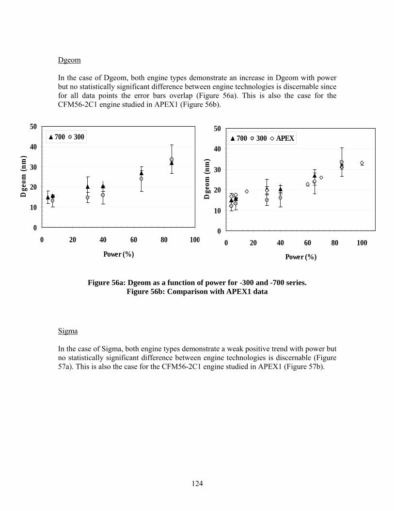
100

50

40

Dge

om (n

m)

Dgeom

In the case of Dgeom, both engine types demonstrate an increase in Dgeom with power but no statistically significant difference between engine technologies is discernable since for all data points the error bars overlap (Figure 56a). This is also the case for the CFM56-2C1 engine studied in APEX1 (Figure 56b).

50 700 300

Dge

om (n

m)

0 20 40 60 80

Power (%)

700 300 APEX

0 20 40 60 80 100

Power (%)

40

30

20

30

20

10 10

0 0

Figure 56a: Dgeom as a function of power for -300 and -700 series. Figure 56b: Comparison with APEX1 data

Sigma

In the case of Sigma, both engine types demonstrate a weak positive trend with power but no statistically significant difference between engine technologies is discernable (Figure 57a). This is also the case for the CFM56-2C1 engine studied in APEX1 (Figure 57b).

124

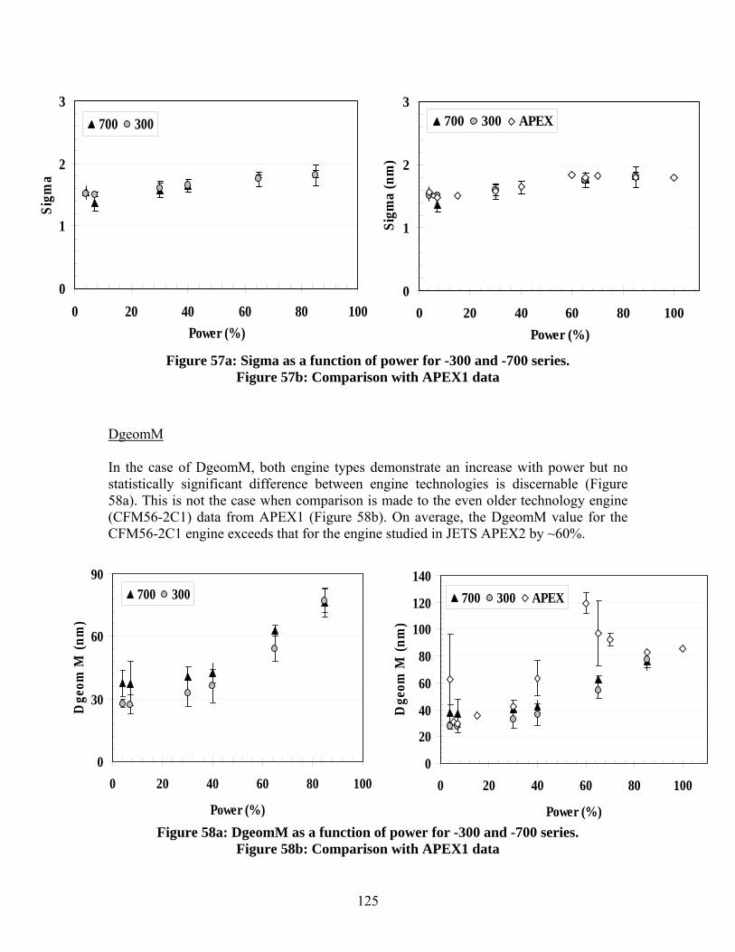
~~I • 0 0 I ~ • 2

- I I I I I I I I I I I I I I I I I I I I I I I I I I I

3

2

1

3

Sigm

a

700 300

0

Sigm

a (n

m)

700 300 APEX

2

1

0 0 20 40 60 80 100 0 20 40 60 80 100

Power (%) Power (%)

Figure 57a: Sigma as a function of power for -300 and -700 series. Figure 57b: Comparison with APEX1 data

DgeomM

In the case of DgeomM, both engine types demonstrate an increase with power but no statistically significant difference between engine technologies is discernable (Figure 58a). This is not the case when comparison is made to the even older technology engine (CFM56-2C1) data from APEX1 (Figure 58b). On average, the DgeomM value for the CFM56-2C1 engine exceeds that for the engine studied in JETS APEX2 by ~60%.

90 140 700 300

0

700 300 APEX

0 20 40 60 80 100

Power (%)

Dge

om M

(nm

)

120

100

80

60

Dge

om M

(nm

)

60

30 40

20

0 0 20 40 60 80 100

Power (%) Figure 58a: DgeomM as a function of power for -300 and -700 series.

Figure 58b: Comparison with APEX1 data

125

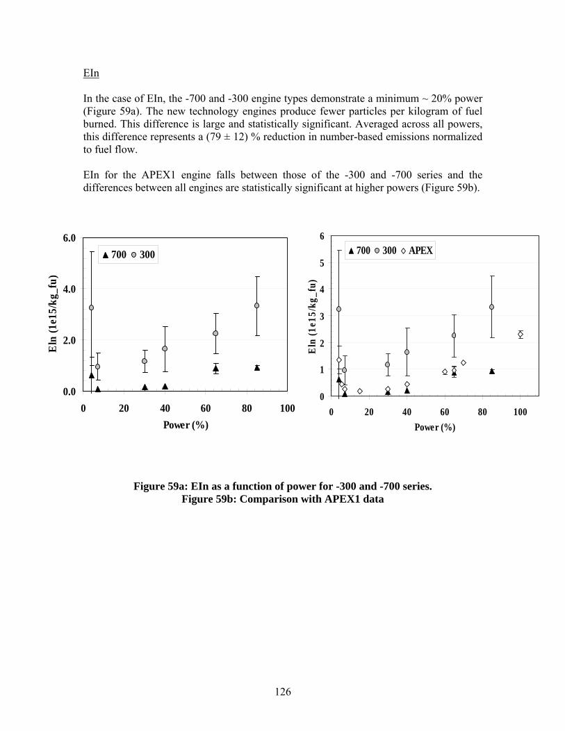
ll

I • I .&1 4 I I I I I

6.0

Eln

(1e1

5/kg

_fu)

EIn

In the case of EIn, the -700 and -300 engine types demonstrate a minimum ~ 20% power (Figure 59a). The new technology engines produce fewer particles per kilogram of fuel burned. This difference is large and statistically significant. Averaged across all powers, this difference represents a (79 ± 12) % reduction in number-based emissions normalized to fuel flow.

EIn for the APEX1 engine falls between those of the -300 and -700 series and the differences between all engines are statistically significant at higher powers (Figure 59b).

6

700 300

E ln

(1e 1

5/kg

_fu)

700 300 APEX

0 20 40 60 80 100 Power (%)

5

4

3

4.0

2.0 2

1

0.0 0 0 20 40 60 80 100

Power (%)

Figure 59a: EIn as a function of power for -300 and -700 series. Figure 59b: Comparison with APEX1 data

126

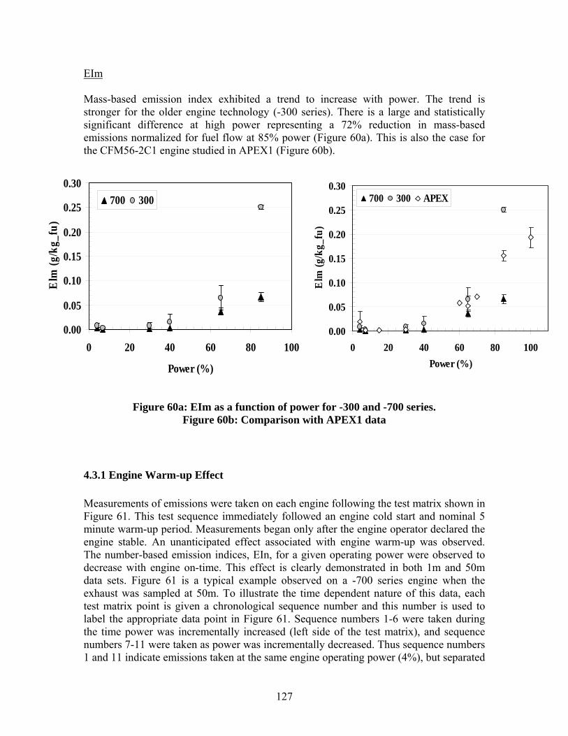
Q a

Elm

(g/k

g_fu

)

EIm

Mass-based emission index exhibited a trend to increase with power. The trend is stronger for the older engine technology (-300 series). There is a large and statistically significant difference at high power representing a 72% reduction in mass-based emissions normalized for fuel flow at 85% power (Figure 60a). This is also the case for the CFM56-2C1 engine studied in APEX1 (Figure 60b).

0.30 0.30

Elm

(g/k

g_fu

)

700 300

0 20 40 60 80 100

Power (%)

700 300 APEX

0 20 40 60 80 100 Power (%)

0.25

0.20

0.15

0.10

0.25

0.20

0.15

0.10

0.05 0.05

0.00 0.00

Figure 60a: EIm as a function of power for -300 and -700 series. Figure 60b: Comparison with APEX1 data

4.3.1 Engine Warm-up Effect

Measurements of emissions were taken on each engine following the test matrix shown in Figure 61. This test sequence immediately followed an engine cold start and nominal 5 minute warm-up period. Measurements began only after the engine operator declared the engine stable. An unanticipated effect associated with engine warm-up was observed. The number-based emission indices, EIn, for a given operating power were observed to decrease with engine on-time. This effect is clearly demonstrated in both 1m and 50m data sets. Figure 61 is a typical example observed on a -700 series engine when the exhaust was sampled at 50m. To illustrate the time dependent nature of this data, each test matrix point is given a chronological sequence number and this number is used to label the appropriate data point in Figure 61. Sequence numbers 1-6 were taken during the time power was incrementally increased (left side of the test matrix), and sequence numbers 7-11 were taken as power was incrementally decreased. Thus sequence numbers 1 and 11 indicate emissions taken at the same engine operating power (4%), but separated

127

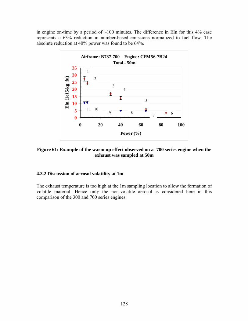
128

in engine on-time by a period of ~100 minutes. The difference in EIn for this 4% case represents a 63% reduction in number-based emissions normalized to fuel flow. The absolute reduction at 40% power was found to be 64%.

Figure 61: Example of the warm up effect observed on a -700 series engine when the exhaust was sampled at 50m

4.3.2 Discussion of aerosol volatility at 1m

The exhaust temperature is too high at the 1m sampling location to allow the formation of volatile material. Hence only the non-volatile aerosol is considered here in this comparison of the 300 and 700 series engines.

Airframe: B737-700 Engine: CFM56-7B24 Total - 50m

0 5

10 15 20 25 30 35

0 20 40 60 80 100

Power (%)

Eln

(1e1

5/kg

_fu)

1

2

3 4

5

6789 1011

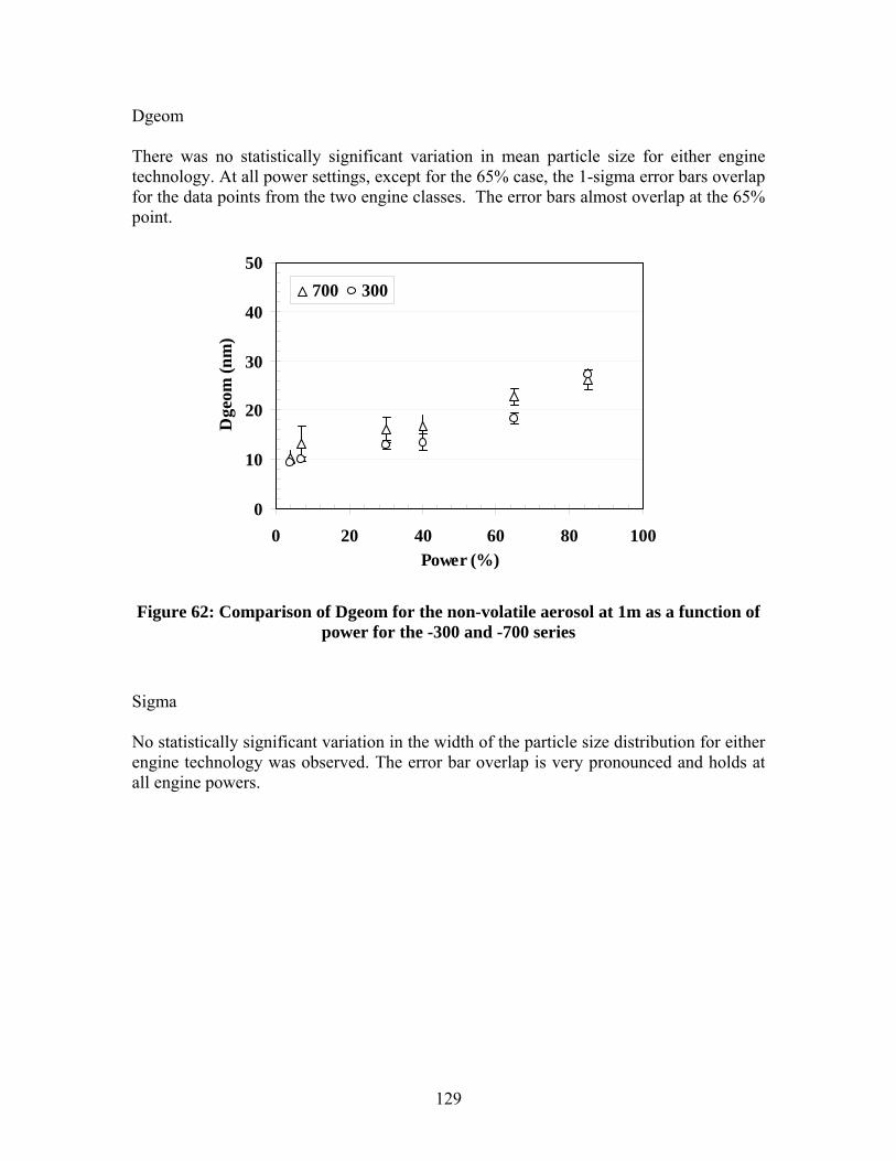
Dgeom

There was no statistically significant variation in mean particle size for either engine technology. At all power settings, except for the 65% case, the 1-sigma error bars overlap for the data points from the two engine classes. The error bars almost overlap at the 65% point.

50 700 300

0 20 40 60 80 100 Power (%)

40

30

20

10

0

Dge

om (n

m)

Figure 62: Comparison of Dgeom for the non-volatile aerosol at 1m as a function of power for the -300 and -700 series

Sigma

No statistically significant variation in the width of the particle size distribution for either engine technology was observed. The error bar overlap is very pronounced and holds at all engine powers.

129

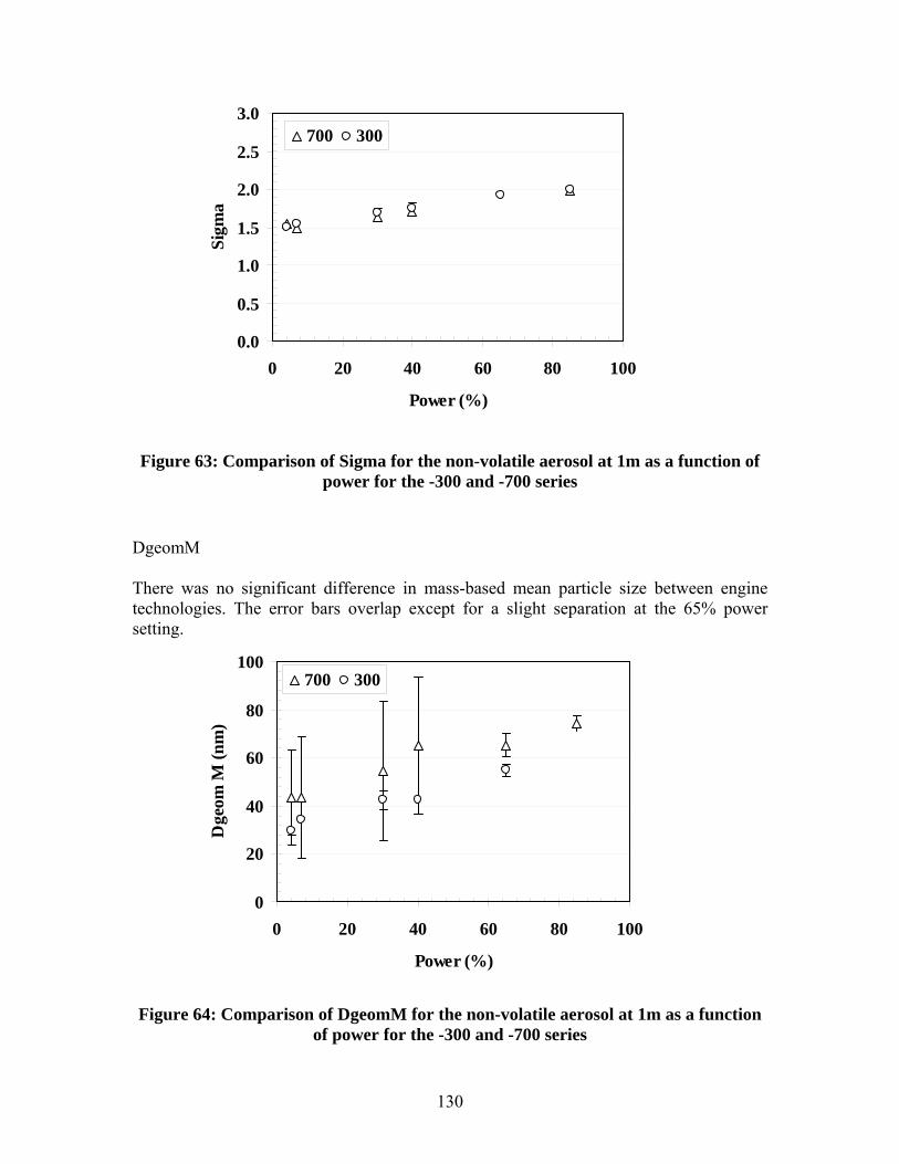
0 Q g g

0

0.0

0.5

1.0

1.5

2.0

2.5

3.0

Sigm

a

700 300

0 20 40 60 80 100

Power (%)

Figure 63: Comparison of Sigma for the non-volatile aerosol at 1m as a function of power for the -300 and -700 series

DgeomM

There was no significant difference in mass-based mean particle size between engine technologies. The error bars overlap except for a slight separation at the 65% power setting.

100 700 300

80

Dge

om M

(nm

)

60

40

20

0 0 20 40 60 80 100

Power (%)

Figure 64: Comparison of DgeomM for the non-volatile aerosol at 1m as a function of power for the -300 and -700 series

130

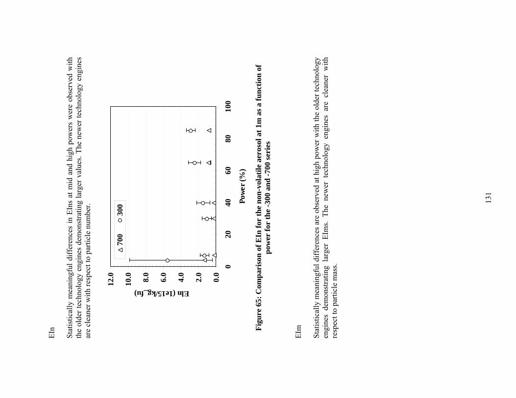
l-0-I Kl

l--0-l I<)

l-0--l

0

<l l-0-l

I O>-----<J----1 ~

EIn

Stat

istic

ally

mea

ning

ful d

iffer

ence

s in

EIn

s at

mid

and

hig

h po

wer

s w

ere

obse

rved

with

th

e ol

der t

echn

olog

y en

gine

s de

mon

stra

ting

larg

er v

alue

s. Th

e ne

wer

tech

nolo

gy e

ngin

es

are

clea

ner w

ith re

spec

t to

parti

cle

num

ber.

0.0

2.0

4.0

6.0

8.0

10.0

12.0

E ln (1e15/kg_fu)

700

300

0 20

40

60

80

10

0

Powe

r (%

)

Figu

re 6

5: C

ompa

riso

n of

EIn

for

the

non-

vola

tile

aero

sol a

t 1m

as a

func

tion

of

pow

er fo

r th

e -3

00 a

nd -7

00 se

ries

EIm

Stat

istic

ally

mea

ning

ful d

iffer

ence

s ar

e ob

serv

ed a

t hig

h po

wer

with

the

olde

r tec

hnol

ogy

engi

nes

dem

onst

ratin

g la

rger

EIm

s. Th

e ne

wer

tec

hnol

ogy

engi

nes

are

clea

ner

with

re

spec

t to

parti

cle

mas

s.

131

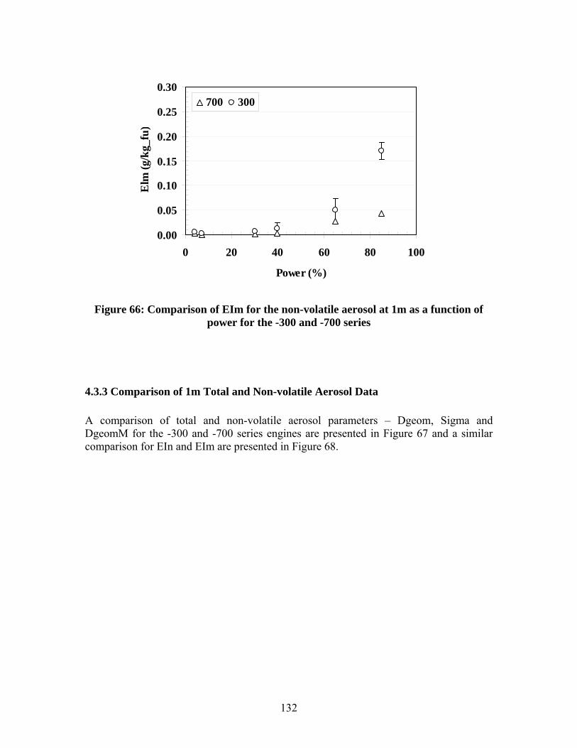
I~ 0 I

0.00

0.05

0.10

0.15

0.20

0.25

0.30

Elm

(g/k

g_fu

)

700 300

0 20 40 60 80 100

Power (%)

Figure 66: Comparison of EIm for the non-volatile aerosol at 1m as a function of power for the -300 and -700 series

4.3.3 Comparison of 1m Total and Non-volatile Aerosol Data

A comparison of total and non-volatile aerosol parameters – Dgeom, Sigma and DgeomM for the -300 and -700 series engines are presented in Figure 67 and a similar comparison for EIn and EIm are presented in Figure 68.

132

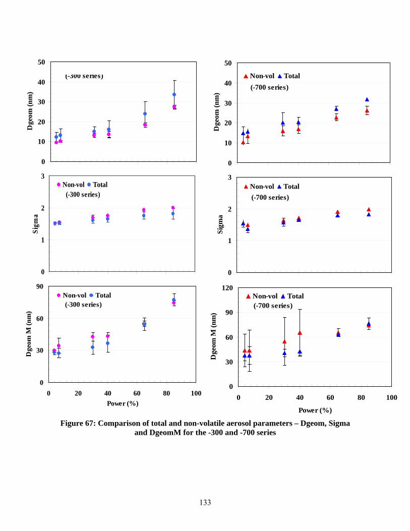
0

10

20

30

40

50

Dge

om (n

m)

Non-vol Total (-300 series)

0

10

20

30

40

50

Dge

om (n

m)

Non-vol Total (-700 series)

0

1

2

3

Sigm

a

Non-vol Total (-300 series)

0

1

2

3

Sigm

a

Non-vol Total (-700 series)

~ ~. • : .&

I l &

i i I t i !

-i

_- ft

• •

•

0 20 40 60 80 100

Power (%)0 20 40 60 80 100

Power (%)

0 20 40 60 80 100

Power (%)

0 20 40 60 80 100

Power (%)

0

30

60

90 Non-vol Total (-300 series)

120 Non-vol Total (-700 series)

0 20 40 60 80 100

Power (%)

Dge

om M

(nm

) 90

60

30

0 0 20 40 60 80 100

Power (%)

Figure 67: Comparison of total and non-volatile aerosol parameters – Dgeom, Sigma and DgeomM for the -300 and -700 series

Dge

om M

(nm

)

133

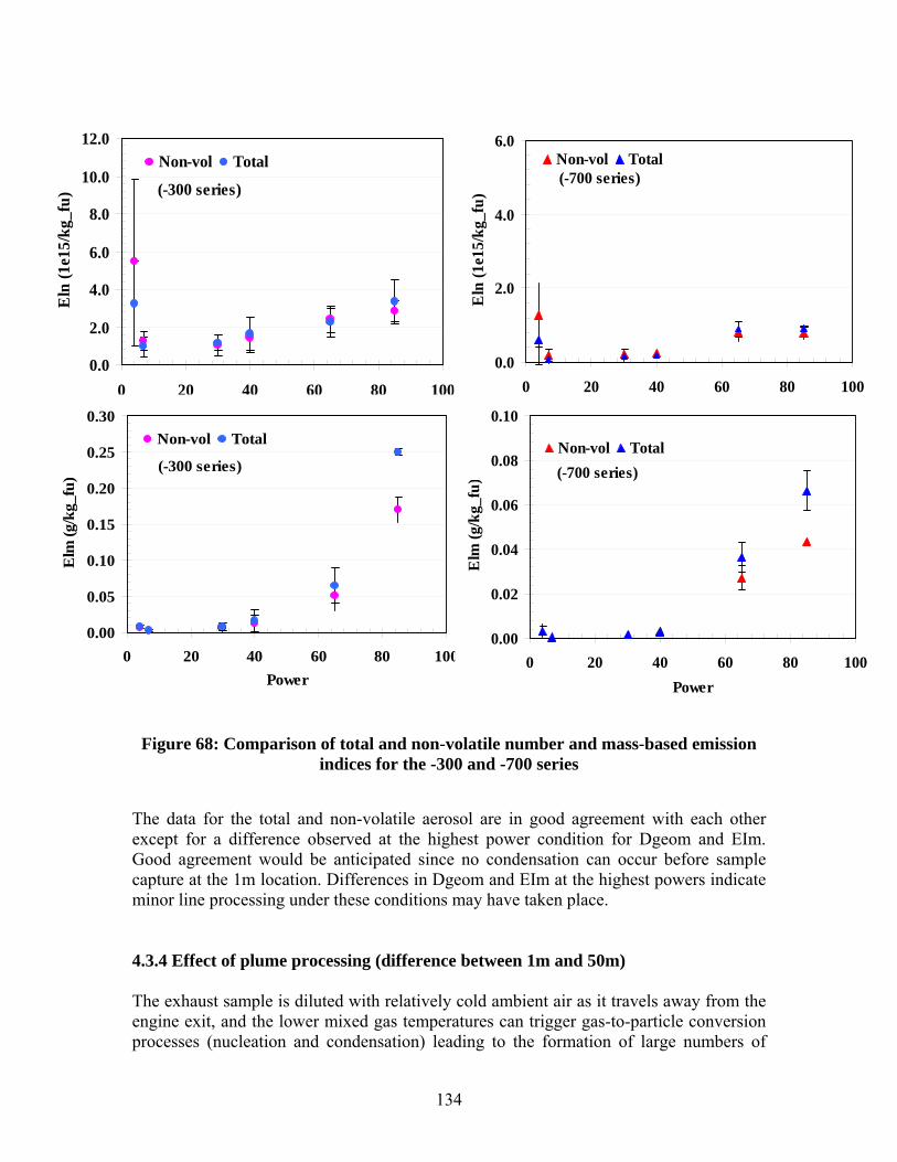
0 20 40 60 80 100

100

• •

• - . .

•

f t

Power (%) Power (%)

8.0

Eln

(1e1

5/kg

_fu)

E

lm (g

/kg_

fu)

12.0 6.0 Non-vol Total

10.0 Non-vol Total (-700 series)

(-300 series)

Elm

(g/k

g_fu

) E

ln (1

e15/

kg_f

u)

4.0

6.0

4.0

2.0

2.0

0.00.0 0 20 40 60 80 100

0.10 0.30 Non-vol Total

(-300 series)

0 20 40 60 80 Power

Non-vol Total (-700 series)

0 20 40 60 80 100 Power

0.25

0.20

0.15

0.10

0.08

0.06

0.04

0.02 0.05

0.00 0.00

Figure 68: Comparison of total and non-volatile number and mass-based emission indices for the -300 and -700 series

The data for the total and non-volatile aerosol are in good agreement with each other except for a difference observed at the highest power condition for Dgeom and EIm. Good agreement would be anticipated since no condensation can occur before sample capture at the 1m location. Differences in Dgeom and EIm at the highest powers indicate minor line processing under these conditions may have taken place.

4.3.4 Effect of plume processing (difference between 1m and 50m)

The exhaust sample is diluted with relatively cold ambient air as it travels away from the engine exit, and the lower mixed gas temperatures can trigger gas-to-particle conversion processes (nucleation and condensation) leading to the formation of large numbers of

134

volatile particles and volatile coatings on the original soot particles. The nucleation processes tend to create small particles and the volatile coatings on soot tend to be thin; hence the left side of the size distribution is impacted more than the right side. The production of these small particles serves to shift Dgeom to smaller values and results in an order of magnitude increase in EIn. These particles do not significantly contribute to the mass dependent parameter values and no significant changes are observed in DgeomM and EIm. It should be noted that the sample experiences ambient temperature and pressure as it passes through the large diameter (5cm) 50m sample line. No further dilution is imposed on the sample beyond that which naturally occurs during plume expansion in transit to the 50m sampling probe. Under these conditions, it is reasonable to conclude that any gas-to-particle conversion in the sample line merely mimics that which would have occurred in the atmosphere. This plume processing is a major effect. Typically the downstream aerosol is substantially different from that found at the engine exit. It should be noted that the final downstream aerosol depends not just on the engine emission characteristics (gas + particulate), but also strongly on the ambient air conditions (e.g. temperature and humidity).

4.4 Organic gases and aerosol chemical speciation

Dramatic increases in the PM concentrations are observed as the power increased to 85% power. The relative distributions of the substituted naphthalenes to non-substituted naphthalenes for the idle modes are in general agreement with the work from Spicer et al.1992, 1994 (see Figures 48, 49). There was a sharp decrease in the relative contribution of substituted naphthalenes at the higher load points. Trends in the non-naphthalenic compounds are also noted with acenaphthylene, present significantly only in the idle mode, and fluoranthene decreasing with increasing power.

With respect to Chromium (VI), results for the aircraft were as expected, except for the sample from N429WN which showed a large response for Chromium (VI). It is important to note that the sample from N429WN was only one of 6 samples collected by UCR that had high chromium (VI). The variability in the metal distributions was much greater between engines than between engine loads (see Figure 52).

The mass of the ions collected on the Teflo filter were so low that only sulfate ions were above the detection limits of the instrument. In the case of the sulfate, the extracted ions (<1 ppm in water) were very close to the lower detection limit of the instrument.

Analysis of the DNPH cartridges and SUMMA canisters revealed anomalous CO2 concentrations which were attributed to a leak in a sub-system of the sampler. Consequently emission factor calculations could not be performed since any dilution taking place in these filter media were no longer quantifiable. As a result, only the mass concentration of species was measured. The major three contributors to the carbonyl emissions are formaldehyde, acetaldehyde, and acetone. Formaldehyde and acetaldehyde are most dominant carbonyl species in the aircraft exhaust emissions. .

135

5.0 Summary and Conclusions

The objectives of the JETS APEX2 study were to produce a comprehensive data set of emission factors for total organic gases and PM for old and new technology CFM56 class engines operating out of a medium size hub airport in the State of California (i.e. Port of Oakland). This study was successful in producing the first state of the art measurements for PM physical characterization of in-service CFM56 type engines. Unfortunately, as a result of the failure of one of the non-real-time sampling systems, the TOG analysis was limited and from that perspective not all of the objectives set out in the proposed effort were accomplished. However, even with the limited TOG data this study represents the first extensive physico-chemical analysis of a series of in-service commercial engines and as such is an extremely valuable dataset. This study is part of a greater multi-agency effort that includes emissions measurements downwind of an active runway at Oakland during normal airport operations, and the results presented here are essential for the interpretation of the downwind measurements which is to follow (not a deliverable in the CARB-funded component of JETS APEX2). Preliminary analysis was presented at the APEX3 Conference in Cleveland, OH (Whitefield et al. 2006, Herndon et al. 2006) [these presentations can be found by accessing the URL: http://particles.grc.nasa.gov/data/apex3_conf/ ]

The emission factors reported here lead to the following conclusions: • Measurement of NOx indicated that the general emissions performance of the

engines was in keeping with certification measurements for the engines studied. • Measurements of individual hydrocarbon species suggest that the Emission

Indices for most of the major species decrease with increasing engine power, in proportion to each other, and specifically with formaldehyde, which is one of the most plentiful emitted hydrocarbons and can be measured accurately.

• The particle composition includes both sulfate and organic volatile fractions at downstream distances, adding to the carbonaceous aerosol that is present already at the engine exit plane. The sulfate contribution has little dependence on engine power, while the organic contribution is greatest at low engine powers.

• The relative distributions of the substituted naphthalenes to non-substituted naphthalenes for the idle modes are in general agreement with the work from Spicer et al.1992, 1994.

• Chromium (VI) results, for all but one of the engines studied, were as expected. • The major three contributors to the carbonyl emissions are formaldehyde,

acetaldehyde, and acetone. Formaldehyde and acetaldehyde are most dominant carbonyl species in the aircraft exhaust emissions.

• The aerosol properties were calculated for the entire aerosol size distribution and not individual size modes.

• Size distributions for exit plane were generally lognormal. Strong and sometimes non-linear dependencies were observed with engine power settings.

• The onset of gas-to-particle conversion was apparent at 50m for low to medium powers. In this data non-lognormal size distributions were often observed, where the mean sizes decreased and EIn increased relative to the 1m size distributions.

136

• The aerosol Soluble Mass Fraction was found to increase with distance from the engine exit plane. Its value was negligible at the engine exit plane and was ~10% at 50m.

137

6.0 Recommendations

The results of this study proved that accurate emission factors can be acquired in a cost effective manner. Since the data is clearly engine/airframe specific, studies of this nature should now be performed on other important engine/airframe combinations e.g. B747/CF6-80.

The GRE at Oakland proved to be an ideal open air laboratory for dedicated aircraft engine emission studies in the exhaust nozzle and near field plumes for B737 commercial transports. The weather conditions and prevailing winds experienced on the east side of San Francisco Bay in late August were also favorable. These factors lead to the recommendation that the GRE at Oakland should be considered a high priority venue for any future scheduled tests.

It should be noted that the mix of transports routinely operating in and out of Oakland will limit the range of engines/airframes that can be studied. For future studies where B747, B757, B767, and B777 and the larger Airbus transports A320, A340 etc. are anticipated test vehicles, it will be necessary to consider attracting other aircraft to the Oakland test site or using GREs located at other airports provided appropriate weather conditions prevail.

In this study, engine operating conditions were recorded only once during each stable engine operating condition. In future tests it is recommended that high frequency data acquisition be employed for engine operating conditions. This may be difficult for older airframes but straight forward for newer additions to the commercial fleet that digitally record engine operating conditions.

Most of the data was gathered and initially analyzed in real-time. However, this was not the case for the UCR samples that were analyzed off-site post test. For future studies efforts should be expended to assure that the analysis could be undertaken for these samples on-site. This would provide quasi-real-time feedback on the integrity of such samples.

Engine to engine variability is difficult to estimate when the engine sample size is small (in this study ≤ 4 engines per model). The value of accurately estimating this parameter warrants the consideration of a longer period of study than the 4 days afforded this project, especially since the per-day costs are small compared to planning, preparation, set-up, and post test analysis costs.

As described in this report, valid measurements for TOG and multiple significant speciated VOCs were not obtained because of sampling and laboratory issues for the light hydrocarbon and carbonyl analyses. These measurements should be repeated at a future engine test, when the opportunity arises, to get better estimates of TOG and speciated VOCs.

138

References

Alofs, D.J. (1978). "Performance of a dual-range cloud nucleus counter", J. Appl. Meteor., 17:1286-1297.

Alofs, D.J. and Trueblood, M.B., (1981)."UMR dual mode CCN counter (Modes: CFD plus Haze)", J. Rech. Atmos., 15:219-223.

Anderson, B. E., Branham, H.-S., Hudgins, C. H., Plant, J. V., Ballenthin, J. O., Miller, T. M., Viggiano, A. A., Blake, D. R., Boudries, H., Canagaratna, M., Maike-Lye, R. C., Onasch, T., Wormhoudt, J., Worsnop, D., Brunke, K. E., Culler, S., Penko, P., Sanders, T., Han, H.-S., Lee, P., Pui, D. Y. H., Thornhill, K. L., and Winstead, E. L., “Experiment to Characterize Aircraft Volatile Aerosol and Trace-Species Emissions (EXCAVATE)”. NASA/TM-2005-213783, National Aeronautics and Space Administration, Hampton, VA, August 2005.

Biskos, G. Reavell, K., and Collings, N., “Description and Theoretical Analysis of a Differential Mobility Spectrometer”, Aerosol Sci. Technol., Vol. 39, 2005, 527-541.

Code of Federal Regulations. Protection of the Environment, 40 CFR 86, §86.1312-88, Weighing chamber and microgram balance specifications

de Gouw, J., Warneke, C., Karl, T., Eerdekens, G., van der Veen, C., and Fall, R. (2003). “Sensitivity and specificity of atmospheric trace gas detection by proton-transfer-reaction mass spectrometry”, International Journal of Mass Spectrometry, 223: 365-382.

Dewes, W., Cottington, R., Hirsinger, F., Petzold, A., Ramaroson, R., Vogels, M., and Westerberg, J. (2000). “The AERONET Network -Emissions, Atmospheric Impact and Regulations”, Air & Space Europe 2 l (3).

Dutton, J. A. (chair), (2002). “Committee on Aeronautics Research and Technology for Environmental Compatibility Report: For Greener Skies – Reducing Environmental Impacts of Aviation”, National Research Council, Washington D.C., ISBN: 0-309-08337-0.

Gerstle, T., Virag, P., Brown, P., and Wade, M. (2002). “Aircraft Engine and Auxiliary Power Unit Emissions Testing: Final Report F119 PW-100 Engine Emissions Testing Report”, Internal Report IERA-RS-BR-SR-2002-0006.

Hagen, D.E., Podzimek, J., Heymsfield, A.J., Trueblood, M.B., and Lutrus, C.K. (1994). "Potential role of nuclei in cloud element formation at high altitudes", Atmospheric Research 31:123-135.

Hagen, D.E., Podzimek, J., and Trueblood, M.B. (1995). "Upper tropospheric aerosol sampled during project FIRE IFO II”, J. Atmos. Sci. 52:4196-4209.

139

Hagen, D.E., Paladino, J., Whitefield, P.D., Trueblood, M.B., and Lilenfeld, H.V. (1997). "Airborne and ground based jet engine aerosol emissions sampling during two NASA field projects: SUCCESS and SNIF", J. Aerosol Sci. 28:S67-S68.

Hagen, D. and Whitefield, P.D. (2003). “A study of the fate of carbonaceous aerosol emissions through a gas turbine engine”, A&WMA Conf. Proc.

Hagen, D.E., Whitefield, P.D., Lobo, P., and Trueblood, M.B. (2005). “PM Emission From a Commercial Jet Engine – Project APEX”, Proc. 9th-Combustion Generated Nanoparticles Conf., Zurich.

Heard, D. E. (ed) (2006). Analytical Techniques for Atmospheric Measurement. Blackwell Publishing, Oxford.

Heland, J. and Schafer, K. (1998). “Determination of Major Combustion Products In Aircraft Exhausts by FTIR Emission Spectroscopy”, Atmospheric Environment 32 (18):3067-3072.

Herndon, S. C., Shorter, J. H., Zahniser, M. S., Nelson, D. D., Jayne, J., Brown, R. C., Miake-Lye, R. C., Waitz, I., Silva, P., Lanni, T., Demerjian, K., and Kolb, C. E. (2004). “NO and NO2 Emission Ratios Measured from In-Use Commercial Aircraft During Taxi and Takeoff”, Environ. Sci. Technol., 38:6078-6084.

Herndon, S. C., Shorter, J. H., Zahniser, M. S., Wormhoudt, J., Nelson, D. D., Demerjian, K. L., and Kolb, C. E. (2005). “Real-time Measurements of SO2, H2CO and CH4 Emissions from in-use Curbside Passenger Buses in New York City using a Chase Vehicle”, Environ. Sci. Technol., 39:7984-7990.

Herndon, S. C., Rogers, T., Dunlea, E. J., Jayne, J. T., Miake-Lye, R. C., and Knighton, B. (2006). “Hydrocarbon Emissions from In-Use Commercial Aircraft during Airport Operations”, Environmental Science & Technology, 40 (14):4406 - 4413.

Herndon, S., Onasch, T., Knighton, B., Wood, E., Timko, M., Jayne, J., Wormhoudt, J., Northway, M., Mortimer, P., Yelvington, P., Wong, H.-W., Shorter, J., McManus, B., Nelson, D., Zahniser, M., Worsnop, D., Kolb, C., Whitefield, P., Lobo, P., Hagen, D., Anderson, B., Wey, C., Howard, R., Kinsey, J., and Miake-Lye, R. "Aviation Engine Emissions Characterization using Wind-Advected Plumes", APEX 3 Conference, Cleveland OH, November 29-December 01, 2006

ICAO, International Civil Aviation Organization Aircraft Engine Emissions DataBank. (2006)

Jayne, J. T., Leard, D. C., Zhang, X. F., Davidovits, P., Smith, K. A., Kolb, C. E., and Worsnop, D. R. (2000). “Development of an aerosol mass spectrometer for size and composition analysis of submicron particles”, Aerosol Science and Technology, 33(1-2):49-70.

140

Jimenez, J. L., Jayne, J. T., Shi, Q., Kolb, C. E., Worsnop, D. R., Yourshaw, I., Seinfeld, J. H., Flagan, R. C., Zhang, X. F., Smith, K. A., Morris, J. W., and Davidovits, P. (2003). “Ambient aerosol sampling using the Aerodyne Aerosol Mass Spectrometer”, Journal of Geophysical Research-Atmospheres, 108(D7).

Knighton, W. B., Rogers, T. M., Anderson, B. E., Herndon, S. C., Yelvington, P. E., and Miake-Lye, R. C. (2007). “Quantification of Aircraft Engine Hydrocarbon Emissions Using Proton Transfer Reaction Mass Spectrometry”, Journal of Propulsion and Power, Vol. 23, No. 5, 949-958

Lilenfeld, H.V., Whitefield, P.D., and Hagen, D.E. (1995). "Soot emissions from jet aircraft", AIAA (Amer. Institute of Aeronautics and Astronautics) paper No. 95-0110.

Li, W., Montassier, N. and Hopke, P. (1992). "A System to Measure the Hygroscopicity of Aerosol Particles", Aerosol Sci. Technol., 17:25-35.

Lister, D. H. and Norman, P. D. (2003). “EC-NEPAir: Work Package 1Aircraft Engine Emissions Certification - a Review of the Development of ICAO Annex 16”, Volume II, GR4D-CT-2000-00182.

Lobo, P., Hagen, D.E., Whitefield, P.D., and Alofs, D.J. (2007). “Physical Characterization of Aerosol Emissions from a Commercial Gas Turbine Engine.” Journal of Propulsion and Power, Vol. 23, No. 5, 919-929

Nelson, D. D., McManus, J. B., Urbanski, S., Herndon, S., and Zahniser, M. S. (2004). High precision measurements of atmospheric nitrous oxide and methane using thermoelectrically cooled mid-infrared quantum cascade lasers and detectors. Spectrochimica Acta A, 60:3325-3335.

NIOSH (National Institute of Occupational Safety and Health), (1996). NIOSH Manual of Analytical Methods, Cincinnati, OH.

NRC (National Research Council), (2003). “Toxicological Assessment of Jet-Propulsion Fuel 8”, The National Academic Press.

Onasch, T.B., Jayne, J.T., Herndon, S., Canagaratna, M.R., Mortimer, I.P., Worsnop, D.R., Miake-Lye, R.C., and Anderson, B.E. (2007) "Chemical Properties of Aircraft Engine Exhaust Aerosols Sampled during APEX", manuscript in preparation

Penner, J. E., Lister, D. H., Griggs, D. J., Dokken, D. J., and McFarland, M. (eds.), (1999). “Aviation and the Global Atmosphere”, IPCC Report, Cambridge University Press, Cambridge, UK, p. 373.

Petzold, A., Strom, J., Schroeder, F. P., and Karcher, B. (1999). “Carbonaceous Aerosol in Jet Engine Exhaust: Emission Characteristics and Implications for Heterogeneous Chemical Reactions”, Atmospheric Environment 33:2689-2698.

141

Petzold, A. (2001). “Aircraft Engine Exhaust Measurement”, Air & Space Europe 3 (1/2):92-95.

Petzold, A., Kramer, H., and Schonlinner, M. (2002). “Continuous Measurement of Atmospheric Black Carbon using a Multi-Angle Absorption Photometer”, Environ. Sci. Poll. Res., 4:78-82.

Petzold, A., and Schonlinner, M. (2004). “Mulit-angle absorption photometry -- a new method for the measurement of aerosol light absorption and atmospheric black carbon”, J. Aerosol Sci., 35:421-441.

Podzimek, J., Hagen, D.E., and Robb, E. (1995). "Large aerosol particles in cirrus type clouds", Atmos. Res. 38:263-282.

Popp, P. J., Bishop, G. A., and Stedman, D. H. (1999). “Method for Commercial Aircraft Nitric Oxide Emission Measurements”, Environ. Sci. Technol. 33:1542-1544.

Samet, J. M., Dominici, F., Curriero, F. C., Coursac, I.,and Zeger, A. L. (2000). “Fine Particulate Air Pollution and Mortality in 20 U. S. Cities, 1987-1994”, N. Engl. J. Med., 343:1742-1749.

Sassen, K., Starr, D.C., Mace, G.G., Poellot, M.R., Melfi, S.H., Eberhard, W.L., Spinhirne, J.D., Eloranta, E.W., Hagen, D.E., and Hallett, J. (1995). "The 5-6 December 1991 FIRE IFO II Jet Stream Cirrus Case Study: Possible influences of volcanic aerosols", J. Atmos. Sci. 52:97-123.

Schmid, O., Hagen, D., Whitefield, P., Trueblood, M., Rutter, A., and Lilenfeld, H. (2004). “Methodology for particle characterization in the exhaust flow of gas turbine engines”, Aerosol Sci. & Techn. 38:1108-1122.

Shah, S.D., Ogunyoku, T. A., Miller, J. W., and Cocker III, D. R. (2004), “On-Road Emission Rates of PAH and n-Alkane Compounds from Heavy-Duty Diesel Vehicles”, Submitted to Environ. Sci. & Technol., November, 2004

Siegl, W. O., Richert, J. F. O., Jensen, T. E., Schuetzle, D., Swarin, S. J., Loo, J. F., Prostak, A., Nagy, D., and Schlenker, A. M. (1993). “Improved Emissions Speciation Methodology for Phase II of The Auto/Oil Air Quality Improvement Research Programs Hydrocarbons and Oxygenates.” SAE Tech. Pap. Ser., No. 930142, Special Publication SP-1000.

Spicer, C.W., Holdren, M.W., Smith, D.L., Hughes, D.P., and Smith, M.D. (1992). “Chemical Composition of Exhaust from Aircraft Turbine Engines”, J. Eng. Gas Turbines Power 114 (1): 111–117.

142

Spicer, C.W., Holdren, M.W., Riggin, R.M., and Lyon, T.F. (1994). “Chemical Composition and Photochemical Reactivity of Exhaust from Aircraft Turbine Engines”, Ann. Geophys. 12:944–955.

Tesseraux, I. (2004). “Risk Factors of Jet Fuel Combustion Products”, Toxicology Letters 149:295–300.

Waitz, I. A., Townsend, J., Cutcher-Gershenfeld, J., Greitzer, E. M., and Kerrebrock, J. L. "Aviation and the Environment: A National Vision Statement, Framework for Goals and Recommended Actions," Report to the United States Congress, on behalf of the U.S. DOT, FAA and NASA, December 2004

Wey, C.C., Anderson, B.E., Hudgins, C., Wey, C., Li-Jones, X., Winstead, E., Thornhill, L.K., Lobo, P., Hagen, D., Whitefield, P., Yelvington, P. E., Herndon, S.C., Onasch, T.B., Miake-Lye, R.C., Wormhoudt, J., Knighton, W.B., Howard, R., Bryant, D., Corporan, E., Moses, C., Holve, D., and Dodds, W. “Aircraft Particle Emissions eXperiment (APEX)” NASA/TM-2006-214382, ARL-TR-3903, National Aeronautics and Space Administration, Cleveland, OH, September 2006.

Whitefield, P.D. and Hagen, D.E. (1995). "Particulates and aerosol sampling from combustor rigs using the UMR mobile aerosol sampling system (MASS)", AIAA (Amer. Institute of Aeronautics and Astronautics) paper No. 95-0111.

Whitefield, P.D., Hagen, D.E., and Lilenfeld, H.V. (1997). "Ground based measurements of particulate emissions from supersonic transports - Concorde Olympus engine", Proc. of the Comite Avion Ozone International Colloquium I:119-124.

Whitefield, P., Hagen, D., Siple, G., and Pherson, J. (2001). “Estimation of particulate emission indices as a function of size for the LTO cycle for commercial jet engines”, A&WMA Conf. Proc. #347.

Whitefield, P. D., Hagen, D. E., Wormhoudt, J. C., Miake-Lye, R. C., Wilson, C., Brundish, K., Waitz, I., Lukachko, S., and Yam, C. K. (2002). NASA/QinetiQ Collaborative Program-Final Report. NASA CR-2002-211900.

Whitefield, P., Lobo, P., and Hagen, D., “JETS APEX2 Runway Study”, APEX3 Conference, Cleveland, OH. November 29- December 01, 2006

Wilson, C. W., Petzold, A., Nyeki, S., Schumann, U., and Zellner, R. (2004). “Measurement and Prediction of Emissions of Aerosols and Gaseous Precursors from Gas Turbine Engines (PartEmis): An Overview”, Aerospace Science and Technology 8:131–143.

Wormhoudt, J., Herndon, S.C., Yelvington, P.E., Miake-Lye, R.C., and Wey, C. (2007) "Nitrogen Oxide (NO/NO2/HONO) Emissions Measurements in Aircraft Exhausts", Journal of Propulsion and Power, Vol. 23, No. 5, 906-911

143

Yelvington, P. E., Herndon, S. C., Wormhoudt, J., Jayne, J. T., Miake-Lye, R. C., Knighton, W. B., and Wey, C. (2007). “Chemical Speciation of Hydrocarbon Emissions from a Commercial Aircraft Engine”, Journal of Propulsion and Power, Vol. 23, No. 5, 912-918

144

List of inventions reported and publications produced

At this time there are no inventions to report and none to be anticipated. With respect to publications, there are no publications at this time; however, several are in preparation once approval for public release of this data has been provided.

145

Glossary of terms, abbreviations and symbols

AMS Aerosol Mass Spectrometer APU Auxiliary Power Unit ARI Aerodyne Research Inc. BC Black Carbon aerosol BDL Below Detection Limit CAEP Committee on Aviation and Environmental Protection CFO critical flow element CFR Code of Federal Regulations CH2O formaldehyde CO Carbon monoxide CO2 Carbon dioxide CPC Condensation Particle Counters Dgeom Number-based geometric mean diameter DMA Differential Mobility Analyzers DMS Differential Mobility Spectrometers DNPH dinitrophenylhydrazine DoD Department of Defense EC Elemental Carbon EI’s emission indices EIm Mass-based emission index EIR Environmental Impact Report EPA Environmental Protection Agency FAA Federal Aviation Administration FID flame ionization detector GC gas chromatograph GC/FID field ionization detector GC/MS mass spectrometer detector GRE Ground Runup Enclosure GSEs ground support equipment H2O Water HC hydrocarbon HCHO Formaldehyde HNO3 nitric acid HPLC high performance liquid chromatograph HRGC high resolution gas chromatography HRMS high resolution mass spectrometry ICAO International Civil Aviation Organization LPC laser particle counter LPM liter per minute LTO landing and takeoff MAAP Multi-Angle Absorption Photometer mz mass-to-charge ratio NASA National Aeronautics and Space Administration NCAR’s National Center for Atmospheric Research

146

NEPAIR New Emissions Parameter NH4

+ ammonium NIOSH National Institute of Occupational Safety and Health NMVOCs -C2–C10 non-methane hydrocarbons NO Nitric Oxide no total particle concentration NOx oxides of nitrogen OAK Oakland International Airport OC organic carbon PAHs Polycyclic Aromatic Hydrocarbons PCDD's polychlorinated dibenzo-p-dioxins PCDF's polychlorinated dibenzofurans Pen penetration factor PM particulate matter PTR-MS Proton-Transfer Reaction Mass Spectroscopy PUF/XAD-4 polyurethane foam R concentration of a HC emission component SMF Soluble Mass Fraction SN smoke number SO2 Sulfur Dioxide SVOCs semi-volatile organic compounds SWA Southwest Airlines TEM Transmission Electronic Microscopy THC total hydrocarbons TILDAS Tunable Infrared Laser Differential Absorption Spectroscopy TOG total organic gases UCR University of California-Riverside UHCs unburned/partially combusted hydrocarbons UMR University of Missouri-Rolla UMRCOE University of Missouri-Rolla Center of Excellence VOC Volatile Organic Compounds VVOCs very volatile organic carbon gases

147

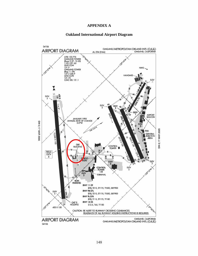
O.t106

1

'-...._Q.Tl 29' l'IOIDING

@)[ 160

~D/MfJROfOl.lfAN O!<tAND INlfll. (OAK} Al.-294 fJMI OA'JGANI), ~ llt-U,!t,

,S,Ta,, 1210, STI75, TT500, oomi() IMnH•:114

S,Ta,, 1210, $TI75, TT500, oomi()

Wll9l~ S,7J1,T115, STI75, m 80

W/11"3 SI 2.5, V65, TTl OO

M'<NS .......

"' H'AN:GAlS

\\I ~

I mv

5

II I •

I

I

8 EIW ~

-!!OH I

BIEV ;I

-

' ,

·-4. CAUTilDN: BE fillrrlrO iUl'<IWAY CROSSlfllG C~Ce'S. ~4.

AIRPORT ID lAGIRAM

lifA£ll!A:OK Or ALIL RlJNlliVAY OOLDING l~lJCDOMS 15 REQIJJlml.

QA't:liANI), CJJIORNIA OA'K~/MEll'ltOPOL!llAN ()IQ.AND INTII. (OAK)

APPENDIX A

Oakland International Airport Diagram

148

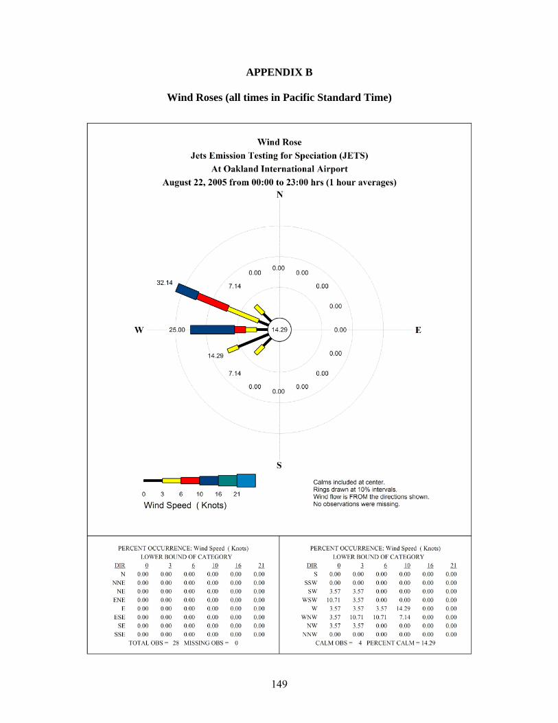
Wind Rose

Jets Emission Testing for Speciation (JETS)

At Oakland International Airport

August 22, 2005 from 00:00 to 23:00 hrs (1 hour averages) N

0.00 0.00

32.14

7.14

0.00 0.00

s

0.00

0.00

0.00

0.00

0.00

0.00

0.00

Calms included at center. Rings drawn at 10% intervals.

E

0 3 6 10 16 21

Wind Speed ( Knots) Wind flow is FROM the directions shown. No observations were missing.

PERCENT OCCURRENCE: Wind Speed ( Knots) PERCENT OCCURRENCE: Wind Speed ( Knots) LOWER BOUND OF CATEGORY LOWER BOUND OF CATEGORY

DIR _Q ;)_ Q _l__Q l.fi I1. DIR _Q ;)_ Q _l__Q l.fi N 0.00 0.00 0.00 0.00 0.00 0.00 s 0.00 0.00 0.00 0.00 0.00

NNE 0.00 0.00 0.00 0.00 0.00 0.00 SSW 0.00 0.00 0.00 0.00 0.00 NE 0.00 0.00 0.00 0.00 0.00 0.00 SW 3.57 3.57 0.00 0.00 0.00

ENE 0.00 0.00 0.00 0.00 0.00 0.00 WSW 10.71 3.57 0.00 0.00 0.00 E 0.00 0.00 0.00 0.00 0.00 0.00 w 3.57 3.57 3.57 14.29 0.00

ESE 0.00 0.00 0.00 0.00 0.00 0.00 WNW 3.57 10.71 10.71 7. 14 0.00

SE 0.00 0.00 0.00 0.00 0.00 0.00 NW 3.57 3.57 0.00 0.00 0.00 SSE 000 000 0.00 0.00 000 000 NNW 000 0.00 0.00 000 0.00

TOTAL OBS= 28 MISSING OBS= 0 CALM OBS= 4 PERCENT CALM = 14.29

I1. 0.00 0.00 0.00 0.00 0.00 0.00

0.00 0.00

APPENDIX B

Wind Roses (all times in Pacific Standard Time)

149

Wind Rose

Jets Emission Testing for Speciation (JETS)

At Oakland International Airport

August 23, 2005 from 00:00 to 23:00 hrs (1 hour averages) N

7.14

42.86 17.86

0.00

0.00

0 .00

-

10.71 0.00

0.00 000

s

0.00

0.00

000

0.00

0.00

Calms included at center. Rings drawn at 10% intervals.

E

0 3 6 10 16 21

Wind Speed ( Knots) Wind flow is FROM the directions shown. No observations were missing.

PERC'F.NT O,C'I IRRF.N,F.- Winil Speeil ( Knors) PERC:F.NT OC'rl IRRF.NC:F.- Winil Speeil ( Knors) LOWER BOUND OF CATEGORY LOWER BOUND OF CATEGORY

DIR .Q 1 Q l.Q l.Q 21 DIR .Q 1 Q l.Q l.Q

N 7.14 3.57 0.00 0.00 0.00 0.00 s 0.00 0.00 0.00 0.00 0.00 NNE 0.00 0.00 0.00 0.00 0.00 0.00 SSW 0.00 0.00 0.00 0.00 0.00

NE 0.00 0.00 0.00 0.00 0.00 0.00 SW 0.00 0.00 0.00 0.00 0.00 ENE 0.00 0.00 0.00 0.00 0.00 0.00 WSW 0.00 0.00 0.00 0.00 0.00

E 0.00 0.00 0.00 0.00 0.00 0.00 w 0.00 3.57 3.57 0.00 0.00 ESE 0.00 0.00 0.00 0.00 0.00 0.00 WNW 0.00 7.14 7.14 28.57 0.00

SE 0.00 0.00 0.00 0.00 0.00 0.00 NW 7.14 10.71 0.00 0.00 0.00 SSE 0.00 0.00 0.00 0.00 0.00 0.00 NNW 0.00 7.14 0.00 0.00 0.00

TOT AL OBS = 28 MISSING OBS = 0 CALM OBS = 4 PERCENT CALM = 14.29

21 0.00 0.00 0.00 0.00 0.00 0.00 0.00 0.00

150

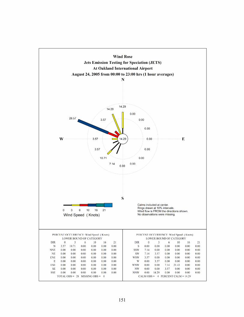
Wind Rose

Jets Emission Testing for Speciation (JETS)

At Oakland International Airport

August 24, 2005 from 00:00 to 23:00 hrs (1 hour averages) N

14.29 14.29

28.57

10.71

7.14 0.00

s

0.00

000

0.00

0.00

000

0.00

0.00

Calms included at center. Rings drawn at 10% intervals.

E

0 3 6 10 16 21

Wind Speed ( Knots) Wind flow is FROM the directions shown. No observations were missing.

PF.RC:F.NT OC:C'I !RR F.NC'F.· Winn Speen ( K nnts) PFRC:F.NT ()('f:l JR R F.NC:F.· Winn Speen ( Knnrs) LOWER BOUND OF CATEGORY LOWER BOUND OF CATEGORY

DIR Q J. Q lQ .!ii ll DIR Q J. Q lQ .!ii N 3.57 10.71 0.00 0.00 0.00 0.00 s 0.00 0.00 0.00 0.00 0.00

NNE 0.00 0.00 0.00 0.00 0.00 0.00 SSW 7.14 0.00 0.00 0.00 0.00 NE 0.00 0.00 0.00 0.00 0.00 0.00 SW 7.14 3.57 0.00 0.00 0.00

ENE 0.00 0.00 0.00 0.00 0.00 0.00 WSW 3.57 0.00 0.00 0.00 0.00 E 0.00 0.00 0.00 0.00 0.00 0.00 w 0.00 3.57 0.00 0.00 0.00

ESE 0.00 0.00 0.00 0.00 0.00 0.00 WNW 0.00 0.00 7.14 21.43 0.00 SE 0.00 000 0.00 000 000 0.00 NW 0.00 0.00 3.57 000 0.00

SSE 0.00 000 0.00 000 000 0.00 NNW 0.00 14.29 0.00 000 0.00 TOTAL OBS= 28 MISSING OBS= 0 CALM OBS= 4 PERCENT CALM= 14.29

ll 0.00 0.00 0.00 0.00 0.00 0.00 0.00 0.00

151

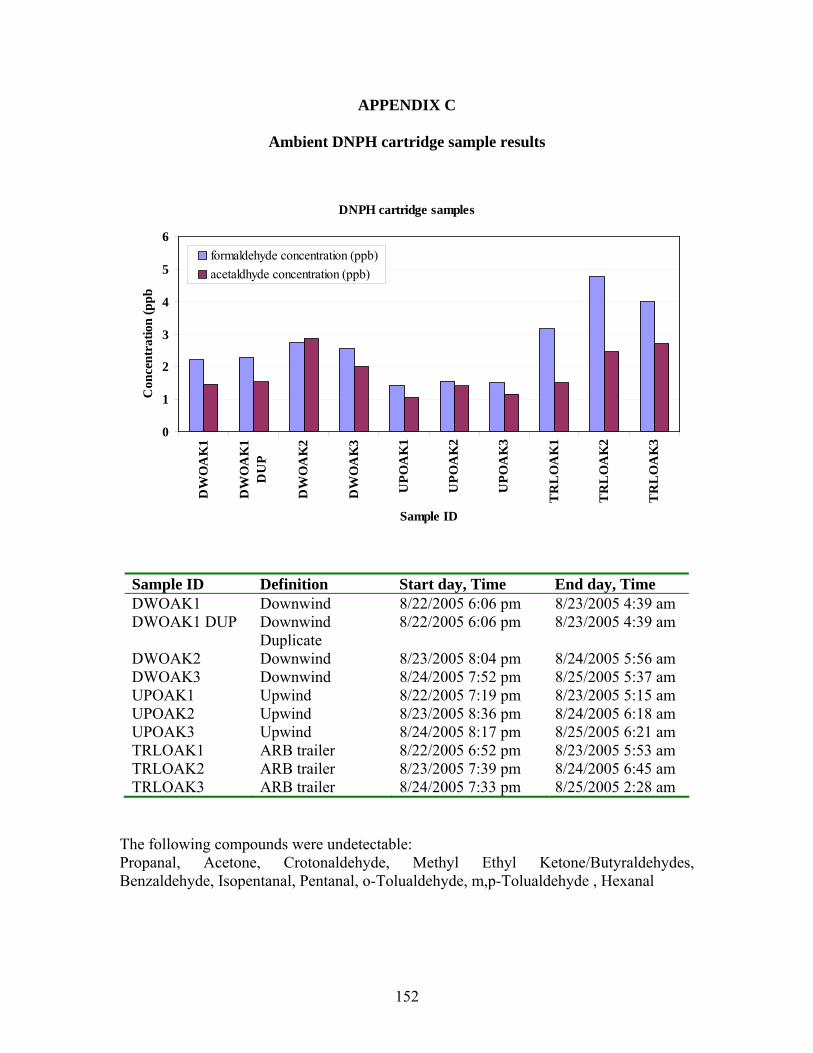
APPENDIX C

Ambient DNPH cartridge sample results

DNPH cartridge samples

6 formaldehyde concentration (ppb)

Con

cent

ratio

n (p

pb

5

4

3

2

1

0

acetaldhyde concentration (ppb)

DW

OA

K1

DW

OA

K1

DU

P

DW

OA

K2

DW

OA

K3

UPO

AK

1

UPO

AK

2

UPO

AK

3

TR

LO

AK

1

TR

LO

AK

2

TR

LO

AK

3

Sample ID

Sample ID Definition Start day, Time End day, Time DWOAK1 Downwind 8/22/2005 6:06 pm 8/23/2005 4:39 am DWOAK1 DUP Downwind 8/22/2005 6:06 pm 8/23/2005 4:39 am

Duplicate DWOAK2 Downwind 8/23/2005 8:04 pm 8/24/2005 5:56 am DWOAK3 Downwind 8/24/2005 7:52 pm 8/25/2005 5:37 am UPOAK1 Upwind 8/22/2005 7:19 pm 8/23/2005 5:15 am UPOAK2 Upwind 8/23/2005 8:36 pm 8/24/2005 6:18 am UPOAK3 Upwind 8/24/2005 8:17 pm 8/25/2005 6:21 am TRLOAK1 ARB trailer 8/22/2005 6:52 pm 8/23/2005 5:53 am TRLOAK2 ARB trailer 8/23/2005 7:39 pm 8/24/2005 6:45 am TRLOAK3 ARB trailer 8/24/2005 7:33 pm 8/25/2005 2:28 am

The following compounds were undetectable: Propanal, Acetone, Crotonaldehyde, Methyl Ethyl Ketone/Butyraldehydes, Benzaldehyde, Isopentanal, Pentanal, o-Tolualdehyde, m,p-Tolualdehyde , Hexanal

152

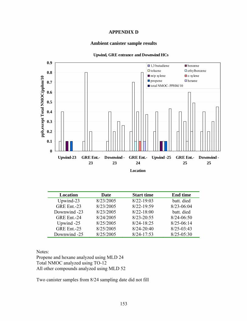
D • D D

-

• D

• D -

• -

-

-

-

-

-I II I I n

APPENDIX D

Ambient canister sample results

Upwind, GRE entrance and Downwind HCs

Upwind-23 GRE Ent.- Downwind - GRE Ent.- Upwind -25 GRE Ent.- Downwind -23 23 24 25 25

Location

0

0.1

0.2

0.3

0.4

0.5

0.6

0.7

0.8

0.9

ppb,

exce

pt T

otal

NM

OC

(pph

m/1

0

1,3 butadiene benzene toluene ethylbenzene m/p xylene o xylene propene hexane total NMOC- PPHM/10

Location Upwind-23

GRE Ent.-23 Downwind -23 GRE Ent.-24 Upwind -25 GRE Ent.-25

Downwind -25

Date 8/23/2005 8/23/2005 8/23/2005 8/24/2005 8/25/2005 8/25/2005 8/25/2005

Start time 8/22-19:03 8/22-19:59 8/22-18:00 8/23-20:55 8/24-18:25 8/24-20:40 8/24-17:53

End time batt. died

8/23-06:04 batt. died

8/24-06:50 8/25-06:14 8/25-03:43 8/25-05:30

Notes: Propene and hexane analyzed using MLD 24 Total NMOC analyzed using TO-12 All other compounds analyzed using MLD 52

Two canister samples from 8/24 sampling date did not fill

153

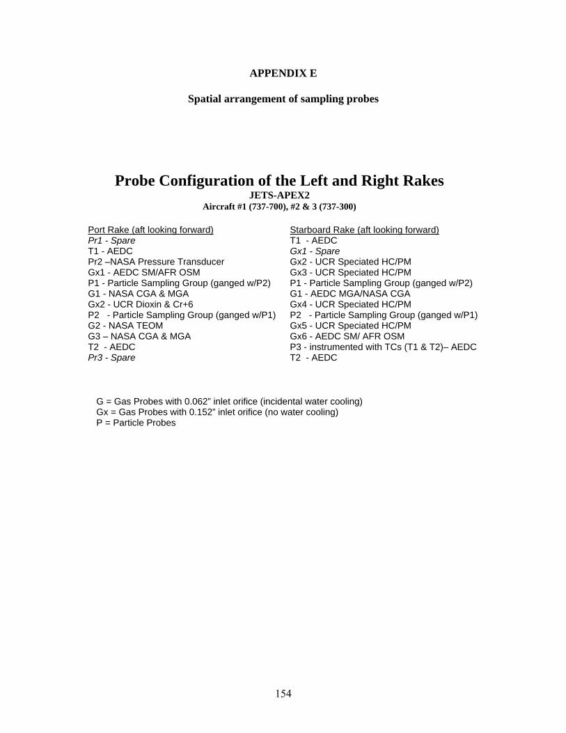
APPENDIX E

Spatial arrangement of sampling probes

Probe Configuration of the Left and Right Rakes JETS-APEX2

Aircraft #1 (737-700), #2 & 3 (737-300)

Port Rake (aft looking forward) Pr1 - Spare T1 - AEDC Pr2 –NASA Pressure Transducer Gx1 - AEDC SM/AFR OSM P1 - Particle Sampling Group (ganged w/P2) G1 - NASA CGA & MGA Gx2 - UCR Dioxin & Cr+6 P2 - Particle Sampling Group (ganged w/P1) G2 - NASA TEOM G3 – NASA CGA & MGA T2 - AEDC Pr3 - Spare

Starboard Rake (aft looking forward) T1 - AEDC Gx1 - Spare Gx2 - UCR Speciated HC/PM Gx3 - UCR Speciated HC/PM P1 - Particle Sampling Group (ganged w/P2) G1 - AEDC MGA/NASA CGA Gx4 - UCR Speciated HC/PM P2 - Particle Sampling Group (ganged w/P1) Gx5 - UCR Speciated HC/PM Gx6 - AEDC SM/ AFR OSM P3 - instrumented with TCs (T1 & T2)– AEDC T2 - AEDC

G = Gas Probes with 0.062” inlet orifice (incidental water cooling) Gx = Gas Probes with 0.152” inlet orifice (no water cooling) P = Particle Probes

154

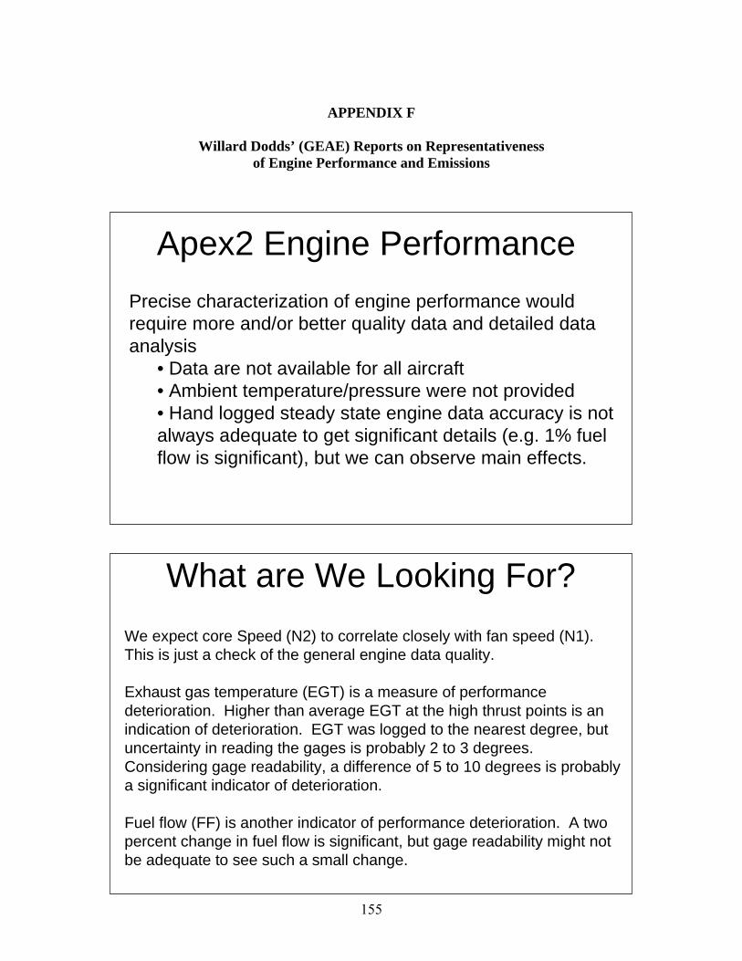
APPENDIX F

Willard Dodds’ (GEAE) Reports on Representativeness of Engine Performance and Emissions

Apex2 Engine Performance Precise characterization of engine performance would require more and/or better quality data and detailed data analysis

• Data are not available for all aircraft • Ambient temperature/pressure were not provided • Hand logged steady state engine data accuracy is not always adequate to get significant details (e.g. 1% fuel flow is significant), but we can observe main effects.

What are We Looking For? We expect core Speed (N2) to correlate closely with fan speed (N1). This is just a check of the general engine data quality.

Exhaust gas temperature (EGT) is a measure of performance deterioration. Higher than average EGT at the high thrust points is an indication of deterioration. EGT was logged to the nearest degree, but uncertainty in reading the gages is probably 2 to 3 degrees. Considering gage readability, a difference of 5 to 10 degrees is probably a significant indicator of deterioration.

Fuel flow (FF) is another indicator of performance deterioration. A two percent change in fuel flow is significant, but gage readability might not be adequate to see such a small change.

155

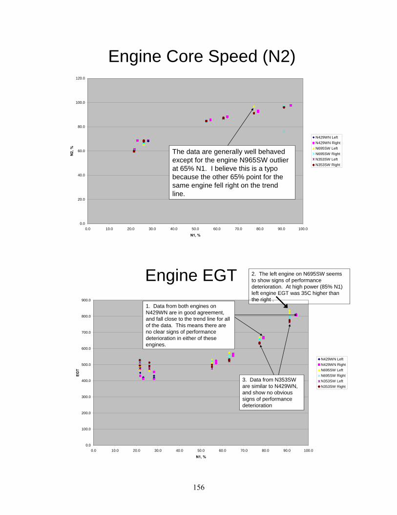
• • •• •• 1··

■ I I j_ JI

'

t--

' JIii

_..

I~ I f

""• I ' it

I \ I t I I • \ I

X e I ii I

♦ •

~

•• _1

~

Engine Core Speed (N2) 120.0

100.0

80.0

60.0

40.0

20.0

0.0 0.0 10.0 20.0 30.0 40.0 50.0 60.0 70.0 80.0 90.0 100.0

N1, %

The data are generally well behaved except for the engine N965SW outlier at 65% N1. I believe this is a typo because the other 65% point for the same engine fell right on the trend line.

N429WN Left N429WN Right N695SW Left N695SW Right N353SW Left N353SW Right

N2,

%

Engine EGT

0.0

100.0

200.0

300.0

400.0

500.0

600.0

700.0

800.0

900.0

EGT

N429WN Left N429WN Right N695SW Left N695SW Right N353SW Left N353SW Right

1. Data from both engines on N429WN are in good agreement, and fall close to the trend line for all of the data. This means there are no clear signs of performance deterioration in either of these engines.

2. The left engine on N695SW seems to show signs of performance deterioration. At high power (85% N1) left engine EGT was 35C higher than the right .

3. Data from N353SW are similar to N429WN, and show no obvious signs of performance deterioration

0.0 10.0 20.0 30.0 40.0 50.0 60.0 70.0 80.0 90.0 100.0

N1, %

156

■

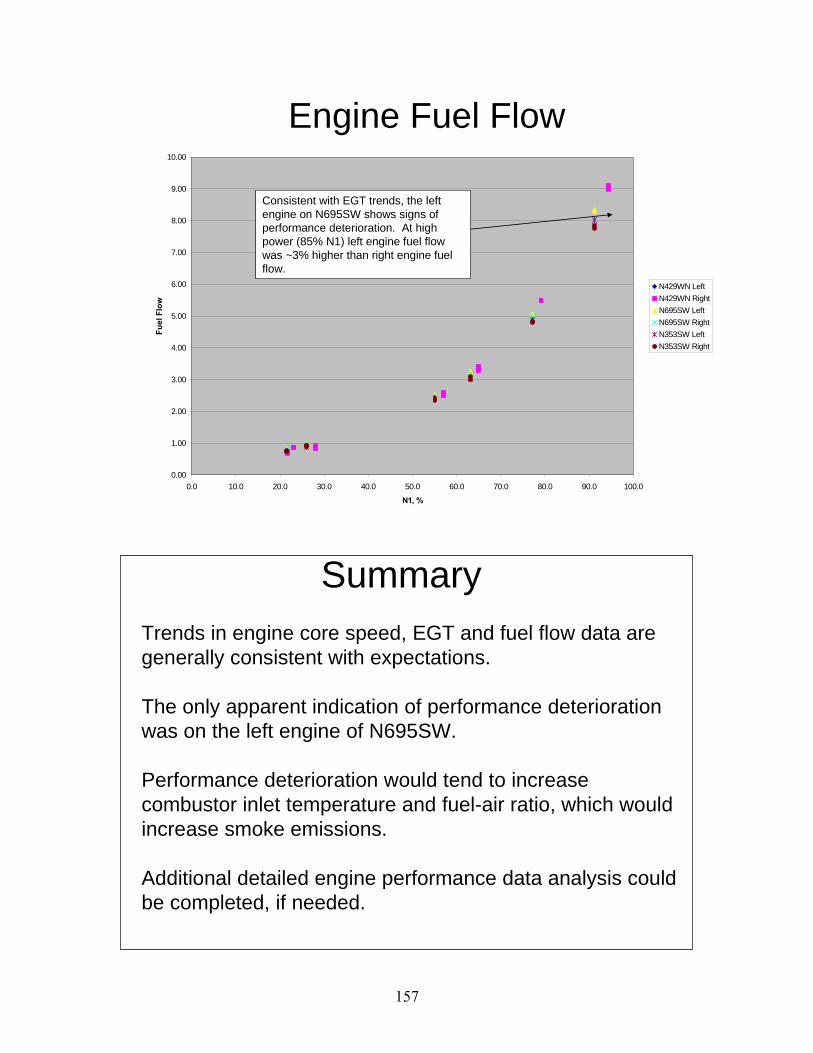
• □ I

••

••

Engine Fuel Flow

0.00

1.00

2.00

3.00

4.00

5.00

6.00

7.00

8.00

9.00

10.00 Fu

el F

low

N429WN Left N429WN Right N695SW Left N695SW Right N353SW Left N353SW Right

Consistent with EGT trends, the left engine on N695SW shows signs of performance deterioration. At high power (85% N1) left engine fuel flow was ~3% higher than right engine fuel flow.

0.0 10.0 20.0 30.0 40.0 50.0 60.0 70.0 80.0 90.0 100.0

N1, %

Summary Trends in engine core speed, EGT and fuel flow data are generally consistent with expectations.

The only apparent indication of performance deterioration was on the left engine of N695SW.

Performance deterioration would tend to increase combustor inlet temperature and fuel-air ratio, which would increase smoke emissions.

Additional detailed engine performance data analysis could be completed, if needed.

157

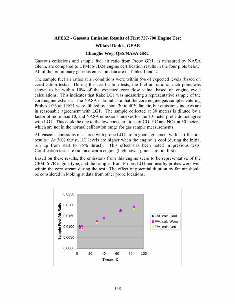
I 7

II

• • "

---- n '

APEX2 - Gaseous Emission Results of First 737-700 Engine Test

Willard Dodds, GEAE

Changlie Wey, QSS/NASA GRC Gaseous emissions and sample fuel air ratio from Probe GR1, as measured by NASA Glenn, are compared to CFM56-7B24 engine certification results in the four plots below. All of the preliminary gaseous emission data are in Tables 1 and 2.

The sample fuel air ratios at all conditions were within 5% of expected levels (based on certification tests). During the certification tests, the fuel air ratio at each point was shown to be within 10% of the expected core flow value, based on engine cycle calculations. This indicates that Rake LG1 was measuring a representative sample of the core engine exhaust. The NASA data indicate that the core engine gas samples entering Probes LG3 and RG1 were diluted by about 30 to 40% fan air, but emissions indexes are in reasonable agreement with LG1. The sample collected at 30 meters is diluted by a factor of more than 10, and NASA emissions indexes for the 30-meter probe do not agree with LG1. This could be due to the low concentrations of CO, HC and NOx at 30 meters, which are not in the normal calibration range for gas sample measurements.

All gaseous emissions measured with probe LG1 are in good agreement with certification results. At 30% thrust, HC levels are higher when the engine is cool (during the initial run up from start to 85% thrust). This effect has been noted in previous tests. Certification tests are run on a warm engine (high power points are run first).

Based on these results, the emissions from this engine seem to be representative of the CFM56-7B engine type, and the samples from Probes LG1 and nearby probes were well within the core stream during the test. The effect of potential dilution by fan air should be considered in looking at data from other probe locations.

0.0000

0.0050

0.0100

0.0150

0.0200

0.0250

0 20 40 60 80 100

Thrust, %

Sam

ple

Fuel

-Air

Rat

io

F/A, calc Cool F/A, calc Warm F/A, calc Cert

158

♦

•

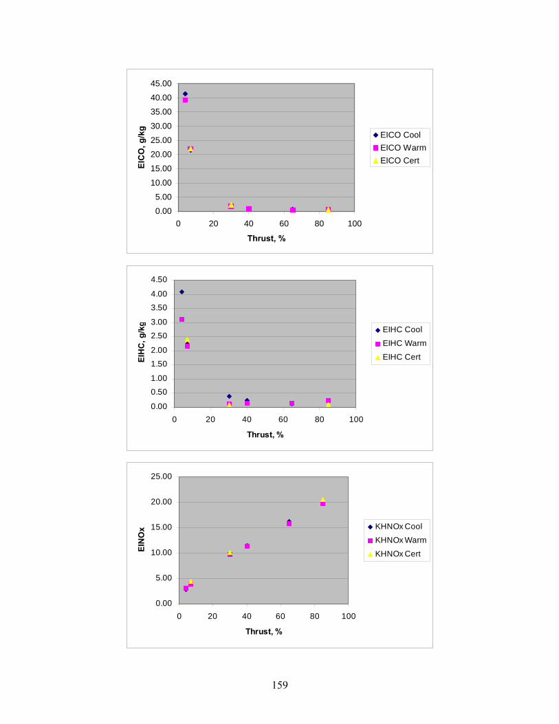
r.~ C w • - ,,

• ■

• C • • • " n

-•

--1----, - • C

0.00

5.00

10.00

15.00

20.00

25.00

30.00

35.00

40.00

45.00

0 20 40 60 80 100

Thrust, %

EIC

O, g

/kg

EICO Cool EICO Warm EICO Cert

0.00

0.50

1.00

1.50

2.00

2.50

3.00

3.50

4.00

4.50

0 20 40 60 80 100

Thrust, %

EIH

C, g

/kg

EIHC Cool

EIHC Warm

EIHC Cert

0.00

5.00

10.00

15.00

20.00

25.00

0 20 40 60 80 100

Thrust, %

EIN

Ox KHNOx Cool

KHNOx Warm

KHNOx Cert

159

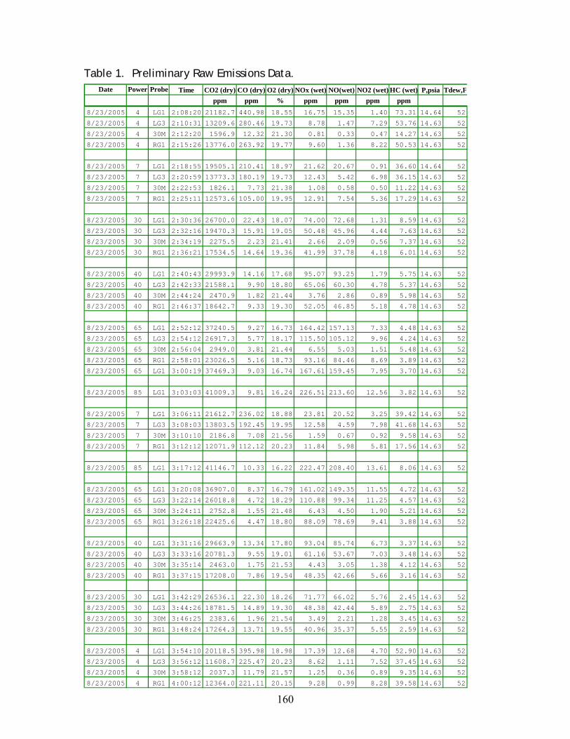
Table 1. Preliminary Raw Emissions Data. Date Power Probe Time CO2 (dry) CO (dry) O2 (dry) NOx (wet) NO(wet) NO2 (wet) HC (wet) P,psia Tdew,F

ppm ppm % ppm ppm ppm ppm 8/23/2005 4 LG1 2:08:20 21182.7 440.98 18.55 16.75 15.35 1.40 73.31 14.64 52

8/23/2005 4 LG3 2:10:31 13209.6 280.46 19.73 8.78 1.47 7.29 53.76 14.63 52

8/23/2005 4 30M 2:12:20 1596.9 12.32 21.30 0.81 0.33 0.47 14.27 14.63 52

8/23/2005 4 RG1 2:15:26 13776.0 263.92 19.77 9.60 1.36 8.22 50.53 14.63 52

8/23/2005 7 LG1 2:18:55 19505.1 210.41 18.97 21.62 20.67 0.91 36.60 14.64 52

8/23/2005 7 LG3 2:20:59 13773.3 180.19 19.73 12.43 5.42 6.98 36.15 14.63 52

8/23/2005 7 30M 2:22:53 1826.1 7.73 21.38 1.08 0.58 0.50 11.22 14.63 52

8/23/2005 7 RG1 2:25:11 12573.6 105.00 19.95 12.91 7.54 5.36 17.29 14.63 52

8/23/2005 30 LG1 2:30:36 26700.0 22.43 18.07 74.00 72.68 1.31 8.59 14.63 52

8/23/2005 30 LG3 2:32:16 19470.3 15.91 19.05 50.48 45.96 4.44 7.63 14.63 52

8/23/2005 30 30M 2:34:19 2275.5 2.23 21.41 2.66 2.09 0.56 7.37 14.63 52

8/23/2005 30 RG1 2:36:21 17534.5 14.64 19.36 41.99 37.78 4.18 6.01 14.63 52

8/23/2005 40 LG1 2:40:43 29993.9 14.16 17.68 95.07 93.25 1.79 5.75 14.63 52

8/23/2005 40 LG3 2:42:33 21588.1 9.90 18.80 65.06 60.30 4.78 5.37 14.63 52

8/23/2005 40 30M 2:44:24 2470.9 1.82 21.44 3.76 2.86 0.89 5.98 14.63 52

8/23/2005 40 RG1 2:46:37 18642.7 9.33 19.30 52.05 46.85 5.18 4.78 14.63 52

8/23/2005 65 LG1 2:52:12 37240.5 9.27 16.73 164.42 157.13 7.33 4.48 14.63 52

8/23/2005 65 LG3 2:54:12 26917.3 5.77 18.17 115.50 105.12 9.96 4.24 14.63 52

8/23/2005 65 30M 2:56:04 2949.0 3.81 21.44 6.55 5.03 1.51 5.48 14.63 52

8/23/2005 65 RG1 2:58:01 23026.5 5.16 18.73 93.16 84.46 8.69 3.89 14.63 52

8/23/2005 65 LG1 3:00:19 37469.3 9.03 16.74 167.61 159.45 7.95 3.70 14.63 52

8/23/2005 85 LG1 3:03:03 41009.3 9.81 16.24 226.51 213.60 12.56 3.82 14.63 52

8/23/2005 7 LG1 3:06:11 21612.7 236.02 18.88 23.81 20.52 3.25 39.42 14.63 52

8/23/2005 7 LG3 3:08:03 13803.5 192.45 19.95 12.58 4.59 7.98 41.68 14.63 52

8/23/2005 7 30M 3:10:10 2186.8 7.08 21.56 1.59 0.67 0.92 9.58 14.63 52

8/23/2005 7 RG1 3:12:12 12071.9 112.12 20.23 11.84 5.98 5.81 17.56 14.63 52

8/23/2005 85 LG1 3:17:12 41146.7 10.33 16.22 222.47 208.40 13.61 8.06 14.63 52

8/23/2005 65 LG1 3:20:08 36907.0 8.37 16.79 161.02 149.35 11.55 4.72 14.63 52

8/23/2005 65 LG3 3:22:14 26018.8 4.72 18.29 110.88 99.34 11.25 4.57 14.63 52

8/23/2005 65 30M 3:24:11 2752.8 1.55 21.48 6.43 4.50 1.90 5.21 14.63 52

8/23/2005 65 RG1 3:26:18 22425.6 4.47 18.80 88.09 78.69 9.41 3.88 14.63 52

8/23/2005 40 LG1 3:31:16 29663.9 13.34 17.80 93.04 85.74 6.73 3.37 14.63 52

8/23/2005 40 LG3 3:33:16 20781.3 9.55 19.01 61.16 53.67 7.03 3.48 14.63 52

8/23/2005 40 30M 3:35:14 2463.0 1.75 21.53 4.43 3.05 1.38 4.12 14.63 52

8/23/2005 40 RG1 3:37:15 17208.0 7.86 19.54 48.35 42.66 5.66 3.16 14.63 52

8/23/2005 30 LG1 3:42:29 26536.1 22.30 18.26 71.77 66.02 5.76 2.45 14.63 52

8/23/2005 30 LG3 3:44:26 18781.5 14.89 19.30 48.38 42.44 5.89 2.75 14.63 52

8/23/2005 30 30M 3:46:25 2383.6 1.96 21.54 3.49 2.21 1.28 3.45 14.63 52

8/23/2005 30 RG1 3:48:24 17264.3 13.71 19.55 40.96 35.37 5.55 2.59 14.63 52

8/23/2005 4 LG1 3:54:10 20118.5 395.98 18.98 17.39 12.68 4.70 52.90 14.63 52

8/23/2005 4 LG3 3:56:12 11608.7 225.47 20.23 8.62 1.11 7.52 37.45 14.63 52

8/23/2005 4 30M 3:58:12 2037.3 11.79 21.57 1.25 0.36 0.89 9.35 14.63 52

8/23/2005 4 RG1 4:00:12 12364.0 221.11 20.15 9.28 0.99 8.28 39.58 14.63 52

160

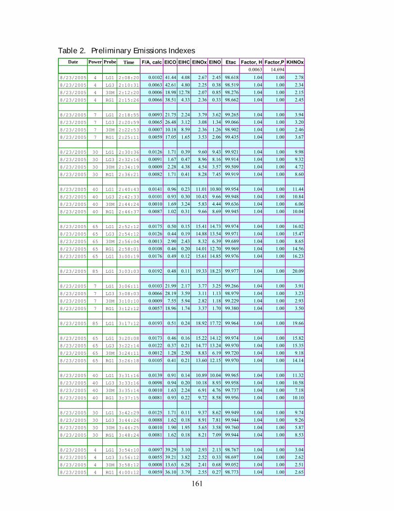
Table 2. Preliminary Emissions Indexes Date Power Probe Time F/A, calc EICO EIHC EINOx EINO Etac Factor, H Factor,P KHNOx

0.0063 14.694 8/23/2005 4 LG1 2:08:20 0.0102 41.44 4.08 2.67 2.45 98.618 1.04 1.00 2.78 8/23/2005 4 LG3 2:10:31 0.0063 42.61 4.80 2.25 0.38 98.519 1.04 1.00 2.34 8/23/2005 4 30M 2:12:20 0.0006 18.98 12.78 2.07 0.85 98.276 1.04 1.00 2.15 8/23/2005 4 RG1 2:15:26 0.0066 38.51 4.33 2.36 0.33 98.662 1.04 1.00 2.45

8/23/2005 7 LG1 2:18:55 0.0093 21.75 2.24 3.79 3.62 99.265 1.04 1.00 3.94 8/23/2005 7 LG3 2:20:59 0.0065 26.48 3.12 3.08 1.34 99.066 1.04 1.00 3.20 8/23/2005 7 30M 2:22:53 0.0007 10.18 8.59 2.36 1.26 98.902 1.04 1.00 2.46 8/23/2005 7 RG1 2:25:11 0.0059 17.05 1.65 3.53 2.06 99.435 1.04 1.00 3.67

8/23/2005 30 LG1 2:30:36 0.0126 1.71 0.39 9.60 9.43 99.921 1.04 1.00 9.98 8/23/2005 30 LG3 2:32:16 0.0091 1.67 0.47 8.96 8.16 99.914 1.04 1.00 9.32 8/23/2005 30 30M 2:34:19 0.0009 2.28 4.38 4.54 3.57 99.509 1.04 1.00 4.72 8/23/2005 30 RG1 2:36:21 0.0082 1.71 0.41 8.28 7.45 99.919 1.04 1.00 8.60

8/23/2005 40 LG1 2:40:43 0.0141 0.96 0.23 11.01 10.80 99.954 1.04 1.00 11.44 8/23/2005 40 LG3 2:42:33 0.0101 0.93 0.30 10.43 9.66 99.948 1.04 1.00 10.84 8/23/2005 40 30M 2:44:24 0.0010 1.69 3.24 5.83 4.44 99.636 1.04 1.00 6.06 8/23/2005 40 RG1 2:46:37 0.0087 1.02 0.31 9.66 8.69 99.945 1.04 1.00 10.04

8/23/2005 65 LG1 2:52:12 0.0175 0.50 0.15 15.41 14.73 99.974 1.04 1.00 16.02 8/23/2005 65 LG3 2:54:12 0.0126 0.44 0.19 14.88 13.54 99.971 1.04 1.00 15.47 8/23/2005 65 30M 2:56:04 0.0013 2.90 2.43 8.32 6.39 99.689 1.04 1.00 8.65 8/23/2005 65 RG1 2:58:01 0.0108 0.46 0.20 14.01 12.70 99.969 1.04 1.00 14.56 8/23/2005 65 LG1 3:00:19 0.0176 0.49 0.12 15.61 14.85 99.976 1.04 1.00 16.23

8/23/2005 85 LG1 3:03:03 0.0192 0.48 0.11 19.33 18.23 99.977 1.04 1.00 20.09

8/23/2005 7 LG1 3:06:11 0.0103 21.99 2.17 3.77 3.25 99.266 1.04 1.00 3.91 8/23/2005 7 LG3 3:08:03 0.0066 28.19 3.59 3.11 1.13 98.979 1.04 1.00 3.23 8/23/2005 7 30M 3:10:10 0.0009 7.55 5.94 2.82 1.18 99.229 1.04 1.00 2.93 8/23/2005 7 RG1 3:12:12 0.0057 18.96 1.74 3.37 1.70 99.380 1.04 1.00 3.50

8/23/2005 85 LG1 3:17:12 0.0193 0.51 0.24 18.92 17.72 99.964 1.04 1.00 19.66

8/23/2005 65 LG1 3:20:08 0.0173 0.46 0.16 15.22 14.12 99.974 1.04 1.00 15.82 8/23/2005 65 LG3 3:22:14 0.0122 0.37 0.21 14.77 13.24 99.970 1.04 1.00 15.35 8/23/2005 65 30M 3:24:11 0.0012 1.28 2.50 8.83 6.19 99.720 1.04 1.00 9.18 8/23/2005 65 RG1 3:26:18 0.0105 0.41 0.21 13.60 12.15 99.970 1.04 1.00 14.14

8/23/2005 40 LG1 3:31:16 0.0139 0.91 0.14 10.89 10.04 99.965 1.04 1.00 11.32 8/23/2005 40 LG3 3:33:16 0.0098 0.94 0.20 10.18 8.93 99.958 1.04 1.00 10.58 8/23/2005 40 30M 3:35:14 0.0010 1.63 2.24 6.91 4.76 99.737 1.04 1.00 7.18 8/23/2005 40 RG1 3:37:15 0.0081 0.93 0.22 9.72 8.58 99.956 1.04 1.00 10.10

8/23/2005 30 LG1 3:42:29 0.0125 1.71 0.11 9.37 8.62 99.949 1.04 1.00 9.74 8/23/2005 30 LG3 3:44:26 0.0088 1.62 0.18 8.91 7.81 99.944 1.04 1.00 9.26 8/23/2005 30 30M 3:46:25 0.0010 1.90 1.95 5.65 3.58 99.760 1.04 1.00 5.87 8/23/2005 30 RG1 3:48:24 0.0081 1.62 0.18 8.21 7.09 99.944 1.04 1.00 8.53

8/23/2005 4 LG1 3:54:10 0.0097 39.29 3.10 2.93 2.13 98.767 1.04 1.00 3.04 8/23/2005 4 LG3 3:56:12 0.0055 39.21 3.82 2.52 0.33 98.697 1.04 1.00 2.62 8/23/2005 4 30M 3:58:12 0.0008 13.63 6.28 2.41 0.68 99.052 1.04 1.00 2.51 8/23/2005 4 RG1 4:00:12 0.0059 36.10 3.79 2.55 0.27 98.773 1.04 1.00 2.65

161

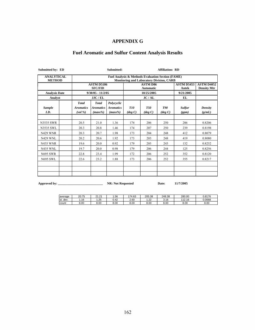
APPENDIX G

Fuel Aromatic and Sulfur Content Analysis Results

Submitted by: ED Submitted: Affiliation: RD

ANALYTICAL METHOD

Fuel Analysis & Methods Evaluation Section (FAME) Monitoring and Laboratory Division, CARB

ASTM D5186 SFC/FID

ASTM D86 Automatic

ASTM D5453 Antek

ASTM D4052 Density Mtr

Analysis Date 9/30/05 - 11/2/05 10/25/2005 9/21/2005 Analyst JJC / EL JC / AL EL

Sample I.D.

Total Aromatics

(vol %)

Total Aromatics (mass%)

Polycyclic Aromatics (mass%)

T10 (deg C)

T50 (deg C)

T90 (deg C)

Sulfur (ppm)

Density (g/mL)

N3535 SWR 20.5 21.0 1.36 174 206 250 206 0.8206 N3535 SWL 20.3 20.8 1.46 174 207 250 239 0.8198 N429 WNR 20.3 20.7 1.98 173 204 248 412 0.8079 N429 WNL 20.2 20.6 1.92 173 203 248 419 0.8080 N435 WNR 19.6 20.0 0.92 179 205 243 132 0.8252 N435 WNL 19.7 20.0 0.98 179 206 244 125 0.8256 N695 SWR 22.8 23.4 1.99 172 206 252 352 0.8120 N695 SWL 22.6 23.2 1.88 173 206 252 355 0.8217

Approved by: ____________________________ NR: Not Requested Date: 11/7/2005

average 20.75 21.21 1.56 174.63 205.38 248.38 280.00 0.8176 st. dev. 1.16 1.25 0.42 2.60 1.22 3.16 112.16 0.0068 count 8.00 8.00 8.00 8.00 8.00 8.00 8.00 8.00

162

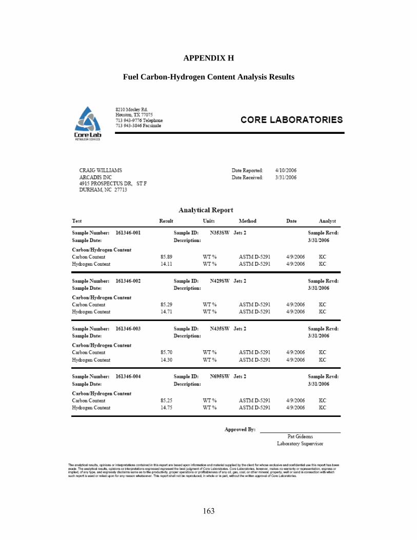
S.210 Mo.;.Jey Rd. r.'.otmou, TX 7i075 • 713 943-9'776 Tetepbone 713 90 -3S46 Fae.simile

Corelab l fflllUll !?UlUS

CRAIG WILLIAMS ARCADISINC 4915 PROSPECTUS DR, ST F DURHAM, NC 27713

Test

Sample ;\umber: 161346-001 Sample Date:

Carboo/H;rdrogen Content

Carbou Content Hydrogen Content

Sample ;\umber: 161346-00l Sample Date:

Carboo/H;rdrogen Content

Carbou C.ontent Hydrogen Content

Sample ;\umber: 161346-003 Sample Date:

Carboo/H;rdrogen Content

Carbou Content

Hydrogen Content

Sample ;\umber: 161346-004 Sample Date:

Carboo/H;rdrogen Content

Carbon Content Hydrogen Content

Result

S5.89 14.11

S5.29 14.71

S5.70 14:J0

S5.25 14.75

CORE LABORATORIES

Date Reported: Date ReceiYed:

Analytical Report

t:nits Method

Sample ID: N3$3SW Jet-. ! Des~riptiou:

\VT% ASTM D-5291 \VT% ASTM D-5291

Sample ID: N4:9SW Jet-. ! Des~riptiou:

\VT% ASTM D-5291 \VT% ASTM D-5291

Sample ID: N435SW Jet-. ! Des~riptiou:

\VT% ASTM D-5291 \VT% ASTM D-5291

Sample ID: N695SW Jet-. ! Des~riptiou:

\VT% ASTM D-5291 \VT% ASTM D-5291

Approved By:

4110/2006 3131/2006

Date

41912006 41912006

41912006 41912006

41912006 41912006

41912006 41912006

Analyst

Sample Rtvd:

J/3l ll006

KC KC

Sample Rtvd: J/3l ll006

KC KC

Sample Rtvd: J/3l ll006

KC KC

Sample Rtvd:

J/3l ll006

KC KC

Pat Gideons Laborato:y Supervisor

Tht IHWl(lioll IIK:b, (flhk:M ot lmilJ;fV.Jllefl5 COIUt'I., l!i 11i, filPM t i. CM., u!Otfl lN'.::mn1l:fl 11'1:I fflli(;ifhil -~ l7t lflt e- e.:r ...tie"' t,C!I. M llfl:I c,:mtd1111i, 1 " "' ,s, ft.:0::1'1 ""' t Wfl m d . 1lltllflill11ioll fff:~Cl'.lfl:Or.scrl! la..'J)fi1iVS:W. t '1f::.SWdftC).-!Olt~~fl\lllrto!C-L1~-lfK_ Co,t LIIXl..'1U)flt$, ~ - l'NIIKIICIWil:N'l)'OI MUtMIUlbl\ • o.-« ~ f:lfd,« .. ~ 11Mt:1,i::-t,lrCISdllil'Ni'illffltU l:) lht f:RXl;!lt "1t', (l«l.:ltl~-« l')!l)(t.Jt llflNSdll>llt'CI, QJIIS,COlll,«~r miMl'lll lW-llltllf, Mll«Sllfld tfl oonflM!'S,--,.'.lhv,filCfl Wdl ll!,:ic!1 Jlr, uWd or 11!.'ltd q:M ~ 111r, --""'- · 1lllli l'lll)O.."! ~I I.ct tot NllfO:llot:1, Iii ..Mlt orrn Pl)ll, ""'7!(M lllt ~ lllfl l,!t'lr.:MII d 0:t1o IAIX!nlO!'III.

APPENDIX H

Fuel Carbon-Hydrogen Content Analysis Results

163

APPENDIX I

Summary Tables

In this section, a series of summary tables based on the data presented in section 3.0 have been prepared for the reader’s convenience.

The following tables present the PM data and speciation profiles for the eight engines studied. In each table PM shape parameters and number and mass based emissions indices are reported as a function engine percent rated thrust (mode). For the TOG each table includes a list of species for which mode-specific emission indices (see Figure 14) are reported along with the CAS, LOD, measurement method and measurement group.

All data acquired through this contract has been archived on a secure website provided by NASA. It can be accessed with appropriate permissions at the following URL: https://owl.grc.nasa.gov

164

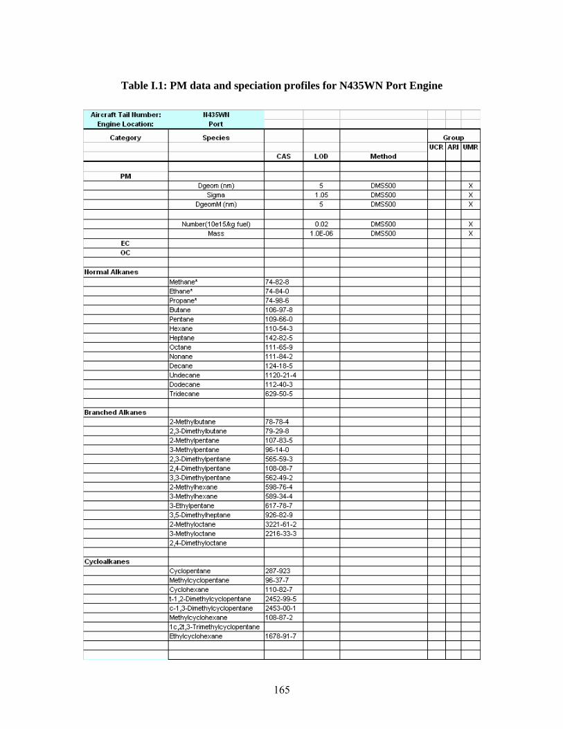
Aircraft Tail ttumber: 11435Wll I Engine Location: Port I

Category S1>ecie s Grou1> UCR ARI UMR

CAS LOD Method

PM Dgeom (nm) 5 DMS500 X

Sigma 1.05 DMS500 X DgeomM (nm) 5 DMS500 X

Number(10e151kg fuel) 0.02 DMS500 X Mass 1.0E-06 DMS500 X

EC oc

ltormal Alkanes

Methane* 74-82-8 Ethane* 74-84-0 Propane* 74-98-6 Butane 106-97-8 Pentane 109-66-0 Hexane 110-54-3 Heptane 142-82-5 Octane 111-65-9 Nonane 111-84-2 Decane 124-18-5 Undecane 1120-21-4 Dodecane 112-40-3 Tridecane 629-50-5

Branched Alkanes 2-Melhylbutane 78-78-4 2,3-Dimethylbutane 79-29-8 2-Methylpentane 107-83-5 3-Methylpentane 96-14-0 2,3-Dimethylpentane 565-59-3 2,4-Dimethylpentane 108-08-7 3,3-Dimethylpentane 562-49-2 2-Methylhexane 598-76-4 3-Methylhexane 589-34-4 3-Ethylpentane 617-78-7 3,5-Dimethylheptane 926-82-9 2-Methyloctane 3221-61-2 3-Methyloctane 2216-33-3 2,4-Dimethyloctane

Cycloalkanes Cyclopentane 287-923 Methylcyclopentane 96-37-7 Cyclohexane 110-82-7 1-1,2-Dimethylcyclopentane 2452-99-5 c-1 ,3-Dimethylcyclopentane 2453-00-1 Methylcyclohexane 108-87-2 1 c,21,3-Trimethylcyclopentane Ethylcyclohexane 1678-91-7

Table I.1: PM data and speciation profiles for N435WN Port Engine

165

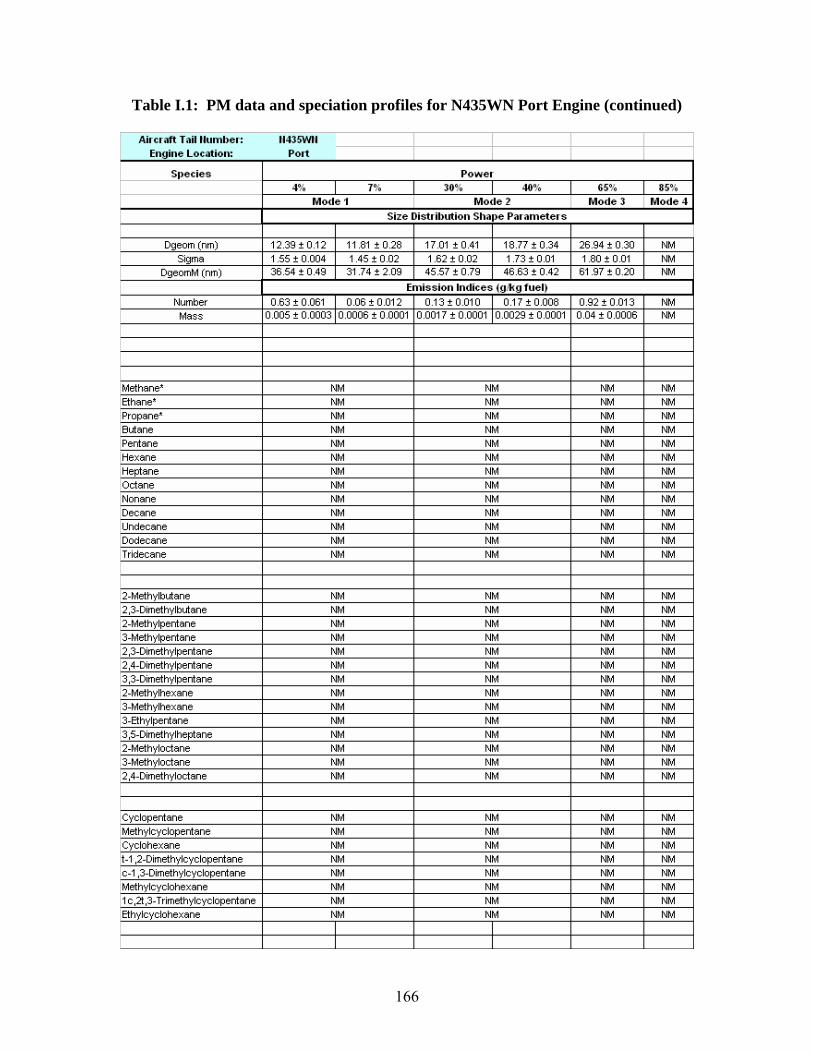
Aircraft Tail ttumber: 1143SWII I I Engine Location: Port I I

S1>ecie s Power 4% I 7°/o 30% I 40% I 65% 85%

Mode 1 Mode 2 I Mode 3 Mode 4 Size Distribution ShaJ>e Parameters

I Dgeom (nm) 12.39 ! 0.12 11.81 ! 0.28 17.01 ! 0.41 18.77 ! 0.34 26.94 ! 0.30 NM

Sigma 1.55 ! 0.004 1.45 ! 0.02 1.62 ! 0.02 1.73 ! 0.01 1.80 ! 0.01 NM DgeomM (nm) 36.54 ! 0.49 31.74 ! 2.09 45.57 ! 0.79 46.63 ! 0.42 61.97 ! 0.20 NM

Emission Indice s {gll<g fuel)

Number 0.63, 0.061 I 0.06, 0.012 0.13, 0.01 o I 0.17, 0.008 0.92 ! 0.013 NM Mass 0.005 ! 0.0003 0.0006 ! 0.0001 0.0017 ! 0.0001 0.0029 ! 0.0001 0.04 ! 0.0006 NM

Methane• NM NM NM NM Ethane• NM NM NM NM Propane• NM NM NM NM Butane NM NM NM NM Pentane NM NM NM NM Hexane NM NM NM NM Heptane NM NM NM NM Octane NM NM NM NM Nonane NM NM NM NM Decane NM NM NM NM Undecane NM NM NM NM Dodecane NM NM NM NM Tridecane NM NM NM NM

2-Melhylbutane NM NM NM NM 2,3-Dimethylbutane NM NM NM NM 2-Methylpentane NM NM NM NM 3-Methylpentane NM NM NM NM 2,3-Dimethylpentane NM NM NM NM 2,4-Dimethylpentane NM NM NM NM 3,3-Dimethylpentane NM NM NM NM 2-Methylhexane NM NM NM NM 3-Methylhexane NM NM NM NM 3-Ethylpentane NM NM NM NM 3,5-Dimethylheptane NM NM NM NM 2-Methyloctane NM NM NM NM 3-Methyloctane NM NM NM NM 2,4-Dimethyloctane NM NM NM NM

Cyclopentane NM NM NM NM Methylcyclopentane NM NM NM NM Cyclohexane NM NM NM NM 1-1,2-Dimethylcyclopentane NM NM NM NM c-1 ,3-Dimethylcyclopentane NM NM NM NM Methylcyclohexane NM NM NM NM 1 c,21,3-Trimethylcyclopentane NM NM NM NM Ethylcyclohexane NM NM NM NM

I I

Table I.1: PM data and speciation profiles for N435WN Port Engine (continued)

166

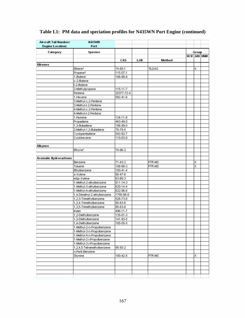
Aircraft Tail ttumber: 11435WII I Engine Location: Port I

Category S1>ecie s Grou1> UCR ARI UMR

CAS LOD Method Alkenes

Ethene* 74-85-1 TILDAS X Propene* 115-07-1 1-Butene 106-98-9 c-2-Butene 1-2-Butene 2-Methylpropene 115-11-7 Pentene 25377-72-4 1-Hexene 592-41-6 3-Methyl-c-2-Pentene 3-Methyl-t-2-Pentene 4-Methyl-c-2-Pentene 4-Methyl-t-2-Pentene 1-Nonene 124-11-8 Propadiene 463-49-0 1 ,3-Butadiene 106-99-0 2-Melhyl-1 ,3-Butadiene 78-79-5 Cyclopentadiene 542-92-7 Cyclohexene 110-83-8

Alkynes Ethyne* 74-86-2

Aromatic Hydrocarbons Benzene 71-43-2 PTR-MS X Toluene 108-88-3 PTR-MS X Ethylbenzene 100-41-4 o-Xylene 95-47-6

m&p-Xylene 63-68-3 1-Methyl-2-elhylbenzene 611-14-3 1-Methyl-3-ethylbenzene 620-14-4 1-Methyl-4-elhylbenzene 622-96-8 1,4-Dimethyl-2-elhylbenzene 1758-88-9 1,2,3-Trimethylbenzene 526-73-8 1,2,4-Trimethylbenzene 95-63-6 1,3,5-Trimethylbenzene 95-63-6 lndan 496-11-7 1,2-Diethylbenzene 135-01-3 1 ,3-Diethylbenzene 141-93-5 1,4-Diethylbenzene 105-05-5 1-Methyl-2-n-Propylbenzene 1-Methyl-3-n-Propylbenzene 1-Methyl-4-n-Propylbenzene 1-Methyl-2-i-Propylbenzene 1-Methyl-3-i-Propylbenzene 1 ,2,4 ,5-T etramethylbenzene 95-93-2 n-Pent-Benzene styrene 100-42-5 PTR-MS X

I

Table I.1: PM data and speciation profiles for N435WN Port Engine (continued)

167

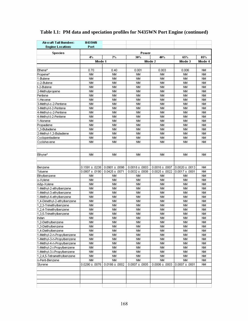
Aircraft Tail ttumber: 1143SWII I I Engine Location: Port I I

S1>ecie s Power 4% I 7°/o 30% I 40% 65% 85%

Mode 1 Mode 2 Mode 3 Mode 4

Ethene• 0.70 0.40 0.001 0.003 0.006 NM Propene• NM NM NM NM NM NM 1-Butene NM NM NM NM NM NM c-2-Butene NM NM NM NM NM NM 1-2-Butene NM NM NM NM NM NM 2-Methylpropene NM NM NM NM NM NM Pentene NM NM NM NM NM NM 1-Hexene NM NM NM NM NM NM 3-Methyl-c-2-Pentene NM NM NM NM NM NM 3-Methyl-1-2-Pentene NM NM NM NM NM NM 4-Methyl-c-2-Pentene NM NM NM NM NM NM 4-Methyl-1-2-Pentene NM NM NM NM NM NM 1-Nonene NM NM NM NM NM NM Propadiene NM NM NM NM NM NM 1 ,3-Butadiene NM NM NM NM NM NM 2-Melhyl-1,3-Butadiene NM NM NM NM NM NM Cyclopentadiene NM NM NM NM NM NM Cyclohexene NM NM NM NM NM NM

Ethyne• NM NM NM NM NM NM

Benzene 0.1591 ! .0238 0.0901 ! .0098 0.0018 ! .0003 0.0016 ! .0007 0.0020 ! .0013 NM Toluene 0.0807 ! .0190 0.0425 ! .0071 0.0032 ! .0008 0.0025 ! .0022 0.0017 ! .0001 NM Ethylbenzene NM NM NM NM NM NM o-Xylene NM NM NM NM NM NM m&p-Xylene NM NM NM NM NM NM 1-Methyl-2-elhylbenzene NM NM NM NM NM NM 1-Methyl-3-elhylbenzene NM NM NM NM NM NM 1-Methyl-4-elhylbenzene NM NM NM NM NM NM 1,4-Dimethyl-2-elhylbenzene NM NM NM NM NM NM 1,2,3-Trimethylbenzene NM NM NM NM NM NM 1,2,4-Trimethylbenzene NM NM NM NM NM NM 1,3,5-Trimethylbenzene NM NM NM NM NM NM lndan NM NM NM NM NM NM 1,2-Diethylbenzene NM NM NM NM NM NM 1 ,3-Diethylbenzene NM NM NM NM NM NM 1,4-Diethylbenzene NM NM NM NM NM NM 1-Methyl-2-n-Propylbenzene NM NM NM NM NM NM 1-Methyl-3-n-Propylbenzene NM NM NM NM NM NM 1-Methyl-4-n-Propylbenzene NM NM NM NM NM NM 1-Methyl-2-i-Propylbenzene NM NM NM NM NM NM 1-Methyl-3-i-Propylbenzene NM NM NM NM NM NM 1 ,2,4 ,5-T etramethylbenzene NM NM NM NM NM NM n-Pent-Benzene NM NM NM NM NM NM styrene 0.0290 ! .0076 0.0166 ! .0002 0.0007 ! .0005 0.0006 ! .0003 0.0007 ! .0001 NM

Table I.1: PM data and speciation profiles for N435WN Port Engine (continued)

168

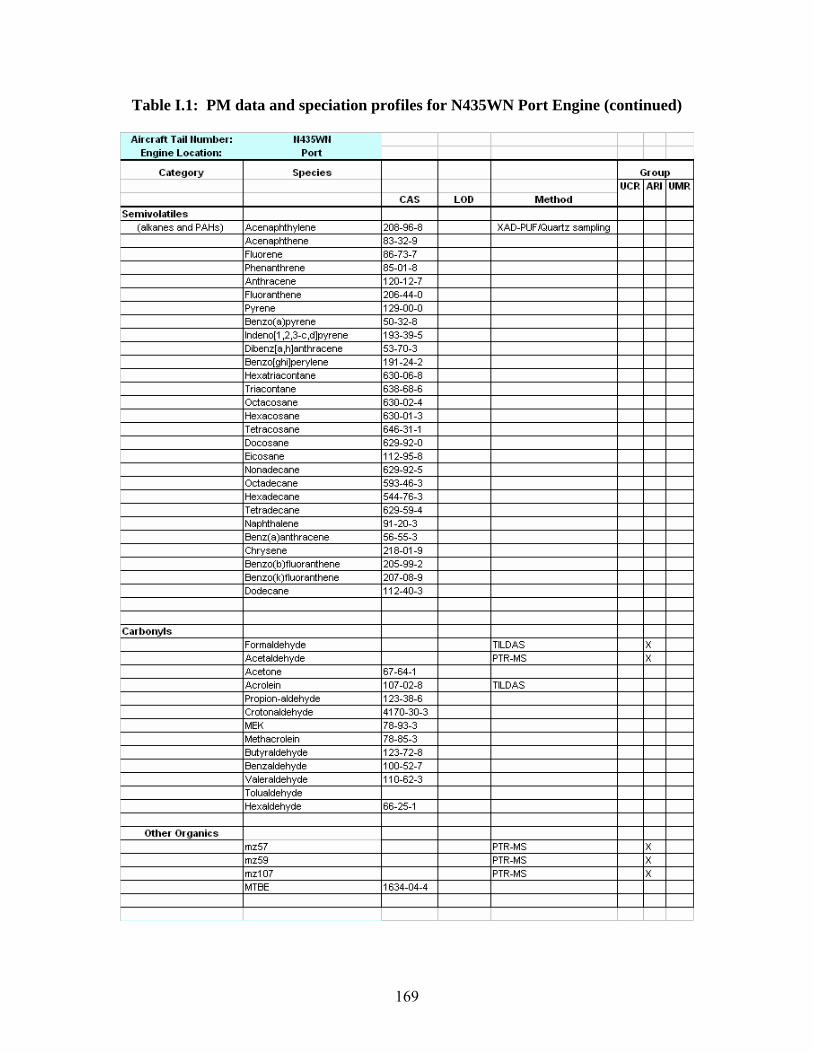
Aircraft Tail ttumber: 11435WII I Engine Location: Port I

Category S1>ecie s Grou1> UCR ARI UMR

CAS LOD Method Semivolatiles

(alkanes and PAHs) Acenaphthylene 208-96-8 XAD-PUF /Quartz sampling

Acenaphthene 83-32-9 Fluorene 86-73-7 Phenanthrene 85-01-8

Anthraeene 120-12-7 Fluoranthene 206-44-0 Pyrene 129-00-0 Benzo(a)pyrene 50-32-8 lndeno[1,2,3-c,d)pyrene 193-39-5 Oibenz[a,h]anthracene 53-70-3 Benzo[ghi]perylene 191-24-2 Hexatriacontane 630-06-8 Triacontane 638-68-6 Octacosane 630-02-4 Hexacosane 630-01-3 T etracosane 646-31-1 Docosane 629-92-0 Eicosane 112-95-8 Nonadecane 629-92-5 Octadecane 593-46-3 Hexadecane 544-76-3 T etradecane 629-59-4 Naphthalene 91-20-3 Benz( a)anthracene 56-55-3 Chrysene 218-01-9 Benzo(b )fluoranthene 205-99-2 Benzo(k)fluoranthene 207-08-9

Dodecane 112-40-3

Carbonyls Formaldehyde TILDAS X Acelaldehyde PTR-MS X Acetone 67-64-1 Acrolein 107-02-8 TILDAS Propion-alclehyde 123-38-6 Crotonaldehyde 4170-30-3 MEK 78-93-3 Methacrolein 78-85-3 Butyraldehyde 123-72-8 Benz aldehyde 100-52-7 Valeraldehyde 110-62-3 T olualdehyde Hex aldehyde 66-25-1

Other Organics mz57 PTR-MS X mz59 PTR-MS X mz107 PTR-MS X MTBE 1634-04-4

I

Table I.1: PM data and speciation profiles for N435WN Port Engine (continued)

169

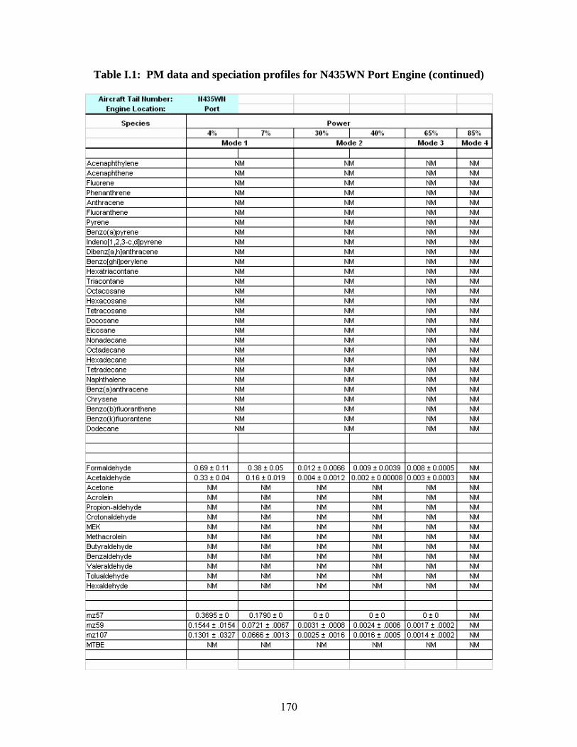
Aircraft Tail ttumber: 1143SWII I I Engine Location: Port I I

S1>ecie s Power 4% I 7°/o 30% I 40% 65% 85%

Mode 1 Mode 2 Mode 3 Mode 4 I I

Acenaphthylene NM NM NM NM Acenaphthene NM NM NM NM Fluorene NM NM NM NM Phenanthrene NM NM NM NM Anthracene NM NM NM NM Fluoranthene NM NM NM NM Pyrene NM NM NM NM Benzo(a)pyrene NM NM NM NM lndeno[1,2,3-c,d)pyrene NM NM NM NM Oibenz[a,h]anthracene NM NM NM NM Benzo[ghi]perylene NM NM NM NM Hexatriacontane NM NM NM NM Triacontane NM NM NM NM Octacosane NM NM NM NM Hexacosane NM NM NM NM T etracosane NM NM NM NM Docosane NM NM NM NM Eicosane NM NM NM NM Nonadecane NM NM NM NM Octadecane NM NM NM NM Hexadecane NM NM NM NM T etradecane NM NM NM NM Naphthalene NM NM NM NM Benz( a)anthracene NM NM NM NM Chrysene NM NM NM NM Benzo(b )fluoranthene NM NM NM NM Benzo(k)fluorantene NM NM NM NM Dodecane NM NM NM NM

Formaldehyde 0.69 ± 0.11 0.38 ± 0.05 0.012 ± 0.0066 0.009±0.0039 0.008 ± 0.0005 NM Acelaldehyde 0.33 ± 0.04 0.16 ± 0.019 0.004 ± 0.0012 0.002 ± 0.00008 0.003 ± 0.0003 NM Acetone NM NM NM NM NM NM Acrolein NM NM NM NM NM NM Propion-aldehyde NM NM NM NM NM NM Crotonaldehyde NM NM NM NM NM NM MEK NM NM NM NM NM NM Methacrolein NM NM NM NM NM NM But yr aldehyde NM NM NM NM NM NM Benz aldehyde NM NM NM NM NM NM Valeraldehyde NM NM NM NM NM NM T olualdehyde NM NM NM NM NM NM Hex aldehyde NM NM NM NM NM NM

mz57 0.3695 ± 0 0.1790 ± 0 O:!:O O:!:O O:!:O NM mz59 0.1544 ± .0154 0.0721 ± .0067 0.0031 ± .0008 0.0024 ± .0006 0.0017 ± .0002 NM mz107 0.1301 ± .0327 0.0666 ± .0013 0.0025 ± .0016 0.0016 ± .0005 0.0014 ± .0002 NM MTBE NM NM NM NM NM NM

Table I.1: PM data and speciation profiles for N435WN Port Engine (continued)

170

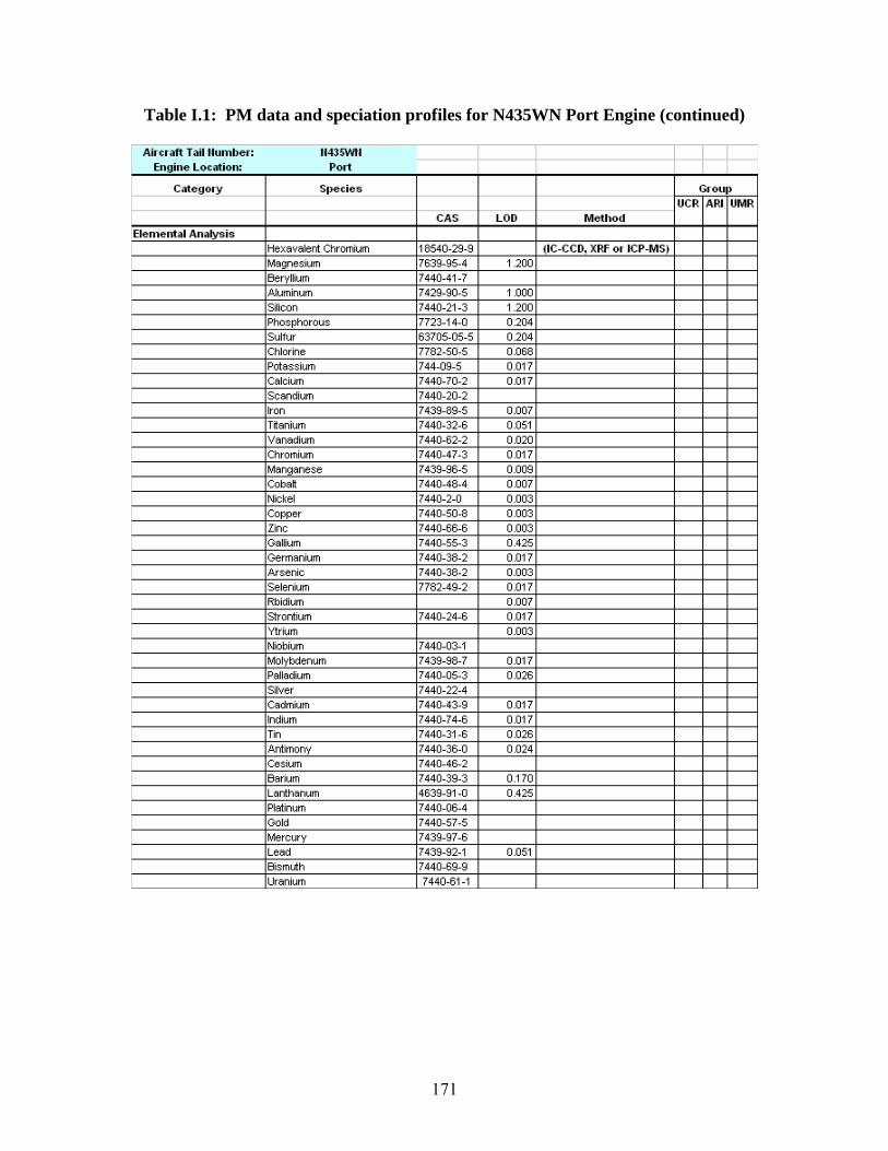
Aircraft Tail ttumber: 11435WII I Engine Location: Port I

Category S1>ecie s Grou1> UCR ARI UMR

CAS LOD Method Elemental Analysis

Hexavalent Chromium 18540-29-9 (IC-CCD, XRF or ICP-MS) Magnesium 7639-95-4 1.200 Beryllium 7440-41-7 Aluminum 7429-90-5 1.000 Silicon 7440-21-3 1.200 Phosphorous 7723-14-0 0.204 Sulfur 63705-05-5 0.204 Chlorine 7782-50-5 0.068 Potassium 744-09-5 0.017 Calcium 7440-70-2 0.017 Scandium 7440-20-2 Iron 7439-89-5 0.007 Titanium 7440-32-6 0.051 Vanadium 7440-62-2 0.020 Chromium 7440-47-3 0.017 Manganese 7439-96-5 0.009 Cobalt 7440-48-4 0.007 Nickel 7440-2-0 0.003 Copper 7440-50-8 0.003 Zinc 7440-66-6 0.003 Gallium 7440-55-3 0.425 Germanium 7440-38-2 0.017 Arsenic 7440-38-2 0.003 Selenium 7782-49-2 0.017 Rbidium 0.007 strontium 7440-24-6 0.017 Ytrium 0.003 Niobium 7440-03-1 Molybdenum 7439-98-7 0.017 Palladium 7440-05-3 0.Q26 Silver 7440-22-4 Cadmium 7440-43-9 0.017 Indium 7440-74-6 0.017 Tin 7440-31-6 0.Q26 Antimony 7440-36-0 0.024 Cesium 7440-46-2 Barium 7440-39-3 0.170 Lanthanum 4639-91-0 0.425 Platinum 7440-06-4 Gold 7440-57-5 Mercury 7439-97-6 Lead 7439-92-1 0.051 Bismuth 7440-69-9 Uranium 7440-61-1

Table I.1: PM data and speciation profiles for N435WN Port Engine (continued)

171

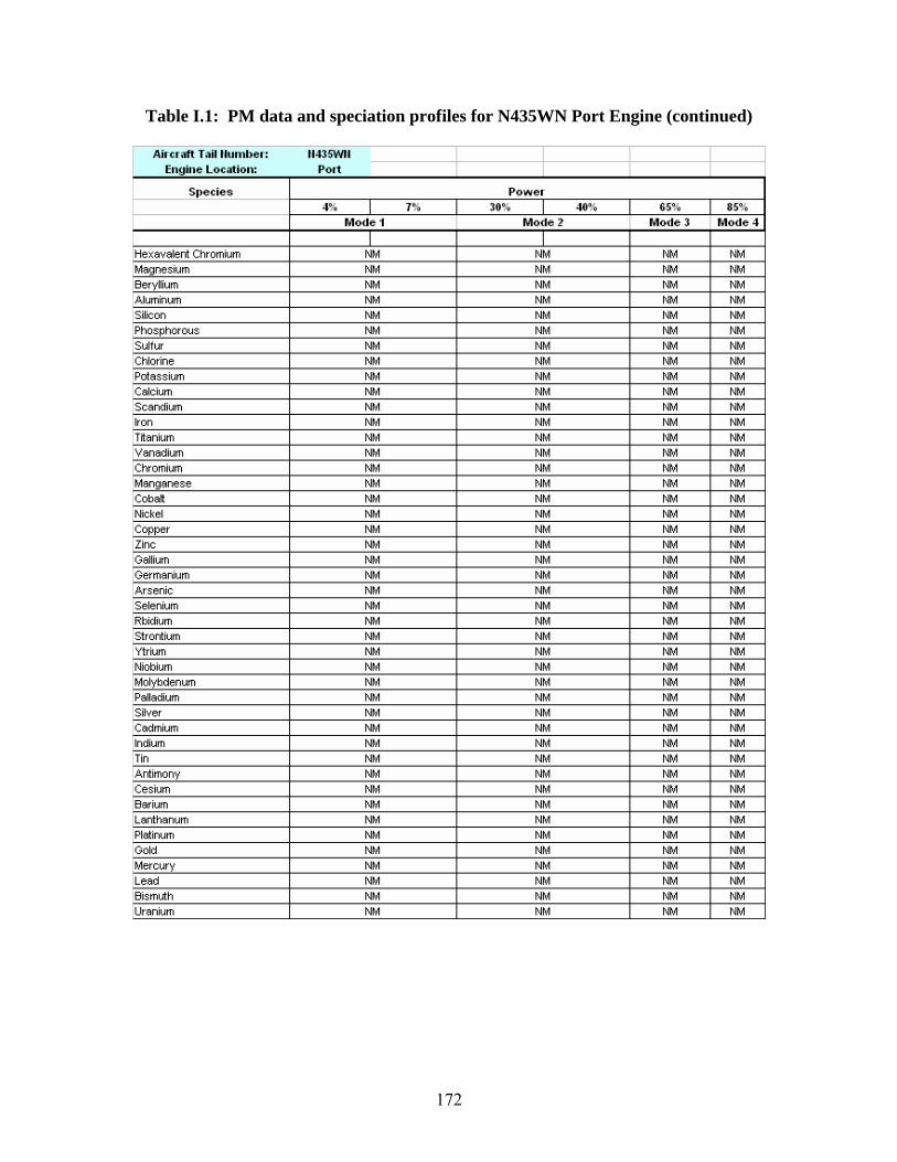
Aircraft Tail ttumber: 1143SWII I I Engine Location: Port I I

S1>ecie s Power 4% I 7°/o 30% I 40% 65% 85%

Mode 1 Mode 2 Mode 3 Mode 4 I I

Hexavalent Chromium NM NM NM NM Magnesium NM NM NM NM Beryllium NM NM NM NM Aluminum NM NM NM NM Silicon NM NM NM NM Phosphorous NM NM NM NM Sulfur NM NM NM NM Chlorine NM NM NM NM Potassium NM NM NM NM Calcium NM NM NM NM Scandium NM NM NM NM Iron NM NM NM NM Titanium NM NM NM NM Vanadium NM NM NM NM Chromium NM NM NM NM Manganese NM NM NM NM Cobalt NM NM NM NM Nickel NM NM NM NM Copper NM NM NM NM Zinc NM NM NM NM Gallium NM NM NM NM Germanium NM NM NM NM Arsenic NM NM NM NM Selenium NM NM NM NM Rbidium NM NM NM NM strontium NM NM NM NM Ytrium NM NM NM NM Niobium NM NM NM NM Molybdenum NM NM NM NM Palladium NM NM NM NM Silver NM NM NM NM Cadmium NM NM NM NM Indium NM NM NM NM Tin NM NM NM NM Antimony NM NM NM NM Cesium NM NM NM NM Barium NM NM NM NM Lanthanum NM NM NM NM Platinum NM NM NM NM Gold NM NM NM NM Mercury NM NM NM NM Lead NM NM NM NM Bismuth NM NM NM NM Uranium NM NM NM NM

Table I.1: PM data and speciation profiles for N435WN Port Engine (continued)

172

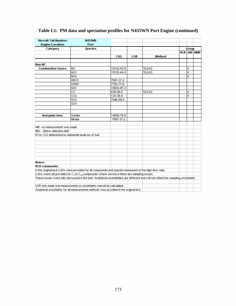
Aircraft Tail ttumber: 11435WII I Engine Location: Port I

Category S1>ecies Grou1> UCR ARI UMR

CAS LOD Method

llon-HC Combustion Gases NO 10102-43-9 TILDAS X

NO2 10102-44-0 TILDAS X NOX X HNO3 7697-37-2

HONO 7782-77-6 N2O 10024-97-2 co 630-08-0 TILDAS X CO2 124-38-9 X SO2 7446-09-5 SOX

Inorganic ions Sulfate 14808-79-8 Nitrate 7697-37-2

NM - no measurement was made BOL - Below detection limit El for CO2 determined by elemental analysis of fuel

Uotes: UCR comments: In the original text LOOs were provided for all compounds and species measured on the high-flow side. LOOs were not provided for C I to C 12 compounds where we know there are sampling issues. These issues were fully discussed in the test. Analytical uncertainties are different and will not reflect the sampling uncertainty.

I UCR only made one measurement so uncertainty cannot be calculated. Analytical uncertainty for all measurement methods was provided in the original text.

Table I.1: PM data and speciation profiles for N435WN Port Engine (continued)

173

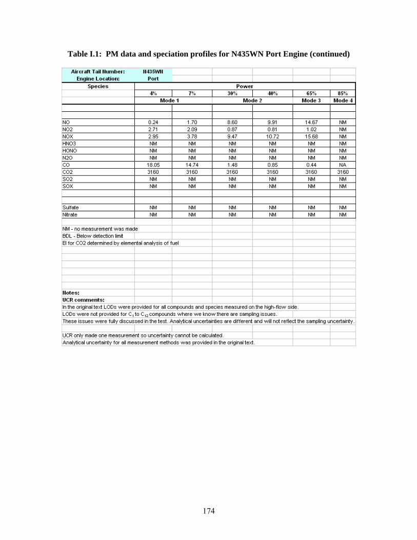
Aircraft Tail ttumber: 1143SWII I I Engine Location: Port I I

S1>ecies Power 4% I 7°/o 30% I 40% 65% 85%

Mode 1 Mode 2 Mode 3 Mode 4

NO 0.24 1.70 8.60 9.91 14.67 NM NO2 2.71 2.09 0.87 0.81 1.02 NM NOX 2.95 3.78 9.47 10.72 15.68 NM HNO3 NM NM NM NM NM NM HONO NM NM NM NM NM NM N2O NM NM NM NM NM NM co 18.05 14.74 1.48 0.85 0.44 NA CO2 3160 3160 3160 3160 3160 3160 SO2 NM NM NM NM NM NM SOX NM NM NM NM NM NM

Sulfate NM NM NM NM NM NM Nitrate NM NM NM NM NM NM

NM - no measurement was made BOL - Below detection limit I El for CO2 determined by elemental analysis of fuel

Uotes: UCR comments: In the original text LOOs were provided for all compounds and species measured on the high-flow side. LOOs were not provided for C I to C ,z compounds where we know there are sampling issues. I These issues were fully discussed in the test. Analytical uncertainties are different and will not reflect the sampling uncertainty.

UCR only made one measurement so uncertainty cannot be calculated. I Analytical uncertainty for all measurement methods was provided in the original text.

Table I.1: PM data and speciation profiles for N435WN Port Engine (continued)

174

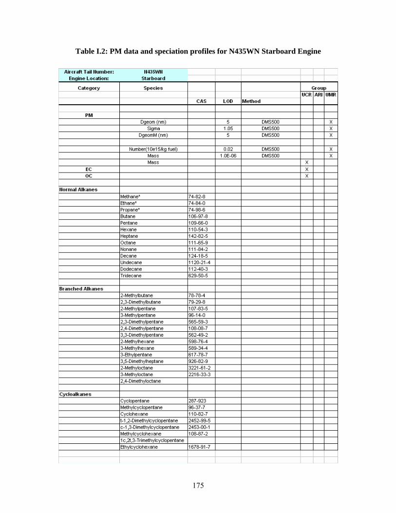
Aircraft Tail ttumber: 11435Wll I Engine Location: Starboard I

Category S1>ecie s Grou1> UCR ARI UMR

CAS LOD Method

PM Dgeom (nm) 5 DMS500 X

Sigma 1.05 DMS500 X DgeomM (nm) 5 DMS500 X

Number(10e151kg fuel) 0.02 DMS500 X Mass 1.0E-06 DMS500 X Mass X

EC X oc X

ltormal Alkanes

Methane* 74-82-8 Ethane* 74-84-0 Propane* 74-98-6 Butane 106-97-8 Pentane 109-66-0 Hexane 110-54-3 Heplane 142-82-5 Octane 111-65-9 Nonane 111-84-2 Decane 124-18-5 Undecane 1120-21-4 Dodecane 112-40-3 TrirlP.r.AnP. R?~-~n-~

Branched Alkanes 2-Melhylbulane 78-78-4 2,3-Dimelhylbulane 79-29-8 2-Melhylpenlane 107-83-5 3-Melhylpenlane 96-14-0 2,3-Dimelhylpenlane 565-59-3 2,4-Dimelhylpenlane 108-08-7 3,3-Dimelhylpenlane 562-49-2 2-Melhylhexane 598-76-4 3-Melhylhexane 589-34-4 3-Elhylpenlane 617-78-7 3,5-Dimelhylheplane 926-82-9 2-Melhyloclane 3221-61-2 3-Melhyloclane 2216-33-3 2,4-Dimelhyloclane

Cycloalkanes Cyclopentane 287-923 Melhylcyclopenlane 96-37-7 Cyclohexane 110-82-7 t-1,2-Dimelhylcyclopenlane 2452-99-5 c-1 ,3-Dimelhylcyclopenlane 2453-00-1 Methylcyclohexane 108-87-2 1 c,21,3-Trimelhylcyclopenlane Ethylcyclohexane 1678-91-7

Table I.2: PM data and speciation profiles for N435WN Starboard Engine

175

Aircraft Tail ttumber: 11435WII I I Engine Location: Starboard I I

S1>ecie s Power 4% 7% I 30% 40% 65% I 85%

Mode 1 I Mode 2 Mode 3 I Mode 4 Size Distribution ShaJ>e Parameters

Dgeom (nm) 14.24 ± 0.15 12.04 ± 0.47 17.09 ± 0.39 19.10 ± 0.27 25.74 ± 0.37 31.27 ± 0.64 Sigma 1.60 ± 0.005 1.44 ± 0.04 1.64 ± 0.01 1.69 ± 0.01 1.81 ± 0.01 1.79 ± 0.01

DgeomM (nm) 37.32 ± 0.37 28.4 ± 2.24 43.08 ± 0.63 44.35 ± 0.52 59.81 ± 0.29 71.09 ± 2.56 Emission Indice s {gll<g fuel)

Number 0.61 ± 0.032 0.15 ± 0.03 0.19 ± 0.013 0.23 ± 0.009 0.83 ± 0.02 0.97 ± 0.033 Mass 0.006 ± 0.0002 0.0005 ± 0.0001 0.003 ± 0.0001 0.004 ± 0.0001 0.03 ± 0.0008 0.06 ± 0.005 Mass 0.0082 0.0209 0.0407 0.0704

0.0025 0.0017 0.0238 0.0414 0.0075 0.0030 0.0065 0.0168

Methane• NM NM NM NM Ethane• NM NM NM NM Propane• NM NM NM NM Butane NM NM NM NM Pentane NM NM NM NM Hexane NM NM NM NM Heptane NM NM NM NM Octane NM NM NM NM Nonane NM NM NM NM Decane NM NM NM NM Undecane NM NM NM NM Dodecane NM NM NM NM Tridecane NM NM NM NM

2-Melhylbutane NM NM NM NM 2,3-Dimethylbutane NM NM NM NM 2-Methylpentane NM NM NM NM 3-Methylpentane NM NM NM NM 2,3-Dimethylpentane NM NM NM NM 2,4-Dimethylpentane NM NM NM NM 3,3-Dimethylpentane NM NM NM NM 2-Methylhexane NM NM NM NM 3-Methylhexane NM NM NM NM 3-Ethylpentane NM NM NM NM 3,5-Dimethylheptane NM NM NM NM 2-Methyloctane NM NM NM NM 3-Methyloctane NM NM NM NM 2,4-Dimethyloctane NM NM NM NM

Cyclopentane NM NM NM NM Methylcyclopentane NM NM NM NM Cyclohexane NM NM NM NM t-1,2-Dimethylcyclopentane NM NM NM NM c-1 ,3-Dimethylcyclopentane NM NM NM NM Methylcyclohexane NM NM NM NM 1 c,21,3-Trimethylcyclopentane NM NM NM NM Ethylcyclohexane NM NM NM NM

Table I.2: PM data and speciation profiles for N435WN Starboard Engine (continued)

176

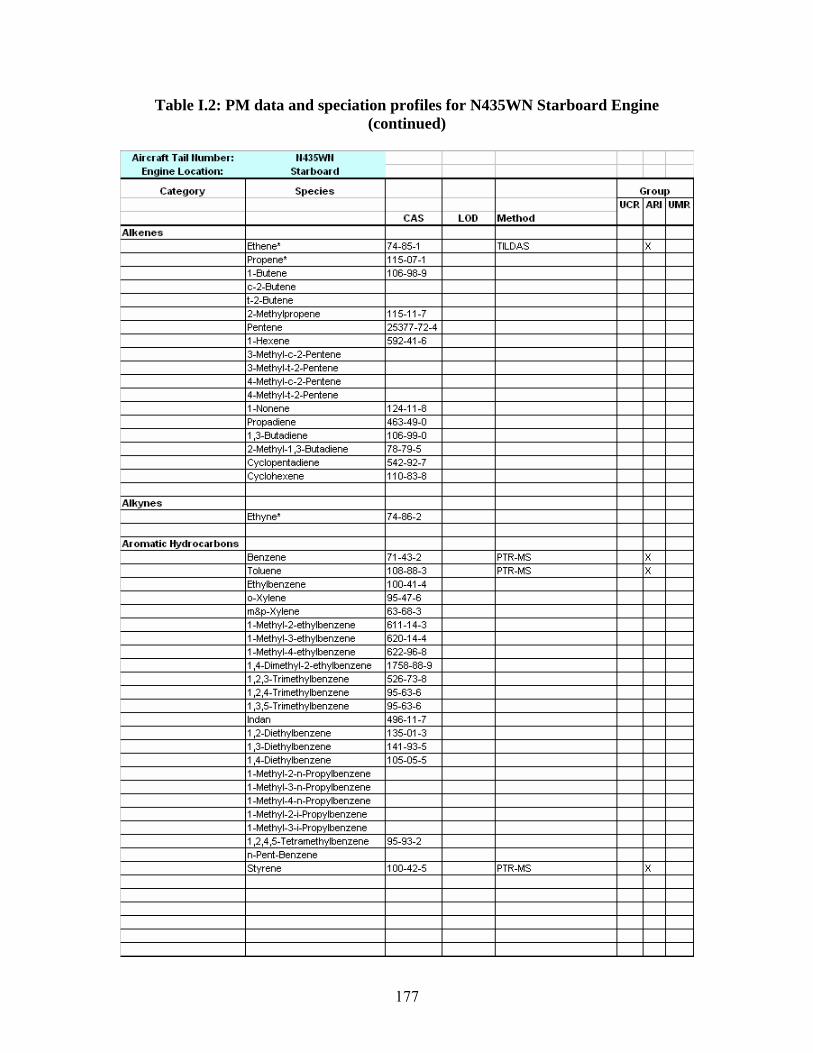
Aircraft Tail ttumber: 11435Wll I Engine Location: Starboard I

Category S1>ecie s Grou1> UCR ARI UMR

CAS LOD Method

Alkenes Ethene• 74-85-1 TILDAS X Propene• 115-07-1 1-Bulene 106-98-9 c-2-Butene 1-2-Bulene 2-Melhylpropene 115-11-7 Pentene 25377-72-4 1-Hexene 592-41-6 3-Melhyl-c-2-Pentene

3-Melhyl-1-2-Penlene 4-Melhyl-c-2-Penlene 4-Melhyl-1-2-Penlene 1-Nonene 124-11-8 Propadiene 463-49-0 1 ,3-Butadiene 106-99-0 2-Melhyl-1,3-Buladiene 78-79-5 Cyclopentadiene 542-92-7 Cyclohexene 110-83-8

Alkynes Ethyne• 74-86-2

Aromatic Hydrocarbons Benzene 71-43-2 PTR-MS X Toluene 108-88-3 PTR-MS X Ethylbenzene 100-41-4 o-Xylene 95-47-6 m&p-Xylene 63-68-3 1-Melhyl-2-elhylbenzene 611-14-3 1-Melhyl-3-elhylbenzene 620-14-4 1-Melhyl-4-elhylbenzene 622-96-8 1,4-Dimelhyl-2-elhylbenzene 1758-88-9 1,2,3-Trimethylbenzene 526-73-8 1,2,4-Trimethylbenzene 95-63-6 1,3,5-Trimethylbenzene 95-63-6 lndan 496-11-7 1,2-Dielhylbenzene 135-01-3 1 ,3-Dielhylbenzene 141-93-5 1,4-Dielhylbenzene 105-05-5 1-Melhyl-2-n-Propylbenzene 1-Melhyl-3-n-Propylbenzene 1-Melhyl-4-n-Propylbenzene 1-Melhvl-2-i-Proov !benzene 1-Melhyl-3-i-Propylbenzene 1 ,2,4 ,5-T elramelhylbenzene 95-93-2 n-Pent-Benzene styrene 100-42-5 PTR-MS X

Table I.2: PM data and speciation profiles for N435WN Starboard Engine (continued)

177

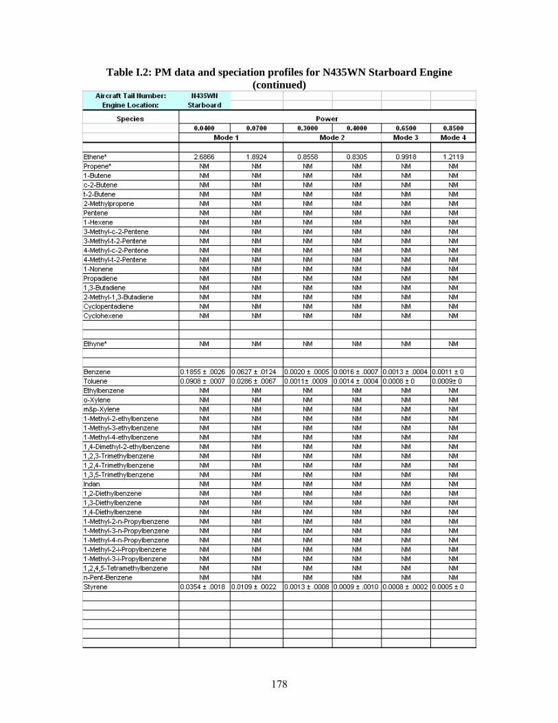
Aircraft Tail ttumber: 11435WII I I Engine Location: Starboard I I

S1>ecies Power 0.0440 0.0700 0.3000 0.4400 0.6500 0.8500

Mode1 Mode 2 I Mode 3 Mode4

Ethene• 2.6866 1.8924 0.8558 0.8305 0.9918 1.2119 Propene• NM NM NM NM NM NM 1-Butene NM NM NM NM NM NM c-2-Butene NM NM NM NM NM NM 1-2-Butene NM NM NM NM NM NM 2-Methylpropene NM NM NM NM NM NM Pentene NM NM NM NM NM NM 1-Hexene NM NM NM NM NM NM 3-Methyl-c-2-Pentene NM NM NM NM NM NM 3-Methyl-1-2-Pentene NM NM NM NM NM NM 4-Methyl-c-2-Pentene NM NM NM NM NM NM 4-Methyl-1-2-Pentene NM NM NM NM NM NM 1-Nonene NM NM NM NM NM NM Propadiene NM NM NM NM NM NM 1 ,3-Butadiene NM NM NM NM NM NM 2-Melhyl-1,3-Butadiene NM NM NM NM NM NM Cyclopentadiene NM NM NM NM NM NM Cyclohexene NM NM NM NM NM NM

Ethyne• NM NM NM NM NM NM

Benzene 0.1855 ! .0026 0.0627 ! .0124 0.0020, .0005 0.0016 ! .0007 0.0013 ! .0004 0.0011 ! 0 Toluene 0.0908 ! .0007 0.0286 ! .0067 0.001H .0009 0.0014 ! .0004 0.0008 ! 0 0.0009! 0 Ethylbenzene NM NM NM NM NM NM o-Xylene NM NM NM NM NM NM m&p-Xylene NM NM NM NM NM NM 1-Methyl-2-elhylbenzene NM NM NM NM NM NM 1-Methyl-3-ethylbenzene NM NM NM NM NM NM 1-Methyl-4-elhylbenzene NM NM NM NM NM NM 1,4-Dimethyl-2-elhylbenzene NM NM NM NM NM NM 1,2,3-Trimethylbenzene NM NM NM NM NM NM 1,2,4-Trimethylbenzene NM NM NM NM NM NM 1,3,5-Trimethylbenzene NM NM NM NM NM NM lndan NM NM NM NM NM NM 1,2-Diethylbenzene NM NM NM NM NM NM 1 ,3-Diethylbenzene NM NM NM NM NM NM 1,4-Diethylbenzene NM NM NM NM NM NM 1-Methyl-2-n-Propylbenzene NM NM NM NM NM NM 1-Methyl-3-n-Propylbenzene NM NM NM NM NM NM 1-Methyl-4-n-Propylbenzene NM NM NM NM NM NM 1-Methyl-2-i-Propylbenzene NM NM NM NM NM NM 1-Methyl-3-i-Propylbenzene NM NM NM NM NM NM 1 ,2,4 ,5-T etramethylbenzene NM NM NM NM NM NM n-Pent-Benzene NM NM NM NM NM NM styrene 0.0354 ! .0018 0.0109 ! .0022 0.0013 ! .0008 0.0009 ! .0010 0.0008 ! .0002 0.0005 ! 0

Table I.2: PM data and speciation profiles for N435WN Starboard Engine (continued)

178

Aircraft Tail ttumber: 11435Wll I Engine Location: Starboard I

Category S1>ecies Grou1> UCR ARI UMR

CAS LOD Method

Semivolatiles (alkanes and PAHs) Acenaphthylene 208-96-8 XAD-PUF /Quartz sampling X

Acenaphthene 83-32-9 XAD-PUF /Quartz sampling X Fluorene 86-73-7 XAD-PUF /Quartz sampling X Phenanthrene 85-01-8 XAD-PUF /Quartz sampling X Anthracene 120-12-7 XAD-PUF /Quartz sampling X Fluoranthene 206-44-0 XAD-PUF /Quartz sampling X Pyrene 129-00-0 XAD-PUF /Quartz sampling X Benzo(a)pyrene 50-32-8 XAD-PUF /Quartz sampling X lndeno[1,2,3-cd)pyrene 193-39-5 XAD-PUF /Quartz sampling X Dibenz[a,h]anthracene 53-70-3 XAD-PUF /Quartz sampling X Benzo[ghi)perylene 191-24-2 XAD-PUF /Quartz sampling X Hexatriacontane 630-06-8 Triacontane 638-68-6 XAD-PUF /Quartz sampling X Octacosane 630-02-4 XAD-PUF /Quartz sampling X Hexacosane 630-01-3 XAD-PUF /Quartz sampling X T etracosane 646-31-1 XAD-PUF /Quartz sampling X Docosane 629-92-0 XAD-PUF /Quartz sampling X Eicosane 112-95-8 XAD-PUF /Quartz sampling X Nonadecane 629-92-5 XAD-PUF /Quartz sampling X Octadecane 593-46-3 XAD-PUF /Quartz sampling X Hexadecane 544-76-3 XAD-PUF /Quartz sampling X T etradecane 629-59-4 XAD-PUF /Quartz sampling X Naphlhalene 91-20-2 XAD-PUF /Quartz sampling X Naphlhalene 91-20-3 PTR-MS X Benz( a)anthracene 56-55-3 XAD-PUF /Quartz sampling X Chrysene 218-01-9 XAD-PUF /Quartz sampling X Benzo(b )fluoranlhene 205-99-2 XAD-PUF /Quartz sampling X Benzo(k )fluoranlhene 207-08-9 XAD-PUF /Quartz sampling X Dodecane 112-40-3 XAD-PUF /Quartz sampling X

Carbonyls Formaldehyde TILDAS X Acelaldehyde PTR-MS X Acetone 67-64-1 Acrolein 107-02-8 TILDAS Propion-aldehyde 123-38-6 Crolonaldehyde 4170-30-3 MEK 78-93-3 Methacrolein 78-85-3 Bui yr aldehyde 123-72-8 Benz aldehyde 100-52-7 Valeraldehyde 110-62-3 T olualdehyde Hex aldehyde 66-25-1

Other Organics mz57 PTR-MS X mz59 PTR-MS X mz107 PTR-MS X MTBE 1634-04-4

Table I.2: PM data and speciation profiles for N435WN Starboard Engine (continued)

179

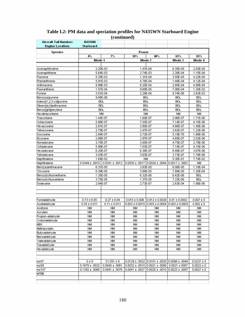
Aircraft Tail ttumber: 11435WII I I Engine Location: Starboard I I

S1>ecie s Power 4% 7% 30% 40% 65% 85%

Mode 1 Mode 2 I Mode 3 Mode 4

Acenaphthylene 2.20E-03 1.41E-04 6.35E-05 2.83E-05 Acenaphthene 5.64E-03 2.74E-03 2.28E-04 1.15E-04 Fluorene 5.35E-03 1.31E-04 3.50E-05 4.22E-05 Phenanthrene 5.91E-03 4.78E-04 1.49E-04 4.12E-04 Anthracene 8.99E-03 6.20E-04 2.80E-04 4.90E-04 Fluoranthene 1.57E-04 9.68E-05 7.06E-04 1.20E-03 Pyrene 3.01E-04 2.29E-04 9.74E-06 2.63E-03 Benzo(a)pyrene 9.88E-06 BDL BDL BDL lndeno[1,2,3-cd)pyrene BDL BDL BDL BDL Dibenz[a,h]anthracene BDL BDL BDL BDL Benzo[ghi)perylene BDL BDL BDL BDL Hexatriacontane NM NM NM NM Triacontane 1.44E-07 1.60E-07 2.96E-07 1.71 E-06 Octacosane 5.98E-07 7.03E-07 7.14E-07 4.15E-06 Hexacosane 2.81E-07 3.80E-07 4.66E-07 1.40E-06 T etracosane 2.79E-07 2.47E-07 3.63E-07 1.22E-06 Docosane 2.84E-07 2.73E-07 5.19E-76 1.86E-06 Eicosane 2.86E-07 2.97E-07 4.65E-07 2.52E-06 Nonadecane 3.75E-07 3.95E-07 4.75E-07 2.79E-06 Octadecane 5.98E-07 7.03E-07 7.14E-07 4.15E-06 Hexadecane 6.20E-07 6.38E-07 6.48E-07 3.67E-06 T etradeeane 3.03E-07 3.63E-07 3.73E-07 1.78E-06 Naphthalene 1.64E-02 NM 5.30E-01 7.74E-02 Naphthalene 0.0349 • .D010 0.0161 • .0012 0.0035 • .0017 0.0D24 • .0004 0.0017 • .0001 NM Benz( a)anthracene 6.31E-05 3.83E-05 6.08E-05 1.18E-04 Chrysene 6.39E-05 3.88E-05 7.89E-05 1.20E-04 Benzo(b )fluoranthene 1.35E-05 6.32E-06 8.42E-06 BDL Benzo(k)fluorantene 3.75E-05 1.37E-05 7.23E-06 BDL Dodecane 2.84E-07 2.73E-07 2.63E-04 1.86E-06

Formaldehyde 0.73 t 0.05 0.27 t 0.04 0.015 t 0.008 0.012 t 0.0026 0.Q1 t0.0002 0.007 t 0 Acelaldehyde 0.35 • 0.D11 0.11 • 0.013 0.003 • 0.0015 0.0D3 • 0.0004 0.003 • 0.0003 0.002 • 0 Acetone NM NM NM NM NM NM Acrolein NM NM NM NM NM NM Propion-aldehyde NM NM NM NM NM NM Crotonaldehyde NM NM NM NM NM NM MEK NM NM NM NM NM NM Methacrolein NM NM NM NM NM NM But yr aldehyde NM NM NM NM NM NM Benz aldehyde NM NM NM NM NM NM Valeraldehyde NM NM NM NM NM NM T olualdehyde NM NM NM NM NM NM Hex aldehyde NM NM NM NM NM NM

mz57 0±0 0.1251 t 0 0.0129 t .0022 0.0101 t .0020 0.0098 t .0048 0.0237 t 0 mz59 0.1678 • .D032 0.0540 • .0061 0.0032 • .0015 0.0D21 • .0006 0.0021 • 0007 0.0022 • 0 mz107 0.1392 t .D068 0.0491 t .0076 0.0041 t .0027 0.0D25 t .0010 0.0023 t .0007 0.0027 t 0 MTBE

Table I.2: PM data and speciation profiles for N435WN Starboard Engine (continued)

180

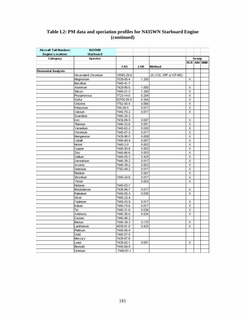
Aircraft Tail ttumber: 1143SWII I Engine Location: Starboard I

Category S1>ecies Grou1> UCR ARI UMR

CAS LOD Method

Elemental An alysis Hexavalent Chromium 18540-29-9 (IC-CCD, XRF or ICP-MS) Magnesium 7639-95-4 1.200 X Beryllium 7440-41-7 Aluminum 7429-90-~ 1.000 X

Silicon 7440-21-3 1.200 X Phosphorous 7723-14-0 0.204 X Sulfur 63705-05-5 0.204 X Chlorine 7782-50-5 0.068 X Potassium 744-09-5 0.017 X Calcium 7440-70-2 0.017 X Scandium 7440-20-2 Iron 7439-89-5 0.007 X Titanium 7440-32-6 0.051 X Vanadium 7440-62-2 0.020 X Chromium 7440-47-3 0.017 X Manganese 7439-96-5 0.009 X Cobalt 7440-48-4 0.007 X Nickel 7440-2-0 0.003 X Copper 7440-50-8 0.003 X Zinc 7440-66-6 0.003 X Gallium 7440-55-3 0.425 X Germanium 7440-38-2 0.017 X Arsenic 7440-38-2 0.003 X Selenium 7782-49-2 0.017 X Rbidium 0.007 X strontium 7440-24-6 0.017 X Ytrium 0.003 X Niobium 7440-03-1 Molybdenum 7439-98-7 0.017 X Palladium 7440-05-3 0.Q26 X Silver 7440-22-4 Cadmium 7440-43-9 0.017 X Indium 7440-74-6 0.017 X Tin 7440-31-6 0.Q26 X Antimony 7440-36-0 0.024 X Cesium 7440-46-2 Barium 7440-39-3 0.170 X Lanthanum 4639-91-0 0.425 X Platinum 7440-06-4 Gold 7440-57-5 Mercury 7439-97-6 Lead 7439-92-1 0.051 X Bismuth 7440-69-9 Uranium 7440-61-1

Table I.2: PM data and speciation profiles for N435WN Starboard Engine (continued)

181

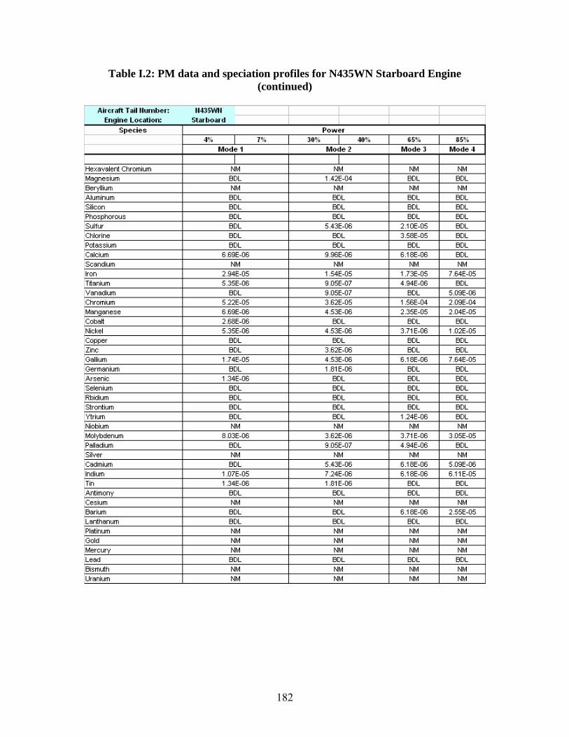
Aircraft Tail ttumber: 1143SWII I I I Engine Location: Starboard I I I

S1>ecies Power 4v, I 7% 30% I «)% 65% 85%

Mode1 Mode2 I Mode 3 Mode4 I I

Hexavalent Chromium NM NM NM NM Magnesium BDL 1.42E-04 BDL BDL Beryllium NM NM NM NM Aluminum BDL BDL BDL BDL Silicon BDL BDL BDL BDL Phosphorous BDL BDL BDL BDL Sulfur BDL 5.43E-06 2.10E-05 BDL Chlorine BDL BDL 3.58E-05 BDL Potassium BDL BDL BDL BDL Calcium 6.69E-06 9.96E-06 6.18E-06 BDL Scandium NM NM NM NM Iron 2.94E-05 1.54E-05 1.73E-05 7.64E-05 Titanium 5.35E-06 9.0SE-07 4.94E-06 BDL Vanadium BDL 9.0SE-07 BDL 5.0SE-06 Chromium 5.22E-05 3.62E-05 1.SSE-04 2.0SE-04

Manganese 6.69E-06 4.53E-06 2.35E-05 2.04E-05 Cobalt 2.68E-06 BDL BDL BDL Nickel 5.35E-06 4.53E-06 3.71E-06 1.02E-05 Copper BDL BDL BDL BDL Zinc BDL 3.62E-06 BDL BDL ua111um 1.14t-U~ 4.~~t-Uij ij_1ijt-Uij / .ij4t-U~

Germanium BDL 1.81E-06 BDL BDL Arsenic 1.34E-06 BDL BDL BDL Selenium BDL BDL BDL BDL Rbidium BDL BDL BDL BDL strontium BDL BDL BDL BDL Ytrium BDL BDL 1.24E-06 BDL Niobium NM NM NM NM Molybdenum 8.03E-06 3.62E-06 3.71E-06 3.0SE-05 Palladium BDL 9.0SE-07 4.94E-06 BDL Silver NM NM NM NM Cadmium BDL 5.43E-06 6.18E-06 5.0SE-06 Indium 1.07E-05 7.24E-06 6.18E-06 6.11E-05 Tin 1.34E-06 1.81E-06 BDL BDL Antimony BDL BDL BDL BDL Cesium NM NM NM NM Barium BDL BDL 6.18E-06 2.SSE-05 Lanthanum BDL BDL BDL BDL Platinum NM NM NM NM Gold NM NM NM NM Mercury NM NM NM NM Lead BDL BDL BDL BDL Bismuth NM NM NM NM Uranium NM NM NM NM

Table I.2: PM data and speciation profiles for N435WN Starboard Engine (continued)

182

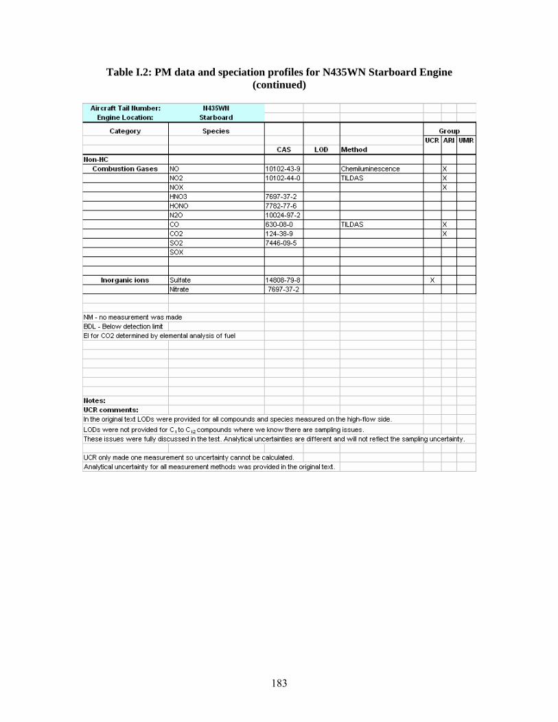
Aircraft Tail ttumber: 11435Wll I Engine Location: Starboard I

Category S1>ecies Grou1> UCR ARI UMR

CAS LOD Method llon-HC

Combustion Gases NO 10102-43-9 Chemiluminescence X N02 10102-44-0 TILDAS X NOX X HN03 7697-37-2 HONO 7782-77-6 N20 10024-97-2 co 630-08-0 TILDAS X CO2 124-38-9 X S02 7446-09-5

SOX

Inorganic ions Sulfate 14808-79-8 X Nitrate 7697-37-2

NM - no measurement was made BOL - Below detection limit El for CO2 determined by elemental analysis of fuel

llotes: UCR comments: In the original text LOOs were provided for all compounds and species measured on the high-flow side.

LOOs were not provided for C I to C 12 compounds where we know there are sampling issues. These issues were fully discussed in the test. Analytical uncertainties are different and will not reflect the sampling uncertainty.

I UCR only made one measurement so uncertainty cannot be calculated. Analytical uncertainty for all measurement methods was provided in the original text.

Table I.2: PM data and speciation profiles for N435WN Starboard Engine (continued)

183

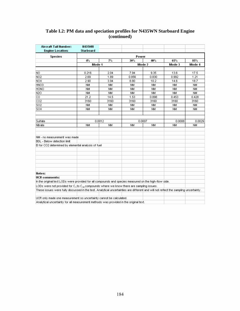
Aircraft Tail ttumber: 11435WII I I Engine Location: Starboard I I

S1>ecies Power 4% 7% 30% 40% 65% 85%

Mode1 Mode2 I Mode 3 Mode4

NO 0.216 2.04 7.94 9.35 13.6 17.5 NO2 2.69 1.89 0.856 0.830 0.992 1.21 NOX 2.90 3.94 8.80 10.2 14.6 18.7 HNO3 NM NM NM NM NM NM HONO NM NM NM NM NM NM N2O NM NM NM NM NM NM co 21.2 14.5 1.53 0.898 0.453 0.428 CO2 3160 3160 3160 3160 3160 3160 SO2 NM NM NM NM NM NM SOX NM NM NM NM NM NM

Sulfate 0.0012 0.0007 0.0008 0.0029 Nitrate NM NM NM NM NM NM

NM - no measurement was made BOL - Below detection limit I El for CO2 determined by elemental analysis of fuel

llotes: UCR comments: In the original text LOOs were provided for all compounds and species measured on the high-flow side.

LOOs were not provided for CI to C 1z compounds where we know there are sampling issues. These issues were fully discussed in the test. Analytical uncertainties are different and will not reflect the sampling uncertainly.

I I UCR only made one measurement so uncertainty cannot be calculated. Analytical uncertainty for all measurement methods was provided in the original text.

Table I.2: PM data and speciation profiles for N435WN Starboard Engine (continued)

184

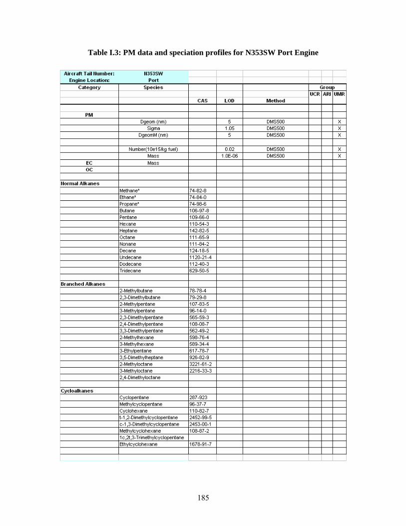
Aircraft Tail ttumber: 113S3SW I Engine Loeation: Pon

Category S1>ecie s Gro1.11> UCR ARI UMR

CAS LOD Method

PM Dgeom (nm) 5 DMS500 X

Sigma 1.05 DMS500 X DgeomM (nm) 5 DMS500 X

Number(1Oe151kg fuel) 0.02 DMS500 X Mass 1.0E-06 DMS500 X

EC Mass oc

normal Alkanes

Methane* 74-82-8 Ethane* 74-84-0 Propane* 74-98-6 Butane 106-97-8 Pentane 109-66-0 Hexane 110-54-3 Heptane 142-82-5 Octane 111-65-9 Nonane 111-84-2 Decane 124-18-5 Undecane 1120-21-4 Dodecane 112-40-3 Tridecane 629-50-5

Branched Alkanes 2-Melhylbutane 78-78-4 2,3-Dimethylbutane 79-29-8 2-Methylpentane 107-83-5 3-Methylpentane 96-14-0 2,3-Dimethylpentane 565-59-3 2,4-Dimethylpentane 108-08-7 3,3-Dimethylpentane 562-49-2 2-Methylhexane 598-76-4 3-Methylhexane 589-34-4 3-Ethylpentane 617-78-7 3,5-Dimethylheptane 926-82-9 2-Methyloctane 3221-61-2 3-Methyloctane 2216-33-3 2,4-Dimethyloctane

Cycloalkanes Cyclopentane 287-923 Methylcyclopentane 96-37-7 Cyclohexane 110-82-7 1-1,2-Dimethylcyclopentane 2452-99-5 c-1 ,3-Dimethylcyclopentane 2453-00-1 Methylcyclohexane 108-87-2 1 c,21,3-Trimethylcyclopentane Ethylcyclohexane 1678-91-7

Table I.3: PM data and speciation profiles for N353SW Port Engine

185

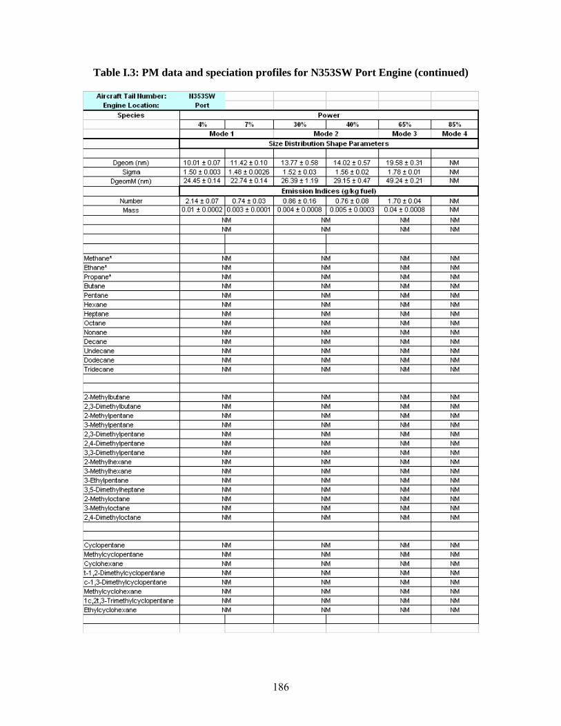
Aircraft Tail ttumber: 113S3SW I I Engine Location: Port I I

S1>ecies Power 4% I 7% 30% I 40% 65% I 85%

Mode 1 Mode 2 Mode l I Mode 4 Size Distribution Sha1>e Parameters

I Dgeom (nm) 10.01 ! 0.07 11.42 ! 0.10 13.77 ! 0.58 14.02 ! 0.57 19.58 ! 0.31 NM

Sigma 1.50 ! 0.003 1.48 ! 0.0026 1.52 ! 0.03 1.56 ! 0.02 1.78 ! 0.01 NM DgeomM (nm) 24.45 ! 0.14 22.74 ! 0.14 26.39 ! 1.19 29.15 ! 0.47 49.24 ! 0.21 NM

Emission Indice s {gll<g fuel)

Number 2.14, 0.07 I 0.74, 0.03 0.86 ! 0.16 I 0.76 ! 0.08 1.70 ! 0.04 NM Mass 0.Q1 ! 0.0002 0.003 ! 0.0001 0.004 ! 0.0008 0.005!0.0003 0.04 ! 0.0008 NM

NM NM NM NM NM NM NM NM

Methane* NM NM NM NM Ethane* NM NM NM NM Propane* NM NM NM NM Butane NM NM NM NM Pentane NM NM NM NM Hexane NM NM NM NM Heptane NM NM NM NM Octane NM NM NM NM Nonane NM NM NM NM Decane NM NM NM NM Undecane NM NM NM NM Dodecane NM NM NM NM Tridecane NM NM NM NM

2-Melhylbutane NM NM NM NM 2,3-Dimethylbutane NM NM NM NM 2-Methylpentane NM NM NM NM 3-Methylpentane NM NM NM NM 2,3-Dimethylpentane NM NM NM NM 2,4-Dimethylpentane NM NM NM NM 3,3-Dimethylpentane NM NM NM NM 2-Methylhexane NM NM NM NM 3-Methylhexane NM NM NM NM 3-Ethylpentane NM NM NM NM 3,5-Dimethylheptane NM NM NM NM 2-Methyloctane NM NM NM NM 3-Methyloctane NM NM NM NM 2,4-Dimethyloctane NM NM NM NM

Cyclopentane NM NM NM NM Methylcyclopentane NM NM NM NM Cyclohexane NM NM NM NM 1-1,2-Dimethylcyclopentane NM NM NM NM c-1 ,3-Dimethylcyclopentane NM NM NM NM Methylcyclohexane NM NM NM NM 1 c,21,3-Trimethylcyclopentane NM NM NM NM Ethylcyclohexane NM NM NM NM

I I I I

Table I.3: PM data and speciation profiles for N353SW Port Engine (continued)

186

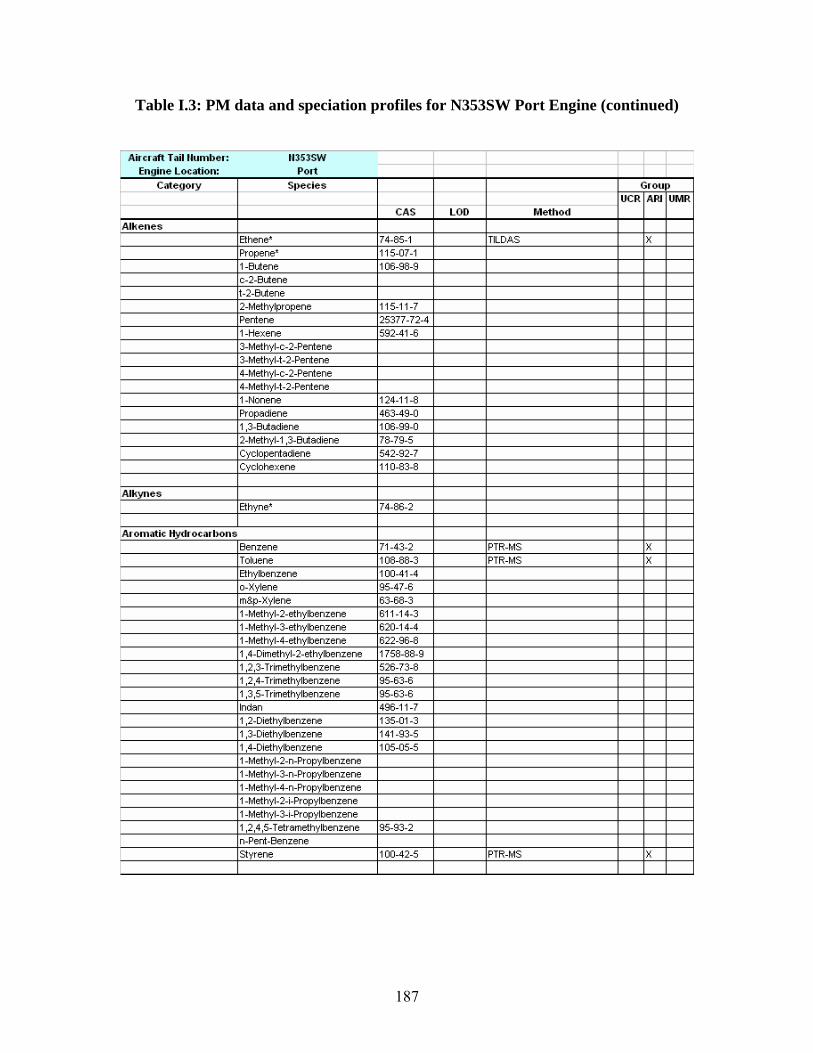
Aircraft Tail ttumber: 113S3SW I Engine Location: Port I

Category S1>ecies Grou1> UCR ARI UMR

CAS LOD Method

Alkenes Ethene* 74-85-1 TILDAS X Propene* 115-07-1 1-Bulene 106-98-9 c-2-Butene 1-2-Bulene 2-Melhylpropene 115-11-7 Pentene 25377-72-4 1-Hexene 592-41-6 3-Melhyl-c-2-Penlene 3-Melhyl-1-2-Penlene 4-Melhyl-c-2-Penlene 4-Melhyl-1-2-Penlene 1-Nonene 124-11-8 Propadiene 463-49-0 1 ,3-Buladiene 106-99-0 2-Melhyl-1,3-Buladiene 78-79-5 Cyclopentadiene 542-92-7 Cyclohexene 110-83-8

Alkynes Ethyne* 74-86-2

Aromatic Hydrocarbons Benzene 71-43-2 PTR-MS X Toluene 108-88-3 PTR-MS X Ethylbenzene 100-41-4 o-Xylene 95-47-6 m&p-Xylene 63-68-3 1-Melhyl-2-elhylbenzene 611-14-3 1-Melhyl-3-elhylbenzene 620-14-4 1-Melhyl-4-elhylbenzene 622-96-8 1,4-Dimelhyl-2-elhylbenzene 1758-88-9 1,2,3-Trimethylbenzene 526-73-8 1,2,4-Trimethylbenzene 95-63-6 1,3,5-Trimethylbenzene 95-63-6 lndan 496-11-7 1,2-Dielhylbenzene 135-01-3 1 ,3-Dielhylbenzene 141-93-5 1,4-Dielhylbenzene 105-05-5 1-Melhyl-2-n-Propylbenzene 1-Melhyl-3-n-Propylbenzene 1-Melhyl-4-n-Propylbenzene 1-Melhyl-2-i-Propylbenzene 1-Melhyl-3-i-Propylbenzene 1 ,2,4 ,5-T elramelhylbenzene 95-93-2 n-Pent-Benzene styrene 100-42-5 PTR-MS X

Table I.3: PM data and speciation profiles for N353SW Port Engine (continued)

187

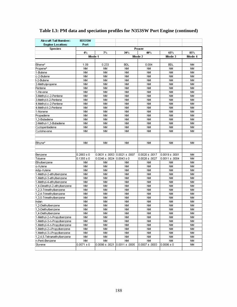
Aircraft Tail ttumber: 113S3SW I I Engine Location: Port I I

S1>ecies Power 4% I 7% 30% I 40% 65% 85%

Mode1 Mode 2 Mode l Mode4

Ethene• 1.09 0.233 BDL 0.004 BDL NM Propene• NM NM NM NM NM NM 1-Butene NM NM NM NM NM NM c-2-Butene NM NM NM NM NM NM 1-2-Butene NM NM NM NM NM NM 2-Methylpropene NM NM NM NM NM NM Pentene NM NM NM NM NM NM 1-Hexene NM NM NM NM NM NM 3-Methyl-c-2-Pentene NM NM NM NM NM NM 3-Methyl-1-2-Pentene NM NM NM NM NM NM 4-Methyl-c-2-Pentene NM NM NM NM NM NM 4-Methyl-1-2-Pentene NM NM NM NM NM NM 1-Nonene NM NM NM NM NM NM Propadiene NM NM NM NM NM NM 1 ,3-Butadiene NM NM NM NM NM NM 2-Melhyl-1,3-Butadiene NM NM NM NM NM NM Cyclopentadiene NM NM NM NM NM NM Cyclohexene NM NM NM NM NM NM

Ethyne• NM NM NM NM NM NM

Benzene 0.2883 ± 0 0.0631 ± .0053 0.0021 ± .0007 0.0020 ± .0017 0.0019 ± .0001 NM Toluene 0.1355 ± 0 0.0246 ± .0024 0.0043 ± 0 0.0028 ± .0027 0.0011 ± .0004 NM Ethylbenzene NM NM NM NM NM NM o-Xylene NM NM NM NM NM NM m&p-Xylene NM NM NM NM NM NM 1-Methyl-2-elhylbenzene NM NM NM NM NM NM 1-Methyl-3-ethylbenzene NM NM NM NM NM NM 1-Methyl-4-elhylbenzene NM NM NM NM NM NM 1,4-Dimethyl-2-elhylbenzene NM NM NM NM NM NM 1,2,3-Trimethylbenzene NM NM NM NM NM NM 1,2,4-Trimethylbenzene NM NM NM NM NM NM 1,3,5-Trimethylbenzene NM NM NM NM NM NM lndan NM NM NM NM NM NM 1,2-Diethylbenzene NM NM NM NM NM NM 1 ,3-Diethylbenzene NM NM NM NM NM NM 1,4-Diethylbenzene NM NM NM NM NM NM 1-Methyl-2-n-Propylbenzene NM NM NM NM NM NM 1-Methyl-3-n-Propylbenzene NM NM NM NM NM NM 1-Methyl-4-n-Propylbenzene NM NM NM NM NM NM 1-Methyl-2-i-Propylbenzene NM NM NM NM NM NM 1-Methyl-3-i-Propylbenzene NM NM NM NM NM NM 1 ,2,4 ,5-T etramethylbenzene NM NM NM NM NM NM n-Pent-Benzene NM NM NM NM NM NM styrene 0.0571 ± 0 0.0098 ± .0021 0.0011 ± .0005 0.0007 ± .0003 0.0006 ± 0 NM

Table I.3: PM data and speciation profiles for N353SW Port Engine (continued)

188

Aircraft Tail ttumber: 113S3SW I Engine Location: Port I

Category S1>ecies Grou1> UCR ARI UMR

CAS LOD Method Semivolatiles

(alkanes and PAHs) Acenaphthylene 208-96-8 XAD-PUF/Quartz samJ>ling Acenaphthene 83-32-9 Fluorene 86-73-7 Phenanthrene 85-01-8 Anthracene 120-12-7 Fluoranthene 206-44-0 Pyrene 129-00-0 Benzo(a)pyrene 50-32-8 lndeno[1,2,3-cd)pyrene 193-39-5 Oibenz[a,h]anthracene 53-70-3 Benzo[ghi]perylene 191-24-2 Hexatriacontane 630-06-8 Triacontane 638-68-6 Octacosane 630-02-4

Hexacosane 630-01-3 T etracosane 646-31-1 Docosane 629-92-0 Eicosane 112-95-8 Nonadecane 629-92-5 Octadecane 593-46-3 Hexadecane 544-76-3 T etradecane 629-59-4 Naphthalene 91-20-3 PTR-MS X Benz( a)anthracene 56-55-3 Chrysene 218-01-9 Benzo(b )fluoranlhene 205-99-2 Benzo(k )fluoranlhene 207-08-9 Dodecane 112-40-3

Carbonyls (ONPH Sampling) Formaldehyde TILOAS X Acelaldehyde PTR-MS X Acetone 67-64-1 Acrolein 107-02-8 TILOAS Propion-aldehyde 123-38-6 Crolonaldehyde 4170-30-3 MEK 78-93-3 Methacrolein 78-85-3 But yr aldehyde 123-72-8 Benz aldehyde 100-52-7 Valeraldehyde 110-62-3 T olualdehyde Hex aldehyde 66-25-1

Other Organics mz57 PTR-MS X mz59 PTR-MS X mz107 PTR-MS X MTBE 1634-04-4

Table I.3: PM data and speciation profiles for N353SW Port Engine (continued)

189

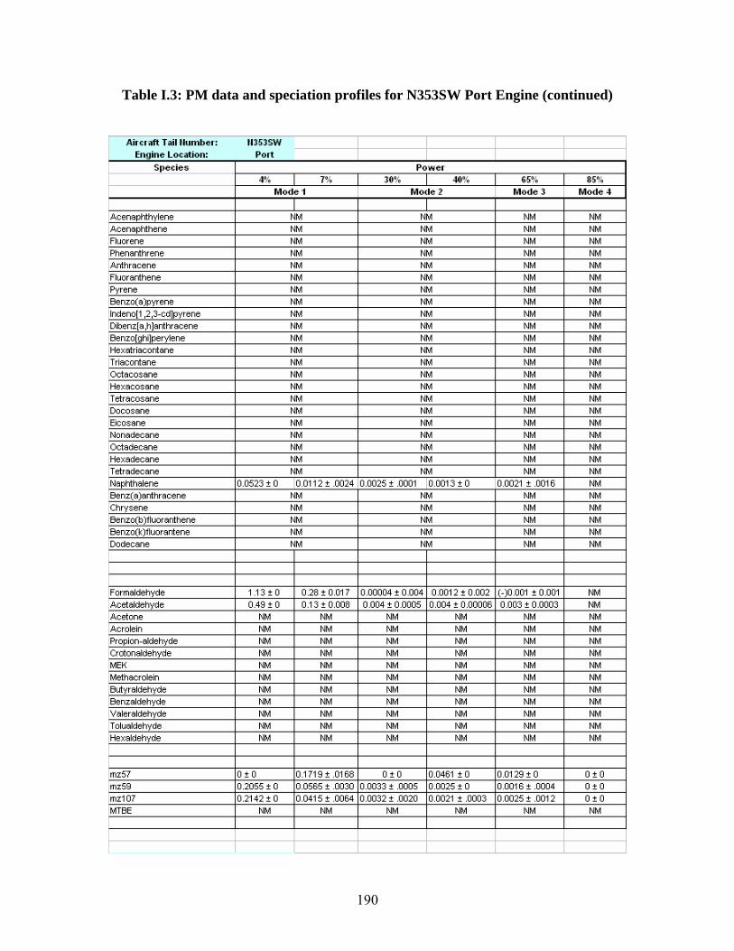
Aircraft Tail ttumber: 113S3SW I I Engine Location: Port I I

S1>ecies Power 4% I 7% 30% I 40% 65% 85%

Mode1 Mode2 Mode l Mode4 I I

Acenaphthylene NM NM NM NM Acenaphthene NM NM NM NM Fluorene NM NM NM NM Phenanthrene NM NM NM NM Anthracene NM NM NM NM Fluoranthene NM NM NM NM Pyrene NM NM NM NM Benzo(a)pyrene NM NM NM NM lndeno[1,2,3-cd)pyrene NM NM NM NM Dibenz[a,h]anthracene NM NM NM NM Benzo[ghi)perylene NM NM NM NM Hexatriacontane NM NM NM NM Triacontane NM NM NM NM Octacosane NM NM NM NM Hexacosane NM NM NM NM T etracosane NM NM NM NM Docosane NM NM NM NM Eicosane NM NM NM NM Nonadecane NM NM NM NM Octadecane NM NM NM NM Hexadecane NM NM NM NM T etradecane NM NM NM NM Naphthalene 0.0523 • 0 10.0112, .0024 10.0025, .0001 10.0013, o 10.0021 • .0016 NM Benz( a)anthracene NM NM NM NM Chrysene NM NM NM NM Benzo(b )fluoranthene NM NM NM NM Benzo(k)fluorantene NM NM NM NM Dodecane NM NM NM NM

Formaldehyde 1.13 t 0 0.28 t 0.017 0.00004 t 0.004 0.0012 t 0.002 (-)0.001 .0.001 NM Acelaldehyde 0.49 • 0 0.13 • 0.008 0.004 • 0.0005 0.004 • 0.00006 0.003 • 0.0003 NM Acetone NM NM NM NM NM NM Acrolein NM NM NM NM NM NM Propion-aldehyde NM NM NM NM NM NM Crotonaldehyde NM NM NM NM NM NM MEK NM NM NM NM NM NM Methacrolein NM NM NM NM NM NM But yr aldehyde NM NM NM NM NM NM Benz aldehyde NM NM NM NM NM NM Valeraldehyde NM NM NM NM NM NM T olualdehyde NM NM NM NM NM NM Hex aldehyde NM NM NM NM NM NM

mz57 O:!:O 0.1719 • .0168 O:!:O 0.0461 • 0 0.0129 • 0 O:!:O mz59 0.2055 t 0 0.0565 t .0030 0.0033> .0005 0.0025 t 0 0.0016 t .0004 O:!:O mz107 0.2142 • 0 0.0415 • .0064 0.0032• .0020 0.0021 • .0003 0.0025 • .0012 O:!:O MTBE NM NM NM NM NM NM

Table I.3: PM data and speciation profiles for N353SW Port Engine (continued)

190

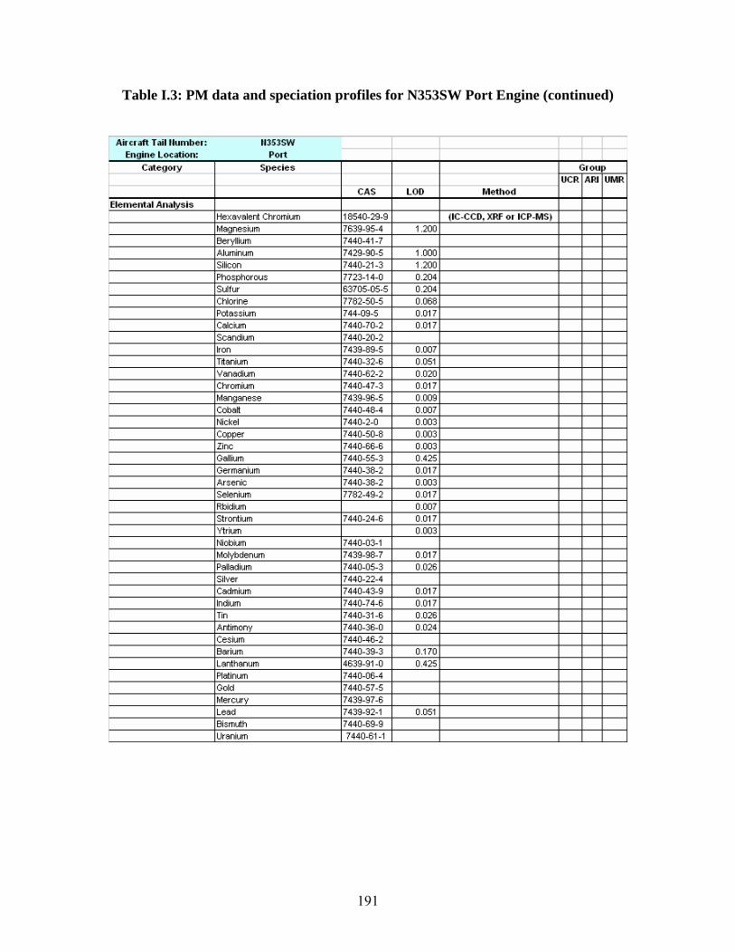
Aircraft Tail ttumber: 113S3SW I Engine Location: Port I

Category S1>ecies Grou1> UCR ARI UMR

CAS LOD Method

Elemental Analysi s Hexavalent Chromium 18540-29-9 (IC-CCD, XRF or ICP-MS) Magnesium 7639-95-4 1.200 Beryllium 7440-41-7 Aluminum 7429-90-5 1.000 Silicon 7440-21-3 1.200 Phosphorous 7723-14-0 0.204 Sulfur 63705-05-5 0.204 Chlorine 7782-50-5 0.068 Potassium 744-09-5 0.017 Calcium 7440-70-2 0.017 Scandium 7440-20-2 Iron 7439-89-5 0.007 Titanium 7440-32-6 0.051 Vanadium 7440-62-2 0.020 Chromium 7440-47-3 0.017 Manganese 7439-96-5 0.009 Cobalt 7440-48-4 0.007 Nickel 7440-2-0 0.003 Copper 7440-50-8 0.003 Zinc 7440-66-6 0.003 Gallium 7440-55-3 0.425 Germanium 7440-38-2 0.017 Arsenic 7440-38-2 0.003 Selenium 7782-49-2 0.017 Rbidium 0.007 strontium 7440-24-6 0.017 Ytrium 0.003 Niobium 7440-03-1 Molybdenum 7439-98-7 0.017 Palladium 7440-05-3 O.Q26 Silver 7440-22-4 Cadmium 7440-43-9 0.017 Indium 7440-74-6 0.017 Tin 7440-31-6 O.Q26 Antimony 7440-36-0 0.024 Cesium 7440-46-2 Barium 7440-39-3 0.170 Lanthanum 4639-91-0 0.425 Platinum 7440-06-4 Gold 7440-57-5 Mercury 7439-97-6 Lead 7439-92-1 0.051 Bismuth 7440-69-9 Uranium 7440-61-1

Table I.3: PM data and speciation profiles for N353SW Port Engine (continued)

191

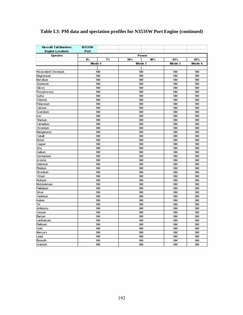
Aircraft Tail ttumber: 113S3SW I I Engine Location: Port I I

S1>ecie s Power 4% I 7% 30% I 40% 65% 85%

Mvde 1 I Mvde 2 I Mvde 3 Mvde4

I I Hexavalent Chromium NM NM NM NM Magnesium NM NM NM NM Beryllium NM NM NM NM Aluminum NM NM NM NM Silicon NM NM NM NM Phosphorous NM NM NM NM Sulfur NM NM NM NM Chlorine NM NM NM NM Potassium NM NM NM NM Calcium NM NM NM NM Scandium NM NM NM NM Iron NM NM NM NM Titanium NM NM NM NM Vanadium NM NM NM NM Chromium NM NM NM NM Manganese NM NM NM NM Cobalt NM NM NM NM Nickel NM NM NM NM Copper NM NM NM NM Zinc NM NM NM NM Gallium NM NM NM NM Germanium NM NM NM NM Arsenic NM NM NM NM Selenium NM NM NM NM Rbidium NM NM NM NM strontium NM NM NM NM Ytrium NM NM NM NM Niobium NM NM NM NM Molybdenum NM NM NM NM Palladium NM NM NM NM Silver NM NM NM NM Cadmium NM NM NM NM Indium NM NM NM NM Tin NM NM NM NM Antimony NM NM NM NM Cesium NM NM NM NM Barium NM NM NM NM Lanthanum NM NM NM NM Platinum NM NM NM NM Gold NM NM NM NM Mercury NM NM NM NM Lead NM NM NM NM Bismuth NM NM NM NM Uranium NM NM NM NM

Table I.3: PM data and speciation profiles for N353SW Port Engine (continued)

192

Aircraft Tail ttumber: 113S3SW I Engine Location: Port I

Category S1>ecies Grou1> UCR ARI UMR

CAS LOD Method llon-HC

Combustion Gase s NO 10102-43-9 Chemiluminescence X N02 10102-44-0 TILDAS X NOX X HN03 7697-37-2 HONO 7782-77-6 N20 10024-97-2 co 630-08-0 TILDAS X CO2 124-38-9 X S02 7446-09-5 SOX

Inorganic ions Sulfate 14808-79-8 Nitrate 7697-37-2

NM - no measuremenl was made BDL - Below deleclion limltl El for CO2 determined by elemental analysis of fuel

llotes: UCR comments: In the original text LOOs were provided for all compounds and species measured on the high-flow side. LOOs were not provided for C I to C 12 compounds where we know there are sampling issues. These issues were fully discussed in the test. Analytical uncertainties are different and will not reflect the sampling uncertainty.

I UCR only made one measurement so uncertainly cannot be calculated. Analytical uncertainty 1or all measurement methods was provided in 1he original text.

Table I.3: PM data and speciation profiles for N353SW Port Engine (continued)

193

Aircraft Tail ttumber: 113S3SW I I Engine Location: Port I I

S1>ecies Power 4% I 7% 30% I 40% 65% 85%

Mode1 I Mode2 I Mode 3 Mode4

NO 0.16 0.892 6.09 7.04 9.36 NM NO2 2.51 2.18 1.00 0.885 0.88 NM NOX 2.67 3.08 7.09 7.92 10.2 NM HNO3 NM NM NM NM NM NM HONO NM NM NM NM NM NM N2O co 22.2 16.9 3.11 1.85 0.786 NM CO2 3160 3160 3160 3160 3160 3160 SO2 NM NM NM NM NM NM SOX NM NM NM NM NM NM

Sulfate NM NM NM NM NM NM Nitrate NM NM NM NM NM NM

NM - no measurement was made BOL - Below detection limit El for CO2 determined by elemental analysis of fuel

llotes: UCR comments: In the original text LOOs were provided for all compounds and species measured on the high-flow side. LOOs were not provided for C I to C 12 compounds where we know there are sampling issues. These issues were fully discussed in the test. Analytical uncertainties are different and will not reflect the sampling uncertainty.

I I UCR only made one measurement so uncertainty cannot be calculated. I Analytical uncertainty for all measurement methods was provided in the original text.

Table I.3: PM data and speciation profiles for N353SW Port Engine (continued)

194

Aircraft Tail ttumber: 113S3SW I Engine Location: Starboard I

Category S1>ecie s Grou1> UCR ARI UMR

CAS LOD Method

PM Dgeom (nm) 5 DMS500 X

Sigma 1.05 DMS500 X DgeomM (nm) 5 DMS500 X

Number(10e151kg fuel) 0.02 DMS500 X Mass 1.0E-06 DMS500 X Mass X

EC X oc X

llormal All<anes Methane* 74-82-8 Ethane* 74-84-0 Propane* 74-98-6 Butane 106-97-8 Pentane 109-66-0 Hexane 110-54-3 Heplane 142-82-5 Octane 111-65-9 Nonane 111-84-2 Decane 124-18-5 Undecane 1120-21-4 Dodecane 112-40-3 Tridecane 629-50-5

Branched Alkanes 2-Melhylbutane 78-78-4 2,3-Dimelhylbutane 79-29-8 2-Melhylpenlane 107-83-5 3-Melhylpenlane 96-14-0 2,3-Dimelhylpenlane 565-59-3 2,4-Dimelhylpenlane 108-08-7 3,3-Dimelhylpenlane 562-49-2 2-Melhylhexane 598-76-4 3-Melhylhexane 589-34-4 3-Elhylpenlane 617-78-7 3,5-Dimelhylheplane 926-82-9 2-Melhyloclane 3221-61-2 3-Melhyloclane 2216-33-3 2,4-Dimelhyloclane

Cycloalkanes Cyclopentane 287-923 Melhylcyclopenlane 96-37-7 Cyclohexane 110-82-7 t-1,2-Dimelhylcyclopenlane 2452-99-5 c-1 ,3-Dimelhylcyclopenlane 2453-00-1 Melhylcyclohexane 108-87-2 1 c,21,3-Trimelhylcyclopenlane Ethylcyclohexane 1678-91-7

Table I.4: PM data and speciation profiles for N353SW Starboard Engine

195

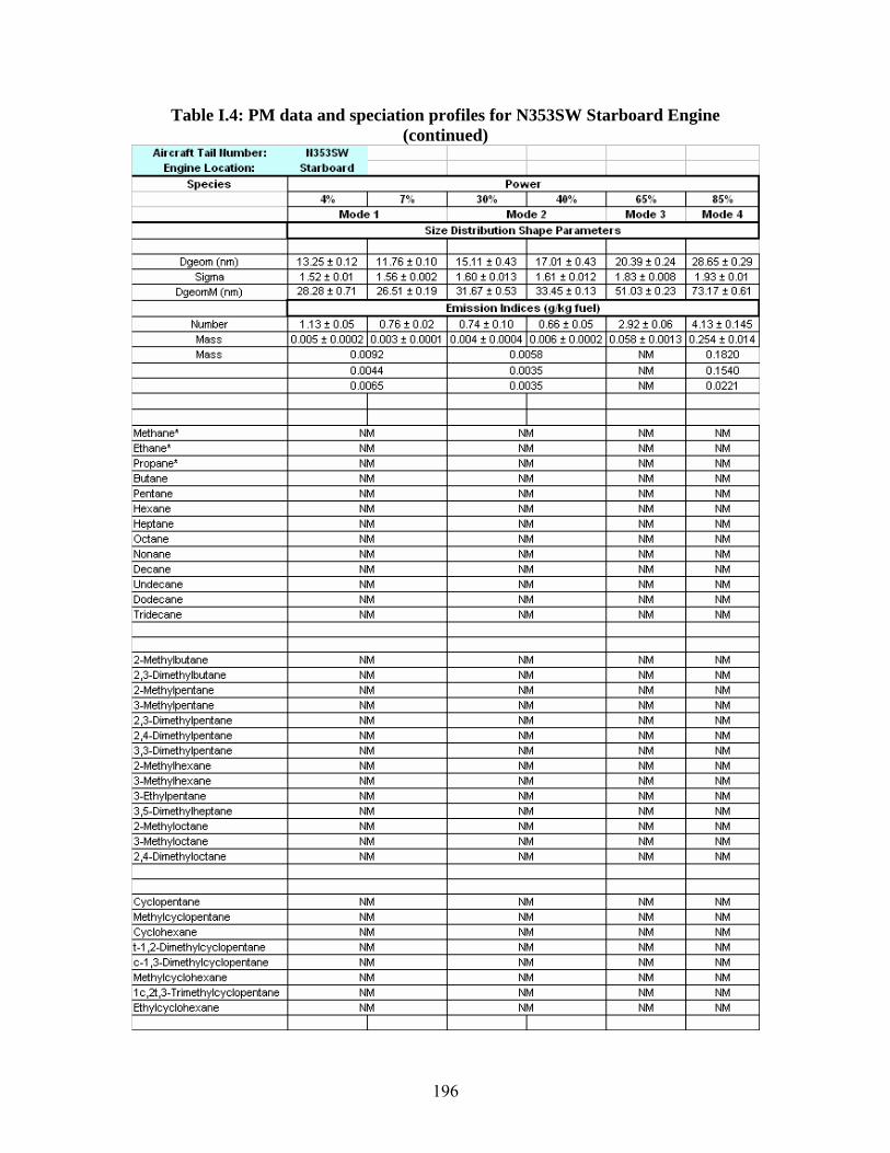
Aircraft Tail ttumber: 113S3SW I I Engine Location: Starboard I I

S1>ecie s Power 4% I 7% 30% I 40% 65% I 85%

Mode 1 Mode 2 Mode 3 I Mode 4 Size Distribution Sha1>e Parameters

I Dgeom (nm) 13.25 ! 0.12 11.76 ! 0.10 15.11 ! 0.43 17.01 ! 0.43 20.39 ! 0.24 28.65 ! 0.29

Sigma 1.52 ! 0.01 1.56 ! 0.002 1.60 ! 0.013 1.61 ! 0.012 1.83 ! 0.008 1.93 ! 0.01 DgeomM (nm) 28.28 ! 0.71 26.51 ! 0.19 31.67 ! 0.53 33.45 ! 0.13 51.03 ! 0.23 73.17 ! 0.61

Emission Indice s {gll<g fuel)

Number 1.13, 0.05 I 0.76, 0.02 0.74, 0.10 I 0.66, 0.05 2.92 ! 0.06 4.13 ! 0.145 Mass 0.005 ! 0.0002 I 0.003 ! 0.0001 0.004 , 0.0004 I 0.006, 0.0002 0.058 ! 0.0013 0.254 ! 0.014 Mass 0.0092 0.0058 NM 0.1820

0.0044 0.0035 NM 0.1540 0.0065 0.0035 NM 0.0221

I I I I

Methane• NM NM NM NM Ethane• NM NM NM NM Propane• NM NM NM NM Butane NM NM NM NM Pentane NM NM NM NM Hexane NM NM NM NM Heptane NM NM NM NM Octane NM NM NM NM Nonane NM NM NM NM Decane NM NM NM NM Undecane NM NM NM NM Dodecane NM NM NM NM Tridecane NM NM NM NM

2-Melhylbutane NM NM NM NM 2,3-Dimethylbutane NM NM NM NM 2-Methylpentane NM NM NM NM 3-Methylpentane NM NM NM NM 2,3-Dimethylpentane NM NM NM NM 2,4-Dimethylpentane NM NM NM NM 3,3-Dimethylpentane NM NM NM NM 2-Methylhexane NM NM NM NM 3-Methylhexane NM NM NM NM 3-Ethylpentane NM NM NM NM 3,5-Dimethylheptane NM NM NM NM 2-Methyloctane NM NM NM NM 3-Methyloctane NM NM NM NM 2,4-Dimethyloctane NM NM NM NM

Cyclopentane NM NM NM NM Methylcyclopentane NM NM NM NM Cyclohexane NM NM NM NM t-1,2-Dimethylcyclopentane NM NM NM NM c-1 ,3-Dimethylcyclopentane NM NM NM NM Methylcyclohexane NM NM NM NM 1 c,21,3-Trimethylcyclopentane NM NM NM NM Ethylcyclohexane NM NM NM NM

I I

Table I.4: PM data and speciation profiles for N353SW Starboard Engine (continued)

196

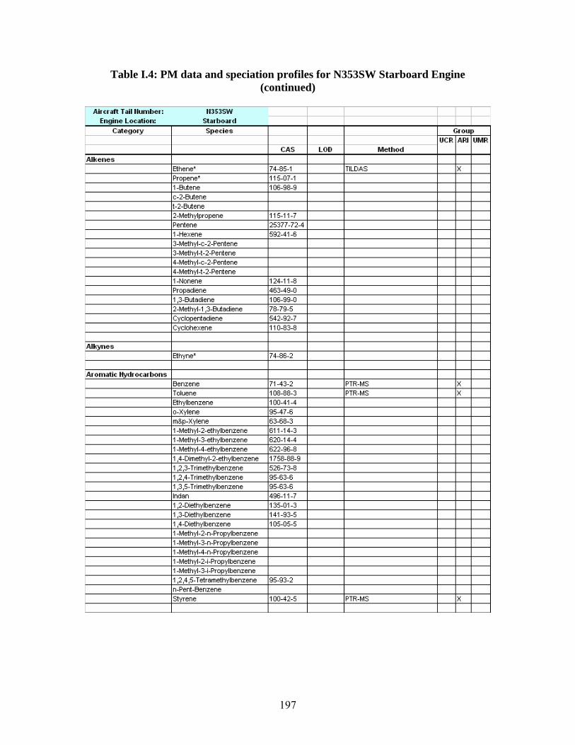
Aircraft Tail ttumber: 113S3SW I Engine Location: Starboard I

Category S1>ecie s Grou1> UCR ARI UMR

CAS LOD Method

Alkenes Ethene• 74-85-1 TILDAS X Propene• 115-07-1 1-Butene 106-98-9 c-2-Butene 1-2-Butene 2-Melhylpropene 115-11-7 Pentene 25377-72-4 1-Hexene 592-41-6 3-Melhyl-c-2-Penlene 3-Melhyl-1-2-Penlene 4-Melhyl-c-2-Penlene 4-Melhyl-1-2-Penlene 1-Nonene 124-11-8 Propadiene 463-49-0 1 ,3-Butadiene 106-99-0 2-Melhyl-1,3-Butadiene 78-79-5 Cyclopenladiene 542-92-7 Cyclohexene 110-83-8

Alkynes Ethyne• 74-86-2

Aromatic Hydrocarbons Benzene 71-43-2 PTR-MS X Toluene 108-88-3 PTR-MS X Ethylbenzene 100-41-4 o-Xylene 95-47-6 m&p-Xylene 63-68-3 1-Melhyl-2-elhylbenzene 611-14-3 1-Melhyl-3-elhylbenzene 620-14-4 1-Melhyl-4-elhylbenzene 622-96-8 1,4-Dimelhyl-2-elhylbenzene 1758-88-9 1,2,3-Trimethylbenzene 526-73-8 1,2,4-Trimethylbenzene 95-63-6 1,3,5-Trimethylbenzene 95-63-6 lndan 496-11-7 1,2-Dielhylbenzene 135-01-3 1 ,3-Dielhylbenzene 141-93-5 1,4-Dielhylbenzene 105-05-5 1-Melhyl-2-n-Propylbenzene 1-Melhyl-3-n-Propylbenzene 1-Melhyl-4-n-Propylbenzene 1-Melhyl-2-i-Propylbenzene 1-Melhyl-3-i-Propylbenzene 1 ,2,4 ,5-T elramelhylbenzene 95-93-2 n-Pent-Benzene styrene 100-42-5 PTR-MS X

Table I.4: PM data and speciation profiles for N353SW Starboard Engine (continued)

197

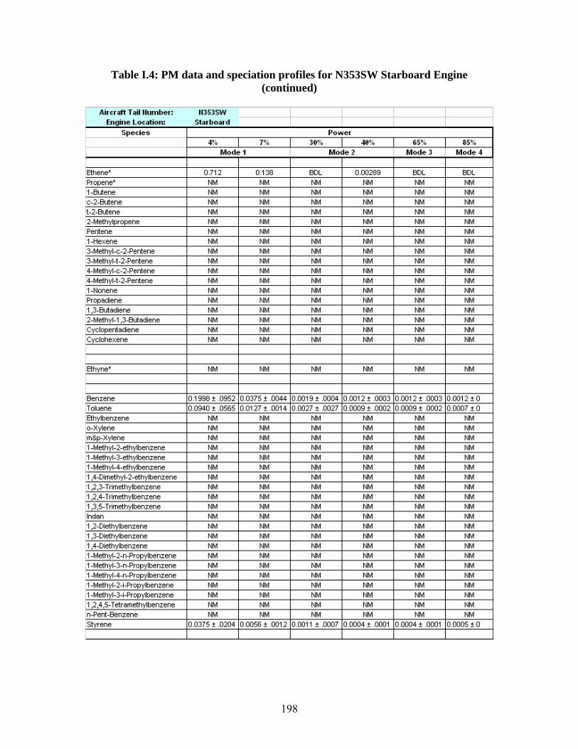
Aircraft Tail ttumber: 113S3SW I I Engine Location: Starboard I I

S1>ecies Power 4% I 7% 30% I 40% 65% 85%

Mode1 Mode2 Mode 3 Mode4

Ethene• 0.712 0.138 BDL 0.00289 BDL BDL Propene• NM NM NM NM NM NM 1-Butene NM NM NM NM NM NM c-2-Butene NM NM NM NM NM NM 1-2-Butene NM NM NM NM NM NM 2-Methylpropene NM NM NM NM NM NM Pentene NM NM NM NM NM NM 1-Hexene NM NM NM NM NM NM 3-Methyl-c-2-Pentene NM NM NM NM NM NM 3-Methyl-1-2-Pentene NM NM NM NM NM NM 4-Methyl-c-2-Pentene NM NM NM NM NM NM 4-Methyl-1-2-Pentene NM NM NM NM NM NM 1-Nonene NM NM NM NM NM NM Propadiene NM NM NM NM NM NM 1 ,3-Butadiene NM NM NM NM NM NM 2-Melhyl-1,3-Butadiene NM NM NM NM NM NM Cyclopentadiene NM NM NM NM NM NM Cyclohexene NM NM NM NM NM NM

Ethyne• NM NM NM NM NM NM

Benzene 0.1998 ± .0952 0.0375 ± .0044 0.0019 ± .0004 0.0012 ± .0003 0.0012 ± .0003 0.0012 ± 0 Toluene 0.0940 ± .0565 0.0127 ± .0014 0.0027 ± .0027 0.0009 ± .0002 0.0009 ± .0002 0.0007 ± 0 Ethylbenzene NM NM NM NM NM NM o-Xylene NM NM NM NM NM NM m&p-Xylene NM NM NM NM NM NM 1-Methyl-2-elhylbenzene NM NM NM NM NM NM 1-Methyl-3-ethylbenzene NM NM NM NM NM NM 1-Methyl-4-elhylbenzene NM NM NM NM NM NM 1,4-Dimethyl-2-elhylbenzene NM NM NM NM NM NM 1,2,3-Trimethylbenzene NM NM NM NM NM NM 1,2,4-Trimethylbenzene NM NM NM NM NM NM 1,3,5-Trimethylbenzene NM NM NM NM NM NM lndan NM NM NM NM NM NM 1,2-Diethylbenzene NM NM NM NM NM NM 1 ,3-Diethylbenzene NM NM NM NM NM NM 1,4-Diethylbenzene NM NM NM NM NM NM 1-Methyl-2-n-Propylbenzene NM NM NM NM NM NM 1-Methyl-3-n-Propylbenzene NM NM NM NM NM NM 1-Methyl-4-n-Propylbenzene NM NM NM NM NM NM 1-Methyl-2-i-Propylbenzene NM NM NM NM NM NM 1-Methyl-3-i-Propylbenzene NM NM NM NM NM NM 1 ,2,4 ,5-T etramethylbenzene NM NM NM NM NM NM n-Pent-Benzene NM NM NM NM NM NM styrene 0.0375 ± .0204 0.0056 ± .0012 0.0011 ± .0007 0.0004 ± .0001 0.0004 ± .0001 0.0005 ± 0

Table I.4: PM data and speciation profiles for N353SW Starboard Engine (continued)

198

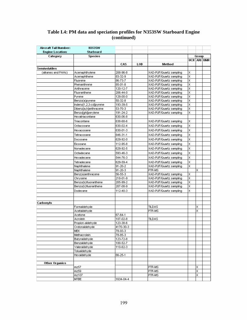
Aircraft Tail ttumber: 113S3SW I Engine Location: Starboard I

Category S1>ecie s Grou1> UCR ARI UMR

CAS LOD Method

Semivolatiles (alkanes and PAHs) Acenaphthylene 208-96-8 XAD-PUF /Quartz sampling X

Acenaphthene 83-32-9 XAD-PUF /Quartz sampling X Fluorene 86-73-7 XAD-PUF /Quartz sampling X Phenanthrene 85-01-8 XAD-PUF /Quartz sampling X Anthracene 120-12-7 XAD-PUF /Quartz sampling X Fluoranthene 206-44-0 XAD-PUF /Quartz sampling X Pyrene 129-00-0 XAD-PUF /Quartz sampling X Benzo(a)pyrene 50-32-8 XAD-PUF /Quartz sampling X lndeno[1,2,3-cd)pyrene 193-39-5 XAD-PUF /Quartz sampling X Dibenz[a,h]anthracene 53-70-3 XAD-PUF /Quartz sampling X Benzo[ghi)perylene 191-24-2 XAD-PUF /Quartz sampling X Hexatriacontane 630-06-8

Triacontane 638-68-6 XAD-PUF /Quartz sampling X Octacosane 630-02-4 XAD-PUF /Quartz sampling X Hexacosane 630-01-3 XAD-PUF /Quartz sampling X T etracosane 646-31-1 XAD-PUF /Quartz sampling X Docosane 629-92-0 XAD-PUF /Quartz sampling X

Eicosane 112-95-8 XAD-PUF /Quartz sampling X Nonadecane 629-92-5 XAD-PUF /Quartz sampling X Octadecane 593-46-3 XAD-PUF /Quartz sampling X Hexadecane 544-76-3 XAD-PUF /Quartz sampling X T etradecane 629-59-4 XAD-PUF /Quartz sampling X Naphlhalene 91-20-2 XAD-PUF /Quartz sampling X Naphthalene 91-20-3 PTR-MS X Benz( a)anthracene 56-55-3 XAD-PUF /Quartz sampling X Chrysene 218-01-9 XAD-PUF /Quartz sampling X Benzo(b )fluoranlhene 205-99-2 XAD-PUF /Quartz sampling X Benzo(k )fluoranlhene 207-08-9 XAD-PUF /Quartz sampling X Dodecane 112-40-3 XAD-PUF /Quartz sampling X

Carbonyls Formaldehyde TILDAS X Acelaldehyde PTR-MS X Acetone 67-64-1 Acrolein 107-02-8 TILDAS Propion-aldehyde 123-38-6 Crolonaldehyde 4170-30-3 MEK 78-93-3 Methacrolein 78-85-3 Bui yr aldehyde 123-72-8 Benz aldehyde 100-52-7 Valeraldehyde 110-62-3 T olualdehyde

Hex aldehyde 66-25-1

Other Organics mz57 PTR-MS X mz59 PTR-MS X mz107 PTR-MS X MTBE 1634-04-4

Table I.4: PM data and speciation profiles for N353SW Starboard Engine (continued)

199

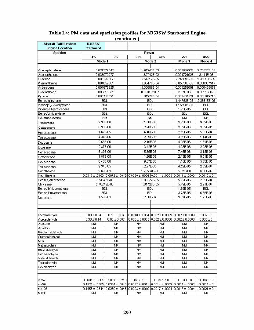
Aircraft Tail ttumber: 113S3SW I I Engine Location: Starboard I I

S1>ecie s Power 4% I 7% 30% I 40% 65% 85%

Mode 1 Mode 2 Mode 3 Mode 4 I I

Acenaphthylene 0.021377042 1.91247E-03 0.000669928 2.72632E-05 Acenaphthene 0.038970077 1.60742E-02 0.004724923 8.414E-05 Fluorene 0.003237607 5.54317E-05 2.24589E-05 1.33099E-05 Phenanthrene 0.004059081 2.63478E-04 3.05338E-05 0.000357917 Anthracene 0.004678825 3.30689E-04 0.000258091 0.000425889 Fluoranthene 0.000315034 0.000102087 2.97E-06 0.001133975 Pyrene 0.000752021 1.81276E-04 0.000437521 0.001819716 Benzo(a)pyrene BDL BDL 1.44753E-05 2.38615E-05 lndeno[1,2,3-cd)pyrene BDL BDL 1 .15698E-05 BDL Dibenz[a,h]anthracene BDL BDL 1.93E-05 BDL Benzo[ghi)perylene BDL BDL BDL BDL Hexatriacontane NM NM NM NM

Triacontane 2.33E-06 1.80E-06 2.73E-06 9.02E-06

Octacosane 6.93E-06 2.20E-06 2.39E-06 3.39E-05

Hexacosane 1.67E-05 4.46E-05 2.59E-05 5.53E-04

T etracosane 4.34E-06 2.99E-06 3.55E-06 1.14E-05

Docosane 2.58E-06 2.49E-06 4.38E-06 1.51E-05

Eicosane 2.87E-06 3.12E-06 4.38E-06 2.23E-05

Nonadecane 5.39E-06 5.85E-06 7.45E-06 3.13E-05

Octadecane 1.87E-05 1.86E-05 2.13E-05 9.21E-05

Hexadecane 6.46E-06 9.87E-06 1.15E-05 5.23E-05

T etradecane 2.94E-05 2.97E-05 4.52E-05 2.32E-04 Naphthalene 9.69E-03 1 .25564E•00 5.52E•00 6.68E-02 Naphthalene 0.0317 ± .0183 I 0.0072 ± .0018 0.0020 ± .0004 I 0.0011 ± .0003 0.0011 ± .0003 0.0010 ± 0 Benz( a)anthracene 2.74547E-05 1.00377E-05 5.22E-05 2.05E-04 Chrysene 2.78242E-05 1.01728E-05 5.49E-05 2.91E-04 Benzo(b )fluoranthene BDL BDL 1.69E-05 BDL Benzo(k)fluorantene BDL BDL 3.73E-05 6.35E-05

Dodecane 1.59E-03 2.68E-04 9.81E-05 1.23E-03

Formaldehyde 0.80 ± 0.34 0.16 ± 0.06 0.0018 ± 0.004 0.002 ± 0.0009 0.002 ± 0.0009 0.002 ± 0 Acelaldehyde 0.36 ± 0.14 0.08 ± 0.007 0.005±0.0005 0.002 ± 0.0008 0.002 ± 0.0008 0.002 ± 0 Acetone NM NM NM NM NM NM Acrolein NM NM NM NM NM NM Propion-aldehyde NM NM NM NM NM NM Crotonaldehyde NM NM NM NM NM NM MEK NM NM NM NM NM NM Methacrolein NM NM NM NM NM NM But yr aldehyde NM NM NM NM NM NM Benz aldehyde NM NM NM NM NM NM Valeraldehyde NM NM NM NM NM NM T olualdehyde NM NM NM NM NM NM Hex aldehyde NM NM NM NM NM NM

mz57 0.3604 ± .0364 0.1031 ± .0218 0.0233 ± 0 0.0461 ± 0 0.0130 ± 0 0.0066 ± 0 mz59 0.1521 ± .0585 0.0354 ± .0042 0.0027 ± .0011 0.0014 ± .0002 0.0014 ± .0002 0.0014 ± 0 mz107 0.1455 ± .0844 0.0250 ± .0045 0.0023 ± .0010 0.0017 ± .0004 0.0017 ± .0004 0.0021 ± 0 MTBE NM NM NM NM NM NM

Table I.4: PM data and speciation profiles for N353SW Starboard Engine (continued)

200

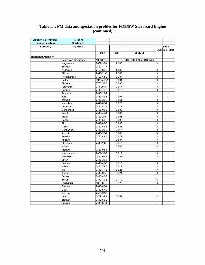
Aircraft Tail ttumber: 113S3SW I Engine Location: Starboard I

Category S1>ecies Grou1> UCR ARI UMR

CAS LOD Method Elemental Analysis

Hexavalent Chromium 18540-29-9 (IC-CCD, XRF or ICP-MS) Magnesium 7639-95-4 1.200 X Beryllium 7440-41-7 Aluminum 7429-90-5 1.000 X Silicon 7440-21-3 1.200 X Phosphorous 7723-14-0 0.204 X Sulfur 63705-05-5 0.204 X Chlorine 7782-50-5 0.068 X Potassium 744-09-5 0.017 X Calcium 7440-70-2 0.017 X Scandium 7440-20-2 Iron 7439-89-5 0.007 X Titanium 7440-32-6 0.051 X Vanadium 7440-62-2 0.020 X Chromium 7440-47-3 0.017 X Manganese 7439-96-5 0.009 X Cobalt 7440-48-4 0.007 X Nickel 7440-2-0 0.003 X Copper 7440-50-8 0.003 X Zinc 7440-66-6 0.003 X Gallium 7440-55-3 0.425 X Germanium 7440-38-2 0.017 X Arsenic 7440-38-2 0.003 X Selenium 7782-49-2 0.017 X Rbidium 0.007 X strontium 7440-24-6 0.017 X Ytrium 0.003 X Niobium 7440-03-1 Molybdenum 7439-98-7 0.017 X Palladium 7440-05-3 0.Q26 X Silver 7440-22-4 Cadmium 7440-43-9 0.017 X Indium 7440-74-6 0.017 X Tin 7440-31-6 0.Q26 X Antimony 7440-36-0 0.024 X Cesium 7440-46-2 Barium 7440-39-3 0.170 X Lanthanum 4639-91-0 0.425 X Platinum 7440-06-4 Gold 7440-57-5 Mercury 7439-97-6 Lead 7439-92-1 0.051 X Bismuth 7440-69-9 Uranium 7440-61-1

Table I.4: PM data and speciation profiles for N353SW Starboard Engine (continued)

201

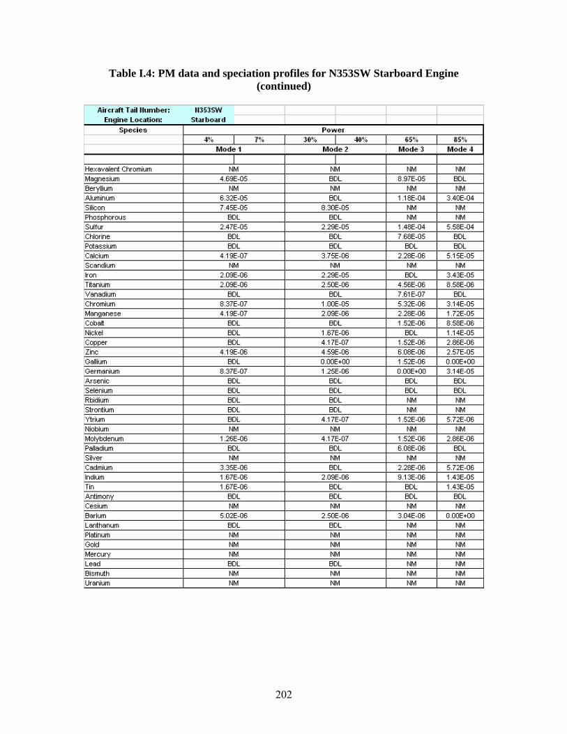
Aircraft Tail ttumber: 113S3SW I I Engine Location: Starboard I I

S1>ecies Power 4% I 7% 30% I 40% 65% 85%

Mode1 Mode2 Mode 3 Mode4 I I

Hexavalent Chromium NM NM NM NM Magnesium 4.69E-05 BDL 8.97E-05 BDL Beryllium NM NM NM NM Aluminum 6.32E-05 BDL 1.18E-04 3.40E-04 Silicon 7.45E-05 8.30E-05 NM NM Phosphorous BDL BDL NM NM Sulfur 2.47E-05 2.29E-05 1.48E-04 5.58E-04 Chlorine BDL BDL 7.68E-05 BDL Potassium BDL BDL BDL BDL Calcium 4.19E-07 3.75E-06 2.28E-06 5.15E-05 Scandium NM NM NM NM Iron 2.0SE-06 2.29E-05 BDL 3.43E-05 Titanium 2.0SE-06 2.S0E-06 4.SSE-06 8.58E-06 Vanadium BDL BDL 7.61E-07 BDL Chromium 8.37E-07 1.00E-05 5.32E-06 3.14E-05 Manganese 4.19E-07 2.0SE-06 2.28E-06 1.72E-05 Cobalt BDL BDL 1.52E-06 8.58E-06 Nickel BDL 1.67E-06 BDL 1.14E-05 Copper BDL 4.17E-07 1.52E-06 2.86E-06 Zinc 4.19E-06 4.59E-06 6.0SE-06 2.57E-05 Gallium BDL 0.00E•00 1.52E-06 0.00E•00 Germanium 8.37E-07 1.25E-06 0.00E•00 3.14E-05 Arsenic BDL BDL BDL BDL Selenium BDL BDL BDL BDL Rbidium BDL BDL NM NM strontium BDL BDL NM NM Ytrium BDL 4.17E-07 1.52E-06 5.72E-06 Niobium NM NM NM NM Molybdenum 1.26E-06 4.17E-07 1.52E-06 2.86E-06 Palladium BDL BDL 6.0SE-06 BDL Silver NM NM NM NM Cadmium 3.35E-06 BDL 2.28E-06 5.72E-06 Indium 1.67E-06 2.0SE-06 9.13E-06 1.43E-05 Tin 1.67E-06 BDL BDL 1.43E-05 Antimony BDL BDL BDL BDL Cesium NM NM NM NM Barium 5.02E-06 2.S0E-06 3.04E-06 0.00E•00 Lanthanum BDL BDL NM NM Platinum NM NM NM NM Gold NM NM NM NM Mercury NM NM NM NM Lead BDL BDL NM NM Bismuth NM NM NM NM Uranium NM NM NM NM

Table I.4: PM data and speciation profiles for N353SW Starboard Engine (continued)

202

Aircraft Tail ttumber: 113S3SW I Engine Location: Starboard I

Category S1>ecies Grou1> UCR ARI UMR

CAS LOD Method llon-HC

Combustion Gase s NO 10102-43-9 Chemiluminescence X N02 10102-44-0 TILDAS X NOX X HN03 7697-37-2 HONO 7782-77-6 N20 10024-97-2 co 630-08-0 TILDAS X CO2 124-38-9 X S02 7446-09-5 SOX

Inorganic ions Sulfale 14808-79-8 X Nltrale 7697-37-2

NM - no measurement was made BDL - Below deleclion limlt I El for CO2 determined by elemental analysis of fuel

Uotes: UCR comn\ents: In the original text LOOs were provided for all compounds and species measured on the high-flow side. LOOs were not provided for C I to C 1z compounds where we know there are sampling issues. These issues were fully discussed in the test. Analytical uncertainties are different and will not reflect the sampling uncertainty.

I I UCR only made one measurement so uncertainty cannot be calculated. I Analytical uncertainty for all measurement methods was provided in the original text.

Table I.4: PM data and speciation profiles for N353SW Starboard Engine (continued)

203

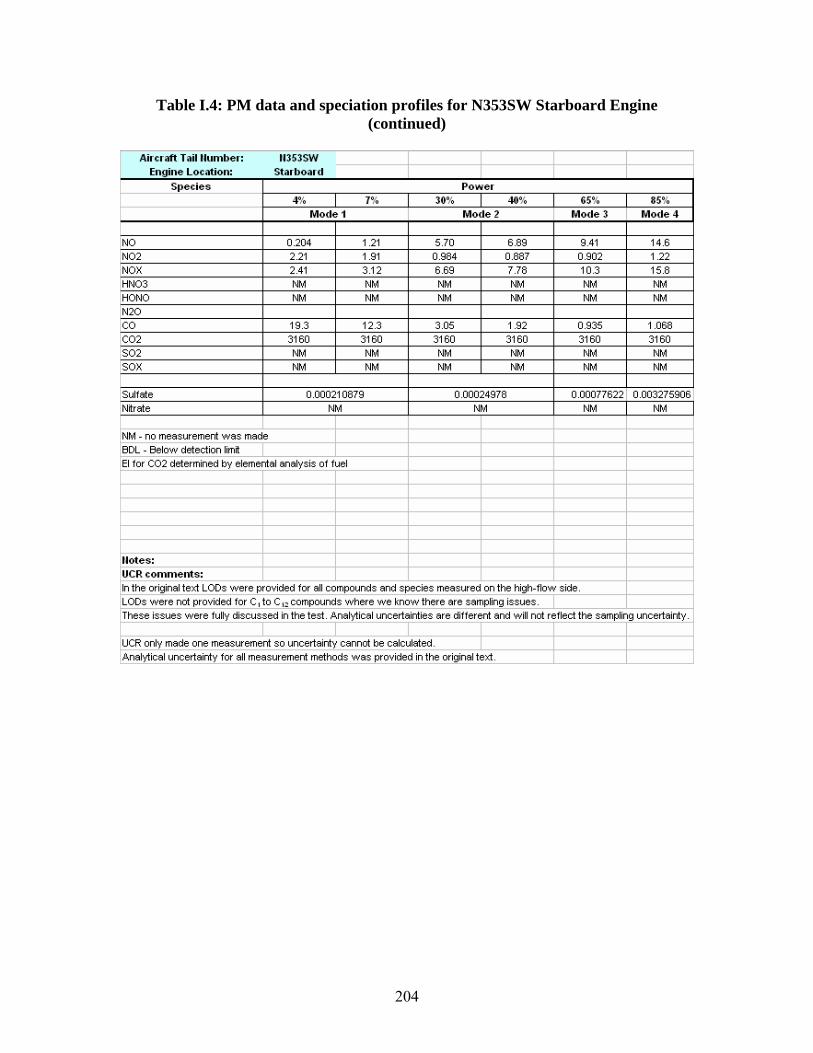
Aircraft Tail ttumber: 113S3SW I I Engine Location: St arboard I I

S1>ecies Power 4% I 7% 30% I 40% 65% 85%

Mode 1 Mode 2 Mode 3 Mode 4

NO 0.204 1.21 5.70 6.89 9.41 14.6 N02 2.21 1.91 0.984 0.887 0.902 1.22 NOX 2.41 3.12 6.69 7.78 10.3 15.8 HN03 NM NM NM NM NM NM HONO NM NM NM NM NM NM N20 co 19.3 12.3 3.05 1.92 0.935 1.068 CO2 3160 3160 3160 3160 3160 3160 S02 NM NM NM NM NM NM SOX NM NM NM NM NM NM

Sulfate 0.000210879 0.00024978 0.00077622 0.003275906 I Nitrate NM NM NM NM

NM - no measurement was made BOL - Below detection limit El for CO2 determined by elemental analysis of fuel

llotes: UCR comments: In the original text LOOs were provided for all compounds and species measured on the high-flow side. LOOs were not provided for C I to C 12 compounds where we know there are sampling issues. These issues were fully discussed in the test. Analytical uncertainties are different and will not reflect the sampling uncertainty.

I I UCR only made one measurement so uncertainty cannot be calculated. I Analytical uncertainty for all measurement methods was provided in the original text.

Table I.4: PM data and speciation profiles for N353SW Starboard Engine (continued)

204

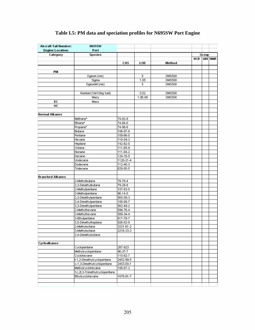
Aircraft Tail ttumber: 1169SSW I Engine Location: Port I

Category S1>ecies Grou1> UCR ARI UMR

CAS LOD Method

PM Dgeom (nm) 5 DMS500

Sigma 1.05 DMS500 DgeomM (nm) 5 DMS500

Number(10e1511(g fuel) 0.02 DMS500 Mass 1.0E-06 DMS500

EC Mass oc

Uormal Alkanes Methane• 74-82-8 Ethane• 74-84-0 Propane• 74-98-6 Butane 106-97-8 Pentane 109-66-0 Hexane 110-54-3 Heplane 142-82-5 Octane 111-65-9 Nonane 111-84-2 Decane 124-18-5 Undecane 1120-21-4 Dodecane 112-40-3 Tridecane 629-50-5

Branched Alkanes 2-Melhylbutane 78-78-4 2,3-Dimelhylbutane 79-29-8 2-Melhylpentane 107-83-5 3-Melhylpentane 96-14-0 2,3-Dimelhylpentane 565-59-3 2,4-Dimelhylpentane 108-08-7 3,3-Dimelhylpentane 562-49-2 2-Melhylhexane 598-76-4 3-Melhylhexane 589-34-4 3-Elhylpentane 617-78-7 3,5-Dimelhylheplane 926-82-9 2-Melhyloclane 3221-61-2 3-Melhyloclane 2216-33-3 2,4-Dimelhyloclane

Cycloallrnnes Cyclopentane 287-923 Methylcyclopentane 96-37-7 Cyclohexane 110-82-7 t-1,2-Dimelhylcyclopentane 2452-99-5 c-1 ,3-Dimelhylcyclopentane 2453-00-1 Methylcyclohexane 108-87-2 1 c,21,3-Trimelhylcyclopentane Ethylcyclohexane 1678-91-7

I

Table I.5: PM data and speciation profiles for N695SW Port Engine

205

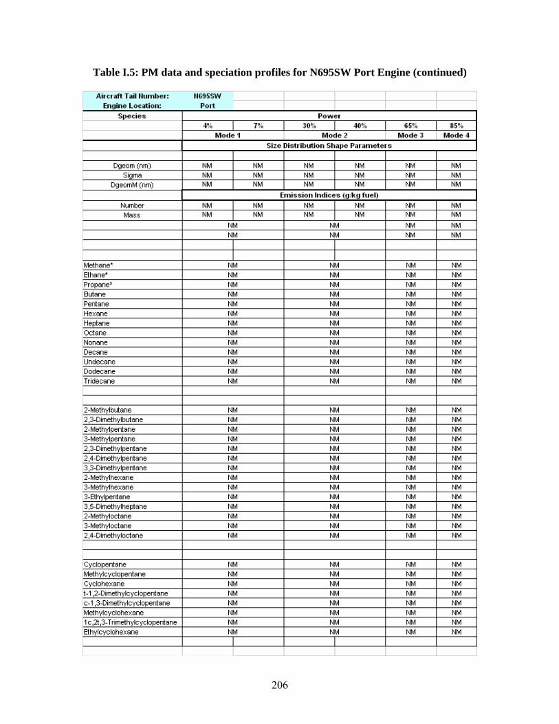
Aircraft Tail ttumber: 1169SSW I I Engine Location: Port I I

S1>ecies Power 4% 7% 30% I 40% 65% I 85%

Mode1 Model Mode 3 I Mode4 Size Distribution ShaJ>e Parameters

I Dgeom (nm) NM NM NM NM NM NM

Sigma NM NM NM NM NM NM DgeomM (nm) NM NM NM NM NM NM

Emission Indices {gll<g fuel) Number NM NM NM I NM NM NM Mass NM NM NM NM NM NM

NM NM NM NM NM NM NM NM

Methane* NM NM NM NM Ethane* NM NM NM NM Propane* NM NM NM NM Butane NM NM NM NM Pentane NM NM NM NM Hexane NM NM NM NM Heptane NM NM NM NM Octane NM NM NM NM Nonane NM NM NM NM Decane NM NM NM NM Undecane NM NM NM NM Dodecane NM NM NM NM Tridecane NM NM NM NM

2-Melhylbutane NM NM NM NM 2,3-Dimethylbutane NM NM NM NM 2-Methylpentane NM NM NM NM 3-Methylpentane NM NM NM NM 2,3-Dimethylpentane NM NM NM NM 2,4-Dimethylpentane NM NM NM NM 3,3-Dimethylpentane NM NM NM NM 2-Methylhexane NM NM NM NM 3-Methylhexane NM NM NM NM 3-Ethylpentane NM NM NM NM 3,5-Dimethylheptane NM NM NM NM 2-Methyloctane NM NM NM NM 3-Methyloctane NM NM NM NM 2,4-Dimethyloctane NM NM NM NM

Cvclooentane NM NM NM NM Methylcyclopentane NM NM NM NM Cyclohexane NM NM NM NM 1-1,2-Dimethylcyclopentane NM NM NM NM c-1 ,3-Dimethylcyclopentane NM NM NM NM Methylcyclohexane NM NM NM NM 1 c,21,3-Trimethylcyclopentane NM NM NM NM Ethylcyclohexane NM NM NM NM

I I

Table I.5: PM data and speciation profiles for N695SW Port Engine (continued)

206

Aircraft Tail ttumber: 1169SSW I Engine Location: Port I

Category S1>ecies Grou1> UCR ARI UMR

CAS LOD Method Alkene s

Ethene* 74-85-1 TILDAS X Propene* 115-07-1 1-Butene 106-98-9 c-2-Butene 1-2-Butene 2-Melhylpropene 115-11-7 Pentene 25377-72-4 1-Hexene 592-41-6 3-Melhyl-c-2-Penlene 3-Melhyl-1-2-Penlene 4-Melhyl-c-2-Penlene 4-Melhyl-1-2-Penlene 1-Nonene 124-11-8 Propadiene 463-49-0 1 ,3-Butadiene 106-99-0 2-Melhyl-1,3-Butadiene 78-79-5 Cyclopentadiene 542-92-7 Cyclohexene 110-83-8

Alkynes Ethyne* 74-86-2

Aromatic Hydrocarbons Benzene 71-43-2 PTR-MS X Toluene 108-88-3 PTR-MS X Ethylbenzene 100-41-4 o-Xylene 95-47-6 m&p-Xylene 63-68-3 1-Melhyl-2-elhylbenzene 611-14-3 1-Melhyl-3-elhylbenzene 620-14-4 1-Melhyl-4-elhylbenzene 622-96-8 1,4-Dimelhyl-2-elhylbenzene 1758-88-9 1,2,3-Trimethylbenzene 526-73-8 1,2,4-Trimethylbenzene 95-63-6 1,3,5-Trimethylbenzene 95-63-6 lndan 496-11-7 1,2-Dielhylbenzene 135-01-3 1 ,3-Dielhylbenzene 141-93-5 1,4-Dielhylbenzene 105-05-5 1-Melhyl-2-n-Propylbenzene 1-Melhyl-3-n-Propylbenzene 1-Melhyl-4-n-Propylbenzene 1-Melhyl-2-i-Propylbenzene 1-Melhyl-3-i-Propylbenzene 1 ,2,4 ,5-T elramelhylbenzene 95-93-2 n-Pent-Benzene styrene 100-42-5 PTR-MS X

Table I.5: PM data and speciation profiles for N695SW Port Engine (continued)

207

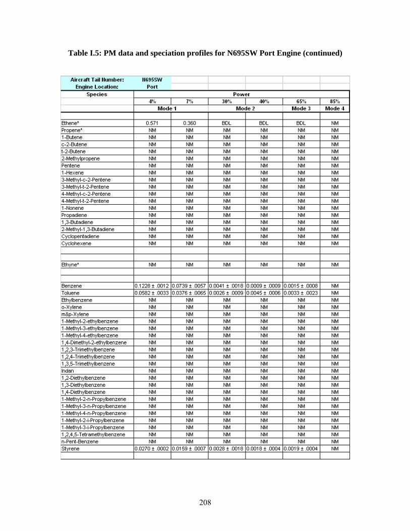
Aircraft Tail ttumber: 1169SSW I I Engine Location: Port I I

S1>ede<J: Pow er

4% 7°/o 30% I 40% 65% 85% Mode1 I Mode2 I Mode 3 Mode 4

Ethene• 0.571 0.360 BDL BDL BDL NM Propene• NM NM NM NM NM NM 1-Butene NM NM NM NM NM NM c-2-Butene NM NM NM NM NM NM 1-2-Butene NM NM NM NM NM NM 2-Methylpropene NM NM NM NM NM NM Pentene NM NM NM NM NM NM 1-Hexene NM NM NM NM NM NM 3-Methyl-c-2-Pentene NM NM NM NM NM NM 3-Methyl-1-2-Pentene NM NM NM NM NM NM 4-Methyl-c-2-Pentene NM NM NM NM NM NM 4-Methyl-1-2-Pentene NM NM NM NM NM NM 1-Nonene NM NM NM NM NM NM Propadiene NM NM NM NM NM NM 1 ,3-Butadiene NM NM NM NM NM NM 2-Mcthyl-1 ,3-Butadicnc NM NM NM NM NM NM Cyclopentadiene NM NM NM NM NM NM Cyclohexene NM NM NM NM NM NM

Ethyne• NM NM NM NM NM NM

Benzene 0.1228 ! .0012 0.0739 ! 0057 0.0041 ! .0018 0.0009! .0009 0.0015 ! .0008 NM Toluene 0.0582 ! .0033 0.0376 ! 0065 0.0026! .0009 0.0045! .0006 0.0033 ! .0023 NM Ethylbenzene NM NM NM NM NM NM o-Xylene NM NM NM NM NM NM m&p-Xylene NM NM NM NM NM NM 1-Methyl-2-elhylbenzene NM NM NM NM NM NM 1-Methyl-3-ethylbenzene NM NM NM NM NM NM 1-Methyl-4-elhylbenzene NM NM NM NM NM NM 1,4-Dimethyl-2-elhylbenzene NM NM NM NM NM NM 1,2,3-Trimethylbenzene NM NM NM NM NM NM 1,2,4-Trimethylbenzene NM NM NM NM NM NM 1 ,3,~-Trimethylbenzene NM NM NM NM NM NM lndan NM NM NM NM NM NM 1,2-Diethylbenzene NM NM NM NM NM NM 1 ,3-Diethylbenzene NM NM NM NM NM NM 1,4-Diethylbenzene NM NM NM NM NM NM 1-Methyl-2-n-Propylbenzene NM NM NM NM NM NM 1-Methyl-3-n-Propylbenzene NM NM NM NM NM NM 1-Methyl-4-n-Propylbenzene NM NM NM NM NM NM 1-Methyl-2-i-Propylbenzene NM NM NM NM NM NM 1-Methyl-3-i-Propylbenzene NM NM NM NM NM NM 1 ,2,4 ,5-T etramethylbenzene NM NM NM NM NM NM n-Pent-Benzene NM NM NM NM NM NM styrene 0.0270 ! .0002 0.0159 ! 0007 0.0028 ! .0018 0.0018 ! .0004 0.0019 ! .0004 NM

Table I.5: PM data and speciation profiles for N695SW Port Engine (continued)

208

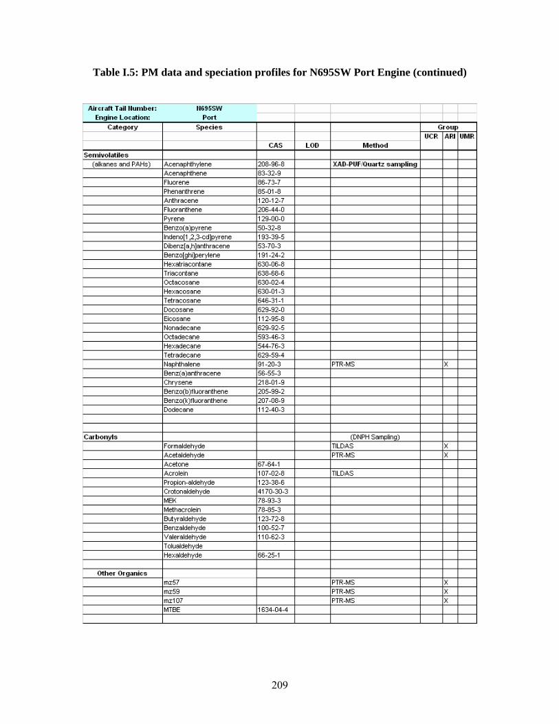
Aircraft Tail ttumber: 1169SSW I Engine Location: Port I

Category S1>ecies Grou1> UCR ARI UMR

CAS LOD Method Semivo-latiles

(alkanes and PAHs) Acenaphthylene 208-96-8 XAD-PUF/Quartz SolO'\J)ling Acenaphthene 83-32-9 Fluorene 86-73-7 Phenanthrene 85-01-8 Anthracene 120-12-7 Fluoranthene 206-44-0 Pyrene 129-00-0 Benzo(a)pyrene 50-32-8 lndeno[1,2,3-cd)pyrene 193-39-5 Dibenz[a,h]anthracene 53-70-3 Benzo[ghi)perylene 191-24-2 Hexatriacontane 630-06-8 Triacontane 638-68-6 Octacosane 630-02-4 Hexacosane 630-01-3 T etracosane 646-31-1 Docosane 629-92-0 Eicosane 112-95-8 Nonadecane 629-92-5 Octadecane 593-46-3 Hexadecane 544-76-3 T etradecane 629-59-4 Naphlhalene 91-20-3 PTR-MS X Benz( a)anthracene 56-55-3 Chrysene 218-01-9 Benzo(b )fluoranthene 205-99-2 Benzo(k )fluoranthene 207-08-9 Dodecane 112-40-3

Carbonyls (DNPH Sampling) Formaldehyde TILDAS X Acelaldehyde PTR-MS X Acetone 67-64-1 Acrolein 107-02-8 TILDAS Propion-aldehyde 123-38-6 Crolonaldehyde 4170-30-3 MEK 78-93-3 Methacrolein 78-85-3 Bui yr aldehyde 123-72-8 Benz aldehyde 100-52-7 Valeraldehyde 110-62-3 T olualdehyde Hex aldehyde 66-25-1

Other Organics mz57 PTR-MS X mz59 PTR-MS X mz107 PTR-MS X MTBE 1634-04-4

Table I.5: PM data and speciation profiles for N695SW Port Engine (continued)

209

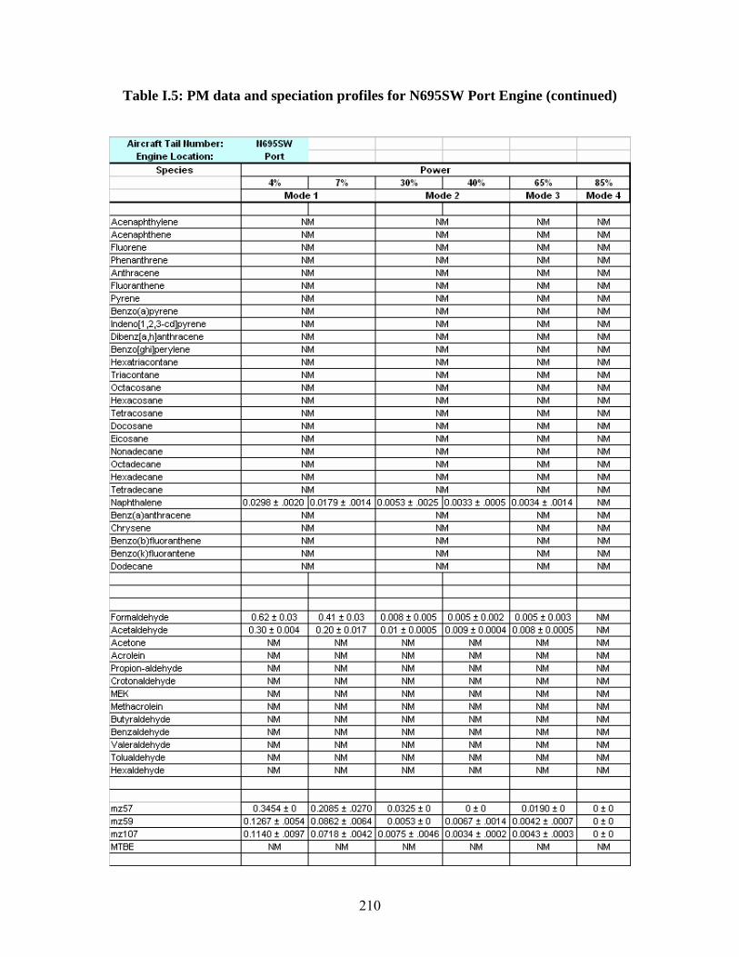
Aircraft Tail ttumber: 1169SSW I I Engine Location: Port I I

S1>e cie c Pow er

4% 7°/o 30% I 40% 65% 85% Mode 1 I Mode 2 I Mode 3 Mode 4

I Acenaphthylene NM NM NM NM Acenaphthene NM NM NM NM Fluorene NM NM NM NM Phenanthrene NM NM NM NM Anthracene NM NM NM NM Fluoranthene NM NM NM NM Pyrene NM NM NM NM Benzo(a)pyrene NM NM NM NM lndeno[1,2,3-cd)pyrene NM NM NM NM Dibenz[a,h]anthracene NM NM NM NM Benzo[ghi)perylene NM NM NM NM Hexatriacontane NM NM NM NM Triacontane NM NM NM NM Octacosane NM NM NM NM Hexacosane NM NM NM NM T etracosane NM NM NM NM Docosane NM NM NM NM Eicosane NM NM NM NM Nonadecane NM NM NM NM Octadecane NM NM NM NM Hexadecane NM NM NM NM T etradecane NM NM NM NM Naphthalene 0.0298 ± .0020 0.0179 ± 0014 0.0053 ± .0025 10.0033 ± .0005 0.0034 ± .0014 NM Benz( a)anthracene NM NM NM NM Chrysene NM NM NM NM Benzo(b )fluoranthene NM NM NM NM Benzo(k)fluorantene NM NM NM NM Dodecane NM NM NM NM

Formaldehyde 0.62 ± 0.03 0.41 ± 0.03 0.008±0.005 0.005±0.002 0.005±0.003 NM Acelaldehyde 0.30 ± 0.004 0.20 ± 0.017 O.Q1 ±0.0005 0.009±0.0004 0.008 ± 0.0005 NM Acetone NM NM NM NM NM NM Acrolein NM NM NM NM NM NM Propion-aldehyde NM NM NM NM NM NM Crotonaldehyde NM NM NM NM NM NM MEK NM NM NM NM NM NM Methacrolein NM NM NM NM NM NM Butyraldehyde NM NM NM NM NM NM Benz aldehyde NM NM NM NM NM NM Valeraldehyde NM NM NM NM NM NM T olualdehyde NM NM NM NM NM NM Hex aldehyde NM NM NM NM NM NM

mz57 0.3454 ± 0 0.2085 ± .0270 0.0325 ± 0 O:!:O 0.0190 ± 0 0 :!: 0 mz59 0.1267 ± .0054 0.0862 ± .0064 0.0053 ± 0 0.0067 ± .0014 0.0042 ± .0007 O:!:O mz107 0.1140 ± .0097 0.0718 ± .0042 0.0075 ± .0046 0.0034 ± .0002 0.0043 ± .0003 0 :!: 0 MTBE NM NM NM NM NM NM

Table I.5: PM data and speciation profiles for N695SW Port Engine (continued)

210

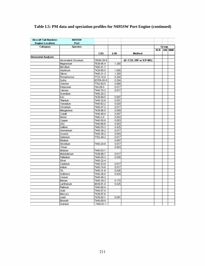
Aircraft Tail ttumber: 1169SSW I Engine Location: Port I

Category S1>ecies Grou1> UCR ARI UMR

CAS LOD Method

Eleme1\tal Analysis Hexavalent Chromium 18540-29-9 (IC-CCD, XRF or ICP-MS) Magnesium 7639-95-4 1.200 Beryllium 7440-41-7 Aluminum 7429-90-5 1.000 Silicon 7440-21-3 1.200 Phosphorous 7723-14-0 0.204 Sulfur 63705-05-5 0.204 Chlorine 7782-50-5 0.068 Potassium 744-09-5 0.017 Calcium 7440-70-2 0.017 Scandium 7440-20-2 Iron 7439-89-5 0.007 Titanium 7440-32-6 0.051 Vanadium 7440-62-2 0.020 Chromium 7440-47-3 0.017 Manganese 7439-96-5 0.009 Cobalt 7440-48-4 0.007 Nickel 7440-2-0 0.003 Copper 7440-50-8 0.003 Zinc 7440-66-6 0.003 Gallium 7440-55-3 0.425 Germanium 7440-38-2 0.017 Arsenic 7440-38-2 0.003 Selenium 7782-49-2 0.017 Rbidium 0.007 strontium 7440-24-6 0.017 Ytrium 0.003 Niobium 7440-03-1 Molybdenum 7439-98-7 0.017 Palladium 7440-05-3 0.Q26 Silver 7440-22-4 Cadmium 7440-43-9 0.017 Indium 7440-74-6 0.017 Tin 7440-31-6 0.Q26 Antimony 7440-36-0 0.024 Cesium 7440-46-2 Barium 7440-39-3 0.170 Lanthanum 4639-91-0 0.425 Platinum 7440-06-4 Gold 7440-57-5 Mercury 7439-97-6 Lead 7439-92-1 0.051 Bismuth 7440-69-9 Uranium 7440-61-1

Table I.5: PM data and speciation profiles for N695SW Port Engine (continued)

211

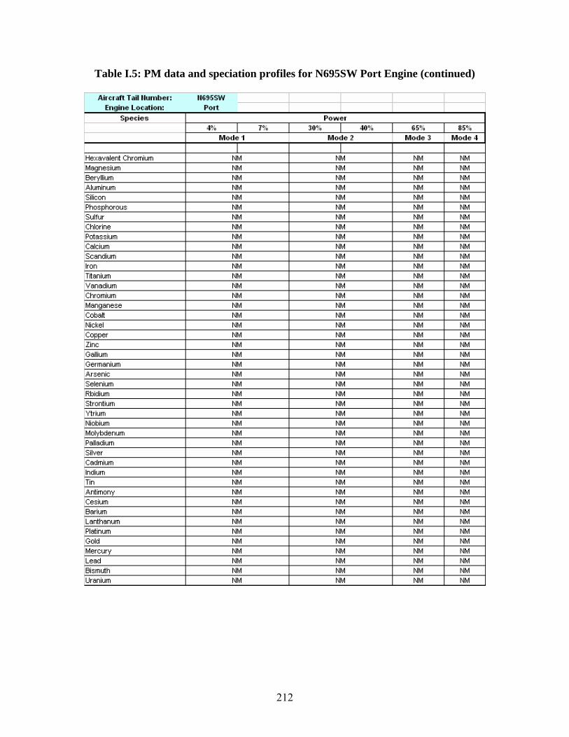
Aircraft Tail ttumber: 1169SSW I I Engine Location: Port I I

S1>ecies Power 4% I 7% 30% I 40% 65% I 85%

Mode1 I Mode l I Mode 3 I Mode4 I I

Hexavalent Chromium NM NM NM NM Magnesium NM NM NM NM Beryllium NM NM NM NM Aluminum NM NM NM NM Silicon NM NM NM NM 1-'hosphorous NM NM NM NM Sulfur NM NM NM NM Chlorine NM NM NM NM Potassium NM NM NM NM Calcium NM NM NM NM Scandium NM NM NM NM Iron NM NM NM NM Titanium NM NM NM NM Vanadium NM NM NM NM Chromium NM NM NM NM Manganese NM NM NM NM Cobalt NM NM NM NM Nickel NM NM NM NM Copper NM NM NM NM Zinc NM NM NM NM Gallium NM NM NM NM Germanium NM NM NM NM Arsenic NM NM NM NM Selenium NM NM NM NM Rbidium NM NM NM NM strontium NM NM NM NM Ytrium NM NM NM NM Niobium NM NM NM NM Molybdenum NM NM NM NM Palladium NM NM NM NM Silver NM NM NM NM Cadmium NM NM NM NM Indium NM NM NM NM Tin NM NM NM NM Antimony NM NM NM NM Cesium NM NM NM NM Barium NM NM NM NM Lanthanum NM NM NM NM Platinum NM NM NM NM Gold NM NM NM NM Mercury NM NM NM NM Lead NM NM NM NM Bismuth NM NM NM NM Uranium NM NM NM NM

Table I.5: PM data and speciation profiles for N695SW Port Engine (continued)

212

Aircraft Tail ttumber: 1169SSW I Engine Loc ation: Port I

Category S1>ecie s Grou1> UCR ARI UMR

CAS LOD Method

llon-HC Comlmstion Gase s NO 10102-43-9 Chemiluminescence X

N02 10102-44-0 TILDAS X NOX X HN03 7697-37-2 HONO 7782-77-6 N20 10024-97-2

co 630-08-0 TILDAS X CO2 124-38-9 X S02 7446-09-5

SOX

Inorganic ions Sulfole 14808-79-8 Nltrole 7697-37-2

NM - no measurement was made BOL - Below detection limit El for CO2 determined by elemental analysis of fuel

llote s: UCR con\ments: In the original text LOOs were provided for all compounds and species measured on the high-flow side.

LOOs were not provided for C I to C 1z compounds where we know there are sampling issues. These issues were fully discussed in the test. Analytical uncertainties are different and will not reflect the sampling uncertainty.

I UCR only made one measurement so uncertainty cannot be calculated. I

Analytical uncertainty for all measurement methods was provided in the original text.

Table I.5: PM data and speciation profiles for N695SW Port Engine (continued)

213

Aircraft Tail ttumber: 1169SSW I I Engine Location: Port I I

S1>ecies Power 4% 7% 30% I 40% 65% I 85%

Mode 1 I Mode l I Mode 3 I Mode 4

NO 0.23 0.6~ 5.54 7.22 10.2 NM NO2 2.30 2.21 0.979 0.905 0.999 NM NOX 2.53 2.9( 6.52 8.12 11.2 NM HNO3 NM NM NM NM NM NM HONO NM NM NM NM NM NM N20 l~M l~M l~M l~M l~M l~M co 19.6 16.E 3.26 1.80 1.04 NM CO2 3160 3160 3160 3160 3160 3160 SO2 NM NM NM NM NM NM SOX NM NM NM NM NM NM

Sulfate NM NM NM NM NM NM Nitrate NM NM NM NM NM NM

NM - no measurement was made BOL - Below detection limit I El for CO2 determined by elemental analysis of fuel

llotes: UCR -ton\n\E-nt<J:: In the original text LOOs were provided for all compounds ,nd species measured on the high-flow side. LOOs were not provided for C I to C 1z compounds where we know there are sampling issues. These issues were fully discussed in the test. Analytical 1..ncertainties are different and will not reflect the sampling 1..ncertaint'y

I I UCR only made one measurement so uncertainty cannot be calculated. I Analytical uncertainty for all measurement methods was p·ovided in the original text.

Table I.5: PM data and speciation profiles for N695SW Port Engine (continued)

214

Aircraft Tail ttumber: 11695SW I Engine Location: Starboard I

Category S1>ecie s Grou1> UCR ARI UMR

CAS LOD Method

PM Dgeom (nm) 5 DMS500 X

Sigma 1.05 DMS500 X DgeomM (nm) 5 DMS500 X

Number(10e151kg fuel) 0.02 DMS500 X Mass 1.0E-06 DMS500 X Mass DMS500 X

EC X oc X

Uormal Alkanes Mett-ane• 74-82-8 Etha1e* 74-84-0 Propane• 74-98-6 Bul..,e 106-97-8 Penbne 109-66-0 Hexane 110-54-3 Heptane 142-82-5 Octane 111-65-9 Nonane 111-84-2 Decane 124-18-5 Undecane 1120-21-4 Dodecane 112-40-3 Tridecane 629-50-5

Branched Alkanes 2-Melhylbulane 78-78-4 2,3-0imelhylbulane 79-29-8 ?-MP.thylpP.nti:mP. 1n7-A~-~

3-Melhylpenlane 96-14-0 2,3-0imelhylpenlane 565-59-3 2,4-0imelhylpenlane 108-08-7 3,3-0imelhylpenlane 562-49-2 2-Melhylhexane 598-76-4 3-Melhylhexane 589-34-4 3-Elhylpenlane 617-78-7 3,5-0imelhylheplane 926-82-9 2-Melhyloclane 3221-61-2 3-Melhyloclane 2216-33-3 2,4-0imelhyloclane

Cycloalkanes Cycbpentane 287-923 Meltylcyclopenlane 96-37-7 Cycbhexane 110-82-7 1-1,2-Dimelhylcyclopenlane 2452-99-5 c-1 ,3-Dimelhylcyclopenlane 2453-00-1 Meltylcyclohexane 108-87-2 1 c ,2: ,3-T rimelhylcyclopenlane Ethycyclohexane 1678-91-7

Table I.6: PM data and speciation profiles for N695SW Starboard Engine

215

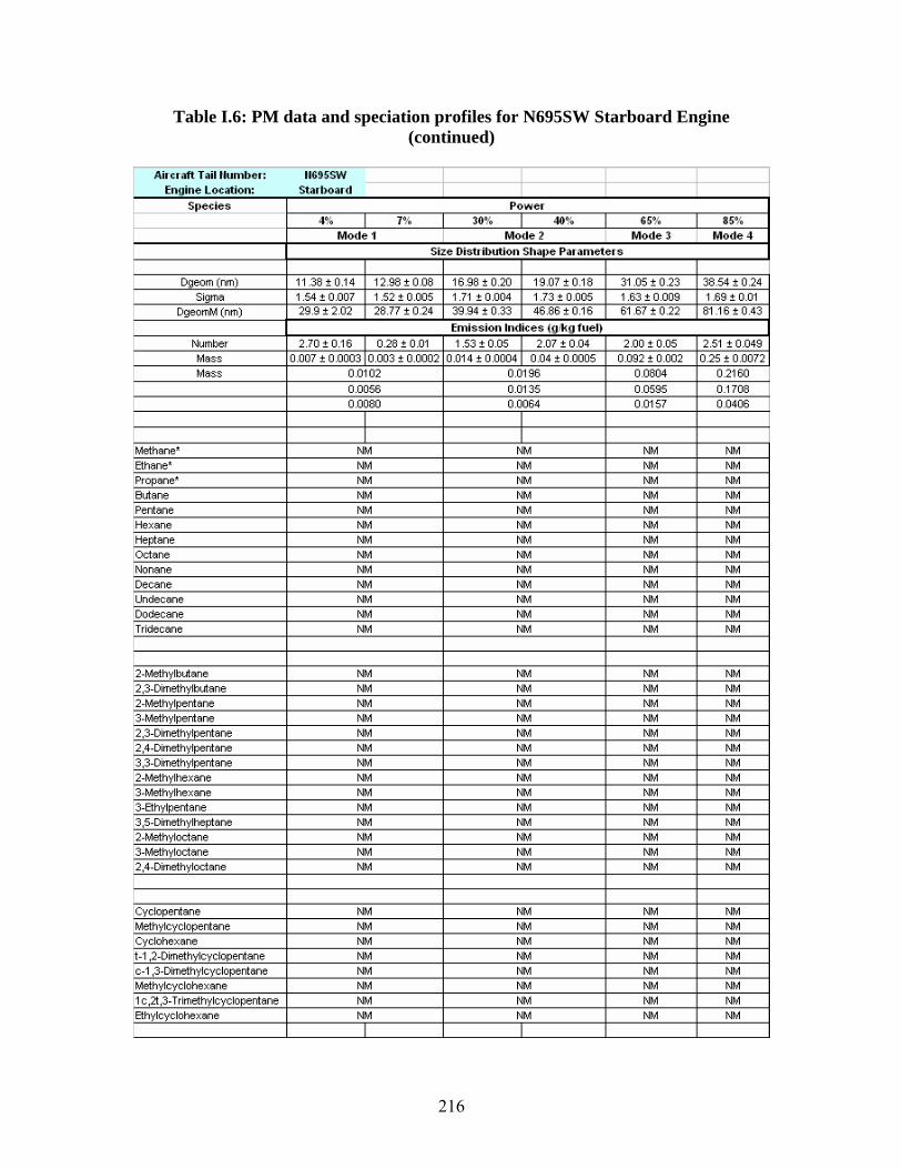
Airerilft Tilil ltombcr: .,,,ssw I I I Engine Location: Starboard I I I

S1>et ies Power 4% 7°/o I 30% 40% I 65% I 85%

Mode 1 I Mode 2 I Mode 3 I Mode 4 Size Distribution Sha1>e Parameters

I Dgeom (nm) 11.38 • 0.14 12.98 • 0.08 16.98 • 0.20 19.07 • 0.18 31.05 • 0.23 38.54 • 0.24

Sigma 1.54 t 0.007 1.52 t 0.005 1.71 t 0.004 1.73 t 0.005 1.63 t 0.009 1.69 t 0.01 DgeomM (nm) 29.9 t 2.02 28.77 t 0.24 39.94 t 0.33 46.86 t 0.16 61.67 t 0.22 81.16 t 0.43

Emission Indite s {gll<g fuel)

Number 2.70 • 0.16 0.28 • 0.01 1.53 • 0.05 2.07 • 0.04 2.00 • 0.05 2.51 • 0.049 Mass C.007 t 0.0003 0.003 t 0.0002 0.014 t 0.0004 0.04 t 0.0005 0.092 t 0.002 0.25 t 0.0072 Mass 0.0102 0.0196 0.0804 0.2160

0.0056 0.0135 0.0595 0.1708 0.0080 0.0064 0.0157 0.0406

Methane• NM NM NM NM Ethane• NM NM NM NM Propane• NM NM NM NM Butane NM NM NM NM Pentane NM NM NM NM Hexane NM NM NM NM Heptane NM NM NM NM octane l~M l~M l~M l~M Nonane NM NM NM NM Decane NM NM NM NM Undecane NM NM NM NM Dodecane NM NM NM NM Tridecane NM NM NM NM

2-Melhylbutane NM NM NM NM 2,3-Dimethylbutane NM NM NM NM 2-Methylpentane NM NM NM NM 3-Methylpentane NM NM NM NM 2,3-Dimethylpentane NM NM NM NM 2,4-Dimethylpentane NM NM NM NM 3,3-Dimethylpentane NM NM NM NM 2-Methylhexane NM NM NM NM 3-Methylhexane NM NM NM NM 3-Ethylpentane NM NM NM NM 3,5-Dimethylheptane NM NM NM NM 2-Methyloctane NM NM NM NM 3-Methyloctane NM NM NM NM 2,4-Dimethyloctane NM NM NM NM

Cyclopentane NM NM NM NM MP.thylr.yr.lnpP.nti:mP. NM NM NM NM Cyclohexane NM NM NM NM t-1,2-Dimethylcyclopentane NM NM NM NM c-1 ,3-Dimethylcyclopentane NM NM NM NM Methylcyclohexane NM NM NM NM 1 c,21,3-Trimethylcyclopentane NM NM NM NM Ethylcyclohexane NM NM NM NM

Table I.6: PM data and speciation profiles for N695SW Starboard Engine (continued)

216

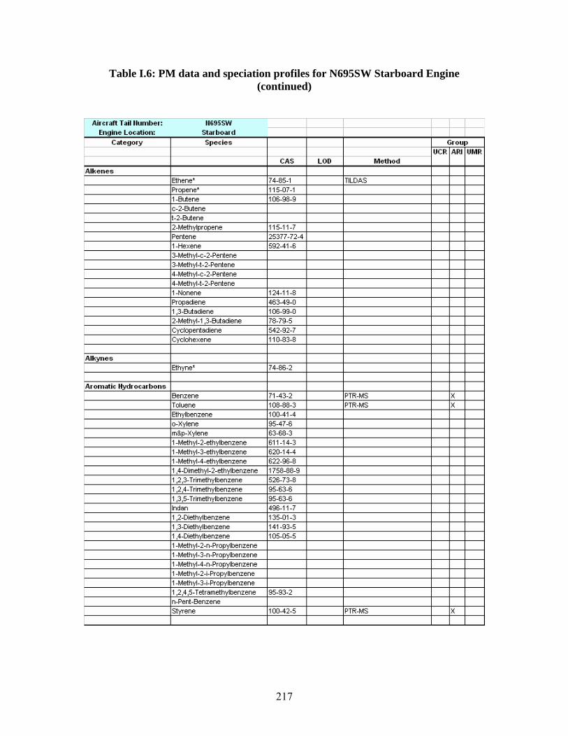
Aircraft Tail ttumber: 11695SW I Engine Location: Starboard I

Category S1>ecie s Grou1> UCR ARI UMR

CAS LOD Method

Alkenes Ethe1e* 74-85-1 TILDAS Proi:ene* 115-07-1 1-81..tene 106-98-9 c-2-Butene 1-2-Bulene 2-Melhylpropene 115-11-7 Pentene 25377-72-4 1-HtX.tillti 592-41-6

3-Melhyl-c-2-Penlene 3-Melhyl-1-2-Penlene 4-Melhyl-c-2-Penlene 4-Melhyl-1-2-Penlene 1-Ncnene 124-11-8 Propadiene 463-49-0 1 ,3-Butadiene 106-99-0 2-Melhyl-1,3-Buladiene 78-79-5 Cycbpentadiene 542-92-7 Cycbhexene 110-83-8

Alkynes Ethy1e* 74-86-2

Aromatic Hydrocarbons

Ben:ene 71-43-2 PTR-MS X Toluene 108-88-3 PTR-MS X Ethybenzene 100-41-4 o-X'ylene 95-47-6 m&p-Xylene 63-68-3 1-Melhyl-2-elhylbenzene 611-14-3 1-Melhyl-3-elhylbenzene 620-14-4 1-Melhyl-4-elhylbenzene 622-96-8 1,4-0imelhyl-2-elhylbenzene 1758-88-9 1,2,3-Trimethylbenzene 526-73-8 1,2,L-Trimethylbenzene 95-63-6 1,3,5-Trimethylbenzene 95-63-6 lndan 496-11-7 1,2-0ielhylbenzene 135-01-3 1 ,3-0ielhylbenzene 141-93-5 1,4-0ielhylbenzene 105-05-5 1-Melhyl-2-n-Propylbenzene 1-Melhyl-3-n-Propylbenzene 1-Melhyl-4-n-Propylbenzene 1-Melhyl-2-i-Propylbenzene 1-Melhyl-3-i-Propylbenzene 1 ,2,L ,5-T etramethylbenzene 95-93-2 n-Pent-Benzene styrene 100-42-5 PTR-MS X

Table I.6: PM data and speciation profiles for N695SW Starboard Engine (continued)

217

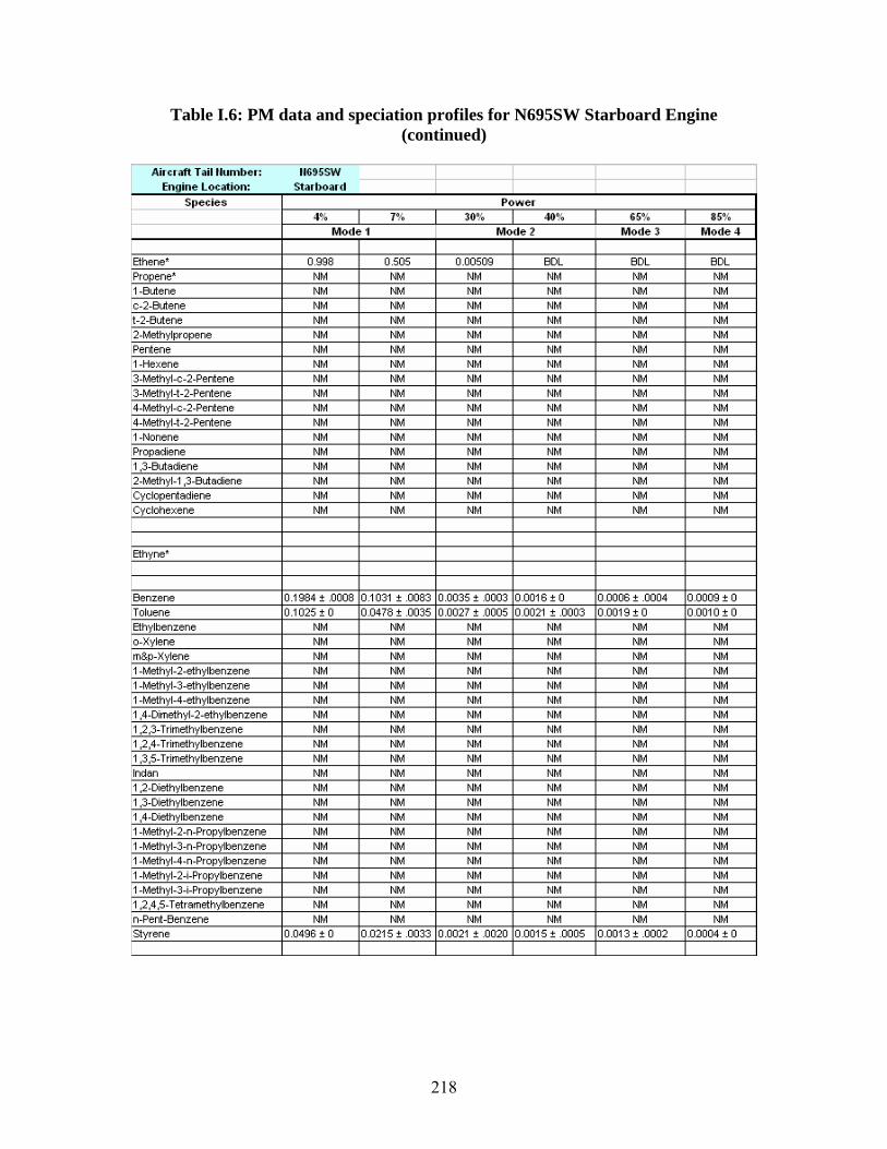
Airerilft Tilil ltombcr: .,,,ssw I I I Engine Location: Starboard I I I

S1>et ies Power 4% 7°/o 30% 40% 65% 85%

Mode 1 Mode 2 Mode 3 Mode 4

Ethene• 0.998 0.505 0.00509 BDL BDL BDL Propene• NM NM NM NM NM NM 1-Butene NM NM NM NM NM NM c-2-Butene NM NM NM NM NM NM 1-2-Butene NM NM NM NM NM NM 2-Methylpropene NM NM NM NM NM NM Pentene NM NM NM NM NM NM 1-Hexene NM NM NM NM NM NM 3-Methyl-c-2-Pentene NM NM NM NM NM NM 3-Methyl-1-2-Pentene NM NM NM NM NM NM 4-Methyl-c-2-Pentene NM NM NM NM NM NM 4-Methyl-1-2-Pentene NM NM NM NM NM NM 1-Nonene NM NM NM NM NM NM Propadiene NM NM NM NM NM NM 1 ,3-Butadiene NM NM NM NM NM NM 2-Melhyl-1,3-Butadiene NM NM NM NM NM NM Cyclopentadiene NM NM NM NM NM NM Cyclohexene NM NM NM NM NM NM

Ethyne•

Benzene 0.1984 ! .0008 0.1031 ! .0083 0.0035 ! .0003 0.0016 ! 0 0.0006 ! .0004 0.0009 ! 0 Toluene 0.1025 ! 0 0.0478 ! .0035 0.0027 ! .0005 0.0021 ! .0003 0.0019 ! 0 0.0010 ! 0 Ethylbenzene NM NM NM NM NM NM o-Xylene NM NM NM NM NM NM m&p-Xylene NM NM NM NM NM NM 1-Methyl-2-elhylbenzene NM NM NM NM NM NM 1-Methyl-3-ethylbenzene NM NM NM NM NM NM 1-Methyl-4-elhylbenzene NM NM NM NM NM NM 1,4-Dimethyl-2-elhylbenzene NM NM NM NM NM NM 1,2,3-Trimethylbenzene NM NM NM NM NM NM 1,2,4-Trimethylbenzene NM NM NM NM NM NM 1,3,5-Trimethylbenzene NM NM NM NM NM NM lndan NM NM NM NM NM NM 1,2-Diethylbenzene NM NM NM NM NM NM 1 ,3-Diethylbenzene NM NM NM NM NM NM 1,4-Diethylbenzene NM NM NM NM NM NM 1-Methyl-2-n-Propylbenzene NM NM NM NM NM NM 1-Methyl-3-n-Propylbenzene NM NM NM NM NM NM 1-Methyl-4-n-Propylbenzene NM NM NM NM NM NM 1-Methyl-2-i-Propylbenzene NM NM NM NM NM NM 1-Methyl-3-i-Propylbenzene NM NM NM NM NM NM 1 ,2,4 ,5-T etramethylbenzene NM NM NM NM NM NM n Pent Benzene NM NM NM NM NM NM styrene 0.0496 ! 0 0.0215 ! .0033 0.0021 ! .0020 0.0015 ! .0005 0.0013 ! .0002 0.0004 ! 0

Table I.6: PM data and speciation profiles for N695SW Starboard Engine (continued)

218

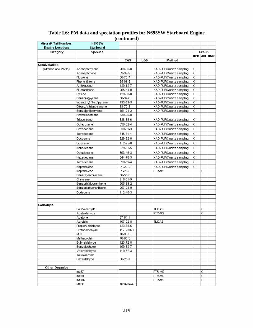
Aircraft Tail ttumber: 1169SSW I Engine Location: Starboard I

Category S1>ecie s Grou1> UCR ARI UMR

CAS LOD Method

Semivolatiles (alkanes and PAHs) Acenaphthylene 208-96-8 XAD-PUF /Quartz sampling X

Acenaphthene 83-32-9 XAD-PUF /Quartz sampling X Fluorene 86-73-7 XAD-PUF /Quartz sampling X Phenanthrene 85-01-8 XAD-PUF /Quartz sampling X Antt-racene 120-12-7 XAD-PUF /Quartz sampling X Fluoranthene 206-44-0 XAD-PUF /Quartz sampling X Pyrene 129-00-0 XAD-PUF /Quartz sampling X Ben:o(a)pyrene 50-32-8 XAD-PUF /Quartz sampling X lndeno[1,2,3-cd)pyrene 193-39-5 XAD-PUF /Quartz sampling X Oibe1z[a,h]anthracene 53-70-3 XAD-PUF /Quartz sampling X Ben:o[ghi]perylene 191-24-2 XAD-PUF /Quartz sampling X Hexatriacontane 630-06-8

Triacontane 638-68-6 XAD-PUF /Quartz sampling X Octecosane 630-02-4 XAD-PUF /Quartz sampling X Hexacosane 630-01-3 XAD-PUF /Quartz sampling X T etracosane 646-31-1 XAD-PUF /Quartz sampling X Docosane 629-92-0 XAD-PUF /Quartz sampling X Eicosane 112-95-8 XAD-PUF /Quartz sampling X Nonadecane 629-92-5 XAD-PUF /Quartz sampling X Octedecane 593-46-3 XAD-PUF /Quartz sampling X Hexadecane 544-76-3 XAD-PUF /Quartz sampling X T etradecane 629-59-4 XAD-PUF /Quartz sampling X Naphthalene 91-20-2 XAD-PUF /Quartz sampling X Naphthalene 91-20-3 PTR-MS X Ben:( a)anthracene 56-55-3 Chr'ysene 218-01-9 Ben:o(b )fluoranlhene 205-99-2 Ben:o(k )fluoranlhene 207-08-9

Dodecane 112-40-3

«;arl>onyls Formaldehyde TILDAS X Acelaldehyde PTR-MS X Acetone 67-64-1 Acrolein 107-02-8 TILDAS Propon-aldehyde 123-38-6 Crolonaldehyde 4170-30-3 MEK 78-93-3 Mett-acrolein 78-85-3 But)'l'aldehyde 123-72-8 Ben:aldehyde 100-52-7 Valeraldehyde 110-62-3 T olualdehyde Hex aldehyde 66-25-1

Other Organics

mz57 PTR-MS X mz59 PTR-MS X mz107 PTR-MS X MTB: 1634-04-4

Table I.6: PM data and speciation profiles for N695SW Starboard Engine (continued)

219

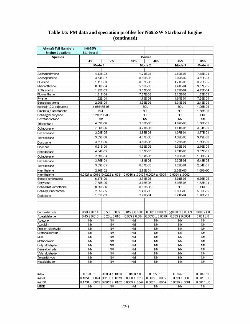
Airerilft Tilil ltombcr: .,,,ssw I I I Engine Location: Starboard I I I

S1>et ies Power 4% 7°/o 30% 40% 65% 85%

Mode 1 Mode 2 Mode 3 Mode 4

Acenaphthylene 4.12E-02 1.24E-03 2.59E-03 7.68E-04 Acenaphthene 3.74E-02 8.60E-03 2.02E-02 4.51E-03 Fluorene 1.11E-03 8.07E-06 4.74E-05 3.21E-05 Phenanthrene 8.58E-04 5.56E-05 1.44E-04 9.57E-05 Anthracene 1.22E-03 9.07E-06 2.29E-04 4.73E-04 Fluoranthene 1.31E-04 7.27E-05 5.10E-06 1.23E-03 Pyrene 1.52E-04 1.73E-04 1.64E-04 7.35E-04 Benzo(a)pyrene 2.26E-05 3.35E-06 5.34E-06 2.43E-05 lndeno[1,2,3-cd)pyrene 4.98547E-06 BDL BDL 1.96E-05 Dibenz[a,h]anthracene BDL BDL BDL 1.65E-05 Benzo[ghi)perylene 5.24029E-06 BDL BDL BDL Hexatriacontane NM NM NM NM

Triacontane 4.89E-06 3.80E-06 4.92E-06 1.50E-05

Octacosane 7.96E-06 4.21E-06 1.11E-05 3.94E-05

Hexacosane 2.08E-05 3.55E-05 1.07E-04 3.77E-04

T etracosane 3.09E-06 4.07E-06 4.32E-06 9.49E-06

Docosane 3.81E-06 4.60E-06 7.23E-06 1.89E-05

Eicosane 5.61E-06 4.86E-06 6.08E-06 2.16E-05

Nonadecane 4.64E-05 1.07E-05 1.21E-05 3.07E-05

Octadecane :2.ti~t-U4 1.::14t-Ut, I .U~t-U~ 1.Utit-U4

Hexadecane 3.75E-04 1.54E-05 2.30E-05 5.43E-05

T etradecane 3.89E-05 6.07E-05 1.22E-04 2.34E-01

Naphthalene 2.16E-02 2.18E-01 2.25E+00 1.06E+00 Naphthalene C.0427 ! .0015 0.0222 ! .0031 0.0046 ! .0040 0.0027 ! .0005 0.0024 ! .0002 Benz( a)anthracene 6.17E-06 3.71E-05 3.91E-05 9.35E-05 Chrysene 7.88E-05 3.76E-05 3.96E-05 1.63E-04 Benzo(b )fluoranthene 9.85E-06 8.62E-06 BDL BDL Benzo(k)fluorantene 2.05E-05 1.42E-05 9.85E-06 5.83E-05

Dodecane 1.55E-03 2.71E-04 5.71E-04 1.76E-03

Formaldehyde 0.98 ! 0.014 0.53 ! 0.039 0.012 ! 0.0008 0.002 ! 0.0032 (-)0.0003 !0.003 0.0005 ! 0 Acelaldehyde 0.45 ! 0.018 0.26 ! 0.018 0.009!0.004 0.0038 ! 0.0016 0.003 ! 0.0004 0.004 ! 0 Acetone NM NM NM NM NM NM Acrolein NM NM NM NM NM NM Propion-aldehyde NM NM NM NM NM NM Crotonaldehyde NM NM NM NM NM NM MEK NM NM NM NM NM NM Methacrolein NM NM NM NM NM NM But yr aldehyde NM NM NM NM NM NM Benz aldehyde NM NM NM NM NM NM Valeraldehyde NM NM NM NM NM NM T olualdehyde NM NM NM NM NM NM Ht:x.tthJt:t1yltt: NM NM NM NM NM NM

mz57 0.6500 ! 0 0.3004 ! .0133 0.0158 ! 0 0.0153 ! 0 0.0142 ! 0 0.0045 ! 0 mz59 C.1854 ! .0024 0.1105 ! .0073 0.0050 ! .0019 0.0029! .0005 0.0023! .0006 0.0015 ! 0 mz107 C.1731 ! .0059 0.0853 ! .0102 0.0069 ! .0047 0.0028 ! .0004 0.0026 ! .0001 0.0015 ! 0 MTBE NM NM NM NM NM NM

Table I.6: PM data and speciation profiles for N695SW Starboard Engine (continued)

220

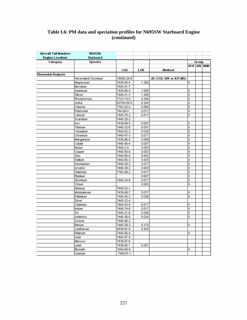
Aircraft Tail ttumber: 11695SW I Engine Location: Starboard I

Category S1>ecies Grou1> UCR ARI UMR

CAS LOD Method Elemental Analysis

Hexavalent Chromium 18540-29-9 (IC-CCD, XRF or ICP-MS) Magnesium 7639-95-4 1.200 X Beryllium 7440-41-7 Aluminum 7429-90-5 1.000 X Silicon 7440-21-3 1.200 X Phoephorous 7723-14-0 0.204 X Sulfur 63705-05-5 0.204 X Chlo•inc 7782-50-5 0.068 X

Potassium 744-09-5 0.017 X Calcum 7440-70-2 0.017 X Scandium 7440-20-2 Iron 7439-89-5 0.007 X Titarium 7440-32-6 0.051 X Vanadium 7440-62-2 0.020 X Chrcmium 7440-47-3 0.017 X Manganese 7439-96-5 0.009 X Cobalt 7440-48-4 0.007 X Nickel 7440-2-0 0.003 X Copper 7440-50-8 0.003 X Zinc 7440-66-6 0.003 X Gallium 7440-55-3 0.425 X Gernanium 7440-38-2 0.017 X Arsenic 7440-38-2 0.003 X Sele1ium 7782-49-2 0.017 X Rbidum 0.007 X strontium 7440-24-6 0.017 X Ytri1..m 0.003 X Niobum 7440-03-1 Mol)'bdenum 7439-98-7 0.017 X Palla::tium 7440-05-3 0.Q26 X Silver 7440-22-4 Cadmium 7440-43-9 0.017 X lndiun 7440-74-6 0.017 X 11n /44U-::11-ti U.U1ij X

Antimony 7440-36-0 0.024 X CesiJm 7440-46-2 Barium 7440-39-3 0.170 X Lant1anum 4639-91-0 0.425 Platinum 7440-06-4 X Gold 7440-57-5 Mercury 7439-97-6 Lead 7439-92-1 0.051 Bisrruth 7440-69-9 X Urarium 7440-61-1

Table I.6: PM data and speciation profiles for N695SW Starboard Engine (continued)

221

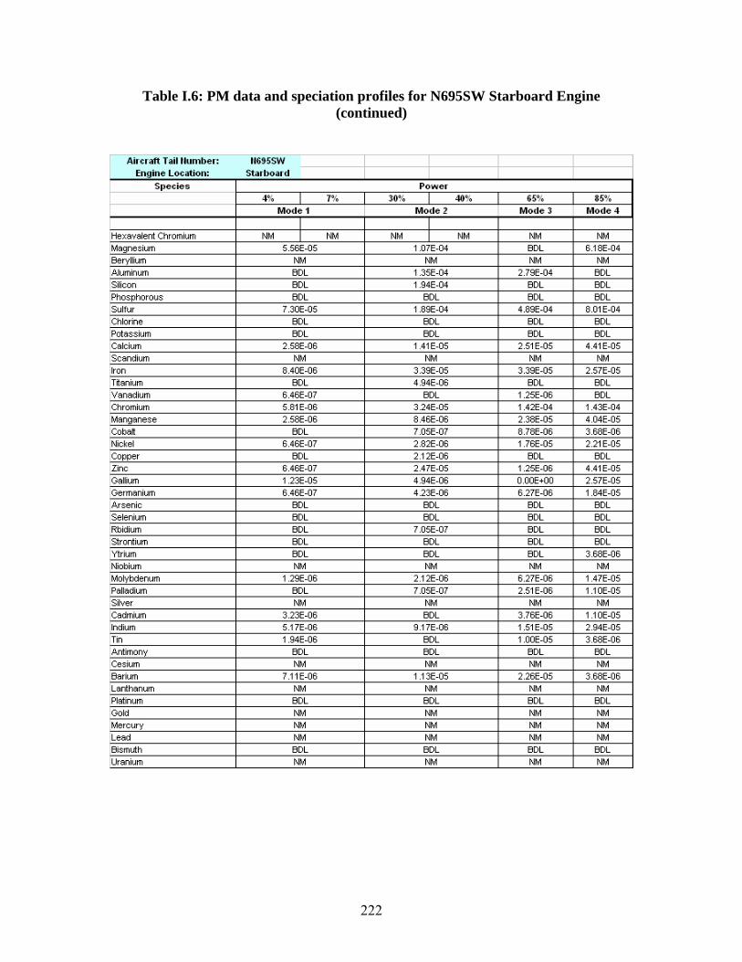
Aircraft Tail ttumber: 11695SW I I I I Engine Location: Starboard I I I I

S1>ecies Power 4% I 7% 30% I 40% 65% 85%

Mode1 Mode 2 Mode 3 Mode4 I I

Hexavalent Chromium NM I NM NM I NM NM NM Magnesium 5.SSE-05 1.07E-04 BDL 6.18E-04 Beryllium NM NM NM NM Aluminum BDL 1.35E-04 2.79E-04 BDL Silicon BDL 1.94E-04 BDL BDL Phosphorous BDL BDL BDL BDL Sulfur 7.30E-05 1.89E-04 4.89E-04 8.01E-04 Chlorine BDL BDL BDL BDL Potassium BDL BDL BDL BDL Calcium 2.58E-06 1.41E-05 2.51E-05 4.41E-05 Scandium NM NM NM NM Iron 8.40E-06 3.39E-05 3.39E-05 2.57E-05 Titanium BDL 4.94E-06 BDL BDL Vanadium 6.46E-07 BDL 1.25E-06 BDL Chromium 5.81E-06 3.24E-05 1.42E-04 1.43E-04 Manganese 2.58E-06 8.46E-06 2.38E-05 4.04E-05 Cobalt BDL 7.0SE-07 8.78E-06 3.68E-06 Nickel 6.46E-07 2.82E-06 1.76E-05 2.21E-05 Copper BDL 2.12E-06 BDL BDL Zinc 6.46E-07 2.47E-05 1.25E-06 4.41E-05 Gallium 1.23E-05 4.94E-06 0.00E•00 2.57E-05 Germanium 6.46E-07 4.23E-06 6.27E-06 1.84E-05 Arsenic BDL BDL BDL BDL Selenium BDL BDL BDL BDL Rbidium BDL 7.0SE-07 BDL BDL strontium BDL BDL BDL BDL Ytrium BDL BDL BDL 3.68E-06 Niobium NM NM NM NM Molybdenum 1.29E-06 2.12E-06 6.27E-06 1.47E-05

Palladium BDL 7.0SE-07 2.51E-06 1.10E-05 Silver NM NM NM NM Cadmium 3.23E-06 BDL 3.76E-06 1.10E-05 Indium 5.17E-06 9.17E-06 1.51E-05 2.94E-05 11n 1.~4t-Uti t:IUL 1.UUt-U~ ~.ijijt-Uij Antimony BDL BDL BDL BDL Cesium NM NM NM NM Barium 7.11E-06 1.13E-05 2.26E-05 3.68E-06 Lanthanum NM NM NM NM Platinum BDL BDL BDL BDL Gold NM NM NM NM Mercury NM NM NM NM Lead NM NM NM NM Bismuth BDL BDL BDL BDL Uranium NM NM NM NM

Table I.6: PM data and speciation profiles for N695SW Starboard Engine (continued)

222

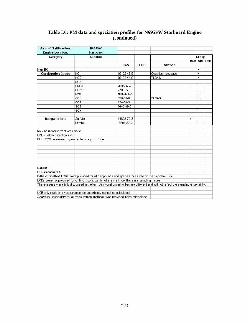
Airerilft Tilil ltombcr: .,,,ssw I Engine Location: St arboard I

Cat egory S1>ecies Grou1> UCR ARI UMR

CAS LOD Method llon-HC X

Combustion Gases NO 10102-43-9 Chemiluminescence X NO2 10102-44-0 TILDAS X NOX HN03 7697-37-2 HONO 7782-77-6 N2O 10024-97-2 X co 630-08-0 TILDAS X CO2 124-38-9 SO2 7446-09-5 SOX

Inorganic ions Sulfale 14808-79-8 X Nltr.te 7697-37-2

NM - no measurement was made BOL - Below detection limit El for CO2 determined by elements.I analysis of fuel

Uotes: UCR comments: In the original text LOOs were prcvided for all compounds and species measured on the high-flow side. LOOs were not provided for C I tc C ,z compounds where we know there are sampling issues. These issues were fully discussed in the test. Analytical uncertainties are different and will not reflect the sampling uncertainty.

I UCR only made one measurement so uncertainty cannot be calculated. I Analytical uncertainty for all meaeurement methods was provided in the original text.

Table I.6: PM data and speciation profiles for N695SW Starboard Engine (continued)

223

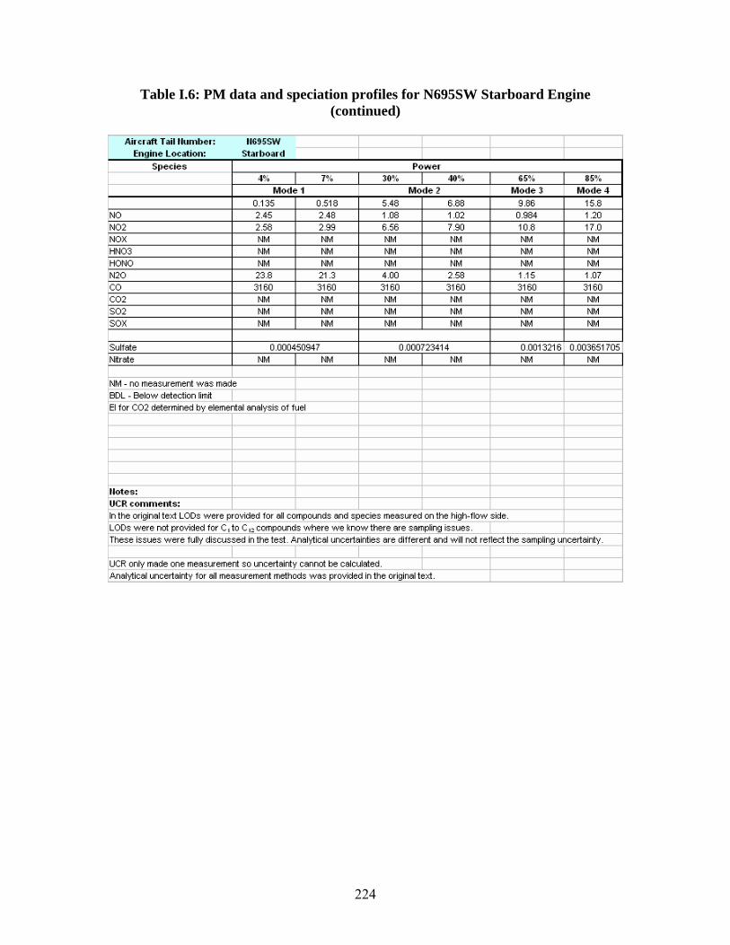
Airerilft Tilil ltombcr: .,,,ssw I I I Engine Location: St arboard I I I

S1>ecies Power 4% 7°/o 30% 40% 65% 85%

Mode 1 Mode 2 Mode 3 Mode 4 0.135 0.518 5.48 6.88 9.86 15.8

NO 2.45 2.48 1.08 1.02 0.984 1.20 N02 2.58 2.99 6.56 7.90 10.8 17.0 NOX NM NM NM NM NM NM HN03 NM NM NM NM NM NM HONO NM NM NM NM NM NM N20 23.8 21.3 4.00 2.58 1.15 1.07 co 3160 3160 3160 3160 3160 3160 CO2 NM NM NM NM NM NM S02 NM NM NM NM NM NM SOX NM NM NM NM NM NM

Sulfate 0.000450947 0.000723414 0.0013216 o.003551705 I Nitrate NM NM NM NM NM NM

NM - no measurement was made BOL - Below detection limit El for CO2 determined by elements.I analysis of fuel

Uotes: UCR comments: In the original text LOOs were prcvided for all compounds and species measured on the high-flow side. LOOs were not provided for C I tc C ,z compounds where we know there are sampling issues. I These issues were fully discussed in the test. Analytical uncertainties are different and will not reflect the sampling uncertainty.

I UCR only made one measurement so uncertainty cannot be calculated. Analytical uncertainty for all meaeurement methods was provided in the original text.

Table I.6: PM data and speciation profiles for N695SW Starboard Engine (continued)

224

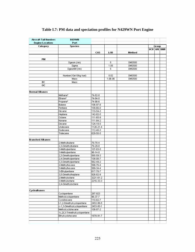
Aircraft Tail ttumber: 11429Wll I Engine Location: Port I

Categooy S1>ecie s Gro1.11> UCR ARI UMR

CAS LOD Method

PM Dgeom (nm) 5 DMS500

Sigma 1.05 DMS500 DgeomM (nm) 5 DMS500

Number(1 ue1 tiJkg tuelJ U.U1 UM~~uu Mass 1.0E-06 DMS500

EC Mass oc

normal Alkanes

Methane* 74-82-8 Ethane* 74-84-0 Propane* 74-98-6 B.dane 106-97-8 Pentane 109-66-0 Hexane 110-54-3 Heptane 142-82-5 Cttane 111-65-9 NJnane 111-84-2 Decane 124-18-5 U1decane 1120-21-4 0Jdecane 112-40-3 Tridecane 629-50-5

Branched Alkanes 2-Melhylbutane 78-78-4 2 3-Dimethylbutane 79-29-8 2-Methylpentane 107-83-5 3-Methylpentane 96-14-0 2 3-Dimethylpentane 565-59-3 2 4-Dimethylpentane 108-08-7 3 3-Dimethylpentane 562-49-2 2-Methylhexane 598-76-4 3-Methylhexane 589-34-4 3-Ethylpentane 617-78-7 3 5-Dimethylheptane 926-82-9 2-Methyloctane 3221-61-2 3-Methyloctane 2216-33-3 2 4-Dimethyloctane

Cycloalkanes Cy'clopentane 287-923 ~hylr.yr.lnpP.ntAnP. ~R-~7-7 Cy'clohexane 110-82-7 1-1,2-Dimethylcyclopentane 2452-99-5 c-1 ,3-Dimethylcyclopentane 2453-00-1 Methylcyclohexane 108-87-2 1 c ,21 ,3-T rimethylcyclopentane Elhylcyclohexane 1678-91-7

Table I.7: PM data and speciation profiles for N429WN Port Engine

225

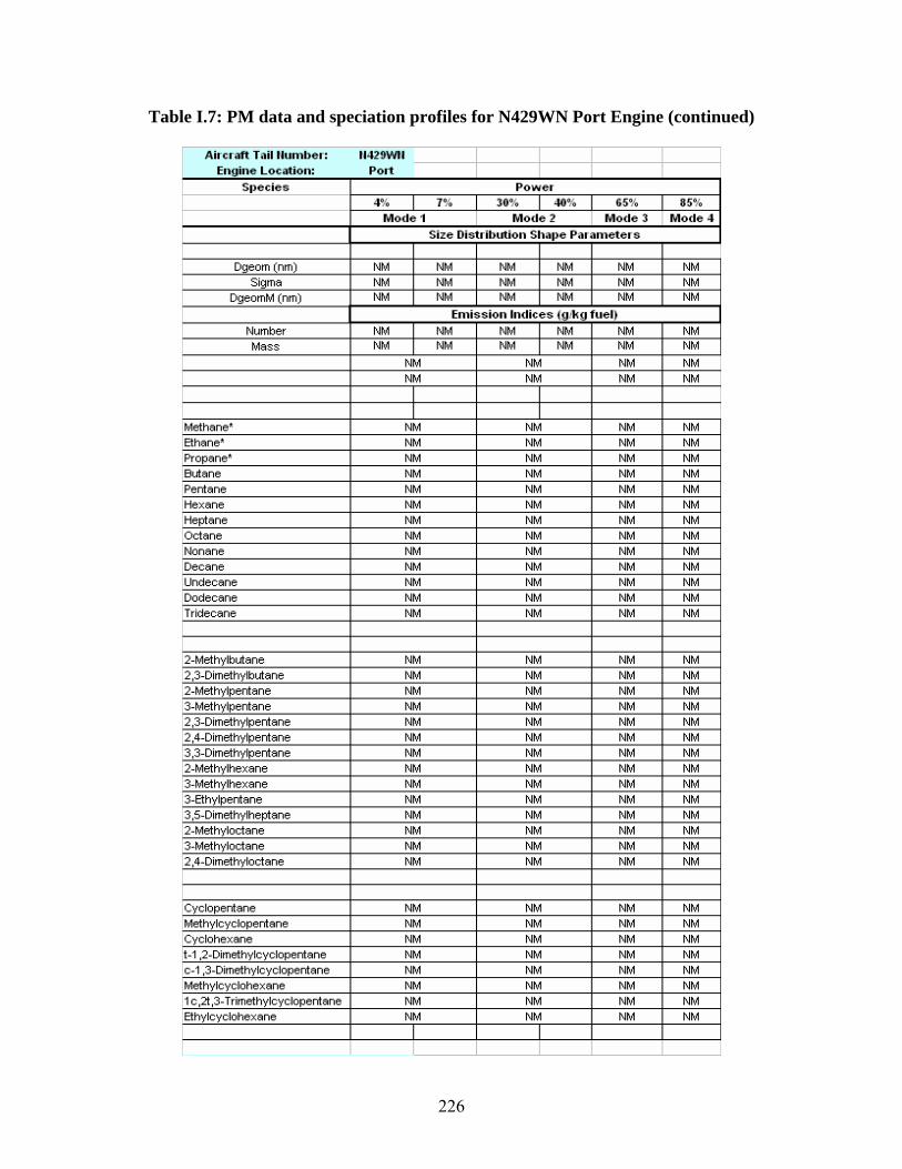
Aircraft Tail Humber: 11429WII I I Engine Location: Port I I

Specie s Power 4% n~ I 30¾ 40¾ I 65,~ I 85~~

Mode 1 MO<le 2 Mode 3 I Mode 4 Size Distribution Shape Parameters

I Dgeom(nm) NM NM NM NM NM NM

Sigma NM NM NM NM NM NM DgeomM (Ml) NM NM NM NM NM NM

Emis sion Indice s (gJkg fuel) Number NM NM NM NM NM NM Mass NM NM NM NM NM NM

NM NM NM NM I NM i'lv1 NM NM I

I I

Methane" NM NM NM NM B hane* NM i'lv1 NM NM Propane .. NM NM NM NM Butane NM i'lv1 NM NM Pentane NM NM NM NM Hexane NM i'lv1 NM NM Heptane NM NM NM NM Octane NM i'lv1 NM NM Nonane NM NM NM NM Decane NM i'lv1 NM NM l.kldecane NM NM NM NM Dodecane NM i'lv1 NM NM Tridecane NM NM NM NM

2-Methylbutane NM i'lv1 NM NM 2 ,3-Dimethylbutane NM NM NM NM 2-Methyfl)enlane NM NM NM NM 3-Methyfl)enlane NM i'lv1 NM NM 2 ,3-Dimethylpentane NM NM NM NM 2 ,4-Dimethylpentane NM i'lv1 NM NM 3 ,3-Dimethylpentane NM NM NM NM 2-Methylhexane NM i'lv1 NM NM 3-Methylhexane NM NM NM NM 3-Elhylpentane NM i'lv1 NM NM 3 ,5-Dimethylheptane NM NM NM NM 2-Methyloctane NM i'lv1 NM NM 3-Methyloctane NM NM NM NM 2 ,4-Dimethyloctane NM i'lv1 NM NM

Cyclopentane NM NM NM NM Melhylcyclopentane NM i'lv1 NM NM Cyclohexane NM NM NM NM 1-1,2-Dimethy lcyclopentane NM i'lv1 NM NM c-1 ,3-Dimethylcyclopentane NM NM NM NM Melhylcyclohexane NM i'lv1 NM NM 1 c ,21,3-Trimethytcyclopernane NM NM NM NM Elhytcyclohexane NM i'lv1 NM NM

Table I.7: PM data and speciation profiles for N429WN Port Engine (continued)

226

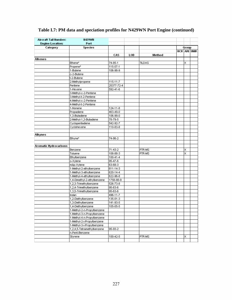
Aircraft Tail ttumber: 11429Wll I Engine Location: Port I

Categooy S1>ecie s Gro1.11> UCR ARI UMR

CAS LOD Method Alkenes

Elhene• 74-85-1 TILDAS X Propene• 115-07-1 1-Butene 106-98-9 c-2-Butene 1-2-Butene 2-Methylpropene 115-11-7 Pentene 25377-72-4 1-Hexene 592-41-6 3-Methyl-c-2-Pentene 3-Methyl-1-2-Pentene 4-Methyl-c-2-Pentene 4-Methyl-1-2-Pentene 1-Nonene 124-11-8 Propadiene 463-49-0 1 3-Butadiene 106-99-0 2-Melhyl-1,3-Butadiene 78-79-5 Cy'clopentadiene 542-92-7 Cy'clohexene 110-83-8

Alkynes Elhyne• 74-86-2

Aromatic Hydrocarbons Benzene 71-43-2 PTR-fo.lS X Toluene 108-88-3 PTR-fo.lS X Elhylbenzene 100-41-4 o-Xylene 95-47-6 m&p-Xylene 63-68-3 1-Methyl-2-elhylbenzene 611-14-3 1-Methyl-3-ethylbenzene 620-14-4 ·I-Methyl-4-ethylbenzene 622-96-8

1 4-Dimethyl-2-elhylbenzene 1758-88-9 1 2,3-Trimethylbenzene 526-73-8 1 2,4-Trimethylbenzene 95-63-6 1 3,5-Trimethylbenzene 95-63-6 lndan 496-11-7 1 2-Diethylbenzene 135-01-3 1 3-Diethylbenzene 141-93-5 1 4-Diethylbenzene 105-05-5 1-Methyl-2-n-Propylbenzene 1-Methyl-3-n-Propylbenzene 1-Methyl-4-n-Propylbenzene 1-Methyl-2-i-Propylbenzene 1-Methyl-3-i-Propylbenzene 12,4,5-Tetramethylbenzene 95-93-2 n-Pent-Benzene S:yrene 100-42-5 PTR-fo.lS X

Table I.7: PM data and speciation profiles for N429WN Port Engine (continued)

227

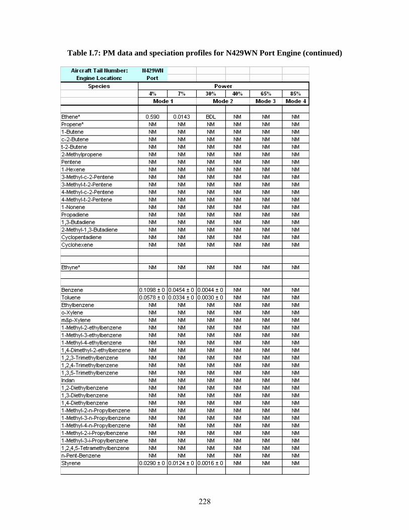
Aircraft Tail ttumber: 11429Wll I Engine Location: Port I

S1>ecies Pow er 4% 7% 30% 40% 65% I 85%

Mode1 I Mode 2 I Mode 3 I Mode 4

Ethene* 0.590 0.0143 BDL NM NM NM Propene* NM NM NM NM NM NM 1-Butene NM NM NM NM NM NM c-2-Butene NM NM NM NM NM NM 1-2-Butene NM NM NM NM NM NM 2-Methylpropene NM NM NM NM NM NM Pentene NM NM NM NM NM NM 1-Hexene NM NM NM NM NM NM 3-Methyl-c-2-Pentene NM NM NM NM NM NM 3-Methyl-1-2-Pentene NM NM NM NM NM NM 4-Methyl-c-2-Pentene NM NM NM NM NM NM 4-Methyl-1-2-Pentene NM NM NM NM NM NM 1-Nonene NM NM NM NM NM NM Propadiene NM NM NM NM NM NM 1 ,3-Butadiene NM NM NM NM NM NM 2-Melhyl-1,3-Butadiene NM NM NM NM NM NM Cyclopentadiene NM NM NM NM NM NM Cyclohexene NM NM NM NM NM NM

Ethyne* NM NM NM NM NM NM

Benzene 0.1098 • 0 0.0454 • 0 0.0044 • 0 NM NM NM Toluene 0.0578 t 0 0.0334 t 0 0.0030 t 0 NM NM NM Ethylbenzene NM NM NM NM NM NM o-Xylene NM NM NM NM NM NM m&p-Xylene NM NM NM NM NM NM 1-Methyl-2-elhylbenzene NM NM NM NM NM NM 1-Methyl-3-ethylbenzene NM NM NM NM NM NM 1-Methyl-4-elhylbenzene NM NM NM NM NM NM 1,4-Dimethyl-2-elhylbenzene NM NM NM NM NM NM 1,2,3-Trimethylbenzene NM NM NM NM NM NM 1,2,4-Trimethylbenzene NM NM NM NM NM NM 1,3,5-Trimethylbenzene NM NM NM NM NM NM lndan NM NM NM NM NM NM 1,2-Diethylbenzene NM NM NM NM NM NM 1 ,3-Diethylbenzene NM NM NM NM NM NM 1,4-Diethylbenzene NM NM NM NM NM NM 1-Methyl-2-n-Propylbenzene NM NM NM NM NM NM 1-Methyl-3-n-Propylbenzene NM NM NM NM NM NM 1-Methyl-4-n-Propylbenzene NM NM NM NM NM NM 1-Methyl-2-i-Propylbenzene NM NM NM NM NM NM 1-Methyl-3-i-Propylbenzene NM NM NM NM NM NM 1 ,2,4 ,5-T etramethylbenzene NM NM NM NM NM NM n-Pent-Benzene NM NM NM NM NM NM styrene 0.0290 t 0 0.0124 t 0 0.0016 t 0 NM NM NM

Table I.7: PM data and speciation profiles for N429WN Port Engine (continued)

228

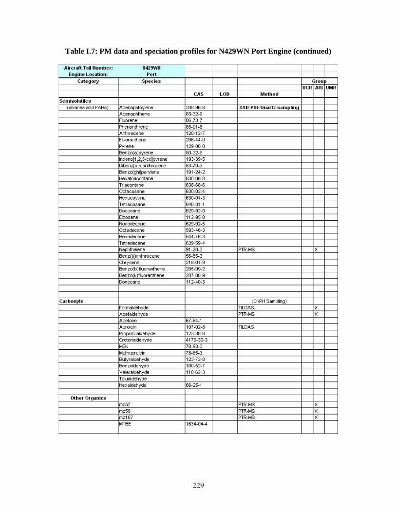
Aircraft Tail ttumber: 11429Wll I Engine Location: Port I

Categooy S1>ecie s Gro1.11> UCR ARI UMR

CAS LOD Method

Semivolatiles (alkanes and PAHs) Acenaphlhylene 208-96-8 XAD-PUF/Quartz sam1>ling

.A.cenaphthene 83-32-9 Fllorene 86-73-7 Phenanthrene 85-01-8 .Arnhracene 120-12-7 Flloranthene 206-44-0 P·,rene 129-00-0 Benzo(a)pyrene 50-32-8 lrdeno[1,2,3-cd)pyrene 193-39-5 Dbenz[a,h]anlhracene 53-70-3 Benzo[ghi]perylene 191-24-2 H~xatriacontanc 630-06-8

Triacontane 638-68-6 Cciacosane 630-02-4 Hexacosane 630-01-3 T etracosane 646-31-1 0Jcosane 629-92-0 ECosane 112-95-8 NJnadecane 629-92-5 Cciadecane 593-46-3 Hexadecane 544-76-3 T etradecane 629-59-4 N,phlhalene 91-20-3 PTR-fo.lS X Benz( a)anthracene 56-55-3 C1rysene 218-01-9 Benzo(b )fluoranthene 205-99-2 Benzo(k )fluoranthene 207-08-9 0Jdecane 112-40-3

Carbonyls (DNPH Sampling) Formaldehyde TILDAS X Acelaldehyde PTR-fo.lS X .A.cetone 67-64-1 .A.crolein 107-02-8 TILDAS Propion-aldehyde 123-38-6 C·otonaldehyde 4170-30-3 lvl:K 78-93-3 tirethacrolein 78-85-3 B.Atyraldehyde 123-72-8 Benz aldehyde 100-52-7 Valer aldehyde 110-62-3 T olualdehyde Hex aldehyde 66-25-1

Other Organics mz57 PTR-fo.lS X mz59 PTR-fo.lS X mz107 PTR-fo.lS X MTBE 1634-04-4

Table I.7: PM data and speciation profiles for N429WN Port Engine (continued)

229

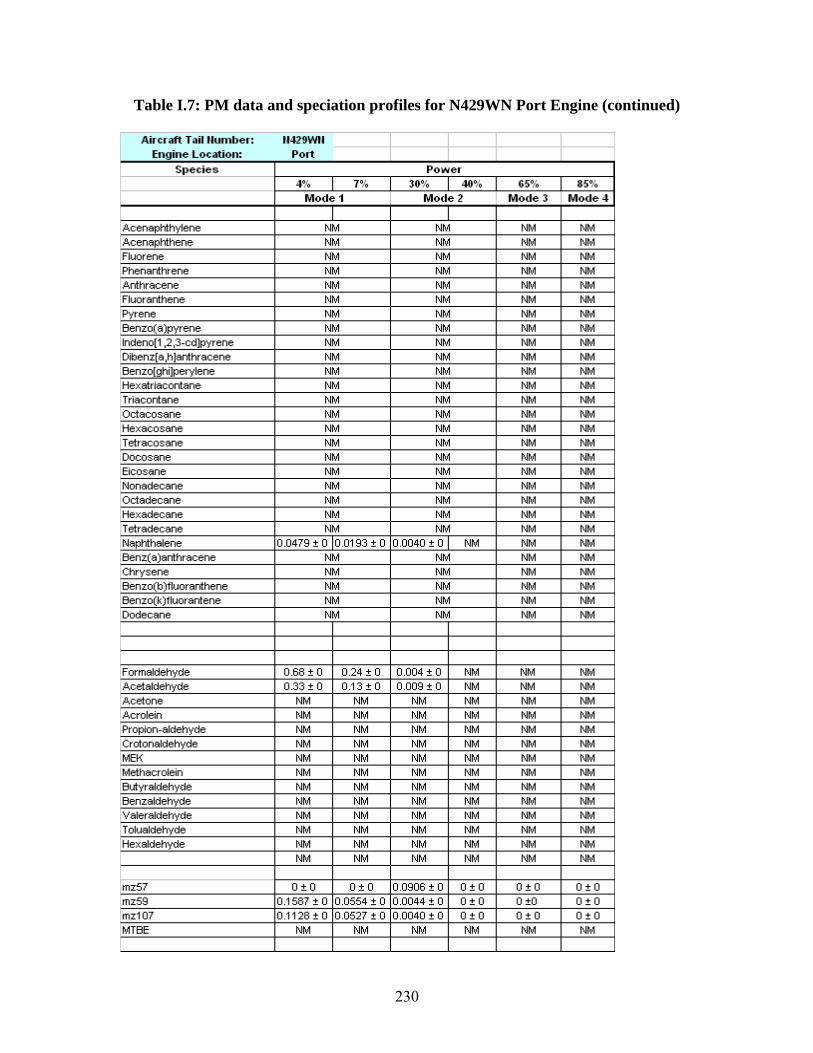
Aircraft Tail llumber: 11429WII I I I Engine Location: Port I I

Species Power 4% 7°/o 30, ~ I 40% I 65~'. I 8-5%

Mode1 Model Mode 3 Mode 4 I

Acenaphlhytene NM l\"1 NM l',a.1

Acenaphthene NM i"'1 NM i"'1 Fliorene NM l\"1 NM l',a.1

Phenarthrene NM i"'1 NM i"'1 Anthracene NM l\"1 NM l',a.1

Fliorarthene NM i"'1 NM i"'1 Pyrene NM l\"1 NM l',a.1

Benzo(a)pyrene NM i"'1 NM i"'1 lndeno(1 ,2,3-cd]pyrene NM l\"1 NM l',a.1

Di:>enz(a ,h Janthracene NM i"'1 NM i"'1 Benzo(ghi]perylene NM l\"1 NM l',a.1

Hexatriacoriane NM i"'1 NM i"'1 Triacoriane NM l\"1 NM l',a.1

Ociacosane NM i"'1 NM i"'1 Hexacosane NM l\"1 NM l',a.1

T etracosane NM i"'1 NM i"'1 Docosane NM l\"1 NM l',a.1

Eicosane NM i"'1 NM i"'1 NnnArfAr.AnP. NM l\"1 NM l',a.1

Ociadecane NM l\"1 NM l',a.1

Hexadecane NM i"'1 NM i"'1 T etradecane NM l\"1 NM l',a.1

Naphthalene 0.0479 ± 0 0.01 93 ± 0 0.0040 ± o I NM NM i"'1 Benz( a)antt.-acene NM l\"1 NM l',a.1

Chrysene NM i"'1 NM i"'1 Benzo(b )fluoranlhene NM l\"1 NM l',a.1

Benzo(k)fluorantene NM i"'1 NM i"'1 Dodecane NM l\"1 NM l',a.1

Formaldehyde 0.68 ± 0 0 .24 ± 0 0.004 ± 0 NM NM l',a.1

Acetaldehyde 0.33 ± 0 0 .13 • 0 0.009 ± 0 NM NM i"'1 Acetone NM NM Ila.I NM NM l',a.1

Acrolein NM NM i"'1 NM NM i"'1 Propion-aldehyde NM NM Ila.I NM NM l',a.1

Crotoneldehyde NM NM i"'1 NM NM i"'1 MEK NM NM Ila.I NM NM l',a.1

Methaa olein NM NM i"'1 NM NM i"'1 But yr aldehyde NM NM Ila.I NM NM l',a.1

Benz aldehyde NM NM i"'1 NM NM i"'1 Valer aldehyde NM NM Ila.I NM NM l',a.1

T olualdehyde NM NM i"'1 NM NM i"'1 Hex aldehyde NM NM Ila.I NM NM l',a.1

NM NM i"'1 NM NM i"'1

mz57 0 :!: 0 0 ± 0 0.0906 ± 0 0 :!: 0 0 ± 0 0 :!: 0 mz59 0.1587 • 0 0.0554 ± 0 0.0044 ± 0 0 :!: 0 0 :!:O 0 :!: 0 rnz107 0 .1128 :!: 0 0 .0527 ± 0 0 .0040 :!: 0 0 ± 0 O :!: O 0 ± 0

MTBE NM NM i"'1 NM NM i"'1

Table I.7: PM data and speciation profiles for N429WN Port Engine (continued)

230

Aircraft Tail ttumber: 11429Wll I Engine Location: Port I

Categooy S1>ecie s Gro1.11> UCR ARI UMR

CAS LOD Method Elemental Analysis

Hexavalent Chromium 18540-29-9 (IC-CCD, XRF or ICP-MS) timgnesium 7639-95-4 1.200 Beryllium 7440-41-7 .e.Juminum 7429-90-5 1.000 Slicon 7440-21-3 1.200 Phosphorous 7723-14-0 0.204 SJlfur 63705-05-5 0.204 C1lorine 7782-50-5 0.068 Potassium 744-09-5 0.017 C31cium 7440-70-2 0.017 S:andium 7440-20-2 Iron 7439-89-5 0.007 Ttanium 7440-32-6 0.051 Vanadium 7440-62-2 0.020 C1romium 7440-47-3 0.017 timnganese 7439-96-5 0.009 c,balt 7440-48-4 0.007 Nckel 7440-2-0 0.003 c,pper 7440-50-8 0.003 Znc 7440-66-6 0.003 Gallium 7440-55-3 0.425 Germanium 7440-38-2 0.017 .Arsenic 7440-38-2 0.003 Selenium 7782-49-2 0.017 Roidium 0.007 S:rontium 7440-24-6 0.017 Ylrium 0.003 Nobium 7440-03-1 Mllybdenum 7439-98-7 0.017 Palladium 7440-05-3 0.Q26 Siver 7440-22-4 C3dmium 7440-43-9 0.017 lrdium 7440-74-6 0.017 Th 7440-31-6 0.Q26 .Antimony 7440-36-0 0.024 Cesium 7440-46-2 83rium 7440-39-3 0.170 Lanthanum 4639-91-0 0.425 Patinum 7440-06-4 Gold 7440-57-5 Mercury 7439-97-6 Lead 7439-92-1 0.051 Bsmuth 7440-69-9 U·anium 7440-61-1

Table I.7: PM data and speciation profiles for N429WN Port Engine (continued)

231

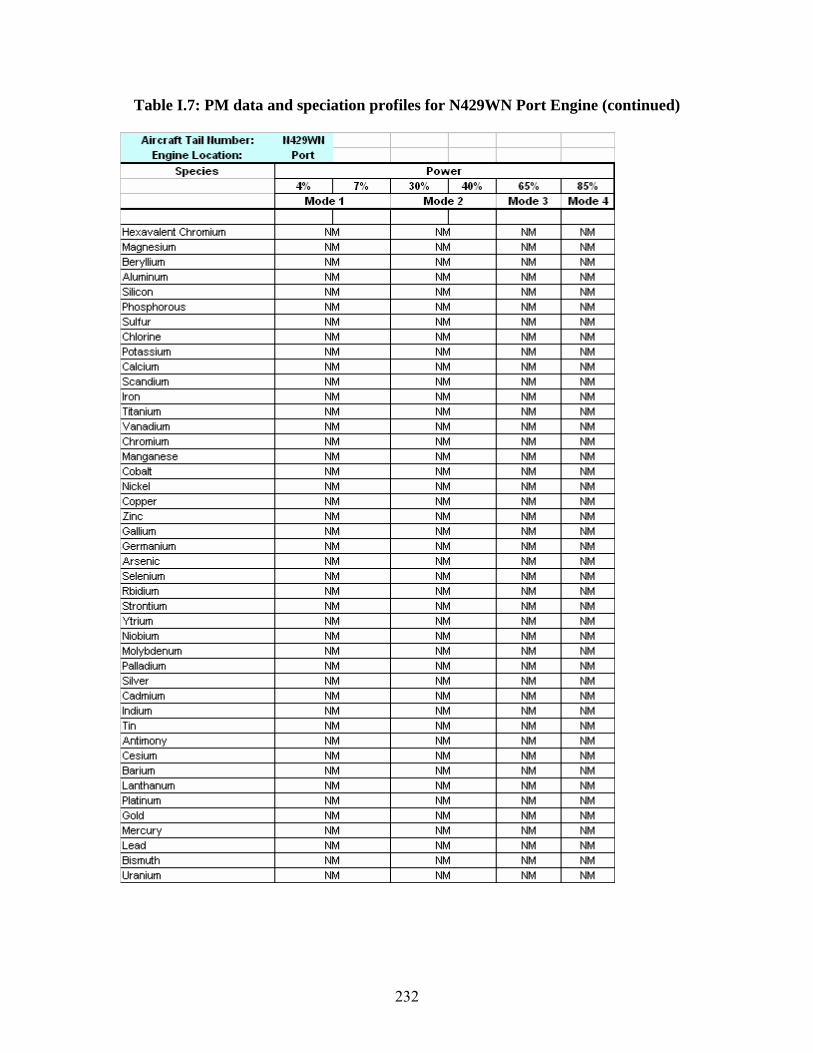
Aircraft Tail ttumber: 11429Wll I I Engine Location: Port I I

S1>ecies Pow er 4% I 7% 30% I 40% 65% I 85%

Mode1 I Mode 2 I Mode 3 I Mode 4

I I Hexavalent Chromium NM NM NM NM Magnesium NM NM NM NM Beryllium NM NM NM NM Aluminum NM NM NM NM Silicon NM NM NM NM Phosphorous NM NM NM NM Sulfur NM NM NM NM Chlorine NM NM NM NM Potassium NM NM NM NM Calcium NM NM NM NM Scandium NM NM NM NM Iron NM NM NM NM Titanium NM NM NM NM Vanadium NM NM NM NM Chromium NM NM NM NM Manganese NM NM NM NM Cobalt NM NM NM NM Nickel NM NM NM NM Copper NM NM NM NM Zinc NM NM NM NM Gallium NM NM NM NM Germanium NM NM NM NM Arsenic NM NM NM NM Selenium NM NM NM NM Rbidium NM NM NM NM strontium NM NM NM NM Ytrium NM NM NM NM Niobium NM NM NM NM Molybdenum NM NM NM NM Palladium NM NM NM NM Silver NM NM NM NM Cadmium NM NM NM NM Indium NM NM NM NM Tin NM NM NM NM Antimony NM NM NM NM Cesium NM NM NM NM Barium NM NM NM NM Lanthanum NM NM NM NM Platinum NM NM NM NM Gold NM NM NM NM Mercury NM NM NM NM Lead NM NM NM NM Bismuth NM NM NM NM Uranium NM NM NM NM

Table I.7: PM data and speciation profiles for N429WN Port Engine (continued)

232

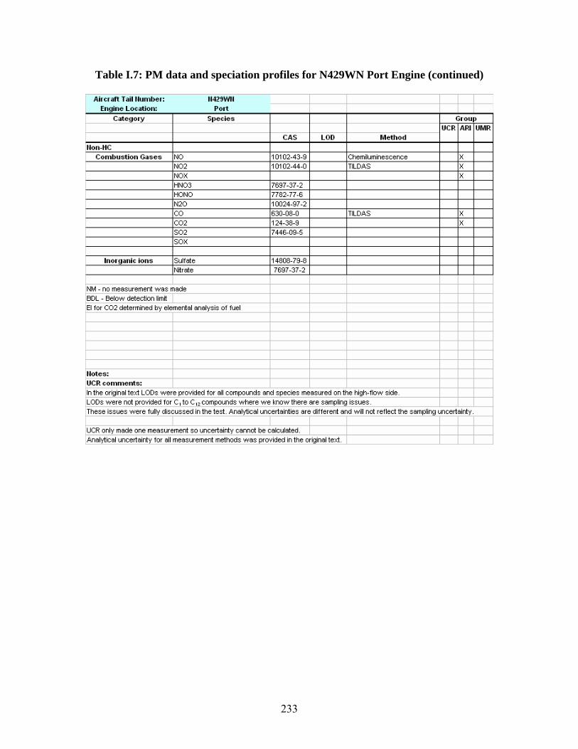
Aircraft Tail ttumber: 11429Wll I Engine Location: Port I

Categooy S1>ecies Gro1.11> UCR ARI UMR

CAS LOD Method llon-HC

Combustion Gases N::> 10102-43-9 Chemluminescence X N::>2 10102-44-0 TILDAS X N::>X X H~03 7697-37-2 H::>NO 7782-77-6 N20 10024-97-2 c::, 630-08-0 TILDAS X C::>2 124-38-9 X S::>2 7446-09-5 s::,x

lnorg.inic ion3 S .. dfatc 14808-70-8 Ntrate 7697-37-2

NM - no measurement was ma:te BDL - Below detection limlt I El for CO2 determined by elemental analysis of fuel

llotes: UCR comments: In the original text LOOs were orovided for all compounds and species measured on the higt--flow side. LOOs were not provided for c, to C 12 compounds where we know there are sampling issues. These issues were fully discussed in the test. Analytical uncertainties are different and will 1ot reflect the sampling uncertainty.

I I UCR only made one measurerrent so uncertainty cannot be calculated. Analytical uncertainty for all measurement methods was provided in the original text.

Table I.7: PM data and speciation profiles for N429WN Port Engine (continued)

233

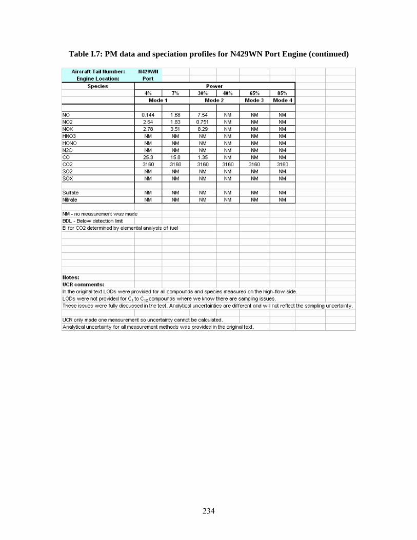
Aircraft Tail ttumber: 11429WII I I I Engine Location: Port I I I

S1>ecies Power 4% 7°/o 30% I 40% 65% 85%

Mode1 Mode 2 Mode 3 Mode 4

NO 0.144 1.68 7.54 NM NM NM NO2 2.64 1.83 0.751 NM NM NM NOX 2.78 3.51 8.29 NM NM NM HNO3 NM NM NM NM NM NM HONO NM NM NM NM NM NM N2O NM NM NM NM NM NM co 25.3 15.8 1.35 NM NM NM CO2 3160 3160 3160 3160 3160 3160 SO2 NM NM NM NM NM NM SOX NM NM NM NM NM NM

Sulfate NM NM NM NM NM NM Nitrate NM NM NM NM NM NM

NM - no measurement was made BOL - Below detection limit El for CO2 determined by elemental analysis Jf fuel

Uotes: UCR comments: In the original text LOOs were provided for al compounds and species measured on the high-flow side. LOOs were not provided for C I to C ,z compcunds where we know there are sampling issues. These issues were fully discussed in the teet. Analytical uncertainties are different and will not reflect the sampling uncertainty.

I I I UCR only made one measurement so uncertainty cannot be calculated. I Analytical uncertainty for all measurement methods was provided in the original text.

Table I.7: PM data and speciation profiles for N429WN Port Engine (continued)

234

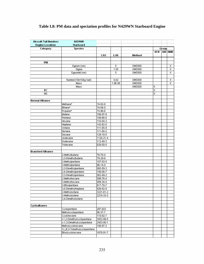
Aircraft Tail ttumber: 11429Wll Engine Location: Starboard I

Category S1>ecies Grou1> UCR ARI UMR

CAS LOD Method

PM Dgeom (nm) 5 DMS500 X

Sigma 1.05 DMS500 X DgeomM (nm) 5 DMS500 X

Number(10e151kg fuel) 0.02 DMS500 X Mass 1.0E-06 DMS500 X Mass DMS500 X

EC X oc X

ltormal Alkanes Methane* 74-82-8 Bhane* 74-84-0 Propane* 74-98-6 Butane 106-97-8 Pentane 109-66-0 Hexane 110-54-3 Heptane 142-82-5 Octane 111-65-9 Nonane 111-84-2 Decane 124-18-5 Undecane 1120-21-4 Dodecane 112-40-3 Tridecane 629-50-5

Branched Alkanes 2-Methylbutane 78-78-4 2,3-Dimethylbutane 79-29-8 2-Methylpentane 107-83-5 3-Methylpentane 96-14-0 2,3-Dimethylpentane 565-59-3 2,4-Dimethylpentane 108-08-7 3,3-Dimethylpentane 562-49-2 2-Methylhexane 598-76-4 3-Methylhexane 589-34-4 3-Ethylpentane 617-78-7 3,5-Dimethylheptane 926-82-9 2-Methyloctane 3221-61-2 3-Methyloctane 2216-33-3 2,4-Dimethyloctane

Cycloalkanes Cyclopentane 287-923 Methylcyclopentane 96-37-7 Cyclohexane 110-82-7 1-1,2-Dimethylcyclopentane 2452-99-5 c-1 ,3-Dimethylcyclopentane 2453-00-1 Methylcyclohexane 108-87-2 1 c,21,3-Trimethylcyclopentane Bhylcyclohexane 1678-91-7

Table I.8: PM data and speciation profiles for N429WN Starboard Engine

235

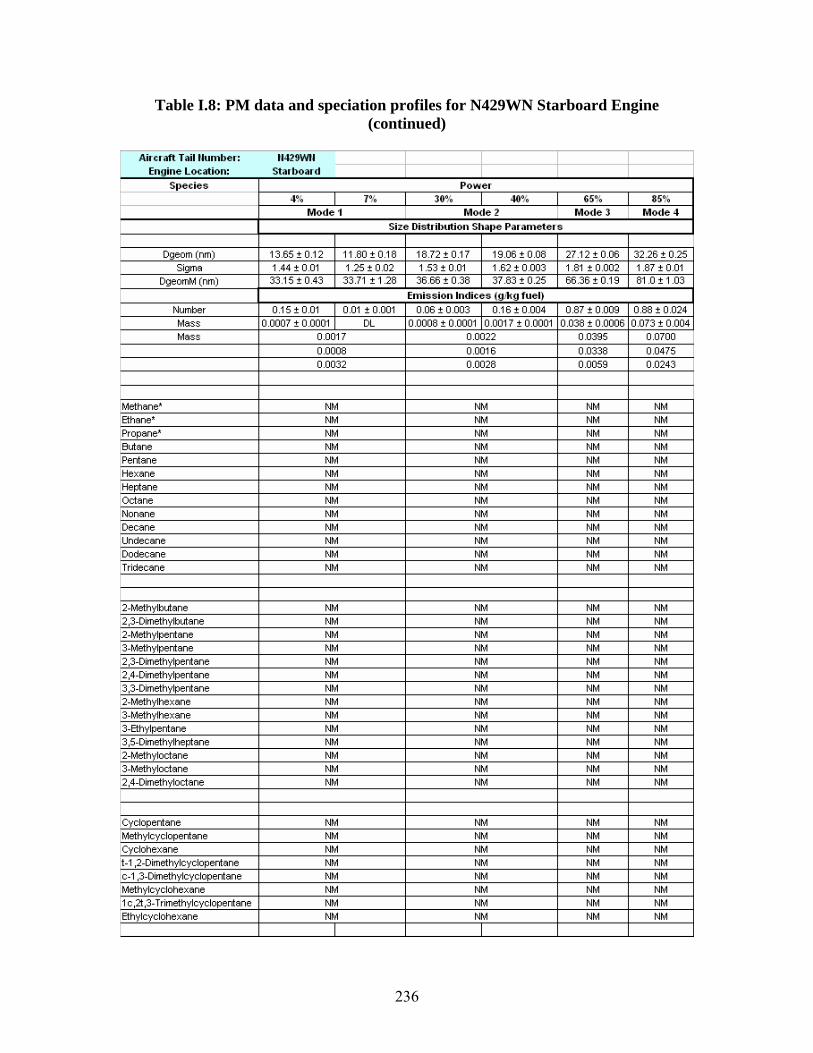
Aircraft Tail ttumber: 11429Wll I I Engine Location: Starboard I I

S1>ecie s Power 4% I 7% 30% I 40% G~% I 8~%

Mode 1 Mode 2 Mode 3 I Mode 4 Size Distribution ShaJ>e Parameters

I Dgeom (nm) 13.65 • 0.12 11.80 • 0.18 18.72 • 0.17 19.06 • 0.08 27.12 • 0.06 32.26 • 0.25

Sigma 1.44 t 0.01 1.25 t 0.02 1.53 t 0.01 1.62 t 0.003 1.81 t 0.002 1.87 t 0.01 DgeomM (nm) 33.15 t 0.43 33.71 t 1.28 36.66 t 0.38 37.83 t 0.25 66.36 t 0.19 81.0>1.03

Emission Indice s {gll<g fuel)

Number 0.15 • 0.01 I 0.D1 t0.001 0.06 • 0.003 I 0.16 • 0.004 0.87 t0.009 0.88 • 0.024 Mass 0.0007 • 0.0001 I DL 0.0008 • 0.0001 I 0.0017 • 0.0001 0.D38t0.0006 0.073 t 0.004 Mass 0.0017 0.0022 0.0395 0.0700

0.0008 0.0016 0.0338 0.0475 0.0032 0.0028 0.0059 0.0243

Methane• NM NM NM NM Ethane• NM NM NM NM Propane• NM NM NM NM Butane NM NM NM NM Pentane NM NM NM NM Hexane NM NM NM NM Heptane NM NM NM NM Octane NM NM NM NM Nonane NM NM NM NM Decane NM NM NM NM Undecane NM NM NM NM Dodecane NM NM NM NM Tridecane NM NM NM NM

2-Melhylbutane NM NM NM NM 2,3-Dimethylbutane NM NM NM NM 2-Methylpentane NM NM NM NM 3-Methylpentane NM NM NM NM 2,3-Dimethylpentane NM NM NM NM 2,4-Dimethylpentane NM NM NM NM 3,3-Dimethylpentane NM NM NM NM 2-Methylhexane NM NM NM NM 3-Methylhexane NM NM NM NM 3-Ethylpentane NM NM NM NM 3,5-Dimethylheptane NM NM NM NM 2-Methyloctane NM NM NM NM 3-Methyloctane NM NM NM NM 2,4-Dimethyloctane NM NM NM NM

Cyclopentane NM NM NM NM Methylcyclopentane NM NM NM NM Cyclohexane NM NM NM NM t-1,2-Dimethylcyclopentane NM NM NM NM c-1 ,3-Dimethylcyclopentane NM NM NM NM Methylcyclohexane NM NM NM NM 1 c,21,3-Trimethylcyclopentane NM NM NM NM Ethylcyclohexane NM NM NM NM

I I

Table I.8: PM data and speciation profiles for N429WN Starboard Engine (continued)

236

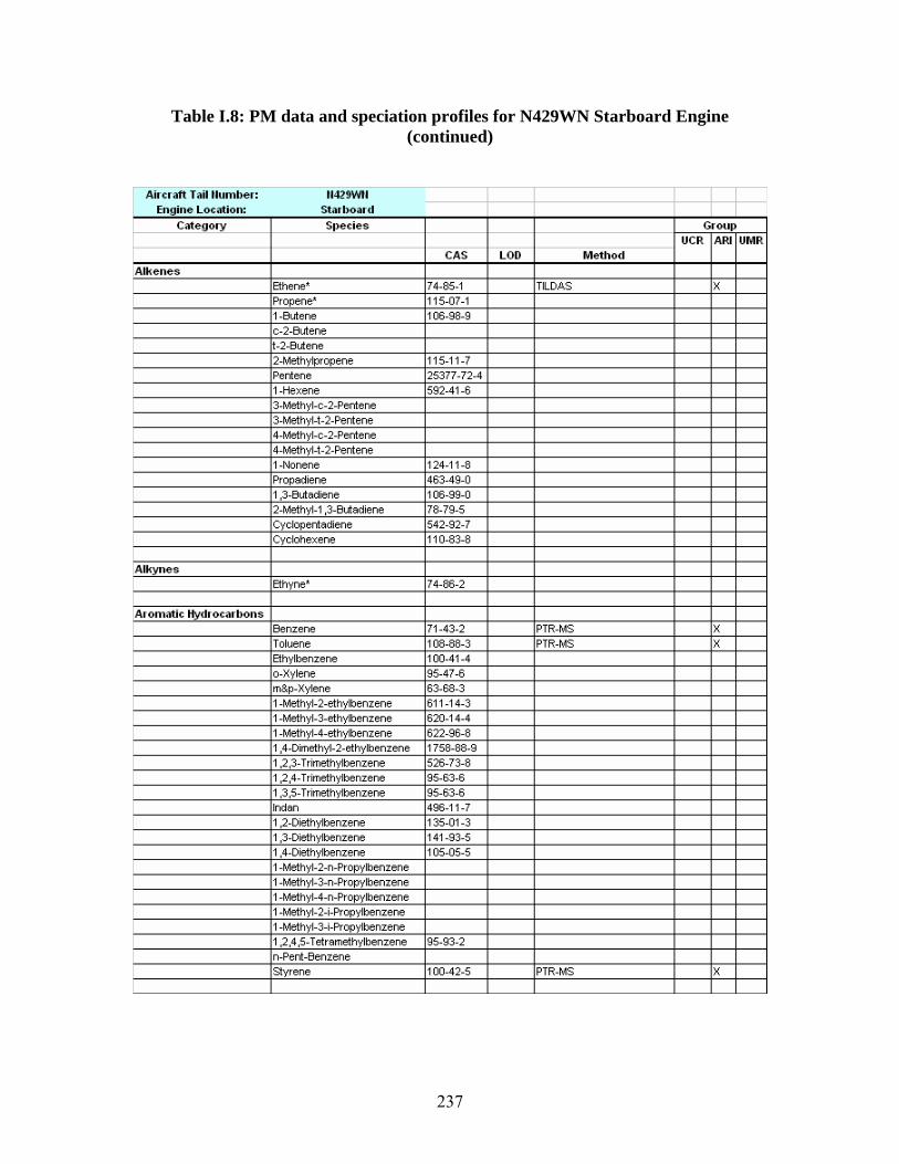
Aircraft Tail ttumber: 11429Wll I Engine Location: Starboard I

Category SI>ecies GrouI> UCR ARI UMR

CAS LOD Method Alkenes

Bhene* 74-85-1 TILDAS X Propene• 115-07-1 1-Butene 106-98-9 c-2-Butene 1-2-Butene 2-Melhylpropene 115-11-7 Pentene 25377-72-4 1-Hexene 592-41-6 3-Melhyl-c-2-Penlene 3-Melhyl-1-2-Penlene 4-Melhyl-c-2-Penlene 4-Melhyl-1-2-Penlene 1-Nonene 124-11-8 Propadiene 463-49-0 1 ,3-Butadiene 106-99-0 2-Melhyl-1,3-Butadiene 78-79-5 Cyclopentadiene 542-92-7 Cyclohexene 110-83-8

Alkynes Bhyne* 74-86-2

Aromatic Hydrocarbons Benzene 71-43-2 PTR-MS X Toluene 108-88-3 PTR-MS X Bhylbenzene 100-41-4 o-Xylene 95-47-6 m&p-Xylene 63-68-3 1-Melhyl-2-elhylbenzene 611-14-3 1-Melhyl-3-elhylbenzene 620-14-4 1-Melhyl-4-elhylbenzene 622-96-8 1,4-Dimelhyl-2-elhylbenzene 1758-88-9 1,2,3-Trimethylbenzene 526-73-8 1,2,4-Trimethylbenzene 95-63-6

1,3,5-Trimethylbenzene 95-63-6 lndan 496-11-7 1,2-Dielhylbenzene 135-01-3 1 ,3-Dielhylbenzene 141-93-5 1,4-Diethylbenzene 105-05-5 1-Melhyl-2-n-Propylbenzene 1-Melhyl-3-n-Propylbenzene 1-Melhyl-4-n-Propylbenzene 1-Melhyl-2-i-Propylbenzene 1-Melhyl-3-i-Propylbenzene 1 ,2,4 ,5-T elramelhylbenzene 95-93-2 n-Pent-Benzene styrene 100-42-5 PTR-MS X

Table I.8: PM data and speciation profiles for N429WN Starboard Engine (continued)

237

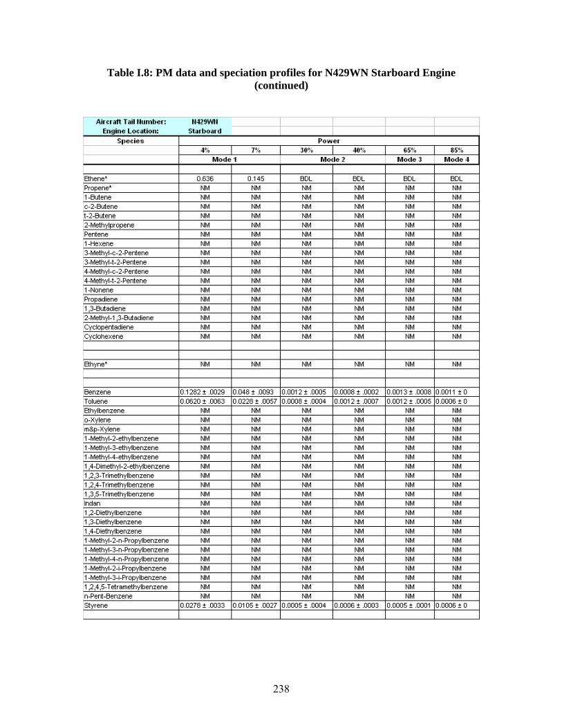
Aircraft Tail ttumber: 11429Wll I I Engine Location: Starboard I I

S1>ecies Power 4% I 7% 30% I 40% 65% 85%

Mode1 I Mode 2 I Mode 3 Mode4

Ethene* 0.636 0.145 BDL BDL BDL BDL Propene* NM NM NM NM NM NM 1-Butene NM NM NM NM NM NM c-2-Butene NM NM NM NM NM NM 1-2-Butene NM NM NM NM NM NM 2-Methylpropene NM NM NM NM NM NM Pentene NM NM NM NM NM NM 1-Hexene NM NM NM NM NM NM 3-Methyl-c-2-Pentene NM NM NM NM NM NM 3-Methyl-1-2-Pentene NM NM NM NM NM NM 4-Methyl-c-2-Pentene NM NM NM NM NM NM 4-Methyl-1-2-Pentene NM NM NM NM NM NM 1-Nonene NM NM NM NM NM NM Propadiene NM NM NM NM NM NM 1 ,3-Butadiene NM NM NM NM NM NM 2-Melhyl-1,3-Butadiene NM NM NM NM NM NM Cyclopentadiene NM NM NM NM NM NM Cyclohexene NM NM NM NM NM NM

Ethyne* NM NM NM NM NM NM

Benzene 0.1282 • .0029 0.048 • .0093 0.0012 • .0005 0.0008 • .0002 0.0013 • .0008 0.0011 • 0 Toluene 0.0620 t .0063 0.0228 t .0057 0.0008 t .0004 0.0012 t .0007 0.0012 t .0005 0.0006 t 0 Ethylbenzene NM NM NM NM NM NM o-Xylene NM NM NM NM NM NM m&p-Xylene NM NM NM NM NM NM 1-Methyl-2-elhylbenzene NM NM NM NM NM NM 1-Methyl-3-ethylbenzene NM NM NM NM NM NM 1-Methyl-4-elhylbenzene NM NM NM NM NM NM 1,4-Dimethyl-2-elhylbenzene NM NM NM NM NM NM 1,2,3-Trimethylbenzene NM NM NM NM NM NM 1,2,4-Trimethylbenzene NM NM NM NM NM NM 1,3,5-Trimethylbenzene NM NM NM NM NM NM lndan NM NM NM NM NM NM 1,2-Diethylbenzene NM NM NM NM NM NM 1 ,3-Diethylbenzene NM NM NM NM NM NM 1,4-Diethylbenzene NM NM NM NM NM NM 1-Methyl-2-n-Propylbenzene NM NM NM NM NM NM 1-Methyl-3-n-Propylbenzene NM NM NM NM NM NM 1-Methyl-4-n-Propylbenzene NM NM NM NM NM NM 1-Methyl-2-i-Propylbenzene NM NM NM NM NM NM 1-Methyl-3-i-Propylbenzene NM NM NM NM NM NM 1 ,2,4 ,5-T etramethylbenzene NM NM NM NM NM NM n-Pent-Benzene NM NM NM NM NM NM styrene 0.0278 t .0033 0.0105 t .0027 0.0005 t .0004 0.0006 t .0003 0.0005 t .0001 0.0006 t 0

Table I.8: PM data and speciation profiles for N429WN Starboard Engine (continued)

238

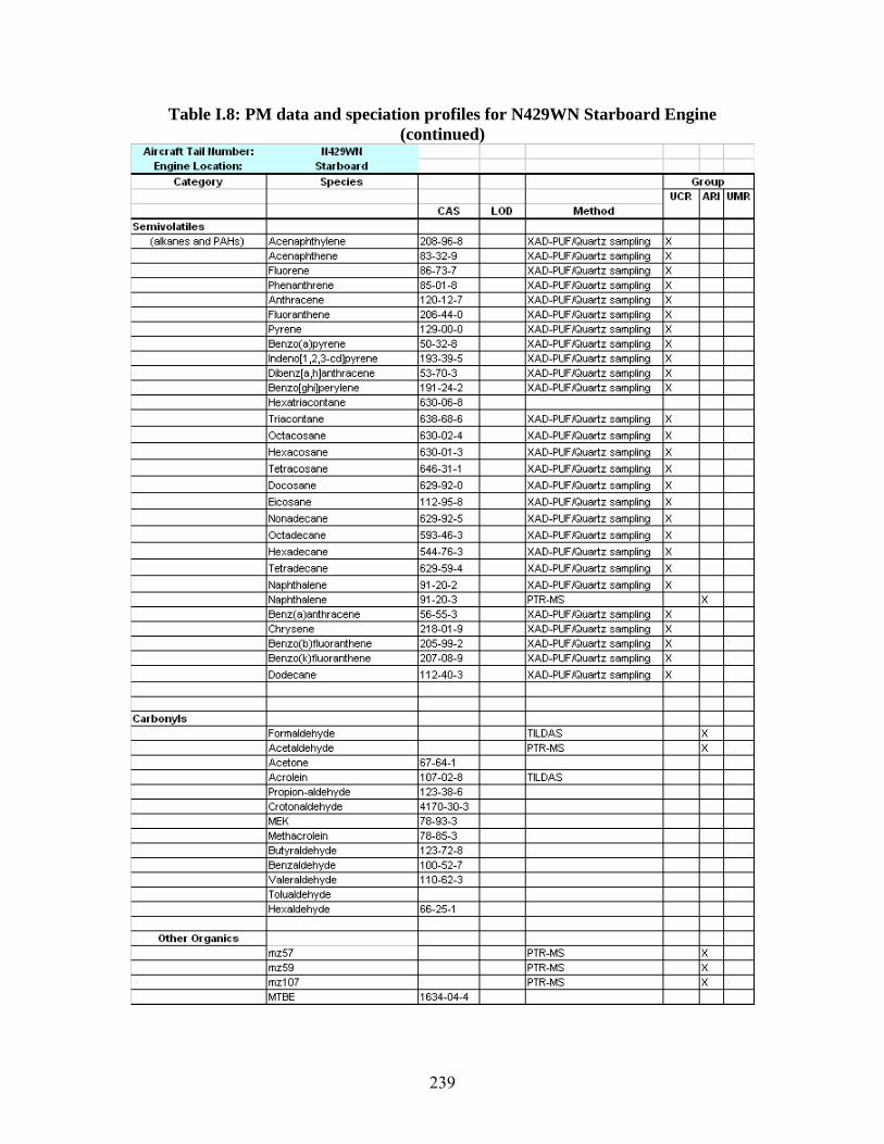
Aircraft Tail ttumber: 11429WII I Engine Location: Starboard I

Category S1>ecies Grou1> UCR ARI UMR

CAS LOD Method Semivolatiles

(alkanes and PAHs) Acenaphthylene 208-96-8 XAD-PUF /Quartz sampling X Acenaphlhene 83-32-9 XAD-PUF /Quartz sampling X Fluorene 86-73-7 XAD-PUF /Quartz sampling X Phenanthrene 85-01-8 XAD-PUF /Quartz sampling X Anthracene 120-12-7 XAD-PUF /Quartz sampling X Fluoranthene 206-44-0 XAD-PUF /Quartz sampling X Pyrene 129-00-0 XAD-PUF /Quartz sampling X Benzo(a)pyrene 50-32-8 XAD-PUF /Quartz sampling X lndeno[1,2,3-cd)pyrene 193-39-5 XAD-PUF /Quartz sampling X Dibenz[a,h]anthracene 53-70-3 XAD-PUF /Quartz sampling X Benzo[ghi]perylene 191-24-2 XAD-PUF /Quartz sampling X Hexatriacontane 630-06-8

Triacontane 638-68-6 XAD-PUF /Quartz sampling X Octacosane 630-02-4 XAD-PUF /Quartz sampling X Hexacosane 630-01-3 XAD-PUF /Quartz sampling X T etracosane 646-31-1 XAD-PUF /Quartz sampling X Docosane 629-92-0 XAD-PUF /Quartz sampling X

Eicosane 112-95-8 XAD-PUF /Quartz sampling X Nonadecane 629-92-5 XAD-PUF /Quartz sampling X Octadecane 593-46-3 XAD-PUF /Quartz sampling X Hexadecane 544-76-3 XAD-PUF /Quartz sampling X T etradecane 629-59-4 XAD-PUF /Quartz sampling X Naphthalene 91-20-2 XAD-PUF /Quartz sampling X Naphthalene 91-20-3 PTR-MS X Benz( a)anthracene 56-55-3 XAD-PUF /Quartz sampling X Chrysene 218-01-9 XAD-PUF /Quartz sampling X Benzo(b )fluoranthene 205-99-2 XAD-PUF /Quartz sampling X Benzo(k)fluoranthene 207-08-9 XAD-PUF /Quartz sampling X Dodecane 112-40-3 XAD-PUF /Quartz sampling X

Carbonyls Formaldehyde TILDAS X Acelaldehyde PTR-MS X Acetone 67-64-1 Acrolein 107-02-8 TILDAS Propion-aldehyde 123-38-6 Crotonaldehyde 4170-30-3 MEK 78-93-3 Methacrolein 78-85-3 But yr aldehyde 123-72-8 Benz aldehyde 100-52-7 Valeraldehyde 110-62-3 T olualdehyde Hex aldehyde 66-25-1

Other Organics mz57 PTR-MS X mz59 PTR-MS X mz107 PTR-MS X MTBE 1634-04-4

Table I.8: PM data and speciation profiles for N429WN Starboard Engine (continued)

239

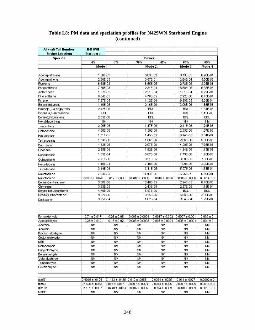
Aircraft Tail ttumber: 11429Wll I I Engine Location: Starboard I I

S1>ecie s Power 4% I 7% 30% I 40% 65% 85%

Mode 1 I Mode 2 I Mode 3 Mode 4 I I

Acenaphthylene 1.56E-03 3.83E-02 3.73E-05 6.90E-04 Acenaphthene 2.38E-03 3.87E-01 2.64E-04 5.30E-03 Fluorene 6.68E-03 6.55E-05 2.78E-05 2.03E-05 Phenanthrene 7.80E-03 2.31E-04 8.68E-05 6.38E-05 Anthracene 1.07E-02 2.21E-04 1.51E-04 3.22E-04 Fluoranthene 6.34E-05 4.70E-05 2.92E-06 8.43E-04 Pyrene 7.37E-05 1.12E-04 9.38E-05 5.03E-04 Benzo(a)pyrene 1.10E-05 2.16E-06 3.06E-06 1.66E-05 lndeno[1,2,3-cd)pyrene 2.42E-06 BDL BDL 1.34E-05 Dibenz[a,h]anthracene BDL BDL BDL 1.13E-05 Benzo[ghi)perylene 2.55E-06 BDL BDL BDL Hexatriacontane NM NM NM NM

Triacontane 2.26E-06 1.47E-06 2.11E-06 1.21E-05

Octacosane 4.36E-06 1.59E-06 2.55E-06 1.07E-05

Hexacosane 1.31E-05 1.45E-05 6.14E-05 2.64E-04

T etracosane 1.84E-06 1.86E-06 2.66E-06 5.96E-06

Docosane 1.52E-06 2.07E-06 4.20E-06 7.36E-06

Eicosane 2.35E-06 1.92E-06 4.34E-06 1.12E-05

Nonadecane 1.53E-04 6.87E-06 7.79E-06 1.78E-05

Octadecane 7.21E-06 3.31E-05 3.50E-05 7.65E-05

Hexadecane 1.19E-04 7.40E-06 1.09E-05 3.02E-05

T etradecane 3.14E-06 3.41E-05 5.27E-05 1.78E-04

Naphthalene 7.53E-03 1.90E•00 6.26E-01 6.85E-01 Naphthalene 0.0369 ± .0028 I 0.D12 ± .0008 0.0018 ± .0006 I 0.0016 ± .0006 0.0015 ± .0006 0.0014 ± 0 Benz( a)anthracene 3.00E-06 2.40E-05 2.24E-05 6.40E-05 Chrysene 3.83E-05 2.43E-05 2.27E-05 1.12E-04 Benzo(b )fluoranthene 4.78E-06 5.57E-06 BDL BDL Benzo(k)fluorantene 9.97E-06 9.15E-06 5.64E-06 3.99E-05

Dodecane 3.95E-04 1.82E-04 3.34E-04 1.20E-04

Formaldehyde 0.74 ± 0.017 0.28 ± 0.05 0.003 ± 0.0008 0.0017 ± 0.002 0.0007 ± 0.001 0.002 ± 0 Acelaldehyde 0.35 ± 0.012 0.13 ± 0.02 0.003 ± 0.0008 0.003 ± 0.0004 0.003 ± 0.0004 0.004 ± 0 Acetone NM NM NM NM NM NM Acrolein NM NM NM NM NM NM Propion-aldehyde NM NM NM NM NM NM Crotonaldehyde NM NM NM NM NM NM MEK NM NM NM NM NM NM Methacrolein NM NM NM NM NM NM But yr aldehyde NM NM NM NM NM NM Benz aldehyde NM NM NM NM NM NM Valeraldehyde NM NM NM NM NM NM T olualdehyde NM NM NM NM NM NM Hex aldehyde NM NM NM NM NM NM

mz57 0.4015 ± .0104 0.1433 ± .0455 0.010 ± .0058 0.0094 ± .0025 0.011 ± .0027 0.0092 ± 0 mz59 0.1596 ± .0083 0.053± .0077 0.0017 ± .0004 0.0014 ± .0005 0.0017 ± .0005 0.0016 ± 0 mz107 0.1191 ± .0087 0.0440 ± .0103 0.0016 ± .0006 0.0014 ± .0009 0.0018 ± .0009 0.0015 ± 0 MTBE NM NM NM NM NM NM

Table I.8: PM data and speciation profiles for N429WN Starboard Engine (continued)

240

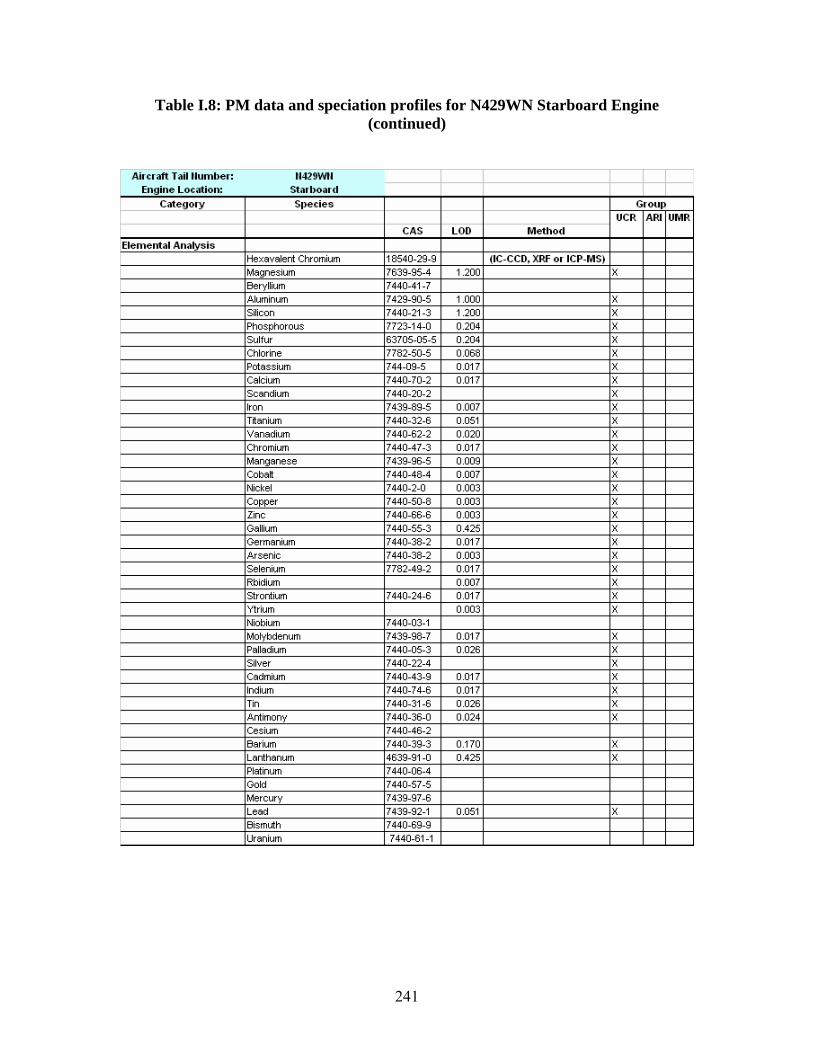
Aircraft Tail ttumber: 11429Wll I Engine Location: Starboard I

Category S1>ecies Grou1> UCR ARI UMR

CAS LOD Method Elemental Analysis

Hexavalent Chromium 18540-29-9 (IC-CCD, XRF or ICP-MS) Magnesium 7639-95-4 1.200 X Beryllium 7440-41-7

Aluminum 7429-90-5 1.000 X Silicon 7440-21-3 1.200 X Phosphorous 7723-14-0 0.204 X Sulfur 63705-05-5 0.204 X Chlorine 7782-50-5 0.068 X Potassium 744-09-5 0.017 X Calcium 7440-70-2 0.017 X Scandium 7440-20-2 X Iron 7439-89-5 0.007 X Titanium 7440-32-6 0.051 X Vanadium 7440-62-2 0.020 X Chromium 7440-47-3 0.017 X Manganese 7439-96-5 0.009 X Cobalt 7440-48-4 0.007 X Nickel 7440-2-0 0.003 X Copper 7440-50-8 0.003 X Zinc 7440-66-6 0.003 X Gallium 7440-55-3 0.425 X Germanium 7440-38-2 0.017 X Arsenic 7440-38-2 0.003 X Selenium 7782-49-2 0.017 X Rbidium 0.007 X strontium 7440-24-6 0.017 X Ytrium 0.003 X Niobium 7440-03-1 Molybdenum 7439-98-7 0.017 X Palladium 7440-05-3 0.Q26 X Silver 7440-22-4 X Cadmium 7440-43-9 0.017 X Indium 7440-74-6 0.017 X Tin 7440-31-6 0.□26 X Antimony 7440-36-0 0.024 X Cesium 7440-46-2 Barium 7440-39-3 0.170 X Lanthanum 4639-91-0 0.425 X Platinum 7440-06-4

Gold 7440-57-5 Mercury 7439-97-6

Lead 7439-92-1 0.051 X Bismuth 7440-69-9

Uranium 7440-61-1

Table I.8: PM data and speciation profiles for N429WN Starboard Engine (continued)

241

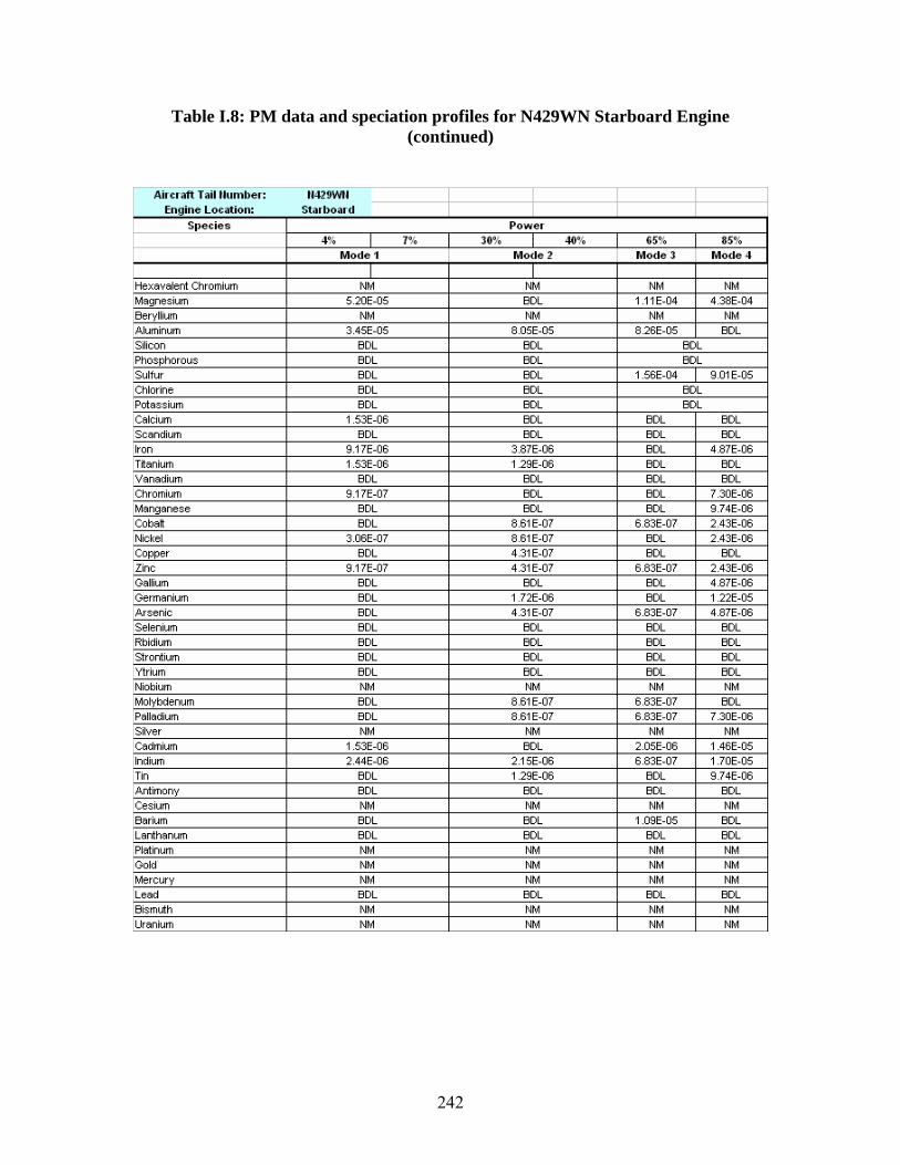
Aircraft Tail ttumber: 11429Wll I I Engine Location: Starboard I I

S1>ecie s Power 4% I 7% 30% I 40% 65% 85%

Mode 1 I Mode 2 I Mode 3 Mode 4 I I

Hexavalent Chromium NM NM NM NM Magnesium 5.20E-05 BDL 1.11E-04 4.38E-04 Beryllium NM NM NM NM Aluminum 3.45E-05 8.0SE-05 8.26E-05 BDL Silicon BDL BDL BDL Phosphorous BDL BDL BDL Sulfur BDL BDL 1.SSE-04 I 9.01E-05 Chlorine BDL BDL BDL Potassium BDL BDL BDL Calcium 1.53E-06 BDL BDL BDL Scandium BDL BDL BDL BDL Iron 9.17E-06 3.87E-06 BDL 4.87E-06

Titanium 1.53E-06 1.29E-06 BDL BDL Vanadium BDL BDL BDL BDL Chromium 9.17E-07 BDL BDL 7.30E-06 Manganese BDL BDL BDL 9.74E-06

Cobalt BDL 8.61E-07 6.83E-07 2.43E-06 Nickel 3.0SE-07 8.61E-07 BDL 2.43E-06 Copper BDL 4.31E-07 BDL BDL Zinc 9.17E-07 4.31E-07 6.83E-07 2.43E-06

Gallium BDL BDL BDL 4.87E-06 Germanium BDL 1.72E-06 BDL 1.22E-05 Arsenic BDL 4.31E-07 6.83E-07 4.87E-06 Selenium BDL BDL BDL BDL Rbidium BDL BDL BDL BDL strontium BDL BDL BDL BDL Ytrium BDL BDL BDL BDL Niobium NM NM NM NM Molybdenum BDL 8.61E-07 6.83E-07 BDL Palladium BDL 8.61E-07 6.83E-07 7.30E-06 Silver NM NM NM NM Cadmium 1.53E-06 BDL 2.0SE-06 1.46E-05

Indium 2.44E-06 2.15E-06 6.83E-07 1.70E-05 Tin BDL 1.29E-06 BDL 9.74E-06 Antimony BDL BDL BDL BDL Cesium NM NM NM NM Barium BDL BDL 1.0SE-05 BDL Lanthanum BDL BDL BDL BDL Platinum NM NM NM NM Gold NM NM NM NM Mercury NM NM NM NM Lead BDL BDL BDL BDL Bismuth NM NM NM NM Uranium NM NM NM NM

Table I.8: PM data and speciation profiles for N429WN Starboard Engine (continued)

242

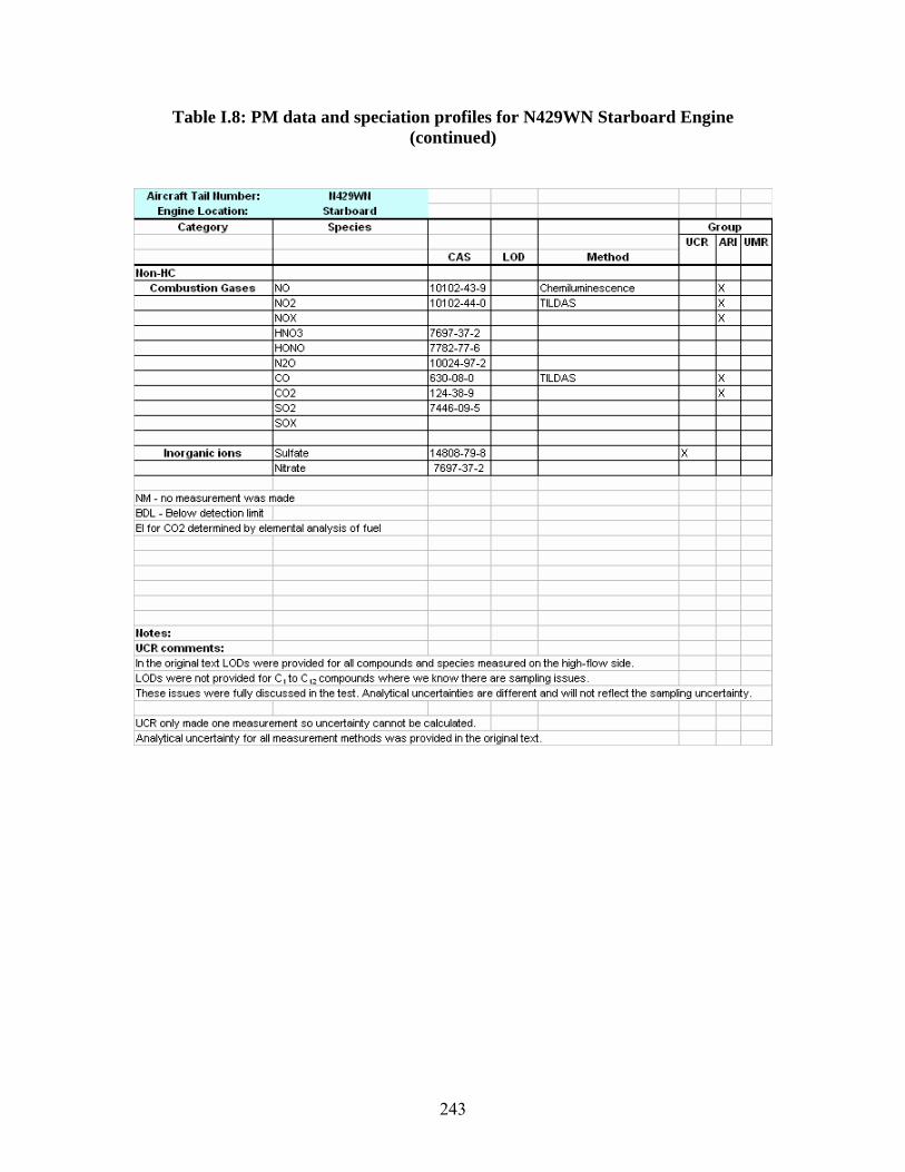
Aircraft Tail ttumber: 11429Wll I Engine Location: St arboard I

Category S1>ecies Grou1> UCR ARI UMR

CAS LOD Method llon-HC

Combustion Gases NO 10102-43-9 Chemiluminescence X NO2 10102-44-0 TILDAS X NOX X HNO3 7697-37-2 HONO 7782-77-6 N2O 10024-97-2 co 630-08-0 TILDAS X CO2 124-38-9 X SO2 7446-09-5 SOX

Inorganic ions Sulfale 14808-79-8 X Nltrale 7697-37-2

NM - no measurement was made BOL - Below detection limit El for CO2 determined by elemental analysis of fuel

Uotes: UCR comments: In the original text LOOs were provided for all compounds and species measured on the high-flow side. LOOs were not provided for C I to C 1z compounds where we know there are sampling issues. These issues were fully discussed in the test. Analytical uncertainties are different and will not reflect the sampling uncertainty.

I UCR only made one measurement so uncertainty cannot be calculated. I Analytical uncertainty for all measurement methods was provided in the original text.

Table I.8: PM data and speciation profiles for N429WN Starboard Engine (continued)

243

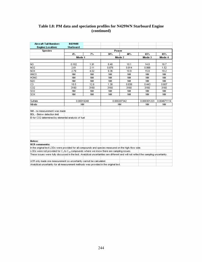
Aircraft Tail ttumber: 11429Wll I I Engine Location: St arboard I I

S1>ecies Power 4% I 7% 30% I 40% 65% 85%

Mode 1 I Mode 2 I Mode 3 Mode 4

NO 0.182 1.91 8.48 10.1 14.8 16.7 N02 2.61 2.11 0.876 0.814 0.998 1.52 NOX 2.79 4.02 9.36 10.9 15.8 18.2 HN03 NM NM NM NM NM NM HONO NM NM NM NM NM NM N20 NM NM NM NM NM NM co 18.5 12.6 1.38 0.838 0.443 0.607 CO2 3160 3160 3160 3160 3160 3160 S02 NM NM NM NM NM NM SOX NM NM NM NM NM NM

Sulfate 0.00019248 0.000207342 0.000301223 o.004671114 I Nitrate NM NM NM NM

NM - no measurement was made BOL - Below detection limit El for CO2 determined by elemental analysis of fuel

Uotes: UCR comments: In the original text LOOs were provided for all compounds and species measured on the high-flow side. LOOs were not provided for C I to C ,z compounds where we know there are sampling issues. These issues were fully discussed in the test. Analytical uncertainties are different and will not reflect the sampling uncertainty.

I I UCR only made one measurement so uncertainty cannot be calculated. I Analytical uncertainty for all measurement methods was provided in the original text.

Table I.8: PM data and speciation profiles for N429WN Starboard Engine (continued)

244