Ultrasonic Tissue CharacterizationUsing Neural NetworksMaurice S. klein GebbinckNovember 4, 1992

AbstractUltrasonic tissue characterization is a technique where on the basis of pa-rameters that have been acquired using ultrasound it is tried to derive someproperties of the tissue under observation. At the Biophysics Laboratory of theInstitute of Opthalmology at the Academic Hospital Nijmegen the applicabilityof this technique for the diagnosis of di�use liver diseases is investigated.An important component of a diagnostic system is the algorithm that clas-si�es the patients into one of the to be discriminated groups. Uptil now dis-criminant analysis, which is a statistical method, has been used as classi�er,but neural networks are known to perform this task also very well. In thisthesis two types of neural networks, back-propagation and feature mapping,are investigated with regard to their classifying capabilities. It is shown thatwith back-propgagation better results can be achieved than with discriminantanalysis.One of the problems when dealing with neural networks is that the dataset containing patients whose disease has already been diagnosed must be su�-ciently large. Another topic of this thesis therefore is the generation of arti�cialdata based on the original patients.

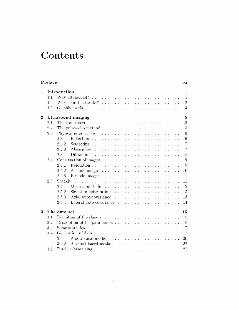
ContentsPreface xi1 Introduction 11.1 Why ultrasound? : : : : : : : : : : : : : : : : : : : : : : : : : : : 11.2 Why neural networks? : : : : : : : : : : : : : : : : : : : : : : : : 21.3 On this thesis : : : : : : : : : : : : : : : : : : : : : : : : : : : : : 32 Ultrasound imaging 52.1 The transducer : : : : : : : : : : : : : : : : : : : : : : : : : : : : 52.2 The pulse-echo method : : : : : : : : : : : : : : : : : : : : : : : : 52.3 Physical interactions : : : : : : : : : : : : : : : : : : : : : : : : : 62.3.1 Re ection : : : : : : : : : : : : : : : : : : : : : : : : : : : 62.3.2 Scattering : : : : : : : : : : : : : : : : : : : : : : : : : : : 72.3.3 Absorption : : : : : : : : : : : : : : : : : : : : : : : : : : 72.3.4 Di�raction : : : : : : : : : : : : : : : : : : : : : : : : : : 82.4 Construction of images : : : : : : : : : : : : : : : : : : : : : : : : 92.4.1 Resolution : : : : : : : : : : : : : : : : : : : : : : : : : : : 92.4.2 A-mode images : : : : : : : : : : : : : : : : : : : : : : : : 102.4.3 B-mode images : : : : : : : : : : : : : : : : : : : : : : : : 112.5 Speckle : : : : : : : : : : : : : : : : : : : : : : : : : : : : : : : : 112.5.1 Mean amplitude : : : : : : : : : : : : : : : : : : : : : : : 122.5.2 Signal-to-noise ratio : : : : : : : : : : : : : : : : : : : : : 132.5.3 Axial auto-covariance : : : : : : : : : : : : : : : : : : : : 132.5.4 Lateral auto-covariance : : : : : : : : : : : : : : : : : : : 143 The data set 153.1 De�nition of the classes : : : : : : : : : : : : : : : : : : : : : : : 153.2 Description of the parameters : : : : : : : : : : : : : : : : : : : : 153.3 Some statistics : : : : : : : : : : : : : : : : : : : : : : : : : : : : 173.4 Generation of data : : : : : : : : : : : : : : : : : : : : : : : : : : 173.4.1 A statistical method : : : : : : : : : : : : : : : : : : : : : 203.4.2 A kernel based method : : : : : : : : : : : : : : : : : : : 223.5 Further formatting : : : : : : : : : : : : : : : : : : : : : : : : : : 27i

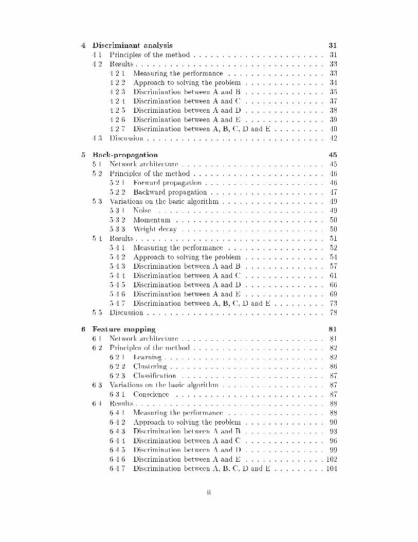
4 Discriminant analysis 314.1 Principles of the method : : : : : : : : : : : : : : : : : : : : : : : 314.2 Results : : : : : : : : : : : : : : : : : : : : : : : : : : : : : : : : : 334.2.1 Measuring the performance : : : : : : : : : : : : : : : : : 334.2.2 Approach to solving the problem : : : : : : : : : : : : : : 344.2.3 Discrimination between A and B : : : : : : : : : : : : : : 354.2.4 Discrimination between A and C : : : : : : : : : : : : : : 374.2.5 Discrimination between A and D : : : : : : : : : : : : : : 384.2.6 Discrimination between A and E : : : : : : : : : : : : : : 394.2.7 Discrimination between A, B, C, D and E : : : : : : : : : 404.3 Discussion : : : : : : : : : : : : : : : : : : : : : : : : : : : : : : : 425 Back-propagation 455.1 Network architecture : : : : : : : : : : : : : : : : : : : : : : : : : 455.2 Principles of the method : : : : : : : : : : : : : : : : : : : : : : : 465.2.1 Forward propagation : : : : : : : : : : : : : : : : : : : : : 465.2.2 Backward propagation : : : : : : : : : : : : : : : : : : : : 475.3 Variations on the basic algorithm : : : : : : : : : : : : : : : : : : 495.3.1 Noise : : : : : : : : : : : : : : : : : : : : : : : : : : : : : 495.3.2 Momentum : : : : : : : : : : : : : : : : : : : : : : : : : : 505.3.3 Weight decay : : : : : : : : : : : : : : : : : : : : : : : : : 505.4 Results : : : : : : : : : : : : : : : : : : : : : : : : : : : : : : : : : 515.4.1 Measuring the performance : : : : : : : : : : : : : : : : : 525.4.2 Approach to solving the problem : : : : : : : : : : : : : : 545.4.3 Discrimination between A and B : : : : : : : : : : : : : : 575.4.4 Discrimination between A and C : : : : : : : : : : : : : : 615.4.5 Discrimination between A and D : : : : : : : : : : : : : : 665.4.6 Discrimination between A and E : : : : : : : : : : : : : : 695.4.7 Discrimination between A, B, C, D and E : : : : : : : : : 735.5 Discussion : : : : : : : : : : : : : : : : : : : : : : : : : : : : : : : 786 Feature mapping 816.1 Network architecture : : : : : : : : : : : : : : : : : : : : : : : : : 816.2 Principles of the method : : : : : : : : : : : : : : : : : : : : : : : 826.2.1 Learning : : : : : : : : : : : : : : : : : : : : : : : : : : : : 826.2.2 Clustering : : : : : : : : : : : : : : : : : : : : : : : : : : : 866.2.3 Classi�cation : : : : : : : : : : : : : : : : : : : : : : : : : 876.3 Variations on the basic algorithm : : : : : : : : : : : : : : : : : : 876.3.1 Conscience : : : : : : : : : : : : : : : : : : : : : : : : : : 876.4 Results : : : : : : : : : : : : : : : : : : : : : : : : : : : : : : : : : 886.4.1 Measuring the performance : : : : : : : : : : : : : : : : : 886.4.2 Approach to solving the problem : : : : : : : : : : : : : : 906.4.3 Discrimination between A and B : : : : : : : : : : : : : : 936.4.4 Discrimination between A and C : : : : : : : : : : : : : : 966.4.5 Discrimination between A and D : : : : : : : : : : : : : : 996.4.6 Discrimination between A and E : : : : : : : : : : : : : : 1026.4.7 Discrimination between A, B, C, D and E : : : : : : : : : 104ii

6.5 Discussion : : : : : : : : : : : : : : : : : : : : : : : : : : : : : : : 1087 Conclusions 1137.1 Applicability of UTC on our data : : : : : : : : : : : : : : : : : : 1137.2 Comparison of the investigated methods : : : : : : : : : : : : : : 1157.3 Suggestions for future research : : : : : : : : : : : : : : : : : : : 116A Software 121B Erratum 141

iii

iv

List of Tables2.1 Acoustical impedance for several materials : : : : : : : : : : : : : 62.2 Axial resolution and penetration depth : : : : : : : : : : : : : : : 103.1 Estimated mean, standard deviation and correlation for class A : 183.2 Estimated mean, standard deviation and correlation for class B : 183.3 Estimated mean, standard deviation and correlation for class C : 183.4 Estimated mean, standard deviation and correlation for class D : 183.5 Estimated mean, standard deviation and correlation for class E : 183.6 New statistics of class A using the statistical method : : : : : : : 233.7 New statistics of class B using the statistical method : : : : : : : 233.8 New statistics of class C using the statistical method : : : : : : : 233.9 New statistics of class D using the statistical method : : : : : : : 233.10 New statistics of class E using the statistical method : : : : : : : 233.11 New statistics of class A using the kernel based method : : : : : 283.12 New statistics of class B using the kernel based method : : : : : 283.13 New statistics of class C using the kernel based method : : : : : 283.14 New statistics of class D using the kernel based method : : : : : 283.15 New statistics of class E using the kernel based method : : : : : 287.1 Comparison of the performance for the di�erent methods : : : : 115B.1 New statistics of class A using the corrected kernel based method 142B.2 New statistics of class B using the corrected kernel based method 142B.3 New statistics of class C using the corrected kernel based method 142B.4 New statistics of class D using the corrected kernel based method 142B.5 New statistics of class E using the corrected kernel based method 142v

vi

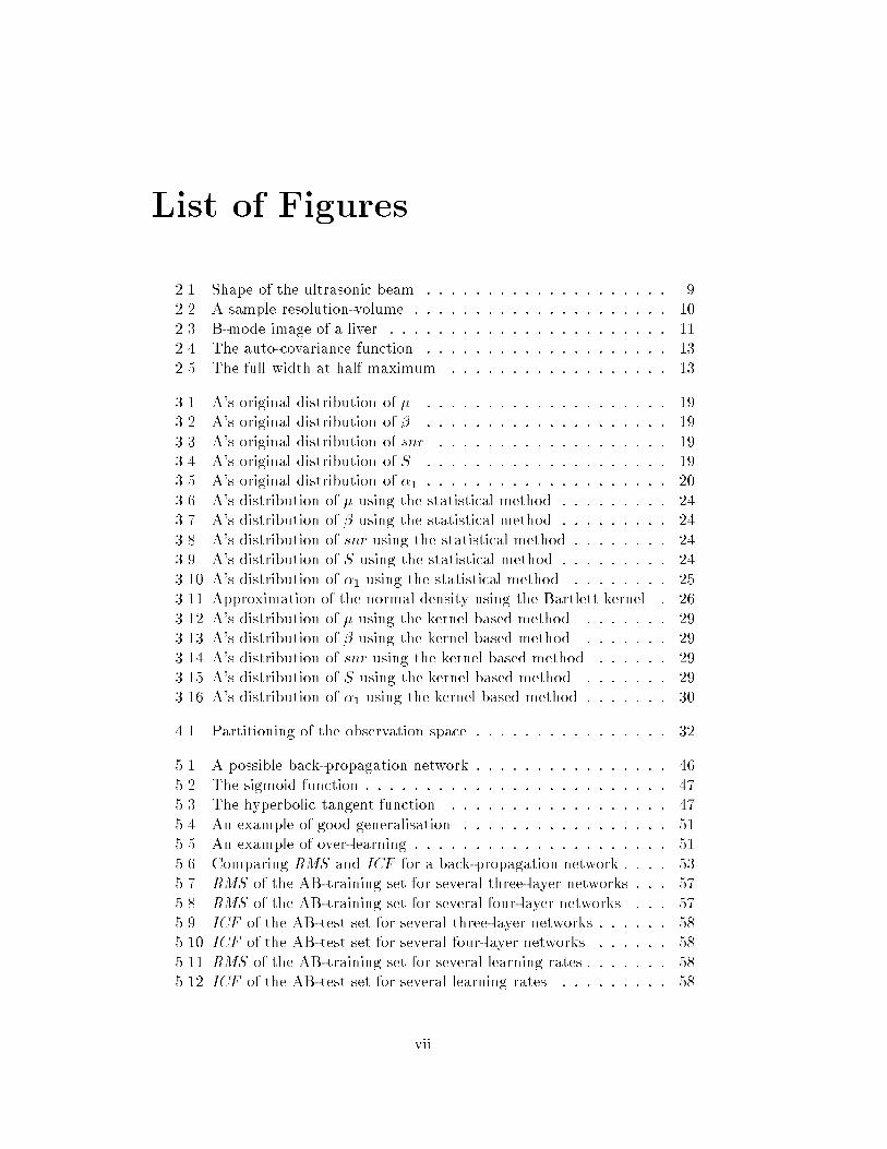
List of Figures2.1 Shape of the ultrasonic beam : : : : : : : : : : : : : : : : : : : : 92.2 A sample resolution-volume : : : : : : : : : : : : : : : : : : : : : 102.3 B-mode image of a liver : : : : : : : : : : : : : : : : : : : : : : : 112.4 The auto-covariance function : : : : : : : : : : : : : : : : : : : : 132.5 The full width at half maximum : : : : : : : : : : : : : : : : : : 133.1 A's original distribution of � : : : : : : : : : : : : : : : : : : : : 193.2 A's original distribution of � : : : : : : : : : : : : : : : : : : : : 193.3 A's original distribution of snr : : : : : : : : : : : : : : : : : : : 193.4 A's original distribution of S : : : : : : : : : : : : : : : : : : : : 193.5 A's original distribution of �1 : : : : : : : : : : : : : : : : : : : : 203.6 A's distribution of � using the statistical method : : : : : : : : : 243.7 A's distribution of � using the statistical method : : : : : : : : : 243.8 A's distribution of snr using the statistical method : : : : : : : : 243.9 A's distribution of S using the statistical method : : : : : : : : : 243.10 A's distribution of �1 using the statistical method : : : : : : : : 253.11 Approximation of the normal density using the Bartlett kernel : 263.12 A's distribution of � using the kernel based method : : : : : : : 293.13 A's distribution of � using the kernel based method : : : : : : : 293.14 A's distribution of snr using the kernel based method : : : : : : 293.15 A's distribution of S using the kernel based method : : : : : : : 293.16 A's distribution of �1 using the kernel based method : : : : : : : 304.1 Partitioning of the observation space : : : : : : : : : : : : : : : : 325.1 A possible back-propagation network : : : : : : : : : : : : : : : : 465.2 The sigmoid function : : : : : : : : : : : : : : : : : : : : : : : : : 475.3 The hyperbolic tangent function : : : : : : : : : : : : : : : : : : 475.4 An example of good generalisation : : : : : : : : : : : : : : : : : 515.5 An example of over-learning : : : : : : : : : : : : : : : : : : : : : 515.6 Comparing RMS and ICF for a back-propagation network : : : : 535.7 RMS of the AB-training set for several three-layer networks : : : 575.8 RMS of the AB-training set for several four-layer networks : : : 575.9 ICF of the AB-test set for several three-layer networks : : : : : : 585.10 ICF of the AB-test set for several four-layer networks : : : : : : 585.11 RMS of the AB-training set for several learning rates : : : : : : : 585.12 ICF of the AB-test set for several learning rates : : : : : : : : : 58vii

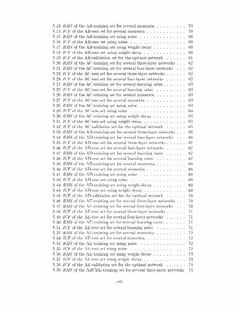
5.13 RMS of the AB-training set for several momenta : : : : : : : : : 595.14 ICF of the AB-test set for several momenta : : : : : : : : : : : : 595.15 RMS of the AB-training set using noise : : : : : : : : : : : : : : 605.16 ICF of the AB-test set using noise : : : : : : : : : : : : : : : : : 605.17 RMS of the AB-training set using weight decay : : : : : : : : : : 605.18 ICF of the AB-test set using weight decay : : : : : : : : : : : : : 605.19 ICF of the AB-validation set for the optimal network : : : : : : 615.20 RMS of the AC-training set for several three-layer networks : : : 625.21 RMS of the AC-training set for several four-layer networks : : : 625.22 ICF of the AC-test set for several three-layer networks : : : : : : 625.23 ICF of the AC-test set for several four-layer networks : : : : : : 625.24 RMS of the AC-training set for several learning rates : : : : : : : 635.25 ICF of the AC-test set for several learning rates : : : : : : : : : 635.26 RMS of the AC-training set for several momenta : : : : : : : : : 635.27 ICF of the AC-test set for several momenta : : : : : : : : : : : : 635.28 RMS of the AC-training set using noise : : : : : : : : : : : : : : 645.29 ICF of the AC-test set using noise : : : : : : : : : : : : : : : : : 645.30 RMS of the AC-training set using weight decay : : : : : : : : : : 655.31 ICF of the AC-test set using weight decay : : : : : : : : : : : : : 655.32 ICF of the AC-validation set for the optimal network : : : : : : 655.33 RMS of the AD-training set for several three-layer networks : : : 665.34 RMS of the AD-training set for several four-layer networks : : : 665.35 ICF of the AD-test set for several three-layer networks : : : : : : 675.36 ICF of the AD-test set for several four-layer networks : : : : : : 675.37 RMS of the AD-training set for several learning rates : : : : : : 675.38 ICF of the AD-test set for several learning rates : : : : : : : : : 675.39 RMS of the AD-training set for several momenta : : : : : : : : : 685.40 ICF of the AD-test set for several momenta : : : : : : : : : : : : 685.41 RMS of the AD-training set using noise : : : : : : : : : : : : : : 685.42 ICF of the AD-test set using noise : : : : : : : : : : : : : : : : : 685.43 RMS of the AD-training set using weight decay : : : : : : : : : : 695.44 ICF of the AD-test set using weight decay : : : : : : : : : : : : : 695.45 ICF of the AD-validation set for the optimal network : : : : : : 705.46 RMS of the AE-training set for several three-layer networks : : : 705.47 RMS of the AE-training set for several four-layer networks : : : 705.48 ICF of the AE-test set for several three-layer networks : : : : : : 715.49 ICF of the AE-test set for several four-layer networks : : : : : : 715.50 RMS of the AE-training set for several learning rates : : : : : : : 715.51 ICF of the AE-test set for several learning rates : : : : : : : : : 715.52 RMS of the AE-training set for several momenta : : : : : : : : : 725.53 ICF of the AE-test set for several momenta : : : : : : : : : : : : 725.54 RMS of the AE-training set using noise : : : : : : : : : : : : : : 725.55 ICF of the AE-test set using noise : : : : : : : : : : : : : : : : : 725.56 RMS of the AE-training set using weight decay : : : : : : : : : : 735.57 ICF of the AE-test set using weight decay : : : : : : : : : : : : : 735.58 ICF of the AE-validation set for the optimal network : : : : : : 745.59 RMS of the ABCDE-training set for several three-layer networks 74viii

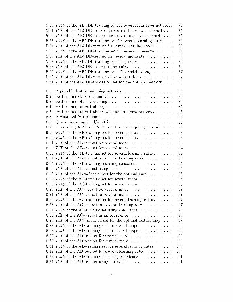
5.60 RMS of the ABCDE-training set for several four-layer networks : 745.61 ICF of the ABCDE-test set for several three-layer networks : : : 755.62 ICF of the ABCDE-test set for several four-layer networks : : : : 755.63 RMS of the ABCDE-training set for several learning rates : : : : 755.64 ICF of the ABCDE-test set for several learning rates : : : : : : : 755.65 RMS of the ABCDE-training set for several momenta : : : : : : 765.66 ICF of the ABCDE-test set for several momenta : : : : : : : : : 765.67 RMS of the ABCDE-training set using noise : : : : : : : : : : : 765.68 ICF of the ABCDE-test set using noise : : : : : : : : : : : : : : 765.69 RMS of the ABCDE-training set using weight decay : : : : : : : 775.70 ICF of the ABCDE-test set using weight decay : : : : : : : : : : 775.71 ICF of the ABCDE-validation set for the optimal network : : : : 786.1 A possible feature mapping network : : : : : : : : : : : : : : : : 826.2 Feature map before training : : : : : : : : : : : : : : : : : : : : : 856.3 Feature map during training : : : : : : : : : : : : : : : : : : : : : 856.4 Feature map after training : : : : : : : : : : : : : : : : : : : : : : 856.5 Feature map after training with non-uniform patterns : : : : : : 856.6 A clustered feature map : : : : : : : : : : : : : : : : : : : : : : : 866.7 Clustering using the U-matrix : : : : : : : : : : : : : : : : : : : : 866.8 Comparing RMS and ICF for a feature mapping network : : : : 906.9 RMS of the AB-training set for several maps : : : : : : : : : : : 936.10 RMS of the AB-training set for several maps : : : : : : : : : : : 936.11 ICF of the AB-test set for several maps : : : : : : : : : : : : : : 946.12 ICF of the AB-test set for several maps : : : : : : : : : : : : : : 946.13 RMS of the AB-training set for several learning rates : : : : : : : 946.14 ICF of the AB-test set for several learning rates : : : : : : : : : 946.15 RMS of the AB-training set using conscience : : : : : : : : : : : 956.16 ICF of the AB-test set using conscience : : : : : : : : : : : : : : 956.17 ICF of the AB-validation set for the optimal map : : : : : : : : 956.18 RMS of the AC-training set for several maps : : : : : : : : : : : 966.19 RMS of the AC-training set for several maps : : : : : : : : : : : 966.20 ICF of the AC-test set for several maps : : : : : : : : : : : : : : 976.21 ICF of the AC-test set for several maps : : : : : : : : : : : : : : 976.22 RMS of the AC-training set for several learning rates : : : : : : : 976.23 ICF of the AC-test set for several learning rates : : : : : : : : : 976.24 RMS of the AC-training set using conscience : : : : : : : : : : : 986.25 ICF of the AC-test set using conscience : : : : : : : : : : : : : : 986.26 ICF of the AC-validation set for the optimal feature map : : : : 986.27 RMS of the AD-training set for several maps : : : : : : : : : : : 996.28 RMS of the AD-training set for several maps : : : : : : : : : : : 996.29 ICF of the AD-test set for several maps : : : : : : : : : : : : : : 1006.30 ICF of the AD-test set for several maps : : : : : : : : : : : : : : 1006.31 RMS of the AD-training set for several learning rates : : : : : : 1006.32 ICF of the AD-test set for several learning rates : : : : : : : : : 1006.33 RMS of the AD-training set using conscience : : : : : : : : : : : 1016.34 ICF of the AD-test set using conscience : : : : : : : : : : : : : : 101ix

6.35 ICF of the AD-validation set for the optimal feature map : : : : 1016.36 RMS of the AE-training set for several maps : : : : : : : : : : : 1026.37 RMS of the AE-training set for several maps : : : : : : : : : : : 1026.38 ICF of the AE-test set for several maps : : : : : : : : : : : : : : 1036.39 ICF of the AE-test set for several maps : : : : : : : : : : : : : : 1036.40 RMS of the AE-training set for several learning rates : : : : : : : 1036.41 ICF of the AE-test set for several learning rates : : : : : : : : : 1036.42 RMS of the AE-training set using conscience : : : : : : : : : : : 1046.43 ICF of the AE-test set using conscience : : : : : : : : : : : : : : 1046.44 ICF of the AE-validation set for the optimal feature map : : : : 1056.45 RMS of the ABCDE-training set for several maps : : : : : : : : 1056.46 RMS of the ABCDE-training set for several maps : : : : : : : : 1056.47 ICF of the ABCDE-test set for several maps : : : : : : : : : : : 1066.48 ICF of the ABCDE-test set for several maps : : : : : : : : : : : 1066.49 RMS of the ABCDE-training set for several learning rates : : : : 1066.50 ICF of the ABCDE-test set for several learning rates : : : : : : : 1066.51 RMS of the ABCDE-training set using conscience : : : : : : : : 1076.52 ICF of the ABCDE-test set using conscience : : : : : : : : : : : 1076.53 ICF of the ABCDE-validation set for the optimal feature map : 1086.54 Distances between neurons for a 5x5 feature map : : : : : : : : : 109B.1 RMS of the corrected ABCDE-training set for back-propagation 143B.2 ICF of the corrected ABCDE-validation set for back-propagation 143B.3 RMS of the corrected ABCDE-training set for feature mapping : 144B.4 ICF of the corrected ABCDE-validation set for feature mapping 144

x

PrefaceThis report is the result of a project carried out in the period from Septem-ber 1991 to October 1992 in order to obtain a Master's Degree in ComputerScience. The project was a co-operation between the department of Real-TimeSystems of the faculty of Mathematics and Computer Science at the Universityof Nijmegen and the Biophysics Laboratory of the Institute of Opthalmologyat the Academic Hospital Nijmegen, under supervision of Theo Schouten andJohan Thijssen.First of all I want to express my special thanks to Hans Verhoeven, JohanThijssen and Theo Schouten, who were always willing to help me and werea source of inspiration. Furthermore I would like to thank Rien Cuypers forsharing his knowledge about SAS/STAT, Bernard Oosterveld for supplying theoriginal patient data, Harry Duys for providing me with additional compu-tational resources, Silvio Bierman for placing his Kohonen Neural NetworksSimulator at my disposal, Parcival Willems for installing the software xgraphand gspreview, and Edwin klein Gebbinck for his constructive comments onthis report. Last but not least I want to thank all members and students ofthe department of Real-Time Systems and the Biophysics Laboratory for thepleasant working atmosphere they created.Maurice S. klein GebbinckDepartment of Real-Time SystemsFaculty of Mathematics and Computer ScienceUniversity of Nijmegenxi

xii

Chapter 1IntroductionThis chapter provides a short introduction into the two main techniques onwhich this thesis is based. After that, the subject of the thesis is explained andits outline is given.1.1 Why ultrasound?Nowadays an clinician can apply several techniques to obtain information on apatient without having to operate on him. Each method has its pros and cons,some of which we will mention brie y.The oldest and most wide-spread technique is Tomography1. Although theterm may be unfamiliar nearly everybody has seen its product: X-ray photos.Tomography is very suited for detecting broken bones, but when dealing withabdominal injuries for instance it is useless. Another disadvantage is that itmakes use of X-rays. This kind of radiation is harmful to biological tissues,therefore its application should be restricted.A more recent method is Computer Tomography or CT2. This techniqueuses X-rays as well so, again, its use should be restricted. A big di�erence withordinary tomography is that with CT many measurements are needed. All thesemeasurements, or slices, are processed by a computer to get a three-dimensionalmodel. With this model all sorts of useful operations can be performed. Someof them are obvious, like viewing from any angle or zooming in on certainareas. A more sophisticated possibility is the detection of tissues with di�erentcharacteristics. This way a tumour may be detected, but peeling of the subject| omitting certain tissues, fat for example | is also possible.The most recent technique is Magnetic Resonance Imaging or MRI3. Withthis method a model of the subject is constructed too, so all the possibilitiesmentioned in the paragraph on CT apply to MRI as well. A big di�erencewith CT is that MRI uses electro-magnetic waves instead of X-rays. Todayscientists assume that electro-magnetic waves are harmless to biological tissues.1The term Planigraphy refers to the same method, but has become a bit out of date.2Sometimes this technique is called Computer Aided Tomography or CAT.3Other names for this method are Nuclear Magnetic Resonance or NMR, and MagneticResonance or MR. 1

2 CHAPTER 1. INTRODUCTIONUnfortunately MRI has an important disadvantage: the necessary equipment isvery expensive. There are several reasons for the high costs. For instance manycomponents are very complicated and must be made by hand. Secondly a lotof quality checking is necessary because a great precision is required. Thesefactors limit the demand for such an apparatus, forcing the price up even more.The method this thesis deals with is Ultrasound Imaging . This method hasmany advantages. First of all UI does not make use of any kind of ionizingradiation. Diagnostic ultrasound is harmless to biological tissues and can beapplied unrestricted, even on pregnant women. Therefore it is often used tocheck on the status of an unborn child. Because ultrasound is completely dif-ferent from ionizing radiation, the type of information obtained with it is verydi�erent as well. While radiation shows the presence of materials that absorbradiation (bone e.g.), ultrasound works best on soft tissues. The informationobtained with UI therefore should be used complementary to the informationobtained by other techniques. Another advantage of this method is that it isrelatively cheap. The reason for this is that the equipment is not extremelycomplicated and the components themselves are not very expensive. Finallythe technique is very fast, making it possible to monitor moving subjects likethe heart. A term that is often used in this context is real-time imaging. Allthese factors have made that ultrasound imaging takes a �rm position amongother medical imaging techniques.Unfortunately the method has a big disadvantage as well. The quality of theimages is a lot poorer than of those obtained by CT or MRI. Today there areseveral approaches to improve the quality. A lot of research is done to improvethe equipment, for equipment with a higher resolution improves the images.Other research is focussed on the underlying physics. A better understandingof the imaging process may lead to the correction for undesired phenomena.1.2 Why neural networks?The human brain with its remarkable features has always fascinated scientists.The last few decades it is tried to simulate the workings of the brain using asimple model, called a neural network . Today, simulating the brain is not theonly goal anymore, for research has shown that neural networks can be used asa new computational model, performing at some tasks much better than othercomputational models.A neural network has many advantages over traditional techniques. First ofall the development of software is greatly reduced, compared to the traditionalway of solving a problem. While traditionally for every new problem thatwas to be tackled a new algorithm had to be developed and programmed, forneural networks only the software for the simulator has to be written. This isa big advantage, because not only can the algorithm be very complex and thusdi�cult to �nd, the development of software that does not contain too manyerrors costs a lot of time and money as well. All this does not apply to neuralnetworks, for a neural network is trained by continuously presenting a problemtogether with its solution. This way problems that are somewhat vague can

1.3. ON THIS THESIS 3be solved also. However some knowledge about the problem domain may berequired to get a good performance of the neural network.In a neural network information is encoded in a distributed and possiblyredundant fashion. An advantage of such a storage scheme is that the networkcan undergo partial destruction and will still be able to function correctly. Thisis especially handy for use in hostile environments, like space, or when correctfunctioning of the application is of the utmost importance (defense systemse.g.).Another advantage of a neural network is that the input presented to itis allowed to be incomplete or incorrect to some extent. Traditional systemshowever would crash if not all input is given.Finally neural networks can well be parallelized. This makes the applicationof parallel computers, which are much cheaper than other computers with thesame computational power, possible.As said before, neural networks learn by example. Although this has manyadvantages, it is at the same time the cause for a disadvantage: neural networksneed many examples to get a good understanding of a problem and its solution.If the number of examples is not su�cient, generation of additional samples canbe a solution.The most important disadvantage of neural networks is that the theoreticalbackground is very limited. The behavior of a neural network can not bepredicted yet. This makes it di�cult to know if a problem can be tackled,and, if it can indeed be tackled, how the network must be tuned to get thebest performance. It is for this reason that neural networks usually involve alot of experiments. However some problems, like the mapping, recognition andcompletion of patterns, are now known to be well suited to be solved with aneural network. Other tasks, administration for example, can better be solvedusing traditional techniques.1.3 On this thesisAt the Biophysics Laboratory of the Institute of Opthalmology at the AcademicHospital Nijmegen a di�erent approach is taken to improve the applicability ofultrasound imaging. Their line of research is that of the ultrasonic tissue char-acterization. From several features derived from the ultrasound signals it istried to determine the disease a patient su�ers from. These features are of twotypes: acoustical parameters, for instance the attenuation, and parameters de-termined from the ultrasound image like the average gray-level. The philosophybehind this approach is that some diseases alter the structure and properties ofcertain tissues, resulting in a di�erent response to the exposure with ultrasound.Uptil now the classi�cation of tissues based on these features is done usingdiscriminant analysis. With this method good results are obtained [1], but neu-ral networks might perform even better, since neural networks are not limitedto linear or quadratic separation functions as discriminant analysis is. Just likein other �elds, researchers of UI investigate the applicability of neural networksas well [2, 3, 4, 5]. For tissue characterization neural networks seem to be useful,

4 CHAPTER 1. INTRODUCTIONboth in the �eld of UI [5] and in other comparable �elds [6, 7].In this light, this graduation-assignment is to investigate the use of neuralnetworks for ultrasonic tissue characterization of di�use liver diseases. Theresults are to be compared with the results obtained with discriminant analysis,in order to see which of the methods prevails.Apart from this chapter, which was intended as a short introduction, thisthesis deals with the following subjects. In chapter 2 the fundamentals of ul-trasound imaging are explained. Some clues on how tissue can be characterizedusing UI are given as well. Chapter 3 discusses the problem domain and theoperations that must be performed on the raw data to get it in the right for-mat. Discriminant analysis and the results obtained with it are dealt with inchapter 4. In chapter 5 back-propagation is explained and the results of thismethod are presented. Feature mapping and its performance are the subject ofchapter 6. Finally in chapter 7 the results of the three methods are comparedand conclusions are drawn. Furthermore some suggestions for future researchare presented.

Chapter 2Ultrasound imagingThis chapter is about the fundamentals of ultrasound imaging. First of all, it isexplained what ultrasound is and how it can be generated. Next the interactionsof ultrasound with the medium it travels through are dealt with. Finally it isshown how the acquired data can be transformed into an image. See [8] formore detailed information on this subject.2.1 The transducerSound with frequencies so high that humans can not hear it, is called ultrasound.Usually this implies a frequency of 20 kHz or more. Unlike most other waves,sound waves are longitudinal. This means that the direction in which theparticles that propagate the wave move, is parallel to the direction of the wave.Such a wave is generated by a transducer .A transducer is a piece of material that exhibits the pi�ezo-electrical e�ect1.This means that if a voltage is applied on the material, the volume of thatmaterial changes, generating a sound wave. The e�ect is the strongest whenthe frequency of the alternating voltage is equal to the resonance frequency ofthe transducer2. If for some reason a di�erent frequency is needed, a di�erenttransducer must be used.The pi�ezo-electrical e�ect also entails the opposite phenomenon. If thevolume of the material changes, for example due to an incoming sound wave, avoltage is generated. A transducer can therefore act as a receiver of ultrasoundas well.2.2 The pulse-echo methodAs will be explained in section 2.3, ultrasound travelling through a non-homo-geneous medium will create echoes. These echoes can be received by the same1These materials, such as some ceramics and crystals, consist of dipoles that have beenpolarized, i.e. forced to point in the same direction.2The resonance frequency depends on the thickness of the transducer; the thicker the pieceof pi�ezo material, the lower its resonance frequency.5

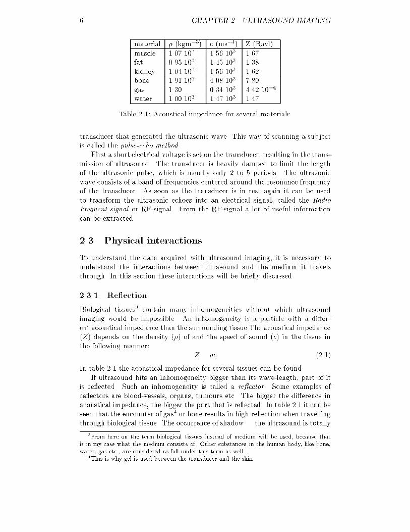
6 CHAPTER 2. ULTRASOUND IMAGINGmaterial � (kgm�3) c (ms�1) Z (Rayl)muscle 1.07 103 1.56 103 1.67fat 0.95 103 1.45 103 1.38kidney 1.04 103 1.56 103 1.62bone 1.91 103 4.08 103 7.80gas 1.30 0.34 103 4.42 10�4water 1.00 103 1.47 103 1.47Table 2.1: Acoustical impedance for several materials.transducer that generated the ultrasonic wave. This way of scanning a subjectis called the pulse-echo method .First a short electrical voltage is set on the transducer, resulting in the trans-mission of ultrasound. The transducer is heavily damped to limit the lengthof the ultrasonic pulse, which is usually only 2 to 5 periods. The ultrasonicwave consists of a band of frequencies centered around the resonance frequencyof the transducer. As soon as the transducer is in rest again it can be usedto transform the ultrasonic echoes into an electrical signal, called the RadioFrequent signal or RF-signal. From the RF-signal a lot of useful informationcan be extracted.2.3 Physical interactionsTo understand the data acquired with ultrasound imaging, it is necessary tounderstand the interactions between ultrasound and the medium it travelsthrough. In this section these interactions will be brie y discussed.2.3.1 Re ectionBiological tissues3 contain many inhomogeneities without which ultrasoundimaging would be impossible. An inhomogeneity is a particle with a di�er-ent acoustical impedance than the surrounding tissue.The acoustical impedance(Z) depends on the density (�) of and the speed of sound (c) in the tissue inthe following manner: Z = �c (2.1)In table 2.1 the acoustical impedance for several tissues can be found.If ultrasound hits an inhomogeneity bigger than its wave-length, part of itis re ected. Such an inhomogeneity is called a re ector . Some examples ofre ectors are blood-vessels, organs, tumours etc. The bigger the di�erence inacoustical impedance, the bigger the part that is re ected. In table 2.1 it can beseen that the encounter of gas4 or bone results in high re ection when travellingthrough biological tissue. The occurrence of shadow | the ultrasound is totally3From here on the term biological tissues instead of medium will be used, because thatis in my case what the medium consists of. Other substances in the human body, like bone,water, gas etc., are considered to fall under this term as well.4This is why gel is used between the transducer and the skin.

2.3. PHYSICAL INTERACTIONS 7re ected and doesn't reach the tissue behind a re ector anymore | is a realpossibility.The depth of a re ector (z) can be determined from the RF-signal. Thefollowing simple proposition can be applied:z = ct2 (2.2)Here c represents the speed of sound in the tissue under observation, and tequals the time elapsed between the transmission of the ultrasonic wave andthe reception of its echo. It is obvious that re ection is dependent on thepositions of the re ectors, i.e. the depth.That part of the ultrasound that is not re ected, travels on. The directionin which it travels will be slightly di�erent from its original direction. Thisphenomenon, well-known in optics, is called refraction. According to the lawof Snellius applied to ultrasound, the amount of refraction depends on thedi�erence in the speed of sound between the two tissues. High refraction leadsto a wrong image of a subject, because the re ectors aren't depicted on theirright place anymore. It is possible that the di�erence in the speed of soundbetween two tissues is so high that instead of refraction total re ection occursbeing another cause of shadow. In table 2.1 you can see that gas and boneresult in high refraction when travelling through biological tissue.2.3.2 ScatteringAn inhomogeneity that is small compared to the wave-length of the ultrasoundused, is called a scatterer . If ultrasound hits a scatterer, the ultrasonic waveis scattered in all directions. Usually the scatterers are uniformly distributedover the tissue, so scattering doesn't depend on the depth. Scattering howeveris dependent on the type of tissue, for di�erent tissues contain scatterers whichare di�erent in size and density. This is one of the phenomenona that makesultrasonic tissue characterization possible. Another factor that determines theamount of scattering is the frequency of the ultrasound. This dependency is ofexponential kind with the exponent between zero, for scatterers with a size inthe order of the wave-length, and four, for scatterers that are much smaller.Scattering has a huge impact on so called B-mode images. In section 2.5this will be explained.2.3.3 AbsorptionPart of the energy of the ultrasonic wave that travels through biological tissuesis transformed into heat. In the early days of ultrasound imaging scientistsassumed this was caused by friction, but today it is commonly accepted thatrelaxation processes are the main reason. When ultrasound travels through abiological tissue, many changes in volume and pressure take place. If all thesechanges are in phase with each other, no energy will be lost. Generally howeverthis will not be the case, due to the already mentioned relaxation processes.Because elasticity of the medium is an important factor, absorption is de-pendent on the type of tissue. This is a second phenomenon that can be of use

8 CHAPTER 2. ULTRASOUND IMAGINGfor ultrasonic tissue characterization. Another factor is the frequency of theultrasound. The amount of absorbtion is proportional to the frequency to thepower 1.5. As the ultrasound travels through the tissue and is absorbed by it,the central frequency of the ultrasound will be shifted downward.Absorption accounts for approximately 90% of the attenuation of an ul-trasonic wave, while scattering accounts for the rest. If the frequency of theultrasound used is increased, scattering accounts for a bigger part of the atten-uation.The amplitude spectrum (Pz) at a certain depth z from the transducer isdescribed by Pz(f) = P0e��(f)z (2.3)with P0 representing the initial amplitude spectrum of the ultrasonic wave and�(f) representing the attenuation-coe�cient of the tissue. Using this equationthe amount of attenuation can be determined experimentally, so the RF-signalcan be corrected for it. Much more on this subject can be found in [9].2.3.4 Di�ractionWhen you examine the beam of ultrasound produced by a transducer regardlessof the tissue it travels through, you �nd that it isn't constant of intensitynor of shape. The beam can be divided in two di�erent zones: the Fresnelzone and the Fraunhofer zone (see �gure 2.1). In the Fresnel zone, or near�eld, the beam is constant of shape, but it di�ers greatly in intensity dueto interference. In the Fraunhofer zone, or far �eld, the beam doesn't su�erfrom complete extinction, but diverges slowly. These e�ects are the result ofthe �niteness of the transducer. The ultrasonic wave that reaches a certainpoint in front of the transducer is composed of contributions coming from allpoints on the transducer surface. If the di�erence in distance between two suchcontributions is half a wave-length of the ultrasound used, they will extinct eachother. The Fresnel zone is de�ned to be that part of the ultrasonic beam wherethe maximum di�erence in distance between a point in this zone and a pointon the transducer surface is greater than or equal to half the wave-length. Inthe Fraunhofer zone the di�erence in distance is always smaller than half thewave-length, so extinction is impossible. If the transducer would be in�nite,all contributions that reach a certain point would be exactly the same as thecontributions that reach another point. This would result in a beam that isconstant of intensity and of shape.As will be explained in section 2.4.1, it is sometimes necessary to focus theultrasonic beam. Focussing in uences the shape of the beam and increasesdi�raction. But just like the factors mentioned in the previous paragraph |the frequency, which depends on the thickness of the transducer, and the size ofthe transducer surface | focussing is dependent only on the system, not on thetissue. The RF-signal can be corrected for the di�raction e�ects. A descriptionof this method can be found in [10].

2.4. CONSTRUCTION OF IMAGES 9Fraunhofer zoneFresnel zoneFigure 2.1: Shape of the ultrasonic beam; the thick solid line represents theunfocussed beam, the thin solid line the beam with medium focus and thedotted line the beam with short focus.2.4 Construction of imagesMany di�erent techniques exist to graphically represent echo signals. Besides A-mode and B-mode images, which we will explain in more detail in sections 2.4.2and 2.4.3, C-mode, AB-mode and M-mode images exist. They all serve di�erentpurposes. C-mode images for instance are useful for a three-dimensional view ona subject, while M-mode images can be used when monitoring moving structureslike the heart. The quality of an image depends of the resolution.2.4.1 ResolutionThere are two types of resolution: axial and lateral resolution. Good values forboth are necessary for a good image.The axial resolution is de�ned as the resolution in the direction parallelto the axis of the transducer. It is a measure for the minimum distance twore ectors that are situated in the ultrasonic beam must have in axial directionto produce two detectable echoes. This means that the amplitude between thetwo peaks must have been decreased with at least 50%. If the two re ectorsdi�er less in depth, the wave-front already reaches the second re ector, whilethe �rst is still re ecting the rest of the wave. These echoes will interfere so thatit looks as if only one re ector is present. It is obvious that the axial resolutiondepends on the length of the ultrasonic pulse: the shorter the pulse, the betterthe resolution. The length of the pulse is de�ned by the number of periods thepulse consists of, and the frequency of the ultrasound used. Usually the numberof periods is already very small, so the only way to improve the resolution isincreasing the frequency. Unfortunately this will increase the attenuation aswell, resulting in a much smaller penetration depth. Table 2.2 shows that insome �elds of medicine the region of interest isn't situated very deeply, so agood axial resolution can be achieved.The lateral resolution is the resolution in the direction perpendicular to theaxis of the transducer. It de�nes how far two re ectors that are at equal depthmust be apart in lateral direction so that they produce two detectable echoes.This resolution depends on the diameter of the ultrasonic beam: the smallerthe diameter, the better the resolution. Due to di�raction the resolution isdependent of the depth. A way to improve the resolution at a certain depth is

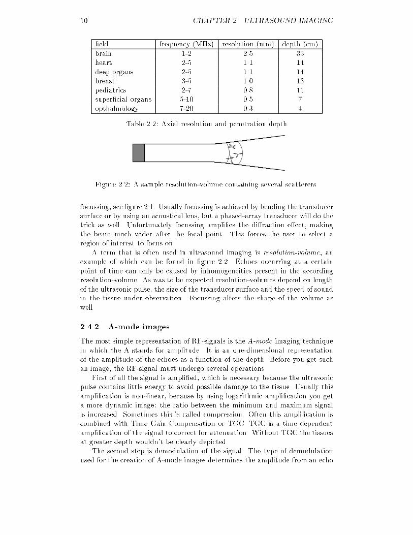
10 CHAPTER 2. ULTRASOUND IMAGING�eld frequency (MHz) resolution (mm) depth (cm)brain 1-2 2.5 33heart 2-5 1.1 14deep organs 2-5 1.1 14breast 3-5 1.0 13pediatrics 2-7 0.8 11super�cial organs 5-10 0.5 7opthalmology 7-20 0.3 4Table 2.2: Axial resolution and penetration depthFigure 2.2: A sample resolution-volume containing several scatterers.focussing, see �gure 2.1. Usually focussing is achieved by bending the transducersurface or by using an acoustical lens, but a phased-array transducer will do thetrick as well. Unfortunately focussing ampli�es the di�raction e�ect, makingthe beam much wider after the focal point. This forces the user to select aregion of interest to focus on.A term that is often used in ultrasound imaging is resolution-volume, anexample of which can be found in �gure 2.2. Echoes occurring at a certainpoint of time can only be caused by inhomogeneities present in the accordingresolution-volume. As was to be expected resolution-volumes depend on lengthof the ultrasonic pulse, the size of the transducer surface and the speed of soundin the tissue under observation. Focussing alters the shape of the volume aswell.2.4.2 A-mode imagesThe most simple representation of RF-signals is the A-mode imaging techniquein which the A stands for amplitude. It is an one-dimensional representationof the amplitude of the echoes as a function of the depth. Before you get suchan image, the RF-signal must undergo several operations.First of all the signal is ampli�ed, which is necessary because the ultrasonicpulse contains little energy to avoid possible damage to the tissue. Usually thisampli�cation is non-linear, because by using logarithmic ampli�cation you geta more dynamic image: the ratio between the minimum and maximum signalis increased. Sometimes this is called compression. Often this ampli�cation iscombined with Time Gain Compensation or TGC. TGC is a time dependentampli�cation of the signal to correct for attenuation. Without TGC the tissuesat greater depth wouldn't be clearly depicted.The second step is demodulation of the signal. The type of demodulationused for the creation of A-mode images determines the amplitude from an echo

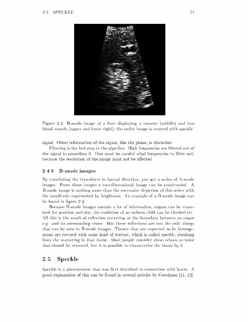
2.5. SPECKLE 11Figure 2.3: B-mode image of a liver displaying a tumour (middle) and twoblood vessels (upper and lower right); the entire image is covered with speckle.signal. Other information of the signal, like the phase, is discarded.Filtering is the last step in the pipe-line. High frequencies are �ltered out ofthe signal to smoothen it. One must be careful what frequencies to �lter out,because the resolution of the image must not be a�ected.2.4.3 B-mode imagesBy translating the transducer in lateral direction, you get a series of A-modeimages. From these images a two-dimensional image can be constructed. AB-mode image is nothing more than the successive depiction of this series withthe amplitude represented by brightness. An example of a B-mode image canbe found in �gure 2.3.Because B-mode images contain a lot of information, organs can be exam-ined for position and size, the evolution of an unborn child can be checked etc.All this is the result of re ection occurring at the boundary between an organe.g. and its surrounding tissue. But these re ections are not the only thingsthat can be seen in B-mode images. Tissues that are expected to be homoge-neous are covered with some kind of texture, which is called speckle, resultingfrom the scattering in that tissue. Most people consider these echoes as noisethat should be removed, but it is possible to characterize the tissue by it.2.5 SpeckleSpeckle is a phenomenon that was �rst described in connection with lasers. Agood explanation of this can be found in several articles by Goodman [11, 12].

12 CHAPTER 2. ULTRASOUND IMAGINGIn ultrasound imaging speckle is caused by scatterers. When an ultrasonicwave hits a scatterer, the ultrasound is scattered is in all directions. Some of theultrasound is scattered back to the transducer. At the transducer surface wavescoming from several scatterers in the same resolution-volume are received at thesame time, see �gure 2.2. Because the scatterers all have a di�erent distance tothe transducer surface, the waves di�er in phase and amplitude. This way theinterfering waves may extinct or amplify each other.As the resolution-volume changes to a greater depth or the transducer istranslated, a completely di�erent interference occurs. This way an irregularpattern of echoes is created. As speckle is intrinsic to UI, it can not be removedby increasing the power of the ultrasound. When regarding speckle as noise, itis of multiplicative instead of additive nature.Speckle is described using �rst- and second-order statistics. First-orderstatistics include the mean amplitude and the signal-to-noise ratio. The second-order statistics include the auto-covariance in both axial and lateral direction.These statistics are dependent on the imaging system and the density of thescatterers. If the density is above a certain level speckle only depends on theimaging system. This situation is often referred to as fully developed speckle.For fully developed speckle a model can be constructed [13]. In sections 2.5.1to 2.5.4 theoretical and practical results [14, 15] are compared.2.5.1 Mean amplitudeTheoretically the probability distribution function for the magnitude of theamplitude can be given byp(A) = A�2 e�A22�2 (A > 0) (2.4)with �2 the backscattered signal power. This probability distribution functionis known as the Rayleigh distribution function. For this function it is knownthat �2A = �2�2 (2.5)�2A = �2(2� �2 )where �A stands for the mean amplitude and �A represents the standard devi-ation of the amplitude.The received signal power depends on a lot of factors. First of all it isdependent on the power of the transmitted ultrasound, for an increase of thispower results in an increase of the backscattered signal power. This is meantwith the remark that speckle is noise of multiplicative nature. Secondly thesignal power is proportional to the number of scatterers. Due to di�ractionthe diameter of the ultrasonic beam is at its smallest in the focal zone, sothe number of scatterers here is smaller than in any other resolution-volume.However, the energy of the transmitted ultrasonic wave per volume unit is muchhigher. Altogether this results in a higher received signal power. Equation 2.5shows that the mean amplitude is proportional to the square root of the signalpower, so the mean amplitude will be dependent on these factors as well.

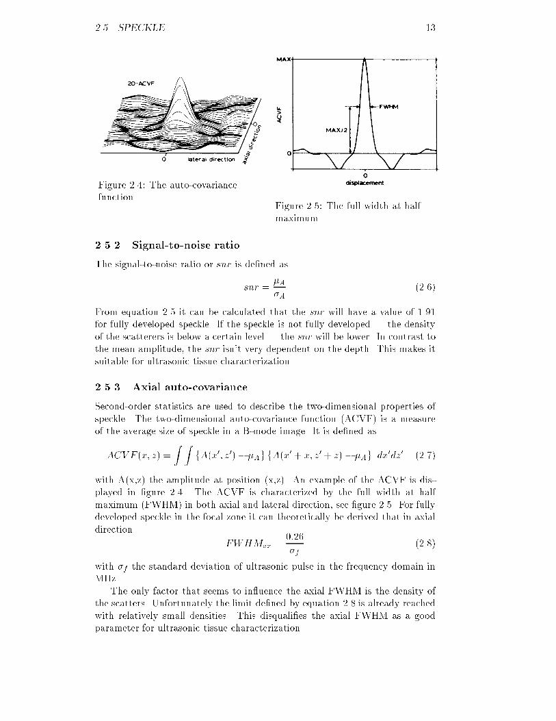
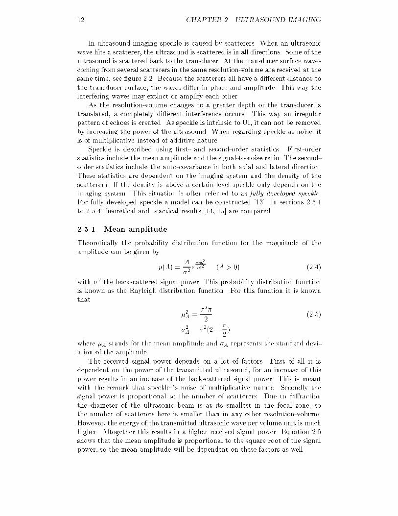
2.5. SPECKLE 13Figure 2.4: The auto-covariancefunction. Figure 2.5: The full width at halfmaximum.2.5.2 Signal-to-noise ratioThe signal-to-noise ratio or snr is de�ned assnr = �A�A (2.6)From equation 2.5 it can be calculated that the snr will have a value of 1.91for fully developed speckle. If the speckle is not fully developed | the densityof the scatterers is below a certain level | the snr will be lower. In contrast tothe mean amplitude, the snr isn't very dependent on the depth. This makes itsuitable for ultrasonic tissue characterization.2.5.3 Axial auto-covarianceSecond-order statistics are used to describe the two-dimensional properties ofspeckle. The two-dimensional auto-covariance function (ACVF) is a measureof the average size of speckle in a B-mode image. It is de�ned asACV F (x; z) = Z Z �A(x0; z0)� �A�A(x0 + x; z0 + z)� �A dx0dz0 (2.7)with A(x,z) the amplitude at position (x,z). An example of the ACVF is dis-played in �gure 2.4. The ACVF is characterized by the full width at halfmaximum (FWHM) in both axial and lateral direction, see �gure 2.5. For fullydeveloped speckle in the focal zone it can theoretically be derived that in axialdirection FWHMax = 0:26�f (2.8)with �f the standard deviation of ultrasonic pulse in the frequency domain inMHz.The only factor that seems to in uence the axial FWHM is the density ofthe scatters. Unfortunately the limit de�ned by equation 2.8 is already reachedwith relatively small densities. This disquali�es the axial FWHM as a goodparameter for ultrasonic tissue characterization.

14 CHAPTER 2. ULTRASOUND IMAGING2.5.4 Lateral auto-covarianceAs mentioned in section 2.5.3 the lateral auto-covariance can be characterizedby the full width at half maximum in lateral direction. For fully developedspeckle in the focal zone it can be shown that in lateral direction the followingequation holds: FWHMlat = 0:864�FD (2.9)Here � represents the wave-length, F the focal distance and D the diameter ofthe transducer.The lateral FWHM increases dramatically with increasing depth. This ismainly due to frequency dependent attenuation, which results in a lower centralfrequency at greater depths. As was predicted by equation 2.9, this will increasethe FWHM. Another factor the FWHM in lateral direction depends on is thescatter density. The FWHM decreases approximately proportional to the log-arithm of the density. Fortunately the limit de�ned by equation 2.9 is reachedonly at relatively high densities. If a correction is made for the frequency de-pendent attenuation, this parameter can be useful for the characterization oftissues.

Chapter 3The data setIn this chapter we will explain what the data exactly represents. Furthermore,two methods for the generation of additional data are explained. Finally adescription is given of the operations the data has to undergo before it can bepresented to a neural network.3.1 De�nition of the classesAt the Biophysics Laboratory a database is maintained, containing patientssuspected of su�ering from some sort of di�use liver disease. For each patienthis number, age, kind of disease and the values of 26 parameters obtainedwith ultrasound imaging are recorded. What disease the patient su�ered fromis determined through a biopsy. The four classes with the largest number ofpatients have been selected in addition to a class consisting of people with ahealthy liver. The �ve groups with their characteristics are the following:A: people with a healthy liver; their classi�cation in the database is 1;B: people su�ering from primary biliary cirrhosis; their classi�cation in thedatabase is 28, 281 or 282;C: people su�ering from hepatitis/cirrhosis; their classi�cation in the databaseis 22, 23, 24, 26 or 27;D: people su�ering from acute hepatitis; their classi�cation in the database is20 or 21;E: people su�ering from alcoholic hepatitis/cirrhosis; their classi�cation in thedatabase is 25.The above classi�cation will be referred to throughout the whole thesis.3.2 Description of the parametersThe database contains the values of 26 parameters per patient obtained byultrasound imaging, from which �ve have been selected that will be used for15

16 CHAPTER 3. THE DATA SETultrasonic tissue characterization in this thesis. The selection was based onthe results of earlier research, partially described in [1]. In the remainder ofthis section these parameters, ordered in decreasing discriminating ability, arebrie y reviewed.Mean amplitudeThis parameter has already been explained in section 2.5.1. The most impor-tant property of this parameter is that it is proportional to the square root ofthe backscattered signal power, which in its turn depends on the number ofscatterers. The symbol for the mean amplitude in this thesis is �A.Attenuation-coe�cient betaAs mentioned in section 2.3.3 attenuation in relatively homogeneous tissues iscaused by absorption and scattering. Because these two factors are dependenton the tissue, the attenuation is a good parameter for the characterization oftissues.The frequency dependent attenuation can be described by the attenuation-coe�cient �(f). A method for determining this coe�cient can be found in [9].Usually it is the sum of a number of terms of which the higher order terms arenegligible small at relatively low frequencies. A good approximation thereforeis �(f) = �f (3.1)in other words a linear �t through the origin. In this thesis the parameter willbe referred to as �.Signal-to-noise ratioIn section 2.5.2 more about the signal-to-noise ratio can be found. The snris dependent on the density of the scatterers. If the density is higher than acertain level, the snr has a value of 1.91. For tissues with such high densitiesthe snr is useless.Backscatter-coe�cientIt is already mentioned several times that tissue can be characterized by itsscattering properties. One of the factors scattering depends on is the size ofthe scatterers, for which a good approximation can be determined from thebackscatter spectrum.First of all the backscatter spectrum is dependent on the spectrum of theultrasonic wave, usually being a narrow band of frequencies. But due to thesize of the scatterers, some frequencies in this band are scattered back morethan others. If you make a linear �t of this spectrum, not necessarily throughthe origin, the slope appears to be a good measure for the size. The symbol forthe slope in this thesis is S.

3.3. SOME STATISTICS 17Attenuation-coe�cient alphaJust as � is a good approximation of the attenuation-coe�cient, there are manymore good approximations possible. One of them is the linear �t not necessarilythrough the origin, described by�(f) = �0 + �1f (3.2)The slope �1 appears to be a good parameter for ultrasonic tissue characteri-zation.3.3 Some statisticsTo get a better insight into the data some statistics are presented in tables 3.1to 3.5. From these tables it can be concluded that separation of the di�erentclasses is not trivial, maybe even impossible, because the classes clearly overlap.However a few annotations on these statistics should be made. From classC patient number 73 has been left out, because his value for �A | which is168.3 | deviated far too much from the rest of his class. The same appliesto patient number 72 from class E, who has a �A of 336.5. Furthermore thenumber of patients di�ers a lot between classes: class A contains 129 patients,class C just 14, class D has 13 members and classes B and E each 10. Forthe use with neural networks and more precise statistics on the performanceof the di�erent methods for classi�cation, larger and more equal numbers arerequired. Section 3.4 deals with this problem.In �gures 3.1 to 3.5 histograms for the selected parameters of class A areshown. Some of these histograms clearly display some kind of Gaussian func-tion, while with a little imagination the other histograms could be seen asGaussians as well. We therefore assume that the data of class A is distributednormally for all parameters, a property that is very useful when dealing withstatistics. In statistical terms a data set with this property is said to be multi-variate normal .For the other classes the number of patients is much too small to draw thesame conclusion, but we assume these classes are multivariate normal as well.In the remainder of this thesis the multivariate normal property will often beused.3.4 Generation of dataIn section 3.3 it can be found that the size of class A is much larger than thesizes of the other classes. Depending on the goal you want to achieve, this canbe very awkward when using neural networks. If you're goal is to get a correctclassi�cation for as many patients as possible, independent of the class theybelong to, there is no problem. If however you want to get a good classi�cationratio for each individual class, these di�erences in number of patients cause aproblem, because the network focusses so much on the large class that the otherclasses are more or less neglected. Of course it is possible to reduce class A to

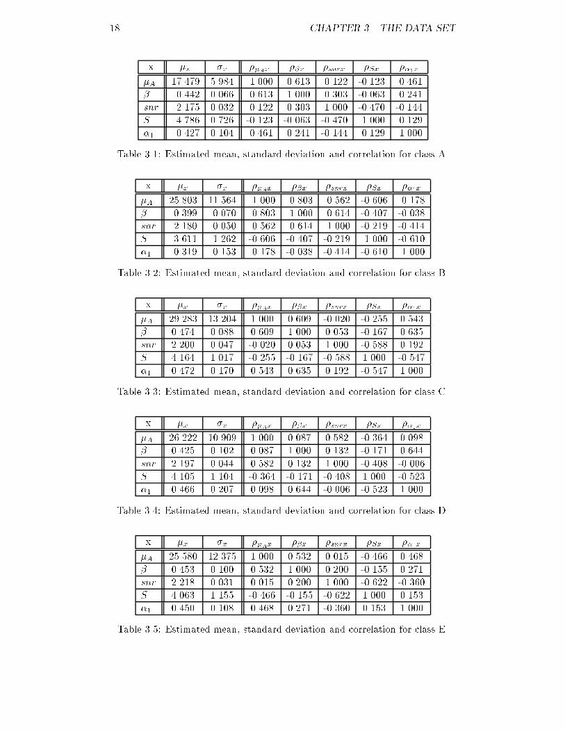
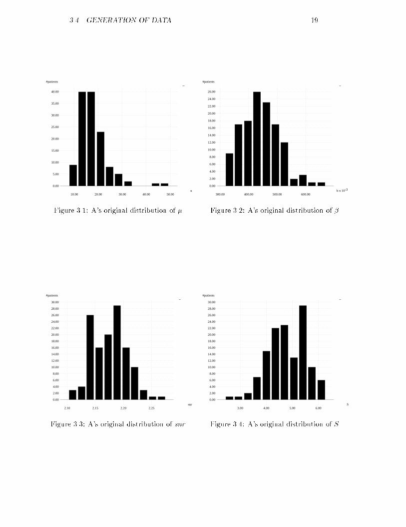
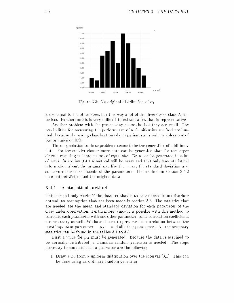
18 CHAPTER 3. THE DATA SETx �x �x ��Ax ��x �snrx �Sx ��1x�A 17.479 5.984 1.000 0.613 0.122 -0.123 0.461� 0.442 0.066 0.613 1.000 0.303 -0.063 0.241snr 2.175 0.032 0.122 0.303 1.000 -0.470 -0.144S 4.786 0.726 -0.123 -0.063 -0.470 1.000 0.129�1 0.427 0.104 0.461 0.241 -0.144 0.129 1.000Table 3.1: Estimated mean, standard deviation and correlation for class A.x �x �x ��Ax ��x �snrx �Sx ��1x�A 25.803 11.564 1.000 0.803 0.562 -0.606 0.178� 0.399 0.070 0.803 1.000 0.614 -0.407 -0.038snr 2.180 0.050 0.562 0.614 1.000 -0.219 -0.414S 3.611 1.262 -0.606 -0.407 -0.219 1.000 -0.610�1 0.319 0.153 0.178 -0.038 -0.414 -0.610 1.000Table 3.2: Estimated mean, standard deviation and correlation for class B.x �x �x ��Ax ��x �snrx �Sx ��1x�A 29.283 13.204 1.000 0.609 -0.020 -0.255 0.543� 0.474 0.088 0.609 1.000 0.053 -0.167 0.635snr 2.200 0.047 -0.020 0.053 1.000 -0.588 0.192S 4.164 1.017 -0.255 -0.167 -0.588 1.000 -0.547�1 0.472 0.170 0.543 0.635 0.192 -0.547 1.000Table 3.3: Estimated mean, standard deviation and correlation for class C.x �x �x ��Ax ��x �snrx �Sx ��1x�A 26.222 10.909 1.000 0.087 0.582 -0.364 0.098� 0.425 0.102 0.087 1.000 0.132 -0.171 0.644snr 2.197 0.044 0.582 0.132 1.000 -0.408 -0.006S 4.105 1.104 -0.364 -0.171 -0.408 1.000 -0.523�1 0.466 0.207 0.098 0.644 -0.006 -0.523 1.000Table 3.4: Estimated mean, standard deviation and correlation for class D.x �x �x ��Ax ��x �snrx �Sx ��1x�A 25.580 12.375 1.000 0.532 0.015 -0.466 0.468� 0.453 0.100 0.532 1.000 0.200 -0.155 0.271snr 2.218 0.031 0.015 0.200 1.000 -0.622 -0.360S 4.063 1.155 -0.466 -0.155 -0.622 1.000 0.153�1 0.450 0.108 0.468 0.271 -0.360 0.153 1.000Table 3.5: Estimated mean, standard deviation and correlation for class E.

3.4. GENERATION OF DATA 19

#patients

u

0.00

5.00

10.00

15.00

20.00

25.00

30.00

35.00

40.00

10.00 20.00 30.00 40.00 50.00Figure 3.1: A's original distribution of �.

#patients

-3b x 10

0.00

2.00

4.00

6.00

8.00

10.00

12.00

14.00

16.00

18.00

20.00

22.00

24.00

26.00

300.00 400.00 500.00 600.00Figure 3.2: A's original distribution of �.

#patients

snr

0.00

2.00

4.00

6.00

8.00

10.00

12.00

14.00

16.00

18.00

20.00

22.00

24.00

26.00

28.00

30.00

2.10 2.15 2.20 2.25Figure 3.3: A's original distribution of snr .

#patients

S

0.00

2.00

4.00

6.00

8.00

10.00

12.00

14.00

16.00

18.00

20.00

22.00

24.00

26.00

28.00

30.00

3.00 4.00 5.00 6.00Figure 3.4: A's original distribution of S.

20 CHAPTER 3. THE DATA SET

#patients

-3a1 x 10

0.00

2.00

4.00

6.00

8.00

10.00

12.00

14.00

16.00

18.00

20.00

22.00

200.00 300.00 400.00 500.00 600.00Figure 3.5: A's original distribution of �1.a size equal to the other sizes, but this way a lot of the diversity of class A willbe lost. Furthermore it is very di�cult to extract a set that is representative.Another problem with the present-day classes is that they are small. Thepossibilities for measuring the performance of a classi�cation method are lim-ited, because the wrong classi�cation of one patient can result in a decrease ofperformance of 10%.The only solution to these problems seems to be the generation of additionaldata. For the smaller classes more data can be generated than for the largerclasses, resulting in large classes of equal size. Data can be generated in a lotof ways. In section 3.4.1 a method will be examined that only uses statisticalinformation about the original set, like the mean, the standard deviation andsome correlation coe�cients of the parameters. The method in section 3.4.2uses both statistics and the original data.3.4.1 A statistical methodThis method only works if the data set that is to be enlarged is multivariatenormal, an assumption that has been made in section 3.3. The statistics thatare needed are the mean and standard deviation for each parameter of theclass under observation. Furthermore, since it is possible with this method tocorrelate each parameter with one other parameter, some correlation coe�cientsare necessary as well. We have chosen to preserve the correlation between themost important parameter | �A | and all other parameters. All the necessarystatistics can be found in the tables 3.1 to 3.5.First a value for �A must be generated. Because the data is assumed tobe normally distributed, a Gaussian random generator is needed. The stepsnecessary to simulate such a generator are the following.1. Draw a xn from a uniform distribution over the interval [0,1]. This canbe done using an ordinary random generator.

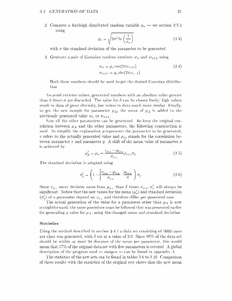
3.4. GENERATION OF DATA 212. Compute a Rayleigh distributed random variable yn | see section 2.5.1| using yn = s2�2 ln� 1xn� (3.3)with � the standard deviation of the parameter to be generated.3. Generate a pair of Gaussian random numbers wn and wn+1 usingwn = yn cos(2�xn+1) (3.4)wn+1 = yn sin(2�xn+1)Both these numbers should be used to get the desired Gaussian distribu-tion.To avoid extreme values, generated numbers with an absolute value greaterthan � times � are discarded. The value for � can be chosen freely; high valuesresult in data of great diversity, low values in data much more similar. Finally,to get the new sample for parameter �A, the mean of �A is added to thepreviously generated value wn or wn+1.Now all the other parameters can be generated. To keep the original cor-relation between �A and the other parameters, the following construction isused. To simplify the explanation p represents the parameter to be generated,v refers to the actually generated value and �xy stands for the correlation be-tween parameter x and parameter y. A shift of the mean value of parameter pis achieved by �0p = �p + v�A � ��A��A �p�A�p (3.5)The standard deviation is adapted using�0p = 1� �����v�A � ��A��A � �p�A� �����!�p (3.6)Since v�A never deviates more from ��A than � times ��A , �0p will always besigni�cant. Notice that the new values for the mean (�0p) and standard deviation(�0p) of a parameter depend on v�A and therefore di�er per generated case.The actual generation of the value for a parameter other than �A is nowstraightforward: the same procedure must be followed that was presented earlierfor generating a value for �A, using the changed mean and standard deviation.StatisticsUsing the method described in section 3.4.1 a data set consisting of 1000 casesper class was generated, with � set at a value of 2.0. Since 95% of the data setshould be within at most 2� distance of the mean per parameter, this wouldmean that 77% of the original data set with �ve parameters is covered. A globaldescription of the program used | statgen | can be found in appendix A.The statistics of the new sets can be found in tables 3.6 to 3.10. Comparisonof these results with the statistics of the original sets shows that the new mean

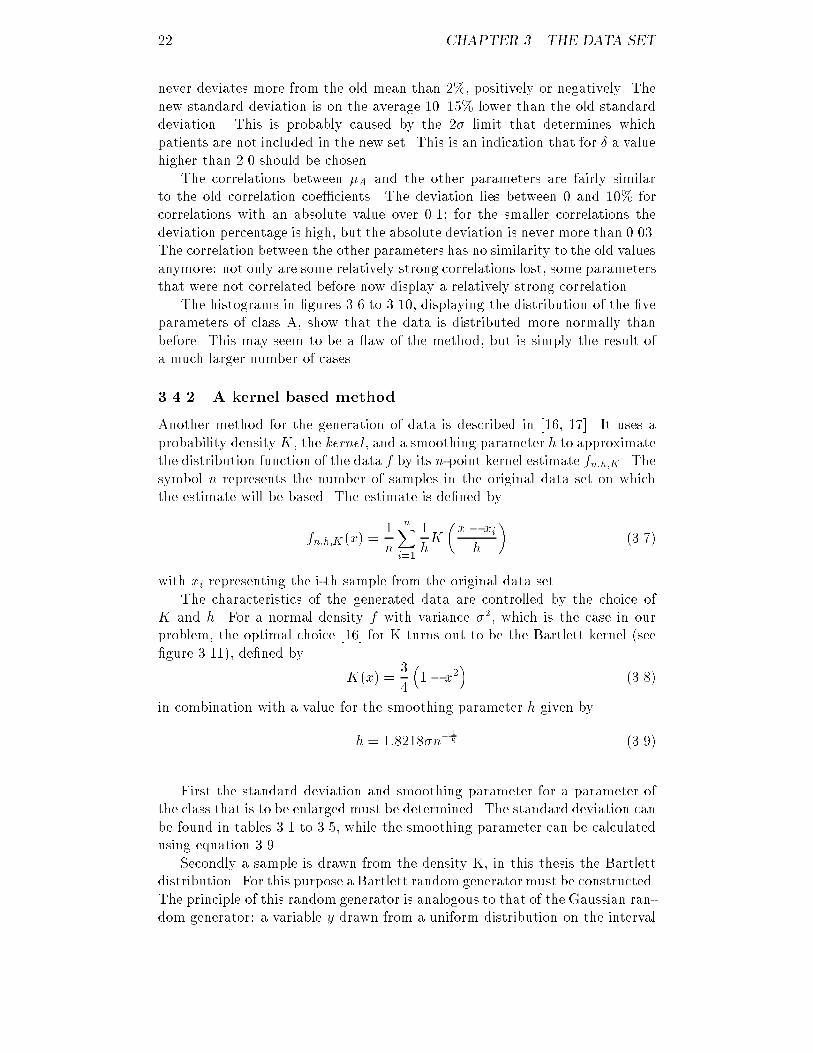
22 CHAPTER 3. THE DATA SETnever deviates more from the old mean than 2%, positively or negatively. Thenew standard deviation is on the average 10{15% lower than the old standarddeviation. This is probably caused by the 2� limit that determines whichpatients are not included in the new set. This is an indication that for � a valuehigher than 2.0 should be chosen.The correlations between �A and the other parameters are fairly similarto the old correlation coe�cients. The deviation lies between 0 and 10% forcorrelations with an absolute value over 0.1; for the smaller correlations thedeviation percentage is high, but the absolute deviation is never more than 0.03.The correlation between the other parameters has no similarity to the old valuesanymore: not only are some relatively strong correlations lost, some parametersthat were not correlated before now display a relatively strong correlation.The histograms in �gures 3.6 to 3.10, displaying the distribution of the �veparameters of class A, show that the data is distributed more normally thanbefore. This may seem to be a aw of the method, but is simply the result ofa much larger number of cases.3.4.2 A kernel based methodAnother method for the generation of data is described in [16, 17]. It uses aprobability density K, the kernel , and a smoothing parameter h to approximatethe distribution function of the data f by its n-point kernel estimate fn;h;K . Thesymbol n represents the number of samples in the original data set on whichthe estimate will be based. The estimate is de�ned byfn;h;K(x) = 1n nXi=1 1hK �x� xih � (3.7)with xi representing the i-th sample from the original data set.The characteristics of the generated data are controlled by the choice ofK and h. For a normal density f with variance �2, which is the case in ourproblem, the optimal choice [16] for K turns out to be the Bartlett kernel (see�gure 3.11), de�ned by K(x) = 34 �1� x2� (3.8)in combination with a value for the smoothing parameter h given byh = 1:8218�n� 15 (3.9)First the standard deviation and smoothing parameter for a parameter ofthe class that is to be enlarged must be determined. The standard deviation canbe found in tables 3.1 to 3.5, while the smoothing parameter can be calculatedusing equation 3.9.Secondly a sample is drawn from the density K, in this thesis the Bartlettdistribution. For this purpose a Bartlett random generator must be constructed.The principle of this random generator is analogous to that of the Gaussian ran-dom generator: a variable y drawn from a uniform distribution on the interval

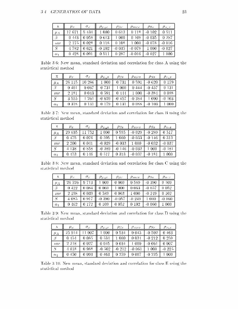
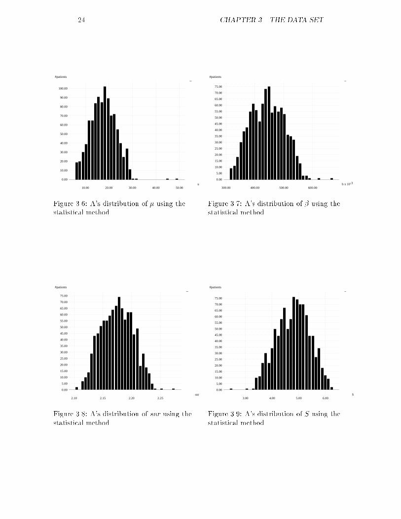
3.4. GENERATION OF DATA 23x �x �x ��Ax ��x �snrx �Sx ��1x�A 17.671 5.434 1.000 0.613 0.118 -0.102 0.511� 0.443 0.058 0.613 1.000 0.108 -0.035 0.287snr 2.175 0.028 0.118 0.108 1.000 -0.078 -0.016S 4.782 0.621 -0.102 -0.035 -0.078 1.000 -0.027�1 0.428 0.091 0.511 0.287 -0.016 -0.027 1.000Table 3.6: New mean, standard deviation and correlation for class A using thestatistical method.x �x �x ��Ax ��x �snrx �Sx ��1x�A 26.115 10.286 1.000 0.731 0.591 -0.620 0.179� 0.401 0.067 0.731 1.000 0.444 -0.457 0.131snr 2.181 0.043 0.591 0.444 1.000 -0.384 0.088S 3.555 1.261 -0.620 -0.457 -0.384 1.000 -0.103�1 0.318 0.131 0.179 0.131 0.088 -0.103 1.000Table 3.7: New mean, standard deviation and correlation for class B using thestatistical method.x �x �x ��Ax ��x �snrx �Sx ��1x�A 29.635 11.752 1.000 0.595 -0.029 -0.289 0.517� 0.475 0.076 0.595 1.000 -0.033 -0.146 0.313snr 2.200 0.041 -0.029 -0.033 1.000 -0.032 -0.037S 4.138 0.858 -0.289 -0.146 -0.032 1.000 -0.181�1 0.473 0.146 0.517 0.313 -0.037 -0.181 1.000Table 3.8: New mean, standard deviation and correlation for class C using thestatistical method.x �x �x ��Ax ��x �snrx �Sx ��1x�A 26.526 9.713 1.000 0.060 0.589 -0.390 0.109� 0.422 0.084 0.060 1.000 0.063 -0.057 0.052snr 2.198 0.039 0.589 0.063 1.000 -0.249 0.102S 4.085 0.917 -0.390 -0.057 -0.249 1.000 -0.060�1 0.462 0.172 0.109 0.052 0.102 -0.060 1.000Table 3.9: New mean, standard deviation and correlation for class D using thestatistical method.x �x �x ��Ax ��x �snrx �Sx ��1x�A 25.914 11.007 1.000 0.534 0.045 -0.502 0.463� 0.454 0.085 0.534 1.000 0.034 -0.212 0.259snr 2.218 0.027 0.045 0.034 1.000 -0.061 0.007S 4.018 0.988 -0.502 -0.212 -0.061 1.000 -0.225�1 0.450 0.093 0.463 0.259 0.007 -0.225 1.000Table 3.10: New mean, standard deviation and correlation for class E using thestatistical method.

24 CHAPTER 3. THE DATA SET

#patients

u

0.00

10.00

20.00

30.00

40.00

50.00

60.00

70.00

80.00

90.00

100.00

10.00 20.00 30.00 40.00 50.00Figure 3.6: A's distribution of � using thestatistical method.

#patients

-3b x 10

0.00

5.00

10.00

15.00

20.00

25.00

30.00

35.00

40.00

45.00

50.00

55.00

60.00

65.00

70.00

75.00

300.00 400.00 500.00 600.00Figure 3.7: A's distribution of � using thestatistical method.

#patients

snr

0.00

5.00

10.00

15.00

20.00

25.00

30.00

35.00

40.00

45.00

50.00

55.00

60.00

65.00

70.00

75.00

2.10 2.15 2.20 2.25Figure 3.8: A's distribution of snr using thestatistical method.

#patients

S

0.00

5.00

10.00

15.00

20.00

25.00

30.00

35.00

40.00

45.00

50.00

55.00

60.00

65.00

70.00

75.00

3.00 4.00 5.00 6.00Figure 3.9: A's distribution of S using thestatistical method.

3.4. GENERATION OF DATA 25

#patients

-3a1 x 10

0.00

5.00

10.00

15.00

20.00

25.00

30.00

35.00

40.00

45.00

50.00

55.00

60.00

65.00

70.00

75.00

200.00 300.00 400.00 500.00 600.00Figure 3.10: A's distribution of �1 using the statistical method.[0,1] is, using a certain function, transformed to a variable w that is distributedaccording to the Bartlett distribution.The function that is needed by the generator is the inverse (F�1(y)) of thecumulative Bartlett distribution function F (x), which is given byF (x) = xZ�1 34 �1� z2�dz = 34 �z � 13z3�����x�1 (3.10)= �14x3 + 34x+ 12Using Cardano's formula Maple1 gives the following three solutions for F�1(y):1. X2 +X12. �12(X2 +X1) + p32 (X2 �X1)i3. �12(X2 +X1)� p32 (X2 �X1)iwhere X1 = 3q1� 2y � 2py2 � y and X2 = 3q1� 2y + 2py2 � y. Clearly thesecond and third solution are imaginary and thus useless, but the �rst mightsatisfy. Unfortunately the term y2 � y is not positive for a y from [0; 1], whichis the domain of interest, so the square root of this term is imaginary. Thisdisquali�es the �rst solution also.The only possible line of action to compute F�1(y) is that of numericalapproximation. In this thesis Newton's method [18] is used because of its fastconvergence. Since the method of Newton can only be used to determine thepoints where a function is zero, a function g(x) is constructed that is zero for1Maple is a computer algebra system developed at the University of Waterloo, Waterloo(Ontario), USA.

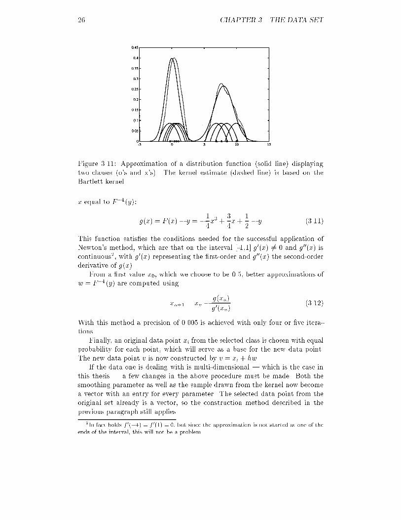
26 CHAPTER 3. THE DATA SETFigure 3.11: Approximation of a distribution function (solid line) displayingtwo classes (o's and x's). The kernel estimate (dashed line) is based on theBartlett kernel.x equal to F�1(y): g(x) = F (x)� y = �14x3 + 34x+ 12 � y (3.11)This function satis�es the conditions needed for the successful application ofNewton's method, which are that on the interval [-1,1] g0(x) 6= 0 and g00(x) iscontinuous2, with g0(x) representing the �rst-order and g00(x) the second-orderderivative of g(x).From a �rst value x0, which we choose to be 0.5, better approximations ofw = F�1(y) are computed usingxn+1 = xn � g(xn)g0(xn) (3.12)With this method a precision of 0.005 is achieved with only four or �ve itera-tions.Finally, an original data point xi from the selected class is chosen with equalprobability for each point, which will serve as a base for the new data point.The new data point v is now constructed by v = xi + hw.If the data one is dealing with is multi-dimensional | which is the case inthis thesis | a few changes in the above procedure must be made. Both thesmoothing parameter as well as the sample drawn from the kernel now becomea vector with an entry for every parameter. The selected data point from theoriginal set already is a vector, so the construction method described in theprevious paragraph still applies.2In fact holds f 0(�1) = f 0(1) = 0, but since the approximation is not started at one of theends of the interval, this will not be a problem.

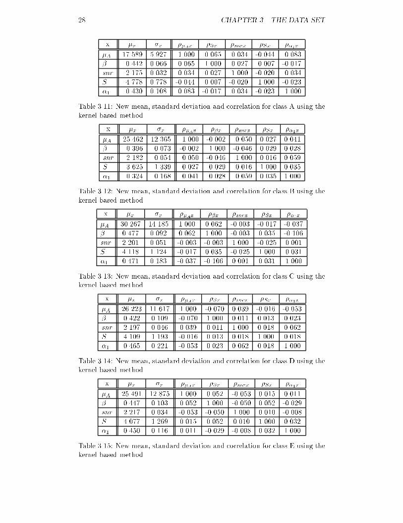
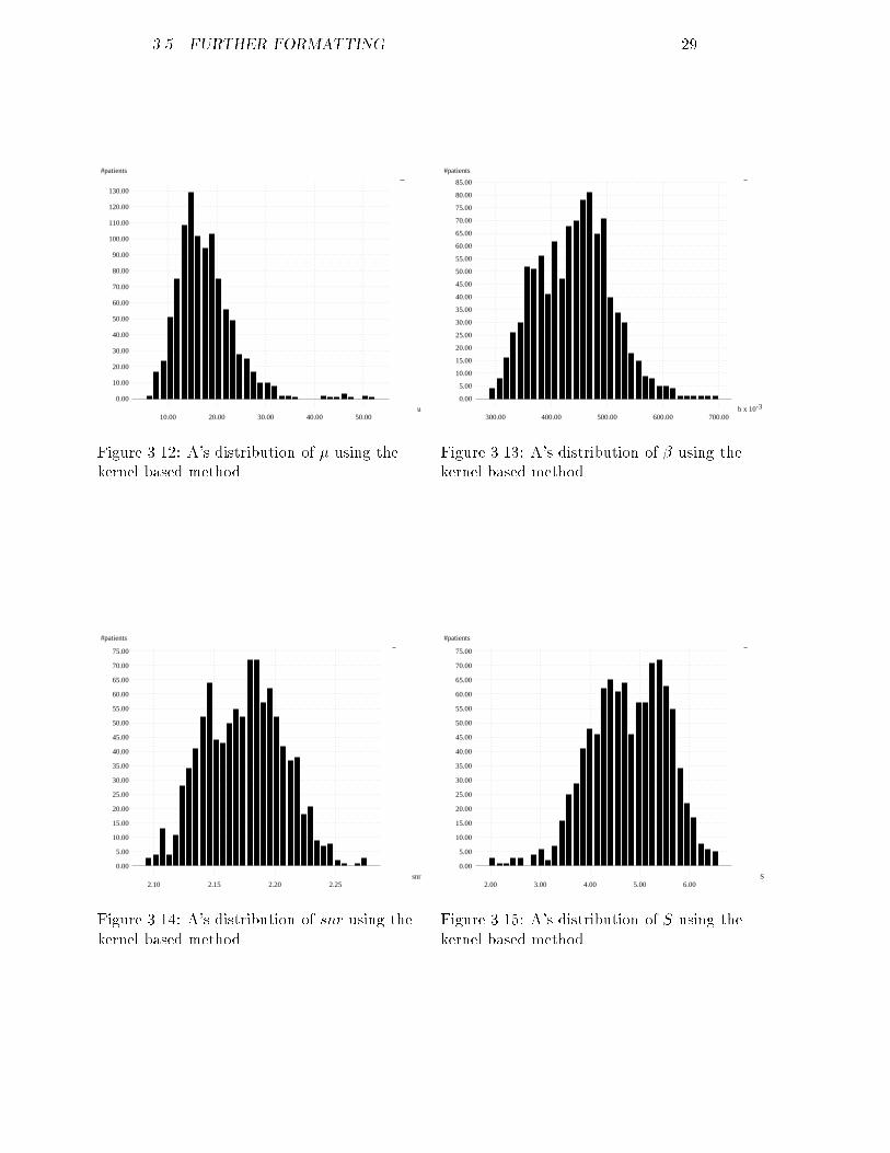
3.5. FURTHER FORMATTING 27StatisticsTo compare this method with the method described in section 3.4.1 a dataset consisting of 1000 cases per class has been generated. In appendix A theprogram that was used | kernelgen | is brie y discussed.Some statistics of the data sets generated with this method can be foundin tables 3.11 to 3.15. Comparing these results with the original results |tables 3.1 to 3.5 | one can see that the mean of the enlarged data sets neverdeviates more from the original estimated mean than 2%. The new standarddeviation is usually 5{10% higher than that of the original sets. A cause forthis could be a too large value of the smoothing parameter.The correlation between the parameters is completely lost for all classes.While in the original sets correlation coe�cients of upto 0.8 occurred, in thenew sets the correlation always stays within the interval [-0.1,0.1]. This is asecond indication that the smoothing parameter should be decreased, for asmaller kernel results in data that is much more similar to the original data.However, this could cause the new set to be less multivariate normal, somethingthat should be avoided.Like in section 3.3 and 3.4.1 the distribution of every parameter is examinedfor class A. The histograms, �gures 3.12 to 3.16, show that the way in whichthe data is distributed is a mixture between the original distribution and a purenormal distribution. This was to be expected, since not only the statistics butalso the original data points were taken as basis for the new data.The| important | decision which method to take for the generation of newdata is not a straightforward one. The statistical method has the advantage thatsome correlation coe�cients are maintained, but has no theoretical foundation.The kernel based method on the other hand has a theoretical background, butleads to complete loss of the correlation between the parameters. Tests usingdiscriminant analysis as well as neural networks have not shown signi�cantdi�erences in classi�cation results. Considering all these facts we have chosento use the kernel based method because of its theoretical basis and the fact thatit has been described in the literature.3.5 Further formattingThe format of data is not suitable yet to feed to a neural network. As mentionedbefore, a big di�erence in the number of patients per class could cause thenetwork to focus itself on the correct classi�cation of the largest class, whileneglecting the smaller classes; it was for this reason that additional data hasbeen generated. For the same reason however, a big di�erence in the variancebetween the parameters is undesirable.Suppose one parameter varies between 0 and 1, while another parametervaries between 0 and 1000. The error function a neural network tries to mini-mize decreases much more when the second parameter is optimized than whenthe �rst parameter is optimized, although the value of the �rst parameter couldbe much more signi�cant for the classi�cation process. The only way to solvethis problem is through scaling.

28 CHAPTER 3. THE DATA SETx �x �x ��Ax ��x �snrx �Sx ��1x�A 17.589 5.927 1.000 0.065 0.034 -0.044 0.083� 0.442 0.066 0.065 1.000 0.027 0.007 -0.017snr 2.175 0.032 0.034 0.027 1.000 -0.020 0.034S 4.778 0.778 -0.044 0.007 -0.020 1.000 -0.023�1 0.430 0.108 0.083 -0.017 0.034 -0.023 1.000Table 3.11: New mean, standard deviation and correlation for class A using thekernel based method.x �x �x ��Ax ��x �snrx �Sx ��1x�A 25.462 12.365 1.000 -0.002 0.050 0.027 0.041� 0.396 0.073 -0.002 1.000 -0.046 0.029 0.028snr 2.182 0.054 0.050 -0.046 1.000 0.016 0.059S 3.625 1.339 0.027 0.029 0.016 1.000 0.035�1 0.324 0.168 0.041 0.028 0.059 0.035 1.000Table 3.12: New mean, standard deviation and correlation for class B using thekernel based method.x �x �x ��Ax ��x �snrx �Sx ��1x�A 30.267 14.185 1.000 0.062 -0.003 -0.017 -0.037� 0.477 0.092 0.062 1.000 -0.003 0.035 -0.106snr 2.201 0.051 -0.003 -0.003 1.000 -0.025 0.001S 4.118 1.124 -0.017 0.035 -0.025 1.000 0.031�1 0.471 0.183 -0.037 -0.106 0.001 0.031 1.000Table 3.13: New mean, standard deviation and correlation for class C using thekernel based method.x �x �x ��Ax ��x �snrx �Sx ��1x�A 26.223 11.617 1.000 -0.070 0.039 -0.016 -0.053� 0.422 0.109 -0.070 1.000 0.011 0.013 0.023snr 2.197 0.046 0.039 0.011 1.000 0.018 0.062S 4.109 1.193 -0.016 0.013 0.018 1.000 0.018�1 0.465 0.221 -0.053 0.023 0.062 0.018 1.000Table 3.14: New mean, standard deviation and correlation for class D using thekernel based method.x �x �x ��Ax ��x �snrx �Sx ��1x�A 25.491 12.875 1.000 0.052 -0.053 0.015 0.011� 0.447 0.103 0.052 1.000 -0.050 0.052 -0.029snr 2.217 0.034 -0.053 -0.050 1.000 0.010 -0.008S 4.077 1.269 0.015 0.052 0.010 1.000 0.032�1 0.450 0.116 0.011 -0.029 -0.008 0.032 1.000Table 3.15: New mean, standard deviation and correlation for class E using thekernel based method.

3.5. FURTHER FORMATTING 29

#patients

u

0.00

10.00

20.00

30.00

40.00

50.00

60.00

70.00

80.00

90.00

100.00

110.00

120.00

130.00

10.00 20.00 30.00 40.00 50.00Figure 3.12: A's distribution of � using thekernel based method.

#patients

-3b x 10

0.00

5.00

10.00

15.00

20.00

25.00

30.00

35.00

40.00

45.00

50.00

55.00

60.00

65.00

70.00

75.00

80.00

85.00

300.00 400.00 500.00 600.00 700.00Figure 3.13: A's distribution of � using thekernel based method.

#patients

snr

0.00

5.00

10.00

15.00

20.00

25.00

30.00

35.00

40.00

45.00

50.00

55.00

60.00

65.00

70.00

75.00

2.10 2.15 2.20 2.25Figure 3.14: A's distribution of snr using thekernel based method.

#patients

S

0.00

5.00

10.00

15.00

20.00

25.00

30.00

35.00

40.00

45.00

50.00

55.00

60.00

65.00

70.00

75.00

2.00 3.00 4.00 5.00 6.00Figure 3.15: A's distribution of S using thekernel based method.

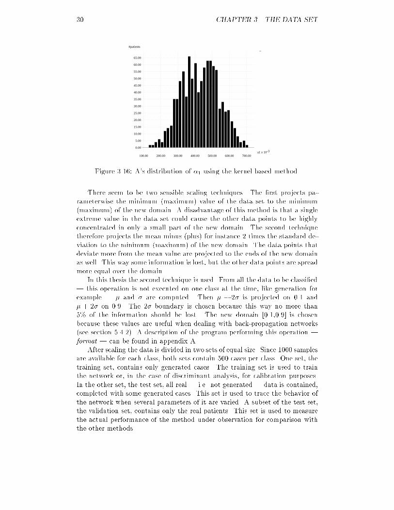
30 CHAPTER 3. THE DATA SET

#patients

-3a1 x 10

0.00

5.00

10.00

15.00

20.00

25.00

30.00

35.00

40.00

45.00

50.00

55.00

60.00

65.00

100.00 200.00 300.00 400.00 500.00 600.00 700.00Figure 3.16: A's distribution of �1 using the kernel based method.There seem to be two sensible scaling techniques. The �rst projects pa-rameterwise the minimum (maximum) value of the data set to the minimum(maximum) of the new domain. A disadvantage of this method is that a singleextreme value in the data set could cause the other data points to be highlyconcentrated in only a small part of the new domain. The second techniquetherefore projects the mean minus (plus) for instance 2 times the standard de-viation to the minimum (maximum) of the new domain. The data points thatdeviate more from the mean value are projected to the ends of the new domainas well. This way some information is lost, but the other data points are spreadmore equal over the domain.In this thesis the second technique is used. From all the data to be classi�ed| this operation is not executed on one class at the time, like generation forexample | � and � are computed. Then � � 2� is projected on 0.1 and� + 2� on 0.9. The 2� boundary is chosen because this way no more than5% of the information should be lost. The new domain [0.1,0.9] is chosenbecause these values are useful when dealing with back-propagation networks(see section 5.4.2). A description of the program performing this operation |format | can be found in appendix A.After scaling the data is divided in two sets of equal size. Since 1000 samplesare available for each class, both sets contain 500 cases per class. One set, thetraining set, contains only generated cases. The training set is used to trainthe network or, in the case of discriminant analysis, for calibration purposes.In the other set, the test set, all real | i.e. not generated | data is contained,completed with some generated cases. This set is used to trace the behavior ofthe network when several parameters of it are varied. A subset of the test set,the validation set, contains only the real patients. This set is used to measurethe actual performance of the method under observation for comparison withthe other methods.

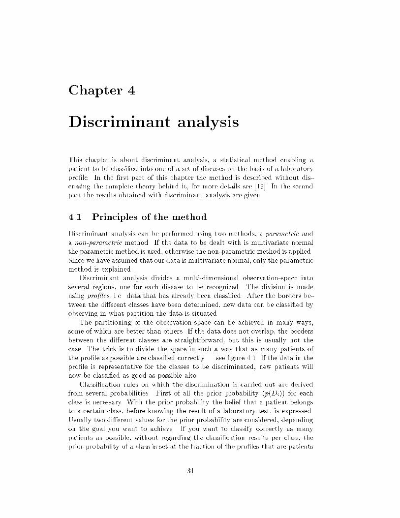
Chapter 4Discriminant analysisThis chapter is about discriminant analysis, a statistical method enabling apatient to be classi�ed into one of a set of diseases on the basis of a laboratorypro�le. In the �rst part of this chapter the method is described without dis-cussing the complete theory behind it, for more details see [19]. In the secondpart the results obtained with discriminant analysis are given.4.1 Principles of the methodDiscriminant analysis can be performed using two methods, a parametric anda non-parametric method. If the data to be dealt with is multivariate normalthe parametric method is used, otherwise the non-parametric method is applied.Since we have assumed that our data is multivariate normal, only the parametricmethod is explained.Discriminant analysis divides a multi-dimensional observation-space intoseveral regions, one for each disease to be recognized. The division is madeusing pro�les , i.e. data that has already been classi�ed. After the borders be-tween the di�erent classes have been determined, new data can be classi�ed byobserving in what partition the data is situated.The partitioning of the observation-space can be achieved in many ways,some of which are better than others. If the data does not overlap, the bordersbetween the di�erent classes are straightforward, but this is usually not thecase. The trick is to divide the space in such a way that as many patients ofthe pro�le as possible are classi�ed correctly | see �gure 4.1. If the data in thepro�le is representative for the classes to be discriminated, new patients willnow be classi�ed as good as possible also.Classi�cation rules on which the discrimination is carried out are derivedfrom several probabilities. First of all the prior probability (p(Di)) for eachclass is necessary. With the prior probability the belief that a patient belongsto a certain class, before knowing the result of a laboratory test, is expressed.Usually two di�erent values for the prior probability are considered, dependingon the goal you want to achieve. If you want to classify correctly as manypatients as possible, without regarding the classi�cation results per class, theprior probability of a class is set at the fraction of the pro�les that are patients31

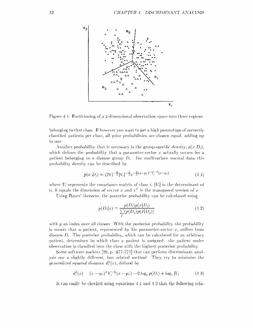
32 CHAPTER 4. DISCRIMINANT ANALYSISFigure 4.1: Partitioning of a 2-dimensional observation space into three regions.belonging to that class. If however you want to get a high percentage of correctlyclassi�ed patients per class, all prior probabilities are chosen equal, adding upto one.Another probability that is necessary is the group-speci�c density, p(xjDi),which de�nes the probability that a parameter-vector x actually occurs for apatient belonging to a disease group Di. For multivariate normal data thisprobability density can be described byp(xjDi) = (2�)� k2 jVij� 12 e� 12 (x��i)TV�1i (x��i) (4.1)where Vi represents the covariance matrix of class i, jVij is the determinant ofit, k equals the dimension of vector x and xT is the transposed version of x.Using Bayes' theorem, the posterior probability can be calculated usingp(Dijx) = p(Di)p(xjDi)Pg (p(Dg)p(xjDg)) (4.2)with g an index over all classes. With the posterior probability the probabilityis meant that a patient, represented by his parameter-vector x, su�ers fromdisease Di. The posterior probability, which can be calculated for an arbitrarypatient, determines to which class a patient is assigned: the patient underobservation is classi�ed into the class with the highest posterior probability.Some software packets [20, p. 677-771] that can perform discriminant anal-ysis use a slightly di�erent, but related method. They try to minimize thegeneralized squared distance d2i (x), de�ned byd2i (x) = (x� �i)TV �1i (x� �i)� 2 loge p(Di) + loge jVij (4.3)It can easily be checked using equations 4.1 and 4.2 that the following rela-

4.2. RESULTS 33tion holds: p(Dijx) = e� 12d2i (x)Pg e� 12d2g(x) (4.4)It is obvious that a minimal d2i (x) conforms to a maximal p(Dijx).An advantage of using generalized squared distances is that, depending oncertain choices, certain terms can be left out. If for instance all prior probabili-ties are equal | either because the number of patients is equal for all classes, orbecause they are chosen equal to get a good classi�cation percentage for everyclass | the term �2 loge p(Di) can be omitted, since it has the same value foreach class.Another term that can sometimes be left out is loge jVij. If the variancesand covariances of the parameters are independent of the disease, the aboveterm is equal for every class and can thus be omitted. This condition can beimposed on the discriminant analysis by stating that instead of the within-groupcovariance matrices Vi the pooled covariance matrix V must be used. Withthe pooled covariance matrix the variances and covariances of all the pro�lestogether are meant. Discriminant analysis based on this principle is called lineardiscriminant analysis . If however the covariance matrix is dependent on thetype of disease, this reduction is not allowed. This type of discriminant analysisis often called quadratic discriminant analysis .4.2 ResultsThe results that are presented in the remainder of this chapter have been ob-tained using a statistical analysis system called SAS/STAT1. More informationabout the procedure used (DISCRIM ) can be found in [20].4.2.1 Measuring the performanceThe performance of discriminant analysis is measured using so called confusionor speci�city/sensitivity matrices, displaying the classi�cation percentages ofthe data set under observation. At position (i; j), where i represents the i-throw and j the j-th column, the percentage of patients belonging to class i thatare classi�ed into class j can be found. Since each patient of a certain class isclassi�ed into some class, the percentages in every row add up to 100%. Onthe diagonal the percentage of correctly classi�ed patients can be found, so if amethod is said to classify well, these percentages should be high.In medicine often a group of healthy people is compared to one group ofpeople su�ering from some disease. In the resulting matrix the percentage \truenegatives" | i.e. healthy people that are classi�ed as being healthy | is calledthe speci�city of a parameter set, while the percentage \true positives" | illpeople that are classi�ed as being ill | is called the sensitivity of that parameterset. The goal that is pursued determines which percentage is to be optimized:if as little healthy people as possible should be classi�ed as being ill in order1SAS/STAT has been developed at SAS Institute Inc., Cary (NC), USA.

34 CHAPTER 4. DISCRIMINANT ANALYSISto avoid unnecessary examination, which could be damaging or very costly, thespeci�city should be high; if as little ill people as possible should be classi�ed asbeing in good health in order to avoid erroneously aborting further treatment,the sensitivity should be high. Although always both goals are striven for,usually they can not be achieved at the same time. The reason for this is thatif the speci�city should be optimized, in doubtful cases a patient is classi�edas being healthy, resulting in a better speci�city but worse sensitivity, while foroptimizing the sensitivity the opposite decision should have been made.4.2.2 Approach to solving the problemIn sections 3.1 and 3.2 our general problem, de�ned in section 1.3, was �lled inby selecting �ve classes that had to be discriminated on the basis of �ve param-eters. But before proceeding with this problem, �rst the ability to discriminatebetween only two classes is investigated. One of these classes is always classA containing healthy people, while for the other class successively class B to E| the four di�erent diseases | is chosen. If these partial problems can not besolved adequately, there is little chance of solving the overall problem.As will be explained in chapters 5 and 6, the way in which neural networksclassify data is completely di�erent from discriminant analysis as we have de-scribed so far. Neural networks use a training set on the basis of which theproblem is learned, and a test set to check if the problem has been learnedproperly. Once a network has been found that seems to solve the problem rea-sonably well, a validation set is presented to it to determine the performance ofthat particular network. To get a fair comparison between neural networks anddiscriminant analysis a similar procedure should be followed, using the samedata sets. Since discriminant analysis always �rst partitions the observationspace in regions and then classi�es a patient on base of the region he is situatedin, the above procedure can be exactly imitated. Furthermore the same set withwhich the neural networks are trained | the training set, described at the endof section 3.5 | is used for calibrating the observation space. Hereafter boththe test and the validation set | also see section 3.5 | are classi�ed using theacquired partitioning.In contrast to neural networks for discriminant analysis it is not necessary tohave classes of approximately equal size if the goal is to get a high percentageof correct classi�cation for each class. Therefore it is possible to work bothwith the original data as well as with the generated data; if the original data isused the classi�cation results are more reliable because no errors are introducedby the generation process, but for a fair comparison with neural networks thegenerated data should be used. We have chosen to use both sets because thisway it may be possible to draw some conclusions about how well the originaldata is represented by the generated data.When using discriminant analysis for the classi�cation of data, several de-cisions are available, some of which have already been described in section 4.1.The �rst option concerns the type of discriminant analysis: both linear discrim-inant analysis as well as the quadratic variant can used. Secondly, dependingon the goal that is to be achieved, the prior probability of each class can be

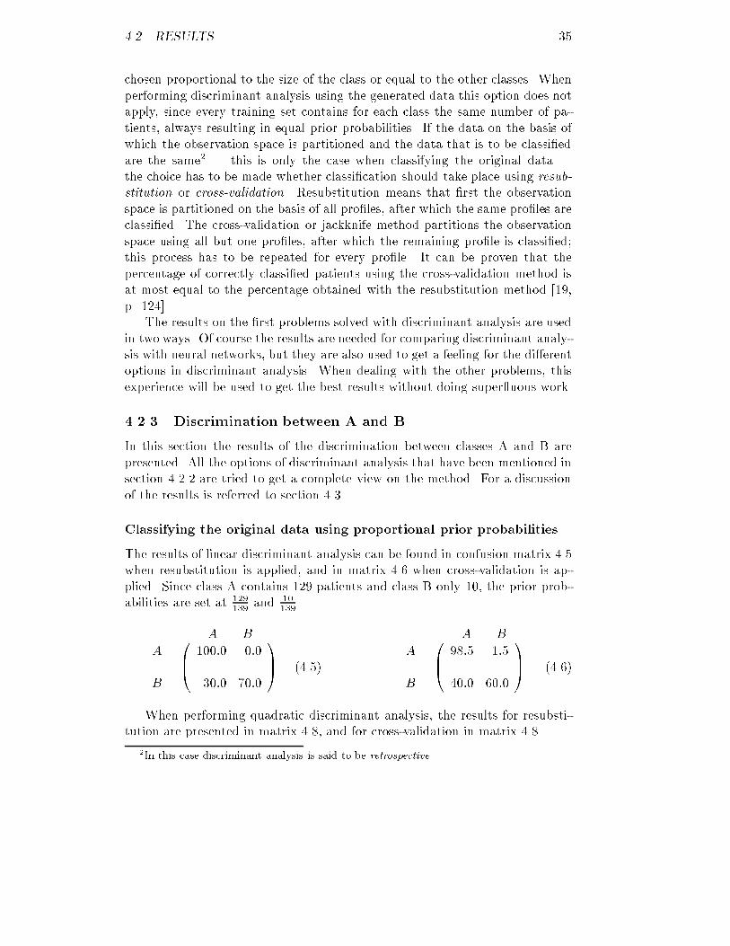
4.2. RESULTS 35chosen proportional to the size of the class or equal to the other classes. Whenperforming discriminant analysis using the generated data this option does notapply, since every training set contains for each class the same number of pa-tients, always resulting in equal prior probabilities. If the data on the basis ofwhich the observation space is partitioned and the data that is to be classi�edare the same2 | this is only the case when classifying the original data |the choice has to be made whether classi�cation should take place using resub-stitution or cross-validation. Resubstitution means that �rst the observationspace is partitioned on the basis of all pro�les, after which the same pro�les areclassi�ed. The cross-validation or jackknife method partitions the observationspace using all but one pro�les, after which the remaining pro�le is classi�ed;this process has to be repeated for every pro�le. It can be proven that thepercentage of correctly classi�ed patients using the cross-validation method isat most equal to the percentage obtained with the resubstitution method [19,p. 124].The results on the �rst problems solved with discriminant analysis are usedin two ways. Of course the results are needed for comparing discriminant analy-sis with neural networks, but they are also used to get a feeling for the di�erentoptions in discriminant analysis. When dealing with the other problems, thisexperience will be used to get the best results without doing super uous work.4.2.3 Discrimination between A and BIn this section the results of the discrimination between classes A and B arepresented. All the options of discriminant analysis that have been mentioned insection 4.2.2 are tried to get a complete view on the method. For a discussionof the results is referred to section 4.3.Classifying the original data using proportional prior probabilitiesThe results of linear discriminant analysis can be found in confusion matrix 4.5when resubstitution is applied, and in matrix 4.6 when cross-validation is ap-plied. Since class A contains 129 patients and class B only 10, the prior prob-abilities are set at 129139 and 10139 .A BAB 0B@ 100:0 0:030:0 70:0 1CA (4.5) A BAB 0B@ 98:5 1:540:0 60:0 1CA (4.6)When performing quadratic discriminant analysis, the results for resubsti-tution are presented in matrix 4.8, and for cross-validation in matrix 4.8.2In this case discriminant analysis is said to be retrospective.

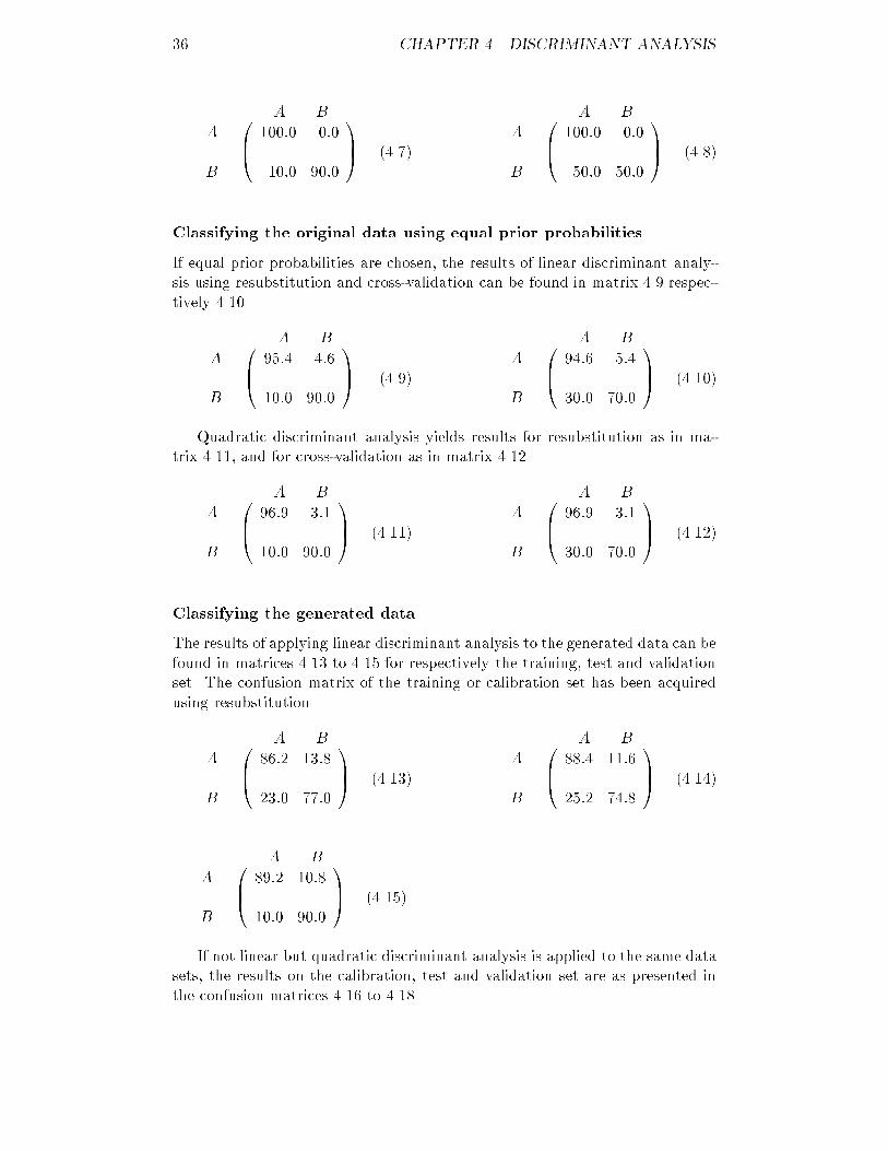
36 CHAPTER 4. DISCRIMINANT ANALYSISA BAB 0B@ 100:0 0:010:0 90:0 1CA (4.7) A BAB 0B@ 100:0 0:050:0 50:0 1CA (4.8)Classifying the original data using equal prior probabilitiesIf equal prior probabilities are chosen, the results of linear discriminant analy-sis using resubstitution and cross-validation can be found in matrix 4.9 respec-tively 4.10. A BAB 0B@ 95:4 4:610:0 90:0 1CA (4.9) A BAB 0B@ 94:6 5:430:0 70:0 1CA (4.10)Quadratic discriminant analysis yields results for resubstitution as in ma-trix 4.11, and for cross-validation as in matrix 4.12.A BAB 0B@ 96:9 3:110:0 90:0 1CA (4.11) A BAB 0B@ 96:9 3:130:0 70:0 1CA (4.12)Classifying the generated dataThe results of applying linear discriminant analysis to the generated data can befound in matrices 4.13 to 4.15 for respectively the training, test and validationset. The confusion matrix of the training or calibration set has been acquiredusing resubstitution.A BAB 0B@ 86:2 13:823:0 77:0 1CA (4.13) A BAB 0B@ 88:4 11:625:2 74:8 1CA (4.14)A BAB 0B@ 89:2 10:810:0 90:0 1CA (4.15)If not linear but quadratic discriminant analysis is applied to the same datasets, the results on the calibration, test and validation set are as presented inthe confusion matrices 4.16 to 4.18.

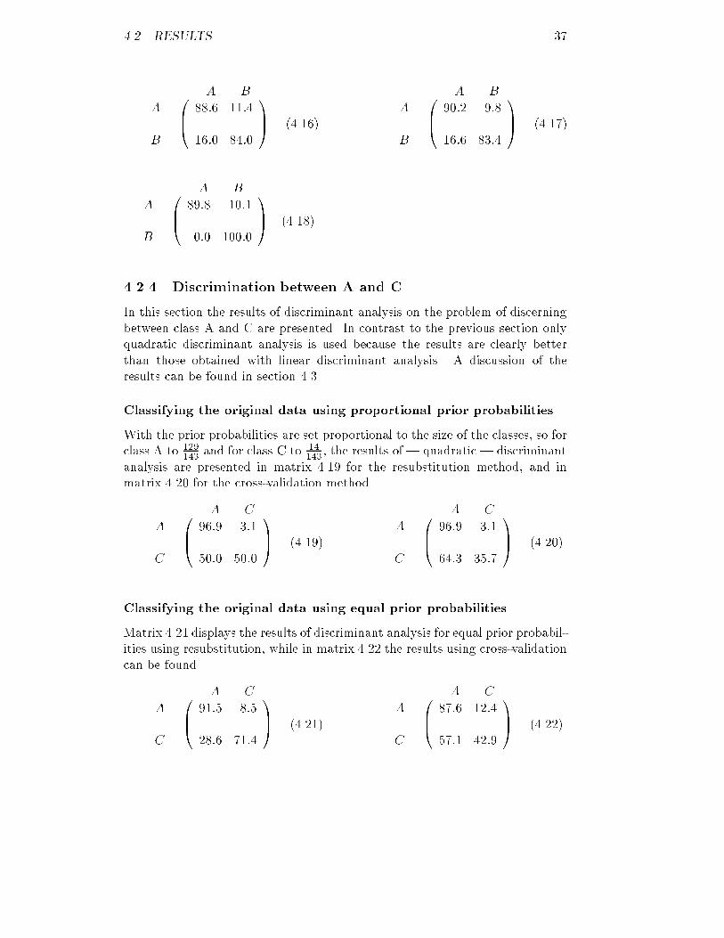
4.2. RESULTS 37A BAB 0B@ 88:6 11:416:0 84:0 1CA (4.16) A BAB 0B@ 90:2 9:816:6 83:4 1CA (4.17)A BAB 0B@ 89:8 10:10:0 100:0 1CA (4.18)4.2.4 Discrimination between A and CIn this section the results of discriminant analysis on the problem of discerningbetween class A and C are presented. In contrast to the previous section onlyquadratic discriminant analysis is used because the results are clearly betterthan those obtained with linear discriminant analysis. A discussion of theresults can be found in section 4.3.Classifying the original data using proportional prior probabilitiesWith the prior probabilities are set proportional to the size of the classes, so forclass A to 129143 and for class C to 14143 , the results of | quadratic | discriminantanalysis are presented in matrix 4.19 for the resubstitution method, and inmatrix 4.20 for the cross-validation method.A CAC 0B@ 96:9 3:150:0 50:0 1CA (4.19) A CAC 0B@ 96:9 3:164:3 35:7 1CA (4.20)Classifying the original data using equal prior probabilitiesMatrix 4.21 displays the results of discriminant analysis for equal prior probabil-ities using resubstitution, while in matrix 4.22 the results using cross-validationcan be found. A CAC 0B@ 91:5 8:528:6 71:4 1CA (4.21) A CAC 0B@ 87:6 12:457:1 42:9 1CA (4.22)

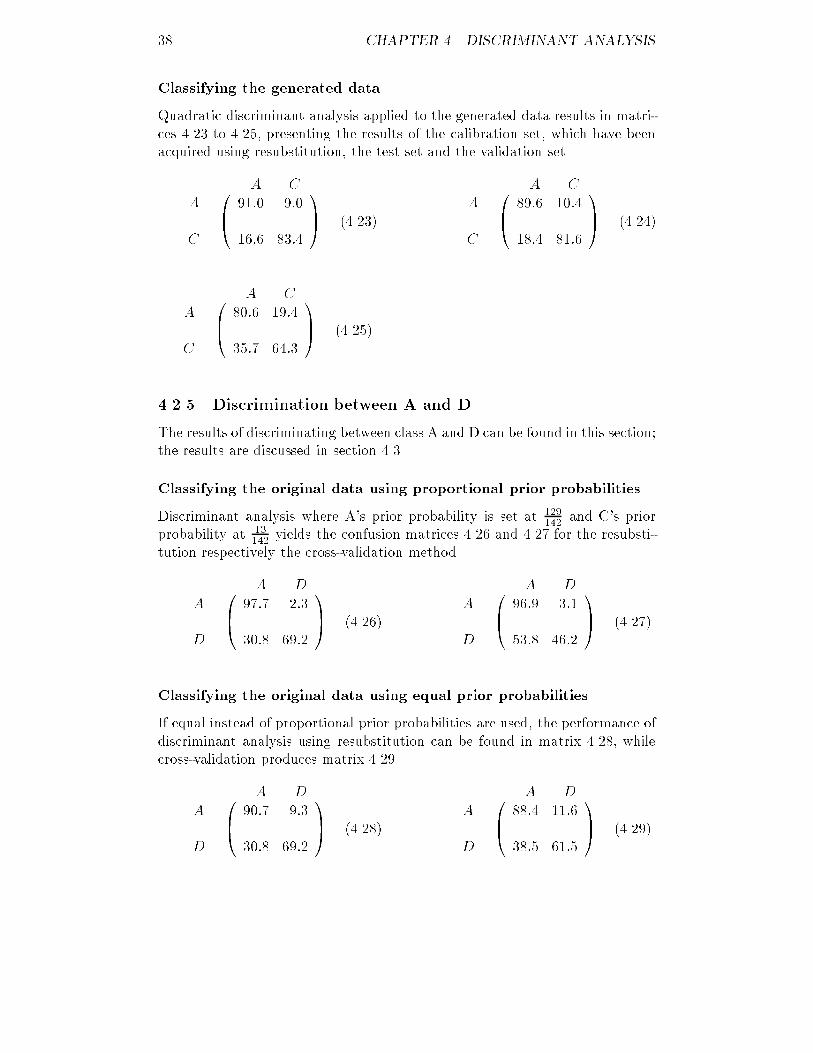
38 CHAPTER 4. DISCRIMINANT ANALYSISClassifying the generated dataQuadratic discriminant analysis applied to the generated data results in matri-ces 4.23 to 4.25, presenting the results of the calibration set, which have beenacquired using resubstitution, the test set and the validation set.A CAC 0B@ 91:0 9:016:6 83:4 1CA (4.23) A CAC 0B@ 89:6 10:418:4 81:6 1CA (4.24)A CAC 0B@ 80:6 19:435:7 64:3 1CA (4.25)4.2.5 Discrimination between A and DThe results of discriminating between class A and D can be found in this section;the results are discussed in section 4.3.Classifying the original data using proportional prior probabilitiesDiscriminant analysis where A's prior probability is set at 129142 and C's priorprobability at 13142 yields the confusion matrices 4.26 and 4.27 for the resubsti-tution respectively the cross-validation method.A DAD 0B@ 97:7 2:330:8 69:2 1CA (4.26) A DAD 0B@ 96:9 3:153:8 46:2 1CA (4.27)Classifying the original data using equal prior probabilitiesIf equal instead of proportional prior probabilities are used, the performance ofdiscriminant analysis using resubstitution can be found in matrix 4.28, whilecross-validation produces matrix 4.29.A DAD 0B@ 90:7 9:330:8 69:2 1CA (4.28) A DAD 0B@ 88:4 11:638:5 61:5 1CA (4.29)

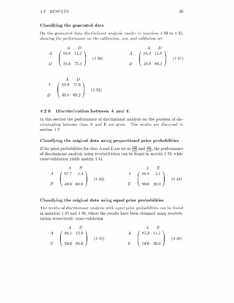
4.2. RESULTS 39Classifying the generated dataOn the generated data discriminant analysis results in matrices 4.30 to 4.32,showing the performance on the calibration, test and validation set.A DAD 0B@ 88:8 11:224:6 75:4 1CA (4.30) A DAD 0B@ 88:2 11:819:8 80:2 1CA (4.31)A DAD 0B@ 83:0 17:030:8 69:2 1CA (4.32)4.2.6 Discrimination between A and EIn this section the performance of discriminant analysis on the problem of dis-criminating between class A and E are given. The results are discussed insection 4.3.Classifying the original data using proportional prior probabilitiesIf the prior probabilities for class A and E are set at 129139 and 10139 , the performanceof discriminant analysis using resubstitution can be found in matrix 4.33, whilecross-validation yields matrix 4.34.A EAE 0B@ 97:7 2:340:0 60:0 1CA (4.33) A EAE 0B@ 96:9 3:180:0 20:0 1CA (4.34)Classifying the original data using equal prior probabilitiesThe results of discriminant analysis with equal prior probabilities can be foundin matrices 4.35 and 4.36, where the results have been obtained using resubsti-tution respectively cross-validation.A EAE 0B@ 86:1 13:920:0 80:0 1CA (4.35) A EAE 0B@ 85:3 14:770:0 30:0 1CA (4.36)

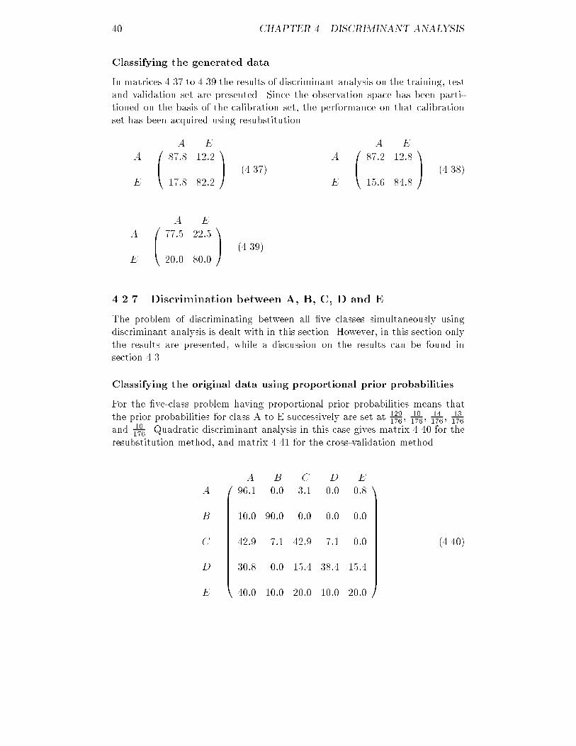
40 CHAPTER 4. DISCRIMINANT ANALYSISClassifying the generated dataIn matrices 4.37 to 4.39 the results of discriminant analysis on the training, testand validation set are presented. Since the observation space has been parti-tioned on the basis of the calibration set, the performance on that calibrationset has been acquired using resubstitution.A EAE 0B@ 87:8 12:217:8 82:2 1CA (4.37) A EAE 0B@ 87:2 12:815:6 84:8 1CA (4.38)A EAE 0B@ 77:5 22:520:0 80:0 1CA (4.39)4.2.7 Discrimination between A, B, C, D and EThe problem of discriminating between all �ve classes simultaneously usingdiscriminant analysis is dealt with in this section. However, in this section onlythe results are presented, while a discussion on the results can be found insection 4.3.Classifying the original data using proportional prior probabilitiesFor the �ve-class problem having proportional prior probabilities means thatthe prior probabilities for class A to E successively are set at 129176 , 10176 , 14176 , 13176and 10176. Quadratic discriminant analysis in this case gives matrix 4.40 for theresubstitution method, and matrix 4.41 for the cross-validation method.A B C D EABCDE 0BBBBBBBBBBBBBB@ 96:1 0:0 3:1 0:0 0:810:0 90:0 0:0 0:0 0:042:9 7:1 42:9 7:1 0:030:8 0:0 15:4 38:4 15:440:0 10:0 20:0 10:0 20:0 1CCCCCCCCCCCCCCA (4.40)

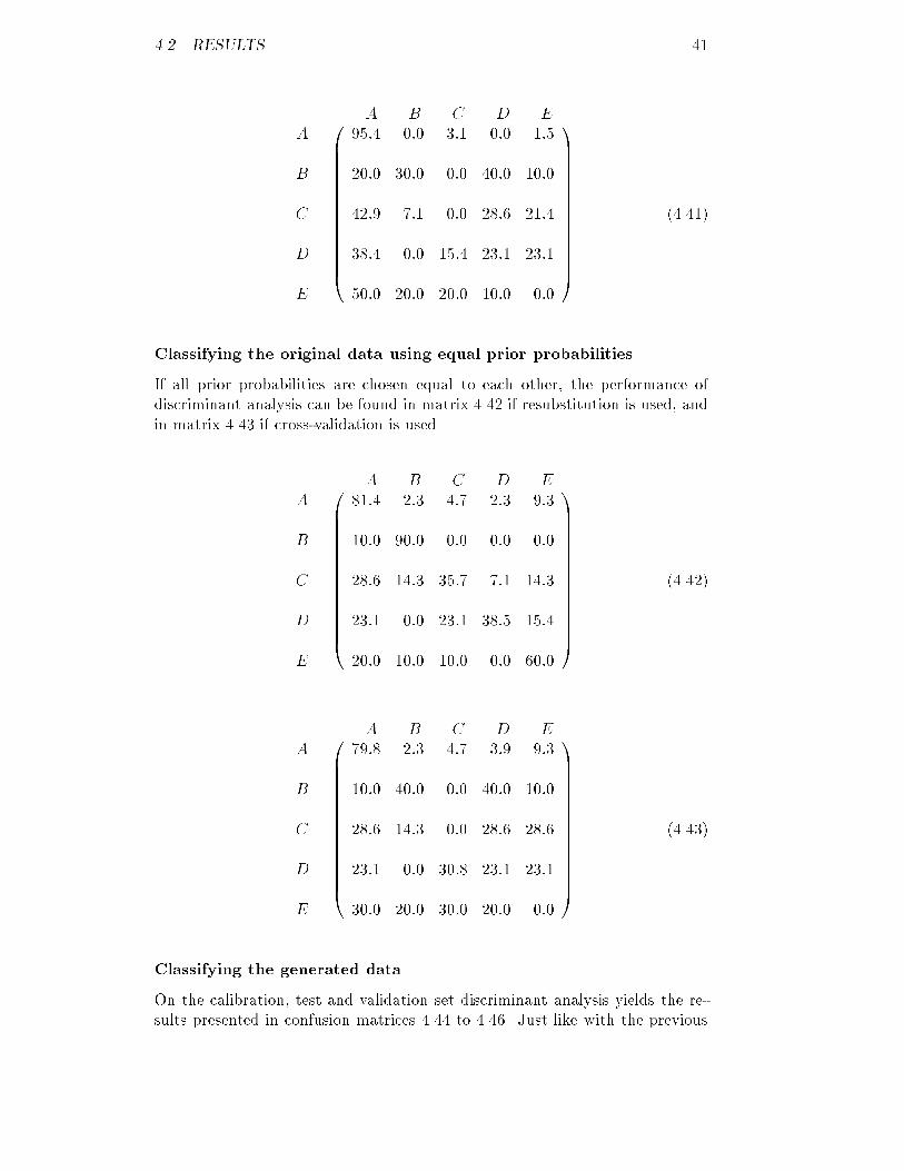
4.2. RESULTS 41A B C D EABCDE 0BBBBBBBBBBBBBB@ 95:4 0:0 3:1 0:0 1:520:0 30:0 0:0 40:0 10:042:9 7:1 0:0 28:6 21:438:4 0:0 15:4 23:1 23:150:0 20:0 20:0 10:0 0:0 1CCCCCCCCCCCCCCA (4.41)Classifying the original data using equal prior probabilitiesIf all prior probabilities are chosen equal to each other, the performance ofdiscriminant analysis can be found in matrix 4.42 if resubstitution is used, andin matrix 4.43 if cross-validation is used.A B C D EABCDE 0BBBBBBBBBBBBBB@ 81:4 2:3 4:7 2:3 9:310:0 90:0 0:0 0:0 0:028:6 14:3 35:7 7:1 14:323:1 0:0 23:1 38:5 15:420:0 10:0 10:0 0:0 60:0 1CCCCCCCCCCCCCCA (4.42)A B C D EABCDE 0BBBBBBBBBBBBBB@ 79:8 2:3 4:7 3:9 9:310:0 40:0 0:0 40:0 10:028:6 14:3 0:0 28:6 28:623:1 0:0 30:8 23:1 23:130:0 20:0 30:0 20:0 0:0 1CCCCCCCCCCCCCCA (4.43)Classifying the generated dataOn the calibration, test and validation set discriminant analysis yields the re-sults presented in confusion matrices 4.44 to 4.46. Just like with the previous

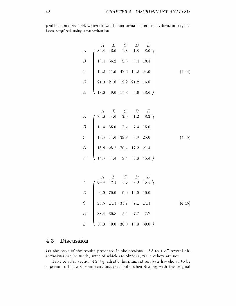
42 CHAPTER 4. DISCRIMINANT ANALYSISproblems matrix 4.44, which shows the performance on the calibration set, hasbeen acquired using resubstitution.A B C D EABCDE 0BBBBBBBBBBBBBB@ 82:4 6:0 1:8 1:8 8:013:4 56:2 5:6 6:4 18:412:2 11:0 42:6 10:2 24:021:0 21:8 19:2 21:2 16:818:0 9:0 17:8 6:6 48:6 1CCCCCCCCCCCCCCA (4.44)A B C D EABCDE 0BBBBBBBBBBBBBB@ 83:0 4:6 3:0 1:2 8:213:4 56:0 7:2 7:4 16:013:8 11:6 39:8 9:8 25:015:8 25:2 20:4 17:2 21:414:8 11:4 19:4 9:0 45:4 1CCCCCCCCCCCCCCA (4.45)A B C D EABCDE 0BBBBBBBBBBBBBB@ 64:4 2:3 15:5 2:3 15:50:0 70:0 10:0 10:0 10:028:6 14:3 35:7 7:1 14:338:4 30:8 15:4 7:7 7:730:0 0:0 30:0 10:0 30:0 1CCCCCCCCCCCCCCA (4.46)4.3 DiscussionOn the basis of the results presented in the sections 4.2.3 to 4.2.7 several ob-servations can be made, some of which are obvious, while others are not.First of all in section 4.2.3 quadratic discriminant analysis has shown to besuperior to linear discriminant analysis, both when dealing with the original

4.3. DISCUSSION 43data set as well as with the generated data. This was to be expected sincelinear discriminant analysis assumes that for all classes the covariance matricesare approximately equal. As can be found in section 3.3, this assumption is nottrue.Another observation that can be made is that the performance of discrimi-nant analysis on the original data sets gets worse when cross-validation insteadof resubstitution is used. This observation is in agreement with the theorywhich states that the percentage of correctly classi�ed patients using the cross-validation method is at most equal to the percentage obtained with the resub-stitution method [19, p. 124]. The deterioration of the percentage of correctlyclassi�ed patients is much stronger for the small classes than for class A, some-thing that can be explained very easily. For a class that consists of only afew patients which are scattered over a relatively large part of the observationspace like class E, each patient has a big in uence on the partitioning of the ob-servation space. If now the observation space is partitioned without regardingsuch a patient as is the case for cross-validation, classi�cation of this patientwill be bound to be erroneous because there are no patients causing the classboundary to be moved towards this patient. For a large class like class A thisproblem applies less because the probability that a patient has other patientsof the same class in its neighbourhood is much larger.A third obvious observation is that the choice of the prior probabilities |proportional or equal | has a big in uence on the percentages of correct clas-si�cation. As said before, proportional prior probabilities result in the correctclassi�cation of as many patients as possible independent of the class they be-long to, while equal prior probabilities result in an as high as possible percentageof correctly classi�ed patients per class. Since the di�erence in size of the classesis big | 10 to 14 against 129 patients | the di�erence in performance betweendiscriminant analysis using proportional and equal prior probabilities will alsobe big.Looking at the performance on the generated data it strikes that for allproblems the confusion matrices of the calibration and the test set are moreor less identical, see for instance matrices 4.44 and 4.45. This is not verysurprising since both sets have been generated on the basis of the same datausing the same procedure. The di�erences between the two sets have beencaused by the random generator, but since both sets are large | 500 patientseach | their distribution functions approximate the distribution function of therandom generator. The similarity between the calibration or training set andthe test set is very useful to detect over-learning, an aspect of neural networksthat is explained in section 5.3.3.As a result of the previous conclusion classi�cation of the test set yieldsbetter results than classi�cation of the validation set; since the observationspace is partitioned in a way that is optimal for the calibration set, to which thetest set is approximately equal, a nearly optimal classi�cation is to be expectedfor the test set as well. The validation set on the other hand deviates muchmore from the calibration set, so on the average for this set the partitioningwill not be optimal.In order to draw some conclusions about the quality of the generating pro-

44 CHAPTER 4. DISCRIMINANT ANALYSIScess the results of discriminant analysis on the original data set and on thevalidation set using a calibration set can be compared. Since in the calibrationset all classes are represented by equally large numbers, it seems to be fair tochoose equal prior probabilities for the comparison with the original data. If theresults on the validation set are compared with the results on the original datausing cross-validation, it strikes that the performance on the validation set ismuch higher. As mentioned before this is probably caused by the small numberof patients for most classes in the original set, resulting in a bad performanceon the original data set. Compared to the performance on the original setusing resubstitution the performance on the validation set is somewhat lower,but more important is that the according confusion matrices share the samecharacteristics. With this sharing of characteristics is meant that the order ofclasses that can best be discriminated is the same: if class X has a much higherpercentage of correctly classi�ed patients than class Y for the original set, thesame di�erence also occurs for the validation set. This observation can not bemade for all classes when discriminating between �ve classes simultaneously,but it does apply to the majority of these classes as well as to all partial prob-lems. Although it is rather hazardous to draw any conclusions on the basis ofthe above observations, we see reason enough to assume that the data that wehave generated extends the limited original data in a way that is reasonablyfair: the new data is not completely independent of the original data, but thisdependency is limited.The performance of discriminant analysis on both the original data usingequal prior probabilities and resubstitution as well as the generated data is forall problems with only two classes reasonably good, but when �ve classes areto be discriminated simultaneously the performance enormously decreases. Inthe latter case the order in which the classes can best be discriminated is B,A, C/E and D, if the validation set is considered (matrix 4.46). Classi�cationof patients belonging to class A and B is still acceptable, but the results forclass D are dramatically bad. We therefore conclude that classes A and Bare situated relatively isolated in the observation space, while the other classesand especially class D are much more spread. Since this is not a problem ofdiscriminant analysis, but intrinsic to the data set, we expect the same resultswhen using neural networks.For comparison with neural networks | see section 7.2 for a comparisonof all classi�cation methods used | not only the classi�cation percentages butalso the computation time is of importance. When discriminant analysis isapplied to the original data set containing all �ve classes and the time consumingcross-validation method was applied, a VAX 6000-410 needs only 34.5 seconds.When, again for the �ve-class problem, the generated training set containing2500 patients is used to calibrate the observation space, after which the entiretest set | also containing 2500 patients | is classi�ed, the VAX 6000-410 needsno more than 33.5 seconds.

Chapter 5Back-propagationThis chapter deals with back-propagation, a supervised method to train feed-forward neural networks. In the �rst part of this chapter the theory behindback-propagation is explained. In the second part the results obtained withthis method are presented. A good introduction to this subject can be foundin [21], while a more mathematical approach is taken in [22].5.1 Network architectureIn the early days of neural networks research a well-known model was theperceptron. Because the perceptron consisted of a single layer of adaptableweights, only linear separable problems could be solved. Since many simpleproblems, the xor-function for instance, are not linearly solvable, a lot of e�ortwas made to extend the perceptron to a multi-layer network, which does notsu�er of this shortcoming. It was not until 1986 that the theory behind sucha network was presented to a wide readership by Rumelhart and McClelland.This new neural network was called the back-propagation network .The back-propagation network consists of two or more layers of processingunits or neurons . Usually every neuron in a layer is connected to all neuronsin the next layer, but this is no requirement. Because the back-propagationnetwork is a feed-forward network , no connections exist between neurons in thesame layer, nor between neurons of layers that are not successive. The �rst layeris called the input layer , the last layer the output layer , and all intermediatelayers hidden layers . An example back-propagation network can be found in�gure 5.1. The hidden layers act as feature detectors, which means that thelayer combines all outputs of its previous layer to �nd certain relations in it.This architecture is very similar to some biological neural networks, with thecell-body being represented by the processing unit, the dendrites by the incom-ing connections, and the axon by the outgoing connections. In biological neuralnetworks information is recorded in the number and strength of the synapses ,which are the connections between the neurons, while in a back-propagationnetwork only the strength of the connections or weights is of importance. Thisdistributive storage method has the advantage that several connections can bedamaged without losing all stored information.45

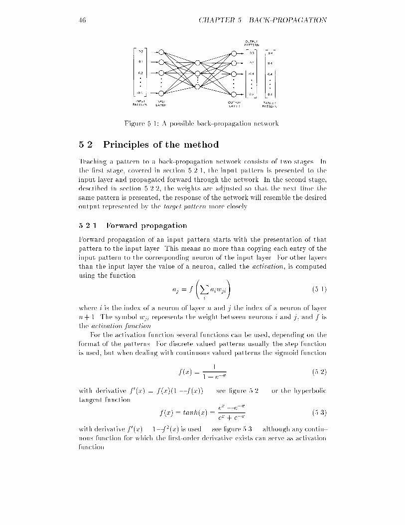
46 CHAPTER 5. BACK-PROPAGATIONFigure 5.1: A possible back-propagation network.5.2 Principles of the methodTeaching a pattern to a back-propagation network consists of two stages. Inthe �rst stage, covered in section 5.2.1, the input pattern is presented to theinput layer and propagated forward through the network. In the second stage,described in section 5.2.2, the weights are adjusted so that the next time thesame pattern is presented, the response of the network will resemble the desiredoutput represented by the target pattern more closely.5.2.1 Forward propagationForward propagation of an input pattern starts with the presentation of thatpattern to the input layer. This means no more than copying each entry of theinput pattern to the corresponding neuron of the input layer. For other layersthan the input layer the value of a neuron, called the activation, is computedusing the function aj = f Xi aiwji! (5.1)where i is the index of a neuron of layer n and j the index of a neuron of layern+ 1. The symbol wji represents the weight between neurons i and j, and f isthe activation function.For the activation function several functions can be used, depending on theformat of the patterns. For discrete valued patterns usually the step functionis used, but when dealing with continuous valued patterns the sigmoid functionf(x) = 11 + e�x (5.2)with derivative f 0(x) = f(x)(1 � f(x)) | see �gure 5.2 | or the hyperbolictangent function f(x) = tanh(x) = ex � e�xex + e�x (5.3)with derivative f 0(x) = 1�f2(x) is used | see �gure 5.3 | although any contin-uous function for which the �rst-order derivative exists can serve as activationfunction.

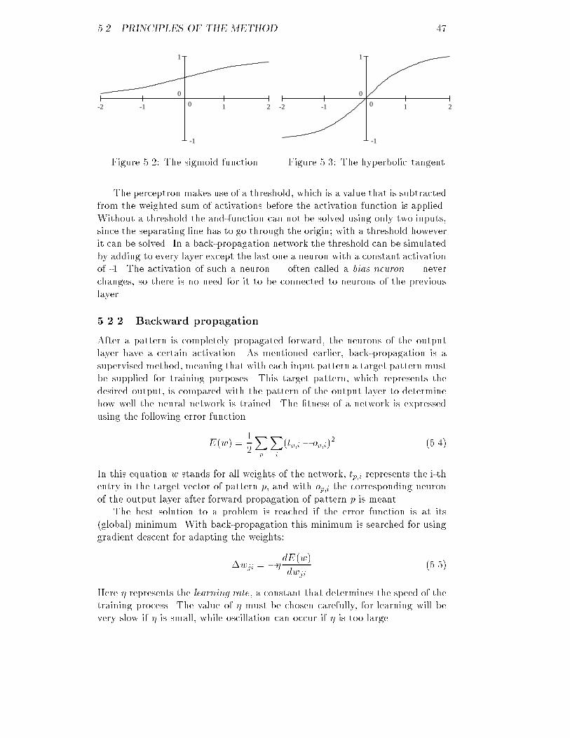
5.2. PRINCIPLES OF THE METHOD 470

0

-1

1

1 2-1-2 Figure 5.2: The sigmoid function. 0

0

-1

1

1 2-1-2 Figure 5.3: The hyperbolic tangent.The perceptron makes use of a threshold, which is a value that is subtractedfrom the weighted sum of activations before the activation function is applied.Without a threshold the and-function can not be solved using only two inputs,since the separating line has to go through the origin; with a threshold howeverit can be solved. In a back-propagation network the threshold can be simulatedby adding to every layer except the last one a neuron with a constant activationof -1. The activation of such a neuron | often called a bias neuron | neverchanges, so there is no need for it to be connected to neurons of the previouslayer.5.2.2 Backward propagationAfter a pattern is completely propagated forward, the neurons of the outputlayer have a certain activation. As mentioned earlier, back-propagation is asupervised method, meaning that with each input pattern a target pattern mustbe supplied for training purposes. This target pattern, which represents thedesired output, is compared with the pattern of the output layer to determinehow well the neural network is trained. The �tness of a network is expressedusing the following error functionE(w) = 12Xp Xi (tp;i � op;i)2 (5.4)In this equation w stands for all weights of the network, tp;i represents the i-thentry in the target vector of pattern p, and with op;i the corresponding neuronof the output layer after forward propagation of pattern p is meant.The best solution to a problem is reached if the error function is at its(global) minimum. With back-propagation this minimum is searched for usinggradient descent for adapting the weights:�wji = ��dE(w)dwji (5.5)Here � represents the learning rate, a constant that determines the speed of thetraining process. The value of � must be chosen carefully, for learning will bevery slow if � is small, while oscillation can occur if � is too large.

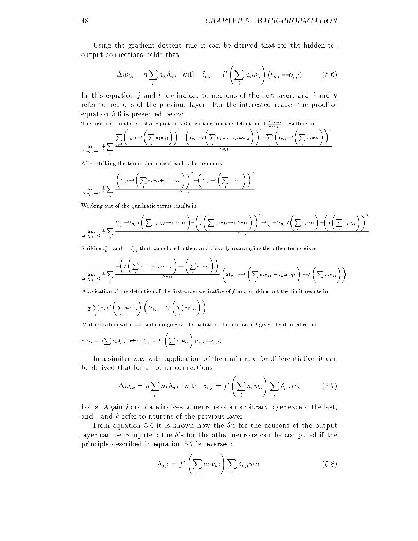
48 CHAPTER 5. BACK-PROPAGATIONUsing the gradient descent rule it can be derived that for the hidden-to-output connections holds that�wlk = �Xp ak�p;l with �p;l = f 0 Xi aiwli! (tp;l � op;l) (5.6)In this equation j and l are indices to neurons of the last layer, and i and krefer to neurons of the previous layer. For the interested reader the proof ofequation 5.6 is presented below.The �rst step in the proof of equation 5.6 is writing out the de�nition of dE(w)dwlk , resulting inlim�wlk!0 12Pp Pj 6=l�tp;j�f�Pi aiwji��2+�tp;l�f�Pi aiwli+ak�wlk��2�Pj �tp;j�f�Pi aiwji��2�wlkAfter striking the terms that cancel each other remainslim�wlk!0 12Pp �tp;l�f�Pi aiwli+ak�wlk��2��tp;l�f�Pi aiwli��2�wlkWorking out of the quadratic terms results inlim�wlk!0 12Pp t2p;l�2tp;lf�Pi aiwli+ak�wlk�+�f�Pi aiwli+ak�wlk��2�t2p;l+2tp;lf�Pi aiwli���f�Pi aiwli��2�wlkStriking t2p;l and � t2p;l that cancel each other, and cleverly rearranging the other terms giveslim�wlk!0 12Pp ��f�Pi aiwli+ak�wlk��f�Pi aiwli���wlk �2tp;l � f�Pi aiwli + ak�wlk�� f�Pi aiwli��Application of the de�nition of the �rst-order derivative of f and working out the limit results in� 12Pp akf 0�Pi aiwli��2tp;l � 2f�Pi aiwli��Multiplication with � � and changing to the notation of equation 5.6 gives the desired result�wlk = �Pp ak�p;l with �p;l = f 0�Pi aiwli� (tp;l � op;l)In a similar way with application of the chain rule for di�erentiation it canbe derived that for all other connections�wlk = �Xp ak�p;l with �p;l = f 0 Xi aiwli!Xi �p;iwli (5.7)holds. Again j and l are indices to neurons of an arbitrary layer except the last,and i and k refer to neurons of the previous layer.From equation 5.6 it is known how the �'s for the neurons of the outputlayer can be computed; the �'s for the other neurons can be computed if theprinciple described in equation 5.7 is reversed:�p;k = f 0 Xi aiwki!Xj �p;jwjk (5.8)

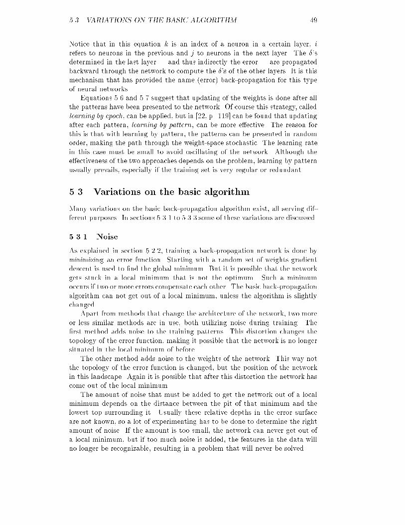
5.3. VARIATIONS ON THE BASIC ALGORITHM 49Notice that in this equation k is an index of a neuron in a certain layer, irefers to neurons in the previous and j to neurons in the next layer. The �'sdetermined in the last layer | and thus indirectly the error | are propagatedbackward through the network to compute the �'s of the other layers. It is thismechanism that has provided the name (error) back-propagation for this typeof neural networks.Equations 5.6 and 5.7 suggest that updating of the weights is done after allthe patterns have been presented to the network. Of course this strategy, calledlearning by epoch, can be applied, but in [22, p. 119] can be found that updatingafter each pattern, learning by pattern, can be more e�ective. The reason forthis is that with learning by pattern, the patterns can be presented in randomorder, making the path through the weight-space stochastic. The learning ratein this case must be small to avoid oscillating of the network. Although thee�ectiveness of the two approaches depends on the problem, learning by patternusually prevails, especially if the training set is very regular or redundant.5.3 Variations on the basic algorithmMany variations on the basic back-propagation algorithm exist, all serving dif-ferent purposes. In sections 5.3.1 to 5.3.3 some of these variations are discussed.5.3.1 NoiseAs explained in section 5.2.2, training a back-propagation network is done byminimizing an error function. Starting with a random set of weights gradientdescent is used to �nd the global minimum. But it is possible that the networkgets stuck in a local minimum that is not the optimum. Such a minimumoccurs if two or more errors compensate each other. The basic back-propagationalgorithm can not get out of a local minimum, unless the algorithm is slightlychanged.Apart from methods that change the architecture of the network, two moreor less similar methods are in use, both utilizing noise during training. The�rst method adds noise to the training patterns. This distortion changes thetopology of the error function, making it possible that the network is no longersituated in the local minimum of before.The other method adds noise to the weights of the network. This way notthe topology of the error function is changed, but the position of the networkin this landscape. Again it is possible that after this distortion the network hascome out of the local minimum.The amount of noise that must be added to get the network out of a localminimum depends on the distance between the pit of that minimum and thelowest top surrounding it. Usually these relative depths in the error surfaceare not known, so a lot of experimenting has to be done to determine the rightamount of noise. If the amount is too small, the network can never get out ofa local minimum, but if too much noise is added, the features in the data willno longer be recognizable, resulting in a problem that will never be solved.

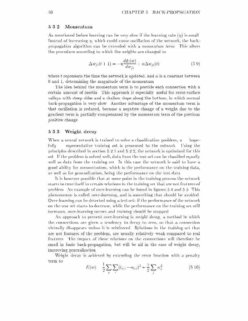
50 CHAPTER 5. BACK-PROPAGATION5.3.2 MomentumAs mentioned before learning can be very slow if the learning rate (�) is small.Instead of increasing �, which could cause oscillation of the network, the back-propagation algorithm can be extended with a momentum term. This altersthe procedure according to which the weights are changed to�wji(t+ 1) = ��dE(w)dwji + ��wji(t) (5.9)where t represents the time the network is updated, and � is a constant between0 and 1, determining the magnitude of the momentum.The idea behind the momentum term is to provide each connection with acertain amount of inertia. This approach is especially useful for error-surfacevalleys with steep sides and a shallow slope along the bottom, in which normalback-propagation is very slow. Another advantage of the momentum term isthat oscillation is reduced, because a negative change of a weight due to thegradient term is partially compensated by the momentum term of the previouspositive change.5.3.3 Weight decayWhen a neural network is trained to solve a classi�cation problem, a | hope-fully | representative training set is presented to the network. Using theprinciples described in section 5.2.1 and 5.2.2, the network is optimized for thisset. If the problem is solved well, data from the test set can be classi�ed equallywell as data from the training set. In this case the network is said to have agood ability for memorization, which is the performance on the training data,as well as for generalization, being the performance on the test data.It is however possible that at some point in the training process the networkstarts to tune itself to certain relations in the training set that are not features ofproblem. An example of over-learning can be found in �gures 5.4 and 5.5. Thisphenomenon is called over-learning , and is something that should be avoided.Over-learning can be detected using a test set: if the performance of the networkon the test set starts to decrease, while the performance on the training set stillincreases, over-learning occurs and training should be stopped.An approach to prevent over-learning is weight decay , a method in whichthe connections are given a tendency to decay to zero, so that a connectionvirtually disappears unless it is reinforced. Relations in the training set thatare not features of the problem, are usually relatively weak compared to realfeatures. The impact of these relations on the connections will therefore besmall in basic back-propagation, but will be nil in the case of weight decay,improving generalization.Weight decay is achieved by extending the error function with a penaltyterm to E(w) = 12Xp Xi (tp;i � op;i)2 + 2Xj w2j (5.10)

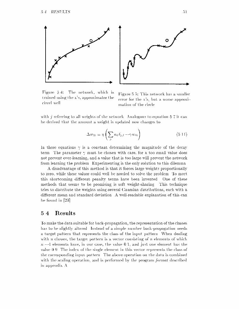
5.4. RESULTS 51Figure 5.4: The network, which istrained using the x's, approximates thecircel well. Figure 5.5: This network has a smallererror for the x's, but a worse approxi-mation of the circle.with j referring to all weights of the network. Analogous to equation 5.7 it canbe derived that the amount a weight is updated now changes to�wlk = � Xp ak�p;l � wlk! (5.11)In these equations is a constant determining the magnitude of the decayterm. The parameter must be chosen with care, for a too small value doesnot prevent over-learning, and a value that is too large will prevent the networkfrom learning the problem. Experimenting is the only solution to this dilemma.A disadvantage of this method is that it forces large weights proportionallyto zero, while these values could well be needed to solve the problem. To meetthis shortcoming di�erent penalty terms have been invented. One of thesemethods that seems to be promising is soft weight-sharing. This techniquetries to distribute the weights using several Gaussian distributions, each with adi�erent mean and standard deviation. A well-readable explanation of this canbe found in [23].5.4 ResultsTo make the data suitable for back-propagation, the representation of the classeshas to be slightly altered. Instead of a simple number back-propagation needsa target pattern that represents the class of the input pattern. When dealingwith n classes, the target pattern is a vector consisting of n elements of whichn � 1 elements have, in our case, the value 0.1, and just one element has thevalue 0.9. The index of the single element in this vector represents the class ofthe corresponding input pattern. The above operation on the data is combinedwith the scaling operation, and is performed by the program format describedin appendix A.

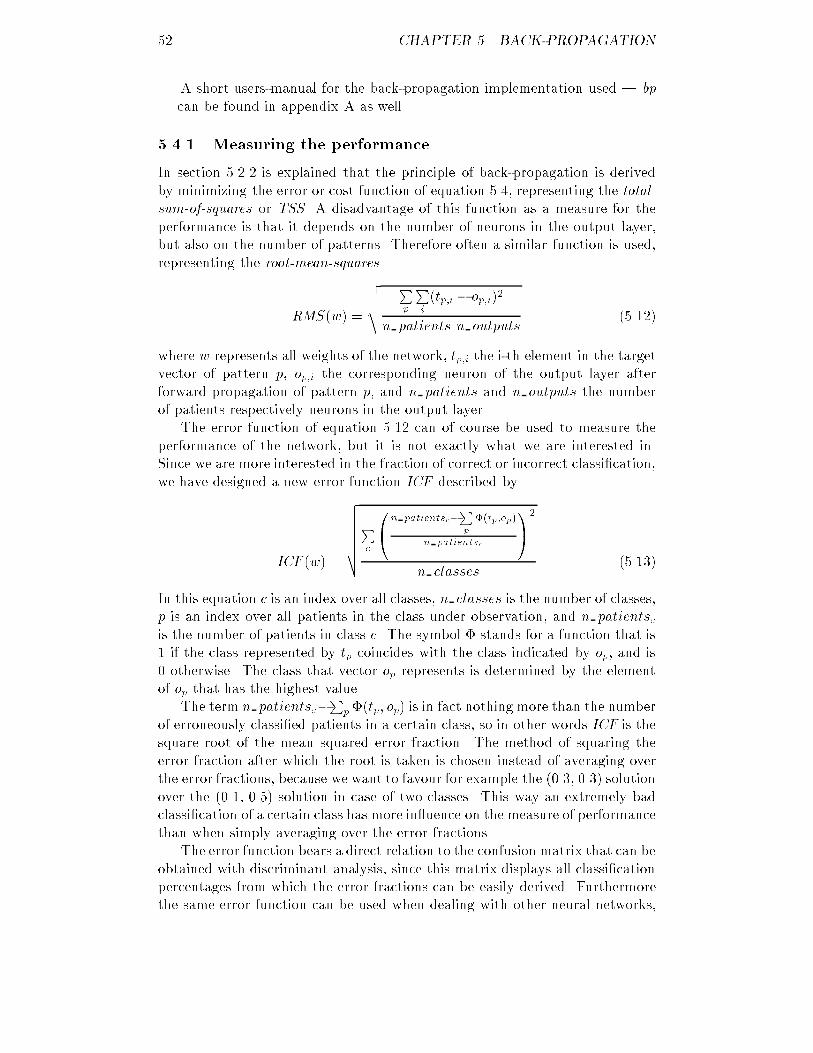
52 CHAPTER 5. BACK-PROPAGATIONA short users-manual for the back-propagation implementation used | bp| can be found in appendix A as well.5.4.1 Measuring the performanceIn section 5.2.2 is explained that the principle of back-propagation is derivedby minimizing the error or cost function of equation 5.4, representing the total-sum-of-squares or TSS . A disadvantage of this function as a measure for theperformance is that it depends on the number of neurons in the output layer,but also on the number of patterns. Therefore often a similar function is used,representing the root-mean-squaresRMS(w) =vuut Pp Pi (tp;i � op;i)2n patients n outputs (5.12)where w represents all weights of the network, tp;i the i-th element in the targetvector of pattern p, op;i the corresponding neuron of the output layer afterforward propagation of pattern p, and n patients and n outputs the numberof patients respectively neurons in the output layer.The error function of equation 5.12 can of course be used to measure theperformance of the network, but it is not exactly what we are interested in.Since we are more interested in the fraction of correct or incorrect classi�cation,we have designed a new error function ICF described byICF(w) =vuuuuutPc 0@n patientsc�Pp �(tp;op)n patientsc 1A2n classes (5.13)In this equation c is an index over all classes, n classes is the number of classes,p is an index over all patients in the class under observation, and n patientscis the number of patients in class c. The symbol � stands for a function that is1 if the class represented by tp coincides with the class indicated by op, and is0 otherwise. The class that vector op represents is determined by the elementof op that has the highest value.The term n patientsc�Pp�(tp; op) is in fact nothing more than the numberof erroneously classi�ed patients in a certain class, so in other words ICF is thesquare root of the mean squared error fraction. The method of squaring theerror fraction after which the root is taken is chosen instead of averaging overthe error fractions, because we want to favour for example the (0.3, 0.3) solutionover the (0.1, 0.5) solution in case of two classes. This way an extremely badclassi�cation of a certain class has more in uence on the measure of performancethan when simply averaging over the error fractions.The error function bears a direct relation to the confusion matrix that can beobtained with discriminant analysis, since this matrix displays all classi�cationpercentages from which the error fractions can be easily derived. Furthermorethe same error function can be used when dealing with other neural networks,

5.4. RESULTS 53RMS

ICF

RMS/ICF x 10-3

3#epochs x 10240.00

260.00

280.00

300.00

320.00

340.00

360.00

380.00

400.00

420.00

440.00

460.00

480.00

500.00

520.00

540.00

560.00

580.00

600.00

0.00 5.00 10.00 15.00 20.00Figure 5.6: Comparison between the RMS and ICF for a back-propagationnetwork.like Kohonen's self-organizing feature map, so a direct comparison of the dif-ferent methods is possible.Because in ICF all classes are of equal importance, minimizing ICF coin-cides with maximizing the correct classi�cation per class. The consequences ofthis choice are that the number of patterns in the training set must approxi-mately be equal per class to prevent the network from focusing on the largestclass, and secondly that, when comparing back-propagation with discriminantanalysis, equal prior probabilities must be assigned to each class.In contrast to many implementations where the error function is computedduring a learning epoch, we compute it after each learning epoch. Althoughthis approach is a bit less e�cient, it is more fair when learning by pattern,because if the performance of the network on a pattern is measured immediatelyafter adjusting the network to it, the performance will be good, while the nextpatterns that are presented to the network will partially cancel this result. Forthis reason it is better to freeze a network before evaluating it.Unfortunately, as can be seen in �gure 5.6, the RMS and ICF are notalways fully correlated. This means that the network does not try to maximizethe fraction of correct classi�cation, something that we would like it to do.Another observation that can be made is that the ICF is much more jumpythan the RMS . The reason for this behaviour is that for the ICF classi�cationof a pattern is correct or incorrect, there is no intermediate possibility. If theweights of the network are slightly adapted, resulting in only a small change ofthe RMS , it is possible that for some patterns a di�erent neuron of the outputlayer becomes the winner, thus resulting in a di�erent classi�cation. For the ICFclassi�cation of these patterns now changes radically, from correct to incorrector vice versa. The jumpy behaviour can partially be resolved by averaging theICF over a number of epochs.

54 CHAPTER 5. BACK-PROPAGATION5.4.2 Approach to solving the problemJust like with discriminant analysis, we �rst try to discriminate between healthypeople | class A | and every disease separately, before proceeding with themore di�cult problem of discriminating between all �ve classes at the sametime. The experience gained from examining these problems is used to get afeeling for the problem domain and to avoid doing super uous work.A back-propagation network has many parameters that have to be adjustedcorrectly to get a good performance. Some of these parameters have a bigin uence on the performance, others are of lesser importance. To �nd theoptimal network all combinations of the parameters should be tried, but thismethod takes a lot of time. The approach we therefore take is determiningthe optimal values for the parameters of the basic algorithm, extended with amomentum term for speed, in order of decreasing in uence. For the parametersthat are not determined yet values are assumed based on rules of thumb orprevious experience. After the | hopefully | optimal network is determined,two variations on the basic algorithm | adding of noise to the learn patternsand weight decay | are tried to see if the performance improves.During training the performance of the network on the training set is mon-itored using the RMS function. The reason for monitoring the training set isthat we want to see if the network converges well, but veri�cation of severaltheoretical propositions | the learning rate in uences the speed of learningfor instance | is now possible as well. For these purposes the RMS is bettersuited than the ICF , because the RMS is the error measure the network triesto minimize1 , while the ICF is a measure the network is completely unaware of.Furthermore we are not interested in the classi�cation results of the networkon the training set, because on this set 100% correct classi�cation can easilybe achieved if only the size of the network is large enough [22, p. 142]. Toreduce the number of points in the �gures to 20 without risking that one of theselected points is non-representative for the performance curve for each pointthe average of 25 successive points is taken.The performance of the network on the test set is also monitored duringtraining, but with this set the ICF function is used. Here monitoring is done tocheck on the generalization capabilities of the network, something that is veryimportant when dealing with classi�cation problems. Although generalizationand detection of over-learning | see section 5.3.3 | could probably be doneat least as well using the RMS , we have chosen for the ICF because it displaysthe fraction of incorrect classi�cation as well, and this is something we wantto minimize. Since from the RMS the ability to classify apparently can notbe determined, which can be seen in �gure 5.6, but over-learning probably canbe detected using classi�cation fractions, the ICF seems to be the only logicalchoice. Again, to limit the number of points in a �gure to 20 and to control thejumpy behaviour of the ICF each point represents the average of 25 successivepoints.The decision to adjust a parameter to a particular value is primarily basedon the performance of the network on the test set. Only if these �gures do not1Actually the network tries to minimize the TSS , but the RMS is fully correlated with it.

5.4. RESULTS 55di�er enough to make a clear choice for a particular value of a parameter, theperformance on the training set is taken into consideration. A better or fasterconvergence could be a reason to favour a particular value.If a network seems to be promising, the validation set is presented to it.From the resulting �gure the number of epochs is determined after which thenetwork classi�es best. The classi�cation results the network achieves in thisstage are used to draw up a confusion matrix, which can be used for comparisonwith other types of neural networks or classifying techniques.In the remainder of this section the parameters in order of expected de-creasing in uence on the performance of a back-propagation network are brie ydiscussed to motivate their earlier mentioned initial adjustments.ArchitectureThe architecture of a neural network is the degree of freedom that has thebiggest in uence on the performance. Although this parameter is the �rst tobe varied and thereby no initial value has to be chosen, some annotations haveto be made.First it has to be remarked that the only aspects of the architecture thatcan be varied are the number of hidden layers and the number of neurons perlayer. The network has to stay a feed-forward network. Although there is norestriction on the number of hidden layers, in [22, p. 142] can be found thata network with three or more hidden layers o�ers no additional computationalpower over a network with only two hidden layers. In view of the fact that, themore layers a network consists of, the less well it can be parallelized, it seemsto be sensible to con�ne the architecture to one or two hidden layers.As mentioned before, also in [22, p. 142] can be found that a function canbe approximated to any given accuracy, if only the size of the network is largeenough. For a classi�cation problem this means that a correct classi�cation ofthe training set up to 100% can be achieved. Unfortunately the performanceon the test set will probably be very poor, because the network has over�ttedthe training set. This is what was called over-learning in section 5.3.3.Learning rateAlthough some people use the rule of thumb that in case of learning by patternthe learning rate in a back-propagation network should approximately be equalto 0.25 divided by the number of patterns in the training set, our experiencewith the same data is that a larger value can be chosen without the risk ofsevere oscillation. Therefore the initial learning rate (�) is set at 0.01, by whichwe hope to limit the number of epochs needed.MomentumThe momentum term | see section 5.3.2 | is not a part of the basic back-propagation algorithm, but we use it anyway because of the acceleration itgives to the training process. If there is only one | global | minimum, themomentum term has no in uence on the performance of the network. If however

56 CHAPTER 5. BACK-PROPAGATIONseveral minima exist, the momentum term could cause the network to get stuckin one of them which it otherwise would have avoided. But just as well could asa result of the momentum term a local minimum be avoided where otherwisethe network would get stuck in.The constant that determines the magnitude of the momentum term (�)must lie between 0 and 1 and is usually chosen relatively high [22, p. 123]. Asan initial value for � we therefore choose 0.8.Initial weightsWhen a neural network is initialized, random values are assigned to its weights.Since every set of weights de�nes a position on the surface of the error func-tion, the initial weights can in uence the performance if this surface containslocal minima. Therefore the probability distribution from which the weights aredrawn is of importance. However, to avoid saturation of the activation function,which will be explained in more detail in the next section about the activationfunction, the initial weights must meet certain requirements. Therefore the ini-tial weights are drawn from an uniform distribution over the interval [-0.5,0.5].Only if the performance curve of the training set suggests that the network hasgot stuck in a local minimum, a di�erent initialization of the weights is tried.Activation functionIn section 5.2.1 two activation functions for continuous valued patterns werepresented, namely the sigmoid and the hyperbolic tangent. Both functionshave a �rst-order derivative that has the highest value in the interval [-1,1];outside this interval the functions are relatively at. If a variation in a patternor a change of weights should have any e�ect on the output of a neuron, theweighted sum to which the activation function is applied should therefore notlie too far outside [-1,1]. It is for this reason that the data is scaled between0.1 and 0.9, and that the initial weights are drawn from the interval [-0.5,0.5].The data is not scaled between -0.9 and 0.9 because this would cause someparameters to become 0, thus not contributing to the weighted sum anymore.For the activation function only the sigmoid is considered, because this func-tion is less at outside the interval [-1,1] than the hyperbolic tangent. Anotherreason to use the sigmoid function is that it is more or less a standard whendealing with back-propagation networks, in contrast to the hyperbolic tangentwhich is used only incidentally. If the hyperbolic tangent is to be used, the tar-get patterns of all sets have to be changed because the range of the hyperbolictangent starts at -1 instead of 0. To have full advantage of this larger intervalit is wise to choose a value for the low value of the target pattern that is closeto -1, usually -0.9 is taken.Learning grainAt the end of section 5.2.2 we have explained that updating of the weights, whichis neural network equivalent of learning, can take place after the presentation ofa single pattern or all patterns of the training set. This di�erence is called the

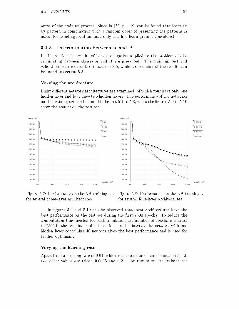
5.4. RESULTS 57grain of the training process. Since in [22, p. 119] can be found that learningby pattern in combination with a random order of presenting the patterns isuseful for avoiding local minima, only this �ne learn grain is considered.5.4.3 Discrimination between A and BIn this section the results of back-propagation applied to the problem of dis-criminating between classes A and B are presented. The training, test andvalidation set are described in section 3.5, while a discussion of the results canbe found in section 5.5.Varying the architectureEight di�erent network architectures are examined, of which four have only onehidden layer and four have two hidden layers. The performance of the networkson the training set can be found in �gures 5.7 to 5.8, while the �gures 5.9 to 5.10show the results on the test set.5-5-2

5-10-2

5-20-2

5-40-2

RMS x 10-3

3#epochs x 10

80.00

100.00

120.00

140.00

160.00

180.00

200.00

220.00

240.00

260.00

280.00

300.00

0.00 5.00 10.00 15.00 20.00Figure 5.7: Performance on the AB-training setfor several three-layer architectures.5-10-5-2

5-10-10-2

5-20-10-2

5-20-20-2

RMS x 10-3

3#epochs x 10

80.00

100.00

120.00

140.00

160.00

180.00

200.00

220.00

240.00

260.00

280.00

300.00

0.00 5.00 10.00 15.00 20.00Figure 5.8: Performance on the AB-training setfor several four-layer architectures.In �gures 5.9 and 5.10 can be observed that most architectures have thebest performance on the test set during the �rst 7500 epochs. To reduce thecomputation time needed for each simulation the number of epochs is limitedto 7500 in the remainder of this section. In this interval the network with onehidden layer containing 40 neurons gives the best performance and is used forfurther optimizing.Varying the learning rateApart from a learning rate of 0.01, which was chosen as default in section 5.4.2,two other values are tried: 0.0005 and 0.2. The results on the training set

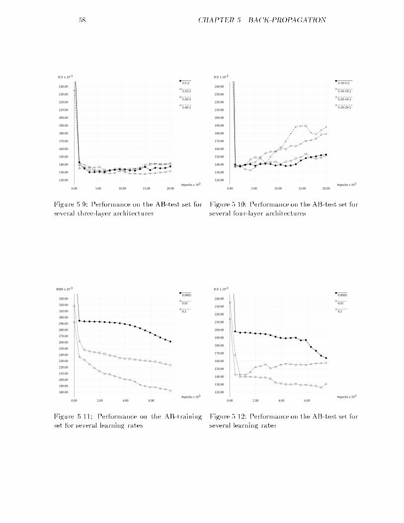
58 CHAPTER 5. BACK-PROPAGATION5-5-2

5-10-2

5-20-2

5-40-2

ICF x 10-3

3#epochs x 10

120.00

130.00

140.00

150.00

160.00

170.00

180.00

190.00

200.00

210.00

220.00

230.00

240.00

0.00 5.00 10.00 15.00 20.00Figure 5.9: Performance on the AB-test set forseveral three-layer architectures.5-10-5-2

5-10-10-2

5-20-10-2

5-20-20-2

ICF x 10-3

3#epochs x 10

120.00

130.00

140.00

150.00

160.00

170.00

180.00

190.00

200.00

210.00

220.00

230.00

240.00

0.00 5.00 10.00 15.00 20.00Figure 5.10: Performance on the AB-test set forseveral four-layer architectures.0.0005

0.01

0.2

RMS x 10-3

3#epochs x 10

180.00

190.00

200.00

210.00

220.00

230.00

240.00

250.00

260.00

270.00

280.00

290.00

300.00

310.00

320.00

330.00

0.00 2.00 4.00 6.00Figure 5.11: Performance on the AB-trainingset for several learning rates.0.0005

0.01

0.2

ICF x 10-3

3#epochs x 10

120.00

130.00

140.00

150.00

160.00

170.00

180.00

190.00

200.00

210.00

220.00

230.00

240.00

0.00 2.00 4.00 6.00Figure 5.12: Performance on the AB-test set forseveral learning rates.

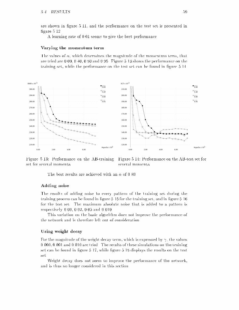
5.4. RESULTS 59are shown in �gure 5.11, and the performance on the test set is presented in�gure 5.12.A learning rate of 0.01 seems to give the best performance.Varying the momentum termThe values of �, which determines the magnitude of the momentum term, thatare tried are 0.00, 0.40, 0.80 and 0.95. Figure 5.13 shows the performance on thetraining set, while the performance on the test set can be found in �gure 5.14.0.00

0.40

0.80

0.95

RMS x 10-3

3#epochs x 10

210.00

220.00

230.00

240.00

250.00

260.00

270.00

280.00

290.00

300.00

0.00 2.00 4.00 6.00Figure 5.13: Performance on the AB-trainingset for several momenta.0.00

0.40

0.80

0.95

ICF x 10-3

3#epochs x 10

120.00

130.00

140.00

150.00

160.00

170.00

180.00

190.00

200.00

210.00

0.00 2.00 4.00 6.00Figure 5.14: Performance on the AB-test set forseveral momenta.The best results are achieved with an � of 0.80.Adding noiseThe results of adding noise to every pattern of the training set during thetraining process can be found in �gure 5.15 for the training set, and in �gure 5.16for the test set. The maximum absolute noise that is added to a pattern isrespectively 0.00, 0.02, 0.05 and 0.010.This variation on the basic algorithm does not improve the performance ofthe network and is therefore left out of consideration.Using weight decayFor the magnitude of the weight decay term, which is expressed by , the values0.000, 0.001 and 0.010 are tried. The results of these simulations on the trainingset can be found in �gure 5.17, while �gure 5.18 displays the results on the testset.Weight decay does not seem to improve the performance of the network,and is thus no longer considered in this section.

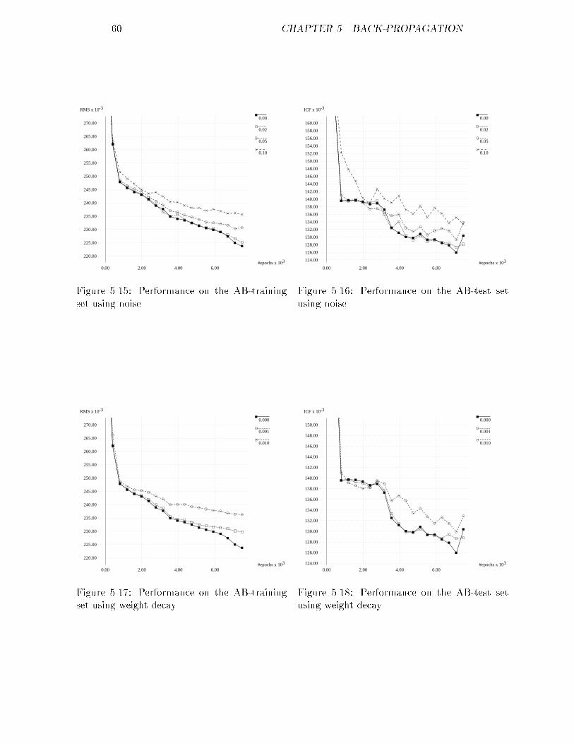
60 CHAPTER 5. BACK-PROPAGATION0.00

0.02

0.05

0.10

RMS x 10-3

3#epochs x 10

220.00

225.00

230.00

235.00

240.00

245.00

250.00

255.00

260.00

265.00

270.00

0.00 2.00 4.00 6.00Figure 5.15: Performance on the AB-trainingset using noise.0.00

0.02

0.05

0.10

ICF x 10-3

3#epochs x 10124.00

126.00

128.00

130.00

132.00

134.00

136.00

138.00

140.00

142.00

144.00

146.00

148.00

150.00

152.00

154.00

156.00

158.00

160.00

0.00 2.00 4.00 6.00Figure 5.16: Performance on the AB-test setusing noise.0.000

0.001

0.010

RMS x 10-3

3#epochs x 10

220.00

225.00

230.00

235.00

240.00

245.00

250.00

255.00

260.00

265.00

270.00

0.00 2.00 4.00 6.00Figure 5.17: Performance on the AB-trainingset using weight decay.0.000

0.001

0.010

ICF x 10-3

3#epochs x 10124.00

126.00

128.00

130.00

132.00

134.00

136.00

138.00

140.00

142.00

144.00

146.00

148.00

150.00

0.00 2.00 4.00 6.00Figure 5.18: Performance on the AB-test setusing weight decay.

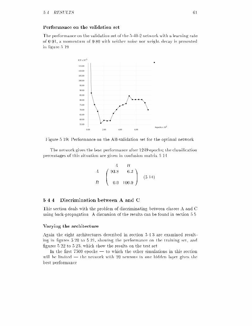
5.4. RESULTS 61Performance on the validation setThe performance on the validation set of the 5-40-2 network with a learning rateof 0.01, a momentum of 0.80 with neither noise nor weight decay is presentedin �gure 5.19.ICF x 10-3

3#epochs x 10

55.00

60.00

65.00

70.00

75.00

80.00

85.00

90.00

95.00

100.00

105.00

110.00

115.00

0.00 2.00 4.00 6.00Figure 5.19: Performance on the AB-validation set for the optimal network.The network gives the best performance after 1249 epochs; the classi�cationpercentages of this situation are given in confusion matrix 5.14.A BAB 0B@ 93:8 6:20:0 100:0 1CA (5.14)5.4.4 Discrimination between A and CThis section deals with the problem of discriminating between classes A and Cusing back-propagation. A discussion of the results can be found in section 5.5.Varying the architectureAgain the eight architectures described in section 5.4.3 are examined result-ing in �gures 5.20 to 5.21, showing the performance on the training set, and�gures 5.22 to 5.23, which show the results on the test set.In the �rst 7500 epochs | to which the other simulations in this sectionwill be limited | the network with 20 neurons in one hidden layer gives thebest performance.

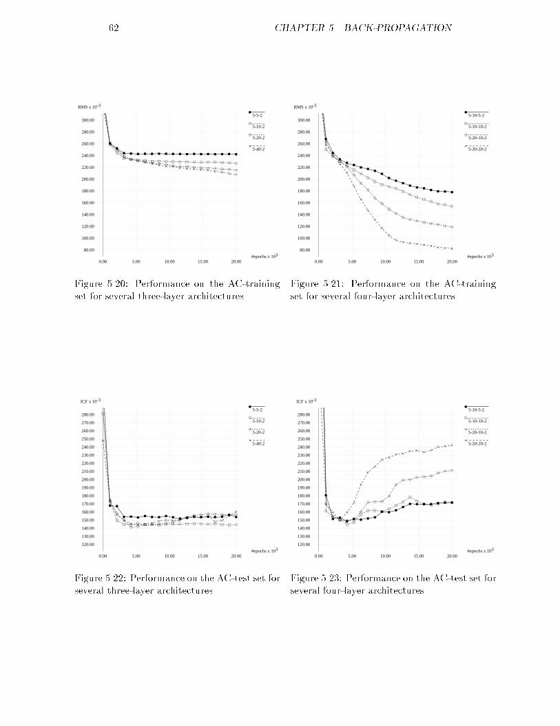
62 CHAPTER 5. BACK-PROPAGATION5-5-2

5-10-2

5-20-2

5-40-2

RMS x 10-3

3#epochs x 10

80.00

100.00

120.00

140.00

160.00

180.00

200.00

220.00

240.00

260.00

280.00

300.00

0.00 5.00 10.00 15.00 20.00Figure 5.20: Performance on the AC-trainingset for several three-layer architectures.5-10-5-2

5-10-10-2

5-20-10-2

5-20-20-2

RMS x 10-3

3#epochs x 10

80.00

100.00

120.00

140.00

160.00

180.00

200.00

220.00

240.00

260.00

280.00

300.00

0.00 5.00 10.00 15.00 20.00Figure 5.21: Performance on the AC-trainingset for several four-layer architectures.5-5-2

5-10-2

5-20-2

5-40-2

ICF x 10-3

3#epochs x 10

120.00

130.00

140.00

150.00

160.00

170.00

180.00

190.00

200.00

210.00

220.00

230.00

240.00

250.00

260.00

270.00

280.00

0.00 5.00 10.00 15.00 20.00Figure 5.22: Performance on the AC-test set forseveral three-layer architectures.5-10-5-2

5-10-10-2

5-20-10-2

5-20-20-2

ICF x 10-3

3#epochs x 10

120.00

130.00

140.00

150.00

160.00

170.00

180.00

190.00

200.00

210.00

220.00

230.00

240.00

250.00

260.00

270.00

280.00

0.00 5.00 10.00 15.00 20.00Figure 5.23: Performance on the AC-test set forseveral four-layer architectures.

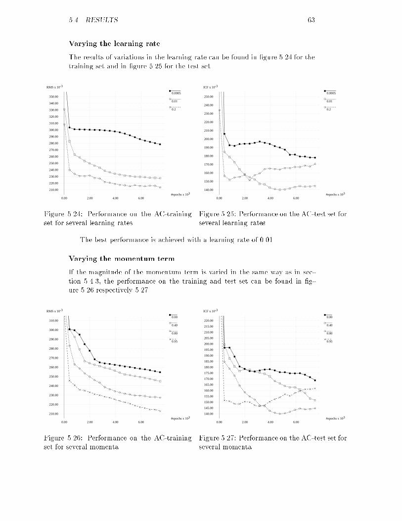
5.4. RESULTS 63Varying the learning rateThe results of variations in the learning rate can be found in �gure 5.24 for thetraining set and in �gure 5.25 for the test set.0.0005

0.01

0.2

RMS x 10-3

3#epochs x 10

210.00

220.00

230.00

240.00

250.00

260.00

270.00

280.00

290.00

300.00

310.00

320.00

330.00

340.00

350.00

0.00 2.00 4.00 6.00Figure 5.24: Performance on the AC-trainingset for several learning rates.0.0005

0.01

0.2

ICF x 10-3

3#epochs x 10

140.00

150.00

160.00

170.00

180.00

190.00

200.00

210.00

220.00

230.00

240.00

250.00

0.00 2.00 4.00 6.00Figure 5.25: Performance on the AC-test set forseveral learning rates.The best performance is achieved with a learning rate of 0.01.Varying the momentum termIf the magnitude of the momentum term is varied in the same way as in sec-tion 5.4.3, the performance on the training and test set can be found in �g-ure 5.26 respectively 5.27.0.00

0.40

0.80

0.95

RMS x 10-3

3#epochs x 10

210.00

220.00

230.00

240.00

250.00

260.00

270.00

280.00

290.00

300.00

310.00

0.00 2.00 4.00 6.00Figure 5.26: Performance on the AC-trainingset for several momenta.0.00

0.40

0.80

0.95

ICF x 10-3

3#epochs x 10

140.00

145.00

150.00

155.00

160.00

165.00

170.00

175.00

180.00

185.00

190.00

195.00

200.00

205.00

210.00

215.00

220.00

0.00 2.00 4.00 6.00Figure 5.27: Performance on the AC-test set forseveral momenta.

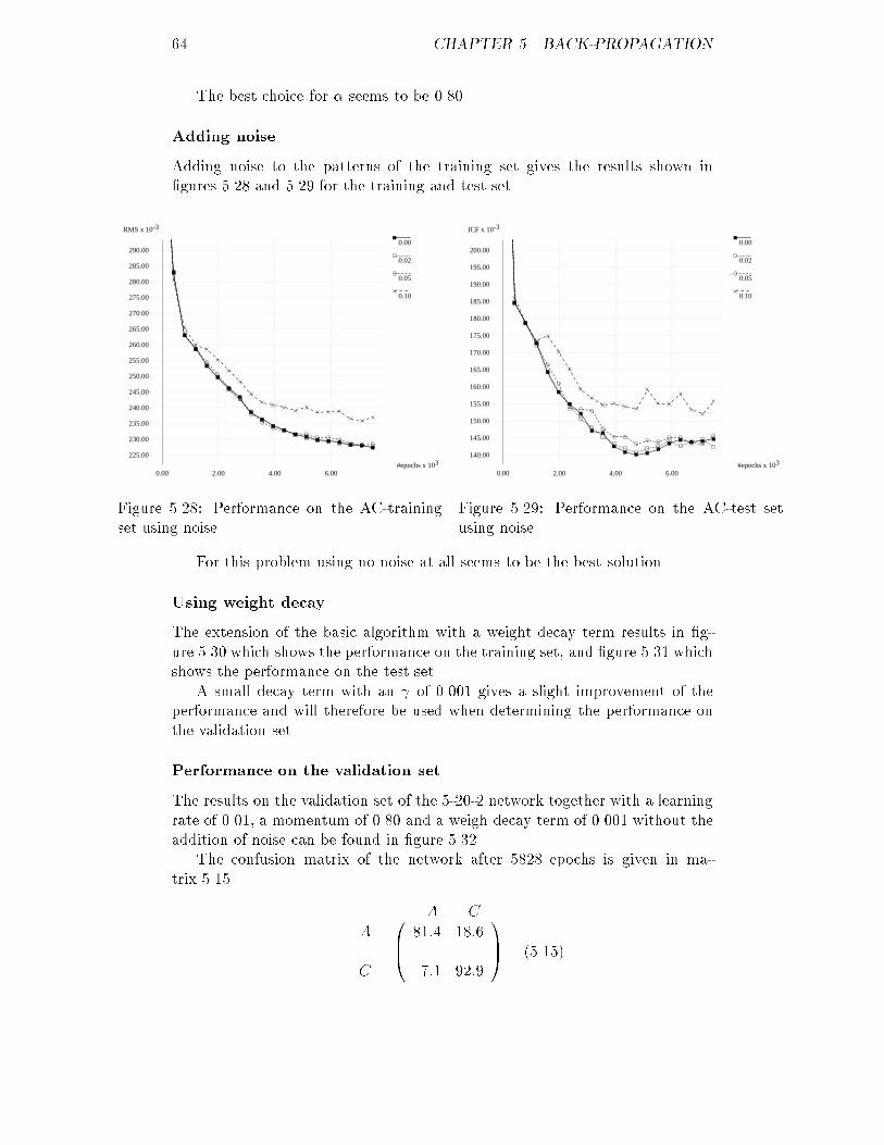
64 CHAPTER 5. BACK-PROPAGATIONThe best choice for � seems to be 0.80.Adding noiseAdding noise to the patterns of the training set gives the results shown in�gures 5.28 and 5.29 for the training and test set.0.00

0.02

0.05

0.10

RMS x 10-3

3#epochs x 10

225.00

230.00

235.00

240.00

245.00

250.00

255.00

260.00

265.00

270.00

275.00

280.00

285.00

290.00

0.00 2.00 4.00 6.00Figure 5.28: Performance on the AC-trainingset using noise.0.00

0.02

0.05

0.10

ICF x 10-3

3#epochs x 10

140.00

145.00

150.00

155.00

160.00

165.00

170.00

175.00

180.00

185.00

190.00

195.00

200.00

0.00 2.00 4.00 6.00Figure 5.29: Performance on the AC-test setusing noise.For this problem using no noise at all seems to be the best solution.Using weight decayThe extension of the basic algorithm with a weight decay term results in �g-ure 5.30 which shows the performance on the training set, and �gure 5.31 whichshows the performance on the test set.A small decay term with an of 0.001 gives a slight improvement of theperformance and will therefore be used when determining the performance onthe validation set.Performance on the validation setThe results on the validation set of the 5-20-2 network together with a learningrate of 0.01, a momentum of 0.80 and a weigh decay term of 0.001 without theaddition of noise can be found in �gure 5.32.The confusion matrix of the network after 5828 epochs is given in ma-trix 5.15. A CAC 0B@ 81:4 18:67:1 92:9 1CA (5.15)

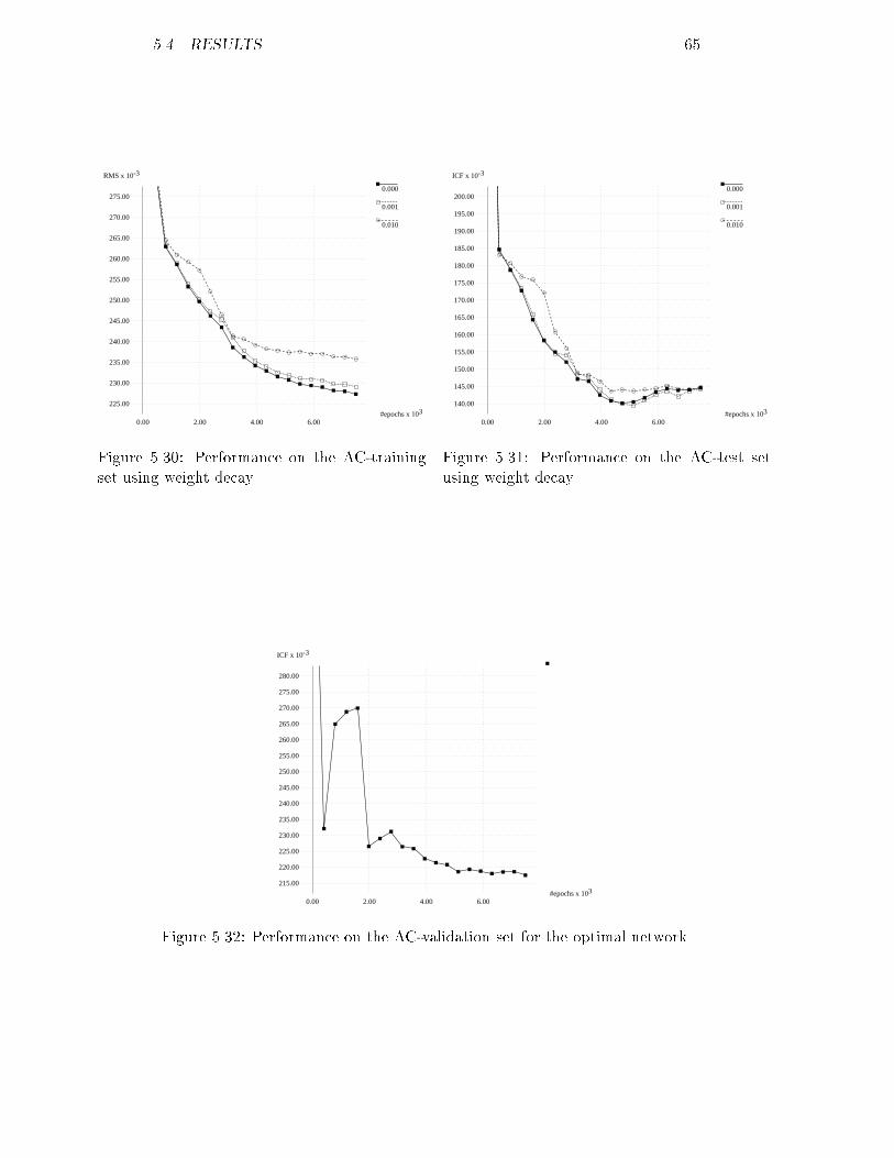
5.4. RESULTS 650.000

0.001

0.010

RMS x 10-3

3#epochs x 10

225.00

230.00

235.00

240.00

245.00

250.00

255.00

260.00

265.00

270.00

275.00

0.00 2.00 4.00 6.00Figure 5.30: Performance on the AC-trainingset using weight decay.0.000

0.001

0.010

ICF x 10-3

3#epochs x 10

140.00

145.00

150.00

155.00

160.00

165.00

170.00

175.00

180.00

185.00

190.00

195.00

200.00

0.00 2.00 4.00 6.00Figure 5.31: Performance on the AC-test setusing weight decay.ICF x 10-3

3#epochs x 10

215.00

220.00

225.00

230.00

235.00

240.00

245.00

250.00

255.00

260.00

265.00

270.00

275.00

280.00

0.00 2.00 4.00 6.00Figure 5.32: Performance on the AC-validation set for the optimal network.

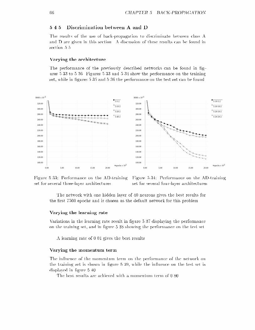
66 CHAPTER 5. BACK-PROPAGATION5.4.5 Discrimination between A and DThe results of the use of back-propagation to discriminate between class Aand D are given in this section. A discussion of these results can be found insection 5.5.Varying the architectureThe performance of the previously described networks can be found in �g-ures 5.33 to 5.36. Figures 5.33 and 5.34 show the performance on the trainingset, while in �gures 5.35 and 5.36 the performance on the test set can be found.5-5-2

5-10-2

5-20-2

5-40-2

RMS x 10-3

3#epochs x 10

100.00

120.00

140.00

160.00

180.00

200.00

220.00

240.00

260.00

280.00

300.00

320.00

0.00 5.00 10.00 15.00 20.00Figure 5.33: Performance on the AD-trainingset for several three-layer architectures.5-10-5-2

5-10-10-2

5-20-10-2

5-20-20-2

RMS x 10-3

3#epochs x 10

100.00

120.00

140.00

160.00

180.00

200.00

220.00

240.00

260.00

280.00

300.00

320.00

0.00 5.00 10.00 15.00 20.00Figure 5.34: Performance on the AD-trainingset for several four-layer architectures.The network with one hidden layer of 40 neurons gives the best results forthe �rst 7500 epochs and is chosen as the default network for this problem.Varying the learning rateVariations in the learning rate result in �gure 5.37 displaying the performanceon the training set, and in �gure 5.38 showing the performance on the test set.A learning rate of 0.01 gives the best results.Varying the momentum termThe in uence of the momentum term on the performance of the network onthe training set is shown in �gure 5.39, while the in uence on the test set isdisplayed in �gure 5.40.The best results are achieved with a momentum term of 0.80.

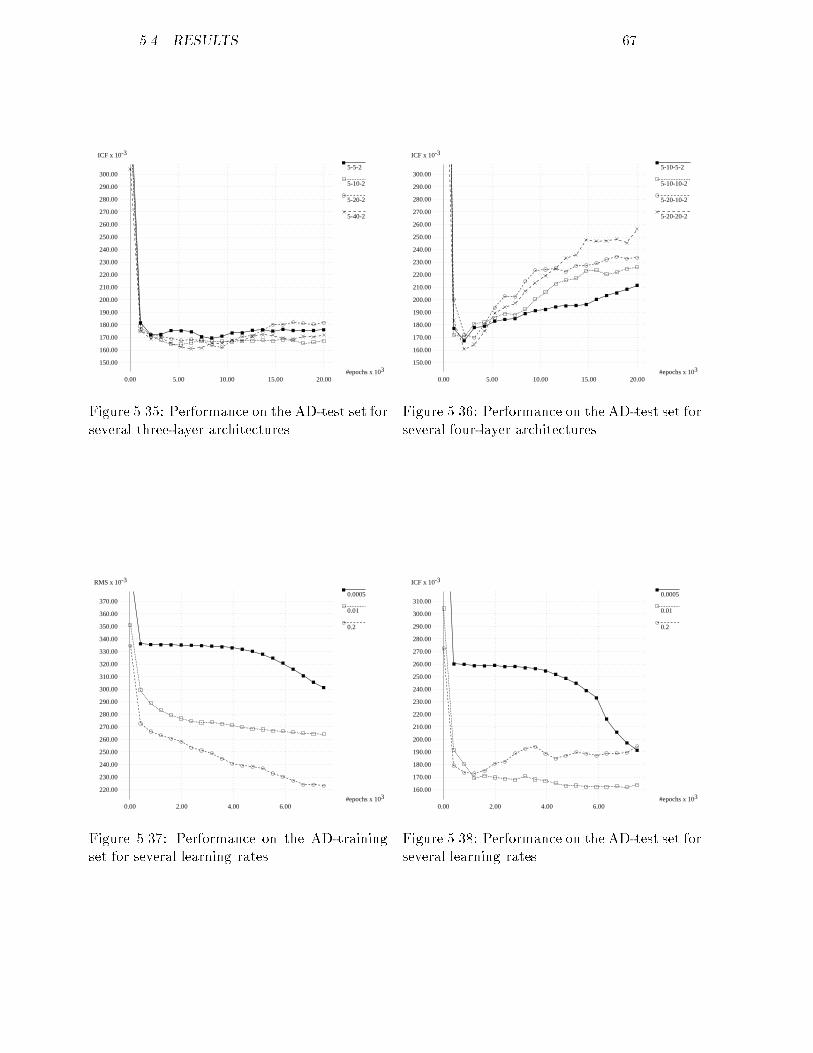
5.4. RESULTS 675-5-2

5-10-2

5-20-2

5-40-2

ICF x 10-3

3#epochs x 10

150.00

160.00

170.00

180.00

190.00

200.00

210.00

220.00

230.00

240.00

250.00

260.00

270.00

280.00

290.00

300.00

0.00 5.00 10.00 15.00 20.00Figure 5.35: Performance on the AD-test set forseveral three-layer architectures.5-10-5-2

5-10-10-2

5-20-10-2

5-20-20-2

ICF x 10-3

3#epochs x 10

150.00

160.00

170.00

180.00

190.00

200.00

210.00

220.00

230.00

240.00

250.00

260.00

270.00

280.00

290.00

300.00

0.00 5.00 10.00 15.00 20.00Figure 5.36: Performance on the AD-test set forseveral four-layer architectures.0.0005

0.01

0.2

RMS x 10-3

3#epochs x 10

220.00

230.00

240.00

250.00

260.00

270.00

280.00

290.00

300.00

310.00

320.00

330.00

340.00

350.00

360.00

370.00

0.00 2.00 4.00 6.00Figure 5.37: Performance on the AD-trainingset for several learning rates.0.0005

0.01

0.2

ICF x 10-3

3#epochs x 10

160.00

170.00

180.00

190.00

200.00

210.00

220.00

230.00

240.00

250.00

260.00

270.00

280.00

290.00

300.00

310.00

0.00 2.00 4.00 6.00Figure 5.38: Performance on the AD-test set forseveral learning rates.

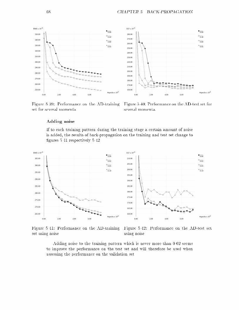
68 CHAPTER 5. BACK-PROPAGATION0.00

0.40

0.80

0.95

RMS x 10-3

3#epochs x 10

250.00

260.00

270.00

280.00

290.00

300.00

310.00

320.00

330.00

340.00

350.00

0.00 2.00 4.00 6.00Figure 5.39: Performance on the AD-trainingset for several momenta.0.00

0.40

0.80

0.95

ICF x 10-3

3#epochs x 10

160.00

170.00

180.00

190.00

200.00

210.00

220.00

230.00

240.00

250.00

260.00

270.00

280.00

0.00 2.00 4.00 6.00Figure 5.40: Performance on the AD-test set forseveral momenta.Adding noiseIf to each training pattern during the training stage a certain amount of noiseis added, the results of back-propagation on the training and test set change to�gures 5.41 respectively 5.42.0.00

0.02

0.05

0.10

RMS x 10-3

3#epochs x 10

265.00

270.00

275.00

280.00

285.00

290.00

295.00

300.00

305.00

0.00 2.00 4.00 6.00Figure 5.41: Performance on the AD-trainingset using noise.0.00

0.02

0.05

0.10

ICF x 10-3

3#epochs x 10

160.00

165.00

170.00

175.00

180.00

185.00

190.00

195.00

200.00

205.00

210.00

0.00 2.00 4.00 6.00Figure 5.42: Performance on the AD-test setusing noise.Adding noise to the training pattern which is never more than 0.02 seemsto improve the performance on the test set and will therefore be used whenassessing the performance on the validation set.

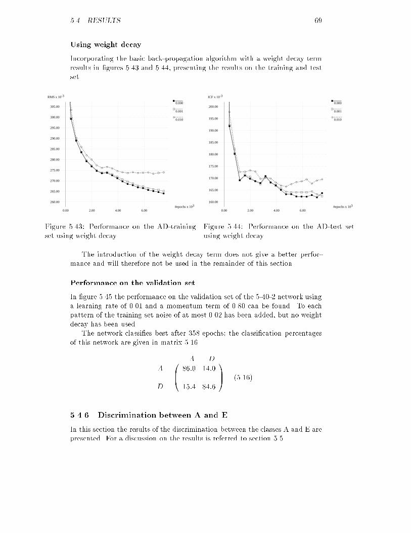
5.4. RESULTS 69Using weight decayIncorporating the basic back-propagation algorithm with a weight decay termresults in �gures 5.43 and 5.44, presenting the results on the training and testset.0.000

0.001

0.010

RMS x 10-3

3#epochs x 10

260.00

265.00

270.00

275.00

280.00

285.00

290.00

295.00

300.00

305.00

0.00 2.00 4.00 6.00Figure 5.43: Performance on the AD-trainingset using weight decay.0.000

0.001

0.010

ICF x 10-3

3#epochs x 10

160.00

165.00

170.00

175.00

180.00

185.00

190.00

195.00

200.00

0.00 2.00 4.00 6.00Figure 5.44: Performance on the AD-test setusing weight decay.The introduction of the weight decay term does not give a better perfor-mance and will therefore not be used in the remainder of this section.Performance on the validation setIn �gure 5.45 the performance on the validation set of the 5-40-2 network usinga learning rate of 0.01 and a momentum term of 0.80 can be found. To eachpattern of the training set noise of at most 0.02 has been added, but no weightdecay has been used.The network classi�es best after 358 epochs; the classi�cation percentagesof this network are given in matrix 5.16.A DAD 0B@ 86:0 14:015:4 84:6 1CA (5.16)5.4.6 Discrimination between A and EIn this section the results of the discrimination between the classes A and E arepresented. For a discussion on the results is referred to section 5.5.

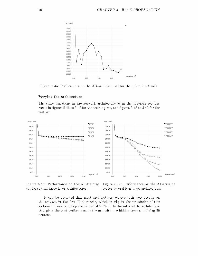
70 CHAPTER 5. BACK-PROPAGATIONICF x 10-3

3#epochs x 10

200.00

205.00

210.00

215.00

220.00

225.00

230.00

235.00

240.00

245.00

250.00

255.00

260.00

265.00

270.00

275.00

280.00

0.00 2.00 4.00 6.00Figure 5.45: Performance on the AD-validation set for the optimal network.Varying the architectureThe same variations in the network architecture as in the previous sectionsresult in �gures 5.46 to 5.47 for the training set, and �gures 5.48 to 5.49 for thetest set.5-5-2

5-10-2

5-20-2

5-40-2

RMS x 10-3

3#epochs x 10

80.00

100.00

120.00

140.00

160.00

180.00

200.00

220.00

240.00

260.00

280.00

300.00

0.00 5.00 10.00 15.00 20.00Figure 5.46: Performance on the AE-trainingset for several three-layer architectures.5-10-5-2

5-10-10-2

5-20-10-2

5-20-20-2

RMS x 10-3

3#epochs x 10

80.00

100.00

120.00

140.00

160.00

180.00

200.00

220.00

240.00

260.00

280.00

300.00

0.00 5.00 10.00 15.00 20.00Figure 5.47: Performance on the AE-trainingset for several four-layer architectures.It can be observed that most architectures achieve their best results onthe test set in the �rst 7500 epochs, which is why in the remainder of thissections the number of epochs is limited to 7500. In this interval the architecturethat gives the best performance is the one with one hidden layer containing 20neurons.

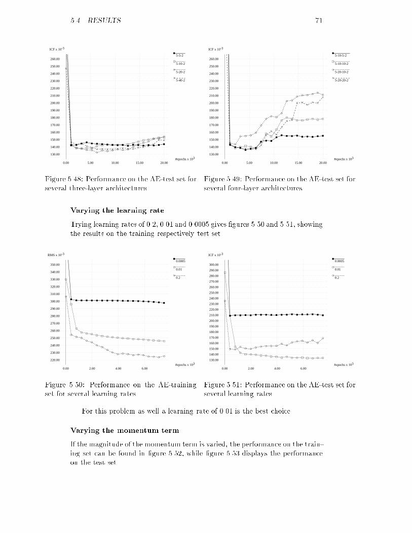
5.4. RESULTS 715-5-2

5-10-2

5-20-2

5-40-2

ICF x 10-3

3#epochs x 10

130.00

140.00

150.00

160.00

170.00

180.00

190.00

200.00

210.00

220.00

230.00

240.00

250.00

260.00

0.00 5.00 10.00 15.00 20.00Figure 5.48: Performance on the AE-test set forseveral three-layer architectures.5-10-5-2

5-10-10-2

5-20-10-2

5-20-20-2

ICF x 10-3

3#epochs x 10

130.00

140.00

150.00

160.00

170.00

180.00

190.00

200.00

210.00

220.00

230.00

240.00

250.00

260.00

0.00 5.00 10.00 15.00 20.00Figure 5.49: Performance on the AE-test set forseveral four-layer architectures.Varying the learning rateTrying learning rates of 0.2, 0.01 and 0.0005 gives �gures 5.50 and 5.51, showingthe results on the training respectively test set.0.0005

0.01

0.2

RMS x 10-3

3#epochs x 10

220.00

230.00

240.00

250.00

260.00

270.00

280.00

290.00

300.00

310.00

320.00

330.00

340.00

350.00

0.00 2.00 4.00 6.00Figure 5.50: Performance on the AE-trainingset for several learning rates.0.0005

0.01

0.2

ICF x 10-3

3#epochs x 10

130.00

140.00

150.00

160.00

170.00

180.00

190.00

200.00

210.00

220.00

230.00

240.00

250.00

260.00

270.00

280.00

290.00

300.00

0.00 2.00 4.00 6.00Figure 5.51: Performance on the AE-test set forseveral learning rates.For this problem as well a learning rate of 0.01 is the best choice.Varying the momentum termIf the magnitude of the momentum term is varied, the performance on the train-ing set can be found in �gure 5.52, while �gure 5.53 displays the performanceon the test set.

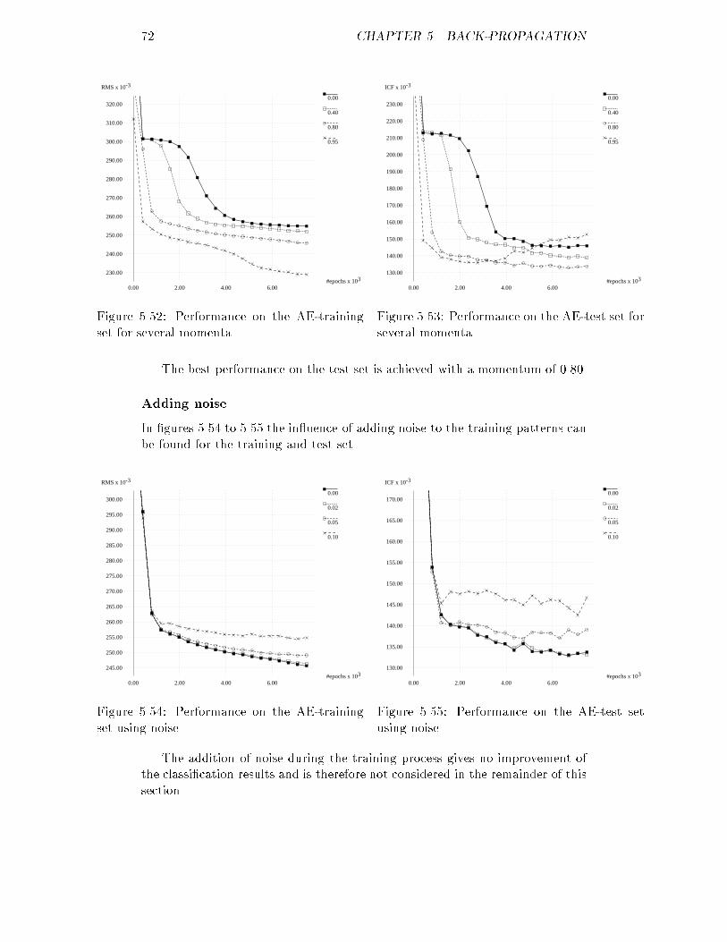
72 CHAPTER 5. BACK-PROPAGATION0.00

0.40

0.80

0.95

RMS x 10-3

3#epochs x 10

230.00

240.00

250.00

260.00

270.00

280.00

290.00

300.00

310.00

320.00

0.00 2.00 4.00 6.00Figure 5.52: Performance on the AE-trainingset for several momenta.0.00

0.40

0.80

0.95

ICF x 10-3

3#epochs x 10

130.00

140.00

150.00

160.00

170.00

180.00

190.00

200.00

210.00

220.00

230.00

0.00 2.00 4.00 6.00Figure 5.53: Performance on the AE-test set forseveral momenta.The best performance on the test set is achieved with a momentum of 0.80.Adding noiseIn �gures 5.54 to 5.55 the in uence of adding noise to the training patterns canbe found for the training and test set.0.00

0.02

0.05

0.10

RMS x 10-3

3#epochs x 10

245.00

250.00

255.00

260.00

265.00

270.00

275.00

280.00

285.00

290.00

295.00

300.00

0.00 2.00 4.00 6.00Figure 5.54: Performance on the AE-trainingset using noise.0.00

0.02

0.05

0.10

ICF x 10-3

3#epochs x 10

130.00

135.00

140.00

145.00

150.00

155.00

160.00

165.00

170.00

0.00 2.00 4.00 6.00Figure 5.55: Performance on the AE-test setusing noise.The addition of noise during the training process gives no improvement ofthe classi�cation results and is therefore not considered in the remainder of thissection.

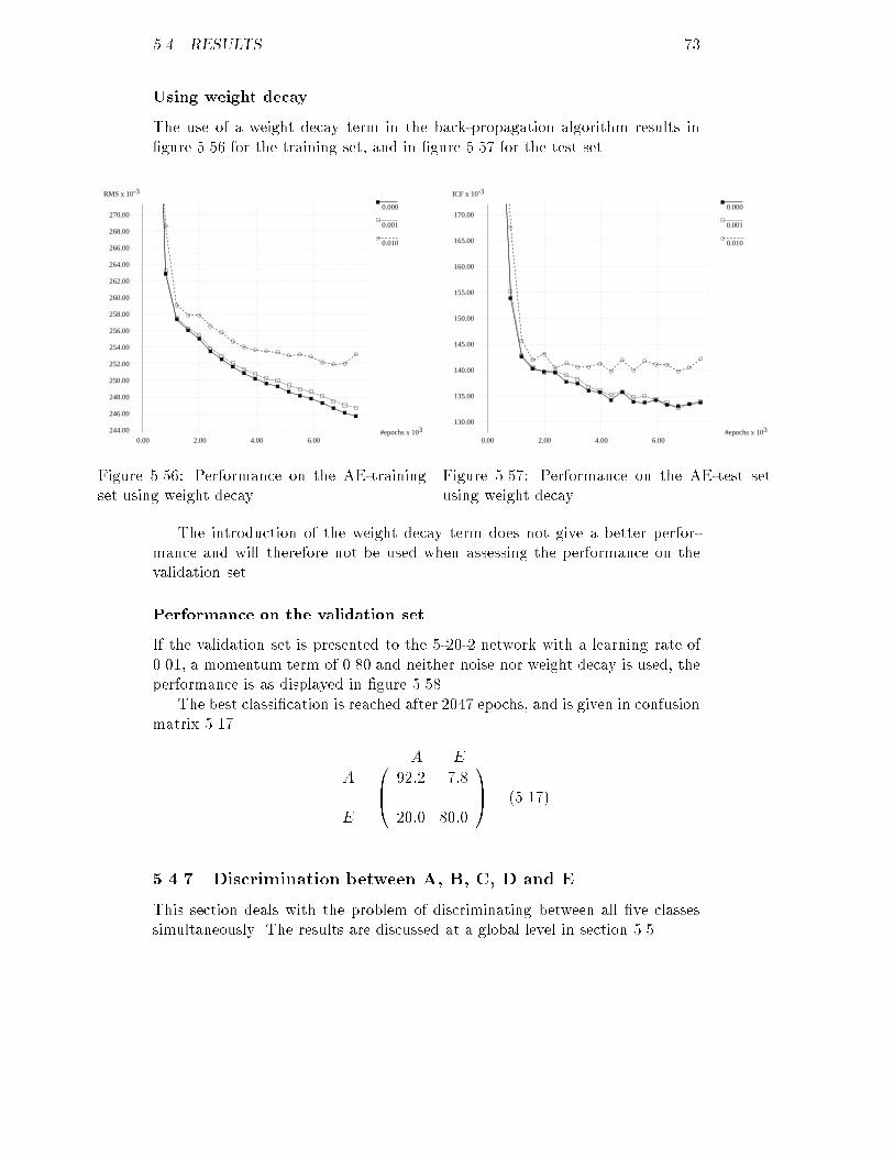
5.4. RESULTS 73Using weight decayThe use of a weight decay term in the back-propagation algorithm results in�gure 5.56 for the training set, and in �gure 5.57 for the test set.0.000

0.001

0.010

RMS x 10-3

3#epochs x 10244.00

246.00

248.00

250.00

252.00

254.00

256.00

258.00

260.00

262.00

264.00

266.00

268.00

270.00

0.00 2.00 4.00 6.00Figure 5.56: Performance on the AE-trainingset using weight decay.0.000

0.001

0.010

ICF x 10-3

3#epochs x 10

130.00

135.00

140.00

145.00

150.00

155.00

160.00

165.00

170.00

0.00 2.00 4.00 6.00Figure 5.57: Performance on the AE-test setusing weight decay.The introduction of the weight decay term does not give a better perfor-mance and will therefore not be used when assessing the performance on thevalidation set.Performance on the validation setIf the validation set is presented to the 5-20-2 network with a learning rate of0.01, a momentum term of 0.80 and neither noise nor weight decay is used, theperformance is as displayed in �gure 5.58.The best classi�cation is reached after 2047 epochs, and is given in confusionmatrix 5.17. A EAE 0B@ 92:2 7:820:0 80:0 1CA (5.17)5.4.7 Discrimination between A, B, C, D and EThis section deals with the problem of discriminating between all �ve classessimultaneously. The results are discussed at a global level in section 5.5.

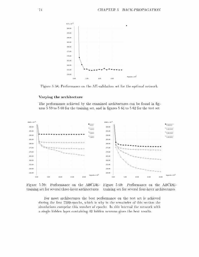
74 CHAPTER 5. BACK-PROPAGATIONICF x 10-3

3#epochs x 10

150.00

155.00

160.00

165.00

170.00

175.00

180.00

185.00

190.00

195.00

200.00

0.00 2.00 4.00 6.00Figure 5.58: Performance on the AE-validation set for the optimal network.Varying the architectureThe performance achieved by the examined architectures can be found in �g-ures 5.59 to 5.60 for the training set, and in �gures 5.61 to 5.62 for the test set.5-5-5

5-10-5

5-20-5

5-40-5

RMS x 10-3

3#epochs x 10

245.00

250.00

255.00

260.00

265.00

270.00

275.00

280.00

285.00

290.00

295.00

300.00

0.00 5.00 10.00 15.00 20.00Figure 5.59: Performance on the ABCDE-training set for several three-layer architectures.5-10-5-5

5-10-10-5

5-20-10-5

5-20-20-5

RMS x 10-3

3#epochs x 10

245.00

250.00

255.00

260.00

265.00

270.00

275.00

280.00

285.00

290.00

295.00

300.00

0.00 5.00 10.00 15.00 20.00Figure 5.60: Performance on the ABCDE-training set for several four-layer architectures.For most architectures the best performance on the test set is achievedduring the �rst 7500 epochs, which is why in the remainder of this section thesimulations comprise this number of epochs. In this interval the network witha single hidden layer containing 40 hidden neurons gives the best results.

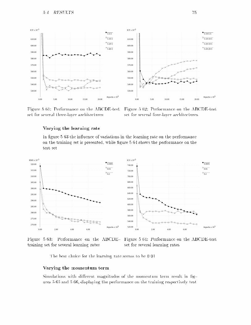
5.4. RESULTS 755-5-5

5-10-5

5-20-5

5-40-5

ICF x 10-3

3#epochs x 10

530.00

540.00

550.00

560.00

570.00

580.00

590.00

600.00

610.00

0.00 5.00 10.00 15.00 20.00Figure 5.61: Performance on the ABCDE-testset for several three-layer architectures.5-10-5-5

5-10-10-5

5-20-10-5

5-20-20-5

ICF x 10-3

3#epochs x 10

530.00

540.00

550.00

560.00

570.00

580.00

590.00

600.00

610.00

0.00 5.00 10.00 15.00 20.00Figure 5.62: Performance on the ABCDE-testset for several four-layer architectures.Varying the learning rateIn �gure 5.63 the in uence of variations in the learning rate on the performanceon the training set is presented, while �gure 5.64 shows the performance on thetest set.0.0005

0.01

0.2

RMS x 10-3

3#epochs x 10270.00

275.00

280.00

285.00

290.00

295.00

300.00

305.00

310.00

315.00

320.00

0.00 2.00 4.00 6.00Figure 5.63: Performance on the ABCDE-training set for several learning rates.0.0005

0.01

0.2

ICF x 10-3

3#epochs x 10520.00

540.00

560.00

580.00

600.00

620.00

640.00

660.00

680.00

700.00

720.00

740.00

0.00 2.00 4.00 6.00Figure 5.64: Performance on the ABCDE-testset for several learning rates.The best choice for the learning rate seems to be 0.01.Varying the momentum termSimulations with di�erent magnitudes of the momentum term result in �g-ures 5.65 and 5.66, displaying the performance on the training respectively test

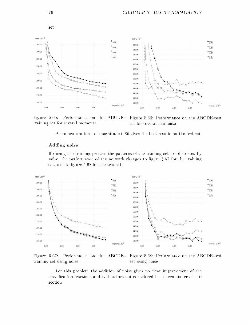
76 CHAPTER 5. BACK-PROPAGATIONset.0.00

0.40

0.80

0.95

RMS x 10-3

3#epochs x 10

265.00

270.00

275.00

280.00

285.00

290.00

295.00

300.00

305.00

0.00 2.00 4.00 6.00Figure 5.65: Performance on the ABCDE-training set for several momenta.0.00

0.40

0.80

0.95

ICF x 10-3

3#epochs x 10

530.00

535.00

540.00

545.00

550.00

555.00

560.00

565.00

570.00

575.00

580.00

585.00

590.00

0.00 2.00 4.00 6.00Figure 5.66: Performance on the ABCDE-testset for several momenta.A momentum term of magnitude 0.80 gives the best results on the test set.Adding noiseIf during the training process the patterns of the training set are distorted bynoise, the performance of the network changes to �gure 5.67 for the trainingset, and to �gure 5.68 for the test set.0.00

0.02

0.05

0.10

RMS x 10-3

3#epochs x 10

272.00

274.00

276.00

278.00

280.00

282.00

284.00

286.00

288.00

290.00

0.00 2.00 4.00 6.00Figure 5.67: Performance on the ABCDE-training set using noise.0.00

0.02

0.05

0.10

ICF x 10-3

3#epochs x 10

530.00

535.00

540.00

545.00

550.00

555.00

560.00

565.00

570.00

575.00

580.00

585.00

590.00

0.00 2.00 4.00 6.00Figure 5.68: Performance on the ABCDE-testset using noise.For this problem the addition of noise gives no clear improvement of theclassi�cation fractions and is therefore not considered in the remainder of thissection.

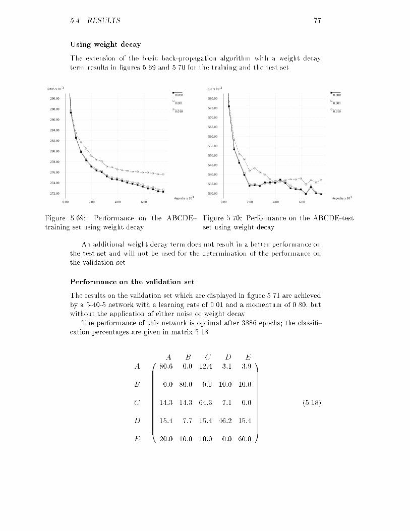
5.4. RESULTS 77Using weight decayThe extension of the basic back-propagation algorithm with a weight decayterm results in �gures 5.69 and 5.70 for the training and the test set.0.000

0.001

0.010

RMS x 10-3

3#epochs x 10

272.00

274.00

276.00

278.00

280.00

282.00

284.00

286.00

288.00

290.00

0.00 2.00 4.00 6.00Figure 5.69: Performance on the ABCDE-training set using weight decay.0.000

0.001

0.010

ICF x 10-3

3#epochs x 10

530.00

535.00

540.00

545.00

550.00

555.00

560.00

565.00

570.00

575.00

580.00

0.00 2.00 4.00 6.00Figure 5.70: Performance on the ABCDE-testset using weight decay.An additional weight decay term does not result in a better performance onthe test set and will not be used for the determination of the performance onthe validation set.Performance on the validation setThe results on the validation set which are displayed in �gure 5.71 are achievedby a 5-40-5 network with a learning rate of 0.01 and a momentum of 0.80, butwithout the application of either noise or weight decay.The performance of this network is optimal after 3886 epochs; the classi�-cation percentages are given in matrix 5.18.A B C D EABCDE 0BBBBBBBBBBBBBB@ 80:6 0:0 12:4 3:1 3:90:0 80:0 0:0 10:0 10:014:3 14:3 64:3 7:1 0:015:4 7:7 15:4 46:2 15:420:0 10:0 10:0 0:0 60:0 1CCCCCCCCCCCCCCA (5.18)

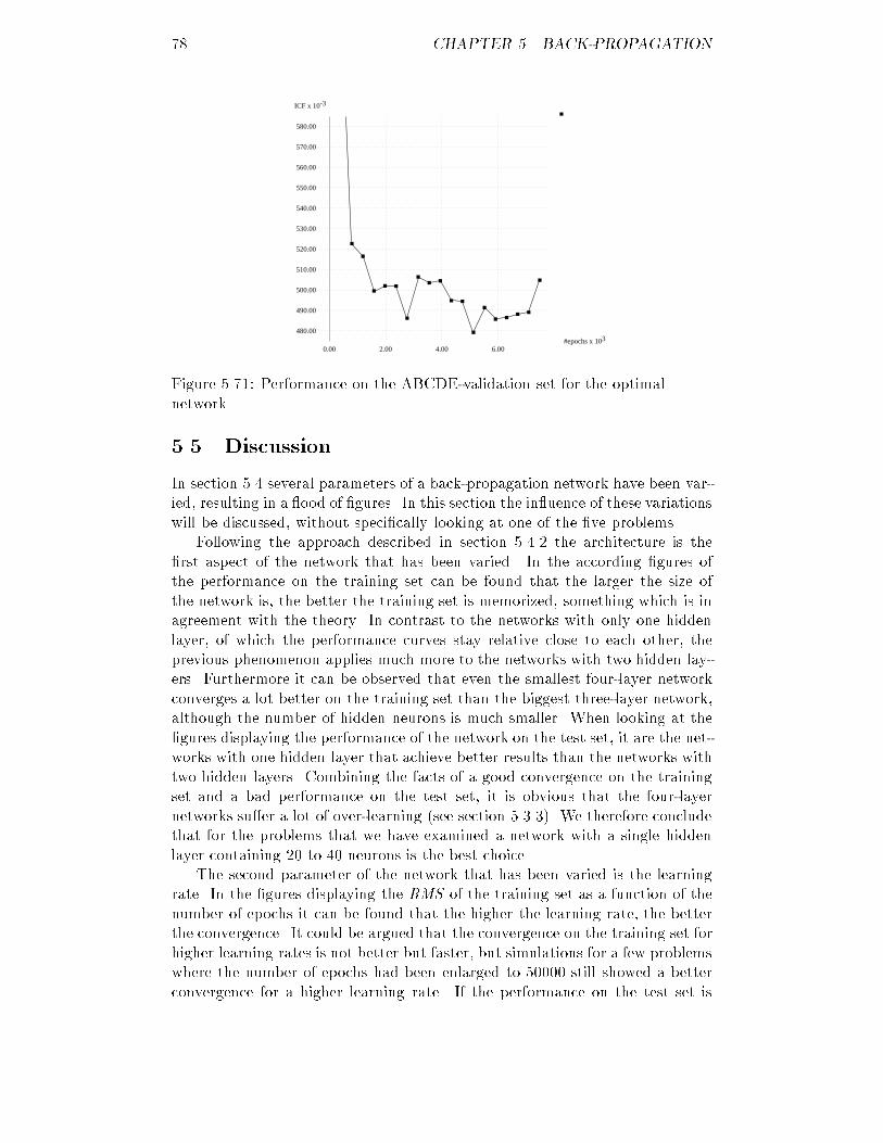
78 CHAPTER 5. BACK-PROPAGATIONICF x 10-3

3#epochs x 10

480.00

490.00

500.00

510.00

520.00

530.00

540.00

550.00

560.00

570.00

580.00

0.00 2.00 4.00 6.00Figure 5.71: Performance on the ABCDE-validation set for the optimalnetwork.5.5 DiscussionIn section 5.4 several parameters of a back-propagation network have been var-ied, resulting in a ood of �gures. In this section the in uence of these variationswill be discussed, without speci�cally looking at one of the �ve problems.Following the approach described in section 5.4.2 the architecture is the�rst aspect of the network that has been varied. In the according �gures ofthe performance on the training set can be found that the larger the size ofthe network is, the better the training set is memorized, something which is inagreement with the theory. In contrast to the networks with only one hiddenlayer, of which the performance curves stay relative close to each other, theprevious phenomenon applies much more to the networks with two hidden lay-ers. Furthermore it can be observed that even the smallest four-layer networkconverges a lot better on the training set than the biggest three-layer network,although the number of hidden neurons is much smaller. When looking at the�gures displaying the performance of the network on the test set, it are the net-works with one hidden layer that achieve better results than the networks withtwo hidden layers. Combining the facts of a good convergence on the trainingset and a bad performance on the test set, it is obvious that the four-layernetworks su�er a lot of over-learning (see section 5.3.3). We therefore concludethat for the problems that we have examined a network with a single hiddenlayer containing 20 to 40 neurons is the best choice.The second parameter of the network that has been varied is the learningrate. In the �gures displaying the RMS of the training set as a function of thenumber of epochs it can be found that the higher the learning rate, the betterthe convergence. It could be argued that the convergence on the training set forhigher learning rates is not better but faster, but simulations for a few problemswhere the number of epochs had been enlarged to 50000 still showed a betterconvergence for a higher learning rate. If the performance on the test set is

5.5. DISCUSSION 79observed, a learning rate of 0.01 presents itself as the best choice; for a learningrate of 0.2 over-learning can again be detected.For the momentum term more or less holds the same as for the learningrate: the higher the magnitude of the momentum term, the better the trainingset is memorized. However, a higher momentum term also entails a fasterconvergence, not only for the training set but also for the test set. For thebest performance on the test set a momentum of 0.80 should be chosen, for allproblems. Also for the momentum term over-learning can be observed, if � isset at 0.95.The �rst variation on the basic algorithm, the addition of noise to the pat-terns of the training set, causes the network to memorize the training set lesswell as the amount of noise increases. This was to be expected, since the intro-duction of noise blurs the borders between the di�erent classes, making a gooddiscrimination between the classes even more di�cult. Furthermore, since thetraining patterns continuously change during the training stage, the networkgets no chance to tune itself optimally to the training set. Although the previ-ously mentioned absence of tuning deteriorates the performance on the trainingset, it could improve the performance on the test set, because the network isprevented from over-learning. Unfortunately, in the �gures displaying the per-formance on the test set no better results can be observed when noise is used.Usually the addition of noise results in a worse performance, especially if theamount of noise is relatively large, although in some cases | discriminationbetween classes A and D | a little noise can bring some improvement. An-other negative aspect of adding noise is that the ICF of the test set starts to uctuate as the noise gets stronger. The reason for this is that the networkdoes not evolve slowly to some kind of optimum, but keeps changing becauseof the continuously changing patterns. Obviously this restlessness has its e�ecton the performance on the test set.What in the previous paragraph was said about the in uence of noise onthe performance of the network largely holds for weight decay as well. Theperformance on the training set gets worse as the magnitude of the decay termincreases, while the performance on the test set in some cases | A vs C | canimprove a little, but usually deteriorates. An explanation for this behaviour isthat, in order to solve the problem, the network needs weights with high values,while weight decay opposes to this. Therefore, as gets higher, the networkgets more problems memorizing the training set as well as correctly classifyingthe test set.When looking at the confusion matrices it can be seen that for all problemswith two classes the percentages of correct classi�cation are rather high, atleast 80% but mostly higher. Although there is no explicit order in which theclasses can best be discriminated, discrimination between class A and B can beperformed extremely well, with classi�cation percentages of respectively 93.8%and 100%. If there is to be discriminated between all �ve classes simultaneously,the percentages of correct classi�cation naturally drop a bit for all classes, butfor class D the deterioration is strikingly large. Probably class D is scatteredmuch more over the observation space than the other classes, making a gooddiscrimination of this class impossible. The order in which the classes can best

80 CHAPTER 5. BACK-PROPAGATIONbe discriminated when using back-propagation on �ve classes is A/B, followedby C/E and concluded by D.A �nal observation that can be made is that the performance curves of thetest and the validation set in most cases di�er a lot. Furthermore is the ICF ofthe validation set, except when discriminating between A and B, structurallyhigher than the ICF of the test set. The reason for this phenomenon is that thetest set is generated in the same way as the training set, and therefore resemblesthe training set much more than the validation set. Since the network tries toachieve the best performance possible on the training set, a good performanceon the test set is achieved automatically. The validation set on the other handdi�ers much more from the training set, resulting in a performance that is lesswell. Another reason for the previously mentioned di�erences in performancebetween the test and the validation set is that the number of patients in thevalidation set is much smaller. As a result of the small number of patients notonly the percentage of correct classi�cation (ICF ) is low (high) when only afew patients of a small class are erroneously classi�ed, but the ICF displaysan unpredictable behaviour as well. All this however is not a aw of the back-propagation algorithm, but simply the hard reality of a limited data set.In the literature back-propagation has the reputation of being slow, some-thing that has been con�rmed by our simulations. Compared to the othermethods of classi�cation | see section 7.2 | back-propagation needed a lot ofcomputation time to achieve good results. For the problem of discriminatingbetween �ve classes simultaneously on the basis of 2500 patterns in the trainingset where a test set of another 2500 patterns was used to monitor the behaviourof the network, the 5-40-5 network needed for 7500 epochs about six days ofcomputing on a Sun SPARCstation SLC. For the 5-20-20-5 network, which has1.5 times the connections of the 5-40-5 network, the same workstation wouldhave needed 24 days for 20000 epochs2!2Fortunately for this simulation a Sun SPARCstation of the 600 MP series could be used;this computer completed the simulation within 10 days.

Chapter 6Feature mappingThe method that is investigated in this chapter is feature mapping, an un-supervised method to train neural networks. How feature mapping works isexplained in the �rst part of this chapter, while in the second part the resultsof the application of feature mapping to our data are presented. More on thissubject can be found in [21, 22].6.1 Network architectureIn 1982 Kohonen presented a new type of neural network called self-organizingfeature map, which is very suitable for classi�cation problems. The algorithmaccording to which the network is trained is unsupervised, meaning that thedata does not have to be classi�ed prior to presentation to the network.A feature mapping network consists of two layers of neurons, an input layerand an output layer . All neurons in the output layer are fully connected tothe neurons in the input layer, while between the neurons in both the inputand the output layer no connections exist. The neurons in the output layer areusually organized in a two-dimensional grid, but a one-dimensional line or anarrangement in more than two dimensions is also possible. An example of afeature mapping network can be found in �gure 6.1.As will be explained in section 6.2.1 feature mapping is topology preservingor topographic, which means that pattern vectors that lie close to (far from)each other in the observation or feature space are mapped to neurons of theoutput layer that lie close to (far from) each other as well. Due to this non-trivial property feature mapping can be used to preprocess data: a data pointis transformed to the position of the neuron in the output layer it is mappedto. Since the vector that describes the position of a neuron depends on thedegree of organization of the output layer, the dimension of the data underobservation can be changed to an arbitrary value; usually the dimension of thedata is reduced.Topographic maps also exist on the surface of the brain, for sensory andmotor phenomena. The details of these maps however di�er from self-organizingfeature maps, not only in architecture | the maps of the brain have a muchmore complex architecture | but also in underlying principles.81

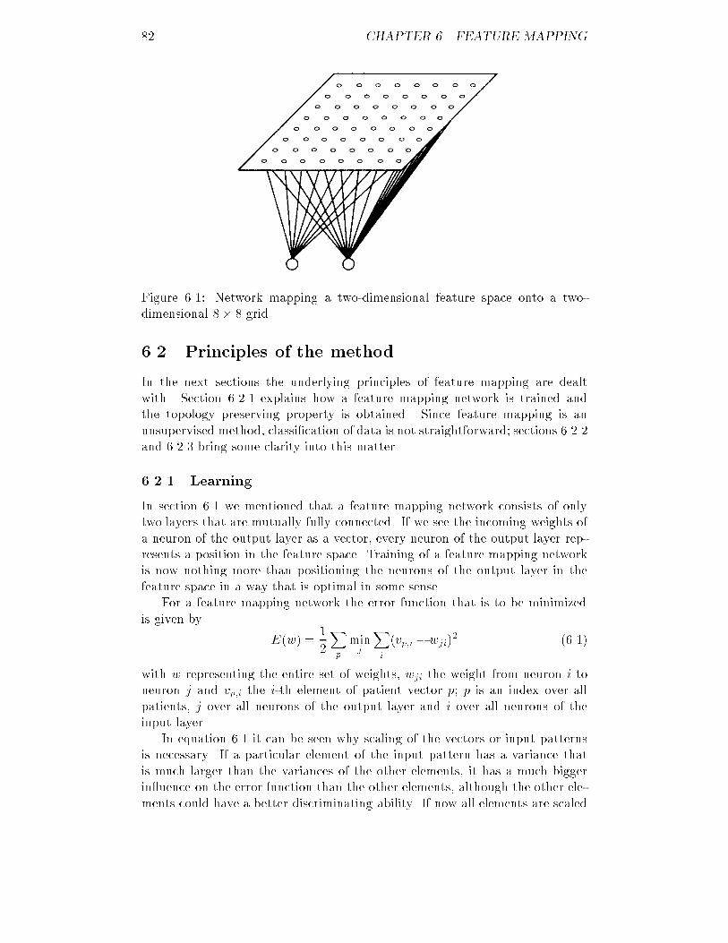
82 CHAPTER 6. FEATURE MAPPINGFigure 6.1: Network mapping a two-dimensional feature space onto a two-dimensional 8� 8 grid.6.2 Principles of the methodIn the next sections the underlying principles of feature mapping are dealtwith. Section 6.2.1 explains how a feature mapping network is trained andthe topology preserving property is obtained. Since feature mapping is anunsupervised method, classi�cation of data is not straightforward; sections 6.2.2and 6.2.3 bring some clarity into this matter.6.2.1 LearningIn section 6.1 we mentioned that a feature mapping network consists of onlytwo layers that are mutually fully connected. If we see the incoming weights ofa neuron of the output layer as a vector, every neuron of the output layer rep-resents a position in the feature space. Training of a feature mapping networkis now nothing more than positioning the neurons of the output layer in thefeature space in a way that is optimal in some sense.For a feature mapping network the error function that is to be minimizedis given by E(w) = 12Xp minj Xi (vp;i � wji)2 (6.1)with w representing the entire set of weights, wji the weight from neuron i toneuron j and vp;i the i-th element of patient vector p; p is an index over allpatients, j over all neurons of the output layer and i over all neurons of theinput layer.In equation 6.1 it can be seen why scaling of the vectors or input patternsis necessary. If a particular element of the input pattern has a variance thatis much larger than the variances of the other elements, it has a much biggerin uence on the error function than the other elements, although the other ele-ments could have a better discriminating ability. If now all elements are scaled

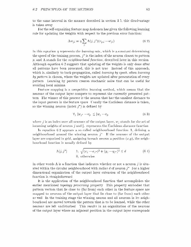
6.2. PRINCIPLES OF THE METHOD 83to the same interval in the manner described in section 3.5, this disadvantageis taken away.For the self-organizing feature map Kohonen has given the following learningrule for updating the weights with respect to the previous error function:�wji = �Xp �(j; j�)(vp;i � wji) (6.2)In this equation � represents the learning rate, which is a constant determiningthe speed of the training process, j� is the index of the neuron closest to patternp, and � stands for the neighbourhood function, described later in this section.Although equation 6.2 suggests that updating of the weights is only done afterall patterns have been presented, this is not true. Instead of this approach,which is, similarly to back-propagation, called learning by epoch, often learningby pattern is chosen, where the weights are updated after presentation of everypattern. Learning by pattern creates stochastic noise that can be useful foravoiding local minima.Feature mapping is a competitive learning method, which means that theneurons of the output layer compete to represent the currently presented pat-tern. The winner of this process is the neuron that has the smallest distance tothe input pattern in the feature space. Usually the Euclidean distance is taken,so the winning neuron (index j�) is de�ned by8j jwj� � vpj � jwj � vpj (6.3)where j is an index over all neurons of the output layer, wj stands for the set ofincoming weights of neuron j and j:j represents the Euclidean distance function.In equation 6.2 appears a so called neighbourhood function �, de�ning aneighbourhood around the winning neuron j�. If the neurons of the outputlayer are organized in grid, assigning to each neuron a position (x,y), the neigh-bourhood function is usually de�ned by�(j; j�) = 1; q(xj � xj�)2 + (yj � yj�)2 � d (6.4)= 0; otherwise.In other words � is a function that indicates whether or not a neuron j is situ-ated within the circular neighbourhood with radius d of neuron j�. For a higherdimensional organization of the output layer extension of the neighbourhoodfunction is straightforward.It is the application of the neighbourhood function that accomplishes theearlier mentioned topology preserving property. This property embodies thatpattern vectors that lie close to (far from) each other in the feature space aremapped to neurons of the output layer that lie close to (far from) each otheras well. In the training stage the winning neuron and all neurons in its neigh-bourhood are moved towards the pattern that is to be learned, while the otherneurons are left undisturbed. This results in an organization of the neuronsof the output layer where an adjacent position in the output layer corresponds

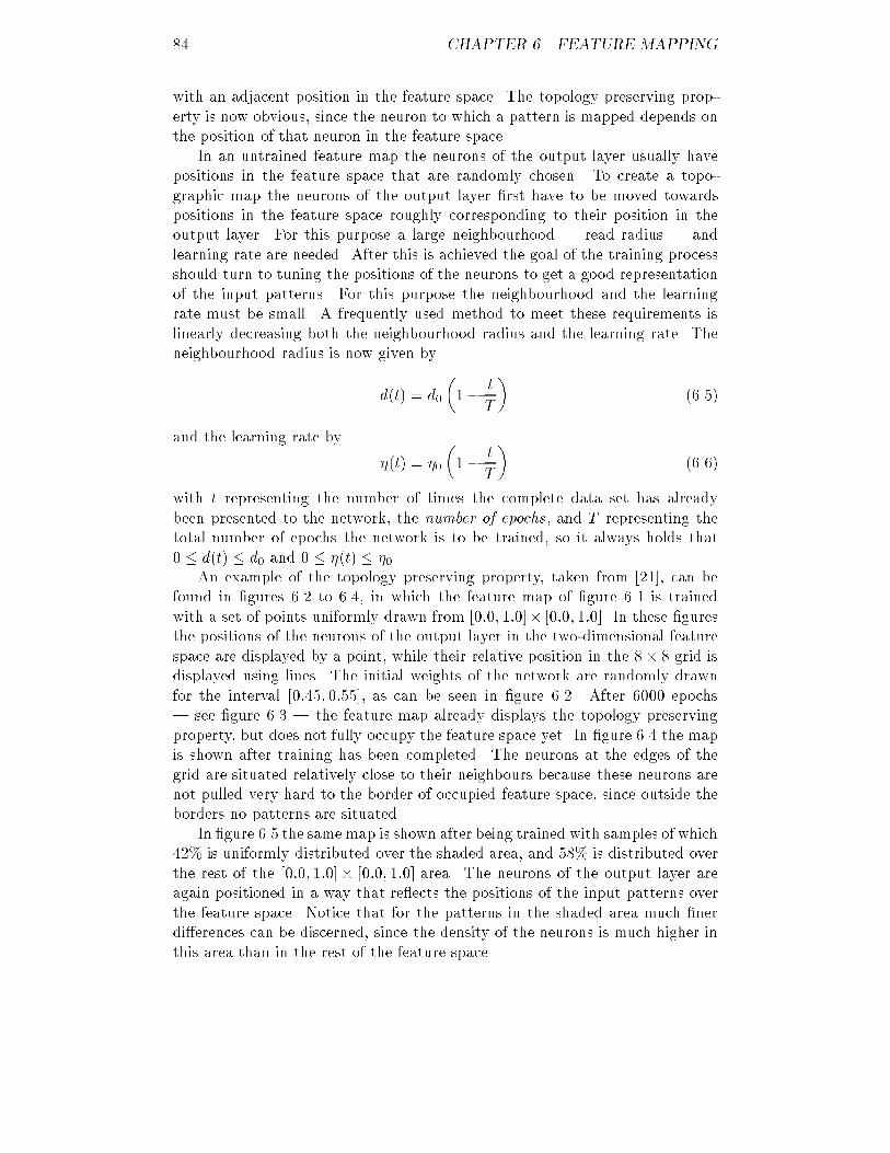
84 CHAPTER 6. FEATURE MAPPINGwith an adjacent position in the feature space. The topology preserving prop-erty is now obvious, since the neuron to which a pattern is mapped depends onthe position of that neuron in the feature space.In an untrained feature map the neurons of the output layer usually havepositions in the feature space that are randomly chosen. To create a topo-graphic map the neurons of the output layer �rst have to be moved towardspositions in the feature space roughly corresponding to their position in theoutput layer. For this purpose a large neighbourhood | read radius | andlearning rate are needed. After this is achieved the goal of the training processshould turn to tuning the positions of the neurons to get a good representationof the input patterns. For this purpose the neighbourhood and the learningrate must be small. A frequently used method to meet these requirements islinearly decreasing both the neighbourhood radius and the learning rate. Theneighbourhood radius is now given byd(t) = d0�1� tT � (6.5)and the learning rate by �(t) = �0�1� tT � (6.6)with t representing the number of times the complete data set has alreadybeen presented to the network, the number of epochs , and T representing thetotal number of epochs the network is to be trained, so it always holds that0 � d(t) � d0 and 0 � �(t) � �0.An example of the topology preserving property, taken from [21], can befound in �gures 6.2 to 6.4, in which the feature map of �gure 6.1 is trainedwith a set of points uniformly drawn from [0:0; 1:0]� [0:0; 1:0]. In these �guresthe positions of the neurons of the output layer in the two-dimensional featurespace are displayed by a point, while their relative position in the 8� 8 grid isdisplayed using lines. The initial weights of the network are randomly drawnfor the interval [0:45; 0:55], as can be seen in �gure 6.2. After 6000 epochs| see �gure 6.3 | the feature map already displays the topology preservingproperty, but does not fully occupy the feature space yet. In �gure 6.4 the mapis shown after training has been completed. The neurons at the edges of thegrid are situated relatively close to their neighbours because these neurons arenot pulled very hard to the border of occupied feature space, since outside theborders no patterns are situated.In �gure 6.5 the same map is shown after being trained with samples of which42% is uniformly distributed over the shaded area, and 58% is distributed overthe rest of the [0:0; 1:0]� [0:0; 1:0] area. The neurons of the output layer areagain positioned in a way that re ects the positions of the input patterns overthe feature space. Notice that for the patterns in the shaded area much �nerdi�erences can be discerned, since the density of the neurons is much higher inthis area than in the rest of the feature space.

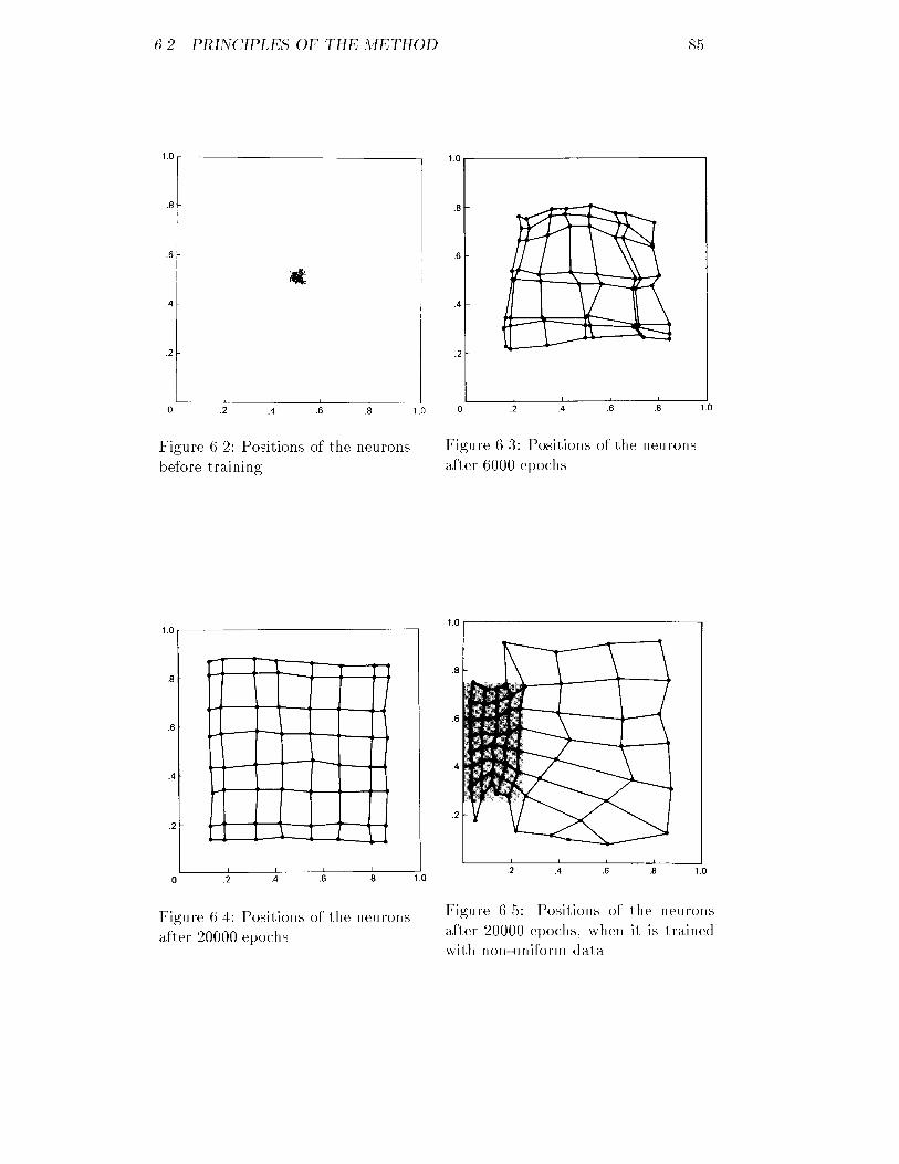
6.2. PRINCIPLES OF THE METHOD 85Figure 6.2: Positions of the neuronsbefore training. Figure 6.3: Positions of the neuronsafter 6000 epochs.

Figure 6.4: Positions of the neuronsafter 20000 epochs. Figure 6.5: Positions of the neuronsafter 20000 epochs, when it is trainedwith non-uniform data.

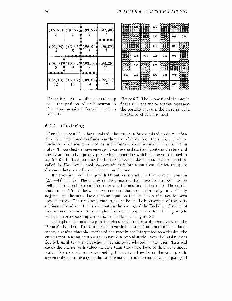
86 CHAPTER 6. FEATURE MAPPINGFigure 6.6: An two-dimensional mapwith the position of each neuron inthe two-dimensional feature space inbrackets. Figure 6.7: The U-matrix of the map in�gure 6.6; the white entries representthe borders between the clusters whena water level of 0.4 is used.6.2.2 ClusteringAfter the network has been trained, the map can be examined to detect clus-ters . A cluster consists of neurons that are neighbours on the map, and whoseEuclidean distance to each other in the feature space is smaller than a certainvalue. These clusters have emerged because the data itself contains clusters andthe feature map is topology preserving, something which has been explained insection 6.2.1. To determine the borders between the clusters a data structurecalled the U-matrix is used [24], containing information about the feature spacedistances between adjacent neurons on the map.If a two-dimensional map with D2 entries is used, the U-matrix will contain(2D � 1)2 entries. The entries in the U-matrix that have both an odd row aswell as an odd column number, represent the neurons on the map. The entriesthat are positioned between two neurons that are horizontally or verticallyadjacent on the map, have a value equal to the Euclidean distance betweenthese neurons. The remaining entries, which lie on the intersection of two pairsof diagonally adjacent neurons, contain the average of the Euclidean distance ofthe two neuron pairs. An example of a feature map can be found in �gure 6.6,while the corresponding U-matrix can be found in �gure 6.7.To explain the next step in the clustering process a di�erent view on theU-matrix is taken. The U-matrix is regarded as an altitude map of some land-scape, meaning that the entries of the matrix are interpreted as altitudes; theentries representing neurons are assigned a zero altitude. Now the landscape is ooded, until the water reaches a certain level selected by the user. This willcause the entries with values smaller than the water level to disappear underwater. Neurons whose corresponding U-matrix entries lie in the same puddleare considered to belong to the same cluster. It is obvious that the quality of

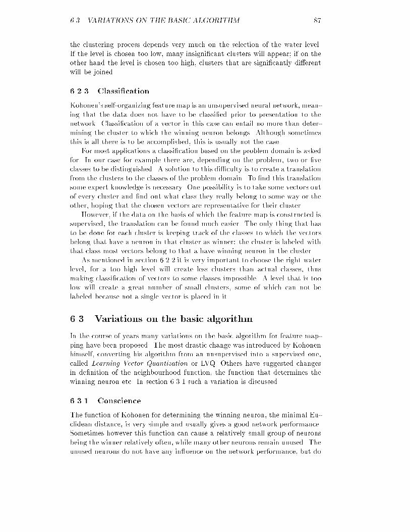
6.3. VARIATIONS ON THE BASIC ALGORITHM 87the clustering process depends very much on the selection of the water level.If the level is chosen too low, many insigni�cant clusters will appear; if on theother hand the level is chosen too high, clusters that are signi�cantly di�erentwill be joined.6.2.3 Classi�cationKohonen's self-organizing feature map is an unsupervised neural network, mean-ing that the data does not have to be classi�ed prior to presentation to thenetwork. Classi�cation of a vector in this case can entail no more than deter-mining the cluster to which the winning neuron belongs. Although sometimesthis is all there is to be accomplished, this is usually not the case.For most applications a classi�cation based on the problem domain is askedfor. In our case for example there are, depending on the problem, two or �veclasses to be distinguished. A solution to this di�culty is to create a translationfrom the clusters to the classes of the problem domain. To �nd this translationsome expert knowledge is necessary. One possibility is to take some vectors outof every cluster and �nd out what class they really belong to some way or theother, hoping that the chosen vectors are representative for their cluster.However, if the data on the basis of which the feature map is constructed issupervised, the translation can be found much easier. The only thing that hasto be done for each cluster is keeping track of the classes to which the vectorsbelong that have a neuron in that cluster as winner: the cluster is labeled withthat class most vectors belong to that a have winning neuron in the cluster.As mentioned in section 6.2.2 it is very important to choose the right waterlevel, for a too high level will create less clusters than actual classes, thusmaking classi�cation of vectors to some classes impossible. A level that is toolow will create a great number of small clusters, some of which can not belabeled because not a single vector is placed in it.6.3 Variations on the basic algorithmIn the course of years many variations on the basic algorithm for feature map-ping have been proposed. The most drastic change was introduced by Kohonenhimself, converting his algorithm from an unsupervised into a supervised one,called Learning Vector Quantization or LVQ. Others have suggested changesin de�nition of the neighbourhood function, the function that determines thewinning neuron etc. In section 6.3.1 such a variation is discussed.6.3.1 ConscienceThe function of Kohonen for determining the winning neuron, the minimal Eu-clidean distance, is very simple and usually gives a good network performance.Sometimes however this function can cause a relatively small group of neuronsbeing the winner relatively often, while many other neurons remain unused. Theunused neurons do not have any in uence on the network performance, but do

88 CHAPTER 6. FEATURE MAPPINGslow down the training process. In 1988 Desieno [22, 24] therefore proposed avariation in the basic algorithm to cancel this disadvantage.Desieno provided every neuron of the output layer with a conscience, makingit for frequently winning neurons di�cult to win again. The conscience isachieved by the following bias termbj = � 1n outputs � cj(t)� (6.7)where j is an index over all neurons of the output layer, index t is increasedevery time a pattern is presented to the network, n outputs equals the numberof neurons of the output layer and is a constant that is usually set at 10. Theterm cj(t) actually implements the conscience and is de�ned bycj(0) = 1 (6.8)cj(t + 1) = (1 + �)cj(t); if neuron j is the winner= (1� �)cj(t); otherwisewith � being a constant usually set at 0.0001. Equation 6.3, according to whichthe winning neuron (index j�) is determined, now changes to8j jwj� � vpj � bj� � jwj � vpj � bj (6.9)where j is an index over all neurons of the output layer, wj represents the setof incoming weights of neuron j, vp is the pattern currently presented to thenetwork and j:j represents the Euclidean distance function.It is easy to understand that due to the conscience mechanism it is impos-sible that a neuron never becomes a winner. For by repeatedly being a looserneuron, the neurons conscience keeps improving in comparison to the other neu-rons consciences. Finally the neuron must be declared the winner, independentof its position in the feature space relative to the position of the input vectors.Although it is not simple, by a good choice of and � a network consisting ofn neurons in the output layer can be forced to declare each neuron on average1n -th of time to be the winner.6.4 ResultsThe results which are presented in the remainder of this chapter are obtainedwith the Kohonen neural networks simulator by Bierman. A short users-manualof this simulator can be found in [24], while our application speci�c alterationsof the simulator | koho | are described in appendix A.6.4.1 Measuring the performanceThe way in which the performance of a feature map is measured is more or lessequal to measuring the performance of a back-propagation network, somethingthat is done deliberately to make a good comparison between the two methodspossible. In this section therefore only the di�erences between back-propagation

6.4. RESULTS 89and feature mapping are dealt with, while for the common principles is referredto section 5.4.1.Analogous to section 5.4.1 two error functions are used, the RMS and theICF . The RMS , which is derived from the internal error function described inequation 6.1, is given byRMS(w) =vuutPp minjPi (vp;i � wji)2n patients n inputs (6.10)Just like in equation 6.1 w represents the entire set of weights, wji the weightfrom neuron i to neuron j and vp;i the i-th element of patient vector p; p isan index over all patients, j over all neurons of the output layer and i over allneurons of the input layer. In addition n patients stands for the number ofpatients and n inputs for the number of neurons in the input layer. This errorfunction is no longer dependent on the magnitude of the data set, nor of thenumber of features that is used to characterize a patient.The fraction of incorrect classi�cation that we are interested in is given bythe ICF , de�ned byICF(w) =vuuuuutPc 0@n patientsc�Pp (cp;lp�)n patientsc 1A2n classes (6.11)In this equation c is an index over all classes, n classes is the number of classes,p is an index over all patients in the class under observation, and n patientscis the number of patients in class c. The symbol stands for a function thatreturns 1 when the class patient p actually belongs to (cp) is equal to the classlabel (lp�) that was assigned to the cluster containing the winning neuron, and0 otherwise. It is obvious that the ICF can only be de�ned if the data issupervised.Although the ICF is de�ned in equation 6.11 using a function , whilein the back-propagation equivalent 5.13 a di�erent function � is used, bothvariants are comparable. The di�erence is caused by the di�ering principlesof the methods: for back-propagation incorrect classi�cation of a patient hasto be checked by comparing the target pattern with the output pattern of thenetwork, while for feature mapping the class of a patient has to be comparedwith the label that has been assigned to the cluster of the winning neuron. Sinceboth � as well as return 1 in case of correct classi�cation and 0 otherwise,both de�nitions of the ICF give results that are completely equal.Just like in case of back-propagation, for a feature mapping network theRMS and ICF are not fully correlated, as can be seen in �gure 6.8. This isnot surprising, since the feature mapping network has no knowledge of the ICFeither. Again the ICF is a bit jumpy; in the case of feature mapping this canbe explained by the way in which it is determined what the label of a class is.Suppose that classes X and Y overlap in such a way that some set of vectorsof class X as well an approximately equally large set of class Y are mapped

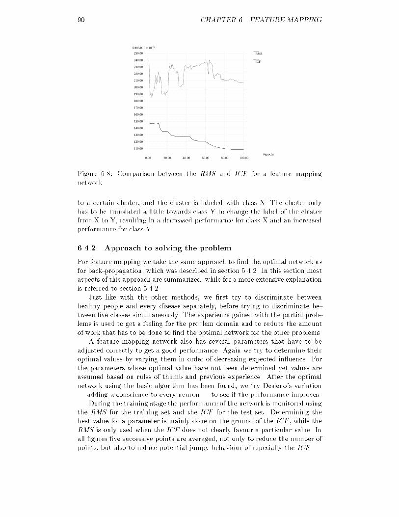
90 CHAPTER 6. FEATURE MAPPINGRMS

ICF

RMS/ICF x 10-3

#epochs

110.00

120.00

130.00

140.00

150.00

160.00

170.00

180.00

190.00

200.00

210.00

220.00

230.00

240.00

250.00

0.00 20.00 40.00 60.00 80.00 100.00Figure 6.8: Comparison between the RMS and ICF for a feature mappingnetwork.to a certain cluster, and the cluster is labeled with class X. The cluster onlyhas to be translated a little towards class Y to change the label of the clusterfrom X to Y, resulting in a decreased performance for class X and an increasedperformance for class Y.6.4.2 Approach to solving the problemFor feature mapping we take the same approach to �nd the optimal network asfor back-propagation, which was described in section 5.4.2. In this section mostaspects of this approach are summarized, while for a more extensive explanationis referred to section 5.4.2.Just like with the other methods, we �rst try to discriminate betweenhealthy people and every disease separately, before trying to discriminate be-tween �ve classes simultaneously. The experience gained with the partial prob-lems is used to get a feeling for the problem domain and to reduce the amountof work that has to be done to �nd the optimal network for the other problems.A feature mapping network also has several parameters that have to beadjusted correctly to get a good performance. Again we try to determine theiroptimal values by varying them in order of decreasing expected in uence. Forthe parameters whose optimal value have not been determined yet values areassumed based on rules of thumb and previous experience. After the optimalnetwork using the basic algorithm has been found, we try Desieno's variation| adding a conscience to every neuron | to see if the performance improves.During the training stage the performance of the network is monitored usingthe RMS for the training set and the ICF for the test set. Determining thebest value for a parameter is mainly done on the ground of the ICF , while theRMS is only used when the ICF does not clearly favour a particular value. Inall �gures �ve successive points are averaged, not only to reduce the number ofpoints, but also to reduce potential jumpy behaviour of especially the ICF .

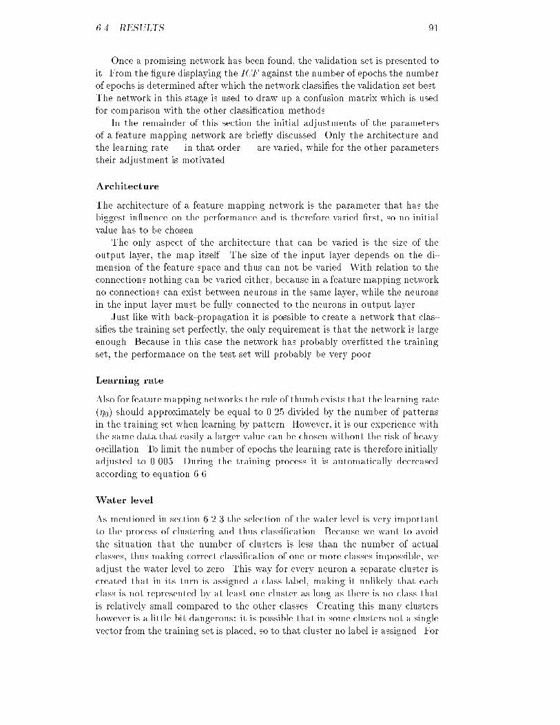
6.4. RESULTS 91Once a promising network has been found, the validation set is presented toit. From the �gure displaying the ICF against the number of epochs the numberof epochs is determined after which the network classi�es the validation set best.The network in this stage is used to draw up a confusion matrix which is usedfor comparison with the other classi�cation methods.In the remainder of this section the initial adjustments of the parametersof a feature mapping network are brie y discussed. Only the architecture andthe learning rate | in that order | are varied, while for the other parameterstheir adjustment is motivated.ArchitectureThe architecture of a feature mapping network is the parameter that has thebiggest in uence on the performance and is therefore varied �rst, so no initialvalue has to be chosen.The only aspect of the architecture that can be varied is the size of theoutput layer, the map itself. The size of the input layer depends on the di-mension of the feature space and thus can not be varied. With relation to theconnections nothing can be varied either, because in a feature mapping networkno connections can exist between neurons in the same layer, while the neuronsin the input layer must be fully connected to the neurons in output layer.Just like with back-propagation it is possible to create a network that clas-si�es the training set perfectly, the only requirement is that the network is largeenough. Because in this case the network has probably over�tted the trainingset, the performance on the test set will probably be very poor.Learning rateAlso for feature mapping networks the rule of thumb exists that the learning rate(�0) should approximately be equal to 0.25 divided by the number of patternsin the training set when learning by pattern. However, it is our experience withthe same data that easily a larger value can be chosen without the risk of heavyoscillation. To limit the number of epochs the learning rate is therefore initiallyadjusted to 0.005. During the training process it is automatically decreasedaccording to equation 6.6.Water levelAs mentioned in section 6.2.3 the selection of the water level is very importantto the process of clustering and thus classi�cation. Because we want to avoidthe situation that the number of clusters is less than the number of actualclasses, thus making correct classi�cation of one or more classes impossible, weadjust the water level to zero. This way for every neuron a separate cluster iscreated that in its turn is assigned a class label, making it unlikely that eachclass is not represented by at least one cluster as long as there is no class thatis relatively small compared to the other classes. Creating this many clustershowever is a little bit dangerous: it is possible that in some clusters not a singlevector from the training set is placed, so to that cluster no label is assigned. For

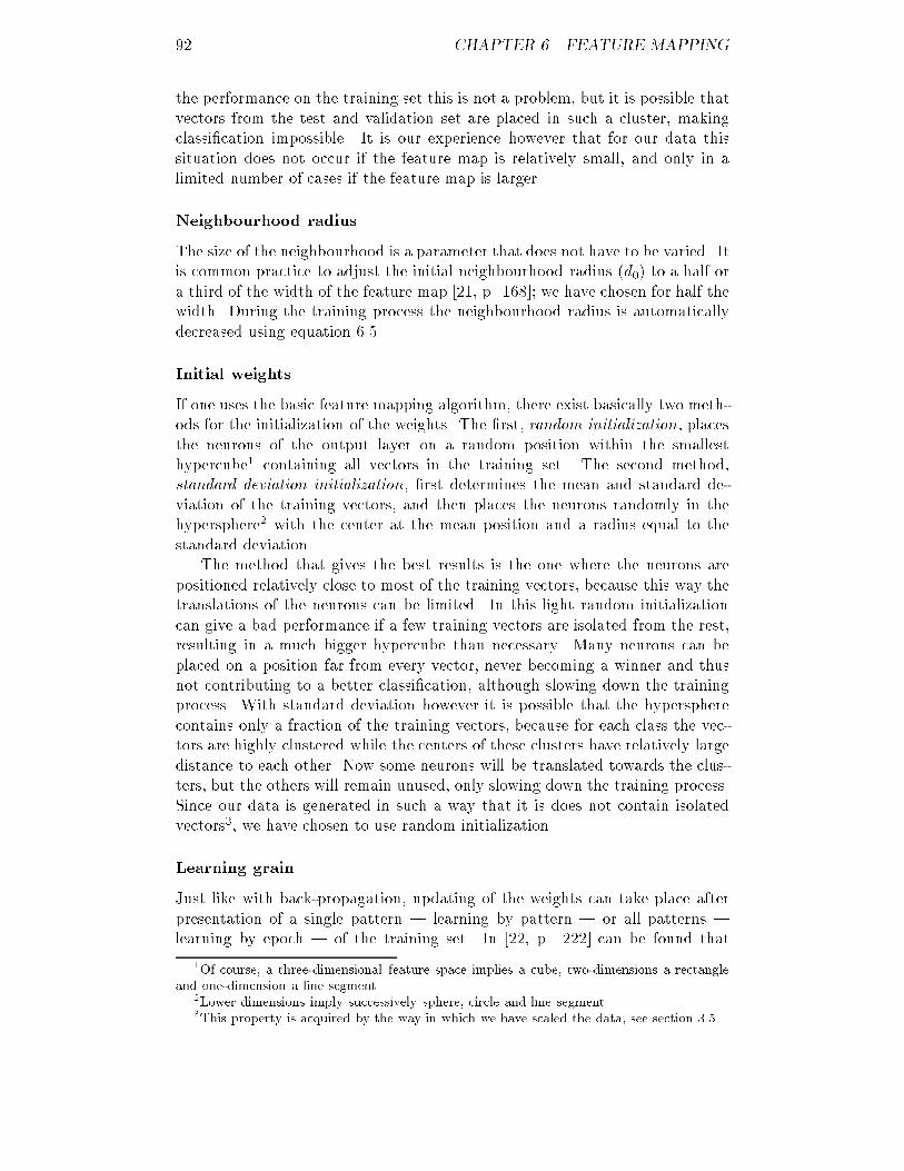
92 CHAPTER 6. FEATURE MAPPINGthe performance on the training set this is not a problem, but it is possible thatvectors from the test and validation set are placed in such a cluster, makingclassi�cation impossible. It is our experience however that for our data thissituation does not occur if the feature map is relatively small, and only in alimited number of cases if the feature map is larger.Neighbourhood radiusThe size of the neighbourhood is a parameter that does not have to be varied. Itis common practice to adjust the initial neighbourhood radius (d0) to a half ora third of the width of the feature map [21, p. 168]; we have chosen for half thewidth. During the training process the neighbourhood radius is automaticallydecreased using equation 6.5.Initial weightsIf one uses the basic feature mapping algorithm, there exist basically two meth-ods for the initialization of the weights. The �rst, random initialization, placesthe neurons of the output layer on a random position within the smallesthypercube1 containing all vectors in the training set. The second method,standard deviation initialization, �rst determines the mean and standard de-viation of the training vectors, and then places the neurons randomly in thehypersphere2 with the center at the mean position and a radius equal to thestandard deviation.The method that gives the best results is the one where the neurons arepositioned relatively close to most of the training vectors, because this way thetranslations of the neurons can be limited. In this light random initializationcan give a bad performance if a few training vectors are isolated from the rest,resulting in a much bigger hypercube than necessary. Many neurons can beplaced on a position far from every vector, never becoming a winner and thusnot contributing to a better classi�cation, although slowing down the trainingprocess. With standard deviation however it is possible that the hyperspherecontains only a fraction of the training vectors, because for each class the vec-tors are highly clustered while the centers of these clusters have relatively largedistance to each other. Now some neurons will be translated towards the clus-ters, but the others will remain unused, only slowing down the training process.Since our data is generated in such a way that it is does not contain isolatedvectors3, we have chosen to use random initialization.Learning grainJust like with back-propagation, updating of the weights can take place afterpresentation of a single pattern | learning by pattern | or all patterns |learning by epoch | of the training set. In [22, p. 222] can be found that1Of course, a three-dimensional feature space implies a cube, two-dimensions a rectangleand one-dimension a line segment.2Lower dimensions imply successively sphere, circle and line segment.3This property is acquired by the way in which we have scaled the data, see section 3.5.

6.4. RESULTS 93learning by pattern combined with a random order in which the patterns arepresented to the network is useful for avoiding local minima, so only this �nelearn grain is considered.6.4.3 Discrimination between A and BThis section deals with the discrimination between classes A and B. A descrip-tion of the training, test and validation set can be found in section 3.5, whilethe results are discussed in section 6.5.Varying the architectureEight di�erent sizes for the feature map are tried, varying from 3x3 to 10x10.The performance of the maps on the training set can be found in �gures 6.9to 6.10, while the �gures 6.11 to 6.12 show the results of the test set.3x3

4x4

5x5

6x6

RMS x 10-3

#epochs

95.00

100.00

105.00

110.00

115.00

120.00

125.00

130.00

135.00

140.00

145.00

150.00

0.00 20.00 40.00 60.00 80.00 100.00Figure 6.9: Performance on the AB-training setfor several architectures.7x7

8x8

9x9

10x10

RMS x 10-3

#epochs

95.00

100.00

105.00

110.00

115.00

120.00

125.00

130.00

135.00

140.00

145.00

150.00

0.00 20.00 40.00 60.00 80.00 100.00Figure 6.10: Performance on the AB-trainingset for several architectures.We have chosen the 7x7 map for further optimizing.Varying the learning rateFor the learning rate three values are tried: 0.1, 0.005 and 0.00025. The resultson the training set are shown in �gure 6.13, and the performance on the testset is presented in �gure 6.14.A learning rate of 0.005 seems to give the best performance.Adding conscienceThe results of adding conscience to each neuron as described in section 6.3.1can be found in �gure 6.15 for the training set, and in �gure 6.16 for the testset.

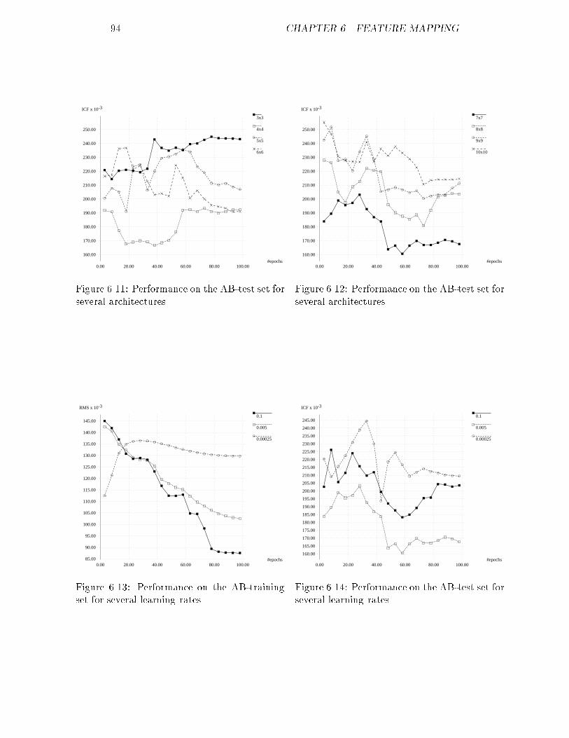
94 CHAPTER 6. FEATURE MAPPING3x3

4x4

5x5

6x6

ICF x 10-3

#epochs

160.00

170.00

180.00

190.00

200.00

210.00

220.00

230.00

240.00

250.00

0.00 20.00 40.00 60.00 80.00 100.00Figure 6.11: Performance on the AB-test set forseveral architectures.7x7

8x8

9x9

10x10

ICF x 10-3

#epochs

160.00

170.00

180.00

190.00

200.00

210.00

220.00

230.00

240.00

250.00

0.00 20.00 40.00 60.00 80.00 100.00Figure 6.12: Performance on the AB-test set forseveral architectures.0.1

0.005

0.00025

RMS x 10-3

#epochs85.00

90.00

95.00

100.00

105.00

110.00

115.00

120.00

125.00

130.00

135.00

140.00

145.00

0.00 20.00 40.00 60.00 80.00 100.00Figure 6.13: Performance on the AB-trainingset for several learning rates.0.1

0.005

0.00025

ICF x 10-3

#epochs160.00

165.00

170.00

175.00

180.00

185.00

190.00

195.00

200.00

205.00

210.00

215.00

220.00

225.00

230.00

235.00

240.00

245.00

0.00 20.00 40.00 60.00 80.00 100.00Figure 6.14: Performance on the AB-test set forseveral learning rates.

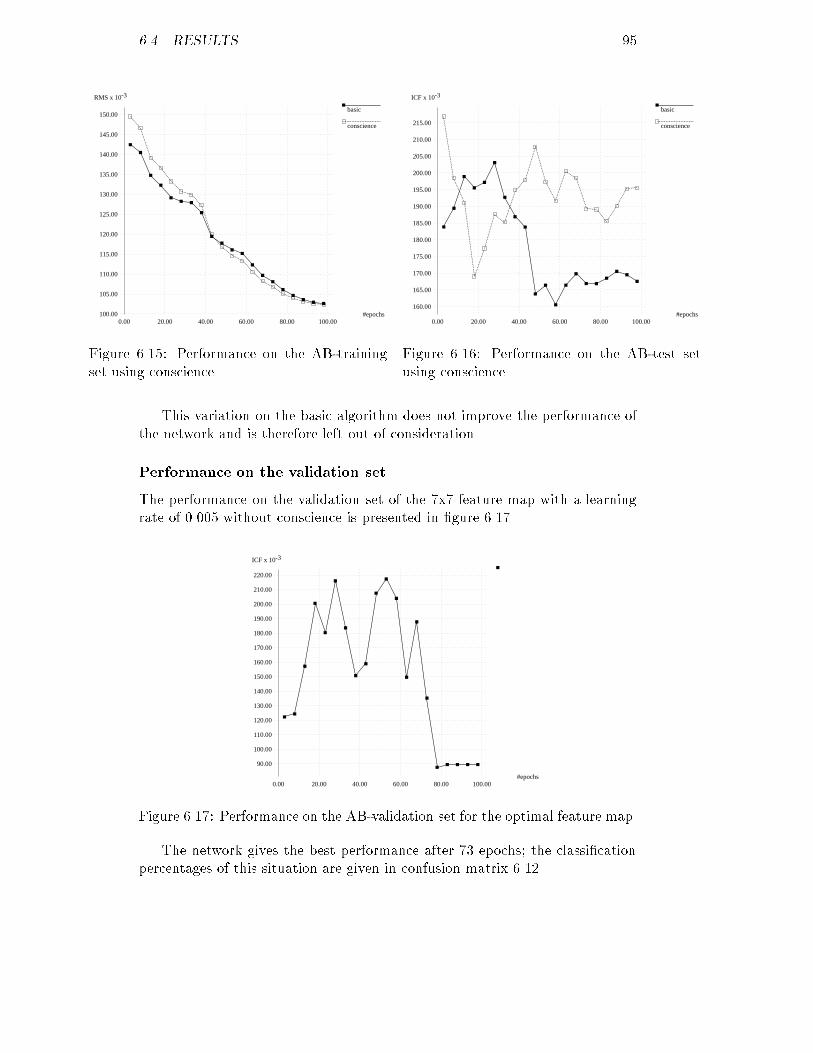
6.4. RESULTS 95basic

conscience

RMS x 10-3

#epochs100.00

105.00

110.00

115.00

120.00

125.00

130.00

135.00

140.00

145.00

150.00

0.00 20.00 40.00 60.00 80.00 100.00Figure 6.15: Performance on the AB-trainingset using conscience.basic

conscience

ICF x 10-3

#epochs160.00

165.00

170.00

175.00

180.00

185.00

190.00

195.00

200.00

205.00

210.00

215.00

0.00 20.00 40.00 60.00 80.00 100.00Figure 6.16: Performance on the AB-test setusing conscience.This variation on the basic algorithm does not improve the performance ofthe network and is therefore left out of consideration.Performance on the validation setThe performance on the validation set of the 7x7 feature map with a learningrate of 0.005 without conscience is presented in �gure 6.17.ICF x 10-3

#epochs

90.00

100.00

110.00

120.00

130.00

140.00

150.00

160.00

170.00

180.00

190.00

200.00

210.00

220.00

0.00 20.00 40.00 60.00 80.00 100.00Figure 6.17: Performance on the AB-validation set for the optimal feature map.The network gives the best performance after 73 epochs; the classi�cationpercentages of this situation are given in confusion matrix 6.12.

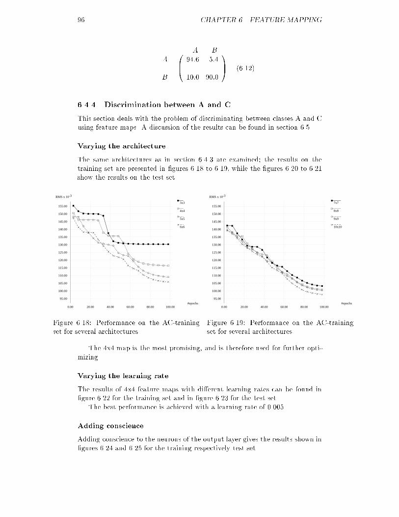
96 CHAPTER 6. FEATURE MAPPINGA BAB 0B@ 94:6 5:410:0 90:0 1CA (6.12)6.4.4 Discrimination between A and CThis section deals with the problem of discriminating between classes A and Cusing feature maps. A discussion of the results can be found in section 6.5.Varying the architectureThe same architectures as in section 6.4.3 are examined; the results on thetraining set are presented in �gures 6.18 to 6.19, while the �gures 6.20 to 6.21show the results on the test set.3x3

4x4

5x5

6x6

RMS x 10-3

#epochs

95.00

100.00

105.00

110.00

115.00

120.00

125.00

130.00

135.00

140.00

145.00

150.00

155.00

0.00 20.00 40.00 60.00 80.00 100.00Figure 6.18: Performance on the AC-trainingset for several architectures.7x7

8x8

9x9

10x10

RMS x 10-3

#epochs

95.00

100.00

105.00

110.00

115.00

120.00

125.00

130.00

135.00

140.00

145.00

150.00

155.00

0.00 20.00 40.00 60.00 80.00 100.00Figure 6.19: Performance on the AC-trainingset for several architectures.The 4x4 map is the most promising, and is therefore used for further opti-mizing.Varying the learning rateThe results of 4x4 feature maps with di�erent learning rates can be found in�gure 6.22 for the training set and in �gure 6.23 for the test set.The best performance is achieved with a learning rate of 0.005.Adding conscienceAdding conscience to the neurons of the output layer gives the results shown in�gures 6.24 and 6.25 for the training respectively test set.

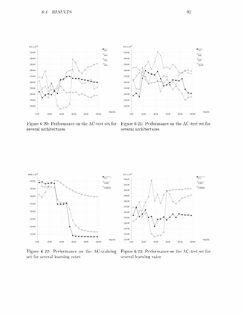
6.4. RESULTS 973x3

4x4

5x5

6x6

ICF x 10-3

#epochs

220.00

230.00

240.00

250.00

260.00

270.00

280.00

290.00

300.00

310.00

0.00 20.00 40.00 60.00 80.00 100.00Figure 6.20: Performance on the AC-test set forseveral architectures.7x7

8x8

9x9

10x10

ICF x 10-3

#epochs

220.00

230.00

240.00

250.00

260.00

270.00

280.00

290.00

300.00

310.00

0.00 20.00 40.00 60.00 80.00 100.00Figure 6.21: Performance on the AC-test set forseveral architectures.0.1

0.005

0.00025

RMS x 10-3

#epochs

115.00

120.00

125.00

130.00

135.00

140.00

145.00

150.00

0.00 20.00 40.00 60.00 80.00 100.00Figure 6.22: Performance on the AC-trainingset for several learning rates.0.1

0.005

0.00025

ICF x 10-3

#epochs210.00

220.00

230.00

240.00

250.00

260.00

270.00

280.00

290.00

300.00

310.00

320.00

0.00 20.00 40.00 60.00 80.00 100.00Figure 6.23: Performance on the AC-test set forseveral learning rates.

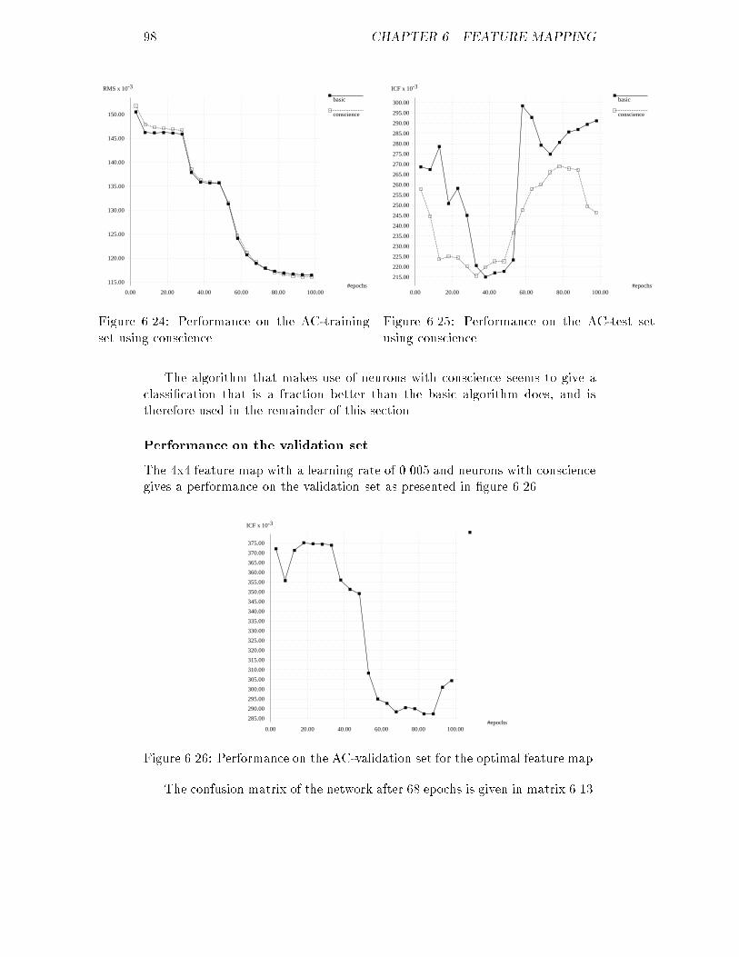
98 CHAPTER 6. FEATURE MAPPINGbasic

conscience

RMS x 10-3

#epochs115.00

120.00

125.00

130.00

135.00

140.00

145.00

150.00

0.00 20.00 40.00 60.00 80.00 100.00Figure 6.24: Performance on the AC-trainingset using conscience.basic

conscience

ICF x 10-3

#epochs

215.00

220.00

225.00

230.00

235.00

240.00

245.00

250.00

255.00

260.00

265.00

270.00

275.00

280.00

285.00

290.00

295.00

300.00

0.00 20.00 40.00 60.00 80.00 100.00Figure 6.25: Performance on the AC-test setusing conscience.The algorithm that makes use of neurons with conscience seems to give aclassi�cation that is a fraction better than the basic algorithm does, and istherefore used in the remainder of this section.Performance on the validation setThe 4x4 feature map with a learning rate of 0.005 and neurons with consciencegives a performance on the validation set as presented in �gure 6.26.ICF x 10-3

#epochs285.00

290.00

295.00

300.00

305.00

310.00

315.00

320.00

325.00

330.00

335.00

340.00

345.00

350.00

355.00

360.00

365.00

370.00

375.00

0.00 20.00 40.00 60.00 80.00 100.00Figure 6.26: Performance on the AC-validation set for the optimal feature map.The confusion matrix of the network after 68 epochs is given in matrix 6.13.

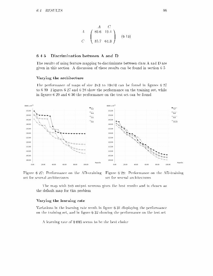
6.4. RESULTS 99A CAC 0B@ 80:6 19:435:7 64:3 1CA (6.13)6.4.5 Discrimination between A and DThe results of using feature mapping to discriminate between class A and D aregiven in this section. A discussion of these results can be found in section 6.5.Varying the architectureThe performance of maps of size 3x3 to 10x10 can be found in �gures 6.27to 6.30. Figures 6.27 and 6.28 show the performance on the training set, whilein �gures 6.29 and 6.30 the performance on the test set can be found.3x3

4x4

5x5

6x6

RMS x 10-3

#epochs

100.00

105.00

110.00

115.00

120.00

125.00

130.00

135.00

140.00

145.00

150.00

155.00

0.00 20.00 40.00 60.00 80.00 100.00Figure 6.27: Performance on the AD-trainingset for several architectures.7x7

8x8

9x9

10x10

RMS x 10-3

#epochs

100.00

105.00

110.00

115.00

120.00

125.00

130.00

135.00

140.00

145.00

150.00

155.00

0.00 20.00 40.00 60.00 80.00 100.00Figure 6.28: Performance on the AD-trainingset for several architectures.The map with 8x8 output neurons gives the best results and is chosen asthe default map for this problem.Varying the learning rateVariations in the learning rate result in �gure 6.31 displaying the performanceon the training set, and in �gure 6.32 showing the performance on the test set.A learning rate of 0.005 seems to be the best choice.

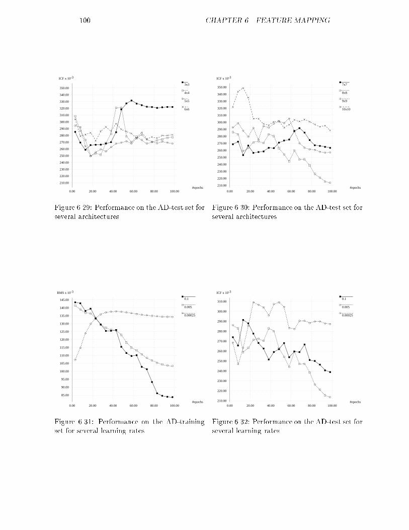
100 CHAPTER 6. FEATURE MAPPING3x3

4x4

5x5

6x6

ICF x 10-3

#epochs

210.00

220.00

230.00

240.00

250.00

260.00

270.00

280.00

290.00

300.00

310.00

320.00

330.00

340.00

350.00

0.00 20.00 40.00 60.00 80.00 100.00Figure 6.29: Performance on the AD-test set forseveral architectures.7x7

8x8

9x9

10x10

ICF x 10-3

#epochs210.00

220.00

230.00

240.00

250.00

260.00

270.00

280.00

290.00

300.00

310.00

320.00

330.00

340.00

350.00

0.00 20.00 40.00 60.00 80.00 100.00Figure 6.30: Performance on the AD-test set forseveral architectures.0.1

0.005

0.00025

RMS x 10-3

#epochs

85.00

90.00

95.00

100.00

105.00

110.00

115.00

120.00

125.00

130.00

135.00

140.00

145.00

0.00 20.00 40.00 60.00 80.00 100.00Figure 6.31: Performance on the AD-trainingset for several learning rates.0.1

0.005

0.00025

ICF x 10-3

#epochs210.00

220.00

230.00

240.00

250.00

260.00

270.00

280.00

290.00

300.00

310.00

0.00 20.00 40.00 60.00 80.00 100.00Figure 6.32: Performance on the AD-test set forseveral learning rates.

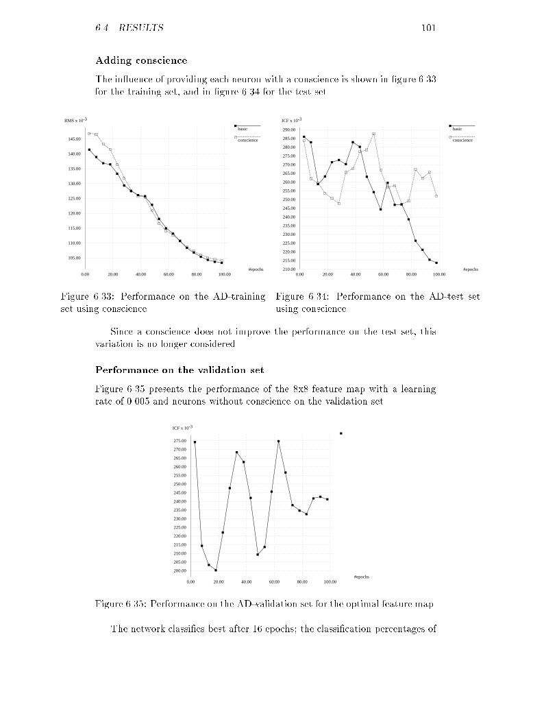
6.4. RESULTS 101Adding conscienceThe in uence of providing each neuron with a conscience is shown in �gure 6.33for the training set, and in �gure 6.34 for the test set.basic

conscience

RMS x 10-3

#epochs

105.00

110.00

115.00

120.00

125.00

130.00

135.00

140.00

145.00

0.00 20.00 40.00 60.00 80.00 100.00Figure 6.33: Performance on the AD-trainingset using conscience.basic

conscience

ICF x 10-3

#epochs210.00

215.00

220.00

225.00

230.00

235.00

240.00

245.00

250.00

255.00

260.00

265.00

270.00

275.00

280.00

285.00

290.00

0.00 20.00 40.00 60.00 80.00 100.00Figure 6.34: Performance on the AD-test setusing conscience.Since a conscience does not improve the performance on the test set, thisvariation is no longer considered.Performance on the validation setFigure 6.35 presents the performance of the 8x8 feature map with a learningrate of 0.005 and neurons without conscience on the validation set.ICF x 10-3

#epochs200.00

205.00

210.00

215.00

220.00

225.00

230.00

235.00

240.00

245.00

250.00

255.00

260.00

265.00

270.00

275.00

0.00 20.00 40.00 60.00 80.00 100.00Figure 6.35: Performance on the AD-validation set for the optimal feature map.The network classi�es best after 16 epochs; the classi�cation percentages of

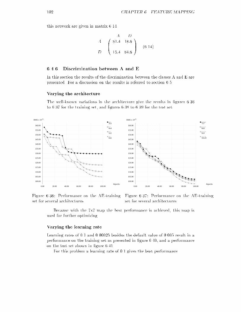
102 CHAPTER 6. FEATURE MAPPINGthis network are given in matrix 6.14.A DAD 0B@ 81:4 18:615:4 84:6 1CA (6.14)6.4.6 Discrimination between A and EIn this section the results of the discrimination between the classes A and E arepresented. For a discussion on the results is referred to section 6.5.Varying the architectureThe well-known variations in the architecture give the results in �gures 6.36to 6.37 for the training set, and �gures 6.38 to 6.39 for the test set.3x3

4x4

5x5

6x6

RMS x 10-3

#epochs

100.00

105.00

110.00

115.00

120.00

125.00

130.00

135.00

140.00

145.00

150.00

155.00

160.00

0.00 20.00 40.00 60.00 80.00 100.00Figure 6.36: Performance on the AE-trainingset for several architectures.7x7

8x8

9x9

10x10

RMS x 10-3

#epochs

100.00

105.00

110.00

115.00

120.00

125.00

130.00

135.00

140.00

145.00

150.00

155.00

160.00

0.00 20.00 40.00 60.00 80.00 100.00Figure 6.37: Performance on the AE-trainingset for several architectures.Because with the 7x7 map the best performance is achieved, this map isused for further optimizing.Varying the learning rateLearning rates of 0.1 and 0.00025 besides the default value of 0.005 result in aperformance on the training set as presented in �gure 6.40, and a performanceon the test set shown in �gure 6.41.For this problem a learning rate of 0.1 gives the best performance.

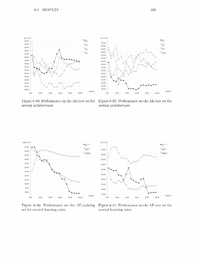
6.4. RESULTS 1033x3

4x4

5x5

6x6

ICF x 10-3

#epochs180.00

185.00

190.00

195.00

200.00

205.00

210.00

215.00

220.00

225.00

230.00

235.00

240.00

245.00

250.00

255.00

0.00 20.00 40.00 60.00 80.00 100.00Figure 6.38: Performance on the AE-test set forseveral architectures.7x7

8x8

9x9

10x10

ICF x 10-3

#epochs

180.00

185.00

190.00

195.00

200.00

205.00

210.00

215.00

220.00

225.00

230.00

235.00

240.00

245.00

250.00

255.00

0.00 20.00 40.00 60.00 80.00 100.00Figure 6.39: Performance on the AE-test set forseveral architectures.0.1

0.005

0.00025

RMS x 10-3

#epochs

90.00

95.00

100.00

105.00

110.00

115.00

120.00

125.00

130.00

135.00

140.00

145.00

0.00 20.00 40.00 60.00 80.00 100.00Figure 6.40: Performance on the AE-trainingset for several learning rates.0.1

0.005

0.00025

ICF x 10-3

#epochs170.00

180.00

190.00

200.00

210.00

220.00

230.00

240.00

250.00

260.00

0.00 20.00 40.00 60.00 80.00 100.00Figure 6.41: Performance on the AE-test set forseveral learning rates.

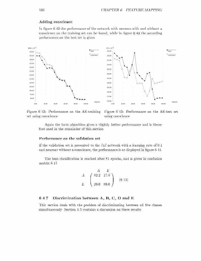
104 CHAPTER 6. FEATURE MAPPINGAdding conscienceIn �gure 6.42 the performance of the network with neurons with and without aconscience on the training set can be found, while in �gure 6.43 the accordingperformance on the test set is given.basic

conscience

RMS x 10-3

#epochs

90.00

95.00

100.00

105.00

110.00

115.00

120.00

125.00

130.00

135.00

140.00

145.00

150.00

0.00 20.00 40.00 60.00 80.00 100.00Figure 6.42: Performance on the AE-trainingset using conscience.basic

conscience

ICF x 10-3

#epochs170.00

175.00

180.00

185.00

190.00

195.00

200.00

205.00

210.00

215.00

220.00

225.00

0.00 20.00 40.00 60.00 80.00 100.00Figure 6.43: Performance on the AE-test setusing conscience.Again the basic algorithm gives a slightly better performance and is there-fore used in the remainder of this section.Performance on the validation setIf the validation set is presented to the 7x7 network with a learning rate of 0.1and neurons without a conscience, the performance is as displayed in �gure 6.44.The best classi�cation is reached after 81 epochs, and is given in confusionmatrix 6.15. A EAE 0B@ 82:2 17:820:0 80:0 1CA (6.15)6.4.7 Discrimination between A, B, C, D and EThis section deals with the problem of discriminating between all �ve classessimultaneously. Section 6.5 contains a discussion on these results.

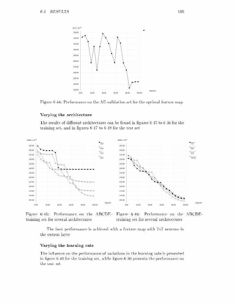
6.4. RESULTS 105ICF x 10-3

#epochs230.00

240.00

250.00

260.00

270.00

280.00

290.00

300.00

310.00

320.00

330.00

0.00 20.00 40.00 60.00 80.00 100.00Figure 6.44: Performance on the AE-validation set for the optimal feature map.Varying the architectureThe results of di�erent architectures can be found in �gures 6.45 to 6.46 for thetraining set, and in �gures 6.47 to 6.48 for the test set.3x3

4x4

5x5

6x6

RMS x 10-3

#epochs

105.00

110.00

115.00

120.00

125.00

130.00

135.00

140.00

145.00

150.00

155.00

160.00

165.00

0.00 20.00 40.00 60.00 80.00 100.00Figure 6.45: Performance on the ABCDE-training set for several architectures.7x7

8x8

9x9

10x10

RMS x 10-3

#epochs

105.00

110.00

115.00

120.00

125.00

130.00

135.00

140.00

145.00

150.00

155.00

160.00

165.00

0.00 20.00 40.00 60.00 80.00 100.00Figure 6.46: Performance on the ABCDE-training set for several architectures.The best performance is achieved with a feature map with 7x7 neurons inthe output layer.Varying the learning rateThe in uence on the performance of variations in the learning rate is presentedin �gure 6.49 for the training set, while �gure 6.50 presents the performance onthe test set.

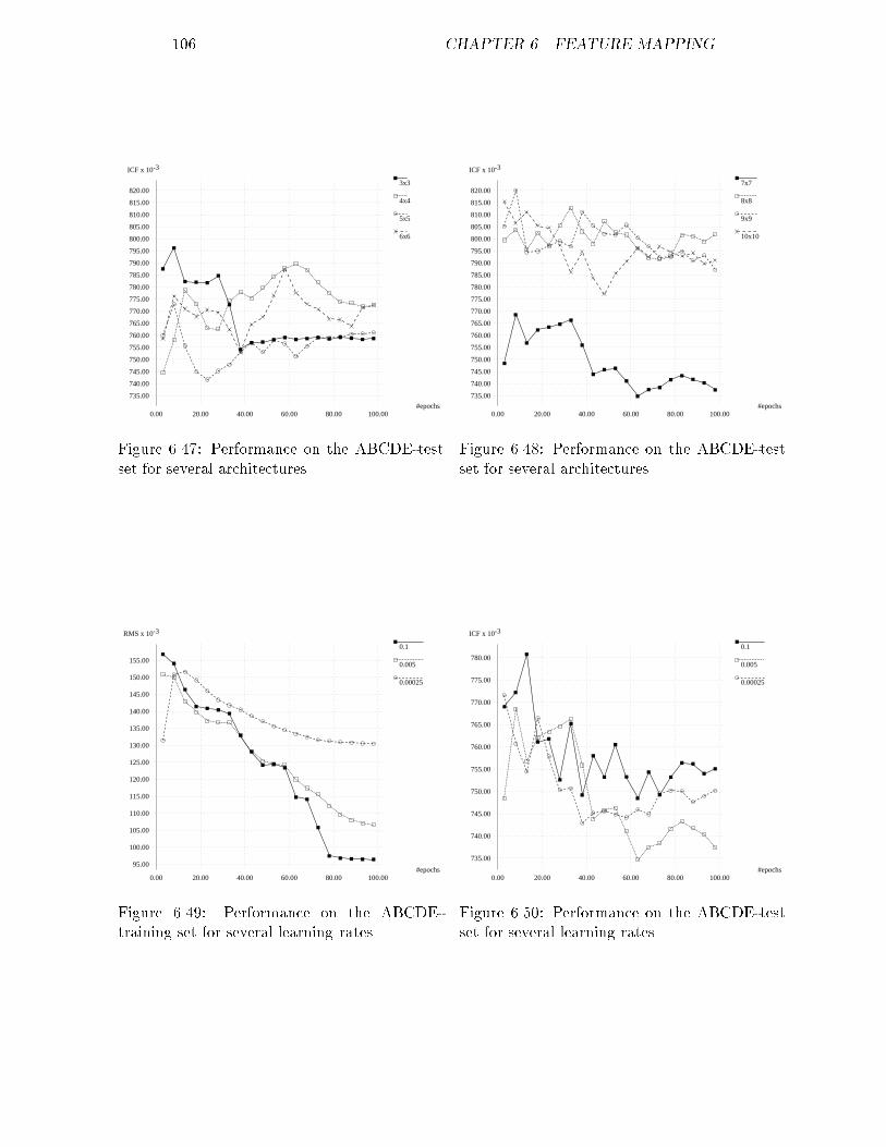
106 CHAPTER 6. FEATURE MAPPING3x3

4x4

5x5

6x6

ICF x 10-3

#epochs

735.00

740.00

745.00

750.00

755.00

760.00

765.00

770.00

775.00

780.00

785.00

790.00

795.00

800.00

805.00

810.00

815.00

820.00

0.00 20.00 40.00 60.00 80.00 100.00Figure 6.47: Performance on the ABCDE-testset for several architectures.7x7

8x8

9x9

10x10

ICF x 10-3

#epochs

735.00

740.00

745.00

750.00

755.00

760.00

765.00

770.00

775.00

780.00

785.00

790.00

795.00

800.00

805.00

810.00

815.00

820.00

0.00 20.00 40.00 60.00 80.00 100.00Figure 6.48: Performance on the ABCDE-testset for several architectures.0.1

0.005

0.00025

RMS x 10-3

#epochs95.00

100.00

105.00

110.00

115.00

120.00

125.00

130.00

135.00

140.00

145.00

150.00

155.00

0.00 20.00 40.00 60.00 80.00 100.00Figure 6.49: Performance on the ABCDE-training set for several learning rates.0.1

0.005

0.00025

ICF x 10-3

#epochs

735.00

740.00

745.00

750.00

755.00

760.00

765.00

770.00

775.00

780.00

0.00 20.00 40.00 60.00 80.00 100.00Figure 6.50: Performance on the ABCDE-testset for several learning rates.

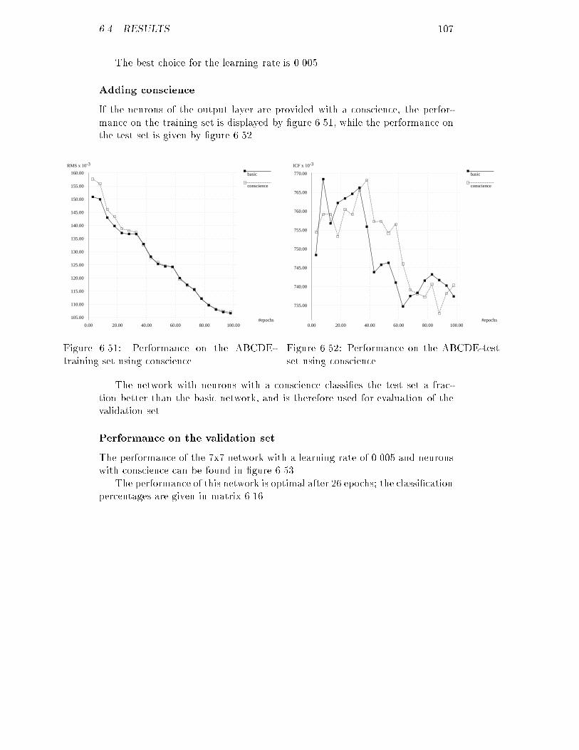
6.4. RESULTS 107The best choice for the learning rate is 0.005.Adding conscienceIf the neurons of the output layer are provided with a conscience, the perfor-mance on the training set is displayed by �gure 6.51, while the performance onthe test set is given by �gure 6.52.basic

conscience

RMS x 10-3

#epochs105.00

110.00

115.00

120.00

125.00

130.00

135.00

140.00

145.00

150.00

155.00

160.00

0.00 20.00 40.00 60.00 80.00 100.00Figure 6.51: Performance on the ABCDE-training set using conscience.basic

conscience

ICF x 10-3

#epochs

735.00

740.00

745.00

750.00

755.00

760.00

765.00

770.00

0.00 20.00 40.00 60.00 80.00 100.00Figure 6.52: Performance on the ABCDE-testset using conscience.The network with neurons with a conscience classi�es the test set a frac-tion better than the basic network, and is therefore used for evaluation of thevalidation set.Performance on the validation setThe performance of the 7x7 network with a learning rate of 0.005 and neuronswith conscience can be found in �gure 6.53.The performance of this network is optimal after 26 epochs; the classi�cationpercentages are given in matrix 6.16.

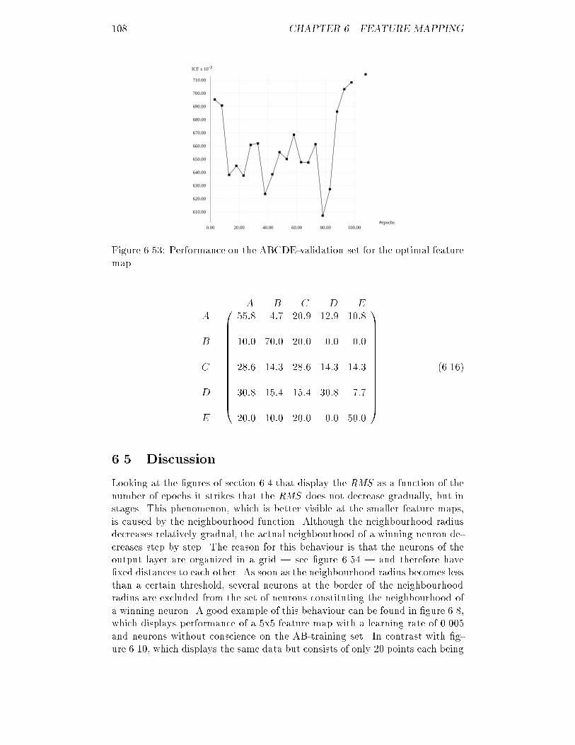
108 CHAPTER 6. FEATURE MAPPINGICF x 10-3

#epochs

610.00

620.00

630.00

640.00

650.00

660.00

670.00

680.00

690.00

700.00

710.00

0.00 20.00 40.00 60.00 80.00 100.00Figure 6.53: Performance on the ABCDE-validation set for the optimal featuremap. A B C D EABCDE 0BBBBBBBBBBBBBB@ 55:8 4:7 20:9 12:9 10:810:0 70:0 20:0 0:0 0:028:6 14:3 28:6 14:3 14:330:8 15:4 15:4 30:8 7:720:0 10:0 20:0 0:0 50:0 1CCCCCCCCCCCCCCA (6.16)6.5 DiscussionLooking at the �gures of section 6.4 that display the RMS as a function of thenumber of epochs it strikes that the RMS does not decrease gradually, but instages. This phenomenon, which is better visible at the smaller feature maps,is caused by the neighbourhood function. Although the neighbourhood radiusdecreases relatively gradual, the actual neighbourhood of a winning neuron de-creases step by step. The reason for this behaviour is that the neurons of theoutput layer are organized in a grid | see �gure 6.54 | and therefore have�xed distances to each other. As soon as the neighbourhood radius becomes lessthan a certain threshold, several neurons at the border of the neighbourhoodradius are excluded from the set of neurons constituting the neighbourhood ofa winning neuron. A good example of this behaviour can be found in �gure 6.8,which displays performance of a 5x5 feature map with a learning rate of 0.005and neurons without conscience on the AB-training set. In contrast with �g-ure 6.10, which displays the same data but consists of only 20 points each being

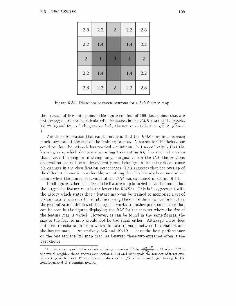
6.5. DISCUSSION 1092.8

2.8 2.8

2.8

2.2

2.2

2.22.2

2.2

2.2

2.2 2.2

1.4 1.4

1.41.4

2

2

2 2

1

1

1

10Figure 6.54: Distances between neurons for a 5x5 feature map.the average of �ve data points, this �gure consists of 100 data points that arenot averaged. As can be calculated4, the stages in the RMS start at the epochs12, 22, 45 and 62, excluding respectively the neurons at distance p5, 2, p2 and1. Another observation that can be made is that the RMS does not decreasemuch anymore at the end of the training process. A reason for this behaviourcould be that the network has reached a minimum, but more likely is that thelearning rate, which decreases according to equation 6.6, has reached a valuethat causes the weights to change only marginally. For the ICF the previousobservation can not be made; evidently small changes in the network can causebig changes in the classi�cation percentages. This suggests that the overlap ofthe di�erent classes is considerable, something that has already been mentionedbefore when the jumpy behaviour of the ICF was explained in section 6.4.1.In all �gures where the size of the feature map is varied it can be found thatthe larger the feature map is the lower the RMS is. This is in agreement withthe theory which states that a feature map can be trained to memorize a set ofvectors to any accuracy by simply increasing the size of the map. Unfortunatelythe generalization abilities of the large networks are rather poor, something thatcan be seen in the �gures displaying the ICF for the test set where the size ofthe feature map is varied. However, as can be found in the same �gures, thesize of the feature map should not be too small either. Although there doesnot seem to exist an order in which the feature maps between the smallest andthe largest map | respectively 3x3 and 10x10 | have the best performanceon the test set, the 7x7 map that lies between these two extremes often is thebest choice.4For instance, epoch 12 is calculated using equation 6.5 by 5=2�p5(5=2)=100 = 11 where 5/2 isthe initial neighbourhood radius (see section 6.4.2) and 100 equals the number of iterations,so starting with epoch 12 neurons at a distance of p5 or more no longer belong to theneighbourhood of a winning neuron.

110 CHAPTER 6. FEATURE MAPPINGThe �gures that display the in uence of the learning rate on the trainingprocess show that with a higher learning rate the network faster and betterconverges on the training set. The faster convergence is in accordance withthe theory, the better convergence is not. A possible explanation for the badconvergence on the test set when using the smallest learning rate | 0.00025| could be that the number of epochs is too small, for the network is updatedin small steps, so many steps are needed to accomplish the same change inweights. However, when the network was trained ten times as long | 1000epochs instead of 100 | convergence improved only a little. In theory thein uence of the learning rate on the performance on the test set is not clear,but in practice choosing the best value is not too di�cult. A value of 0.00025,given by the rule of thumb which states that a good value could be 0.25 dividedby the number of patterns in the training set, gives the worst results. On theother hand a value of 0.1 usually seems to be too large, while for most problemsa learning rate of 0.005 gives the best performance.The shape of the RMS when using a learning rate of 0.00025 suggests thatthe initial distribution of the neurons over the feature space is rather good,because when the map is roughly organized and many neurons are translatedover relatively large distances | this takes place in the start of the trainingprocess, see section 6.2.1 | the performance of the network on the training setgets worse, only improving again at the end of the training process when thenetwork is tuned more �nely to the training set. This phenomenon can not beobserved when using a higher learning rate, because in this case the stage inwhich the map is roughly organized is much shorter because the neurons aretranslated over much larger distances.The mechanism of providing each neuron with a conscience as described insection 6.3.1 does not improve the performance of the network on the trainingset. Evidently all neurons of the output layer represent some part of the trainingset, making the conscience of the neurons super uous. On the test set thisvariation does not seem to give a structural improvement of the performanceeither.The performance of the \optimal" network on the validation set is for allproblems with only two classes over 80%, except for the problem of discrim-inating between classes A and C where the correct classi�cation of class C isonly 64.3%. These classes probably overlap more with each other than theother classes do. According to the confusion matrices 6.12 to 6.15 the order inwhich the classes can best be discriminated against class A is B, D/E and C.When discriminating between �ve classes simultaneously the order changes toB, A, E and C/D. The only di�erence between the two orders is that class Dfalls a place. While for all other classes the percentage of correct classi�cationdecreases 20 to 30%, the percentage of class D decreases about 45%. The addi-tional 15% class D loses to class A: the percentage of patterns of class D thatare classi�ed as belonging to class A is doubled, while for the other classes thispercentage stays the same or even decreases compared to the same percentagewhen discriminating between only two classes.A last observation that is made is that the shapes of the ICF showing theperformance of a feature map on the test set and the validation set are totally

6.5. DISCUSSION 111di�erent. This could suggest that the test set is not representative for thevalidation set, but we assume that it is simply the result of the small numberof patterns in the validation set which causes the ICF to react very strongly onthe incorrect classi�cation of just one more pattern. The fact that the achievedpercentages of correct classi�cation are rather high supports our con�dence inthe method by which we have generated the additional data.For comparison with the other methods of classi�cation | see section 7.2| not only the classi�cation percentages but also the computation time is ofimportance. For the worst problem that we have examined, a 10x10 featuremap containing neurons without conscience to classify 2500 training patternsand 2500 test patterns, a Sun SPARCstation 1 needed 1 hour and 51 minutes.

112 CHAPTER 6. FEATURE MAPPING

Chapter 7ConclusionsAt the end of each chapter on discriminant analysis, back-propagation andfeature mapping the results of the method under observation were discussedindividually and conclusions were drawn. In this chapter however the results ofall three methods are discussed at a higher level in order to answer the questionposed in my graduation-assignment. The conclusions of this thesis can roughlybe divided in two parts: the �rst set of conclusions | see section 7.1 | dealswith the use of ultrasonic tissue characterization on our speci�c application,using the data set that is at our disposal, while the other subject | see sec-tion 7.2 | is more of computer scienti�c nature, being the comparison of themethods that have been investigated. Finally some recommendations for futureinvestigations are made in section 7.3.7.1 Applicability of UTC on our dataNowadays at the Biophysics Laboratory discriminant analysis is used to clas-sify patients based on the principle of ultrasonic tissue characterization. Forthe type of di�use liver diseases that we have examined, using the �ve param-eters described in section 3.2, discriminant analysis applying cross-validationresulted in an unsatisfactory performance for most of the small classes, see forinstance matrix 4.36 or 4.43. If instead of cross-validation resubstitution is used,the percentage of correct classi�cation for these classes enormously increases,without decreasing the percentage of correct classi�cation for the large class.Obviously a good partitioning is possible, only it can not be found because theoriginal data set is much too small to extract the general characteristics of theclasses from it.But there are more reasons to extend the original data set with generatedcases. One ground is that in case of such small classes as for our problem thedetermination of the performance is very rough: if the classi�cation of onlyone patient belonging to one of the smallest classes changes, the percentageof correct classi�cation for that class changes with 10%. Even if the originaldata set would contain some general characteristics for each class, it wouldbe impossible to �nd the optimal partitioning of the feature space, because asmall change in the positioning of the borders between the classes does not113

114 CHAPTER 7. CONCLUSIONSnecessarily imply a change in performance, although it could be a signi�cantchange. Another motivation for the extension of the data set is that we want touse neural networks for the classi�cation of patients. Usually when dealing withneural networks the data set is classwise split into a training and a validationset using a 2:1 ratio; for a class containing only 10 patients this would meana training set of 7 and a validation set of 3 patients! The problems describedpreviously in this section apply to this situation even more.The method we have used for the generation of additional data | the kernelbased method, see section 3.4.2 | results in data that can well be used for ourpurposes. A large training set has been generated on the basis of which thefeature space is partitioned, after which an equally large test set has beenused to check whether the partitioning follows the general characteristics of theclasses or is based on features that are coincidentally present. Especially forback-propagation the test set has proven to be very useful for the detection ofover-learning. The performance on the validation set that is achieved using thepartitioning acquired in this manner is in every respect acceptable compared tothe results using discriminant analysis with cross-validation. It could be arguedthat a good performance on the validation set is obvious, since the training sethas been generated on the basis of the validation set and thus is fully correlatedwith it, but this is not true. For the performance on the validation set ofdiscriminant analysis using the training set to partition the feature space is forall problems worse than the performance on the original data of discriminantanalysis using resubstitution, which corresponds to discriminant analysis usinga training and a validation set that are completely correlated.For the performance of the individual classes holds that good results can beachieved, if there is to be discriminated between only two classes at the sametime. In this case the percentage of correctly classi�ed patients is for all classesover 80%, while for some classes even 90% or 100% can be reached. If thereis to be discriminated between all �ve classes simultaneously, the performancedeteriorates for all methods, but for discriminant analysis and feature mappingthe drop in performance is much higher than for back-propagation. Whilefor discriminant analysis the minimum percentage of correct classi�cation is7.7%, for back-propagation this is 46.2%. Although little can be said aboutthe order in which the classes can best be discriminated, it strikes that forall methods class A | the healthy people | and class B | people su�eringfrom primary biliary cirrhosis | score percentages of correct classi�cation thatare signi�cantly higher than those of the other classes, while class D | peoplesu�ering from acute hepatitis | usually has the lowest percentage. Evidentlyclasses A and B are situated relatively isolated in the feature space or containpatterns that are rather similar, making a good discrimination possible, whilethe other classes and especially class D are much more scattered.Considering all the facts summarized in this section we come to the con-clusion that classi�cation of patients on the basis of the parameters and forthe diseases that we have selected is impossible because the original data setis much too small. However, if the data set is extended with some generatedcases based on the original data, good results can be achieved.

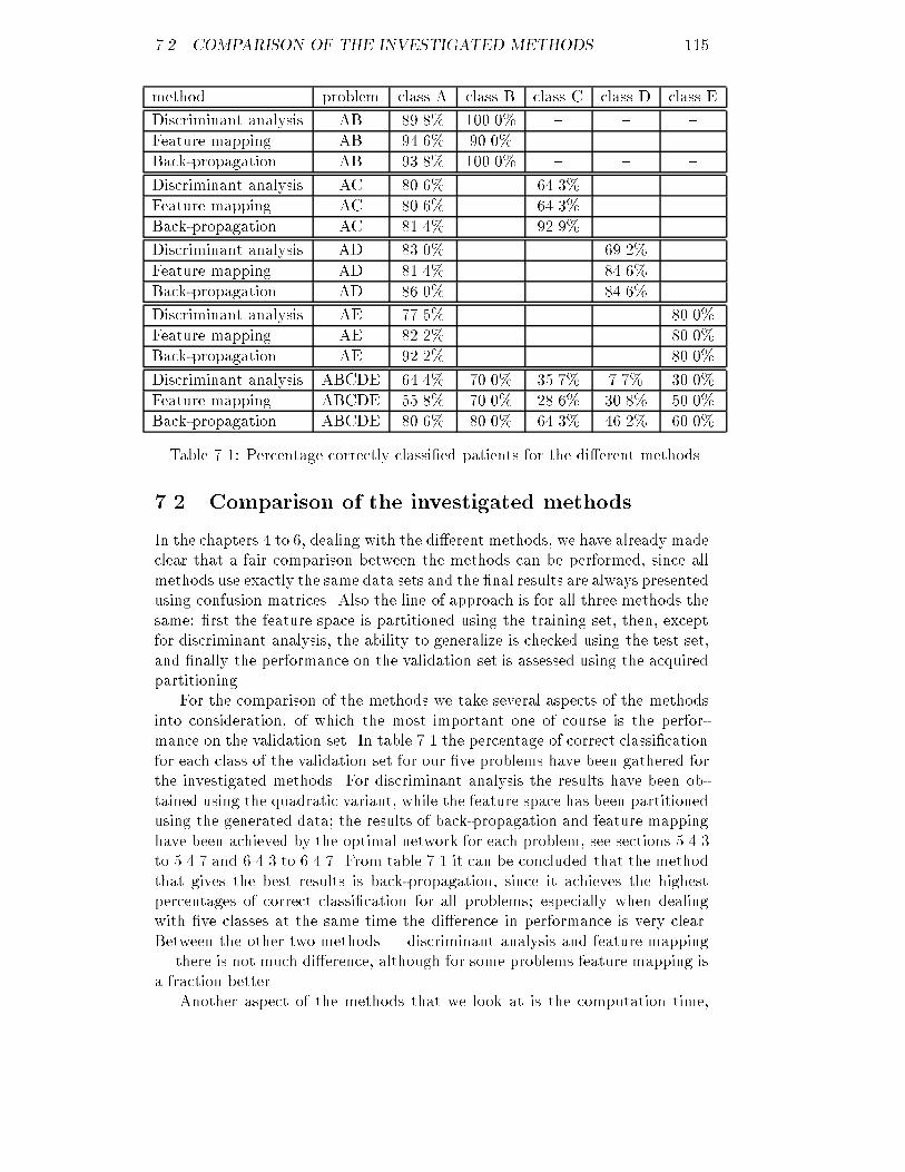
7.2. COMPARISON OF THE INVESTIGATED METHODS 115method problem class A class B class C class D class EDiscriminant analysis AB 89.8% 100.0% { { {Feature mapping AB 94.6% 90.0% { { {Back-propagation AB 93.8% 100.0% { { {Discriminant analysis AC 80.6% { 64.3% { {Feature mapping AC 80.6% { 64.3% { {Back-propagation AC 81.4% { 92.9% { {Discriminant analysis AD 83.0% { { 69.2% {Feature mapping AD 81.4% { { 84.6% {Back-propagation AD 86.0% { { 84.6% {Discriminant analysis AE 77.5% { { { 80.0%Feature mapping AE 82.2% { { { 80.0%Back-propagation AE 92.2% { { { 80.0%Discriminant analysis ABCDE 64.4% 70.0% 35.7% 7.7% 30.0%Feature mapping ABCDE 55.8% 70.0% 28.6% 30.8% 50.0%Back-propagation ABCDE 80.6% 80.0% 64.3% 46.2% 60.0%Table 7.1: Percentage correctly classi�ed patients for the di�erent methods.7.2 Comparison of the investigated methodsIn the chapters 4 to 6, dealing with the di�erent methods, we have already madeclear that a fair comparison between the methods can be performed, since allmethods use exactly the same data sets and the �nal results are always presentedusing confusion matrices. Also the line of approach is for all three methods thesame: �rst the feature space is partitioned using the training set, then, exceptfor discriminant analysis, the ability to generalize is checked using the test set,and �nally the performance on the validation set is assessed using the acquiredpartitioning.For the comparison of the methods we take several aspects of the methodsinto consideration, of which the most important one of course is the perfor-mance on the validation set. In table 7.1 the percentage of correct classi�cationfor each class of the validation set for our �ve problems have been gathered forthe investigated methods. For discriminant analysis the results have been ob-tained using the quadratic variant, while the feature space has been partitionedusing the generated data; the results of back-propagation and feature mappinghave been achieved by the optimal network for each problem, see sections 5.4.3to 5.4.7 and 6.4.3 to 6.4.7. From table 7.1 it can be concluded that the methodthat gives the best results is back-propagation, since it achieves the highestpercentages of correct classi�cation for all problems; especially when dealingwith �ve classes at the same time the di�erence in performance is very clear.Between the other two methods | discriminant analysis and feature mapping| there is not much di�erence, although for some problems feature mapping isa fraction better.Another aspect of the methods that we look at is the computation time,

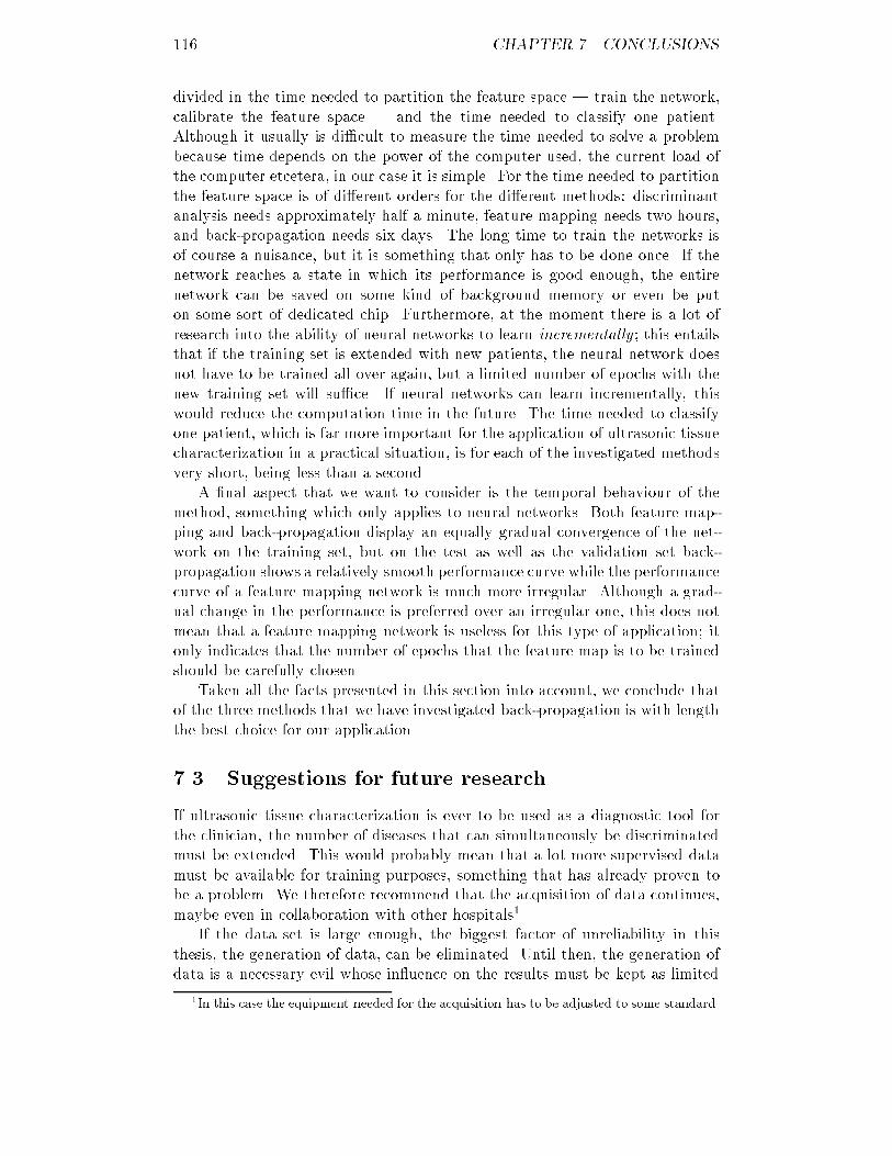
116 CHAPTER 7. CONCLUSIONSdivided in the time needed to partition the feature space | train the network,calibrate the feature space | and the time needed to classify one patient.Although it usually is di�cult to measure the time needed to solve a problembecause time depends on the power of the computer used, the current load ofthe computer etcetera, in our case it is simple. For the time needed to partitionthe feature space is of di�erent orders for the di�erent methods: discriminantanalysis needs approximately half a minute, feature mapping needs two hours,and back-propagation needs six days. The long time to train the networks isof course a nuisance, but it is something that only has to be done once. If thenetwork reaches a state in which its performance is good enough, the entirenetwork can be saved on some kind of background memory or even be puton some sort of dedicated chip. Furthermore, at the moment there is a lot ofresearch into the ability of neural networks to learn incrementally ; this entailsthat if the training set is extended with new patients, the neural network doesnot have to be trained all over again, but a limited number of epochs with thenew training set will su�ce. If neural networks can learn incrementally, thiswould reduce the computation time in the future. The time needed to classifyone patient, which is far more important for the application of ultrasonic tissuecharacterization in a practical situation, is for each of the investigated methodsvery short, being less than a second.A �nal aspect that we want to consider is the temporal behaviour of themethod, something which only applies to neural networks. Both feature map-ping and back-propagation display an equally gradual convergence of the net-work on the training set, but on the test as well as the validation set back-propagation shows a relatively smooth performance curve while the performancecurve of a feature mapping network is much more irregular. Although a grad-ual change in the performance is preferred over an irregular one, this does notmean that a feature mapping network is useless for this type of application; itonly indicates that the number of epochs that the feature map is to be trainedshould be carefully chosen.Taken all the facts presented in this section into account, we conclude thatof the three methods that we have investigated back-propagation is with lengththe best choice for our application.7.3 Suggestions for future researchIf ultrasonic tissue characterization is ever to be used as a diagnostic tool forthe clinician, the number of diseases that can simultaneously be discriminatedmust be extended. This would probably mean that a lot more supervised datamust be available for training purposes, something that has already proven tobe a problem. We therefore recommend that the acquisition of data continues,maybe even in collaboration with other hospitals1.If the data set is large enough, the biggest factor of unreliability in thisthesis, the generation of data, can be eliminated. Until then, the generation ofdata is a necessary evil whose in uence on the results must be kept as limited1In this case the equipment needed for the acquisition has to be adjusted to some standard.

7.3. SUGGESTIONS FOR FUTURE RESEARCH 117as possible. It may be a good idea to investigate more thoroughly the statisticalcorrectness of the data generation method used, or of the many other methodsavailable for the generation of data, since the data set is the basis on which theentire research of this application is built.Another interesting point that could be investigated is the in uence of se-lecting di�erent parameters or a di�erent number of parameters on the classi-�cation results. The choice of the parameters that have been selected in thisthesis is based on similar research performed for discriminant analysis, but itcould well be possible that for neural networks other or more parameters resultin a better performance.In this thesis only three methods have been investigated, but of course thereexist many more, both in the �eld of statistics as well as neural networks. Asa possible statistical method we think of Principal Component Analysis, whileas neural network one of the models based on the Adaptive Resonance Theoryseems to be very suitable. On problems similar to our problem ARTMAP hasshown to yield good results.

118 CHAPTER 7. CONCLUSIONS

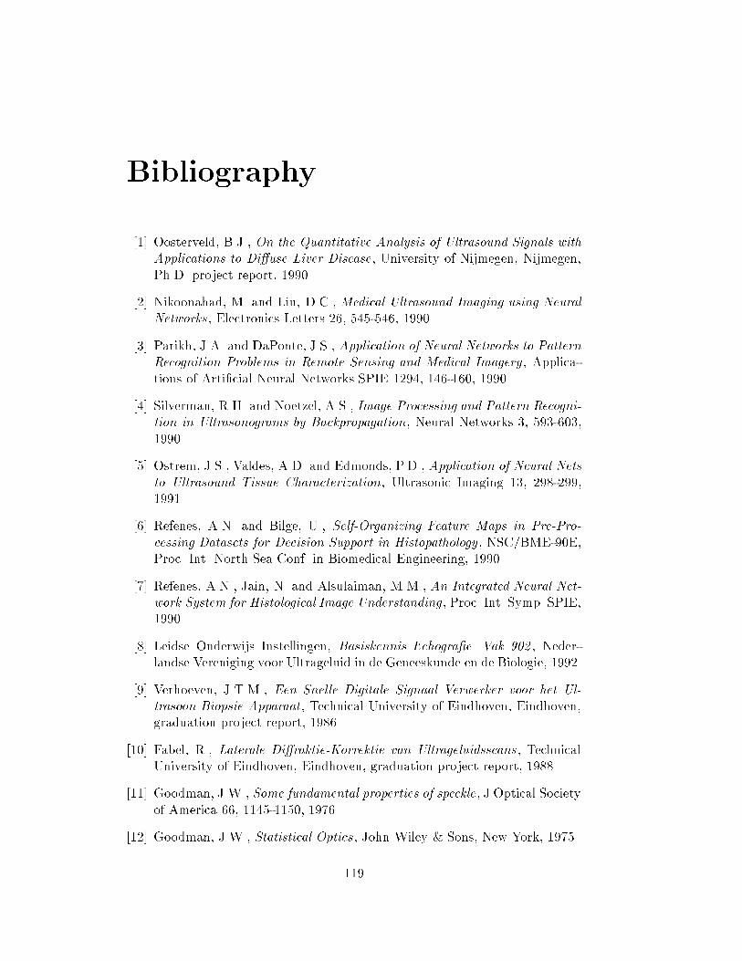
Bibliography[1] Oosterveld, B.J., On the Quantitative Analysis of Ultrasound Signals withApplications to Di�use Liver Disease, University of Nijmegen, Nijmegen,Ph.D. project report, 1990.[2] Nikoonahad, M. and Liu, D.C., Medical Ultrasound Imaging using NeuralNetworks , Electronics Letters 26, 545-546, 1990.[3] Parikh, J.A. and DaPonte, J.S., Application of Neural Networks to PatternRecognition Problems in Remote Sensing and Medical Imagery , Applica-tions of Arti�cial Neural Networks SPIE 1294, 146-160, 1990.[4] Silverman, R.H. and Noetzel, A.S., Image Processing and Pattern Recogni-tion in Ultrasonograms by Backpropagation, Neural Networks 3, 593-603,1990.[5] Ostrem, J.S., Valdes, A.D. and Edmonds, P.D., Application of Neural Netsto Ultrasound Tissue Characterization, Ultrasonic Imaging 13, 298-299,1991.[6] Refenes, A.N. and Bilge, U., Self-Organizing Feature Maps in Pre-Pro-cessing Datasets for Decision Support in Histopathology , NSC/BME-90E,Proc. Int. North Sea Conf. in Biomedical Engineering, 1990.[7] Refenes, A.N., Jain, N. and Alsulaiman, M.M., An Integrated Neural Net-work System for Histological Image Understanding , Proc. Int. Symp. SPIE,1990.[8] Leidse Onderwijs Instellingen, Basiskennis Echogra�e. Vak 902 , Neder-landse Vereniging voor Ultrageluid in de Geneeskunde en de Biologie, 1992.[9] Verhoeven, J.T.M., Een Snelle Digitale Signaal Verwerker voor het Ul-trasoon Biopsie Apparaat , Technical University of Eindhoven, Eindhoven,graduation project report, 1986.[10] Fabel, R., Laterale Di�raktie-Korrektie van Ultrageluidsscans , TechnicalUniversity of Eindhoven, Eindhoven, graduation project report, 1988.[11] Goodman, J.W., Some fundamental properties of speckle, J Optical Societyof America 66, 1145-1150, 1976.[12] Goodman, J.W., Statistical Optics , John Wiley & Sons, New York, 1975.119

120 BIBLIOGRAPHY[13] Wagner, R.F., Smith, S.W., Sandrik, J.M. and Lopez, H., Statistics ofSpeckle in Ultrasound B-Scans , IEEE Transactions on Sonics and Ultra-sonics 30, 156-163, 1983.[14] Thijssen, J.M. and Oosterveld, B.J., Texture in Tissue Echograms. Speckleor Information? , J Ultrasound Medicine 9, 215-229, 1990.[15] Oosterveld, B.J., Thijssen, J.M. and Verhoef, W.A., Texture of B-ModeEchograms: 3-D Simulations and Experiments of the E�ects of Di�ractionand Scatterer Density , Ultrasonic Imaging 7, 142-160, 1985.[16] Holmstr�om, L. and Koistinen, P., Using Additive Noise in BackPropagationTraining , IEEE Transactions on Neural Networks 3, 24-38, 1992.[17] Duin, R.P.W., On the Choice of Smoothing Parameters for Parzen Esti-mators of Probability Density Functions , IEEE Transactions on ComputersC-25, 1175-1179, 1976.[18] Schikhof, W., Analyse en Calculus 2 , University of Nijmegen, Nijmegen,reader, 1984.[19] Albert, A and Harris, E.K., Multivariate Interpretation of Clinical Labo-ratory Data, Marcel Dekker, Inc., New York, 1987.[20] SAS Institute Inc., SAS/STAT User's Guide Version 6 Volume 1 , SASInstitute Inc., Cary (NC), 1989.[21] Dayho�, J.E., Neural Network Architectures. An Introduction, Van Nos-trand Reinhold, New York, 1990.[22] Hertz, J., Krogh, A. and Palmer, R.G., Introduction to the Theory of NeuralComputation, Addison-Wesley Publishing Company, Redwood City, 1991.[23] Nowlan, S.J. and Hinton, G.E., Soft Weight-Sharing , University ofToronto, Toronto, technical report, 1991.[24] Bierman, S. and Hooft, H. van, A Kohonen Neural Networks Simulator ,University of Nijmegen, M.Sc. project report in preparation.

Appendix ASoftwareThis chapter contains short user manuals for the various programs written forthis thesis. At the end of the chapter the manual page about the changes inthe Kohonen Neural Networks Simulator | called koho | by S. Bierman andH. van Hooft can be found.The programs for which the user manual or, in the case of koho, the addi-tional manual page is included are:� classify� shu�e� kernelgen� statgen� merge� format� histogram� analyze� plot� bp� kohoFor a more detailed description of these programs is referred to the com-mentary in the source code, while more information about the Kohonen NeuralNetworks Simulator can be found in [24].121

122 APPENDIX A. SOFTWARECLASSIFY(n) MISC. REFERENCE MANUAL PAGES CLASSIFY(n)

NAME classify - select patients and parameters from a database

SYNOPSIS classify class_____

DESCRIPTION classify selects all patients belonging to class_____ and saves them in a file. For every patient the parameters MU, B, SNR, S and A1 are saved in that order, preceded by the patient number and a new class identification. The first line of the new file contains the number of patients followed by the number of parameters, which in this case is 5.

OPTIONS For class_____ the following options are available:

A Select patients with database classification 1. Their new classification is 0.

B Select patients with database classification 28, 281, or 282. Their new classification is 1.

C Select patients with database classification 22, 23, 24, 26 or 27. Their new classification is 2.

D Select patients with database classification 20 or 21. Their new classification is 3.

E Select patients with database classification 25. Their new classification is 4.

FILES ~/data/original/parameters0.txt first part of patient database

~/data/original/parameters1.txt second part of patient database

~/data/A/org new file for class A

~/data/B/org new file for class B

~/data/C/org new file for class C

~/data/D/org new file for class D

~/data/E/org new file for class E

SEE ALSO shuffle(n), kernelgen(n), statgen(n), merge(n), format(n), histogram(n)

Sun Release 4.1 Last change: 26 October 1992 1

123CLASSIFY(n) MISC. REFERENCE MANUAL PAGES CLASSIFY(n)

BUGS The program is not very flexible, since the file names, the new class indices and the selected parameters can not be changed without recompilation. However, all these dependen- cies can easily be changed because the program is written using #define-statements.

If the number of parameters is different from 5 or a new class is to be added, the source code has to be changed in a few places after which the program has to be recompiled.

AUTHOR Maurice klein Gebbinck <mauricek@cs.kun.nl>

Sun Release 4.1 Last change: 26 October 1992 2

124 APPENDIX A. SOFTWARESHUFFLE(n) MISC. REFERENCE MANUAL PAGES SHUFFLE(n)

NAME shuffle - shuffle the order of patients in a file

SYNOPSIS shuffle file____

DESCRIPTION shuffle reads the patients contained in file____ and writes them in a random order to the same file. The first line of file____ should contain the number of patients followed by the number of parameters, which corresponds the output generated by the program classify. This information is incorporated in the shuffled version of the file as well.

SEE ALSO classify(n), kernelgen(n), statgen(n), merge(n), format(n), histogram(n)

AUTHOR Maurice klein Gebbinck <mauricek@cs.kun.nl>

Sun Release 4.1 Last change: 26 October 1992 1

125KERNELGEN(n) MISC. REFERENCE MANUAL PAGES KERNELGEN(n)

NAME kernelgen - generate new patients using the kernel based method

SYNOPSIS kernelgen class_____

DESCRIPTION kernelgen generates new patients for class_____ adding up to 1000 patients. The algorithm that is the basis of this program has been designed by Holstrom and Koistinen, and can be found in IEEE trans. Neural Networks 3, p. 24-38, 1992. The Bartlett random generator is implemented using the method of Newton with a precision of 0.005. The new patients are also provided with an unique patient number, depending on their class. For every parameter of the patients the mean and standard deviation are displayed. The first line of the input file of kernelgen, see FILES, should contain the number of patients followed by the number of parameters. This corresponds to the output generated by the programs classify and shuffle. The first line of the output file, see FILES, also contains the number of patients followed by the number of parameters.

OPTIONS For class_____ the following options are available:

A Generate new patients for class A. The new patient numbers start with 5000.

B Generate new patients for class B. The new patient numbers start with 1000.

C Generate new patients for class C. The new patient numbers start with 2000.

D Generate new patients for class D. The new patient numbers start with 3000.

E Generate new patients for class E. The new patient numbers start with 4000.

FILES ~/data/A/use input file for class A

~/data/A/gen output file for class A

~/data/B/use input file for class B

~/data/B/gen output file for class B

~/data/C/use input file for class C

Sun Release 4.1 Last change: 26 October 1992 1

126 APPENDIX A. SOFTWAREKERNELGEN(n) MISC. REFERENCE MANUAL PAGES KERNELGEN(n)

~/data/C/gen output file for class C

~/data/D/use input file for class D

~/data/D/gen output file for class D

~/data/E/use input file for class E

~/data/E/gen output file for class E

SEE ALSO classify(n), shuffle(n), statgen(n), merge(n), format(n), histogram(n) L. Holmstrom and P. Koistinen, Using_____ Additive________ Noise_____ in__ Back____-Propagation___________ Training________

BUGS The program is not very flexible, since the file names, the start of the new patient numbers, the total number of patients and the precision can not be changed without recom- pilation. However, all these dependencies can easily be changed because the program is written using #define- statements.

AUTHOR Maurice klein Gebbinck <mauricek@cs.kun.nl>

Sun Release 4.1 Last change: 26 October 1992 2

127STATGEN(n) MISC. REFERENCE MANUAL PAGES STATGEN(n)

NAME statgen - generate new patients using a statistical method

SYNOPSIS statgen class_____

DESCRIPTION statgen generates new patients for class_____ to a total number of patients of 1000. The algorithm that is the basis of this program has been described by Maurice klein Gebbinck in Ultrasonic Tissue Characterization Using Neural Networks, the University of Nijmegen, M.Sc. project report, 1992. The segment out of which new patients are drawn has a length of 4 SD, 2 SD to the left and 2 SD to the right of the mean for each parameter. The new patients are also provided with an unique patient number, depending on their class. For every parameter of the patients the mean and standard deviation are displayed. The first line of the input file of kernel- gen, see FILES, should contain the number of patients fol- lowed by the number of parameters. This corresponds to the output generated by the programs classify and shuffle. The first line of the output file, see FILES, also contains the number of patients followed by the number of parameters. For class_____ the following options are available:

A Generate new patients for class A. The new patient numbers start with 5000.

B Generate new patients for class B. The new patient numbers start with 1000.

C Generate new patients for class C. The new patient numbers start with 2000.

D Generate new patients for class D. The new patient numbers start with 3000.

E Generate new patients for class E. The new patient numbers start with 4000.

FILES ~/data/A/use input file for class A

~/data/A/owngen output file for class A

~/data/B/use input file for class B

~/data/B/owngen output file for class B

~/data/C/use input file for class C

~/data/C/owngen output file for class C

Sun Release 4.1 Last change: 26 October 1992 1

128 APPENDIX A. SOFTWARESTATGEN(n) MISC. REFERENCE MANUAL PAGES STATGEN(n)

~/data/D/use input file for class D

~/data/D/owngen output file for class D

~/data/E/use input file for class E

~/data/E/owngen output file for class E

SEE ALSO classify(n), shuffle(n), kernelgen(n), merge(n), format(n), histogram(n) M. klein Gebbinck, Ultrasonic__________ Tissue______ Characterization________________ Using_____ Neural______ Networks________

BUGS The program is not very flexible, since the file names, the start of the new patient numbers, the total number of patients, the correlation coefficients and the length of the segment out of which the patients are drawn can not be changed without recompilation. However, all these dependen- cies can easily be changed because the program is written using #define-statements.

If the number of parameters is different from 5, the source code has to be changed in a few places after which the pro- gram has to be recompiled to incorporate a different number of correlation coefficients.

AUTHOR Maurice klein Gebbinck <mauricek@cs.kun.nl>

Sun Release 4.1 Last change: 26 October 1992 2

129MERGE(n) MISC. REFERENCE MANUAL PAGES MERGE(n)

NAME merge - merge several patient files into one

SYNOPSIS merge problem_______

DESCRIPTION merge reads the patients of several files and places them in a new file. The input files, see FILES, should all have a first line containing the number of patients and the number of parameters. This file format conforms to the output of the programs kernelgen and statgen. merge checks whether all input files contain the same number of parameters and aborts if this is not the case. After merging, the first line of the output file, see FILES, contains the number of patients and the number of parameters.

OPTIONS For problem_______ the following options are available:

AB Merge classes A and B.

AC Merge classes A and C.

AD Merge classes A and D.

AE Merge classes A and E.

ABCDE Merge classes A, B, C, D and E.

FILES ~/data/A/gen input file for problems AB, AC, AD, AE and ABCDE

~/data/B/gen input file for problems AB and ABCDE

~/data/C/gen input file for problems AC and ABCDE

~/data/D/gen input file for problems AD and ABCDE

~/data/E/gen input file for problems AE and ABCDE

~/data/problems/AB/gen output file for problem AB

~/data/problems/AC/gen output file for problem AC

~/data/problems/AD/gen output file for problem AD

~/data/problems/AE/gen output file for problem AE

~/data/problems/ABCDE/gen output file for problem ABCDE

Sun Release 4.1 Last change: 26 October 1992 1

130 APPENDIX A. SOFTWAREMERGE(n) MISC. REFERENCE MANUAL PAGES MERGE(n)

SEE ALSO classify(n), shuffle(n), kernelgen(n), statgen(n), format(n), histogram(n)

BUGS The program is not very flexible, since the file names can not be changed without recompilation. However, they can easily be changed because the program is written using #define-statements.

If a new problem is to be added, the source code has to be changed in a few places after which the program has to be recompiled.

AUTHOR Maurice klein Gebbinck <mauricek@cs.kun.nl>

Sun Release 4.1 Last change: 26 October 1992 2

131FORMAT(n) MISC. REFERENCE MANUAL PAGES FORMAT(n)

NAME format - scale patient parameters and add target patterns

SYNOPSIS format problem_______ target______

DESCRIPTION format scales all parameters of the patients of problem_______ between 0.1 and 0.9. For each parameter the mean minus 2 SD is projected to 0.1 and the mean plus 2 SD to 0.9, while intermediate values are scaled linearly in this interval; values lower (higher) than the mean minus (plus) 2 SD are projected to 0.1 (0.9). Furthermore, each patient is pro- vided with a target pattern, depending on the target______. The target pattern is nothing more than a representation of the class a patient belongs to that is needed when dealing with neural networks. The first line of the input file, see FILES, should contain the number of patients and the number of parameters. This file format is conform the output of the program merge. The information contained in the first line of the output file, see FILES, is also dependent on the tar-____ get___.

OPTIONS For problem_______ the following options are available:

AB Format problem AB.

AC Format problem AC.

AD Format problem AD.

AE Format problem AE.

ABCDE Format problem ABCDE.

For target______ the following options are available:

BACKPROP The first line of the output file contains the number of patients, the number of parame- ters and the number of classes. The target pattern of a patient is placed immediately below the data of the corresponding patient and consists of a vector containing one ele- ment with a high value, while all other ele- ments have low values. The patient number is saved as well.

SIMPLEKOHO The first line of the output file contains a zero, followed by the number of parameters and the number of patients. Since this option

Sun Release 4.1 Last change: 26 October 1992 1

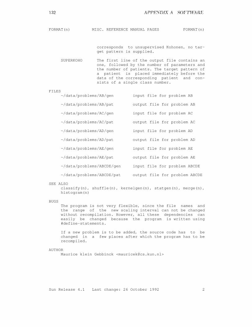
132 APPENDIX A. SOFTWAREFORMAT(n) MISC. REFERENCE MANUAL PAGES FORMAT(n)

corresponds to unsupervised Kohonen, no tar- get pattern is supplied.

SUPERKOHO The first line of the output file contains an one, followed by the number of parameters and the number of patients. The target pattern of a patient is placed immediately before the data of the corresponding patient and con- sists of a single class number.

FILES ~/data/problems/AB/gen input file for problem AB

~/data/problems/AB/pat output file for problem AB

~/data/problems/AC/gen input file for problem AC

~/data/problems/AC/pat output file for problem AC

~/data/problems/AD/gen input file for problem AD

~/data/problems/AD/pat output file for problem AD

~/data/problems/AE/gen input file for problem AE

~/data/problems/AE/pat output file for problem AE

~/data/problems/ABCDE/gen input file for problem ABCDE

~/data/problems/ABCDE/pat output file for problem ABCDE

SEE ALSO classify(n), shuffle(n), kernelgen(n), statgen(n), merge(n), histogram(n)

BUGS The program is not very flexible, since the file names and the range of the new scaling interval can not be changed without recompilation. However, all these dependencies can easily be changed because the program is written using #define-statements.

If a new problem is to be added, the source code has to be changed in a few places after which the program has to be recompiled.

AUTHOR Maurice klein Gebbinck <mauricek@cs.kun.nl>

Sun Release 4.1 Last change: 26 October 1992 2

133HISTOGRAM(n) MISC. REFERENCE MANUAL PAGES HISTOGRAM(n)

NAME histogram - create a histogram of a patient file suitable for xgraph

SYNOPSIS histogram

DESCRIPTION histogram is an interactive program that, for every parame- ter a patient file consists of, creates a histogram file suitable for xgraph. After starting the program, first it is prompted for the name of the patient file containing the data for the histograms. The first line of the patient file should contain the number of patients followed by the number of parameters. This file format corresponds to the output of the programs classify, kernelgen and statgen. Next, it is asked how many bars each histogram should consist of; a minimum of 3 bars is required. The next choice that has to be made is whether the histograms should range from the minimum value to the maximum value, or from the mean minus 2 SD to the mean plus 2 SD. If the SD-range is chosen, the leftmost (rightmost) bar of each histogram represents the number of patients with a value less (greater) than the mean minus (plus) 2 SD. Depending on the range, the minimum and maximum or the mean value and standard deviation appear at the standard output for each parameter. The file names the histograms are written to consist of two parts: a prefix and a parameter-dependent suffix; the prefix will be prompted for only once, the suffix once for each parameter.

SEE ALSO classify(n), shuffle(n), kernelgen(n), statgen(n), merge(n), format(n), histogram(n), xgraph(l)

AUTHOR Maurice klein Gebbinck <mauricek@cs.kun.nl>

Sun Release 4.1 Last change: 26 October 1992 1

134 APPENDIX A. SOFTWAREANALYZE(n) MISC. REFERENCE MANUAL PAGES ANALYZE(n)

NAME analyze - analyze a neural network performance file to determine the optimal epoch

SYNOPSIS analyze file____ number______-of__-classes_______

DESCRIPTION analyze compares the results of the neural network of each epoch listed in file____ and searches the optimal epoch. Every line in file____ should contain an epoch number, followed by the root mean squares (RMS) and the incorrect classification fractions (ICF), and, for every class, the number of errone- ously classified patients, all of the training set. The number______-of__-classes_______ should be equal to the actual number of classes in file____. The rest of the line should contain the RMS, ICF and, again for every class, the number of errone- ously classified patients of the test set. This file format corresponds to the output of the neural network simulators bp and koho. An epoch is found to be optimal if it has the lowest ICF for the test set in the file. If there exist other epochs with an equally low ICF, it has among these the lowest RMS for the training set. If there still remain several epochs, the epoch with the lowest number is chosen. The output is written to the standard output.

SEE ALSO plot(n), bp(n), koho(n)

AUTHOR Maurice klein Gebbinck <mauricek@cs.kun.nl>

Sun Release 4.1 Last change: 26 October 1992 1

135PLOT(n) MISC. REFERENCE MANUAL PAGES PLOT(n)

NAME plot - create a plot of a neural network performance file suitable for xgraph

SYNOPSIS plot

DESCRIPTION plot is an interactive program that creates a polygon file suitable for xgraph. After starting the program, first it is prompted for the name of the file where plot should write the polygon plot to. Hereafter the choice must be made whether a plot of the results of the training or the test set is to be made, using the root mean squares (RMS) or the incorrect classification fractions (ICF). Next, the number of classes contained in the performance file that is to be plotted must be given, followed by the highest epoch number in the performance file. The next question concerns the number of points the polygon sould consist of, and the number of epochs that should be averaged to constitute one point of the polygon. It is obvious that the number of available epochs puts some restrictions on the number of points and the number of epochs to be averaged. After all previous input has been validated, the user will repeatedly be prompted for the name of a performance file to be plotted and its corresponding name for the legend. After every plot it is asked if another plot is to be added. Every line in the performance file should contain an epoch number, fol- lowed by the total sum of squares (RMS) and the incorrect classification fractions (ICF), and, for every class, the number of erroneously classified patients, all of the train- ing set. The earlier input number-of-classes should be equal to the actual number of classes in the performance file. The rest of the line should contain the RMS, ICF and, again for every class, the number of erroneously classified patients of the test set. This file format corresponds to the output of the neural network simulators bp and koho.

SEE ALSO analyze(n), bp(n), koho(n)

AUTHOR Maurice klein Gebbinck <mauricek@cs.kun.nl>

Sun Release 4.1 Last change: 26 October 1992 1

136 APPENDIX A. SOFTWAREBP(n) MISC. REFERENCE MANUAL PAGES BP(n)

NAME bp - a back-propagation neural networks simulator

SYNOPSIS bp

DESCRIPTION bp is an interactive program that simulates a neural network based on the back-propagation algorithm. After starting the program, the main menu is displayed. The following menu items are available:

create network... Create a new network from scratch. If another network has already been defined, it is asked whether or not to destroy the current network. The parameters that have to be filled in are the lower and upper boundary of the weights, the number of layers including the input and output layer, and for each layer the number of neurons.

load network... If a network has been saved with bp previously, it can be loaded using this command. If another network has already been defined, it is asked whether or not to destroy the current network. For the filename of the network is prompted.

save network... Save the current network. For the filename of the net- work is prompted; if the file already exists, it is asked whether or not to overwrite that file.

load configuration... If a configuration has been saved with bp previously, it can be loaded using this command. Since the program starts with a default configuration, it is always asked whether or not to overwrite the current configuration. The configuration consists all parameters except the architecture and weights of the network, and the currently loaded patterns. For the filename of the net- work is prompted.

save configuration... Save the current configuration. For the filename of the configuration is prompted; if the file already exists, it is asked whether or not to overwrite that file.

load learn patterns... Load the patterns with which the network is trained; if another set of learn patterns has already been loaded, it is asked whether or not to overwrite these patterns. The format of the pattern file should be conform to the

Sun Release 4.1 Last change: 26 October 1992 1

137BP(n) MISC. REFERENCE MANUAL PAGES BP(n)

output of the program format where the target is chosen to be BACKPROP. This entails a first line containing the number of patterns in the file, the dimension of the input vector and the dimension of the target vec- tor. Each patient takes up two lines: the first line contains the patient number followed by the input vec- tor, while the second line contains the target vector. For the filename of the patterns is prompted.

load test patterns... For this command accounts the same as for load learn patterns..., except that the network uses these pat- terns only for recalling. This mechanism can be used to detect over-learning.

learn... This is the main command of the program; here the con- figuration is changed and learning is initiated. Before the network can start learning, a network must have been created or loaded, and training patterns must be available in the right format. This implies that the dimension of the input (target) vector must be equal to the number of neurons in the input (output) layer. Loading of test patterns is optional. Many parameters have to be filled in. First of all the error function has to be chosen; the common squares can be selected, but also weight decay can be chosen. If the error func- tion is set at weight decay, a value for gamma has to be input. The next choice is that of the activation function, sigmoidal or hyperbolic tangent can be chosen. Now the learn mode must be selected: by pat- tern, update the weights after each pattern, or by epoch, where the weights are updated after all patterns have been presented. If learning by pattern is chosen, the user will be prompted for the learn mode. The order in which the patterns are presented can either be per- muted or round robin (cyclic). Other parameters for which values are to be given are the learning rate, the momentum and the maximum noise percentage. The maximum noise percentage determines the maximum amount of noise that is added to the training patterns; the percentage doesn´t imply an amount relative to the value of the input vector, but an absolute amount expressed in units of one hundredth. Next the number of epochs that the network is to be trained is asked, followed by the show and save frequencies. The show frequency determines the number of epochs after which the performance of the network is saved to the performance file, while the save frequency determines the number of epochs after which both the network as well as the configuration are saved to respectively the files network.save and configuration.save. Finally for the filename of the

Sun Release 4.1 Last change: 26 October 1992 2

138 APPENDIX A. SOFTWAREBP(n) MISC. REFERENCE MANUAL PAGES BP(n)

performance file is prompted; if the file already exists, it is asked whether or not to overwrite that file. The format of the performance file starts with the epoch number, followed by the root mean squares (RMS) and the incorrect classification fractions (ICF), and, for every class, the number of erroneously classi- fied patients, all of the training set. The rest of the line should contain the RMS, ICF and, again for every class, the number of erroneously classified patients of the test set. The resulting performance file can be analyzed and plotted using the programs analyze and plot.

show misclassified learn patterns Show all learn patterns where the classification based on the output vector doesn´t agree with the classifica- tion based on the target vector. The output is written to the standard output. Of course a network and learn patterns in the right format have to be available.

show misclassified test patterns For this command accounts the same as for show misclas- sified learn patterns.

quit Quit bp; if a network has been defined, it is asked whether or not it can be deleted.

SEE ALSO analyze(n), plot(n) M. klein Gebbinck, Ultrasonic__________ Tissue______ Characterization________________ Using_____ Neural______ Networks________

BUGS If a different network (patterns) is to be loaded while a network (patterns) already exists, and the filename of the network (patterns) to be loaded is invalid, no network (pat- terns) are available anymore.

It shouldn´t be possible to load patterns before a network is available, because the format of the patterns has to agree with the architecture of the network. Now for several commands the same checks have to be performed.

AUTHOR Maurice klein Gebbinck <mauricek@cs.kun.nl>

Sun Release 4.1 Last change: 26 October 1992 3

139KOHO(n) MISC. REFERENCE MANUAL PAGES KOHO(n)

NAME koho - a Kohonen neural networks simulator

SYNOPSIS koho

DESCRIPTION koho is in fact nothing more than a shell script that starts up the program iface and sequent, and creates pipes that these programs use to communicate. iface is an ascii-based interface for the user to be able to communicate with the actual simulator sequent. In these manual pages only the changes in iface and sequent are discussed, for more infor- mation on the neural networks simulator is referred to the master thesis in preparation called A Kohonen Neural Net- works Simulator by Silvio Bierman and Hans van Hooft.

Apart from the many bugs that have been resolved, the pro- gram has been altered to incorporate a neighbourhood that linearly decreases to zero with the number of epochs. A second alteration concerns the monitoring of the performance of the neural network. Now, after selecting the learning menu, the user is prompted for the name of the file the simulator writes the performance results to. The format of the performance file is equal to that of the back- propagation simulator bp. This implies a file where every line starts with an epoch number, followed by the root mean squares (RMS) and the incorrect classification fractions (ICF), and, for every class, the number of erroneously clas- sified patients, all of the training set. The rest of the line should contain the RMS, ICF and, again for every class, the number of erroneously classified patients of the test set. This last change has a negative influence on the speed of the simulator. The resulting performance file can be analyzed and plotted using the programs analyze and plot.

SEE ALSO analyze(n), plot(n) S. Bierman and H. van Hooft, A_ Kohonen_______ Neural______ Networks________ Simu-_____ lator_____

AUTHOR Maurice klein Gebbinck <mauricek@cs.kun.nl>

Sun Release 4.1 Last change: 26 October 1992 1

140 APPENDIX A. SOFTWARE

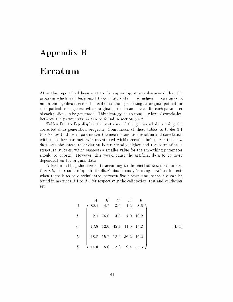
Appendix BErratumAfter this report had been sent to the copy-shop, it was discovered that theprogram which had been used to generate data | kernelgen | contained aminor but signi�cant error. Instead of randomly selecting an original patient foreach patient to be generated, an original patient was selected for each parameterof each patient to be generated. This strategy led to complete loss of correlationbetween the parameters, as can be found in section 3.4.2.Tables B.1 to B.5 display the statistics of the generated data using thecorrected data generation program. Comparison of these tables to tables 3.1to 3.5 show that for all parameters the mean, standard deviation and correlationwith the other parameters is maintained within certain limits. For this newdata sets the standard deviation is structurally higher and the correlation isstructurally lower, which suggests a smaller value for the smoothing parametershould be chosen. However, this would cause the arti�cial data to be moredependent on the original data.After formatting this new data according to the method described in sec-tion 3.5, the results of quadratic discriminant analysis using a calibration set,when there is to be discriminated between �ve classes simultaneously, can befound in matrices B.1 to B.3 for respectively the calibration, test and validationset. A B C D EABCDE 0BBBBBBBBBBBBBB@ 82:4 4:2 3:6 1:2 8:62:4 76:8 3:6 7:0 10:218:8 12:6 42:4 11:0 15:218:8 15:2 13:6 36:2 16:214:0 8:0 13:0 9:4 55:6 1CCCCCCCCCCCCCCA (B.1)141

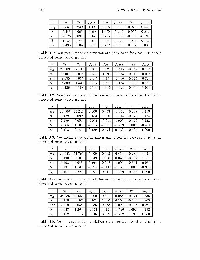
142 APPENDIX B. ERRATUMx �x �x ��Ax ��x �snrx �Sx ��1x�A 17.557 6.230 1.000 0.568 0.098 -0.075 0.440� 0.443 0.068 0.568 1.000 0.290 -0.055 0.212snr 2.176 0.033 0.098 0.290 1.000 -0.425 -0.137S 4.788 0.748 -0.075 -0.055 -0.425 1.000 0.132�1 0.430 0.109 0.440 0.212 -0.137 0.132 1.000Table B.1: New mean, standard deviation and correlation for class A using thecorrected kernel based method.x �x �x ��Ax ��x �snrx �Sx ��1x�A 26.003 12.184 1.000 0.622 0.445 -0.447 0.144� 0.401 0.076 0.622 1.000 0.473 -0.313 0.016snr 2.180 0.055 0.445 0.473 1.000 -0.175 -0.323S 3.590 1.329 -0.447 -0.313 -0.175 1.000 -0.464�1 0.326 0.168 0.144 0.016 -0.323 -0.464 1.000Table B.2: New mean, standard deviation and correlation for class B using thecorrected kernel based method.x �x �x ��Ax ��x �snrx �Sx ��1x�A 29.708 14.246 1.000 0.453 -0.051 -0.187 0.459� 0.478 0.092 0.453 1.000 -0.014 -0.076 0.474snr 2.199 0.051 -0.051 -0.014 1.000 -0.479 0.122S 4.205 1.107 -0.187 -0.076 -0.479 1.000 -0.424�1 0.473 0.181 0.459 0.474 0.122 -0.424 1.000Table B.3: New mean, standard deviation and correlation for class C using thecorrected kernel based method.x �x �x ��Ax ��x �snrx �Sx ��1x�A 26.058 11.769 1.000 0.043 0.464 -0.289 0.091� 0.430 0.108 0.043 1.000 0.092 -0.137 0.511snr 2.198 0.048 0.464 0.092 1.000 -0.321 -0.030S 4.131 1.187 -0.289 -0.137 -0.321 1.000 -0.386�1 0.461 0.221 0.091 0.511 -0.030 -0.386 1.000Table B.4: New mean, standard deviation and correlation for class D using thecorrected kernel based method.x �x �x ��Ax ��x �snrx �Sx ��1x�A 25.986 13.666 1.000 0.401 0.086 -0.371 0.336� 0.458 0.107 0.401 1.000 0.168 -0.124 0.209snr 2.219 0.034 0.086 0.168 1.000 -0.526 -0.282S 4.038 1.263 -0.371 -0.124 -0.526 1.000 0.192�1 0.452 0.118 0.336 0.209 -0.282 0.192 1.000Table B.5: New mean, standard deviation and correlation for class E using thecorrected kernel based method.

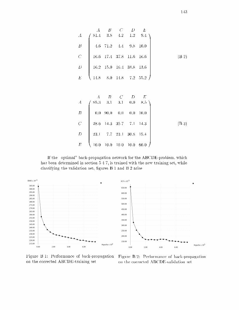
143A B C D EABCDE 0BBBBBBBBBBBBBB@ 81:4 3:8 4:2 1:2 9:44:6 71:2 4:4 9:8 10:016:6 17:4 37:8 11:6 16:616:2 15:0 16:4 38:8 13:614:8 8:0 14:8 7:2 55:2 1CCCCCCCCCCCCCCA (B.2)A B C D EABCDE 0BBBBBBBBBBBBBB@ 85:3 3:1 3:1 0:0 8:50:0 90:0 0:0 0:0 10:028:6 14:3 35:7 7:1 14:323:1 7:7 23:1 30:8 15:410:0 10:0 10:0 10:0 60:0 1CCCCCCCCCCCCCCA (B.3)If the \optimal" back-propagation network for the ABCDE-problem, whichhas been determined in section 5.4.7, is trained with the new training set, whileclassifying the validation set, �gures B.1 and B.2 arise.RMS x 10-3

3#epochs x 10215.00

220.00

225.00

230.00

235.00

240.00

245.00

250.00

255.00

260.00

265.00

270.00

275.00

280.00

285.00

290.00

295.00

300.00

305.00

0.00 2.00 4.00 6.00Figure B.1: Performance of back-propagationon the corrected ABCDE-training set.ICF x 10-3

3#epochs x 10

150.00

200.00

250.00

300.00

350.00

400.00

450.00

500.00

550.00

600.00

650.00

0.00 2.00 4.00 6.00Figure B.2: Performance of back-propagationon the corrected ABCDE-validation set.

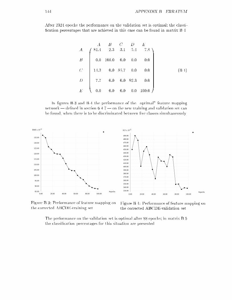
144 APPENDIX B. ERRATUMAfter 2324 epochs the performance on the validation set is optimal; the classi-�cation percentages that are achieved in this case can be found in matrix B.4.A B C D EABCDE 0BBBBBBBBBBBBBB@ 81:4 2:3 3:1 5:4 7:80:0 100:0 0:0 0:0 0:014:3 0:0 85:7 0:0 0:07:7 0:0 0:0 92:3 0:00:0 0:0 0:0 0:0 100:0 1CCCCCCCCCCCCCCA (B.4)In �gures B.3 and B.4 the performance of the \optimal" feature mappingnetwork | de�ned in section 6.4.7 | on the new training and validation set canbe found, when there is to be discriminated between �ve classes simultaneously.RMS x 10-3

#epochs85.00

90.00

95.00

100.00

105.00

110.00

115.00

120.00

125.00

130.00

135.00

0.00 20.00 40.00 60.00 80.00 100.00Figure B.3: Performance of feature mapping onthe corrected ABCDE-training set.ICF x 10-3

#epochs330.00

340.00

350.00

360.00

370.00

380.00

390.00

400.00

410.00

420.00

430.00

440.00

450.00

460.00

470.00

480.00

490.00

0.00 20.00 40.00 60.00 80.00 100.00Figure B.4: Performance of feature mapping onthe corrected ABCDE-validation set.The performance on the validation set is optimal after 88 epochs; in matrix B.5the classi�cation percentages for this situation are presented.

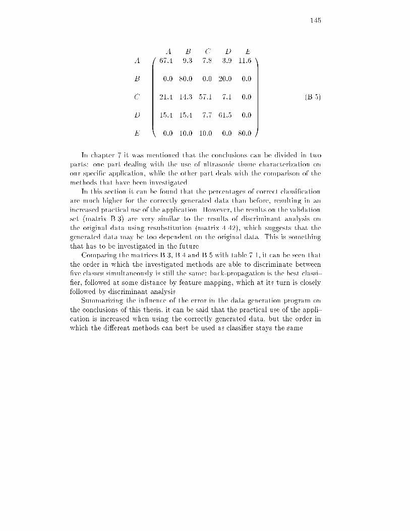
145A B C D EABCDE 0BBBBBBBBBBBBBB@ 67:4 9:3 7:8 3:9 11:60:0 80:0 0:0 20:0 0:021:4 14:3 57:1 7:1 0:015:4 15:4 7:7 61:5 0:00:0 10:0 10:0 0:0 80:0 1CCCCCCCCCCCCCCA (B.5)In chapter 7 it was mentioned that the conclusions can be divided in twoparts: one part dealing with the use of ultrasonic tissue characterization onour speci�c application, while the other part deals with the comparison of themethods that have been investigated.In this section it can be found that the percentages of correct classi�cationare much higher for the correctly generated data than before, resulting in anincreased practical use of the application. However, the results on the validationset (matrix B.3) are very similar to the results of discriminant analysis onthe original data using resubstitution (matrix 4.42), which suggests that thegenerated data may be too dependent on the original data. This is somethingthat has to be investigated in the future.Comparing the matrices B.3, B.4 and B.5 with table 7.1, it can be seen thatthe order in which the investigated methods are able to discriminate between�ve classes simultaneously is still the same: back-propagation is the best classi-�er, followed at some distance by feature mapping, which at its turn is closelyfollowed by discriminant analysis.Summarizing the in uence of the error in the data generation program onthe conclusions of this thesis, it can be said that the practical use of the appli-cation is increased when using the correctly generated data, but the order inwhich the di�erent methods can best be used as classi�er stays the same.

146 APPENDIX B. ERRATUM