Ultrasonic Analysis and Tools for Quantitative Material

University of South CarolinaScholar Commons

Theses and Dissertations

Fall 2018

Ultrasonic Analysis and Tools for QuantitativeMaterial State Awarness of Engineered MaterialsSubir Patra

Follow this and additional works at: https://scholarcommons.sc.edu/etd

Part of the Mechanical Engineering Commons

This Open Access Dissertation is brought to you by Scholar Commons. It has been accepted for inclusion in Theses and Dissertations by an authorizedadministrator of Scholar Commons. For more information, please contact [email protected].

Recommended CitationPatra, S.(2018). Ultrasonic Analysis and Tools for Quantitative Material State Awarness of Engineered Materials. (Doctoral dissertation).Retrieved from https://scholarcommons.sc.edu/etd/5057

https://scholarcommons.sc.edu?utm_source=scholarcommons.sc.edu%2Fetd%2F5057&utm_medium=PDF&utm_campaign=PDFCoverPages

https://scholarcommons.sc.edu/etd?utm_source=scholarcommons.sc.edu%2Fetd%2F5057&utm_medium=PDF&utm_campaign=PDFCoverPages

https://scholarcommons.sc.edu/etd?utm_source=scholarcommons.sc.edu%2Fetd%2F5057&utm_medium=PDF&utm_campaign=PDFCoverPages

http://network.bepress.com/hgg/discipline/293?utm_source=scholarcommons.sc.edu%2Fetd%2F5057&utm_medium=PDF&utm_campaign=PDFCoverPages

https://scholarcommons.sc.edu/etd/5057?utm_source=scholarcommons.sc.edu%2Fetd%2F5057&utm_medium=PDF&utm_campaign=PDFCoverPages

mailto:[email protected]

ULTRASONIC ANALYSIS AND TOOLS FOR QUANTITATIVE

MATERIAL STATE AWARNESS OF ENGINEERED MATERIALS

by

Subir Patra

Bachelor of Engineering Jadavpur University, 2009

Master of Technology

Indian Institute of Technology Bombay, 2011

Submitted in Partial Fulfillment of the Requirements

For the Degree of Doctor of Philosophy in

Mechanical Engineering

College of Engineering and Computing

University of South Carolina

2018

Accepted by:

Sourav Banerjee, Major Professor

Victor Giurgiutiu, Committee Member

Xiaomin Deng, Committee Member

Lingyu Yu, Committee Member

Paul Ziehl, Committee Member

Cheryl L. Addy, Vice Provost and Dean of the Graduate School

ii

© Copyright by Subir Patra, 2018 All Rights Reserved.

iii

ACKNOWLEDGEMENTS

First and foremost, I would like to express my sincere gratitude to my advisor, Prof.

Sourav Banerjee, for his vital support, consistent encouragement, and invaluable guidance

I received throughout the research work. I consider myself fortunate that I got the

opportunity to do my Ph.D. under his guidance.

I would like to thank Prof. Victor Giurgiutiu, Prof. Xiaomin Deng, Prof. Lingyu Yu,

and Prof. Paul Ziehl, for being part of Dissertation Committee and for careful review of

this work. I am thankful to all my dear colleagues in iMAPS for all their support and

friendship over these past five years. I also want to thank PVATepla, Germany for

providing valuable inputs on the SAM scanning procedures.

Financial support from NASA Langley Research Center, NIH, and Office of the Vice

President for Research at the University of South Carolina are gratefully acknowledged.

Finally, I would like to thank my parents for their endless love, encouragement and

support throughout life.

iv

ABSTRACT

The objective of this research is to devise new methods and tools to generate real time

awareness of the material state of composite and metallic structures through ultrasonic

nondestructive evaluation (NDE) and structural health monitoring (SHM) at its very early

stage of failure. To device new methodology it is also important to verify the method

through virtual experiments and hence computational NDE is getting popular in the recent

years. In this thesis, while experimental methodology is developed to understand the

material state at its early stage of failure, a new peridynamic based Peri-Elastodynamic

(PED) computational method is also developed for virtual NDE and SHM experiments. In

the experimental part, material state awareness through precursor damage quantification is

proposed for composite materials and in the predictive part modelling of ultrasonic wave

propagation in the engineered materials is developed. Symbiotic information fusion

between the Guided Coda Wave Interferometry (CWI) and Quantitative Ultrasonic Image

Correlation (QUIC) was devised for the awareness and the quantification of the precursor

damage state in composites. The proposed research work is divided into two major parts a)

Experimental and b) Computational.

a) Experimental: In composite materials, the precursor damages (for example matrix

cracking, microcracks, voids, fiber micro-buckling, local fiber breakage, local debonding,

etc.) are insensitive to the low-frequency ultrasonic NDE or Structural Health Monitoring

(SHM) (~100–~500 kHz) methods. Overcoming this barrier, an online method using the

v

later part of the guided wave signal, which is often neglected is proposed for the precursor

damage quantification. Although the first-arrival wave packets that contain the

fundamental guided Lamb wave modes are unaltered, the following part of the wave

packets however carry significant information about the precursor events with predictable

phase shifts. The Cross-correlation and Taylor-series-based modified CWI technique is

proposed to quantify the stretch parameter to compensate the phase shifts in the coda wave

as a result of precursor damage in composites. The results are thoroughly validated with

newly formulated high frequency (>~25MHz) QUIC method. The proposed process is

validated and verified with American Society of Testing of Materials (ASTM) standards

woven composite-fiber-reinforced-laminate specimens (CFRP). Both online CWI and

offline QUIC was performed to prove the feasibility and reliability of the proposed

precursor damage quantification process. Visual proof of the precursor events is provided

from the digital micro optical microscopy and scanning electron microscopy. Additionally,

acoustic-nonlinearity of analysis Lamb wave propagation was employed to investigate,

stress-relaxation phenomena in composites. Fatigue loading on composite specimens

followed by relaxation experiments were conducted to examine influence of damage and

relaxation on acoustic-nonlinearity. It was observed that the stress-relaxation in composite

is primarily coupled with the second-order nonlinearity parameters derived from the Lamb

wave modes. Furthermore, these parameters were found inherently associated with the

remaining strength of the composites. Results from the nonlinear analysis were found to

be in good agreement with those obtained from CWI analysis.

In the near future, it is expected that the structure, structural component or individual

material states could be digitally certified for their future missions by including a predictive

vi

tool in a “Digital Twin” software fusing the information from experimental finding. This

thesis contributes to this concept and the information obtained from experimental NDE

discussed above can be utilized by a predictive tool to predict accurate material behavior

as well as NDE or SHM sensor signals off-line, simultaneously. Considering multiple

advantages of peridynamic based approach in incorporating experimental data and damage

modelling capability over tradition approaches, newly devised Peri-Elastodynamic (PED)

is discussed in the following paragraph to simulate the three-dimensional (3D) Lamb wave

modes in materials for the first time.

b) Computational: PED is a nonlocal meshless approach which is a scale-independent

generalized technique to visualize the acoustic and ultrasonic waves in plate-like structures.

Characteristics of the fundamental Lamb wave modes are simulated in a plate-like structure

with a surface mounted piezoelectric (PZT) transducer which is actuated from the top

surface. In addition, guided ultrasonic wave modes were also simulated in a damaged plate.

the PED results were validated with the experimental results which shows that the newly

developed method is more accurate and computationally cheaper than the FEM to be used

for computational NDE and SHM. PED was also extended to investigate the wave-damage

interaction with damage (e.g., a crack) in the plate. The accuracy of the proposed technique

herein is confirmed by performing the error analysis on symmetric and anti-symmetric

Lamb wave modes compared to the experimental results for both pristine and damaged

plate

vii

TABLE OF CONTENTS

Acknowledgements ............................................................................................................ iii

Abstract .............................................................................................................................. iv

List of Tables ..................................................................................................................... xi

List of Figures ................................................................................................................... xii

CHAPTER 1 INTRODUCTION .....................................................................................1

1.1 BACKGROUND AND MOTIVATION ...................................................................1

1.2 PROGRESSIVE COMPOSITE FAILURE MODEL ................................................6

1.3 CODA WAVE INTERFEROMETRY IN A HETEROGENOUS MEDIUM ........19

1.4 NONLOCAL THEORIES .......................................................................................20

1.5 QUANTITATIVE ULTRASONIC IMAGE CORRELATION (QUIC)-BASED ON SAM AND NONLOCAL MECHANICS ................................................................22 1.6 ENTROPY AS MEASURE OF MATERIAL DEGRADATION IN COMPOSITES .........................................................................................................24 1.7 COMPUTATIONAL NDE FOR BETTER UNDERSTANDING OF THE SHM/NDE DATA ...................................................................................................25 1.8 OUTLINE OF THE DISSERTATION ....................................................................34

CHAPTER 2 PRECURSOR DAMAGE ANALYSIS USING ULTRASONIC GUIDED CODA WAVE INTERFEROMETRY .................................................... 36 2.1 CODA WAVE INTERFEROMETRY ....................................................................40

2.2 PITCH-CATCH ULTRASONIC LAMB WAVE EXPERIMENTS .......................43

2.3 EXPERIMENTAL PROCEDURE .........................................................................44

viii

2.4 EXPERIMENTAL DATA PROCESSING .............................................................49

2.5 RESULTS ................................................................................................................52

2.6 DISCUSSION ..........................................................................................................57

2.7 CONCLUSIONS......................................................................................................64

CHAPTER 3 PRECURSOR DAMAGE ANALYSIS AND QUANTIFICATION OF DEGRADED MATERIAL PROPERTIES USING QUANTITATIVE ULTRASONIC IMAGE CORRELATION(QUIC) ....................................................................... 65 3.1 QUANTIFICATION OF DEGRADED MATERIAL PROPERTIES ....................66

3.2 THE PROPOSED STUDY ......................................................................................68

3.3 EXPERIMENTAL PROCEDURE ..........................................................................68

3.4 THEORETICAL DEVELOPMENT OF QUIC.......................................................71

3.5 RESULTS AND DISCUSSION ..............................................................................79

3.6 DAMAGE CHARACTERIZATION USING SCANNING ELECTRON MICROSCOPY (SEM) ...........................................................................................85 3.7 DAMAGE CHARACTERIZATION USING SCANNING ACOUSTIC MICROSCOPY (SAM) ..........................................................................................85 3.8 CONCLUSIONS......................................................................................................86 CHAPTER 4 CHARACTERIZATION OF STRESS-RELAXATION IN FATIGUE INDUCED WOVEN-COMPOSITE BY GUIDED CODA WAVE INTERFEROMETRY(CWI) ............................................................................... 88 4.1 MATERIALS AND METHODS .............................................................................89 4.2 RESULTS AND DISCUSSION ..............................................................................93 4.3 CONCLUSIONS......................................................................................................96 CHAPTER 5 CHARACTERIZATION OF STRESS-RELAXATION IN FATIGUE INDUCED WOVEN-COMPOSITE BY GUIDED WAVE-BASED ACOUSTIC NON-LINEARITY TECHNIQUE ................................................................................ 97

ix

5.1 THEORETICAL DEVELOPMENT FOR NON-LINEAR LAMB WAVE ...........99 5.2 RESULTS AND DISCUSSION ............................................................................102 5.3 CONCLUSIONS....................................................................................................108 CHAPTER 6 PERI-ELASTODYANMIC SIMULATIONS OF GUIDED ULTRASONIC WAVE IN PLATE WITH SURFACE MOUNTED PZT ................ 109 6.1 PERI-ELASTODYNAMIC FORMULATION .....................................................113 6.2 LAMB WAVE DISPERSION RELATION ..........................................................121 6.3 NUMERICAL COMPUTATION AND RESULTS ..............................................122 6.4 ANALYSIS OF THE SENSOR SIGNALS ...........................................................127 6.5 CONCLUSIONS....................................................................................................132 CHAPTER 7 EXPERIMENTAL VALIDATION OF PERIDYANMIC SIMULATION FOR GUIDED LAMB WAVE PROPAGATION AND DAMAGE INTERACTION 134 7.1 MATERIAL GEOMETRY AND CRACK MODELLING ..................................134 7.2 EXPERIMENTAL DESIGN FOR THE VALIDATION OF PED .......................135 7.3 COMPUTATIONAL VERIFICATION OF THE SIMULATION .......................137 7.4 VALIDATION AND VERIFICATION OF THE PED SIMULATION ...............138 7.5 CONCLUSIONS....................................................................................................146 CHAPTER 8 SUMMARY AND CONCLUSIONS ........................................... 147

CHAPTER 9 SUBSURFACE PRESUURE PROFOLING: A NOVEL MATHEMATICAL PARADIGM FOR COMPUTING COLONY PRESSURE ON SUBSTRATE DURING FUNGUL INFECTIONS ............................................... 150 9.1 IMAGING OF THE WRINKLES IN THE GROWTH SUBSTRATE WITH Q- ACT........................................................................................................................153 9.2 FORMULATION OF THE RELATION BETWEEN SUBSTRATE WRINKLES AND THE PRESSURE DISTRIBUTION FROM THE FUNGAL COLONY ....154

x

9.3 DETERMINATION OF PRESSURE PROFILES ON THE SUBSTRATE FROM THE ASPERGILLUS COLONY ................................................................................161 9.4 CONCLUSIONS....................................................................................................163 REFERENCES ............................................................................................................165

xi

LIST OF TABLES

Table 2.1: Specimen Nomenclature ...................................................................................45

Table 2.2: Percent change in relative wave velocity ..........................................................60

Table 5.1: Reduced (% and [norm. magnitude])) due to Stress-relaxation ..............106

Table 6.1: Material properties ..........................................................................................122

xii

LIST OF FIGURES

Figure 1.1 Operation and cost for maintenance of defense equipment ................................2

Figure 1.2 Composite usage of Boeing 787-dreamliner ......................................................3

Figure 1.3 Weiss Curve for condition monitoring of composite structure ..........................4

Figure 1.4 NDE interface with the failure models ...............................................................5

Figure 1.5 (a) Unidirectional Lamina, (b) Off-axis Lamina ................................................7

Figure 1.6 laminate with different plies ...............................................................................8

Figure 1.7 Comparison of different mode dependent failure criteria under biaxial loading

condition [Material: AS4/3501-6 Graphite epoxy system] [1] .........................................13

Figure 1.8 Basics of degradation model ............................................................................15

Figure 1.9 Principal planes of the UD lamina ....................................................................17

Figure 1.10 Local and nonlocal approaches ......................................................................20

Figure 1.11 Schematic of a scanning acoustic microscope lens and working principle ....23

Figure 1.12 Types of solid mechanics problem modeled by peridynamic approach, (a) continuous body, (b) Material body with crack, (c) Discrete particles ..............................27 Figure 1.13 Relationship and major differences of continuum mechanics (local) and peridynamic approach (nonlocal) ......................................................................................29 Figure 1.14 Homogenous expansion of isotropic material ................................................33

Figure 2.1 (a) Condition monitoring of composite structure shows the P point when the early detection should be started; (b) Fatigue damage evolution in the composite material shows no change in global stiffness when the incubation of embryonic damage precursor is underway ........................................................................................................................37 Figure 2.2 A typical waveform recorded at pristine state and 15,000 cycles fatigue loading................................................................................................................................40

xiii

Figure 2.3 (a) Schematic of the specimen geometry and the material used for precursor damage experiments; (b) Stress-strain curves and failure images from T1 and T3 specimens; (c) Damages that were observed in a woven composite specimen after ~2 million cycles, delamination started after ~1 million cycles .............................................45 Figure 2.4 (a) Composite specimens that were used for fatigue testing; (b) Experimental set-up for fatigue testing; (c) Setup for pitch-catch experiments; (d) Scanning Acoustic Microscopy for ultrasonic inspection of the specimen; (e) Digital microcopy for damage inspection; (f) Gaussian wave signal (tone burst) used for pitch-catch experiments and its frequency transformation; (g) Experimental sequence ......................................................46 Figure 2.5 (a) Sliding coda window technique operated on two consecutive signals; (b) Cross-correlation factors and corresponding stretch parameters obtained at different time from the specimen S-A; (c) Cross-correlation factor and corresponding stretch parameters obtained at different time from the specimen S-B; (d) Cross-correlation factor and corresponding stretch parameters obtained at different time from the specimen S-C; (e) Cross-correlation factor and corresponding stretch parameters obtained at different time from the specimen S-D; (f) Cross-correlation factor and corresponding stretch parameters obtained at different time from the specimen S-E .............................................................51 Figure 2.6 A typical comparison between two sensor signals obtained after two consecutive material states, which shows that the first arrival of Lamb wave signals are unaffected, but the coda wave signals are time-shifted; (b) A conceptual schematic showing the relation between the positive and the negative stretch parameters with coda wave velocity between two consecutive material states; (c) A conceptual schematic showing the change in stretch parameter over the fatigue cycles and a typical scenario when the precursor damage event could be identified..............................................................................................................53 Figure 2.7 Precursor Damage Index (PDI) and stretch parameter plots for specimens, (a) S-A, (b) S-B, (c) S-C, and (d) S-D. Precursor events are marked using the red rectangles; all specimen shows precursor initiation near ~120–160 k fatigue cycles ..........................56 Figure 2.8 Close investigation of the peaks a, b, and c, in the PDI indicated in Figure 5: figures show the phase shifts between two consecutive coda wave signals that resulted in the peaks at a, b, and, c in the PDI with P1, P2, and P3 being the PDI data points ...........59 Figure 2.9 Optical microscopy images of the decommissioned specimen S-A at the end of 300,000...............................................................................................................................62 Figure 2.10 Scanning Acoustic Microscopy images at pristine state, 160,000 cycles, and 300,000 cycles....................................................................................................................63 Figure 3.1 (a) Schematic of specimen geometry: Pristine internal structures are shown by digital microscope and scanning acoustic microscope; (b) Damages in woven composite specimen observed after ~2 million cycles, delamination started after ~1 million cycles 69

xiv

Figure 3.2 (a) Schematic of Scanning Acoustic Microscopy (SAM); (b) A typical A-Scan signal at a pixel point; (c) scanning areas on the specimen; (d) quasi-longitudinal wave velocity profile on a selected area ......................................................................................71 Figure 3.3 (a) Dispersion of quasi-longitudinal wave mode in carbon-fiber composite specimen; (b) variation of the nonlocal parameter at ~25 MHz ........................................76 Figure 3.4 Process flow diagram showing the steps for damage quantification using nonlocal physics .................................................................................................................77 Figure 3.5 Probability density distribution of wave velocities. (a) Pristine state; (b) 110,000 cycles..................................................................................................................................80 Figure 3.6 The data shows the cumulative growth of damage entropy quantified by QUIC. Sudden change is gradient in the NLDE are the indication of precursor damage event which tends to get distributed until the next event occurs ............................................................82 Figure 3.7 (a) Optical microscopy images of the decommissioned specimen S-A at the end of 300,000 cycles; (b) Scanning Electron Microscopy (SEM) images from the decommissioned specimen S-A after 300, 000 cycles of fatigue loading .........................84 Figure 3.8 Scanning Acoustic Microscopy (SAM) images from the decommissioned specimen S-A after 300,000 cycles of fatigue loading ......................................................85 Figure 4.1 (a) Precursor Damage Index (PDI) and stretch parameter plots for specimen (S-A) .......................................................................................................................................89 Figure 4.2 (a) Material architecture of a 3-D woven composite plate, (b) Stress-strain plot of the material, (c) Cross sectional view and damage state of the specimen at pristine state, (d) Failure image of the specimen at ultimate load............................................................90 Figure 4.3 (a) Tone-burst signal used in the experiments, (b) Fast Fourier Transform of the tone-burst ...........................................................................................................................91 Figure 4.4 (a) Sample woven carbon fiber composite specimens with piezoelectric sensors used for fatigue testing and relaxation experiments, (b) Pitch-catch experimental set-up, (c) Experimental schedule of each specimens .........................................................................91 Figure 4.5 (a) Comparison between two sensor signals obtained at 150k-0Hrs and 150k-8Hrs for specimen NL05SP1, (b) First arrival, (c) Coda wave .........................................93 Figure 4.6 Stress-relaxation ( ( )n ) in the composites, (a) 2Hz, (b) 5Hz, (c) 10Hz, ( ( )n ) at (a) ¼-hr and 8-hrs for 2Hz, (b) ¼-hr and 8-hrs for 5Hz, (c) ¼-hr and 8-hrs for 10Hz ..94

xv

Figure 4.7 Comparison between two sensor signals obtained at 0Hrs and 8Hrs after each fatigue loading interval for specimen NL05SP1, (a) 75k fatigue loading, (b) 150k fatigue loading, (c) 225k fatigue loading, zoomed in view of the coda wave, (d) 75k fatigue loading, (e) 150k fatigue loading, (f) 225k fatigue loading ...............................................95 Figure 4.8 (a) Comparison between two sensor signals obtained at 150k-0Hr and 225k-8Hr after each fatigue loading interval for the specimen NL05SP1, (b) Zoomed in view of the coda wave...........................................................................................................................96 Figure 5.1 (a) Woven carbon fiber composite plate used for experiments, (b) Variation of

with the propagation distance .....................................................................................101 Figure 5.2 (a) FFT of the sensor signals (collected at pristine, 75,000, 150,000, and 225,000 cycles at zero hours) vs fatigue cycles from unrelaxed sample, (b) A zoomed view of the second harmonics of the sensor signals (collected at pristine, 75,000, 150,000, and 225,000 cycles) vs fatigue cycles from unrelaxed specimen, (c) FFT of the sensor signals collected at pristine, 75,000, 150,000, and 225,000 from unrelaxed specimen, d) A zoomed view of the second harmonics in the sensor signals collected at pristine, 75,000, 150,000, and 225,000 from unrelaxed specimen ..................................................................................103 Figure 5.3 (a) FFT of the sensor signals (collected during relaxation after 225,000 cycles fatigue loading) vs. relaxation, (b) A zoomed view of the second harmonics, (c) FFT of the sensor signals collected at 225,000 cycles from unrelaxed and relaxed state of the specimen, d) A zoomed view of the second harmonics in the sensor signals collected at 225,000 cycles from unrelaxed and relaxed state of the specimens ................................104

Figure 5.4 Comparison of acoustic nonlinearity, , obtained from second harmonics of the sensor signals at un-relaxed (0-hrs)and 8-hrs-relaxed state after each loading cycles interval, (a) 2Hz-second harmonic, (b) 5Hz-second harmonic, (c) 10Hz-second harmonic,

Change of normalized with relaxation time after each fatigue loading sequence, d) 2Hz-second harmonic, (e) 5Hz-second harmonic, (f) 10Hz-second harmonic .......................106 Figure 5.5 Remaining ultimate strength of the materials before and after the fatigue-relaxation experiments .....................................................................................................107 Figure 5.6 Optical Microscopy images of the specimens after 225,000 fatigue cycles, (a) Specimen NL02SP1, (b) Specimen NL05SP1, (c) Specimen NL10SP1 .........................107 Figure 6.1 Kinetics of peridynamics deformation: (a) Horizon, bond and family of a material point x in the reference configuration, (b) Deformed configuration, (c) Illustration of interactions of material points within a family in three-dimension, (d) Interactions of material points in two-dimension.....................................................................................114 Figure 6.2 The schematics showing the geometry of an Aluminum 6061-T6 plate used in the simulation: (a) Pristine plate with PZT mounted on the top surface, (b) Discretization

xvi

of the plate and material layers (top, middle and bottom surfaces, L1, L2 and L3, respectively), (c) Discretization of the plate for top surfaces, (d) Boundary condition: Particle displacement due to the PZT excitation ..............................................................117 Figure 6.3 (a) Dispersion curves for 2 mm thick Aluminum 6061-T6 plate, (b) Tuning curve of an Aluminum 6061-T6 plate (2 mm thickness) with a standard 7 mm PZT, (c) 3.5 count tone burst signal (displacement input signal) with 150 kHz central frequency shown in time domain, (d) Frequency domain representation of the excitation signal ...............118 Figure 6.4 Time domain in plane and out of plane displacement waveform: (a) ( , , )xu x y t

at t = 20, 30 and 40 S , (b) ( , , )yu x y t at t = 20, 40 and 60 S , (c) ( , , )zu x y t at t = 20, 40

and 60 S ). ......................................................................................................................123 Figure 6.5 Space-time in plane and out of plane displacement fields: (a-1) ( , )xu x t at the

top (L1), (a-2) ( , )xu x t at the middle layer (L2), (a-3) ( , )xu x t at the bottom layer (L3), (b-

1) ( , )zu x t at the top layer (L1), (b-2) ( , )zu x t at the middle layer (L2), (b-3) ( , )zu x t at the

bottom layer (L3) .............................................................................................................125 Figure 6.6 Peri-Elastodynamics (PED) simulation, vector field and displacement distribution of the S0 and A0 modes across the thickness of the plate: (a) Vector field of the A0 mode for out of plane motion, (b) Vector field of the A0 mode for in plane motion, (c) Vector field of the S0 mode for out of plane motion, (d) Vector field of the S0 mode for in plane motion ...........................................................................................................127 Figure 6.7 Frequency-wavenumber (FW) representation of the displacement field at the pristine state: (a-1) FW of the in plane displacement at the top surface (L1), (a-2) FW of the in plane displacement at the mid-surface (L2), (a-3) FW of the in plane displacement at the bottom surface (L3), (b-1) FW of the out of plane displacement at the top surface (L1), (b-2) FW of the out of plane displacement at the mid-surface (L2), (b-3) FW of the out of plane displacement at the bottom surface (L3)......................................................129 Figure 6.8 3D Fourier transform of the in plane and the out of plane displacement at the top surface (L1). Wavenumber domain plots of (a) xu at 110 kHz, 150 kHz, 185 kHz and

225 kHz, (b) yu at 110 kHz, 150 kHz, 185 kHz and 225 kHz, (c) zu at 110 kHz, 150 kHz,

185 kHz and 225 kHz ......................................................................................................130 Figure 6.9 Comparison of theoretical and numerical (Peri-Elastodynamics) wavenumber domain at 150 kHz: (a) xu at 150 kHz, (b) yu at 150 kHz, (c) zu at 150 kHz ..................131

Figure 7.1 The geometry of aluminum 6061-T6 plate with crack: (a) central-crack, (b) offset-crack ......................................................................................................................135 Figure 7.2 (a) Experimental set-up of pitch-catch experiments, (b) Pristine plate, (c) Plate with a center-crack, (d) Plate with a offset-crack ............................................................136

xvii

Figure 7.3 Three-dimensional FE discretization of the aluminum plate and PZT: (a) Discretization of the PZT, (b) Discretization of the plate and PZT, (c) Discretization of the plate ..................................................................................................................................138 Figure 7.4 Time-domain comparison of sensor signal: (a) Experiment, COMSOL, WFR and PED, (b) PED and Experiment, (c) COMSOL and Experiment, (d) WFR and Experiment, (d) Error of simulated symmetric and anti-symmetric modes with respect to experimental results, (d) Memory requirement and simulation run time of PED and COMSOL simulation .......................................................................................................141 Figure 7.5 Time-domain displacement waveform in a plate with a central-crack: (a1)

( , , )xu x y t at t=40 S , (a2) ( , , )xu x y t at t=50 S , (a3) ( , , )xu x y t at t=60 S ,(b1) ( , , )zu x y t

at t=40 S , (b2) ( , , )zu x y t at t=50 S , (b3) ( , , )zu x y t at t=60 S ...............................142

Figure 7.6 Time-domain displacement waveform in a plate with an offset-crack: (a1)

( , , )xu x y t at t=40 S , (a2) ( , , )xu x y t at t=50 S , (a3) ( , , )xu x y t at t=60 S ,(b1) ( , , )zu x y t

at t=40 S , (b2) ( , , )zu x y t at t=50 S , (b3) ( , , )zu x y t at t=60 S .................................142

Figure 7.7 Space-time wavefield representations for the top surface of the plate with a through-thickness crack: (a-1) ( , )xu x t for a plate with a central-crack, (a-2) ( , )zu x t for a

plate with a with a central-crack, (b-1) ( , )xu x t for a plate with offset-crack, (b-2) ( , )zu x t

for a plate with offset- crack ............................................................................................144 Figure 7.8 Comparison of time dependent signals obtained from PED and experiment at sensor location S1, in a pristine plate, plate with a crack along centerline and a plate with an off-set crack a) sensor signals at location S1 obtained from experiment, b) sensor signals at location S1 obtained from PED, c) sensor signals for centerline crack obtained from PED and experiment, d) sensor signals for offset crack obtained from PED and experiment .145 Figure 9.1 Wrinkle formation within the Aspergillus growth medium: (a) A. parasiticus grown on solid YES agar growth medium for 2d was studied using Q-ACT. Lower panel illustrates the force profiles exerted on the solid agar substrate from the colony edge within inset E; (b) Representative ultrasound micrographs along the depth obtained from Q-ACT at the colony edge within inset E, green arrows denote the wrinkles observed in the substrate due to colony expansion; (c) Demonstration of the variation of wrinkle wavelengths along the depths of agar that are 16 m apart; (d) plot of wrinkle wavelength along depth of the substrate .............................................................................................152 Figure 9.2 Comparison of Critical pressure / Shear modulus ratio with the Wavelength/Thickness ratio obtained from the Euler buckling theory and the linearized Biot theory. Euler theory predicts that critical pressure goes to infinity when Wavelength/Thickness ratio is less than ~5, whereas, Biot’s theory predicts a finite value at the same range ..............................................................................................................155

xviii

Figure 9.3 A schematic illustration of our proposed incremental stress model. Upper panel. Force profiles resulting from colony edge pushing onto the substrate. Incremental stress condition in the cube within the substrate is shown below. Lower panel. I. Representation of initial stresses S11, S12, S22 and the incremental stresses s11, s12, s22. II. sξξ, sηη, sηξ are the increment of total stress at the displacement point P (ξ, η) after deformation .....157 Figure 9.4 Pressure exerted on the substrate along depth. Upper panel. Cartoon describing the wrinkle formation in the substrate as a result of the Aspergillus expansion. Lower panel. Pressure values computed along depth. Mean values of the wrinkle wavelengths across different depths of the media are also shown alongside pressure values along the depth of the substrate .....................................................................................................................160 Figure 9.5 Comparison of pressure values for different wavelengths calculated from our incremental stress model and Biot’s theory. Biot model predicts almost contact pressure for different wrinkle wavelengths, which is a significant divergence from the reality. On the contrary, our analytical model was able to describe the variations in pressure with the variation at different wavelengths ....................................................................................162

1

CHAPTER 1

INTRODUCTION

1.1 BACKGROUND AND MOTIVATION

In recent years, Material State Awareness (MSA) of the structures by utilizing

structural health monitoring (SHM) and/Nondestructive Evaluation (NDE) has gain

enormous popularity to reduce maintenance cost for aircraft, bridges and mechanical

equipment’s. United States spends 65-80% (Figure 1.1) of total operating cost for

maintenance and operation of defense equipment’s and facilities [2-5]. A major portion of

the cost comes from unnecessary maintenance activity and unscheduled repairs. To

minimizing excessive operating costs and improving life cycle for Department of Defense

(DoD) equipment’s and weaponry systems, U.S. adopted implementation of effective

Condition Based Maintenance (CBM+) system to prevent failure of critical structural

components [6, 7]. MSA is a key component of CBM+ system, seeks remaining useful

lifetime of the structural components. Integration of information’s from various

disciplines such as, mechanics of material, material science and NDE are employed for

MSA of the structural component. Estimation of remaining life of the structural

components is estimated based on the knowledge of the initial state, failure model,

material degradation mechanism, operational environment and NDE of the structural

components. Major advantages of incorporating MSA into critical defense systems are

followings:

2

o Increase the sustainability of the structural components, since

maintenance, repair and replacement decision are taken based on the

current condition of the components.

o Enabling advanced planning for the maintenance action.

o Minimizing catastrophic failure of the structural components.

Figure 1.1 Operation and cost for maintenance of defense equipment [3]

Carbon fiber composites are widely used as structural material for aircrafts and other

mechanical equipment’s due to their superior properties over metals, such as higher

specific strength, higher specific modulus [8, 9]. Material properties of the composite

materials are engineered based on respective structural requirements. Recently, more than

50 percent composites (Figure 1.2) were used as structural materials for the Dreamliner

787 to decrease the weight of the aircraft and increase fuel efficiency. For future vertical

lift air fighter jet programs, composites are being used as main structural material. Despite

numerous benefits of composites as potential structural material, during its exposer to

severe environment and extreme loading conditions under operation, internal damages in

the form of micro-cracks, fiber breakage and voids are developed. These internal damages

3

inside composite structures could have serious consequences on operation and safety of the

structures [2, 10, 11]. Internal damages interact and grow over the time which can lead to

severe damages in the structure. Material State Awareness (MSA) can be used to estimate

severity of damage development and to estimate remaining useful life of the structural

components.

Figure 1.2 Composite usage of Boeing 787-dreamliner [3, 12]

The key to success in MSA involves efficient implementation of Structural health

monitoring (SHM) [13] and Nondestructive Evaluation (NDE) techniques. Ultrasonic

waves such as Lamb wave and Bulk wave are widely used for MSA of different

engineering structures [14]. For online inspection of engineering structure, ultrasonic

sensors are strategically mounted on critical locations of the structure and sensors signals

are collected continuously or on-demand basis. Efficient diagnostic and prognostic

algorithms are then employed to estimate the severity of the damage and the damage

growth [15]. For offline inspections of the structure, ultrasonic transducers are used for

4

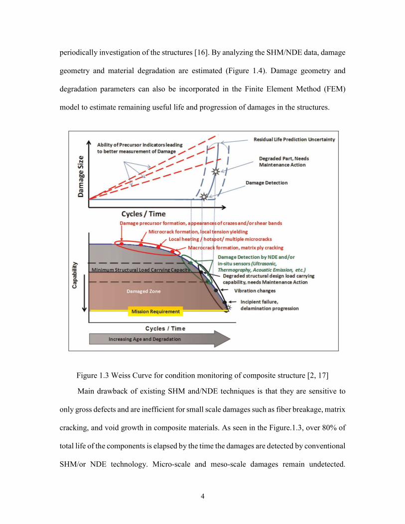
periodically investigation of the structures [16]. By analyzing the SHM/NDE data, damage

geometry and material degradation are estimated (Figure 1.4). Damage geometry and

degradation parameters can also be incorporated in the Finite Element Method (FEM)

model to estimate remaining useful life and progression of damages in the structures.

Figure 1.3 Weiss Curve for condition monitoring of composite structure [2, 17]

Main drawback of existing SHM and/NDE techniques is that they are sensitive to

only gross defects and are inefficient for small scale damages such as fiber breakage, matrix

cracking, and void growth in composite materials. As seen in the Figure.1.3, over 80% of

total life of the components is elapsed by the time the damages are detected by conventional

SHM/or NDE technology. Micro-scale and meso-scale damages remain undetected.

5

Detecting early stage damage state of composites is a major challenge in SHM/or NDE.

Therefore, it is necessary to devise new tools and techniques that are sensitive to small-

scale damages.

Figure 1.4 NDE interface with the failure models.

Additionally, good understanding of sensor signals obtained in SHM/NDE

experiments are required to extract information of current damage state of the structure and

prediction of remaining useful life of the structure. To understand the sensor signals, it is

essential to perform wave propagation experiments for structures with representative

damage states. However, there could be infinite possibilities of damage states in the

material and it is impossible to experimentally obtain the understanding of the sensor

signals due to the varying damage states. An offline NDE simulation tool will add

tremendous value [18] to the understanding of the physics of the wave propagation and

its interaction with the damages. Unlike experiments, in simulations, various host

structure geometries and different damage scenarios could be analyzed more

6

inexpensively. Thus recently, Computational NDE and SHM [13, 19] have gained

enormous popularity.

MSA estimates remaining useful life of the structural components based on information

obtained from composite failure analysis, degradation mechanism and NDE/SHM data,

therefore, in the subsequent section various composites failure models, degradation

methods and NDE techniques are reviewed.

1.2 PROGRESSIVE COMPOSITE FAILURE MODEL

Failure prediction of the composite structures is very complicated since composites

show different mechanical behavior than metallic structures. To design a reliable

composite structure, there is a need to predict composite failure under different loading and

boundary conditions. Various progressive failure models are developed for different

composite materials during past few decades [20]. These models can be employed to

predict structural damage progression from damage initiation to ultimate failure of the

structure. A progressive failure model for a composite structure consists of three major

parts: laminate theory for structural stress analysis, failure models for prediction of onset

of different damage modes and a material property degradation models to control how a

specific property need to be changed due to progressive failure [21].

1.2.1 CLASSICAL LAMINATE THEORY FOR STRESS ANALYSIS

Composite laminate consists of multiple layers bonded together. Each layer of the

composite is called lamina. Figure 1.5(a) is the schematic of an unidirectional fiber-

reinforced composite lamina. Stiffness of the lamina along fiber direction is denoted by 1E

and Stiffness transverse to the fiber direction is denoted by 2E , Stress-strain relationship

for two-dimensional lamina can be written as [22],

7

1 11 12 1

1 21 22 1

12 66 12

0

0

0 0

Q Q

Q Q

Q

(1.1)

where, 111

12 211

EQ

; 12 2

1212 211

EQ

; 222

12 211

EQ

; 66 12Q G (1.2)

Figure 1.5 (a) Unidirectional Lamina, (b) Off-axis Lamina.

If the principle material coordinate axis does not coincide with the loading direction as

shown in the Figure 1.5(b), stress-strain relationships along loading direction coordinate is

obtained by performing coordinate transformation. Stress-strain relationship are expressed

as,

11 12 16

21 22 26

16 26 66

x x

y y

xy xy

Q Q Q

Q Q Q

Q Q Q

(1.3)

Where,

4 4 2 211 11 22 12 66cos ( ) sin ( ) 2( 2 )sin ( )cos ( )Q Q Q Q Q

2 2 4 4 412 21 11 22 66 22 12( 4 )sin ( )cos ( ) sin ( ) (sin ( ) cos ( ))Q Q Q Q Q Q Q

4 4 2 222 11 22 12 66sin ( ) cos ( ) 2( 2 )sin ( )cos ( )Q Q Q Q Q

8

3 316 61 11 12 66 22 12 66( 2 )cos ( )sin( ) ( 2 ) cos( )sin ( )Q Q Q Q Q Q Q Q

3 326 62 11 12 66 22 12 66( 2 )cos( )sin ( ) ( 2 )cos ( )sin( )Q Q Q Q Q Q Q Q

2 2 4 466 11 22 12 66 66( 2 2 ) cos ( )sin ( ) (sin ( ) cos ( ))Q Q Q Q Q Q (1.4)

Figure 1.6 laminate with different plies.

Stress-strain relationship for a laminate is given by,

11 12 16

21 22 261 1

16 26 66

1

k k k kx x xn n

k k kky k y y

k k k k kxy xy xy

Q Q Qt

t Q Q Qt t

Q Q Q

(1.5)

Where t is total thickness of the laminate, n is the number of layers, and kt is thickness of

the kth layer.

9

1.2.2 FAILURE CRITERION OF LAMINA

Failure criteria for composite materials is defined by the mathematical equations to

predict onset of a damage mode. Unlike metallic structures, composite materials typically

fail under different damage modes such as, fiber breakage, matrix damage, shear failure or

combination of both matrix damage and delamination. Failure criteria in the composite

material often classified into two major categories, named as, damage mode-depended or

damage mode-independed criteria [23]. A vast amount of research has been accomplished

during past five decades to develop failure criteria and a large amount of literature available

for composite materials.

1.2.2.1 Mode-independed failure criteria

Mode independed failure criteria are mathematical equations in stress/strain space to

predict damage onset. These criteria do not provide indication of typical failure modes. The

simplest and widely used mode-independed criteria are maximum stress theory and

maximum strain theory. They are represented by inequality condition of stress and strain

where individual stress and strain components are compared with the associated allowable

limits. They area also called as non-interactive failure criteria as there is no interaction

between stress and strain components in the failure equation. The most popular Interactive

failure criteria are the Tsai-Hill Criteria and Tsai-Wu Criteria. These criteria generally

use interaction between stress and strain in the form of quadratic equation.

1.2.2.1.1 Maximum stress theory

In maximum stress criteria, failure occurs where applied stress exceeds the

corresponding allowable stress. Failure criteria can be represented by following

mathematical equation:

10

1 2 12

, ,

max , , 1T C T CX Y S

(1.6)

Where TX , CX , TY , CY and S are maximum allowable stress in the composite.

TX =maximum allowable tensile strength in the fiber direction.

CX =maximum allowable compressive strength in the fiber direction.

TY =maximum allowable tensile strength in the matrix direction.

CY = maximum allowable compressive strength in the matrix direction.

S =maximum allowable shear strength.

The safe zone to avoid failure is represented by following condition:

1C TX X

2C TY Y

12 S (1.7)

1.2.2.1.2 Maximum strain theory

In maximum strain criteria, failure occurs when applied strain exceeds the

corresponding allowable strain in the composite materials. Failure condition can be

expressed by following mathematical equations:

1 2 1

1 , 2 , 12

max , , 1U U UT C T C

(1.8)

Where 1UT 1

UC , 2

UT , 2

UC and 12

U are maximum allowable strain in the composite.

1UT =maximum allowable tensile strain in the fiber direction.

1UC =maximum allowable compressive strain in the fiber direction.

11

2UT =maximum allowable tensile strain in the matrix direction.

2U

C = maximum allowable compressive strain in the matrix direction.

12U =maximum allowable shear strain.

Safe zone to avoid failure can be expressed by following condition:

1, 1 1,U U

C T

2, 2 2,U U

C T

12 12C (1.9)

1.2.2.1.3 Tsai-Hill Criteria

Under plane stress conditions, Tsai-Hill Criteria includes interaction among the

stress components in the form of quadratic polynomial equation. Failure in the lamina

occurs if and when following condition is fulfilled:

2 2 2

1 2 12 1 22

, , ,

1T C T C T CX Y S X

(1.10)

Where ,T CX and ,T CY is chosen as either TX or CX and TY or CY , depending on the sign of

the applied stress, 1 and 2 , respectively.

1.2.2.1.4 Tsai-Wu Criteria

Tsai-Wu Criteria predicts failure of a lamina under plane stress conditions when

the following condition is satisfied:

1i i ij i jF F

2 2 211 1 11 2 66 12 1 1 2 2 12 1 22 1F F F F F F (1.11)

12

1F , 2F , 6F , 11F , 22F and 66F are strength coefficients and are function of strength

parameters, is expressed by,

1

1 1

T C

FX X

2

1 1

T C

FY Y

11

1

T C

FX X

22

1

T C

FY Y

66 2

1F

S

1212

11 22

FF

F F

121 1F (1.12)

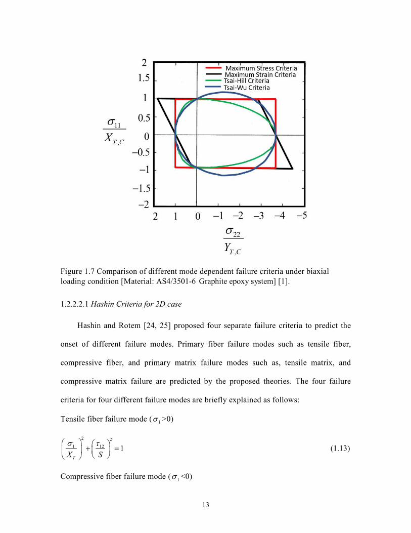
Failure envelops of the different mode independent failure model under bi-axial loading

condition are shown in the Figure 1.7.

1.2.2.2 Mode-depended failure criteria

Mode-dependent failure criteria consists of a set of quadratic equations where each

equation defines a failure mode. These criteria distinguish the different failure modes, such

as tensile fiber failure, compressive fiber failure, tensile matrix failure and compressive

failure. Failure modes are determined by comparing the ratio of applied stress and

corresponding allowable limit in interactive equation. Widely used mode-dependent

criteria are Hashin Criteria and Christensen Criteria.

13

Figure 1.7 Comparison of different mode dependent failure criteria under biaxial loading condition [Material: AS4/3501-6 Graphite epoxy system] [1].

1.2.2.2.1 Hashin Criteria for 2D case

Hashin and Rotem [24, 25] proposed four separate failure criteria to predict the

onset of different failure modes. Primary fiber failure modes such as tensile fiber,

compressive fiber, and primary matrix failure modes such as, tensile matrix, and

compressive matrix failure are predicted by the proposed theories. The four failure

criteria for four different failure modes are briefly explained as follows:

Tensile fiber failure mode ( 1 >0)

2 2

1 12 1TX S

(1.13)

Compressive fiber failure mode ( 1 <0)

14

2

1 1CX

(1.14)

Tensile Matrix failure mode ( 2 >0)

2 2

2 12 1TY S

(1.15)

Compressive Matrix failure mode ( 2 <0)

2 2 2

2 2 121 12 2

C

C

Y

Y S S S

(1.16)

1.2.2.2.2 Christensen Criteria

Christensen proposed a strain energy-based failure criterion to distinguish different

failure modes of composites. This theory includes out-of-place stress components into

the mathematical model. This theory is well suited for carbon fiber composites with

high anisotropy for both stiffness and strength.

For matrix-mode of failure, the safe zone to avoid failure must meet following

conditions,

2 2 2 2 222 33 22 33 23 22 33 12 312 2

23 12

1 1 1 1 1( ) ( ) 1

T C T CY Y Y Y S S

223

1 1

4 3T C T CY Y S Y Y

223

2

7 T CS Y Y (1.17)

For fiber-mode of failure, the safe zone must satisfy following conditions,

211 11

1 1 11

T C T CX X X X

15

11C TX X (1.18)

1.2.3 MATERIAL DEGRADATION MODEL

For prediction of failure of a composite laminate, it is important to estimate stress

and strain distribution at each lamina by using laminate theory. Stresses and strains

components for each lamina are then transformed from the global coordinate to local

principal coordinate. Appropriate failure criteria are then employed for failure prediction

of each lamina. Load carrying capacity of a lamina depends on the types of failure

modes. Once the lamina is failed, stress-strains are redistributed and increase stresses

on remaining laminas. Several methods have been proposed to account effect of failed

lamina and include it in the progressive damage model to predict behavior of the

laminate.

Figure 1.8 Basics of degradation model [20].

16

1.2.3.1 Sudden degradation model

According to sudden degradation model, the properties of the composite are

degraded into some fraction of the pristine properties depending on the types of the

failure modes (path ABCD, shown in Figure 1.8). Based on sudden degradation model,

conservative prediction of structural strength and stiffness are obtained. Also damage

accumulation during composite failure process is overlooked by the sudden degradation

model since the material is assumed to have two states: undamaged or totally damaged.

Sudden degradation model falls into two categories: total discount method and limited

discount method.

1.2.3.1.1 Total discount model zero stiffness and strength are assigned to the failed lamina in all direction for any

types of failure mode. For any failure modes, stiffness of an UD lamina (Figure 1.9) is

assigned as follows [26],

1 0E ; 2 0E ; 12 0G (1.19)

1.2.3.1.2 Limited discount model

In this method, when a lamina fails due to matrix cracking, zero stiffness and

strength are assigned to failed lamina for the transverse and shear mode. If the lamina

fails due to fiber breakage, total discount method is applied [26].

1 1E E ; 2 2(1 )E d E ; 12 12(1 )G d G (1.20)

Where d is the damage parameter,

17

Figure 1.9 Principal planes of the UD lamina.

1.2.3.2 Gradual degradation model

For accurate prediction of the damage progression in the composite materials,

gradual degradation models are used. Gradual degradation of the material property is

assumed of accumulation of damages inside the material. The material property of the

composites changes from pristine to damaged state gradually by following a nonlinear

path [20](represented by path ABD) as shown in the Figure 1.8. Degradation of the

property is controlled by external field such as strains. In composite materials different

types of damages modes are developed when they are subjected to different types of

loading. Onset of different damage modes depend on laminate sequence, composition

and types of loading. Fracture in the laminate takes place when different interacting

damage modes accumulate significantly [23]. A vast amount ofnstudies have

demonstrated the accuracy of the gradual degradation model to model progressive

damage progression. Few important researches are discussed here. Chang and Chang

18

[27] proposed a damage degradation model based on the fiber bundle theory to analyzed

different laminates and pin loaded joints under different types loading and boundary

conditions. Lee at al. [28] used shear lag model to estimate degradation parameter for

fiber failure. Joo et al. [29, 30] also employed shear lag analysis between plies to calculate

degradation parameters for transverse matrix cracking.

1.2.3.3 Shortcomings and new opportunities

Progressive damage models provide an excellent capability to predict failure in the

composite structures, however, degradation rules have not established as an acknowledged

form. Most of the degradation factors are in empirical forms and are determined from

experiments. Extensive tests are required to obtain the parameters of the empirical

equation. Also, empirical models developed for a particular material is not suitable for

different material types. Additionally, conducting series of experiments to obtain

degradation model is expensive cost. Nondestructive testing method based on Lamb wave

and bulk wave-based techniques can be employed to obtain parameters of the degradation

model. It is very easy to implement SHM/NDE to obtain real time values of the degradation

parameters. Few novel techniques that can be employed to obtain degradation parameters

at early very stage are discussed in subsequent sections. An online technique-based coda

wave interferometry was discussed. Also, an offline, named as QUIC was also discussed.

QUIC is a hybrid approach, developed based on Scanning Acoustic Microscopy and

nonlocal theories of wave equation [4].

1.3 CODA WAVE INTERFEROMETRY IN A HETEROGENOUS MEDIUM

Ultrasonic techniques based on the coda wave interferometry are widely being used

to quantify weak and local changes in the complex heterogeneous material medium. While

19

passing though the heterogenous medium sound wave scattered multiple times and create

a slowly decaying wave, called as coda wave. Coda waves are found to be extremely

sensitive to small-scale damages in the material medium, and in nondestructive testing the

technique is being widely used to monitor formation of microcracks in the material [31-

37].

1.3.1 THEORY

Suppose a wave passes through a strongly scattered medium that changes with time.

The wave field before any change can be written as sum of the waves that propagate along

the multiple scattering path of the medium, is expressed by [32-34, 38],

( ) ( )UnT

Tr

U t A t (1.21)

where Tr is the multiple scattering trajectories of the medium, TA is wave which propagate

along the trajectories.

when there is a change in the medium, the perturbed wavefield can be expressed by [32-34, 38],

( ) ( )PuT T

Tr

U t A t (1.22)

where T is the change of change in arrival time of the wave that propagates along each

trajectory. In order to estimate change in the waveform, cross correlation of the two-wave

form is performed. The cross-correlation factor is expressed by following equation,

' ' '

' 2 ' ' 2 '

( ) ( )

( )

( ( )) ( ( ))

win

win

win win

win win

t tUn Pu

s

t ts t t t t

Un Pu

t t t t

U t U t t dt

R t

U t dt U t dt

(1.23)

20

Value of the st that gives maximum correlation is used to measure the change of the

waveform.

1.4 NONLOCAL THEORIES

Nonlocal continuum theories are widely used to predict material response at

macroscale as well as molecular and atomic scales. It was first introduced by Kroner [39]

who formulated a continuum theory for an elastic material body with long range force.

Classical continuum mechanics approach was modified to model material behavior at

smaller length scale while retaining almost all advantages of the classical approach.

Nonlocal theory has been widely used in the areas of fracture mechanics [40], dislocation

mechanics [41], wave propagation in composite materials [42], lattice dispersion of elastic

wave [43], and surface tension in fluid medium [44]. Most important application of

nonlocal theory is to solve crack-tip problem where stresses were predicted bounded rather

than unbounded (singularity) as predicted by the classical continuum theory [40, 45-48].

Figure 1.10 Local and nonlocal approaches.

21

Various nonlocal theories have been proposed in the past to connect continuum

mechanics theory with atomistic theory [45]. Nonlocal theories including higher-order

displacement gradients and integral type were introduced [49]. Both types of nonlocal

theories are associated with an intrinsic length scale parameter, which is a variable and

problem dependent, is related with fracture process zone size, lattice size and void size

[45]. Eringen et al. [50-54] proposed nonlocal continuum theory (integral type) which

include nonlocality of balance laws and thermodynamic laws. Later the theory was

modified by Eringen and co-researchers [40] by including nonlocality in the constitutive

equations. In this approach stress at a point in a material body is expressed as weighed

value the strain field within a finite distance. The constitutive equation in nonlocal

continuum theory proposed by Eringen is expressed as [42],

' ' ' ' '( ) [ ( ) ( ) 2 ( ) ( )] ( )ij kk ij kk

V

x M x x e x M x x e x dv x (1.24)

Where ij and kke are stress and strain at a point in the material body; and are

Lames constant; 'M x x is a nonlocal kernel function or modulus function, which is

included in the model to bring the influence of strain at a distant points 'x to stress at x .

The balance laws is expressed as [42],

, , , , ,[ ( )] [( ) ] ( ) 0k k ij i j j i i i ij j ii j j

v v

u u u n dS u u dv f u

(1.25)

Another type of nonlocal model, which is called as gradient type nonlocal model,

express stress at a point as function of strain and its gradient at the same location [49].

Most of the nonlocal theory, break down at crack as their formulation spatial derivative.

To circumvent this obstacle, Silling [55] proposed a nonlocal theory that does not require

spatial derivative instead uses displacements in the constitutive equation.

22

1.5 QUANTITATIVE ULTRASONIC IMAGE CORRELATION (QUIC)-BASED ON SCANNING ACOUSTIC MICROSCOPY AND NONLOCAL MECHANICS

Quantitative Ultrasonic Image Correlation (QUIC) technique using scanning acoustic

microscopy (SAM) has emerged as a promising tool method for the noninvasive micro-

structural characterization of the materials [56-61]. Surface and subsurface mechanical

properties of metallic, composites and thin films can be measured accurately by QUIC

technique. Broad band ultrasonic transducers are used as a key element in QUIC for

ultrasonic scanning and imaging. Traditionally acoustic transducers with frequencies

ranging from 1 MHz to 1.2 GHz are used for imaging. Depth of penetration and frequency

selection of the transducer are inversely related. Higher frequency transducer allows better

resolution of images but limits penetration depth whereas low frequency transducer allows

more penetration depth with low resolution.

1.5.1 BASICS PRINCIPLES OF SCANNING ACOUSTIC MICROSCOPY

The schematics of scanning acoustic microscopes with broad band ultrasonic

transducers for generating images is depicted in the Figure 1.11. A ultrasonic transducer is

typically mounted on a sapphire buffer rod as shown in Figure 1.11. A tone-burst signal

excites the transducer at driving frequency for generation of a plane sound wave. Sound

wave propagates through the lens rod down to the concave spherical surface located at the

end of the lens rod. Ultrasonic wave energy focused at a point by the concave spherical

surface as shown in the Figure 1.11. The specimen is immersed inside coupling fluid

between the lens and the focal point of the converging ultrasonic wave. After interactions

with the specimen, the incoming ultrasonic wave reflects back to the transducer in different

ways. The wave energy which propagates parallel to the center axis of the sapphire lens

rod reflect back to the transducer after reflection from the top surface specimen, which is

23

called as normal reflection. Part of the ultrasonic energy transmitted through the specimen

and reflected at the back surface of the specimen. The wave energy that hit the specimen

surface at Rayleigh critical angle, generates leaky Rayleigh wave that propagates along the

sample surface and leaked back to the fluid and eventually received by the transducer. In a

typical signal obtain by scanning acoustic microscopy, normal reflection, back side

reflection and Rayleigh wave are observed.

Figure 1.11 Schematic of a scanning acoustic microscope lens and working principle.

1.5.2 NONLOCAL EFFECT OF DAMAGE

Problems where long-range forces exist, the nonlocal interaction between neighboring

material points prevail. For examples, relaxation of material properties, damage

reconfiguration, distributed microcracking, microstructural heterogeneity and regeneration

of stress concentrations, are few examples of such states where nonlocal interactions could

24

be presumed. Bazant [62] showed that nonlocality is exhibited in the phenomena of matrix

cracking. It is also maintained in the Ref [62] that the generation of microcracks is not

depended only on the local displacements at the location of the cracks but also depends on

the displacement that occurs away from the crack [45, 62]. Hence, to investigate the

material state using high-frequency wave propagation, the constitutive law from continuum

mechanics is not enough. A suitable kernel function is used to modify the constitutive law,

to account for the nonlocal effect. The Christofell’s equation of the wave propagation is

modified using the nonlocal constitutive law, and the eigenvalue problem was solved to

obtain the nonlocal dispersion curves for different wave modes (quasi-longitudinal and

quasi-shear) as functions of nonlocal parameters [5]. Experimentally measured wave

velocities were used to calculate the nonlocal parameters from the dispersion curves.

Parametric variations of the nonlocal parameters were used to quantify the precursor state

[5].

1.6 ENTROPY AS MEASURE OF MATERIAL DEGRADATION IN COMPOSITES

Composite structures under operation gradually degrade progressively during fatigue

loading. Degradation of the material is driven by dissipative process and induce a

disorder/chaos in the material. Damage Entropy which is understood as disorder/chaos in

the material as damage. Entropy increases with material degradation in the material [63].

Heterogeneous microstructure of the composite and material property difference of the

constituents provide favorable conditions for development of various types of damage

modes such as interfacial debonding, matrix microcracking, interfacial sliding,

delamination/interlaminar cracking, fiber breakages, fiber micro-buckling and void-growth

[8]. Damage development mechanism in composites is very complex process. Often

25

combination of the different damage modes accumulates, interact and lead to change in

material stress state and local stress-concentration in the composites. Local properties of

the composites change due loading and aging. Microstructural changes and damage

induced disorder in the system are quantifiable by ultrasonic techniques [5].

1.7 COMPUTATIONAL NDE FOR BETTER UNDERSTANDING OF THE SHM/NDE DATA

SHM/NDE data are employed for the quantitative material state awareness (MSA) of

the structure. MSA of the structure is performed in terms of initial states of the damage,

damage types, damage accumulation, and degradation of material properties due to damage

development. For better understanding of the SHM/NDE data, realistic simulation of wave

propagation and damage modelling in a structural component are needed. In the subsequent

section, a brief literature review on existing wave-propagation tools is performed and

advantage and disadvantages of various techniques are discussed.

1.7.1 COMPUTATIONAL NDE

Over the years, researchers have attempted using various techniques to correctly to

simulate wave propagation in the composite and metallic structure. Finite Element Method

(FEM) [64], Boundary Element Method (BEM) [65, 66], Indirect Boundary Integral

Equation (IBIE) [67-70] , Multi-Gaussian Beam Model (MGBM) [71-73], Spectral

Element Method (SEM) [74], Elastodynamic Finite Integration Technique (EFIT) [75-77],

Charge Simulation Technique (CST) [78] & Multiple Multi-pole Program (MMP) [79-81]

have been tried. Shortcomings of all these methods are multiple, as detailed in ref [82]. For

sake of brevity few relevant ones are discussed. To incorporate any arbitrary geometry in

the SHM/NDE simulation, the FEM, BEM, IBIE methods are more appropriate. However,

26

the most significant issue in FEM wave modeling comes from the spurious reflection of

high frequency waves at the multi-scale interfaces [83-85]. Spurious reflection is not only

an issue at the multi-scale interface but also at the continuum when different element sizes

are used [86]. FEM is very computationally intensive: it requires huge amount of

computation memory and execution time. Above all, due to spurious reflection phenomena,

the FEM results are not very reliable. BEM and IBIE are faster methods and can handle

any arbitrary problem geometry like FEM; however, the boundaries are discretized by

placing point source on the boundary and resulting integral equation with singular kernel

that give rise to the Fredholm integral equation of the second kind; this results in additional

background computation. EFIT is essentially a finite different method and fares

comparably better than FEM for modeling wave propagation.

Although all those techniques are well established for wave propagation simulation,

one of the greatest disadvantages of these computation techniques is that to study wave-

damage interaction, the damage path is required to be defined ahead of time. Whereas, in

the practical scenario, it is almost impossible to predict a damage route. Additionally, it is

also essential to update the meshing of the domain alongside the damage propagation,

which makes these techniques also computationally expensive. Hence, a method is required

which should be capable of handling both damage prediction and wave propagation,

simultaneously, without much difficulty. It is expected that the predictive models would

be integrated with the ‘digital-twin [87]’ software (software for the virtual off-line

interface), such that the material behavior and the sensor signals could be predicted off-

line simultaneously, by the predictive tool. In the near future, it is also expected that the

structure, structural component or individual material states could be digitally certified for

27

their future missions [87]. This will impact the maintenance efforts significantly in two

ways, 1) help in predicting unseen events through the dedicated simulations, and 2) saving

materials from being abandoned based on statistical rules. Peridynamic, a nonlocal

approach, which has capability in predicting material behavior at different length scale and

simulating wave propagation, can be used as an efficient technique in computational NDE.

1.7.2 PERIDYNAMICS-A NONLOCAL APPROACH

Classical theory of continuum mechanics (CCM) has been used successfully to solve

problems in solid mechanics. The underlying assumption of CCM is that the material body

remains continuous before and after deformation. Although, CCM approaches has been

used successfully to solve problems at macro-scale, it encounters difficulty in the solving

crack propagation problems, since the mathematical model of the CCM approach uses

spatial partial differential equation which become undefined at crack location (gradient of

stress-tensor become undefined).

Figure 1.12 Types of solid mechanics problem modeled by peridynamic approach, (a) continuous body, (b) Material body with crack, (c) Discrete particles.

To overcome the limitations of the CCM approach in solving with the crack

propagation problem, Liner Elastic Fracture Mechanics (LEFM) [88] was developed.

Within LEFM framework, crack initiation and growth are modelled by introducing external

crack growth criteria such as critical energy release rate and which is not part of the

28

governing equation of the CCM approach. Crack surface evolution is started from a pre-

exiting crack [88].

LEFM was included in the traditional Finite Element Analysis (FEA) tool to model

fracture mechanics problem. Special elements are used to model singular stress at the crack

tip. To model the crack growth, the crack is treated as boundary and meshing of the material

body need to be updated after each incremental crack growth. A pre-defined mathematical

equation for crack growth and propagation direction is needed to supply to the FEA model.

However, there is a major difficulty to obtain the kinetic relation from experiments. Also,

modelling multiple crack propagation and their interaction in the 3-dimensional domain

become extremely complex using traditional finite element method. To circumvent the

difficulty in modelling the multiple crack propagation by FEA, Peridynamic theory was

proposed.

Peridynamic theory (PD) is a nonlocal formulation, which was developed by Silling

[55, 89-93] in Sandia National Laboratory, is being used successfully to understand

material behavior at different length scale. The word “peridynamic” was derived from two

Greek words which are “Peri” and “Dynamic”. In the Greek Language “Peri” means near

and “Dynamic” means force. Modelling of continuous body, material body with cracks

and discrete particles can be performed within a single framework of peridynamic theory.

In contrast to partial differential equation used in classical continuum theory, peridynamic

theory utilizes intergo-differential, which makes the approach suitable to solve crack

propagation problem. Integro-differential equations of PD approach are valid at the crack

surface. Additionally, damage parameters are included in the constitutive equations which

29

make peridynamic approach suitable to model crack initiation and crack branching in the

material, without any special need of defining external crack growth criteria [89].

Figure 1.13 Relationship and major differences of continuum mechanics (local) and peridynamic approach (nonlocal).

In Peridynamic approach, the material body is discretized into number of material

points where each point has finite volume. Interaction between the material points takes

place within a finite internal length, which is called as Horizon (shown in Figure 1.13).

Interaction between two material points depends on material properties, internal length and

relative distance between particles. Internal length of the peridynamic approach is selected

based on the nonlocality of the problem. For continuum mechanics problem, internal length

scale approaches to zero and material points interact with its immediate neighbor whereas,

atomistic simulation internal length is selected as interatomic distance. Therefore,

30

peridynamic technique can be used to analyze the material behavior across different scale

[92].

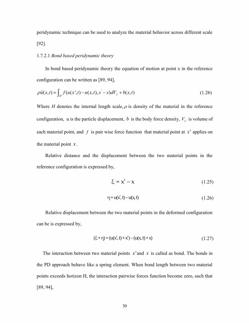
1.7.2.1 Bond based peridynamic theory

In bond based peridynamic theory the equation of motion at point x in the reference

configuration can be written as [89, 94],

''( , ) ( ( ', ) ( , ), ) ( , )xH

u x t f u x t u x t x x dV b x t (1.26)

Where H denotes the internal length scale, is density of the material in the reference

configuration, u is the particle displacement, b is the body force density, 'xV is volume of

each material point, and f is pair wise force function that material point at 'x applies on

the material point x .

Relative distance and the displacement between the two material points in the

reference configuration is expressed by,

ξ = x x (1.25)

η= u(x,t) u(x,t) (1.26)

Relative displacement between the two material points in the deformed configuration

can be is expressed by,

(ξ+η) = (u(x,t)+x) (u(x,t)+x) (1.27)

The interaction between two material points 'x and x is called as bond. The bonds in

the PD approach behave like a spring element. When bond length between two material

points exceeds horizon H, the interaction pairwise forces function become zero, such that

[89, 94],

31

( , ) 0f if >H (1.28)

The pair wise force function is required to satisfy the conservation of the linear

momentum as follows [89, 94],

( , ) ( , )f f , (1.29)

Eq. 1.29 also called linear admissibility condition. To satisfy conservation of the angular

momentum following equation must hold [89, 94],

( , ) ( ) 0f , (1.30)

Eq.1.30 is called angular admissibility condition. The pair-wise force vector between two

particle acts opposite to each other and is parallel to current relative position in order to

hold conditions in equations 1.29&1.30.

In PD, pair-wise force function is derived from a scaler micro-potential function , as

follows [89, 94],

( , ) ( , )f

(1.31)

Micro-potential of the bond is the strain energy of a single bond. A peridynamic body is

said to be microelastic if equation (1.31) is satisfied.

Total strain energy at a point can be defined by following equation [89, 94],

1( , )

2E

H

W dV (1.32)

The factor of half is included in the equation because each endpoint of the bond share half

of the strain energy of the bond.

A linearized peridynamic mode for micro-elastic material is expressed in the following

form [89, 94]:

32

( , ) ( )f C , (1.33)

where ( )C is micro-modulus function for the PD material.

1.7.2.2 Constitutive models for PD

To model fracture in a deforming body, a damage parameter is included in the

peridynamic model. Modified constitutive equation for the peridynamic material can be

expressed as [89, 94],

( , , ) ( ) ( , ) ( , )f t c s t

(1.34)

Where ( )c is a bond constant, ( , )s is bond stretch and ( , ) is a history-depended

scaler value function. Value of ( , ) is taken as either 0 or 1.

( , ) 1 if ''( , )s t > 0s for ''0 t t

( , ) 0 otherwise (1.35)

0s is the critical stretch of the bond. Bond stretch is defined by,

( , )s

(1.36)

Local damage at a material point is defined by [89, 94],

( , , )

( , ) 1 H

H

x t dV

x tdV

(1.37)

1.7.2.3 Bond Constant estimation for isotropic material

PD bond constant determination of an isotropic material is performed by considering a

large homogenous body under isotropic extension as shown in the Figure 1.14. A uniform

stretch s is applied to the all material points to achieve uniform expansion of the material

33

Figure 1.14 Homogenous expansion of isotropic material

body. Length of a bond before and after deformation is expressed as and (1 )s ,

respectively.

(1 )s , where s (1.38)

Force density vector is expressed as,

c

f cs

(1.39)

Micropotential can takes the follwing from by applying equation (1.31)

2 / 2cs (1.40)

Starin energy at point can be expressed as,

2 2 42

0

1 1 44

2 2 2 4E

H

cs csW dV d

(1.41)

Strain energy density (SED) by applying CCM approach for the same uniform expansion

of the material body becomes,

29

2EW ks (1.42)

34

The PD bond constant can be calculated by equating SED obtained from both CCM and

PD approach,

4

18kc

(1.43)

Where k is the bulk modulus of the material.

1.8 OUTLINE OF THE DISSERTATION

The focus of the dissertation is to devise new methods and tools for understanding

material state awareness of engineered materials through ultrasonic NDE and SHM. The

dissertation is divided into two major parts. In the Part-I, material state awareness of woven

composite is performed using guided Coda Wave Interferometry (CWI) and Quantitative

Ultrasonic Image Correlation (QUIC) Technique. Additionally, stress-relaxation behavior

in the composite was quantified by nonlinear ultrasonic technique. Part II of the dissertation

is focused on development of the new wave propagation modelling tool, called Peri-

Elastodynamic (PED) based on peridynamic theory. QUIC technique was also extended

for biological system characterization and development of a predictive tool for quantifying

the internal instability of a biological system. The organization of the proposed dissertation

is given below:

In Chapter-1, background, motivation, various progressive failure model, local and

nonlocal theories, online and offline ultrasonic inspection techniques and computational

nondestructive evaluation (NDE) was discussed.

In Chapter-2, discusses the Material State Awareness (MAW) of composite materials

through precursor damage state quantification. Guided coda wave interferometry is

proposed first time for precursor damage state quantitation in composite under fatigue

35

loading. Development of damage in the materials is investigated by using Optical

Microscopy (OM) and Scanning Acoustic Microscopy(SAM).

In Chapter-3, Damage development due to precursor damage state is quantified by QUIC

technique. Results from the CWI and QUIC techniques are correlated to investigate the

potential of the CWI for precursor damage state quantification.

In Chapter-4, Stress-relaxation in the composites was monitored by using CWI technique.

In Chapter 5, Stress-relaxation in the composites was monitored by using acoustic

nonlinearity of Lamb waves.

In Chapter 6, a wave propagation tool named as Peri-Elastodyanmic is developed for Lamb

wave propagation simulation in a plate-like structure. Fundamental lamb wave modes are

simulated accurately. The technique is verified by comparing dispersion results obtained

from simulation with those from “Waveform Revealer”.

In Chapter 7 Peri-Elastodynamic technique is extended for simulation of wave-damage

interaction in a plate-like structure. Wave reflection and transmission at crack is observed

from the simulation results. The Peri-Elastodynamic is verified by comparing simulated

sensor signals with those obtained from the experimental results for both pristine and

damaged plates.

In Chapter 8 Summary and conclusion of the thesis.

In Chapter 9, Other work, QUIC technique is also extended for biomedical research. QUIC

technique is used for material characterization of a biological system (fungus colony).

Internal instability such as wrinkles in the medium is measures by acoustic microscopy. A

predictive model based on incremental stress theory is developed for quantification of

pressure quantification in the

36

CHAPTER 2

PRECURSOR DAMAGE ANALYSIS USING ULTRASONIC GUIDED CODA WAVE INTERFEROMETRY

The early detection and quantification of embryonic precursor damage in composites

are currently challenging due to lack of an online ultrasonic method. Typical precursor

damages are developed in the form of matrix cracking, microcracks, voids, micro-buckling,

local fiber breakage, local fiber-matrix debonding, etc. [8, 95]. These damages can be

visualized using off-line laboratory-based nondestructive evaluation (NDE) methods, for

example, X-ray tomography [96], Scanning Acoustic Microscopy [5], Ultrasonic

immersion scanning [97], etc. However, it is realized that the conventional ultrasonic

guided-wave-based Structural Health Monitoring (SHM) at low frequencies (~100–~500

kHz) are not sensitive to these precursor damages, and often demands sophisticated pattern

recognition algorithms for signal processing, offline. These statistical signal processing

algorithms sometimes result in heavy computational burden.

Ultrasonic guided waves are popular for online NDE and SHM of composites [98,

99]. Guided waves in a thin composite structure generate two fundamental Lamb wave

modes, symmetric S0 and antisymmetric A0. In SHM, the fundamental S0 and A0 modes

are analyzed to find the damages in the composite. The fundamental wave modes are useful

for detecting the delamination and cracks when the physical size of the damages is

comparable to the wavelengths of the propagating wave modes between the frequencies

37

Figure 2.1 (a) Condition monitoring of composite structure [6, 100] shows the P point when the early detection should be started; (b) Fatigue damage evolution in the composite material [95] shows no change in global stiffness when the incubation of embryonic damage precursor is underway.

~100–~500 kHz. However, it was found that these modes are not sensitive enough [101]

to detect the precursor damage in composites. Damage precursor in composites, like micro-

cracks, fiber-breakages, and crazing, starts to occur during the first 30% of the lifespan of

the structure, as shown in Figure 2.1a. Currently, the low-frequency online NDE or SHM

methods cannot detect the damages at very early stage (during the first ~30% of the life of

the composites). After 80%–90% of the composite life, the interaction between the local

material damages and the global structural damage is very rapid (Figure 2.1b). Hence, this

rapid interaction causes a catastrophic failure of a structure. However, it is noted that the

prelude of this event starts even before 30% of the life of the composites. So, to avoid this

impending failure of the structure, it is important to implement the ‘material state

awareness’ through detection of distributed precursor damages as early as possible (i.e.,

during the initial 30% of the lifespan of the composites). It is the objective of this

dissertation to represent the precursor state using a unique quantified parameter. Low-

frequency SHM is well accepted for detecting macro scale damages in composite but is not

38

used for precursor detection. However, in this dissertation, to overcome the challenge in

detecting the precursor damages, an online SHM method with Coda Wave Interferometry

(CWI) capability is proposed.

Symmetric S0 and Antisymmetric A0 modes are not sensitive to the small-scale

distributed damages such as matrix microcracking (transverse and longitudinal cracking),

fiber breakages, and local fiber-matrix debonding in composites. Thus, to enable online

precursor monitoring, a few researchers suggest embedding carbon nanotube networks

[102] or magnetostrictive particles [103] during the manufacturing of the composites.

These methods require additional material species to be added to the material, which is

often discouraged. Hence, a method is required that will not alter the constituents of the

composites but detect the precursor damages online.

Here in this dissertation, guided coda wave analysis is proposed. It is reported that

when there is absolutely no change in the Lamb wave mode velocities, the latter part of the

signal that reaches after the dominant Lamb wave modes, called “Coda wave”, is highly

sensitive to the weak changes in the material. The coda wave interferometry (CWI)

technique is a promising nondestructive technique, which was first used by the seismologist

to detect the changes in the coda wave velocities in the earth crust during the earthquakes

[33, 104]. Later, this technique was successfully extended to measure the relative changes

of wave velocities in the concrete due to the development of the small-scale (~mm)

damages [105, 106]. The frequency-dependent shifts in the coda wave velocities were

estimated in the range ~150 kHz–~1 MHz [106]. Thermal effect on the coda wave

velocities was estimated in [107]. Larose et al. [105] estimated the relative change (𝛁) in

39

the coda wave velocity (V) in concrete in the order of ∇𝑉 𝑉 = ⁄ 10 . With precise

measurement of the wave velocities, it was found that the CWI was always more accurate

compared to the conventional time-of-flight measurement from the direct wave analysis.

Commonly, the CWI analysis was performed using two techniques, (a) doublet [35, 38,

108], and (b) stretching [105-107, 109] methods. In the doublet method, several time

windows are selected in the coda part of the signal, and the shift in each time windows are

calculated using the cross-correlation technique. Although promising, CWI was never used

for detecting or evaluating the distributed precursor damages in carbon-fiber-composite

materials.

Composite is a heterogeneous medium designed to develop damage precursors in a

distributed form. These distributed local damages interact with one another and form a

fracture path when further load is applied. It was found that the coda waves are sensitive

to these weak changes when they interact with the distributed damages. Perhaps, while

traveling through a composite specimen, multiple interactions of the Lamb wave causes

the coda signal affected by the distributed damage. It is identified that if the conventional

CWI is modified for composites, the method can be a promising online tool for precursor

damage detection. In this work, using a modified stretching technique, an attempt has been

made for the detection of precursor damage state in woven carbon-reinforced-fiber-plastic

under fatigue loading. To verify, prove, and explain the occurrence of the precursor

damages in the specimens from the CWI method, benchmark studies using optical

microscopy, Scanning Acoustic Microscopy (SAM), and Scanning Electron Microscopy

(SEM) are conducted.

40

2.1 CODA WAVE INTERFEROMETRY

Coda wave interferometry is a technique for monitoring small changes in heterogenous

material medium over time using ultrasonic wave. While propagating in a strongly

Figure 2.2 A typical waveform recorded at pristine state and 15,000 cycles fatigue loading: a) First arrival, b) Coda wave.

heterogenous material medium, ultrasonic waves are scattered multiple times due to

heterogeneities and generate late-arriving wave form, called coda waves as shown in

41

Figure2.2b. Small changes in the medium due to due to formation of damages, will result

in an observable change in the coda waves. Coda wave interferometry uses this sensitivity

to monitor weak changes in material medium. There are two techniques, namely Stretching

technique and Taylor series expansion technique, commonly used to measure temporal

changes in a material medium.

2.1.1 STRETCHING TECHNIQUE WITH CROSS-CORRELATION

If the coda part of the wave signals (the signal that arrives after the Lamb wave modes)

from two material states (1 = pristine and k = kth material state) are represented as s1(t) and

sk(t), respectively, then their relation can be written as.

sk(t) = s1(t(1 + α)) + d(t) (2.1)

where, α is a relative stretch parameter, and d(t) is the distortion. In the stretching method,

the time scale of the perturbed state signal was stretched (+ sign) or compressed (− sign)

by a suitable stretch parameter value, α as tk = t (1 + α). A range of α values was selected

[−value ≤ α ≤ value], and cross-correlation was performed between, sk[t(1 + α)] and s1(t).

A value of α that maximizes the normalized cross-correlation was considered as the critical

stretch parameter (αk) and was used to measure the relative average velocity change in the

medium [106]. Item α is the relative change of velocity between two material states (1

and k).

CrCr(α) =∫ s [t(1 + α)]s (t)dt

/

/

∫ s [t(1 + α)]dt ∫ s (t)/

/dt

/

/

(2.2)

42

α = max∈

(CrCr (α)) (2.3)

where T is the time window selected in the calculation above.

2.1.2 STRETCHING TECHNIQUE TAYLOR SERIES EXPANSION

An alternative approach to calculate 𝛼 is presented herein. Using the Taylor series

expansion of s1(t(1+α)) up to 1st order the Equation (1) can be as follows,

s (t) = s (t) + s (t)tα + Higer order terms (2.4)

As the stretch parameter, α, is very small, the higher order terms in the Equation (2.4), can

be neglected. α is approximated as follows,

N

j jj

jjk

tt's

tsts

Nα

1 1

1

)(

)()(1 (2.5)

By employing the explicit finite difference scheme, the gradient term, 𝑠 (𝑡) can be

calculated as follows,

11

11111

)()()('

jj

jjj tt

tststs (2.6)

where, 1 1 2 2/j j st t t f , sf is the sampling rate. Substituting equation (2.6) in

equation (2.5), relative stretch parameter, 𝛼 after the kth material state (here kth fatigue

interval) is calculated as follows.

1

2 1111

1

)]()([

)]()([21 N

i iiis

iikk tststf

tsts

Nα (2.7)

43

where N is the total number of data points used in the calculation, it is the timestamp of the

ith data, and sf is the sampling frequency. This technique is computationally less

expensive than the cross-correlation technique and is used to calculate the stretch parameter

for the long-range signals [110], which is used in this study for the precursor damage

quantification in composites.

2.2 PITCH-CATCH ULTRASONIC LAMB WAVE EXPERIMENTS

Two high-frequency PZT sensors were attached to the specimens. A 5-count tone

burst signal with central frequency, fc = 324 kHz, was used for the actuation of the guided

wave, as shown in the Figure 2.4f. The central frequency ~324 kHz was selected from a

tuning experiment with the specimen S-A, where the fundamental antisymmetric wave

mode had a maximum amplitude. Tektronix AFG3021C (25 MHz, 1-Ch Arbitrary

Function Generator, Tektronix Inc., Oregon, USA) was used to generate the tone burst

actuation at the interval of 1 ms. Peak to peak amplitude of the burst signal was set to 20

V for the wave actuation. Tektronix MDO3024 (200 MHz, 4-Ch Mixed Domain

Oscilloscope, Tektronix Inc., Oregon, USA) was used to record the sensor signals. Sensor

signals were collected at 50.0 MS/s with 10,000 data points. Online pitch-catch

experiments were performed keeping the specimen on the loading machine. All benchmark

studies were performed at the pristine state and after the 300,000 cycles of fatigue. Sensor

signals using PZT sensors were recorded every 5000 cycles using an oscilloscope (Figure

2.4c) and a total of 61 data files were saved for each specimen during the 300,000-cycle

experiment.

44

2.3 EXPERIMENTAL PROCEDURE

2.3.1 MATERIALS AND SPECIMEN PREPARATION

Four-layer woven carbon-fiber composites are used in this study (Figure 2.3a). The

thickness of each lamina is ~280 μm. Dimension of the specimens, length and width of the

tabs, and chamfer angles were chosen according to the ASTM D 3039 [111] standards. The

average length, width, and thickness of the specimens were ~250 mm, ~25 mm, and ~1.5

mm, respectively. Epoxy 9340 from Loctite (48 h curing time) was used for bonding the

tabs with the specimens.

Next, 7-mm-diameter PZT sensors from Steminc Steiner & Martins, Inc. (Miami, FL,

USA) were mounted on the specimens using Hysol 9340 (Henkel Loctite, Stamford, CT,

USA). Eleven (S-A, S-B, S-C, S-D, S-E, S-F S-G, F-L, T-1, T-2 and T-3) specimens were

prepared. Three specimens (T1–T3) were tested under pure tensile load (Figure 2.3b), one

specimen (F-L) was tested under fatigue loading to estimate the maximum fatigue life of

the material type. The fatigue life was intentionally marked at ~1 million cycles when an

onset of delamination was first detected (Figure 2.3c) in the specimen F-L. However, the

fatigue test was continued until the end of ~2 million cycles. From the remaining six

specimens (S-A, S-B, S-C, S-D, S-E), each was tested under tensile–tensile fatigue load up

to ~30% of the fatigue life, i.e., up to ~300,000 cycles. Note that, S-A, S-B, S-C and S-D

were used for online precursor damage detection and results are discussed in this chapter.

Specimen S-F and S-G were used for offline precursor damage detection. Specimen S-E

was used for both online and offline precursor damage detection and correlation between

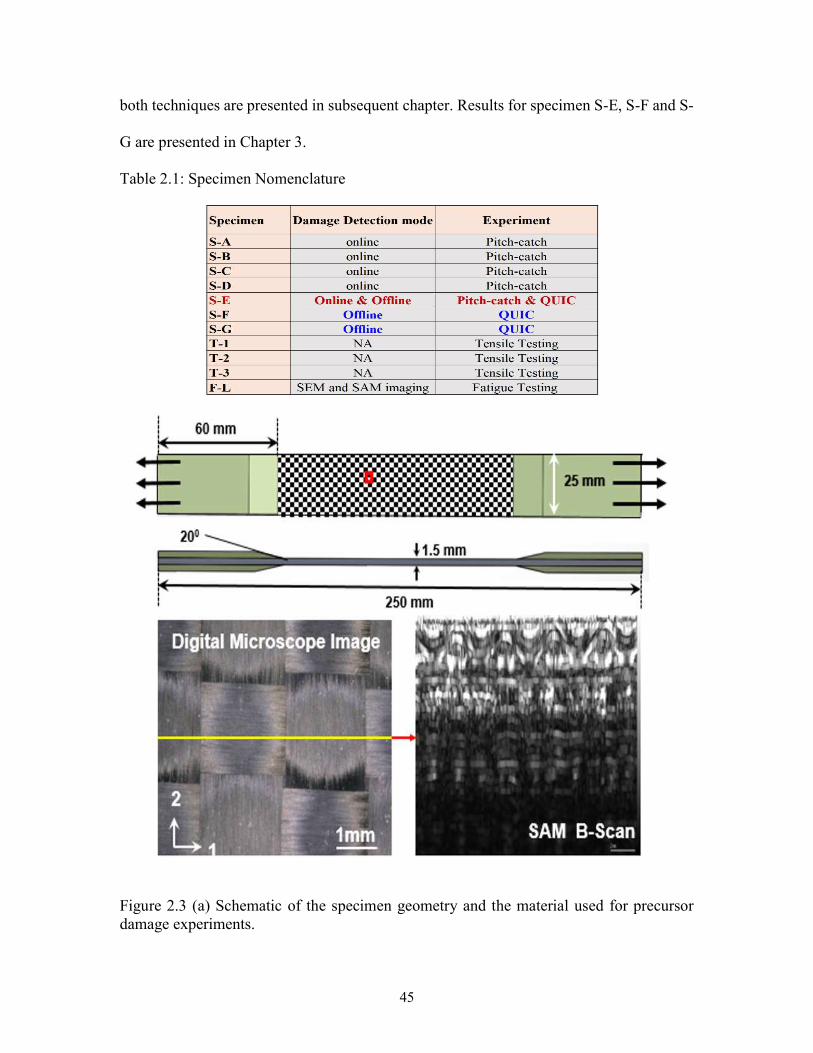
45

both techniques are presented in subsequent chapter. Results for specimen S-E, S-F and S-

G are presented in Chapter 3.

Table 2.1: Specimen Nomenclature

Figure 2.3 (a) Schematic of the specimen geometry and the material used for precursor damage experiments.

46

Figure 2.3 (b) Stress-strain curves and failure images from T1 and T3 specimens.

2.3.2 TENSILE TESTS AND NON-ACCELERATED FATIGUE TESTING

Tensile tests were performed on the specimens T1–T3 to obtain the ultimate tensile

strength of the composite material. Wire lead strain gauges 5 mm in length with size 9.5

mm× 3.5 mm were mounted on the tensile specimens using standard M-Bond 200 adhesive.

Tensile load was applied with the displacement control mode at the rate of 0.03 cm/min.

The average strain rate was 3.25 × 10−5 s−1. National Instrument’s data acquisition system

(NI-DAQ) was used to acquire the load-strain data at the rate of 3 Hz. Figure 2.3b shows

the test results from the T1 and T3 specimens (the specimen T2 failed accidentally at the

stress level ~780 MPa and is discarded from Figure 2.3b). The average maximum strength

of the material was ~950 MPa. Next, to study the precursor damage initiation, the

remaining

47

Figure 2.3 (c) Damages that were observed in a woven composite specimen after ~2 million cycles, delamination started after ~1 million cycles [37, 59].

48

specimens were tested with the tensile–tensile fatigue loading on an MTS 810 machine,

with loading frequency of 10 Hz, load ratio R = 0.01 (R = Fmin/Fmax), and maximum load

kept ~50% of the tensile strength, i.e., 17.8 kN, up to ~300,000 cycles (Figure 2.4a, b).

During the fatigue testing, at an interval of 5000 cycles, ultrasonic guided Lamb wave

experiments (Figure 2.4c) were performed using piezoelectric sensors mounted on the

specimens in the pitch-catch mode. S-A, S-B, S-C, and S-D were used for online precursor

damage detection and were equipped with piezoelectric wafer active sensors. S-E was used

for both online CWI and offline SAM and optical microscopy (Figure 2.4d, e)

investigation. Specimen S-A was decommissioned after 300,000 cycles to perform the

SAM. The specimen S-A was subjected to similar fatigue loading until 300,000 cycles.

Figure 2.4 (a) Composite specimens that were used for fatigue testing; (b) Experimental set-up for fatigue testing; (c) Setup for pitch-catch experiments; (d) Scanning Acoustic Microscopy for ultrasonic inspection of the specimen; (e) Digital microcopy for damage inspection.

49

Figure 2.4 (f) Gaussian wave signal (tone burst) used for pitch-catch experiments and its frequency transformation; (g) Experimental sequence.

2.4 EXPERIMENTAL DATA PROCESSING

2.4.1. PRECURSOR DAMAGE GROWTH PARAMETER

It was found that the change in the stretch parameter due to the coda wave velocities

could be incremental in both positive and negative direction with respect to the positive

time axis. Hence, instead of calculating the stretch parameter by comparing the pristine and

damaged state signals, as a baseline-free method, incremental stretch parameter is

50

calculated between two signals recorded at two consecutive states ((k−1)-th state and kth

state) as follows,

1

2 1111

1

)]()([

)]()([21 n

i ikikis

ikikk tststf

tsts

nα (2.8)

This helps to avoid the distortion part d(t) in the Equation (1), where two very closely

correlated signals in the two consecutive fatigue states were used to calculate incremental

stretch parameter. Overall, the damage growth is quantified using the Precursor Damage

Index (PDI) from the cumulative sum of the stretch parameters over the total duration of

the fatigue life. The absolute value of the sum of the stretch parameters was defined as PDI,

as written in Equation (10).

𝑃𝐷𝐼 = ( 𝛼

) (2.9)

2.4.2 SELECTION OF TIME-WINDOW

One important aspect that needs some discussion, is with the selection of the time

windows in the above analysis. Time windows should be selected such a way that after

stretching or compressing of the time axis, the perturbed state signal from any loading cycle

is correlated with the signals from the pristine state or the signals from the previous or

neighboring fatigue state to minimize the effect of noisy environment. Figure 2.5a shows

the time segment of the signals that should be used in our CWI analysis based on both cross

correlation and Taylor series expansion method. In our analysis, a time window Tw with 8

μs size was used and was slide over the entire coda part of the signal as shown in the Figure

51

2.5a. To demonstrate the process cross correlation coefficients were calculated at the

interval of 8 μs for the specimens S-A, S-B, S-C, S-D & S-E as shown in Fig. 2.5b-2.5f.

From the figure it is evident that in the S-A specimen good correlation was obtained until

Figure 2.5 (a) Sliding coda window technique operated on two consecutive signals; (b) Cross-correlation factors and corresponding stretch parameters obtained at different time from the specimen S-A; (c) Cross-correlation factor and corresponding stretch parameters obtained at different time from the specimen S-B; (d) Cross-correlation factor and corresponding stretch parameters obtained at different time from the specimen S-C; (e) Cross-correlation factor and corresponding stretch parameters obtained at different time from the specimen S-D; (f) Cross-correlation factor and corresponding stretch parameters obtained at different time from the specimen S-E.

296 μs. But afterwards the coda waves were uncorrelated and random. The random part of

the coda wave signals is not of any interest in our analysis. Hence, we call ‘sweet coda

window’ where the coda wave analysis should be performed and must be identified for

each specimen. In our work the ‘sweet coda window’ windows were found between [136

μs - 296 μs], [133 μs - 290 μs], [134 μs - 299 μs], [129 μs - 292 μs], and [138 μs - 297 μs]

52

for S-A, S-B, S-C, S-D and S-E, respectively. Although seems laborious, with a simple

MATLAB code it took few seconds to obtain the ‘sweet coda windows’.

2.5 RESULTS

2.5.1 UNDERSTANDING THE STRETCH PARAMETER

Coda part of a guided wave ultrasonic signal is affected by multiple scattering and

reflection of the propagating Lamb wave modes. It was found that the coda part of the

signals preserves the shape of the coda wave packets between the two consecutive loading

intervals. However, the phases are shifted in time. It is to be clearly noted that the signal

analyzed in this dissertation are observed during the first 30% of the lifespan of the

specimens (See Materials and Methods). During this first 30% of the lifespan, it is

confirmed that there were no phase shifts (Figure 2.6a) in the Lamb wave packets

consisting of symmetric and antisymmetric wave modes. However, such shifts (Figure

2.6a) are evident from the coda part of the signals. The phase shifts observed in the coda

part of the wave signals are independent or decoupled from the first arrival of the Lamb

wave modes. This unique phenomenon in composite was not reported before and reported

for the first time herein. Two sensor signals, one after 100,000 cycles of fatigue loading

and another after 110,000 cycles of fatigue loading, are presented and compared in Figure

2.6a to prove the above claim. Phase shifts in the Lamb wave signals due to the precursor

damages is zero in Figure 2.6a. However, the phase shifts in the coda wave signals are

significant, and in fact, these shifts are very predictable. Thus, the traditional opinion about

the randomness of the coda signals in the composites is incorrect. Their predictive behavior

is demonstrated in the Figure 2.6b, c.

53

Figure 2.6 (a) A typical comparison between two sensor signals obtained after two consecutive material states, which shows that the first arrival of Lamb wave signals are unaffected, but the coda wave signals are time-shifted; (b) A conceptual schematic showing the relation between the positive and the negative stretch parameters with coda wave velocity between two consecutive material states; (c) A conceptual schematic showing the change in stretch parameter over the fatigue cycles and a typical scenario when the precursor damage event could be identified.

(a)

(b) (c)

54

A conceptual schematic describing the meaning of the parameter used in this dissertation

is presented in Figure 2.6b, c. A few statements are deduced based on the knowledge

obtained from the data and are written below:

A positive (+) stretch parameter (𝛼 ) is defined, when it is required to pull the coda signal

from the (𝑘) state towards the positive time axis to match the previous signal from the

previous fatigue interval (𝑘 − 1). This means that the +𝛼 is to compensate the increased

coda wave velocity.

A negative (−) stretch parameter (𝛼 ) is defined, when it is required to push or squeeze the

coda signal from the (𝑘) state towards the negative time axis to match the previous signal

from the previous fatigue interval (𝑘 − 1). This means that the −𝛼 is to compensate the

decreased coda wave velocity.

Next, using the definition of PDI in Equation (10), it is observed that when the stretch

parameter flips its sign from negative to positive or positive to negative, the PDI decreases

or increases, respectively.

It was found from the fatigue experiments that the stretch parameter is usually negative for

the decreasing wave velocity, which should give rise to the PDI. However, after a sudden

peak in the negative stretch parameter, the stretch parameter switches its sign to the

positive, whenever the negative stretch is maximum. This makes the PDI decrease due to

the increase in the coda wave velocity. Again, this is specific to the coda wave velocity

only.

55

Almost every time when the stretch parameter switches to positive at the end of any

material state k, it is observed that at the end of the following state, k + 1 resulted inevitable

negative stretch parameter. The reason for this phenomenon is explained in the Discussion

section.

The above is not applicable for the Lamb wave modes that arrive first. In case of macro-

scale damage, the resulted slowness in fundamental Lamb wave modes result

monotonically increasing damage index, but this is not the case reported in this dissertation.

It is emphasized again that the decrease in the PDI happens only and only due to the coda

wave characteristics during the precursor events. A decrease in PDI is an indication of

accumulated damage due to precursor in the composite which cannot be ignored and must

be reported.

It is reported herein that these unique features are found to be the pivotal in studying the

precursor damage in composites using the guided coda wave.

2.5.2 DAMAGE GROWTH QUANTIFICATION USING PDI

Damage growths in five specimens S-A, S-B, S-C, S-D, and S-E were quantified with

the increasing number of fatigue cycles (50,000 cycles to 300,000 cycles). The precursor

damage index (PDI) was calculated employing both the cross-correlation and the Taylor

series expansion technique (Figure 2.7). It is evident that with the help of the stretch

parameter obtained from the cross-correlation and the Taylor series expansion method,

overall the cumulative PDI increases with the fatigue cycles in all the four specimens,

indicative of material degradation. However, few specific peaks and dips were observed in

56

Figure 2.7 Precursor Damage Index (PDI) and stretch parameter plots for specimens, (a) S-A, (b) S-B, (c) S-C, and (d) S-D. Precursor events are marked using the red rectangles; all specimen shows precursor initiation near ~120–160 k fatigue cycles.

the PDI from both the methods at certain intervals, as explained in Figure 2.6c. Lifespan

of the specimens under operation, simulated by the number of fatigue cycles associated

with these fluctuations, are consistent between these two methods. These fluctuations are

57

even consistent among all the specimens. Thus, it is evident that the PDI has indicated a

physical phenomenon which is realized to be the indicators of precursor damage in

composites.

2.6 DISCUSSION

2.6.1 EXPLANATION OF PDI DATA

A peak in the PDI corresponds to the decrease in the wave velocity in the guided coda

wave signal (defined as negative stretch, see Figure 2.6b), whereas a dip in the PDI

correspond to the increase in the wave velocity in the coda signal (defined as positive

stretch, see Figure 2.6b, c).

From here onwards in this dissertation, the ‘wave velocity’ is synonymous with the

wave velocity of the coda wave signal but does not represent the fundamental Lamb wave

mode velocity by any means. The decrease in the wave velocity in the coda wave signal

(i.e., negative stretch) is due to the distributed damages at the microscale, which led to the

local degradation of the material properties and local stress concentrations, whereas, the

increase in the wave velocity in the coda wave signal (i.e., positive stretch) is due to the

microstructure reorientation and relaxation of the local stress concentrations. The increase

and the decrease in the coda wave velocities are manifested by respective decrease and

increase in the PDI. Almost every time when the stretch parameter switches to the positive

at the end of any material state k, it is observed that the following state k + 1 resulted

inevitable negative stretch parameter. With the gradual increase in the distributed damages,

the material was degraded and was locally stressed, however, there is a limit to

accommodate the local stress concentrations and suddenly the material tends to reorganize

58

itself by relaxing the stresses. This causes an inevitable negative stretch followed by a

positive stretch. Hence, the sudden decrease immediately followed by the increase in the

PDI can be explained by the local formation of microscale defects and gradual healing or

microstructural reorientation, which periodically takes place inside the composite

specimens during the fatigue experiment. To investigate and explain this phenomenon,

three peaks from the Figure 2.7a are selected after 75,000, 140,000, and 185,000 cycles,

respectively, with their neighboring points. Slopes between the points (P1, P2, and P3) at

70,000, 75,000, and 80,000 cycles, respectively, are shown in Figure 2.8. The slope of the

PDI curve between two consecutive fatigue intervals (at 5000 cycles) could decrease and/or

increase with the loading cycles. While analyzing the PDI peak designated as (a) in Figure

2.7a, it can be found that the slope of the curve between P1 and P2 is positive, and slope

between P2 and P3 is negative. While investigating the peaks designated as (b) and (c),

similar phenomena can be observed. To calculate the stretch parameter at P2, the coda

wave of the two consecutive signals (70,000 and 75,000 cycles) are compared as shown in

the Figure 2.8a. It is observed from the figure that the phase of the coda part of the signal

at the end of 75,000 fatigue cycles, leads the phase of the signal at the end of 70,000 fatigue

cycles. It signifies that the average relative wave velocity in the material is decreased due

to the initiation of new local damages. However, at P3 (after 80,000 cycles), the relative

wave velocity is suddenly increased and can be concluded from the positive phase shift

between two signals collected after 75,000 cycles and 80,000 cycles of fatigue loading.

The stretch parameter at locations P1, P2, and P3 are calculated as 0.00029, −0.0042, and

0.0029, respectively, which corresponds to 0.03%, −0.42%, and 0.29% change in the

average wave velocity between the two successive loading intervals. It is also interesting

59

Figure 2.8 Close investigation of the peaks a, b, and c, in the PDI indicated in Figure 2.7: figures show the phase shifts between two consecutive coda wave signals that resulted in the peaks at a, b, and, c in the PDI with P1, P2, and P3 being the PDI data points, see Table 1.2

60

to note that, irrespective of the direction along time, the magnitude of the phase difference

between points P2 and P3 is always higher compared to the phase difference between

points P1 and P2, as evident from the Figure 2.8a–c. This is also in agreement with the

calculated stretch parameters, respectively. Using a similar process, the percent changes in

the relative wave velocity between two successive fatigue intervals were calculated at the

peaks located at (a), (b), and (c) in Figure 2.8a and are listed below.

Table 2.2: Percent change in relative wave velocity.

P1 P2 P3

Figure 2.8a 0.03% −0.42% 0.29%

Figure 2.8b −0.02% −0.15% 0.17%

Figure 2.8c −0.07% −0.21% 0.22%

It is identified that whenever there has been a change in the sign of the stretch

parameter, from positive to negative or from negative to positive followed by an immediate

positive stretch or negative stretch value, respectively, it is a potential indication of the

precursor damage in the specimen. This unique and consistent phenomenon will help

devise new damage detection algorithm for online precursor damage quantification. After

300,000 cycles of fatigue loading, all the specimens were visually healthy and free from

any damages or delamination(s). Hence, apparently, the strengths of the specimens are not

compromised and should remain the same ~950 MPa. However, when the specimen S-H

61

was tested under pure tensile load, which was subjected to similar loading cycles like in S-

A to S-D, it failed at ~790 MPa. This concludes a ~17% decrease in total strength of the

material after 30% of the life of the material due to the material degradation due to the

precursor damages.

2.6.2 PROOF OF DAMAGE DEVELOPMENT USING OPTICAL MICROSCOPY

Optical microscopy imaging was performed on the composite specimens to examine

the development of the micro-cracks inside the specimens. At the pristine state, very few

damages were present in the form of local voids caused by manufacturing defects in the

specimens (max. size ~±5 µm). However, it is evident from the microscopy images that

the density of the microstructural damages increased due to the fatigue loading. Matrix

cracking, fiber breakage, and localized inter-laminar delamination were observed at the

end of the ~160,000 and ~300,000 cycles. The average size of the matrix-cracks was

observed close to ~224 μm. Large-scale damages such as edge delamination were not

observed in the specimens. To investigate the development of the precursor damages across

the width, the specimen S-A was decommissioned and was cut into three pieces (Figure

2.9a) after 300,000 cycles of fatigue loading. Pre-delamination, fiber separation, and fiber

disbond, voids from fiber slippage, and interlaminar delamination crack joining two

adjacent matrix cracks are evident in the specimen S-A (Figure 2.9a). It is evident that the

precursor damages were initiated.

2.6.3 DAMAGE CHARACTERIZATION USING SAM

Scanning Acoustic Microscopy (SAM) was performed on the specimen to investigate

the damage developments on the surface as well as inside the specimens, which were not-

62

Figure 2.9 (a) Optical microscopy images of the decommissioned specimen S-A at the end of 300,000.

(a)

63

accessible by the Micro-optical microscopy. SAM method is previously described

elsewhere and the details are omitted herein. TSAM is a laboratory-based nondestructive

method. SAM was performed on the specimen S-E at every ~30,000 cycles until 300,000

cycles. Specimen S-E was also simultaneously investigated using the PDI analysis at every

5000 cycles to have a comparative study. To investigate the status of the specimens S-A to

S-D, S-A was decommissioned and was investigated using SAM after 300,000 cycles.

Figure 2.10 Scanning Acoustic Microscopy images at pristine state, 160,000 cycles, and 300,000 cycles.

2.6.4 SAM ON THE DECOMMISSIONED SPECIMEN S-A

After the specimen S-A is decommissioned, SAM was performed using high

resolution ~100 MHz ultrasonic transducers, as shown in Figure 2.10. Matrix cracking was

clearly visible on the surface of the specimens. A couple of pre-delamination sites were

also observed (Chapter 3, Fig.3.8). Additionally, degraded materials properties were

observed beneath the pre-delamination site. Multiple immature interlaminar delamination

tracks were observed joining two matrix cracks or the tracks from the matrix-fiber

disbonds. Together, it is concluded that the precursor damages are initiated in the

composite

64

specimens during as early as 30% of the life of the material. Using online CWI analysis

such precursor damage events can be identified. A precursor damaged state can

compromise ~17% of the ultimate strength of the material.

2.7 CONCLUSIONS

The objective of chapter was to device and prove the applicability of a reliable online

precursor damage detection method. This was achieved by analyzing the coda part of the

guided wave signals which are usually discarded in the conventional damage detection

methods used in SHM. The proposed modified coda wave interferometry (CWI) created

an opportunity to reliably detect precursor damage state in the materials. The statement is

validated via multiple benchmark studies that show the actual state of the materials through

images. In this work, fiber composite specimens were tested under high-cycle-low-load

(HCLL) fatigue loading to develop progressive damage inside the specimen within their

30% of life calculated to be ~300,000 cycles. The modified CWI technique based on the

stretching method was used for the first time for damage detection and quantification in

the composite material under fatigue loading. It is identified that whenever there has been

a change in the sign of the stretch parameter (in the coda wave) from positive to negative

or from negative to positive followed by immediate positive stretch or negative stretch,

respectively, it is an indication of the precursor damage in the specimen.

65

CHAPTER 3

PRECURSOR DAMAGE ANALYSIS AND QUANTIFICATION OF DEGRADED MATERIAL PROPERTIES USING QUANTITATIVE

ULTRASONIC IMAGE CORRELATION (QUIC)

To predictively conclude the material state during the precursor, the microcontinuum

mechanics-based features hybrid with the high frequency ultrasonic (>~25 MHz) is

proposed in this dissertation. With previous research [10,11] it was found that the high

frequency (>~25 MHz) Ultrasonic wave, propagated through the composite material,

interacts with the precursor damages and potentially carries the features that are linked to

the local degradation of the material properties. However, these hidden features are subtle

and sometimes confusing to make a conclusion. Opposing the existing norms Quantitative

Ultrasonic Image Correlation (QUIC) is devised with the help of high-frequency Scanning

Acoustic Microscopy (SAM) [12] and nonlocal mechanics. Acoustic microscopy was

previously used for quantifying the residual stress [13] and determining the local

mechanical properties [14–16]. However, was never utilized for the precursor damage state

quantification. Here in the QUIC, the wave signal at each pixel of an ultrasonic image is

analyzed in the context of nonlocal mechanics.

Nonlocal mechanics [17] considers the effect of all the neighboring material points on

a parent material point of interest, unlike the continuum mechanics, where the constitutive

law is valid only at one point. In the precursor state in a distributed sense, the neighboring

material points interact with each other to reconfigure/reorient themselves to relax the local

66

stress concentrations, loosening or hardening the material. Previously nonlocal

mechanics [17] was studied for failure analysis but was never studied for quantifying

precursor damage state. In the following paragraph, the material state awareness about the

precursor damage states is discussed.

Material state awareness with precursor is knowledge-based information about a state

of the material that is not necessarily damaged with respect to the macro scale interpretation

of the cracks/delamination. During the operation, due to compromised material properties

at the lower scales, there is a potential for generating the distributed damages. Material

state awareness should be a scale-dependent concept. Say for example a material with a

crack or delamination with a 1 mm size (macroscale) has a larger footprint of damage

around that 1 mm x 1 mm pixel area at the lower scale (microscales). It can be argued that

when discrete macroscale damage is detected by a conventional nondestructive evaluation

(NDE) method, several microscale damages have already taken place in the material in a

distributed sense. Currently, such damage state cannot be quantified. Material properties

are degraded even far away from that discrete damage sites. As mentioned before, such

states are non-static, dynamic or/and rather chaotic.

3.1 QUANTIFICATION OF DEGRADED MATERIAL PROPERTIES

Based on the above discussions, it can be said that the precursor damage state of the

material is a spatiotemporal function of the progressive damage state of the material which

cannot be predictively incorporated in the progressive failure models. Here, for the

awareness of the material state, an attempt has been made to quantify this chaotic state of

a material by calling the ‘precursor damage state’, such that an appropriate quantified

67

parameter can be used to sacrifice the material properties in progressive composite failure

models. The damage mechanics approach always had an advantage over other approaches

[18]. In the damage mechanics-based approach, damage tensors are used to degrade the

local material properties [19,20], and failure mechanisms are introduced relating the

damage variables to the strain energy release rate. Damage development laws depend on

few failure criteria, such as exceeding the local stress above a specified, designed value.

These criteria are based on the material parameters used in the failure equations, which

depends on the material characteristics that are either heuristically measured from the

specimen load tests or just randomly assumed. This research may provide an opportunity

to rethink these criteria in the progressive failure models where quantified damage

parameter called ‘damage entropy’ can be used to sacrifice the material properties,

predictively as opposed to the current random processes. In the following paragraph, the

term entropy is explained in the light of the precursor damage state.

Entropy is a mathematical definition that is associated with a naturally changing

chaotic system. Entropy measures the degree of disorder or the randomness of an inherent

property of a system. When a composite material is subjected to fatigue loading, at different

locations of the composite, the local stiffness changes randomly due to the microstructural

reorientation and the development of distributed damage. This process is irreversible and

hence, could be defined in terms of an increasing entropy at a given time point, that

represents the cumulative sum of the probability of different possible states of the system.

To quantify the change in this chaotic material system, quasi-longitudinal wave velocity

(along thickness) is calculated at each pixel point using acoustic microscopy. Thereafter,

nonlocal parameters are calculated from the theoretical dispersion curves. Nonlocal

68

parameters were then used to calculate an irreversible quantified parameter that is tied to

the damage information and hence the ‘damage entropy’ term is introduced.

3.2 THE PROPOSED STUDY

In this study, the QUIC is proposed with very high frequency ultrasonic between ~25

MHz–~100 MHz because the high-frequency waves are sensitive to the small-scale

damages. First, the high-frequency SAM images with the wave velocity data recorded at

each pixel point are correlated. Then QUIC tracks every pixel [11,21] over the total loading

period and quantifies the chaotic state that evolves in the composite specimens.

Additionally, to confirm the visualization of the fluctuation in the nonlocal parameter,

Micro-optical microscopy using Keyence VHX-5000 series digital microscope (Itasca, IL,

USA) was used. It was found that over the course of the material life, initially few pixels

on the material were comparatively more compromised in terms of wave velocity than the

other pixels. With the QUIC the compromised pixels were identified as local areas with

precursor damages and was verified with the micro-optical microscopy images. Following

the trend of the damage sites, after the 30% of the composite life, damage initiation was

identified using SEM on a decommissioned specimen, where the internal precursor damage

states were explicitly visualized.

3.3 EXPERIMENTAL PROCEDURE

3.3.1 COMPOSITE FATIGUE TESTING

In this study four-layer woven carbon-fiber composite material was used. The

thickness of each lamina was 280 μm. A 2D woven structure is shown in Figure 3.1.

Dimensions of the specimens are chosen according to the American Standard for Testing

69

and Material standard, ASTM D 3039 [22], as shown in Figure 3.1a. The average length,

width and thickness of the specimens were ~249.7 mm, ~24.7 mm, ~1.5 mm.

Figure 3.1 (a) Schematic of specimen geometry: Pristine internal structures are shown by digital microscope and scanning acoustic microscope; (b) Damages in woven composite specimen observed after ~2 million cycles, delamination started after ~1 million cycles [59].

A total of Twelve specimens (T1, T2, T3, F-L, S-A, S-B, S-C, S-D S-E, S-F, and S-G)

were prepared as maintained in previous chapter. Three specimens T1-T3 were tested under

pure tensile test using MTS 810 to estimate the ultimate load. The average ultimate load

was 8200 lbf or 36.43 kN. Further only ~50% of the maximum load was used to create the

tensile–tensile fatigue sequence with a load ratio R = 0.01 (R = Fmin/Fmax). The specimen

F-L was used to estimate the fatigue life of the composite. The F-L specimen did not fail

until ~2 million cycles, but significant damages were observed when it was placed under the

70

light microscope, SAM and SEM (Figure 3.1b). S-E, S-F, and S-G were used for offline

precursor damage detection by Quantitative ultrasonic image correlation technique (QUIC).

Delamination was first observed at the end of ~1 million cycles, marked as the fatigue

life of the material. ~30% of that fatigue life, i.e., 300,000 cycles of fatigue loading were

further considered for precursor damage analysis in the remaining four (4) specimens (S-

A, S-E, S-F, and S-G). S-E, S-F, and S-G were used for offline precursor damage detection

using QUIC, S-A specimen was tested in the similar loading environment and was

decommissioned at the end of 300,000 cycles. SEM was performed to visualize the

precursor indications. During the fatigue testing until the 300,000 cycles, the experiments

were stopped every 10,000 cycles. QUIC and micro-optical microcopy imaging were

performed at every interval on the S-E, S-F, and S-G specimens.

3.3.2 EXPERIMENTAL PROCESS FOR QUIC

Gage areas on the specimens S-E, S-F, and S-G, were scanned using the SAM (25

MHz, 50 MHz, and 100 MHz). Gage area of each specimen was divided into three different

zones, Area-A, Area-B, and Area-C, respectively as shown in Figure 3.2. The specimens

were submerged in to the water. Scanning probe was lower to the water level to focus the

transducer and the scans were performed. Scans were performed every 10,000 cycles until

the scheduled 300,000 cycles using ~25 MHz focused lens. To visualize the degraded

material properties or development of micro-cracks across the depth of the specimens, ~50

MHz, and ~100 MHz transducers were used to perform the C-scans and X-scans. More

details on this technique can be found in the operation principles of scanning acoustic

microscopy (SAM) [23,24].

71

Figure 3.2 (a) Schematic of Scanning Acoustic Microscopy (SAM); (b) A typical A-Scan signal at a pixel point; (c) scanning areas on the specimen; (d) quasi-longitudinal wave velocity profile on a selected area.

3.3.3 BENCHMARK STUDY USING MICRO-OPTICAL IMAGING

Digital Microscopy (VHX-5000 series, Keyence Corporation of America, Itasca, IL,

USA) imaging was performed at the interval of 10,000 cycles up to 300,000 cycles.

Specimens were viewed at different magnifications between 0.1× and 50×, nondestructively.

Similar to the QUIC, Area-A, Area-B, and Area-C were selected, and images were taken

every 10,000 cycles.

3.4 THEORETICAL DEVELOPMENT OF QUIC

3.4.1 DAMAGE STATE QUANTIFICATION USING NONLOCAL CONTINUUM THEORY

In problems where long-range forces exist, the nonlocal interaction between neighboring

material points prevail. For example, relaxation of material properties, damage

72

reconfiguration, relaxation and regeneration of stress concentrations, are few examples of

such states where nonlocal interactions could be presumed. To investigate the material state

using high-frequency wave propagation, the constitutive law from continuum mechanics

is not enough. Hence, a suitable kernel function was used to modify the constitutive law.

The Christofell’s equation was modified using the nonlocal constitutive law, and the

Eigenvalue problem was solved to obtain the nonlocal dispersion curves for different wave

modes (quasi-longitudinal and quasi-shear) as functions of nonlocal parameters.

Experimentally measured wave velocities were used to calculate the nonlocal parameters

from the dispersion curves. Parametric variations of the nonlocal parameters were used to

quantify the precursor state. A detailed discussion on this technique for damage state

quantification can be found in references [25,26]. The basic formulation is briefly

discussed herein.

According to the continuum theory, stress-strain relation can be written at a point x in

a body Ω as follows

𝜎 (𝑥) = 𝐶 (𝑥)𝜀 (𝑥) (3.1)

where 𝐶 (𝑥) are the constitutive material properties at a point x. By employing the

nonlocal approach, stress-strain relation at a point 𝑦(𝑥 ) in the material body is modified

by introducing the nonlocal kernel function as follows,

( ) ( ) - ( )ij y C x H y x x dijkl kl

(3.2)

where, 𝐻(|𝑦 − 𝑥|) is the nonlocal kernel function.

Equation of motion is written as,

73

,ij j i iF a (3.3)

By substituting the non-local constitutive law in the equation of motion (Eq.3.3), the

integro-differential form of the equation at the point y can be written as,

..( ) - ( ) ( ) ( )x H y x d x F y y ukij i ikx j

(3.4)

Equation (3.4) is modified by using an operator L. The operator L is defined to make

the kernel function a Green’s function.

..

( ) - - ( ), kC y L y u LF yiijkl kl j ik

(3.5)

Bi-Helmholtz type operator L can be written as Lazar et al. [27]

2 2 2 4 4 4(1 )0 0L (3.6)

where, 2 is a Laplace operator, 𝜏 and 𝜆 are the intrinsic length scale parameters, 𝜏 = 𝜏

and 𝜈 = 𝜈 . The homogeneous nonlocal Christoffel equation is viz.,

2 ..( , )

- ( , ) 0u y tkC y L u y tkijkl ikx xj l

(3.7)

By substituting the displacement function, exp( . - )u A ik x i tk k , in the Equation (3.7),

viz.

2 2 42 4- 1 - 002

Tikk k k ikx

(3.8)

74

where, 2 2 2 2= ( + + )1 2 3k k k k , defining,

Ω = 2

Tikik ρ x ω

, Equation (3.8) is rewritten as follows,

1 22 4( - ) - -0 2 kik ik ikk

0 (3.9)

By solving the Eigenvalue problem, the dispersions of the wave modes are obtained

for different 𝜏 parameters. Only the positive roots of the equation were considered. The

nonlocal parameter 𝜈 was first introduced by Lazar et al. [27] to influence the dispersion

relation further down the scale with a condition 𝜏 > √2𝜈 . In this study a smallest non-

zero value of 𝜏 was arbitrarily selected and was assumed to be 0.0017. Applying the

condition given in reference [27] 𝜈 was calculated to be 0.0012 and was kept constant in

this study. Next, the dispersion of the quasi-longitudinal wave mode in woven carbon-fiber

composite specimens was calculated using the Equation (3.9). Material properties

(obtained from the vendor, listed in Ref. [28]) were used to calculate the wave velocities

are listed below.

⎣⎢⎢⎢⎢⎡81.64 27.7427.47 76.98

27.74 015.51 0

0 00 0

27.74 15.510 0

76.98 00 5

0 00 0

0 00 0

0 00 0

5 00 5⎦

⎥⎥⎥⎥⎤

GPa

The dispersions of the wave velocities obtained from the nonlocal Christoffel equation

depend on the frequency and the nonlocal parameters presented in the Figure 3.3a. Further

to find the relation between the change in the wave velocity concerning the nonlocal

parameters at a fixed frequency (here ~25 MHz), a nonlocal-wave velocity plot is created

as shown in Figure 3.3b. Through regression analysis, a mathematical equation for the

75

relation between the nonlocal parameter and the quasi-longitudinal wave velocity in the

composite material was obtained. Further, to calculate the nonlocal parameter from the

equation, experimentally measured wave velocities (Figure 3.2) were used. The step-by-

step processes to calculate the quasi-longitudinal wave velocity across the thickness of the

composite specimen and the quantification of the precursor state at different fatigue

interval are discussed below [56-58, 60, 61, 112-114]:

Z-scans, where SAM scans were performed at different defocus distances across

depth using a broadband ~25 MHz transducer manufactured by PVA Tepla AG,

Wettenberg, Germany. Scans were performed at three different areas (Area-A,

Area-B, and Area-C) on the specimen to cover the whole gage area as shown in the

Figure 3.2c. Each area was discretized into a number of pixels, and the A-scan

signal at each pixel point was recorded for further analysis.

A typical A-scan signal at a pixel point is shown in the Figure 3.3b. The first wave

packet in the signal is the normal reflection of the incident wave while the second

one is the backside reflection of the transmitted wave.

Time-of-flight (TOF) between the front and backside reflections can be seen as the

time taken by the transmitted wave to travel through the specimen. TOF was

calculated at each pixel point. By dividing the wave path (twice the thickness) of

the specimen by TOF, quasi-longitudinal wave velocity at each pixel point was

obtained. Then the 2D distributions of the wave velocities were obtained at three

different scanning areas as shown in the Figure 3.2c.

76

Next the nonlocal parameter, τ, were obtained from the nonlocal dispersion curve

at ~25 MHz as shown in Figure 3.3b at each pixel.

The nonlocal parameter obtained at the pristine state is called the intrinsic material

property adjuster, 𝜏 , while the parameter calculated at different fatigue interval is

called the intrinsic material state parameter, 𝜏 . Next, the average and the standard

deviation of the intrinsic material state parameters were calculated from the data.

The overall damage state of the material was quantified by the Nonlocal Damage

Entropy (NLDE), using the above mentioned nonlocal parameters calculated at each

pixel,

𝑁𝐿𝐷𝐸 =𝜏 + 𝜏

2𝜏 (3,10)

where i denotes the i-th pixel on the specimen, and the NLDE is the summation of the

nonlocal parameters (Equation (3.10)) over all the pixel points.

Figure 3.3 (a) Dispersion of quasi-longitudinal wave mode in carbon-fiber composite specimen; (b) variation of the nonlocal parameter at ~25 MHz

(a) (b)

77

Cumulative damage growth was then calculated to obtain the damage growth under the

fatigue loading. The detailed process is shown in Figure 3.4.

Figure 3.4 Process flow diagram showing the steps for damage quantification using nonlocal physics.

3.4.2 DAMAGE STATE QUANTIFICATION FROM THE EVALUATION OF STIFFNESS DEGRADATION

In this study, the quasi-longitudinal wave velocity was measured at each pixel point

along the thickness (direction-3) direction. The pixel points are distributed over the

scanning areas Area-A, Area-B, and Area-C as described in the previous section. At a

regular fatigue interval, the velocity profiles were obtained from the measured quasi-

longitudinal wave velocity at each pixel point. Damage tensor was then calculated using a

wave slowness model similar to the stiffness degradation model described in reference

[29].

1 - 0

1, 2, ...., 6

CiiDiiCii

i

(3.11)

78

0 -¹0 0( - ).

1, 2, ...., 6

1, 2, ...., 6

C Cii ijD i jij

C sign C C C Cij ii ij ii ij

i

j

(3.12)

where Cij is the stiffness tensor. To calculate the degradation of the material properties

across the thickness of the specimen, stiffness component (C33) in Equation (3.11) was

replaced by the measured quasi-longitudinal wave velocity as follows,

𝐷 = 1 −𝑞𝐿

𝑞𝐿 (3.13)

where, 𝑞𝐿 is the quasi-longitudinal wave velocity at the pristine state of the composite

specimen along the direction-3, and 𝑞𝐿 is the wave velocity after N-th fatigue cycle in

the same specimen. Then the cumulative damage growth was calculated as,

𝐷𝐼 = 𝐷 (3.14)

Results are presented and discussed in the Result and Discussion section.

3.4.3 PROBABILITY DISTRIBUTION OF QUASI-LONGITUDINAL WAVE VELOCITY

To investigate the effect of degradation of material properties on the probabilistic

distribution function for the wave velocity pattern, quasi-longitudinal wave velocity profile

was obtained from the pristine state specimens. Next, at the end of each fatigue interval, a

probability density function that best explains the distribution of the wave velocities over

the areas Area-A, Area-B, and Area-C, collectively, were calculated. It was found that the

degradation of the mean stiffness, between the pristine state and the state, at the end of

79

110,000 cycles are not negligible, which is conventionally assumed unchanged, during

the first 10% of the life of a composite. This affirms that the reduction of the quasi-

longitudinal wave velocities is random over the material surface. These reductions are

distributed in nature. This signifies that the material properties started to compromise as

early as 10% of the fatigue life of the composite specimens when the QUIC was able to

indicate the initiation of precursor state.

3.5 RESULTS AND DISCUSSION

With the studies discussed above, it was confirmed that it is possible to detect and

quantify the precursor damage state using the proposed technique. In the following

subsections, findings from all the methods stated above are discussed.

3.5.1 DAMAGE QUANTIFICATION USING QUANTITATIVE ULTRASONIC IMAGE

CORRELATION (QUIC)

3.5.1.1 A Proof of Material Degradation

As described in Section 3.3 the probability distribution of quasi-longitudinal wave

velocities was analyzed in specimen S-E at the pristine state and at the end of 110,000

cycles (Figure 3.5), which is at the end of 10% of the life of the composite. To find, if the

distributed damages are developed inside as well as on the surface of the specimens, QUIC

was performed on 125 × 125 pixels. Probability density function that best explains the

distribution of the wave velocity over the areas Area-A, Area-B and Area-C were

calculated by using MATLAB Statistical toolbox (R13, MathWorks, Natick, MA, USA).

It was observed that the distribution of the quasi-longitudinal wave velocity was

significantly altered.

80

The mean velocity and the standard deviation of the wave velocity profile changed due to

the distributed precursor damage inside the specimen. The standard deviation of the quasi-

longitudinal wave velocity distribution was decreased from the pristine state to the end of

110,000 cycles, indicative of a reduction of the broader distribution of the local material

properties in the specimen. It is argued here that the wave velocity has decreased due to

the reconfiguration of the material points, i.e., reconfiguration of local stiffness and/or

density. When the material is in the pristine state, there were several manufacturing defects,

Figure 3.5 Probability density distribution of wave velocities. (a) Pristine state; (b) 110,000 cycles.

and the material had local stress concentrations which were relaxed due to the initial set of

fatigue loading. Overall the material state was going towards a converged state, but only

by compromising the material properties. However, on the contrary, according to the

81

definition of the entropy from statistical mechanics, it is the sum of all the possible ways a

system can be taken back from its current state to the original state, which always increases.

By that definition, each material point in the specimen has actually diverged, from its

original pristine state to the current state, with inevitable increase in the entropy of the

system. This is indeed a challenging new argument to perceive, however, true, further

which is under study to be conclusively verified.

3.5.1.2 Damage Quantification Using Nonlocal-Continuum Mechanics

As described in Section 3.3.2, in three composite specimens S-E, S-F, and S-G, the

damage development stages were studied using the QUIC. Quasi-longitudinal wave

velocity along the thickness directions at each pixel was calculated covering the scanning

areas, Area-A, Area-B, and Area-C, respectively. Each scanning area was discretized into

125 × 125-pixel points, and wave velocity was calculated at each pixel point. At the pristine

state, the average quasi-longitudinal wave velocity obtained from the specimens S-E, S-F,

and S-G were ~5057 m/s, ~5171 m/s, and ~4959 m/s, respectively. However, the quasi-

longitudinal wave velocity calculated after 300,000 cycles were ~4950 m/s, ~4754 m/s, ~4796

m/s, respectively. Precursor damage state in the specimens was quantified by plotting the

cumulative Nonlocal Damage Entropy (NLDE) described in Section 3.4.1 (Figure 3.3

&3.4). Although the increasing trend of the NLDE growth pattern is promising, it is

relevant to focus on the incremental changes in the NLDE (bar charts in Figure 3.6) which

were observed consistently in all three specimens near similar fatigue intervals. In fact, the

sudden jumps (explained in Section 3.5.2) in NLDE and CDI were evident after ~70,000,

~110,000 and ~240,000 cycles. These are the states when material switched its state from

one form of damage to the others. As per the Section 3.5.1.1 at the end of 110,000 cycles,

82

i.e., after ~10% of the specimen life, material properties degraded and at the end of 240,000

cycles, i.e., after ~25% of the specimen life, micro-cracks were evident.

Figure 3.6 The data shows the cumulative growth of damage entropy quantified by QUIC. Sudden change is gradient in the NLDE are the indication of precursor damage event which tends to get distributed until the next event occurs.

3.5.2 BENCHMARK DAMAGE QUANTIFICATION FROM STIFFNESS DEGRADATION

As described in Section 3.4.2 the continuum damage index (CDI) from the degradation

of the material properties, the equivalence of material stiffness in terms of the quasi-

longitudinal wave velocity was calculated at each pixel on the specimen. As QUIC was

employed with high-frequency ultrasonic testing, it is expected that the CDI be

qualitatively consistent with the NLDE for indicating the precursor damage in the

specimens. In Figure 3.6, both the CDI and the NLDE for the specimens S-E, S-F and S-G

are plotted to facilitate the discussion on identifying the precursor damage state that

initiated in the specimens. In Figure 3.6a–c it was observed that the CDI indicated

83

cumulative damage growth with fatigue cycles, the precursor events were identified in very

close proximity to the similar fatigue intervals indicated by the NLDE independently, which

were between ~50,000 to ~80,000 cycles, ~110,000 to ~175,000 cycles and ~225,000 cycles

to ~280,000 cycles, inclusive all methods and all specimens. It is concluded that the

material type tested initiated the precursor damage within ~30% of its lifespan.

In this section further it is recommended, what percentage of material properties

should be degraded during the progressive failure model tested under fatigue. It is proposed

to mark a threshold value (dotted red line in Figure 3.6) of the NLDE based on the Student

t-distribution analysis and identify the outlier, which is defined as the jumps in the NLDE

and the CDI plots. Next, the value of the outlier NLDE occurred at the end of the respective

fatigue interval should be used to compromise the material properties. For example, as per

Figure 3.6b, in specimen S-F, it is recommended to compromise the material properties by

3.5% at the end of 200,000 cycles. The new constitutive material property tensor can be

written as,

𝐶,

= 𝐶 − 𝐶 ∗ (𝑁𝐿𝐷𝐸) , /100 (3.1)

3.5.3 BENCHMARK DAMAGE CHARACTERIZATION USING MICRO-OPTICAL MICROSCOPY

Optical microscopy imaging was performed on the composite specimens to examine

the precursor damage. In the pristine state manufacturing defects were present in the

specimens in the form of local voids with size ~6 ± 1 µm. However, it is evident from

the microscopy images that the density of the microstructural damages increased due to the

fatigue loading. Matrix cracking, fiber breakage, and localized inter-laminar delamination

are observed at the end of ~160,000 and ~300,000 cycles. The average size

84

Figure 3.7 (a) Optical microscopy images of the decommissioned specimen S-A at the end of 300,000 cycles; (b) Scanning Electron Microscopy (SEM) images from the decommissioned specimen S-A after 300, 000 cycles of fatigue loading.

of the matrix-cracks was observed close to ~224 μm. Large-scale damages such as edge

delamination were not observed in the specimens. To investigate the development of the

precursor damages across the width, at the end of 300,000 cycles specimen

S-A was decommissioned and was cut at three locations (Figure 3.7), carefully using

waterjet machine. Face A, B, and C, were then ground up to 3 mm by using P1200

sandpaper. Afterwards, all faces were polished with P2400 sandpaper to get a smooth

surface. Pre-delamination, fiber separation, and fiber debond, voids from the fiber slippage

and interlaminar delamination crack joining two adjacent matrix cracks [1] are evident in

the specimen S-A (Figure 3.7).

85

3.6 DAMAGE CHARACTERIZATION USING SCANNING ELECTRON MICROSCOPY (SEM)

Face A, C and E were further investigated using SEM VEGA3 (TESCAN, Brno-

Kohoutovice, Czech Republic), and a summary of the findings is presented in Figure 3.7.

Working distance in SEM was 7.22 mm and the accelerating voltage was 10 kV. Multiple

sites of void initiation, the existence of large voids, fiber breakage, were identified and they

confirm the findings from the benchmark studies.

Figure 3.8 Scanning Acoustic Microscopy (SAM) images from the decommissioned specimen S-A after 300,000 cycles of fatigue loading.

3.7 DAMAGE CHARACTERIZATION USING SCANNING ACOUSTIC MICROSCOPY (SAM)

SAM was performed on the specimen to investigate the damage developments on the

surface as well as inside the specimens which were not accessible by the micro-optical

microscopy. SAM C-scans were performed using high resolution ~100 MHz ultrasonic

transducer at three defocused distances (Figure 3.8) at three locations, Face A, C and E.

86

Matrix cracking was clearly visible on the surface of the specimens. A couple of

delamination sites were also observed. Additionally, from the grayed zone with lower wave

amplitude, degraded materials properties were observed beneath the pre-delamination site.

Multiple immature interlaminar delamination tracks were observed joining two matrix

cracks or matrix fiber disbond tracks.

3.8 CONCLUSIONS

The objective of this chapter is to aid the progressive failure model with a quantified

physics-based parameter to predictively degrade the material properties of the composites

under fatigue. Hence, a hybrid nonlocal mechanics based offline ultrasonic NDE method

is devised to quantify the material degradation. In this work, four woven fiber composite

specimens were tested under high cycle low load fatigue loading to develop the progressive

damage inside the specimen within their 30% of life calculated to be more than 300,000

cycles. The QUIC was used to measure the wave velocities on the gage sections of the

specimen to transform the information to a nonlocal parameter calculated from the

dispersion curve obtained from the nonlocal Christoffel equation. Damage growth was

quantified by nonlocal damage entropy (NLDE). Continuum damage index (CDI) across

the thickness of the specimen was also quantified by the stiffness-degradation method.

Cumulative damage growth was plotted with the number of fatigue cycles. The probability

distribution of the degraded wave velocity over the specimen was plotted at the pristine

state and at the end of ~110,000 cycles. This unique and consistent phenomenon will help

devise new damage detection algorithm for online precursor damage detection and

quantification. Further using the outlier NLDE parameter, the recommendation is given, how

87

to sacrifice the material property tensor during the virtual fatigue testing in the simulation

environment.

88

CHAPTER 4

CHARACTERIZATION OF STRESS-RELAXATION IN FATIGUE INDUCED WOVEN-COMPOSITE BY GUIDED CODA WAVE

INTERFEROMETRY(CWI)

It has been observed that the material state of the composite structures changes due to

the application of various external static stimuli (i.e., tension, compression or thermo-

mechanical), however, when the external stimuli are removed, the material follow a slow

recovery during relaxation and returned to an equilibrium condition [115]. This

phenomenon is mainly attributed to the reduction of the internal stresses due to the

viscoelastic nature of the polymer matrix [95, 116-118].

It is observed in the damage growth curve in the Figure 4.1 (From Chapter-2) that the

slope of the PDI curve between two consecutive fatigue intervals could decrease and/or

increase with the loading cycles. While analyzing the PDI peak designated as (b) in Figure

4.1a, it is found that the slope of the curve between P1 and P2 is positive, and slope between

P2 and P3 is negative. We hypothesized that the reduction and increase of the PDI is mainly

contributed by the stress-relaxation and damage accumulation in the composite,

respectively. To prove the hypothesis, CWI analysis of the Lamb wave was extended for

stress-relaxation quantification in composite materials. Nonlinear ultrasonic of Lamb wave

was also employed in the next chapter (Chapter-5) to verify results obtained from the CWI

analysis.

89

In this chapter, an attempt has been made to characterize the relaxation behavior of the

fatigue induced damage woven composite structures through cross-correlation of the coda

wave. Variation of cumulative stretch parameter due to stress-relaxation phenomena is

reported. Damage in the specimens were developed under tensile-tensile fatigue loading.

The damage level inside the specimens were varied by changing the fatigue-cycles and

loading frequencies. The correlation between the stress-relaxation phenomenon and the

cumulative stretch parameter was observed.

Figure 4.1. Precursor Damage Index (PDI) and stretch parameter plots for specimen (S-A).

4.1 MATERIALS AND METHODS 4.1.1 SPECIMENS PREPARATION

The carbon-fiber composite plate used in this study had four woven layers. Material

architecture and layers of a 3-D woven composite plate are shown in the Figure 4.2(a) and

Figure 4.2(c). Specimens were prepared according to ASTM D 3039 (~250 mm, ~25 mm,

90

and ~1.5 mm). A total of nine specimens were prepared (Figure 4.4(a)). Specimens

NL02SP1, NL02SP2 and NL02SP3 were tested under 2Hz, NL05SP1, NL05SP2 and

NL05SP3 were tested under 5Hz, NL10SP1, NL10SP2 and NL10SP3 were tested under

10Hz loading frequency, respectively. Two piezoelectric wafers or PZT were attached to

the specimens with Epoxy 9340 adhesive and were cured in room temperature for 72 hours

to achieve sufficient bonding strength. Adhesive thickness was kept approximately ~120

µm in all the specimens to reduce the thickness effect on the sensor signals.

Figure 4.2 (a) Material architecture of a 3-D woven composite plate, (b) Stress-strain plot of the material, (c) Cross sectional view and damage state of the specimen at pristine state, (d) Failure image of the specimen at ultimate load.

Average capacitance of the PZTs was measured to be 1.2 nF. Tensile strength ( ult

) of the composite was estimated before the fatigue loading by conducting tensile testing

91

on three specimens. A Typical stress-strain curve for a specimen are shown in Figure

4.2(b). Average ult was estimated ~995 MPa.

4.1.2 TENSILE-TENSILE FATIGUE TESTING AND RELAXATION EXPERIMENTS

Specimens were subjected to tensile-tensile fatigue loading to generate distributed

damages and localized stresses in the material.

Figure 4.3 (a) Tone-burst signal used in the experiments, (b) Fast Fourier Transform of the tone-burst.

Figure 4.4 (a) Sample woven carbon fiber composite specimens with piezoelectric sensors used for fatigue testing and relaxation experiments, (b) Pitch-catch experimental set-up, (c) Experimental schedule of each specimens.

92

Three different fatigue loading frequencies were chosen to explore its influence on

the stress-relaxation if any, which is currently not known. Fatigue parameters are selected

as follows: loading ratio, min max/ 0.01R , and max 0.6 ult . The experimental

process followed is shown in the Figure 4.4(c). Specimens were subjected to tensile-tensile

fatigue loading by Material Testing System (MTS 820). Ultrasonic Lamb wave-based

pitch-catch experiments were conducted at every 15 minutes interval during the 8-hrs

relaxation period to investigate the stress-relaxation in the specimens. Pitch-catch

experiments were performed by keeping the specimens at zero load with free-free boundary

conditions as shown in the Figure 4.4(b). The capacitance of the PZTs were checked

throughout the experiment to confirm that the sensors were not damaged during fatigue

loading. A standard 5-count tone-burst signal with a central frequency of 330 kHz with

20V peak-to-peak as shown in the Figure 4.3(a) was used to excite the actuator for the

generation of Lamb wave propagation, which was previously found using a tuning

experiment. Sensor signals were collected averaging 500 signals to improve the signal-to-

noise ratio.

4.1.3 DATA INTERPRETATION

Signal collected at 0-hr and 8-hrs during relaxation experiment for specimen

NL05SP1 are shown in the Figure 4.5 (a). It is observed from the figure that first part of

the signal is unaltered whereas the coda part (late wave trains) of the signal affected and

phase shift is observed. A time window between time-step 60µS and 200µS that covers

entire tail part of the signal was used to perform cross-correlation analysis. Incremental

stretch parameter (α), which measure relative wave velocity change of the coda wave

93

between two signals collected at two relaxation time states (r -1 and r) is calculated by

the equations below,

Figure 4.5 (a) Comparison between two sensor signals obtained at 150k-0Hrs and 150k-8Hrs for specimen NL05SP1, (b) First arrival, (c) Coda wave.

/2

1

/2

/2 /22 2

1

/2 /2

[ (1 )] ( )

( )

[ (1 ) ( )

t T

r k r

t Tr k t T t T

r k r

t T t T

s t s t dt

CrCr

s t dt s t dt

(4.1)

Where a range of α was selected [−value ≤ k ≤ value] to perform cross-correlation

max( ( ))r r kCrCr where r=1: n, n is the number of sensor signals

collected during 8-hrs of relaxation experiments. Relaxation in composite can be

quantified by the expression below,

1

( )n

rr

n

(4.2)


To investigate how changes during relaxation, the average was obtained from

identical specimens fatigued with loading frequencies (2Hz, 5Hz, and 10Hz) are plotted

with relaxation time, as shown in the Figure 4.6(a), Figure 4.6(b), and Figure 4.6(c),

94

respectively. It is observed from the figure that the grows with relaxation time. The

value of at ¼-hr and 8-hrs are plotted at 75k, 150k and 225k fatigue cycles for 2Hz,

5Hz, and 10Hz loading frequency, respectively, as shown in the Figure 4.6 (d), Figure 4.6

(e), and Figure 4.6 (f). From the figure, it is observed that the is influenced by number

Figure 4.6 Stress-relaxation ( ( )n ) in the composites, (a) 2Hz, (b) 5Hz, (c) 10Hz, ( )n at (a) ¼-hr and 8-hrs for 2Hz, (b) ¼-hr and 8-hrs for 5Hz, (c) ¼-hr and 8-hrs for 10Hz.

fatigue cycles the specimens undergone before relaxation. grows with number of

fatigue cycle. In Figure 4.6(a), Figure 4.6(b), and Figure 4.6(c), it is observed that the

specimens with 5Hz loading frequency shows higher relaxation compared to 2 Hz and 10

Hz loading frequency, which is due to the fact that 5Hz develops more damage compared

95

Figure 4.7 Comparison between two sensor signals obtained at 0-Hrs and 8-Hrs after each fatigue loading interval for specimen NL05SP1, (a) 75k fatigue loading, (b) 150k fatigue loading, (c) 225k fatigue loading, Zoomed in view of the coda wave for (d) 75k fatigue loading, (e) 150k fatigue loading, (f) 225k fatigue loading.

to 2 Hz and 10 Hz. Rate and degree relaxation in composite material depends on the

depends amount of accumulated damage inside the material [115]. To confirm amount of

damage accumulation in the material due to different loading frequencies, nonlinear

ultrasonic technique based on the Lamb wave propagation was employed, which is

discussed in the subsequent chapter (Chapter-5). To investigate how the number fatigue

cycles, influence the relaxation of the material, sensor signals for specimen NL05SP1

(collected at 0-hrs., ¼ -hrs., and 8-hrs.) are compared at 75k, 150k and 225k fatigue cycles,

respectively as shown in Figure 4.7(a), Figure 4.7(b), and Figure 4.7(c). A window of 5 S

length was selected on the coda wave and zoomed in view of the windowed signals were

shown in Figure 4.7(a), Figure 4.7(b), and Figure 4.7(c), respectively. It is seen from the

figure that the phase shift between 0-hr and 8-hrs increases with fatigue cycles. Also, due

96

to relaxation, the sensor signals (¼ -hrs. and 8-hrs.) shifted towards left from the 0-hr sensor

signal.

To investigate influence of amount damage accumulation in the material on the sensor

signal, two sensor signals collected at 150k-0hr and 225k-0hr are compared as shown in

the Figure 4.8(a). A time window on coda wave was selected as shown in the figure and

zoomed in view of the signal is depicted in the Figure 4.8(b). An opposite phenomenon,

where the sensor signal collected at 225k-0hr shifted toward the right from the 150k-0hr is

observed. This is due to the fact that damage accumulation leads to deceases the coda wave

velocity.

Figure 4.8 (a) Comparison between two sensor signals obtained at 150k-0Hr and 225k-8Hr after each fatigue loading interval for the specimen NL05SP1, (b) Zoomed in view of the coda wave.

4.3 CONCLUSIONS

In conclusion, stress-relaxation in the composite increases coda wave velocity,

damage accumulation decreases coda wave velocity. Incremental stretch parameter is

found to be very sensitive to the stress-relaxation in the composites. Monotonic increase

of the stretch parameter is observed due to relaxation. This technique has potential to be

used for monitoring of stress-relaxation behavior in composite materials.

97

CHAPTER 5

CHARACTERIZATION OF STRESS-RELAXATION IN FATIGUE INDUCED WOVEN-COMPOSITE BY GUIDED WAVE-BASED

ACOUSTIC NON-LINEARITY TECHNIQUE

Although the linear Lamb waves [119] were proposed to investigate the material state

awareness [37, 59] of the composite structures, the applications are limited to the inspection

of discrete damage like, delamination and open cracks. To overcome the limitations

nonlinear ultrasonic methods are proposed [120-122]. Considering the multi-advantages of

the guided waves over the bulk waves, nonlinear ultrasonic Lamb waves have received

great attention in the recent years for material state awareness and structural health

monitoring (SHM) [123-129].

Existing literature are mainly focused on the physics of nonlinear interaction of Lamb

waves with isotropic metallic structures. Limited resources are available on the physics of

nonlinear interaction of Lamb waves with anisotropic composite materials. Material

degradation in composite laminates due to thermal fatigue was investigated by Li et al.

[130]. Acoustic nonlinearity of the sensor signals obtained from experiments were shown

to be sensitive to the thermal fatigue cycles. Additionally, sensitivity of acoustic

nonlinearity of the ultrasonic waves was found to be more promising in detecting micro-

damages than the linear parameters (i.e., group velocity, attenuation coefficient).

98

The development of nonlinear higher harmonics is one of the important features of

nonlinearity in Lamb waves analysis, which allows to investigate the existence and the

degree of micro-damages in structures [131]. Several researches in the recent review paper

have reported that the material nonlinearity developed due to the micro-cracks was linked

to the generation of higher harmonics in Lamb waves [132]. Higher harmonics generation

depends on the interaction of input excitation signal with hysteretic nonlinearity and

contact acoustic nonlinearity [131]. The Lamb waves’ second-harmonic generated from a

high amplitude input tone-burst excitation signal was used to detect and characterize the

fatigue damages in metallic structures [125, 132, 133]. Deng and Pei [125] utilized the

nonlinear effect of Lamb waves and quantified the fatigue induced damages in the

Aluminum plates. A new term, “stress wave factor” was introduced to quantify the

damages associated with the number of fatigue cycles. Pruell et al. [126] investigated the

correlation of higher harmonic generation and level of plasticity in Al-1100-H14 plate.

Extensive studies were conducted on the second harmonic generation due to the interaction

of Lamb wave modes with contact type nonlinearity. Yi Yang et al. [134] conducted

experimental and numerical studies on the second harmonic generation due to the

interactions of low-frequency Lamb waves with fatigue cracks. They reported that the

magnitude of the second harmonic induced by the interaction of the fundamental

symmetric mode (S0) of Lamb waves with the fatigue crack is much higher than that by the

fundamental anti-symmetric mode (A0) of Lamb waves. Shen and Giurgiutiu [131]

conducted numerical and analytical modelling of the interactions of the Lamb waves with

a breathing crack. They showed that acoustic-nonlinearity grows with breathing crack

length. Most recently, Mandal and Banerjee [135] also employed nonlinear Lamb waves

99

to detect a breathing type disbond in a stiffened metallic panel. However, a comprehensive

investigation of micro-cracks developments and subsequent relaxation to realize the

material state awareness in composite structures utilizing non-linearity analysis in Lamb

wave propagation is missing.

The main objective of the present work is to understand and report the variation of

acoustic nonlinearity in composite structures encountered stress-relaxation phenomena. In

this chapter, an attempt has been made to characterize the stress-relaxation behavior of the

fatigue induced damage woven composite structures through acoustic nonlinearity of the

Lamb wave. The correlation between the stress-relaxation phenomenon in the specimens

and the acoustic nonlinearity is investigated.

5.1. THEORETICAL DEVELOPMENT FOR NON-LINEAR LAMB WAVE

5.1.1 ACOUSTIC NONLINEARITY QUANTIFICATION USING 2ND HARMONICS

Higher harmonic generation due to the material nonlinearity is a classical nonlinear

phenomenon, where a sinusoidal signal after propagation of a certain distance in the

medium and interaction with material non-linearity, generates higher harmonics

components in addition to the original component [131].

Constitutive equation for nonlinear materials in one-dimension (1-D) can be written as

[132, 136],

(1 .......)xx xx xx xxE (5.1)

Where xx , xx , xxE , and are stress in the x-direction, strain in the x-direction,

Young’s modulus, and nonlinearity parameter, respectively.

1-D wave equation in the x-direction can be written as,

100

2

2xxu

t x

(5.2)

Substituting the Eq. (5.1) in 1-D wave equation (Eq. (5.2)) we obtain [121],

2 2 2

2 2 22xx xx

u u u uE E

t x x x

(5.3)

Solution of displacement u can be obtained by applying perturbation theory. u is

expressed as follows [121],

1 2cos( ) cos 2( )u A kx t A kx t (5.4)

Absolute second-order nonlinearity parameters can be expressed as [123, 124],

22 2

1

8. . ( )A

fk x A

(5.5)

where, 1A and 2A are the amplitude of the fundamental frequency and the second

harmonic of the Lamb wave, respectively, x is the propagation distance, k is the

wavenumber, and ( )f is a frequency function of the nonlinear parameter. Normalized

second harmonic amplitude, which is proportional to the absolute second-order

nonlinearity, , written as [130],

22

1

Ax

A (5.6)

5.1.2 CUMULATIVE 2ND HARMONIC GENERATION

To estimate material nonlinearity, first, it is essential to ensure that nonlinear

parameter grows with the wave propagation distance, which is called as cumulative

phenomena [130, 136]. “Phase velocity matching” condition for the S1-S2 wave modes is

performed to ensure a cumulative effect [125, 132, 137-139]; however, in practice, phase

matching of the S1-S2 modes is not always feasible, especially when material properties

101

change due to the accumulated fatigue damage [125]. Chillara and Lissenden [136]

reviewed the second harmonic generation by satisfying the phase matching condition of

different primary modes, i.e., S0-S0 and S1-S2 modes, and it was found that the amplitude

of the second harmonic grows with the propagation distance for the S1-S2 mode matching,

while for the S0-S0 mode matching cumulative effect is prominent up to a certain

propagation distance and then deceases afterward. Thus, there is a potential for an

approximate phase matching of the S0-S0 mode at a low frequency guided Lamb waves to

estimate the actual material nonlinearity, if the propagation distance of the Lamb wave is

kept within a permissible distance. Recently Masurkar et al. [140] showed that approximate

phase matching of the S0 mode at low frequency can be used to estimate material

nonlinearity accurately. In this study, permissible distance is measured by demonstrating

the cumulative effect of S0-S0 mode. was measured at several different distances on a

woven carbon composite plate used in this study, as shown in the Figure 5.1(b). It is

Figure 5.1 (a) Woven carbon fiber composite plate used for experiments, (b) Variation of with the propagation distance.

102

observed from the figure that grows with the propagation distance up to 230cL mm

and drops after that. In this work distance between actuator and sensor was kept as 90 mm

to effectively exploit the cumulative effect as shown in the Figure 5.1(b). The

experimental process followed for relaxation experiments were discussed in Chapter-4.

Before starting the experiments inherent nonlinearity parameter from all pristine specimens

were calculated by measuring . The average value of was calculated ~0. 0014.


Sensor signals from the specimens during relaxation experiments were recorded at the

interval of 15 minutes for a duration of 8-hrs. To investigate the development of damages

(mainly in the form of micro-cracks) through acoustic-nonlinearity, frequency responses

of the normalized time-domain signals collected after 75,000, 150,000, and 225,000 cycles

from specimen NL05SP1 tested with 5Hz fatigue frequency are plotted in 2-D as shown in

the Figure 5.2 (a). X-axis, Y-axis represent the number of fatigue cycles and frequency,

respectively. Central frequency (1 ( )cA A f ) and the 2nd harmonic ( 2 (2 )cA A f ) were

clearly shown. Slices of the Figure 5.2(a), at 75,000, 150,000 and 225,000 cycles were

shown in the Figure 5.2(c). Zoomed in view of the 2nd harmonic from Figure 5.2(a) and

Figure 5.2(c) were shown in Figure 5.2(b) and Figure 5.2(d), respectively. It is seen from

the Figure 5.2(b) and Figure 5.2(d) that the amplitude of the second harmonic increases

with the number of fatigue cycles, which confirms the increase of material nonlinearity due

to fatigue damage accumulation. Figure 5.2(b) and Figure 5.2(d) both shows a frequency

shift of the higher harmonics towards the lower frequency with the increased amplitude,

which confirms the damage accumulation in the specimens, based on the current

knowledge.

103

To investigate how acoustic nonlinearity changes during relaxation time, frequency

responses of the normalized time-domain signals collected during relaxation after 225,000

cycles fatigue loading from specimen NL05SP1 were plotted with relaxation time as shown

in the Figure 5.3(a). Central frequency and the 2nd harmonic were marked in the figure.

Cuts at 0-hrs. and 8-hrs. from the Figure 5.3(a) are represent as 225k-unrelaxed and 225k-

relaxed(8-hrs.) state, respectively, as shown in the Figure 5.3(c). Enlarged view of the 2nd

Harmonic from the Figure 5.3(c) is shown in the Figure 5.3(d).

Figure 5.2 (a) FFT of the sensor signals (collected at pristine, 75,000, 150,000, and 225,000 cycles at zero hours) vs fatigue cycles from unrelaxed sample, (b) A zoomed view of the second harmonics of the sensor signals (collected at pristine, 75,000, 150,000, and 225,000 cycles) vs fatigue cycles from unrelaxed specimen, (c) FFT of the sensor signals collected at pristine, 75,000, 150,000, and 225,000 from unrelaxed specimen, d) A zoomed view of the second harmonics in the sensor signals collected at pristine, 75,000, 150,000, and 225,000 from unrelaxed specimen.

104

Figure 5.3(b) represents zoomed in view of the 2nd harmonic ( 2A ). It is observed from the

Figure 5.3(b) and Figure 5.3(d), that the amplitude of the second harmonic decreases due

to the relaxation. This is realized due to the decrease in the nonlinearity in the composite

specimen due to the internal stress-relaxation. In the Figure 5.3(b) and Figure 5.3(d), an

opposite phenomenon which was noticed due to stress-relaxation where the higher

harmonics were shifted back towards higher frequency with decreased amplitude. Here, a

measurement of the amplitude of the second harmonic was performed by selecting the

maximum value from the window between two frequencies and as shown in Figure 5.3(d).

Figure 5.3 (a) FFT of the sensor signals (collected during relaxation after 225,000 cycles fatigue loading) vs. relaxation, (b) A zoomed view of the second harmonics, (c) FFT of the sensor signals collected at 225,000 cycles from unrelaxed and relaxed state of the specimen, d) A zoomed view of the second harmonics in the sensor signals collected at 225,000 cycles from unrelaxed and relaxed state of the specimens.

105

To explore the influence of the fatigue damage accumulation and stress-relaxation on

relative parameter , the average was obtained from identical specimens fatigued with

loading frequency 2Hz, 5Hz, and 10Hz. Ultrasonic Lamb wave signals were acquired at

the unrelaxed and after every 15 minutes during the 8-hours of relaxed state. Concurrently,

parameter was also calculated, illustrated in the Figure 5.4(a), Figure 5.4(b), and Figure

5.4(c), respectively. It is observed that, as the fatigue cycle increases, the value of the

also increases significantly. This increase is however dependent on the frequency of the

loading. Specimens with 5Hz loading frequency tend to realize higher compared to 2 Hz

and 10 Hz loading frequency. It was mentioned in Ref [141, 142], that an optimum loading

frequency tends cause more distributed defects in composite than higher frequency with

same number loading cycle. Similarly, it is shown in Ref [141, 142] that frequency of

loading has a nonlinear effect on the fatigue life of the composite. Similar evidence was

observed in the nonlinear parameter in our study. It is realized that increased

nonlinearity is mainly contributed by the developments of the micro-damages in the form

of matrix micro-cracks, fiber breakage, local delimitations, and local plastic strain, etc.

Higher (Figure 5.4(b)) may justify higher degree of distributed micro damages in

composites loaded with 5 Hz compared to 2 Hz and 10 Hz loading frequency. It is noted

that at 5 Hz, the rate of decrease and reduction of normalized amplitude of the parameter

(Figure [5.4(e)) is also higher due to the stress relaxation, simultaneously. This may

indicate that the lower frequency has higher degree of stress relaxation while incurrign

higer degree of distributed damage. It is evident that there is a resonant loading frequency

where composite incurs more precursor damage than other lower or higher frequency of

106

loading. The calculated decrease in the percentage of an averaged nonlinearity due to the

stress relaxation is presented in Table 5.1.

Table 5.1: Reduced (% and [norm. magnitude])) due to Stress Relaxation

Figure 5.4 Comparison of acoustic nonlinearity, , obtained from second harmonics of the sensor signals at un-relaxed (0-hrs)and 8-hrs-relaxed state after each loading cycles interval, (a) 2Hz-second harmonic, (b) 5Hz-second harmonic, (c) 10Hz-second harmonic, Change of normalized with relaxation time after each fatigue loading sequence, d) 2Hz-second harmonic, (e) 5Hz-second harmonic, (f) 10Hz-second harmonic.

107

Figure 5.5 Remaining ultimate strength of the materials at pristine state and after the fatigue-relaxation experiments. To validate the above explanations, the remaining strength of the specimens were

tested. Figure 5.5 shows that the ultimate strength of the specimens subjected to 5 Hz

fatigue loading is much lower (889 MPa) than the specimens subjected 2 Hz and 10 Hz

loading frequency, resulted 950 MPa and 939 MPa, respectively.

Figure 5.6 Optical Microscopy images of the specimens after 225,000 fatigue cycles, (a) Specimen NL02SP1, (b) Specimen NL05SP1, (c) Specimen NL10SP1.

To investigate amount of damage development during fatigue loading, optical

microscopy images were taken for specimens NL02SP1, NL05SP1 and NL10SP1,

respectively, after 225,000 cycles fatigue loading. Images were taken across the cross-

section of the specimens as shown in the Figure 5.6(a), Figure 5.6(b) and Figure 5.6(c),

108

respectively. Different types of damages in the form of matrix micro-cracking, fiber

breakage and edge-delamination were observed. Concentration of damages were

significant for the NL05SP1, which also validates our findings in Figure 5.5.

5.3 CONCLUSIONS

In conclusion, fatigue damage accumulation in composites increases material

nonlinearity, while the stress-relaxation decreases material nonlinearity, which can be

quantified using guided Lamb wave modes. The second harmonic of the Lamb wave is

sensitive to the stress-relaxation. The approximate phase-matching of the wave mode pair

(S0-S0) at low frequency is also found to be efficient at detecting the stress-relaxation

phenomena in the composite. A nonlinear Lamb wave technique, based on higher harmonic

generation, can be employed as a promising tool for quantification of stress-relaxation in

composites.

109

CHAPTER 6

PERI-ELASTODYANMIC SIMULATIONS OF GUIDED ULTRASONIC WAVE IN PLATE WITH SURFACE MOUNTED PZT

In Structural Health Monitoring (SHM) research, Lamb waves are widely used for

damage detection in the metallic plate-like structures [37, 98]. High-frequency ultrasonic

actuators and sensors are strategically mounted on the plate-like structure to detect, localize

and characterize the damages [15]. Symmetric (S0) and Antisymmetric (A0) Rayleigh-

Lamb wave modes while travel through the plate, interacts with the boundaries and the

discontinuities [143] and are subjected to mode conversion. Efficient diagnostic and

prognostic algorithms are then employed to estimate the severity of the damage and the

damage growth.

Sensor signals play a critical role in quantifying the extent of damage within the

structure. In most practical cases with SHM, the damage state of the material is unknown,

and the sensor signals are the observables. There could be infinite possibilities of damage

states in the material and it is impossible to experimentally obtain the understanding of the

sensor signals due to the varying damage states. Hence, for SHM, an offline simulation

tool will add tremendous value [18] to the understanding of the physics of the wave

propagation and its interaction with the damages. Unlike experiments, in simulations,

various host structure geometries and different damage scenarios could be analyzed more

inexpensively. Thus recently, Computational NDE and SHM [19, 144-147] have gained

110

enormous popularity. Existing analytical approaches are insufficient to simulate the wave

propagation in three-dimensional structures with complex geometries and boundary

conditions. Thus, a number of numerical techniques such as spectral finite element method

(SEM) [148-150], finite element method (FEM) [64], boundary element method (BEM)

[151], mass-spring lattice model (MSLM) [152], finite difference method (FDM) [153],

finite strip method [150, 154], cellular automata [155, 156], Elastodynamic finite

integration technique (EFIT) [157] were developed. While these techniques can predict the

sensor signals with a considerable accuracy, fine discretization in spatial and time domains

makes them computationally expensive. To overcome this issue, a few semi-analytical

techniques, such as distributed point source method (DPSM) [158], local interaction

simulation approach (LISA) [19, 159, 160] and semi-analytical finite element (SAFE)

[161] methods were developed to reduce computational burden. DPSM is a meshless semi-

analytical method which requires displacement and stress Green’s functions in the problem

formulation. It was found that the frequency domain DPSM is a much faster method than

the FEM, BEM, SEM, etc. Moreover, DPSM is more accurate than the FEM, while it

avoids the inherent issue with the spurious reflection [158]. Among the time domain

approaches, LISA is similar to the EFIT method, requires additional local interaction of

material points in time and space domain. This makes them computationally expensive. A

parallel computing facility would be necessary for a problem similar to the one presented

in this chapter. Additional advantages and disadvantages of these techniques can be found

in Ref. [162]. In this chapter, a newly formulated technique, Peri-elastodynamics is

proposed as an alternative approach to simulate the wave propagation in three dimension

(3D). The objective of this chapter is to present the Peri-elastodynamic formulation for the

111

3D ultrasonic wave simulation and demonstrate that the guided ultrasonic waves can be

accurately simulated using peridynamic theory.

The reason for proposing a new method herein, is that by changing the boundary

conditions virtual wave propagation can be studied while the material is still under

operation or loading. Complementary to the existing methods like DPSM, EFIT, LISA,

SEM, Peri-elastodynamics can be used to predict both the damage growth as well as the

wave propagation signals, simultaneously. In Peri-elastodynamic, damage detection and

characterization can be performed while the damage is still growing, without altering any

meshing or discretization keeping the same parent model. This would not only be

impossible using Finite Element Method (FEM) but would be equally impossible by the

newer models like DPSM, EFIT, LISA, SEM. Hence, Peri-elastodynamic would be

advantageous over the existing wave simulation tools. Using the proposed Peri-

elastodynamic simulation, when the damage grows under operation, only the damage

matrix can be modified. Damage propagation in metallic and composite structures [55, 89]

were successfully presented by the earlier researchers using peridynamics. Similarly, two

dimensional (2D) in plane wave propagation were also simulated [154-156, 163] using

peridynamic theory. However, no work has been reported so far to simulate the 3D Lamb

wave modes in a plate-like structure that could be used for simulating virtual NDE and

SHM experiments.

Peridynamic theory (PD) was developed by Silling et al. [55]. In the fundamental

equation of motion of a body, the peridynamic formulation employs the integral of the

force density instead of the divergence of the stress tensor. The integral approach makes it

suitable to simulate the damage propagation problem [93] without altering the mesh. Ha

112

and Bobaru [164] studied dynamic crack propagation and crack branching in glass under

dynamic loading. Madenci and Oterkus [45] employed PD theory to predict the crack

propagation in a composite and metallic plate. However, only a few articles can be found

on the application of PD to solve the wave propagation problems. Nishawala et al. [155]

recently used bond-based peridynamic theory to simulate Rayleigh wave propagation in a

2D isotropic (CR-39) plate. In this work, a ramp loading with a short time pulse was used

to displace the material points located at one end of the plate to generate the surface

skimming Rayleigh wave. Only recently, Hafezi et al. [148, 163, 165] employed PD theory

to model the in plane longitudinal ultrasonic wave in an aluminum plate [154, 156]. In

these works, the elastic wave propagation was simulated by considering only one layer of

the material points without out of plane deformation. Hence, the method is inefficient and

insufficient to simulate the Lamb wave modes. Additionally, comparing the peridynamic

and continuum formulation of strain energy density, the mathematical equation for the

bond constant used in these articles [148, 163, 165] were incorrect, but they are correctly

presented in this chapter. Studies reported were neither validated with any analytical

solution nor compared with any experimental results. In this work, it is argued with

corrected bond constant that one layer of the material point is not only insufficient but also

inaccurate to simulate the Lamb wave modes. Monolayer simulation cannot accommodate

the out of plane deformation. Therefore, it is shown that with specific discretization

schemes, at least three layers of spatial material points are required to correctly capture the

fundamental Lamb wave modes (S0 and A0) in a plate.

113

6.1 PERI-ELASTODYNAMIC (PED) FORMULATION

6.1.1 BASICS OF BOND-BASED PERIDYNAMIC FORMULATION

Peridynamic is a meshless simulation method where a material body is discretized

into a series of material points. To illustrate the kinetics, an undeformed and a deformed

state of two particles are shown in Figure 6.1a, b, respectively. The deformation between

two material points produces a pairwise interaction along the bond (Figure 6.1b). The

equation of equilibrium at the material point x at time t can be written as follows [55],

where, u , ρ , b , f and V are the displacement, density, body force per unit volume at

the material point, the pairwise force acting along the bond between x and x and the

volume of the material point at x , respectively. The integral of the forces acting at the

parent material point x is performed over a finite region H , called Horizon in the

peridynamic theory. The material points inside a Horizon are called the family members of

the parent material point. The parent material point interacts with the other material points

within its family while the interactions with the points outside the Horizon are negligible.

Figure 6.1c, d represent a family of a material point in three-dimension and in two-

dimension, respectively.

Relative distance and the displacement between the two material points in the

reference configuration (Figure 6.1a) can be viz.,

ξ = x x (6.2)

η= u(x,t) u(x,t) (6.3)

ρu(x, t) = f(u(x , t) u(x, t), x x)dV + b(x, t)H

(6.1)

114

Figure 6.1 Kinetics of peridynamics deformation [166, 167]: (a) Horizon, bond and family of a material point x in the reference configuration, (b) Deformed configuration, (c) Illustration of interactions of material points within a family in three-dimension, (d) Interactions of material points in two-dimension.

Relative displacement between the two material points in the deformed configuration can

be expressed as (Figure 6.1),

(ξ+η) =(u(x,t)+x) (u(x,t)+x) (6.4)

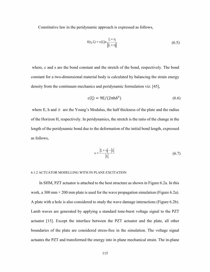
115

Constitutive law in the peridynamic approach is expressed as follows,

ξ + ηf(η,ξ) = c(ξ)s

ξ + η (6.5)

where, c and s are the bond constant and the stretch of the bond, respectively. The bond

constant for a two-dimensional material body is calculated by balancing the strain energy

density from the continuum mechanics and peridynamic formulation viz. [45],

c(ξ) = 9E (2πhδ )⁄ (6.6)

where E, h and δ are the Young’s Modulus, the half thickness of the plate and the radius

of the Horizon H, respectively. In peridynamics, the stretch is the ratio of the change in the

length of the peridynamic bond due to the deformation of the initial bond length, expressed

as follows,

ξ + η ξs =

ξ (6.7)

6.1.2 ACTUATOR MODELLING WITH IN PLANE EXCITATION

In SHM, PZT actuator is attached to the host structure as shown in Figure 6.2a. In this

work, a 300 mm × 200 mm plate is used for the wave propagation simulation (Figure 6.2a).

A plate with a hole is also considered to study the wave damage interactions (Figure 6.2b).

Lamb waves are generated by applying a standard tone-burst voltage signal to the PZT

actuator [15]. Except the interface between the PZT actuator and the plate, all other

boundaries of the plate are considered stress-free in the simulation. The voltage signal

actuates the PZT and transformed the energy into in plane mechanical strain. The in-plane

116

strain causes the rapid localized displacement in the host structure, which results in the

Lamb wave propagation in the plate. The Lamb wave modes create out of plane

displacements and hence, to accommodate such deformation three layers of material points

are used in the modeling (Figure 6.2b). Figure6.2c shows the discretization used in this

study which is further described in Section 6.1.4. Displacement in the structure varies

linearly along the length of the PZT and attains a maximum value at the boundaries [168]

as shown in Figure 6.2d. In this study, a square PZT with a dimension of 2.4 × 2.4 mm is

modeled by applying a maximum of 1 μm in plane radial displacement to the

circumferential material points, shown in the Figure 6.2d. The displacements of the

material points at the center of the PZT were enforced to zero. The equation for variation

of displacement due to the application of a tone burst signal is expressed as,

u(x, t) = U(x)e / sin (ω t) (6.8)

where, ωc and U(x) are the central frequency and the maximum displacement amplitude

of the excitation signal given to different material points, respectively. The parameter p

in the Equation (32) is expressed as,

p = (2khω N⁄ ) (6.9)

where, k , h and Nc are the signal shape factor, the half thickness of the specimen and the

number of cycles of the actuation signal, respectively. To select the desired excitation

frequency, the tuning curves for S0 and A0 modes in the Aluminum 6061-T6 were obtained

from an open source software “Waveform Revealer” [165], developed by the LAMSS

laboratory at the University of South Carolina (USC). As shown in Figure 6.3 a,b, the

central frequency of 150 kHz is chosen to make sure that only the S0 and A0 modes are

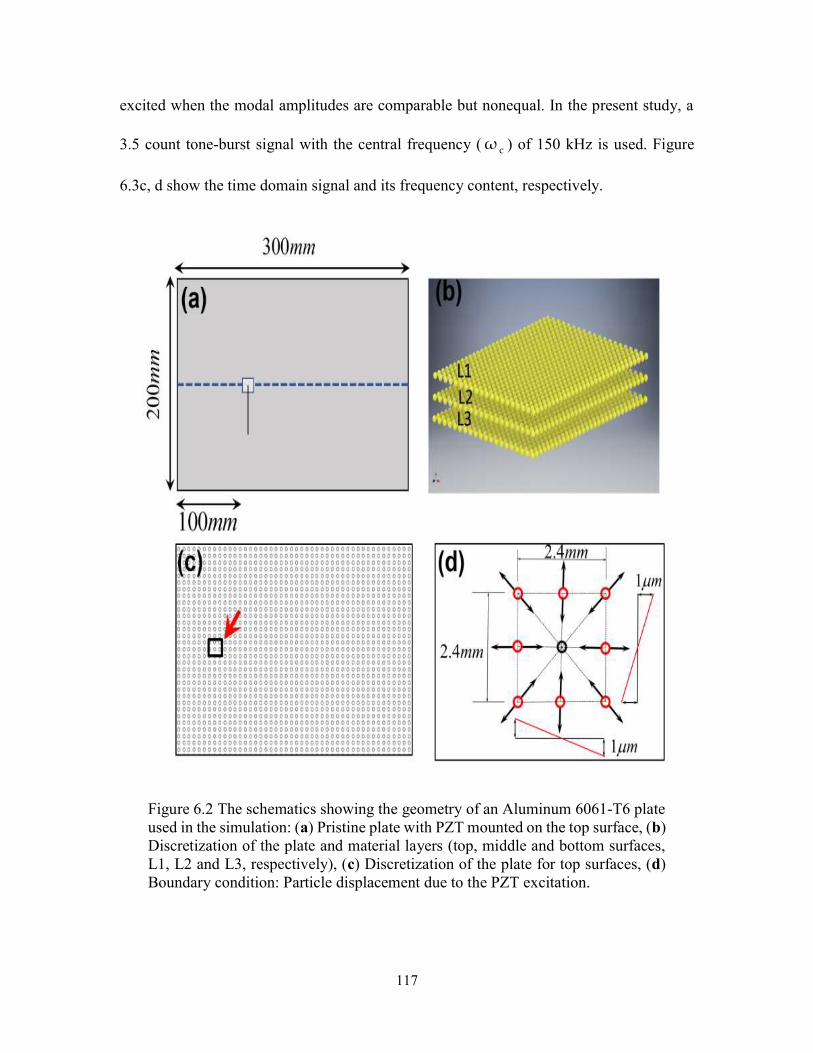
117

excited when the modal amplitudes are comparable but nonequal. In the present study, a

3.5 count tone-burst signal with the central frequency ( cω ) of 150 kHz is used. Figure

6.3c, d show the time domain signal and its frequency content, respectively.

Figure 6.2 The schematics showing the geometry of an Aluminum 6061-T6 plate used in the simulation: (a) Pristine plate with PZT mounted on the top surface, (b) Discretization of the plate and material layers (top, middle and bottom surfaces, L1, L2 and L3, respectively), (c) Discretization of the plate for top surfaces, (d) Boundary condition: Particle displacement due to the PZT excitation.

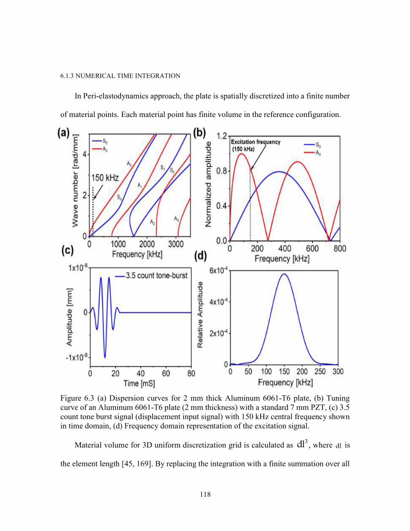
118

6.1.3 NUMERICAL TIME INTEGRATION

In Peri-elastodynamics approach, the plate is spatially discretized into a finite number

of material points. Each material point has finite volume in the reference configuration.

Figure 6.3 (a) Dispersion curves for 2 mm thick Aluminum 6061-T6 plate, (b) Tuning curve of an Aluminum 6061-T6 plate (2 mm thickness) with a standard 7 mm PZT, (c) 3.5 count tone burst signal (displacement input signal) with 150 kHz central frequency shown in time domain, (d) Frequency domain representation of the excitation signal.

Material volume for 3D uniform discretization grid is calculated as 3dl , where dl is

the element length [45, 169]. By replacing the integration with a finite summation over all

119

the material points inside the Horizon, the equation of motion at material point i after the

time step n can be expressed as,

n n n nρu = f(u u , x x )V + bi i i if f fN f

(6.10)

The net force (f) acting on a material point is calculated by summing the peridynamic forces

on the parent material point due to all the neighboring points inside its Horizon. N f

represents the number of material points within the Horizon enclosing the parent material

point i. The Velocity-Verlet integration [31] scheme is employed in this study to calculate

the displacements in the time domain for given boundary and initial conditions as follows,

Δtn+1/2 n nv = v + fi i i2ρi

Δtn+1/2 n n+1/2u = u + vi i i2ρi

n+1i

Δtn+1 n+1/2v = v + fi i 2ρi

(6.11)

Stability of the numerical solution can be obtained for a small-time step Δ t and a spatial

discretization step ΔS . To have a convergence of the displacements, the detailed procedure

to select the time step ( Δ t ) and spatial discretization ( ΔS ) is discussed in Section 6.1.4.

6.1.4 PERI-ELASTODYNAMIC SPATIAL AND TEMPORAL DISCRETIZATION

Proper spatial and temporal discretization are the critical parameters for the

convergence of the solution in wave propagation simulation. Maximum spatial

discretization ( ΔS ) must meet the criterion below [170],

120

cminλ =min f; ΔS = λ / 10min (6.12)

where, minλ is the minimum wavelength of the Lamb wave modes and minc is the minimum

phase velocity of the simulated modes at the excitation frequency f . Phase velocity at the

excitation frequency can be easily obtained from the theoretical dispersion curves. In this

work, the phase velocity of the 0A mode at 150 kHz is used as cmin in Equation (36). The

Courant–Friedrichs–Levy condition is used to obtain a numerically stable time step ( t)

[170].

ΔSΔt =

c 3max (6.13)

where, maxc is the maximum phase wave velocity of the propagating modes. In this work,

the phase velocity of the S0 mode at 150 kHz is the maxc in Equation (6.13). Thus, to obtain

a converging solution, the spatial and the temporal step sizes are chosen to be 1.2 mm and

0.01 μS, respectively, satisfying the Equations (6.12) and (6.13).

Material points are chosen in a grid fashion with a spacing of ΔS to model the plate

with a layer spacing of 1 mm between each layer L1, L2 and L3. 41,750 material points

were used in each layer in the pristine plate. A total of 125,250 material points was used in

the simulation including all the three layers L1, L2 and L3. In case of the damaged plate

(with hole), there was 41,610 material points in each layer and a total of 124,830 material

points were used for the Peri-elastodynamic simulation. Each parent point is assigned with

a family based on its Horizon and bonds were established between each pair of material

points within the family. A 3.015ΔS was used as the Horizon size in the simulation. To

121

model a plate with a through-thickness hole, a pristine discretization is performed and then

the material points are removed from the geometry to produce the hole.

6.2 LAMB WAVE DISPERSION RELATION

Dispersion curves of various Lamb wave modes are used to predict the existence of

various modes at a particular excitation frequency [15]. Two types of Lamb wave modes

exist in a plate based on the particle motion, named Symmetric modes (i.e., S0, S1, S2…)

and Antisymmetric modes (i.e., A0, A1, A2…). Generation of the Lamb wave modes in a

plate depends on the frequency of excitation, the thickness of the plate and the material

properties (Density, Young’s modulus or Shear Modulus and Poisson’s ratio) of the

material. Dispersion of various Lamb wave modes is obtained by solving Rayleigh-Lamb

wave equations. Rayleigh-Lamb wave equation for symmetric Lamb wave modes is

expressed by,

2tan(qh) 4k qp= 2 2 2tan(ph) (k q )

(6.14)

For antisymmetric modes, equation is written as follows,

2 2 2tan(qh) (k q )= 2tan(ph) 4k qp

(6.15)

Parameters in the above equations are expressed as,

p = − k ; q = − k ; 2μ(1 - ν)

c =L ρ(1 - 2ν);

μc =s ρ

(6.16)

122

where ω , k , cs , c L , ν , μ , ρ and h are the angular frequency, wavenumber, the shear

wave velocity, the longitudinal wave velocity, the poison’s ratio, the shear modulus, the

density and the half thickness of the plate, respectively. In this work, the dispersion curves

for various Lamb wave modes in an Aluminum 6061-T6 plate were calculated using the

commercially available ‘Disperse’ software [160], designed by the Imperial College,

London, UK, as shown in Figure 6.3a. The plate thickness was set to 2 mm and the material

properties were set to the values listed in Table 6.1

Table 6.1: Material properties.

6.3 NUMERICAL COMPUTATION AND RESULTS

The Peri-elastodynamic simulations were performed on a workstation with two Intel

Xeon (R) CPU E5-2650 V3 2.30 GHz processors with total 128 GB RAM, in a single core.

The simulation was run on MATLAB-18. a. One simulation was completed within a

reasonable time of ~24 h. Note that this problem is highly parallelizable and can be

implemented with distributed clusters, GPUs, multiple threads, or a combination of these

methods. Preliminary translation of this MATLAB program into multithreaded C++

resulted in a 20 times speedup.

Aluminum 6061-T6 Material Properties

Density, ρ 2700 kg/m3

Young’s Modulus, E 69 GPa

Poisson ratio, ν 0.33

123

6.3.1 LAMB WAVE PROPAGATION IN THE PRISTINE PLATE

In this work, fundamental Lamb wave modes (S0 and A0) are simulated which are

Figure 6.4 Time domain in plane and out of plane displacement waveform: (a) ( , , )xu x y t

at t = 20, 30 and 40 S , (b) ( , , )yu x y t at t = 20, 40 and 60 S , (c) ( , , )zu x y t at t = 20, 40

and 60 S )

124

widely used in the damage detection with ultrasonic SHM. Figure 6.4 shows the out of

plane displacements ( , , )zu x y t and, in plane displacements ( , , )xu x y t and ( , , )yu x y t for

the Lamb wave propagation plotted at t = 20, 40 and 60 μS, respectively. Each stack of the

figure is plotted with the respective displacement pattern in the layers L1, L2 and L3. It

can be seen that the S0 mode travels faster than the A0 mode and confirms the dispersion

curves. In wave propagation simulation, most inaccuracy comes from the boundary

reflections if the results are not converged. The best approach to judge if the simulation of

the wave propagation is converged is to evaluate the boundary reflections. In the present

simulation, the reflected modes from the plate boundaries are clearly visible in the figures.

Usually, there is a possibility of divergence of the solution at the boundaries due to the

nonconvergence of the solution. However, with the specific steps with the Peri-

elastodynamic process described in this paper, the results will be converged, and bounded

boundary reflections will be achieved.

In the top (L1) and the bottom (L3) layers in Figure 6.4(a-1–a-3) and Figure 6.4(b-1–

b-3), both Symmetric and Antisymmetric modes (S0 and A0) are visible in the wave fields

composed of in plane displacements. The contribution of the A0 mode in the in-plane

motion at the middle layer (L2) of the plate is negligible but the out of plane motion is

dominant. As shown in Figure 6.4(c-1–c-3), the out of plane displacement of the A0 mode

is visible (i.e., contribution from ( , , )zu x y t ) while the S0 mode is barely noticeable. This

is because the displacements of the in-plane particles of the S0 mode dominates over the

out of plane motion of the particles. Also, the contribution of the S0 mode in the

displacement

125

Figure 6.5 Space-time in plane and out of plane displacement fields: (a-1) ( , )xu x t at the

top (L1), (a-2) ( , )xu x t at the middle layer (L2), (a-3) ( , )xu x t at the bottom layer (L3), (b-

1) ( , )zu x t at the top layer (L1), (b-2) ( , )zu x t at the middle layer (L2), (b-3) ( , )zu x t at the

bottom layer (L3).

of the middle layer (L2) of the plate is negligible, because, in the S0 mode, the middle layer

(L2) remains undisturbed.

Time-space representation of the in plane ( ( , )xu x t ) and the out of plane displacement (

( , )zu x t ) are presented in Figure 6.5. Displacements at the top, middle and the bottom

surfaces (L1, L2 and L3), are presented to investigate the existence of the different Lamb

wave modes and their contribution to the displacement in each layer. In Figure 6.5(a-1–a-3),

it is observed that the S0 mode contributes to the in-plane displacement in all layers and the

A0 mode contributes only to the top and the bottom layers. Time-space representation of the

out of plane displacement is shown in Figure 6.5(b-1–b-3), which show that the A0 mode had

126

a higher amplitude than the S0 mode. A0 mode contributed to the displacement of all the

layers (L1, L2 and L3), whereas, S0 mode contributed only to the top (L1) and the bottom

(L3) layers.

6.3.2 VECTOR FIELD REPRESENTATION OF THE LAMB WAVE MODES

To prove the accuracy of the Peri-Elastodynamic (PED) simulation, the characteristics

of the Lamb wave modes (S0 and A0), in plane and out of plane particle motion across-the-

thickness are plotted in Figure 6.6, after 41 μS. Out of plane ( ( , , )zu x y t ) and in plane (

( , , )xu x y t ) displacement distribution of A0 mode are extracted along the cross-sections

C - C1 2 and ' 'C - C1 2 , of the plate. Similarly, the out of plane and the in-plane displacement

distribution of S0 mode is plotted along the cross-section lines D - D1 2 and ' 'D - D1 2 ,

respectively. Vector fields and displacement distributions are shown in Figure 6.6a–d. It is

observed in Figure 6.6a that all particles moved either upwards (+Z) or downwards (−Z)

with variable amplitude (like bending motion) due to the generation of the A0 mode. In

Figure 6.6c, the top and the bottom layers are symmetrically displaced with respect to the

mid-plane and the displacement of the mid-plane is almost zero due to the generation of

the S0 mode. In plane particle motion in A0 and S0 modes are also shown in Figure 6.6b, d.

In Figure 6.6b, the particles at the top and the bottom layers are moved in the opposite

directions along the in-plane direction and the displacement of the mid-plane is zero due

to the generation of the A0 mode. In Figure 6.6c, the particle displacements are constant

across the thickness due to the S0 mode. Vector fields and the mode shapes in Figure 6.6

indicate that the Peri-Elastodynamics simulated the Lamb waves accurately.

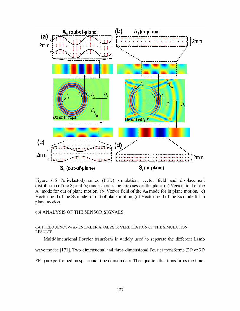
127

Figure 6.6 Peri-elastodynamics (PED) simulation, vector field and displacement distribution of the S0 and A0 modes across the thickness of the plate: (a) Vector field of the A0 mode for out of plane motion, (b) Vector field of the A0 mode for in plane motion, (c) Vector field of the S0 mode for out of plane motion, (d) Vector field of the S0 mode for in plane motion.

6.4 ANALYSIS OF THE SENSOR SIGNALS

6.4.1 FREQUENCY-WAVENUMBER ANALYSIS: VERIFICATION OF THE SIMULATION RESULTS

Multidimensional Fourier transform is widely used to separate the different Lamb

wave modes [171]. Two-dimensional and three-dimensional Fourier transforms (2D or 3D

FFT) are performed on space and time domain data. The equation that transforms the time-

128

space wavefield data into the frequency-wavenumber representation of the wave field and

can be expressed as follows [171],

𝑢 𝑘 , 𝜔 = 𝑢 𝑥 ,𝑡 𝑒 (𝐤.𝐱)𝑒 𝑑𝑥 𝑑𝑥 𝑑𝑡 (6.17)

where, 𝑗 take the values, 1 and 2, 𝑝 take values 1, 2 and 3, 𝑢 (𝑥 ,𝑡) designates the 𝑝-th

displacement after time 𝑡 at the point 𝑥 located on the 2D x-y plane. 𝑢 𝑘 , 𝜔 designates

the 𝑝-th displacement at frequency 𝜔 in reciprocal space of wavenumbers at the point 𝑘

located on the 2D reciprocal 𝑘 − 𝑘 plane. Here index, 1, 2 and 3 stands for the coordinate

x, y and z.

In multi-modal wave propagation analysis, distinguishing the different modes from a

time domain signal is difficult, especially on a small plate where the wave modes tend to

overlap. In this work, frequency-wavenumber plots are presented to visualize the different

modes separately. This is also verified by comparing the simulated dispersion results with

the theoretical dispersion curves. For this purpose, 2D and 3D Fast Fourier Transforms

(FFT) were performed on the simulated displacement wave field to obtain the frequency-

wavenumber representations.

To perform the 2D-FFT, out of plane ( ( , , )zu x y t ) and in plane ( ( , , )xu x y t ),

displacement data are obtained across-the-thickness of the plate along the selected red

dotted line shown in Figure 6.4(a-1). 163 spatial points with a resolution of 1.2 mm along

the red line shown in Figure 6.4(a-1) were used in the analysis. Matrix size used to store

the displacements wave field was 163 × 8000. Note that, the 2D FFT was performed on the

displacement vectors obtained from all the three material layers (L1, L2 and L3).

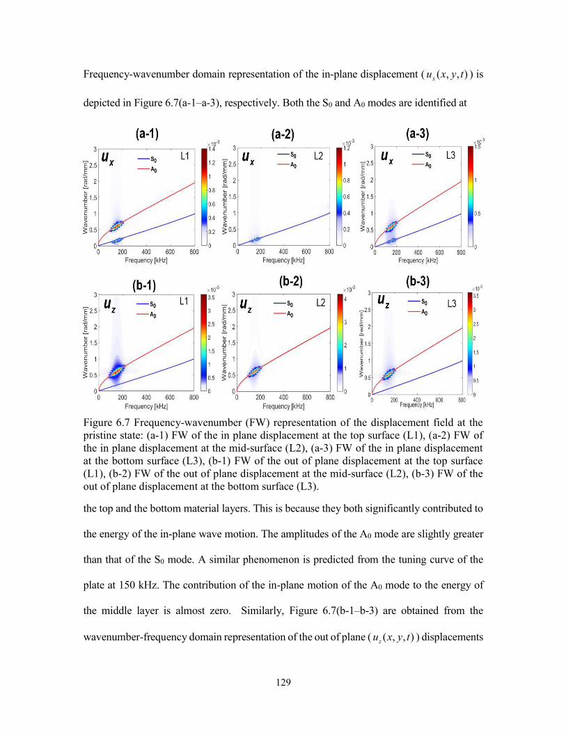
129

Frequency-wavenumber domain representation of the in-plane displacement ( ( , , )xu x y t ) is

depicted in Figure 6.7(a-1–a-3), respectively. Both the S0 and A0 modes are identified at

Figure 6.7 Frequency-wavenumber (FW) representation of the displacement field at the pristine state: (a-1) FW of the in plane displacement at the top surface (L1), (a-2) FW of the in plane displacement at the mid-surface (L2), (a-3) FW of the in plane displacement at the bottom surface (L3), (b-1) FW of the out of plane displacement at the top surface (L1), (b-2) FW of the out of plane displacement at the mid-surface (L2), (b-3) FW of the out of plane displacement at the bottom surface (L3).

the top and the bottom material layers. This is because they both significantly contributed to

the energy of the in-plane wave motion. The amplitudes of the A0 mode are slightly greater

than that of the S0 mode. A similar phenomenon is predicted from the tuning curve of the

plate at 150 kHz. The contribution of the in-plane motion of the A0 mode to the energy of

the middle layer is almost zero. Similarly, Figure 6.7(b-1–b-3) are obtained from the

wavenumber-frequency domain representation of the out of plane ( ( , , )zu x y t ) displacements

130

at the top (L1), middle (L2) and the bottom layer (L3), respectively. The energy distribution

of the A0 mode is higher than the S0 mode at all the material layers. The S0 mode is visible

only at the top and the bottom layers of very low amplitude. This is because the out of plane

motion of the particles in S0 mode is very low and the displacement at the midplane is

almost zero.

Next, the 3D-FFT is employed to transform the 3D displacement data ( ( , , )xu x y t ,

( , , )yu x y t and ( , , )zu x y t ) into the frequency-wavenumber domain ( ( , , )x x yu k k ,

( , , )y x yu k k and ( , , )z x yu k k ) and are shown in Figure 6.8a–c, respectively. In this work,

frequency transformation is performed only on the data obtained from the top surface (L1).

The size of the matrix used to store the 3D displacement data was 163 × 250 × 8000.

Figure 6.8 3D Fourier transform of the in plane and the out of plane displacement at the

top surface (L1). Wavenumber domain plots of (a) xu at 110 kHz, 150 kHz, 185 kHz and

225 kHz, (b) yu at 110 kHz, 150 kHz, 185 kHz and 225 kHz, (c) zu at 110 kHz, 150 kHz,

185 kHz and 225 kHz.

131

Wavenumber plots at the frequencies 110 kHz, 150 kHz, 185 kHz and 225 kHz, are

presented in the Figures. It is seen that both the S0 and the A0 modes appeared in the form

of two concentric circular rings. The radius of the circles corresponds to the wave numbers

at the respective frequencies. Wavenumbers of the S0 and A0 modes at the 150 kHz are

obtained from the Peri-Elastodynamic simulation and are 0.56 rad/mm and 0.187 rad/mm,

respectively. A smaller circle corresponds to the S0 while the larger corresponds to the A0

mode. It is also observed that the energy of the modes at the frequencies 110 kHz, 185 kHz

and 225 kHz are lower compared to that of at the 150 kHz. This is because most of the

energy of the modes is concentrated around the excitation frequency (150 kHz).

Figure 6.9 Comparison of theoretical and numerical (Peri-Elastodynamics) wavenumber domain at 150 kHz: (a) xu at 150 kHz, (b) yu at 150 kHz, (c) zu at 150 kHz.

To verify the directional dependency of the Lamb wave propagation, 2D wavenumber

plots ( ( , )x x yu k k , ( , )y x yu k k and ( , )z x yu k k ) at ω = 150 kHz, are obtained from the 3D FFT

and were compared with those obtained from the theoretical predictions using Disperse

software at 150 kHz. Theoretical wavenumber plot is superimposed on the numerically

obtained wavenumber plots in Figure 6.9a–c. Good agreements between the numerical and

analytical results are obtained. It shows that the Peri-elastodynamic can predict the

dispersion relation of fundamental Lamb wave modes accurately in all directions.

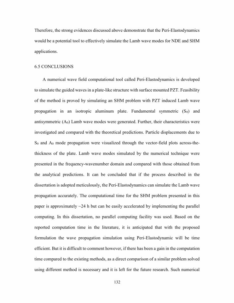
132

Therefore, the strong evidences discussed above demonstrate that the Peri-Elastodynamics

would be a potential tool to effectively simulate the Lamb wave modes for NDE and SHM

applications.

6.5 CONCLUSIONS

A numerical wave field computational tool called Peri-Elastodynamics is developed

to simulate the guided waves in a plate-like structure with surface mounted PZT. Feasibility

of the method is proved by simulating an SHM problem with PZT induced Lamb wave

propagation in an isotropic aluminum plate. Fundamental symmetric (S0) and

antisymmetric (A0) Lamb wave modes were generated. Further, their characteristics were

investigated and compared with the theoretical predictions. Particle displacements due to

S0 and A0 mode propagation were visualized through the vector-field plots across-the-

thickness of the plate. Lamb wave modes simulated by the numerical technique were

presented in the frequency-wavenumber domain and compared with those obtained from

the analytical predictions. It can be concluded that if the process described in the

dissertation is adopted meticulously, the Peri-Elastodynamics can simulate the Lamb wave

propagation accurately. The computational time for the SHM problem presented in this

paper is approximately ~24 h but can be easily accelerated by implementing the parallel

computing. In this dissertation, no parallel computing facility was used. Based on the

reported computation time in the literature, it is anticipated that with the proposed

formulation the wave propagation simulation using Peri-Elastodynamic will be time

efficient. But it is difficult to comment however, if there has been a gain in the computation

time compared to the existing methods, as a direct comparison of a similar problem solved

using different method is necessary and it is left for the future research. Such numerical

133

computation is valuable for the computational NDE of structures and devices, where

experimentally studying the wave damage interactions are expensive tasks. In future,

virtual wave propagation in structure using the complementary tools will help avoid

expensive experiments but extract the right wave feature to first characterize and then

certify the materials and devices.

134

CHAPTER 7

EXPERIMENTAL VALIDATION OF PERIDYANMIC SIMULATION FOR GUIDED LAMB WAVE PROPAGATION AND DAMAGE

INTERACTION

In this chapter, PED was further extended to simulate Lamb wave-damage interaction

with specific damages scenarios such as cracks in aluminum 6061-T6 plate. PED simulated

sensor signals for pristine and damaged plate were verified with those obtained from

conducting pitch-catch experiments on plates with similar dimensions and damage

scenarios. Further, accuracy of PED was investigated by comparing simulated symmetric

and anti-symmetric Lamb wave modes to the experimenal results. Additinally, effeciency

of the PED was investigated by comparing simulation parameters (i.e., Memory

requirement, Simulation run time and CPU core used) with FEM based COMSOL

simulation results.

7.1 MATERIAL GEOMETRY AND CRACK MODELLING

The wave-damage interaction study is performed using a through-thickness crack of

length 16 mm x 2.4 mm, located at a 70 mm distance from the PZT actuator (Ref. Fig. 7.1).

A crack on the centerline (red dotted line in Fig. 7.1) and a crack offset from the centerline

are considered as shown in Fig. 7.1(a) and 7.1(b). Spatial and the temporal step sizes are

chosen to be 1.2 mm and 0.01 μS, respectively, satisfying the requirements of equations

(6.12) and (6.13). A total of 41,750 material points was used to discretize each layer. Each

parent point is assigned with a family based on its Horizon and bonds were established

135

between each pair of material points within the family. A 3.015ΔS was used as the Horizon

size in the simulation. To model a plate with a through-thickness crack, first a pristine

discretization is performed and then crack is modelled by assigning bond constant zero to

bonds those pass through the crack zone.

Figure 7.1 The geometry of aluminum 6061-T6 plate with crack: (a) central-crack, (b) offset-crack.

7.2 EXPERIMENTAL DESIGN FOR THE VALIDATION OF PED

To validate the PED results, pitch-catch experiments were conducted on pristine and

damaged aluminum 6061-T6 plates as shown in the Figure 7.2a and 7.2b. In this study, the

plates with a crack along the center line and with a crack offset from the center line were

considered as shown in Figure 7.2c & Figure 7.2d. Dimensons of the plate are the same as

used in the PED simulation. Two high-frequency PZT (type PZT 5A, Purchased from

STEMiNC, Florida) were attched to the plate with Hysol 9340 adhesive. PZT’s were 7

mm in diamater and 0.5 mm in thickness. Distance between two PZT’s was kept 104 mm,

measured from their center. One of the PZT was used as an actuator while the other was

used as a sensor. A 3.5 count tone-burst, with a central-frequency of ~150 KHz and ~20V

amplitude (~10V peak-to-peak) was used to excite the actuator to generate the Lamb wave

136

propagation in the plate. Tektronix AFG3021C (25 MHz, 1-Ch Arbitrary Function

Generator, Tektronix Inc.) was used to generate the tone-burst actuation at the interval

of 1 ms and Tektronix MDO3024 (200 MHz, 4-Ch Mixed Domain Oscilloscope,

Tektronix Inc.) was used to record the signals from the sensor. Sensor signal was

recorded after averaging a total of 500 signals (to improve signal-to-noise ratio).

Sampling rate and signal length were set to 50MS/s and 10,000, respectively.

Figure 7.2 (a) Experimental set-up of pitch-catch experiments, (b) Pristine plate, (c) Plate with a center-crack, (d) Plate with a offset-crack.

137

7.3 COMPUTATIONAL VERIFICATION OF THE SIMULATION

Commercially available Finite Element (FE) based computational tool COMSOL

Multiphysics was used to simulate the structural mechanics problem coupled with the

piezoelectric actuator and sensor. To model the ultrasonic guided wave propagation in the

aluminum plate, Solid Mechanics and Electrostatics modules, a multi-physics approach in

COMSOL, was employed. COMSOL utilizes implicit scheme to solve the transient

problems. In this study, the direct solver MUMPS was chosen over an iterative solver for

its robustness. All the direct solvers in COMSOL require significant amounts of RAM

where MUMPS can store the solution out-of-core i.e., on to the hard disk. Moreover,

MUMPS is substantially faster than iterative solvers. The absolute tolerance of the time-

dependent solver used a global method of scaling with a specified tolerance of 0.001. The

setting for time steps was set to generalized-alpha method with intermediate time steps,

a linear predictor and a maximum time step of 50 ns.

The mechanical and electrical properties of the aluminum plate and the piezoelectric

components were considered same as the properties used in the experimental design. To

excite the PZT of the actuator, a 20V 3.5 count tone-burst signal was applied at the electric

potential terminal. The signal response was collected from the sensing PZT for the entire

duration of the simulation which was 80 𝜇𝑠. Free tetrahedral (tets) meshes generated by

COMSOL multi-physics were utilized to generate mesh for the entire aluminum domain

where the minimum mesh size was varied from 0.1 mm to 1.2 mm as shown in Figure 7.3

(b&c). On the other hand, the minimum mesh size for the PZT actuator and sensor were

varied from 0.01 mm to 0.2 mm as shown in Figure7.3(a). A mesh convergence study was

performed starting from the maximum mesh size of 2 mm to a minimum mesh size of 1.2

138

mm. As the mesh size was decreased the accuracy of the simulation improved at the

expense of increased computational time. A total of 24 CPU cores with a maximum

memory of 80 GB were utilized to solve this problem in 45 hours.

Figure 7.3 Three-dimensional FE discretization of the aluminum plate and PZT: (a) Discretization of the PZT, (b) Discretization of the plate and PZT, (c) Discretization of the plate.

7.4 VALIDATION AND VERIFICATION OF THE PED SIMULATION

In this section, accuracy and efficiency of the PED technique to simulate Lamb wave

propagation is presented. Time domain signal (at sensor location S1) obtained from the

PED was compared with the numerically (COMSOL) and analytically

(WaveFormRevealer [172, 173]) obtained sensor signals and the signals acquired from the

pitch-catch experiments on a pristine aluminum plate. Note that, in this study a square PZT

139

was employed for PED simulation whereas circular PZT was used for COMSOL and the

experiment. However, due to isotropic nature of the plate, at the far-field wave fronts were

circular and the guided wave mode when fully developed, the effect of PZT size was not

diagnosed. In plane displacement ( ( , , )xu x y t ) from the PED was used to compare with the

output voltage obtained from COMSOL, WFR and Experiment. Since sensor in the plate

is located on the center line along the X-axis as shown in Figure 7.2. (b, c and d), output

voltage at sensor terminal is contributed primarily by ( , , )xu x y t . To capture sensor signal

from the PED simulation, time-domain signal was collected from a material point located

at 97 mm away from the PZT edge along the center line from the actuator ( 104centerL mm

& 97effL mm ). Normalized amplitude of the sensor signals obtained from Experiment,

COMSOL, WFR and PED, respectively, was plotted in the time-domain as shown in the

Figure 7.4. Sensor signals obtained from the PED, COMSOL and WFR were also

compared with the experimental results to check the accuracy of those techniques. Good

agreement between PED and the experiment was observed for both symmetric and anti-

symmetric modes as shown in the Figure 7.4.b. the symmetric mode from COMSOL is in

good agreement with the experiment whereas the anti-symmetric mode slightly deviates as

shown in the Figure 7.4.c, WaveFormRevealer (WFR) predicted the anti-symmetric mode

well but overestimated the symmetric mode as shown in the Figure 7.4.d. Mismatch of the

symmetric mode may be attributed to limitation of the WFR software such as, being an

analytical method, material property of PZT could not be provided. To verify accuracy of

the proposed PED techniques and to compare with existing simulation techniques, error of

symmetric and anti-symmetric mode is calculated by comparing them with experimental

results by using the Eq.7.1.

140

2exp

exp

( ( ) ( ))

100

( )

f

i

f

i

t

env envsim

t

t

env

t

A t A t dt

Error

A t dt

(7.1)

Where, ( ) ( ( )envsim simA t H A t ; exp( ) ( ( )env

expA t H A t (7.2)

( )envsimA t and ( )env

expA t are the envelope of experimental and simulated sensor signal.

A similar approach was used to calculate error of the COMSOL and WFR predicted

sensor signal. Error analysis results are shown in the Figure 7.4.e. Error of symmetric and

anti-symmetric mode of the PED simulation were 2.2% and 0.5%, respectively, which is

less than the maximum permissible error tolerance of 3%. Significant error for symmetric

mode of the WFR was observed. Error percentage for COMSOL simulation was 2.2% and

0.5%, respectively. PED simulation provided a better accuracy for wave propagation

simulation then COMSOL and WFR.

To investigate the efficiency of the PED with respect to other numerical tool, to solve

the proposed wave propagation problem, memory requirement, simulation run time and

CPU core used for both PED and COMSOL were plotted in the Figure 7.4.f. Note that,

element size was kept same. While COMSOL can use multiple cores (i.e., 24 cores) for

running the simulation, PED used only one core. Memory consumption and simulation run

time for PED is smaller than that of COMSOL simulation. However, parallelization of the

PED code can improve simulation run time significantly.

141

Figure 7.4 Time-domian comaprison of sensor signal: (a) Experiment, COMSOL, WFR and PED, (b) PED and Experiment, (c) Comsol and Experiment, (d) WFR and Experiment, (d) Error of simulated symmteric and anti-symmteric modes with respect to experimental results, (d) Memory requirement and simulation run time of PED and COMSOL simulation.

Simulation results from the central-crack and offset-crack are presented in Figure 7.5

and 7.6, respectively. To observe the reflection and transmission of the respective wave

modes from the damage location, in-plane displacement wavefields, after three different

time steps (40µS, 50µS and 60µS), are shown in Figure 7.5(a1-a3). It can be seen that,

while the reflected S0 mode from the crack location is observed after time 40µS, the same

mode disappeared after 50µS and 60µS due to the interference with the parent mode with

the reflected boundary mode. Alternatively, reflected A0 mode is identifiable after both

50µS and 60µS time steps. In case of out-of-plane displacements, reflected S0 mode is not

quite

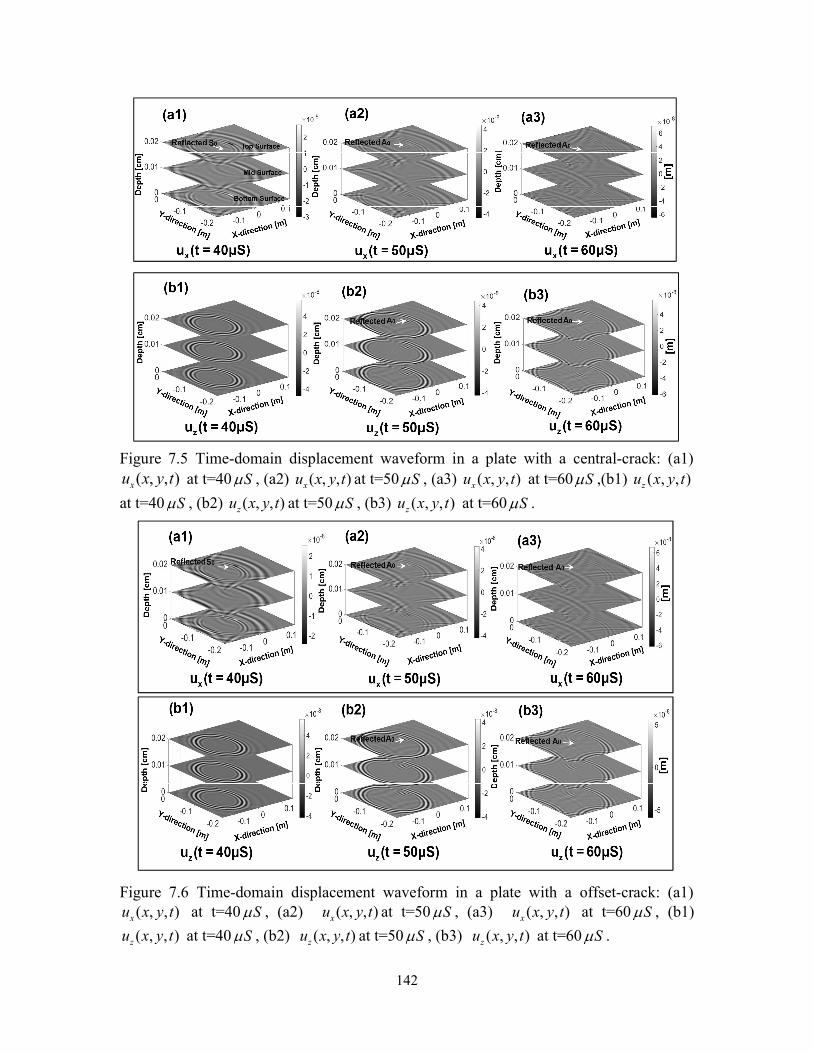
142

Figure 7.5 Time-domain displacement waveform in a plate with a central-crack: (a1) ( , , )xu x y t at t=40 S , (a2) ( , , )xu x y t at t=50 S , (a3) ( , , )xu x y t at t=60 S ,(b1) ( , , )zu x y t

at t=40 S , (b2) ( , , )zu x y t at t=50 S , (b3) ( , , )zu x y t at t=60 S .

Figure 7.6 Time-domain displacement waveform in a plate with a offset-crack: (a1) ( , , )xu x y t at t=40 S , (a2) ( , , )xu x y t at t=50 S , (a3) ( , , )xu x y t at t=60 S , (b1)

( , , )zu x y t at t=40 S , (b2) ( , , )zu x y t at t=50 S , (b3) ( , , )zu x y t at t=60 S .

143

visible in any of the time steps (See Figure 7.5(b1 – b3)) due to its minor contribution to

the out-of-plane wave propagation. However, reflected A0 mode is observed after both

50µS and 60µS time steps.

In-plane displacement wave fields for offset-crack (See Figure 7.1(b)) after times

40µS, 50µS and 60µS are shown in Figure 7.6(a1-a3). Both reflection and transmission of

the fundamental Lamb wave modes are observed. Similar to the center-crack scenario, in

the case of the offset-crack, the reflected S0 mode is observed only after the time 40µS.

Reflection of the S0 mode after other two-time steps is barely noticeable due to the

interference with the boundary reflections. However, the reflected A0 mode is visible after

50µS and 60µS. Evaluating Figure 7.6(b1-b3), in comparison to the center-crack, a similar

argument can also be made for the offset-crack in relation to the A0 and S0 modes existed

at different time steps.

Next, to distinguish the amplitude of the reflected and transmitted Lamb wave modes,

time-space representation of the in-plane and out-of-plane displacements for both the

scenarios with center-crack and the offset-crack are analyzed. Displacement wave fields

are computed along a selected line shown in the Figure 7.1b. In case of the center-crack

scenario, both the in-plane ( ( , )xu x t ) reflection and the transmission of the incident wave

are clearly visible in Figure 7.7(a1). A similar phenomenon can also be noticed from Figure

7.7(a2) for the center-crack out-of-plane displacement ( ( , )zu x t ). Boundary reflection of

the modes can be observed in Figure 7.7(a1 and a2). Likewise, in case of offset-crack

scenario, reflection and transmission from the offset-crack damage are also demonstrated

in Figure15(b1 and b2) considering the in-plane and the out-of-plane displacement modes.

144

Further the time history signals from the damage free pristine plate at sensor location

S1 marked in Figure 7.1a are compared with the signals from the center-line crack and

offset-crack scenario. Fig. 7.8.a compares the output response (at S1) obtained from

experiments for pristine, center-crack and offset-crack, respectively. Figure7.8. b compares

the output response (at S1) obtained from PED for the pristine, center-crack and offset

crack, respectively. it can be seen that the first arrival of the symmetric and anti-symmetric

wave modes for both experiment and PED at the sensor location S1 are slightly delayed

Figure 7.7 Space-time wavefield representations for the top surface of the plate with a through-thickness crack: (a-1) ( , )xu x t for a plate with a central-crack, (a-2) ( , )zu x t for a

plate with a with a central-crack, (b-1) ( , )xu x t for a plate with offset-crack, (b-2) ( , )zu x t

for a plate with offset- crack.

145

Figure 7.8 Comparison of time dependent signals obatined from PED and experiment at sensor location S1, in a pristine plate, plate with a crack along centerline and a plate with a off-set crack a) sensor signals at location S1 obtained from experiment, b) sensor signals at location S1 obtained from PED, c) sensor signals for centerline crack obtained from PED and experiment, d) sensor signals for offset crack obtained from PED and experiment.

due to the encounter of the crack. The delay is comparatively higher at S1 location due to

the center-line crack, compared to the offset-crack. Due to an offset-crack edge, the

reflected wave energy reflects at an angle and the senor S1 on the centerline have less effect

compared to a crack present along the centerline. In Figure 7.8.c, sensor signal for center-

line crack obatined from both PED and experiment compared. Error of symmetric and anti-

symmetric wave modes by PED prediction was 1.92% and 0.479%, respectively. In Figure

16.d, sensor signal for offset-crack obatined from both PED and experiment compared.

Error of symmetric and anti-symmetric wave modes by PED prediction was 1.21% and

146

0.81%, respectively. These features were properly simulated by the PED method. Hence,

it can be concluded that PED method is a suitable wave simulation tool for computational

NDE and SHM.

7.5 CONCLUSION

In this chapter, accuracy of the PED was tested. Time domain sensor signals from PED

was compared with those obtained from experiments, analytical (WaveformRevealer

[131]) and COMSOL. It was found that PED simulated Lamb wave modes accurately.

Error of symmetric and anti-symmetric Lamb wave modes by PED prediction was less than

3%. PED was found to very efficient (in terms of memory consumption and simulation run

time) compare to COMSOL. PED was also extended to wave-damage interaction

simulation by considering plate with cracks (i.e., centerline-crack and offset-crack

scenario) and verified with experimental results for center and offset-crack. PED method

can be employed as a suitable wave propagation simulation tool for computational NDE

and SHM.

147

CHAPTER 8

SUMMARY AND CONCLUSIONS

Material state awareness (MSA) of composites using conventional Structural health

monitoring (SHM) and Nondestructive Evaluation (NDE) method is limited by finding the

size and the locations of the cracks and the delamination in a composite structure. To aid

the progressive failure models using the gradual degradation model, the awareness of the

precursor damage state and quantification of the degraded material properties at the early

stage is necessary, which is challenging using the current SHM/NDE methods.

To quantify the material degradation during early stage of damage of composites,

online method, named guided coda wave interferometry (CWI) was employed for damage

accumulation quantification in woven composite material under cyclic loading. Stretch

parameter (Quantifies change in the coda wave) was measured by performing cross-

correlation of two consecutive sensor signals collected at specific cycle interval during

fatigue loading. Damage growth in the composite material was obtained from the

cumulative stretch parameter. Precursor damage events and stress-relaxation were

identified from the damage growth curve. To verify the online method, a complementary

offline NDE method, named Quantitative Ultrasonic Image Correlation (QUIC) based on

scanning acoustic microscope was employed. The unique combination of nonlocal

mechanics and scanning acoustic microscope resulted in a parameter called Nonlocal

Damage Entropy for the precursor awareness. During the early stage of the life of the

composite, the nonlocal damage entropy was plotted to demonstrate the degradation of the

148

material properties via awareness of the precursor damage state. Visual proofs for the

precursor damage states are provided with the digital images obtained from the micro-

optical microscopy, the scanning acoustic microscopy and the scanning electron

microscopy. It was found that sensor signals and QUIC data are influenced by stress-

relaxation phenomena of the composite. To verify, CWI was extended to quantify stress-

relaxation phenomena in the composites and which was verified by nonlinear ultrasonic of

Lamb wave.

Stress-relaxation phenomena in composites is characterized by CWI and nonlinearity

analysis in Lamb wave propagation. Cumulative stretch parameter from the CWI analysis

was found to be sensitive to stress-relaxation in composites. The second-order nonlinearity

parameter of the Lamb wave was also found to be influenced by damage and relaxation.

Remarkably, ~27% reduction of acoustic-nonlinearity was observed during the relaxation

periods. The relaxation parameters (i.e., rate and degree) were correlated to the fatigue

cycles and loading frequencies.

Experimental data obtained from the MSA can be included in a predictive tool for

accurate wave propagation simulation. Degradation parameters and relaxation parameters

from experiments can be included in a computational NDE tool for accurate prediction of

signals from diagnostic embedded sensors. Additionally, to understand the sensor signals

and extract damage information, a new efficient and accurate wave propagation tool was

devised.

Peridynamic based elastodynamic computation tool named Peri-elastodynamics

(PED) was developed to simulate the Lamb wave modes in materials. This newly

developed technique can simulate the fundamental Lamb wave modes accurately. In

149

addition to simulating the guided ultrasonic wave modes in pristine material, PED was also

employed to simulate Lamb wave propagation in plate with crack. The accuracy of the

proposed technique is verified by comparing results with those obtained from experiments.

The proposed tool is expected to significantly advance the virtual analysis of wave

propagation, computational nondestructive evaluation (CNDE) and computational

structural health monitoring (CSHM).

150

CHAPTER 9

SUBSURFACE PRESSURE PROFOLING: A NOVEL MATHEMATICAL PARADIGM FOR COMPUTING COLONY PRESSURE ON

SUBSTRATE DURING FUNGUL INFECTIONS

With changes in global climate, fungal pathogens are a growing global threat to

human health, agricultural sustainability, and economy [174-180]. Contamination of crops

with mycotoxins upon infections by plant pathogens result in an annual loss of $1.3-2.5

billions only to the United States alone [181]. In addition, fungal infections in humans have

significantly increased globally with the increasing immunocompromised world

population over the last two decades [182]. Children and the elderly, as well as individuals

undergoing organ transplantation or other major surgery, or who are suffering from AIDS

are at high risk of developing life-threatening fungal infections from common human

pathogens such as Candida albicans, Aspergillus fumigatus, and Cryptococcus neoformans

[183, 184]. It is estimated that the total direct cost for US healthcare to treat these invasive

fungal infections is $2.6 billion annually with an average per patient cost of approximately

$31,000 [185, 186]. Hence, there is a new drive for discovery of new antifungal molecules,

which will need reliable and robust quantitative tools for determination of therapeutic

efficacy. Such tools should be able to accurately compare fungal expansion and potency of

hyphal penetration in a host under pathophysiological and therapeutic conditions.

151

To address the critical need for quantitative tools for measuring fungal invasion, we

have recently developed a methodology for 3D tomography of a growing fungal colony

[187]. We have already demonstrated in Aspergillus parasiticus, an aflatoxin producing

plant pathogen, that our method that we call Quantitative Acosutic Contrast Tomography

(Q-ACT), can provide physical strength profiles (viscoelastic parameters) as well as hyphal

architecture at multiple scales in a growing colony [187]. In this study we have expanded

the functionality of Q-ACT by investigating the physical changes that occur within the

substrate beneath and around the fungal colony. It is already established that fungal

invasions during infection are associated with enormous turgor pressure [188] that helps

the hyphae to penetrate the substrate [188-191]. We reason that such an orchestrated

pressure distribution on the substrate will depend on the mycelial growth pattern and the

physical parameters that determine the strength of the fungal hyphae. Interestingly, our

recent Q-ACT based studies already demonstrated that physical strength profiles within the

mycelia correlate inherently with secondary metabolism [187] suggesting that pressure

profiles generated by fungal colonies are critical determinants of their metabolic state as

well as their invasiveness into the substrate. Currently, very little is known about relation

between the generation of the pressure by a fungal colony on the substrate and the

collective physical behavior of the multicellular system of the fungal colony. The primary

reason for this knowledge gap is the absence of an existing methodology to map the

pressure profiles exerted by a fungal colony on its substrate. In this work, we introduce an

analytical model for computation of the mechanical pressure exerted by an A. parasiticus

colony.

152

Figure 9.1 Wrinkle formation within the Aspergillus growth medium: (a) A. parasiticus grown on solid YES agar growth medium for 2d was studied using Q-ACT. Lower panel illustrates the force profiles exerted on the solid agar substrate from the colony edge within inset E; (b) Representative ultrasound micrographs along the depth obtained from Q-ACT at the colony edge within inset E, green arrows denote the wrinkles observed in the substrate due to colony expansion; (c) Demonstration of the variation of wrinkle wavelengths along the depths of agar that are 16 m apart; (d) plot of wrinkle wavelength along depth of the substrate

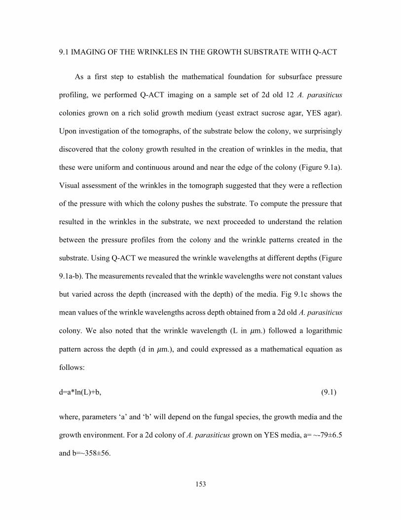
153

9.1 IMAGING OF THE WRINKLES IN THE GROWTH SUBSTRATE WITH Q-ACT

As a first step to establish the mathematical foundation for subsurface pressure

profiling, we performed Q-ACT imaging on a sample set of 2d old 12 A. parasiticus

colonies grown on a rich solid growth medium (yeast extract sucrose agar, YES agar).

Upon investigation of the tomographs, of the substrate below the colony, we surprisingly

discovered that the colony growth resulted in the creation of wrinkles in the media, that

these were uniform and continuous around and near the edge of the colony (Figure 9.1a).

Visual assessment of the wrinkles in the tomograph suggested that they were a reflection

of the pressure with which the colony pushes the substrate. To compute the pressure that

resulted in the wrinkles in the substrate, we next proceeded to understand the relation

between the pressure profiles from the colony and the wrinkle patterns created in the

substrate. Using Q-ACT we measured the wrinkle wavelengths at different depths (Figure

9.1a-b). The measurements revealed that the wrinkle wavelengths were not constant values

but varied across the depth (increased with the depth) of the media. Fig 9.1c shows the

mean values of the wrinkle wavelengths across depth obtained from a 2d old A. parasiticus

colony. We also noted that the wrinkle wavelength (L in 𝜇m.) followed a logarithmic

pattern across the depth (d in 𝜇m.), and could expressed as a mathematical equation as

follows:

d=a*ln(L)+b, (9.1)

where, parameters ‘a’ and ‘b’ will depend on the fungal species, the growth media and the

growth environment. For a 2d colony of A. parasiticus grown on YES media, a= ~-79±6.5

and b=~358±56.

154

Based on the wavelength profile, we hypothesized that the pressures exerted by the colony

were also not uniform across the depth. Hence, we proceeded to determine the pressure

profiles using a computational analysis based on the fundamental physics of incremental

stress.

9.2 FORMULATION OF THE RELATION BETWEEN SUBSTRATE WRINKLES AND THE PRESSURE DISTRIBUTION FROM THE FUNGAL COLONY

Euler buckling theory is conventionally employed in Engineering to predict the

critical buckling pressure. According to this theory, buckling pressure is inherently

correlated to the mode of buckling, which represents the number of inflection points in the

structure. However, previous studies have indicated that the Euler buckling theory is most

effective in predicting the critical buckling pressure when the thickness of the medium is

~5 times less than the wavelength of the instabilities. Below the wavelength/thickness ratio

~5, the Euler theory results infinite critical pressure [192], as shown in Fig. 9.2. To avoid

such singularity problem, Biot’s incremental stress theory was proposed [192]. Biot’s

theory was used extensively in geophysics to study low–amplitude wrinkle formation in

the stratified sedimentary rock bed [192-197]. According to this theory, wrinkles originated

from the instability caused by compressive load acting parallel to the media [195, 196,

198]. A general relation between the wrinkle wavelengths and the critical compressive load

was formulated to quantify the pressure required to form the wrinkles in the rock bed. It

has been used extensively for the study of folding in isotropic material as well as in

anisotropic and viscoelastic media [192, 193, 199, 200]. In this work, since a fungal colony

is bounded by its growth medium, we reasoned that the application of incremental stress

theory [201] in viscoelastic media proposed by Biot is not adequate to calculate the critical

pressure exerted by a fungal colony.

155

Figure 9.2 Comparison of Critical pressure / Shear modulus ratio with the Wavelength/Thickness ratio obtained from the Euler buckling theory and the linearized Biot theory. Euler theory predicts that critical pressure goes to infinity when Wavelength/Thickness ratio is less than ~5, whereas, Biot’s theory predicts a finite value at the same range.

To address the uniqueness of the wrinkles created by a fungal colony, here we modified

the Biot’s formulation and derived the equilibrium equation from the fundamental physics

by applying the physics of incremental stress theory, which allowed us to determine the

physics of deformations of the agar medium under the initial stress with small incremental

perturbations. Incremental stresses at a point is generated due to the displacement and

rotation of the continuum body from the reference to deformed configuration [202]. In the

conventional linear continuum mechanics incremental stresses are not considered.

However, for determination of pressure profiles below the Aspergillus colony, the

156

incremental stress was a critical feature that needed consideration. Based on our visual

assessment of creation of wrinkles with fungal growth, we speculated that the when

sufficient initial stress builds up on the growth medium due to expansion of the pathogenic

colony, wrinkles are developed due to the resistance by the media. As the colony expanded,

further pressure applied on the agar media acted as the initial stress and was further

incremented. This incremental pressure was less than the initial pressure that existed in the

medium.

Our proposed analytical model is shown in Figure 9.3. The model takes into account

the assumption for a fungal colony, that the incremental stress is much smaller than the

initial stress as described above. The annotations used to denote the stress fields are

described under SI-1. Based on our observations that the colony predominantly expands

radially, we considered that the initial stresses acting on the growth medium were only

axial stress (S11= Px). The vertical pressure (S22) and shear stress (S12) were neglected based

on the assumption that the colony weight was negligibly smaller than the value needed to

create a wrinkle in the agar medium. Further, in our analysis, vertical pressure is developed

due to the accumulation of the fungal biomass on the surface of host medium. However,

the wrinkles that formed as a result were away from the colony (Figure 9.1). Formation of

wrinkles were not observed in a 1d old colony but were clearly visible in 2d old colonies,

which suggested that a minimum threshold physical strength profile of the colony is needed

to exert enough pressure from the colony tips to form such wrinkles. The phenomenon was

repeatable in all 12 A. parasiticus colonies that were studied. Based on these observations

we conducted all the computational analyses for this work with 2d old colonies.

157

Figure 9.3 A schematic illustration of our proposed incremental stress model. Upper panel. Force profiles resulting from colony edge pushing onto the substrate. Incremental stress condition in the cube within the substrate is shown below. Lower panel. I. Representation of initial stresses S11, S12, S22 and the incremental stresses s11, s12, s22. II. sξξ, sηη, sηξ are the increment of total stress at the displacement point P(ξ,η) after deformation.

Through rigorous mathematical derivation, applying the incremental stress theory the

linearized equation of equilibrium for incremental displacement could be written as [192]

+2A +B =0

158

+2A +B =0, (9.2)

Where, u and v are the displacement of the medium along X & Y direction, respectively.

Coefficients A and B are the function of the initial stresses and the material properties and

could be expressed as [192],

A= [𝐴 -(B+S11+G) (B+S22+G) + (S22+G) (S11+G)]/ [2A (S22+G)],

B= (S11+G)/ (S22+G), A=2G+λ, B=λ, G=E/ [2(1+ ν)]

λ=Eν /[(1+ ν)(1-2ν)],

Where, G is modulus of Rigidity, E is Young's modulus, ν is Poisson's ratio and G and λ

are the lame’s constant, respectively. Total displacements are equal to the initial

displacement plus the incremental displacement. Incremental boundary stresses which is

defined as the difference between the actual boundary forces after deformation and their

initial value before deformation were expressed as [203]

Δfx = ( S11 - S12ω + S11eyy - S12exy) cos (n,x) + (S12 – S22ω -S11exy +S12exy) cos (n,y)

Δfy = (S12 + S11ω + S12eyy – S22exy) cos (n,x) +(S22 + S12 ω -S12exy +S22exx) cos (n,y) (9.3)

where S11, S12 S22 are the incremental stress components, S11,S22, and S12 are Intital stress

components, exx, exy, and eyy are the strain components,respectively.

Since our Q-ACT revealed that wrinkles are formed a sinusoidal pattern, we used

sinusoidal displacement function that satisfied the boundary condition and was assumed to

represent the wrinkle formation in the medium. The solution of the equation Eq.(43)

therefore could be expressed as [192]

159

u= Ca1(ly) sin (lx) and v= Ca2(ly) cos (lx) (9.4)

where, l=2π/L, L is wrinkle wavelength and Ca1(ly), Ca2(ly) are the functions of y. We

expressed the displacement function as

u= [C1cos (m1ly) +C2cos (m2ly)] sin (lx) &

v=[C3cos (m1ly) +C4cos (m2ly)] cos (lx), (9.5)

Where, m1=+ 𝐀 + √𝐀𝟐 − 𝐁 and m2=+ 𝐀 − √𝐀𝟐 − 𝐁.

The displacement functions are the solution of the equilibrium equation and must

satisfy the boundary conditions. In order to apply boundary conditions, the displacement

functions at the bottom of the agar media should be zero, as the displacements between the

interface of the agar and plate are negligible. To impose the boundary conditions at the free

surface, we needed to calculate the incremental boundary stresses after the deformation.

The initial stress S11 =Px, acted parallel to the x axis, due to which, the surface is free from

the stress. After deformation the free surface deformed as a corrugated sinusoidal surface

and incremental stresses (Δfx and Δfy) were generated due to the deformation of the

medium. The boundary conditions were applied to represent the physics,

u=0 & v=0, at Y=0 and also Δfx=S12+Pxexy =0, Δfy=S22 =0 at Y=H, traction free surface.

Upon substituting the displacement functions into the boundary conditions and setting

S11=Px, S22=0 and S12=0 in the incremental stress-strain relationship, S22=A +B ,

S12=G( + ) and 𝑒 = + , we obtained four homogenous equations which was

160

written in a matrix form (not shown) and for which, a solution exists if the determinant of

the matrix becomes zero.

Figure 9.4 Pressure exerted on the substrate along depth. Upper panel. Cartoon describing the wrinkle formation in the substrate as a result of the Aspergillus expansion. Lower panel. Pressure values computed along depth. Mean values of the wrinkle wavelengths across different depths of the media are also shown alongside pressure values along the depth of the substrate.

161

In the matrix the input parameters are wrinkle wavelength, L, height of agar media, H,

elastic modulus, E, and the Poisson ratio, ν, respectively. The horizontal pressure, S11 =Px,

was calculated by optimizing the error function when minimum. The horizontal pressure

distributions (axial stress) were determined at different wrinkle wavelengths across the

depth for all the specimens.

9.3 DETERMINATION OF PRESSURE PROFILES ON THE SUBSTRATE FROM THE ASPERGILLUS COLONY

To determine the pressure from the A. parasiticus colony that created the observed

wrinkles in Fig. 8.1, we incorporated in our calculations the following values: depth of the

agar media, H=2.14±0.08 mm, Elastic Modulus, E, of the Agar media = 700± 21 kPa, that

was determined from the wave velocity in the medium [187] [204], and Poisson ratio, 0.49.

Figure 9.4 depicts the mean value of the pressure distribution across the depth obtained

from 12 specimens. Our results show that the pressure decreased with depth following a

third order polynomial function. This can be explained by the fact that wavelength

increased with depth and hence reduced pressure was required to wrinkle the media. Our

results are also in line with our previous observations [187] that the strength of the fungus

colony decreases with the depth, possibly due to the significant decrease in number of

active hyphae compared to the surface.

Finally, to demonstrate that our model is more realistic that the Biot’s model to

demonstrate the variations in pressure with the varying wrinkle wavelengths (with substrate

depth), we Have conducted a comparison of the pressure vs. wavelength relation rendered

from Biot’s model [192] and our model for a single isolated layer with same

wavelength/thickness ratio (~5). The results are shown in Figure 9.5. Our results show that

162

although Biot’s model successfully avoided the drawbacks of Euler’s predictions at

wavelength/thickness less than ~5 (in which the critical pressure diverges towards the

infinite [192]), it still predicted almost constant pressure with varying wrinkle wavelengths.

Our model on the contrary successfully depicted the variations of pressure that resulted in

variations of wavelength in the substrate. There was a good agreement, as we expected,

between Biot’s and our model when the wrinkle wavelengths are smaller (< 100 𝜇𝑚) with

H =2.4 mm. However, they constantly diverged with increasing wrinkle wavelengths, with

Figure 9.5 Comparison of pressure values for different wavelengths calculated from our incremental stress model and Biot’s theory. Biot model predicts almost contact pressure for different wrinkle wavelengths, which is a significant divergence from the reality. On the contrary, our analytical model was able to describe the variations in pressure with the variation at different wavelengths

pressure values ranging within ~100-180 KPa. This phenomenon can be explained by the

fact that smaller wavelength at the top of agar media neglects the effects from the boundary

constraints and reflects same physics as a single isolated layer described by Biot [195, 196,

198]. As the wavelength increases across the depth of media the boundary constraints

163

dominate in the critical pressure calculation and thus diverge. Hence, we report our model

as a more generalized incremental stress model with boundary effect. Comparison of

pressure values for different wavelengths calculated from our incremental stress model and

Biot’s theory. Biot model predicts almost contact pressure for different wrinkle

wavelengths, which is a significant divergence from the reality. On the contrary, our

analytical model was able to describe the variations in pressure with the variation at

different wavelengths.

9.4 CONCLUSIONS

Here we demonstrate for the first time, the feasibility of development of analytical

models to study pressure profiles exerted by a fungal colony on its substrate, which in turn,

depend on the 3D physical property profiles of the colony. To establish this initial

mathematical infrastructure, we computed the mechanical pressure exerted on a solid agar

growth medium, from a colony of the plant pathogen, A. parasiticus, by measuring the

wavelengths of the wrinkles that the fungus generates in the medium during colony

expansion and establishing the generalized equilibrium equations of incremental stresses

from these measurements. The creation of wrinkles in solid growth medium (a most

realistic model of the substrates on which fungi grow in nature) was not previously reported

and is also a novel finding in this study. Further, the novel analytical technique proposed

here could successfully determine the critical pressure for low amplitude/ thickness ratio

with constrained boundary where Euler buckling theory and Biot’s theory could not be

used to predict the critical pressure accurately. We also emphasize here that developing

such a mathematical infrastructure was possible only due to the 3D wavelength

measurements generated by Q-ACT. In our previous studies [187] we had established the

164

technique as the most non-invasive method suited for 3D imaging of fungal colonies

compared to existing state of the art quantitative ultrasonic methods. Here we demonstrate

here that Q-ACT can also be used to obtain subsurface information across the depth of a

fungal substrate.

Our results suggest that the changes in colony morphologies with growth that were

observed in our previous work [205] could be deterministic in the formation of the uniform

and continuous wrinkles around and near the edge of the colony. Our current work is

focused on performing a series of time-dependent experiments using an array of different

media and A. parasiticus mutants to provide quantitative comparisons of ‘threshold

morphologies’ that are needed to initiate such wrinkles. These time-dependent experiments

will be key in studying the role of different morphological parameters on fungal pressures

exerted on the substrate.

Finally, it should also be noted that the pressure profiles exerted from a fungal colony

are a function of the material property of the substrate. Hence, same wavelength could

result in different pressure magnitudes. Pressure profile with higher magnitude in a

substrate with similar strength is the result of higher strength of the colony and hence

implicates greater severity of fungal invasion. Our future studies will use the mathematical

foundation developed in this work to model pressure profiles generated by fungal

pathogens in plant and animal tissues.

165

REFERENCES

1. Sun, C., COMPARATIVE EVALUATION OF FAILURE ANALYSIS METHODS FOR COMPOSITE LAMINATES. 1996.

2. Weiss, V. and A. Ghoshal, On the search for optimal damage precursors. Structural Health Monitoring, 2014. 13(6): p. 601-608.

3. Condition Based Maintenance Plus DoD Guidebook, D.o.D. (US), Editor. 2008. 4. Banerjee, S. and R. Ahmed, Precursor/Incubation of Damage State Quantification

using Hybrid Microcontinuum Approach and High Frequency Ultrasonic. IEEE Transaction on Ultrasonics, Ferroelectric and Frequency Control, 2013. 60(6): p. 1141-1151.

5. Banerjee, S. and R. Ahmed, Precursor/incubation of multi-scale damage state quantification in composite materials: Using hybrid microcontinuum field theory and high-frequency ultrasonics. IEEE transactions on ultrasonics, ferroelectrics, and frequency control, 2013. 60(6): p. 1141-1151.

6. Bell, J., Condition based maintenance plus DoD guidebook. 2008. 7. Jardine, A.K., D. Lin, and D. Banjevic, A review on machinery diagnostics and

prognostics implementing condition-based maintenance. Mechanical systems and signal processing, 2006. 20(7): p. 1483-1510.

8. Talreja, R. and J. Varna, Modeling Damage, Fatigue and Failure of Composite Materials. 2015: Elsevier.

9. Ahmed, H., et al., Investigation and development of friction stir welding process for unreinforced polyphenylene sulfide and reinforced polyetheretherketone. Journal of Thermoplastic Composite Materials, 2016: p. 0892705718785676.

10. Yadav, S., Banerjee, S., Kundu, T. , On Sequencing The Feature Extraction Techniques For Online Damage Characterization Journal of Intelligent Material Systems and Structures, 2013. Vol. 24: p. pp. 473-483.

11. Buck, O., Fatigue damage and its nondestructive evaluation: An overview, in Review of Progress in Quantitative Nondestructive Evaluation. 1998, Springer. p. 1-13.

12. Kotha, S., et al., Boeing 787: Dreamliner. Harvard Business School Case Study, 2005: p. 9-305.

13. Raghavan, A. and C.E. Cesnik, Lamb-wave based structural health monitoring. Damage Prognosis: For Aerospace, Civil and Mechanical Systems, 2005: p. 235-258.

14. Rose, J.L., Ultrasonic waves in solid media. 2000, ASA. 15. Giurgiutiu, V., Structural health monitoring: with piezoelectric wafer active

sensors. 2007, Academic Press.

166

16. Michaels, J.E., Detection, localization and characterization of damage in plates with an in situ array of spatially distributed ultrasonic sensors. Smart Materials and Structures, 2008. 17(3): p. 035035.

17. Hall, A.J., et al., Damage Precursor Investigation of Fiber-Reinforced Composite Materials Under Fatigue Loads. 2013, ARL: USA.

18. Kim, Y., S. Ha, and F. Chang, Time-domain spectral element method for built-in piezoelectric-actuator-induced lamb wave propagation analysis. AIAA journal, 2008. 46(3): p. 591.

19. Paćko, P., et al., Lamb wave propagation modelling and simulation using parallel processing architecture and graphical cards. Smart Materials and Structures, 2012. 21(7): p. 075001.

20. Garnich, M.R. and V.M. Akula, Review of degradation models for progressive failure analysis of fiber reinforced polymer composites. Applied Mechanics Reviews, 2009. 62(1): p. 010801.

21. Zhao, L., et al., 3D gradual material degradation model for progressive damage analyses of unidirectional composite materials. Mathematical Problems in Engineering, 2015. 2015.

22. Jones, R.M., Mechanics of composite materials. 2018: CRC press. 23. Zhang, J., et al., A micromechanics-based degradation model for composite

progressive damage analysis. Journal of Composite Materials, 2016. 50(16): p. 2271-2287.

24. Hashin, Z., Failure criteria for unidirectional fiber composites. Journal of applied mechanics, 1980. 47(2): p. 329-334.

25. Hashin, Z. and A. Rotem, A fatigue failure criterion for fiber reinforced materials. Journal of composite materials, 1973. 7(4): p. 448-464.

26. Mallick, P.K., Fiber-reinforced composites: materials, manufacturing, and design. 2007: CRC press.

27. Chang, F.-K. and K.-Y. Chang, Post-failure analysis of bolted composite joints in tension or shear-out mode failure. Journal of Composite Materials, 1987. 21(9): p. 809-833.

28. Lee, J.-W. and I. Daniel, Progressive transverse cracking of crossply composite laminates. Journal of Composite Materials, 1990. 24(11): p. 1225-1243.

29. Joo, S. and C.S. Hong. Progressive failure analysis of composite laminates using 3-D finite element method. in Key Engineering Materials. 2000. Trans Tech Publ.

30. Joo, S.-G., C.-S. Hong, and C.-G. Kim, Free edge effect on the post failure behavior of composite laminates under tensile loading. Journal of reinforced plastics and composites, 2001. 20(3): p. 191-221.

31. Stähler, S.C., C. Sens-Schönfelder, and E. Niederleithinger, Monitoring stress changes in a concrete bridge with coda wave interferometry. The Journal of the Acoustical Society of America, 2011. 129(4): p. 1945-1952.

32. Snieder, R. and M. Vrijlandt, Constraining the source separation with coda wave interferometry: Theory and application to earthquake doublets in the Hayward fault, California. Journal of Geophysical Research: Solid Earth, 2005. 110(B4).

33. Snieder, R., et al., Coda wave interferometry for estimating nonlinear behavior in seismic velocity. Science, 2002. 295(5563): p. 2253-2255.

167

34. Snieder, R. and H. Douma, Coda wave interferometry. 2004 McGraw-Hill Yearbook of Science and Technology, 2004. 54.

35. Schurr, D.P., et al., Damage detection in concrete using coda wave interferometry. Ndt & E International, 2011. 44(8): p. 728-735.

36. Schurr, D.P., Monitoring damage in concrete using diffuse ultrasonic coda wave interferometry. 2010.

37. Patra, S. and S. Banerjee, Material State Awareness for Composites Part I: Precursor Damage Analysis Using Ultrasonic Guided Coda Wave Interferometry (CWI). Materials, 2017. 10(12): p. 1436.

38. Snieder, R., The theory of coda wave interferometry. Pure and Applied geophysics, 2006. 163(2-3): p. 455-473.

39. Kröner, E., Elasticity theory of materials with long range cohesive forces. International Journal of Solids and Structures, 1967. 3(5): p. 731-742.

40. Eringen, A.C., C. Speziale, and B. Kim, Crack-tip problem in non-local elasticity. Journal of the Mechanics and Physics of Solids, 1977. 25(5): p. 339-355.

41. Eringen, A.C., Vistas of nonlocal continuum physics. International Journal of Engineering Science, 1992. 30(10): p. 1551-1565.

42. Wang, Y.-S., Nonlocal elastic analogy for wave propagation in periodic layered composites. Mechanics research communications, 1999. 26(6): p. 719-723.

43. Eringen, A.C., On differential equations of nonlocal elasticity and solutions of screw dislocation and surface waves. Journal of applied physics, 1983. 54(9): p. 4703-4710.

44. Eringen, A.C., On nonlocal fluid mechanics. International Journal of Engineering Science, 1972. 10(6): p. 561-575.

45. Madenci, E. and E. Oterkus, Peridynamic theory and its applications. Vol. 17. 2014: Springer.

46. Eringen, A.C., Mechanics of Continua. 1967: John Wiley 47. Eringen, A.C., Nonlocal continuum field theories. 2002: Springer Science &

Business Media. 48. Peddieson, J., G.R. Buchanan, and R.P. McNitt, Application of nonlocal

continuum models to nanotechnology. International Journal of Engineering Science, 2003. 41(3-5): p. 305-312.

49. Polizzotto, C., Nonlocal elasticity and related variational principles. International Journal of Solids and Structures, 2001. 38(42-43): p. 7359-7380.

50. Eringen, A.C., Linear theory of nonlocal elasticity and dispersion of plane waves. International Journal of Engineering Science, 1972. 10(5): p. 425-435.

51. Eringen, A.C., Nonlocal polar elastic continua. International journal of engineering science, 1972. 10(1): p. 1-16.

52. Eringen, A.C. and D. Edelen, On nonlocal elasticity. International Journal of Engineering Science, 1972. 10(3): p. 233-248.

53. Eringen, A.C. and B.S. Kim, Stress concentration at the tip of crack. Mechanics Research Communications, 1974. 1(4): p. 233-237.

54. Eringen, A.C., Continuum mechanics at the atomic scale. Crystal Lattice Defects, 1977. 7: p. 109-130.

55. Silling, S.A., Reformulation of elasticity theory for discontinuities and long-range forces. Journal of the Mechanics and Physics of Solids, 2000. 48(1): p. 175-209.

168

56. PATRA, S. and S. BANERJEE. On Nonlocal Mechanics Based Ultrasonic Methods for the Detection of Inception of Damage in Composites. in American Society of Composites-30th Technical Conference. 2015.

57. Patra, S. and S. Banerjee. Ultrasonic measurement and detection of precursor delamination damage in composite under tension-torsion loading. in Control, Measurement and Instrumentation (CMI), 2016 IEEE First International Conference on. 2016. IEEE.

58. Patra, S. and S. Banerjee. Progressive damage state evolution and quantification in composites. in Health Monitoring of Structural and Biological Systems 2016. 2016. International Society for Optics and Photonics.

59. Patra, S. and S. Banerjee, Material State Awareness for Composites Part II: Precursor Damage Analysis and Quantification of Degraded Material Properties Using Quantitative Ultrasonic Image Correlation (QUIC). Materials, 2017. 10(12): p. 1444.

60. Patra, S., et al. A Novel Ultrasonic Technique for the Detection of Distributed Precursor Damages in Composites. in ASME 2016 International Mechanical Engineering Congress and Exposition. 2016. American Society of Mechanical Engineers.

61. Patra, S., et al., Subsurface pressure profiling: a novel mathematical paradigm for computing colony pressures on substrate during fungal infections. Scientific reports, 2015. 5: p. 12928.

62. Bažant, Z.P. and M. Jirásek, Nonlocal integral formulations of plasticity and damage: survey of progress. Journal of Engineering Mechanics, 2002. 128(11): p. 1119-1149.

63. Kahirdeh, A., C. Sauerbrunn, and M. Modarres. Acoustic emission entropy as a measure of damage in materials. in AIP Conference Proceedings. 2016. AIP Publishing.

64. Moser, F., L.J. Jacobs, and J. Qu, Modeling elastic wave propagation in waveguides with the finite element method. Ndt & E International, 1999. 32(4): p. 225-234.

65. Shaw, R.P., Ch.6 Boundary Integral Equation Methods Applied to Wave Problems, in Developments in Boundary Element Methods - 1, P.K.B.a.R. Butterfield, Editor. 1979, Appl Sci. Pub. p. 121-153.

66. X. Zhao., J.L.R., Boundary Element Modeling for Defect Characterization potential in a wave guide. International Journal of Solids and Structures, 2003. 40(11): p. 2645.

67. M, S.-S.F.J.C., Diffraction of P, SV and Rayleigh waves by topographic features: a boundary integral formulation. Bull. Seism. Soc. Am. , 1991. 81: p. 2234-2253.

68. M, S.-S.F.J.C., Topographic effects for incident P, SV and Rayleigh waves. Tectonophysics, 1993. 218: p. 113-125.

69. Pointer T, L.E.H.J.A., Numerical modeling of seismic waves scattered by hydrofractures: application of the indirect boundary element method. Geophys J., Int., 1998. 135: p. 289-303.

70. J, B.M.S.-S.F., Boundary Integral Equations and Boundary Elements Methods in Elastodynamics, in Advances in wave propagation in heterogeneous earth,

169

Advances in Geophysicis, V.M.R.D. R-S Wu, Editor. 2007, Elsevier-Academic Press, : New York, Boston.

71. J. J. Wen, M.A.B., A Diffraction Beam Field Expressed as the Superposition of Gaussian Beams. Journal of the Acoustical Society of America, 1988. 83: p. 1752.

72. B. P. Newberry, R.B.T., A Paraxial Theory for the Propagation of Ultrasonic Beams in Anisotropic Solids. Journal of the Acoustical Society of America, 1989. 85: p. 2290.

73. Spies, M., Transducer Field Modeling in Anisotropic Media by Superposition of Gaussian Base Functions. Journal of the Acoustical Society of America, 1999. 105: p. 633.

74. J Moll, C.R.-S., R T Schulte, T Klinkert, C -P Fritzen, A Kolb, Modelling of Wave-Based SHM Systems Using the Spectral Element Method, under Interactive Simulation and Visualization of Lamb Wave Propagation in Isotropic and Anisotropic Structures. Journal of Physics: Conference Series, 2011. 305: p. 012095.

75. C.T. Ng, M.V., L.R.F.Rose, C.H.Wang, Analytical andfiniteelementpredictionofLambwavescattering at delaminationsinquasi-isotropiccompositelaminates. Journal of Sound and Vibration, 2012. 331: p. 4870-4883.

76. Cara A.C. Leckey, M.D.R., Corey A. Miller, Mark K. Hinders, Multiple-mode Lamb wave scattering simulations using 3D elastodynamic finite integration technique. Ultrasonics, 2012. 52: p. 193-207.

77. Cara A.C. Leckey, M.D.R., F. Raymond Parker, Guided waves in anisotropic and quasi-isotropic aerospace composites: Three-dimensional simulation and experiment. Ultrasonics, 2014. 54: p. 385-394.

78. C. Rajamohan, J. Raamachandran, Bending of anisotropic plates by charge simulation method. Advances in Engineering Software, 1999. 30(5): p. 369.

79. Ballisti, C.H., The multiple multipole method (MMP) in electro and magnetostatic problems. IEEE Transactions on Magnetics, 1983. 19(6): p. 2367.

80. Hafner, C., MMP calculations of guided waves. IEEE Transactions on Magnetics, 1985. 21: p. 2310.

81. Imhof, M.G., Computing the elastic scattering from inclusions using the multiple multipoles method in three dimensions. Geophysics, J. Int., 2004. 156: p. 287.

82. Banerjee, S., Kundu, T., Elastic Wave Field Computation in Multilayered Non-Planar Solid Structures: A Mesh-free Semi-Analytical Approach. Journal of Acoustical Society of America, 2008. 123(3): p. 1371-1382.

83. A., A.S. and J.D. Doll, Generalized Langevin equation approach for atom/solid‐surface scattering: General formulation for classical scattering off harmonic solids. Journal of Chemical Physics, 1976. 64: p. 2375-2388.

84. Abraham, F.F., Broughton, J. Q., Bernstein, N., Kaxiras, E., Spanning the continuum to quantum length scales in a dynamic simulation of brittle fracture. Europhysics Letter, 1998. 44(6): p. 783-787.

85. Abraham, F.F. and H. Gao, How fast can cracks propagate? Physical Review Letters, 2000. 84(14): p. 3113-3116.

170

86. Belytsckko, T. and S.P. Xiao, Coupling methods for continuum model with molecular model. International Journal of Multiscale Computational Engineering, 2003. 1: p. 115-126.

87. Glaessgen, E. and D. Stargel. The digital twin paradigm for future NASA and US Air Force vehicles. in 53rd AIAA/ASME/ASCE/AHS/ASC Structures, Structural Dynamics and Materials Conference 20th AIAA/ASME/AHS Adaptive Structures Conference 14th AIAA. 2012.

88. Rice, J., Elastic fracture mechanics concepts for interfacial cracks. Journal of applied mechanics, 1988. 55(1): p. 98-103.

89. Silling, S.A. and E. Askari, A meshfree method based on the peridynamic model of solid mechanics. Computers & structures, 2005. 83(17): p. 1526-1535.

90. Macek, R.W. and S.A. Silling, Peridynamics via finite element analysis. Finite Elements in Analysis and Design, 2007. 43(15): p. 1169-1178.

91. Silling, S.A., et al., Peridynamic states and constitutive modeling. Journal of Elasticity, 2007. 88(2): p. 151-184.

92. Askari, E., et al. Peridynamics for multiscale materials modeling. in Journal of Physics: Conference Series. 2008. IOP Publishing.

93. Bobaru, F., et al., Handbook of peridynamic modeling. 2016, CRC Press. 94. Silling, S. and R. Lehoucq, Peridynamic theory of solid mechanics. Advances in

applied mechanics, 2010. 44: p. 73-168. 95. Reifsnider, K.L. and S.W. Case, Damage tolerance and durability of material

systems. Damage Tolerance and Durability of Material Systems, by Kenneth L. Reifsnider, Scott W. Case, pp. 435. ISBN 0-471-15299-4. Wiley-VCH, April 2002., 2002: p. 435.

96. Bathias, C. and A. Cagnasso, Application of X-ray tomography to the nondestructive testing of high-performance polymer composites, in Damage Detection in Composite Materials. 1992, ASTM International.

97. Aymerich, F. and S. Meili, Ultrasonic evaluation of matrix damage in impacted composite laminates. Composites Part B: Engineering, 2000. 31(1): p. 1-6.

98. Kessler, S.S., S.M. Spearing, and C. Soutis, Damage detection in composite materials using Lamb wave methods. Smart materials and structures, 2002. 11(2): p. 269.

99. Diamanti, K. and C. Soutis, Structural health monitoring techniques for aircraft composite structures. Progress in Aerospace Sciences, 2010. 46(8): p. 342-352.

100. Hall, A.J., et al., Damage precursor investigation of fiber-reinforced composite materials under fatigue loads. 2013, ARMY RESEARCH LAB ABERDEEN PROVING GROUND MD VEHICLE TECHNOLOGY DIRECTORATE.

101. Banerjee, S., Estimation of intrinsic damage state in materials using non-local perturbation: Application to active health monitoring. Journal of Intelligent Material Systems and Structures, 2009. 20(10): p. 1221-1232.

102. Thostenson, E.T. and T.W. Chou, Carbon nanotube networks: sensing of distributed strain and damage for life prediction and self healing. Advanced Materials, 2006. 18(21): p. 2837-2841.

103. Haile, M.A., et al., Detection of damage precursors with embedded magnetostrictive particles. Journal of Intelligent Material Systems and Structures, 2016. 27(12): p. 1567-1576.

171

104. Martini, F., et al., Seasonal cycles of seismic velocity variations detected using coda wave interferometry at Fogo volcano, São Miguel, Azores, during 2003–2004. Journal of Volcanology and Geothermal Research, 2009. 181(3-4): p. 231-246.

105. Larose, E. and S. Hall, Monitoring stress related velocity variation in concrete with a 2×10−5 relative resolution using diffuse ultrasound. The Journal of the Acoustical Society of America, 2009. 125(4): p. 1853-1856.

106. Planès, T. and E. Larose, A review of ultrasonic Coda Wave Interferometry in concrete. Cement and Concrete Research, 2013. 53: p. 248-255.

107. Zhang, Y., et al., Study of stress-induced velocity variation in concrete under direct tensile force and monitoring of the damage level by using thermally-compensated coda wave interferometry. Ultrasonics, 2012. 52(8): p. 1038-1045.

108. Zhang, Y., et al., Diffuse ultrasound monitoring of stress and damage development on a 15-ton concrete beam. The Journal of the Acoustical Society of America, 2016. 139(4): p. 1691-1701.

109. Abraham, O., et al. Monitoring of a large cracked concrete sample with non-linear mixing of ultrasonic coda waves. in EWSHM-7th European Workshop on Structural Health Monitoring. 2014.

110. Liu, S., et al., A Novel Coda Wave Interferometry Calculation Approach Using Taylor Series Expansion. Structural Health Monitoring 2015, 2015.

111. Materials, A.C.D.-o.C., Standard test method for tensile properties of polymer matrix composite materials. 2008: ASTM International.

112. Banerjee, S. and S. Patra, Nonlocal and Coda Wave Quantification of Damage Precursors in Composite from Nonlinear Ultrasonic Response, in Nonlinear Ultrasonic and Vibro-Acoustical Techniques for Nondestructive Evaluation. 2019, Springer. p. 583-626.

113. PATRA, S. and S. BANERJEE. Precursor Damage Inception Quantification in Composites Using Coda Wave Interferometry based on Taylor Series Expansion Technique. in Proceedings of the American Society for Composites: Thirty-First Technical Conference. 2016.

114. Patra, S. and S. Banerjee. Precursor to damage state quantification in composite materials (Conference Presentation). in Health Monitoring of Structural and Biological Systems 2017. 2017. International Society for Optics and Photonics.

115. Bentahar, M. and R.E. Guerjouma, Monitoring progressive damage in polymer-based composite using nonlinear dynamics and acoustic emission. The Journal of the Acoustical Society of America, 2009. 125(1): p. EL39-EL44.

116. Obaid, N., M.T. Kortschot, and M. Sain, Understanding the stress relaxation behavior of polymers reinforced with short elastic fibers. Materials, 2017. 10(5): p. 472.

117. Obaid, N., M.T. Kortschot, and M. Sain, Modeling and Predicting the Stress Relaxation of Composites with Short and Randomly Oriented Fibers. Materials, 2017. 10(10): p. 1207.

118. Obaid, N., M.T. Kortschot, and M. Sain, Predicting the stress relaxation behavior of glass-fiber reinforced polypropylene composites. Composites Science and Technology, 2018. 161: p. 85-91.

172

119. Patra, S., H. Ahmed, and S. Banerjee, Peri-Elastodynamic Simulations of Guided Ultrasonic Waves in Plate-Like Structure with Surface Mounted PZT. Sensors, 2018. 18(1): p. 274.

120. Gebrekidan, S., et al., Nonlinear ultrasonic characterization of early degradation of fatigued Al6061-T6 with harmonic generation technique. Ultrasonics, 2018. 85: p. 23-30.

121. Jhang, K.-Y., Nonlinear ultrasonic techniques for nondestructive assessment of micro damage in material: a review. International journal of precision engineering and manufacturing, 2009. 10(1): p. 123-135.

122. Zabolotskaya, E., Nonlinear propagation of plane and circular Rayleigh waves in isotropic solids. The Journal of the Acoustical Society of America, 1992. 91(5): p. 2569-2575.

123. Bermes, C., et al., Experimental characterization of material nonlinearity using Lamb waves. Applied physics letters, 2007. 90(2): p. 021901.

124. Bermes, C., et al., Nonlinear Lamb waves for the detection of material nonlinearity. Mechanical Systems and Signal Processing, 2008. 22(3): p. 638-646.

125. Deng, M. and J. Pei, Assessment of accumulated fatigue damage in solid plates using nonlinear Lamb wave approach. Applied physics letters, 2007. 90(12): p. 121902.

126. Pruell, C., et al., Evaluation of plasticity driven material damage using Lamb waves. Applied Physics Letters, 2007. 91(23): p. 231911.

127. Pruell, C., et al., Evaluation of fatigue damage using nonlinear guided waves. Smart Materials and Structures, 2009. 18(3): p. 035003.

128. Semperlotti, F. and S. Conlon, Nonlinear structural surface intensity: An application of contact acoustic nonlinearity to power flow based damage detection. Applied Physics Letters, 2010. 97(14): p. 141911.

129. Semperlotti, F., K. Wang, and E. Smith, Localization of a breathing crack using nonlinear subharmonic response signals. Applied Physics Letters, 2009. 95(25): p. 254101.

130. Li, W., Y. Cho, and J.D. Achenbach, Detection of thermal fatigue in composites by second harmonic Lamb waves. Smart Materials and Structures, 2012. 21(8): p. 085019.

131. Shen, Y. and V. Giurgiutiu, Predictive modeling of nonlinear wave propagation for structural health monitoring with piezoelectric wafer active sensors. Journal of Intelligent Material Systems and Structures, 2014. 25(4): p. 506-520.

132. Matlack, K., et al., Review of second harmonic generation measurement techniques for material state determination in metals. Journal of Nondestructive Evaluation, 2015. 34(1): p. 273.

133. Junfeng, D.M.P., Nondestructive evaluation of fatigue damage in solid plates using nonlinear ultrasonic Lamb wave method [J]. Acta Acustica, 2008. 4: p. 013.

134. Yang, Y., et al., Second harmonic generation at fatigue cracks by low-frequency Lamb waves: experimental and numerical studies. Mechanical Systems and Signal Processing, 2018. 99: p. 760-773.

135. Mandal, D.D. and S. Banerjee, Identification of breathing type disbonds in stiffened panels using non-linear lamb waves and built-in circular PWT array. Mechanical Systems and Signal Processing, 2019. 117: p. 33-51.

173

136. Chillara, V.K. and C.J. Lissenden, Review of nonlinear ultrasonic guided wave nondestructive evaluation: theory, numerics, and experiments. Optical Engineering, 2015. 55(1): p. 011002.

137. Matlack, K.H., et al., Experimental characterization of efficient second harmonic generation of Lamb wave modes in a nonlinear elastic isotropic plate. Journal of Applied Physics, 2011. 109(1): p. 014905.

138. Deng, M., Y. Xiang, and L. Liu, Time-domain analysis and experimental examination of cumulative second-harmonic generation by primary Lamb wave propagation. Journal of Applied Physics, 2011. 109(11): p. 113525.

139. Deng, M., P. Wang, and X. Lv, Experimental observation of cumulative second-harmonic generation of Lamb-wave propagation in an elastic plate. Journal of Physics D: Applied Physics, 2005. 38(2): p. 344.

140. Masurkar, F., W.T. Peter, and N. Yelve, Investigating the critical aspects of evaluating the material nonlinearity in metal plates using Lamb waves: Theoretical and numerical approach. Applied Acoustics, 2018. 140: p. 301-314.

141. Sun, C. and W. Chan. Frequency effect on the fatigue life of a laminated composite. in Composite materials: testing and design (fifth conference). 1979. ASTM International.

142. Reifsnider, K., W. Stinchcomb, and T. O'Brien, Frequency effects on a stiffness-based fatigue failure criterion in flawed composite specimens, in Fatigue of filamentary composite materials. 1977, ASTM International.

143. Giurgiutiu, V., Lamb wave generation with piezoelectric wafer active sensors for structural health monitoring. Smart Structures and Materials 2003, 2003. 5056: p. 111-122.

144. Lee, B. and W. Staszewski, Lamb wave propagation modelling for damage detection: I. Two-dimensional analysis. Smart Materials and Structures, 2007. 16(2): p. 249.

145. Dawe, D.J., Use of the finite strip method in predicting the behaviour of composite laminated structures. Composite Structures, 2002. 57(1): p. 11-36.

146. Ahmed, H., et al., Multifunction acoustic modulation by a multi-mode acoustic metamaterial architecture. Journal of Physics Communications

2018. 147. Saadatzi, M., et al., AEVE 3D: Acousto Electrodynamic 3-Dimensional Vibration

Exciter for Engineering Testing. 2018. 148. Hafezi, M.H. and T. Kundu, Peri-Ultrasound Modeling of Dynamic Response of

an Interface Crack Showing Wave Scattering and Crack Propagation. Journal of Nondestructive Evaluation, Diagnostics and Prognostics of Engineering Systems, 2018. 1(1): p. 011003.

149. Ha, S. and F.-K. Chang, Optimizing a spectral element for modeling PZT-induced Lamb wave propagation in thin plates. smart materials and structures, 2009. 19(1): p. 015015.

150. Bergamini, A. and F. Biondini, Finite strip modeling for optimal design of prestressed folded plate structures. Engineering Structures, 2004. 26(8): p. 1043-1054.

174

151. Cho, Y. and J.L. Rose, A boundary element solution for a mode conversion study on the edge reflection of Lamb waves. The Journal of the Acoustical Society of America, 1996. 99(4): p. 2097-2109.

152. Yim, H. and Y. Sohn, Numerical simulation and visualization of elastic waves using mass-spring lattice model. IEEE transactions on ultrasonics, ferroelectrics, and frequency control, 2000. 47(3): p. 549-558.

153. Balasubramanyam, R., et al., A finite-difference simulation of ultrasonic Lamb waves in metal sheets with experimental verification. Journal of Physics D: Applied Physics, 1996. 29(1): p. 147.

154. Diehl, P. and M.A. Schweitzer, Simulation of wave propagation and impact damage in brittle materials using peridynamics, in Recent trends in computational engineering-CE2014. 2015, Springer. p. 251-265.

155. Nishawala, V.V., et al., Simulation of elastic wave propagation using cellular automata and peridynamics, and comparison with experiments. Wave Motion, 2016. 60: p. 73-83.

156. Martowicz, A., et al. Non-local modeling and simulation of wave propagation and crack growth. in AIP Conference Proceedings. 2014. AIP.

157. Leckey, C.A., et al., Multiple-mode Lamb wave scattering simulations using 3D elastodynamic finite integration technique. Ultrasonics, 2012. 52(2): p. 193-207.

158. Banerjee, S., T. Kundu, and N.A. Alnuaimi, DPSM technique for ultrasonic field modelling near fluid–solid interface. Ultrasonics, 2007. 46(3): p. 235-250.

159. Kijanka, P., et al., GPU-based local interaction simulation approach for simplified temperature effect modelling in Lamb wave propagation used for damage detection. Smart materials and structures, 2013. 22(3): p. 035014.

160. Shen, Y. and C.E. Cesnik, Local Interaction Simulation Approach for Efficient Modeling of Linear and Nonlinear Ultrasonic Guided Wave Active Sensing of Complex Structures. Journal of Nondestructive Evaluation, Diagnostics and Prognostics of Engineering Systems, 2018. 1(1): p. 011008.

161. Marzani, A., et al., A semi-analytical finite element formulation for modeling stress wave propagation in axisymmetric damped waveguides. Journal of Sound and Vibration, 2008. 318(3): p. 488-505.

162. Balikin, A., Numerical Simulation of Guided Waves for SHM-a Literature Survey. UPSSP Platform Grant Report, Dynamics Research Group, Department of Mechanical Engineering, University of Sheffield, 2007.

163. Hafezi, M.H., R. Alebrahim, and T. Kundu, Peri-ultrasound for modeling linear and nonlinear ultrasonic response. Ultrasonics, 2017. 80: p. 47-57.

164. Ha, Y.D. and F. Bobaru, Studies of dynamic crack propagation and crack branching with peridynamics. International Journal of Fracture, 2010. 162(1): p. 229-244.

165. Hafezi, M.H. and T. Kundu, Peri-ultrasound modeling for surface wave propagation. Ultrasonics, 2018. 84: p. 162-171.

166. Zhou, W., D. Liu, and N. Liu, Analyzing dynamic fracture process in fiber-reinforced composite materials with a peridynamic model. Engineering Fracture Mechanics, 2017. 178(Supplement C): p. 60-76.

167. Xu, J., et al., Peridynamic Analysis of Impact Damage in Composite Laminates. Journal of Aerospace Engineering, 2008. 21(3): p. 187-194.

175

168. Giurgiutiu, V., Tuned Lamb wave excitation and detection with piezoelectric wafer active sensors for structural health monitoring. Journal of intelligent material systems and structures, 2005. 16(4): p. 291-305.

169. Parks, M.L., et al., Peridynamics with LAMMPS: A User Guide, v0. 3 Beta. Sandia Report (2011–8253), 2011.

170. Leckey, C.A.C., M.D. Rogge, and F. Raymond Parker, Guided waves in anisotropic and quasi-isotropic aerospace composites: Three-dimensional simulation and experiment. Ultrasonics, 2014. 54(1): p. 385-394.

171. Michaels, T.E., J.E. Michaels, and M. Ruzzene, Frequency–wavenumber domain analysis of guided wavefields. Ultrasonics, 2011. 51(4): p. 452-466.

172. Shen, Y. and V. Giurgiutiu. WFR-2D: an analytical model for PWAS-generated 2D ultrasonic guided wave propagation. in SPIE Smart Structures and Materials + Nondestructive Evaluation and Health Monitoring. 2014. SPIE.

173. Shen, Y. and V. Giurgiutiu, WaveForm Revealer-An analytical predictive tool for the simulation of multi-mode guided waves interaction with damage. AIAA SDM, 2013.

174. Dostal, P., et al., The impact of an invasive plant changes over time. Ecol Lett, 2013. 16(10): p. 1277-84.

175. Nyachuba, D.G., Foodborne illness: is it on the rise? Nutr Rev, 2010. 68(5): p. 257-69.

176. Borchers, A., et al., Food safety. Clin Rev Allergy Immunol, 2010. 39(2): p. 95-141.

177. Dixon, D.M., et al., Fungal infections: a growing threat. Public Health Rep, 1996. 111(3): p. 226-35.

178. Helfer, S., Rust fungi and global change. New Phytol, 2014. 201(3): p. 770-80. 179. Weber, C.J., Update on global climate change. Urol Nurs, 2010. 30(1): p. 81-4. 180. Porras-Alfaro, A. and P. Bayman, Hidden fungi, emergent properties: endophytes

and microbiomes. Annu Rev Phytopathol, 2011. 49: p. 291-315. 181. CAST, Mycotoxins: Risks in Plant Animal and Human Systems, in Council for

Agricultural Science and Technology. 2003: Ames, Iowa. 182. Wilson, L.S., et al., The direct cost and incidence of systemic fungal infections.

Value Health, 2002. 5(1): p. 26-34. 183. Lai, C.-C., et al., Current challenges in the management of invasive fungal

infections. Journal of Infection and Chemotherapy, 2008. 14(2): p. 77-85. 184. Park, B.J., et al., Estimation of the current global burden of cryptococcal

meningitis among persons living with HIV/AIDS. Aids, 2009. 23(4): p. 525-530. 185. van Gool, R., The cost of treating systemic fungal infections. Drugs, 2001. 61

Suppl 1: p. 49-56. 186. Rentz, A.M., M.T. Halpern, and R. Bowden, The impact of candidemia on length

of hospital stay, outcome, and overall cost of illness. Clin Infect Dis, 1998. 27(4): p. 781-8.

187. Banerjee, S., Gummadidala, P. M., Rima, R. A., Ahmed, R. U., Kenne, G. J., Mitra, C., Gomma, O. M., Hill, J., mcFadden, S., Banaszek, N., Fayad, R., Terejanu, G., Chnada, A.,, Quantitative acoustic contrast tomography reveals unique multiscale physical fluctuations during aflatoxin synthesis in Aspergillus parasiticus. Fungal Genetics and Biology, 2014. 73:61.

176

188. Money, N.P., Mechanics of Invasive Fungal Growth and the Significance of Turgor in Plant Infection, in Molecular Genetics of Host-Specific Toxins in Plant Disease. 1998, Kluwer: Dordrecht. p. 261-271.

189. Davidson, F.A. and A.W. Park, A mathematical model for fungal development in heterogeneous environments. Applied Mathematics Letters, 1998. 11(6): p. 51-56.

190. Webster, J., Weber, R. , Introduction to Fungi. 2007: New York: Cambridge University Press.

191. Brand, A., Gow, N. AR., Mechanisms of hypha orientation of fungi. Current Opinion in Microbiology, 2009. 17: p. 350-357.

192. Johnson, A.M., Styles of Folding: Mechanics and Mechanisms of Folding of Natural Elastic Materials. 1977: Elsevier Scientific Publishing Company.

193. Biot, M.A., Folding instability of a layered viscoelastic medium under compression. Proc. R. Soc. Lond, 1957. A242: p. 111-454.

194. Biot, M.A., Theory of folding of stratified viscoelastic media and its implications in tectonics and orogenesis. Geol. Soc. Am. Bull, 1961. 72: p. 1595-1620.

195. Biot, M.A., Theory of internal buckling of a confined multilayered structure. Geol. Soc. Am. Bull., 1964. 75: p. 563-568.

196. Biot, M.A., Further development of the theory of internal buckling of multilayers. Geol. Soc. Am. Bull, 1965b. 75: p. 833-840.

197. Biot, M.A., Similar folding of the first and second kinds. Geol. Soc. Am. Bull, 1965d. 75: p. 251-258.

198. Biot, M.A., Theory of viscous buckling and gravity instability of multilayers with large deformation. Geol. Soc. Am. Bull, 1965c. 76: p. 371-378.

199. Biot, M.A., Theory of Stress-Strain Relations in Anisotropic Viscoelasticity and Relaxation Phenomena. Journal of Applied Physics, 1954. 25: p. 1385-1391.

200. Biot, M.A., Theory of Deformation of a Porous Viscoelastic Anisotropic Solid. Journal of Applied Physics, 1956. 27: p. 459-467.

201. Biot, M.A., Non-linear theory of elasticity and the linearized case for a body under initial stress. Philos. Mag, 1939. 28: p. 468-489.

202. Biot, M.A., Fundamental skin effect in anisotropic solid mechanics. Int. J. Solids Struct, 1966a. 2: p. 645-663.

203. Biot, M.A., Mechanics of Incremental Deformations. . Vol. 504pp. 1965: John Wiley, New York. 504pp.

204. Nayar, V.T., et al., Elastic and viscoelastic characterization of agar. J Mech Behav Biomed Mater, 2012. 7: p. 60-8.

205. Banerjee, S., et al., Quantitative acoustic contrast tomography reveals unique multiscale physical fluctuations during aflatoxin synthesis in Aspergillus parasiticus. Fungal Genetics and Biology, 2014. 73: p. 61-68.

Documents

Ultrasonic Analysis and Tools for Quantitative Material