Ultra Wideband Interference on Third-Generation Wireless ... · Gustavo Nader Dissertation submitted to the Faculty of the ... I thank my parents Paulo (in memoriam) and Lúcia, and

Ultra Wideband Interference on Third-Generation

Wireless Networks

Gustavo Nader

Dissertation submitted to the Faculty of the

Virginia Polytechnic Institute and State University

in partial fulfillment of the requirements for the degree of

Doctor of Philosophy

In

Electrical Engineering

Committee:

Dr. Luiz DaSilva, Chair

Dr. Amir Zaghloul

Dr. Denis Gracanin

Dr. Gary Brown

Dr. Timothy Pratt

December 7, 2006

Falls Church, Virginia

Keywords:

UWB, UMTS, 3G, Coexistence, Interference, Wireless Network Performance

Copyright 2006, Gustavo Nader

Ultra Wideband Interference on Third-Generation

Wireless Networks

Gustavo Nader

(ABSTRACT)

As a license-exempt technology, Ultra Wideband (UWB) can be used for

numerous commercial and military applications, including ranging, sensing, low-range

networking and multimedia consumer products. In the networking and consumer fields,

the technology is envisioned to reach the mass market, with a very high density of UWB

devices per home and office. The technology is based on the concept of transmitting a

signal with very low power spectral density (PSD), while occupying a very wide

bandwidth. In principle, the low emissions mask protects incumbent systems operating in

the same spectrum from being interfered with, while the wide bandwidth offers the

possibility of high data rates, in excess of 250 Mbps.

UWB has been regulated to operate in the 3.1 to 10.6 GHz portion of the

spectrum, with an emissions mask for the lower and upper bands outside this range. The

commercial wireless mobile services based on third generation (3G) networks occupy a

portion of the spectrum in the 2 GHz band, falling under the UWB emissions mask.

UWB and UMTS (Universal Mobile Telephone Systems) devices will coexist, sharing

the same spectrum.

In this research, we investigate the UWB-3G coexistence problem, analyzing the

impact of UWB on UMTS networks. Firstly, we review the mathematical model of the

UWB signal, its temporal and spectral properties. We then analyze and model the effects

of the UWB signal on a narrowband receiver. Next, we characterize the response of the

UMTS receiver to UWB interference, determining its statistical behavior, and

establishing a model to replicate it. We continue by proposing a link level model that

offers a first order quantitative estimate of the impact of a UWB interferer on a UMTS

victim receiver, demonstrating the potentially harmful effect of UWB on the UMTS link.

iii

We elaborate on that initial evidence by proposing and implementing a practical

system- level algorithm to realistically simulate the behavior of the UMTS network in the

presence of multiple sources of UWB interference.

We complete the research by performing UMTS system level simulations under

various conditions of UWB interference, with the purpose of assessing its impact upon a

typical UMTS network. We analyze the sensitivity of the main UWB parameters

affecting UMTS performance, investigating the coverage and capacity performance

aspects of the network. The proposed analysis methodology creates a framework to

characterize the impact that mass-deployed UWB can have on the performance of a 3G

system.

The literature on UWB-3G coexistence is inconclusive, and even contradictory, as

to the impact UWB can have on the performance of third-generation wireless networks.

While some studies show that UWB can be highly detrimental to 3G networks, others

have concluded that both systems can gracefully coexist. Through this study, we found

that at the current emissions limits regulated for UWB, a mass uptake of this technology

can negatively affect the performance of third-generation (3G) wireless networks. The

quality of service experienced by a 3G user in close proximity to an active UWB device

can be noticeably degraded, in the form of reduced coverage range, poor voice quality

(for a voice call), lower data rates (for a data session) or, in a extreme situation, complete

service blockage. As the ratio of UWB devices surrounding a 3G user grows, the

degradation becomes increasingly more evident. We determined that in order for UWB to

coexist with 3G networks without causing any performance degradation, a minimum

power backoff of 20 dB should be applied to the current emission limits.

iv

Acknowledgements

I would like to thank my advisor, Dr. Luiz DaSilva, for his support, knowledge

and trust.

I would also like to thank my committee members, Dr. Amir Zaghloul, Dr. Gary

Brown, Dr. Denis Gracanin and Dr. Timothy Pratt, for their valuable suggestions and

feedback.

I would like to thank Dr. Annamalai Annamalai, for his support and mentoring

throughout this research.

I also wish to express my gratitude to CelPlan Technologies, Inc, for sponsoring a

very important part of this research effort. I would like to single out Mr. Leonhard

Korowajczuk, for his unconditional support.

I would also like to thank Sprint Nextel Corporation and Mobile Satellite

Ventures for the tuition reimbursement support.

I thank my parents Paulo (in memoriam) and Lúcia, and my uncle José (in

memoriam), for always showing me from an early age the importance and value of

education and knowledge.

Finally, I would like to thank my wife Mônica, for her enduring support and love

throughout this long journey. I could not have accomplished it without her.

v

TABLE OF CONTENTS

CHAPTER 1..........................................................................................................1

INTRODUCTION ..................................................................................................1

1.1 Ultra Wideband (UWB).....................................................................................1

1.2 Motivation and Contribution ............................................................................4

1.3 Document Overview...........................................................................................6

CHAPTER 2..........................................................................................................7

THE UWB INTERFERENCE ON NARROWBAND RADIO SYSTEMS................7

2.1 The UWB Signal Model.....................................................................................7

2.2 The UWB Power Spectral Density ..................................................................10

2.2.1 PSD of the UWB Signal with Discrete Pulse Positions...............................11

2.2.2 PSD of the UWB Pulse with Uniform Pulse Position .................................13

2.2.3 PSD of the Generalized UWB Signal Model ..............................................14

2.3 The UWB Interference on Narrowband Radio Systems ................................15

2.4 Narrowband Receiver Response to the UWB Signal......................................17

2.5 The Effects of UWB Interference on Narrowband Receivers ........................20

2.5.1 Simulation of UWB Interference on a UMTS Receiver..............................21

2.6 Simulation Results ...........................................................................................30

2.7 Discussion.........................................................................................................41

2.8 Multi-band OFDM Interference on Narrowband Receivers .........................42

vi

2.9 Summary ..........................................................................................................43

CHAPTER 3........................................................................................................45

UWB INTERFERENCE ON UMTS: CELL LEVEL ANALYSIS ..........................45

3.1 Introduction .....................................................................................................45

3.2 The Effects of Interference in the UMTS Radio Link ....................................45

3.2.1 The UWB Interference Model ....................................................................46

3.2.2 Single-Source UWB Interference on UMTS Cells ......................................48

3.3 Considerations on UWB Propagation Modeling ............................................49

3.4 The UWB-UMTS Single-Source, Single-Cell Model ......................................52

3.4.1 Downlink Model ........................................................................................53

3.4.2 Discussion of Downlink Results.................................................................60

3.4.3 Uplink Model.............................................................................................62

3.4.4 Discussion of Uplink Results .....................................................................67

3.5 Summary ..........................................................................................................69

CHAPTER 4........................................................................................................70

UWB INTERFERENCE ON UMTS: SYSTEM LEVEL ANALYSIS.....................70

4.1 Introduction .....................................................................................................70

4.2 The UMTS System Level Simulator................................................................73

4.2.1 Tool Description ........................................................................................74

4.2.2 The Proposed UWB - UMTS Monte Carlo Algorithm................................85

4.2.3 Considerations on the Validation of the Tool..............................................89

4.3 System Level Simulations ................................................................................89

4.3.1 Service Classes ..........................................................................................90

vii

4.3.2 UMTS User Terminal Configuration ..........................................................91

4.3.3 Environment Configuration........................................................................92

4.3.4 User Profiles ..............................................................................................93

4.3.5 Radio Base Station Configuration ..............................................................93

4.3.6 UMTS System Parameters .........................................................................95

4.3.7 UMTS Network Topology .........................................................................95

4.3.8 UMTS Traffic Demand Grid ......................................................................97

4.3.9 Simulation Parameters..............................................................................100

4.4 Simulation Results & Discussion...................................................................101

4.4.1 UMTS Baseline Scenario .........................................................................101

4.4.2 UMTS Network in the Presence of UWB Interference..............................122

4.4.3 Sensitivity Analysis of the UWB-UMTS Device Ratio.............................148

4.4.4 Sensitivity Analysis of the UWB Power Spectral Density (PSD) ..............150

4.5 Summary ........................................................................................................153

CHAPTER 5......................................................................................................155

CONCLUSIONS ...............................................................................................155

5.1 Summary and Contributions.........................................................................155

5.2 Related Areas of Research.............................................................................157

5.2.1 Impact of UWB on the 3G Power Control ................................................157

5.2.2 Impact of UWB Detect- and-Avoid Mechanisms......................................158

5.2.3 Cognitive Radios, UWB & Coexistence ...................................................158

BIBLIOGRAPHY ..............................................................................................159

VITA..................................................................................................................175

viii

Table of Figures

Figure 1-1 - The definition of Ultra Wideband (UWB) signal bandwidth according to the

Federal Communications Commission (FCC). The bandwidth is measured at the –10

dB points. ................................................................................................................2

Figure 1-2 – UWB spectrum versus existing narrowband systems. UWB is intended to

coexist with legacy systems without the need for spectral separation........................3

Figure 2-1 Energy spectral density (ESD) of the Gaussian monocycle relative to the

maximum value, in dB. The pulse duration is 0.5 ns. .............................................12

Figure 2-2 Continuous power spectral density (PSD) of the Gaussian monocycle for a

total UWB signal power of 10 dBm. The pulse duration is 0.5 ns, M=10,εc=10ns

and R=10 MHz. .....................................................................................................13

Figure 2-3 Block diagram of a typical dual-conversion super heterodyne receiver. ........16

Figure 2-4 Comparison between the IF filter response and the UWB signal bandwidth..17

Figure 2-5 Block diagram of the time dithered bandpass ultra wideband (UWB)

transmitter used to model the effect of UWB interference on the narrowband UMTS

receiver..................................................................................................................23

Figure 2-6 Normalized impulse response of the UWB Gaussian pulse shaping filter. The

pulse width is 0.25 ns, corresponding to a bandwidth of 4 GHz..............................24

Figure 2-7 Normalized UWB pulse after differentiation. The pulse width is 0.25 ns,

corresponding to a bandwidth of 4 GHz. ................................................................24

Figure 2-8 Pulse position modulated (PPM) Gaussian monocycle pulse train with 0.5 ns

pulse duration and 200 MHz repetition rate. The data is modulated with 4.5 %

(0.045T) dither and time hopping with 50% dither (0.5T). The pulse peak amplitude

is 1 Volt (chart created with System View). ...........................................................25

Figure 2-9 Power spectrum of a Pulse position modulated (PPM) Gaussian monocycle

pulse train with 0.5 ns pulse duration and 10 MHz repetition rate. The data is

modulated with 4.5 % (0.045T) dither and time hopping with 50% dither (0.5T). The

pulse peak amplitude is 1 Volt (chart created with System View)...........................25

Figure 2-10 Comparison between the UWB power spectral density at the output of the

transmitter and the FCC/ETSI emission masks for indoor and

ix

outdoor/handheld/portable UWB devices. In this chart, the power spectral density is

expressed in dBm/MHz..........................................................................................26

Figure 2-11 UMTS receiver model used in the simulations. It follows the classic optimal

QPSK correlation receiver architecture, with direct conversion from RF to baseband.

..............................................................................................................................27

Figure 2-12 Normalized impulse response of the UMTS RF bandpass front-end filter. ..28

Figure 2-13 Transfer function of the UMTS RF bandpass front-end filter. The filter is

centered at 2140 MHz with 60 MHz of bandwidth, passband ripple < 1dB and out of

band rejection > 45 dB...........................................................................................28

Figure 2-14 Transfer function of the UMTS Root Raise Cosine (RRC) baseband filter.

The filter’s pass band spans from 0 to 3.84 MHz, corresponding to the chip rate of

UMTS. ..................................................................................................................29

Figure 2-15 Normalized impulse response of the UMTS Root Raised Cosine (RRC)

baseband filter. ......................................................................................................29

Figure 2-16 UWB signal at the UMTS front-end filter input. The pulse repetition rate is 1

Mpps. ....................................................................................................................31

Figure 2-17 UWB signal at the UMTS front-end filter input. The pulse repetition rate is

10 Mpps. ...............................................................................................................31

Figure 2-18 UWB signal at the UMTS front-end filter input. The pulse repetition rate is

100 Mpps...............................................................................................................31

Figure 2-19 UMTS front-end filter response to the UWB signal. The pulse repetition rate

is 1 Mpps. ..............................................................................................................32


is 10 Mpps. ............................................................................................................32


is 100 Mpps. ..........................................................................................................32

Figure 2-22 In-phase component of the UWB signal at UMTS receiver after baseband

filtering. The pulse repetition frequency is 1 Mpps.................................................33


filtering. The pulse repetition frequency is 10 Mpps...............................................33

x


filtering. The pulse repetition frequency is 100 Mpps.............................................33

Figure 2-25 Quadrature component of the UWB signal at UMTS receiver after baseband

filtering. The pulse repetition frequency is 1 Mpps.................................................34


filtering. The pulse repetition frequency is 10 Mpps...............................................34


filtering. The pulse repetition frequency is 100 Mpps.............................................34

Figure 2-28 Probability density function (pdf) of the in-phase component of the UWB

interference signal at the UMTS receiver, after IF filtering, for a pulse repetition

frequency (PRF) of 1 Mpps. The dotted line represents the equivalent AWGN pdf.35

Figure 2-29 Cumulative distribution function (CDF) of the in-phase component of the

UWB interference signal at the UMTS receiver, after IF filtering, for a pulse

repetition frequency (PRF) of 1 Mpps. The dotted line represents the equivalent

AWGN pdf. ...........................................................................................................35



frequency (PRF) of 10 Mpps. The dotted line represents the equivalent AWGN pdf.

..............................................................................................................................36




AWGN pdf. ...........................................................................................................36




..............................................................................................................................37




AWGN pdf. ...........................................................................................................37

xi

Figure 2-34 Probability density function (pdf) of the quadrature component of the UWB


frequency (PRF) of 1 Mpps. The dotted line represents the equivalent AWGN pdf.38

Figure 2-35 Cumulative distribution function (CDF) of the quadrature component of the



AWGN pdf. ...........................................................................................................38




..............................................................................................................................39




AWGN pdf. ...........................................................................................................39




..............................................................................................................................40




AWGN pdf. ...........................................................................................................40

Figure 3-1 Far-field, or Fraunhofer distance, as a function of the physical linear

dimension of the antenna. ......................................................................................51

Figure 3-2 Urban UMTS maximum cell range as a function of the separation between the

UWB interference source and the UMTS victim receiver. The model assumes line-

of-sight between the UWB interferer and the UMTS victim receiver. ....................61

Figure 3-3 Suburban UMTS maximum cell range as a function of the separation between

the UWB interference source and the UMTS victim receiver. The model assumes

line-of-sight between the UWB interferer and the UMTS victim receiver. .............61

xii

Figure 3-4 Geometry for the modeling of UWB interference in the UMTS uplink. The

gain of the UMTS base station receive antenna is determined by its distance to the

UWB interference source.......................................................................................62

Figure 3-5 Vertical gain of a typical UMTS directional antenna as a function of the

elevation angle. The data is for Andrew Corporation’s antenna model UMW-06517-

2DH. The antenna has 65 º of horizontal beamwidth and 4 ºof vertical beamwidth.

The nominal gain is 17.5 dBi at bore sight, with two degrees of electrical downtilt

and operation band ranging from 1920 MHz to 2170 MHz. ...................................64

Figure 3-6 Vertical gain of a typical UMTS microcell omni directional antenna as a

function of the elevation angle. The data is for Andrew Corporation’s antenna model

DB 909E-U. The antenna 4 ºof vertical beamwidth and nominal gain of 11 dBi at

bore sight. The operation band ranges from 1920 MHz to 2170 MHz.....................64

Figure 3-7 UWB uplink signal path loss as function of the separation between the UWB

interferer and the UMTS base station receive antenna. The base station antenna

height of 30 m corresponds to a macrocell, whereas the height of 6m corresponds to

a microcell. ............................................................................................................68

Figure 3-8 UWB uplink signal power at the UMTS victim receiver, as a function of the

separation between the UWB interferer and the UMTS base station receiver antenna.

Both plots refer to an outdoor UWB device. The macrocell plot corresponds to a

UMTS antenna height of 30 m, whereas the microcell plot corresponds to an antenna

height of 6 m. ........................................................................................................68

Figure 4-1 The propagation model utilizes the topography and morphology layers to

produce propagation data. ......................................................................................75

Figure 4-2 Graphical example of the Digital Elevation Model (DEM) the propagation

prediction module relies upon to estimate the signal strength produced by a radio

base station. Each color shade represents a different elevation above the mean sea

level (AMSL). .......................................................................................................76

Figure 4-3 Graphical example of the land use (Morphology). Each color shade represents

a different land use attribute, such as water, vegetation, roads, etc. ........................76

Figure 4-4 Example of how the topography (shown in gray) and the morphology (shown

in colors) are used in combination in the path loss estimation process. The color

xiii

plots show the signal attenuation along the radio path, from a radio base station to a

user-selected position.............................................................................................77

Figure 4-5 – Example of a raster Image layer produced from maps with scale 1:250,000.

..............................................................................................................................78

Figure 4-6 - Example of a raster Image layer produced from maps with scale 1:24,000. 78

Figure 4-7 - Example of graphical prediction output from the propagation prediction

module. The color keys represent different signal strength thresholds. ...................79

Figure 4-8 Example of a composite graphical prediction output from the propagation

prediction module. The color keys represent different signal strength thresholds....79

Figure 4-9 The user profile is a combination of three elements: service type, user terminal

and environment. The examples highlighted in red represent a pedestrian outdoor

user requesting interactive Web access via a PDA device [114]. ............................81

Figure 4-10 Radio access network parameters taken into consideration in the Monte Carlo

simulation [117].....................................................................................................82

Figure 4-11 High-level block diagram, showing the interrelation between the functional

blocks. The Monte Carlo simulation engine receives data from all the key modules

in order to produce the proper output results. .........................................................83

Figure 4-12 High-level model flow of the Monte Carlo simulation engine.....................84

Figure 4-13 Proposed simulation algorithm to model UWB interference on UMTS

networks................................................................................................................86

Figure 4-14 – Definition of the mean correlation distance between the UMTS user and

the UWB interference source. UWB interferers can be randomly located anywhere

inside the depicted yellow circle. ...........................................................................88

Figure 4-15 UMTS network topology used in the simulations. The three lines pointing

out of the center of each radio base station’s icon indicate the azimuth of each sector

– 0, 120 and 240 degrees........................................................................................96

Figure 4-16 View of the demand grid for the Voice 12.2 Kbps user profile. The colors

represent the different degrees of user activity. ......................................................99

Figure 4-17 Monte Carlo simulation setup parameters .................................................100

Figure 4-18 – Aggregated graphical representation of the UMTS users simulated at each

snapshot...............................................................................................................101

xiv

Figure 4-19 –Pilot channel (CPICH) Ec/Io (dB), no UWB interference - 12.2 Kbps

Vehicular Voice...................................................................................................104

Figure 4-20 - Pilot channel (CPICH) Ec/Io (dB), no UWB interference - 12.2 Kbps

Indoor Voice........................................................................................................104

Figure 4-21 - Pilot channel (CPICH) Ec/Io (dB), no UWB interference -144 Kbps Indoor

Circuit Switched Data..........................................................................................105

Figure 4-22 - Pilot channel (CPICH) Ec/Io (dB), no UWB interference -384 Kbps Indoor

Packet Switched Data. .........................................................................................105

Figure 4-23 - Pilot channel (CPICH) Best Server Plot, no UWB interference - 12.2 Kbps

Vehicular Voice...................................................................................................107

Figure 4-24 - Pilot channel (CPICH) Best Server Plot, no UWB interference - 12.2 Kbps

Indoor Voice........................................................................................................107

Figure 4-25 - Pilot channel (CPICH) Best Server Plot, no UWB interference - 144 Kbps

Indoor Circuit Switched Data...............................................................................108

Figure 4-26 - Pilot channel (CPICH) Best Server Plot, no UWB interference - 384 Kbps

Indoor Packet Switched Data. ..............................................................................108

Figure 4-27 – Forward traffic channel Eb/Io (dB), no UWB interference - 12.2 Kbps

Vehicular Voice...................................................................................................109

Figure 4-28 - Forward traffic channel Eb/Io (dB), no UWB interference - 12.2 Kbps

Indoor Voice........................................................................................................109

Figure 4-29 - Forward traffic channel Eb/Io (dB), no UWB interference - 144 Kbps


Figure 4-30 - Forward traffic channel Eb/Io (dB), no UWB interference - 384 Kbps


Figure 4-31 – Mobile terminal radiated power (ERP), in dBm, no UWB interference -

12.2 Kbps Vehicular Voice. .................................................................................111

Figure 4-32 - Mobile terminal radiated power (ERP), in dBm, no UWB interference -

12.2 Kbps Indoor Voice. ......................................................................................111

Figure 4-33 - Mobile terminal radiated power (ERP), in dBm, no UWB interference - 144

Kbps Indoor Circuit Switched Data......................................................................112

xv

Figure 4-34 - Mobile terminal radiated power (ERP), in dBm, no UWB interference - 384

Kbps Indoor Packet Switched Data. .....................................................................112

Figure 4-35 – Forward/Reverse Link Service Areas, no UWB interference - 12.2 Kbps

Vehicular Voice...................................................................................................113

Figure 4-36 - Forward/Reverse Link Service Areas, no UWB interference - 12.2 Kbps

Indoor Voice........................................................................................................113

Figure 4-37 - Forward/Reverse Link Service Areas, no UWB interference - 144 Kbps


Figure 4-38 - Forward/Reverse Link Service Areas, no UWB interference - 384 Kbps


Figure 4-39 – Forward link load factor, no UWB interference - 12.2 Kbps Vehicular

Voice. ..................................................................................................................116

Figure 4-40 - Forward link load factor, no UWB interference - 12.2 Kbps Indoor Voice.

............................................................................................................................116

Figure 4-41 - Forward link load factor, no UWB interference - 144 Kbps Indoor Circuit

Switched Data......................................................................................................117

Figure 4-42 - Forward link load factor, no UWB interference - 384 Kbps Indoor Packet

Switched Data......................................................................................................117

Figure 4-43 – Handoff areas plot, no UWB interference - 12.2 Kbps Vehicular Voice. 118

Figure 4-44 - Handoff areas plot, no UWB interference - 12.2 Kbps Indoor Voice. .....118

Figure 4-45 - Handoff areas plot, no UWB interference - 144 Kbps Indoor Circuit

Switched Data......................................................................................................119

Figure 4-46 - Handoff areas plot, no UWB interference - 384 Kbps Indoor Packet

Switched Data......................................................................................................119

Figure 4-47 – Composite reverse load factor plot, no UWB interference – all service

classes. ................................................................................................................120

Figure 4-48 – Number of simultaneous users per cell, no UWB interference - all service

classes combined. ................................................................................................120

Figure 4-49 – Number of simultaneous handoff connections per cell, no UWB

interference - all service classes combined. .........................................................121

xvi

Figure 4-50 - Total Base Station TX Power: common pilot channel, traffic and other pilot

channels, no UWB interference............................................................................121

Figure 4-51 -Total Forward link sector throughput (Kbps), no UWB interference........122

Figure 4-52 - Aggregated graphical representation of the UMTS users simulated at each

snapshot, in the presence of UWB interference. ...................................................123

Figure 4-53 - Pilot channel (CPICH) Ec/Io (dB) – 12.2 Kbps Vehicular Voice. Mean

UWB-UMTS ratio=1, reference PSD= -130 dBm/Hz...........................................127

Figure 4-54 - Pilot channel (CPICH) Ec/Io (dB) – 12.2 Kbps Indoor Voice. Mean UWB-

UMTS ratio=1, reference PSD= -130 dBm/Hz.....................................................127

Figure 4-55 - Pilot channel (CPICH) Ec/Io (dB) - 144 Kbps Indoor Circuit Switched

Data. Mean UWB-UMTS ratio=1, reference PSD= -130 dBm/Hz........................128

Figure 4-56 - Pilot channel (CPICH) Ec/Io (dB) - 384 Kbps Indoor Packet Switched


Figure 4-57 - Pilot channel (CPICH) Best Server Plot – 12.2 Kbps Vehicular Voice.

Mean UWB-UMTS ratio=1, reference PSD= -130 dBm/Hz. ................................129

Figure 4-58 - Pilot channel (CPICH) Best Server Plot – 12.2 Kbps Indoor Voice. Mean


Figure 4-59 - Pilot channel (CPICH) Best Server Plot - 144 Kbps Indoor Circuit Switched


Figure 4-60 - Pilot channel (CPICH) Best Server Plot - 384 Kbps Indoor Packet Switched

Data. . Mean UWB-UMTS ratio=1, reference PSD= -130 dBm/Hz......................130

Figure 4-61 - Forward traffic channel Eb/Io (dB) – 12.2 Kbps Vehicular Voice. Mean


Figure 4-62 - Forward traffic channel Eb/Io (dB) – 12.2 Kbps Indoor Voice. Mean UWB-

UMTS ratio=1, reference PSD= -130 dBm/Hz.....................................................131

Figure 4-63 - Forward traffic channel Eb/Io (dB) - 144 Kbps Indoor Circuit Switched


Figure 4-64 - Forward traffic channel Eb/Io (dB) - 384 Kbps Indoor Packet Switched


Figure 4-65 - Mobile terminal radiated power (ERP), in dBm – 12.2 Kbps Vehicular

Voice. Mean UWB-UMTS ratio=1, reference PSD= -130 dBm/Hz......................134

xvii

Figure 4-66 - Mobile terminal radiated power (ERP), in dBm – 12.2 Kbps Indoor Voice.

Mean UWB-UMTS ratio=1, reference PSD= -130 dBm/Hz. ................................134

Figure 4-67 - Mobile terminal radiated power (ERP), in dBm - 144 Kbps Indoor Circuit

Switched Data. Mean UWB-UMTS ratio=1, reference PSD= -130 dBm/Hz. .......135

Figure 4-68 - Mobile terminal radiated power (ERP), in dBm - 384 Kbps Indoor Packet

Switched Data. Mean UWB-UMTS ratio=1, reference PSD= -130 dBm/Hz. .......135

Figure 4-69 - Forward/Reverse Link Service Areas - 12.2 Kbps Vehicular Voice. Mean


Figure 4-70 - Forward/Reverse Link Service Areas - 12.2 Kbps Indoor Voice. Mean


Figure 4-71 - Forward/Reverse Link Service Areas - 384 Kbps Indoor Packet Switched


Figure 4-72 - Forward/Reverse Link Service Areas - 384 Kbps Indoor Packet Switched


Figure 4-73 - Forward link load factor – 12.2 Kbps Vehicular Voice. Mean UWB-UMTS

ratio=1, reference PSD= -130 dBm/Hz. ...............................................................138

Figure 4-74 - Forward link load factor – 12.2 Kbps Vehicular Voice. Mean UWB-UMTS

ratio=1, reference PSD= -130 dBm/Hz. ...............................................................138

Figure 4-75 - Forward link load factor - 144 Kbps Indoor Circuit Switched Data. Mean


Figure 4-76 - Forward link load factor - 384 Kbps Indoor Packet Switched Data. Mean


Figure 4-77 - Handoff areas plot – 12.2 Kbps Vehicular Voice. Mean UWB-UMTS

ratio=1, reference.................................................................................................140

Figure 4-78 - Handoff areas plot – 12.2 Kbps Indoor Voice. Mean UWB-UMTS ratio=1,

reference..............................................................................................................140

Figure 4-79 - Handoff areas plot - 144 Kbps Indoor Circuit Switched Data. Mean UWB-

UMTS ratio=1, reference PSD=-130 dBm/Hz......................................................141

Figure 4-80 - Handoff areas plot - 384 Kbps Indoor Packet Switched Data. Mean UWB-

UMTS ratio=1, reference PSD=-130 dBm/Hz......................................................141

xviii

Figure 4-81 - Composite reverse load factor plot – all service classes. Mean UWB-UMTS

ratio=1, reference PSD=-130 dBm/Hz. ................................................................143

Figure 4-82 - Number of simultaneous users per cell - all service classes combined. Mean

UWB-UMTS ratio=1, reference PSD=-130 dBm/Hz............................................143

Figure 4-83 - Number of simultaneous handoff connections per cell - all service classes

combined. Mean UWB-UMTS ratio=1, reference PSD=-130 dBm/Hz.................144

Figure 4-84 – Total Base Station TX Power: common pilot channel, traffic and other pilot

channels. Mean UWB-UMTS ratio=1, reference PSD=-130 dBm/Hz. .................144

Figure 4-85 – Total Forward link sector throughput (Kbps). Mean UWB-UMTS ratio=1,

reference PSD=-130 dBm/Hz...............................................................................145

Figure 4-86 – Reverse link load factor variation per sector due to UWB interference, in

comparison with the baseline UMTS network scenario. .......................................145

Figure 4-87 - Variation in the number of active users per sector due to UWB interference,

in comparison with the baseline UMTS network scenario. ...................................146

Figure 4-88 - Variation in the number of simultaneous handoffs per sector due to UWB

interference, in comparison with the baseline UMTS network scenario................146

Figure 4-89 - Variation in the total base station transmitted power per sector due to UWB

interference, in comparison with the baseline UMTS network scenario................147

Figure 4-90 - Variation in the total base station forward link throughput per sector due to

UWB interference, in comparison with the baseline UMTS network scenario. .....147

Figure 4-91 Variation of the UMTS network capacity with the variation of the UWB-

UMTS device ratio. .............................................................................................148

Figure 4-92 Variation of the UMTS network traffic loss caused by power saturation, as a

function of the UWB-UMTS device ratio. ...........................................................149

Figure 4-93 Variation of the UMTS network capacity with the variation of the UWB

power spectral density (PSD), for a mean UWB-UMTS ratio equal to 1. .............151

Figure 4-94 Variation of the UMTS network traffic loss caused by power saturation, as a

function of the UWB power spectral density (PSD), for a mean UWB-UMTS ratio

equal to 1.............................................................................................................152

Figure 4-95 Variation of the PSD backoff required to preserve the UMTS network

performance as a function of the UWB-UMTS device ratio. ................................153

xix

List of Tables

Table 1-1 - FCC emission requirements for indoor and handheld UWB systems [5] ........3

Table 3-1 Penetration losses assumed in the UMTS link budget analysis .......................53

Table 3-2 UMTS mobile terminal parameters assumed in the link budget analysis.......54

Table 3-3 UMTS base station parameters assumed in the link budget analysis .............54

Table 3-4 UMTS frequency bands allocated for FDD (Frequency Division Duplex)......55

Table 3-5 UWB transmitter power levels in the UMTS receiver’s intermediate frequency

(IF) bandwidth.......................................................................................................55

Table 3-6 ob NE requirements for the service types considered in the simulations........58

Table 3-7 Antenna heights above ground level (AGL) assumed in the analysis of UWB

interference on the UMTS uplink...........................................................................63

Table 4-1 Service configuration parameters for the four service classes modeled in the

UMTS simulation ..................................................................................................91

Table 4-2 UMTS user terminal configuration parameters employed in the system level

simulations ............................................................................................................92

Table 4-3 Propagation environment parameters used in the system level simulations.....92

Table 4-4 User profiles used in the simulations. Each user profile is composed of a

service class, a user terminal type and an environment setting................................93

Table 4-5 Physical configuration of the radio base stations that compose the UMTS

network used in the simulations .............................................................................94

Table 4-6 Link budget parameters for the radio base stations that com pose the UMTS

network used in the simulations .............................................................................94

Table 4-7 – UMTS network simulation parameters applied to all radio base stations .....95

Table 4-8 Coverage prediction parameters used in the UMTS system level simulations.97

Table 4-9 - Traffic spreading weighting factors per morphology type ............................98

Table 4-10 - Parameters used in the generation of the demand grid employed in the

system level simulations ........................................................................................99

Table 4-11 Number of simulated active UMTS users per user profile ............................99

Table 4-12 – Summary of the traffic simulation results for the baseline scenario – no

UWB interference................................................................................................102

xx

Table 4-13 – UWB interference parameters used in the simulation ..............................123

Table 4-14 – Summary of the traffic simulation results for UMTS network subjected to

UWB interference................................................................................................124

Table 4-15 – Comparison of the traffic simulation results for the UMTS network with no

UWB interference and in the presence of interference..........................................126

1

Chapter 1

Introduction

1.1 Ultra Wideband (UWB)

The term “Ultra Wideband” (UWB) refers to the spectral characteristics of a

method to generate, transmit, receive and process information. The fundamental principle

of UWB is the use of pulses of extremely short duration instead of continuous waves to

carry information. The pulses produce a signal with wide instantaneous bandwidth, thus

the name ultra wideband. Alternative terms used for the same method are impulse radio

(IR), impulse radar, impulse communications, carrierless, carrier-free, time-domain,

baseband, sub-nanosecond, non-sinusoidal, and others.

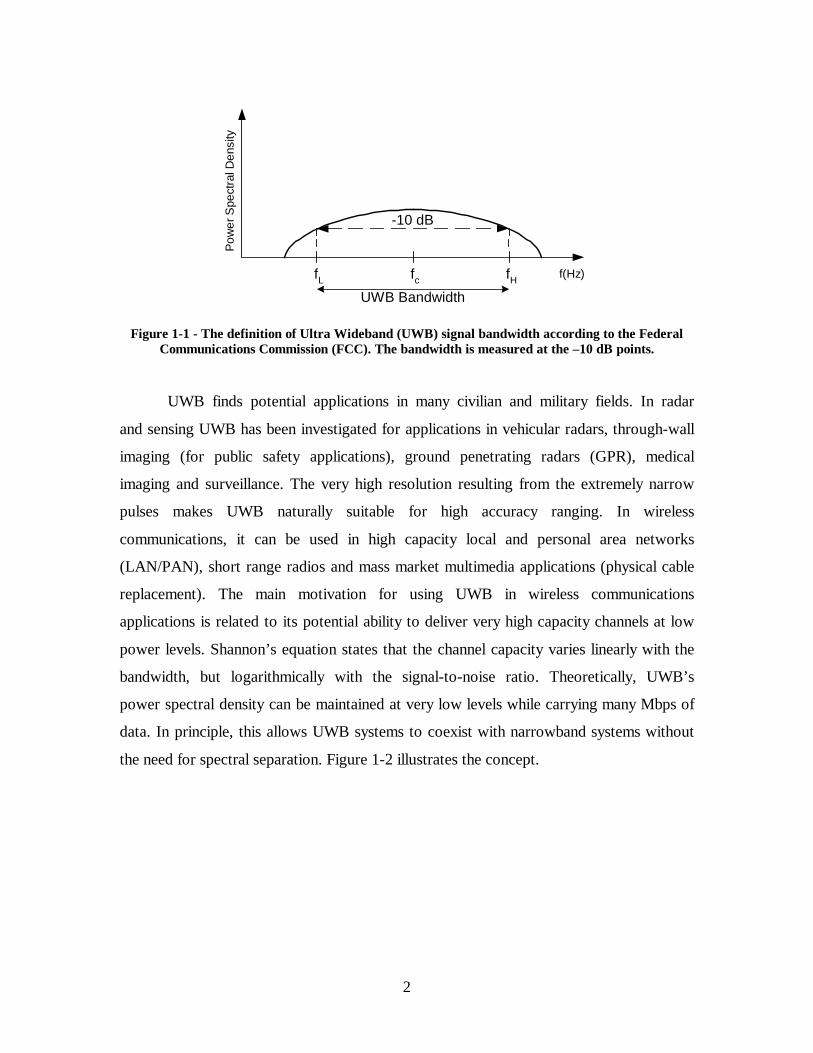
A common definition characterizes a UWB signal as having a fractional

bandwidth greater than 25% [2,3,4,5,6] or total bandwidth greater than 1.5 GHz [2,3,5,6].

The Federal Communications Commission (FCC), on its April 2002 First Report and

Order (R&O), defined a UWB signal as having fractional bandwidth greater than 20% or

total bandwidth greater 500 MHz, with the bandwidth measured at the –10 dB points

[2,5]. Figure 1-1 illustrates the FCC definition of the UWB signal bandwidth. The FCC’s

definition changed the interpretation of what UWB encompasses, detaching it from the

signal generation technique. The scope of UWB is no longer attached to a particular

method of transmitting information over the air, but rather associated to bandwidth

occupation and power spectral density, allowing modulation techniques other than pulsed

radio to be employed.

2

fcfL fH

Pow

er S

pect

ral D

ensi

ty

f(Hz)

-10 dB

UWB Bandwidth

Figure 1-1 - The definition of Ultra Wideband (UWB) signal bandwidth according to the Federal Communications Commission (FCC). The bandwidth is measured at the –10 dB points.

UWB finds potential applications in many civilian and military fields. In radar

and sensing UWB has been investigated for applications in vehicular radars, through-wall

imaging (for public safety applications), ground penetrating radars (GPR), medical

imaging and surveillance. The very high resolution resulting from the extremely narrow

pulses makes UWB naturally suitable for high accuracy ranging. In wireless

communications, it can be used in high capacity local and personal area networks

(LAN/PAN), short range radios and mass market multimedia applications (physical cable

replacement). The main motivation for using UWB in wireless communications

applications is related to its potential ability to deliver very high capacity channels at low

power levels. Shannon’s equation states that the channel capacity varies linearly with the

bandwidth, but logarithmically with the signal-to-noise ratio. Theoretically, UWB’s

power spectral density can be maintained at very low levels while carrying many Mbps of

data. In principle, this allows UWB systems to coexist with narrowband systems without

the need for spectral separation. Figure 1-2 illustrates the concept.

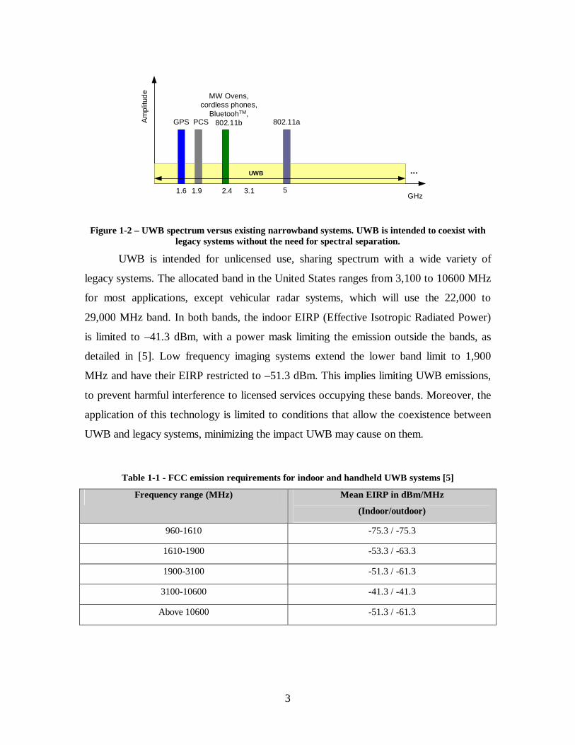
3

1.6 1.9 2.4 5

GPS PCS

MW Ovens,cordless phones,

BluetoohTM,802.11b

GHz

UWB

3.1

802.11a

...

Am

plitu

de

Figure 1-2 – UWB spectrum versus existing narrowband systems. UWB is intended to coexist with legacy systems without the need for spectral separation.

UWB is intended for unlicensed use, sharing spectrum with a wide variety of

legacy systems. The allocated band in the United States ranges from 3,100 to 10600 MHz

for most applications, except vehicular radar systems, which will use the 22,000 to

29,000 MHz band. In both bands, the indoor EIRP (Effective Isotropic Radiated Power)

is limited to –41.3 dBm, with a power mask limiting the emission outside the bands, as

detailed in [5]. Low frequency imaging systems extend the lower band limit to 1,900

MHz and have their EIRP restricted to –51.3 dBm. This implies limiting UWB emissions,

to prevent harmful interference to licensed services occupying these bands. Moreover, the

application of this technology is limited to conditions that allow the coexistence between

UWB and legacy systems, minimizing the impact UWB may cause on them.

Table 1-1 - FCC emission requirements for indoor and handheld UWB systems [5]

Frequency range (MHz) Mean EIRP in dBm/MHz

(Indoor/outdoor)

960-1610 -75.3 / -75.3

1610-1900 -53.3 / -63.3

1900-3100 -51.3 / -61.3

3100-10600 -41.3 / -41.3

Above 10600 -51.3 / -61.3

4

1.2 Motivation and Contribution

Amongst the many legacy systems that will share the spectrum with UWB are the

commercial wireless mobile networks, also commonly referred to as cellular networks.

Such networks have evolved dramatically since their inception in the early 1980’s,

having grown from first-generation, small-coverage, low-penetration, voice-only systems

to the third-generation (3G), nationwide, multi-million subscribers, multimedia services

Universal Mobile Telecommunications Systems (UMTS) networks currently being rolled

out. They have also become a key component of the public safety infrastructure,

providing services such as E911.The carriers operating these networks have invested –

and continue to invest –, substantial capital to acquire exclusive rights to use the

spectrum. For example, in the United States, wireless carriers currently operating

personal communications services (PCS) networks in the 1900 MHz band, have invested

over US$7 billion to acquire spectrum usage rights during the 1994/1995 FCC auctions

[115].

The consumer applications envisioned for UWB will place these devices

physically close to the 3G mobile terminals. In a mature market deployment, the UWB

device density could far exceed that of mobile phones, potentially resulting in several

UWB devices per 3G terminal. The emergence of a license-exempt technology based on

spectrum coexistence, with main applications in mass-market products, suggests that the

impact of the newcomer on incumbent systems be thoroughly investigated. The literature

on UWB-3G coexistence is inconclusive, and even contradictory, as to the impact UWB

can have on the performance of third-generation wireless networks. While some studies

show that UWB can be highly detrimental to 3G networks, others have concluded that

both systems can gracefully coexist. The lack of consistent, conclusive studies on the

potential impact of UWB on 3G networks constitutes the primary motivation for this

research.

The research considers the theoretical and practical aspects of the coexistence

between UWB and third-generation wireless mobile networks, with particular emphasis

on UMTS. It investigates the impact of UWB on the performance of 3G networks,

5

modeling the effects that UWB, as regulated by the FCC, can have on existing wireless

networks. In particular, this study addresses the following areas of interest:

• Quality of service (QoS): The 3G user experience in the presence of

in-band interference caused by UWB.

• Network coverage: The effects of UWB interference in the coverage

area of the 3G network.

• Network capacity: The effects of UWB interference in the traffic

handling capacity of the 3G network.

The available literature describes 3G system level performance simulations in the

presence of UWB for very controlled scenarios, limited to theoretical network

configurations and scarce set of relevant input variables. The results obtained from those,

while offering some insight into the actual impact of UWB on 3G, do not allow for a

thorough quantitative assessment of interference in real network deployments. This

contribution intends to overcome the limitations posed by those studies, offering a

thorough investigation, which can be used to assess both theoretical and practical

network scenarios. The major contribution of this effort is to demonstrate that UWB can

have a detrimental effect on the performance of third-generation networks. However,

unlike in the work available in the literature, this study shows that coexistence is possible

under certain circumstances. It also analyses the effect of UWB device density and

emission power on the performance of 3G networks, studying the conditions that would

allow the coexistence of both systems. These contributions are enabled by a

methodology that provides realistic, comprehensive and scalable analyses of the effects

of UWB on third-generation wireless networks. The proposed methodology was realized

with the aid of a commercial off-the-shelf wireless network planning tool, which had the

author’s involvement during various stages of its development. This tool is obtainable for

general use, making this contribution readily available to anyone interested in the UWB-

UMTS coexistence problem.

6

1.3 Document Overview

This document compiles the theoretical and practical aspects of this research. It

also presents the methodology proposed for the analysis of UWB interference on UMTS

networks and the results from simulations completed following this methodology.

Chapter 2 introduces and reviews the properties of the UWB signal and its power

spectral density, exploring the effects of pulse shape, modulation and dithering on the

power spectral density (PSD). In addition, this chapter models the UWB interference on

narrowband radio systems, with particular emphasis on a UMTS receiver. Through

simulations, we model the statistical behavior of the UWB interference on the UMTS

receiver with the variation of the pulse repetition frequency (prf) of the UWB signal.

Chapter 3 discusses the UWB interference on UMTS at the cell level, isolating a

single source of interference and a single UMTS victim, both under a single UMTS cell.

It investigates both the downlink and uplink, taking into consideration the various factors

relevant in each case. This analysis provides a first order quantitative estimate of the

effects of UWB on UMTS, laying the ground for the subsequent system level study.

Chapter 4 addresses the UWB interference on UMTS at the system level. It

discusses the limitations of the cell level analysis and shows the need for statistical

modeling for a realistic representation of UWB interference on UMTS. We propose a

Monte Carlo algorithm to simulate the dynamics between UWB and UMTS users. The

algorithm captures the effects of this interaction on the network, replicating the behavior

expected in a real environment. The UMTS network model applies all the elements

typically employed in actual network design, making it as sophisticated as those adopted

by wireless carriers and network infrastructure manufacturers. We present the results of

simulations for different UMTS user profiles, as well as a sensitivity analysis for UWB

user density and radiated power.

Chapter 5 summarizes the contributions of this research and indicates areas of

future research related to this topic.

7

Chapter 2

The UWB Interference on Narrowband Radio

Systems

This chapter describes the mathematical model of the UWB signal and its effect on

a narrowband receiver. The analysis concentrates on the signal representation for pulsed

UWB systems. Applications based on other technologies, such as OFDM, would yield

different results. However, the analytical methodology used to quantify the UWB

interference on a narrowband receiver is generic and can be applied to any modulation. In

addition, we analyze the effects of UWB interference on a UMTS receiver. We use the

results of simulations to determine the statistical behavior of the UWB interference in a

generic UMTS victim receiver.

2.1 The UWB Signal Model

The UWB signal utilized in this analysis can be represented by a series of pulses

)(tp of very short duration, described as

∑−

=−=

1

0

)()(N

kk kTtpatw , Equation 2-1

where ka is the amplitude of the thk pulse and T is the pulse repetition interval.

Alternatively, the UWB signal can also be described in the form

)()()( tptdtw ∗= , Equation 2-2

where )(td is

8

∑−

=−=

1

0

)()(N

kk kTtatd δ , Equation 2-3

)(tδ is the Dirac delta function and ∗ represents the convolution operation.

Let )( fW be the frequency domain representation of the UWB signal, obtained

via the Fourier transform of its time domain version. )( fW is then

fkTjN

kkeafPfDfPfW π2

1

0

)()()()( −−

=∑== , Equation 2-4

where )( fD denotes the Dirac delta function in the frequency domain.

When using an UWB signal to carry data, the amplitude ka and the pulse delay

kT can be used as modulation variables. The random nature of the modulating signal

implies that the UWB signal must be modeled as a random process. In this case, the

power spectral density (PSD) is a more suitable descriptor of its frequency domain

behavior. The power spectral density of the UWB signal )(tw , denoted by )( fSw is

)()()(2

fSfPfS dw = , Equation 2-5

where )( fSw represents the average power per Hz (W/Hz) as a function of the frequency,

while )( fSd is the power spectral density of )(td . The term 2

)( fP is the magnitude of

the Fourier transform of the pulse )(tp , representing the energy spectral density (ESD) of

a single pulse and expressed in units of joules/Hz. )( fP is given by

∫∞

∞−

−= dtetpfP ftπ2)()( . Equation 2-6

9

Equation 2-5 shows that the power spectral density of the UWB signal )(tw

comprises two components: the energy spectral density of the pulse )(tp and the power

spectral density of )(td .

Typically, UWB systems do not use one single pulse to represent a data symbol.

Many pulse repetitions, in the order of hundreds, are transmitted for each symbol, to

assure its proper reception [2,37]. Consequently, the power spectrum of these pulse trains

shows spectral lines, or comb lines. The regularity of these spectral lines may cause

UWB systems to interfere on conventional narrowband systems sharing the spectrum.

The use of time hopping by applying dithering to the pulses can minimize this

phenomenon, introducing a degree of randomness to the pulse train. It also allows for the

introduction of data modulation and multiple access (channelization) to UWB. Pulse

position modulation (PPM) is generally employed for this purpose. For instance, a binary

0 may represent no dithering and a binary 1 a small dithering, generally indicated as a

percentage of the pulse period. Channelization can be introduced via the use of a second,

larger pulse dithering that provides further smoothing of the spectral lines and permits

multiple access. This is generally accomplished using pseudo-random noise codes (PN

codes). The noise-like nature of PN codes adds the random component responsible for

reducing the spectral lines on the modulated signal. This approach is also known as

Direct Sequence Ultra Wideband (DS-UWB).

The resulting UWB signal, affected by pulse position modulation and dithering

can be expressed as

∑−

=−−=

1

0

][)(N

kkk kTdtpatw , Equation 2-7

where kd represents the total time dither (data plus PN code), in time units and T the

pulse repetition interval (PRI).

10

The energy in a single pulse is

dffPEp

2

)(∫∞

∞−

= Equation 2-8

and the total average power can be expressed as

REaP pkw2= , Equation 2-9

where R is the average pulse repetition frequency (PRF)

T

R1= Equation 2-10

2.2 The UWB Power Spectral Density

The power spectral density (PSD) of the UWB signal is of central importance in the

analysis of its interference effects on other radio systems. The UWB pulse power

distribution over the signal bandwidth depends on the shape of the pulse spectrum and on

the modulation mechanism. As indicated by equation (2-5), the power spectral density of

the UWB signal is a function of the energy spectral density of the UWB pulse and the

power spectral density of the impulse sequence )(td . The PSD for various UWB signal

models has been developed through different techniques - albeit with agreeing results, in

[89], [90], [91] and [92]. The generic expression for the PSD of a UWB signal of frame

duration T has the form

∑=l

flTjfcw elR

T

fPfS π2

)(

2

][)(

)( , Equation 2-11

where

11

)()(][)( fcfclR lkkfc∗

+= , Equation 2-12

with

kfjkk eafc επ2)( −= . Equation 2-13

The transmit time kT of the thk pulse is related to T and kε by

kk kTT ε+= Equation 2-14

The PSD often consists of a continuous and a discrete component, which can be

derived from equation (2-11) by expressing the modulation term ( )fck in terms of its

mean value )( fcµ , its variance and a white, zero-mean process )()()(~ fufcfc ckk −= ,

as shown in equation (2-15). The PSD can then be denoted by

−+= ∑k

ccw T

kf

T

f

T

ffPfS δ

µσ2

222 )()(

)()( Equation 2-15

The first term of equation (2-15) represents the continuous component of the PSD, while

the second term corresponds to the discrete components, or spectral lines.

2.2.1 PSD of the UWB Signal with Discrete Pulse Positions

For the UWB pulse shape corresponding to the first derivative of the Gaussian

monocycle, the continuous component of the PSD for a pulse position modulated signal

with M2 possible pulse positions is [89]

∆−=

22

)sin(

)sin(2cos1)()(

c

cwc fM

fMffPRfS

επεππ Equation 2-16

12

and the power in the thn discrete spectral component is

2

22

)/sin(

)/sin(2cos)(

∆=TnM

TnM

T

nnRPRP

c

cn επ

εππ, Equation 2-17

where TR /1= Hz is the pulse repetition frequency (PRF), ∆ is the time offset produced

by the modulation process, cε the granularity of the code-controlled pulse position. It is

worth noting that the continuous component of the PSD is proportional to the pulse

repetition frequency R , whereas the discrete component is proportional to 2R . In

addition, the spectral lines appear at multiples of R .

Figure 2-1 illustrates the energy spectral density (ESD) of the Gaussian

monocycle relative to its maximum value, for pulse duration ns5.0=τ . Figure 2-2

shows the continuous power spectral density for an UWB signal based on a Gaussian

monocycle, with total power equal to 10 dBm, pulse duration ns5.0=τ , nsc 10=ε and

MHzR 10= .

-40

-35

-30

-25

-20

-15

-10

-5

0

5

0 1 2 3 4 5

Frequency (GHz)

Rel

ativ

e E

ner

gy

Sp

ectr

al D

ensi

ty (

dB

)

Figure 2-1 Energy spectral density (ESD) of the Gaussian monocycle relative to the maximum value, in dB. The pulse duration is 0.5 ns.

13

-60

-55

-50

-45

-40

-35

-30

-25

-20

-15

-10

0 1 2 3 4 5

Frequency (GHz)

Co

nti

nu

ou

s P

SD

(d

Bm

)

Figure 2-2 Continuous power spectral density (PSD) of the Gaussian monocycle for a total UWB

signal power of 10 dBm. The pulse duration is 0.5 ns, M=10,εεεεc=10ns and R=10 MHz.

2.2.2 PSD of the UWB Pulse with Uniform Pulse Position

When the pulse can occur anywhere within the frame interval and its position

follows a uniform distribution, the continuous component of the PSD for the pulse shape

corresponding to the first derivative of the Gaussian monocycle is

[ ])(sinc1)(1

)( 2 απφ ffT

fS vp −= , Equation 2-18

with the power spectral component at frequency Tn being

= απφT

n

T

n

TP vn

22

sinc1

, Equation 2-19

where α is the width of the time interval. If T=α , the pulse can appear anywhere in the

UWB frame. In this case, the PSD has no spectral lines, except at 0=f .

14

2.2.3 PSD of the Generalized UWB Signal Model

The models described in the previous sections assume each information symbol to

be limited to one UWB frame and infinite-length pseudo random dithering codes. A more

generalized case accounts for multi-frame information symbols and for dithering codes of

finite length. Such UWB signal can be described as

∑ ∆−−=n

nnn nTtvatw )()( , Equation 2-20

where na and n∆ represent the thn pulse amplitude and position modulation,

respectively, and )(tvn denotes

∑−

=−−=

1

0,, )()(

M

mmnfmnn mTtptv εα , Equation 2-21

where )(tvn is non-zero for vtt ≤≤0 , with Ttv ≤∆+ max . fT is the UWB frame interval,

mn,ε and mn,α represent the dithering delay and amplitude of frame m of pulse n and

)(tp is the fundamental pulse waveform. In the frequency domain )(tvn is expressed by

∑−

=

−=1

0

2,)()(

M

m

mTjmnn

fefPfVπβ , Equation 2-22

where

mnjmnmn e ,2

,,πεαβ −= . Equation 2-23

Both mn,ε and mn,α can be modeled as deterministic or random, as appropriate. In

the deterministic case, these variables represent a periodic dithering code with period

NT , yielding the PSD expression

15

∑ ∑−

=

∗+=

l

N

klnn

flTjcw fVfVelR

NTfS

1

0

2 )()(][1

)( π , Equation 2-24

The PSD expression for the non-periodic dithering case is

∑=l

flTjVcw elRlR

TfS π2][][

1)( , Equation 2-25

where

)()(][ fVfVlR lnnV∗+≡ . Equation 2-26

2.3 The UWB Interference on Narrowband Radio Systems

The operation of ultra wideband (UWB) devices and systems is intended to be

unlicensed, implying that existing licensed systems and networks whose spectrum

overlaps with that used by UWB may be subject to interference. Most systems operating

in this common band can be classified as narrowband in comparison with UWB. Radars

and high-capacity microwave links have signal bandwidth of orders of magnitude less

than a typical UWB pulse bandwidth.

The effect UWB interference will have on the operation of a coexisting system

depends on the ability of the victim receiver to reject the undesired signal. The front-end

RF bandwidth of a radio receiver is usually much wider than the actual signal bandwidth,

for the receiver is usually designed to be able to tune over a range of frequency channels.

In a conventional dual-conversion super heterodyne receiver, the output of the

intermediate frequency (IF) stage feeds the demodulator responsible for recovering the

baseband signal. Consequently, the IF filtering stage ultimately determines the bandwidth

of the signal applied to the demodulator. The amount of UWB interference reaching the

demodulator therefore depends on the victim receiver’s IF filtering characteristics. Figure

16

2-3 shows the block diagram of a typical dual-conversion super heterodyne receiver.

Usually, the RF front-end includes an RF band filter and a low-noise amplifier (LNA).

Depending on the application, it may also contain a duplexer or antenna switching

circuitry.

RFFront-end

IF1 IF2Detection/

Demodulation

0f 1IFf2IFf

1LO 2LO

Figure 2-3 Block diagram of a typical dual-conversion super heterodyne receiver.

An interfering UWB signal goes through the same receiver path as the desired

signal and appears to the demodulator as a signal processed by the IF filter block (IF2),

which has a transfer function )( fH IF . The IF filter output response to the interfering

UWB signal is

)()()( fHfWfG IF= , Equation 2-27

where )( fG is the frequency domain representation of the IF filter output time domain

response and )( fW the frequency domain representation of the UWB signal. For this

analysis, let 02 ff IF = . This assumption simplifies the analysis by eliminating the need to

consider the effect of frequency down conversion prior to the final IF stage. In essence, it

models the final IF filter with its intended bandwidth, but centered at frequency 0f .

Figure 2-4 compares the frequency response of the IF filter with the UWB signal. The

shaded area of the UWB signal under the IF response curve represents the portion of the

signal that is processed by the filter.

This study assumes that the receiver is operating in linearity. It considers that the

RF front-end stage and first mixer do not produce third-order intermodulation products

that cause observable performance degradation. However, it must be noted that UWB

17

signals may contain discrete tones of relatively high power, offering the potential for such

effects.

ffo-fo

)( fH IF −

)( fP −

)( fH IF

)( fP

Figure 2-4 Comparison between the IF filter response and the UWB signal bandwidth.

2.4 Narrowband Receiver Response to the UWB Signal

In general, the bandwidth of the UWB pulse is much greater than the channel

bandwidth of the victim receiver, effectively making the receiver response to a single

UWB pulse equal to the impulse response of the IF filter. Hence, the actual shape of the

UWB pulse becomes of secondary relevance for this analysis, as the UWB signal energy

will be perceived as constant over the receiver passband. Equation 2-27 can be rewritten

as

∑−

=

−==1

0

2)()()()()()(N

k

fTjkIFIF

keafPfHfDfPfHfG π . Equation 2-28

)( fH IF can also be represented by its baseband equivalent response, indicated as

)( fH if [9]

)()()( 00 ffHffHfH ififIF −−+−= ∗ . Equation 2-29

Applying Equation 2-29 to 2-28 yields

18

{ }∑−

=

−∗ −−+−=1

0

200 )()()()(

N

k

fTjkifif

keaffHffHfPfG π . Equation 2-30

Since )(tp is real, its frequency domain representation )( fP is conjugate-

symmetric:

)()( fPfP ∗=− . Equation 2-31

Also, )( fP can be expressed in terms of its magnitude and phase as

)()()( fjefPfP ψ= . Equation 2-32

Therefore, Equation 2-30 can be rewritten in the form

{ }∑−

=

−−∗ −−+−=1

0

2)(0

)(0 )()()()(

N

k

fTjk

fjif

fjif

keaeffHeffHfPfG πψψ . Equation 2-33

As previously mentioned, the bandwidth of the UWB signal is much larger than

the bandwidth of the IF filtering stages of the victim receivers of narrowband coexisting

systems. Thus, )( fP is essentially constant over the passband of )( fH IF and equation

(2-33) can be expressed as

{ }∑−

=

−−∗ −−+−=1

0

2)(0

)(00

00 )()()()(N

k

fTjk

fjif

fjif

keaeffHeffHfPfG πψψ . Equation 2-34

The bandpass process )(tg can also be represented by its in-phase and quadrature

components )(tx and )(ty , respectively:

19

tftytftxtg 00 2sin)(2cos)()( ππ −= , Equation 2-35

where )(tg represents the entire UWB pulse sequence and

∑−

==

1

0

)()(N

kk txtx , Equation 2-36

∑−

==

1

0

)()(N

kk tyty . Equation 2-37

The signal envelope is denoted by

22 )()()( tytxtag += , Equation 2-38

and the phase is

= −

)(

)(tan)( 1

tx

tytθ . Equation 2-39

The envelope power of )(tg is

2

)()(

2 tatP g

g = . Equation 2-40

)( fG can then be expressed in terms of the )( fX and )( fY components as

20

−−+= ∑ ∑

−

=

−

=

−−∗+−1

0

1

0

)(20

)(20

00 )()()()()(N

k

N

k

Tffjkif

Tffjkif

kk eafPfHeafPfHfX ππ Equation 2-41

−−−= ∑ ∑

−

=

−

=

−−∗+−1

0

1

0

)(20

)(20

00 )()()()(1

)(N

k

N

k

Tffjkif

Tffjkif

kk eafPfHeafPfHj

fY ππ Equation 2-42

If )(thif is complex, it can be represented in the form )()(0( tjifif ethth θ= . Hence,

Equations 2-41 and 2-42 can be expressed in the time domain, via the inverse Fourier

transform as:

[ ]kk

N

kKifk TffTtTthafptx 00

1

00 2)()(cos)()(2)( πψθ −+−−= ∑

−

= Equation 2-43

[ ]kk

N

kKifk TffTtTthafpty 00

1

00 2)()(sin)()(2)( πψθ −+−−= ∑

−

=. Equation 2-44

The envelope output power of )(tg is

2

)()()(

22 tytxtpg

+= Equation 2-45

2.5 The Effects of UWB Interference on Narrowband Receivers

In the majority of the interference scenarios of interest, the UWB pulse bandwidth

is much wider than the victim receiver’s bandwidth. As a result, the response of the IF

filtering stage to a single UWB pulse can be considered equivalent to the filter’s impulse

response. The IF stage response to a series of UWB pulses depends on the pulse rate. The

settling time of the filter’s response is inversely proportional to the IF bandwidth and if

the UWB pulse rate is low in comparison to that bandwidth, the output response will be a

series of individual impulse responses with the same timing as that of the UWB pulses.

If the UWB pulse rate exceeds the IF bandwidth, the responses will overlap and

the resulting signal will depend on the phase interaction amongst the overlapping

21

components. For a constant pulse, with no modulation or dithering, the filter response

will present spectral lines at multiples of the pulse rate. If the pulse rate or one of its

harmonics coincide with the central IF frequency, the responses to each pulse will be in

phase and the output signal will be constant.

In [116], Miller analytically derives that the noise rise due to UWB interference

on a direct conversion quadrature receiver is directly related to the UWB pulse waveform

spectrum and the variance of the modulation symbols. That result, albeit useful and

somewhat intuitive, cannot be readily applied as the net effect of UWB interference at

baseband, as [116] promptly concludes. Miller concedes that proper statistical

characterization of UWB interference on narrowband receivers requires further analytical

and simulation efforts. Simulations presented in [7] suggest that if the average UWB

pulse rate exceeds the IF bandwidth and the signal is dithered, the IF output will appear

noise-like and have a Gaussian response [89]. This assertion is of particular relevance to

the analysis of the effect of UWB signals on UMTS receivers, because it implies that the

UWB interference can be modeled as AWGN. Based on the appealing, but inconclusive

amount of information in the available literature, we felt compelled to carry out

simulations with the objective of determining the statistical response of a narrowband

receiver to UWB interference at varying pulse rates, establishing a base upon which to

rely in the next steps of this research. The next section details the implementation of the

simulator and the assumptions around the model.

2.5.1 Simulation of UWB Interference on a UMTS Receiver

We built a simulator to determine the impact of UWB interference on a UMTS

receiver. It models a pulsed UWB transmitter at the pulse repetition rates of 1, 10 and 100

Mpps and its effect on a UMTS receiver located at short distance – 1m for the results

presented herein.

The time domain analysis of the results examines two major effects of the UWB

signal on the receiver:

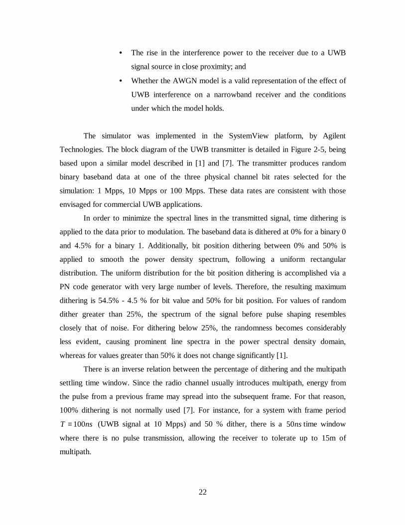
22

• The rise in the interference power to the receiver due to a UWB

signal source in close proximity; and

• Whether the AWGN model is a valid representation of the effect of

UWB interference on a narrowband receiver and the conditions

under which the model holds.

The simulator was implemented in the SystemView platform, by Agilent

Technologies. The block diagram of the UWB transmitter is detailed in Figure 2-5, being

based upon a similar model described in [1] and [7]. The transmitter produces random

binary baseband data at one of the three physical channel bit rates selected for the

simulation: 1 Mpps, 10 Mpps or 100 Mpps. These data rates are consistent with those

envisaged for commercial UWB applications.

In order to minimize the spectral lines in the transmitted signal, time dithering is

applied to the data prior to modulation. The baseband data is dithered at 0% for a binary 0

and 4.5% for a binary 1. Additionally, bit position dithering between 0% and 50% is

applied to smooth the power density spectrum, following a uniform rectangular

distribution. The uniform distribution for the bit position dithering is accomplished via a

PN code generator with very large number of levels. Therefore, the resulting maximum

dithering is 54.5% - 4.5 % for bit value and 50% for bit position. For values of random

dither greater than 25%, the spectrum of the signal before pulse shaping resembles

closely that of noise. For dithering below 25%, the randomness becomes considerably

less evident, causing prominent line spectra in the power spectral density domain,

whereas for values greater than 50% it does not change significantly [1].

There is an inverse relation between the percentage of dithering and the multipath

settling time window. Since the radio channel usually introduces multipath, energy from

the pulse from a previous frame may spread into the subsequent frame. For that reason,

100% dithering is not normally used [7]. For instance, for a system with frame period

nsT 100= (UWB signal at 10 Mpps) and 50 % dither, there is a ns50 time window

where there is no pulse transmission, allowing the receiver to tolerate up to 15m of

multipath.

23

The bit value and bit position dithering functions are summed and applied to a

Pulse Position Modulator (PPM) operating at one of the pulse repetition rates (PRR)

selected for the simulation. The output of the PPM stage is a train of Dirac delta functions

as described by equation (2-7). The pulse duration is set 0.1 ns. This pulse train is shaped

in the pulse generator block by a Gaussian filter, to limit the spectral emissions outside

the desired band. The pulse generator block also differentiates the signal, simulating the

effect of the transmitter antenna on the UWB signal [1, 93]. Figure 2-6 shows the

normalized impulse response of the Gaussian pulse-shaping filter and Figure 2-7

illustrates the UWB pulse shape after differentiation. The Gaussian filter has bandwidth

of 4 GHz.

The signal power control block adjusts the transmitted UWB signal level, making

it compliant with the emission requirements for UWB devices. Figure 2-8 shows the

pulse train at the output of the power control block and Figure 2-9 shows the

corresponding power spectral density. The gain of the power control block is adjusted

according to the pulse repetition, to maintain the power spectral density constant and

within the emissions requirements for any pulse repetition rate.

Data Binary DataDither

+

PN CodeDither

Pulse PositionModulator (PPM)

Clock

Pulse Generator(Gaussian Filter/

Differentiator)

Signal PowerControl

Figure 2-5 Block diagram of the time dithered bandpass ultra wideband (UWB) transmitter used to model the effect of UWB interference on the narrowband UMTS receiver.

24

Figure 2-6 Normalized impulse response of the UWB Gaussian pulse shaping filter. The pulse width is 0.25 ns, corresponding to a bandwidth of 4 GHz.

Figure 2-7 Normalized UWB pulse after differentiation. The pulse width is 0.25 ns, corresponding to a bandwidth of 4 GHz.

25

Figure 2-8 Pulse position modulated (PPM) Gaussian monocycle pulse train with 0.5 ns pulse duration and 200 MHz repetition rate. The data is modulated with 4.5 % (0.045T) dither and time

hopping with 50% dither (0.5T). The pulse peak amplitude is 1 Volt (chart created with System View).

Figure 2-9 Power spectrum of a Pulse position modulated (PPM) Gaussian monocycle pulse train with 0.5 ns pulse duration and 10 MHz repetition rate. The data is modulated with 4.5 % (0.045T) dither and time hopping with 50% dither (0.5T). The pulse peak amplitude is 1 Volt (chart created

with System View).

Figure 2-10 compares the power spectral density of the transmitted UWB signal

with the FCC and ETSI emission masks for indoor and outdoor (portable) applications.

The UWB signal produced by the transmitter used in the simulations is largely compliant

with the emission masks defined by the FCC and ETSI. The signal does not comply with

the outdoor FCC mask in the 1.5~3.0 GHz band and with the ETSI masks for frequencies

below 2.3 GHz. Even though these bands coincide with the operation bands of UMTS

26

systems, the simulations will show that the excess emission is not harmful. Additional

pulse shaping or filtering at RF can be used to control the PSD to achieve full compliance

with the masks. Pulse shaping is an active area of research and it is beyond the scope of

this work. References [10] and [12] present solutions for PSD control and pulse shaping

that could be used as part of the simulations at the expense of additional complexity. For

the simulations presented, the pulse width is more important than the pulse shape,

because the former determines the total spectrum occupied by the UWB signal, while the

specific details of the latter are lost at baseband, as the pulses are filtered and spread in

the time domain [7].

-80.0

-75.0

-70.0

-65.0

-60.0

-55.0

-50.0

-45.0

-40.0

0 2000 4000 6000 8000 10000 12000 14000

Frequency (MHz)

PS

D (

dB

m /

MH

z) -

----

PSD (dBm/MHz)FCC IndoorFCC Outdoor/HandheldETSI IndoorETSI Portable

Figure 2-10 Comparison between the UWB power spectral density at the output of the transmitter and the FCC/ETSI emission masks for indoor and outdoor/handheld/portable UWB devices. In this

chart, the power spectral density is expressed in dBm/MHz.

The implementation of the UMTS receiver used in the time domain simulations is

presented in Figure 2-11. It follows the classic optimal QPSK correlation receiver

architecture, with direct conversion from RF to baseband. The block diagram in Figure

2-11 corresponds to the path responsible for recovering the Dedicated Physical Channel

(DPCH) data.

27

The RF front-end bandpass filter is centered at 2140 MHz, with 60 MHz of

bandwidth, allowing all frequencies in the WCDMA FDD downlink band, spanning from

2110 MHz to 2170 MHz, to pass through. It was implemented as a finite impulse

response (FIR) filter with 3018 poles, passband ripple of < 1dB and out of band rejection

>45 dB. Figure 2-12 shows its normalized impulse response and Figure 2-13 shows its

transfer function.

The band-limited signal delivered by the frond-end filter is divided in two equal

branches by a power splitter, which feeds the In-phase (I) and Quadrature (Q) paths of a

QPSK Direct Conversion Receiver (DCR).

Low pass baseband Finite Impulse Response (FIR) filters with pass band between

0 and 3.84 MHz were used to eliminate undesired mixing products and out of band

signals. They are 2048-pole filters with a Raised Root Cosine transfer function response

and roll-off factor 22.0=α , as illustrated in Figure 2-14. The filter’s normalized impulse

response is shown in Figure 2-15.

Bits Q

Bits I

BandpassFilter

-90o

LowpassFilter

MHzfc 2140=MHzBw 60=

PowerSplitter

MHzfc 2140=

LowpassFilter

MHzBw 84.3=

MHzBw 84.3=

Q

UWB signal

OVSF SpreadingCode

IntegratorThresholdDetector

IntegratorThresholdDetector

I

Figure 2-11 UMTS receiver model used in the simulations. It follows the classic optimal QPSK correlation receiver architecture, with direct conversion from RF to baseband.

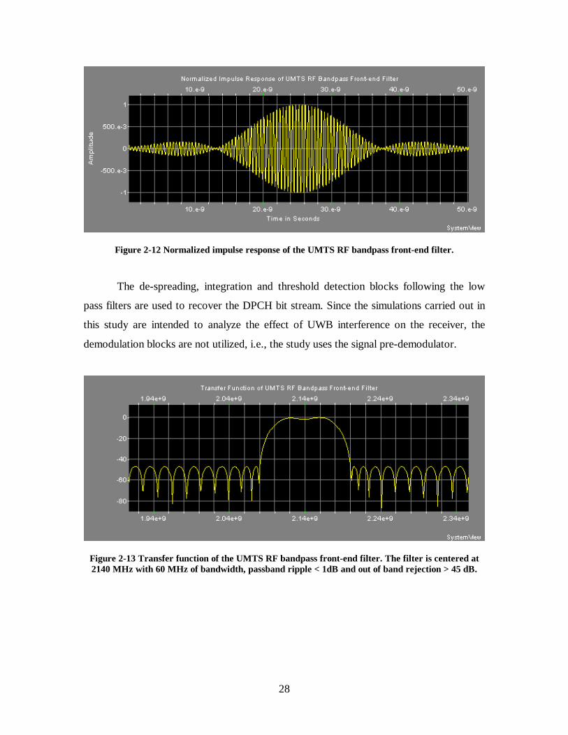
28

Figure 2-12 Normalized impulse response of the UMTS RF bandpass front-end filter.

The de-spreading, integration and threshold detection blocks following the low

pass filters are used to recover the DPCH bit stream. Since the simulations carried out in

this study are intended to analyze the effect of UWB interference on the receiver, the

demodulation blocks are not utilized, i.e., the study uses the signal pre-demodulator.

Figure 2-13 Transfer function of the UMTS RF bandpass front-end filter. The filter is centered at 2140 MHz with 60 MHz of bandwidth, passband ripple < 1dB and out of band rejection > 45 dB.

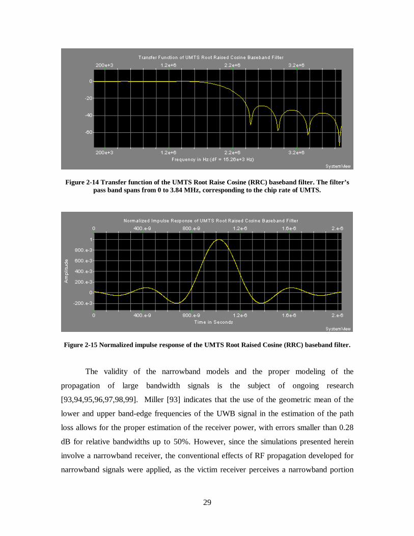
29

Figure 2-14 Transfer function of the UMTS Root Raise Cosine (RRC) baseband filter. The filter’s pass band spans from 0 to 3.84 MHz, corresponding to the chip rate of UMTS.

Figure 2-15 Normalized impulse response of the UMTS Root Raised Cosine (RRC) baseband filter.

The validity of the narrowband models and the proper modeling of the

propagation of large bandwidth signals is the subject of ongoing research

[93,94,95,96,97,98,99]. Miller [93] indicates that the use of the geometric mean of the

lower and upper band-edge frequencies of the UWB signal in the estimation of the path

loss allows for the proper estimation of the receiver power, with errors smaller than 0.28

dB for relative bandwidths up to 50%. However, since the simulations presented herein

involve a narrowband receiver, the conventional effects of RF propagation developed for

narrowband signals were applied, as the victim receiver perceives a narrowband portion

30

of the large bandwidth UWB signal. The UMTS channel center frequency 2140=cf

MHZ was used. The physical separation between the UWB signal source and the victim

receiver was chosen as 1 meter, resulting in the free space loss of 39 dB. This physical

separation assumption is based on the expected usage of UWB devices in close proximity

to mobile phones. In addition to the free space loss, a multipath gain component of 6 dB

was also considered, resulting in a total path loss of 33 dB. The multipath margin

assumes a Rician channel where the line-of-sight (LOS) component is 3 dB greater than

the multipath component. Under this assumption, the Rician fading model yields a 98%

probability that the received UWB signal will be less than that received when only the

LOS component is assumed. It is worth noting that the primary objectives of the

simulation can also be achieved under different propagation modeling conditions and

UWB-UMTS separations, since the key variable affecting the outcome is the UWB pulse

repetition rate (prf). Even if the propagation environment offers a different loss behavior,

or if the physical separation between the UWB source and the victim receiver varies, the

interaction between the signals at the receiver will not change.

2.6 Simulation Results

The time domain results of simulations for UWB pulse rates of 1, 10 and 100

Mpps are presented in Figure 2-16 to Figure 2-27. The statistical behavior of the UWB

signal is represented by probability density functions (pdf) and cumulative distribution

functions (cdf), assembled for each of the simulated pulse rates and signal components (I

and Q). Those results are show in Figure 2-28 to Figure 2-39. A discussion of these

results is presented in Section 2.7.

31

Figure 2-16 UWB signal at the UMTS front-end filter input. The pulse repetition rate is 1 Mpps.



32

Figure 2-19 UMTS front-end filter response to the UWB signal. The pulse repetition rate is 1 Mpps.



33

Figure 2-22 In-phase component of the UWB signal at UMTS receiver after baseband filtering. The pulse repetition frequency is 1 Mpps.



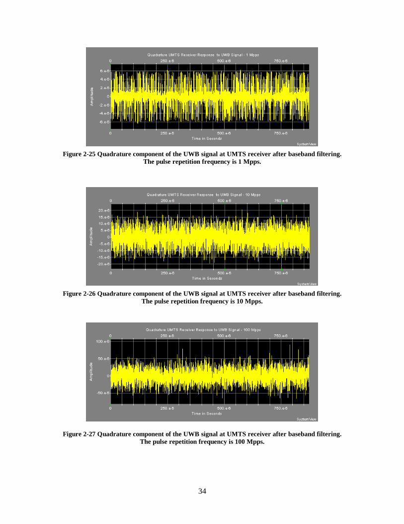
34

Figure 2-25 Quadrature component of the UWB signal at UMTS receiver after baseband filtering. The pulse repetition frequency is 1 Mpps.



35

0

10000

20000

30000

40000

50000

60000

70000

-6.1E-06 -4.9E-06 -3.7E-06 -2.5E-06 -1.2E-06 0.0E+00 1.2E-06 2.4E-06 3.6E-06 4.9E-06 6.1E-06

Amplitude (V)

pd

f (N

um

ber

of

ocu

rren

ces)

In-phase pdf

AWGN pdf

Figure 2-28 Probability density function (pdf) of the in-phase component of the UWB interference signal at the UMTS receiver, after IF filtering, for a pulse repetition frequency (PRF) of 1 Mpps. The

dotted line represents the equivalent AWGN pdf.

0

0.1

0.2

0.3

0.4

0.5

0.6

0.7

0.8

0.9

1

-6.1E-06 -4.9E-06 -3.7E-06 -2.5E-06 -1.2E-06 0.0E+00 1.2E-06 2.4E-06 3.6E-06 4.9E-06 6.1E-06

Amplitude (V)

Pro

b (

X<

absc

issa

)

In-phase cdf

AWGN CDF fit

Figure 2-29 Cumulative distribution function (CDF) of the in-phase component of the UWB interference signal at the UMTS receiver, after IF filtering, for a pulse repetition frequency (PRF) of

1 Mpps. The dotted line represents the equivalent AWGN pdf.

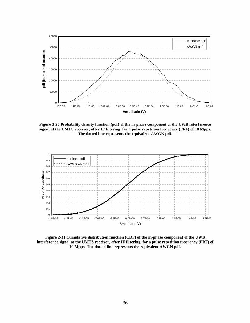
36

0

10000

20000

30000

40000

50000

60000

-1.8E-05 -1.4E-05 -1.1E-05 -7.0E-06 -3.4E-06 0.0E+00 3.7E-06 7.3E-06 1.1E-05 1.4E-05 1.8E-05

Amplitude (V)

pd

f (N

um

ber

of

ocu

rren

ces)

In-phase pdf

AWGN pdf

Figure 2-30 Probability density function (pdf) of the in-phase component of the UWB interference signal at the UMTS receiver, after IF filtering, for a pulse repetition frequency (PRF) of 10 Mpps.

The dotted line represents the equivalent AWGN pdf.

0

0.1

0.2

0.3

0.4

0.5

0.6

0.7

0.8

0.9

1

-1.8E-05 -1.4E-05 -1.1E-05 -7.0E-06 -3.4E-06 0.0E+00 3.7E-06 7.3E-06 1.1E-05 1.4E-05 1.8E-05

Amplitude (V)

Pro

b (

X<

absc

issa

)

In-phase pdf

AWGN CDF Fit



37

0

5000

10000

15000

20000

25000

30000

35000

40000

-6.6E-05 -5.3E-05 -4.0E-05 -2.6E-05 -1.3E-05 0.0E+00 1.4E-05 2.7E-05 4.0E-05 5.3E-05 6.6E-05

Amplitude (V)

pd

f (N

um

ber

of

ocu

rren

ces)

AWGN pdf

In-phase pdf

Figure 2-32 Probability density function (pdf) of the in-phase component of the UWB interference signal at the UMTS receiver, after IF filtering, for a pulse repetition frequency (PRF) of 100 Mpps.


0

0.1

0.2

0.3

0.4

0.5

0.6

0.7

0.8

0.9

1

-6.6E-05 -4.0E-05 -1.3E-05 1.4E-05 4.0E-05 6.6E-05

Amplitude (V)

Pro

b (

X<

absc

issa

)

In-phase pdf

AWGN CDF Fit



38

0

10000

20000

30000

40000

50000

60000

70000

-6.2E-06 -5.0E-06 -3.8E-06 -2.5E-06 -1.3E-06 0.0E+00 1.2E-06 2.4E-06 3.7E-06 4.9E-06 6.2E-06

Amplitude (V)

pd

f (N

um

ber

of

ocu

rren

ces)

---

----

--Quadrature pdf

AWGN pdf

Figure 2-34 Probability density function (pdf) of the quadrature component of the UWB interference signal at the UMTS receiver, after IF filtering, for a pulse repetition frequency (PRF) of 1 Mpps. The

dotted line represents the equivalent AWGN pdf.

0

0.1

0.2

0.3

0.4

0.5

0.6

0.7

0.8

0.9

1

-6.2E-06 -5.0E-06 -3.8E-06 -2.5E-06 -1.3E-06 0.0E+00 1.2E-06 2.4E-06 3.7E-06 4.9E-06 6.2E-06

Amplitude (V)

Pro

b (

X<

absc

issa

)

Quadrature CDF

AWGN CDF fit

Figure 2-35 Cumulative distribution function (CDF) of the quadrature component of the UWB interference signal at the UMTS receiver, after IF filtering, for a pulse repetition frequency (PRF) of


39

0

10000

20000

30000

40000

50000

60000

-1.8E-05 -1.4E-05 -1.1E-05 -7.0E-06 -3.4E-06 0.0E+00 3.7E-06 7.3E-06 1.1E-05 1.4E-05 1.8E-05

Amplitude (V)

pd

f (N

um

ber

of

ocu

rren

ces)

Quadrature pdf

AWGN pdf

Figure 2-36 Probability density function (pdf) of the quadrature component of the UWB interference signal at the UMTS receiver, after IF filtering, for a pulse repetition frequency (PRF) of 10 Mpps.


0

0.1

0.2

0.3

0.4

0.5

0.6

0.7

0.8

0.9

1

-1.8E-05 -1.4E-05 -1.1E-05 -7.0E-06 -3.4E-06 0.0E+00 3.7E-06 7.3E-06 1.1E-05 1.4E-05 1.8E-05

Amplitude (V)

Pro

b (

X<

absc

issa

)

Quadrature CDF

AWGN CDF fit



40

0

5000

10000

15000

20000

25000

30000

35000

40000

-6.6E-05 -5.1E-05 -3.5E-05 -2.0E-05 -4.5E-06 1.1E-05 2.6E-05 4.2E-05 5.7E-05 6.6E-05

Amplitude (V)

pd

f (N

um

ber

of

ocu

rren

ces)

Quadrature pdf

AWGN pdf

Figure 2-38 Probability density function (pdf) of the quadrature component of the UWB interference signal at the UMTS receiver, after IF filtering, for a pulse repetition frequency (PRF) of 100 Mpps.


0

0.1

0.2

0.3

0.4

0.5

0.6

0.7

0.8

0.9

1

-6.6E-05 -3.5E-05 -4.5E-06 2.6E-05 5.7E-05

Amplitude (V)

Pro

b (

X<a

bsc

issa

)

Quadrature CDF

AWGN CDF fit



41

2.7 Discussion

Figure 2-16, Figure 2-17 and Figure 2-18 show the UWB signal as received at the

input of the UMTS receiver for the pulse repetition frequencies (PRF) of 1 Mpps, 10

Mpps and 100 Mpps, respectively. The difference in the amplitude of the received pulses

for each PRF is due to the compensation in the transmission level to keep the power

spectral density constant.

Figure 2-19, Figure 2-20 and Figure 2-21 illustrate the UMTS receiver’s front-end

filter response to the UWB interfering signal at the pulse repetition frequencies of 1

Mpps, 10 Mpps and 100 Mpps. As previously stated, the difference in the amplitude of

the received pulses for each PRF is due to the compensation in the transmission level to

maintain the power spectral density constant. These responses demonstrate how the UWB

interference becomes less impulsive as the PRF increases, since the filter’s response to

each pulse tends to overlap to that of adjacent pulses as the rate increases. This effect is

particularly evident on the filter’s response to the 100 Mpps UWB interference.

Figure 2-22, Figure 2-23 and Figure 2-24 show the IF in-phase component of the

UMTS receiver response to the UWB signal for the pulse repetition frequencies of 1

Mpps, 10 Mpps and 100 Mpps, respectively. Similarly, Figure 2-25, Figure 2-26 and

Figure 2-27 show the IF quadrature responses for the same signals. Both the in-phase and

quadrature waveforms for the 1Mpps signal show a distinctive burstiness, whereas the 10

Mpps and 100 Mpps waveforms suggest randomness. The IF stage’s response to the

UWB pulse train is a sequence of IF impulse responses, whose durations are inversely

proportional to the IF bandwidth. When the pulse repetition frequency is less than the IF

bandwidth, each single impulse response settles before the next pulse, resulting in an

overall IF response equal to a sequence of individual impulse responses. In this situation,

the relative timing between pulses is preserved.

When the pulse rate exceeds the IF bandwidth, the individual impulse responses

will overlap and the resulting signal will depend on the phase relationships among the

overlapping components. If the UWB signal has no dithering, the IF response shows

spectral lines at harmonics of the pulse repetition frequency, whereas if the IF center

frequency coincides with one of the harmonics, the individual impulse responses will be

42

in phase, causing the IF response to be constant. If the UWB signal is dithered and the

average rate exceeds the IF bandwidth, the IF filter’s output appears noise-like, tending to

a Gaussian behavior.

Figure 2-28 to Figure 2-33 illustrate the probability density functions (pdf)

cumulative distribution functions (cdf) of the in-phase voltage component of the UWB

signal at the UMTS victim receiver, after the IF stage, for the pulse repetition frequencies

(prf) of 1 Mpps, 10 Mpps and 100 Mpps, respectively. Figure 2-34 to Figure 2-39 show

the corresponding quadrature voltage component for the same signals. The equivalent

Additive White Gaussian Noise (AWGN) pdf is also plotted in each chart, to allow for a

direct comparison against the UWB signal. These results show the evident signal

departure from Gaussian statistics on the 1Mpps case, i.e., when PRF < IF. They also

show that for PRF > IF – both the 10 Mpps and 100 Mpps, the signal closely follows a

Gaussian behavior. In all cases, the in-phase and quadrature voltage components present

similar response.

2.8 Multi-band OFDM Interference on Narrowband Receivers

Multi-band Orthogonal Frequency Division Multiplexing (MB-OFDM) has also

been considered as viable physical layer for ultra wideband systems. Differently from the

impulse radio, or carrierless, approach described and analyzed in the previous sections of

this study, MB-OFDM utilizes a multiplicity of simultaneous narrowband sub-carriers, or

tones, to transmit information. The data rate capacity in each tone is small, but the

composite effect of many such tones (in the order of hundreds) yields the potential for a

very high overall data rate. Additionally, multiple frequency blocks are employed,

enabling the utilization of frequency hopping for channelization and multiple access. The

narrowband characteristic provides for multipath fading robustness, as a fading null is

likely to affect only one tone at any given point in time, allowing the cyclic prefix to

preserve the orthogonality between carriers. This results in little degradation to the

overall data rate capacity. Narrowband interference robustness is also achieved by the

same principle.

43

The effect of MB-OFDM UWB interference on narrowband receivers has been

investigated and detailed studies are available in the literature. References [118,120]

derive exact bit error rate (BER) formulae for a BPSK narrowband receiver in the

presence of MB-OFDM UWB interference and fading, showing that the Gaussian

approximation is very accurate for arbitrary narrowband signal bandwidths. Simulations

presented in Reference [119] show that MB-OFDM UWB interference on a narrowband

receiver closely follows the Additive White Gaussian Noise (AWGN) behavior for a MB-

OFDM signal hopping over three bands, which is the minimum mandatory configuration

specified for UWB devices using MB-OFDM.

2.9 Summary

This chapter focused on describing the generic mathematical model of the UWB

signal and on determining its power spectral density (PSD). The power spectral density

measures the average power per Hz as a function of the frequency. The expressions

derived in Section 2.2 show that the PSD of the UWB signal generally has a continuous

and a discrete component. Depending on the pulse shape, modulation and dithering

properties of the UWB signal, both components will vary and the PSD will present a

different aspect.

In addition, we determined that the amount of interference caused by an UWB

signal on a narrowband system depends primarily on the bandwidth of the intermediate

frequency (IF) stage of the victim receiver, as the front-end stage generally offers a much

wider passband. The resulting interference is the consequence of the convolution of the

UWB interfering signal with the impulse response of the victim receiver’s IF stage

passband filter. In the frequency domain that result can be represented as the linear

product between the spectrum of the UWB interfering signal and the IF stage’s passband

transfer function.

The effects of UWB interference on a narrowband receiver were investigated

through simulations performed using a test setup. The setup consisted of a dithered UWB

signal source transmitting at pulse repletion frequencies of 1 Mpps, 10 Mpps and 100

Mpps, with power spectral density emissions partially compliant with both the FCC and

44

ETSI emissions masks. The victim receiver consisted of a UMTS receiver operating at

the center frequency of 2140 MHz, in compliance with the ITU-assigned bands for

UMTS systems. The intermediate frequency (IF) bandwidth of the UMTS victim receiver

is 3.84 MHz. The interference analysis used the signal path of a UMTS Dedicated

Physical Channel (DPCH), which employs QPSK modulation. The simulations assumed

a physical separation of 1 meter between the UWB interference source and the victim

receiver, to model the expected typical situation where an UWB device would be near an

UMTS portable phone.

The simulations show that when the UWB pulse repetition frequency (prf) is lower

than the victim receiver’s IF bandwidth, the interference does not follow Gaussian

statistics. Conversely, when the pulse repetition frequency exceeds the IF bandwidth, the

interference presents a Gaussian behavior. Therefore, under these conditions, UWB

interference can be modeled as Additive White Gaussian Noise (AWGN). These results,

produced by means of detailed simulations, are in agreement with those presented in the

literature [7,89], adding confidence to their validity and allowing their use in the next

phases of this study.

45

Chapter 3

UWB Interference on UMTS: Cell Level Analysis

3.1 Introduction

This chapter presents an analysis of the effect of a single source of UWB

interference on UMTS receivers. The analysis is carried out assuming a single-cell

UMTS environment. The single source, single cell scenario allows for a clear

understanding of the way a UWB interference source impacts UMTS receivers,

corresponding to the building block that contributes to the interference effects in a

network. Following the approach of link budget models, the analysis produces a first

order quantitative estimate of the effects of UWB on UMTS. When properly scaled, this

analysis supports the characterization of the impact of UWB on UMTS at the system

level.

3.2 The Effects of Interference in the UMTS Radio Link

UMTS is based on spread spectrum techniques, employing wideband code division

multiple access (WCDMA) with a RF bandwidth of 5 MHz. The system uses orthogonal

spreading codes at a chip rate equal to 3.84 Mcps to distinguish data sequences from

different users. In addition, scrambling sequences are used to allow the differentiation of

terminals at the base station and vice-versa. All users share the same center frequency

and bandwidth, making the total amount of intra-system interference (noise level)

variable and a function of the number of active users. From a radio link budget

perspective, the varying interference level implies variable link performance, which in

turn suggests variable coverage. Therefore, the UMTS cell range is not fixed. It is rather

described by a distribution function whose instantaneous value depends on the sum of the

46

received powers at the site. Since the aggregate received power is directly proportional to

the number of simultaneous users, the cell range is also affected by the instantaneous

traffic. Furthermore, UMTS offers multiple voice and data services, each imposing a

different network load and requiring different link budgets, thus affecting the cell ranges

and their distribution in a different manner. The quantification of the effects of a

coexisting system - UWB in this case, on a UMTS network, must consider the

interdependency of coverage and capacity. It must also account for the service mix

supported by the network and the influence it has on both. This chapter investigates the

impact of UWB interference on the UMTS cell range (coverage), while the impact on

capacity is deferred to the next chapter.

3.2.1 The UWB Interference Model

The total noise power at a UMTS base station receiver depends on the receiver’s

noise figure and the interference power contributions from the uplinks of the active users

in that cell. It also depends on the interference power contribution from other cells’ active

users – both their downlink and uplink. The load factor, or cell load quantifies the

amount of interference, or load, a cell experiences as a function of the number of users

and other system characteristics. For the uplink, the load factor ( ULη ) is defined as [101]

( )∑

= ++=

N

j

jjjob

UL

RNE

Wi

1 1

1)1(

υ

η , Equation 3-1

where:

i : Ratio of other cell to own cell interference;

N : Number of active users;

W : UMTS carrier bandwidth;

jR : Bit rate of user j ;

job NE )( : Energy per user bit per noise spectral density for user j ; and

47

jυ : activity factor of user j .

Similarly, the downlink load factor (DLn ) can be defined as [101]

( ) ( )[ ]jj

N

j j

job

jDL iRW

NE+−=∑

=αυη 1

1

, Equation 3-2

where jα represents the orthogonality factor of the downlink spreading codes, varying

from 0 (no orthogonality) to 1 (complete orthogonality). In the absence of multipath

propagation, the orthogonality is preserved when the signal is received by the mobile.

However, in the presence of multipath, the radio channel delay spread may cause the

mobile receiver to detect the delayed versions of the signal as multiple access

interference. When this happens the orthogonality is compromised.

The simulation results presented in Chapter 2 show that UWB interference on a

narrowband receiver can be modeled as additive white Gaussian noise (AWGN) if the

UWB pulse repetition frequency (prf) is greater than the victim receiver’s intermediate

frequency (IF) bandwidth. When a UMTS receiver is subject to UWB interference from

one or multiple sources, the aggregate interference power will appear to the victim

receiver as noise rise, contributing to the noise power at the receiver. When the UWB

interference is much smaller than the receiver noise power, the degradation is negligible.

Generically, the noise rise is defined as the ratio of the total received wideband power

( TI ) to the noise power (NP )

N

Trise P

IN = . Equation 3-3

In the uplink, the noise rise is related to the load factor by Equation 3-4 [100].

When ULη increases and approaches 1, the noise rise approaches infinity and the system

reaches its pole capacity.

48

UL

riseNη−

=1

1 Equation 3-4

The load factor ties coverage and capacity in UMTS. Interference sources external

to the UMTS network, such as UWB, will be perceived as noise rise and directly affect

the load factor. The greater the noise rise, the higher is the load factor, implying that

UWB interference to a UMTS cell will directly affect its coverage and traffic-serving

capacity. Therefore, the UWB interference can be factored in the UMTS uplink radio link

budget as an interference margin, allowing for a first order estimation of its impact in

coverage and capacity.

3.2.2 Single-Source UWB Interference on UMTS Cells

Few references in the available literature offer a specific detailed treatment of the

single-source interference scenario, particularly in regards to the UWB interference

source-UMTS victim receiver physical separation and its impact on cell range analysis.

One can argue that the topic has little absolute relevance, because the situation is unlikely

and unrealistic, so a detailed study does not offer much insight into the overall problem.

However, in the context of this research, the single-source model grows in importance,

because it is used as a building block to the system level interference analysis discussed

in Chapter 4. Reference [37] performs simulations at the 900 MHz (GSM) and 2GHz

(UMTS) bands, but presents results for worst-case scenarios. In that study the effects of

the radio channel are ignored, i.e., path loss and multipath are not considered, making the

UWB interference much more pronounced than it actually is, thus limiting the value of

the results. In [42], the interference limit for a single UWB-UMTS link is calculated, but

no cell range analysis is developed, as that study focus on an indoor interference

simulation investigation. In [7], a single source, single cell range analysis is presented,

but the study is limited to a single UMTS service class. Reference [116] presents the

results for a laboratory UWB-UMTS interference test. In that study, a UWB signal was

applied to a UMTS mobile phone via a variable attenuator and the BER of the UMTS

49

downlink was measured as the UWB signal attenuation changed. In the same setup, the

noise rise was also measured. Both measurements can be valuable as a link quality

estimator, but cannot be readily mapped to cell range data and/or UWB-UMTS physical

separation. In this study, we develop a detailed single-source, single-cell interference

model aimed at allowing for the determination of the variation of the cell range as a

function of the physical separation between the UWB interference source and the UMTS

victim receiver. The model addresses both the UMTS downlink and uplink.

3.3 Considerations on UWB Propagation Modeling

Conventional path loss modeling based on the Friis transmission formula has been

derived for narrowband channels, where the change in the received power over the signal

bandwidth is negligible [110,111,121]. The frequency dependency in that formulation

comes from the relation between the gain of the antennas and their effective aperture,

implying that for constant gain antennas, the received signal will vary as a function of the

frequency [121]. Since UWB signals can occupy several octave, or even decade

bandwidths, if the transmit and receive antennas do not present constant gain over the

band, the Friis transmission formula can yield misleading results. In this research, we

adopt the constant gain assumption, therefore allowing for the use of path loss modeling

based on the Friis transmission formula for UWB propagation modeling. In the analyses

carried out in this work, the portion of the total UWB signal bandwidth of relevance to

the victim receiver is very small, equating to the channel bandwidth of the interfered

system. Thus, for the purpose of the studies discussed herein, the UWB signal can be

treated as narrowband, with no practical impact to the rigor of the results. Nevertheless,

the compensation of the model for antennas with constant aperture can be

straightforwardly achieved, as indicated in [121], should different assumptions be

required.

50

Conventionally, the received signal in a mobile radio link is estimated using path

loss models of the form [109]

α

=d

ddPdP o

orr )()( , Equation 3-5

where od is a reference distance, α is an arbitrary path loss exponent and )( or dP is the

received power at the reference distance, in the far-field of the transmitting antenna.

Reference [121] presents a theoretical dissection of the Friis transmission formula,

supported by detailed UWB large- and small-scale propagation measurements. That study

shows that while the antennas may introduce frequency dependency to the received

power, the channel does not. Therefore, the traditional path loss model given in equation

3-5 is valid for UWB path loss calculations.

In the scenarios considered in this research, the UWB interferer can be in close

proximity to the 3G victim receiver, at separations as small as 1 m or less, implying

proximity between the transmit and receive antennas involved in the link. This invites

scrutiny of the validity of the antenna radiation properties at such separation distances.

The space surrounding an antenna can be subdivided into three regions: the reactive

near-field, the radiating near-field (Fresnel) and the far-field (Fraunhofer) regions. These

regions identify the field structure in each, but no abrupt changes in the field

configurations, in the transition between them are noted. The reactive near-field region is

the portion of the near-field region immediately surrounding the antenna, wherein the

reactive field predominates. The radiating near-field, or Fresnel field, is the region of the

field of an antenna between the reactive near-field region and the far-field region,

wherein radiation fields predominate and wherein the angular field distribution is

dependent upon the distance from the antenna. The far-field, also known as Fraunhofer

region, is the region of the field of an antenna where the angular field distribution is

essentially independent of the distance from the antenna [122]. Propagation models based

on the Friis transmission formula are valid for distances d in the far-field of the

51

transmitting antenna. The Fraunhofer distance demarcates the boundary between the

radiating near-field and the far-field, being given by [122]

λ

22Dd f = , Equation 3-6

where D is the largest physical linear dimension of the antenna. fd must satisfy the

condition fd >> D. Figure 3-1 plots the far-field distance as a function of the largest

linear dimension of the antenna for different frequencies around the band utilized for 3G

wireless networks. It is apparent from the chart that the far-field distance is less than 10

cm, or 0.1 m, for antennas with linear distance under approximately 9 cm. The form

factor of most third-generation wireless devices conceals the antenna in the device’s case,

forcing the physical dimension of the antenna to be very small, usually under 3 cm.

Similar physical dimensions apply to the radiating element in UWB devices, which in

many applications use patch antennas. Therefore, the use of the far-field distance of 0.1m

as the reference distance complies with the conditions for the validity of the propagation

model described in equation 3-5.

0

5

10

15

20

25

30

35

1 2 3 4 5 6 7 8 9 10 11 12 13 14 15Antenna Linear Dimension (cm)

Fra

un

ho

fer

Dis

tan

ce (

cm)

f = 1500 MHz

f = 1800 MHz

f = 2000 MHz

f = 2100 MHz

f = 2200 MHz

Figure 3-1 Far-field, or Fraunhofer distance, as a function of the physical linear dimension of the antenna.

52

3.4 The UWB-UMTS Single-Source, Single-Cell Model

The study and results presented herein are based on link budget analyses, on

which the noise rise, sometimes also referred to as interference margin, is used as the

entry point for factoring in the UWB interference. This model, albeit conceptually

simple, provides a straightforward methodology for the single-source interference

analysis. The different services supported in UMTS have distinct link budget

requirements, since the bit rate, ob NE and processing gain vary for each service. The

analyses presented in this work consider three service types – speech, real time data and

non-real time data, simulated in different environments, as described:

1. Vehicular speech, macrocell: models voice service using the AMR

(Adaptive Modulation Rate) vocoder with bit rate equal to 12.2 Kbps in an

in-car scenario. This test case simulates mobile users utilizing UMTS

voice services while in transit, for example, on a moving train.

2. Outdoor speech, microcell: this scenario models voice service using the

AMR vocoder with bit rate equal to 12.2 Kbps in an outdoor environment.

This test case simulates mobile users utilizing UMTS voice services while

outdoors, for example, standing or walking on a street or park.

3. Indoor speech, macrocell: this scenario models voice service using the

AMR vocoder with bit rate equal to 12.2 Kbps in an indoor environment.


indoors, for example, standing or walking inside an office or residential

building.

4. Vehicular real time data, macrocell: models real time circuit switched data

(CSD) at 144 Kbps in an in-car scenario. This test case simulates mobile

users utilizing UMTS data services while in transit, for example, on a

moving train.

5. Outdoor real time data, microcell: models real time circuit switched data

(CSD) at 144 Kbps in an outdoor environment. The UMTS terminal is

served by a microcell and there is line-of-sight between the UWB

53

interference source and the victim receiver. This test case simulates

mobile users utilizing UMTS data services while outdoors, for example,

standing or walking on a street or park.

6. Vehicular non-real time data, macrocell: models non-real time packet

switched data (PSD) at 384 Kbps in an in-car scenario. This test case

simulates mobile users using UMTS data services while in transit, for

example, on a moving train.

7. Outdoor non-real time data, microcell: models non-real time circuit

switched data (PSD) at 384 Kbps in an outdoor environment. This test

case simulates mobile users utilizing UMTS data services while outdoors,

for example, standing or walking on a street or park.

All the test cases presume the UWB interference source to have line-of-sight to

the UMTS victim receiver. This is the situation expected in the majority of cases where

interference between UWB and UMTS may occur. UWB is expected to find applications

primarily in portable devices, which would be in close proximity to UMTS portable

phones and data devices.

3.4.1 Downlink Model

The path loss between the UWB device and the UMTS receiver was calculated

using the free space propagation model. No lognormal fading margins were considered.

The penetration losses used in the modeling are listed in Table 3-1 [101]. They apply to

the UMTS link budgets only, i.e., between base station and mobile terminal. The UMTS

mobile terminal link budget parameters common to all scenarios are summarized in Table

3-2 [102] and the UMTS base station parameters are listed in Table 3-3 [102].

Table 3-1 Penetration losses assumed in the UMTS link budget analysis

UMTS victim receiver location UWB interferer location UMTS Penetration Loss

Outdoor Outdoor 0

In-car In-car 8

Indoor Indoor 15

54

Table 3-2 UMTS mobile terminal parameters assumed in the link budget analysis

Parameter Voice Terminal Data terminal

Maximum Transmission Power 21 dBm 24 dBm

Antenna gain 0 dBi omnidirectional 0 dBi omnidirectional

Noise Figure 9 dB 9 dB

Body shielding loss 3dB 0 dB

Table 3-3 UMTS base station parameters assumed in the link budget analysis

Parameter Macrocell Microcell

Maximum TX Power (TCH) 30 dBm 20 dBm

Cable loss 2.0 dB 2.0 dB

Antenna Gain 17 dBi sectorized 11 dBi omnidirectional

System noise figure 5.0 dB 5.0 dB

The UWB interference source was modeled as a generic ultra wideband device,

generating AWGN-like interference. This generic approach can be applied to any UWB

technology, since the bandwidth of interest for the analysis of UMTS interference is

small compared to that of the UWB signal. The UWB transmitter power was calculated

to provide compliance with the power spectral density (PSD) emissions masks

determined by the FCC for outdoor and indoor applications, as illustrated in Figure 2-10

[5]. The frequency bands designated for UMTS FDD (Frequency Division Duplex)

operation are listed in Table 3-4 [103]. Band I UTRA Absolute Radio Frequency

Channel Number (UARFCN) 10638, corresponding to the center frequency 2127.6 MHz,

was used in the downlink simulations. UARFCN 9688, corresponding to the center

frequency 1937.6 MHz, was used in the uplink. Variations in the results due to the use of

other channels are expected to be small and due primarily to the differences in the path

loss between the UWB interferer and the UMTS victim receiver. Each UMTS channel

has 5 MHz of bandwidth. For the simulations presented in this study, the IF (Intermediate

Frequency) receiver bandwidth was set to 4.096 MHZ, as determined in [102].

Considering the UWB transmitter in compliance with the FCC power spectral density

55

emissions masks for indoor and outdoor operation, the equivalent UWB power levels in

the UMTS receiver bandwidth were calculated by equation (3-5).

UMTSF UMTSIF

log10IFCC WUWBUWB BPSDP += , Equation 3-7

where:

UMTSIFUWBP : Power of the UWB signal in the UMTS receiver’s intermediate frequency

bandwidth

FCCUWBPSD : FCC power spectral density emission limit for the UWB signal; and

UMTSIFWB : Intermediate frequency (IF) bandwidth of the UMTS receiver.

The results are summarized in Table 3-5.

Table 3-4 UMTS frequency bands allocated for FDD (Frequency Division Duplex).

Band Uplink (MHz) Downlink (MHz)

I 1920 - 1980 2110 - 2170

II 1850 - 1910 1930 - 1990

III 1710 – 1785 1805 - 1880

IV 1710 - 1755 2110 - 2155

V 824 – 849 869 – 894

VI 830 – 840 875 - 885

Table 3-5 UWB transmitter power levels in the UMTS receiver’s intermediate frequency (IF) bandwidth

Environment FCC PSD

(dBm/MHz)

UMTS IF

Bandwidth (MHz)

UWB Transmitter Power

(dBm)

Indoor -51.3 4.096 -45.2

Outdoor -61.3 4.096 -55.2

56

The calculation of the path loss between the UWB interference source and the

UMTS receiver assumed free-space condition and line-of-sight between the transmitter

and the receiver. The path loss was calculated using the Friis equation

fdLUWB log20log2044.32 ++= , Equation 3-8

where:

UWBL : Path loss, in dB;

d : Distance separating the UWB transmitter and the UMTS receiver, in Km; and

f : Frequency of the UWB interference signal, in MHz.

The UWB signal level at the UMTS victim receiver (UWBRP ) can be calculated

using the expression

UWBUWBR LPP −= UMTSIF UWB . Equation 3-9

The UWB interference on the UMTS receiver has the effect of adding to the noise power

perceived by the demodulator following the intermediate frequency (IF) stage. Therefore,

the UWB noise contribution must be included in the computation of the UMTS receiver

sensitivity. The UMTS receiver noise power, in dBm, is calculated by

FKTBdBmPUMTSN ++= 30)log(10)( , Equation 3-10

where:

UMTSNP : Receiver noise power in dBm;

K : Boltzmann constant, -231.38x10 J/K;

T : Noise temperature, in degrees Kelvin (in this work, the noise temperature used was

290 K);

57

B : Noise bandwidth, in Hz (for the analysis of noise power in the UMTS receiver the

bandwidth considered was that of the intermediate frequency (IF) filter - UMTSIFWB ); and

F : System noise figure, in dB.

The UMTS receiver sensitivity, accounting for the effect of the desensitization

caused by the UWB interference signal, the spread spectrum processing gain and signal-

to-noise ratio requirement, can be computed as

( )

o

bp

PP

NEGP R

UMTSNPNUMTSNPUMTSN +−++= −+

)101010log(10 10)1010log(1010

minUWB

1010UMTS rise

,

Equation 3-11

where:

minP :UMTS receiver sensitivity, in dBm;

UMTSNP : UMTS receiver noise power, in dBm;

UMTSrise N : Noise rise caused by UMTS users, in dB;

UWBRP : UWB signal level at the UMTS victim receiver, in dBm;

pG : Spread spectrum processing gain, in dB (the processing gain is defined as

)log(10 RW , with W being the chip rate and R the user bit rate); and

o

bN

E : Signal energy per bit divided by noise spectral density, in dB.

The value of o

bN

E depends on the UMTS type of service under consideration,

depending primarily on the user data rate. The values applied in this study are shown in

Table 3-6 for each UMTS service and cell type.

58

Table 3-6 ob NE requirements for the service types considered in the simulations

Service Cell type ob NE (dB)

Voice Macrocell - Vehicular 7.9

Voice Microcell/Macrocell - Indoor 6.1

Circuit Switched Data (CSD) – 144 Kbps Macrocell - Vehicular 2.5

Circuit Switched Data (CSD) – 144 Kbps Microcell 1.9

Packet Switched Data (PSD) – 384 Kbps Macrocell - Vehicular 1.5

Packet Switched Data (PSD) – 384 Kbps Microcell 1.0

The reduced sensitivity of the UMTS receiver due to UWB interference will

be apparent in the cell range. In the downlink, a UWB interference source in close

proximity to a mobile terminal can result in an increase in the noise rise, affecting the

receiver’s ability to detect the serving cell’s signal. The stronger the UWB interference,

the lower the UMTS receiver sensitivity, which implies reduced cell range. The

maximum path loss between the UMTS base station and the mobile terminal is

determined by

FAATUMTS MGPGPLMBSTXBS

−+−+= min,, Equation 3-12

where:

UMTSL : Maximum path loss between the UMTS base station and the mobile terminal, in

dB;

BSTP : UMTS base station transmitter power, in dBm (the traffic channel (TCH) power

was used in the analysis);

BSTXAG,

:UMTS base station transmission antenna gain, in dB (the bore sight gain was

considered in the analysis);

minP : UMTS receiver sensitivity, in dBm, as defined by equation (3-9);

MAG : Mobile terminal antenna gain, in dB; and

FM : Fast fading margin, in dB.

59

This margin FM is applied in the link budget analysis of slow moving mobiles, where

the UMTS closed loop power control is able to effectively compensate for fast fading.

Reference [106] presents a comprehensive study of the effect of fast fading on the UMTS

power control.

The maximum propagation loss is determined by considering additional loss and gain

factors that affect the radio link. The lognormal fading, or shadowing fading, is

considered as a margin factor, to provide the desired confidence level in the maximum

cell range. In this study, a dB10=σ [102] lognormal fading margin was applied to all

scenarios. The signal penetration loss is also considered, to account for in-car and in-

building losses, depending on the link budget scenario. The maximum propagation loss is

computed as

pUMTSUMTS LLL −−= σmax

, Equation 3-13

where:

maxUMTSL : Maximum UMTS propagation loss, in dB;

UMTSL : Maximum path loss between the UMTS base station and the mobile terminal, in

dB, as defined by equation (3-9);

σ : Lognormal fading margin, in dB; and

pL : Penetration loss, in dB.

The maximum cell range can be computed using the Hata empirical propagation

model [107,108,109,110,111]. This model is computationally straightforward, while

providing realistic results, being one of the most widely used propagation models for

signal prediction in urban areas [109]. Other suitable propagation models such as the Lee

and the Walfisch-Ikegami models can be applied as well. Differences in the maximum

range results may occur, but the trend in the behavior of the cell range as a function of the

UWB interference is similar. The Hata equation for the path loss of an urban macro cell

with base station antenna height of 15 m, mobile antenna height of 1.5m and carrier

frequency of 1950 MHz is [111]

60

)log(2.354.137 RL += , Equation 3-14

where:

L : Path loss, in dB; and

R : Distance between the UMTS base station and the mobile receiver, in Km.

For suburban areas, a correction factor of 8 dB is applied to Equation 3-11 to compensate

for the lower attenuation in the environment. For the base station antenna height of 30 m,

mobile antenna height of 1.5 m and carrier frequency of 1950 MHz, the Hata path loss

equation for suburban macro cells becomes [111]

)log(2.354.129 RL += Equation 3-15

The maximum cell range for urban and suburban environments can be determined by

applying Equation 3-11 to Equations 3-12 and 3-13, respectively.

3.4.2 Discussion of Downlink Results

Figure 3-2 and Figure 3-3 illustrate the maximum UMTS downlink cell range as

a function of the separation between the UWB interference source and the UMTS victim

receiver for the seven service classes described previously. Figure 3-2 shows the

maximum UMTS cell range in an urban propagation environment and Figure 3-3 shows

the equivalent for a suburban environment. Both charts demonstrate that the cell range

can be significantly affected by UWB interference when the UWB device is near the

UMTS victim receiver, particularly when the separation is less than 5 m. The most

critical scenario, as expected, is that of a UWB device co-located with the UMTS mobile,

when the cell range is the shortest for all service classes. Furthermore, both charts show

that when the separation exceeds 5m, the range does not suffer any further degradation,

becoming independent of the separation between the UWB device and the UMTS

receiver. The curves presented in both charts reflect the total interference at the UMTS

61

receiver, i.e., the combination of the UWB noise rise and the UMTS internal noise rise.

As the separation increases, the UWB interference lessens, but the UMTS interference

remains constant. Therefore, the UWB contribution to the total interference declines,

having negligible effect on the cell range. For the indoor scenario depicted in both charts,

the cell range is more affected by the separation between the UWB device and the UMTS

victim, because of the 10 dB of additional power allowed for UWB devices operating

indoors, according to the FCC emissions masks.

0.0

0.2

0.4

0.6

0.8

1.0

1.2

1.4

1.6

0 5 10UWB-UMTS Separation (m)

UM

TS

Cel

l Ran

ge

(Km

) Vehicular Speech - Macrocell

Vehicular Data - Macrocell

Vehicular HS Data - Macrocell

Indoor Speech - Macrocell

Outdoor Speech -Microcell

Outdoor Data - Microcell

Outdoor HS Data - Microcell

Figure 3-2 Urban UMTS maximum cell range as a function of the separation between the UWB interference source and the UMTS victim receiver. The model assumes line-of-sight between the

UWB interferer and the UMTS victim receiver.

0.0

0.5

1.0

1.5

2.0

2.5

3.0

0 5 10UWB-UMTS Separation (m)

UM

TS

Cel

l Ran

ge

(Km

)

Vehicular Speech - Macrocell

Vehicular Data - Macrocell

Vehicular HS Data - Macrocell

Indoor Speech - Macrocell

Outdoor Speech -Microcell

Outdoor Data - Microcell

Outdoor HS Data - Microcell

Figure 3-3 Suburban UMTS maximum cell range as a function of the separation between the UWB interference source and the UMTS victim receiver. The model assumes line-of-sight between the

UWB interferer and the UMTS victim receiver.

62

3.4.3 Uplink Model

The UWB interference in the UMTS uplink can be modeled based on the

same principles proposed for the downlink. In this case, the UMTS base station receiver

is subject to the UWB interference. The UMTS base station antenna is generally

positioned at greater heights than the UWB devices, since they are installed on towers. In

turn, UWB devices are expected to be portable devices, likely to be at heights similar to

those of mobile phones. Because of this height difference, the uplink interference model

must account for the minimum coupling loss (MCL) .The minimum coupling loss

represents the minimum path loss between the UWB source and the UMTS base station

receiving antenna, due to their different antenna heights. Moreover, the UMTS receiving

antenna generally presents narrow elevation beamwidth, by virtue of the intended

directional radiation pattern. The antenna gain at the elevation angle where the UWB

interference source is located must also be considered in the interference model. The

geometry for the modeling of the uplink interference is presented in Figure 3-4. Table 3-7

shows the base station and mobile antenna heights assumed in the study for the different

combinations of propagation environment and cell type.

UMTS base station

UWB interferer

UWB uplink interference

.

θ

α

hbs

hUWB

dUMTS-UWB

Figure 3-4 Geometry for the modeling of UWB interference in the UMTS uplink. The gain of the UMTS base station receive antenna is determined by its distance to the UWB interference source.

63

Table 3-7 Antenna heights above ground level (AGL) assumed in the analysis of UWB interference on the UMTS uplink.

Environment Base Station

Antenna Height (m)

UWB Antenna Height (m)

Urban - Macrocell 30 1.5

Suburban - Macrocell 30 1.5

Urban - Microcell 6 1.5

Suburban - Microcell 6 1.5

In the calculation of the UWB interference to a UMTS base station, the height of

the base station antenna (radiation center above ground level) represents a significant

portion of the total separation distance. Hence, the elevation angle from the UWB device

to the UMTS receiving antenna bore sight is high, causing the antenna gain to be

substantially lower than the bore sight nominal value. The vertical gain as a function of

the elevation angle (θ ) of a typical directional UMTS antenna is illustrated in Figure 3-5.

The data plotted in the chart is for Andrew Corporation’s antenna model UMW-06517-

2DH [112]. This antenna has 65 º of horizontal beamwidth and 4 ºof vertical beamwidth.

The nominal gain is 17.5 dBi at bore sight, with two degrees of electrical downtilt and

operation band ranging from 1920 MHz to 2170 MHz. Figure 3-6 illustrates the vertical

pattern of a typical omni directional antenna for a UMTS microcell. The pattern

corresponds to Andrew’s DB909E-U. The antenna has 7 º of vertical beamwidth and

nominal gain of 11 dBi at bore sight. The operation band ranges from 1920 MHz to 2170

MHz.

64

-25

-20

-15

-10

-5

0

5

10

15

20

25

0 20 40 60 80 100 120 140 160 180 200 220 240 260 280 300 320 340

Elevation Angle (degrees)

An

ten

na

Gai

n (

dB

i)

Figure 3-5 Vertical gain of a typical UMTS directional antenna as a function of the elevation angle. The data is for Andrew Corporation’s antenna model UMW-06517-2DH. The antenna has 65 º of

horizontal beamwidth and 4 ºof vertical beamwidth. The nominal gain is 17.5 dBi at bore sight, with two degrees of electrical downtilt and operation band ranging from 1920 MHz to 2170 MHz.

-30

-25

-20

-15

-10

-5

0

5

10

15

0 20 40 60 80 100 120 140 160 180 200 220 240 260 280 300 320 340

Elevation Angle (degrees)

An

ten

na

Gai

n (

dB

i)

Figure 3-6 Vertical gain of a typical UMTS microcell omni directional antenna as a function of the elevation angle. The data is for Andrew Corporation’s antenna model DB 909E-U. The antenna 4 ºof vertical beamwidth and nominal gain of 11 dBi at bore sight. The operation band ranges from 1920

MHz to 2170 MHz.

Equation 3-7 can be modified to include the UMTS base station receive antenna gain, to

properly model the uplink:

65

)(, UMTSIF UWB θBSRXAUWBUWBUR GLPP +−= , Equation 3-16

where:

URP UWB : UWB signal level at the UMTS base station victim receiver, in dBm;

UMTSIFUWBP : Power of the UWB signal in the UMTS receiver’s bandwidth, in dBm;

UWBL : Path loss, in dB (the free space model described by equation (3-6) was used to

determine the path loss between the UWB device and the UMTS victim base station); and

)(,

θBSRXAG : UMTS base station receiving antenna gain as a function of the elevation

angle, in dB.

The base station receiver sensitivity can be determined by

( )

o

bp

PP

NEGP UR

UMTSNPNUMTSNPUMTSN +−++= −+

)101010log(10 10)1010log(1010

minUWB

1010UMTS rise

,

Equation 3-17

where:

minP : UMTS receiver sensitivity, in dBm;

UMTSNP : UMTS receiver noise power, in dBm;

UMTSrise N : Noise rise caused by UMTS users, in dB;

URP UWB : UWB signal level at the UMTS base station victim receiver, in dBm;

pG : Spread spectrum processing gain, in dB (the processing gain is defined as

)log(10 RW , with W being the chip rate and R the user bit rate); and

o

bN

E : Signal energy per bit divided by noise spectral density, in dB.

The value of o

bN

E depends on the UMTS type of service under consideration,

fluctuating primarily with the user data rate. The values applied in this study are shown in

Table 3-6 for each UMTS service and cell type.

66

Similarly to the downlink analysis, the maximum UMTS uplink path loss can

be computed by

FAATUUMTS MGPGPLMBSRXM

−+−+= min,, Equation 3-18

where:

UUMTSL : Uplink maximum path loss (between the mobile terminal and the UMTS base

station), in dB;

MTP : Mobile terminal transmission power, in dBm. The traffic channel (TCH) power was

used in the analysis;

BSRXAG,

: UMTS base station receiving antenna gain, in dB. The boresight gain was

considered in the analysis;

minP : UMTS bas station receiver sensitivity, in dBm, as defined by equation (3-15);

MAG : Mobile terminal antenna gain, in dB; and

FM : Fast fading margin, in dB.

The fast fading margin is applied in the link budget analysis of slow moving mobiles,

where the UMTS closed loop power control is able to effectively compensate for fast

fading. Reference [106] presents a comprehensive study of the effect of fast fading on the

UMTS power control.

The maximum uplink propagation loss is determined by considering additional loss

and gain factors that affect the radio link. The lognormal fading, or shadowing fading, is

considered as a margin factor, to provide the desired confidence level in the maximum

cell range. In this study, a dB10=σ [102] lognormal fading margin was applied to all

scenarios. The signal penetration loss is also considered, to account for in-car and in-

building losses, depending on the link budget scenario. The maximum propagation loss is

computed as

pUMTSUMTS LLLUU

−−= σmax

Equation 3-19

67

where:

UUMTSL

max: Maximum uplink UMTS propagation loss, in dB;

UUMTSL : Uplink maximum path loss (between the mobile terminal and the UMTS base

station), in dB;

σ : Lognormal fading margin, in dB; and

pL : Penetration loss, in dB.

The Hata empirical propagation model, described by Equations 3-12 and 3-13 for urban

and suburban environments, respectively, was used in the estimation of the maximum

uplink cell range. The analysis assumed the base station and mobile antenna heights

shown in Table 3-7.

3.4.4 Discussion of Uplink Results

The path loss between the UWB interferer and the victim UMTS base station

receiver is plotted in Figure 3-7 for the base station antenna heights of 30 and 6 m,

corresponding to the macrocell and microcell cases, respectively. The chart shows that

for a separation of zero meters, i.e., when the UWB device is positioned underneath the

base station antenna, the path loss is equal to 51.3 dB for a microcell and 67.3 dB for a

macrocell. This initial path loss is named minimum coupling loss (MCL) and is due to the

difference in the height of the UMTS base station and the UWB antennas. This initial

loss, in conjunction with the elevation gain of the base station receive antenna, make the

UWB interference in the uplink inconsequential. The level of UWB interference at the

UMTS victim receiver is far below the receiver sensitivity of a typical UMTS base

station receiver, as shown in Figure 3-8 for an outdoor UWB device. The chart shows the

variation in the received UWB interference at the UMTS base station receiver, as a

function of the separation between the UWB device and the base station, for an outdoor

UWB device. In a vehicular or indoor scenario, additional attenuation of the UWB signal

would be factored in, further reducing its impact on the victim UMTS receiver. The

UMTS receiver sensitivity varies depending on the test case, ranging from –121.9 dBm

68

for the microcell outdoor speech service class to –111.5 dBm, for the macrocell vehicular

non-real time data scenario. The UWB signal received at the base station, as shown in

Figure 3-8, causes negligible noise rise, having insignificant impact on the uplink cell

range.

40

45

50

55

60

65

70

75

80

0 5 10 15 20 25 30 35 40 45 50 55 60

UWB-UMTS Separation (m)

UW

B P

ath

Lo

ss (

dB

)

BS Height: 30m

BS Height:6m

Figure 3-7 UWB uplink signal path loss as function of the separation between the UWB interferer and the UMTS base station receive antenna. The base station antenna height of 30 m corresponds to

a macrocell, whereas the height of 6m corresponds to a microcell.

-160.0

-150.0

-140.0

-130.0

-120.0

-110.0

-100.0

-90.0

-80.0

0 5 10 15 20 25 30 35 40 45 50 55 60

Uplink UWB - UMTS Separation (m)

UW

B S

ign

al P

ow

er (

dB

m)

Microcell - Outdoor

Macrocell - Outdoor

Figure 3-8 UWB uplink signal power at the UMTS victim receiver, as a function of the separation between the UWB interferer and the UMTS base station receiver antenna. Both plots refer to an

outdoor UWB device. The macrocell plot corresponds to a UMTS antenna height of 30 m, whereas the microcell plot corresponds to an antenna height of 6 m.

69

3.5 Summary

This chapter focused on investigating the effect of a single UWB interference

source on a UMTS receiver. The study concentrated on the single cell, single user case,

i.e., a stand-alone UMTS cell serving one user. The analysis was carried out for seven

different classes of UMTS service: vehicular speech; macrocell, outdoor speech;

microcell, indoor speech; macrocell, vehicular real time data; macrocell, outdoor real

time data; microcell, vehicular non-real time data; macrocell and outdoor non-real time

data; microcell. The speech services assumed a data rate of 12.2 Kbps, whereas the real

time data used 144 Kbps and the non-real time data considered 384 Kbps.

A methodology for the estimation of the impact of the UWB interference on the

UMTS receiver was developed, based on link budget models. It considers the UWB

power in the UMTS channel bandwidth, accounting for the power spectral density

emission limits currently regulated by the FCC. Should those limits change, the

methodology remains valid. The proposed approach is valid for both the UMTS downlink

and uplinks, with minor variations in the formulation.

The downlink analysis shows that a single UWB device at close distances from a

UMTS mobile terminal – up to 3 meters for outdoor scenarios and 8 meters for indoor

cases, can desensitize the receiver, resulting in a reduction of the maximum cell range.

This is an important result, since in situations where the UMTS cell is heavily loaded the

victim user may be driven out of range due to the UWB interference. Similarly, in the

case of multiple UWB interference sources, the aggregate interference power may result

in further range reduction. Therefore, the effect of UWB interference on the UMTS

downlink cannot be ignored.

Conversely, the analysis of the effect of a single interference source on the uplink

showed that UWB causes negligible impact. The difference in height between the UMTS

base station receive antenna and the UWB interference source add extra path loss to the

link (this factor is known as minimum coupling loss, or MCL), attenuating the UWB

signal to a level that makes it harmless to the UMTS receiver. Additionally, the elevation

pattern of the base station receive antenna further attenuates the signal, by virtue of its

side lobes, given the high elevation angles of arrival of the UWB interference.

70

Chapter 4

UWB Interference on UMTS: System Level

Analysis

4.1 Introduction

This chapter discusses the effects of multiple sources of UWB interference on a

UMTS network comprised of many cells.

In the previous chapter, a link budget approach was employed to study the effect

of UWB on a single user link. Despite being useful to provide a first order quantitative

estimate of the impact of UWB on the UMTS radio link, that model offers limited insight

into the dynamics of an actual network, as it can only assess one user link at any given

time. Conventionally, the single-cell, single-interference source model lends itself to

upper and lower bound estimations, assuming the extremes of maximum load or no or

minimum load, for a given target ob NE . Therefore, it cannot properly model the

average link, nor is it able to provide information about the relative likelihood of that

scenario occurring. In order to overcome these limitations, an adequate network-level

analysis must be carried out with proper statistical treatment.

Numerous papers in the literature [7], [35], [37], [38], [41], [42], [123] describe

simulations to assess the impact of UWB on UMTS with various levels of depth. Due to

the complexities of a realistic model - including implementation and simulation time,

those papers often make simplifying assumptions, some of which limit the thoroughness

of the study. Moreover, the results presented in these studies often differ from one

another, and in some cases are contradictory. For instance, [7] presents the results

obtained on a small-scale simulator implemented on the MATLAB platform. The results

are derived from a setup with seven tri-sectored UMTS sites subject to interference

originating from 350 uniformly distributed UWB devices in close proximity to UMTS

users. The UMTS service mix is represented by three different service classes. While that

study can lend insight into the basic behavior of the UMTS network in the presence of

71

UWB interference, it fails to depict the actual random dynamics of the UWB offenders.

The results of that study show that UWB can be highly detrimental to the performance of

UMTS networks. Reference [123] elaborates on the results in [7], suggesting that a UWB

power backoff of 30 dB is needed if both systems are to coexist. Conversely, reference

[42] describes a similar schema, but limits the analysis to an in-building UWB system.

That study concludes that even for very large UWB device densities, there is no practical

risk of interference on UMTS networks. Reference [37] limits the analysis to worst case

scenarios, by not taking into account the radio channel effects. This simplification greatly

limits the contribution of the study, as the radio channel directly affects the propagation

conditions, therefore influencing the interaction between the UWB interference source

and the UMTS victim receiver.

A comprehensive model of the UWB-UMTS coexistence problem should take into

account the following key elements and variables:

♦ Accurate propagation modeling of UMTS cells, using models that benefit

from digital terrain e morphology data: this increases the confidence level

on the coverage footprint of the UMTS network, allowing for better

accuracy in the assessment of interference;

♦ Realistic representation of the UMTS site, with consideration of the

antenna radiation pattern and site sectorization: this contributes to the

correct modeling of the coverage footprint and determines the individual

capacity performance of each site and sector;

♦ Emulation of technology-specific mechanisms aimed at improving network

performance, such as Radio Resource Management (RRM), admission

control, load control and power control: these mechanisms improve the

network’s tolerance to interference, assisting in maintaining the

performance as the network load changes;

♦ Diversity of UMTS service classes: UMTS networks support multiple

classes of service, e.g., voice, circuit switched data and packet switched

data. Each of these service classes will be affected by UWB interference in

a different manner, depending on their data rate requirements; and

72

♦ Realistic modeling of the interaction between the UWB interference sources

and the UMTS victim receivers, taking into consideration the mobility of

UMTS users and the randomness associated with the number and location

of UWB interferers.

In general, the existing work on UWB-3G coexistence lacks a comprehensive

treatment of the dynamics between both systems, whereby the key variables mentioned

above are factored in into a single simulation engine. The contributions in this work aim

at filling that gap, providing a deeper insight into the actual interaction between UWB

and UMTS. They are particularly important to wireless carriers, which invested

significant amounts of capital on licensed spectrum and network infrastructure. A mass

uptake of the UWB technology can potentially harm the quality of service they offer,

compromising their technical and financial situations.

We propose a methodology that exploits the key aspects described above by

creating - unlike the models described in the literature - a simulation environment that

accounts for all of them simultaneously. The thorough emulation of the behavior of both

the UMTS and UWB systems allows us to derive results that more accurately reflect the

actual dynamics between UWB and UMTS. It also allows for simulations that can

account for the many possible different combinations of variables that can affect the

performance of the UMTS network in the presence of UWB interference. With the

proposed model, we show that UWB interference can be detrimental to the performance

of UMTS networks. However, unlike in the studies presented in the literature, we present

results derived from simulation scenarios that more closely resemble those expected

when UWB reaches mass adoption. We also adopt a UMTS network model that better

describes the size and topology of actual networks. Therefore, the methodology proposed

in this study yields results based on a more complete set of input parameters and on more

elaborate modeling, offering a consistent base for the study of the UWB-UMTS

coexistence problem. This sets the contributions in this study apart from those in the

literature, by avoiding simplifications and abstractions that lead to results of limited

validity.

73

The solution proposed in this chapter employs a Monte Carlo model to randomize

the positions of users and UWB interferers across a network of UMTS cells, simulating

the dynamics of several simultaneous UMTS users and UWB interferers on multiple

cells. The consolidation of the individual results of a large number of such Monte Carlo

iterations provides for a statistically meaningful summary of the effects of UWB

interference on the victim UMTS network.

The use of a Monte Carlo model offers further benefits. The basic mathematical

formulation commonly used to relate the noise rise to traffic levels in UMTS link budgets

(equation (3-1)), has been derived based on the assumption that the ratio of inter-cell to

intra-cell interference, i , is constant irrespective of the cell radius and load. This

assumption does not reflect the reality. As users enter and leave the UMTS network, i

varies, causing both the noise rise and load level to change. The Monte Carlo model

dynamically captures these changes at each iteration by aggregating the interference from

all offenders at all receivers during the simulation. In addition, the link budget model

omits the effects of soft handover. The Monte Carlo algorithm accounts for the potential

uplink gain by analyzing the possibility of a user being served by multiple cells, when

applicable.

4.2 The UMTS System Level Simulator

Since the primary objective of this work is to propose a methodology for the

analysis of UWB interference on UMTS networks and assess its results, the author chose

not to invest research time on the development of the system level simulator, rather

selecting a commercially available software package. The development of a system level

simulator able to appropriately consider the key elements required in this work, would

require an incommensurate amount of effort and could become the topic of an entirely

new dissertation by itself. Some off-the-shelf commercially available packages offer the

required features and allow the user to focus on analyzing simulations results, rather than

on how to produce them. The choice was the CelPlanner Suite, by CelPlan

Technologies, Inc. While selecting the most appropriate tool, the author pondered,

amongst others, the following factors:

74

♦ Comprehensiveness of the simulation engine;

♦ Accuracy and reliability of the propagation module;

♦ User friendliness;

♦ Previous exposure to the tool, eliminating the learning curve to become

proficient and productive with it;

♦ Access to the implementation details, allowing for the adequate

understanding of the tool’s capabilities and limitations; and

♦ Ability to have changes and/or enhancements to the tool implemented, as

required, so that the tool could suit the needs of the research.

Other available software packages considered were PlaNET EV, by Ericsson,

Wizard, by Optimi Corporation and Atoll, by Forsk. Each package presented positive

features, but had some limiting deficiencies. The CelPlanner Suite package offered the

most flexibility and reporting capabilities, streamlining the research process.

4.2.1 Tool Description

The tool is comprised of several modules, each performing a distinct set of tasks

commonly employed in the process of designing and optimizing a wireless network. It

supports a variety of wireless technologies, including UMTS. Of particular interest to this

dissertation are the propagation prediction and network traffic simulation modules,

described in the following sections.

4.2.1.1 Propagation Prediction Module

This module relies on a digital elevation model (DEM) and on land use

information to estimate the expected signal strength produced by a radio base station

around its geographical location. The tool allows the user to choose which propagation

75

model to use, from a selection of the most common models discussed in the literature. It

also allows for customization of the model parameters. Examples of widely employed

models are the Lee, Hata-Okumura and COST 231 [108], [109], [110], [113]. There are

five layers of geographical information available, with the first two used to create

propagation data. They are:

1. Terrain elevation, or “Topography”;

2. Land use, or “Morphology” (also known as “clutter”);

3. Raster images, or “Images”;

4. Geographical landmarks in vectorial format, or “Vectors”; and

5. Polygons with user-define attributes, or “Regions”.

Propagation Data

Topography M orphology

Propagation M odel

Propagation Data

Topography M orphology

Propagation M odel

Figure 4-1 The propagation model utilizes the topography and morphology layers to produce propagation data.

The digital elevation model, referred to in the tool as Topography, offers information

about the terrain elevation above the mean sea level (AMSL) at each geographical point.

The data is available in raster format, and its resolution in arc sec, or meters, determines

the area represented by each graphical pixel. Typical resolutions are 1 arc sec

(approximately 30x30m per pixel) and 3 arc sec (approximately 90x90m per pixel).

Figure 4-2 shows a graphical representation of the DEM layer.

76

Figure 4-2 Graphical example of the Digital Elevation Model (DEM) the propagation prediction module relies upon to estimate the signal strength produced by a radio base station. Each color shade

represents a different elevation above the mean sea level (AMSL).

In addition to the terrain elevation, the tool also considers land use information in the

propagation prediction process. The raster layer, named Morphology, contains a land

cover attribute for each geographical point, following the same data resolution parameters

described above for the topography layer. Both the topography and morphology layers

are commonly produced from topographical maps, aerophotogrametry, satellite imagery,

or a combination of them. An example of the morphology layer is shown in Figure 4-3.

Figure 4-3 Graphical example of the land use (Morphology). Each color shade represents a different land use attribute, such as water, vegetation, roads, etc.

77

Both the topography and morphology layers can be taken into account in the propagation

prediction process, although some propagation models do not take advantage of the latter.

The variations on the terrain elevation, as well as natural and man-made obstacles, are

considered in the estimation of path loss, as illustrated in Figure 4-4.

Figure 4-4 Example of how the topography (shown in gray) and the morphology (shown in colors) are used in combination in the path loss estimation process. The color plots show the signal

attenuation along the radio path, from a radio base station to a user-selected position.

The Images layer is available as a graphical aid to the users, having no function in

the propagation module. It can be used as a raster underlay to the prediction plots, to help

the user visualize the range and footprint of the signal coverage, as well as compare it

against geographical points of interest. The tool supports images of different scales,

allowing the user to switch between scales depending on the desired level of detail.

Figure 4-5 and Figure 4-6 illustrate two levels of detail. The first picture shows a raster

image with scale 1:250,000, while the latter shows a zoomed-in portion of that area with

scale 1:24,000.

78

Figure 4-5 – Example of a raster Image layer produced from maps with scale 1:250,000.

Figure 4-6 - Example of a raster Image layer produced from maps with scale 1:24,000.

Relying on the topography and - optionally, on the morphology, the propagation

prediction module can create the radio signal strength footprint map for a radio base

station transmitter. The tool uses the following user-defined input parameters:

♦ Geographical location of the transmitter (latitude and longitude);

♦ Transmitter antenna height above ground level (AGL);

♦ Composite antenna radiation pattern: elevation and azimuth;

♦ Link budget parameters: transmitter power, feeder losses and other losses

and gains, including the antenna gain;

♦ Antenna orientation and tilting (both mechanical and electrical); and

♦ Operating frequency.

79

The outcome of the coverage prediction run can be displayed graphically, as exemplified

in Figure 4-7. The various color keys represent different signal strength thresholds, which

can be customized to fit the desired ranges. The shadowing effect caused by the

variations in the terrain elevation is noticeable and results in a rather irregular footprint. It

is worth noting how it departs from the hexagon-shaped footprint commonly used in

cellular network theory. Composite plots, comprised of multiple transmitters, can also be

produced, as illustrated in Figure 4-8. In this example, the tool assembles the footprint by

selecting the transmitter that offers the strongest signal amongst all in each geographical

pixel.

Figure 4-7 - Example of graphical prediction output from the propagation prediction module. The color keys represent different signal strength thresholds.

Figure 4-8 Example of a composite graphical prediction output from the propagation prediction module. The color keys represent different signal strength thresholds.

80

4.2.1.2 The Monte Carlo Simulation Module

The Monte Carlo module can be used to simulate the behavior of a UMTS

network at the system level. It takes as inputs the signal strength predictions described in

the previous section, amongst other variables, as described in the next paragraphs. The

algorithm uses a snapshot model to analyze the network at different instantaneous states.

Multiple UMTS service classes, each with its own traffic density and user profile, can be

used simultaneously, to emulate the different situations of load the network can be

subjected to. The statistical combination of the results from multiple successive snapshots

for a given user mix, allows the estimation of network performance and quality of service

for a certain offered traffic load. The traffic density layer for each class of service is

represented by the number of active simultaneous users offering traffic to the network.

The modeling of the traffic layer as a function of the service type is a current area of

research, beyond the scope of this work. An excellent treatment of the topic can be found

in [114]. In the tool, the traffic layer can be created from input parameters that include the

service class and user density (derived from the morphology layer).

The user profile is composed of three elements: service type, whose parameters

are used in the modeling of the traffic layer, user terminal characteristics and

environment model. The service type defines the usage pattern for the user – voice, data,

streaming video, etc. -, as well as the quality of service (QoS) requirements. The user

terminal refers to the radio and technology details of the UMTS mobile device to be

modeled – power, antenna gain, noise figure, etc. The environment model defines

propagation characteristics to be considered in the simulation – indoor, outdoor, fading

modeling, loss of orthogonality, etc. The diagram in Figure 4-9 [114] illustrates the

concept of a user profile.

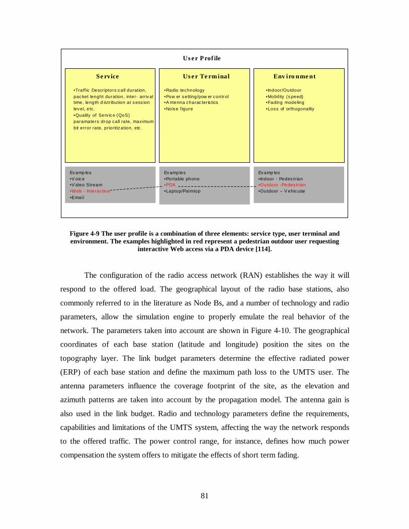
81

•Traff ic Descr iptors :call duration, pac ket lenght duration, inter- arr iv al time, length d is tr ibution at s ess ion lev el, etc .•Quality of Serv ic e (QoS)paramaters :drop call rate, maximum bit error rate, prioritization, etc .

•Radio technology•Pow er s etting/pow er control•A ntenna charac ter is tics•Noise f igure

•Indoor/Outdoor•Mobil ity (s peed)•Fading modeling•Loss of orthogonality

Se rvice Use r Te rminal Env iro nme nt

Ex amp les•V oic e•V ideo Stream•Web - Interactive•Emai l

Ex amp les•Portable phone•PDA•Laptop/Palmtop

Ex amp les•Indoor - Pedes tr ian•Outdoor -Pedes tr ian•Outdoor – V ehicular

User Prof ile

Figure 4-9 The user profile is a combination of three elements: service type, user terminal and environment. The examples highlighted in red represent a pedestrian outdoor user requesting

interactive Web access via a PDA device [114].

The configuration of the radio access network (RAN) establishes the way it will

respond to the offered load. The geographical layout of the radio base stations, also

commonly referred to in the literature as Node Bs, and a number of technology and radio

parameters, allow the simulation engine to properly emulate the real behavior of the

network. The parameters taken into account are shown in Figure 4-10. The geographical

coordinates of each base station (latitude and longitude) position the sites on the

topography layer. The link budget parameters determine the effective radiated power

(ERP) of each base station and define the maximum path loss to the UMTS user. The

antenna parameters influence the coverage footprint of the site, as the elevation and

azimuth patterns are taken into account by the propagation model. The antenna gain is

also used in the link budget. Radio and technology parameters define the requirements,

capabilities and limitations of the UMTS system, affecting the way the network responds

to the offered traffic. The power control range, for instance, defines how much power

compensation the system offers to mitigate the effects of short term fading.

82

•Transmission po we r•Noise Figu re•TX/RX losses /gains

Link Budget Pa ra meters

Radio Network Configuration

Base Station loca tio n (Latitude/Lo ng itude)

Antenna Para mete rs

•Elevation a nd Azimuth ra diation p atterns•Gain•Tilting•Bore s ight az imuth•Radiation Center h eight

Radio & Technology Pa ra meters•Num b er o f UM TS carrie rs•Han do ff p ara meters•Powe r control rang es

•Transmission po we r•Noise Figu re•TX/RX losses /gains

Link Budget Pa ra meters


Base Station loca tio n (Latitude/Lo ng itude)

Antenna Para mete rs

•Elevation a nd Azimuth ra diation p atterns•Gain•Tilting•Bore s ight az imuth•Radiation Center h eight

Radio & Technology Pa ra meters•Num b er o f UM TS carrie rs•Han do ff p ara meters•Powe r control rang es

Figure 4-10 Radio access network parameters taken into consideration in the Monte Carlo simulation [117].

The Monte Carlo module uses all the parameters described above as inputs to the

algorithm. It is worth noting that the large number of parameters constitutes a

sophisticated and complex model, representing an actual UMTS network in a rather

realistic manner. Figure 4-11 illustrates the high-level block diagram showing the

relationship between the described modules. The Monte Carlo simulator draws data from

all modules, performing iterative calculations for network load and power control

convergence, with the goal of obtaining the system resources requirements for each

service class. The high-level iterative model flow of the Monte Carlo simulator is detailed

in Figure 4-12. The first step into the process is the generation of the snapshot. The

algorithm performs a random draw from the input traffic layers for the different services

to be modeled, assembling a mix of active UMTS users randomly located around the

network sites. This snapshot intends to model the actual random placement of users and

services that exists in a network at any given time. Based on the location of each user, the

algorithm determines the best serving sector (using the signal strength predictions as a

reference), estimating power requirements and noise rise. For each user added to the

network, the algorithm executes a convergence loop, whereby it iteratively adjusts the

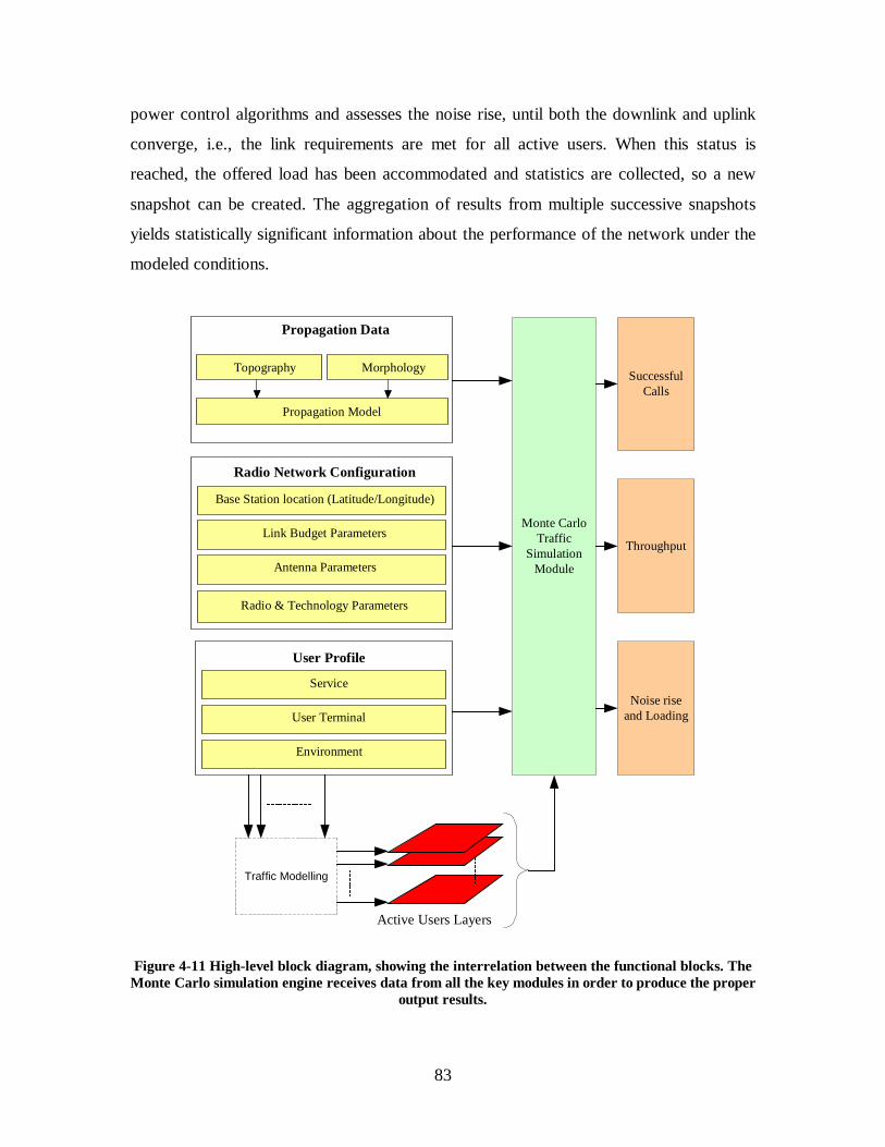
83

power control algorithms and assesses the noise rise, until both the downlink and uplink

converge, i.e., the link requirements are met for all active users. When this status is

reached, the offered load has been accommodated and statistics are collected, so a new

snapshot can be created. The aggregation of results from multiple successive snapshots

yields statistically significant information about the performance of the network under the

modeled conditions.

Monte CarloTraffic

SimulationModule

SuccessfulCalls

Throughput

Noise riseand Loading

Propagation Data

Topography Morphology

Propagation Model

Link Budget Parameters


Radio & Technology Parameters


Base Station location (Latitude/Longitude)

Antenna Parameters


User Profile

User Terminal

Service

Environment

Active Users Layers

Traffic Modelling

Figure 4-11 High-level block diagram, showing the interrelation between the functional blocks. The Monte Carlo simulation engine receives data from all the key modules in order to produce the proper

output results.

84

Snapshot generation randomly generate user characteristics: location, service

For each user: downlink allocation

uplink allocationsoft-handoff analysis

Convergence loop

Collect System Statistics

Statistics loop

Use traffic layers as input

Best server selectionPower control setting

Admission controlRadio Resource Management

Traffic per sectorBlocking per sector

Channel requirementsUplink noise rise

Base station power

Figure 4-12 High-level model flow of the Monte Carlo simulation engine

It is worth noting that during the convergence process, the algorithm emulates Radio

Resource Management (RRM) functions that are key to the optimal performance of

UMTS networks. Load control and admission control are exercised to maintain the load

at a level that does not compromise the network’s performance. The network monitors

the load for each sector, denying service to new users as they attempt to access the

system if the load reaches or exceeds a pre-defined limit. Similarly, the network may

deny service if a sectors runs out of orthogonal codes, radio resources or reaches its

throughput limit. Additionally, where appropriate, the effects of soft handoff are

considered and analyzed. Soft handoff gains are accounted for in the convergence process

and the corresponding radio resources requirements are reflected in the statistics.

The performance of the UMTS network under the simulated conditions is

summarized in the statistical report produced from the aggregation of the results captured

at the end of each iteration. A set of statistical variables is collected. The following

variables are captured during the simulation, offering a detailed depiction of the

network’s performance:

♦ Average and standard deviation of number of users supported by each

sector, when the sector is the main server. The information is available per

service class and totalized for all classes.

85

♦ Average and standard deviation of number of users supported by each

sector, when the sector is a soft-handoff server. The information is

available per service class and totalized for all classes.

♦ Average and standard deviation of the total number of users per sector –

main plus soft-handoff traffic.

♦ Average and standard deviation of power levels foreach sector’s traffic

channels. The information is available per service class and totalized for

all classes.

♦ Average and standard deviation of the noise rise experienced by each

sector.

4.2.2 The Proposed UWB - UMTS Monte Carlo Algorithm

The functional modules and Monte Carlo algorithm described in the previous

sections make up a comprehensive network-level UMTS simulator. However, in that

configuration the simulator cannot capture the effects of external interference on the

UMTS network. This section proposes an enhancement to the tool, creating additional

inputs for the pertinent UWB variables and modifying the algorithm to account for them.

The proposed solution allows the tool to simulate the behavior of the UMTS network

with the same level of completeness as in its original form, with the added ability of

simultaneously modeling the impact of UWB interference on the network performance.

The available literature describes UMTS system level performance simulations in the

presence of UWB for very controlled scenarios, with simplistic network configurations

and limited input variables [7], [42], [123]. The results obtained from those, while

offering some insight into the actual impact of UWB on UMTS, do not allow for a

thorough quantitative assessment of interference in real network deployments.

Furthermore, those studies offer contradicting conclusions. While [7], [123] suggest that

UWB interference on UMTS networks can be severe, [42] concludes that UWB can

coexist with UMTS networks without causing harmful interference. This contribution

intends to overcome the limitations posed by those studies, offering a thorough and

86

scalable implementation, which can be used to assess both theoretical and practical

network scenarios. Figure 4-13 illustrates the modified algorithm, highlighting the added

functional blocks.

UMTS Users Snapshot generation randomly generate user characteristics: location, service

For each user: downlink allocation

uplink allocationsoft-handoff analysis

Convergence loop

Collect System Statistics

Statistics loop

Use traffic layers as input

Best server selectionPower control setting

Admission controlRadio Resource Management

Traffic per sectorBlocking per sector

Channel requirementsUplink noise rise

Base station power

UWB Interferers Snapshot generation randomly generate interferer characteristics: location,

power

Location correlated with UMTS usersNumber of UWB devices per UMTS user

Power per UWB device

Aggregate UWB interference at UMTS user locationand add to noise power

Figure 4-13 Proposed simulation algorithm to model UWB interference on UMTS networks.

The modified algorithm adds new input variables to the simulator, so that it can consider

the UWB parameters required for the proper modeling of the technology. These new

variables also allow for the creation of different simulation scenarios and sensitivity

analyses, as discussed in the next section.

At the present time, UWB has not yet come to fruition as a mass-market

technology. However, there is a consensus amongst industry organizations and

government regulatory bodies, that the evolution of these devices is likely to be

dominated by personal area network (PAN) applications and by the home entertainment

market. It is envisaged that UWB devices will be very low power, for short-range

applications and capable of high data rate transfers, with a few devices per household or

office. Based on this scenario, the algorithm implementation assumes the UWB devices

to be spatially correlated with the UMTS users, which seems the most likely situation to

87

be encountered in a mature UWB deployment, as UWB devices are anticipated to operate

in the same geographical surroundings where UMTS devices are usually located. The

algorithm offers two options for the active UWB device density, represented as the

average ratio of the number of active UWB devices and the number of active UMTS

users. The UWB to UMTS user ratio can be either constant or follow a Poisson

distribution, characterized by its mean. The Poisson distribution has been used to model

the number of active UWB interferers in similar coexistence studies [123]. The algorithm

reads the number of active UMTS users from the traffic layers. Once the number of

active UWB devices for a UMTS user is determined, their aggregate power spectral

density contribution at the UMTS user location is calculated. If the active UWB-UMTS

user ratio is constant, the aggregate power spectral density is the product of the number of

active UWB devices and the individual power spectral density per device. The individual

reference power spectral density per UWB device is an input variable, added to the

modified algorithm. If the active UWB-UMTS user ratio follows the Poisson distribution,

the aggregate power spectral density is the sum of the individual contributions from each

UWB device. In this case, each UWB device is separated from the UMTS user by a

different distance, randomly selected from a uniform distribution with mean correlation

distance cord , which depends on another user-defined input variable - the maximum

separation distance. The mean correlation distance cord is defined as one half of the

maximum separation distance, as shown in Figure 4-14. The UWB devices are assumed

to be randomly located anywhere inside a circle of radius cord×2 centered at the UMTS

user location. The different separation distances for each UWB device cause their

individual power spectral density contributions to differ from one another. The individual

power spectral densities at the UMTS user location are calculated using a slope-intercept

model in the form

−⋅++=

)(()log

0,0

0, ddrandd

dPSDPSD

iUMTSUWBUWBiUMTSUWB α , Equation 4-1

where:

88

iUMTSUWBPSD , : Power spectral density of the thi UWB device at the UMTS user location;

UWBPSD : Power spectral density radiated by the UWB device;

α : Attenuation coefficient for the propagation environment – input variable;

0d : Minimum distance from the UMTS user – input variable;

iUMTSUWBd , : Separation distance between the thi UWB device and the UMTS users,

randomly selected from a uniform distribution with mean correlation distance cord ; and

()rand : Random number between 0 and 1.

dmax

UMTS user location

dUWB,UMTS

p(d)

dcor=dmax/2

maximum correlation distance - dmax

Figure 4-14 – Definition of the mean correlation distance between the UMTS user and the UWB interference source. UWB interferers can be randomly located anywhere inside the depicted yellow

circle.

The aggregate power spectral density at the UMTS user location is the sum of all

individual contributions, as described by equation (4-2).

∑=

=n

iUMTSUWBUMTSUWB i

PSDPSD1

,, Equation 4-2

After appropriate bandwidth denormalization, the result from equation (4-2) is added to

the total downlink noise power at the UMTS user’s receiver, integrating the UWB

89

interference into the remaining algorithm calculations. The convergence and statistics

loops operate as described in section 4.2.1.2.

4.2.3 Considerations on the Validation of the Tool

The CelPlanner tool selected for this study has been used commercially for the

design and optimization of real wireless networks for over ten years. During this time, its

algorithms have been refined and improved to model the actual behavior of wireless

networks, based on meticulous modeling and on the experience and feedback gathered

from extensively employing the tool in real designs. Reference [117] presents a formal

validation study where the results produced by CelPlanner are compared to those

generated with the NPSW tool, independently developed by Nokia Corporation. That

study shows the tools to be qualitatively equivalent, adding credence to the use of

CelPlanner in this research.

4.3 System Level Simulations

The UWB-UMTS Monte Carlo algorithm proposed and described in the previous

section is applied to a notional UMTS network, allowing for the assessment of the impact

UWB interference can have on its capacity. The analysis includes the variation of the

UWB power level and device density, providing insight into the expected trending of

these variables. Firstly, a baseline UMTS network that suffers no external interference is

analyzed. The performance results are used as a baseline for comparison against the

results obtained in the scenarios where UWB interference is present. The same network is

then subjected to a coexisting UWB device population of fixed transmission power

levels. The UWB device density is varied and the UMTS network performance is

analyzed as the density changes. In the final scenario, the UWB device density is kept

constant and the UWB radiated power is varied, to allow for the study of the UMTS

network’s sensitivity to the FCC emission limits established for UWB.

90

4.3.1 Service Classes

The UMTS users were simulated in four different service classes – a subset of

those used in the study presented in Chapter 3. The chosen service classes are those

where there is greater potential spatial correlation between the UWB source and the

UMTS device, namely in the in-car and indoor environments. The applications

envisioned for UWB focus on home and office personal area networks, home

entertainment and high-data rate, low range multimedia, making it intrinsically an indoor

technology. Considering that UMTS handsets are likely to share these same spaces, the

physical distance between UWB interferer and UMTS victim receiver is potentially

small. Therefore, this study concentrates on the analysis of UWB interference on UMTS

in closed environments, assuming line-of-sight between the UWB interference source and

victim receiver. The four service classes included in the simulations are:

1. Vehicular speech, macrocell: models voice service using the AMR

(Adaptive Modulation Rate) vocoder with bit rate equal to 12.2 Kbps in an

in-car scenario. This test case simulates mobile users utilizing UMTS

voice services while in transit, for example, on a moving train.

2. Indoor speech, macrocell: this scenario models voice service using the

AMR vocoder with bit rate equal to 12.2 Kbps in an indoor environment.


indoors, for example, standing or walking inside an office or residential

building.

3. Indoor real time data, macrocell: models real time circuit switched data

(CSD) at 144 Kbps in an indoor scenario. This test case simulates mobile

users utilizing UMTS data services while indoors, for example, standing

or walking inside an office or residential building.

4. Indoor non-real time data, macrocell: models non-real time packet

switched data (PSD) at 384 Kbps in an indoor scenario. This test case

simulates mobile users using UMTS data services while indoors, for

example, standing or walking inside an office or residential building.

91

The service parameters of each class differentiate the type of UMTS service to be

simulated. Table 4-1 summarizes the parameters and values employed in the study.

Table 4-1 Service configuration parameters for the four service classes modeled in the UMTS simulation

Configuration Parameters

Service Class Voice

Vehicular

Voice

Indoor

Circuit Switched

Data Indoor

Packet Switched

Data Indoor

Service Type Voice Voice Data Data

Allocation Priority 0 0 1 2

Forward 12.2 kbps 12.2 kbps 144 kbps 384 kbps Data Rate

Reverse 12.2 kbps 12.2 kbps 144 kbps 384 kbps

Forward 0.6 0.6 0.1 0.1 Activity Factor

Reverse 0.5 0.5 0.1 0.1

Data Overhead Factor 0 0 0 0

Max. # of handoff

servers

3 3 3 3

Forward 7.9 6.1 1.9 1.0 Eb/Io

Reverse 7.9 6.1 1.9 1.0

Max. TCH Power Forward 2W 2W 2W 2W

Forward 1 dB 1 dB 1 dB 1 dB Power control margin

above threshold

Reverse 1 dB 1 dB 1 dB 1 dB

4.3.2 UMTS User Terminal Configuration

Two types of UMTS user terminals were considered in the simulations: voice and

data. The relevant parameters are summarized in Table 4-2. These parameters define how

the UMTS users interact with the network at the radio level.

92

Table 4-2 UMTS user terminal configuration parameters employed in the system level simulations

UMTS User Terminal Configuration

User Terminal Type Voice Data

Maximum Transmission Power 21 dBm 24 dBm

Noise Figure 7 dB 7 dB

Antenna Radiation Pattern Omnidirectional Omnidirectional

Antenna Height Above Ground 1.5 m 1.5 m

Antenna gain 0 dBi (-2.14 dBd) 0 dBi (-2.14 dBd)

4.3.3 Environment Configuration

The UMTS users were modeled in two distinct propagation environments: in-car

and in building, as shown in Table 4-3. The in-car profile uses the Rayleigh distribution

to model the multipath, due to the mobility associated with it, whereas the in-building

profile assumes the UMTS device to be essentially stationary. In this case, the lognormal

distribution better represents the link condition.

Table 4-3 Propagation environment parameters used in the system level simulations

Environment Configuration

Environment Type In-car In-building

Body shielding loss 3 dB 3 dB

Penetration Attenuation 8 dB 15 dB

Fading Model

Distribution Rayleigh Lognormal

Confidence Margin (cell area) 90% 90%

Standard Deviation 6 dB 6 dB

Slope 40 dB/dec 40 dB/dec

Total Link Margin 15.8 dB 21.0 dB

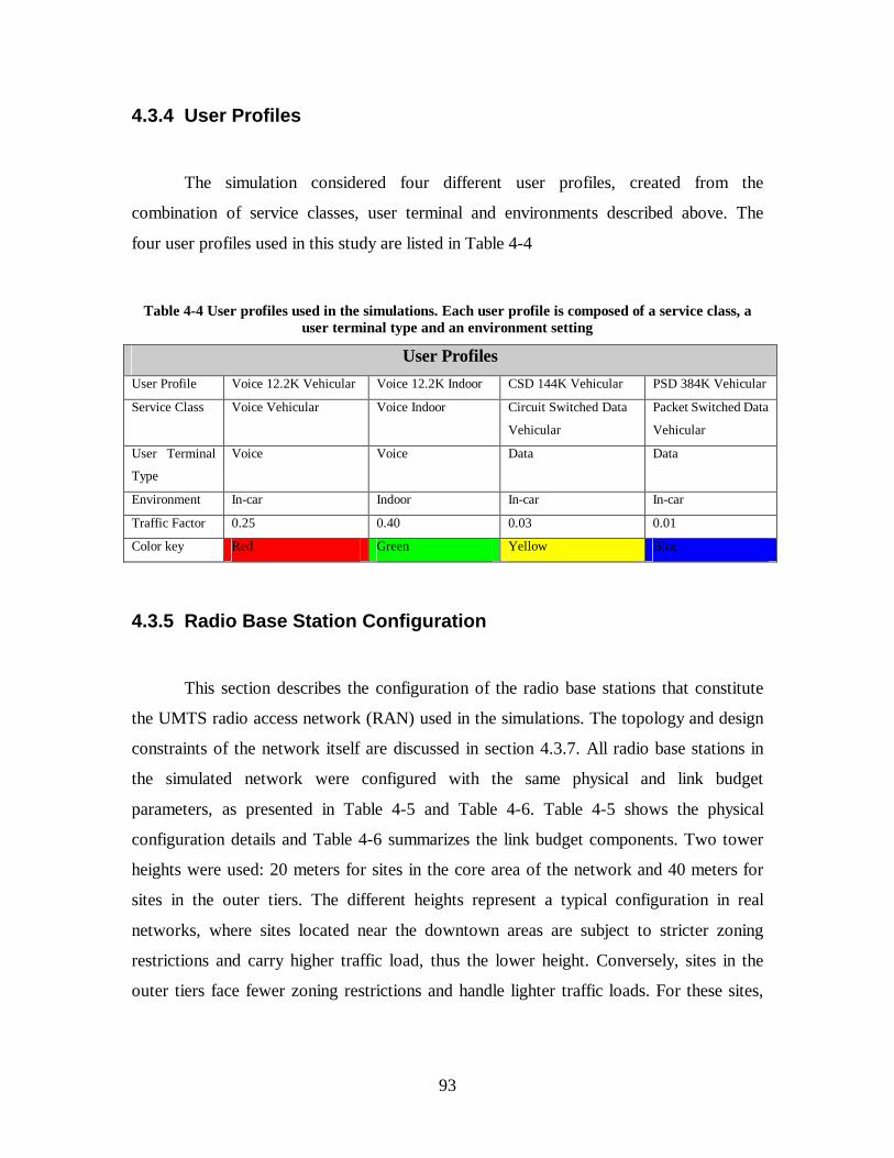
93

4.3.4 User Profiles

The simulation considered four different user profiles, created from the

combination of service classes, user terminal and environments described above. The

four user profiles used in this study are listed in Table 4-4

Table 4-4 User profiles used in the simulations. Each user profile is composed of a service class, a user terminal type and an environment setting

User Profiles

User Profile Voice 12.2K Vehicular Voice 12.2K Indoor CSD 144K Vehicular PSD 384K Vehicular

Service Class Voice Vehicular Voice Indoor Circuit Switched Data

Vehicular

Packet Switched Data

Vehicular

User Terminal

Type

Voice Voice Data Data

Environment In-car Indoor In-car In-car

Traffic Factor 0.25 0.40 0.03 0.01

Color key Red Green Yellow Blue

4.3.5 Radio Base Station Configuration

This section describes the configuration of the radio base stations that constitute

the UMTS radio access network (RAN) used in the simulations. The topology and design

constraints of the network itself are discussed in section 4.3.7. All radio base stations in

the simulated network were configured with the same physical and link budget

parameters, as presented in Table 4-5 and Table 4-6. Table 4-5 shows the physical

configuration details and Table 4-6 summarizes the link budget components. Two tower

heights were used: 20 meters for sites in the core area of the network and 40 meters for

sites in the outer tiers. The different heights represent a typical configuration in real

networks, where sites located near the downtown areas are subject to stricter zoning

restrictions and carry higher traffic load, thus the lower height. Conversely, sites in the

outer tiers face fewer zoning restrictions and handle lighter traffic loads. For these sites,

94

higher tower are actually desirable, to maximize the coverage with as few sites as

possible.

Table 4-5 Physical configuration of the radio base stations that compose the UMTS network used in the simulations

Radio Base Station Physical Configuration

20 m for core sites Antenna Height Above Ground Level (AGL)

40 m for outer tier sites

Number of Sectors 3

Sector Azimuth 0, 120 and 240 degrees

Antenna Model Andrew UMW-06517-2DH

Antenna Tilting 2 degrees of electrical tilting – all sectors

Antenna Gain 18.9 dBi at boresight

Table 4-6 Link budget parameters for the radio base stations that com pose the UMTS network used in the simulations

Radio Base Station Link Budget

Forward Link

Pilot Channel Power (CPICH) 1.5 W

Combined Power for Other Control Channels (Sync, Paging, etc.) 1.0 W

Maximum Traffic Channel Power (per channel) 2.0W

Orthogonality Factor 0.5

TX Branch Losses (feeders, jumpers, etc.) 2.8 dB

TX Antenna Gain 18.9 dBi

Reverse Link

RX Antenna Gain 18.9 dBi

Diversity Gain 2 dB

RX Branch Losses (feeders, jumpers, etc.) 2.8 dB

Front-end Noise Figure 5.0 dB

95

4.3.6 UMTS System Parameters

The following parameters define the basic UMTS network in the simulator, being

applied globally to all radio base stations and UMTS users.

Table 4-7 – UMTS network simulation parameters applied to all radio base stations

UMTS System Parameters

UMTS Carrier Bandwidth 3.84 MHz

Maximum Throughput per Carrier 2048 kbps

Maximum Number of Vocoders per Carrier 60

Maximum Load Factor – Forward Link 1

Maximum Load Factor – Reverse Link 1

Maximum Number of Allocation Failures per Call 8

Maximum Combined Base Station Output Power (per sector) 45 W

4.3.7 UMTS Network Topology

The UMTS network used in the simulations consists of 45 radio base stations

(sites), as depicted in Figure 4-15. The network was designed with the goal of providing

coverage to the area delimited by the red polygon. The placement of each radio base

station was manually optimized through an iterative process, aiming at fulfilling the

coverage requirement while minimizing the number of sites. The result is a network

topology that loosely resembles a classical hexagon grid. The sites closer to the center

of the area of interest have lower tower heights, covering a smaller geographical area,

resulting in a higher site density. Conversely, the outer tier sites have higher tower

heights, resulting in larger coverage areas and lower site density. Each base station is

composed of three sectors, or cells, resulting in 135 cells for the entire network. In the

layout depicted in Figure 4-15, the geographical location of each base station is indicated

by the icon, which coincides with the junction of the three cells encompassing the

site. The setup parameters for the coverage predictions are summarized in Table 4-8.

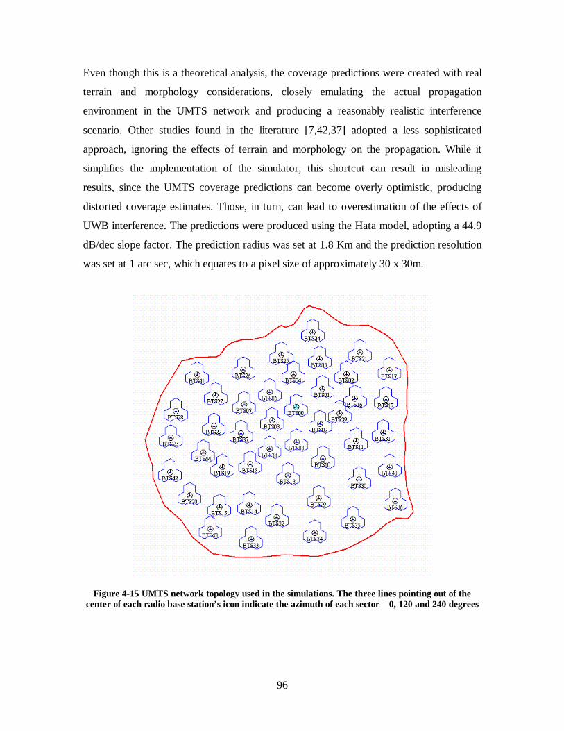
96

Even though this is a theoretical analysis, the coverage predictions were created with real

terrain and morphology considerations, closely emulating the actual propagation

environment in the UMTS network and producing a reasonably realistic interference

scenario. Other studies found in the literature [7,42,37] adopted a less sophisticated

approach, ignoring the effects of terrain and morphology on the propagation. While it

simplifies the implementation of the simulator, this shortcut can result in misleading

results, since the UMTS coverage predictions can become overly optimistic, producing

distorted coverage estimates. Those, in turn, can lead to overestimation of the effects of

UWB interference. The predictions were produced using the Hata model, adopting a 44.9

dB/dec slope factor. The prediction radius was set at 1.8 Km and the prediction resolution

was set at 1 arc sec, which equates to a pixel size of approximately 30 x 30m.

Figure 4-15 UMTS network topology used in the simulations. The three lines pointing out of the center of each radio base station’s icon indicate the azimuth of each sector – 0, 120 and 240 degrees

97

Table 4-8 Coverage prediction parameters used in the UMTS system level simulations

Coverage Prediction Parameters

Prediction radius 1.8 Km

Prediction resolution 1 arc sec

Terrain & Morphology (Clutter) 30 m resolution

Propagation Model Hata - single slope, 44.9 dB/decade

4.3.8 UMTS Traffic Demand Grid

The UMTS traffic demand distribution for the area to be simulated is represented

as a grid or, optionally, a raster file. Both have a bin size (pixel size) specified in meters

or arc sec, which indicate the granularity of the data. The traffic demand files are an input

to the simulations, being used by the algorithm to draw users from during the execution

of the Monte Carlo process. Essentially, the traffic demand files contain the number of

active users in each geographical bin or pixel. They are generated in the tool, using as

input parameters the user profile information described in section 4.3.4 and other

variables that are a function of the desired type of demand grid, including the shape and

size of the area and distribution pattern –uniform or weighted. When the distribution is

uniform, all bins or pixels will have the same number of active users. For weighted

distributions, the land use classes in the morphology can be used to determine the traffic

density in each bin or pixel, based on input weighing factors.

For the simulations discussed in this study, the UMTS demand grid was assumed

to have 4000 active UMTS users. A percentage of this total – 70%, was assigned to the

four service classes, according to the Traffic Factors listed in Table 4-4. The remaining

30% were allocated to other user profiles that are not included in this study, for they

represent outdoor traffic. As previously mentioned, UWB is anticipated to be

predominantly an indoor technology. Therefore, UMTS outdoor traffic is unlikely to be

subject to UWB interference. The relevant users were distributed over the area encircled

by the polygon depicted in Figure 4-15, following a set of user-defined morphology

weighting factors, as shown in Table 4-9. The weighting factors emulate the different

98

user densities encountered in each type of morphology. For instance, the factors in Table

4-9 indicate that the UMTS user density in streets and roads is twice as high as that of

residential areas of low concentration (intensity). During the design phase of commercial

wireless networks, these weighting factors are derived from demographic studies of the

area of interest. The numbers used in this study are typical figures based on the author’s

professional experience in wireless network design.

The traffic demand grid is approximately 12.8 Km long in the East-West direction

and 12.3 Km long in the North-South direction, representing a total area of 124.3 Km2, or

32 active users/Km2. The 4000 active users were proportionately divided amongst the

four user profiles described in Table 4-4, following the traffic factors indicated in that

table. Table 4-10 summarizes the demand grid parameters discussed above, whereas

Table 4-11 shows the number of simulated active users per user profile. Figure

4-16 illustrates the graphical aspect of the demand grid. The grid shown refers to the

distribution of Voice 12.2 Kbps indoor users.

Table 4-9 - Traffic spreading weighting factors per morphology type

Morphology Type (Clutter) Traffic Spreading Weighing Factor

Open Water 1

Woody Wetlands, Emergent Herbaceous 2

Perennial Ice/Snow, Bare Rock 1

Grasslands/Herbaceous, Pasture 1

Shrubland, Orchards/Vineyards 4

Deciduous Forest 2

Evergreen Forest 2

Mixed Forest 2

Urban/Recreational Grasses 16

Roads 128

Streets 128

Low Intensity Residential 64

High Intensity Residential 128

Commercial/Industrial/Transportation 255

99

Table 4-10 - Parameters used in the generation of the demand grid employed in the system level simulations

Demand Grid Parameters

Number of Active UMTS Users 4000

Grid resolution 30 m

Distribution mode Uniform

Table 4-11 Number of simulated active UMTS users per user profile

Number of active UMTS users

User Profile Voice 12.2K Vehicular Voice 12.2K Indoor CSD 144K Indoor PSD 384K Indoor

Number of active users 1000 1600 120 40

Figure 4-16 View of the demand grid for the Voice 12.2 Kbps user profile. The colors represent the different degrees of user activity.

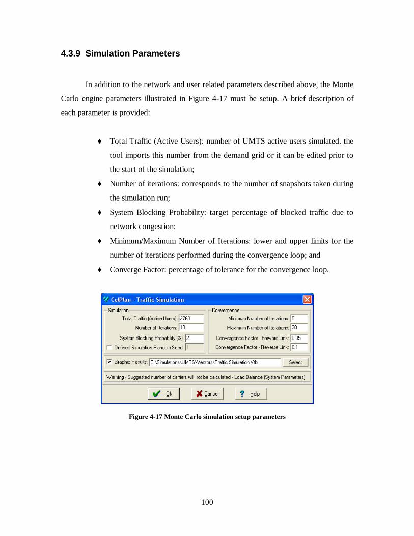
100

4.3.9 Simulation Parameters

In addition to the network and user related parameters described above, the Monte

Carlo engine parameters illustrated in Figure 4-17 must be setup. A brief description of

each parameter is provided:

♦ Total Traffic (Active Users): number of UMTS active users simulated. the

tool imports this number from the demand grid or it can be edited prior to

the start of the simulation;

♦ Number of iterations: corresponds to the number of snapshots taken during

the simulation run;

♦ System Blocking Probability: target percentage of blocked traffic due to

network congestion;

♦ Minimum/Maximum Number of Iterations: lower and upper limits for the

number of iterations performed during the convergence loop; and

♦ Converge Factor: percentage of tolerance for the convergence loop.

Figure 4-17 Monte Carlo simulation setup parameters

101

4.4 Simulation Results & Discussion

This section presents and discusses the simulation results for the four scenarios

introduced in section 4.3.

4.4.1 UMTS Baseline Scenario

In this scenario, the UMTS network suffers no external UWB interference. It is

used as a baseline for comparison against the other two scenarios presented below. The

network configuration and parameters are as described in Section 4.3. The simulation

included 2760 UMTS users, divided in four classes of service, as detailed in Table 4-11.

An aggregated graphical depiction of the UMTS users simulated at each snapshot is

presented in Figure 4-18. The colors represent the different user profiles, as described in

Table 4-4. The pixels shown in black indicate failed connection attempts.

Voice 12.2 Kbps - Indoor

Voice 12.2 Kbps - Vehicular

CSD 144 Kbps - Indoor

PSD 384 Kbps - Indoor

Failed Connections

Figure 4-18 – Aggregated graphical representation of the UMTS users simulated at each snapshot.

102

The simulation results for the baseline scenario are summarized in Table 4-12.

They are shown for the total number of simulated users, but reflect the individual traffic

contributions by each of the four user profiles. The subsequent set of figures - Figure

4-19 thru Figure 4-51, offers detailed insight into the UMTS network performance,

illustrating through various metrics its behavior under the simulated load condition.

Figure 4-19 to Figure 4-46 show the composite performance of the UMTS network for

each user profile separately, whereas Figure 4-47 to Figure 4-51 show a set of metrics for

the combined user profiles, i.e., the complete population of users. A discussion of the

results shown in these figures is presented below.

Table 4-12 – Summary of the traffic simulation results for the baseline scenario – no UWB interference

Metric Active

Users

Percentage of

Total

Total Simulated Traffic 2760.0 100 %

Carried traffic - Main traffic 2505.8 90.8 %

Carried traffic - Handoff traffic 1158.9 42 %

Not carried traffic - Pilot channel coverage 26.6 1.0 %

Not carried traffic - Directed to other carriers 0 0

Not carried traffic - Throughput per carrier limit 0 0

Not carried traffic - Forward traffic channel power limit 17.9 0.6 %

Not carried traffic - Forward sector total power limit 0 0

Not carried traffic - Forward load factor limit 0 0

Not carried traffic - Reverse mobile power limit 209.7 7.6 %

The results in Table 4-12 show that in the absence of external interference, the

UMTS network performance is similar to that expected of real operational networks. In

the simulated scenario, the network carried 90.8% of the offered traffic. The remaining

9.2% were not carried due to three limiting conditions: lack of pilot channel coverage,

lack of forward traffic channel power and lack of reverse link power, due to handset

power limitations. The 1% of traffic not carried due to lack of pilot channel coverage

103

indicates that, in that configuration, the network does not reach 100% of the geographical

area where there is demand for the UMTS service. This is generally the case in most

commercial networks, because it becomes prohibitively costly to build a ubiquitous

network. The 0.6% of traffic not carried due to lack of forward traffic channel power

indicates that some sectors are experiencing power saturation, even in the absence of

external interference. This implies that there is already enough intra-network noise at

some sectors to cause the base station to reach power saturation. The power saturation

can be a consequence of traffic – too many active connections, or coverage – users are

too far from the site and require additional power in the forward link. The lack of reverse

link power prevented 7.6% of the offered traffic to be served, indicating that the link

budget is unbalanced, allowing more forward link coverage than reverse link. Even

though the three metrics mentioned above can most likely be optimized through

traditional network optimization techniques, for the purpose of this dissertation they can

be considered as adequate, since the study aims at comparing the relative degradation in

coverage due to UWB interference.

Figure 4-19 to Figure 4-22 illustrate the pilot channel (CPICH) coverage for the

four service classes, for the resulting network load offered by the simulated user

population. These plots show that the pilot channel coverage is virtually ubiquitous, with

oc IE above the –15 dB threshold in most of the area of interest. As expected, the indoor

service classes show as smaller footprint for the same oc IE threshold, due to the larger

attenuation caused by buildings.

104

Figure 4-19 –Pilot channel (CPICH) Ec/Io (dB), no UWB interference - 12.2 Kbps Vehicular Voice.

Figure 4-20 - Pilot channel (CPICH) Ec/Io (dB), no UWB interference - 12.2 Kbps Indoor Voice.

105

Figure 4-21 - Pilot channel (CPICH) Ec/Io (dB), no UWB interference -144 Kbps Indoor Circuit Switched Data.

Figure 4-22 - Pilot channel (CPICH) Ec/Io (dB), no UWB interference -384 Kbps Indoor Packet Switched Data.

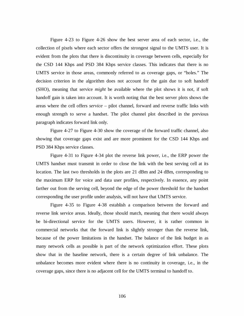
106

Figure 4-23 to Figure 4-26 show the best server area of each sector, i.e., the

collection of pixels where each sector offers the strongest signal to the UMTS user. It is

evident from the plots that there is discontinuity in coverage between cells, especially for

the CSD 144 Kbps and PSD 384 Kbps service classes. This indicates that there is no

UMTS service in those areas, commonly referred to as coverage gaps, or “holes.” The

decision criterion in the algorithm does not account for the gain due to soft handoff

(SHO), meaning that service might be available where the plot shows it is not, if soft

handoff gain is taken into account. It is worth noting that the best server plots shows the

areas where the cell offers service – pilot channel, forward and reverse traffic links with

enough strength to serve a handset. The pilot channel plot described in the previous

paragraph indicates forward link only.

Figure 4-27 to Figure 4-30 show the coverage of the forward traffic channel, also

showing that coverage gaps exist and are more prominent for the CSD 144 Kbps and

PSD 384 Kbps service classes.

Figure 4-31 to Figure 4-34 plot the reverse link power, i.e., the ERP power the

UMTS handset must transmit in order to close the link with the best serving cell at its

location. The last two thresholds in the plots are 21 dBm and 24 dBm, corresponding to

the maximum ERP for voice and data user profiles, respectively. In essence, any point

farther out from the serving cell, beyond the edge of the power threshold for the handset

corresponding the user profile under analysis, will not have that UMTS service.

Figure 4-35 to Figure 4-38 establish a comparison between the forward and

reverse link service areas. Ideally, those should match, meaning that there would always

be bi-directional service for the UMTS users. However, it is rather common in

commercial networks that the forward link is slightly stronger than the reverse link,

because of the power limitations in the handset. The balance of the link budget in as

many network cells as possible is part of the network optimization effort. These plots

show that in the baseline network, there is a certain degree of link unbalance. The

unbalance becomes more evident where there is no continuity in coverage, i.e., in the

coverage gaps, since there is no adjacent cell for the UMTS terminal to handoff to.

107

Figure 4-23 - Pilot channel (CPICH) Best Server Plot, no UWB interference - 12.2 Kbps Vehicular Voice.

Figure 4-24 - Pilot channel (CPICH) Best Server Plot, no UWB interference - 12.2 Kbps Indoor Voice.

108

Figure 4-25 - Pilot channel (CPICH) Best Server Plot, no UWB interference - 144 Kbps Indoor Circuit Switched Data.

Figure 4-26 - Pilot channel (CPICH) Best Server Plot, no UWB interference - 384 Kbps Indoor Packet Switched Data.

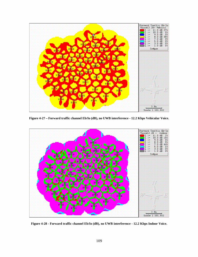
109

Figure 4-27 – Forward traffic channel Eb/Io (dB), no UWB interference - 12.2 Kbps Vehicular Voice.

Figure 4-28 - Forward traffic channel Eb/Io (dB), no UWB interference - 12.2 Kbps Indoor Voice.

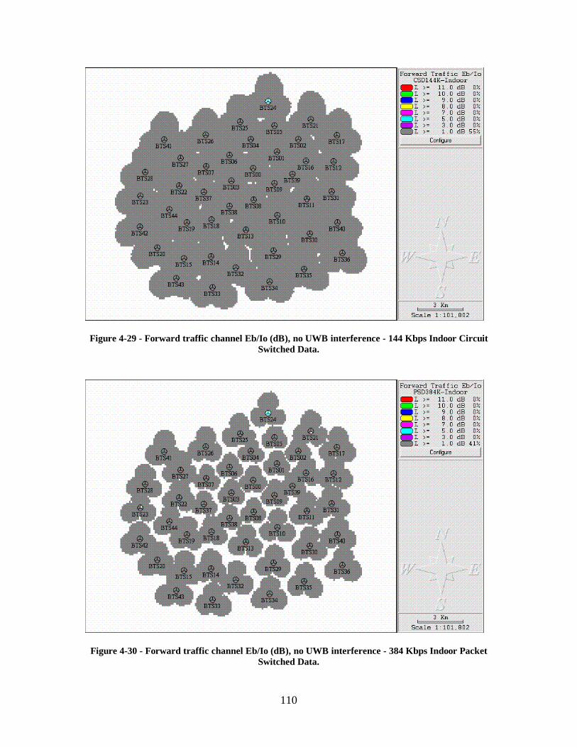
110

Figure 4-29 - Forward traffic channel Eb/Io (dB), no UWB interference - 144 Kbps Indoor Circuit Switched Data.

Figure 4-30 - Forward traffic channel Eb/Io (dB), no UWB interference - 384 Kbps Indoor Packet Switched Data.

111

Figure 4-31 – Mobile terminal radiated power (ERP), in dBm, no UWB interference - 12.2 Kbps Vehicular Voice.

Figure 4-32 - Mobile terminal radiated power (ERP), in dBm, no UWB interference - 12.2 Kbps Indoor Voice.

112

Figure 4-33 - Mobile terminal radiated power (ERP), in dBm, no UWB interference - 144 Kbps Indoor Circuit Switched Data.

Figure 4-34 - Mobile terminal radiated power (ERP), in dBm, no UWB interference - 384 Kbps Indoor Packet Switched Data.

113

Figure 4-35 – Forward/Reverse Link Service Areas, no UWB interference - 12.2 Kbps Vehicular Voice.

Figure 4-36 - Forward/Reverse Link Service Areas, no UWB interference - 12.2 Kbps Indoor Voice.

114

Figure 4-37 - Forward/Reverse Link Service Areas, no UWB interference - 144 Kbps Indoor Circuit Switched Data.

Figure 4-38 - Forward/Reverse Link Service Areas, no UWB interference - 384 Kbps Indoor Packet Switched Data.

115

Figure 4-39 to Figure 4-42 show the forward link noise rise, representing the

contribution of the forward link channels to the noise rise. The noise rise is proportional

to the number of active forward channels – pilot and traffic, and their respective power

levels.

Figure 4-43 to Figure 4-46 depict the areas where soft handoffs are expected,

based on the variation of the pilot channel ob NE as the UMTS terminal moves away

from one cell and towards another.

Figure 4-47 offers valuable insight into the reverse link load factor, showing the

contribution of the reverse link ERP from all active UMTS devices served by a sector -

the more active users per sector, the greater the load factor. It is worth mentioning that

the number of active users per cell used to produce these plots was derived from the

Monte Carlo simulation.

Figure 4-48 and Figure 4-49 show the number of active users and number of

active users in soft handoff per cell, respectively. The difference in traffic densities

across the area of interest is apparent in both figures, where it can be observed that the

traffic is not balanced amongst the cells. Cells with smaller footprint tend to carry less

traffic, whereas those with larger coverage areas tend to absorb more traffic. In addition,

the cells at the edge of the area of interest, pointing outwards, tend to have less soft

handoff traffic, because there are no adjacent cells other than the neighbor cells in their

own base station.

Figure 4-50 illustrates the total base station power per cell. The total power is

composed of the common pilot channel, other pilot channels and the traffic channels. It

shows a strong correlation with the number of simultaneous active users plot depicted in

Figure 4-48 – the more active users, the greater total power.

Figure 4-51 shows the total forward link throughput per cell. It also shows a

strong correlation with the number of active users and the total base station power per

sector. The total forward link throughput for the simulated network is 66.6 Mbps,

representing an average of 493.3 Kbps per cell.

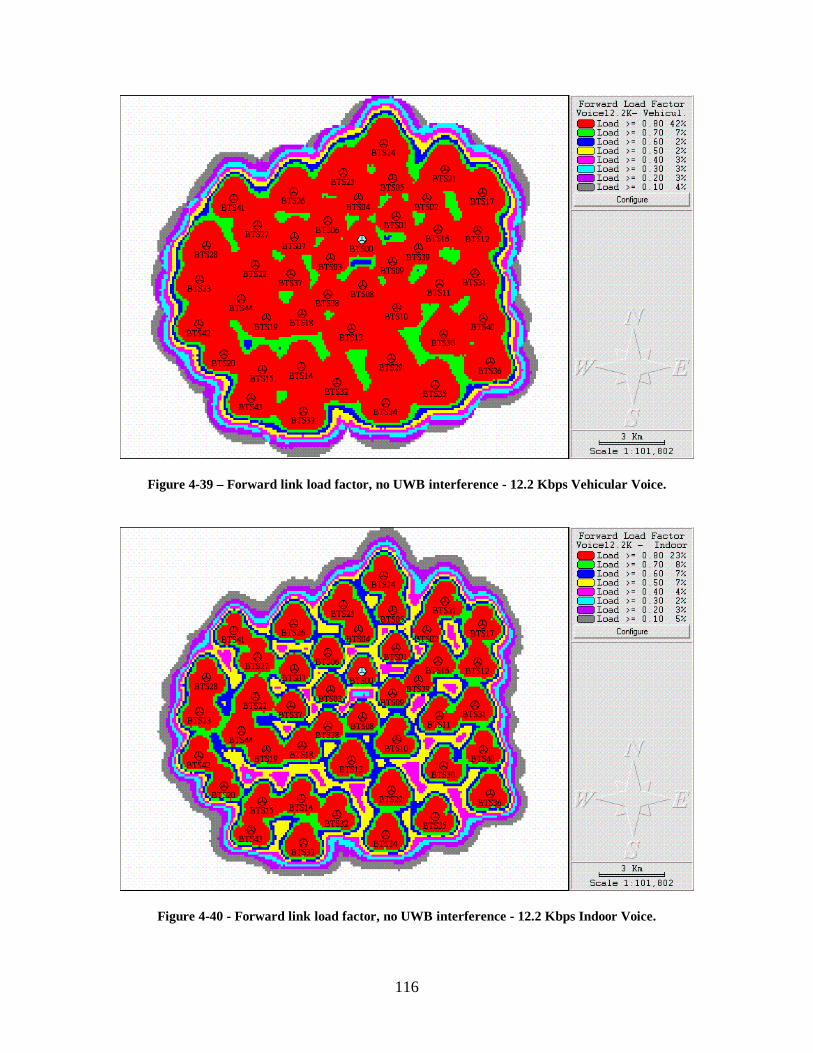
116

Figure 4-39 – Forward link load factor, no UWB interference - 12.2 Kbps Vehicular Voice.

Figure 4-40 - Forward link load factor, no UWB interference - 12.2 Kbps Indoor Voice.

117

Figure 4-41 - Forward link load factor, no UWB interference - 144 Kbps Indoor Circuit Switched Data.

Figure 4-42 - Forward link load factor, no UWB interference - 384 Kbps Indoor Packet Switched Data.

118

Figure 4-43 – Handoff areas plot, no UWB interference - 12.2 Kbps Vehicular Voice.

Figure 4-44 - Handoff areas plot, no UWB interference - 12.2 Kbps Indoor Voice.

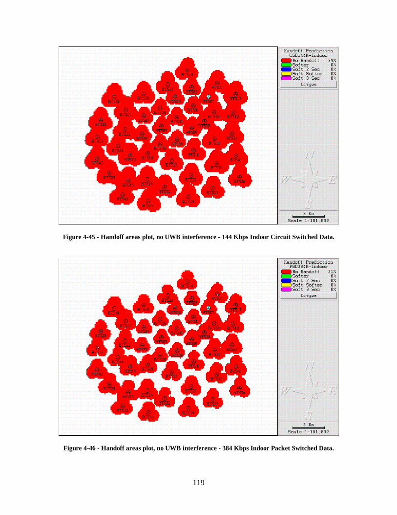
119

Figure 4-45 - Handoff areas plot, no UWB interference - 144 Kbps Indoor Circuit Switched Data.

Figure 4-46 - Handoff areas plot, no UWB interference - 384 Kbps Indoor Packet Switched Data.

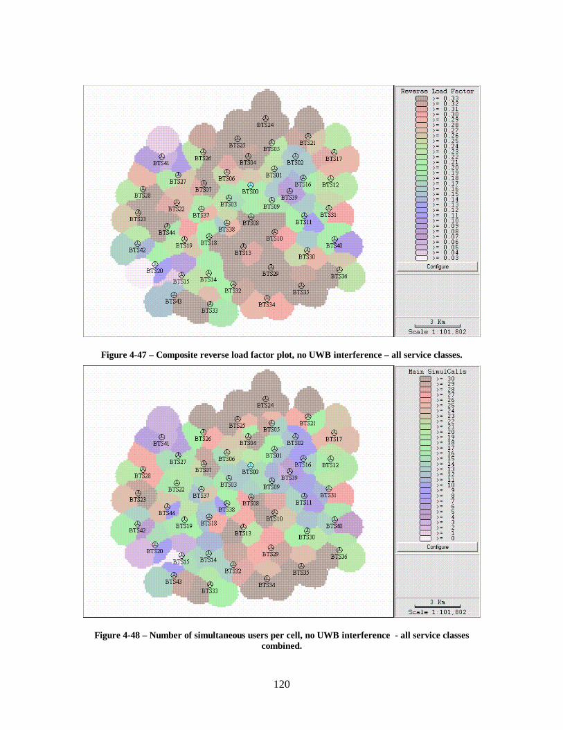
120

Figure 4-47 – Composite reverse load factor plot, no UWB interference – all service classes.

Figure 4-48 – Number of simultaneous users per cell, no UWB interference - all service classes combined.

121

Figure 4-49 – Number of simultaneous handoff connections per cell, no UWB interference - all service classes combined.

Figure 4-50 - Total Base Station TX Power: common pilot channel, traffic and other pilot channels, no UWB interference.

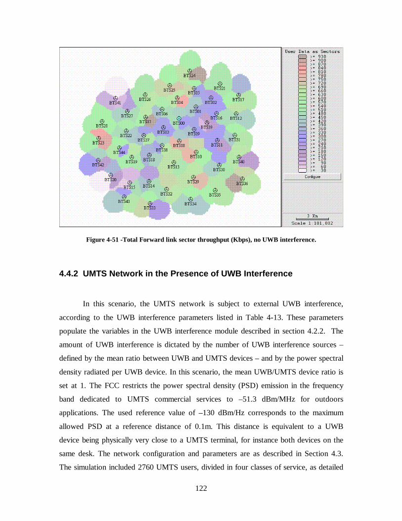
122

Figure 4-51 -Total Forward link sector throughput (Kbps), no UWB interference.

4.4.2 UMTS Network in the Presence of UWB Interference

In this scenario, the UMTS network is subject to external UWB interference,

according to the UWB interference parameters listed in Table 4-13. These parameters

populate the variables in the UWB interference module described in section 4.2.2. The

amount of UWB interference is dictated by the number of UWB interference sources –

defined by the mean ratio between UWB and UMTS devices – and by the power spectral

density radiated per UWB device. In this scenario, the mean UWB/UMTS device ratio is

set at 1. The FCC restricts the power spectral density (PSD) emission in the frequency

band dedicated to UMTS commercial services to –51.3 dBm/MHz for outdoors

applications. The used reference value of –130 dBm/Hz corresponds to the maximum

allowed PSD at a reference distance of 0.1m. This distance is equivalent to a UWB

device being physically very close to a UMTS terminal, for instance both devices on the

same desk. The network configuration and parameters are as described in Section 4.3.

The simulation included 2760 UMTS users, divided in four classes of service, as detailed

123

in Table 4-11. An aggregated graphical depiction of the UMTS users simulated at each

snapshot is presented in Figure 4-52. The colors represent the different user profiles, as

described in Table 4-4. The pixels shown in black indicate failed connection attempts. A

comparison between Figure 4-18 and Figure 4-52 reveals the higher concentration of

black pixels in the latter, indicating that more connection attempts fail in the presence of

UWB interference.

Table 4-13 – UWB interference parameters used in the simulation

Parameter Setting

Maximum UWB/UMTS Separation Distance 30 m

Separation Distance Distribution Uniform

Mean UWB/UMTS User Ratio 1

Ratio Distribution Poisson

Reference Power Spectral Density per UWB Device -130 dBm/Hz

Reference Distance 0.1 m

Attenuation Slope 20 dB/dec

Voice 12.2 Kbps - Indoor

Voice 12.2 Kbps - Vehicular

CSD 144 Kbps - Indoor

PSD 384 Kbps - Indoor

Failed Connections

Figure 4-52 - Aggregated graphical representation of the UMTS users simulated at each snapshot, in the presence of UWB interference.

124

The simulation results for this scenario are summarized in Table 4-14; they are

shown for the total number of simulated users, but reflect the individual traffic

contributions by each of the four user profiles. The subsequent set of figures - Figure

4-19 thru Figure 4-51, offers detailed insight into the UMTS network performance,

illustrating through various metrics its behavior under the simulated load condition.

Figure 4-19 to Figure 4-46 show the composite performance of the UMTS network for

each user profile separately, whereas Figure 4-47 to Figure 4-51 show a set of metrics for

the combined user profiles, i.e., the complete population of users. A discussion of the

results shown in these figures is presented below.

Table 4-14 – Summary of the traffic simulation results for UMTS network subjected to UWB interference.

Metric Active

Users

Percentage of

Total

Total Simulated Traffic 2460.0 100 %

Carried traffic - Main traffic 2344.8 85 %

Carried traffic - Handoff traffic 899.9 32.6 %

Not carried traffic - Pilot channel coverage 264.7 9.6 %

Not carried traffic - Directed to other carriers 0 0

Not carried traffic - Throughput per carrier limit 0 0

Not carried traffic - Forward traffic channel power limit 27.3 1.0 %

Not carried traffic - Forward sector total power limit 0 0

Not carried traffic - Forward load factor limit 0 0

Not carried traffic - Reverse mobile power limit 123.2 4.5 %

A comparison of the traffic simulation results for the UMTS network with no

UWB interference and in the presence of interference is shown in Table 4-15. The

performance degradation is notable across the majority of the key metrics. The total

traffic carried by the UMTS network decreased by 6.4%, which indicates that its

performance is suffering degradation caused by the presence of external UWB

interference. The noise rise caused by this interference has resulted in a reduction of the

125

pilot channel coverage area – an effect known as cell breathing. Cell breathing is

generally caused by noise rise produced intra-network, as the number of active users

varies over time. When the number of users grows, more noise is present, causing the

pilot coverage area to shrink. Conversely, when the number of users drops, the coverage

expands. In the case where UWB interference is present, the cell breathing is also being

affected by that component. In this simulation, the pilot channel coverage reduction

resulted in an increase of 895.1% in the number of UMTS users that could not establish a

connection due to the lack of pilot coverage. In addition, the handoff traffic decreased by

22.3%, also a consequence of the reduced pilot coverage area. The overall increase in the

noise rise forces the base stations to elevate the transmission power in the traffic

channels, to preserve the link quality of established connections. Since the total power

per base station is limited, this increase in transmission power per active user reduces the

total number of users that can be served per base station. This phenomenon is apparent in

the simulations, where 52.5% more users were denied service because there was not

enough forward link power in the traffic channel to establish a connection. The number

of users not served due to lack reverse link power has decreased in the presence of UWB

interference. The decline occurred because fewer connection attempts have been initiated.

Since the pilot channel coverage has shrunk, fewer users can actually initiate a

connection. The network can only determine whether a particular base station has enough

power left on the traffic channel to admit a new user after that user has requested a

connection through the control channel. Only then can the network assess the link

requirements of that user and make a determination as to whether the user can be served.

126

Table 4-15 – Comparison of the traffic simulation results for the UMTS network with no UWB interference and in the presence of interference

Metric Active Users -

No UWB

Active Users -

UWB

Variation

Total Simulated Traffic 2760.0 2760.0 -

Carried traffic - Main traffic 2505.8 2344.8 -6.4%

Carried traffic - Handoff traffic 1158.9 899.9 -22.3%

Not carried traffic - Pilot channel coverage 26.6 264.7 895.1%

Not carried traffic - Directed to other carriers 0 0 -

Not carried traffic - Throughput per carrier limit 0 0 -

Not carried traffic - Forward traffic channel power limit 17.9 27.3 52.5%

Not carried traffic - Forward sector total power limit 0 0 -

Not carried traffic - Forward load factor limit 0 0 -

Not carried traffic - Reverse mobile power limit 209.7 123.2 -41.2%

Figure 4-53 thru Figure 4-85 show the same graphical outputs presented for the

baseline scenario, now with the UMTS network in the presence of UMTS interference.

Figure 4-53 to Figure 4-56 illustrate the resulting pilot channel (CPICH) coverage

for the four service classes, for the resulting network load offered by the simulated user

population in the presence of UWB interference. The increased network load is reflected

in the reduced overall oc IE footprint. Similarly, the best server area of each sector is

reduced, as illustrated in Figure 4-57 to Figure 4-60.

Figure 4-61 to Figure 4-64 show the coverage of the forward traffic channel,

displaying a smaller overall footprint and showing that coverage gaps that existed

previously become more evident, especially for the CSD 144 Kbps and PSD 384 Kbps

service classes.

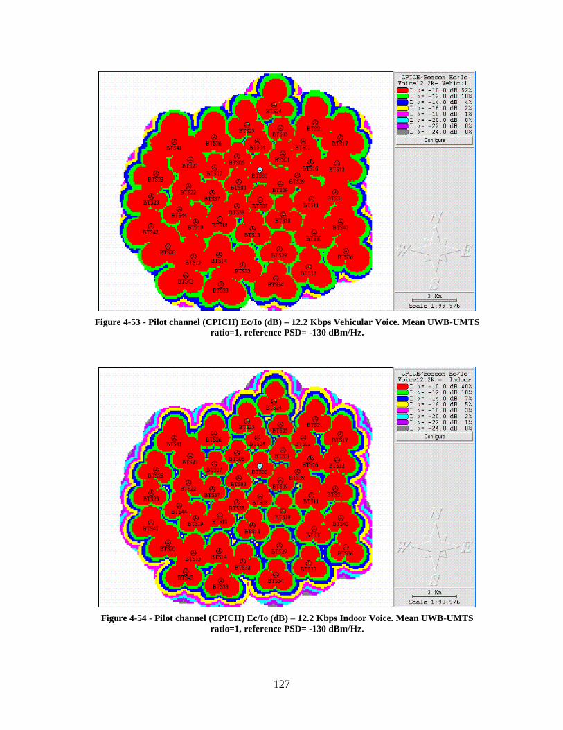
127

Figure 4-53 - Pilot channel (CPICH) Ec/Io (dB) – 12.2 Kbps Vehicular Voice. Mean UWB-UMTS ratio=1, reference PSD= -130 dBm/Hz.

Figure 4-54 - Pilot channel (CPICH) Ec/Io (dB) – 12.2 Kbps Indoor Voice. Mean UWB-UMTS ratio=1, reference PSD= -130 dBm/Hz.

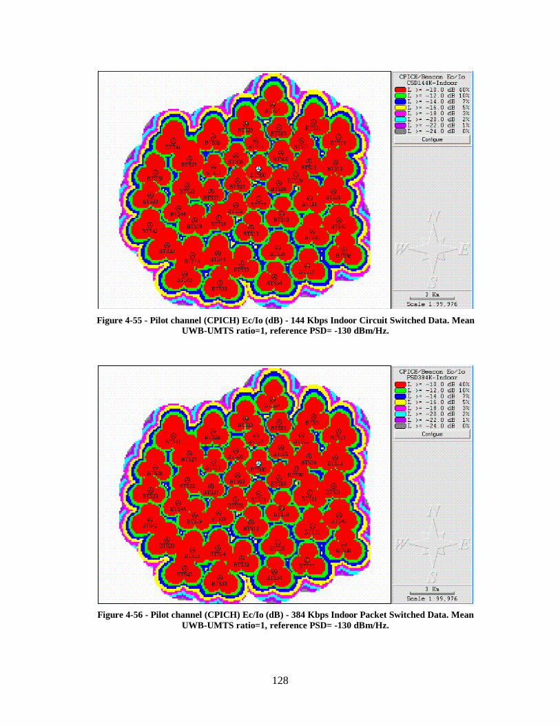
128

Figure 4-55 - Pilot channel (CPICH) Ec/Io (dB) - 144 Kbps Indoor Circuit Switched Data. Mean UWB-UMTS ratio=1, reference PSD= -130 dBm/Hz.

Figure 4-56 - Pilot channel (CPICH) Ec/Io (dB) - 384 Kbps Indoor Packet Switched Data. Mean UWB-UMTS ratio=1, reference PSD= -130 dBm/Hz.

129

Figure 4-57 - Pilot channel (CPICH) Best Server Plot – 12.2 Kbps Vehicular Voice. Mean UWB-UMTS ratio=1, reference PSD= -130 dBm/Hz.

Figure 4-58 - Pilot channel (CPICH) Best Server Plot – 12.2 Kbps Indoor Voice. Mean UWB-UMTS ratio=1, reference PSD= -130 dBm/Hz.

130

Figure 4-59 - Pilot channel (CPICH) Best Server Plot - 144 Kbps Indoor Circuit Switched Data. Mean UWB-UMTS ratio=1, reference PSD= -130 dBm/Hz.

Figure 4-60 - Pilot channel (CPICH) Best Server Plot - 384 Kbps Indoor Packet Switched Data. . Mean UWB-UMTS ratio=1, reference PSD= -130 dBm/Hz.

131

Figure 4-61 - Forward traffic channel Eb/Io (dB) – 12.2 Kbps Vehicular Voice. Mean UWB-UMTS ratio=1, reference PSD= -130 dBm/Hz.

Figure 4-62 - Forward traffic channel Eb/Io (dB) – 12.2 Kbps Indoor Voice. Mean UWB-UMTS ratio=1, reference PSD= -130 dBm/Hz.

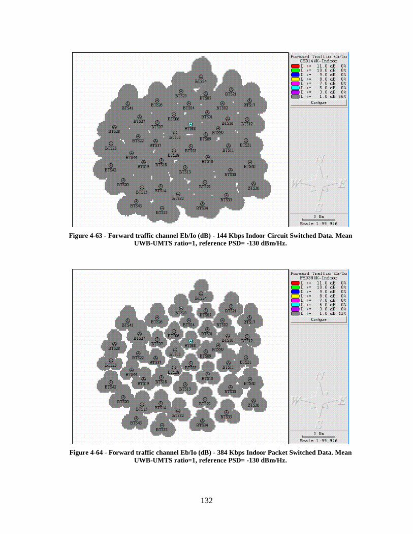
132

Figure 4-63 - Forward traffic channel Eb/Io (dB) - 144 Kbps Indoor Circuit Switched Data. Mean UWB-UMTS ratio=1, reference PSD= -130 dBm/Hz.

Figure 4-64 - Forward traffic channel Eb/Io (dB) - 384 Kbps Indoor Packet Switched Data. Mean UWB-UMTS ratio=1, reference PSD= -130 dBm/Hz.

133

Figure 4-65 to Figure 4-68 plot the reverse link power, i.e., the ERP power the

UMTS handset must transmit in order to close the link with the best serving cell at its

location. The last two thresholds in the plots are 21 dBm and 24 dBm, corresponding to

the maximum ERP for voice and data user profiles, respectively. A comparison with

Figure 4-31 to Figure 4-34 clearly shows that more reverse link power is required from

the UMTS terminals when UWB interference is present, contributing to reverse link

noise rise.

Figure 4-69 to Figure 4-72 contrast the forward and reverse link service areas. A

comparison with Figure 4-35 to Figure 4-38 shows that the unbalance between forward

and reverse links deceases slightly in the presence of UWB interference. This is a result

of the increased noise level, which reduces the forward link range.

Figure 4-73 to Figure 4-76 show the increase in the forward link noise rise

because of the UWB interference. The increased noise rise is a consequence of the extra

forward link power required in the traffic channels, to compensate for the higher noise

floor.

Figure 4-77 to Figure 4-80 depict the areas where soft handoffs are expected,

based on the variation of the pilot channel ob NE as the UMTS terminal moves away

from one cell and towards another. UWB interference causes the reduction of some of the

handoff areas, because the higher noise floor at the UMTS terminal eliminates some

candidate cells with weaker service at its location.

134

Figure 4-65 - Mobile terminal radiated power (ERP), in dBm – 12.2 Kbps Vehicular Voice. Mean UWB-UMTS ratio=1, reference PSD= -130 dBm/Hz.

Figure 4-66 - Mobile terminal radiated power (ERP), in dBm – 12.2 Kbps Indoor Voice. Mean UWB-UMTS ratio=1, reference PSD= -130 dBm/Hz.

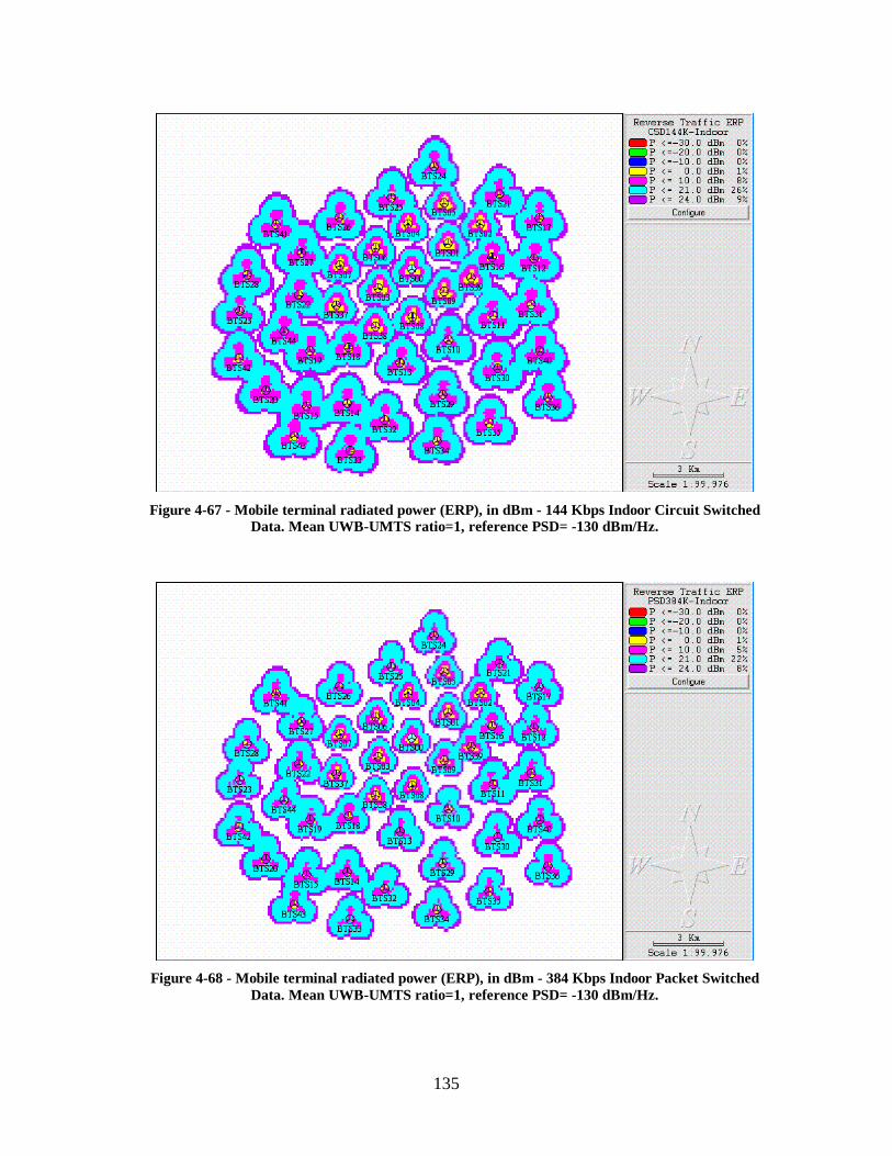
135

Figure 4-67 - Mobile terminal radiated power (ERP), in dBm - 144 Kbps Indoor Circuit Switched Data. Mean UWB-UMTS ratio=1, reference PSD= -130 dBm/Hz.

Figure 4-68 - Mobile terminal radiated power (ERP), in dBm - 384 Kbps Indoor Packet Switched Data. Mean UWB-UMTS ratio=1, reference PSD= -130 dBm/Hz.

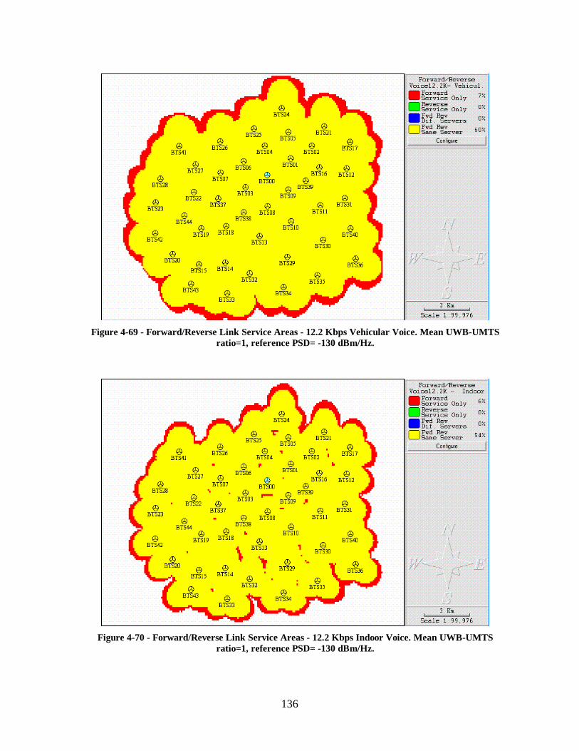
136

Figure 4-69 - Forward/Reverse Link Service Areas - 12.2 Kbps Vehicular Voice. Mean UWB-UMTS ratio=1, reference PSD= -130 dBm/Hz.

Figure 4-70 - Forward/Reverse Link Service Areas - 12.2 Kbps Indoor Voice. Mean UWB-UMTS ratio=1, reference PSD= -130 dBm/Hz.

137

Figure 4-71 - Forward/Reverse Link Service Areas - 384 Kbps Indoor Packet Switched Data. Mean UWB-UMTS ratio=1, reference PSD= -130 dBm/Hz.

Figure 4-72 - Forward/Reverse Link Service Areas - 384 Kbps Indoor Packet Switched Data. Mean UWB-UMTS ratio=1, reference PSD= -130 dBm/Hz.

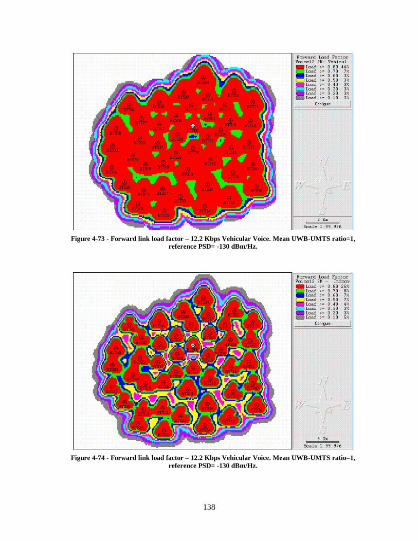
138

Figure 4-73 - Forward link load factor – 12.2 Kbps Vehicular Voice. Mean UWB-UMTS ratio=1, reference PSD= -130 dBm/Hz.

Figure 4-74 - Forward link load factor – 12.2 Kbps Vehicular Voice. Mean UWB-UMTS ratio=1, reference PSD= -130 dBm/Hz.

139

Figure 4-75 - Forward link load factor - 144 Kbps Indoor Circuit Switched Data. Mean UWB-UMTS ratio=1, reference PSD= -130 dBm/Hz.

Figure 4-76 - Forward link load factor - 384 Kbps Indoor Packet Switched Data. Mean UWB-UMTS ratio=1, reference PSD= -130 dBm/Hz.

140

Figure 4-77 - Handoff areas plot – 12.2 Kbps Vehicular Voice. Mean UWB-UMTS ratio=1, reference

PSD= -130 dBm/Hz.

Figure 4-78 - Handoff areas plot – 12.2 Kbps Indoor Voice. Mean UWB-UMTS ratio=1, reference

PSD= -130 dBm/Hz.

141

Figure 4-79 - Handoff areas plot - 144 Kbps Indoor Circuit Switched Data. Mean UWB-UMTS ratio=1, reference PSD=-130 dBm/Hz.

Figure 4-80 - Handoff areas plot - 384 Kbps Indoor Packet Switched Data. Mean UWB-UMTS ratio=1, reference PSD=-130 dBm/Hz.

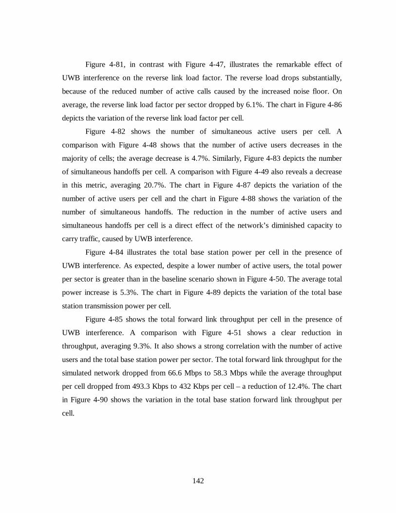
142

Figure 4-81, in contrast with Figure 4-47, illustrates the remarkable effect of

UWB interference on the reverse link load factor. The reverse load drops substantially,

because of the reduced number of active calls caused by the increased noise floor. On

average, the reverse link load factor per sector dropped by 6.1%. The chart in Figure 4-86

depicts the variation of the reverse link load factor per cell.

Figure 4-82 shows the number of simultaneous active users per cell. A

comparison with Figure 4-48 shows that the number of active users decreases in the

majority of cells; the average decrease is 4.7%. Similarly, Figure 4-83 depicts the number

of simultaneous handoffs per cell. A comparison with Figure 4-49 also reveals a decrease

in this metric, averaging 20.7%. The chart in Figure 4-87 depicts the variation of the

number of active users per cell and the chart in Figure 4-88 shows the variation of the

number of simultaneous handoffs. The reduction in the number of active users and

simultaneous handoffs per cell is a direct effect of the network’s diminished capacity to

carry traffic, caused by UWB interference.

Figure 4-84 illustrates the total base station power per cell in the presence of

UWB interference. As expected, despite a lower number of active users, the total power

per sector is greater than in the baseline scenario shown in Figure 4-50. The average total

power increase is 5.3%. The chart in Figure 4-89 depicts the variation of the total base

station transmission power per cell.

Figure 4-85 shows the total forward link throughput per cell in the presence of

UWB interference. A comparison with Figure 4-51 shows a clear reduction in

throughput, averaging 9.3%. It also shows a strong correlation with the number of active

users and the total base station power per sector. The total forward link throughput for the

simulated network dropped from 66.6 Mbps to 58.3 Mbps while the average throughput

per cell dropped from 493.3 Kbps to 432 Kbps per cell – a reduction of 12.4%. The chart

in Figure 4-90 shows the variation in the total base station forward link throughput per

cell.

143

Figure 4-81 - Composite reverse load factor plot – all service classes. Mean UWB-UMTS ratio=1, reference PSD=-130 dBm/Hz.

Figure 4-82 - Number of simultaneous users per cell - all service classes combined. Mean UWB-UMTS ratio=1, reference PSD=-130 dBm/Hz.

144

Figure 4-83 - Number of simultaneous handoff connections per cell - all service classes combined. Mean UWB-UMTS ratio=1, reference PSD=-130 dBm/Hz.

Figure 4-84 – Total Base Station TX Power: common pilot channel, traffic and other pilot channels. Mean UWB-UMTS ratio=1, reference PSD=-130 dBm/Hz.

145

Figure 4-85 – Total Forward link sector throughput (Kbps). Mean UWB-UMTS ratio=1, reference PSD=-130 dBm/Hz.

-30.0%

-20.0%

-10.0%

0.0%

10.0%

20.0%

30.0%

40.0%

50.0%

BTS00A

BTS02A

BTS04A

BTS06A

BTS08A

BTS10A

BTS12A

BTS14A

BTS16A

BTS18A

BTS20A

BTS22A

BTS24A

BTS26A

BTS28A

BTS30A

BTS32A

BTS34A

BTS36A

BTS38A

BTS40A

BTS42A

BTS44A

Sector

Rev

erse

Lin

k L

oad

Fac

tor

Var

iati

on

Figure 4-86 – Reverse link load factor variation per sector due to UWB interference, in comparison with the baseline UMTS network scenario.

146

-60.0%

-40.0%

-20.0%

0.0%

20.0%

40.0%

60.0%

BTS00A

BTS02A

BTS04A

BTS06A

BTS08A

BTS10A

BTS12A

BTS14A

BTS16A

BTS18A

BTS20A

BTS22A

BTS24A

BTS26A

BTS28A

BTS30A

BTS32A

BTS34A

BTS36A

BTS38A

BTS40A

BTS42A

BTS44A

Sector

Nu

mb

er o

f A

ctiv

e U

sers

Var

iati

on

Figure 4-87 - Variation in the number of active users per sector due to UWB interference, in comparison with the baseline UMTS network scenario.

-60.0%

-40.0%

-20.0%

0.0%

20.0%

40.0%

60.0%

BTS00A

BTS02A

BTS04A

BTS06A

BTS08A

BTS10A

BTS12A

BTS14A

BTS16A

BTS18A

BTS20A

BTS22A

BTS24A

BTS26A

BTS28A

BTS30A

BTS32A

BTS34A

BTS36A

BTS38A

BTS40A

BTS42A

BTS44A

Sector

Sim

ult

aneo

us

Han

do

ffs

Var

iati

on

Figure 4-88 - Variation in the number of simultaneous handoffs per sector due to UWB interference, in comparison with the baseline UMTS network scenario.

147

-40.0%

-20.0%

0.0%

20.0%

40.0%

60.0%

80.0%

100.0%

BTS00A

BTS02A

BTS04A

BTS06A

BTS08A

BTS10A

BTS12A

BTS14A

BTS16A

BTS18A

BTS20A

BTS22A

BTS24A

BTS26A

BTS28A

BTS30A

BTS32A

BTS34A

BTS36A

BTS38A

BTS40A

BTS42A

BTS44A

Sector

To

tal B

S T

X P

ow

er V

aria

tio

n

Figure 4-89 - Variation in the total base station transmitted power per sector due to UWB interference, in comparison with the baseline UMTS network scenario.

-60.0%

-40.0%

-20.0%

0.0%

20.0%

40.0%

60.0%

80.0%

100.0%

120.0%

140.0%

BTS00A

BTS02A

BTS04A

BTS06A

BTS08A

BTS10A

BTS12A

BTS14A

BTS16A

BTS18A

BTS20A

BTS22A

BTS24A

BTS26A

BTS28A

BTS30A

BTS32A

BTS34A

BTS36A

BTS38A

BTS40A

BTS42A

BTS44A

Sector

Fo

rwar

d L

ink

Th

rou

gh

pu

t V

aria

tio

n

Figure 4-90 - Variation in the total base station forward link throughput per sector due to UWB interference, in comparison with the baseline UMTS network scenario.

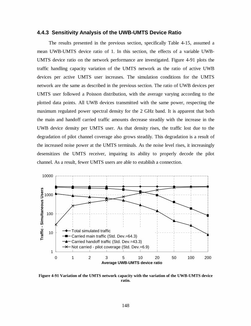
148

4.4.3 Sensitivity Analysis of the UWB-UMTS Device Ratio

The results presented in the previous section, specifically Table 4-15, assumed a

mean UWB-UMTS device ratio of 1. In this section, the effects of a variable UWB-

UMTS device ratio on the network performance are investigated. Figure 4-91 plots the

traffic handling capacity variation of the UMTS network as the ratio of active UWB

devices per active UMTS user increases. The simulation conditions for the UMTS

network are the same as described in the previous section. The ratio of UWB devices per

UMTS user followed a Poisson distribution, with the average varying according to the

plotted data points. All UWB devices transmitted with the same power, respecting the

maximum regulated power spectral density for the 2 GHz band. It is apparent that both

the main and handoff carried traffic amounts decrease steadily with the increase in the

UWB device density per UMTS user. As that density rises, the traffic lost due to the

degradation of pilot channel coverage also grows steadily. This degradation is a result of

the increased noise power at the UMTS terminals. As the noise level rises, it increasingly

desensitizes the UMTS receiver, impairing its ability to properly decode the pilot

channel. As a result, fewer UMTS users are able to establish a connection.

1

10

100

1000

10000

0 1 2 3 5 10 20 50 100 200Average UWB-UMTS device ratio

Tra

ffic

- S

imu

ltan

eou

s U

sers

Total simulated trafficCarried main traffic (Std. Dev.=64.3)Carried handoff traffic (Std. Dev.=43.3)Not carried - pilot coverage (Std. Dev.=6.9)

Figure 4-91 Variation of the UMTS network capacity with the variation of the UWB-UMTS device ratio.

149

Figure 4-92 shows the variation in the number of simultaneous active UMTS users

that cannot access the network, distributed according to the reasons causing the service

denial. It is evident that as the ratio of active UWB devices per active UMTS users

increases, the traffic loss due to the lack of reverse link mobile power drops steadily.

However, this decrease indicates an undesired phenomenon. Fewer UMTS users are

experiencing reverse link power limitation because their connection attempts are actually

failing in the forward link, due to poor link quality caused by the excessive noise level. In

other words, the connection attempts fail in the downlink first, more specifically in the

pilot reception, resulting in fewer reverse link failures due to mobile power saturation.

Similarly, Figure 4-92 also shows that the traffic loss due to forward link traffic channel

saturation experiences less variation with the increase in the UWB-UMTS device ratio,

eventually decreasing as that ratio increases. This is also explained by the precedence of

requirement for pilot coverage over traffic channel coverage, i.e., even though both

channels are affected by downlink interference from UWB users, the users denied access

due to lack of pilot do not get to experience the restrictions in traffic channel power.

1

10

100

1000

10000

0 1 2 3 5 10 20 50 100 200

Average UWB-UMTS device ratio

Tra

ffic

- S

imu

ltan

eou

s U

sers

Not carried traffic - Forward traffic channel power limit (Std. Dev.=4.1)

Not carried traffic - Reverse mobile power limit (Std. Dev.=15.7)

Not carried - pilot coverage (Std. Dev.=6.9)

Not carried - total

Figure 4-92 Variation of the UMTS network traffic loss caused by power saturation, as a function of the UWB-UMTS device ratio.

150

4.4.4 Sensitivity Analysis of the UWB Power Spectral Density (PSD)

The simulations discussed thus far assumed the UWB devices transmitting at the

maximum power allowed by the FCC regulations. The results indicate that for a mean

UWB-UMTS device ratio equal to 1, the UMTS network could suffer noticeable

performance degradation, as shown in Table 4-15. The variation of the maximum power

spectral density (PSD) of the UWB interference to values below the maximum allowed

by the FCC could reduce the detrimental effects of UWB on 3G networks. The

simulation scenario described in Section 4.4.2, for a mean UWB-UMTS device ratio of 1,

was repeated considering different values of the maximum UWB power spectral density

(PSD) interference. In this study, the PSD was monotonically decreased from the upper

limit of -130 dBm/Hz until the level where the network performance was the same as

that achieved for the baseline scenario discussed in section 4.4.1, where no UWB was

present.

Figure 4-93 illustrates the variation of the network capacity as the maximum UWB

power spectral density (PSD) is decreased, for a mean UWB-UMTS device ratio of 1.

The total simulated traffic is 2760 simultaneous users. In the presence of UWB

interference at the power spectral density level of –130 dBm/Hz, the UMTS network is

able to carry 2344.8 simultaneous users, or 6.4% less than when no interference is

present. The carried handoff traffic equates to 899.9 users, representing a 22.3% decrease

from the baseline scenario. The network traffic missed due to lack of pilot coverage is

264.7 users, or 891% above the baseline scenario. As the UWB interference level

decreases, these metrics change monotonically, asymptotically approaching the levels

measured for the baseline scenario. At PSD levels below –150 dBm/Hz, the degradation

due to UWB interference is negligible and the performance of the UMTS network is no

longer affected by the presence of UWB devices. This equates to a backoff of 20 dB from

the emission limits established by the FCC [5]. Reference [7] presents results of a similar

study, where a backoff of 30 dB is recommended. In that study, the behavior of a

theoretical UMTS network was simulated using the noise figure of the users’ receivers as

the compensation variable to account for the UWB interference. The simulation did not

consider the mobility and power variation due to the geographical distribution of the

UWB interference. The simplified nature of the model adopted in that study, lacking the

151

stochastic approach employed here, suggests that the recommendation should be treated

as an upper bound figure.

Similarly, Figure 4-94 shows the variation on the network traffic loss due to power

saturation, caused by the increased noise level generated by the UWB interference. The

graph clearly shows the correlation between the drop in traffic loss due to lack of pilot

and the increase in traffic loss due to lack of reverse link mobile power. As the UWB

interference decreases, the pilot coverage increases and the UMTS network captures

more traffic. This increase in traffic results in more UMTS users loading the network,

requiring more reverse link power from each UMTS terminal. Figure 4-94 also shows

that the traffic loss due to forward traffic channel power saturation remains constant,

indicating that the amount of UWB interference in the network is not affecting that

metric.

0

500

1000

1500

2000

2500

3000

-130-131-133-136-140-141-143-146-150-153NoUWB

UWB Power Spectral Density (dBm/Hz)

Tra

ffic

- S

imu

ltan

eou

s U

sers

Total simulated trafficCarried main traffic (Std. Dev.=64.3)Carried handoff traffic (Std. Dev.=43.3)Not carried - Pilot coverage (Std. Dev.=6.9)

Figure 4-93 Variation of the UMTS network capacity with the variation of the UWB power spectral density (PSD), for a mean UWB-UMTS ratio equal to 1.

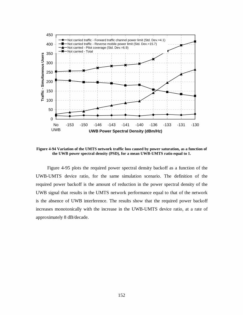
152

0

50

100

150

200

250

300

350

400

450

-130-131-133-136-140-141-143-146-150-153NoUWB UWB Power Spectral Density (dBm/Hz)

Tra

ffic

- S

imu

ltan

eou

s U

sers

Not carried traffic - Forward traffic channel power limit (Std. Dev.=4.1)Not carried traffic - Reverse mobile power limit (Std. Dev.=15.7)Not carried - Pilot coverage (Std. Dev.=6.9)Not carried - Total

Figure 4-94 Variation of the UMTS network traffic loss caused by power saturation, as a function of the UWB power spectral density (PSD), for a mean UWB-UMTS ratio equal to 1.

Figure 4-95 plots the required power spectral density backoff as a function of the

UWB-UMTS device ratio, for the same simulation scenario. The definition of the

required power backoff is the amount of reduction in the power spectral density of the

UWB signal that results in the UMTS network performance equal to that of the network

is the absence of UWB interference. The results show that the required power backoff

increases monotonically with the increase in the UWB-UMTS device ratio, at a rate of

approximately 8 dB/decade.

153

0

5

10

15

20

25

30

35

40

45

1 2 3 5 10 20 50 100 200 500

UWB-UMTS Device Ratio

PS

D B

acko

ff (

dB

)

PSD Backoff (dB)

Figure 4-95 Variation of the PSD backoff required to preserve the UMTS network performance as a function of the UWB-UMTS device ratio.

4.5 Summary

This chapter presented a methodology for system level simulation of the

coexistence between UWB and 3G technologies, using UMTS as an example. The details

of 3G network planning tools have been explored and the impact of their most relevant

blocks has been discussed.

An algorithm for the simulation of the interaction between UWB interferers and

UMTS devices has been proposed, leveraging on the capabilities of existing commercial

planning tools. A realization of such algorithm has been presented, along with simulation

results for a notional UMTS network subjected to varying levels of UWB interference,

respecting the emission limits established by the FCC. The results of these simulations

characterize the performance degradation UWB interference can cause on 3G networks.

At the present emission limits authorized for UWB, 3G networks will likely suffer

noticeable performance degradation in terms of capacity and coverage, if UWB uptake

achieves its forecasted mass adoption levels of multiple devices per household or office.

154

While this study focused on UMTS as a third-generation technology, the principles

and methodologies discussed herein can be extrapolated in their entirety to other air

interfaces, such as CDMA 2000. The major adjustment required to enable the reuse of the

models proposed in this study to other 3G air interfaces is in the carrier bandwidth, which

varies depending on the technology.

This concludes the development of this work. The following chapter summarizes

the contributions of this research and points to areas of future research related to this

topic.

155

Chapter 5

Conclusions

5.1 Summary and Contributions

The main contribution of this work is the characterization of UWB interference on

third-generation (3G) wireless networks, showing the impact that mass adoption of UWB

technology can have on those networks. We achieve this contribution by proposing and

implementing a methodology that enables realistic, comprehensive and scalable analyses

of the effects of UWB on 3G networks. A fundamental component of this framework is

the development of an algorithm to model the behavior of the 3G network in the presence

of UWB interference. The proposed solution considers the stochastic variables that

influence both the 3G users and the UWB interference sources, namely the number of

interferers and their spatial distribution.

Studies available in the literature have partially addressed the problem, presenting

inconclusive and even contradictory results. The complexities that arise from a

comprehensive statistical treatment of the interaction between two systems, with mobile

interference sources and victims, have inhibited the exploration of a thorough solution. In

available studies, simplifying assumptions about the 3G propagation environment, traffic

distribution, usage pattern and UWB interference distribution make the modeling

realizable with low complexity, at the expense of accuracy and realism. The range of

simplifying assumptions and abstractions in the work available in the literature prevents

consistent and converging conclusions.

This work focused on building a simulation framework that takes into consideration

the fundamental variables affecting the UWB-3G coexistence problem. Initially, the

UWB interference on a narrowband receiver was investigated, with the purpose of

determining how to best model its impact on 3G receivers.

156

Next, and using the results from that investigation, a UWB-3G link level analysis

methodology was proposed, aiming at determining how much UWB interference can be

expected in a 3G device under typical real single-link situations, assuming the UWB

emissions in compliance with the limits established by the FCC.

The link level analysis was then evolved to an in-depth modeling of the 3G system,

including the propagation component, with digital elevation models of the terrain and

morphology; complete modeling of the radiation pattern of the base station antennas was

also accounted for. The technology-specific admission control and radio resource

management features encountered in 3G networks were also implemented in the model.

Additionally, the mix of service classes 3G networks support was considered. The

combination of these components result in a model that realistically describes the

behavior of a 3G network.

In the proposed methodology, UWB interference was simulated as a random

variable, in which both the number of interferers and their location around the 3G victim

receivers change over time. A Monte Carlo algorithm was used to simulate the stochastic

behavior of the 3G users and UWB interferers. This algorithm represents the key

contribution of this work.

The approach was demonstrated through a practical realization of the framework,

with the aid of a commercially available 3G network planning tool, modified to support

the UWB interference modeling algorithm proposed in this study.

To complete the research, the performance of a notional UMTS network was

simulated using the described implementation. The coverage and capacity aspects were

investigated in the presence and absence of UWB interference, allowing for an

assessment of the degradation UWB can cause to the overall network performance. The

network performance variation as a function of the UWB device density was also studied,

showing that the current UWB emission limits established by the FCC can be detrimental

to 3G networks. Finally, an illustrative study on the amount of power backoff required to

avoid UWB interference on 3G networks is presented, based on the notional UMTS

network used as reference.

157

In summary, the main benefits expected from this research are to:

� Demonstrate that UWB interference can be detrimental to the performance of

3G networks;

� Enable the understanding of how the variables that affect the operation of

UWB and 3G affect the coexistence of both systems;

� Allow the study of the UWB-3G coexistence problem in a realistic fashion,

accounting for the key variables affecting both systems;

� Allow network operators to model the expected impact of a mass uptake of

UWB on 3G networks, should the current FCC-dictated UWB emission limits

remain unchanged.

5.2 Related Areas of Research

There are other areas of research related to UWB and its coexistence with legacy

systems that were not covered in this dissertation, They could be explored in future

research, eventually benefiting from the contributions presented herein.

5.2.1 Impact of UWB on the 3G Power Control

Third-generation air interfaces are equipped with a fast closed-loop power control

mechanism intended to mitigate the effects of short-term fading on the link performance.

They act on the signal at a rate of, typically, 5 KHz, updating the power level in response

to changes in the channel. The burstiness of the UWB signal could potentially attack the

3G power control mechanism, affecting its ability to compensate for channel variations,

further impairing the performance of the 3G link. This phenomenon has not been studied

in this dissertation, but deserves further probing. Nonetheless, the framework presented

here could be used and eventually enhanced to account for such modeling.

158

5.2.2 Impact of UWB Detect- and-Avoid Mechanisms

As the concern surrounding the impact of UWB on legacy systems grows, UWB

technology supporters and manufacturers have been proposing mechanisms to minimize

the potential for interference. Detect-and-avoid algorithms, based on sensing the

spectrum prior to transmission, have recently been proposed, but their effectiveness on

complex network scenarios, such as those discussed in this dissertation, is yet to be

assessed. This has not been addressed in this study and could be an area of future

research, building upon the work presented here.

5.2.3 Cognitive Radios, UWB & Coexistence

As the need for wideband applications increases, the demand for spectrum grows

proportionately. In this context, higher-efficiency methods of spectrum utilization

become relevant. Ultra wideband technology can be seen as an attempt to improve the

efficiency of spectrum utilization, by allowing the UWB signal to occupy a very large

portion of spectrum also used by many other systems. However, UWB is an unlicensed

technology, implying that spectrum coordination with legacy systems is not required,

creating the potential for interference and performance degradation.

Cognitive radios can be an appealing solution to the burden of spectrum

coordination and interference mitigation. They have been receiving increasing interest by

the research community, as a solution to improve the efficiency of spectrum utilization

while minimizing coordination. Cognitive radios utilize spectrum intelligently, sensing

the spectrum before transmitting, aiming at avoid interference with other transmissions.

They also utilize spectrum adaptively, adjusting their bandwidth occupation dynamically,

according to the transmission requirements and spectrum availability. These principles

can be applied to UWB, allowing the technology to better coexist with legacy systems,

including 3G networks. The research of cognitive radios applied to UWB, and the benefit

it can bring to UWB coexistence with legacy systems could be a potential area of future

research.

159

Bibliography

[1] William A. Kissick, NTIA Report 01-383 - The Temporal and Spectral

Characteristics of Ultrawideband Signals, January 2001.

[2] Jeffrey Reed, Michael R. Bueher, Dong S. Ha, “Introduction to UWB: Impulse Radio

for Radar and Wireless Communications”, Virginia Polytechnic Institute and State

University, 2003.

[3] Marc Seibert, “Why Ultra Wideband Communications may be in your future”, John

Glenn Research Center, NASA, March 2001.

[4] Sathaporn Promwong, “Ultra Wideband Part II”, Takada Laboratory, Tokyo Institute

of Technology, May 2002.

[5] FCC 02-48 – First Report and Order, Federal Communications Commission, April

2002.

[6] Terence W. Barrett, “History of Ultra Wideband (UWB) Radar and Communications:

Pioneers and Innovators”, Progress in Electromagnetics Symposium 2000 (PIERS 2000),

Cambridge, MA, July 2000.

[7] Mason Communications, Impact of UWB on Third-Generation Telecommunications

(3G) – Final Report, Manchester, England, February 2003.

[8] István Z. Kovács, Patrick C.F. Eggers, “Ultra Wide-Band Communication for

WLAN/WPAN Applications”, FACE Research Project, Aalborg University, Denmark,

December 2002.

160

[9] John G. Proakis, Digital Communications, Third Edition, McGraw Hill, 1995.

[10] Lachlan B. Michael, Mohammad Ghavani, Ryuji Kohno, “Multiple Pulse Generator

for Ultra-Wideband Communication using Hermite Polynomial Based Pulses”, Sony

Computer Science Laboratories, Inc., Shinagawa, Japan, 2002.

[11] Lachlan B. Michael, Mohammad Ghavani, Ryuji Kohno, “Effect of Timing Jitter on

Hermite Function Based Orthogonal Pulses for Ultra Wideband Communication”, Sony

Computer Science Laboratories, Inc., Shinagawa, Japan, 2002.

[12] Wolfram Research, “Hermite Polynomial”, Internet material available at

http://mathworld.wolfram.com/HermitePolynomial.html.

[13] Sathaporn Promwong, “Indoor Propagation Measurement and Modeling of Ultra

Wideband Radio”, Takada Laboratory, Tokyo Institute of Technology, May 2002.

[14] Time Domain Technologies web site, http://www.timedomain.com.

[15] Aether Wire and Locations web site, http://www.aetherwire.com.

[16] Multispectral Solutions, Inc. web site, http://www.multispectral.com.

[17] Moe Z. Win, “Impulse Radio: How It Works, IEEE Communications Letters”, Vol.

2, No.2, February 1998, pp.36-38.

[18] IEEE P802.15-04/0137r0, DS-UWB Physical layer Submission to 802.15 Task

Group 3a, March 2004

[19] IEEE P802.15-03/268r3, Multiband OFDM Physical Layer Proposal for 802.15

Task Group 3a, March 2004

161

[20] D.A. Cummings, “Aggregate ultra wideband impact on Global Positioning System

Receivers”, Radio and Wireless Conference, RAWCON 2001, 19-22 Aug. 2001, pp.101

–104.

[21] Robert J. Achatz, Richard N. Statz, Roger A. Dalke, Measurements to Determine

Potential Interference to GPS Receivers from Ultra wideband Transmission Systems,

NTIA Report 01-384, U.S. Department of Commerce, February 2001.

[22] J. Randy Hoffman, Michael G. Cotton, Robert J. Achatz, Richard N. Statz,

Addendum to NTIA Report 01-384: Measurements to Determine Potential Interference to

GPS Receivers from Ultrawideband Transmission Systems, NTIA Report 01-389, U.S.

Department Of Commerce, February 2001.

[23] The Johns Hopkins University/Applied Physics Laboratory, Final report – UWB-

GPS Compatibility Analysis Project, 8 March 2001.

[24] M. Hämäläinen, J. Iinatti, V. Hovinen, M. Latva-aho, “In-band interference of three

kinds of UWB signals in GPS L1 band and GSM900 uplink band”, The 12th IEEE

International Symposium on Personal, Indoor and Mobile Radio Communications,

PIMRC2001, Volume: 1, 30 Sept.-3 Oct. 2001, vol.1, pp. D-76 -D-80.

[25] J.J. Ely, G.L. Fuller, T.W. Shaver, “Ultrawideband electromagnetic interference to

aircraft radios”, Proceedings of the 21st Digital Avionics Systems Conference, 2002, vol

2, pp. 13E4-1 -13E4-12.

[26] B. Juhel, G. Vezzosi, M. Le Goff, “Radio frequency interferences suppression for

noisy ultra wide band SAR measurements”, IEEE Ultra-Wideband Short-Pulse

Electromagnetics 4, 1998, pp. 387 –393.

162

[27] X. Luo, L.M.H. Ulander, J. Askne, G. Smith, P. -O. Frolind, “RFI suppression in

ultra-wideband SAR systems using LMS filters in frequency domain” IEEE Electronics

Letters, vol. 37, issue 4, 15 Feb 2001, pp. 241-243.

[28] R. Giuliano, G. Guidoni, F. Mazzenga, D. Porcino, Study of the Coexistence UWB -

Fixed Wireless Access (FWA) Systems, Ultrawaves W02-02-0011-P02, 2002

[29] R. Macchi, M18_20A5-1R0_SE24_UWB_skeletton_annex5-1_FS – Updated UWB

and FS coexistence report (Annex 5-1), updated version of: "Preliminary Study on

Coexistence between UWB and the Fixed Service in Bands from 1 to 6 GHz",

International Telecommunication Union (ITU), Radiocommunication Study Groups

Document 1A/xx-E 2002, Italy, (document agreed at the CEPT ECC WGPT SE-24)

[30] J. Foerster, “Interference of Ultra-Wideband Emitters into Fixed Wireless Access

Receivers”, International Workshop on Ultra Wideband Systems, Oulu, June 2-5, 2003.

[31] D. Porcino, R. Giuliano, G. Guidoni, F. Mazzenga, "Study of the Coexistence UWB

- Fixed Wireless Access (FWA) Systems", M18_11R0_SE24_UWB_Ultrawaves-W02-

02-0011-P02, CEPT, Copenhagen, 16-19 December 2002

[32] D. Porcino, R. Giuliano, G. Guidoni, F. Mazzenga, "Study of the Coexistence UWB

– Fixed Wireless Access (FWA) Systems (with power control variation analysis)",

M19_44R0_SE24_UWB_FWA_W02-03-0011-P03, CEPT SE24, Copenhagen, 10-12

March 2003

[33] D. Porcino, R. Giuliano, G. Guidoni, F. Mazzenga, "Coexistence UWB – Fixed

Wireless Access (FWA) Systems. Simulations with Point to Point links",

M20_25R0_SE24_UWB_FWA_PtP_W09-03-0024-P01, CEPT SE24, Maisons- Alfort

(Paris), 7-11 April 2003

163

[34] R. Giuliano, G. Guidoni, F. Mazzenga, F. Vatalaro: “On the coexistence of UWB

with Fixed Wireless Access Systems”, IEEE Personal Wireless Communications, Venice

(Italy), vol. 1, 2003, pp. 111-113

[35] M. Hämäläinen, J. Iinatti, V. Hovinen, M. Latva-aho, “In-band interference power

caused by different kinds of UWB signals at UMTS/WCDMA frequency bands”, Radio

and Wireless Conference, RAWCON 2001, pp. 97-100

[36] M. Hämäläinen, J. Iinatti, V. Hovinen, "Performance Comparison between Various

UWB Signals in AWGN Channel in Presence of Multitone Interference at the GSM

Downlink Band", The 4th International Symposium on Wireless Personal Multimedia

Communications, WPMC01. Aalborg, Denmark, September 9-12, 2001, pp. 449-453.

[37] M. Hämäläinen, V. Hovinen, R. Tesi, J. Iinatti, M. Latva-aho, “On the UWB system

coexistence with GSM900, UMTS/WCDMA, and GPS”, IEEE Journal on Selected Areas

in Communications, vol. 20, issue 9, December 2002, pp. 1712-1721

[38] M. Hämäläinen, R. Tesi, J. Iinatti, “On the UWB system performance studies in

AWGN channel with interference in UMTS band”, Digest of Papers of Ultra Wideband

Systems and Technologies, 21-23 May 2002, pp. 321-325

[39] M. Hämäläinen, R. Tesi, V. Hovinen, N. Laine, J. Iinatti, “Ultra Wideband System

Performance Studies in AWGN Channel with Intentional Interference”, International

Workshop on Ultra Wideband Systems, Oulu, June 2-5, 2003.

[40] R. Tesi, M. Hämäläinen, J. Iinatti, V. Hovinen, "On the Influence of Pulsed

Jamming and Coloured Noise in UWB Transmission", The 3rd Finnish Wireless

Communication Workshop, FWCW2002, Helsinki, 2002.

[41] D. Porcino, R. Giuliano, G. Guidoni, F. Mazzenga, "Peaceful Coexistence between

164

UWB (FCC Report and Order level) devices and UMTS terminals",

M21_43R1_SE24_UWB_UMTScoexistence_ULTRAWAVES, CEPT ECC WGPT

SE24, M21, Copenhagen, 1-4 September, 2003

[42] R. Giuliano, F. Mazzenga, F. Vatalaro, “On the Interference Between UMTS and

UWB Systems”, IEEE Conference on Ultra Wideband Systems and Technologies 2003,

Reston, VA, USA, Nov. 17-19, 2003, pp. 339-343.

[43] D. Gerakoulis, P. Salmi, “Link performance of an ultra wide bandwidth wireless in-

home network”, Proceedings of the Seventh International Symposium on Computers and

Communications, ISCC 2002, 1-4 July 2002, pp. 699-704

[44] M. Hämäläinen, J. Saloranta, J-P. Mäkelä, T. Patana, I. Oppermann, “Ultra

Wideband Signal Impact on IEEE802.11b Network Performance”, The 12th IST Summit

2003, Aveiro, Portugal, pp. 488-492

[45] “UWB Impact on IEEE802.11b Wireless Local Area Network” Wireless Personal

Multimedia Communications Conference, WPMC03, Yokosuka, Japan.


Wideband Signal Impact on IEEE802.11b and Bluetooth Performances”, International

Symposium on Personal, Indoor and Mobile Radio Communications, PIMRC03, Peking,

China, 2003, pp. 280-284.


Wideband Signal Impact on the Performance of IEEE802.11b and Bluetooth Networks”

International Journal on Wireless Communications Networks, Jan. 2004, USA.

[48] S. Choi, S. Cho, H. Lee, “UWB interference test in IEEE802.11b WLAN

environment”, Proceedings of the 2003 International Workshop on Ultra Wideband

Systems, 2-5 June 2003, Oulu, Finland.

165

[49] M. Jang, S. Choi, H. Lee, “(2003) Experimental Study on 802.11b DSSS WLAN

Performance with UWB Device”, Proceedings of the 2003 International Workshop on

Ultra Wideband Systems, 2-5 June 2003, Oulu, Finland.

[50] B. Firoozbakhsh, T.G. Pratt, N. Jayant, “Analysis of IEEE 802.11a Interference on


Reston, VA, USA, Nov. 17-19, 2003, pp.473-477.

[51] K. Eshima, Y. Hase, S. Oomori, F. Takahashi, R. Kohno, “Performance analysis of

interference between UWB and SS signals”, 2002 IEEE Seventh International

Symposium on Spread Spectrum Techniques and Applications, vol 1, pp. 59 -63.

[52] W.A. Kissick et.al., The Temporal and Spectral Characteristics of Ultrawideband

Signals, NTIA Report 01-383, Jan 2001.

[53] Zhao Li, A.M. Haimovich, “Performance of ultra-wideband communications in the

presence of interference”, IEEE Journal on Selected Areas in Communications, vol. 20,

issue 9, December 2002, pp. 1684 -1691

[54] Zhao Li, A.M. Haimovich, H. Grebel, ”Performance of ultra-wideband

communications in the presence of interference”, IEEE International Conference on

Communications, ICC 2001, vol. 10, 11-14 June 2001, pp. 2948 –2952.

[55] J. Romme, L. Piazzo, “On the power spectral density of time-hopping impulse

radio”, 2002 IEEE Conference on Ultra Wideband Systems and Technologies, 21-23

May 2002, pp. 241-244

[56] R.A. Scholtz, R. Weaver, E. Homier, J. Lee, P. Hilmes, A. Taha, R. Wilson, “UWB

radio deployment challenges”, The 11th IEEE International Symposium on Personal,

166

Indoor and Mobile Radio Communications, PIMRC 2000, vol. 1, 18-21 Sept. 2000, pp.

620-625

[57] K. Siwiak, “Impact of ultra wide band transmissions on a generic receiver”, IEEE

53rd Vehicular Technology Conference, VTC 2001 Spring, vol. 2, 6-9 May 2001, pp.

1181-1183

[58] R.J. Fontana, “An insight into UWB interference from a shot noise perspective”,

2002 IEEE Conference on Ultra Wideband Systems and Technologies, Baltimore, MD,

21-23 May 2002, pp. 309 -313

[59] R. Tesi, M. Hämäläinen, J. Iinatti, “Impact of the Number of Fingers of a Selective

Rake Receiver for UWB Systems in Modified Saleh-Valenzuela Channel”, The 4th

Finnish Wireless Communication Workshop, Oulu, Finland, 2003.

[60] G. Yue, L. Ge, S. Li, “Performance of UWB Impulse Radio in the Presence of

Jamming”, International Workshop on Ultra Wideband Systems, Oulu, June 2-5, 2003.

[61] J.R. Foerster, “The performance of a direct-sequence spread ultrawideband system in

the presence of multipath, narrowband interference, and multiuser interference”, 2002

IEEE Conference on Ultra Wideband Systems and Technologies, Baltimore, MD, 21-23

May 2002, pp. 87-91.

[62] M.S. Iacobucci, M.G. Di Benedetto, L. De Nardis, “Radio frequency interference

issues in impulse radio multiple access communication systems”, 2002 IEEE Conference

on Ultra Wideband Systems and Technologies, Baltimore, MD, 21-23 May 2002, pp.293-

296.

[63] A. Mansour, J. Scheim, B.Z. Bobrovsky, “Acquisition of an UWB communications

system in the presence of a large UWB interference user”, The 22nd Convention of

Electrical and Electronics Engineers in Israel, December 2002, p.307.

167

[64] Li Qinghua, L.A. Rusch, “Multiuser receivers for DS-CDMA UWB”, 2002 IEEE

Conference on Ultra Wideband Systems and Technologies, Baltimore, MD, 21-23 May

2002, pp.163 –167.

[65] Y.C. Yoon, R. Kohno, “Optimum multi-user detection in ultra-wideband (UWB)

multiple-access communication systems”, IEEE International Conference on

Communications, ICC 2002, vol. 2, 28 April-2 May 2002, pp. 812-816.

[66] A. Taha, KM. Chugg, “A Theoretical Study on the Effects of Interference on UWB

Multiple Access Impulse Radio”, 36th Asilomar Conference on Signals, Systems and

Computers, vol. 1, Nov. 2002, pp. 728-732.

[67] Zhao Li, A.M. Haimovich, “Multi-user capacity of M-ary PPM ultra-wideband

communications”, 2002 IEEE Conference on Ultra Wideband Systems and Technologies,

Baltimore, MD, 21-23 May 2002, pp.175-179.

[68] B. Hu, N.C. Beaulieu, “Precise Bit Error Rate of TH-PPM UWB Systems in the

Presence of Multiple Access Interference”, IEEE Conference on Ultra Wideband Systems

and Technologies 2003, Reston, VA, USA, Nov. 17-19, 2003, pp.106-110.

[69] P. Liu, Z. Xu, J. Tang, “Minimum Variance Multiuser Detection for Impulse Radio



[70] P. Liu, Z. Xu, J. Tang, “Subspace Multiuser Receivers for UWB Communication

Systems”, IEEE Conference on Ultra Wideband Systems and Technologies 2003, Reston,

VA, USA, Nov. 17-19, 2003, pp. 116-120.

168

[71] L. Yang, G. Giannakis, “Ultra-Wideband Multiple Access: Unification and

Narrowband Interference Analysis”, IEEE Conference on Ultra Wideband Systems and

Technologies 2003, Reston, VA, USA, Nov. 17-19, 2003, pp. 320-324.

[72] G. Giancola, L. De Nardis, MG. Di Benedetto, “Multi User Interference in Power-

Unbalanced Ultra Wide Band Systems: Analysis and Verification”, IEEE Conference on

Ultra Wideband Systems and Technologies 2003, Reston, VA, USA, Nov. 17-19, 2003,

pp. 325-329.

[73] D.J. Clabaugh, M.A. Temple, R.A. Raines, C.M. Canadeo, ”UWB Multiple Access

Performance Using Time Hopped Pulse Position Modulation with Biorthogonal

Signaling”, IEEE Conference on Ultra Wideband Systems and Technologies 2003,


[74] R.T. Hoctor, “Multiple Access Capacity in Multipath Channels of Delay-Hopped

Transmitted-Reference UWB”, IEEE Conference on Ultra Wideband Systems and


[75] E. Baccarelli, M. Biagi, L. Taglione, “A novel approach to in-band interference

mitigation in ultra wideband radio systems”, 2002 IEEE Conference on Ultra Wideband

Systems and Technologies, Baltimore, MD, 21-23 May 2002, pp. 297-301.

[76] A. Bayesteh, M. Nasiri-Konari, “Iterative interference cancellation and decoding for

a coded UWB-TH-CDMA system in AWGN channel”, The 2002 IEEE Seventh

International Symposium on Spread Spectrum Techniques and Applications, vol 1, 2002,

pp. 263-267.

[77] I. Bergel, E. Fishler, H. Messer, “Narrowband interference suppression in time

hopping impulse-radio systems”, 2002 IEEE Conference on Ultra Wideband Systems and

Technologies, Baltimore, MD, 21-23 May 2002, pp. 303-307

169

[78] D.R. McKinstry and R. M. Buehre, “LMS Analog and Digital Narrowband

Rejection System for UWB Communications”, IEEE Conference on Ultra Wideband

Systems and Technologies 2003, Reston, VA, USA, Nov. 17-19, 2003, pp. 91-95.

[79] J.R. Foerster, “The effects of multipath interference on the performance of UWB

systems in an indoor wireless channel”, IEEE VTS 53rd Vehicular Technology

Conference, 2001. VTC 2001 Spring, vol. 2, 6-9 May 2001, pp. 1176-1180.

[80] J.R. Foerster, “Interference modeling of pulse-based UWB waveforms on

narrowband systems”, The 55th IEEE Vehicular Technology Conference, VTC Spring

2002, vol. 4, 6-9, May 2002, pp. 1931-1935.

[81] A. Swami, B. Sadler, J. Turner, “On the coexistence of ultra-wideband and

narrowband radio systems”, IEEE Military Communications Conference, MILCOM

2001, Communications for Network-Centric Operations: Creating the Information Force,

vol. 1, 28-31 Oct. 2001.

[82] R.D. Wilson, R.D. Weaver, M.-H. Chung, R.A. Scholtz, “Ultra wideband

interference effects on an amateur radio receiver”, 2002 IEEE Conference on Ultra

Wideband Systems and Technologies, Baltimore, MD, 21-23 May 2002, pp. 315-319.

[83] SY. Jung, DJ. Park, YH. Kwon, SM. Lee, “Design and Performance Analysis of

UWB TH-MA Scheme Using Multi-code Based PPM”, IEEE Conference on Ultra

Wideband Systems and Technologies 2003, Reston, VA, USA, Nov. 17-19, 2003, pp.

463-467.

[84] Z. Zhang, F. Zeng, L. Ge, “Multiple-Access Interference in Relation to Time-

Hopping Correlation Properties in Multiple-Access UWB System”, IEEE Conference on

Ultra Wideband Systems and Technologies 2003, Reston, VA, USA, Nov. 17-19, 2003,

pp. 453-457.

170

[85] K. Mandke, H. Nam, L. Yerramneni, C. Zuniga, T. Rappaport, “The Evolution of

Ultra Wideband Radio for Wireless Personal Area Networks”, High Frequency

Electronics, September 2003, pp. 22-32

[86] UWB Forum Web site - http://www.uwbforum.org/

[87] WiMedia Alliance Web site - http://www.wimedia.org

[88] IEEE 802.15 Working Group Web site - http://grouper.ieee.org/groups/802/15/

[89] Jay E. Padget, John C. Koshy, Anthony A. Triolo, Physical Layer Modeling of UWB

Interference Effects, Telcordia Technologies, January 2003

[90] J. Romme, L. Piazzo, “On the Power Spectral Density of Time-Hopping Impulse

Radio”, 2002 IEEE Conference on Ultra Wideband Systems and Technologies,

Baltimore, MD, 21-23 May 2002, pp. 241-244.

[91] M.Z. Win, “Spectral density of random time-hopping spread spectrum UWB signals

with uniform timing jitter”, Proceedings MILCOM, vol. 2, 1999, pp. 1196-1200.

[92] M.K. Simon, S.M. Hinedi, W.C. Lindsey, Digital Communication Techniques –

Signal Design and Detection, Prentice Hall, Upper Saddle River, NJ, 1995.

[93] Leonard E. Miller, Why UWB? A review of Ultrawideband Technology, Report to

NETEX Project Office, DARPA, April 2003.

[94] J. Kunisch, J. Pamp, “An Ultra-Wideband Space-Variant Multipath Indoor Radio

Channel Model”, IEEE Conference on Ultra Wideband Systems and Technologies 2003,


171

[95] Ali H. Muqaibel et al, “Measurement and Characterization of Indoor Ultra

Wideband Propagation”, IEEE Conference on Ultra Wideband Systems and Technologies

2003, Reston, VA, USA, Nov. 17-19, 2003, pp. 295-299.

[96] S. Licul et al, “Ultra Wideband (UWB) Communication Link Modeling and

Characterization”, IEEE Conference on Ultra Wideband Systems and Technologies 2003,


[97] Leonard E. Miller, Propagation Models Used In The Studies of UWB/GPS

Interference, Draft, October 2001.

[98] M. Z. Win et al., "Ultra-Wide Bandwidth (UWB) Signal Propagation for Outdoor

Wireless Communications", Proc. 1997 IEEE Vehicular Technologies Conference, pp.

251-255.

[99] R. A. Scholtz, R. J. -M. Cramer, M. Z. Win, "Evaluation of the Propagation

Characteristics of Ultra-Wideband Communication Channels", 1998 Antennas and

Propagation Society International Symposium, 21-26 June, 1998, vol. 2, pp. 626-630.

[100] CEPT ECC WGPT SE24 M18, “Generic power spectral density limits for a single

UWB interferer into the uplink of UMTS”, Copenhagen, 16-20 December 2002.

[101] Harry Holma and Anti Toskala, WCDMA for UMTS, John Wiley & Sons, 2000.

[102] 3GPP TR 25.942 V 6.3.0, 3rd Generation Partnership Project; Technical

Specification Group Radio Access Network; Radio Frequency (RF) system scenarios

(Release 6), 3GPP, 2005.

[103] 3GPP TS 25.104 V 6.8.0, 3rd Generation Partnership Project; Technical

Specification Group Radio Access Network; Base Station (BS) radio transmission and

reception (FDD) (Release 6), 3GPP, 2005.

172

[104] 3GPP TS 25.101 V 6.6.0, 3rd Generation Partnership Project; Technical

Specification Group Radio Access Network; User Equipment (UE) radio transmission

and reception (FDD) (Release 6), 3GPP, 2005.

[105] ETSI TR 101 994-1 V1.1.1, Electromagnetic compatibility and Radio spectrum

Matters (ERM); Short Range Devices (SRD); Technical characteristics for SRD

equipment using Ultra Wide Band technology (UWB); Part 1: Communications

applications, 2004.

[106] K. Sipilä, J. Laiho-Steffens, M. Jäsberg, A. Wacker,, “Modeling the Impact of the

Fast Power Control on the WCDMA Uplink”, Proceedings of VTC’99, Houston, Texas,

May 1999, pp. 1266-1270.

[107] William C. Jakes, Microwave Mobile Communications, IEEE Press, 1974.

[108] William C. Y. Lee, Mobile Cellular Telecommunications Systems, McGraw Hill,

1990.

[109] Theodore S. Rappaport, Wireless Communications – Principles & Practice,

Prentice Hall, 1996.

[110] Michel D. Yacoub, Foundations of Mobile Radio Engineering, CRC Press, 1993.

[111] J. Lee, L. Miller, CDMA Systems Engineering Handbook, Artech House, 1998.

[112] Andrew Corporation Web site - http://www.andrew.com/products/antennas/bsa/.

[113] John Doble, Introduction to Radio Propagation for Fixed and Mobile

Communcations, Artech Hous, 1996.

173

[114] Leila Zurba Ribeiro, Traffic Dimensioning for Multimedia Wireless Networks,

Doctorate Dissertation, Virginia Polytechnic Institute and State University, 2003.

[115] Federal Communications Commission – FCC, Press Release,

http://www.fcc.gov/Bureaus/Wireless/News_Releases/nrwl5010.txt.

[116] Leonard E. Miller, “Models for UWB Pulses and Their Effects on Narrowband

Direct Conversion Receivers”, IEEE Conference on Ultra Wideband Systems and


[117] D. Cassioli, S. Persia, Final UWB Interference Model Report, Ultrawaves (IST-

2001-35189) D3.2, October 2004 .

[118] A. Nasri, R. Schober, L. Lampe, “Analysis of NB BPSK in MB-OFDM

Interference and Fading”, Proc. 2006 IEEE Vehicular Technology Conference, vol. 3,

pp.1440-1444.

[119] IEEE 802.15, Multiband OFDM Physical Layer Proposal for IEEE 802.15 Task

Group 3a, Document Number 802.15-03/343r1, September 2003.

[120] A. Nasri, R. Schober, L. Lampe, “Performance of a BPSK NB Receiver in MB

OFDM UWB Interference”, Proc. of IEEE International Conference on Communications

ICC '06, Istanbul, June 2006.

[121] R.M Buehrer, W.A. Davis, A. Safaai-Jazi, D. Sweeney, “Characterization of the

Ultra-wideband Channel”, IEEE Conference on Ultra Wideband Systems and


[122] C.-A. Balanis, Antenna Theory, Analysis and Design Wiley, 1997

174

[123] Mason Communications, Study into the Effects of Ultra Wide Band Technology on

Third Generation Telecommunications, Manchester, England, October 2003.

175

Vita

Gustavo Nader received his M.S. degree in Electrical Engineering from the

Virginia Polytechnic Institute and State University, Virginia Tech, in May 2002 and his

B.S. degree in Electrical Engineering from the National Institute of Telecommunications,

Brazil in December 1992.

For the past 14 years, Gustavo has held several positions in the wireless

communications industry, including tenures in network design, network optimization and

project management. For six years, he was also involved in the development of software

planning tools for radio frequency propagation and wireless network design. He is

currently the Principal Network Planning Engineer for Mobile Satellite Ventures (MSV),

overseeing the design of a fourth-generation (4G) nationwide terrestrial wireless network

to operate in tandem with a mobile satellite network.

Recent Publications:

G. Nader, A. Annamalai, L.Z. Ribeiro, “On the Coexistence of UWB Systems

with Third-Generatiion (3G) Wireless Networks”, The 9th International Symposium on

Wireless Personal Multimedia Communications, WPMC2006, San Diego, September

2006.

Papers Accepted for Future Publication:

G. Nader, A. Annamalai, “An Approach for the Analysis of UWB Interference on

Third-Generation (3G) Wireless Networks”, Accepted for presentation at the 4th IEEE

Consumer Communications and Networking Conference, CCNC2007, Las Vegas,

January 2007.

176

G. Nader, A. Annamalai, “Ultra Wideband Interference (UWB) on UMTS

Receivers”, Accepted for presentation at the IEEE International Symposium on Wireless

Pervasive Computing, ISWPC2007, Puerto Rico, February 2007.

G. Nader, A. Annamalai, “A Method for the Analysis of the Impact of Ultra

Wideband (UWB) interference on the performance of UMTS Receivers”, Accepted for

presentation at the IEEE International Symposium on Wireless Pervasive Computing,

ISWPC2007, Puerto Rico, February 2007.

Contact Information:

Email: [email protected]

Documents

Ultra Wideband Interference on Third-Generation Wireless ... · Gustavo Nader Dissertation submitted to the Faculty of the ... I thank my parents Paulo (in memoriam) and Lúcia, and