University of ConnecticutOpenCommons@UConn

Master's Theses University of Connecticut Graduate School

5-5-2016

Ultra-High Resolution Steady-State Micro-Thermometry Using a Bipolar Direct CurrentReversal TechniqueJason Y. Wuyingzhi.wu@uconn.edu

This work is brought to you for free and open access by the University of Connecticut Graduate School at OpenCommons@UConn. It has beenaccepted for inclusion in Master's Theses by an authorized administrator of OpenCommons@UConn. For more information, please contactopencommons@uconn.edu.

Recommended CitationWu, Jason Y., "Ultra-High Resolution Steady-State Micro-Thermometry Using a Bipolar Direct Current Reversal Technique" (2016).Master's Theses. 988.https://opencommons.uconn.edu/gs_theses/988

Ultra-High Resolution Steady-State Micro-Thermometry Using a Bipolar Direct Current

Reversal Technique

by

Jason Yingzhi Wu

B.S., University of Connecticut, 2015

A Thesis

Submitted in Partial Fulfillment of the

Requirements for the Degree of

Master of Science

at the

University of Connecticut

2016

ii

Copyright by

Jason Yingzhi Wu

2016

iii

Master of Science Thesis.

Ultra-High Resolution Steady-State Micro-Thermometry Using a Bipolar Direct Current

Reversal Technique

Presented by

Jason Yingzhi Wu, B.S.

Major Advisor ___________________________________________________________________ Michael Thompson Pettes

Associate Advisor ___________________________________________________________________ Ugur Pasaogullari

Associate Advisor ___________________________________________________________________ Boris Sinkovic

University of Connecticut

2016

vi

Acknowledgments

I would not be able to make these achievements without the mentorship of my

advisor, Prof. Michael Pettes, who has led me into the field of nanoscale heat transfer,

I have been able to develop intellectually in this research field with his encouragement

and inspiration. I am also thankful to my fellow lab member, Wei Wu, whose

discussions and technical experiences have been helping me in this interdisciplinary

research field. Additionally, I would like to thank the faculty and staff of the Institute

of Materials Science at the University of Connecticut for providing the specialized

facilities and discussions to complete this research.

I would like to thank two funding agencies, NSF and Board of Education and

Services for the Blind, for the support of finances to complete this experimental study.

Particularly, Board of Education and Services for Blind allows me to achieve my

master’s degree in engineering freely and the National Science Foundation Graduate

Research Fellowship Program offers me the freedom to broaden the scope of my

dissertation research.

Finally, I would not have been able to complete this study without the moral

support and understanding of my family. I am deeply appreciative of their

encouragement to pursue these achievements.

vii

Table of contents

Acknowledgments.......................................................................................................................... vi

Table of contents ........................................................................................................................... vii

Abstract .......................................................................................................................................... ix

Nomenclature .................................................................................................................................. x

List of figures ................................................................................................................................ xii

List of tables .................................................................................................................................. xv

Chapter 1 – Introduction ................................................................................................................. 1

1.1. Background ................................................................................................................... 1

1.2. Suspended micro-thermometry measurement ............................................................... 1

1.3. Motivation and scope of the study ................................................................................ 5

Chapter 2 – Thermal conductance measurement ............................................................................ 6

2.1. Measurement setup ....................................................................................................... 6

2.2. Data processing ............................................................................................................. 9

2.3. DC reversal technique ................................................................................................. 16

Chapter 3 – Temperature and background thermal conductance resolution ................................. 19

3.1. Noise analysis ............................................................................................................. 19

3.2. Temperature resolution ............................................................................................... 24

3.3. Thermal conductance resolution ................................................................................. 28

Chapter 4 – Conclusion ................................................................................................................. 31

viii

References ..................................................................................................................................... 32

ix

Abstract

The suspended micro-thermometry technique is one of the most prominent methods for

probing the in-plane thermal conductance of low dimensional materials (nanowires, nanotubes,

and nanoplates), where a suspended mircrodevice containing two built-in platinum resistors that

serve as both heater and thermometer is used to measure the temperature and heat flow across the

sample. In previous lock-in-based measurement schemes, the thermal conductance resolution of

this method is on the order of 1 nW/K. The presence temperature fluctuations in the sample

chamber, background thermal conductance through the device, residual gases, and radiation are

significant sources of error when the sample thermal conductance is comparable or smaller than

the background thermal conductance, on the order of 300 pW/K at room temperature.

In this thesis, a high resolution and high throughput thermal conductance measurement

scheme is presented in which a bipolar direct current reversal technique is adopted to replace the

lock-in technique. This scheme benefits from a bipolar direct current (DC) reversal measurement

which is a well-established technique to remove offset and low frequency noises during

measurement, and involves less instrumentation and simple data analysis. This modern DC

reversal technique exhibits less than one half the amount of white noise and an order of magnitude

lower 1/f noise than the most commonly used lock-in amplifiers. Over a temperature range of 30–

375 K, we demonstrate a temperature resolution of 0.97–2.62 mK and a thermal conductance

resolution of 2–26 pW/K. The background conductance of the suspended microdevice is

determined accurately by this method and allows for straightforward isolation of this source of

error. This simple and high-throughput measurement technique will allow for more accurate and

effective investigation of fundamental phonon transport mechanisms in individual nanomaterials.

x

Nomenclature

fh = AC excitation frequency of heating PRT (Hz)

fs = AC excitation frequency of sensing PRT (Hz)

Gb = thermal conductance of the 6 beams supporting each membrane (W/K)

Gbg = background thermal conductance (W/K)

Gs = sample thermal conductance (W/K)

iac = AC sensing current (A)

Idc = DC current passing through the heating PRT (A)

kB = Boltzmann constant (J/K)

NEG = noise equivalent thermal conductance (W/K)

NETJohnson = noise equivalent temperature arising from Johnson noise (K)

NETs = noise equivalent temperature of sensing membrane PRT (K)

NETtemperature drift = noise equivalent temperature arising from temperature drift (K)

P = pressure (bar)

Q1 = heat dissipated from heating membrane to silicon chip (W)

Qac+dc = AC + DC Joule heat generated on the heating membrane (W)

Qh = Joule heat generated on the heating membrane (W)

QL = Joule heat generated on each Pt lead (W)

Qs = heat transfer from heating membrane to sensing membrane (W)

Rb = Gb-1 = thermal resistance of the 6 beams supporting each membrane (K/W)

Rh = electrical resistance of the heating membrane PRT (Ω)

RL = electrical resistance of each Pt lead (Ω)

Rs = electrical resistance of the sensing membrane PRT (Ω)

xi

t = time (s)

T0 = sample mount temperature (K)

Tavg = average temperature (K)

Th = temperature on the heating membrane (K)

Ts = temperature on the sensing membrane (K)

V1, 2, 3 or final = voltage response of the PRTs during DC reversal measurement (V)

∆f = noise equivalent bandwidth (Hz)

∆Rh = electrical resistance rise on the heating membrane (K)

∆Rs = electrical resistance rise on the sensing membrane (K)

∆Th = temperature rise on the heating membrane (K)

∆Ts = temperature rise on the sensing membrane (K)

∆Velectrical = electrical noise arising from the total intrinsic noise of resistance (V)

∆VJohnson = electrical noise arising from the Johnson noise of resistance (V)

∆Vnoise = total voltage noise in the electrical resistance measurement (V)

∆Vtemperature drift = electrical noise arising from the ambient temperature drift (V)

αh,s = temperature coefficient of resistance of the heating and sensing PRTs (K-1)

κair = thermal conductivity of residual air molecules [W/(m⋅K)]

σ = standard derivation of the measured resistance (Ω)

σGbg = standard derivation of the measured background thermal conductance (W/K)

σtemp = Overall (pooled) standard derivation of the measured sensing temperature (K)

τ = thermal time constant of the suspended microdevice (s)

ζ = numerical factor correlating resistance rise with temperature rise on heating membrane

xii

List of figures

Figure 1.1. Suspended micro-thermometry measurement schemes. (a) Electrical and thermal circuits of the suspended micro-thermometry device with unmodulated heating current and modulated sensing current (reproduced from Ref. 3). (b) Electrical circuit of the suspended micro-thermometry device adapted by a differential measurement scheme. The matching device allows this technique to isolate the background thermal conductance during the measurement (reproduced from Ref. 36), (c) A modified suspended micro-thermometry device adapted by a Wheatstone bridge scheme with modulated heating current and unmodulated sensing current (reproduced from Ref. 38). The Wheatstone bridge circuit is used to eliminate the temperature drift from the sample chamber. (d) A single-pad suspended micro-thermometry device with two PRTs on the suspended membrane adapted by a differential scheme with modulated heating current and unmodulated sensing current (reproduced from Ref. 37). The matching resistor is used to eliminate the temperature drift from the sample chamber.

Figure 2.1. Schematic of the suspended microdevice and circuit diagram of the DC reversal technique to measure the electrical resistances of the heating and sensing PRTs on a suspended microdevice. Shown below is the corresponding thermal circuit. A 10 MΩ ultra high precision resistor is used to convert the voltage source into a DC current source. A high input impedance (1014 Ω) programmable current source and high input impedance nanovoltmeter (>1012 Ω) are connected to obtain the 4-probe differential voltage on each PRT.

Figure 2.2. Kinetic theory calculation of the thermal conductivity of residual air molecules, κair, inside an enclosure chamber with a diameter of 2.5 inches (~ sample chamber diameter) as a function of pressure, P, from 10-10 to 1000 mbar at certain ambient chamber temperature (T = 4, 150, and 300 K) by kinetic theory of gases. inset shows corresponded air thermal conductivity within cryostat chamber pressure range (10-10 to 10-8 mbar).

Figure 2.3. (a) Ultra high vacuum cryostat chamber pressure as a function of temperature recorded at the sample mount, T0 over a temperature range from 4 to 300 K. (b) Measured cryostat chamber pressure as a function of time at 4 K sample mount temperature, the system maintained vacuum better than 8.5×10-10 mbar over 24 hours. (c) Measured cryostat sample mount temperature as a function of time at 4 K, it maintained a stability better than 1 mK over 24 hours. (d) Measured cryostat chamber pressure as a function of time at 375 K sample mount temperature, it maintained vacuum better than 1.5×10-8 mbar over 24 hours. (e) Measured cryostat sample mount temperature as a function of time at 375 K, it maintained a stability better than 20 mK over 24 hours. Data depicted in (b) and (c) were collected while the temperature of the heater was set at 4.0000 K, (e) and (f) were collected while the temperature of heater was set at 375.000 K. The temperature drift in the thermal conductance measurement was much smaller than above data because each measurement set was taken within 0.5 hours.

xiii

Figure 2.4. Electrical resistance, R, and temperature coefficient of resistance (TCR), α, of the heating and sensing PRTs as a function of temperature recorded at the sample mount, T0. (a) Measured heating and sensing PRT electrical resistances, Rh and Rs respectively, over a temperature range from 4 to 375 K and (b) the corresponding TCR of heating and sensing PRTs, αh and αs respectively. The TCR at each temperature point is calculated over 15 measured resistance points which corresponds to a local temperature range of approxiately T0 ± 3 K.

Figure 2.5. Normalized first harmonic component of the measured resistance rise of the heating PRT as a function of the frequency of AC current coupled to the DC heating current for different AC waveforms at 290 K. The value of ζ in Eq.4 can be determined by the following relationship, ζ = 3∆Rh(fh)/∆Rh(fh=1 Hz). Note, the DC heating current here was provided by a Keithley 6221.

Figure 2.6. Normalized first harmonic component of the measured resistance rise of the heating PRT as a function of the frequency of AC current coupled to the DC heating with a lock-in technique, measured using a Keithley 6221 DC current source and a Keithley 6517B electrometer with a 10 MΩ precision resistor at 290 K. The value of ζ in Eq. 4 can be determined by the following relationship, ζ = 3∆Rh(fh)/∆Rh(fh=1 Hz).

Figure 2.7. Normalized first harmonic component of the measured resistance rise of the heating PRT as a function of the frequency of AC current coupled to the DC heating current at 375, 290, and 75 K obtained by the DC reversal technique and by the lock-in technique with square wave excitation. The value of ζ in Eq.4 can be determined by following relationship, ζ = 3∆Rh(fh)/∆Rh(fh=1 Hz). Note, the DC heating current was provided by a Keithley 6221 when the lock-in technique was used.

Figure 2.8. Schematic of the Keithley 6221 current source and Keithley 2182A nanovoltmeter DC reversal measurement technique (Delta Mode) data processing. The time period is not shown to scale.

Figure 3.1. Rise in measured resistance of the PRT caused by self-heating from the AC sensing current, ∆R(iac) = R(iac) – R(iac = 0.3 µA), as a function of AC sensing current amplitude at 22.37 Hz. The measured standard derivation of the resistance, σ / R(iac), is shown for comparison in units of parts per million. An optimal iac of 1.5 µA peak-to-peak is used for the DC reversal technique based on minimizing noise while maintaining an acceptably small resistance rise corresponding to 71.6 mK.

Figure 3.2. Measured sensing PRT temperature rise as a function of Qh = Idc2Rh, shown for varied

AC excitation current (f = 22.37 Hz) of 0.5, 1.5, 2.5, and 3.5 µA and obtained at T0 = 375 K. The inset shows the low Qh regime, note that 1.5 uA is sufficient to achieve high resolution without inducing a large self-heating effect.

Figure 3.3. Measured sensing PRT temperature rise as a function of Qh = Idc2Rh, shown for varied

AC excitation frequency of 22.37, 12.95, and 2.97 Hz (iac = 1.5 µA) and obtained at T0 = 375 K. The inset shows the low Qh regime. Note that 22.97 Hz is the optimal frequency

xiv

to achieve high temperature resolution, this is near the maximum frequency for the Delta mode (fmax = 24 Hz, limited by instrumentation communication) and corresponds to the settings listed in Table 2.1.

Figure 3.4. Temperature dependence of contributions to the sensing noise equivalent temperature (NETs) of the DC reversal technique (NETtemperature drift and NETJohnson), shown in comparison to the total (pooled) standard deviation of the measured temperature rise, σtemp, and the calculated delta mode instrumentation detection limit based on minimum resolution of 4.2 − 5 nV.

Figure 3.5. Measured temperature rise on the sensing PRT, ∆Ts, as a function of heating power Qh detected using the DC reversal technique with a 1.5 µA AC excitation current at 22.37 Hz. T0 = (a) 375 K, (b) 290 K, (c) 75 K, and (d) 30 K. Error bars are defined as one standard deviation of ∆Ts(Qh) over five separate measurement sets (one set is defined as Idc = 0 to –Idc,max to +Idc,max to 0). The measured total (pooled) standard deviation of the temperature rise, σtemp, is shown for comparison at each T0.

Figure 3.6. Measured sensing PRT temperature rise ∆Ts as a function of heating power Qh at 290 K. The DC reversal technique is measured with 1.5 µA AC excitation current at 22.37 Hz. The lock-in technique is measured with 1.5 µA (peak-to-peak) AC excitation current at 199.03 Hz using a 1 MΩ precision resistor to convert the lock-in amplifier internal voltage source to a current source. The total (pooled) uncertainty of ∆Ts , defined as σtemp, measured by the lock-in method is 9.38 mK while that of DC reversal technique is an order of magnitude lower at 1.59 mK.

Figure 3.7. (a) Total heat conducted through the six beams supporting the heating membrane to the environment, the the slope of Qh + QL as a function of ∆Th + ∆Ts yields Gb. (b) Corresponding temperature rise on the sensing membrane, ∆Ts as a function of ∆Th – ∆Ts, the slope yields the ratio of Gb/Gs.

Figure 3.8. (a) Measured beam conductance Gb at different average temperature Tavg. The uncertainty of Gb is better than 2.2 % within a 20 K temperature range. (b) Measured background conductance Gbg at different average temperature Tavg. The uncertainty of Gbg is on the order of ~ 2.47 – 6.75 % within a 20 K temperature range. This is an impressive improvement from the traditional lock-in-based technique which exhibits uncertainty of ~ 9.35-86 % and requires a much higher temperature rise of 50 K at T0 = 77 K. The lock-in data is reproduced from Ref. 44, which uses a voltage source and high-value resistor to generate DC heating current. The red square indicates Gbg measured with lock-in technique in this work by employing a DC current source and using two times higher AC sensing current than Ref. 44. The uncertainty of Gbg is 9.2% within a 20 K temperature range and while it showed certain improvement from previous work but it is not as good as DC reversal technique.

xv

List of tables

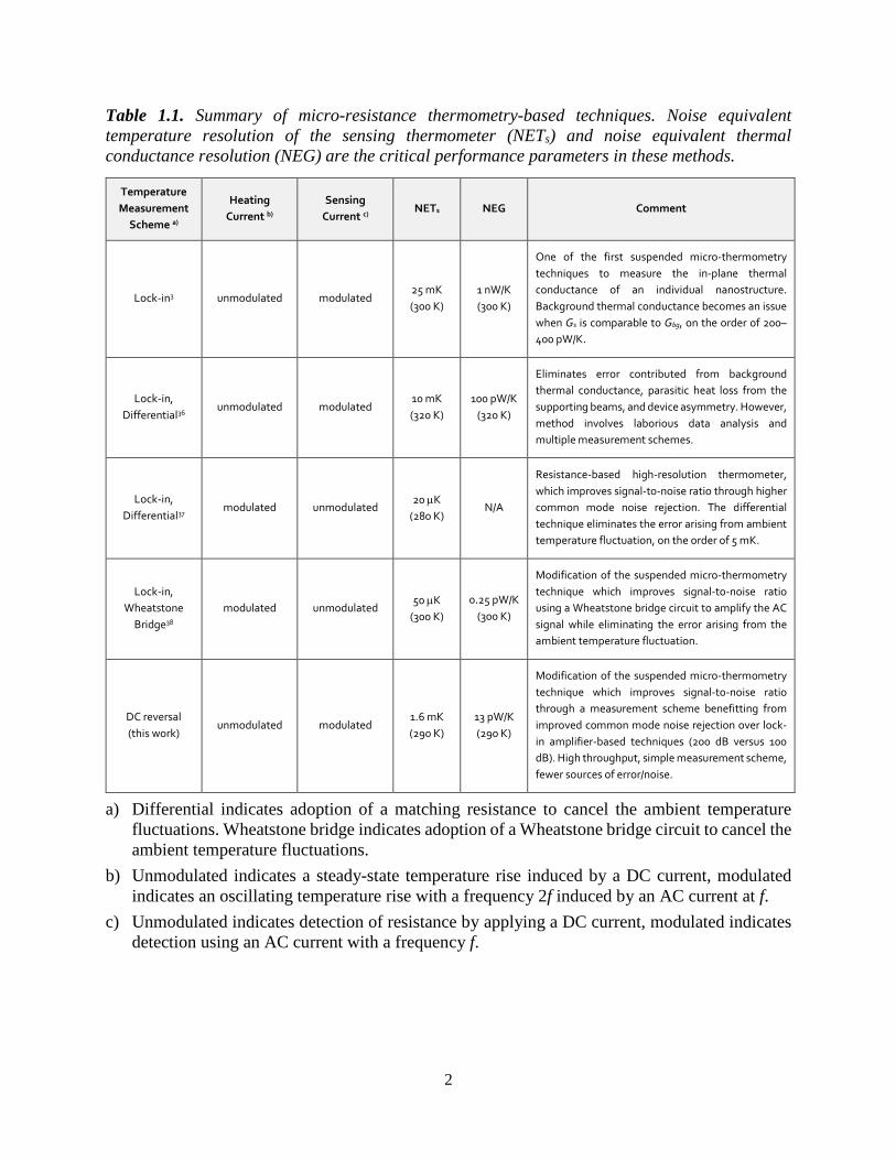
Table 1.1. Summary of micro-resistance thermometry-based techniques. Noise equivalent temperature resolution of the sensing thermometer (NETs) and noise equivalent thermal conductance resolution (NEG) are the critical performance parameters in these methods.

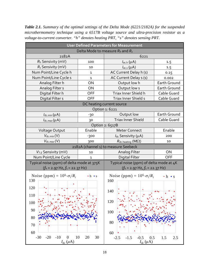
Table 2.1. Summary of the optimal settings of the Delta Mode (6221/2182A) for the suspended microthermometry technique using a 6517B voltage source and ultra-precision resistor as a voltage-to-current converter. “h” denotes heating PRT, “s” denotes sensing PRT.

Table 3.1. Summary of temperature and thermal conductance resolution for the DC reversal technique. The measured standard deviation of the sensing temperature rise, σtemp, and the measured standard deviation of the background thermal conductance σGbg compare favorably with the NETs and NEG values.

1

Chapter 1 – Introduction

1.1. Background

Low dimensional materials such as carbon nanotubes1-6, inorganic nanowires7-12, organic

nanofibers13-15, superlattices16, 17, and two dimensional materials18-24 have been the focus of

significant research interest over the past two decades due to their unique thermal transport

properties which can be significantly different than in their bulk form. In addition to establishing

fundamental structure-property relationships in these materials, these investigations have also

enabled novel thermal device applications25-29. Hence, further development of new experimental

techniques for characterization of thermal transport in nanostructures remains an important area as

advancement continues in the prediction, design, and synthesis of new materials.

1.2. Suspended micro-thermometry measurement

Several thermal measurement techniques have been developed for probing in-plane

thermal transport properties in low dimensional materials, the most prominent of which are the

suspended micro-thermometry2-4, 11, 19, Raman thermometry5, 18, 30, bi-material atomic force

microscopy (AFM) cantilever thermometry13, and steady-state Joule heating4, 31-33 methods. Of

these, the suspended micro-thermometry technique is the most common method to measure in-

plane thermal conductance in individual nanostructures as phonons are fully thermalized, in

contrast to optothermal techniques34, 35. Platinum resistance thermometers (PRTs) are used to

measure the temperature and heat flow on the suspended microdevice as platinum’s electrical

2

Table 1.1. Summary of micro-resistance thermometry-based techniques. Noise equivalent temperature resolution of the sensing thermometer (NETs) and noise equivalent thermal conductance resolution (NEG) are the critical performance parameters in these methods.

Temperature Measurement

Scheme a)

Heating Current b)

Sensing Current c)

NETs NEG Comment

Lock-in3 unmodulated modulated 25 mK (300 K)

1 nW/K (300 K)

One of the first suspended micro-thermometry techniques to measure the in-plane thermal conductance of an individual nanostructure. Background thermal conductance becomes an issue when Gs is comparable to Gbg, on the order of 200–400 pW/K.

Lock-in, Differential36

unmodulated modulated 10 mK (320 K)

100 pW/K (320 K)

Eliminates error contributed from background thermal conductance, parasitic heat loss from the supporting beams, and device asymmetry. However, method involves laborious data analysis and multiple measurement schemes.

Lock-in, Differential37

modulated unmodulated 20 µK

(280 K) N/A

Resistance-based high-resolution thermometer, which improves signal-to-noise ratio through higher common mode noise rejection. The differential technique eliminates the error arising from ambient temperature fluctuation, on the order of 5 mK.

Lock-in, Wheatstone

Bridge38 modulated unmodulated

50 µK (300 K)

0.25 pW/K (300 K)

Modification of the suspended micro-thermometry technique which improves signal-to-noise ratio using a Wheatstone bridge circuit to amplify the AC signal while eliminating the error arising from the ambient temperature fluctuation.

DC reversal (this work)

unmodulated modulated 1.6 mK (290 K)

13 pW/K (290 K)

Modification of the suspended micro-thermometry technique which improves signal-to-noise ratio through a measurement scheme benefitting from improved common mode noise rejection over lock-in amplifier-based techniques (200 dB versus 100 dB). High throughput, simple measurement scheme, fewer sources of error/noise.

a) Differential indicates adoption of a matching resistance to cancel the ambient temperature fluctuations. Wheatstone bridge indicates adoption of a Wheatstone bridge circuit to cancel the ambient temperature fluctuations.

b) Unmodulated indicates a steady-state temperature rise induced by a DC current, modulated indicates an oscillating temperature rise with a frequency 2f induced by an AC current at f.

c) Unmodulated indicates detection of resistance by applying a DC current, modulated indicates detection using an AC current with a frequency f.

3

resistance has a nearly-linear relationship with temperature and large temperature coefficient of

resistance (TCR) over a wide range of temperatures. Based upon the original reports2, 3, several

different electrical resistance measurement techniques have been developed to achieve higher

temperature and thermal conductance resolution in the suspended micro-thermometry method36, 38,

39. A summary of these techniques is shown in Table 1.1 and Figure 1.1.

In a pioneering work published a decade ago, Philip Kim et al.2 developed a suspended

micro-thermometry device and used it to probe the in-plane thermal conductance of a multi-

walled carbon nanotube, where the suspended microdevice containing two built-in platinum

resistors was used to measure the temperature and heat flow across the sample. In this and other

previous lock-in-based measurement schemes, the thermal conductance resolution was reported

on the order of 1 nW/K. The presence of temperature fluctuations in the sample chamber and

background thermal conductance through the device, residual gases, and radiation are dominant

sources of errors when the sample thermal conductance is comparable to or smaller than the

background thermal conductance, on the order of 300 pW/K at room temperature.

Sadat el al.37, 39 have analyzed the temperature resolution of this technique in four

different scenarios and demonstrated a temperature resolution of ~20 µK at 280K by measuring

modulated temperature changes on the PRT’s resistance with an unmodulated sensing current

and a matching PRT which has nearly the same resistance and temperature drift as the sensing

PRT. In particular, detecting an unmodulated temperature change requires instrumentation with

large dynamic range to eliminate the ambient temperature drift at the same time. First, a large

sensing current and PRT with a large electrical resistance was used to improve signal-to-noise

ratio but it should be noted that these approaches are limited by the microdevice fabrication and

self-heating issues.

4

Figure 1.1. Suspended micro-thermometry measurement schemes. (a) Electrical and thermal circuits of the suspended micro-thermometry device with unmodulated heating current and modulated sensing current (reproduced from Ref. 3). (b) Electrical circuit of the suspended micro-thermometry device adapted by a differential measurement scheme. The matching device allows this technique to isolate the background thermal conductance during the measurement (reproduced from Ref. 36), (c) A modified suspended micro-thermometry device adapted by a Wheatstone bridge scheme with modulated heating current and unmodulated sensing current (reproduced from Ref. 38). The Wheatstone bridge circuit is used to eliminate the temperature drift from the sample chamber. (d) A single-pad suspended micro-thermometry device with two PRTs on the suspended membrane adapted by a differential scheme with modulated heating current and unmodulated sensing current (reproduced from Ref. 37). The matching resistor is used to eliminate the temperature drift from the sample chamber.

Previous improvements on the micro-thermometry technique have resulted in two major

contributions. First, the voltage noise and ambient temperature drift that arises from an

unmodulated temperature signal can be eliminated using a high frequency detecting current with

(a) (b)

(c) (d)

5

a lock-in amplifier and a differential scheme36, 39, but a complicated setup and data analysis is

involved to achieve this high temperature and thermal conductance resolution. Second, a

temperature signal modulated at specific frequency with an unmodulated sensing current can

further improve temperature resolution37, 38, however, the attenuation of modulated temperature

due to the large thermal time constant of the suspended microdevice becomes an issue during the

thermal conductance measurement.

1.3. Motivation and scope of the study

In this work, I have developed a high throughput suspended micro-thermometry

measurement scheme involving less instrumentation and simple data analysis. Specifically, we

have introduced a bipolar DC reversal measurement which is a well-established alternative

technique to remove offset and low frequency noises during measurement. This modern DC

reversal technique exhibits less than one half the amount of white noise and an order of magnitude

lower 1/f noise than the most commonly used lock-in amplifiers40. As a result, I have demonstrated

resolution near the instrumentation limit of this technique: a sensing noise equivalent temperature

(NETs) of 2.62 and 1.12 mK and a noise equivalent thermal conductance (NEG) of 26.42 and 1.73

pW/K at an ambient temperature of 375 and 30 K respectively. The NET reaches a minimum of

0.96 mK at 75K without the need for using complicated schemes involving matching resistors or

Wheatstone bridge to cancel the ambient temperature drift.

6

Chapter 2 – Thermal conductance measurement

2.1. Measurement setup

The microfabricated suspended device consists of two symmetric adjacent low stress

silicon nitride (SiNx, 22 µm by 22 µm) membranes each suspended by six 400 µm long by 2 µm

wide SiNx beams. One 35 nm thick, ~250 nm wide and 350 µm long serpentine platinum resistance

heater/thermometer is patterned on each membrane. One 1 µm wide by 16.25 µm long inner

electrode and one 1.25 µm wide by 19 µm long outer electrode are also patterned on each

membrane. The heater/thermometer and electrodes are connected to electrical contact pads with

400 µm long by 2 µm wide Pt metal lines, as shown in Figure. 2.1. The silicon substrate beneath

the suspended membranes is completely removed. The detail of the fabrication processes can be

found in Ref. 41.

Figure 2.1. Schematic of the suspended microdevice and circuit diagram of the DC reversal technique to measure the electrical resistances of the heating and sensing PRTs on a suspended microdevice. Shown below is the corresponding thermal circuit. A 10 MΩ ultra high precision resistor is used to convert the voltage source into a DC current source. A high input impedance (1014 Ω) programmable current source and high input impedance nanovoltmeter (>1012 Ω) are connected to obtain the 4-probe differential voltage on each PRT.

7

Figure 2.2. Kinetic theory calculation of the thermal conductivity of residual air molecules, κair, inside an enclosure chamber with a diameter of 2.5 inches (~ sample chamber diameter) as a function of pressure, P, from 10-10 to 1000 mbar at certain ambient chamber temperature (T = 4, 150, and 300 K) by kinetic theory of gases. inset shows corresponded air thermal conductivity within cryostat chamber pressure range (10-10 to 10-8 mbar).

The suspended microdevice was placed in a Janis SHI-4ST-UHV closed cycle cryostat

connected to an Oerlikon Leybold TURBOVAC TW250S/TRIVAC D16BCS turbo pumping

system providing a vacuum environment better than 10-8 mbar during thermal transport

measurements (Figure 2.3). The cryostat sample temperature was controlled by a Lakeshore 336

cryogenic temperature controller which provided a measured ambient temperature stability of

better than 2 mK (Figure 2.3). The suspended microdevice contains two symmetric adjacent silicon

nitride (SiNx) membranes each suspended by six long SiNx beams. A serpentine PRT is fabricated

on each membrane and it connects to four contact pads by platinum lines on the suspended beams.

The heating PRT was electrically heated by an unmodulated current provided by a Keithely 6517B

electrometer in series with a 10 MΩ high precision resistor (Caddock USF370-10.0M-0.01%-

5ppm). The DC current passing through the device was directly measured by the low-impedance

10-10 10-7 10-4 10-1 102

10-9

10-7

10-5

10-3

10-1

κ air (W

/m·K

)

P (mbar)

T = 4 K T = 150 K T = 300 K

10-10 10-9 10-8

10-9

10-8

10-7

10-6

κ air (

W/m

∗K)

P (mbar)

8

Figure 2.3. (a) Ultra high vacuum cryostat chamber pressure as a function of temperature recorded at the sample mount, T0 over a temperature range from 4 to 300 K. (b) Measured cryostat chamber pressure as a function of time at 4 K sample mount temperature, the system maintained vacuum better than 8.5×10-10 mbar over 24 hours. (c) Measured cryostat sample mount temperature as a function of time at 4 K, it maintained a stability better than 1 mK over 24 hours. (d) Measured cryostat chamber pressure as a function of time at 375 K sample mount temperature, it maintained vacuum better than 1.5×10-8 mbar over 24 hours. (e) Measured cryostat sample mount temperature as a function of time at 375 K, it maintained a stability better than 20 mK over 24 hours. Data depicted in (b) and (c) were collected while the temperature of the heater was set at 4.0000 K, (e) and (f) were collected while the temperature of heater was set at 375.000 K. The temperature drift in the thermal conductance measurement was much smaller than above data because each measurement set was taken within 0.5 hours.

0 50 100 150 200 250 30010-9

10-8

10-7

0 5 10 15 20 25

6x10-10

7x10-10

8x10-10

0 5 10 15 20 25

4.052

4.054

4.056

4.058

4.060

0 5 10 15 20 25

1.3x10-8

1.4x10-8

1.5x10-8

1.6x10-8

1.7x10-8

0 5 10 15 20 25

373.914

373.920

373.926

373.932

373.938

P (m

bar)

T0 (K)

(a)

P (m

bar)

t (hrs)

(b)

T 0 (K)

t (hrs)

(c)

P (m

bar)

t (hrs)

(d)

T 0 (K)

t (hrs)

(e)

9

input of the Keithley 6517B. During the measurement, a certain amount of this heat is transferred

to the adjacent sensing membrane and PRT through parallel mechanisms: (i) through the

nanostructure, (ii) through the thermal sink (the silicon substrate), and (iii) through radiation and

residual gas conduction. Mechanisms (ii) and (iii) are denoted background thermal conductance,

Gbg. The uncertainty arising from the thermal radiation contributes less than 2% to the thermal

conductance of the beam and sample over 30 to 400 K42. At 10-8 mbar and 300 K, thermal

conductivity of air is on the order of 10-7 W/(m⋅K), as shown in Figure 2.2 and yields thermal

conductance of less than 5 pW/K which accounts for 1.5 % of the total Gbg.

2.2. Data processing

A schematic of the measurement is shown in Figure 2.1. Both of the PRTs serve as

thermometers to measure the temperature rise on each suspended membrane, which is determined

by the PRT’s temperature-dependent electrical resistance and its temperature coefficient of

resistance (TCR) using two Keithley 6221/2182A Delta-mode systems. The electrical resistances

of the heating membrane PRT and each Pt lead are denoted as Rh and RL respectively. A Joule

heat, Qh = Idc2Rh, is generated when a DC current Idc passes through the heating membrane and

causes its temperature to rise from T0 to Th. Meanwhile, the two current-carrying Pt leads generate

and dissipate Joule heat, 2QL = 2Idc2RL, due to the DC current. The uniform temperature on the

heating membrane is a justified assumption since the internal thermal resistance of the PRT is two

orders of magnitude smaller than the thermal resistance of the six long Pt leads connecting it to

the silicon chip at ambient temperature T042. A certain portion of the Joule heat, Qs, is transferred

from the heating membrane through the nanostructure to to the sensing membrane. The sensing

membrane is raised from T0 to Ts, which is assumed uniform on the sensing membrane by the

10

previous justification. This amount of heat then is conducted to the silicon heat sink at T0 through

the six beams supporting the sensing membrane. With the conservation of energy, the remaining

heat, Q1 = Qh + 2QL – Qs, is conducted to the silicon chip through the six beams supporting the

heating membrane. The thermal conductance of six beams supporting each membrane Gb and the

total sample thermal conductance Gs from the heating membrane to sensing membrane are

determined with the thermal circuit in Figure 2.1 as

sh

Lh

bb

1TT

QQR

G∆+∆

+== and (1)

sh

sb

sh

ss TT

TGTT

QG∆−∆

∆=

∆−∆= , respectively. (2)

The temperature of the heating membrane and sensing membrane, Th and Ts respectively,

are accurately determined by a DC reversal 4-point differential electrical resistance measurement,

as depicted in Figure 2.1. A small positive DC current (1.5 µA) is passed through the PRT and the

voltage V1 across the PRT is measured, then the DC current is reversed (-1.5 µA) and a second

voltage V2 is recorded. The positive DC current (1.5 µA) is applied again and a third voltage V3 is

measured. A three point moving average algorithm is used to determine the final voltage responses,

where Vfinal = (V1 – 2V2 + V3)/4. This data processing is completed internally and the DC reversal

system outputs the final voltage and resistance responses corresponding to the DC current (1.5 µA)

I apply.

The change of the temperature caused by DC heating results in an electrical resistance

change of the PRT which is interpreted back to a temperature rise using the measured TCR of each

PRT, ( )[ ] ( )TRTTR iii ∂∂≡α , i = h, s. To obtain steady-state resistance versus temperature and

TCR, I have measured the PRT resistances every ~ 0.4 K while the temperature of the chamber

was slowly cooled at a rate of 3.33 mK/s from 375 to 4 K, as shown in Figure 2.4. The

11

Figure 2.4. Electrical resistance, R, and temperature coefficient of resistance (TCR), α, of the heating and sensing PRTs as a function of temperature recorded at the sample mount, T0. (a) Measured heating and sensing PRT electrical resistances, Rh and Rs respectively, over a temperature range from 4 to 375 K and (b) the corresponding TCR of heating and sensing PRTs, αh and αs respectively. The TCR at each temperature point is calculated over 15 measured resistance points which corresponds to a local temperature range of approxiately T0 ± 3 K.

corresponding TCR of each PRT at each ambient temperature point T0 is used to calculate the

temperature change caused by the DC joule heating. The TCRs at each T0 are determined over a

T0 ± 3 K temperature range to define a local α for use in Eqs. 3–4. Consequently, the resulting

temperature rise on the sensing membrane ∆Ts is a function of the Idc applied on the heating PRT

and can be determined as

( ) ( )

=

=−=∆

)0(01)(

dcs

dcsdcs

sdcs IR

IRIRITα

. (3)

Measurement of the temperature rise on the heating membrane is complicated by the

copling between AC and DC currents. An AC current iac with a frequency fh is coupled to the much

larger DC heating current during the electrical resistance measurement and this AC current will

generate modulated heating at frequency 2fh at when fh is low. Shi et al.3 have experimentally

demonstrated a factor of 3 difference between the low frequency and high frequency limits of an

0 100 200 300 400

1200

1600

2000

2400

2800

R (Ω

)

T0 (K)

Rh

Rs

Rh

Rs

0 100 200 300 400

0

1000

2000

3000

4000

αh

αs

α (1

0-6 K

-1)

T0 (K)

αh

αs

(a) (b)

12

unmodulated temperature rise calculation when the DC current heating is coupled with a sinusoidal

AC current. The AC and DC coupling effect remains important in this work because I am

employing a square wave AC current in our measurement scheme. Joule heating, Qac+dc = [Idc +

iac(fh)]2Rh, is generated on the heating membrane by the AC + DC current. This modulated heating

will yield a nontrivial component in Th when the frequency of the AC current is much smaller than

1/(2πτ), where τ is the thermal time constant of the suspended microdevice. Thus the measured

resistance rise of the heating PRT, ∆Rh, is affected by this AC + DC heating effect in the low

frequency regime. Thus the temperature rise ∆Th is a function of Idc applied on the heating PRT

can be determined as

( ) ( ) ( )( )

>>=<<=

=

=−=∆

τζτζ

ζα π21,1π21,3

,)0(

01)(h

h

dch

dchdch

hdch f

fIR

IRIRIT (4)

To investigate the waveform-dependence of the frequency-dependent resistance rise, I have

measured the ∆Rh(fh) by a lock-in technique using a 1 µA peak-to-peak excitation current in the

frequency range from 0.8 to 5864 Hz for square, sine, and triangle waveforms while DC heating

is applied (Figure 2.5). The factor ζ does not show a significant change with different types of AC

waveform, where the normalized resistance change due to DC heating ∆Rh(fh)/∆Rh(fh=1 Hz)

corresponds to ζ /3. Furthermore, the cut-off frequency between the low and high frequency

regimes increases with temperature since τ decreases with decreasing temperature. As shown in

Figure 2.6, I observed a higher cutoff frequency at 4 K than 375 K as τ is smaller at 4 K than at

375 K.

13

Figure 2.5. Normalized first harmonic component of the measured resistance rise of the heating PRT as a function of the frequency of AC current coupled to the DC heating current for different AC waveforms at 290 K. The value of ζ in Eq.4 can be determined by the following relationship, ζ = 3∆Rh(fh)/∆Rh(fh=1 Hz). Note, the DC heating current here was provided by a Keithley 6221.

Figure 2.6. Normalized first harmonic component of the measured resistance rise of the heating PRT as a function of the frequency of AC current coupled to the DC heating with a lock-in technique, measured using a Keithley 6221 DC current source and a Keithley 6517B electrometer with a 10 MΩ precision resistor at 290 K. The value of ζ in Eq. 4 can be determined by the following relationship, ζ = 3∆Rh(fh)/∆Rh(fh=1 Hz).

1 10 100 1000 10000

0.2

0.3

0.4

0.5

0.6

0.7

0.8

0.9

1.0

∆R (f

h) / ∆

R (f h =

1 H

z)

fh (Hz)

Square wave Sine wave Triangle wave

ζ / 3 = 1/3

1 10 100 1000 10000

0.2

0.4

0.6

0.8

1.0

∆R (f

h)/∆R

(f h = 1

Hz)

fh (Hz)

6221 Current source 6517B Electrometer + 10 MΩ Resistor

ζ / 3 = 1/3

14

The DC current provided by a Keithley 6517B electrometer and large resistor introduced

unknown noises on the measured resistance rise as function of heating frequency. I have compared

the resistance rise measured with a lock-in technique using a Keithley 6221 DC current source and

Keithley 6517B in Figure 2.6. The lock-in technique picked up unpredicted noise when using the

Keithley 6517B electrometer, consequently, DC current sourced with a Keithley 6517B and large-

value resistor is not recommended to use when the lock-in technique is employed to measure the

measured resistance rise. In this thesis, a Keithley 6221 has been used as the DC current source

when resistance has been measured with lock-in amplifiers.

I have also compared the resistance rise measured with a DC reversal technique to the

resistance rise measured with a lock-in technique in Figure 2.7. The frequency of the DC reversal

technique is based on the current source delay time, nanovoltmeter measuring time (number of

power line cycles), and instrument communication time. We calculate the frequency based on the

average measured timestamp, reported twice per period by the instrumentation. The frequency-

dependent resistance rise of the DC reversal technique was then used as a reference to determine

the cut-off frequency defined as ∆Rh(fh)/∆Rh(fh=1 Hz) = 0.998, which is 12.94, 6.39, 3.02, and 2.97

Hz at 4, 75, 290, and 375 K respectively. As our technique is designed for use in the low frequency

regime, 3 Hz is appropriate over the full temperature range of 4–375 K, ensuring ζ = 3 in Eq. 4.

15

Figure 2.7. Normalized first harmonic component of the measured resistance rise of the heating PRT as a function of the frequency of AC current coupled to the DC heating current at 375, 290, and 75 K obtained by the DC reversal technique and by the lock-in technique with square wave excitation. The value of ζ in Eq.4 can be determined by following relationship, ζ = 3∆Rh(fh)/∆Rh(fh=1 Hz). Note, the DC heating current was provided by a Keithley 6221 when the lock-in technique was used.

0.1 1 10 100 1000 100000.2

0.3

0.4

0.5

0.6

0.7

0.8

0.9

1.0

∆R (f

h) / ∆

R (f h =

1 H

z)

fh (Hz)

DC Reversal 375 K DC Reversal 290 K DC Reversal 75 K DC Reversal 4 K Lock-in 375 K Lock-in 290 K Lock-in 75 K Lock-in 4 K

ζ / 3 = 1/3

16

2.3. DC reversal technique

I have introduced a bipolar DC reversal technique to measure the 4-probes electrical

resistances of each PRT which is a well-established alternative technique to remove offset and low

frequency noises during measurement. This modern technique exhibits less than one half the

amount of white noise and an order of magnitude lower 1/f noise than the most commonly used

lock-in amplifiers40. Generally, the DC reversal system (Keithley 6221 + 2182A) performs a

resistance measurement with following steps: (i) the 2182A nanovoltmeter triggers the 6221

current source to provide a positive current to the PRT, (ii) the 6221 sends a trigger signal to the

2182A after an operator-defined current delay time, (iii) the 2182A measures the voltage V1 with

an operator-defined measuring time (number of power line cycles), (iv) the 2182A sends the a

trigger signal to stop the current source, (v) steps (i) to (iv) are repeated with a negative current

and the voltage V2 is recorded, (vi) steps (i) to (iv) are repeated again with a positive current and

voltage V3 is recorded, (vii) a three point moving average algorithm is used to determine the final

voltage responses, where Vfinal = (V1 – 2V2 + V3)/4. The voltage Vfinal is then associated with the

operator-set current, iac, to calculate the resistance of the PRT (Figure 2.8). The optimal conditions

for this technique are shown in Table 2.1 and have been used to measure the background thermal

conductance in Chapter 3.

17

6221 source

iac

-iac

iac

6221 current delay

6221 outputs a trigger to

2182A

2182A voltage

measuring delay

(NPLC)

V1 2182A outputs a trigger to

6221

6221 current delay

2182A voltage

measuring delay

(NPLC)

6221 outputs a trigger to

2182A

V2

2182A outputs a trigger to

6221

6221 current delay

6221 outputs a trigger to

2182A

2182A voltage

measuring delay

(NPLC)

V3 2182A outputs a trigger to

6221

Vfinal

1st timestamp is reported, it will report every half cycle after the 1st one.

Figure 2.8. Schematic of the Keithley 6221 current source and Keithley 2182A nanovoltmeter DC reversal measurement technique (Delta Mode) data processing. The time period is not shown to scale.

18

Table 2.1. Summary of the optimal settings of the Delta Mode (6221/2182A) for the suspended microthermometry technique using a 6517B voltage source and ultra-precision resistor as a voltage-to-current converter. “h” denotes heating PRT, “s” denotes sensing PRT.

User Defined Parameters for Measurement Delta Mode to measure Rh and Rs

2182A 6221 Rh Sensivity (mV) 100 Iac.h (µA) 1.5 Rs Sensivity (mV) 10 Iac.s (µA) 1.5

Num Point/Line Cycle h 1 AC Current Delay h (s) 0.15 Num Point/Line Cycle s 1 AC Current Delay s (s) 0.002

Analog Filter h ON Output low h Earth Ground Analog Filter s ON Output low s Earth Ground Digital Filter h OFF Triax Inner Shield h Cable Guard Digital Filter s OFF Triax Inner Shield s Cable Guard

DC heating current source Option 1: 6221

Idc.min (µA) -30 Output low Earth Ground Idc.max (µA) 30 Triax Inner Shield Cable Guard

Option 2: 6517B Voltage Output Enable Meter Connect Enable

Vdc.min (V) -300 Idc Sensivity (µA) 200 Vdc.max (V) 300 Rdc.heating (MΩ) 10

2182A (channel 1) to measure Seebeck VT.E Sensivity (mV) 10 Analog Filter ON

Num Point/Line Cycle 1 Digital Filter OFF Typical noise (ppm) of delta mode at 375K

(fh = 2.97 Hz, fs = 22.37 Hz) Typical noise (ppm) of delta mode at 4K

(fh = 2.97 Hz, fs = 22.37 Hz)

60

70

80

90

100

110

120

130

-30 -20 -10 0 10 20 30Idc (µA)

Noise (ppm) = 106⋅σ i/Ri h s

60

80

100

120

140

160

-2.5 -1.5 -0.5 0.5 1.5 2.5Idc (µA)

Noise (ppm) = 106⋅σ i/Ri h s

19

Chapter 3 – Temperature and background thermal conductance resolution

3.1. Noise analysis

Resistance-based thermometry is based on temperature-dependent electrical resistance, so

that the measured resistance can be correlated with the temperature of the object to which the PRT

is attached. On the sensing membrane, where only an AC signal is used in the resistance

measurement, Eq. 3 can be used to convert the measured resistance change to temperature change.

Thus, the noise equivalent temperature of the sensing PRT (NETs) is calculated based on Eq. 3 and

the lowest total voltage noise in the electrical resistance measurement ∆Vnoise as

( )TRiVT

sac

noiseResolutions

ΔΔNETα

== . (5)

Improving NETs can be achieved by employing a larger resistance PRT and larger sensing

current. However, self-heating and the device stability are both detrimental to the measurement

when the sensing current is too high (Figure 3.1). Thus, lowering ∆Vnoise is a more appropriate

strategy to enhance the temperature resolution of suspended micro-thermometry technique.

Contributions to the voltage noises are categorized as intrinsic noises (Johnson and shot noises)

and non-intrinsic noises (1/f noise, temperature drift, etc.). In this experiment, the total noise in the

voltage signal can be estimated from

2drift etemperatur

2electrical

2noise ΔΔΔ VVV += , (6)

where 2electricalΔV is the mean square of electrical noises arising from the intrinsic noises of

resistance and the non-intrinsic nosie from the instrumentation, and 2drift etemperaturΔV is the measured

mean square voltage noise due the ambient temperature drift of the sample mount.

20

.

Figure 3.1. Rise in measured resistance of the PRT caused by self-heating from the AC sensing current, ∆R(iac) = R(iac) – R(iac = 0.3 µA), as a function of AC sensing current amplitude at 22.37 Hz. The measured standard derivation of the resistance, σ / R(iac), is shown for comparison in units of parts per million. An optimal iac of 1.5 µA peak-to-peak is used for the DC reversal technique based on minimizing noise while maintaining an acceptably small resistance rise corresponding to 71.6 mK.

A higher AC sensing current, iac is a separate strategy to lower the noise equivalent

temperature as per Eq. 5, as well as the noise equivalent conductance, without contributing

substantial modulated heating. I have measured the PRT resistance and its noise (ppm, [σ/R(iac)]*

106) as a function of sensing current from 0.3 µA to 5 µA (Figure 3.1). The electrical resistance

of the PRT does not show a significant increase with a sensing current between 0.3 – 1.5 µA,

indicating a negligible self-heating effect on the suspended membrane. In contrast, the standard

derivation of measured resistance dramatically decreases with increasing iac. In other words, the

noises contributed from the electrical measurement can be minimized by applying a higher AC

current, but this will also induce non-negligible self-heating. I calculated the temperature rise with

1.5 µA AC current is ~70 mK. Nevertheless, the rise of resistance due to AC current heating is a

constant offset which will cancel out during the calculation of ∆Ri(Idc) = Ri(Idc) – Ri(Idc = 0), i = h,

s on each suspended membrane. To examine the effect of AC self-heating on the heat flow

0.0 1.0 2.0 3.0 4.0

0.0

0.3

0.6

0.9

1.2

1.5

iac (µA)

R(i ac

) - R

(i ac =

0.3

µΑ

) (Ω

)

iac = 1.5 µA

0

50

100

150

200

250

σ / R

(i ac) (

ppm

)

21

measurement, I have measured the temperature rise ∆Ts on the sensing PRT as a function of DC

heating power applied to the heating PRT from 0 to 3000 nW with 0.5, 1.5, 2.5, and 3.5 µA AC

excitation current at 22.37 Hz. The ∆Ts measured with 1.5 µA or higher AC excitation current

offers three times better temperature resolution than 0.5 µA and does not show a significant self-

heating effect caused by the AC current. Device stability is also an important aspect during the

measurement, thus 1.5 µA has been chosen as the optimal AC excitation current to measure the

NETs described subsequently as this current exhibits roughly the same temperature resolution as

the higher currents shown in Figure 3.2.

I have measured the temperature rise ∆Ts on the sensing PRT as a function of DC heating

power applied to the heating PRT from 0 to 3000 nW with 22.73, 12.95, and 2.97 µA AC excitation

frequency using 1.5 µA AC excitation current. 1/f noise becomes the dominant noise as the

frequency decreases. Thus I have chosen 22.37 Hz as the optimal AC excitation frequency to

measure the NETs described subsequently as this frequency exhibits the best temperature

resolution shown in Figure 3.3.

In order to determine NETs, we need to identify the noise components of ∆Vnoise. The major

advantage of the DC reversal technique is that it can diminish 1/f noises and noise due to offsets

due to thermal drift. The common mode rejection ratio (CMRR) of an instrument describes the

ability of common noise rejection in the measurement. The DC reversal system (Keithley 6221

and 2182A) has a CMRR of more than 200 dB (Vsignal ± Vnoise/1010), this is extremely high in

comparison to high-resolution lock-in amplifiers (Stanford Research Systems SR830) which only

22

Figure 3.2. Measured sensing PRT temperature rise as a function of Qh = Idc2Rh, shown for varied

AC excitation current (f = 22.37 Hz) of 0.5, 1.5, 2.5, and 3.5 µA and obtained at T0 = 375 K. The inset shows the low Qh regime, note that 1.5 uA is sufficient to achieve high resolution without inducing a large self-heating effect.

Figure 3.3. Measured sensing PRT temperature rise as a function of Qh = Idc2Rh, shown for varied

AC excitation frequency of 22.37, 12.95, and 2.97 Hz (iac = 1.5 µA) and obtained at T0 = 375 K. The inset shows the low Qh regime. Note that 22.97 Hz is the optimal frequency to achieve high temperature resolution, this is near the maximum frequency for the Delta mode (fmax = 24 Hz, limited by instrumentation communication) and corresponds to the settings listed in Table 2.1.

0 500 1000 1500 2000 2500 30000

10

20

30

40

50

1 10 1000

2

4

6

8

10∆T

s (m

K)

Qh (nW)

iac = 0.5 µA iac = 1.5 µA iac = 2.5 µA iac = 3.5 µA

Qh (nW)

∆T s (m

K)

0 500 1000 1500 2000 2500 30000

10

20

30

40

50

1 10 1000.0

2.0

4.0

6.0

8.0

10.0

∆Ts (m

K)

Qh (nW)

fs = 2.97 Hz fs = 12.95 Hz fs = 22.37 Hz

Qh (nW)

∆Ts (m

K)

23

have a CMRR of 100 dB (Vsignal ± Vnoise/105). In other words, the instrumentation used in the DC

reversal technique has a much better capability to reject non-intrinsic noises. In addition, the

programmable current source used in this technique has an input impedance of >1014 Ω which is

able to provide a stable and load-independent current through the PRTs (δiac/iac ~ 10-7), effectively

eliminating shot noise. Therefore, the Johnson noise is the only contribution to electrical noise and

is expressed as

( ) 50BJohnsonelectrical Δ4ΔΔ .fTRkVV == (7)

and temperature drift ∆Vtemperature drift are the major contributions to the ∆Vnoise in the DC reversal

measurement scheme used here. The noise equivalent bandwidth ∆f is ~1 Hz for the DC reversal

system. The NETJohnson at each ambient temperature point is calculated based on Eqs. 5 and 7. The

NETtemperature drift represents the stability of the cryostat sample mount temperature and is directly

obtained as the standard deviation of recorded sample mount temperatures during measurement.

A summary of the temperature dependent contributions to NET is shown in Figure 3.4.

As I have obtained the NETs of the DC reversal technique, the noise equivalent

conductance (NEG) of the suspended microdevice, which is the minimum thermal conductance

that can be detected by the suspended device, can be expressed using Eqs. 2 and 5 as

sh

sb ΔΔ

NETNEGTT

G−

= , (8)

where Gb is the measured thermal conductance of the six beams supporting each membrane. The

NETs and NEG are calculated from the above analysis and shown in Table 3.1 for different sample

mount temperatures.

24

Figure 3.4. Temperature dependence of contributions to the sensing noise equivalent temperature (NETs) of the DC reversal technique (NETtemperature drift and NETJohnson), shown in comparison to the total (pooled) standard deviation of the measured temperature rise, σtemp, and the calculated delta mode instrumentation detection limit based on minimum resolution of 4.2 − 5 nV.

3.2. Temperature resolution

I have measured the background conductance on a blank device to experimentally

determine the minimum temperature resolution and minimum thermal conductance resolution of

the DC reversal suspended micro-thermometry technique over a temperature range of 1.0 – 2.6 K

(Figure 3.5). During each measurement set, Idc is applied to the heating membrane at discrete

values from 0 to +Idc,max to -Idc,max and back to 0. At each Idc value, the average of 20 electrical

resistance measurements of ∆Rh(Idc) and the average of 200 measurements of ∆Rs(Idc) are taken to

determine ∆Th(Idc) and ∆Ts(Idc) respectively. The difference in number of data points ensures both

measurements end at roughly the same time, as fh = 3 Hz and fs = 22.37 Hz. Figure 3.5 shows the

measured temperature rise ∆Ts on the sensing membrane as function of heating power Qh at

different sample mount temperatures. The standard derivation at each measured ∆Ts is calculated

25

Figure 3.5. Measured temperature rise on the sensing PRT, ∆Ts, as a function of heating power Qh detected using the DC reversal technique with a 1.5 µA AC excitation current at 22.37 Hz. T0 = (a) 375 K, (b) 290 K, (c) 75 K, and (d) 30 K. Error bars are defined as one standard deviation of ∆Ts(Qh) over five separate measurement sets (one set is defined as Idc = 0 to –Idc,max to +Idc,max to 0). The measured total (pooled) standard deviation of the temperature rise, σtemp, is shown for comparison at each T0.

based on five measurement sets at each heating power. In order to obtain statistics on the

uncertainty of the entire measurement, the overall standard derivation of temperature rise, σtemp, is

computed as a pooled standard deviation estimation from different populations43. The twenty

0 50 100 150 200 250 300

0.0

1.0

2.0

3.0

4.0

5.0

∆Ts (m

K)

Qh (nW)

σtemp = 0.96 mK

75 K

0 500 1000 15000369

1215

∆Ts (

mK

)

Qh (nW)

(a)

(c)

(b)

(d)

26

measured ∆Ts(Qh) at each heating power were considered as one statistical population (one set is

defined as Idc = 0 to –Idc,max to +Idc,max to 0), the error bars in Figure 3.5 are defined to have a

magnitude of one standard deviation of this population. As we used the same instruments

throughout the whole experiment, the overall (pooled) standard derivation of the all the measured

temperature rises was calculated as:

∑

∑

=

=

−

−= k

ii

k

iii

1

1

2

temp

1n

)1n( σσ , (9)

where σi and ni are the sample standard derivation and sample size of the measured temperature

rise at each heating power. The DC reversal method exhibits sensing temperature resolution,

defined here as σtemp, of 2.62 mK, 1.60 mK, 0.96 mK, and 1.12 mK at ambient sample temperatures

of T0 = 375 K, 290 K, 75 K, and 30 K respectively. This is slightly higher than the NETs given in

Table 3.1 and Figure 3.4. Thus, the temperature resolution is limited by the DC reversal

measurement instrumentation which has a voltage resolution of ~ 4.2 – 5 nV. This yields

NETinstrumentation limit = 0.65 – 0.74 mK. In other words, 0.65 – 0.74 mK is the smallest temperature

which the unmodified system can measure regardless of the NETs. Impressively, the temperature

resolution of this technique is able to achieve 1 mK without using complicating schemes such as

a matching resistance or Wheatstone bridge to cancel the temperature drift. This prevents the need

for complicated calibration processes, multiple measurement schemes, and laborious data analysis

and enables high-throughput measurement of the thermal conductance of individual

nanostructures.

27

Table 3.1. Summary of temperature and thermal conductance resolution for the DC reversal technique. The measured standard deviation of the sensing temperature rise, σtemp, and the measured standard deviation of the background thermal conductance σGbg compare favorably with the NETs and NEG values.

T0 [K]

NETJohnson [mK]

NETtemperature drift [mK]

NETs [mK] a)

σtemp [mK] NEG

[pW/K] b) σGbg [pW/K]

375 1.24 1.99 2.35 2.62 22.75 26.42

290 0.96 1.08 1.38 1.60 12.72 13.54

75 0.31 0.49 0.58 0.96 3.42 6.16

40 0.22 0.19 0.30 1.14 1.24 3.49

30 0.21 0.29 0.36 1.12 1.21 1.73

a) 2drift etemperatur

2Johnson

2s NET +NET = NET

b) ( )maxshsb ΔΔNET =NEG TTG −⋅

I have also compared the DC reversal technique to the lock-in technique at 290 K, as shown

in Figure 3.6. The temperature resolution of the DC reversal technique is 5.9 times lower than the

lock-in technique because the lock-in method has noise contribution from the voltage source of

the amplifier, voltage to current converter, and short noises as well as the relatively poor CMNR

of the SR830 in comparison to the DC reversal instrumentation. A reduced number of noise sources

and improvement of the CMNR of the DC reversal system allow us to achieve this improvement

in resolution. The NETs can be further improved if a matching resistance or Wheatstone Bridge is

used to cancel the temperature drift with differential amplifiers that have same order of CMNR as

the current system. But the matching resistance, Wheatstone bridge, or the differential amplifiers

would contribute non-intrinsic noises to the measurement system as well as increase the

experimental complexity by requiring each measurement to be calibrated and hence would void

the high-throughput nature of our technique.

28

Figure 3.6. Measured sensing PRT temperature rise ∆Ts as a function of heating power Qh at 290 K. The DC reversal technique is measured with 1.5 µA AC excitation current at 22.37 Hz. The lock-in technique is measured with 1.5 µA (peak-to-peak) AC excitation current at 199.03 Hz using a 1 MΩ precision resistor to convert the lock-in amplifier internal voltage source to a current source. The total (pooled) uncertainty of ∆Ts , defined as σtemp, measured by the lock-in method is 9.38 mK while that of DC reversal technique is an order of magnitude lower at 1.59 mK.

3.3. Thermal conductance resolution

The resolution of thermal conductance is also substantially improved in this work. Based

on five measurement sets at ambient sample temperature T0 = 375 K, 290 K, 75 K, and 30 K, the

measured thermal background conductance Gbg is 548.75 pW/K, 347.46 pW/K, 91.45 pW/K, and

46.41 pW/K and the standard derivation of Gbg is 26.42 pW/K, 13.54 pW/K, 6.16 pW/K, and 1.73

pW/K respectively. As standard deviation of the measurement is on the order of NEG, I have

confidence that I have reached the instrumentation limitation of this technique. The Gb and Gbg

measured at different average temperature, Tavg = T0 + ½Tmax where Tmax is the maximum

temperature rise by the DC current on the heating membrane, is shown in Figure 3.8. The δGb/Gb

and δGbg/Gbg are better than 2.2% and 4.5% respectively and Gb and Gbg were able to be measured

0 500 1000 1500 2000 2500

0

10

20

30

40

∆Ts (m

K)

Qh (nW)

DC Reversal Lock-in

0 100 200 300-5.0

0.0

5.0

∆Ts (

mK

)

Qh (nW)

29

without a significant heating on the heating membrane. The DC reversal technique has a significant

improvement on measuring thermal conductance over the lock-in technique (Figure 3.8).

Additionally, in comparison with Gb measured by the DC reversal technique, where ζ = 3

in Eq. 4, the Gb measured at 290 K by the lock-in method is ~5% lower (Figure 3.7). This is a

significant unreported uncertainty of the lock-in technique, where at high frequencies ζ ≠ 1 (see

Figures 2.5–2.7) as is commonly assumed. An additional complication is that the actual value of

ζ is a function of temperature in the high frequency regime as shown in Figure 2.7. Assuming ∆Th

>> ∆Ts, this leads to an overestimation of ∆Th by a factor of 1/ζ according to Eq. 4 and a

corresponding underestimation in Gb by a factor of ζ. Similarly, Gb/Gs is underestimated by a

factor of ζ based on Eq. 2, and the calculated Gs is then underestimated by a factor of ζ 2. At 290

K, I have measured ζ (f = 747.7 Hz) = 1.043 and a corresponding underestimation of Gb by 4.4 %

compared to the DC reversal technique, in good agreement with the 4.3 % underestimation

predicted based on the measured value of ζ. This problem is remedied using the DC reversal

technique which is stable at very low frequencies where the value of ζ is uniquely 3.

30

Figure 3.7. (a) Total heat conducted through the six beams supporting the heating membrane to the environment, the the slope of Qh + QL as a function of ∆Th + ∆Ts yields Gb. (b) Corresponding temperature rise on the sensing membrane, ∆Ts as a function of ∆Th – ∆Ts, the slope yields the ratio of Gb/Gs.

Figure 3.8. (a) Measured beam conductance Gb at different average temperature Tavg. The uncertainty of Gb is better than 2.2 % within a 20 K temperature range. (b) Measured background conductance Gbg at different average temperature Tavg. The uncertainty of Gbg is on the order of ~ 2.47 – 6.75 % within a 20 K temperature range. This is an impressive improvement from the traditional lock-in-based technique which exhibits uncertainty of ~ 9.35-86 % and requires a much higher temperature rise of 50 K at T0 = 77 K. The lock-in data is reproduced from Ref. 44, which uses a voltage source and high-value resistor to generate DC heating current. The red square indicates Gbg measured with lock-in technique in this work by employing a DC current source and using two times higher AC sensing current than Ref. 44. The uncertainty of Gbg is 9.2% within a 20 K temperature range and while it showed certain improvement from previous work but it is not as good as DC reversal technique.

0 5 10 15 200

500

1000

1500

2000

2500

3000

3500 DC Reversal Lock-in Linear Fit DC Reversal Linear Fit Lock-in

Qh +

QL (n

W)

∆Th + ∆Ts (K)

0 5 10 15 20

0.00

0.01

0.02

0.03

0.04 DC Reversal Lock-in Linear Fit DC Reversal Linear Fit Lock-in

∆Ts (K

)

∆Th - ∆Ts (K)

(a) (b)

0 100 200 300 400

80

100

120

140

160

180

200

DC Reversal Lock-in

Gb (n

W/K

)

Tavg (K)

0 100 200 300 4002468

101214

% U

nder

estim

atio

n

Tavg (K)

0 100 200 300 4000

100

200

300

400

500

600

DC Reversal Lock-in

Gbg

(pW

/K)

Tavg (K)

0 100 200 300 4005

10

15

20

% U

nder

estim

atio

n

Tavg (K)

(a) (b)

31

Chapter 4 – Conclusion

In summary, we have developed a new resistance thermometry measurement scheme

benefitting from improved common mode noise rejection over traditional lock-in amplifier-based

techniques. This DC reversal technique offers a high throughput and simple measurement scheme

with ~1.6 mK temperature resolution and ~14 pW/K thermal conductance resolution at 290 K.

Additionally, the DC reversal technique removes offset and low frequency noises and exhibits less

than one half the amount of white noise and an order of magnitude lower 1/f noise than commonly

used lock-in amplifiers. Given these results, the DC reversal technique combined with suspended

micro-thermometry will enable fundamental studies of phonon transport at the molecular scale

where both high throughput and high resolution are required.

32

References

[1] J. Hone, B. Batlogg, Z. Benes, A. T. Johnson, and J. E. Fischer, "Quantized phonon spectrum of single-wall carbon nanotubes," Science 289, 1730 (2000). http://dx.doi.org/10.1126/science.289.5485.1730

[2] P. Kim, L. Shi, A. Majumdar, and P. L. McEuen, "Thermal transport measurements of individual multiwalled nanotubes," Phys. Rev. B 87, 215502 (2001). http://dx.doi.org/10.1103/PhysRevLett.87.215502

[3] L. Shi, D. Li, C. Yu, W. Jang, D. Kim, Z. Yao, P. Kim, and A. Majumdar, "Measuring thermal and thermoelectric properties of one-dimensional nanostructures using a microfabricated device," J. Heat Transfer 125, 881 (2003). http://dx.doi.org/10.1115/1.1597619

[4] E. Pop, D. Mann, Q. Wang, K. Goodson, and H. Dai, "Thermal conductance of an individual single-wall carbon nanotube above room temperature," Nano Lett. 6, 96 (2006). http://dx.doi.org/10.1021/nl052145f

[5] I.-K. Hsu, R. Kumar, A. Bushmaker, S. B. Cronin, M. T. Pettes, L. Shi, T. Brintlinger, M. S. Fuhrer, and J. Cumings, "Optical measurement of thermal transport in suspended carbon nanotubes," Appl. Phys. Lett. 92, 063119 (2008). http://dx.doi.org/10.1063/1.2829864

[6] I.-K. Hsu, M. T. Pettes, M. Aykol, C.-C. Chang, W.-H. Hung, J. Theiss, L. Shi, and S. B. Cronin, "Direct observation of heat dissipation in individual suspended carbon nanotubes using a two-laser technique," J. Appl. Phys. 110, 044328 (2011). http://dx.doi.org/10.1063/1.3627236

[7] D. Li, Y. Wu, P. Kim, L. Shi, P. Yang, and A. Majumdar, "Thermal conductivity of individual silicon nanowires," Appl. Phys. Lett. 83, 2934 (2003). http://dx.doi.org/10.1063/1.1616981

[8] J. Zhou, C. Jin, J. H. Seol, X. Li, and L. Shi, "Thermoelectric properties of individual electrodeposited bismuth telluride nanowires," Appl. Phys. Lett. 87, 133109 (2005). http://dx.doi.org/10.1063/1.2058217

[9] A. Boukai, K. Xu, and J. R. Heath, "Size-dependent transport and thermoelectric properties of individual polycrystalline bismuth nanowires," Adv. Mater. 18, 864 (2006). http://dx.doi.org/10.1002/adma.200502194

[10] A. L. Moore, M. T. Pettes, F. Zhou, and L. Shi, "Thermal conductivity suppression in bismuth nanowires," J. Appl. Phys. 106, 034310 (2009). http://dx.doi.org/10.1063/1.3191657

33

[11] A. Mavrokefalos, A. L. Moore, M. T. Pettes, L. Shi, W. Wang, and X. Li, "Thermoelectric and structural characterizations of individual electrodeposited bismuth telluride nanowires," J. Appl. Phys. 105, 104318 (2009). http://dx.doi.org/10.1063/1.3133145

[12] J. Kim, S. Lee, Y. M. Brovman, P. Kim, and W. Lee, "Diameter-dependent thermoelectric figure of merit in single-crystalline Bi nanowires," Nanoscale 7, 5053 (2015). http://dx.doi.org/10.1039/C4NR06412G

[13] S. Shen, A. Henry, J. Tong, R. Zheng, and G. Chen, "Polyethylene nanofibres with very high thermal conductivities," Nat. Nanotechnol. 5, 251 (2010). http://dx.doi.org/10.1038/nnano.2010.27

[14] V. Singh, T. L. Bougher, A. Weathers, Y. Cai, K. Bi, M. T. Pettes, S. A. McMenamin, W. Lv, D. P. Resler, T. R. Gattuso, D. H. Altman, K. H. Sandhage, L. Shi, A. Henry, and B. A. Cola, "High thermal conductivity of chain-oriented amorphous polythiophene," Nat. Nanotechnol. 9, 384 (2014). http://dx.doi.org/10.1038/nnano.2014.44

[15] A. Weathers, Z. U. Khan, R. Brooke, D. Evans, M. T. Pettes, J. W. Andreasen, X. Crispin, and L. Shi, "Significant electronic thermal transport in the conducting polymer poly(3,4-ethylenedioxythiophene)," Adv. Mater. 27, 2101 (2015). http://dx.doi.org/10.1002/adma.201404738

[16] C. Chiritescu, D. G. Cahill, N. Nguyen, D. Johnson, A. Bodapati, P. Keblinski, and P. Zschack, "Ultralow thermal conductivity in disordered, layered WSe2 crystals," Science 315, 351 (2007). http://dx.doi.org/10.1126/science.1136494

[17] A. Mavrokefalos, Q. Lin, M. Beekman, J. H. Seol, Y. J. Lee, H. Kong, M. T. Pettes, D. C. Johnson, and L. Shi, "In-plane thermal and thermoelectric properties of misfit-layered [(PbSe)0.99]x(WSe2)x superlattice thin films," Appl. Phys. Lett. 96 (2010). http://dx.doi.org//10.1063/1.3428577

[18] A. A. Balandin, S. Ghosh, W. Bao, I. Calizo, D. Teweldebrhan, F. Miao, and C. N. Lau, "Superior thermal conductivity of single-layer graphene," Nano Lett. 8, 902 (2008). http://dx.doi.org/10.1021/nl0731872

[19] J. H. Seol, I. Jo, A. L. Moore, L. Lindsay, Z. H. Aitken, M. T. Pettes, X. Li, Z. Yao, R. Huang, D. Broido, N. Mingo, R. S. Ruoff, and L. Shi, "Two-dimensional phonon transport in supported graphene," Science 328, 213 (2010). http://dx.doi.org/10.1126/science.1184014

[20] R. Yan, J. R. Simpson, S. Bertolazzi, J. Brivio, M. Watson, X. Wu, A. Kis, T. Luo, A. R. Hight Walker, and H. G. Xing, "Thermal conductivity of monolayer molybdenum disulfide obtained from temperature-dependent raman spectroscopy," ACS Nano 8, 986 (2014). http://dx.doi.org/10.1021/nn405826k

34

[21] I. Jo, M. T. Pettes, E. Ou, W. Wu, and L. Shi, "Basal-plane thermal conductivity of few-layer molybdenum disulfide," Appl. Phys. Lett. 104, 201902 (2014). http://dx.doi.org/10.1063/1.4876965

[22] I. Jo, M. T. Pettes, J. Kim, K. Watanabe, T. Taniguchi, Z. Yao, and L. Shi, "Thermal conductivity and phonon transport in suspended few-layer hexagonal boron nitride," Nano Lett. 13, 550 (2013). http://dx.doi.org/10.1021/nl304060g

[23] J. Yang, Y. Yang, S. W. Waltermire, X. Wu, H. Zhang, T. Gutu, Y. Jiang, Y. Chen, A. A. Zinn, R. Prasher, T. T. Xu, and D. Li, "Enhanced and switchable nanoscale thermal conduction due to van der Waals interfaces," Nat. Nanotechnol. 7, 91 (2012). http://dx.doi.org/10.1038/nnano.2011.216

[24] Z. Wang, R. Xie, C. T. Bui, D. Liu, X. Ni, B. Li, and J. T. L. Thong, "Thermal transport in suspended and supported few-layer graphene," Namo Lett. 11, 113 (2011). http://dx.doi.org/10.1021/nl102923q

[25] G. Chen and A. Shakouri, "Heat transfer in nanostructures for solid-state energy conversion," J. Heat Transfer 124, 242 (2001). http://dx.doi.org/10.1115/1.1448331

[26] M. F. L. De Volder, S. H. Tawfick, R. H. Baughman, and A. J. Hart, "Carbon nanotubes: present and future commercial applications," Science 339, 535 (2013). http://dx.doi.org/10.1126/science.1222453

[27] L. Shi, C. Dames, J. R. Lukes, P. Reddy, J. Duda, D. G. Cahill, J. Lee, A. Marconnet, K. E. Goodson, J.-H. Bahk, A. Shakouri, R. S. Prasher, J. Felts, W. P. King, B. Han, and J. C. Bischof, "Evaluating broader impacts of nanoscale thermal transport research," Nanosc. Microsc. Therm. 19, 127 (2015). http://dx.doi.org/10.1080/15567265.2015.1031857

[28] A. A. Balandin, "Thermal properties of graphene and nanostructured carbon materials," Nat. Mater. 10, 569 (2011). http://dx.doi.org/10.1038/nmat3064

[29] S. Z. Butler, S. M. Hollen, L. Cao, Y. Cui, J. A. Gupta, H. R. Gutiérrez, T. F. Heinz, S. S. Hong, J. Huang, A. F. Ismach, E. Johnston-Halperin, M. Kuno, V. V. Plashnitsa, R. D. Robinson, R. S. Ruoff, S. Salahuddin, J. Shan, L. Shi, M. G. Spencer, M. Terrones, W. Windl, and J. E. Goldberger, "Progress, challenges, and oportunities in two-dimensional materials beyond graphene," ACS Nano 7, 2898 (2013). http://dx.doi.org/10.1021/nn400280c

[30] S. Chen, Q. Wu, C. Mishra, J. Kang, H. Zhang, K. Cho, W. Cai, A. A. Balandin, and R. S. Ruoff, "Thermal conductivity of isotopically modified graphene," Nat. Mater. 11, 203 (2012). http://dx.doi.org/10.1038/nmat3207

[31] K. E. Goodson and Y. S. Ju, "Heat conduction in novel electronic films," Annu. Rev. Mater. Sci. 29, 261 (1999). http://dx.doi.org/10.1146/annurev.matsci.29.1.261

35

[32] T. Kodama, A. Jain, and K. E. Goodson, "Heat conduction through a DNA−gold composite," Nano Lett. 9, 2005 (2009). http://dx.doi.org/10.1021/nl900272m

[33] M. T. Pettes, H. Ji, R. S. Ruoff, and L. Shi, "Thermal transport in three-dimensional foam architectures of few-layer graphene and ultrathin graphite," Nano Lett. 12, 2959 (2012). http://dx.doi.org/10.1021/nl300662q

[34] A. K. Vallabhaneni, D. Singh, H. Bao, J. Murthy, and X. Ruan, "Reliability of raman measurements of thermal conductivity of single-layer graphene due to selective electron-phonon coupling: a first-principles study," Phys. Rev. B 93, 125432 (2016). http://dx.doi.org/10.1103/PhysRevB.93.125432

[35] V. V. Deshpande, S. Hsieh, A. W. Bushmaker, M. Bockrath, and S. B. Cronin, "Spatially resolved temperature measurements of electrically heated carbon nanotubes," Phys. Rev. Lett. 102, 105501 (2009). http://dx.doi.org/10.1103/PhysRevLett.102.105501

[36] A. Weathers, K. Bi, M. T. Pettes, and L. Shi, "Reexamination of thermal transport measurements of a low-thermal conductance nanowire with a suspended micro-device," Rev. Sci. Instrum. 84, 084903 (2013). http://dx.doi.org/10.1063/1.4816647

[37] S. Sadat, E. Meyhofer, and P. Reddy, "Resistance thermometry-based picowatt-resolution heat-flow calorimeter," Appl. Phys. Lett. 102, 163110 (2013). http://dx.doi.org/10.1063/1.4802239

[38] J. Zheng, M. C. Wingert, E. Dechaumphai, and R. Chen, "Sub-picowatt/kelvin resistive thermometry for probing nanoscale thermal transport," Rev. Sci. Instrum. 84, 114901 (2013). http://dx.doi.org/doi:http://dx.doi.org/10.1063/1.4826493

[39] S. Sadat, E. Meyhofer, and P. Reddy, "High resolution resistive thermometry for micro/nanoscale measurements," Rev. Sci. Instrum. 83, 084902 (2012). http://dx.doi.org/10.1063/1.4744963

[40] A. Daire, W. Goeke, and M. A. Tupta, "New Instruments Can Lock Out Lock-ins," Keithley Instruments, Inc. http://www.tek.com/sites/tek.com/files/media/document/resources/Lock-In%20WP.pdf

[41] M. T. Pettes and L. Shi, "Thermal and structural characterizations of individual single-, double-, and multi-walled carbon nanotubes," Adv. Funct. Mater. 19, 3918 (2009). http://dx.doi.org/10.1002/adfm.200900932

[42] A. L. Moore and L. Shi, "On errors in thermal conductivity measurements of suspended and supported nanowires using micro-thermometer devices from low to high temperatures," Meas. Sci. Technol. 22, 015103 (2011). http://dx.doi.org/10.1088/0957-0233/22/1/015103

[43] R. M. Bethea, Statistical Methods for Engineers and Scientists (CRC Press, Boca Raton, FL, 1995), p. 672. ISBN 9780824793357. https://www.crcpress.com/Statistical-Methods-for-Engineers-and-Scientists-Third-Edition/Bethea/9780824793357

36

[44] M. T. Pettes, I. Jo, Z. Yao, and L. Shi, "Influence of polymeric residue on the thermal conductivity of suspended bilayer graphene," Nano Lett. 11, 1195 (2011). http://dx.doi.org/10.1021/nl104156y