SCA2017-002 1/12

ULTRA FAST CAPILARY PRESSURE AND RESISTIVITY

INDEX MEASUREMENTS (UFPCRI) COMBINING

CENTRIFUGATION, NMR IMAGING, AND RESISTITY

PROFILING

Pierre Faurissoux, Alison Colombain, Ghislain Pujol, Oscar Fraute, Benjamin Nicot

TOTAL

This paper was prepared for presentation at the International Symposium of the Society

of Core Analysts held in Vienna, Austria, 27 August – 1 September 2017

ABSTRACT The knowledge of water saturation is essential to determine hydrocarbon in place in an

early discovery and also to monitor the sweep efficiency during the production phase.

Water saturation can be measured using different logging techniques such as: resistivity,

NMR (Nuclear Magnetic Resonance), dielectric, and pulsed neutrons. However

resistivity measurement is the only means capable of giving information in the virgin

zone around the well. These electrical measurements are used to estimate the water

saturation using Archie’s law.

Archie’s law requires the knowledge of certain parameters such as the cementation factor

(m) and the saturation exponent (n). These parameters can be measured in the laboratory

and the time required to obtain these values differs considerably. While the cementation

factor can be measured in hours, the saturation exponent measurement may take up to six

months and therefore the cost associated to the experiment is higher.

The common technique to derive the saturation exponent is based on the use of a porous

plate to ensure the uniformity of the saturation profile along the rock sample, but the

price to pay is a very long and expensive experiment, driven by the low permeability of

the porous plate.

This paper presents a new and radically faster alternative approach to measure both

capillary pressure and saturation exponent. The general idea is to remove the porous plate

and to generate a saturation profile in the sample using centrifugation. The generated

saturation profile is then characterized by NMR and a multiple electrode resistivity

profiling method developed “in house”. This method can be applied together with the

GIT (Green Imaging Technologies) patented capillary pressure method and therefore

provide capillary pressure and resistivity index values in parallel.

This method has been tested and validated on outcrop samples from Bentheimer

(sandstone) and Estaillades (carbonate). Also, it has been successfully applied to

reservoir samples from a gas field under drainage and imbibitions processes.

INTRODUCTION Accurate evaluation of hydrocarbon in place requires the knowledge of rock volume,

porosity and fluid saturations. Resistivity measurements, performed during logging

SCA2017-002 2/12

operations, are converted into saturations using Archie’s equation [1]. Thus, the

knowledge of the Archie parameters “m” and “n” is essential. The cementation exponent

“m” is easily and quickly determined in the laboratory from electrical measurements

performed on 100% water saturated samples. In contrast, classical measurements of the

Archie saturation exponent “n” are long and prone to experimental artifacts. The classical

method relies on the establishment of a homogeneous water saturation profile along the

sample using a porous plate, but this process can be extremely long. It may take from

weeks (continuous injection method- no capillary equilibrium) to months (classical

porous-plate method). Often, the results of laboratory measurements of the factor “n”

arrive too late to be used in the electrical logs interpretation.

Attempts have been made in the past to shorten this experiment. Fleury proposed the

FRIM method [2], which is much faster, but does not allow for simultaneous

measurement of capillary pressure. Bona et al. [3] proposed a method based on centrifuge

and saturation profiling. Assuming the validity of Archie’s law, they calculate a

saturation exponent “n”.

Another drawback of the classical methods (porous plate or continuous injection) is that

they are very sensitive to the heterogeneity of water saturation (Sw) in the sample. The

only way to circumvent this issue is to use in-situ saturation monitoring techniques: Bona

et al. [4] proposed to use MRI; Durand [5] proposed X-ray CT together with a first

attempt to introduce resistivity profiling.

The method proposed in this paper combines centrifugation, NMR profiling and local

resistivity measurements to derive the capillary pressure and the saturation exponent. It

consists in generating a saturation profile along the sample by centrifugation at a given

speed. Then, NMR is used to measure the saturation profile and resistivity is measured

using an “in house” multi electrode device. This process is performed at different speeds

in order to cover different ranges of capillary pressures and saturations. Results are

available in weeks and the method is applicable to heterogeneous samples.

OUTLINE OF THE METHOD This method starts with samples saturated 100% by brine, measuring NMR and resistivity

profiles. Next, samples were centrifuged. This creates a saturation profile along the plug

induced by the capillary pressure gradient applied in the centrifuge. NMR and resistivity

profiles are measured again, and then converted respectively to saturation and resistivity

index profiles using the data acquired at 100% water.

The resolution of the resistivity profile is limited by the electrode spacing, creating N

virtual slices (for N+1 electrodes). Matching the saturation to the resistivity in each slice,

N points are obtained in the Rt=f(Sw) plot at each centrifuge step.

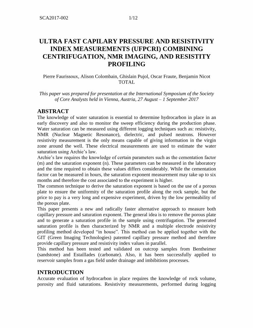
An example is given on Figure 1 on which 7 electrodes were used (6 slices), Following

this method, we obtain for each of the 6 slices a triplet [Pc, Sw, RI]; and therefore are

able to plot the RI=f(Sw) curve together with the Pc=f(Sw) curve (as already proposed by

Green et al.[6][7].

Minimal redistribution of fluids was observed during the timescale of NMR and

resistivity measurements, and affected neither NMR nor resistivity profiles.

SCA2017-002 3/12

EQUIPMENT AND PROCEDURE

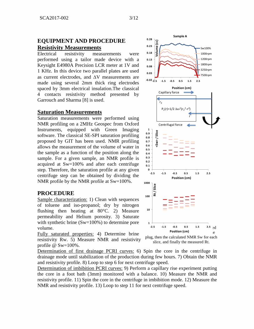
Resistivity Measurements Electrical resistivity measurements were

performed using a tailor made device with a

Keysight E4980A Precision LCR meter at 1V and

1 KHz. In this device two parallel plates are used

as current electrodes, and V measurements are

made using several 2mm thick ring electrodes

spaced by 3mm electrical insulation.The classical

4 contacts resistivity method presented by

Garrouch and Sharma [8] is used.

Saturation Measurements Saturation measurements were performed using

NMR profiling on a 2MHz Geospec from Oxford

Instruments, equipped with Green Imaging

software. The classical SE-SPI saturation profiling

proposed by GIT has been used. NMR profiling

allows the measurement of the volume of water in

the sample as a function of the position along the

sample. For a given sample, an NMR profile is

acquired at Sw=100% and after each centrifuge

step. Therefore, the saturation profile at any given

centrifuge step can be obtained by dividing the

NMR profile by the NMR profile at Sw=100%.

PROCEDURE Sample characterization: 1) Clean with sequences

of toluene and iso-propanol; dry by nitrogen

flushing then heating at 80°C. 2) Measure

permeability and Helium porosity. 3) Saturate

with synthetic brine (Sw=100%) to determine pore

volume.

Fully saturated properties: 4) Determine brine

resistivity Rw. 5) Measure NMR and resistivity

profile @ Sw=100%.

Determination of first drainage PCRI curves: 6) Spin the core in the centrifuge in

drainage mode until stabilization of the production during few hours. 7) Obtain the NMR

and resistivity profile. 8) Loop to step 6 for next centrifuge speed.

Determination of imbibition PCRI curves: 9) Perform a capillary rise experiment putting

the core in a foot bath (3mm) monitored with a balance. 10) Measure the NMR and

resistivity profile. 11) Spin the core in the centrifuge in imbibition mode. 12) Measure the

NMR and resistivity profile. 13) Loop to step 11 for next centrifuge speed.

Figure 1: The NMR profiles are presented

on top, then the Pc distribution along the

plug, then the calculated NMR Sw for each

slice, and finally the measured Rt.

1

10

100

1000

-2.5 -1.5 -0.5 0.5 1.5 2.5

Rt

/ Sl

ice

Position (cm)

-0.02

0.03

0.08

0.13

0.18

0.23

0.28

-2.5 -1.5 -0.5 0.5 1.5 2.5

Vo

lum

e (c

c)

Position (cm)

Sample A

Sw100%

1000rpm

1200rpm

1800rpm

3250rpm

7500rpm

0

0.1

0.2

0.3

0.4

0.5

0.6

0.7

0.8

0.9

1

-2.5 -1.5 -0.5 0.5 1.5 2.5

<Sw

> /

Slic

e

Position (cm)

Centrifugal force

Capillary force

r

r2

Pc(r)=1/2 w2(r22-r2)

SCA2017-002 4/12

VALIDATION OF THE TECHNIQUE ON OUTCROP ROCKS In order to validate the UFPCRI technique, electrical measurements were performed on

the same samples, with the continuous injection (CI) method [9]. The classical porous

plate was not considered due to the long time required to get the results.

Two outcrop samples (diameter 38mm and length 45mm) were selected: Bentheimer

sandstone (28p.u., 2.2D) and Estaillades carbonate (31p.u. & 288mD). All measurements

were performed at ambient conditions using mineral oil (non wetting fluid) to displace

brine (wetting fluid), using confining stress of 15 bars only for CI.

Once the experiment was completed, the samples were cleaned, dried and saturated to

100% with the same brine used in the continuous injection technique. Then, the UFPCRI

method was applied. The experiment was conducted twice in drainage mode, using gas

and mineral oil. The purpose was to verify that the same Archie exponent “n” was found

for both cases and to show that there was no experimental bias due to the fluid used.

With this technique, one centrifuge step would be enough to determine Archie’s

saturation exponent “n” (i.e. the slope of the RI=f(Sw) log-log curve). This is due to the

multiple resistivity measurements on the different slices of the sample. However, it is

better to cover a larger range of water saturation to determine “n”. For this reason we

performed 3 centrifuge steps to investigate a wider Sw range and to derive the capillary

pressure curve.

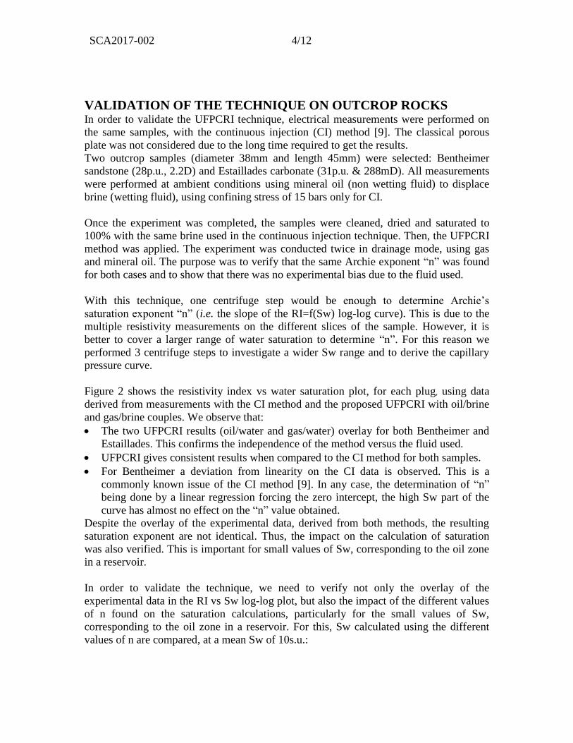
Figure 2 shows the resistivity index vs water saturation plot, for each plug, using data

derived from measurements with the CI method and the proposed UFPCRI with oil/brine

and gas/brine couples. We observe that:

• The two UFPCRI results (oil/water and gas/water) overlay for both Bentheimer and

Estaillades. This confirms the independence of the method versus the fluid used.

• UFPCRI gives consistent results when compared to the CI method for both samples.

• For Bentheimer a deviation from linearity on the CI data is observed. This is a

commonly known issue of the CI method [9]. In any case, the determination of “n”

being done by a linear regression forcing the zero intercept, the high Sw part of the

curve has almost no effect on the “n” value obtained.

Despite the overlay of the experimental data, derived from both methods, the resulting

saturation exponent are not identical. Thus, the impact on the calculation of saturation

was also verified. This is important for small values of Sw, corresponding to the oil zone

in a reservoir.

In order to validate the technique, we need to verify not only the overlay of the

experimental data in the RI vs Sw log-log plot, but also the impact of the different values

of n found on the saturation calculations, particularly for the small values of Sw,

corresponding to the oil zone in a reservoir. For this, Sw calculated using the different

values of n are compared, at a mean Sw of 10s.u.:

SCA2017-002 5/12

• For the Bentheimer sample, the maximum difference between the UFPCRI and CI

is n=0.05. This translates toSw=0.7s.u. at Sw=10s.u.. For higher Sw, the

maximum error remains below 1.1s.u..

• For the Estaillades sample, the maximum difference between the UFPCRI and CI

is n=0.06. This translates toSw=0.6s.u. at Sw=10s.u.. For higher Sw, the

maximum error remains below 1.0s.u..

Figure 2: Comparison of Resistivity Index curves obtained by CI method (Oil/Water) in green and our

UFPCRI method for both Oil/Water (red) and Gas/Water (blue): Bentheimer (left) and Estaillades (right).

The observed repeatability of the UFPCRI method regardless of the fluid used (gas or oil)

and its good agreement with the CI method, clearly validate the UFPCRI technique.

The proposed method allows the joint determination of the Archie parameter “n” and the

capillary pressure curve (as presented and already validated by Green [6]) in less than a

week for drainage, compared to:

• Several weeks for RI only using the CI method,

• Several months for RI and Pc with the porous plate method.

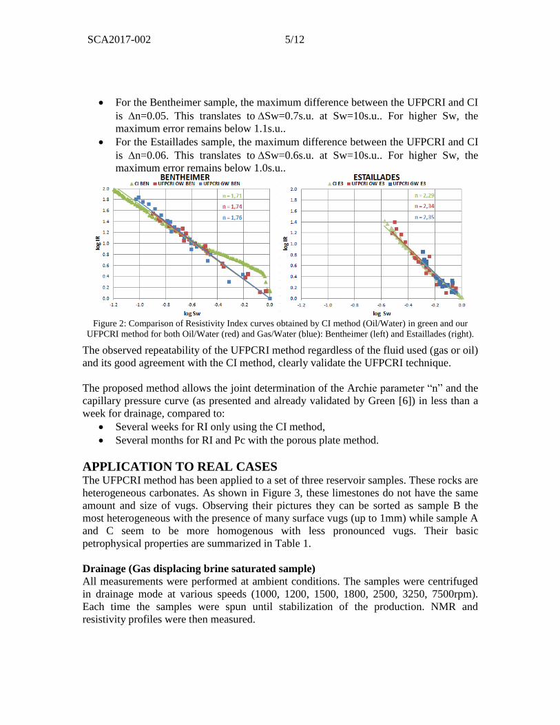
APPLICATION TO REAL CASES The UFPCRI method has been applied to a set of three reservoir samples. These rocks are

heterogeneous carbonates. As shown in Figure 3, these limestones do not have the same

amount and size of vugs. Observing their pictures they can be sorted as sample B the

most heterogeneous with the presence of many surface vugs (up to 1mm) while sample A

and C seem to be more homogenous with less pronounced vugs. Their basic

petrophysical properties are summarized in Table 1.

Drainage (Gas displacing brine saturated sample)

All measurements were performed at ambient conditions. The samples were centrifuged

in drainage mode at various speeds (1000, 1200, 1500, 1800, 2500, 3250, 7500rpm).

Each time the samples were spun until stabilization of the production. NMR and

resistivity profiles were then measured.

SCA2017-002 6/12

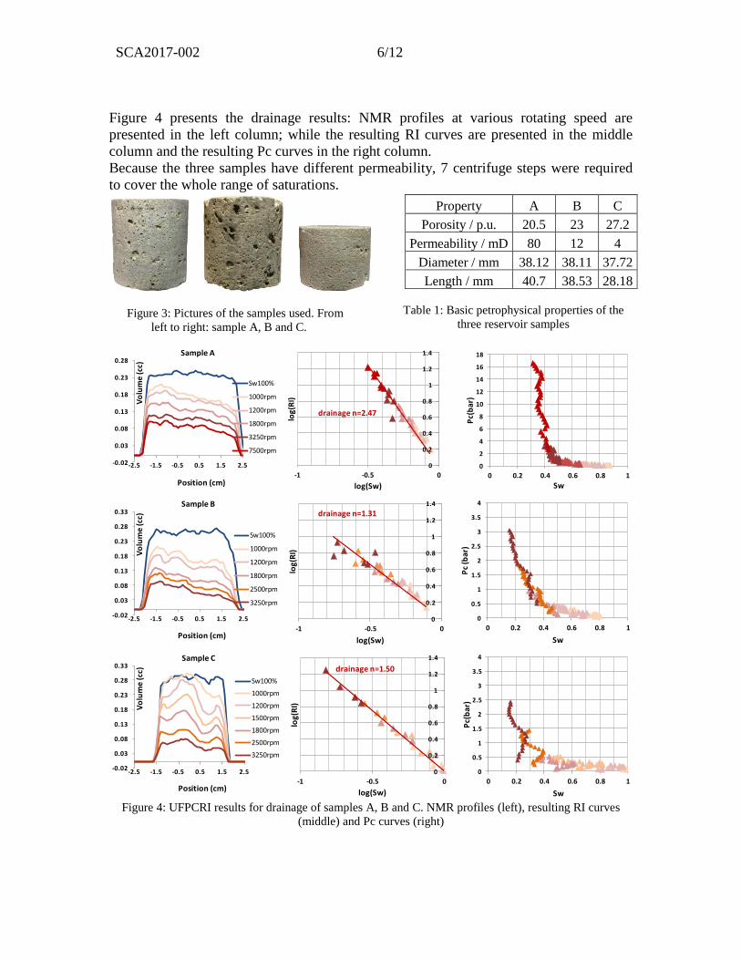
Figure 4 presents the drainage results: NMR profiles at various rotating speed are

presented in the left column; while the resulting RI curves are presented in the middle

column and the resulting Pc curves in the right column.

Because the three samples have different permeability, 7 centrifuge steps were required

to cover the whole range of saturations.

Figure 3: Pictures of the samples used. From

left to right: sample A, B and C.

Figure 4: UFPCRI results for drainage of samples A, B and C. NMR profiles (left), resulting RI curves

(middle) and Pc curves (right)

Sample A Sample CSample B

-0.02

0.03

0.08

0.13

0.18

0.23

0.28

-2.5 -1.5 -0.5 0.5 1.5 2.5

Vo

lum

e (c

c)

Position (cm)

Sample A

Sw100%

1000rpm

1200rpm

1800rpm

3250rpm

7500rpm

0

0.2

0.4

0.6

0.8

1

1.2

1.4

-1 -0.5 0

log(

RI)

log(Sw)

drainage n=2.47

0

2

4

6

8

10

12

14

16

18

0 0.2 0.4 0.6 0.8 1P

c(b

ar)

Sw

-0.02

0.03

0.08

0.13

0.18

0.23

0.28

0.33

-2.5 -1.5 -0.5 0.5 1.5 2.5

Vo

lum

e (c

c)

Position (cm)

Sample B

Sw100%

1000rpm

1200rpm

1800rpm

2500rpm

3250rpm

0

0.2

0.4

0.6

0.8

1

1.2

1.4

-1 -0.5 0

log

(RI)

log(Sw)

drainage n=1.31

0

0.5

1

1.5

2

2.5

3

3.5

4

0 0.2 0.4 0.6 0.8 1

Pc

(ba

r)

Sw

-0.02

0.03

0.08

0.13

0.18

0.23

0.28

0.33

-2.5 -1.5 -0.5 0.5 1.5 2.5

Vo

lum

e (c

c)

Position (cm)

Sample C

Sw100%

1000rpm

1200rpm

1500rpm

1800rpm

2500rpm

3250rpm

0

0.2

0.4

0.6

0.8

1

1.2

1.4

-1 -0.5 0

log(

RI)

log(Sw)

drainage n=1.50

0

0.5

1

1.5

2

2.5

3

3.5

4

0 0.2 0.4 0.6 0.8 1

Pc(

bar

)

Sw

Property A B C

Porosity / p.u. 20.5 23 27.2

Permeability / mD 80 12 4

Diameter / mm 38.12 38.11 37.72

Length / mm 40.7 38.53 28.18

Table 1: Basic petrophysical properties of the

three reservoir samples

SCA2017-002 7/12

The number of NMR profiles is not the same for all the samples. These types of

measurements were only performed if significant brine production was observed between

the centrifuge steps. Moreover, the NMR acquisition time for samples containing limited

amount of water was too long (up to days for a SNR close to 100).

In this case, if there was not enough production for a given sample at a given centrifugal

speed, neither saturation profiles nor resistivity profiles were acquired. This explains, for

example, why there is no data presented for samples B and C at 7500rpm. These latter

did not produce enough brine from 3250rpm to 7500rpm and the NMR acquisition time

for samples containing limited amount of water were too long. So samples B and C have

also been spun to 7500rpm but no data is presented.

From the NMR profiles, sample A seems homogeneous, while sample B shows

heterogeneities and sample C is the most heterogeneous. The impact of the heterogeneity

on the results will be discussed below in a separate section.

The RI curves show a straight line for the three samples, verifying the validity of

Archie’s law for these samples. Sample B data dispersion will be covered in the

heterogeneity section. The following Archie’s saturation exponents can be derived:

• For sample A: ndrainage = 2.47

• For sample B: ndrainage = 1.31

• For sample C: ndrainage = 1.50

Capillary pressure curves were computed using the Green-Imaging GIT-Cap-Pressure

software. The shape of the Pc curve for sample C can be attributed to the heterogeneity

and will be discussed in detail later in this paper.

With the centrifuge steps used, many points overlap. Thus this result could have been

achieved with a reduced number of centrifuge steps. As proposed by Green et al. [6], as

few as three centrifuge steps can be used for this purpose.

Imbibition (Brine displacing gas from the sample at residual water saturation)

Once the drainage was completed, the next step was to perform the spontaneous

imbibitions by capillary rise to create a saturation profile. Then, NMR and resistivity

profiles were measured.

Imbibition under centrifugation was performed at 800, 1000 and 2500 rpm. The criteria

to change the centrifuge speed were the same as used during the drainage experiments.

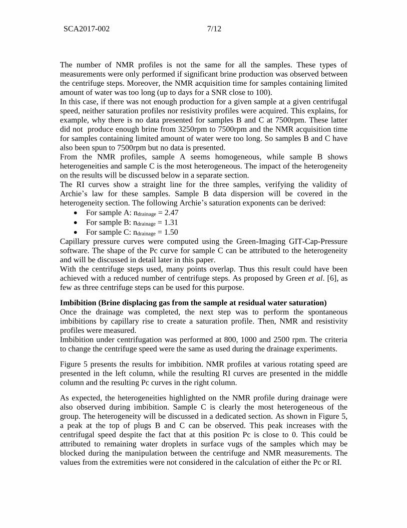
Figure 5 presents the results for imbibition. NMR profiles at various rotating speed are

presented in the left column, while the resulting RI curves are presented in the middle

column and the resulting Pc curves in the right column.

As expected, the heterogeneities highlighted on the NMR profile during drainage were

also observed during imbibition. Sample C is clearly the most heterogeneous of the

group. The heterogeneity will be discussed in a dedicated section. As shown in Figure 5,

a peak at the top of plugs B and C can be observed. This peak increases with the

centrifugal speed despite the fact that at this position Pc is close to 0. This could be

attributed to remaining water droplets in surface vugs of the samples which may be

blocked during the manipulation between the centrifuge and NMR measurements. The

values from the extremities were not considered in the calculation of either the Pc or RI.

SCA2017-002 8/12

Figure 5: UFPCRI results for imbibition of samples A, B and C. NMR profiles (left), RI curves (middle)

and Pc curves (right)

RI curves show a straight line for the three samples, verifying the validity of Archie’s law

for these samples. A greater dispersion of the points in the RI plot can be observed for

sample B; this will be discussed in details in the section dedicated to heterogeneity. The

following Archie’s saturation exponents can be derived:

• For sample A: nimbibition = 1.70, while ndrainage = 2.47

• For sample B: nimbibition = 0.77, while ndrainage = 1.31

• For sample C: nimbibition = 1.09, while ndrainage = 1.50

Pc curves were computed using the GIT-Cap-Pressure software. The surprising shape of

the Pc curve for sample C can be explained by heterogeneity. Its small length highlights

the limit of UFPCRI to describe a whole range of Sw especially with local heterogeneity.

DISCUSSION For drainage, the following observations can be made:

Sample A: the most homogenous based on the NMR profiles at 100% Sw, ndrainage =2.47.

The RI vs. Sw plot shows good linearity. Despite having the largest permeability (80mD),

-0.02

0.03

0.08

0.13

0.18

0.23

0.28

-2.5 -1.5 -0.5 0.5 1.5 2.5

Vo

lum

e (c

c)

Position (cm)

Sample A

Sw100%

2500rpm

1000rpm

800rpm

Capillary rise

0

0.2

0.4

0.6

0.8

1

1.2

1.4

-1 -0.5 0

log

(RI)

log(Sw)

drainage n=2.47

imbibition n= 1.70

-6

-5

-4

-3

-2

-1

0

0 0.2 0.4 0.6 0.8 1

Pc(

bar

)

Sw

-0.02

0.03

0.08

0.13

0.18

0.23

0.28

-2.5 -1.5 -0.5 0.5 1.5 2.5

Vo

lum

e (c

c)

Position (cm)

Sample B

Sw100%

2500rpm

1000rpm

800rpm

Capillary rise

0

0.2

0.4

0.6

0.8

1

1.2

1.4

-1 -0.5 0

log(

RI)

log(Sw)

drainage n=1.31

imbibition n=0.77

-6

-5

-4

-3

-2

-1

0

0 0.2 0.4 0.6 0.8 1

Pc(

bar

)

Sw

-0.02

0.03

0.08

0.13

0.18

0.23

0.28

-2.5 -1.5 -0.5 0.5 1.5 2.5

Vo

lum

e (c

c)

Position (cm)

Sample C

Sw100%

2500rpm

1000rpm

800rpm

Capillary rise

0

0.2

0.4

0.6

0.8

1

1.2

1.4

-1 -0.5 0

log(

RI)

log(Sw)

drainage n=1.50

imbibition n=1.09

-6

-5

-4

-3

-2

-1

0

0 0.2 0.4 0.6 0.8 1

Pc(

bar

)

Sw

SCA2017-002 9/12

Swi (37 s.u) is higher than the rest of the samples with lower permeabilities.

Sample B and C: NMR profiles highlight their heterogeneities and identify sample C as

the most heterogeneous. Their saturation exponents, respectively ndrainage = 1.31 and

ndrainage = 1.50, seem relatively low when compared to sample A. Furthermore, their Pc

curves reach similar Sw.

For the imbibition curves:

Samples A and C: nimbibition = 1.70 and nimbibition = 1.09, a significant ratio of

approximately 1.4 is observed against drainage, and a poorer linearity than others plugs

for sample A. Furthermore, NMR profiles and Pc show that its irreducible gas saturation

seems close to zero with <Sw> = 93%.

Sample B: nimbibition = 0.77, a large ratio of 1.7 is observed between drainage and

imbibition. The trend follows a pretty good linearity with a really good match between

slices close to zero.

These results emphasize the importance of measuring the saturation exponent for both

drainage and imbibition.

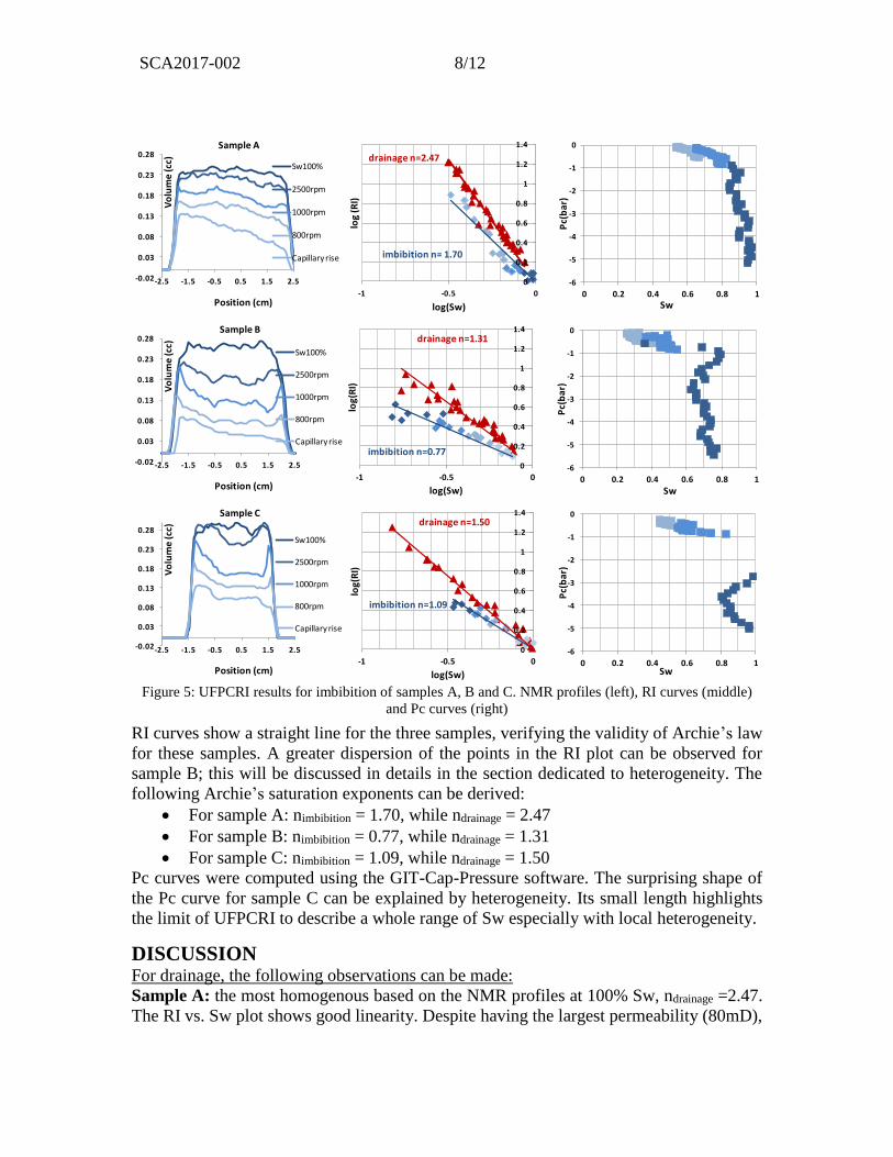
All the samples show the same behavior upon the transition to the imbibition cycle: the

points, in the RI vs. Sw plots, corresponding to the imbibitions are always located below

the ones measured in drainage. This type of hysteresis has already been observed ([10],

[11]). Such behavior was successfully modeled by Toumelin et al. [12] and Man [13].

Comparison of experimental data with the model available in the literature requires NMR

profile at Swi, which was only measurable for Sample A. During measurements, the

saturation profile was not acquired at maximum centrifuge speed for Sample B and C as

mentioned above. Hence, we will focus the discussion of hysteresis between drainage and

imbibition of Sample A. As shown in Figure 6 the RI data for sample A follow the trends

modeled by Toumelin[12] for a water wet system. In fact, the drop of n could be

described as a water film thickening. Following this theory, the imbibition in Figure 6

could be decomposed into three parts:

• P1: the water film thickness increases rapidly at the pore throat,

• P2: rising of surface layers,

• P3: water film thickening reaches a critical gas saturation where the air phase is

disconnected.

Figure 6: RI data acquired on sample A (left) and the model proposed by Toumelin [12] (right).

0

0.2

0.4

0.6

0.8

1

1.2

1.4

-0.6 -0.1

log

(R

I)

log(Sw)

P1

P3

P2

Sample A

SCA2017-002 10/12

Heterogeneity:

The UFPCRI method provides directly the local saturation and resistivity. Therefore this

method is independent of the Sw heterogeneity.

Heterogeneity of the studied samples can be inferred from the NMR profiles at

Sw=100%, and after each centrifuge step. For sample C, the most heterogeneous, NMR

profiles shows bumps and valleys; certain regions of the plug de-saturate faster than

others despite the Pc gradient imposed by centrifugation.

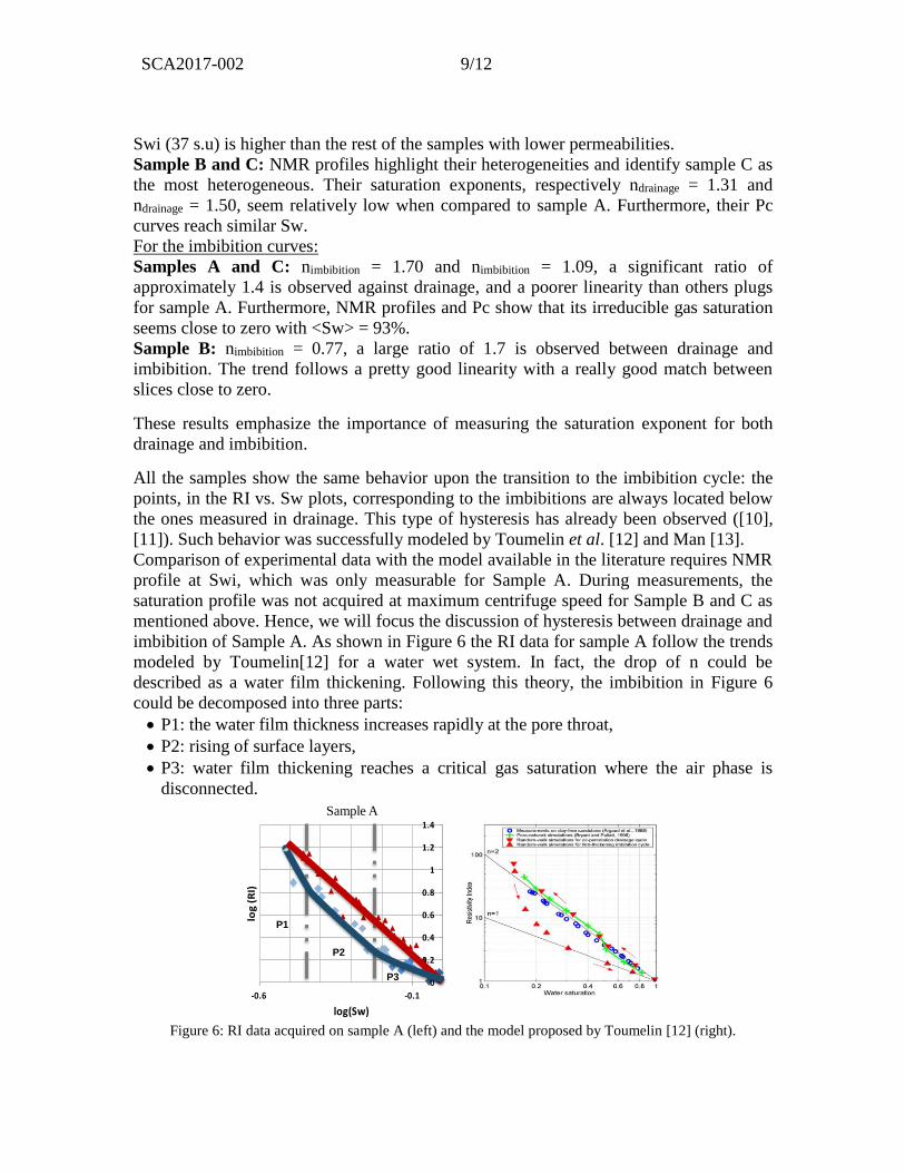
Figure 7 shows NMR profiles and the resulting Pc curve for sample C where two trends

can be observed and each response can be attributed to a particular section of the sample.

Considering only the bottom part of the plug (orange rectangle in NMR profiles), all the

points in the Pc curve corresponding to this section fall on the orange line. Similarly the

Pc curve corresponding to the middle of the plug (red rectangle in NMR profiles) is

represented in red. Thus, the shape of the Pc curve for sample C is not due to

uncertainties of the technique but rather reveals the heterogeneity of the sample.

Additionally, data from both trends could be used to derive Pc curves for both “rock

types”. The heterogeneity observed in the Pc curve of sample C does not translate into the

RI curve as the RI vs. Sw plot showed linearity between the different values. This means

that the two “rock types” present in the bottom and the middle of sample C have different

Pc curves, but have the same electrical characteristics.

Figure 7: NMR profiles from sample C (left) and the resulting Pc curve. Pc curves obtained from the

bottom of the sample (orange rectangle) and the middle (red rectangle) are drawn in corresponding colors.

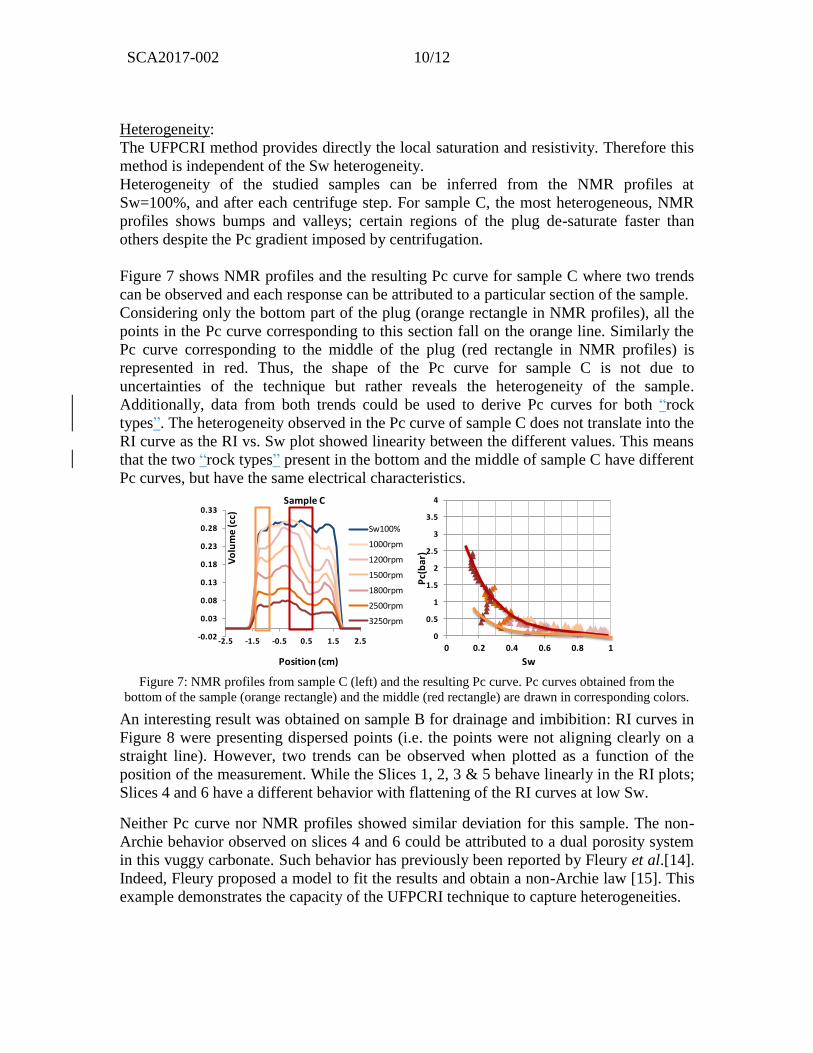
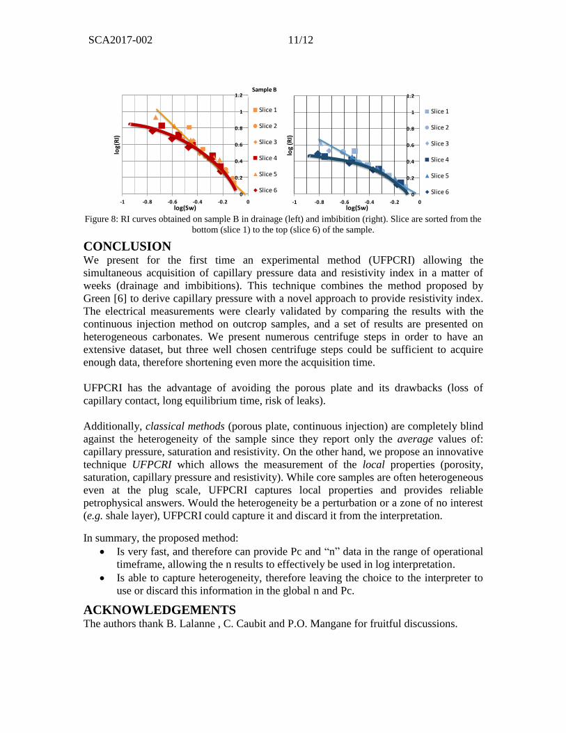
An interesting result was obtained on sample B for drainage and imbibition: RI curves in

Figure 8 were presenting dispersed points (i.e. the points were not aligning clearly on a

straight line). However, two trends can be observed when plotted as a function of the

position of the measurement. While the Slices 1, 2, 3 & 5 behave linearly in the RI plots;

Slices 4 and 6 have a different behavior with flattening of the RI curves at low Sw.

Neither Pc curve nor NMR profiles showed similar deviation for this sample. The non-

Archie behavior observed on slices 4 and 6 could be attributed to a dual porosity system

in this vuggy carbonate. Such behavior has previously been reported by Fleury et al.[14].

Indeed, Fleury proposed a model to fit the results and obtain a non-Archie law [15]. This

example demonstrates the capacity of the UFPCRI technique to capture heterogeneities.

-0.02

0.03

0.08

0.13

0.18

0.23

0.28

0.33

-2.5 -1.5 -0.5 0.5 1.5 2.5

Vo

lum

e (c

c)

Position (cm)

Sample C

Sw100%

1000rpm

1200rpm

1500rpm

1800rpm

2500rpm

3250rpm

0

0.5

1

1.5

2

2.5

3

3.5

4

0 0.2 0.4 0.6 0.8 1

Pc(

bar

)

Sw

SCA2017-002 11/12

Figure 8: RI curves obtained on sample B in drainage (left) and imbibition (right). Slice are sorted from the

bottom (slice 1) to the top (slice 6) of the sample.

CONCLUSION We present for the first time an experimental method (UFPCRI) allowing the

simultaneous acquisition of capillary pressure data and resistivity index in a matter of

weeks (drainage and imbibitions). This technique combines the method proposed by

Green [6] to derive capillary pressure with a novel approach to provide resistivity index.

The electrical measurements were clearly validated by comparing the results with the

continuous injection method on outcrop samples, and a set of results are presented on

heterogeneous carbonates. We present numerous centrifuge steps in order to have an

extensive dataset, but three well chosen centrifuge steps could be sufficient to acquire

enough data, therefore shortening even more the acquisition time.

UFPCRI has the advantage of avoiding the porous plate and its drawbacks (loss of

capillary contact, long equilibrium time, risk of leaks).

Additionally, classical methods (porous plate, continuous injection) are completely blind

against the heterogeneity of the sample since they report only the average values of:

capillary pressure, saturation and resistivity. On the other hand, we propose an innovative

technique UFPCRI which allows the measurement of the local properties (porosity,

saturation, capillary pressure and resistivity). While core samples are often heterogeneous

even at the plug scale, UFPCRI captures local properties and provides reliable

petrophysical answers. Would the heterogeneity be a perturbation or a zone of no interest

(e.g. shale layer), UFPCRI could capture it and discard it from the interpretation.

In summary, the proposed method:

• Is very fast, and therefore can provide Pc and “n” data in the range of operational

timeframe, allowing the n results to effectively be used in log interpretation.

• Is able to capture heterogeneity, therefore leaving the choice to the interpreter to

use or discard this information in the global n and Pc.

ACKNOWLEDGEMENTS The authors thank B. Lalanne , C. Caubit and P.O. Mangane for fruitful discussions.

0

0.2

0.4

0.6

0.8

1

1.2

-1 -0.8 -0.6 -0.4 -0.2 0

log(

RI)

log(Sw)

Slice 1

Slice 2

Slice 3

Slice 4

Slice 5

Slice 60

0.2

0.4

0.6

0.8

1

1.2

-1 -0.8 -0.6 -0.4 -0.2 0

log

(RI)

log(Sw)

Slice 1

Slice 2

Slice 3

Slice 4

Slice 5

Slice 6

Sample B

SCA2017-002 12/12

REFERENCES

[1] G. Archie, "Electrical Resistivity Log as an Aid in Determining Some Reservoir

Characteristics," Petroleum Transactions AIME, 1942.

[2] M. Fleury, "FRIM, a Fast Resistivity Index Measurement Method," in SCA, 1998.

[3] N. Bona, E. Rossi and B. Bam, "Ultrafast Determination of Archie and Indonesia

m&n Exponents for Electric log Interpretation: a Tight Gas Example," IPTC, 2014.

[4] N. Bona, B. Bam, M. Pirrone and E. Rossi, "Use of a New Impedance Cell and 3D

MRI to Obtain Fast and Accurate Resistivity Index Measurements from a Single

Centrifuge Step," Petrophysics, 2012.

[5] C. Durand, "Combined Use of X-Ray CT Scan and Local Resistivity Measurments:

A New approach to Fluid Distribution Description in Cores," SPE, 2003.

[6] D. Green, J. Dick, J. Gardner, B. Balcom and B. Zhou, "Comparison Study of

Capillary Pressure Curves Obtained Using Traditional Centrifuge and Magnetic

Resonance Imaging Techniques," in SCA, 2007.

[7] D. Green, J. McAloon, P. Cano-Barrita, J. Burger and B. Balcom, "Oil/Water

Imbibition and Drainage Capillary Pressure Determined by MRI on a Wide

Sampling of Rocks," in SCA, 2008.

[8] A. Garrouch and M. Sharma, "Techniques for the Measurment of Electrical

Properties of Cores in the Frequency Range 10Hz to 10MHz," in SCA, 1992.

[9] H. Zeelenberg and B. Schipper, "Developments in I-Sw Measurements," in

Advances in Core Avaluation II, Reservoir Appraisal, Gordon and Breach Science

Publishers, 1991, p. 257.

[10] M. Han, M. Fleury and P. Levitz, "Effect of the Pore Structure on Resistivity Index

Curves," in SCA, 2007.

[11] R. Knight, "Hysteresis in electrical Resistivity of Partially Saturated Sandstones,"

Geophysics, vol. 56, no. 12, 1991.

[12] E. Toumelin, C. Torres-Verdin, S. Devarajan and B. Sun, "An Integrated Pore-Scale

Approach for the Simulation of Grain Morphology, Wettability, and Saturation-

History Effects on Electrical Resistivity and NMR Measurements of Saturated

Rocks," in SCA, 2006.

[13] H. Man and X. Jing, "Network Modelling of Mixed-Wettability on Electrical

Resistivity, Capillary Pressure and Wettability Indices," Journal of Petroleum

Science and Engineering, vol. 33, 2002.

[14] M. Fleury, M. Efnik and M. Kalam, "Evaluation of Water Saturation from

Resistivity in a Carbonate Field. From Laboratory to Logs," in SCA, 2004.

[15] M. Fleury, "Advances in Resistivity Measurments using the FRIM MEthod at

Reservoir Conditions. Application to Carbonates," in SCA, 2003.