FACOLTÀ DI INGEGNERIA DELL’INFORMAZIONE,

INFORMATICA E STATISTICA

Corso di Laurea Magistrale in Ingegneria Elettronica

Ultra-broadband mobile networks: evaluation of

massive MIMO and multi-carrier aggregation

performances in LTE-Advanced

Relatrice

Prof.ssa Maria-Gabriella Di Benedetto

Correlatori Candidato

Ing. Andrea Castellani Marco Neri

Ing. Pamela Sciarratta Armani Campanella

TIM

Anno Accademico 2016 - 2017

2

A Filippo, la mia ispirazione

3

Acknowledgements

First and foremost, I want to thank my advisor, Mrs. Maria-Gabriella Di Benedetto for

her encouragement, backing and guidance in carrying out this thesis. She gave me the

chance to develop it at TIM allowing me to delve into topics that are at the forefront of

technology and to get into the business reality, still too far from the academic world.

This work would have never been possible without the help of my co-advisors, Andrea

and Pamela, whose guidelines and suggestions have been fundamental during the six

months spent together. Thanks also to Camillo and Pietro that have been willing to help

me with the troubles I encountered, always with a smile on their faces. I express my

gratitude to Tommaso and the whole ns-3 community for having solved some of my

problems with the simulator. Special thanks to Renzo, Nicola and the to the lab guys that

made me feel a part of their group from the very beginning.

Last six months were definitely intense and my family had to stand my anxieties,

indecisions and some moments of impatience. Despite this, they never made me feel

guilty and they have always been by my side, indulging my needs and my moods, like

they have always done for the last 24 years. To my Mom and Dad, to Fede, to Grandma

Mirella and to all my relatives, my unconditioned fondness and my eternal gratitude. My

thanks go, moreover, to my inspiration Filippo, to whom I dedicate this thesis.

Thanks to my “αλήθειες φίλοι”, a branch of my family, whose affinity and help have

never been called into question. Thanks also to all those friends, that make me feel at

home, wherever I am.

Finally, a special thanks to my travel companions, Claudio and Marco. We spent six

incredible months together, working shoulder to shoulder. It has been an amazing

adventure thanks to their company. I will miss working with those nuts!

Grazie,

4

Ringraziamenti

Prima di tutto vorrei ringraziare la mia Relatrice, la professoressa Maria-Gabriella Di

Benedetto, per l’incoraggiamento, il supporto e la guida nello svolgimento di questa tesi

e per avermi dato la possibilità di svilupparla all’interno della TIM, permettendomi di

approfondire argomenti all’avanguardia e conoscere una realtà, quella aziendale, ancora

troppo lontana dal mondo universitario.

Tale lavoro non sarebbe stato possibile senza l’aiuto dei miei Correlatori, Andrea e

Pamela, le cui linee guida e suggerimenti sono stati fondamentali nei sei mesi passati

insieme. Prezioso è stato anche l’aiuto di Camillo e Pietro, che sono stati sempre

disponibili nel darmi una mano a risolvere i problemi incontrati, sempre con il sorriso.

Grazie anche a Tommaso e a tutta la comunità ns-3 per l’aiuto con il simulatore. Un

ringraziamento particolare va poi a Renzo, Nicola e ai ragazzi del laboratorio, che mi

hanno fatto sentire parte di un gruppo sin dal primo giorno.

Gli ultimi sei mesi sono stati decisamente intensi e la mia famiglia ha dovuto sopportare

le mie ansie, le indecisioni e qualche momento di impazienza. Nonostante ciò, non me

l’hanno mai fatto pesare e, anzi, sono stati sempre al mio fianco, assecondando le mie

necessità e i miei stati d’animo, come sempre da 24 anni a questa parte. A Mamma e Papà,

a Fede, a Nonna Mirella e a tutta la banda vanno il mio incondizionato affetto e la mia

eterna gratitudine. La mia riconoscenza va, inoltre, alla mia fonte di ispirazione, Filippo,

a cui è dedicata questa tesi.

Grazie ai miei “αλήθειες φίλοι”, ormai un ramo della famiglia, la cui vicinanza e aiuto

non sono mai in discussione. Grazie anche a tutti quegli amici che, indipendentemente

da dove mi trovi, mi fanno sempre sentire come se fossi a casa.

Infine, un ringraziamento speciale va ai compagni di viaggio, Claudio e Marco, con cui

abbiamo passato sei mesi incredibili, spalla a spalla. È stata una fantastica avventura,

soprattutto grazie alla loro compagnia. Mi mancherà lavorare con quei due pazzi!

Grazie,

5

Abstract

LTE-Advanced networks are spreading widely across the world and they are

continuing to evolve as new device features are being released to move towards the peak

data rates introduced by 3GPP Release 11, 12 and 13. Mobile network Operators are

looking for technologies that guarantee better performances but they have to deal with

limitations due to commercial devices’ RF components that prevent the Operator from

exploiting such technologies at their best.

Then, they are \

The aim of this thesis was to study the LTE-Advanced system in order to figure out

which would be the best deployment strategy. For this scope, we used a network

simulator first born for LTE and we adapted it to last LTE-A features. We analyzed a

dense urban scenario and deduced the system performance in terms of throughput and

we evaluated the performances of MIMO 4x4 and Carrier Aggregation. A set of

conclusions is derived from the comparison between the system simulations and real

measures made on commercial devices.

6

Abstract [IT]

I sistemi LTE-Advanced sono in via di diffusione in tutto il mondo e continuano ad

evolversi con l’inserimento di nuove funzionalità che permettano il raggiungimento dei

target fissati dalle Release 11, 12 e 13 del 3GPP. Gli Operatori mobili sono alla ricerca di

tecnologie che garantiscano migliori performance ma si stanno scontrando con delle

limitazioni dovute ai componenti RF dei device commerciali. Tali limitazioni

impediscono di coniugare le tecnologie che puntano all’aumento dello spettro e quelle

che garantiscono una migliore efficienza spettrale.

Fin quando tali limitazioni non saranno superate, gli Operatori dovranno agire secondo

un compromesso e stanno cercando di capire in quale direzione muoversi ed investire.

Lo scopo di questa tesi è quello di studiare il sistema LTE-A nella sua interezza per

capire quale sia la miglior scelta di deployment dal punto di vista dell’Operatore. Per

questo fine, abbiamo utilizzato un simulatore di rete, nato per il sistema LTE a lo abbiamo

adattato includendo le ultime funzionalità rilasciate. Abbiamo analizzato uno scenario

urbano densamente popolato ed estratto dalle simulazioni la prestazione del sistema dal

punto di vista del throughput smaltito e valutato le performance del MIMO 4x4 e della

Carrier Aggregation.

Infine, abbiamo tratto delle conclusioni e dato dei suggerimenti, sfruttando anche il

paragone tra i risultati delle simulazioni e delle misure reali fatte su nuovi device

commerciali.

7

Table of contents

List of the Abbreviations 9

Introduction 12

Context and objectives 12

1. LTE 15

1.1 Background 15

1.2 LTE System Architecture 16

1.3 LTE Radio Interface 17

1.3.1 Radio Resource Control 18

1.3.2 Packet Data Convergence Protocol 20

1.3.3 Radio Link Control 20

1.3.4 Medium Access Control 20

1.4 Physical layer 21

1.4.1 Multiple Access Techniques 21

1.4.1.1 OFDMA 22

1.4.1.2 SC-FDMA 23

1.4.2 Frame Structure 24

1.5 Multiple Input Multiple Output 25

1.6 Resources Scheduling 26

1.6.1 Round Robin Scheduler 27

1.6.2 Proportional Fair Scheduler 27

1.6.3 Best CQI Scheduler 27

1.7 LTE UE Categories 27

1.8 Frequency Allocation 28

2. LTE-Advanced 30

2.1 Beyond Release 8 30

2.2 Enhancements for LTE-Advanced 30

2.2.1 Carrier Aggregation 30

2.2.2 Enhanced Multi-Antenna Techniques 32

2.2.3 Heterogeneous Networks 33

2.3 LTE-Advanced UE Categories 34

3. Scenario 36

3.1 Case study 36

3.2 Analytical considerations 37

8

4. NS3 Simulator 52

4.1 Architecture and features 52

4.1.1 LTE Module 54

4.1.2 Internet Module 57

4.1.3 Application Module 58

4.1.4 Mobility Module 58

4.1.5 Propagation Module 59

4.1.6 Flow Monitor Module 59

4.2 Assumptions and settings 60

4.3 Changes applied 63

5. Simulations and results 67

5.1 Preliminary Simulations 67

5.1.1 MIMO Simulations 67

5.1.2 Carrier Aggregation Simulations 68

5.1.3 Tri-Sector Antenna and Handover Implementation 68

5.2 Complete Simulations 69

5.2.1 Coverage Analysis 70

5.2.2 Category 6 Deployment 74

5.2.3 Category 11 Deployment 76

5.2.4 Category 16 Deployment 77

6. Real measures and validation 81

6.1 Category 11 81

6.2 Category 16 89

6.3 MIMO 4x4 Downlink performances 92

7. Conclusions and future work 96

References 98

9

List of the Abbreviations

1G First Generation

2G Second Generation

3G Third Generation

3GPP Third Generation Partnership Project

4G Fourth Generation

ABS Almost Blank Subframes

AM Acknowledged Mode

AMC Adaptive Modulation and Coding

API Application Programming Interface

BER Bit Error Rate

BLER Block Error Rate

BS Base Station

CA Carrier Aggregation

CB Coordinated Beamforming

CCS Cross-Carrier Scheduling

CDF Cumulative Density Function

CDMA Code Division Multiple Access

CL Closed Loop

CM Connection Management

CoMP Coordinated Multi Point

CP Cyclic Prefix

CQI Channel Quality Indicator

CS Coordinated Scheduling

DL DownLink

DL-SCH DownLink Shared Channel

DPS Dynamic Point Selection

DRB Data Radio Bearer

EARFCN EUTRA Absolute Radio-Frequency Channel Number

eICIC Enhanced Inter-Cell Interference Coordination

eNB eNodeB

EPC Evolved Packet Core

EPS Evolved Packet System

ESM EPS Session Management

E-UTRA Evolved Universal Terrestrial Access

E-UTRAN Evolved Universal Terrestrial Access Network

FDD Frequency Division Duplexing

GSM Global System for Mobile Communications

HARQ Hybrid Automatic ReQuest

HetNet Heterogeneous Networks

10

HSPA High Speed Packet Access

ICMP Internet Control Message Protocol

IP Internet Protocol

ITU International Telecommunication Union

JP Joint Processing

LAA Licensed Assisted Access

LoS Line of Sight

LSM Link-to-System Mapping

LTE Long Term Evolution

LTE-A LTE-Advanced

MAC Medium Access Control

MCS Modulation and Coding Scheme

MIB Master Information Block

MIESM Mutual Information Effective SINR Mapping

MIMO Multiple Input Multiple Output

MM Mobility Management

MU-MIMO Multi-User MIMO

NAS Non-Access Stratum

NLoS Non-Line of Sight

NPRB Number of PRB

OFDM Orthogonal Frequency Division Multiplexing

OFDMA Orthogonal Frequency Division Multiple Access

OL Open Loop

PAPR Peak-to-Average Power Ratio

PCC Principal Component Carrier

PCRF Policy and Charging Rules Function

PDCP Packet Data Convergence Protocol

PDF Probability Density Function

PDN Packet Data Network

PDSCH Physical Downlink Shared Channel

PDU Protocol Data Unit

PF Proportional Fair

PGW Packet GateWay

PHY Physical Layer

PRACH Physical Random-Access Channel

PRB Physical Resource Block

PS Packet Switch

PSC Primary Serving Cell

PUCCH Physical Uplink Control Channel

PUSCH Physical Uplink Shared Channel

11

QAM Quadrature Amplitude Modulation

QoS Quality of Service

QPSK Quadrature Phase-Shift Keying

QXDM Qualcomm eXtensible Diagnostic Monitor

RAT Radio Access Technology

RBG Resource Block Group

RBS Radio Base Station

RE Resource Element

RLC Radio Link Control

RNC Radio Network Controller

RNTI Radio Network Temporary Identifier

ROHC Robust Header Compression

RRC Radio Resource Control

RSRP Reference Signal Received Power

S&W Stop & Wait

SAE System Architecture Evolution

SCC Secondary Component Carrier

SC-FDMA Single Carrier Frequency Division Multiple Access

SCS called Single Carrier-Scheduling

SGW Serving Gateway

SIB System Information Block

SINR Signal-to-Noise Ratio

SISO Single Input Single Output

SON Self-Organizing Networks

SRB Signaling Radio Bearer

SRS Sounding Reference Signal

TBS Transport Block Size

TCP Transmission Control Protocol

TDD Time Division Duplexing

TM Transmission Mode

TP Throughput

TR Technical Report

TS Technical Specification

TSG RAN Technical Specification Group Radio Access Network

TTI Transmission Time Interval

UDP User Datagram Protocol

UE User Equipment

UL UpLink

UM Unacknowledged Mode

UMTS Universal Mobile Telecommunications System

12

Introduction

Context and objectives

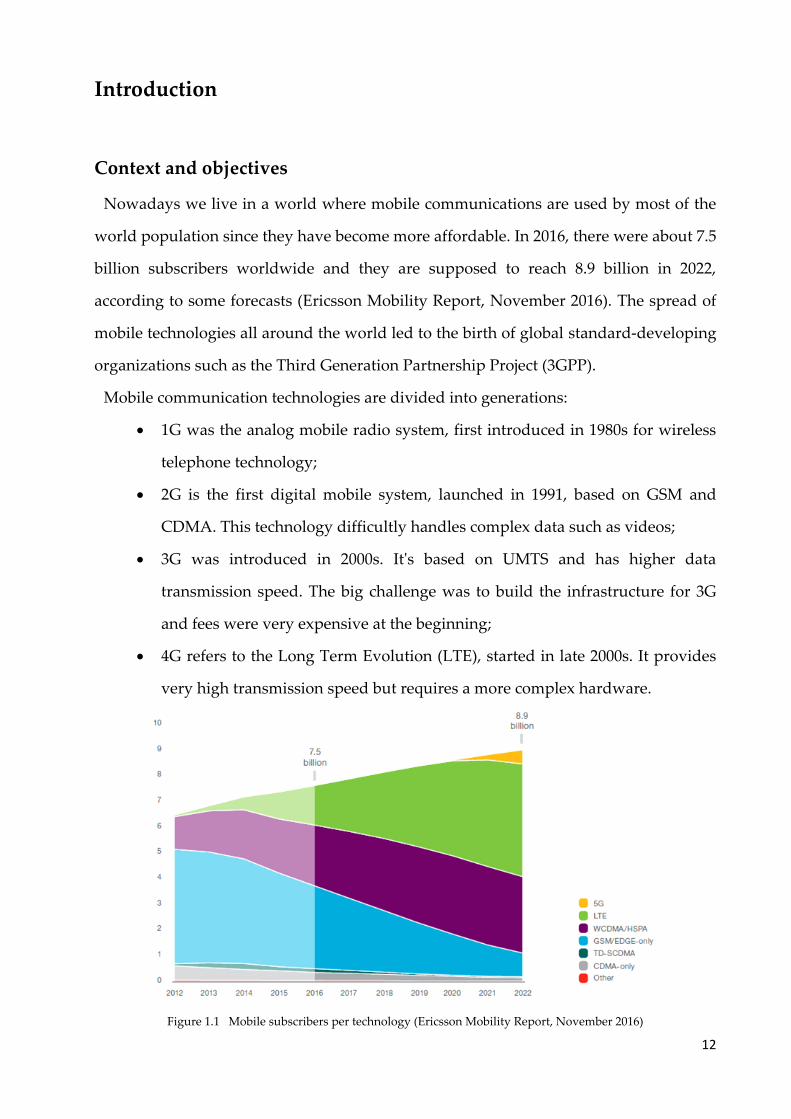
Nowadays we live in a world where mobile communications are used by most of the

world population since they have become more affordable. In 2016, there were about 7.5

billion subscribers worldwide and they are supposed to reach 8.9 billion in 2022,

according to some forecasts (Ericsson Mobility Report, November 2016). The spread of

mobile technologies all around the world led to the birth of global standard-developing

organizations such as the Third Generation Partnership Project (3GPP).

Mobile communication technologies are divided into generations:

• 1G was the analog mobile radio system, first introduced in 1980s for wireless

telephone technology;

• 2G is the first digital mobile system, launched in 1991, based on GSM and

CDMA. This technology difficultly handles complex data such as videos;

• 3G was introduced in 2000s. It's based on UMTS and has higher data

transmission speed. The big challenge was to build the infrastructure for 3G

and fees were very expensive at the beginning;

• 4G refers to the Long Term Evolution (LTE), started in late 2000s. It provides

very high transmission speed but requires a more complex hardware.

Figure 1.1 Mobile subscribers per technology (Ericsson Mobility Report, November 2016)

13

From the figure above we can see how LTE is becoming the market dominant

technology and it will be so for at least 10 years, even after the upcoming of 5G. By 2022,

LTE subscribers are predicted to be 4.6 billion, more than the half of the whole mobile

subscriptions. This demand pushes LTE Data Rates to new limits. However, LTE as it

was first intended in Release 8 could guarantee at maximum a downlink data rate of

300Mbps (even though typical maximum data rate for early devices was no more than

150 Mbps). This limit has been overtaken with the birth of LTE Advanced (LTE-A), first

introduced in Release 10, that was frozen by 3GPP in April 2011. New commercially

available LTE capabilities provide greater spectral efficiency and allow to reach the

milestone data rate of 1Gbps using 60 MHz of spectrum. These capabilities, which will

be discussed more accurately further in this work, are:

• 3~4 Component Carrier Aggregation over licensed or unlicensed bands;

• 256 Quadrature Amplitude Modulation (256QAM);

• 4x4 Multiple Input Multiple Output (4X4 MIMO).

Commercial LTE-A devices are growing throughout the world and Operators are

upgrading mobile networks with Category 16 implementations that will support up to

1Gbps data rates. Typically, this target data rate is not fully achievable so far because of

Operators spectrum fragmentation and commercial devices limitation due to RF

components (mainly transceivers). In fact, the maximum number of downlink antenna

ports managed by current commercial devices is 8. This number can be exploited in

diverse ways, either using MIMO 4x4 on two aggregated bands, or using MIMO 4x4 on

one band and MIMO 2x2 on two bands. In this way, the theoretical maximum throughput

is about 800 Mbps. When this constraint will be overcome, devices will be able to also

support MIMO 8x8 and above to guarantee the target peak data rata for next generation

technologies.

Two possible approaches open up. The first based on bandwidth broadening and the

second on the improvement of the spectral efficiency. At the moment, mobile Operators

are trying to figure out which approach or combination of approaches is the best in

terms of performance and costs.

14

The aim of this work is to analyze every single capability among those just presented,

for a given outdoor scenario, to study the advantages that each one gives in terms of

throughput and the deployment strategies. We also try to determine the capacity of a real

LTE network composed of five sites in a dense urban scenario.

Nowadays, video accounts for 50% of mobile data traffic while in 2022 the percentage

will rise to 75%. For this reason, we focused our simulations on a high-quality video

sharing, that requires a minimum user throughput of 12 Mbps.

This study was carried on with a network simulator and the results were compared with

real measures taken in collaboration with TIM on new commercial devices.

The fundamentals of LTE and of LTE-A are described in Chapters 1 and 2as well as the

features and the innovations introduced by the latter. The scenario is described in

Chapter 3 with some while Chapter 4 is focused on the Network Simulator NS3 that has

been used as platform for the simulations whose implementations and results are

described in Chapter 5. Chapter 6 presents real measurements and the validation of the

simulated results. Finally, in Chapter 7 main results of this thesis are summarized and

likely future works to be done are exposed.

15

1 LTE

1.1 Background

With Long Term Evolution, we refer to a specific technology born in the first decade of

2000s as the evolution of the UMTS. The first steps towards the standardization started

in December 2004. Several motivations brought to the birth of this Study Item within the

3GPP:

• Need to ensure the continuity of competitiveness of the 3G system for the future

• User demand for higher data rates and Quality of Service (QoS)

• Packet Switch (PS) optimized system

• Continued demand for cost reduction

• Low complexity

In particular, in 3GPP Technical Report TR 25.913 “Requirements for Evolved UTRA (E-

UTRA) and Evolved UTRAN (E-UTRAN)” the goals and the minimum requirements for

this technology are exposed:

• Efficient support for PS and Real-Time services

• Peak data rate up to 150Mbps in Downlink (DL) and 75Mbps in Uplink (UL) based

on MIMO 2x2 and 20MHz bandwidth with 64QAM. These values correspond to a

peak spectral efficiency of 7.5bps/Hz in DL and 3.75bps/Hz in UL. As comparison,

note that UMTS Release 6 provides a peak data rate of 14.4Mbps in DL and 11Mbps

in UL based on Single Antenna transmission on 5MHz.

• Higher average user throughput per MHz

• Higher spectral efficiency

• Lower latency: ~ 10ms

• Possibility to work both on paired (FDD) and unpaired (TDD) bands

• Bandwidth scalability: LTE can work on a flexible bandwidth from 1.4 to 20MHz.

16

1.2 LTE System Architecture

LTE architecture is called Evolved Packet System (EPS). It encompasses the Evolved

UMTS Terrestrial Radio Access Network (E-UTRAN) and the Evolved Packet Core

(EPC). The latter takes care of all the non-radio aspects and is also named System

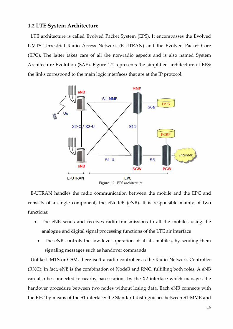
Architecture Evolution (SAE). Figure 1.2 represents the simplified architecture of EPS:

the links correspond to the main logic interfaces that are at the IP protocol.

Figure 1.2 EPS architecture

E-UTRAN handles the radio communication between the mobile and the EPC and

consists of a single component, the eNodeB (eNB). It is responsible mainly of two

functions:

• The eNB sends and receives radio transmissions to all the mobiles using the

analogue and digital signal processing functions of the LTE air interface

• The eNB controls the low-level operation of all its mobiles, by sending them

signaling messages such as handover commands

Unlike UMTS or GSM, there isn’t a radio controller as the Radio Network Controller

(RNC): in fact, eNB is the combination of NodeB and RNC, fulfilling both roles. A eNB

can also be connected to nearby base stations by the X2 interface which manages the

handover procedure between two nodes without losing data. Each eNB connects with

the EPC by means of the S1 interface: the Standard distinguishes between S1-MME and

17

S1-U. The former links the eNB and Mobility Management Entity while the latter is

responsible of the data flow between eNB and Serving Gateway (SGW). SGW and MME

are mutually linked by S11 interface, whilst interface S5 links SGW and Packet Data

Network Gateway (PGW). Here, we briefly describe the functions exploited by the nodes

included in the EPC:

• MME is the control node that handles the Non-Access Stratum (NAS) signaling

from and to UE. It oversees the Mobility Management (MM) and of Connection

Management (CN). Moreover, it is in charge of Session Management (SM) through

ESM protocol. This protocol instantiates the logic connections between UE and

PDN.

• IP packets from and towards the eNBs pass through the SGW whose function is to

anchor the user plane data in case of mobility among different nodes.

• PGW is the access to external Packet Data Networks (PDN): a UE can have several

connections towards multiple PGW in order to reach multiple PDNs. Moreover,

PGW assigns the IP addresses to the devices.

• Home Subscriber Server (HSS) contains subscription data and possible roaming

access restrictions. It also holds information on the PDN to which the user

equipment can attach.

• Policy and Charging Rules Function (PCRF) is the network element that oversees

the Policy and Charging Control (PCC). It determines the services management in

terms of QoS and communicates the relative parameters to the PGW that

configures the appropriate data bearers.

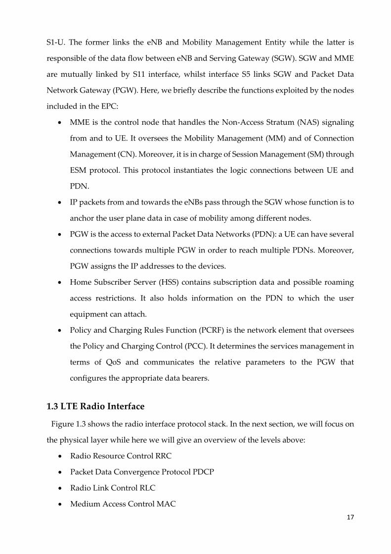
1.3 LTE Radio Interface

Figure 1.3 shows the radio interface protocol stack. In the next section, we will focus on

the physical layer while here we will give an overview of the levels above:

• Radio Resource Control RRC

• Packet Data Convergence Protocol PDCP

• Radio Link Control RLC

• Medium Access Control MAC

18

Figure 1.3 LTE Protocol Stack (3GPP)

1.3.1 Radio Resource Control

As for UMTS, RRC is used on the Air Interface. This level is responsible for the signaling

between UE and eNB and exists at the IP level. It is mainly used for the management of

radio resources and for the configuration of lower levels. In LTE, there are only two states

for the mobile devices: RRC_IDLE and RRC_CONNECTED. The former mode has the

lowest energy consumption: the UE monitors the paging channels, acquires the System

Information, measures the adjacent cells and makes the cell selection/reselection. In the

latter mode, the UE can exchange data with the core and monitors the downlink channels

to determine whether he should receive packets.

The main functionalities carried out by the RRC are:

• Broadcast of the System Information: within this information the User Equipment

finds the parameters needed to access the radio network. These messages are

structured as blocks named System Information Blocks (SIB) each of which

contains a limited number of information. The principal SIB is the Master

Information Block (MIB) which reports i.e. the system frequency bandwidth, the

19

configuration of some channels. It is mapped in the frequency domain and it is

transmitted every 40ms. Other SIBs are defined in 3GPP TS 36.331:

o SIB1 is transmitted every 80ms and reports the information to access a cell.

Moreover, it provides the scheduling of the other SIBs

o SIB2 includes the information on the radio configuration of common

channels and signals (PRACH, PDSCH, PUCCH, PUSCH, SRS)

o SIB3 contains information to regulate the Cell Re-selection both inter-

frequency and intra-frequency. It also holds the s-IntraSearch parameter,

corresponding to the threshold over which the UE can decide not to make

intra-frequency measures.

o SIB4 encompasses specific information to govern the Cell Re-selection in

case of intra-LTE intra-frequency

o SIB5 reports specific information to carry out the Cell Re-selection in case

of intra-LTE inter-frequency

o SIB6 and SIB7 include specific information to control the Cell Re-selection

for inter-RAT respectively towards UTRAN and GERAN

Other SIBs (8-13) are used for precise scopes, like the search for home eNB.

• Paging: its aim is mainly to awake a UE in IDLE mode, to notify the arrival of

incoming calls

or of an update of the System Information.

• UE Cell Selection and Re-selection: when in IDLE mode, the UE selects a suitable cell

and camps to it. Differently from older technologies, in LTE, the eNB can provide

the UE with a specific priority for the frequency layers within or outside the

technology. If the UE camps to the highest priority cell (or frequency) it doesn’t

make further measures until the signal level of the serving cell is higher than a

threshold value. On the contrary, if it attached to a low-level

cell (or frequency) he must make measures searching for a higher priority cell.

• RRC Connection Establishment: with this procedure, it is possible to assign radio

resources to

20

the UE. Once the procedure is completed, the UE is in CONNECTED mode.

• Measurement Control and Reporting: this function comprehends the procedures

through which the eNB makes the UE start one or more measures.

1.3.2 Packet Data Convergence Protocol

This protocol furnishes to higher levels the so-called Radio Bearer. In particular, it

provides the RRC Control Plane with the Signaling Radio Bearer (SRB) and the RRC User

Plane with the Data Radio Bearer (DRB). The main functionalities of the PDCP are:

• Sequence PDU Numbering

• Header Compression: in order to compress the protocol overhead, it is used the

Robust Header Compression (ROHC) so that the transmission efficiency improves

• Integrity Protection for signaling messages

1.3.3 Radio Link Control

RLC can be set in three ways: Acknowledged Mode (AM), Unacknowledged Mode

(UM) and Transparent Mode (TM). In AM, the RLC delivers PDU to higher levels without

errors. It uses ACK/NACK with specific “Status Report” PDUs. On the contrary, UM

doesn’t call for the ACK/NACK and consequently there aren’t retransmissions: even if

the PDU is received with errors, it is however delivered to the upper level. Finally, in TM

there aren’t overheads so that it allows neither retransmission nor error recognition. Its

only aim it to buffer the PDUs to be transmitted.

Although the RLC is capable of handling transmission errors, error-free delivery is in

most cases handled by the MAC-based Hybrid Automatic ReQuest protocol (HARQ).

Then, the double retransmission mechanism might seem redundant. Nonetheless,

sometimes the HARQ retransmissions can fail and the RLC layer ensures the correct

transmission.

1.3.4 Medium Access Control

MAC layer carries out the following three actions:

• Multiplexing of PDUs coming from upper levels into a physical Transport Block

21

• HARQ: the retransmission protocol used by MAC is the N-channel Stop&Wait. In

general, in the S&W protocol, the transmitter sends each PDU only after the

acknowledgement of the occurred transmission by the receiver. Then, it might be

subject to a deadlock situation. To prevent it, LTE has introduced the N-channel

variant (with N=8), to parallelize up to 8 processes operating in independent

manner.

• Radio resources Dynamic Scheduling: as in HSPA, in LTE there are shared

channels that are regulated by MAC. Notably, MAC scheduler determines the UE

that can be served during the i-th Transmission Time Interval (TTI) which

corresponds to 1ms.

During each TTI the eNB scheduler considers the physical radio environment per UE.

They report the perceived quality to decide which Modulation and Coding Scheme

(MCS) to use. Then, it assigns the priority amongst the UE and finally, informs them of

allocated radio resources. The eNB schedules both on the downlink and on the uplink.

1.4 Physical layer

The PHY layer is a highly efficient mean of transferring both data and control

information between an eNB and a UE. This layer employs technologies that are new in

mobile applications with respect to UMTS. In this section, we will give an overview of

these novelties introduced by LTE.

1.4.1 Multiple Access Techniques

3G telecommunications use the code division access technique. Each UE is given one or

more codes to transmit or receive. In the frequency domain, a fixed band portion is

assigned to each user. The transition from UMTS to LTE led to the usage of different

multiple access techniques: the Orthogonal Frequency Division Multiple Access

(OFDMA) on the downlink and the Single Carrier Frequency Division Multiple Access

(SC-FDMA) on the uplink. OFDM is a multi-carrier technology that subdivides the

bandwidth into a multitude of mutually orthogonal narrowband subcarriers. Multiple

users can share these subcarriers. Since the OFDMA leads to high Peak-to-Average Power

22

Ratio, it requires expensive power amplifiers that would lead to highly expensive

devices. Hence, in UL LTE provides for the SC-FDMA that guarantees a low PAPR and

lower costs.

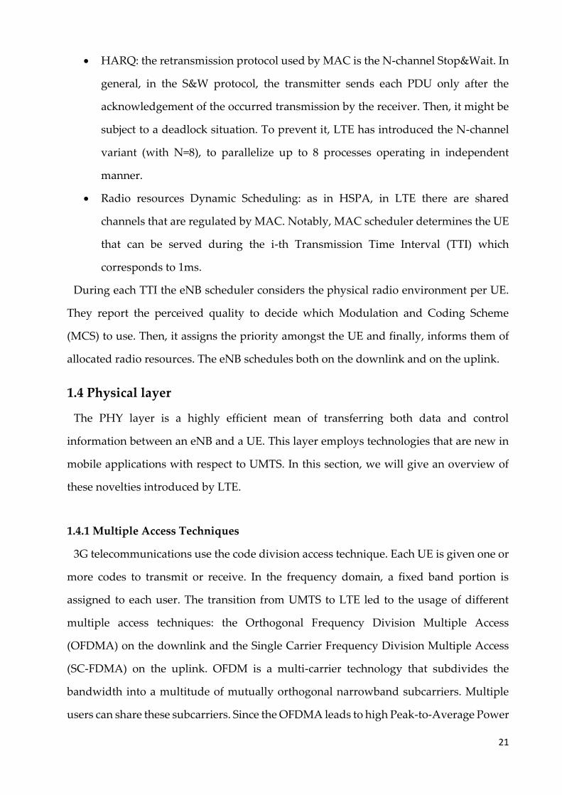
1.4.1.1 OFDMA

This technique is based on Orthogonal Frequency Division Multiplexing (OFDM), that

uses a very high number of carriers to transport the information from and to the UE. Each

carrier is closely spaced with a subcarrier spacing Δf = 15kHz. The higher the number of

carriers is, the better is the instantaneous capacity assigned to a single user.

Figure 1.4 OFDMA in LTE

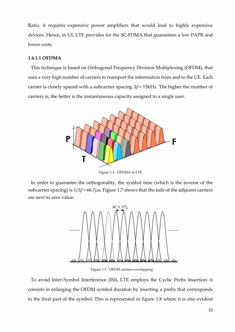
In order to guarantee the orthogonality, the symbol time (which is the inverse of the

subcarrier spacing) is 1/Δf = 66.7µs. Figure 1.7 shows that the tails of the adjacent carriers

are next to zero value.

Figure 1.5 OFDM carriers overlapping

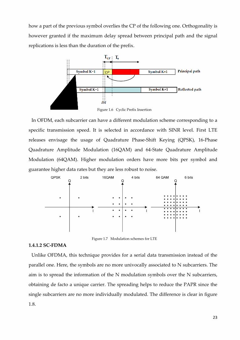
To avoid Inter-Symbol Interference (ISI), LTE employs the Cyclic Prefix Insertion: it

consists in enlarging the OFDM symbol duration by inserting a prefix that corresponds

to the final part of the symbol. This is represented in figure 1.8 where it is also evident

23

how a part of the previous symbol overlies the CP of the following one. Orthogonality is

however granted if the maximum delay spread between principal path and the signal

replications is less than the duration of the prefix.

Figure 1.6 Cyclic Prefix Insertion

In OFDM, each subcarrier can have a different modulation scheme corresponding to a

specific transmission speed. It is selected in accordance with SINR level. First LTE

releases envisage the usage of Quadrature Phase-Shift Keying (QPSK), 16-Phase

Quadrature Amplitude Modulation (16QAM) and 64-State Quadrature Amplitude

Modulation (64QAM). Higher modulation orders have more bits per symbol and

guarantee higher data rates but they are less robust to noise.

Figure 1.7 Modulation schemes for LTE

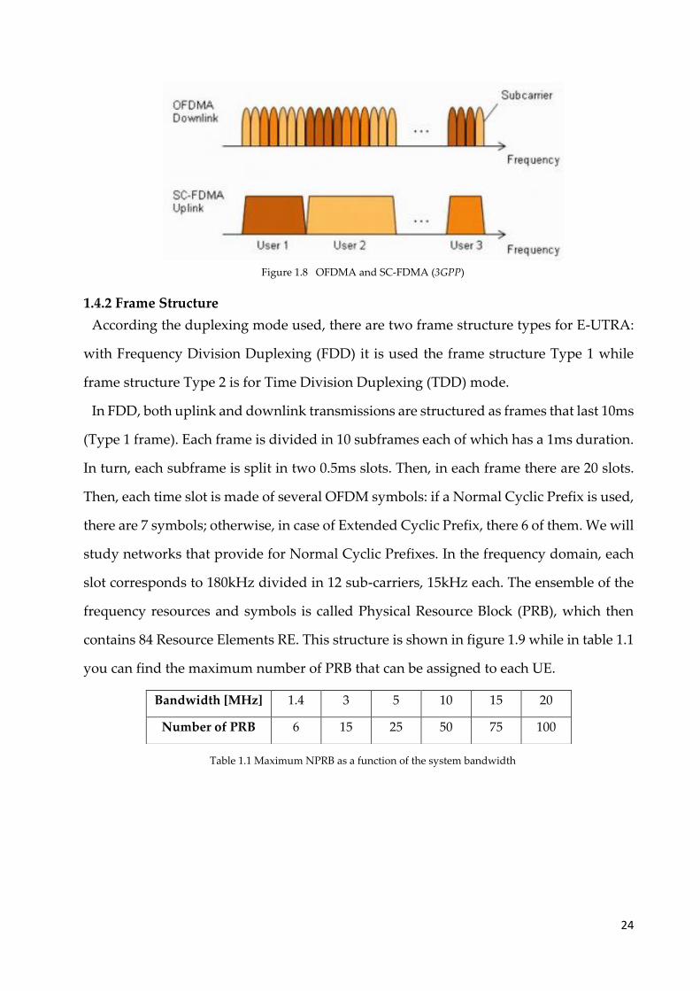
1.4.1.2 SC-FDMA

Unlike OFDMA, this technique provides for a serial data transmission instead of the

parallel one. Here, the symbols are no more univocally associated to N subcarriers. The

aim is to spread the information of the N modulation symbols over the N subcarriers,

obtaining de facto a unique carrier. The spreading helps to reduce the PAPR since the

single subcarriers are no more individually modulated. The difference is clear in figure

1.8.

24

Figure 1.8 OFDMA and SC-FDMA (3GPP)

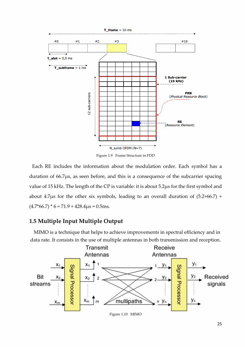
1.4.2 Frame Structure

According the duplexing mode used, there are two frame structure types for E-UTRA:

with Frequency Division Duplexing (FDD) it is used the frame structure Type 1 while

frame structure Type 2 is for Time Division Duplexing (TDD) mode.

In FDD, both uplink and downlink transmissions are structured as frames that last 10ms

(Type 1 frame). Each frame is divided in 10 subframes each of which has a 1ms duration.

In turn, each subframe is split in two 0.5ms slots. Then, in each frame there are 20 slots.

Then, each time slot is made of several OFDM symbols: if a Normal Cyclic Prefix is used,

there are 7 symbols; otherwise, in case of Extended Cyclic Prefix, there 6 of them. We will

study networks that provide for Normal Cyclic Prefixes. In the frequency domain, each

slot corresponds to 180kHz divided in 12 sub-carriers, 15kHz each. The ensemble of the

frequency resources and symbols is called Physical Resource Block (PRB), which then

contains 84 Resource Elements RE. This structure is shown in figure 1.9 while in table 1.1

you can find the maximum number of PRB that can be assigned to each UE.

Table 1.1 Maximum NPRB as a function of the system bandwidth

Bandwidth [MHz] 1.4 3 5 10 15 20

Number of PRB 6 15 25 50 75 100

25

Figure 1.9 Frame Structure in FDD

Each RE includes the information about the modulation order. Each symbol has a

duration of 66.7μs, as seen before, and this is a consequence of the subcarrier spacing

value of 15 kHz. The length of the CP is variable: it is about 5.2μs for the first symbol and

about 4.7μs for the other six symbols, leading to an overall duration of (5.2+66.7) +

(4.7*66.7) * 6 = 71.9 + 428.4μs = 0.5ms.

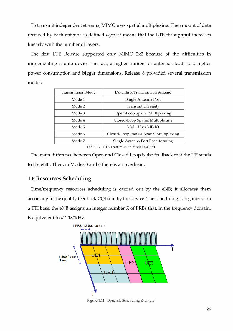
1.5 Multiple Input Multiple Output

MIMO is a technique that helps to achieve improvements in spectral efficiency and in

data rate. It consists in the use of multiple antennas in both transmission and reception.

Figure 1.10 MIMO

26

To transmit independent streams, MIMO uses spatial multiplexing. The amount of data

received by each antenna is defined layer; it means that the LTE throughput increases

linearly with the number of layers.

The first LTE Release supported only MIMO 2x2 because of the difficulties in

implementing it onto devices: in fact, a higher number of antennas leads to a higher

power consumption and bigger dimensions. Release 8 provided several transmission

modes:

Transmission Mode Downlink Transmission Scheme

Mode 1 Single Antenna Port

Mode 2 Transmit Diversity

Mode 3 Open-Loop Spatial Multiplexing

Mode 4 Closed-Loop Spatial Multiplexing

Mode 5 Multi-User MIMO

Mode 6 Closed-Loop Rank-1 Spatial Multiplexing

Mode 7 Single Antenna Port Beamforming

Table 1.2 LTE Transmission Modes (3GPP)

The main difference between Open and Closed Loop is the feedback that the UE sends

to the eNB. Then, in Modes 3 and 6 there is an overhead.

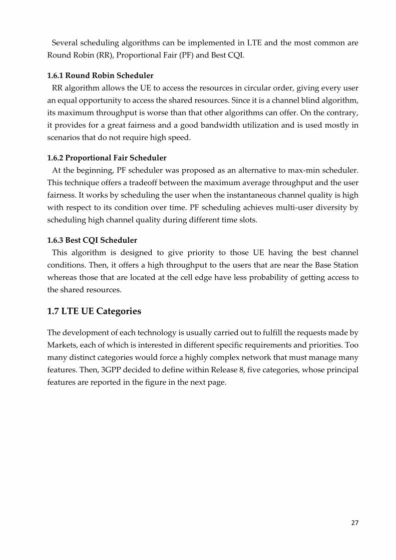
1.6 Resources Scheduling

Time/frequency resources scheduling is carried out by the eNB; it allocates them

according to the quality feedback CQI sent by the device. The scheduling is organized on

a TTI base: the eNB assigns an integer number K of PRBs that, in the frequency domain,

is equivalent to K * 180kHz.

Figure 1.11 Dynamic Scheduling Example

27

Several scheduling algorithms can be implemented in LTE and the most common are

Round Robin (RR), Proportional Fair (PF) and Best CQI.

1.6.1 Round Robin Scheduler

RR algorithm allows the UE to access the resources in circular order, giving every user

an equal opportunity to access the shared resources. Since it is a channel blind algorithm,

its maximum throughput is worse than that other algorithms can offer. On the contrary,

it provides for a great fairness and a good bandwidth utilization and is used mostly in

scenarios that do not require high speed.

1.6.2 Proportional Fair Scheduler

At the beginning, PF scheduler was proposed as an alternative to max-min scheduler.

This technique offers a tradeoff between the maximum average throughput and the user

fairness. It works by scheduling the user when the instantaneous channel quality is high

with respect to its condition over time. PF scheduling achieves multi-user diversity by

scheduling high channel quality during different time slots.

1.6.3 Best CQI Scheduler

This algorithm is designed to give priority to those UE having the best channel

conditions. Then, it offers a high throughput to the users that are near the Base Station

whereas those that are located at the cell edge have less probability of getting access to

the shared resources.

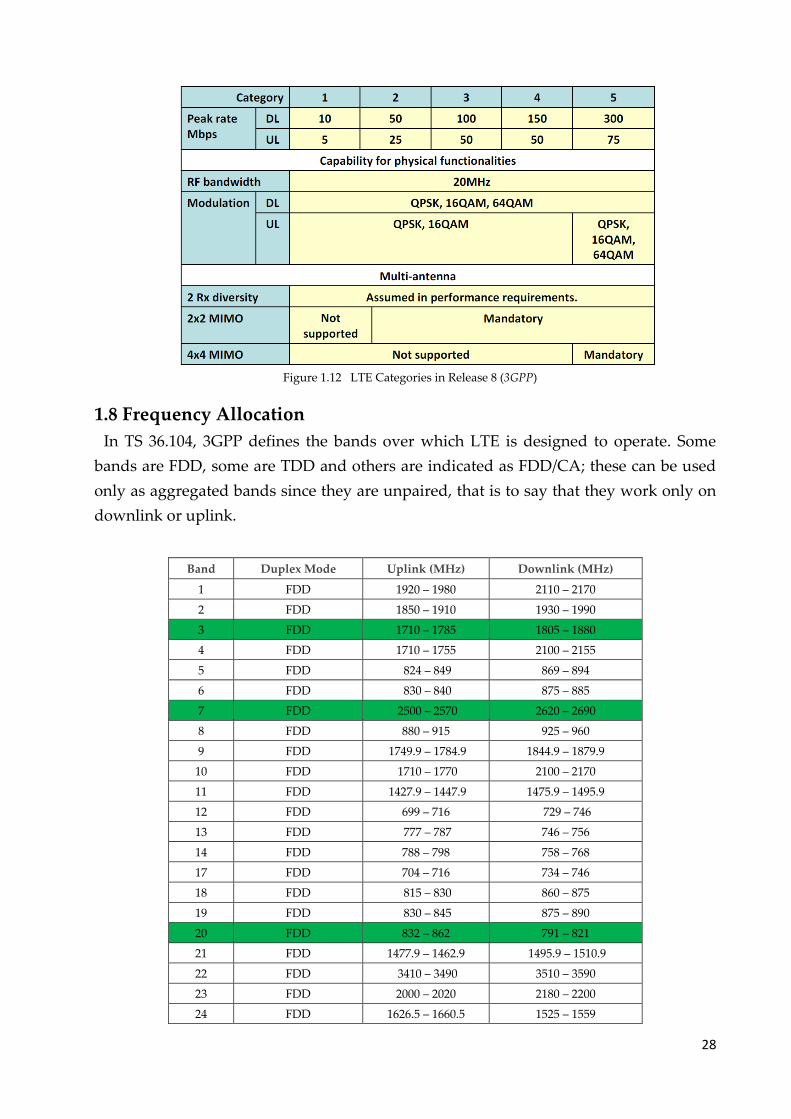
1.7 LTE UE Categories

The development of each technology is usually carried out to fulfill the requests made by

Markets, each of which is interested in different specific requirements and priorities. Too

many distinct categories would force a highly complex network that must manage many

features. Then, 3GPP decided to define within Release 8, five categories, whose principal

features are reported in the figure in the next page.

28

Figure 1.12 LTE Categories in Release 8 (3GPP)

1.8 Frequency Allocation

In TS 36.104, 3GPP defines the bands over which LTE is designed to operate. Some

bands are FDD, some are TDD and others are indicated as FDD/CA; these can be used

only as aggregated bands since they are unpaired, that is to say that they work only on

downlink or uplink.

Band Duplex Mode Uplink (MHz) Downlink (MHz)

1 FDD 1920 – 1980 2110 – 2170

2 FDD 1850 – 1910 1930 – 1990

3 FDD 1710 – 1785 1805 – 1880

4 FDD 1710 – 1755 2100 – 2155

5 FDD 824 – 849 869 – 894

6 FDD 830 – 840 875 – 885

7 FDD 2500 – 2570 2620 – 2690

8 FDD 880 – 915 925 – 960

9 FDD 1749.9 – 1784.9 1844.9 – 1879.9

10 FDD 1710 – 1770 2100 – 2170

11 FDD 1427.9 – 1447.9 1475.9 – 1495.9

12 FDD 699 – 716 729 – 746

13 FDD 777 – 787 746 – 756

14 FDD 788 – 798 758 – 768

17 FDD 704 – 716 734 – 746

18 FDD 815 – 830 860 – 875

19 FDD 830 – 845 875 – 890

20 FDD 832 – 862 791 – 821

21 FDD 1477.9 – 1462.9 1495.9 – 1510.9

22 FDD 3410 – 3490 3510 – 3590

23 FDD 2000 – 2020 2180 – 2200

24 FDD 1626.5 – 1660.5 1525 – 1559

29

25 FDD 1850 – 1915 1930 – 1995

26 FDD 814 – 849 859 – 894

27 FDD 807 – 824 852 – 869

28 FDD 703 – 748 758 – 803

29 FDD / CA 717 – 728

30 FDD 2305 – 2315 2350 – 2360

31 FDD 452.5 – 457.5 462.5 – 467.5

32 FDD / CA 1452 – 1496

33 TDD 1900 – 1920 1900 – 1920

34 TDD 2010 – 2025 2010 – 2025

35 TDD 1850 – 1910

36 TDD 1930 – 1990

37 TDD 1910 – 1930 1910 – 1930

38 TDD 2570 – 2620 2570 – 2620

39 TDD 1880 – 1920 1880 – 1920

40 TDD 2300 – 2400 2300 – 2400

41 TDD 2496 – 2690 2496 – 2690

42 TDD 3400 – 3600 3400 – 3600

43 TDD 3600 – 3800 3600 – 3800

44 TDD 703 – 803 703 – 803

45 TDD 1447 – 1467 1447 – 1467

46 TDD 5150 – 5925 5150 – 5925

65 FDD 1920 – 2010 2110 – 2200

66 FDD 1710 – 1780 2110 – 2200

67 FDD / CA 738 – 758

68 FDD 698 – 729 753 – 758

69 FDD / CA 2570 – 2620

70 FDD 1695 – 1710 1995 – 2020

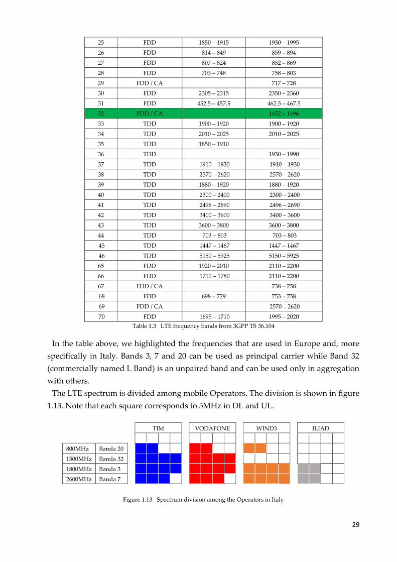
Table 1.3 LTE frequency bands from 3GPP TS 36.104

In the table above, we highlighted the frequencies that are used in Europe and, more

specifically in Italy. Bands 3, 7 and 20 can be used as principal carrier while Band 32

(commercially named L Band) is an unpaired band and can be used only in aggregation

with others.

The LTE spectrum is divided among mobile Operators. The division is shown in figure

1.13. Note that each square corresponds to 5MHz in DL and UL.

TIM VODAFONE WIND3 ILIAD

800MHz Banda 20

1500MHz Banda 32

1800MHz Banda 3

2600MHz Banda 7

Figure 1.13 Spectrum division among the Operators in Italy

30

2 LTE-Advanced

2.1 Beyond Release 8

Following the freeze of Release 8, 3GPP started working on a further evolution of LTE,

to be defined in Release 10, in order to guarantee to this technology the worldwide

leadership among mobile networks. In May 2008, 3GPP defined the bases of the so-called

LTE-Advanced in TR 36.913 “Requirements for further advancements for Evolved Universal

Terrestrial Radio Access (E-UTRA) LTE-Advanced”:

• Backward compatibility of LTE-A Release 10 with the LTE systems in Release 8

• Target peak data rate of 1Gbps in DL and 500Mbps in UL based on MIMO 4x4 and

64QAM on a 100MHz spectrum

• Capability to aggregate more spectrum (Carrier Aggregation) up to 100MHz

Further improvements have been introduced by Release 12 such as the higher order

modulation 256QAM. This led to a peak data rate of 3Gbps with a spectral efficiency up

to 30bps/Hz with MIMO 8x8. Moreover, Release 13 introduced the possibility to

aggregate up to 32 carrier components even among different spectrum types.

2.2 Enhancements for LTE-Advanced

The improved Carrier Aggregation, MIMO and 256QAM are not the only novelties

introduced in LTE-A. In fact, further enhancements have been developed and the most

significant are the deployment of Heterogeneous Networks (HetNets) to increase

capacity with Enhanced Inter-Cell Interference Coordination (eICIC) and Coordinated

Multi Point (CoMP) technique and the evolution towards Self Organizing Networks

(SON).

2.2.1 Carrier Aggregation

CA allows to increase the peak data rate by concatenating several bands in order to

transmit on a wider bandwidth, up to 100MHz. Moreover, it leads to a more flexible

handling of the frequencies in heterogeneous scenarios. Carrier aggregation supports

both contiguous and non-contiguous spectrum as well as asymmetric bandwidth for

31

FDD. This technology requires the sharing of baseband between the nodes that work on

the involved frequencies.

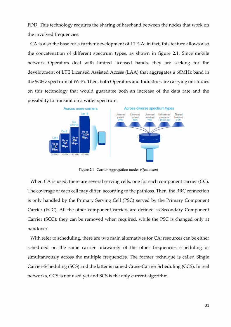
CA is also the base for a further development of LTE-A: in fact, this feature allows also

the concatenation of different spectrum types, as shown in figure 2.1. Since mobile

network Operators deal with limited licensed bands, they are seeking for the

development of LTE Licensed Assisted Access (LAA) that aggregates a 60MHz band in

the 5GHz spectrum of Wi-Fi. Then, both Operators and Industries are carrying on studies

on this technology that would guarantee both an increase of the data rate and the

possibility to transmit on a wider spectrum.

Figure 2.1 Carrier Aggregation modes (Qualcomm)

When CA is used, there are several serving cells, one for each component carrier (CC).

The coverage of each cell may differ, according to the pathloss. Then, the RRC connection

is only handled by the Primary Serving Cell (PSC) served by the Primary Component

Carrier (PCC). All the other component carriers are defined as Secondary Component

Carrier (SCC): they can be removed when required, while the PSC is changed only at

handover.

With refer to scheduling, there are two main alternatives for CA: resources can be either

scheduled on the same carrier unawarely of the other frequencies scheduling or

simultaneously across the multiple frequencies. The former technique is called Single

Carrier-Scheduling (SCS) and the latter is named Cross-Carrier Scheduling (CCS). In real

networks, CCS is not used yet and SCS is the only current algorithm.

32

2.2.2 Enhanced Multi-Antenna Techniques

MIMO schemes for DL in LTE provide for up to 4 layers. In Release 10, these have been

extended to up to 8 layers. It is very difficult to implement such a complex radio interface

on a device; in fact, nowadays there are few devices that can implement MIMO 4x4, while

devices with 8 antennas are still being studied. It is important to underline that MIMO

4x4 is not very robust with respect to noise and requires high SINRs.

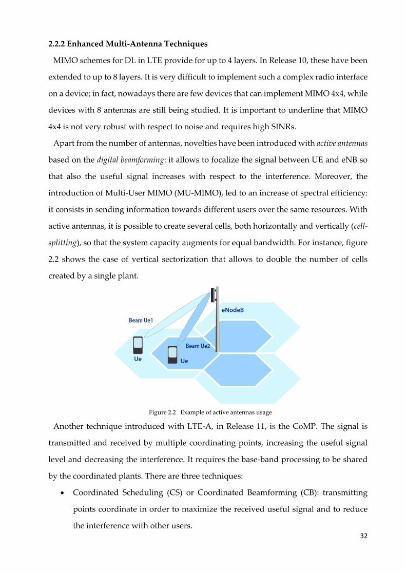
Apart from the number of antennas, novelties have been introduced with active antennas

based on the digital beamforming: it allows to focalize the signal between UE and eNB so

that also the useful signal increases with respect to the interference. Moreover, the

introduction of Multi-User MIMO (MU-MIMO), led to an increase of spectral efficiency:

it consists in sending information towards different users over the same resources. With

active antennas, it is possible to create several cells, both horizontally and vertically (cell-

splitting), so that the system capacity augments for equal bandwidth. For instance, figure

2.2 shows the case of vertical sectorization that allows to double the number of cells

created by a single plant.

Figure 2.2 Example of active antennas usage

Another technique introduced with LTE-A, in Release 11, is the CoMP. The signal is

transmitted and received by multiple coordinating points, increasing the useful signal

level and decreasing the interference. It requires the base-band processing to be shared

by the coordinated plants. There are three techniques:

• Coordinated Scheduling (CS) or Coordinated Beamforming (CB): transmitting

points coordinate in order to maximize the received useful signal and to reduce

the interference with other users.

33

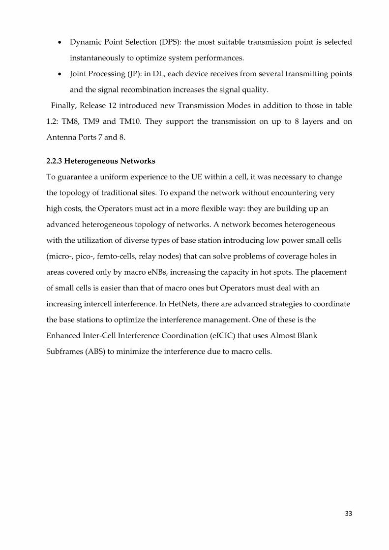
• Dynamic Point Selection (DPS): the most suitable transmission point is selected

instantaneously to optimize system performances.

• Joint Processing (JP): in DL, each device receives from several transmitting points

and the signal recombination increases the signal quality.

Finally, Release 12 introduced new Transmission Modes in addition to those in table

1.2: TM8, TM9 and TM10. They support the transmission on up to 8 layers and on

Antenna Ports 7 and 8.

2.2.3 Heterogeneous Networks

To guarantee a uniform experience to the UE within a cell, it was necessary to change

the topology of traditional sites. To expand the network without encountering very

high costs, the Operators must act in a more flexible way: they are building up an

advanced heterogeneous topology of networks. A network becomes heterogeneous

with the utilization of diverse types of base station introducing low power small cells

(micro-, pico-, femto-cells, relay nodes) that can solve problems of coverage holes in

areas covered only by macro eNBs, increasing the capacity in hot spots. The placement

of small cells is easier than that of macro ones but Operators must deal with an

increasing intercell interference. In HetNets, there are advanced strategies to coordinate

the base stations to optimize the interference management. One of these is the

Enhanced Inter-Cell Interference Coordination (eICIC) that uses Almost Blank

Subframes (ABS) to minimize the interference due to macro cells.

34

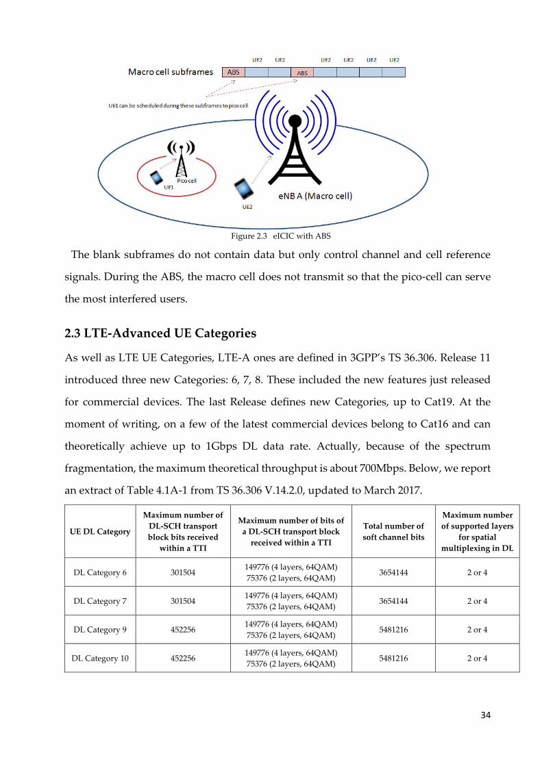
Figure 2.3 eICIC with ABS

The blank subframes do not contain data but only control channel and cell reference

signals. During the ABS, the macro cell does not transmit so that the pico-cell can serve

the most interfered users.

2.3 LTE-Advanced UE Categories

As well as LTE UE Categories, LTE-A ones are defined in 3GPP’s TS 36.306. Release 11

introduced three new Categories: 6, 7, 8. These included the new features just released

for commercial devices. The last Release defines new Categories, up to Cat19. At the

moment of writing, on a few of the latest commercial devices belong to Cat16 and can

theoretically achieve up to 1Gbps DL data rate. Actually, because of the spectrum

fragmentation, the maximum theoretical throughput is about 700Mbps. Below, we report

an extract of Table 4.1A-1 from TS 36.306 V.14.2.0, updated to March 2017.

UE DL Category

Maximum number of

DL-SCH transport

block bits received

within a TTI

Maximum number of bits of

a DL-SCH transport block

received within a TTI

Total number of

soft channel bits

Maximum number

of supported layers

for spatial

multiplexing in DL

DL Category 6 301504 149776 (4 layers, 64QAM)

75376 (2 layers, 64QAM) 3654144 2 or 4

DL Category 7 301504 149776 (4 layers, 64QAM)

75376 (2 layers, 64QAM) 3654144 2 or 4

DL Category 9 452256 149776 (4 layers, 64QAM)

75376 (2 layers, 64QAM) 5481216 2 or 4

DL Category 10 452256 149776 (4 layers, 64QAM)

75376 (2 layers, 64QAM) 5481216 2 or 4

35

DL Category 11 603008

149776 (4 layers, 64QAM)

195816 (4 layers, 256QAM)

75376 (2 layers, 64QAM)

97896 (2 layers, 256QAM)

7308288 2 or 4

DL Category 12 603008

149776 (4 layers, 64QAM)

195816 (4 layers, 256QAM)

75376 (2 layers, 64QAM)

97896 (2 layers, 256QAM)

7308288 2 or 4

DL Category 13 391632 195816 (4 layers, 256QAM)

97896 (2 layers, 256QAM) 3654144 2 or 4

DL Category 14 3916560 391656 (8 layers, 256QAM) 47431680 8

DL Category 15 749856-798800

149776 (4 layers, 64QAM)

195816 (4 layers, 256QAM)

75376 (2 layers, 64QAM)

97896 (2 layers, 256QAM)

9744384 2 or 4

DL Category 16 978960 -1051360

149776 (4 layers, 64QAM)

195816 (4 layers, 256QAM)

75376 (2 layers, 64QAM)

97896 (2 layers, 256QAM)

12789504 2 or 4

DL Category 17 25065984 391656 (8 layers, 256QAM) 303562752 8

DL Category 18 1174752-1206016

[299856 (8 layers, 64QAM)

391656 (8 layers, 256QAM)

149776 (4 layers, 64QAM)

195816 (4 layers, 256QAM)

75376 (2 layers, 64QAM)

97896 (2 layers, 256QAM)

14616576 2 or 4 [or 8]

DL Category 19 1566336 -1658272

[299856 (8 layers, 64QAM)

391656 (8 layers, 256QAM)

149776 (4 layers, 64QAM)

195816 (4 layers, 256QAM)

75376 (2 layers, 64QAM)

97896 (2 layers, 256QAM)

19488768 2 or 4 [or 8]

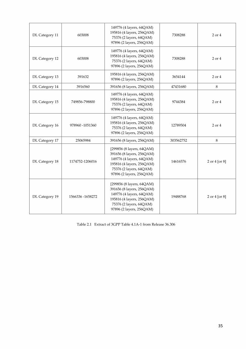
Table 2.1 Extract of 3GPP Table 4.1A-1 from Release 36.306

36

3 Scenario

3.1 Case Study

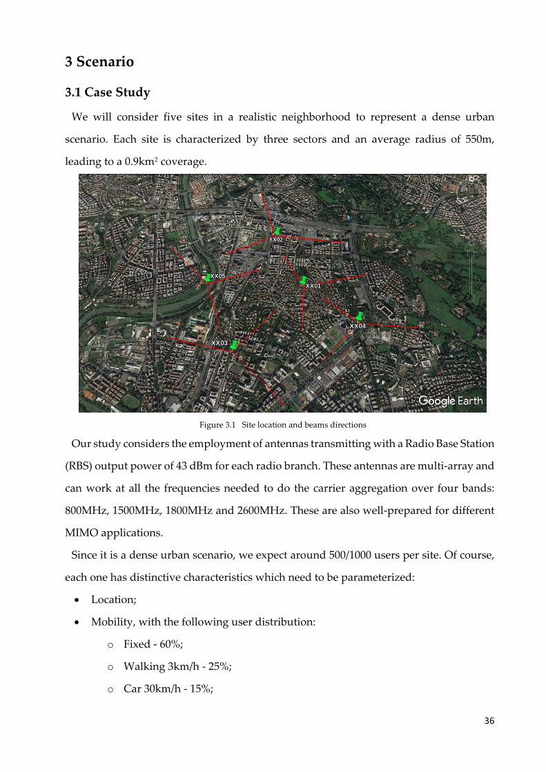
We will consider five sites in a realistic neighborhood to represent a dense urban

scenario. Each site is characterized by three sectors and an average radius of 550m,

leading to a 0.9km2 coverage.

Figure 3.1 Site location and beams directions

Our study considers the employment of antennas transmitting with a Radio Base Station

(RBS) output power of 43 dBm for each radio branch. These antennas are multi-array and

can work at all the frequencies needed to do the carrier aggregation over four bands:

800MHz, 1500MHz, 1800MHz and 2600MHz. These are also well-prepared for different

MIMO applications.

Since it is a dense urban scenario, we expect around 500/1000 users per site. Of course,

each one has distinctive characteristics which need to be parameterized:

• Location;

• Mobility, with the following user distribution:

o Fixed - 60%;

o Walking 3km/h - 25%;

o Car 30km/h - 15%;

37

• Device category, according to which we determine the capabilities of each user:

o Category 6 supports 64QAM, MIMO 2X2 and Carrier Aggregation over 2 bands;

o Category 11 supports 256QAM, MIMO 2x2 and Carrier Aggregation over 3 bands;

o Category 16 supports 256QAM, MIMO 4x4 and Carrier Aggregation over 4 bands.

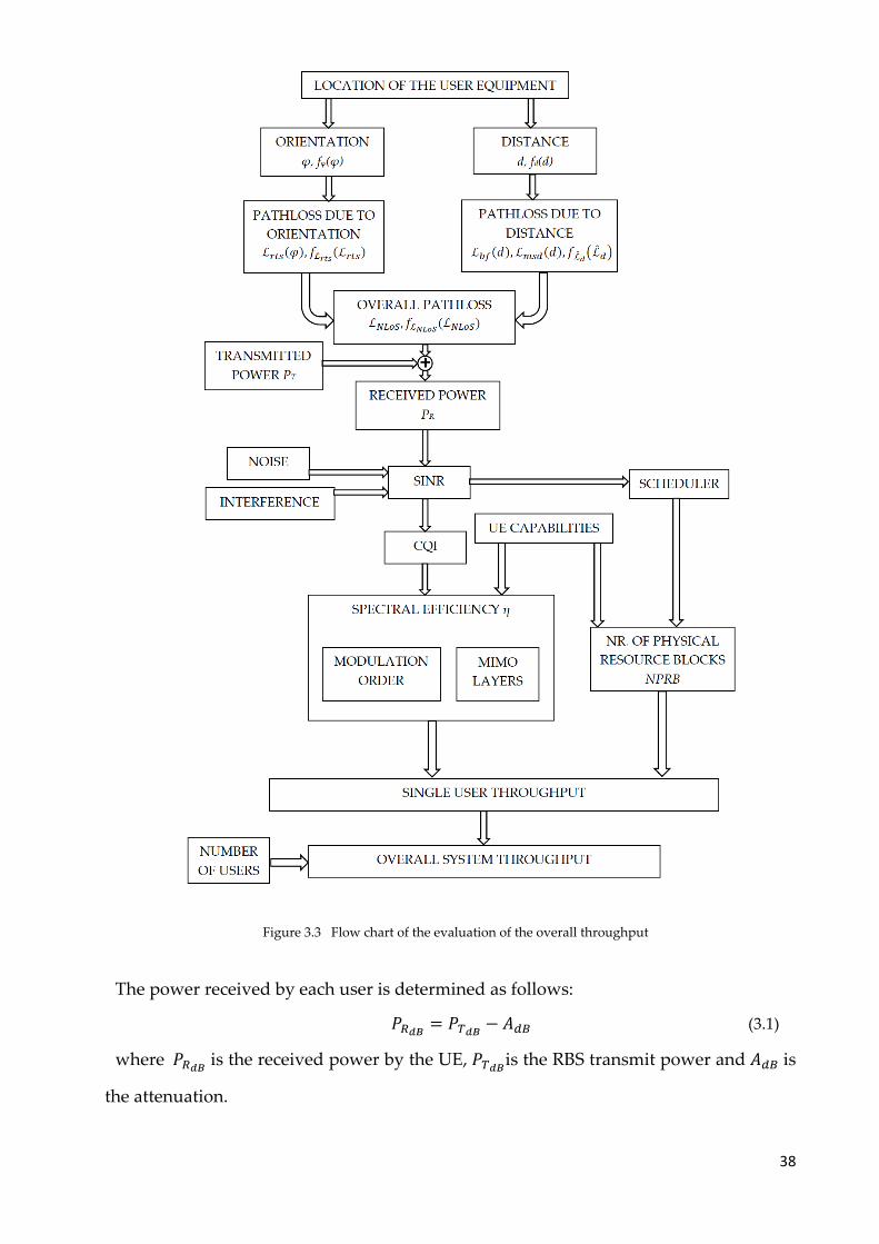
3.2 Analytical description

Since we are interested in evaluating the overall system throughput, we first need to

identify the parameters that can influence it. At first glance, we can say that these are

mainly the spectral efficiency and the Number of Physical Resource Blocks, which in turn

depend on the Channel Quality Indicator and then on the received power. A

schematization is given in figure 3.3. Here, one can distinguish also some elements

referring to probability density functions: in fact, our treatise tries to analyze the whole

network from a statistic perspective in order to give description of the propagation

phenomena without loss of generality. There are also other parameters who are fixed or,

anyway, considered constant. Note that the following consideration will be made on a

single site.

First, the transmitted power is fixed as well as the transmission and reception gains are

determined. The number and the category of the user equipment are supposed to be

known.

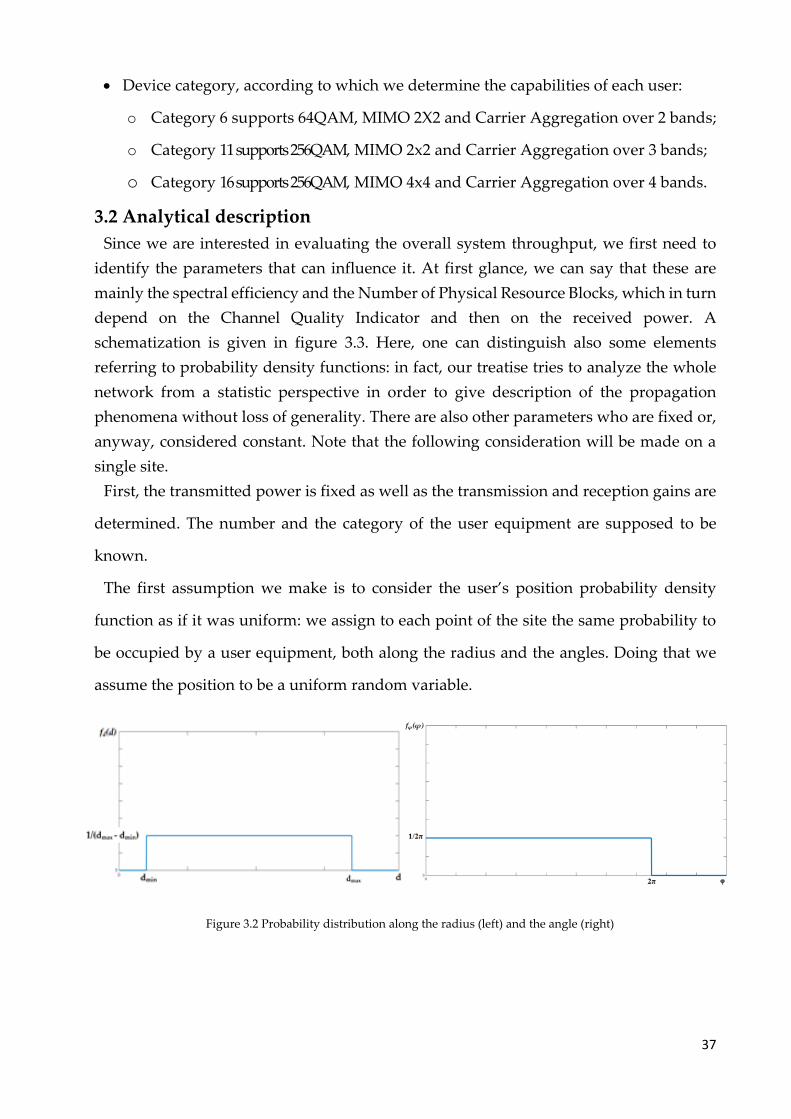
The first assumption we make is to consider the user’s position probability density

function as if it was uniform: we assign to each point of the site the same probability to

be occupied by a user equipment, both along the radius and the angles. Doing that we

assume the position to be a uniform random variable.

Figure 3.2 Probability distribution along the radius (left) and the angle (right)

38

Figure 3.3 Flow chart of the evaluation of the overall throughput

The power received by each user is determined as follows:

𝑃𝑅𝑑𝐵 = 𝑃𝑇𝑑𝐵 − 𝐴𝑑𝐵 (3.1)

where 𝑃𝑅𝑑𝐵 is the received power by the UE, 𝑃𝑇𝑑𝐵is the RBS transmit power and 𝐴𝑑𝐵 is

the attenuation.

39

To evaluate the attenuation in a complex scenario like the one we are keen to study we

will refer to the ITU Recommendation ITU-R P.1411-8, "Propagation data and prediction

methods for the planning of short-range outdoor radiocommunication systems and radio local area

networks in the frequency range 300 MHz to 100 GHz". This recommendation provides

guidance on outdoor short range (less than 1km) for both line-of-sights (LoS) and non-

line-of-sight (NLoS) environments. In particular, we are interested in the over rooftop

propagation described in section 4.2.

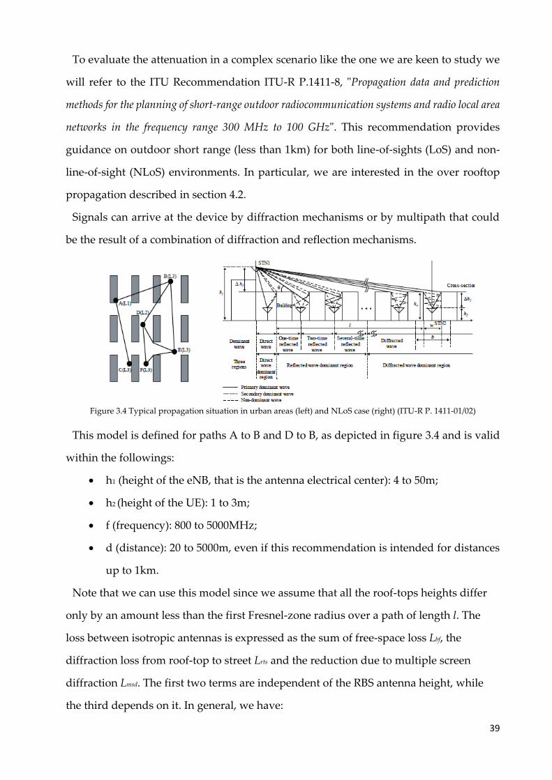
Signals can arrive at the device by diffraction mechanisms or by multipath that could

be the result of a combination of diffraction and reflection mechanisms.

Figure 3.4 Typical propagation situation in urban areas (left) and NLoS case (right) (ITU-R P. 1411-01/02)

This model is defined for paths A to B and D to B, as depicted in figure 3.4 and is valid

within the followings:

• h1 (height of the eNB, that is the antenna electrical center): 4 to 50m;

• h2 (height of the UE): 1 to 3m;

• f (frequency): 800 to 5000MHz;

• d (distance): 20 to 5000m, even if this recommendation is intended for distances

up to 1km.

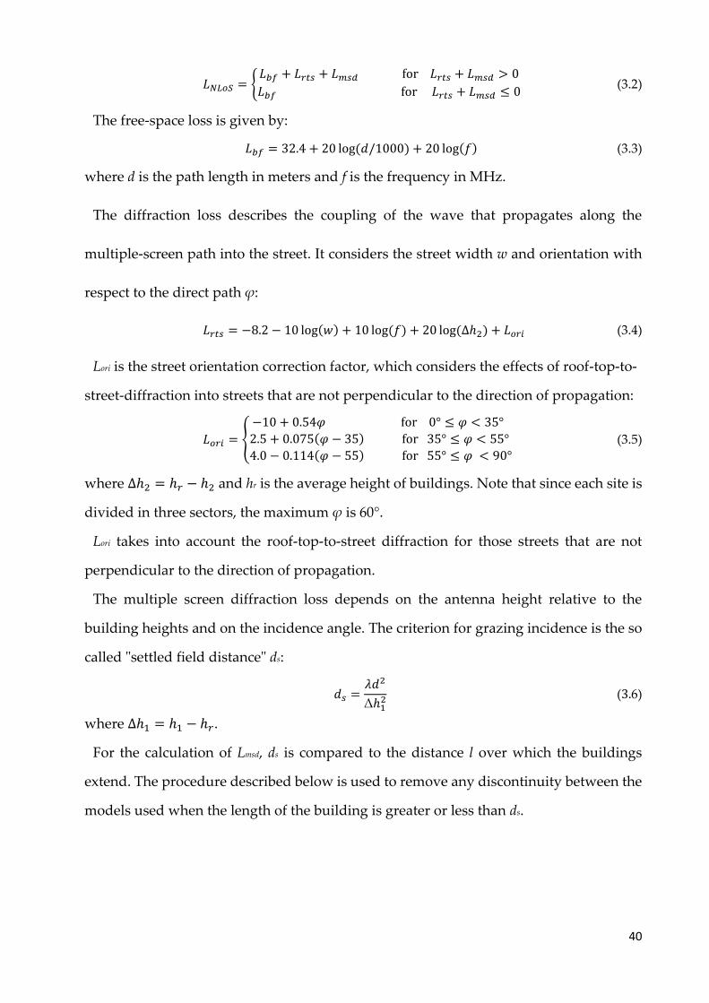
Note that we can use this model since we assume that all the roof-tops heights differ

only by an amount less than the first Fresnel-zone radius over a path of length l. The

loss between isotropic antennas is expressed as the sum of free-space loss Lbf, the

diffraction loss from roof-top to street Lrts and the reduction due to multiple screen

diffraction Lmsd. The first two terms are independent of the RBS antenna height, while

the third depends on it. In general, we have:

40

𝐿𝑁𝐿𝑜𝑆 = {𝐿𝑏𝑓 + 𝐿𝑟𝑡𝑠 + 𝐿𝑚𝑠𝑑 for 𝐿𝑟𝑡𝑠 + 𝐿𝑚𝑠𝑑 > 0

𝐿𝑏𝑓 for 𝐿𝑟𝑡𝑠 + 𝐿𝑚𝑠𝑑 ≤ 0 (3.2)

The free-space loss is given by:

𝐿𝑏𝑓 = 32.4 + 20 log(𝑑/1000) + 20 log(𝑓) (3.3)

where d is the path length in meters and f is the frequency in MHz.

The diffraction loss describes the coupling of the wave that propagates along the

multiple-screen path into the street. It considers the street width w and orientation with

respect to the direct path φ:

𝐿𝑟𝑡𝑠 = −8.2 − 10 log(𝑤) + 10 log(𝑓) + 20 log(∆ℎ2) + 𝐿𝑜𝑟𝑖 (3.4)

Lori is the street orientation correction factor, which considers the effects of roof-top-to-

street-diffraction into streets that are not perpendicular to the direction of propagation:

𝐿𝑜𝑟𝑖 = {

−10 + 0.54𝜑 for 0° ≤ 𝜑 < 35°

2.5 + 0.075(𝜑 − 35) for 35° ≤ 𝜑 < 55°

4.0 − 0.114(𝜑 − 55) for 55° ≤ 𝜑 < 90° (3.5)

where ∆ℎ2 = ℎ𝑟 − ℎ2 and hr is the average height of buildings. Note that since each site is

divided in three sectors, the maximum φ is 60°.

Lori takes into account the roof-top-to-street diffraction for those streets that are not

perpendicular to the direction of propagation.

The multiple screen diffraction loss depends on the antenna height relative to the

building heights and on the incidence angle. The criterion for grazing incidence is the so

called "settled field distance" ds:

𝑑𝑠 =𝜆𝑑2

Δℎ12 (3.6)

where Δℎ1 = ℎ1 − ℎ𝑟.

For the calculation of Lmsd, ds is compared to the distance l over which the buildings

extend. The procedure described below is used to remove any discontinuity between the

models used when the length of the building is greater or less than ds.

41

𝐿𝑚𝑠𝑑 =

{

− tanh(

log(𝑑) − log(𝑑𝑏𝑝)

𝜒) ∙ (𝐿1𝑚𝑠𝑑(𝑑) − 𝐿𝑚𝑖𝑑) + 𝐿𝑚𝑖𝑑 for 𝑙 > 𝑑𝑠 and 𝑑ℎ𝑏𝑝 > 0

𝑡𝑎𝑛ℎ (𝑙𝑜𝑔(𝑑) − 𝑙𝑜𝑔(𝑑𝑏𝑝)

𝜒) ∙ (𝐿2𝑚𝑠𝑑(𝑑) − 𝐿𝑚𝑖𝑑) + 𝐿𝑚𝑖𝑑 for 𝑙 ≤ 𝑑𝑠 and 𝑑ℎ𝑏𝑝 > 0

𝐿2𝑚𝑠𝑑(𝑑) for 𝑑ℎ𝑏𝑝 = 0

𝐿1𝑚𝑠𝑑(𝑑) − tanh(log(𝑑) − log(𝑑𝑏𝑝)

𝜁) ∙ (𝐿𝑢𝑝𝑝 − 𝐿𝑚𝑖𝑑) − 𝐿𝑢𝑝𝑝 + 𝐿𝑚𝑖𝑑 for 𝑙 > 𝑑𝑠 and 𝑑ℎ𝑏𝑝 < 0

𝐿2𝑚𝑠𝑑(𝑑) + 𝑡𝑎𝑛ℎ (𝑙𝑜𝑔(𝑑) − 𝑙𝑜𝑔(𝑑𝑏𝑝)

𝜁) ∙ (𝐿𝑚𝑖𝑑 − 𝐿𝑙𝑜𝑤) + 𝐿𝑚𝑖𝑑 − 𝐿𝑙𝑜𝑤 for 𝑙 ≤ 𝑑𝑠 and 𝑑ℎ𝑏𝑝 < 0

(3.7)

where 𝑑ℎ𝑏𝑝 = 𝐿𝑢𝑝𝑝 − 𝐿𝑙𝑜𝑤

𝜁 = (𝐿𝑢𝑝𝑝 − 𝐿𝑙𝑜𝑤) ∙ 𝜐

𝐿𝑚𝑖𝑑 =𝐿𝑢𝑝𝑝+𝐿𝑙𝑜𝑤

2

𝐿𝑢𝑝𝑝 = 𝐿1𝑚𝑖𝑑(𝑑𝑏𝑝)

𝐿𝑙𝑜𝑤 = 𝐿2(𝑑𝑏𝑝)

𝑑𝑏𝑝 = |Δℎ1|√1

𝜆

𝜐 = 0.0417𝜒 = 0.1

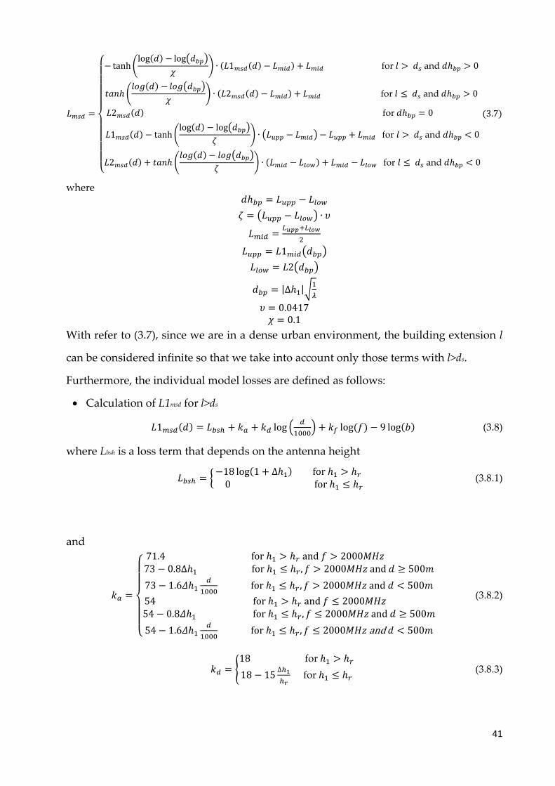
With refer to (3.7), since we are in a dense urban environment, the building extension l

can be considered infinite so that we take into account only those terms with l>ds.

Furthermore, the individual model losses are defined as follows:

• Calculation of L1msd for l>ds

𝐿1𝑚𝑠𝑑(𝑑) = 𝐿𝑏𝑠ℎ + 𝑘𝑎 + 𝑘𝑑 log (𝑑

1000) + 𝑘𝑓 log(𝑓) − 9 log(𝑏) (3.8)

where Lbsh is a loss term that depends on the antenna height

𝐿𝑏𝑠ℎ = {−18 log(1 + Δℎ1) for ℎ1 > ℎ𝑟 0 for ℎ1 ≤ ℎ𝑟

(3.8.1)

and

𝑘𝑎 =

{

71.4 for ℎ1 > ℎ𝑟 and 𝑓 > 2000𝑀𝐻𝑧 73 − 0.8Δℎ1 for ℎ1 ≤ ℎ𝑟 , 𝑓 > 2000𝑀𝐻𝑧 and 𝑑 ≥ 500𝑚

73 − 1.6𝛥ℎ1𝑑

1000 for ℎ1 ≤ ℎ𝑟 , 𝑓 > 2000𝑀𝐻𝑧 and 𝑑 < 500𝑚

54 for ℎ1 > ℎ𝑟 and 𝑓 ≤ 2000𝑀𝐻𝑧 54 − 0.8𝛥ℎ1 for ℎ1 ≤ ℎ𝑟 , 𝑓 ≤ 2000𝑀𝐻𝑧 and 𝑑 ≥ 500𝑚

54 − 1.6𝛥ℎ1𝑑

1000 for ℎ1 ≤ ℎ𝑟 , 𝑓 ≤ 2000𝑀𝐻𝑧 and 𝑑 < 500𝑚

(3.8.2)

𝑘𝑑 = {18 for ℎ1 > ℎ𝑟

18 − 15∆ℎ1

ℎ𝑟 for ℎ1 ≤ ℎ𝑟

(3.8.3)

42

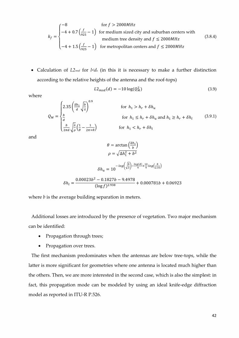
𝑘𝑓 =

{

−8 for 𝑓 > 2000𝑀𝐻𝑧

−4 + 0.7 (𝑓

925− 1) for medium sized city and suburban centers with

medium tree density and 𝑓 ≤ 2000𝑀𝐻𝑧

−4 + 1.5 (𝑓

925− 1) for metropolitan centers and 𝑓 ≤ 2000𝑀𝐻𝑧

(3.8.4)

• Calculation of L2msd for l<ds (in this it is necessary to make a further distinction

according to the relative heights of the antenna and the roof-tops)

𝐿2𝑚𝑠𝑑(𝑑) = −10 log(𝑄𝑀2 ) (3.9)

where

𝑄𝑀 =

{

2.35 (

∆h1

𝑑√𝑏

𝜆)

0.9

for ℎ1 > ℎ𝑟 + 𝛿ℎ𝑢

𝑏

𝑑 for ℎ1 ≤ ℎ𝑟 + 𝛿ℎ𝑢 and ℎ1 ≥ ℎ𝑟 + 𝛿ℎ𝑙

𝑏

2𝜋𝑑√𝜆

𝜌(1

𝜃−

1

2𝜋+𝜃) for ℎ1 < ℎ𝑟 + 𝛿ℎ𝑙

(3.9.1)

and

𝜃 = arctan (∆ℎ1

𝑏)

𝜌 = √∆ℎ12 + 𝑏2

𝛿ℎ𝑢 = 10− 𝑙𝑜𝑔(√

𝑏

𝜆)−

𝑙𝑜𝑔(𝑑)

9+10

9𝑙𝑜𝑔(

𝑏

2.35)

𝛿ℎ𝑙 =0.00023𝑏2 − 0.1827𝑏 − 9.4978

(log 𝑓)2.938+ 0.000781𝑏 + 0.06923

where b is the average building separation in meters.

Additional losses are introduced by the presence of vegetation. Two major mechanism

can be identified:

• Propagation through trees;

• Propagation over trees.

The first mechanism predominates when the antennas are below tree-tops, while the

latter is more significant for geometries where one antenna is located much higher than

the others. Then, we are more interested in the second case, which is also the simplest: in

fact, this propagation mode can be modeled by using an ideal knife-edge diffraction

model as reported in ITU-R P.526.

43

The whole model is a function of two random variables, then it can be described as a

random variable itself. Since the variables are independent it is possible to analyze each

contribution to the total path loss separately. First, we provide a brief theory recall.

Given a random variable x, with density function fX(x), let y=g(x) be its correspondence.

Now, we want to determine the probability distribution fY(y). If g is a monotonically

increasing (or decreasing) and differentiable function we have

𝑓𝑦(𝑦)𝑑𝑦 = 𝑓𝑥(𝑥)𝑑𝑥 (3.10)

and for differentiability hypothesis we can write

𝑑𝑦 = 𝑔′(𝑥)𝑑𝑥 (3.11)

so that we finally have

𝑓𝑦(𝑦)𝑔′(𝑥)𝑑𝑥 = 𝑓𝑥(𝑥)𝑑𝑥

𝑓𝑦(𝑦) =𝑓𝑥(𝑥)

𝑔′(𝑥) (3.12)

So, we divide the terms depending on distance 𝑑, 𝐿𝑏𝑓 and 𝐿𝑚𝑠𝑑, from that depending on

the orientation 𝜑, 𝐿𝑟𝑡𝑠.

First, we study this last:

𝐿𝑟𝑡𝑠 = −8.2 − 10 log(𝑤) + 10 log(𝑓) + 20 log(𝛥ℎ2) + 𝐿𝑜𝑟𝑖

𝐿𝑜𝑟𝑖 = {

−10 + 0.354𝜑 𝑓𝑜𝑟 0° < 𝜑 < 35°

2.5 + 0.075(𝜑 − 35) 𝑓𝑜𝑟 35° ≤ 𝜑 ≤ 55°

4.0 − 0.114(𝜑 − 55) 𝑓𝑜𝑟 55° < 𝜑 ≤ 90°

From these formulas, we can see that the only term depending on 𝜑 is 𝐿𝑜𝑟𝑖. Since it is a

piecewise function, we need to analyze each sub-term. First, we linearize 𝐿𝑟𝑡𝑠:

ℒ𝑟𝑡𝑠 = 10−8.2

10 𝑓

𝑤 ∆ℎ2

2 10𝐿𝑜𝑟𝑖10 = 𝑇 10

𝐿𝑜𝑟𝑖10 (3.13)

where:

𝑇 = 10−8.2

10 𝑓

𝑤 ∆ℎ2

2

To evaluate the overall probability density function 𝑓ℒ𝑟𝑡𝑠(ℒ𝑟𝑡𝑠) we have to verify that the

integral of the probability density function (pdf) over the considered range 𝜑 =

[−60°; +60°] is one. Then the sum of the pdf integrals corresponding to each sub-term

must be one.

The first sub-term is defined for 0° < 𝜑 < 35° and the corresponding probability density

function is

44

𝑓𝜑(𝜑) =1

𝜑max1 − 𝜑min1=1

35 (3.14)

and, from (3.5) we have

𝐿𝑜𝑟𝑖 = −10 + 0.354𝜑

then

ℒ𝑟𝑡𝑠 = 𝑇 10−1 100.0354𝜑 = 𝑇′100.0354𝜑 (3.15)

from here, we get:

𝜑 =log (

ℒ𝑟𝑡𝑠

𝑇′)

0.0354=log(ℒ𝑟𝑡𝑠) − log(𝑇

′)

0.0354 (3.15.1)

so, from (3.11) we need to evaluate

𝑔′(𝜑) =𝑑𝜑

𝑑ℒ𝑟𝑡𝑠≝ 𝑔′(ℒ𝑟𝑡𝑠)

𝑔′(ℒ𝑟𝑡𝑠) =1

0.0354 log(𝑒)

ℒ𝑟𝑡𝑠 (3.16)

and then:

𝑓ℒ𝑟𝑡𝑠(ℒ𝑟𝑡𝑠) = 𝛽11

35 0.0354

log(𝑒) ℒ𝑟𝑡𝑠 = 𝛽1𝛾1ℒ𝑟𝑡𝑠 (3.17)

where:

𝛾1 =1

35 0.0354

log(𝑒)

𝛽1 is a normalization term that we have to introduce since the original pdf is uniform:

in this way, we force the integral of 𝑓ℒ𝑟𝑡𝑠(ℒ𝑟𝑡𝑠) to be equal to the corresponding sub-range

∫ 𝑓ℒ𝑟𝑡𝑠(ℒ𝑟𝑡𝑠)ℒ𝑟𝑡𝑠max1

ℒ𝑟𝑡𝑠min1

𝑑ℒ𝑟𝑡𝑠 =35

120 (3.18)

ℒ𝑟𝑡𝑠min 1 = ℒ𝑟𝑡𝑠|𝜑=0° = 10−8.2

10 𝑓

𝑤 ∆ℎ2

2 10−10+0.354𝜑

10 |𝜑=0°

= 10−1.82 𝑓

𝑤 ∆ℎ2

2

ℒ𝑟𝑡𝑠max1 = ℒ𝑟𝑡𝑠|𝜑=35° = 10−8.2

10 𝑓

𝑤 ∆ℎ2

2 10−10+0.354𝜑

10 |𝜑=35°

= 10−0.581 𝑓

𝑤 ∆ℎ2

2

then, substituting them into (3.18):

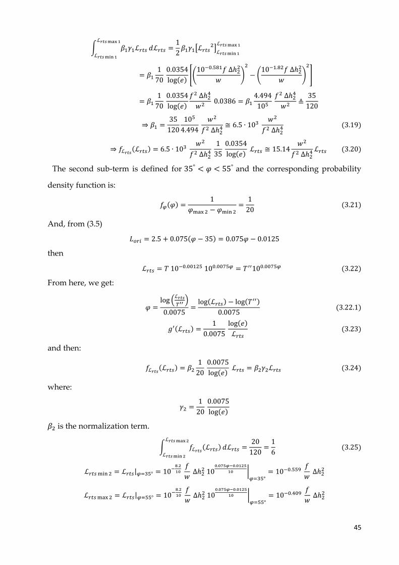
45

∫ 𝛽1𝛾1ℒ𝑟𝑡𝑠

ℒ𝑟𝑡𝑠max1

ℒ𝑟𝑡𝑠min1

𝑑ℒ𝑟𝑡𝑠 =1

2𝛽1𝛾1[ℒ𝑟𝑡𝑠

2]ℒ𝑟𝑡𝑠min1

ℒ𝑟𝑡𝑠max1

= 𝛽11

70 0.0354

log(𝑒)[(10−0.581𝑓 ∆ℎ2

2

𝑤)

2

− (10−1.82𝑓 ∆ℎ2

2

𝑤)

2

]

= 𝛽11

70 0.0354

log(𝑒)

𝑓2 ∆ℎ24

𝑤2 0.0386 = 𝛽1

4.494

105 𝑓2 ∆ℎ2

4

𝑤2≜35

120

⇒ 𝛽1 =35

120

105

4.494 𝑤2

𝑓2 ∆ℎ24 ≅ 6.5 ∙ 10

3 𝑤2

𝑓2 ∆ℎ24 (3.19)

⇒ 𝑓ℒ𝑟𝑡𝑠(ℒ𝑟𝑡𝑠) = 6.5 ∙ 103

𝑤2

𝑓2 ∆ℎ24 1

35 0.0354

log(𝑒) ℒ𝑟𝑡𝑠 ≅ 15.14

𝑤2

𝑓2 ∆ℎ24 ℒ𝑟𝑡𝑠 (3.20)

The second sub-term is defined for 35° < 𝜑 < 55° and the corresponding probability

density function is:

𝑓𝜑(𝜑) =1

𝜑max2 − 𝜑min2=1

20 (3.21)

And, from (3.5)

𝐿𝑜𝑟𝑖 = 2.5 + 0.075(𝜑 − 35) = 0.075𝜑 − 0.0125

then

ℒ𝑟𝑡𝑠 = 𝑇 10−0.00125 100.0075𝜑 = 𝑇′′100.0075𝜑 (3.22)

From here, we get:

𝜑 =log (

ℒ𝑟𝑡𝑠

𝑇′′)

0.0075=log(ℒ𝑟𝑡𝑠) − log(𝑇

′′)

0.0075 (3.22.1)

𝑔′(ℒ𝑟𝑡𝑠) =1

0.0075 log(𝑒)

ℒ𝑟𝑡𝑠 (3.23)

and then:

𝑓ℒ𝑟𝑡𝑠(ℒ𝑟𝑡𝑠) = 𝛽21

20 0.0075

log(𝑒) ℒ𝑟𝑡𝑠 = 𝛽2𝛾2ℒ𝑟𝑡𝑠 (3.24)

where:

𝛾2 =1

20 0.0075

log(𝑒)

𝛽2 is the normalization term.

∫ 𝑓ℒ𝑟𝑡𝑠(ℒ𝑟𝑡𝑠)ℒ𝑟𝑡𝑠max2

ℒ𝑟𝑡𝑠min2

𝑑ℒ𝑟𝑡𝑠 =20

120=1

6 (3.25)

ℒ𝑟𝑡𝑠min 2 = ℒ𝑟𝑡𝑠|𝜑=35° = 10−8.2

10 𝑓

𝑤 ∆ℎ2

2 100.075𝜑−0.0125

10 |𝜑=35°

= 10−0.559 𝑓

𝑤 ∆ℎ2

2

ℒ𝑟𝑡𝑠max2 = ℒ𝑟𝑡𝑠|𝜑=55° = 10−8.2

10 𝑓

𝑤 ∆ℎ2

2 100.075𝜑−0.0125

10 |𝜑=55°

= 10−0.409 𝑓

𝑤 ∆ℎ2

2

46

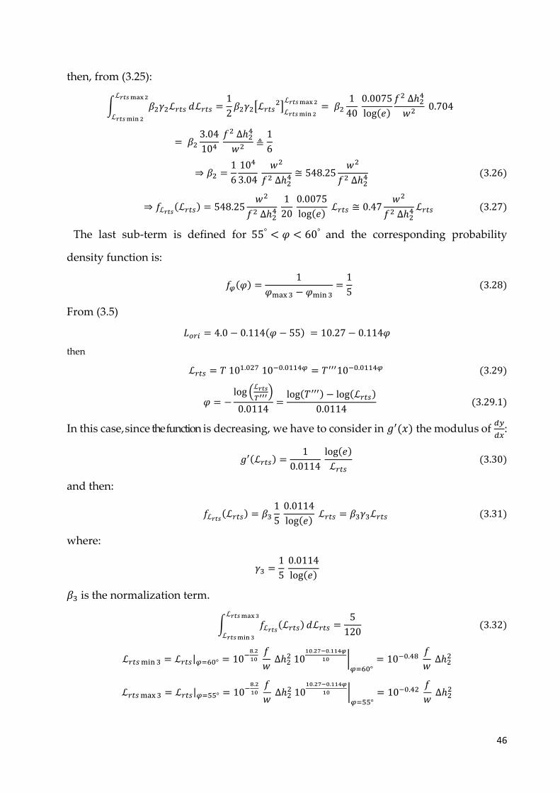
then, from (3.25):

∫ 𝛽2𝛾2ℒ𝑟𝑡𝑠

ℒ𝑟𝑡𝑠max2

ℒ𝑟𝑡𝑠min2

𝑑ℒ𝑟𝑡𝑠 =1

2𝛽2𝛾2[ℒ𝑟𝑡𝑠

2]ℒ𝑟𝑡𝑠min2

ℒ𝑟𝑡𝑠max2= 𝛽2

1

40 0.0075

log(𝑒)

𝑓2 ∆ℎ24

𝑤2 0.704

= 𝛽23.04

104 𝑓2 ∆ℎ2

4

𝑤2≜1

6

⇒ 𝛽2 =1

6

104

3.04 𝑤2

𝑓2 ∆ℎ24 ≅ 548.25

𝑤2

𝑓2 ∆ℎ24 (3.26)

⇒ 𝑓ℒ𝑟𝑡𝑠(ℒ𝑟𝑡𝑠) = 548.25𝑤2

𝑓2 ∆ℎ24 1

20 0.0075

log(𝑒) ℒ𝑟𝑡𝑠 ≅ 0.47

𝑤2

𝑓2 ∆ℎ24 ℒ𝑟𝑡𝑠 (3.27)

The last sub-term is defined for 55° < 𝜑 < 60° and the corresponding probability

density function is:

𝑓𝜑(𝜑) =1

𝜑max3 − 𝜑min3=1

5 (3.28)

From (3.5)

𝐿𝑜𝑟𝑖 = 4.0 − 0.114(𝜑 − 55) = 10.27 − 0.114𝜑

then

ℒ𝑟𝑡𝑠 = 𝑇 101.027 10−0.0114𝜑 = 𝑇′′′10−0.0114𝜑 (3.29)

𝜑 = −log (

ℒ𝑟𝑡𝑠

𝑇′′′)

0.0114=log(𝑇′′′) − log(ℒ𝑟𝑡𝑠)

0.0114 (3.29.1)

In this case, since the function is decreasing, we have to consider in 𝑔′(𝑥) the modulus of 𝑑𝑦

𝑑𝑥:

𝑔′(ℒ𝑟𝑡𝑠) =1

0.0114 log(𝑒)

ℒ𝑟𝑡𝑠 (3.30)

and then:

𝑓ℒ𝑟𝑡𝑠(ℒ𝑟𝑡𝑠) = 𝛽31

5 0.0114

log(𝑒) ℒ𝑟𝑡𝑠 = 𝛽3𝛾3ℒ𝑟𝑡𝑠 (3.31)

where:

𝛾3 =1

5 0.0114

log(𝑒)

𝛽3 is the normalization term.

∫ 𝑓ℒ𝑟𝑡𝑠(ℒ𝑟𝑡𝑠)ℒ𝑟𝑡𝑠max3

ℒ𝑟𝑡𝑠min3

𝑑ℒ𝑟𝑡𝑠 =5

120 (3.32)

ℒ𝑟𝑡𝑠min 3 = ℒ𝑟𝑡𝑠|𝜑=60° = 10−8.2

10 𝑓

𝑤 ∆ℎ2

2 1010.27−0.114𝜑

10 |𝜑=60°

= 10−0.48 𝑓

𝑤 ∆ℎ2

2

ℒ𝑟𝑡𝑠max3 = ℒ𝑟𝑡𝑠|𝜑=55° = 10−8.2

10 𝑓

𝑤 ∆ℎ2

2 1010.27−0.114𝜑

10 |𝜑=55°

= 10−0.42 𝑓

𝑤 ∆ℎ2

2

47

∫ 𝛽3𝛾3ℒ𝑟𝑡𝑠

ℒ𝑟𝑡𝑠max3

ℒ𝑟𝑡𝑠min3

𝑑ℒ𝑟𝑡𝑠 =1

2𝛽3𝛾3[ℒ𝑟𝑡𝑠

2]ℒ𝑟𝑡𝑠min3

ℒ𝑟𝑡𝑠max3= 𝛽3

1

10 0.0114

log(𝑒)

𝑓2 ∆ℎ24

𝑤2 (0.035)

= 𝛽39.18

105 𝑓2 ∆ℎ2

4

𝑤2≜

5

120

⇒ 𝛽3 =5

120

105

9.18 𝑤2

𝑓2 ∆ℎ24 ≅ 453.89

𝑤2

𝑓2 ∆ℎ24 (3.33)

⇒ 𝑓ℒ𝑟𝑡𝑠(ℒ𝑟𝑡𝑠) = 453.89𝑤2

𝑓2 ∆ℎ24 1

5 0.0114

log(𝑒) ℒ𝑟𝑡𝑠 ≅ 2.38

𝑤2

𝑓2 ∆ℎ24 ℒ𝑟𝑡𝑠 (3.34)

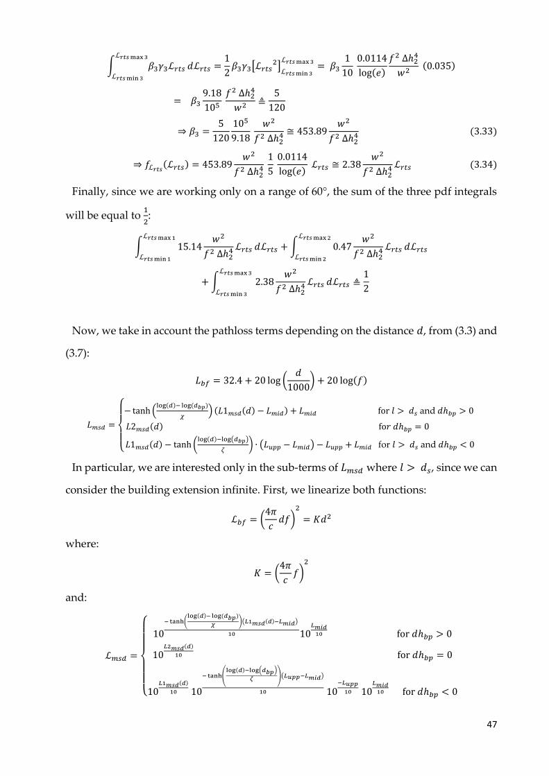
Finally, since we are working only on a range of 60°, the sum of the three pdf integrals

will be equal to 1

2:

∫ 15.14𝑤2

𝑓2 ∆ℎ24 ℒ𝑟𝑡𝑠

ℒ𝑟𝑡𝑠max1

ℒ𝑟𝑡𝑠min1

𝑑ℒ𝑟𝑡𝑠 +∫ 0.47𝑤2

𝑓2 ∆ℎ24 ℒ𝑟𝑡𝑠

ℒ𝑟𝑡𝑠max2

ℒ𝑟𝑡𝑠min2

𝑑ℒ𝑟𝑡𝑠

+∫ 2.38𝑤2

𝑓2 ∆ℎ24 ℒ𝑟𝑡𝑠

ℒ𝑟𝑡𝑠max3

ℒ𝑟𝑡𝑠min3

𝑑ℒ𝑟𝑡𝑠 ≜1

2

Now, we take in account the pathloss terms depending on the distance 𝑑, from (3.3) and

(3.7):

𝐿𝑏𝑓 = 32.4 + 20 log (𝑑

1000) + 20 log(𝑓)

𝐿𝑚𝑠𝑑 =

{

− tanh (

log(𝑑)− log(𝑑𝑏𝑝)

𝜒) (𝐿1𝑚𝑠𝑑(𝑑) − 𝐿𝑚𝑖𝑑) + 𝐿𝑚𝑖𝑑 for 𝑙 > 𝑑𝑠 and 𝑑ℎ𝑏𝑝 > 0

𝐿2𝑚𝑠𝑑(𝑑) fo𝑟 𝑑ℎ𝑏𝑝 = 0

𝐿1𝑚𝑠𝑑(𝑑) − tanh (log(𝑑)−log(𝑑𝑏𝑝)

𝜁) ∙ (𝐿𝑢𝑝𝑝 − 𝐿𝑚𝑖𝑑) − 𝐿𝑢𝑝𝑝 + 𝐿𝑚𝑖𝑑 for 𝑙 > 𝑑𝑠 and 𝑑ℎ𝑏𝑝 < 0

In particular, we are interested only in the sub-terms of 𝐿𝑚𝑠𝑑 where 𝑙 > 𝑑𝑠, since we can

consider the building extension infinite. First, we linearize both functions:

ℒ𝑏𝑓 = (4𝜋

𝑐𝑑𝑓)

2

= 𝐾𝑑2

where:

𝐾 = (4𝜋

𝑐𝑓)

2

and:

ℒ𝑚𝑠𝑑 =

{

10

−tanh(log(𝑑)− log(𝑑𝑏𝑝)

𝜒)(𝐿1𝑚𝑠𝑑(𝑑)−𝐿𝑚𝑖𝑑)

10 10𝐿𝑚𝑖𝑑10 for 𝑑ℎ𝑏𝑝 > 0

10𝐿2𝑚𝑠𝑑(𝑑)

10 for 𝑑ℎ𝑏𝑝 = 0

10𝐿1𝑚𝑠𝑑(𝑑)

10 10

−tanh(log(𝑑)−log(𝑑𝑏𝑝)

𝜁)(𝐿𝑢𝑝𝑝−𝐿𝑚𝑖𝑑)

10 10−𝐿𝑢𝑝𝑝

10 10𝐿𝑚𝑖𝑑10 for 𝑑ℎ𝑏𝑝 < 0

48

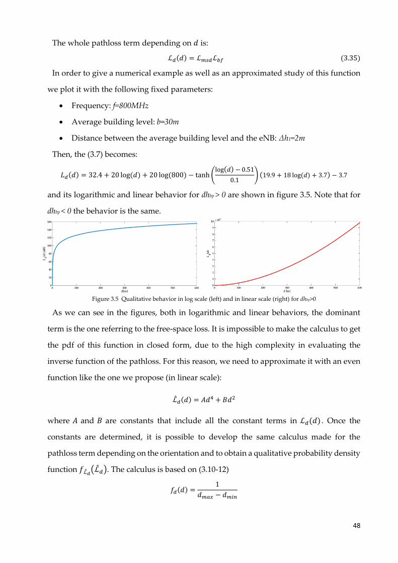
The whole pathloss term depending on 𝑑 is:

ℒ𝑑(𝑑) = ℒ𝑚𝑠𝑑ℒ𝑏𝑓 (3.35)

In order to give a numerical example as well as an approximated study of this function

we plot it with the following fixed parameters:

• Frequency: f=800MHz

• Average building level: b=30m

• Distance between the average building level and the eNB: Δh1=2m

Then, the (3.7) becomes:

𝐿𝑑(𝑑) = 32.4 + 20 log(𝑑) + 20 log(800) − tanh (log(𝑑) −0.51

0.1) (19.9 + 18 log(𝑑) + 3.7) − 3.7

and its logarithmic and linear behavior for dhbp > 0 are shown in figure 3.5. Note that for

dhbp < 0 the behavior is the same.

Figure 3.5 Qualitative behavior in log scale (left) and in linear scale (right) for dhbp>0

As we can see in the figures, both in logarithmic and linear behaviors, the dominant

term is the one referring to the free-space loss. It is impossible to make the calculus to get

the pdf of this function in closed form, due to the high complexity in evaluating the

inverse function of the pathloss. For this reason, we need to approximate it with an even

function like the one we propose (in linear scale):

ℒ̂𝑑(𝑑) = 𝐴𝑑4 + 𝐵𝑑2

where 𝐴 and 𝐵 are constants that include all the constant terms in ℒ𝑑(𝑑) . Once the

constants are determined, it is possible to develop the same calculus made for the

pathloss term depending on the orientation and to obtain a qualitative probability density

function 𝑓ℒ̂𝑑(ℒ̂𝑑). The calculus is based on (3.10-12)

𝑓𝑑(𝑑) =1

𝑑𝑚𝑎𝑥 − 𝑑𝑚𝑖𝑛

49

𝑔(ℒ̂𝑑) =1

√2[ 𝐵√4𝐴ℒ̂𝑑 + 𝐵

2 − 2𝐴ℒ̂𝑑 − 𝐵2

2ℒ̂𝑑2√4𝐴ℒ̂𝑑 + 𝐵

2√√4𝐴ℒ̂𝑑+𝐵

2−𝐵

ℒ̂𝑑 ]

𝑓ℒ̂𝑑(ℒ̂𝑑) =√2

𝑑𝑚𝑎𝑥 − 𝑑𝑚𝑖𝑛

2ℒ̂𝑑2√4𝐴ℒ̂𝑑 + 𝐵

2√√4𝐴ℒ̂𝑑+𝐵

2−𝐵

ℒ̂𝑑

𝐵√4𝐴ℒ̂𝑑 + 𝐵2 − 2𝐴ℒ̂𝑑 − 𝐵

2

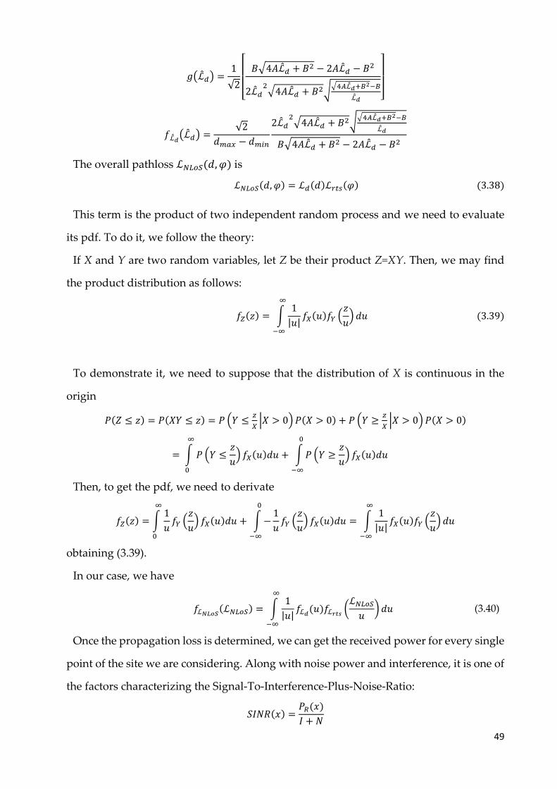
The overall pathloss ℒ𝑁𝐿𝑜𝑆(𝑑, 𝜑) is

ℒ𝑁𝐿𝑜𝑆(𝑑, 𝜑) = ℒ𝑑(𝑑)ℒ𝑟𝑡𝑠(𝜑) (3.38)

This term is the product of two independent random process and we need to evaluate

its pdf. To do it, we follow the theory:

If X and Y are two random variables, let Z be their product Z=XY. Then, we may find

the product distribution as follows:

𝑓𝑍(𝑧) = ∫1

|𝑢|𝑓𝑋(𝑢)𝑓𝑌 (

𝑧

𝑢)

∞

−∞

𝑑𝑢 (3.39)

To demonstrate it, we need to suppose that the distribution of X is continuous in the

origin

𝑃(𝑍 ≤ 𝑧) = 𝑃(𝑋𝑌 ≤ 𝑧) = 𝑃 (𝑌 ≤𝑧

𝑋|𝑋 > 0)𝑃(𝑋 > 0) + 𝑃 (𝑌 ≥

𝑧

𝑋|𝑋 > 0)𝑃(𝑋 > 0)

= ∫ 𝑃 (𝑌 ≤𝑧

𝑢) 𝑓𝑋(𝑢)𝑑𝑢 + ∫𝑃 (𝑌 ≥

𝑧

𝑢) 𝑓𝑋(𝑢)𝑑𝑢

0

−∞

∞

0

Then, to get the pdf, we need to derivate

𝑓𝑍(𝑧) = ∫1

𝑢𝑓𝑌 (

𝑧

𝑢) 𝑓𝑋(𝑢)𝑑𝑢

∞

0

+ ∫−1

𝑢𝑓𝑌 (

𝑧

𝑢) 𝑓𝑋(𝑢)𝑑𝑢

0

−∞

= ∫1

|𝑢|𝑓𝑋(𝑢)𝑓𝑌 (

𝑧

𝑢)

∞

−∞

𝑑𝑢

obtaining (3.39).

In our case, we have

𝑓ℒ𝑁𝐿𝑜𝑆(ℒ𝑁𝐿𝑜𝑆) = ∫

1

|𝑢|𝑓ℒ𝑑(𝑢)𝑓ℒ𝑟𝑡𝑠 (

ℒ𝑁𝐿𝑜𝑆𝑢

)

∞

−∞

𝑑𝑢 (3.40)

Once the propagation loss is determined, we can get the received power for every single

point of the site we are considering. Along with noise power and interference, it is one of

the factors characterizing the Signal-To-Interference-Plus-Noise-Ratio:

𝑆𝐼𝑁𝑅(𝑥) =𝑃𝑅(𝑥)

𝐼 + 𝑁

50

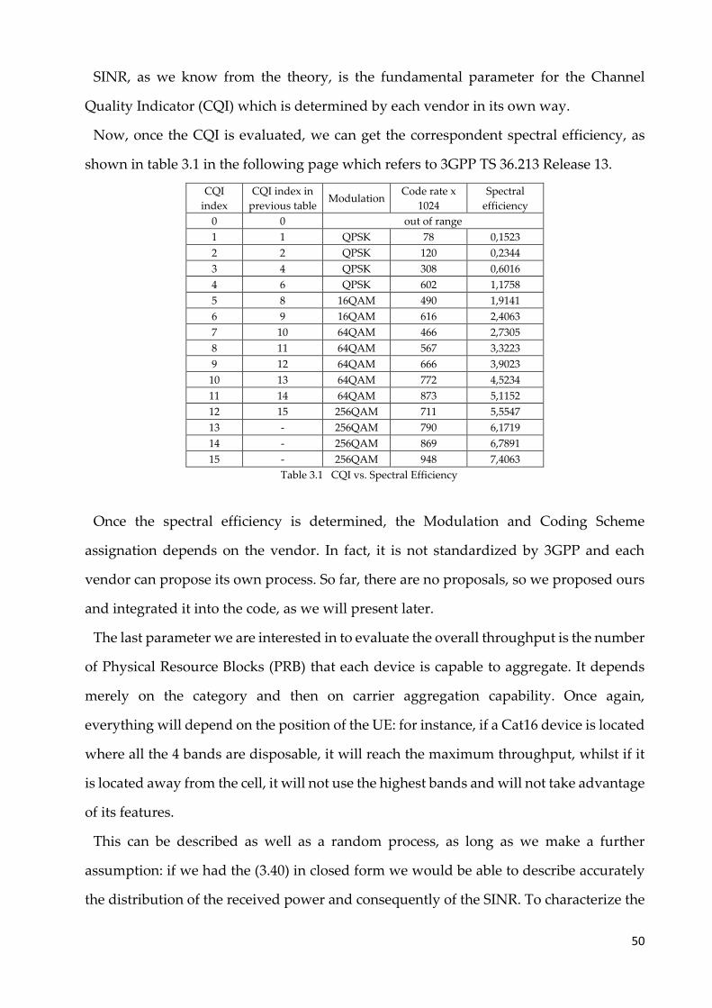
SINR, as we know from the theory, is the fundamental parameter for the Channel

Quality Indicator (CQI) which is determined by each vendor in its own way.

Now, once the CQI is evaluated, we can get the correspondent spectral efficiency, as

shown in table 3.1 in the following page which refers to 3GPP TS 36.213 Release 13.

CQI

index

CQI index in

previous table Modulation

Code rate x

1024

Spectral

efficiency

0 0 out of range

1 1 QPSK 78 0,1523

2 2 QPSK 120 0,2344

3 4 QPSK 308 0,6016

4 6 QPSK 602 1,1758

5 8 16QAM 490 1,9141

6 9 16QAM 616 2,4063

7 10 64QAM 466 2,7305

8 11 64QAM 567 3,3223

9 12 64QAM 666 3,9023

10 13 64QAM 772 4,5234

11 14 64QAM 873 5,1152

12 15 256QAM 711 5,5547

13 - 256QAM 790 6,1719

14 - 256QAM 869 6,7891

15 - 256QAM 948 7,4063

Table 3.1 CQI vs. Spectral Efficiency

Once the spectral efficiency is determined, the Modulation and Coding Scheme

assignation depends on the vendor. In fact, it is not standardized by 3GPP and each

vendor can propose its own process. So far, there are no proposals, so we proposed ours

and integrated it into the code, as we will present later.

The last parameter we are interested in to evaluate the overall throughput is the number

of Physical Resource Blocks (PRB) that each device is capable to aggregate. It depends

merely on the category and then on carrier aggregation capability. Once again,

everything will depend on the position of the UE: for instance, if a Cat16 device is located

where all the 4 bands are disposable, it will reach the maximum throughput, whilst if it

is located away from the cell, it will not use the highest bands and will not take advantage

of its features.

This can be described as well as a random process, as long as we make a further

assumption: if we had the (3.40) in closed form we would be able to describe accurately

the distribution of the received power and consequently of the SINR. To characterize the

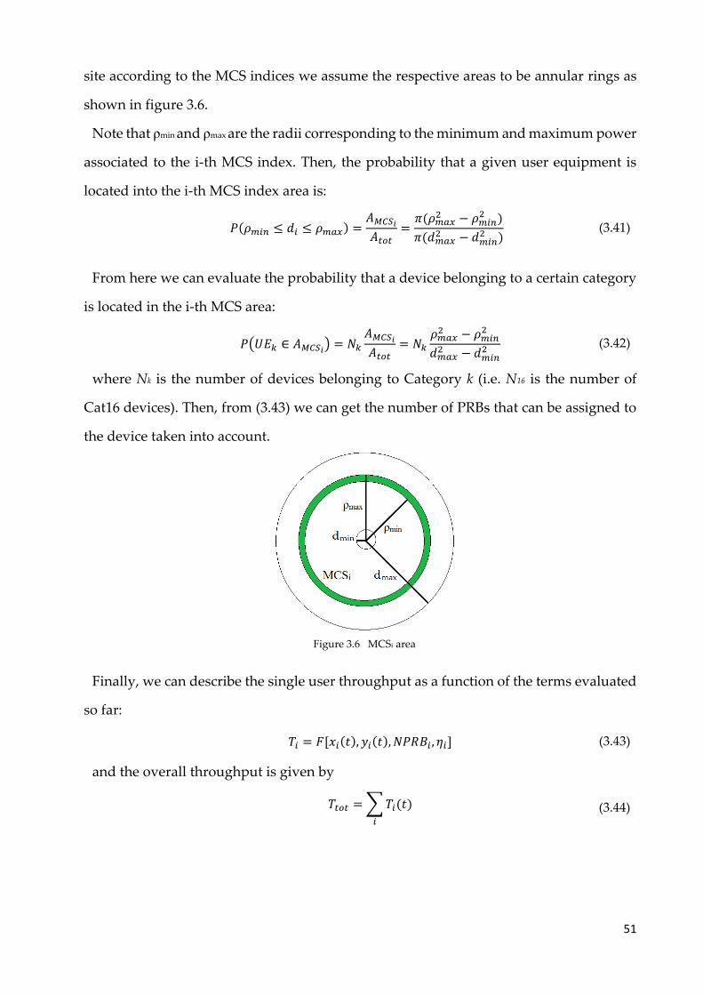
51

site according to the MCS indices we assume the respective areas to be annular rings as

shown in figure 3.6.

Note that ρmin and ρmax are the radii corresponding to the minimum and maximum power

associated to the i-th MCS index. Then, the probability that a given user equipment is

located into the i-th MCS index area is:

𝑃(𝜌𝑚𝑖𝑛 ≤ 𝑑𝑖 ≤ 𝜌𝑚𝑎𝑥) =𝐴𝑀𝐶𝑆𝑖𝐴𝑡𝑜𝑡

=𝜋(𝜌𝑚𝑎𝑥

2 − 𝜌𝑚𝑖𝑛2 )

𝜋(𝑑𝑚𝑎𝑥2 − 𝑑𝑚𝑖𝑛

2 ) (3.41)

From here we can evaluate the probability that a device belonging to a certain category

is located in the i-th MCS area:

𝑃(𝑈𝐸𝑘 ∈ 𝐴𝑀𝐶𝑆𝑖) = 𝑁𝑘

𝐴𝑀𝐶𝑆𝑖𝐴𝑡𝑜𝑡

= 𝑁𝑘𝜌𝑚𝑎𝑥2 − 𝜌𝑚𝑖𝑛

2

𝑑𝑚𝑎𝑥2 − 𝑑𝑚𝑖𝑛

2 (3.42)

where Nk is the number of devices belonging to Category k (i.e. N16 is the number of

Cat16 devices). Then, from (3.43) we can get the number of PRBs that can be assigned to

the device taken into account.

Figure 3.6 MCSi area

Finally, we can describe the single user throughput as a function of the terms evaluated

so far:

𝑇𝑖 = 𝐹[𝑥𝑖(𝑡), 𝑦𝑖(𝑡), 𝑁𝑃𝑅𝐵𝑖 , 𝜂𝑖] (3.43)

and the overall throughput is given by

𝑇𝑡𝑜𝑡 =∑𝑇𝑖(𝑡)

𝑖

(3.44)

52

4 NS-3 Simulator

4.1 Architecture and features

The ns-3 simulator is a discrete-event network simulator whose main target are research

and education. It has been developed in an open-source project and provides models of

how packet data networks perform. Differently from other simulation tools, it is designed

as a set of libraries that can be combined together also with external software libraries.

Moreover, there are several animators and data analysis tools that can be used. User

programs are mainly written in C++ even if Python can be used as well.

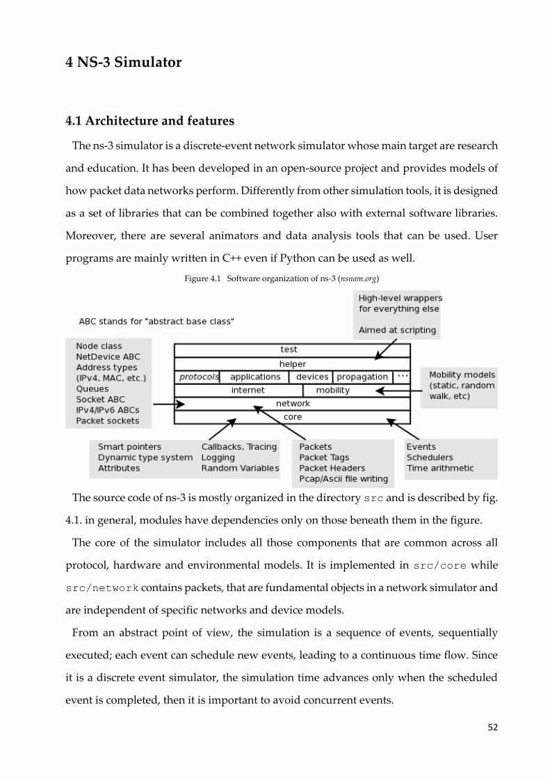
Figure 4.1 Software organization of ns-3 (nsnam.org)

The source code of ns-3 is mostly organized in the directory src and is described by fig.

4.1. in general, modules have dependencies only on those beneath them in the figure.

The core of the simulator includes all those components that are common across all

protocol, hardware and environmental models. It is implemented in src/core while

src/network contains packets, that are fundamental objects in a network simulator and

are independent of specific networks and device models.

From an abstract point of view, the simulation is a sequence of events, sequentially

executed; each event can schedule new events, leading to a continuous time flow. Since

it is a discrete event simulator, the simulation time advances only when the scheduled

event is completed, then it is important to avoid concurrent events.

53

The main concepts in this simulator are:

• Event

• Node

• NetDevice

• Channel

• Protocol

• Application

Now we will give a brief description of each of the these.

An event is something scheduled to happen at a given time. It has a target function and

can have parameters. A simulation-wise scheduler takes care of ordering the events and

executing them sequentially.

A node is an object used to aggregate other objects. It is the representation of a device

connected to a network.

A NetDevice is the logical representation of a Layer2 communication interface. In ns-3,

NetDevice design and functionality are kept as close as possible to the reality by

replicating the interface described in the standards.

Channels are the abstract representation of the effect of a given medium on the signal,

including the propagation loss and the interference from other sources. The most

advanced channels are based on the propagation module that we will describe later.

Protocols represent specific high-level protocol (i.e. IPv6, ICMP). Each protocol is

modelled following the standards, so that there should not be differences between the

implemented and the real ones.

Applications are simply used to generate traffic according to specific statistical

distributions and/or reacting to data reception.

Each ns-3 element can be configured with the Attributes, which are the way to change

an object property. We can modify both the default behavior of a class or of a single

instance.

The simulator is organized in modules, each providing a single functionality or layer.

In our case, we are mainly interested in the followings:

• LTE

• Internet

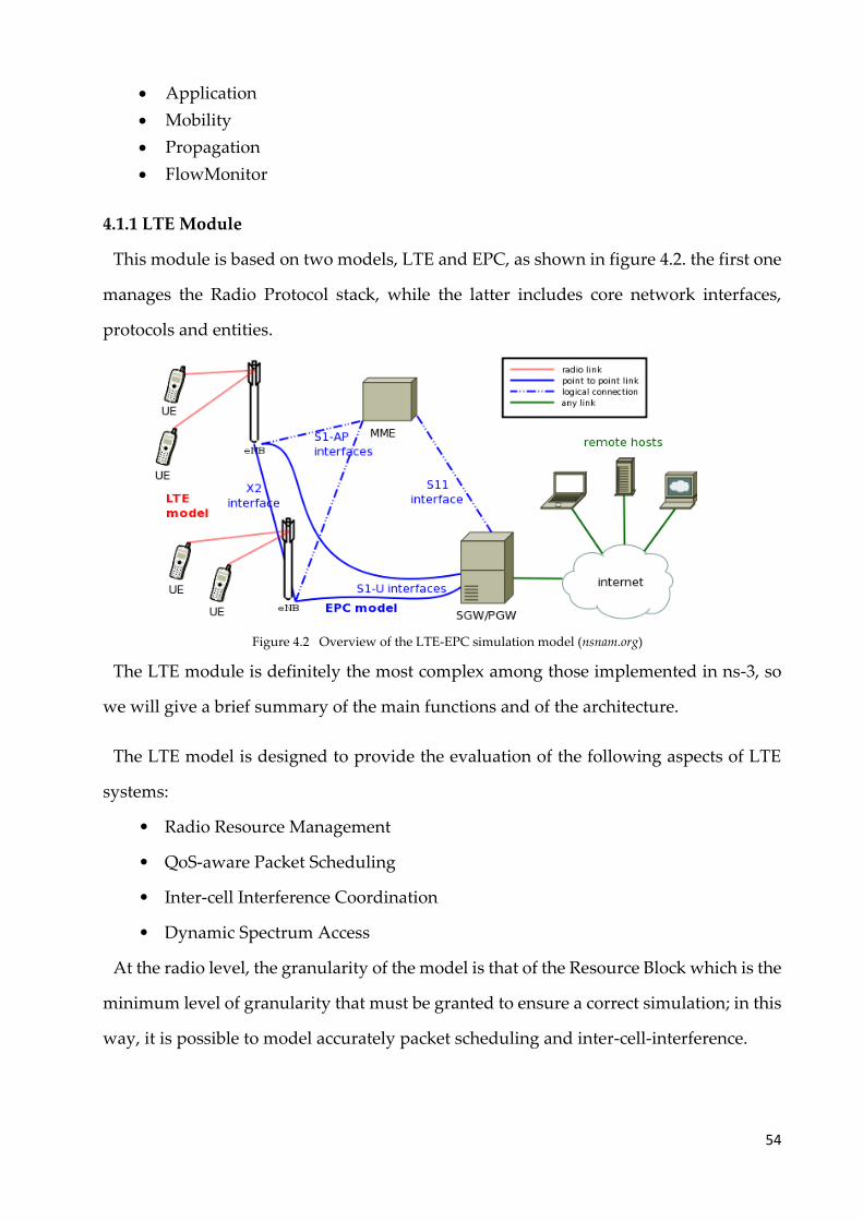
54

• Application

• Mobility

• Propagation

• FlowMonitor

4.1.1 LTE Module

This module is based on two models, LTE and EPC, as shown in figure 4.2. the first one

manages the Radio Protocol stack, while the latter includes core network interfaces,

protocols and entities.

Figure 4.2 Overview of the LTE-EPC simulation model (nsnam.org)

The LTE module is definitely the most complex among those implemented in ns-3, so

we will give a brief summary of the main functions and of the architecture.

The LTE model is designed to provide the evaluation of the following aspects of LTE

systems:

• Radio Resource Management

• QoS-aware Packet Scheduling

• Inter-cell Interference Coordination

• Dynamic Spectrum Access

At the radio level, the granularity of the model is that of the Resource Block which is the

minimum level of granularity that must be granted to ensure a correct simulation; in this

way, it is possible to model accurately packet scheduling and inter-cell-interference.

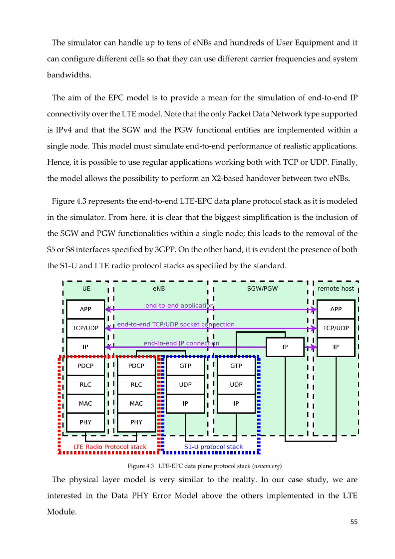
55

The simulator can handle up to tens of eNBs and hundreds of User Equipment and it

can configure different cells so that they can use different carrier frequencies and system

bandwidths.

The aim of the EPC model is to provide a mean for the simulation of end-to-end IP

connectivity over the LTE model. Note that the only Packet Data Network type supported

is IPv4 and that the SGW and the PGW functional entities are implemented within a

single node. This model must simulate end-to-end performance of realistic applications.

Hence, it is possible to use regular applications working both with TCP or UDP. Finally,

the model allows the possibility to perform an X2-based handover between two eNBs.

Figure 4.3 represents the end-to-end LTE-EPC data plane protocol stack as it is modeled

in the simulator. From here, it is clear that the biggest simplification is the inclusion of

the SGW and PGW functionalities within a single node; this leads to the removal of the

S5 or S8 interfaces specified by 3GPP. On the other hand, it is evident the presence of both

the S1-U and LTE radio protocol stacks as specified by the standard.

Figure 4.3 LTE-EPC data plane protocol stack (nsnam.org)

The physical layer model is very similar to the reality. In our case study, we are

interested in the Data PHY Error Model above the others implemented in the LTE

Module.

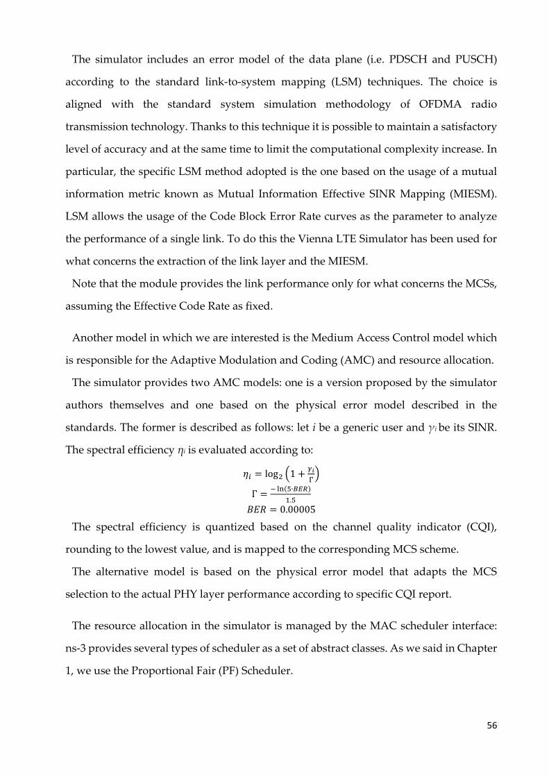
56

The simulator includes an error model of the data plane (i.e. PDSCH and PUSCH)

according to the standard link-to-system mapping (LSM) techniques. The choice is

aligned with the standard system simulation methodology of OFDMA radio

transmission technology. Thanks to this technique it is possible to maintain a satisfactory

level of accuracy and at the same time to limit the computational complexity increase. In

particular, the specific LSM method adopted is the one based on the usage of a mutual

information metric known as Mutual Information Effective SINR Mapping (MIESM).

LSM allows the usage of the Code Block Error Rate curves as the parameter to analyze

the performance of a single link. To do this the Vienna LTE Simulator has been used for

what concerns the extraction of the link layer and the MIESM.

Note that the module provides the link performance only for what concerns the MCSs,

assuming the Effective Code Rate as fixed.

Another model in which we are interested is the Medium Access Control model which

is responsible for the Adaptive Modulation and Coding (AMC) and resource allocation.

The simulator provides two AMC models: one is a version proposed by the simulator

authors themselves and one based on the physical error model described in the

standards. The former is described as follows: let i be a generic user and γi be its SINR.

The spectral efficiency ηi is evaluated according to:

𝜂𝑖 = log2 (1 +𝛾𝑖

Γ)

Γ =− ln(5∙𝐵𝐸𝑅)

1.5

𝐵𝐸𝑅 = 0.00005

The spectral efficiency is quantized based on the channel quality indicator (CQI),

rounding to the lowest value, and is mapped to the corresponding MCS scheme.

The alternative model is based on the physical error model that adapts the MCS

selection to the actual PHY layer performance according to specific CQI report.

The resource allocation in the simulator is managed by the MAC scheduler interface:

ns-3 provides several types of scheduler as a set of abstract classes. As we said in Chapter

1, we use the Proportional Fair (PF) Scheduler.

57

It works by scheduling user when its instantaneous channel quality is high relatively to

its own average channel condition over time. Let i, j denote generic users; let t be the

subframe index and k be the resource block index; let Mi,k(t) be MCS usable by user i on

resource block k according to what reported by the AMC model; finally, let S(M,B) be the

TB size in bits for the case where a number B of resource blocks is used. The achievable

rate Ri(k, t) in bit/s for user i on resource block group k at subframe t is defined as

𝑅𝑖(𝑘, 𝑡) =𝑆(𝑀𝑖,𝑘(𝑡), 1)

𝜏

where τ is the TTI duration.

Then, the index 𝑖�̂�(𝑡) to which RBG k is assigned at time t is determine as follows

𝑖�̂�(𝑡) = argmax𝑗=1,…,𝑁

(𝑅𝑗(𝑘, 𝑡)

𝑇𝑗(𝑡))

where 𝑇𝑗(𝑡) is the past throughput performance perceived by the user j. According to

the above scheduling algorithm, a user can be allocated to different RBGs, which can be

either adjacent or not, depending on the current condition of the channel and the past

throughput performance 𝑇𝑗(𝑡) which is determined at the end of the subframe t in this

way

𝑇𝑗(𝑡) = (1 −1

𝛼)𝑇𝑗(𝑡 − 1) +

1

𝛼�̂�𝑗(𝑡)

where α is the time constant of the exponential moving average and �̂�𝑗(𝑡) is the actual

throughput achieved by the user i in the subframe t.

4.1.2 Internet Module

The internet module offers several functionalities belonging to the TCP/IP stack. As an

example, available models are:

• IP (v4 and v6)

• ICMP (v4 and v6)

• UDP

• TCP (NewReno, Westwood, Westwood+, with more being developed)

Moreover, some routing protocols are included in this module like RIPng or Static

Routing. We use this module to configure the IP addresses of the core network and of the

devices. The internet module must work in combination with the application module.

58

4.1.3 Application Module

This module provides the base class for ns-3 applications. They are associated with

individual nodes. Each node holds a list of references (smart pointers) to its applications.

To create an API, it is necessary to define a socket, that can be both TCP or UDP, in

accordance with the transport protocol. The socket is selected by modifying the

PacketSink module. Then, there are client classes that are used to define the data flow.

4.1.4 Mobility Module

This module includes:

• a set of mobility models used to track and/or maintain the position and speed of

an object

• several helper classes which are used to set the position and the mobility of a

node.

The initial position of objects is typically set with a PositionAllocator. These types

of objects will lay out the position on a notional canvas. The MobilityHelper combines

a mobility model and position allocator, and can be used with a node container to install

mobility capability on a set of nodes.

The position of a node can be assigned either randomly or assigning precisely the

coordinates. Both these assignations are made with one of the following position

allocators:

• ListPositionAllocator

• GridPositionAllocator

• RandomRectanglePositionAllocator

• RandomBoxPositionAllocator

• RandomDiscPositionAllocator

• UniformDiscPositionAllocator

The mobility of a node is described with one the following subclasses:

• ConstantPosition

• ConstantVelocity

59

• ConstantAcceleration

• GaussMarkov

• Hierarchical

• RandomDirection2D

• RandomWalk2D

• RandomWaypoint

• SteadyStateRandomWaypoint

• Waypoint

4.1.5 Propagation Module

This module defines the interface to model the propagation loss. It calculates the

received signal power considering the transmitted power and the mutual positions of the

antennas. Several models are implemented, from the simplest ones (free space loss

model) to the most complex. Some of these refer to propagation loss models that have

been described by ITU, like the one we used for the simulation:

ItuR1411NlosOverRooftopPropagationLossModel.

Models can be chained in order to combine, for instance, different fading effects. The

accurate description of the model will be given later.

4.1.6 Flow Monitor Module

The aim of this module is to provide a flexible system to measure the performance of

network protocols. This module can track the packets exchanged by the nodes and can

measure several parameters. The statistics collected for each data flow can be exported in

XML format. At the moment of writing, this module works only at IP level and can give

as output the transmitted and received bytes and packets, the lost packets, the duration

of the transmission and the throughput.

4.2 Assumptions and settings

This paragraph is focused on the description of the implementation choices that have

been made when simulating, both to lighten the simulation and to face some limitations

of the simulator. In fact, the simulator is continuously renewing and enhancing its

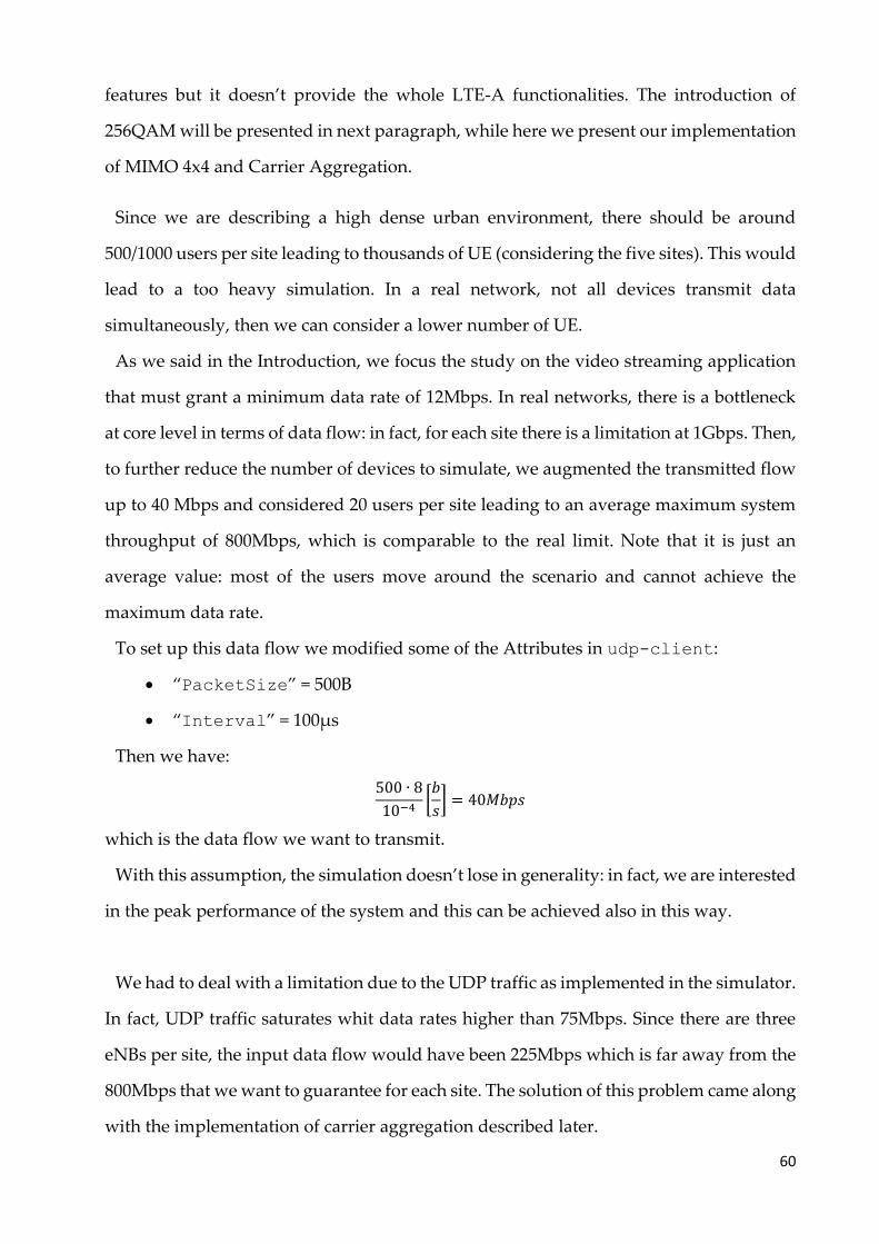
60

features but it doesn’t provide the whole LTE-A functionalities. The introduction of

256QAM will be presented in next paragraph, while here we present our implementation

of MIMO 4x4 and Carrier Aggregation.

Since we are describing a high dense urban environment, there should be around

500/1000 users per site leading to thousands of UE (considering the five sites). This would

lead to a too heavy simulation. In a real network, not all devices transmit data

simultaneously, then we can consider a lower number of UE.

As we said in the Introduction, we focus the study on the video streaming application

that must grant a minimum data rate of 12Mbps. In real networks, there is a bottleneck

at core level in terms of data flow: in fact, for each site there is a limitation at 1Gbps. Then,

to further reduce the number of devices to simulate, we augmented the transmitted flow

up to 40 Mbps and considered 20 users per site leading to an average maximum system

throughput of 800Mbps, which is comparable to the real limit. Note that it is just an

average value: most of the users move around the scenario and cannot achieve the

maximum data rate.

To set up this data flow we modified some of the Attributes in udp-client:

• “PacketSize” = 500B

• “Interval” = 100μs

Then we have:

500 ∙ 8

10−4[𝑏

𝑠] = 40𝑀𝑏𝑝𝑠

which is the data flow we want to transmit.

With this assumption, the simulation doesn’t lose in generality: in fact, we are interested

in the peak performance of the system and this can be achieved also in this way.

We had to deal with a limitation due to the UDP traffic as implemented in the simulator.

In fact, UDP traffic saturates whit data rates higher than 75Mbps. Since there are three

eNBs per site, the input data flow would have been 225Mbps which is far away from the

800Mbps that we want to guarantee for each site. The solution of this problem came along

with the implementation of carrier aggregation described later.

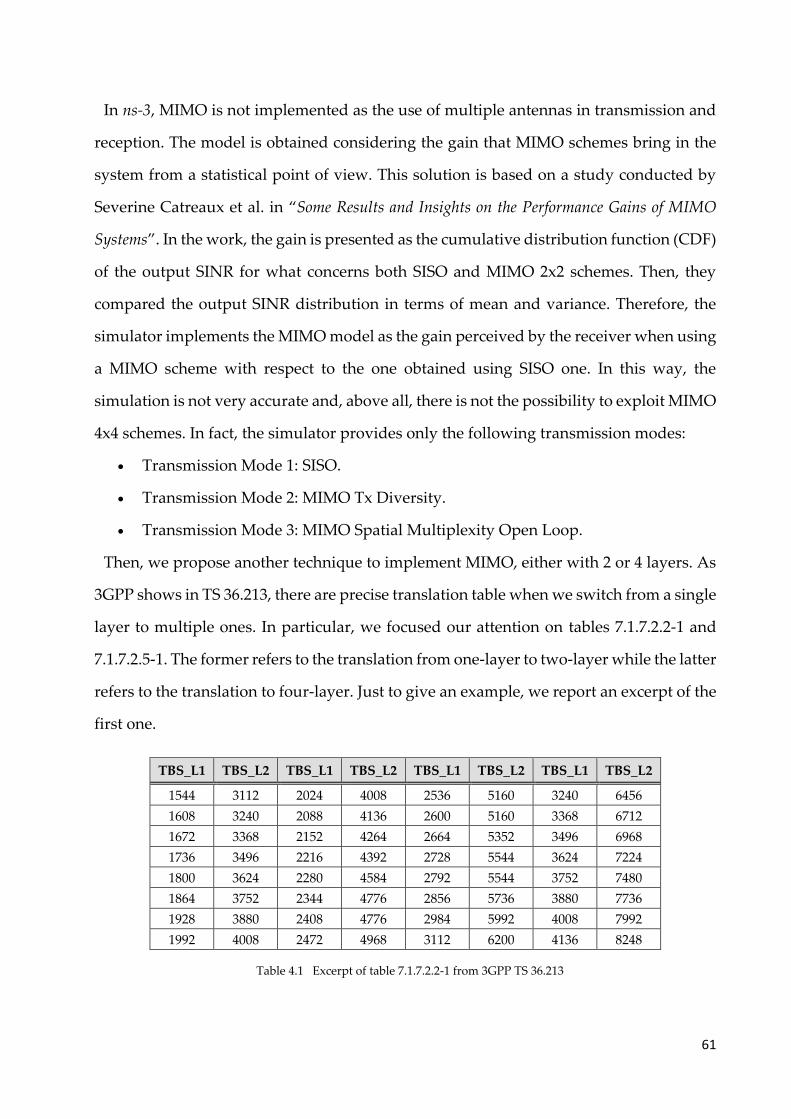
61

In ns-3, MIMO is not implemented as the use of multiple antennas in transmission and

reception. The model is obtained considering the gain that MIMO schemes bring in the

system from a statistical point of view. This solution is based on a study conducted by

Severine Catreaux et al. in “Some Results and Insights on the Performance Gains of MIMO

Systems”. In the work, the gain is presented as the cumulative distribution function (CDF)

of the output SINR for what concerns both SISO and MIMO 2x2 schemes. Then, they

compared the output SINR distribution in terms of mean and variance. Therefore, the

simulator implements the MIMO model as the gain perceived by the receiver when using

a MIMO scheme with respect to the one obtained using SISO one. In this way, the

simulation is not very accurate and, above all, there is not the possibility to exploit MIMO

4x4 schemes. In fact, the simulator provides only the following transmission modes:

• Transmission Mode 1: SISO.

• Transmission Mode 2: MIMO Tx Diversity.

• Transmission Mode 3: MIMO Spatial Multiplexity Open Loop.

Then, we propose another technique to implement MIMO, either with 2 or 4 layers. As

3GPP shows in TS 36.213, there are precise translation table when we switch from a single

layer to multiple ones. In particular, we focused our attention on tables 7.1.7.2.2-1 and

7.1.7.2.5-1. The former refers to the translation from one-layer to two-layer while the latter

refers to the translation to four-layer. Just to give an example, we report an excerpt of the

first one.

Table 4.1 Excerpt of table 7.1.7.2.2-1 from 3GPP TS 36.213

TBS_L1 TBS_L2 TBS_L1 TBS_L2 TBS_L1 TBS_L2 TBS_L1 TBS_L2

1544 3112 2024 4008 2536 5160 3240 6456

1608 3240 2088 4136 2600 5160 3368 6712

1672 3368 2152 4264 2664 5352 3496 6968

1736 3496 2216 4392 2728 5544 3624 7224

1800 3624 2280 4584 2792 5544 3752 7480

1864 3752 2344 4776 2856 5736 3880 7736

1928 3880 2408 4776 2984 5992 4008 7992

1992 4008 2472 4968 3112 6200 4136 8248

62

From here, it is evident that the usage of MIMO 2x2 leads to an average doubling of the

TBS. Equally, the TBS is quadrupled in presence of MIMO 4x4. This observation of this

relationship between the transport block size and the number of layer led us to

implement MIMO schemes as the multiplication of the TBS. We adapted the function

GetTbSizeFromMcs in LteAmc so that it returns the TBS doubled (or quadrupled)

depending on the MIMO scheme.

As seen in Chapter 2, the four-layer technology is more sensitive to SINR with respect

to the two-layer scheme. To regard this aspect, it is useful to evaluate the CQI of each

transmission and decide whether to allow the adoption of MIMO 4x4. To do this, we

made an if-clause inside the function mentioned above.

Our proposal for implementing the Carrier Aggregation is simple: we locate multiple

devices or eNBs in the same place and, if necessary, we make them move jointly. This

follows the reality: in fact, a device has an antenna for each frequency used to received

and/or transmit. One problem would be the unawareness when scheduling resources.

Actually, there are two kinds of scheduling procedure: Single-Carrier Scheduler and

Cross-Carrier Scheduler. The former is the one used nowadays in real networks and

doesn’t imply each frequency receiver to be aware one another.

A second problem was the mobility of co-located devices: in fact, we wanted them to

move randomly across the scenario. We would have used the RandomDirection2D

mobility model but in this way the devices wouldn’t have moved jointly. The we decided

to use the GaussMarkov mobility model.

Unlike the other mobility models in ns-3, which are memoryless, the Gauss Markov

model has both memory and variability. The tunable alpha parameter determines the

amount of memory and randomness in the model. Each object starts with a specific

velocity, direction (radians), and pitch angle (radians) equivalent to the mean velocity,

direction, and pitch. At each timestep, a new velocity, direction, and pitch angle are

generated based upon the previous value, the mean value, and a gaussian random

variable. Then, applying this model contemporaneously to the “carrier” devices, we

obtain co-located entities that move jointly with a certain randomness.

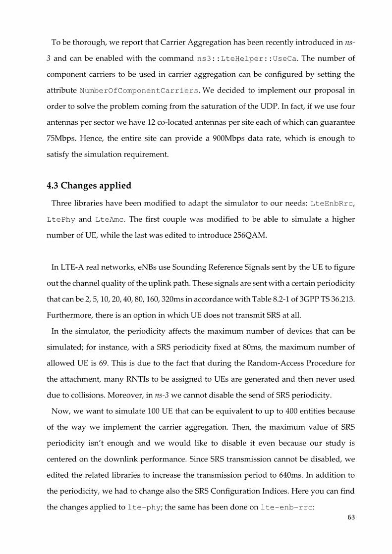
63

To be thorough, we report that Carrier Aggregation has been recently introduced in ns-

3 and can be enabled with the command ns3::LteHelper::UseCa. The number of

component carriers to be used in carrier aggregation can be configured by setting the

attribute NumberOfComponentCarriers. We decided to implement our proposal in

order to solve the problem coming from the saturation of the UDP. In fact, if we use four

antennas per sector we have 12 co-located antennas per site each of which can guarantee

75Mbps. Hence, the entire site can provide a 900Mbps data rate, which is enough to

satisfy the simulation requirement.

4.3 Changes applied

Three libraries have been modified to adapt the simulator to our needs: LteEnbRrc,

LtePhy and LteAmc. The first couple was modified to be able to simulate a higher

number of UE, while the last was edited to introduce 256QAM.

In LTE-A real networks, eNBs use Sounding Reference Signals sent by the UE to figure

out the channel quality of the uplink path. These signals are sent with a certain periodicity

that can be 2, 5, 10, 20, 40, 80, 160, 320ms in accordance with Table 8.2-1 of 3GPP TS 36.213.

Furthermore, there is an option in which UE does not transmit SRS at all.

In the simulator, the periodicity affects the maximum number of devices that can be

simulated; for instance, with a SRS periodicity fixed at 80ms, the maximum number of

allowed UE is 69. This is due to the fact that during the Random-Access Procedure for

the attachment, many RNTIs to be assigned to UEs are generated and then never used

due to collisions. Moreover, in ns-3 we cannot disable the send of SRS periodicity.

Now, we want to simulate 100 UE that can be equivalent to up to 400 entities because

of the way we implement the carrier aggregation. Then, the maximum value of SRS

periodicity isn’t enough and we would like to disable it even because our study is

centered on the downlink performance. Since SRS transmission cannot be disabled, we

edited the related libraries to increase the transmission period to 640ms. In addition to

the periodicity, we had to change also the SRS Configuration Indices. Here you can find

the changes applied to lte-phy; the same has been done on lte-enb-rrc:

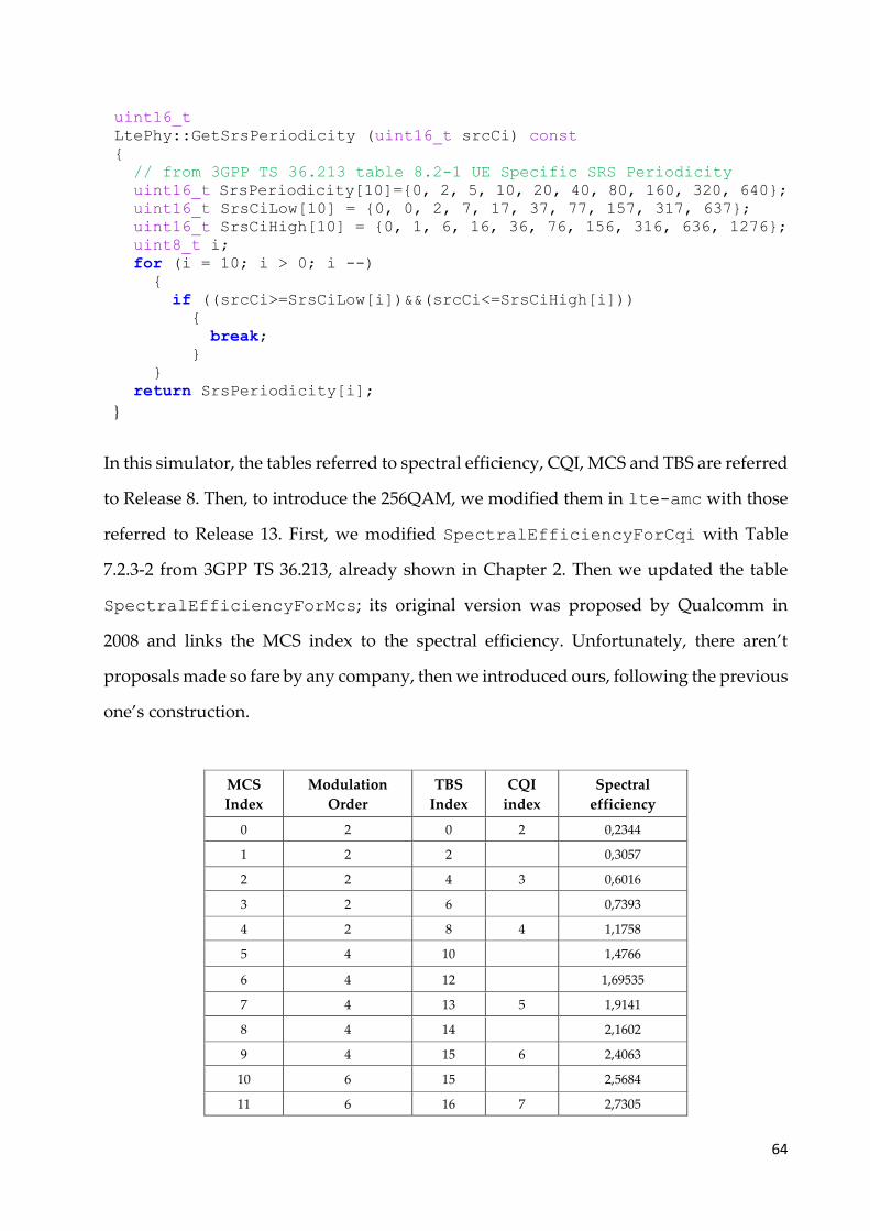
64

uint16_t

LtePhy::GetSrsPeriodicity (uint16_t srcCi) const

{

// from 3GPP TS 36.213 table 8.2-1 UE Specific SRS Periodicity

uint16_t SrsPeriodicity[10]={0, 2, 5, 10, 20, 40, 80, 160, 320, 640};

uint16_t SrsCiLow[10] = {0, 0, 2, 7, 17, 37, 77, 157, 317, 637};

uint16_t SrsCiHigh[10] = {0, 1, 6, 16, 36, 76, 156, 316, 636, 1276};

uint8_t i;

for (i = 10; i > 0; i --)

{

if ((srcCi>=SrsCiLow[i])&&(srcCi<=SrsCiHigh[i]))

{

break;

}

}

return SrsPeriodicity[i];

}

In this simulator, the tables referred to spectral efficiency, CQI, MCS and TBS are referred

to Release 8. Then, to introduce the 256QAM, we modified them in lte-amc with those

referred to Release 13. First, we modified SpectralEfficiencyForCqi with Table

7.2.3-2 from 3GPP TS 36.213, already shown in Chapter 2. Then we updated the table

SpectralEfficiencyForMcs; its original version was proposed by Qualcomm in

2008 and links the MCS index to the spectral efficiency. Unfortunately, there aren’t

proposals made so fare by any company, then we introduced ours, following the previous

one’s construction.

MCS

Index

Modulation

Order

TBS

Index

CQI

index

Spectral

efficiency

0 2 0 2 0,2344

1 2 2 0,3057

2 2 4 3 0,6016

3 2 6 0,7393

4 2 8 4 1,1758

5 4 10 1,4766

6 4 12 1,69535

7 4 13 5 1,9141

8 4 14 2,1602

9 4 15 6 2,4063

10 6 15 2,5684

11 6 16 7 2,7305

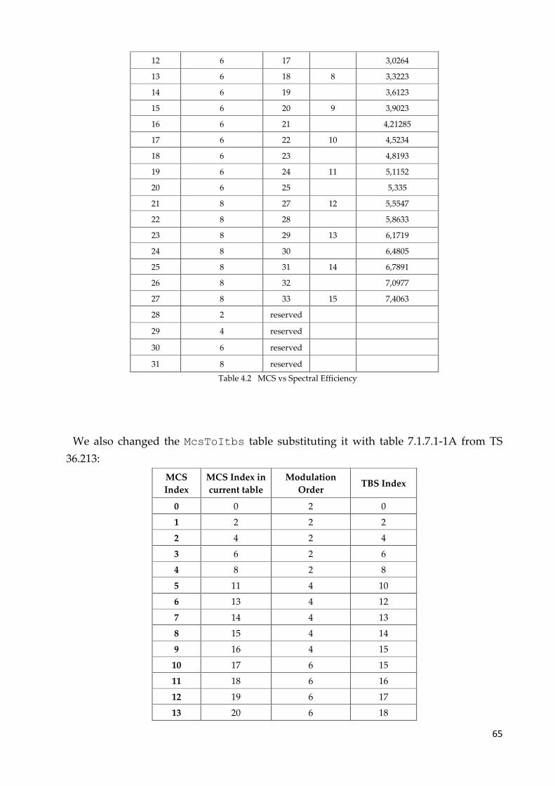
65

12 6 17 3,0264

13 6 18 8 3,3223

14 6 19 3,6123

15 6 20 9 3,9023

16 6 21 4,21285

17 6 22 10 4,5234

18 6 23 4,8193

19 6 24 11 5,1152

20 6 25 5,335

21 8 27 12 5,5547

22 8 28 5,8633

23 8 29 13 6,1719

24 8 30 6,4805

25 8 31 14 6,7891

26 8 32 7,0977

27 8 33 15 7,4063

28 2 reserved

29 4 reserved

30 6 reserved

31 8 reserved

Table 4.2 MCS vs Spectral Efficiency

We also changed the McsToItbs table substituting it with table 7.1.7.1-1A from TS

36.213:

MCS

Index

MCS Index in

current table

Modulation

Order TBS Index

0 0 2 0

1 2 2 2

2 4 2 4

3 6 2 6

4 8 2 8

5 11 4 10

6 13 4 12

7 14 4 13

8 15 4 14

9 16 4 15

10 17 6 15

11 18 6 16

12 19 6 17

13 20 6 18

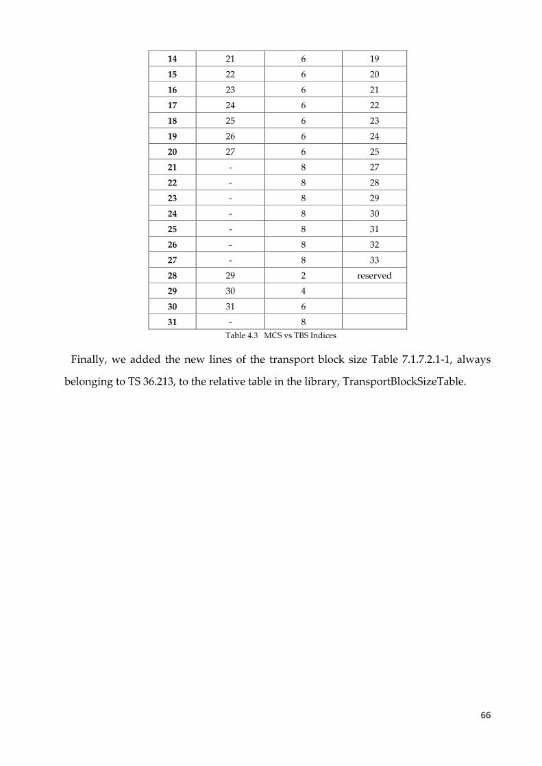
66

14 21 6 19

15 22 6 20

16 23 6 21

17 24 6 22

18 25 6 23

19 26 6 24

20 27 6 25

21 - 8 27

22 - 8 28

23 - 8 29

24 - 8 30

25 - 8 31

26 - 8 32

27 - 8 33

28 29 2 reserved

29 30 4

30 31 6

31 - 8

Table 4.3 MCS vs TBS Indices

Finally, we added the new lines of the transport block size Table 7.1.7.2.1-1, always

belonging to TS 36.213, to the relative table in the library, TransportBlockSizeTable.

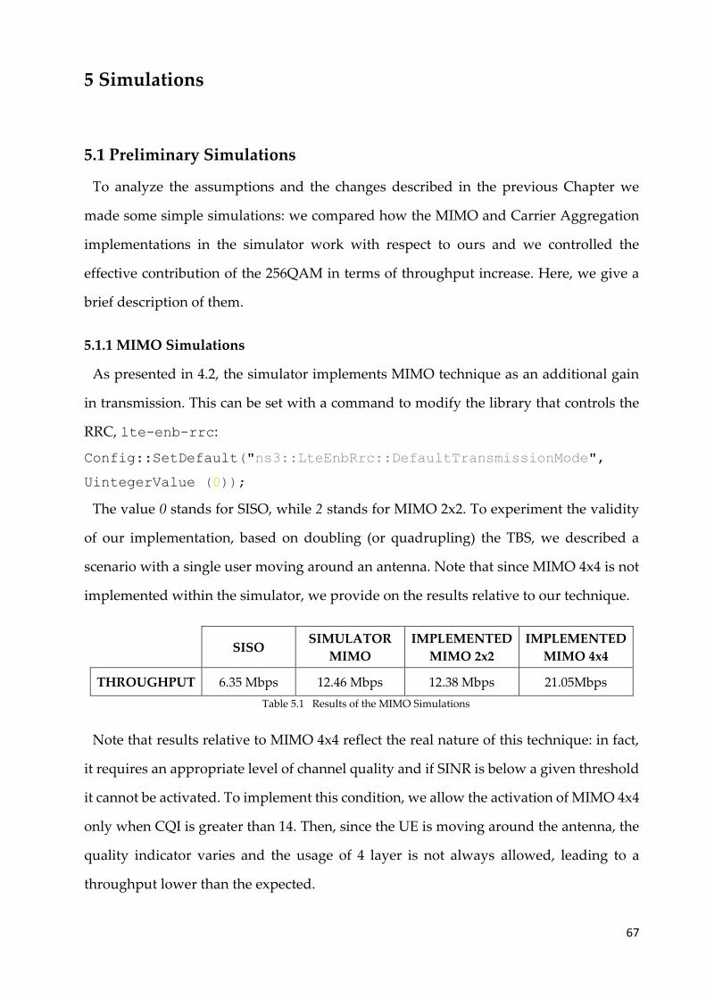
67

5 Simulations

5.1 Preliminary Simulations

To analyze the assumptions and the changes described in the previous Chapter we

made some simple simulations: we compared how the MIMO and Carrier Aggregation

implementations in the simulator work with respect to ours and we controlled the

effective contribution of the 256QAM in terms of throughput increase. Here, we give a

brief description of them.

5.1.1 MIMO Simulations

As presented in 4.2, the simulator implements MIMO technique as an additional gain

in transmission. This can be set with a command to modify the library that controls the

RRC, lte-enb-rrc:

Config::SetDefault("ns3::LteEnbRrc::DefaultTransmissionMode",

UintegerValue (0));

The value 0 stands for SISO, while 2 stands for MIMO 2x2. To experiment the validity

of our implementation, based on doubling (or quadrupling) the TBS, we described a

scenario with a single user moving around an antenna. Note that since MIMO 4x4 is not

implemented within the simulator, we provide on the results relative to our technique.

SISO SIMULATOR

MIMO

IMPLEMENTED

MIMO 2x2

IMPLEMENTED

MIMO 4x4

THROUGHPUT 6.35 Mbps 12.46 Mbps 12.38 Mbps 21.05Mbps

Table 5.1 Results of the MIMO Simulations

Note that results relative to MIMO 4x4 reflect the real nature of this technique: in fact,

it requires an appropriate level of channel quality and if SINR is below a given threshold

it cannot be activated. To implement this condition, we allow the activation of MIMO 4x4

only when CQI is greater than 14. Then, since the UE is moving around the antenna, the

quality indicator varies and the usage of 4 layer is not always allowed, leading to a

throughput lower than the expected.

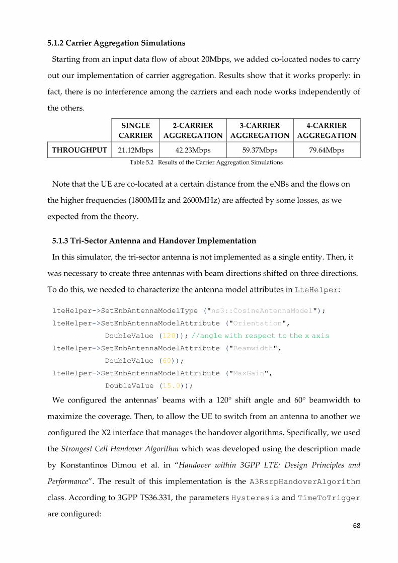
68

5.1.2 Carrier Aggregation Simulations

Starting from an input data flow of about 20Mbps, we added co-located nodes to carry

out our implementation of carrier aggregation. Results show that it works properly: in

fact, there is no interference among the carriers and each node works independently of

the others.

SINGLE

CARRIER

2-CARRIER

AGGREGATION

3-CARRIER

AGGREGATION

4-CARRIER

AGGREGATION

THROUGHPUT 21.12Mbps 42.23Mbps 59.37Mbps 79.64Mbps

Table 5.2 Results of the Carrier Aggregation Simulations

Note that the UE are co-located at a certain distance from the eNBs and the flows on

the higher frequencies (1800MHz and 2600MHz) are affected by some losses, as we

expected from the theory.

5.1.3 Tri-Sector Antenna and Handover Implementation

In this simulator, the tri-sector antenna is not implemented as a single entity. Then, it

was necessary to create three antennas with beam directions shifted on three directions.

To do this, we needed to characterize the antenna model attributes in LteHelper:

lteHelper->SetEnbAntennaModelType ("ns3::CosineAntennaModel");

lteHelper->SetEnbAntennaModelAttribute ("Orientation",

DoubleValue (120)); //angle with respect to the x axis

lteHelper->SetEnbAntennaModelAttribute ("Beamwidth",

DoubleValue (60));

lteHelper->SetEnbAntennaModelAttribute ("MaxGain",

DoubleValue (15.0));

We configured the antennas’ beams with a 120° shift angle and 60° beamwidth to

maximize the coverage. Then, to allow the UE to switch from an antenna to another we

configured the X2 interface that manages the handover algorithms. Specifically, we used

the Strongest Cell Handover Algorithm which was developed using the description made

by Konstantinos Dimou et al. in “Handover within 3GPP LTE: Design Principles and

Performance”. The result of this implementation is the A3RsrpHandoverAlgorithm

class. According to 3GPP TS36.331, the parameters Hysteresis and TimeToTrigger

are configured:

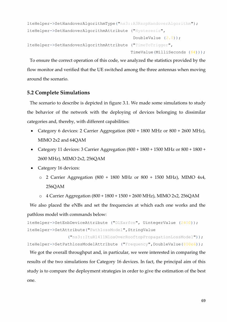
69

lteHelper->SetHandoverAlgorithmType("ns3::A3RsrpHandoverAlgorithm");

lteHelper->SetHandoverAlgorithmAttribute ("Hysteresis",

DoubleValue (2.0));

lteHelper->SetHandoverAlgorithmAttribute ("TimeToTrigger",

TimeValue(MilliSeconds (64)));

To ensure the correct operation of this code, we analyzed the statistics provided by the

flow monitor and verified that the UE switched among the three antennas when moving

around the scenario.

5.2 Complete Simulations

The scenario to describe is depicted in figure 3.1. We made some simulations to study

the behavior of the network with the deploying of devices belonging to dissimilar

categories and, thereby, with different capabilities:

• Category 6 devices: 2 Carrier Aggregation (800 + 1800 MHz or 800 + 2600 MHz),

MIMO 2x2 and 64QAM

• Category 11 devices: 3 Carrier Aggregation (800 + 1800 + 1500 MHz or 800 + 1800 +

2600 MHz), MIMO 2x2, 256QAM

• Category 16 devices:

o 2 Carrier Aggregation (800 + 1800 MHz or 800 + 1500 MHz), MIMO 4x4,

256QAM

o 4 Carrier Aggregation (800 + 1800 + 1500 + 2600 MHz), MIMO 2x2, 256QAM

We also placed the eNBs and set the frequencies at which each one works and the

pathloss model with commands below:

lteHelper->SetEnbDeviceAttribute ("DlEarfcn", UintegerValue (2400));

lteHelper->SetAttribute("PathlossModel",StringValue

("ns3::ItuR1411NlosOverRooftopPropagationLossModel"));

lteHelper->SetPathlossModelAttribute ("Frequency",DoubleValue(800e6));

We got the overall throughput and, in particular, we were interested in comparing the

results of the two simulations for Category 16 devices. In fact, the principal aim of this

study is to compare the deployment strategies in order to give the estimation of the best

one.

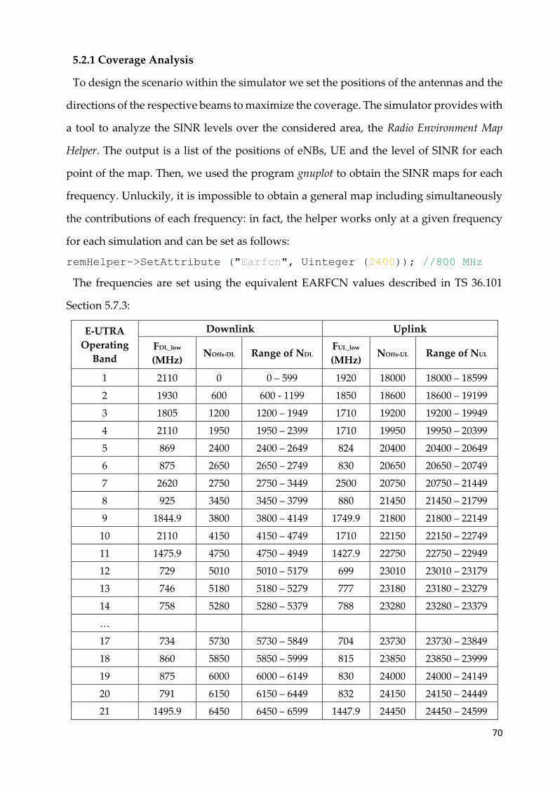
70

5.2.1 Coverage Analysis

To design the scenario within the simulator we set the positions of the antennas and the

directions of the respective beams to maximize the coverage. The simulator provides with

a tool to analyze the SINR levels over the considered area, the Radio Environment Map

Helper. The output is a list of the positions of eNBs, UE and the level of SINR for each

point of the map. Then, we used the program gnuplot to obtain the SINR maps for each

frequency. Unluckily, it is impossible to obtain a general map including simultaneously

the contributions of each frequency: in fact, the helper works only at a given frequency

for each simulation and can be set as follows:

remHelper->SetAttribute ("Earfcn", Uinteger (2400)); //800 MHz

The frequencies are set using the equivalent EARFCN values described in TS 36.101

Section 5.7.3:

E-UTRA

Operating

Band

Downlink Uplink

FDL_low

(MHz) NOffs-DL Range of NDL

FUL_low

(MHz) NOffs-UL Range of NUL

1 2110 0 0 – 599 1920 18000 18000 – 18599

2 1930 600 600 - 1199 1850 18600 18600 – 19199

3 1805 1200 1200 – 1949 1710 19200 19200 – 19949

4 2110 1950 1950 – 2399 1710 19950 19950 – 20399

5 869 2400 2400 – 2649 824 20400 20400 – 20649

6 875 2650 2650 – 2749 830 20650 20650 – 20749

7 2620 2750 2750 – 3449 2500 20750 20750 – 21449

8 925 3450 3450 – 3799 880 21450 21450 – 21799

9 1844.9 3800 3800 – 4149 1749.9 21800 21800 – 22149

10 2110 4150 4150 – 4749 1710 22150 22150 – 22749

11 1475.9 4750 4750 – 4949 1427.9 22750 22750 – 22949

12 729 5010 5010 – 5179 699 23010 23010 – 23179

13 746 5180 5180 – 5279 777 23180 23180 – 23279

14 758 5280 5280 – 5379 788 23280 23280 – 23379

…

17 734 5730 5730 – 5849 704 23730 23730 – 23849

18 860 5850 5850 – 5999 815 23850 23850 – 23999

19 875 6000 6000 – 6149 830 24000 24000 – 24149

20 791 6150 6150 – 6449 832 24150 24150 – 24449

21 1495.9 6450 6450 – 6599 1447.9 24450 24450 – 24599

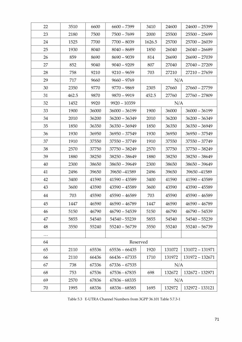
71

22 3510 6600 6600 – 7399 3410 24600 24600 – 25399

23 2180 7500 7500 – 7699 2000 25500 25500 – 25699

24 1525 7700 7700 – 8039 1626.5 25700 25700 – 26039

25 1930 8040 8040 – 8689 1850 26040 26040 – 26689

26 859 8690 8690 – 9039 814 26690 26690 – 27039

27 852 9040 9040 – 9209 807 27040 27040 – 27209

28 758 9210 9210 – 9659 703 27210 27210 – 27659

29 717 9660 9660 – 9769 N/A

30 2350 9770 9770 – 9869 2305 27660 27660 – 27759

31 462.5 9870 9870 – 9919 452.5 27760 27760 – 27809

32 1452 9920 9920 – 10359 N/A

33 1900 36000 36000 – 36199 1900 36000 36000 – 36199

34 2010 36200 36200 – 36349 2010 36200 36200 – 36349

35 1850 36350 36350 – 36949 1850 36350 36350 – 36949

36 1930 36950 36950 – 37549 1930 36950 36950 – 37549

37 1910 37550 37550 – 37749 1910 37550 37550 – 37749

38 2570 37750 37750 – 38249 2570 37750 37750 – 38249

39 1880 38250 38250 – 38649 1880 38250 38250 – 38649

40 2300 38650 38650 – 39649 2300 38650 38650 – 39649

41 2496 39650 39650 –41589 2496 39650 39650 –41589

42 3400 41590 41590 – 43589 3400 41590 41590 – 43589

43 3600 43590 43590 – 45589 3600 43590 43590 – 45589

44 703 45590 45590 – 46589 703 45590 45590 – 46589

45 1447 46590 46590 – 46789 1447 46590 46590 – 46789

46 5150 46790 46790 – 54539 5150 46790 46790 – 54539

47 5855 54540 54540 - 55239 5855 54540 54540 – 55239

48 3550 55240 55240 – 56739 3550 55240 55240 – 56739

…

64 Reserved

65 2110 65536 65536 – 66435 1920 131072 131072 – 131971

66 2110 66436 66436 – 67335 1710 131972 131972 – 132671

67 738 67336 67336 – 67535 N/A

68 753 67536 67536 - 67835 698 132672 132672 - 132971

69 2570 67836 67836 - 68335 N/A

70 1995 68336 68336 - 68585 1695 132972 132972 - 133121

Table 5.3 E-UTRA Channel Numbers from 3GPP 36.101 Table 5.7.3-1

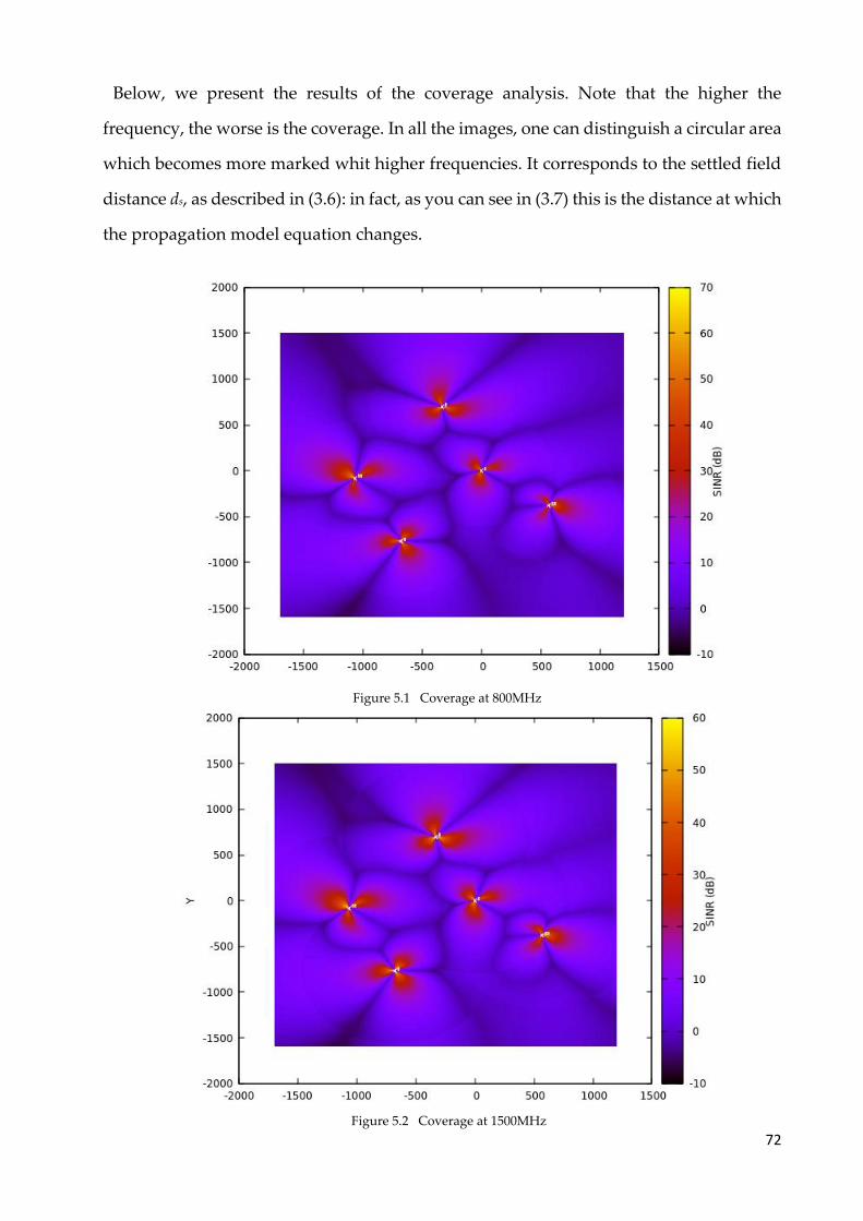
72

Below, we present the results of the coverage analysis. Note that the higher the

frequency, the worse is the coverage. In all the images, one can distinguish a circular area

which becomes more marked whit higher frequencies. It corresponds to the settled field

distance ds, as described in (3.6): in fact, as you can see in (3.7) this is the distance at which

the propagation model equation changes.

Figure 5.1 Coverage at 800MHz

Figure 5.2 Coverage at 1500MHz

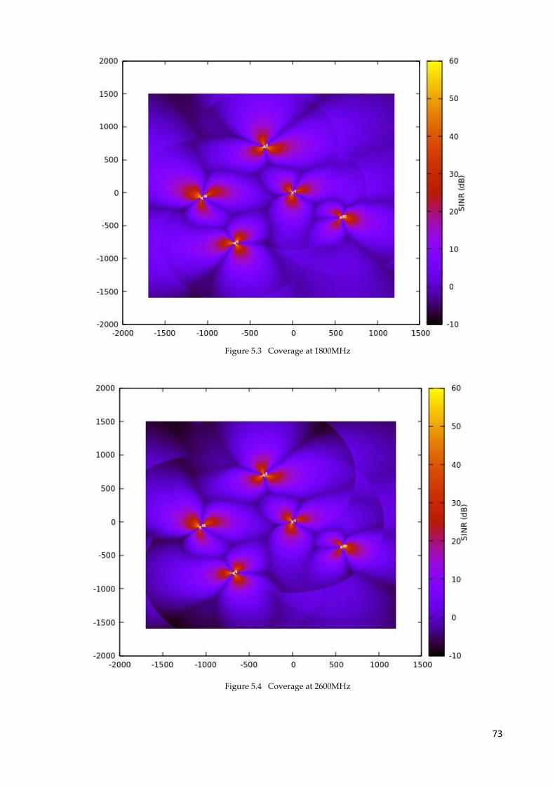
73

Figure 5.3 Coverage at 1800MHz

Figure 5.4 Coverage at 2600MHz

74

5.2.2 Category 6 Deployment

First of all, to implement a Cat6 device we created two distinct entities to configure the

2 Carrier Aggregation. Since the modulation for these devices is the 64QAM, we used the

LteAmc file as it was first intended by the simulators developers, without updating the

TBS tables. Then, after the configuration of the IP addresses, we attached the devices to

the eNBs with the proper frequencies using "for cycles" where the fundamental command

is:

lteHelper->AttachToClosestEnb (ueDevs_cat6.Get(i), enbDevs_800);

Note that we used the AttachToClosestEnb instead of the more common Attach

function because the former allows to link a single user to multiple eNBs at the same time

so that the UE can do the handover among them.

The peak data rate for a single Cat6 UE is 300Mbps. This comes from the following

considerations: the 64QAM uses 6 bits per symbol. In each symbol there are 12 subframes.

Moreover, we need to consider the number of Sub-Carriers: with a 20MHz bandwidth,

there are 1200 Sub-Carriers. Then, considering that the duration of a TTI is 1ms the peak

data rate with SISO and 64QAM is:

Number of bits/symbol ∙ Number of symbols/subframe ∙ Number of Sub-Carriers

TTI =

6 ∙ 12 ∙ 1200

10−3= 86.4Mbps

This is what we obtain at PHY layer. The peak data rate should be evaluated at the MAC

layer and one should consider the overheads introduced, e.g. for signaling. Hence, we

consider that for 20MHz with 64QAM and SISO transmission the peak data rate is

75Mbps.

The best configuration to employ MIMO 2x2 as well was given by the usage of 1500 and

1800MHz to aggregate 35MHz and the peak throughput is:

(75 + 75) ∙ 2 = 300Mbps

Of course, this value is only a theoretical one and cannot be achieved in a dense urban

scenario, with many devices transmitting simultaneously. Moreover, the peak data rate

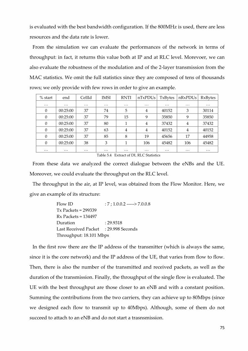
75

is evaluated with the best bandwidth configuration. If the 800MHz is used, there are less

resources and the data rate is lower.

From the simulation we can evaluate the performances of the network in terms of

throughput: in fact, it returns this value both at IP and at RLC level. Morevoer, we can

also evaluate the robustness of the modulation and of the 2-layer transmission from the

MAC statistics. We omit the full statistics since they are composed of tens of thousands

rows; we only provide with few rows in order to give an example.

% start end CellId IMSI RNTI nTxPDUs TxBytes nRxPDUs RxBytes

… … … … … … … … …

0 00:25:00 37 74 5 4 40152 3 30114

0 00:25:00 37 79 15 9 35850 9 35850

0 00:25:00 37 80 1 4 37432 4 37432

0 00:25:00 37 63 4 4 40152 4 40152

0 00:25:00 37 85 8 19 45656 17 44958

0 00:25:00 38 3 1 106 45482 106 45482

… … … … … … … … …

Table 5.4 Extract of DL RLC Statistics

From these data we analyzed the correct dialogue between the eNBs and the UE.

Moreover, we could evaluate the throughput on the RLC level.

The throughput in the air, at IP level, was obtained from the Flow Monitor. Here, we

give an example of its structure:

Flow ID : 7 ; 1.0.0.2 -----> 7.0.0.8

Tx Packets = 299339 Rx Packets = 134497 Duration : 29.9318 Last Received Packet : 29.998 Seconds Throughput: 18.101 Mbps

In the first row there are the IP address of the transmitter (which is always the same,

since it is the core network) and the IP address of the UE, that varies from flow to flow.

Then, there is also the number of the transmitted and received packets, as well as the

duration of the transmission. Finally, the throughput of the single flow is evaluated. The

UE with the best throughput are those closer to an eNB and with a constant position.

Summing the contributions from the two carriers, they can achieve up to 80Mbps (since

we designed each flow to transmit up to 40Mbps). Although, some of them do not

succeed to attach to an eNB and do not start a trasnsmission.

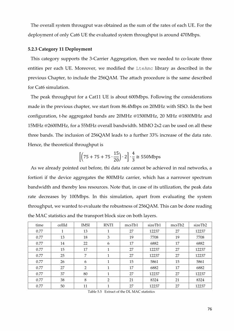
76

The overall system througput was obtained as the sum of the rates of each UE. For the

deployment of only Cat6 UE the evaluated system throughput is around 470Mbps.

5.2.3 Category 11 Deployment

This category supports the 3-Carrier Aggregation, then we needed to co-locate three

entities per each UE. Moreover, we modified the LteAmc library as described in the

previous Chapter, to include the 256QAM. The attach procedure is the same described

for Cat6 simulation.

The peak throughput for a Cat11 UE is about 600Mbps. Following the considerations

made in the previous chapter, we start from 86.4Mbps on 20MHz with SISO. In the best

configuration, t-he aggregated bands are 20MHz @1500MHz, 20 MHz @1800MHz and

15MHz @2600MHz, for a 55MHz overall bandwidth. MIMO 2x2 can be used on all these

three bands. The inclusion of 256QAM leads to a further 33% increase of the data rate.

Hence, the theoretical throughput is

[(75 + 75 + 75 ∙15

20) ∙ 2] ∙

4

3≅ 550Mbps

As we already pointed out before, thi data rate cannot be achieved in real networks, a

fortiori if the device aggregates the 800MHz carrier, which has a narrower spectrum

bandwidth and thereby less resources. Note that, in case of its utilization, the peak data

rate decreases by 100Mbps. In this simulation, apart from evaluating the system

throughput, we wanted to evaluate the robustness of 256QAM. This can be done reading

the MAC statistics and the transport block size on both layers.

time cellId IMSI RNTI mcsTb1 sizeTb1 mcsTb2 sizeTb2

0.77 1 13 1 27 12237 27 12237

0.77 13 18 3 19 7708 19 7708

0.77 14 22 6 17 6882 17 6882

0.77 15 17 1 27 12237 27 12237

0.77 25 7 1 27 12237 27 12237

0.77 26 6 1 15 5861 15 5861

0.77 27 2 1 17 6882 17 6882

0.77 37 80 1 27 12237 27 12237

0.77 38 8 2 21 8324 21 8324

0.77 50 11 1 27 12237 27 12237

Table 5.5 Extract of the DL MAC statistics

77

The TB size on the two layers are expressed in bytes and must be multiplied by 8 to be

compared to the ones in LteAmc. For instance, the first row takes into account the channel

condition of a UE with a fix position, very close to the eNB. In fact, the MCS is the

maximum one as well as the TBS that is 97986 bits.

As reported in Table 4.3, the 256QAM can be activated only when the MCS is 21 or more.

Then, to evaluate the robustness of this modulation, we read through the complete MAC

statistics to evaluate the efficiency as the ratio between the transmission with the

256QAM and the whole transmissions. As result, we obtained a 75% efficiency, which is

a very high percentage if we consider the dense urban environment.

As in the previous case, we also evaluated the system throughput. We summed the

throughputs of each flow and we obtained about 750Mbps.

5.2.3 Category 16 Simulations

The Cat16 devices can achieve their maximum data rate in the two ways already

described and that will be examined in depth below. Since one of them requires the

employ of MIMO 4x4, it was necessary to decrease the input flow: in fact, if we used

40Mbps we could not figure out the real adoption because of the 75Mbps limitation

introduced by the UDP traffic in this simulator. Then, differently from the simulations

made so far, we decreased it to 20Mbps.

The first approach we studied is the one focused on spectrum broadening that provides

for 4-Carrier Aggregation that leads to a usage of 65MHz on the four bands 800, 1500,

1800 and 2600MHz. MIMO 4x4 cannot be used since the limitation to 8 Antenna Port due

of RF component on the transceivers.

The maximum single user theoretical throughput for this configuration is evaluated in

the same way we obtained the previous ones:

[(75 + 75 + 75 ∙15

20+ 75 ∙

10

20) ∙ 2] ∙

4

3≅ 650Mbps

The overall system throughput, evaluated as the sum of each UE data rate, is about

790Mbps.

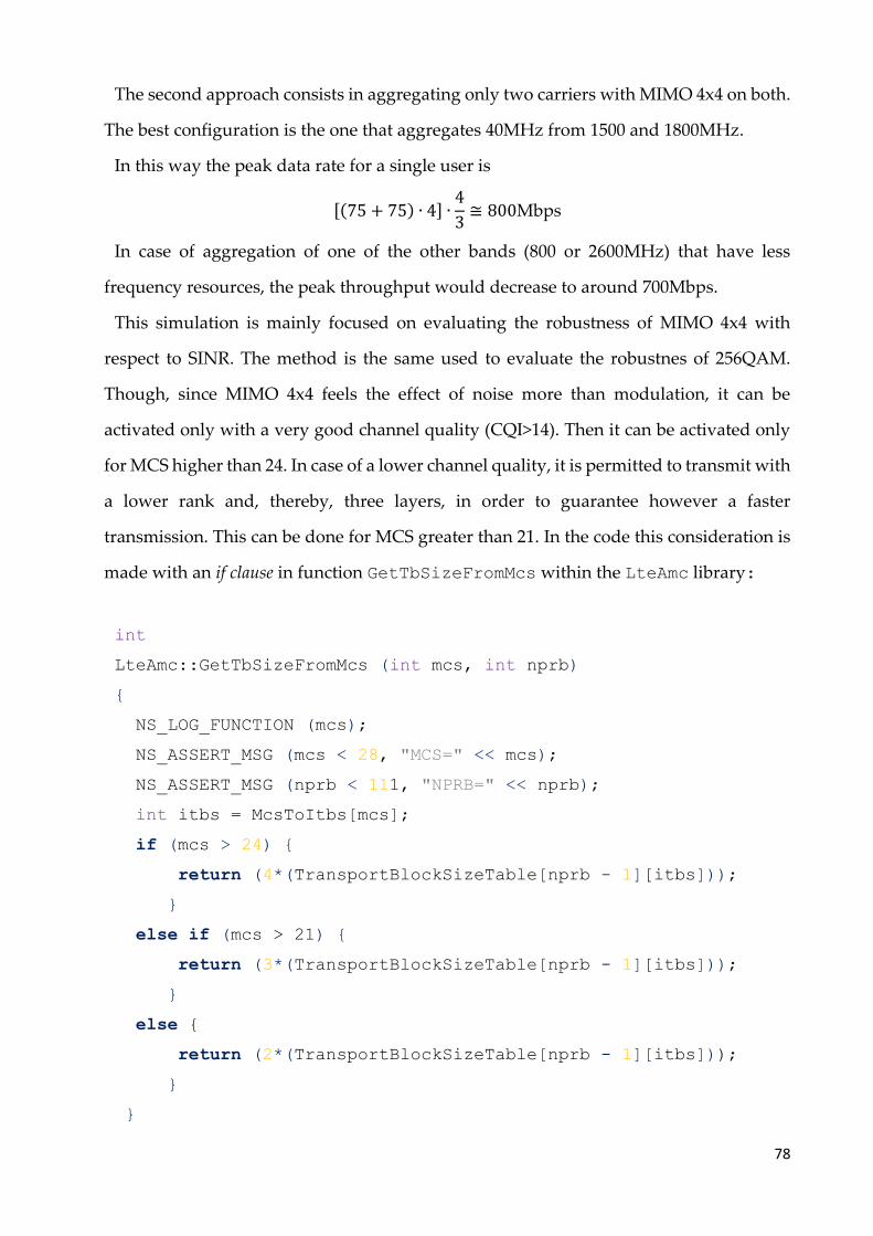
78

The second approach consists in aggregating only two carriers with MIMO 4x4 on both.

The best configuration is the one that aggregates 40MHz from 1500 and 1800MHz.

In this way the peak data rate for a single user is

[(75 + 75) ∙ 4] ∙4

3≅ 800Mbps

In case of aggregation of one of the other bands (800 or 2600MHz) that have less

frequency resources, the peak throughput would decrease to around 700Mbps.

This simulation is mainly focused on evaluating the robustness of MIMO 4x4 with

respect to SINR. The method is the same used to evaluate the robustnes of 256QAM.

Though, since MIMO 4x4 feels the effect of noise more than modulation, it can be

activated only with a very good channel quality (CQI>14). Then it can be activated only

for MCS higher than 24. In case of a lower channel quality, it is permitted to transmit with

a lower rank and, thereby, three layers, in order to guarantee however a faster

transmission. This can be done for MCS greater than 21. In the code this consideration is

made with an if clause in function GetTbSizeFromMcs within the LteAmc library:

int

LteAmc::GetTbSizeFromMcs (int mcs, int nprb)

{

NS_LOG_FUNCTION (mcs);

NS_ASSERT_MSG (mcs < 28, "MCS=" << mcs);

NS_ASSERT_MSG (nprb < 111, "NPRB=" << nprb);

int itbs = McsToItbs[mcs];

if (mcs > 24) {

return (4*(TransportBlockSizeTable[nprb - 1][itbs]));

}

else if (mcs > 21) {

return (3*(TransportBlockSizeTable[nprb - 1][itbs]));

}

else {

return (2*(TransportBlockSizeTable[nprb - 1][itbs]));

}

}

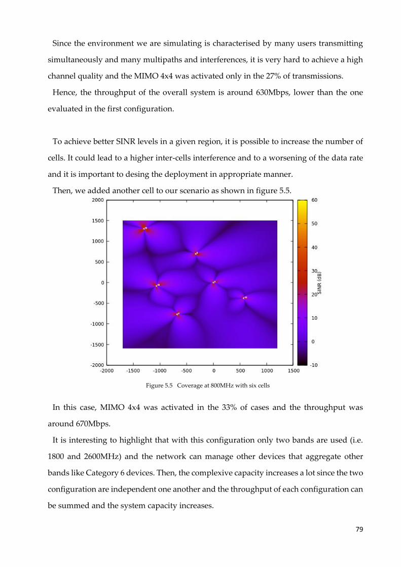
79

Since the environment we are simulating is characterised by many users transmitting

simultaneously and many multipaths and interferences, it is very hard to achieve a high

channel quality and the MIMO 4x4 was activated only in the 27% of transmissions.

Hence, the throughput of the overall system is around 630Mbps, lower than the one

evaluated in the first configuration.

To achieve better SINR levels in a given region, it is possible to increase the number of

cells. It could lead to a higher inter-cells interference and to a worsening of the data rate

and it is important to desing the deployment in appropriate manner.

Then, we added another cell to our scenario as shown in figure 5.5.

Figure 5.5 Coverage at 800MHz with six cells

In this case, MIMO 4x4 was activated in the 33% of cases and the throughput was

around 670Mbps.

It is interesting to highlight that with this configuration only two bands are used (i.e.

1800 and 2600MHz) and the network can manage other devices that aggregate other

bands like Category 6 devices. Then, the complexive capacity increases a lot since the two

configuration are independent one another and the throughput of each configuration can

be summed and the system capacity increases.

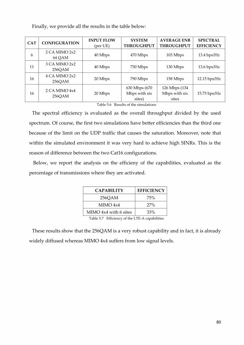
80

Finally, we provide all the results in the table below:

CAT CONFIGURATION INPUT FLOW

(per UE)

SYSTEM

THROUGHPUT

AVERAGE ENB

THROUGHPUT

SPECTRAL

EFFICIENCY

6 2 CA MIMO 2x2

64 QAM 40 Mbps 470 Mbps 103 Mbps 13.4 bps/Hz

11 3 CA MIMO 2x2

256QAM 40 Mbps 750 Mbps 130 Mbps 13.6 bps/Hz

16 4 CA MIMO 2x2

256QAM 20 Mbps 790 Mbps 158 Mbps 12.15 bps/Hz

16 2 CA MIMO 4x4

256QAM 20 Mbps

630 Mbps (670

Mbps with six

sites)

126 Mbps (134

Mbps with six

sites

15.75 bps/Hz

Table 5.6 Results of the simulations

The spectral efficiency is evaluated as the overall throughput divided by the used

spectrum. Of course, the first two simulations have better efficiencies than the third one

because of the limit on the UDP traffic that causes the saturation. Moreover, note that

within the simulated environment it was very hard to achieve high SINRs. This is the

reason of difference between the two Cat16 configurations.

Below, we report the analysis on the efficieny of the capabilities, evaluated as the

percentage of transmissions where they are activated.

CAPABILITY EFFICIENCY

256QAM 75%

MIMO 4x4 27%

MIMO 4x4 with 6 sites 33%

Table 5.7 Efficiency of the LTE-A capabilities

These results show that the 256QAM is a very robust capability and in fact, it is already

widely diffused whereas MIMO 4x4 suffers from low signal levels.

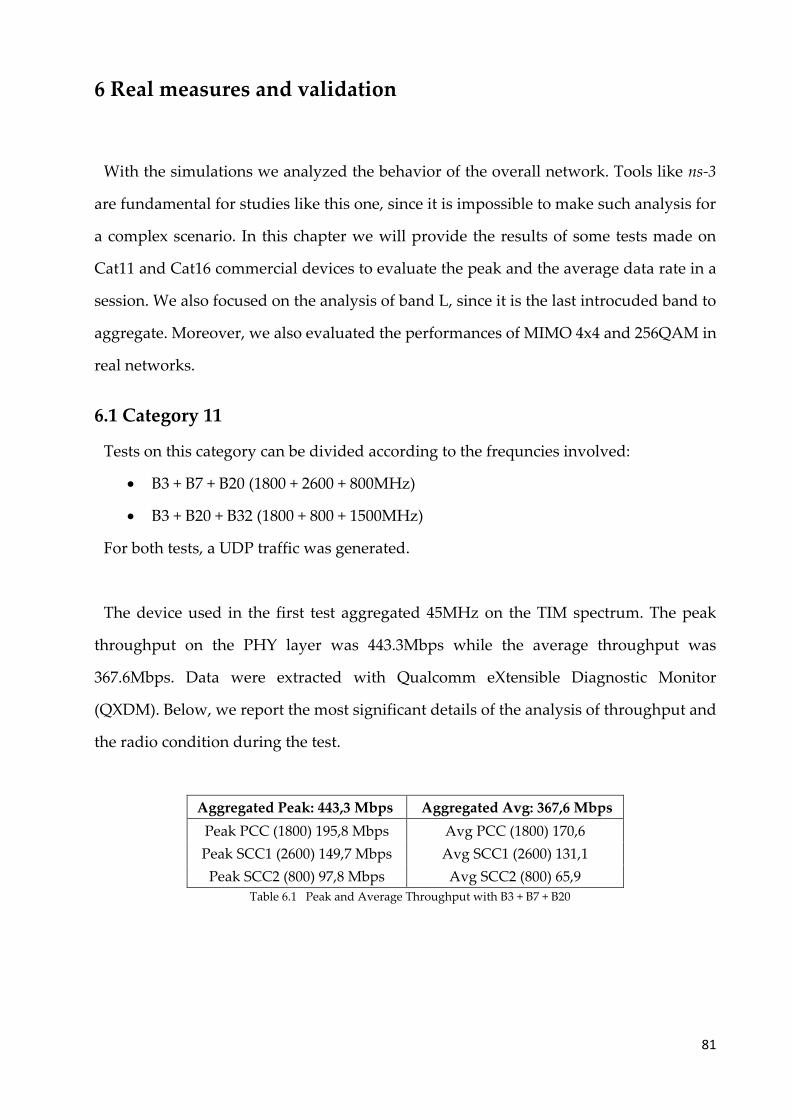
81

6 Real measures and validation

With the simulations we analyzed the behavior of the overall network. Tools like ns-3

are fundamental for studies like this one, since it is impossible to make such analysis for

a complex scenario. In this chapter we will provide the results of some tests made on

Cat11 and Cat16 commercial devices to evaluate the peak and the average data rate in a

session. We also focused on the analysis of band L, since it is the last introcuded band to

aggregate. Moreover, we also evaluated the performances of MIMO 4x4 and 256QAM in

real networks.

6.1 Category 11

Tests on this category can be divided according to the frequncies involved:

• B3 + B7 + B20 (1800 + 2600 + 800MHz)

• B3 + B20 + B32 (1800 + 800 + 1500MHz)

For both tests, a UDP traffic was generated.

The device used in the first test aggregated 45MHz on the TIM spectrum. The peak

throughput on the PHY layer was 443.3Mbps while the average throughput was

367.6Mbps. Data were extracted with Qualcomm eXtensible Diagnostic Monitor

(QXDM). Below, we report the most significant details of the analysis of throughput and

the radio condition during the test.

Aggregated Peak: 443,3 Mbps Aggregated Avg: 367,6 Mbps

Peak PCC (1800) 195,8 Mbps Avg PCC (1800) 170,6

Peak SCC1 (2600) 149,7 Mbps Avg SCC1 (2600) 131,1

Peak SCC2 (800) 97,8 Mbps Avg SCC2 (800) 65,9

Table 6.1 Peak and Average Throughput with B3 + B7 + B20

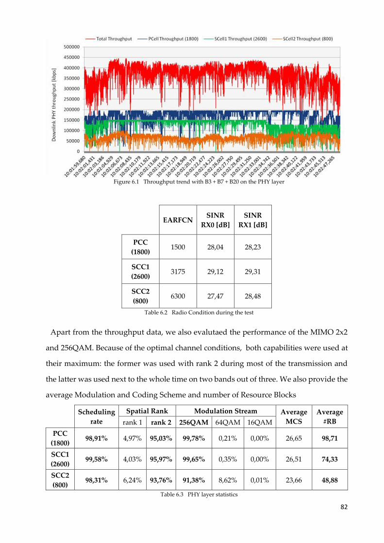
82

Figure 6.1 Throughput trend with B3 + B7 + B20 on the PHY layer

EARFCN SINR

RX0 [dB]

SINR

RX1 [dB]

PCC

(1800) 1500 28,04 28,23

SCC1

(2600) 3175 29,12 29,31

SCC2

(800) 6300 27,47 28,48

Table 6.2 Radio Condition during the test

Apart from the throughput data, we also evalutaed the performance of the MIMO 2x2

and 256QAM. Because of the optimal channel conditions, both capabilities were used at

their maximum: the former was used with rank 2 during most of the transmission and

the latter was used next to the whole time on two bands out of three. We also provide the

average Modulation and Coding Scheme and number of Resource Blocks

Scheduling

rate

Spatial Rank Modulation Stream Average

MCS

Average

#RB rank 1 rank 2 256QAM 64QAM 16QAM

PCC

(1800) 98,91% 4,97% 95,03% 99,78% 0,21% 0,00% 26,65 98,71

SCC1

(2600) 99,58% 4,03% 95,97% 99,65% 0,35% 0,00% 26,51 74,33

SCC2

(800) 98,31% 6,24% 93,76% 91,38% 8,62% 0,01% 23,66 48,88

Table 6.3 PHY layer statistics

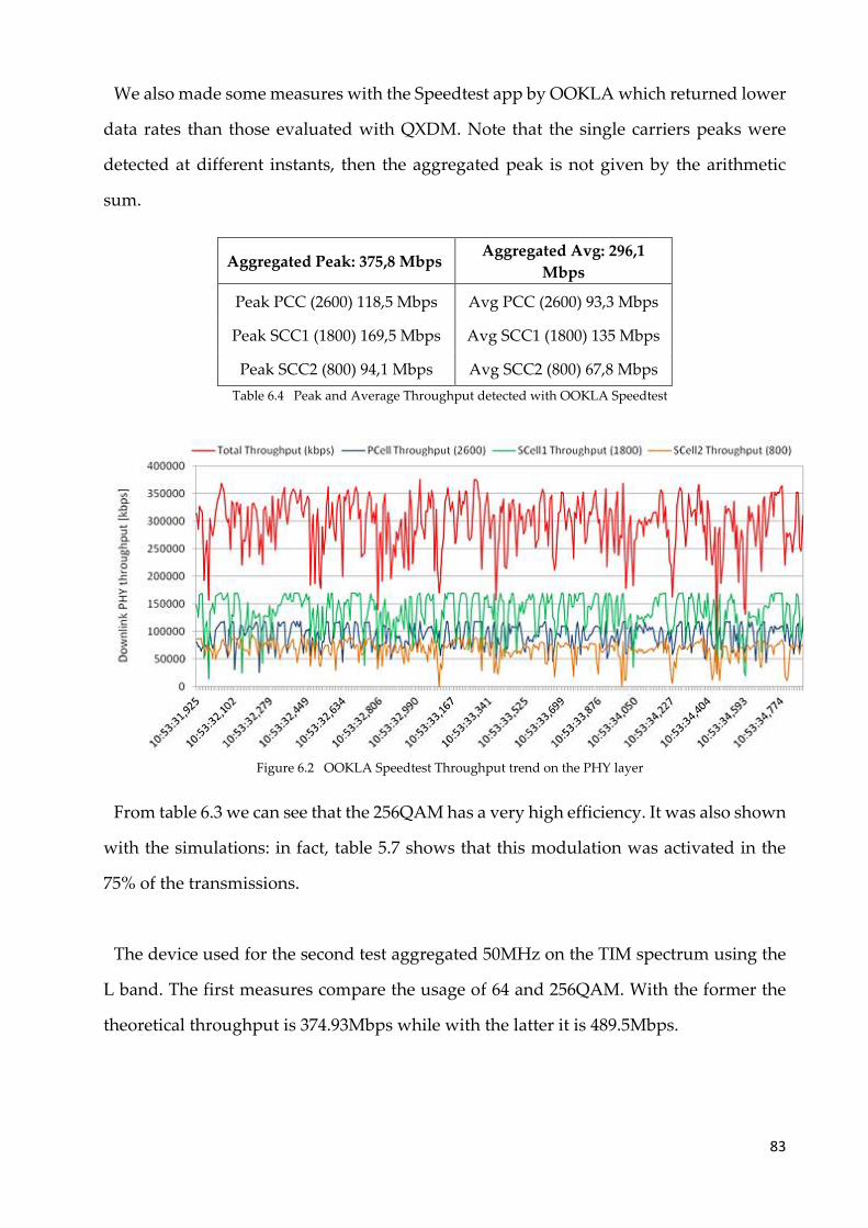
83

We also made some measures with the Speedtest app by OOKLA which returned lower

data rates than those evaluated with QXDM. Note that the single carriers peaks were

detected at different instants, then the aggregated peak is not given by the arithmetic

sum.

Aggregated Peak: 375,8 Mbps Aggregated Avg: 296,1

Mbps

Peak PCC (2600) 118,5 Mbps Avg PCC (2600) 93,3 Mbps

Peak SCC1 (1800) 169,5 Mbps Avg SCC1 (1800) 135 Mbps

Peak SCC2 (800) 94,1 Mbps Avg SCC2 (800) 67,8 Mbps

Table 6.4 Peak and Average Throughput detected with OOKLA Speedtest

Figure 6.2 OOKLA Speedtest Throughput trend on the PHY layer

From table 6.3 we can see that the 256QAM has a very high efficiency. It was also shown

with the simulations: in fact, table 5.7 shows that this modulation was activated in the

75% of the transmissions.

The device used for the second test aggregated 50MHz on the TIM spectrum using the

L band. The first measures compare the usage of 64 and 256QAM. With the former the

theoretical throughput is 374.93Mbps while with the latter it is 489.5Mbps.

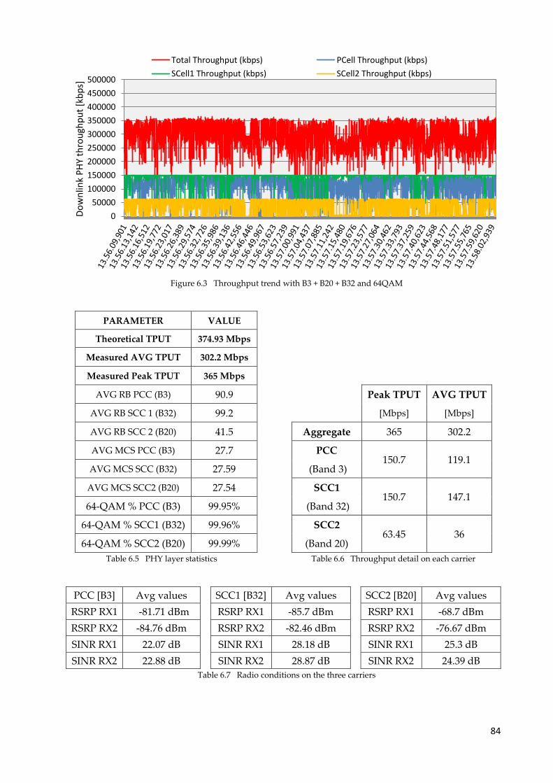
84

Figure 6.3 Throughput trend with B3 + B20 + B32 and 64QAM

PARAMETER VALUE

Theoretical TPUT 374.93 Mbps

Measured AVG TPUT 302.2 Mbps

Measured Peak TPUT 365 Mbps

AVG RB PCC (B3) 90.9 Peak TPUT AVG TPUT

AVG RB SCC 1 (B32) 99.2 [Mbps] [Mbps]

AVG RB SCC 2 (B20) 41.5 Aggregate 365 302.2

AVG MCS PCC (B3) 27.7 PCC 150.7 119.1

AVG MCS SCC (B32) 27.59 (Band 3)

AVG MCS SCC2 (B20) 27.54 SCC1 150.7 147.1

64-QAM % PCC (B3) 99.95% (Band 32)

64-QAM % SCC1 (B32) 99.96% SCC2 63.45 36

64-QAM % SCC2 (B20) 99.99% (Band 20)

Table 6.5 PHY layer statistics Table 6.6 Throughput detail on each carrier

PCC [B3] Avg values SCC1 [B32] Avg values SCC2 [B20] Avg values

RSRP RX1 -81.71 dBm RSRP RX1 -85.7 dBm RSRP RX1 -68.7 dBm

RSRP RX2 -84.76 dBm RSRP RX2 -82.46 dBm RSRP RX2 -76.67 dBm

SINR RX1 22.07 dB SINR RX1 28.18 dB SINR RX1 25.3 dB

SINR RX2 22.88 dB SINR RX2 28.87 dB SINR RX2 24.39 dB

Table 6.7 Radio conditions on the three carriers

0

50000

100000

150000

200000

250000

300000

350000

400000

450000

500000D

ow

nlin

k P

HY

thro

ugh

pu

t [k

bp

s]

Total Throughput (kbps) PCell Throughput (kbps)

SCell1 Throughput (kbps) SCell2 Throughput (kbps)

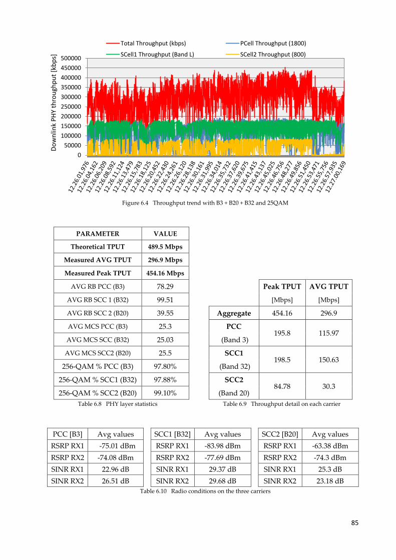
85

0

50000

100000

150000

200000

250000

300000

350000

400000

450000

500000D

ow

nlin

k P

HY

thro

ugh

pu

t [k

bp

s]

Total Throughput (kbps) PCell Throughput (1800)

SCell1 Throughput (Band L) SCell2 Throughput (800)

Figure 6.4 Throughput trend with B3 + B20 + B32 and 25QAM

PARAMETER VALUE

Theoretical TPUT 489.5 Mbps

Measured AVG TPUT 296.9 Mbps

Measured Peak TPUT 454.16 Mbps

AVG RB PCC (B3) 78.29 Peak TPUT AVG TPUT

AVG RB SCC 1 (B32) 99.51 [Mbps] [Mbps]

AVG RB SCC 2 (B20) 39.55 Aggregate 454.16 296.9

AVG MCS PCC (B3) 25.3 PCC 195.8 115.97

AVG MCS SCC (B32) 25.03 (Band 3)

AVG MCS SCC2 (B20) 25.5 SCC1 198.5 150.63

256-QAM % PCC (B3) 97.80% (Band 32)

256-QAM % SCC1 (B32) 97.88% SCC2 84.78 30.3

256-QAM % SCC2 (B20) 99.10% (Band 20)

Table 6.8 PHY layer statistics Table 6.9 Throughput detail on each carrier

PCC [B3] Avg values SCC1 [B32] Avg values SCC2 [B20] Avg values

RSRP RX1 -75.01 dBm RSRP RX1 -83.98 dBm RSRP RX1 -63.38 dBm

RSRP RX2 -74.08 dBm RSRP RX2 -77.69 dBm RSRP RX2 -74.3 dBm

SINR RX1 22.96 dB SINR RX1 29.37 dB SINR RX1 25.3 dB

SINR RX2 26.51 dB SINR RX2 29.68 dB SINR RX2 23.18 dB

Table 6.10 Radio conditions on the three carriers

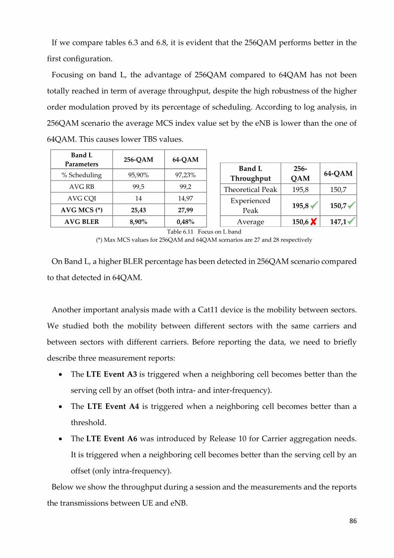
86

If we compare tables 6.3 and 6.8, it is evident that the 256QAM performs better in the

first configuration.

Focusing on band L, the advantage of 256QAM compared to 64QAM has not been

totally reached in term of average throughput, despite the high robustness of the higher

order modulation proved by its percentage of scheduling. According to log analysis, in

256QAM scenario the average MCS index value set by the eNB is lower than the one of

64QAM. This causes lower TBS values.

Band L

Parameters 256-QAM 64-QAM

% Scheduling 95,90% 97,23%

AVG RB 99,5 99,2

AVG CQI 14 14,97

AVG MCS (*) 25,43 27,99

AVG BLER 8,90% 0,48%

Table 6.11 Focus on L band

(*) Max MCS values for 256QAM and 64QAM scenarios are 27 and 28 respectively

On Band L, a higher BLER percentage has been detected in 256QAM scenario compared

to that detected in 64QAM.

Another important analysis made with a Cat11 device is the mobility between sectors.

We studied both the mobility between different sectors with the same carriers and

between sectors with different carriers. Before reporting the data, we need to briefly

describe three measurement reports:

• The LTE Event A3 is triggered when a neighboring cell becomes better than the

serving cell by an offset (both intra- and inter-frequency).

• The LTE Event A4 is triggered when a neighboring cell becomes better than a

threshold.

• The LTE Event A6 was introduced by Release 10 for Carrier aggregation needs.

It is triggered when a neighboring cell becomes better than the serving cell by an

offset (only intra-frequency).

Below we show the throughput during a session and the measurements and the reports

the transmissions between UE and eNB.

Band L

Throughput

256-

QAM 64-QAM

Theoretical Peak 195,8 150,7

Experienced

Peak 195,8 150,7

Average 150,6 147,1

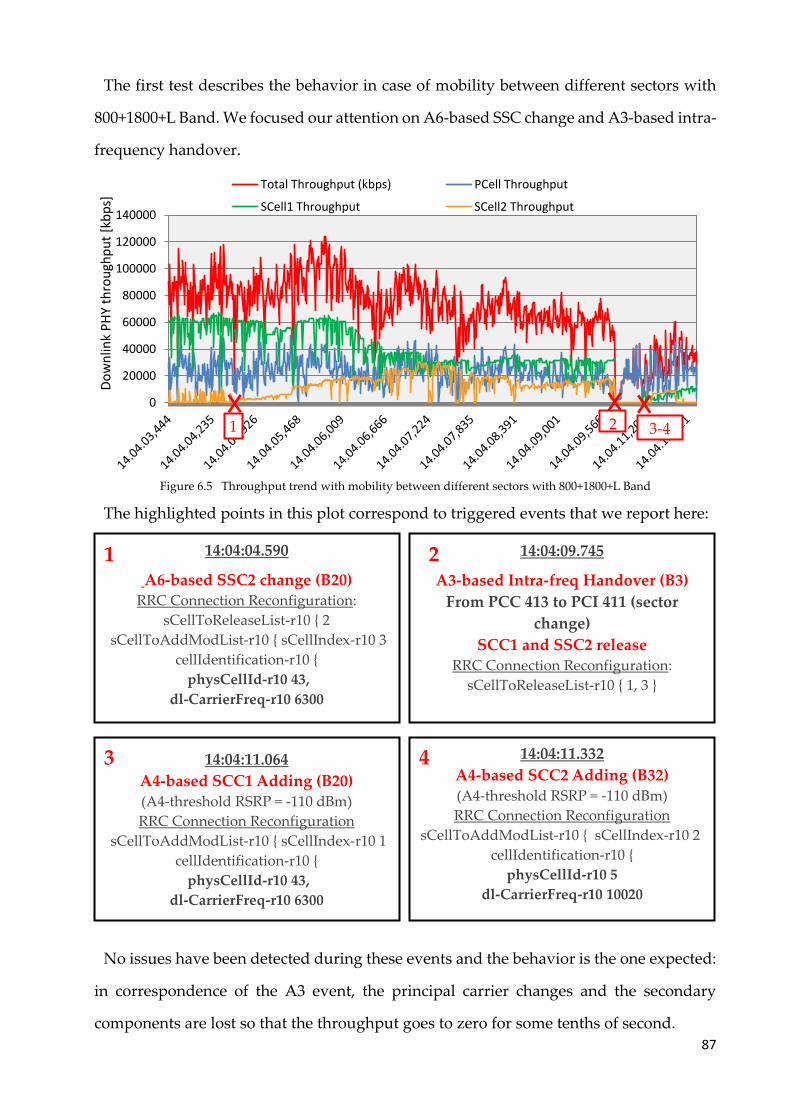
87

The first test describes the behavior in case of mobility between different sectors with

800+1800+L Band. We focused our attention on A6-based SSC change and A3-based intra-

frequency handover.

Figure 6.5 Throughput trend with mobility between different sectors with 800+1800+L Band

The highlighted points in this plot correspond to triggered events that we report here:

No issues have been detected during these events and the behavior is the one expected:

in correspondence of the A3 event, the principal carrier changes and the secondary

components are lost so that the throughput goes to zero for some tenths of second.

0

20000

40000

60000

80000

100000

120000

140000

Do

wn

link

PH

Y th

rou

ghp

ut

[kb

ps]

Total Throughput (kbps) PCell Throughput

SCell1 Throughput SCell2 Throughput

1 2 3-4

14:04:04.590

A6-based SSC2 change (B20) RRC Connection Reconfiguration:

sCellToReleaseList-r10 { 2 sCellToAddModList-r10 { sCellIndex-r10 3

cellIdentification-r10 { physCellId-r10 43,

dl-CarrierFreq-r10 6300

1 14:04:09.745

A3-based Intra-freq Handover (B3)

From PCC 413 to PCI 411 (sector

change)

SCC1 and SSC2 release RRC Connection Reconfiguration:

sCellToReleaseList-r10 { 1, 3 }

2

14:04:11.064

A4-based SCC1 Adding (B20) (A4-threshold RSRP = -110 dBm)

RRC Connection Reconfiguration sCellToAddModList-r10 { sCellIndex-r10 1

cellIdentification-r10 { physCellId-r10 43,

dl-CarrierFreq-r10 6300

3 14:04:11.332

A4-based SCC2 Adding (B32) (A4-threshold RSRP = -110 dBm)

RRC Connection Reconfiguration sCellToAddModList-r10 { sCellIndex-r10 2,

cellIdentification-r10 { physCellId-r10 5

dl-CarrierFreq-r10 10020

4

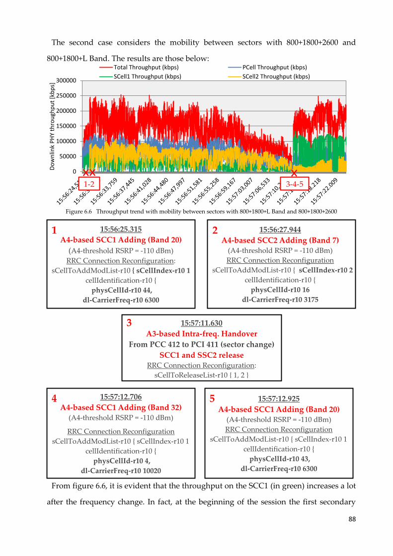
88

0

50000

100000

150000

200000

250000

300000

Do

wn

link

PH

Y th

rou

ghp

ut

[kb

ps]

Total Throughput (kbps) PCell Throughput (kbps)

SCell1 Throughput (kbps) SCell2 Throughput (kbps)

1-2 3-4-5

The second case considers the mobility between sectors with 800+1800+2600 and

800+1800+L Band. The results are those below:

Figure 6.6 Throughput trend with mobility between sectors with 800+1800+L Band and 800+1800+2600

From figure 6.6, it is evident that the throughput on the SCC1 (in green) increases a lot

after the frequency change. In fact, at the beginning of the session the first secondary

15:56:25.315

A4-based SCC1 Adding (Band 20)

(A4-threshold RSRP = -110 dBm) RRC Connection Reconfiguration:

sCellToAddModList-r10 { sCellIndex-r10 1 cellIdentification-r10 {

physCellId-r10 44, dl-CarrierFreq-r10 6300

15:56:27.944

A4-based SCC2 Adding (Band 7) (A4-threshold RSRP = -110 dBm)

RRC Connection Reconfiguration sCellToAddModList-r10 { sCellIndex-r10 2

cellIdentification-r10 { physCellId-r10 16

dl-CarrierFreq-r10 3175

1 2

15:57:11.630

A3-based Intra-freq. Handover

From PCC 412 to PCI 411 (sector change)

SCC1 and SSC2 release RRC Connection Reconfiguration:

sCellToReleaseList-r10 { 1, 2 }

3

15:57:12.706

A4-based SCC1 Adding (Band 32) (A4-threshold RSRP = -110 dBm)

RRC Connection Reconfiguration sCellToAddModList-r10 { sCellIndex-r10 1

cellIdentification-r10 { physCellId-r10 4,

dl-CarrierFreq-r10 10020

4 15:57:12.925

A4-based SCC1 Adding (Band 20) (A4-threshold RSRP = -110 dBm)

RRC Connection Reconfiguration sCellToAddModList-r10 { sCellIndex-r10 1

cellIdentification-r10 { physCellId-r10 43,

dl-CarrierFreq-r10 6300

5

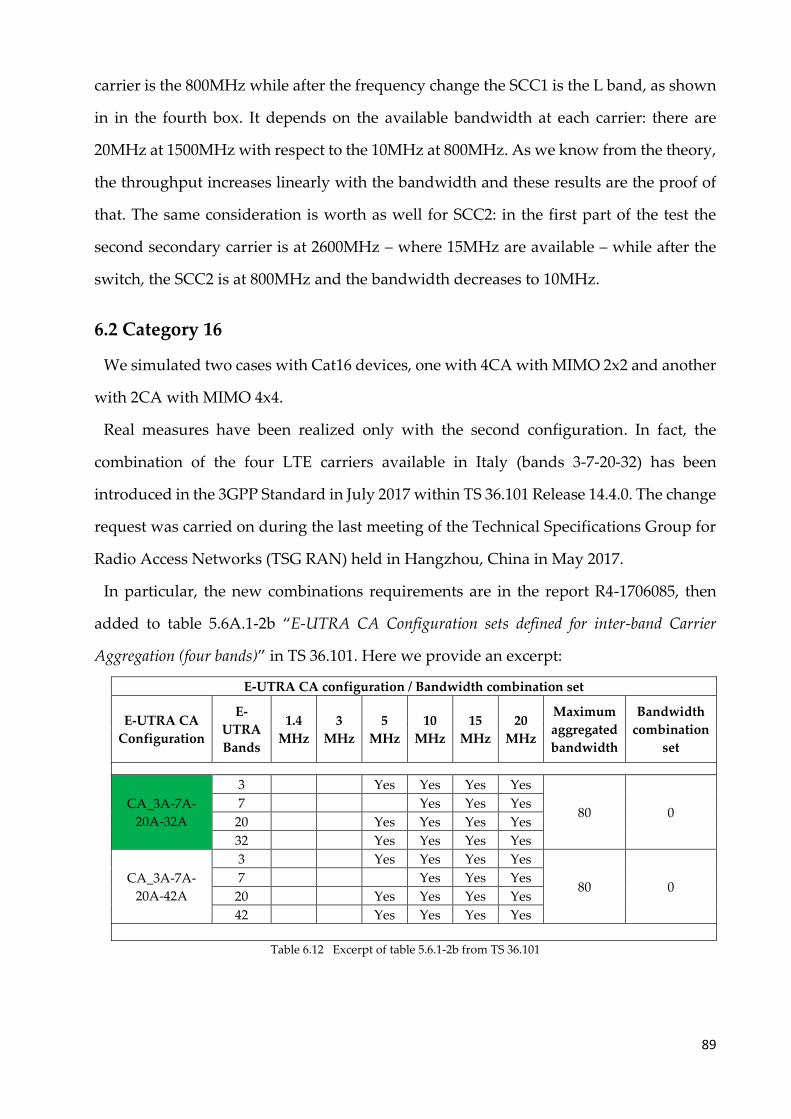
89

carrier is the 800MHz while after the frequency change the SCC1 is the L band, as shown

in in the fourth box. It depends on the available bandwidth at each carrier: there are

20MHz at 1500MHz with respect to the 10MHz at 800MHz. As we know from the theory,

the throughput increases linearly with the bandwidth and these results are the proof of

that. The same consideration is worth as well for SCC2: in the first part of the test the

second secondary carrier is at 2600MHz – where 15MHz are available – while after the

switch, the SCC2 is at 800MHz and the bandwidth decreases to 10MHz.

6.2 Category 16

We simulated two cases with Cat16 devices, one with 4CA with MIMO 2x2 and another

with 2CA with MIMO 4x4.

Real measures have been realized only with the second configuration. In fact, the

combination of the four LTE carriers available in Italy (bands 3-7-20-32) has been

introduced in the 3GPP Standard in July 2017 within TS 36.101 Release 14.4.0. The change

request was carried on during the last meeting of the Technical Specifications Group for

Radio Access Networks (TSG RAN) held in Hangzhou, China in May 2017.

In particular, the new combinations requirements are in the report R4-1706085, then

added to table 5.6A.1-2b “E-UTRA CA Configuration sets defined for inter-band Carrier

Aggregation (four bands)” in TS 36.101. Here we provide an excerpt:

E-UTRA CA configuration / Bandwidth combination set

E-UTRA CA

Configuration

E-

UTRA

Bands

1.4

MHz

3

MHz

5

MHz

10

MHz

15

MHz

20

MHz

Maximum

aggregated

bandwidth

Bandwidth

combination

set

CA_3A-7A-

20A-32A

3 Yes Yes Yes Yes

80 0 7 Yes Yes Yes

20 Yes Yes Yes Yes

32 Yes Yes Yes Yes

CA_3A-7A-

20A-42A

3 Yes Yes Yes Yes

80 0 7 Yes Yes Yes

20 Yes Yes Yes Yes

42 Yes Yes Yes Yes

Table 6.12 Excerpt of table 5.6.1-2b from TS 36.101

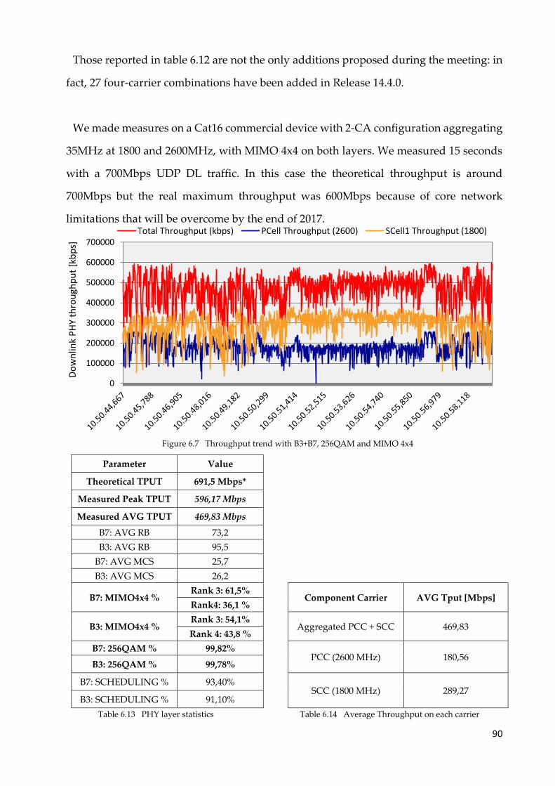
90

0

100000

200000

300000

400000

500000

600000

700000

Do

wn

link

PH

Y th

rou

ghp

ut

[kb

ps]

Total Throughput (kbps) PCell Throughput (2600) SCell1 Throughput (1800)

Those reported in table 6.12 are not the only additions proposed during the meeting: in

fact, 27 four-carrier combinations have been added in Release 14.4.0.

We made measures on a Cat16 commercial device with 2-CA configuration aggregating

35MHz at 1800 and 2600MHz, with MIMO 4x4 on both layers. We measured 15 seconds

with a 700Mbps UDP DL traffic. In this case the theoretical throughput is around

700Mbps but the real maximum throughput was 600Mbps because of core network

limitations that will be overcome by the end of 2017.

Figure 6.7 Throughput trend with B3+B7, 256QAM and MIMO 4x4

Parameter Value

Theoretical TPUT 691,5 Mbps*

Measured Peak TPUT 596,17 Mbps

Measured AVG TPUT 469,83 Mbps

B7: AVG RB 73,2

B3: AVG RB 95,5

B7: AVG MCS 25,7

B3: AVG MCS 26,2

B7: MIMO4x4 % Rank 3: 61,5%

Component Carrier AVG Tput [Mbps] Rank4: 36,1 %

B3: MIMO4x4 % Rank 3: 54,1%

Aggregated PCC + SCC 469,83 Rank 4: 43,8 %

B7: 256QAM % 99,82%

PCC (2600 MHz) 180,56 B3: 256QAM % 99,78%

B7: SCHEDULING % 93,40%

SCC (1800 MHz) 289,27 B3: SCHEDULING % 91,10%

Table 6.13 PHY layer statistics Table 6.14 Average Throughput on each carrier

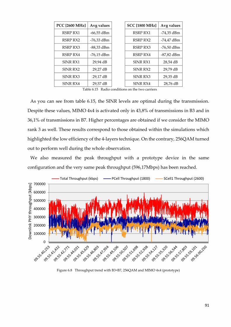
91

PCC [2600 MHz] Avg values SCC [1800 MHz] Avg values

RSRP RX1 -66,55 dBm RSRP RX1 -74,35 dBm

RSRP RX2 -76,33 dBm RSRP RX2 -74,47 dBm

RSRP RX3 -88,33 dBm RSRP RX3 -76,50 dBm

RSRP RX4 -76,15 dBm RSRP RX4 -87,82 dBm

SINR RX1 29,94 dB SINR RX1 28,54 dB

SINR RX2 29,27 dB SINR RX2 29,79 dB

SINR RX3 29,17 dB SINR RX3 29,35 dB

SINR RX4 29,57 dB SINR RX4 28,76 dB

Table 6.15 Radio conditions on the two carriers

As you can see from table 6.15, the SINR levels are optimal during the transmission.

Despite these values, MIMO 4x4 is activated only in 43,8% of transmissions in B3 and in

36,1% of transmissions in B7. Higher percentages are obtained if we consider the MIMO

rank 3 as well. These results correspond to those obtained within the simulations which

highlighted the low efficiency of the 4-layers technique. On the contrary, 256QAM turned

out to perform well during the whole observation.

We also measured the peak throughput with a prototype device in the same

configuration and the very same peak throughput (596,17Mbps) has been reached.

Figure 6.8 Throughput trend with B3+B7, 256QAM and MIMO 4x4 (prototype)

0

100000

200000

300000

400000

500000

600000

700000

Do

wn

link

PH

Y th

rou

ghp

ut

[kb

ps]

Total Throughput (kbps) PCell Throughput (1800) SCell1 Throughput (2600)

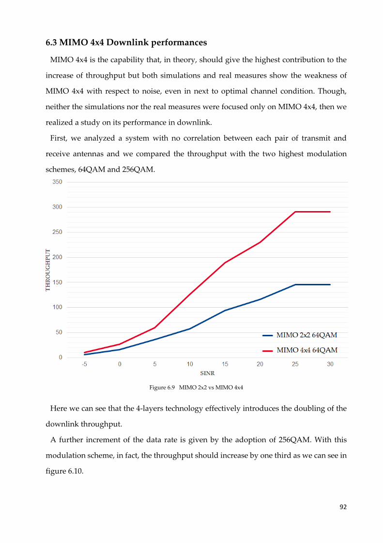
92

6.3 MIMO 4x4 Downlink performances

MIMO 4x4 is the capability that, in theory, should give the highest contribution to the

increase of throughput but both simulations and real measures show the weakness of

MIMO 4x4 with respect to noise, even in next to optimal channel condition. Though,

neither the simulations nor the real measures were focused only on MIMO 4x4, then we

realized a study on its performance in downlink.

First, we analyzed a system with no correlation between each pair of transmit and

receive antennas and we compared the throughput with the two highest modulation

schemes, 64QAM and 256QAM.

Figure 6.9 MIMO 2x2 vs MIMO 4x4

Here we can see that the 4-layers technology effectively introduces the doubling of the

downlink throughput.

A further increment of the data rate is given by the adoption of 256QAM. With this

modulation scheme, in fact, the throughput should increase by one third as we can see in

figure 6.10.

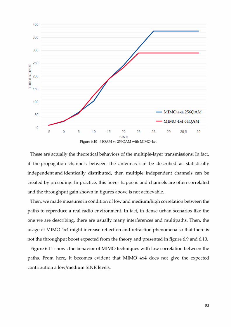
93

Figure 6.10 64QAM vs 256QAM with MIMO 4x4

These are actually the theoretical behaviors of the multiple-layer transmissions. In fact,

if the propagation channels between the antennas can be described as statistically

independent and identically distributed, then multiple independent channels can be

created by precoding. In practice, this never happens and channels are often correlated

and the throughput gain shown in figures above is not achievable.

Then, we made measures in condition of low and medium/high correlation between the

paths to reproduce a real radio environment. In fact, in dense urban scenarios like the

one we are describing, there are usually many interferences and multipaths. Then, the

usage of MIMO 4x4 might increase reflection and refraction phenomena so that there is

not the throughput boost expected from the theory and presented in figure 6.9 and 6.10.

Figure 6.11 shows the behavior of MIMO techniques with low correlation between the

paths. From here, it becomes evident that MIMO 4x4 does not give the expected

contribution a low/medium SINR levels.

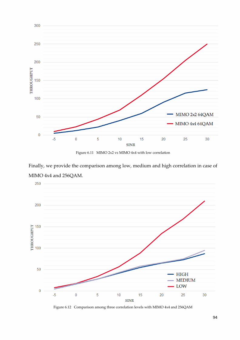
94

Figure 6.11 MIMO 2x2 vs MIMO 4x4 with low correlation

Finally, we provide the comparison among low, medium and high correlation in case of

MIMO 4x4 and 256QAM.

Figure 6.12 Comparison among three correlation levels with MIMO 4x4 and 256QAM

95

The theoretical limit with MIMO 4x4 and 256QAM is around 400Mbps on 20MHz. In

figure 6.12, we can see that this value cannot be reached at all, rather it is very far from

being achieved, in particular with medium/high correlation.

Even these measures showed the weakness of MIMO 4x4 in real scenarios with

multipaths and low signal levels, as it was already highlighted by the simulations and

general measures. However, in case of optimal channel quality, this technology given a

huge contribution to throughput, even in case of low correlation.

96

7 Conclusions and future work

The ever-changing mobile communications market and the request for higher speed

rates led to the birth and development of LTE-Advanced which will be the dominant

technology in the upcoming years.

In this thesis, we explored the architecture of LTE and LTE-A technologies and studied

the last introduced features. We also dealt with Standards and Specifications by 3GPP to

fully understand all the processes behind mobile transmissions. The key work was the

adaptation of a network simulator with the introduction of Carrier Aggregation, MIMO

4x4 and 256QAM and the simulation of a dense urban scenario to study the overall

system in terms of data rate and capacity.

We studied several deployments in order to evaluate the effectiveness of the LTE-A

capabilities and compared the results with real measures to figure out the deployment

strategies that mobile Operators should implement. In fact, there are two main

approaches that they could follow, either the spectrum broadening or the spectral

efficiency increase. Each of them has its advantages and disadvantages and we tried to

analyze all of them. In particular, we focused our attention on new devices that have just

entered the market or will be commercial by the end of 2017.

256QAM is already widely diffused and many devices support it. Our study showed

the robustness to noise of this feature and the contribution it gives in terms of data rate.

New devices can support up to 4-Carrier Aggregation over the licensed spectrum and

can aggregate also 100MHz. This leads to very high throughputs with a good robustness

to noise. But, since mobile Operators have a limited spectrum they are looking for ways

not to waste it. Innovative technologies for the forthcoming future will allow to aggregate

also unlicensed bands and studies on the coexistence with Wi-Fi are being carried on.

Then, the further enhancement of the spectral efficiency with multiple layers

transmissions seems to be the best strategy for mobile Operators: in fact, this would lead

to even higher throughputs without using the whole disposable spectrum. On the other

hand, this feature is highly affected by noise effects. In fact, our analysis showed the need

97

for very high SINR levels that are very difficult to achieve in an urban scenario. A solution

might be the deployment of small cells that, if well dimensioned, would guarantee a

better coverage and better signal levels but it would also entail elevated deploying costs

for Operators.

Hence, we suggest deploying MIMO 4x4 – and 8x8 when it will be available – only in

those sites where high SINRs are achievable like indoor scenarios or for those

applications that require very high data rates and low latency. Massive MIMO will be the

dominant technology for 5G communications that will provide for very dense cells and

very high SINR levels.

LTE-Advanced target data rate is 3Gbps but as we said in the Introduction it is not

achievable because of the limitation on the number of Antenna Port which is 8 nowadays.

It is interesting to underline that the peak spectral efficiency in the 800Mbps configuration

is 20bps/Hz which is comparable to 30bps/Hz required by the Standard for 5G

telecommunications (3GPP TR 38.913), although the restriction of the maximum Antenna

Port that will be overcome with the next generation technologies. This to remark that the

LTE-A is already near to the best performance that next generation telecommunication

networks will fulfill.

Future work will consist in the total adaptation of the ns-3 simulator to the requirements

of LTE-A, in the finalization of Carrier Aggregation and in the implementation of MIMO

4x4 (and above) within it.

Moreover, the limit on UDP traffic shall be overcome in order to completely fulfil the

data rate requirements of new devices.

Furthermore, measures on real Cat16 devices with the 4-Carrier Aggregation shall be

made as soon as they will be commercialized to compare real data to the results of the

simulation.

98

References

3GPP, “Requirements for Evolved UTRA (E-UTRA) and Evolved UTRAN (E-UTRAN)”,

3rd Generation Partnership Project (3GPP), TR 25.913, v. 7.0.0

3GPP, “Evolved Universal Terrestrial Radio Access (E-UTRA); User Equipment (UE)

radio transmission and reception”, 3rd Generation Partnership Project (3GPP), TS 36.101,

v. 14.4.0

3GPP, “Evolved Universal Terrestrial Radio Access (E-UTRA); Base Station (BS) radio

transmission and reception”, 3rd Generation Partnership Project (3GPP), TS 36.104,

v.13.0.0

3GPP, “Evolved Universal Terrestrial Radio Access (E-UTRA); Physical layer

procedures”, 3rd Generation Partnership Project (3GPP), TS 36.213, v. 13.0.0

3GPP, “Evolved Universal Terrestrial Radio Access (E-UTRA); User Equipment (UE)

radio access capabilities”, 3rd Generation Partnership Project (3GPP), TS 36.306, v.14.1.0

3GPP, “Evolved Universal Terrestrial Radio Access (E-UTRA); Radio Resource Control

(RRC); Protocol specification”, 3rd Generation Partnership Project (3GPP), TS 36.331, v.

13.0.0

3GPP, “Requirements for further advancements for Evolved Universal Terrestrial Radio

Access (E-UTRA) (LTE-Advanced)”, 3rd Generation Partnership Project (3GPP), TR

36.913, v. 8.0.0

3GPP, “Study on scenarios and requirements for next generation access technologies”,

3rd Generation Partnership Project (3GPP), TR 38.913, v. 14.0.0

Baker M., “LTE-Advanced Physical Layer”, Alcatel-Lucent, 3GPP, December 2009

Castellani A., Angilè F., “Introduzione all’LTE (Long Term Evolution) e alle funzionalità

in tecnologia Huawei”, Technical Note, TIM, July 2009

99

Catreaux S., Erceg V., Greenstein L.J., “Some results and insights on the performance

gains of MIMO systems”, IEEE Journal on Selected Areas in Communications, vol. 21, n. 5,

pp. 839-847, 2003

Ericsson, “Ericsson Mobility Report” Tech. Rep., November 2016

Ferrero U., Gamberini M., “Dal LTE a LTE-Advanced: l’Evoluzione Tecnologica”,

Technical Report, February 2013

ITU-R P.526-13, “Propagation by Diffraction”, November 2013

ITU-R P.1411-8, "Propagation data and prediction methods for the planning of short-

range outdoor radiocommunication systems and radio local area networks in the

frequency range 300 MHz to 100 GHz", July 2015

“ns-3” [Online]. Available: http://www.nsnam.org

Parikh J., Basu A., “Scheduling Schemes for Carrier Aggregation in LTE-Advanced

Systems”, International Journal of Research in Engineering and Technology, vol. 3, n. 8, pp.

219-223

Qualcomm, “Delivering on the LTE Advanced promise”, March 2016