Embed Size (px)
Citation preview

ÇUKUROVA UNIVERSITY
INSTITUTE OF NATURAL AND APPLIED SCIENCES
PhD THESIS Kerimcan ÇELEBİ VIBRATION ANALYSIS OF HETEROGENEOUS RODS AND BEAMS
DEPARTMENT OF MECHANICAL ENGINEERING ADANA, 2010

ÇUKUROVA UNIVERSITY INSTITUTE OF NATURAL AND APPLIED SCIENCES
VIBRATION ANALYSIS OF HETEROGENEOUS RODS AND BEAMS
Kerimcan ÇELEBİ
PhD THESIS
DEPARTMENT OF MECHANICAL ENGINEERING
We certify that the thesis titled above was reviewed and approved for the award of degree of the Doctor of Philosophy by the board of jury on …./.…/2010. …………………… ………………. ………………...
Prof. Dr. Naki TÜTÜNCÜ Prof. Dr.Vebil YILDIRIM Prof. Dr.A.Kamil TANRIKULU
SUPERVISOR MEMBER MEMBER
……………………… …………………
Assoc. Prof. Dr.Ahmet PINARBAŞI Asst. Prof. Dr. İbrahim KELEŞ
MEMBER MEMBER
This PhD Thesis is written at the Department of Institute of Natural And Applied Sciences of Çukurova University. Registration Number:
Prof. Dr. İlhami YEĞİNGİL Director Institute of Natural and Applied Sciences
Not:The usage of the presented specific declerations, tables, figures, and photographs either in this thesis or
in any other reference without citiation is subject to "The law of Arts and Intellectual Products" number of 5846 of Turkish Republic

I
ABSTRACT
Ph.D. THESIS
VIBRATION ANALYSIS OF HETEROGENEOUS RODS AND BEAMS
Kerimcan ÇELEBİ
ÇUKUROVA UNIVERSITY INSTITUTE OF NATURAL AND APPLIED SCIENCES
DEPARTMENT OF MECHANICAL ENGINEERING
Supervisor : Prof. Dr. Naki TÜTÜNCÜ Year: 2010, Pages: 133
Jury : Prof. Dr. Naki TÜTÜNCÜ Prof. Dr. Vebil YILDIRIM Prof. Dr. A. Kamil TANRIKULU Assoc. Prof. Dr. Ahmet PINARBAŞI Asst. Prof. Dr. İbrahim KELEŞ
In the first part, the longitudinal motion of a rod with varying cross-section
and elastic properties will be examined. The longitudinal vibration of non-uniform rods is a subject of considerable scientific and practical interest that has been studied extensively. The methods of formulation and solution of an axially loaded rod modeled as a continuous system will be analyzed. The motions of continuous systems will be obtained from the superposition of the modes. In superposition analysis, Duhamel’s integral equation will used to evaluate the response of the system to any form of dynamic loading. The transient response of an axially-loaded bar will also be studied by performing the formulation in the Laplace transform space. The solution in the time domain will be obtained by an appropriate numerical inverse Laplace transformation method. The results will be compared with superposition analysis.
In the second part, free vibration analysis of functionally graded (FG) beam will be performed. Young’s modulus of the beam varies in thickness direction according to an exponential law. Using plane strain equation of elasticity, governing equation of axial and transverse motion are solved and exact natural frequencies are obtained. The results are compared with those of various beam theories. Keywords: FGM beam, Non-uniform rod, Vibration analysis, Laplace transform,
Elasticity analysis.

II
ÖZ
DOKTORA TEZİ
HETEROJEN ÇUBUK VE KİRİŞLERDE TİTREŞİM ANALİZİ
Kerimcan ÇELEBİ
ÇUKUROVA ÜNİVERSİTESİ FEN BİLİMLERİ ENSTİTÜSÜ
MAKİNA MÜHENDİSLİĞİ ANABİLİM DALI
Danışman : Prof. Dr. Naki TÜTÜNCÜ Yıl: 2010, Sayfa: 133
Jüri : Prof. Dr. Naki TÜTÜNCÜ Prof. Dr. Vebil YILDIRIM
Prof. Dr. A. Kamil TANRIKULU Doç. Dr. Ahmet PINARBAŞI Yrd. Doç. Dr. İbrahim KELEŞ
Bu tezin ilk bölümünde, değişken kesit ve elastik özelliğe sahip bir çubuğun eksenel titreşimi ele alınacaktır. Değişken kesitli çubukların eksenel titreşimleri bilimsel ve pratik anlamda kayda değer bir ilgi görmüş ve derinlemesine incelenmiştir. Sürekli bir sistem olarak modellenmiş eksenel dinamik yüklü bir çubuğun titreşim analizi yapılacaktır. Devamlı sistemlerin hareketleri, serbest titreşim modları yardımı ile elde edilecektir. Superpozisyon analizinde, sistemin her tür dinamik yüke olan tepkisini değerlendirmek için Duhamel integral denklemi kullanılacaktır. Eksenel yüklü bir çubuğun titreşimi, ayrıca, Laplace transform uzayında gerçekleştirerek incelenecektir. Zaman uzayındaki çözüm uygun bir nümerik ters Laplace tranformasyon metodu ile elde edilecektir. Sonuçlar Superpozisyon analizi ile karşılaştırılacaktır.
İkinci bölümde, fonksiyonel derecelendirilmiş kirişe ait serbest titreşim analizi yapılmıştır. Kirişe ait Young modülü kalınlık doğrultusunda eksponansiyel olarak değişmektedir. Düzlem şekil değiştirme kabulü ile kirişin eksenel ve enine titreşim denklemleri analitik olarak çözülmüş ve kesin doğal frekans değerleri hesaplanmıştır. Sonuçlar değişik kiriş teorileri sonuçları ile karşılaştırılmıştır.
Anahtar kelimeler: FGM kiriş, Değişken kesitli çubuk, Titreşim analizi, Laplace
transformasyon, Elastisite Analizi.

III
ACKNOWLEDGEMENT
I am truly grateful to my research supervisor, Prof. Dr. Naki TÜTÜNCÜ, for
his invaluable guidance and support throughout the preparation of this thesis.
I would like to express my special thanks to Advisory Committee Members,
Prof. Dr. Vebil YILDIRIM, Prof. Dr. A. Kamil TANRIKULU, for their devotion of
invaluable time throughout my research activities.
Another point that should be emphasized here is the continuous moral
support, motivation, encouragement and patience of my parents during my studies.

IV
LIST OF CONTENTS PAGE
ABSTRACT…………………………………………………………………... I
ÖZ…………………………………………………………………...………… II
ACKNOWLEDGMENT………………………………………………………. III
LIST OF CONTENTS………………………………………………………… IV
LIST OF TABLES ……………………………………………………………. VIII
LIST OF FIGURES ………………………………………………….....….…. IX
NOMENCLATURE…………………………………………………………... XI
1.INTRODUCTION………………………………………………………….. 1
2.PREVIOUS STUDIES……………………………………………………... 3
2.1. Non-uniform and Heterogeneous Rods………………………….……... 3
2.2. Application of Laplace Transform to Dynamic Problems……………… 5
2.3. FGM Beams…………………………………………………………….. 6
3.MATERIAL AND METHOD……………………………………….…….... 9
3.1. An Overview of the Differential Equation……………………………… 9
3.1.1. Classical Solution…………………………………………………. 9
3.1.2. Duhamel’s Integral………………………………………………... 9
3.1.3. Transform Methods……………………………………………….. 10
3.2. Partial Differential Equations of Motion of an Axially-Loaded Bar…… 11
3.2.1 Axial Deformations (Undamped)…………………………………. 11
3.2.2. Orthogonality of Axial Vibrations Modes………………………... 12
3.2.3. Analysis of Dynamic response (Normal Coordinates)…………… 14
3.2.4. Uncoupled Axial Equations of Motion…………………………… 14
3.2.5. Formulation of Duhamel Integral………………………………… 16
3.3. Free Vibration Analysis of Non-uniform and Heterogeneous Rods…… 18
3.3.1. Free Vibration Analysis of Non-uniform Rods…………………... 18
3.3.1.1. Solution for Area Variation of the Form 2
0 )1()( ηη aAA += ………………………………………... 18

V
3.3.1.2. Solution for Area Variation of the Form
][sin 20 baAA += η ………………………………………..
20
3.3.1.3. Solution for Area Variation of the Form ηη aeAA −= 0)( …. 22
3.3.2. Free Vibration Analysis of Heterogeneous Rods…………………. 24
3.3.2.1 Solution for 20 )1()( ηη aEE += and 2
0 )1()( ηρηρ a+= .... 25
3.3.2.2. Solution for ][sin)( 20 baEE += ηη and
][sin)( 20 ba += ηρηρ ……………………………………
26
3.3.2.3. Solution for ηη aeEE −= 0)( and ηρηρ ae−= 0)( ………….… 27
3.4. Forced Vibration Analysis of Non-uniform and Heterogeneous Rods…. 28
3.4.1. Laplace Transformation…………………………………………... 28
3.4.1.1. Solution of Boundary-Value Problems by Laplace
Transforms………………………………………………… 30
3.4.1.2. Displacement Solution of Axially Loaded Non-Uniform
Rods Using Laplace Transform Technique……………….. 30
3.4.1.2.(1). Displacement Solution for Area Variation of
the Form 20 )1()( ηη aAA += ………………….
31
3.4.1.2.(2). Displacement Solution for Area Variation of
the Form ][sin)( 20 baAA += ηη ……………...
33
3.4.1.2.(3). Displacement Solution for Area Variation of
the Form ηη aeAA −= 0)( ………….…………... 36
3.4.1.3 Displacement Solution of Axially Loaded Heterogeneous
Rods Using Laplace Transform Technique……………….. 38
3.4.1.3.(1). Displacement Solution for 20 )1()( ηη aEE +=
and 20 )1()( ηρηρ a+= ………………………..
38
3.4.1.3.(2). Displacement Solution for ][sin)( 20 baEE += ηη
and ][sin)( 20 ba += ηρηρ ………
40

VI
3.4.1.3.(3). Displacement Solution for ηη aeEE −= 0)( and
ηρηρ ae−= 0)( ………………………………….. 41
3.4.2. Numerical Direct Laplace Transform Methods…………………... 43
3.4.2.1. Direct Laplace Transform which Utilizes FFT…………… 43
3.4.3. Numerical Inverse Laplace Transform Methods…………………. 44
3.4.3.1. Durbin’s Inverse Transform Method……………………... 45
3.4.4. Use of Residue Theorem in Finding Inverse Laplace Transforms.. 46
3.4.4.1. Solutions for the form 2)1( ηa+ ………………………….. 48
3.4.4.1.(1). Displacements due to the Cosine Type Force…... 48
3.4.4.1.(2). Displacements due to the Step Force…………… 50
3.4.4.1.(3). Displacements due to the Exponential Type
Force…….………………………………………. 53
3.4.4.2. Solutions for the form ][sin 2 ba +η ………………….….. 55
3.4.4.2.(1). Displacements due to the Cosine Type Force…... 56
3.4.4.2.(2). Displacements due to the Step Force…………… 58
3.4.4.2.(3). Displacements due to the Exponential Type
Force…………………………………………….. 61
3.4.4.3 Solutions for the form ηae− ………………………………. 64
3.4.4.3.(1). Displacements due to the Cosine Type Force…... 64
3.4.4.3.(2). Displacements due to the Step Force…………... 67
3.4.4.3.(3). Displacements due to the Exponential Type
Force…………………………………………….. 69
3.4.5 Mode-Superposition Analysis……………………………………... 72
3.5 Free Vibration Analysis of FGM Beam…………………………………. 78
3.5.1 Elasticity Analysis………………………………………………… 79
3.5.2 Mode Shapes………………………………………………………. 85
3.5.3 Beam Theory……………………………………………………… 87
4.RESULTS AND DISCUSSIONS…………………………………………… 93
5. CONCLUSIONS……………………………………………………………. 112

VII
REFERENCES…………..……………………………………………………. 114
CURRICULUM VITAE …...…………………………………………………. 118
APPENDIX A…………….……………………………………………….…... 120
APPENDIX B…………….……………………………………………….…... 124
VIII
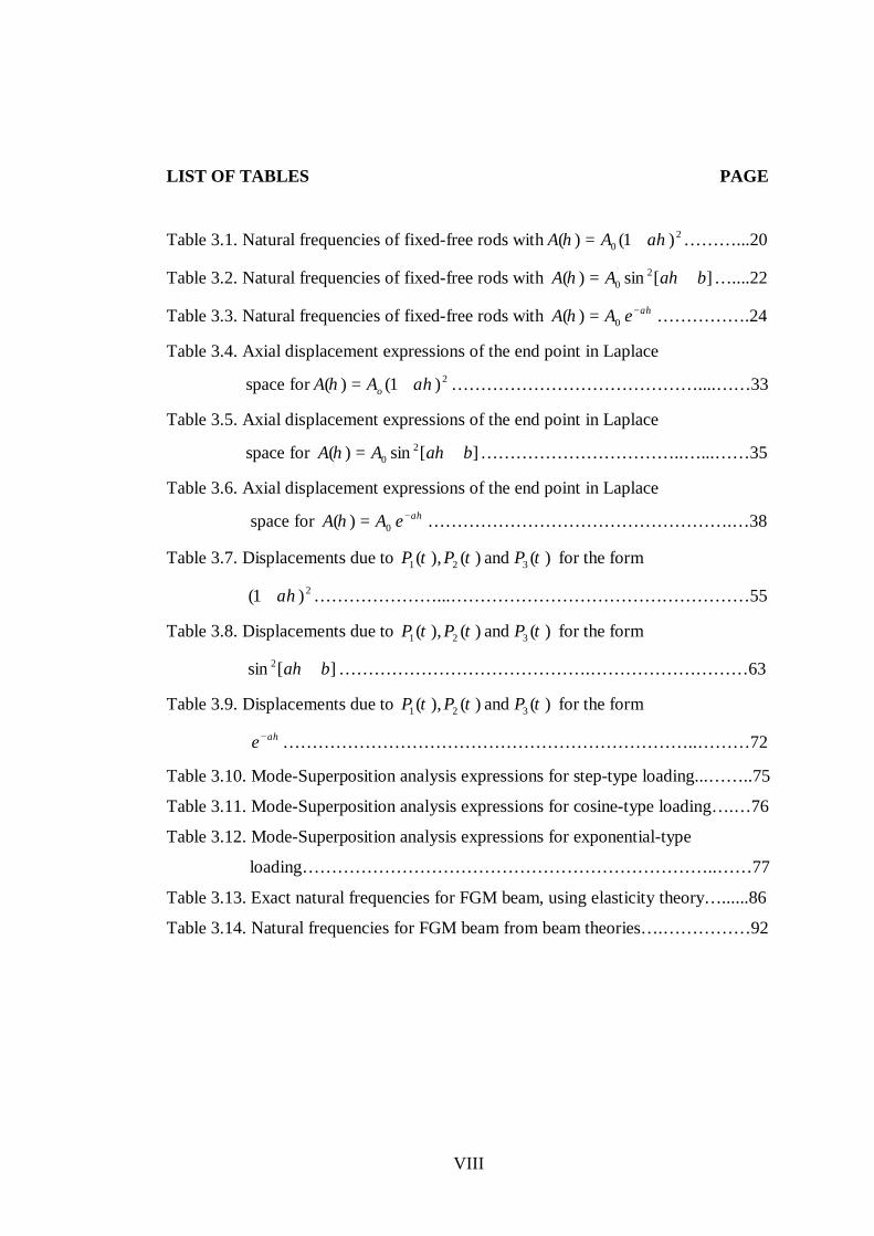
LIST OF TABLES PAGE
Table 3.1. Natural frequencies of fixed-free rods with 20 )1()( ηη aAA += ………...20
Table 3.2. Natural frequencies of fixed-free rods with ][sin)( 20 baAA += ηη …....22
Table 3.3. Natural frequencies of fixed-free rods with ηη aeAA −= 0)( …………….24
Table 3.4. Axial displacement expressions of the end point in Laplace
space for 2)1()( ηη aAA o += ……………………………………....……33
Table 3.5. Axial displacement expressions of the end point in Laplace
space for ][sin)( 20 baAA += ηη ……………………………..…...……35
Table 3.6. Axial displacement expressions of the end point in Laplace
space for ηη aeAA −= 0)( …………………………………………….…38
Table 3.7. Displacements due to )( and )(),( 321 τττ PPP for the form
2)1( ηa+ …………………...……………………………………………55
Table 3.8. Displacements due to )( and )(),( 321 τττ PPP for the form
][sin 2 ba +η …………………………………….………………………63
Table 3.9. Displacements due to )( and )(),( 321 τττ PPP for the form
ηae− ……………………………………………………………..………72
Table 3.10. Mode-Superposition analysis expressions for step-type loading...……..75
Table 3.11. Mode-Superposition analysis expressions for cosine-type loading….…76
Table 3.12. Mode-Superposition analysis expressions for exponential-type
loading……………………………………………………………..……77
Table 3.13. Exact natural frequencies for FGM beam, using elasticity theory…......86
Table 3.14. Natural frequencies for FGM beam from beam theories….……………92

IX
LIST OF FIGURES
PAGE
Figure 3.1. Two modes of vibration for the same rod. 13 Figure 3.2 Derivation of the Duhamel integral (undamped). 16 Figure 3.3 Integration contour C 47 Figure 3.4. An FGM beam 78 Figure 3.5. Variation of Young’s modulus in the thickness direction. 79 Figure 4.1. End displacement for the form ][sin 2 ba +η under 02 )( PP =τ , a=0,
m=10. 94
Figure 4.2. End displacement for the form ][sin 2 ba +η under 02 )( PP =τ , a=1, m=10.
94
Figure 4.3. End displacement for the form ][sin 2 ba +η under 02 )( PP =τ , a=2, m=10.
95
Figure 4.4. End displacement for the form ][sin 2 ba +η under ])cos[1()( 01 τγτ −= PP , a=0, m=10, γ =0.6.
95
Figure 4.5. End displacement for the form ][sin 2 ba +η under ])cos[1()( 01 τγτ −= PP , a=1, m=10, γ =0.6.
96
Figure 4.6. End displacement for the form ][sin 2 ba +η under ])cos[1()( 01 τγτ −= PP , a=2, m=10, γ =0.6.
96
Figure 4.7. End displacement for the form ][sin 2 ba +η under )1()( 03
γττ −−= ePP , a=0, m=10, γ =0.6. 97
Figure 4.8. End displacement for the form ][sin 2 ba +η under )1()( 03
γττ −−= ePP , a=1, m=10,γ =0.6. 97
Figure 4.9. End displacement for the form ][sin 2 ba +η under )1()( 03
γττ −−= ePP , a=2, m=10, γ =0.6. 98
Figure 4.10. End displacement for the form 2)1( ηa+ under 02 )( PP =τ , a=0, m=10.
98
Figure 4.11. End displacement for the form 2)1( ηa+ under 02 )( PP =τ , a=1, m=10.
99
Figure 4.12. End displacement for the form 2)1( ηa+ under 02 )( PP =τ , a=2, m=10.
99
Figure 4.13. End displacement for the form 2)1( ηa+ under ])cos[1()( 01 τγτ −= PP , a=0, m=10, γ =0.6.
100
Figure 4.14. End displacement for the form 2)1( ηa+ under ])cos[1()( 01 τγτ −= PP , a=1, m=10, γ =0.6.
100

X
Figure 4.15. End displacement for the form 2)1( ηa+ under ])cos[1()( 01 τγτ −= PP , a=2, m=10, γ =0.6.
101
Figure 4.16. End displacement for the form 2)1( ηa+ under )1()( 03
γττ −−= ePP , a=0, m=10, γ =0.6. 101
Figure 4.17. End displacement for the form 2)1( ηa+ under )1()( 03
γττ −−= ePP , a=1, m=10, γ =0.6. 102
Figure 4.18. End displacement for the form 2)1( ηa+ under )1()( 03
γττ −−= ePP , a=2, m=10, γ =0.6. 102
Figure 4.19. End displacement for the form ηae− under 02 )( PP =τ , a=0, m=10. 103 Figure 4.20. End displacement for the form ηae− under 02 )( PP =τ , a=1, m=10. 103 Figure 4.21. End displacement for the form ηae− under 02 )( PP =τ , a=2, m=10. 104 Figure 4.22. End displacement for the form ηae− under ])cos[1()( 01 τγτ −= PP , a=0, m=10,γ =0.6.
104
Figure 4.23. End displacement for the form ηae− under ])cos[1()( 01 τγτ −= PP , a=1, m=10, γ =0.6.
105
Figure 4.24. End displacement for the form ηae− under ])cos[1()( 01 τγτ −= PP , a=2, m=10, γ =0.6.
105
Figure 4.25. End displacement for the form ηae− under )1()( 03γττ −−= ePP ,
a=0, m=10, γ =0.6 106
Figure 4.26. End displacement for the form ηae− under )1()( 03γττ −−= ePP ,
a=1, m=10, γ =0.6. 106
Figure 4.27. End displacement for the form ηae− under )1()( 03γττ −−= ePP ,
a=2, m=10, γ =0.6. 107
Figure 4.28. Variation of the fundemental frequency of FGM beam with L/h ratio for n=1 108
Figure 4.29. Variation of the fundemental frequency of FGM beam with L/h ratio for n=3 108
Figure 4.30. Variation of the fundemental frequency of FGM beam with L/h ratio for n=5 109
Figure 4.31. Variation of the fundemental frequency of FGM beam with n forL/h=5 109
Figure 4.32. Variation of the fundemental frequency of FGM beam with n forL/h=10 110
Figure 4.33. Variation of the fundemental frequency of FGM beam with n forL/h=20 110
Figure 4.34. Flexural mode shapes at the bottom surface and upper surface of the FGM beam. 111

XI
NOMENCLATURE a Inhomogeneity parameter A Area c Velocity of the Propagation of the Displacement E Young’s Modulus
),( txf I Inertial Force FFT Fast Fourier Transform Im Imaginary h Thickness k Spring Constant L Length n Wave number m Mass
nM Generalized Mass of n’th Normal Mode OP Load
P(x,t) Applied Axial Loading )(tPn Generalized Loading of n’th Normal Mode in Time Domain
Re Real p Laplace Constant SDOF Single Degree of Freedom t Time u Displacement in x direction
ijQ Transformed stiffness constants α Undamped Natural Circular Frequencies Y(t) Displacement in Time Domain
t∆ Time Interval ε Normal Strain σ Normal Stress ρ Mass per Unit Volume τ Time (dimensionless) η Coordinate in x direction (dimensionless) β Free Vibration Frequencies Φ Shape Function

1.INTRODUCTION Kerimcan ÇELEBİ
1
1. INTRODUCTION
Longitudinal vibrations of non-uniform bars have attracted considerable
scientific and practical attention in the study of composite structures subjected to
high velocity impact and the study of foundations. The use of variable cross-section
members can help the designer reduce the weight, improve strength and stability of
structures. Free vibration analysis and presentation of fundamental frequencies along
with mode shapes constitute most of the archival works. The researchers are
expected to subsequently obtain the forced vibration response through other methods
such as mode superposition.
In the first part of this thesis, the dynamic response of non-uniform rods
subjected at the end point to various time-dependent axial forces will be presented as
closed-form equations. The need for exact solutions is obvious: they give adequate
insight into the physics of the problem as well as establishing the accuracy of the
approximate or numerical solutions. In optimization problems using closed-form
solutions will greatly reduce the solution time. Laplace transformation will be
employed in the analysis. The inversion into the time domain is performed
analytically using calculus of residues and numerically by Durbin’s inverse
transfrom method. Free vibration behavior is readily obtained since substituting the
complex Laplace parameter in the governing equation directly gives natural
frequencies. Uniform mass and stiffness are assumed along the rod. The cross section
is assumed to vary along the non-dimensional axial coordinate in the forms
][sin)( 2 baAA o += ηη , 2)1()( ηη aAA o += and ηη ao eAA −=)( . Natural
frequencies for these cross sections are given in tabular form and good agreement
with other benchmark results are observed. The first ten fundamental frequencies are
listed. Using only the first ten frequencies in the forced vibration response provided
six-digit accuracy. The results are compared to those obtained via Mode
Superposition Method (MSM). Among other advantages, the efficiency of analytical
results is obvious: for some cases, up to a hundred frequencies were needed in MSM
to achieve the same accuracy.

1.INTRODUCTION Kerimcan ÇELEBİ
2
Also, free and forced vibration of heterogeneous rod, which exhibit
inhomogeneity both in material density and in elastic modulus, is studied. These
inhomogeneities are described in forms of ][sin 2 ba +η , 2)1( ηa+ and ηae− .
Closed-from expressions for the fundemental natural frequencies are derived. It is
noted that if the nonuniform cross-sectional area and heterogeneous material
properties vary according to the same functional form, the governing equation for
both cases will be in the same form.
The materials with elastic properties varying in the coordinate direction are
termed as functionally graded materials (FGM). FGM can be fabricated by
continuously intermixing several materials without generating a boundary. Thus, it
was named for this feature of the gradual changes (gradient) of functions.
Beams are incontestably the simplest and the most commonly used of all
structural elements. Consequently, many researches have been involved in modeling
behavior of beams. In the last part of this study, we analyze the free vibration of an
FGM beam. The plane elasticity equations are solved exactly to obtain natural
frequencies by using Laplace transform method. Different higher order shear
deformation theories and classical beam theories were also used in the literature
where, governing equations were found by applying Hamilton’s principle. Navier
type solution method was used to obtain frequencies. The beam theory results are
compared with elasticity solutions.
The aim of the present thesis may be stated as the efforts to obtain analytical
benchmark solution for vibration behaviour of rods and beams.

2.PREVIOUS STUDIES Kerimcan ÇELEBİ
3
2. PREVIOUS STUDIES
2.1. Non-uniform Rods and Heterogeneous Rods
The vibration of beams and rods has been studied extensively, and continues
to receive considerable attention in the literature.
Raj and Sujith (2005) have presented exact solutions for the longitudinal
vibration of variable area-rods. The eigen frequencies of rods with certain area
variations are obtained.
Li et al. (1999) have presented exact analytical solutions for longitudinal
vibration of non-uniform rods with concentrated masses coupled by translational
springs. The governing differential equation for longitudinal vibration of a rod with
varying crossection is reduced to Bessel’s equation or an ordinary differential
equation with constant coefficients by selecting suitable expressions such as power
function for the area variation. They have shown in their research that the proposed
methods were in good agreement with the full-scale measured data and it is
applicable to engineering practices.
Abrate (1994) has shown that for some non-uniform rods and beams the
equation of motion can be transformed into the equation of motion for a uniform rod
or beam. Also, when the ends were completely fixed, the eigenvalues of the non-
uniform continuum were the same as those of uniform rods or beams. They used an
efficient procedure to analyze the free vibration of non-unifrom beams with general
shape and arbitrary boundary conditions. Simple formulas were presented for
predicting the fundamental natural frequency of non-uniform beams with various end
support conditions.
Qiusheng et al. (1996) have determined the natural frequencies and mode
shapes of multi-storey buildings and high-rise structures with variably distributed
stiffness and variably distributed mass.
Horgan and Chan (1999) have obtained exact solutions for polynomial and
exponential variations of strings, rods and membranes.

2.PREVIOUS STUDIES Kerimcan ÇELEBİ
4
Li, Fang and Jeary (1997) have established the differential equations of free
longitudinal vibrations of bars with variably distributed mass and stiffness
considering damping effects. They proposed an approach to determine the natural
frequencies and mode shapes in vertical direction for tall buildings with variably
distributed stiffness and variably distributed mass. The numerical examples showed
that the computed values of the fundamental longitudinal natural frequency and
mode shape by the proposed method were close to the full-scale measured data.
Eisenberg (1991) has presented the solution for exact longitudinal vibration
frequencies of a variable cross-section rod. The solution is found using the exact
element method, where the dynamic axial stiffness for the rod is found. The natural
frequencies for the variable cross-section member are those for which the stiffness is
equal to zero. These values can be found up to any desired accuracy. This method is
good for any polynomial variation in the cross-sectional area and the mass
distribution along the member. The results of several examples are compared with
results obtained from finite element analysis.
Kumar and Sujith (1997) have presented exact analytical solutions for the
longitudinal vibration of rods with non-uniform cross section. Using appropriate
transformations, the equation of motion of axial vibration of a rod with varying cross
section was reduced to analytically-solvable standard differential equations whose
form depend upon the specific area variation. The governing equation for the
problem was the same as that of wave propagation through ducts with non-uniform
cross sections. Therefore, solutions they have presented could be used to investigate
such problems.
Li (2000) has presented exact analytical solutions for the free longitudinal
vibrations of bar with variably distributed stiffness and mass. By using appropriate
transformations, the differential equations of free longitudinal vibrations of bars with
variably distributed stiffness and mass are reduced to Bessel’s equations or ordinary
differential equations with constant coefficients.
Candan and Elishakoff (2001) have presented close-form solutions of
nonhomogeneous rod under two sets of boundary conditions. Closed-form
expressions for the natural frequency can serve as benchmark solutions.

2.PREVIOUS STUDIES Kerimcan ÇELEBİ
5
Elishakoff and Candan (2001) used the inverse method and obtained the exact
natural frequencies in rods and beams with polynomially varying material and
geometrical properties.
Nachum and Altus (2007) found the natural frequencies and mode-shapes of
the k-th-order of non-homogeneous rods and beams. The solution is based on the
functional perturbation method.
Celebi, Keles and Tütüncü (2009) have obtained the exact displacement
solutions of heterogeneous rods under dynamic axial load by using the Laplace
transform method. Inverse transformation into the time domain is performed using
modified Durbin’s method.
2.2. Application of Laplace Transform to Dynamic Problems
Many of the works obtained through a literature survey on vibration analysis
have been about the Laplace transform and Fourier transform methods applied to
dynamic problems.
Durbin (1974) has presented an accurate method for the numerical inversion
of Laplace transform which was a natural continuation to Dubner and Abate’s
method.
Narayanan (1977) has described the use and importance of dynamic stiffness
influence coefficients in flexural forced vibrations of structures composed of beams.
The dynamic problem was formulated in terms of dynamic influence coefficients and
reduced to a static form. They used the Fourier transform plane and a numerical
inversion based on the Cooley-Tukey algorithm of the transformed solution.
Beskos and Narayanan (1981) have presented a general method for
determining the dynamic response of complex three dimensional frameworks to
dynamic shocks, wind forces or earthquake excitations. The method consisted of
formulating and solving the dynamic problem in the Laplace transform domain by
the finite element method and of obtaining the response by a numerical inversion of
the transformed solution. They provided a basis for comparing the accuracy of other
approximate methods such as conventional finite element method. The proposed

2.PREVIOUS STUDIES Kerimcan ÇELEBİ
6
method appeared to be better than the conventional finite element method in
conjunction with either modal analysis or numerical integration.
Manolis and Beskos (1981) used the Laplace transform in the free vibration
analysis. They replaced the complex Laplace parameter with αi in the transient
formulation which directly gives the natural frequency α with no inversion required.
Calım (2009) studied the forced vibration of non-uniform composite beams
subjected to impulsive loads in the Laplace domain. The solutions obtained are
transformed to the time domain using the Durbin’s numerical inverse Laplace
transform method.
2.3. FGM Beams
Functionally graded materials (FGM) are composite materials intentionally
designed so that they possess desirable properties for specific applications. As the
application of FGM increases, new methodologies have to be developed to
characterize them, and to design and analyze structural components made of these
materials. The literature on the response of FGM beam to mechanical and other
loadings are mostly inclusive of beam theories.
Sankar (2001) gave an elasticity solution based on the Euler-Bernoulli beam
theory for functionally graded beam subjected to static transverse loads by assuming
that Young’s modulus of the beam vary exponentially through the thickness. Sankar
found that beam theory results agree quite well with elasticity solution for beams
with large length-to-thickness ratio subjected to more uniform loading characterized
by longer wave length of the sinusoidal loading.
Zhong and Yu (2007) presented a general two-dimensional solution for a
cantilever FG beam in terms of the Airy stress function.
Sankar and Tzeng (2002) developed a simple Euler-Bernoulli type beam
theory to obtain elasticity solution FGM beams subjected to temparature gradients.
They found that the thermoelastic properties of the beam can be tailored to reduce
thermal stresses for a given temparature distribution.

2.PREVIOUS STUDIES Kerimcan ÇELEBİ
7
Aydogdu and Taskin (2007) investigated free vibration of simply supported
FGM beams. They used different higher order shear deformation theories and
classical beam theory (CBT) and showed that CBT gives higher results and the
difference between CBT and higher order theories is increased with increasing mode
number.
Calio and Elishakoff (2005) derived closed-form solutions for the natural
frequencies for axially graded beam-columns on elastic foundations with guided end
conditions.
Ying et al. (2008) obtained the exact solutions for bendind and free vibration
of FGM beams resting on a Winkler-Pasternak elastic foundation based on the two-
dimensional elasticity theory by assuming that the beam is orthotropic at any point
and the material properties vary exponentially along the thickness direction.
Sina et al. (2009) used a new beam theory different from the tradional first-
order shear deformation beam theory to analyze the free vibration of FGM beams.
Simsek and Kocaturk (2009) have investigated the forced and free vibration
characteristics of an FGM Euler-Bernoulli beam under a moving harmonic load.
Kadoli et al. (2008) studied the static behaviour of an FGM beam by using
higher-order shear deformation theory and finite element method.
Simsek (2010) has studied the dynamic deflections and the stresses of an
FGM simply-supported beam subjected to a moving mass by using Euler-Bernoulli,
Timoshenko and the parabolic shear deformation beam theories.
Li (2008) proposed a new unified approach to investigate the static and the
free vibration behaviour of Euler-Bernoulli and Timoshenko beams.
Aydogdu (2005) has investigated the vibration of cross-ply composite beams
for six different boundary conditions by using the Ritz method. Polynomial trial
functions are used in the analyses.
Abbasi et al. (2008) have presented the vibration behavior of an FGM
Timoshenko beam under lateral thermal shocks with coupled thermoelastic
assumption. The solution obtained by transfinite element method where time is
eliminated using the Laplace transform.

2.PREVIOUS STUDIES Kerimcan ÇELEBİ
8
Soldatos and Sophocleous (2001) have developed some higher-order shear
deformation theories in which there is no need to use shear correction factors.
Simsek (2009) has investigated the static analysis of a functionally graded
simply supported beam under a uniformly distributed load by Ritz method. The
material properties of the beam vary continuously in the thickness direction
according to a power law.

3.MATERIAL AND METHOD Kerimcan ÇELEBİ
9
3. MATERIAL AND METHOD
3.1. An Overview of the Differential Equation
The equation of motion for a linear single–degree-of-freedom (SDF) system
subjected to external force is the second order differential equation for the
displacement:
)()()()( tPtkutuctum =++•••
The initial displacement u(0) and initial velocity )0(•
u at time zero must be
specified to define the problem completely. Typically, the structure is at rest before
the onset of dynamic excitation, so that the initial velocity and the displacement are
zero. A brief review of three methods of solution is given in the following sections.
3.1.1. Classical Solution
Complete solution of the linear differential equation of motion consists of the
sum of the complementary solution )(tuc and particular solution )(tu p , that is,
)()()( tututu pc += . Since the differential equation is of second order, two constants
of integration are involved. They appear in the complementary solution and are
evaluated from knowledge of the initial conditions.
3.1.2. Duhamel’s Integral
Another well-known approach to the solution of linear differential equations,
such as the equation of the motion of an SDF system, is based on representing the
applied force as a sequence of infinitesimally short impulses. The response of the
system to an applied force, )(tp , at time t is obtained by adding the responses to all

3.MATERIAL AND METHOD Kerimcan ÇELEBİ
10
impulses up to that time. We develop this method in the next section, leading to the
following result for an undamped SDF system:
[ ] τττ dtwpwm
tu n
t
n
)(sin)(1)(0
−= ∫
where mkwn /= . Implicit in this result are “at rest” initial conditions. This
equation, known as Duhamel’s integral-the derivation of which will be discussed in
subsequent sections- is a special form of the convolution integral.
Duhamel’s integral provides an alternative method to the classical solution if
the applied force p(t) is defined analytically by a simple function that permits
analytical evaluation of the integral. For complex excitations that are defined only by
numerical values of p(t) at discrete time instants, Duhamel’s integral can be
evaluated by numerical methods.
3.1.3. Transform Methods
The Laplace and Fourier transforms provide powerful tools for the solution of
linear differential equations, in particular the equation of motion for a linear SDF
system. Because the transform methods are similar in concept, here we mention only
the Laplace transform method, which leads to the frequency-domain method of
dynamic analysis. The frequency-domain method, which is an alternative to the time-
domain method symbolized by Duhamel’s integral, is especially useful and powerful
for dynamic analysis of structures. The solutions in Laplace transform space can be
calculated numerically for real problems. For time-space transition, numerical
inverse Laplace transforms are needed. Various inverse Laplace transform methods
have been improved for this purpose. Exact inversion into the time domain is
performed via the theory of Residues and Durbin’s inverse transform method. The
analytical results are tractable and allow for parametric studies.

3.MATERIAL AND METHOD Kerimcan ÇELEBİ
11
3.2. Partial Differential Equations of Motion of an Axially-Loaded Bar
The analysis of continuous systems leads to governing partial differential
equations in displacement.
3.2.1 Axial Deformations (Undamped)
The axial motion of a rod with varying cross-section )(xA , uniform density
and Young’s modulus is governed by the differantial equation
),(),()(),()( 2
2
txqx
txuxAExt
txuxm =
∂
∂∂∂
−∂
∂ (3.1)
Using the dimensionless variables
Ltc
Lx
Luv === τη ,, (3.2)
Renders Eq.(3.1) in the form
),()),()((),()( 2
22 τη
ητη
ηητ
τηη qLvAEvmc =
∂∂
∂∂
−∂
∂ (3.3)
where ρ/2 Ec = , c is the velocity of propagation of the displacement.
Usually, the external axial loading consists only of end loads, in which case
the right hand side of this equation would be zero. However, when solving Equation
(3.3) the boundary conditions imposed at 0=η and 1=η must be satisfied. It
should be noted that in this formulation damping is neglected. The free-vibration
equation of motion – setting 0),( =τηq in Equation (3.3) - becomes

3.MATERIAL AND METHOD Kerimcan ÇELEBİ
12
0)),()((),()( 2
22 =
∂∂
∂∂
−∂
∂η
τηη
ηττη
ηvAEvmc (3.4)
3.2.2. Orthogonality of Axial Vibrations Modes
The axial vibration mode shapes have orthogonality properties. The
orthogonality of the axial mode shapes with respect to the mass distribution can be
derived using Betti’s law. Consider the beam shown in Figure (3.1). Two different
vibration modes, m and n, are shown for the beam. In each mode, the displaced shape
and the inertial forces producing the displacements are indicated.
Betti’s law applied to these two deflection patterns means that the work done
by the inertial forces of mode n acting on the deflection mode m is equal to the work
of the forces of mode m acting on the displacement of mode n; that is,
∫ ∫=1
0
1
0
ηη dfvdfv mInnIm (3.5)
Expressing these in terms of the modal shape functions shown in Figure (3.1) gives
ηηηηττ
ηηηηαττ
dVmVwGG
dVmVGG
mnmnm
nmnnm
∫
∫
=1
0
2
1
0
2
)()()()()(
)()()()()( (3.6)
which may be written as
∫ =−1
0
22 0)()()()( ηηηηαα dmVV nmmn (3.7)
Since the frequencies of these two modes are different, their mode shape must satisfy
the orthogonality condition

3.MATERIAL AND METHOD Kerimcan ÇELEBİ
13
nmnm dmVV ααηηηη ≠=∫ ,0)()()(1
0
(3.8)
If the two modes have the same frequency, the orthogonality condition does not
apply, but this condition does not occur often in ordinary structural problems.
Mode “n” Mode “m”
η η
)()(),( τητη mmm GVv =
)()(),( 2 τηατη mmmmI GVf =)()(),( τητη nnn GVv =
)()(),( 2 τηατη nnnnI GVf =
Figure 3.1. Two modes of vibration for the same rod.
The orthogonality relationship with respect to the axial stiffness property can be
derived from the homogenous form of the equation of motion [Equation (3.4)] in
which the harmonic time variation of free vibration has been substituted. In other
words, when the nth-mode displacements are expressed as (Clough and Penzien,
1993)
)sin()(),( nnnnn Vv ϕταρητη += (3.9)
and this displacement expression is substituted into the homogeneous form of
Equation (3.4), one obtains
−=
ηη
ηηηα
ddV
AEddVmc n
nn )()()(22 (3.10)

3.MATERIAL AND METHOD Kerimcan ÇELEBİ
14
Substituting this relation into both sides of Equation (3.6) and canceling the common
term )()( ττ nm GG gives
0)()()( 1
02
22
=
−− ∫ η
ηη
ηα
ααddV
AEddV n
mn
mn (3.11)
Since the frequencies are different, modes m and n must satisfy the orthogonality
condition
0)(
)()(1
0
=
∫ η
ηη
ηη
η dd
dVAE
ddV n
m (3.12)
3.2.3. Analysis of Dynamic response (Normal Coordinates)
The essential operation of the mode-superposition analysis is the
transformation from the geometric displacement coordinates to the modal-amplitude
or normal coordinates. For a one-dimensional system, this transformation is
expressed as
)()(),(1
τητη ii
i GVv ∑∞
=
= (3.13)
which is simply a statement that any physically permissible displacement pattern can
be made up by superposing appropriate amplitudes of the vibration mode shapes for
the structure.
3.2.4. Uncoupled Axial Equations of Motion
The mode-shape (normal) coordinate transformation serves to uncouple the
equations of motion of any dynamic system and therefore is applicable to the axial

3.MATERIAL AND METHOD Kerimcan ÇELEBİ
15
motion of a one-dimensional member. Introducing Equation (3.13) into the equation
of axial motion, Equation (3.3), leads to
),()()(
)()()()(11
2 τητη
ηη
ητηη qLG
dGd
AEddGVmc i
i
ii
ii =
− ∑∑
∞
=
••∞
=
(3.14)
Multiplying each term by )(ηnV and applying the orthogonality relationships
[Equation (3.8) and Equation (3.12)] leads to
ητηη
ηηη
ηη
ητηηητ
dqVL
dd
dVAEddVGdVmcG
n
nnnnn
),()(
)()()()()()()(
1
0
1
0
1
0
22
∫
∫∫
=
−
••
(3.15)
multiplying Equation (3.10) by )(ηnV and integrating yields
ηηη
ηη
ηηηηα dd
dVAE
ddVdVmc n
nnn∫ ∫
−=
1
0
1
0
222 )()()()()( (3.16)
Substituting Equation (3.16) into Equation (3.15), we get uncoupled axial equation of motion
)()()( 2 ττατ nnnnnn PGMGM =+••
(3.17)
where
ηηη dVmcM nn )()( 21
0
2∫= (3.18)
is generalized mass of the n’th mode and

3.MATERIAL AND METHOD Kerimcan ÇELEBİ
16
ητηη dqVLP nn ∫=1
0
),()( (3.19)
is the generalized loading associated with mode shape )(ηnV .
From this discussion it is apparent that after the vibration mode shapes have
been determined, the reduction to the normal-coordinate form involves exactly the
same type of operations for all structures.
3.2.5. Formulation of Duhamel Integral
In theory of vibrations, Duhamel’s integral is a way of calculating the
response of linear systems and structures to arbitrary time-varying external
excitations.
The procedure described in (Clough and Penzien, 1993) for approximating
the response of an undamped SDOF structure to short duration impulsive loads can
be used as the basis for developing a formula for evaluating response to a general
dynamic loading. This formula is:
10
,]sin[)(1)(1
τττταττα
ττ
−=
=
−−
∫ dPm
G (3.20)
t
p (t)
p(τ)
τ dτ
(t-τ)
(t-τ) >0
dY(t)
R esp o ns e d Y ( t) Figure 3.2 Derivation of the Duhamel integral (undamped).
3.MATERIAL AND METHOD Kerimcan ÇELEBİ
17
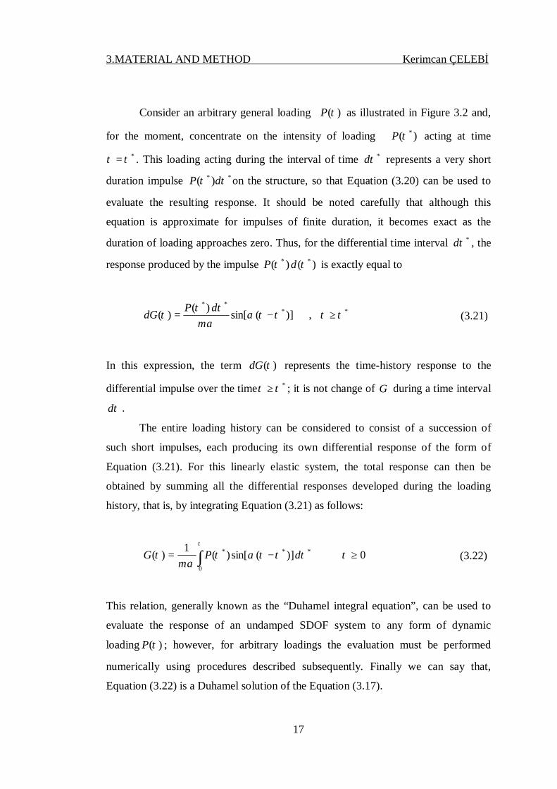
Consider an arbitrary general loading )(τP as illustrated in Figure 3.2 and,
for the moment, concentrate on the intensity of loading )( *τP acting at time *ττ = . This loading acting during the interval of time *τd represents a very short
duration impulse ** )( ττ dP on the structure, so that Equation (3.20) can be used to
evaluate the resulting response. It should be noted carefully that although this
equation is approximate for impulses of finite duration, it becomes exact as the
duration of loading approaches zero. Thus, for the differential time interval *τd , the
response produced by the impulse )()( ** ττ dP is exactly equal to
****
,)](sin[)()( τττταα
τττ ≥−=
mdPdG (3.21)
In this expression, the term )(τdG represents the time-history response to the
differential impulse over the time *ττ ≥ ; it is not change of G during a time interval
τd .
The entire loading history can be considered to consist of a succession of
such short impulses, each producing its own differential response of the form of
Equation (3.21). For this linearly elastic system, the total response can then be
obtained by summing all the differential responses developed during the loading
history, that is, by integrating Equation (3.21) as follows:
0)](sin[)(1)( **
0
* ≥−= ∫ ττττατα
ττ
dPm
G (3.22)
This relation, generally known as the “Duhamel integral equation”, can be used to
evaluate the response of an undamped SDOF system to any form of dynamic
loading )(τP ; however, for arbitrary loadings the evaluation must be performed
numerically using procedures described subsequently. Finally we can say that,
Equation (3.22) is a Duhamel solution of the Equation (3.17).

3.MATERIAL AND METHOD Kerimcan ÇELEBİ
18
3.3. Free Vibration Analysis of Non-uniform and Heterogeneous Rods
By applying the so-called product method, or method of separating variables,
we shall obtain ordinary differential equation which satisfies the motion of a rod.
3.3.1. Free Vibration Analysis of Non-uniform Rods
The longitudinal motion of a rod with varying cross-section )(ηA , uniform
density and Young’s modulus is governed by the differential equation
2
2
2
2 ),(),()()(
1),(τ
τηη
τηηη
ηητη
∂∂
=∂
∂∂
∂+
∂∂ vvA
Av
0,10 ><< τη (3.23)
Assuming a solution of the form )()(),( τητη GVv = , Equation (3.23) reduces to the
second order differential equation for the complex amplitude )(ηV :
0)()()()(
1)( 22
2
=++ ηαηη
ηη
ηηη V
ddV
ddA
AdVd (3.24)
The above equation will be solved for rods with cross-sections varying
as ][sin)( 2 baAA o += ηη , 2)1()( ηη aAA o += and ηη ao eAA −=)( .
3.3.1.1. Solution for Area Variation of the Form 2
0 )1()( ηη aAA +=
In this section the exact solution for the longitudinal vibration of a rod with
an area variation of the form
2
0 )1()( ηη aAA += (3.25)
is derived. To simplify equation (3.24) a new variable z is introduced (Abrate, 1995):
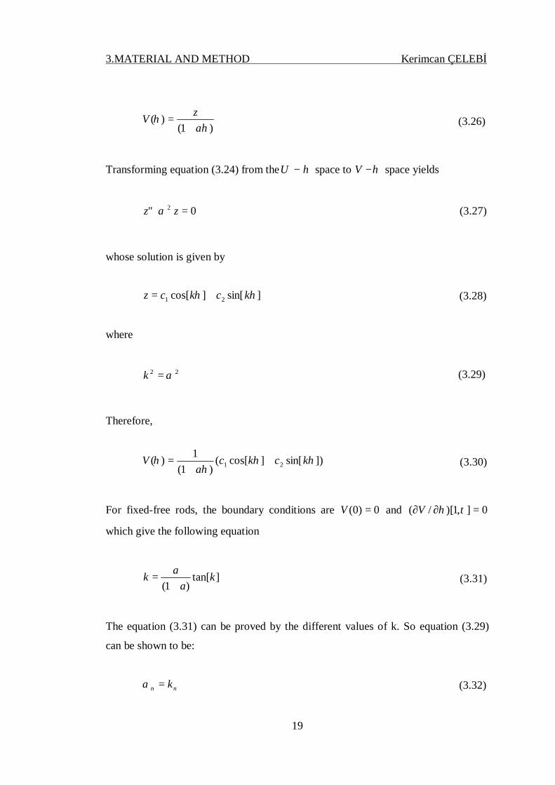
3.MATERIAL AND METHOD Kerimcan ÇELEBİ
19
)1()(
ηη
azV
+= (3.26)
Transforming equation (3.24) from the η−U space to η−V space yields
0" 2 =+ zz α (3.27)
whose solution is given by
]sin[]cos[ 21 ηη kckcz += (3.28)
where
22 α=k (3.29)
Therefore,
])sin[]cos[()1(
1)( 21 ηηη
η kckca
V ++
= (3.30)
For fixed-free rods, the boundary conditions are 0)0( =V and 0],1)[/( =∂∂ τηV
which give the following equation
]tan[)1(
ka
ak+
= (3.31)
The equation (3.31) can be proved by the different values of k. So equation (3.29)
can be shown to be:
nn k=α (3.32)

3.MATERIAL AND METHOD Kerimcan ÇELEBİ
20
Table 3.1 shows the natural frequencies for tapered rods with a=0,1,2 and
L=1.
Table 3.1. Natural frequencies of fixed-free rods with 2
0 )1()( ηη aAA +=
Mode a=0 a=1 a=2
1 1.57079 1.165561 0.967402
2 4.71239 4.604216 4.567452
3 7.85398 7.789883 7.768373
4 10.9956 10.949943 10.934681
5 14.1372 14.101725 14.089886
6 17.2788 17.249781 17.240109
7 20.4204 20.395842 20.387664
8 23.5619 23.540708 23.533624
9 26.7035 26.684801 26.678553
10 29.8451 29.828369 29.822779
3.3.1.2. Solution for Area Variation of the Form ][sin 20 baAA += η
In this section the exact solution for the longitudinal vibration of a rod with
an area variation of the form
][sin)( 20 baAA += ηη (3.33)
is derived. To simplify equation (3.24) a new variable z is introduced (Kumar and
Sujith, 1997):
]sin[)(
bazV
+=
ηη (3.34)

3.MATERIAL AND METHOD Kerimcan ÇELEBİ
21
Transforming equation (3.24) from the η−V space to η−z space yields
0)(" 22 =++ zaz α (3.35)
whose solution is given by
]cos[]sin[ 21 ηη kckcz += (3.36)
where
222 ak += α (3.37)
Therefore,
])cos[]sin[(]sin[
1)( 21 ηηη
η kckcba
V ++
= (3.38)
For fixed-free rods, the boundary conditions are 0)0( =V and
0],1)[/( =∂∂ τηV which give the following equation
]tan[]tan[
baakk
+= (3.39)
The equation (3.39) can be proved by the different values of k. So equation
(3.37) can be shown to be:
222 aknn −=α (3.40)

3.MATERIAL AND METHOD Kerimcan ÇELEBİ
22
Table 3.2. shows the natural frequencies for tapered rods with a=0,1,2 and L=1.
Table 3.2. Natural frequencies of fixed-free rods with ][sin 20 baAA += η
Mode a=0 a=1 a=2
1 1.57079 1.51764 2.14856
2 4.71239 4.70214 5.53576
3 7.85398 7.84831 8.63281
4 10.9956 10.9916 11.6946
5 14.1372 14.1341 14.7579
6 17.2788 17.2763 17.8306
7 20.4204 20.4183 20.9137
8 23.5619 23.5601 24.0062
9 26.7035 26.7019 27.1064
10 29.8451 29.8437 30.2129
3.3.1.3. Solution for Area Variation of the Form ηη aeAA −= 0)(
In this section the exact solution for the longitudinal vibration of a rod with
an area variation of the form
ηη aeAA −= 0)( (3.41)
is derived. The equation (3.24) becomes
022
2
=+− VddVa
dVd
αηη
(3.42)
it is obvious that if

3.MATERIAL AND METHOD Kerimcan ÇELEBİ
23
04 22 ≥− αa (3.43)
then, only zero solution exists. When
04 22 pα−a (3.44)
the general solution of )(ηV is given by (Li, 2000)
])sin[]cos[()( 212 ηηηη
kckceVa
+= (3.45)
where
4
222 ak −= α (3.46)
For fixed-free rods, the boundary conditions are 0)0( =V and
0],1)[/( =∂∂ τηV which give the following equation
[ ]k
ak2
cot −= (3.47)
The equation (3.47) can be supplied by the different values of k. Equation
(3.46) can be shown to be.
4
222 aknn +=α (3.48)
Table 3.3. shows the natural frequencies for tapered rods with a=0,1, 2 and L=1

3.MATERIAL AND METHOD Kerimcan ÇELEBİ
24
Table 3.3. Natural frequencies of fixed-free rods with ηη aeAA −= 0)(
Mode a=0 a=1 a=2
1 1.57079 1.90344 2.26183
2 4.71239 4.84173 5.01391
3 7.85398 7.93283 8.04109
4 10.9956 11.0521 11.1306
5 14.1372 14.1812 14.2426
6 17.2788 17.3149 17.3652
7 20.4204 20.4509 20.4936
8 23.5619 23.5884 23.6255
9 26.7035 26.7269 26.7596
10 29.8451 29.8661 29.8953
3.3.2. Free Vibration Analysis of Heterogeneous Rods
The longitudinal motion of a rod with uniform cross-section, varying density
)(ηρ and varying Young’s modulus )(ηE is governed by the differential equation
2
22
2
2 ),()()(),()(
)(1),(
ττη
ηηρ
ητη
ηη
ηητη
∂∂
=∂
∂∂
∂+
∂∂ v
EcvE
Ev 0,10 ><< τη (3.49)
Assuming a solution of the form )()(),( τητη GVv = , Equation (3.49) reduces to the
second order differential equation for the complex amplitude )(ηV :
0)()()()()(
)(1)( 22
2
2
=++ ηηηρ
αηη
ηη
ηηη V
Ec
ddV
ddE
EdVd (3.50)
The above equation will be solved for rods with densitiy and Young’ modulus
varying as ][sin 2 ba +η , 2)1( ηa+ and ηae− . Since the density and elasticity

3.MATERIAL AND METHOD Kerimcan ÇELEBİ
25
variations of the heterogeneous rods are of the same form of the area variations of
non-uniform rods they have the same natural frequencies.
3.3.2.1 Solution for 20 )1()( ηη aEE += and 2
0 )1()( ηρηρ a+=
In this section the exact solution for the longitudinal vibration of a rod with a
densitiy and elastic modulus variation of the forms
2
0 )1()( ηη aEE +=
20 )1()( ηρηρ a+=
(3.51)
is derived. To simplify equation (3.50) a new variable z is introduced:
)1()(
ηη
azV
+= (3.52)
Transforming equation (3.50) from the η−U space to η−V space yields
0" 2 =+ zz α (3.53)
whose solution is given by
]sin[]cos[ 21 ηη kckcz += (3.54)
where
22 α=k (3.55)

3.MATERIAL AND METHOD Kerimcan ÇELEBİ
26
Following the same steps as in the section (3.3.1.1), the same mode shapes
and natural frequncies at Table 3.1 can be found for 20 )1()( ηη aEE += and
20 )1()( ηρηρ a+= .
3.3.2.2. Solution for ][sin)( 20 baEE += ηη and ][sin)( 2
0 ba += ηρηρ
In this section the exact solution for the longitudinal vibration of a rod with a
densitiy and elastic modulus variation of the forms
][sin)( 20 baEE += ηη
][sin)( 20 ba += ηρηρ
(3.56)
is derived. To simplify equation (3.50) a new variable z is introduced:
]sin[)(
bazV
+=
ηη (3.57)
Transforming equation (3.50) from the η−V space to η−z space yields
0)(" 22 =++ zaz α (3.58)
whose solution is given by
]cos[]sin[ 21 ηη kckcz += (3.59)
where
222 ak += α (3.60)

3.MATERIAL AND METHOD Kerimcan ÇELEBİ
27
Following the same steps as in the section (3.3.1.2), the same mode shapes
and natural frequncies at Table 3.2 can be found for ][sin)( 20 baEE += ηη and
][sin)( 20 ba += ηρηρ .
3.3.2.3. Solution for ηη aeEE −= 0)( and ηρηρ ae−= 0)(
In this section the exact solution for the longitudinal vibration of a rod with a
densitiy and elastic modulus variation of the forms
ηη aeEE −= 0)(
ηρηρ ae−= 0)( (3.61)
is derived. The equation (3.50) becomes
022
2
=+− VddVa
dVd
αηη
(3.62)
it is obvious that if
04 22 ≥− αa (3.63)
then, only zero solution exists. When
04 22 pα−a (3.64)
the general solution of )(ηV is given by
])sin[]cos[()( 212 ηηηη
kckceVa
+= (3.65)
3.MATERIAL AND METHOD Kerimcan ÇELEBİ
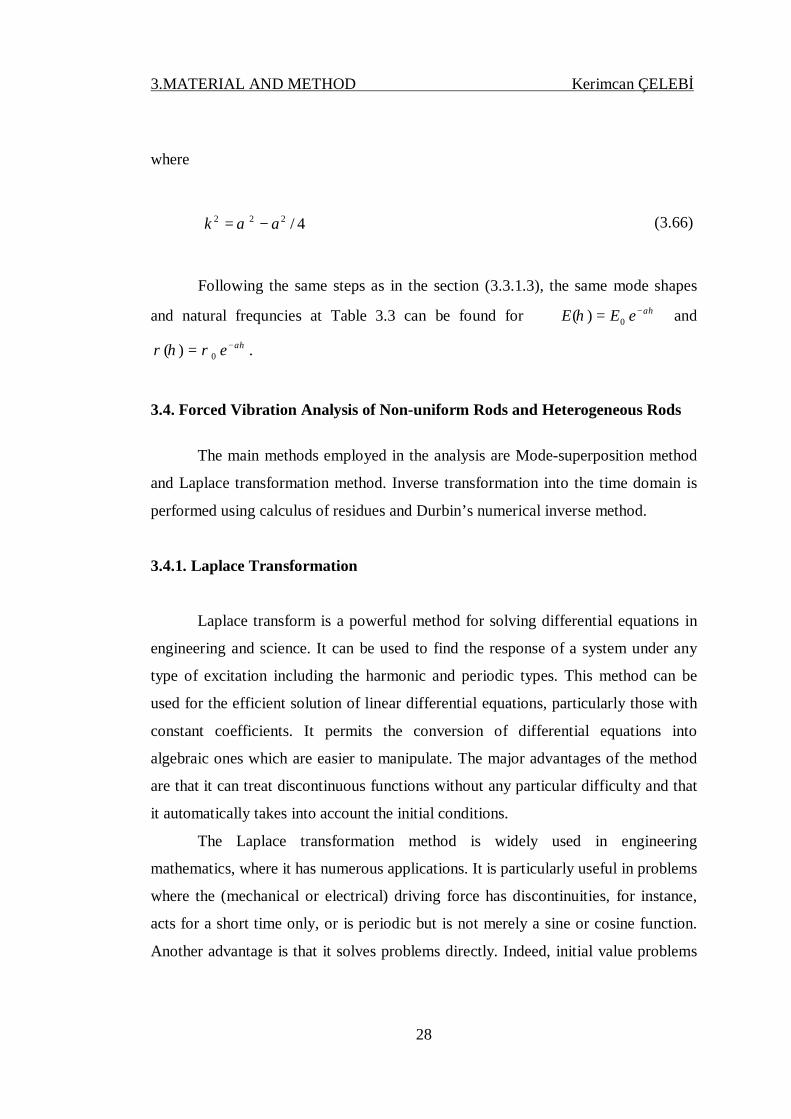
28
where
4/222 ak −= α (3.66)
Following the same steps as in the section (3.3.1.3), the same mode shapes
and natural frequncies at Table 3.3 can be found for ηη aeEE −= 0)( and
ηρηρ ae−= 0)( .
3.4. Forced Vibration Analysis of Non-uniform Rods and Heterogeneous Rods
The main methods employed in the analysis are Mode-superposition method
and Laplace transformation method. Inverse transformation into the time domain is
performed using calculus of residues and Durbin’s numerical inverse method.
3.4.1. Laplace Transformation
Laplace transform is a powerful method for solving differential equations in
engineering and science. It can be used to find the response of a system under any
type of excitation including the harmonic and periodic types. This method can be
used for the efficient solution of linear differential equations, particularly those with
constant coefficients. It permits the conversion of differential equations into
algebraic ones which are easier to manipulate. The major advantages of the method
are that it can treat discontinuous functions without any particular difficulty and that
it automatically takes into account the initial conditions.
The Laplace transformation method is widely used in engineering
mathematics, where it has numerous applications. It is particularly useful in problems
where the (mechanical or electrical) driving force has discontinuities, for instance,
acts for a short time only, or is periodic but is not merely a sine or cosine function.
Another advantage is that it solves problems directly. Indeed, initial value problems

3.MATERIAL AND METHOD Kerimcan ÇELEBİ
29
are solved without first determining a general solution. Similarly, nonhomogeneous
equations are solved without first solving the corresponding homogeneous equation.
The Laplace transform of a function )(tf , denoted symbolically as
)()( tfLpF = , is defined as
dttfetfLpF tp )()()(0∫∞
−== (3.67)
where p is, in general, a complex quantity and is called the subsidiary variable. The
function tpe− is called the kernel of the transformation. Since the integration is with
respect to t, the transformation gives a function of p. Here and in the following
sections, a capital F will represent the function in the Laplace domain, whose
inversion in real time, f(t), is required. It is noted that t can be any independent
variable. However, in this thesis, and because of its association with “time”, in many
engineering applications we will call it “time”. The inversion integral is defined as
follows (Abramowitz and Stegun, 1982).
dppFej
tfj
j
ts )(2
1)( ∫∞+∂
∞−∂
=π
(3.68)
where ∂ is chosen so that all the singular points of )( pF lie to the left of the line
∂=}Re{p in the complex p-plane.
In order to solve a vibration problem using the Laplace transform method, the
following steps are necessary:
1. Write the equation of motion of the system.
2. Transform each term of the equation, using known initial
conditions.
3. Solve for the transformed response of the system.

3.MATERIAL AND METHOD Kerimcan ÇELEBİ
30
4. Obtain the desired solution (response) by using inverse Laplace
transformation.
The Laplace transform method of solving the differential equation provides a
complete solution, yielding both transient and forced vibration.
3.4.1.1. Solution of Boundary-Value Problems by Laplace Transforms
Various problems in science and engineering, when formulated
mathematically, lead to partial differential equations involving one or more unknown
functions together with certain prescribed conditions on the functions which arise
from the physical situation.
These conditions are called boundary conditions. The problem of finding
solutions to the equations which satisfy the boundary conditions is called a
boundary-value problem.
By use of the Laplace transformation (with respect to t or x) in a one-
dimensional boundary-value problem, the partial differential equation can be
transformed into an ordinary differential equation. The required solution can then be
obtained by solving this equation and inverting by use of the inversion formula or
any other methods.
3.4.1.2. Displacement Solution of Axially Loaded Non-Uniform Rods Using
Laplace Transform Technique
In this section, the same problem in section 3.3.1 will be investigated again. A
fixed-free rod with the axial force applied at the free end 0.1=η will be considered.
In order to obtain equation of the motion of the system, equation (3.23) can be used
again. The above equation is solved for a rods with a same cross-section area
variations in section 3.3.1.

3.MATERIAL AND METHOD Kerimcan ÇELEBİ
31
3.4.1.2.(1). Displacement Solution for Area Variation of the Form
2)1()( ηη aAA o +=
If ),( τηv is longitudinal displacement of any point “η ” of the beam at
dimensionless time “τ ”, the boundary value problem is
2
2
2
2 ),(),()()(
1),(τ
τηη
τηηη
ηητη
∂∂
=∂
∂∂
∂+
∂∂ vvA
Av
, 0,10 ><< τη ( 3.69-a )
EAPvvvv
)1()( ,0),0( ,0)0,( ,0)0,(
1
τη
ττη
ηη
=∂∂
==∂
∂=
=
( 3.69-b )
where E is Young’s modulus. Substituting 2)1()( ηη aAA o += and taking the
Laplace transform of equations (3.69-a) and (3.69-b) yields
0),(),(')1(
2),( 2'' =−+
+ pyppyaapy ηηη
η ( 3.70-a )
{ })()1(
1),1(,0),0( τη
PLAE
pypy =∂
∂= ( 3.70-b )
where { }),(),( τηη vLpy = , p being the complex Laplace parameter. Introducing a
new variable z defined as (Abrate, 1995).
)1(),(
ηη
azpy
+= (3.71)
into equation (3.70-a) results in
02'' =− zpz (3.72)

3.MATERIAL AND METHOD Kerimcan ÇELEBİ
32
At this stage free vibration analysis can easily be performed and
determination of fundamental frequencies would be in order. If the Laplace
parameter p in Eq. (3.72) is replaced by αi , we will get again Eq. (3.27) at “3.3.1.1”
and the end we will find the same frequencies at Table-3.1. Note that α corresponds
to the natural frequency whose determination will not require inverse transformation
(Manolis and Beskos, 1981). The general solution of equation (3.72) is
]cos[]sin[ 21 ηη kckcz += (3.73)
where
22 pk −= (3.74)
Therefore,
])cos[]sin[()1(
121 ηη
ηkckc
ay +
+= (3.75)
From the first condition in (3.70-b), 02 =c and so
)1(][sin),( 1 η
ηη
akcpy
+= (3.76)
From the second condition in (3.70-b), we have
[ ] [ ] { })()1(
1)1(
sincos)1(),1(21 τ
ηPL
aAEakakakcpy
o +=
+
−+=
∂∂ (3.77)
From equation (3.77), we can find “ 1c ” for the different loading types and then put it
into the equation (3.76) to find the displacement in Laplace space. Later, we use

3.MATERIAL AND METHOD Kerimcan ÇELEBİ
33
Direct Laplace Transform methods and Theory of Residues for finding displacement
of rod under dynamic loading in real time.
Table 3.4. Axial displacement expressions of the end point in laplace space for
2)1()( ηη aAA o +=
)(τP { })(τPL ( )py ,1
STEP
FO
RC
E
OP p
PO1
( ) [ ] [ ]( )[ ]
( )ak
kakakpAEP
O +−+ 1sin
sincos1110
CO
S. T
YPE
FO
RC
E
])cos[1( τγ−oP )( 22
2
γγ
+ppPO
( ) [ ] [ ]( )
[ ]( )a
kkakakppAE
P
O +−++ 1sin
sincos11
)( 22
20
γγ
EXP.
TYPE
FO
RC
E
)1( τγ−− ePO )( γ
γ+pp
PO
( ) [ ] [ ]( )[ ]
( )ak
kakakppAEP
O +−++ 1sin
sincos11
)(0
γγ
3.4.1.2.(2). Displacement Solution for Area Variation of the Form
][sin 20 baAA += η :
If ),( τηv is longitudinal displacement of any point “η ” of the beam at
dimensionless time “τ ”, the boundary value problem is
2
2
2
2 ),(),()()(
1),(τ
τηη
τηηη
ηητη
∂∂
=∂
∂∂
∂+
∂∂ vvA
Av
, 0,10 ><< τη (3.78-a)
EAPvvvv
)1()( ,0),0( ,0)0,( ,0)0,(
1
τη
ττη
ηη
=∂∂
==∂
∂=
=
(3.78-b)
where E is Young’s modulus. Substituting ][sin)( 2 baAA o += ηη and taking the
Laplace transform of equations (3.78-a) and (3.78-b) yields

3.MATERIAL AND METHOD Kerimcan ÇELEBİ
34
0),(),(']cot[2),( 2'' =−++ pyppybaapy ηηηη (3.79-a)
{ })()1(
1),1(,0),0( τη
PLAE
pypy =∂
∂= (3.79-b)
where { }),(),( τηη vLpy = , p being the complex Laplace parameter. Introducing a
new variable z defined as (Kumar and Sujith, 1997)
]sin[),(
bazpy
+=
ηη (3.80)
into equation (3.79-a) results in
0)( 22'' =−+ zpaz (3.81)
At this stage free vibration analysis can easily be performed and
determination of fundamental frequencies would be in order. If the Laplace
parameter p in Eq. (3.81) is replaced by αi , we will get again Eq. (3.35) at “3.3.1.2”
and the end we will find the same frequencies at Table-3.2. The general solution of
equation (3.81) is
]cos[]sin[ 21 ηη kckcz += (3.82)
where
222 pak −= (3.83)
Therefore,
])cos[]sin[(]sin[
121 ηη
ηkckc
bay +
+= (3.84)

3.MATERIAL AND METHOD Kerimcan ÇELEBİ
35
From the first condition in (3.79-b), 02 =c and so
]sin[][sin),( 1 ba
kcpy+
=η
ηη (3.85)
From the second condition in (3.79-b), we have
[ ]
{ })(][sin
1
])sin[]cot[]cos[(]csc[),1(
2
1
τ
η
PLbaAE
kbaakkbacpy
o +=
+−+=∂
∂
(3.86)
From equation (3.86), we can find “ 1c ” for the different loading types and
then put it into the equation (3.85) to find the displacement in Laplace space. Later,
we use Direct Laplace Transform methods and Theory of Residues for finding
displacement of rod under dynamic loading in real time.
Table 3.5. Axial displacement expressions of the end point in laplace space for a
][sin 20 baAA += η
)(τP { })(τPL ( )py ,1
STEP
FO
RC
E
OP pPO
1 [ ]]sin[
sin]sin[]cos[]sin[]cos[
110
bak
kbaabakkpAEP
O ++−+
CO
S. T
YPE
FO
RC
E
])cos[1( τγ−oP
)( 22
2
γγ
+ppPO
[ ]]sin[
sin]sin[]cos[]sin[]cos[
1)( 22
20
bak
kbaabakkppAEP
O ++−++ γγ
EXP.
TYPE
FO
RC
E
)1( τγ−− ePO )( γγ+pp
PO
[ ]]sin[
sin]sin[]cos[]sin[]cos[
1)(
0
bak
kbaabakkppAEP
O ++−++ γγ

3.MATERIAL AND METHOD Kerimcan ÇELEBİ
36
3.4.1.2.(3). Displacement Solution for Area Variation of the Form ηη aeAA −= 0)(
If ),( τηv is longitudinal displacement of any point “η ” of the beam at
dimensionless time “τ ”, the boundary value problem is
2
2
2
2 ),(),()()(
1),(τ
τηη
τηηη
ηητη
∂∂
=∂
∂∂
∂+
∂∂ vvA
Av
, 0,10 ><< τη (3.87-a)
EAPvvvv
)1()( ,0),0( ,0)0,( ,0)0,(
1
τη
ττη
ηη
=∂∂
==∂
∂=
=
(3.87- b)
where E is Young’s modulus. Substituting ηη aeAA −= 0)( and taking the Laplace
transform of equations (3.87-a) and (3.87-b) yields
0),(),('),( 2'' =−− pyppyapy ηηη (3.88-a)
{ })()1(
1),1(,0),0( τη
PLAE
pypy =∂
∂= (3.88-b)
At this stage free vibration analysis can easily be performed and
determination of fundamental frequencies would be in order. If the Laplace
parameter p in Eq. (3.88-a) is replaced by αi , we will get again Eq. (3.42) at
“3.3.1.3” and the end we will find the same frequencies at Table-3.3. For equation
(3.88-a), it is obvious that if
04 22 ≤+ pa (3.89)
then, only zero solution exists. When
04 22 fpa + (3.90)

3.MATERIAL AND METHOD Kerimcan ÇELEBİ
37
the general solution of ),( py η is given by
ηληλη ececpy 21),( += (3.91)
where 2
_
2,1∆+
=a
λ and 22 4 pa +=∆ .
From the first condition in (3.88-b), 12 cc −= and so
][),( 2221
ηηη
η∆
−∆
−= eeecpya
(3.92)
Result of the use of hyperbolic equalities, the equation (3.92) becomes
]2
sinh[),( 23 ηη
η ∆=
a
ecpy (3.93)
From the second condition in (3.88-b), we have
{ })(1]2
sinh[]2
cosh[2
),1( 2/
3 τPLeAE
aecx
pya
o
a
−=
∆+
∆∆=
∂∂ (3.94)
From equation (3.94), we can find “ 3c ” for the different loading types and then put it
into the equation (3.93) to find the displacement in Laplace space. Later, we use
Direct Laplace Transform methods and Theory of Residues for finding displacement
of rod under dynamic loading in real time.

3.MATERIAL AND METHOD Kerimcan ÇELEBİ
38
Table 3.6. Axial displacement expressions of the end point in laplace space for
ηη aeAA −= 0)(
)(τP { })(τPL ( )py ,1
STEP
FO
RC
E
OP p
PO1
]2
4sinh[]
24
cosh[4
]2
4sinh[12
222222
22
0
paa
papa
pa
pAEeP
O
a
++
++
+
CO
S. T
YPE
FO
RC
E
])cos[1( τγ−oP
( 22
2
γγ
+ppPO
]2
4sinh[]
24
cosh[4
]2
4sinh[
)(2
222222
22
22
20
paa
papa
pa
ppAEeP
O
a
++
++
+
+ γγ
EXP.
TYPE
FO
RC
E
)1( τγ−− ePO )( γγ+pp
PO
]2
4sinh[]
24
cosh[4
]2
4sinh[
)(2
222222
22
0
paa
papa
pa
ppAEePO
a
++
++
+
+ γγ
3.4.1.3 Displacement Solution of Axially Loaded Heterogeneous Rods Using
Laplace Transform Technique
In this section, the same problem in section 3.3.2 will be investigated again.
A fixed-free rod with the axial force applied at the free end 0.1=η will be
considered. In order to obtain equation of the motion of the system, equation (3.49)
can be used again. The above equation is solved for a rods with a same densitiy and
same Young’s modulus variations at (3.3.2). The heterogeneous rod shares the same
displacement expressions of the non-uniform one. Since the density and elasticity
variations of the heteogeneous rod must be same.
3.4.1.3.(1). Displacement Solution for 2)1()( ηη aEE o += and 2)1()( ηρηρ ao +=
If ),( τηv is longitudinal displacement of any point “η ” of the beam at
dimensionless time “τ ”, the boundary value problem is

3.MATERIAL AND METHOD Kerimcan ÇELEBİ
39
2
22
2
2 ),()()(),()(
)(1),(
ττη
ηηρ
ητη
ηη
ηητη
∂∂
=∂
∂∂
∂+
∂∂ v
EcvE
Ev , 0,10 ><< τη ( 3.95-a )
AEPvvvv
)1()( ,0),0( ,0)0,( ,0)0,(
1
τη
ττη
ηη
=∂∂
==∂
∂=
=
( 3.95-b )
where E is Young’s modulus. Substituting 2)1()( ηη aEE o += - 2)1()( ηρηρ ao += and
taking the Laplace transform of equations (3.95-a) and (3.95-b) yields
0),(),(')1(
2),( 2'' =−+
+ pyppyaapy ηη
ηη ( 3.96-a )
{ })()1(
1),1(,0),0( τη
PLAE
pypy =∂
∂= ( 3.96-b )
where { }),(),( τηη vLpy = , p being the complex Laplace parameter. Introducing a
new variable z defined as
)1(),(
ηη
azpy
+= (3.97)
into equation (3.96-a) results in
02'' =− zpz (3.98)
The general solution of equation (3.98) is
]cos[]sin[ 21 ηη kckcz += (3.99)
where

3.MATERIAL AND METHOD Kerimcan ÇELEBİ
40
22 pk −= (3.100)
Following the same steps as in the section (3.4.1.2.(1)), the same axial displacement
expressions of the end point in the Laplace space for 2)1()( ηη aAA o += at Table 3.4
can be found for 2)1()( ηη aEE o += and 2)1()( ηρηρ ao += .
3.4.1.3.(2). Displacement Solution for ][sin)( 2 baEE o += ηη and
][sin)( 2 bao += ηρηρ
If ),( τηv is longitudinal displacement of any point “η ” of the beam at
dimensionless time “τ ”, the boundary value problem is
2
22
2
2 ),()()(),()(
)(1),(
ττη
ηηρ
ητη
ηη
ηητη
∂∂
=∂
∂∂
∂+
∂∂ v
EcvE
Ev , 0,10 ><< τη (3.101-a)
AEPvvvv
)1()( ,0),0( ,0)0,( ,0)0,(
1
τη
ττη
ηη
=∂∂
==∂
∂=
=
(3.101-b)
where E is Young’s modulus. Substituting ][sin)( 2 baEE o += ηη -
][sin)( 2 bao += ηρηρ and taking the Laplace transform of equations (3.101-a) and
(3.101-b) yields
0),(),(']cot[2),( 2'' =−++ pyppybaapy ηηηη ( 3.102-a)
{ })()1(
1),1(,0),0( τη
PLAE
pypy =∂
∂= ( 3.102-b)
where { }),(),( τηη vLpy = , p being the complex Laplace parameter. Introducing a
new variable z defined as

3.MATERIAL AND METHOD Kerimcan ÇELEBİ
41
]sin[),(
bazpy
+=
ηη (3.103)
into equation (3.102-a) results in
0)( 22'' =−+ zpaz (3.104)
The general solution of equation (3.104) is
]cos[]sin[ 21 ηη kckcz += (3.105)
where
222 α+= ak (3.106)
Following the same steps as in the section (3.4.1.2.(2)), the same axial displacement
expressions of the end point in the Laplace space for ][sin)( 2 baAA o += ηη at
Table 3.5 can be found for ][sin)( 2 baEE o += ηη and ][)( 2 baSino += ηρηρ .
3.4.1.3.(3). Displacement Solution for ηη aeEE −= 0)( and ηρηρ ae−= 0)( :
If ),( τηv is longitudinal displacement of any point “η ” of the beam at
dimensionless time “τ ”, the boundary value problem is
2
22
2
2 ),()()(),()(
)(1),(
ττη
ηηρ
ητη
ηη
ηητη
∂∂
=∂
∂∂
∂+
∂∂ v
EcvE
Ev , 0,10 ><< τη (3.107-a)
AEPvvvv
)1()( ,0),0( ,0)0,( ,0)0,(
1
τη
ττη
ηη
=∂∂
==∂
∂=
=
(3.107-b)

3.MATERIAL AND METHOD Kerimcan ÇELEBİ
42
where E is Young’s modulus. Substituting ηη aeEE −= 0)( - ηρηρ ae−= 0)( and
taking the Laplace transform of equations (3.107-a) and (3.107-b) yields
0),(),('),( 2'' =−− pyppyapy ηηη (3.108-a)
{ })()1(
1),1(,0),0( τη
PLAE
pypy =∂
∂= (3.108-b)
For equation (3.108-a), it is obvious that if
04 22 ≤+ pa (3.109)
then, only zero solution exists. When
04 22 fpa + (3.110)
the general solution of ),( py η is given by
ηληλη ececpy 21),( += (3.111)
where 2
_
2,1∆+
=a
λ and 22 4 pa +=∆ .
Following the same steps as in the section (3.4.1.2.(3)), the same axial displacement
expressions of the end point in the Laplace space for ηη aeAA −= 0)( at Table 3.6 can
be found for ηη aeEE −= 0)( and ηρηρ ae−= 0)( .

3.MATERIAL AND METHOD Kerimcan ÇELEBİ
43
3.4.2. Numerical Direct Laplace Transform Methods
Some load functions analytical expressions are complicated and their Laplace
transforms can not be found from tables. In such cases, numerical values of functions
should be calculated separately. Their transforms can be obtained by a direct Laplace
transform method which depends on Fast Fourier Transform (FFT).
The Fast Fourier Transform (FFT) was developed by (Cooley and Tukey,
1965), which enables us to compute numerically direct and inverse Fourier
transforms and convolution integrals. This algorithm, originally developed for
electrical engineering needs, has also been successfully applied to various problems
of applied mechanics.
3.4.2.1. Direct Laplace Transform which Utilizes FFT
If )(tf function in time space is:
)()( tftf = for Tt ≤≤0
0)( =tf for 0<t and Tt > (3.112)
Laplace transformation of )(tf is
dtetfpFT
tp∫ −=0
)()( (3.113)
tntt n ∆== for the separated values of )(tf in separated Equation (3.113) form,
[ ] NkniN
n
tank eetftpf n
π21
0)()(
−−
=
−∑∆= (3.114)

3.MATERIAL AND METHOD Kerimcan ÇELEBİ
44
Here, T
kiapkπ2
+= (the k’th Laplace transform parameter) and tTN ∆= / .
Equation (3.114) can be calculated by the help of FFT algorithm. The term in the
summation [ ]ntan etf −)( is input to the FFT algorithm (Clough and Penzien,1993).
The FFT algortithm is also given in Appendix-A.
3.4.3. Numerical Inverse Laplace Transform Methods
Using the Laplace transform for solving differential equations, however,
sometimes leads to solutions in the Laplace domain that are not readily invertible to
the real domain by analytical means. Numerical inversion methods are then used to
convert the obtained solution from the Laplace domain into the real domain. Each
individual method has its own application and is suitable for a particular type of
function. All the inversion methods are based on approximations used to evaluate the
integral given in Eq.(3.68).
The solutions in Laplace transform space can be calculated numerically for
real problems. For time-space transition, numerical inverse Laplace transforms are
needed. Various inverse Laplace transform methods have been improved for this
purpose (Canat, 1975) and (Beskos and Narayan, 1982). Three important methods
are given below:
• Maximum Degree of Precision Method
• Dubner and Abate Inverse Transform Method
• Durbin’s Inverse Transform Method
As it can be seen from (Temel, 1995), the best solution is provided by
Durbin’s inverse Transform Method, so Modified Durbin’s Method is to be used in
the prepared program in the present thesis.

3.MATERIAL AND METHOD Kerimcan ÇELEBİ
45
3.4.3.1. Durbin’s Inverse Transform Method
A numerical inverse Laplace transform technique is necessary to obtain the
values in the time domain. For this purpose, Durbin’s inverse Laplace transform
technique based on the fast fourier transform is used (Durbin,1974). Durbin’s
formulation for inverse Laplace transform is summarized as follows:
The real-time function )( jtf is obtained from the corresponding transform
values )( kpF as
{ }
++−≅ ∑−
=
∆ 1
0))()((Re)(Re
212)(
N
k
kjtja
j WkBikAaFT
etf
(j=0,1,2,............,N-1)
(3.115)
where
]2[
)2)((Im)(
)2)((Re)(
0
0
NiExpW
TNIkiaFkB
TNIkiaFkA
L
l
L
I
π
π
π
=
++=
++=
∑
∑
=
=
(3.116)
Here, i is the complex number, T
kiapkπ2
+= is the kth Laplace transform
parameter. There are N units of equal time intervals and T is the solution interval.
f(t) is calculated for all )1,....,2,1,0(,/ −==∆= NjNTjtjt j . The selection of
constant “a” in numerical direct and inverse Laplace transform is explained in
(Durbin, 1974). It is implied that if the value of “at” is chosen from range 5 to 10,
good results are obtained. Therefore, for the numerical examples presented in this
thesis the value of “aT” is generally taken as “6”. Finally, results can be modified
multiplying each term by Fejer ( kF ) or Lanczos ( kL ) factors to obtain better results

3.MATERIAL AND METHOD Kerimcan ÇELEBİ
46
in the Laplace domain (Narayan, 1977). The terms in Equation (3.116) are input to
the FFT subprogram as
[ ]∑−
=
+1
0
)2()()(
N
k
kjN
iekBikA
π
(3.117)
As proposed by (Narayan, 1977), the equation (3.116) is modified as follows:
{ } [ ]
++−≅ ∑−
=
∆ kjN
iN
kk
tja
j eLkiBkAaFT
etf)2(1
0
))()((Re)(Re212)(
π
(3.118)
Each value calculated in the Laplace space is multiplied by Lanczos
correction factor (Lk). This correction factor is;
>=
==
⇒0
01
kfor
Nk
NkSin
L
kforL
Lk
O
k
π
π (3.119)
The inverse transformation outlined above is used in the present thesis work
for transforming displacement equations at Table 3.7, Table 3.8 and Table 3.9.
3.4.4. Use of Residue Theorem in Finding Inverse Laplace Transforms
Another way of inverse transformation into the time domain is performed
using calculus of residues. We consider the inverse Laplace integral:
∫∫+
−∞→
∞+
∞−
==iRc
iRc
tp
R
ic
c
tp dpepFi
dpepFi
tf )(lim2
1)(2
1)(ππ
(3.120)

3.MATERIAL AND METHOD Kerimcan ÇELEBİ
47
where t>0 and c is to the right of all singularities of F(p).
1. Check that 0)( →pF as ∞→R on the contour
≤≤+=∈=
23
2,Re: π
φπ
γ φiR czCz (3.121)
2. Check that F(p) has only isolated singularities to the left of cp =)Re( and
compute residue terms at each singularity.
3. Compute the inverse Laplace integral by the Residue Theorem:
cpj
tp
j
pepFstfp)Re(
];)([Re)( ∑= (3.122)
If a Laplace transform involves a branch point, the contour in Fig.3.3 must be
modified by inserting a branch cut to make the function single valued inside the
contour, and this often involves making a cut along the negative real axis. The
Residue Theorem and Branch point issue are also given in Appendix-B.
Figure 3.3 Integration contour C

3.MATERIAL AND METHOD Kerimcan ÇELEBİ
48
3.4.4.1. Solutions for the form 2)1( ηa+
The displacement equations of the rod are almost the same for Case 1 (non-
uniform rod with varying cross-section 2)1()( ηη aAA o += ) and Case 2
(heterogeneous rod with varying density 2)1()( ηρηρ ao += and varying Young’s
modulus 2)1()( ηη aEE o += ), as shown in Table 3.4. As a result of this, Case 1 and
Case 2 will be handled together. A detailed analysis for the load types
])cos[1()( 01 τγτ −= PP , 02 )( PP =τ and )1()( 03γττ −−= ePP will be presented, and
subsequently, the outline of analyses and results will be listed.
3.4.4.1.(1). Displacements due to the Cosine Type Force
Expression given in Table-3.4 can be rewritten as follows;
)()()(
)1( 220
20
pGpppF
aAEP
yγ
γ++
= (3.123)
where
][sin)( 2ppF −= (3.124)
]sin[]cos[)1()( 222 papappG −−−+−= (3.125)
and the complex Laplace parameter p has been maintained in the formulation.
Using the inversion theorem we may write the displacement function v in the real
time space as
∫∞+
∞− ++=
ic
ic GdFe
iaAEPv
ξξγξξξ
πγ
τηξτ
)()()(
2)1(),( 22
0
20 (3.126)

3.MATERIAL AND METHOD Kerimcan ÇELEBİ
49
Applying the residue theorem yields
),( τηv = ∑iπ2 Residues at the poles of v (3.127)
The points of Eq. (3.126) are γξ i±= and the zeros of the equation 0)( =ξG
and 0=ξ . These points are singular points, not branch points (see Appendix-B). The
residues at the pole γi and γi− can be obtained readily. They are
)(2)(
2 γγγγτ
iGiFe i
− and )(2)(
2 γγγγτ
iGiFe i
−−
−−
(3.128)
Noting that F(-iγ)= F(iγ) and G(-iγ)= G(iγ) sum of the residues becomes
)(]cos[)(
21 γγτγγ
iGiFR −= (3.129)
As for the roots of 0)( =ξG ; in view of Eq. (3.125), replacing ξ with αi and
setting )()( αα iGiG −= equal to zero gives
0]sin[]cos[)1( 222 =−+ sss aa ααα (3.130)
The roots ,...2,1 , =ssα of Eq.(3.130) correspond to natural frequencies given by
Eq. (3.32). Without resorting to lengthy discussions, based on this observation, it can
be concluded that these are all real and simple.
The residues of the integrand at the simple poles siαξ ±= are
s
ss
ssi
ddG
iFe
αξξααγ
ατα
=− )(
)(22
and
s
ss
ssi
ddG
iFe
αξξααγ
ατα
−=−
−−
)(
)(22
(3.131)

3.MATERIAL AND METHOD Kerimcan ÇELEBİ
50
The residue sum is expressed explicitly as
])sin[)1(])(cos[)((
]sin[]cos[2222
2
sssss
sss
aR
αααααγ
ατα
+−−= (3.132)
The sum of the residues at the poles of the zeros of )(ξG is
∑∞
==
12
ssRR (3.133)
For 0=ξ the residue is as follows:
]0sin[)(]0sin[
23 aR
−=
γ (3.134)
The result of Eq.(3.134) is 0/0 , so L’Hospital’s rule must be used.
231
γ=R (3.135)
Final form of the displacement can now be written as
)()1(
),1( 3210
20 RRR
aAEP
v +++
=γ
τ (3.136)
3.4.4.1.(2). Displacements due to the Step Force
Expression given in Table-3.4. can be rewritten as follows;
)()(
)1(0
0
pGppF
aAEPy
+= (3.137)

3.MATERIAL AND METHOD Kerimcan ÇELEBİ
51
where
][sin)( 2ppF −= (3.138)
]sin[]cos[)1()( 222 papappG −−−+−= (3.139)
Using the inversion theorem we may write the displacement function v in the real
time space as
∫∞+
∞−+=
ic
ic GdFe
iaAEPv
ξξξξ
πτη
ξτ
)()(
2)1(),(
0
0 (3.140)
Applying the residue theorem yields
),( τηv = ∑iπ2 Residues at the poles of v (3.141)
The singular points of Eq.(3.140) are 0=ξ and the zeros of the equation 0)( =ξG .
As for the roots of 0)( =ξG ; in view of Eq. (3.139), replacing ξ with αi and
setting )()( αα iGiG −= equal to zero gives
0]sin[]cos[)1( 222 =−+ sss aa ααα (3.142)
The roots ,...2,1 , =ssα of Eq.(3.142) correspond to natural frequencies. The
residues of the integrand at the simple poles siαξ ±= are
3.MATERIAL AND METHOD Kerimcan ÇELEBİ
52
s
s
ssi
ddG
iFe
αξξα
ατα
=
)( and
s
s
ssi
ddG
iFe
αξξα
ατα
−=
−− )(
(3.143)
The residue sum is expressed explicitly as
])sin[)1(])(cos[(
]sin[]cos[22
2
ssss
sss
aR
αααα
ατα
+−= (3.144)
The sum of the residues at the poles of the zeros of )(ξG is
∑∞
==
12
ssRR (3.145)
For 0=ξ the residue is as follows:
]0sin[)(]0sin[
3 aR
−= (3.146)
The result of Eq.(3.146) is 0/0 , so L’Hospital’s rule must be used.
13 =R (3.147)
Final form of the displacement can now be written as
)()1(
),1( 3210
0 RRRaAE
Pv ++
+=τ (3.148)
3.MATERIAL AND METHOD Kerimcan ÇELEBİ
53
3.4.4.1.(3). Displacements due to the Exponential Type Force
Expression given in Table-3.4 can be rewritten as follows;
)()()(
)1(0
0
pGpppF
aAEPy
γγ
++= (3.149)
where
][sin)( 2ppF −= (3.150)
]sin[]cos[)1()( 222 papappG −−−+−= (3.151)
Using the inversion theorem we may write the displacement function v in the real
time space as
∫∞+
∞− ++=
ic
ic GdFe
iaAEPv
ξξγξξξ
πγ
τηξτ
)()()(
2)1(),(
0
0 (3.152)
Applying the residue theorem yields
),( τηv = ∑iπ2 Residues at the poles of v (3.153)
The singular points of Eq. (3.152) are γξ −= and the zeros of the equation 0)( =ξG
and 0=ξ . The residues at the pole γ− can be obtained readily. It is
)()(
1 γγγ τγ
−−
−=−
GeFR (3.154)

3.MATERIAL AND METHOD Kerimcan ÇELEBİ
54
As for the roots of 0)( =ξG ; in view of Eq. (3.113), replacing ξ with αi and
setting )()( αα iGiG −= equal to zero gives
0]sin[]cos[)1( 222 =−+ sss aa ααα (3.155)
The roots ,...2,1 , =ssα of Eq.(3.155) correspond to natural frequencies. The
residues of the integrand at the simple poles siαξ ±= are
s
ss
ssi
ddGi
iFe
αξξααγ
ατα
=+ )(
)( and
s
ss
ssi
ddGi
iFe
αξξααγ
ατα
−=−
−−
)(
)(
(3.156)
The residue sum is expressed explicitly as
])sin[)1(])(cos[)((])sin[2]cos[2(]sin[
22sssss
sssss a
Rαααααγ
τααταγα
+−+
+= (3.157)
The sum of the residues at the poles of the zeros of )(ξG is
∑∞
==
12
ssRR (3.158)
For 0=ξ the residue is as follows:
]0sin[)(]0sin[
3 aR
−=
γ (3.159)
The result of Eq.(3.159) is 0/0 , so L’Hospital’s rule must be used.

3.MATERIAL AND METHOD Kerimcan ÇELEBİ
55
γ1
3 =R (3.160)
Final form of the displacement can now be written as
)()1(
),1( 3210
0 RRRaAE
Pv ++
+=
γτ (3.161)
Table 3.7. Displacements due to )( and )(),( 321 τττ PPP for the form 2)1( ηa+
)(1 τP
)()1(
),1( 32100
20 RRR
aAEP
v +++
=γ
τ
1R )(
]cos[)(2 γγ
τγγiG
iF−
2R ])sin[)1(](cos[)(
]cos[)(2
1 22sssss
ss
aiF
s αααααγ
ταα
+−−
∞
=Σ
3R 2/1 γ
)(2 τP
)()1(
),1( 32100
0 RRRaAE
Pv ++
+=τ
1R 0
2R )]sin[)1(](cos[
]cos[)(2
1 ssss
ss
aiF
s ααααταα
+−
∞
=Σ
3R 1
)(3 τP
)()1(
),1( 32100
0 RRRaAE
Pv ++
+=
γτ
1R )(
)(γγ
γ γτ
−−
−−
GeF
2R ])sin[)1(](cos[)(
])cos[2]sin[2)((
1 22sssss
ssss
aiF
s αααααγ
ταγτααα
+−+
+∞
=Σ
3R γ1
3.4.4.2. Solutions for the form ][sin 2 ba +η
The displacement equations of the rod are almost the same for Case 3 (non-
uniform rod with varying cross-section ][sin)( 2 baAA o += ηη ) and Case 4
(heterogeneous rod with varying density ][sin)( 2 bao += ηρηρ and varying

3.MATERIAL AND METHOD Kerimcan ÇELEBİ
56
Young’s modulus ][sin)( 2 baEE o += ηη ), as shown in Table 3.5. As a result of
this, Case 3 and Case 4 will be handled together. A detailed analysis for the load
types ])cos[1()( 01 τγτ −= PP , 02 )( PP =τ and )1()( 03γττ −−= ePP will be
presented, and subsequently, the outline of analyses and results will be listed.
3.4.4.2.(1). Displacements due to the Cosine Type Force
Expression given in Table-3.5. can be rewritten as follows;
)()()(
]sin[ 220
20
pGpppF
baAEP
yγ
γ++
= (3.162)
where
][sin)( 22 papF −= (3.163)
]sin[]cos[]cos[]sin[)( 222222 pabaapabapapG −+−−+−=
(3.164)
Using the inversion theorem we may write the displacement function v in the real
time space as
∫∞+
∞− ++=
ic
ic GdFe
ibaAEPv
ξξγξξξ
πγ
τηξτ
)()()(
2]sin[),( 22
0
20 (3.165)
Applying the residue theorem yields
),( τηv = ∑iπ2 Residues at the poles of v (3.166)

3.MATERIAL AND METHOD Kerimcan ÇELEBİ
57
The singular points of Eq. (3.165) are γξ i±= and the zeros of the equation
0)( =ξG and 0=ξ . The residues at the pole γi and γi− can be obtained readily.
They are
)(2)(
2 γγγγτ
iGiFe i
− and )(2)(
2 γγγγτ
iGiFe i
−−
−−
(3.167)
Noting that F(-iγ)= F(iγ) and G(-iγ)= G(iγ) sum of the residues becomes
)(]cos[)(
21 γγτγγ
iGiFR −= (3.168)
As for the roots of 0)( =ξG ; in view of Eq. (3.164), replacing ξ with αi and
setting )()( αα iGiG −= equal to zero gives
0]sin[]cos[]cos[]sin[ 222222 =++−+++ sss abaaabaa ααα (3.169)
The roots ,...2,1 , =ssα of Eq.(3.169) correspond to natural frequencies given by
Eq. (3.40). The residues of the integrand at the simple poles siαξ ±= are
s
ss
ssi
ddG
iFe
αξξααγ
ατα
=− )(
)(22
and
s
ss
ssi
ddG
iFe
αξξααγ
ατα
−=−
−−
)(
)(22
(3.170)
The residue sum is expressed explicitly as

3.MATERIAL AND METHOD Kerimcan ÇELEBİ
58
])))[]cos[](sin[
]cos[]cos[()((
)(]sin[]cos[2
222222
22222
2222
sss
sss
ssss
aSinaaba
abaa
aaR
ααα
αααγ
αατα
++++−++
++−
++=
(3.171)
The sum of the residues at the poles of the zeros of )(ξG is
∑∞
==
12
ssRR (3.172)
For 0=ξ the residue is as follows:
]sin[)(]sin[
23 baaR
γ= (3.173)
If parameter “a” is equal to zero, the result of Eq.(3.173) is 0/0 , so L’Hospital’s rule
must be used.
]sin[
123 b
Rγ
= (3.174)
Final form of the displacement can now be written as
)(]sin[
),1( 3210
20 RRR
baAEP
v +++
=γ
τ (3.175)
3.4.4.2.(2). Displacements due to the Step Force
Expression given in Table 3.5. can be rewritten as follows;

3.MATERIAL AND METHOD Kerimcan ÇELEBİ
59
)()(
]sin[0
0
pGppF
baAEPy
+= (3.176)
where
][sin)( 22 papF −= (3.177)
]sin[]cos[]cos[]sin[)( 222222 pabaapabapapG −+−−+−=
(3.178)
Using the inversion theorem we may write the displacement function v in the real
time space as
∫∞+
∞−+=
ic
ic GdFe
ibaAEPv
ξξξξ
πτη
ξτ
)()(
2]sin[),(
0
0 (3.179)
Applying the residue theorem yields
),( τηv = ∑iπ2 Residues at the poles of v (3.180)
The singular points of Eq. (3.179) are 0=ξ and the zeros of the equation 0)( =ξG .
As for the roots of 0)( =ξG ; in view of Eq. (3.178), replacing ξ with αi and
setting )()( αα iGiG −= equal to zero gives
0]sin[]cos[]cos[]sin[ 222222 =++−+++ sss abaaabaa ααα (3.181)
The roots ,...2,1 , =ssα of Eq.(3.181) correspond to natural frequencies. The
residues of the integrand at the simple poles siαξ ±= are

3.MATERIAL AND METHOD Kerimcan ÇELEBİ
60
s
s
ssi
ddG
iFe
αξξα
ατα
=
)( and
s
s
ssi
ddG
iFe
αξξα
ατα
−=
−− )(
(3.182)
The residue sum is expressed explicitly as
]))sin[
]cos[](sin[]cos[]cos[(
)(]sin[]cos[2
2222
22222
2222
ss
sss
ssss
aa
abaabaa
aaR
αα
ααα
αατα
+++
+−++++
++−=
(3.183)
The sum of the residues at the poles of the zeros of )(ξG is
∑∞
==
12
ssRR (3.184)
For 0=ξ the residue is as follows:
]sin[]sin[
3 baaR = (3.185)
If parameter “a” is equal to zero, the result of Eq.(3.185) is 0/0 , so L’Hospital’s rule
must be used.
]sin[1
3 bR = (3.186)
Final form of the displacement can now be written as

3.MATERIAL AND METHOD Kerimcan ÇELEBİ
61
)(]sin[
),1( 3210
0 RRRbaAE
Pv ++
+=τ (3.187)
3.4.4.2.(3). Displacements due to the Exponential Type Force
Expression given in Table 3.5. can be rewritten as follows;
)()()(
]sin[0
0
pGpppF
baAEPy
γγ
++= (3.188)
where
][sin)( 22 papF −= (3.189)
]sin[]cos[]cos[]sin[)( 222222 pabaapabapapG −+−−+−=
(3.190)
Using the inversion theorem we may write the displacement function v in the real
time space as
∫∞+
∞− ++=
ic
ic GdFe
ibaAEPv
ξξγξξξ
πγ
τηξτ
)()()(
2]sin[),(
0
0 (3.191)
Applying the residue theorem yields
),( τηv = ∑iπ2 Residues at the poles of v (3.192)
The singular points of Eq. (3.191) are γξ −= , the zeros of the equation 0)( =ξG
and 0=ξ . The residues at the pole γ− can be obtained readily. It is
)()(
1 γγγ τγ
−−
−=−
GeFR (3.193)

3.MATERIAL AND METHOD Kerimcan ÇELEBİ
62
As for the roots of 0)( =ξG ; in view of Eq. (3.190), replacing ξ with αi and
setting )()( αα iGiG −= equal to zero gives
0]sin[]cos[]cos[]sin[ 222222 =++−+++ sss abaaabaa ααα (3.194)
The roots ,...2,1 , =ssα of Eq. (3.194) correspond to natural frequencies. The
residues of the integrand at the simple poles siαξ ±= are
s
ss
ssi
ddGi
iFe
αξξααγ
ατα
=+ )(
)( and
s
ss
ssi
ddGi
iFe
αξξααγ
ατα
−=−
−−
)(
)(
(3.195)
The residue sum is expressed explicitly as
])))sin[
]cos[](sin[]cos[]cos[()((
)(]sin[)]sin[2]cos[2(
2222
2222222
2222
ss
ssss
ssssss
aa
abaabaa
aaR
αα
ααααγ
αατααταγ
+++
+−+++++
+++−=
(3.196)
The sum of the residues at the poles of the zeros of )(ξG is
∑∞
==
12
ssRR (3.197)
For 0=ξ the residue is as follows:
]sin[)(]sin[
3 baaR
γ= (3.198)

3.MATERIAL AND METHOD Kerimcan ÇELEBİ
63
If parameter “a” is equal to zero, the result of Eq.(3.198) is 0/0 , so L’Hospital’s rule
must be used.
]sin[1
3 bR
γ= (3.199)
Final form of the displacement can now be written as
)(]sin[
),1( 3210
0 RRRbaAE
Pv ++
+=
γτ (3.200)
Table 3.8. Displacements due to )( and )(),( 321 τττ PPP for the form ][sin 2 ba +η
)(1 τP
)(]sin[
),1( 32100
20 RRR
baAEP
v +++
=γ
τ
1R )(
]cos[)(2 γγ
τγγiG
iF−
2R ])))sin[]cos[](sin[
]cos[]cos[()((
)(]sin[]cos[2
1222222
22222
2222
sss
sss
sss
aaaba
abaa
aa
s
ααα
αααγ
αατα
++++−++
++−
++∞
=Σ
3R ]sin[)(
]sin[2 ba
aγ
)(2 τP
)(]sin[
),1( 32100
0 RRRbaAE
Pv ++
+=τ
1R 0
2R ]))sin[
]cos[](sin[]cos[]cos[(
)(]sin[]cos[2
12222
22222
2222
ss
sss
sss
aa
abaabaa
aa
s
αα
ααα
αατα
+++
+−++++
++∞
=Σ
3R ]sin[
]sin[ba
a
)(3 τP
)(]sin[
),1( 32100
0 RRRbaAE
Pv ++
+=
γτ
1R )(
)(γγ
γ γτ
−−
−−
GeF
2R ])))sin[
]cos[](sin[]cos[]cos[()((
)(]sin[)]sin[2]cos[2(
12222
2222222
2222
ss
ssss
sssss
aa
abaabaa
aa
s
αα
ααααγ
αατααταγ
+++
+−+++++
+++∞
=Σ
3R ]sin[)(
]sin[ba
aγ

3.MATERIAL AND METHOD Kerimcan ÇELEBİ
64
3.4.4.3 Solutions for the form ηae−
The displacement equations of the rod are almost the same for Case 5 (non-
uniform rod with varying cross-section ηη ao eAA −=)( ) and Case 6 (heterogeneous
rod with varying density ηρηρ ao e−=)( and varying Young’s modulus
ηη ao eEE −=)( ), as shown in Table 3.6. As a result of this, Case 5 and Case 6 will
be handled together. A detailed analysis for the load types ])cos[1()( 01 τγτ −= PP ,
02 )( PP =τ and )1()( 03γττ −−= ePP will be presented, and subsequently, the outline
of analyses and results will be listed.
3.4.4.3.(1). Displacements due to the Cosine Type Force
Expression given in Table 3.6. can be rewritten as follows;
)()()(2
220
20
pGpppF
AEeP
ya
γγ
+= (3.201)
where
]2
4[sinh)(
22 papF
+= (3.202)
]2
4sinh[]
24
cosh[4)(2222
22 paa
papapG
++
++= (3.203)
Using the inversion theorem we may write the displacement function v in the real
time space as
∫∞+
∞− +=
ic
ic GdFe
iAEePv
a
ξξγξξξ
πγ
τηξτ
)()()(
22
),( 220
20 (3.204)

3.MATERIAL AND METHOD Kerimcan ÇELEBİ
65
Applying the residue theorem yields
),( τηv = ∑iπ2 Residues at the poles of v (3.205)
The singular points of Eq. (3.204) are γξ i±= and the zeros of the equation
0)( =ξG and 0=ξ . The residues at the pole γi and γi− can be obtained readily.
They are
)(2)(
2 γγγγτ
iGiFe i
− and )(2)(
2 γγγγτ
iGiFe i
−−
−−
(3.206)
Noting that F(-iγ)= F(iγ) and G(-iγ)= G(iγ) sum of the residues becomes
)(]cos[)(
21 γγτγγ
iGiFR −= (3.207)
As for the roots of 0)( =ξG ; in view of Eq. (3.203), replacing ξ with αi and
setting )()( αα iGiG −= equal to zero gives
0]2
4sinh[]
24
cosh[42222
22 =+
++
+pa
apa
pa (3.208)
The roots ,...2,1 , =ssα of Eq.(3.208) correspond to natural frequencies given by
Eq. (3.48). The residues of the integrand at the simple poles siαξ ±= are
s
ss
ssi
ddG
iFe
αξξααγ
ατα
=− )(
)(22
and
s
ss
ssi
ddG
iFe
αξξααγ
ατα
−=−
−−
)(
)(22
(3.209)

3.MATERIAL AND METHOD Kerimcan ÇELEBİ
66
The residue sum is expressed explicitly as
]))2
4sinh[)4
]24
[cosh)2((2()((
)4(]24
sinh[]cos[2
2222
2222
2222
ss
ssss
ss
s
s
aa
aa
aa
R
αα
ααααγ
αα
τα
−−+
−+−−
−−
=
(3.210)
The sum of the residues at the poles of the zeros of )(ξG is
∑∞
==
12
ssRR (3.211)
For 0=ξ the residue is as follows:
])2
sinh[]2
(cosh[)(
]2
sinh[
23 aaa
a
R+
=γ
(3.212)
If parameter “a” is equal to zero, the result of Eq.(3.212) is 0/0 , so L’Hospital’s rule
must be used.
23 21γ
=R (3.213)
Final form of the displacement can now be written as
)(2
),1( 3210
20 RRR
AEeP
va
++=γ
τ (3.214)

3.MATERIAL AND METHOD Kerimcan ÇELEBİ
67
3.4.4.3.(2). Displacements due to the Step Force
Expression given in Table 3.6. can be rewritten as follows;
)()(2
0
0
pGppF
AEeP
ya
= (3.215)
where
]2
4[sinh)(
22 papF
+= (3.216)
]2
4sinh[]
24
cosh[4)(2222
22 paa
papapG
++
++= (3.217)
Using the inversion theorem we may write the displacement function v in the real
time space as
∫∞+
∞−=
ic
ic GdFe
iAEePv
a
ξξξξ
πτη
ξτ
)()(
22
),(0
0 (3.218)
Applying the residue theorem yields
),( τηv = ∑iπ2 Residues at the poles of v (3.219)
The singular points of Eq. (3.218) are 0=ξ and the zeros of the equation 0)( =ξG .
As for the roots of 0)( =ξG ; in view of Eq. (3.217), replacing ξ with αi and
setting )()( αα iGiG −= equal to zero gives

3.MATERIAL AND METHOD Kerimcan ÇELEBİ
68
0]2
4sinh[]
24
cosh[42222
22 =+
++
+pa
apa
pa (3.220)
The roots ,...2,1 , =ssα of Eq. (3.220) correspond to natural frequencies. The
residues of the integrand at the simple poles siαξ ±= are
s
s
ssi
ddG
iFe
αξξα
ατα
=
)( and
s
s
ssi
ddG
iFe
αξξα
ατα
−=
−− )(
(3.221)
The residue sum is expressed explicitly as
]))2
4sinh[)4
]2
4[cosh)2((2((
)4(]2
4sinh[]cos[2
2222
22
2222
ss
sss
ss
s
s
aa
aa
aa
R
αα
ααα
αα
τα
−−+
−+−
−−
=
(3.222)
The sum of the residues at the poles of the zeros of )(ξG is
∑∞
==
12
ssRR (3.223)
For 0=ξ the residue is as follows:
])2
sinh[]2
(cosh[
]2
sinh[3 aaa
a
R+
= (3.224)

3.MATERIAL AND METHOD Kerimcan ÇELEBİ
69
If parameter “a” is equal to zero, the result of Eq.(3.224) is 0/0 , so L’Hospital’s rule
must be used.
21
3 =R (3.225)
Final form of the displacement can now be written as
)(2
),1( 3210
0 RRRAEeP
va
++=τ (3.226)
3.4.4.3.(3). Displacements due to the Exponential Type Force
Expression given in Table 3.6. can be rewritten as follows;
)()()(2
0
0
pGpppF
AEeP
ya
γγ
+= (3.227)
where
]2
4[sinh)(
22 papF
+= (3.228)
]2
4sinh[]
24
cosh[4)(2222
22 paa
papapG
++
++= (3.229)
Using the inversion theorem we may write the displacement function v in the real
time space as
∫∞+
∞− +=
ic
ic GdFe
iAEePv
a
ξξγξξξ
πγ
τηξτ
)()()(
22
),(0
0 (3.230)

3.MATERIAL AND METHOD Kerimcan ÇELEBİ
70
Applying the residue theorem yields
),( τηv = ∑iπ2 Residues at the poles of v (3.231)
The singular points of Eq. (3.230) are γξ −= and the zeros of the equation 0)( =ξG
and 0=ξ . The residues at the pole γ− can be obtained readily. It is
)()(
1 γγγ τγ
−−
−=−
GeFR (3.232)
As for the roots of 0)( =ξG ; in view of Eq. (3.229), replacing ξ with αi and
setting )()( αα iGiG −= equal to zero gives
0]2
4sinh[]
24
cosh[42222
22 =+
++
+pa
apa
pa (3.233)
The roots ,...2,1 , =ssα of Eq.(3.233) correspond to natural frequencies. The
residues of the integrand at the simple poles siαξ ±= are
s
ss
ssi
ddGi
iFe
αξξααγ
ατα
=+ )(
)( and
s
ss
ssi
ddGi
iFe
αξξααγ
ατα
−=−
−−
)(
)(
(3.234)
The residue sum is expressed explicitly as

3.MATERIAL AND METHOD Kerimcan ÇELEBİ
71
])))2
4sinh[)4
]2
4[cosh)2((2(()(
)4(]2
4sinh[])cos[2]sin[2(
2222
2222
2222
ss
ssss
ss
sss
s
aa
aa
aa
R
αα
ααααγ
αα
ταγταα
−−+
−+−+
−−
+=
(3.235)
The sum of the residues at the poles of the zeros of )(ξG is
∑∞
==
12
ssRR (3.236)
For 0=ξ the residue is as follows:
])2
sinh[]2
(cosh[)(
]2
sinh[3 aaa
a
R+
=γ
(3.237)
If parameter “a” is equal to zero, the result of Eq.(3.237) is 0/0 , so L’Hospital’s rule
must be used.
γ21
3 =R (3.238)
Final form of the displacement can now be written as
)(2
),1( 3210
0 RRRAEeP
va
++=γ
τ (3.239)

3.MATERIAL AND METHOD Kerimcan ÇELEBİ
72
Table 3.9. Displacements due to )( and )(),( 321 τττ PPP for the form ηae−
)(1 τP
)(2
),1( 32100
20 RRR
AEPe
va
++=γ
τ
1R )(
]cos[)(2 γγ
τγγiG
iF−
2R )))]4
21sinh[)4]4
21cosh[)2((2(()(
4]421sinh[]cos[2
1 22222222
2222
ssssss
sss
aaaa
aa
s ααααααγ
αατα
−−+−+−−
−−∞
=Σ
3R 2)]2/sinh[]2/(cosh[]2/sinh[
γaaaa
+
)(2 τP
)(2
),1( 32100
0 RRRAEPe
va
++=τ
1R 0
2R ])))4
21sinh[)4]4
21cosh[)2((2((
4]421sinh[]cos[2
1 222222
2222
sssss
sss
aaaa
aa
s ααααα
αατα
−−+−+−
−−∞
=Σ
3R ])2/sinh[]2/(cosh[
]2/sinh[aaa
a+
)(3 τP
)(2
),1( 32100
0 RRRAEPe
va
++=γ
τ
1R )(
)(γγ
γ γτ
−−
−−
GeF
2R ])))4
21sinh[)4]4
21cosh[)2((2(()(
4]421sinh[])cos[2]sin[2(
1 22222222
2222
ssssss
sssss
aaaa
aa
s ααααααγ
ααταγταα
−−+−+−+
−−+∞
=Σ
3R ])2/sinh[]2/(cosh[
]2/sinh[aaa
a+γ
3.4.5 Mode-Superposition Analysis
In this section we use mode-superposition analysis for finding the
displacements of these rods under dynamic loading.
In mode-superposition analysis, we must follow certain steps. These are:
• Determine Mode Shapes and Frequencies:
For these fixed-free rods, the expressions were found in previous stages

3.MATERIAL AND METHOD Kerimcan ÇELEBİ
73
• Compute Generalized Mass and Loading:
ηηη∫=1
0
22 )()( dmVcM nn
ητηητ dqVLP nn ∫=1
0
),()()(
where
)()(),( LxtPtxq −= δ
After using dimensionless variables and appliying Delta function, ),( txq becomes;
)1(1)(),( −= ηδττηL
Pq
• Solve The Normal-Coordinate Response:
In this analysis, the Duhamel integral equation can be used to evaluate the
response of an undamped SDOF system to any form of dynamic loading )(τP
∫ −=τ
ττττα
τ0
*** )](sin[)(1)( dwPM
Y nnnn
n
• Evaluate Displacement:
∑∞
=
=1
)()(),(n
nn YVv τητη
3.MATERIAL AND METHOD Kerimcan ÇELEBİ
74
If we want to use mode-superposition analysis, firstly the forces, which we
applied to the rod, must be determined. These forces must be dynamic and the
following forces will be used:
- Cosine Type Force : ])cos[1()( 01 τγτ −= PP
- Step Force : 02 )( PP =τ
- Exponential Type Force : )1()( 03γττ −−= ePP
Also, only the displacement expression for the end point 1=η will be
obtained and the behavior of the end point under dynamic load will be examined.

3.MATERIAL AND METHOD Kerimcan ÇELEBİ
75
Table 3.10. Mode-superposition analysis expressions for step force loading.
For the form: 2)1( ηa+
nα nk
)(ηnV [ ]
)1( ηη
akSin n
+
nM [ ]( )nnn
OO kSinkk
Ac 224
2−
ρ
)(τnP [ ]
)1( akSin
P nO +
)(τnY [ ] [ ]( )τα
αn
n
nn
O CosakSin
MP
−+
1)1(2
),1( τv ( )[ ] [ ]( )ταα
n
m
n nn
nO CosM
kSina
P−
+∑
=1
1 12
2
2
For the form: ][2 baSin +η
nα 22 akn −
)(ηnV [ ]
[ ]baSinkSin n
+ηη
nM [ ]( )nnn
OO kSinkk
Ac 224
2−
ρ
)(τnP [ ]
[ ]baSinkSinP n
O +
)(τnY [ ]
[ ] [ ]( )ταα
nn
nn
O CosbaSin
kSinM
P−
+12
),1( τv [ ][ ] [ ]( )ταα
n
m
n nn
nO CosM
kSinbaSin
P−
+∑
=1
12
2
2
For the form: ηae−
nα 4
22 a
kn +
)(ηnV [ ]ηη
n
a
kSine 2
nM [ ]( )nnn
OO kSinkk
Ac 224
2−
ρ
)(τnP [ ]na
o kSineP 2/
)(τnY [ ] [ ]( )ταα
na
nnn
o CosekSinM
P−12/
2
),1( τv [ ] [ ]( )ταα
n
m
n nn
nao Cos
MkSin
eP −∑=
11
2
2

3.MATERIAL AND METHOD Kerimcan ÇELEBİ
76
Table 3.11. Mode-superposition analysis expressions for cosine type force loading
For the form: 2)1( ηa+
nα nk
)(ηnV [ ]
)1( ηη
akSin n
+
nM [ ]( )nnn
OO kSinkk
Ac 224
2−
ρ
)(τnP [ ]
)1(])[1(
akSin
CosP nO +
− τγ
)(τnY [ ]
)])[][(][1
()1( 2γα
τγτααα
ταα −
−+
−+ n
nn
n
nn
nn
O CosCosCosakSin
MP
),1( τv ( )[ ] )])[][(][1(
1 21
2
2 γατγταα
ατα
α −−
+−
+∑
= n
nn
n
nm
n nn
nO CosCosCosM
kSina
P
For the form: ][2 baSin +η
nα 22 akn −
)(ηnV [ ]
[ ]baSinkSin n
+ηη
nM [ ]( )nnn
OO kSinkk
Ac 224
2−
ρ
)(τnP [ ]
[ ]baSinkSinCosP n
O +− )][1( τγ
)(τnY [ ]
[ ] )])[][(][1( 2γατγταα
ατα
α −−
+−
+ n
nn
n
nn
nn
O CosCosCosbaSin
kSinM
P
),1( τv [ ][ ] )])[][(][1( 2
1
2
2 γατγταα
ατα
α −−
+−
+∑
= n
nn
n
nm
n nn
nO CosCosCosM
kSinbaSin
P
For the form: ηae−
nα 4/22 ak n +
)(ηnV [ ]ηη
n
a
kSine 2
nM [ ]( )nnn
OO kSinkk
Ac 224
2−
ρ
)(τnP [ ]na
o kSineCosP 2/])[1( τγ−
)(τnY [ ] )])[][(][1
( 22/
γα
τγτααα
ταα −
−+
−
n
nn
n
nan
nn
o CosCosCosekSin
MP
),1( τv [ ]
)])[][(][1
( 21
2
γα
τγτααα
ταα −
−+
−∑
= n
nn
n
nm
n nn
naO
CosCosCosM
kSineP

3.MATERIAL AND METHOD Kerimcan ÇELEBİ
77
Table 3.12. Mode-superposition analysis expressions for exp. type force loading
For the form: 2)1( ηa+
nα nk
)(ηnV [ ]
)1( ηη
akSin n
+
nM [ ]( )nnn
OO kSinkk
Ac 224
2−
ρ
)(τnP [ ]
)1()1(
akSin
eP nO +
− − τγ
)(τnY [ ]
))(
][][(
)1( 2
2222
γαα
ταγαταγγααα
γτ
+
−−+−+
−
nn
nnnnnn
nn
O SinCosea
kSinM
P
),1( τv ( )[ ] )][][(
1 2
2222
12
2
2 γαταγαταγγαα
α
γτ
+−−+−
+
−
=∑
n
nnnnnm
n nn
nO SinCoseM
kSina
P
For the form: ][2 baSin +η
nα 22 akn −
)(ηnV [ ]
[ ]baSinkSin n
+ηη
nM [ ]( )nnn
OO kSinkk
Ac 224
2−
ρ
)(τnP [ ]
[ ]baSinkSin
eP nO +
− − )1( γτ
)(τnY [ ]
[ ] ))(
][][(
22
2222
γαα
ταγαταγγααα
γτ
+
−−+−+
−
nn
nnnnnn
nn
O SinCosebaSin
kSinM
P
),1( τv [ ][ ] )][][( 2
2222
12
2
2 γαταγαταγγαα
α
γτ
+−−+−
+
−
=∑
n
nnnnnm
n nn
nO SinCoseM
kSinbaSin
P
For the form: ηae−
nα 4/22 ak n +
)(ηnV [ ]ηη
n
a
kSine 2
nM [ ]( )nnn
OO kSinkk
Ac 224
2−
ρ
)(τnP [ ]na
o kSineeP 2/)1( τγ−−
)(τnY [ ] ))(
][][(
2
22222/
γαα
ταγαταγγααα
γτ
+
−−+− −
nn
nnnnnan
nn
o SinCoseekSin
MP
),1( τv [ ]
))(
][][( 2
2222
12
2
γαα
ταγαταγγαα
α
γτ
+
−−+− −
=∑
nn
nnnnnm
n nn
nao
SinCoseM
kSineP

3.MATERIAL AND METHOD Kerimcan ÇELEBİ
78
3.5 Free Vibration Analysis of FGM Beam
A functionally graded beam of constant thickness of “h” with rectangular
cross-sectional dimensions “L” and unit depth is considered and shown in Figure 3.4.
A Cartesian coordinate system O(x,y,z) is defined on the bottom axis of the beam,
where the x-axis is taken along the bottom axis, the y-axis in the width direction and
the z-axis in the depth direction. The nomenclature developed by (Sankar, 2001) will
be closely followed. It is assumed that the Young’s modulus of FG beam varies
through the thickness according to exponential form. The exponential form is given
by
btbtb
tb EE
EELog
hzExpEzE ρρλλ //,][,][)( === (3.240)
where tE , bE and tρ , bρ denote values of the elasticity modulus and density at the
top and bottom of the beam. A typical material used in applications is metal-ceramic
FGM. According to this distribution, bottom surface (z=0) of functionally graded
beam is pure metal, whereas the top surface (z=h) is pure ceramics. Figure 3.5 shows
the variation of Young’s modulus of metal in the thickness direction of FG beam. In
this thesis we analyze the free vibration analysis of FG beams using plane strain
elasticity. The results will then be compared to those from beam theories.
Figure 3.4. A FGM beam
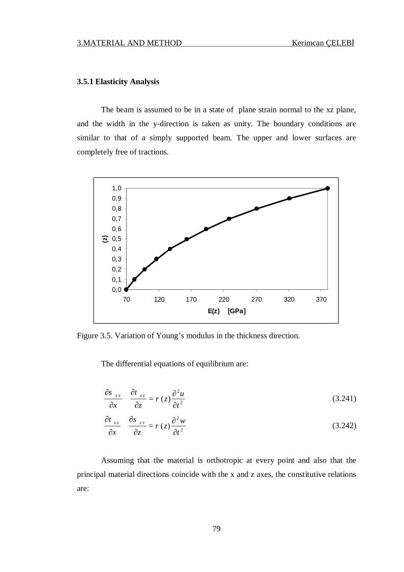
3.MATERIAL AND METHOD Kerimcan ÇELEBİ
79
3.5.1 Elasticity Analysis
The beam is assumed to be in a state of plane strain normal to the xz plane,
and the width in the y-direction is taken as unity. The boundary conditions are
similar to that of a simply supported beam. The upper and lower surfaces are
completely free of tractions.
0,00,10,20,30,40,50,60,70,80,91,0
70 120 170 220 270 320 370
E(z) [GPa]
(z)
Figure 3.5. Variation of Young’s modulus in the thickness direction.
The differential equations of equilibrium are:
2
2
)(tuz
zxzxxx
∂∂
=∂
∂+
∂
∂ρ
τσ (3.241)
2
2
)(twz
zxzzzx
∂∂
=∂
∂+
∂
∂ρ
στ (3.242)
Assuming that the material is orthotropic at every point and also that the
principal material directions coincide with the x and z axes, the constitutive relations
are:

3.MATERIAL AND METHOD Kerimcan ÇELEBİ
80
=
zx
zz
xx
zx
zz
xx
ccccc
γ
ε
ε
τ
σ
σ
55
3313
1311
0000
(3.243)
Assuming that all elastic stiffness coefficients vary exponentially in the z
direction, the elasticity matrix can be written as:
[ ]
=055
033
013
013
011
000
0
)(c
cccc
ezc hz
ji
λ
(3.244)
where )0(0jiji cc = . Substituting from Eq.(3.243) into (3.241) and (3.242), than using
strain-displacement relations we obtain the following two equations in u(x,z,t) and
w(x,z,t):
2
2
55551311 )(tuz
xwc
zuc
zzwc
xuc
x ∂∂
=
∂∂
+∂∂
∂∂
+
∂∂
+∂∂
∂∂
ρ (3.245)
2
2
33135555 )(twz
zwc
xuc
zxwc
zuc
x ∂∂
=
∂∂
+∂∂
∂∂
+
∂∂
+∂∂
∂∂
ρ (3.246)
where hz
b ezλ
ρρ =)( .We will assume solutions of the form:
]cos[),(),,( xtzUtzxu ξ=
]sin[),(),,( xtzWtzxw ξ= (3.247)
where Ln /πξ = .
From the forms of the displacements one can note that the boundary
conditions at the left and right end faces of the beam are given by:
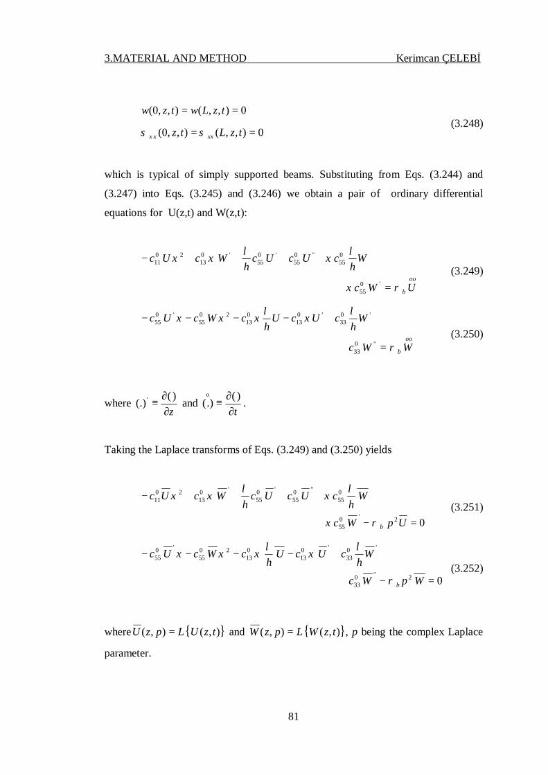
3.MATERIAL AND METHOD Kerimcan ÇELEBİ
81
0),,(),,0( == tzLwtzw
0),,(),,0( == tzLtz xxxx σσ (3.248)
which is typical of simply supported beams. Substituting from Eqs. (3.244) and
(3.247) into Eqs. (3.245) and (3.246) we obtain a pair of ordinary differential
equations for U(z,t) and W(z,t):
oo
b UWc
Wh
cUcUch
WcUc
ρξ
λξ
λξξ
=+
++++−
'055
055
''055
'055
'013
2011
(3.249)
oo
b WWc
Wh
cUcUh
cWcUc
ρ
λξ
λξξξ
=+
+−−−−
''033
'033
'013
013
2055
'055
(3.250)
where z∂
∂≡
)((.) ' and t
o
∂∂
≡)(.)( .
Taking the Laplace transforms of Eqs. (3.249) and (3.250) yields
02'055
055
''055
'055
'013
2011
=−+
++++−
UpWc
Wh
cUcUch
WcUc
bρξ
λξ
λξξ
(3.251)
02''033
'033
'013
013
2055
'055
=−+
+−−−−
WpWc
Wh
cUcUh
cWcUc
bρ
λξ
λξξξ
(3.252)
where { }),(),( tzULpzU = and { }),(),( tzWLpzW = , p being the complex Laplace
parameter.

3.MATERIAL AND METHOD Kerimcan ÇELEBİ
82
To simplify the calculations, we will assume that the FGM is isotropic at
every point. Further we will assume that the Poisson’s ratio is a constant through the
thickness. Then the variation of Young’s modulus is given by hz
b eEzEλ
=)( . The
elasticity matrix [c] is related to the Young’s modulus and Poisson’s ratio by:
[ ]
−−
−
−+=
22100
0101
)21()1(v
vvvv
vvEc (3.253)
The solution of Eqs. (3.251) and (3.252) can be derived as:
hzp
ii
ieapzU)(4
1),(
α
∑=
=
hzp
ii
iebpzW)(4
1),(
α
∑=
=
(3.254)
where ia and ib are arbitrary constants to be determined from the traction boundary
conditions on the top and bottom surfaces, also at this stage free vibration analysis
can easily be performed, the Laplace parameter p in Eqs. (3.251) and (3.252) are
replaced by βi to get
0))()(
(
))()(
(
055
055
013
22
2055
055
2011
=+++
+++−
hc
hc
hcb
hc
hc
hca
iii
bii
i
βαξ
λξ
βαξ
βρβαβαλ
ξ (3.255)
0))()(
())()(
(
22
2033
033
2055
013
013
055
=+++
−+−−−
βρβαβαλ
ξβα
ξλ
ξβα
ξ
bii
iii
i
hc
hhc
cbh
ch
ch
ca (3.256)
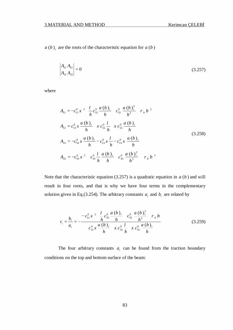
3.MATERIAL AND METHOD Kerimcan ÇELEBİ
83
i)(βα are the roots of the characteristic equation for )(βα
022
12
21
11 =AA
AA
(3.257)
where
22
2055
055
201111
)()(βρ
βαβαλξ b
ii
hc
hc
hcA +++−=
hc
hc
hcA ii )()( 0
55055
01312
βαξ
λξ
βαξ ++=
hc
hc
hcA ii )()( 0
13013
05521
βαξ
λξ
βαξ −−−=
22
2033
033
205522
)()(βρ
βαβαλξ b
ii
hc
hhccA +++−=
(3.258)
Note that the characteristic equation (3.257) is a quadratic equation in )(βα and will
result in four roots, and that is why we have four terms in the complementary
solution given in Eq.(3.254). The arbitrary constants ia and ib are related by
hc
hc
hc
hc
hc
hc
abr
ii
bii
i
ii )()(
)()(
055
055
013
2
2055
055
2011
βαξ
λξ
βαξ
βρβαβαλ
ξ
++
+++−−== (3.259)
The four arbitrary constants ia can be found from the traction boundary
conditions on the top and bottom surface of the beam:

3.MATERIAL AND METHOD Kerimcan ÇELEBİ
84
0),0,( 055055 =∂∂
+∂∂
= == zzxz xwc
zuctxτ
0),,( 5555 =∂∂
+∂∂
= == hzhzxz xwc
zucthxτ
0),0,( 033013 =∂∂
+∂∂
= == zzzz zwc
xuctxσ
0),,( 3313 =∂∂
+∂∂
= == hzhzzz zwc
xucthxσ
(3.260)
Substituting for u and w from Eq. (3.248), we obtain the BCs in terms of U
and W:
0),0(),0(' =+ tWtU ξ
0),(),(' =+ thWthU ξ
0),0('),0( 033
013 =+− tWctUc ξ
0),('),( 3313 =+− thWcthUc hh ξ
(3.261)
where )(hcc ijhij = . Taking the Laplace transform of Eq. (3.261) to get
0),0(),0(' =+ pWpU ξ
0),(),(' =+ phWphU ξ
0),0('),0( 033
013 =+− pWcpUc ξ
0),('),( 3313 =+− phWcphUc hh ξ
(3.262)
Substituting for U and W from Eqs. (3.254) into (3.262) and replaced
Laplace parameter p with βi , we obtain four equations for ia :

3.MATERIAL AND METHOD Kerimcan ÇELEBİ
85
0))(
(4
1=+∑
=i
i
ii r
ha ξ
βα
0))(
( )(4
1=+∑
=
ierh
a ii
ii
βαξβα
0))(
( 033
013
4
1=+−∑
= hrcca i
ii
iβα
ξ
0))(
( )(033
013
4
1=+−∑
=
λβαβαξ ee
hrcca ii
ii
i
(3.263)
Eq. (3.263) can be written as
0
4
3
2
1
44434241
34333231
24232221
14131211
=
aaaa
SSSSSSSSSSSSSSSS
(3.264)
in which ijS represents costants which includes β . For finding free vibration
frequencies, the determinant of constant matrix ijS is set equal to zero.
In the present work, since the beam is modelled as a continuum, infinitely
many frequencies may be obtained. Table 3.13 shows the first ten natural frequencies
for FGM beam with v=0.3, 2707=bρ 3/ mkg , 70=bE GPa, L/h=5,10,20 and
n=1,3,5.
3.5.2. Mode Shapes
)(βα values related to natural frequencies can be obtained from equation
(3.257) in imaginary form.
iqpiqpiqpiqp
224222
113111
)(,)()(,)(
−=+=−=+=
βαβαβαβα
(3.265)
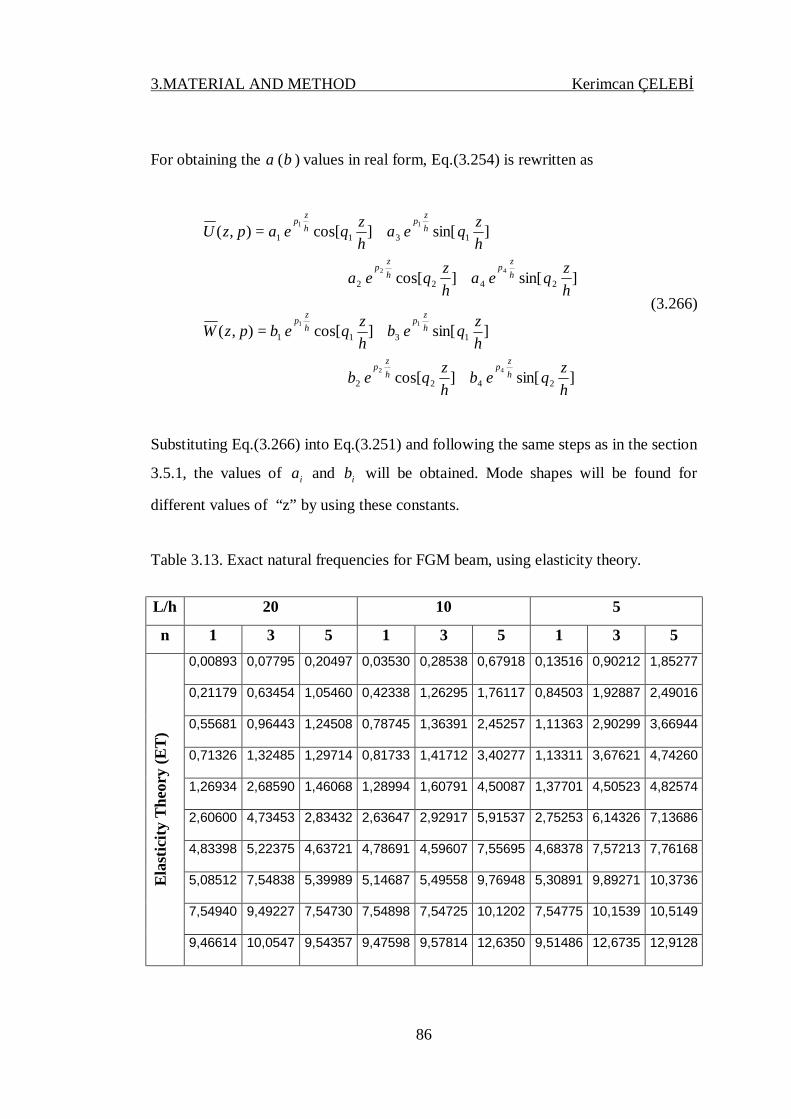
3.MATERIAL AND METHOD Kerimcan ÇELEBİ
86
For obtaining the )(βα values in real form, Eq.(3.254) is rewritten as
]sin[]cos[
]sin[]cos[),(
2422
1311
42
11
hzqea
hzqea
hzqea
hzqeapzU
hzp
hzp
hzp
hzp
++
+=
]sin[]cos[
]sin[]cos[),(
2422
1311
42
11
hzqeb
hzqeb
hzqeb
hzqebpzW
hzp
hzp
hzp
hzp
++
+=
(3.266)
Substituting Eq.(3.266) into Eq.(3.251) and following the same steps as in the section
3.5.1, the values of ia and ib will be obtained. Mode shapes will be found for
different values of “z” by using these constants.
Table 3.13. Exact natural frequencies for FGM beam, using elasticity theory.
L/h 20 10 5
n 1 3 5 1 3 5 1 3 5
Elas
ticity
The
ory
(ET)
0,00893
0,07795 0,20497 0,03530 0,28538 0,67918 0,13516 0,90212 1,85277
0,21179
0,63454 1,05460 0,42338 1,26295 1,76117 0,84503 1,92887 2,49016
0,55681
0,96443 1,24508 0,78745 1,36391 2,45257 1,11363 2,90299 3,66944
0,71326
1,32485 1,29714 0,81733 1,41712 3,40277 1,13311 3,67621 4,74260
1,26934
2,68590 1,46068 1,28994 1,60791 4,50087 1,37701 4,50523 4,82574
2,60600
4,73453 2,83432 2,63647 2,92917 5,91537 2,75253 6,14326 7,13686
4,83398
5,22375 4,63721 4,78691 4,59607 7,55695 4,68378 7,57213 7,76168
5,08512
7,54838 5,39989 5,14687 5,49558 9,76948 5,30891 9,89271 10,3736
7,54940
9,49227 7,54730 7,54898 7,54725 10,1202 7,54775 10,1539 10,5149
9,46614
10,0547 9,54357 9,47598 9,57814 12,6350 9,51486 12,6735 12,9128

3.MATERIAL AND METHOD Kerimcan ÇELEBİ
87
3.5.3 Beam Theory
In the present thesis, free vibration of simply supported FG beams using
classical beam theory (CBT) and parabolic shear deformation beam theory (PSDBT)
and first order shear deformation beam theory (FSDBT) will also be given from the
literature (Aydogdu and Taskin, 2007). Governing equations of FG beam for free
vibration problem were found by applying Hamilton principle and Navier type
solution method was used to solve vibration problem.
The state of stress in the beam is given by the generalised Hooke’s law as
follows:
xx Q εσ 11= , xzxz Q γτ 55= (3.267)
where ijQ are the transformed stiffness constants in the beam co-ordinate system and
are defined as
211 1)(
vzEQ
−= ,
)1(2)(
255 vzEQ
+= (3.268)
Assuming that the deformations of the beam are in the x-z plane and denoting the
displacement components along the x, y and z-directions by U, V and W [Timarci
and Soldatos, 1995]:
),()(),(),,( 1. txuzwztxutzxU x Φ+−=
0),,( =tzxV
),(),,( txwtzxW =
(3.269)
It may be noted that u and w denotes the displacement of points on the bottom
surfaces of the beam, and not points in the mid-plane. 1u is an unknown function
that represents the effect of transverse shear strain on the beam bottom surface, and

3.MATERIAL AND METHOD Kerimcan ÇELEBİ
88
Φ represents the shape function determining the distribution of the transverse strain
and stress through the thickness.
Classical beam theory is obtained as a particular case by taking the shape
function as zero. Although different shape functions are applicable, only the ones
which convert the present theory to the corresponding parabolic shear deformation
beam theory (PSDBT) and first order shear deformation beam theory (FSDBT) are
employed in the present thesis. This is achived by choosing the shape function as
follows:
0)(: =Φ zCBT
zzFSDBT =Φ )(:
)3/41()(: 22 hzzzPSDBT −=Φ
(3.270)
The displacement equations yields the following kinematic relations:
xxxxx uzwzu ,1,, )(Φ+−=ε
1' )( uzxz Φ=γ
(3.271)
where a prime denotes the derivative with respect to z and “x” represents the partial
derivative with respect to x. By substituting the stress-strain relations into the
definitions of the force and moment resultants of the theory given in [Soldatos and
Timarci, 1993] and using the notation given by [Soldatos and Sophocleous, 2001],
the following constitutive equations are obtained:
−
=
x
xx
x
aaaa
acc
acc
ax
cx
cx
uw
u
DDBDDBBBA
MMN
,1
,
,
111111
111111
111111
(3.272)
155 uAQ aax = (3.273)

3.MATERIAL AND METHOD Kerimcan ÇELEBİ
89
The extensional, coupling and bending rigidities appearing in Eq. (3.272) are,
respectively, defined as follows:
∫=h
c dzQA0
1111
dzzzQBBh
ac ∫ Φ=0
111111 )](,[),(
dzzzzzQDDDh
aaac ∫ ΦΦ=0
2211111111 )](),(,[),,(
(3.274)
Moreover, the transverse shear rigidity appearing in Eq. (3.273) is defined according
to
dzzQAh
a 2
05555 )('Φ= ∫ (3.275)
It should be pointed out that the extensional cA11 , coupling cB11 and bending cD11 rigidities are the ones usually appearing even in the classical beam theories.
Among the additional rigidities in Eq. (3.272), the one denoted as aB11 is considered
as additional coupling rigidity while the ones denoted as aD11 and aaD11 are considered
as additional bending rigidities.
Upon employing the Hamilton’s principle, the three variationally consistent
equilibrium equations of the beam are obtained as:
ttxc
xx wuuN ,,11010, )( ρρρ −+=
ttxxxxc
xxx wwuuM ,,20,111,1, )( ρρρρ −++=
ttxax
axx wuuQM ,,1110201, )( ρρρ −+=−
(3.276)
Here, tt, denotes time derivatives and the ρ ’s are defined as:

3.MATERIAL AND METHOD Kerimcan ÇELEBİ
90
)2,1,0(,)( == ∫ idzzz ih
oi ρρ
)2,1;1,0(,)()( ==Φ= ∫ mjdzzzzh
o
mj
jjm ρρ
(3.277)
where ][)(hzExpz b λρρ = . The force and moment components are
dzzMNh
xcx
cx ∫=
0
),1(),( σ
∫ Φ=h
ıxz
ax dzzQ
0
)(τ
∫ Φ=h
xax dzzM
0
)(σ
(3.278)
Here, the appearance of the higher order moment axM and the transverse shear force
resultant axQ in Eq.(3.278) is due to the particular form of the displacement field
(3.269). In particular, the superscript “a” in these definitions is used only for a
distinction between higher order transverse shear resultants and the corresponding
conventional ones used in classical beam theory.
Moreover, the following sets of boundary conditions at the edges of the beam
are obtained by the application of Hamilton’s principle: at x=0,L.
Either u or xcx NN = prescribed,
Either w or xc
xx QM =, prescribed,
Either xw, or xcx MM = prescribed,
Either 1u or ax
ax MM = prescribed,
(3.279)

3.MATERIAL AND METHOD Kerimcan ÇELEBİ
91
Here, the over-barred quantities appearing in the right sides of natural boundary
conditions denote prescribed force and moment resultants acting on the beam
boundaries .
The simply supported boundary conditions are
0==== ax
cx
cx MMwN (3.280)
Navier-type solutions to Eq. (3.276) that satisfy the boundary conditions Eq.
(3.280) can be expressed in the form of
]sin[]cos[ tL
xnAu n βπ
=
]sin[]cos[1 tL
xnBuL n βπ
=
]sin[]sin[ tL
xnCw n βπ
=
(3.281)
where “n” is the wave number in the x direction and nA , nB and nC are
undetermining coefficients. Inserting Eq. (3.281) in Eq. (3.276) leads to following
problem.
0
333231
232221
131211
=
n
n
n
CBA
KKKKKKKKK
(3.282)
in which ijK represents costants which includes β . For finding free vibration
frequencies, the determinant of constant matrix ijK is set equal to zero.
Table 3.14 shows the fundemental natural frequencies for FGM beam with
v=0.3, 3/2707 mkgb =ρ , GPaEb 70= , L/h=5,10,20 and n=1,3,5.

3.MATERIAL AND METHOD Kerimcan ÇELEBİ
92
Table 3.14. Natural frequencies for FGM beam from beam theories.
n L/h CBT FSDBT PSDBT ET
1
5 0,141475 0,137088 0,141107 0.13516
10 0,035745 0,035446 0,035720 0.03530
20 0,00896 0,008941 0,008959 0.00893
3
5 1,151350 0,966028 1,134500 0.90212
10 0,312914 0,293397 0,311228 0.28538
20 0,08007 0,078611 0,079949 0.07795
5
5 2,737690 2,061590 2,681100 1.85277
10 0,825849 0,718196 0,816126 0.67916
20 0,219342 0,209255 0,218483 0.20497
The result from Elasticity Theory (ET) corresponding to “m” and “L/h”
values used in beam theories are also included for comparison purposes.
4. RESULTS AND DISCUSSIONS Kerimcan ÇELEBİ
93
4. RESULTS AND DISCUSSIONS
For non-uniform rods and heterogeneous rods, the end-point displacements
will be calculated using the various methods outlined in previous sections and the
results will be compared to assure the efficiency of the Laplace transform method as
it is applied to the particular problem on hand.
The results are presented graphically using the following analyses for each
loading type:
A1 (MSM): The resulting end-point displacement equations summarized in Table-
3.10 to Table-3.12 are used directly.
A2 (DURBIN): Inverse Laplace transformation of the end-point displacement
expressions given in Table-3.4 to Table-3.6 are obtained. Durbin’s Inverse
Transform Method is used to obtain the values in the time domain
A3 (RESIDUE): The numerical results obtained from Residue theorem summarized
in Table-3.7 to Table-3.9 are used directly.
First ten frequencies have been taken in the calculations. Figs. 4.1 - 4.27
show the results for given variations subjected to dynamic loads
])cos[1()( 01 τγτ −= PP , 02 )( PP =τ and )1()( 03γττ −−= ePP , respectively. A γ
value of 0.6 has been used throughout. Increasing a causes an increase in
displacement. In all loading cases, for 2=a , a noticeable difference was present
between the exact and MSM results. To achieve the accuracy of the exact results, up
to a hundred frequencies were needed in MSM.
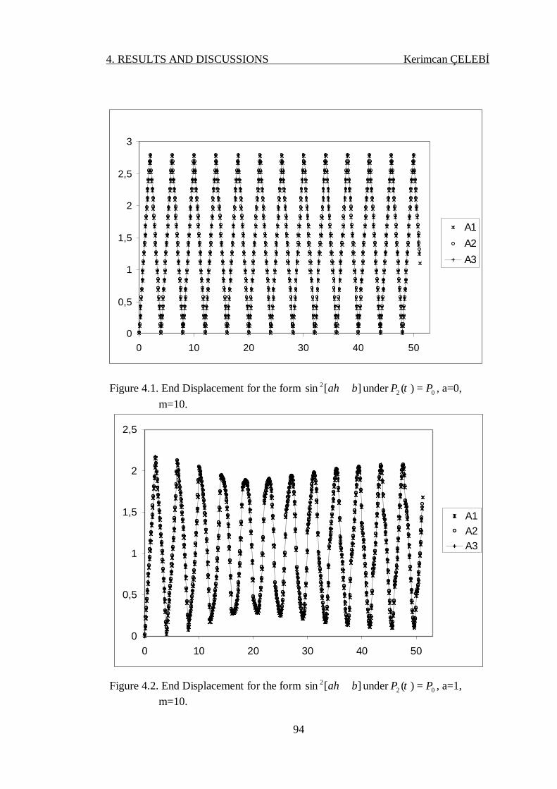
4. RESULTS AND DISCUSSIONS Kerimcan ÇELEBİ
94
0
0,5
1
1,5
2
2,5
3
0 10 20 30 40 50
A1A2A3
Figure 4.1. End Displacement for the form ][sin 2 ba +η under 02 )( PP =τ , a=0, m=10.
0
0,5
1
1,5
2
2,5
0 10 20 30 40 50
A1A2A3
Figure 4.2. End Displacement for the form ][sin 2 ba +η under 02 )( PP =τ , a=1, m=10.

4. RESULTS AND DISCUSSIONS Kerimcan ÇELEBİ
95
0
1
2
3
4
5
6
7
0 10 20 30 40 50
A1A2A3
Figure 4.3. End Displacement for the form ][sin 2 ba +η under 02 )( PP =τ , a=2, m=10.
-0,5
0
0,5
1
1,5
2
2,5
3
3,5
0 10 20 30 40 50
A1A2A3
Figure 4.4. End displacement for the form ][sin 2 ba +η under ])cos[1()( 01 τγτ −= PP , a=0, m=10,γ =0.6.

4. RESULTS AND DISCUSSIONS Kerimcan ÇELEBİ
96
-0,5
0
0,5
1
1,5
2
2,5
3
0 10 20 30 40 50
A1A2A3
Figure 4.5. End displacement for the form ][sin 2 ba +η under ])cos[1()( 01 τγτ −= PP , a=1, m=10,γ =0.6.
-1
0
1
2
3
4
5
6
7
8
9
0 10 20 30 40 50
A1A2A3
Figure 4.6. End displacement for the form ][sin 2 ba +η under ])cos[1()( 01 τγτ −= PP , a=2, m=10,γ =0.6.

4. RESULTS AND DISCUSSIONS Kerimcan ÇELEBİ
97
0
0,2
0,4
0,6
0,8
1
1,2
1,4
1,6
1,8
2
0 10 20 30 40 50
A1A2A3
Figure 4.7. End displacement for the form ][sin 2 ba +η under )1()( 03
γττ −−= ePP , a=0, m=10,γ =0.6.
0
0,2
0,4
0,6
0,8
1
1,2
1,4
1,6
0 10 20 30 40 50
A1A2A3
Figure 4.8. End displacement for the form ][sin 2 ba +η under )1()( 03
γττ −−= ePP , a=1, m=10,γ =0.6.

4. RESULTS AND DISCUSSIONS Kerimcan ÇELEBİ
98
0
0,5
1
1,5
2
2,5
3
3,5
4
4,5
0 10 20 30 40 50
A1A2A3
Figure 4.9. End displacement for the form ][sin 2 ba +η under )1()( 03
γττ −−= ePP , a=2, m=10,γ =0.6.
0
0,5
1
1,5
2
2,5
0 10 20 30 40 50
A1A2A3
Figure 4.10. End displacement. for the form 2)1( ηa+ under 02 )( PP =τ , a=0, m=10.

4. RESULTS AND DISCUSSIONS Kerimcan ÇELEBİ
99
0
0,2
0,4
0,6
0,8
1
1,2
0 10 20 30 40 50
A1A2A3
Figure 4.11. End displacement for the form 2)1( ηa+ under 02 )( PP =τ , a=1, m=10.
0
0,1
0,2
0,3
0,4
0,5
0,6
0,7
0 10 20 30 40 50
A1A2A3
Figure 4.12. End displacement for the form 2)1( ηa+ under 02 )( PP =τ , a=2, m=10.

4. RESULTS AND DISCUSSIONS Kerimcan ÇELEBİ
100
-0,5
0
0,5
1
1,5
2
2,5
0 10 20 30 40 50
A1A2A3
Figure 4.13. End displacement for the form 2)1( ηa+ under ])cos[1()( 01 τγτ −= PP , a=0, m=10,γ =0.6.
-0,4
-0,2
0
0,2
0,4
0,6
0,8
1
1,2
1,4
1,6
0 10 20 30 40 50
A1A2A3
Figure 4.14. End displacement for the form 2)1( ηa+ under ])cos[1()( 01 τγτ −= PP , a=1, m=10,γ =0.6.

4. RESULTS AND DISCUSSIONS Kerimcan ÇELEBİ
101
-0,6
-0,4
-0,2
0
0,2
0,4
0,6
0,8
1
1,2
0 10 20 30 40 50
A1A2A3
Figure 4.15. End displacement for the form 2)1( ηa+ under ])cos[1()( 01 τγτ −= PP , a=2, m=10,γ =0.6.
0
0,2
0,4
0,6
0,8
1
1,2
1,4
0 10 20 30 40 50
A1A2A3
Figure 4.16. End displacement for the form 2)1( ηa+ under )1()( 03γττ −−= ePP ,
a=0, m=10, γ =0.6.
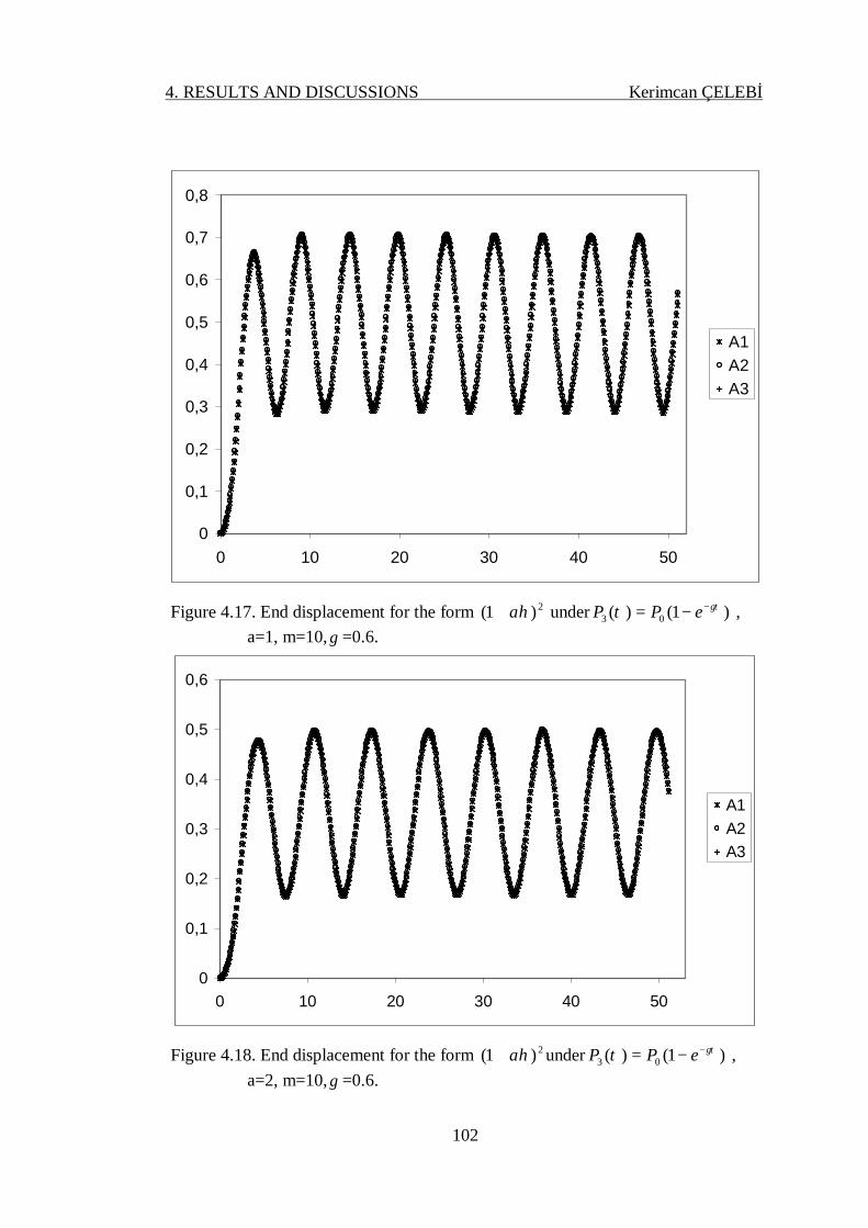
4. RESULTS AND DISCUSSIONS Kerimcan ÇELEBİ
102
0
0,1
0,2
0,3
0,4
0,5
0,6
0,7
0,8
0 10 20 30 40 50
A1A2A3
Figure 4.17. End displacement for the form 2)1( ηa+ under )1()( 03γττ −−= ePP ,
a=1, m=10, γ =0.6.
0
0,1
0,2
0,3
0,4
0,5
0,6
0 10 20 30 40 50
A1A2A3
Figure 4.18. End displacement for the form 2)1( ηa+ under )1()( 03γττ −−= ePP ,
a=2, m=10, γ =0.6.

4. RESULTS AND DISCUSSIONS Kerimcan ÇELEBİ
103
0
0,2
0,4
0,6
0,8
1
1,2
1,4
1,6
1,8
2
0 10 20 30 40 50
A1A2A3
Figure 4.19. End displacement for the form ηae− under 02 )( PP =τ , a=0, m=10.
0
0,5
1
1,5
2
2,5
3
3,5
0 10 20 30 40 50
A1A2A3
Figure 4.20. End displacement for the form ηae− under 02 )( PP =τ , a=1, m=10.

4. RESULTS AND DISCUSSIONS Kerimcan ÇELEBİ
104
0
1
2
3
4
5
6
0 10 20 30 40 50
A1A2A3
Figure 4.21. End displacement for the form ηae− under 02 )( PP =τ , a=2, m=10.
-0,5
0
0,5
1
1,5
2
2,5
0 10 20 30 40 50
A1A2A3
Figure 4.22. End displacement for the form ηae− under ])cos[1()( 01 τγτ −= PP , a=0, m=10, γ =0.6.

4. RESULTS AND DISCUSSIONS Kerimcan ÇELEBİ
105
-0,5
0
0,5
1
1,5
2
2,5
3
3,5
4
0 10 20 30 40 50
A1A2A3
Figure 4.23. End displacement for the form ηae− under ])cos[1()( 01 τγτ −= PP , a=1, m=10, γ =0.6.
-1
0
1
2
3
4
5
6
7
8
0 10 20 30 40 50
A1A2A3
Figure 4.24. End displacement for the form ηae− under ])cos[1()( 01 τγτ −= PP , a=2, m=10, γ =0.6.

4. RESULTS AND DISCUSSIONS Kerimcan ÇELEBİ
106
0
0,2
0,4
0,6
0,8
1
1,2
1,4
0 10 20 30 40 50
A1A2A3
Figure 4.25. End displacement for the form ηae− under )1()( 03γττ −−= ePP , a=0,
m=10, γ =0.6.
0
0,5
1
1,5
2
2,5
0 10 20 30 40 50
A1A2A3
Figure 4.26. End displacement for the form ηae− under )1()( 03
γττ −−= ePP , a=1, m=10, γ =0.6.

4. RESULTS AND DISCUSSIONS Kerimcan ÇELEBİ
107
0
0,5
1
1,5
2
2,5
3
3,5
4
0 10 20 30 40 50
A1A2A3
Figure 4.27. End displacement for the form ηae− under )1()( 03γττ −−= ePP , a=2,
m=10, γ =0.6.
In numerical analysis, fundemental frequencies of FG beams with clamped-
free support are given in tabular form for different values of slenderness ratio (L/h=5,
10, 20) and wave number (n=1,3,5). Assume that the FG beam is a mixture of two
materials and material properties were chosen as follows:
GPaEb 70= , 3.0=bv , 3/2707 mkgb =ρ
GPaEt 380= , 3.0=tv , 3/14695 mkgt =ρ
For the given material properties btbt EE ρρ // = .
The results are presented graphically using the following analyses for each
L/h ratio and wave number (n).
B1: Elasticity solution (ET)
B2: Classical beam theory (CBT)
B3: First order shear deformation beam theory (FSDBT)
B4: Parabolic shear deformation beam theory (PSDBT)

4. RESULTS AND DISCUSSIONS Kerimcan ÇELEBİ
108
0 5 10 15 20 25
L/h
Fund
emen
tal f
requ
ency
B1B2B3B4
Figure 4.28. Variation of the fundemental frequency of FGM beam with L/h ratio for
n=1
0 5 10 15 20 25
L/h
Fund
emen
tal f
requ
ency
B1B2B3B4
Figure 4.29. Variation of the fundemental frequency of FGM beam with L/h ratio for
n=3

4. RESULTS AND DISCUSSIONS Kerimcan ÇELEBİ
109
0 5 10 15 20 25
L/h
Fund
emen
tal f
requ
ency
B1B2B3B4
Figure 4.30. Variation of the fundemental frequency of FGM beam with L/h ratio for
n=5
0 1 2 3 4 5 6
n
Fund
emen
tal f
requ
ency
B1B2B3B4
Figure 4.31. Variation of the fundemental frequency of FGM beam with n for
L/h=5

4. RESULTS AND DISCUSSIONS Kerimcan ÇELEBİ
110
0 1 2 3 4 5 6
n
Fund
emen
tal f
requ
ency
B1B2B3B4
Figure 4.32. Variation of the fundemental frequency of FGM beam with n for
L/h=10
0 1 2 3 4 5 6
n
Fund
emen
tal f
requ
ency
B1B2B3B4
Figure 4.33. Variation of the fundemental frequency of FGM beam with n for
L/h=20

4. RESULTS AND DISCUSSIONS Kerimcan ÇELEBİ
111
Figures 4.28 - 4.33 show the fundemental frequencies of FG beams for
different values of slenderness ratio and wave number. As it seen from the figures,
L/h ratio is more effective for higher modes. The differences between analysis are
increasing with increasing mode number and decreasing L/h ratio.
In Figure 4.34, the first, third and fifth flexural mode shapes of FGM beam
using elasticity theory are shown for different L/h ratios. It is clear that mode shapes
are affected by the variations of L/h ratio.
Figure 4.34. Flexural mode shapes at the bottom surface and upper surface of the
FGM beam.

4. RESULTS AND DISCUSSIONS Kerimcan ÇELEBİ
112

5. CONCLUSIONS Kerimcan ÇELEBİ
113
5. CONCLUSIONS
Closed-form solutions for free and forced vibration analyses of a non-uniform
rod and heterogeneous rod have been performed using Laplace transform technique.
The problem is solved in the Laplace domain and the inversion into the time domain
is done exactly by the residue theorem and modified Durbin’s inverse transform
method. The numerical results obtained from Residue theorem and Durbin’s inverse
transform method are compared with those from Mode Superposition Method
(MSM). It is seen that when use of first ten frequencies in the analytical solutions
gave six-digit accuracy, for certain cases, up to a hundred frequencies were needed in
MSM. In addition to their efficient use, exact solutions give adequate insight into the
physics of the problem. In optimization problems using closed-form solutions will
greatly reduce the solution time. The inhomogeneity parameter “a” used in rod
models is found to be effective in the response of the material such that increasing
the inhomogeneity parameter consistently caused a decrease in the amplitude of
displacements.
Free vibration analysis of FG beam has been performed using elasticity
analysis and beam theory. The advantage of using elasticity theory is, since the beam
is modelled as a continuum, infinitely many frequencies may be obtained. But in
beam theories, only limited number of natural frequencies are obtained. Figure 4.28-
4.33 show the variation of the fundemental frequencies of FGM beam. The most
important observation is the fact that the frequencies are increased when the value of
L/h decreased or value of n increased.The difference between the frequencies of CBT
and those of the other higher-order beam theories and elasticity solution is
significiant when L/h<20. The results of the higher-order beam theories and elasticity
solution are very close to each other when L/h>20. The difference between the
results increases with increasing value of n and decreasing value of L/h.
Also similar situation is valid for mode shapes; the difference between the
mode shapes of upper and lower surfaces increases with decreasing L/h. For long
slender beams, there is no variation through the thickness. In short and thick beams,

5. CONCLUSIONS Kerimcan ÇELEBİ
114
however, the flexural mode shape for top and bottom surfaces are different. Because
of this, for short and thick beams, beam theory should not be used.

115
REFERENCES
ABBASI, M., ESLAMI, M.R. and SABBAGHIAN, M., 2008. Coupled
Thermoelastic Vibrations Analysis of Functionally Graded Timoshenko
Beams Using the Galerkin Finite Elemet Method. 2008 ASME International
Mechanical Engineering Congress and Exposition, October 31-November 6,
Boston, Massachussets, USA.
ABRAMOWITZ, M. and STEGUN, I.A., 1982. Handbook of Mathematical
Functions. Dover, USA.
ABRATE, S., 1995. Vibration of Non-Uniform Rods and Beams. Journal of Sound
and Vibration, 185, 703-716.
AYDOGDU, M., 2005. Vibration Analysis of Cross-ply Laminated Beams with
General Boundary Conditions by Ritz Method. International Journal of
Mechanical Science, 47, 1740-1755.
AYDOGDU, M. and TASKIN, V., 2007. Free Vibration Analysis of Functionally
Graded Beams with Simply Supported Edges. Materials and Design, 28,
1651- 1656.
BESKOS, D.E. and NARAYANAN, G.V., 1981. Dynamic Response of Frameworks
by Numerical Laplace Transform. Computer Methods in Applied Mechanics
and Engineering, 37, 289-307.
CALIM, F.F., 2009. Free and Forced Vibrations of Non-uniform Composite Beams.
Composite Structures, 88, 413-423.
CALIO, I. and ELISHAKOFF, I., 2005. Closed-form Solutions for Axially Graded
Beam-Columns. Journal of Sound and Vibration, 280, 1083-1094.
CANDAN, S. and ELISHAKOFF, I., 2001. Constucting the Axial Stiffness of
Longitudinally Vibrating Rod from Fundamental Mode Shape. International
Journal of Solids and Structures, 38, 3443-3452.
CELEBI, K., KELES, I. and TUTUNCU, N., 2009. Homojen Olmayan Çubuk, disk
ve Silindirlerin Laplace Transformasyonu ile Zorlanmış Titreşim Analizi.
XVI. Ulusal Mekanik Kongresi, 22-26 Haziran, Erciyes Üniversitesi,
Kayseri.

116
COOLEY, W. and TUKEY, J.W., 1965. An Algorithm for Machine Calculation of
Complex Fourier Series, Math. Computation, 19, 297-301.
CLOUGH, R.W. and PENZIEN, J., 1993. Dynamics of Structures, McGraw-Hill,
USA.
DURBIN, F., 1974. Numerical Inversion of Laplace Transforms: An Efficient
Improvement to Dubner and Abate’s Method. Commissariat a l’Energie
Atomique Centre U-Service Electronique, 17, 371-376.
EISENBERGER, M., 1991. Exact Longitudinal Vibration Frequencies of a Variable
Cross-Section Rod. Applied Acoustics, 34, 123-130.
ELISHAKOFF, I. and CANDAN, S., 2001. Apparently First Closed-Form Solution
for Vibrating: Inhomogeneous Beam. International Journal of Solids and
Structures, 38, 3411-3441.
HORGAN, C.O. and CHAN, A.M., 1999. Vibration of Inhomogeneous strings, rods
and membranes. Journal of Sound and Vibration, 225, 503-513.
KADOLI, R., AKHTAR, K. and GANESAN, N., 2008. Static Analysis of
Functionally Graded Beams Using Higher Order Shear Deformation
Theory. Applied Mathematical Modelling, 32, 2509-2525.
KUMAR, B.M. and SUJITH, R.I., 1997. Exact Solutions for the Longitudinal
Vibrations of Non-Uniform Rods. Journal of Sound and Vibration, 207, 721 -
729.
LI, Q.S., FANG, J.Q. and JEARY, A.P., 1998. Calculation of Vertical Dynamic
Characteristics of Tall Buildings with Viscous Damping. International
Journal of Solids Structures, 35 (24), 3165-3176.
LI, Q.S., LI, G.Q. and LIU, D.K., 1999. Exact Solutions for Longitudinal Vibration
of Rods Coupled by Translational Springs. International Journal of
Mechanical Sciences, 42, 1135-1152.
LI, Q.S., 2000. Free Longitudinal Vibration analysis of Multi-Step Non-Uniform
Bars Based on Piecewise Analytical Solutions. Engineering Structures, 22,
1205-1215.

117
LI, Q.S., WU, J.R. and XU, J., 2002. Longitudinal Vibration of Multi-Step Non-
Uniform Structures with Lumped Masses and Spring Supports. Applied
Acoustics, 63, 333-350.
LI, X.F., 2008. A Unified Approach for Analyzing Static and Dynamic Behaviors of
Functionally Graded Timoshenko and Euler-Bernoulli Beams. Journal of
Sound and Vibration, 313, 1210-1229.
MANOLIS, R.W. and BESKOS, D.E., 1981. Dynamic Stress Concentration Studies
by Boundary Integrals and Laplace Transfrom. International Journal of
Numerical Methods for Engineering, 17, 573-599.
NACHUM, S. and ALTUS, E., 2007. Natural Frequencies and Mode Shapes of
Deterministic and Stochastic Non-homogeneous Rods and Beams. Journal of
Sound and Vibration, 302, 903-924.
NARAYANAN, G.V., 1977. Use of Dynamic Influence Coefficients in Forced
Vibration Problems with the Aid of Fast Fourier Transform. Computers and
Structures, 9, 145-150.
QIUSHENG, L., HONG, C. and GUIGING, L., 1996. Static and Dynamic Analysis
of Straight Bars with Variable Cross-Section, 59, 1185-1191.
RAJ, A. and SUJITH, R.I., 2005. Closed-form Solutions for the Free Longitudinal
Vibration of Inhomogeneous Rods. Journal of Sound and Vibration, 283,
1015- 1030.
SANKAR, B.V., 2001. An Elasticity Solution for Functionally Graded Beams.
Composites Science and Technology, 61, 689-696.
SANKAR, B.V. and TZENG, J.T., 2002. Thermal Stresses in Functionally Graded
Beams. AIAA Journal, 40, 1228-1232.
SINA, S.A., NAVAZI, H.M. and HADDADPOUR, H., 2009. An Analytical Method
for Free Vibration Analysis of Functionally Graded Beams. Materials and
Design, 30, 741-747.
SIMSEK, M. and KOCATURK, T., 2009. Free and Forced Vibration of a
Functionally Graded Beam Subjected to a Concentrated Moving Harmonic
Load. Composite Structures, 90, 465-473.

118
SIMSEK, M., 2009. Static Analysis of a Functionally Graded Beam Under a
Uniformly Distributed Load by Ritz Method. International Journal of
Engineering and Applied Science, 1, 1-11.
SIMSEK, M., 2010. Vibration Analysis of a Functionally Graded Beam Under a
Moving Mass by Using Different Beam Theories. Composite Structures,
Article in press.
SOLDATOS, K.P. and SOPHOCLEOUS, C., 2001. On Shear Deformable Beam
Theories: The Frequency and Normal Mode Equations of the Homogeneous
Orthotropic Bickford Beam. Journal of Sound and Vibration, 242, 215-245.
TEMEL, B., 1996. Dinamik Zemin-Yapı Etkileşimi Problemlerinin Sonlu-Sonsuz
Elemanlar ve Laplace Dönüşüm Yöntemi ile Analizi. Çukurova University
Civil Engineering Department, Adana, 82-83.
YING, J., LU, C.F. and CHEN, W.Q., 2008. Two-Dimensional Elasticity Solutions
for Functionally Graded Beams Resting on Elastic Foundations. Composite
Structures, 84, 209-219.
ZHONG, Z. and Yu, T., 2007. Analytical Solution of a Cantilever Functionally
Graded Beam. Composites Science and Technology, 67, 689-696.

119
CURRICULUM VITAE
The author was born in ADANA in 1978. He graduated from Yeni College
in 1995. He registered to have his BS education at the Mechanical Engineering
Department of Çukurova University in 1996. He completed his BS education and
started his MS education in 2001. He started his PhD study at the Mechanical
Engineering Department of Çukurova University in 2004. He has been working as a
R&D Engineer at the Temsa Global A.Ş.

120

121
APPENDIX A.
Fast Fourier Transforms
The Fast Fourier transform, which allows very efficient and accurate
evaluations of the discrete Fourier transforms, is based on an algorithm developed by
Cooley and Tukey. Since the algorithm is used in exactly the same way in evaluating
both the direct and inverse FFTs, let us now consider only the direct FFT, namely
)1(,.....,3,2,1,21
0−==≡
−−
=∑ NnepNPA N
mniN
mmnn
π
(1)
in which mp denotes )( mttp = . In the present work, mp corresponds to
mtam etf −)( from Equation (3.99). A straightforward evaluation of this summation for
all values of n requires 2N complex multiplications. This number would be
prohibitive for most practical solutions requiring large values of N, say N>1000, thus
providing the incentive to develop the FFT algorithm.
The FFT algorithm based on letting γ2=N where γ is an integer. In this
case, each value of n and m in their common range from zero to N-1 can be
expressed in terms of binary coefficients as given by
022
11 .....22 nnnn +++= −
−−
−γ
γγ
γ
(2)
022
11 .....22 mmmm +++= −
−−
−γ
γγ
γ

122
in which each binary coefficient is either +1 or 0 depending upon the particular value
of n or m being represented. Using these relations and letting Ni
N eWπ2
−≡ , Equation
(1) can be expressed as
mnN
mmmWmmmpnnnA ),.....,,(.....),.....,,( 0210
1
0
1
0
1
0021
110
−−===
−− ∑∑∑−
= γγγγγ
(3)
Note that each coefficient nA for n=0,1,2,…..,N-1 is represented by
),.....,,( 021 nnnA −− γγ and each load ordinate mp for m=0,1,2,…..,N-1 is represented
by ),.....,,( 021 mmmpo −− γγ . The subscript zero has been added to p only to indicate
the multiplier of the mnNW term in the first summation. The reason for introducing
this addition to the notation will become apparent as the algorithm develops.
Consider now the term mnNW of Equation (3) in the form
).....22().....22( 022
11
022
11 mmmnnn
Nmn
N WW ++++++ −−
−−
−−
−−
= γγ
γγ
γγ
γγ
(4)
Making use of bN
aN
baN WWW =+ )( , this equation can be modified to
)2().....22( 1
102
21
1−
−−
−−
− +++= γλ
γγ
γγ mnnn
Nmn
N WW
*)2()......22( 2
202
21
1−
−−
−−
− +++ γγ
γγ
γγ mnnn
NW
*…..* 0022
11 ).....22( mnnn
NW +++ −−
−−
γγ
γγ
(5)
let us now examine each individual NW term on the right hand side of this equation
separately. The first term can be written

123
)2().....22( 1
102
21
1−
−−
−−
− +++ γλ
γγ
γγ mnnn
NW
= .....** )12(2)2(2 23
112 −−
−−−
− γγγγ
γγγγ mn
Nmn
N WW
)(2)2(2 10
111 ** −
−− γ
γγ
γ mnN
mnN WW
=)(2 10
1−
−γ
γ mnNW (6)
since each nW term of the form
1)(int2
)(int2 =
=
−egerN
Nieger
N eWπ
γ (7)
writing the second term similarly and making use of Equation (7), one finds that
201
22
202
21
1 )2(2)2().....22( −−
−−
−−
−− ++++ = γ
γγ
λγ
γγ
γ mnnN
mnnnN WW (8)
This pattern continues up to the last term which has no cancellations due to Equation
(7); therefore, it must remain in the same form shown in Equation (5).
After substituting all NW terms, except the last, in their reduced forms,
Equation (3) becomes
)1(1
110
20210
1
0
1
0
1
0021 *),.....,,(.....),.....,,(
−−
−
−−===
−− ∑∑∑=γγ
γ
γγγγ
mon
Nmmm
WmmmpnnnA
* 00.....22
112)012(2 )22(2 *....* mnn
NNn
mnn
WW ++−−
−−−+− + γ
γγ
γγγ
(9) Carrying out all summations in this equation in succession gives
),.....,,(),.....,,( 02012
1
00210
)10(1
1
mmnpWmmmpMN
Nm
−=
−− ≡−−
−
∑ γγγ
γγ
γ

124
),.....,,,(),.....,,( 031022
1
00201
2)012(2
2
mmnnpWmmnpmnn
Nm
−=
− ≡−+−
−
∑ γγ
γγ
γ
…
….. …..
00221
0
)....212(1
002101 ),,....,,( mnnn
Nm
Wmnnnp +++−
=−−
−−−
∑ λγγ γ
γγ
= ),.....,,( 021 nnnA −− γγ (10)
these recursive equations, leading to the desired result ),.....,,( 021 nnnA −− γγ ,
represent the Cooley-Tukey algorithm used in modern FFT analysis. They are
extremely efficient due to the fact that each summation is used immediately in the
next summation. The fact that the exponential has unit value in the first term of each
summation and that 2/NmnN
mnN WW +−= adds to the efficiency. The reduction in
computational effort which results from the use of Equation (10) is enormous when
the time duration pT is divided into a large number of intervals. For example, when
N=1024 (γ =10), the computer time required by the FFT to obtain all nAN -values is
approximately 0.5 percent of the time required to obtain the same values by direct
use of Equation (1). Not only is the FFT extremely efficient but it is very accurate as
well, thus making the frequency-domain approach to the dynamic- response analysis
of structures very attractive indeed.

125
APPENDIX B
1. Residue Theorem
Consider the counter integral
∫=C
dzzfI )( (1)
where f has a finite number of singular points within C, and each of them is
isolated. We do not permit singularities on the contour C, and whether or not f
has singular points outside C will not be relevant.
(a) (b)
Figure1. Deformation of countour.
For definiteness, suppose that f has two isolated singular points within C , z1
and z2 , as showb in Fig. 1a. Using Cauchy’s theorem to deform the countour into
C1 and C2 (fig. 1b), we have
∫∫∫ +==21
)()()(CCC
dzzfdzzfdzzfI (2)
To evaluate the latter two integrals, which we denote as I1 and I2, respectively,
expand f in Laurent series
z2
z1
z2
z1
C
C2
C1

126
∑∞
−∞=−=
n
nn zzczf )()( 1
)1( in 0< 1zz − < 1ρ (3a)
and
∑∞
−∞=−=
n
nn zzczf )()( 2
)2( in 0< 2zz − < 2ρ (3b)
and be sure that C1 is small enough to fit entrirely within the
0< 1zz − < 1ρ annulus, and that C2 is small enough to fit entrirely within the
0< 2zz − < 2ρ annulus. The (3a) holds on C1 and (3b) C2 , so we can re-
express (2) as
)2(1
)1(12
)2(1
)1( 22)()(21
−−
∞
−∞=
∞
−∞=+=−+−= ∫ ∑∫ ∑ icicdzzzcdzzzcI
Cn
nnC
n
nn ππ (4)
where the last step follows our “important little integral”. Understand that (3a)
and (3b) are two different Laurent series- of the same function of f(z), but about
z1 and z2 , respectively. Hence, their coefficients are in general different, and we
denote them as )1(nc and )2(
nc , respectively.
Observe that of the infinite number of terms in the C1 integral, only n=-1 term
survives and contributes to the answer its contribution being )1(12 −icπ ; similarly
for the C2 integral. Thus, the surviving coefficients in (4) )1(1−c and )2(
1−c , are
called the residues of f(z) at z1 and z2 ,and we have found in (4) that
∫=C
dzzfI )( is equal to iπ2 times the sum of the residues.
The foregoing derivation is attractive in its directness, but it does beg
justification of the termwise integration of two Laurent series, expressed by the
equality (4). With n=-1, that equation gives, immediately,

127
)1(12)(
1−=∫ icdzzf
Cπ and )2(
12)(2
−=∫ icdzzfC
π (5)
In agreement with the result obtained above.Surely the same method applies if C
contains any finite number of isolated singular points so we can state the residues
theorem:
Let C be a piecewise smooth simple closed curve oriented counterclockwise, and
let f(z) be analytic inside and on C except at finitely many points isolated z1,…..,
zk within C. If )(1jc− denotes the residue of f at zj , then
∑∫=
−=k
j
jC
cidzzf1
)(12)(
1
π (6)
That is, the integral equals iπ2 times the sum of the residues of f within C.
Again, by the residue of f at zj we mean the )(1jc− coefficient in the Laurent
expansion
∑∞
−∞=−=
n
nj
jn zzczf )()( )( (7)
of f about zj , in some annulus 0< jzz − < jρ .
Calculating residues:
a) Expansions
Example: Find the Laurent series expansion of 3
2
)1()(
−=
z
ezfz
Singular at z=1
Let 1,1 +==− uzuz

128
++++==+
.....!3)2(
2)2(21.
32
3
22
3
2
3
22 uuuu
eeu
e
u
e uu
(8)
Substitute back ; uz =−1
Residue : 22e
223
2422
)1(eieidz
z
e zππ ==
−∫ (9)
b) Ratios of Analytic Functions:
If )()()(
zQzPzf = where P and Q are both analytic with no common factors, then
the function is not analytic at zeros of Q(z).
Suppose that Q(z) has a simple zero at z=a.
)()(/)(
.....))(()(
.....))(()()(az
aQaPazaQaQazaPaPzf
−′
=+−′++−′+
= (10)
)()(Re
aQaPsidue az ′
== (11)
Example: Find the residues of 1
1)(3
2
−
+=
z
zzf
Singularities are at 3
2
23 1,02sin2cos1ik
ik
ez
kkikezπ
π ππ
==
±=+===

129
−−=+==⇒=
+−=+==⇒=
=⇒=
−
23
21)
32sin()
32cos(1
23
21)
32sin()
32cos(1
10
32
3
32
2
1
iiiieak
iiiieak
ak
i
i
ππ
ππ
π
π
Singular points (12)
)11(31
3
1)(Re3)(
1)(22
2
2
2
aa
aszzQ
zzPaz +=
+=
=′
+== (13)
32)11(
31)(Re 1 =+==zs (14)
)23
21(
31)1(
31)(Re 3
4
32 ies
i
ezi ±=+=
±
=±
ππ (15)
∫ ++=−
+ )23
21(
31
32(2
1
13
2ii
z
zπ (16)
c) Residue of a Pole
{ }
−
−=
−
−
→= )()(
)!1(1lim)(Re 1
1zfaz
dz
dm
s mm
m
azaz (17)
If 1=m it’s called a simple pole. m= Pole of order.

130
Example:
Find the residue of 3)(cos)(
π−=
zzzezf
z
.
Singularities are at 310
====
mzmz
π
330
0
001}]
)(cos{
!01[lim)(Re
1,0
ππ−=
−=
==
→= zzzez
dzds
mzz
zz (18)
)11(}])(
cos){(!2
1[lim)(Re
3,
233
2
2
ππππ
ππ
ππ −=−
−=
==
→=e
zzzez
dzds
mzz
zz (19)
∫ −+−=−
)}11(1{2)(
cos233 πππ
ππ
πeidzzz
ze z
(20)
Determining the points, Singular point or Branch Point
The displacement equation of sinusoidal rod under cosinus type force is
)()()(
]sin[ 220
20
pGpppF
baAEP
yγ
γ++
= (21)
where
][sin)( 22 papF −= (22)
]sin[]cos[]cos[][)( 222222 pabaapabaSinpapG −+−−+−= (23)
If same value of )( py are obtained by successively encircling 0=p and
γip ±= , we call 0=p and γip ±= are singular points, otherwise they are
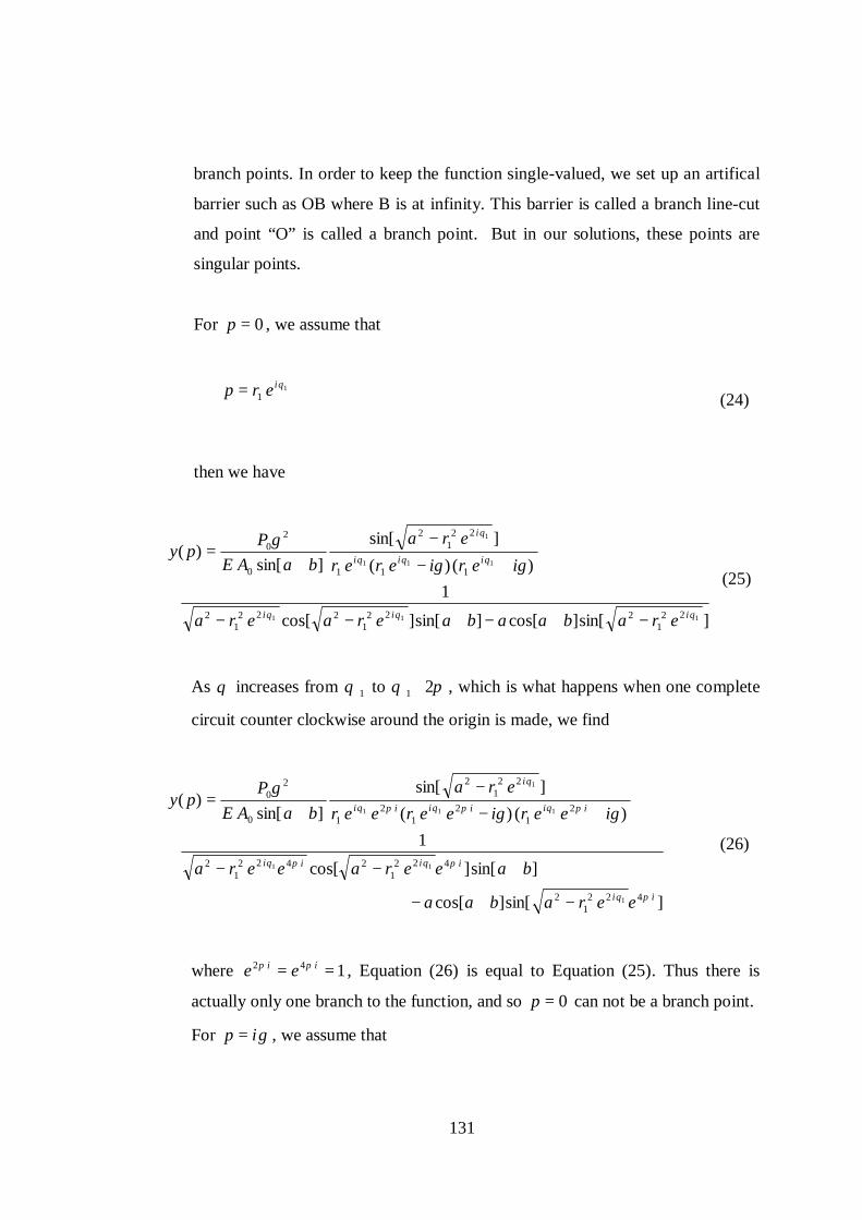
131
branch points. In order to keep the function single-valued, we set up an artifical
barrier such as OB where B is at infinity. This barrier is called a branch line-cut
and point “O” is called a branch point. But in our solutions, these points are
singular points.
For 0=p , we assume that
1
1θierp = (24)
then we have
]sin[]cos[]sin[]cos[
1)()(
]sin[]sin[
)(
111
111
1
221
2221
2221
2
111
221
2
0
20
θθθ
θθθ
θ
γγγ
iii
iii
i
erabaabaeraera
ieriererera
baAEPpy
−+−+−−
+−
−+
= (25)
As θ increases from 1θ to πθ 21+ , which is what happens when one complete
circuit counter clockwise around the origin is made, we find
]sin[]cos[
]sin[]cos[1
)()(]sin[
]sin[)(
4221
2
4221
24221
2
21
21
21
221
2
0
20
1
11
111
1
ii
iiii
iiiiii
i
eerabaa
baeeraeera
ieerieereerera
baAEP
py
πθ
πθπθ
πθπθπθ
θ
γγγ
−+−
+−−
+−
−+
=
(26)
where 142 == ii ee ππ , Equation (26) is equal to Equation (25). Thus there is
actually only one branch to the function, and so 0=p can not be a branch point.
For γip = , we assume that

132
11
θγ ierip =− (27)
then we have
]2sin[]cos[
]sin[]2cos[21
)2())((]2sin[
]sin[)(
21
221
2
21
221
221
221
2
111
21
221
2
0
20
11
1111
111
11
γγ
γγγγ
γγ
γγγ
θθ
θθθθ
θθθ
θθ
+−−+−
++−−+−−
++
+−−+
=
ii
iiii
iii
ii
erierabaa
baerieraeriera
iereriereriera
baAEP
py
(28)
As θ increases from 1θ to πθ 21+ , which is what happens when one complete
circuit counter clockwise around the origin is made, we find
]2sin[]cos[
]sin[]2cos[
2
1)2())((]2sin[
]sin[)(
221
4221
2
221
4221
2
221
4221
2
21
21
21
221
4221
2
0
20
11
11
11
111
11
γγ
γγ
γγ
γγ
γγγ
πθπθ
πθπθ
πθπθ
πθπθπθ
πθπθ
+−−+−
++−−
+−−
++
+−−+
=
iiii
iiii
iiii
iiiiii
iiii
eerieerabaa
baeerieera
eerieera
ieereerieereerieera
baAEPpy
(29)
where 142 == ii ee ππ , Equation (29) is equal to Equation (28). Thus there is
actually only one branch to the function, and so γip = can not be a branch
point.
For γip −= , we assume that
1
1θγ ierip =+ (30)

133
then we have
]2sin[]cos[
]sin[]2cos[21
)()2)((]2sin[
]sin[)(
21
221
2
21
221
221
221
2
111
21
221
2
0
20
11
1111
111
11
γγ
γγγγ
γγ
γγγ
θθ
θθθθ
θθθ
θθ
++−+−
+++−++−
−−
++−+
=
ii
iiii
iii
ii
erierabaa
baerieraeriera
erieriereriera
baAEP
py
(31)
As θ increases from 1θ to πθ 21+ , which is what happens when one complete
circuit counter clockwise around the origin is made, we find
]2sin[]cos[
]sin[]2cos[
2
1)()2)((]2sin[
]sin[)(
221
4221
2
221
4221
2
221
4221
2
21
21
21
221
4221
2
0
20
11
11
11
111
11
γγ
γγ
γγ
γγ
γγγ
πθπθ
πθπθ
πθπθ
πθπθπθ
πθπθ
++−+−
+++−
++−
−−
++−+
=
iiii
iiii
iiii
iiiiii
iiii
eerieerabaa
baeerieera
eerieera
eerieerieereerieera
baAEPpy
(32)
where 142 == ii ee ππ , Equation (32) is equal to Equation (31). Thus there is
actually only one branch to the function, and so γip −= can not be a branch
point.