Embed Size (px)
Citation preview
UKRAINIAN BANK FAILURE PREDICTION USING EFFICIENCY
MEASURES
by
Ievgen Bobykin
A thesis submitted in partial fulfillment of the requirements for the degree of
MA in Economics
Kyiv School of Economics
2010
Thesis Supervisor: Professor Valentin Zelenyuk Approved by ___________________________________________________ Head of the KSE Defense Committee, Professor Roy Gardner
Date ___________________________________
Kyiv School of Economics
Abstract
UKRAINIAN BANK FAILURE PREDICTION USING
EFFICIENCY MEASURES
by Ievgen Bobykin
Thesis Supervisor: Professor Valentin Zelenyuk
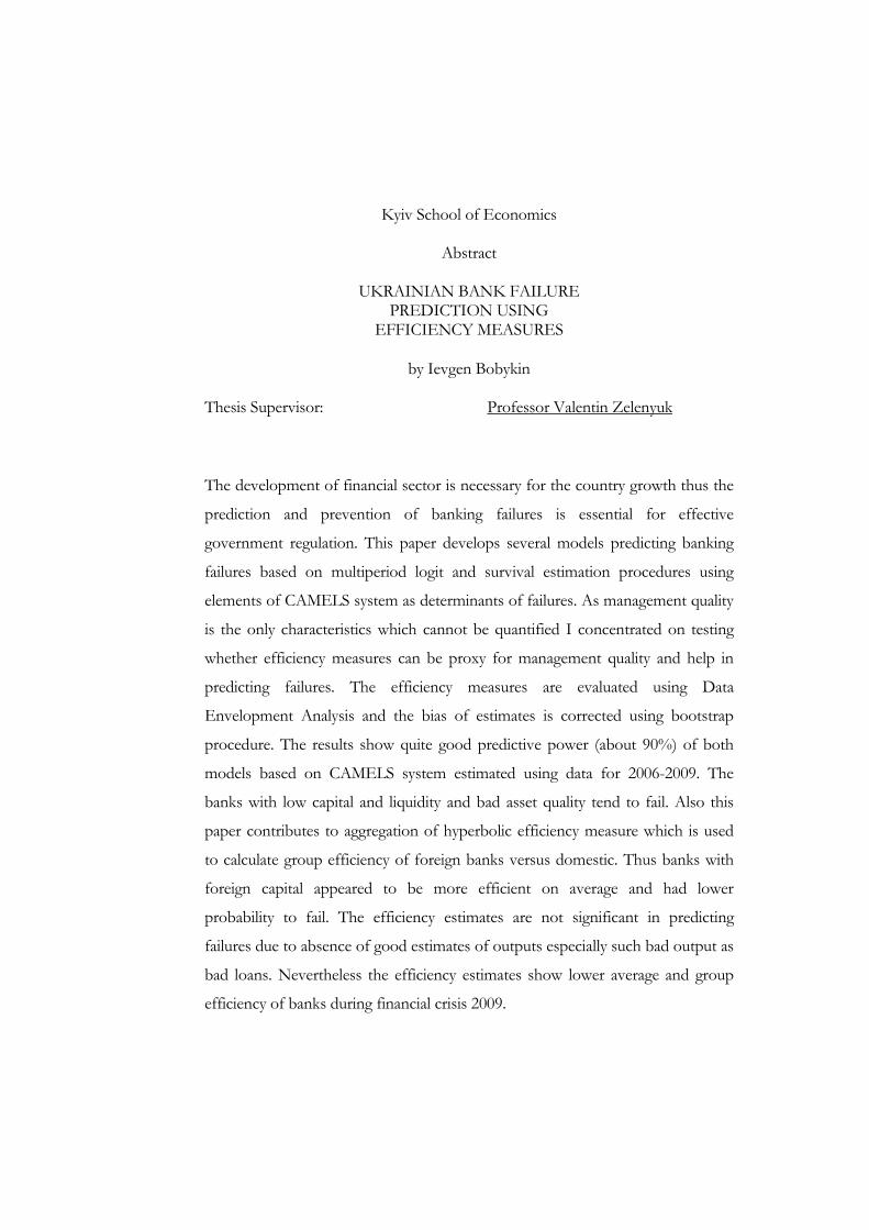
The development of financial sector is necessary for the country growth thus the
prediction and prevention of banking failures is essential for effective
government regulation. This paper develops several models predicting banking
failures based on multiperiod logit and survival estimation procedures using
elements of CAMELS system as determinants of failures. As management quality
is the only characteristics which cannot be quantified I concentrated on testing
whether efficiency measures can be proxy for management quality and help in
predicting failures. The efficiency measures are evaluated using Data
Envelopment Analysis and the bias of estimates is corrected using bootstrap
procedure. The results show quite good predictive power (about 90%) of both
models based on CAMELS system estimated using data for 2006-2009. The
banks with low capital and liquidity and bad asset quality tend to fail. Also this
paper contributes to aggregation of hyperbolic efficiency measure which is used
to calculate group efficiency of foreign banks versus domestic. Thus banks with
foreign capital appeared to be more efficient on average and had lower
probability to fail. The efficiency estimates are not significant in predicting
failures due to absence of good estimates of outputs especially such bad output as
bad loans. Nevertheless the efficiency estimates show lower average and group
efficiency of banks during financial crisis 2009.
TABLE OF CONTENTS
Chapter 1. Introduction .................................................................................................. 1
Chapter 2. Literature Review ......................................................................................... 5
Chapter 3. Theoretical framework ................................................................................ 10
3.1. Individual Technical Efficiencies ........................................................... 10
3.2. Relation of Hyperbolic Technical Efficiency to Return per Dollar (Extension) ................................................................................... 12
3.3. Group Hyperbolic Efficiency Measure (Extension) .......................... 14
3.4. Efficiency Measures Estimation ............................................................ 17
3.5. Modeling Bank Failures ........................................................................... 18
Chapter 4. Data Description .......................................................................................... 21
Chapter 5. Estimation Results ....................................................................................... 26
Chapter 6. Conclusion ..................................................................................................... 34
Bibliography ................................................................................................................... 36
Appendix A1. Theorem .................................................................................................. 40
Appendix A2. Proof of Proposition ............................................................................ 42
ii
LIST OF FIGURES AND TABLES
Number Page Figure 1. Technical efficiency in single-output single-input space .......................... 11
Number Page Table 1. Definition of inputs and outputs for the DEA analysis (intermediation approach) .............................................................................................. 21
Table 2. Definition of inputs and outputs for the DEA analysis (operating approach) ........................................................................................................................... 22
Table 3. DEA estimation results .................................................................................. 22
Table 4. Group Efficiency ............................................................................................. 23
Table 5. Failed banks ...................................................................................................... 24
Table 6. Definition and Expected signs of variables ................................................. 25
Table 7. Logit estimates .................................................................................................. 26
Table 8. Marginal effects of one standard deviation for a median bank, logit model % .................................................................................................................... 29
Table 9. Goodness of fit ................................................................................................. 29
Table 10. List of the banks with highest and lowest probabilities according to Logit model to fail in the next period ...................................................................... 30
Table 11. Hazard model estimates ................................................................................ 30
Table 12. Marginal effects of one standard deviation for a median bank,
hazard model (survival time) .......................................................................................... 32
Table 13. List of the banks with highest and lowest probabilities according to Hazard model to survive in the next period ........................................................... 33

iii
ACKNOWLEDGMENTS
The author wishes to express sincere gratitude to his advisor Valentin Zelenyuk,
whose encouragement, guidance and support from the initial to the final level
enabled me to develop an understanding of the subject.
This work has benefited a lot from valuable comments and suggestions from
Prof. Tom Coupé. The author expresses gratefulness to Volodymyr Vakhitov for
his understanding and support. I owe my deepest gratitude to research workshop
professors Olesia Verchenko, Hanna Vakhitova, Denys Nizalov, Olena Nizalova,
Oleksandr Shepotylo for their valuable comments and suggestions.
Lastly, I offer my regards and blessings to all of those who supported me in any
respect during the completion of the project.
iv
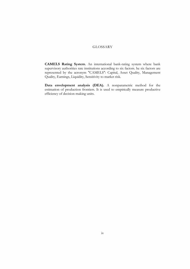
GLOSSARY
CAMELS Rating System. An international bank-rating system where bank supervisory authorities rate institutions according to six factors. he six factors are represented by the acronym "CAMELS": Capital, Asset Quality, Management Quality, Earnings, Liquidity, Sensitivity to market risk.
Data envelopment analysis (DEA). A nonparametric method for the estimation of production frontiers. It is used to empirically measure productive efficiency of decision making units.

C h a p t e r 1
INTRODUCTION
It is impossible to imagine a modern economy without a banking sector. Like
most transition economies, Ukraine liberalized its financial sector in the 1990s.
Currently, the Ukrainian banking sector consists of 196 registered banks (NBU),
19 of which are in the process of liquidation. As global and Ukrainian financial
crisis had negative impact on financial institutions, scientists need to pay attention
to the banks and their operations to prevent bank failures in future.
There are quite a lot different approaches to analyze the risks of financial
institutions especially banks (Sahajwala and Van den Bergh 2000). One of the
most widely applied is the CAMEL system which was introduced for the first
time by the three US supervision agencies in 1978 (the Federal Reserve, the
Controller of the Currency and the Federal Deposit Insurance Corporation). The
rating is based on financial statements and on-site examination by regulators.
CAMEL includes evaluation of capital adequacy (C), asset quality (A),
management (M), Earnings (E), and liquidity (L). In 1997 the sixth component
was included: sensitivity to market risk (S). (Grier 2007). Currently the National
Bank of Ukraine applies the CAMELS rating system to evaluate the banks and to
prevent their failure. It was introduced to Ukrainian banking sector in 2007
(NBU). Unfortunately the process of examination is time consuming and not
frequently repeated. The frequency is set by the NBU and depends on current
CAMELS rating. Also the ratings are not publicly available. Cole and Gunther
(1998) showed that although CAMEL ratings provide useful information, its
usefulness decays within several accounting periods because of changes in banks
and new data available. Also one of the shortcomings is that the ratings are based
on expert decision and is subjective in some sense.
2
Trying to overcome these shortcomings scientists tried to model bank failures
using public available data and some proxies for elements from CAMELS system.
The absence of quantitative characteristics for some parameters in CAMELS
system especially management quality (M) makes some difficulties to model bank
failures. As Seballos and Thompson (1990) stated ¨the ultimate determinant of
whether or not a bank fails is the ability of its management to operate the
institution efficiently and to evaluate and manage risk.¨ One of the ways to
overcome this problem is measuring efficiency using efficiency frontier analysis.
This method allows evaluating the changes in efficiencies, ranking financial
institutions and is relatively less costly than other methods, which usually imply
some expert decision (Barr and Siems 1992). Being developed for any decision
making unit it may be applied for analysis of banking sector.
For the last two decades the efficiency of financial institutions is analyzed in many
economic studies (Berger and Humphrey, 1998). However, most of the
researches are concentrated on the developed countries and there are only several
studies devoted to transition economies and Ukraine especially. The global
financial crisis contributed to the necessity of further development of instruments
which allow analyzing financial sectors and efficiencies of financial institutes.
In this study I will try to use several efficiency measures. The first two are
classical Farell output and input oriented technical efficiencies. The third one is
the hyperbolic measure of efficiency, which has some advantages such as
avoiding the problem of choosing input or output direction of efficiency measure
and it has relation to per dollar return which allows measuring the loss in
profitability due to inefficiency. Usually the measures of efficiency uses either
input direction (input oriented) which measures the possibility to reduce the
amount of used inputs or output direction (output oriented) which measures the
possibility to increase the amount of produced outputs. The usage of hyperbolic
3
function allows simultaneous reduction in inputs and increase in outputs. A lot of
studies considered methods of measuring efficiency but almost no studies
considered methods of aggregation efficiency measures into industry or country
measure. Several steps were made by Blackorby and Russell (1999), Färe and
Zelenyuk (2003) and Nesterenko and Zelenyuk (2007) but these studies
considered only Debreu-Farrell (Debreu 1951, Farrell 1957) measures of
technical efficiency.
This paper will have theoretical contribution to hyperbolic efficiency
measurement. The relation to Georgescu-Roegen’s (1951) notion of “return to
the dollar” will be introduced. Using this relation the formula for aggregated
hyperbolic efficiency measure will be derived. This theoretical contribution will
allow to measure of the groups (for example foreign and domestic) separately and
compare the efficiencies of the groups.
There are several approaches to model failures of financial institution. The most
frequently used are logit, discriminant function analysis and hazard models. The
study will analyze the assumptions behind these models and will use the most
recent data for Ukraine. The analysis will be based on publicly available data
which is gathered by National Bank of Ukraine during 2006-2009.
The main hypothesis of this research is whether the efficiency measures can help
in prediction of bank failure. I will test all three measures and try to determine
which better help in prediction bank failures. Generally the hyperbolic measure
has advantage of avoiding choosing the input or output orientation to measure
efficiency. To model failures I will use two-step estimation procedure. On the
first step the measures of efficiency will be estimated. It is worth mentioning that
hyperbolic efficiency measure is widely applied to developed countries (Cuesta
and Zofio 2005) but has never been applied to Ukrainian banking sector. Also
based on estimators of individual hyperbolic efficiency and derived formula for

4
group measures I will compare efficiencies of foreign versus domestic banks. On
the second step using obtained measures as indicator of management quality and
other variables of CAMELS system the model of bank failures will be developed.
On this step the significance of variables will be tested thus making conclusion on
possibility of using efficiency analysis to predict failures.
5
C h a p t e r 2
LITERATURE REVIEW
In this paper I will use two-steps estimation procedure that is why I will review
literature which considers efficiency analysis and which tries to model banks
failure separately.
As to efficiency analysis, it has been considered by economists since 1950s. The
first attempt to define technical efficiency of the firm was made by Koopman
(1957, p.60). According to his definition inefficient producer can either increase
production of one output without change in other outputs and inputs or decrease
input without change in outputs and other inputs. The first attempts to generate
quantitative measures were the Shephard distance function (Shephard 1953) and
the Debreu-Farrell technical efficiency measures (Debreu 1951, Farrell 1957).
Farrell (1957) showed the relation between these measures.
The analysis of these measures showed that they are not perfect and there were
several attempts to introduce new indexes. Färe and Lovell introduced axioms
which are required for efficiency measure (Färe and Lovell 1978). One of the
attempts was introducing an additive measure (Charnes et al. 1985) and a non-
radial efficiency measure (Färe and Lovell 1978) which allowed capturing some
inefficiencies which Debreu-Farrell measure does not. However they were
strongly criticized by Russell (1990) as they violate important axioms. There are
several measures that combine the previous attempts but still researchers cannot
find a unique measure which will capture all axioms and inefficiencies.
To estimate the measures for real data a number of techniques were developed.
All techniques can be divided into parametric and non-parametric. The first non-
parametric method applied to efficiency analysis which was introduced by Farrell
6
(1957) and was applied by Charnes et al. (1978) was Data Envelopment Analysis
(DEA). Nowadays this technique allows not only obtaining point estimators but,
using bootstraps, also to construct confidence intervals (Simar and Wilson 2007,
Simar and Zelenyuk 2007). Among parametric techniques one of the most widely
used is Stochastic Frontier Analysis (SFA). It was independently developed by
Aigner et al. (1977) and Meeusen and van den Broeck (1977). Later studies tried
to compare the results provided by different techniques and their sensitivity for
initial assumptions (for example Grosskopf 1996). Despite the discussion of these
techniques in the literature there is no agreement on the best techniques and it is
better to combine the techniques and double-check the results (Bauer et al. 1998).
The application of efficiency theory is wide. As theory can be applied for any
decision making unit (DMU) it is used to analyze not only producers but also
different types of financial institutions. The applications to the financial sector are
usually limited to developed countries and there are few studies that take a cross
country comparison. Such small number of cross-country studies can be
explained by the country differences which can influence efficiency frontier and
so do not allow comparing firms from different countries (Holló and Nagy 2006).
There are several papers which analyze developing and transition economies
(Yildirim and Philippatos 2002). Grigorian and Manole (2002) analyzed efficiency
in transition economies including Ukraine from 1995 till 1998. They found low
efficiency of banks, on average 47%. Fries and Taci (2004) tried to measure
efficiency of 289 banks in 15 East European countries for the years 1994-2001.
They analyzed the impact of different country factors on efficiency of the banks.
Both studies found low efficiency of Ukrainian banks. But as stated above there is
ambiguity about the possibility to compare banks from different countries as each
country can face its own efficient frontier.
7
Several studies analyzed Ukrainian banking sector. One of the studies made by
Mertens and Urga (2001) tried to analyze cost and profit efficiencies of the banks
and compare them for different groups based on size. Kyj and Isik (2008)
investigated managerial and X-inefficiencies of commercial banks in Ukraine
from 1998 to 2003. They concluded that banks waste almost half of their
resources and are very inefficient. However the study conducted by Rabtsun
(2003) found that Ukrainian banking sector is quite competitive and the level of
competition can be even compared to developed countries. Such conclusion was
based on quite high level of efficiency scores and quite a big number of banks
with high efficiency. As we see these studies give contradictory results and further
research of efficiency measures should be conducted. Also the biasness of
efficiency estimates was not eliminated in these researches which can be made
using bootstraps for efficiency measures (Kneip and others 2008). Probably the
most recent usage of efficiency measures is using them as proxy for managerial
quality in predicting bank failure.
In general, for several decades scientists have been analyzing bank failures (from
review of Shumway 2001). The earliest research applied statistical techniques
(ANOVA) to determine the factors of bank failure (Hardy and Meech 1925).
However the first quantitative measure was made by Altman (1968). In his
analysis he used linear discriminator analysis, which has been the major technique
for quite long time until probability models were introduced into bank failure
analysis (Santomero and Vinso 1977). They showed that such models are more
appropriate as they are less restrictive than linear discriminator analysis. However
Shumway (2001) showed that such models are biased and inconsistent as they are
static models and do not use the whole information available and proposed to use
hazard models.
8
Recently there are different early warning models which are used to monitor
banking sector and they widely used by supervisory authorities in different
countries. In general they are usually based on financial ratios and not on
econometric modeling (Sahajwala and Van den Bergh 2000). Despite the
difference of examinations they are usually based on analyzing almost the same
ratios which can be associated with fundamental risks classes: environmental
risks, management risks, delivery risks and financial risks (Grier 2007). Most of
them are captured by the CAMELS rating system.
The first early warning system for banks was developed by Meyer and Pifer
(1970). Since then different mostly two types modeling failure were used:
multinomial logit and hazard models. Shumway (2001) showed that multiperiod
logit model is equivalent to discrete time hazard model. So in this research both
models will be applied as there is no single opinion which is better.
Barr and Siems (1992) were the first who introduced data envelopment analysis to
qualify management quality and use this estimator to predict bank failures. Their
model was predicting failures with accuracy about 95%. Since this study there
were quite many studies of bank failures but they usually considered developed
countries (Wheelock and Wilson 2000).
There were only several studies trying to model the bank failure in Ukraine:
Popruga (2001) and Nikolsko-Rzhevskyy (2003). The first study analyzed banks
in 1995-1996 and used only financial indices and some dummies for location and
ownership. The absence of data did not allow using hazard or multiperiod logit
models. The next research is more precise and uses efficiency measures as proxy
for managerial quality estimated by DEA. Also the data did not allow using
precise proxies for inputs and outputs for efficiency estimators and not precise
variables for other elements of CAMELS system. Another shortcoming of this
study is defining failures like banks which stopped reporting data, which is not

9
precise and captures acquisitions and mergers. The recent data will allow
eliminating those shortcomings. Another innovation will be using hyperbolic
efficiency measure, which was not the case in the previous studies. It will allow
avoiding the problem of choosing the direction (input or output) of efficiency
measure. Also I will compare different approaches to define outputs and different
approaches to measure efficiency.
10
C h a p t e r 3
THEORETICAL FRAMEWORK
3.1. INDIVIDUAL TECHNICAL EFFICIENCIES
Let’s consider K decision making units (DMU) within a group which produce
, … , outputs using , … , inputs each. I
will assume that 0, 01 or that firm to exist should produce something
and therefore use some resources, which is quite natural assumption.
Individual technology is described by following function:
T , : "yk is producible from xk" (3.1)
Let’s define input and output technical efficiencies according to Shephard (1953),
which is reciprocal of the Farrell (1957) input and output efficiencies.
Inpurt oriented technical efficiency
0: , T (3.2)
Output oriented technical efficiency
0: , / T (3.3)
I will use definition of technical efficiency used by Färe and others (1985).
0: / , T (3.4)
1 we will use notation for vectors that at least one element of the vector is greater than zero and in usual meaning for numbers
11
As can be seen the input oriented and hyperbolic technical efficiencies take values
greater than one for inefficient firms and one when the firm is technically
efficient. The closer technical efficiency is to one the more efficient the bank is. It
can be easily computed percentage of inefficiency as 1 100%. Output
oriented measure varies from zero to one with efficient firms close to one. The
percentage of inefficiency is computed as 1 100%.
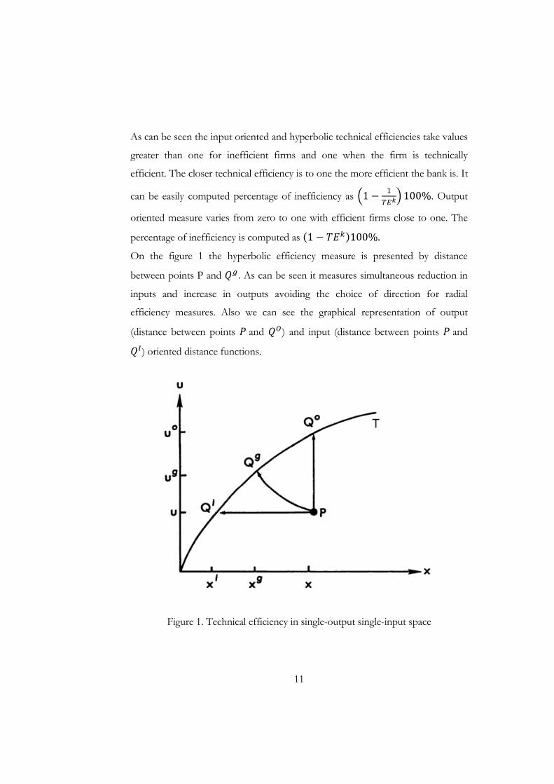
On the figure 1 the hyperbolic efficiency measure is presented by distance
between points P and . As can be seen it measures simultaneous reduction in
inputs and increase in outputs avoiding the choice of direction for radial
efficiency measures. Also we can see the graphical representation of output
(distance between points and ) and input (distance between points and
) oriented distance functions.
Figure 1. Technical efficiency in single-output single-input space
12
It is worth mentioning that under constant return to scale there is relationship
among these measures (Farrell 1957, Färe and Lovell 1978):
(3.5)
3.2. RELATION OF HYPERBOLIC TECHNICAL EFFICIENCY TO RETURN PER DOLLAR (EXTENSION)
Let’s define technical efficient level of outputs · and technical
efficient level of inputs . By definition of hyperbolic technical
efficiency – , T .
Thus for single output single input case squared hyperbolic efficiency can be
represented as:
· (3.6)
As for multi output multi input case it is impossible to use simple ratios of
outputs and inputs it can be easily shown the relationship between revenues,
costs and squared hyperbolic efficiency.
Lemma 1
· (3.7)
where , … , and , … , are price vectors for
outputs and inputs respectively. The proof can be easily seen from definition of
and . I will assume price vectors common to all firms. The assumption of
prices being the same is also used to obtain aggregated Farrell technical efficiency
(Färe and Zelenyuk, 2003, Nesterenko and Zelenyuk, 2007).
13
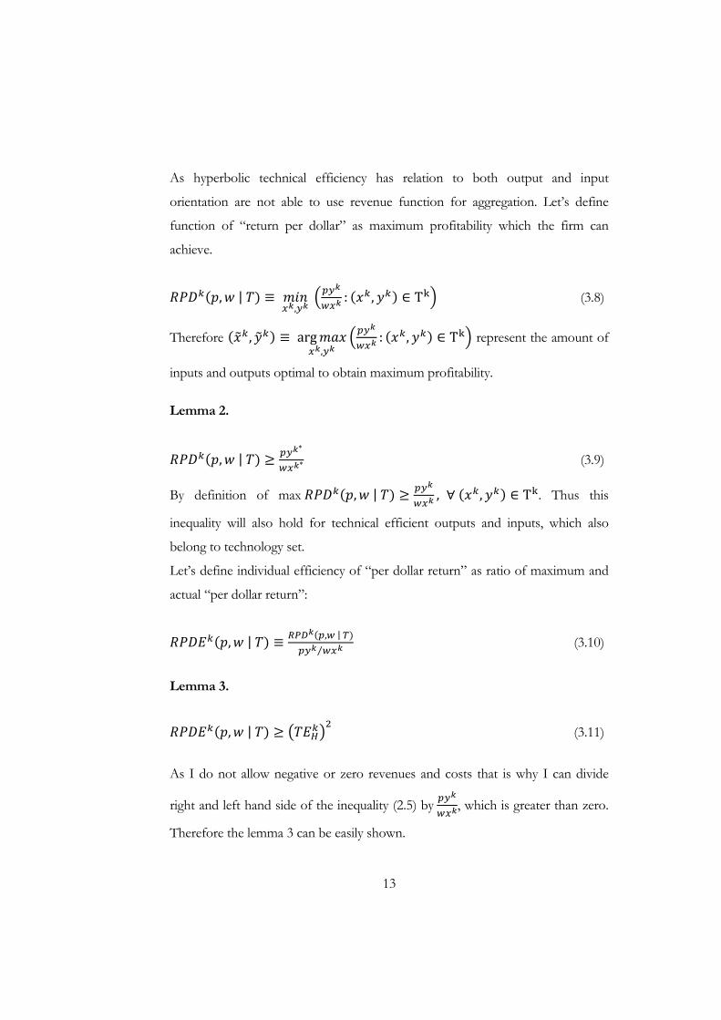
As hyperbolic technical efficiency has relation to both output and input
orientation are not able to use revenue function for aggregation. Let’s define
function of “return per dollar” as maximum profitability which the firm can
achieve.
, | , : , T (3.8)
Therefore , arg,
: , T represent the amount of
inputs and outputs optimal to obtain maximum profitability.
Lemma 2.
, | (3.9)
By definition of max , | , , T . Thus this
inequality will also hold for technical efficient outputs and inputs, which also
belong to technology set.
Let’s define individual efficiency of “per dollar return” as ratio of maximum and
actual “per dollar return”:
, | , | ⁄
(3.10)
Lemma 3.
, | (3.11)
As I do not allow negative or zero revenues and costs that is why I can divide
right and left hand side of the inequality (2.5) by , which is greater than zero.
Therefore the lemma 3 can be easily shown.
14
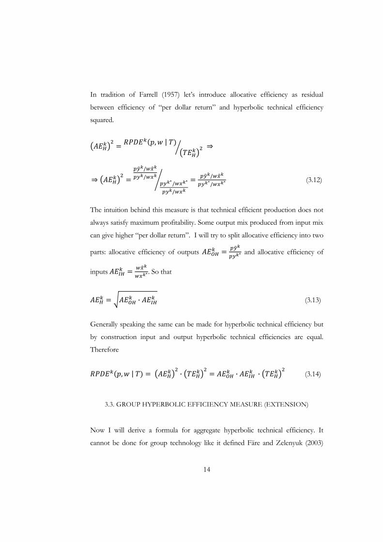
In tradition of Farrell (1957) let’s introduce allocative efficiency as residual
between efficiency of “per dollar return” and hyperbolic technical efficiency
squared.
, |
//
//
//
(3.12)
The intuition behind this measure is that technical efficient production does not
always satisfy maximum profitability. Some output mix produced from input mix
can give higher “per dollar return”. I will try to split allocative efficiency into two
parts: allocative efficiency of outputs and allocative efficiency of
inputs . So that
· (3.13)
Generally speaking the same can be made for hyperbolic technical efficiency but
by construction input and output hyperbolic technical efficiencies are equal.
Therefore
, | · · · (3.14)
3.3. GROUP HYPERBOLIC EFFICIENCY MEASURE (EXTENSION)
Now I will derive a formula for aggregate hyperbolic technical efficiency. It
cannot be done for group technology like it defined Färe and Zelenyuk (2003)
15
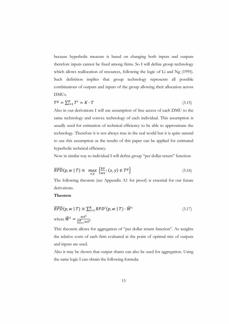
because hyperbolic measure is based on changing both inputs and outputs
therefore inputs cannot be fixed among firms. So I will define group technology
which allows reallocation of resources, following the logic of Li and Ng (1995).
Such definition implies that group technology represents all possible
combinations of outputs and inputs of the group allowing their allocation across
DMUs.
∑ · (3.15)
Also in our derivations I will use assumption of free access of each DMU to the
same technology and convex technology of each individual. This assumption is
usually used for estimation of technical efficiency to be able to approximate the
technology. Therefore it is not always true in the real world but it is quite natural
to use this assumption as the results of this paper can be applied for estimated
hyperbolic technical efficiency.
Now in similar way to individual I will define group “per dollar return” function:
, | , : , (3.16)
The following theorem (see Appendix A1 for proof) is essential for our future
derivations.
Theorem
, | ∑ , | · (3.17)
where ∑ .
This theorem allows for aggregation of “per dollar return function”. As weights
the relative costs of each firm evaluated at the point of optimal mix of outputs
and inputs are used.
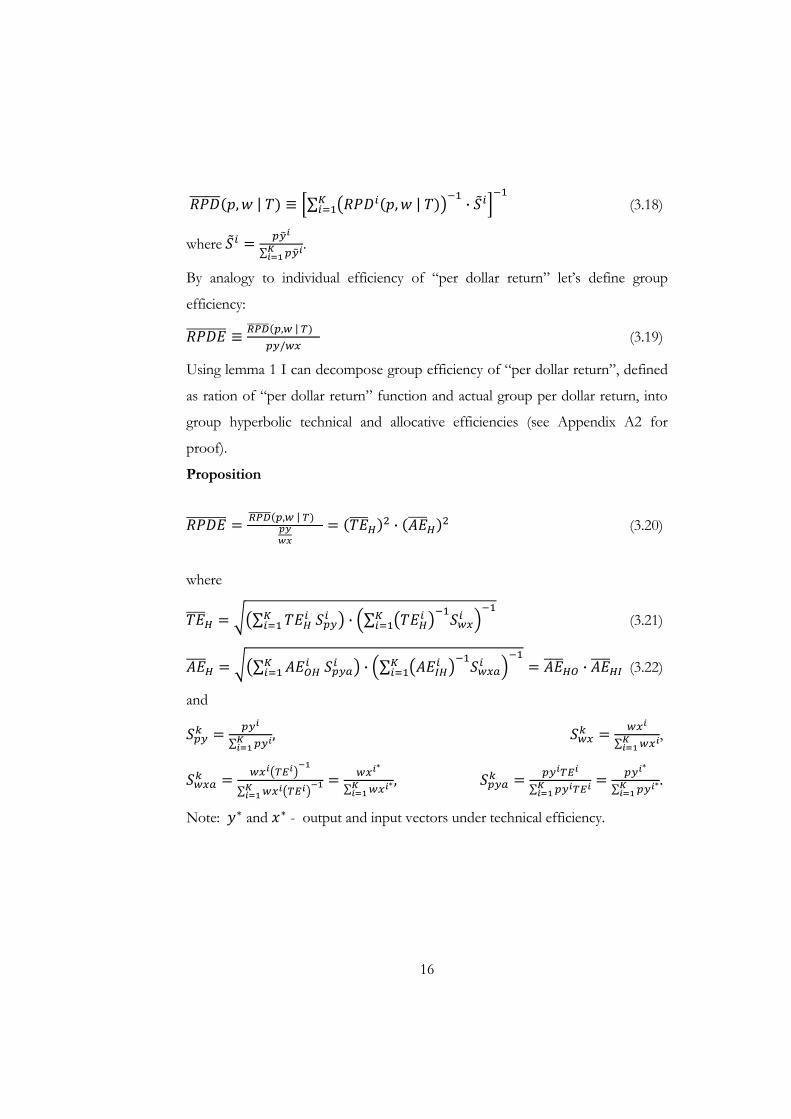
Also it may be shown that output shares can also be used for aggregation. Using
the same logic I can obtain the following formula:
16
, | ∑ , | · (3.18)
where ∑ .
By analogy to individual efficiency of “per dollar return” let’s define group
efficiency: , | /
(3.19)
Using lemma 1 I can decompose group efficiency of “per dollar return”, defined
as ration of “per dollar return” function and actual group per dollar return, into
group hyperbolic technical and allocative efficiencies (see Appendix A2 for
proof).
Proposition
, | · (3.20)
where
∑ · ∑ (3.21)
∑ · ∑ · (3.22)
and
∑ , ∑ ,
∑ ∑,
∑ ∑.
Note: and - output and input vectors under technical efficiency.
17
3.4. EFFICIENCY MEASURES ESTIMATION
To get the estimates of technical efficiency I will use Data Envelopment Analysis.
This technique allow to construct a piecewise linear approximation to the linearly
homogeneous technology in order to identify best practice technology. According
to this technique the following problem should be solved:
Inpurt oriented technical efficiency
, 0: , (3.23)
Output oriented technical efficiency
0: , / (3.24)
Where, if assume variable return to scale and assume the same access of all
DMUs to technology, then:
, :
∑
∑
1, … ,
∑ 1 .
The last restriction is added in order to consider variable return to scale.
The estimation of hyperbolic technical efficiency is more complex as it involves
nonlinear optimization:
0: , (3.25)
Where , :
∑
18
∑
1, … ,
∑ 1 .
The hyperbolic technical efficiency is calculated using a bisectional method.
Obtained measures of efficiency can used to calculate aggregated measures.
To eliminate the bias of these measures the homogeneous bootstrap procedure
introduced by Simar and Wilson (1998) is applied.
3.5. MODELING BANK FAILURES
On the second stage the efficiency measures obtained and aggregated industry
hyperbolic efficiency measure will be used as explanatory variables to explain
banking failures. It will allow to test whether coefficient for technical efficiency is
significant thus our estimate of technical efficiency helps predicting bank failure.
For this purpose several models can be applied. Among the most widely applied
are multi-period logit and hazard model. I will use both models as according to
Shumway (2001) usually hazard models produce better results but if the data
set is small the logit model is more precise.
Logit model.
As our data set has discrete time (one quarter) the multi-period logit model will
be applied. Generally the cumulative logistic distribution function of a number
Pi, which ranges from 0 to 1, can be presented as:
Δ 1| . (3.26)
As I can see is nonlinearly related to , which ranges from ∞ to ∞. To
be able to estimate this relationship the natural logarithm of odds ratio is taken:
19
L ln . (3.27)
L is called logit. Note that L , but not , is linear to . Thus to get expression
for marginal effect one needs to take the derivative of with respect to
particular .
. (3.28)
The difference between logit and multi-period logit is that multi-period logit
uses pooled paned data allowing for different constant terms each time period
(in practice using dummies for each period except one).
Hazard model.
The second model I use is duration hazard model. The basic idea of any
duration model is to investigate time to failure (Cleves and others 2008). Let T
represent the lifetime of decision making unit with density function (or
F(t) distribution function) Then the survival distribution function can be
represented as:
1 . (3.29)
The hazard function is the limiting probability that the failure event
occurs in a given interval, conditional upon the subject having survived to the
beginning of that interval, divided by the width of the interval:
lim∆ ∆ |
∆. (3.30)
Certainly the hazard function gives mathematically equivalent specification of
distribution of T. To proceed further the hazard function needs to be
parameterized. I will use natural for this type of analysis assumption of log-
logistic distribution (Cleves and others 2008):

20
, . (3.31)
The model is estimated “by parameterizing and treating scale
parameter as an ancillary parameter to be estimated” (Stata’s manual).
21
C h a p t e r 4
DATA DESCRIPTION
As in my work I will use two step procedure the data to be used I will define for
each step separately. There are two common approaches to look at banks
operations. To estimate hyperbolic efficiency measure I will use intermediation
approach to define inputs and outputs for input, output and hyperbolic efficiency
measures. Also I will try operating approach to define inputs and outputs for
hyperbolic efficiency and compare to intermediation approach. According to
intermediation approach banks are considered to use owned capital, labor and
deposits to produce loans and other investments. Such approach has clear
advantage to other approaches as interest bearing income is more than 50% of
income in the whole banking sector (NBU). I expect that this approach will give
better results. Thus as inputs labor costs, individual and corporate deposits,
capital will be used. As outputs – corporate and individual loans, securities for
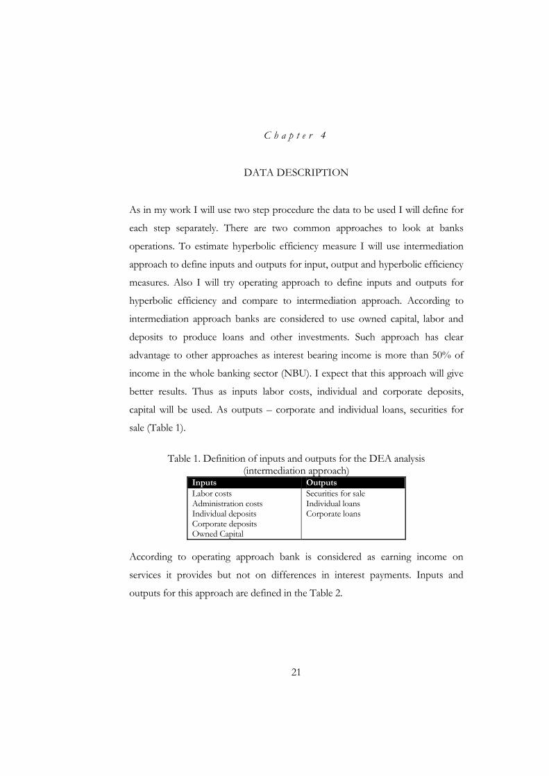
sale (Table 1).
Table 1. Definition of inputs and outputs for the DEA analysis (intermediation approach)
Inputs OutputsLabor costsAdministration costs Individual deposits Corporate deposits Owned Capital
Securities for saleIndividual loans Corporate loans
According to operating approach bank is considered as earning income on
services it provides but not on differences in interest payments. Inputs and
outputs for this approach are defined in the Table 2.
22
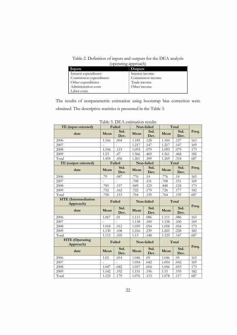
Table 2. Definition of inputs and outputs for the DEA analysis (operating approach)
Inputs OutputsInterest expendituresCommission expenditures Other expenditures Administration costs Labor costs
Interest incomeCommission income Trade income Other income
The results of nonparametric estimation using bootstrap bias correction were
obtained. The descriptive statistics is presented in the Table 3.
Table 3. DEA estimation results TE (input oriented) Failed Non-failed Total
Freq.date Mean
Std. Dev.
MeanStd. Dev.
Mean Std. Dev.
2006 1.106 .004 1.185 .128 1.184 .127 1632007 - - 1.217 .147 1.217 .147 1692008 1.106 .115 1.093 .079 1.093 .079 1732009 1.53 .47 1.566 .469 1.561 .468 182Total 1.454 .456 1.261 .309 1.269 .318 687
TE (output oriented) Failed Non-failed Total Freq.
date MeanStd. Dev.
MeanStd. Dev.
Mean Std. Dev.
2006 .79 .047 .776 .14 .776 .14 1632007 - - .708 .151 .708 .151 1692008 .783 .157 .849 .123 .848 .124 1732009 .752 .162 .722 .179 .726 .177 182Total .758 .153 .764 .159 .764 .159 687
HTE (Intermediation Approach)
Failed Non-failed Total Freq.
date MeanStd. Dev.
MeanStd. Dev.
Mean Std. Dev.
2006 1.067 .01 1.111 .086 1.111 .086 1632007 - - 1.138 .100 1.138 .100 1692008 1.018 .012 1.059 .054 1.058 .054 1732009 1.130 .108 1.216 .239 1.205 .228 182Total 1.113 .105 1.13 .148 1.129 .147 687
HTE (Operating Approach)
Failed Non-failed Total Freq.
date MeanStd. Dev.
MeanStd. Dev.
Mean Std. Dev.
2006 1.02 .014 1.046 .05 1.046 .05 1632007 - - 1.054 .042 1.054 .042 1692008 1.047 .042 1.057 .054 1.056 .053 1732009 1.142 .192 1.151 .196 1.15 .195 182Total 1.123 .179 1.076 .113 1.078 .117 687
23
From the estimates can be seen that efficiency measures indicate that banks for
2006-2008 banks were all quite efficient with low variance. Can be note that in
2009 the efficiency has decreased which is due to financial crisis and reduction in
outputs such as loans. Also it can be seen that on average banks which failed do
not differ a lot from other banks in terms of efficiency and even more efficient
according to hyperbolic efficiency measures obtained from intermediation
approach. This fact can be explained that outputs also capture such bad outputs
as bad loans and thus the banks which were not able to reduce this output failed.
Unfortunately there is no information about amount of bad loans in each bank
which do not allow estimating efficiency more precisely.
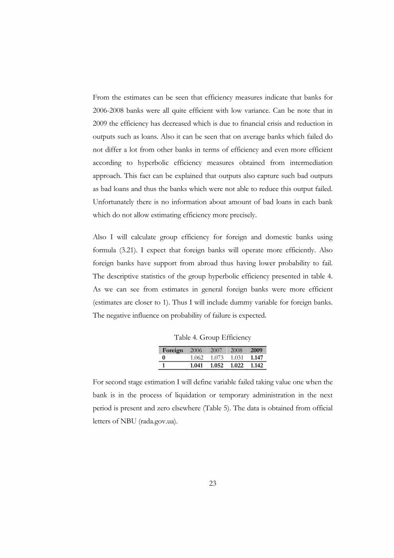
Also I will calculate group efficiency for foreign and domestic banks using
formula (3.21). I expect that foreign banks will operate more efficiently. Also
foreign banks have support from abroad thus having lower probability to fail.
The descriptive statistics of the group hyperbolic efficiency presented in table 4.
As we can see from estimates in general foreign banks were more efficient
(estimates are closer to 1). Thus I will include dummy variable for foreign banks.
The negative influence on probability of failure is expected.
Table 4. Group Efficiency
Foreign 2006 2007 2008 20090 1.062 1.073 1.031 1.1471 1.041 1.052 1.022 1.142
For second stage estimation I will define variable failed taking value one when the
bank is in the process of liquidation or temporary administration in the next
period is present and zero elsewhere (Table 5). The data is obtained from official
letters of NBU (rada.gov.ua).
24
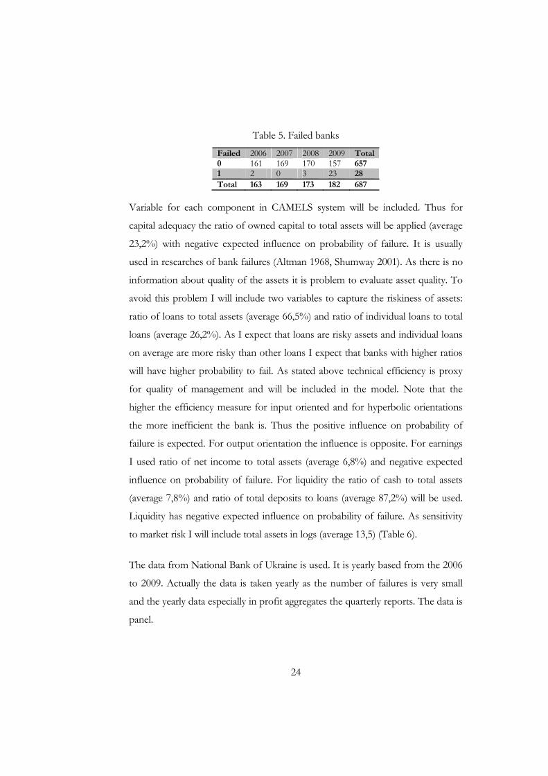
Table 5. Failed banks
Failed 2006 2007 2008 2009 Total0 161 169 170 157 6571 2 0 3 23 28 Total 163 169 173 182 687
Variable for each component in CAMELS system will be included. Thus for
capital adequacy the ratio of owned capital to total assets will be applied (average
23,2%) with negative expected influence on probability of failure. It is usually
used in researches of bank failures (Altman 1968, Shumway 2001). As there is no
information about quality of the assets it is problem to evaluate asset quality. To
avoid this problem I will include two variables to capture the riskiness of assets:
ratio of loans to total assets (average 66,5%) and ratio of individual loans to total
loans (average 26,2%). As I expect that loans are risky assets and individual loans
on average are more risky than other loans I expect that banks with higher ratios
will have higher probability to fail. As stated above technical efficiency is proxy
for quality of management and will be included in the model. Note that the
higher the efficiency measure for input oriented and for hyperbolic orientations
the more inefficient the bank is. Thus the positive influence on probability of
failure is expected. For output orientation the influence is opposite. For earnings
I used ratio of net income to total assets (average 6,8%) and negative expected
influence on probability of failure. For liquidity the ratio of cash to total assets
(average 7,8%) and ratio of total deposits to loans (average 87,2%) will be used.
Liquidity has negative expected influence on probability of failure. As sensitivity
to market risk I will include total assets in logs (average 13,5) (Table 6).
The data from National Bank of Ukraine is used. It is yearly based from the 2006
to 2009. Actually the data is taken yearly as the number of failures is very small
and the yearly data especially in profit aggregates the quarterly reports. The data is
panel.
25
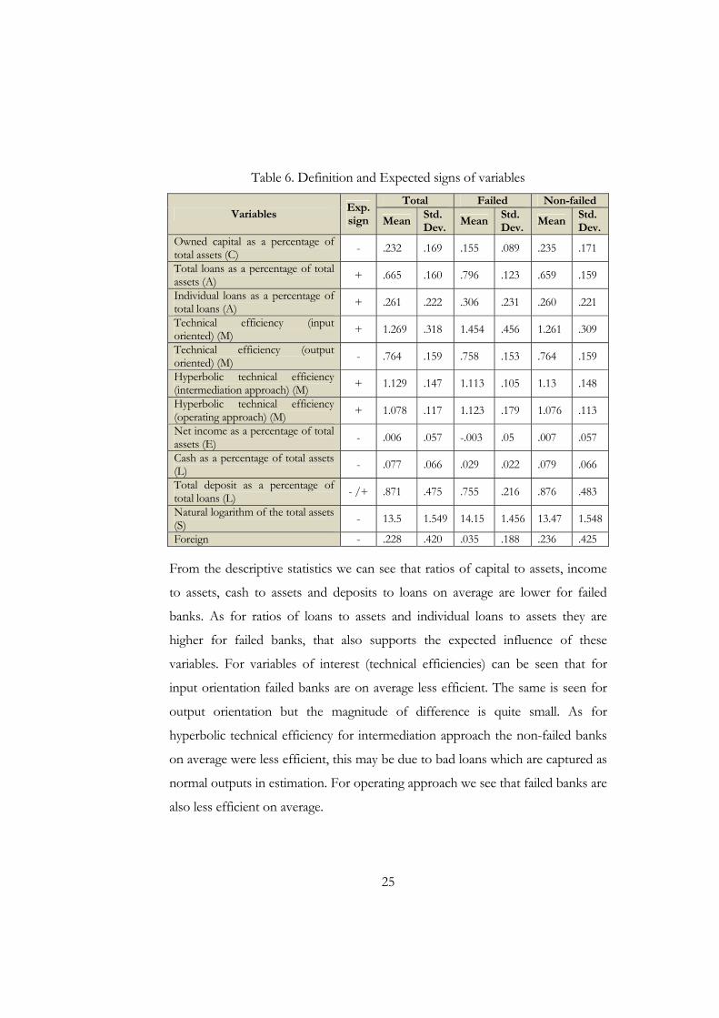
Table 6. Definition and Expected signs of variables
Variables Exp. sign
Total Failed Non-failed
MeanStd.Dev.
MeanStd. Dev.
Mean Std.Dev.
Owned capital as a percentage of total assets (C) - .232 .169 .155 .089 .235 .171
Total loans as a percentage of total assets (A) + .665 .160 .796 .123 .659 .159
Individual loans as a percentage of total loans (A) + .261 .222 .306 .231 .260 .221
Technical efficiency (input oriented) (M) + 1.269 .318 1.454 .456 1.261 .309
Technical efficiency (output oriented) (M) - .764 .159 .758 .153 .764 .159
Hyperbolic technical efficiency (intermediation approach) (M) + 1.129 .147 1.113 .105 1.13 .148
Hyperbolic technical efficiency (operating approach) (M) + 1.078 .117 1.123 .179 1.076 .113
Net income as a percentage of totalassets (E) - .006 .057 -.003 .05 .007 .057
Cash as a percentage of total assets (L) - .077 .066 .029 .022 .079 .066
Total deposit as a percentage of total loans (L) - /+ .871 .475 .755 .216 .876 .483
Natural logarithm of the total assets (S) - 13.5 1.549 14.15 1.456 13.47 1.548
Foreign - .228 .420 .035 .188 .236 .425
From the descriptive statistics we can see that ratios of capital to assets, income
to assets, cash to assets and deposits to loans on average are lower for failed
banks. As for ratios of loans to assets and individual loans to assets they are
higher for failed banks, that also supports the expected influence of these
variables. For variables of interest (technical efficiencies) can be seen that for
input orientation failed banks are on average less efficient. The same is seen for
output orientation but the magnitude of difference is quite small. As for
hyperbolic technical efficiency for intermediation approach the non-failed banks
on average were less efficient, this may be due to bad loans which are captured as
normal outputs in estimation. For operating approach we see that failed banks are
also less efficient on average.
26
C h a p t e r 5
ESTIMATION RESULTS
Logit Model
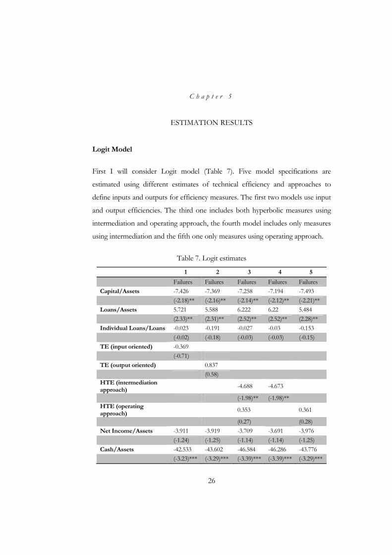
First I will consider Logit model (Table 7). Five model specifications are
estimated using different estimates of technical efficiency and approaches to
define inputs and outputs for efficiency measures. The first two models use input
and output efficiencies. The third one includes both hyperbolic measures using
intermediation and operating approach, the fourth model includes only measures
using intermediation and the fifth one only measures using operating approach.
Table 7. Logit estimates
1 2 3 4 5
Failures Failures Failures Failures Failures Capital/Assets -7.426 -7.369 -7.258 -7.194 -7.493
(-2.18)** (-2.16)** (-2.14)** (-2.12)** (-2.21)** Loans/Assets 5.721 5.588 6.222 6.22 5.484
(2.33)** (2.31)** (2.52)** (2.52)** (2.28)** Individual Loans/Loans -0.023 -0.191 -0.027 -0.03 -0.153
(-0.02) (-0.18) (-0.03) (-0.03) (-0.15) TE (input oriented) -0.369
(-0.71) TE (output oriented) 0.837
(0.58) HTE (intermediation approach)
-4.688 -4.673 (-1.98)** (-1.98)**
HTE (operating approach)
0.353 0.361
(0.27) (0.28) Net Income/Assets -3.911 -3.919 -3.709 -3.691 -3.976
(-1.24) (-1.25) (-1.14) (-1.14) (-1.25) Cash/Assets -42.533 -43.602 -46.584 -46.286 -43.776
(-3.23)*** (-3.29)*** (-3.39)*** (-3.39)*** (-3.29)***
27
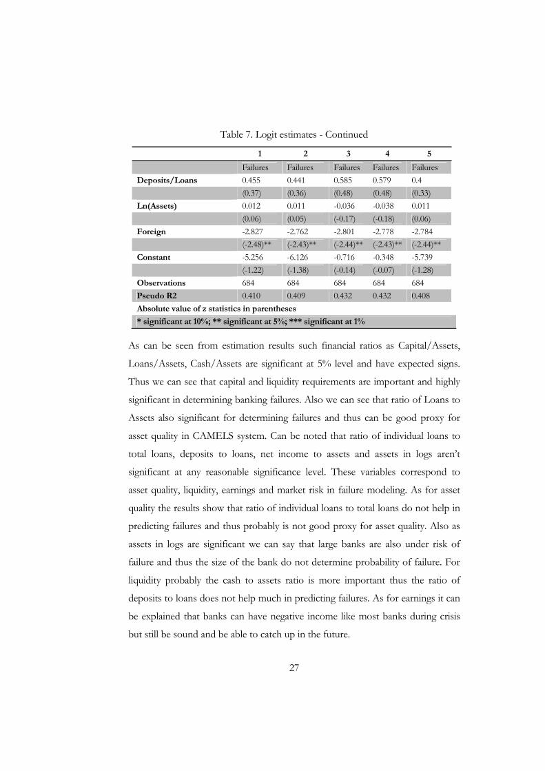
Table 7. Logit estimates - Continued
1 2 3 4 5
Failures Failures Failures Failures Failures Deposits/Loans 0.455 0.441 0.585 0.579 0.4
(0.37) (0.36) (0.48) (0.48) (0.33) Ln(Assets) 0.012 0.011 -0.036 -0.038 0.011
(0.06) (0.05) (-0.17) (-0.18) (0.06) Foreign -2.827 -2.762 -2.801 -2.778 -2.784
(-2.48)** (-2.43)** (-2.44)** (-2.43)** (-2.44)** Constant -5.256 -6.126 -0.716 -0.348 -5.739
(-1.22) (-1.38) (-0.14) (-0.07) (-1.28) Observations 684 684 684 684 684 Pseudo R2 0.410 0.409 0.432 0.432 0.408 Absolute value of z statistics in parentheses
* significant at 10%; ** significant at 5%; *** significant at 1%
As can be seen from estimation results such financial ratios as Capital/Assets,
Loans/Assets, Cash/Assets are significant at 5% level and have expected signs.
Thus we can see that capital and liquidity requirements are important and highly
significant in determining banking failures. Also we can see that ratio of Loans to
Assets also significant for determining failures and thus can be good proxy for
asset quality in CAMELS system. Can be noted that ratio of individual loans to
total loans, deposits to loans, net income to assets and assets in logs aren’t
significant at any reasonable significance level. These variables correspond to
asset quality, liquidity, earnings and market risk in failure modeling. As for asset
quality the results show that ratio of individual loans to total loans do not help in
predicting failures and thus probably is not good proxy for asset quality. Also as
assets in logs are significant we can say that large banks are also under risk of
failure and thus the size of the bank do not determine probability of failure. For
liquidity probably the cash to assets ratio is more important thus the ratio of
deposits to loans does not help much in predicting failures. As for earnings it can
be explained that banks can have negative income like most banks during crisis
but still be sound and be able to catch up in the future.
28
Also we can see as expected the dummy foreign is statistically significant at 5%
level. Thus it can be seen that foreign banks has lower probabilities to fail. Also
these results are supported by calculated group efficiencies which show the better
performance of foreign banks.
As to variables of interest neither Farrell measures nor hyperbolic efficiencies are
statistically significant. There are several explanations why it may happen.
According to intermediation approach as one of the outputs loans are used for
both Farrell efficiencies and hyperbolic measure using intermediation approach.
Loans consist of portion of bad loans which are bad output. Thus as can be seen
in descriptive statistics for example hyperbolic efficiency according to
intermediation approach for failed banks is on average even lower than for sound
banks, which means that according to this approach failed banks are more
efficient. This can be interpreted that banks which were able to reduce the loans
during crisis were able to stay sound and thus banks with lower hyperbolic
efficiency failed. As such effect is captured by the estimates we cannot rely on it.
As to operating approach I believe that this approach is not well applied for
Ukraine as most of its income banks earn on interest payments.
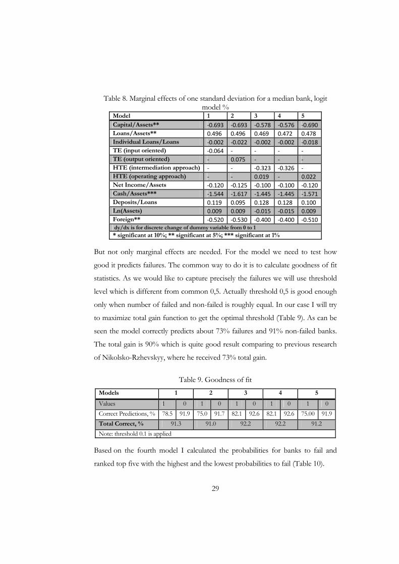
As estimated results do not provide information about the size of impact of each
variable on probability of failure, thus the next step is calculating marginal effects
(Table 8). Thus using results from the fourth model increase in Capital/Assets
and Cash/Assets ratios by one standard deviation decreases probability of failure
by 0,576% and 1,445% correspondingly. Increase in Loans/Assets increases
probability of failure by 0,473%. Note that these effects calculated for median
bank. As for foreign banks, according to estimates the probability of failure is
lower by 0,4%.
29
Table 8. Marginal effects of one standard deviation for a median bank, logit model %
Model 1 2 3 4 5 Capital/Assets** ‐0.693 ‐0.693 ‐0.578 ‐0.576 ‐0.690 Loans/Assets** 0.496 0.496 0.469 0.472 0.478 Individual Loans/Loans ‐0.002 ‐0.022 ‐0.002 ‐0.002 ‐0.018 TE (input oriented) ‐0.064 ‐ ‐ ‐ ‐ TE (output oriented) ‐ 0.075 ‐ ‐ ‐ HTE (intermediation approach) ‐ ‐ ‐0.323 ‐0.326 ‐ HTE (operating approach) ‐ ‐ 0.019 ‐ 0.022 Net Income/Assets ‐0.120 ‐0.125 ‐0.100 ‐0.100 ‐0.120 Cash/Assets*** ‐1.544 ‐1.617 ‐1.445 ‐1.445 ‐1.571 Deposits/Loans 0.119 0.095 0.128 0.128 0.100 Ln(Assets) 0.009 0.009 ‐0.015 ‐0.015 0.009 Foreign** ‐0.520 ‐0.530 ‐0.400 ‐0.400 ‐0.510 dy/dx is for discrete change of dummy variable from 0 to 1* significant at 10%; ** significant at 5%; *** significant at 1%
But not only marginal effects are needed. For the model we need to test how
good it predicts failures. The common way to do it is to calculate goodness of fit
statistics. As we would like to capture precisely the failures we will use threshold
level which is different from common 0,5. Actually threshold 0,5 is good enough
only when number of failed and non-failed is roughly equal. In our case I will try
to maximize total gain function to get the optimal threshold (Table 9). As can be
seen the model correctly predicts about 73% failures and 91% non-failed banks.
The total gain is 90% which is quite good result comparing to previous research
of Nikolsko-Rzhevskyy, where he received 73% total gain.
Table 9. Goodness of fit
Models 1 2 3 4 5
Values 1 0 1 0 1 0 1 0 1 0 Correct Predictions, % 78.5 91.9 75.0 91.7 82.1 92.6 82.1 92.6 75.00 91.9Total Correct, % 91.3 91.0 92.2 92.2 91.2 Note: threshold 0.1 is applied
Based on the fourth model I calculated the probabilities for banks to fail and
ranked top five with the highest and the lowest probabilities to fail (Table 10).
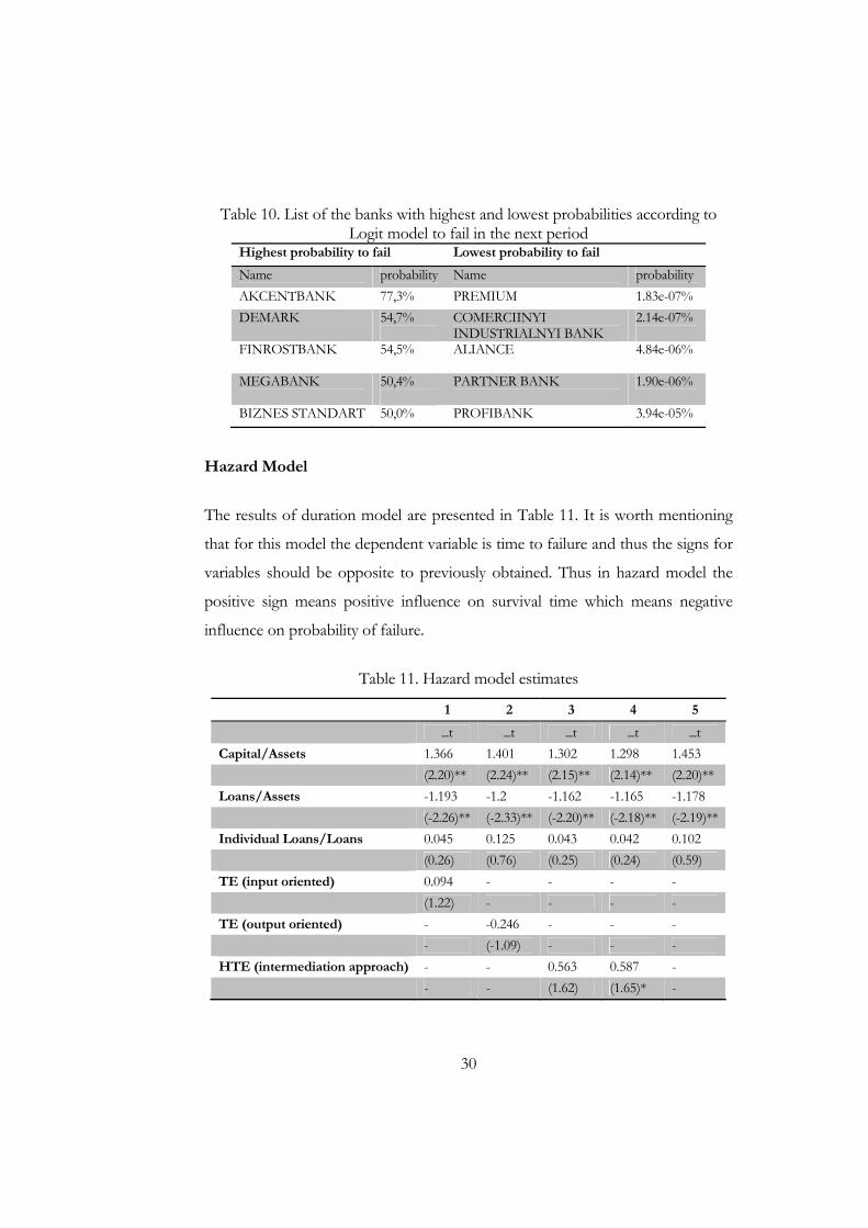
30
Table 10. List of the banks with highest and lowest probabilities according to Logit model to fail in the next period
Highest probability to fail Lowest probability to fail
Name probability Name probability AKCENTBANK 77,3% PREMIUM 1.83e-07% DEMARK 54,7% COMERCIINYI
INDUSTRIALNYI BANK2.14e-07%
FINROSTBANK 54,5%
ALIANCE 4.84e-06%
MEGABANK 50,4%
PARTNER BANK 1.90e-06%
BIZNES STANDART 50,0% PROFIBANK 3.94e-05%
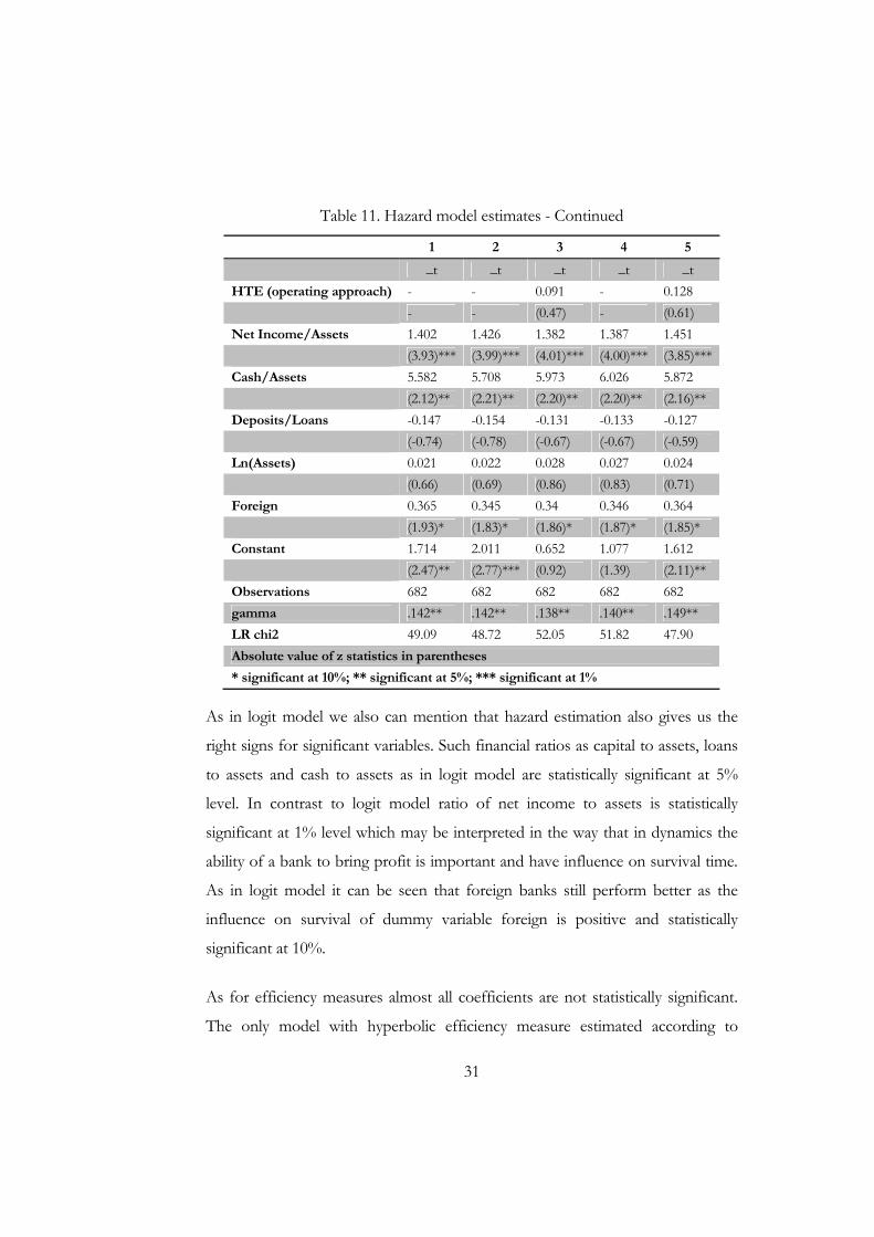
Hazard Model
The results of duration model are presented in Table 11. It is worth mentioning
that for this model the dependent variable is time to failure and thus the signs for
variables should be opposite to previously obtained. Thus in hazard model the
positive sign means positive influence on survival time which means negative
influence on probability of failure.
Table 11. Hazard model estimates
1 2 3 4 5
_t _t _t _t _t Capital/Assets 1.366 1.401 1.302 1.298 1.453
(2.20)** (2.24)** (2.15)** (2.14)** (2.20)** Loans/Assets -1.193 -1.2 -1.162 -1.165 -1.178
(-2.26)** (-2.33)** (-2.20)** (-2.18)** (-2.19)**Individual Loans/Loans 0.045 0.125 0.043 0.042 0.102
(0.26) (0.76) (0.25) (0.24) (0.59) TE (input oriented) 0.094 - - - -
(1.22) - - - - TE (output oriented) - -0.246 - - -
- (-1.09) - - - HTE (intermediation approach) - - 0.563 0.587 -
- - (1.62) (1.65)* -
31
Table 11. Hazard model estimates - Continued
1 2 3 4 5
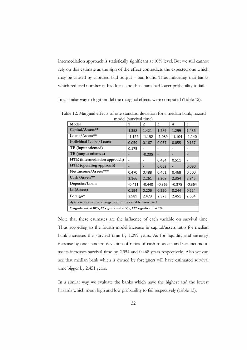
_t _t _t _t _t HTE (operating approach) - - 0.091 - 0.128
- - (0.47) - (0.61) Net Income/Assets 1.402 1.426 1.382 1.387 1.451
(3.93)*** (3.99)*** (4.01)*** (4.00)*** (3.85)*** Cash/Assets 5.582 5.708 5.973 6.026 5.872
(2.12)** (2.21)** (2.20)** (2.20)** (2.16)** Deposits/Loans -0.147 -0.154 -0.131 -0.133 -0.127
(-0.74) (-0.78) (-0.67) (-0.67) (-0.59) Ln(Assets) 0.021 0.022 0.028 0.027 0.024
(0.66) (0.69) (0.86) (0.83) (0.71) Foreign 0.365 0.345 0.34 0.346 0.364
(1.93)* (1.83)* (1.86)* (1.87)* (1.85)* Constant 1.714 2.011 0.652 1.077 1.612
(2.47)** (2.77)*** (0.92) (1.39) (2.11)** Observations 682 682 682 682 682 gamma .142** .142** .138** .140** .149** LR chi2 49.09 48.72 52.05 51.82 47.90 Absolute value of z statistics in parentheses
* significant at 10%; ** significant at 5%; *** significant at 1%
As in logit model we also can mention that hazard estimation also gives us the
right signs for significant variables. Such financial ratios as capital to assets, loans
to assets and cash to assets as in logit model are statistically significant at 5%
level. In contrast to logit model ratio of net income to assets is statistically
significant at 1% level which may be interpreted in the way that in dynamics the
ability of a bank to bring profit is important and have influence on survival time.
As in logit model it can be seen that foreign banks still perform better as the
influence on survival of dummy variable foreign is positive and statistically
significant at 10%.
As for efficiency measures almost all coefficients are not statistically significant.
The only model with hyperbolic efficiency measure estimated according to
32
intermediation approach is statistically significant at 10% level. But we still cannot
rely on this estimate as the sign of the effect contradicts the expected one which
may be caused by captured bad output – bad loans. Thus indicating that banks
which reduced number of bad loans and thus loans had lower probability to fail.
In a similar way to logit model the marginal effects were computed (Table 12).
Table 12. Marginal effects of one standard deviation for a median bank, hazard model (survival time)
Model 1 2 3 4 5 Capital/Assets** 1.358 1.421 1.289 1.299 1.486 Loans/Assets** ‐1.122 ‐1.152 ‐1.089 ‐1.104 ‐1.140 Individual Loans/Loans 0.059 0.167 0.057 0.055 0.137 TE (input oriented) 0.175 ‐ ‐ ‐ ‐ TE (output oriented) ‐ ‐0.235 ‐ ‐ ‐ HTE (intermediation approach) ‐ ‐ 0.484 0.511 ‐ HTE (operating approach) ‐ ‐ 0.062 ‐ 0.090 Net Income/Assets*** 0.470 0.488 0.461 0.468 0.500 Cash/Assets** 2.166 2.261 2.308 2.354 2.345 Deposits/Loans ‐0.411 ‐0.440 ‐0.365 ‐0.375 ‐0.364 Ln(Assets) 0.194 0.206 0.250 0.244 0.224 Foreign* 2.589 2.473 2.373 2.451 2.654 dy/dx is for discrete change of dummy variable from 0 to 1
* significant at 10%; ** significant at 5%; *** significant at 1%
Note that these estimates are the influence of each variable on survival time.
Thus according to the fourth model increase in capital/assets ratio for median
bank increases the survival time by 1.299 years. As for liquidity and earnings
increase by one standard deviation of ratios of cash to assets and net income to
assets increases survival time by 2.354 and 0.468 years respectively. Also we can
see that median bank which is owned by foreigners will have estimated survival
time bigger by 2.451 years.
In a similar way we evaluate the banks which have the highest and the lowest
hazards which mean high and low probability to fail respectively (Table 13).
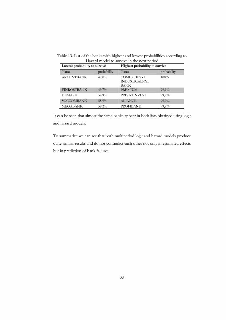
33
Table 13. List of the banks with highest and lowest probabilities according to Hazard model to survive in the next period
Lowest probability to survive Highest probability to survive
Name probability Name probability AKCENTBANK 47,0% COMERCIINYI
INDUSTRIALNYI BANK
100%
FINROSTBANK 49,7% PREMIUM 99,9% DEMARK 54,9% PRIVATINVEST 99,9% SOCCOMBANK 58,9% ALIANCE 99,9% MEGABANK 59,2% PROFIBANK 99,9%
It can be seen that almost the same banks appear in both lists obtained using logit
and hazard models.
To summarize we can see that both multiperiod logit and hazard models produce
quite similar results and do not contradict each other not only in estimated effects
but in prediction of bank failures.
34
C h a p t e r 6
CONCLUSION
The current financial crisis and number of bank liquidations makes it necessary to
investigate the causes of failures and develop tool for predicting bank failures. In
this work I managed to apply efficiency measures to banking sector, calculate the
group efficiencies of foreign and domestic banks and estimate two models of
banking failures. In general we can see that both models Multiperiod Logit and
Hazard model perform good and relatively to previous study (Nikolsko-Rzhevsky
2003) even produce better results. The gain of logit model is 91% which is quite
high level of prediction.
Also we may see that current data does not provide enough information to
evaluate managerial efficiency using data envelopment analysis. Such conclusion
is made based on insignificance of efficiency measures in all models estimated.
This is explained by problem of defining outputs especially loans which consist of
portion of bad loans which need to be considered as bad output. Especially
during crisis when there was reduction in loans we can see that on average banks
with higher efficiency failed, which contradicts the expected effect of efficiency
on failures.
The extension of theory on aggregation of efficiency measures especially group
hyperbolic efficiency allowed to evaluate efficiency of foreign banks versus
domestic and make conclusion of higher efficiency of banks with foreign capital
and thus the lower probability to fail.
The analysis of determinants of failure shows that the most important factors are
capital, asset quality and liquidity. These factors in the models are presented by
following financial ratios capital to assets, loans to assets and cash to assets and
35
are significant in almost all model specifications at 5% significance level. Also it is
worth mentioning that banks with foreign capital on average have lower
probability to fail.
In general models perform quite well but still the estimation of efficiency can be
improved by including the information about share of bad loans as bad output.
Unfortunately this information is not obtained and National Bank of Ukraine
should develop procedure to get this data from banks. Also the increase in
sample can make the analysis more precise and will allow testing the predictive
power of the models. The further research can also use aggregated efficiency to
evaluate performance of different groups of banks. For example compare the
efficiency of banks grouped by size or by age.
36
BIBLIOGRAPHY
Aigner, D.J., C.A.K. Lovell and P. Schmidt. 1977. Specification and estimation of frontier production, profit and cost functions. Journal of Econometrics 25: 21–37.
Barr, R. S., and T. F. Siems. 1992. Predicting Bank Failure Using DEA to Quantify Management Quality. Technical Report 92. Department of Computer Science and Engineering, Southern Methodist University,
Bauer, Paul W., Allen N. Berger, Gary D. Ferrier and David B. Humphrey. 1998. Consistency Conditions for Regulatory Analysis of Financial Institutions: A Comparison of Frontier Efficiency Methods. Journal of Economics and Business, Elsevier, vol. 50(2): 85-114, March.
Berger, A.N., D.B. Humphrey. 1998. Efficiency of financial institutions: International survey and directions for future research. European Journal of Operational Research 98: 175-212.
Blackorby, C. and R. R. Russell. 1999. Aggregation of Efficiency Indices, Journal of Productivity Analysis 12: 5–20.
Charnes, A., W.W. Cooper and E. Rhodes. 1978. Measuring the Inefficiency of Decision Making Units, European Journal of Operational Research 2(6): 429-444
Cleves Mario Alberto,William Gould,Roberto Gutierrez. 2008. An introduction to survival analysis using Stata. College Station, Tex. : Stata Press
Cole, R. A. and J. W.Gunther. 1998. Predicting Bank Failures: A Comparison of On- and Off-Site Monitoring Systems, Journal of Financial Services Research 13(2): 103-118
Cuesta, Rafael A. and José L. Zofío. 2005. Hyperbolic Efficiency and Parametric Distance Functions: With Application to Spanish Savings Banks. Journal of Productivity Analysis 24(1): 31-48, September.
Debreu, G. 1951. The Coefficient of Resource Utilization. Econometrica 19(3): 273–292.
Färe, Rolf and C. A. Knox Lovell. 1978. Measuring the technical efficiency of production, Journal of Economic Theory, Elsevier 19(1): 150-162, October.
37
Färe, Rolf and Valentin Zelenyuk. 2003. On Aggregate Farrell Efficiencies. European Journal of Operations Research 146(3): 615-621.
Färe, R., S. Grosskopf, C.A.K. Lovell. 1985. The Measurement of Efficiency of Production. Kluwer Academic Publishers, Boston.
Färe, R. and V. Zelenyuk. 2003. On Aggregate Farrell Efficiencies, European Journal of Operational Research, vol.146, p.615-620.
Farrell, M.J. 1957. The Measurement of Productive Efficiency. Journal of the Royal Statistical Society 120: 253-281.
Fries, S. and A. Taci. 2005. Cost efficiency of banks in transition: Evidence from 289 banks in 15 post-communist countries. Journal of Banking and Finance 29: 55–81.
Georgescu-Roegen, N. 1951. The aggregate linear production function and its applications to von Neumann’s economic model. In: Koopmans, T. (Ed.), Activity Analysis of Production and Allocation. Wiley, New York, pp. 98-115.
Holló, D. and M. Nagy. 2006. Bank Efficiency in the Enlarged European Union, A chapter in The banking system in emerging economies: how much progress has been made? Bank for International Settlements 28: 217-350.
Grier, Waymond A. 2007. Credit analysis of financial institutions. London: Euromoney Institutional Investor Plc.
Grigorian, D. and V. Manole. 2006. Determinants of commercial bank performance in transition: An application of data envelopment analysis. Comparative Economic Studies 48: 497–522.
Grosskopf, S. 1996. Statistical Inference and Nonparametric Efficiency: A Selective Survey, Journal of Productivity Analysis, 7 July: 161-76.
Kneip, Alois, Leopold Simar and Paul W. Wilson. 2008. Asymptotics And Consistent Bootstraps For DEA Estimators In Nonparametric Frontier Models. Econometric Theory, Cambridge University Press, 24(06): 1663-1697, December.
Koopmans, T. C. 1957. Three Essays on the State of Economic Analysis, NewYork: McGraw-Hill.
38
Kyj, L. and I. Isik. 2005. Effects of production scale, location and foreign participation on bank efficiency in a transition economy: The Ukrainian experience? International Development Research Yearbook XIV: 609–616.
Li, S.-K. and Y.-C. Ng. 1995. Measuring the Productive Efficiency of a Group of a Firms, International Advances in Economic Resarch, vol.1 (4), p.377-390.
Meeusen, W., and J. van den Broeck.1977. Efficiency Estimation from Cobb-Douglas Production Function with Composed Error, International Economic Review 8: 435-444.
Mertens, A. and G. Urga. 2001. Efficiency, scale and scope economies in the Ukrainian banking sector in 1998, Emerging Markets Review 2(3): 292-308.
Meyer, Paul A. and Howard W. Pifer. 1970. Prediction of Bank Failures, The Journal of Finance Vol. 25 ( 4) (Sep., 1970), pp. 853-868
Nesterenko, Volodymyr and Valentin Zelenyuk. 2007. Measuring potential gains from reallocation of resources. Journal of Productivity Analysis, Springer 28(1): 107-116, October.
Nikolsko-Rzhevskyy, O. 2003. Bank bankruptcy in Ukraine: what are the determinants and can bank failure be forecasted. EERC MA Thesis. Kyiv.
Popruga, O. 2001. Which factors cause failure of Ukrainian banks. EERC MA Thesis. Kyiv.
Rabtsun, K. 2003. Evaluating the performance of commercial banks in Ukraine: frontier efficiency approach. EERC MA Thesis. Kyiv.
Russell, R.R. 1990. Continuity of Measures of Technical Efficiency. Journal of Economic Theory 52: 255-267.
Sahajwala, Ranjana and Paul Van den Bergh. 2000. Supervisory risk assessment and early warning systems. Basel committee on banking supervision working papers 4 (December).
Seballos, L.D., and J.B. Thomson. 1990. Understanding Causes of Commercial Bank Failures in the 1980s. Economic Commentary, Federal Reserve Board of Cleveland, September.
Shephard, R. W. 1953. Cost and Production Functions, Princeton: Princeton University Press.
39
Shumway, Tyler. 2001. Forecasting Bankruptcy More Accurately: A Simple Hazard model, The Journal of Business 74(1):101-124
Simar, Léopold and Paul W. Wilson. 2007. Estimation and inference in two-stage, semi-parametric models of production processes, Journal of Econometrics, Elsevier, 136(1): 31-64, January.
Simar, Léopold and Paul W. Wilson. 1998. Sensitivity analysis of efficiency scores: How to bootstrap in nonparametric frontier models, Management Science, 44, 49–61.
Simar, Léopold and Valentin Zelenyuk. 2007. Statistical inference for aggregates of Farrell-type efficiencies, Journal of Applied Econometrics, John Wiley & Sons, Ltd., 22(7):1367-1394.
Wheelock, D.C. and P.W. Wilson. 2000. Why do banks disappear? The determinants of US bank failures and acquisitions. Review of Economics and Statistics - MIT Press
Yildirim, H. S. and G. C. Philippatos. 2002. Efficiency of banks: Recent evidence from the transition economies.1993–2003. Unpublished paper, University of Tennessee, Knoxville, TN.
NBU – National Bank of Ukraine - Методичні вказівки щодо організації, проведення інспекційних перевірок та встановлення рейтингової оцінки банку
40
APPENDIX
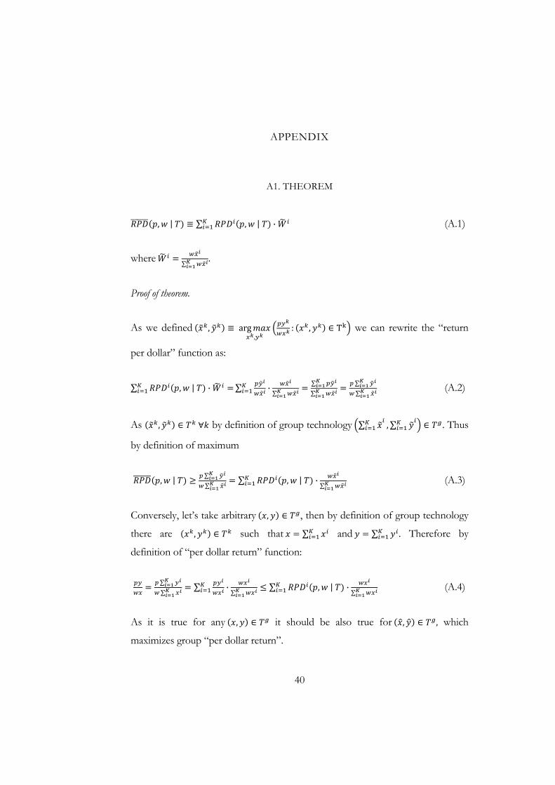
A1. THEOREM
, | ∑ , | · (A.1)
where ∑
.
Proof of theorem.
As we defined , arg,
: , T we can rewrite the “return
per dollar” function as:
∑ , | · ∑ ·∑
∑∑
∑∑
(A.2)
As , by definition of group technology ∑ , ∑ . Thus
by definition of maximum
, | ∑∑
∑ , | ·∑
(A.3)
Conversely, let’s take arbitrary , , then by definition of group technology
there are , such that ∑ and ∑ . Therefore by
definition of “per dollar return” function:
∑∑
∑ ·∑
∑ , | ·∑
(A.4)
As it is true for any , it should be also true for , , which
maximizes group “per dollar return”.
41
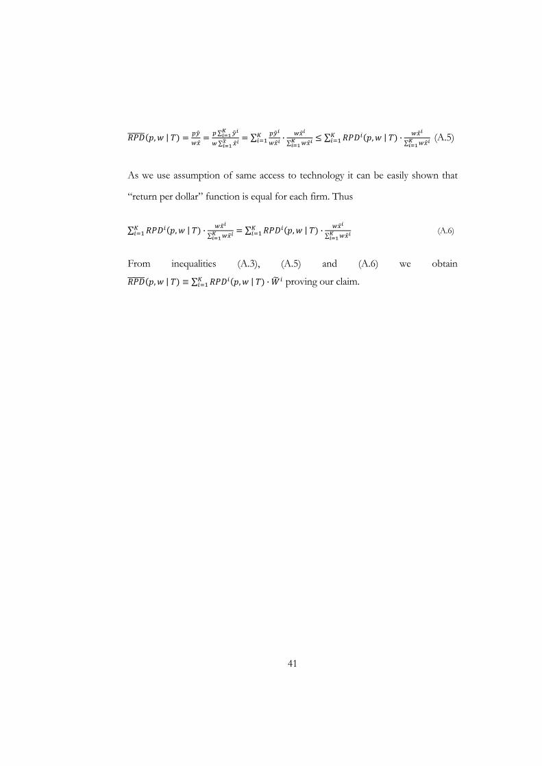
, | ∑∑
∑ ·∑
∑ , | ·∑
(A.5)
As we use assumption of same access to technology it can be easily shown that
“return per dollar” function is equal for each firm. Thus
∑ , | ·∑
∑ , | ·∑
(A.6)
From inequalities (A.3), (A.5) and (A.6) we obtain
, | ∑ , | · proving our claim.
42
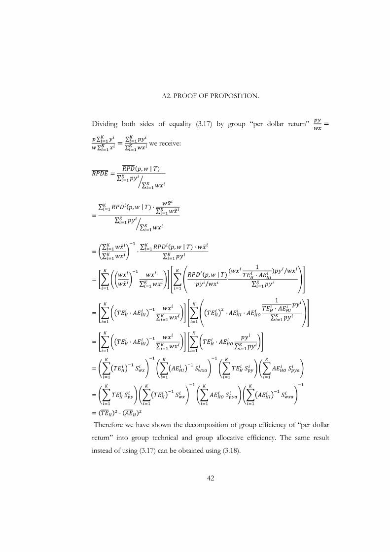
A2. PROOF OF PROPOSITION.
Dividing both sides of equality (3.17) by group “per dollar return”
∑∑
∑∑
we receive:
, | ∑
∑
∑ , | · ∑∑
∑
∑∑ ·
∑ , | ·∑
∑, | /
1·
/
∑
· ∑ · ·
1·
∑
· ∑ · ∑
·
Therefore we have shown the decomposition of group efficiency of “per dollar
return” into group technical and group allocative efficiency. The same result
instead of using (3.17) can be obtained using (3.18).