UKAEA Thomson Scattering Tutorial for EFTS/EODI, 12 th June 2009, M.Kempenaars 1/35 A Brief tutorial to Thomson Scattering With a focus on LIDAR By Mark

UKAEAThomson Scattering Tutorial for EFTS/EODI, 12th June 2009,

M.Kempenaars 1/35

A Brief tutorial to

Thomson Scattering

With a focus on LIDAR

By Mark KempenaarsFor the EFTS/EODI training, 12th June 2009 at Culham Science centre


M.Kempenaars 2/35

Outline of TalkOutline of Talk

1. Introduction

2. Thomson scattering theory – the highlights

3. Conventional TS

4. LIDAR TS

5. Towards ITER


M.Kempenaars 3/35

IntroductionIntroduction Thomson scattering was first described in

1903 by J.J. Thomson, many years before lasers existed. Thomson discovered electrons in 1897.

First application to a laboratory plasma in 1963 by Fünfer (First ruby laser in 1960)

First measurements in hot plasmas by Peacock et al., in 1969 at the Russian T3 Tokamak


M.Kempenaars 4/35

Thomson scattering theoryThomson scattering theoryThomson scattering is nothing more than the interaction of EM radiation with an electron any light will do. We can use Maxwell’s equations (1873) to describe the forces on and movements of the electrons. The highlights…

Let’s consider this experimental setup:

Incident EM wave with amplitude E0, propagation vector k0, and angular frequency 0, so electric field at the electron is given by:

d

ks

Rk

k0

E0

Scattering Electron

Origin

rj

trkEE j 000 cos


M.Kempenaars 5/35

This electric field will then apply a force on the electron (with mass m and charge e at position rj) and following Maxwell’s equations, we get the acceleration of the electron:

Theory cont’d - 1Theory cont’d - 1

trkEm

er jj 000 cos

This equation clearly shows us that the electron will be oscillating up and down, together with the electric field of the light wave.

Since this electron is now a moving charged particle it will create an EM field of its own, with the same wavelength as the incoming light!

d

ksRk

k0

E0

Scattering Electron

Origin

rj

d

ksRk

k0

E0

Scattering Electron

Origin

rj


M.Kempenaars 6/35

Theory cont’d - 2Theory cont’d - 2When a moving electron like this is observed from a large distance (R>>) its radiation can be described as dipole radiation:

d

ksRk

k0

E0

Scattering Electron

Origin

rj

d

ksRk

k0

E0

Scattering Electron

Origin

rj

trkR

ErtRE js 0

02

0 cossin

,

This equation shows us that the radiation from ions is negligible compared to that of electrons, since r0 ~ 1/m:

Where k is the differential vector (ks-k0). and r0 is the classical electron radius:

mmc

er 15

20

2

0 1082.24

7

2

10966.2

i

e

m

m


M.Kempenaars 7/35

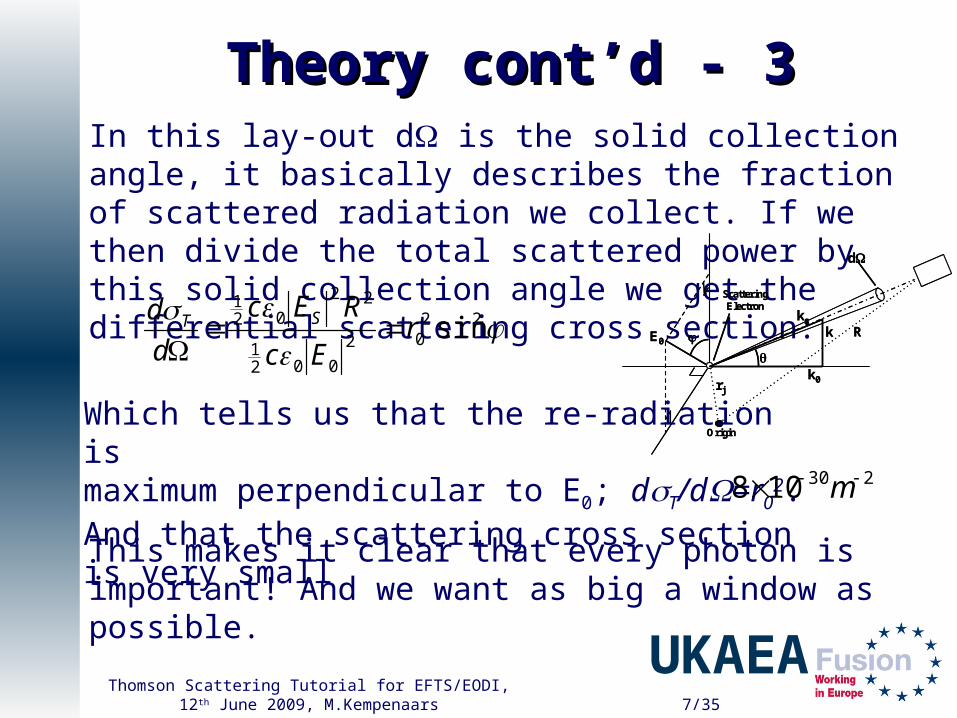
Theory cont’d - 3Theory cont’d - 3In this lay-out d is the solid collection angle, it basically describes the fraction of scattered radiation we collect. If we then divide the total scattered power by this solid collection angle we get the differential scattering cross section: d

ksRk

k0

E0

Scattering Electron

Origin

rj

d

ksRk

k0

E0

Scattering Electron

Origin

rj

2202

0021

22

021

sinrEc

REc

d

d ST

Which tells us that the re-radiation ismaximum perpendicular to E0; dT/d=r0

2.And that the scattering cross section is very small

230108 m

This makes it clear that every photon is important! And we want as big a window as possible.


M.Kempenaars 8/35

Theory cont’d - 4Theory cont’d - 4Obviously the scattered power depends on the number of electrons caught by the laser, but also on the interaction between them. This interaction start to happen above the Debye length.

e

eD n

T3104.7 So this depends on the density and temperature of the electrons

If << 1 : then the scattering is from individual electron: Incoherent TS

If ≥ 1 : then scattering by electrons surrounding ions;(Ion) Coherent Thomson Scattering

If ~ 5-20 : Scattering by electron density fluctuations, or Bragg-scattering

Coherent Thomson scattering

2

sin4

01

D

Dk

For Te = 10 keV, ne = 5×1019 m-3: D ~ 100 m (typical for JET)

The so-called Salpeter-parameter tells us whether the scattering we are observing is coherent or not:


M.Kempenaars 9/35

The scattered light is clearly proportional to the density.

The form function is given by:where f() is the velocity distribution

In this equation the delta function tells you about the Doppler

shift:

Theory cont’d - 5Theory cont’d - 5

20 sin, kSLn

d

dPP e

Ts

With P0 : Incident (laser) powerne : Electron density in the plasmaL : Length of scattering volumeS(k,w) : Scattering form factor

describes frequency shifts from electron motion aswell as correlation between electrons.

The total scattered power is given by:

kSk dvvvfkS

0,

vkvS 0


M.Kempenaars 10/35

Theory cont’d - 6Theory cont’d - 6If the velocity distribution f(v) is Maxwellian (i.e. low density, no interaction between particles) then:

with ‘a’ the thermal velocity:

2

exp1

a

v

avf k

k e

B

m

Tka 22

One then finally finds an equation that contains wavelengths:

With 0 the incident wavelength and s the scattered wavelengthWhere we then find the spectral width of the scattered light, which has a Gaussian shape:

If we were to take a Ruby laser (694.3nm) and 90º scattering then this would give:

2

0exp1

S

SS

e

eB

m

Tk

cc

a 2

2sin

2

2sin2 0

0

eVTnm e94.1


M.Kempenaars 11/35

Theory cont’d - 6Theory cont’d - 6Once the electrons get really hot (i.e. really fast) we have to start including relativistic effects, which effectively change the scattering cross section of the electrons, by a factor 1/ 2 where

is the Lorentz factor , which shows that for a 1%

deviation we need an electron temperature of 2.56 keV.

Also there is a “search light” effect or relativistic aberration, which means that the electrons radiate preferentially in their forward direction. E.g. moving at 10% of c, then power in forward direction increases by 36%, it decreases by 26% in backwards direction. This leads to a blue shift of the spectrum…

22 ac

c


M.Kempenaars 12/35

TS spectraTS spectraSo, what does this look like?

/laser


M.Kempenaars 13/35

0

1

2

3

0 0.2 0.4 0.6 0.8 1 1.2 1.4 1.6 1.8 2

Normalised Wavelength

Sp

ec

tra

l In

ten

sit

y

0

1

2

3

0 0.2 0.4 0.6 0.8 1 1.2 1.4 1.6 1.8 2

Normalised Wavelength

Sp

ec

tra

l In

ten

sit

y

TS SpectrometerTS SpectrometerWhat does a spectrometer look like?If we cut our scattered light “broadband” light into sections:

1234

1

2

3

4Incoming

collected light


M.Kempenaars 14/35

So, what do we need?So, what do we need? A powerful pulsed laser

– Typically one would get 1 photon in every 1×1014 back, e.g. if we use a 3GW laser pulse we get 30 W back on a high density plasma (1020m-3) and 100% transmission.

Fire this laser into the plasma– A window on the machine that can stand the high laser

power and does not get dirty– plus the optics to deliver it there.

Collect as much light as possible– A large window is needed that can see the laser line– This window can’t get dirty, or if it does we must be able

to clean it.– The other optics need to be aligned and stable (also during

disruptions etc.)


M.Kempenaars 15/35

9090ºº TS - Single point TS - Single pointIn the early days of TS on Fusion devices all TS systems were “single point” diagnostics, i.e. the optics were only looking at one point. This seems archaic but it was still one of the better and more reliable diagnostics.

This was also the case on JET, where a ruby laser was fired vertically into the plasma. A large set of windows and mirrors was used to relay the light to a spectrometer.

Collection optics

Plasma

Laser


M.Kempenaars 16/35

9090ºº TS - Multi point TS - Multi pointMore modern systems have a range of points. Where each spatial point is imaged onto an optical fibre.

Laser

Collection optics

Plasma

Each fibre then represents a spatial point in the plasma, a high spatial resolution can be achieved by using a lot of fibres. Keep in mind however that a smaller volume will scatter fewer photons.

And this setup means one needs a spectrometer for each spatial position, so can get very expensive


M.Kempenaars 17/35

9090ºº TS on JET – HRTS TS on JET – HRTSA new system was installed on JET in 2004. High Resolution Thomson Scattering.

- High power (5J, 15ns) Nd:YAG laser.

- Fire at 20Hz, horizontally

- Scattered light is then collected from a window at the top of the machine.

In order to collect as many photons as possible we need a big window, largest on JET 20cm diameter.

63 spatial points on the LFS, at approximately 1.5cm resolution

20 m20 + 10 m (50 ns)

20 + 20 m (100 ns)

Fiber bundle into each polychromator

Signal reconstruction with 50 ns delay

ns

20 m20 + 10 m (50 ns)

20 + 20 m (100 ns)

20 m20 + 10 m (50 ns)

20 + 20 m (100 ns)

Fiber bundle into each polychromator

Signal reconstruction with 50 ns delay

ns


M.Kempenaars 18/35

9090ºº TS on JET – HRTS cont’d 1 TS on JET – HRTS cont’d 1


M.Kempenaars 19/35

MAST 90MAST 90ºº TS TS

A set of lasers can be fired in sequence or in a burst, giving a high temporal resolution ~1s


M.Kempenaars 20/35

LIDAR – 180LIDAR – 180ºº TS TSNow we go to = 180º, or back scattering

Light detection and ranging, we fire a laser pulse and count the elapsed time before we get a signal back, like in radar.

Plasma

Laser

(short pulse)

Mirror labyrinth

Of course we have to count very quickly, since light travels at ~3×106 m/s (or 1m every 3ns)

Major advantages: ‘Point and shoot’ method, which requires minimum access

Very short laser pulse ~250ps

Only one spectrometer needed, but it has to be fast!


M.Kempenaars 21/35

LIDAR – 2LIDAR – 2The main advantages of LIDAR: The alignment is relatively easy Only one spectrometerBecause of the previous two, much easier to calibrate and maintain

The main disadvantage of LIDAR: Time is of the essence!If anything is slow it will contribute to the spatial resolution.HOWEVER! Time is on our side:


M.Kempenaars 22/35

Note that the profile length in time is dt=2L/c.Effectively 15cm/ns! Instead of normal 30cm/nsDetector and laser response defines spatial resolution

Plasma,Length L

LaserPulse

ScatteredLight

ScatteredLight

LIDAR – 3LIDAR – 3

7cm (ITER requirement) is equivalent to ~460ps combined laser and detector response time (so det/laser response ~300ps FWHM)


M.Kempenaars 23/35

LIDAR on JET - 1LIDAR on JET - 1JET is the only fusion machine in the world that has LIDAR.

LIDAR only really works on big machines due to its limitations in spatial resolution.

Two LIDAR systems on JET, the Core LIDAR and the Edge LIDAR. The edge LIDAR has recently been upgraded with new detectors and digitiser, so it has better resolution.

Core LIDAR Edge LIDAR

Laser pulse length ~ 300ps ~ 300ps

Laser power 3J/pulse = 10GW 1J/pulse = 3GW

Detector response ~ 300ps ~ 650ps

Digitiser response 8GHz, 20GSa/s 1GHz, 4GSa/s

Spatial resolution ~ 6.5cm ~ 12cm


M.Kempenaars 24/35

LIDAR on JET - 2LIDAR on JET - 2The total distance the laser beam has to travel is about 50m, important to keep the beam “nice”.

Light is collected through a set of 6 windows


M.Kempenaars 25/35

LIDAR on JET - 3LIDAR on JET - 3Collected light is relayed via a set of mirrors and lenses to the spectrometer. The Core LIDAR spectrometer has 6 detectors in a 3D layout.

Each detector generates its own trace, these are then combined to form a temperature and density profile


M.Kempenaars 26/35


M.Kempenaars 27/35

NEXT: ITER LIDARNEXT: ITER LIDAR

10 ms(100 Hz)

r/a < 0.9~7см (a/30)

Te 0.5 – 40 keV (10%)

ne 3x1019-3x1020m-3(5%)Targetrequirements

Core LIDAR (C.01 group 1b – advanced plasma control)

Short line indicates the required measurement resolution of a/30.

This is equivalent to approximately 7cm in real space.

Note: the full profile from -0.9r/a to 0.9r/a is required

~2m


M.Kempenaars 28/35

ITER LIDAR - 1ITER LIDAR - 1


M.Kempenaars 29/35


Low impact diagnostic access required In vacuum mirror protection

(passive/active)Detectors (sensitivity, response time, wavelength)

Materials (neutrons/radiation)--fit purposeLong term, low maintenance reliabilityLaser development

Beam dump

Access to anywhere inside this area is similar to accessing a satellite-very infrequent

Mirrors

Lasers

enter machine

boundary

Mirrors

Large mirrors collect suitable amount of light

Exposed to plasma

~2

m


M.Kempenaars 30/35

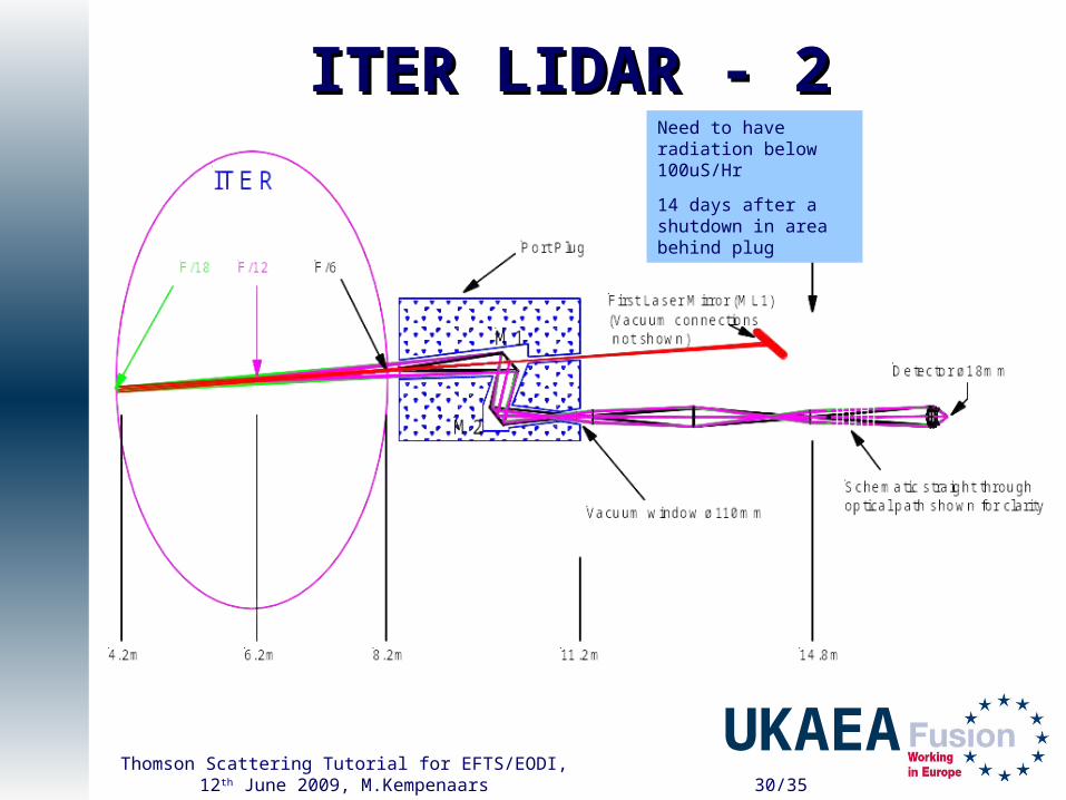
ITER LIDAR - 2ITER LIDAR - 2Need to have radiation below 100uS/Hr

14 days after a shutdown in area behind plug


M.Kempenaars 31/35


Influence of optical labyrinth Minimising activation of components just outside

the tokamak will be key to easier maintenance in the future

From Attila code


M.Kempenaars 32/35


Photocathode Response time, ns Wavelength coverage

S-20 0.2 ns(below) UV, visible up to 500 nm

GaAsP 0.3 ns (as above) visible up to 750 nm

GaAs 0.35ns (estimated) visible up to 850 nm

InGaAs ? NIR

S-20

GaAsPGaAs

NIR

Several options, but none good enough yet.


M.Kempenaars 33/35

ITER LIDAR - 5ITER LIDAR - 5Needs reasonable energy and short pulse simultaneouslyOptions to chose from:

– Nd:YAG (1064nm)

– Ruby (694nm)

– Ti:Sapphire (~800nm)

– Nd:YLF (1056nm)

Wide temperature rangeTime repetition expected from laser(s) – 100HzAlso need to consider

– Space envelope/ Maintainability/ Power consumption/ Data quality


M.Kempenaars 34/35

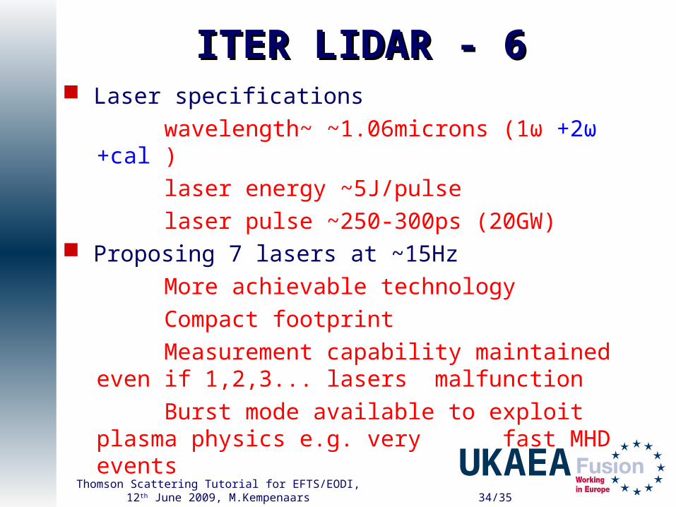
ITER LIDAR - 6ITER LIDAR - 6 Laser specifications

wavelength~ ~1.06microns (1ω +2ω +cal )

laser energy ~5J/pulse

laser pulse ~250-300ps (20GW) Proposing 7 lasers at ~15Hz

More achievable technology

Compact footprint

Measurement capability maintained even if 1,2,3... lasers malfunction

Burst mode available to exploit plasma physics e.g. very fast MHD events


M.Kempenaars 35/35

At the end…At the end… This tutorial is intended as a first introduction in

to Thomson scattering and not as an exhaustive review

Only some typical examples were given (mostly JET), every fusion machine has TS

I’ve only focused on incoherent TS The aim was mainly on demonstrating how it

works and how powerful a technique it can be

Epilogue

Thank you for your attention


M.Kempenaars 36/35

Any extras… ?Any extras… ?


M.Kempenaars 37/35

Space time domainSpace time domain

Documents

UKAEA Thomson Scattering Tutorial for EFTS/EODI, 12 th June 2009, M.Kempenaars 1/35 A Brief tutorial to Thomson Scattering With a focus on LIDAR By Mark