Embed Size (px)
Citation preview

Springer ComplexitySpringer Complexity is an interdisciplinary program publishing the best research and academic-levelteaching on both fundamental and applied aspects of complex systems - cutting across all traditionaldisciplines of the natural and life sciences, engineering, economics, medicine, neuroscience, social andcomputer science.
Complex Systems are systems that comprise many interacting parts with the ability to generate a newquality of macroscopic collective behavior the manifestations of which are the spontaneous formationof distinctive temporal, spatial or functional structures. Models of such systems can be successfullymapped onto quite diverse “real-life" situations like the climate, the coherent emission of light fromlasers, chemical reaction-diffusion systems, biological cellular networks, the dynamics of stock marketsand of the internet, earthquake statistics and prediction, freeway traffic, the human brain, or the formationof opinions in social systems, to name just some of the popular applications.
Although their scope and methodologies overlap somewhat, one can distinguish the following mainconcepts and tools: self-organization, nonlinear dynamics, synergetics, turbulence, dynamical systems,catastrophes, instabilities, stochastic processes, chaos, graphs and networks, cellular automata, adaptivesystems, genetic algorithms and computational intelligence.
The two major book publication platforms of the Springer Complexity program are the monographseries “Understanding Complex Systems" focusing on the various applications of complexity, and the“Springer Series in Synergetics", which is devoted to the quantitative theoretical and methodologicalfoundations. In addition to the books in these two core series, the program also incorporates individualtitles ranging from textbooks to major reference works.
Editorial and Programme Advisory BoardDan Braha
New England Complex Systems, Institute and University of Massachusetts, Dartmouth
Péter Érdi
Center for Complex Systems Studies, Kalamazoo College, USA and Hungarian Academy of
Sciences, Budapest, Hungary
Karl Friston
Institute of Cognitive Neuroscience, University College London, London, UK
Hermann Haken
Center of Synergetics, University of Stuttgart, Stuttgart, Germany
Janusz Kacprzyk
System Research, Polish Academy of Sciences, Warsaw, Poland
Scott Kelso
Center for Complex Systems and Brain Sciences, Florida Atlantic University, Boca Raton, USA
Jürgen Kurths
Potsdam Institute for Climate Impact Research (PIK), Potsdam, Germany
Linda Reichl
Center for Complex Quantum Systems, University of Texas, Austin, USA
Peter Schuster
Theoretical Chemistry and Structural Biology, University of Vienna, Vienna,
Austria
Frank Schweitzer
System Design, ETH Zürich, Zürich, Switzerland
Didier Sornette
Entrepreneurial Risk, ETH Zürich, Zürich, Switzerland

Understanding Complex Systems
Founding Editor: J.A. Scott Kelso
Future scientific and technological developments in many fields will necessarily depend upon comingto grips with complex systems. Such systems are complex in both their composition - typically manydifferent kinds of components interacting simultaneously and nonlinearly with each other and their envi-ronments on multiple levels - and in the rich diversity of behavior of which they are capable.
The Springer Series in Understanding Complex Systems series (UCS) promotes new strategies andparadigms for understanding and realizing applications of complex systems research in a wide variety offields and endeavors. UCS is explicitly transdisciplinary. It has three main goals: First, to elaborate theconcepts, methods and tools of complex systems at all levels of description and in all scientific fields,especially newly emerging areas within the life, social, behavioral, economic, neuroand cognitive sci-ences (and derivatives thereof); second, to encourage novel applications of these ideas in various fieldsof engineering and computation such as robotics, nano-technology and informatics; third, to provide asingle forum within which commonalities and differences in the workings of complex systems may bediscerned, hence leading to deeper insight and understanding.
UCS will publish monographs, lecture notes and selected edited contributions aimed at communicat-ing new findings to a large multidisciplinary audience.

Sifeng Liu and Jeffrey Yi-Lin Forrest (Eds.)
Advances in Grey SystemsResearch
ABC

Editors
Prof. Sifeng LiuNanjing University of Aeronautics and AstronauticsInstitute for Grey Systems Studies,29 Imperial StreetNanjing 210016P.R. ChinaE-mail: [email protected]
Prof. Jeffrey Yi-Lin ForrestSlippery Rock UniversityDepartment of MathematicsSlippery RockPA 16057USAE-mail: [email protected]
ISBN 978-3-642-13937-6 e-ISBN 978-3-642-13938-3
DOI 10.1007/978-3-642-13938-3
Understanding Complex Systems ISSN 1860-0832
Library of Congress Control Number: 2010929357
c© 2010 Springer-Verlag Berlin Heidelberg
This work is subject to copyright. All rights are reserved, whether the whole or part of the mate-rial is concerned, specifically the rights of translation, reprinting, reuse of illustrations, recitation,broadcasting, reproduction on microfilm or in any other way, and storage in data banks. Dupli-cation of this publication or parts thereof is permitted only under the provisions of the GermanCopyright Law of September 9, 1965, in its current version, and permission for use must alwaysbe obtained from Springer. Violations are liable to prosecution under the German Copyright Law.
The use of general descriptive names, registered names, trademarks, etc. in this publication doesnot imply, even in the absence of a specific statement, that such names are exempt from the relevantprotective laws and regulations and therefore free for general use.
Typeset & Cover Design: Scientific Publishing Services Pvt. Ltd., Chennai, India.
Printed on acid-free paper
9 8 7 6 5 4 3 2 1
springer.com
Synopsis
This volume contains some of the highly selective, best quality research works presented at the 2009 IEEE International Conference on Grey Systems and intel-ligent Services (IEEE GSIS 2009), November 10 – 12, 2009, Nanjing, P. R. China. Grey systems theory was initiated by Professor Deng Julong in 1982 with the pub-lication of the first paper in the international journal Systems and Control Letters. In the past 20+ years, this theory has been developed and matured rapidly and applied widely in almost all areas of scientific learning. Currently, many universities from around the globe offer courses and workshops on grey systems and information; and hundreds of graduate students are studying and/or applying grey systems theory in their works and their writing of dissertations. This book is appropriate as a ref-erence for graduate students or high level undergraduate students, majoring in areas of science, technology, agriculture, medicine, astronomy, earth science, economics, and management. It can also be utilized by researchers and technicians in research institutions, business entities, and government agencies.

Editorial Board
Yaoguo Dang, Zhigeng Fang, Xinping Xiao, Qishan Zhang, Kunli Wen, Dang Luo, Shunxiang Wu, Lirong Jian, Jianjun Zhu, Naiming Xie, Richard Chen, Yingjie Yang, Hans Kuijper, Emil Scarlat, Rih-Chang Chao, Der-Bang Wu, Baiming Yin, Hongzhuan Chen, Kejia Chen, Benhai Guo, Zhongmin Song, Wenping Wang, Xuerui Tan, Xiufeng Zuo, Jianling Wang, Yinao Wang, Yong Wei, Chuanmin Mi.
Professor Dr. Sifeng Liu earned a BS degree in mathematics at Henan University, China, in 1981, an MS degree in economics and a PhD in systems engineering at Huazhong University of Science and Technology, Wuhan, China, in 1986 and 1998, respectively. He has attended Slippery Rock University of Pennsylvania and Sydney University in Australia as a visiting professor. Professor Liu is currently director of the Institute for Grey Systems Studies and dean of the college of economics and management at Nanjing University of aeronautics and astronautics, where he is a distinguished professor, academic leader, and a doctor tutor in management
science and systems engineering disciplines. Dr. Liu’s main research activities are in grey systems theory and econometrics.
He has published over 200 research papers and 16 books. He has been awarded 18 provincial and national prizes for his outstanding achievements in scientific re-search and applications, and was selected by the Personnel Ministry of China as a distinguished professor. He was recognized in 2002 by the World Organization of Systems and Cybernetics.
Dr. Liu is a member of teaching direct committee of management science and engineering of the Ministry of Education, China. He is also the expert of soft sci-ence at the Ministry of Science and Technology, China, and Development of Management Science of the National Natural Science Foundation of China. Pro-fessor Liu currently serves as a chair of the Technical Committee on Grey Systems of the IEEE Systems, Man, and Cybernetics Society, is president of the Grey Sys-tems Society of China, vice president of the Chinese Society for Optimization, Overall Planning and Economic Mathematics, vice president of the Beijing Chapter of the IEEE SMC, vice president of the Econometrics and Management Science

Editoral BoardVIII
Society of Jiangsu Province, and vice president of the Systems Engineering Society of Jiangsu Province. He is a member of the editorial board of over 10 professional journals, including The Journal of Grey System (UK), Scientific Inquiry (USA), Journal of Grey System (Taiwan), Chinese Journal of Management Science, Sys-tems, Theory and Applications, Systems Science and Comprehensive Studies in Agriculture, and Journal of Nanjing University of Aeronautics and Astronautics, among others.
Dr. Liu was selected as National Excellent Teacher in 1995, was awarded Expert Enjoying Government’s Special Allowance by the State Council of China in 2000, National Expert with Prominent Contribution in 1998, and Outstanding Managerial Personnel of China in 2005.
Professor Jeffrey Yi-Lin Forrest earned all his edu-cational degrees in pure mathematics. His PhD degree was granted in 1988 by Auburn University, Alabama; and he did one year post-doctoral research in statistics at Carnegie Mellon University, Pittsburgh, during 1990 – 1991. Dr. Lin is currently a specially appointed professor in economics, finance, and systems science of Nanking University of Aeronautics and Astronautics, a specially appointed professor in mathematics and systems science of National University of Defense Technology, China, and a tenured professor of mathematics at Slippery Rock University of Pennsylvania. Dr. Lin is a founder and the present president of the International Institute for Gen-eral Systems Studies (IIGSS), a non-profit organization registered in PA in mid-1990s. Since 1984, Lin has had
over 300 research papers, over 20 monographs and edited volumes published by a large array of prestigious publishers, such as Springer, World Scientific, Kluwer Academic (currently part of Springer), Academic Press (currently part of Springer), Wiley, Taylor and Francis, Meteorological Press, etc. He serves or served on the editorial boards of 11 professional journals, including Kybernetes: The Interna-tional Journal of Systems, Cybernetics and Management Science, Journal of Sys-tems Science and Complexity, and International Journal of General Systems. He is currently a co- editor of the book series “Systems Evaluation, Prediction and De-cision-Making,” published by Auerbach, an imprint of Taylor and Francis.
Some of Dr. Lin’s research was funded by the United Nations, the State of Pennsylvania, the National Science Foundation of China, and the German National Research Center for Information Architecture and Software Technology. Over the years, Dr. Yi Lin’s scientific achievements have been recognized by various pro-fessional organizations and academic publishers. In 2001, he was inducted into the honorary fellowship of the World Organisation of Systems and Cybernetics. His research interests are wide ranging, covering areas like mathematical and general systems theory and applications, foundations of mathematics, data analysis, pre-dictions, economics and finance, management science, and philosophy of science.

Preface
This book contains contributions by some of the leading researchers in the area of grey systems theory and applications. All the papers included in this volume are selected from the contributions physically presented at the 2009 IEEE International Conference on Grey Systems and Intelligent Services, November 11 – 12, 2009, Nanjing, Jiangsu, People’s Republic of China. This event was jointly sponsored by IEEE Systems, Man, and Cybernetics Society, Natural Science Foundation of China, and Grey Systems Society of China. Additionally, Nanjing University of Aeronautics and Astronautics also invested heavily in this event with its direct and indirect financial and administrative supports.
The conference aimed at bringing together all scholars and experts in the fields of grey systems and intelligent services from around the world to share their cutting edge research results, exchange innovative ideas, promote mutual understanding, and seek potential opportunities for collaboration. The conference program com-mittee received 1054 full paper submissions from 16 countries and geographical regions. Nine hundred sixty four papers were submitted for regular sessions and 90 papers were tunnelled directly for special topic sessions. All the submitted papers, including those aiming at special topic sessions, were rigorously reviewed by at least 3 reviewers. Based on the reviewers’ reports, 251 papers were accepted for oral presentations, while 99 accepted for poster presentations. In other words, only slightly over 33% of the submitted papers were accepted by this conference. The rate of acceptance was lower than one third of the total submissions.
All the contributions selected for this volume are divided into 6 parts, entitled (1) Buffer operator and theoretical basis of grey systems theory. This part includes 9 papers. (2) Grey incidence analysis and application. This part contains 8 papers. (3) Grey cluster evaluation models. This part includes 7 papers. (4) Grey forecast model. This part includes 10 papers. (5) Grey decision-making, which includes 7 papers. (6) Grey cybernetics and intelligent services, which contains 10 papers. All of the 51 contributions were judged by a panel of scholars as among the best papers of the above-mentioned conference.
At this junction we would like to express our sincere appreciation to Professor Hans Kuijper who initially suggested such a book in grey systems theory, and our gratitude to Dr. Thomas Ditzinger of Springer for providing us his very timely support for this important project.

PrefaceX
Finally, but not the least, we would like to thank all the authors, speakers, anonymous reviewers, and participants of the event for taking part in and contrib-uting to the IEEE GSIS '09.
December 20, 2009 Sifeng Liu Yi Lin
Contents
Part I: Buffer Operator and Theoretical Basis of GreySystems Theory
The Design of the Driving-Coupling Algorithm inUnconventional Incidents Based on the Gerts Network . . . . . . 3Zhigeng Fang, Hengwu Wei, Baohua Yang, Sifeng Liu, Ye Chen
On the Priority Models of the Grey Interval PreferenceRelation . . . . . . . . . . . . . . . . . . . . . . . . . . . . . . . . . . . . . . . . . . . . . . . . . . . . 13Zaiwu Gong, Tianxiang Yao, Jie Cao, Lianshui Li
The Nation-State a Systemic View . . . . . . . . . . . . . . . . . . . . . . . . . . 23Hans Kuijper
Critical Path for a Grey Interval Project Network . . . . . . . . . . 37Zhongmin Song, Xizu Yan
A New Dynamic Clustering Algorithm for an Interval GreyNumber . . . . . . . . . . . . . . . . . . . . . . . . . . . . . . . . . . . . . . . . . . . . . . . . . . . . . 47Shunxiang Wu, Junjie Yang, Wenchang Wei, Lihua Lin,Zhifeng Luo
Research on the New Algorithms of Simple Grey Numbers,Complex Grey Numbers and Multiple Grey Numbers . . . . . . . 59Naiming Xie, Sifeng Liu
Extended Grey Numbers . . . . . . . . . . . . . . . . . . . . . . . . . . . . . . . . . . . . 73Yingjie Yang
Industrial Restructuring of Jiangsu Based on the GreyLinear Programming Model Considering Energy-Saving . . . . . 87Chaoqing Yuan, Sifeng Liu

XII Contents
Location of Logistics Distribution Centers with GreyProduction Capacity Based on Hybrid PSO . . . . . . . . . . . . . . . . . 95Qishan Zhang, Hong Liu
Part II: Grey Incidence Analysis and Application
The Diagnosis of Firm’s “Diseases” Using the GreySystems Theory Methods . . . . . . . . . . . . . . . . . . . . . . . . . . . . . . . . . . . 105Camelia Delcea, Emil Scarlat
Apply GRA in CSL Communication Topics Selection . . . . . . . . 121Rih-Chang Chao, Nagai Masatake, Tien-Yu Hsieh, Tian-Wei Sheu,Bor-Chen Kuo, Ya-Hsun Tsai, Shin-I Yeh
The Model of New Grey Incidence and Its Application . . . . . 131Lizhi Cui, Sifeng Liu
The Analysis of China’s Macro-economy with GreyDynamic Model in 30 Years of Reform and Opening Up . . . . 141Juan Du, Xuemeng Wang
Piecewise Analysis and Prediction of Spring Flow BasedON GM(1,1) Model . . . . . . . . . . . . . . . . . . . . . . . . . . . . . . . . . . . . . . . . . 153Yonghong Hao, Lixia Zhang, Ting Wei, Xuemeng Wang
Relational Analysis between Technological Progress andEconomic Growth: An Empirical Study in Counties fromJiangsu Province . . . . . . . . . . . . . . . . . . . . . . . . . . . . . . . . . . . . . . . . . . . . 165Ning Luo, Weijun Zhong, Shu’e Mei
Optimization Method of Grey Relation Analysis Based onthe Minimum Sensitivity of Attribute Weights . . . . . . . . . . . . . . 177Xinping Xiao, Huan Guo
Research on Extended Cluster of Grey Incidences and ItsApplication . . . . . . . . . . . . . . . . . . . . . . . . . . . . . . . . . . . . . . . . . . . . . . . . . . 191Ke Zhang, Sifeng Liu
Part III: Grey Cluster Evaluation Models
Study of an Improved Grey Integrated Clustering Methodand Its Application . . . . . . . . . . . . . . . . . . . . . . . . . . . . . . . . . . . . . . . . . . 203Fenyi Dong, Junjuan Liu, Bin Liu

Contents XIII
Study of the Influencing Factors of the Development ofChinese Medicine with Gray Clustering Analysis . . . . . . . . . . . . 215Lizhong Duan, Ying Zhang, Xingxing Fan
Studies of Science and Technology Talent’ Managementof New Regional Industrial Development: Research withAnhui Province as an Example . . . . . . . . . . . . . . . . . . . . . . . . . . . . . . 229Benhai Guo, Zhigeng Fang, Dejin Song
Empirical Research on the Selection of Regional KeyTechnology for International S&T Cooperation . . . . . . . . . . . . . 245Lirong Jian, Sifeng Liu, Hongfang Ma
Dynamic Evaluation and Analysis of Regional TechnologicalInnovation Capacity Based on a Gray Target . . . . . . . . . . . . . . . . 255Meijuan Li, Hua Zhuang, Guohong Chen
Analysis of the Regional Characteristics of the Distributionof Scientific and Technological Talents in Jiangsu Province . . . 267Sifeng Liu, Keqin Sheng
The Novel Energy Policy Evaluation Method and ItsApplication in Oil and Gas Fields in China . . . . . . . . . . . . . . . . . 281Jianjun Zhu, Sifeng Liu, Ningning Zhu, Ye Ding
Part IV: Grey Forecast Model
The Comparison of Transfer Model and MetabolismGM(1,1) Model in Fuzhou Port’s Throughput Prediction . . . 297Kejia Chen, Jiaying Chen, Qishan Zhang
Research on MGM (1, N |τ , r)Model and Application . . . . . . . . 305Huan Guo, Xinping Xiao, Xiuqin Feng
A Modified GM(1,1) Model and Its Application . . . . . . . . . . . . . 317Peirong Ji, Hongbo Zou, Xinyu Hu
The Interval Forecasting Method Based on Non-equidistantGM(1,1) with Application to Regional Grain Production . . . 327Bingjun Li, Chunhua He
An Optimization Method of Estimating Parameters inGM(1,1) Model . . . . . . . . . . . . . . . . . . . . . . . . . . . . . . . . . . . . . . . . . . . . . . 341Xuemei Li, Yaoguo Dang, Jiejue Zhao
Research on Grey Wave Forecasting Model . . . . . . . . . . . . . . . . . . 349Qin Wan, Yong Wei, Xiongqiong Yang
XIV Contents
A Method of Modeling Logistics . . . . . . . . . . . . . . . . . . . . . . . . . . . . . 361Yinao Wang, Lifeng Wu, Fengjing Cai
An Application of GM(0,N) on Analyzing the First VanHiele Geometrical Thinking Level . . . . . . . . . . . . . . . . . . . . . . . . . . . 371Der-Bang Wu, Hsiu-Lan Ma, Guey-Shya Chen, Hei-Tsz Chang
The Discrete Grey Prediction Model Based on OptimizedInitial Value . . . . . . . . . . . . . . . . . . . . . . . . . . . . . . . . . . . . . . . . . . . . . . . . . 385Tianxiang Yao, Zaiwu Gong, Naiming Xie, Hong Gao
The Excel Test Modeling via Four Data in Evaluation ofEducation Information . . . . . . . . . . . . . . . . . . . . . . . . . . . . . . . . . . . . . . . 395Chi Tang, Boming Yin
Part V: Grey Decision-Making
The Chain Structure Model of Evolutionary Game ofProduction-Study-Research Collaboration . . . . . . . . . . . . . . . . . . . 407Hongzhuan Chen, Sifen Liu, Zhenxin Jin
Development and Application of ComputerDecision-Making System for Crop Grey Breeding(CDSCGB) . . . . . . . . . . . . . . . . . . . . . . . . . . . . . . . . . . . . . . . . . . . . . . . . . . 419Ruilin Guo, Zhanzhong Wang, Yafei Liu, Jingshun Wang
Positive Fractional Linear Systems . . . . . . . . . . . . . . . . . . . . . . . . . . . 429Tadeusz Kaczorek
Integrated Method of Grey Multi-attribute Risk GroupDecision-Making . . . . . . . . . . . . . . . . . . . . . . . . . . . . . . . . . . . . . . . . . . . . . 437Luo Dang, Zhou Ling
Grey Relational Analysis Method of Linguistic Informationand Its Application in Group Decision . . . . . . . . . . . . . . . . . . . . . . . 449Qiuping Wang, Daohong Zhang, Haiqing Hu
The Relation between Grey Relational Decision Makingand Grey Situation Decision Making under the ProperCondition . . . . . . . . . . . . . . . . . . . . . . . . . . . . . . . . . . . . . . . . . . . . . . . . . . . . 461Yong Wei, Xinhai Kong
Use of Grey System for Assessment of Drinking WaterQuality: A Case Study of Jiaozuo City, China . . . . . . . . . . . . . . . 469Liangming Hu, Changhui Zhang, Caihong Hu, Guiqin Jiang
Contents XV
Part VI: Grey Cybernetics and Intelligent Services
Research on the Support System of Dual-Use CoreTechnologies Integration Based on Open Innovation . . . . . . . . . 481Jianmin Fan, Guangming Hou, Xinwen He
Operational Risk Measurement via the Loss DistributionApproach . . . . . . . . . . . . . . . . . . . . . . . . . . . . . . . . . . . . . . . . . . . . . . . . . . . . 493Jichuang Feng, Jianming Chen, Jianping Li
Research on Greedy Simulated Annealing Algorithm forIrregular Flight Schedule Recovery Model . . . . . . . . . . . . . . . . . . . 503Qiang Gao, Xiaowei Tang, Jinfu Zhu
Network Externality, Call Externality and Price Policy:A Consumer Development Analysis of China’s 3G MobileData Services . . . . . . . . . . . . . . . . . . . . . . . . . . . . . . . . . . . . . . . . . . . . . . . . 515Yonghua Gong, Bangyi Li
Coordinating an Online Dual-Channel Supply Chain withAsymmetrical Information . . . . . . . . . . . . . . . . . . . . . . . . . . . . . . . . . . . 527Liu Bin, Zhang Rong, Bai Hongyuan
The Optimization of Supply Chain Components’ QualityCharacteristics Based on the Structural Equation Model . . . . 541Yuan Liu, Zhigeng Fang, Sifeng Liu, Baohua Yang
The Gap Prediction for the Sci-tech Innovative Talent ofJiangsu Province . . . . . . . . . . . . . . . . . . . . . . . . . . . . . . . . . . . . . . . . . . . . 553Jianling Wang, Sifeng Liu, Yun Wang
Community Degree, Clustering Coefficient and KnowledgePropagation Efficiency in Complex Networks . . . . . . . . . . . . . . . . 561Wenping Wang, Qiuying Shen, Yuqing Chen
A Study on E-Government Information Sharing . . . . . . . . . . . . . 571Zhijun Yan, Baowen Sun, Tianmei Wang
Research on Situations and Development Trends ofEmergency Logistics at Home and Abroad . . . . . . . . . . . . . . . . . . 581Xiufeng Zuo, Qian Ran, Wenzhuo Gu
Author Index . . . . . . . . . . . . . . . . . . . . . . . . . . . . . . . . . . . . . . . . . . . . . . . . 589
Index . . . . . . . . . . . . . . . . . . . . . . . . . . . . . . . . . . . . . . . . . . . . . . . . . . . . . . . . 591
Part I Buffer Operator and Theoretical Basis
of Grey Systems Theory
The Design of the Driving-Coupling Algorithm in Unconventional Incidents Based on the Gerts Network
Zhigeng Fang, Hengwu Wei, Baohua Yang, Sifeng Liu, and Ye Chen*
In this chapter, the concept of coupling has been proposed to tackle the issue of disaster derivative coupling in the GERTS network. Then we designed the logical structure of driving-coupling nodes based on GERTS and defined the driv-ing-coupling algorithm as the idea acceleration model in physics, and we then studied the problem of estimating the parameters of the algorithm. The study pro-vided a tool for analyzing the driving-couple of unconventional incidents and also provided new research ideas for the study of the coupling rules of unconventional incidents.
1 Introduction
The unconventional incidents are emergencies that have insufficient precursors, obvious complex features, potential hazards and huge destruction, and they are difficult to deal with. If we lack scientific knowledge of unconventional incidents and the coupling rules of its potential disasters, we cannot identify the incident conduction and variation, and the government will also have difficulty with effec-tive early warnings and emergency measures for unconventional incidents. While studying the coupling rules of unconventional incidents will help us understand the unconventional nature of these events, mastering the laws of unconventional inci-dents can help us prevent or reduce the aftermath damage inflicted by these inci-dents. Therefore, how to quantify the coupling of unconventional incidents and how to make quantitative forecasts and estimates are important problems that need to be solved in today's emergency management theory and practice. For relevant studies on forecasting unconventional incidents, please consult with (Lin and OuYang, 2010; OuYang, et al., 2009; Lin, 2001).
In recent years, the study of coupling rules of unconventional incidents has be-come an important aspect in the study of emergency management.
(Zhang, 2002) presents a new method to couple the finite element method (FEM) and the discontinuous boundary element method (BEM) for fluid–structure Zhigeng Fang, Hengwu Wei, Baohua Yang, Sifeng Liu, and Ye Chen Nanjing University of Aeronautics and Astronautics, Nanjing 210016, P.R. China

4 Z. Fang et al.
interaction and 2D elastostatics. The converting matrix for coupling the FEM and the discontinuous BEM is obtained in an explicit form, and the relationship between the physical variables at the FEM nodes and those at the BEM collocation points is established. The proposed method overcomes the numerical difficulties caused by the discontinuous traction and corner nodes and was applied to a fluid–structure interaction problem in a time domain, a 2D elastostatics problem and the patch test given in Lu et al. [Comput. Meth. Appl. Mech. 85 (1991) 21]. The results indicate that the proposed method is accurate and efficient.
In (Lu and Chen, 2006), a general framework is presented for analyzing the synchronization stability of Linearly Coupled Ordinary Differential Equations (LCODEs). The uncoupled dynamical behavior at each node is general and can be chaotic or otherwise; the coupling configuration is also general, with the coupling matrix not assumed to be symmetric or irreducible. On the basis of geometrical analysis of the synchronization manifold, a new approach is proposed for investi-gating the stability of the synchronization manifold of coupled oscillators. Fur-thermore, the roles of the uncoupled dynamical behavior on each node and the coupling configuration in the synchronization process are also studied.
In (Ormberg and Larsen, 1998) in a coupled analysis procedures where floater motions and mooring and riser dynamics are calculated simultaneously, these drawbacks are avoided. Motions and mooring line tensions from model tests and simulations using coupled and separated analysis procedures are compared. Illus-trations are given by extensive case studies of a turret-moored ship operating in 150 m, 330 m and 2000 m water depths. The main conclusions are that the traditional separated approach may be severely inaccurate, especially for floating structures operating in deep waters. Coupled analysis should be applied for deep water con-cepts, at least as a check of important design cases. The agreement between model test results and results from coupled analysis is very good.
In (Liu and Fan, 2008) the leading mode of the ocean-atmosphere coupling that presents the dominate signal of the ocean-atmosphere interaction in global tropical oceans is indentified in this chapter based on the NCEP reanalyzed monthly SST and atmosphere data from January 1948 to December 2005. The influences of the following summer atmosphere circulation in the Leading mode mainly include the impact of Tropical Indian Ocean basin mode on the East Asia monsoon.
(Wang et al., 2008) used simulations of precipitation in 40 years of a regional ocean-atmosphere coupled model, defining extreme precipitation events through the percentile method and analyzing the characteristics of extreme precipitation events simulated by the coupled model in the summer in China. The regional cou-pled model can basically simulate the correlation among extreme precipitation, total summer precipitation and the count of days of extreme precipitation in high tem-poral and spatial areas.
(Chen et al., 2005) thinks that the exploration and study of the face of the ancient structure of the different stages of evolution in the Ordos Basin and the environment of the tectonic stress field and its relation to transformation and overlay during the time of key changes will help us have an objective understanding of the unified
The Design of the Driving-Coupling Algorithm in Unconventional Incidents 5
structure the environment, and its dynamics may be the controlled coupled miner-alization effect of a variety of energy resources’ coexistence and accumulation.
(Li et al., 2003) combined SVD technology with the phase space and proposed a new SVD phase space analysis method, and then it applied the method to study the main coupling contact between the tropical Pacific SST and the atmospheric cir-culation in East Asia and deepened the understanding of the interaction between the East Asian winter monsoon and El Nino event, and it finally obtained some valu-able results.
(Yue et al., 2004) systematically and comprehensively summed up the applica-tion and analysis of the Zebiak-Cane coupled ocean-atmosphere model at home and abroad and pointed out the merits and shortcomings, and it assessed the improve-ments of pattern and finally preceded a discussion and prospected the direction of development in future.
(Peng et al., 2003) pointed out that the ore-forming geological event has a couple of basic features that include a rhythm coupled relationship between different levels of mineralization events and their corresponding geology (tectonic, magmatic, metamorphic, etc.).
In this chapter the node of the driving-couple in the GERTS network is designed to visually represent the driving-coupling event of unconventional incidents in a GERTS network diagram. In addition, the chapter also refers to the idea of the acceleration model in physics to establish the model of driving-couple and uses it to estimate the results of the driving-coupling event. The parameters in the model are mainly deter-mined through the Least-squares method, by obtaining a least-squares parabola ap-proaching a series of historical data points and thus determining the parameters. Finally, taking the example of Daxinganling forest fires, the chapter shows how to apply the least square method to determine the parameters in the model and how to predict and estimate the fire area of forest fires in the future by using the model.
2 Design of the Driving-Coupling Node in the GERTS Network
Definition 2.1. Event B is a induction factor of coupling event C ; event
iA ( i =1,2, …, n ) is not an induction factor of coupling event C , but event
iA ( i =1,2, …, n ) can affect event C by affecting event B , so we define event C
as a driving-couple of event iA ( i =1,2, …, n ) and event B . Here we define event
iA ( i =1,2, …, n ) as a driving factor; event iA ( i =1,2, …, n ) can affect the pro-
gress of event C by giving a driving effect to event B . For example, in a fire disaster, wind can aggravate the result by affecting the fire. Here we use event A to
represent the summation of event iA ( i =1,2, …, n ), namely 1
n
ii
A A=
=∑ . In a
GERTS network we can construct the node of a driving-couple based on the above idea as follows:
6 Z. Fang et al.
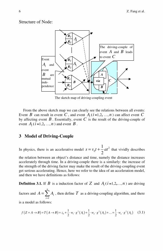
Structure of Node:
From the above sketch map we can clearly see the relations between all events:
Event B can result in event C , and event iA ( i =1,2, …, n ) can affect event C by affecting event B . Essentially, event C is the result of the driving-couple of event iA ( i =1,2, …, n ) and event B .
3 Model of Driving-Couple
In physics, there is an accelerative model 20
1
2s v t at= + that vividly describes
the relation between an object’s distance and time, namely the distance increases accelerately through time. In a driving-couple there is a similarly: the increase of the strength of the driving factor may make the result of the driving-coupling event get serious accelerating. Hence, here we refer to the idea of an acceleration model, and then we have definitions as follows:
Definition 3.1. If B is a induction factor of Z and iA ( i =1,2,…, n ) are driving
factors and 1
n
ii
A A=
=∑ , then define T as a driving-coupling algorithm, and there
is a model as follows:
( ) ( ) ( ) ( ) ( )2 2 20 1 1 2 2
1 1 1
2 2 2 n nf Z A B T A B z w g A w g A w g A= → = → = + ⋅ ⋅ + ⋅ ⋅ +…+ ⋅ ⋅
(3.1)
R1
R2
C
A
B
via
R1
R2 1A
R1
R2
B
Event
iA and
event
B are mutual inde-pendence
The driving-couple of
event A and B leads
to event C
The sketch map of driving-coupling event
R1
R2nA
......

The Design of the Driving-Coupling Algorithm in Unconventional Incidents 7
Formula (3.1) is the model of a driving-couple, where 0z represents the result
without driving factors and ( )f Z A B= → represents the result of the driv-
ing-coupling event Z , ( )ig A the strength of driving factors iA ( i =1,2,…, n ).
For example, if event 1A represents wind, then ( )1g A can represent the average
speed of wind. The symbols iw represent the accelerate coefficient of driv-
ing-couple of driving factors iA ( i =1,2,…, n ). Thus, iw stand for a key data to
measuring the relation between the driving-coupling event Z and driving factors
iA ( i = 1, 2, …, n ).
Especially when 1n = , there is only one driving factor A , and we get a simple model as follows:
( ) ( ) ( )20
1
2f Z A B T A B z w g A= → = → = + ⋅ ⋅ (3.2)
Theorem 3.1. When the strength of driving factors
( ) 0ig A = , ( )f Z A B= → = 0z .
Theorem 3.2. In the simple model (3.2), the historical data of the strength of driving factor A and driving-coupling event Z are recorded as
( )1 1,A Z , ( )2 2,A Z ,…, ( ),N NA Z , and then the result without driving factors
0z , and the accelerate coefficient of driving-couple of A can be obtained from the
following formula:
( )( ) ( )( )
( )4 2 2
0 24 2
Z A A A Zz
N A A
−=
−
∑ ∑ ∑ ∑∑ ∑
(3.3)
( )( )
( )2 2
24 2
2 N A Z A Zw
N A A
⎡ ⎤−⎣ ⎦=−
∑ ∑ ∑∑ ∑
(3.4)
We prove this theorem as follows: Suppose that the equation of the Least-squares parabola approaching a series of
points ( )1 1,A Z , ( )2 2,A Z , …, ( ),N NA Z is:
20
1
2Z z w A= + ⋅ ⋅ (3.5)
Then the Residual sum of squares can be represented as:
8 Z. Fang et al.
22 2
01 1
1SSE=
2
N N
i i ii i
D Z z w A= =
⎛ ⎞= − − ⋅ ⋅⎜ ⎟⎝ ⎠
∑ ∑ (3.6)
In order to let the SSE be the minimum the Partial derivative of 0z , w should
be 0:
20
2 20
12 0
2
10
2
i i
i i i
Z z w A
Z z w A A
⎧ ⎛ ⎞− − − ⋅ ⋅ =⎜ ⎟⎪⎪ ⎝ ⎠⎨
⎛ ⎞⎪− − − ⋅ =⎜ ⎟⎪ ⎝ ⎠⎩
∑
∑ (3.7)
Equations (3.7) can be simplified to:
20
2 2 40
1
21
2
Z z N w A
A Z z A w A
⎧ = + ⋅ ⋅⎪⎪⎨⎪ = + ⋅ ⋅⎪⎩
∑ ∑
∑ ∑ ∑ (3.8)
By solving equations (3.8), we can obtain 0z and w :
( )( ) ( )( )( )
4 2 2
0 24 2
Z A A A Zz
N A A
−=
−
∑ ∑ ∑ ∑∑ ∑
( )( )
( )2 2
24 2
2 N A Z A Zw
N A A
⎡ ⎤−⎣ ⎦=−
∑ ∑ ∑∑ ∑
Namely, they are formula (3.3) and (3.4).
Notation: In formula (3.3), (3.4) and (3.8) we use simplified marks Z∑ ,
2A Z∑ , etc. to represent 1
NZ∑ , 2
1
NA Z∑ , etc. respectively.
4 Implementation and Results
Since 1950, the quantity of China's average annual forest fires is 13,067, the af-fected forest area is 653,019 hectares, and tolls are 580 casualties. Forest fires in the country are a natural disaster of strong suddenness and great destruction, and they are difficult to dispose of. They occur mainly due to man-made causes, though
The Design of the Driving-Coupling Algorithm in Unconventional Incidents 9
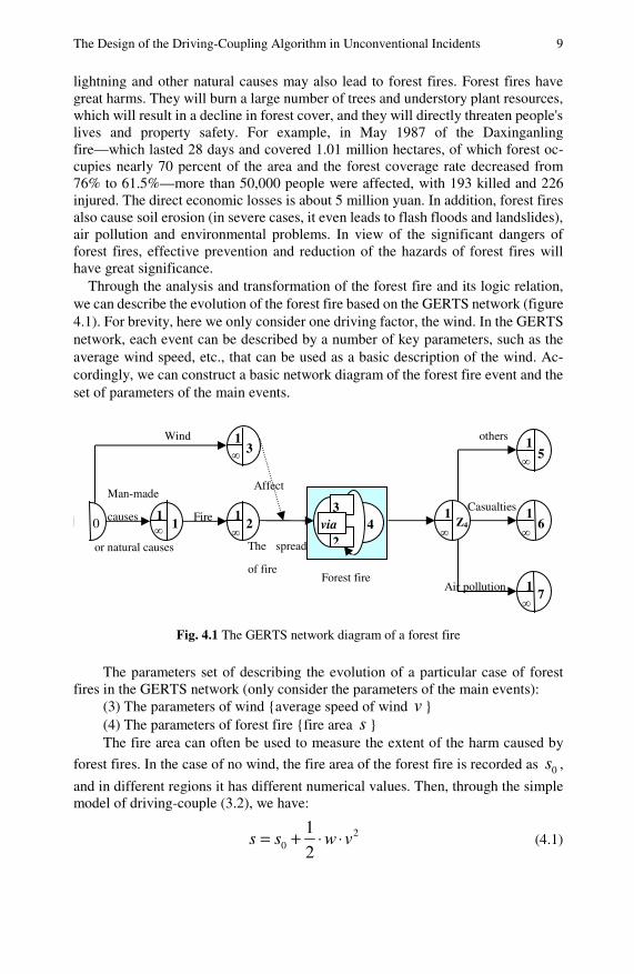
lightning and other natural causes may also lead to forest fires. Forest fires have great harms. They will burn a large number of trees and understory plant resources, which will result in a decline in forest cover, and they will directly threaten people's lives and property safety. For example, in May 1987 of the Daxinganling fire—which lasted 28 days and covered 1.01 million hectares, of which forest oc-cupies nearly 70 percent of the area and the forest coverage rate decreased from 76% to 61.5%—more than 50,000 people were affected, with 193 killed and 226 injured. The direct economic losses is about 5 million yuan. In addition, forest fires also cause soil erosion (in severe cases, it even leads to flash floods and landslides), air pollution and environmental problems. In view of the significant dangers of forest fires, effective prevention and reduction of the hazards of forest fires will have great significance. Through the analysis and transformation of the forest fire and its logic relation, we can describe the evolution of the forest fire based on the GERTS network (figure 4.1). For brevity, here we only consider one driving factor, the wind. In the GERTS network, each event can be described by a number of key parameters, such as the average wind speed, etc., that can be used as a basic description of the wind. Ac-cordingly, we can construct a basic network diagram of the forest fire event and the set of parameters of the main events.
Fig. 4.1 The GERTS network diagram of a forest fire
The parameters set of describing the evolution of a particular case of forest fires in the GERTS network (only consider the parameters of the main events):
(3) The parameters of wind {average speed of wind v } (4) The parameters of forest fire {fire area s } The fire area can often be used to measure the extent of the harm caused by
forest fires. In the case of no wind, the fire area of the forest fire is recorded as 0s ,
and in different regions it has different numerical values. Then, through the simple model of driving-couple (3.2), we have:
20
1
2s s w v= + ⋅ ⋅ (4.1)
1 1 Wind others
3
2via0
∞
1 ∞
1 ∞
∞
1 ∞
1
1 ∞
1 2
3
4 Z4
5
6
7
Man-made
causes
or natural causes
Fire
Affect
The spread
of fireForest fire
Casualties
Air pollution ∞
10 Z. Fang et al.
In formula (4.1), s represents the fire area of the forest fire in the case of wind,
0s represents the fire area of the forest fire in the case of no wind, and w repre-
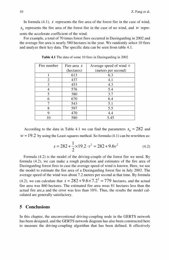
sents the accelerate coefficient of the wind. For example, a total of 70 times forest fires occurred in Daxinganling in 2002 and the average fire area is nearly 580 hectares in the year. We randomly select 10 fires and analyze their key data. The specific data can be seen from table 4.1.
Table 4.1 The data of some 10 fires in Daxinganling in 2002
Fire number Fire area s (hectares)
Average speed of wind v (meters per second)
1 613 6.3 2 437 4.1 3 453 4.3 4 576 5.4 5 380 3.7 6 670 6.4 7 543 5.1 8 597 5.5 9 470 4.4
10 580 5.45
According to the data in Table 4.1 we can find the parameters 0 282s ≈ and
19.2w ≈ by using the Least-squares method. So formula (4.1) can be rewritten as:
2 21282 19.2 282 9.6
2s v v= + × ⋅ = + (4.2)
Formula (4.2) is the model of the driving-couple of the forest fire we need. By formula (4.2), we can make a rough prediction and estimates of the fire area of Daxinganling forest fires in case the average speed of wind is known. Here, we use the model to estimate the fire area of a Daxinganling forest fire in July 2003. The average speed of the wind was about 7.2 meters per second at that time. By formula
(4.2), we can calculate that 2282 9.6 7.2 779s = + × = hectares, and the actual fire area was 860 hectares. The estimated fire area weas 81 hectares less than the actual fire are,a and the error was less than 10%. Thus, the results the model cal-culated are generally satisfactory.
5 Conclusions
In this chapter, the unconventional driving-coupling node in the GERTS network has been designed, and the GERTS network diagram has also been constructed here to measure the driving-coupling algorithm that has been defined. It effectively
The Design of the Driving-Coupling Algorithm in Unconventional Incidents 11
resolved the problem of measuring the results of driving-coupling events, and it also provided an effective mathematical tool for the scenario deduction of unconven-tional incidents. The research in this chapter will have an important practical sig-nificance in advancing the scientific of emergency management of unconventional incidents and improving the effectiveness of emergency measures. However, if we want to have a clearer understanding of the coupling rules of unconventional inci-dents, we should do more research in the future.
References
Chen, G., Li, X.P., Zhou, L.F.: Ordos basin tectonics relative to the coupling coexistence of multiple energy resources. Earth Science Frontiers 12(4) (2005)
Li, Y.Q., Li, C.Y., Huang, R.H.: SVD phase space analysis and its preliminary application to sea-air coupling relationship. Plateau Meteorology (1) (2003)
Lin, Y.: Information, prediction and structural whole: an introduction. Kybernetes: The International Journal of Cybernetics, Systems and Management Science 30(4), 350–364 (2001)
Lin, Y., OuYang, S.C.: Irregularities and Prediction of Major Disasters. Auerbach Publica-tions, an imprint of Taylor and Francis, New York (2010)
Liu, Q.Y., Fan, L.: The leading mode of the tropical ocean-atmosphere coupling. Periodical of Ocean University of China (4) (2008)
Lu, W.L., Chen, T.P.: New approach to synchronization analysis of linearly coupled ordinary differential systems. Physica D: Nonlinear Phenomena 213(2), 214–230 (2006)
Ormberg, H., Larsen, K.: Coupled analysis of floater motion and mooring dynamics for a turret-moored ship. Applied Ocean Research 20(1-2), 55–67 (1998)
OuYang, S.C., Lin, Y., Xie, N., Hao, L.P.: Prediction of suddenly appeared disasters and emergency measures. Scientific Inquiry 10(1), 17–24 (2009)
Peng, Y.J., Chen, E.Z., Zhang, N.K.: A preliminary study on the ore-forming geologic events. Jilin Geology (3) (2003)
Wang, Z.F., Qian, Y.F., Lin, H.J.: Analysis of numerical simulation on extreme precipitation in China using a coupled regional ocean-atmosphere model. Plateau Meteorology (1) (2008)
Yue, C.J., Lu, W.S., Li, Q.Q., Liang, X.D., Duan, Y.H.: The advances on the research of Zebiak-Cane ocean-atmosphere coupled model. Journal of Tropical Meteorology (6) (2004)
Zhang, X.S.: Coupling FEM and discontinuous BEM for elastostatics and fluid–structure interaction. Engineering Analysis with Boundary Elements 26(8), 719–725 (2002)
On the Priority Models of the Grey Interval Preference Relation*
Zaiwu Gong, Tianxiang Yao, Jie Cao, and Lianshui Li1
The optimal priority method of the grey interval preference relation (GIPR) is proposed. In this chapter, based on the proposed multiplicative consistent conditions of GIPR, we construct three optimal models to get the priority of the GIPR. This method can reduce the information distortion of the operations of grey intervals. It is illustrated by a numerical example to show the feasibility and effectiveness of the proposed method.
1 Introduction
In situations of multiple attribute decision making, decision makers are used to provide their subjective opinions by comparing each pair of alternatives and then constructing the judgment matrices (preference relations) (Saaty, 1980; Wang and Xu, 1990) to order a finite number of alternatives from the best to the worst. Usually, the elements in judgment matrices may take the form of crisp numbers. However, in many practical decision making problems, due to either the uncertainty of objective things or the vague nature of human beings, it is hard for DMs to give a precise judgment. In this sense, they may prefer uncertainty intervals to exact
–––––––––––––––––––––––––––
Zaiwu Gong Research Center for Meteorological Engineering & Management, Nanjing University of Information Science and Technology, Nanjing 210044 e-mail: [email protected]
Tianxiang Yao, Jie Cao, and Lianshui Li College of Economics and Management, Nanjing University of Information Science and Technology, Nanjing 210044 e-mail: [email protected]
* The work is supported by the National Natural Science Foundation of China (No.70901043,No.70873063,No.60804047), Qing Lan Project (No.0911), Humanities and Social Sciences Foundation of Ministry of Education of China, Philosophical and Social Science Foundation of Higher Education of Jiangsu Province of China under Grant (09SJB630043,09SJD630059), Foundation of Nanjing University of Information Science and Technology (SK20080114, 20070122), Research Program of Humanities and Social Sciences at Universities of Anhui Province (2008SK180). Meteorological Soft Science Foundation of China Meteorological Administration (GQR2009023).

14 Z. Gong et al.
numbers. Usually, these intervals are called grey intervals (Liu et al., 2000; Liu and Lin, 2006; Lin et al., 2004; Lin and Liu, 2006). There are many works on intervals judgment matrices. For example, Sugihara and Tanaka (Sugihara et al., 2004) propose an interval approach for obtaining interval weights of priority from the interval preference relations. In literature (Qin and Lv, 2008), the concepts and properties of weak consistency and consistency in the grey-AHP are presented. However, these papers pay no attention of the uncertainty of grey intervals operations.
In this chapter, in order to reduce the uncertainty of the grey intervals operations, we will propose three optimal models to get the priority of the grey interval preference relations.
2 The Definition of Grey Interval Preference Relation
Some basic operational laws of any two positive grey intervals (Moore, 1966; Dubois and Prade, 1978) are given below.
Let 1 1 1[ , ]M l u= , 2 2 2[ , ]M l u= , then
1 1 2 2 1 2 1 2[ , ] [ , ] [ , ];l u l u l l u u+ = + + 1 1 2 2 1 2 1 2[ , ] [ , ] [ , ];l u l u l u u l− = − −
1 1 2 2 1 2 1 2[ , ] [ , ] [ , ];l u l u l l u u=i 1 1 2 2 1 2 1 2[ , ] /[ , ] [ / , / ]l u l u l u u l= .
Any a R∈ can be denoted as [ , ]A a a= , and if 1 1[ , ] ,l u a≥ then
1 1,l a u a≥ ≥ .
For simplicity, we denote 1, ,N n= , 1, ,M m= .
If a preference relation ( )ij n nA a ×= satisfies 0.5,iia =
1,ij jia a+ = 0, ,ija i j N> ∈ , then A is called a fuzzy preference relation (FPR).
A preference relation ( )ij n nA a ×= is multiplicative consistent if there exists a
priority vector 1( , , )TnV v v= such that 1/(1 / )ij j ia v v= +
/( ), , .i i jv v v i j N= + ∈
Let 1{ , , }nX x x= be an alternative set. If a preference relation ( )ij n nR r ×=
satisfies [0.5,0.5],iir = ijl jiur r+ = 1iju jilr r+ = , then R is called a grey interval
preference relation (GIPR), where [ , ]ij ijl jiur r r= denotes the grey preference
degree range to which the alternative ix is preferred to the alternative
jx , ,i j N∈ . If [0.5,0.5],iir = then there is no difference between ix and jx ;
if [0.5,0.5],ijr > then ix is preferred to jx ; and if [0.5,0.5],ijr < then jx is
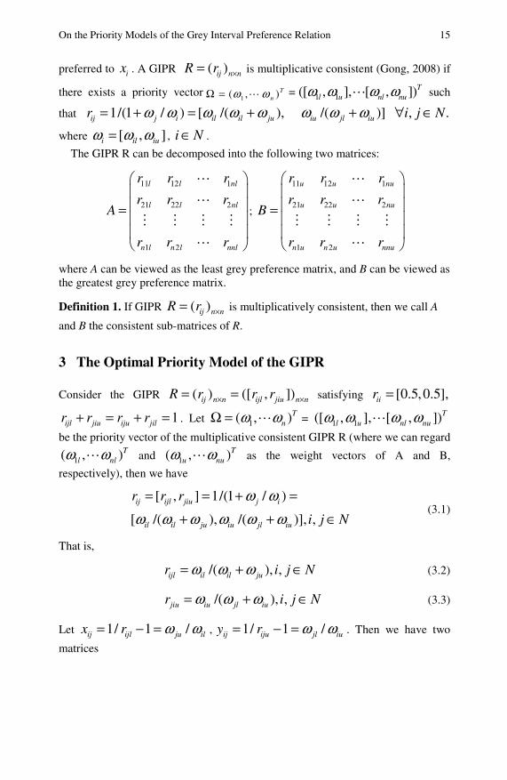
On the Priority Models of the Grey Interval Preference Relation 15
preferred to ix . A GIPR ( )ij n nR r ×= is multiplicative consistent (Gong, 2008) if
there exists a priority vector1( , )T
nω ωΩ = = 1 1([ , ], [ , ])Tl u nl nuω ω ω ω
such
that 1/(1 / ) [ /( ),ij j i il il jur ω ω ω ω ω= + = +
/( )]iu jl iuω ω ω+ , .i j N∀ ∈
where [ , ]i il iuω ω ω= , i N∈ .
The GIPR R can be decomposed into the following two matrices:
11 12 1
21 22 2
1 2
l l nl
l l nl
n l n l nnl
r r r
r r rA
r r r
⎛ ⎞⎜ ⎟⎜ ⎟=⎜ ⎟⎜ ⎟⎝ ⎠
;
11 12 1
21 22 2
1 2
u u nu
u u nu
n u n u nnu
r r r
r r rB
r r r
⎛ ⎞⎜ ⎟⎜ ⎟=⎜ ⎟⎜ ⎟⎝ ⎠
where A can be viewed as the least grey preference matrix, and B can be viewed as the greatest grey preference matrix.
Definition 1. If GIPR ( )ij n nR r ×= is multiplicatively consistent, then we call A
and B the consistent sub-matrices of R.
3 The Optimal Priority Model of the GIPR
Consider the GIPR ( ) ([ , ])ij n n ijl jiu n nR r r r× ×= = satisfying [0.5,0.5],iir =
1ijl jiu iju jilr r r r+ = + = . Let 1( , )Tnω ωΩ = = 1 1([ , ], [ , ])T
l u nl nuω ω ω ω
be the priority vector of the multiplicative consistent GIPR R (where we can regard
1( , )Tl nlω ω and 1( , )T
u nuω ω as the weight vectors of A and B,
respectively), then we have
[ , ] 1/(1 / )
[ /( ), /( )], ,ij ijl jiu j i
il il ju iu jl iu
r r r
i j N
ω ωω ω ω ω ω ω
= = + =
+ + ∈ (3.1)
That is,
/( ), ,ijl il il jur i j Nω ω ω= + ∈ (3.2)
/( ), ,jiu iu jl iur i j Nω ω ω= + ∈ (3.3)
Let 1/ 1 /ij ijl ju ilx r ω ω= − = , 1/ 1 /ij iju jl iuy r ω ω= − = . Then we have two
matrices
16 Z. Gong et al.
1 1 2 1 1
2 2 2 2 2
1
/ / /
/ / /( )
/ / /
u l u l nu l
u l u l nu lij n n
u nl nu nl nu nl
X x
ω ω ω ω ω ωω ω ω ω ω ω
ω ω ω ω ω ω
×
⎛ ⎞⎜ ⎟⎜ ⎟= =⎜ ⎟⎜ ⎟⎝ ⎠
1 1 2 1 1
2 2 2 2 2
1
/ / /
/ / /( )
/ / /
l u l u nl u
l u l u nl uij n n
l nu nl nu nl nu
Y y
ω ω ω ω ω ωω ω ω ω ω ω
ω ω ω ω ω ω
×
⎛ ⎞⎜ ⎟⎜ ⎟= =⎜ ⎟⎜ ⎟⎝ ⎠
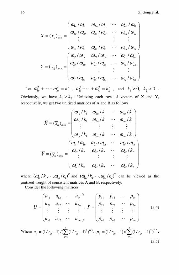
Let1
2 2 21u nu kω ω+ + = , 2 2 2
1 2l nl kω ω+ + = , and 1 0,k > 2 0k > .
Obviously, we have 1 2k k> . Unitizing each row of vectors of X and Y,
respectively, we get two unitized matrices of A and B as follows:
1 1 2 1 1
2 1 2 1 1
1 1 1 1
/ / /
/ / /( )
/ / /
u u nu
u u nuij n n
u nu nu
k k k
k k kX x
k k k
ω ω ωω ω ω
ω ω ω
×
⎛ ⎞⎜ ⎟⎜ ⎟= =⎜ ⎟⎜ ⎟⎝ ⎠
1 1 2 1 1
2 2 2 2 2
1 2 2 2
/ / /
/ / /( )
/ / /
l u l u nl u
l l nlij n n
l nl nl
k k kY y
k k k
ω ω ω ω ω ωω ω ω
ω ω ω
×
⎛ ⎞⎜ ⎟⎜ ⎟= =⎜ ⎟⎜ ⎟⎝ ⎠
where 1 1 1( / , , / )Tu nuk kω ω and 1 2 2( / , , / )T
L nLk kω ω can be viewed as the
unitized weight of consistent matrices A and B, respectively. Consider the following matrices:
11 12 1
21 22 2
1 2
n
n
n n nn
u u u
u u uU
u u u
⎛ ⎞⎜ ⎟⎜ ⎟=⎜ ⎟⎜ ⎟⎝ ⎠
,
11 12 1
21 22 2
1 2
n
n
n n nn
p p p
p p pP
p p p
⎛ ⎞⎜ ⎟⎜ ⎟=⎜ ⎟⎜ ⎟⎝ ⎠
(3.4)
Where 2 0.5
1
(1/ 1) /( (1/ 1) )n
ij ijl ijlj
u r r=
= − −∑ , 2 0.5
1
(1/ 1) /( (1/ 1) )n
ij iju ijuj
p r r=
= − −∑ .
(3.5)

On the Priority Models of the Grey Interval Preference Relation 17
As matter of fact, U and P are also the unitized matrices of A and B, respectively. The following lemma is obvious.
Lemma 1. Suppose 1( , )Tnω ωΩ = = 1 1([ , ],l uω ω [ , ])T
nl nuω ω is the
priority vector of multiplicative consistent GIPR ( ) ([ , ])ij n n ijl jiu n nR r r r× ×= = ,
and suppose 2 21
1
,n
iui
kω=
=∑ 2 22
1
n
ili
kω=
=∑ . Then ,U X= .P Y= That is,
1/ ,ij juu kω= 2/ij jlp kω= .
Obviously, we have
22
1 1
( / )n n
ij jli j
p k nω= =
=∑ ∑ (3.6)
21
1 1
( / )n n
ij jui j
u k nω= =
=∑ ∑ (3.7)
If the GIPR R is multiplicative consistent, then 22
1 1
( / )n n
ij jli j
p kω= =∑ ∑ reaches the
maximum of n, and 21
1 1
( / )n n
ij jui j
u kω= =∑ ∑ reaches the maximum of n. That is, if R is
multiplicative consistent, then we have
22
1 1
max ( / )n n
ij jli j
p k nω= =
=∑ ∑ (3.8)
21
1 1
max ( / )n n
ij jui j
u k nω= =
=∑ ∑ (3.9)
However, in reality, the multiplicative consistent condition of R may hardly
hold. This denotes that ,U X≠ P Y≠ and eqs. (3.8) and (3.9) may not hold.
Let 1 2( , , , ),i nX x x x= 1 2( , , , )i nY y y y= satisfying 1
2
1
1n
i
x=
=∑ ,
1
2
1
1n
i
y=
=∑ denote the unitized weight row vectors of inconsistent matrices A and B,

18 Z. Gong et al.
respectively. In order to get the priority vector of the inconsistent GIPR R, we introduce three nonlinear optimal models as follows:
Model (1)
2
1 1
2
1
max ( ) ( )
. . 1
n nT T
j iji j
n
jj
f X x u XU UX
s t x
= =
=
⎧ = =⎪⎪⎨⎪ =⎪⎩
∑ ∑
∑ (3.10)
Model (2)
2
1 1
2
1
max ( ) ( )
. . 1
n nT T
j iji j
n
jj
f Y y p YP PY
s t y
= =
=
⎧ = =⎪⎪⎨⎪ =⎪⎩
∑ ∑
∑ (3.11)
Model (3)
1 2
2 1
1 2 2 1
min
,. .
0i i
k k
y k x k i Ns t
k kδ δ
+≤ ∈⎧
⎨ < < < ≤⎩
The solutions to Model (1) and Model (2) are the optimal weight vectors of
inconsistent matrices A and B. In Model (3), the meaning of minimizing 1 2k k+ is
to make each weight interval [ , ]il iuω ω as narrow as possible, and
2 1i iy k x k≤ denotes that iu il i Nω ω≥ ∀ ∈ . 1δ and 2δ ,
satisfying 1 2 2 10 k kδ δ< < < ≤ , can be interpreted as two adjustment factors,
which ensure 2 0k > and 2 1k k< . Usually, we set 1 1δ < and 2 1δ = .
Theorem 1. Given the unitized matrix of U with the maximum eigenvalue maxλ ,
the maximum value of 2
1 1
( ) ( )n n
T Tj ij
i j
f X x u XU UX= =
= =∑ ∑ is maxλ , and the
optimal solution vector to Model (1) is the unique positive eigenvector of TU U corresponding to maxλ .

On the Priority Models of the Grey Interval Preference Relation 19
Theorem 2. Given the unitized matrix of P with the maximum eigenvalue maxγ ,
the maximum value of 2
1 1
( ) ( )n n
T Tj ij
i j
f Y y p YP PY= =
= =∑ ∑ is maxγ , and the
optimal solution vector to Model (2) is the unique positive eigenvector of TP P corresponding to maxγ .
4 The Decision Making Algorithms of the GIPR
Step 1. Decompose the GIPR R into sub-matrices A and B. Step 2. Construct the unitized matrices U and P by using the equ. (3.4). Step 3. Solve Model (1-3), getting the optimal priority vectors
1 1([ , ], [ , ])Tl u nl nuω ω ω ω of the GIPR R.
Step 4. Rank the grey intervals [ , ],il iu i Nω ω ∈ by utilizing the ranking method
of intervals (Sugihara et al., 2004). We get the priority chain of the alternatives. (For any two positive intervals [a,b] and [c,d], the degree of preference of [a,b] over [c,d] (or [a,b]>[c,d]) is defined as P([a,b]>[c,d])= {max{0,b-c}-max{0,a-d}}/ [(b-a)+(d-c)]}.
5 Numerical Examples
Example 1. Suppose that the weather bureau invites experts to evaluate the
integrated service of its 4 subdivisions, so 1 2 3 4{ , , , }S s s s s= . The GIPR is
constructed as follows:
[0.5,0.5] [0.2,0.4] [0.3,0.4] [0.6,0.9]
[0.6,0.8] [0.5,0.5] [0.6,0.7] [0.7,0.8]
[0.6,0.7] [0.3,0.4] [0.5,0.5] [0.7,0.7]
[0.1,0.4] [0.2,0.3] [0.3,0.3] [0.5,0.5]
⎛ ⎞⎜ ⎟⎜ ⎟⎜ ⎟⎜ ⎟⎝ ⎠
Step 1: Decompose R into the following matrices:
0.5 0.2 0.3 0.6
0.6 0.5 0.6 0.7
0.6 0.3 0.5 0.7
0.1 0.2 0.3 0.5
A
⎛ ⎞⎜ ⎟⎜ ⎟=⎜ ⎟⎜ ⎟⎝ ⎠
0.5 0.4 0.4 0.9
0.8 0.5 0.7 0.8
0.7 0.4 0.5 0.7
0.4 0.3 0.3 0.5
B
⎛ ⎞⎜ ⎟⎜ ⎟=⎜ ⎟⎜ ⎟⎝ ⎠
Step 2: Unitize A and B, respectively. We get the unitized matrices U and V as follows:
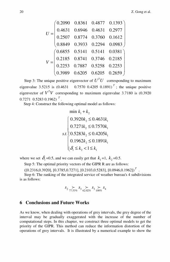
20 Z. Gong et al.
0.2090 0.8361 0.4877 0.1393
0.4631 0.6946 0.4631 0.2977
0.2507 0.8774 0.3760 0.1612
0.8849 0.3933 0.2294 0.0983
U
⎛ ⎞⎜ ⎟⎜ ⎟=⎜ ⎟⎜ ⎟⎝ ⎠0.6855 0.5141 0.5141 0.0381
0.2185 0.8741 0.3746 0.2185
0.2253 0.7887 0.5258 0.2253
0.3989 0.6205 0.6205 0.2659
V
⎛ ⎞⎜ ⎟⎜ ⎟=⎜ ⎟⎜ ⎟⎝ ⎠
Step 3: The unique positive eigenvector of TU U corresponding to maximum
eigenvalue 3.5215 is (0.4631 0.7570 0.4205 0.1891) T ; the unique positive
eigenvector of TV V corresponding to maximum eigenvalue 3.7180 is (0.3920
0.7271 0.5283 0.1962) T . Step 4: Construct the following optimal model as follows:
1 2
2 1
2 1
2 1
2 1
1 2 1
min
0.3920 0.4631
0.7271 0.7570
. . 0.5283 0.4205
0.1962 0.1891
1
k k
k k
k k
s t k k
k k
k kδ
+≤⎧
⎪ ≤⎪⎪ ≤⎨⎪ ≤⎪⎪ ≤ < ≤⎩
where we set 1δ =0.5, and we can easily get that 1k =1, 2k =0.5.
Step 5: The optimal priority vectors of the GIPR R are as follows:
([0.2316,0.3920], [0.3785,0.7271], [0.2103,0.5283], [0.0946,0.1962]) T . Step 6: The ranking of the integrated service of weather bureau's 4 subdivisions
is as follows:
2 3 3 477.53% 62.02% 100%s s s s
6 Conclusions and Future Works
As we know, when dealing with operations of grey intervals, the grey degree of the interval may be gradually exaggerated with the increase of the number of computational steps. In this chapter, we construct three optimal models to get the priority of the GIPR. This method can reduce the information distortion of the operations of grey intervals. It is illustrated by a numerical example to show the
On the Priority Models of the Grey Interval Preference Relation 21
feasibility and effectiveness of the proposed methods. In this chapter, we only consider the GIPR with one decision maker, so we will focus on the priority research on the collective GIPRs will in future research.
References
Dubois, D., Prade, H.: Operations on fuzzy numbers. International Journal Systems Science 6, 613–626 (1978)
Gong, Z.W.: Least square method to priority of the fuzzy preference relation with incomplete information. International Journal of Approximate Reasoning 47, 258–264 (2008)
Gong, Z.W., Liu, S.F.: Research on consistency and priority of interval number complementary judgment matrix. Chinese Journal of Management Science 14, 64–68 (2006)
Horn, R.A., Johnson, C.R.: Matrix Analysis. Cambridge University Press, New York (1985) Lin, Y., Chen, M.-Y., Liu, S.-F.: Theory of grey systems: capturing uncertainties of grey
information. Kybernetes: The International Journal of Systems and Cybernetics 33(2), 196–218 (2004)
Lin, Y., Liu, S.F.: Solving Problems with incomplete information: a grey systems approach. In: Advances in Imaging and Electron Physics, vol. 141, pp. 77–174. Elsevier, Oxford (2006)
Liu, S.F., Lin, Y.: Grey Information: Theory and Practical Applications. Springer, London (2006)
Liu, S.F., Guo, T.B., Dang, Y.G.: The Grey System Theory and Applications. Science Press, Beijing (2000)
Moore, R.E.: Interval Analysis. Prentice-Hall, Enblewood Cliffs (1966) Qin, J.Y., Lv, Y.J.: The concepts and the nature of weak consistency, consistency in the
gray-AHP. Systems Engineering Theory & Practice 28, 159–165 (2008) Saaty, T.L.: The Analytic Hierarchy Process. McGraw-Hill, New York (1980) Sugihara, K., Ishii, H., Tanaka, H.: Interval priorities in AHP by interval regression analysis.
European Journal of Operational Research 158, 745–754 (2004) Wang, L.F., Xu, S.B.: The Introduction to Analytic Hierarchy Process. China Renmin
University Press, Beijing (1990)

The Nation-State a Systemic View
Hans Kuijper1
The chapter pleads for a new approach in studying nation-states. Having defined the composite and complex notion of ‘nation-state’, the author groups the main nation-state theories into two categories, and claims that systems science goes far beyond the current attempts to bridge the gap between agency theorists and structuralists.
1 ‘Nation-State’ Defined
A STATE distinguishes itself from other forms of human association, a golf or football club, say. It is a human community with territory and sovereignty. Let us be more specific about these distinctive elements.
A state without territory doesn’t exist really. ‘Territory’ implies borders and/or frontiers, depending on whether the lines of demarcation are drawn by nature or man, grounded in some physical discontinuity/qualitative heterogeneity or not (in the first place). The territory is a state’s cadre de compétence. Differently put, land lying beyond, or outside, a state’s scope of competence does not belong to its territory. Territoriality is a powerful principle. It defines state membership in a way that may not correspond with identity. The borders/frontiers of a state may not at all circumscribe a people, and may in fact encompass several peoples, as national self-determination and irredentist movements make evident. Being member of a family, fraternity/sorority, wandering tribe or religion is disassociated with a particular piece of land or geographic area (country), but being member of a state is not. State membership is defined territorially.
Sovereignty, the other essential element of a state, is a matter of authority. That is to say, the holder of sovereignty does not merely wield coercive power, defined as A’s ability to cause B to do what he would otherwise not do. Authority is rather ‘the right to command and, correlatively, the right to be obeyed’. Sovereignty, however, is not a matter of mere authority; it is a matter of supreme authority within a territory. The state demands, and usually gets, our highest loyalty. It does not only accompany us to the grave; it can put us there. The rules of the state are laws which, in principle, override all other commitments and allegiances, including the voice of our conscience. There are three dimensions to sovereignty: the holder of it, the Hans Kuijper Joliotplaats 5, 3069 JJ Rotterdam, The Netherlands e-mail: [email protected]
24 H. Kuijper
absolute or non-absolute nature of it, and the relationship between internal and external sovereignty.
A) The character of the holder of supreme authority within a territory is probably the most important dimension. Jean Bodin (1529-1596) thought that sovereignty must reside in a single individual. Both he and Thomas Hobbes (1588-1679), following Niccolò Machiavelli (1469-1527), the ‘Florentine secretary’ whose masterpiece, The Prince (1513) ushered in a new era of political thinking, conceived the sovereign as being above the law. Later thinkers differed, coming to envision a new locus for sovereignty, but remaining committed to the principle. The starting-point of the political philosophy of John Locke (1632-1704) is that by nature human beings are equal and therefore nothing can put anyone under the authority of anybody else except his own consent. He argued that a king had responsibilities to his subjects, and revolt was justified when he failed to protect their rights. Jean-Jacques Rousseau (1712-1778), one of the most profound and complex political thinkers in the West, distinguished between the people as sovereign and the government as agent of the volonté générale.
B) Sovereignty can also be absolute or non-absolute. Here, ‘absolute’ refers not to the extent or character of sovereignty, which must always be supreme, but to the range of matters over which the holder of authority is sovereign. Bodin and Hobbes considered sovereignty as absolute, extending to all matters within a territory, unconditionally. However, it is possible to be sovereign over some matters only. Take the European Union member states; they are sovereign in governing defense, but not in governing the euro.
C) The third dimension of sovereignty concerns different aspect of it. Supreme authority is exercised within borders/frontiers, but a state derives its sovereignty also from being recognized by outsiders. To states, this recognition is what a no-trespassing law is to private property: immunity from interference.
Sovereignty has met with critics. Many of them have regarded any claim to sovereign status as a form of idolatry, sometimes as a carapace behind which cruelties and injustices are carried out free from legitimate outside scrutiny, let alone intervention. Perhaps the two most prominent attacks on sovereignty launched by political philosophers came from Jacques Maritain (1882-1973) and Bertrand de Jouvenel (1903-1987). The set of internally and externally sovereign states is the international system that we euphemistically call the ‘United Nations’, the word ‘nations’ being used (a) to prevent confusion with the ‘United States’ (of America) and (b) to emphasize the fact that each of the UN member states geographically coincides with a nation – with a culturally and/or ethnically dominant people, that is.
Enthusiasts for globalization apparently believe that the nation-state is fading away, but ‘the process whereby the world population is increasingly bonded into a single society’ is not neutral; it doesn’t just happen. The creation of a ‘flat’ world, of a global society in which people of all nations and colors are singing of ‘perfect harmony’ (Coca-Cola) is the project of a hegemonic nation-state, not the undirected, necessary outcome of human actions and interactions. Globalization is to a large extent imposed; it is driven by capitalism, which is not simply a matter of economics separate from politics. “Globalization is best understood as a spatial phenomenon,

The Nation-State a Systemic View 25
lying on a continuum with ‘the local’ at one end and ‘the global’ at the other,” David Held says, but he forgets to tell how, in a world divided into some 200 contending countries, we will end up with a single polity (politically organized society), a ‘borderless world’. Nation-states matter; they are here to stay, the activities of transnational corporations, and of international bodies such as the United Nations, Interpol, the International Court of Justice, the World Trade Organization, the International Monetary Fund and the World Bank Group, notwithstanding. Playing down the importance of nationalism in pursuit of cosmopolitanism, as Martin Köhler, Daniele Archibugi, Kwame Appiah and Ulrich Beck do, exclusively focusing attention on the ‘global network society’, as Immanuel Wallerstein, Manuel Castells, Barry Wellman and John Urry do, or advocating a world government system, as Terence Amerasinghe, Richard Falk, Joseph Schwartzberg and Stephen Damours do, makes a dangerous illusion manifest.
2 Theories of the Nation-State
The notion of ‘nation-state’ emerged in England during the Glorious Revolution (1688), was strongly articulated during the American Revolution (1776) and the French Revolution (1789), and has arguably been the axis of political reflection ever since. It has been elaborated on and restated in various ways. Indeed, it is the warp and woof of social-political thinking. The majority of the nation-state theories can conveniently be grouped into two categories: the individualistic and the collectivistic category.
The individualistic view The adherents of this view are committed to explaining a nation-state/country in terms of individuals, considering statements about collectives like ‘the American people’, ‘the employers’, ‘the voters’ and ‘readership’ as shorthand ways of referring to individuals who share certain characteristics. References to groups, or to group behavior, which suggest that these are entities other than individuals having needs, wants, interests and goals are regarded as holistic fallacies. Individualists do not deny that a politically organized society exists, or that people benefit from living in it, but they see a polity as a set of individuals, not as something over and above them. They hold that every person is an end in himself or herself, and that the individual is the unit of achievement. His genius is the wellspring of invention or discovery. While not denying that one person can build on the achievements, or stand on the shoulders, of others, they point out that achievement goes beyond what has already been done; it is something new, created by the individual.
Individualism involves a value system, a theory of human nature, and a general attitude:
1) Its value system may be described in terms of three propositions: (a) the individual is of supreme value, society being a means to his/her ends, (b) all values are man-centered – that is, they are experienced by human beings, and (c) all

26 H. Kuijper
individuals are morally equal, meaning, no one should ever be treated as a means to the well-being of another person.
2) Its theory of human nature holds that the interests of the adult are best served by allowing him/her maximum freedom for choosing objectives and the means for obtaining them. This belief is based upon two assumptions: (a) each person is the best judge of his/her own interests and, granted educational opportunities, can discover how to advance them, and (b) the act of pursuing the chosen objectives contributes to the welfare of the society.
3) As general attitude, individualism subscribes to self-reliance, privacy and the right of the individual to be different from, to compete with and to get ahead of others. Negatively, individualists are opponents of control and interference, particularly when exercised by the government.
Individualism is close to the heart of liberalism, the way of thinking (conserved by the conservatives and radicalized by the radicals) which holds that freedom is everybody’s natural condition, and that institutions are to be judged by their success in facilitating it. Individualism, the view that every person is sovereign and has a frontier, is deeply ingrained in the Western tradition. So much so, that it is thought not to be a common characteristic of humanity, indeed almost an eccentricity among cultures. Though the development of individualism/liberalism can be traced back to the Hebrew prophets, the teachings of the pre-Socratic philosophers and the Sermon on the Mount, from all of which there emerged a sense of liberation of the individual from subservience to the (leader of the) group, its prestige rose during the latter part of the eighteenth century, especially after the publication of the ideas of Adam Smith (1723-1790) and Jeremy Bentham (1748-1832). Twentieth century champions of individualism are (amongst many): James Buchanan, Robert Dahl, Ralf Dahrendorf, Hernando de Soto, Milton Friedman, Friedrich Hayek, Robert Nozick, Karl Popper, Ayn Rand, John Rawls, Amartya Sen, and Ludwig von Mises.
The collectivistic view The adherents of this view regard a polity, ultimate standard of value, as something over and above its members. They do not deny the reality of the individual, but hold that one’s identity is essentially made up of relationships and achievement is the product of a group of people sharing values, interests and goals. The individual, who is expected, even required to sacrifice himself or herself for the alleged good of the group, is just a replaceable cog in the machine, an exchangeable piece of equipment. Read Tolstoy’s retrospective final chapter of War and Peace and see how he comes to the conclusion that the trends initiated in Europe by the French Revolution would have worked themselves through with or without Napoleon.
Collectivism, which reflects the human instinct to belong to a herd, is close to the heart of socialism, the way of thinking (grown up in opposition to capitalism) which holds that human activities be described in terms of personal, social, economic and/or political relations rather than in terms of individual actions. In the early nineteenth century, when modern socialism made its first appearance (Saint-Simon, Fourier, Owen a.o.), Georg Wilhelm Friedrich Hegel (1770-1831), inspired by the work of Rousseau, argued that the individual realizes his/her true being and freedom only in unqualified submission to the laws and institutions of the
The Nation-State a Systemic View 27
nation-state. Karl Marx later provided the most succinct statement of the collectivist view by positing, in the preface to his Contributions to the Critique of Political Economy (1859), the primacy of Produktionsverhältnisse (relations of production). Twentieth century champions of the basic tenets of collectivism are (amongst many): Stephen Bronner, Cornelius Castoriadis, Jürgen Habermas, David Harvey, Robert Heilbronner, Eric Hobsbawm, Alexandre Kojève, Ernesto Laclau, Ernest Mandel, Ralph Miliband, Nicos Poulantzas, and Paul Sweezy.
Individualism/liberalism versus collectivism/socialism – the views seem to be irreconcilable. Individualism is found wanting for making no room for society’s peculiar properties, collectivism for losing sight of man’s uniqueness. The former is blind to social values, the latter is devoid of respect for the person. Each avoids the other’s error by making an opposite mistake of its own. Individualism (politically, economically or sociologically oriented) is inadequate because individuals are interrelated; collectivism (politically, economically or sociologically oriented) is deficient because there are no relations without relata (‘things’ related). The one underrates the bonds among people, the other plays down individual actions. Individualists tend to overlook the emergence of things with properties that their parts don’t have; collectivists are inclined to overlook man’s creativity.
Whereas Émile Durkheim (1858-1917), working in the positivist tradition and tending to reification, maintained that the collective possesses a life of its own, external to and coercing its members, Max Weber (1864-1920), working in the anti-positivist tradition and inclined to voluntarism, contended that society is the result of the intentional and meaningful behavior of human beings. After World War II, the ‘existentialists’ (Jean-Paul Sartre, Maurice Merleau-Ponty, Karl Jaspers, Martin Heidegger, Martin Buber, Gabriel Marcel, Emmanuel Levinas a.o.) were challenged by the ‘structuralists’ (Claude lévi-Strauss, Edmund Leach, Louis Althusser, Marshall Sahlins, Georges Dumézil, Gilles Deleuze, Tzvetan Todorov a.o.). The former emphasized the idea that man is a being ‘for-itself’ (as against the being ‘in-itself’ of mere things), and the related idea that what the individual becomes can only be explained by the choices he/she makes in resolving the ‘issue’ of his or her life. The latter considered the identification and analysis of underlying, the individual transcending structures to be of paramount importance. In 1966, when somebody had the nerve to write on the Berlin Wall ‘Man denkt zu schieben aber man wird geschoben’, Michel Foucault thought he could certainly wager that ‘man would be erased, like a face drawn in sand at the edge of the sea’.
Various attempts have been made to bridge the gap between the agency theorists (‘agency’ referring to the capacity of individuals to act independently) and the structuralists, Anthony Giddens, Pierre Bourdieu, Roy Bhaskar, Margaret Archer, and Nicos Mouzelis being the most prominent, ingenious bridge builders. Interesting though their theories are, we venture to say that systemics, or ‘systems science’, goes far beyond them.
3 The Systemic View
Before we go into the matter of viewing a nation-state/country systemically (as distinct from: systematically), it might be useful to pay some attention to the concept of ‘system’.

28 H. Kuijper
A system is a special type of set (Menge). A set is a well-defined collection, or a grouping into a single entity, of objects. These objects are called the ‘elements’ or ‘members’ of the set. The rivers in China, the people living on the earth, the students who are absent from school, the vowels of the alphabet, the solutions of the equation x² - 3x – 2 = 0, and the numbers 2, 4, 6, 8, … are examples of a set. Set theory, the branch of mathematics that deals with properties of, operations on and relations between sets, aims at a description of the fundamental structure of the mathematical universe. It is a vibrant field of research, with many interrelated subfields. The elements (or parts) of a system are organized, making the system an integrated whole, an object whose parts are held together by bonds of some kind. A system is a set of things and their relations, or in George Klir’s formula: S = (T, R). There are numerous kinds of systems that can be studied, qualitatively or quantitatively: physical, geological, mechanical, biological, ecological, social, political, military, medical, educational, legal, economic, financial, managerial, technological, religious, artistic, linguistic, cultural, perceptual and conceptual systems. An atom, the Milky Way, the human brain (containing up to 100 billion interconnected neurons [systems!]), a city and CERN’s Large Hadron Collider is a system, but a mathematical model, a computer program, a logic, a scientific discipline, a value configuration, a game, a debate and the Internet is a system too. Other distinctions can be made: there are stable and unstable systems, homo- and heterogeneous systems, animate and inanimate systems, material and immaterial systems, discrete and continuous (and hybrid) systems, causal and anticausal systems, deterministic, probabilistic and grey systems, static and dynamic systems, hard and soft systems, natural and artificial systems, linear and nonlinear systems, autopoietic and allopoietic systems, anticipatory and self-organizing systems, chaotic and solitonic systems, finite-dimensional and infinite-dimensional systems, active and reactive systems, mindless and (uni-or multi)minded systems, ‘simple’ and ‘complex’ systems. Usually, a system contains a number of subsystems. Think of a molecule, the human body, a family, an airplane, an airport, a company, an industry, an economy, a university, a library, a medical center, a government, the media, the European Union, the Olympic Games, the animal kingdom, a rainforest, the Blue Planet. So one may wonder whether all these systems have something in common.
Talking about systems, we should bear four points in mind 1) That a system consists of parts seems to be stating what is obvious, if not trivial. Yet the part-whole relation in all domains of reality and conceptualization (differently put: what it means for two or more things to fit together) is the object of a study (mereology) that has a long history (going all the way back to Thales of Miletus [fl. 6th century BC]) and a high degree of sophistication. The word ‘part’ has many meanings in ordinary language. ‘The handle is part of the mug’. ‘The cutlery is part of the tableware’. ‘The first act was the best part of the play’. ‘Sodium is one of the parts of salt’. ‘The point is part of the line, which is part of the plane, which is part of the sphere’. Broadly speaking, the word ‘part’ can be used to indicate any portion, fraction, fragment, share, piece, division, section, sector, compartment, unit, ingredient, constituent, element, member, component,
The Nation-State a Systemic View 29
percentage, particle, branch or bit of a given entity. Mereology (from the Greek meros, part) is an attempt to lay down the principles underlying the relationships between an entity and its constituent parts, whatever the nature of the entity. Unlike set theory, mereology is not committed to the existence of abstracta: the whole can be as concrete as the parts. But mereology carries no commitment to concreta either: the parts can be as abstract as the whole. In other words, mereology is topic-neutral. Areas of space and eras of time stand in part-whole relationship. Likewise, events and actions (not being the same!) may have parts and be parts. Indeed, everything has parts and, simultaneously, is part of something else, the universe and the subatomic constituents of matter (the elementary particles) probably being the exceptions.It was Stanisław Leśniewski (1886-1939), famous member of the Lvóv-Warsaw School of analytical philosophy,[1] who began to codify the formal principles of part/whole theory. For him, the minimal properties of a part/whole relation are that it is asymmetric (if a is part of b, b is not part of a), transitive (if a is part of b and b is part of c, then a is part of c), and supplemental (if a is part of b, then there is a part of b having no common part with a). Whereas Leśniewski developed the theory of the ‘part of’ relations, assuming that given an object x, its parts form a Boolean algebra (classical mereology), Lech Polkowski and Andrzej Skowron, leaving the domain of two-valued logic, and drawing on the pioneering work of Zdzisław Pawlak (1926-2006), introduced the theory of the ‘part of to a degree’ relations (rough mereology).
2) The structure, pattern, architecture, or Gestalt of a ‘system’ (from the Greek sun-histèmi, com-pose) is an entity of dependencies. It is determined by (a) the number, nature and function of its elements/subsystems (modules), (b) the number and nature of the relations among these parts, and (c) the number and nature of the relations between the system and its surroundings. ‘Relation’, a basic term or category, is difficult to define, for it seems to be impossible to make any statement of what relation is without using the notion of ‘relation’ in doing so, and without acknowledging that a relation cannot exist apart from the ‘things related’. Leaving this maddening fact for another occasion to deal with, we comfort ourselves with the following mathematical definition: a relation R from set A to set B is a subset of the product set A × B, also called the Cartesian product of A and B. Let A = {1,2,3} and B = {a, b}. Then A × B = {(1, a), (1, b), (2, a), (2, b), (3, a), (3, b)}, and R = {(1, a), (1, b), (3, a)}, a relation from A to B. The definition can be extended to more than two sets, and the relations between them can be of many sorts.As ‘structure’ is tied up with ‘system’, the focus of attention is usually on the total of a system’s constituents. However, this total is a ‘whole’ (Gr. holon), or Ganzheit, rather than merely an ‘aggregate’ (Gr. pan), or Gesamtheit. Systems are embedded entities the (sometimes ‘identical’) parts of which are organized. A pile of bricks, being an aggregate, is not the system we call ‘building’. By the same token, a succession of sounds is not necessarily a melody. A system, typically, is different from the sum of its parts; it has properties none of its constituents has, much in the same way as the nature of water is irreducible to the attributes of hydrogen and oxygen. Those being in favor of analysis (dividing things up into ever smaller parts for research) should not overlook the subtle difference between Gesamtheit and Ganzheit. The breaking down (either physically or mentally) of any system, micro or macro, into elements
30 H. Kuijper
should not result in losing sight of its supersummative properties and the conditions under which the subsystems operate within the supersystem. It cannot be overstressed: composition is more than, and critically different from, juxtaposition. A good physician and a commander-in-chief are acutely aware of this. If and only if they are organized, entities or modules form a whole, as every architect, chef de cuisine, composer, fashion designer, Japanese flower-arranger, even a football-coach can tell. This does not alter the fact that, for a composition to be harmonious, or for a team to be victorious, each of its elements/members needs to be given due care and attention. A chain is only as strong as its weakest link. Setting the whole (group) over against the parts (individuals), as the collectivists/socialists and individualists/liberals persistently do, is misleading, indeed risky. Tertium datur: taking both, the whole as well as the parts, into account by focusing on the system-hood (i.e. on the T and the R in Klir’s deceptively simple formula), one discovers that there is a third possibility. There is no primacy or priority to be assigned, because individuals and the group they belong to are mutually implicated, recursively related. The two may be distinguished, but shall never be separated, from each other. A group of individuals is not like a bunch of pencils, nor is the nation-state an aggregate; they are structured, integrated wholes, even if there are internal states of conflict.
3) Everything seems to have a boundary. It makes identification possible. Without boundaries we can neither differentiate nor decide; chaos would prevail. There is a line demarcating the interior of a circle from its exterior. A soccer game begins and ends when the referee blows his whistle. However, the boundary subject is a highly problematic issue.[2] Anaximander, Thales’s disciple and successor, contrasted the ‘cosmos’ (ordered world) with the ‘boundless’(apeiron), the indefinite and imperceptible from which all distinguishable things come and to which they return ‘in accordance with the ordinance of time’. One of the persistent questions concerning infinity (∞) is whether we can know or comprehend it. Another is whether the infinite exists, and if so, to what kind of thing it belongs (to space, time, number?). Limit processes are used throughout analysis, the part (!) of mathematics that studies numbers, or points, and functions (mappings). The conception of these processes is based on the idea of closeness. Augustin-Louis Cauchy (1789-1857), one of the greatest of modern mathematicians, defined a limit (more than 150 years after Newton and, independently, Leibniz had discovered the infinitesimal calculus) as follows: ‘When the values successively attributed to the same variable approach indefinitely a fixed value, so as to differ from it as little as one might wish, this latter is called the limit of all the others’. So analysis makes approximations into exact quantities, as when the area inside a curved region is defined to be the limit of approximations by rectangles (Archimedes).It may also be observed that ordinary objects, events, and concepts often elude the idealized notion of ‘being sharply bounded’. What is the boundary of a cloud, mountain, ecosystem, concept or scientific discipline? Is the killing of humans always wrong? When did the Industrial Revolution begin, and where did it take place? What is the reach of somebody’s power or authority? When do we call a man ‘bald’, ‘tall’, ‘rich’, or ‘free’? Is our skin the outer envelope of an inner self? When is the beginning and when is the end of man’s life? Where is the line demarcating Europe from Asia?

The Nation-State a Systemic View 31
When does a number of rain drops (quantity) start being a shower (quality)? What are the boundaries of love, beauty, experience and creativity? How far radiates a culture or civilization? All these boundaries are unclear, hazy, vague, imprecise and indeterminate. Classical logic/hard computing breaks here down and has to be replaced by fuzzy logic/soft computing, because one of the essential features of the concept of ‘set’ as Georg Cantor (1845-1918) understood it is conspicuous by its absence, namely, given an object x and a set A, exactly one of the statements ‘x is an element of A’ (symbolized x ∈ A) and ‘x is not an element of A’ (symbolized x ∉ A) is true and the other is false.Physical systems can be ‘isolated’, ‘closed’ or ‘open’, depending on whether matter and/or energy is exchanged with the environment. A casserole being used exemplifies an open physical system; it exchanges both matter (vapour) and energy (heat). Exact calculation of open systems is not possible. One has to put up with approximations by means of models. Living systems and (often over time in complexity increasing) social systems, which continuously interact with their surroundings, are open systems too, but — distinct from physical systems. Their permeable borders allow matter, energy and information to pass, the openness being a condition for, rather than a guarantee of, their survival. Whether or not the principles of thermodynamics (entropy) also obtain in the world of living and social systems, how information is to be defined and how it relates to knowledge/insight, are intriguing questions we leave to others to answer, but there is one thing we wish to point out, just for the sake of argument: the relation between the concepts of ‘openness’ and ‘boundary/limit’ is strained.
4) An important distinction is to be made between two kinds of part-whole relation: composition and extension. The parts of a composition are its components; the identity of a component (what makes it different from the other components) is its what or who. The parts of an extended whole are its regions/periods; the identity of a region/period (what makes it different from the other regions/periods) is respectively its where and when. Spatial and temporal parts, irrespective of scale, are no more or less basic than the wholes they compose. Thinking, far from being static, is the constant, imaginary moving backwards and forwards between composition and extension, between installing and de-installing parts. Cognition, allegedly being computational in nature, is conceiving how things actually were, are or will be and, counterfactually, how they would have been or would be in this, that or the next eventuality. It is from the what, the who, the where as well as the when that the how and the why transpire. The relation between structure/form/being and process/flux/change, another subject that has haunted social scientists, is that between composition and extension. A process takes time and place; it lasts, has duration, continues for a particular length(!) of time (interval, period, or term); it is the concatenation of configurations, the sometimes mathematically tractable sequence of system states; it is a trans-formation involving transient structures, a structure change with structure. The word ‘process’ refers to the way a system works/operates/functions/behaves, to its ‘mechanism’, which is frequently coupled to other ‘mechanisms’, and can be spontaneous or engineered.The subject of change, the fast or slow process of becoming different (we are aware of change only when a different pattern becomes discernible), leads us to the very complicated problem of causality.[3] Dealing with this conundrum adequately would require

32 H. Kuijper
writing a book. Suffice it to say that (a), besides ‘material’ causes (‘The table is made of wood’), there are ‘efficient’ causes (‘She fell because he pushed her’, ‘The fire heated the water’), ‘formal’ causes (‘A pianist needs the score to play a concerto’, ‘The blueprint of a house is necessary for its construction’) and ‘final’ causes (‘Shoes are made to protect/embellish feet’, ‘He moved to the seaside for the sake of his health’, ‘The monument was built in commemoration of those who died in the war’), and (b), in contradistinction to the assumption of reductionist scientists, causality can be and usually is a rather convoluted phenomenon, meaning that in nature and society nonlinear systems (where the whole is not equal to the sum of its parts) are far more common than the linear ones.
4 The Systemic View of a Nation-State
A nation-state, or country, is a huge, highly complex, multi-minded/agent-based, evolving, non-equilibrium, rule following, open system. It is a Ganzheit in which things hang together, tightly or loosely, but in a way that is distinctive. A nation-state is an intricate network of interfacing networks ‘different in extensiveness and intensiveness’ (Michael Mann). Its basic units are ‘involved in a continuous interplay of complex determinations’ (Evelyne Andreewsky). Indeed, a country is a unique individuum, something indivisible, a territory-bound and history-moulded organization, a layered, hierarchically ordered, whole that, distinctly interrelated with its parts, constantly changes, sometimes turbulently. Having properties that each of its constituent subsystems lacks, and being a series of complex networks the pattern of which can be analyzed using the tools of graph theory, it is best viewed as an intersection of four fields: the geographic field, the individual-creative field, the socio-cultural field and the historic field: C = G ∩ I ∩ S ∩ H. Heuristically, the combination of these fields, each of which supposes, and maps onto, the other three (!), can be represented by a tetrahedron, the regular, Plato (and Buckminster Fuller) fascinating polyhedron with four equilateral triangular faces.[4]
The words of John Donne, ‘no man is […] entire of it self’, are also applicable to a nation-state, because, being part of a ‘globalizing’ world, it has a number of relations, vital to its development, with its natural and cultural (non-natural) surroundings. It matters a lot whether a country is located in the tropics or in the temperate zone, whether it is land-locked or sea-washed. The nature of the bilateral or multilateral relations with other countries is reflected in its changing balance of international payments, which – it tends to be forgotten – shall not be left only to economists to scrutinize. How, then, is a nation-state to be studied?
Country studies, to which some institutions of tertiary/higher education, such as School of Oriental and African Studies (SOAS) in London and German Institute of Global and Area Studies (GIGA) in Hamburg, are devoted solely, are domains of research not pertaining to a particular aspect of, but – the difference is important – to a particular region in the world.[5] Basically, students of a nation-state, irrespective of their view (individualistic or collectivistic), and other than cultural anthropologists (who study a particular people or folk), can be classified as follows:

The Nation-State a Systemic View 33
1) Students who – without a textbook containing a presentation of the principles and vocabulary of their trade, and unaware of the pitfalls of synopsis – claim to synthesize the results of all kinds of professional study regarding the country of their choice. Having no degree in any of the disciplines concerned, nor having contributed to the development of any of them, they do not shrink from rushing in where angels fear to tread. These jacks-of-all-trades (but masters of none) leave the reader/listener in the dark as to where the parts fit into the whole (the larger scheme), and, conversely, how the whole stands interconnected with the parts, reminding us of the old Chinese proverb Ben bu guan yu mo yi bu xian yu duo (the roots are not connected with the twigs; the one is not shown in the many). We are not suggesting that these all-rounders are useless. Certainly not; the (historical or contemporary!) sweep of the country they selected is a broad one, which can be refreshing, when fragmentation of science is rife and nobody seems to know how Humpty is to be put together again. What we do accuse these heroic polymaths of, however, is their refusal to be explicit about the shallowness of their knowledge. They shy away from admitting that they are muddle-headed about their assumptions, parameters and methodology. They get embarrassed if we ask them to define the theoretical structure of their research activities (their unified frame of perception and understanding), to mention their discipline’s central concept, or to spell out the principles of their trade (the study of a country), as distinct from the business of, say, political scientists, jurists, military scientists, linguists, literary scientists, and biologists.
2) Students who – having good grounding in the discipline required – attempt to deepen their understanding by exploring, e.g., the flora/fauna, population, language(s), economy, agriculture, religion, mores, education, geological features, public health, or arts of/in a particular country – that is, by applying/testing and, if necessary, adjusting the theories of their textbooks. Scientifically drilled and trained, these students have an in-depth view, which is indispensable for writing authoritatively on subjects within their purview, but — is upheld at the expense of breadth of view. Being professionals (Fach-Menschen), they have a tendency towards stove-pipe peering and cylindrical thinking. Enclosed within their universe of concepts (silo) and single-mindedly dedicated to their domain, these Cyclops easily forget that the parts of an aggregate (Gesamtheit) can, but the parts of a whole (Ganzheit) can not be understood in isolation.
This raises the important, all too often neglected, question as to whether, in terms of research and (higher) education, both the Scylla of being mile-wide-but-inch-deep and the Charybdis of being mile-deep-but-inch-wide can be avoided, whether generalization and specialization can be reconciled.
It is our conviction that a safe way between the two monsters can be navigated. That way is the systemic way. Only by zooming in and out (as in the film Powers of Ten), by paying heed, not only to the system as a whole but also to its constituent parts, by studying a country horizontally as well as vertically (and by addressing the nature of its part structures, not only in their static state but also as a function of time), the strength of group 1 and group 2 (respectively breadth and depth of view) can be obtained. There shall be no looking at the forest without seeing the trees. The two are reciprocally related. To have an eye for the supersystem only, and not for its
34 H. Kuijper
intimately connected subsystems (and, subsequently, the related parts of these parts), would be foolish. It would betray a leaning towards reification. Neither shall there be looking at the trees without seeing the forest. To cut a country mentally into morsels for single sciences to chew on, would amount to destroying a system (constitution) in order to comprehend it. No matter how many aspects of a country can be discerned, they are and will always remain different ‘aspects’ (from the Latin aspectūs, views) of the same study object. ‘Aspect’ is not an onto- but epistemological category. Reality does not abide by academic distinctions.
Being a Gefüge, a four-dimensional, tetrahedron-like system of systems (of geological, biological, demographic, ecological, political, legal, military, economic, financial, managerial, educational, technological, linguistic, social, religious, artistic or other nature), a nation-state can only be understood interdisciplinarily, through ‘comprehensive observation of changes’ (tongbian). This implies teamwork, scientific collaboration, syntegrity, for no country student can be expected to become a master of all weapons. Should he/she want to be one, he/she would be oblivious to Goethe’s famous dictum: ‘In der Beschränkung zeigt sich erst der Meister’. Exploration of the meaning, necessity and possibility of scientific collaboration, about which a heated debate is going on, and which is essentially a matter of composition rather than juxtaposition (multidisciplinarity), has to wait for another occasion, but, given the established facts that the best team (rather than the Gesamtheid of the best players) wins, and collaboration is impossible without communication, three final remarks have to be made.
1) We are on the verge of a new era of computing. E(lectronic)-science (also known as cyberinfrastructure) is making collaborative research of complex systems possible. Its key concept is ‘computational grid’. The exciting thing about this system (!) is the combination of vast quantities of digitized data (‘digital libraries’), high performance computers (running sophisticated software), and connectivity between computers supported by high-tech telecommunications (Internet technology), all three of which are expanding rapidly. Grid computing will be the new paradigm, allowing users who are distributed throughout the world to share computational resources across the intergradational boundaries between disciplines.
2) Those involved in country studies have a lot to learn from (intelligent) ‘service science’, a burgeoning branch of knowledge comparable with computer science. The success of the latter is first and foremost in its ability to bring together disciplines in order to solve problems. Service science is, potentially, an interdisciplinary umbrella too. Intimately connected to grid computing, it aims at understanding and innovating service systems, which usually are complex systems – that is to say, systems the parts of which interact nonlinearly. Given the growing importance of service systems, their great diversity, and the extensive range of disciplinary knowledge needed to understand them, effective teamwork is considered necessary. Presently, there are over 130 institutes in the world that are conducting service science programs, and there are worked-out plans to create a ‘Service Systems Lab Network’ in order to connect the laboratories supporting these programs, and to foster collaboration. Since nobody can hope to become an expert on every subject in the fast expanding field of service science, much value is placed on T-shaped professionals: scientists with profound knowledge in one
The Nation-State a Systemic View 35
particular area of research (discipline), proficiency in communicating with other experts and adeptness in using the tools and techniques of ‘visual analytics’– that is to say, scientists keen on interoperability and in search of isomorphic transfer (or mapping) rather than analogy.
3) The objective of Logic, Epistemology, and the Unity of Science, the Springer book series that started in 2004, and in which 18 titles have been published so far (July 2009), is to reconsider the question of the unity of science in light of recent developments in logic and theory of knowledge, and ‘to provide an integrated picture of the scientific enterprise in all its diversity’. Though no single logical, semantic or methodological framework dominates the philosophy of science, the editors of this series believe that formal techniques like independence friendly logic, dialogical logic, multimodal logic, linear logic and game theoretic semantics ‘have the potential to cast new light on basic issues in the discussion of the unity of science’ – issues also being a major concern for Diederik Aerts, Editor-in-Chief of the interdisciplinary journal, published since 1995, Foundations of Science.
Briefly then, viewing a nation-state/country systemically, or relationally, is the ability to see it as a giant, composite system that, provided the willingness to go wide and deep (collaborate), and to draw upon the theoretical, empirical and methodological advancements in complexity science, could be domesticated (apprivoisé) and, provided the harnessing of the power of grid computing, could be correctly represented by a model, which is essentially the artistic product of highlighting what is important and leaving out everything else. Taking our advice (‘Immer strebe zum Ganzen’) seriously, and vigorously implementing the systemics-based research recommendations we have made, in expectation of dogged resistance from certain quarters, may result in more intercultural understanding and better international relations, things that mankind desperately needs.
References
http://plato.stanford.edu/entries/lvov-warsaw http://plato.stanford.edu/entries/boundary http://plato.stanford.edu/entries/change http://mathworld.wolfram.com/tetrahedron http://www.asvj91.dsl.pipex.com

Critical Path for a Grey Interval Project Network
Zhongmin Song and Xizu Yan*
In systems analysis, uncertainties may exist in model parameters and input data. Those uncertainties can propagate through the analysis and generate uncertainties in systems analysis. Grey systems theory offers a method for incorporating uncertainties into systems analysis. According to grey systems theory and the characteristics of the interval plan network, this paper gives the method of the multiobjective making critical path. Examples are provided at the end to verify the feasibility of this method, which combines subjective factors with objective factors.
1 Introduction
It is well known that the network activity times are uncertain in the network schedule. Therefore, the network activity times should be seen as grey numbers (Liu and Lin, 2006; Lin et al., 2004; Lin and Liu, 2006) when making the network schedule. These grey numbers usually have been expressed by certain numbers in the methods of network schedule CPM (Critical Path Method) and PERT (Program Evaluation and Review Technique). A certain number, in fact, can only represent one of the infinite whitening values of a grey number. Therefore, it is incomplete to use a certain number or expectation of the probability distribution to express an uncertain problem. In many cases, we can only obtain their grey intervals (without distribution information).
The critical path technology is a currency technology of the network schedule. It concentrates the decision maker’s attention on the critical paths because the activi-ties on the critical path usually are deemed to result in project success or failure. The critical path of the network activity times being grey numbers was researched in (Chanas and Zielinski, 2002; Liu and Chen, 1991). The definition and solution of the interval critical path (ICP) were first given in (Chanas and Zielinski, 2002). On the basis of (Chanas and Zielinski, 2002), the definition and solution of the deadline
Zhongmin Song
School of Mathematics and Information Science, Yantai University, Shandong, China, 264005 e-mail: [email protected] Xizu Yan* School of Mathematics and Information Science, Yantai University, Shandong, China, 264005 e-mail: [email protected]

38 Z. Song and X. Yan based interval critical path (DBICP) were given in (Liu and Chen, 1991). The in-terval critical path in (Chanas and Zielinski, 2002) was defined by an objective target. The interval critical path in (Liu and Chen, 1991) was defined by a subjective target. Since the network activity times are uncertain, total duration is also uncertain in the network schedule (total duration is obviously uncertain in fact). The critical path defined by a single objective is obviously inadequate. The critical path being defined by a multiobjective objective is proposed in this paper, and examples are provided at the end to verify the rationality of this method, which combines sub-jective factors with objective factors.
2 Correlative Concepts and Properties
In this section, we will first introduce some useful definitions.
A. The definition of a grey number
Definition 1. Let x denote a closed and bounded set of real numbers. A grey
number ±x is defined as an interval with known upper and lower bounds but un-known distribution information for x :
],|[],[ +−+−± ≤≤∈== xtxxtxxx
where −x and +x are the lower and upper bounds of ±x , respectively.
When +− = xx , ±x becomes a deterministic number, i.e. +−± == xxx .
Definition 2. The whitening value of a grey number ±x is defined as a determi-
nistic number with its value lying between the upper and lower bounds of ±x : +±− ≤≤ xxx α , where, ±
αx is a whitening value of ±x . This relation can be ex-
pressed as )( −+−± −+= xxxx αα , where α is a grey coefficient. When
10 << α , i.e., )1,0(∈α , ±αx will change between its upper and lower bounds,
i.e. ),( +−± ∈ xxxα ; when 0=α , ±αx will reach its lower bound, i.e. −± = xxα ;
when 1=α , ±αx will reach its upper bound, i.e. +± = xxα .
Definition 3. Let λ be a real number and call
⎪⎩
⎪⎨⎧
<
≥=
−+
+−±
0 ],[
0 ],[
λλλλλλ
λxx
xxx
the product of real and grey numbers. The operations of grey numbers were shown in (Gou et al., 1995; Okada and
Gen, 1994; Wu and Huan, 2004; Liu and Chen, 1991; Liu et al., 1991; Xiao et al., 2005; Chans and Zielinski, 2002).

Critical Path for a Grey Interval Project Network 39
B. The definition of a certain critical path
In a certain network ),( VAG , V is set of nodes and VVA ×= is a set of arcs
(arcs express activities). Let 1 denote the start node and n denote the end node. Let
)(nP denote the set of paths from 1 to n . For activity Aji ∈),( , let ),( jit de-
note activity time. For )(nPp ∈ , let )( pt denote length of path p .
Definition 4. The path )(nPp ∈∗ is a critical path if and only if it is the
lengthiest path in network ),( VAG , i.e.
∑∈∈
∗ =pji
nPpjitpt
),()(
),(max)( (2.1)
3 The Grey Network and the Critical Path
The grey network ),( VAGN has the same configuration as the certain net-
work ),( VAG ; the dissimilarity is the network activity times are grey num-
bers ),( jit ± . In ),( VAGN , since the network activity times are grey numbers,
the network total duration is also a grey number. Let ],[ +−± = TTT denote total
duration, i.e.
∑∈
−
∈
− =pji
nPpjitT
),()(
),(max (3.1)
∑∈
+
∈
+ =pji
nPpjitT
),()(
),(max (3.2)
The grey network ),( VAGN has the following properties:
Theorem 1. In grey network ),( VAGN , let ij
Tα be the total duration of the
network schedule. When ),(),( jitjitij
±= α , ±αT is whitening value of the total
duration ±T , then ±≤ αα TTij
, where 10 <≤< αα ij .
Proof. Let )(nPpij
∈α be a critical path when ),(),( jitjitij
±= α . We have
±−+−+−
∈
+
∈∈
−
∈
∈ ∈
+
∈
−−+−
∈ ∈
−+−±
=−+=+−=
+−≤
+−=−+≤
−+==
∑∑
∑ ∑∑
∑ ∑
α
αα
ααα
αα
ααα
α
α αα
α α
TTTTTT
jitjit
jitjitjitjitjit
jitjitjitjitT
pjinPp
pjinPp
pji pjipji
pji pjiij
ij ijij
ij ij
ijij
)()1(
),(max),(max)1(
),(),()1()]},(),([),({
)]},(),([),({),(
),()(
),()(
),( ),(),(
),( ),(
So, we have ±≤ αα TTij
.
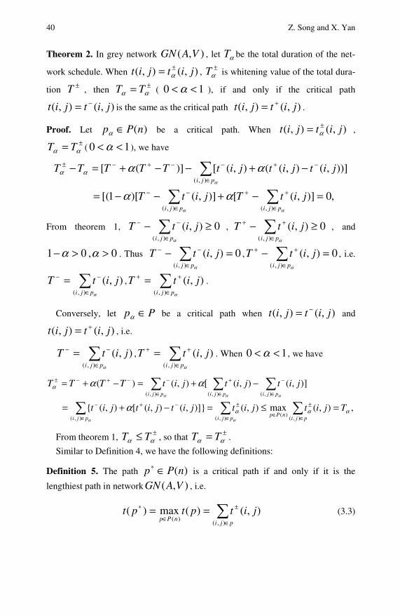
40 Z. Song and X. Yan
Theorem 2. In grey network ),( VAGN , let αT be the total duration of the net-
work schedule. When ),(),( jitjit ±= α , ±αT is whitening value of the total dura-
tion ±T , then ±= αα TT ( 10 << α ), if and only if the critical path
),(),( jitjit −= is the same as the critical path ),(),( jitjit += .
Proof. Let )(nPp ∈α be a critical path. When ),(),( jitjit ±= α , ±= αα TT ( 10 << α ), we have
,0]),([]),()[1[(
))],(),((),([)]([
),(),(
),(
=−+−−=
−+−−+=−
∑∑
∑
∈
++
∈
−−
∈
−+−−+−±
αα
α
αα
αααα
pjipji
pji
jitTjitT
jitjitjitTTTTT
From theorem 1, 0),(),(
≥− ∑∈
−−
αpji
jitT , 0),(),(
≥− ∑∈
++
αpji
jitT , and
0, 01 >>− αα . Thus 0),(),(
=− ∑∈
−−
αpji
jitT , 0),(),(
=− ∑∈
++
αpji
jitT , i.e.
∑∈
−− =αpji
jitT),(
),( , ∑∈
++ =αpji
jitT),(
),( .
Conversely, let Pp ∈α be a critical path when ),(),( jitjit −= and
),(),( jitjit += , i.e.
∑∈
−− =αpji
jitT),(
),( , ∑∈
++ =αpji
jitT),(
),( . When 10 << α , we have
,),(max),()]},(),([),({
]),(),([),()(
),()(
),(),(
),(),(),(
ααα
α
αα
ααα
α
αα
Tjitjitjitjitjit
jitjitjitTTTT
pjinPp
pjipji
pjipjipji
=≤=−+=
−+=−+=
∑∑∑
∑∑∑
∈
±
∈∈
±
∈
−+−
∈
−
∈
+
∈
−−+−±
From theorem 1, ±≤ αα TT , so that ±= αα TT .
Similar to Definition 4, we have the following definitions:
Definition 5. The path )(nPp ∈∗ is a critical path if and only if it is the
lengthiest path in network ),( VAGN , i.e.
∑∈
±
∈
∗ ==pji
nPpjitptpt
),()(
),()(max)( (3.3)
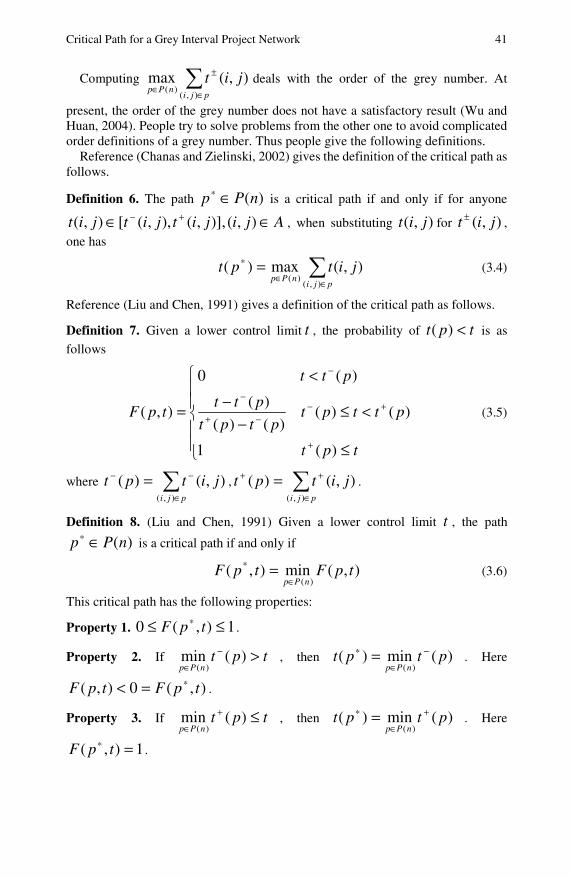
Critical Path for a Grey Interval Project Network 41
Computing ∑∈
±
∈pji
nPpjit
),()(
),(max deals with the order of the grey number. At
present, the order of the grey number does not have a satisfactory result (Wu and Huan, 2004). People try to solve problems from the other one to avoid complicated order definitions of a grey number. Thus people give the following definitions.
Reference (Chanas and Zielinski, 2002) gives the definition of the critical path as follows.
Definition 6. The path )(nPp ∈∗ is a critical path if and only if for anyone
Ajijitjitjit ∈∈ +− ),()],,(),,([),( , when substituting ),( jit for ),( jit ± ,
one has
∑∈∈
∗ =pji
nPpjitpt
),()(
),(max)( (3.4)
Reference (Liu and Chen, 1991) gives a definition of the critical path as follows.
Definition 7. Given a lower control limit t , the probability of tpt <)( is as
follows
⎪⎪⎩
⎪⎪⎨
⎧
≤
<≤−
−
<
=
+
+−−+
−
−
tpt
pttptptpt
ptt
ptt
tpF
)( 1
)()( )()(
)(
)( 0
),( (3.5)
where ∑∈
−− =pji
jitpt),(
),()( , ∑∈
++ =pji
jitpt),(
),()( .
Definition 8. (Liu and Chen, 1991) Given a lower control limit t , the path
)(nPp ∈∗ is a critical path if and only if
),(min),()(
* tpFtpFnPp∈
= (3.6)
This critical path has the following properties:
Property 1. 1),(0 ≤≤ ∗ tpF .
Property 2. If tptnPp
>−
∈)(min
)(, then )(min)(
)(ptpt
nPp
−
∈
∗ = . Here
),(0),( tpFtpF ∗=< .
Property 3. If tptnPp
≤+
∈)(min
)(, then )(min)(
)(ptpt
nPp
+
∈
∗ = . Here
1),( =∗ tpF .
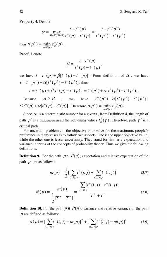
42 Z. Song and X. Yan
Property 4. Denote
)()(
)(
)()(
)(max
)( ∗−∗+
∗−
−+
−
Γ∈ −−=
−−=
ptpt
ptt
ptpt
pttGWGH
α
then )(min)()(
ptptnPp
±
∈
∗ = α .
Proof. Denote
)()(
)(
ptpt
ptt−+
−
−−=β ,
we have )]()([)( ptptptt −+− −+= β . From definition of α , we have
)]()([)( ∗−∗+∗− −+= ptptptt α , thus
)]()([)( ptptptt −+− −+= β )]()([)( ∗−∗+∗− −+= ptptpt α .
Because βα ≥ , we have )]()([)( ∗−∗+∗− −+ ptptpt α
)]()([)( ptptpt −+− −+≤ α . Therefore )(min)()(
ptptnPp
±
∈
∗ = α .
Since α is a deterministic number for a given t , from Definition 4, the length of
path ∗p is a minimum in all the whitening values )( pt ±α . Therefore, path ∗p is a
critical path. For uncertain problems, if the objective is to solve for the maximum, people’s
preference in many cases is to follow two aspects. One is the upper objective value, while the other one is lesser uncertainty. They stand for similarly expectation and variance in terms of the concepts of probability theory. Thus we give the following definitions.
Definition 9. For the path )(nPp ∈ , expectation and relative expectation of the
path p are as follows:
]),(),([2
1)(
),(),(∑∑
∈
−
∈
+ +=pjipji
jitjitpm (3.7)
−+∈
−+
−+ +
+=
+=
∑TT
jitjit
TT
pmpm pji ),(
)],(),([
][
2
1)(
)(~ (3.8)
Definition 10. For the path )(nPp ∈ , variance and relative variance of the path
p are defined as follows:
2
),(
2
),(
)](),([)](),([)( pmjitpmjitpdpjipji
−+−= ∑∑∈
+
∈
− (3.9)

Critical Path for a Grey Interval Project Network 43
2
2
),(
2 )(
])),(),(([
)(2
1)(
)(~
−+∈
−+
−+ −
−=
−=
∑TT
jitjit
TT
pdpd pji
(3.10)
Definition 11. Given a lower control limit t , the path )(nPp ∈∗ is a critical path
if and only if
)},(),(~
),(~{min)(
tpFpdpmnPp
−∈
(3.11)
where )(~ pm denotes the expectation of a decision-maker and )(~
pd denotes
variance of a decision-maker. They reflect objective demands of a decision-maker, and ),( tpF reflects subjective demands of a decision-maker.
There are many methods to solve a multiobjective problem; we adopt the method of weighted average, i.e.
),()(~
)(~min 321)(
tpFpdpmnPp
λλλ ++−∈
(3.12)
Here ,10 1 ≤≤ λ ,10 2 ≤≤ λ ,10 3 ≤≤ λ .1321 =++ λλλ
It is obvious that the solution ∗p of the above method must be the Pareto effec-
tive solution of formula (3.12).
C. Example
Suppose some project was shown in Fig. 3.1 as follows
Fig. 3.1
where ]6,5[)3,1( ],4,4[)2,1( == ±± tt , ]7,7[)5,2( ],4,4[)4,2( == ±± tt ,
],4,3[)4,3( =±t ]4,3[)6,3( =±t , ]8,7[)7,4( =±t , ],5,3[)7,5( =±t ]2,2[)8,5( =±t ,
]7,7[)7,6( =±t , ]20,18[)10,6( ],15,6[)9,6( == ±± tt , ]12,2[)9,7( ],3,2[)8,7( == ±± tt ,
11
3
1
2 5 8
4 7 9
6 10
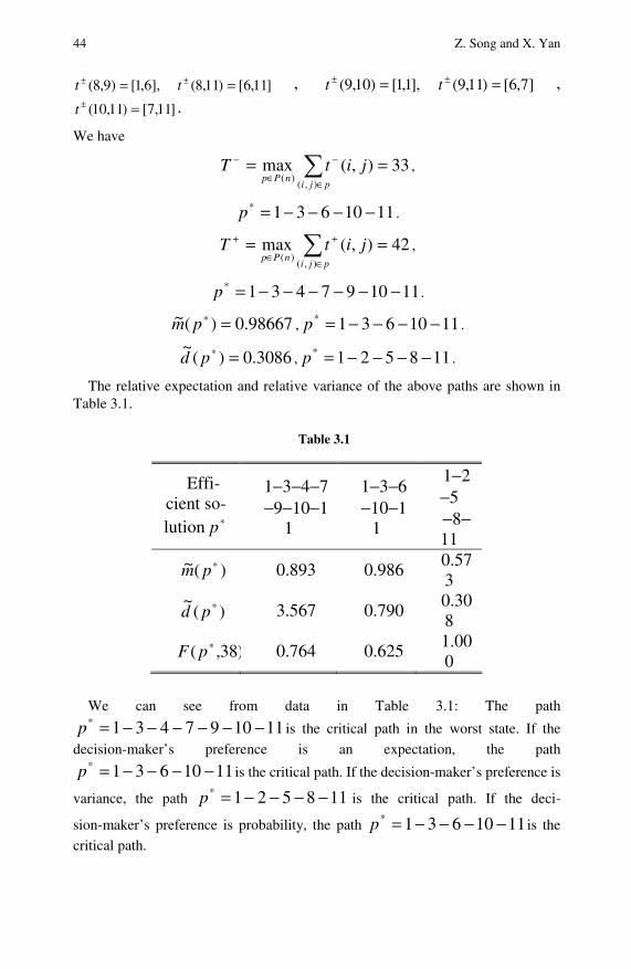
44 Z. Song and X. Yan
]11,6[)11,8( ],6,1[)9,8( == ±± tt , ]7,6[)11,9( ],1,1[)10,9( == ±± tt ,
]11,7[)11,10( =±t .
We have
33),(max),(
)(== ∑
∈
−
∈
−
pjinPp
jitT ,
1110631* −−−−=p .
42),(max),(
)(== ∑
∈
+
∈
+
pjinPp
jitT ,
111097431* −−−−−−=p .
98667.0)(~ =∗pm , 1110631* −−−−=p .
3086.0)(~ =∗pd , 118521* −−−−=p .
The relative expectation and relative variance of the above paths are shown in Table 3.1.
Table 3.1
Effi-cient so-lution ∗p
1−3−4−7 −9−10−1
1
1−3−6 −10−1
1
1−2−5 −8−11
)(~ ∗pm 0.893 0.986 0.573
)(~ ∗pd 3.567 0.790
0.308
)38,( ∗pF 0.764 0.625 1.000
We can see from data in Table 3.1: The path
111097431* −−−−−−=p is the critical path in the worst state. If the
decision-maker’s preference is an expectation, the path
1110631* −−−−=p is the critical path. If the decision-maker’s preference is
variance, the path 118521* −−−−=p is the critical path. If the deci-
sion-maker’s preference is probability, the path 1110631* −−−−=p is the
critical path.
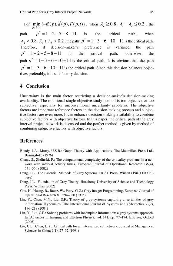
Critical Path for a Grey Interval Project Network 45
For )},(),(~
),(~{min)(
tpFpdpmnPp
−∈
, when 8.02 ≥λ , 2.031 ≤+ λλ , the
path 118521* −−−−=p is the critical path; when
8.02 <λ , 2.031 >+ λλ , the path 1110631* −−−−=p is the critical path.
Therefore, if decision-maker’s preference is variance, the path
118521* −−−−=p is the critical path, otherwise the
path 1110631* −−−−=p is the critical path. It is obvious that the path
1110631* −−−−=p is the critical path. Since this decision balances objec-
tives preferably, it is satisfactory decision.
4 Conclusion
Uncertainty is the main factor restricting a decision-maker’s decision-making availability. The traditional single objective study method is too objective or too subjective, especially for unconventional uncertainty problems. The objective factors are important reference factors in the decision-making process and subjec-tive factors are even more. It can enhance decision-making availability to combine subjective factors with objective factors. In this paper, the critical path of the grey interval project network is discussed and the perfect method is given by method of combining subjective factors with objective factors.
References
Bondy, J.A., Murty, U.S.R.: Graph Theory with Applications. The Macmillan Press Ltd., Basingstoke (1976)
Chans, S., Zielinski, P.: The computational complexity of the criticality problems in a net-work with interval activity times. European Journal of Operational Research 136(4), 541–550 (2002)
Deng, J.L.: The Essential Methods of Grey Systems. HUST Press, Wuhan (1987) (in Chi-nese)
Deng, J.L.: Foundation of Grey Theory. Huazhong University of Science and Technology Press, Wuhan (2002)
Gou, H., Huang, B., Baetz, W., Patry, G.G.: Grey integer Programming. European Journal of Operational Research 83, 594–620 (1995)
Lin, Y., Chen, M.Y., Liu, S.F.: Theory of grey systems: capturing uncertainties of grey information. Kybernetes: The International Journal of Systems and Cybernetics 33(2), 196–218 (2004)
Lin, Y., Liu, S.F.: Solving problems with incomplete information: a grey systems approach. In: Advances in Imaging and Electron Physics, vol. 141, pp. 77–174. Elsevier, Oxford (2006)
Liu, C.L., Chen, H.Y.: Critical path for an interval project network. Journal of Management Sciences in China 9(1), 27–32 (1991)

46 Z. Song and X. Yan Liu, S.F., Dang, Y.G., Fang, Z.G.: Grey Systems Theory and Application. Science Press,
Beijing (1991) (in Chinese) Liu, S.F., Lin, Y.: Grey Information Theory and Practical Applications. Springer, New York
(2006) Okada, S., Gen, M.: Order relation between intervals and its application to shortest path
problem. Computers Industrial Engineering 25(2), 147–150 (1994) Wu, J., Huan, D.S.: An review on ranking methods of interval numbers. Systems Engineer-
ing 22(8), 1–4 (2004) Xiao, X.P., Song, Z.M., Li, F.: Grey technology foundation and Application. Science Press,
Beijing (2005) (in Chinese)
A New Dynamic Clustering Algorithm for an Interval Grey Number*
Shunxiang Wu, Junjie Yang, Wenchang Wei, Lihua Lin, and Zhifeng Luo
In this chapter, the grey dynamic clustering algorithm of an interval grey number is proposed by the joint application of the basic idea of fuzzy equivalent clustering and the method of the grey system theory. Firstly, the similarity coefficient formula of the interval grey number is discussed, and then the clustering of the interval grey number is realized by making use of the transitive closure method. This algorithm combines the grey system theory and the fuzzy set theory, which expands the range of classical equivalent clustering algorithms from the legible number to the interval grey number. Therefore, it’s more versatile, and its effectiveness is testified by an example.
1 Introduction
Grey system theory ((Liu and Dang, 2004; Liu and Lin, 2006; Lin et al., 2004; Lin and Liu, 2006), proposed by Professor Deng Julong in the 80s of the 20th century, is a new, powerful tool that can deal with the uncertainty of information. Grey clus-tering is a method that divides a number of objects into classes according to the grey incidence matrix or the white whitenization function. The classical decision- making method of grey clustering is established based on the clarity of the defini-tion of the index evaluation, and it cannot deal with the evaluation of the interval grey number. However, with the continuous development of society, people face more and more complex problems, and the uncertainty of the problems and human
Shunxiang Wu, Junjie Yang, Wenchang Wei, Lihua Lin, and Zhifeng Luo Department of Amtumation, Xiamen University, Xiamen, China, 361005; Key Laboratory of Intelligent Manufacture of Hunan Province, Xiangtan University, Xiangtan. Phone: (86)592/5805872 e-mail: [email protected]
* This work was supported in part by the Planning Project of the National Eleventh-Five Science and Technology (2007BAK34B04), the Chinese National Natural Science Fund (60704042), the Aeronautical Science Foundation (20080768004), the Open Project Program of the Key Lab. of Intelligent Manufacture of Hunan Province (XTU) and the Program of 211 Innovation Engineering on Information in Xiamen University (2009-2011).
48 S. Wu et al.
thinking have been enhanced. In the actual decision-making process, we often cannot obtain all the decision-making information, but we can usually get deci-sion-making information about the rough scope of the information, the information of the interval grey number. Based on that, the reference (Luo, 2004) has discussed clustering decision-making when the index evaluation of object is an interval grey number, and it also has established the incidence coefficient formula and relative incidence coefficient formulas for the grey interval number. The clustering deci-sion-making method has been proposed based on the grey interval incidence coef-ficient and a pre-set class number by making use of the grey whitenization function. The above problems have been resolved to some extent by this method. However, firstly, this method should determine the number of classes in advance, and if the number of classes is unknown, the algorithm is not feasible. Secondly, it needs experts to predetermine the whitenization weight function, so the subjective factors of the experts have influence on the classification results. Finally, the calculation process of the algorithm is complex and difficult for decision-making.
Fuzzy mathematics has been developed enormously since Zadeh introduced the concept of fuzzy sets in 1965. With in-depth study, we find that the membership function of fuzzy sets is difficult to be determined in the application, and then the membership degree of interval value is easier to be determined. Moreover, the results of fuzzy reasoning expressed by fuzzy sets for interval value can better reflect the fuzziness of day-to-day reasoning (Wu, 1992). Therefore, the ex-tending form of fuzzy sets, interval-valued fuzzy sets, are more and more common in recent years (Wu, 1992; Zhang and Wang, 1991; Ibuchih and Tanaka, 1993; Mandal, 1997; Fan, 1998). The three FCM clustering algorithm of interval-valued data is given in the reference (Gao et al., 2003; Wu et al., 2005), and they can directly cluster by the classical FCM algorithm with the membership function through pretreatment, but the algorithms cluster by turning the interval grey number into a white number (that is, a definite number), or they cluster by making the use of a simple distance formula. Although the above-mentioned methods can make use of the existing classical FCM algorithm, they reduce the credibility of the results.
In this chapter, the algorithm of interval grey clustering based on the equivalence relation overcomes the above-mentioned shortcomings: Firstly, a similarity coefficient formula for the interval grey number is established by making full use of all information of the interval grey number and on the basis that the interval grey number isn’t turned into white number. Secondly, it needn’t predetermination of the number of classes that can perform dynamic classification of the transitive closure method by making use of fuzzy equiva-lence relations. Thirdly, it also needn’t subjective determination of the whit-enization weight function by experts, so it can increase the objectivity of the algorithm, and it greatly simplifies the process of calculation so that it is easy for decision-making.
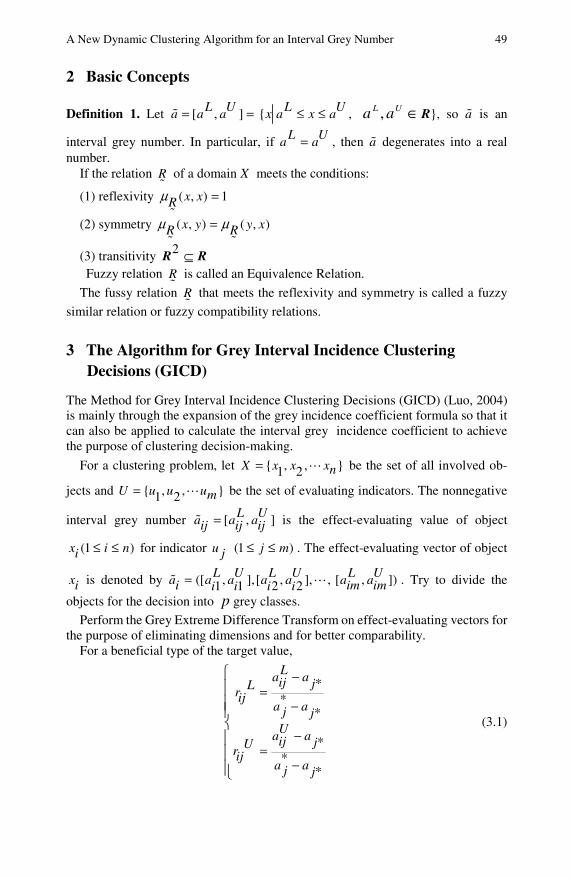
A New Dynamic Clustering Algorithm for an Interval Grey Number 49
2 Basic Concepts
Definition 1. Let [ , ]L Ua a a= = { ,L Ux a x a≤ ≤ ∈UL aa , R}, so a is an
interval grey number. In particular, if L Ua a= , then a degenerates into a real number.
If the relation R of a domain X meets the conditions:
(1) reflexivity ( , ) 1x xRμ =
(2) symmetry ( , ) ( , )x y y xR Rμ μ=
(3) transitivity 2 ⊆R R Fuzzy relation R is called an Equivalence Relation.
The fussy relation R that meets the reflexivity and symmetry is called a fuzzy
similar relation or fuzzy compatibility relations.
3 The Algorithm for Grey Interval Incidence Clustering Decisions (GICD)
The Method for Grey Interval Incidence Clustering Decisions (GICD) (Luo, 2004)
is mainly through the expansion of the grey incidence coefficient formula so that it can also be applied to calculate the interval grey incidence coefficient to achieve the purpose of clustering decision-making.
For a clustering problem, let { , , }1 2X x x xn= be the set of all involved ob-
jects and { , , }1 2U u u um= be the set of evaluating indicators. The nonnegative
interval grey number [ , ]L Ua a aij ij ij= is the effect-evaluating value of object
(1 )x i ni ≤ ≤ for indicator u j (1 )j m≤ ≤ . The effect-evaluating vector of object
xi is denoted by ([ , ],[ , ], ,1 1 2 2L U L Ua a a a ai i i i i= [ , ])L Ua aim im . Try to divide the
objects for the decision into p grey classes.
Perform the Grey Extreme Difference Transform on effect-evaluating vectors for the purpose of eliminating dimensions and for better comparability.
For a beneficial type of the target value,
**
*
**
*
La aij jLrija aj jUa aij jUrij
a aj j
−=
−
−=
−
⎧⎪⎪⎪⎨⎪⎪⎪⎩
(3.1)

50 S. Wu et al.
For the cost type of the target value,
*
**
*
**
Ua aj ijLrija aj j
La aj ijUrija aj j
−=
−
−=
−
⎧⎪⎪⎪⎨⎪⎪⎪⎩
(3.2)
where * max { }1
Ua aj iji n=
≤ ≤, min { }* 1
La aijj i n=
≤ ≤, ( 1, 2, )j m= . Then we get a Nor-
malized evaluation vector ([ , ],[ , ], ,[ , ]1 1 2 2L U L U L Ur r r r r r ri im imi i i i= .
Definition 2. Suppose that the effect-evaluating vector of every object is denoted by the following: After normalization
([ , ],[ , ], ,[ , ]1 1 2 2L U L U L Ur r r r r r ri im imi i i i=
where [ , ]L Ur rij ij is a nonnegative interval grey number within [0,1]. Let
max { }1
L Lr rj iji n+ =
≤ ≤, max { }
1U Ur rj iji n
+ =≤ ≤
, ( 1, 2, )j m= (3.3)
Then, the m-dimensional vector of nonnegative interval grey number
([ , ],[ , ], [ , ])1 1 2 2L U L U L Ur r r r r r rm m
+ + + + + + += (3.4)
is called the ideal effect-evaluating vector of the evaluated objects.
Definition 3. Suppose that the effect-evaluating vector and the ideal ef-fect-evaluating vector of objects are defined as formula (3.3), respectively, in Definition 2, then
min min max max1 1 1 1 1
2 max max1 1
L L L Lr r r rj ij j iji n j m i n j m
ij L L L Lx x x xj ij j iji n j m
λγ
λ
+ +− + −≤ ≤ ≤ ≤ ≤ ≤ ≤ ≤+ = + +− + −
≤ ≤ ≤ ≤
⎛⎜⎜⎜⎝
min min max max1 1 1 1
max max1 1
U U U Ux x x xj ij j iji n j m i n j m
U U U Ux x x xj ij j iji n j m
λ
λ
+ +− + −≤ ≤ ≤ ≤ ≤ ≤ ≤ ≤
+ + +− + −≤ ≤ ≤ ≤
⎞⎟⎟⎟⎠
(3.5)
is called the grey interval incidence coefficient of sub-factor [ , ]L Ur rij ij to the ideal
factor [ , ]L Ur rj j+ + ( 1, 2, ,i n= , 1, 2, , )j m= , where [0,1]λ ∈ is the recog-
nition coefficient (or call it the relative factor adjusted to the environment).

A New Dynamic Clustering Algorithm for an Interval Grey Number 51
The GICD arithmetic steps are as follows:
Step 1: Normalize the effect-evaluating vectors (the evaluating vector for a non-negative grey number) by formula (3.1) or (3.2) (the grey extreme difference
transform), and the normalization is shown as ([ , ],1 1L Ur r ri i i=
[ , ], ,[ , ])2 2L U L Ur r r rim imi i ; then, we can get the ideal effect-evaluating vector of
object by Definition 2, as shown in formula (3.4).
Step 2: For all objects, calculate their grey incidence coefficient vectors, which are
( , , , )1 2i imi iγ γ γ γ+ + + += , ( 1, 2, , )i n= by the grey interval incidence coefficient
formula (3.5).
Step 3: To decide the number of grey classes p according to the decision problem,
divide the range of the grey interval incidence coefficient of the object, related to
the ideal object for indicator u j ( 1, 2, , )j m= , into p smaller intervals.
Step 4: By practical application or the qualitative research of experts, we can get the
whitenization weight function ( )kf xj ( 1, 2, ,j m= ; 1, 2, , )k p= of grey class
k for indicator u j if the weight vector ( , ,1 2η η η= , )mη of the indicator is
unknown, then it may be calculated by the formula
{ } 12 2(1 ) (1 )
1 11
m n nj ij iki ik
η γ γ−
+ += − −∑ ∑ ∑= ==
⎡ ⎤⎢ ⎥⎣ ⎦
, ( 1, 2, , )j m= .
Step 5: For object xi ( 1, 2, , )i n= , belonging to grey class k ( 1, 2, , )k p= ,
calculate the synthetic clustering coefficient kiσ ( 1, 2, ,i n= ; 1, 2, , )k p= as
( )1
mk k kfi j ij jjσ γ η+= ⋅∑
=. Calculate the grey class to which object xi belongs by
using the formula { }max1
k ki ik p
σ σ∗
=≤ ≤
. Then, in the same grey class, rank the order
of the objects for the decision by their clustering coefficients.
4 The Interval Grey Number Dynamic Clustering Algorithm Based on the Equivalence Relations
In order to quantify the classification, we must first determine some number indi-cators of the classifications. The number index denotes the degree of similarity between samples (or variables), known as the clustering statistics. Clustering sta-tistics can be divided into two categories, similarity and distance. By comparing a
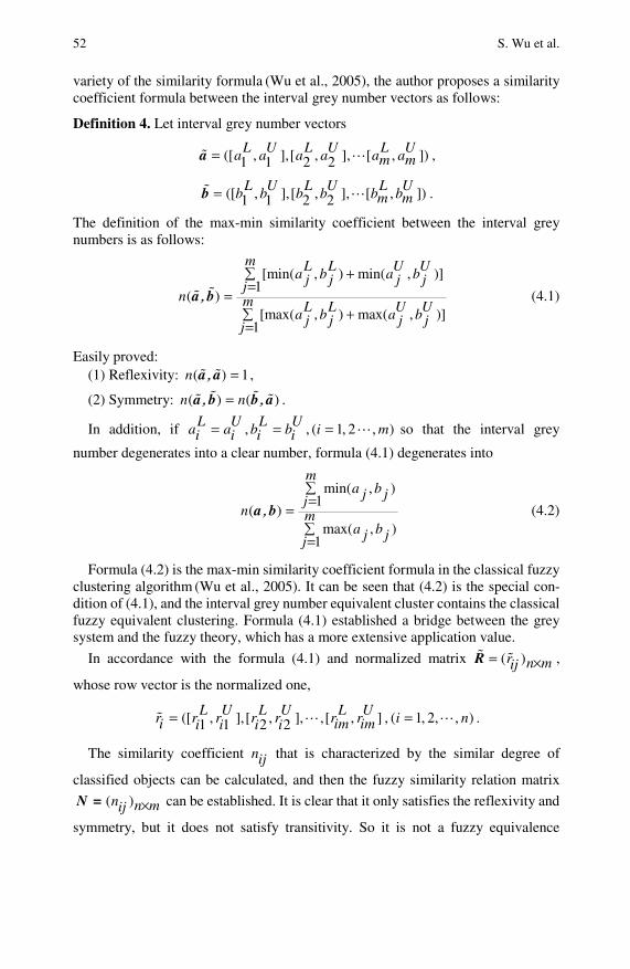
52 S. Wu et al.
variety of the similarity formula (Wu et al., 2005), the author proposes a similarity coefficient formula between the interval grey number vectors as follows:
Definition 4. Let interval grey number vectors
([ , ],[ , ], [ , ])1 1 2 2L U L U L Ua a a a a am m=a ,
([ , ],[ , ], [ , ])1 1 2 2L U L U L Ub b b b b bm m=b .
The definition of the max-min similarity coefficient between the interval grey numbers is as follows:
[min( , ) min( , )]1
( )[max( , ) max( , )]
1
m L L U Ua b a bj j j jjn m L L U Ua b a bj j j jj
+∑=
=+∑
=
a b, (4.1)
Easily proved: (1) Reflexivity: ( ) 1n =a a, ,
(2) Symmetry: ( ) ( )n n=a b b a, , .
In addition, if , , ( 1, 2 , )L U L Ua a b b i mi i i i= = = so that the interval grey
number degenerates into a clear number, formula (4.1) degenerates into
min( , )1
( )max( , )
1
ma bj jj
n ma bj jj
∑=
=∑=
a b, (4.2)
Formula (4.2) is the max-min similarity coefficient formula in the classical fuzzy clustering algorithm (Wu et al., 2005). It can be seen that (4.2) is the special con-dition of (4.1), and the interval grey number equivalent cluster contains the classical fuzzy equivalent clustering. Formula (4.1) established a bridge between the grey system and the fuzzy theory, which has a more extensive application value.
In accordance with the formula (4.1) and normalized matrix ( )r n mij= ×R ,
whose row vector is the normalized one,
([ , ],[ , ], ,[ , ]1 1 2 2L U L U L Ur r r r r r ri im imi i i i= , ( 1, 2, , )i n= .
The similarity coefficient nij that is characterized by the similar degree of
classified objects can be calculated, and then the fuzzy similarity relation matrix
( )n n mij ×N = can be established. It is clear that it only satisfies the reflexivity and
symmetry, but it does not satisfy transitivity. So it is not a fuzzy equivalence
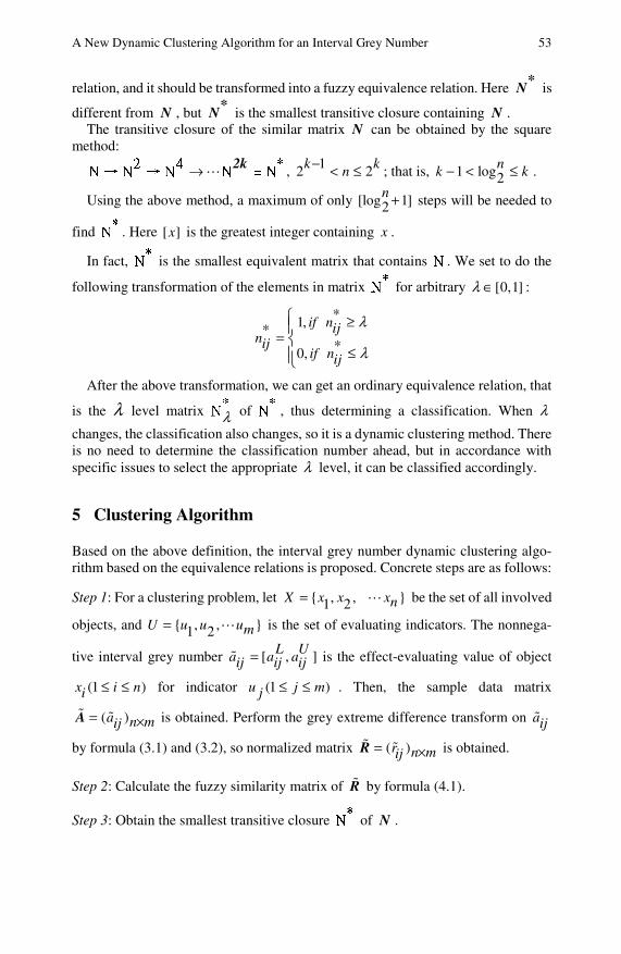
A New Dynamic Clustering Algorithm for an Interval Grey Number 53
relation, and it should be transformed into a fuzzy equivalence relation. Here *N is
different from N , but *N is the smallest transitive closure containing N . The transitive closure of the similar matrix N can be obtained by the square
method:
→2 4 *N → N → N N = N
2k , 12 2k kn− < ≤ ; that is, 1 log2nk k− < ≤ .
Using the above method, a maximum of only [log 1]2n + steps will be needed to
find *N . Here [ ]x is the greatest integer containing x .
In fact, *N is the smallest equivalent matrix that contains N . We set to do the
following transformation of the elements in matrix *N for arbitrary [0,1]λ ∈ :
*1,**0,
if nijnij
if nij
λ
λ
≥=
≤
⎧⎪⎨⎪⎩
After the above transformation, we can get an ordinary equivalence relation, that
is the λ level matrix λ*
N of *N , thus determining a classification. When λ
changes, the classification also changes, so it is a dynamic clustering method. There is no need to determine the classification number ahead, but in accordance with specific issues to select the appropriate λ level, it can be classified accordingly.
5 Clustering Algorithm
Based on the above definition, the interval grey number dynamic clustering algo-rithm based on the equivalence relations is proposed. Concrete steps are as follows:
Step 1: For a clustering problem, let { , ,1 2X x x= }xn be the set of all involved
objects, and { , , }1 2U u u um= is the set of evaluating indicators. The nonnega-
tive interval grey number [ , ]L Ua a aij ij ij= is the effect-evaluating value of object
(1 )x i ni ≤ ≤ for indicator (1 )u j mj ≤ ≤ . Then, the sample data matrix
( )a n mij= ×A is obtained. Perform the grey extreme difference transform on aij
by formula (3.1) and (3.2), so normalized matrix ( )r n mij= ×R is obtained.
Step 2: Calculate the fuzzy similarity matrix of R by formula (4.1).
Step 3: Obtain the smallest transitive closure *N of N .
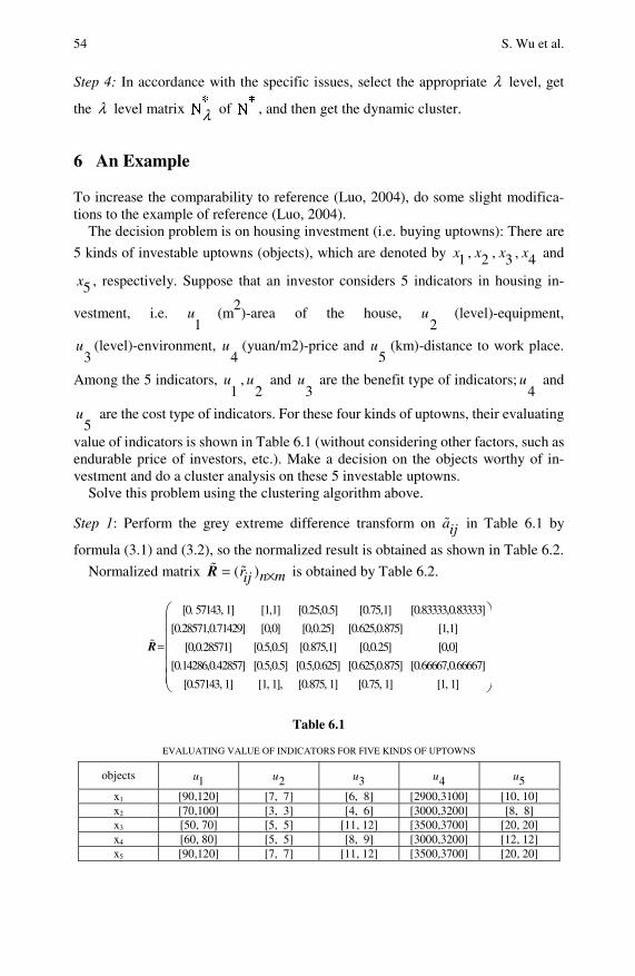
54 S. Wu et al.
Step 4: In accordance with the specific issues, select the appropriate λ level, get
the λ level matrix λ*
N of *N , and then get the dynamic cluster.
6 An Example
To increase the comparability to reference (Luo, 2004), do some slight modifica-tions to the example of reference (Luo, 2004).
The decision problem is on housing investment (i.e. buying uptowns): There are
5 kinds of investable uptowns (objects), which are denoted by 1x , 2x , 3x , 4x and
5x , respectively. Suppose that an investor considers 5 indicators in housing in-
vestment, i.e. 1
u (m2)-area of the house, 2
u (level)-equipment,
3u (level)-environment,
4u (yuan/m2)-price and
5u (km)-distance to work place.
Among the 5 indicators, 1
u ,2
u and 3
u are the benefit type of indicators;4
u and
5u are the cost type of indicators. For these four kinds of uptowns, their evaluating
value of indicators is shown in Table 6.1 (without considering other factors, such as endurable price of investors, etc.). Make a decision on the objects worthy of in-vestment and do a cluster analysis on these 5 investable uptowns.
Solve this problem using the clustering algorithm above.
Step 1: Perform the grey extreme difference transform on aij in Table 6.1 by
formula (3.1) and (3.2), so the normalized result is obtained as shown in Table 6.2.
Normalized matrix ( )r n mij= ×R is obtained by Table 6.2.
[0. 57143, 1] [1,1] [0.25,0.5] [0.75,1] [0.83333,0.83333]
[0.28571,0.71429] [0,0] [0,0.25] [0.625,0.875] [1,1]
[0,0.28571] [0.5,0.5] [0.875,1] [0,0.25] [0,0]
[0.14286,0.42857] [0.5,0.5] [0.5,0.625] [0.625,0.875] [0.6
=R
6667,0.66667]
[0.57143, 1] [1, 1], [0.875, 1] [0.75, 1] [1, 1]
⎛ ⎞⎜ ⎟⎜ ⎟⎜ ⎟⎜ ⎟⎜ ⎟⎝ ⎠
Table 6.1
EVALUATING VALUE OF INDICATORS FOR FIVE KINDS OF UPTOWNS
objects 1u 2u 3u 4u 5u
x1 [90,120] [7, 7] [6, 8] [2900,3100] [10, 10] x2 [70,100] [3, 3] [4, 6] [3000,3200] [8, 8] x3 [50, 70] [5, 5] [11, 12] [3500,3700] [20, 20] x4 [60, 80] [5, 5] [8, 9] [3000,3200] [12, 12] x5 [90,120] [7, 7] [11, 12] [3500,3700] [20, 20]
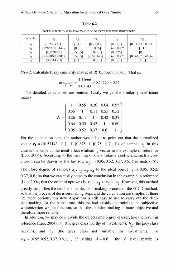
A New Dynamic Clustering Algorithm for an Interval Grey Number 55
Table 6.2
NORMALIZED EVALUATING VALUE OF OBJECTS FOR FIVE INDICATORS
objects 1u 2u 3u 4u 5u
x1 [0. 57143, 1] [1,1] [0.25,0.5] [0.75,1] [0.83333,0.83333] x2 [0.28571,0.71429] [0,0] [0,0.25] [0.625,0.875] [1,1] x3 [0,0.28571] [0.5,0.5] [0.875,1] [0,0.25] [0,0] x4 [0.14286,0.42857] [0.5,0.5] [0.5,0.625] [0.625,0.875] [0.66667,0.66667] x5 [0.57143, 1] [1,1] [0.875,1] [0.75,1] [1, 1]
Step 2: Calculate fuzzy similarity matrix of R by formula (4.1). That is,
4.41666( , ) 0.54720 0.551 2 8.07143
n x x = = ≈
The detailed calculations are omitted. Lastly we get the similarity coefficient matrix:
1 0.55 0.26 0.64 0.95
0.55 1 0.11 0.55 0.52
0.26 0.11 1 0.42 0.37
0.64 0.55 0.42 1 0.60
0.95 0.52 0.37 0.6 1
=
⎛ ⎞⎜ ⎟⎜ ⎟⎜ ⎟⎜ ⎟⎜ ⎟⎝ ⎠
N
For the calculation here, the author would like to point out that the normalized
vector ([0.57143, 1],[1, 1],[0.875, 1],[0.75, 1],[1, 1])5 =r of sample 5x in this
case is the same as the ideal effect-evaluating vector in the example in reference (Luo, 2004). According to the meaning of the similarity coefficient, such a con-
clusion can be drawn by the last row (0.95, 0.52, 0.37, 0.6,1)5 =n in matrix N :
The close degree of samples , , ,1 2 3 4x x x x to the ideal object 5x is 0.95, 0.52,
0.37, 0.61 so that we can easily come to the conclusion in the example in reference
(Luo, 2004) that the order of uptowns is 1 4 2 3x x x x . However, this method
greatly simplifies the cumbersome decision-making process of the GICD method, so that the process of decision-making steps and the calculation are simpler. If there are more options, this new Algorithm is still easy to use to carry out the deci-sion-making. At the same time, this method avoids determining the subjective whitenization weight function, so that the decision-making is more objective and therefore more reliable.
In addition, we may now divide the objects into 3 grey classes, like the result in
reference (Luo, 2004): 1h (the grey class worthy of investment), 2h (the grey class
backup), and 3h (the grey class not suitable for investment). For
(0.95, 0.52, 0.37, 0.6,1)5 =n , if setting 0.6λ = , the λ level matrix is

56 S. Wu et al.
(1, 0, 0,1,1) , so we get the result that { , }3 2 3h x x= . For the same reason, if set-
ting 0.6λ = , we get { }1 1h x= . If setting 0.6λ = and weeding out the best 1x , we
can get { }2 4h x= . It can be seen that the conclusion by the GICD method is the
conclusion that makes 5x the sole standard of a "classification". It is not a true
cluster analysis.
Step 3: Obtain the smallest transitive closure *N of N .
1 0.55 0.42 0.64 0.95
0.55 1 0.42 0.55 0.552 4
0.42 0.42 1 0.42 0.42
0.64 0.55 0.42 1 0.64
0.95 0.55 0.42 0.64 1
= = =
⎛ ⎞⎜ ⎟⎜ ⎟⎜ ⎟⎜ ⎟⎜ ⎟⎝ ⎠
N N *N
Step 4: Get the λ level matrix λ*
N of *N , then obtain the dynamic cluster.
If setting 0.55λ = , the λ level matrix of *N is the following:
1 1 0 1 1
1 1 0 1 1
0 0 1 0 00.551 1 0 1 1
1 1 0 1 1
=
⎛ ⎞⎜ ⎟⎜ ⎟⎜ ⎟⎜ ⎟⎜ ⎟⎝ ⎠
*N
It is easily seen from *N that 5 uptowns can be divided into 2 classes:
, , , 51 2 4x x x x are in a class , and 3x is another class.
If setting 0.64λ = , the λ level matrix of *N is the following:
1 0 0 1 1
0 1 0 0 0
0 0 1 0 00.551 0 0 1 0
1 0 0 0 1
=
⎛ ⎞⎜ ⎟⎜ ⎟⎜ ⎟⎜ ⎟⎜ ⎟⎝ ⎠
*N
So they can be divided into 3 classes: , , 51 4x x x are in a class, and ,2 3x x are 2
other classes.
If setting 1λ = or 0.42λ = , then ,1 0.42= =* *N NI E . The former one divides
these five uptowns into their respective categories for classes of 5, but the latter one merges these 5 uptowns into a class.

A New Dynamic Clustering Algorithm for an Interval Grey Number 57
From the above classification process, it’s not difficult to see that the class result is relevant to λ values. The greater λ is, the more classes there are. When λ is low to a value, all samples are classified as a class. Therefore, we can adjust the value of λ to obtain the appropriate classes, according to the needs of practical problems, without setting the number of classes first.
7 Conclusion
In this chapter, the following work is summarized:
1. The similarity coefficient formula of a interval grey number is established, which lays the foundation for the grey dynamic cluster.
2. The grey dynamic cluster algorithm of the interval grey number is proposed to overcome the limitation that fuzzy equivalent clustering cannot apply to the interval grey number.
3. The subjectivity and limitations of the GICD method is analyzed and sim-plified, and the decision-making of the interval grey number is made easier.
4. An example is given to illustrate the rationality of the grey dynamic cluster algorithm of an interval grey number and the validity of the relational arithmetic.
In short, this chapter presents a new algorithm to analyze the clustering of the in-terval grey number based on the idea of the grey system theory, and the estab-lishment of the similarity coefficient formula of the interval grey number, which combines with the use of the fuzzy equivalent clustering to achieve the clustering of the interval grey number, and it expands the range of the classical equivalent clus-tering algorithms from the legible number to the interval grey number.
References
Liu, S.F., Dang, Y.G.: Theory and Application of Grey Systems. Science Press, Beijing (2004)
Wu, W.M.: Interval-valued Fuzzy Sets and Interval-valued Fuzzy Reasoning. Fuzzy Systems and Mathematics 2(6), 77–85 (1992)
Zhang, W.X., Wang, G.J.: Introduction of Fuzzy Mathematics. Xi’an Jiaotong University Press, Xi’an (1991)
Ibuchih, I., Tanaka, H.: An Architecture of Networks with Interval Weights and Its Appli-cations to Fuzzy Regression Analysis. Fuzzy Sets and Systems 57(1), 27–39 (1993)
Mandal, D.P.: Partitioning of Feature Space for Pattern Classification. Pattern Recogni-tion 30(12), 1971–1990 (1997)
Fan, J.L.: Studies on New Fuzzy Clustering Algorithms and Clustering Validity Problems. Xidian University Press, Xi’an (1998)
Luo, D.: The Method for Grey Interval Clustering Decision. Journal of Zhengzhou Univer-sity (Natural.Science Edition) 39(1), 119–124 (2004)
Gao, X.B., Fan, J.L., Xie, W.X.: A novel algorithm of FCM clustering for interval valued data. Journal of Xidian University 26(3), 604–609 (2003)

58 S. Wu et al. Wu, S.X., Liu, S.F., Li, M.Q.: Study of integrate models of rough sets and grey systems. In:
Wang, L., Jin, Y. (eds.) FSKD 2005. LNCS (LNAI), vol. 3613, pp. 1313–1323. Springer, Heidelberg (2005)
Liu, S.F., Lin, Y.: Grey Information: Theory and Practical Applications. Springer, London (2006)
Lin, Y., Chen, M.Y., Liu, S.F.: Theory of grey systems: capturing uncertainties of grey information. Kybernetes: The International Journal of Systems and Cybernetics 33(2), 196–218 (2004)
Lin, Y., Liu, S.F.: Solving Problems with incomplete information: a grey systems approach. In: Advances in Imaging and Electron Physics, vol. 141, pp. 77–174. Elsevier, Oxford (2006)

Research on the New Algorithms of Simple Grey Numbers, Complex Grey Numbers and Multiple Grey Numbers*
Naiming Xie and Sifeng Liu
Although the grey systems theory has been successfully utilized in many fields and demonstrates promising results, literature shows that its performance still could be improved. Remarks on grey numbers and algorithms of grey numbers need to be farther discussed. The grey number is the basic element of the grey systems theory. The algorithms of grey numbers are the foundation of grey mathematics. This chapter modifies the definition of a grey number and discusses several remarks on grey numbers. We propose a method for abstracting the information of a grey number covered set. And, we propose the algorithms of simple grey numbers, complex grey numbers and multiple grey numbers. All these works are meaningful to bringing grey mathematics to perfection, and they propose more grey applying models.
1 Introduction
Based on widespread divisions in activities of scientific research, a highly synthetic tendency has brought forward many cross-disciplinary theories. Systems science has revealed more profoundly and essentially some important internal relations among the subjects, which deeply promoted the integrative progress of modern science and technology, see (Liu and Lin, 2006; Lin et al., 2004). With the help of these new theories, many complicated or unsolvable problems can now be resolved successfully. These theories include systems theory, information theory, cybernet-ics, synergetic theory and general systems theory. Because the information people obtain is always uncertain and limited, a variety of uncertainty theories emerged. Young R.C. and Moore R E. proposed the interval number (see (Young, 1931; Naiming Xie and Sifeng Liu
College of Economic & Management, Nanjing University of Aeronautics and Astronautics, CO 210016 Nanjing, China e-mail: xienaiming@ yahoo.com.cn, [email protected]
* The work is partially supported by the Research Fund for the Doctoral Program of National Ministry of Education though Grant NO. 200802870020. At the same time the authors would like to acknowledge the philosophy and social science research fund of NUAA via Grant V0865-091.
60 N. Xie and S. Liu
Moore, 1979; Ishihuchi and Tanaka, 1990), L.A. Zadeh proposed fuzzy mathe-matics and Z. Pawlark proposed the rough sets theory (Pawlak, 1982; Pawlak et al., 1995; Zadeh, 1965). In the meantime, because of limited information and knowl-edge, only part of system structure could be fully realized. To overcome this problem, Deng J.L. proposed the grey systems theory (Deng, 1982; Deng, 1988a; 1988b; 1992; 1993a; 1993b; 1995a; 1995b; 1995c; 1999a). The grey systems theory has been successfully utilized in many fields and has demonstrated promising re-sults (Zhang et al., 2003; Wu and Chang, 2003; 2004; Shen Victor et al., 2005; Li et al., 2006). Deng compared the difference among the grey systems theory, prob-ability theory and fuzzy theory (Deng, 1995d). A grey number is used to describe the problems with small samples of poor information, and it has been applied in systematic analysis, forecasting, control and decision-making. Although grey sys-tems have been widely used, there are many problems that need to be solved. The algorithms of the numbers are the most important problem. We can analyze the problem using the following example.
Example 1.1. For grey numbers 1 [2,3]⊗ ∈ , 2 [4,6]⊗ ∈ , if
3 1 2⊗ = ⊗ + ⊗ , 4 1 2⊗ = ⊗ ×⊗ ,
then
3 1 2 [2,3] [4,6] [6,9]⊗ = ⊗ + ⊗ ∈ + = ,
4 1 2 [2,3] [4,6] [8,18]⊗ = ⊗ ×⊗ ∈ × =
But
3 1 2[6,9] [2,3] [3,7]⊗ − ⊗ ∈ − = ≠ ⊗
and
4 1 2[8,18] [2,3] [2.667,9]⊗ ÷ ⊗ ∈ ÷ = ≠ ⊗ .
From example 1.1, we know that the operations + and − are not invertible op-erations and that the operations × and ÷ are not invertible operations in existing algorithms of grey numbers. Therefore, we need to establish new algorithms. Presently, there are many difficulties in the grey systems theory. Grey numbers and their algorithm are the essential problems. Literature is misconceived or incorrectly expressed on grey numbers and their algorithm (Deng, 1999b; 2002; Li and Liu, 2007)). The paper (Deng, 1999b) proposed the grey number and several simple algorithms. The paper (Deng, 2002) showed the concrete algorithm, which is analogous with the algorithm of interval numbers. The paper (Li and Liu, 2007) farther discussed the algorithm of grey numbers. More algorithms were proposed and suited for discrete grey numbers, continuous grey numbers and mixed grey numbers. All the literature could not solve the invertible operations problems. For these reasons, grey mathematics has not been correctly established. In this chapter, in order to promote the grey systems theory and establish grey mathematics, we will modify some remarks on the grey number and propose new algorithms.
The remaining chapter is organized as follows: In section 2, we modify the definition of the grey number, and some remarks on the grey number are discussed. We also propose a method of abstracting information of grey numbers. In section 3,
Research on the New Algorithms of Simple Grey Numbers 61
the algorithms of grey numbers are discussed. Finally, section 4 comes to the con-clusions of this chapter.
2 Definitions and Information on the Abstracting Method of Grey Numbers
A. Definition and some remarks of grey numbers
Definition 2.1. A proposition is a sentence that includes an object and some char-acters of the object. We marked the proposition asP .
Definition 2.2. The whole character information of an object is called the proposi-tion-information field or the information background of the proposition, which is marked as ( )θP .
Definition 2.3. Due to some proposition P , ( )θP is the proposi-
tion-information field. Since the proposition is expressed incompletely and since it is difficult to catch all the information of the proposition, we can only know the probable range of the proposition’s value or a set, including several values. The set is marked as D . So, the proposition can be expressed as an uncertain number ⊗
under the ( )θP . d ∗ is the true value of the proposition. Then, we call
(1) ⊗ is a grey number under the proposition P .
(2) D is the value-covered set of ⊗ .
(3) ( )θP is the information background of grey number ⊗ .
(4) d ∗ is the true value of grey number ⊗ .
Generally, we mark the grey number as d D∗∀⊗⇒ ∈ . From definitions 2.1-3, we can farther comprehend the meaning of a grey
number.
Remark 2.1. Grey number ⊗ is a real number, but its certain value is unknown.
⊗ is not isolated but exists with a proposition P . There is no concrete proposi-tion, and the grey number is meaningless.
Remark 2.2. Value-covered D is a real number set, including the true value d ∗ . It
is the extension of propositionP under the information background ( )θP . The
value-covered D depends on the information background ( )θP . With the in-
formation increasing continually, the range of value-covered D becomes less. When all the information is obtained, the grey number becomes a real number. So, the value-covered D embodies dynamic and evolutive properties.
Remark 2.3. True value d ∗ is a real number. It is the connotation of the proposition
P and the grey number ⊗ . We know the value d ∗ exists in the value-covered set D , but we don’t know the certain value.

62 N. Xie and S. Liu
Remark 2.4. The true value d ∗ is unknown. When we do the operations of grey numbers, no information of the grey number can be decreased arbitrarily, i.e. all the values in value-covered D are needed to do the operations or we could lost the true
value d ∗ .
Remark 2.5. When the grey number ⊗ is defined, the value-covered set D and
the true value d ∗ are defined accordingly.
Example 2.1. The stature of an adult is a grey number. Suppose the value is esti-mated to be 1.8 to 1.9 meters before measuring. Then, [1.8,1.9]D = is the
value-covered set of the stature. If we measured the value of the stature to be 1.86
meter, 1.86d ∗ = is the true value of the stature. The grey number is a real number under a given information background, and we
merely know the range of the grey number but don’t know the certain value of it. As a real number, it can’t be differentiated as continuous or discrete. But as a value-covered set D , it can be differentiated as continuous or discrete. According to the different form of the value-covered set, we can propose the concept of the continuous grey number, discrete grey number and mixed grey number.
Definition 2.4. Let D be a value-covered set of grey number ⊗ , if (1) D is a continuous set, i.e. an interval number, we call D the continuous
covered set of grey number ⊗ and ⊗ as a continuous grey number. It is marked as
, [ , ]d D D a b∗∀⊗⇒ ∈ = or [ , ]a b⊗ = .
(2) D is a discrete set, and we call D as the discrete covered set of grey number ⊗ and ⊗ as a discrete grey number. It is marked as
{ }1 2, , , , nd D D d d d∗∀⊗⇒ ∈ = or { }1 2, , , nd d d⊗= .
(3) D is a union set of continuous sets and discrete sets, and we call D the mixed covered set of grey number ⊗ , and the grey number ⊗ is called a mixed
grey number. ⊗ is marked as { }1 2, [ , ] , , , nd D D a b d d d∗∀⊗⇒ ∈ = ∪ or
{ }1 2[ , ] , , , na b d d d⊗ = ∪ .
Example 2.2. (1) Suppose someone’s age is probably 18, 19, 20 or 21. Then the age
is a discrete grey number, marked as { }18,19,20,21⊗ = .
(2) Suppose someone’s avoirdupois is between 70 and 75 kg. Then the avoir-dupois is a continuous grey number, marked as [70,75]⊗ = .
(3) Suppose a company needs to add investment. There are two channels of adding investment; one channel is when stockholders add 3000, 4000 or 5000 dollars. The other channel is when the employees collect 2000 to 4000 thousands dollars. So, the total investment is a mixed grey number, marked as
{ }[2000,4000] 3000, 4000,5000⊗ = ∪ .
Research on the New Algorithms of Simple Grey Numbers 63
B. Information abstracting method of grey numbers
Definition 2.5. Suppose 1D and 2D are the value-covered set of grey number ⊗ .
If 1 2D D⊂ , then we call 1D the relative superior value-covered set of ⊗ and
2D the relative inferior value-covered set of it.
Due to the same grey number, we can abstract valid information from the un-certain information, and the grey number will become a real number when we abstract all the valid information. We can abstract information from the operations of grey number-covered sets.
Theorem 2.1. Suppose 1 2, , , nD D D are the n different value-covered sets of
grey number ⊗ . Then we can get 1
,n
kk
d D D D∗
=∀⊗⇒ ∈ = ∩ or abbreviated as
1
n
kk =
⊗ = ⊗∩ .
Proof: We prove the conclusion with the continuous value-covered sets of grey number ⊗ . The discrete or mixed value-covered sets can be proved analogously.
Due to a grey number ⊗ , we have n different value-covered sets:
1 1 1 2 2 2[ , ], [ , ], , [ , ]n n na b a b a b⊗ = ⊗ = ⊗ =
then
1 1 2 2[ , ], [ , ], , [ , ]n nd a b d a b d a b∗ ∗ ∗∈ ∈ ∈
so
1 1 2 2, , , n na d b a d b a d b∗ ∗ ∗≤ ≤ ≤ ≤ ≤ ≤
Let
{ }1 2max , , , na a a a= , { }1 2min , , , nb b b b=
and we can get
[ , ]d a b∗ ∈
but
1[ , ] [ , ]
n
k kk
a b a b=
= ∩
Therefore, 1[ , ]
n
k kk
d a b∗
=∈ ∩ , i.e.
1
n
kk =
⊗ = ⊗∩ .
Example 2.3. Suppose grey number ⊗ has the value-covered sets
1 2
2 4
[0.5,1.3], [0.4,1.2],
[0.6,1.5], [0.55,1.35]
⊗ = ⊗ =⊗ = ⊗ =
Then we know
64 N. Xie and S. Liu
[0.5,1.3] [0.4,1.2] [0.6,1.5] [0.55,1.35]
[0.6,1.2]
⊗ ==
∩ ∩ ∩.
3 The Algorithms of Grey Numbers
Definition 3.1. If and only if the grey number ⊗ can be linearly expressed by an exclusive proposition-information field, then the grey number is called a simple grey number.
Definition 3.2. If the grey number ⊗ can be expressed by a linear combination of two or more proposition-information fields, then the grey number is called a com-plex grey number.
Definition 3.3. Let iD and *id be the value-covered set and true value of grey
number i⊗ . Let jD and *jd be the value-covered set and true value of grey num-
ber j⊗ . is an operation. Let ij⊗ be the result of i⊗ and j⊗ for the operation.
Let ijD be the value-covered set of the grey number ij⊗ . Then we have the general
operation formula:
{ }* * * * * *, , ,
i j ij
i i j j ij ij i j ij i j ijd D d D d D d d d D D D
⊗ ⊗ =⊗ ⇔
∀ ∈ ∈ ∃ ∈ ⇒ = =
abbreviated as i j ij⊗ ⊗ = ⊗ .
Due to the grey numbers i⊗ and j⊗ , their true values *id and *
jd are unknown.
So, the most important operation is the operation of iD and jD in the general
operation formula.
C. Self-minus and self-divide of a grey number
Theorem 3.1. The result of the self-minus of a grey number is zero. That is, 0⊗ − ⊗ = .
Proof: d ∗ is the true value of ⊗ . So d ∗ ∈⊗ , for d ∗ is a real number. For the
real number, we have 0d d∗ ∗− = . Therefore, 0⊗ − ⊗ = .
Theorem 3.2. The result of the self-divide of a grey number is 1. That is, 1⊗ =⊗
.
Research on the New Algorithms of Simple Grey Numbers 65
Proof: d ∗ is the true value of ⊗ . So, d ∗ ∈⊗ , for d ∗ is a real number. For the
real number, when 0d ∗ ≠ , we have 1d
d
∗
∗ = . Therefore, 1⊗ =⊗
. It is marked as
k
k
⊗ = ⊗×⊗× ×⊗ , k
k⊗ = ⊗ + ⊗ + + ⊗ , where k is the amount of ⊗ .
Theorem 3.3. For the discretional grey number ⊗ , we have
0k k⊗ − ⊗ = and 0k k⊗ − ⊗ = . When 0 is not the true value of ⊗ , we have
1k k⊗ ÷ ⊗ = and ( ) ( ) 1k k⊗ ÷ ⊗ = .
D. Covered operation of a simple grey number
When i⊗ and j⊗ are simple grey numbers, we can define the covered operation of
a simple grey number with the idiographic value-covered sets as iD and jD .
Definition 3.4. Suppose the grey numbers i⊗ and j⊗ have the corresponding
discrete value-covered sets { }1,2, ,i ikD d k n= = and { }1,2, ,j jlD d l m= = .
If i j ij⊗ ⊗ = ⊗ , { }, , ,∈ + − × ÷ , then i j ijD D D= . So, the value-covered set
ijD of complex grey number ij⊗ is
(1) { }1,2, , ; 1,2, ,ij i j ik jlD D D d d k n l m= + = + = =
(2) { }1,2, , ; 1,2, ,ij i j ik jlD D D d d k n l m= − = − = =
(3) { }1,2, , ; 1,2, ,ij i j ik jlD D D d d k n l m= × = × = =
(4) { }1,2, , ; 1,2, ,ij i j ik jlD D D d d k n l m= ÷ = ÷ = = , where 0 jD∉ .
Example 3.1. { }1 3,4,5⊗ = , { }2 2, 4⊗ = . Calculate the value-covered sets of
1 2⊗ + ⊗ , 1 2⊗ − ⊗ , 1 2⊗ ×⊗ and 1 2⊗ ÷ ⊗ .
According to Definition 3.4, we get the results { }1 2 5,6,7,8,9⊗ +⊗ = ,
{ }1 2 1,0,1,2,3⊗ −⊗ = − ,
{ }1 2 6,8,10,12,16,20⊗ ×⊗ =
and
{ }1 2 0.75,1,1.25,1.5,2, 2.5⊗ ÷ ⊗ = .

66 N. Xie and S. Liu
Definition 3.5. Suppose the grey numbers i⊗ and j⊗ have the corresponding
continuous value-covered sets [ , ]i i iD a b= and [ , ]j j jD a b= .
If i j ij⊗ ⊗ = ⊗ , { }, , ,∈ + − × ÷ , then i j ijD D D= . So, the value-covered set
ijD of complex grey number ij⊗ is
(1) [ , ]ij i j i j i jD D D a a b b= + = + +
(2) [ , ]ij i j i j i jD D D a b b a= − = − −
(3) { } { }[min , , , ,max , , , ]
ij i j
i j i i i j i j i j i i i j i j
D D D
aa ab ba bb aa ab ba bb
= ×
=
(4)[min{ , , , },max{ , , , }]
ij i j
i i i i i i i i
j j j j j j j j
D D D
a a b b a a b b
a b a b a b a b
= ÷
=, where 0 jD∉
Example 3.2. [ ]1 3,5⊗ = , [ ]2 2, 4⊗ = . Calculate the value-covered sets of
1 2⊗ + ⊗ , 1 2⊗ − ⊗ , 1 2⊗ ×⊗ and 1 2⊗ ÷ ⊗ .
According to Definition 3.5, we get the results [ ]1 2 5,9⊗ +⊗ = , [ ]1 2 1,3⊗ −⊗ = − ,
[ ]1 2 6,20⊗ ×⊗ = and [ ]1 2 0.75,2.5⊗ ÷⊗ = .
Definition 3.6. Suppose the grey number i⊗ has the corresponding discrete
value-covered set { }1,2, ,i ikD d k n= = , and j⊗ has the corresponding con-
tinuous value-covered set [ , ]j j jD a b= . If i j ij⊗ ⊗ = ⊗ , { }, , ,∈ + − × ÷ , then
i j ijD D D= . So, the value-covered set ijD of the complex grey number ij⊗ (or
the value-covered set jiD of the complex grey number ji⊗ ) is
(1) 1[ , ]nij i j k ik j ik jD D D d a d b== + = + +∪
(2) 1[ , ]nij i j k ik j ik jD D D d b d a== − = − −∪ or
1[ , ]nji j i k j ik j ikD D D a d b d== − = − −∪
(3) 1[min{ , },max{ , }]nij i j k ik j ik j ik j ik jD D D d a d b d a d b== × =∪
(4)1[min{ , },max{ , }]
ij i j
nk ik j ik j ik j ik j
D D D
d a d b d a d b=
= ÷
=∪, where 0 jD∉
Research on the New Algorithms of Simple Grey Numbers 67
(5)1[min{ , },max{ , }]
ji j i
nk j ik j ik j ik j ik
D D D
a d b d a d b d=
= ÷
=∪, where 0 iD∉
Example 3.3. { }1 3,6⊗ = , [ ]2 2, 4⊗ = . Calculate the value-covered sets of
1 2⊗ + ⊗ , 1 2⊗ − ⊗ , 1 2⊗ ×⊗ and 1 2⊗ ÷ ⊗ .
According to Definition 3.6, we get the results:
[ ] [ ]1 2 5,7 8,10⊗ +⊗ = ∪ , [ ] [ ]1 2 1,1 2,4⊗ −⊗ = − ∪ , [ ] [ ] [ ]1 2 6,12 12,24 6,24⊗ ×⊗ = =∪ ,
2 1
1 2 2 4 1 4[ , ] [ , ] [ , ]3 3 3 3 3 3
⊗ ÷ ⊗ = =∪
1 2 [0.75,1.5] [1.5,3] [0.75,3]⊗ ÷ ⊗ = =∪ .
E. Covered operation of a complex grey number
Suppose i⊗ is the linear combination of n grey numbers, and
1 2, , ,i i in⊗ ⊗ ⊗ , j⊗ is the linear combination of m grey num-
bers 1 2, , ,j j jm⊗ ⊗ ⊗ . If any element of 1 2, , ,i i in⊗ ⊗ ⊗ is independent of any
element of 1 2, , ,j j jm⊗ ⊗ ⊗ , then we call i⊗ independent of j⊗ , or we call
i⊗ dependent on j⊗ .
Definition 3.12. Due to the complex grey number ij⊗ and the simple grey number
j⊗ , ijD and jD are the corresponding value-covered sets of ij⊗ and j⊗ . If
ij⊗ is the calculated result of j⊗ and another grey number i⊗ under the op-
eration, where { }, , ,∈ + − × ÷ , then we can calculate the value-covered set iD of
grey number i⊗ with the invertible operation of operation. If i j ij⊗ ⊗ = ⊗ ,
then i ij jD D D= ∗ , { }, , ,∗∈ − + ÷ × . The value-covered set iD of the grey number
i⊗ is
(1) if ij i jD D D= + , then i ij jD D D= − .
(2) if ij i jD D D= − , then i ij jD D D= + .
(3) if ij i jD D D= × , then i ij jD D D= ÷ , where 0 jD∉ .
(4) if ij i jD D D= ÷ , then i ij jD D D= × , where 0 jD∉ .
68 N. Xie and S. Liu
F. Covered operation of a multiple grey number
Definition 3.13. Suppose grey numbers 1 2, , , n⊗ ⊗ ⊗ have the corresponding
discrete covered sets { }1,2, ,ii ik i iD d k m= = . If 1 2( , , , , )nf⊗= ⊗ ⊗ ⊗ is the
result of two or more operations, where { }, , ,∈ + − × ÷ , then we have the cor-
responding value-covered set 1 2( , , , , )nD f D D D= of the complex number ⊗ .
The set is
{ }1 21 2 1 2
1 1 2 2
( , , , , ) ( , , , , )
1,2, , ; 1,2, , ; ; 1,2, ,nn k k nk
n n
D f D D D f d d d
k m k m k m
= =
= = =
Example 3.4. Suppose { }1 3,4,5⊗ = , { }2 2, 4⊗ = and { }3 1,4⊗ = . Calculate
the value-covered set of 1 3 2⊗ ⊗ + ⊗ , 21 2⊗ − ⊗ and 1 3 2( )⊗ + ⊗ ÷ ⊗ .
According to Definition 3.13, we can get the results:
1 3 2 {5,6,7,8,9,14,16,18,20,22,24}⊗ ⊗ + ⊗ = , 21 2 {5,7,12,14,21,23}⊗ − ⊗ = ,
1 3 2( ) {1,1.25,1.5,1.75,2,2.25,2.5,3,3.5,4,4.5}⊗ +⊗ ÷⊗ =
Definition 3.14. Suppose the grey numbers 1 2, , , n⊗ ⊗ ⊗ have the corresponding
continuous covered sets [ , ]i i iD a b= . If 1 2( , , , , )nf⊗ = ⊗ ⊗ ⊗ is the result
of two or more operations, where { }, , ,∈ + − × ÷ , then the corresponding
value-covered set 1 2( , , , , )nD f D D D= of complex number ⊗ can be calcu-
lated by the two optimized models:
1 2
1 1 1
2 2 2
min ( , , , , )
.
n
n n n
f x x x
a x b
a x bs t
a x b
≤ ≤⎧⎪ ≤ ≤⎪⎨⎪⎪ ≤ ≤⎩
and
1 2
1 1 1
2 2 2
max ( , , , , )
.
n
n n n
f x x x
a x b
a x bs t
a x b
≤ ≤⎧⎪ ≤ ≤⎪⎨⎪⎪ ≤ ≤⎩

Research on the New Algorithms of Simple Grey Numbers 69
Let 1 2min ( , , , , )na f x x x= , 1 2max ( , , , , )nb f x x x= . Then, the cor-
responding value-covered set 1 2( , , , , ) [ , ]nD f D D D a b= = .
Example 3.5. Suppose 1 [1, 2]⊗ = , 2 [3,5]⊗ = and 3 [2,4]⊗ = . Calculate the
value-covered set of 21 2 3⊗ ⊗ + ⊗ , 2
1 2 3 2⊗ − ⊗ + ⊗ ⊗ and 1 3 2( )⊗ + ⊗ ÷ ⊗ .
According to Definition 3.14, we can get the results: 2
1 2 3 [3,10] [4,16] [7,26]⊗ ⊗ + ⊗ = + = ,21 2 3 2 [1, 4] [3,15] [4,19]⊗ − ⊗ + ⊗ ⊗ = + = , 1 3 2( ) [0.6,2]⊗ + ⊗ ÷ ⊗ =
Definition 3.15. Suppose the grey numbers 1 2, , , n⊗ ⊗ ⊗ are composed of two
parts, 1 2, , , s⊗ ⊗ ⊗ and 1 2, , ,s s n+ +⊗ ⊗ ⊗ . 1 2, , , s⊗ ⊗ ⊗ have the corresponding
discrete covered sets { }1, 2, ,ii ik i iD d k m= = and 1 2, , ,s s n+ +⊗ ⊗ ⊗ have the
corresponding continuous covered sets [ , ]i i iD a b= . If
1 2( , , , , )nf⊗ = ⊗ ⊗ ⊗ is the result of two or more operations, where
{ }, , ,∈ + −×÷ , then the corresponding value-covered set 1 2( , , , , )nD f D D D= of
complex number ⊗ can be calculated by the two optimized models:
1 21 2 1 2
1 1 1
2 2 2
min ( , , , , , , , , )
.
sk k sk s s n
s s s
s s s
n n n
f d d d x x x
a x b
a x bs t
a x b
+ +
+ + +
+ + +
≤ ≤⎧⎪ ≤ ≤⎪⎨⎪⎪ ≤ ≤⎩
and
1 21 2 1 2
1 1 1
2 2 2
max ( , , , , , , , , )
.
sk k sk s s n
s s s
s s s
n n n
f d d d x x x
a x b
a x bs t
a x b
+ +
+ + +
+ + +
≤ ≤⎧⎪ ≤ ≤⎪⎨⎪⎪ ≤ ≤⎩
Let
1 2
1 2
1 2
1 2 1 2
( , , , )
min ( , , , , , , , , )s
s
k k sk
k k sk s s n
a d d d
f d d d x x x+ +=,
70 N. Xie and S. Liu
1 2
1 2
1 2
1 2 1 2
( , , , )
max ( , , , , , , , , )s
s
k k sk
k k sk s s n
b d d d
f d d d x x x+ +=
Then, the corresponding value-covered set
1 2 1 2
1 2
1 2 1 21,2, , ; 1,2, ,
( , , , , )
[ ( , , , ), ( , , , )]s s
i i
n
k k sk k k skk m i s
D f D D D
a d d d b d d d= =
== ∪ .
4 Conclusion
It is meaningful to comprehend correctly the connotation and the algorithm of grey numbers. In this chapter, we discussed two important aspects, the connotation and the value-covered set operation algorithm of grey numbers. We defined the grey number value-covered set with a proposition-information field and put forth several remarks on the definition of a grey number. We proposed a method for abstracting the information of a grey number covered set. According to the different forms of grey numbers, we proposed three kinds of different and associated algorithms, including simple grey numbers, complex grey numbers and multiple grey numbers. In fact, the algorithm of simple grey numbers is the basic form that is suited for the covered set operations of simple grey numbers or independent grey numbers. The algorithm of complex grey numbers is suited for the dependent grey numbers. The covered algorithms of simple grey numbers and complex grey numbers are both dualistic operations, i.e. there are two grey numbers in an equation. The covered algorithm of multiple grey numbers is suited for the covered set operations of more grey numbers. The simple algorithm and the complex algorithm are both particular forms of the multiple algorithm. All these works are meaningful to bringing grey mathematics closer to perfection, and they propose more grey applying models.
Grey systems theory is a young subject of systematical methods. Although we have made some progress in algorithms of grey numbers in this chapter, there are many problems that still need to be researched. These include how to combine the algorithm with the function and matrix; how to combine the algorithm with the existed grey applying model; how to combine the algorithm with other subject, such as decision-making, input-output analysis, management and economics, etc. These may be our upcoming works.
References
Deng, J.L.: The Control problem of grey systems. System & Control Letters 1(5), 288–294 (1982)
Deng, J.L.: Interpreting the kernel in grey haze set. The Journal of Grey System (2), 132 (1988a)
Deng, J.L.: The 4INs property of kernel of @GHZ. The Journal of Grey System (2), 140 (1988b)
Deng, J.L.: Grey hazy sets. The Journal of Grey System (1), 13–30 (1992)
Research on the New Algorithms of Simple Grey Numbers 71 Deng, J.L.: Grey layer hazy sets. The Journal of Grey System (2), 75–86 (1993a) Deng, J.L.: Properties of grey layer hazy sets. The Journal of Grey System (3), 171–180
(1993b) Deng, J.L.: Extent information cover in grey system theory. The Journal of Grey System (2),
131–138 (1995a) Deng, J.L.: Connotation of information cover in grey system theory. The Journal of Grey
System (4), 315–322 (1995b) Deng, J.L.: Greyness and uncertainty of grey system. The Journal of Grey System (3), 236
(1995c) Deng, J.L.: Difference among grey, probability, fuzzy. The Journal of Grey System (3),
256–262 (1995d) Deng, J.L.: Significance of difference information in grey theory. The Journal of Grey Sys-
tem (3), 256 (1999a) Deng, J.L.: Definition on grey number. The Journal of Grey System (3), 190 (1999b) Deng, J.L.: The Foundation of Grey Systems Theory. Wuhan: The Press of the Central China
University of Science and Technology (2002) (in Chinese) Ishihuchi, H., Tanaka, M.: Multi-objective programming in optimization of the interval
objective function. European Journal of Operation Research 48, 219–225 (1990) Li, G.D., Yamaguchi, D., Nagai, M.: A GM(1, 1) Markov chain combined model with an
application to predict the number of Chinese international airlines. In: Technological Forecasting and Social Change, pp. 1–17 (2006)
Li, Q.X., Liu, S.F.: The foundation of the grey matrix and the grey input-output analysis. Applied Mathematical Modelling 32(1), 267–291 (2007)
Lin, Y., Chen, M.Y., Liu, S.F.: Theory of grey systems: capturing uncertainties of grey information. Kybernetes: The International Journal of Systems and Cybernetics 33(2), 196–218 (2004)
Lin, Y., Liu, S.F.: Solving Problems with incomplete information: a grey systems approach. In: Advances in Imaging and Electron Physics, vol. 141, pp. 77–174. Elsevier, Oxford (2006)
Liu, S.F., Lin, Y.: Grey Information: Theory and Practical Applications. Springer, London (2006)
Moore, R.E.: Method and Application of Interval Analysis. Prentice Hall, London (1979) Pawlak, Z.: Rough sets. International Journal of Information & Computer Sciences 11,
341–356 (1982) Pawlak, Z., Grzymala-Busse, J.W., Slowinski, R.: Rough sets. Communication of
ACM 38(11), 89–95 (1995) Shen Victor, R.L., Chen, T.S., Shai, K.Q.: A novel cryptosystem based on grey system theory
and genetic algorithm. Applied Mathematical Computation 170, 1290–1302 (2005) Wu, C.C., Chang, N.B.: Grey input–output analysis and its application for environmental
cost allocation. European Journal of Operation Research 145, 100–125 (2003) Wu, C.C., Chang, N.B.: Corporate optimal production planning with varying environmental
costs: a grey compromise programming approach. European Journal of Operation Re-search 155, 68–95 (2004)
Young, R.C.: The algebra of many-valued quantities. Annals of Mathematics 31, 260–290 (1931)
Zadeh, L.A.: Fuzzy sets. Information and Control 8, 338–353 (1965) Zhang, H., Li, Z.G., Chen, Z.N.: Application of grey modeling method to fitting and fore-
casting wear trend of marine diesel engines. International Tribology 36, 753–756 (2003)
Extended Grey Numbers
Yingjie Yang1
Combining both intervals and discrete sets of numbers, this paper presents a definition for an extended grey number model representing both continuous and discrete grey numbers. Based on the new definition, the operation properties and degree of greyness are investigated and a new formula for arithmetic operations of grey numbers is derived.
1 Introduction
Grey numbers are usually represented as closed intervals, and hence its calculus (Liu et al., 2000; Liu and Lin, 2006; Lin et al., 2004; Lin and Liu, 2006) is very similar to interval calculus (Alefeld and Herzberger, 1983). However, grey numbers can also be discrete in nature, and the continuous intervals can not fully reveal the available information in a discrete grey number. For instance, we may know that a grey number g can only select one value from 12, 15 and 18. The probability for each number to be the white number is 0.3333. If we write it as g = [12, 18], then the probability of each number being the white number is close to 0. Obviously, the continuous grey numbers can not express this situation. In fact, discrete grey numbers are part of grey numbers in grey systems, although their use has not gained as much attention as continuous grey numbers. In this paper, we extend a grey number to a combination of both continuous and discrete representation, and investigate various operations.
In order to do this, this paper is structured as follows. In the next section a brief overview of grey systems and grey numbers is provided. Section 3 defines extended grey numbers. Section 4 discusses various operations of grey numbers and gives some examples of the operation of grey numbers. Finally, in section 5 we draw out the conclusions.
2 Grey Systems and Grey Numbers
Grey systems were proposed by Professor Julong Deng in 1982 (Deng, 1982). In this system, the information is classified into three categories: white with
Yingjie Yang Centre for Computational Intelligence, Department of Informatics, De Montfort University, Leicester, LE1 9BH, UK e-mail: [email protected]
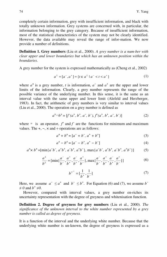
74 Y. Yang
completely certain information, grey with insufficient information, and black with totally unknown information. Grey systems are concerned with, in particular, the information belonging to the grey category. Because of insufficient information, most of the statistical characteristics of the system may not be clearly identified. However, the data available may reveal the range of infor-mation. We now provide a number of definitions.
Definition 1. Grey numbers (Liu et al., 2000). A grey number is a num-ber with clear upper and lower boundaries but which has an unknown position within the boundaries.
A grey number for the system is expressed mathematically as (Cheng et al., 2002)
}|{],[ +−±+−± <<∈== ataataaa (1)
where a± is a grey number, t is information, a− and a+ are the upper and lower limits of the information. Clearly, a grey number represents the range of the possible variance of the underlying number. In this sense, it is the same as an interval value with the same upper and lower limit (Alefeld and Herzberger, 1983). In fact, the arithmetic of grey numbers is very similar to interval values (Liu et al., 2000). The operation on a grey number is defined as
a± ⊗b± = [f−(a+, b+, a−, b−), f+(a+, b+, a−, b−)] (2)
where ⊗ is an operator, f+ and f− are the functions for minimum and maximum values. The +, −, × and ÷ operations are as follows:
a± + b± = [a− + b−, a+ + b+] (3)
a± − b± = [a− − b+, a+ − b−] (4)
a±× b± =[min{a−b−, a+b+, a−b+, a+b−}, max{a−b−, a+b+, a−b+, a+b−}] (5)
}],,,max{},,,,[min{ −
+
+
−
+
+
−
−
−
+
+
−
+
+
−
−
±
±
=b
a
b
a
b
a
b
a
b
a
b
a
b
a
b
a
b
a (6)
]1
,1
[1
−+± =
−
bbb (7)
Here, we assume a− ≤ a+ and b− ≤ b+. For Equation (6) and (7), we assume b− ≠ 0 and b+ ≠0.
However, compared with interval values, a grey number en-riches its uncertainty representation with the degree of greyness and whitenisation function.
Definition 2. Degree of greyness for grey numbers (Liu et al., 2000). The significance of the unknown interval to the white number represented by a grey number is called as degree of greyness.
It is a function of the interval and the underlying white number. Because that the underlying white number is un-known, the degree of greyness is expressed as a
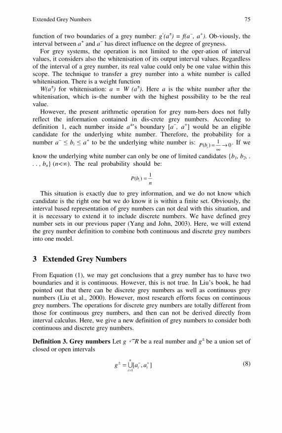
Extended Grey Numbers 75
function of two boundaries of a grey number: g◦(a±) = f(a−, a+). Ob-viously, the interval between a+ and a− has direct influence on the degree of greyness.
For grey systems, the operation is not limited to the oper-ation of interval values, it considers also the whitenisation of its output interval values. Regardless of the interval of a grey number, its real value could only be one value within this scope. The technique to transfer a grey number into a white number is called whitenisation. There is a weight function
W(a±) for whitenisation: a = W (a±). Here a is the white number after the whitenisation, which is the number with the highest possibility to be the real value.
However, the present arithmetic operation for grey num-bers does not fully reflect the information contained in dis-crete grey numbers. According to definition 1, each number inside a±’s boundary [a−, a+] would be an eligible candidate for the underlying white number. Therefore, the probability for a number a− ≤ bi ≤ a+ to be the underlying white number is: 0
1)( →
∞=ibP . If we
know the underlying white number can only be one of limited candidates {b1, b2, . . . , bn} (n<∞). The real probability should be:
nbP i
1)( =
This situation is exactly due to grey information, and we do not know which candidate is the right one but we do know it is within a finite set. Obviously, the interval based representation of grey numbers can not deal with this situation, and it is necessary to extend it to include discrete numbers. We have defined grey number sets in our previous paper (Yang and John, 2003). Here, we will extend the grey number definition to combine both continuous and discrete grey numbers into one model.
3 Extended Grey Numbers
From Equation (1), we may get conclusions that a grey number has to have two boundaries and it is continuous. However, this is not true. In Liu’s book, he had pointed out that there can be discrete grey numbers as well as continuous grey numbers (Liu et al., 2000). However, most research efforts focus on continuous grey numbers. The operations for discrete grey numbers are totally different from those for continuous grey numbers, and then can not be derived directly from interval calculus. Here, we give a new definition of grey numbers to consider both continuous and discrete grey numbers.
Definition 3. Grey numbers Let g ∈R be a real number and g± be a union set of closed or open intervals
],[1
+−
=
± = ii
n
iaag ∪ (8)
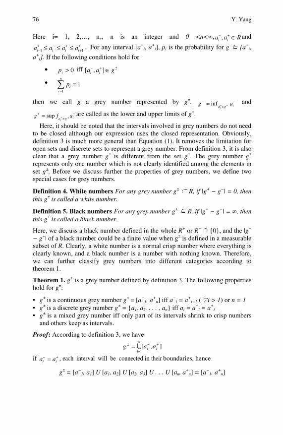
76 Y. Yang
Here i= 1, 2,…, n+, n is an integer and 0 <n<∞, Raa ii ∈+− , and ++
+−+− ≤≤≤ 11 iiii aaaa . For any interval [a−
i, a+
i], pi is the probability for g ∈ [a−i,
a+i]. If the following conditions hold for
• 0>ip iff ±+− ∈ gaa ii ],[
• 11
=∑=
n
iip
then we call g a grey number represented by g±. −∈
−±−= iga
agi
inf and
+∈
+±+= igaafg
isup are called as the lower and upper limits of g±.
Here, it should be noted that the intervals involved in grey numbers do not need to be closed although our expression uses the closed representation. Obviously, definition 3 is much more general than Equation (1). It removes the limitation for open sets and discrete sets to represent a grey number. From definition 3, it is also clear that a grey number g± is different from the set g±. The grey number g± represents only one number which is not clearly identified among the elements in set g±. Before we discuss further the properties of grey numbers, we define two special cases for grey numbers.
Definition 4. White numbers For any grey number g± ∈ R, if |g+ − g−| = 0, then this g± is called a white number.
Definition 5. Black numbers For any grey number g± ∈ R, if |g+ − g−| = ∞, then this g± is called a black number.
Here, we discuss a black number defined in the whole R+ or R+ ∩ {0}, and the |g+ − g−| of a black number could be a finite value when g± is defined in a measurable subset of R. Clearly, a white number is a normal crisp number where everything is clearly known, and a black number is a number with nothing known. Therefore, we can further classify grey numbers into different categories according to theorem 1.
Theorem 1. g± is a grey number defined by definition 3. The following properties hold for g±:
• g± is a continuous grey number g± = [a−1, a
+n] iff a
−i = a+
i−1 (∀i > 1) or n = 1 • g± is a discrete grey number g± = {a1, a2, . . . , an} iff ai = a−
i = a+i
• g± is a mixed grey number iff only part of its intervals shrink to crisp numbers and others keep as intervals.
Proof: According to definition 3, we have
],[1
+−
=
± = ii
n
iaag ∪
if +− = ii aa , each interval will be connected in their boundaries, hence
g± = [a−1, a1] U [a1, a2] U [a2, a3] U . . . U [an, a
+n] = [a−
1, a+
n]
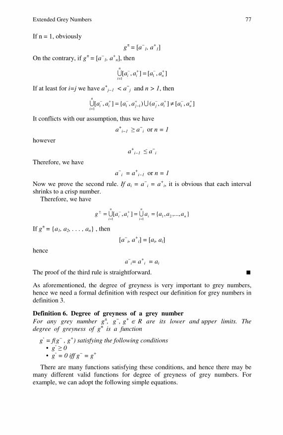
Extended Grey Numbers 77
If n = 1, obviously
g± = [a−1, a
+1]
On the contrary, if g± = [a−1, a
+n], then
],[],[ 11
+−+−
== nii
n
iaaaa∪
If at least for i=j we have a+j−1 < a−
j and n > 1, then
],[],(),{],[ 1111
+−+−+−
−+−
=≠= nijjii
n
iaaaaaaaa ∪∪
It conflicts with our assumption, thus we have
a+i−1 ≥ a−
i or n = 1
however
a+i−1 ≤ a−
i
Therefore, we have
a−i = a+
i−1 or n = 1
Now we prove the second rule. If ai = a−i = a+
i, it is obvious that each interval shrinks to a crisp number.
Therefore, we have
},...,,{],[ 2111
ni
n
iii
n
iaaaaaag ===
=
+−
=
± ∪∪
If g± = {a1, a2, . . . , an} , then
[a−i, a
+i] = [ai, ai]
hence
a−i= a+
i = ai
The proof of the third rule is straightforward.
As aforementioned, the degree of greyness is very important to grey numbers, hence we need a formal definition with respect our definition for grey numbers in definition 3.
Definition 6. Degree of greyness of a grey number For any grey number g±, g−, g+ ∈ R are its lower and upper limits. The degree of greyness of g± is a function
g◦ = f(g− , g+) satisfying the following conditions • g◦ ≥ 0 • g◦ = 0 iff g− = g+
There are many functions satisfying these conditions, and hence there may be many different valid functions for degree of greyness of grey numbers. For example, we can adopt the following simple equations.

78 Y. Yang
If we consider grey numbers in the positive R+ U {0}, we can define it as
−+
−+
+−=
gg
ggg (9)
From equation (9), g◦ = 1 when g− = 0. Under this situation, g± is a black number.
It is obvious that Equation (9) satisfies all properties in definition 6. From definition 6 and Equation (9) we can also see that the degree of greyness of a grey number depends only on the two limits of a grey number and has nothing to do with the cardinality of its candidate set. For example, both g1
± = [40, 60] and g2± =
{40, 60} have the same degree of greyness using Equation (9)
2.04060
406021 =
+−== gg
but their cardinalities are completely different
Card(g1±) = ∞, Card(g2
±) = 2
This indicates that the degree of greyness is a parameter for the grey number rather than any candidate in its candidate set. This is different from the probability for each number in its candidate set to be the underlying white number.
4 Operations on Grey Numbers
For any two numbers ],[1
+−
=
± = ii
m
iaaa ∪ and ],[
1
+−
=
± = ii
n
ibbb ∪ defined by definition 3, their
arithmetic operations follow the same rules as in Equation (2). However, because of the involvement of discrete grey numbers and mixed grey numbers, the operation has to consider those separate intervals or numbers. Therefore, Equation (2) has to be modified to consider these new parameters.
)],,,(),,,,([11
−−+++−−++−
==
±± =⊗ jijijiji
n
j
m
ibabafbabafba ∪∪ (10)
Obviously, Equation (2) is a special case of Equation (10) when m=n=1. From this, we can derive the corresponding operations for addition, subtract, times and division operations.
According to Equation (3)–(7), the +, −, × and ÷ opera-tions can be derived from Equation (10) as follows:
],[11
++−−
==
±± ++=+ jiji
n
j
m
ibababa ∪∪ (11)
],[11
−++−
==
±± −−=− jiji
n
j
m
ibababa ∪∪ (12)
}],,,max{},,,,[min{`11
−++−++−−−++−++−−
==
±± =× jijijijijijijiji
n
j
m
ibababababababababa ∪∪ (13)
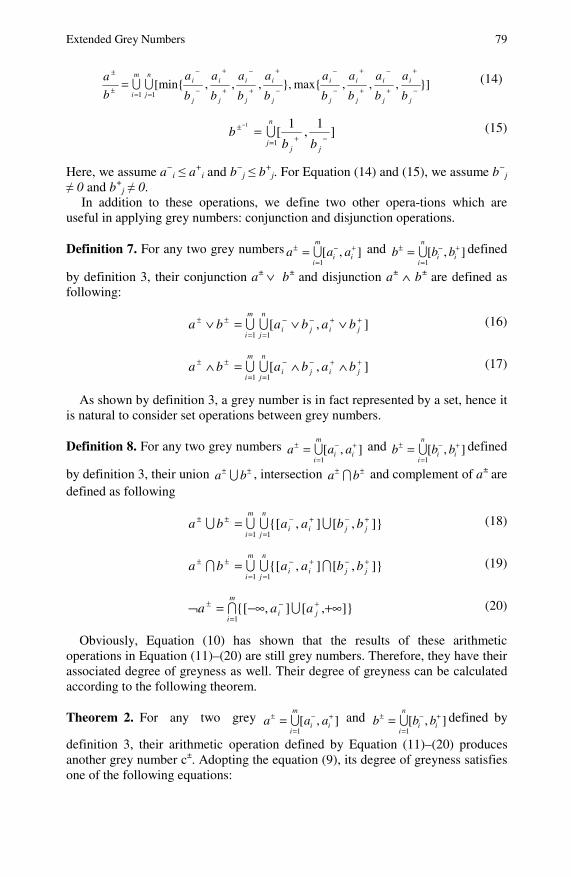
Extended Grey Numbers 79
}],,,max{},,,,[min{11 −
+
+
−
+
+
−
−
−
+
+
−
+
+
−
−
==±
±
=j
i
j
i
j
i
j
i
j
i
j
i
j
i
j
in
j
m
i b
a
b
a
b
a
b
a
b
a
b
a
b
a
b
a
b
a ∪∪ (14)
]1
,1
[1
1
−+=
± =−
jj
n
j bbb ∪ (15)
Here, we assume a−i ≤ a+
i and b−j ≤ b+
j. For Equation (14) and (15), we assume b−j
≠ 0 and b+j ≠ 0.
In addition to these operations, we define two other opera-tions which are useful in applying grey numbers: conjunction and disjunction operations.
Definition 7. For any two grey numbers ],[1
+−
=
± = ii
m
iaaa ∪ and ],[
1
+−
=
± = ii
n
ibbb ∪ defined
by definition 3, their conjunction a± ∨ b± and disjunction a± ∧ b± are defined as following:
],[11
++−−
==
±± ∨∨=∨ jiji
n
j
m
ibababa ∪∪ (16)
],[11
++−−
==
±± ∧∧=∧ jiji
n
j
m
ibababa ∪∪ (17)
As shown by definition 3, a grey number is in fact represented by a set, hence it is natural to consider set operations between grey numbers.
Definition 8. For any two grey numbers ],[1
+−
=
± = ii
m
iaaa ∪ and ],[
1
+−
=
± = ii
n
ibbb ∪ defined
by definition 3, their union ±± ba ∪ , intersection ±± ba ∩ and complement of a± are defined as following
]},[],{[11
+−+−
==
±± = jjii
n
j
m
ibbaaba ∪∪∪∪ (18)
]},[],{[11
+−+−
==
±± = jjii
n
j
m
ibbaaba ∩∪∪∩ (19)
]},[],{[1
+∞−∞=¬ +−
=
±ji
m
iaaa ∪∩ (20)
Obviously, Equation (10) has shown that the results of these arithmetic operations in Equation (11)–(20) are still grey numbers. Therefore, they have their associated degree of greyness as well. Their degree of greyness can be calculated according to the following theorem.
Theorem 2. For any two grey ],[1
+−
=
± = ii
m
iaaa ∪ and ],[
1
+−
=
± = ii
n
ibbb ∪ defined by
definition 3, their arithmetic operation defined by Equation (11)–(20) produces another grey number c±. Adopting the equation (9), its degree of greyness satisfies one of the following equations:
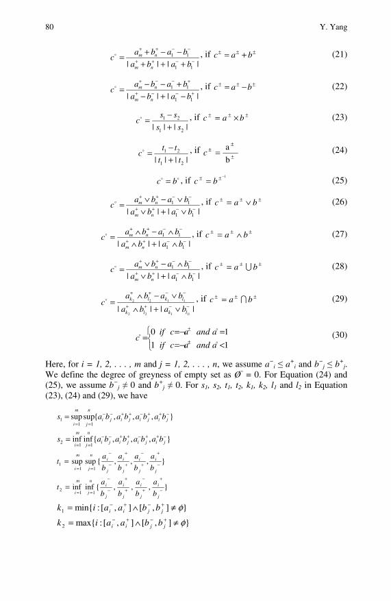
80 Y. Yang
|||| 11
11−−++
−−++
+++−−+=
baba
babac
nm
nm , if ±±± += bac (21)
|||| 11
11+−−+
+−−+
−+−+−−=
baba
babac
nm
nm , if ±±± −= bac (22)
|||| 21
21
ss
ssc
+−= , if ±±± ×= bac (23)
|||| 21
21
tt
ttc
+−= , if
±
±± =
b
a c (24)
bc = , if 1−±± = bc (25)
|||| 11
11−−++
−−++
∨+∨∨−∨=
baba
babac
nm
nm , if ±±± ∨= bac (26)
|||| 11
11−−++
−−++
∧+∧∧−∧=
baba
babac
nm
nm , if ±±± ∧= bac (27)
|||| 11
11−−++
−−++
∧+∨∧−∨=
baba
babac
nm
nm , if ±±± = bac ∪ (28)
|||||1122
1122
−−++
−−++
∨+∧∨−∧
=lklk
lklk
baba
babac , if ±±± = bac ∩ (29)
⎩⎨⎧
<¬==¬=
=±
±
11
10
aandacif
aandacifc (30)
Here, for i = 1, 2, . . . , m and j = 1, 2, . . . , n, we assume a−i ≤ a+
i and b−j ≤ b+
j. We define the degree of greyness of empty set as Ø◦ = 0. For Equation (24) and (25), we assume b−
j ≠ 0 and b+j ≠ 0. For s1, s2, t1, t2, k1, k2, l1 and l2 in Equation
(23), (24) and (29), we have
},,,{supsup11
1−++−++−−
=== jijijiji
n
j
m
ibabababas
},,,{infinf11
2−++−++−−
=== jijijiji
n
j
m
ibabababas
},,,{supsup11
1 −
+
+
−
+
+
−
−
===
j
i
j
i
j
i
j
in
j
m
i b
a
b
a
b
a
b
at
},,,{infinf11
2 −
+
+
−
+
+
−
−
===
j
i
j
i
j
i
j
in
j
m
i b
a
b
a
b
a
b
at
}],[],[:min{1 φ≠∧= +−+−jjii bbaaik
}],[],[:max{2 φ≠∧= +−+−jjii bbaaik
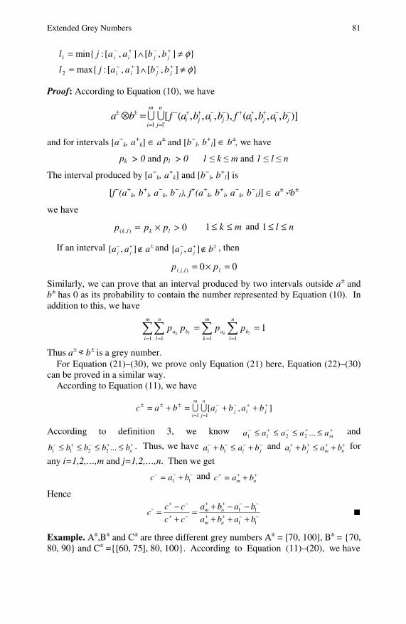
Extended Grey Numbers 81
}],[],[:min{1 φ≠∧= +−+−jjii bbaajl
}],[],[:max{2 φ≠∧= +−+−jjii bbaajl
Proof: According to Equation (10), we have
)],,,(),,,,([11
−−+++−−++−
==
±± =⊗ jijijiji
n
j
m
ibabafbabafba ∪∪
and for intervals [a−k, a
+k] ∈ a± and [b−
l, b+
l] ∈ b±, we have
pk > 0 and pl > 0 1 ≤ k ≤ m and 1 ≤ l ≤ n
The interval produced by [a−k, a
+k] and [b−
l, b+
l] is
[f−(a+k, b
+l, a
−k, b
−l), f
+(a+k, b
+l, a
−k, b
−l)] ∈ a± ⊗b±
we have
0),( >×= lklk ppp mk ≤≤1 and nl ≤≤1
If an interval ±+− ∉ aaa jj ],[ and ±+− ∉ baa jj ],[ , then
00),( =×= llj pp
Similarly, we can prove that an interval produced by two intervals outside a± and b± has 0 as its probability to contain the number represented by Equation (10). In addition to this, we have
1111 1
== ∑∑∑∑=== =
n
lb
m
ka
m
i
n
lba lklk
pppp
Thus a± ⊗ b± is a grey number. For Equation (21)–(30), we prove only Equation (21) here, Equation (22)–(30)
can be proved in a similar way. According to Equation (11), we have
],[11
++−−
==
±±± ++=+= jiji
n
j
m
ibababac ∪∪
According to definition 3, we know ++−+− ≤≤≤≤ maaaaa ...2211 and
++−+− ≤≤≤≤ nbbbbb ...2211. Thus, we have −−−− +≤+ ji baba 11
and ++++ +≤+ nmji baba for
any i=1,2,…,m and j=1,2,…,n. Then we get −−− += 11 bac and +++ += nm bac
Hence
−−++
−−++
−+
−+
+++−−+=
+−=
11
11
baba
baba
cc
ccc
nm
nm
Example. A±,B± and C± are three different grey numbers A± = [70, 100], B± = {70, 80, 90} and C± ={[60, 75], 80, 100}. According to Equation (11)–(20), we have
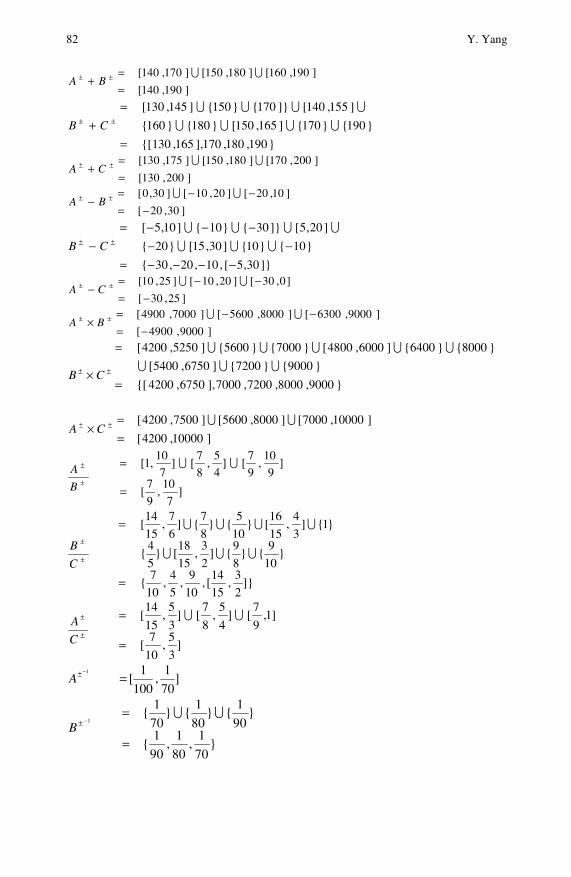
82 Y. Yang
]190,140[
]190,160[]180,150[]170,140[
==
+ ±± ∪∪BA
}190,180,170],165,130{[
}190{}170{]165,150[}180{}160{
]155,140[]}170{}150{]145,130[
=
=+ ±± ∪∪∪∪
∪∪∪∪CB
]200,130[
]200,170[]180,150[]175,130[
==
+ ±± ∪∪CA
]30,20[
]10,20[]20,10[]30,0[
−=−−=
− ±± ∪∪BA
]}30,5[,10,20,30{
}10{}10{]30,15[}20{
]20,5[]}30{}10{]10,5[
−−−−=−−
−−−=− ±± ∪∪∪
∪∪∪∪CB
]25,30[
]0,30[]20,10[]25,10[
−=−−=
− ±± ∪∪CA
]9000,4900[
]9000,6300[]8000,5600[]7000,4900[
−=−−=
× ±± ∪∪BA
}9000,8000,7200,7000],6750,4200{[
}9000{}7200{]6750,5400[
}8000{}6400{]6000,4800[}7000{}5600{]5250,4200[
=
=
× ±± ∪∪∪∪∪∪∪∪
CB
]10000,4200[
]10000,7000[]8000,5600[]7500,4200[
==
× ±± ∪∪CA
]7
10,
9
7[
]9
10,
9
7[]
4
5,
8
7[]
7
10,1[
=
=±
± ∪∪
B
A
]}2
3,
15
14[,
10
9,
5
4,
10
7{
}10
9{}
8
9{]
2
3,
15
18[}
5
4{
}1{]3
4,
15
16[}
10
5{}
8
7{]
6
7,
15
14[
=
=
±
±
∪∪∪
∪∪∪∪
C
B
]3
5,
10
7[
]1,9
7[]
4
5,
8
7[]
3
5,
15
14[
=
=±
± ∪∪
C
A
]70
1,
100
1[
1
=−±A
}70
1,
80
1,
90
1{
}90
1{}
80
1{}
70
1{
1
=
=−±
∪∪B

Extended Grey Numbers 83
]}60
1,
75
1[,
80
1,
100
1{
}100
1{}
80
1{]
60
1,
75
1[
1
=
=−±
∪∪C
]100,70[
]100,90[]100,80[]100,70[
==
∨ ±± ∪∪BA
}100,90,80],75,70{[
}100{}90{]90,90[}100{}80{
]80,80[}100{}80{]75,70[
=
=∨ ±± ∪∪∪∪
∪∪∪∪CB
]100,70[
]100,100[]100,80[]100,70[
==
∨ ±± ∪∪CA
]90,70[
]90,70[]80,70[]70,70[
==
∧ ±± ∪∪BA
}90,80],75,60{[
}90{}80{]75,60[}80{}80{
]75,60[}70{}70{]70,60[
=
=∧ ±± ∪∪∪∪
∪∪∪∪CB
]100,60[
]100,70[]80,70[]75,60[
==
∧ ±± ∪∪CA
]100,70[
]100,70[]100,70[]100,70[
==±± ∪∪
∪ BA
}100,90,80],75,60{[
}100,90{}90,80{}90],75,60{[
}100,80{}80{}80],75,60{[
}100,70{}80,70{]75,60[
=
=
±±
∪∪∪∪∪
∪∪∪
∪ CB
]100,60[
]100,70[]100,70[]100,60[
==±± ∪∪
∪ CA
}90,80,70{
}90{}80{}70{
==±± ∪∪
∩ BA
}80,70{
}80{}70{
==±± ∪
∩ CB
}100,80},75,70{[
}100{}80{]}75,70[
==±± ∪∪
∩ CA
]},100(),70,{[
]},100()70,{[
+∞−∞=+∞−∞=
¬ ± ∪A
]},90(),90,80(),80,70(),60,{[
],90()90,[
],80()80,[],70()70,[
+∞−∞=+∞−∞
+∞−∞+∞−∞=¬ ± ∪∪
∪∪∪B
]},100(),100,80(),80,75(),60,{[
],100()100,[
],80()80,[],75()60,[
+∞−∞=+∞−∞
+∞−∞+∞−∞=¬ ± ∪∪
∪∪∪C
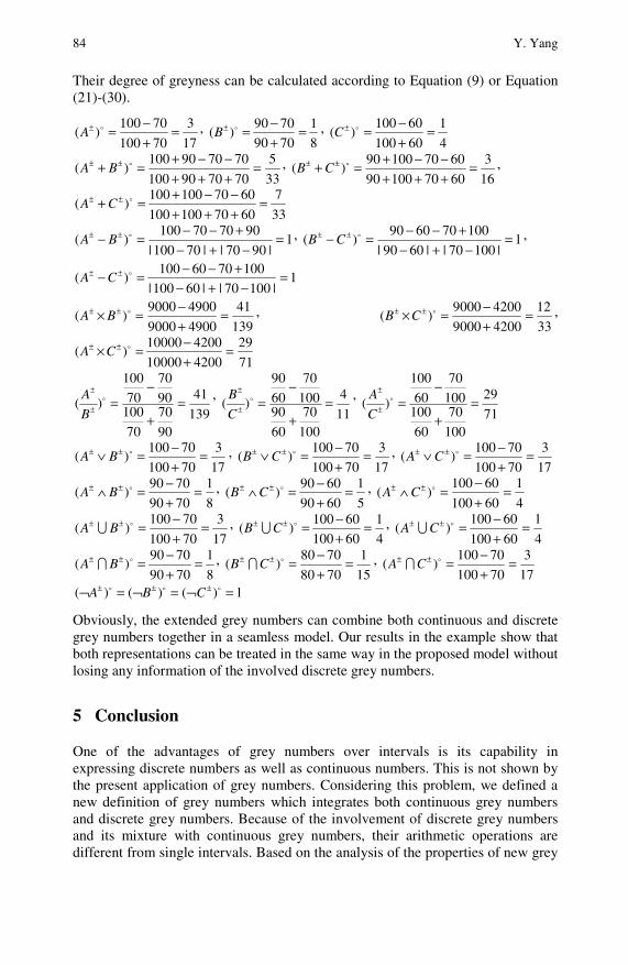
84 Y. Yang
Their degree of greyness can be calculated according to Equation (9) or Equation (21)-(30).
17
3
70100
70100)( =
+−=±A ,
8
1
7090
7090)( =
+−=±B ,
4
1
60100
60100)( =
+−=±C
33
5
707090100
707090100)( =
+++−−+=+ ±± BA ,
16
3
607010090
607010090)( =
+++−−+=+ ±± CB ,
33
7
6070100100
6070100100)( =
+++−−+=+ ±± CA
1|9070||70100|
907070100)( =
−+−+−−=− ±± BA , 1
|10070||6090|
100706090)( =
−+−+−−=− ±± CB ,
1|10070||60100|
1007060100)( =
−+−+−−=− ±± CA
139
41
49009000
49009000)( =
+−=× ±± BA ,
33
12
42009000
42009000)( =
+−=× ±± CB ,
71
29
420010000
420010000)( =
+−=× ±± CA
139
41
90
70
70
10090
70
70
100
)( =+
−=±
±
B
A , 11
4
100
70
60
90100
70
60
90
)( =+
−=±
±
C
B , 71
29
100
70
60
100100
70
60
100
)( =+
−=±
±
C
A
17
3
70100
70100)( =
+−=∨ ±± BA ,
17
3
70100
70100)( =
+−=∨ ±± CB ,
17
3
70100
70100)( =
+−=∨ ±± CA
8
1
7090
7090)( =
+−=∧ ±± BA ,
5
1
6090
6090)( =
+−=∧ ±± CB ,
4
1
60100
60100)( =
+−=∧ ±± CA
17
3
70100
70100)( =
+−=±± ∪ BA ,
4
1
60100
60100)( =
+−=±± ∪CB ,
4
1
60100
60100)( =
+−=±± ∪CA
8
1
7090
7090)( =
+−=±± ∩ BA ,
15
1
7080
7080)( =
+−=±± ∩CB ,
17
3
70100
70100)( =
+−=±± ∩CA
1)()()( =¬=¬=¬ ±±± CBA
Obviously, the extended grey numbers can combine both continuous and discrete grey numbers together in a seamless model. Our results in the example show that both representations can be treated in the same way in the proposed model without losing any information of the involved discrete grey numbers.
5 Conclusion
One of the advantages of grey numbers over intervals is its capability in expressing discrete numbers as well as continuous numbers. This is not shown by the present application of grey numbers. Considering this problem, we defined a new definition of grey numbers which integrates both continuous grey numbers and discrete grey numbers. Because of the involvement of discrete grey numbers and its mixture with continuous grey numbers, their arithmetic operations are different from single intervals. Based on the analysis of the properties of new grey
Extended Grey Numbers 85
numbers, we discussed their degree of greyness and derived their arithmetic operations and relevant degree of greyness. Our results show that grey numbers are different from intervals and have more powerful capability in expressing uncertainty caused by missing information.
References
Alefeld, G., Herzberger, J.: Introduction to Interval Computations. Academic Press Inc., New York (1983); Transl. by J. Rokne from the original German ‘Einfuhrung" In Die Intervallrechnung’
Cheng, F.J., Hui, S.H., Chen, Y.C.: Reservoir operation using grey fuzzy stochastic dynamic programming. Hydrological Processes 16, 2395–2408 (2002)
Deng, J.L.: The control problems of grey systems. Systems and Control Letters 1(5), 288–294 (1982)
Liu, S., Gao, T., Dang, Y.: Grey Systems Theory and Its Applications. Science Press, Beijing (2000)
Yang, Y., John, R.: Grey systems and interval valued fuzzy sets. In: Wagenknecht, M., Hampel, R. (eds.) Third EUSFLAT Proceedings, Zittau, Germany, September 2003, pp. 193–197. European Society for Fuzzy Logic and Technology (2003)
Liu, S.F., Lin, Y.: Grey Information: Theory and Practical Applications. Springer, London (2006)
Lin, Y., Chen, M.Y., Liu, S.F.: Theory of grey systems: capturing uncertainties of grey information. Kybernetes: The International Journal of Systems and Cybernetics 33(2), 196–218 (2004)
Lin, Y., Liu, S.F.: Solving Problems with incomplete information: a grey systems approach. In: Advances in Imaging and Electron Physics, vol. 141, pp. 77–174. Elsevier, Oxford (2006)

Industrial Restructuring of Jiangsu Based on the Grey Linear Programming Model Considering Energy-Saving*
Chaoqing Yuan and Sifeng Liu1
It was found that the change of industrial structure increased energy intensity from 2000 to 2007 in Jiangsu. The reason is that the second industry grew very rapidly, and the proportion of the second industry increased. A grey linear programming model was created to find an ideal industry structure to decrease energy consumption. It was concluded that the energy intensity of Jiangsu will decline by the industrial restructuring from 2007 to 2010.
1 Introduction
Since 2000, the economy has grown rapidly in Jiangsu province; meanwhile, the energy consumption has grown along with economy. Economy growth depends on the growth of secondary industry in Jiangsu, but the secondary industry consumes more energy, so the industrial structure has a great effect on energy consumption in Jiangsu. Many researchers have studied the energy-saving effect of the industrial structure. The energy intensity in China has declined, and efficiency effects contributed the majority while structure effects contributed less (X. Lin, 1995; Hua Liao, 1997). It is similar in Chinese industrial sectors (Stinton, 1994; Zhong, 2003). With the exception of few years, industry restructuring even has had a negative effect on energy efficiency (Wu Qiaosheng, 2006). The secondary industry is predominantly a driving force to reducing comprehensive energy intensity, while tertiary industry development will also lead the energy intensity ascending in Shanghai (Lin Yanjun, 2006). The efficiency share is a major factor affecting energy consumption intensity, and the structure share is playing a negative role in the decrease of energy consumption intensity. Moreover, the impact of efficiency
Chaoqing Yuan and Sifeng Liu Economics and Management College, Nanjing University of Aeronautics and Astronautics, CO 210016 China e-mail: [email protected], [email protected]
* This work was supported in part by the United Nations Development Programme (UNDP) Tender Project (00035738C27), Jiangsu Social Science Fund (07EYA017), and Social Project of the Ministry of Education (07JC630064).
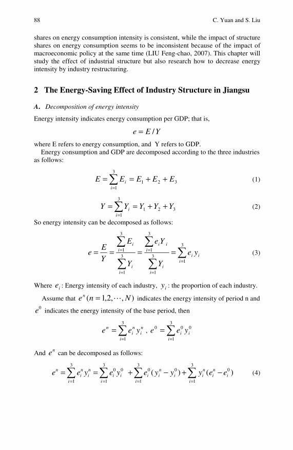
88 C. Yuan and S. Liu
shares on energy consumption intensity is consistent, while the impact of structure shares on energy consumption seems to be inconsistent because of the impact of macroeconomic policy at the same time (LIU Feng-chao, 2007). This chapter will study the effect of industrial structure but also research how to decrease energy intensity by industry restructuring.
2 The Energy-Saving Effect of Industry Structure in Jiangsu
A. Decomposition of energy intensity
Energy intensity indicates energy consumption per GDP; that is,
YEe /=
where E refers to energy consumption, and Y refers to GDP. Energy consumption and GDP are decomposed according to the three industries
as follows:
321
3
1
EEEEEi
i ++==∑=
(1)
321
3
1
YYYYYi
i ++==∑=
(2)
So energy intensity can be decomposed as follows:
∑∑
∑
∑
∑=
=
=
=
= ====3
13
1
3
13
1
3
1
iii
ii
iii
ii
ii
yeY
Ye
Y
E
Y
Ee (3)
Where ie : Energy intensity of each industry, iy : the proportion of each industry.
Assume that ),,2,1( Nnen = indicates the energy intensity of period n and 0e indicates the energy intensity of the base period, then
∑=
=3
1i
ni
ni
n yee , ∑=
=3
1
000
iii yee
And ne can be decomposed as follows:
∑∑==
==3
1
003
1 iii
i
ni
ni
n yeyee ∑∑==
−+−+3
1
03
1
00 )()(i
ini
ni
ii
nii eeyyye (4)
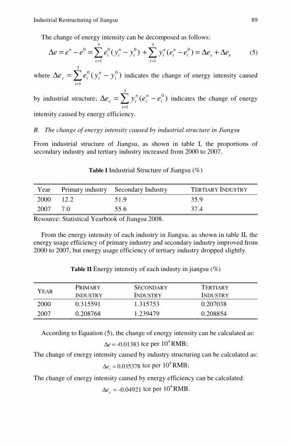
Industrial Restructuring of Jiangsu 89
The change of energy intensity can be decomposed as follows:
∑=
−=−=Δ3
1
000 )(i
inii
n yyeeee esi
ini
ni eeeey Δ+Δ=−+∑
=
3
1
0 )( (5)
where ∑=
−=Δ3
1
00 )(i
iniis yyee indicates the change of energy intensity caused
by industrial structure; ∑=
−=Δ3
1
0 )(i
ini
nie eeye indicates the change of energy
intensity caused by energy efficiency.
B. The change of energy intensity caused by industrial structure in Jiangsu
From industrial structure of Jiangsu, as shown in table I, the proportions of secondary industry and tertiary industry increased from 2000 to 2007.
Table I Industrial Structure of Jiangsu (%)
Year Primary industry Secondary Industry TERTIARY INDUSTRY
2000 12.2 51.9 35.9
2007 7.0 55.6 37.4
Resource: Statistical Yearbook of Jiangsu 2008.
From the energy intensity of each industry in Jiangsu, as shown in table II, the energy usage efficiency of primary industry and secondary industry improved from 2000 to 2007, but energy usage efficiency of tertiary industry dropped slightly.
Table II Energy intenstiy of each industy in jiangsu (%)
YEAR PRIMARY
INDUSTRY SECONDARY
INDUSTRY TERTIARY
INDUSTRY 2000 0.315591 1.315753 0.207038
2007 0.208768 1.239479 0.208854
According to Equation (5), the change of energy intensity can be calculated as:
-0.01383=Δe tce per 104 RMB;
The change of energy intensity caused by industry structuring can be calculated as:
0.035378=Δ se tce per 104 RMB;
The change of energy intensity caused by energy efficiency can be calculated:
-0.04921=Δ ee tce per 104 RMB.

90 C. Yuan and S. Liu
The improvement of energy efficiency decreased energy intensity 0.04921 tce per 104 RMB, but industrial structure increased energy intensity 0.035378 tce per 104 RMB, so energy intensity decreased 0.01383 tce per 104 RMB. The growth of the proportion of secondary industry increased the energy intensity from 2000 to 2007. Jiangsu has a large proportion of secondary industry, so industrial restructuring is very important to save energy.
3 Industrial Restructuring to Save Energy
A. Model
In this chapter, a grey linear programming model (Lin and Liu, 1999) is created to study how to decrease energy intensity by industrial restructuring, considering fixed assets, labor, water resource constraints, as well as the characteristics of regional economic growth.
Table III Value added of secondary industry and tertiary industry (100 million yuan)
Year Secondary industry Tertiary Industry
1992 1664.17 1235.333
1993 2052.606 1545.868
1994 2519.692 1721.936
1995 2926.665 1977.836
1996 3288.103 2261.523
1997 3703.228 2580.025
1998 4152.445 2913.057
1999 4621.258 3205.202
2000 5156.966 3563.766
2001 5721.246 3971.866
2002 6503.31 4432.34
2003 7623.117 4980.003
2004 8927.957 5647.072
2005 10355.04 6489.14
2006 12011.85 7494.957
2007 13877.93 8708.081
Resource: Statistical Yearbook of Jiangsu2008.
The development of tertiary industry is closely related to that of the secondary industry in Jiangsu Province, as shown in table III. A linear regression model is set up in which the Value Added of secondary industry is an independent variable and
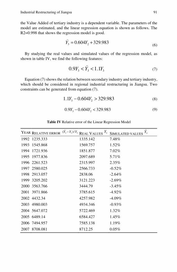
Industrial Restructuring of Jiangsu 91
the Value Added of tertiary industry is a dependent variable. The parameters of the model are estimated, and the linear regression equation is shown as follows. The R2=0.998 that shows the regression model is good.
983.293604.0 23 += YY (6)
By studying the real values and simulated values of the regression model, as shown in table IV, we find the following features:
333 1.19.0 YYY << (7)
Equation (7) shows the relation between secondary industry and tertiary industry, which should be considered in regional industrial restructuring in Jiangsu. Two constraints can be generated from equation (7).
983.293604.01.1 23 >− YY (8)
983.293604.09.0 23 <− YY (9)
Table IV Relative error of the Linear Regression Model
YEAR RELATIVE ERROR 333 /)( YYY − REAL VALUES 3Y SIMULATED VALUES 3Y 1992 1235.333 1335.142 7.48%
1993 1545.868 1569.757 1.52%
1994 1721.936 1851.877 7.02%
1995 1977.836 2097.689 5.71%
1996 2261.523 2315.997 2.35%
1997 2580.025 2566.733 -0.52%
1998 2913.057 2838.06 -2.64%
1999 3205.202 3121.223 -2.69%
2000 3563.766 3444.79 -3.45%
2001 3971.866 3785.615 -4.92%
2002 4432.34 4257.982 -4.09%
2003 4980.003 4934.346 -0.93%
2004 5647.072 5722.469 1.32%
2005 6489.14 6584.427 1.45%
2006 7494.957 7585.138 1.19%
2007 8708.081 8712.25 0.05%
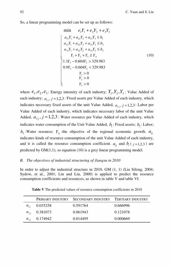
92 C. Yuan and S. Liu
So, a linear programming model can be set up as follows:
332211min YeYeYe ++
⎪⎪⎪⎪⎪⎪
⎩
⎪⎪⎪⎪⎪⎪
⎨
⎧
>>>
<−>−≥++
≤++≤++≤++
0
00
983.293604.09.0
983.293604.01.1
3
2
1
23
23
321
3333232131
2323222121
1313212111
Y
YY
YY
YY
YYYY
bYaYaYa
bYaYaYa
bYaYaYa
A (10)
where 321 ,, eee : Energy intensity of each industry; 321 ,, YYY : Value Added of
each industry; 3,2,1,1 =ja j: Fixed assets per Value Added of each industry, which
indicates necessary fixed assets of the unit Value Added, 3,2,1,2 =ja j: Labor per
Value Added of each industry, which indicates necessary labor of the unit Value
Added, 3,2,1,3 =ja j : Water resource per Value Added of each industry, which
indicates water consumption of the Unit Value Added, 1b : Fixed assets; 2b : Labor;
3b :Water resource; AY :the objective of the regional economic growth. ija
indicates kinds of resource consumption of the unit Value Added of each industry, and it is called the resource consumption coefficient. ija and ib ( 3,2,1=j ) are
predicted by GM(1,1), so equation (10) is a grey linear programming model.
B. The objectives of industrial structuring of Jiangsu in 2010
In order to adjust the industrial structure in 2010, GM (1, 1) (Liu Sifeng, 2004; Sydow, et al., 2001; Lin and Liu, 2000) is applied to predict the resource consumption coefficients and resources, as shown in table V and table VI.
Table V The predicted values of resource consumption coefficients in 2010
PRIMARY INDUSTRY SECONDARY INDUSTRY TERTIARY INDUSTRY
ja1 0.035258 0.591764 0.666996
ja2 0.381073 0.061943 0.121078
ja3 0.174942 0.014495 0.000669
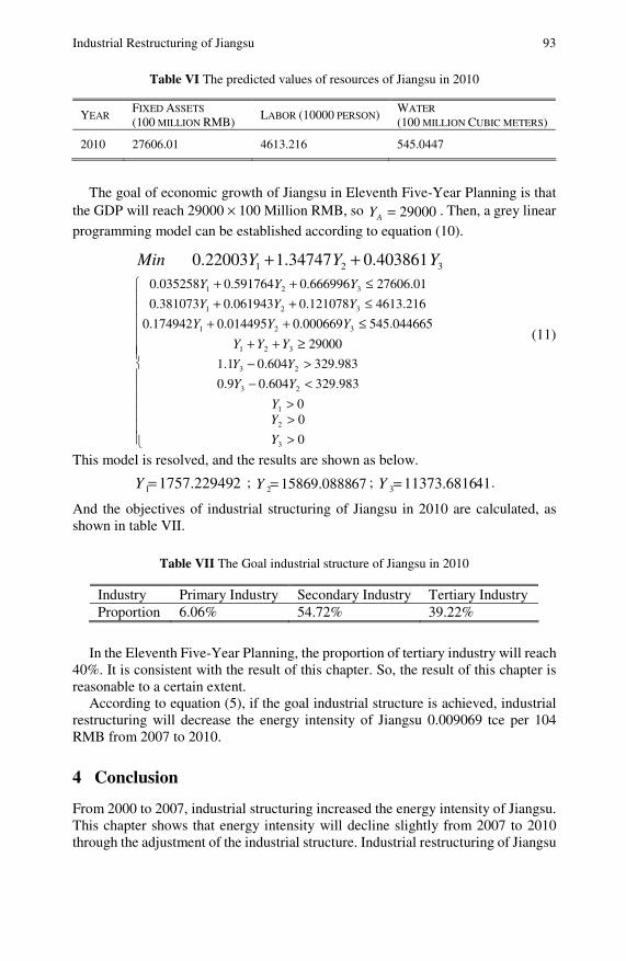
Industrial Restructuring of Jiangsu 93
Table VI The predicted values of resources of Jiangsu in 2010
YEAR FIXED ASSETS (100 MILLION RMB)
LABOR (10000 PERSON) WATER (100 MILLION CUBIC METERS)
2010 27606.01 4613.216 545.0447
The goal of economic growth of Jiangsu in Eleventh Five-Year Planning is that the GDP will reach 29000 × 100 Million RMB, so 29000=AY . Then, a grey linear
programming model can be established according to equation (10).
321 0.4038611.347470.22003 YYYMin ++
⎪⎪⎪⎪⎪⎪
⎩
⎪⎪⎪⎪⎪⎪
⎨
⎧
>>>
<−>−
≥++≤++≤++≤++
0
00
983.293604.09.0
983.293604.01.1
29000
545.0446650.0006690.0144950.174942
4613.2160.1210780.0619430.381073
27606.010.6669960.5917640.035258
3
2
1
23
23
321
321
321
321
Y
YY
YY
YY
YYY
YYY
YYY
YYY
(11)
This model is resolved, and the results are shown as below.
21757.229491=Y ; 6715869.08882=Y ; 4111373.68163=Y .
And the objectives of industrial structuring of Jiangsu in 2010 are calculated, as shown in table VII.
Table VII The Goal industrial structure of Jiangsu in 2010
Industry Primary Industry Secondary Industry Tertiary Industry Proportion 6.06% 54.72% 39.22%
In the Eleventh Five-Year Planning, the proportion of tertiary industry will reach 40%. It is consistent with the result of this chapter. So, the result of this chapter is reasonable to a certain extent.
According to equation (5), if the goal industrial structure is achieved, industrial restructuring will decrease the energy intensity of Jiangsu 0.009069 tce per 104 RMB from 2007 to 2010.
4 Conclusion
From 2000 to 2007, industrial structuring increased the energy intensity of Jiangsu. This chapter shows that energy intensity will decline slightly from 2007 to 2010 through the adjustment of the industrial structure. Industrial restructuring of Jiangsu

94 C. Yuan and S. Liu
is a difficult task. Secondary industry grows rapidly and promotes the development of Jiangsu. North of Jiangsu is a new and important growth pole of Jiangsu. Industrializing north of Jiangsu will accelerate the development of secondary industry in Jiangsu. The south of Jiangsu has entered an advanced stage of industrialization, with a foundation for the development of tertiary industry. Because the GDP of south of Jiangsu is much more than that of the north, the development of the tertiary industry of the south of Jiangsu is related to the overall optimization of industrial structure in Jiangsu. So, some industries should be focused in Nanjing, Suzhou, Wuxi and Changzhou, such as the modern logistics industry, the software industry, financial services, business and technology services, cultural industries, tourism and so on.
References
Lin, X., Polenske, K.R.: Input–output anatomy of China’s energy use changes in the 1980s. Econometrica 7, 67–84 (1995)
Liao, H., Fan, Y., Wei, Y.M.: What induced China’s energy intensity to fluctuate: 1997 – 2006. Energy Policy 25, 727–744 (1997)
Sinton, J.E., Levine, M.D.: Changing energy intensity in Chinese industry: the relative importance of structural shift and intensity change. Energy Policy 22, 239–255 (1994)
Zhong, X.Z.: Why did the energy intensity fall in China’s industrial sector in the 1990s, The relative importance of structural change and intensity change. Energy Economy 25, 625–638 (2003)
Wu, Q.H., Cheng, J.H.: Change in energy consumption intensity and the main factors during the process of China’s industrialization: An empirical analysis based on the decomposition model. Journal of Finance and Economics 2(6), 75–85 (2006)
Lin, Y.J., Feng, C.P.: The changes and trends of energy intensity and its’ influences the changes of energy intensity in Shanghai. Energy of China 28(2), 40–43 (2006)
Liu, F.C., Pan, X.F., Xu, G.Q.: An assessment of China’s energy consumption intensity based on structure share and efficiency share methods. Resources Science 29(4), 2–6 (2007)
Liu, S.F., Dang, Y.G., Fang, Z.G.: Grey Theory and Its Application, pp. 26–35. Science Press, Beijing (2004)
Lin, Y., Liu, S.F.: Several programming models with unascertained parameters and their applications. Multi-Criteria Decision Analysis 8, 206–220 (1999)
Sydow, A., Lin, Y., Liu, S.F., DeNu, R., Mennell, W.: Exponential prediction models based on sequence operators. Kybernetes 30(4), 397–410 (2001)
Lin, Y., Liu, S.F.: Law of exponentiality and exponential curve fitting. Systems Analysis Modelling Simulation 38, 621–636 (2000)
Location of Logistics Distribution Centers with Grey Production Capacity Based on Hybrid PSO*
Qishan Zhang and Hong Liu1
At the location of logistics distribution centers, there are a lot of grey information, which are helpful to the location of logistics distribution centers. The principal purpose of this chapter is to develop a method for dealing with the grey production capacity at the location of logistics distribution centers. A grey programming model of the distribution center location with the grey production capacity was proposed, and its grey chance-constrained programming and the algorithm based on hybrid particle swarm optimization were obtained. The results of an example show that the model and algorithm are effective for dealing with the grey production capacity at the location of logistics distribution centers.
1 Introduction
The logistics distribution network is an important component of the logistics system. Recently, uncertain network optimization has become a hot field in logistics research. Location optimization is an important problem of distribution network optimization, in which there are fuzzy information, stochastic information, grey information and mixed information, and so on. If the uncertain information can be dealt with effectively, the practicability of location optimization results can be improved. At present, the distribution location of fuzzy or stochastic information has been extensively studied (Hua and Sheu, 2003; Yang et al., 2007; Chen, 2001; Sheu, 2007; Yang et al., 2002; Li et al., 2000), while the optimization problem of distribution location with grey information has not been covered. In this chapter, grey chance-constrained programming and particle swarm optimization (PSO) are combined to study the problem of distribution location with grey production capacity, and an effective approach is proposed to resolve it. For more details on grey information and related methodology, please consult with (Liu and Lin 2006; Lin et al., 2004; Lin and Liu, 2006).
Qishan Zhang and Hong Liu School of Management, Fuzhou University, Fuzhou 350002, China e-mail: [email protected], [email protected]
* This work is supported by Natural Science Foundation of China under the project of 70871024.

96 Q. Zhang and H. Liu
2 The Optimization Models
A. Mathematical model
Suppose there is a manufacturer whose production capacity is P. It must be decided to establish m distribution centers from M distribution nodes and n sales centers from N sales points, which produces the minimum total cost of logistics under the conditions satisfied with the demands and constraints.
Parameter symbols are expressed as follows.
Wi : fixed fee that distribution center i selected to be established. Qi : capacity of distribution center i. Ci : freight by factory into logistics center i. Fi : unit processing cost of distribution center i. Cij: freight by distribution center i into sales center j. Wj: fixed fee that sales center j selected to be established. Fi : unit processing cost of sales center j. dj: distance between factory and distribution center i. dij: distance between distribution center i and sales center j. I : the set of distribution centers. J : the set of sales centers.
P⊗ : a grey quantity throughput of the factory.
Decision-making variables are as follows:
Xi = (0,1), 1 denotes that distribution center i is selected, 0 is that it’s not. Yj = (0,1), 1 denotes that sales center j is selected, 0 is that it’s not. qi : flux by factory into distribution center i. fij : flux by distribution center i into sales center j.
Model I, the mathematical model of logistics distribution location, is described as follows:
∑ ∑∑∑∑∑∑= = =====
+++++=m
i
m
i
n
jijijijiii
n
jjj
m
iii
n
jjj
m
iii dCfdCqFYFXWYWXf
1 1 11111
min
(1)
s.t.
Pqm
ii ⊗≤∑
=1
(2)
iii QXq ≤ (3)
Iiqf i
n
jij ∈∀=∑
=
,1
(4)
Location of Logistics Distribution Centers with Grey Production Capacity 97
1,1 , ,11
≥≥== ∑∑==
nmnYmXn
jj
m
ii , JjIi ∈∀∈∀ , (5)
where objective function (1) minimizes the total cost, function (2) guarantees that the total flux is less than or equal to the grey throughput of the factory, function (3) expresses that the flux of every distribution center is less than their maximum capacity, respectively, function (4) shows that the outflow from every distribution center is equal to the inflow, function (5) denotes the number of distribution centers and sales centers selected to be established.
B. Transferred grey chance-constrained model
Chance-constrained programming (CCP) was proposed by Charnes and Cooper (Charnes and Cooper, 1959), and it can deal with stochastic variables in a constraint condition. Similarly, if the constraint contains grey information, it is grey chance-constrained programming model (GCCP) (Deng, 1988; Liu and Guo, 1999; Zhang, 2002; Liu and Wang, 2003; Zhang and Wang, 2009; Liu and Zhang, 2007; Zhang and Chen, 2007), which can be expressed as follows:
⎪⎩
⎪⎨
⎧
≥=≤⊗≥≥⊗
αβ
},,2,1 },0),(Pr{
}),(Pr{ ..
min
pkxg
fxfts
f
k
(6)
where } Pr{ ⋅ is the possibility of event } { ⋅ , α is the confidence level of
constraints, and β is the confidence level of the objective function, which are
pre-given. A point is feasible if and only if the possibility of event
},,2,1 },0),({ pkxgk =≤⊗ is not less than α , viz. the possibility of
violation of constraints is less than )1( α− . f is the optimal objective value
when the objective function ensures the confidence level is at least β , ⊗ is a grey
parameter whose bound and whitenization weight function )(xϕ are known.
For any given decision variable x , grey simulation is used to test whether the
chance-constrained is satisfactory or not. The test method is as follows:
Step 1: Generate N random values, which are in [0,1] and uniformly distributed,
then calculate the whiten values N⊗⊗⊗ ,, 21 by the whitening weight function
)(xϕ .
Step 2: Accumulate the number 'N when Nlpkxg lk ,,2,1 ,,,2,1 ,0),( ==≤⊗
is satisfactory. Then, by the law of large numbers, the test condition is transformed as if and only if α≥NN /' .
98 Q. Zhang and H. Liu
Then, Model I can be transformed into the chance-constrained Model II as follows:
⎪⎪⎩
⎪⎪⎨
⎧
≥=≤⊗≥≥⊗
=
αβ
},,2,1 },0),(Pr{
}),(Pr{ ..
min
],,,[
pkPxg
fPxfts
f
fqYXx
k
iji
(7)
3 The Algorithm
Model II needs to confirm the location of the distribution centers and sales centers, and it needs to determine the distribution route. It is a NP hard problem. The PSO algorithm has the advantages of fast convergence and intelligence (Kennedy and Eberhart, 1995; Eberhart and Kennedy, 1995; Liu and Zhang, 2007), and it is suitable for solving the problem. In this chapter, a hybrid PSO is proposed to resolve model II, and the implementation method is as follows:
Step 1: Set the parameters of the PSO. Step 2: Initialize the particle x.
] [ iji fqYXx = , where
),,,( 21 MXXXX = is the M-dimensional binary vector,
),,,( 21 NYYYY = is the N-dimensional binary vector,
),,,( 21 Miiii qqqq = is the M-dimensional decimal vector, and
⎥⎥⎥⎥
⎦
⎤
⎢⎢⎢⎢
⎣
⎡
=
NMNN
N
ij
fff
fff
fff
f
21
212221
11211
is the MN × decimal matrix.
Step 3: Take f as the fitness function. Step 4: Updating: calculate the new velocity and position of every particle
according to formula (8), where ω is inertia weight, c1 and c2 are positive constants
and are called the acceleration coefficient; ]1,0[, 21 ∈rr are random numbers, idp
is the best position of each particle, and gdp is the global best particle.
⎩⎨⎧
+=−+−+=
ididid
idgdidididid
vxx
xprcxprcvv )()( 1111ω (8)
Step 5: Stop rule: when the iterative number attains the maximum generation, or the optimal solution remains unchanged after several iterations. Otherwise, return to step 3 and go on searching.
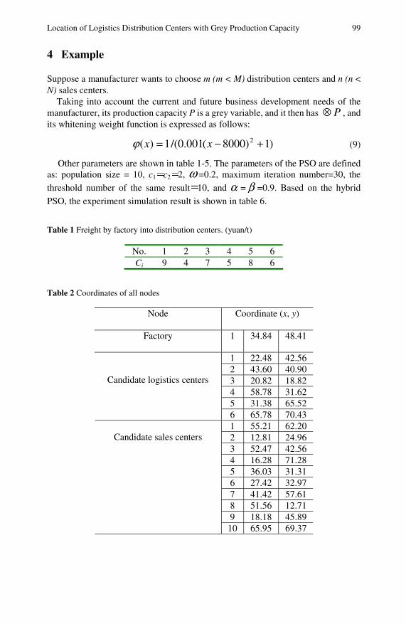
Location of Logistics Distribution Centers with Grey Production Capacity 99
4 Example
Suppose a manufacturer wants to choose m (m < M) distribution centers and n (n < N) sales centers.
Taking into account the current and future business development needs of the manufacturer, its production capacity P is a grey variable, and it then has P⊗ , and its whitening weight function is expressed as follows:
)1)8000(001.0/(1)( 2 +−= xxϕ (9)
Other parameters are shown in table 1-5. The parameters of the PSO are defined as: population size = 10, c1=c2=2, ω =0.2, maximum iteration number=30, the
threshold number of the same result=10, and α = β =0.9. Based on the hybrid
PSO, the experiment simulation result is shown in table 6.
Table 1 Freight by factory into distribution centers. (yuan/t)
No. 1 2 3 4 5 6 Ci 9 4 7 5 8 6
Table 2 Coordinates of all nodes
Node Coordinate (x, y)
Factory 1 34.84 48.41
1 22.48 42.56 2 43.60 40.90 3 20.82 18.82 4 58.78 31.62 5 31.38 65.52
Candidate logistics centers
6 65.78 70.43 1 55.21 62.20 2 12.81 24.96 3 52.47 42.56 4 16.28 71.28 5 36.03 31.31 6 27.42 32.97 7 41.42 57.61 8 51.56 12.71 9 18.18 45.89
Candidate sales centers
10 65.95 69.37
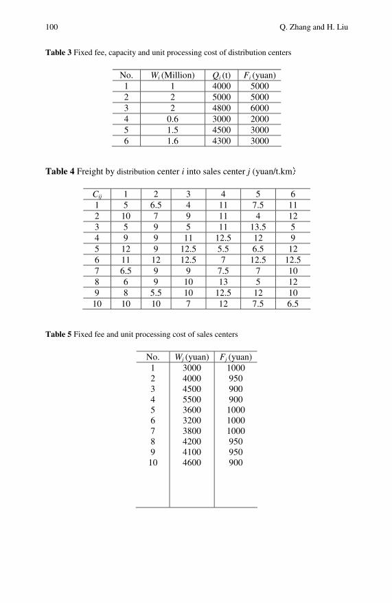
100 Q. Zhang and H. Liu
Table 3 Fixed fee, capacity and unit processing cost of distribution centers
No. Wi (Million) Qi (t) Fi (yuan) 1 1 4000 5000 2 2 5000 5000 3 2 4800 6000 4 0.6 3000 2000 5 1.5 4500 3000 6 1.6 4300 3000
Table 4 Freight by distribution center i into sales center j (yuan/t.km)
Cij 1 2 3 4 5 6 1 5 6.5 4 11 7.5 11 2 10 7 9 11 4 12 3 5 9 5 11 13.5 5 4 9 9 11 12.5 12 9 5 12 9 12.5 5.5 6.5 12 6 11 12 12.5 7 12.5 12.5 7 6.5 9 9 7.5 7 10 8 6 9 10 13 5 12 9 8 5.5 10 12.5 12 10
10 10 10 7 12 7.5 6.5
Table 5 Fixed fee and unit processing cost of sales centers
No. Wj (yuan) Fj (yuan) 1 2 3 4 5 6 7 8 9
10
3000 4000 4500 5500 3600 3200 3800 4200 4100 4600
1000 950 900 900
1000 1000 1000 950 950 900
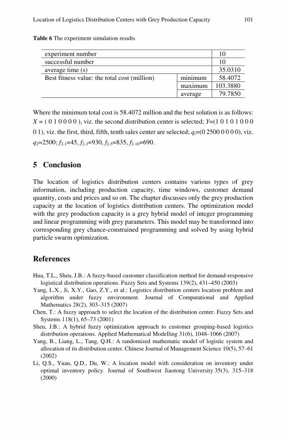
Location of Logistics Distribution Centers with Grey Production Capacity 101
Table 6 The experiment simulation results
experiment number 10 successful number 10 average time (s) 35.0310
minimum 58.4072 maximum 103.3880
Best fitness value: the total cost (million)
average 79.7850
Where the minimum total cost is 58.4072 million and the best solution is as follows: X = ( 0 1 0 0 0 0 ), viz. the second distribution center is selected; Y=(1 0 1 0 1 0 0 0
0 1), viz. the first, third, fifth, tenth sales center are selected; qi=(0 2500 0 0 0 0), viz.
q2=2500; f2-1=45, f2-3=930, f2-5=835, f2-10=690.
5 Conclusion
The location of logistics distribution centers contains various types of grey information, including production capacity, time windows, customer demand quantity, costs and prices and so on. The chapter discusses only the grey production capacity at the location of logistics distribution centers. The optimization model with the grey production capacity is a grey hybrid model of integer programming and linear programming with grey parameters. This model may be transformed into corresponding grey chance-constrained programming and solved by using hybrid particle swarm optimization.
References
Hua, T.L., Sheu, J.B.: A fuzzy-based customer classification method for demand-responsive logistical distribution operations. Fuzzy Sets and Systems 139(2), 431–450 (2003)
Yang, L.X., Ji, X.Y., Gao, Z.Y., et al.: Logistics distribution centers location problem and algorithm under fuzzy environment. Journal of Computational and Applied Mathematics 28(2), 303–315 (2007)
Chen, T.: A fuzzy approach to select the location of the distribution center. Fuzzy Sets and Systems 118(1), 65–73 (2001)
Sheu, J.B.: A hybrid fuzzy optimization approach to customer grouping-based logistics distribution operations. Applied Mathematical Modelling 31(6), 1048–1066 (2007)
Yang, B., Liang, L., Tang, Q.H.: A randomized mathematic model of logistic system and allocation of its distribution center. Chinese Journal of Management Science 10(5), 57–61 (2002)
Li, Q.S., Yuan, Q.D., Du, W.: A location model with consideration on inventory under optimal inventory policy. Journal of Southwest Jiaotong University 35(3), 315–318 (2000)

102 Q. Zhang and H. Liu Charnes, A., Cooper, W.W.: Chance-constrained programming. Management Science 6(1),
73–79 (1959) Deng, J.L.: Grey Control System. Huazhong University of Science and Technology Press,
Wuhan (1988) Liu, S.F., Guo, T.B.: Grey System Theory and Application. Henan Unviversity Press,
Kaifeng (1999) Zhang, Q.S.: Difference Information Theory of Grey Hazy Set. Petroleum Industry Press,
Beijing (2002) Liu, Y.J., Wang, X.Y.: Grey chance-constrained programming based on grey emulation.
Journal of East China University of Science and Technology 29(4), 405–408 (2003) Zhang, Q.S., Wang, H.Y.: Measuring the greyness of grey cluster knowledge. The Journal of
Grey System 21(3), 259–268 (2009) Liu, H., Zhang, Q.S.: The life prediction of mechanical products of GM(1,1) based on the
particle swarm optimization algorithm. In: Proceedings of 2007 IEEE International Conference on Grey Systems and Intelligent Services, Grand Metro Park, Nanjing, China, November 18-20, pp. 409–413 (2007)
Zhang, Q.S., Chen, K.J.: Measuring grey characteristics of association grey knowledge. In: Proceedings of 2007 IEEE International Conference on Systems, Man and Cybernetics, The Delta Centre-Ville at Montreal, Quebec, Canada, October 7-10, pp. 2196–2199 (2007)
Kennedy, J., Eberhart, R.C.: Particle swarm optimization. In: Proceeding of 1995 IEEE International Conference on Neural Networks, pp. 1942–1948. IEEE, New York (1995)
Eberhart, R.C., Kennedy, J.: A new optimizer using particle swarm theory. In: Proceedings of the Sixth International Symposium on Micro Machine and Human Science, pp. 39–43. IEEE, New York (1995)
Liu, H., Zhang, Q.S.: Chaos-particle swarm optimization algorithm and its application to mechanical optimal design. Machine Design and Research 23(5), 6–8 (2007)
Liu, S.F., Lin, Y.: Grey Information: Theory and Practical Applications. Springer, London (2006)
Lin, Y., Chen, M.Y., Liu, S.F.: Theory of grey systems: capturing uncertainties of grey information. Kybernetes: The International Journal of Systems and Cybernetics 33(2), 196–218 (2004)
Lin, Y., Liu, S.F.: Solving Problems with incomplete information: a grey systems approach. In: Advances in Imaging and Electron Physics, vol. 141, pp. 77–174. Elsevier, Amsterdam (2006)

Part II Grey Incidence Analysis and
Application
The Diagnosis of Firm’s “Diseases” Using the Grey Systems Theory Methods*
Camelia Delcea and Emil Scarlat
The core of our proposal is the determination of a “matrix of symptoms”, based on grey systems theory. The symptoms of a firm can be represented by eco-nomic-financial ratios, usually used by analysts to make predictions and sugges-tions. The ability to create such a matrix of symptoms implies that given level of symptom’s intensity, we can determinate if the analyzed firm presents some “dis-eases”. By diseases we understand the causes which generate anomalies at the firm. With the utilization of such a matrix, the activity of the analyst can be really improved.
1 Introduction
Prediction of firm’s “diseases” is a relatively new field in the economic and financial analysis. The economic context in which firms carry out their activities is dynamic and constantly changing. Creditors, auditors, stockholders and senior management all have a vasted interest in utilizing and developing a methodology or model that will allow them to monitor and regulate the financial performance of a firm via accounting ratios. By identifying changes and anticipating them, firms can take decisions to compensate or eliminate any negative effects and leverage the positive effects, thus facilitating the achievement of the firm’s goals.
In this study, we propose to construct a matrix of symptoms, as this is the main element on which the diagnosis of the situation of the firm will be based. The symptoms of a firm can be represented by ratios, which are the indicators the analysts look at to make their predictions and suggestions. The occurrence of symptoms, which are objectively measurable, allows certain methods to be used to construct membership functions for symptoms, related to the idea of relative
Camelia Delcea
University of Economics, Bucharest, Romania e-mail: [email protected]
Emil Scarlat Department of Cybernetics, University of Economics, Bucharest, Romania e-mail: [email protected]
* This work was supported in part by the European Structural Founds under project nr. 7832, “Doctoral Research and PhD students in Education- Research- Innovation, DOC- ECI”.
106 C. Delcea and E. Scarlat
frequency. That is why the field is suitable for tools taken from grey systems theory, which allow us to properly model the variables taken into consideration.
2 Evolution of Models and Methods for Diagnosis and Prediction of Diseases of Firms
The starting point in making a prediction on the firm’s evolution was the desire to early understand the precursor signals of a disaster and to take action that would try to improve the financial situation of a firm, even avoid its bankruptcy.
The assumption on which such predictions are based was that certain preliminary aspects regarding the insolvency of a firm can be seen by studying the dynamics of growth rates for a set of indicators derived from the financial accounting.
The first papers belonged to Fitz Patrick (FitzPatrick, 1932), who considered a set of 19 bankrupt firms and another set of 19 non-bankrupt firms. Following the research, it was found that 3 years before bankruptcy, the financial ratios were significantly changed. Another study is that made by Winakor and Smith (Winakor and Smith, 1935), who conducted research for a period of ten years before the bankruptcy establish, noting that the financial ratios deteriorate as firms were di-rected towards bankruptcy. Mervin (1942) reached similar conclusions.
However, the scientific concerns in this area began in 1967 with the research made by Beaver (1967). His research is intended to a benchmark for future research in purpose of finding alternatives for bankruptcy prediction using the financial ratios of a firm. Beaver developed a univariate discriminant analysis model, taking into account two sets of firms, bankrupt and non-bankrupt, and different ratios of them on a period equal to one year before the bankruptcy established. Those ratios have been selected following a dichotomous classification test. These models are now part of the classical models of bankruptcy prediction.
1966 is the year of birth of the risk index models. In these models, to each ana-lyzed firm is assigned a number of points between 0 and 100, according to the rates involved in the model, so that the higher points indicate a better financial situation. Points are allocated so that the most important rates to get a higher weight. How-ever, the allocation of weights is subjective (Balcaen and Ooghe, 2006). These models were introduced by Tamari (1966) and later extended by Moses and Liao (1987).
An important moment in the development of bankruptcy prediction models was the one in which Altman (1968) introduced a statistical multivariate analysis tech-nique called multiple discriminant analysis to the problem of firm failure prediction and estimated a Z-score model. His model was used to discriminate between ab-normal and healthy firms, using a statistical function.
After 1968, there have been an enormous number of studies based on Altman’s Z-score model. Many of these hane focused on verification and assessment of the results obtained by the mentioned model (Altman et al., 1977; Deakin, 1972; Ed-minster, 1972; Taffler, 1982).
Fuzzy logic ( Zadeh, 1965) was also widely used in firms’ bankruptcy prediction. Thus, Siegel, Korvin and Omer (1995) argue that quantitative models based on

The Diagnosis of Firm’s “Diseases” Using the Grey Systems Theory Methods 107
fuzzy systems theory can solve this problem. It goes to a new approach to problem that may occur at firm level, both from the view point of quantitative variables, but especially in the qualitative variables, related to the subjectivity of decisions taken therein.
In 1982, Professor Deng Ju-Long published “Problems of Grey Control Sys-tems”, which proposed a new theory: the grey systems theory which managed to develop and mature rapidly, and even to impose. In practice, grey systems theory has been widely applied in analysis, modeling, prediction, control, decision making, in almost all areas: social, economic, mechanical and technical science, agriculture, industry, transport, petrology, meteorological, ecological, hydrological, geological, financial, medical, military, and others (Liu and Lin, 2005). Its main characteristic is that it manages to achieve good performance in analysis conducted on a small range of data and on a large number of variables.
3 Methods of Grey System Theory and Their Application in Diagnosis
Grey systems theory, unlike other interdisciplinary theories, has found and has managed to retain a place within them, especially because its success in real sys-tems applications. This theory exceeds the drawbacks encountered in the use of probability theory and statistical methods (the need of reasonable size samples and determination of certain distributions to make inferences) and those of fuzzy mathematics (which deals with the study of problems with cognitive uncertainty phenomena, using so-called “membership functions”, based on experience).
A. Methods of Grey Numbers’ Generation Based on Average
A frequently problem encountered in any economic analysis is the lack of data. There are many cases where the collected data set of an observed economic system is incomplete, and thus, the researcher faces some difficulties in the undertaken analysis. Also, on the collected data, it may happened that in the initial data set, some values to be abnormal, much higher or much lower than the other values of the series, and, an analysis based on such a data set is leading to erroneous results. For the existence of some abnormal values, a possibility can be to identify and to ex-clude them from the data set, but the problem cannot be considered resolved either in this case, because it returns to the case where we have “gaps” in the data set. Grey system theory gives us, however, a method to solve this problem, namely to gen-erate new values for filling empty spaces in data sequence.
We consider therefore that the data sequence analyzed contains“empty” infor-mation, which we note with )(kφ , where k stands for the position in the data se-
quence. In this case, the data sequence X shows as follows:
))(),...,1(),(),1(),...,2(),1(( nxkxkkxxxX +−= φ
The number value )(kφ is in the range delimited by )1( −kx and )1( +kx , and
the two values represents the lower and the upper limit of the unknown value.
108 C. Delcea and E. Scarlat
Based on the series presented above we define the following value:
)1(5.0)1(5.0)( ++−=∗ kxkxkx
As being a generated average value based on two non-consecutive neighborhood values.
The sequence obtained from using this method is called a generated sequence of non-consecutive neighbors (Liu and Lin, 2005).
We can generate sequences based on consecutive neighbors, in this way: We consider the following data sequence:
))(),...,1(),(),1(),...,2(),1(( nxkxkxkxxxX +−= and the relation:
)(5.0)1(5.0)( kxkxkx +−=∗
It can be obtained the sequence:
))(),...,3(),2(( nxxxX ∗∗∗∗ =
One of the most popular models of grey system theory is the GM model (“mean generation”), which is based on this method of generating average using the con-secutive neighbor. This method is mainly used to emphasize a particular trend, if any.
In the firm analysis, the method of generating numbers based on average may be used if the purpose of the research is to observe the evolution in time of a specific variable, and for certain periods of time, for various reasons, those are unknown to the researcher.
For example, we consider the following sequence, which represents the quantity of products sold by the firm F (expressed in pieces) during an year, with monthly sales record:
)710,710,480,440,520,690,470(
))12(),11(),9(),5(),4(),2(),1((
== cccccccC
As can be seen, from a total of 12 months, we know only the quantities sold in 7 months, and for the other months, we can calculate the quantities by using the method of generating numbers based on average:
605)520690(2
1)]4()2([
2
1)3( =+=+= ccc
450)460440(2
1)]7()5([
2
1)6( =+=+= ccc
460)480440(2
1)]9()5([
2
1)7( =+=+= ccc
470)480460(2
1)]9()7([
2
1)8( =+=+= ccc
The Diagnosis of Firm’s “Diseases” Using the Grey Systems Theory Methods 109
595)710480(2
1)]11()9([
2
1)10( =+=+= ccc
We obtained the series:
)710,710,595,480,470,460,450,440,520,605,690,470(
))12(),11(),10(),9(),8(),7(),6(),5(),4(),3(),2(),1((
=== ccccccccccccC
B. Methods of Grey Clusters Theory
Grey data analysis is the base of many applications, such as economic applications and diagnosis and prediction of diseases of firms’ applications. Data representation techniques are various, and different characteristics that data might have are causing difficulties in accurate classification of the object.
As we all know, classification can be of two types: unsupervised classification, when we speak about clustering, and supervised classification, namely discrimi-nated analysis.
Through clustering it is trying to skip some of the variables of the analyzed system without this operation to affect the fundamental characteristics of the system.
Grey clustering is a method, based on matrices of grey incidence or whitenization weight functions of grey numbers, to classify observation indices or observational objects into definable classes (Liu and Lin, 2005). Regarding grey clustering based on grey incidence matrix, we test the connections among the analyzed factors so that we can make use of one of these factors to represent its group of factors, in a way that doesn’t affect the available information. The second method, which refers to the cluster of whitenization weight functions of grey classes, it is applied to check whether a specified object belongs to a certain predefined class.
Next, we present clusters of grey incidences. We consider a set of n observational objects and m characteristic data values for each of these n objects. In terms of grey system theory, we have the following representation (Liu and Lin, 2005):
minxxxX iiii ,...,2,1)),(),...,2(),1(( ==
We note the absolute degree of incidence of iX and jX with , calculated as
it follows:
jiji
jiij
ssss
ss
−+++
++=
1
1ε
Where : dtxXs i
n
ii ))1((1
−= ∫
We obtain a triangular matrix A, called the incidence matrix of the characteristic variables:
1,......
...
...
222
11211
=
⎟⎟⎟⎟⎟
⎠
⎞
⎜⎜⎜⎜⎜
⎝
⎛
= ii
mm
m
m
A ε
ε
εεεεε
110 C. Delcea and E. Scarlat
Taken a fixed critical value ]1,0[∈r , for any value ,rij ≥ε ji ≠ , the
variables iX and jX are treated as those of the same characteristics. Depending
on the value chosen for the r parameter, the number of variables included in a cer-tain class can be higher or less.
In practical analyses, it is quite difficult or impossible sometimes to classify each firm into groups of firms where, theoretically, it would be possible that some “diseases” to display. This is the reason why the classical method of forming classes of firms based on different ratios, so used in practice, haven’t obtain the expected results and many opportunities have been lost.
Before extending on a large scale the information regarding on the set of firms taken under consideration, we can try another approach in order to reduce the cost of the research, with the method of clusters of grey incidences. In this way, we obtain a reduction of the considerate variables. The manner of applying the method of clustering based on grey incidence matrix has been exposed in the previous paragraph.
An important element is even the manner in which we choose the critical value r, because it depends on the number of variables included in each class. So, taken under consideration the purpose of the research, different values of r in [0, 1] can be chosen. If the number of variables in each class is desired to be as small as possible, then we choose a critical value r as close as 1, and, in contrary, as close as 0.
C. Methods of Grey Incidence Analysis
Solving the problem of diagnosis of “diseases” that can appear at firm level depends on the identified symptoms. We won’t discuss in this case about how we choose the firms that analyzed or about the way we establish the set of symptoms that we use, because in many cases symptoms are represented by the financial ratios and indi-cators of a firm, which have a quantitative dimension that can be easily measured.
Most of the models used in diagnosis are based on a set of data collected at firm level (sometimes processed data), in a given period of time. Usually, we consider the values of symptoms at the level of year t, in most of the cases this is the year before bankruptcy, without attempting to link these values with the changes that have occurred in the indicator over a greater period, for example 3-5 years.
To have an overview of how the symptoms are evolving, until the moment they actually get to determine the bankruptcy of a firm, we propose a 5 years analysis and we use a matrix of symptoms expressed for each firm. If data are partially missing, these can be calculated using the grey method shown in paragraph 3.A.
We propose to determine which one of the considered symptoms manifest the biggest influence in each firm and to establish a hierarchy of then, in order to build a matrix of symptoms at the level of all the firms considered.
4 Firm Analysis
We note the set of symptoms Sj, with j = 1... n. The correlation matrix between the level of each symptom of a firm and the
corresponding year, for a universe of time equal to 5 years, is noted as follows:
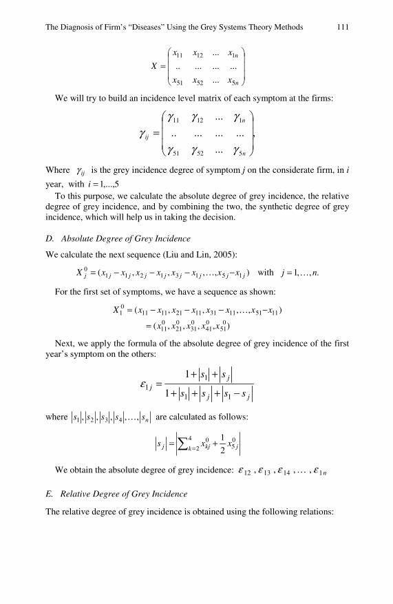
The Diagnosis of Firm’s “Diseases” Using the Grey Systems Theory Methods 111
⎟⎟⎟
⎠
⎞
⎜⎜⎜
⎝
⎛=
n
n
xxx
xxx
X
55251
11211
...
...........
...
We will try to build an incidence level matrix of each symptom at the firms:
,
...
...........
...
55251
11211
⎟⎟⎟
⎠
⎞
⎜⎜⎜
⎝
⎛=
n
n
ij
γγγ
γγγγ
Where ijγ is the grey incidence degree of symptom j on the considerate firm, in i
year, with 5,...,1=i To this purpose, we calculate the absolute degree of grey incidence, the relative
degree of grey incidence, and by combining the two, the synthetic degree of grey incidence, which will help us in taking the decision.
D. Absolute Degree of Grey Incidence
We calculate the next sequence (Liu and Lin, 2005):
),,,,( 151312110
jjjjjjjjj xxxxxxxxX −−−−= … with .,,1 nj …=
For the first set of symptoms, we have a sequence as shown:
),,,,(
),,,,(0
51041
031
021
011
115111311121111101
xxxxx
xxxxxxxxX
=
−−−−= …
Next, we apply the formula of the absolute degree of grey incidence of the first year’s symptom on the others:
jj
jj
ssss
ss
−+++
++=
11
11
1
1ε
where nsssss ,,,,, 4321 … are calculated as follows:
∑ =+= 4
205
0
2
1k jkjj xxs
We obtain the absolute degree of grey incidence: n1141312 ,,,, εεεε …
E. Relative Degree of Grey Incidence
The relative degree of grey incidence is obtained using the following relations:
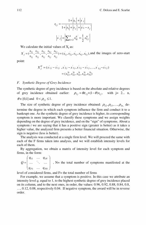
112 C. Delcea and E. Scarlat
'1'''
1
''1
11
1
jj
j
jssss
ssr
−+++
++=
∑ =+= 4
2
'05
'0'
2
1k jkjj xxs
We calculate the initial values of Xj as:
),,,,,(),,,,( '5
'4
'3
'2
'1
1
5
1
4
1
3
1
2
1
1'jjjjj
j
j
j
j
j
j
j
j
j
jj xxxxx
x
x
x
x
x
x
x
x
x
xX == and the images of zero-start
point:
),,,,(
),,,,(
0'51
0'41
0'31
0'21
0'11
1'
5'
1'
3'
1'
2'
1'
1''0
xxxxx
xxxxxxxxX jjjjjjjjj
=
−−−−= …
F. Synthetic Degree of Grey Incidence
The synthetic degree of grey incidence is based on the absolute and relative degrees of grey incidence obtained earlier: ,)1( 111 jjj rθθερ −+= with j= 2... n,
]1,0[∈θ and .10 1 ≤< jρ
The size of synthetic degree of grey incidence obtained: ,11312 ,,, nρρρ … de-
termine the degree in which each symptom influence the firm and conduct it to a bankrupt one. As the synthetic degree of grey incidence is higher, its corresponding symptom is more important. We classify these symptoms and we assign weights depending on the degree of grey incidence, and on the “sign” of symptoms. About a symptom i we are saying that it has a positive sign (greater is better) as it takes a higher value, the analyzed firm presents a better financial situation. Otherwise, the sign is negative (less is better).
The analysis was conducted at a single firm level. We will proceed the same with each of the F firms taken into analysis, and we will establish intensity levels for each of them.
By aggregation, we obtain a matrix of intensity level for each symptom and firms, in the form:
⎟⎟⎟
⎠
⎞
⎜⎜⎜
⎝
⎛=
FNF
N
Q
………
…
1
111
, N= the total number of symptoms manifested at the
level of considered firms, and F= the total number of firms For example, we assume that a symptom is positive. In this case we attribute an
intensity level q, equal to 1, to the highest synthetic degree of grey incidence placed on its column, and to the next ones, in order, the values: 0.96, 0.92, 0.88, 0.84, 0.8, …, 0.12, 0.08, respectively 0.04. If negative symptom, the award will be in reverse order.
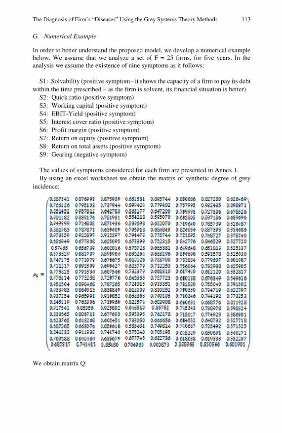
The Diagnosis of Firm’s “Diseases” Using the Grey Systems Theory Methods 113
G. Numerical Example
In order to better understand the proposed model, we develop a numerical example below. We assume that we analyze a set of F = 25 firms, for five years. In the analysis we assume the existence of nine symptoms as it follows:
S1: Solvability (positive symptom - it shows the capacity of a firm to pay its debt within the time prescribed – as the firm is solvent, its financial situation is better)
S2: Quick ratio (positive symptom) S3: Working capital (positive symptom) S4: EBIT-Yield (positive symptom) S5: Interest cover ratio (positive symptom) S6: Profit margin (positive symptom) S7: Return on equity (positive symptom) S8: Return on total assets (positive symptom) S9: Gearing (negative symptom) The values of symptoms considered for each firm are presented in Annex 1. By using an excel worksheet we obtain the matrix of synthetic degree of grey
incidence:
We obtain matrix Q:
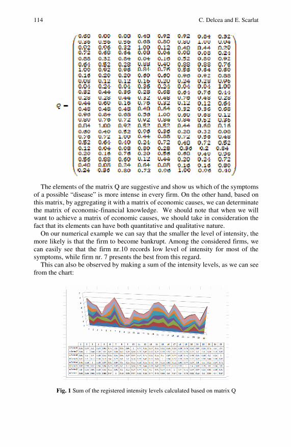
114 C. Delcea and E. Scarlat
The elements of the matrix Q are suggestive and show us which of the symptoms of a possible “disease” is more intense in every firm. On the other hand, based on this matrix, by aggregating it with a matrix of economic causes, we can determinate the matrix of economic-financial knowledge. We should note that when we will want to achieve a matrix of economic causes, we should take in consideration the fact that its elements can have both quantitative and qualitative nature.
On our numerical example we can say that the smaller the level of intensity, the more likely is that the firm to become bankrupt. Among the considered firms, we can easily see that the firm nr.10 records low level of intensity for most of the symptoms, while firm nr. 7 presents the best from this regard.
This can also be observed by making a sum of the intensity levels, as we can see from the chart:
Fig. 1 Sum of the registered intensity levels calculated based on matrix Q
The Diagnosis of Firm’s “Diseases” Using the Grey Systems Theory Methods 115
5 Conclusions
Determination of “diseases” of firms is an actual field in economic analysis, and the papers that deal with this problem are numerous. Theories that have grown since the research begun in this field are many and their purpose is the same: to find a way by which a possible “disease” or bankruptcy can be anticipated, to find a way to highlight the occurrence of such a phenomena.
In prediction of “diseases” of firms, particularly in the stage of diagnosis, a great attention must be given to symptoms manifested by the firms under analysis and to their quantification.
The method of constructing symptoms’ matrix is based on facilities offered by the grey systems theory and it tries to find a way of determining the rank to which individual symptoms affect the final status of a firm or of a group of firms.
This method can be applied even to determine the matrix of economic causes that generate these symptoms, with the only difference that when we talk about causes, it should be taken into account that the non-quantitative aspect may be an issue. This implies certain conditions, so that the qualitative causes to be transformed in quantitative causes.
The research can be extended to determine a matrix of economic-financial knowledge, by aggregating the matrix of symptoms and causes, both using all methods of grey systems theory, but also by using hybrid methods. An example of a hybrid model that can be created by combining the methods of grey systems theory with the benefits of CBR (Case Based Reasoning) methods, so that after we obtain the matrix of economic-financial knowledge, we can attribute it the ability to learn from experience. But, such an approach will be the subject of future research.

116 C. Delcea and E. Scarlat
Annex 1
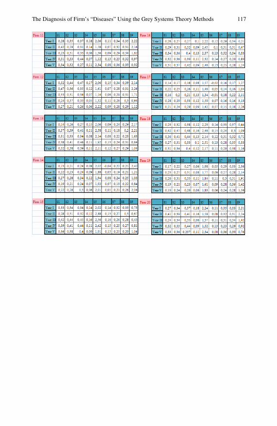
The Diagnosis of Firm’s “Diseases” Using the Grey Systems Theory Methods 117
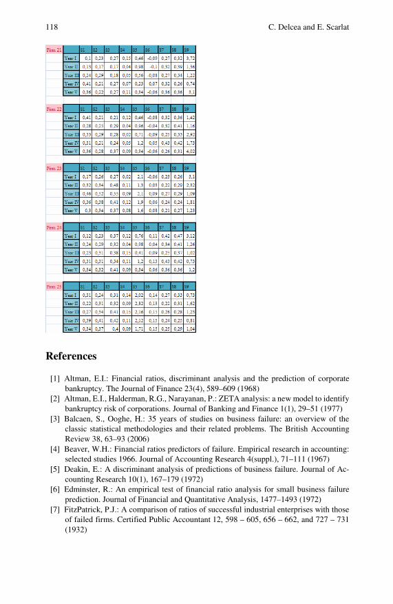
118 C. Delcea and E. Scarlat
References
[1] Altman, E.I.: Financial ratios, discriminant analysis and the prediction of corporate bankruptcy. The Journal of Finance 23(4), 589–609 (1968)
[2] Altman, E.I., Halderman, R.G., Narayanan, P.: ZETA analysis: a new model to identify bankruptcy risk of corporations. Journal of Banking and Finance 1(1), 29–51 (1977)
[3] Balcaen, S., Ooghe, H.: 35 years of studies on business failure: an overview of the classic statistical methodologies and their related problems. The British Accounting Review 38, 63–93 (2006)
[4] Beaver, W.H.: Financial ratios predictors of failure. Empirical research in accounting: selected studies 1966. Journal of Accounting Research 4(suppl.), 71–111 (1967)
[5] Deakin, E.: A discriminant analysis of predictions of business failure. Journal of Ac-counting Research 10(1), 167–179 (1972)
[6] Edminster, R.: An empirical test of financial ratio analysis for small business failure prediction. Journal of Financial and Quantitative Analysis, 1477–1493 (1972)
[7] FitzPatrick, P.J.: A comparison of ratios of successful industrial enterprises with those of failed firms. Certified Public Accountant 12, 598 – 605, 656 – 662, and 727 – 731 (1932)
The Diagnosis of Firm’s “Diseases” Using the Grey Systems Theory Methods 119
[8] Li, G.D., Yamaguchi, D., Nagai, M.: A Grey-based approach to suppliers selection problem. LNCS. Springer, Berlin (2006)
[9] Mervin, C.L.: Financing small corporations in five manufacturing industries, 1926 – 36. National Bureau of Economic Research (1942)
[10] Moses, D., Liao, S.S.: On developing models for failure prediction. Journal of Com-mercial Bank Lending 69, 27–38 (1987)
[11] Siegel, P.H., Korvin, A.D., Omer, K.: Application of fuzzy sets and the theory of evi-dence to accounting. Jai Press Inc. (1995)
[12] Liu, S.F., Lin, Y.: Grey Information: Theory and Practical Applications. Springer, London (2005)
[13] Taffler, R.J.: Forecasting company failure in the UK using discriminant analysis and financial ratio data. Journal of the Royal Statistical Society 145, 342–358 (part 3) (1982)
[14] Tamari, M.: Financial ratios as a means of forecasting bankruptcy. Management In-ternational Review 4, 15–21 (1966)
[15] Vigier, H.P., Terceno, A.: A model for prediction of “diseases” of firms by means of fuzzy relations. Fuzzy Sets and Systems 159, 2299–2316 (2008)
[16] Wilson, R.L., Sharda, R.: Bankruptcy prediction using neural networks. Decision Support Systems 11, 545–557 (1994)
[17] Winakor, A., Smith, R.F.: Changes in financial structure of unsuccessful industrial companies. Bureau of Business Research Bulletin No. 51 (1935)
[18] Xia, J.: Grey System Theory Applied to Hydrology. Huazhong University of Science and Technology Press, Wuhan (2000)
[19] Zadeh, L.A.: Fuzzy sets. Information and Control 9, 338–353 (1965)
Apply GRA in CSL Communication Topics Selection*
Rih-Chang Chao, Nagai Masatake, Tien-Yu Hsieh, Tian-Wei Sheu, Bor-Chen Kuo, Ya-Hsun Tsai, and Shin-I Yeh
This chapter is to utilize grey incidence analysis to calibrate and analyze the pri-orities of communication topics for learning Chinese as second language (CSL) learners based on their interests. Presently there are no appropriate studies discussed regard how to measure CSL learners’ interests and categorization of their interests in prioritized format. This is the first development through survey approach for this category of study. There are 84 questionnaire data of kindergarten level used in this chapter collected by the Overseas Compatriot Affairs Commission (OCAC) during teaching material development research project conducted in USA in 2008. The result of this chapter will provide further reference for OCAC and other relative CSL editing and publishing industries uses. Rih-Chang Chao Graduate Institute of Measurement and Statistics, National Taichung University, Taichung, Taiwan e-mail: rchang.chao@ msa.hinet.net
Nagai Masatake Kanagawa University, Japan e-mail: [email protected]
Tien-Yu Hsieh National Taichung University, Taichung, Taiwan e-mail: [email protected]
Tian-Wei Sheu National Taichung University, Taichung, Taiwan e-mail: [email protected]
Bor-Chen Kuo National Taichung University, Taichung, Taiwan e-mail: [email protected]
Ya-Hsun Tsai National Taiwan Normal University, Taipei, Taiwan e-mail: [email protected]
Shin-I Yeh Education Department Chiayi County Government, Chiayi, Taiwan e-mail: [email protected]
* This work was supported in part by both the National Science Council under Grant NSC 97-2631-S-003-002 and the Overseas Compatriot Affairs Commission.
122 R.-C. Chao et al.
1 Introduction
Learning Chinese as second language (CSL) has become popular recently due to the economic boost in China. From the present languages practice in the world today, Chinese has become the second major language used in comparison with English. Majority of CSL learner includes Chinese born overseas and foreigners whom are also interest to learn Chinese. With the increase of demand on learning CSL which bring about the essentiality of quality improvement on the teaching materials contents.
A successful CSL teaching material contents design has a direct motivation to CSL learners and the impact on their learning effectiveness. It is a great importance to focus on the interest of CSL learner when editing the contents of CSL teaching materials in order to fulfill their needs and increase their learning effectiveness. Currently there are no such appropriate studies discussed regards how to measure CSL learners’ interests and categorization of their interests in prioritized format.
There are numbers of directions to evaluate teaching CSL in overseas such as referring to the heritage programs; teachers’ professional development, teachers’ role in multilingual children’s English and French language development, and children’s discursive practices (Curdt-Christiansen, 2006). Some of the articles focus on the learning characteristics (Lijing, 2006) of Chinese students, or the ac-tivities used inside classroom to discuss the CSL contents (Huang, 2003; Kuma-moto-Healey, 2000). There was one article discuss how to select situation content for US kindergarten and elementary (Tsai, 2008). However, the information on the discussion of what CSL communication content taught is very insufficient.
We assume data was approximately normally distributed and collected as many data as possible to minimize random errors during data analysis via statistical methods. According to an experimental study from Chang, there are no significant differences in the methods used between AHP, ELECTRE, TOPSIS and GRA when data approximately normally distributed (Chang, 2001). Contrary to this point of view, it is not appropriate to assume data we collected from survey hold the property of normal distribution. To address this problem, GRA can effectively discriminate the differences between subjects for fewer amounts of data or with uncertain data distribution (Deng and Guo, 1996). Other than this, data calibration is easily calculated and convenient and accurately locates the key factors or indi-cators selection. These are the major issues making of GRA so popular for data analysis (Lin, 2004). It is not surprise that we can find a lot of articles or papers applying GRA as the major method for data analysis. For example, Guo and Huang utilize GRA to prioritize factors from 25 steal companies’ performance appraisal and review system (Guo and Huang, 2007). Wang used GRA to select evaluating indicators during Taiwan shipping container company performance review (Wang, 2006). Applying GRA on the performance review can often been utilized in hospital industry (Sun, 1999). In addition, GRA also used during decision making proce-dures such as finding key factor for investment strategy (Lin, and Yang, 1999), unemployment rate forecasting (Hu et al., 2008), etc. Many researchers integrate GRA with other methods for data analysis. For example, integrate GRA with Fuzzy

Apply GRA in CSL Communication Topics Selection 123
measurement (Zhao and Mei, 1999), or with DEA (Guo and Huang, 2007), or with Neural Network, or with Case-based Reasoning (Tong and Shi, 2001).
The CSL teaching material topics we had listed in our survey were implemented by Functionalist Approach in Europe. There are total of 90 different topics in 6 different categories (Tsai, 2009). It is not appropriate to include all 90 topics in one CSL teaching material even though we had utilized GRA to prioritize the topics. It is necessary to make decision on which topics should include and which one should not.
This chapter applied GRA as the major method for CSL teaching material topic selection. The total of 84 questionnaire data of kindergarten level used in this chapter were collected from the Overseas Compatriot Affairs Commission (OCAC) during teaching material development research project conducted in USA 2008. All of them represented their students’ interested topics in the kindergarten classes in USA. The data was in ordinal ratings. The result of this chapter will provide further reference for OCAC and other relative CSL editing and publishing industries uses.
2 Methods
The validity of traditional statistical analysis techniques is based on assumptions such as normal distribution as well as large sample size. However, it is not realistic to make decisions under those assumptions. Deng argued that making decisions under uncertainty and with insufficient or limited data available for analysis is actually a norm for managers in either public or private sectors (Deng, 1989). To address this problem, grey relational analysis, which first proposed by Deng in 1982 (Deng, 1982), is one of the most important and well-known methods to analyze uncertain and insufficient data in various fields. The procedures applying GRA used in this article consist of the following steps.
A. Generate comparison vector
The data we had collected came from 6 different categories. Each category consists of different numbers of teaching material topics in ordinal rating scale format. Total of 30 out of 90 CSL teaching material topics from 6 different categories were selected from each participant. There are 5 topics selected from first category and 3, 10, 8, 2 and 2 topics separately selected for 2nd, 3rd, 4th, 5th, and 6th category (Overseas Compatriot Affairs Commission, 2008) respectively. The reason of using proportion of total topics to standardized data before generating comparison data was due to its attribute of trend of original data. For example, there were 5 out of 12 topics selected in prioritize format of 1st category. The first priority topic in the 1st category is de-
fined as12
90 and the fifth priority in the 1st category is defined as
8
90 . For those
unselected topics in each category were all defined as1
90 . Let
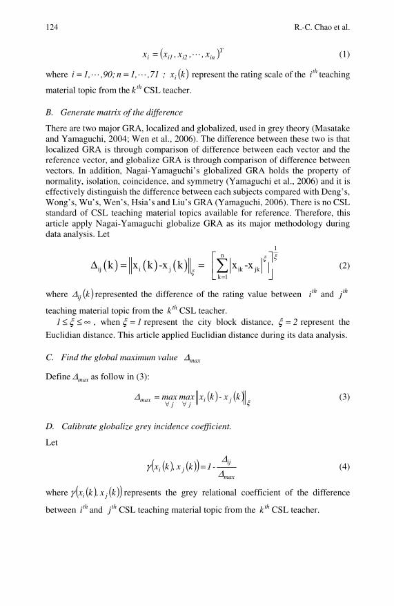
124 R.-C. Chao et al.
( )Tini2i1i x ,,x ,xx = (1)
where ,711,n ,90;1,i == ; ( ) kxi represent the rating scale of the thi teaching
material topic from the thk CSL teacher.
B. Generate matrix of the difference
There are two major GRA, localized and globalized, used in grey theory (Masatake and Yamaguchi, 2004; Wen et al., 2006). The difference between these two is that localized GRA is through comparison of difference between each vector and the reference vector, and globalize GRA is through comparison of difference between vectors. In addition, Nagai-Yamaguchi’s globalized GRA holds the property of normality, isolation, coincidence, and symmetry (Yamaguchi et al., 2006) and it is effectively distinguish the difference between each subjects compared with Deng’s, Wong’s, Wu’s, Wen’s, Hsia’s and Liu’s GRA (Yamaguchi, 2006). There is no CSL standard of CSL teaching material topics available for reference. Therefore, this article apply Nagai-Yamaguchi globalize GRA as its major methodology during data analysis. Let
( ) ( ) ( )1
n
ij i j ik jkk 1
k x k -x k x -xξξ
ξ=
⎡ ⎤Δ = = ⎢ ⎥⎣ ⎦∑ (2)
where ( )kijΔ represented the difference of the rating value between thi and thj
teaching material topic from the thk CSL teacher. ∞≤≤ ξ1 , when 1=ξ represent the city block distance, 2=ξ represent the
Euclidian distance. This article applied Euclidian distance during its data analysis.
C. Find the global maximum value maxΔ
Define maxΔ as follow in (3):
( ) ( )ξ
Δ kx-kx max max jij j
max∀∀
= (3)
D. Calibrate globalize grey incidence coefficient.
Let
( ) ( )( )max
ijji -1 kx ,kx
ΔΔ
γ = (4)
where ( ) ( )( )kx ,kx jiγ represents the grey relational coefficient of the difference
between thi and thj CSL teaching material topic from the thk CSL teacher.
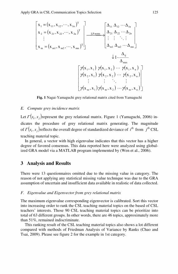
Apply GRA in CSL Communication Topics Selection 125
( )( )
( )
( ) ( ) ( )( ) ( ) ( )
( ) ( ) ( ) ⎥⎥⎥⎥
⎦
⎤
⎢⎢⎢⎢
⎣
⎡
ΔΔ
↓
⎥⎥⎥⎥
⎦
⎤
⎢⎢⎢⎢
⎣
⎡
ΔΔΔ
ΔΔΔΔΔΔ
⎯⎯⎯ →⎯
⎥⎥⎥⎥⎥
⎦
⎤
⎢⎢⎢⎢⎢
⎣
⎡
=
=
=
x,x x,x x,x
x,x x,x x,x
x,x x,x x,x
-1
x,,x,xx
x,,x,xx
x,,x,xx
nm2m1m
n22212
n12111
max
ij
mnm2m1
2n2221
1n1211
norm LP
Tmnm2m1m
T2n22212
T1n12111
γγγ
γγγγγγ
Fig. 1 Nagai-Yamaguchi grey relational matrix cited from Yamaguchi
E. Compute grey incidence matrix
Let ( )ji x ,xΓ represent the grey relational matrix. Figure 1 (Yamaguchi, 2006) in-
dicates the procedure of grey relational matrix generating. The magnitude
of ( )ji x ,xΓ reflects the overall degree of standardized deviance of thi from thj CSL
teaching material topic. In general, a vector with high eigenvalue indicates that this vector has a higher
degree of favored consensus. This data reported here were analyzed using global-ized GRA model via a MATLAB program implemented by (Wen et al., 2006).
3 Analysis and Results
There were 13 questionnaires omitted due to the missing value in category. The reason of not applying any statistical missing value technique was due to the GRA assumption of uncertain and insufficient data available in realistic of data collected.
F. Eigenvalue and Eigenvector from grey relational matrix
The maximum eigenvalue corresponding eigenvector is calibrated. Sort this vector into increasing order to rank the CSL teaching material topics on the based of CSL teachers’ interests. Those 90 CSL teaching material topics can be prioritize into total of 63 different groups. In other words, there are 46 topics, approximately more than 51%, remained indiscriminate.
This ranking result of the CSL teaching material topics also shows a lot different compared with methods of Friedman Analysis of Variance by Ranks (Chao and Tsai, 2009). Please see figure 2 for the example in 1st category.
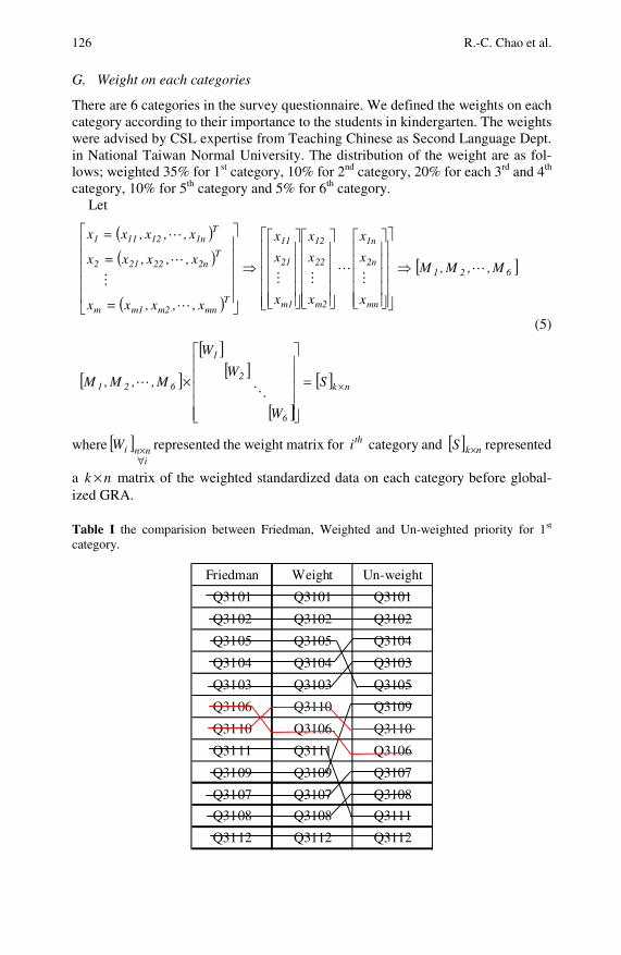
126 R.-C. Chao et al.
G. Weight on each categories
There are 6 categories in the survey questionnaire. We defined the weights on each category according to their importance to the students in kindergarten. The weights were advised by CSL expertise from Teaching Chinese as Second Language Dept. in National Taiwan Normal University. The distribution of the weight are as fol-lows; weighted 35% for 1st category, 10% for 2nd category, 20% for each 3rd and 4th category, 10% for 5th category and 5% for 6th category.
Let
( )( )
( )
[ ]
[ ][ ]
[ ]
[ ][ ] nk
6
2
1
621
621
mn
2n
1n
m2
22
12
m1
21
11
Tmnm2m1m
T2n22212
T1n12111
S
W
W
W
M,, M,M
M,, M,M
x
x
x
x
x
x
x
x
x
x,,x,xx
x,,x,xx
x,,x,xx
×=
⎥⎥⎥⎥⎥
⎦
⎤
⎢⎢⎢⎢⎢
⎣
⎡
×
⇒
⎥⎥⎥⎥⎥
⎦
⎤
⎢⎢⎢⎢⎢
⎣
⎡
⎥⎥⎥⎥⎥
⎦
⎤
⎢⎢⎢⎢⎢
⎣
⎡
⎥⎥⎥⎥⎥
⎦
⎤
⎢⎢⎢⎢⎢
⎣
⎡
⎥⎥⎥⎥⎥
⎦
⎤
⎢⎢⎢⎢⎢
⎣
⎡
⇒
⎥⎥⎥⎥⎥
⎦
⎤
⎢⎢⎢⎢⎢
⎣
⎡
=
=
=
(5)
where [ ]inniW
∀× represented the weight matrix for thi category and [ ] nkS × represented
a nk × matrix of the weighted standardized data on each category before global-ized GRA. Table I the comparision between Friedman, Weighted and Un-weighted priority for 1st category.
Friedman Weight Un-weight
Q3101 Q3101 Q3101
Q3102 Q3102 Q3102
Q3105 Q3105 Q3104
Q3104 Q3104 Q3103
Q3103 Q3103 Q3105
Q3106 Q3110 Q3109
Q3110 Q3106 Q3110
Q3111 Q3111 Q3106
Q3109 Q3109 Q3107
Q3107 Q3107 Q3108
Q3108 Q3108 Q3111
Q3112 Q3112 Q3112

Apply GRA in CSL Communication Topics Selection 127
After globalized GRA calibrating, the maximum eigenvalue, 59.4524, corre-sponding eigenvector is observed. Sort this vector into increasing order to rank the CSL teaching material topics on the based of CSL teachers’ interests. This weighted priority result of the CSL teaching material topics (Table I) shows no significant difference compared with methods of Friedman Analysis.
4 Conclusions
Those weighted 90 CSL teaching material topics can be discriminate into 79 dif-ferent groups of topic compared with 63 groups without weighted. This result in-dicated that weighted data can be easily distinguishing the distance between each topic compared with un-weighted data.
Under Friedman Analysis of Variance by Ranks, grouping of 1st category can only be discriminated into 3 significant groups compared with weighted GRA which are able to discriminate topics in 1st category into 12 groups. Practically weighted GRA are more appropriate used for CSL text book design.
The comparison of the effectiveness between the weighted and un-weight data is another major issue need to focus on. This result of the priority with weighted CSL teaching material topics shows no significant different compared with the result utilized methods of Friedman analysis of variance by rank.
After plotting these ranking data into the figure indicated as figure 2 below, there are 7 CSL teaching material topics apparently are not correlated to the others 83 topics. Therefore, we recommended not to including those 7 topics during kinder-garten textbook design. Appendix indicated the finial rank of CSL teaching material topics.
0
0.02
0.04
0.06
0.08
0.1
0.12
0.14
0 10 20 30 40 50 60 70 80 90 100
Fig. 2 CSL teaching topic ranking structure
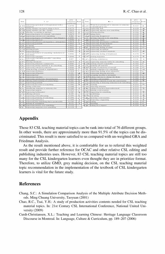
128 R.-C. Chao et al.
I te m N a m e
g r e yr e l a t i o n a l
c o e f fi c i e n tR a n k I te m N a m e
g re yr e l a ti o n a l
c o e ff i c i e n tR a n k
Q 3 3 0 1e x p r e s s in g a g r e e m e n t o r d i s a g re e m e n t w i t h as t a t e m e n t
0 . 0 7 5 4 1 Q 3 1 0 3W h e n b e e n i n t r o d u c e d t o s o m e o n e o r s o m e o n ei s in t r o d u c e d to y o u .
0 .1 1 2 7 4 3
Q 3 3 0 9 s t a t i n g w h e t h e r o n e k n o w s th in g o r fa c t s 0 . 0 7 7 9 2 Q 3 4 1 5 e x p re ss i n g lu c k 0 .1 1 2 8 4 4
Q 3 4 0 1 s t a t i n g w h e t h e r o n e l ik e / d i s l ik e 0 . 0 8 3 5 3 Q 3 4 2 3 e x p re ss i n g u rg e n c y o v e r s o m e t h in g 0 .1 1 3 4 4 5
Q 3 3 1 9 o ff e r in g / a c c e p t in g a n a p o lo g y 0 . 0 8 7 5 4 Q 3 1 1 0 o f f e r in g g re e t in g 0 .1 1 4 4 4 6
Q 3 3 0 2 e x p r e s s in g d e g r e e o f c e r t a i n ty / u n c e rt a i n t y 0 . 0 8 7 9 5 Q 3 1 0 6 t a k i n g l e a v e 0 .1 1 4 9 4 7
Q 3 3 2 5 e x p r e s s in g c o n c e r n o v e r s o m e t h i n g 0 .0 8 8 6 Q 3 3 2 8 e x p re ss i n g d i s a p p ro v a l 0 .1 1 5 2 4 8
Q 3 4 0 3 e x p r e s s in g d e g r e e o f w i l l i n g n e s s / u n w i l l in g n e s s 0 . 0 9 0 3 7 Q 3 1 1 1 i n v i t in g s o m e o n e t o d o s o m e th i n g 0 .1 1 5 3 4 9
Q 3 3 1 5 e x p r e s s in g a p p ro v a l 0 . 0 9 0 8 8 Q 3 4 0 6 e x p re ss i n g re g re t 0 .1 1 5 3 4 9
Q 3 4 0 2 e x p r e s s in g p l e a s u r e a n d h a p p in e s s / u n h a p p i n e s s 0 . 0 9 1 8 9 Q 3 4 1 9 e x p re ss i n g u n c e r t a i n ty / c o n fu s io n 0 .1 1 5 3 4 9
Q 3 4 0 7 e x p r e s s in g g r a t i t u d e 0 . 0 9 2 1 1 0 Q 3 4 1 0 e x p re ss i n g d i s a p p o in t m e n t 0 .1 1 5 5 5 2
Q 3 3 1 2 a c c e p t i n g 0 . 0 9 3 2 1 1 Q 3 1 0 9 c o n g ra tu l a t i o n s o m e o n e 0 .1 1 5 7 5 3
Q 3 3 2 7 s u p p o r t in g 0 . 0 9 5 1 1 2 Q 3 4 2 1 e x p re ss i n g fe e l in g o f r e l i e f 0 .1 1 5 7 5 3
Q 3 1 0 1 g re e t in g p e o p l e 0 . 0 9 5 4 1 3 Q 3 3 1 6 e x p re ss i n g a n o p in i o n 0 .1 1 7 6 5 5
Q 3 4 0 9 e x p r e s s in g h o p e 0 . 0 9 6 1 1 4 Q 3 3 2 9 e x p re ss i n g a m u tu a l s t a t e m e n t 0 .1 1 7 7 5 6
Q 3 3 0 4e x p r e s s in g b e l i e v e o f s o m e th in g / d i s b e l i e v e o fs o m e th in g
0 . 0 9 6 2 1 5 Q 3 4 0 5 e x p re ss i n g fe e l in g o f d i s p le a se d 0 .1 1 7 8 5 7
Q 3 3 2 4 e x p r e s s in g s y m p a th y 0 . 0 9 6 8 1 6 Q 3 1 0 7 m a k i n g d e p a r tu re 0 .1 1 7 9 5 8
Q 3 3 0 8e x p r e s s in g s o m e th i n g p o s s ib le / s o m e t h in gi m p o s s i b l e
0 .0 9 7 1 7 Q 3 4 2 5 o f f e r in g c o n d o le n c e s 0 . 1 1 8 5 9
Q 3 3 0 3 d e n y in g s ta t e m e n ts 0 . 0 9 7 9 1 8 Q 3 4 1 8 e x p re ss i n g so m e o n e l i a b l e fo r s o m e th i n g 0 .1 1 8 2 6 0
Q 3 4 0 8 e x p r e s s in g a f f e c t i o n / c o m p a s s i o n 0 . 0 9 8 3 1 9 Q 3 3 2 2 m a k i n g o n e s e l f r e s p o n s i b le 0 .1 1 8 3 6 1
Q 3 3 0 7 e x p r e s s in g a b i l i t y / i n a b i l i t y t o d o s o m e t h in g 0 . 0 9 8 4 2 0 Q 3 1 0 8 S e n d i n g - o ff s o m e o n e 0 .1 1 8 5 6 2
Q 3 3 2 3 e x p r e s s in g c o m f o r t t o s o m e o n e 0 . 0 9 8 4 2 0 Q 3 4 1 7 F e e l in g o f i n fe ri o r i t y o f o n e s e l f 0 .1 1 8 6 6 3
Q 3 1 0 2 w h e n m e e t in g a f r i e n d o r a c q u a in t a n c e 0 . 0 9 9 8 2 2 Q 3 4 1 4 m a k i n g c o m p la i n o v e r s o m e t h i n g 0 .1 1 9 1 6 4
Q 3 3 2 1 e x p r e s s in g o b e d i e n c e 0 . 1 0 1 6 2 3 Q 3 4 2 2 e x p re ss i n g fe e l in g o f n o a l t e r n a t iv e 0 .1 1 9 4 6 5
Q 3 3 1 0 e x p r e s s in g o b l i g a t i o n 0 .1 0 2 2 4 Q 3 3 1 1 e x p re ss i n g d e n y in g n e c e s s i t y 0 .1 1 9 6 6 6
Q 3 4 1 2 e x p r e s s in g f e a r 0 . 1 0 3 4 2 5 Q 3 1 1 2 a c c e p t i n g a n o f f e r o r i n v i t a t io n 0 .1 1 9 8 6 7
Q 3 3 1 3 e x p r e s s in g r e j e c t io n 0 . 1 0 4 1 2 6 Q 3 6 0 5 a s k in g s o m e o n e t o c h a n g e t h e t h e m e 0 .1 2 0 5 6 8
Q 3 4 0 4 e x p r e s s in g s a t i s f a c t i o n / d i s s a t i s f a c t i o n 0 . 1 0 4 7 2 7 Q 3 6 0 7 c lo s i n g a c o n v e rs a t i o n 0 .1 2 0 6 6 9
Q 3 3 2 6 o ff e r in g u n d e r s ta n d i n g o f c e rt a in t h i n g s 0 .1 0 5 2 8 Q 3 6 0 4 e n c o u r a g e s o m e o n e t o jo i n th e c o n v e r sa t i o n 0 .1 2 0 9 7 0
Q 3 1 0 5 e x p r e s s in g g r a t i t u d e 0 . 1 0 5 3 2 9 Q 3 5 0 5 i n s tr u c t i n g o r d i r e c t in g s o m e o n e t o d o s o m e th i n g 0 . 1 2 1 7 1
Q 3 3 1 7 e x p r e s s in g d e c i s io n o n so m e t h in g 0 . 1 0 6 2 3 0 Q 3 5 0 4 w a r n i n g 0 .1 2 1 2 7 2
Q 3 3 0 6 s t a t i n g c o n fe ss i o n 0 . 1 0 6 6 3 1 Q 3 6 0 2 a tt r a c ti n g a t t e n t i o n 0 .1 2 1 2 7 2
Q 3 1 0 4 i n tr o d u c in g s o m e o n e t o s o m e o n e e l s e 0 . 1 0 6 9 3 2 Q 3 6 0 3 a s k in g i f y o u h a v e b e e n u n d e rs to o d 0 .1 2 1 2 7 2
Q 3 4 1 6 e x p r e s s in g s u r p r i s e 0 . 1 0 7 2 3 3 Q 3 6 0 6 j o i n i n g a c o n v e r s a t i o n 0 .1 2 1 2 7 2
Q 3 3 2 0 e x p r e s s in g f o r b e a r a n c e 0 . 1 0 8 7 3 4 Q 3 5 0 6 r e q u e s t i n g f o r s o m e th in g 0 .1 2 1 4 7 6
Q 3 3 3 0 o ff e r in g a d v is o r y 0 .1 0 9 3 5 Q 3 5 0 7 p r o h ib i t in g 0 .1 2 1 4 7 6
Q 3 4 2 4 e x p r e s s in g o f h e a rt b r e a k in g 0 . 1 0 9 3 3 6 Q 3 5 0 3 r e m i n d in g 0 .1 2 1 5 7 8
Q 3 3 1 4 e x p r e s s in g p l a n n i n g o f so m e t h in g 0 . 1 0 9 4 3 7 Q 3 6 0 1 o p e n i n g a c o n v e r sa t io n 0 .1 2 1 8 7 9
Q 3 4 1 3 e x p r e s s in g a n n o y a n c e 0 . 1 0 9 9 3 8 Q 3 5 0 2 p r o p o s in g / s u g g e s t in g 0 .1 2 1 9 8 0
Q 3 3 1 8 e x p r e s s in g t h a t s o m e t h i n g t h a t is p e r m is s ib le 0 . 1 1 0 7 3 9 Q 3 2 0 9 a s k in g 0 .1 2 2 1 8 1
Q 3 4 2 0 m a k i n g a n a s s u m p t i o n 0 .1 1 2 4 0 Q 3 2 0 1 n a rr a t in g 0 .1 2 2 5 8 2
Q 3 4 1 1 e x p r e s s in g a n x i e ty o v e r s o m e th in g 0 . 1 1 2 2 4 1 Q 3 5 0 1 a s k in g f o r a r e q u e s t 0 .1 2 2 9 8 3
Q 3 3 0 5 e x p r e s s in g s u s p i c io n o v e r s o m e th i n g 0 . 1 1 2 4 4 2
Appendix
Those 83 CSL teaching material topics can be rank into total of 76 different groups. In other words, there are approximately more than 91.5% of the topics can be dis-criminated. This result is more satisfied to us compared with un-weighted GRA and Friedman Analysis.
As the result mentioned above, it is comfortable for us to referral this weighted result and provide further reference for OCAC and other relative CSL editing and publishing industries uses. However, 83 CSL teaching material topics are still too many for the CSL kindergarten learners even thought they are in prioritize format. Therefore, to utilize GMD, grey making decision, on the CSL teaching material topic recommendation in the implementation of the textbook of CSL kindergarten learners is vital for the future study.
References
Chang, S.C.: A Simulation Comparison Analysis of the Multiple Attribute Decision Meth-ods. Ming Chuang University, Taoyuan (2001)
Chao, R.C., Tsai, Y.H.: A study of production activities contents needed for CSL teaching material topics. In: 21st Century CSL International Conference, National United Uni-versity (2009)
Curdt-Christiansen, X.L.: Teaching and Learning Chinese: Heritage Language Classroom Discourse in Montreal. In: Language, Culture & Curriculum, pp. 189–207 (2006)

Apply GRA in CSL Communication Topics Selection 129 Deng, J.L.: Introduction to Grey System Theory. Journal of Grey System 1(1), 1–24 (1989) Deng, J.L.: Control Problems of Grey System. System and Control Letters 1(5), 288–294
(1982) Deng, J.L., Guo, H.: GRA Theory and Application. Chuan Hwa Book Co. Ltd., Taipei (1996) Guo, Y.X., Huang, S.: Performance Evaluation of Steel Industry by DEA and GRA. In:
Chinese Society and Quality annual meeting, Taiwan National University, p. 13 (2007) Hu, J.L., Liu, P.L., Hung, H.C.: A grey analysis of regional unemployment in Taiwan.
Taiwan Economic Forum 6(11), 38–67 (2008) Huang, J.: Activities as a vehicle for linguistic and sociocultural knowledge at the elementary
level. In: Language Teaching Research, pp. 3–33 (2003) Kumamoto-Healey, J.: Website Creation: A Japanese Learning Project. In: Computer As-
sisted Language Learning, Routledge, pp. 449–455 (2000) Lijing, S.: The Successors to Confucianism or a New Generation? A Questionnaire Study on
Chinese Students’ Culture of Learning English. Language, Culture & Curriculum, 122–147 (2006)
Lin, C.T., Yang, S.Y.: Selection of home mortgage loans using grey relational analysis. Journal of Grey System 11(4), 359–368 (1999)
Lin, S.Y.: Evaluation of business reputation in information service industry: An application of grey relational analysis. Journal of Information, Technology and Society 2, 17 (2004)
Overseas Compatriot Affairs Commission, CSL Guideline for USA Elementary School. OCAC, Taipei (2008)
Masatake, N., Yamaguchi, D.: Apply GRA in Engineering, Tokyo (2004) Sun, M.: Grey relational analyzing the influencing factors of economic benefit in hospital.
Journal of Grey System 11(1), 53–59 (1999) Tong, L.L., Shi, B.Z.: Predict the financial crisis by using grey relation analysis, neural
network, and case-based reasoning. Chinese Management Review 4(2), 25–37 (2001) Tsai, Y.H.: USA K-12 CSL Teaching Material Design - Communication Topic. Chung Yuan
Journal of Teaching Chinese as a Second Language 2, 205–224 (2008) Tsai, Y.H.: Construction of CSL Teaching Material. CHENG CHUNG BOOK, Taipei
(2009) Wang, Y.J.W.: Applying grey relation analysis to find the representative indicators of fi-
nancial ratios for evaluating financial performance of container shipping companies on Taiwan. Maritime Quarterly 15(1), 1–17 (2006)
Wen, K.L., Zhang-Jian, S.K., Yeh, K.Z., et al.: Apply MATLAB in Grey System Theory. Chuan Hwa Book Co. Ltd., Taipei (2006)
Yamaguchi, D., Li, G.D., Mizutani, K., et al.: On the Generalization of Grey Relational Analysis. Journal of Grey System 9(1), 23–34 (2006)
Yamaguchi, D.: Report of GRA Priority Investigation. Graduate School of Engineering, Kanagawa University, Kanagawa (2006)
Zhao, Y., Mei, Z.: Pattern Recognition Method Based on Fuzzy Grey Incidence and Its Application: Theory and Practice on System Engineer, Guangxi University (1999)
The Model of New Grey Incidence and Its Application*
Lizhi Cui and Sifeng Liu
Grey incidence is an important part of grey system theory on the basis of grey decision-making and grey cluster. Analyzing departed grey incidence models, this chapter constructed a new grey incidence model by gradual tempo difference be-tween reference sequence and relevant sequence. Meanwhile, the new model has some characters. A real example shows its simplification and practicability.
1 Introduction
Grey incidence analysis is an important part of grey system theory and the founda-tion of grey system analysis, grey decision-making and grey cluster. It’s a model of studying relationship degree among factors in system. Since Professor Deng created Grey system theory in 1982, more and more scholars have taken part in research of grey system theory (Liu and Lin, 2006; Lin et al., 2004; Lin and Liu, 2006). Grey incidence analysis can be applied to cases of various sample sizes and distributions with a relatively small amount of computation. And, in general, each application of grey incidence analysis does not result in situations of disagreement between quantitative analysis and qualitative analysis. When analyzing an abstract system or a phenomenon, what’s most important is to choose the right sequence of charac-teristic data to describe the system’s behavior. The sequence of data is called a mapping quantity of the special system’s behavior. The fundamental idea of grey incidence analysis is that the closeness of a relationship is judged based on the similarity level of the geometric patterns of sequence curves. The more similar the curves are, the higher the degree of incidence between sequence, and vice versa. A lot of grey incidence models have been put forward, for example, Deng’s degree of grey incidence (Deng, 2002), absolute degree of grey incidence (Mei, 1992)], rela-tive degree of grey incidence (Liu et al., 2004), grey incidence of B-model (Wang, 1989), grey incidence of C-model (Wang and Zhao, 1999), grey incidence of Lizhi Cui and Sifeng Liu College of Economics and Management, Nanjing University of Aeronautics and Astronautics, Nanjing 210006, PR China e-mail: [email protected]
* This work is supported by the National Science Foundation of China (No.70701017) and Ministry of Education, research of grey prediction model (200802870020).
132 L. Cui and S. Liu
T-model (Tang, 1995), grey incidence of entropy (Zhang and Guo, 1996), degree of grey Euclid incidence (Zhao et al., 1998), degree of grey slope incidence (Dang and Liu, 2004), and some improvement model afterwards (Cui, 2008; Tang et al., 2008; Sun and Dang, 2008; Shi et al., 2008; Cao, 2008). Some properties have been dis-cussed in the literature (Xiao, 1997; Lv et al., 2000; Xie and Liu, 2007). These scholars have researched grey incidence models from different aspects, and have obtained some application effect. However the relationship of closeness between sequences is considered in most of the literature. There are some defects in some literature: (1) Degree value of grey incidence is not unique. Degree of grey inci-dence is influenced by many factors, for instance data conversion way between reference sequence and comparative sequence, different value of distinguishing
coefficient ξ , etc. (2) Commonly distinguishing coefficient 0.5ξ = , then degree
of grey incidence 0.333iγ > . (3) Degree of grey incidence is mostly not symmetry,
so grey incidence theory is not perfect. It is necessary in constructing a new grey incidence model. Under the professor Deng’s grey incidence thought, we put for-ward a grey similarity incidence model on the base of gradual tempo and to get some basic properties. A real example shows its simplification and practicability.
2 A New Grey Incidence Model
If each factor in a space of grey incidence factors is seen as a point in the space without size and volume, and each data value of the factor, observed at a different time moment, different index, or different object, is seen as the coordinate of the point, then we will be able to study the relationship between factors or between factors and the system’s characteristics in a special n-dimensional space. In this way, the relevant degree of grey incidence can be defined by using the distance function in the n-dimensional space. If growth trend of two factors is consistent, i.e. the synchronized change degree is high, we think that degree of grey incidence is big, otherwise then low. Time series exist in the social economy. Gradual tempo is one of the important characteristics in time series, so correlative degree of two time series is very important. We may study degree of grey incidence by using of de-velopment level, and may also consider from gradual tempo. If the gradual tempo between reference sequence and relevant sequence is consistent, we may think the degree of grey incidence is very big. It is our thought.
In systems analysis, after the mapping quantities which describe system’s be-haviors well, have been chosen, thus we need to clarify all the factors that effec-tively affect the systems’ behaviors. The space, consisting of system factors, forms a base for grey incidence analysis. On such a base, comparisons and evaluations can be done in order to study system’s behaviors of factors. If each factor in a space of grey incidence factors is seen as a point in the space without size and volume, and each data value of the factor, observed at a different time moment, different index, or different object, is seen as the coordinate of the point, then we will be able to study the relationship between factors or between factors and the system’s charac-teristics in a special n-dimensional space. In this way, degree of grey incidence can be defined by using the gradual tempo in the space.
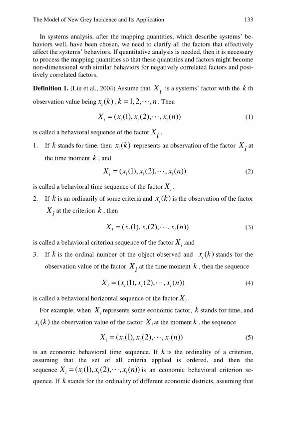
The Model of New Grey Incidence and Its Application 133
In systems analysis, after the mapping quantities, which describe systems’ be-haviors well, have been chosen, we need to clarify all the factors that effectively affect the systems’ behaviors. If quantitative analysis is needed, then it is necessary to process the mapping quantities so that these quantities and factors might become non-dimensional with similar behaviors for negatively correlated factors and posi-tively correlated factors.
Definition 1. (Liu et al., 2004) Assume that Xi is a systems’ factor with the k th
observation value being ( )ix k , 1, 2, ,k n= . Then
( (1), (2), , ( ))i i i iX x x x n= (1)
is called a behavioral sequence of the factor Xi .
1. If k stands for time, then ( )ix k represents an observation of the factor Xi at
the time moment k , and
( (1), (2), , ( ))i i i iX x x x n= (2)
is called a behavioral time sequence of the factor iX .
2. If k is an ordinarily of some criteria and ( )ix k is the observation of the factor
Xi at the criterion k , then
( (1), (2), , ( ))i i i iX x x x n= (3)
is called a behavioral criterion sequence of the factor iX .and
3. If k is the ordinal number of the object observed and ( )ix k stands for the
observation value of the factor Xi at the time moment k , then the sequence
( (1), (2), , ( ))i i i iX x x x n= (4)
is called a behavioral horizontal sequence of the factor iX .
For example, when iX represents some economic factor, k stands for time, and
( )ix k the observation value of the factor iX at the moment k , the sequence
( (1), (2), , ( ))i i i iX x x x n= (5)
is an economic behavioral time sequence. If k is the ordinality of a criterion, assuming that the set of all criteria applied is ordered, and then the
sequence ( (1), (2), , ( ))i i i iX x x x n= is an economic behavioral criterion se-
quence. If k stands for the ordinality of different economic districts, assuming that

134 L. Cui and S. Liu
the set of all economic districts studies have been ordered, then the sequence
( (1), (2), , ( ))i i i iX x x x n= is an economic behavioral horizontal sequence.
No matter which sequence we have, being time, or criterion, or horizontal, we can always conduct the needed incidence analysis.
Definition 2. Assume that
0 0 0 0( (1), (2), , ( ))X x x x n= (6)
is a sequence of data representing a system’s characteristics, and
( (1), (2), ( ))i i i iX x x x n= , 1, 2,i n= (7)
are sequences of relevant factors. For a given real number 0 ( )i kγ , if the real
number
00
1( )
1 ( ) ( )ii
kd k d k
γ =+ −
(8)
and 0 0 0( ) ( ) / ( 1)d k x k x k= − , ( ) ( )/ ( 1)i i id k x k x k= − ,
0 02
1( )
1
m
i ik
kn
γ γ=
=− ∑ (9)
Then 0iγ is called the degree of grey incidence of iX with respect to 0X , and
0 ( )i kγ the incidence coefficient of iX with respect to 0X at point k .
The concept of the degree of grey incidence of sequence 0X and iX is a quan-
titative representation of the development rate of 0X and iX relative to their last
time points. The closer the rates of development of 0X and iX are, the greater
0iγ is, and vice versa.
Proposition 1. 0iγ satisfies
1. The property of normality.
00 1iγ< ≤ , { }1,2,i m∈ and 0 1iγ = { } 01,2, , ( ) ( )ik m d k d k⇔ ∀ ∈ = .
2. The property of symmetry.
For iX , jX X∈ then ij jiγ γ= .
3. The property of closeness .The smaller 0( ) ( )id k d k− is the larger 0iγ .
Proof 1. If 0( ) ( )id k d k= , then 0 ( ) 1i kγ =
If 0( ) ( )id k d k≠ , then 0( ) ( ) 0id k d k− > .Therefore, 01 1 ( ) ( )id k d k< + − .
So 0 ( ) 1i kγ < . It is obvious that for any k , 0 ( ) 0i kγ > . Hence, 00 1iγ< ≤ .

The Model of New Grey Incidence and Its Application 135
2. For any k , ( ) ( ) ( ) ( )i j j id k d k d k d k− = − , then ( ) ( )ij jik kγ γ= ,
so ij jiγ γ= .Degree of the new grey incidence satisfies the property of symmetry.
3. The property of closeness. It is obvious. The closer gradual tempo between reference sequence and relevant sequence is, the greater degree of grey incidence is.
Proposition 2. Assume that 0X and iX are two sequences of the same length with
non-zero values. If 0iX cX= , where 0c > is a constant, then 0 1iγ = .
Proof 2. Assume that ( )0 0 0 0(1), (2), , ( )X x x x n=
Then
0 0 0
( (1), (2), , ( ))
( (1), (2), , ( ))i i i iX x x x n
cx cx cx n
==
(10)
And
0
0
00
0
( ) ( )( ) ( 1) ( 1)
( ) ( )( 1)
ii
i
x k cx kd k x k cx k
x k d kx k
= =− −
= =−
(11)
So 0 1iγ = .
Proposition 3. Assume that 0X and iX are sequences of the same length with
non-zero values, a and b non-zero constants, and the degree of grey incidence of
0aX and ibX is '0iγ . Then '
0 0i iγ γ= . In other words, scalar multiplication does
not change the degree of grey incidence.
Proof 3. Assume that
( )0 0 0 0(1), (2), , ( )X x x x n= (12)
( (1), (2), , ( ))i i i iX x x x n= (13)
Then
( )0 0 0 0(1), (2), , ( )aX ax ax ax n= (14)
( (1), (2), , ( ))i i i ibX bx bx bx n= (15)
And
' 0 00 0
0 0
( ) ( )( ) ( )( 1) ( 1)ax k x kd k d kax k x k= = =− − (16)

136 L. Cui and S. Liu
' ( ) ( )( ) ( )( 1) ( 1)i i
i ii i
bx k x kd k d kbx k x k= = =− − (17)
For any k , then '0 0( ) ( )i ik kγ γ= . So '
0 0i iγ γ= .
In fact, the gradual tempos of 0aX and ibX is respectively equal to those of
0X and iX .So, scalar multiplication does not act in any way .Hence, '0 0i iγ γ= .
3 Practical Application
In national economy system, the level of development on tertiary industry not only affects tertiary industry, but also influences employment situation. Tertiary industry will be main industry department in China, which can absorb labors and alleviate employment pressure very much. Therefore, it is necessary to analyze the main influencing factors of tertiary industry of China, in order to take some corre-sponding measurements to enhance employment level and promote industry structure. Per person GDP, level of urbanization, industrial added values etc. are introduced in this article. Then the relation between these indexes with employment of tertiary industry is studied. Some mutual reactions among these factors determine the development situation and tendency of the systems. We want to know: which factors among the many are more important? Which factors have more effects on the future development of the systems than others? Which factors actually cause desirable changes in the systems so that these factors need to be strengthened?
Table 1 Recorded values of variables for the years 1995 to 2007
index X0 (employment of tertiary) X1(per person GDP) X2 (urbanization ) X3 (industrial added
value)
1995 16880 5046 29.04 24718
1996 17927 5846 30.48 28580
1997 18432 6420 31.91 31752
1998 18860 6796 33.35 33541
1999 19205 7159 34.78 35357
2000 19823 7858 36.22 39570
2001 20228 8622 37.66 42607
2002 21090 9398 39.09 45935
2003 21809 10542 40.53 53612
2004 23011 12336 41.76 62815
2005 23771 14053 42.99 76190
2006 24614 16165 43.9 90351
2007 24917 18934 44.94 107367
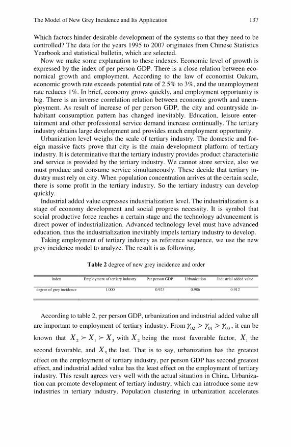
The Model of New Grey Incidence and Its Application 137
Which factors hinder desirable development of the systems so that they need to be controlled? The data for the years 1995 to 2007 originates from Chinese Statistics Yearbook and statistical bulletin, which are selected.
Now we make some explanation to these indexes. Economic level of growth is expressed by the index of per person GDP. There is a close relation between eco-nomical growth and employment. According to the law of economist Oakum, economic growth rate exceeds potential rate of 2.5% to 3%, and the unemployment rate reduces 1%. In brief, economy grows quickly, and employment opportunity is big. There is an inverse correlation relation between economic growth and unem-ployment. As result of increase of per person GDP, the city and countryside in-habitant consumption pattern has changed inevitably. Education, leisure enter-tainment and other professional service demand increase continually. The tertiary industry obtains large development and provides much employment opportunity.
Urbanization level weighs the scale of tertiary industry. The domestic and for-eign massive facts prove that city is the main development platform of tertiary industry. It is determinative that the tertiary industry provides product characteristic and service is provided by the tertiary industry. We cannot store service, also we must produce and consume service simultaneously. These decide that tertiary in-dustry must rely on city. When population concentration arrives at the certain scale, there is some profit in the tertiary industry. So the tertiary industry can develop quickly.
Industrial added value expresses industrialization level. The industrialization is a stage of economy development and social progress necessity. It is symbol that social productive force reaches a certain stage and the technology advancement is direct power of industrialization. Advanced technology level must have advanced education, thus the industrialization inevitably impels tertiary industry to develop.
Taking employment of tertiary industry as reference sequence, we use the new grey incidence model to analyze. The result is as following.
Table 2 degree of new grey incidence and order
index Employment of tertiary industry Per person GDP Urbanization Industrial added value
degree of grey incidence 1.000 0.923 0.986 0.912
According to table 2, per person GDP, urbanization and industrial added value all
are important to employment of tertiary industry. From 02 01 03γ γ γ> > , it can be
known that 2 1 3X X X with 2X being the most favorable factor, 1X the
second favorable, and 3X the last. That is to say, urbanization has the greatest
effect on the employment of tertiary industry, per person GDP has second greatest effect, and industrial added value has the least effect on the employment of tertiary industry. This result agrees very well with the actual situation in China. Urbaniza-tion can promote development of tertiary industry, which can introduce some new industries in tertiary industry. Population clustering in urbanization accelerates
138 L. Cui and S. Liu
service industry development. The level of per person GDP shows the degree of economic growth to some extent. The economy level of development is high, and people have large service demands. Additionally, the industry development inevi-tably impels tertiary industry, especially finance, insurance, leisure entertainment and so on. So degree of grey incidence between employment of tertiary industry and industrial added value is 0.912.
4 Conclusion
According to the idea of grey incidence theory, a new grey incidence model is constructed by gradual tempo difference of reference sequence and relevant se-quence. Meanwhile, the model has properties of normality, symmetry closeness. Scalar multiplication does not change the degree of grey incidence. Finally, a practical example shows its simplification and practicability.
References
Cao, M.X.: Study and improvement on properties of positive and negative of grey incidence degree model. Systems Engineering and Electronics 30(6), 1086–1088 (2008)
Cui, J.A.: Kind of new grey similarity incidence and application. Statistics and Deci-sion-making 20, 14–16 (2008)
Dang, Y.G., Liu, S.G.: Improvement degree of grey slope incidence. Engineering Sci-ence 6(3), 23–26 (2004)
Deng, J.L.: Grey Theory Basis. Huazhong University of Science and Technology Press, Wuhan (2002)
Lin, Y., Chen, M.Y., Liu, S.F.: Theory of grey systems: capturing uncertainties of grey information. Kybernetes: The International Journal of Systems and Cybernetics 33(2), 196–218 (2004)
Lin, Y., Liu, S.F.: Solving problems with incomplete information: A grey systems approach. In: Advances in Imaging and Electron Physics, vol. 141, pp. 77–174. Elsevier, Oxford (2006)
Liu, S.F., Dang, Y.G., Fang, Z.G.: Grey System Theory and Its Application. Science Press, Beijing (2004)
Liu, S.F., Lin, Y.: Grey Information: Theory and Practical Applications. Springer, London (2006)
Lv, F., Liu, X., Liu, Q.: The theory of grey relative analysis and its new research. Journal of Wuhan University of Technology 22(2), 41–43 (2000)
Mei, Z.G.: The concept and computation method of grey absolute correlation degree. Sys-tems Engineering 5(8), 15–18 (1992)
Shi, H.X., Liu, S.F., Fang, Z.G., Zhang, A.: The model of grey periodic incidence and their rehabilitation. Chinese Journal of Management Science 16(3), 131–136 (2008)
Sun, Y.G., Dang, Y.G.: Improvement on grey T’s correlation degree. Systems Engineering Theory & Practice 4, 135–139 (2008)
Tang, S.L., Li, N., Gong, Z.W.: Research on properties of combination forecasting model based on absolute of grey incidence. Systems Engineering and Electronics 30(1), 89–92 (2008)

The Model of New Grey Incidence and Its Application 139 Tang, W.X.: The concept and computation method of T’s correlation degree. Application of
Statistics and Management 14(1), 34–37 (1995) Wang, Q.Y.: The grey relational analysis of B-model. Journal of Huazhong University of
Science and Technology 17(6), 77–82 (1989) Wang, Q.Y., Zhao, X.H.: The relational analysis of C-model. Journal of Huazhong Univer-
sity of Science and Technology 27(3), 75–77 (1999) Xiao, X.P.: Theoretical study and reviews on the computation method of grey interconnect
degree. Systems Engineering Theory & Practice 17(8), 76–81 (1997) Xie, N.M., Liu, S.F.: The parallel and uniform properties of several relational models. Sys-
tems Engineering 25(8), 98–103 (2007) Zhang, Q.S., Guo, X.J.: Grey relation entropy method of grey relation analysis. Systems
Engineering Theory & Practice 8(8), 7–11 (1996) Zhao, Y.L., Wei, S.Y., Mei, Z.X.: Grey Euclid relation grade. Journal of Guan Xi Univer-
sity 23(1), 10–13 (1998)
The Analysis of China’s Macro-economy with Grey Dynamic Model in 30 Years of Reform and Opening up
Juan Du and Xuemeng Wang
Macro-economic system is a multi-factor, multi-level, multi-aim typical grey sys-tem possessed of indefinite. Its running process is a grey dynamic one composed with many relations of many complex structures and interlaced functions. By using the grey systematic theory model, this chapter studies two major problems in China’s macro-economic system during the reform and opening up. First, it obtains the incidence degree between the gross domestic product (GDP) and the three in-dustries (primary industry, secondary industry and tertiary industry), the productive values of the three industries and their internal industries according to the grey dynamic relation analysis. It also builds the industrial related trees of China’s macro-economy in each “Five-Year Plan” period. Second, it analyzes the economic cycle of China since 1990s and forecasts the economic scale for the next cycle through GM (1, 1) model and the analysis of the residual error. Moreover, it ana-lyzes the dynamic change of China’s macro-economy, the development state and existing problems, meanwhile, counter-measures and suggestions are put forward to provide a scientific basis for China’s macro-economic adjustment and the further economic growth.
1 Introduction
Ever since the reform and opening up, China’s economic construction has made remarkable achievements. The total value of economy maintains a growing trend and the industrial structure is more practical. However, in the process of rapid industrialization, resource and environmental restrains loom gradually and become more and more serious in restricting the strength of economic development and there exists the periodic variation in the process of development. These require us to positively promote the fundamental change of economic growth mode, optimize the Juan Du School of Environmental and Resources, Shanxi University, Taiyuan 030006, P.R. China e-mail: [email protected]
Xuemeng Wang Institute of Integrated survey of Agriculture Resource, Taiyuan 030006, P.R. China e-mail: [email protected]
142 J. Du and X. Wang
industrial structure, coordinate the industrial development, recognize and master the inner periodic principles in the economic development, thus achieve sustain-able, rapid and healthy economic development. Therefore it is supposed to have a dynamic analysis of the impact of all the industries within ever-changing overall economic system and have a correct understanding of the relational grade between the progress of industries with overall economic growth and a scientific forecast of future tendency of economic development after mastering the periodic principles in the past.
Macro-economic system is a multi-factor, multi-level, multi-aim complex, with complex structure and function (Yu, 1997). Grey system theory believes that macro-economic system is a typical grey system and all the factors in the system jointly act on the entire system (Liu and Lin, 2006; Lin et al., 2004; Lin et al., 2006). Meanwhile, these factors also interact and they themselves have dynamic changes over time. The industrial structure is the changing grey volume of each factor in correspondence with certain period in this system, and the process of changing can be studied by using the grey relational analysis method. Meanwhile, the exact process path of time series which reflects the dynamic characteristic of macro-economy is a sum of vector composed by three separated parts, that is, long-term trend, periodic variation, and random fluctuation These three parts em-body the dynamic characteristics in system. Grey system model is a differential equation describing the dynamic variation. We obtain the long-term trend of eco-nomic development and periodic variation by using GM (1, 1) model, predict the future economic development of China, analyze and understand the dynamic de-velopment process of macro-economy in a higher level, which may provide a sci-entific basis for economic structure adjustment and economic development.
2 The Basic Principles of the Grey System Model
A. The Model of the Grey Dynamic Relation Analysis (Deng, 1992)
The essence of grey relational analysis is to make a geometric comparison in the data series which are responded to the changing characteristics of all the factors. The closer the curves are, the greater the relational grade of the corresponding series is, and vice versa. It analyzes the close level between the characteristic behavior of grey system and relevant factors to determine which is primary and which is sec-ondary, and which has small impact and which has great impact.
Macro-economy is a system with continuous dynamic change, and the relational grade of factors within the system is that in the process of development it changes over time series. With the use of dynamic relation analysis, we could further un-derstand the trend that relevant factors in the system change and develop over time. If such change makes the relational grade of behavior series of relevant factors increase, it shows that the correlation of the factors will develop in a closer direc-tion; on the contrary, their correlations are weakening.
The use of the grey relation analysis can definite the changing trend of all factors in this system and find out the main factors which affect the further development of
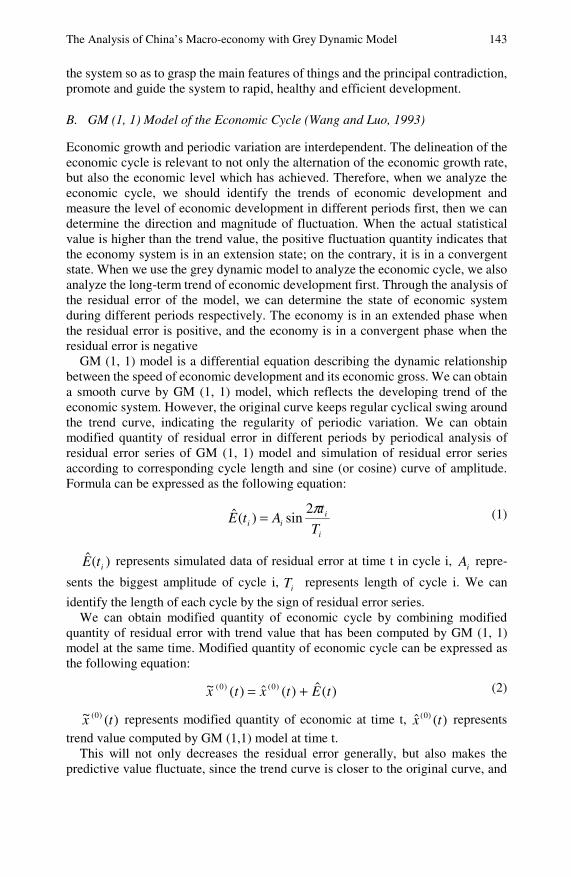
The Analysis of China’s Macro-economy with Grey Dynamic Model 143
the system so as to grasp the main features of things and the principal contradiction, promote and guide the system to rapid, healthy and efficient development.
B. GM (1, 1) Model of the Economic Cycle (Wang and Luo, 1993)
Economic growth and periodic variation are interdependent. The delineation of the economic cycle is relevant to not only the alternation of the economic growth rate, but also the economic level which has achieved. Therefore, when we analyze the economic cycle, we should identify the trends of economic development and measure the level of economic development in different periods first, then we can determine the direction and magnitude of fluctuation. When the actual statistical value is higher than the trend value, the positive fluctuation quantity indicates that the economy system is in an extension state; on the contrary, it is in a convergent state. When we use the grey dynamic model to analyze the economic cycle, we also analyze the long-term trend of economic development first. Through the analysis of the residual error of the model, we can determine the state of economic system during different periods respectively. The economy is in an extended phase when the residual error is positive, and the economy is in a convergent phase when the residual error is negative
GM (1, 1) model is a differential equation describing the dynamic relationship between the speed of economic development and its economic gross. We can obtain a smooth curve by GM (1, 1) model, which reflects the developing trend of the economic system. However, the original curve keeps regular cyclical swing around the trend curve, indicating the regularity of periodic variation. We can obtain modified quantity of residual error in different periods by periodical analysis of residual error series of GM (1, 1) model and simulation of residual error series according to corresponding cycle length and sine (or cosine) curve of amplitude. Formula can be expressed as the following equation:
(1)
)(ˆitE represents simulated data of residual error at time t in cycle i, iA repre-
sents the biggest amplitude of cycle i, iT represents length of cycle i. We can
identify the length of each cycle by the sign of residual error series. We can obtain modified quantity of economic cycle by combining modified
quantity of residual error with trend value that has been computed by GM (1, 1) model at the same time. Modified quantity of economic cycle can be expressed as the following equation:
(2)
)(~ )0( tx represents modified quantity of economic at time t, )(ˆ )0( tx represents
trend value computed by GM (1,1) model at time t. This will not only decreases the residual error generally, but also makes the
predictive value fluctuate, since the trend curve is closer to the original curve, and
i
iii T
tAtE
π2sin)(ˆ =
)(ˆ)(ˆ)(~ )0()0( tEtxtx +=
144 J. Du and X. Wang
the accuracy of the model can be improved. In the course of forecast, the cycle of future series can refer to the variation trend of residual error cycle of known series; the amplitude can be selected and controlled reasonably according to range allowed by system and is likely changed. Then we can forecast after determining the cycle and amplitude of future.
The process of economic development often shows the random fluctuation which can be decided by many unpredictable natural and human factors. Due to the un-predictability, it is difficult to study the random fluctuation by quantity and model.
3 Grey Dynamic Relation Analysis between China’s Economy and Its Industrial Structure
The chapter divides the structure of China’s economic system into three levels (Fig. 1), making the relation analysis of each level regarded as one collectivity. The figures of GDP of China, the productive values of three industries, and the pro-ductive values of three industrial internal industries from 1978 to 2006 are obtained from the China Statistical Yearbook (National Bureau of Statistics of China). For the convenience of consistency with the “Five-Year Plan” while analyzing and discussing, the six dynamic periods of 1978-2006, 1981-2006, 1986-2006, 1991-2006, 1996-2006, 2001-2006 are picked to calculate the relational grade of GDP and three industries, three industries and internal industries, and three typical periods. Among them are chosen to form the related trees between China’s econ-omy and industry (Fig. 2-Fig. 4). Line the correlation sequence based on the rela-tional grade, then score for the correlation sequence of all relevant factors in the rules as follows: the factor at first has N points, then the one followed by has N-1 points. The factor in the N place gets 1 point, then sum up the points of each factors in each period of time. Finally, we get the total points of all the factors (Hao et al., 2004) on the basis of which to have a comprehensive assessment of all the indus-tries’ position in macro-economy. The results are shown in table I and II.
1) The Grey Relation Analysis of GDP and the Three Industries: As is seen from the figures and tables, in GDP, the secondary industry has the greatest relational grade with GDP, then followed by the tertiary, and the primary has the least impact, i.e., the total productive value of the secondary industry has the greatest impact on GDP. From the dynamic point of view, the relational grade of the secondary was the first before 2001, while was lower than the primary before 1986. In 1986, the ter-tiary started to exceed the primary coming to the second place. In 1978, the pro-portions of the productive value of the primary, the secondary and the tertiary in GDP respectively are 28.19%, 47.88% and 23.94% respectively. In 2006, the re-sults are 11.73%, 48.92%and 39.36% respectively. Since the reform and opening up policy, industrial structure had been adjusted constantly, from “secondary > pri-mary > tertiary” to “tertiary > secondary > primary”, which is more reasonable and high-grade, but still at a low level, mainly, manifesting that the proportions of the primary and secondary industries were too high while that of tertiary industry ware
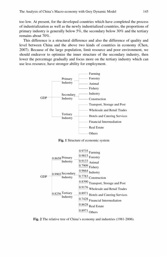
The Analysis of China’s Macro-economy with Grey Dynamic Model 145
too low. At present, for the developed countries which have completed the process of industrialization as well as the newly industrialized countries, the proportions of primary industry is generally below 5%, the secondary below 30% and the tertiary remains about 70%.
This difference is a structural difference and also the difference of quality and level between China and the above two kinds of countries in economy (Chen, 2007). Because of the large population, limit resource and poor environment, we should endeavor to optimize the inner structure of the secondary industry, then lower the percentage gradually and focus more on the tertiary industry which can use less resource, have stronger ability for employment.
Farming
Forestry
Animal
Fishery
Industry
Construction
Transport, Storage and Post
Wholesale and Retail Trades
Hotels and Catering Services
Financial Intermediation
Real Estate
Others
Primary Industry
Secondary Industry
Tertiary Industry
GDP
Fig. 1 Structure of economic system
0.9735 Farming0.9815 Forestry0.9133 Animal0.7909 Fishery0.9664 Industry0.7783 Construction0.8390 Transport, Storage and Post0.9176 Wholesale and Retail Trades0.8971 Hotels and Catering Services0.7428 Financial Intermediation0.8628 Real Estate0.8971 Others
Primary Industry
0.8658
0.9903 Secondary Industry
0.8256 Tertiary Industry
GDP
Fig. 2 The relative tree of China’s economy and industries (1981-2006).

146 J. Du and X. Wang
0.8216
0.9624 Secondary Industry
0.8595 Tertiary Industry
GDP
0.9468 Farming0.9347 Forestry0.9038 Animal0.7546 Fishery0.9483 Industry0.7383 Construction0.9375 Transport, Storage and Post0.8601 Wholesale and Retail Trades0.9668 Hotels and Catering Services0.8882 Financial Intermediation0.9283 Real Estate0.8457 Others
Primary Industry
Fig. 3 The relative tree of China’s economy and industries (1986-2006)
0.7502
0.8865 Secondary Industry
0.9454 Tertiary Industry
GDP
0.7165 Farming0.7940 Forestry0.7387 Animal0.8340 Fishery0.9587 Industry0.8046 Construction0.7646 Transport, Storage and Post0.7517 Wholesale and Retail Trades0.8089 Hotels and Catering Services0.6766 Financial Intermediation0.8089 Real Estate0.7423 Others
Primary Industry
Fig. 4 The relative tree of China’s economy and industries (2001-2006).
2) The Grey Relation Analysis of the Primary Industry and All Its Internal In-
dustries: As is demonstrated in the charts, among the relevant factors that affect the primary industry, forestry has the greatest relational grade with the primary. For-estry is closely relational to agricultural production and the development of forestry is one of the key points of agricultural work, but the output value of China’s forestry and its proportion in the total productive value of the primary are both low. In 2006, the total output value of forestry is 160.2 billion Yuan, which is merely 3.78% of that of the agriculture. Being the second one, farming is still the backbone project of agriculture and is the basis of all agricultural work. The third and fourth are, re-spectively, animal and fishery, such relational grade is contradictory to China’s large population but limit land, the adjustment of food structure to high-grade and
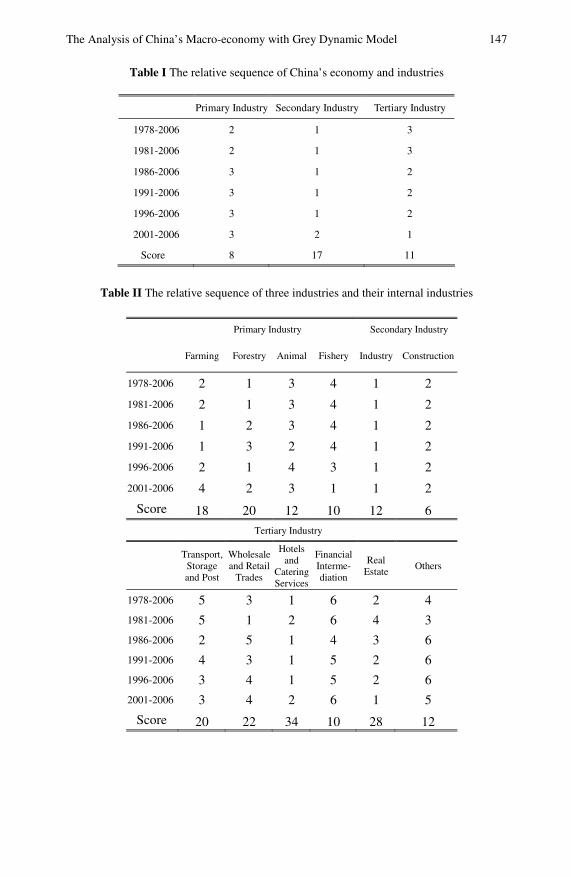
The Analysis of China’s Macro-economy with Grey Dynamic Model 147
Table I The relative sequence of China’s economy and industries
Primary Industry Secondary Industry Tertiary Industry
1978-2006 2 1 3
1981-2006 2 1 3
1986-2006 3 1 2
1991-2006 3 1 2
1996-2006 3 1 2
2001-2006 3 2 1
Score 8 17 11
Table II The relative sequence of three industries and their internal industries
Primary Industry Secondary Industry
Farming Forestry Animal Fishery Industry Construction
1978-2006 2 1 3 4 1 2
1981-2006 2 1 3 4 1 2
1986-2006 1 2 3 4 1 2
1991-2006 1 3 2 4 1 2
1996-2006 2 1 4 3 1 2
2001-2006 4 2 3 1 1 2
Score 18 20 12 10 12 6
Tertiary Industry
Transport,
Storage and Post
Wholesale and Retail
Trades
Hotels and
Catering Services
Financial Interme-diation
Real Estate
Others
1978-2006 5 3 1 6 2 4
1981-2006 5 1 2 6 4 3
1986-2006 2 5 1 4 3 6
1991-2006 4 3 1 5 2 6
1996-2006 3 4 1 5 2 6
2001-2006 3 4 2 6 1 5
Score 20 22 34 10 28 12

148 J. Du and X. Wang
the increasing demand for animal food. Animal production maintains a good mo-mentum of development, but its contribution to agriculture is not very positive and has a comparatively less investment than forestry and farming industry. Among our land resource 13.5% is plantation, 41.7% is ley which can be used, and 16.5% is forestland. Land which can be used for forestry and stockbreeding is vast. Ac-cording to the producing rate, forestry is 1/16 of farming, and animal is just 1/5 of farming (He and Liao, 2005). The improvement of forestry and animal is an im-portant way to develop our primary industry. For our country, forestry is not only an economic industry, but also an important part to protect and improve the environ-ment and maintain our ecologic balance. The trend of development of stockbreed-ing is to promote the industry which is in need of large labor but independent on the plantation and its deep processed industries.
3) The Grey Relation Analysis of the Secondary Industry and All Its Internal Industries: As is shown in the figures and tables, for quite a long time, among the relevant factors which affect the secondary industry. Industry has the greatest cor-relation with the secondary, followed by construction. Industry is an important basis and leading force of national economic development, but the contradictions of the industrial structure in China are conspicuous, which restrains the better economic development. One problem is that the proportion of heavy industry is too high which reached to 70% in 2006. Another problem is that the general industrial products with a serious oversupply of the process capacity coexist with the lack of high value-added and hi-tech products. In 2006, the productive value of hi-tech industries was 4199.6 billion Yuan, which is simply 13.27% of that of all industries. This industrial structure has a tremendous pressure on China’s already-strained resources and poor ecologic environment, resulting in lower economic efficiency. We must control low-level redundant construction and restrain total amount of promotion in the secondary industry especially industry development. We should mainly depend on the high technology to optimize the industrial structure and en-hance the quality and efficiency of economy. For one thing, the advanced and ap-propriate high technology should be used to transform traditional industries and to promote the upgrade of industry, and for another, we should develop knowl-edge-intensive industries such as communications, electronics, bio-pharmacy etc. Through these industries, we can develop with the application of high technology and the technological innovation so that we can get more benefit (Jing and Shen, 2005).
4) The Grey Relation Analysis of the Tertiary Industry and All Its Interment Industries: As is illustrated in the charts, hotels and catering services has the greatest correlation. Those ranking from the second to sixth are: real estate, wholesale and retail trades, transport, storage and post, others and financial inter-mediation. It suggests that these traditional industries such as catering services, business, transportation, post and telecommunications have a greater correlation with tertiary industry while finance and insurance, tourism, information, consulta-tion, technology services, education, culture and other emerging industries have a relatively smaller correlation, implying that the internal structural level of tertiary industry in China is still low and has much room to upgrade. Since the reform and opening up, the implementation of the compensation for the use of land,
The Analysis of China’s Macro-economy with Grey Dynamic Model 149
monetization of housing distribution and commercialized reform in housing con-sumption have made the real estate experience a great development, a rapid growth in investment and a marked increase in the amount of real estate transactions, which play an obvious role in developing the tertiary industry, even the overall national economy. Nevertheless, the lack of a sound operational mechanism, and the inef-ficiency of macro-regulation have put the development of the industry into a false inflation and in a condition of confusion. It has excessively negative effects on development of the tertiary industry and the national economy.
During the development process of world economy, newly emerging service industry gives impetus to the development of world economy; they are character-ized to be clean, have low level of consumption and high benefit. It is so prosperous that it becomes the symbol of modern economy. But traditional ones still stay in leading position in our service industry, while newly emerging types of knowl-edge-intensive stay lower. We should highlight on science and technology, strengthen competing ability of knowledge and technology, and develop the high-leveled service industries such as culture, consultation, management, tech-nique patent, finance and communications etc (Dong, 2007).
4 Analysis and Forecast of the Economy of China
The weak economic base in early period of reform and opening up made little in-crease in value, though the speed of economy was not slow and the trend was up-ward between 1978 to 1990; with the great success of reform and opening up and the increase speed of economic development, the periodic variation in economy varies gradually from hidden invisible variation to obvious periodic variation. So, we adopt the GDP of China in 1991-2007 as original data of grey dynamic model to analyze the economic cycle of China and forecast the economic scale for the next cycle.
C. Analysis on the Economic Cycle of China
We use GDP data in 1991-2007 to establish GM (1, 1) model for the expected a=-0.1243476; u=31893.39 through calculation and further get GM (1,1) model, that is 7.2564857.278266)1( 1243476.0)1( −=+ − tetx ; then obtain simulated data of
GDP of every year through inverse accumulated generating operation. We use the absolute average value of residual error as amplitude, that is A=5499.063; calculate correction quantity of every point, form correctional curve by combining correction quantity with trend curve. The stimulant situation of trend curve of GM (1, 1) with correction curve and original curve are shown in figure 5, and curves of residual error series are shown in fig 6.
In Fig. 6, the cycle of residual error series can be divided into two periods: 1991-1993 is the first period that is a remnant period of last cycle; 1994-2005 is the second period that is an entire cycle, the economic cycle is twelve years (T1=12), which is a medium-and-long period. During the second period the economy system was extended in the states of 1994-1999, while was convergent in 2000-2005. This
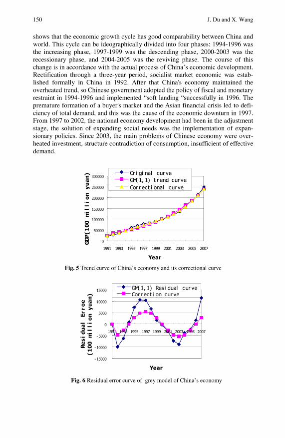
150 J. Du and X. Wang
shows that the economic growth cycle has good comparability between China and world. This cycle can be ideographically divided into four phases: 1994-1996 was the increasing phase, 1997-1999 was the descending phase, 2000-2003 was the recessionary phase, and 2004-2005 was the reviving phase. The course of this change is in accordance with the actual process of China’s economic development. Rectification through a three-year period, socialist market economic was estab-lished formally in China in 1992. After that China's economy maintained the overheated trend, so Chinese government adopted the policy of fiscal and monetary restraint in 1994-1996 and implemented “soft landing “successfully in 1996. The premature formation of a buyer's market and the Asian financial crisis led to defi-ciency of total demand, and this was the cause of the economic downturn in 1997. From 1997 to 2002, the national economy development had been in the adjustment stage, the solution of expanding social needs was the implementation of expan-sionary policies. Since 2003, the main problems of Chinese economy were over-heated investment, structure contradiction of consumption, insufficient of effective demand.
0
50000
100000
150000
200000
250000
300000
1991 1993 1995 1997 1999 2001 2003 2005 2007
Year
GDP
(10
0 mi
lli
on y
uan
) Or i gi nal cur veGM( 1, 1) t r end cur veCor r ect i onal cur ve
Fig. 5 Trend curve of China’s economy and its correctional curve
- 15000
-10000
-5000
0
5000
10000
15000
1991 1993 1995 1997 1999 2001 2003 2005 2007
Year
Res
idu
al
Err
oe(1
00
mil
lio
n y
uan
)
GM( 1, 1) Res i dual cur veCor r ect i on cur ve
Fig. 6 Residual error curve of grey model of China’s economy
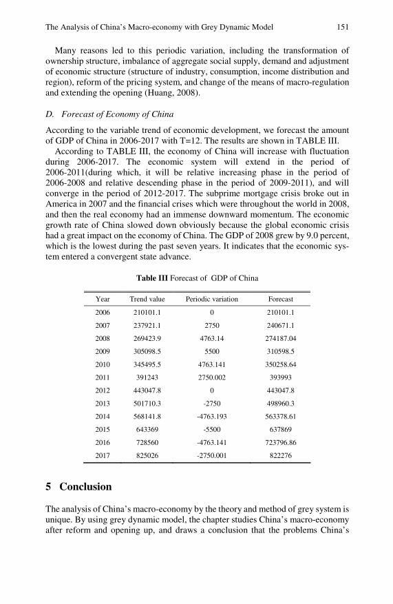
The Analysis of China’s Macro-economy with Grey Dynamic Model 151
Many reasons led to this periodic variation, including the transformation of ownership structure, imbalance of aggregate social supply, demand and adjustment of economic structure (structure of industry, consumption, income distribution and region), reform of the pricing system, and change of the means of macro-regulation and extending the opening (Huang, 2008).
D. Forecast of Economy of China
According to the variable trend of economic development, we forecast the amount of GDP of China in 2006-2017 with T=12. The results are shown in TABLE III.
According to TABLE III, the economy of China will increase with fluctuation during 2006-2017. The economic system will extend in the period of 2006-2011(during which, it will be relative increasing phase in the period of 2006-2008 and relative descending phase in the period of 2009-2011), and will converge in the period of 2012-2017. The subprime mortgage crisis broke out in America in 2007 and the financial crises which were throughout the world in 2008, and then the real economy had an immense downward momentum. The economic growth rate of China slowed down obviously because the global economic crisis had a great impact on the economy of China. The GDP of 2008 grew by 9.0 percent, which is the lowest during the past seven years. It indicates that the economic sys-tem entered a convergent state advance.
Table III Forecast of GDP of China
Year Trend value Periodic variation Forecast
2006 210101.1 0 210101.1
2007 237921.1 2750 240671.1
2008 269423.9 4763.14 274187.04
2009 305098.5 5500 310598.5
2010 345495.5 4763.141 350258.64
2011 391243 2750.002 393993
2012 443047.8 0 443047.8
2013 501710.3 -2750 498960.3
2014 568141.8 -4763.193 563378.61
2015 643369 -5500 637869
2016 728560 -4763.141 723796.86
2017 825026 -2750.001 822276
5 Conclusion
The analysis of China’s macro-economy by the theory and method of grey system is unique. By using grey dynamic model, the chapter studies China’s macro-economy after reform and opening up, and draws a conclusion that the problems China’s

152 J. Du and X. Wang
economy faced are the result of own structural adjustment, business fluctuation and international financial crisis. China’s economy has to undergo a period of painful adjustment, which may last two or three years or even longer, and it is an inevitable process.
References
Chen, Y.: Evolution and enlightenment of the relation between secondary industry and tertiary industry in developed countries. Economic Review (8), 53–57 (2007)
Deng, J.: Basic Method of Grey System, pp. 17–34. Huazhong University of Technology Press, Wuhan (1992)
Dong, M.: The developing laws of the third industries inherent constructions in China. Market Modernization (7), 250–251 (2007)
Hao, Y., Zhang, Z., Wang, R., Du, S., Wang, X.: Grey dynamic analysis of consumption structure of urban residents in Shanxi Province. Consumer Economics (2), 28–31 (2004)
He, Y., Liao, B.: Analysis on spatial-temporal features of agricultural structure adjustment in China. Contemporary Manager (15), 170–171 (2005)
Huang, Z.: Study on China’s economic cycle and macro-control efforts in 30 years of reform and opening-up. Journal of Finance and Economics 34(11), 88–100 (2008)
Jing, Y., Shen, S.: Studies on the development tendency and economic effect of internal structure of the secondary industry in U.S.A. Population Journal (5), 18–23 (2005)
Lin, Y., Chen, M.Y., Liu, S.F.: Theory of grey systems: capturing uncertainties of grey information. Kybernetes: The International Journal of Systems and Cybernetics 33(2), 196–218 (2004)
Lin, Y., Liu, S.F.: Solving Problems with incomplete information: a grey systems approach. In: Advances in Imaging and Electron Physics, vol. 141, pp. 77–174. Elsevier, Oxford (2006)
Liu, S.F., Lin, Y.: Grey Information: Theory and Practical Applications. Springer, London (2006)
National Bureau of Statistics of China. China Statistical Yearbook, China Statistics Press, Beijing (1979-2007)
Wang, X., Luo, J.: Concise Guide of the Grey System Method, pp. 50–54. Chengdu Uni-versity of Science and Technology Press, Chengdu (1993)
Yu, F.: Grey analysis of economic system in Juancheng county, Shandong province. System Sciences and Comprehensive Studies in Agriculture 13(2), 121–123 (1997)
Piecewise Analysis and Prediction of Spring Flow Based ON GM(1,1) Model*
Yonghong Hao, Lixia Zhang, Ting Wei, and Xuemeng Wang
One of the largest springs in North China, the Liulin Karst Springs, has been de-caying since 1950s. We introduced the piecewise analytical concept to GM (1, 1) model focusing on analysis and prediction of Liulin Karst Springs discharge. We divided the spring discharge processes into two phases: pre-1973 and post-1973. In the first phase (i.e. 1957-1974) the spring discharge was affected by climate change and in the second phase (i.e.1973-2007) the spring discharge was influenced by both climate change and anthropogenic activities. In the first phase, spring flow was simulated by the grey system GM (1, 1) decomposition model, then the effects of climate change were modeled. By extrapolating the model, we acquired a calculation of the spring discharge in the second phase solely under the effects of climate change. Based on water balance analysis, we conclude that the contribution of cli-mate change to depletion of Liulin Springs is 0.18-0.34 m3/s from 1974-2007. However, the contribution of anthropogenic activities to depletion of spring flow is Yonghong Hao Key Laboratory of Water Environment and Resources, Tianjin Normal University, 393 Binshuixidao Road, Xiqing District, Tianjin 300387, P.R. China, Phone: +86-22-23766557 e-mail: [email protected], [email protected]
Lixia Zhang College of management, Tianjin Normal University, 393 Binshuixidao Road, Xiqing District, Tianjin 300387, PR China e-mail: [email protected]
Ting Wei National Marine Data & Information Service, 93 Liuwei Road, Hedong District, Tianjin 300171, PR China e-mail: [email protected]
Xuemeng Wang Institute of Agriculture Resources Survey of Shanxi Province, Taiyuan 030006, PR China e-mail: [email protected]
* This work was supported in part by the National Natural Science Foundation of China NSFC-40572150, the Scientific and Technological Development Planning Project of Tianjin 06YFSZSF05100, the Start-up Fund of Tianjin Normal University 5RL070, the Planning Project for Tianjin New Coastal Region of Tianjin Normal University 52LE24, and Open Fund of State Key Laboratory of Environmental Geochemistry of China.
154 Y. Hao et al.
2.55-2.70 m3/s in 2007. The contribution of climate change only accounts for 10% of human activities, therefore human activities have large contribution to Linlin Spring depletion. Regarding to the contribution of human activity effects on spring dis-charge decline, groundwater pumping only account for 20%-35% of the spring flow depletion; 65%-80% of the depletion are likely to be caused by other human activi-ties including dam-building, dewatering during coal mining, and deforestation.
1 Introduction
YDROLOGICAL processes with natural or artificially created inconsistency and nonhomogeneity can be segmented into parts with different statistical characteris-tics. It is known that water resources systems are influenced by climate change and anthropogenic activities, but the large scale water resources developments were the events in recent five decades. So, hydrological processes can be divided into two phases: pre-development and post-development. During the first phase (i.e. pre-development), hydrological processes are affected by climate change, while during the second phase (i.e. post-development), the hydrological processes are dominated by climate change and human activities. In this chapter, we introduced the piecewise analytical concept to GM (1, 1) model focusing on analysis and pre-diction of Liulin Karst Springs discharge in China. This allows us to obtain a better understanding of karst hydrological processes and sustainable development in karst systems by differentiating the contribution of climate change from anthropogenic impacts on the decline of Liulin Springs.
Karst formations often constitute significant aquifers. It is estimated that 25% of the global population is supplied largely or entirely by groundwater from karst aquifers (Jaquet et al., 2004; Ford and Williams, 1989). However, karst aquifers are generally considered to be particularly vulnerable to climate change and anthro-pogenic impacts (Leibundgut, 1998). Climate change influences hydrological processes and alters the recharge and discharge of karst aquifers. There are many human activities that, intentionally or not, produce severe impacts in karst, and often with irreparable damage (Parise and Gunn, 2007). Large withdrawals of water in karst areas for municipal, agricultural, and industrial use may affect the water supply in surrounding areas (Parise et al., 2004). Karst groundwater has become an important indicator to assess climate change and anthropogenic effects on hydro-logical processes (Taminskas and Marcinkevicius, 2002; Guo et al., 2005). Based on the projected climate change scenarios using general circulation models, Loáiciga et al. (2000) simulated the potential impacts on groundwater in the Ed-wards Balcones Fault Zone (BFZ) karst aquifer in Texas, USA (Loáiciga et al., 2000). The results showed that the Edwards BFZ aquifer could be severely im-pacted under a warmer climate. Viles (2003) analyzed the impacts of climate change on karst geomorphology in the UK and Ireland using a conceptual model (Viles, 2003). The author reached some general conclusions over the magnitude and nature of impacts of climate change on karst hydrology, dissolution rates and mass movements, but none of these impacts of climatic change are likely to be as serious as some of the local human impacts such as quarrying and pollution. Nkhuwa
H

Piecewise Analysis and Prediction of Spring Flow Based on GM(1,1) Model 155
(2003) found that impacts of urbanization on groundwater quality are a conse-quence of human activities on a very fragile and vulnerable geologic environment according to chemical and bacteriological analyses in Lusaka karst aquifer (Nkhuwa, 2003). Li et al. (2008) gained a better understanding of natural and an-thropogenic influences on water quality based on carbon isotope studies and water chemistry in Southwest China (Li et al., 2008). The results show that local rain events in summer and a longer water residence time in winter play an important role in groundwater carbon evolution in karst flow systems of Southwest China. And they also indicate that urban anthropogenic activities have an effect on the carbon evolution of groundwater and might threaten water quality. Hao et al. (2006; 2007) introduced grey system theory to simulation of karst springs flow and proposed GM (1, 2) model with time-lags and GM (1, 1) decomposition model (Hao et al., 2006; Hao et al., 2007). Then the models were used to study the relations between pre-cipitation and Liulin Springs flow in China. The results showed that the influence of climate change on spring discharge at Liulin Springs is long-term and evident. But these models mainly studied the combined effects of both climate change and hu-man activities on spring flow. Few of these studies differentiate the contribution of climate change from those of anthropogenic effects on karst spring flow processes. However, for further sustainable development of karst groundwater, it is essential to discern the contribution of climate change from anthropogenic effects on karst spring flows. The purpose of this chapter is to investigate the depletion of Liulin Springs in North China by differentiating the respective effects of climate change and anthropogenic activities.
China has some of the largest karst terrains in the world. One-quarter of the world’s carbonate rock occurs in China. Carbonate rock outcrops cover 1.3 million km2 or one-seventh of China’s area. If more deeply covered and buried karsts are included, up to one-third of the country can be classified as karst, which is 3,463,000 km2 (Sweeting, 1995). Karst terrain of China is concentrated in two regions: an area located in a semiarid climate zone in the northern part of China, and a humid climate zone in the southwest part of China (He et al., 1997; Yuan, 1994). Karstification is highly influenced by precipitation and topography, which can cause large differences in karst aquifers between different regions. In the northern part of China, annual precipitation is less than 800 mm, and most carbonate aquifers are overlain by thick Permian carboniferous-sandstone and shale, and Quaternary sediments. Karstification in these areas is generally not very developed, in contrast to the karst systems in humid, southwest China, where well-developed caves and highly-connected ground flow channels are abundant (Hao et al., 2007). However, large karst basins provide an inflow of more than 1 m3/s to many big karst springs in the northern part of China.
The Liulin Spring complex is one of the biggest in the north part of China. They are located in the Sanchuan River Valley in the west of Shanxi Province. Groundwater from the middle Ordovician karst aquifer has been one of the most important sources of water supply in Liulin Springs Basin. The Liulin Spings flow has been declining since the 1950s, especially after the early 1970s when the groundwater resources of the basin begin to be developed for industrial, municipal, and irrigation uses. In this project, we concentrated on investigating the depletion of
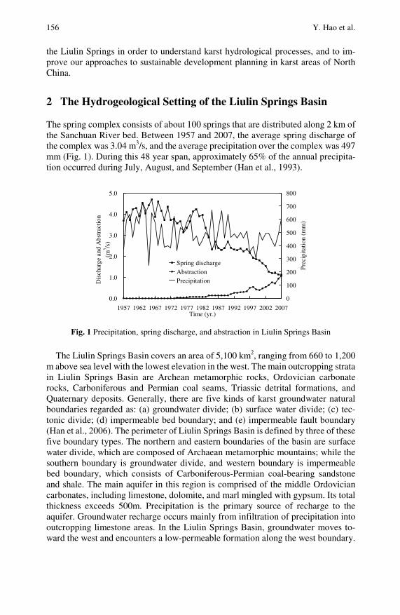
156 Y. Hao et al.
the Liulin Springs in order to understand karst hydrological processes, and to im-prove our approaches to sustainable development planning in karst areas of North China.
2 The Hydrogeological Setting of the Liulin Springs Basin
The spring complex consists of about 100 springs that are distributed along 2 km of the Sanchuan River bed. Between 1957 and 2007, the average spring discharge of the complex was 3.04 m3/s, and the average precipitation over the complex was 497 mm (Fig. 1). During this 48 year span, approximately 65% of the annual precipita-tion occurred during July, August, and September (Han et al., 1993).
0.0
1.0
2.0
3.0
4.0
5.0
1957 1962 1967 1972 1977 1982 1987 1992 1997 2002 2007Time (yr.)
Dis
char
ge a
nd A
bstr
acti
on
(m3 /s
)
0
100
200
300
400
500
600
700
800
Prec
ipita
tion
(mm
)
Spring dischargeAbstractionPrecipitation
Fig. 1 Precipitation, spring discharge, and abstraction in Liulin Springs Basin
The Liulin Springs Basin covers an area of 5,100 km2, ranging from 660 to 1,200
m above sea level with the lowest elevation in the west. The main outcropping strata in Liulin Springs Basin are Archean metamorphic rocks, Ordovician carbonate rocks, Carboniferous and Permian coal seams, Triassic detrital formations, and Quaternary deposits. Generally, there are five kinds of karst groundwater natural boundaries regarded as: (a) groundwater divide; (b) surface water divide; (c) tec-tonic divide; (d) impermeable bed boundary; and (e) impermeable fault boundary (Han et al., 2006). The perimeter of Liulin Springs Basin is defined by three of these five boundary types. The northern and eastern boundaries of the basin are surface water divide, which are composed of Archaean metamorphic mountains; while the southern boundary is groundwater divide, and western boundary is impermeable bed boundary, which consists of Carboniferous-Permian coal-bearing sandstone and shale. The main aquifer in this region is comprised of the middle Ordovician carbonates, including limestone, dolomite, and marl mingled with gypsum. Its total thickness exceeds 500m. Precipitation is the primary source of recharge to the aquifer. Groundwater recharge occurs mainly from infiltration of precipitation into outcropping limestone areas. In the Liulin Springs Basin, groundwater moves to-ward the west and encounters a low-permeable formation along the west boundary.
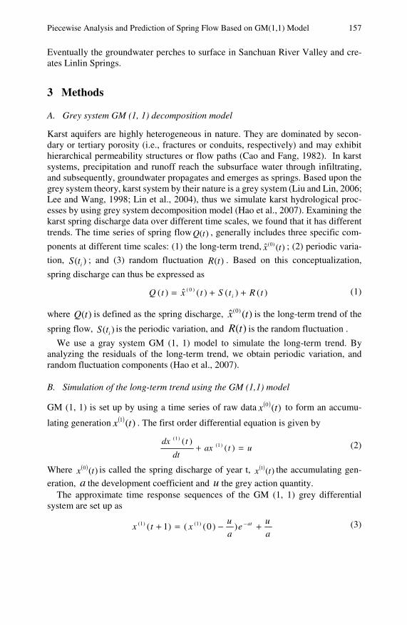
Piecewise Analysis and Prediction of Spring Flow Based on GM(1,1) Model 157
Eventually the groundwater perches to surface in Sanchuan River Valley and cre-ates Linlin Springs.
3 Methods
A. Grey system GM (1, 1) decomposition model
Karst aquifers are highly heterogeneous in nature. They are dominated by secon-dary or tertiary porosity (i.e., fractures or conduits, respectively) and may exhibit hierarchical permeability structures or flow paths (Cao and Fang, 1982). In karst systems, precipitation and runoff reach the subsurface water through infiltrating, and subsequently, groundwater propagates and emerges as springs. Based upon the grey system theory, karst system by their nature is a grey system (Liu and Lin, 2006; Lee and Wang, 1998; Lin et al., 2004), thus we simulate karst hydrological proc-esses by using grey system decomposition model (Hao et al., 2007). Examining the karst spring discharge data over different time scales, we found that it has different trends. The time series of spring flow )(tQ , generally includes three specific com-
ponents at different time scales: (1) the long-term trend, )(ˆ )0( tx ; (2) periodic varia-
tion, )( itS ; and (3) random fluctuation )(tR . Based on this conceptualization,
spring discharge can thus be expressed as
( 0 )ˆ( ) ( ) ( ) ( )iQ t x t S t R t= + + (1)
where )(tQ is defined as the spring discharge, )(ˆ )0( tx is the long-term trend of the
spring flow, )( itS is the periodic variation, and )(tR is the random fluctuation .
We use a gray system GM (1, 1) model to simulate the long-term trend. By analyzing the residuals of the long-term trend, we obtain periodic variation, and random fluctuation components (Hao et al., 2007).
B. Simulation of the long-term trend using the GM (1,1) model
GM (1, 1) is set up by using a time series of raw data ( ) )(0 tx to form an accumu-
lating generation ( ) )(1 tx . The first order differential equation is given by
utaxdt
tdx=+ )(
)( )1()1(
(2)
Where ( ) )(0 tx is called the spring discharge of year t, ( ) )(1 tx the accumulating gen-
eration, a the development coefficient and u the grey action quantity. The approximate time response sequences of the GM (1, 1) grey differential
system are set up as
a
ue
a
uxtx at +−=+ −))0(()1( )1()1( (3)
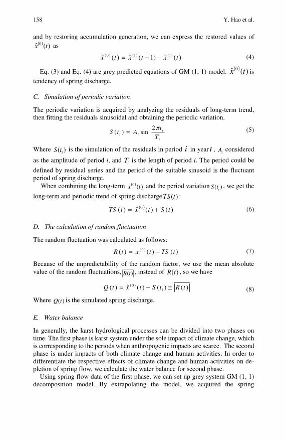
158 Y. Hao et al.
and by restoring accumulation generation, we can express the restored values of ( ) )(ˆ 0 tx as
)(ˆ)1(ˆ)(ˆ )1()1()0( txtxtx −+= (4)
Eq. (3) and Eq. (4) are grey predicted equations of GM (1, 1) model. ( ) )(ˆ 0 tx is
tendency of spring discharge.
C. Simulation of periodic variation
The periodic variation is acquired by analyzing the residuals of long-term trend, then fitting the residuals sinusoidal and obtaining the periodic variation,
i
iii T
tAtS
π2sin)( = (5)
Where )( itS is the simulation of the residuals in period i in year t , iA considered
as the amplitude of period i, and iT is the length of period i. The period could be
defined by residual series and the period of the suitable sinusoid is the fluctuant period of spring discharge.
When combining the long-term ( ) )(0 tx and the period variation )( itS , we get the
long-term and periodic trend of spring discharge )(tTS :
( ) )()(ˆ)( 0 tStxtTS += (6)
D. The calculation of random fluctuation
The random fluctuation was calculated as follows:
)()()( )0( tTStxtR −= (7)
Because of the unpredictability of the random factor, we use the mean absolute value of the random fluctuations, )(tR , instead of )(tR , so we have
( 0 )ˆ( ) ( ) ( ) ( )iQ t x t S t R t= + ± (8)
Where )(tQ is the simulated spring discharge.
E. Water balance
In generally, the karst hydrological processes can be divided into two phases on time. The first phase is karst system under the sole impact of climate change, which is corresponding to the periods when anthropogenic impacts are scarce. The second phase is under impacts of both climate change and human activities. In order to differentiate the respective effects of climate change and human activities on de-pletion of spring flow, we calculate the water balance for second phase.
Using spring flow data of the first phase, we can set up grey system GM (1, 1) decomposition model. By extrapolating the model, we acquired the spring
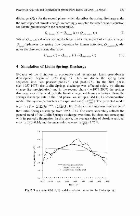
Piecewise Analysis and Prediction of Spring Flow Based on GM(1,1) Model 159
discharge )(tQ for the second phase, which describes the spring discharge under
the sole impact of climate change. Accordingly we setup the water balance equation for karstic groundwater in the second phase,
)()()(lim tQtQtQ obsevationhumanatec += (9)
Where )(lim tQ atec denotes spring discharge under the impact of climate change;
)(tQhumandenotes the spring flow depletion by human activities; )(tQ nobservatio de-
notes the observed spring discharge.
)()()( lim tQtQtQ obsevationatechuman −= (10)
4 Simulation of Liulin Springs Discharge
Because of the limitation in economics and technology, karst groundwater development began at 1973 (Fig. 1). Thus we divide the spring flow sequence into two phases: pre-1973 and post-1973. In the first phase (i.e. 1957-1973) the Liulin Springs discharge was affected solely by climate change (i.e. precipitation) and in the second phase (i.e.1974-2007) the springs discharge was influenced by both climate change and human activities. Using the springs discharge data in the first phase, we set up a GM (1, 1) decomposition model. The system parameters are expressed as ( ) ( )002.0
4.183=au
. The predicted model
is 2426.5 -2422.7e)1( -0.002t)1( +=+tx . Fig. 2 shows the long-term trend curve of
the Liulin Springs discharge from 1957-1973. The curve accurately reflects the general trend of the Liulin Springs discharge over time, but does not correspond with its periodic fluctuation. In this curve, the average value of absolute residual error is )(tε =0.14, and the mean relative error is )(tq =3.76%.
3.4
3.6
3.8
4.0
4.2
4.4
4.6
1957 1959 1961 1963 1965 1967 1969 1971 1973
Time(yr.)
Spri
ng D
isch
arge
(m
3 /s)
Observed spring dischargeLong-term trend curveLong-term and periodic trend
Fig. 2 Grey system GM (1, 1) model simulation curves for the Liulin Springs
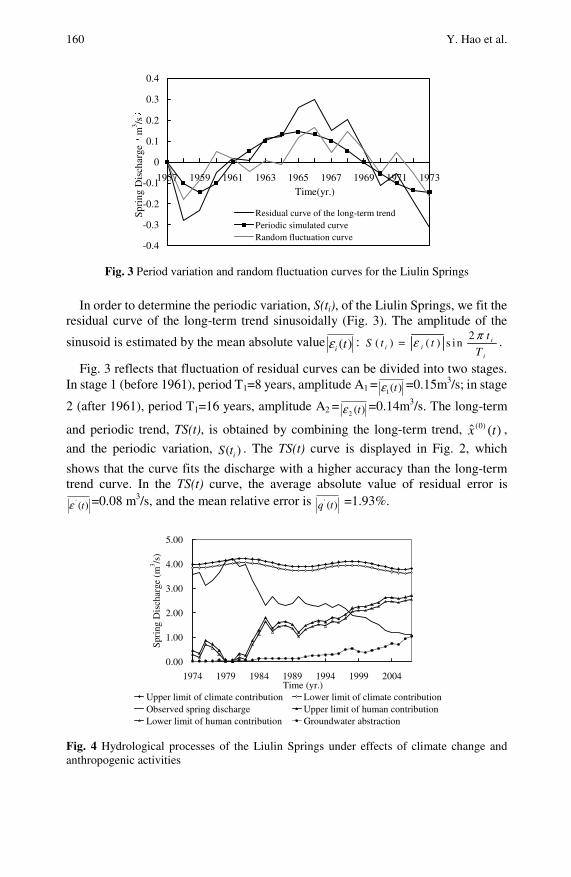
160 Y. Hao et al.
-0.4
-0.3
-0.2
-0.1
0
0.1
0.2
0.3
0.4
1957 1959 1961 1963 1965 1967 1969 1971 1973Time(yr.)
Spri
ng D
isch
arge
(m
3 /s
)
Residual curve of the long-term trendPeriodic simulated curveRandom fluctuation curve
Fig. 3 Period variation and random fluctuation curves for the Liulin Springs
In order to determine the periodic variation, S(ti), of the Liulin Springs, we fit the
residual curve of the long-term trend sinusoidally (Fig. 3). The amplitude of the
sinusoid is estimated by the mean absolute value )(tiε : 2( ) ( ) s in i
i ii
tS t t
T
πε= .
Fig. 3 reflects that fluctuation of residual curves can be divided into two stages. In stage 1 (before 1961), period T1=8 years, amplitude A1 = )(1 tε =0.15m3/s; in stage
2 (after 1961), period T1=16 years, amplitude A2 = )(2 tε =0.14m3/s. The long-term
and periodic trend, TS(t), is obtained by combining the long-term trend, )(ˆ )0( tx ,
and the periodic variation, )( itS . The TS(t) curve is displayed in Fig. 2, which
shows that the curve fits the discharge with a higher accuracy than the long-term trend curve. In the TS(t) curve, the average absolute value of residual error is
)(' tε =0.08 m3/s, and the mean relative error is )(' tq =1.93%.
0.00
1.00
2.00
3.00
4.00
5.00
1974 1979 1984 1989 1994 1999 2004Time (yr.)
Spr
ing
Dis
char
ge (
m3 /s
)
Upper limit of climate contribution Lower limit of climate contributionObserved spring discharge Upper limit of human contribution Lower limit of human contribution Groundwater abstraction
Fig. 4 Hydrological processes of the Liulin Springs under effects of climate change and anthropogenic activities

Piecewise Analysis and Prediction of Spring Flow Based on GM(1,1) Model 161
The random fluctuation curve )(tR is acquired on the basis of Equation 7, and the
curve is shown in Fig. 3. The average value of random fluctuation )(tR =0.079 m3/s.
According to Equation (8), GM (1, 1) decomposed model of the Liulin Springs from 1957-1973 was obtained. Running the model, we acquired the spring flow under sole impact of climate change in second phase (i.e.1974-2007). Then through water balance equations (9) and (10), we differentiate the respective effects of climate change and human activities on depletion of spring discharges. Results show in Fig. 4.
5 Results and Discussion
Fig. 4 shows that the spring discharge decreased during the years from 1974 to 2007 under effects of climate change. The average annual spring discharge was 3.84-4.00 m3/s in 1974 and 3.66-3.81 m3/s in 2007. Therefore, the contribution of climate change effects on depletion of the Liulin Springs is 0.18-0.34 m3/s from 1974-2007. However, the contribution of anthropogenic activities effects on depletion of spring flow is 2.55 -2.70 m3/s in 2007. Therefore, human activities have large contribution to Linlin Spring depletion.
Regarding to the contribution of human activity effects on spring discharge de-cline, groundwater pumping only account for 20%-35% of the declines; 65%-80% of the declines are likely to be caused by other human activities (Fig. 4).
Following important human activities are supposed to have the important con-tribution to change the regional hydrological processes. Dam-building causes the recharge decline from river bed. Three larger reservoirs were constructed on branches of the Sanchuan River. Wucheng Reservoir that lies on Dongchuan River constructed in 1957 with the storage of 12.44 million m3; Chenjiawan Reservoir that lies on Nanchuan River constructed in 1967 with the capacity of 10 millin m3 and Hengquan Reservoir that lies on Beichuan River that being under construction with the storage of 85.6 million m3. These reservoirs changed the regional hydro-logical processes, causing the decline of surface water recharge to karst ground-water. In the Liulin Springs Basin, the annual recharge capacity from river bed reduced from 38.6 million m3 in 1956 to 18 million m3 in 2000.
Coal mining is one of the main industries in the Liulin Springs Basin. There are a total of 74 coal mines throughout the Liulin Springs Basin and the annual coal output reached to 13.4 million tons in the 2006. The estimated annual dewatering from coal mining is 12.7 million m3. Because Carboniferous-Permian coal-bearing formations are above Ordovician karst aquifer in elevation in Liulin Springs Basin, dewatering from coal mining artificially decreases the recharge of precipitation to karst aquifer. Therefore, dewatering from coal mining is one of the important arti-ficial activities causes the depletion of Liulin Springs flow.
Deforestation changed the underlying surface and the hydrological processes of the Liulin Springs Basin. Percentage of forest cover reduced from 36% in 1980s to 24% in beginning of 21 century. Consequently, the infiltration of precipitation to karst aquifer is decreased. It is likely to be one of the main reasons that cause the spring flow depletion.

162 Y. Hao et al.
6 Conclusions
One of the largest springs in North China, the Liulin Karst Springs, is vulnerable to anthropogenic impacts and regional climate change and has declined since 1950s. This chapter discussed the response of Liulin Springs discharge to climate change and human activities by introducing the piecewise analytical concept to GM (1, 1) model. In Liulin Springs Basin, the development of karst groundwater began in 1973. Accordingly, the spring discharge data were divided into two phases: pre-1973 and post-1973. In the first phase (i.e. 1957-1973) the spring discharge was affected by climate change, and in the second phase (i.e.1974-2007) the spring discharge was influenced by both climate change and human activities. In the first phase, spring flow was simulated by the grey system GM (1, 1) decomposition model. Then the effects of climate change were modeled. By extrapolating the model, we acquired a calculation of the spring discharge in the second phase sole under the effects of climate change. Based on water balance analysis, we conclude that the contribution of climate change to depletion of Liulin Springs is 0.18-0.34 m3/s from 1974-2007. However, the contribution of anthropogenic activities to depletion of spring flow is 2.55 -2.70 m3/s in 2007. The contribution of climate change only accounts for 10% of contribution of human activities. Therefore, hu-man activities have large contribution to Linlin Spring depletion.
Regarding to the contribution of human activity effects on spring discharge de-cline, groundwater pumping only account for 20%-35% of the spring flow deple-tion; 65%-80% of the depletions are likely to be caused by other human activities. Firstly dam-building caused the recharge capacity from river bed to karst aquifer decline from 38.6 million m3 in 1956 to 18 million m3 in 2000. Secondly dewatering from coal mining artificially decreases the recharge of precipitation to karst aquifer and the estimated annual dewatering from coal mining is 12.7 million m3 in 2006. Finally deforestation changed the underlying surface and hydrological processes. Percentage of forest cover reduced from 36% in 1980s to 24% in beginning of 21 century. Consequently, the infiltration of precipitation to karst aquifer is decreased, which caused the spring flow decline. Therefore, it is unreasonable only consider-ing groundwater pumping as human activity while ignoring the contributions of other human activities.
As a representative of karst springs in North China, the Liulin Springs reflect varieties of karst spring discharge and exploitation processes of groundwater for recent 50 years. Before the 1970s, karst groundwater is mainly on natural circula-tion. After that time, human exploitation increased and spring discharge decreased. In the 21st century, karst groundwater exploitation and economic activities dis-turbed groundwater circulation that have exceeded natural supplement.
Grey system model successfully simulated effects of climate change and human activities on spring discharge. It investigated the response of spring discharge to climate change and human activities. The GM (1, 1) model is a useful tool in re-gional groundwater plan and sustainable development.
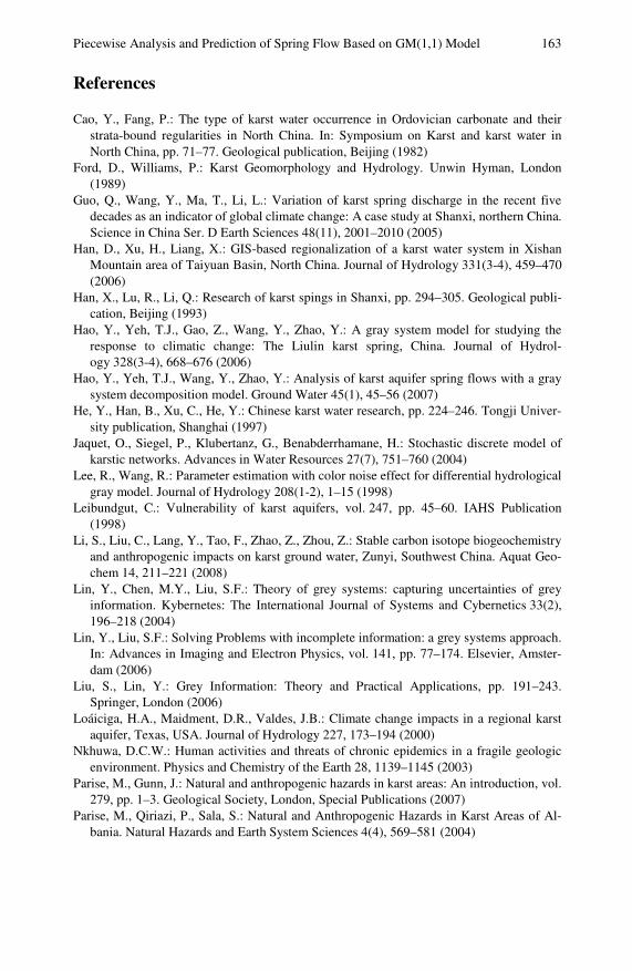
Piecewise Analysis and Prediction of Spring Flow Based on GM(1,1) Model 163
References
Cao, Y., Fang, P.: The type of karst water occurrence in Ordovician carbonate and their strata-bound regularities in North China. In: Symposium on Karst and karst water in North China, pp. 71–77. Geological publication, Beijing (1982)
Ford, D., Williams, P.: Karst Geomorphology and Hydrology. Unwin Hyman, London (1989)
Guo, Q., Wang, Y., Ma, T., Li, L.: Variation of karst spring discharge in the recent five decades as an indicator of global climate change: A case study at Shanxi, northern China. Science in China Ser. D Earth Sciences 48(11), 2001–2010 (2005)
Han, D., Xu, H., Liang, X.: GIS-based regionalization of a karst water system in Xishan Mountain area of Taiyuan Basin, North China. Journal of Hydrology 331(3-4), 459–470 (2006)
Han, X., Lu, R., Li, Q.: Research of karst spings in Shanxi, pp. 294–305. Geological publi-cation, Beijing (1993)
Hao, Y., Yeh, T.J., Gao, Z., Wang, Y., Zhao, Y.: A gray system model for studying the response to climatic change: The Liulin karst spring, China. Journal of Hydrol-ogy 328(3-4), 668–676 (2006)
Hao, Y., Yeh, T.J., Wang, Y., Zhao, Y.: Analysis of karst aquifer spring flows with a gray system decomposition model. Ground Water 45(1), 45–56 (2007)
He, Y., Han, B., Xu, C., He, Y.: Chinese karst water research, pp. 224–246. Tongji Univer-sity publication, Shanghai (1997)
Jaquet, O., Siegel, P., Klubertanz, G., Benabderrhamane, H.: Stochastic discrete model of karstic networks. Advances in Water Resources 27(7), 751–760 (2004)
Lee, R., Wang, R.: Parameter estimation with color noise effect for differential hydrological gray model. Journal of Hydrology 208(1-2), 1–15 (1998)
Leibundgut, C.: Vulnerability of karst aquifers, vol. 247, pp. 45–60. IAHS Publication (1998)
Li, S., Liu, C., Lang, Y., Tao, F., Zhao, Z., Zhou, Z.: Stable carbon isotope biogeochemistry and anthropogenic impacts on karst ground water, Zunyi, Southwest China. Aquat Geo-chem 14, 211–221 (2008)
Lin, Y., Chen, M.Y., Liu, S.F.: Theory of grey systems: capturing uncertainties of grey information. Kybernetes: The International Journal of Systems and Cybernetics 33(2), 196–218 (2004)
Lin, Y., Liu, S.F.: Solving Problems with incomplete information: a grey systems approach. In: Advances in Imaging and Electron Physics, vol. 141, pp. 77–174. Elsevier, Amster-dam (2006)
Liu, S., Lin, Y.: Grey Information: Theory and Practical Applications, pp. 191–243. Springer, London (2006)
Loáiciga, H.A., Maidment, D.R., Valdes, J.B.: Climate change impacts in a regional karst aquifer, Texas, USA. Journal of Hydrology 227, 173–194 (2000)
Nkhuwa, D.C.W.: Human activities and threats of chronic epidemics in a fragile geologic environment. Physics and Chemistry of the Earth 28, 1139–1145 (2003)
Parise, M., Gunn, J.: Natural and anthropogenic hazards in karst areas: An introduction, vol. 279, pp. 1–3. Geological Society, London, Special Publications (2007)
Parise, M., Qiriazi, P., Sala, S.: Natural and Anthropogenic Hazards in Karst Areas of Al-bania. Natural Hazards and Earth System Sciences 4(4), 569–581 (2004)

164 Y. Hao et al. Sweeting, M.M.: Karst in China: Its geomorphology and environment, pp. 1–31. Springer,
Berlin (1995) Taminskas, J., Marcinkevicius, V.: Karst geoindicators of environmental change: the case of
Lithuania. Environmental Geology 42, 757–766 (2002) Viles, H.A.: Conceptual modeling of the impacts of climate change on karst geomorphology
in the UK and Ireland. Journal for Nature Conservation 11, 59–66 (2003) Xia, J.: Hydrology of Grey System, pp. 24–53. Press of Huazhong University of Science and
Technology, Wuhan (2000) Yuan, D.: Chinese Karst, pp. 149–164. Geological publication, Beijing (1994)

Relational Analysis between Technological
Ning Luo, Weijun Zhong, and Shu’e Mei
Based on the improved grey T’s correlation degree, the chapter employs data of 50 counties in Jiangsu Province that participated in the nationwide technological pro-gress assessment from 2003 to 2006, and takes an empirical analysis on the relation between technical input-output indicators and gross domestic product (GDP). This chapter also proposes the identity and difference of how technological progress advances economy in southern, middle and northern Jiangsu from the perspective of the whole province and each of the three regions.
1 Introduction
Technological progress is the primary impetus that improves local productivity and comprehensive competence for a region. A great number of studies have shown that inputs in science and technology (S&T) especially research and development (R&D) expenditures, exert a significant and far-reaching influence on economic development and productivity growth. Griliches and Lichtenberg (1984) modeled the relation between growth of total factor productivity (TFP) and R&D stocks based on Cobb-Douglas production function at the industry level, and concluded that there appeared a rather strong relationship between the intensity of private (but not federal) R&D expenditures and subsequent growth in productivity (Griliches, 1984). Becker and Murphy (1992) conducted a study on the ratio of R&D expen-diture to gross domestic product (GDP) in OECD countries, and concluded that nation wealth had certain affinity with investment in R&D (Becker and Murphy, 1992). The study of Galor and Tsiddon (1997) analyzed the interaction between
Ning Luo Southeast University, Nanjing, CO 211189 China (Phone: 025-52084321) e-mail: [email protected]
Weijun Zhong School of Economics & Management, Southeast University, Nanjing, CO 211189 China e-mail: [email protected]
Shu’e Mei School of Economics & Management, Southeast University, Nanjing, CO 211189 China e-mail: [email protected]

166 N. Luo, W. Zhong, and S. Mei technological progress, economic growth and earning equality, revealing that the reduction in concentration of ability in technologically advanced sectors and con-venient access to technology as well slowed future economic growth (Tsiddon, 1997). Guellec and Bruno (2001) employed data from 16 OECD countries during the period between 1980 and 1998, and utilized panel data to analyze how different types of R&D expenditures affected multi-factor productivity in the long term (Guellec and de la Potterie, 2001). Bronzini and Piselli (2009) estimated the long-run relationship between total factor productivity (TPF) and R&D stock as one of the three capitals between 1980 and 2001 across Italian regions, and found that regional productivity was positively affected by R&D activity and R&D stock was the bi-directional causality found through Granger-causality tests (Bronzini and Piselli, 2009). In Coccia’s research (2009), a regression analysis based on quadratic function and mathematical optimization methods was applied to find the optimal range of domestic expenditure on R&D expressed as percentage of GDP (GERD), which was concluded between 2.3 percent and 2.6 percent (Mi et al., 2004).
Compared with econometric methods, grey incidence analysis (Liu and Lin, 2006; Lin et al., 2004; Lin and Liu, 2006) that could be easily implemented on the computer has few specific limitations on the quantity as well as the distribution of samples. It also has been widely used in studies of the correlation between technological progress and economic development. Mi and Liu (2004) calculated grey relative relational grade between technology input and economic increase in Jiangsu province, con-firming that both R&D expenditure and input in technical human resources positively affected on economy, while the influence of the latter one was more significant (Hu and Gao, 2004); Data from five provinces in Middle China were used in Hu and Gao’s research (2004) and their conclusion was similar to the study of Mi and Liu (Tang and Liu, 2006); Tang and Liu (2006) took into account hysteresis effect of input in S&T on economic growth in their grey T’s incidence degree analysis be-tween distinct types of R&D expenditures and economic development (Deng, 1989).
However, current studies are mostly concentrated on technical inputs, especially investments in R&D and the input of technical talents. Few research concerns about the correlation between technical outputs and economic outputs. However, tech-nical achievements, as a matter of fact, might not be certainly transferred into economic benefits. As a result, this chapter brings technical outputs into techno-logical progress system.
The chapter is organized as follows. In the second part, indicators and data are described and the necessary descriptive statistical analysis is presented. The methodology of grey T’s correlation degree analysis and the application in this empirical study are illustrated in the third section. The fourth section presents analysis of results in the third part, which summarized the identity and difference of correlation between economic growth and technological progress in counties in three regions in Jiangsu province. The fifth section concludes and proposes several policy suggestions.
2 Data Collection and Description
In this chapter we utilize data from 50 counties in Jiangsu Province, the primary source of which is the database of nationwide technological progress assessment.
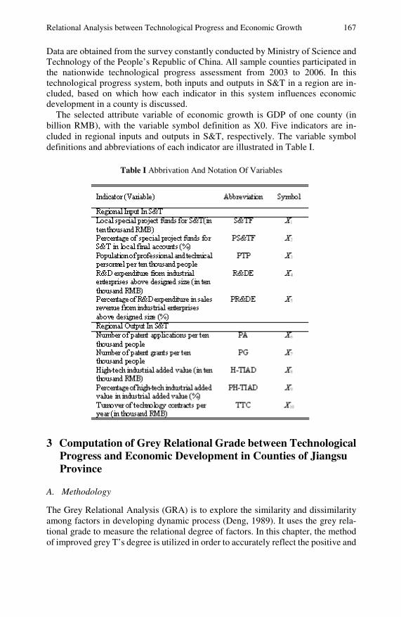
Relational Analysis between Technological Progress and Economic Growth 167 Data are obtained from the survey constantly conducted by Ministry of Science and Technology of the People’s Republic of China. All sample counties participated in the nationwide technological progress assessment from 2003 to 2006. In this technological progress system, both inputs and outputs in S&T in a region are in-cluded, based on which how each indicator in this system influences economic development in a county is discussed.
The selected attribute variable of economic growth is GDP of one county (in billion RMB), with the variable symbol definition as X0. Five indicators are in-cluded in regional inputs and outputs in S&T, respectively. The variable symbol definitions and abbreviations of each indicator are illustrated in Table I.
Table I Abbrivation And Notation Of Variables
3 Computation of Grey Relational Grade between Technological Progress and Economic Development in Counties of Jiangsu Province
A. Methodology
The Grey Relational Analysis (GRA) is to explore the similarity and dissimilarity among factors in developing dynamic process (Deng, 1989). It uses the grey rela-tional grade to measure the relational degree of factors. In this chapter, the method of improved grey T’s degree is utilized in order to accurately reflect the positive and
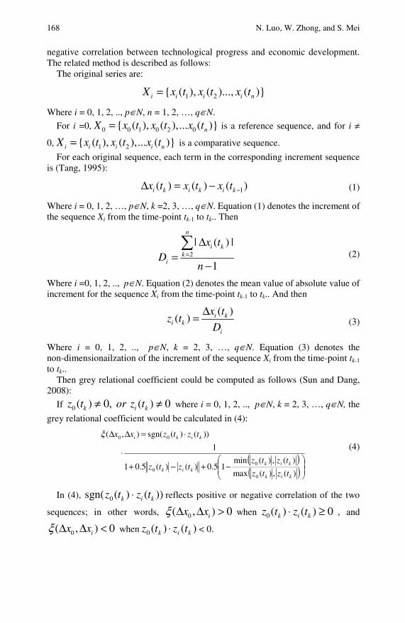
168 N. Luo, W. Zhong, and S. Mei
negative correlation between technological progress and economic development. The related method is described as follows:
The original series are:
1 2{ ( ), ( )..., ( )}i i i i nX x t x t x t=
Where i = 0, 1, 2, .., p∈N, n = 1, 2, …, q∈N.
For i =0, 0 0 1 0 2 0{ ( ), ( ),... ( )}nX x t x t x t= is a reference sequence, and for i ≠
0, 1 2{ ( ), ( ),... ( )}i i i i nX x t x t x t= is a comparative sequence.
For each original sequence, each term in the corresponding increment sequence is (Tang, 1995):
1( ) ( ) ( )i k i k i kx t x t x t −Δ = − (1)
Where i = 0, 1, 2, …, p∈N, k =2, 3, …, q∈N. Equation (1) denotes the increment of the sequence Xi from the time-point tk-1 to tk.. Then
2
| ( ) |
1
n
i kk
i
x tD
n=
Δ=
−
∑
(2)
Where i =0, 1, 2, .., p∈N. Equation (2) denotes the mean value of absolute value of increment for the sequence Xi from the time-point tk-1 to tk.. And then
( )( ) i k
i ki
x tz t
D
Δ=
(3)
Where i = 0, 1, 2, .., p∈N, k = 2, 3, …, q∈N. Equation (3) denotes the non-dimensionailzation of the increment of the sequence Xi from the time-point tk-1 to tk..
Then grey relational coefficient could be computed as follows (Sun and Dang, 2008):
If 0 ( ) 0, ( ) 0k i kz t or z t≠ ≠ where i = 0, 1, 2, .., p∈N, k = 2, 3, …, q∈N, the
grey relational coefficient would be calculated in (4):
( )( )⎟⎟⎠
⎞⎜⎜⎝
⎛−+−+
⋅
⋅=ΔΔ
)(,)(max
)(,)(min15.0)()(5.01
1
))()(sgn(),(
0
00
00
kik
kikkik
kiki
tztz
tztztztz
tztzxxξ (4)
In (4), ))()(sgn( 0 kik tztz ⋅ reflects positive or negative correlation of the two
sequences; in other words, 0( , ) 0ix xξ Δ Δ > when 0)()(0 ≥⋅ kik tztz , and
0( , ) 0ix xξ Δ Δ < when )()(0 kik tztz ⋅ < 0.
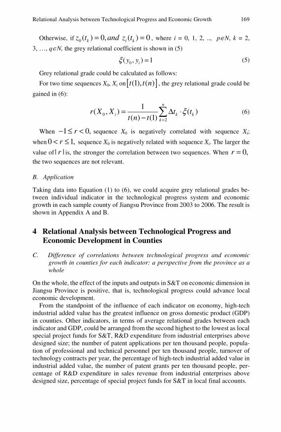
Relational Analysis between Technological Progress and Economic Growth 169
Otherwise, if 0 ( ) 0, ( ) 0k i kz t and z t= = , where i = 0, 1, 2, .., p∈N, k = 2,
3, …, q∈N, the grey relational coefficient is shown in (5)
0( , ) 1iy yξ = (5)
Grey relational grade could be calculated as follows:
For two time sequences X0, Xi on[ ](1), ( )t t n , the grey relational grade could be
gained in (6):
02
1( , ) ( )
( ) (1)
n
i k kk
r X X t tt n t
ξ=
= Δ ⋅− ∑ (6)
When 1 0,r− ≤ < sequence X0 is negatively correlated with sequence Xi;
when 0 1,r< ≤ sequence X0 is negatively related with sequence Xi. The larger the
value of | |r is, the stronger the correlation between two sequences. When 0,r =
the two sequences are not relevant.
B. Application
Taking data into Equation (1) to (6), we could acquire grey relational grades be-tween individual indicator in the technological progress system and economic growth in each sample county of Jiangsu Province from 2003 to 2006. The result is shown in Appendix A and B.
4 Relational Analysis between Technological Progress and Economic Development in Counties
C. Difference of correlations between technological progress and economic growth in counties for each indicator: a perspective from the province as a whole
On the whole, the effect of the inputs and outputs in S&T on economic dimension in Jiangsu Province is positive, that is, technological progress could advance local economic development.
From the standpoint of the influence of each indicator on economy, high-tech industrial added value has the greatest influence on gross domestic product (GDP) in counties. Other indicators, in terms of average relational grades between each indicator and GDP, could be arranged from the second highest to the lowest as local special project funds for S&T, R&D expenditure from industrial enterprises above designed size; the number of patent applications per ten thousand people, popula-tion of professional and technical personnel per ten thousand people, turnover of technology contracts per year, the percentage of high-tech industrial added value in industrial added value, the number of patent grants per ten thousand people, per-centage of R&D expenditure in sales revenue from industrial enterprises above designed size, percentage of special project funds for S&T in local final accounts.

170 N. Luo, W. Zhong, and S. Mei
From variations of correlation between each index and economic development, the impact on GDP of percentage of R&D expenditure in sales revenue from in-dustrial enterprises above designed size province sharply vary in 50 counties in Jiangsu (with a variance that equals 0.125). Other indicators, in terms of variance of relational grades between each indicator and GDP in 50 counties, could be arranged from the second largest to the smallest as the number of patent grants per ten thousand people, percentage of high-tech industrial added value in industrial added value, population of professional and technical personnel per ten thousand people, percentage of special project funds for S&T in local final accounts, turnover of technology contracts per year, the number of patent applications per ten thousand people, R&D expenditure from industrial enterprises above designed size, high-tech industrial added value, local special project funds for S&T.
D. Difference of correlations between technological progress and economic de-velopment for each region in Jiangsu Province: A perspective from southern, middle and northern Jiangsu
As is shown in Table II, each indicator of input and output in S&T affects economic development differently in southern, middle and northern Jiangsu.
In southern Jiangsu, factors in technological progress system owning relatively great effects on county economy (indices with the average relational grades larger than 0.5) include R&D expenditure from industrial enterprises above designed size, the number of patent applications per ten thousand people, population of profes-sional and technical personnel in ten thousand people, high-tech industrial added value, local special project funds for S&T, the number of patent grants per ten thousand people, indicators above ordered from the strongest correlation to the weakest one with GDP. Specifically, the population of professional and technical personnel has a universal far-reaching influence on economic growth in southern Jiangsu. In other words, social and economic conditions that have been rapidly developed in this region could effectively attract and encourage technical talents, who in return propel local economy forward through their technology-intensive work; therefore, it is regarded as a virtuous circle in which economic development appeals to talents while input in human resource contributes to the constant growth in GDP. On the other hand, impetuses local special project funds for S&T and high-tech industrial added value give to GDP in counties in this region are not as distinctive as that in the average degree of the whole province. Thus, more gov-ernmental attention is requested in southern Jiangsu to the input-output efficiency of technical resources, and the industrial structure should also be further improved and optimized.
Among the three regions, influence of technological progress on economic di-mension is the most significant in middle Jiangsu; such a fact also illustrates that the rapid development of this region during recent years, to certain degree, has bene-fited from the technological advance. Factors in input and output in S&T that positively affect economy of these counties (indices with the average relational grades larger than 0.5) include high-tech industrial added value, R&D expenditure from industrial enterprises above designed size, local special project funds for S&T, the number of patent applications per ten thousand people, the percentage of
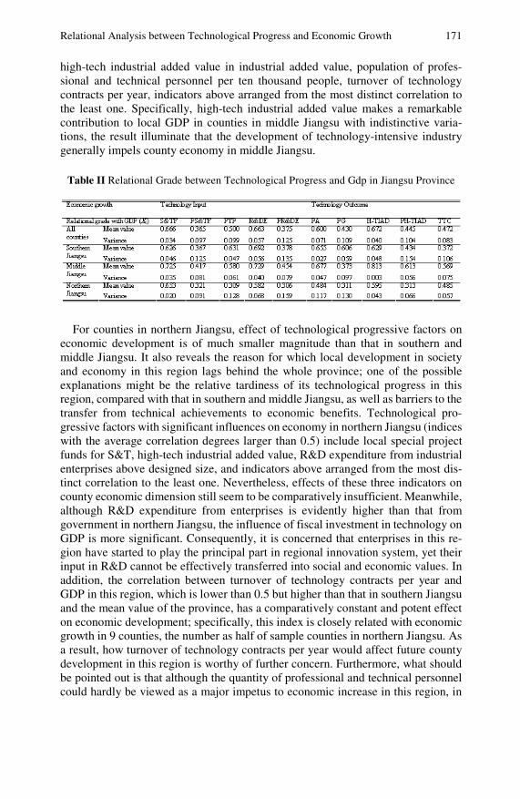
Relational Analysis between Technological Progress and Economic Growth 171
high-tech industrial added value in industrial added value, population of profes-sional and technical personnel per ten thousand people, turnover of technology contracts per year, indicators above arranged from the most distinct correlation to the least one. Specifically, high-tech industrial added value makes a remarkable contribution to local GDP in counties in middle Jiangsu with indistinctive varia-tions, the result illuminate that the development of technology-intensive industry generally impels county economy in middle Jiangsu.
Table II Relational Grade between Technological Progress and Gdp in Jiangsu Province
For counties in northern Jiangsu, effect of technological progressive factors on
economic development is of much smaller magnitude than that in southern and middle Jiangsu. It also reveals the reason for which local development in society and economy in this region lags behind the whole province; one of the possible explanations might be the relative tardiness of its technological progress in this region, compared with that in southern and middle Jiangsu, as well as barriers to the transfer from technical achievements to economic benefits. Technological pro-gressive factors with significant influences on economy in northern Jiangsu (indices with the average correlation degrees larger than 0.5) include local special project funds for S&T, high-tech industrial added value, R&D expenditure from industrial enterprises above designed size, and indicators above arranged from the most dis-tinct correlation to the least one. Nevertheless, effects of these three indicators on county economic dimension still seem to be comparatively insufficient. Meanwhile, although R&D expenditure from enterprises is evidently higher than that from government in northern Jiangsu, the influence of fiscal investment in technology on GDP is more significant. Consequently, it is concerned that enterprises in this re-gion have started to play the principal part in regional innovation system, yet their input in R&D cannot be effectively transferred into social and economic values. In addition, the correlation between turnover of technology contracts per year and GDP in this region, which is lower than 0.5 but higher than that in southern Jiangsu and the mean value of the province, has a comparatively constant and potent effect on economic development; specifically, this index is closely related with economic growth in 9 counties, the number as half of sample counties in northern Jiangsu. As a result, how turnover of technology contracts per year would affect future county development in this region is worthy of further concern. Furthermore, what should be pointed out is that although the quantity of professional and technical personnel could hardly be viewed as a major impetus to economic increase in this region, in
172 N. Luo, W. Zhong, and S. Mei
certain exceptional districts (such as Sheyang County, Yancheng City) it is the primary factor that contributes to local economic development.
5 Conclusion and Policy Suggestion
E. Conclusions
This chapter utilizes the methodology of grey relational analysis and employs data from 50 counties in Jiangsu Province to discern primary factors in technological progress system which exert the significant influence on local economic growth from 2003 to 2006 in each county in Jiangsu Province. Results in the study are described as follows:
1) From perspective of correlations between technological progress and county economy in the whole province, effects of those absolute value indicators on eco-nomic dimension, such as local special project funds for S&T and R&D expenditure from industrial enterprises above designed size in technical input and high-tech industrial added value in technical output, are more remarkable and less variant than corresponding relative value indicators. The fact that the quantity of patent appli-cations in a district has a greater impact on GDP than that of patent grants, it illus-trates that the will of innovation in a region exerts a positive effect on economic advancement in counties.
2) Generally, counties in middle Jiangsu possess the closest correlation between technological progress and GDP in these three regions, while the relational grade in northern Jiangsu is the lowest one. Additionally, counties where technological progress indicators significantly propel regional economy are concentrated in southern and middle Jiangsu.
3) For counties in southern Jiangsu, enterprises play a consequential role in the procedure of impelling economy through technological progress, and the input of technical talents in this region is closely correlated with economic growth. In mid-dle Jiangsu, most technological progress indicators are relevant to GDP in counties within this region, and the variances of relational grades between input-out in S&T and economic growth are comparatively small. Taken northern Jiangsu as a whole, the effects of technological progress on GDP is not sufficient enough that it could rarely be the major driving force to economic development; however, in certain indicators and counties’ potential influence of technological advance on economic might be exploited and released.
F. Policy Suggestion
Based on the analysis above, policy suggestions are made as follows: 1) From the perspective of the whole province, county governments should in-
crease fiscal investment in science and technology. Also, corresponding policies could be taken to encourage R&D activities in enterprises. Furthermore, supports should be provided to high-tech industries that help the transfer from technical achievements to production value. The series of measures would have a universal positive effect on economic development in counties from Jiangsu province.

Relational Analysis between Technological Progress and Economic Growth 173
2) For county governments in southern Jiangsu, it is necessary to establish and complete the incentive mechanism for technical talents and to concentrate on the quantity as well as the quality of innovation. It is also concerned that the industrial structure should be adjusted to improve the status of high-tech industry and tech-nology-intensive corporations.
3) For county governments in middle Jiangsu, the next step on concern is to further encourage the industrialization of technique innovation, and to ameliorate the outside in which high-tech industry develops. Specifically, it is of necessity to provide corresponding fiscal and financial policies in support of the development of small and middle-sized high-tech enterprises under the condition of global financial crisis and economic recession.
4) For county governments in northern Jiangsu, policies that foster the devel-opment of technology transaction market would be helpful because through tech-nique transaction and technology introduction counties in northern Jiangsu could improve their regional innovation capabilities and lay a foundation for driving economic growth from technological progress.
5) Based on the recognition of how regional technological progress influences economic growth, each county should adjust its policies and measures in accor-dance with local conditions. To counties where scientific and technological strength lags behind and technological progress is relatively tardy, it is essential for county governments to discern the primary factors in technological progress system that have the most significant effects on economy, to increase inputs of these indicators and to promote corresponding outputs, all measures were taken with an orientation and target that technological advance would effectively serve the development of economy and society.
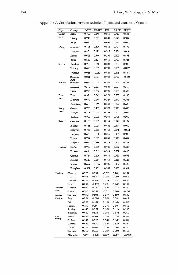
174 N. Luo, W. Zhong, and S. Mei
Appendix A Correlation between technical Inputs and economic Growth

Relational Analysis between Technological Progress and Economic Growth 175
Appendix b Correlation between Technical Outputs and Economic Growth
176 N. Luo, W. Zhong, and S. Mei
References
Becker, G.S., Murphy, K.M.: The division of labor, coordination costs, and knowledge. The Quarterly Journal of Economics 107, 69–103 (1992)
Bronzini, R., Piselli, P.: Determinants of long-run regional productivity with geographical spillover: the role of R&D, human capital and public infrastructure. Regional Science and Urban Economics 39, 187–199 (2009)
Coccia, M.: What is the optimal rate of R&D investment to maximize productivity growth? Technological forecasting & Social Change 76, 433–446 (2009)
Deng, J.L.: The introduction of grey system. Journal of Grey System 1, 1–24 (1989) Griliches, Z.: R&D, Patents, and Productivity, pp. 465–502. University of Chicago Press,
Chicago (1984) Guellec, B., de la Potterie, P.: R&D and productivity growth: Panel data analysis of 16
OECD countries. STI Working Papers (2001), http://www.oecd.org/dataoecd/26/32/1958639.pdf
Hu, S.H., Gao, Y.: Status of technology input in middle China And correlation analysis with economic growth. In: Science & Technology Progress And Policy, pp. 56–58 (2004)
Lin, Y., Chen, M.Y., Liu, S.F.: Theory of grey systems: capturing uncertainties of grey information. Kybernetes: The International Journal of Systems and Cybernetics 33(2), 196–218 (2004)
Lin, Y., Liu, S.F.: Solving Problems with incomplete information: a grey systems approach. In: Advances in Imaging and Electron Physics, vol. 141, pp. 77–174. Elsevier, Oxford (2006)
Liu, S.F., Lin, Y.: Grey Information: Theory and Practical Applications. Springer, London (2006)
Mi, M., Liu, S.F., Yang, J.: Grey relational degree study on technological input and economic growth in Jiangsu Province. Science of Science and Management of S&T, 34–36 (2004)
Sun, Y.G., Dang, Y.G.: Improvement on grey T’s correlation degree. In: Systems Engi-neering Theory and Practice, pp. 135–139 (2008)
Tang, W.X.: The concept and the computation method of T’s correlation degree. Application of Statistics and Management 14, 34–37 (1995)
Tang, W.X., Liu, Z.H.: Grey T’s degree analysis between technology input and economic growth in Beijing. Industrial Technology & Economics 25, 100–102 (2006)
Tsiddon, G.D.: Technological progress, mobility And economic Growth. American Eco-nomic Review 87, 363–382 (1997)
Optimization Method of Grey Relation Analysis Based on the Minimum Sensitivity of Attribute Weights
Xinping Xiao and Huan Guo*
Changes of attribute weights directly affect the results of grey incidence analysis for advancing the stability of results on grey relation decision-making. This chapter proposes an optimization method of grey relation analysis based on the minimum sensitivity of attribute weights. The main idea is as follows: First, we certify that sensitivity satisfies the properties of outer measure, explains that it is reasonable to use the sensitivity to measure the stability of grey relation analysis. Then the con-ditions and properties are given when the changes of attribute weights in grey re-lation analysis are effective. On the purpose of getting the minimum sensitivity we construct a multi-objective quadratic programming model based on objective weighting method and the partial preference information of the decision maker. The particle swarm optimization (PSO) algorithm is used to solve the model, and then we get grey relation analysis based on the weight. Finally, this method is used to evaluate R&D human resources.
1 Introduction
Grey incidence analysis is to serialize and patternize grey relation order, whose operating mechanism and physical principle are not clear, or those lack of physical prototype fundamentally, and then build grey relation analysis model, so as to make the grey relation quantitative, ordering and visible. It can also provide important means of technical analysis for complex systems’ modeling (Deng, 2000). Grey relation analysis is an important part of grey system theory (Liu and Lin, 2006; Lin et al., 2004; Lin and Liu, 2006), which is the cornerstone of grey system’s analysis, modeling, prediction and decision-making. It has wide application in various areas, such as investment decision-making, project evaluation, program optimization, plant siting, resource allocation, industrial sector developing sorting, tender bidding and economic benefits’ comprehensive evaluation (Wen, 2004; Xie and Hu, 2005; Song et al., 2005; Chen et al., 2006; Lee et al., 2006).
However, the data’s uncertainty and variability are often extremely difficult for decision makers. In order to obtain reasonable and stable grey relation analysis, Xinping Xiao and Huan Guo School of Sciences, Wuhan University of Technology, Wuhan 430063, China
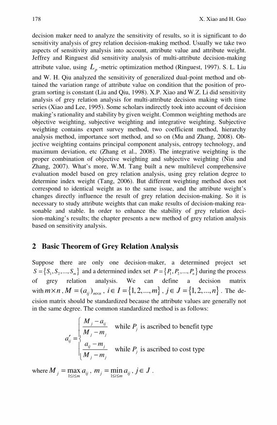
178 X. Xiao and H. Guo
decision maker need to analyze the sensitivity of results, so it is significant to do sensitivity analysis of grey relation decision-making method. Usually we take two aspects of sensitivity analysis into account, attribute value and attribute weight. Jeffrey and Ringuest did sensitivity analysis of multi-attribute decision-making
attribute value, using pL -metric optimization method (Ringuest, 1997). S. L. Liu
and W. H. Qiu analyzed the sensitivity of generalized dual-point method and ob-tained the variation range of attribute value on condition that the position of pro-gram sorting is constant (Liu and Qiu, 1998). X.P. Xiao and W.Z. Li did sensitivity analysis of grey relation analysis for multi-attribute decision making with time series (Xiao and Lee, 1995). Some scholars indirectly took into account of decision making’s rationality and stability by given weight. Common weighting methods are objective weighting, subjective weighting and integrative weighting. Subjective weighting contains expert survey method, two coefficient method, hierarchy analysis method, importance sort method, and so on (Mu and Zhang, 2008). Ob-jective weighting contains principal component analysis, entropy technology, and maximum deviation, etc (Zhang et al., 2008). The integrative weighting is the proper combination of objective weighting and subjective weighting (Niu and Zhang, 2007). What’s more, W.M. Tang built a new multilevel comprehensive evaluation model based on grey relation analysis, using grey relation degree to determine index weight (Tang, 2006). But different weighting method does not correspond to identical weight as to the same issue, and the attribute weight’s changes directly influence the result of grey relation decision-making. So it is necessary to study attribute weights that can make results of decision-making rea-sonable and stable. In order to enhance the stability of grey relation deci-sion-making’s results; the chapter presents a new method of grey relation analysis based on sensitivity analysis.
2 Basic Theorem of Grey Relation Analysis
Suppose there are only one decision-maker, a determined project set
{ }1 2, ,..., mS S S S= and a determined index set { }1 2, ,..., nP P P P= during the process
of grey relation analysis. We can define a decision matrix
with m n× , ( )ij m nM a ×= , { }1, 2,...,i I m∈ = , { }1,2,...,j J n∈ = . The de-
cision matrix should be standardized because the attribute values are generally not in the same degree. The common standardized method is as follows:
while is ascribed to benefit type
while is ascribed to cost type
j ijj
j j
ijij j
jj j
M aP
M ma
a mP
M m
−⎧⎪ −⎪′ = ⎨ −⎪⎪ −⎩
where1maxj ij
i mM a
≤ ≤= ,
1minj ij
i mm a
≤ ≤= , j J∈ .

Optimization Method of Grey Relation Analysis 179
Suppose the matrix ( )ij m nM a ×= has been standardized, in which the element
ija stands for the value of i th project iS under the j th attribute jP . As for the
above standardized method, we can confirm attribute value of ideal project as (1,1, ,1) .Then we calculate relation coefficient,
min min max max
max max
ij iji j i j
ijij ij
i j
rξ
ξ
Δ + Δ=
Δ + Δ
Where 1ij ijaΔ = − . For the character of decision matrix M , we know that
min min 0iji j
Δ = , max max 1iji j
Δ = , so ijij
rξ
ξ=
Δ +. Then we can get relation
coefficient matrix ( )ij m nr r ×= and relation degree1
n
i j ijj
R w r=
=∑ , there-
fore, { }1 2, ,..., mR R R R= corresponding to S , which is a vector composed by
relation degree between decision-making project and ideal project.
3 The Definition and Theorem Related to Sensitivity Analysis
Based on the definition proposed by Traintaphyllou and Sabchez (2007), we can define sensitivity as follows:
Definition 1. For two arbitrary projects ,i kS S in S , if their existing relation order
is changed following by changing current weight of a certain attribute jP , then the
change of the attribution weight is effective. Otherwise, it is ineffective.
Definition 2. For two projects ,i kS S in S , if the change of jP is effective, and the
relation order of ,i kS S is changed when jw is changed to j j ikjw w ε′ = + , and
then ikjε is called the smallest change of jP .
Definition 3. For all the j J∈ , { }minj ikji k I
D ε≠ ∈
= is the threshold value of jP ,
and 1
Sens( )jj
PD
= is the sensitivity of jP . Especially, Sens( ) 0jP = when all
the changes of jP are ineffective.
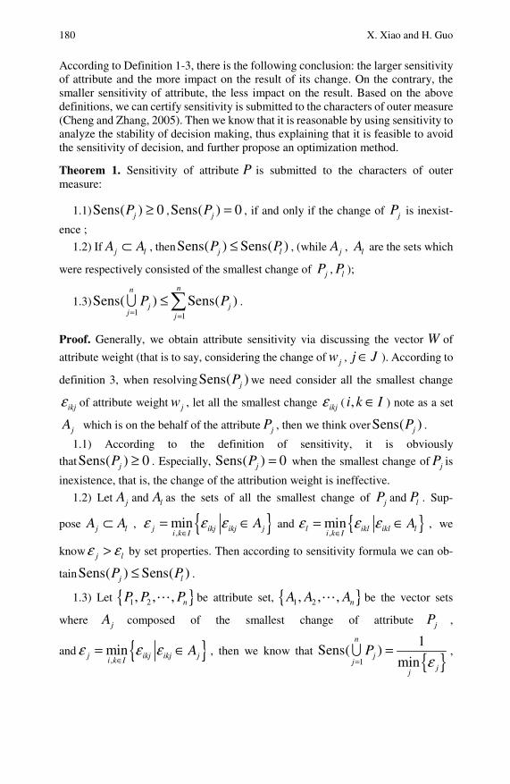
180 X. Xiao and H. Guo
According to Definition 1-3, there is the following conclusion: the larger sensitivity of attribute and the more impact on the result of its change. On the contrary, the smaller sensitivity of attribute, the less impact on the result. Based on the above definitions, we can certify sensitivity is submitted to the characters of outer measure (Cheng and Zhang, 2005). Then we know that it is reasonable by using sensitivity to analyze the stability of decision making, thus explaining that it is feasible to avoid the sensitivity of decision, and further propose an optimization method.
Theorem 1. Sensitivity of attribute P is submitted to the characters of outer measure:
1.1)Sens( ) 0jP ≥ ,Sens( ) 0jP = , if and only if the change of jP is inexist-
ence ;
1.2) If j lA A⊂ , thenSens( ) Sens( )j lP P≤ , (while jA , lA are the sets which
were respectively consisted of the smallest change of jP , lP );
1.3)1 1
Sens( ) Sens( )nn
j jj j
P P= =
≤∑∪ .
Proof. Generally, we obtain attribute sensitivity via discussing the vector W of
attribute weight (that is to say, considering the change of jw , j J∈ ). According to
definition 3, when resolvingSens( )jP we need consider all the smallest change
ikjε of attribute weight jw , let all the smallest change ikjε ( ,i k I∈ ) note as a set
jA which is on the behalf of the attribute jP , then we think overSens( )jP .
1.1) According to the definition of sensitivity, it is obviously
thatSens( ) 0jP ≥ . Especially, Sens( ) 0jP = when the smallest change of jP is
inexistence, that is, the change of the attribution weight is ineffective.
1.2) Let jA and lA as the sets of all the smallest change of jP and lP . Sup-
pose j lA A⊂ , { },
minj ikj ikj ji k I
Aε ε ε∈
= ∈ and { },
minl ikl ikl li k I
Aε ε ε∈
= ∈ , we
know j lε ε> by set properties. Then according to sensitivity formula we can ob-
tainSens( ) Sens( )j lP P≤ .
1.3) Let { }1 2, , , nP P P be attribute set, { }1 2, , , nA A A be the vector sets
where jA composed of the smallest change of attribute jP ,
and { },
minj ikj ikj ji k I
Aε ε ε∈
= ∈ , then we know that { }1
1Sens( )
min
n
jj
jj
Pε=
=∪ ,

Optimization Method of Grey Relation Analysis 181
where 1
n
jj
P=∪ be the union of all the smallest change set of attribute weight, whereas
1 1
1Sens( )
n n
jj j j
Pε= =
=∑ ∑ , obviously1 1
Sens( ) Sens( )nn
j jj j
P P= =
≤∑∪ .
Through the above proof, Theorem 1.1 shows that sensitivity is non-negative. Sensitivity of the attribute is zero if and only if the change of attribute is ineffective, in other words, the attribute which is not sensitive is correspondingly stable; Theorem 1.2 affords a method of comparing the attribute sensitivity, that is to say, if the smallest change set of a attribute is included in the other one, then the sensitivity of the included one is no larger than the other’s; Theorem 1.3 shows that it is pos-sible to lower the sensitivity by considering all the attributes, so we always look for the most insensitive weight. Based on the characters of sensitivity, we propose an optimization method of grey relation analysis aiming at the smallest sensitivity.
4 Quadratic Programming Model Based on Sensitivity Analysis and Its Algorithm
4.1 The Property of Sensitivity Analysis Based on Preference Information
In relation coefficient matrix ( )ij m nr × , iR , kR are the relation degree be-
tween ,i kS S and ideal project respectively, 1 2( , ,..., )TnW w w w= is the weight
vector of P which satisfies 1jj J
w∈
=∑ , 0jw ≥ , j J∈ .
Theorem 2. Suppose i kS S ( , )i k I∈ , then
2.1) If ij kjr r= , then the weight change of ,i kS S in jP is ineffective;
2.2) If ( )( ) 0i k ij kjR R r r− − > and1
( ) 0l j
n
l il kll
w r r≠=
− >∑ , then the weight
change of ,i kS S in jP is ineffective;
2.3) If ( )( ) 0i k ij kjR R r r− − < , then the weight change of ,i kS S in jP is
effective.
Proof. 2.1) it is obvious.
2.2) ,i kR R are the relation degree between ,i kS S and ideal project respec-
tively, by the preference information i kR R> , and ( )( ) 0i k ij kjR R r r− − > , it is

182 X. Xiao and H. Guo
easy to say that ij kjr r> . Suppose the weight change of ,i kS S in jP ( )j J∈ is
effective, then there exists ikjε ,
01
j ikjj
ikj
ww
εε
−′ = ≥
−( )j J∈ , 0
1l
likj
ww
ε′ = ≥
−( )l j J≠ ∈
1 2( , ,..., )TnW w w w′ ′ ′ ′= is the vector of changed weight.
,i kR R′ ′ are the changed relation degree between ,i kS S and ideal project respec-
tively, then i kR R′ ′< , thus
1 1
1 1
n n
j ij ikj ij j kj ikj kjj j
ikj ikj
w r r w r rε ε
ε ε= =
− −<
− −
∑ ∑
By
1
n
i j ijj
R w r=
=∑ ,1
n
k j kjj
R w r=
=∑ , ij kjr r>
Then
i ikj ij k ikj kjR r R rε ε− < − (1)
i kikj
ij kj
R R
r rε −>
− (2)
Because of
1
( ) 0l j
n
l il kll
w r r≠=
− >∑
we have
( )i k j ij kjR R w r r− > −
i kj
ij kj
R Rw
r r
−<−
(3)
According to (2) and (3), we know j ikjw ε< , then 01
j ikjj
ikj
ww
εε
−′ = ≥
−which is
not reasonable, so we can certify the hypothesis is wrong, therefore, the weight
change of ,i kS S in jP is ineffective.
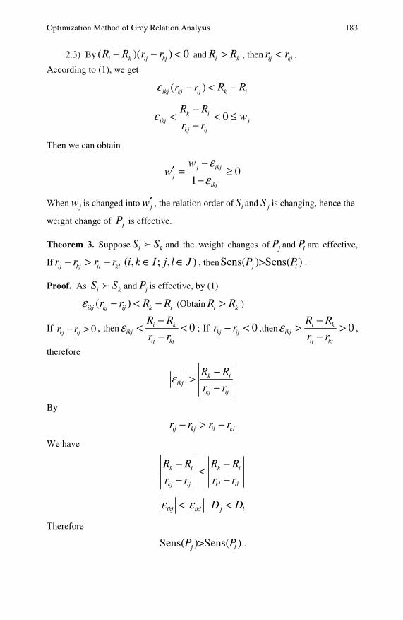
Optimization Method of Grey Relation Analysis 183
2.3) By ( )( ) 0i k ij kjR R r r− − < and i kR R> , then ij kjr r< .
According to (1), we get
( )ikj kj ij k ir r R Rε − < −
0k iikj j
kj ij
R Rw
r rε −< < ≤
−
Then we can obtain
01
j ikjj
ikj
ww
εε
−′ = ≥
−
When jw is changed into jw′ , the relation order of iS and jS is changing, hence the
weight change of jP is effective.
Theorem 3. Suppose i kS S and the weight changes of jP and lP are effective,
If ij kj il klr r r r− > − ( , ; , )i k I j l J∈ ∈ , thenSens( )>Sens( )j lP P .
Proof. As i kS S and jP is effective, by (1)
( )ikj kj ij k ir r R Rε − < − (Obtain i kR R> )
If 0kj ijr r− > , then 0i kikj
ij kj
R R
r rε −< <
−; If 0kj ijr r− < ,then 0i k
ikjij kj
R R
r rε −> >
−,
therefore
k iikj
kj ij
R R
r rε −>
−
By
ij kj il klr r r r− > −
We have
k i k i
kj ij kl il
R R R R
r r r r
− −<− −
ikj iklε ε< j lD D<
Therefore
Sens( )>Sens( )j lP P .
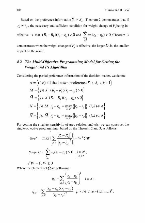
184 X. Xiao and H. Guo
Based on the preference information i kS S , Theorem 2 demonstrates that if
ij kjr r≠ , the necessary and sufficient condition for weight change of jP being in-
effective is that ( )( ) 0i k ij kjR R r r− − > and 1
( ) 0l j
n
l il kll
w r r≠=
− >∑ ;Theorem 3
demonstrates when the weight change of jP is effective, the larger jD is, the smaller
impact on the result.
4.2 The Multi-Objective Programming Model for Getting the Weight and Its Algorithm
Considering the partial preference information of the decision-maker, we denote
{ }( , ) all the known preference , Ii ki k S S i kΛ = ∈
{ } ( )( ) 0i k ij kjM j J R R r r= ∈ − − >
{ }( )( ) 0i k ij kjM j J R R r r= ∈ − − <
{ }{ }max ( , )ij kj il kll M
N j M r r r r i k∈
= ∈ − = − ∈ Λ
{ }{ }max ( , )ij kj il kll M
N j M r r r r i k∈
= ∈ − = − ∈ Λ
For getting the smallest sensitivity of grey relation analysis, we can construct the single-objective programming�based on the Theorem 2 and 3, as follows:
Goal:
2
2max i k T
j Nij kj
R RW QW
r r∈
⎧ ⎫−⎪ ⎪ =⎨ ⎬−⎪ ⎪⎩ ⎭
∑
Subject to: 1
( ) 0l j
n
l il kll
w r r≠=
− >∑ ( ),i k
j N∈Λ
∈ ;
1Te W = ; 0W ≥
Where the elements of Q are following: 2
il klll
j N ij kj
r rq
r r∈
⎛ ⎞−= ⎜ ⎟⎜ ⎟−⎝ ⎠∑ l J∈ ;
2
( )( )
( )ip kp il kl
plj N ij kj
r r r rq
r r∈
− −=
−∑ p l J≠ ∈ ; e = (1,1,...,1)T .
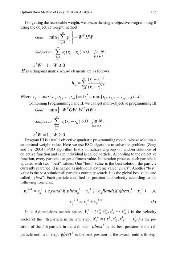
Optimization Method of Grey Relation Analysis 185
For getting the reasonable weight, we obtain the single-objective programming II using the objective weight method
Goal: 1
minn
Tj
j
g W HW=
⎧ ⎫=⎨ ⎬
⎩ ⎭∑
Subject to: 1
( ) 0l j
n
l il kll
w r r≠=
− >∑ ( ),i k
j N∈Λ
∈ ;
1Te W = ; 0W ≥ H is a diagonal matrix whose elements are as follows:
2
21
( )
( )
mj ij
jji j j
r rh
r r=
−=
′−∑
Where 1 2max{ , ,..., }j j j mjr r r r= and 1 2min{ , ,..., },j j j mjr r r r j J′ = ∈ .
Combining Programming I and II, we can get multi-objective programming III
Goal: { }min ,T TW QW W HW−
Subject to: 1
( ) 0l j
n
l il kll
w r r≠=
− >∑ ( ),i k
j N∈Λ
∈ ;
1Te W = ; 0W ≥ Program III is a multi-objective quadratic programming model, whose solution is
an optimal weight value. Here we use PSO algorithm to solve the problem (Zeng and Jie, 2004). PSO algorithm firstly initializes a group of random solutions of objective function and each individual is called particle. According to the objective function, every particle can get a fitness value. In iteration process, each particle is updated with two “best” values. One “best” value is the best solution the particle currently searched. It is named as individual extreme value “pbest”. Another “best” value is the best solution all particles currently search. It is the global best value and called “gbest”. Each particle modified its position and velocity according to the following formulas:
11 2
k k k k k kij ij ij ij j ijv v c rand()( pbest x ) c Rand()( gbest x )+ = + − + − (4)
1 1k k kij ij ijx x v+ += + (5)
In a d-dimensions search space, 1 2 3k k k k k
i i i i idV ( v ,v ,v , ,v )= is the velocity
vector of the i th particle in the k th step; 1 2 3k k k k k
i i i i idX ( x ,x ,x , ,x )= is the po-
sition of the i th particle in the k th step; kipbest is the best position of the i th
particle until k th step; kgbest is the best position in the swarm until k th step;

186 X. Xiao and H. Guo
1c and 2c are constants known as acceleration coefficients and usually
221 == cc ; ()rand and ()Rand are two separately random functions in the
range [0,1]. The calculation procedure of PSO is shown as bellow:
1) Initialize particle population in the feasible region, set the size as Pnum ,and initialize the particle velocity;
2) According to formulas (4) and (5), calculate each particle’s fitness value, then choose global extreme value and individual extreme value;
3) If requirement is met (up to a certain accuracy or up to the maximum cycle number), go to step (5), or else go to step (4);
4) Update particles’ velocity and position according to above formulas, then go to step (2);
5) Get out global extreme value and corresponding solution, exit the loop.
5 Application Analyses
In order to evaluate the level of an industry’s R&D human resource in Wuhan, expert analyzed four large-scale enterprises iS ( 1,2,..., 4)i = in this industry. There
are five attributes jP ( 1,2,...,5)j = for evaluating the level, such as knowledge
quantity, innovation ability, communion ability, health condition, heart bearing capacity, which are all belonging to benefit type. Expert marks the enterprises aiming at the five attributes, whose values range from 1 to 10, and then gets the decision matrix:
5 8 8 6 9
8 6 10 8 8
6 9 7 10 7
9 7 9 8 6
A
⎡ ⎤⎢ ⎥⎢ ⎥=⎢ ⎥⎢ ⎥⎣ ⎦
Using the above standardization method to deal with A , then we get
0 0.67 0.33 0 1
0.75 0 1 0.5 0.67
0.25 1 0 1 0.33
1 0.33 0.67 0.5 0
A
⎡ ⎤⎢ ⎥⎢ ⎥′ =⎢ ⎥⎢ ⎥⎣ ⎦
During the process of resolving relation coefficient, suppose 0.5ξ = , then we
can get relation coefficient matrix
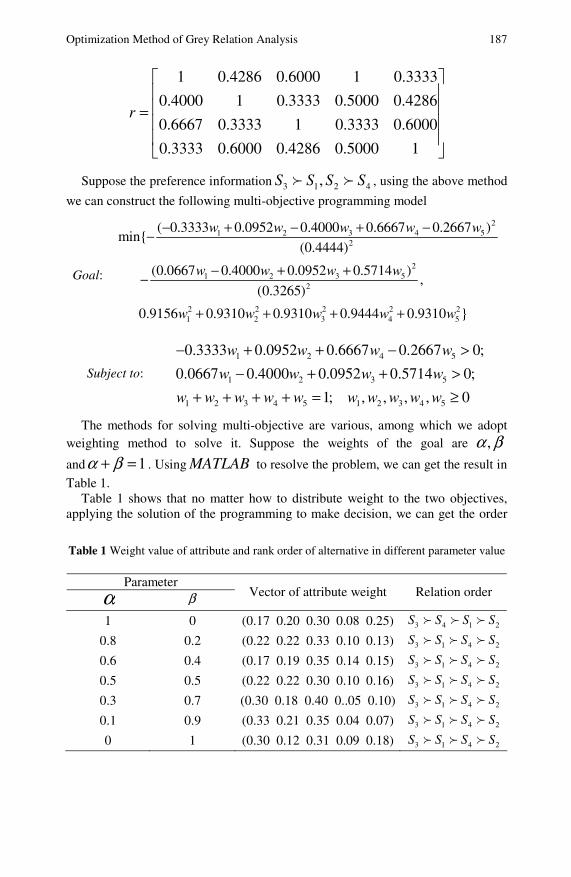
Optimization Method of Grey Relation Analysis 187
1 0.4286 0.6000 1 0.3333
0.4000 1 0.3333 0.5000 0.4286
0.6667 0.3333 1 0.3333 0.6000
0.3333 0.6000 0.4286 0.5000 1
r
⎡ ⎤⎢ ⎥⎢ ⎥=⎢ ⎥⎢ ⎥⎣ ⎦
Suppose the preference information 3 1 2 4,S S S S , using the above method
we can construct the following multi-objective programming model
Goal:
21 2 3 4 5
2
21 2 3 5
2
2 2 2 2 21 2 3 4 5
( 0.3333 0.0952 0.4000 0.6667 0.2667 )min{
(0.4444)
(0.0667 0.4000 0.0952 0.5714 ),
(0.3265)
0.9156 0.9310 0.9310 0.9444 0.9310 }
w w w w w
w w w w
w w w w w
− + − + −−
− + +−
+ + + +
Subject to: 1 2 4 5
1 2 3 5
1 2 3 4 5 1 2 3 4 5
0.3333 0.0952 0.6667 0.2667 0;
0.0667 0.4000 0.0952 0.5714 0;
1; , , , , 0
w w w w
w w w w
w w w w w w w w w w
− + + − >− + + >
+ + + + = ≥
The methods for solving multi-objective are various, among which we adopt weighting method to solve it. Suppose the weights of the goal are ,α β
and 1α β+ = . Using MATLAB to resolve the problem, we can get the result in
Table 1. Table 1 shows that no matter how to distribute weight to the two objectives,
applying the solution of the programming to make decision, we can get the order
Table 1 Weight value of attribute and rank order of alternative in different parameter value
Parameter α β Vector of attribute weight Relation order
1 0 (0.17 0.20 0.30 0.08 0.25) 3 4 1 2S S S S
0.8 0.2 (0.22 0.22 0.33 0.10 0.13) 3 1 4 2S S S S
0.6 0.4 (0.17 0.19 0.35 0.14 0.15) 3 1 4 2S S S S
0.5 0.5 (0.22 0.22 0.30 0.10 0.16) 3 1 4 2S S S S
0.3 0.7 (0.30 0.18 0.40 0..05 0.10) 3 1 4 2S S S S
0.1 0.9 (0.33 0.21 0.35 0.04 0.07) 3 1 4 2S S S S
0 1 (0.30 0.12 0.31 0.09 0.18) 3 1 4 2S S S S
188 X. Xiao and H. Guo
which can guarantee the preference information and the smallest sensitivity of the decision-making. It is the result that the decision-maker expects. This method has more practical significance for decision-maker making the reasonable and stable decision.
6 Conclusion
The chapter presents an optimization grey relation method, based on the minimum of attribute weight’s sensitivity. We demonstrate that sensitivity submits to the essential property of outer measure. According to the definition of sensitivity, characteristics of grey relation operator and reasonable objective weighting method, we construct a multi-objective quadratic programming model about weight and solve attribute weights using particle swarm algorithm. The optimal grey relation method obtained by attribute weights above, not only ensures decision makers' preference information, but also lowers the sensitivity of results of grey relation analysis, which has great and actual benefits for decision maker to make reasonable and stable decision. The approach avoids sensitivity and ensures the stability of decision-making on a certain extent. Of course, we only considered the sensitivity of grey relation analysis attribute weights. With regard to the sensitivity of attribute value, we need further study.
Acknowledgement. Thanks are due to the anonymous referees for many instructive suggestions, which have improved this chapter. This work was supported by National Natural Science Foundation of China (Grant No. 70971103) and Specialized Research Fund for the Doctoral Program of Higher Education (Grant No.200804970005)
References
Chen, G., Zhang, X.W., Li, Y.B.: The application of tank acoustic target recognition system based on grey correlation analysis. Journal of Detection & Control 28, 39–43 (2006)
Cheng, Q.X., Zhang, D.Z.: Real Variable Function and Basic Function Analysis. Higher Education Press, Beijing (2005)
Deng, J.L.: Grey System Theory & Applications, ch. 2. Cao-Li Publishing Co., Taipei (2000) Lee, P.C., Wang, Y.Q., Zhong, L.: Grey relative analysis of human error causal factors.
Systems Engineering-Theory &Practice 3, 131–135 (2006) Lin, Y., Chen, M.Y., Liu, S.F.: Theory of grey systems: capturing uncertainties of grey
information. Kybernetes: The International Journal of Systems and Cybernetics 33(2), 196–218 (2004)
Lin, Y., Liu, S.F.: Solving Problems with incomplete information: a grey systems approach. In: Advances in Imaging and Electron Physics, vol. 141, pp. 77–174. Elsevier, Oxford (2006)
Liu, S.F., Dang, Y.G., Fang, Z.G.: Grey Systems Theory and Its Application. Science Press, Beijing (2008)
Liu, S.F., Lin, Y.: Grey Information: Theory and Practical Applications. Springer, London (2006)
Optimization Method of Grey Relation Analysis 189 Liu, S.L., Qiu, W.H.: Theoretic research on sensitivity analysis of the generalized double
base points method. Systems Engineering-Theory &Practice 18, 26–30 (1998) Mu, R., Zhang, J.T.: Research of hierarchy synthetic evaluation based on grey relational
analysis. Systems Engineering-Theory &Practice 10, 125–130 (2008) Niu, D.X., Zhang, C.: The application of comprehensive evaluation on the effect of power
supply corporate marketing based on grey correlation analysis of the combined weight. Techno-economics & Management Research 5, 55–58 (2007)
Ringuest, J.L.: Lp-metric sensitivity analysis for single and multi-attribute decision analysis. European Journal of Operations Research 98, 563–570 (1997)
Song, Q.B., Shepperd, M., Mair, C.: Using grey relational analysis to predict software effort with small data sets. In: IEEE International Software Metrics Symposium, vol. 11, pp. 1435–1444 (2005)
Tang, W.M.: A research of multi-hierarchy synthetic evaluation based on the grey relation analysis: The model of synthetic assessment in the venture investment items. Systems Engineering-Theory & Practice 6, 25–29 (2006)
Traintaphyllou, E., Sabchez, A.: A sensitivity analysis approach for some deterministic multi-criteria decision-making methods. Decision Sciences 28, 151–194 (2007)
Wen, K.L.: The grey system analysis and its application in gas breakdown and vat com-pensator finding. International Journal of Computational Cognition 2, 21–44 (2004)
Xiao, X.P., Lee, W.Z.: The relative degree analysis method and sensitivity analysis for multiple attribute decision making with time series. Systems Engineering and Electron-ics 7, 36–43 (1995)
Xie, Z.W., Hu, H.H.: Discussions on grey relation analysis in the selection of safety in-vestment method. Industrial Safety and Environmental Protection 31, 51–53 (2005)
Zeng, J.H., Jie, J.: Particle Swarm Optimization. Science Press, Beijing (2004) Zhang, F.T., Su, W.C., Zhou, J.X.: Assessment of urban ecological security based on en-
tropy-weighted grey correlation analysis. Chinese Journal of Ecology 28, 1249–1254 (2008)
Research on Extended Cluster of Grey Incidences and Its Application*
Ke Zhang and Sifeng Liu
This chapter studies extended clusters of grey incidences for indexes in panel data. Firstly it discusses the expression of a panel data by matrix sequence, and describes its geometric characteristic though a cluster of curved surfaces. Thereafter, in a three dimensional space, the chapter analyzes the geometric similarity of indexes in panel data. According to the principle of grey incidence analysis, it proposes an absolute degree of grey incidences for matrixes, which maintains the consistent form with the classic one. Furthermore the formula of zeroing starting point op-erator and parameters are redefined. On this basis, the chapter constructs the ex-tended incidence matrix of indexes and discusses the cluster analysis process of panel data. Finally, an instance is studied. The results prove the method is effective.
1 Introduction
The grey incidence analysis and clusters of grey incidences are not only the impor-tant components of the grey theory, but also the basis of modeling, forecasting and deciding in grey system (Liu and Lin, 2006; Lin et al., 2004; Lin and Liu, 2006). Because of less restriction of sample number and convenient computation, grey incidence analysis and clusters have been successfully applied to a great deal of domains, for example, economics, sociology, industry, agriculture, education and medicine (Chen and Zhou, 2008; Hu and Zhang, 2007; Ma and Hao, 2004). But current fruits of the grey incidence analysis, e.g., the degree of grey incidences (Deng, 1989), the absolute degree of grey incidences, the B-type incidences (Wang, 1987), C-type incidences (Wang and Zhao, 1999) and the T-type incidences (Tang, 1995), are only fit for the analysis of time series and cluster of cross section data. It is still a blank to study methods for incidences analysis and cluster among panel data. Ke Zhang and Sifeng Liu College of Economics and Management, Nanjing University of Aeronautics and Astronautics, 29#, Yudao Street, Nanjing City, 210016, China; phone: 86-025-84893507 e-mail: [email protected] * The work is partially supported by National Natural Science Foundation of China though
Grant NO. 70701017, 70473037, by the Research Fund for the Doctoral Program of Na-tional Ministry of Education though Grant NO. 200802870020. At the same time the au-thors would like to acknowledge the partial support of National Soft Science Research Program via Grant 2008GXS5D115, Also acknowledgements are given to Social Science Fund of National Education Ministry though Grant NO. 08JA630039.

192 K. Zhang and S. Liu
Table I Three-Dimensional Table of a Panel Data
Time 1 … N Sample Index 1 LX X … Index 1 LX X
1 11 (1)x … 1 (1)Lx … 11 ( )x N … 1 ( )Lx N
… 1 (1)ix … (1)iLx … 1 ( )ix N … ( )iLx N
M 1 (1)Mx … (1)MLx … 1 ( )Mx N … ( )MLx N
At the same time, although there are a few clustering methods for panel data, these methods are almost based on the multivariate statistics which requires the large samples. For example, (Bonzo and Hermosilla, 2002) first introduces multi-variate statistics into panel data analysis. He improves clustering algorithm in virtue of probability function, and applies clustering algorithm to panel data analysis. Zhu establishes the statistic for single index panel data, and constructs its similar crite-rion (Zhu and Chen, 2007). Zheng structures the similar criterion for muti-indexes panel data, through composing statistics. But when using statistic clustering method, there is the limitation for sample number. Moreover, the average value of variance and covariance in literature (Zhen, 2008) neglects the diversity of the data, and partially loses the data information.
Therefore, this chapter studies extended cluster of grey incidences for indexes in panel data, based on literature (Liu and Lin, 2006; Lin et al., 2004; Lin and Liu, 2006). First, we transform panel data into behavioral matrix sequence of indexes, and discuss the geometric expression of matrix sequence through a cluster of curved surfaces. According to the principle of grey incidence analysis, we pro-pose a matrix absolute degree of grey incidences, which maintains the consistent form of the classic one, at the same time, its parameters and the formula of zeroing starting point operator are redefined. On this basis, we construct the extended incidence matrix of indexes and discuss the clustering analysis process of indexes in panel data. Finally, an instance is studied and the results prove the method is effective.
2 Geometric Expression of Panel Data
The form of panel data is more complex, including both cross section data and time series. Thereby, there are characteristics of both spatial dimension and time di-mension in a panel data. In literature (Zhen, 2008; Cheng, 1988), three-dimensional table is employed to describe panel data. Assume the sample size is M , the number of a sample’s indexes is L and the length of time is N . Then, ( )ijX t expresses the
value of the i th sample with the j th index at the t th time. A three-dimensional
table of a panel can be turn into a series of two-dimensional tables which are illus-trated in TABLE I.
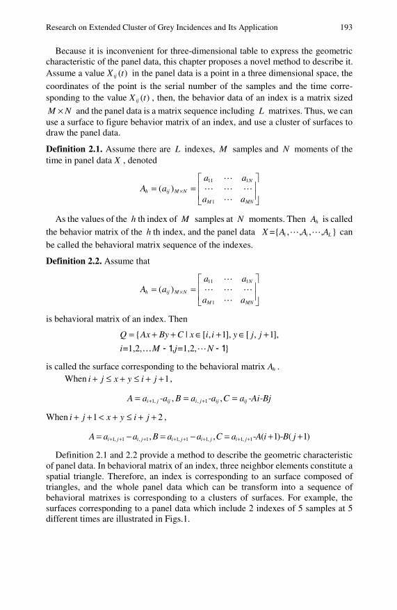
Research on Extended Cluster of Grey Incidences and Its Application 193
Because it is inconvenient for three-dimensional table to express the geometric characteristic of the panel data, this chapter proposes a novel method to describe it. Assume a value ( )ijX t in the panel data is a point in a three dimensional space, the
coordinates of the point is the serial number of the samples and the time corre-sponding to the value ( )ijX t , then, the behavior data of an index is a matrix sized
M N× and the panel data is a matrix sequence including L matrixes. Thus, we can use a surface to figure behavior matrix of an index, and use a cluster of surfaces to draw the panel data.
Definition 2.1. Assume there are L indexes, M samples and N moments of the time in panel data X , denoted
11 1
1
( )N
h ij M N
M MN
a aA a
a a×
⎡ ⎤⎢ ⎥= =⎢ ⎥⎣ ⎦
As the values of the h th index of M samples at N moments. Then hA is called the behavior matrix of the h th index, and the panel data 1={ , , , , }i LX A A A can
be called the behavioral matrix sequence of the indexes.
Definition 2.2. Assume that
11 1
1
( )N
h ij M N
M MN
a aA a
a a×
⎡ ⎤⎢ ⎥= =⎢ ⎥⎣ ⎦
is behavioral matrix of an index. Then
{ | [ , 1], [ , 1],
=1,2, , =1,2, }
Q Ax By C x i i y j j
i M j N
= + + ∈ + ∈ +… - 1 - 1
is called the surface corresponding to the behavioral matrix hA . When 1i j x y i j+ ≤ + ≤ + + ,
1, , 1- , - , - -i j ij i j ij ijA a a B a a C a Ai Bj+ += = =
When 1 2i j x y i j+ + < + ≤ + + ,
1, 1 , 1 1, 1 1, 1, 1, , - ( 1)- ( 1)i j i j i j i j i jA a a B a a C a A i B j+ + + + + + + += − = − = + +
Definition 2.1 and 2.2 provide a method to describe the geometric characteristic of panel data. In behavioral matrix of an index, three neighbor elements constitute a spatial triangle. Therefore, an index is corresponding to an surface composed of triangles, and the whole panel data which can be transform into a sequence of behavioral matrixes is corresponding to a clusters of surfaces. For example, the surfaces corresponding to a panel data which include 2 indexes of 5 samples at 5 different times are illustrated in Figs.1.
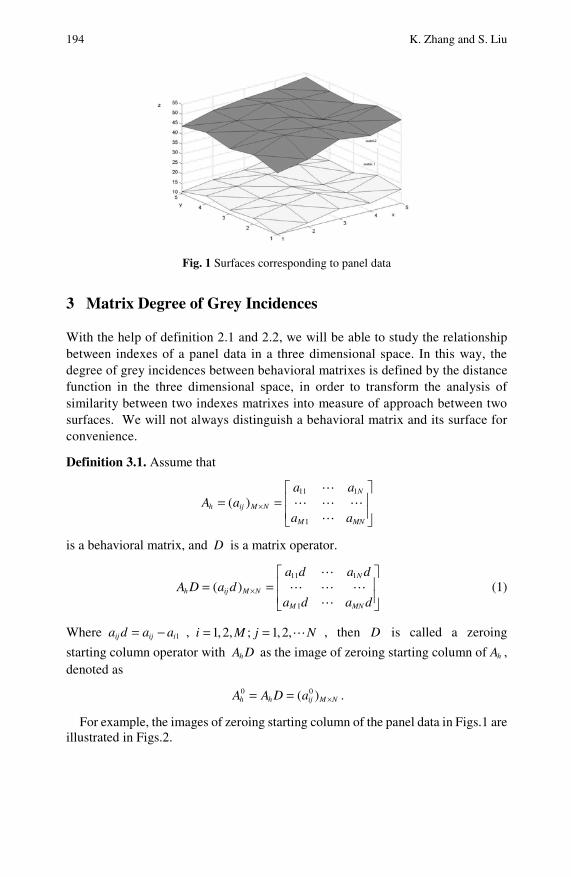
194 K. Zhang and S. Liu
Fig. 1 Surfaces corresponding to panel data
3 Matrix Degree of Grey Incidences
With the help of definition 2.1 and 2.2, we will be able to study the relationship between indexes of a panel data in a three dimensional space. In this way, the degree of grey incidences between behavioral matrixes is defined by the distance function in the three dimensional space, in order to transform the analysis of similarity between two indexes matrixes into measure of approach between two surfaces. We will not always distinguish a behavioral matrix and its surface for convenience.
Definition 3.1. Assume that
11 1
1
( )N
h ij M N
M MN
a aA a
a a×
⎡ ⎤⎢ ⎥= =⎢ ⎥⎣ ⎦
is a behavioral matrix, and D is a matrix operator.
11 1
1
( )N
h ij M N
M MN
a d a dA D a d
a d a d×
⎡ ⎤⎢ ⎥= =⎢ ⎥⎣ ⎦
(1)
Where 1ij ij ia d a a= − , 1, 2, ; 1, 2,i M j N= = , then D is called a zeroing
starting column operator with hA D as the image of zeroing starting column of hA , denoted as
0 0( )h h ij M NA A D a ×= = .
For example, the images of zeroing starting column of the panel data in Figs.1 are illustrated in Figs.2.

Research on Extended Cluster of Grey Incidences and Its Application 195
Fig. 2 Images of zeroing starting column
Proposition 3.1. Assume that
11 1
1
( )N
h ij M N
M MN
a aA a
a a×
⎡ ⎤⎢ ⎥= =⎢ ⎥⎣ ⎦
is a behavioral matrix, and that the surface of zeroing starting column of hA is
denoted as 0hQ . Let
0
1 1
M N
hs Q dxdy= ∫ ∫
Then 1ºwhen [1, ], [1, ],i M j N∀ ∈ ∈ always , 1 ,i j i ja a+ ≥ , then 0s ≥ ;
2ºwhen [1, ], [1, ],i M j N∀ ∈ ∈ always , 1 ,i j i ja a+ ≤ , then 0s ≤ ;
3ºelse the sign of s is not fixed. The proof of this proposition is based on the properties of double integral. Here
all the details are omitted.
Proposition 3.2. Assume that the surfaces corresponding to images of zeroing starting column of two behavioral matrixes, ( )p ij M NA a ×= , and ( )q ij M NA b ×= are
0pQ , and 0
qQ , respectively. Let
0 0
1 1
( )M N
p qp qs Q dxdys Q=− −∫ ∫
Then 1º if 0
pQ is always above 0qQ , then 0p qs s− ≥ ; and
2º if 0pQ is always underneath 0
qQ , then 0p qs s− ≤ ; and
3º if 0pQ and 0
qQ alternate their positions, the sign of p qs s− is not fixed;
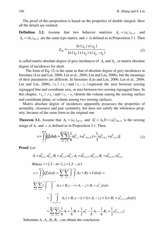
196 K. Zhang and S. Liu
The proof of this proposition is based on the properties of double integral. Here all the details are omitted.
Definition 3.2. Assume that two behavior matrixes ( )p ij M NA a ×= and
( )q ij M NA b ×= are the same type matrix, and s is defined as in Proposition 3.1. Then
1 | | | |
1 | | | | | |p q
pqp q p q
s s
s s s sε + +
=+ + + − (2)
is called matrix absolute degree of grey incidences of pA and qA , or matrix absolute
degree of incidences for short. The form of Eq. (2) is the same as that of absolute degree of grey incidences in
literature (Liu and Lin, 2006; Lin et al., 2004; Lin and Liu, 2006), but the meanings of their parameters are different. In literature (Liu and Lin, 2006; Lin et al., 2004; Lin and Liu, 2006), | |is , | |js and | |i js s− represent the area between zeroing
zigzagged line and coordinate axis, or area between two zeroing zigzagged lines. In this chapter, | |ps ,| |qs and | |p qs s− denote the volume among the zeroing surface
and coordinate plane, or volume among two zeroing surfaces. Matrix absolute degree of incidences apparently possesses the properties of
normality, closeness and pair symmetry, but does not satisfy the wholeness prop-erty, because of the same form as the original one.
Theorem 3.1. Assume that ( )h ij M NA a ×= and 0 0( )h h ij M NA A D a ×= = is the zeroing
image of hA and s is defined as in Proposition 3.1. Then,
1 10 0 0 0 0
, 1, 1 1, , 11 11 1
1 1[ ( ) ( )]6 3
M N M N
h i j i j i j i ji j
s Q dxdy a a a a− −
+ + + += =
= = + + +∑∑∫∫ (3)
Proof: Let
1 1 2 20 0 0 0 0 0 0 0
1, , , 1 , 1, 1 , 1 1, 1 1,, ; ,- - - -i j i j i j i j i j i j i j i jA B A Ba a a a a a a a+ + + + + + + += = = =
Where 1,2 1, 1,2 , -1i m j n= − = 111 1
0
1 11 1
jM N iM N
hi j i j
s Q dxdy Ax By Cdxdy++− −
= =
= = + + =∑∑∫ ∫ ∫ ∫
111 10
1 1 1 1 ,1 1
[i j xiM N
i ji j i j
A x B y i A j B a dxdy+ + −+− −
= =
+ − × − × +∑∑ ∫ ∫
110
2 2 2 2 1, 1
1
( 1) ( 1) ]ji
i j
i i j x
A x B y i A j B a dxdy++
+ ++ + −
+ + − + × − + × +∫ ∫
1 10 0
1 1 2 2 1, 11 1
1 1 1 1 1 1[ ]6 6 2 6 6 2
M N
ij i ji j
A B a A B a− −
+ += =
= + + − − +∑∑
Substitute 1 2 1 2, , ,A A B B , can obtain the conclusion.
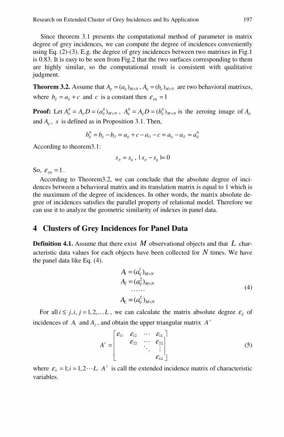
Research on Extended Cluster of Grey Incidences and Its Application 197
Since theorem 3.1 presents the computational method of parameter in matrix degree of grey incidences, we can compute the degree of incidences conveniently using Eq. (2)-(3). E.g. the degree of grey incidences between two matrixes in Fig.1 is 0.83. It is easy to be seen from Fig.2 that the two surfaces corresponding to them are highly similar, so the computational result is consistent with qualitative judgment.
Theorem 3.2. Assume that ( )p ij M NA a ×= , ( )q ij M NA b ×= are two behavioral matrixes,
where ij ijb a c= + and c is a constant then 1pqε =
Proof: Let 0 0( )p p ij M NA A D a ×= = , 0 0( )q q ij M NA A D b ×= = is the zeroing image of pA
and qA , s is defined as in Proposition 3.1. Then,
0 01 1 1ij ij i ij i ij i ijb b b a c a c a a a= − = + − − = − =
According to theorem3.1:
p qs s= , | | 0p qs s− =
So, 1pqε = .
According to Theorem3.2, we can conclude that the absolute degree of inci-dences between a behavioral matrix and its translation matrix is equal to 1 which is the maximum of the degree of incidences. In other words, the matrix absolute de-gree of incidences satisfies the parallel property of relational model. Therefore we can use it to analyze the geometric similarity of indexes in panel data.
4 Clusters of Grey Incidences for Panel Data
Definition 4.1. Assume that there exist M observational objects and that L char-acteristic data values for each objects have been collected for N times. We have the panel data like Eq. (4).
11
22
( )( )
( )
ij M N
ij M N
LL ij M N
A aA a
A a
×
×
×
==
= (4)
For all , , 1, 2,i j i j L≤ = … , we can calculate the matrix absolute degree ijε of
incidences of iA and jA , and obtain the upper triangular matrix rA
11 12 1
22 2
L
r L
LL
A
ε ε εε ε
ε
⎡ ⎤⎢ ⎥
= ⎢ ⎥⎢ ⎥⎣ ⎦
(5)
where 1; 1,2 .ii i Lε = = rA is call the extended incidence matrix of characteristic variables.
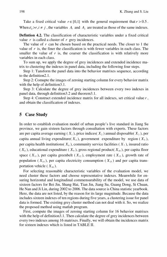
198 K. Zhang and S. Liu
Take a fixed critical value [0,1]r ∈ with the general requirement that 0.5r > .
When > ,ij r i jε ≠ , the variables iA and jA are treated as those of the same indexes.
Defintion 4.2. The classification of characteristic variables under a fixed critical value r is called a cluster of r grey incidences.
The value of r can be chosen based on the practical needs. The closer to 1 the value of r is, the finer the classification is with fewer variables in each class. The smaller the value of r is, the coarser the classification is with relatively more variables in each class.
To sum up, we apply the degree of grey incidences and extended incidence ma-trix to clustering the indexes in panel data, including the following four steps.
Step 1: Tansform the panel data into the behavior matrixes sequence, according to the definition2.1.
Step 2: Comupte the images of zeroing starting column for every behavior matrix with the help of definition3.1.
Step 3: Calculate the degree of grey incidences between every two indexes in panel data, through definition3.2 and theorem3.1.
Step 4: Construct extended incidence matrix for all indexes, set critical value r , and obtain the classification of indexes.
5 Case Study
In order to establish evaluation model of urban people’s live standard in Jiang Su province, we gain sixteen factors through consultation with experts. These factors are per capita average earning ( 1X ), price indices( 2X ) annual disposable( 3X ), per capita annual living expenditure( 4X ), government expenditure by region ( 5X ), per capita health institutions( 6X ), community service facilities ( 7X ), insured ratio ( 8X ), educational expenditure ( 9X ), gross regional product( 10X ), per capita floor
space ( 11X ), per capita greenbelt ( 12X ), employment rate ( 13X ), growth rate of population ( 14X ), per capita electricity consumption ( 15X ) and per capita trans-portation vehicle ( 16X ).
For selecting reasonable characteristic variables of the evaluation model, we need cluster these factors and choose representative indexes. Meanwhile for en-suring horizontal and longitudinal commensurability of the model, we use data of sixteen factors for Bei Jin, Shang Hai, Tian Jin, Jiang Su, Guang Dong, Si Chuan, He Nan and Ji Lin, during 2002 to 2006. The data source is China statistic yearbook. Here, the data are not listed, by the reason for its large magnitude. Because the data includes sixteen indexes of ten regions during five years, a clustering issue for panel data is formed. The existing grey cluster method can not deal with it. So, we realize the proposed method using matlab program.
First, compute the images of zeroing starting column for 16 behavior matrixes with the help of definition3.1. Then calculate the degree of grey incidences between every two indexes among 16 matrixes. Finally, we will obtain the incidences matrix for sixteen indexes which is listed in TABLE II.
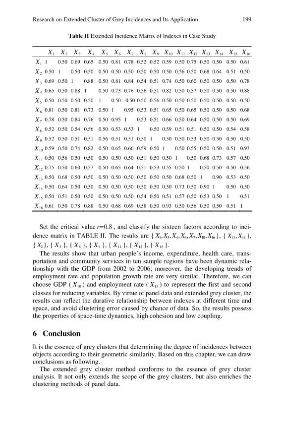
Research on Extended Cluster of Grey Incidences and Its Application 199
Table II Extended Incidence Matrix of Indexes in Case Study
1X 2X 3X 4X 5X 6X 7X 8X 9X 10X 11X 12X 13X 14X 15X 16X
1X 1 0.50 0.69 0.65 0.50 0.81 0.78 0.52 0.52 0.59 0.50 0.75 0.50 0.50 0.50 0.61
2X 0.50 1 0.50 0.50 0.50 0.50 0.50 0.50 0.50 0.50 0.56 0.50 0.68 0.64 0.51 0.50
3X 0.69 0.50 1 0.88 0.50 0.81 0.84 0.54 0.51 0.74 0.50 0.60 0.50 0.50 0.50 0.78
4X 0.65 0.50 0.88 1 0.50 0.73 0.76 0.56 0.51 0.82 0.50 0.57 0.50 0.50 0.50 0.88
5X 0.50 0.50 0.50 0.50 1 0.50 0.50 0.50 0.56 0.50 0.50 0.50 0.50 0.50 0.50 0.50
6X 0.81 0.50 0.81 0.73 0.50 1 0.95 0.53 0.51 0.65 0.50 0.65 0.50 0.50 0.50 0.68
7X 0.78 0.50 0.84 0.76 0.50 0.95 1 0.53 0.51 0.66 0.50 0.64 0.50 0.50 0.50 0.69
8X 0.52 0.50 0.54 0.56 0.50 0.53 0.53 1 0.50 0.59 0.51 0.51 0.50 0.50 0.54 0.58
9X 0.52 0.50 0.51 0.51 0.56 0.51 0.51 0.50 1 0.50 0.50 0.53 0.50 0.50 0.50 0.50
10X 0.59 0.50 0.74 0.82 0.50 0.65 0.66 0.59 0.50 1 0.50 0.55 0.50 0.50 0.51 0.93
11X 0.50 0.56 0.50 0.50 0.50 0.50 0.50 0.51 0.50 0.50 1 0.50 0.68 0.73 0.57 0.50
12X 0.75 0.50 0.60 0.57 0.50 0.65 0.64 0.51 0.53 0.55 0.50 1 0.50 0.50 0.50 0.56
13X 0.50 0.68 0.50 0.50 0.50 0.50 0.50 0.50 0.50 0.50 0.68 0.50 1 0.90 0.53 0.50
14X 0.50 0.64 0.50 0.50 0.50 0.50 0.50 0.50 0.50 0.50 0.73 0.50 0.90 1 0.50 0.50
15X 0.50 0.51 0.50 0.50 0.50 0.50 0.50 0.54 0.50 0.51 0.57 0.50 0.53 0.50 1 0.51
16X 0.61 0.50 0.78 0.88 0.50 0.68 0.69 0.58 0.50 0.93 0.50 0.56 0.50 0.50 0.51 1
Set the critical value =0.8r , and classify the sixteen factors according to inci-
dence matrix in TABLE II. The results are { 1 3 4 6 7 10 16, , , , , ,X X X X X X X }, { 13 14,X X }, { 2X }, { 5X }, { 8X }, { 9X }, { 11X }, { 12X }, { 15X }.
The results show that urban people’s income, expenditure, health care, trans-portation and community services in ten sample regions have been dynamic rela-tionship with the GDP from 2002 to 2006; moreover, the developing trends of employment rate and population growth rate are very similar. Therefore, we can choose GDP ( 10X ) and employment rate ( 13X ) to represent the first and second classes for reducing variables. By virtue of panel data and extended grey cluster, the results can reflect the durative relationship between indexes at different time and space, and avoid clustering error caused by chance of data. So, the results possess the properties of space-time dynamics, high cohesion and low coupling.
6 Conclusion
It is the essence of grey clusters that determining the degree of incidences between objects according to their geometric similarity. Based on this chapter, we can draw conclusions as following.
The extended grey cluster method conforms to the essence of grey cluster analysis. It not only extends the scope of the grey clusters, but also enriches the clustering methods of panel data.

200 K. Zhang and S. Liu
The extended grey clusters method is fit for the analysis of panel data, which overcome the shortcoming of classical methods; also it can describe the dynamic relationship between objects. The case study proves the new method possesses the properties of space-time dynamics, high cohesion and low coupling.
The method fully utilizes the information, and solves the problem of losing the data information in literature (Zhen, 2008). Because of convenient realization on computer, the method is very practical and has good applicable prospects in image process, automatic control, and other fields.
References
Bonzo, D.C., Hermosilla, A.Y.: Clustering panel data via perturbed adaptive simulated annealing and genetic algorithms. Advances in Complex Systems 5(4), 339–360 (2002)
Chen, H.T., Zhou, D.Q.: Study on the time difference between prices of China and interna-tional oil futures based on grey relativity theory. Systems Engineering Theory & Prac-tice 28(3), 166–170 (2008)
Cheng, H.: Analysis of Panel Data, pp. 124–135. Cambridge University Press, Cambridge (1988)
Deng, J.L.: Introduction to grey system theory. The Journal of Grey System (UK), 1–24 (1989)
Hu, Q.Z., Zhang, W.H.: Grey related degree model for the optimization of urban public transport network. Journal of Systems Engineering 22(6), 607–612 (2007)
Lin, Y., Chen, M.Y., Liu, S.F.: Theory of grey systems: capturing uncertainties of grey information. Kybernetes: The International Journal of Systems and Cybernetics 33(2), 196–218 (2004)
Lin, Y., Liu, S.F.: Solving Problems with incomplete information: a grey systems approach. In: Advances in Imaging and Electron Physics, vol. 141, pp. 77–174. Elsevier, Oxford (2006)
Liu, S.F., Lin, Y.: Grey Information: Theory and Practical Applications, pp. 1–4. Springer, London (2006)
Ma, M., Hao, C.Y.: Image Fidelity Criterion Based on Grey Relational Analysis. Journal of Computer-Aided Design & Computer Graphics 16(7), 978–983 (2004)
Tang, W.X.: The concept and the computation method of T’s correlation degree. Application of Statistics and Manageme 14(1), 34–37 (1995)
Wang, Q.Y.: The grey relational analysis of B-model. Journal of Huazhong University of Science and Technology 17(6), 77–82 (1987)
Wang, Q.Y., Zhao, X.H.: The relational analysis of C-mode. Journal of Huazhong University of Science and Technology 27(3), 75–77 (1999)
Zhen, B.Y.: The clustering analysis of multivariable panel data and its application. Applica-tion of Statistics and Management 27(2), 265–270 (2008)
Zhu, J.P., Chen, M.K.: The cluster analysis of panel data and its application. Statistical Research 24(4), 11–14 (2007)

Part III Grey Cluster Evaluation Models
Study of an Improved Grey Integrated Clustering Method and Its Application
Fenyi Dong, Junjuan Liu, and Bin Liu
Literature on general grey clustering methods and their improved methods all give the clustering results based on the principle of the maximal element of a grey clus-tering coefficient vector. Such methods neglect the effect of other elements, except the maximal one of a grey clustering coefficient vector to the cluster result. Because the grey integrated clustering method comprehensively considers the effect of all elements of a grey clustering coefficient vector on the cluster result, it is an important development for grey clustering techniques. But the way that the value area of in-tegrated clustering coefficients is divided into s equal intervals needs improving. This chapter puts forth an improved grey integrated clustering method, with which the value interval of a grey integrated clustering coefficient for a grey class was divided by k±0.5 as boundary points. It is proven that when the difference of clus-tering coefficients of ordinary grey clustering methods is more than 1-1/(s-1), there are the same clustering results for the improved grey integrated clustering and the ordinary grey clustering. At last, we illustrate the improved grey integrated cluster-ing method with the evaluation of rural economic development in Henan Province.
1 Introduction
Grey system theory has obtained great development since its founding in 1982 (Liu and Lin, 2006; Lin et al., 2004; Lin and Liu, 2006). Grey clustering evaluation is a technique that was developed earliest and is widely used in grey system theory. It’s also one of the grey techniques that is widely discussed. Commonly used grey clustering methods are the grey variable-weight clustering method, founded by Professor Deng (Deng, 1990); the grey fixed-weight clustering method, founded by Professor Liu (Liu, 1993); and the grey clustering based on the triangle whiteniza-tion function, founded by Professor Liu, Zhu (Liu et al., 1993). The process of grey clustering evaluation is given by the following definitions (Liu et al., 2004): Fenyi Dong College of Information and Management Science, Henan Agricultural University, Zhengzhou, CO 450002, P.R. China Phone: +86+371-6355-5084; Fax: +86+371-6355-8090; e-mail: [email protected]
Junjuan Liu and Bin Liu College of Information and Management Science, Henan Agricultural University, Zhengzhou, CO 450002, P.R. China
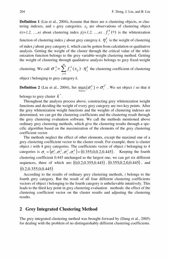
204 F. Dong, J. Liu, and B. Liu
Definition 1 (Liu et al., 2004). Assume that there are n clustering objects, m clus-tering indexes, and s grey categories. xij are observations of clustering object
i(i=1,2, …,n) about clustering index j(j=1,2, …,n) . )(∗kjf is the whitenization
function of clustering index j about grey categroy k. kjη is the weight of clustering
of index j about grey category k, which can be gotten from calculation or qualitative analysis. Getting the weight of the cluster through the critical value of the whit-enization function belongs to the grey variable-weight clustering method. Getting the weight of clustering through qualitative analysis belongs to grey fixed-weight
clustering. We call ∑=
⋅=m
jij
kj
ki xf
1
)(σ kjη the clustering coefficient of clustering
object i belonging to grey category k.
Definition 2 (Liu et al., 2004). Set =≤≤
}{max1
ki
skσ
∗kiσ . We set object i so that it
belongs to grey cluster ∗k . Throughout the analysis process above, constructing grey whitenization weight
functions and deciding the weight of every grey category are two key points. After the grey whitenization weight functions and the weights of clustering indexes are determined, we can get the clustering coefficients and the clustering result through the grey clustering evaluation software. We call the methods mentioned above ordinary grey clustering methods, which give the clustering results through a spe-cific algorithm based on the maximization of the elements of the grey clustering coefficient vector.
The methods neglect the effect of other elements, except the maximal one of a grey clustering coefficient vector to the cluster result. For example, there is cluster object i with 4 grey categories. The coefficients vector of object i belonging to 4 categories is ( ) ( )445.0,2.0,0,355.0,,, 4321 == iiiii σσσσσ . Keeping the fourth
clustering coefficient 0.445 unchanged as the largest one, we can get six different sequences, three of which are: ( )445.0,355.0,2.0,0 , ( )445.0,0,2.0,355.0 , and
( )445.0,0,355.0,2.0
According to the results of ordinary grey clustering methods, i belongs to the fourth grey category. But the result of all four different clustering coefficients vectors of object i belonging to the fourth category is unbelievable intuitively. This leads to the third key point in grey clustering evaluation methods: the effect of the clustering coefficient vector on the cluster results and adjusting the clustering results.
2 Grey Integrated Clustering Method
The grey integrated clustering method was brought forward by (Dang et al., 2005)
for dealing with the problem of no distinguishably different clustering coefficients.

Study of an Improved Grey Integrated Clustering Method and Its Application 205
Definition 3 (Dang et al., 2005). Set
∑=
=s
k
ki
kik
i
1
σ
σδ . We call kiδ the normalized
clustering coefficient of clustering object i belonging to grey classification k; call
( ),,,, 21 siiii δδδδ = (i=1,2,…,n) the normalized clustering coefficient vector of
object i.
Definition 4 (Dang et al., 2005). Assume there are n clustering objects and m grey
categories. ( ),,,, 21 siiii δδδδ = (i=1,2,…,n) is the normalized clustering coeffi-
cient vector of object i. ( )Tss ,1,,2,1 −=η , and we call
ηδω ⋅= ii ∑=
⋅=s
k
kik
1
δ the integrated clustering coefficient of object i.
( )Tss ,1,,2,1 −=η is the weight vector of the integrated clustering coeffi-
cient. They have proven that the value range of the integrated clustering coefficient of
object i is si ≤≤ ω1 and divided the value range into s uncrossed ranges with the
same length as ( )[ ]ss 11,1 −+ , ( ) ( )[ ]ssss 121,11 −+−+ , …,
( )[ ]ssss ,1−− .
Definition 5 (Dang et al., 2005). When the integrated clustering coefficient of
object i ( )( ) ( )[ ]ssksski 11,111 −+−−+∈ω , we say that object i belongs
to k grey category.
Definition 6 (Dang et al., 2005). Assume the clustering coefficient vector is
( ),,,, 21 siiii δδδδ = (i=1,2,…,n). We range the elements in clustering coeffi-
cient vector from largest to smallest, and the new sequence is ( ) ( ) ( )siii δδδ ,,, 21 ,
( ) ( ) ( )siii δδδ ≥≥≥ 21 . Then the ordering clustering coefficient vector of object
i is ( ) ( ) ( ) ),,,( 21' siiii δδδδ = .
Definition 7 (Dang et al., 2005). Assume the clustering coefficient vector is
( )siiii δδδδ ,,, 21= , and ( ) ( ) ( ) ),,,( 21' s
iiii δδδδ = is its ordering clustering
coefficient vector. If named ( ) ( )21iii δδθ −= , we call iθ the distinguished dif-
ference coefficient of object i. If ( ) ( )siii
2121 −≤−= δδθ , there is no distin-
guishable difference on clustering coefficient of i, otherwise there is a distinguished difference for the clustering coefficient of i.
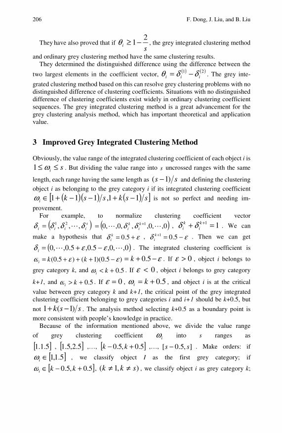
206 F. Dong, J. Liu, and B. Liu
They have also proved that if si
21−≥θ , the grey integrated clustering method
and ordinary grey clustering method have the same clustering results. They determined the distinguished difference using the difference between the
two largest elements in the coefficient vector, ( ) ( )21iii δδθ −= . The grey inte-
grated clustering method based on this can resolve grey clustering problems with no distinguished difference of clustering coefficients. Situations with no distinguished difference of clustering coefficients exist widely in ordinary clustering coefficient sequences. The grey integrated clustering method is a great advancement for the grey clustering analysis method, which has important theoretical and application value.
3 Improved Grey Integrated Clustering Method
Obviously, the value range of the integrated clustering coefficient of each object i is
si ≤≤ ω1 . But dividing the value range into s uncrossed ranges with the same
length, each range having the same length as ss )1( − and defining the clustering
object i as belonging to the grey category i if its integrated clustering coefficient
( )( ) ( )[ ]ssksski 11,111 −+−−+∈ω is not so perfect and needing im-
provement. For example, to normalize clustering coefficient vector
( )siiii δδδδ ,,, 21= ( )0,,0,,,0,,0 1+= k
iki δδ , 11 =+ +k
iki δδ . We can
make a hypothesis that εδ += 5.0ki
, εδ −=+ 5.01ki
. Then we can get
( )0,,0,5.0,5.0,,0 εεδ −+=i . The integrated clustering coefficient is
)5.0)(1()5.0( εεω −+++= kki ε−+= 5.0k . If 0>ε , object i belongs to
grey category k, and 5.0+< kiω . If 0<ε , object i belongs to grey category
k+1, and 5.0+> kiω . If 0=ε , 5.0+= kiω , and object i is at the critical
value between grey category k and k+1, the critical point of the grey integrated clustering coefficient belonging to grey categories i and i+1 should be k+0.5, but
not ssk )1(1 −+ . The analysis method selecting k+0.5 as a boundary point is
more consistent with people’s knowledge in practice. Because of the information mentioned above, we divide the value range
of grey clustering coefficient iω into s ranges as
[ ]5.1.1 , [ ]5.2,5.1 ,…, [ ]5.0,5.0 +− kk ,…, ],5.0[ ss − . Make orders: if
[ ]5.1,1∈iω , we classify object I as the first grey category; if
[ ]5.0,5.0 +−∈ kkiω , ),1( skk ≠≠ , we classify object i as grey category k;

Study of an Improved Grey Integrated Clustering Method and Its Application 207
if [ ]ssi ,5.0−∈ω , we classify object i as grey category s. We call this analysis
method the improved grey integrated clustering method.
Theorem. To improve the grey integrated clustering method, if the distinguished
difference of the clustering coefficient 1
11
−−≥
sθ , there are the same results for
ordinary grey clustering methods and the improved grey integrated clustering method.
Proof: Appendix. The inverse proposition of this theorem is untenable. When we get the same clus-tering results from the general grey clustering method and the improved grey inte-grated clustering method, the condition that the prominent difference coefficient is
bigger than 1
11
−−
s was not necessarily met.
4 Instance Analysis
We evaluated the development level of the rural economy in eighteen cities of Henan province, based on data from the second national census of agriculture (2007) and the Statistical Yearbook of Henan (2007). Eight indexes classified into four types were adopted. They are (1) The proportion of the population not en-gaging in the primary industry among the working people in countryside; (2) Per capita output value of people engaging in primary industry; (3) Per capita net in-come of peasants; (4) Per capita expenditure of cost of living in the country; (5) Consumer durables ownership of every 100 families; (6) Proportion of villages having cultural and educational facilities; (7) Proportion of villages having medical facilities and medical staff; (8) Per capita saving.
We divide the development level of the rural economy in the eighteen cities of Henan province into four categories. They are the highly developed region, the medium developed region, the low developed region, and the least developed re-gion. Then, we divide the difference between the maximal value and the minimal
value of each index ij
i
ij
ij XX minmax −=Δ into ten parts with the same
length. We select
])5
4min
5
3min[1
,——,, jij
ij
ij
ij XXf Δ+Δ+ ;
]5
4min
2
1min
5
2min[2
jij
ij
ij
ij
ij
ij XXXf Δ+Δ+Δ+ ,—,, ;
]2
1min
10
3min
5
1min[3
jij
ij
ij
ij
ij
ij XXXf Δ+Δ+Δ+ ,—,, ;
]10
3min
10
1min[4
jij
ij
ij
ij XXf Δ+Δ+ ,,——,
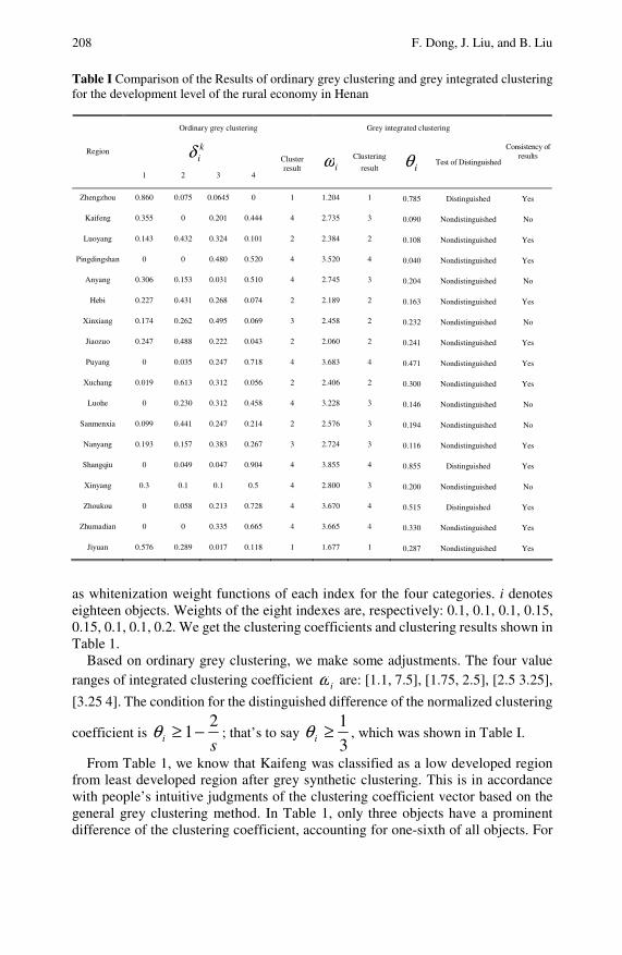
208 F. Dong, J. Liu, and B. Liu Table I Comparison of the Results of ordinary grey clustering and grey integrated clustering for the development level of the rural economy in Henan
Ordinary grey clustering Grey integrated clustering
kiδ Region
1 2 3 4
Cluster result iω
Clustering
result iθ Test of Distinguished
Consistency of results
Zhengzhou 0.860 0.075 0.0645 0 1 1.204 1 0.785 Distinguished Yes
Kaifeng 0.355 0 0.201 0.444 4 2.735 3 0.090 Nondistinguished No
Luoyang 0.143 0.432 0.324 0.101 2 2.384 2 0.108 Nondistinguished Yes
Pingdingshan 0 0 0.480 0.520 4 3.520 4 0.040 Nondistinguished Yes
Anyang 0.306 0.153 0.031 0.510 4 2.745 3 0.204 Nondistinguished No
Hebi 0.227 0.431 0.268 0.074 2 2.189 2 0.163 Nondistinguished Yes
Xinxiang 0.174 0.262 0.495 0.069 3 2.458 2 0.232 Nondistinguished No
Jiaozuo 0.247 0.488 0.222 0.043 2 2.060 2 0.241 Nondistinguished Yes
Puyang 0 0.035 0.247 0.718 4 3.683 4 0.471 Nondistinguished Yes
Xuchang 0.019 0.613 0.312 0.056 2 2.406 2 0.300 Nondistinguished Yes
Luohe 0 0.230 0.312 0.458 4 3.228 3 0.146 Nondistinguished No
Sanmenxia 0.099 0.441 0.247 0.214 2 2.576 3 0.194 Nondistinguished No
Nanyang 0.193 0.157 0.383 0.267 3 2.724 3 0.116 Nondistinguished Yes
Shangqiu 0 0.049 0.047 0.904 4 3.855 4 0.855 Distinguished Yes
Xinyang 0.3 0.1 0.1 0.5 4 2.800 3 0.200 Nondistinguished No
Zhoukou 0 0.058 0.213 0.728 4 3.670 4 0.515 Distinguished Yes
Zhumadian 0 0 0.335 0.665 4 3.665 4 0.330 Nondistinguished Yes
Jiyuan 0.576 0.289 0.017 0.118 1 1.677 1 0.287 Nondistinguished Yes
as whitenization weight functions of each index for the four categories. i denotes eighteen objects. Weights of the eight indexes are, respectively: 0.1, 0.1, 0.1, 0.15, 0.15, 0.1, 0.1, 0.2. We get the clustering coefficients and clustering results shown in Table 1.
Based on ordinary grey clustering, we make some adjustments. The four value ranges of integrated clustering coefficient iω are: [1.1, 7.5], [1.75, 2.5], [2.5 3.25],
[3.25 4]. The condition for the distinguished difference of the normalized clustering
coefficient is si
21−≥θ ; that’s to say
3
1≥iθ , which was shown in Table I.
From Table 1, we know that Kaifeng was classified as a low developed region from least developed region after grey synthetic clustering. This is in accordance with people’s intuitive judgments of the clustering coefficient vector based on the general grey clustering method. In Table 1, only three objects have a prominent difference of the clustering coefficient, accounting for one-sixth of all objects. For

Study of an Improved Grey Integrated Clustering Method and Its Application 209
the clustering coefficient, there are no prominent differences for the other fifteen objects. Among the fifteen objects, the clustering results of six objects changed, accounting for 40%. This shows the phenomenon that clustering results are dif-ferent is universal if there is no prominent difference for the clustering coefficient. This fully explains the necessity of grey synthetic clustering based on the general grey clustering coefficient, when grey clustering analysis is adopted with more grey clusters.
We make some adjustments based on the improved grey integrated clustering method. The four value ranges of grey clusters of the improved grey integrated clustering coefficient are: [1, 1.5], [1.5, 2.5], [2.5 3.5], [3.5, 4]. The condition for the normalized clustering coefficient having a distinguished difference is
1
11
−−≥
siθ ; that’s to say 3
2≥iθ . The results are shown in Table II.
Table II Comparison of the Results of ordinary grey clustering and improved grey integrated clustering for the development level of the rural economy in Henan
Ordinary grey clustering Improved grey integrated clustering
kiδ Region
1 2 3 4
Clusteringresult iω
Clustering result iθ
Test of
distinguished
Consistency of results
Zhengzhou 0.860 0.075 0.0645 0 1 1.204 1 0.785 notable consistent
Kaifeng 0.355 0 0.201 0.444 4 2.735 3 0.090 unobtrusive not consistent
Luoyang 0.143 0.432 0.324 0.101 2 2.384 2 0.108 unobtrusive consistent
Pingdingshan 0 0 0.480 0.520 4 3.520 4 0.040 unobtrusive consistent
Anyang 0.306 0.153 0.031 0.510 4 2.745 3 0.204 unobtrusive not consistent
Hebi 0.227 0.431 0.268 0.074 2 2.189 2 0.163 unobtrusive consistent
Xinxiang 0.174 0.262 0.495 0.069 3 2.458 2 0.232 unobtrusive not consistent
Jiaozuo 0.247 0.488 0.222 0.043 2 2.060 2 0.241 unobtrusive consistent
Puyang 0 0.035 0.247 0.718 4 3.683 4 0.471 unobtrusive consistent
Xuchang 0.019 0.613 0.312 0.056 2 2.406 2 0.300 unobtrusive consistent
Luohe 0 0.230 0.312 0.458 4 3.228 3 0.146 unobtrusive not consistent
Sanmenxia 0.099 0.441 0.247 0.214 2 2.576 3 0.194 unobtrusive not consistent
Nanyang 0.193 0.157 0.383 0.267 3 2.724 3 0.116 unobtrusive consistent
Shangqiu 0 0.049 0.047 0.904 4 3.855 4 0.855 notable consistent
Xinyang 0.3 0.1 0.1 0.5 4 2.800 3 0.200 unobtrusive not consistent
Zhoukou 0 0.058 0.213 0.728 4 3.670 4 0.515 unobtrusive consistent
Zhumadian 0 0 0.335 0.665 4 3.665 4 0.330 unobtrusive consistent
Jiyuan 0.576 0.289 0.017 0.118 1 1.677 2 0.287 unobtrusive not consistent

210 F. Dong, J. Liu, and B. Liu
From Table 2, we know Jiyuan was classified as a medium developed region from a highly developed region after the improved grey integrated clustering. At the same time, the distinguished difference for the clustering coefficient of Zhoukou become a non-distinguished difference.
5 Conclusion
The literature on ordinary grey clustering methods and their improved methods all give the clustering results based on the maximization of the elements of a grey clustering coefficient vector. Such methods neglect the effect of other elements, except the maximal one of a grey clustering coefficient vector on the cluster result. Because the grey integrated clustering method comprehensively considers the ef-fect of all elements of a grey clustering coefficient vector on the clustering result, it is an important development for grey clustering techniques. This method has im-portant theoretical and applicable value. For the problem of dividing value ranges of a grey integrated clustering coefficient belonging to a corresponding grey category, the value range of the integrated clustering coefficient [ ]s,1 was divided into s
uncrossed ranges with same length ss )1( − , and object i was classified as grey
category k if ( )( ) ( )[ ]ssksski 11,111 −+−−+∈ω . This method is not perfect,
because grey integrated clustering with iδ ( )0,,0,,,0,,0 1+= ki
ki δδ can’t be
resolved using this method. This method needs improving. The method put forth in this chapter divides grey integrated clustering coefficient by 5.0±k as the critical point. The above problem can be resolved to some extent by this method. This chapter also proved that, when the distinguished difference of ordinary grey clus-
tering coefficient 1
11
−−≥
sθ , the improved grey integrated clustering method
and ordinary grey clustering methods have the same clustering results for a clus-tering object. At last, we look at a case analysis of the development level of the rural economy in Henan province in China. The improved grey integrated clustering method was feasible.
Appendix
Proof: There are three situations.
1) When 1iδ is the maximal one, object i belongs to the first grey category based
on ordinary grey clustering methods. If we want get the same results for the im-
proved grey integrated clustering method, [ ]5.1,1∈iω must be satisfied. 1≥iω
is inevitable, so we can get the same results if only 5.1≤iω . Because
∑=
⋅=s
k
kii k
1
δω , iω will be maximal only when ( )siii δδδ ,0,,0,1= ,
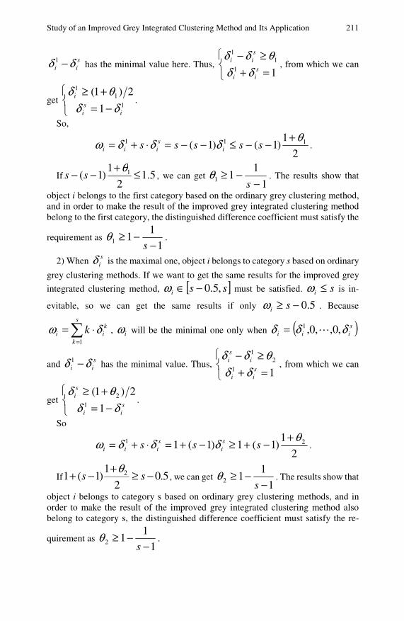
Study of an Improved Grey Integrated Clustering Method and Its Application 211
sii δδ −1 has the minimal value here. Thus,
⎩⎨⎧
=+≥−
111
1
sii
sii
δδθδδ
, from which we can
get ⎩⎨⎧
−=+≥
11
1
1
2)1(
isi
i
δδθδ
.
So,
siii s δδω ⋅+= 1 1)1( iss δ−−=
2
1)1( 1θ+
−−≤ ss .
If 5.12
1)1( 1 ≤+−− θ
ss , we can get 1
111 −
−≥s
θ . The results show that
object i belongs to the first category based on the ordinary grey clustering method, and in order to make the result of the improved grey integrated clustering method belong to the first category, the distinguished difference coefficient must satisfy the
requirement as 1
111 −
−≥s
θ .
2) When siδ is the maximal one, object i belongs to category s based on ordinary
grey clustering methods. If we want to get the same results for the improved grey
integrated clustering method, [ ]ssi ,5.0−∈ω must be satisfied. si ≤ω is in-
evitable, so we can get the same results if only 5.0−≥ siω . Because
∑=
⋅=s
k
kii k
1
δω , iω will be the minimal one only when ( )siii δδδ ,0,,0,1=
and sii δδ −1 has the minimal value. Thus,
⎩⎨⎧
=+≥−
112
1
sii
isi
δδθδδ
, from which we can
get ⎩⎨⎧
−=+≥
sii
si
δδθδ
1
2)1(1
2 .
So
siii s δδω ⋅+= 1 s
is δ)1(1 −+=2
1)1(1 2θ+
−+≥ s .
If 5.02
1)1(1 2 −≥
+−+ ss
θ, we can get
1
112 −
−≥s
θ . The results show that
object i belongs to category s based on ordinary grey clustering methods, and in order to make the result of the improved grey integrated clustering method also belong to category s, the distinguished difference coefficient must satisfy the re-
quirement as 1
112 −
−≥s
θ .
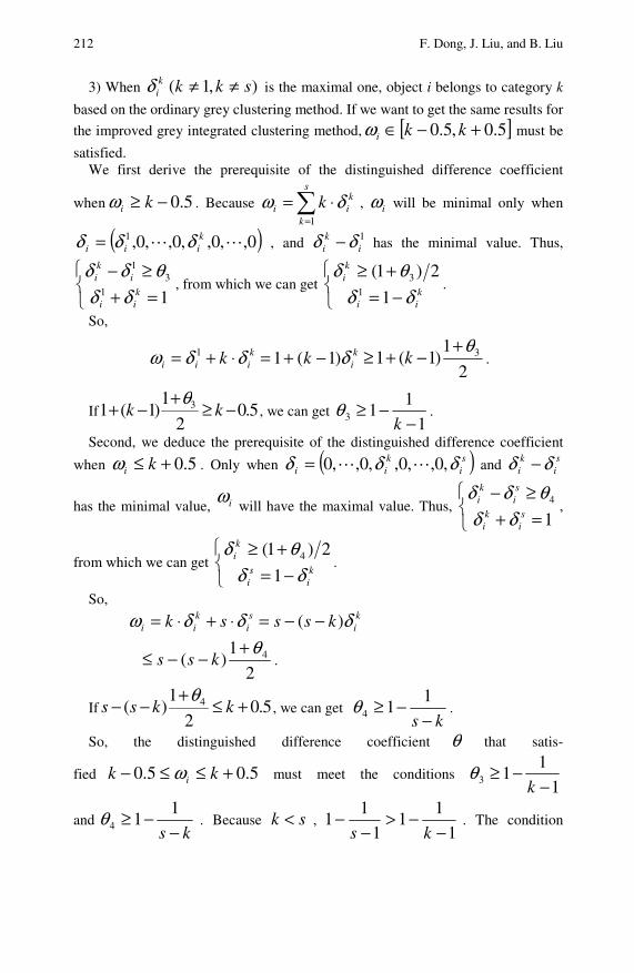
212 F. Dong, J. Liu, and B. Liu
3) When kiδ ),1( skk ≠≠ is the maximal one, object i belongs to category k
based on the ordinary grey clustering method. If we want to get the same results for
the improved grey integrated clustering method, [ ]5.0,5.0 +−∈ kkiω must be
satisfied. We first derive the prerequisite of the distinguished difference coefficient
when 5.0−≥ kiω . Because ∑=
⋅=s
k
kii k
1
δω , iω will be minimal only when
( )0,,0,,0,,0,1 kiii δδδ = , and 1
iki δδ − has the minimal value. Thus,
⎩⎨⎧
=+≥−
113
1
kii
iki
δδθδδ
, from which we can get ⎩⎨⎧
−=+≥
kii
ki
δδθδ
1
2)1(1
3 .
So,
kiii k δδω ⋅+= 1 k
ik δ)1(1 −+=2
1)1(1 3θ+
−+≥ k .
If 5.02
1)1(1 3 −≥
+−+ kk
θ, we can get
1
113 −
−≥k
θ .
Second, we deduce the prerequisite of the distinguished difference coefficient
when 5.0+≤ kiω . Only when ( )si
kii δδδ ,0,,0,,0,,0= and s
iki δδ −
has the minimal value, iω will have the maximal value. Thus,
⎩⎨⎧
=+≥−
14
si
ki
si
ki
δδθδδ
,
from which we can get ⎩⎨⎧
−=+≥
ki
si
ki
δδθδ
1
2)1( 4 .
So, si
kii sk δδω ⋅+⋅= k
ikss δ)( −−=
2
1)( 4θ+
−−≤ kss .
If 5.02
1)( 4 +≤
+−− kkss
θ, we can get
ks −−≥ 1
14θ .
So, the distinguished difference coefficient θ that satis-
fied 5.05.0 +≤≤− kk iω must meet the conditions 1
113 −
−≥k
θ
andks −
−≥ 114θ . Because sk < ,
1
11
1
11
−−>
−−
ks. The condition
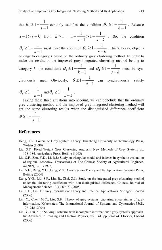
Study of an Improved Grey Integrated Clustering Method and Its Application 213
that1
113 −
−≥s
θ certainly satisfies the condition 1
113 −
−≥k
θ . Because
kss −>−1 from 1>k , kss −
−>−
− 11
1
11 . So, the condition
1
114 −
−≥s
θ must meet the condition ks −
−≥ 114θ . That’s to say, object i
belongs to category k based on the ordinary grey clustering method. In order to make the results of the improved grey integrated clustering method belong to
category k, the conditions 1
113 −
−≥k
θ and ks −
−≥ 114θ must be syn-
chronously met. Obviously, 1
11
−−≥
sθ can synchronously satisfy
1
113 −
−≥k
θ andks −
−≥ 114θ .
Taking these three situations into account, we can conclude that the ordinary grey clustering method and the improved grey integrated clustering method will get the same clustering results when the distinguished difference coefficient
1
11
−−≥
sθ .
References
Deng, J.L.: Course of Grey System Theory. Huazhong University of Technology Press, Wuhan (1990)
Liu, S.F.: Fixed Weight Grey Clustering Analysis, New Methods of Grey System, pp. 178–184. Agriculture Press, Beijing (1993)
Liu, S.F., Zhu, Y.D., Li, B.J.: Study on triangular model and indexes in synthetic evaluation of regional economy. Transactions of The Chinese Society of Agricultural Engineer-ing 9(2), 8–13 (1993)
Liu, S.F., Dang, Y.G., Fang, Z.G.: Grey System Theory and Its Application. Science Press, Beijing (2004)
Dang, Y.G., Liu, S.F., Liu, B., Zhai, Z.J.: Study on the integrated grey clustering method under the clustering coefficient with non-distinguished difference. Chinese Journal of Management Science 13(4), 69–73 (2005)
Liu, S.F., Lin, Y.: Grey Information: Theory and Practical Applications. Springer, London (2006)
Lin, Y., Chen, M.Y., Liu, S.F.: Theory of grey systems: capturing uncertainties of grey information. Kybernetes: The International Journal of Systems and Cybernetics 33(2), 196–218 (2004)
Lin, Y., Liu, S.F.: Solving Problems with incomplete information: a grey systems approach. In: Advances in Imaging and Electron Physics, vol. 141, pp. 77–174. Elsevier, Oxford (2006)

Study of the Influencing Factors of the Development of Chinese Medicine with Gray Clustering Analysis
Lizhong Duan, Ying Zhang, and Xingxing Fan1
Due to the development of Chinese medicine, the grey clustering analytical method of influencing factors of the development of Chinese medicine was studied. The factors were put forth. The investigation results of the factors were simulated. The investigation results of the factor was quantified, analyzed, and ranked from strongest to weakest with the grey clustering analytical method. Some of the correlative departments in the government could be assisted with the research results.
1 The Problem with the Theory and Diagnosis and Treatment of Chinese Medicine Occurring
Whether Chinese medicine could exit or not is a problem of sensitivity nowadays. Management, hospitals, experts and the public are very interested in the subject. The problem is very important to everyone. Since Western scientific results (including Western medicine) came to China, people have argued four times whether or not to abolish Chinese medicine.
The first case was when “Chinese medicine was omitted by the education system” by the Beiyang government in the 20th century. The second case “abolished Chinese medicine” in 1929. The third case was when it was thought that Chinese medicine was a superstition, forbidding Chinese medicine during the culture revolution. The last case was when Zhang Gong-yao (a professor in the technology and social development department in Zhongnan University) advocated that the commonalty underwrote on the web if they agreed to abolish Chinese medicine. It was said that there were a great number of people who underwrote on the web. The
Lizhong Duan, Ying Zhang, and Xingxing Fan College of Management, Beijing University of Chinese Medicine, Beijing 100029, China e-mail: [email protected]
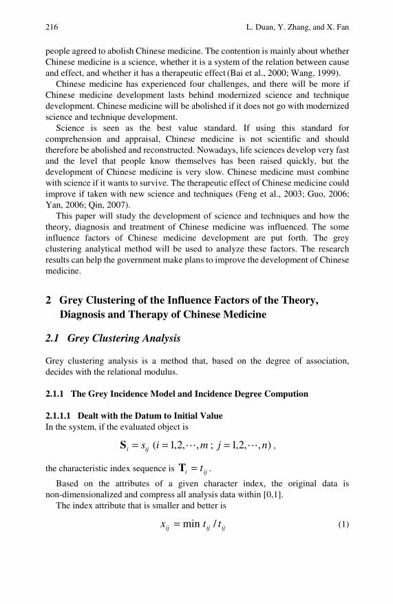
216 L. Duan, Y. Zhang, and X. Fan
people agreed to abolish Chinese medicine. The contention is mainly about whether Chinese medicine is a science, whether it is a system of the relation between cause and effect, and whether it has a therapeutic effect (Bai et al., 2000; Wang, 1999).
Chinese medicine has experienced four challenges, and there will be more if Chinese medicine development lasts behind modernized science and technique development. Chinese medicine will be abolished if it does not go with modernized science and technique development.
Science is seen as the best value standard. If using this standard for comprehension and appraisal, Chinese medicine is not scientific and should therefore be abolished and reconstructed. Nowadays, life sciences develop very fast and the level that people know themselves has been raised quickly, but the development of Chinese medicine is very slow. Chinese medicine must combine with science if it wants to survive. The therapeutic effect of Chinese medicine could improve if taken with new science and techniques (Feng et al., 2003; Guo, 2006; Yan, 2006; Qin, 2007).
This paper will study the development of science and techniques and how the theory, diagnosis and treatment of Chinese medicine was influenced. The some influence factors of Chinese medicine development are put forth. The grey clustering analytical method will be used to analyze these factors. The research results can help the government make plans to improve the development of Chinese medicine.
2 Grey Clustering of the Influence Factors of the Theory, Diagnosis and Therapy of Chinese Medicine
2.1 Grey Clustering Analysis
Grey clustering analysis is a method that, based on the degree of association, decides with the relational modulus.
2.1.1 The Grey Incidence Model and Incidence Degree Compution
2.1.1.1 Dealt with the Datum to Initial Value In the system, if the evaluated object is
),,2,1;,,2,1( njmisiji ===S ,
the characteristic index sequence is iji t=T .
Based on the attributes of a given character index, the original data is non-dimensionalized and compress all analysis data within [0,1].
The index attribute that is smaller and better is
ijijij ttx /min= (1)

Study of the Influencing Factors of the Development of Chinese Medicine 217
The index attribute that is bigger and better is
ijijij ttx max/= (2)
Analyze the practice question. List 0T is decided to be the greatest one in the
same list ijt in list jT , 0it is in every line of list 0T . Divide every number, which
is in the same line of ijt in list iT , so we can consult list )( 00 ix=X and the
comparative list ),,2,1;,,2,1(),( njmixiji ===X .
2.1.1.2 Difference List and Least and Greatest Difference If in k , 0X is )(0 kx ; 1X is )(kxi , and the result is
)()()( 0 kxkxk ii −=Δ (3)
If a is the least difference and b is the greatest, the expression of a and b is
akiki
=Δ )(minmin
bkiki
=Δ )(maxmax
2.1.1.3 Relating Modulus and Relating Degree
bk
bak
ii δ
δξ+Δ
+=)(
)( (4)
)(kiξ is the relating modulus iX to 0X at k and δ is the differentiate
modulus. It is between 0 - 1, usually 0.5. The average of the relation modulus is
∑=
=n
kii k
nr
1
)(1 ξ (5)
ir is the relating degree of iX to 0X (Deng, 2002; 2005; Liu et al., 1991; Jin,
1993; Liu and Lin, 2006; Lin et al., 2004; Lin and Liu, 2006).
2.1.2 The Computation of Clustering Analysis
If S is all the evaluated objects, the expression of S is ),,2,1( miSi ==S
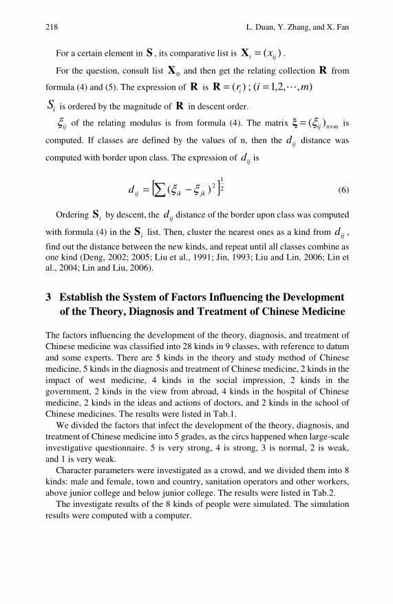
218 L. Duan, Y. Zhang, and X. Fan
For a certain element in S , its comparative list is )( iji x=X .
For the question, consult list 0X and then get the relating collection R from
formula (4) and (5). The expression of R is ),,2,1(;)( miri ==R
iS is ordered by the magnitude of R in descent order.
ijξ of the relating modulus is from formula (4). The matrix mnij ×= )(ξξ is
computed. If classes are defined by the values of n, then the ijd distance was
computed with border upon class. The expression of ijd is
[ ]2
12)(∑ −= jkikijd ξξ (6)
Ordering iS by descent, the ijd distance of the border upon class was computed
with formula (4) in the iS list. Then, cluster the nearest ones as a kind from ijd ,
find out the distance between the new kinds, and repeat until all classes combine as one kind (Deng, 2002; 2005; Liu et al., 1991; Jin, 1993; Liu and Lin, 2006; Lin et al., 2004; Lin and Liu, 2006).
3 Establish the System of Factors Influencing the Development of the Theory, Diagnosis and Treatment of Chinese Medicine
The factors influencing the development of the theory, diagnosis, and treatment of Chinese medicine was classified into 28 kinds in 9 classes, with reference to datum and some experts. There are 5 kinds in the theory and study method of Chinese medicine, 5 kinds in the diagnosis and treatment of Chinese medicine, 2 kinds in the impact of west medicine, 4 kinds in the social impression, 2 kinds in the government, 2 kinds in the view from abroad, 4 kinds in the hospital of Chinese medicine, 2 kinds in the ideas and actions of doctors, and 2 kinds in the school of Chinese medicines. The results were listed in Tab.1.
We divided the factors that infect the development of the theory, diagnosis, and treatment of Chinese medicine into 5 grades, as the circs happened when large-scale investigative questionnaire. 5 is very strong, 4 is strong, 3 is normal, 2 is weak, and 1 is very weak.
Character parameters were investigated as a crowd, and we divided them into 8 kinds: male and female, town and country, sanitation operators and other workers, above junior college and below junior college. The results were listed in Tab.2.
The investigate results of the 8 kinds of people were simulated. The simulation results were computed with a computer.

Study of the Influencing Factors of the Development of Chinese Medicine 219
Table 1 The factors influencing the development of the theory, diagnosis, and treatment of Chinese medicine
The 9 classes of factors The 28 kinds of factors and name
1S :logic of Chinese medicine
2S :science of Chinese medicine
3S :study method of Chinese
medicine
4S :professors of Chinese
medicine
the theory and study method of Chinese medicine
5S :standardization of the
language of Chinese medicine
6S :the path and method of the
traditional Chinese drug
7S :cure effective of Chinese
medicine
8S :enter the new technology
9S : the tool for diagnosis and
treatment of Chinese medicine
the diagnosis and treat of Chinese medicine
10S :the mode for diagnosis and
treatment of Chinese medicine
11S :the impact from west
medicinal the impact from west medicinal
12S :Chinese medicine and west
medicinal combination
13S :the trust from the country
14S :the change of the ill chart
15S :enter WTO the social impressive
16S :the need from society
17S :mangers and organizers in
sanitation department the government
18S :the law of the impact from
west medicinal
the view from abroad 19S :the view from abroad

220 L. Duan, Y. Zhang, and X. Fan
Table 1 (continued)
20S :the overseas development of
Chinese medicine
21S :the profit of the hospital of
Chinese medicine
22S :the skill of the hospital of
Chinese medicine
23S :the resource collocate of the
hospital of Chinese medicine
the hospital of Chinese medicine
24S :the intension build of
Chinese medicine
25S :country doctors the ideas and actions from the doctors
26S :Chinese medicines
27S :education model of Chinese
medicine the school of Chinese medicines
28S :the profit of the hospital of
Chinese medicine
Table 2 The character parameter of the factors influencing the development of the theory, diagnosis, and treatment of Chinese medicine
character parameter
1t male
2t female
3t Town denizen
4t Non town denizen
5t sanitation workers
6t Non sanitation workers
7t Above junior college
8t Bellow junior college

Study of the Influencing Factors of the Development of Chinese Medicine 221
Tab
le 3
The
gra
y re
lati
ng m
odul
us a
nd re
lati
ng d
egre
e of
the
fact
ors
infl
uenc
ing
the
deve
lopm
ent o
f the
theo
ry, d
iagn
osis
, and
trea
tmen
t of
Chi
nese
med
icin
e an
d se
quen
cing
(si
mul
atin
g th
e re
sult
s)
logic
1S
scie
nce
2S
stu
dy
met
ho
d
3Spro
fess
or
4S
stan
dar
diz
atio
n o
f th
e
lan
gu
age
5S
the
pat
h
and
met
hod o
f
the
trad
itio
nal
Chin
ese
dru
g6S
cure
effe
ctiv
e
7S
ente
r th
e
new
tech
no
logy
8S
the
too
l fo
r
dia
gn
osi
s
and
trea
tmen
t
9S
the
mode
for
dia
gnosi
s
and
trea
tmen
t
10
S
the
imp
act
fro
m w
est
med
icin
al
11
S
Ch
ines
e
med
icin
e
and
wes
t
med
icin
al
com
bin
atio
n
12
S
the
tru
st
from
the
cou
ntr
y
13
S
the
chan
ge
of
the
ill
char
t1
4S
mal
e j
ir 10.4
46809
0.4
46809
0.4
46809
0.4
46809
0.4
46809
0.5
38462
0.6
77419
0.3
81
81
8
0.4
46
80
9
0.3
81
81
8
0.3
33
33
3
0.4
46
80
9
0.3
33
33
3
0.5
38
46
2
acco
rdin
g t
oj
ir 1
arra
y3
4
3
4
4
1
1
2
2
6
6
4
5
3
fem
ale
jir 2
0.5
12
19
5
0.5
12
19
5
0.4
11
76
5
0.5
12
19
5
0.3
44
26
2
0.4
11
76
5
0.4
11
76
5
0.6
77
41
9
0.4
11
76
5
0.6
77
41
9
1.0
00
00
0
0.5
12
19
5
0.6
77
41
9
1.0
00
00
0
acco
rdin
g t
o
jir 2
arra
y2
3
4
3
6
2
4
1
3
1
1
3
2
1
To
wn
den
izen
jir 3
0.5
12
19
5
0.5
12
19
5
0.6
77
41
9
0.5
12
19
5
0.5
12
19
5
0.3
44
26
2
0.6
77
41
9
0.6
77
41
9
0.4
11
76
5
0.5
12
19
5
0.3
44
26
2
0.6
77
41
9
1.0
00
00
0
0.5
12
19
5
acco
rdin
g t
o
jir 3
arra
y2
3
1
3
3
4
1
1
3
3
5
1
1
4
No
n t
ow
n d
eniz
en
jir 4
0.3
81818
0.4
46809
0.4
46809
0.3
81818
0.5
38462
0.3
33333
0.3
81818
0.3
33
33
3
0.3
33
33
3
0.4
46
80
9
0.6
77
41
9
0.3
81
81
8
0.6
77
41
9
0.5
38
46
2
acco
rdin
g t
o
jir 4
arra
y4
4
3
5
2
5
5
4
4
4
2
5
2
3
san
itat
ion
wo
rker
s
jir 5
0.4
46809
0.4
46809
0.4
46809
0.4
46809
0.3
81818
0.3
33333
0.3
81818
0.6
77419
0.6
77
41
9
0.3
33
33
3
0.6
77
41
9
0.5
38
46
2
0.3
81
81
8
0.4
46
80
9
acco
rdin
g t
o
jir 5
arra
y3
4
3
4
5
5
5
1
1
7
2
2
4
5
No
n s
anit
atio
n
wo
rker
sj
ir 6
0.3
44262
0.6
77419
0.6
77419
1.0
00000
0.6
77419
0.4
11
76
5
0.5
12
19
5
0.3
44
26
2
0.6
77
41
9
0.4
11
76
5
0.6
77
41
9
0.6
77
41
9
1.0
00
00
0
0.6
77
41
9

222 L. Duan, Y. Zhang, and X. Fan
T
able
3 (
cont
inue
d)
acco
rdin
g t
o
jir 6
arra
y5
1
1
1
1
2
3
3
1
5
2
1
1
2
Above
jun
ior
coll
ege
jir 7
0.6
77419
0.5
38462
0.5
38462
0.5
38462
0.6
77419
0.3
81818
0.5
38462
0.3
33
33
3
0.6
77
41
9
0.5
38
46
2
0.5
38
46
2
0.3
33
33
3
0.4
46
80
9
0.4
46
80
9
acco
rdin
g t
o
jir 7
arra
y1
2
2
2
1
3
2
4
1
2
3
6
3
5
Bel
low
jun
ior
coll
ege
jir 8
0.3
81818
0.5
38462
0.5
38462
0.4
46809
0.5
38462
0.3
81818
0.6
77419
0.3
33
33
3
0.6
77
41
9
0.5
38
46
2
0.4
46
80
9
0.5
38
46
2
0.3
81
81
8
0.6
77
41
9
acco
rdin
g t
o
jir 8
arra
y4
2
2
4
2
3
1
4
1
2
4
2
4
2
the
fact
ors
th
at
infl
uen
ced
th
e
devel
opm
ent
of
Ch
ines
e m
edic
ine
0.4
62916
0.5
14895
0.5
22994
0.5
35637
0.5
14606
0.3
92070
0.5
32289
0.4
69792
0.5
39
16
9
0.4
80
03
3
0.5
86
89
0
0.5
13
24
0
0.6
12
32
7
0.6
04
69
7
acco
rdin
g t
o
arra
y2
4
13
12
8
15
28
9
21
6
19
3
16
1
2

Study of the Influencing Factors of the Development of Chinese Medicine 223
T
able
3 (
Sim
ulat
ing
the
resu
lts)
ente
r
WT
O
15
S
the
nee
d
from
soci
ety
16
S
man
ger
s
and
org
aniz
ers
in
sanit
atio
n
dep
artm
ent
17
S
the
law
of
the
imp
act
fro
m w
est
med
icin
al
18
S
the
vie
w
fro
m
abro
ad
19
S
the
ov
erse
as
dev
elo
pm
ent
20
S
the
pro
fit
of
the
hosp
ital
21
S
the
skil
l o
f
the
hosp
ital
22
S
the
reso
urc
e
coll
oca
te o
f
the
ho
spit
al
23
S
the
inte
nsi
on
buil
d o
f
the
hosp
ital
24
S
cou
ntr
y
do
cto
rs
25
S
Ch
ines
e
med
icin
es
26
S
edu
cati
on
model
of
Ch
ines
e
med
icin
e
27
S
the
vie
wp
oin
t
fro
m t
he
studen
t
28
S
mal
e
jir 1
0.5
38462
0.4
46809
0.5
38
46
2
0.4
46
80
9
0.4
46
80
9
0.3
81818
0.6
77419
0.4
46809
0.4
46
80
9
0.4
46
80
9
0.4
46
80
9
0.3
81
81
8
0.3
81
81
8
0.4
46
80
9
acco
rdin
g t
oj
ir 1
arra
y3
5
2
3
3
4
1
3
4
4
3
5
5
4
fem
ale
jir 2
0.3
44
26
2
0.5
12195
0.5
12
19
5
0.5
12
19
5
0.6
77
41
9
0.5
12
19
5
0.3
44
26
2
0.4
11
76
5
0.6
77
41
9
1.0
00
00
0
0.4
11
76
5
0.5
12
19
5
0.4
11
76
5
0.5
12
19
5
acco
rdin
g t
o
jir 2
arra
y6
4
3
2
1
2
6
4
2
1
4
3
4
3
To
wn
den
izen
jir 3
0.6
77
41
9
1.0
00000
0.6
77
41
9
0.4
11
76
5
0.4
11
765
1.0
00000
0.4
11765
0.4
11765
1.0
00
00
0
0.4
11
76
5
0.6
77
41
9
0.5
12
19
5
0.5
12
19
5
1.0
00
00
0
acco
rdin
g t
o
jir 3
arra
y2
1
1
4
4
1
5
4
1
5
1
3
3
1
No
n t
ow
n d
eniz
en
jir 4
0.3
81818
0.4
46809
0.3
81
81
8
0.3
33
33
3
0.4
46
809
0.4
46809
0.6
77419
0.3
81818
0.3
81
81
8
0.5
38
46
2
0.4
46
80
9
0.3
81
81
8
0.3
81
81
8
0.4
46
80
9
acco
rdin
g t
o
jir 4
arra
y5
5
6
5
3
3
1
5
6
3
3
5
5
4
san
itat
ion
wo
rker
s
jir 5
0.4
46
80
9
0.5
38
46
2
0.3
33
33
3
0.5
38
46
2
0.5
38
46
2
0.4
46
80
9
0.4
46
80
9
0.5
38
46
2
0.5
38
46
2
0.4
46
80
9
0.4
46
80
9
0.5
38
46
2
0.5
38
46
2
0.3
33
33
3
acco
rdin
g t
o
jir 5
arra
y4
3
7
1
2
3
4
1
3
4
3
2
2
6
No
n s
anit
atio
n
wo
rker
s j
ir 6
1.0
00000
0.6
77419
0.4
11
76
5
0.5
12
19
5
0.6
77419
0.5
12195
0.5
12195
0.5
12195
0.4
11
76
5
0.4
11
76
5
0.5
12
19
5
0.6
77
41
9
0.5
12
19
5
0.4
11
76
5
acco
rdin
g t
o
jir 6
arra
y1
2
5
2
1
2
3
2
5
5
2
1
3
5

224 L. Duan, Y. Zhang, and X. Fan
T
able
3 (
cont
inue
d)
Ab
ov
e ju
nio
r
coll
ege
jir 7
0.3
81818
0.3
81818
0.4
46809
0.4
46
80
9
0.5
38
46
2
0.4
46
80
9
0.5
384
62
0
.53
84
62
0.3
81
81
8
0.6
77
41
9
0.3
81
81
8
0.4
46
80
9
0.6
77
41
9
0.3
33
33
3
acco
rdin
g t
o
jir 7
arra
y5
6
4
3
2
3
2
1
6
2
5
4
1
6
Bel
low
junio
r
coll
ege
jir 8
0.5
38
46
2
0.5
38462
0.4
46
80
9
0.4
46
80
9
0.3
81
81
8
0.4
46
80
9
0.4
46
80
9
0.3
81
81
8
0.3
81
81
8
0.5
38
46
2
0.3
33
33
3
0.3
81
81
8
0.3
33
33
3
0.5
38
46
2
acco
rdin
g t
o
jir 8
arra
y3
3
4
3
5
3
4
5
6
3
6
5
6
2
the
fact
ors
th
at
infl
uen
ced
th
e
dev
elopm
ent
of
Ch
ines
e m
edic
ine
0.5
38631
0.5
67747
0.4
68
57
6
0.4
56
04
7
0.5
14
87
0
0.5
24
18
0
0.5
06
89
2
0.4
52
88
7
0.5
27
48
9
0.5
58
93
6
0.4
57
12
0
0.4
79
06
7
0.4
68
62
6
0.5
02
83
8
acco
rdin
g t
o
arra
y7
4
23
2
6
14
1
1
17
2
7
10
5
25
2
0
22
1
8
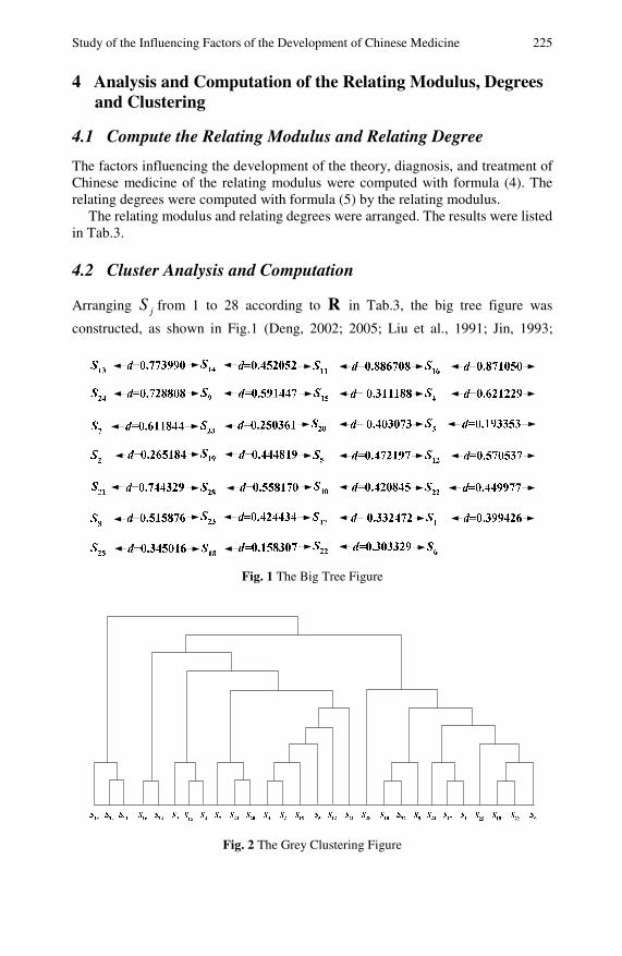
Study of the Influencing Factors of the Development of Chinese Medicine 225
4 Analysis and Computation of the Relating Modulus, Degrees and Clustering
4.1 Compute the Relating Modulus and Relating Degree
The factors influencing the development of the theory, diagnosis, and treatment of Chinese medicine of the relating modulus were computed with formula (4). The relating degrees were computed with formula (5) by the relating modulus.
The relating modulus and relating degrees were arranged. The results were listed in Tab.3.
4.2 Cluster Analysis and Computation
Arranging jS from 1 to 28 according to R in Tab.3, the big tree figure was
constructed, as shown in Fig.1 (Deng, 2002; 2005; Liu et al., 1991; Jin, 1993;
Fig. 1 The Big Tree Figure
Fig. 2 The Grey Clustering Figure

226 L. Duan, Y. Zhang, and X. Fan
Liu and Lin, 2006; Lin et al., 2004; Lin and Liu, 2006). According to the border of
jS , d was computed with formula (4). The numerical values d were marked up
figure 2 and clustered. So, the grey clustering figure was drawn (Deng, 2002; 2005; Liu et al., 1991; Jin, 1993; Liu and Lin, 2006; Lin et al., 2004; Lin and Liu, 2006), as shown in Fig.2.
Table 4 The results of clustering the factors influencing the development of the theory, diagnosis, and treatment of Chinese medicine and sequencing (simulating the results)
breed Names
1 the trust from country 13S ; change of the ill chart 14S ; the impact from west
medicinal 11S
2 the need from society 16S ; the intension build of hospital 24S ;
3 the tools for diagnosis and treatment 9S ; enter WTO 15S ; professors of
Chinese medicine 4S ;
4
curing effective of Chinese medicine 7S ; resource collocation of the hospital
of Chinese medicine 23S ; overseas development of Chinese medicine 20S ;
the view from abroad 19S
5
the study method of Chinese medicine 3S ; the science of Chinese
medicine 2S ; standardization of the language of Chinese medicine 5S ; east
and west medicinal combination 12S ; the profit of the hospital of Chinese
medicine 21S
6 the profit of the hospital of Chinese medicine 28S ;
7
the mode for diagnosis and treatment of Chinese medicine 10S ; the skill of the
hospital of Chinese medicine 22S ; entering new technology 8S ; resource
collocation of the hospital of Chinese medicine 23S ; mangers and organizers
in sanitation department 17S ; the logic of Chinese medicine 1S ; country
doctors 25S ; the law of the impact of west medicinal 18S ; the skill of the
hospital of Chinese medicine 22S ; the path and methods of traditional Chinese
drugs 6S
Study of the Influencing Factors of the Development of Chinese Medicine 227
5 The Result of Grey Clustering Analysis
5.1 The Result of the Influencing Factors of Grey Clustering
Based on figure 2, the factors that influenced the development of Chinese medicine were distinguish. The factors had 7 breeds from strong to weak. The result was listed in Tab.4.
5.2 Analysis
According to the results, we divided the factors that influenced the development of Chinese medicine into 7 breeds from strong to weak. The first 3 breeds are the most important, the following 2 breeds are less important, and the last 2 breeds are the least important. This information can give the government some ideas when they make policies. For the first three kinds, the government should pay more attention to manpower, material resources and finances. According to the conclusion, some suggestions were brought forth to improve the development of Chinese medicine.
References
Bai, C.K., Wang, X.D., Zhang, L.L., et at.: The sanitation calling impeled by science and technology advancement. Chinese Journal of Hospital Administration (12), 712–713 (2000)
Deng, J.L.: Grey Theory. Huazhong University of Science and Technology Press, Wuhan (2002)
Deng, J.L.: The Primary Methods of Grey System Theory. Huazhong University of Science and Technology Press, Wuhan (2005)
Feng, G.X., Xiao, S.W., Jang, G.F.: The consideration on modernization of traditional Chinese medicine. Hunan Guiding Journal of Traditional Chinese Medicine and Pharmacology 10, 2–3 (2003)
Guo, B.: Thinking on relationship between medical technology improvement and human health. Chinese Journal of Public Health Management 6, 453–454 (2006)
Jin, X.Z.: Methods and applications of grey clustering of grey relational analysis. Journal of Systems Engineering 8(12), 25–28 (1993)
Lin, Y., Chen, M.Y., Liu, S.F.: Theory of grey systems: capturing uncertainties of grey information. Kybernetes: The International Journal of Systems and Cybernetics 33(2), 196–218 (2004)
Lin, Y., Liu, S.F.: Solving Problems with incomplete information: a grey systems approach. In: Advances in Imaging and Electron Physics, vol. 141, pp. 77–174. Elsevier, Oxford (2006)
Liu, S.F., Guo, T.B., Dang, Y.G., et al.: Methods and Application of Grey System Theory. Science Press, Beijing (1991)
Liu, S.F., Lin, Y.: Grey Information: Theory and Practical Applications. Springer, London (2006)

228 L. Duan, Y. Zhang, and X. Fan
Qin, X.W.: The relation of technology and economy in harmonious society. Academic Journal of Shanxi Provincial Committee Party School of C.P.C. (2), 55–57 (2007)
Wang, L.T.: The Countermeasure of Chinese medicine Work of the Science and Technology at present. Chinese Journal of Management in Chinese Medicine 5, 60–61 (1999)
Yan, X.F.: The relational science and technology advancement with the society in world. Theoretical Investigation 5, 75–77 (2006)
Studies of Science and Technology Talent’ Management of New Regional Industrial Development:* Research with Anhui Province as an Example
Benhai Guo, Zhigeng Fang, and Dejin Song
In the process of accelerating industrialization, different regions of China are giving great efforts to develop new industries in order to enhance the competitiveness of regional industries and overall economic strength; scientific and technological human resources are bound up with the development of emerging industries, and they are even at the core of the development of new industries. This chapter provides the case of Anhui Province, and it analyzes the province's present status and management problems of scientific and technical personnel in the development of new industries, and it also puts forth relevant countermeasures and suggestions.
1 Introduction
As a dynamic industrial concept, emerging industries represent the new requirements of the market to the whole output of the economic system and new direction of the conversion of industrial structure. The development of new industries relies on technological innovation to create an uncertain new market, building a new arena for industrial explorers who have numerous technique or capital. In the process of accelerating industrialization, different regions in China are accelerating the development of competitive manufacturing industry and focusing on developing advantageous high-tech industries that rely on its regional
Benhai Guo, Zhigeng Fang, and Dejin Song School of Economics and Management, Nanjing University of Aeronautics and Astronautics, Nanjing 210016, China
* The work presented in this chapter was subsidized by the National Soft Science Research Project (2008GXS5D115) and National Social Science Foundation Key Project (08AJY024).

230 B. Guo, Z. Fang, and D. Song
advantages and comprehensive economic advantages, so that they can develop a number of new industries with characteristics, potential and marketability. Science and technology are primary production forces, and science and technology talent are at the core of the development of new industries. In the process of the development of new industries, the management of science and technology talent problems in different Chinese regions is a major issue worthy of study.
Li Fuzhu (Li and Ding, 2005; Liu and Li, 2005) and others thought that the management of science and technology talent should focus on the environment construction of science and technology talent, such as improving the remuneration of scientific and technological personnel, providing a good working system for scientific and technological personnel, establishing inter-district movement mechanisms of scientific and technological personnel and implementing different project mechanisms to tap the potential of scientific and technological talent. Literature (Yu, 2005) put forth the main managerial points of scientific and technological talent in the software industry. It thought software talent training mode innovation must be implemented, and reasonable and feasible talent strategy must be implemented on this basis in order to resolve the current crisis of scientific and technological talent in the software industry. Literature (Li and Xie, 2006) studied the supply and demand model of scarce talent in the emerging industry of China, and this model presented solutions for the emerging industry talent shortage. It thought that we must implement science and education strategies, change the mode of education and train more new talent. At the same time, enterprises also need to create a reasonable remuneration system to retain and motivate scientific and technological personnel. Literature (Fu, 2000) proposed a talent-strategy of high-tech industry development; the literature summarized the quality of talent in high-tech industries and their developing ways, and it put forth development and allocation strategies for high-tech industry personnel in cognizance of the present problems and situation of high-tech talent. Literature (Wang et al., 2008) studied the emerging industry of service outsourcing. It explored the market positioning the service outsourcing talent, and it summarized the corresponding government behavior, corporate behavior and social behavior.
In general, there are many deficiencies in the current studies of science and technology talent management of new regional industry development, especially since there is almost no related research of a specific area. As a central province, Anhui Province is in foreland areas that undertake the capital spillovers and industrial transfer of the developed coastal areas. To seize the new opportunity of industrial transfer, since “the tenth five-year”, Anhui Province set "speeding up the development, enriching people and strengthening the province" as their theme and also strategically adjusted their economic structure as the main line. It actively implemented the "leapfrog-development" strategy, "developing Wan by science and education" strategy and "industrial province" strategy, and it will vigorously

Studies of Science and Technology Talent’ 231
develop new industries as an important strategic point. Studying science and technology talent management issues of new industrial development in Anhui Province not only has practical significance for the development of new industries in Anhui Province, but it also will have profound effects for the strategic adjustment of economic structure in Anhui. Moreover, it will have reference value for dealing with other science and technology personnel management issues of emerging industrial development in central and western provinces.
Based on the basic connotation of new industries, combined with the practicalness of Anhui Province, this chapter selected the following categories of new industries for a research sample:
(1) High-tech Industries: information-chemical manufacturing, pharmaceutical manufacturing, aviation and spacecraft manufacturing, electronics and communications equipment manufacturing, computer and office equipment manufacturing, medical equipment and instrumentation manufacturing, information transmission, computer services and software industry;
(2) Scientific Research and Comprehensive Technical Services: Research and experimental development, professional technical services, technology exchange and promotion services;
(3) Finance and Insurance Industry: banking, securities, insurance, other financial activities;
(4) Real Estate Industry: real estate development and management, property management, intermediary services of real estate, and other real estate activities;
(5) Culture, Sports and Entertainment: news publishing industry, radio television film and audiovisual industry, arts and culture industry, sports entertainment.
2 Analysis of the Fundamental Role of Scientific and Technological Talent in the Development of New Industry in Anhui Province
During 1998-2007 in Anhui Province, the annual average growth rate of the GDP was 11.5%, and that of emerging industries was 17.59%. The proportion of emerging industry adding value to the GDP was from 12.93% in 1998 to 19.25% in 2007. New industries provided 228 thousand employment opportunities in 1998, and the number was one million in 2007, which showed an annual average growth rate of 17.85%. (See Table 1).
After further study of the relationship between human input (the total number of technological people), financial inputs (expenditures of scientific and technological research and development) and the output of scientific and technological achievements (turnover of the technical market), and the emerging industrial added
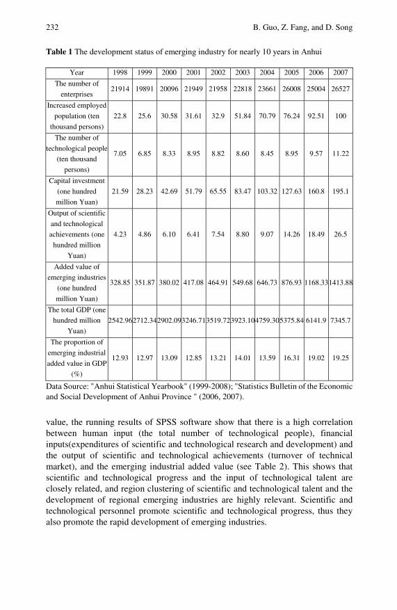
232 B. Guo, Z. Fang, and D. Song
Table 1 The development status of emerging industry for nearly 10 years in Anhui
Year 1998 1999 2000 2001 2002 2003 2004 2005 2006 2007
The number of
enterprises 21914 19891 20096 21949 21958 22818 23661 26008 25004 26527
Increased employed
population (ten
thousand persons)
22.8 25.6 30.58 31.61 32.9 51.84 70.79 76.24 92.51 100
The number of
technological people
(ten thousand
persons)
7.05 6.85 8.33 8.95 8.82 8.60 8.45 8.95 9.57 11.22
Capital investment
(one hundred
million Yuan)
21.59 28.23 42.69 51.79 65.55 83.47 103.32 127.63 160.8 195.1
Output of scientific
and technological
achievements (one
hundred million
Yuan)
4.23 4.86 6.10 6.41 7.54 8.80 9.07 14.26 18.49 26.5
Added value of
emerging industries
(one hundred
million Yuan)
328.85 351.87 380.02 417.08 464.91 549.68 646.73 876.93 1168.331413.88
The total GDP (one
hundred million
Yuan)
2542.962712.342902.093246.713519.723923.104759.305375.84 6141.9 7345.7
The proportion of
emerging industrial
added value in GDP
(%)
12.93 12.97 13.09 12.85 13.21 14.01 13.59 16.31 19.02 19.25
Data Source: "Anhui Statistical Yearbook" (1999-2008); "Statistics Bulletin of the Economic and Social Development of Anhui Province " (2006, 2007).
value, the running results of SPSS software show that there is a high correlation between human input (the total number of technological people), financial inputs(expenditures of scientific and technological research and development) and the output of scientific and technological achievements (turnover of technical market), and the emerging industrial added value (see Table 2). This shows that scientific and technological progress and the input of technological talent are closely related, and region clustering of scientific and technological talent and the development of regional emerging industries are highly relevant. Scientific and technological personnel promote scientific and technological progress, thus they also promote the rapid development of emerging industries.

Studies of Science and Technology Talent’ 233
Table 2 Correlation analysis results of human input, capital input and output of scientific and technological achievements, and new industries added value
human
input
capital
input
output of scientific
and technological
achievements
new
industries
added value
Correlation 1.000 .878 .888 .855
Significance(1-tailed) . .000 .000 .001 human input
df 0 8 8 8
Correlation .878 1.000 .967 .983
Significance (1-tailed) .000 . .000 .000 capital input
df 8 0 8 8
Correlation .888 .967 1.000 .990
Significance (1-tailed) .000 .000 . .000
output of scientific and
technological
achievements df 8 8 0 8
Correlation .855 .983 .990 1.000
Significance (1-tailed) .001 .000 .000 . new industries added
value df 8 8 8 0
3 Present Status Analysis of Anhui Science and Technology Talent and Forecast of the Demand of Emerging Industrial Development to Talent
3.1 Present Status Analysis of Science and Technology Talent
The total number of Anhui scientific and technological talent is relatively insufficient. At present, there are more than one million professional and technical personnel in Anhui Province, but among these, there are only 115,000 people engaged in scientific and technological activities, and only 30,000 people are R & D staff. In comparison to other central provinces, the amount of scientific and technological talent is relatively insufficient in Anhui Province. The total number of scientific and technological talent in Anhui Province ranks No. 5 among central regions (data of 2007), but the number of people who engage in scientific and technological activities and R & D activities in per ten thousand people is less than half of the national average, which ranks the bottom of the central region (see Table 3 ).
The distribution of scientific and technological talent is uneven. In Anhui, the regional distribution, industrial distribution, different ownership tissue distribution and different sectors distribution of scientific and technological personnel have shown a certain degree of imbalance.
The regional distribution of Anhui science and technology personnel has shown a trend of concentration in areas such as Hefei, Wuhu, Bengbu, Ma’anshan and Chuzhou, and the number of the S&T talent in the above-mentioned five cities

234 B. Guo, Z. Fang, and D. Song
Table 3 Comparison of scientific and technological human resources in Central 6 provinces (data of the end of 2006)
Anhui Index
Year2006Year2007Hubei Hunan He’nan Shanxi Jiangxi Nation
The number of professional and technical personnel (ten
thousand persons) 100.78 101.96 153.6 126.8 204.1 97.2 95.8 3256.8
The number of scientific and technological people (persons)
95,716 112,160 170,151130,239177,272121,76871,8484,131,542
The number of scientists and engineers (persons)
62,658 74,149 122,241 87,989 108,592 71,254 44,199 2,797,839
The number of R&D people
(persons /year) 28,826 33,380 62,100 39,752 59,692 38,767 25,797 1,502,472
The number of S&T people per ten thousand people (persons)
15 16 30 20 19 36 16 31
The number of R&D people per ten thousand people
(persons /year) 5 5 11 6 6 11 6 11
accounted for 63.7% of the total number of the province. In the industry distribution, education concentrates the absolute majority of the professional and technical personnel, which accounts for 46.13%. It is followed by the health, social security and social welfare sector, which accounts for 13.31%. Then it is the manufacturing sector, accounting for 9.47%, while professional and technical personnel who engage in the emerging industries (the high-tech industry, information transmission, computer services and software industry, the financial industry, real estate, culture, sports and entertainment) account for 12%. From the sector distribution, the proportion of technological people in large and medium industrial enterprises accounted for more than half of that of the province. In 2007, there were 66.5 thousand scientific and technological workers in industrial enterprises, which accounted for 59.27% in the province. The number of scientific and technical workers in research institutions, universities and other executive branches were 4700, 29000 and 12000, accounting for 4.19%, 25.85% and 10.76%. The distribution of science and technology professionals in Anhui in different forms of ownership, enterprises and institutions is prominently uneven, and scientific and technological people are intensive in public economic units. In 2007, the proportion of scientific and technological talent in the state-owned economic units was 78.7%, so one would induce that scientific and technological talent in other non-state-owned economic units cannot be supplemented in a short time.
The remuneration of scientific and technical personnel is relatively low. The contribution that scientific and technical personnel in Anhui Province have made is out of proportion to their remuneration. In 2002, 88.2 thousand scientific and technical personnel made great contributions to the economic added value of 32.885 billion yuan in the emerging industry, while their labor cost only accounts for 2.7% in new value-added production and 0.36% in GDP. By 2007, the proportion of
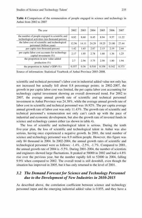
Studies of Science and Technology Talent’ 235 Table 4 Comparison of the remuneration of people engaged in science and technology in Anhui from 2002 to 2007
The year 2002 2003 2004 2005 2006 2007
the number of people engaged in scientific and technological activities (ten thousand person)
8.82 8.60 8.45 8.94 9.57 11.22
the labor cost of scientific and technological personnel (billion yuan)
12.56 14.11 24.29 19.25 21.00 27.44
per capita (ten thousand person) 1.42 1.65 2.87 2.15 2.19 2.44
per capita labor cost accounts for technology capital investment (%)
2.17 1.95 2.78 1.68 1.36 1.25
the proportion in new value-added
production (%) 2.7 2.56 3.75 2.58 1.80 1.94
the proportion in Anhui’s GDP (%) 0.357 0.36 0.510 0.358 0.342 0.373
Source of information: Statistical Yearbook of Anhui Province 2003-2008.
scientific and technical personnel’s labor cost in industrial added value not only has not increased but actually fell about 0.8 percentage points; in 2002-2007, the growth in per capita labor cost was limited, the per capita labor cost accounting for technology capital investment showing an overall downward trend. For 2002 to 2007, the average annual growth rate of scientific and technical personnel investment in Anhui Province was 24.38%, while the average annual growth rate of labor cost in scientific and technical personnel was 16.92%. The per capita average annual growth rate of labor cost was only 11.43%. The growth rate of scientific and technical personnel’s remuneration not only can’t catch up with the pace of industrial and economic development, but also the growth rate of invested funds in science and technology cannot either (as shown in table 4).
The loss of scientific and technological talent is serious. During the tenth five-year plan, the loss of scientific and technological talent in Anhui was also serious, having once experienced a negative growth. In 2001, the total number of science and technology personnel was 8.9 million people. However, this figure was only 84 thousand in 2004. In 2002-2004, the annual growth rates of scientific and technological personnel were as follows: -1.4%, -2.5%, -1.7%. Compared to 2001, the annual growth rate of 2004 is -5.5%. During 2001-2004, the number of scientists and engineers showed large fluctuations. It peaked at 58000 in 2002 and had a 4.8% rise over the previous year, but the number rapidly fell to 52000 in 2004, falling 9.9% when compared to 2002. The overall trend is still downhill, even though the situation has improved in 2005, but it has only returned to the level of 2001.
3.2 The Demand Forecast for Science and Technology Personnel due to the Development of New Industries in 2010-2015
As described above, the correlation coefficient between science and technology personnel input and the emerging industrial added value is 0.855, and they have a
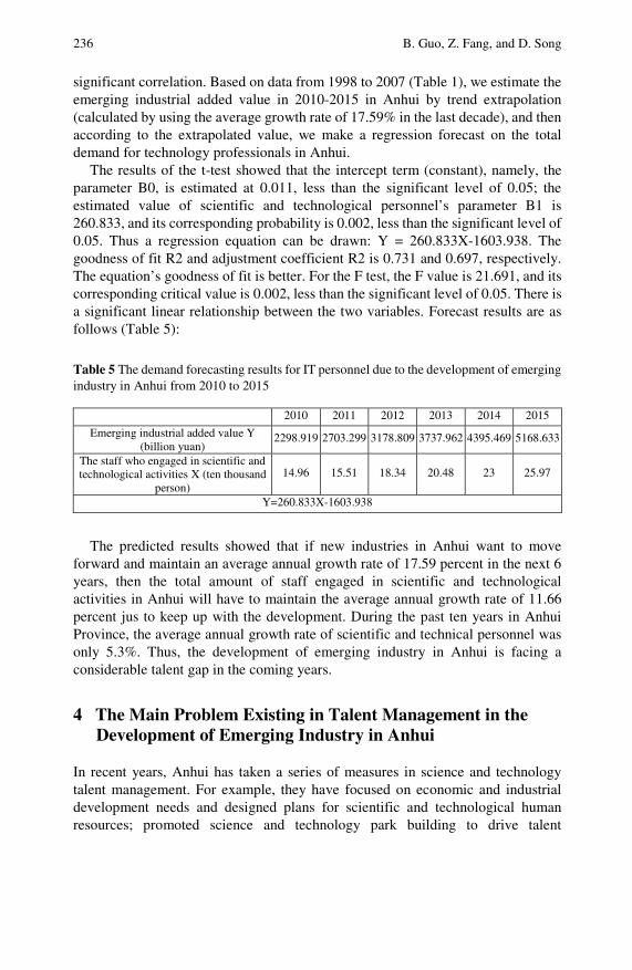
236 B. Guo, Z. Fang, and D. Song
significant correlation. Based on data from 1998 to 2007 (Table 1), we estimate the emerging industrial added value in 2010-2015 in Anhui by trend extrapolation (calculated by using the average growth rate of 17.59% in the last decade), and then according to the extrapolated value, we make a regression forecast on the total demand for technology professionals in Anhui.
The results of the t-test showed that the intercept term (constant), namely, the parameter B0, is estimated at 0.011, less than the significant level of 0.05; the estimated value of scientific and technological personnel’s parameter B1 is 260.833, and its corresponding probability is 0.002, less than the significant level of 0.05. Thus a regression equation can be drawn: Y = 260.833X-1603.938. The goodness of fit R2 and adjustment coefficient R2 is 0.731 and 0.697, respectively. The equation’s goodness of fit is better. For the F test, the F value is 21.691, and its corresponding critical value is 0.002, less than the significant level of 0.05. There is a significant linear relationship between the two variables. Forecast results are as follows (Table 5):
Table 5 The demand forecasting results for IT personnel due to the development of emerging industry in Anhui from 2010 to 2015
2010 2011 2012 2013 2014 2015
Emerging industrial added value Y (billion yuan)
2298.919 2703.299 3178.809 3737.962 4395.469 5168.633
The staff who engaged in scientific and technological activities X (ten thousand
person) 14.96 15.51 18.34 20.48 23 25.97
Y=260.833X-1603.938
The predicted results showed that if new industries in Anhui want to move forward and maintain an average annual growth rate of 17.59 percent in the next 6 years, then the total amount of staff engaged in scientific and technological activities in Anhui will have to maintain the average annual growth rate of 11.66 percent jus to keep up with the development. During the past ten years in Anhui Province, the average annual growth rate of scientific and technical personnel was only 5.3%. Thus, the development of emerging industry in Anhui is facing a considerable talent gap in the coming years.
4 The Main Problem Existing in Talent Management in the Development of Emerging Industry in Anhui
In recent years, Anhui has taken a series of measures in science and technology talent management. For example, they have focused on economic and industrial development needs and designed plans for scientific and technological human resources; promoted science and technology park building to drive talent
Studies of Science and Technology Talent’ 237
concentration; carried out Yinzhi engineering and then have opened the green channel to attract high-level personnel; organized and implemented a new independent innovation system and its support system; strengthened the cultivation of innovative and entrepreneurial talent; promoted the dynamic integration of production and research; and boosted innovation and entrepreneurship. These initiatives have played a vital role in improving science and technology talent management and promoting the development of new industries in Anhui, but with the new situation of economic and social development, Anhui must vigorously develop new industries, promote industrial upgrading and enhance the quality of economic development and overall industrial competitiveness. Science and technology talent management faces more challenges and is easily affected by uncertainties, so it has reached the point where the problem of science and technology talent management must be solved.
4.1 The Level of Economic Development and Layer of Industrial Structure Are Low; Science and Technology Talent’s Carrier Environment Needs to Be Improved
In horizontal comparison, the level of economic and industrial development in Anhui is low. During the tenth five-year plan, the per capita GDP in Anhui was 8597 yuan, which is lower than the national average of 5443 yuan, ranking the last among the six central provinces; the per capita revenue was 1012 yuan, equivalent to 41.7% of the country; the evolution of industrial structure, despite the acceleration of industry structure in the upgraded trend of recent years, hasn’t gotten rid of rough agricultural and resource-based economic structure in general. The results of the economic census showed that during the tenth five-year plan, prime operating revenue of the traditional industrial sectors (coal, electricity, electronics, tobacco, transport equipment, construction materials, textile, food, beverage, petroleum, chemicals, ferrous metallurgy, non-ferrous metals and machinery, etc.) in Anhui took up nearly 90%, while the proportion of electronic and communications equipment and other high-tech industry was less than 2%, lower than the national average of 8.7 percent and much lower than developed provinces and cities, such as Shanghai, Jingsu, Guangdong. In addition, the non-public economic development lagged behind. During the tenth five-year plan, the number of non-public enterprises accounting for second and tertiary industries was 76.3%, under the nationwide average of 7 percentage points. Self-employed households were not only significantly lower than that of economically developed areas, such as Jiangsu, Zhejiang, Guangdong, but also less than central provinces, such as Hubei and Henan.
Anhui urgently needs to enhance its level of economic and industrial development and improve its scientific and technological talent growth environment to provide technology professionals with a good vehicle and reinforce the foundation to attract and retain technology professionals.
238 B. Guo, Z. Fang, and D. Song
4.2 Industrial Development Planning Is Still Inadequate; Science and Technology Human Resources Plan Contains Flaws
First, the human resource plan did not receive adequate attention. The human resource plan is just regarded as "human security measures", and it shows that the work of scientific and technological talent in Anhui Province did not rise to the strategic level to some extent. Second, there is a lack of scientific and technological personnel structure planning. The human resource planning will be radiated by the flaw of the industrial development planning. To meet the development strategy in Anhui Province, the industrial development plan in Anhui during the eleventh five-year plan, characterized by a "focused" strategy, stood out the prominent national scientific and technological innovation-oriented pilot project in Hefei city, highlighting the high-tech industrial belt along the river and focusing on key park enterprises. The industry neglected the coordinated development of the regional economy, leading to concentrate the spatial distribution of all kinds of professional and technical personnel on Hefei, Wuhu and a few other urban areas. The problem of regional imbalances in the distribution is further exacerbated. In addition, the eleventh five-year industrial development plan ignored non-public economic development, and it is not conducive to guide the transfer of scientific and technological talent to the non-public economy.
4.3 The Science and Technology Capital Investment Was Insufficient; the Level of Technological Innovation and Entrepreneurial Talent Is Not High
Although Anhui Province has increased scientific and technological input annually since 2001, from the horizontal comparison, the financial investment of the Anhui provincial government is still very limited. Compared to other central provinces during the tenth five-year plan, the absolute number of government investment in science and technology in Anhui was only higher than that of Jiangxi, but the proportion of government investment in science and technology accounted for in fiscal expenditure was at the bottom of the six central provinces. To a large extent, the level of creative ability and scientific and technological achievements was limited by little scientific and technological input; input-output is relatively low. (Table 6)
International experience shows that the country or region where the proportion of R&D funding accounts for less than 1% of the GDP is basically at the level of technology introduction and application; the proportion of medium-developed countries or regions that had a strong technological introduction, digestion, and absorption capacity generally enjoys more than 1.5% of their GDP on R&D, while the proportion of more than 2% of their GDP’s is spent in developed countries or
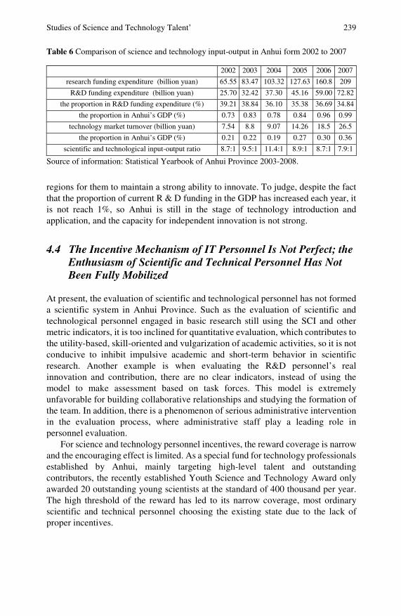
Studies of Science and Technology Talent’ 239
Table 6 Comparison of science and technology input-output in Anhui form 2002 to 2007
2002 2003 2004 2005 2006 2007
research funding expenditure (billion yuan) 65.55 83.47 103.32 127.63 160.8 209
R&D funding expenditure (billion yuan) 25.70 32.42 37.30 45.16 59.00 72.82
the proportion in R&D funding expenditure (%) 39.21 38.84 36.10 35.38 36.69 34.84
the proportion in Anhui’s GDP (%) 0.73 0.83 0.78 0.84 0.96 0.99
technology market turnover (billion yuan) 7.54 8.8 9.07 14.26 18.5 26.5
the proportion in Anhui’s GDP (%) 0.21 0.22 0.19 0.27 0.30 0.36
scientific and technological input-output ratio 8.7:1 9.5:1 11.4:1 8.9:1 8.7:1 7.9:1
Source of information: Statistical Yearbook of Anhui Province 2003-2008.
regions for them to maintain a strong ability to innovate. To judge, despite the fact that the proportion of current R & D funding in the GDP has increased each year, it is not reach 1%, so Anhui is still in the stage of technology introduction and application, and the capacity for independent innovation is not strong.
4.4 The Incentive Mechanism of IT Personnel Is Not Perfect; the Enthusiasm of Scientific and Technical Personnel Has Not Been Fully Mobilized
At present, the evaluation of scientific and technological personnel has not formed a scientific system in Anhui Province. Such as the evaluation of scientific and technological personnel engaged in basic research still using the SCI and other metric indicators, it is too inclined for quantitative evaluation, which contributes to the utility-based, skill-oriented and vulgarization of academic activities, so it is not conducive to inhibit impulsive academic and short-term behavior in scientific research. Another example is when evaluating the R&D personnel’s real innovation and contribution, there are no clear indicators, instead of using the model to make assessment based on task forces. This model is extremely unfavorable for building collaborative relationships and studying the formation of the team. In addition, there is a phenomenon of serious administrative intervention in the evaluation process, where administrative staff play a leading role in personnel evaluation.
For science and technology personnel incentives, the reward coverage is narrow and the encouraging effect is limited. As a special fund for technology professionals established by Anhui, mainly targeting high-level talent and outstanding contributors, the recently established Youth Science and Technology Award only awarded 20 outstanding young scientists at the standard of 400 thousand per year. The high threshold of the reward has led to its narrow coverage, most ordinary scientific and technical personnel choosing the existing state due to the lack of proper incentives.

240 B. Guo, Z. Fang, and D. Song
4.5 The Channel from Scientific and Technological Talent to Enterprises Is Not Clear Enough, and Enterprises Lack the High-Level Scientific and Technological Talent
The scientific and technological talent of Anhui Province is highly gathered in universities, research institutions and other non-corporate social organizations. The channel from scientific and technological talent into enterprises is not clear enough. Scientific and technological talent is the fundamental guarantee of enterprise independent innovation, and the shortage of them seriously hampered enterprise R&D. In developed countries that are enterprise innovation-oriented, the nationwide R&D talent is concentrated to enterprises; for example, the U.S. enterprises gathered 75.4% of the nationwide R&D talent, Japanese talent accounted for 64.80%, and British talent accounted for 68.5%. But in our country, a large part of scientific and technological talent is focused on scientific research institutes and universities. At universities, the scientific and technological personnel evaluation system is paper-oriented, government issues-oriented, incentives-oriented and so on. Considering the title evaluation, wages, and social security of university research institutes, the technological professionals cannot flow to enterprises according to market rules. The phenomenon is even more serious in Anhui Province, which is located in the Central Region.
At the same time, the training and motivation mechanism of business technological professionals is not sound. Enterprise technological brain drain is more serious. Many enterprises lack an effective mechanism for personnel selection, training and incentives. They do not to pursue performance maximization of talent use, instead one-sidedly pursuing cost minimization. Without a reasonable allocation mechanism and with short-term talent incentives and simplistic methods, the growth of enterprise technological innovation talent has been seriously affected, resulting in the loss of enterprise talent. Moreover, our country's attraction to high-level talent improved by a large margin due to a significant increase of science and technology investment in universities and research institutions. Some enterprises’ leading talent have accepted the invitation of universities and research institutions, leaving enterprises for universities and research institutions. The talent flowed in reverse, from enterprises to universities and research institutions. The brain drain of enterprise and scientific and technological talent, especially that of key technological fields, has a greater negative impact on the safety of the enterprise research work
5 Countermeasures and Proposals
5.1 Plan the Industrial Layout Scientifically and Optimize the Distribution of Scientific and Technological Talent
On the basis of the industrial input-output influence coefficients and sensitivity coefficients, and taking full account of such factors as economic and energy

Studies of Science and Technology Talent’ 241
consumption, Anhui Province should take ten more industries as leading sectors of industrial development in the future: communication equipment, computer and other electronic equipment manufacturing; transportation equipment manufacturing; the chemical industry; general and special equipment manufacturing; electrical machinery and equipment manufacturing; instrumentation and cultural office machinery manufacturing; modern food manufacturing and the tobacco processing industry; textile industry; metal smelting and calendering processing industry; and non-metallic mineral products industry. These sectors have good growth, enterprises in them have a certain maturity, and the products have a broader market space, which all have a great effect on the economics of Anhui. Not only should Anhui Province place the ten industries in important positions, but also it should allow them to become group advantages, that is, to future-mindedly cultivate leading industrial groups in order to play their leading role in the industrial structure system; to promote talent, technology and enterprise gathering; and to optimize the distribution structure of scientific and technological personnel, depending on the optimization of the industrial layout.
5.2 Improve the Combination Degree of Production, Education and Research, and Accelerate the Transformation of Technological Achievements
If we want to promote technological achievements and transform them into practical productive forces, we must combine production, education and research. First, we should give full play to the advantage of existing scientific and technological resources in Anhui Province (the university town, scientific island, and research units of Central Authorities in Anhui) and continue to organize "co-operations between province and schools", " co-building between province and colleges". Second, we should further run good high-tech industrial development zones and the University Science Park, make them truly become bases that nurture and develop high-tech industry. Third, we must make great efforts to develop intermediary service institutions of science and technology; foster a number of service agencies, such as productivity centers, property rights transactions institutions, achievements transformation centers, modern logistics institutions and so on; speed up the province and city (Hefei) to build innovative and pioneering service centers; and set up a co-operation platform among production, education and research.
5.3 Increase Scientific and Technological Investment and Improve the Level of Scientific and Technological Personnel Innovation and Intrapreneurship
First, we must increase financial and technological investment, timely establish special financial technology funds, and increase the growth range and speed of
242 B. Guo, Z. Fang, and D. Song
financial and technological investment in order to ensure the financial support of independent innovation capacity building. Second, we must establish a diversified and multi-level technological investment and financing mechanism to smooth investment and financing channels. We should actively explore the methods and measures of the combinations between finance and technology to enhance the leading function of financial investment, actively seeking credit funds to support the infrastructure and key industrial projects in line with macro-control needs. We should adjust investment and financing structure to encourage and support more qualified enterprises to find a way of listing and financing. We should promote the development and improvement of Anhui credit institutions to provide a government credit guarantee for scientific and technical personnel and projects. Third, we must set up a risk investment mechanism to create new input methods. The Anhui risk investment firm is still in its infancy with not much registered capital, so it’s very harsh in the choice of investment projects. Anhui Province should actively learn from advanced experience at home and abroad to try to establish and perfect the mechanism of risk investment and make innovations in investment approaches; to lead and support venture capital firms and financial institutions to increase investment in high-tech enterprises, especially in the medium and small high-tech enterprises; and to provide further financial assurance for strengthening technical innovation and industrialization of scientific and technological achievements.
5.4 Promote Institutional Innovation and Strengthen Incentives for Scientific and Technological Personnel
First of all, we must advance the reform of the personnel system and strive to form a kind of working mechanism with which scientific and technological personnel can move up or down, enter or exit, and be sorted based on their contributions. We should deal with the use of scientific and technological personnel, avoiding the phenomenon of high talent consumption. During the process of selecting and employing, we should adhere to confirming Heroes by their performance to avoid the "Gresham effect" (that is, the phenomenon of mediocrity push talent). Scientific and technical personnel should be given the full right to speak. Especially for vital decisions, we must allow them full play in their corresponding fields, as they are irreplaceable roles. Second, we must improve the evaluation system of scientific and technological personnel. We should build a scientific evaluation system of scientific and technical personnel, to distinguish the evaluation between basic research and applied research, and strive to form the institutional and standardized evaluation, to reduce the interference of human factors and administrative factors. Finally, we should strengthen the incentive system, to fully mobilize the enthusiasm, initiative and creativity of scientific and technological personnel. And then, we need to speed up distribution system reform and carry out revenue policies to stimulate scientific and technical personnel. We should strengthen the incentives for technological innovation and implement incentive methods according to scientific and technological innovation achievements to award the scientific and
Studies of Science and Technology Talent’ 243
technical personnel who made outstanding contributions to enterprises. In addition, we can expand the coverage of incentives to inspire more potential scientific and technological personnel, to make innovation and entrepreneurship, and to create value for society.
5.5 Combine the Government with Corporations and Make a Difference among Management Issues of Scientific and Technological Talent at Different Levels
Government and enterprises should have complementary strengths in the management of scientific and technological talent in order to promote positive interactions between the development of the new industries and technological talent. The government should effectively change its personnel management functions and gradually turn to macro-management from micro-management. The government should significantly act on optimizing the external development environment of emerging industries and technological professionals, strengthening talent infrastructure construction. Moreover, the government must be more proactive in the process of promoting talent, technology and equipment and other manufacturing factors to flow to emerging industries. Enterprises should make great efforts to establish the management system according to the actual situation of enterprises, and they should establish the training mechanism aimed at scientific and technological talent of enterprises in order to train and bring up a large number of high-tech entrepreneurs and technical elites who are skilled; good at technology, business and management; and brave in innovation and fight. Enterprises must build their talent to attract more high-tech professionals and retain technological personnel, depending on its system, business, treatment, environment and culture. Lastly, enterprises should distribute their technological talent reasonably and establish a comprehensive assessment, the trinity system, of talent, based on post and performance.
References
Anhui Bureau of Statistics. Anhui Science and Technology Statistics Bulletin. Anhui Bureau of Statistics website (2006-2007)
Feng, F.: Investigation and analysis of Anhui scientific and technological development capacity. Decision-Making Advice (3) (2003)
Fu, D.S.: Talent strategy in high-tech industrial development. Reform and Strategy (4) (2000)
Li, B., Xie, D.H.: Research on the shortage of talent supply and demand in Chinese emerging industry. Value Engineering (10) (2006)
Li, F.Z., Ding, S.B.: Research on technological personnel environmental construction in northeastern old industrial base. Science and Technology Progress and Policy (5) (2005)
Liu, F., Wang, Z.L., Zhang, N.: Effect of human resources development to the achievement of Anhui Province’s leap-forward development. Special Zone Economy (9) (2007)

244 B. Guo, Z. Fang, and D. Song Liu, W.Z., Li, F.Z.: Countermeasures of Chinese technological talent resources regional
allocation and sustainable development. In: China Forum on Sustainable Development – Chinese Sustainable Development Research Society at 2005 Annual Meeting Proceedings (the book) (2005)
Lu, S.Q., Zou, Y.: Analysis of Anhui technology-based SMEs development environment. Anhui Science and Technology (3) (2005)
The, P.R.: China National Bureau of Statistics. In: China Statistical Yearbook. China Statistics Press, Beijing (2009)
Wang, W.Y., Guo, Y.L., Zhang, W.: Research on talent management of Chinese service outsourcing. Modernization of Shopping Malls (February 2008)
Wang, Y.: An empirical study on scientific and technical personnel building of Jiangsu Province. Journal of Southeast University (7) (2005)
Yu, J.: Software industry personnel crisis. Technology of Shenzhen Special Economic Zone (10) (2005)
Empirical Research on the Selection of Regional Key Technology for International S&T Cooperation*
Lirong Jian, Sifeng Liu, and Hongfang Ma
The selection of key technology for international cooperation is a new field to be developed both domestically and abroad. Furthermore, there are few research documents on such basic research as how to systemically select high quality foreign technology and project sources based on analyzing the demand of local technology and the economy. In this paper, an urgent index and feasible index are proposed, in which the former is to evaluate the urgency of the technology demand for the local economy and the latter to measure the feasibility of obtaining key technology through international cooperation. By applying the Delphi method, the corresponding evaluation index system is set up based on which an integrated evaluation method of multiple objective fuzzy index is built. The proposed method is applied to the selection of key technology for international cooperation in Jiangsu province. The evaluation set is quantified to an extract urgent index and feasible index, followed by the incorporation of two indexes into an integrated one. Then the key technologies of international cooperation are ranked according to the integrated index. Finally, key technologies that are urgently needed and possibly gained by Jiangsu province through international technology cooperation are screened out.
1 Introduction
Affected by the rapidly developing S&T, increasingly international competition and production internationalization, international S&T cooperation is flourishing. Lirong Jian School of Economics & Management, Nanjing University of Aeronautics and Astronautics, Nanjing 210016, China Phone: 13913852651 e-mail: [email protected]
Sifeng Liu and Hongfang Ma School of Economics & Management, Nanjing University of Aeronautics and Astronautics, Nanjing 210016, China e-mail: [email protected], [email protected].
* This work was supported by the Social Sciences Key Fund of China, Grant NO. 08AJY024, and by the Soft Science Key Fund of Jiangsu Province, Grant NO BR2008099.

246 L. Jian, S. Liu, and H. Ma
International S&T cooperation is growing both in key and general technology. However, the cooperation of different kinds of technologies has different features. It is generally supported and unlimited for the international cooperation of general mature biotechnologies, patents, know-how’s and general soft technologies. Exporting these technologies is beneficial to the exporters, including the country and the company. Developed countries encourage exporting these technologies because the many advantages: it can increase national employment and extend the technologies’ lifecycle and accelerate the updating of technologies. For example, Japanese banks provide some preferential policies to encourage exporting, such as low-interest loans, export insurance and tax incentives. However, transferring key technologies is most limited. Because key technology is a strategic asset, it is controlled by many countries. To a different extent, US-led developed countries have made some policies on export control to limit key technology cooperation with China. These limited key technologies have a close relation with China’s major S&T plan. Those limits impede China’s technology introduction and affect the key technology cooperation scale and transfer direction. According to relative statistics, about 30% of technology export applications in the USA are objected every year. How to avoid these export limits and get more key technologies is the problem we must urgently solve. The selection of key technology for international cooperation is a new field to be developed both domestically and abroad. Furthermore, there are few research documents on such basic research as how to systemically select high quality foreign technology and project sources based on analyzing the demand of local technology and the economy. In this paper, a study on the selection of key technology for international cooperation is done based on analyzing the demand of local technology and the economy. Finally, key technologies that are urgently needed and possibly beneficial for Jiangsu province through international technology cooperation are screened out.
2 Urgent and Feasible Index System
Generally, a technology that plays a decisive role in achieving a strategic task or program objective, promotes the development of whole Industrial clusters and is practical or partly practical is called a key technology. To evaluate the urgency of the technology demand for the local economy and measure the feasibility of obtaining key technology through international cooperations, this paper proposes an urgent index and feasible index and builds two corresponding evaluation index systems.
The basic criteria for selecting local international key technology are as follows: it can promote economic development and new industry forming, it is beneficial for environment protection, it has an available foreign technology source, there are funding and policy guarantees, and it can be achieved in short time. According to these basic criteria, when defining the urgent index and feasible index, we must consider these factors: importance of pulling the market (technological bottlenecks, the formation of independent intellectual property rights, promoting the development of related industries), importance of pushing technology (technology
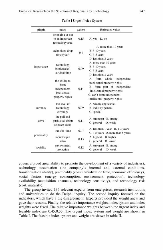
Empirical Research on the Selection of Regional Key Technology 247
Table I Urgent Index System
covers a broad area, ability to promote the development of a variety of industries), technology sustentation (the company’s internal and external conditions, transformation ability), practicality (commercialization time, economic efficiency), social factors (energy consumption, environment protection), technology availability (acquisition channels, technology sensitivity), and technology risk (cost, maturity).
The group invited 135 relevant experts from enterprises, research institutions and universities to do the Delphi inquiry. The second inquiry focused on the indicators, which have a big disagreement. Experts provided the weight anew and gave their reasons. Finally, the relative importance weights, index system and index weights were fixed. The relative importance weights between the urgent index and feasible index are 0.45:0.55. The urgent index system and weight are shown in Table I. The feasible index system and weight are shown in table II.
criteria index weight Estimated value
belonging or not to an important technology area
0.15 A. yes D. no
technology drop time (year)
0.1
A. more than 10 years B. 5-10 years C. 3-5 years D. less than 3 years
technology bottlenecks’ survival time
0.09
A. more than 10 years B. 5-10 years C. 3-5 years D. less than 3 years
importance
the ability to form
independent intellectual
property rights
0.14
A. form whole independent intellectual property rights B. form part of independent intellectual property rights
C. can’t form independent intellectual property rights
currency the level of technology coverage
0.09 A. widely applicable B. industry general C. special
drive the pull and
push level about relevant areas
0.11 A. strongest B. strong C. general D. weak
transfer time 0.07 A. less than 1 year B. 1-3 years C. 4-5 years D. more than 5 years
practicality input/output
ratio 0.13
A. highest B. higher C. general D. lower
sociality environment protection
0.12 A. strongest B. strong C. general D. weak

248 L. Jian, S. Liu, and H. Ma
Table II Feasible index system
3 The Method of Key Technologic Selection for International Cooperation
A. Fuzzy Comprehensive Evaluation Method
The fuzzy comprehensive evaluation method evaluates things’ belonging grade status from several factors with the principle of fuzzy relation synthesis.
Suppose there are two finite sets:
},...,,{ 21 nuuuU = , },...,,{ 21 nvvvV =
Here, U represents the index set, V represents the evaluation level set. Let
},...,,{ 21 naaaA = ,
⎥⎥⎥⎥
⎦
⎤
⎢⎢⎢⎢
⎣
⎡
=
nmnn
m
m
rrr
rrr
rrr
R
...
............
...
...
21
22221
11211
criteria index weight Estimated value
degree belonging to
sensitive technology
0.14
A. no sensitive B. sensitive C. more sensitive D. most sensitive
number of acquisition channels
0.10 A. several B. sole C. none
foreign technology availability
deadline of patent
protection overseas
0.11
A. less than 3 years B. 3-5 years C. 5-10 years D. more than 10 years
ability of digestion,
absorption and innovation
0.18
A. strongest B. strong C. general D. weak
ability of digestion
and absorption
personnel base 0.18
A. strongest B .strong C. general D. weak
maturity level 0.17 A. mature B. general mature C. immature
technology risk
acquisition cost 0.12 A. lower B. low C. high D. higher
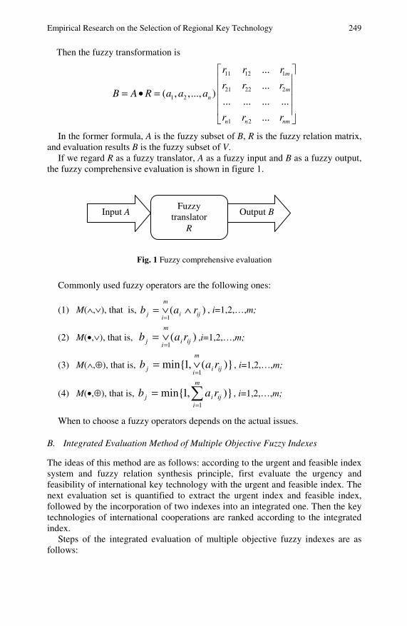
Empirical Research on the Selection of Regional Key Technology 249
Then the fuzzy transformation is
11 12 1
21 22 21 2
1 2
...
...( , ,..., )
... ... ... ...
...
m
mn
n n nm
r r r
r r rB A R a a a
r r r
⎡ ⎤⎢ ⎥⎢ ⎥= • =⎢ ⎥⎢ ⎥⎣ ⎦
In the former formula, A is the fuzzy subset of B, R is the fuzzy relation matrix, and evaluation results B is the fuzzy subset of V.
If we regard R as a fuzzy translator, A as a fuzzy input and B as a fuzzy output, the fuzzy comprehensive evaluation is shown in figure 1.
Fig. 1 Fuzzy comprehensive evaluation
Commonly used fuzzy operators are the following ones:
(1) M(∧,∨), that is, )(1
iji
m
ij rab ∧∨=
=, i=1,2,…,m;
(2) M(•,∨), that is, )(1
iji
m
ij rab
=∨= ,i=1,2,…,m;
(3) M(∧,⊕), that is, )}(,1min{1
iji
m
ij rab
=∨= , i=1,2,…,m;
(4) M(•,⊕), that is, )},1min{1∑
=
=m
iijij rab , i=1,2,…,m;
When to choose a fuzzy operators depends on the actual issues.
B. Integrated Evaluation Method of Multiple Objective Fuzzy Indexes
The ideas of this method are as follows: according to the urgent and feasible index system and fuzzy relation synthesis principle, first evaluate the urgency and feasibility of international key technology with the urgent and feasible index. The next evaluation set is quantified to extract the urgent index and feasible index, followed by the incorporation of two indexes into an integrated one. Then the key technologies of international cooperations are ranked according to the integrated index.
Steps of the integrated evaluation of multiple objective fuzzy indexes are as follows:
Input A Fuzzy
translator R
Output B
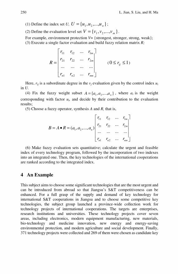
250 L. Jian, S. Liu, and H. Ma
(1) Define the index set U, },...,,{ 21 nuuuU = ;
(2) Define the evaluation level set },...,,{ 21 mvvvV = .
For example, environment protection V= {strongest, stronger, strong, weak}; (3) Execute a single factor evaluation and build fuzzy relation matrix R;
⎥⎥⎥⎥
⎦
⎤
⎢⎢⎢⎢
⎣
⎡
=
nmnn
m
m
rrr
rrr
rrr
R
...
............
...
...
21
22221
11211
( 10 ≤≤ ijr )
Here, rij is a subordinate degree in the vj evaluation given by the control index ui in U.
(4) Fix the fuzzy weight subset },...,,{ 21 naaaA = , where ai is the weight
corresponding with factor ui, and decide by their contribution to the evaluation results;
(5) Choose a fuzzy operator, synthesis A and R, that is,
11 12 1
21 22 21 2
1 2
...
...( , ,..., )
... ... ... ...
...
m
mn
n n nm
r r r
r r rB A R a a a
r r r
⎡ ⎤⎢ ⎥⎢ ⎥= • =⎢ ⎥⎢ ⎥⎣ ⎦
(6) Make fuzzy evaluation sets quantitative; calculate the urgent and feasible index of every technology program, followed by the incorporation of two indexes into an integrated one. Then, the key technologies of the international cooperations are ranked according to the integrated index.
4 An Example
This subject aims to choose some significant technologies that are the most urgent and can be introduced from abroad so that Jiangsu’s S&T competitiveness can be enhanced. For a full grasp of the supply and demand of key technology for international S&T cooperations in Jiangsu and to choose some competitive key technologies, the subject group launched a province-wide collection work for technology projects of international cooperations. The targets are enterprises, research institutions and universities. These technology projects cover seven areas, including electronics, modern equipment manufacturing, new materials, bio-technology and medicine innovation, new energy and energy-saving environmental protection, and modern agriculture and social development. Finally, 371 technology projects were collected and 269 of them were chosen as candidate key
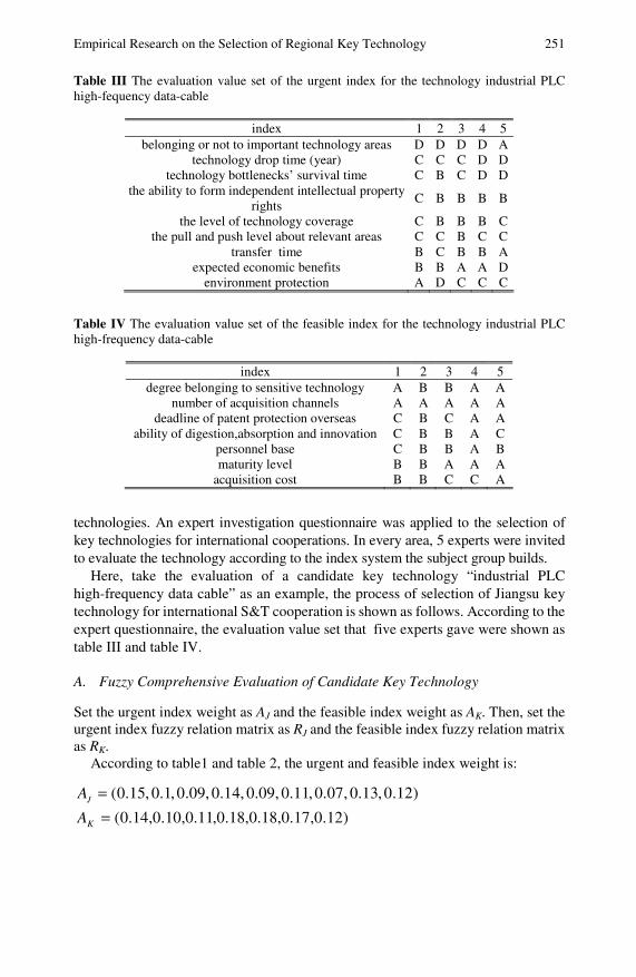
Empirical Research on the Selection of Regional Key Technology 251 Table III The evaluation value set of the urgent index for the technology industrial PLC high-fequency data-cable
index 1 2 3 4 5 belonging or not to important technology areas D D D D A
technology drop time (year) C C C D D technology bottlenecks’ survival time C B C D D
the ability to form independent intellectual property rights
C B B B B
the level of technology coverage C B B B C the pull and push level about relevant areas C C B C C
transfer time B C B B A expected economic benefits B B A A D
environment protection A D C C C
Table IV The evaluation value set of the feasible index for the technology industrial PLC high-frequency data-cable
index 1 2 3 4 5 degree belonging to sensitive technology A B B A A
number of acquisition channels A A A A A deadline of patent protection overseas C B C A A
ability of digestion,absorption and innovation C B B A C personnel base C B B A B maturity level B B A A A
acquisition cost B B C C A
technologies. An expert investigation questionnaire was applied to the selection of key technologies for international cooperations. In every area, 5 experts were invited to evaluate the technology according to the index system the subject group builds.
Here, take the evaluation of a candidate key technology “industrial PLC high-frequency data cable” as an example, the process of selection of Jiangsu key technology for international S&T cooperation is shown as follows. According to the expert questionnaire, the evaluation value set that five experts gave were shown as table III and table IV.
A. Fuzzy Comprehensive Evaluation of Candidate Key Technology
Set the urgent index weight as AJ and the feasible index weight as AK. Then, set the urgent index fuzzy relation matrix as RJ and the feasible index fuzzy relation matrix as RK.
According to table1 and table 2, the urgent and feasible index weight is:
(0.15, 0.1, 0.09, 0.14, 0.09, 0.11, 0.07, 0.13, 0.12)JA =)12.0,17.0,18.0,18.0,11.0,10.0,14.0(=KA

252 L. Jian, S. Liu, and H. Ma
Then, the urgent and feasible index fuzzy relation matrixes of this technology are as follows:
⎥⎥⎥⎥⎥⎥⎥⎥⎥⎥⎥⎥
⎦
⎤
⎢⎢⎢⎢⎢⎢⎢⎢⎢⎢⎢⎢
⎣
⎡
=
⎥⎥⎥⎥⎥⎥⎥⎥⎥⎥⎥⎥
⎦
⎤
⎢⎢⎢⎢⎢⎢⎢⎢⎢⎢⎢⎢
⎣
⎡
=
2.06.002.0
2.004.04.0
02.06.02.0
08.02.00
04.06.00
02.08.00
4.04.02.00
4.06.000
8.0002.0
94939291
84838281
74737271
64636261
54535251
44434241
34333231
24232221
14131211
rrrr
rrrr
rrrr
rrrr
rrrr
rrrr
rrrr
rrrr
rrrr
RJ
⎥⎥⎥⎥⎥⎥⎥⎥⎥
⎦
⎤
⎢⎢⎢⎢⎢⎢⎢⎢⎢
⎣
⎡
=
⎥⎥⎥⎥⎥⎥⎥⎥⎥
⎦
⎤
⎢⎢⎢⎢⎢⎢⎢⎢⎢
⎣
⎡
=
04.04.02.0
004.06.0
02.06.02.0
04.04.02.0
04.02.04.0
0001
004.06.0
74737271
64636261
54535251
44434241
34333231
24232221
14131211
rrrr
rrrr
rrrr
rrrr
rrrr
rrrr
rrrr
RK
When sample is small, the fuzzy operator formula (4) can reflect the views of experts, avoiding the evaluation from becoming affected by extreme values. So formula (4) is selected as the fuzzy operator for fuzzy comprehensive evaluation.
With fuzzy operator bj, the integrated value of the urgent and feasible index for “industrial PLC high-frequency data cable” was calculated.
)25.0,34.0,30.0,12.0(== JJJ RAB
)0,2.0,37.0,43.0(== KKK RAB
B. Calculate the fuzzy integrated value and rank candidate key technologies
In this subject, the order of the index evaluation value of the urgent and feasible index is A>B>C>D.
Make the evaluation set quantitative and let evaluation set )1.0,2.0,3.0,4.0(),,,( == DCBAV .
Then, the urgent index value (JI) and feasible index value (KI) are:
%1.23)1.0,2.0,3.0,4.0()25.0,34.0,3.0,12.0( =•=•= TTJJ VBI
%3.32)1.0,2.0,3.0,4.0()0,2.0,37.0,43.0( =•=•= TTKK VBI According to
the relative weight of the urgent and feasible index
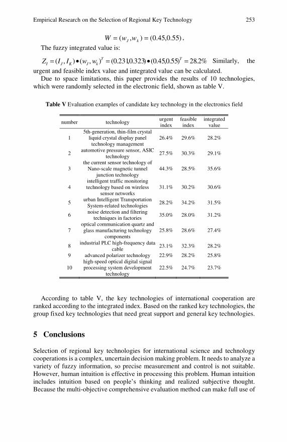
Empirical Research on the Selection of Regional Key Technology 253
)55.0,45.0(),( == kJ wwW ,
The fuzzy integrated value is:
%2.28)55.0,45.0()323.0,231.0(),(),( =•=•= TTkJKJI wwIIZ Similarly, the
urgent and feasible index value and integrated value can be calculated. Due to space limitations, this paper provides the results of 10 technologies,
which were randomly selected in the electronic field, shown as table V.
Table V Evaluation examples of candidate key technology in the electronics field
According to table V, the key technologies of international cooperation are ranked according to the integrated index. Based on the ranked key technologies, the group fixed key technologies that need great support and general key technologies.
5 Conclusions
Selection of regional key technologies for international science and technology cooperations is a complex, uncertain decision making problem. It needs to analyze a variety of fuzzy information, so precise measurement and control is not suitable. However, human intuition is effective in processing this problem. Human intuition includes intuition based on people’s thinking and realized subjective thought. Because the multi-objective comprehensive evaluation method can make full use of
number technology urgent index
feasible index
integrated value
1 5th-generation, thin-film crystal
liquid crystal display panel technology management
26.4% 29.6% 28.2%
2 automotive pressure sensor, ASIC
technology 27.5% 30.3% 29.1%
3 the current sensor technology of
Nano-scale magnetic tunnel junction technology
44.3% 28.5% 35.6%
4 intelligent traffic monitoring technology based on wireless
sensor networks 31.1% 30.2% 30.6%
5 urban Intelligent Transportation
System-related technologies 28.2% 34.2% 31.5%
6 noise detection and filtering
techniques in factories 35.0% 28.0% 31.2%
7 optical communication quartz and glass manufacturing technology
components 25.8% 28.6% 27.4%
8 industrial PLC high-frequency data
cable 23.1% 32.3% 28.2%
9 advanced polarizer technology 22.9% 28.2% 25.8%
10 high-speed optical digital signal processing system development
technology 22.5% 24.7% 23.7%
254 L. Jian, S. Liu, and H. Ma
people's intuition and knowledge, it is a good method to solve uncertain decision problems with sick boundaries. In the paper, the urgent index and feasible index are proposed, in which the former is to evaluate the urgency of the technology demand for the local economy, and the latter to measure the feasibility of obtaining key technology through international cooperations. By applying the Delphi method, the corresponding evaluation index system is set up, based on which an integrated evaluation method of a multiple objective fuzzy index is built. The proposed method is applied to the selection of key technology for international cooperations in Jiangsu province. The evaluation set is quantified to extract the urgent index and feasible index, followed by the incorporation of two indexes into an integrated one. Then, the key technologies of international cooperations are ranked according to the integrated index. Finally, key technologies, which are urgently needed and possibly beneficial for Jiangsu province through international technology cooperation, are screened out.
The chosen key technologies were illustrated as realistic by the insiders. Meanwhile, the research results have been applied to guide the Jiangsu Province S&T Department to develop international cooperations. Also, it provided a reference for Jiangsu when carrying out international cooperations and developing a long-term strategy for international S&T cooperation.
References
Han, H.S., Chen, J.: Defense key technology selection and evaluation methods. Aerospace China (7), 12–14 (2006)
Hou, R.Y., Hu, S.H.: Regional science and technology development strategy, the key technology choices. Science of Science and Management of S&T (to appear)
Jia, X.F., Zhang, X.L.: Strategic selection and developments of Jiangsu’s leading industries. Economy & Audit Study 21(1), 71–75 (2006)
Luan, W.X., Cao, Y.: The exploitation strategy of Chinese international regional resources and the choice of the critical technology. Areal Research and Development 24(4), 5–11 (2005)
Ning, X.X., Liu, S.F.: Management Forecasting and Decision-Making Method. Science Press, Beijing (2003)
Peng, J.L., An, H.X., Li, Q.: Selection of key technology areas and key development objectives of domain analysis. Science & Technology Progress and Policy 16(5), 53–54 (1999)
Radzikowska, A., Kerre, E.E.: Characterizations of main classes of fuzzy relations using fuzzy modal operators. Fuzzy Sets and Systems 152, 223–247 (2005)
Wan, J.B., Cui, Z.M., Pu, G.X.: Technology foresight, the key technology choice and industrial development. Studies in Science of Science 21(1), 41–46 (2003)
Yu, X.J.: The choice of the key common technology within the industry clusters–take Zhejiang Province as example. Science Research Management (1), 80–84 (2005)
Zadeh, L.A.: Is there a need for fuzzy logic? Information Sciences 178, 2751–2779 (2008)

Dynamic Evaluation and Analysis of Regional Technological Innovation Capacity Based on a Gray Target*
Meijuan Li, Hua Zhuang, and Guohong Chen**
Regional technological innovation capacities of 31 regions in China from 2004 to 2007 are dynamicly evaluated and analyzed by using the gray target theory to find out their changes and development trends. The bull’s eye degree was utilized to classify and sort the regional technological innovation capacity. Through the analysis of the contribution degree of the regional technological innovation capacity, the evaluation indicator identified the key influence factors and classified and sorted the evaluation indicator.
1 Introduction
Nowadays, the technological innovation capacity has become a decisive factor of the competitive capacity of a country or region. The enhancement independent innovation capacity and the construction innovation country are taken as an important strategy of the Eleventh Five-Year Plan of the People's Republic of China
Meijuan Li School of Management, Fuzhou University, P.R. China Phone: 86-591-28342023; Fax: 86-591-22866402 e-mail: [email protected]
Hua Zhuang School of Management, Fuzhou University, P.R. China
Guohong Chen School of Management, Fuzhou University, P.R. China Phone: 86-591-22866770; Fax: 86-591-22866402 e-mail: [email protected]
* This work was supported by the National Soft Science Foundation of China (No.2006GXQ3D108), the Research Fund for the Doctoral Program of Higher Education (No.20070386001), the Social Science Foundation of Fujian (No.2008C023 and No.2008A073 ), the Soft Science Foundation of Fujian (No.2009R0054 ), and the Science Foundation of Fuzhou University (No.2006-XY(S)-06).
** Corresponding author.

256 M. Li, H. Zhuang, and G. Chen
for National Economic and Social Development at the fifth Plenary Session of the Sixteenth Party Central Committee of the Communist Party of China. Objective and scientific evaluation and comparative research on the technological innovation capacity of various regions are helpful to identify their advantages and disadvantages. It is important to correctly select a regional technological innovation strategy and to lay down a scientific regional technological innovation policy.
At present, domestic and international scholars have carried out some research on regional technological innovation capacity (Riddel and Schwer, 2003; Chinese S&T Development Strategy Research Group, 2003; Shao et al., 2003; Shao and Tang, 2005; Zhu, 2004; Bi et al., 2005; He et al., 2006; Jian et al., 2006; Lu et al., 2008; Li 2009; Chen et al., 2009; Li et al., 2008; Li et al., 2009). For example, a Chinese science and technology (S&T) development strategy research group set up a regional technological innovation capacity evaluation indicator system and evaluated the regional technological innovation capacity of various provinces (Chinese S&T Development Strategy Research Group, 2003); Shao Yunfei, Tang Xiaowo and Chen Guang used an empirical cluster to analyze the capacity of the region technological innovation of China (Shao et al., 2003); subsequently, they used the principal component analysis study on the capacity of the regional technical innovation of China (Shao and Tang, 2005); Zhu Haijiu set up an evaluation indicator system of the regional technological innovation capacity (Zhu, 2004). Bi Kexin put forth a comprehensive evaluation method based on the fuzzy integral to measure and evaluate regional technological innovation in small and medium enterprises (Bi et al., 2005); He Yaqiong, Qing Pei and Sun Jun evaluated the growth efficiency of regional innovation capacity in thirty-one Chinese provinces (He et al., 2006); Jian Cheng Guan, Richard C.M. Yam, Chiu Kam Mok and Ning Ma (2006) set up a DEA model to study the relationship between the innovative capacity and competitiveness; Lu Shiyu and Zhao Shukuang (2008) used factor analysis to analyze and evaluate the situation of our regional technological innovation capacity; Li Xibao (2009) used the Stochastic frontier model to explain the difference of regional technological innovation capacity; Chen Yunwei (2009) evaluated the technological innovation capacity in eight economic regions in the PR China based on patents, and so on.
Most scholars used a single comprehensive evaluation method to statically evaluate the regional technological innovation capacity for an existing reference. Static evaluation pays more attention to the status quo of the regional technological innovation capacity, while the capacity of technological innovation is a dynamic development and continuous improvement process. Riddel and Schwer proposed that regional innovation capacity is a time variable, and any regional innovation capacity is not an easy thing. Some gaps generate, develop and expand in the dynamic changes; some gaps gradually shrink in the dynamic changes. Objective, fair and comprehensive analysis of dynamic changes and the evaluation of dynamic changes to grasp the change and trends of the various provinces’ and cities’ technological innovation capacity are very practical and can provide important feedback for upper policy-makers. Therefore, we use dynamic evaluation to reflect the development and change process of the regional technological innovation
Dynamic Evaluation and Analysis of Regional Technological Innovation Capacity 257
capacity and find its trend in order to get more scientific, meaningful evaluation results on the region technological innovation capacity.
Dynamic comprehensive evaluation is an important multi-attribute decision-making problem. This issue has attracted much attention but has been researched little. The main results of research are from Professor Guo Yajun. He put forth the timing perspective of the dynamic comprehensive evaluation methods as follows (Guo, 2008): the second-weighted method; the incentive (or punishment) characteristics of the dynamic comprehensive evaluation method; the longitudinal level of the analysis method; the longitudinal and transverse level of the evaluation method; based on dual incentives to control the line, the multi-stage information gathering methods; and an operator based on the timing of the dynamic comprehensive evaluation method. But these methods only get the comprehensive evaluation values and sorts and cannot classify results or identify the contribution of the evaluation indicator.
The gray target theory is used to evaluate the technological innovation capacity of 31 provinces and cities in China, covering a time period of 2004-2007, in order to grasp the dynamics of their development and changes. Using a bull’s eye analysis to classify and sort the regional technological innovation capacity of 31 regions, we utilize a contributions degree analysis to classify and sort the evaluation indicators of the regional technological innovation to identify the key influencing factors.
2 Gray Target Theory
The gray target theory was put forth by Professor Deng Julong in recent years. It includes two parts: the bull’s eye degree analysis and the contribution degree analysis. Its principle lies in satisfying the requirements of the information
domain )(θΦ , and in a set of model sequences, finding the target data that is
closest to the sub-information domain )(θiΦ to the structure standard mode. Then,
the mode and standard mode aggregate together to constitute a gray target, and the standard model is a bull’s eye. According to the meaning of sub-information
domain )(θiΦ , the mode that is away from the bull’s eye is regarded as the target
side. The mode that is upper and away from the bull’s eye is regarded as the upper target side, and the mode that is lower and away from the bull’s eye is regarded as the lower target side. While the upper target side is large data, the lower target side is small data. The gray relation degree between each mode of information differences space and the bull’s eye can be regarded as the degree of proximity to the bull’s eye, namely, the bull’s eye degree. Pattern recognition, classification and selection are based on the bull’s eye degree. Based on the analysis of the contribution degree, it can analyze the impact of the indicator to bull’s eye degree in order to find the key factor. It is very good at studying less data and uncertainty problems. It has been successful in many areas (Deng , 1993; 2000; Nie et al., 2005; Yang, et al., 2006).
258 M. Li, H. Zhuang, and G. Chen
A. Bull’s Eye Degree Analysis (Deng , 1993; 2000; Nie et al., 2005; Yang, et al., 2006)
Let 00 xTw = , 0w be a standard pattern, 0x be
)1,...,1,1())(),...,2(),1(( 0000 == nxxxx , and 0x be called the standard bull’s
eye.
Suppose that GFR@ is a gray relational factor set when
GRF@ = INUiiii wTwxIiX @,,{ ∈=∈ , and T is the gray target transform}.
Suppose that GRΔ stands for the GRF@ of the different information spaces of the
gray relation.
(min))(max),,,( oioiGR ΔΔΔ=Δ ξ, 5.0=ξ
},,...,2,1{},,...,2,1{)({ nKkmIikoi =∈=∈Δ=Δ
,)(1)()(0 kxkxkx iioi −=−=Δ })( 0000 Twxxkx =⇒∈
(max) maxmax ( ) maxmax 1 ( ) ,oi oi ii k i k
k x kΔ = Δ = −
(min) min min ( ) min min 1 ( )oi oi ii k i k
k x kΔ = Δ = −,
The gray incidence coefficient
),0(maxmax),0(
),0(maxmax),0(minmin))(),0((
kikiki
kikikikikixix
Δ+Δ
Δ+Δ=
ξ
ξγ
),( 0 ixxγ refers to ix bull’s eye degree:
∑=
=n
kii kxkx
nxx
100 ))(),((
1),( γγ
B. Contribution Degree Theory (Deng , 1993; 2000; Nie et al., 2005; Yang, et al., 2006)
Suppose that GFR@ is the gray relational factor set, and it can be described as
follows:
⎪⎪⎪⎪
⎩
⎪⎪⎪⎪
⎨
⎧
∈=∈=∈=
∈=⇒∈∀
==⇒∈∀==∈
=
),()(
(min),)(
(max),)(
},,,{
),()()()(
)),(),...,(),(()(),0()0()0()0(
)),0(),...,0(),0(()0(},,...,2,1{},0{)(
@
21
21
memPOLkPOLwFORTT
POLkPOLwFORTT
POLkPOLwFORTT
TTTT
kwTkxkxkx
kxkxkxkxwTxxx
xxxxnKKkkx
imv
ilv
iuv
mlUv
ivii
milii
m
GRF
∪
Dynamic Evaluation and Analysis of Regional Technological Innovation Capacity 259
Then GRF@ represents the contribution factor set, and )(kx stands for the kth
contribution factor; ),0( kiΔ stands for the information difference between )0(ix
and )(kix :
),0( kiΔ = )()0( kxx ii − , KkIi ∈∈ , ;
),0( kΔ stands for the information difference between )0(x and )(kx :
)),0(),...,,0()),,0((),0( 21 kkkk mΔΔΔ=Δ ;
Δ stands for the information difference set:
}},...,2,1{),0({ nKkk =∈Δ=Δ ;
),0(max kΔ stands for the upper environment parameter in the contribution
factor set:
);,0(maxmax),0(max kk iki
Δ=Δ
),0(min kΔ stands for the lower environment parameter in the contribution
factor set:
);,0(minmin),0(min kk iki
Δ=Δ
GRΔ stands for the GR information difference space of the contribution
factor set:
GRΔ = )),0(),,0(,,( minmax kk ΔΔΔ ξ ,
5.0=ξ },,...,2,1{),0({ nKkk =∈Δ=Δ
)),0(),...,,0(),,0((),0( 21 kkkk mΔΔΔ=Δ ,
};)()0(),0( kxxk iii −=Δ
And the gray relational coefficient is:
),0(maxmax),0(
),0(maxmax),0(minmin))(),0((
kk
kkkxx
ki
ii
ki
iki
ii Δ+Δ
Δ+=
ξ
ξγ
which stands for the contribution coefficient of indicator k at pattern i. Gray
incidence degree, and ∑=
=m
iiiii kxx
mkxx
1
))(),0((1
))(),0(( γγ stands for the
contribution degree of indicator k.

260 M. Li, H. Zhuang, and G. Chen
3 Evaluation Indicator System for Regional Technological Innovation Capacity
In (Chen et al., 2008), based on the connotation and elements analysis of the regional technological innovation capacity and the existing research results, an initial comprehensive evaluation indicator system is formed; then, an evaluation indicator identification framework of the regional technological innovation capacity is established through expert appraisal, relative analysis, discrimination analysis and the effectiveness analysis of the indicator rules; meanwhile, a more comprehensive, reliable and effective evaluation indicator system is developed for the regional technological innovation capacity. Finally, the effectiveness of the indicator system is verified by using several comprehensive evaluation methods.
The per capita disposable income reflects the life quality of residents better than the total revenue, so "the net income of urban residents" indicator was changed to "the per capita disposable income of urban residents". The data of “the number of technology centers recognized by [the] nation” is from the website of thematic data of statistics that only provided those for 2004 and 2005. It is difficult to get data from other years, so in place of "the number of large and medium-sized industrial enterprises that included science and technological institutions". Finally, the regional technological innovation capacity evaluation indicator system is as follows (Li et al., 2009).
Regional technological innovation input capacity B1: R&D personnel D1; government appropriation D2; R&D expenditure D3; the number of large and medium-sized industrial enterprises, including science and technology institutions D4.
Regional technology transference and diffusion capacity B2: R&D funded by enterprises D5, transaction value in technology market D6, foreign technology introduction expenditure D7, domestic technology purchases expenditure D8, technology digestion absorption expenditure D9, foreign direct investment D10.
Regional technological innovation output capacity B3: domestic Chinese journal S&T papers D11, the number of S&T papers cited by overseas main search tool D12, patents granted D13, patent applications D14, the share of high-tech industry in the industrial enterprise added value above the designated size D15, the share of high-tech product exports in the total product exports D16, new product output value D17, GDP D18, value added of the industry D19, market volume of business D20.
Regional technological innovation support capacity B4: length of paved roads D21, business volume of post and telecommunication services D22, number of mobile telephone subscribers D23, number of internet users D24, the per capita disposable income of urban residents D25, risk capital amount D26.
Dynamic Evaluation and Analysis of Regional Technological Innovation Capacity 261
The evaluation indicators coverage is broad, and intrinsically logical, and the quantity is moderate and feasible. So it is suitable to evaluate the region technological innovation capacity.
4 Empirical Research
C. Evaluation Objects
Thirty-one regions in China: Beijing, Tianjin, Hebei, Shanghai, Jiangsu, Zhejiang, Fujian, Shandong, Guangdong, Hainan, Shanxi, Anhui, Jiangxi, He’nan, Hebei, Hunan, Inner Mongolia, Guangxi, Chongqing, Sichuan, Guizhou, Yunnan, Tibet, Shanxi, Gansu, Qinghai, Ningxia, Xinjiang, Liaoning, Jilin, Heilongjiang.
D. Data Source
Data come from the Chinese statistics yearbook (2005—2008), the Chinese science and technology statistics yearbook (2005—2008), the website of the People’s Republic of China Ministry of Science and Technology (http://www.most.gov.cn/kjtj/), which provides a major database of China's science and technology indicators. The database provides the main data of the indicators from 2004 to 2007, which include the major provincial and municipal science and technology indicators and the main socio-economic indicators in the major cities and provinces. The Chinese science and technology statistics yearbook (2008) provides the indicator value of the number of S&T papers cited by overseas; the main search tool is 2006, but we cannot get the data of 2007. They can be forecasted according to the growth trend. Data missing inevitably led to a number of indicators for evaluating the deviation from reality. But as a whole, the individual data missing does not affect the objectivity of evaluation (Chinese S&T Development Strategy Research Group, 2003). Because of the limits of length, the original indicator value data aren’t listed here.
E. The Analysis of the Bull’s Eye Degree of the Regional Technological Innovation Capacity
The bull’s eye degree of 31 regions in China from 2004 to 2007 is shown in Table I.
According to the principle of minimum information, if ),( 0 ixxγ ≥ 0.3333, we
will divide the bull’s eye degree into 7 levels: [0.9, 1], [0.8, 0.9], [0.7, 0.8], [0.7, 0.6], [0.5, 0.6], [0.4, 0.5], [0.3333, 0.4]. Therefore, Guangdong is the third level; Jiangsu is the fourth level; Beijing, Shanghai, Zhejiang and Shangdong are the fifth level; Tianjin and Liaoning are the sixth level; Sichun was the sixth level in 2005 and was the seventh level in 2004, 2007 and 2008; and the other 22 regions are the seventh level.
The sorting value of the bull’s eye degree from 2004 to 2007 is shown in Table II.
There are 7 regions whose regional technological innovation capacity increased from 2004 to 2007: Zhejiang ranked sixth in 2004, fifth in 2005 and 2006, and
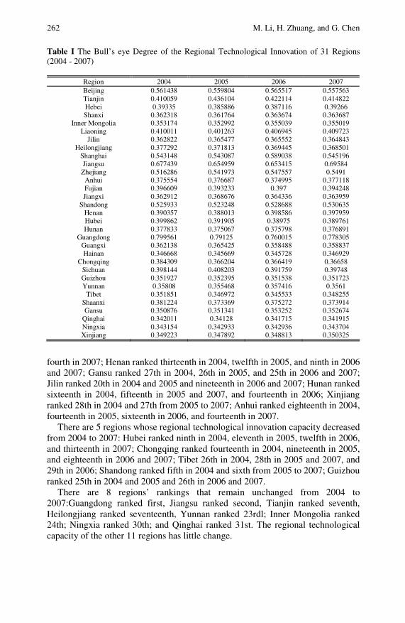
262 M. Li, H. Zhuang, and G. Chen
Table I The Bull’s eye Degree of the Regional Technological Innovation of 31 Regions (2004 - 2007)
Region 2004 2005 2006 2007 Beijing 0.561438 0.559804 0.565517 0.557563 Tianjin 0.410059 0.436104 0.422114 0.414822 Hebei 0.39335 0.385886 0.387116 0.39266 Shanxi 0.362318 0.361764 0.363674 0.363687
Inner Mongolia 0.353174 0.352992 0.355039 0.355019 Liaoning 0.410011 0.401263 0.406945 0.409723
Jilin 0.362822 0.365477 0.365552 0.364843 Heilongjiang 0.377292 0.371813 0.369445 0.368501
Shanghai 0.543148 0.543087 0.589038 0.545196 Jiangsu 0.677439 0.654959 0.653415 0.69584
Zhejiang 0.516286 0.541973 0.547557 0.5491 Anhui 0.375554 0.376687 0.374995 0.377118 Fujian 0.396609 0.393233 0.397 0.394248 Jiangxi 0.362912 0.368676 0.364336 0.363959
Shandong 0.525933 0.523248 0.528688 0.530635 Henan 0.390357 0.388013 0.398586 0.397959 Hubei 0.399862 0.391905 0.38975 0.389761 Hunan 0.377833 0.375067 0.375798 0.376891
Guangdong 0.799561 0.79125 0.760015 0.778305 Guangxi 0.362138 0.365425 0.358488 0.358837 Hainan 0.346668 0.345669 0.345728 0.346929
Chongqing 0.384309 0.366204 0.366419 0.36658 Sichuan 0.398144 0.408203 0.391759 0.39748 Guizhou 0.351927 0.352395 0.351538 0.351723 Yunnan 0.35808 0.355468 0.357416 0.3561
Tibet 0.351851 0.346972 0.345533 0.348255 Shaanxi 0.381224 0.373369 0.375272 0.373914 Gansu 0.350876 0.351341 0.353252 0.352674
Qinghai 0.342011 0.34128 0.341715 0.341915 Ningxia 0.343154 0.342933 0.342936 0.343704 Xinjiang 0.349223 0.347892 0.348813 0.350325
fourth in 2007; Henan ranked thirteenth in 2004, twelfth in 2005, and ninth in 2006 and 2007; Gansu ranked 27th in 2004, 26th in 2005, and 25th in 2006 and 2007; Jilin ranked 20th in 2004 and 2005 and nineteenth in 2006 and 2007; Hunan ranked sixteenth in 2004, fifteenth in 2005 and 2007, and fourteenth in 2006; Xinjiang ranked 28th in 2004 and 27th from 2005 to 2007; Anhui ranked eighteenth in 2004, fourteenth in 2005, sixteenth in 2006, and fourteenth in 2007.
There are 5 regions whose regional technological innovation capacity decreased from 2004 to 2007: Hubei ranked ninth in 2004, eleventh in 2005, twelfth in 2006, and thirteenth in 2007; Chongqing ranked fourteenth in 2004, nineteenth in 2005, and eighteenth in 2006 and 2007; Tibet 26th in 2004, 28th in 2005 and 2007, and 29th in 2006; Shandong ranked fifth in 2004 and sixth from 2005 to 2007; Guizhou ranked 25th in 2004 and 2005 and 26th in 2006 and 2007.
There are 8 regions’ rankings that remain unchanged from 2004 to 2007:Guangdong ranked first, Jiangsu ranked second, Tianjin ranked seventh, Heilongjiang ranked seventeenth, Yunnan ranked 23rdl; Inner Mongolia ranked 24th; Ningxia ranked 30th; and Qinghai ranked 31st. The regional technological capacity of the other 11 regions has little change.
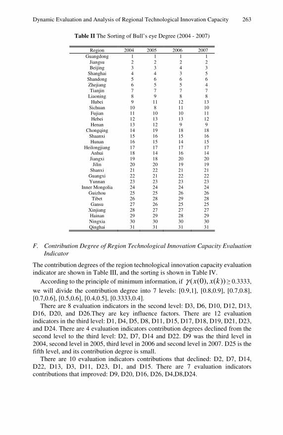
Dynamic Evaluation and Analysis of Regional Technological Innovation Capacity 263
Table II The Sorting of Bull’s eye Degree (2004 - 2007)
Region 2004 2005 2006 2007 Guangdong 1 1 1 1
Jiangsu 2 2 2 2 Beijing 3 3 4 3
Shanghai 4 4 3 5 Shandong 5 6 6 6 Zhejiang 6 5 5 4 Tianjin 7 7 7 7
Liaoning 8 9 8 8 Hubei 9 11 12 13
Sichuan 10 8 11 10 Fujian 11 10 10 11 Hebei 12 13 13 12 Henan 13 12 9 9
Chongqing 14 19 18 18 Shaanxi 15 16 15 16 Hunan 16 15 14 15
Heilongjiang 17 17 17 17 Anhui 18 14 16 14 Jiangxi 19 18 20 20
Jilin 20 20 19 19 Shanxi 21 22 21 21
Guangxi 22 21 22 22 Yunnan 23 23 23 23
Inner Mongolia 24 24 24 24 Guizhou 25 25 26 26
Tibet 26 28 29 28 Gansu 27 26 25 25
Xinjiang 28 27 27 27 Hainan 29 29 28 29 Ningxia 30 30 30 30 Qinghai 31 31 31 31
F. Contribution Degree of Region Technological Innovation Capacity Evaluation Indicator
The contribution degrees of the region technological innovation capacity evaluation indicator are shown in Table III, and the sorting is shown in Table IV.
According to the principle of minimum information, if ))(),0(( kxxγ ≥ 0.3333,
we will divide the contribution degree into 7 levels: [0.9,1], [0.8,0.9], [0.7,0.8], [0.7,0.6], [0.5,0.6], [0.4,0.5], [0.3333,0.4].
There are 8 evaluation indicators in the second level: D3, D6, D10, D12, D13, D16, D20, and D26.They are key influence factors. There are 12 evaluation indicators in the third level: D1, D4, D5, D8, D11, D15, D17, D18, D19, D21, D23, and D24. There are 4 evaluation indicators contribution degrees declined from the second level to the third level: D2, D7, D14 and D22. D9 was the third level in 2004, second level in 2005, third level in 2006 and second level in 2007. D25 is the fifth level, and its contribution degree is small.
There are 10 evaluation indicators contributions that declined: D2, D7, D14, D22, D13, D3, D11, D23, D1, and D15. There are 7 evaluation indicators contributions that improved: D9, D20, D16, D26, D4,D8,D24.
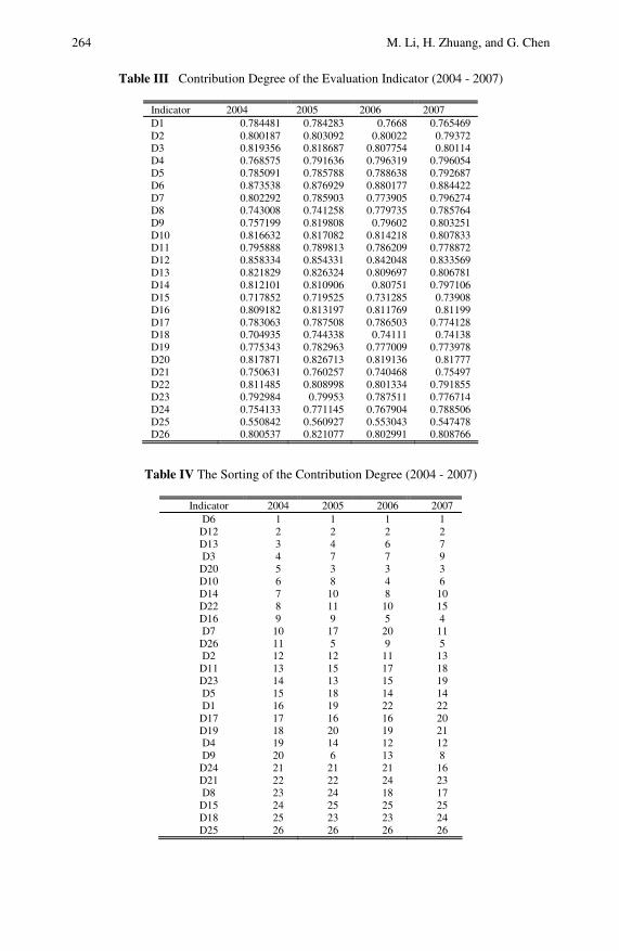
264 M. Li, H. Zhuang, and G. Chen
Table III Contribution Degree of the Evaluation Indicator (2004 - 2007)
Indicator 2004 2005 2006 2007 D1 0.784481 0.784283 0.7668 0.765469 D2 0.800187 0.803092 0.80022 0.79372 D3 0.819356 0.818687 0.807754 0.80114 D4 0.768575 0.791636 0.796319 0.796054 D5 0.785091 0.785788 0.788638 0.792687 D6 0.873538 0.876929 0.880177 0.884422 D7 0.802292 0.785903 0.773905 0.796274 D8 0.743008 0.741258 0.779735 0.785764 D9 0.757199 0.819808 0.79602 0.803251 D10 0.816632 0.817082 0.814218 0.807833 D11 0.795888 0.789813 0.786209 0.778872 D12 0.858334 0.854331 0.842048 0.833569 D13 0.821829 0.826324 0.809697 0.806781 D14 0.812101 0.810906 0.80751 0.797106 D15 0.717852 0.719525 0.731285 0.73908 D16 0.809182 0.813197 0.811769 0.81199 D17 0.783063 0.787508 0.786503 0.774128 D18 0.704935 0.744338 0.74111 0.74138 D19 0.775343 0.782963 0.777009 0.773978 D20 0.817871 0.826713 0.819136 0.81777 D21 0.750631 0.760257 0.740468 0.75497 D22 0.811485 0.808998 0.801334 0.791855 D23 0.792984 0.79953 0.787511 0.776714 D24 0.754133 0.771145 0.767904 0.788506 D25 0.550842 0.560927 0.553043 0.547478 D26 0.800537 0.821077 0.802991 0.808766
Table IV The Sorting of the Contribution Degree (2004 - 2007)
Indicator 2004 2005 2006 2007 D6 1 1 1 1
D12 2 2 2 2 D13 3 4 6 7 D3 4 7 7 9
D20 5 3 3 3 D10 6 8 4 6 D14 7 10 8 10 D22 8 11 10 15 D16 9 9 5 4 D7 10 17 20 11
D26 11 5 9 5 D2 12 12 11 13
D11 13 15 17 18 D23 14 13 15 19 D5 15 18 14 14 D1 16 19 22 22
D17 17 16 16 20 D19 18 20 19 21 D4 19 14 12 12 D9 20 6 13 8
D24 21 21 21 16 D21 22 22 24 23 D8 23 24 18 17
D15 24 25 25 25 D18 25 23 23 24 D25 26 26 26 26
Dynamic Evaluation and Analysis of Regional Technological Innovation Capacity 265
4 Conclusion
The gray target theory is used to dynamically evaluate and analyze the technological innovation capacity of 31 regions in China in this chapter. We also used the bull’s eye degree to classify and sort the regional technological innovation capacity and used the contribution degree to find out the contribution degree of the regional technological innovation capacity evaluation indicator in order to find out their changes and development trends.
References
Bi, K.X., Sun, J.H., Zhang, T.Z., Feng, Y.J.: Measurement and evaluation of regional technological innovation in small and medium enterprises based on fuzzy integral. Systems Engineering-theory & Practice (2), 40–46 (2005)
Chen, Y.W., Yang, Z.P., Fang, S., Hu, Z.Y., Meyer, M., Bhattacharya, S.: A patent based evaluation of technological innovation capability in eight economic regions in PR China. World Patent Information, 104–110 (2009)
Chen, G.H., Xiao, X.F., Li, M.J.: Study on identification for the evaluation indicator system of the regional technological innovation capability. In: Proc. 4th IEEE WiCOM Conf., Dalian, China (2008)
Chinese S&T Development Strategy Research Group, Regional innovation ability evaluation of China in 2002. Science of Science and Management of S.& T., pp. 5–11 (2003)
Chinese S&T Development Strategy Research Group. Interpretation the evaluation of regional innovation capability of China. Science of Science and Management of S.& T. (5), 5–10 (2003)
Deng, J.L.: On gray target. The Journal of Gray System (3), 173 (1993) Deng, J.L.: Contributing degree in gray target theory. The Journal of Gray System (1), 40
(2000) Guo, Y.J.: Comprehensive Evaluation Theory Method and Applications, pp. 101–144.
Science Press, Beijing (2008) He, Y.Q., Qin, P., Su, J.: The evaluation on growth efficiency of regional innovation capacity
in thirty-one Chinese province. Journal of Harbin Institute of Technology 38, 101–103 (2006)
Jian, C.G., Yam, R.C.M., Chiu, K.M., Ning, M.: A study of the relationship between competitiveness and technological innovation capability based on DEA models. European Journal of Operational Research, 971–986 (2006)
Li, M.J., Chen, G.H., Xiao, X.F.: Empirical research on regional technological innovation ability based on consistency combination evaluation. In: Proc. 4th IEEE WiCOM Conf., Dalian, China (2008)
Li, M.J., Chen, G.H., Xiao, X.F.: Evaluation and comparative analysis on regional technological innovation capability based on consistency combination evaluation. Chinese Journal of Management Science 17, 131–139 (2009)
Li, X.B.: China’s regional innovation capacity in transition: An empirical approach. Research Policy, 338–357 (2009)
Lu, S.Y., Zhao, S.K., Ju, X.W.: Evaluation and empirical study on the capacity of regional technical innovation. Information Science 26, 942–946 (2008)

266 M. Li, H. Zhuang, and G. Chen
Nie, M., Zhang, L.B., Lu, Y.T.: Gray theory applied to recognizing the core rigidities in high-tech firms. Statistical Research (6), 62–65 (2005)
Riddel, M., Schwer, R.K.: Regional innovative capacity with endogenous employment: Empirical evidence from the U.S. The Review of Regional Studies 33, 73–81 (2003)
Shao, Y.F., Tang, X.W.: PCA empirical study on the capacity of region technical innovation of China. Journal of Industrial Engineering/Engineering Management 19, 71–76 (2005)
Shao, Y.F., Tang, X.W., Chen, G.: Cluster empirical analyses on the capacity of region technical innovation of China. China Soft Science, 113–118 (2003)
Yang, Z.L., Bo, Y.C., Bai, Y., Ma, X.W.: Improvement and application of gray target contribution degree technology. Journal of Gun Launch & Control (3), 23–26 (2006)
Zhu, H.J.: A research of regional innovation capability evaluation index system. Science Research Management 25, 30–35 (2004)
Analysis of the Regional Characteristics of the Distribution of Scientific and Technological Talents in Jiangsu Province*
Sifeng Liu and Keqin Sheng
This chapter is an overall summary of the scientific and technological human resources of Jiangsu Province and builds an index system of the "regional characteristics of the distribution of scientific and technological talents” by selecting the four system cluster method to carry on the cluster analysis of distributions of scientific and technological talents in 13 municipalities of Jiangsu Province. On this basis, according to different types of areas, including scientific and technological talent-intensive areas, comparably intensive areas, the lacking scientific and technological talent areas and the areas having rare scientific and technological talents, this chapter makes an in-depth analysis of the typical features of the regional distribution of scientific and technological talents in Jiangsu Province.
1 Introduction
In general, scientific and technological talents refer to those with virtue and scientific and technological expertise, and they have mastered the knowledge or the technology of the production process. Nevertheless, it is a broad, abstract and dynamic concept that varies with the understandings of different people. Scientific and technological talents can be divided into three levels in accordance to the content and scope of scientific activities they have been engaged in: professional and technical personnel, scientific and technological activities and research and development personnel. In the context of a knowledge-based economy, science and technology personnel, as well as the development of science and technology decided by the scientific and technological talents, often play a dominant role in the economic development and technological innovation of a nation or region. So the study of the characteristics of the regional distribution of scientific and technological personnel and the analysis of the key issues of the development of Sifeng Liu and Keqin Sheng School of Economics and Management, Nanjing University of Aeronautics and Astronautics, Nanjing 210016, China
* This work was subsidized by the National Soft Science Research Project (2008GXS5D115) and National Social Science Foundation Key Project (08AJY024).
268 S. Liu and K. Sheng
scientific and technological personnel in different parts have a strong practical significance for decision-making departments to adopt targeted policies and measures for personnel, as well as a great and far-reaching importance for advancing regional economic development and improving the level of regional scientific and technological innovation.
Currently, the study of regional characteristics of the distribution of scientific and technological talents has just started. Existing literature have carried on beneficial discussions on the imbalance of the regional distribution of China's scientific and technological personnel, the structural characteristics of geographical distribution and the mobility of IT personnel, etc. Zhou Guirong, etc. (2005) has taken a systematic study of problems in the regional distribution of China's scientific and technological personnel and countermeasures. She thinks that the differences in the number of talents is widening between coastal and inland areas of China, and the proportion of regional scientific and technological talents to their geographic areas is losing its balance and that the uneven economic development in central and western regions of talent has fundamentally led to the uneven distribution. On this basis, she put forth the relevant countermeasures. Gui Zhaoming, etc. (2001) researched the spatial distribution and structural features of China’s scientific and technological talents and analyzed the regional spatial characteristics of the distribution of scientific and technological talents. Wang Wei (2006) pointed out that the idleness and shortage of China's scientific and technological personnel co-exist, particularly in developed areas along the southeast coast, where there is serious talent idleness and waste, and analyzed this phenomenon with the use of the Gambling model. Zuo Hanbin (2004) made a detailed analysis of the distribution and structure of scientific and technological talents in Hubei Province and thought that the distribution of the province was a structural shortage of talent. LI Fuchu (2005) not only respectively calculated the deviation coefficient of each of the million scientific and technological talents between and within the different regions of central and western of China to analyze the differences to the degree, but also divided various cities into 5 types, and pointed out the typical types of provinces and cities according to the total science and technology human resources, the per capita indicators and the three departments that have the entropy value. Overall, research on the characteristics of the distribution of scientific and technological personnel has yet to be made further in-depth. Among the existing literatures, there are still few comprehensive studies in addition to studying only larger regions’ characteristics of the geographic distribution of scientific and technological personnel. In view of this, it is particularly essential to conduct a detailed study on the regional characteristics of the distribution of scientific and technological personnel for typical provinces.
2 Overview of Science and Technology Human Resources in Jiangsu Province
In recent years, the number of scientific and technical personnel of Jiangsu Province has been expanding. The number of technological activities, scientists and

Analysis of the Regional Characteristics of the Distribution 269 Table 1 The total scientific and technological personnel of Jiangsu Province compared to other coastal areas (2006). Unit: ten thousand persons.
Area Technological activities personnel Scientists and engineers R & D personnel
Shandong 28.54 18.77 9.66
Jiangsu 38.11 23.9 13.89
Zhejiang 31.05 18.98 10.28
Fujian 10.11 6.48 4.02
Guangdong 36.88 25.93 14.72
Shanghai 20.07 15.04 8.02
National 413.15 279.78 150.25
Source: Ministry of Science and Technology of the People's Republic of China website.
engineers, and R & D personnel are ahead of the number of its neighboring provinces Shandong, Zhejiang, Fujian, and Shanghai, while the latter two are slightly lower than that in Guangdong Province (as shown in Table 1). Personnel of Jiangsu Province engaging in scientific and technological activities accounted for more of the total amount of technological activities in recent years, which results from the emphasis on innovation and the strengthening of the high-tech industrial development and science and technology talent of Jiangsu Province.
Since 2000, among the staff of scientific and technological activities of Jiangsu Province, personnel who have gotten high or intermediate professional titles or a university undergraduate degree or above have increased year by year, of which the average annual growth rate in the higher education institutions is 17.8%, and the growth rate even reaches 21.15 % in medium-sized enterprises, both of which far exceed the average annual growth rate of technological activities in Jiangsu Province.
In Jiangsu Province, the distribution of the scientific and technological talents industry is concentrated. For instance, R & D personnel are mainly in business and government R & D institutions and universities. For example, in 2005, Jiangsu Province had 128,028 full-time R & D personnel, a total of 12,326 of which were at government R & D institutions and accounted for 9.63%; R & D personnel in medium-sized enterprises were 72,388, accounting for 56.54%; and researchers of institutions of higher education are 16,535, accounting for 12.92%. The sum total of the three parts made up 79.09% of the province's R & D personnel. Other departments involved in D & R activities of the researchers accounted for only 20.91%.
In recent years, in Jiangsu Province, the research results obtained a rapid growth, and transaction contracts of the technological market were increased year by year. Among those from 2000 to 2007, the amount of received patent applications and invention patent applications granted increased, respectively, at a average rate of 38.62%, and 44.59%; the annual average growth rate of the two separately were 21.64%, and 27.61%. Thus, the vitality of innovation has been noticeably strengthened. The volume of full-year technology contracts in 2000 in Jiangsu Province reached 45 billion Yuan. In 2007, the province signed a total of 18,000
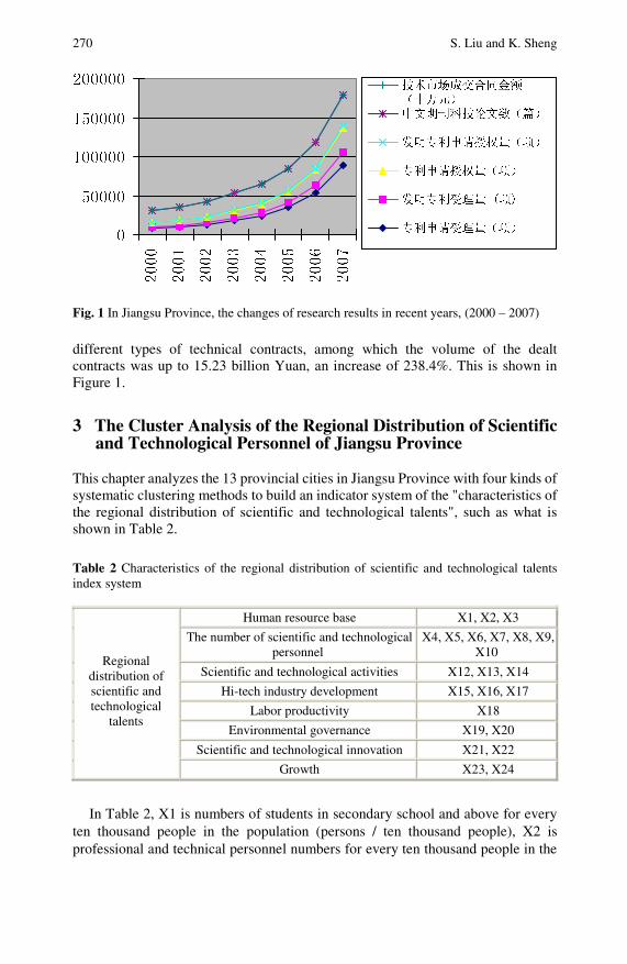
270 S. Liu and K. Sheng
Fig. 1 In Jiangsu Province, the changes of research results in recent years, (2000 – 2007)
different types of technical contracts, among which the volume of the dealt contracts was up to 15.23 billion Yuan, an increase of 238.4%. This is shown in Figure 1.
3 The Cluster Analysis of the Regional Distribution of Scientific and Technological Personnel of Jiangsu Province
This chapter analyzes the 13 provincial cities in Jiangsu Province with four kinds of systematic clustering methods to build an indicator system of the "characteristics of the regional distribution of scientific and technological talents", such as what is shown in Table 2.
Table 2 Characteristics of the regional distribution of scientific and technological talents index system
Human resource base X1, X2, X3
The number of scientific and technological personnel
X4, X5, X6, X7, X8, X9, X10
Scientific and technological activities X12, X13, X14
Hi-tech industry development X15, X16, X17
Labor productivity X18
Environmental governance X19, X20
Scientific and technological innovation X21, X22
Regional distribution of scientific and technological
talents
Growth X23, X24
In Table 2, X1 is numbers of students in secondary school and above for every ten thousand people in the population (persons / ten thousand people), X2 is professional and technical personnel numbers for every ten thousand people in the
0
50000
100000
150000
200000
2000
2001
2002
2003
2004
2005
2006
2007
技术市场成交合同金额(十万元)中文期刊科技论文数(篇)
发明专利申请授权量(项)
专利申请授权量(项)
发明专利受理量 (项)
专利申请受理量(项)
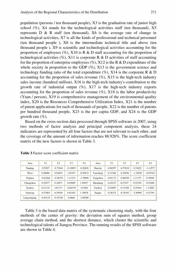
Analysis of the Regional Characteristics of the Distribution 271
population (persons / ten thousand people), X3 is the graduation rate of junior high school (%), X4 stands for the technological activities staff (ten thousand), X5 represents D & R staff (ten thousand), X6 is the average rate of change in technological activities, X7 is all the kinds of professional and technical personnel (ten thousand people ), X8 is the intermediate technical title and above (ten thousand people ), X9 is scientific and technological activities accounting for the proportion of employees (%), X10 is R & D staff accounting for the proportion of technological activities (%), X11 is corporate R & D activities of staff accounting for the proportion of enterprise employees (%), X12 is the R & D expenditure of the whole society in proportion to the GDP (%), X13 is the government science and technology funding ratio of the total expenditure (%), X14 is the corporate R & D accounting for the proportion of sales revenue (%), X15 is the high-tech industry sales income (hundred million), X16 is the high-tech industry's contribution to the growth rate of industrial output (%), X17 is the high-tech industry exports accounting for the proportion of sales revenue (%), X18 is the labor productivity (Yuan / person), X19 is comprehensive management of the environmental quality index, X20 is the Resources Comprehensive Utilization Index, X21 is the number of patent applications for each of thousands of people, X22 is the number of patents per hundred thousand people, X23 is the per capita GDP, and X24 is the GDP growth rate (%).
Based on the cross-section data processed through SPSS software in 2007, using two methods of factor analysis and principal component analysis, these 24 indicators are represented by all four factors that are not relevant to each other, and the coverage of the amount of information reaches 88.928%. The score coefficient matrix of the new factors is shown in Table 3.
Table 3 Factor score coefficient matrix
Area Y1 Y2 Y3 Y4 Area Y1 Y2 Y3 Y4
Nanjing 3.07657 -0.73644 -0.10093 -0.26836 Huai'an -0.80397 -0.57618 0.33622 -1.14577
Wuxi 0.48066 0.94835 1.02107 -0.56913 Yancheng -0.31566 -0.36456 -1.32638 -0.65542
Xuzhou -0.62266 -0.38378 1.11212 -1.39898 Yangzhou -0.01173 -0.86548 1.11757 0.76094
Changzhou 0.25877 0.16871 0.05609 1.49837 Zhenjiang -0.42147 0.27437 0.52194 0.92406
Suzhou 0.21134 2.81171 -0.66159 -0.5402 Taizhou -0.45887 -0.33189 0.25264 1.13885
Nantong -0.57803 0.39436 0.01452 1.19078 Suqian -0.36375 -0.78192 -2.40985 0.15794
Lianyungang -0.45119 -0.55726 0.0666 -1.09308
Table 3 is the based data matrix of the systematic clustering study, with the four methods of the center of gravity: the deviation sum of squares method, group average chain method, and the shortest distance, which cluster the scientific and technological talents of Jiangsu Province. The running results of the SPSS software are shown in Table 4.
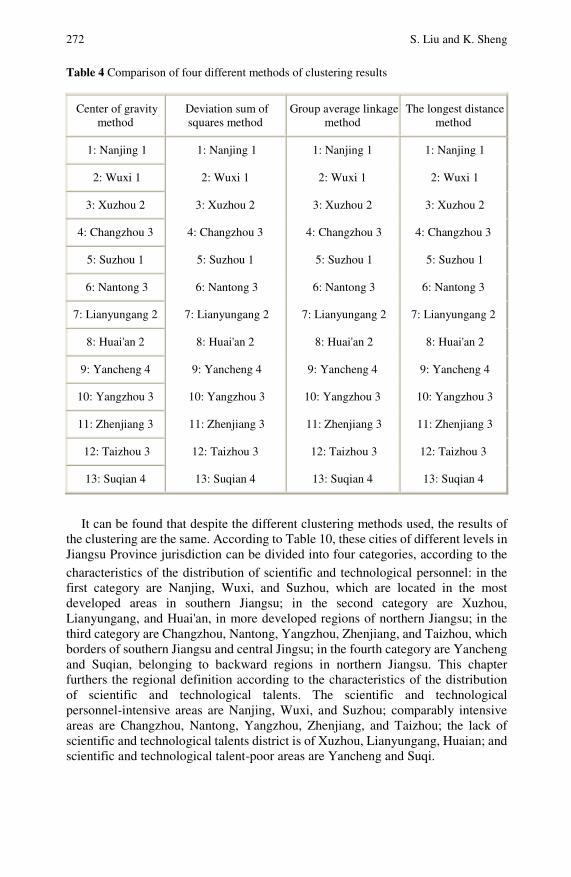
272 S. Liu and K. Sheng Table 4 Comparison of four different methods of clustering results
Center of gravity method
Deviation sum of squares method
Group average linkage method
The longest distance method
1: Nanjing 1 1: Nanjing 1 1: Nanjing 1 1: Nanjing 1
2: Wuxi 1 2: Wuxi 1 2: Wuxi 1 2: Wuxi 1
3: Xuzhou 2 3: Xuzhou 2 3: Xuzhou 2 3: Xuzhou 2
4: Changzhou 3 4: Changzhou 3 4: Changzhou 3 4: Changzhou 3
5: Suzhou 1 5: Suzhou 1 5: Suzhou 1 5: Suzhou 1
6: Nantong 3 6: Nantong 3 6: Nantong 3 6: Nantong 3
7: Lianyungang 2 7: Lianyungang 2 7: Lianyungang 2 7: Lianyungang 2
8: Huai'an 2 8: Huai'an 2 8: Huai'an 2 8: Huai'an 2
9: Yancheng 4 9: Yancheng 4 9: Yancheng 4 9: Yancheng 4
10: Yangzhou 3 10: Yangzhou 3 10: Yangzhou 3 10: Yangzhou 3
11: Zhenjiang 3 11: Zhenjiang 3 11: Zhenjiang 3 11: Zhenjiang 3
12: Taizhou 3 12: Taizhou 3 12: Taizhou 3 12: Taizhou 3
13: Suqian 4 13: Suqian 4 13: Suqian 4 13: Suqian 4
It can be found that despite the different clustering methods used, the results of the clustering are the same. According to Table 10, these cities of different levels in Jiangsu Province jurisdiction can be divided into four categories, according to the
characteristics of the distribution of scientific and technological personnel: in the first category are Nanjing, Wuxi, and Suzhou, which are located in the most developed areas in southern Jiangsu; in the second category are Xuzhou, Lianyungang, and Huai'an, in more developed regions of northern Jiangsu; in the third category are Changzhou, Nantong, Yangzhou, Zhenjiang, and Taizhou, which borders of southern Jiangsu and central Jingsu; in the fourth category are Yancheng and Suqian, belonging to backward regions in northern Jiangsu. This chapter furthers the regional definition according to the characteristics of the distribution of scientific and technological talents. The scientific and technological personnel-intensive areas are Nanjing, Wuxi, and Suzhou; comparably intensive areas are Changzhou, Nantong, Yangzhou, Zhenjiang, and Taizhou; the lack of scientific and technological talents district is of Xuzhou, Lianyungang, Huaian; and scientific and technological talent-poor areas are Yancheng and Suqi.
Analysis of the Regional Characteristics of the Distribution 273
4 The Typical Characteristics of the Regional Distribution of Scientific and Technological Personnel of Jiangsu Province
4.1 The Regional Distribution of Scientific and Technological Talents Has Apparently Become Non-equilibrium
View the results of the clustering, the uneven distribution of scientific and technological personnel in each city of Jiangsu Province and the regional economics mainly is the same as the development imbalances that are inseparable between geographical location, economic environment, and historical development in Jiangsu Province. The distribution of scientific and technological personnel in different kinds of regions has distinct characteristics.
Nanjing, Wuxi and Suzhou all belong to the southern Jiangsu area and are also the main gathering places of high-tech industry development, so it is nature for high-tech talent to gather there. Nanjing is a city; Jiangsu is the most concentrated with politics, economy, culture, science and technology, education, transportation, international markets, information and other resources, and it has the largest the number of research institutions and universities in the province, so its status and location advantages of are not accessible for other cities. Suzhou is located south of the fertile Yangtze River Delta. It is in this city that the new technology industry rapidly develops with an increased scale and speed, thus enhancing the whole economy of Suzhou at a constant rapid growth and drawing global attention to the emerging technological cities. Wuxi is located in Taihu Lake and is an important industrial and tourist city, having long been "little Shanghai". It is now renowned for its textile, microelectronics, machinery and industry. Taking new roads to industrialization with science and technology as support, southern Jiangsu forms electronic information, biological medicine, new materials and a number of high-tech industries, and the petrochemical industry, metallurgy, machinery and other traditional industries; it glows with a new vitality after a high-tech transformation.
From a geographical point of view, scientific and technological personnel-intensive areas are mainly located in the southern and central parts of Jiangsu and in the transition location. The cities in these areas emphasize the development of high-tech industries, and a crowd of more types of scientific and technological talents is also gathered here. To speed up the transformation of scientific and technological achievements of overseas students, Jiangsu Province has established a "talent zone" and vigorously given priority to the returned overseas Chinese talent. Along the Yangtze River in eight cities, Jiangsu establishes an employment zone in eight cities, except Nanjing, Wuxi, and Suzhou. "Talent special economic zones" strengthen science and technology entrepreneurship parks, high-tech incubator base construction, innovation and entrepreneurial excellence, and the students can build a "special platform," to attract more high-tech talent to join. At present, internationally renowned enterprises have stationed in the Changzhou High-tech Zone, so the high-tech region continues to absorb international advanced technology, and the high-tech economy continues to increase. Zhenjiang is the ship industry, and the development of the domestic part of the ship is on behalf of the shipbuilding technology level of our country's marine technology research and

274 S. Liu and K. Sheng
development. Jiangsu Science and Technology University has the mechanical strength of a domestic first-class engineering group and is located in Zhenjiang, as well as Jiangsu University. Zhenjiang has a more competitive edge over other cities in the shipping industry, scientific research, design and professional skills. Taizhou City has a state-level Torch Plan Project. Jiangyan is a car key components industry base and medicine and industrial base. There is a Russian cooperation along the Yangtze River in Taixing, Jiangsu, within the inside of the new material industrial park and the National "863" plan Chunlan Group industrial base. These are seven state-level, high-tech characteristic industry bases. Yangzhou, with its unique ecological, historical and cultural advantages, has a formation of cultural industries, and its eco-industry complements the modern economy; motor vehicles and parts, metal sheet processing and equipment manufacturing and semiconductor lighting are classified as state-level industrial bases. CAS application technology, R & D and industry Jan-based centers and similar institutions settle down here, so it will form high-tech enterprises in Yangzhou with a certain amount of momentum and will form a strong combined effect of scientific and technological talents. Nantong continuously increases the introduction of high-level personnel training efforts and organizes experts and academic leaders at all levels for selection and training. High-level professionals continue to increase.
Xuzhou, Lianyungang, and Huai'an, which are in the lack of scientific and technological talents district, are located in the northern Jiangsu area. They are also relatively well developed in the northern Jiangsu area. The Northern Jiangsu area, with an excellent natural environment and land, fresh water, non-metallic minerals and more abundant marine resources, has strong education and well-grounded, deep cultural heritage, abundant labor resources, and strong power in mining, machinery, marine, agriculture and other fields of scientific research. The construction of the Longhai industrial belt cities of Xuzhou and Lianyungang has brought new opportunities for development, and high-tech talent aggregation is higher. Huai'an city is located in the hinterland of the northern plains, and the main concentration of high-tech talent is in the Huai'an economic development zone.
Yancheng is located in the hinterland of the North Jiangsu Plain with an unbalanced development of the three industries in the region. Although the secondary industry takes a dominant position, the proportion of primary industry is still quite large; the third industries are not being developed. An irrational industrial structure causes sluggish growth in the electronics, machinery, medical and other high-tech industries, as well as poor high-tech talent. Suqian city has certain economic advantages because it has the coastal Longhai economic zones along the Yangtze River economic belt cross-radiation zone; but because of the region's weak economic foundation, long-term economic development lags behind, and the Suqian high-tech industry has not yet developed.
4.2 The Human Resource Base in Various Regions Is Quite Different
The development of higher education and the distribution of professional and technical personnel are the base of science and technology talent development.
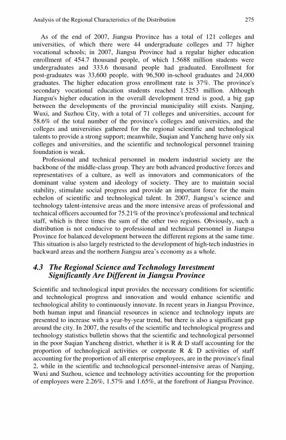
Analysis of the Regional Characteristics of the Distribution 275
As of the end of 2007, Jiangsu Province has a total of 121 colleges and universities, of which there were 44 undergraduate colleges and 77 higher vocational schools; in 2007, Jiangsu Province had a regular higher education enrollment of 454.7 thousand people, of which 1.5688 million students were undergraduates and 333.6 thousand people had graduated. Enrollment for post-graduates was 33,600 people, with 96,500 in-school graduates and 24,000 graduates. The higher education gross enrollment rate is 37%. The province's secondary vocational education students reached 1.5253 million. Although Jiangsu's higher education in the overall development trend is good, a big gap between the developments of the provincial municipality still exists. Nanjing, Wuxi, and Suzhou City, with a total of 71 colleges and universities, account for 58.6% of the total number of the province's colleges and universities, and the colleges and universities gathered for the regional scientific and technological talents to provide a strong support; meanwhile, Suqian and Yancheng have only six colleges and universities, and the scientific and technological personnel training foundation is weak.
Professional and technical personnel in modern industrial society are the backbone of the middle-class group. They are both advanced productive forces and representatives of a culture, as well as innovators and communicators of the dominant value system and ideology of society. They are to maintain social stability, stimulate social progress and provide an important force for the main echelon of scientific and technological talent. In 2007, Jiangsu’s science and technology talent-intensive areas and the more intensive areas of professional and technical officers accounted for 75.21% of the province's professional and technical staff, which is three times the sum of the other two regions. Obviously, such a distribution is not conducive to professional and technical personnel in Jiangsu Province for balanced development between the different regions at the same time. This situation is also largely restricted to the development of high-tech industries in backward areas and the northern Jiangsu area’s economy as a whole.
4.3 The Regional Science and Technology Investment Significantly Are Different in Jiangsu Province
Scientific and technological input provides the necessary conditions for scientific and technological progress and innovation and would enhance scientific and technological ability to continuously innovate. In recent years in Jiangsu Province, both human input and financial resources in science and technology inputs are presented to increase with a year-by-year trend, but there is also a significant gap around the city. In 2007, the results of the scientific and technological progress and technology statistics bulletin shows that the scientific and technological personnel in the poor Suqian Yancheng district, whether it is R & D staff accounting for the proportion of technological activities or corporate R & D activities of staff accounting for the proportion of all enterprise employees, are in the province's final 2, while in the scientific and technological personnel-intensive areas of Nanjing, Wuxi and Suzhou, science and technology activities accounting for the proportion of employees were 2.26%, 1.57% and 1.65%, at the forefront of Jiangsu Province.
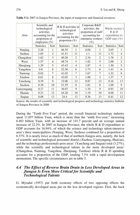
276 S. Liu and K. Sheng Table 5 In 2007 in Jiangsu Province, the input of manpower and financial resources
Scientific and technological
activities accounting for the
proportion of employees (%)
R & D activities in technological
activities accounting for the
proportion (%)
Corporate R&D activities, the
proportion of staff accounting for
enterprise workers (%)
Whole society’s R & D
expenditure to GDP ratio (%)
Area
Statistics Sort Statistics Sort Statistics Sort Statistics Sort Nanjing 2.26 1 46.55 1 4.04 1 2.65 1 Suzhou 1.65 2 41.51 11 1.1 11 1.72 4
Changzhou 1.62 3 40.26 2 2.34 2 1.78 3 Wuxi 1.57 4 48.74 5 1.82 5 2.00 2
Zhenjiang 1.29 5 43.43 4 1.87 4 1.50 5 Yangzhou 0.8 6 52.36 6 1.73 6 1.43 6 Nantong 0.62 7 41.02 7 1.67 7 1.22 8 Taizhou 0.61 8 43.05 3 1.88 3 1.37 7
Yancheng 0.39 9 32.06 12 0.87 12 0.16 13 Xuzhou 0.38 10 51.55 8 1.61 8 1.09 9
Lianyungang 0.27 11 36.07 9 1.34 9 0.93 10 Huaian 0.21 12 44.28 10 1.19 10 0.68 11 Suqian 0.08 13 24.4 13 0.36 13 0.41 12
Source: the results of scientific and technological progress and technology statistics bulletin of Jiangsu Province in 2008.
During the "Tenth Five-Year" period, the overall financial technology industry spent 11.057 billion Yuan, which is more than the "ninth five-year," increasing 6.483 billion Yuan, with an increase of 141.7 percent and an average annual increase of 22.2%. In 2007 in Jiangsu Province, the whole R & D expenditure to GDP accounts for 16.94%, of which the science and technology talent-intensive area’s three municipalities (Nanjing, Wuxi, Suzhou) combined for a proportion of 6.37%. It is nearly twice as much of that of northern Jiangsu area, namely, the lack of scientific and technological personnel district (Xuzhou, Lianyungang, Huai'an), and the technology professionals-poor areas’ (Yancheng and Suqian) total (3.27%), while the scientific and technological talents in the more developed areas’ (Changzhou, Nantong, Yangzhou, Zhenjiang, Taizhou) whole R & D spending accounts for a proportion of the GDP, totaling 7.3% with a rapid development momentum. The specific circumstances are in table 5.
4.4 The Effect of Reverse Brain Drain in Less Developed Areas in Jiangsu Is Even More Critical for Scientific and Technological Talents
G. Myradal (1957) put forth economy effects of two opposing effects the economically developed areas put on the less developed regions: First, the back

Analysis of the Regional Characteristics of the Distribution 277
effect, which is the performance of each factor of production from underdeveloped regions to developed regions, inevitably producing differences in the expansion of regional economic development. Secondly, the diffusion effect, which is the performance of each factor of production from the developed regions to developed regions so that the regional development differences are narrowing. Prior to reaching a critical point in the market mechanism, the return flow is much larger than the spillover effect, leading to more developed regions and less-developed regions. Looking at different regions of Jiangsu Province and their scientific and technological personnel changes, the return flow is typically much larger than the diffusion effect.
During the "Tenth Five-Year" period in Jiangsu Province, with a total of 13 municipal areas for technology professionals, major changes in the distribution pattern did not occur; at the first stage of the "Eleventh Five-Year", this trend had not been fundamentally reversed and even possibility of further exacerbated. Table 6 is for Jiangsu Province science and technology activities and R & D activities for the geographical distribution of staff. The table data shows that over 50% of workers’ science and technology activities are in Jiangsu Province, and R & D activities are concentrated in Nanjing, Wuxi, and Suzhou. There is an inadequate proportion for Suqian of 1%; Xuzhou, Huaian, Lianyungang, Yancheng and Suqian, are basically the first and second industry, and the high-tech industrial development is slow, so the economic development gap is further widened. The flow of scientific and technological personnel performance represents the grounds for the main flow in northern Jiangsu and the southern flow of small cities to major cities, namely, from the area lacking scientific and technological personnel and poor area-intensive areas to the talent-intensive scientific and technological areas. At present in Jiangsu Province, the imbalanced distribution of technological innovation for all kinds of talent are mostly concentrated in Nanjing, Suzhou, Wuxi and other cities in southern Jiangsu, especially in universities, research institutes, large enterprises and foreign-funded enterprises. However, in the northern small and medium cities, especially those in areas below the county-level, scientific and technological personnel are in shortage. For pay and benefits, social environment, living environment, personal career development and meeting the spiritual needs, such areas cannot compete with the large and medium cities in southern Jiangsu. On one hand, trained students and graduate students who are sent out are unwilling to return to work; on the other hand, most of the middle-aged experts with high-level technical positions are of the serious-tech brain drain. The reverse brain drain effect could lead to areas lacking scientific and technological personnel and poor areas of scientific and technological talent cities. The science and technology talent gap is serious, and the situation is more severe; particularly those small and medium-sized companies, which are rich in potential for development but face a severe manpower shortage.
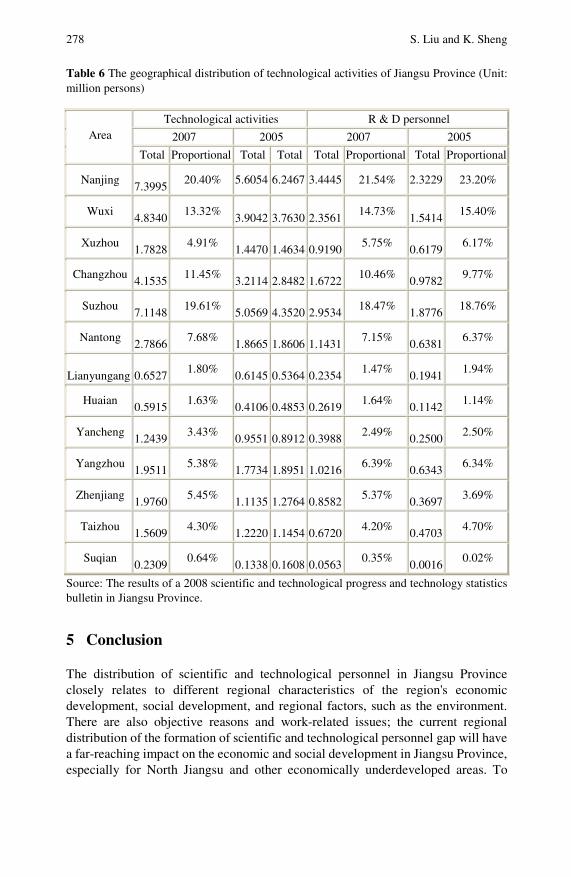
278 S. Liu and K. Sheng Table 6 The geographical distribution of technological activities of Jiangsu Province (Unit: million persons)
Technological activities R & D personnel
2007 2005 2007 2005 Area
Total Proportional Total Total Total Proportional Total Proportional
Nanjing
7.3995 20.40% 5.6054 6.2467 3.4445 21.54% 2.3229 23.20%
Wuxi
4.8340 13.32%
3.9042
3.7630
2.3561
14.73%
1.5414 15.40%
Xuzhou
1.7828 4.91%
1.4470
1.4634
0.9190
5.75%
0.6179 6.17%
Changzhou
4.1535 11.45%
3.2114
2.8482
1.6722
10.46%
0.9782 9.77%
Suzhou
7.1148 19.61%
5.0569
4.3520
2.9534
18.47%
1.8776 18.76%
Nantong
2.7866 7.68%
1.8665
1.8606
1.1431
7.15%
0.6381 6.37%
Lianyungang
0.6527
1.80%
0.6145
0.5364
0.2354 1.47%
0.1941
1.94%
Huaian
0.5915 1.63%
0.4106
0.4853
0.2619
1.64%
0.1142 1.14%
Yancheng
1.2439 3.43%
0.9551
0.8912
0.3988
2.49%
0.2500 2.50%
Yangzhou
1.9511 5.38%
1.7734
1.8951
1.0216
6.39%
0.6343 6.34%
Zhenjiang
1.9760 5.45%
1.1135
1.2764
0.8582
5.37%
0.3697 3.69%
Taizhou
1.5609 4.30%
1.2220
1.1454
0.6720
4.20%
0.4703 4.70%
Suqian
0.2309 0.64%
0.1338
0.1608
0.0563
0.35%
0.0016 0.02%
Source: The results of a 2008 scientific and technological progress and technology statistics bulletin in Jiangsu Province.
5 Conclusion
The distribution of scientific and technological personnel in Jiangsu Province closely relates to different regional characteristics of the region's economic development, social development, and regional factors, such as the environment. There are also objective reasons and work-related issues; the current regional distribution of the formation of scientific and technological personnel gap will have a far-reaching impact on the economic and social development in Jiangsu Province, especially for North Jiangsu and other economically underdeveloped areas. To
Analysis of the Regional Characteristics of the Distribution 279
reverse the current negative situation of the distribution of scientific and technological personnel and to relieve the pressure of demanding talents in echnology professional-poor areas (Yancheng and Suqian) and the manpower shortage areas (Xuzhou, Lianyungang, Huai'an), there is a need to work together in Jiangsu from top to bottom. In particular, mobilizing these two types of enthusiasm in the region, changing the idea of human resources work, and increasing personnel policy innovations are needed. On the other hand, there is a need for IT personnel in Jiangsu Province to further study the status of the regional distribution of deep-seated problems so that they can reveal the development of the internal mechanism and evolution in order to provide theoretical support for solving the problem of the development of more science and technology professionals in Jiangsu Province. A follow-up study associated with this chapter will focus on these areas.
References
Gui, Z.M., Hui, T.Y., Zhang, W.X., Cheng, F.: China’s scientific and technological human resources of the spatial distribution and structural characteristics of study. Science and Technology Progress and Policy (05) (2001)
Li, F.Z.: Chinese science and technology human resources, regional differences and types. Resource Development and the Market 21(1) (2005)
Science and Technology Department in Jiangsu Province (2008). The results of scientific and technological progress, science and technology statistics bulletin 2008 in Jiangsu. Jiangsu Science and Technology Information Network (October 2008)
The People’s Republic of China Ministry of Science (2008). Scientific and technological advancement through statistical monitoring results and technology bulletin. The People’s Republic of China Ministry of Science website (October 2008)
The People’s Republic of China National Bureau of Statistics. China Statistical Yearbook. China Statistics Press, Beijing (September 2009)
Wang, W.: China’s scientific and technological talents of excessive liquidity in the regional employment of game theory. Science and Technology Progress and Policy (05) (2006)
Zhou, G.R., Du, Z.: Regional distribution of China’s scientific and technological personnel problems and countermeasures. Journal of Tianjin Normal University (06) (2005)
Zuo, H.B.: Hubei scientific and technological personnel research report. Science and Technology Progress and Policy (11) (2004)
The Novel Energy Policy Evaluation Method and Its Application in Oil and Gas Fields in China
Jianjun Zhu, Sifeng Liu, Ningning Zhu, and Ye Ding1
With industrialization and urbanization constantly speeding up in China, the energy consumption grows rapidly. As the energy consumption rapidly increases, the energy production has been unable to meet the requirements of the energy consumption growth. Energy saving is mainly focused on energy-saving technologies and the choice of energy-saving measures, but the research of appraisal on energy conservation policies are few. Based on the property of the energy policy evaluation, the evaluation method of the three-point interval number comparison matrix is put forth to solve the problem of preference information that is often lost by modeling complex group decision-making processes. The proposed method’s consistency, weight estimation approach and group decision-making aggregation approach are studied. Based on the complete consistency definition of the three-point interval number matrix, a definition of the possible value error is introduced. Lastly, several energy policies on oil and gas fields in China are evaluated via the suggested approach, and it illustrates the steps and its validity.
1 Introduction
With industrialization and urbanization constantly speeding up in China, the energy consumption grows rapidly. The growth rate of the GDP in 2003 and 2004 was 9.5%, while the growth rate of energy consumption reached 15.33% and 15.24%, respectively, greatly exceeding the GDP growth rate. As energy consumption increases rapidly, energy production has been unable to meet the requirements of energy consumption growth since 1992. The energy gaps increased sharply from
Jianjun Zhu College of Economics and Management, Nanjing University of Aeronautics and Astronautics, Nanjing 210016, P.R. China Tel./Fax: 86-25-84896149 e-mail: [email protected]
Sifeng Liu, Ningning Zhu, and Ye Ding College of Economics and Management, Nanjing University of Aeronautics and Astronautics, Nanjing 210016, P.R. China

282 J. Zhu et al.
1998 to 2000, and it achieved a historical peak in 2000. The unit GDP energy consumption in 2002, 2003 and 2004 is 1.30, 1.36 and 1.43 tons of standard coal per thousand. Although the unit GDP energy consumption dropped in 2006, the energy use situation was still stern. High energy consumption often brings high pollution. In recent years, dust and smoke emissions in China haven’t been significantly reduced. The emissions of SO2 have increased gradually. The air pollution is serious, and the environmental situation is bad. The Chinese government is firmly determined in regards to energy consumption, and energy-saving policies appeared one by one. “The saving energy law of the People's Republic of China” brought China energy conservation work to the legal system track. The "11th Five-Year Plan" identified that the unit of the GDP will reduce 20 percent in 2010 compared to 2005. It was the first time energy conservation was established in the form of legal documents that must be completed. Although the government has the ambition to conserve energy, the energy conservation work encountered many obstacles. Energy-saving work faces tremendous pressure and challenges in the first year of the "11th Five-Year Plan". The effectiveness of the government’s energy conservation policy is actually the appraisal of the government energy conservation policies. In regards to fundamental energy conservation research, Klein (2004) discussed the DSS department, which the energy conservation project developed to support local authorities in implementing the energy conservation projects. Nandwani (2006) discussed Costa Rica's existing resource condition and its electricity generation, and the frugal energy condition that uses solar energy. At present, papers on energy saving mainly focus on their own research on energy-saving technologies and the choice of energy-saving measures, but the research on the appraisal of energy conservation policies are few.
Because of differences in knowledge structure, judgment level and individual preference, decision-makers express their judgment preferences via different structured decision-making processes (see Chiclana et al., 1998). Owing to the complexity and uncertainty of decision-making problems and the fuzziness of human thought, it is unrealistic to depict complex problems in the certain preference style. When investigating uncertain decision-making scenarios, some scholars focus on uncertain mathematical methods, such as interval numbers (see Zhu et al., 2004; Mikhailov, 2004; Bryson et al., 2000; Wang et al., 2005), fuzzy numbers (see Buckley et al., 2001; Zhu et al., 1999), the random theory (see Basak, 1998; Haines, 1998) and unascertained numbers (see Zhu et al., 2005; Liu et al., 1999; Wan et al., 2004). These are all widely used in the decision-making field. Based on existing studies (see Bu et al., 2001; Wang et al., 1996), the three-point interval number comparison matrix is suggested here as an alternative method of expressing the decision-maker’s uncertain preferences. For decision-making preference structures, group decision-making aggregation approaches include aggregation of the same kind of preference structure and the different kinds of preference structures. The study on the aggregation of the same kind of preference structure has received a deal of attention (see Beynon et al., 2000; Ray et al., 1998), but the study of the aggregation of the different kinds of preference structures is still a new field
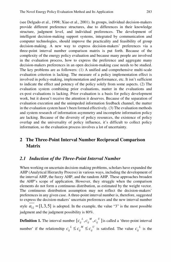
The Novel Energy Policy Evaluation Method and Its Application 283
(see Delgado et al., 1998; Xiao et al., 2001). In groups, individual decision-makers provide different preference structures, due to differences in their knowledge structure, judgment level, and individual preferences. The development of intelligent decision-making support systems, integrated by communication and computer technologies, should improve the practicality and feasibility of group decision-making. A new way to express decision-makers’ preferences via a three-point interval number comparison matrix is put forth. Because of the complexity of the energy policy evaluation and because many people are involved in the evaluation process, how to express the preference and aggregate many decision-makers preferences in an open decision-making case needs to be studied. The key problems are as followers: (1) A unified and comprehensive multi-scale evaluation criterion is lacking. The measure of a policy implementation effect is involved in policy-making, implementation and performance, etc. It isn’t sufficient to indicate the effect and potency of the policy solely from some aspects. (2) The evaluation system combining prior evaluations, matter in the evaluations and ex-post evaluations is lacking. Prior evaluation is a basis for policy development work, but it doesn’t receive the attention it deserves. Because of the separation of evaluation execution and the unimpeded information feedback channel, the matter in the evaluation system hasn’t been formed effectively. (3) The evaluation methods and system research of information asymmetry and incomplete information policy are lacking. Because of the diversity of policy resources, the existence of policy overlap and the universality of policy influence, it’s difficult to collect policy information, so the evaluation process involves a lot of uncertainty.
2 The Three-Point Interval Number Reciprocal Comparison Matrix
2.1 Induction of the Three-Point Interval Number
When working on uncertain decision-making problems, scholars have expanded the AHP (Analytical Hierarchy Process) in various ways, including the development of the interval AHP, the fuzzy AHP, and the random AHP. These approaches broaden the AHP’s scope of application. However, they struggle when the comparison elements do not form a continuous distribution, as estimated by the weight vector. The continuous distribution assumption may not reflect the decision-makers’ preferences in any given case. A three-point interval number is, therefore, suggested to express the decision-makers’ uncertain preferences and the new interval number
style 12 [1,3,5]a = is adopted. In the example, the value “3” is the most possible
judgment and the judgment possibility is 80%.
Definition 1. The interval number [ , , ]L M Uij ij ijc c c is called a ‘three-point interval
number’ if the relationship L M Uij ij ijc c c≤ ≤ is satisfied. The value L
ijc is the

284 J. Zhu et al.
lower possible value of the judgment, the value Uijc is the upper possible value,
and Mijc is the most possible judgment value.
When applying the three-point interval number in the decision-making process, a single decision-maker can adopt the two-point interval number to estimate the
upper and lower value [ , ]L Uij ijc c . Meanwhile, he should provide the most possible
judgment value Mijc according to his estimation. For group decision-making, a
statistical approach can be used to fit decision-makers’ preferences, and a three-point interval number judgment can be obtained. The distribution probability
of the most possible value ( ) ,ijP c δ δ≥ is constant, and its value is decided by
the decision-makers’ experience. Only when δ reaches a certain degree, can it be
called the most possible value. In group decision-making, if 60%δ < , it indicates that the preference is too diverse.
2.2 Consistency and Weight Estimation of Three-Point Interval Number Comparison Matrices
Definition 2. The comparison matrix ( , , )L M Uij ij ij n nC c c c ×= is called a
‘three-point interval number reciprocal comparison matrix’ where: L M U
ij ij ijc c c≤ ≤ , [1/ ,1/ ,1/ ]U M Lji ij ij ijc c c c= and [1,1,1]iic = .
This is a new way of expressing uncertain preferences using a three-point interval number composed of upper, lower and most possible values. The decision-makers’ real preference is amongst the upper, lower and most possible values, but it is difficult to ascertain. One cannot simply split the three-point interval number comparison matrix into a matrix composed of the lower judgment value, most possible value, and upper one. In addition, the matrix composed of upper and lower judgments may be non-consistent (see Zhu et al., 2004).
Definition 3. The set , 1, ,iw i n= is said to be the “weight” of a three-point
interval number reciprocal comparison matrix. If formula (1) is satisfied, the three-point interval number reciprocal comparison matrix is completely consistent.
If the , 1, ,iw i n= does not satisfy formula (1), the three-point interval number
reciprocal comparison matrix is not completely consistent.
, , 1, , ,L M Uiij ij ij
j
wc c c i j n i j
w≤ = ≤ = ≠ (1)

The Novel Energy Policy Evaluation Method and Its Application 285
If a matrix C is completely consistent, formula M iij
j
wc
w= is satisfied, which
means the decision-makers’ judgment corresponds to the most possible value. If C
is not completely consistent, M iij
j
wc
w≠ , or L i
ijj
wc
w≥ , or U i
ijj
wc
w≤ . Error
variables ,ij ijcpo cdo are introduced to the relationship of M iij
j
wc
w≠ , such that it
satisfies 0, 0, 0ij ij ij ijcpo cdo cpo cdo≥ ≥ × = . This satisfies formula (2):
0, , 1, , ,Mij j i ij ijc w w cpo cdo i j n i j− + − = = ≠ (2)
If formula (2) does not satisfy L Uiij ij
j
wc c
w≤ ≤ , the error variables ,ij ijcp cd
are introduced, with 0, 0ij ijcp cd≥ ≥ . This satisfies formula (3):
, , 1, , ,
, , 1, , ,
Lij j i ij
Ui ij j ij
c w w cp i j n i j
w c w cd i j n i j
⎧ ≤ + = ≠⎪⎨
≤ + = ≠⎪⎩ (3)
The lower the value of ,
ij iji j
cpo cdo+∑ , the shorter the deviation distance from
the most possible value Mijc . In addition, the lower the value of
,ij ij
i j
cp cd+∑ ,
the shorter the deviation distance from the upper and lower values. The better the
consistency of the three-point interval number comparison matrix, the lower the
values of ,
ij iji j
cpo cdo+∑ and ,
ij iji j
cp cd+∑ . One can record the error
as,
( ) ( )ij ij ij iji j
s cpo cdo t cp cd+ + +∑ , where s, t are constants that denote the
priority of these two errors. If ,
( ) ( ) minij ij ij iji j
s cpo cdo t cp cd+ + + →∑ , the
consistency of the three-point interval number comparison matrix is improved.
Based on these ideas, P1 is suggested to estimate the weight of the three-point
interval number comparison matrix:
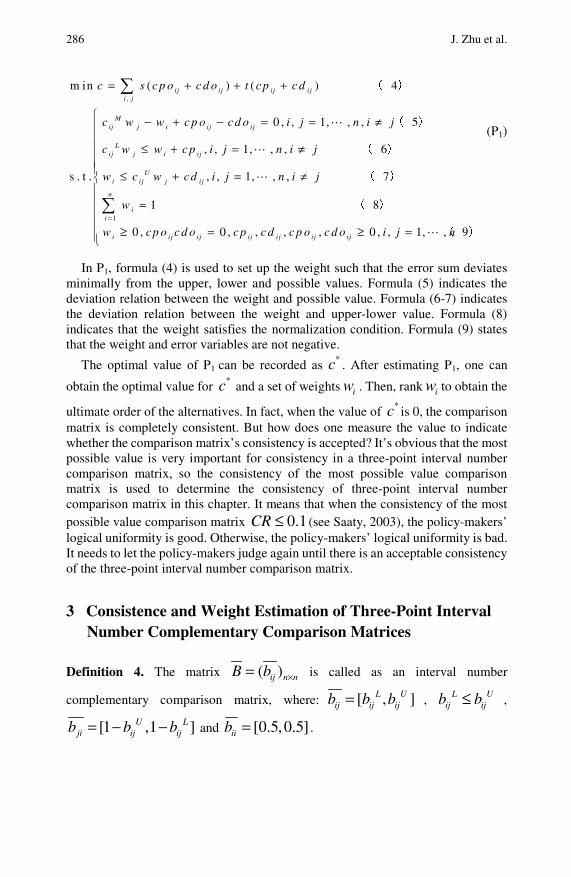
286 J. Zhu et al.
,
1
m in ( ) ( ) 4
0 , , 1, , , 5
, , 1, , , 6
s . t . , , 1, , , 7
1 8
0 , 0 , , , , 0 ,
i j i j i j i ji j
Mij j i ij i j
Lij j i i j
Ui ij j ij
n
ii
i ij i j i j i j i j i j
c s c p o c d o t c p c d
c w w c p o c d o i j n i j
c w w c p i j n i j
w c w cd i j n i j
w
w cp o c d o cp c d c p o c d o i=
= + + +
− + − = = ≠
≤ + = ≠
≤ + = ≠
=
≥ = ≥
∑
∑
( (
( (
( (
( (
( (
, 1, , 9j n
⎧⎪⎪⎪⎪⎪⎨⎪⎪⎪⎪ =⎪⎩
( (
(P1)
In P1, formula (4) is used to set up the weight such that the error sum deviates minimally from the upper, lower and possible values. Formula (5) indicates the deviation relation between the weight and possible value. Formula (6-7) indicates the deviation relation between the weight and upper-lower value. Formula (8) indicates that the weight satisfies the normalization condition. Formula (9) states that the weight and error variables are not negative.
The optimal value of P1 can be recorded as *c . After estimating P1, one can
obtain the optimal value for *c and a set of weights iw . Then, rank iw to obtain the
ultimate order of the alternatives. In fact, when the value of *c is 0, the comparison matrix is completely consistent. But how does one measure the value to indicate whether the comparison matrix’s consistency is accepted? It’s obvious that the most possible value is very important for consistency in a three-point interval number comparison matrix, so the consistency of the most possible value comparison matrix is used to determine the consistency of three-point interval number comparison matrix in this chapter. It means that when the consistency of the most possible value comparison matrix 0.1CR ≤ (see Saaty, 2003), the policy-makers’ logical uniformity is good. Otherwise, the policy-makers’ logical uniformity is bad. It needs to let the policy-makers judge again until there is an acceptable consistency of the three-point interval number comparison matrix.
3 Consistence and Weight Estimation of Three-Point Interval Number Complementary Comparison Matrices
Definition 4. The matrix ( )ij n nB b ×= is called as an interval number
complementary comparison matrix, where: [ , ]L Uij ij ijb b b= , L U
ij ijb b≤ ,
[1 ,1 ]U Lji ij ijb b b= − − and [0.5,0.5]iib = .
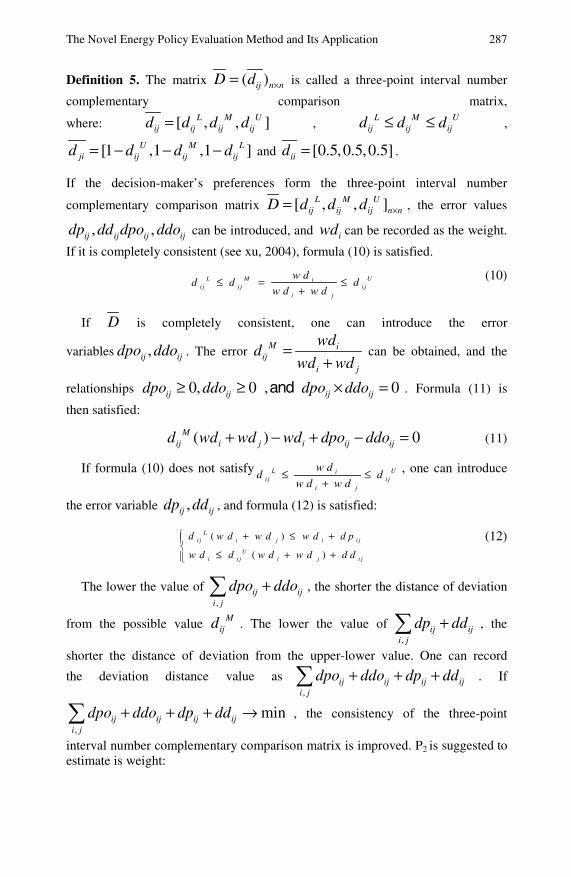
The Novel Energy Policy Evaluation Method and Its Application 287
Definition 5. The matrix ( )ij n nD d ×= is called a three-point interval number
complementary comparison matrix,
where: [ , , ]L M Uij ij ij ijd d d d= , L M U
ij ij ijd d d≤ ≤ ,
[1 ,1 ,1 ]U M Lji ij ij ijd d d d= − − − and [0.5,0.5,0.5]iid = .
If the decision-maker’s preferences form the three-point interval number
complementary comparison matrix [ , , ]L M Uij ij ij n nD d d d ×= , the error values
, ,ij ij ij ijdp dd dpo ddo can be introduced, and iwd can be recorded as the weight.
If it is completely consistent (see xu, 2004), formula (10) is satisfied.
L M Uii j i j i j
i j
w dd d d
w d w d≤ = ≤
+ (10)
If D is completely consistent, one can introduce the error
variables ,ij ijdpo ddo . The error M iij
i j
wdd
wd wd=
+ can be obtained, and the
relationships 0, 0ij ijdpo ddo≥ ≥ , 0ij ijdpo ddo× =and . Formula (11) is
then satisfied:
( ) 0Mij i j i ij ijd wd wd wd dpo ddo+ − + − = (11)
If formula (10) does not satisfy L Uii j i j
i j
w dd d
w d w d≤ ≤
+, one can introduce
the error variable ,ij ijdp dd , and formula (12) is satisfied:
( )
( )
Li j i j i i j
Ui i j i j i j
d w d w d w d d p
w d d w d w d d d
⎧ + ≤ +⎪⎨
≤ + +⎪⎩
(12)
The lower the value of ,
ij iji j
dpo ddo+∑ , the shorter the distance of deviation
from the possible value Mijd . The lower the value of
,ij ij
i j
dp dd+∑ , the
shorter the distance of deviation from the upper-lower value. One can record
the deviation distance value as,
ij ij ij iji j
dpo ddo dp dd+ + +∑ . If
,
minij ij ij iji j
dpo ddo dp dd+ + + →∑ , the consistency of the three-point
interval number complementary comparison matrix is improved. P2 is suggested to estimate is weight:
288 J. Zhu et al.
,
1
m i n
( ) 0
( ) , , 1 , , ,
s . t . ( ) , , 1 , , ,
1
0 , 0 , , , , 0 , , 1 , ,
i j i j i j i ji j
Mi j i j i i j i j
Li j i j i i j
Ui i j i j i j
n
ii
i i j i j i j i j i j i j
d d p d d d p o d d o
d w d w d w d d p o d d o
d w d w d w d d p i j n i j
w d d w d w d d d i j n i j
w d
w d d p o d d o d p d d d p o d d o i j n=
= + + +
⎧ + − + − =
+ ≤ + = ≠
≤ + + = ≠
=
≥ = ≥ =
∑
∑
⎪⎪⎪⎪⎪⎨⎪⎪⎪⎪⎪⎩
(P2)
Then the most possible value comparison matrix of the three-point interval number comparison matrix is changed to the reciprocal judgment matrix (see Xu, 2004). When the proportion of 0.1CR ≤ , the policy-makers’ logical uniformity is good. Otherwise, the policy-makers’ logical uniformity is bad. It needs to let the policy-makers judge again until there is an acceptable consistency of the most possible value comparison matrix.
4 Oil and Gas Energy Policy Evaluation in China via the Suggested Approach
4.1 Evaluate Policy and Background Analysis
The characters of the Chinese oil industry management system can be depicted as follows: firstly, the energy board is set up to manage Chinese energy affairs while the natural gas industry management function is still scattered in a number of comprehensive economic management and law enforcement departments. Secondly, the oil industry is the state's important energy sector. The majority of producers have almost set up a special body to manage the affairs. However, oil companies in China have been restructured. To strengthen management functions, energy policy, oil strategy and market regulators are put forth by the government. In fact, it is weakened, not uniform and unclear. The government is both the policy-making department and supervision department. It is lacking an effective supervision mechanism. The main policy of the oil and gas industry in China can be described as follows:
(1) The reform of the original. The notice of refined oil circulation system can be obtained. (State of the [1994] No. 21, April 5, 1994, China). The notification requires the government to do a good job comprehensively balancing demand and supply. The price of crude oil will be implemented by the government, and the circulation chain is reduced.
(2) The reform of crude oil price. The goals and principles of crude oil and the finished oil price formation mechanism are reformed. The price of the domestic will be set by consultation between the two sale sides. The price of gasoline and diesel oil will be instructed by the government.

The Novel Energy Policy Evaluation Method and Its Application 289
(3) The principle of the price of refined oil. "On the principle of refined oil price notice" requires the price of liquefied petroleum gas, kerosene lamps, chemical light oil, and heavy oil to be set by the companies of oil and petrochemical. Moreover, the price of the four oils must maintain a reasonable price. The ability of consumers’ purchasing abilities should be considered to adjust the price of civilian gas prices.
(4) The reform of oil price. Adjust the price of domestic oil products further and improve the oil price formation mechanism to achieve the international market price. The state council decided to further speed up the step of the oil price formation mechanism to achieve the international market price. The state development planning commission formulated the benchmark price in accordance to international market prices of crude oil and refined oil. Adjust once a month. It is to implement the state council's decision and is also an important indication of the formation mechanism.
(5) Chinese oil laws and regulations. Firstly, ownership of oil resources: the ownership of oil resources belongs to the countries. It will not change because of their attachment to land ownership and different uses. Secondly, oil mining rights: oil mining rights is an important part of property rights for the country's mineral resources. It is not only a result of a national ownership and executive power, but also a possibility of the pursuit of self-interest. They can be denoted as Chinese oil and gas fields’ typical major policies before 2000.
There are four policies, referred to as Policy P1, Policy P2, Policy P3, and Policy P4. Policy1, the oil and gas exploration and mining registered Interim Measures; Policy2, the State Council passed the State Development Planning Commission, State Economic and Trade Commission for the reform of crude oil, also finishing the oil circulation system views notice; Policy3, crude oil finished oil price reform program; Policy4, foreign cooperative exploitation of land mines to use oil resources to pay for temporary regulations.
4.2 Policy Appraisal Index System
Suppose m decision-makers are invited to make decisions (m≥2) on the goodness or badness of the oil and gas policy of Chinese situations. The three-point number reciprocal comparison matrix and three-point number complementary comparison matrix are adopted separately to express their preference. Example data are just for the suggested approach application steps.
During the process of policy-making (A), which includes: The need for policy-making (A1): It’s serious for policy-making and urgent for the implementation of policy-making objectively. The rationality of policy objectives (A2): It must be targeted, specific, non-ambiguous, clear expression. It also has to
290 J. Zhu et al.
be cleared whether it can be implemented with politics, the economy, culture, technology and individuals. Science of policy options (A3): It must be cleared that the policy options are set up at a reliable basis and have been full proofed. Is it flexible? Is it consistent with other policies in the internal and external fields? What are the benefits of policy implementation for the target groups, economy and society? What are the gains and losses for individuals, groups and society, materialistically and spiritually? Legitimacy of policy-making (A4): Inspect the entire policy-making. Make sure it has the scientific integrity of the policy-making process.
(2) During the Policy implementation (B), which includes: Policy acceptance (B1): Is the function of policy consistent with the functions of government behavior, company behavior and market behavior? Does the public, especially the objects of the policy, accept the policy? Main policy implementation (B2): There are specialized agencies, personnel and systems to ensure policy implementation. The policy staff must be a rational division of labor and have right to clear. They must communicate and coordinate effectively. The implementation staff must be professional, responsible and organized. Objects of policy (B3): The policy objects must have good acceptance, the ability and degree of policy implementation. Implementation supervision mechanisms (B4): There are specialized agencies to investigate the behavior of violating policies and revise them.
(3) Policy performance (C), which includes: The effect of policy implementation (C1): The realized degree of the policy predetermined target and the display degree of the policy must be controlled. The efficiency of policy implementation (C2): the gains and losses of input and output of the policies must be considered. The satisfaction of policy implementation (C3): the current and long-term, regional and overall influence of policies must be considered.
4.3 The Appraisal Process and Result Analysis
(1) Comparison matrix based on the target level According to the method of the three-point interval number comparison matrix in this chapter, the policy-maker carries the judgment based on the appraisal target. Then the three-point interval number comparison matrix can be set up. Considering the differences of policy-makers’ preferences, the reciprocal comparison matrix and supplementary comparison matrix of three-point interval number comparison matrix can be obtained. The processes of comparison matrixes are abbreviated.
(3) Result analysis According to the model proposed in this chapter, the weights of comparison matrixes can be obtained. It is shown in Table1.
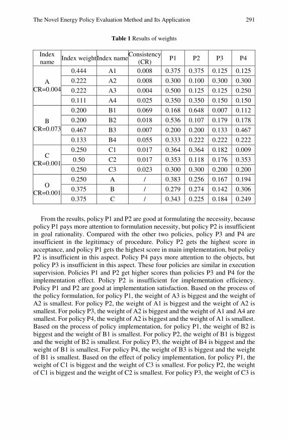
The Novel Energy Policy Evaluation Method and Its Application 291
Table 1 Results of weights
Index name
Index weight Index nameConsistency
(CR) P1 P2 P3 P4
0.444 A1 0.008 0.375 0.375 0.125 0.125
0.222 A2 0.008 0.300 0.100 0.300 0.300
0.222 A3 0.004 0.500 0.125 0.125 0.250 A
CR=0.004
0.111 A4 0.025 0.350 0.350 0.150 0.150
0.200 B1 0.069 0.168 0.648 0.007 0.112
0.200 B2 0.018 0.536 0.107 0.179 0.178
0.467 B3 0.007 0.200 0.200 0.133 0.467 B
CR=0.073
0.133 B4 0.055 0.333 0.222 0.222 0.222
0.250 C1 0.017 0.364 0.364 0.182 0.009
0.50 C2 0.017 0.353 0.118 0.176 0.353 C
CR=0.0010.250 C3 0.023 0.300 0.300 0.200 0.200
0.250 A / 0.383 0.256 0.167 0.194
0.375 B / 0.279 0.274 0.142 0.306 O
CR=0.0010.375 C / 0.343 0.225 0.184 0.249
From the results, policy P1 and P2 are good at formulating the necessity, because policy P1 pays more attention to formulation necessity, but policy P2 is insufficient in goal rationality. Compared with the other two policies, policy P3 and P4 are insufficient in the legitimacy of procedure. Policy P2 gets the highest score in acceptance, and policy P1 gets the highest score in main implementation, but policy P2 is insufficient in this aspect. Policy P4 pays more attention to the objects, but policy P3 is insufficient in this aspect. These four policies are similar in execution supervision. Policies P1 and P2 get higher scores than policies P3 and P4 for the implementation effect. Policy P2 is insufficient for implementation efficiency. Policy P1 and P2 are good at implementation satisfaction. Based on the process of the policy formulation, for policy P1, the weight of A3 is biggest and the weight of A2 is smallest. For policy P2, the weight of A1 is biggest and the weight of A2 is smallest. For policy P3, the weight of A2 is biggest and the weight of A1 and A4 are smallest. For policy P4, the weight of A2 is biggest and the weight of A1 is smallest. Based on the process of policy implementation, for policy P1, the weight of B2 is biggest and the weight of B1 is smallest. For policy P2, the weight of B1 is biggest and the weight of B2 is smallest. For policy P3, the weight of B4 is biggest and the weight of B1 is smallest. For policy P4, the weight of B3 is biggest and the weight of B1 is smallest. Based on the effect of policy implementation, for policy P1, the weight of C1 is biggest and the weight of C3 is smallest. For policy P2, the weight of C1 is biggest and the weight of C2 is smallest. For policy P3, the weight of C3 is
292 J. Zhu et al.
biggest and the weight of C2 is smallest. For policy P4, the weight of C2 is biggest and the weight of C1 is smallest. Overall, the order of these four policies is
1 4 2 3P P P P> > > .
5 Conclusion
In this chapter, a new energy policy evaluation method is suggested, which is based on the new uncertainty preference expression. As decision-making problems increase in complexity, more and more people join the decision-making process; group decision-making is now widely used. Decision-makers adopt wide varieties of preferences and preference structures, and it is often unrealistic to depict complex problems using definite preference techniques. To address this issue, a three-point interval number comparison matrix is suggested. This chapter discusses the consistency and weight estimation and proposes three-point interval number comparison matrices. This chapter presents a new uncertain mathematical method that solves the problem of preference information lost by many existing systems used to model complex group decision-making processes. Some theoretical questions should be studied in further work, specifically the availability of other effective approaches for weight estimation. For the research of the energy problem, the energy policy suggestions should also be considered.
Acknowledgements. This work is supported by the National Natural Science Foundation of China (70701017), the Education Department Human and Social Science Project of China (07JC630064), and the China Postgraduate Science Research Fund Project (2005038575).
References
Basak, I.: Probabilistic judgments specified partially in the analytic hierarchy process. European Journal of Operational Research 108, 153–164 (1998)
Bu, G., Zhang, Y.: Fuzzy comprehensive evaluation based on three parameters interval gray number. Engineering and Electronic Technology 23, 43–45 (2001)
Buckley, J., Feuring, T., Hayashi, Y.: Fuzzy hierarchical analysis revisited. European Journal of Operational Research 129, 48–64 (2001)
Beynon, M., Curry, B., Morgan, P.: The dempster-shafer theory of evidence: An alternative approach to multi-criteria decision modeling. Omega 28, 37–50 (2000)
Bryson, N., Joseph, A.: Generating consensus priority interval vectors for group decision-making in the AHP. Journal of Multi-Criteria Decision Analysis 9, 127–137 (2000)
Chiclana, F., Herrera, F.: Integrating three representation models in fuzzy multipurpose decision-making based in fuzzy preference relations. Fuzzy Sets and Systems 97, 33–48 (1998)
Delgado, M., Herrera, F., Herrera, V.: Combining numerical and linguistic information in-group decision-making. Information Sciences 107, 177–194 (1998)
The Novel Energy Policy Evaluation Method and Its Application 293 Haines, L.: A statistical approach to the analytic hierarchy process with interval judgments
distributions on feasible regions. European Journal of Operational Research 110, 112–125 (1998)
Klein, M.R.: Government Support for Energy Saving Projects. LNCS. Springer, Heidelberg (2004)
Liu, K., Wu, H., Pang, Y.: The Processing and Application of Uncertainty Information Mathematics. Science Press, Beijing (1999)
Mikhailov, L.: A fuzzy approach to deriving priorities from interval pairwise comparison judgments. European Journal of Operational Research 159, 687–704 (2004)
Nandwani, S.S.: Uses of solar energy in Costa Rica. Renewable Energy 31, 689–701 (2006) Ray, T., Triantaphyllou, E.: Evaluation of rankings with regard to the possible number of
agreements and conflicts. European Journal of Operational Research 106, 129–136 (1998)
Saaty, T.: Decision-making with the AHP: Why is the principal eigenvector necessary. European Journal of Operational Research 145, 85–91 (2003)
Wan, Y., Sheng, Z., Xin, H.: The unascertained analytic hierarchy process and its application in venture capital. Systems Engineering 22, 13–16 (2004)
Wang, Q.Y., Wang, F.S., Zuo, Q.: Gray Math Basis. Huazhong University of Science and Technology Press, Wuhan (1996)
Wang, Y.M., Yang, J.B., Xu, D.L.: A two–stage logarithmic goal alternative programming methods for generating weights from interval comparison matrices. Fuzzy Sets and Systems 152, 475–498 (2005)
Xiao, S.H., Fan, Z.P., Wang, M.G.: Integrated approach to two judgment matrices in group decision-making. Control and Decision 16, 569–572 (2001)
Xu, Z.S.: Uncertain Multi-Attribute Decision-Making Method and Its Application. Tsinghua University Press, Beijing (2004)
Zhu, J.J., Wang, M.G., Liu, S.X.: Estimation of weight vectors of interval numbers judgment matrix in AHP using genetic algorithm. Journal of Systems Engineering 19, 344–350 (2004)
Zhu, J.J., Wang, M.G., Liu, S.X.: Research on application of new uncertainty model in analytical hierarchy process. Journal of Management Sciences in China 8, 15–19 (2005)
Zhu, K., Jing, Y.: A discussion on extent analysis method and applications of fuzzy AHP. European Journal of Operational Research 116, 450–456 (1999)

Part IV Grey Forecast Model

The Comparison of Transfer Model and Metabolism GM(1,1) Model in Fuzhou Port’s Throughput Prediction*
Kejia Chen, Jiaying Chen, and Qishan Zhang
Both transfer model and metabolism GM (1, 1) model are usually used to establish dynamic prediction model. This chapter applies these two models to Fuzhou port’s throughput prediction and compares the results. The results show that both models can obtain satisfying predicted values. Furthermore, metabolism GM (1, 1) needs fewer data and performs better in terms of prediction accuracy.
1 Introduction
Ports are key infrastructures and play great roles in the economy progress. The development of a port can be reflected by its throughput. The port’s throughput prediction is an important part in the port development strategy study. The correct throughput prediction is of significance to the reasonable port layout and trans-portation planning (Fung, 2002; Lam et al., 2004; Chen and Zhao, 2006).
Different prediction models have different modeling methodologies and are adopted in various situations. The preferred models are the ones that need few data, have simple procedure, and perform well in most conditions. Both transfer model and metabolism GM (1, 1) model are usually used to establish dynamic prediction model. This chapter applies these two models to Fuzhou port’s throughput predic-tion and compares the results. The results show that both models can obtain satis-fying predicted values. Furthermore, metabolism GM (1, 1) needs fewer data and Kejia Chen School of Management, Fuzhou University, P.R. China
Phone: 86-591-22866463; Fax: 86-591-22866402 e-mail: [email protected]
Jiaying Chen and Qishan Zhang School of Management, Fuzhou University, P.R. China e-mail: [email protected], [email protected]
* This work is financially supported by National Natural Science Foundation of China under the project of 70871024, Fujian Natural Science Foundation of China under the project of 2009J05159, Fujian Social Science Foundation of China under the project of 2008A020, Social Scientific Research Fund of Fujian Provincial Education Department of China under the project of JA07017S, and Talent Foundation of Fuzhou University under the project of XRC-0635.

298 K. Chen, J. Chen, and Q. Zhang
performs better in terms of prediction accuracy. For recent works on the GM(1,1) model, please consult with (Lin et al., 2002; Sydow, Lin, et al., 2001; Lin and Liu, 2000).
2 Transfer Model Prediction
A. Transfer Model
In real economic systems, the influence of one economic variable on another one often appears some periods later, not immediately. In order to better describe this dynamic process, we introduce transfer model.
Transfer model, which is also called ARIMAX model, is a multivariate time se-ries model and is the combination of time series analysis and regression analysis.
The procedure of building a transfer model includes three steps: model identifi-cation, parameter estimation and diagnostic testing. Before building a model, we often require that the behavioral sequence is stable. However, in practice, this re-quirement often can not be satisfied. Thus, we usually use difference operation to make it stable. For one input variable, denote X as the input variable and Y as the response variable.
iktii
i
itd
L
LX
L
LuY ε
φθ
φω
)(
)(
)(
)(, ++=∇ −∑ (1)
where ∇: difference operator, d: difference order, u: mean, L: lag operator, k: k-th lag, εt: error term, satisfying E(εt)=0, Var(εt)=σ2, Cov(εi,εj)≠0 (i≠j).
For )(Liω , )(Liφ , )(Lθ and )(Lφ , we have
s
q
nniiii
hhiiii
LLLL
LLLL
LLLLL
LLLLL
s
q
φφφ
θθθ
φφφφ
ωωωω
+−−=
+−−=
−−−−=
−−−−=
1
1
22,1,
,2
2,1,
1)(
1)(
1)(
1)(
(2)
The difference between transfer model and ARMA model is that transfer model should whiten the input variable before computing the cross correlation coefficient between the response variable and the input variable. In other words, we can em-ploy Box-Jaenkins to establish ARMA model for the input variable sequence and make it whitened (Elliott et al., 2006; Box et al., 2008).
B. Prediction Results
Generally, the port’s throughput in one area depends on the economic development level in that area. Therefore, we select Fuzhou’s gross domestic product (GDP) as the input variable and Fuzhou port’s throughput (Y) as the response variable (TABLE I).
First, we use the data in 1980-2004 as the sample and predict the values in 2005-2006.
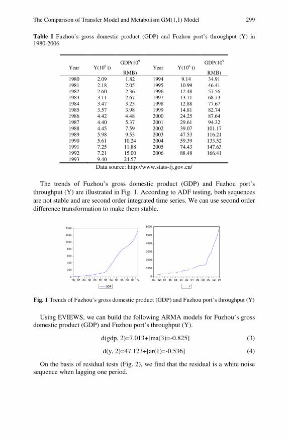
The Comparison of Transfer Model and Metabolism GM(1,1) Model 299 Table I Fuzhou’s gross domestic product (GDP) and Fuzhou port’s throughput (Y) in 1980-2006
Year Y(106 t) GDP(109
RMB) Year Y(106 t)
GDP(109
RMB) 1980 2.09 1.82 1994 9.14 34.91 1981 2.18 2.05 1995 10.99 46.41 1982 2.60 2.36 1996 12.48 57.56 1983 3.11 2.67 1997 13.71 68.73 1984 3.47 3.25 1998 12.88 77.67 1985 3.57 3.98 1999 14.81 82.74 1986 4.42 4.48 2000 24.25 87.64 1987 4.40 5.37 2001 29.61 94.32 1988 4.45 7.59 2002 39.07 101.17 1989 5.98 9.53 2003 47.53 116.21 1990 5.61 10.24 2004 59.39 133.52 1991 7.25 11.88 2005 74.43 147.63 1992 7.21 15.00 2006 88.48 166.41 1993 9.40 24.57
Data source: http://www.stats-fj.gov.cn/ The trends of Fuzhou’s gross domestic product (GDP) and Fuzhou port’s
throughput (Y) are illustrated in Fig. 1. According to ADF testing, both sequences are not stable and are second order integrated time series. We can use second order difference transformation to make them stable.
0
200
400
600
800
1000
1200
1400
80 82 84 86 88 90 92 94 96 98 00 02 04
GDP
0
1000
2000
3000
4000
5000
6000
80 82 84 86 88 90 92 94 96 98 00 02 04
Y
Fig. 1 Trends of Fuzhou’s gross domestic product (GDP) and Fuzhou port’s throughput (Y)
Using EVIEWS, we can build the following ARMA models for Fuzhou’s gross
domestic product (GDP) and Fuzhou port’s throughput (Y).
d(gdp, 2)=7.013+[ma(3)=-0.825] (3)
d(y, 2)=47.123+[ar(1)=-0.536] (4)
On the basis of residual tests (Fig. 2), we find that the residual is a white noise sequence when lagging one period.
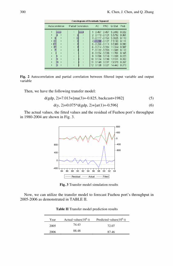
300 K. Chen, J. Chen, and Q. Zhang
Fig. 2 Autocorrelation and partial correlation between filtered input variable and output variable
Then, we have the following transfer model:
d(gdp, 2)=7.013+[ma(3)=-0.825, backcast=1982] (5)
d(y, 2)=0.075*d(gdp, 2)+[ar(1)=-0.596] (6)
The actual values, the fitted values and the residual of Fuzhou port’s throughput in 1980-2004 are shown in Fig. 3.
-400
0
400
800
-800
-400
0
400
800
84 86 88 90 92 94 96 98 00 02 04
Residual Actual Fitted
Fig. 3 Transfer model simulation results
Now, we can utilize the transfer model to forecast Fuzhou port’s throughput in
2005-2006 as demonstrated in TABLE II.
Table II Transfer model prediction results
Year Actual values(106 t) Predicted values(106 t)
2005 74.43 72.07
2006 88.48 87.46
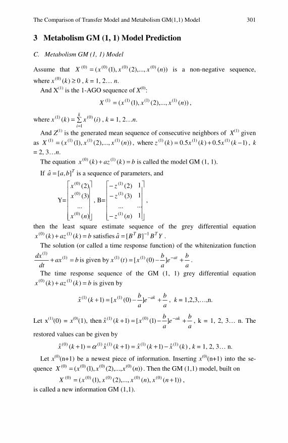
The Comparison of Transfer Model and Metabolism GM(1,1) Model 301
3 Metabolism GM (1, 1) Model Prediction
C. Metabolism GM (1, 1) Model
Assume that ))(),...,2(),1(( )0()0()0()0( nxxxX = is a non-negative sequence,
where 0)()0( ≥kx , k = 1, 2… n.
And X(1) is the 1-AGO sequence of X(0):
))(),...,2(),1(( )1()1()1()1( nxxxX = ,
where ∑==
k
iixkx
1
)0()1( )()( , k = 1, 2…n.
And Z(1) is the generated mean sequence of consecutive neighbors of X(1) given
as ))(),...,2(),1(( )1()1()1()1( nxxxX = , where )1(5.0)(5.0)( )1()1()1( −+= kxkxkz , k
= 2, 3…n.
The equation bkazkx =+ )()( )1()0( is called the model GM (1, 1).
If Tbaa ],[ˆ = is a sequence of parameters, and
Y=
⎥⎥⎥⎥⎥
⎦
⎤
⎢⎢⎢⎢⎢
⎣
⎡
)(
...
)3(
)2(
)0(
)0(
)0(
nx
x
x
, B=
⎥⎥⎥⎥⎥
⎦
⎤
⎢⎢⎢⎢⎢
⎣
⎡
−
−−
1
...
1
1
)(
...
)3(
)2(
)1(
)1(
)1(
nz
z
z
,
then the least square estimate sequence of the grey differential equation
bkazkx =+ )()( )1()0( satisfies YBBBa TT 1][ˆ −= .
The solution (or called a time response function) of the whitenization function
baxdt
dx =+ )1()1(
is given bya
be
a
bxtx at +−= −])0([)( )1()1( .
The time response sequence of the GM (1, 1) grey differential equation
bkazkx =+ )()( )1()0( is given by
a
be
a
bxkx ak +−=+ −])0([)1(ˆ )1()1( , k = 1,2,3,…,n.
Let x(1)(0) = x(0)(1), thena
be
a
bxkx ak +−=+ −])1([)1(ˆ )0()1( , k = 1, 2, 3… n. The
restored values can be given by
)(ˆ)1(ˆ)1(ˆ)1(ˆ )1()1()1()1()0( kxkxkxkx −+=+=+ α , k = 1, 2, 3… n.
Let x(0)(n+1) be a newest piece of information. Inserting x(0)(n+1) into the se-
quence ))(),...,2(),1(( )0()0()0()0( nxxxX = . Then the GM (1,1) model, built on
))1(),(),...,2(),1(( )0()0()0()0()0( += nxnxxxX ,
is called a new information GM (1,1).
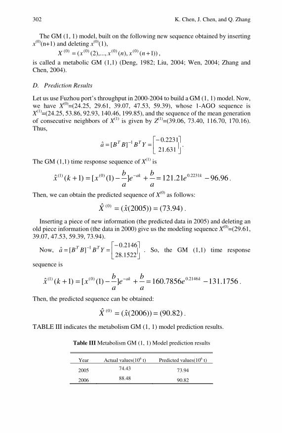
302 K. Chen, J. Chen, and Q. Zhang
The GM (1, 1) model, built on the following new sequence obtained by inserting x(0)(n+1) and deleting x(0)(1),
))1(),(),...,2(( )0()0()0()0( += nxnxxX ,
is called a metabolic GM (1,1) (Deng, 1982; Liu, 2004; Wen, 2004; Zhang and Chen, 2004).
D. Prediction Results
Let us use Fuzhou port’s throughput in 2000-2004 to build a GM (1, 1) model. Now, we have X(0)=(24.25, 29.61, 39.07, 47.53, 59.39), whose 1-AGO sequence is X(1)=(24.25, 53.86, 92.93, 140.46, 199.85), and the sequence of the mean generation of consecutive neighbors of X(1) is given by Z(1)=(39.06, 73.40, 116.70, 170.16). Thus,
⎥⎦
⎤⎢⎣
⎡−== −
631.21
2231.0][ˆ 1 YBBBa TT .
The GM (1,1) time response sequence of X(1) is
96.9621.121 ])1([)1(ˆ 2231.0)0()1( −=+−=+ − kak ea
be
a
bxkx .
Then, we can obtain the predicted sequence of X(0) as follows:
)94.73())2005(ˆ(ˆ )0( == xX .
Inserting a piece of new information (the predicted data in 2005) and deleting an old piece information (the data in 2000) give us the modeling sequence X(0)=(29.61, 39.07, 47.53, 59.39, 73.94).
Now, ⎥⎦
⎤⎢⎣
⎡−== −
1522.28
2146.0][ˆ 1 YBBBa TT . So, the GM (1,1) time response
sequence is
1756.1317856.160 ])1([)1(ˆ 2146.0)0()1( −=+−=+ − kak ea
be
a
bxkx .
Then, the predicted sequence can be obtained:
)90.82( ))2006(ˆ(ˆ )0( == xX .
TABLE III indicates the metabolism GM (1, 1) model prediction results.
Table III Metabolism GM (1, 1) Model prediction results
Year Actual values(106 t) Predicted values(106 t)
2005 74.43 73.94
2006 88.48 90.82
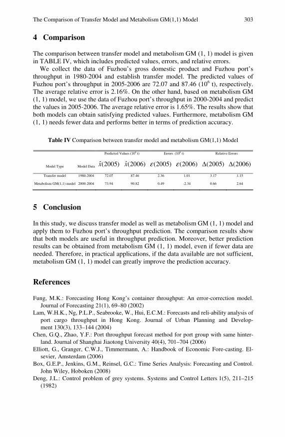
The Comparison of Transfer Model and Metabolism GM(1,1) Model 303
4 Comparison
The comparison between transfer model and metabolism GM (1, 1) model is given in TABLE IV, which includes predicted values, errors, and relative errors.
We collect the data of Fuzhou’s gross domestic product and Fuzhou port’s throughput in 1980-2004 and establish transfer model. The predicted values of Fuzhou port’s throughput in 2005-2006 are 72.07 and 87.46 (106 t), respectively. The average relative error is 2.16%. On the other hand, based on metabolism GM (1, 1) model, we use the data of Fuzhou port’s throughput in 2000-2004 and predict the values in 2005-2006. The average relative error is 1.65%. The results show that both models can obtain satisfying predicted values. Furthermore, metabolism GM (1, 1) needs fewer data and performs better in terms of prediction accuracy.
Table IV Comparison between transfer model and metabolism GM(1,1) Model
Predicted Values (106 t) Errors (106 t) Relative Errors
Model Type Model Data )2005(x )2006(x )2005(ε )2006(ε )2005(Δ )2006(Δ
Transfer model 1980-2004 72.07 87.46 2.36 1.01 3.17 1.15
Metabolism GM(1,1) model 2000-2004 73.94 90.82 0.49 -2.34 0.66 2.64
5 Conclusion
In this study, we discuss transfer model as well as metabolism GM (1, 1) model and apply them to Fuzhou port’s throughput prediction. The comparison results show that both models are useful in throughput prediction. Moreover, better prediction results can be obtained from metabolism GM (1, 1) model, even if fewer data are needed. Therefore, in practical applications, if the data available are not sufficient, metabolism GM (1, 1) model can greatly improve the prediction accuracy.
References
Fung, M.K.: Forecasting Hong Kong’s container throughput: An error-correction model. Journal of Forecasting 21(1), 69–80 (2002)
Lam, W.H.K., Ng, P.L.P., Seabrooke, W., Hui, E.C.M.: Forecasts and reli-ability analysis of port cargo throughput in Hong Kong. Journal of Urban Planning and Develop-ment 130(3), 133–144 (2004)
Chen, G.Q., Zhao, Y.F.: Port throughput forecast method for port group with same hinter-land. Journal of Shanghai Jiaotong University 40(4), 701–704 (2006)
Elliott, G., Granger, C.W.J., Timmermann, A.: Handbook of Economic Fore-casting. El-sevier, Amsterdam (2006)
Box, G.E.P., Jenkins, G.M., Reinsel, G.C.: Time Series Analysis: Forecasting and Control. John Wiley, Hoboken (2008)
Deng, J.L.: Control problem of grey systems. Systems and Control Letters 1(5), 211–215 (1982)

304 K. Chen, J. Chen, and Q. Zhang Liu, S.F.: Emergence and development of grey systems theory and its forward trends. Journal
of Nanjing University of Aeronautics and Astronautics 36(2), 267–272 (2004) Wen, K.L.: Grey Systems: Modeling and Prediction. Yang’s Scientific Press, Tucson (2004) Zhang, Q.S., Chen, G.H.: Rough grey set. Kybernetes 33(2), 336–452 (2004) Lin, Y., DeNu, R., Patel, N.: True distance fit of exponential curves and tests of applications.
International J. of Applied Mathematics 9(1), 49–68 (2002) Sydow, A., Lin, Y., Liu, S.-F., DeNu, R., Mennell, W.: Exponential prediction models based
on sequence operators. Kybernetes 30(4), 397–410 (2001) Lin, Y., Liu, S.F.: Law of exponentiality and exponential curve fitting. Systems Analysis
Modelling Simulation 38, 621–636 (2000)
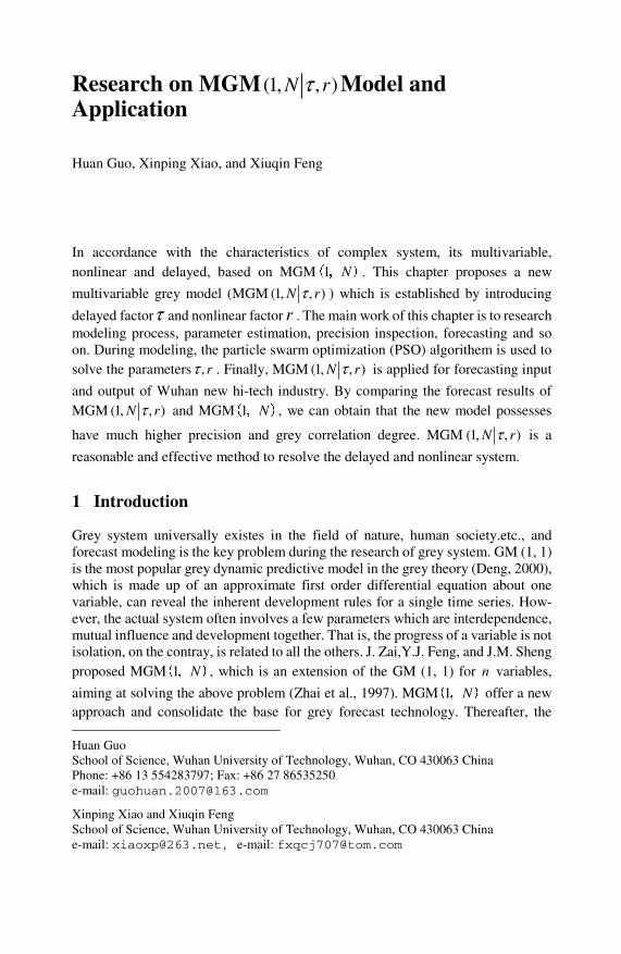
Research on MGM (1, , )N rτ Model and Application
Huan Guo, Xinping Xiao, and Xiuqin Feng*
In accordance with the characteristics of complex system, its multivariable, nonlinear and delayed, based on MGM 1 N(, ). This chapter proposes a new
multivariable grey model (MGM (1, , )N rτ ) which is established by introducing
delayed factorτ and nonlinear factor r . The main work of this chapter is to research modeling process, parameter estimation, precision inspection, forecasting and so on. During modeling, the particle swarm optimization (PSO) algorithem is used to solve the parameters , rτ . Finally, MGM (1, , )N rτ is applied for forecasting input
and output of Wuhan new hi-tech industry. By comparing the forecast results of MGM (1, , )N rτ and MGM 1 N(, ), we can obtain that the new model possesses
have much higher precision and grey correlation degree. MGM (1, , )N rτ is a
reasonable and effective method to resolve the delayed and nonlinear system.
1 Introduction
Grey system universally existes in the field of nature, human society.etc., and forecast modeling is the key problem during the research of grey system. GM (1, 1) is the most popular grey dynamic predictive model in the grey theory (Deng, 2000), which is made up of an approximate first order differential equation about one variable, can reveal the inherent development rules for a single time series. How-ever, the actual system often involves a few parameters which are interdependence, mutual influence and development together. That is, the progress of a variable is not isolation, on the contray, is related to all the others. J. Zai,Y.J. Feng, and J.M. Sheng proposed MGM 1 N(, ), which is an extension of the GM (1, 1) for n variables,
aiming at solving the above problem (Zhai et al., 1997). MGM 1 N(, ) offer a new approach and consolidate the base for grey forecast technology. Thereafter, the Huan Guo School of Science, Wuhan University of Technology, Wuhan, CO 430063 China Phone: +86 13 554283797; Fax: +86 27 86535250 e-mail: [email protected]
Xinping Xiao and Xiuqin Feng School of Science, Wuhan University of Technology, Wuhan, CO 430063 China e-mail: [email protected], e-mail: [email protected]
306 H. Guo, X. Xiao, and X. Feng
model has been extensively used in city programming, society economic forecast-ing, mode controlling, and has got good results in application, as in (Chen and Zhang, 2005; Xiao et al., 2008; Xu et al., 2006; Wang et al., 2006).
MGM 1 N(, ) is approximate first order differential equations, which reflects that the change of a variable in t lies on the value of others in t . Whereas practical system has delayed effect universally, that is to say, the input in t impacts not only the output and change at t but also the output and change after t . Comprehensively considering the nonlinear and delayed of system, Professor J.L. Deng structured GM (1, 1|τ, r) based on GM (1, 1) (Deng, 2001a). He also presented matrix form of the model and the parameter range (Deng, 2001b; 2001c). The model was widely applied in port resource distribution, economic policy modulate and so on, and has obtained the very good effect (Huang and Kuo, 2004; Zhang and Zou, 2002). Nevertheless, the study about the delayed and nonlinear of a complex system is few till now. As in the input and output system of new hi-tech industry, the factors which influence the total output value are not independent but correlated with the input and return of each other, and it is not a simple linear correlation. Furthermore, the effect of the input in t , which is not one-off, will influence return not only in t but also after t . Generally speaking, delayed effects is more significant. As we all know, the present grey model are seldom considering the delayed and nonlinear. Therefore, Based on MGM 1 N(, ), we propose a new model MGM (1, , )N rτ by
introducing delay factor and nonlinear factor, then apply the model to analyze and forecast the input and output of wuhan new hi-tech industry simultaneously. Finally, the simulation and forecast results are given to show the reasonable and effective of the proposed model.
2 Modeling
Let ( ) ( ) ( ) ( ) ( ) ( ) ( )( )0 0 0 01 2i i i ix x x x m= , , , be a time series,
and ( ) ( ) ( ) ( ) ( ) ( ) ( )( )1 1 1 11 2i i i ix x x x m= , , , denote the sequence obtained
through accumulating generation; that is
( ) ( ) ( ) ( )1 0
1
k
i ij
x k x j=
=∑ (1)
where 1,2, ,i N= and N is the number of time-series; 1, 2, ,k m= and
k denotes the time. Considering the relationship and influence of one another of n time-series, Reference (Zhai et al., 1997) extended the differential equation of GM 1 N(, ) as follows:
( ) ( ) ( ) ( ) ( ) ( ) ( ) ( )1
1 1 1111 1 12 2 1 1n n
dx ta x t a x t a x t u
dt= + + + +

Research on MGM Model and Application 307
( ) ( ) ( ) ( ) ( ) ( ) ( ) ( )1
1 1 1221 1 22 2 2 2n n
dx ta x t a x t a x t u
dt= + + + + (2)
( ) ( ) ( ) ( ) ( ) ( ) ( ) ( )1
1 1 11 1 2 2
nn n nn n n
dx ta x t a x t a x t u
dt= + + + +
Noting ( ) ( ) ( ) ( ) ( ) ( ) ( ) ( )( )0 0 0 01 2, ,...,
T
nX k x k x k x k= , ( ) ( ) ( ) ( ) ( ) ( ) ( ) ( )( )1 1 1 11 2, ,...,
T
nX k x k x k x k= ,
11 12 1
21 22 2
1 2
n
n
n n nn
a a a
a a aA
a a a
⎡ ⎤⎢ ⎥⎢ ⎥=⎢ ⎥⎢ ⎥⎣ ⎦
, ( )1 2, ,...,T
nU u u u= , the matrix representation
of (2) is as follows:
( ) ( ) ( ) ( )1
1dX tAX t U
dt= + (3)
Based on the above model, introducing delay factorτ and nonlinear factor r , the
differential equation of MGM 1 N(, ) is changed as following:
( ) ( ) ( ) ( ) ( )( ) ( ) ( ) ( )
11 1
1
1 12
( ) 1
2 r
dX tAX t B X t
dt
B X t B X t Utτ τ
= + −
+ − + + − +
(4)
where t τ≥ , 1, 2,...,l τ= , and
11 12 1
21 22 2
1 2
l l ln
l l ln
l
l l ln n nn
b b b
b b bB
b b b
⎡ ⎤⎢ ⎥⎢ ⎥=⎢ ⎥⎢ ⎥⎢ ⎥⎣ ⎦
Therefore
( ) ( ) ( ) ( ) ( ) ( )1
1 1
1
rl
l
dX tAX t B X t l Ut
dt
τ
=
= + − +∑ (5)
Supposing ( ) ( ) ( ) ( ) ( ) ( )0 0 01 2, ,..., nx t x t x t are equidistant discrete time-series, the
grey differential equation of (5) is following:
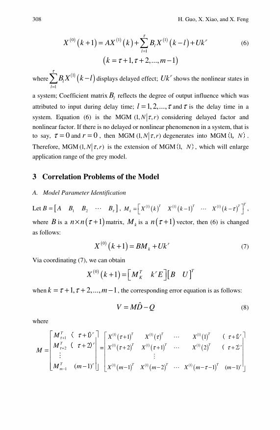
308 H. Guo, X. Xiao, and X. Feng
( ) ( ) ( ) ( ) ( ) ( )0 1 1
1
1 rl
l
X k AX k B X k l Ukτ
=+ = + − +∑
(6)
( )1, 2,..., 1k mτ τ= + + −
where( ) ( )1
1l
l
B X k lτ
=
−∑ displays delayed effect; rUk shows the nonlinear states in
a system; Coefficient matrix lB reflects the degree of output influence which was
attributed to input during delay time; 1, 2,...,l τ= andτ is the delay time in a
system. Equation (6) is the MGM (1, , )N rτ considering delayed factor and
nonlinear factor. If there is no delayed or nonlinear phenomenon in a system, that is to say, 0τ = and 0r = , then MGM (1, , )N rτ degenerates into MGM 1 N(, ).
Therefore, MGM (1, , )N rτ is the extension of MGM 1 N(, ), which will enlarge
application range of the grey model.
3 Correlation Problems of the Model
A. Model Parameter Identification
Let [ ]1 2B A B B Bτ= , ( ) ( ) ( ) ( ) ( ) ( )1 1 11TT T T
kM X k X k X k τ⎡ ⎤= − −⎣ ⎦ ,
where B is a ( )1n n τ× + matrix, kM is a ( )1n τ + vector, then (6) is changed
as follows:
( ) ( )0 1 rkX k BM Uk+ = + (7)
Via coordinating (7), we can obtain
( ) ( ) [ ]0 1TT r
KX k M k E B U⎡ ⎤+ = ⎣ ⎦
when 1, 2,..., 1k mτ τ= + + − , the corresponding error equation is as follows:
ˆV MD Q= − (8)
where
1
2
1
1
2
( 1)
T r
T r
T rm
M
MM
M m
τ
τ
ττ
+
+
−
⎡ ⎤+⎢ ⎥+⎢ ⎥=⎢ ⎥⎢ ⎥
−⎢ ⎥⎣ ⎦
( )
( ) =
( ) ( ) ( ) ( ) ( ) ( )( ) ( ) ( ) ( ) ( ) ( )
( ) ( ) ( ) ( ) ( ) ( )
1 1 1
1 1 1
1 1 1
1 1 1
2 1 2 2
1 2 1 ( 1)
T T T r
T T T r
T T T r
X X X
X X X
X m X m X m m
τ τ τ
τ τ τ
τ
⎡ ⎤+ +⎢ ⎥⎢ ⎥+ + +⎢ ⎥⎢ ⎥⎢ ⎥− − − − −⎣ ⎦
( )
( )
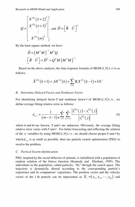
Research on MGM Model and Application 309
( ) ( )( ) ( )
( ) ( )
0
0
0
2
3
T
T
T
X
XQ
X m
τ
τ
⎡ ⎤+⎢ ⎥⎢ ⎥+= ⎢ ⎥⎢ ⎥⎢ ⎥⎣ ⎦
, and ˆ ˆ ˆ T
D B U⎡ ⎤= ⎣ ⎦
By the least-square method, we have:
( ) 1ˆ T TD M M M Q−
=
( ) 1ˆ ˆ ˆ T T TB U D Q M M M−⎡ ⎤ = =⎣ ⎦
Based on the above analysis, the time response formula of MGM (1, , )N rτ is as
follows:
( ) ( ) ( ) ( ) ( ) ( )0 1 1
1
ˆ 1 rl
l
X k AX k B X k l Ukτ
=+ = + − +∑
B. Determine Delayed Factor and Nonlinear Factor
For identifying delayed factorτ and nonlinear factor r of MGM (1, , )N rτ , we
define average fitting relative error as follows:
( )
( ) ( ) ( ) ( )( ) ( )
0 0
, 01 2
ˆ1
1
n mi i
ri j i
x j x j
m n x jτ
τε
τ = = +
−=
− − ∑ ∑ (9)
where n and m are known, τ and r are unknown. Obviously, the average fitting relative error varies withτ and r . For better forecasting and reflecting the relation
of the n variables by using MGM (1, , )N rτ , we should choose properτ and r by
which ,rτε is as small as possible, then use particle swarm optimization (PSO) to
resolve the problem.
C. Partical Swarm Optimization
PSO, inspired by the social behavior of animals, is initiallized with a population of random solution of the fitness function (Kennedy and Eberhart, 1995). The individuals in the population, called particles, “fly” through the search space. The trajectory is dynamiclly altered according to the corresponding particle’s experience and its companions’ experience. The position vector and the velocity
vector of the i th particle can be represented as 1 2, , ,i i i imX x x x=( ) and
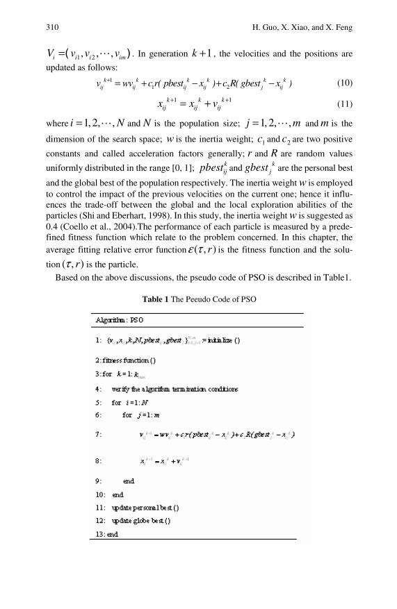
310 H. Guo, X. Xiao, and X. Feng
1 2, , ,i i i imV v v v=( ) . In generation 1k + , the velocities and the positions are
updated as follows: 1
1 2k k k k k k
ij ij ij ij j ijv wv c r( pbest x ) c R( gbest x )+ = + − + − (10)
1 1k k kij ij ijx x v+ += + (11)
where 1,2, ,i N= and N is the population size; 1, 2, ,j m= and m is the
dimension of the search space; w is the inertia weight; 1c and 2c are two positive
constants and called acceleration factors generally; r and R are random values
uniformly distributed in the range [0, 1]; kijpbest and k
jgbest are the personal best
and the global best of the population respectively. The inertia weight w is employed to control the impact of the previous velocities on the current one; hence it influ-ences the trade-off between the global and the local exploration abilities of the particles (Shi and Eberhart, 1998). In this study, the inertia weight w is suggested as 0.4 (Coello et al., 2004).The performance of each particle is measured by a prede-fined fitness function which relate to the problem concerned. In this chapter, the average fitting relative error function ( , )rε τ is the fitness function and the solu-
tion ( , )rτ is the particle.
Based on the above discussions, the pseudo code of PSO is described in Table1.
Table 1 The Peeudo Code of PSO
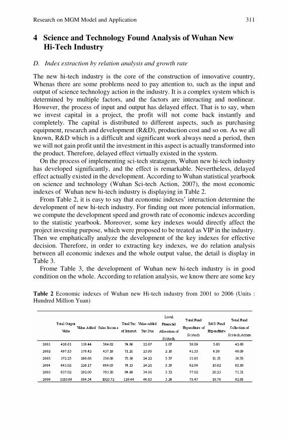
Research on MGM Model and Application 311
4 Science and Technology Found Analysis of Wuhan New Hi-Tech Industry
D. Index extraction by relation analysis and growth rate
The new hi-tech industry is the core of the construction of innovative country, Whenas there are some problems need to pay attention to, such as the input and output of science technology action in the industry. It is a complex system which is determined by multiple factors, and the factors are interacting and nonlinear. However, the process of input and output has delayed effect. That is to say, when we invest capital in a project, the profit will not come back instantly and completely. The capital is distributed to different aspects, such as purchasing equipment, research and development (R&D), production cost and so on. As we all known, R&D which is a difficult and significant work always need a period, then we will not gain profit until the investment in this aspect is actually transformed into the product. Therefore, delayed effect virtually existed in the system.
On the process of implementing sci-tech stratagem, Wuhan new hi-tech industry has developed significantly, and the effect is remarkable. Nevertheless, delayed effect actually existed in the development. According to Wuhan statistical yearbook on science and technology (Wuhan Sci-tech Action, 2007), the most economic indexes of Wuhan new hi-tech industry is displaying in Table 2.
From Table 2, it is easy to say that economic indexes’ interaction determine the development of new hi-tech industry. For finding out more potencial information, we compute the development speed and growth rate of economic indexes according to the statistic yearbook. Moreover, some key indexes would directly affect the project investing purpose, which were proposed to be treated as VIP in the industry. Then we emphatically analyze the development of the key indexes for effective decision. Therefore, in order to extracting key indexes, we do relation analysis between all economic indexes and the whole output value, the detail is display in Table 3.
Frome Table 3, the development of Wuhan new hi-tech industry is in good condition on the whole. According to relation analysis, we know there are some key
Table 2 Economic indexes of Wuhan new Hi-tech industry from 2001 to 2006 (Units : Hundred Million Yuan)
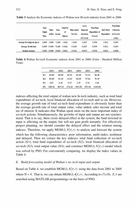
312 H. Guo, X. Xiao, and X. Feng Table 3 Analyze the Economic indexes of Wuhan new Hi-tech industry from 2001 to 2006
Table 4 Wuhan Sci-tech Economic indexes from 2001 to 2006 (Units : Hundred Million Yuan)
indexes affecting the total output of wuhan new hi-tech industry, such as total fund expenditure of sci-tech, local financial allocation of sci-tech and so on. However, the average growth rate of total sci-tech fund expenditure is obviously faster than the average growth rate of total output value, value added, sales income and total tax of interest. It indicates that Wuhan spent more on the most important index of sci-tech actions. Simultaneously, the growths of input and output are not synchro-nized. That is to say, there exists delayed effect in the system, the fund invested in input is affecting on the output, but will not gain profit instantly. For effectively project planning, we should consider the delayed effect and the relation among indexes. Therefore, we apply MGM (1, , )N rτ to analyze and forecast the system
which has the following characteristics: poor information, multi-index, nonlinear and delayed. Then we extract the key indexes: total fund collection of sci-tech action (X1), total fund expenditure of sci-tech (X2), local financial allocation of sci-tech (X3), total output value (X4), and construct MGM (1, , )N rτ model which
was solved by PSO. For conveniently comparing, we display the index values in Table 4.
E. Build forecasting model of Wuhan’s sic-tech input and output
Based on Table 4, we establish MGM (1, , )N rτ using the data from 2001 to 2005
where N 4= . That is, we can obtain MGM (1,4 , )rτ . According to (7)-(9), , rτ are
searched using MATLAB programmings on the basis of PSO.
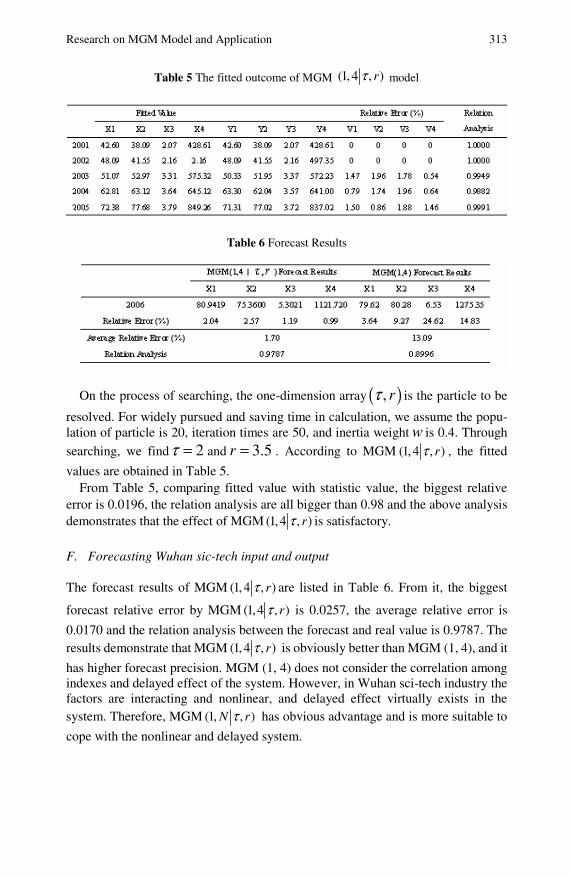
Research on MGM Model and Application 313
Table 5 The fitted outcome of MGM (1,4 , )rτ model
Table 6 Forecast Results
On the process of searching, the one-dimension array ( ), rτ is the particle to be
resolved. For widely pursued and saving time in calculation, we assume the popu-lation of particle is 20, iteration times are 50, and inertia weight w is 0.4. Through
searching, we find 2τ = and 3.5r = . According to MGM (1,4 , )rτ , the fitted
values are obtained in Table 5. From Table 5, comparing fitted value with statistic value, the biggest relative
error is 0.0196, the relation analysis are all bigger than 0.98 and the above analysis demonstrates that the effect of MGM (1,4 , )rτ is satisfactory.
F. Forecasting Wuhan sic-tech input and output
The forecast results of MGM (1,4 , )rτ are listed in Table 6. From it, the biggest
forecast relative error by MGM (1,4 , )rτ is 0.0257, the average relative error is
0.0170 and the relation analysis between the forecast and real value is 0.9787. The results demonstrate that MGM (1,4 , )rτ is obviously better than MGM (1, 4), and it
has higher forecast precision. MGM (1, 4) does not consider the correlation among indexes and delayed effect of the system. However, in Wuhan sci-tech industry the factors are interacting and nonlinear, and delayed effect virtually exists in the system. Therefore, MGM (1, , )N rτ has obvious advantage and is more suitable to
cope with the nonlinear and delayed system.

314 H. Guo, X. Xiao, and X. Feng
5 Conclusion
Grey modeling and forecasting are important issues in grey system theory. Re-searching on grey modeling, which is nonlinear and delayed, we are expected to make the grey system theory itself to be more and more close to the essence of practical problems. By comprehensive consideration of nonlinear and delay, this chapter proposed MGM (1, , )N rτ and made detailed elaboration on the process of
modeling, parameter estimation and model testing. What’s more, combining with statistical data of Wuhan science and technology, based on PSO, we have pro-grammed the grey model on MATLAB, simulated and forecasted the input and output of Wuhan new hi-tech industry using this model simultaneously. By com-paring simulation and forecasting result with MGM 1 N(, ), we can see that this model is effective to resolve the delay and nonlinear states of systems. As the practical system is nonlinear, there are interrelated constraints and interactions between variables, and the delay phenomenon is increasingly outstanding, referring to the above questions in practical system, how to make decisions is difficult for obtaining optimal input and output. The MGM (1, , )N rτ can commendably resolve
the difficult problem. Therefore, MGM (1, , )N rτ has broad application prospects
in the complex system, but the more abstract theory of the model need further study.
References
Chen, X.Z., Zhang, X.J.: Application of multi-factored grey MGM (1, N) model to the load-strain relation. Mechanical Science and Technology 24, 1475–1478 (2005)
Coello, C., Pulido, G., Lechuga, M.: Handling multiple objectives with particle swarm op-timization. IEEE Trans. Evolutionary Computation 3, 256–279 (2004)
Deng, J.L.: Grey System Theory & Applications, ch. 2. Cao-Li publishing Co., Taipei (2000) Deng, J.L.: A novel grey model GM (1,1|τ, r): Generalizing GM (1,1). Journal of Grey
System 13, 1–8 (2001a) Deng, J.L.: Solution of grey differential equation for GM (1, 1|τ, r) in matrix train. Journal of
Grey System 13, 105–110 (2001b) Deng, J.L.: On boundary of parameters in GM (1, 1|τ, r). Journal of Grey System 13, 199–200
(2001c) Huang, W.C., Kuo, M.S.: Application of GM (1,1| τ, r) to analyze the ports for putting in
resources. Journal of Grey System 16, 211–220 (2004) Kennedy, J., Eberhart, R.: Particle swarm optimization. In: 1995 Proc. IEEE Int. Conf.
Neural Network, pp. 1942–1948 (1995) Lin, Y., Chen, M.Y., Liu, S.F.: Theory of grey systems: capturing uncertainties of grey
information. Kybernetes: The International Journal of Systems and Cybernetics 33(2), 196–218 (2004)
Lin, Y., Liu, S.F.: Solving Problems with incomplete information: a grey systems approach. In: Advances in Imaging and Electron Physics, vol. 141, pp. 77–174. Elsevier, Oxford (2006)
Liu, S.F., Lin, Y.: Grey Information: Theory and Practical Applications. Springer, London (2006)

Research on MGM Model and Application 315 Shi, Y., Eberhart, R.: Parameter selection in particle swarm optimization. In: 1998 Proc.
Evolutionary Programming. Conf., pp. 591–600 (1998) Wang, W.X., Zhang, W., Cui, H.R., Liu, B.: Application of grey multi-variable model MGM
(1,N) in the R&D investment forecast. R&D Management 18(2), 32–37 (2006) Wuhan Sci-tech Action, Wuhan Statistical Yearbook on Science and Technology. New
Hi-tech Industry, 2001-2006, ch. 1-2. Wuhan Science and Technology Bureau (2007) Xiao, P., Lee, S.G., Zhang, J.: Forecasting of gas emissions based on MGM (1, N) model.
Journal of Xi’an University of Science and Technology 28(2), 301–305 (2008) Xu, H.F., Zhe, X.R., Chen, B.: Application of grey model MGM (1, N) to deformation
monitoring of deep excavation. Industrial Construction 36(11), 83–86 (2006) Zhai, J., Feng, Y.J., Sheng, J.M.: The grey model MGM (1,N) and its application. Systems
Engineering-Theory & Practice 5, 109–113 (1997) Zhang, P., Zou, S.G.: Grey evaluating the policy repayment via GM (1, 1| τ, r). Journal of
Grey System 14, 45–48 (2002)

A Modified GM(1,1) Model and Its Application
Peirong Ji, Hongbo Zou, and Xinyu Hu
A modified GM (1, 1) model is constructed by producing new data sequence with the method of transforming every datum of raw data sequence into its n-th root. It is demonstrated that the property of the modified GM (1, 1) model is superior to GM (1, 1) model by numerical experiment. Moreover the modified model is applied in the prediction of fruit price index in China. The actual results also show that the modified model is more accurate.
1 Introduction
Grey forecasting model (GM (1, 1) model) (Deng, 2002; Tsai and Yang, 2003; Lin et al., 2002; Sydow et al., 2001; Lin and Liu, 2000) presented by Professor Deng Julong, has been successfully used in many fields. The model is fit for non-negative raw data, which accords with or basically accords with exponential form and doesn’t have quick growth rate (Wang and He, 1990; Xiong and Chen, 1992 ; Ji et al., 1997). The literature (Ji et al., 2007) interprets that GM (1, 1) model is useful when the change of the raw data sequence is slower; otherwise GM (1, 1) model is useless. In this chapter, the authors put forward a modified GM (1, 1) model. The results of statistical experiment show that the accuracy of the modified GM (1, 1) model is better than that of GM (1, 1) model. And the modified GM (1, 1) model is used to model the fruit price index in China from 2001 to 2006. The results show the accuracy of the model is very high and the prediction of fruit price index in China from year 2007 to 2014 is also given in the chapter. Peirong Ji College of Electrical engineering and information technology, China Three Gorges University, Yichang 443002, China Phone: 13094169343; Fax: 86-717-6394492 e-mail: [email protected]
Hongbo Zou College of Electrical engineering and information technology, China Three Gorges University, Yichang 443002, China Phone:13886722903; Fax: 86-717-6394492 e-mail: [email protected]
Xinyu Hu College of Electrical engineering and information technology, China Three Gorges University, Yichang 443002, China e-mail: [email protected]

318 P. Ji, H. Zou, and X. Hu
2 GM (1,1) Model
Let (0) (0) (0) (0)(1), (2), (3)..., ( )x x x x N be a raw sequence,
and (0) ( ) 0, 1,2,...,x k k N≥ = .Using these data to build GM (1, 1) model, the
steps are as follows:
(1) Give (1)x by applying first-order accumulating generation operator (1-AGO)
on (0)x
(1) (0)
1
( ) ( ), 1,2,...,k
m
x k x m k n=
= =∑ (1)
(2) Ascertain data matrixes B , NY
( ) ( )
( ) ( )
( ) ( )
(1) (1)
(1) (1)
(1) (1)
11 2 1
21
2 3 12
11 1
2
x x
x xB
x N x N
⎛ ⎞⎡ ⎤− +⎜ ⎟⎣ ⎦⎜ ⎟⎜ ⎟⎡ ⎤− +⎣ ⎦⎜ ⎟=⎜ ⎟⎜ ⎟⎜ ⎟
⎡ ⎤− +⎜ ⎟⎣ ⎦⎝ ⎠ ,
(0)
(0)
(0)
(2)
(3)
( )
N
x
xY
x N
⎡ ⎤⎢ ⎥⎢ ⎥=⎢ ⎥⎢ ⎥⎣ ⎦
(3) Solve the parameter column
[ ] ( ) 1ˆ ˆ
T T TNa u B B B Y
−= (2)
(4) Establish the model of new data sequence
(1)(1)dx
a x udt
∧ ∧+ = (1) (0) ˆˆ ˆ
ˆ ( 1) ( (1) ) , 1, 2,...ˆ ˆ
aku ux k x e k
a a−+ = − + = (3)
(5) Establish the model of raw data sequence
(0) (0)ˆ (1) (1)x x= (4)
(0) (1) (1)ˆ ˆ ˆ( ) ( ) ( 1)x k x k x k= − −
(0) ( 1)ˆ ˆˆ(1 )( (1) ) , 2,3...
ˆka au
e x e ka
− − −= − − = (5)
where (0)ˆ ( ), 1,2,...,x k k N= are called fitting values of the raw data se-
quence ( ) ( )0 , 1,2,...,x k k N= , while (0)ˆ ( ),x k k N> are called prediction
values of the raw data sequence

A Modified GM(1,1) Model and Its Application 319
3 Characteristics of GM(1,1) Model
We have given a detail analysis on the characteristics of GM (1, 1) model in (Ji et al., 2007). Some key contents of the analysis are repeated here for convenience of the readers of the chapter.
A. Formula Development
Assume a system ( ) atx t Ae= is written in a discrete form:
(0) ( 1)( ) , 1, 2,..., ,...a kx k Ae k N−= = (6)
Take the first N items as the raw data sequence, the first-order accumulating gen-eration sequence is:
(1) 1( ) , 1,2,...,
1
ak
a
ex k A k N
e
−= =−
(7)
Construct a GM(1,1) model, then
2
2 3
( 1)
1 21
2 1
1 21
2 1... ...
1 21
2 1
a a
a
a a
a
N a Na
a
e eA
e
e eA
B e
e eA
e
−
⎡ ⎤− −−⎢ ⎥−⎢ ⎥− −⎢ ⎥−⎢ ⎥= −⎢ ⎥
⎢ ⎥⎢ ⎥− −⎢ ⎥−
−⎣ ⎦
,
(0)
(0)
(0)
(2)
(3)
...
( )
N
x
xY
x N
⎡ ⎤⎢ ⎥⎢ ⎥=⎢ ⎥⎢ ⎥⎣ ⎦
Then
11 12
21 22
T a aB B
a a
⎡ ⎤= ⎢ ⎥⎣ ⎦
(8)
In formula,
211 3
1 4( 1)(1 ) (1 )( )( 4)
4 (1 )
a a a Na a Na
a
N e e e e e ea A
e
− − + + − + −=−
12 21 2
1 2( 1)(1 ) (1 )( )
2 (1 )
a a a Na
a
N e e e ea a A
e
− − − + −= = −−
22 1a N= −
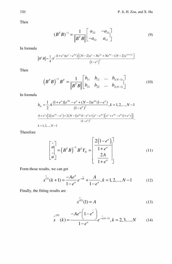
320 P. Ji, H. Zou, and X. Hu
Then
22 211
12 11
1( )T
T
a aB B
a aB B− −⎡ ⎤
= ⎢ ⎥−⎣ ⎦ (9)
In formula
( ) ( )( )
2 ( 1)
24
(1 )( ) 2 21
4 1
a a Na a a Na N a
T
a
e e e N e Ne Ne N eB B A
e
+⎡ ⎤+ − − − + − −⎣ ⎦=−
Then
( ) 1 11 12 1( 1)
21 22 2( 1)
...1
...NT T
TN
b b bB B B
b b bB B
− −
−
⎡ ⎤= ⎢ ⎥
⎣ ⎦ (10)
In formula
1 2
1 (1 )[ ( 1) (1 ), 1, 2,..., 1
2 (1 )
a Na a ka a
k a
e e e N e eb A k N
e
+ − + − −= = −−
( ) ( ) ( ){ }3
(1 ) 2 2 1 (1 ) (1 ),
(1 )
1, 2,..., 1
a Na a ka a a Na a Na ka a
a
e ee e N e e e e e e e e
e
k N
⎡ ⎤+ − + − − + − + − +⎣ ⎦−
= −
Therefore
( )( )
1
2 1
12
1
a
aT TN
a
ea eB B B Y
Aue
∧−
∧
⎡ ⎤−⎡ ⎤ ⎢ ⎥
+⎢ ⎥ ⎢ ⎥= =⎢ ⎥ ⎢ ⎥⎣ ⎦ ⎢ ⎥+⎣ ⎦
(11)
Form those results, we can get
(1) ( 1) , 1, 2,..., 11 1
aak
a a
Ae Ax k e k N
e e
∧∧−−+ = + = −
− − (12)
Finally, the fitting results are
(0) (1)x A∧
= (13)
(0)( 1)
1( ) , 2,3,...,
1
a a
a ka
Ae ex k e k N
e
∧
∧∧− −
⎛ ⎞− −⎜ ⎟⎝ ⎠= =−
(14)
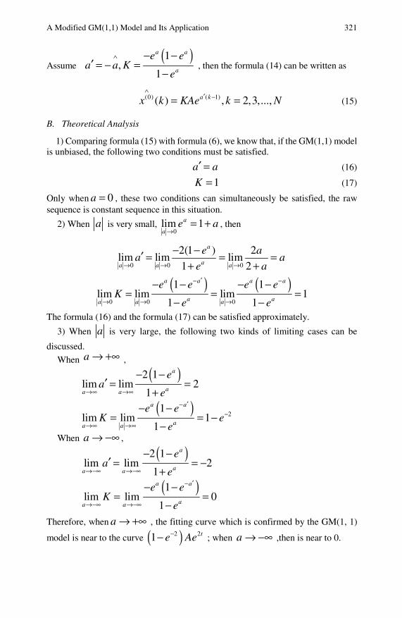
A Modified GM(1,1) Model and Its Application 321
Assume ( )1
,1
a a
a
e ea a K
e
∧ − −′ = − =
− , then the formula (14) can be written as
(0) ( 1)( ) , 2,3,...,a kx k KAe k N∧
′ −= = (15)
B. Theoretical Analysis
1) Comparing formula (15) with formula (6), we know that, if the GM(1,1) model is unbiased, the following two conditions must be satisfied.
a a′ = (16)
1K = (17)
Only when 0a = , these two conditions can simultaneously be satisfied, the raw sequence is constant sequence in this situation.
2) When a is very small, 0
lim 1a
ae a
→= + , then
0 0 0
2(1 ) 2lim lim lim
1 2
a
aa a a
e aa a
e a→ → →
− −′ = = =+ +
( ) ( )0 0 0
1 1lim lim lim 1
1 1
a a a a
a aa a a
e e e eK
e e
′− −
→ → →
− − − −= = =
− −
The formula (16) and the formula (17) can be satisfied approximately.
3) When a is very large, the following two kinds of limiting cases can be
discussed.
When a → +∞ ,
( )2 1lim lim 2
1
a
aa a
ea
e→∞ →∞
− −′ = =
+
( ) 21
lim lim 11
a a
aa a
e eK e
e
′−−
→∞ →∞
− −= = −
−
When a → −∞ ,
( )2 1lim lim 2
1
a
aa a
ea
e→−∞ →−∞
− −′ = = −
+
( )1lim lim 0
1
a a
aa a
e eK
e
′−
→−∞ →−∞
− −= =
−
Therefore, when a → +∞ , the fitting curve which is confirmed by the GM(1, 1)
model is near to the curve ( )2 21 te Ae−− ; when a → −∞ ,then is near to 0.
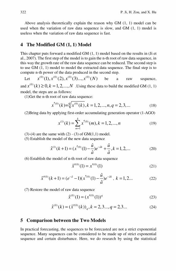
322 P. Ji, H. Zou, and X. Hu
Above analysis theoretically explain the reason why GM (1, 1) model can be used when the variation of raw data sequence is slow, and GM (1, 1) model is useless when the variation of raw data sequence is fast.
4 The Modified GM (1, 1) Model
This chapter puts forward a modified GM (1, 1) model based on the results in (Ji et al., 2007). The first step of the model is to gain the n-th root of raw data sequence, in this way the growth rate of the raw data sequence can be reduced. The second step is to use GM (1, 1) model to model the extracted data sequence. The final step is to compute n-th power of the data produced in the second step.
Let (0) (0) (0) (0)(1), (2), (3)..., ( )x x x x N be a raw sequence,
and (0) ( ) 0, 1,2,...,x k k N≥ = .Using these data to build the modified GM (1, 1)
model, the steps are as follows: (1)Get the n-th root of raw data sequence:
(0) (0)( )= ( ), 1, 2,..., , 2,3,...qx k x k k n q′ = = (18)
(2)Bring data by applying first-order accumulating generation operator (1-AGO)
(1) (0)
1
( ) ( ), 1,2,...,k
m
x k x m k n=
′= =∑ (19)
(3)-(4) are the same with (2) - (3) of GM(1,1) model. (5) Establish the model of the new data sequence
ˆ(1) (0) ˆ ˆˆ ( 1) ( (1) ) , 1,2,...
ˆ ˆaku u
x k x e ka a
−′+ = − + = (20)
(6) Establish the model of n-th root of raw data sequence (0) (0)ˆ (1) (1)x x′ ′= (21)
ˆ ˆ(0) (0) ˆˆ ( 1) ( 1)( (1) )
ˆa aku
x k e x ea
− −′′ + = − − , 1, 2...k = (22)
(7) Restore the model of raw data sequence (0) (0)ˆ (1) ( (1))qx x′= (23)
(0) (0)ˆ ˆ( ) ( ( )) , 2,3..., 2 3...qx k x k k q′= = = , (24)
5 Comparison between the Two Models
In practical forecasting, the sequences to be forecasted are not a strict exponential sequence. Many sequences can be considered to be made up of strict exponential sequence and certain disturbance. Here, we do research by using the statistical
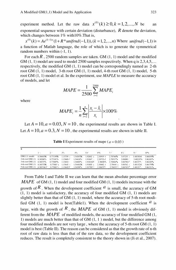
A Modified GM(1,1) Model and Its Application 323
experiment method. Let the raw data (0) ( ) 0, 1,2,...,x k k N≥ = be an
exponential sequence with certain deviation (disturbance), R denote the deviation, which changes between 1% with10%.That is,
(0) ( 1)( ) (1 * ( 1,1)), ( 1,2,..., )k ax k Ae R unifrnd k n−= + − = Where ( 1,1)unifrnd − is
a function of Matlab language, the role of which is to generate the symmetrical random numbers within (-1, 1).
For each R , 2500 random samples are taken. GM (1, 1) model and the modified GM (1, 1) model are used to model 2500 samples respectively. When q is 2,3,4,5,… respectively, the modified GM (1, 1) model can be correspondingly named as 2-th root GM (1, 1) model, 3-th root GM (1, 1) model, 4-th root GM (1, 1) model, 5-th root GM (1, 1) model et al. In the experiment, use MAPLE to measure the accuracy of models, and let
2500
1
1
2500 ii
MAPE MAPE=
= ∑
where
2
ˆ1100%
ni i
ii i
x xMAPE
n x=
−= ×∑.
Let 10, 0.03, 10A a N= = = , the experimental results are shown in Table I.
Let 10, 0.3, 10A a N= = = , the experimental results are shown in table II.
Table I Experiment results of mape ( 0.03a = )
R
1% 2% 3% 4% 5% 6% 7% 8% 9% 10%
GM(1,1) model 0.38603% 0.77159% 1.15759% 1.54507% 1.92002% 2.30919% 2.70760% 3.07235% 3.48530% 3.86839% 2-th root GM(1,1) 0.38580% 0.77101% 1.15669% 1.54418% 1.91847% 2.30732% 2.70517% 3.06880% 3.48219% 3.86345% 3-th root GM(1,1) 0.38575% 0.77089% 1.15652% 1.54405% 1.91816% 2.30696% 2.70464% 3.06796% 3.48157% 3.86228% 4-th root GM(1,1) 0.38575% 0.77085% 1.15645% 1.54401% 1.91805% 2.30682% 2.70444% 3.06762% 3.48132% 3.86179% 5-th root GM(1,1) 0.385746% 0.77083% 1.15642% 1.54399% 1.91799% 2.30675% 2.70433% 3.06743% 3.48121% 3.86151%
From Table I and Table II we can learn that the mean absolute percentage error
MAPE of GM (1, 1) model and four modified GM (1, 1) models increase with the
growth of R . When the development coefficient a is small, the accuracy of GM (1, 1) model is satisfactory, the accuracy of four modified GM (1, 1) models are slightly better than that of GM (1, 1) model, where the accuracy of 5-th root modi-fied GM (1, 1) model is best(Table1). When the development coefficient a is
large, with the growth of R , the MAPE of GM (1, 1) model is obviously dif-ferent from the MAPE of modified models, the accuracy of four modified GM (1, 1) models are much better than that of GM (1, 1 ) model, but the difference among four modified models are not very large , where the accuracy of 5-th root GM (1, 1) model is best (Table II). The reason can be considered as that the growth rate of n-th root of raw data is less than that of the raw data, so the development coefficient reduces. The result is completely consistent to the theory shown in (Ji et al., 2007).

324 P. Ji, H. Zou, and X. Hu
Table II Experiment results of mape ( 0.3a = )
R
1% 2% 3% 4% 5% 6% 7% 8% 9% 10% GM(1,1) model 1.63459% 1.89050% 2.26235% 2.70231% 3.21073% 3.64996% 4.24505% 4.78976% 5.28557% 5.92719% 2-th root GM(1,1) 0.62968% 0.91931% 1.27571% 1.64110% 2.02849% 2.42124% 2.79467% 3.20402% 3.59948% 3.98996% 3-th root GM(1,1) 0.46747% 0.81964% 1.19559% 1.56762% 1.95564% 2.34924% 2.71676% 3.12363% 3.51228% 3.89070% 4-th root GM(1,1) 0.42308% 0.79405% 1.17513% 1.54980% 1.93748% 2.33155% 2.69824% 3.10527% 3.49149% 3.86686% 5-th root GM(1,1) 0.40588% 0.78416% 1.16732% 1.54296% 1.93051% 2.32479% 6 91140% 3.09863% 3.48332% 3.85729%
6 Application of the Modified GM(1,1) Model
The fruit price index (100 is a standard) in China from year 2001 to 2006 (Zhu, 2007) is shown in table III. Using GM (1, 1) model and the modified GM (1, 1) model to build models separately, the fitting results shown in table IV can be obtained.
Here, using MAPE (mean absolute percentage error) to measure the precision of the models, we can gain the comparison results of accuracy between GM (1, 1) model and the modified GM (1, 1) models, which is shown in table V. From the results in table V, we can see that the precision of 5-th root GM (1, 1) model is superior to other GM (1, 1) models.
Table III The fruit price index (100 is a standard) in china from year 2001 to 2006
year 2001 2002 2003 2004 2005 2006 fruit price index
99.9 103.1 103.0 104.0 102.2 123.6
Table IV The fitting result of GM(1,1) and modified GM(1,1) models to the fruit price index in china
year 2001 2002 2003 2004 2005 2006 GM(1,1) 99.9 98.97 102.90 106.99 111.24 115.66 2-th root GM(1,1)
99.9 99.28 103.04 106.95 111.00 115.20
3-th root GM(1,1)
99.9 99.38 103.09 106.93 110.91 115.05
4-th root GM(1,1)
99.9 99.43 103.10 106.92 110.87 114.97
5-th root GM(1,1)
99.9 99.45 103.12 106.91 110.85 114.93
Table V The comparison of accuracy between GM(1,1) and modified GM(1,1) models
model GM(1,1) 2-th root GM(1,1) 3-th root GM(1,1) 4-th root GM(1,1) 5-th root GM(1,1)
MAPE 3.7071% 3.6635% 3.6585% 3.6559% 3.6543%
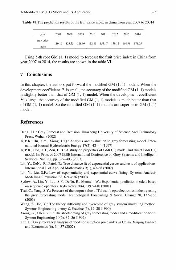
A Modified GM(1,1) Model and Its Application 325
Table VI The prediction results of the fruit price index in china from year 2007 to 20014
year 2007 2008 2009 2010 2011 2012 2013 2014
fruit price
index 119.16 123.55 128.09 132.81 153.47 159.12 164.98 171.05
Using 5-th root GM (1, 1) model to forecast the fruit price index in China from year 2007 to 2014, the results are shown in the table VI.
7 Conclusions
In this chapter, the authors put forward the modified GM (1, 1) models. When the development coefficient a is small, the accuracy of the modified GM (1, 1) models is slightly better than that of GM (1, 1) model. When the development coefficient a is large, the accuracy of the modified GM (1, 1) models is much better than that of GM (1, 1) model. So the modified GM (1, 1) models are superior to GM (1, 1) model.
References
Deng, J.L.: Grey Forecast and Decision. Huazhong University of Science And Technology Press, Wuhan (2002)
Ji, P.R., Hu, X.Y., Xiong, D.Q.: Analysis and evaluation to grey forecasting model. Inter-national Journal Hydroelectric Energy 17(2), 42–44 (1997)
Ji, P.R., Luo, X.J., Zou, H.B.: A study on properties of GM(1,1) model and direct GM(1,1) model. In: Proc. of 2007 IEEE International Conference on Grey Systems and Intelligent Services, Nanjing, pp. 399–403 (2007)
Lin, Y., DeNu, R., Patel, N.: True distance fit of exponential curves and tests of applications. International J. of Applied Mathematics 9(1), 49–68 (2002)
Lin, Y., Liu, S.F.: Law of exponentiality and exponential curve fitting. Systems Analysis Modelling Simulation 38, 621–636 (2000)
Sydow, A., Lin, Y., Liu, S.F., DeNu, R., Mennell, W.: Exponential prediction models based on sequence operators. Kybernetes 30(4), 397–410 (2001)
Tsai, C., Yang, S.Y.: Forecast of the output value of Taiwan’s optoelectronics industry using the grey forecasting mode. Technological Forecasting & Social Change 70, 177–186 (2003)
Wang, Z., He, Y.: The theory difficulty and overcome of grey system modelling method. Systems Engineering-theory & Practice (5), 17–20 (1990)
Xiong, G., Chen, Z.C.: The shortcoming of grey forecasting model and a modification for it. System Engineering 10(6), 32–36 (1992)
Zhu, L.: Grey relevancy analysis of food consumption price index in China. Xinjing Finance and Economics (6), 34–37 (2007)

The Interval Forecasting Method Based on Non-Equidistant GM(1,1) with Application to Regional Grain Production*
Bingjun Li and Chunhua He1
Based on a raw sequence with some aberrant data, it is difficult for any prediction technique to give out an accurate point forecasting value. However, an interval forecasting value obtained by one or more different techniques should be reasonable and acceptable. In this chapter, a data sequence having a linear tendency with upper/positive and lower/negative aberrances is analyzed. Upon the linear regression analysis, the data sequence is classified into three parts: upper/positive aberrant data, lower/negative aberrant data and normal data. Then introducing the non-equidistant GM (1, 1), we establish three models: a non-equidistant GM (1, 1) based on upper aberrant data, a non-equidistant GM (1, 1) based on lower aberrant data and a linear regression model based on the remaining normal data. Using the established models, we can obtain three prediction intervals. Applying it to the prediction of regional grain production, we demonstrate the good performance and effectiveness of the proposed prediction method.
1 Introduction
Prediction is an estimation of unknown situation based on the investigation on all available knowledge and information including past and present data. In principle, it is based on the discovery of the law of the system and a model identification using
Bingjun Li College of Information and Management Science, Henan Agricultural University, Zhengzhou, 450002, China Phone: 86-371-63558580 e-mail: [email protected]
Chunhua He College of Information and Management Science, Henan Agricultural University, Zhengzhou, 450002, China * The work was supported in part by the Science-tech Innovative talents plan project of
Henan Province (No.551(2008)); the Soft-science Foundation of Henan Province (No.072400420650); Innovation Scientists and Technicians Troop Construction Projects of Henan Province (094100510013).
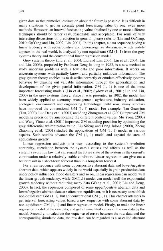
328 B. Li and C. He
given data so that numerical estimation about the future is possible. It is difficult in many situations to get an accurate point forecasting value by one, even more methods. However, an interval forecasting value obtained by one or more different techniques should be rather easy, reasonable and acceptable. For some of very interesting discussions on prediction in general, please refer to (Lin and OuYang, 2010; OuYang and Lin, 2002; Lin, 2001). In this chapter, a data sequence having a linear tendency with upper/positive and lower/negative aberrances, which widely appears in the real world, is analyzed by non-equidistant GM (1, 1) from the grey systems theory and the conventional linear regression model.
Grey systems theory (Liu et al., 2004; Liu and Lin, 2006; Lin et al., 2004; Lin and Liu, 2006), proposed by Professor Deng Ju-long in 1982, is a new method to study uncertain problems with a few data and poor information. It works on uncertain systems with partially known and partially unknown information. The grey system theory enables us to describe correctly or emulate effectively systems behavior by drawing out valuable information through the generalization and development of the given partial information. GM (1, 1) is one of the most important forecasting models (Lin et al., 2002; Sydow et al., 2001; Lin and Liu, 2000) in the grey systems theory. Since it was presented in 1982, the model has been widely applied to economy, management, agriculture, industry, education, ecological environment and engineering technology. Until now, many scholars have improved the conventional GM (1, 1) model. For example, Tan Guan-jun (Tan, 2000), Luo Dang et al. (2003) and Song Zhongmin et al. (2001) improved GM modeling precision by ameliorating the different context values. Mu Yong (2003) and Wang Yinao et al. (2001) improved GM modeling precision by optimizing the grey differential whitenization value. Liu Sifeng and Deng Julong (2000), Zheng Zhaoning et al. (2001) studied the applications of GM (1, 1) model in various aspects. Such studies advance the GM (1, 1) model and expand the area of applications greatly.
Linear regression analysis is a way, according to the system’s evolution continuity, correlation between the system’s causes and affects as well as the system’s evolution law that can regard the future state of the system as the current’s continuation under a relatively stable condition. Linear regression can give out a better result in a short-term forecast than in a long-term forecast.
For a raw sequence with some upper/positive aberrant data and lower/negative aberrant data, which appears widely in the world especially in grain production data under policy influences, flood disasters and so on, linear regression can model well the linear growth tendency, while GM(1,1) model can model well the exponential growth tendency without requiring many data (Wang et al., 2001; Liu and Deng, 2000). In fact, the sequences composed of some upper/positive aberrant data and lower/negative aberrant data are often non-equidistant, so it is necessary to establish non-equidistant GM (1, 1), but not conventional GM (1, 1). This chapter attempts to get interval forecasting values based a raw sequence with some aberrant data by non-equidistant GM (1, 1) and linear regression model. Firstly, to make the linear regression model of the raw data, and get all simulated values of the raw data by the model. Secondly, to calculate the sequence of errors between the raw data and the corresponding simulated data, the raw data can be regarded as a so-called aberrant

The Interval Forecasting Method Based on Non-Equidistant GM(1,1) 329
point or abnormal point if the error of a raw data is bigger than a given critical value. At this time, the raw data sequence with some abnormal data is classified into three parts: upper/positive aberrant data, lower/negative aberrant data and normal data. Thirdly, we establish three models: a non-equidistant GM (1, 1) model based on upper aberrant data, a non-equidistant GM (1, 1) model based on lower aberrant data and a linear regression model based on the remaining normal data. Finally, we can use the three established models to obtain three prediction intervals. A positive study shows that this forecasting method can effectively get some better forecasting results.
2 Classification of Raw Data
A. The rough procedure of classifying raw data
Analyzing raw data reasonably is an important task of modeling. In a raw data sequence, what kinds of values are abnormal? In general, people often use their experience and subjective criteria to determine what values are normal and what are not. But it is hard to get ideal results in many situations due to the limitations of people’s experience and choice of subjective criteria. Where, we propose a new approach to classify raw data. The rough procedure of the proposed approach is given as follows: First, applying the linear regression model obtained by the least square method for a data sequence having a linear tendency, we calculate estimated values and the signed residual errors at all data points. Then, the raw data can be classified into so-called aberrant data points (upper/positive and lower/negative) and normal data points depending on the residual errors. If the residual error is positive and larger than a predetermined threshold, the data is regarded as an upper/positive aberrant data. If the residual error is negative and its absolute value is larger than the threshold, the data is regarded as a lower/negative aberrant data. Otherwise, the data is regarded as normal.
B. The concrete steps of classifying raw data
The concrete steps of classifying raw data are followed:
Step 1: Assume that (0) (0)andX Q are raw data sequence and time sequence
respectively:
( 0 ) ( 0 ) ( 0 ) ( 0 )( (1)), ( (2 )), , ( ( ))X X q X q X q m= (1)
(0) ( (1), (2), , ( ))Q q q q m= .
Step 2: Based on (0)X and (0)Q , we get the linear regression function
)0(00
)0( QbaX += . (2)
Then, we can get a residual error sequence0ε between (0)X and the simulated
(0)X through the function (2).

330 B. Li and C. He
)()(,),()(
,),2()2(),1()1((
))(,),2(),1((
^00
^00
^00
^00
0
mqXmqXkqXkqX
qXqXqXqX
m
−−
−−=
=
…
…
… εεεε (3)
Step 3: If the absolute value of )(kε is bigger than the given abnormal critical
value ξ (according to the required linear regression precision, we may give the value. It is acceptable to set an upper critical value and a lower critical value if necessary), we can deem the corresponding data as the aberrant data points, if not then the normal data point. Therefore according to positive or negative residual error, we can classify the aberrant data points into two parts: upper/positive aberrant data, lower/negative aberrant data.
Let (0)P and (0)AX denote the upper/positive aberrant time sequence and data
sequence, respectively. Then we have
(0) ( (1), (2), , ( ))P p p p s= , (4)
))((,)),2(()),1(( )0()0()0()0( spXpXpXX A = (5)
Let (0)R and (0)BX denote the lower/negative aberrant time sequence and data
sequence, respectively. Then we have
(0) ( (1), (2), , ( ))R r r r t= , (6)
(0) (0 ) (0 ) (0 )( (1)), ( (2)), , ( ( ))BX X r X r X r t= (7)
Step 4: Assume that (0)L and (0)CX are other normal data time sequence and data
sequence respectively. Then we have
(0) ( (1), (2), , ( ))( ),L l l l m m n s t= = − − (8)
(0) (0 ) (0 ) (0 )( (1)), ( (2)), , ( ( )).CX X l X l X l m= (9)
3 The Establishment of Forecasting Models
The conventional GM (1, 1) modeling is based on the equidistant data sequence. In fact, the raw data sequence we often get is incomplete or lack of some data so that it is hard to establish appropriate GM (1, 1) based on non-equidistant data sequence by the principle of the conventional GM (1, 1) modeling. So we have to study the principle of non-equidistant GM(1,1).
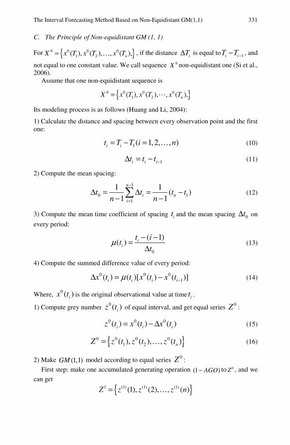
The Interval Forecasting Method Based on Non-Equidistant GM(1,1) 331
C. The Principle of Non-equidistant GM (1, 1)
For { }0 0 0 01 2( ), ( ), , ( ),nX x T x T x T= … , if the distance iTΔ is equal to 1i iT T −− , and
not equal to one constant value. We call sequence 0X non-equidistant one (Si et al., 2006).
Assume that one non-equidistant sequence is
{ }0 0 0 01 2( ), ( ), , ( ),nX x T x T x T=
Its modeling process is as follows (Huang and Li, 2004):
1) Calculate the distance and spacing between every observation point and the first one:
1( 1,2, , )i it T T i n= − = … (10)
1i i it t t −Δ = − (11)
2) Compute the mean spacing:
1
0 11
1 1( )
1 1
n
i ni
t t t tn n
−
=Δ = Δ = −
− −∑ (12)
3) Compute the mean time coefficient of spacing it and the mean spacing 0tΔ on
every period:
0
( 1)( ) i
i
t it
tμ − −=
Δ (13)
4) Compute the summed difference value of every period:
0 0 01( ) ( )[ ( ) ( )]i i i ix t t x t x tμ −Δ = − (14)
Where, 0 ( )ix t is the original observational value at time it .
1) Compute grey number 0 ( )iz t of equal interval, and get equal series 0Z :
0 0 0( ) ( ) ( )i i iz t x t x t= − Δ (15)
{ }0 0 0 01 2( ), ( ), , ( )nZ z t z t z t= … (16)
2) Make (1,1)GM model according to equal series 0Z :
First step: make one accumulated generating operation (1 )AGO− to 0Z , and we
can get
{ }1 (1) (1) (1)(1), (2), , ( )Z z z z n= …
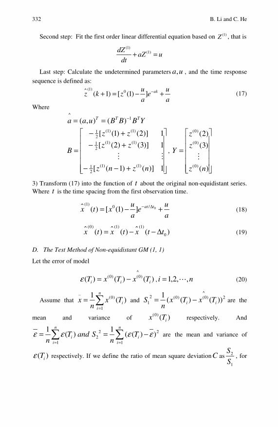
332 B. Li and C. He
Second step: Fit the first order linear differential equation based on (1)Z , that is
(1)(1)dZ
aZ udt
+ =
Last step: Calculate the undetermined parameters ,a u , and the time response
sequence is defined as: (1) 0( 1) [ (1) ] aku u
z k z ea a
−+ = − + (17)
Where
YBBBuaa TTT 1^
)(),( −==
⎥⎥⎥⎥⎥
⎦
⎤
⎢⎢⎢⎢⎢
⎣
⎡
+−−
+−+−
=
1)]()1([
1)]3()2([
1)]2()1([
)1()1(21
)1()1(21
)1()1(21
nznz
zz
zz
B ,
⎥⎥⎥⎥⎥
⎦
⎤
⎢⎢⎢⎢⎢
⎣
⎡
=
)(
)3(
)2(
)0(
)0(
)0(
nz
z
z
Y
3) Transform (17) into the function of t about the original non-equidistant series. Where t is the time spacing from the first observation time.
0(1) /0( ) [ (1) ] at tu u
x t x ea a
− Δ= − + (18)
(0) (1) (1)
0( ) ( ) ( )x t x t x t t= − − Δ (19)
D. The Test Method of Non-equidistant GM (1, 1)
Let the error of model
)()()(^
)0()0(iii TxTxT −=ε , ni ,,2,1= (20)
Assume that ∑=
=n
iiTx
nx
1
)0(_
)(1
and 2^
)0()0(21 ))()((
1ii TxTx
nS −= are the
mean and variance of )()0(iTx respectively. And
2 22
1 1
1 1( ) ( ( ) )
n n
i ii i
T and S Tn n
ε ε ε ε= =
= = −∑ ∑ are the mean and variance of
( )iTε respectively. If we define the ratio of mean square deviation C as 2
1
S
S, for
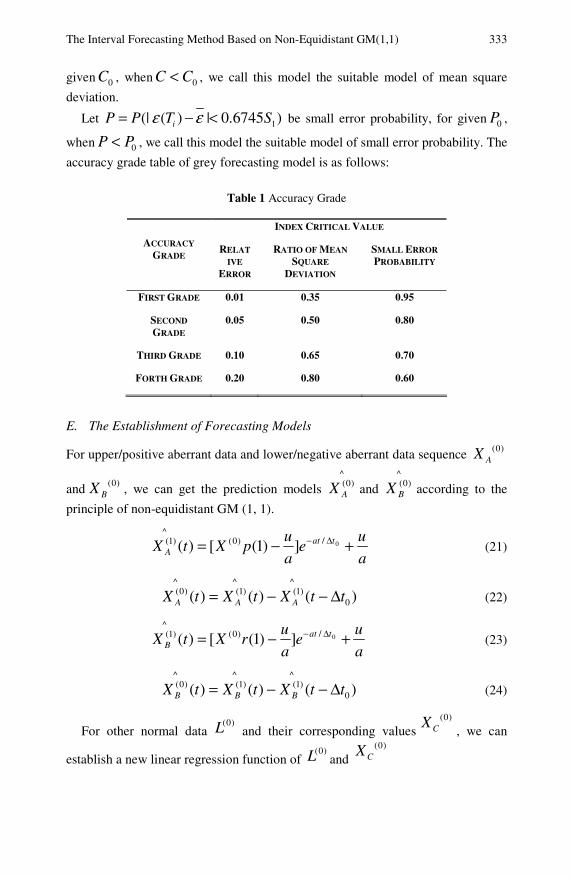
The Interval Forecasting Method Based on Non-Equidistant GM(1,1) 333
given 0C , when 0C C< , we call this model the suitable model of mean square
deviation.
Let 1(| ( ) | 0.6745 )iP P T Sε ε= − < be small error probability, for given 0P ,
when 0P P< , we call this model the suitable model of small error probability. The
accuracy grade table of grey forecasting model is as follows:
Table 1 Accuracy Grade
INDEX CRITICAL VALUE
ACCURACY GRADE RELAT
IVE ERROR
RATIO OF MEAN SQUARE
DEVIATION
SMALL ERROR PROBABILITY
FIRST GRADE 0.01 0.35 0.95
SECOND GRADE
0.05 0.50 0.80
THIRD GRADE 0.10 0.65 0.70
FORTH GRADE 0.20 0.80 0.60
E. The Establishment of Forecasting Models
For upper/positive aberrant data and lower/negative aberrant data sequence (0)AX
and (0)BX , we can get the prediction models
^)0(
AX and ^
)0(BX according to the
principle of non-equidistant GM (1, 1).
a
ue
a
upXtX tat
A +−= Δ− 0/)0(^
)1( ])1([)( (21)
)()()( 0
^)1(
^)1(
^)0( ttXtXtX AAA Δ−−= (22)
a
ue
a
urXtX tat
B +−= Δ− 0/)0(^
)1( ])1([)( (23)
)()()( 0
^)1(
^)1(
^)0( ttXtXtX BBB Δ−−= (24)
For other normal data (0)L and their corresponding values
(0)CX
, we can
establish a new linear regression function of (0)L and
(0)CX
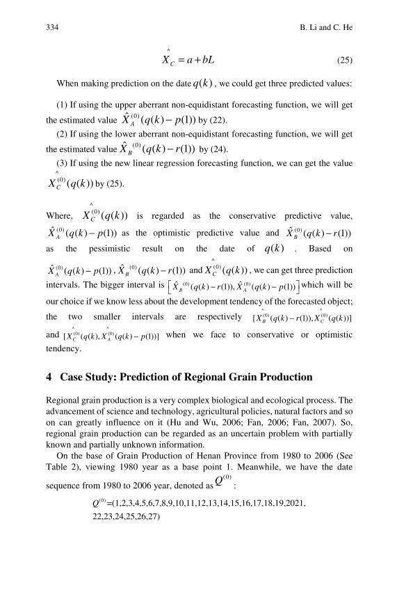
334 B. Li and C. He
^
CX a bL= + (25)
When making prediction on the date ( )q k , we could get three predicted values:
(1) If using the upper aberrant non-equidistant forecasting function, we will get
the estimated value (0)ˆ ( ( ) (1))AX q k p− by (22).
(2) If using the lower aberrant non-equidistant forecasting function, we will get
the estimated value (0)ˆ ( ( ) (1))BX q k r− by (24).
(3) If using the new linear regression forecasting function, we can get the value
))((^
)0( kqXC by (25).
Where, ))((^
)0( kqXC is regarded as the conservative predictive value,
(0)ˆ ( ( ) (1))AX q k p− as the optimistic predictive value and (0)ˆ ( ( ) (1))BX q k r− as the pessimistic result on the date of ( )q k . Based on
(0)ˆ ( ( ) (1))AX q k p− , (0)ˆ ( ( ) (1))BX q k r− and ))((^
)0( kqXC , we can get three prediction
intervals. The bigger interval is (0) (0)ˆ ˆ( ( ) (1)), ( ( ) (1))B AX q k r X q k p⎡ ⎤− −⎣ ⎦which will be
our choice if we know less about the development tendency of the forecasted object;
the two smaller intervals are respectively ))](()),1()(([^
)0(^
)0( kqXrkqX CB − and ))]1()((),(([
^)0(
^)0( pkqXkqX AC − when we face to conservative or optimistic
tendency.
4 Case Study: Prediction of Regional Grain Production
Regional grain production is a very complex biological and ecological process. The advancement of science and technology, agricultural policies, natural factors and so on can greatly influence on it (Hu and Wu, 2006; Fan, 2006; Fan, 2007). So, regional grain production can be regarded as an uncertain problem with partially known and partially unknown information.
On the base of Grain Production of Henan Province from 1980 to 2006 (See Table 2), viewing 1980 year as a base point 1. Meanwhile, we have the date
sequence from 1980 to 2006 year, denoted as(0)Q :
(0) =(1,2,3,4,5,6,7,8,9,10,11,12,13,14,15,16,17,18,19,2021,
22,23,24,25,26,27)
Q
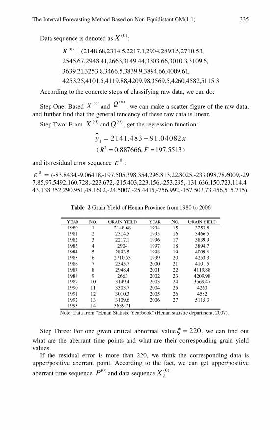
The Interval Forecasting Method Based on Non-Equidistant GM(1,1) 335
Data sequence is denoted as (0)X :
3.5115,4582,4260,5.3569,98.4209,88.4119,5.4101,25.4253
,61.4009,66.3894,9.3839,5.3466,8.3253,21.3639
,6.3109,3.3010,66.3303,44.3149,2663,41.2948,67.2545
,53.2710,5.2893,2904,1.2217,5.2314,68.2148()0( =X
According to the concrete steps of classifying raw data, we can do:
Step One: Based ( 0 )X and
( 0 )Q , we can make a scatter figure of the raw data, and further find that the general tendency of these raw data is linear.
Step Two: From )0(X and )0(Q , get the regression function:
1 2141.483 91.04082y x= +
( 2 0.887666, 197.5513R F= = )
and its residual error sequence 0ε : 0ε = (-83.8434,-9.06418,-197.505,398.354,296.813,22.8025,-233.098,78.6009,-29
7.85,97.5492,160.728,-223.672,-215.403,223.156,-253.295,-131.636,150.723,114.443,138.352,290.951,48.1602,-24.5007,-25.4415,-756.992,-157.503,73.456,515.715).
Table 2 Grain Yield of Henan Province from 1980 to 2006
YEAR NO. GRAIN YIELD YEAR NO. GRAIN YIELD 1980 1 2148.68 1994 15 3253.8 1981 2 2314.5 1995 16 3466.5 1982 3 2217.1 1996 17 3839.9 1983 4 2904 1997 18 3894.7 1984 5 2893.5 1998 19 4009.6 1985 6 2710.53 1999 20 4253.3 1986 7 2545.7 2000 21 4101.5 1987 8 2948.4 2001 22 4119.88 1988 9 2663 2002 23 4209.98 1989 10 3149.4 2003 24 3569.47 1990 11 3303.7 2004 25 4260 1991 12 3010.3 2005 26 4582 1992 13 3109.6 2006 27 5115.3 1993 14 3639.21
Note: Data from “Henan Statistic Yearbook” (Henan statistic department, 2007).
Step Three: For one given critical abnormal value 220ξ = , we can find out
what are the aberrant time points and what are their corresponding grain yield values.
If the residual error is more than 220, we think the corresponding data is upper/positive aberrant point. According to the fact, we can get upper/positive
aberrant time sequence (0)P and data sequence (0)AX
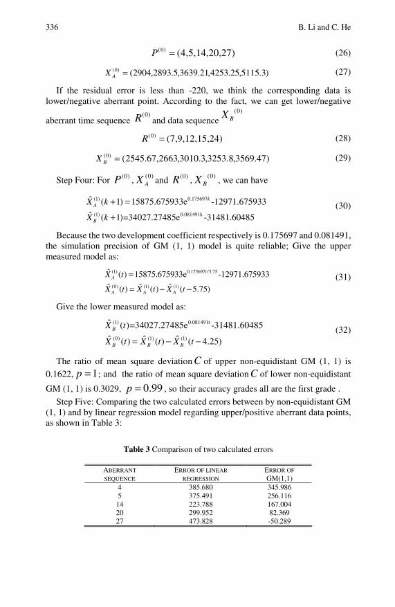
336 B. Li and C. He
(0) (4,5,14,20,27)P = (26)
)3.5115,25.4253,21.3639,5.2893,2904()0( =AX (27)
If the residual error is less than -220, we think the corresponding data is lower/negative aberrant point. According to the fact, we can get lower/negative
aberrant time sequence (0)R and data sequence
(0)BX
(0) (7,9,12,15,24)R = (28)
)47.3569,8.3253,3.3010,2663,67.2545()0( =BX (29)
Step Four: For (0)P , (0)AX and (0)R , (0)
BX , we can have
(1) 0.175697
(1) 0.081491k
ˆ ( 1) 15875.675933e -12971.675933
ˆ ( 1)=34027.27485e -31481.60485
kA
B
X k
X k
+ =
+ (30)
Because the two development coefficient respectively is 0.175697 and 0.081491, the simulation precision of GM (1, 1) model is quite reliable; Give the upper measured model as:
(1) 0.175697 /5.75
(0) (1) (1)
ˆ ( ) 15875.675933e -12971.675933
ˆ ˆ ˆ( ) ( ) ( 5.75)
tA
A A A
X t
X t X t X t
=
= − − (31)
Give the lower measured model as:
(1) 0.081491t
(0) (1) (1)
ˆ ( )=34027.27485e -31481.60485
ˆ ˆ ˆ( ) ( ) ( 4.25)
B
B B B
X t
X t X t X t= − − (32)
The ratio of mean square deviation C of upper non-equidistant GM (1, 1) is
0.1622, 1p = ; and the ratio of mean square deviation C of lower non-equidistant
GM (1, 1) is 0.3029, 0.99p = , so their accuracy grades all are the first grade .
Step Five: Comparing the two calculated errors between by non-equidistant GM (1, 1) and by linear regression model regarding upper/positive aberrant data points, as shown in Table 3:
Table 3 Comparison of two calculated errors
ABERRANT
SEQUENCE ERROR OF LINEAR
REGRESSION ERROR OF
GM(1,1) 4 385.680 345.986 5 375.491 256.116
14 223.788 167.004 20 299.952 82.369 27 473.828 -50.289
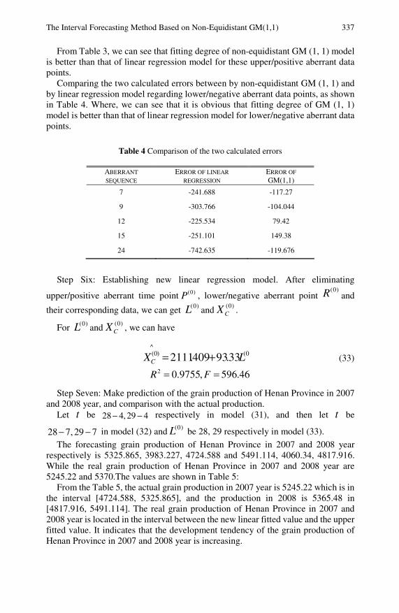
The Interval Forecasting Method Based on Non-Equidistant GM(1,1) 337
From Table 3, we can see that fitting degree of non-equidistant GM (1, 1) model is better than that of linear regression model for these upper/positive aberrant data points.
Comparing the two calculated errors between by non-equidistant GM (1, 1) and by linear regression model regarding lower/negative aberrant data points, as shown in Table 4. Where, we can see that it is obvious that fitting degree of GM (1, 1) model is better than that of linear regression model for lower/negative aberrant data points.
Table 4 Comparison of the two calculated errors
ABERRANT
SEQUENCE ERROR OF LINEAR
REGRESSION ERROR OF
GM(1,1)
7 -241.688 -117.27
9 -303.766 -104.044
12 -225.534 79.42
15 -251.101 149.38
24 -742.635 -119.676
Step Six: Establishing new linear regression model. After eliminating
upper/positive aberrant time point (0)P , lower/negative aberrant point (0)R and
their corresponding data, we can get (0)L and (0)CX .
For (0)L and (0)CX , we can have
0(^
)0( 33.93409.2111 LXC += (33)
46.596,9755.02 == FR
Step Seven: Make prediction of the grain production of Henan Province in 2007 and 2008 year, and comparison with the actual production.
Let t be 28 4,29 4− − respectively in model (31), and then let t be
28 7, 29 7− − in model (32) and )0(L be 28, 29 respectively in model (33).
The forecasting grain production of Henan Province in 2007 and 2008 year respectively is 5325.865, 3983.227, 4724.588 and 5491.114, 4060.34, 4817.916. While the real grain production of Henan Province in 2007 and 2008 year are 5245.22 and 5370.The values are shown in Table 5:
From the Table 5, the actual grain production in 2007 year is 5245.22 which is in the interval [4724.588, 5325.865], and the production in 2008 is 5365.48 in [4817.916, 5491.114]. The real grain production of Henan Province in 2007 and 2008 year is located in the interval between the new linear fitted value and the upper fitted value. It indicates that the development tendency of the grain production of Henan Province in 2007 and 2008 year is increasing.
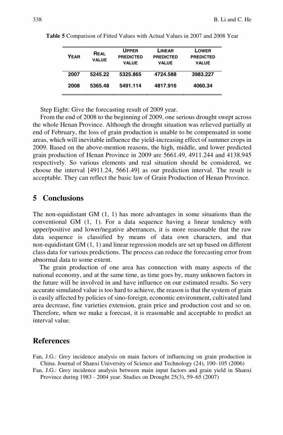
338 B. Li and C. He
Table 5 Comparison of Fitted Values with Actual Values in 2007 and 2008 Year
YEAR REAL VALUE
UPPER PREDICTED
VALUE
LINEAR PREDICTED
VALUE
LOWER PREDICTED
VALUE
2007 5245.22 5325.865 4724.588 3983.227
2008 5365.48 5491.114 4817.916 4060.34
Step Eight: Give the forecasting result of 2009 year. From the end of 2008 to the beginning of 2009, one serious drought swept across
the whole Henan Province. Although the drought situation was relieved partially at end of February, the loss of grain production is unable to be compensated in some areas, which will inevitable influence the yield-increasing effect of summer crops in 2009. Based on the above-mention reasons, the high, middle, and lower predicted grain production of Henan Province in 2009 are 5661.49, 4911.244 and 4138.945 respectively. So various elements and real situation should be considered, we choose the interval [4911.24, 5661.49] as our prediction interval. The result is acceptable. They can reflect the basic law of Grain Production of Henan Province.
5 Conclusions
The non-equidistant GM (1, 1) has more advantages in some situations than the conventional GM (1, 1). For a data sequence having a linear tendency with upper/positive and lower/negative aberrances, it is more reasonable that the raw data sequence is classified by means of data own characters, and that non-equidistant GM (1, 1) and linear regression models are set up based on different class data for various predictions. The process can reduce the forecasting error from abnormal data to some extent.
The grain production of one area has connection with many aspects of the national economy, and at the same time, as time goes by, many unknown factors in the future will be involved in and have influence on our estimated results. So very accurate simulated value is too hard to achieve, the reason is that the system of grain is easily affected by policies of sino-foreign, economic environment, cultivated land area decrease, fine varieties extension, grain price and production cost and so on. Therefore, when we make a forecast, it is reasonable and acceptable to predict an interval value.
References
Fan, J.G.: Grey incidence analysis on main factors of influencing on grain production in China. Journal of Shanxi University of Science and Technology (24), 100–105 (2006)
Fan, J.G.: Grey incidence analysis between main input factors and grain yield in Shanxi Province during 1983 - 2004 year. Studies on Drought 25(3), 59–65 (2007)
The Interval Forecasting Method Based on Non-Equidistant GM(1,1) 339 Henan statistic department, Henan Statistic Yearbook 2007, pp. 10–25. Statistic Publishing
Company of China, Beijing (2007) Hu, B.C., Wu, Q.: Analysis on factors of influencing on input-output of grain production.
Resource and Environment of Yangzi-river Region 15(1), 89–94 (2006) Huang, S.H., Li, Z.C.: Grey modeling of non-equidistant data sequence for forecasting
subsidence of engineering buildings. Geospatial Information (1), 41–43 (2004) Lin, Y.: Information, prediction and structural whole: An introduction. Kybernetes 30(4),
350–364 (2001) Lin, Y., Chen, M.Y., Liu, S.F.: Theory of grey systems: capturing uncertainties of grey
information. Kybernetes: The International Journal of Systems and Cybernetics 33(2), 196–218 (2004)
Lin, Y., DeNu, R., Patel, N.: True distance fit of exponential curves and tests of applications. International J. of Applied Mathematics 9(1), 49–68 (2002)
Lin, Y., Liu, S.F.: Law of exponentiality and exponential curve fitting. Systems Analysis Modelling Simulation 38, 621–636 (2000)
Lin, Y., Liu, S.F.: Solving Problems with incomplete information: a grey systems approach. In: Advances in Imaging and Electron Physics, vol. 141, pp. 77–174. Elsevier, Oxford (2006)
Lin, Y., OuYang, S.C.: Irregularities and Prediction of Major Disasters. Auerbach Publications, an imprint of Taylor and Francis, New York (2010)
Liu, S.F., Dang, Y.G., Fang, Z.G.: Grey System Theory and Application, pp. 145–167. Science Press, Beijing (2004)
Liu, S.F., Deng, J.L.: The range suitable for GM(1,1). Systems Engineering Theory & Practice 21(5), 121–124 (2000)
Liu, S.F., Lin, Y.: Grey Information: Theory and Practical Applications. Springer, London (2006)
Luo, D., Liu, S.F., Dang, Y.G.: Optimizing grey model GM(1,1). China Engineering Science 5(8), 50–53 (2003)
Mu, Y.: Optimizing grey differential whitenization value algorithm of model GM(1,1). The Practice And Acquaintance of Mathematics (1), 13–16 (2003)
OuYang, S.C., Lin, Y.: Structural rolling currents and disastrous weather forecasting. In: Wu, Y., Lin, Y. (eds.) Beyond Nonstructural Quantitative Analysis: Blown-ups, Spinning Currents and Modern Science. World Scientific, River Edge (2002)
Si, X.R., Wang, Z.L., Zhang, Z.D.: GM(1,1) model with variational parameter for non-equidistant sequence and its application. Mathematics in Practice and Theory (6), 216–220 (2006)
Song, Z.M., Tong, X.J., Xiao, X.P.: Centre approach model of grey GM(1,1). System Engineering Theory and Practice 21(5), 110–113 (2001)
Sydow, A., Lin, Y., Liu, S.F., DeNu, R., Mennell, W.: Exponential prediction models based on sequence operators. Kybernetes 30(4), 397–410 (2001)
Tan, G.J.: The application And constitution method of context value of model GM(1,1). System Engineering Theory and Practice 20(4), 99–103 (2000)
Wang, Y.N., Liu, K.D., Li, Y.C.: The modeling GM(1,1) method of optimizing grey differential whitenization value. System Engineering Theory and Practice 21(5), 124–128 (2001)
Zheng, Z.N., Wu, Y.Y., Bao, H.L.: The morbidity problem of model GM(1,1). Chinese Management Science 15(5), 38–44 (2001)

An Optimization Method of Estimating Parameters in GM(1,1) Model
Xuemei Li, Yaoguo Dang, and Jiejue Zhao1
According to Principle of New Information Priority in grey theory, giving the new information larger weight in modeling can improve the effectiveness of gray model. For the GM(1,1) model has very small samples, and the high overall simulation accuracy does not necessarily guarantee high prediction accuracy, we put forward weighted least square method to estimate parameters in GM(1,1) model. Focusing on improving the simulation accuracy of new information, focusing on grasping the latest development’ law of things, and aiming at improving the prediction accuracy by giving residual sum of squares of new information larger weight. Finally, we use an example to verify the practicality and reliability of the model.
1 Introduction
GM(1,1) model is one of the core content of gray prediction models, which has been widely used in industry, agriculture, social, economic and other fields because it requires very small samples with simple calculation. It is especially on the case of small samples and poor information uncertain systems that it was successfully applied. Many scholars have done a lot of research in order to improve the prediction accuracy. These studies mainly concentrated in the following respects: 1. Do pre-processing on the original sequence using sequence operator, buffer operator and date transformation in order to make them suitable to GM(1,1) model
(Dang et al., 2006; Dai and Li, 2004; Li and Dai, 005; Cui and Dang, 2009; Lin et al., 2002; Sydow et al., 2001; Lin and Liu, 2000); 2. Optimize the background date (Tan, 2000; Luo et al., 2003; Wang et al., 2007); 3. Optimize method of estimating
Xuemei Li College of Economics and Management, Nanjing University of Aeronautics & Astronautics, Naning, P.R. China Phone: 15151861926 e-mail: [email protected]
Yaoguo Dang and Jiejue Zhao College of Economics and Management, Nanjing University of Aeronautics & Astronautics, Naning, P.R. China e-mail: [email protected], [email protected]
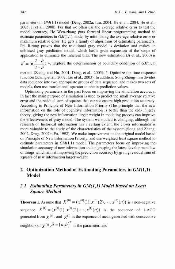
342 X. Li, Y. Dang, and J. Zhao
parameters in GM(1,1) model (Deng, 2002a; Liu, 2004; He et al., 2004; He et al., 2005; Ji et al., 2000). For that we often use the average relative error to test the model accuracy, He Wen-zhang puts forward linear programming method to estimate parameters in GM(1,1) model by minimizing the average relative error or maximum relative error. He gets a family of algorithms of estimating parameters. Pei Ji-rong proves that the traditional gray model is deviation and makes an unbiased gray prediction model, which has a great expansion of the scope of application to eliminate the inherent bias. The new estimation (Ji et al., 2000) is
ˆ2ˆ ln
ˆ2
aa
a
−′ =+
; 4. Explore the determination of boundary condition of GM(1,1)
method (Zhang and Hu, 2001; Dang, et al., 2005); 5. Optimize the time response function (Zhang et al., 2002; Liu et al., 2003). In addition, Song Zhong-min divides data sequence into two appropriate groups of data sequence, and makes two sets of models, then use translational operator to obtain prediction values.
Optimizing parameters in the past focus on improving the simulation accuracy. In fact the main purpose of simulation is used to predict the small average relative error and the residual sum of squares that cannot ensure high prediction accuracy. According to Principle of New Information Priority (The principle that the new information on the role of cognitive information is better than the old) in grey theory, giving the new information larger weight in modeling process can improve the effectiveness of gray model. The system we studied is changing, although the research on historical information has a certain extent, the closer information is more valuable to the study of the characteristics of the system (Song and Zhang, 2002; Deng, 2002b; Fu, 1992). We make improvement on the original model based on Principle of New Information Priority, and use weighted least square method to estimate parameters in GM(1,1) model. The parameters focus on improving the simulation accuracy of new information and on grasping the latest development law of things which aim at improving the prediction accuracy by giving residual sum of squares of new information larger weight.
2 Optimization Method of Estimating Parameters in GM(1,1) Model
2.1 Estimating Parameters in GM(1,1) Model Based on Least Square Method
Theorem 1. Assume that ( ) ( ) ( ) ( )0 0 0 0( (1), (2), , ( ))X x x x n= is a non-negative
sequence ( ) ( ) ( ) ( )1 1 1 1( (1), (2), , ( ))X x x x n= is the sequence of 1-AGO
generated from ( )0X , and ( )1Z is the sequence of mean generated with consecutive
neighbors of ( )1X . ( ),T
a a b= is the parameter, and
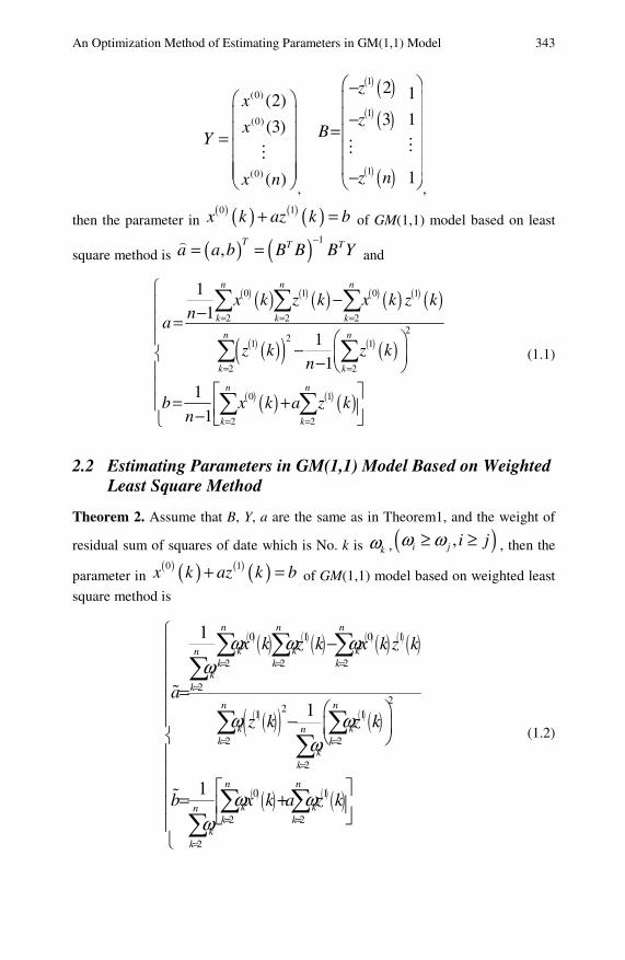
An Optimization Method of Estimating Parameters in GM(1,1) Model 343
(0)
(0)
(0)
(2)
(3)
( )
x
xY
x n
⎛ ⎞⎜ ⎟⎜ ⎟= ⎜ ⎟⎜ ⎟⎜ ⎟⎝ ⎠ ,
( ) ( )( ) ( )
( ) ( )
1
1
1
2 1
3 1
1
z
zB
z n
⎛ ⎞−⎜ ⎟⎜ ⎟−
=⎜ ⎟⎜ ⎟⎜ ⎟−⎝ ⎠,
then the parameter in ( ) ( ) ( ) ( )0 1x k az k b+ = of GM(1,1) model based on least
square method is ( ) ( ) 1,
T T Ta a b B B B Y−
= = and
( ) ( ) ( ) ( ) ( ) ( ) ( ) ( )
( ) ( )( ) ( ) ( )
( ) ( ) ( ) ( )
0 1 0 1
2 2 22
21 1
2 2
0 1
2 2
11
11
1
1
n n n
k k k
n n
k k
n n
k k
x k z k x k z kn
a
z k z kn
b x k a z kn
= = =
= =
= =
⎧ −⎪ −⎪ =⎪ ⎛ ⎞−⎨ ⎜ ⎟− ⎝ ⎠⎪⎪ ⎡ ⎤= +⎪ ⎢ ⎥− ⎣ ⎦⎩
∑ ∑ ∑
∑ ∑
∑ ∑
(1.1)
2.2 Estimating Parameters in GM(1,1) Model Based on Weighted Least Square Method
Theorem 2. Assume that B, Y, a are the same as in Theorem1, and the weight of
residual sum of squares of date which is No. k is kω , ( ),i j i jω ω≥ ≥ , then the
parameter in ( ) ( ) ( ) ( )0 1x k az k b+ = of GM(1,1) model based on weighted least
square method is
( ) ( ) ( ) ( ) ( ) ( ) ( ) ( )
( ) ( )( ) ( ) ( )
( ) ( ) ( ) ( )
0 1 0 1
2 2 2
22
21 1
2 2
2
0 1
2 2
2
1
1
1
n n n
k k knk k k
kk
n n
k knk k
kk
n n
k knk k
kk
x k z k x k z k
a
z k z k
b x k a z k
ω ω ωω
ω ωω
ω ωω
= = =
=
= =
=
= =
=
⎧ −⎪⎪⎪ =⎪ ⎛ ⎞⎪ − ⎜ ⎟⎨ ⎝ ⎠⎪⎪
⎡ ⎤⎪ = +⎢ ⎥⎪ ⎣ ⎦⎪⎩
∑ ∑ ∑∑
∑ ∑∑
∑ ∑∑
(1.2)
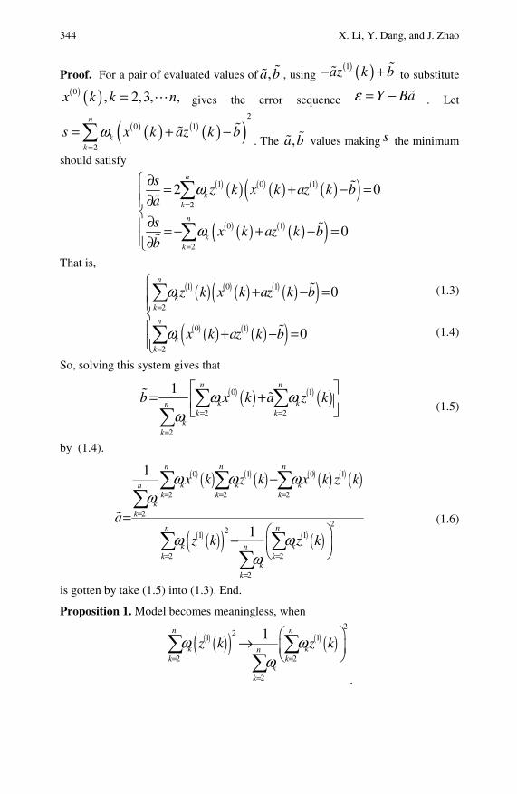
344 X. Li, Y. Dang, and J. Zhao
Proof. For a pair of evaluated values of ,a b , using ( ) ( )1az k b− + to substitute
( ) ( )0 , 2,3, ,x k k n= gives the error sequence Y Baε = − . Let
( ) ( ) ( ) ( )( )2
0 1
2
n
kk
s x k az k bω=
= + −∑ . The ,a b values making s the minimum
should satisfy
( ) ( ) ( ) ( ) ( ) ( )( )( ) ( ) ( ) ( )( )
1 0 1
2
0 1
2
2 0
0
n
kk
n
kk
sz k x k az k b
a
sx k az k b
b
ω
ω
=
=
∂⎧ = + − =⎪∂⎪⎨
∂⎪ = − + − =⎪∂⎩
∑
∑
That is,
( ) ( ) ( ) ( ) ( ) ( )( )( ) ( ) ( ) ( )( )
1 0 1
2
0 1
2
0
0
n
kk
n
kk
z k x k az k b
x k az k b
ω
ω
=
=
⎧ + − =⎪⎪⎨⎪ + − =⎪⎩
∑
∑
(1.3)
(1.4)
So, solving this system gives that
( ) ( ) ( ) ( )0 1
2 2
2
1 n n
k knk k
kk
b x k a z kω ωω = =
=
⎡ ⎤= +⎢ ⎥⎣ ⎦∑ ∑
∑
(1.5)
by (1.4).
( ) ( ) ( ) ( ) ( ) ( ) ( ) ( )
( ) ( )( ) ( ) ( )
0 1 0 1
2 2 2
22
21 1
2 2
2
1
1
n n n
k k knk k k
kk
n n
k knk k
kk
x k z k x k z k
a
z k z k
ω ω ωω
ω ωω
= = =
=
= =
=
−
=⎛ ⎞− ⎜ ⎟⎝ ⎠
∑ ∑ ∑∑
∑ ∑∑
(1.6)
is gotten by take (1.5) into (1.3). End.
Proposition 1. Model becomes meaningless, when
( ) ( )( ) ( ) ( )2
21 1
2 2
2
1n n
k knk k
kk
z k z kω ωω= =
=
⎛ ⎞→ ⎜ ⎟⎝ ⎠
∑ ∑∑
.
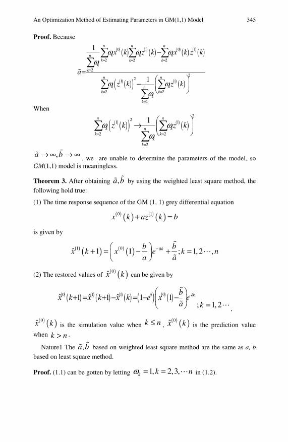
An Optimization Method of Estimating Parameters in GM(1,1) Model 345
Proof. Because
( ) ( ) ( ) ( ) ( ) ( ) ( ) ( )
( ) ( )( ) ( ) ( )
0 1 0 1
2 2 2
22
21 1
2 2
2
1
1
n n n
k k knk k k
kk
n n
k knk k
kk
x k z k x k z k
a
z k z k
ω ω ωω
ω ωω
= = =
=
= =
=
−
=⎛ ⎞− ⎜ ⎟⎝ ⎠
∑ ∑ ∑∑
∑ ∑∑
When
( ) ( )( ) ( ) ( )2
21 1
2 2
2
1n n
k knk k
kk
z k z kω ωω= =
=
⎛ ⎞→ ⎜ ⎟⎝ ⎠
∑ ∑∑
,a b→ ∞ → ∞ , we are unable to determine the parameters of the model, so
GM(1,1) model is meaningless.
Theorem 3. After obtaining ,a b by using the weighted least square method, the
following hold true:
(1) The time response sequence of the GM (1, 1) grey differential equation
( ) ( ) ( ) ( )0 1x k az k b+ =
is given by
( ) ( ) ( ) ( )1 0ˆ 1 1 ; 1,2 ,akb bx k x e k n
a a−⎛ ⎞+ = − + =⎜ ⎟
⎝ ⎠
(2) The restored values of ( ) ( )0x k can be given by
( ) ( ) ( ) ( ) ( ) ( ) ( ) ( ) ( )0 1 1 0ˆ ˆ ˆ1 1 1 1a akbx k x k x k e x e
a−⎛ ⎞
+ = + − = − −⎜ ⎟⎝ ⎠ ; 1, 2k = ,
( ) ( )0x k is the simulation value when k n≤ , ( ) ( )0x k is the prediction value
when k n> .
Nature1 The ,a b based on weighted least square method are the same as a, b
based on least square method.
Proof. (1.1) can be gotten by letting 1, 2,3,k k nω = = in (1.2).
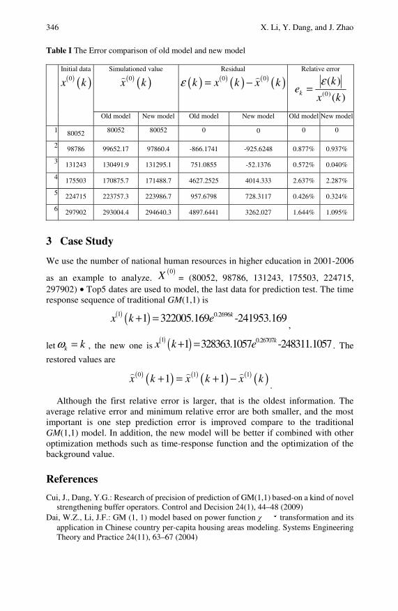
346 X. Li, Y. Dang, and J. Zhao Table I The Error comparison of old model and new model
Simulationed value ( ) ( )0x k
Residual
( ) ( ) ( ) ( ) ( )0 0k x k x kε = −Relative error
)(
)()0( kx
kek
ε=
Initial data ( ) ( )0x k
Old model New model Old model New model Old model New model
1 80052 80052 80052 0 0 0 0
2 98786 99652.17 97860.4 -866.1741 -925.6248 0.877% 0.937%
3 131243 130491.9 131295.1 751.0855 -52.1376 0.572% 0.040%
4 175503 170875.7 171488.7 4627.2525 4014.333 2.637% 2.287%
5 224715 223757.3 223986.7 957.6798 728.3117 0.426% 0.324%
6 297902 293004.4 294640.3 4897.6441 3262.027 1.644% 1.095%
3 Case Study
We use the number of national human resources in higher education in 2001-2006
as an example to analyze. ( )0X = (80052, 98786, 131243, 175503, 224715,
297902) • Top5 dates are used to model, the last data for prediction test. The time response sequence of traditional GM(1,1) is
( ) ( )1 0.26961 322005.169 -241953.169kx k e+ =,
let k kω = , the new one is( ) ( )1 0.267071 328363.1057 -248311.1057kx k e+ = . The
restored values are
( ) ( ) ( ) ( ) ( ) ( )0 1 11 1x k x k x k+ = + −.
Although the first relative error is larger, that is the oldest information. The average relative error and minimum relative error are both smaller, and the most important is one step prediction error is improved compare to the traditional GM(1,1) model. In addition, the new model will be better if combined with other optimization methods such as time-response function and the optimization of the background value.
References
Cui, J., Dang, Y.G.: Research of precision of prediction of GM(1,1) based-on a kind of novel strengthening buffer operators. Control and Decision 24(1), 44–48 (2009)
Dai, W.Z., Li, J.F.: GM (1, 1) model based on power function χ − α transformation and its application in Chinese country per-capita housing areas modeling. Systems Engineering Theory and Practice 24(11), 63–67 (2004)
An Optimization Method of Estimating Parameters in GM(1,1) Model 347 Dang, Y.G., Liu, S.F., Liu, B.: The GM models that x(1)(n) is taken as initial value. Chinese
Journal of Management Science 13(1), 132–135 (2005) Dang, Y.G., Liu, S.F., Mi, C.M., Zhou, J.: Study on the strengthing buffer operators and their
applications. In: IEEE SMC 2006, International Conference on System, Man and Cybernetics, pp. 2267–2271 (2006)
Deng, J.L.: Gray Forecast and Decision-Making. Press of Huazhong University of Science & Technology, Wuhan (2002a)
Deng, J.L.: The Foundation of Grey Systems. Press of Huazhong University of Science & Technology, Wuhan (2002b)
Fu, L.: Gray System Theory and Its Application. Press of Science and Technology Literature, Beijing (1992)
He, W.Z., Song, G.X., Wu, A.D.: Estimation of GM(1,1) model parameter based on linear programming. Systems Engineering and Electronics 26(12), 1826–1828 (2004)
He, W.Z., Song, G.X., Wu, A.D.: A class of algorithms for estimating GM(1,1) model parameter. Systems Engineering Theory and Practice (1), 69–75 (2005)
Ji, P.R., Huang, W.S., Hu, X.Y.: An unbiased grey forecasting model. Systems Engineering and Electronics 22(6), 6–7 (2000)
Li, C.F., Dai, W.Z.: An approach of the grey modeling based on cotx transformation. Systems Engineering 23(3), 110–114 (2005)
Lin, Y., DeNu, R., Patel, N.: True distance fit of exponential curves and tests of applications. International J. of Applied Mathematics 9(1), 49–68 (2002)
Lin, Y., Liu, S.F.: Law of exponentiality and exponential curve fitting. Systems Analysis Modelling Simulation 38, 621–636 (2000)
Liu, B., Liu, S.F., Zhai, Z.J., Dang, Y.G.: Optimum time response sequence for GM(1,1). Chinese Journal of Management Science 11(4), 54–57 (2003)
Liu, S.F.: Gray System Theory and Its Application, pp. 229–233. Press of Science, Beijing (2004)
Luo, D., Liu, S.F., Dang, Y.G.: The optimization of grey model GM(1,1). Engineering Science 5(8), 50–53 (2003)
Song, Z.M., Zhang, S.H.: Separated modeling method in grey systems. Systems Engineering Theory and Practice 22(5), 103–107 (2002)
Sydow, A., Lin, Y., Liu, S.F., DeNu, R., Mennell, W.: Exponential prediction models based on sequence operators. Kybernetes 30(4), 397–410 (2001)
Tan, G.J.: The structure method and application of background value in grey system GM(1,1) model (I, II, III). Systems Engineering Theory and Practice (4, 5, 6) (2000)
Wang, Z.X., Dang, Y.G., Liu, S.F.: The optimization of background value in GM(1,1) model. Journal of Grey System 10(2), 69–74 (2007)
Zhang, D.H., Jiang, S.F., Shi, K.Q.: Theoretical defect of grey prediction formula and its improvement. Systems Engineering Theory and Practice (8), 140–142 (2002)
Zhang, H., Hu, S.G.: Analysis of boundary condition for GM(1,1) model. J. Huazhong Univ. of Sci. & Tech. 29(4), 110–111 (2001)

Research on Grey Wave Forecasting Model*
Qin Wan, Yong Wei, and Xiongqiong Yang1
This chapter is according to the basic process and principle of grey wave forecasting. It presents concrete method and steps of how to choose effective contour lines. Then the author have made improvement on the forecasting formula of grey wave forecasting model, so that the forecasting formula would be closer to original intention of the grey wave forecasting theory founder. In the end it can enhance the validity and the accuracy of grey wave forecasting model.
1 Introduction
The grey system forecasting is to find development rule of system through the primary data processing and the grey model establishing, then makes scientific and quantitative forecasting of system's future. When data in the primitive sequence is fluctuating and its swing range is greater, it’s difficult to find a suitable model for the primitive sequence. Then we can consider forecasting the wave of behavioral data development in the future based on the wave of original data, and this kind of
forecasting is called wave forecasting ]1[ . Wave forecasting is one of the grey forecasting system’s important content with a modeling process that is clear and simple, so wave forecasting obtains high application value in many domains. Wave forecasting model divides six steps approximately, and the author emphasizes on
Qin Wan College of Mathematics and Information, China West Normal University Phone: 13890719855 e-mail: [email protected]
Yong Wei College of Mathematics and Information, China West Normal University Phone: 0817-3306866 e-mail: [email protected]
Xiongqiong Yang College of Mathematics and Information, China West Normal University Phone:13990717516 e-mail: [email protected]
* This work was supported in part by Research fund of Si chuan Education Department (2006A007) and basic application research fund of Sichuan (2008JY0112).
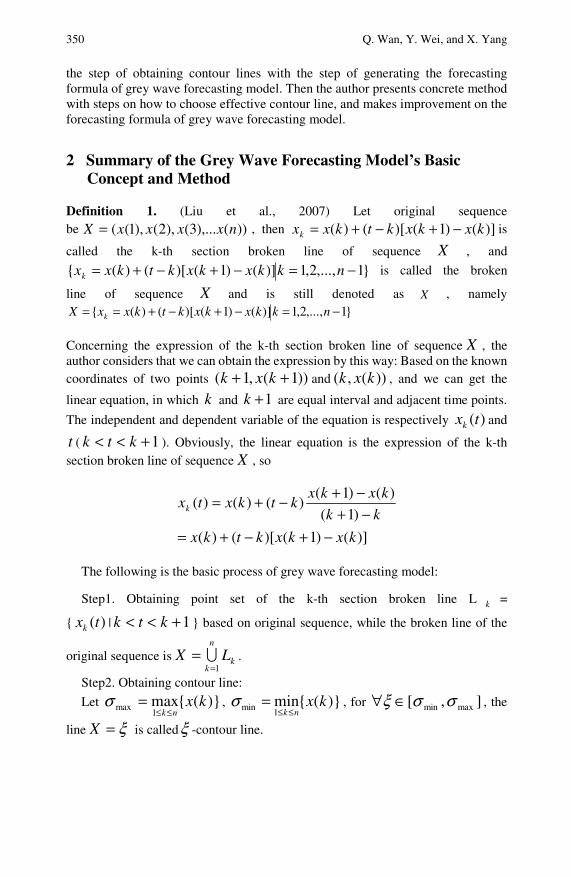
350 Q. Wan, Y. Wei, and X. Yang
the step of obtaining contour lines with the step of generating the forecasting formula of grey wave forecasting model. Then the author presents concrete method with steps on how to choose effective contour line, and makes improvement on the forecasting formula of grey wave forecasting model.
2 Summary of the Grey Wave Forecasting Model’s Basic Concept and Method
Definition 1. (Liu et al., 2007) Let original sequence be ))(),...3(),2(),1(( nxxxxX = , then )]()1()[()( kxkxktkxxk −+−+= is
called the k-th section broken line of sequence X , and
}1,...,2,1)]()1()[()({ −=−+−+= nkkxkxktkxxk is called the broken
line of sequence X and is still denoted as X , namely }1,...,2,1)]()1()[()({ −=−+−+== nkkxkxktkxxX k
Concerning the expression of the k-th section broken line of sequence X , the author considers that we can obtain the expression by this way: Based on the known coordinates of two points ))1(,1( ++ kxk and ))(,( kxk , and we can get the
linear equation, in which k and 1+k are equal interval and adjacent time points.
The independent and dependent variable of the equation is respectively )(txk and
t ( 1+<< ktk ). Obviously, the linear equation is the expression of the k-th section broken line of sequence X , so
)]()1()[()(
)1(
)()1()()()(
kxkxktkx
kk
kxkxktkxtxk
−+−+=−+
−+−+=
The following is the basic process of grey wave forecasting model:
Step1. Obtaining point set of the k-th section broken line L k =
{ )(txk | 1+<< ktk } based on original sequence, while the broken line of the
original sequence is k
n
kLX
1== ∪ .
Step2. Obtaining contour line:
Let )}({max1
max kxnk≤≤
=σ , )}({min1
min kxnk≤≤
=σ , for ],[ maxmin σσξ ∈∀ , the
line ξ=X is calledξ -contour line.
Research on Grey Wave Forecasting Model 351
Step3. Calculating contour point:
The solution of the equations
⎩⎨⎧
=−=−+−+==
ξX
nkkxkxktkxxX k }1,...,2,1)]()1()[()({
is calledξ -contour point. Namely, ξ -contour point is the intersection which is
generated by contour line ξ=X and the broken line of original sequence X .
Step4. Obtaining contour time sequence:
Let ),...,( 21 mPPPX =ξ be ξ -contour time sequence, in which iP is located
in the ik -th section broken line and its coordinate is ),)()1(
)(( ξξ
ii
ii kxkx
kxk
−+−
+ .
Let be ),...2,1()()1(
)()( mi
kxkx
kxkiq
ii
ii =
−+−
+=ξ
, and then
))(),...,2(),1(()0( mqqqQ = is called ξ -contour time sequence.
Step5. Establishing GM (1, 1) model group, then forecast each contour time sequence:
For ],[ maxmin σσξ ∈∀ , we can establish GM(1,1) model (Lin et al., 2002;
Sydow et al., 2001; Lin and Liu, 2000) based on theξ -contour time sequence, thus
make simulation and prediction with the contour time sequence, and then obtain forecasting value with it.
Definition 2. (Liu et al., 2007) let ),..,2,1( siX i == ξ be s different contour
lines, ))(),...,2(),1(()0(iiiii mqqqQ = si ,...,2,1= be the −iξ contour time
sequence, sikmqmqmq iiiiiii ,...,2,1),(),...,2(),1(^^^
=+++ be the
forecasting value of the −iξ contour time sequence form the GM (1, 1) model. If
there exists ji ≠ , makes )()(^^
jjjiii lmqlmq +=+ , then )(^
iii lmq + and
)(^
jjj lmq + is called a pair of ineffective forecasting time.
Step6. Generating forecasting wave:
Let )(),...,2(),1(^^^
iiiiiii kmqmqmq +++ be forecasting value of the
−iξ contour time sequence from the GM (1, 1) model. Ranking all of the
rest forecasting value trend to be larger after rejecting the ineffective forecasting
time among them, when)(
^kq
X ξ= is the contour line corresponding to )(^
kq ,

352 Q. Wan, Y. Wei, and X. Yang
then the forecasting broken line of sequence X is
},...,2,1)))((({)()1(
^
)(
^
^^^ skqkqkq
nkkqtX =−−+=+
ξξξ
3 How to Choose Effective Contour Lines
In above 6 steps of grey wave forecasting model, the purpose of the step of obtaining contour line and the step of calculating point is to obtain contour time sequence of each contour line, and collecting data for establishing GM (1, 1) model. The author considers that there are two problems needed attention: 1) we can take
any value from ],[ maxmin σσ asξ , and let the line ξ=X be contour line. But we
always expect that the contour line ξ=X and the broken line of original
sequence X will generate four or more intersections. Because we can just establish GM (1, 1) model on four or more data, therefore we call the contour line which can generate four or more contour points as an effective contour line. However, not any contour line ξ=X is an effective contour line, so we often waste much time and
energy on verification whether the number of intersections which is generated by the contour line and the broken line of original sequence meets the requirement of establishing GM(1,1) model or not. 2) The waveform graph that we have forecasted consists of several broken lines, and the amount of broken lines has great relationship with the amount of contour lines. It can be considered that if obtain more contour lines, then the forecasting waveform graph would be closer to the actual situation. That is to say, choosing contour lines is a crucial link in the preparatory work of grey wave forecasting. The author presents a method of choosing effective contour lines. On the premise that obtaining enough contour lines, we can insure that every contour line which be chosen would generate four or more contour points by this method. It greatly reduces the working load of choosing effective contour lines.
A. The related definition and theorem
Definition 3. We call the contour line which can generate four or more contour points as an effective contour line.
Definition 4. Drawing the waveform graph of original sequence X in a coordinate planes which is composed by the lateral axis t and the longitudinal axis x .1) If
for itt = , it exits a neighborhood )( itδ of it , which makes )( itt δ∈∀ ,
)()( txtx i > , then )( itx is called a wave crest of X ; 2) If for jtt = , it exits a
neighborhood )( jtδ of jt , which makes )( jtδ , )()( txtx j < , then )( jtx is
called a wave trough of X ;( There may be two wave troughs adjacent to a wave crest, we can differentiate them with left-adjacent wave trough and right-adjacent
Research on Grey Wave Forecasting Model 353
wave trough; also there may be two wave crests adjacent to a wave trough, we can differentiate them with left-adjacent wave crest and right-adjacent wave crest).
Theorem 1. Among any three wave crests )3(),2(),1( fff and their
right-adjacent wave troughs )3(),2(),1( ggg , let )}3(),2(),1(min{ ffff = ,
)}3(),2(),1(max{ gggg = . If gf > , namely the minimum wave crest is bigger
than the maximum wave trough, we can obtain any ),( fg∈ξ , and then the
contour line ξ=x and the original sequence X will generate at Least five
contour points.
Proof: As we known )}3(),2(),1(min{ ffff = )}3(),2(),1(max{ gggg =
and gf > , so we can get ))(),((),( jfigfg ⊆ , }3,2,1{, ∈ji . Because
there are at least five broken lines between the wave crests )3(),2(),1( fff and
the right-adjacent wave troughs )3(),2(),1( ggg , then the contour line
ξ=x would intersect with above five broken lines respectively, so we can obtain
five contour points from the contour line ξ=x . End.
B. The concrete method and steps of how to choose effective contour lines
Draw the waveform graph of original sequence X , and find out all wave crests and wave troughs. Then rank all wave crests trended to be larger as )(......)()( 21 nkfkfkf <<< , rank all wave troughs trended to be smaller
as )(......)()( 21 msgsgsg >>> .
Step1: Find out the maximum wave trough )( 1isg which is smaller than the
wave crest )( 1kf , and find out the wave trough )( 1jsg which is the right-adjacent
wave crest of )( 1kf . Obviously, )()( 11 ji sgsg ≥ .Let
)}(),......,(),({ 221 −= msgsgsgA (still trended to be smaller), namely A is a set
which consists of all wave troughs except the last two; Let )}()......,2(),1(),({ 1111 jiii sgsgsgsgB ++= (still trended to be smaller), namely B is
consisted by the wave troughs which is between )( isg and )( jsg ; Let
BAG ∩= , for Gsg t ∈∀ )( ,we can take any ))(),(( 1kfsg t∈ξ and form the
contour line ξ=x . Then the contour line ξ=x and the original sequence X will
generate at least five contour points.
Proof: Observing the arrangements of all wave crests and all wave troughs:
⎩⎨⎧
>>>>><<<<<
−−
−−
)()()(......)()(
)()()(......)()(
1221
1221
mmm
nnn
sgsgsgsgsg
kfkfkfkfkf (1)
354 Q. Wan, Y. Wei, and X. Yang
It is easy to see that wave crest )( 1kf is the minimum among all wave crests.
Gsg t ∈∀ )( , we can always find out two wave troughs are both smaller than it.
(Because the smaller two wave troughs are both beyond the set G).
1) When the wave trough )( tsg which we have chosen is the right-adjacent
wave crest of )( 1kf , let the wave trough )( 1tsg and )( 2tsg both smaller
than )( tsg . Let the left-adjacent wave crests )( 1tsf and )( 2tsf which are
corresponding to )( 1tsg and )( 2tsg respectively. And )( 1kf is the minimum
among all wave crests, so )( 1tsf and )( 2tsf are both bigger than )( 1kf . That is
to say, )( tsg is the biggest one in three wave trough and )( 1kf is the smallest one
in three wave crests. Namely the conditions in theorem 1 have been satisfied, we
can obtain the contour line ξ=x in which ))(),(( 1kfsg t∈ξ , and it would
generate at least five contour points according to theorem 1.
2) When the wave trough )( tsg which we have chosen isn’t the right-adjacent
wave crest of )( 1kf , let be the wave trough )( 1tsg is smaller than )( tsg . Then
among the wave trough )( tsg and its left-adjacent wave, the wave trough
)( 1tsg and its left-adjacent wave, the wave crest )( 1kf and its right-adjacent
wave trough, we can find that )( tsg is the biggest one in three wave troughs and
)( 1kf is the smallest one in three wave crests. Namely the conditions in theorem 1
have been satisfied, we can obtain the contour line ξ=x in
which ))(),(( 1kfsg t∈ξ , and it would generate at least five contour points
according to theorem 1. So we can get several effective contour lines with the minimum wave crest
)( 1kf by step1.
Step2: Removing the minimum wave crest )( 1kf and its right-adjacent wave
trough )( 1jsg in the formula (1). Carry step1 on the existing minimum wave
crest )( 2kf again, then we can get several effective contour lines with the
wave crest )( 2kf . Namely find out the maximum wave trough )( 2isg which
is smaller than the wave crest )( 2kf , and find out the wave trough )( 2jsg
which is right-adjacent to )( 2kf . Obviously, )()( 22 ji sgsg ≥ . Let
)}(),......,(),({ 221 −= msgsgsgA (still trended to be smaller), namely A is a set
which consists of all the rest wave troughs except the last two; Let )}()......,2(),1(),({ 2222 jiii sgsgsgsgB ++= (still trended to be smaller), namely

Research on Grey Wave Forecasting Model 355
B is consisted by the wave troughs which is between )( 2isg and )( 2jsg ; Let
BAG ∩= , for Gsg t ∈∀ )( ,we can take any ))(),(( 2kfsg t∈ξ and form
the contour line ξ=x . Then the contour line ξ=x and the original sequence X
will generate at least five contour points.
Step3: Removing the minimum wave crest )( 2kf and its right-adjacent wave
trough )( 2jsg in the formula (1) again. Carry step1 on the existing minimum wave
crest )( 3kf again, then we can get several effective contour lines with the wave
crest )( 3kf .
Until get several effective contour lines with the wave crest )( 2−nkf .
In a word, expect the biggest two wave crests; we can obtain several effective contour lines with every rest wave crest accurately by the new method.
4 The Improvement on Forecasting Formula of the Grey Wave Forecasting Model
In the sixth step of grey wave forecasting model, after ranking the forecasting value of the contour time sequence trend to be larger, the broken line between
)1(),(^^
+kqkq is the k-th section forecasting broken line of original sequence X .
Then its expression should be the linear equation which is generated by the
coordinates of two points )),(()(
^
^
kq
kq ξ and )),1(()1(
^
^
+
+kq
kq ξ , and the
independent with dependent variables of the equation is respectively ^
kx and
t ( )1()(^^
+<< kqtkq ). Namely the k-th section forecasting broken line
is
)()1(
)())((
^^
)()1(^
)(
^ ^^
^
kqkqkqtx kqkq
kqk
−+
−−+= +
ξξξ , and the forecasting broken line of
sequence X is },...,2,1)()1(
)())(({
^^
)()1(^
)(
^ ^^
^ nkkqkq
kqtX kqkq
kq=
−+
−−+= +
ξξξ
The footnote of the forecasting value )1(),(^^
+kqkq is
k and 1+k respectively, and the footnote of them is adjacent. But when we find out
the value of )1(),(^^
+kqkq on the lateral axis t , the spacing in the value of
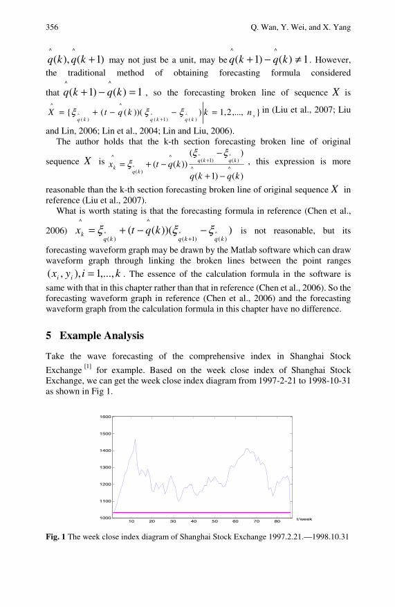
356 Q. Wan, Y. Wei, and X. Yang
)1(),(^^
+kqkq may not just be a unit, may be 1)()1(^^
≠−+ kqkq . However,
the traditional method of obtaining forecasting formula considered
that 1)()1(^^
=−+ kqkq , so the forecasting broken line of sequence X is
},...,2,1)))((({)()1(
^
)(
^
^^^ skqkqkq
nkkqtX =−−+=+
ξξξ in (Liu et al., 2007; Liu
and Lin, 2006; Lin et al., 2004; Lin and Liu, 2006). The author holds that the k-th section forecasting broken line of original
sequence X is
)()1(
)())((
^^
)()1(^
)(
^ ^^
^
kqkqkqtx kqkq
kqk
−+
−−+= +
ξξξ , this expression is more
reasonable than the k-th section forecasting broken line of original sequence X in reference (Liu et al., 2007).
What is worth stating is that the forecasting formula in reference (Chen et al.,
2006) )))((()()1(
^
)(
^
^^^kqkqkq
k kqtx ξξξ −−+=+
is not reasonable, but its
forecasting waveform graph may be drawn by the Matlab software which can draw waveform graph through linking the broken lines between the point ranges
kiyx ii ,...,1),,( = . The essence of the calculation formula in the software is
same with that in this chapter rather than that in reference (Chen et al., 2006). So the forecasting waveform graph in reference (Chen et al., 2006) and the forecasting waveform graph from the calculation formula in this chapter have no difference.
5 Example Analysis
Take the wave forecasting of the comprehensive index in Shanghai Stock
Exchange ]1[ for example. Based on the week close index of Shanghai Stock Exchange, we can get the week close index diagram from 1997-2-21 to 1998-10-31 as shown in Fig 1.
10 20 30 40 50 60 70 801000
1100
1200
1300
1400
1500
1600
t/week
Fig. 1 The week close index diagram of Shanghai Stock Exchange 1997.2.21.—1998.10.31
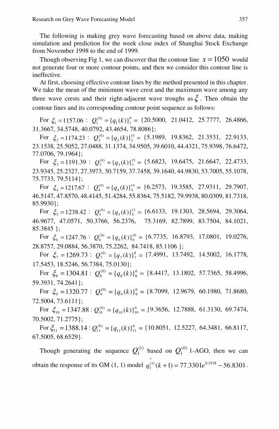
Research on Grey Wave Forecasting Model 357
The following is making grey wave forecasting based on above data, making simulation and prediction for the week close index of Shanghai Stock Exchange from November 1998 to the end of 1999.
Though observing Fig 1, we can discover that the contour line 1050=x would not generate four or more contour points, and then we consider this contour line is ineffective.
At first, choosing effective contour lines by the method presented in this chapter. We take the mean of the minimum wave crest and the maximum wave among any three wave crests and their right-adjacent wave troughs as ξ . Then obtain the
contour lines and its corresponding contour point sequence as follows:
For 06.11571 =ξ : == 911
)0(1 )}({ kqQ {20.5000, 21.0412, 25.7777, 26.4866,
31.3667, 34.5748, 40.0792, 43.4654, 78.8086}; For 23.11742 =ξ : == 15
22)0(
2 )}({ kqQ {5.1989, 19.8362, 21.3531, 22.9133,
23.1538, 25.5052, 27.0488, 31.1374, 34.9505, 39.6010, 44.4321, 75.9398, 76.6472, 77.0706, 79.1964};
For 39.11913 =ξ : == 1533
)0(3 )}({ kqQ {5.6823, 19.6475, 21.6647, 22.4733,
23.9345, 25.2327, 27.3973, 30.7159, 37.7458, 39.1640, 44.9830, 53.7005, 55.1078, 75.7733, 79.5114};
For 67.12174 =ξ : == 1444
)0(4 )}({ kqQ {6.2573, 19.3585, 27.9311, 29.7907,
46.5147, 47.8570, 48.4145, 51.4284, 55.8364, 75.5182, 79.9938, 80.0309, 81.7318, 85.9930};
For 42.12385 =ξ : == 1355
)0(5 )}({ kqQ {6.6133, 19.1303, 28.5694, 29.3064,
46.9677, 47.0571, 50.3766, 56.2376, 75.3169, 82.7899, 83.7504, 84.1021, 85.3845 };
For 76.12476 =ξ : == 1066
)0(6 )}({ kqQ {6.7735, 16.8793, 17.0801, 19.0276,
28.8757, 29.0884, 56.3870, 75.2262, 84.7418, 85.1106 }; For 73.12697 =ξ : == 8
77)0(
7 )}({ kqQ {7.4991, 13.7492, 14.5002, 16.1778,
17.5453, 18.5246, 56.7384, 75.0130}; For 81.13048 =ξ : == 6
88)0(
8 )}({ kqQ {8.4417, 13.1802, 57.7365, 58.4996,
59.3931, 74.2641}; For 77.13209 =ξ : == 6
99)0(
9 )}({ kqQ {8.7099, 12.9679, 60.1980, 71.8680,
72.5004, 73.6111}; For 88.134710 =ξ : == 6
1010)0(
10 )}({ kqQ {9.3656, 12.7888, 61.3130, 69.7474,
70.5002, 71.2775}; For 14.138811 =ξ : == 6
1111)0(
11 )}({ kqQ {10.8051, 12.5227, 64.3481, 66.8117,
67.5005, 68.6529}.
Though generating the sequence )1(1Q based on )0(
1Q 1-AGO, then we can
obtain the response of its GM (1, 1) model 8301.563301.77)1( 1938.0^
)1(1 −=+ ekq .

358 Q. Wan, Y. Wei, and X. Yang
Simultaneously, we can obtain the response of GM(1,1) model with
)11,...,3,2()0( =iQi (omission).
Let )()1()1()1(^)1(^^
kqkqkq iii −+=+ , we can obtain −iξ contour time
forecasting sequence( 11,...,2,1=i ) :
== )}12(),11(),10({ 1
^
1
^
1
^)0(
1
^
qqqQ {94.5464, 114.7597, 139.2946}
== )}18(),17(),16({ 2
^
2
^
2
^)0(
2
^
qqqQ {111.7, 127.3, 145.1}
== )}19(),18(),17(),16({ 3
^
3
^
3
^
3
^)0(
3
^
qqqqQ {96.8373, 109.4591, 123.7260, 139.8525}
== )}19(),18(),17(),16(),15({ 4
^
4
^
4
^
4
^
4
^)0(
4
^
qqqqqQ {95.5754, 105.2375, 115.8764,
127.5908, 140.4895}
== )}18(),17(),16(),15(),14({ 5
^
5
^
5
^
5
^
5
^)0(
5
^
qqqqqQ {89.0488, 99.1198, 110.3297,
122.8075, 136.6964}
== )}12(),11({ 6
^
6
^)0(
6
^
qqQ {100.5, 126.0}
== )}10(),9({ 7
^
7
^)0(
7
^
qqQ {93.8, 140.7}
== )}9(),8(),7({ 8
^
8
^
8
^)0(
8
^
qqqQ {95.8, 118.0, 145.4}
== )}8(),7({ 9
^
9
^)0(
9
^
qqQ {101.7, 123.2}
== )}10(),9(),8(),7({ 10
^
10
^
10
^
10
^)0(
10
^
qqqqQ {81.3, 97.7, 117.4, 141}
== )}9(),8(),7({ 11
^
11
^
11
^)0(
11
^
qqqQ {92.4, 109.6, 130.1}
90 100 110 120 130 1401000
1200
1400
1600
1800
2000
2200
2400
2600
2800
3000
t/week
actual diagram
forecasting diagram
Fig. 2 The week close index forecasting diagram of Shanghai Stock Exchange (1998.11.6. - 1999.12.30)
Research on Grey Wave Forecasting Model 359
After rejecting the ineffective forecasting time, we can draw the week close index forecasting diagram of Shanghai Stock Exchange from November 1998 to the end of 1999 based on the forecasting formula presented in this chapter. Then compare the forecasting diagram with actual situation as shown in Fig 2.
From Figure 2, we can find that the agreement between forecasting wave and the actual wave is good. The similarity degree between the short or middle-term forecasting wave and the actual wave is higher. It confirms the grey wave forecasting has certain validity and the usability.
6 Conclusions
This article according to the basic process and principle of grey wave forecasting presents concrete method and steps on how to choose effective contour lines. It also gives a strict proof that the counter lines which is chosen by the method in this chapter will generate at least five contour points, thus we can establish GM (1, 1) model to forecast the development of behavioral data wave in the future. Secondly, the author have made improvement on the forecasting formula of grey wave forecasting model, so that the forecasting formula would be much closer to original intention of the grey wave forecasting theory founder. Then it can enhance the validity and the accuracy of grey wave forecasting model.
Acknowledgment. Research fund of Si chuan Education Department (2006A007) And basic application research fund of Sichuan (2008JY0112).
References
Chen, K.J., Ji, P., Liu, S.F.: An application of grey wave forecasting on economic fluctuation. In: Proceedings of the 2006 Grey Systems Theory and Application Academic Conference, pp. 475–479 (2006)
Lin, Y., Chen, M.Y., Liu, S.F.: Theory of grey systems: capturing uncertainties of grey information. Kybernetes: The International Journal of Systems and Cybernetics 33(2), 196–218 (2004)
Lin, Y., DeNu, R., Patel, N.: True distance fit of exponential curves and tests of applications. International J. of Applied Mathematics 9(1), 49–68 (2002)
Lin, Y., Liu, S.F.: Law of exponentiality and exponential curve fitting. Systems Analysis Modelling Simulation 38, 621–636 (2000)
Lin, Y., Liu, S.F.: Solving problems with incomplete information: A grey systems approach. In: Advances in Imaging and Electron Physics, vol. 141, pp. 77–174. Elsevier, Oxford (2006)
Liu, S.F., Dang, Y.G., Fang, Z.G.: Grey Systems Theory and Applications. Scientific Press, Beijing (2007)
Liu, S.F., Lin, Y.: Grey Information: Theory and Practical Applications. Springer, London (2006)
Sydow, A., Lin, Y., Liu, S.F., DeNu, R., Mennell, W.: Exponential prediction models based on sequence operators. Kybernetes 30(4), 397–410 (2001)

A Method of Modeling Logistics
Yinao Wang, Lifeng Wu, and Fengjing Cai1
Based on the grey system direct modeling method, we put forward a method of modeling Logistic under the criterion on minimized the sum of the squares of the modified relative error (SSMRE). Then applied it in the U.S.A population forecasting, with results showing that this method can remarkably reduce mean absolute percentage error (MAPE) and the built model can preferably represent the whole historical population law. The process of modeling shows that this method is more convenient than the traditional modeling method.
1 Introduction
Grey system theory has already been widely used in many fields since 1982 (Deng, 1982; Liu and Lin, 2006; Lin et al., 2004; Lin and Liu, 2006), and grey modeling method is an important component of the grey system theory. As one of the grey modeling methods, direct modeling method has been presented (Wang, 1988) and the characteristics of the direct modeling method are studied (Wang et al., 2000; Wang, 2003; Mu, 2003; Shui and Qin, 1998).
In this chapter we consider the fitting problem for Logistic model (Jukic and Scitovski, 2003)
0,,/ >−= srsxrx
dtdx, (1)
Parameter 0>r can be interpreted as the maximum possible rate of population
growth, while parameter s
1 is the upper limit of population growth and it is called
Yinao Wang College of Mathematics and Information Science, Wenzhou University, Wenzhou, 325035, Zhejiang Province, P.R. China Phone: +86-577-86689529 e-mail: [email protected]
Lifeng Wu and Fengjing Cai College of Mathematics and Information Science, Wenzhou University, Wenzhou, 325035, Zhejiang Province, P.R. China e-mail: [email protected]
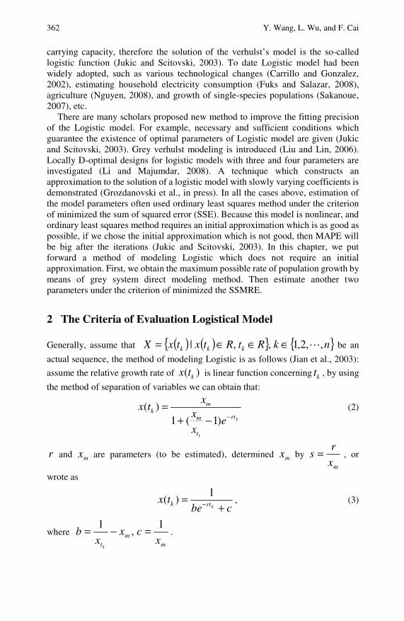
362 Y. Wang, L. Wu, and F. Cai
carrying capacity, therefore the solution of the verhulst’s model is the so-called logistic function (Jukic and Scitovski, 2003). To date Logistic model had been widely adopted, such as various technological changes (Carrillo and Gonzalez, 2002), estimating household electricity consumption (Fuks and Salazar, 2008), agriculture (Nguyen, 2008), and growth of single-species populations (Sakanoue, 2007), etc.
There are many scholars proposed new method to improve the fitting precision of the Logistic model. For example, necessary and sufficient conditions which guarantee the existence of optimal parameters of Logistic model are given (Jukic and Scitovski, 2003). Grey verhulst modeling is introduced (Liu and Lin, 2006). Locally D-optimal designs for logistic models with three and four parameters are investigated (Li and Majumdar, 2008). A technique which constructs an approximation to the solution of a logistic model with slowly varying coefficients is demonstrated (Grozdanovski et al., in press). In all the cases above, estimation of the model parameters often used ordinary least squares method under the criterion of minimized the sum of squared error (SSE). Because this model is nonlinear, and ordinary least squares method requires an initial approximation which is as good as possible, if we chose the initial approximation which is not good, then MAPE will be big after the iterations (Jukic and Scitovski, 2003). In this chapter, we put forward a method of modeling Logistic which does not require an initial approximation. First, we obtain the maximum possible rate of population growth by means of grey system direct modeling method. Then estimate another two parameters under the criterion of minimized the SSMRE.
2 The Criteria of Evaluation Logistical Model
Generally, assume that ( ) ( ){ } { }nkRtRtxtxX kkk ,,2,1,,| ∈∈∈= be an
actual sequence, the method of modeling Logistic is as follows (Jian et al., 2003):
assume the relative growth rate of ( )kx t is linear function concerning kt , by using
the method of separation of variables we can obtain that:
krt
t
m
mk
ex
xx
tx−−+
=)1(1
)(
1
(2)
r and mx are parameters (to be estimated), determined mx by mx
rs = , or
wrote as
cbetx
krtk += −
1)( , (3)
where m
mt x
cxx
bk
1,
1 =−= .
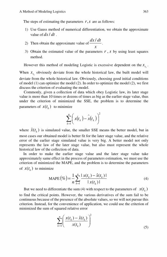
A Method of Modeling Logistics 363
The steps of estimating the parameters sr, are as follows:
1) Use Gauss method of numerical differentiation, we obtain the approximate value of /dx dt .
2) Then obtain the approximate value of/dx dt
x.
3) Obtain the estimated value of the parameters ,r s by using least squares
method.
However this method of modeling Logistic is excessive dependent on the1t
x .
When 1t
x obviously deviate from the whole historical law, the built model will
deviate from the whole historical law. Obviously, choosing good initial conditions of model (1) can optimize the model (2). In order to optimize the model (2), we first discuss the criterion of evaluating the model.
Commonly, given a collection of data which obey Logistic law, its later stage value is more than 10 times or dozens of times as big as the earlier stage value, thus under the criterion of minimized the SSE, the problem is to determine the
parameters of )( ktx to minimize
( ) ( )∑=
∧
⎟⎠⎞
⎜⎝⎛ −
n
kkk txtx
1
2
where )(ˆ ktx is simulated value, the smaller SSE means the better model, but in
most cases our obtained model is better fit for the later stage value, and the relative error of the earlier stage simulated value is very big. A better model not only represents the law of the later stage value, but also must represent the whole historical law of the collection of data.
In order to make the earlier stage value and the later stage value take approximately same effect in the process of parameters estimation, we must use the criterion of minimized the MAPE, and the problem is to determine the parameters
of ( )kx t to minimize
MAPE ( ) ∑=
−=n
k k
kk
tx
txtx
n 1 |)(|
|)(ˆ)(|1% (4)
But we need to differentiate the sum (4) with respect to the parameters of )( ktx
to find the critical points. However, the various derivatives of the sum fail to be continuous because of the presence of the absolute values, so we will not pursue this criterion. Instead, for the convenience of application, we could use the criterion of minimized the sum of squared relative error
∑=
⎟⎟⎠
⎞⎜⎜⎝
⎛ −n
k k
kk
tx
txtx
1
2
)()(ˆ)(
(5)

364 Y. Wang, L. Wu, and F. Cai
Especially for the logistic model (3), we consider the criterion of minimized the
SSMRE, that is, determine the parameters of )( ktx to minimize
SSMRE ∑=
⎟⎟⎠
⎞⎜⎜⎝
⎛ −=n
k k
kk
tx
txtx
1
2
)(ˆ)(ˆ)(
(6)
The smaller SSMRE means the better model, thus estimation of the parameters
of )( ktx can be solved easily.
An optimum modeling method of logistic The steps of modeling Logistic by using grey direct modeling method are as
follows (Wang, 1988):
1) by differential equation model (1)
sxrx
dtdx −=/
2sxrxdt
dx −=
We use grey direct modeling method to obtain
( ) ( ) ( ) ( ) ,2''
1
1kk
kk
kk tsztrztt
txtx −≈−−
−
−
where
( ) ( ) ( )2
1' −+= kkk
txtxtz .,2 nk =
Then the least squares estimate of the parameter sequence [ ]Tsra =∧
of the model
(1) is given by (Wang, 1988)
[ ] YBBBa TT 1−∧=
( ) ( ) ( ) ( )
( ) ( ) ( ) ( )
( ) ( ) ( ) ( )
,
22
22
22
2
11
2
3232
2
2121
⎥⎥⎥⎥⎥⎥⎥⎥⎥⎥
⎦
⎤
⎢⎢⎢⎢⎢⎢⎢⎢⎢⎢
⎣
⎡
⎟⎠⎞
⎜⎝⎛ +−+
⎟⎠⎞
⎜⎝⎛ +−+
⎟⎠⎞
⎜⎝⎛ +−+
=
−− nnnn txtxtxtx
txtxtxtx
txtxtxtx
B
( ) ( )
( ) ( )
( ) ( )⎥⎥⎥⎥⎥⎥⎥⎥⎥
⎦
⎤
⎢⎢⎢⎢⎢⎢⎢⎢⎢
⎣
⎡
−−
−−−−
=
−
−
1
1
23
23
12
12
nn
nn
tt
txtx
tt
txtx
tt
txtx
Y

A Method of Modeling Logistics 365
Then obtain estimated value sr ˆ,ˆ of the parameters sr, of model (1), by mx
rs = ,
mm x
cxx
bˆ1
ˆ,ˆ1ˆ
0
=−= , we obtain estimated value mxr ˆ,ˆ of the parameters mxr,
of model (2), substitute mxr ˆ,ˆ into model (2), we obtain
cebkx
ktr ˆˆ1
)(ˆˆ +
=−
, where m
mt x
cxx
bˆ1
ˆ,ˆ1ˆ
1
=−= (7)
Thus
∑=
⎟⎟⎠
⎞⎜⎜⎝
⎛ −=n
k k
kk
tx
txtx
1
2
)(ˆ)(ˆ)(
SSMRE
[ ]∑=
− −+=n
k
trk cebtx k
1
2ˆ 1)ˆˆ)((
in order to make the SSMRE smaller, ∧b and
∧c can be regards as the unknown
parameters, ∧r is known parameter, thus object function the SSMRE is linear
concerning b and ∧c , by means of the ordinary least squares method, the,
∧b and
∧c
making the SSMRE minimum should satisfy
[ ] [ ]
[ ] [ ]⎪⎪⎪
⎩
⎪⎪⎪
⎨
⎧
=−+=∂∂
=−
+=∂∂
∑∑∑
∑
∑∑
===
−
=
−
=
−
=
−
0)()(ˆ)(ˆˆ
0)(
)(ˆ)(ˆˆ
11
2
1
2
1
1
2
1
2
n
kk
n
k
n
k
rkk
n
k
rtk
n
k
rtk
n
k
rtk
txkxcetxbc
S
etx
etxcetxbb
S
k
kk
That is
[ ] [ ]
[ ] [ ]⎪⎪⎩
⎪⎪⎨
⎧
=−+
=−+
∑∑∑
∑∑∑
===
−
=
−
=
−
=
−
0)()(ˆ)(ˆ
0)()(ˆ)(ˆ
11
2
1
2
11
2
1
2
n
kk
n
kk
n
k
rtk
n
k
rtk
n
k
rtk
n
k
rtk
txtxcetxb
etxetxcetxb
k
kkk
So, solving this system gives that
,ˆ,ˆ 21
D
Dc
D
Db == (8)
where
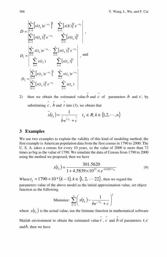
366 Y. Wang, L. Wu, and F. Cai
[ ] [ ]
[ ] [ ],
)()(
)()(
1
2
1
2
1
2
1
2
∑∑
∑∑
==
−
=
−
=
−
= n
kk
n
k
rtk
n
k
rtn
k
rtk
txetx
ekxetxD
k
kk
[ ]
[ ],
)()(
)()(
1
2
1
1
2
11
∑∑
∑∑
==
=
−
=
−
= n
kk
n
kk
n
k
rtk
n
k
rtk
txtx
etxetxD
kk
and
[ ][ ] ∑∑
∑∑
==
−
=
−
=
−
= n
kk
n
k
rtk
n
k
rtk
n
k
rtk
txetx
etxetxD
k
kk
11
2
11
2
2
)()(
)()(
2) then we obtain the estimated value∧b and
∧c of parameters b and c , by
substituting ∧c ,
∧b and
∧r into (3), we obtain that
( ) ∧∧
∧
+= ∧
cebtx
ktrk
1 { }nkRtk ,,2,1, ∈∈
3 Examples
We use two examples to explain the validity of this kind of modeling method; the first example is American population data from the first census in 1790 to 2000. The U. S. A. takes a census for every 10 years, so the value of 2000 is more than 72 times as big as the value of 1790. We simulate the data of Census from 1790 to 2000 using the method we proposed, then we have
( )kt*0.0281-23104.58391
301.5620e
tx k ××+= (9)
Where ( ) { }222,1,1*101790 ,kktk ∈−+= , then we regard the
parameters value of the above model as the initial approximation value, set object function as the following
Minimize: ( )∑=
− ⎟⎠⎞
⎜⎝⎛
+−
n
krtk cbe
txk
1
21
where ( )ktx is the actual value, use the fminunc function in mathematical software
Matlab environment to obtain the estimated value∧r ,
∧c and
∧b of parameters cr,
andb, then we have

A Method of Modeling Logistics 367
Table I Simulation value and error
Year ktA
∧ ktp
∧
model (9)
RE model (9) ktp
∧
model (10)
RE model (10)
1790 3.9 4.3519 -11.59 3.7578 3.65
1800 5.3 5.7358 -8.22 4.9535 6.54
1810 7.2 7.5485 -4.84 6.5222 9.41
1820 9.6 9.9149 -3.28 8.5744 10.68
1830 12.9 12.9904 -0.70 11.2500 12.79
1840 17.1 16.9643 0.79 14.7223 13.9
1850 23.2 22.0611 4.91 19.2019 17.23
1860 31.4 28.5355 9.12 24.9368 20.58
1870 38.6 36.6609 5.02 32.2072 16.56
1880 50.2 46.7041 6.96 41.3107 17.71
1890 62.9 58.8870 6.38 52.5340 16.48
1900 76.0 73.3335 3.51 66.1092 13.01
1910 92.0 90.0095 2.16 82.1553 10.7
1920 106.5 108.6719 -2.04 100.6134 5.53
1930 123.2 128.8472 -4.58 121.1941 1.63
1940 131.7 149.8580 -13.79 143.3583 -8.85
1950 150.7 170.9048 -13.41 166.3530 -10.39
1960 179.3 191.1823 -6.63 189.3033 -5.58
1970 204.0 209.9989 -2.94 211.3411 -3.6
1980 226.5 226.8611 -0.16 231.7312 -2.31
1990 251.4 241.5060 3.94 249.9589 0.57
2000 281.4 253.8833 9.78 265.7590 5.56
MAPE 5.67 9.69

368 Y. Wang, L. Wu, and F. Cai
( )k*t0.0280-23105.0224e1
330.4117
etx k ××+
= (10)
where ( ) { }222,1,1*101790 ,kktk ∈−+= ,
Refer to table I (actual value, simulation value and error), compare each result. From the table I, we can see that the error between the actual value and the simulation value from 1790 to 1930 is positive according to the mode (10), so model (10) does not represent the whole historical law of the data. On the contrary, according to the mode (9), the error between the actual value and the simulation value from 1790 to 1830 is negative, from 1840 to 1910 is positive, and from 1920 to 1980 is negative, so the model (9) can preferably represent the whole historical law of the data. From the mode (9), we can see the error approximately obey sine rule, we can combine the model (9) with sine model, the fitting accuracy and forecasting accuracy will be better. From the table I, we can see that obtained model (9) and (10) are not better fit for the later stage value, and that’s because a great number of foreigners immigrated to America with the development of globalization since 1950.
The second example from (Zhu, 2002), refer to table II (actual value, simulation value and error), compare each result with (Zhu, 2002), we can see that this method has remarkably reduced the MAPE.
Table II Simulation value and error
Order ktp
∧
this chapter
RE this
chapter ktp
∧
(Zhu, 2002)
RE (Zhu, 2002)
1 0.3439 -114.9 2.833 -1670
2 1.2483 16.78 4.584 -205.6
3 4.2480 -17.67 7.348 -103.55
4 11.9699 -15.94 11.612 18.46
5 23.3781 -3.49 17.955 20.52
6 31.4163 -18.69 26.904 -1.64
7 34.6110 6.46 38.624 -4.39
MAPE 27.71 289.25
ktA∧
is the actual value at time kt , ktp
∧is the simulation value at time kt ,
RE= %100×−
∧
∧∧
k
kk
t
tt
A
pA.
A Method of Modeling Logistics 369
4 Conclusion and Analysis
It is difficult to estimate the parameters of the Logistic model. To solve this problem, we give a method for estimating its parameters based on grey direct modeling under the criterion of minimized the SSMRE. This method is very easy to implement in mathematical software Matlab environment, thus comparisons of the obtained results with the results of existing approach demonstrate that this method can reduce the MAPE of Logistic model and estimation of the parameters of Logistic model must be under the criterion of minimized the SSMRE.
References
Carrillo, M., Gonzalez, J.M.: A new approach to modelling sigmoid curves. Technological Forecasting & Social Change 69, 233–241 (2002)
Deng, J.L.: Control problems of grey system. System and Control Letters 1(1), 288–294 (1982)
Fuks, M., Salazar, E.: Applying models for ordinal logistic regression to the analysis of household electricity consumption classes in Rio de Janeiro. Brazil Energy Economics 30(4), 1672–1692 (2008)
Grozdanovski, T., Shepherd, J.J., Stacey, A.: Multi-scaling analysis of a logistic model with slowly varying coefficients. Applied Mathematics Letters (to appear) (in press)
Jian, Q.Y., Xie, J.X., Ye, J.: Mathematical Models, 3rd edn., pp. 10–14. Higher Education Press, Beijing (2003)
Jukic, D., Scitovski, R.: Solution of the least-square problem for Logistic function. Journal of Computational and Applied Mathematics 156(1), 159–177 (2003)
Li, G., Majumdar, D.: D-optimal designs for logistic models with three and four parameters. Journal of Statistical Planning and Inference 138(7), 1950–1959 (2008)
Lin, Y., Chen, M.Y., Liu, S.F.: Theory of grey systems: capturing uncertainties of grey information. Kybernetes: The International Journal of Systems and Cybernetics 33(2), 196–218 (2004)
Lin, Y., Liu, S.F.: Solving Problems with incomplete information: a grey systems approach. In: Advances in Imaging and Electron Physics, vol. 141, pp. 77–174. Elsevier, Oxford (2006)
Liu, S.F., Lin, Y.: Grey Information: Theory and Practical Applications. Springer, London (2006)
Mu, Y.: A direct modeling method of the unbiased GM(1,1). Systems Engineering and Electronics 25, 1094–1096 (2003)
Nguyen, M.D.: Farmers’ satisfaction with aquaculture: A logistic model in Vietnam. Ecological Economics 68(1-2), 525–531 (2008)
Sakanoue, S.: Extended logistic model for growth of single-species populations. Ecological Modeling 205(10), 159–168 (2007)
Shui, N.X., Qin, Y.C.: On some theoretical problems of GM(1,1) model of grey systems. System Engineering Theory & Practice 18(4), 59–63 (1998)
Wang, Y.N.: Properties and method of direct GM(1,1) model. System Engineering Theory & Practice 1, 27–31 (1988)

370 Y. Wang, L. Wu, and F. Cai Wang, Y.N.: An extended step by step optimum direct modeling method of GM(1,1). System
Engineering Theory & Practice 23, 120–124 (2003) Wang, Y.N., Liu, G.Z., Liu, K.D.: A step by step optimum direct modeling method of
GM(1,1). System Engineering Theory & Practice 20, 99–105 (2000) Zhu, M.R.: Fitting gompertz model and logistic model. Mathematics in Practice and
theory 32, 705–709 (2002)
An Application of ),0( NGM on Analyzing the First Van Hiele Geometrical Thinking Level*
Der-Bang Wu, Hsiu-Lan Ma, Guey-Shya Chen, and Hei-Tsz Chang1
This study is going to use Grey System Theory on analyzing the different types of the first van Hiele’s geometric thinking level. There are five levels of the van Hiele’s geometric thought: “visual”, “descriptive”, “theoretical”, “formal logic”, and “the nature of logical laws” as well as nine types in the first level. The results of this study is not only identify the easiest and the most difficult concepts for students, but also displays that the Grey Model can really found out the fact, therefore the analysis of Grey Model is better than that of tradition method.
1 Introduction
Geometry is one of the most important topics in mathematics (MET, 1993; 2000; 2003; NCTM, 1989; 1991; 1995; 2000). Geometry curriculum is developed and designed according to the van Hiele model of geometric thought (MET, 1993; 2000; 2003).
In 1957, the van Hiele model was developed by two Dutch mathematics educators, P. M. van Hiele, and his wife (Van Hiele, 1986). Several studies have
Der-Bang Wu, Graduate Institute of Educational Measurement, National Taichung University, Taichung, Taiwan 40306, Phone: 886-93673-1088; Fax: 886-42218-3500 e-mail: [email protected]
Hsiu-Lan Ma Department of Business Administration, Ling Tung University, Taichung, Taiwan 40852 e-mail: [email protected]
Guey-Shya Chen Graduate Institute of Educational Measurement, National Taichung University, Taichung, Taiwan 40306 e-mail: [email protected]
Hei-Tsz Chang Graduate Institute of Educational Measurement, National Taichung University, Taichung, Taiwan 40306 e-mail: [email protected]
* This work was supported in part by the National Science Council of Taiwan under Grant NSC92-2521 -S-142-004.
372 D.-B. Wu et al.
been conducted to discover the implications of the theory for current K 12 geometry curricula, and to validate aspects of the van Hiele model (Burger and Shaughnessy, 1986; Clements and Battista, 1992; Eberle, 1989; Fuys et al., 1988; Ma and Wu, 2000; Mayberry, 1983; Molina, 1990; Senk, 1983; Usiskin, 1982; Wu, 1995; Wu and Ma, 2005a; 2005b; 2006). Most of researchers focus on the geometry curricula of secondary school. To discover the implications of the van Hiele theory for elementary school students, however, it is also very important. The focus of this study is at the elementary level.
The main objective of this study was as follows: The grey model GM(0,N) is used to analyze the first van Hiele level.
2 The Van Hiele Geometric Thinking
There are five levels of the van Hiele’s geometric thought: “visual”, “descriptive”, “theoretical”, “formal logic”, and “the nature of logical laws” (Van Hiele, 1986). These five levels have two different labels: Level 1 through Level 5 or Level 0 through Level 4. Researchers have not yet come to a conclusion of which one to use. In this study, these five levels were called Level 1 through Level 5, and the focus of this study was on Level 1, visual.
At the first level, students learned the geometry through visualization. “Figures are judged by their appearance. A child recognizes a rectangle by its form and a rectangle seems different to him than a square (Van Hiele, 1986).” At this first level students identify and operate on shapes (e.g., squares, triangles, etc.) and other geometric parts (e.g., lines, angles, grids, etc.) according to their appearance (Wu and Ma, 2005a; 2005b; 2006).
At the second level, figures are bearers of their properties. That a figure is a rectangle means that it has four right angles, diagonals are equal, and opposite sides are equal. Figures are recognized by their properties. If one tells us that the figure drawn on a blackboard has four right angles, it is a rectangle even if the figure is drawn badly. But at this level properties are not yet ordered, so that a square is not necessarily identified as being a rectangle (Van Hiele, 1986).
At the third level, Properties are ordered. They are deduced one from another: one property precedes or follows another property. At this level the intrinsic meaning of deduction is not understood by the students. The square is recognized as being a rectangle because at this level definitions of figure come into play (Van Hiele, 1986).
Wu and Ma catalog nine types based on its geometric attributions in van Hiele level one (Wu and Ma, 2005a; 2005b; 2006). They are Type 1: Identification of open and closed figures, Type 2: Identification of convex and concave figures, Type 3: Identification of straight line and curve line, Type 4: Identification of rotate figure, Type 5: Identification of figures of different sizes, Type 6: Identification of extremely obtuse figures, Type 7: Identification of wide and narrow figures, Type 8: Identification on the width of contour line, Type 9: Identification on filled and hollow figures (Wu and Ma, 2005a; 2005; 2006).

An Application of ),0( NGM on Analyzing the First Van Hiele Geometrical Thinking Level 373
Some types are not taught in the elementary school. In order to understand the important rank of types ),0( NGM is used to analyze factors affecting in this study. In addition, the data was processed and analyzed by the software “gn01.p”, designed by Nagai, et. al. and Wen, et. al. (Nagai et al., 2005b; Wen et al., 2007) using the package Matlab. The results of this study would offer the directions for teaching geometry in the elementary school.
3 Methods and Procedures
A. Participants
The participants were 2,848 elementary school students who were randomly selected from 23 elementary schools in 23 counties/cities in Taiwan. There were 1,409 girls and 1,439 boys. The numbers of participants, from 1st to 6th grades, were 428, 471, 472, 478, 477, 522 students, respectively.
B. Instrument
The instrument used in this study, Wu’s Geometry Test (WGT), was specifically designed for this project due to there were no suitable Chinese instruments available (Wu and Ma, 2005a; 2005b; 2006). This instrument was designed base on van Hiele level descriptors and sample responses identified by Fuys, Geddes, and Tischler (Fuys et al., 1988). There are 25 multiple-choose questions of the first van Hiele level (Part 1); 20 multiple-choose questions of the second van Hiele level in the second (Part 2); and 25 multiple-choose questions of the third van Hiele level (Part 3). The test is focus on three basic geometric concepts: triangle, quadrilateral and circle. The result of the first part of WGT was used in this research report.
Twenty-five questions at level one were characterized into nine types based on its geometric attributions. The questions 1, 2, and 3 are included in Type 1. The questions 4, 5, and 6 are included in Type 2 as well as questions 7, 8, and 9 are included in Type 3. The questions 10, 11, and 12 are included in Type 4 as well as questions 13, 14, and 15 are included in Type 5. Type 6 is included in questions 16 and 17 as well as Type 7 include questions 18 and 19. The questions 20, 11, and 22 are included in Type 8 as well as questions 23, 24, and 25 are included in Type 9.
The scoring criteria were based on the van Hiele Geometry Test (VHG), developed by Usiskin, in the project “van Hiele Levels and Achievement in Secondary School Geometry” (CDASSG Project) (Usiskin, 1982). In the VHG test, each level has five questions. If the student answers four or five the first level questions correctly, he/she has reached the first level. If the students (a) answered 4 questions or more correctly from the second level; (b) reached the criteria of the first level; and (c) did not correctly answer 4 or more questions, from level 3, level 4, and level 5, they were classified as in second level. Therefore, using the same criteria set by Usiskin (1982), the passing rate of this study was set at 60%.
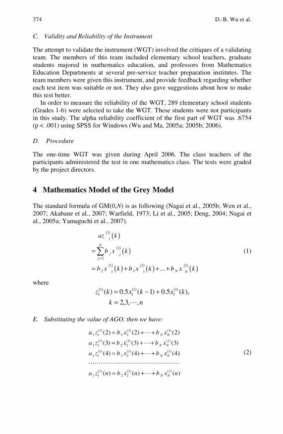
374 D.-B. Wu et al.
C. Validity and Reliability of the Instrument
The attempt to validate the instrument (WGT) involved the critiques of a validating team. The members of this team included elementary school teachers, graduate students majored in mathematics education, and professors from Mathematics Education Departments at several pre-service teacher preparation institutes. The team members were given this instrument, and provide feedback regarding whether each test item was suitable or not. They also gave suggestions about how to make this test better.
In order to measure the reliability of the WGT, 289 elementary school students (Grades 1-6) were selected to take the WGT. These students were not participants in this study. The alpha reliability coefficient of the first part of WGT was .6754 (p < .001) using SPSS for Windows (Wu and Ma, 2005a; 2005b; 2006).
D. Procedure
The one-time WGT was given during April 2006. The class teachers of the participants administered the test in one mathematics class. The tests were graded by the project directors.
4 Mathematics Model of the Grey Model
The standard formula of GM(0,N) is as following (Nagai et al., 2005b; Wen et al., 2007; Akabane et al., 2007; Warfield, 1973; Li et al., 2005; Deng, 2004; Nagai et al., 2005a; Yamaguchi et al., 2007).
( ) ( )( ) ( )
( ) ( ) ( ) ( ) ( ) ( )
1
1
1
2
1 1 1
2 32 3...
N
j jj
N N
az k
b x k
b x k b x k b x k
=
=
= + + +
∑ (1)
where
nk
kxkxkz
,,3,2
),(5.0)1(5.0)( )1(1
)1(1
)1(1
=+−=
E. Substituting the value of AGO, then we have:
(1) (1) (1)1 1 2 2
(1) (1) (1)1 1 2 2
(1) (1) (1)1 1 2 2
(1) (1) (1)1 1 2 2
(2) (2) (2)
(3) (3) (3)
(4) (4) (4)
( ) ( ) ( )
N N
N N
N N
N N
a z b x b x
a z b x b x
a z b x b x
a z n b x n b x n
= + +
= + +
= + +
= + +
(2)

An Application of ),0( NGM on Analyzing the First Van Hiele Geometrical Thinking Level 375
F. Dividing 1 a in both sides, then transfer into matrix form:
(1) (1)1 1
(1) (1)1 1
(1) (1)1 1
2
(1) (1) 12
3(1) (1)2
1
(1) (1)2
1
0.5 (1) 0.5 (2)
0.5 (2) 0.5 (3)
0.5 ( 1) 0.5 ( )
(2), , (2)
(3), , (3)
( ), , ( )
N
N
NN
x x
x x
x n x n
b
ax x
bx x
a
x n x n b
a
⎡ ⎤+⎢ ⎥
+⎢ ⎥⎢ ⎥⎢ ⎥⎢ ⎥− +⎣ ⎦
⎡ ⎤⎢ ⎥⎢ ⎥⎡ ⎤⎢ ⎥⎢ ⎥⎢ ⎥⎢ ⎥= ⎢ ⎥⎢ ⎥⎢ ⎥⎢ ⎥⎢ ⎥⎢ ⎥⎣ ⎦⎢ ⎥⎢ ⎥⎣ ⎦
(3)
Assume 1
,jm
bb
a
∧= where 1,2,3, ,j m= then Equation (3) can be rearranged
into
(1) (1)1 1
(1) (1)1 1
(1) (1)1 1
(1) (1)22
(1) (1)2 3
(1) (1)2
0.5 (1) 0.5 (2)
0.5 (2) 0.5 (3)
0.5 ( 1) 0.5 ( )
ˆ(2), , (2)
ˆ(3), , (3)
ˆ( ), , ( )
N
N
N N
x x
x x
x n x n
bx x
x x b
x n x n b
⎡ ⎤+⎢ ⎥
+⎢ ⎥⎢ ⎥⎢ ⎥⎢ ⎥− +⎣ ⎦
⎡ ⎤⎡ ⎤⎢ ⎥⎢ ⎥⎢ ⎥⎢ ⎥= ⎢ ⎥⎢ ⎥⎢ ⎥⎢ ⎥⎢ ⎥⎢ ⎥⎣ ⎦ ⎣ ⎦
(4)
3. In the same way, using the matrix solving equation ( ) 1T TB Y Y Y X∧
−= to find
the values of mb∧
, where
(1) (1)1 1
(1) (1)1 1
(1) (1)1 1
0.5 (1) 0.5 (2)
0.5 (2) 0.5 (3)
0.5 ( 1) 0.5 ( )
x x
x xX
x n x n
⎡ ⎤+⎢ ⎥
+⎢ ⎥= ⎢ ⎥⎢ ⎥⎢ ⎥− +⎣ ⎦
(5)
(1) (1)2
(1) (1)2
(1) (1)2
(2), , (2)
(3), , (3)
( ), , ( )
N
N
N
x x
x xY
x n x n
⎡ ⎤⎢ ⎥⎢ ⎥= ⎢ ⎥⎢ ⎥⎢ ⎥⎣ ⎦
(6)
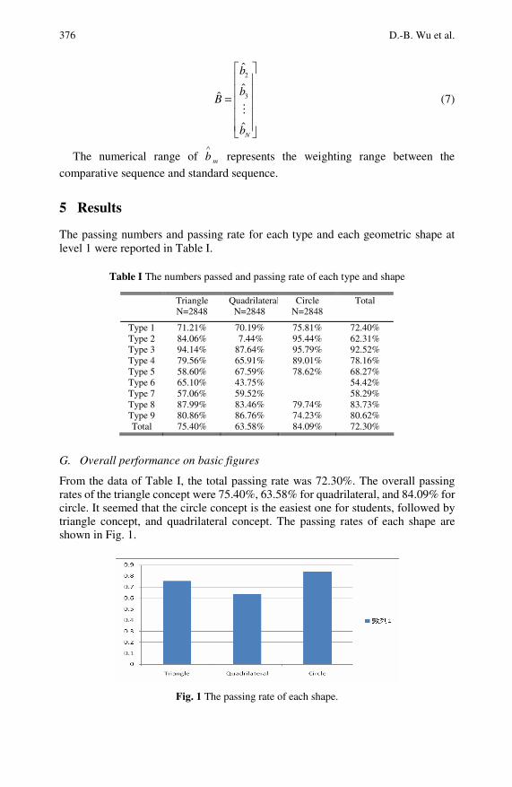
376 D.-B. Wu et al.
2
3
ˆ
ˆˆ
ˆN
b
bB
b
⎡ ⎤⎢ ⎥⎢ ⎥= ⎢ ⎥⎢ ⎥⎢ ⎥⎣ ⎦
(7)
The numerical range of mb∧
represents the weighting range between the
comparative sequence and standard sequence.
5 Results
The passing numbers and passing rate for each type and each geometric shape at level 1 were reported in Table I.
Table I The numbers passed and passing rate of each type and shape
Triangle N=2848
QuadrilateralN=2848
Circle N=2848
Total
Type 1 71.21% 70.19% 75.81% 72.40% Type 2 84.06% 7.44% 95.44% 62.31% Type 3 94.14% 87.64% 95.79% 92.52% Type 4 79.56% 65.91% 89.01% 78.16% Type 5 58.60% 67.59% 78.62% 68.27% Type 6 65.10% 43.75% 54.42% Type 7 57.06% 59.52% 58.29% Type 8 87.99% 83.46% 79.74% 83.73% Type 9 80.86% 86.76% 74.23% 80.62% Total 75.40% 63.58% 84.09% 72.30%
G. Overall performance on basic figures
From the data of Table I, the total passing rate was 72.30%. The overall passing rates of the triangle concept were 75.40%, 63.58% for quadrilateral, and 84.09% for circle. It seemed that the circle concept is the easiest one for students, followed by triangle concept, and quadrilateral concept. The passing rates of each shape are shown in Fig. 1.
Fig. 1 The passing rate of each shape.
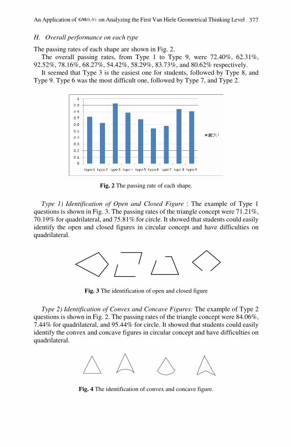
An Application of ),0( NGM on Analyzing the First Van Hiele Geometrical Thinking Level 377
H. Overall performance on each type
The passing rates of each shape are shown in Fig. 2. The overall passing rates, from Type 1 to Type 9, were 72.40%, 62.31%,
92.52%, 78.16%, 68.27%, 54.42%, 58.29%, 83.73%, and 80.62% respectively. It seemed that Type 3 is the easiest one for students, followed by Type 8, and
Type 9. Type 6 was the most difficult one, followed by Type 7, and Type 2.
Fig. 2 The passing rate of each shape.
Type 1) Identification of Open and Closed Figure : The example of Type 1 questions is shown in Fig. 3. The passing rates of the triangle concept were 71.21%, 70.19% for quadrilateral, and 75.81% for circle. It showed that students could easily identify the open and closed figures in circular concept and have difficulties on quadrilateral.
Fig. 3 The identification of open and closed figure
Type 2) Identification of Convex and Concave Figures: The example of Type 2 questions is shown in Fig. 2. The passing rates of the triangle concept were 84.06%, 7.44% for quadrilateral, and 95.44% for circle. It showed that students could easily identify the convex and concave figures in circular concept and have difficulties on quadrilateral.
Fig. 4 The identification of convex and concave figure.

378 D.-B. Wu et al.
Type 3) Identification of Straight Line and Curve Line: The example of Type 3 questions is shown in Fig. 3. The passing rates of the triangle concept were 94.14%, 87.64% for quadrilateral, and 95.79% for circle. It showed that students could easily identify the straight line and curve lines in circular concept and have difficulties on quadrilateral.
Fig. 5 The identification of straight line and curve line.
Type 4) Identification of Rotate Figure: The example of Type 4 questions is shown in Fig. 4. The passing rates of the triangle concept were 79.56%, 65.91% for quadrilateral, and 89.01% for circle. It showed that students could easily identify the rotate figures in circular concept and have difficulties on quadrilateral.
Fig. 6 The identification of rotate figures.
Type 5) Identification of Figures of Different Sizes: The example of Type 5 questions is shown in Fig. 5. The passing rates of the triangle concept were 58.60%, 67.59% for quadrilateral, and 78.62% for circle. It showed that students could easily identify the figures of different sizes in circular concept and have difficulties on quadrilateral.
Fig. 7 The identification of figures of different sizes.
Type 6) Identification of Extremely Obtuse Figures: The example of Type 6 questions is shown in Fig. 6. The passing rates of the triangle concept were 65.10%, and 43.75% for quadrilateral. It showed that students could easily identify the figures of extremely obtuse figures in triangular concept and have difficulties on quadrilateral.

An Application of ),0( NGM on Analyzing the First Van Hiele Geometrical Thinking Level 379
Fig. 8 The identification of extremely obtuse figures.
Type 7) Identification of Wide and Narrow Figures: The example of Type 7 questions is shown in Fig. 7. The passing rates of the triangle concept were 57.06% and 59.52% for quadrilateral. It showed that students could easily identify the figures of wide and narrow figures in quadrilateral concept and have difficulties on triangular.
Fig. 9 The identification of wide and narrow figures.
Type 8) Identification on Width of the Contour Line: The example of Type 8 questions is shown in Fig. 8. The passing rates of the triangle concept were 87.99%, 83.46% for quadrilateral, and 79.74% for circle. It showed that students could easily identify the width of the contour line in triangular concept and have difficulties on circle.
Fig. 10 The identification of width of the contour line.
Type 9) Identification on Filled and Hollow Figures: The example of Type 9 questions is shown in Fig. 9. The passing rates of the triangle concept were 80.86%, 86.76% for quadrilateral, and 74.23% for circle. It showed that students could easily identify the filled and hollow figures in triangular concept and have difficulties on circle.
Fig. 11 The identification of filled and hollow figures.

380 D.-B. Wu et al.
6 Analysis with Grey Model
The raw scores of each type of students are shown in Table II. (0, )NGM is chosen as our approach. The analysis steps are shown as follows.
1) Building the original sequences:
(0)1 (3,3,3,3,3, ,3)x = (0)2 (3,3,3,0,3, ,2)x = (0)3 (3,3,3,3,3, ,2)x = (8)
… (0)9 (3,1,3,3,3, ,2)x =
2) Building the AGO sequences:
(1)1 (3,6,9,12,15, ,8544)x = (1)2 =(3,6,9, ,6186)x
(9) (1)9 (3,4,10, ,6888)x = (1)1 ( ,4.5,7.5,10.5, ,8542.5)z = −−
3) Substituting Eq. with the values from Table II, where the output is full point and the result of Table III is obtained.
4) Because of the amount of data are enormous, therefore, the computer toolbox is also used to analyze and verify.
Table II The raw scores of each type of students
1 2 3 4 5 … 2848
Type 1 3 3 3 0 3 … 2 Type 2 2 2 2 2 2 … 1 Type 3 3 3 3 3 3 … 2 Type 4 1 2 3 2 3 … 1 Type 5 1 0 1 1 3 … 0 Type 6 1 0 0 0 2 … 1 Type 7 0 0 1 0 2 … 0 Type 8 3 0 3 3 3 … 0 Type 9
Full Point 3 3
1 3
3 3
3 3
3 3
… …
2 3
The first three ranks of Types are Type 2, Type 3, and Type 8 and the last three ranks of Types are Type 9, Type 4, and Type 6. The graph of the weightings is shown in Fig. 12.

An Application of ),0( NGM on Analyzing the First Van Hiele Geometrical Thinking Level 381
Table III The analyzed weighting of Grey model
Geometrical Types Weighting Rank
Type 1: open and closed figure 0.2430 4 Type 2: convex and concave figures 1.5076 1 Type 3: straight line and curve line 0.6277 2 Type 4: rotate figure 0.1027 8 Type 5: figures of different sizes 0.1210 7 Type 6: extremely obtuse figures 0.1351 6 Type 7: wide and narrow figures 0.1710 5 Type 8: identification on width of the contour
line 0.2750 3
Type 9: identification on filled and hollow figures
0.0023 9
Fig. 12 The graph of the weightings.
7 Conclusions
At the first van Hiele level (visual), students judged the figures by their appearance. The circular concept is the easiest for students; on the other hand, the concept of quadrilateral is the most difficult to students. Based on the analysis of the Grey Model, Type 9 (identification on filled and hollow) is the easiest for students and Type 2 (convex and concave figures) is the most difficult one among these nine different types of figures in this study. Because the concave figures are not taught in the elementary school, only 7.44% students make the correct answer. This finding displays that the Grey Model can really found out the fact, therefore the analysis of Grey Model is better than that of tradition method.
The results of this study identified the easiest and the most difficult concepts for students, it is important to investigate the reason behind this result. The authors of this study are interested to investigate why elementary students have difficulties in identifying extremely obtuse figures. One reason might be that extremely obtuse figures are rarely shown in the textbook, and in their daily lives. Researchers might consider this as their research interests and use the Interpretive Structure Modeling of Grey System to analyze the geometrical structure.

382 D.-B. Wu et al.
References
Akabane, T., Yamaguchi, D., Li, G.D., Mizutani, K., Nagai, M.: A Kansei expression method based on the simultaneous GM with the Kansei map. Fuzzy Sets and Systems 10(2), 89–96 (2007)
Burger, W.F., Shaughnessy, J.M.: Assessing children’s intellectual growth in geometry (Final report of the Assessing Children’s Intellectual Growth in Geometry project). Oregon State University, Department of Mathematics, Corvallis (1986)
Clements, D.H., Battista, M.T.: Geometry and spatial Reasoning. In: Grouws, D.A. (ed.) Handbook of Research on Mathematics Teaching and Learning, pp. 420–464. National Council of Teachers of Mathematics, Reston (1992)
Deng, J.L.: Grey Systems. China Ocean Press (2004) Eberle, R.S.: The effects of instruction on the van Hiele levels of geometric reasoning in
preservice elementary teachers. Unpublished master’s thesis, The University of Texas at Austin (1989)
Fuys, D., Geddes, D., Tischler, R.: The van Hiele Model of Thinking in Geometry among Adolescents. National Council of Teachers of Mathematics, Reston (1988)
Li, G.-D., Yamaguchi, D., Nagai, M.: New methods and accuracy improvement of GM according to Laplace transform. Fuzzy Sets and Systems 8(1), 13–24 (2005)
Ma, H.L., Wu, D.B.: An Introduction to the van Hiele Model of Geometric Thought. Journal of Ling-Tung College (11), 289–310 (2000)
Mayberry, J.W.: The van Hiele levels of geometric thought in undergraduate preservice teachers. Journal for Research in Mathematics Education 14(1), 58–69 (1983)
Ministry of Education of Taiwan (MET), Curriculum Standards for National Elementary School in Taiwan. Taipei, Taiwan: The Author (1993) (in Chinese)
Ministry of Education of Taiwan (MET), Grade 1-9 Curriculum Provisional Guidelines – Mathematics. Taipei, Taiwan: The Author (2000) (in Chinese)
Ministry of Education of Taiwan (MET), Grade 1-9 Curriculum Guidelines – Mathematics. Taipei, Taiwan: Author (2003) (in Chinese)
Molina, D.D.: The applicability of the van Hiele theory to transformational geometry. Unpublished doctoral dissertation, The University of Texas at Austin (1990)
Nagai, M., Yamaguchi, D., Li, G.D.: Grey structural modeling. Journal of Grey System 8(2), 119–130 (2005a)
Nagai, M., Yamaguchi, D., Li, G.D., Mizutani, K.: New System Modeling Method Based on Grey Theory. IPSJ SIG Technical Report, vol. 2005(40), AL-101-9, pp. 59 – 66 (2005b) (in Japanese)
National Council of Teachers of Mathematics (NCTM), Curriculum and Evaluation Standards for School Mathematics. Reston, VA: Author (1989)
National Council of Teachers of Mathematics (NCTM), Professional Standards for Teaching Mathematics. Reston, VA: Author (1991)
National Council of Teachers of Mathematics (NCTM), Assessment Standards for School Mathematics. Reston, VA: Author (1995)
National Council of Teachers of Mathematics (NCTM), Curriculum and Evaluation Standards for School Mathematics. Reston, VA: Author (2000)
Senk, S.L.: Proof writing achievement and van Hiele levels among secondary school geometry students (Doctoral Dissertation, The University of Chicago). Dissertation Abstracts International 44, 417A (1983)
An Application of ),0( NGM on Analyzing the First Van Hiele Geometrical Thinking Level 383 Usiskin, Z.P.: van Hiele levels and achievement in secondary school geometry (Final Report
of the Cognitive Development and Achievement in Secondary School Geometry Project). University of Chicago, Department of Education, Chicago (1982) (ERIC Reproduction Service No. ED 220 288)
Van Hiele, P.M.: Structure and Insight: A Theory of Mathematics Education. Academic Press, Orlando (1986)
Warfield, J.N.: Binary matrices in system modeling. IEEE Trans. Syst. Man. and Cybern. SMC-3(5), 441–449 (1973)
Wen, K.L., Changchien, S.K., Yeh, C.K., Wang, C.W., Lin, H.S.: Applying Matlab in Grey System Theory. Chwa Publishing Co., Taiwan (2007)
Wu, D.B.: A study of the use of the van Hiele model in the teaching of non-Euclidean geometry to prospective elementary school teachers in Taiwan, the Republic of China. Journal of National Taichung Teachers College (9), 443–474 (1995)
Wu, D.B., Ma, H.L.: A study of the geometric concepts of the elementary school students at the van Hiele level one. In: Chick, H.L., Vincent, J.L. (eds.) Proceedings 29th Conference of the International Group for the Psychology of Mathematics Education, vol. 4, pp. 329–336. PME, Melbourne (2005a)
Wu, D.B., Ma, H.L.: A study of the developing procedure of the van Hiele geometry test for elementary school students. Paper presented in The Third East Asia Regional Conference on Mathematics Education (ICMI Regional Conference), Shanghei, Nanjing, and Hangzhou China, August 7-12 (2005b)
Wu, D.B., Ma, H.L.: The distributions of van Hiele levels of geometric thinking among 1st through 6th graders. In: Novotna, J. (ed.) Proceedings 30th Conference of the International Group for the Psychology of Mathematics Education, vol. 5, pp. 409–416. PME, Prague (2006)
Yamaguchi, D., Li, G.D., Mizutani, K., Akabane, T., Nagai, M., Kitaoka, M.: A realization algorithm of grey structural modeling. Journal of Grey System 10(1), 33–40 (2007)
The Discrete Grey Prediction Model Based on Optimized Initial Value*
Tianxiang Yao, Zaiwu Gong, Naiming Xie, and Hong Gao
When GM (1, 1) model is applied to simulate a pure exponential sequence, the errors usually occur. There are many limitations to the development coefficient and the primary sequence. The characteristics of the discrete GM (1, 1) model are analogous to the GM (1, 1) model. It can be regarded as the precise form of the formal model. The chapter studied the growth rate of the simulation values under different initial values of discrete GM (1, 1) model. Appling optimization technique to solve the initial value, it proved that the modified discrete GM (1, 1) model can perfectly simulate the exponential sequence.
1 Introduction
GM(1,1) model is widely used (Liu and Lin, 1998; Liu and Lin, 2006; Lin et al., 2004; Lin and Liu, 2006; Lin et al., 2002; Sydow et al., 2001; Lin and Liu, 2000) as Tianxiang Yao College of Economics and Management, Nanjing University of Information Science and Technology, Nanjing, 210044, P.R. China Phone: 86-025-5869190 e-mail: [email protected]
Zaiwu Gong College of Economics and Management, Nanjing University of Information Science and Technology, Nanjing, 210044, P.R. China e-mail: [email protected]
Naiming Xie College of Economics and Management, Nanjing University of Aeronautics and Astronautics, Nanjing, 210016, P.R. China e-mail: [email protected]
Hong Gao College of Computer Science and Technology, Changchun University of Science and Technology, Changchun 130021, P.R. China e-mail: [email protected]
* This work was supported in part by the National Natural Science Foundation of China under Grants 70901041 and 70901043, Humanities and Social Sciences Foundation of Ministry of Education of China, Doctoral Fund of Ministry of Education of China under Grants 20093218120032 and 200802870020, and Philosophical and Social Science Foundation of Higher Education of Jiangsu Province of China under Grants 09SJD630059 and 09SJB630043.

386 T. Yao et al.
some scholars studied the suitable range and simulation accuracy of GM(1,1) model (Liu and Deng, 1999). The improvement methods mainly include discrete GM (1, 1) model (Xie and Liu, 2005; Yao, et al., 2009; Yao and Liu, 2007), constructing background value (Tan, 2005), error correction (Liu and Lin, 2006; Deng, 2002), optimizing grey differential derivative method (Wang et al., 2001), and central approach method (Song et al., 2001). Because GM(1,1) model has error when is applied to simulate geometric sequence, it is necessary to improve GM (1, 1) model
(Ji et al., 2001). The basic form of GM (1, 1) model is discrete function, but the whitenization form is continuous form. The jump from discrete function to con-tinuous form leads to the errors and instabilities of simulation values (Xie and Liu, 2005). The research of reference (Xie and Liu, 2005) indicates discrete GM (1, 1) model is the accurate form of traditional GM (1, 1) model. This chapter applied the parameters solution formula and incursion formula put forward by the reference (Xie and Liu, 2005) to study the characteristic of growth rate of different initial values. It applied optimization theory to solve the initial values and studied expo-nential curve fitting by the improved discrete GM (1, 1) model.
2 The Optimization Solution of Initial Value of Discrete GM(1,1) Model
Definition 2.1. (Xie and Liu, 2005) (1) (1)1 2( 1) ( )x k x kβ β+ = + is called discrete
GM (1, 1) model (DGM), where 1β is development coefficient.
The time response sequence of DGM is (Xie and Liu, 2005)
(1) (1) 11 2
1
1ˆ ( 1) (1) , 1, 2,..., 1
1
kkx k x k n
ββ ββ
−+ = + = −
− (1)
The parameters solution formula is
1 1 1(1) (1) (1) (1)
1 1 11 1 1
(1) 2 (1) 2
1 1
1( 1) ( ) ( 1) ( )
11
( ( )) ( ( ))1
n n n
k k kn n
k k
x k x k x k x kn
x k x kn
β
− − −
= = =− −
= =
+ − +−=
−−
∑ ∑ ∑
∑ ∑ (2)
1 1(1) (1)
2 11 1
1( ( 1) ( ))
1
n n
k k
x k x kn
β β− −
= =
= + −− ∑ ∑ (3)
Theorem 2.1. Let the simulation sequence of DGM be
{ }(0) (0) (0) (0)ˆ ˆ ˆ ˆ(2), (3),..., ( )X x x x n= . ˆ( )u k is the growth rate of simulation sequence.
Let(0) (0)
(0)
ˆ ˆ( 1) ( )ˆ( )
ˆ ( )
x k x ku k
x k
+ −= , where 2,3,...,k n= , so 1ˆ( ) 1u k β= − .
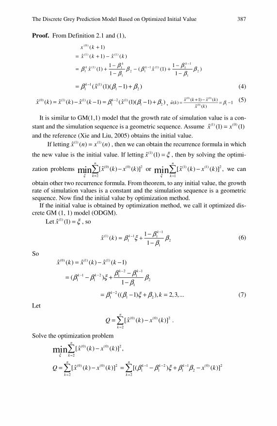
The Discrete Grey Prediction Model Based on Optimized Initial Value 387
Proof. From Definition 2.1 and (1), (0 )
(1) (1)
1(1) 1 (1)1 1
1 2 1 21 1
( 1)
ˆ ˆ( 1) ( )
1 1ˆ ˆ(1) ( (1) )
1 1
k kk k
x k
x k x k
x xβ ββ β β ββ β
−−
+= + −
− −= + − +
− −
1 (1)1 1 2ˆ( (1)( 1) )k xβ β β−= − + (4)
(0) (1) (1) 2 (1)
1 1 2ˆ ˆ ˆ ˆ( ) ( ) ( 1) ( (1)( 1) )kx k x k x k xβ β β−= − − = − + , (0) (0)
1(0)
ˆ ˆ( 1) ( )ˆ( ) 1
ˆ ( )
x k x ku k
x kβ+ −= = − (5)
It is similar to GM(1,1) model that the growth rate of simulation value is a con-stant and the simulation sequence is a geometric sequence. Assume (1) (0)ˆ (1) (1)x x=
and the reference (Xie and Liu, 2005) obtains the initial value. If letting (1) (1)ˆ ( ) ( )x n x n= , then we can obtain the recurrence formula in which
the new value is the initial value. If letting (1)ˆ (1)x ξ= , then by solving the optimi-
zation problems (0) (0) 2
2
ˆ[ ( ) ( )]minn
k
x k x kξ =
−∑ or (1) (1) 2
1
ˆ[ ( ) ( )] ,minn
k
x k x kξ =
−∑ we can
obtain other two recurrence formula. From theorem, to any initial value, the growth rate of simulation values is a constant and the simulation sequence is a geometric sequence. Now find the initial value by optimization method.
If the initial value is obtained by optimization method, we call it optimized dis-crete GM (1, 1) model (ODGM).
Let (1)ˆ (1)x ξ= , so
1(1) 1 1
1 21
1ˆ ( )
1
kkx k
ββ ξ ββ
−− −
= +−
(6)
So (0) (1) (1)ˆ ˆ ˆ( ) ( ) ( 1)x k x k x k= − −
2 11 2 1 1
1 1 21
( )1
k kk k β ββ β ξ β
β
− −− − −
= − +−
21 1 2(( 1) ), 2,3,...k kβ β ξ β−= − + = (7)
Let
(0) (0) 2
2
ˆ[ ( ) ( )]n
k
Q x k x k=
= −∑ .
Solve the optimization problem
(0) (0) 2
2
ˆ[ ( ) ( )] ,minn
k
x k x kξ =
−∑
(0) (0) 2
2
ˆ[ ( ) ( )]n
k
Q x k x k=
= −∑ 1 2 1 (0) 21 1 1 2
2
[( ) ( )]n
k k k
k
x kβ β ξ β β− − −
=
= − + −∑

388 T. Yao et al.
1 2 2 21 1
2
1 2 1 (0)1 1 1 2
1
1 (0) 21 2
( )
2 ( )( ( ))
( ( ))
nk k
k
nk k k
k
k
x k
x k
β β ξ
β β β β ξ
β β
− −
=
− − −
=
−
= −
+ − −
+ −
∑
∑ (8)
1 2 21 1
2
1 2 1 (0)1 1 1 2
2
2 ( )
2 ( )( ( ))
nk k
k
nk k k
k
dQ
d
x k
β β ξξ
β β β β
− −
=
− − −
=
= −
+ − −
∑
∑ (9)
Let 0dQ
dξ= , namely
1 2 2 1 2 (0) 11 1 1 1 1 2
2 2
( ) ( )( ( ) )n n
k k k k k
k k
x kβ β ξ β β β β− − − − −
= =
− = − −∑ ∑ (10)
1 2 (0) 11 1 1 2
2
1 2 21 1
2
( )( ( ) )
( )
nk k k
kn
k k
k
x kβ β β βξ
β β
− − −
=
− −
=
− −=
−
∑
∑ (11)
Here (0) (0) 2
2
ˆ[ ( ) ( )]n
k
Q x k x k=
= −∑ is a minimum.
3 The Properties of ODGM
Theorem 3.1. Let { }(0) (0) (0) (0)(1), (2),..., ( )X x x x n= . Establish ODGM model and
obtain the simulation sequence (0) (0)X X= . Let (0) (0)Y Xλ= , so the simulation
value of (0)Y is (0) (0)Y Y= .
Proof. Let
{ }(0) (0) (0) (0)(1), (2),..., ( )X x x x n= , { }(0) (0) (0) (0)(1), (2),..., ( )Y y y y n= ,
The parameters of (0)X and (0)Y are 1 2[ , ]β β , 1 2[ , ]γ γ , respectively. Let 1
(1) (1)1
1
( 1) ( ),n
k
M x k x k−
=
= +∑ 1 1
(1) (1)2
1 1
( 1) ( ),n n
k k
M x k x k− −
= =
= +∑ ∑
1(1) 2
31
( ( ))n
k
M x k−
=
=∑ , 1
(1) 24
1
( ( ))n
k
M x k−
=
= ∑ .
From the formula in the reference (Xie and Liu, 2005)
1 21
3 4
( 1)
( 1)
n M M
n M Mβ − −
=− −
. (12)
Similarly, let
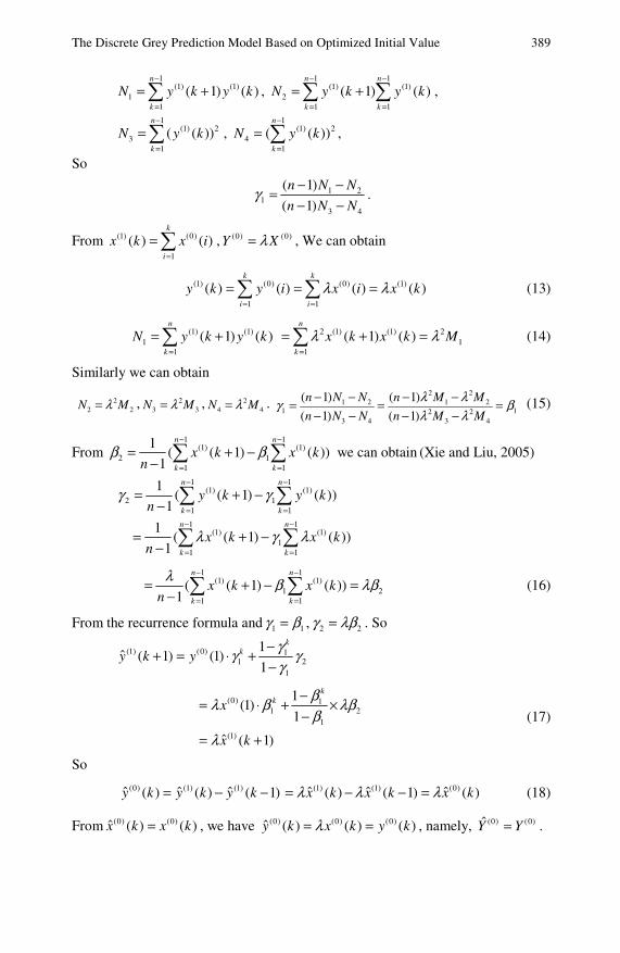
The Discrete Grey Prediction Model Based on Optimized Initial Value 389
1(1) (1)
11
( 1) ( )n
k
N y k y k−
=
= +∑ , 1 1
(1) (1)2
1 1
( 1) ( )n n
k k
N y k y k− −
= =
= +∑ ∑ ,
1(1) 2
31
( ( ))n
k
N y k−
=
=∑ , 1
(1) 24
1
( ( ))n
k
N y k−
=
= ∑ ,
So
1 21
3 4
( 1)
( 1)
n N N
n N Nγ − −
=− −
.
From (1) (0)
1
( ) ( )k
i
x k x i=
=∑ , (0) (0)Y Xλ= , We can obtain
(1) (0) (0) (1)
1 1
( ) ( ) ( ) ( )k k
i i
y k y i x i x kλ λ= =
= = =∑ ∑ (13)
(1) (1)1
1
( 1) ( )n
k
N y k y k=
= +∑ 2 (1) (1) 21
1
( 1) ( )n
k
x k x k Mλ λ=
= + =∑ (14)
Similarly we can obtain
22 2N Mλ= , 2
3 3N Mλ= , 24 4N Mλ= .
2 21 2 1 2
1 12 23 4 3 4
( 1) ( 1)
( 1) ( 1)
n N N n M M
n N N n M M
λ λγ βλ λ
− − − −= = =
− − − − (15)
From 1 1
(1) (1)2 1
1 1
1( ( 1) ( ))
1
n n
k k
x k x kn
β β− −
= =
= + −− ∑ ∑ we can obtain (Xie and Liu, 2005)
1 1(1) (1)
2 11 1
1 1(1) (1)
11 1
1( ( 1) ( ))
1
1 ( ( 1) ( ))
1
n n
k k
n n
k k
y k y kn
x k x kn
γ γ
λ γ λ
− −
= =
− −
= =
= + −−
= + −−
∑ ∑
∑ ∑
1 1
(1) (1)1 2
1 1
( ( 1) ( ))1
n n
k k
x k x kn
λ β λβ− −
= =
= + − =− ∑ ∑ (16)
From the recurrence formula and 1 1γ β= , 2 2γ λβ= . So
(1) (0) 11 2
1
1ˆ ( 1) (1)
1
kky k y
γγ γγ
−+ = ⋅ +
−
(0) 11 2
1
(1)
1(1)
1
ˆ ( 1)
kkx
x k
βλ β λββ
λ
−= ⋅ + ×
−
= +
(17)
So
(0) (1) (1)ˆ ˆ ˆ( ) ( ) ( 1)y k y k y k= − − (1) (1) (0)ˆ ˆ ˆ( ) ( 1) ( )x k x k x kλ λ λ= − − = (18)
From (0) (0)ˆ ( ) ( )x k x k= , we have (0) (0) (0)ˆ ( ) ( ) ( )y k x k y kλ= = , namely, (0) (0)Y Y= .
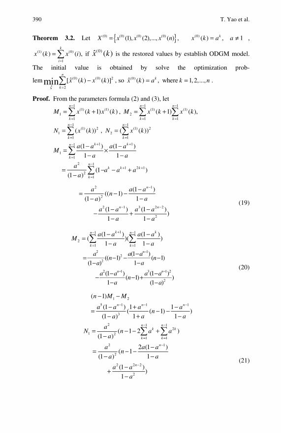
390 T. Yao et al.
Theorem 3.2. Let { }(0) (0) (0) (0)(1), (2),..., ( ) ,X x x x n=
(0) ( ) ,kx k a= 1a ≠ ,
(1) (0)
1
( ) ( ),k
i
x k x i=
=∑ if (0)ˆ ( )x k is the restored values by establish ODGM model.
The initial value is obtained by solve the optimization prob-
lem (0) (0) 2
2
ˆ[ ( ) ( )]minn
k
x k x kξ =
−∑ , so (0)ˆ ( ) ,kx k a= where 1, 2,...,k n= .
Proof. From the parameters formula (2) and (3), let 1
(1) (1)1
1
( 1) ( )n
k
M x k x k−
=
= +∑ , 1 1
(1) (1)2
1 1
( 1) ( ),n n
k k
M x k x k− −
= =
= +∑ ∑
1(1) 2
11
( ( ))n
k
N x k−
=
=∑ , 1
(1) 22
1
( ( ))n
k
N x k−
=
= ∑
1 11
11
2 11 2 1
21
(1 ) (1 )
1 1
(1 )(1 )
k kn
k
nk k k
k
a a a aM
a a
aa a a
a
+ +−
=
−+ +
=
− −= ×− −
= − − +−
∑
∑
2 1
2
2 1 3 2 2
2
(1 )(( 1)
1(1 )
(1 ) (1 ) )
1 1
n
n n
a a an
aa
a a a a
a a
−
− −
−= − −−−
− −− +− −
(19)
11 1
21 1
(1 ) (1 )( )( )
1 1
k kn n
k k
a a a aM
a a
+− −
= =
− −=− −∑ ∑
2 12
2
2 1 3 1 2
2
(1 )(( 1) ( 1)
1(1 )
(1 ) (1 ) ( 1) )
1 (1 )
n
n n
a a an n
aa
a a a an
a a
−
− −
−= − − −−−
− −− − +− −
(20)
1 2
5 1 1 1
3
( 1)
(1 ) 1 1( ( 1) )
1 1(1 )
n n n
n M M
a a a an
a aa
− − −
− −
− + −= − −+ −−
2 1 12
1 21 1
( 1 2 )(1 )
n nk k
k k
aN n a a
a
− −
= =
= − − +− ∑ ∑
2 1
2
2 2 2
2
2 (1 )( 1
1(1 )
(1 ) )
1
n
n
a a an
aa
a a
a
−
−
−= − −−−
−+−
(21)
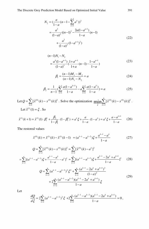
The Discrete Grey Prediction Model Based on Optimized Initial Value 391
12
21
( ( 1 ))1
nk
k
aN n a
a
−
=
= − −− ∑
2 12
2
21 2
2
2 (1 )(( 1) ( 1)
1(1 )
(1 ) )(1 )
n
n
a a an n
aa
aa
a
−
−
−= − − −−−
+ −−
(22)
1 2
4 1 1 1
3
( 1)
(1 ) 1 1 ( ( 1) )
1 1(1 )
n n n
n N N
a a a an
a aa
− − −
− −
− + −= − −+ −−
(23)
1 21
1 2
( 1)
( 1)
n M Ma
n N Nβ − −
= =− −
(24)
11 1
21 1
1 (1 ) (1 )( )
1 1 1
k kn n
k k
a a a aa a
n a aβ
+− −
= =
− −= − =− − −∑ ∑ (25)
Let (0) (0) 2
1
ˆ[ ( ) ( )]n
k
Q x k x k=
= −∑ . Solve the optimization (0) (0) 2
2
ˆ[ ( ) ( )]minn
k
x k x kξ =
−∑ .
Let (1)ˆ (1)x ξ= . So
(1) (1) 21 1
1
ˆ ˆ( 1) (1) (1 )1
k kx k xββ β
β+ = ⋅ + ⋅ −
−
1
(1 )1 1
kk k ka a a
a a aa a
ξ ξ+−= + ⋅ − = +
− − (26)
The restored values
(0) (1) (1)ˆ ˆ ˆ( ) ( ) ( 1)x k x k x k= − − 1
1 2( )1
k kk k a a
a aa
ξ−
− − −= − +−
(27)
(0) (0) 2 (0) 2
2 2
ˆ ˆ[ ( ) ( )] [ ( ) ]n n
k
k k
Q x k x k x k a= =
= − = −∑ ∑
11 2 2
2
[( ) ]1
k knk k k
k
a aa a a
aξ
−− −
=
−= − + −−∑
1 11 2 2
2
2[( ) ]
1
k k knk k
k
a a aa a
aξ
− +− −
=
− += − +−∑ (28)
1 1 21 2 2 2
22 1
1 2 1 1
2
( 2 )( )
(1 )
( )( 2 ) 2
1
k k kn nk k
k k
k k k k kn
k
a a aQ a a
a
a a a a a
a
ξ
ξ
− +− −
= =
− − − +
=
− += − +−
− − ++−
∑ ∑
∑ (29)
Let
1 2 2
1
2 ( )n
k k
k
dQa a
dξ
ξ− −
== −∑
1 2 1 1
2
( )( 2 )2 0
1
k k k k kn
k
a a a a a
a
− − − +
=
− − ++ =−∑ ,

392 T. Yao et al.
so we have
1 2 2 2 2 2 3
2 1
( ) ( ) ( 2 ) 0n n
k k k
k k
a a a a a aξ− − −
= =− − − + =∑ ∑ (30)
1 2 2 1 2 2
2 2
( ) ( ) 0n n
k k k k
k k
a a a a aξ− − − −
= =− − − =∑ ∑ (31)
Namely, when aξ = , 0dQ
dξ= . Substitute aξ = into (0) (0) 2
2
ˆ[ ( ) ( )]n
k
Q x k x k=
= −∑ , we
obtain 0Q = . Because 0Q ≥ , when aξ = , the average relative error of the simu-
lation values is a minimum, namely (0) (1) (1)ˆ ˆ ˆ( ) ( ) ( 1)x k x k x k= − − 1
1( ) ( )1 1
k kk ka a a a
a aa a
−−− −= + − +
− −
11 (1 )
( )1
kk k ka a
a a aa
−− −= − + =
−. Namely,
(0) (0)ˆ ( ) ( )x k x k= , 1, 2,...,k n= .
Similarly we can prove that when the initial value is (1) (0)(1) (1)x x=
or (1) (0)(1) ( )x x n= , DGM model can completely fit the geometric sequence.
Theorem 3.3. (Yao and Liu, 2007) Let { }(0) (0) (0) (0)(1), (2),..., ( ) ,X x x x n= where
(0) ( ) ,kx k a= (1) (0)
1
( ) ( ),k
i
x k x i=
=∑ (1) (0)ˆ (1) (1)x x= (or (1) (0)ˆ (1) ( )x x n= ).
Assume (0)ˆ ( )x k is the restored values of DGM model, then (0)ˆ ( ) ,kx k a= where 1, 2,...,k n= .
Proof. Omitted.
Corollary 3.1. For the sequence (0)X we have (0) ( ) ,kx k aλ= 1, 2,...,k n= , 1a ≠ . Assume (0)ˆ ( )x k is restored value by estab-
lishing ODGM model. The initial value is obtained by solving the optimization
problem (0) (0) 2
2
ˆ[ ( ) ( )]minn
k
x k x kξ =
−∑ , so (0)ˆ ( ) ,kx k aλ= where 1, 2,...,k n= .
Proof. Let { }(0) (0) (0) (0)(1), (2),..., ( ) ,Z z z z n= (0)Z is a geometric sequence, namely,
(0) ( ) ,kz k a= from Theorem 3.3, we obtain (0) (0)Z Z= . From (0) (0)X Zλ= and
Theorem 3.1 we can obtain (0) (0)X X= , namely, (0)ˆ ( ) ,kx k aλ= 1, 2,...,k n= ....
4 Conclusion
Different initial values can obtain different recurrence formula. This chapter studied several kinds of DGM model. The growth rate of simulation data is a constant for
The Discrete Grey Prediction Model Based on Optimized Initial Value 393
these models. Utilize optimization method to obtain the initial value and the simu-lation accuracy can be improved. The research results indicate ODGM model can obviously improve the simulation accuracy.
References
Deng, J.L.: The Base of Grey Theory. Press of Huazhong University of Science & Tech-nology, Wuhan (2002)
Ji, P.R., Huang, W.S., Hu, X.Y.: A study on the properties of grey forecasting model. Sys-tems Engineering Theory & Practice (9), 105–108 (2001)
Lin, Y., Chen, M.Y., Liu, S.F.: Theory of grey systems: capturing uncertainties of grey information. Kybernetes: The International Journal of Systems and Cybernetics 33(2), 196–218 (2004)
Lin, Y., DeNu, R., Patel, N.: True distance fit of exponential curves and tests of applications. International J. of Applied Mathematics 9(1), 49–68 (2002)
Lin, Y., Liu, S.F.: Law of exponentiality and exponential curve fitting. Systems Analysis Modelling Simulation 38, 621–636 (2000)
Lin, Y., Liu, S.F.: Solving problems with incomplete information: A grey systems approach. In: Advances in Imaging and Electron Physics, vol. 141, pp. 77–174. Elsevier, Oxford (2006)
Liu, S.F., Deng, J.L.: The range suitable for GM(1,1). The Journal of Grey System 11(1), 131–138 (1999)
Liu, S.F., Lin, Y.: An Introduction to Grey Systems: Foundations, Methodology and Ap-plications. IIGSS academic Publisher, Grove City (1998)
Liu, S.F., Lin, Y.: Grey Information: Theory and Practical Applications. Springer, London (2006)
Song, Z.M., Tong, X.J., Xiao, X.P.: Center approach of grey GM(1,1) model. Systems En-gineering Theory & Practice (5), 110–113 (2001)
Sydow, A., Lin, Y., Liu, S.F., DeNu, R., Mennell, W.: Exponential prediction models based on sequence operators. Kybernetes 30(4), 397–410 (2001)
Tan, G.J.: The structure method and application of background value in grey system GM(1,1) model. Systems Engineering Theory & Practice (1), 98–103 (2005)
Wang, Y.N., Liu, K.D., Li, Y.C.: GM (1, 1) modeling method of optimum the whiting values of grey derivative. Systems Engineering Theory & Practice (5), 124–128 (2001)
Xie, N.M., Liu, S.F.: Discrete GM(1,1) and mechanism of grey Forecasting model. S. Sys-tems Engineering Theory & Practice (1), 93–98 (2005)
Yao, T.X., Liu, S.F.: The improvement of a forecasting discrete GM(1,1). Systems Engi-neering 25(9), 103–106 (2007)
Yao, T.X., Liu, S.F., Xie, N.M.: On the properties of small sample of GM(1,1) model. Ap-plied Mathematical Modelling 33(4), 1894–1903 (2009)
The Excel Test Modeling via Four Data in Evaluation of Education Information
Chi Tang and Boming Yin
In this chapter, we are using 4 data of the proficiency degree of adopting the IT (Information Technology) by all the teachers in Chinese, Mathematics and English groups in 20 schools of Pudong New Area. We are using test-method modeling Verhulst Model in Excel, and making three categories on the 20 schools. At the same time, first derivation to the model in the education study, this gets the speed of adoption the IT for a school at different stages.
1 Introduction
Author statistics, that assessment in the field of primary and secondary education the use of qualitative reasoning and analytical study account for 92.6%, the use of forms and percentage etc. general Quantitative methods account for 6.3%, and the application of analysis of variance, hypothesis testing, regression analysis only account for 1.1% (Yin, 2001).
To this end, author has been trying to introduce assessment into the field of primary and secondary schools for the thinking and method of the gray system.
The proficiency degree of adoption the IT is an important component in the in-formation level of personal attainment of the contemporary teachers, and is an important component of information level for a school.
In May 2006, Pudong New Area carried out the evaluation to the 20 experimental schools of information level. At each school, the expert group based on systems theory put through a questionnaire to obtain data in a table format using the method of modeling via four Data (Deng, 2005). Test method modeling a Verhulst Math-model for proficiency degree of adoption the six IT (Word, Excel, Chi Tang Superintend and Director, Shanghai Pudong office of Education, No. 86-8, Pudian road, Shanghai, CO 200122 China Phone: 0086-21-68885608 e-mail: [email protected]
Boming Yin Shanghai Pudong Institute of Education Development, No. 10, 658 nong, Zaozhuang road, Shanghai, CO 200136 China Phone: 0086-21-50709012-8204 e-mail: [email protected]

396 C. Tang and B. Yin
PowerPoint, Flash, FrontPage, Geometer’s Sketchpad) for the teachers in Chinese, Mathematics and English group in every school (Yin, 2009).
Professor Deng Julong has discussed the power GM in Classic Gray system monograph (Deng, 2005). Professor Liu Sifeng also has discussed the power GM (Liu, 2004; Liu and Lin, 2006; Lin et al., 2004; Lin and Liu, 2006). To this end, the methods of gray system preparation used to study. In the same time, they pointed out the power GM is based on the GM(1,1) (Lin et al., 2002; Sydow et al., 2001; Lin and Liu, 2000), and the power GM turns into a grey Verhulst model when the index α equals to two (Liu, 2004).
For application of Grey Verhulst model, Wang Haoping published “Application of Grey Verhulst model to close Planting of the Blacknerrylily” (Wang, 1991). Fang Ying published “The mathematical model of incidence curve for malaria and its gray range forecast” (Deng, 1990). Ni Yan issued a “population growth projec-tions” (Deng, 1990). Yin Boming has published papers about Verhulst Model for Beijing SARS (Yin, 2003a; 2003b).
Since 2001, in order to permeate the grey system theory and methods to Primary and secondary school teachers, Yin Boming took up with the test method modeling in Excel (Yin, 2001; Yin, 2000; Yin, 2005).
2 The Modeling via Four Data Sets in Process of the Evaluation for Information Level
A. Collection the Data for adopting the IT
At each school, We collected the data for adopt the Word, Excel, PowerPoint, Flash, FrontPage, Geometer's Sketchpad etc. six IT tools software by all the teachers in Chinese, Mathematics, and English group. According to commonly status of proficiency degree, at the different situations such as the understanding, use of start, use several times, skilled use etc., collection and aggregation the data, are shown in table I. Due to space limitations, Only one example of a school PN, which out of the aggregate data for 56 teachers×6 six IT tools = 336 person-time, so that 15/336 = 4.46%, and similar to the rest, in the table I.
Table I Collection Person-time of Adoption Six IT for Proficiency Degree
UNDER-
STANDING USE OF
START USE OF SEVERAL
TIMES SKILLED
USE
15 4.46%
31 9.22%
92 27.38%
110 32.74%
B. One method of math-modeling (least squares)
When the collection of data in distribution is S-shaped curve, we may be math-modeling by both of the original sequence and IAGO (Inverse Accumulated Generating Operation) sequence (Liu, 2004; Deng, 1986; 1993). From table I, we

The Excel Test Modeling via Four Data in Evaluation of Education Information 397
gain the original sequence, IAGO (Inverse Accumulated Generating Operration) sequence, and data array for adopting the IT:
x 0 (n) = (15, 31, 92, 110), x -1 (n) = (0, 16, 61, 18), yn = (16, 61, 18)T
⎥⎥⎥
⎦
⎤
⎢⎢⎢
⎣
⎡
−−−
=⎥⎥⎥
⎦
⎤
⎢⎢⎢
⎣
⎡
+−+−+−
=12100101
84655.61
96123
110)10092(5.0
92)9231(5.0
31)3115(5.0
2
2
2
B
⎥⎦
⎤⎢⎣
⎡−−
=⎥⎦
⎤⎢⎣
⎡−⎥⎦
⎤⎢⎣
⎡=
−−
03695.0
62.1
749480
39701
2189726171764739
176473925.14512)(
1
T1TnyBBB
Therefore, b = 0.03695,
K = – 1.62/ –0.03695 = 43.84 C = K / x0(0) –1 = 43.84/4.46 – 1 = 8.83
There is the Verhulst Model of adoption the IT of PN School in recent years:
e83.81
84.43
e1)(
62.1 nbKnC
Knv −− +
=+
=
(1)
Where, v is the degree of adoption (the percentage of the person-time number), e = 2.718 is the end of the natural logarithm, n = 0, 1, 2, 3 for the degree of proficiency (the same below).
Because classical least squares method attending to the starting point for time-oriented data x0(0), therefore the overall accuracy of the model might not be very high. In some cases, to give up a little accuracy of the starting point, and give attention to some of the overall data, the model can improve the accuracy of it.
C. Second way to build math-models (test method modeling via four data with the Excel)
In order to reduce the threshold of the difficulty in math-modeling, we will improve the overall accuracy of the model. In recent years, we have proposed a simple “Verhulst modeling via four Data by Excel testing” (see Fig. 1, Fig. 2).
To obtain the corresponding Verhulst Math-mode of PN School:
e39.121
38
e1)(
6184.1 nbKnC
Knv −− +
=+
= (2)
Order derivative to equation (2), may be:
)e39.121(e6184.139.1238
26184.1
6184.1
n
n
dn
dv−
−
+×××=
(3)
According to equation (3), we could obtain the speed of adoption the IT for PN School at different stages (order derivative, shown in Fig.1 at the end of column):
The speed of “the use several times” stage for 13.54%; the speed of “skilled use” phase for 4.94%, there has been saturation phenomenon.
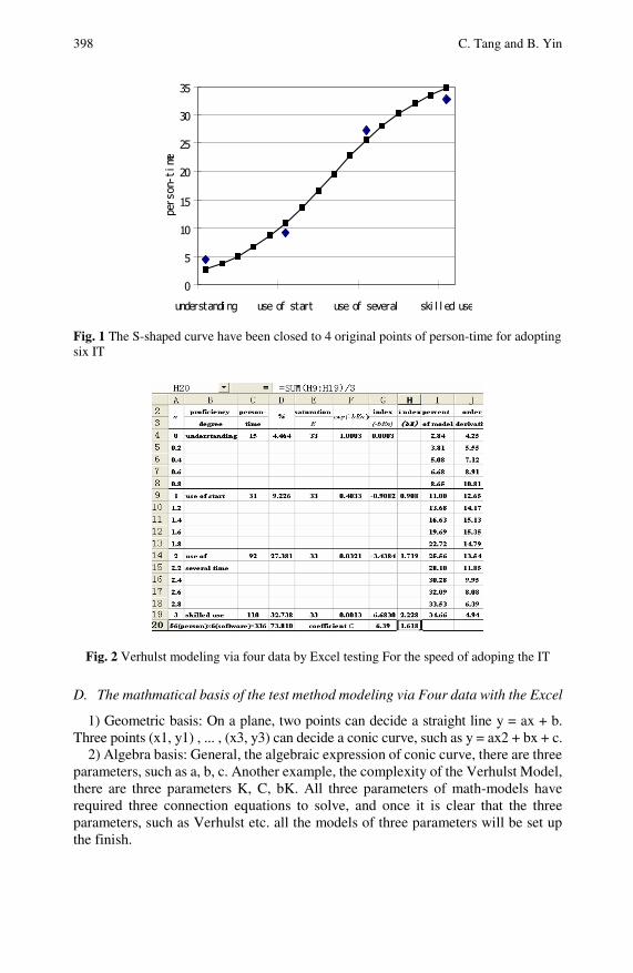
398 C. Tang and B. Yin
0
5
10
15
20
25
30
35
understandi ng use of start use of several ski l l ed use
pers
on-t
ime
Fig. 1 The S-shaped curve have been closed to 4 original points of person-time for adopting six IT
Fig. 2 Verhulst modeling via four data by Excel testing For the speed of adoping the IT
D. The mathmatical basis of the test method modeling via Four data with the Excel
1) Geometric basis: On a plane, two points can decide a straight line y = ax + b. Three points (x1, y1) , ... , (x3, y3) can decide a conic curve, such as y = ax2 + bx + c.
2) Algebra basis: General, the algebraic expression of conic curve, there are three parameters, such as a, b, c. Another example, the complexity of the Verhulst Model, there are three parameters K, C, bK. All three parameters of math-models have required three connection equations to solve, and once it is clear that the three parameters, such as Verhulst etc. all the models of three parameters will be set up the finish.
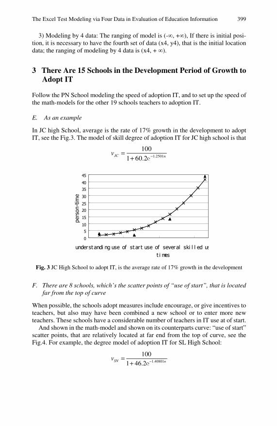
The Excel Test Modeling via Four Data in Evaluation of Education Information 399
3) Modeling by 4 data: The ranging of model is (-∞, +∞), If there is initial posi-tion, it is necessary to have the fourth set of data (x4, y4), that is the initial location data; the ranging of modeling by 4 data is (x4, + ∞).
3 There Are 15 Schools in the Development Period of Growth to Adopt IT
Follow the PN School modeling the speed of adoption IT, and to set up the speed of the math-models for the other 19 schools teachers to adoption IT.
E. As an example
In JC high School, average is the rate of 17% growth in the development to adopt IT, see the Fig.3. The model of skill degree of adoption IT for JC high school is that
1.2501
100
1 60.2JC nv −=
+ e
0
5
10
15
20
25
30
35
40
45
underst andi ng use of st ar t use of severalt i mes
ski l l ed us
pers
on-t
ime
Fig. 3 JC High School to adopt IT, is the average rate of 17% growth in the development
F. There are 8 schools, which’s the scatter points of “use of start”, that is located far from the top of curve
When possible, the schools adopt measures include encourage, or give incentives to teachers, but also may have been combined a new school or to enter more new teachers. These schools have a considerable number of teachers in IT use at of start.
And shown in the math-model and shown on its counterparts curve: “use of start” scatter points, that are relatively located at far end from the top of curve, see the Fig.4. For example, the degree model of adoption IT for SL High School:
1.40801
100
1 46.2SN nv −=
+ e
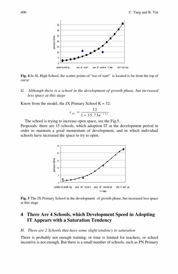
400 C. Tang and B. Yin
0
5
10
15
20
25
30
35
understandi ng use of start use of several t i mes ski l l ed use
pers
on-t
ime
Fig. 4 In SL High School, the scatter points of “use of start” is located is far from the top of curve
G. Although there is a school in the development of growth phase, but increased less space at this stage
Know from the model, the JX Primary School K = 32:
1 .5
3 2
1 3 5 .7 3JX nv −=
+ e
The school is trying to increase open space, see the Fig.5. Proposals: there are 15 schools, which adoption IT in the development period in order to maintain a good momentum of development, and in which individual schools have increased the space to try to open.
0
5
10
15
20
25
under st andi ng use of st ar t use of sever al
t i mes
ski l l ed us
pers
on-t
ime
Fig. 5 The JX Primary School in the development of growth phase, but increased less space at this stage
4 There Are 4 Schools, which Development Speed in Adopting IT Appears with a Saturation Tendency
H. There are 2 Schools that have some slight tendency to saturation
There is probably not enough training, or time is limited for teachers, or school incentive is not enough. But there is a small number of schools, such as PN Primary

The Excel Test Modeling via Four Data in Evaluation of Education Information 401 Schools, the degree of adoption IT have emerged with some slight tendency of saturation, see the fig.2. For these schools, the model of skill degree in adoption IT is shown in the equation (2).
I. There are 2 Schools have a more obvious tendency in saturation
There are 2 schools where their number of teachers to “use of several times” are slightly more than the quantity of “skilled use” stages, see the Fig.6. For example, the model of proficiency degree for LQ primary schools of adopting IT:
1.6034
23
1 2.833LQ nv −=
+ e
5
8
11
14
17
20
23
understandi ng use of start use of several t i mes ski l l ed use
pers
on-t
ime
Fig. 6 The number of Teachers to “use of several times” slightly more than the quantity of “skilled use”
Proposals: The 4 schools, in which speed of development when adopting IT has emerged with some saturation tendency, so we must to try to find new incentive factor both inside and outside in order to breakthrough saturation tendency.
5 In CD School the Number of Teachers That “Use of Several Times” Are Far More Than Quantity of “Skilled Use”
In CD School, the numbers of teachers are adopting IT to “use of several times” are far more than the quantity of teachers, which “skilled use”, shown in fig.7. In CD school the model of proficiency degree of adoption IT:
3,2,1,5.151
70
5.151
70)1(8.18.1
=+
−+
= −−− nvnnCD ee
Proposals: In such school, the model of proficiency degree to adoption IT have significantly shaped single peak of a tendency, to do attribution analysis, looking for reasons to change the status.

402 C. Tang and B. Yin
0
5
10
15
20
25
30
35
40
under st andi ng use of st ar t use of sever al
t i mes
ski l l ed use
pers
on-t
ime
Fig. 7 The number of teachers of adoption the IT to " use of several times " is far more than the quantity of teachers, which "skilled use "
6 Sort Based on the Parameters of Verhulst Model for Each School
Based on the parameters of the degree model to adopt IT for teachers of 20 schools, we can sort descending, shown the Tab.2.
Table II The Sort Results with the Parameters of the Verhulst Model
MIDDLE K BK PRIMARY K BK
SL 100 1.41 GL 100 1.62 JC 100 1.25 FS 100 0.95
DC 100 1.15 LS 100 0.92 YS 100 0.99 YX 100 0.8 JPS 100 0.89 JY 100 0.76 SN 100 0.8 LSE 100 0.65 JP 100 0.77 CY 100 0.42 CD 70 LX 41 1.91
PN 38 1.62
JX 32 1.5 LQ 23 1.6 JL 21 1.49
According with the first keyword to saturation value K in the degree model, with
the second keyword to increase the speed value bK in the degree model, and pri-mary and secondary schools were apart sorted. From table I, we can see that on these schools, the sort results are in accordance with the assessment indicator sys-tem, and the sort results with the parameters of the Verhulst Model have striking similarities.
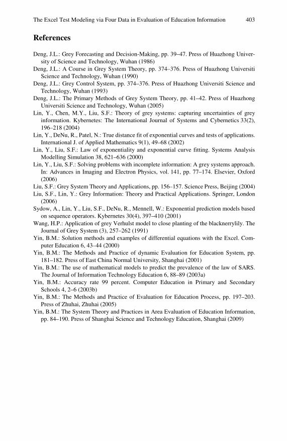
The Excel Test Modeling via Four Data in Evaluation of Education Information 403
References
Deng, J.L.: Grey Forecasting and Decision-Making, pp. 39–47. Press of Huazhong Univer-sity of Science and Technology, Wuhan (1986)
Deng, J.L.: A Course in Grey System Theory, pp. 374–376. Press of Huazhong Universiti Science and Technology, Wuhan (1990)
Deng, J.L.: Grey Control System, pp. 374–376. Press of Huazhong Universiti Science and Technology, Wuhan (1993)
Deng, J.L.: The Primary Methods of Grey System Theory, pp. 41–42. Press of Huazhong Universiti Science and Technology, Wuhan (2005)
Lin, Y., Chen, M.Y., Liu, S.F.: Theory of grey systems: capturing uncertainties of grey information. Kybernetes: The International Journal of Systems and Cybernetics 33(2), 196–218 (2004)
Lin, Y., DeNu, R., Patel, N.: True distance fit of exponential curves and tests of applications. International J. of Applied Mathematics 9(1), 49–68 (2002)
Lin, Y., Liu, S.F.: Law of exponentiality and exponential curve fitting. Systems Analysis Modelling Simulation 38, 621–636 (2000)
Lin, Y., Liu, S.F.: Solving problems with incomplete information: A grey systems approach. In: Advances in Imaging and Electron Physics, vol. 141, pp. 77–174. Elsevier, Oxford (2006)
Liu, S.F.: Grey System Theory and Applications, pp. 156–157. Science Press, Beijing (2004) Liu, S.F., Lin, Y.: Grey Information: Theory and Practical Applications. Springer, London
(2006) Sydow, A., Lin, Y., Liu, S.F., DeNu, R., Mennell, W.: Exponential prediction models based
on sequence operators. Kybernetes 30(4), 397–410 (2001) Wang, H.P.: Application of grey Verhulst model to close planting of the blacknerrylily. The
Journal of Grey System (3), 257–262 (1991) Yin, B.M.: Solution methods and examples of differential equations with the Excel. Com-
puter Education 6, 43–44 (2000) Yin, B.M.: The Methods and Practice of dynamic Evaluation for Education System, pp.
181–182. Press of East China Normal University, Shanghai (2001) Yin, B.M.: The use of mathematical models to predict the prevalence of the law of SARS.
The Journal of Information Technology Education 6, 88–89 (2003a) Yin, B.M.: Accuracy rate 99 percent. Computer Education in Primary and Secondary
Schools 4, 2–6 (2003b) Yin, B.M.: The Methods and Practice of Evaluation for Education Process, pp. 197–203.
Press of Zhuhai, Zhuhai (2005) Yin, B.M.: The System Theory and Practices in Area Evaluation of Education Information,
pp. 84–190. Press of Shanghai Science and Technology Education, Shanghai (2009)

Part V Grey Decision-Making
The Chain Structure Model of Evolutionary Game of Production-Study-Research Collaboration*
Hongzhuan Chen, Sifen Liu, and Zhenxin Jin
Some progress of economic activities can be intuitionally described and imitatively analyzed by the chain model of evolutionary game. To the evolutional law of combination of production, study and research which is based on the bounded rationality of human, the symmetric chain model of evolutionary game of combi-nation of production, study and research and Dynamic Decision-making Equation have been established; the state of balance and equilibrium of co-evolutionary game has been discussed. Through the imitative analysis, the evolution of Chinese com-bination of production, study and research has been well explained and the profound conclusion of it has been drawn out, which offer reasons to Chinese managerial decision and mode selection to the combination of production, study and research.
1 Introduction
From 1992, a co-operation of a development work with the joint of industry, aca-demia and research was organized and implemented by the former State Economic and Trade Commission. The Ministry of Education and the Chinese Academy of Sciences across the country has begun an organized, planned, systematic production Hongzhuan Chen School of Economics and Management, Nanjing University of Aeronautics and Astronautics, 29 Yudao Street, Nanjing, Jiangsu 210016, China e-mail: [email protected]
Sifen Liu School of Economics and Management, Nanjing University of Aeronautics and Astronautics, 29 Yudao Street, Nanjing, Jiangsu 210016, China e-mail: [email protected]
Zhenxin Jin School of Economics and Management, Nanjing University of Aeronautics and Astronautics, 29 Yudao Street, Nanjing, Jiangsu 210016, China e-mail: [email protected]
* This work is sponsored by soft science of china funds(2008GXS5D115).
408 H. Chen, S. Liu, and Z. Jin
and research to promote the work of co-operation. A study of 767 companies in 10 provinces and cities including Beijing, Guangdong and Hubei and so on by Liu Yingqiu and other scholars shows that about 36% of enterprises take joint innova-tion with universities, research institutions or enterprises (Liu, 2008). According to statistics, in 2007, universities and enterprises in Zhejiang Province reached 8040 production and research co-operation projects, the co-operation funding reached 1.13337 billion Yuan. Now industry-university co-operation has achieved initial results with full of opportunities, but there are also a huge challenge. Indus-try-university cooperation involves a very wide scope, and the problems are also complex, with the biggest being pursue of "fashion". Some enterprises and scien-tific research institutions, co-blind half-way abandonment of production and re-search co-operation, scientific research and chain fracture.
As the main co-operation means of scientific research results’ development and promotion, domestic and foreign scholars have begun to explore and research about co-operation model for years. There are more scholars abroad than domestic who study on research co-operation, such as David, etc. (1986) considered: the Univer-sity - enterprise relation had both interest and risk to academic institutions, the university’s challenge was to find ways to manage this relationship in order to retain the interest and minimize risk at the same time (David, Michael, et al., 1986); Rustum (1972) analyzed several co-operation models between University and en-terprises (Ruston, 1972);
Since then, some scholars probed the research co-operation from the perspective of knowledge management, such as Elias (2000) believed that research co-operation as a cross-organizational phenomenon, and had the motivation of sharing knowledge, but trust and social capital had significant impact. Thus knowledge transactions and knowledge of a total of Frederick is the basement of trust and innovation. Domestic scholars also made research studies about it, such as: Wang Juanru(2002) etc. probed direct co-operation modes of industry, academia and research in micro-level, and classified co-operation modes into 3 categories: technical cooperation type, contract type and integration-type (Wang and Pan, 2002). Zhou Zhu (2004) considered that intellectual property rights conflict be-tween all parties involved in research co-operation was an important factor, there-fore our country should coordinate the intellectual property rights conflict through Science and Technology Council (Zhou and Huang, 2004); Ye Xiaoqing etc. (2003) researched on the base of the conditions of information asymmetry and used game models to analyze adverse selection problem of enterprises and scientific research institutions’ co-operation and innovation It also established a non-symmetric in-formation dynamic game model to discuss how the enterprise innovation and commercialization value impact the choice of innovative ways of co-operation and co-operation partners (Ye and Xu, 2003). Hu Enhua (2001) analyzed 5 questions such as technology supply, technology needs in the co-operation innovation be-tween industry, academia and research (Hu, 2002). Zhu Guilong (2003) etc. inte-grated the implication of industry, academia and research cooperation, innovation and network organization, he also proposed the definition of industry, academia and research cooperation innovation network (Zhe and Peng, 2003). Luo Wei etc. (2002) analyzed the choice between co-operation way and co-operation partner in
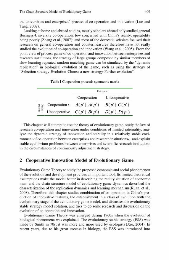
The Chain Structure Model of Evolutionary Game 409
the universities and enterprises’ process of co-operation and innovation (Luo and Tang, 2002).
Looking at home and abroad studies, mostly scholars abroad only studied general Business-University co-operation, few concerned with China's reality, operability being poorly (Zhang et al., 2007); and most of the domestic scholars focused their research on general co-operation and countermeasures therefore have not really studied the evolution of co-operation and innovation (Wang et al., 2005). From the point view of process game of co-operation and innovation between enterprises and research institutions, the strategy of large groups composed by similar members of slow learning repeated random matching game can be simulated by the "dynamic replication” in biological evolution of the game, such as using the strategy of “Selection strategy-Evolution-Choose a new strategy-Further evolution”.
Table I Cooperation proceeds symmetric matrix
Enterprise
Cooperation Uncooperative
Cooperation A ( ), ( )t tA p A p ( ), ( )t tB p C p
Partici-pation1 Uncooperative ( ), ( )t tC p B p ( ), ( )t tD p D p
This chapter will attempt to use the theory of evolutionary game, study the law of
research co-operation and innovation under conditions of limited rationality, ana-lyze the dynamic strategy of innovation and stability in a relatively stable envi-ronment of co-operation between enterprises and research institutions, and explain stable equilibrium problems between enterprises and scientific research institutions in the circumstances of continuously adjustment strategy.
2 Cooperative Innovation Model of Evolutionary Game
Evolutionary Game Theory to study the proposed economic and social phenomenon of the evolution and development provides an important tool. Its limited theoretical assumptions make the model better in describing the reality situation of economic man; and the chain structure model of evolutionary game dynamics described the characterization of the replication dynamics and learning mechanism (Ruan, et al., 2008). Therefore, this chapter studies combination of co-operation in China's pro-duction of innovative features, the establishment in a class of evolution with the evolutionary stage of the evolutionary game model, and discusses the evolutionary stable strategy model solution, and tries to do some research and discussion on the evolution of co-operation and innovation.
Evolutionary Game Theory was emerged during 1960s when the evolution of biological phenomena was explained. The evolutionary stable strategy (ESS) was made by Smith in 70s; it was more and more used by ecologists (Xie, 2004). In recent years, due to his great success in biology, the ESS was introduced into
410 H. Chen, S. Liu, and Z. Jin
economics and it became a popular field of game theory in economics. The basic idea of evolutionary game is that the economy balanced thumbtack state cannot rightly know where the state of their own interests, limited the ability of economic agents (bounded rationality of economic agents)which had found the best course of action, imitated the most beneficial strategy gradually, and reached the final state. Evolutionary game theory holds that economic model was not designed, but for those new structures adapted by the environment, social changes have been found and are better preserved, that is, it is emerged in the process of so-called "adaptive evolution" as a result of the existence of "limited rationality"(Fang and Liu, 2003).
A. Model Assumptions
In order to discuss easily and maintain the practical significance of the model as far as possible, we make the assumptions as follows:(1) Studying the two research of co-operation, and assuming that the actual result of the game in each board is zero.(2)In this chapter, studying the entire period of research co-operation without distinguishing between technical trading and commercial collaboration. (3)Co-operation agencies are all from large groups of random pairing, the two sides to participate in the game are "rational" and the game they are acts of "rational behavior. Game strategy sets between the two sides are finite sets, and are common knowledge for both parties.
B. Profit and Loss of Matrix Game
Indicator responses to the evolution of the extent and the stage of development are multi-faceted, so we use a change proportion of participants as a measured pa-rameter in this chapter. The proportion is an objective existence in the marketplace, and co-operators can only have subjective probability estimates based on their experience. Slow learning, limited low-level rational imitation participators heighten the profit through learning the game and adjust the strategy and tactics of the stability of dynamic replication.
Co-operation between the parties to co-operate in different stages have different strategies, and their income is different, if the earnings stage and evolution meet the income conditions of symmetric matrix, the matrix gains that can be used in table I, where P is the proportion of participants in time t. The profits in tables 1 and 2 are a function of co-operation, and the following table expresses that the income function contains grey parameter(s), for references on grey systems and information, please consult with (Liu and Lin, 2006; Lin et al., 2004; Lin and Liu, 2006). This evolu-tionary game model of the chain structure of the game can be used to describe the chain model, shown in Figure 1.
C. Cooperation and innovation chain structure of the evolutionary game
In the game process, business and science research groups in both games all has the respond to the current game situation (not necessarily best response). They either learn from each other, or choose the strategy by imitating a neighbor. Using the circle means the evolutionary game strategy1.2, and using the arrow means the
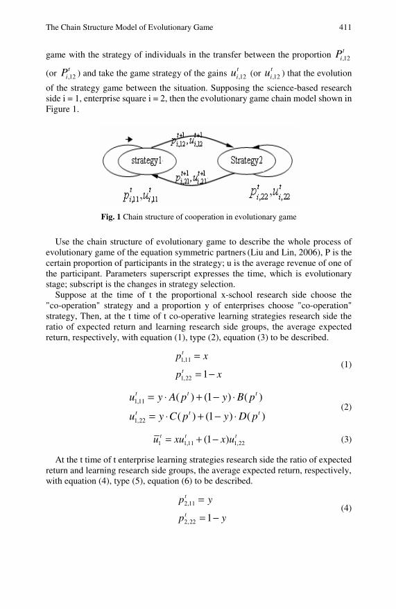
The Chain Structure Model of Evolutionary Game 411
game with the strategy of individuals in the transfer between the proportion ,12t
iP
(or ,12t
iP ) and take the game strategy of the gains ,12tiu (or ,12
tiu ) that the evolution
of the strategy game between the situation. Supposing the science-based research side i = 1, enterprise square i = 2, then the evolutionary game chain model shown in Figure 1.
Fig. 1 Chain structure of cooperation in evolutionary game
Use the chain structure of evolutionary game to describe the whole process of
evolutionary game of the equation symmetric partners (Liu and Lin, 2006), P is the certain proportion of participants in the strategy; u is the average revenue of one of the participant. Parameters superscript expresses the time, which is evolutionary stage; subscript is the changes in strategy selection.
Suppose at the time of t the proportional x-school research side choose the "co-operation" strategy and a proportion y of enterprises choose "co-operation" strategy, Then, at the t time of t co-operative learning strategies research side the ratio of expected return and learning research side groups, the average expected return, respectively, with equation (1), type (2), equation (3) to be described.
xp
xpt
t
−=
=
122,1
11,1 (1)
1,11
1,22
( ) (1 ) ( )
( ) (1 ) ( )
t t t
t t t
u y A p y B p
u y C p y D p
= ⋅ + − ⋅
= ⋅ + − ⋅ (2)
1 1,11 1,22(1 )t t tu xu x u= + − (3)
At the t time of t enterprise learning strategies research side the ratio of expected return and learning research side groups, the average expected return, respectively, with equation (4), type (5), equation (6) to be described.
yp
ypt
t
−=
=
122,2
11,2 (4)
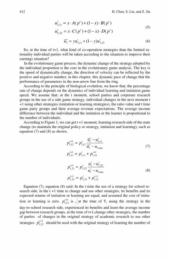
412 H. Chen, S. Liu, and Z. Jin
2,11
2,22
( ) (1 ) ( )
( ) (1 ) ( )
t t t
t t t
u x A p x B p
u x C p x D p
= ⋅ + − ⋅
= ⋅ + − ⋅ (5)
2 2,11 2,22(1 )t t tu yu y u= + − (6)
So, at the time of t+1, what kind of co-operation strategies than the limited ra-tionality individual parties will be taken according to the situation to improve their earnings situation?
In the evolutionary game process, the dynamic change of the strategy adopted by the individual proportion is the core in the evolutionary game analysis. The key is the speed of dynamically change, the direction of velocity can be reflected by the positive and negative number, in this chapter, this dynamic pace of change that the performance of parameters in the non-arrow line from the ring.
According to the principle of biological evolution, we know that, the percentage rate of change depends on the dynamics of individual learning and imitation game speed. We assume that: at the t moment, school parties and corporate research groups in the use of a side game strategy, individual changes in the next moment t +1 using other strategies (imitation or learning strategies), the ratio value and t time game party groups and their average revenue expectations. The average income difference between the individual and the imitation or the learner is proportional to the number of individuals.
According to Figure 1, we can get t +1 moment, learning research side of the state change (to maintain the original policy or strategy, imitation and learning), such as equation (7) and (8) as shown.
121,111,1
111,1
min11
11,1111,1
112,1
++
+
+=
−−
=
ttt
t
tttt
ppp
uu
uupp
(7)
112,122,1
122,1
min11
22,1122,1
121,1
++
+
+=
−−
=
ttt
t
tttt
ppp
uu
uupp
(8)
Equation (7), equation (8) said: In the t time the use of a strategy for school re-search side, in the t +1 time to change and use other strategies, its benefits and its expected returns of imitation or learning are equal, and assumed the cost of imita-
tion or learning is zero. 112,1+tp is , at the time of T, using the strategy in the
day-to-school research side, experienced its benefits and learn the average income gap between research groups, at the time of t+1,change other strategies, the number of parties of changes in the original strategy of academic research to use other
strategies 11,12tp + should be used with the original strategy of learning the number of
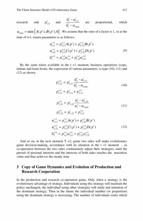
The Chain Structure Model of Evolutionary Game 413
research side 1,11tp and 1 1,11
1 1min
t t
t
u u
u u
−−
are proportional, which
}{1min min ( ), ( ),0t tu A p B p= . We assume that the ratio of a factor is 1, so at the
time of t+1, return parameters is as follows:
1 1 11,11 2,11 2,22
1 1 11,22 2,11 2,22
1 1 1 1 11 1,11 1,11 1,22 1,22
( ) ( )
( ) ( )
t t t t t
t t t t t
t t t t t
u p A p p B p
u p C p p D p
u p u p u
+ + +
+ + +
+ + + + +
= +
= +
= +
(9)
By the same token available in the t +1 moment, business operations (copy, imitate and learn from), the expression of various parameters, is type (10), (11) and (12) as shown.
121,211,2
111,2
min22
11,2211,2
112,2
++
+
+=
−−
=
ttt
t
tttt
ppp
uu
uupp
(10)
112,222,2
122,2
min22
22,2222,2
121,2
++
+
+=
−−
=
ttt
t
tttt
ppp
uu
uupp
(11)
1 1 12,11 1,11 1,22
1 1 12,22 1,11 1,22
1 1 1 1 12 2,11 2,11 2,22 2,22
( ) ( )
( ) ( )
t t t t t
t t t t t
t t t t t
u p A p p B p
u p C p p D p
u p u p u
+ + +
+ + +
+ + + + +
= +
= +
= +
(12)
And so on, in the next moment T +2, game two sides will make evolutionary game decision-making, accordance with its situation in the t +1 moment , so co-operation between the two sides continuously adjust their strategies, until the pursuit of personal interests and the interests of both sides reaches the maximize value and thus achieves the steady state.
3 Copy of Game Dynamics and Evolution of Production and Research Cooperation
In the production and research co-operation game, Only when a strategy is the evolutionary advantage of strategy, Individuals using this strategy will maintain the policy unchanged, the individual using other strategies will study and imitation of the dominant strategy; Then in the future the individual number (or proportion) using the dominant strategy is increasing. The number of individuals (ratio which
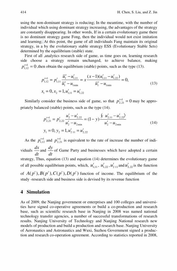
414 H. Chen, S. Liu, and Z. Jin
using the non-dominant strategy is reducing; In the meantime, with the number of individual which using dominant strategy increasing, the advantages of the strategy are constantly disappearing. In other words, If in a certain evolutionary game there is no dominant strategy game Fong, then the individual would not exist imitation and learning; At this point, the game of all individuals Fang maintain its original strategy, in a by the evolutionary stable strategy ESS (Evolutionary Stable Sets) determined by the equilibrium (stable) state.
First of all ,analytics research side of game, as time goes on, learning research side choose a strategy remain unchanged, to achieve balance, making
0112,1 =+tp ,then obtain the equilibrium (stable) points, such as the type (13).
1 1,11 1,11 1,2211,12 1,11
1 1min 1 1min
1 2 1,11 1,22
( 1)( )0,
0, 1,
t t t tt t
t t
t t
u u x u up p x
u u u u
x x u u
+ − − −= = =
− −
= = =
(13)
Similarly consider the business side of game, so that 0121,2 =+tp may be appro-
priately balanced (stable) points, such as the type (14).
2 2,22 2 11 2,2212,21 2,22
2 2min 2 2min
1 2 2 11 2,22
(1 )
0, 1,
t t t tt t
t t
t t
u u y u up p y
u u u u
y y u u
+ − −= = −
− −
= = =
,
,
( )
(14)
As the 112,1+tp and 1
21,2+tp is equivalent to the rate of increase the number of indi-
viduals dt
dxand
dt
dyof Game Party and businesses which have adopted a certain
strategy, Thus, equation (13) and equation (14) determines the evolutionary game
of all possible equilibrium points, which, 1,11tu , 1,22
tu , 2 11tu,
and 2,22tu is the function
of ( ), ( ), ( ), ( )t t t tA p B p C p D p function of income. The equilibrium of the
study -research side and business side is devised by its revenue function
4 Simulation
As of 2009, the Nanjing government or enterprises and 100 colleges and universi-ties have signed co-operative agreements or build a co-production and research base, such as scientific research base in Nanjing in 2008 was named national technology transfer agencies, a number of successful transformations of research results. Nanjing University of Technology and Nanjing National research new models of production and build a production and research base. Nanjing University of Aeronautics and Astronautics and Wuxi, Suzhou Government signed a produc-tion and research co-operation agreement. According to statistics reported in 2008,
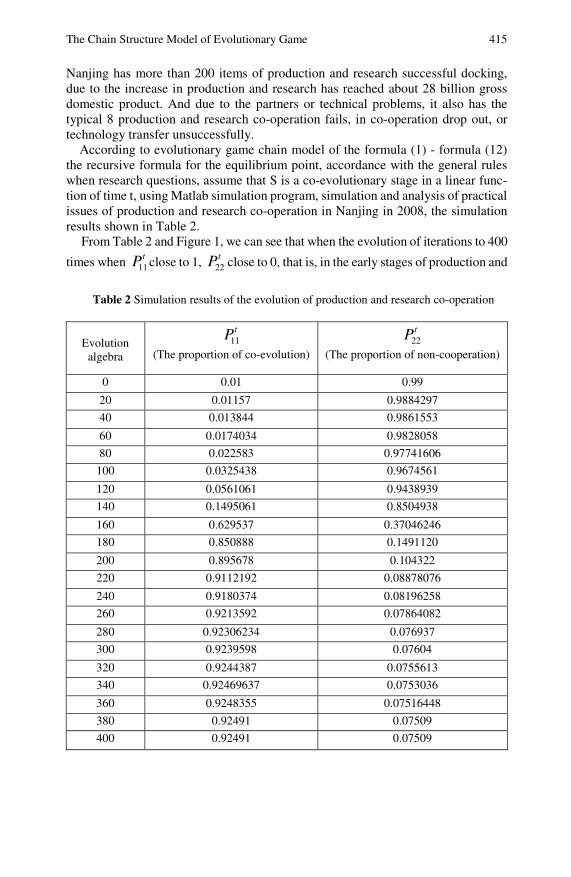
The Chain Structure Model of Evolutionary Game 415
Nanjing has more than 200 items of production and research successful docking, due to the increase in production and research has reached about 28 billion gross domestic product. And due to the partners or technical problems, it also has the typical 8 production and research co-operation fails, in co-operation drop out, or technology transfer unsuccessfully.
According to evolutionary game chain model of the formula (1) - formula (12) the recursive formula for the equilibrium point, accordance with the general rules when research questions, assume that S is a co-evolutionary stage in a linear func-tion of time t, using Matlab simulation program, simulation and analysis of practical issues of production and research co-operation in Nanjing in 2008, the simulation results shown in Table 2.
From Table 2 and Figure 1, we can see that when the evolution of iterations to 400
times when 11tP close to 1, 22
tP close to 0, that is, in the early stages of production and
Table 2 Simulation results of the evolution of production and research co-operation
Evolution algebra
11tP
(The proportion of co-evolution) 22tP
(The proportion of non-cooperation)
0 0.01 0.99
20 0.01157 0.9884297
40 0.013844 0.9861553
60 0.0174034 0.9828058
80 0.022583 0.97741606
100 0.0325438 0.9674561
120 0.0561061 0.9438939
140 0.1495061 0.8504938
160 0.629537 0.37046246
180 0.850888 0.1491120
200 0.895678 0.104322
220 0.9112192 0.08878076
240 0.9180374 0.08196258
260 0.9213592 0.07864082
280 0.92306234 0.076937
300 0.9239598 0.07604
320 0.9244387 0.0755613
340 0.92469637 0.0753036
360 0.9248355 0.07516448
380 0.92491 0.07509
400 0.92491 0.07509
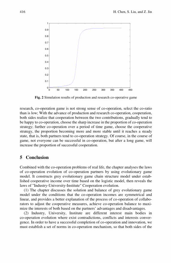
416 H. Chen, S. Liu, and Z. Jin
0 50 100 150 200 250 300 350 400 4500
0.1
0.2
0.3
0.4
0.5
0.6
0.7
0.8
0.9
1
Fig. 2 Simulation results of production and research co-operative game
research, co-operation game is not strong sense of co-operation, select the co-ratio than is low; With the advance of production and research co-operation, cooperation, both sides realize that cooperation between the two contributions, gradually tend to be happy to co-operation, choose the sharp increase in the proportion of co-operation strategy; further co-operation over a period of time game, choose the cooperative strategy, the proportion becoming more and more stable until it reaches a steady state, that is, both partners tend to co-operation strategy. Of course, in the course of game, not everyone can be successful in co-operation, but after a long game, will increase the proportion of successful cooperation.
5 Conclusion
Combined with the co-operation problems of real life, the chapter analyses the laws of co-operation evolution of co-operation partners by using evolutionary game model. It constructs grey evolutionary game chain structure model under estab-lished cooperative income over time based on the logistic model, then reveals the laws of "Industry-University-Institute" Cooperation evolution.
(1) The chapter discusses the solution and balance of grey evolutionary game model under the conditions that the co-operation incomes are symmetrical and linear, and provides a better explanation of the process of co-operation of collabo-rators to adjust the cooperative measures, achieve co-operation balance to maxi-mize the interests of both based on the partners’ advantages and disadvantages.
(2) Industry, University, Institute are different interest main bodies in co-operation evolution where exist contradictions, conflicts and interests conver-gence. In order to have a successful completion of co-operation and innovation, we must establish a set of norms in co-operation mechanism, so that both sides of the
The Chain Structure Model of Evolutionary Game 417
game reach a consensus on the basis of maximize the benefit in the pursuit of in-dividual interests and achieve a mutual benefit and win-win situation.
(3)The establishment and maintenance of "Industry-University-Institute" Co-operation faces a "Prisoner's Dilemma" problem, no matter what the probability of the strategic choice is, the enterprises will choose some strategy to maximize long-term interests, and achieve a balance ultimately.
(4) The evolution and stability of production and research co-operation and evolutionary stages by strong revenue function related to the decision, production and research cooperation in technology research and development phase and commercialization stage, revenue function is different from its stability are also different, such as the revenue function from the symmetric to the non-symmetric, linear function to the sub-function, non-linear function and so on. These questions await further research.
References
David, B., Michael, G., et al.: University-industry research relationships in biotechnology: implications for the university. Science, New Series 232(4756), 1361–1366 (1986)
Fang, Z.G., Liu, S.F.: Grey matrix name model based on pure strategy. J of Nanjing univer-sity of Aeronautics &Astronautics 35(4), 441–445 (2003)
Fang, Z.G., Liu, S.F., Ruan, A.Q.: Study on chain structure model of evolutionary name based on symmetric case. In: 2005 IEEE Int. Conf. on Networking, Sensing and Control, Sponsored by the IEEE Systems, Man and Cybernetics Society, Tucson, pp. 19–22 (2005)
Hu, E.H.: Problems and countermeasures in co-innovation among industry, university and research institute. R&D Management (1), 54–57 (2002)
Lin, Y., Chen, M.Y., Liu, S.F.: Theory of grey systems: capturing uncertainties of grey information. Kybernetes: The International Journal of Systems and Cybernetics 33(2), 196–218 (2004)
Lin, Y., Liu, S.F.: Solving problems with incomplete information: A grey systems approach. In: Advances in Imaging and Electron Physics, vol. 141, pp. 77–174. Elsevier, Oxford (2006)
Liu, H.D.: Analysis of the evolutionary game of “industry-university-institute” cooperation. Industrial Technology & Economy 27(1), 28–31 (2008)
Liu, S.F., Dang, Y.G., Fang, Z.G.: Grey Systems Theory and Applications. Press of Science, Beijing (2004)
Liu, S.F., Lin, Y.: Grey Information: Theory and Practical Applications. Springer, London (2006)
Luo, W., Tang, Y.H.: A game analysis on university-industry cooperative innovation. Sys-tems Engineering 20(1), 28–31 (2002)
Ruan, A.Q., Liu, S.F., Fang, Z.G.: Category of symmetric grey evolutionary game under strong correlation between individual pay-off and evolution stage. Control and Deci-sion 23(6), 665–670 (2008)
Ruston, R.: University-industry interaction patterns. Science, New Series 178(4064), 955–960 (1972)
Wang, J.R., Pan, Y.J.: Study on “industry-university-institute” cooperation model. Scientific Management Research 20(1), 25–27 (2002)

418 H. Chen, S. Liu, and Z. Jin Wang, L.P., Zhang, X.F., Liu, Z.Y.: Analysis of the evolutionary game of enterprise-R&D
institute cooperative innovation. Journal of Hefei University of Technology (Natural Science Edition) 28(12), 1555–1559 (2005)
Xie, S.Y.: Game Theory in Economics. Fu Dan Press, Shanghai (2004) Ye, X.Q., Xu, Y.: A non-symmetric information game analysis on industry-university co-
operative innovation. Science Research Management 24(5), 88–91 (2003) Zhang, Q.F., Fang, C.L., Hu, D.H.: Choice of the paths for the cooperative innovation of
industries, universities and research institutes by game analysis. Chinese Journal of Management 4(6), 748–752 (2007)
Zhe, G.N., Peng, Y.F.: The research on organization mode and operation mechanism of innovation network in cooperation of industry university and research institute. Soft Science 17(4), 49–52 (2003)
Zhou, Z., Huang, R.H.: Coordination to the conflict of intellectual property in the “indus-try-university-institute” cooperation. R&D Management (2), 90–94 (2004)

Development and Application of Computer Decision-Making System for Crop Grey Breeding (CDSCGB)*
Ruilin Guo, Zhanzhong Wang, Yafei Liu, and Jingshun Wang
In this chapter, we introduce the theory basis of Computer Decision-making System for Crop Grey Breeding, development environment and procedure, main models and its functions and demonstrate its application living example. Based on this, we discuss the merits and demerits of the system and its wide application prospects.
1 Introduction
With the development of computer techniques, the development and research of crop breeding expert system have begun since the eighties of the 20th century. F. J .Muehlbauer et al. (1981) made the first computer simulation for the single seed descent and mass selection method: Mokinion. J .M (1985) took the breeding expert system as the potential domain of development of agricultural expert system; Chinese Academy of Agricultural Sciences (1990) developed breeding expert sys-tem for winter wheat and breeding expert system for corn hybrid respectively on the basis of the breeding experiences of Academician Zhuang Qiaosheng, a well-known expert in wheat genetic breeding, and Academician Li Jingxiong, a Ruilin Guo
School of Biotechnology and Food Engineering e-mail: [email protected]
Zhanzhong Wang Department of Computer Science and Information Engineering, Anyang Institute of Technology, Huanghe Road, Anyang, Henan, 455000, P.R. China
Yafei Liu School of Biotechnology and Food Engineering e-mail: [email protected]
Jingshun Wang School of Biotechnology and Food Engineering e-mail: [email protected]
* Manuscript received on March 3, 2009. This work was supported in part by Nation Ministy of Science and Technology.
420 R. Guo et al.
well-known expert in corn genetic breeding (Zhao et al., 1994; Cheng et al., 1996). Sun Qixing and Zhang Aiming et al. (1991) established the computer evaluation system for wheat parent selective breeding according to the system method of wheat yield breeding, the least two multiplication method of parent selective breeding, the method of combination expression index, and the method of forecasting strong superiority combination (Zhang, 1994). Liaoning Academy of Agricultural Sciences (1993) developed the breeding expert system for rice in ac-cordance with the breeding of northern rice improved variety (Yue et al., 1993). The expert systems above-mentioned advance the crop breeding works to a certain degree, but they have limitations: either confine to a certain breeding link lacking integration, or do not have extensive adaptability owing to learning from the ex-periences of breeding expert to a certain specific stage. Thus, Ma Hongweng et al. (2002) and Guo Ruilin et al. (2003) developed the crop grey breeding computer decision-making system based on the Visual Basic 6.0 and PowerBuilder 6.0 sepa-rately taking the book Crop Grey Breeding Science as the original version (Guo, 1995; Ma et al., 2002; Guo et al., 2003).The two systems make up some deficiencies of expert systems above-mentioned, but their applications are limited because the former without succession, doesn’t support multithread technique, and doesn’t run cutting across the platform; the latter is incompatible with Windows XP and Vista. For this reason, we carried out the development of crop grey breeding computer decision-making system based on the Java technique in 2007, made considerable headway, and provided a convenient, swift and effective means for the breeding workers (Guo and Wang, 2008).
2 Theory Basis of Computer Decision-Making System for Crop Grey Breeding (CDSCGB)
Computer decision-making system for crop grey breeding (CDSCGB) is set up on the basis of crop grey breeding science which is a new interdisciplinary subject combing the theory of grey system with the theory of crop breeding. The birth of it indicated a revolutionary leap from traditional crop breeding to modernized, in-formational and quantitative breeding, thus making the crop breeding level climb to a quantitative stage from a qualitative one, and developing the crop breeding subject into a precise one from a qualitative and descriptive one. Adopting the theory and method during the course of the crop breeding, breeding workers can not only consider multi-factors comprehensively and supply exact effective deci-sion-making methods for modern crop breeding, but also realize highly intelli-gence for crop breeding. Even breeding newcomers can also come up to the decision-making standards of a breeding expert. Consequently, developing the computer decision-making system for crop grey breeding (CDSCGB) based on the theory of crop grey breeding science is of momentous significance to promote the crop breeding.
Development and Application of CDSCGB 421
3 Development Circumstances of Computer Decision-Making System for Crop Grey Breeding (CDSCGB) and Its Procedure
A. Development circumstances
Computer decision-making system for crop grey breeding (CDSCGB) adopts the MVC model, using the Java2 developed by Sun Corporation in America as tech-nique support, using JBuilder 2006 as integrated development circumstances, and using Microsoft Access 2000 as background data base. JBuilder 2006 is a strong enterprise development platform of Java which can develop various application programs under the frame of J2EE, integrating all Java techniques and containing every process of soft life cycle. It can not only stride across platform, accomplish writing program once, running anywhere, and fit in with various computer opera-tion system, but also program facing the object. Design of soft structure in JBuilder 2006 is distinct and obvious, strengthening its extension and duplication. It also provides 4 unitary interfaces which can make the system connect all current man-agement systems of data base such as Oracle, Sybase, Microsoft SQL Server, IBM DB2, Informix, Access, Foxpro, Paradox and so on. It is special commendable that the soft is apt to bring about network. Thus it can be seen that the development circumstances of computer decision-making system for crop grey breeding (CDSCGB) is very advantageous.
B. Development procedure
The second innovation and development of computer decision-making system for crop grey breeding (CDSCGB) has been made based on the book Crop Grey Breeding Science combined with Guo Ruilin’s study fruits in recent years. Its de-velopment procedures are as follows: system analysis of crop grey breeding →system design of crop grey breeding →set up application objects of crop grey breeding →generate user object, function and structure of crop grey breeding →establish windows and menu of crop grey breeding →create data window object of crop grey breeding →compile events of crop grey breeding →debugging and application →test system →product executable file.
4 Main Modules of Computer Decision-Making System for Crop Grey Breeding (CDSCGB) and Their Functions
A series of activities of crop breeding are a great deal of decision-making processes in essence. Multiple modules will be used during those processes which constitute core contents of computer decision-making system for crop grey breeding (CDSCGB).
C. Module and function of grey incidence analysis of breeding targets
Adopting the principle and method of grey relational analysis, the module is used to analyze influence of main characters on the yield and quality, to distinguish main
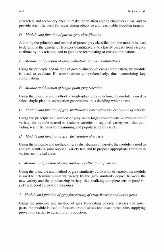
422 R. Guo et al.
characters and secondary ones, to make the relation among characters clear, and to provide scientific basis for ascertaining objective and reasonable breeding targets.
D. Module and function of parent grey classification
Adopting the principle and method of parent grey classification, the module is used to determine the genetic differences quantitatively, to classify parents from essence attribute by this relation, and to guide the formulating of cross combinations.
E. Module and function of grey evaluation of cross combinations
Using the principle and method of grey evaluation of cross combination, the module is used to evaluate F1 combinations comprehensively, thus determining key combinations.
F. Module and function of single-plant grey selection
Using the principle and method of single-plant grey selection, the module is used to select single-plant in segregation generations, thus deciding which to use.
G. Module and function of grey multi-target comprehensive evaluation of variety
Using the principle and method of grey multi-target comprehensive evaluation of variety, the module is used to evaluate varieties in regional variety test, thus pro-viding scientific basis for examining and popularizing of variety.
H. Module and function of grey distribution of variety
Using the principle and method of grey distribution of variety, the module is used to analyze results in joint regional variety test and to propose appropriate varieties in various ecological areas.
I. Module and function of grey similarity cultivation of variety
Using the principle and method of grey similarity cultivation of variety, the module is used to determine similarity variety by the grey similarity degree between the new variety and the popularizing variety, thus realizing complete sets of good va-riety and good cultivation measures.
J. Module and function of grey forecasting of crop diseases and insect pests
Using the principle and method of grey forecasting of crop diseases and insect pests, the module is used to forecast crop diseases and insect pests, thus supplying prevention tactics to agricultural production.
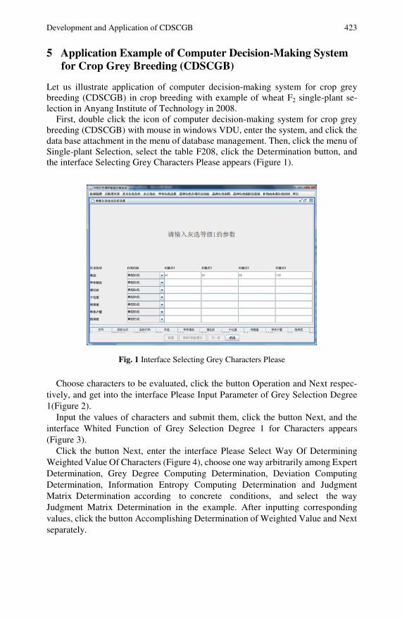
Development and Application of CDSCGB 423
5 Application Example of Computer Decision-Making System for Crop Grey Breeding (CDSCGB)
Let us illustrate application of computer decision-making system for crop grey breeding (CDSCGB) in crop breeding with example of wheat F2 single-plant se-lection in Anyang Institute of Technology in 2008.
First, double click the icon of computer decision-making system for crop grey breeding (CDSCGB) with mouse in windows VDU, enter the system, and click the data base attachment in the menu of database management. Then, click the menu of Single-plant Selection, select the table F208, click the Determination button, and the interface Selecting Grey Characters Please appears (Figure 1).
Fig. 1 Interface Selecting Grey Characters Please
Choose characters to be evaluated, click the button Operation and Next respec-tively, and get into the interface Please Input Parameter of Grey Selection Degree 1(Figure 2).
Input the values of characters and submit them, click the button Next, and the interface Whited Function of Grey Selection Degree 1 for Characters appears (Figure 3).
Click the button Next, enter the interface Please Select Way Of Determining Weighted Value Of Characters (Figure 4), choose one way arbitrarily among Expert Determination, Grey Degree Computing Determination, Deviation Computing Determination, Information Entropy Computing Determination and Judgment Matrix Determination according to concrete conditions, and select the way Judgment Matrix Determination in the example. After inputting corresponding values, click the button Accomplishing Determination of Weighted Value and Next separately.
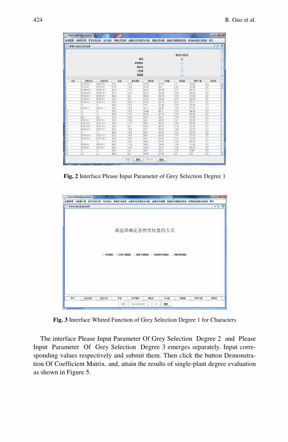
424 R. Guo et al.
Fig. 2 Interface Please Input Parameter of Grey Selection Degree 1
Fig. 3 Interface Whited Function of Grey Selection Degree 1 for Characters
The interface Please Input Parameter Of Grey Selection Degree 2 and Please
Input Parameter Of Grey Selection Degree 3 emerges separately. Input corre-sponding values respectively and submit them. Then click the button Demonstra-tion Of Coefficient Matrix, and, attain the results of single-plant degree evaluation as shown in Figure 5.
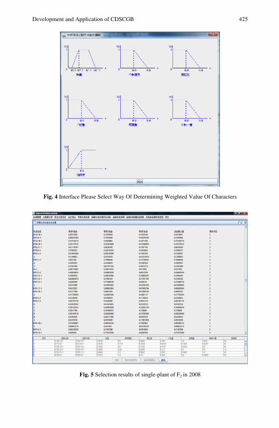
Development and Application of CDSCGB 425
Fig. 4 Interface Please Select Way Of Determining Weighted Value Of Characters
Fig. 5 Selection results of single-plant of F2 in 2008
426 R. Guo et al.
The results show that 635 single-plants are first degree single-plant, 1204 sin-gle-plants are second degree single-plant, and 192 single-plants are third degree single-plant. Among them, the growing scale of the first degree single-plant should be extended adequately according to concrete conditions next year, and be observed and selected as key plant lines; the second degree single-plant should be retained to grow, and be selected continuously; the third degree single-plant should be elimi-nated. The whole process above takes only 5 minutes, 100 times faster than the usual time required in accordance with the experiences of breeding expert, so a lot of time are spared, the work efficiency of breeding researchers and breeding selec-tion effects are raised greatly.
6 Conclusion
For a long time, the selection of crop new variety has been at a qualitative experi-ence stage. This is why only few breeding experts with rich experiences can achieve success. Undoubtedly, the breeding experiences include breeding art and skill which are not only the fruit of painstaking labor and wisdom of breeding expert's whole lifetime, but also valuable spiritual wealth of crop breeding area. However, only a few breeding experts have these experiences, others do not have. Let alone the breeding experiences which are only effective for a given period of time. For example, it is very difficult to apply the experiences of high yield breeding in guiding the high quality breeding. This status increases the mystery of breeding experiences, and becomes one of the difficult problems puzzled the breeding workers. The development of computer decision-making system for crop grey breeding (CDSCGB) based on the Java technique brings about hopes for getting rid of the difficult problem. Leaping from the traditional experience breeding to quan-titative breeding has been realized because of introducing the grey math, even the breeding newcomer can also attain the level of breeding expert by the system, and the work efficiency can be increased extremely. This is the first significant feature of computer decision-making system for crop grey breeding (CDSCGB).
The second feature of computer decision-making system for crop grey breeding (CDSCGB) is that it can run on different platforms. As mentioned above, the sys-tem writes programs facing up to the object by using the Java technique in the development circumstances of JBuilder 2006, which can be transplanted conven-iently, and can obtain writing once, running anywhere.
The third feature of computer decision-making system for crop grey breeding (CDSCGB) is that it has a complete range of functions and amiable interface, and can be learned and used easily. The system can realize all decision-making func-tions of various links during the process of crop breeding.
The fourth feature of computer decision-making system for crop grey breeding (CDSCGB) is that it has excellent robustness and security. As a kind of net lan-guage, the system can provide enough safeguard, and protect it from virus.
The fifth feature of computer decision-making system for crop grey breeding (CDSCGB) is that it supports multithread technique.
Development and Application of CDSCGB 427
The features mentioned above promise that computer decision-making system for crop grey breeding (CDSCGB) has a wide application prospect. We believe that computer decision-making system for crop grey breeding (CDSCGB) will be an effective implement for breeding workers with the lapse of time. Certainly, there are some weaknesses in the system. For example, the establishment of tables, inputting and modifying of data and so on are not as convenient as Excel, which will be settled by further study and improvement.
References
Cheng, Y.W., Zhao, S.N., Cao, M.L., Gao, S.J.: Knowledge expression of expert selection system for winter wheat. Computer Agriculture and Appication (1), 57 (1996) (in Chi-nese)
Guo, R.L.: Crop Grey Breeding Science. Chinese Agricultural Science and Technology Press, Peking (1995)
Guo, R.L., Wang, Z.Z.: Crop Grey Breeding Computer Decision-making System and Its Application. Chinese Agricultural Science and Technology Press, Peking (2008)
Guo, R.L., Wang, Y.G., Zhang, Y.F.: Study on computer decision-making system of crop grey breeding. System Sciences and Comprehensive Studies in Agriculture 19(1), 60–62 (2003) (in Chinese)
Ma, H.W., Yin, Y.B., Gao, Z.J., Geng, W.P.: Design of grey evaluation system for crop new variety. Science and Technology of Agriculture and Forestry in Ninxia (5), 17–18 (2002)
Maxwell, J.C.: A Treatise on Electricity and Magnetism, 3rd edn., pp. 68–73. Clarendon, Oxford (1892)
Yue, G.L., Guo, J., Zhang, J.G., Du, Y.Y., Shi, Y.S.: Development of expert selection system for rice new variety. Computer Agriculture and Appication (1), 12–15 (1993) (in Chinese)
Zhang, A.M.: Theory and Method of Plant Parent Selection, pp. 270–289. Agricultural Press, Peking (1994) (in Chinese)
Zhao, S.N., Cheng, Y.E., Cao, M.L., Gao, S.J., Zeng, Q.M.: Application and prospects of computer in crop breeding and cultivation. Computer Agriculture and Appication (1), 16 (1994) (in Chinese)

Positive Fractional Linear Systems
Tadeusz Kaczorek*
1 Introduction
The main purpose of this chapter is to give an overview of some recent results on positive fractional continuous-time and discrete-time linear systems.
The set of real n m× matrices with nonnegative entries is denoted by n m×+ℜ
and 1: .n n×+ +ℜ = ℜ A matrix [ ] n n
ijA a ×+= ∈ℜ (a vector nx +∈ℜ ) is called strictly
positive and denoted by 0A > ( 0x > ) if 0ija > for , 1, 2,..., .i j n= A ma-
trix [ ] n nijA a ×= = ℜ is called the Metzler matrix if its off-diagonal entries are
nonnegative ( 0,ija i j≥ ≠ ).The set of nonnegative integers is denoted by Z+ .
2 Positive Fractional Continuous-Time Linear System
The following Caputo definition of the fractional derivative will be used (Kaczorek, 2008a)
( )
10
1 ( )( ) ( ) ,
( ) ( )
t k
k
d fD f t f t d
dt k t
αα
α ατ τ
α τ + −= =Γ − −∫ 1 {1, 2,...}k k Nα− < ≤ ∈ = (2.1)
where ℜ∈α is the order of fractional derivative and ( ) ( )( ) .
kn
k
d ff
d
τττ
=
Consider the continuous-time fractional linear system described by the state equations
( ) ( ) ( ), 0 1d
x t Ax t Bu tdt
α
α α= + < ≤ (2.2a)
Tadeusz Kaczorek Faculty of Electrical Engineering, Bialystok Technical University, Wiejska 45D, 15-351 Bialystok, Poland e-mail: [email protected]
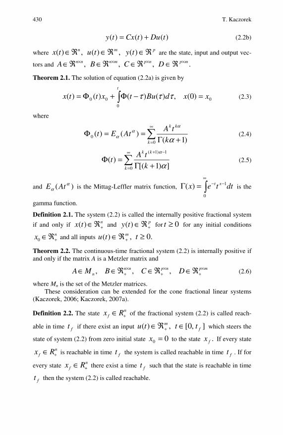
430 T. Kaczorek
)()()( tDutCxty += (2.2b)
where ( ) ,nx t ∈ℜ ,)( mtu ℜ∈ pty ℜ∈)( are the state, input and output vec-
tors and ,n nA ×∈ℜ ,n mB ×∈ℜ ,p nC ×∈ℜ .mpD ×ℜ∈
Theorem 2.1. The solution of equation (2.2a) is given by
∫ =−Φ+Φ=t
xxdButxttx0
000 )0(,)()()()( τττ (2.3)
where
∑∞
= +Γ==Φ
00 )1(
)()(k
kk
k
tAAtEt
α
αα
α (2.4)
∑∞
=
−+
+Γ=Φ
0
1)1(
])1[()(
k
kk
k
tAt
α
α
(2.5)
and )( αα AtE is the Mittag-Leffler matrix function, ∫
∞−−=Γ
0
1)( dttex xt is the
gamma function.
Definition 2.1. The system (2.2) is called the internally positive fractional system
if and only if ( ) nx t +∈ℜ and pty +ℜ∈)( for 0≥t for any initial conditions
0nx +∈ℜ and all inputs ,)( mtu +ℜ∈ .0≥t
Theorem 2.2. The continuous-time fractional system (2.2) is internally positive if and only if the matrix A is a Metzler matrix and
, , ,n n p n p mnA M B C D× × ×
+ + +∈ ∈ℜ ∈ℜ ∈ℜ (2.6)
where Mn is the set of the Metzler matrices. These consideration can be extended for the cone fractional linear systems
(Kaczorek, 2006; Kaczorek, 2007a).
Definition 2.2. The state nfx R+∈ of the fractional system (2.2) is called reach-
able in time ft if there exist an input ],0[,)( fm tttu ∈ℜ∈ + which steers the
state of system (2.2) from zero initial state 00 =x to the state .fx If every state
nfx R+∈ is reachable in time ft the system is called reachable in time ft . If for
every state nfx R+∈ there exist a time ft such that the state is reachable in time
ft then the system (2.2) is called reachable.
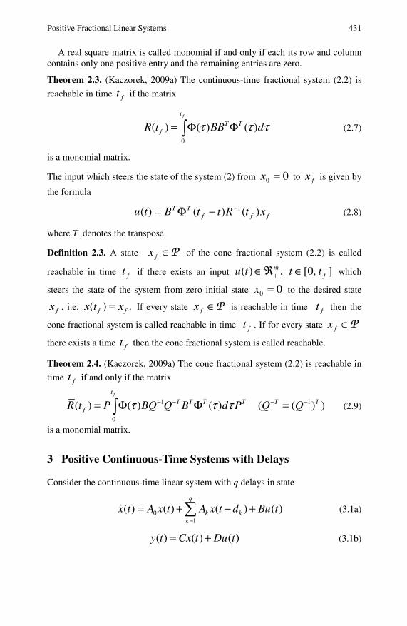
Positive Fractional Linear Systems 431
A real square matrix is called monomial if and only if each its row and column contains only one positive entry and the remaining entries are zero.
Theorem 2.3. (Kaczorek, 2009a) The continuous-time fractional system (2.2) is
reachable in time ft if the matrix
0
( ) ( ) ( )ft
T TfR t BB dτ τ τ= Φ Φ∫ (2.7)
is a monomial matrix.
The input which steers the state of the system (2) from 00 =x to fx is given by
the formula
fffTT xtRttBtu )()()( 1−−Φ= (2.8)
where T denotes the transpose.
Definition 2.3. A state P∈fx of the cone fractional system (2.2) is called
reachable in time ft if there exists an input ],0[,)( fm tttu ∈ℜ∈ + which
steers the state of the system from zero initial state 00 =x to the desired state
fx , i.e. ( ) .f fx t x= If every state P∈fx is reachable in time ft then the
cone fractional system is called reachable in time ft . If for every state P∈fx
there exists a time ft then the cone fractional system is called reachable.
Theorem 2.4. (Kaczorek, 2009a) The cone fractional system (2.2) is reachable in
time ft if and only if the matrix
1 1
0
( ) ( ) ( ) ( ( ) )ft
T T T T T TfR t P BQ Q B d P Q Qτ τ τ− − − −= Φ Φ =∫ (2.9)
is a monomial matrix.
3 Positive Continuous-Time Systems with Delays
Consider the continuous-time linear system with q delays in state
01
( ) ( ) ( ) ( )q
k kk
x t A x t A x t d Bu t=
= + − +∑ (3.1a)
( ) ( ) ( )y t Cx t Du t= + (3.1b)
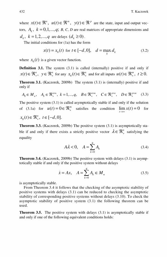
432 T. Kaczorek
where ( ) ,nx t ∈ℜ ,)( mtu ℜ∈ pty ℜ∈)( are the state, input and output vec-
tors, , 0,1,..., ;kA k q= B, C, D are real matrices of appropriate dimensions and
,kd 1, 2,...,k q= are delays ( 0)kd ≥ .
The initial conditions for (1a) has the form
0( ) ( )x t x t= for [ ,0], max kk
t d d d∈ − = (3.2)
where 0 ( )x t is a given vector function.
Definition 3.1. The system (3.1) is called (internally) positive if and only if
( ) ,nx t +∈ℜ ny +∈ℜ for any 0 ( ) nx t +∈ℜ and for all inputs ( ) , 0.mu t t+∈ℜ ≥
Theorem 3.1. (Kaczorek, 2009b) The system (3.1) is (internally) positive if and only if
0 , , 1,..., , , ,n n n m p n p mn kA M A k q B C D× × × ×
+ + + +∈ ∈ℜ = ∈ℜ ∈ℜ ∈ℜ (3.3)
The positive system (3.1) is called asymptotically stable if and only if the solution
of (3.1a) for ( ) 0 mu t += ∈ℜ satisfies the condition lim ( ) 0t
x t→∞
= for
0 ( ) , [ ,0].nx t t d+∈ℜ ∈ −
Theorem 3.3. (Kaczorek, 2009b) The positive system (3.1) is asymptotically sta-
ble if and only if there exists a strictly positive vector nλ +∈ℜ satisfying the
equality
0
0,q
kk
A A Aλ=
< =∑ (3.4)
Theorem 3.4. (Kaczorek, 2009b) The positive system with delays (3.1) is asymp-totically stable if and only if the positive system without delays
0
,q
k nk
x Ax A A M=
= = ∈∑ (3.5)
is asymptotically stable. From Theorem 3.4 it follows that the checking of the asymptotic stability of
positive systems with delays (3.1) can be reduced to checking the asymptotic stability of corresponding positive systems without delays (3.10). To check the asymptotic stability of positive system (3.1) the following theorem can be used.
Theorem 3.5. The positive system with delays (3.1) is asymptotically stable if and only if one of the following equivalent conditions holds:
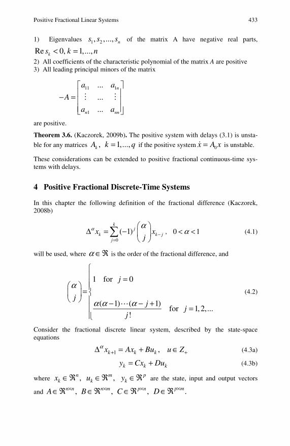
Positive Fractional Linear Systems 433
1) Eigenvalues 1 2, ,..., ns s s of the matrix A have negative real parts,
Re 0, 1,...,ks k n< =
2) All coefficients of the characteristic polynomial of the matrix A are positive 3) All leading principal minors of the matrix
11 1
1
...
...
...
n
n nn
a a
A
a a
⎡ ⎤⎢ ⎥− = ⎢ ⎥⎢ ⎥⎣ ⎦
are positive.
Theorem 3.6. (Kaczorek, 2009b). The positive system with delays (3.1) is unsta-
ble for any matrices ,kA 1,...,k q= if the positive system 0x A x= is unstable.
These considerations can be extended to positive fractional continuous-time sys-tems with delays.
4 Positive Fractional Discrete-Time Systems
In this chapter the following definition of the fractional difference (Kaczorek, 2008b)
0
( 1)k
jk k j
j
x xj
α α−
=
⎛ ⎞Δ = − ⎜ ⎟
⎝ ⎠∑ , 0 1α< < (4.1)
will be used, where α ∈ℜ is the order of the fractional difference, and
1 for 0
( 1) ( 1)for 1,2,...
!
j
jj
jj
α
α α α
⎧⎪ =⎪⎛ ⎞ ⎪= ⎨⎜ ⎟
⎝ ⎠ ⎪ − − +⎪ =⎪⎩
(4.2)
Consider the fractional discrete linear system, described by the state-space equations
1 ,k k kx Ax Bu u Zα+ +Δ = + ∈ (4.3a)
k k ky Cx Du= + (4.3b)
where ,nkx ∈ℜ ,m
ku ∈ℜ pky ∈ℜ are the state, input and output vectors
and ,n nA ×∈ℜ ,n mB ×∈ℜ ,p nC ×∈ℜ .p mD ×∈ℜ
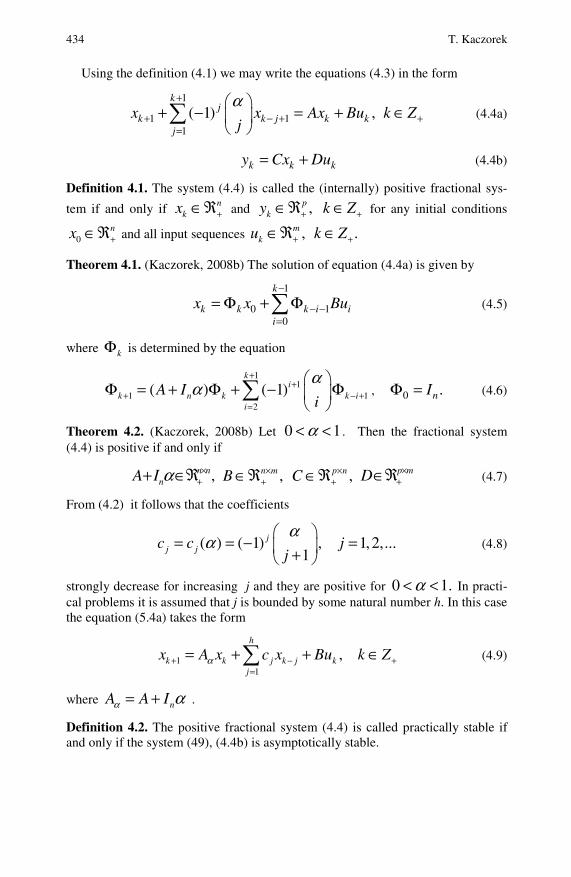
434 T. Kaczorek
Using the definition (4.1) we may write the equations (4.3) in the form
1
1 11
( 1) ,k
jk k j k k
j
x x Ax Bu k Zj
α+
+ − + +=
⎛ ⎞+ − = + ∈⎜ ⎟
⎝ ⎠∑ (4.4a)
k k ky Cx Du= + (4.4b)
Definition 4.1. The system (4.4) is called the (internally) positive fractional sys-
tem if and only if nkx +∈ℜ and ,p
ky +∈ℜ k Z+∈ for any initial conditions
0nx +∈ℜ and all input sequences ,m
ku +∈ℜ .k Z+∈
Theorem 4.1. (Kaczorek, 2008b) The solution of equation (4.4a) is given by
1
0 10
k
k k k i ii
x x Bu−
− −=
= Φ + Φ∑ (4.5)
where kΦ is determined by the equation
11
1 12
( ) ( 1)k
ik n k k i
i
A Ii
αα
++
+ − +=
⎛ ⎞Φ = + Φ + − Φ⎜ ⎟
⎝ ⎠∑ , 0 .nIΦ = (4.6)
Theorem 4.2. (Kaczorek, 2008b) Let 0 1α< < . Then the fractional system (4.4) is positive if and only if
,n nnA I α ×
++ ∈ℜ ,n mB ×+∈ℜ ,p nC ×
+∈ℜ p mD ×+∈ℜ (4.7)
From (4.2) it follows that the coefficients
( ) ( 1) , 1,2,...1
jj jc c j
j
αα ⎛ ⎞
= = − =⎜ ⎟+⎝ ⎠ (4.8)
strongly decrease for increasing j and they are positive for 0 1.α< < In practi-cal problems it is assumed that j is bounded by some natural number h. In this case the equation (5.4a) takes the form
11
,h
k k j k j kj
x A x c x Bu k Zα+ − +=
= + + ∈∑ (4.9)
where nA A Iα α= + .
Definition 4.2. The positive fractional system (4.4) is called practically stable if and only if the system (49), (4.4b) is asymptotically stable.
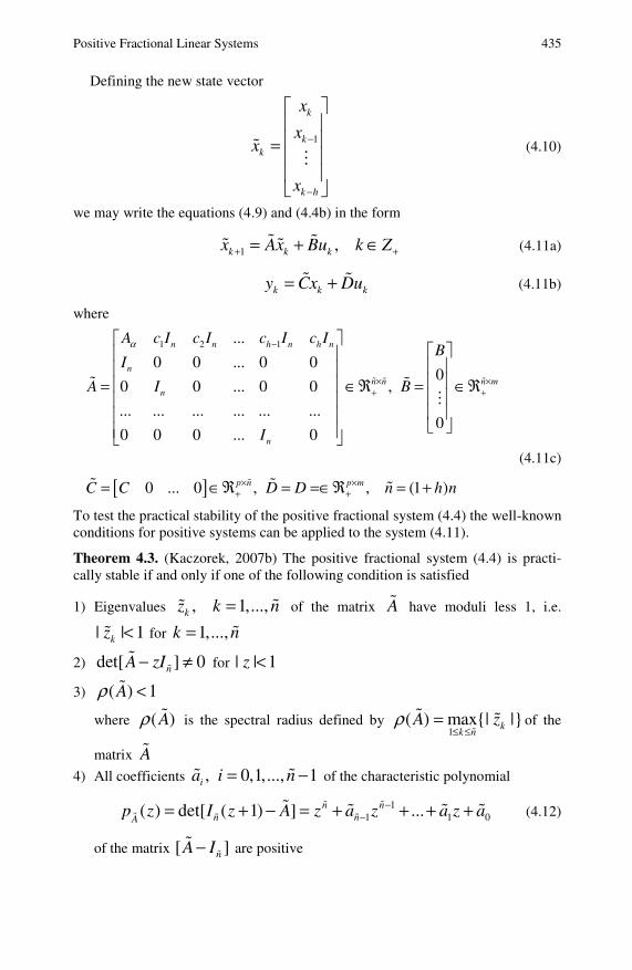
Positive Fractional Linear Systems 435
Defining the new state vector
1
k
kk
k h
x
xx
x
−
−
⎡ ⎤⎢ ⎥⎢ ⎥=⎢ ⎥⎢ ⎥⎣ ⎦
(4.10)
we may write the equations (4.9) and (4.4b) in the form
1 ,k k kx Ax Bu k Z+ += + ∈ (4.11a)
k k ky Cx Du= + (4.11b)
where
[ ]
1 2 1...
0 0 ... 0 00
0 0 ... 0 0 ,
... ... ... ... ... ...0
0 0 0 ... 0
0 ... 0 , , (1 )
n n h n h n
nn n n m
n
n
p n p m
A c I c I c I c IB
I
A I B
I
C C D D n h n
α −
× ×+ +
× ×+ +
⎡ ⎤⎡ ⎤⎢ ⎥⎢ ⎥⎢ ⎥⎢ ⎥⎢ ⎥= ∈ℜ = ∈ℜ⎢ ⎥⎢ ⎥⎢ ⎥⎢ ⎥⎣ ⎦⎢ ⎥⎣ ⎦
= ∈ℜ = =∈ℜ = +
(4.11c)
To test the practical stability of the positive fractional system (4.4) the well-known conditions for positive systems can be applied to the system (4.11).
Theorem 4.3. (Kaczorek, 2007b) The positive fractional system (4.4) is practi-cally stable if and only if one of the following condition is satisfied
1) Eigenvalues , 1,...,kz k n= of the matrix A have moduli less 1, i.e.
| | 1kz < for 1,...,k n=
2) det[ ] 0nA zI− ≠ for | | 1z <
3) ( ) 1Aρ <
where ( )Aρ is the spectral radius defined by 1
( ) max{| |}kk n
A zρ≤ ≤
= of the
matrix A
4) All coefficients , 0,1,..., 1ia i n= − of the characteristic polynomial
11 1 0( ) det[ ( 1) ] ...n n
n nAp z I z A z a z a z a−
−= + − = + + + + (4.12)
of the matrix [ ]nA I− are positive
436 T. Kaczorek
5) All principal minors of the matrix
11 12 1
21 21 2
1 1
...
...[ ]
... ... ... ...
...
n
nn
n n nn
a a a
a a aA I
a a a
⎡ ⎤⎢ ⎥⎢ ⎥− =⎢ ⎥⎢ ⎥⎣ ⎦
(4.13)
are positive
Theorem 4.5. The positive fractional system (5.4) is practically unstable if at least
one diagonal entry of the matrix Aα is greater than 1.
Reachability and controllability to zero of positive fractional discrete-time linear systems have been investigated in (Kaczorek, 2007b). LMI approaches to check-ing the practical stability of positive fractional discrete-time linear systems have been applied in (Kaczorek, 2009c).
References
Kaczorek, T.: Computation of realizations of discrete-time cone systems. Bull. Pol. Acad. Sci. Techn. 54(3), 347–350 (2006)
Kaczorek, T.: Reachability and controllability to zero of cone fractional linear systems. Archives of Control Sciences 17(3), 357–367 (2007a)
Kaczorek, T.: Reachability and controllability to zero of positive fractional discrete-time systems. Machine Intelligence and Robotic Control 6(4), 139–143 (2007b)
Kaczorek, T.: Fractional positive continuous-time linear systems and their reachability. Int. J. Appl. Math. Sci. 18(2), 223–228 (2008a)
Kaczorek, T.: Practical stability of positive fractional discrete-time linear systems. Bull. Pol. Acad. Techn. Sci. 56(4), 313–324 (2008b)
Kaczorek, T.: Reachability of cone fractional continuous-time linear systems. Int. J. Appl. Math. Comput. Sci. 19(1) (2009a)
Kaczorek, T.: Stability of positive continuous-time linear systems with delays. Bull. Pol. Acad. Sci. Techn. 57(4) (2009b) (in Press)
Kaczorek, T.: LMI approaches to practical stability of positive fractional discrete-time lin-ear systems. Int. J. Appl. Math. Comput. Sci. 19(4) (2009c)
Integrated Method of Grey Multi-attribute Risk Group Decision-Making
Luo Dang and Zhou Ling
The problem of grey multi-attribute risk group decision-making is studied, when the attributive values are interval grey numbers and the attribute weights are unknown. Using grey incidence method of the grey system theory, Relative deviation degree based on the optimum alternative group and the worst alternative group, a new method is proposed. It establishes the integrated optimization model dealing the weights of index based on that the deviation of group members is minimum and the deviation between two groups is maximum. By using the model, the attribute weights can be gotten. Then, based on subjective preferences of decision-maker group, synthetically deviations of each alternative to the optimum alternative group and the worst alternative group are calculated to determine the ranking order of alternatives. Finally, an example is given to show the feasibility and availability of this method.
1 Introduction
Group decision–making is a very important research field of decision science and it has extensive practical background. Group decision–making problem is solved by the expert group by exerting their advantages, evaluating the alternative from dif-ferent aspects and assembling different opinions so as to sort and optimize the alternative. In the recent years, researches on group decision–making theory and Luo Dang College of Mathematics and Information Sciences, North China University of Conservancy and Hydroelectric Power, Zhengzhou, China e-mail: [email protected]
Zhou Ling College of Mathematics and Information Sciences, North China University of Conservancy and Hydroelectric Power, Zhengzhou, China e-mail: [email protected]
* This work was Supported by the Science and Technology Attack Projects of Henan Prov-ince (072102340009); Supported by the Natural Science Foundation of Department of Henan Province (2009A110011); Supported by the Philosophy and Social Sciences Plan Project of Henan Province (2007BJJ014); Supported by Soft Science Foundation of Sci-ence and Technology Department of Henan Province (082400440100).
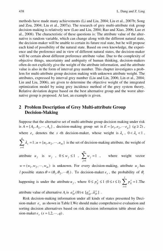
438 L. Dang and Z. Ling
methods have made many achievements (Li and Liu, 2004; Liu et al., 2007b; Song and Zou, 2004; Liu et al., 2007a). The research of grey multi-attribute risk group decision-making is relatively new (Luo and Liu, 2004; Rao and Xiao, 2006; Luo et al., 2008). The characteristic of these questions is: The attribute value of the alter-native is random variable, which can change along with the different natural state, the decision-maker will be unable to certain its future real state, but he will propose each kind of possibility of the natural state. Based on own knowledge, the experi-ence and the preference and in view of different natural states, the decision-maker will be certain about different preference attribute value. Due to the complexity of objective things, uncertainty and ambiguity of human thinking, decision-makers often do not explicitly give the weight of the attribute information, and the attribute value is also in the form of interval gray number. This chapter investigates a prob-lem for multi-attribute group decision making with unknown attribute weight. The attributes, expressed by interval grey number (Liu and Lin, 2006; Lin et al., 2004; Lin and Liu, 2006), are given to determine the objective weight of the integrated optimization model by using grey incidence method of the grey system theory. Relative deviation degree based on the best alternative group and the worst alter-native group is proposed. At last, an example is given.
2 Problem Description of Grey Multi-attribute Group Decision-Making
Suppose that the alternative set of multi-attribute group decision making under risk is },,,{ 21 nAAAA = , decision-making group set is },,{ 21 qeeeE = )2( ≥q ,
where se denotes the s -th decision-maker, whose weight is sλ , 10 << sλ ,
11
=∑=
q
ssλ ; },,,{ 21 muuuu = is the set of decision-making attribute, the weight of
attribute ju is jw , 10 ≤≤ jw , 11
=∑=
m
jjw , where weight vector
),,,( 21 mwwww = is unknown. For every decision-making, attribute ju has
l possible states ),,( 21 lθθθθ = . To decision-maker se , the probability of tθ
happening is under the attribute ju , where 10 ≤≤ stjp )10( ≤≤ t 1
1
=∑=
l
t
stjp .The
attribute value of alternative iA is ∈⊗)(sijta ],[ s
ijtsijt aa .
Risk decision-making information under all kinds of states presented by Deci-sion-maker se as shown in Table I.We should make comprehensive evaluation and
sorting decision alternatives based on risk decision information table about deci-sion-maker se ),,2,1( qs = .

Integrated Method of Grey Multi-attribute Risk Group Decision-Making 439
Table I Risk decision-making table )(⊗sE for decision-maker se
scheme u1 u2 ... um
1θ 2θ ...
lθ
1θ 2θ ...
lθ ...1θ
2θ ... lθ
sp11 sp 21
... s
lp 1
sp12 sp 22
... s
lp 2... s
jp1 s
jp 2 ... s
ljp
A1 )(111 ⊗sa )(112 ⊗sa ... )(11 ⊗s
la )(121
⊗sa )(122
⊗sa ... )(12
⊗s
la ... )(11 ⊗s
ja )(21 ⊗s
ja ... )(1 ⊗s
jla
A2 )(
211⊗sa )(212 ⊗sa … )(
21⊗s
la )(
221⊗sa )(222 ⊗sa ... )(
22⊗s
la ... )(12 ⊗s
ja )(22 ⊗s
ja ... )(2 ⊗s
jla
... ... ... ... ...
An )(
11⊗s
na )(12 ⊗s
na ... )(1
⊗s
lna )(21 ⊗s
na )(22 ⊗s
na ... )(2 ⊗s
lna ... )(1 ⊗s
nja )(2 ⊗s
nja ... )(⊗s
njla
3 Decision-Making Principle and Method
A. Data processing and concept
Definition 1. (Liu et al., 2004) Suppose that ;],,[1 baba <∈⊗ dcdc <∈⊗ ],,[2,
then the sum of 1⊗ and 2⊗ is remarked by 21 ⊗+⊗ ,
],[21 dbca ++∈⊗+⊗
Definition 2. (Liu et al., 2004) Suppose that kbaba , ],[ <∈⊗ is real number,
then ],[ kbkak ∈⊗⋅ .
According to the above definitions we could get the expected value of the attribute under all kinds of states in risk decision table for deci-
sion-maker ),,2,1( qses …= , and then we consider the expected revenue instead
of natural revenue under different kinds of states and put several grey risk decision tables into one grey non- risk decision table. Finally, we obtain the non-risk deci-
sion matrix )(⊗sX ),,2,1( qs …= .
∑=
⊗=l
t
stj
sijt
sij pax
1
)(
In order to dispel the impact of different physical dimension on the decision re-sult, we need to normalize the decision matrix. The most common attribute is cost and benefit,
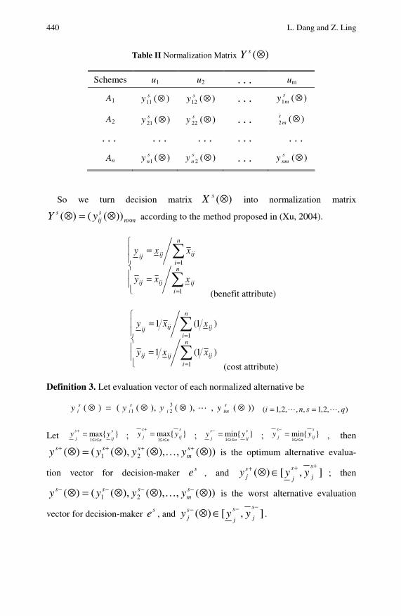
440 L. Dang and Z. Ling
Table II Normalization Matrix )(⊗sY
Schemes u1 u2 ... um
A1 )(11 ⊗sy )(12 ⊗sy ... )(1 ⊗s
my
A2 )(21 ⊗sy )(22 ⊗sy ... )(2 ⊗s
m
... ... ... ... ...
An )(1 ⊗sny )(2 ⊗s
ny...
)(⊗snmy
So we turn decision matrix )(⊗sX into normalization matrix
mnsij
s yY ×⊗=⊗ ))(()( according to the method proposed in (Xu, 2004).
⎪⎪
⎩
⎪⎪
⎨
⎧
=
=
∑
∑
=
=n
iijijij
n
iijijij
xxy
xxy
1
1
(benefit attribute)
⎪⎪
⎩
⎪⎪
⎨
⎧
=
=
∑
∑
=
=n
iijijij
n
iijijij
xxy
xxy
1
1
)1(1
)1(1
(cost attribute)
Definition 3. Let evaluation vector of each normalized alternative be
))(,),(),(()( 321 ⊗⊗⊗=⊗ s
imisi
si yyyy ),,2,1,,,2,1( qsni ==
Let }{max1
s
ijni
s
jyy
≤≤
+ = ; }{max1
s
ijni
s
j yy≤≤
+= ; }{min
1
s
ijni
s
jyy
≤≤
− = ; }{min1
s
ijni
s
j yy≤≤
−= , then
))(,),(),(()( 21 ⊗…⊗⊗=⊗ ++++ sm
sss yyyy is the optimum alternative evalua-
tion vector for decision-maker se , and ],[)(+++ ∈⊗
s
js
j
sj yyy ; then
))(,),(),(()( 21 ⊗…⊗⊗=⊗ −−−− sm
sss yyyy is the worst alternative evaluation
vector for decision-maker se , and ],[)(−−− ∈⊗
s
js
j
sj yyy .
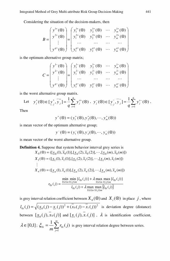
Integrated Method of Grey Multi-attribute Risk Group Decision-Making 441
Considering the situation of the decision-makers, then
⎟⎟⎟⎟⎟
⎠
⎞
⎜⎜⎜⎜⎜
⎝
⎛
⊗⊗⊗
⊗⊗⊗⊗⊗⊗
=
⎟⎟⎟⎟⎟
⎠
⎞
⎜⎜⎜⎜⎜
⎝
⎛
⊗
⊗⊗
=
+++
+++
+++
+
+
+
)()()(
)()()(
)()()(
)(
)(
)(
21
222
21
112
11
2
1
qm
m
m
q yyy
yyy
yyy
y
y
y
B
is the optimum alternative group matrix;
⎟⎟⎟⎟⎟
⎠
⎞
⎜⎜⎜⎜⎜
⎝
⎛
⊗⊗⊗
⊗⊗⊗⊗⊗⊗
=
⎟⎟⎟⎟⎟
⎠
⎞
⎜⎜⎜⎜⎜
⎝
⎛
⊗
⊗⊗
=
−−−
−−−
−−−
−
−
−
)()()(
)()()(
)()()(
)(
)(
)(
21
222
21
112
11
2
1
qm
m
m
q yyy
yyy
yyy
y
y
y
C
is the worst alternative group matrix.
Let )(1
],[)(1
⊗=∈⊗ ∑=
++++q
s
sjjjj y
qyyy , )(
1],[)(
1
⊗=∈⊗ ∑=
−−−−q
s
sjjjj y
qyyy ,
Then
))(,),(),(()( 21 ⊗⊗⊗=⊗ ++++myyyy
is mean vector of the optimum alternative group;
))(,),(),(()( 21 ⊗⊗⊗=⊗ −−−−myyyy
is mean vector of the worst alternative group.
Definition 4. Suppose that system behavior interval grey series is )])(),([,)],2(),2([)],1(),1(([)( 0000000 mxmxxxxxX =⊗
)])(),([,)],2(),2([)],1(),1(([)( 1111111 mxmxxxxxX =⊗
)])(),([,)],2(),2([)],1(),1(([)( mxmxxxxxX nnnnnnn =⊗
{ })(maxmax)(
)}({maxmax)}({minmin)(
011
0
011
011
0 jljl
jljljr
imjni
i
imjni
imjni
i
≤≤≤≤
≤≤≤≤≤≤≤≤
+
+=
λ
λ
is grey interval relation coefficient between )(0 ⊗X and )(⊗iX in place j , where
))()(())()(()( 20
200 jxjxjxjxjl iii −+−= is deviation degree (distance)
between )](),([ 00 jxjx and )](),([ jxjx ii , λ is identification coefficient,
]1,0[∈λ ; ∑=
=m
jii jr
m 100 )(
1ξ is grey interval relation degree between series.

442 L. Dang and Z. Ling
Theorem 1. )(0 jr i satisfies the following properties:
(1) 1)(0 0 ≤≤ jr i ;
(2) when )(0 jl i is smaller, )(0 jr i is bigger.
B. Modeling Principle
When people make decisions, the smaller the internal group deviation of the op-timum alternation group and the worst group is the better. Because it indicates that
the group opinions tend to coincide. Besides, under the attribute ju , the smaller the
difference in the evaluation value of all the optimum schemes (or the worst) within the group is, the smaller role this attribute plays in scheme decision and sorting. At the same time, we hope that the internal group deviation between the two groups is bigger. According to Definition 4
22
11
22
2
11
22
11)1(
)()(maxmax)()(
)()(maxmax)()(minmin)(
++++
≤≤≤≤
++++
++++
≤≤≤≤
++++
≤≤≤≤
−+−+−+−
−+−+−+−=
kj
tj
k
j
t
jmjqk
kj
tj
kj
t
j
kj
tj
k
j
t
jmjqk
kj
tj
k
j
t
jmjqk
tk
yyyyyyyy
yyyyyyyyjr
λ
λ
is the grey interval relation coefficient under the attribute ju and the optimum
alternative evaluation vector +ky corresponding to alternative +ty , [0,1]λ ∈ is
identification coefficient, 0.5λ = in this chapter.
)()1( wvtj denotes the grey interval relation degree between the optimum alterna-
tive evaluation vector +ky and others under attribute ju , then
∑=
=q
kjtktj wjrwv
1
)1()1( )()(
Let
∑ ∑∑= = =
==q
t
q
t
q
kjtktjj wjrwvwv
1 1 1
)1()1()1( )()()( ( mj ,,2,1= )
To attribute ju , )()1( wv j denotes the total relation degree between all the opti-
mum alternative evaluation vectors and others. According to the above, the selec-tion of weight vector w should make the sum of total relational degree the largest.
To construct the following Model (I)
⎪⎪⎩
⎪⎪⎨
⎧
=≥=
=
∑
∑∑∑
=
= = =
),,2,1(0,1..
)()(max
1
2
1 1 1
)1()1(
mjwwts
wjrwv
m
jjj
m
j
q
t
q
kjtk
Similar to the above definition
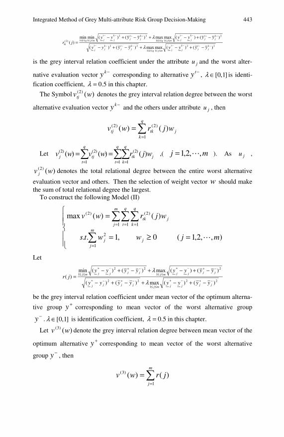
Integrated Method of Grey Multi-attribute Risk Group Decision-Making 443
22
11
22
2
11
22
11)2(
)()(maxmax)()(
)()(maxmax)()(minmin)(
−−−−
≤≤≤≤
−−−−
−−−−
≤≤≤≤
−−−−
≤≤≤≤
−+−+−+−
−+−+−+−=
kj
tj
k
j
t
jmjqk
kj
tj
kj
t
j
kj
tj
k
j
t
jmjqk
kj
tj
k
j
t
jmjqk
tk
yyyyyyyy
yyyyyyyyjr
λ
λ
is the grey interval relation coefficient under the attribute ju and the worst alter-
native evaluation vector −ky corresponding to alternative −ty , [0,1]λ ∈ is identi-
fication coefficient, 0.5λ = in this chapter.
The Symbol )()2( wvtj denotes the grey interval relation degree between the worst
alternative evaluation vector −ky and the others under attribute ju , then
∑=
=q
kjtktj wjrwv
1
)2()2( )()(
Let ∑ ∑∑= = =
==q
t
q
t
q
kjtktjj wjrwvwv
1 1 1
)2()2()2( )()()( ,( mj ,,2,1= ). As ju ,
)()2( wv j denotes the total relational degree between the entire worst alternative
evaluation vector and others. Then the selection of weight vector w should make the sum of total relational degree the largest.
To construct the following Model (II)
⎪⎪⎩
⎪⎪⎨
⎧
=≥=
=
∑
∑∑∑
=
= = =
),,2,1(0,1..
)()(max
1
2
1 1 1
)2()2(
mjwwts
wjrwv
m
jjj
m
j
q
t
q
kjtk
Let
22
1
22
2
1
22
1
)()(max)()(
)()(max)()(min)(
−+−+
≤≤
−+−+
−+−+
≤≤
−+−+
≤≤
−+−+−+−
−+−+−+−=
jjjjmjjjjj
jjjjmjjjjjmj
yyyyyyyy
yyyyyyyyjr
λ
λ
be the grey interval relation coefficient under mean vector of the optimum alterna-
tive group +y corresponding to mean vector of the worst alternative group −y . [0,1]λ ∈ is identification coefficient, 0.5λ = in this chapter.
Let )()3( wv denote the grey interval relation degree between mean vector of the
optimum alternative +y corresponding to mean vector of the worst alternative
group −y , then
∑=
=m
j
jrwv1
)3( )()(
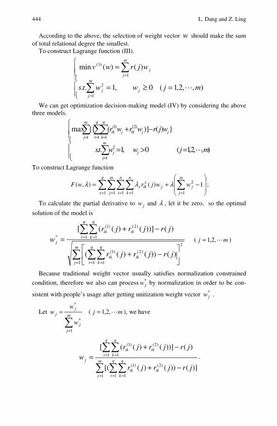
444 L. Dang and Z. Ling
According to the above, the selection of weight vector w should make the sum of total relational degree the smallest.
To construct Lagrange function (III).
⎪⎪⎩
⎪⎪⎨
⎧
=≥=
=
∑
∑
=
=
),,2,1(0,1..
)()(min
1
2
1
)3(
mjwwts
wjrwv
m
jjj
m
jj
We can get optimization decision-making model (IV) by considering the above three models.
⎪⎪⎩
⎪⎪⎨
⎧
=>=
−+
∑
∑ ∑∑
=
= = =
),,2,1(0,1..
})()]({[max
1
2
1 1 1
)2()1(
mjwwts
wjrwrwr
m
jjj
m
j
q
t
q
kjjtkjtk
To construct Lagrange function
=),( λwF ⎟⎟
⎠
⎞
⎜⎜
⎝
⎛−+ ∑∑∑∑∑
== = = =
m
jj
q
s
m
j
n
i
n
kj
siks wwjr
1
2
1 1 1 1
1)( λλ ;
To calculate the partial derivative to jw and λ , let it be zero, so the optimal
solution of the model is
∑ ∑∑
∑∑
= = =
= =
⎥⎦
⎤⎢⎣
⎡−+
−+=
m
j
q
t
q
ktktk
q
t
q
ktktk
j
jrjrjr
jrjrjrw
1
2
1 1
)2()1(
1 1
)2()1(
*
)())()((
)()])()(([ ( mj ,2,1= )
Because traditional weight vector usually satisfies normalization constrained
condition, therefore we also can process *jw by normalization in order to be con-
sistent with people’s usage after getting unitization weight vector *jw .
Let
∑=
=m
jj
jj
w
ww
1
*
*
( mj ,2,1= ), we have
∑ ∑∑
∑∑
= = =
= =
−+
−+=
m
j
q
t
q
ktktk
q
t
q
ktktk
j
jrjrjr
jrjrjrw
1 1 1
)2()1(
1 1
)2()1(
)]())()([(
)()])()(([.

Integrated Method of Grey Multi-attribute Risk Group Decision-Making 445
C. Decision Algorithms
Step 1: By the counting formula of the expected value, getting the non- risk de-
cision matrix and turning decision matrix )(⊗sX into normalization matrix
)(⊗sy ( 1,2, , )s q= .
Step 2: Establishing the optimum alternative group matrix and the worst alter-native group matrix.
Step 3: According to Model (IV), we get the attribute weight.
Step 4: According to the attribute weight and normalization matrix )(⊗sy , we
get weighted normalization matrix )(⊗swY .
Step 5: Calculating the distances, which are respectively
⎟⎠⎞⎜
⎝⎛ −+−=
++
=∑ j
s
ijj
s
ij
m
jjis yyyywd
1
)1(
and
⎟⎠⎞⎜
⎝⎛ −+−=
−−
=∑ j
s
ijj
s
ij
m
jjis yyyywd
1
)2( ( ),,2,1 ni =
between the alternative iA of every decision-maker se ),,2,1( qs = and the opti-
mum alternative group, as well as between iA and the worst alternative group.
Step 6: Consider the distances
∑=
+ =q
sissi dD
1
)1(λ and ∑=
− =q
sissi dD
1
)2(λ
respectively, between the alternative of all decision-makers and the optimum al-ternative group, as well as between the alternative iA and the worst alternative
group. Step 7: Calculating closeness degree of each alternative to the optimum alterna-
tive group
+−
−
+=
ii
ii
DD
DC ( ni ,,2,1= )
The bigger iC is the more superior the alternative is.
4 Example
An enterprise decides to modify its products. Now there are 3 design alterna-
tives )3,2,1( =iAi . By studying the 3 main attributes: 1u —cost (unit: ten thousand
Yuan), 2u —reliability (non-fault working time. unit: ten thousand hours) and
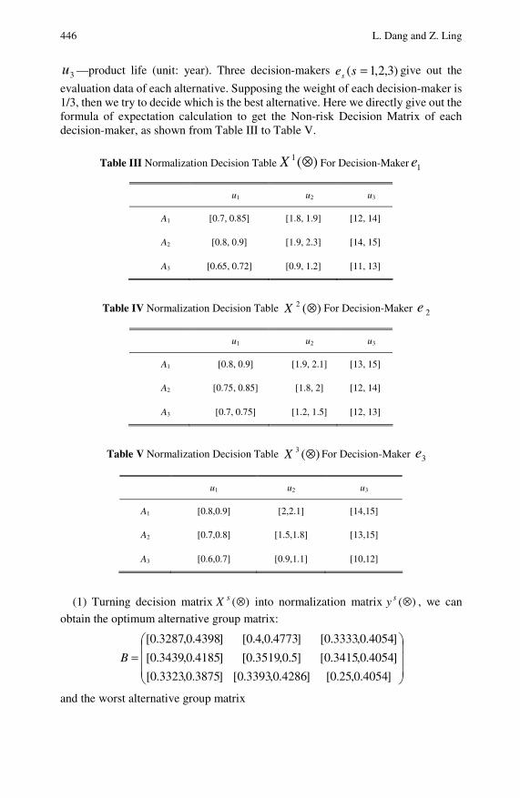
446 L. Dang and Z. Ling
3u —product life (unit: year). Three decision-makers )3,2,1( =ses give out the
evaluation data of each alternative. Supposing the weight of each decision-maker is 1/3, then we try to decide which is the best alternative. Here we directly give out the formula of expectation calculation to get the Non-risk Decision Matrix of each decision-maker, as shown from Table III to Table V.
Table III Normalization Decision Table )(1 ⊗X For Decision-Maker 1e
u1 u2 u3
A1 [0.7, 0.85] [1.8, 1.9] [12, 14]
A2 [0.8, 0.9] [1.9, 2.3] [14, 15]
A3 [0.65, 0.72] [0.9, 1.2] [11, 13]
Table IV Normalization Decision Table )(2 ⊗X For Decision-Maker 2e
u1 u2 u3
A1 [0.8, 0.9] [1.9, 2.1] [13, 15]
A2 [0.75, 0.85] [1.8, 2] [12, 14]
A3 [0.7, 0.75] [1.2, 1.5] [12, 13]
Table V Normalization Decision Table )(3 ⊗X For Decision-Maker 3e
u1 u2 u3
A1 [0.8,0.9] [2,2.1] [14,15]
A2 [0.7,0.8] [1.5,1.8] [13,15]
A3 [0.6,0.7] [0.9,1.1] [10,12]
(1) Turning decision matrix )(⊗sX into normalization matrix )(⊗sy , we can
obtain the optimum alternative group matrix:
⎟⎟⎟
⎠
⎞
⎜⎜⎜
⎝
⎛=
]4054.0,25.0[]4286.0,3393.0[]3875.0,3323.0[
]4054.0,3415.0[]5.0,3519.0[]4185.0,3439.0[
]4054.0,3333.0[]4773.0,4.0[]4398.0,3287.0[
B
and the worst alternative group matrix
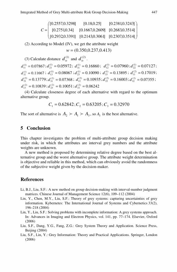
Integrated Method of Grey Multi-attribute Risk Group Decision-Making 447
⎟⎟⎟
⎠
⎞
⎜⎜⎜
⎝
⎛=
]3514.0,2307.0[]3061.0,2143.0[]3391.0,2932.0[
]3514.0,2683.0[]2609.0,1667.0[]34.0,2751.0[
]3243.0,2381.0[]25.0,18.0[]3298.0,2557.0[
C
(2) According to Model (IV), we get the attribute weight
)413.0,237.0,350.0(=w
(3) Calculate distance )1(isd and )2(
isd .
07867.0)1(11 =d ; 05972.0)1(
21 =d ; 16860.0)1(31 =d ; 07960.0)1(
12 =d ; 07127.0)1(22 =d ;
11667.0)1(32 =d ; 08067.0)1(
13 =d ; 10090.0)1(23 =d ; 13895.0)1(
33 =d ; 17019.0)2(11 =d ;
13779.0)2(21 =d ; 07368.0)2(
31 =d ; 10935.0)2(12 =d ; 16003.0)2(
22 =d ; 07355.0)2(32 =d ;
10839.0)2(13 =d ; 10051.0)2(
23 =d ; 06242.0)2(33 =d
(4) Calculate closeness degree of each alternative with regard to the optimum alternative group.
62842.01 =C ; 63205.02 =C ; 32970.03 =C
The sort of alternative is 312 AAA , so 2A is the best alternative.
5 Conclusion
This chapter investigates the problem of multi-attribute group decision making under risk, in which the attributes are interval grey numbers and the attribute weights are unknown.
A new method is proposed by determining relative degree based on the best al-ternative group and the worst alternative group. The attribute weight determination is objective and reliable in this method, which can obviously avoid the randomness of the subjective weight given by the decision-maker.
References
Li, B.J., Liu, S.F.: A new method on group decision-making with interval-number judgment matrices. Chinese Journal of Management Science 12(6), 109–112 (2004)
Lin, Y., Chen, M.Y., Liu, S.F.: Theory of grey systems: capturing uncertainties of grey information. Kybernetes: The International Journal of Systems and Cybernetics 33(2), 196–218 (2004)
Lin, Y., Liu, S.F.: Solving problems with incomplete information: A grey systems approach. In: Advances in Imaging and Electron Physics, vol. 141, pp. 77–174. Elsevier, Oxford (2006)
Liu, S.F., Dang, Y.G., Fang, Z.G.: Grey System Theory and Application. Science Press, Beijing (2004)
Liu, S.F., Lin, Y.: Grey Information: Theory and Practical Applications. Springer, London (2006)

448 L. Dang and Z. Ling Liu, X.Q., Chen, X., Zhang, H.: A multi-character group-decision-making method and ap-
plication based on group ideal solution. Journal of Shenyang Institute of Aeronautical Engineering 24(2), 38–41 (2007a)
Liu, Y.Z., Xu, D.P., Jiang, Y.C.: Method of adaptive adjustment weights in multi-attribute group decision-making. Systems Engineering and Electronics 29(1), 45–48 (2007b)
Luo, D., Liu, S.F.: Research on grey multi-criteria risk decision-making method. Systems Engineering and Electronics 26(8), 1057–1059 (2004)
Luo, D., Zhou, L., Luo, D.X.: Grey multi-attribute risk group decision-making method. Systems Engineering and Electronics 30(9), 1674–1678 (2008)
Rao, C.J., Xiao, X.P.: Method of grey matrix relative degree for dynamic hybrid multi-attribute decision making under risk. Systems Engineering and Electronics 28(9), 1353–1357 (2006)
Song, G.X., Zou, P.: The method of determining the weight of the decision-maker in multi attribute group decision-making. Systems Engineering 19(4), 84–89 (2004)
Xu, Z.S.: Uncertain Multiple Attribute Decision Making: Methods and Applications. Qinghua University Press, Beijing (2004)
Grey Relational Analysis Method of Linguistic Information and Its Application in Group Decision
Qiuping Wang, Daohong Zhang, and Haiqing Hu1
Grey relational analysis based on grey relational degree is a very successful theory and method in grey system theory. On the basis of grey relational four axioms, this chapter extends general grey relational degree formula to the case of linguistic term sequence. This work may extend the application field of grey relational degree. This chapter puts forward a method for group multiple attribute decision making problems with linguistic information, in which the preference values take the form of linguistic variables. Then a procedure to group multiple attribute decision making is provided under linguistic environment. Finally, an example of risk investment problem is given to verify the proposed method, and practicality of the proposed method is shown by illustrative example.
1 Introduction
Grey relational analysis was pioneered by Deng Julong in 1984 (Deng, 1984; Liu and Lin, 2006; Lin et al., 2004; Lin and Liu, 2006). Grey relational analysis is an important part of grey system theory. It is a quantitative method of analyzing grey relational degree among each factor in grey system. Its basic idea is to judge the relational degree of the development situation during grey process based on the geometrical figure similar degree of the sequences curves. The application of grey relational analysis to practical problem, the key is to calculate relational degree. Qiuping Wang School of Business Management e-mail: [email protected]
Daohong Zhang School of Business Management Xi’an People’s Government e-mail: [email protected]
Haiqing Hu School of Business Administration, Xi’an University of Technology, Xi’an 710054, China, Phone: +86-13991904585 e-mail: [email protected]
450 Q. Wang, D. Zhang, and H. Hu
Therefore, how to define grey relational degree is very important. Over the recent twenty years, the study of grey relational degree has aroused maximum concern and many results have been achieved. Grey relational models of the real number sequence are as follows: classical relational models proposed by Deng Julong (Deng, 1985; Deng, 1989), grey B-mode relational degree and grey C-mode relational degree proposed by Wang Qingyin (Wang, 1989; Wang and Zhao, 1999), the generalized degree of grey incidence (including the absolute degree of grey incidence, the relative degree of grey incidence, and the synthetic degree of grey incidence proposed by S. F. Liu (Liu, 1992; Liu et al., 2004), grey absolute correlation degree proposed by Mei Zhenguo (Mei, 1992), T’s correlation degree proposed by Tang Wuxiang (Tang, 1995), a kind of modified grey correlation degree proposed by Xiao Xinping (Xiao et al., 1995), Grey slope incidence degree and improved degree of grey slope incidence proposed by Dang Yaoguo (Dang, 1994; Dang et al., 2004a). Grey relational models of the interval number sequence are as follows: interval number incidence degree proposed by Dang Yaoguo (Dang et al., 2004b), interval number related degree proposed by ZHANG Jijun (Zhang, 2005), the incidence degree coefficient formula and relative incidence degree coefficient formula for interval grey numbers constructed by LUO Dang (Luo, 2005). Grey relational models of the triangular fuzzy number sequence are as follows: the grey incidence coefficient formula of triangular fuzzy number based on idea of grey system theory and expectation formula of triangular fuzzy number proposed by Qiu-Ping WANG et al (Wang et al., 2007), the method of grey relational analysis of triangular fuzzy number based on triangular fuzzy number distance formula (Chen, 2000) proposed by Wei Gui-Wu (Wei and Wang, 2008). Moreover, Xiong Hejin proposed grey vector relational degree and complex number relational degree (Xiong et al., 2000), etc. These relational degree models have been used widely in practice.
Qualitative evaluating information is often given directly when evaluating such as ideological moral character of human, performance of a car and so on(e.g., linguistic form like “excellent”, “good”, “poor” and so forth). Linguistic variable approach is an effective tool which deals with problem not to be assessed precisely in a quantitative form. Therefore, a study of linguistic term grey relational model has important theoretical and actual application value. At present, research achievement relating to the problem at home and abroad has been rare. In literature (Wei and Lin, 2008), semantic grey relational coefficient was given and a method for multiple attribute group decision making based on two-tuple linguistic setting was proposed. Motivated by the idea of Zeshui Xu (Ze, 2005), this chapter defines the distance of linguistic term. On this basis, this chapter proposes the computational method of linguistic term sequence grey relational degree according to grey relational analysis axioms, thus extending grey relational analysis theory from real number sequence to linguistic term sequence. We take further steps to research multiple attribute group decision making problems and establish grey relational model for multiple attribute group decision making with linguistic term.
The rest of this chapter is organized as follows. Section 2 introduces some basic notations and operational laws of linguistic variables. Section 3 proposes grey relational degree of linguistic terms. Section 4 gives a representation of group
Grey Relational Analysis Method of Linguistic Information and Its Application 451
decision making problem with linguistic information, gives the method of grey relational analysis for group decision making with linguistic information. Section 5 gives an illustrative example. And finally, conclusion is made in Section 6.
2 Basic Notations and Operational Laws
The linguistic approach is an approximate technique, which represents qualitative aspects as linguistic values by means of linguistic variables (Zadeh, 1975; Herrera-Viedma and Verdegay, 1995; Herrera-Viedma and Martinez, 2000; Herrera and Herrera-Viedma, 2000; Torra, 2001).
Suppose that },,1,0,1,,{ ttsS −−== αα is a finite and totally
ordered discrete term set whose cardinality value is an odd one, such as 7 and 9,
where αs represents a possible value for a linguistic variable. For example, a set of
nine terms S could be given as follows (Ze, 2005):
}.goodextremely ,goodvery ,good
,goodslightly ,fair,poorslightly
,poor,poorvery ,poorextremely {
432
101
234
======
====
−
−−−
sss
sss
sssS
In these cases, it usually requires that αs and βs satisfies the following
additional characteristics (Herrera-Viedma and Martinez, 2000; Herrera and Herrera-Viedma, 2000).
(1) The set is ordered: βα ss > if and only if βα > ;
(2) There is the negation operator: αα −= ss )(neg , especially, 00 )(neg ss = ;
(3) Max operator: ,),max( αβα sss = if ji ≥ ;
(4) Min operator: ,),min( αβα sss = if ji ≤ .
The operation on two linguistic terms can be converted to the operation on subscript variables of the corresponding terms.
Definition 1. Let Sss ∈βα , be two linguistic variables, we define the distance
between αs and βs as follows:
βαβα −=),( ssd .
We can prove ),( βα ssd to satisfy condition of distance measure axiom, and it
has properties in the following:

452 Q. Wang, D. Zhang, and H. Hu
(1) βα ss = if and only if 0),( =βα ssd ;
(2) Let Ssss ∈γβα ,, , βs are closer to αs than γs , if and only
if ),(),( γαβα ssdssd < .
3 Grey Relational Degree of Linguistic Terms
Let X be sequence set of linguistic terms, Xx ∈0 be reference sequence of
linguistic terms, Xxi ∈ be comparison sequences of linguistic terms
( ni ,,2,1 …= ).
))(,),2(),1(( 0000 mxxxx …= ,
))(,),2(),1(( mxxxx iiii …= ,
where )(0 jx and )( jxi are linguistic terms, ))((0 0)( jxIsjx = , ))(()( jxIi i
sjx = ,
),,2,1( mj …= .
Let ))(( 0 jxI and ))(( jxI be the subscript variables of linguistic values of
))(( 0 jxIs and ))(( jxIs respectively. For example, if 4)( sjxi = , then 4))(( =jxI i .
Let
))(())(()( 0 jxIjxIj ii −=Δ ,
))(()((minmin 0min jxIjxI iji
−=Δ ,
))(()((maxmax 0max jxIjxI iji
−=Δ .
Definition 2. A nonnegative real number ))(),(( 0 jxjx iγ is called grey relational
coefficient between 0x and ix at j , which is defined as
max
maxmin0 ))(),((
Δ+ΔΔ+Δ=
ρργ
ii jxjx . (1)
where ]1,0[∈ρ is the distinguishing coefficient, generally 5.0=ρ . And iγ is
called grey relational degree of ix with respect to 0x , which is defined as
∑=
==m
jiii jxjx
mxx
100 ))(),((
1),( γγγ (2)
Theorem 1. The grey relational degree ),( 0 ixxγ of ix with respect to 0x obtained
from (1) and (2) satisfies the following four grey axioms.
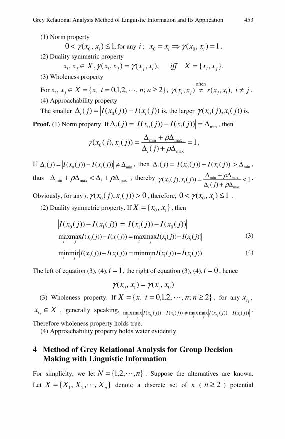
Grey Relational Analysis Method of Linguistic Information and Its Application 453
(1) Norm property
,1),(0 0 ≤< ixxγ for any i ; 1),( 00 =⇒= ii xxxx γ .
(2) Duality symmetric property
}.,{ ),,(),(,, jiijjiji xxXiffxxxxXxx ==∈ γγ
(3) Wholeness property
For }2;,,2,1,0{, ≥==∈ nntxXxx tji , j ixxrxx ijji ≠≠ ,),(),(often
γ .
(4) Approachability property
The smaller ))(())(()( 0 jxIjxIj ii −=Δ is, the larger ))(),(( 0 jxjx iγ is.
Proof. (1) Norm property. If min0 ))(())(()( Δ=−=Δ jxIjxIj ii , then
1)(
))(),((max
maxmin0 =
Δ+ΔΔ+Δ=
ρργ
jjxjx
ii ,
If min0 ))(())(()( Δ≠−=Δ jxIjxIj ii
, then min0 ))(())(()( Δ>−=Δ jxIjxIj ii ,
thus maxmaxmin Δ+Δ<Δ+Δ ρρ i , thereby 1)(
))(),((max
maxmin0 <
Δ+ΔΔ+Δ=
ρργ
jjxjx
ii
.
Obviously, for any j, 0))(),(( 0 >jxjx iγ , therefore, 1),(0 0 ≤< ixxγ .
(2) Duality symmetric property. If },{ 10 xxX = , then
))(())(())(())(( 0110 jxIjxIjxIjxI −=−
))(())((maxmax))(())((maxmax 10 jxIjxIjxIjxI iji
iji
−=− (3)
))(())((minmin))(())((minmin 10 jxIjxIjxIjxI iji
iji
−=− (4)
The left of equation (3), (4), 1=i , the right of equation (3), (4), 0=i , hence
),(),( 0110 xxxx γγ =
(3) Wholeness property. If }2;,,2,1,0{ ≥== nntxX t , for any ,1t
x
Xxt ∈2
, generally speaking, ))(())((maxmax))(())((maxmax21
jxIjxIjxIjxI itji
itji
−≠− .
Therefore wholeness property holds true. (4) Approachability property holds water evidently.
4 Method of Grey Relational Analysis for Group Decision Making with Linguistic Information
For simplicity, we let },,2,1{ nN = . Suppose the alternatives are known.
Let },,,{ 21 nXXXX = denote a discrete set of n ( 2≥n ) potential
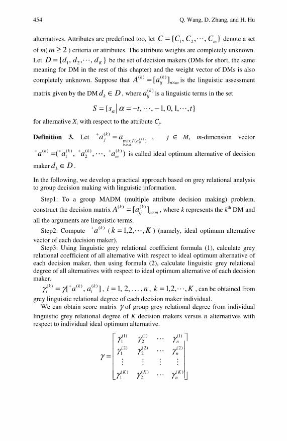
454 Q. Wang, D. Zhang, and H. Hu
alternatives. Attributes are predefined too, let },,,{ 21 mCCCC = denote a set
of m( 2≥m ) criteria or attributes. The attribute weights are completely unknown.
Let },,,{ 21 KdddD = be the set of decision makers (DMs for short, the same
meaning for DM in the rest of this chapter) and the weight vector of DMs is also
completely unknown. Suppose that mnk
ijk aA ×= ][ )()( is the linguistic assessment
matrix given by the DM Ddk ∈ , where )(kija is a linguistic terms in the set
},,1,0,1,,{ ttsS −−== αα
for alternative Xi with respect to the attribute Cj.
Definition 3. Let )(max
)()(
1
kij
niaI
kj aa
≤≤
=+ , j ∈ M, m-dimension vector
),,,( )()(2
)(1
)( km
kkk aaaa ++++ = is called ideal optimum alternative of decision
maker Ddk ∈ .
In the following, we develop a practical approach based on grey relational analysis to group decision making with linguistic information.
Step1: To a group MADM (multiple attribute decision making) problem,
construct the decision matrix mnk
ijk aA ×= ][ )()( , where k represents the kth DM and
all the arguments are linguistic terms.
Step2: Compute )(ka+ ( Kk ,,2,1= ) (namely, ideal optimum alternative
vector of each decision maker). Step3: Using linguistic grey relational coefficient formula (1), calculate grey
relational coefficient of all alternative with respect to ideal optimum alternative of each decision maker, then using formula (2), calculate linguistic grey relational degree of all alternatives with respect to ideal optimum alternative of each decision maker.
],[ )()()( ki
kki aa+= γγ , ni ,,2,1 …= , Kk ,,2,1= , can be obtained from
grey linguistic relational degree of each decision maker individual. We can obtain score matrix γ of group grey relational degree from individual
linguistic grey relational degree of K decision makers versus n alternatives with respect to individual ideal optimum alternative.
⎥⎥⎥⎥⎥
⎦
⎤
⎢⎢⎢⎢⎢
⎣
⎡
=
)()(2
)(1
)2()2(2
)2(1
)1()1(2
)1(1
Kn
KK
n
n
γγγ
γγγγγγ
γ
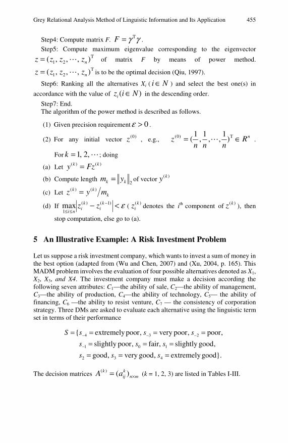
Grey Relational Analysis Method of Linguistic Information and Its Application 455
Step4: Compute matrix F. γγ T=F .
Step5: Compute maximum eigenvalue corresponding to the eigenvector T
21 ),,,( nzzzz = of matrix F by means of power method. T
21 ),,,( nzzzz = is to be the optimal decision (Qiu, 1997).
Step6: Ranking all the alternatives Xi ( Ni ∈ ) and select the best one(s) in
accordance with the value of )( Nizi ∈ in the descending order.
Step7: End. The algorithm of the power method is described as follows.
(1) Given precision requirement 0>ε .
(2) For any initial vector )0(z , e.g., nRnnn
z ∈= T)0( )1
,,1
,1
( .
For ,2,1=k ; doing
(a) Let )()( kk Fzy =
(b) Compute length 2kk ym = of vector )(ky
(c) Let kkk myz )()( =
(d) If ε<− −
≤≤
)1()(
1max k
ik
ini
zz ( )(kiz denotes the ith component of )(kz ), then
stop computation, else go to (a).
5 An Illustrative Example: A Risk Investment Problem
Let us suppose a risk investment company, which wants to invest a sum of money in the best option (adapted from (Wu and Chen, 2007) and (Xu, 2004, p. 165). This MADM problem involves the evaluation of four possible alternatives denoted as X1, X2, X3, and X4. The investment company must make a decision according the following seven attributes: C1—the ability of sale, C2—the ability of management, C3—the ability of production, C4—the ability of technology, C5— the ability of financing, C6 —the ability to resist venture, C7 — the consistency of corporation strategy. Three DMs are asked to evaluate each alternative using the linguistic term set in terms of their performance
}.goodextremely ,goodvery ,good
,goodslightly ,fair,poorslightly
,poor,poorvery ,poorextremely {
432
101
234
======
====
−
−−−
sss
sss
sssS
The decision matrices mnkij
k aA ×= )()( (k = 1, 2, 3) are listed in Tables I-III.

456 Q. Wang, D. Zhang, and H. Hu
Table I Decision matrices A(1)
C1 C2 C3 C4 C5 C6 C7 X1 s1 s3 s3 s0 s1 s2 s2 X2 s3 s2 s0 s2 s3 s1 s-1 X3 s2 s2 s3 s1 s4 s3 s2 X4 s2 s2 s-1 s1 s3 s1 s1
Table II Decision matrices A(2)
C1 C2 C3 C4 C5 C6 C7 X1 s1 s2 s3 s0 s2 s2 s4 X2 s0 s1 s0 s1 s2 s2 s1 X3 s3 s1 s2 s2 s4 s4 s1 X4 s0 s1 s0 s1 s0 s1 s-1
Table III Decision matrices A(3)
C1 C2 C3 C4 C5 C6 C7 X1 s0 s2 s2 s1 s3 s2 s3 X2 s2 s1 s1 s2 s0 s2 s-1 X3 s2 s1 s2 s2 s2 s3 s2 X4 s0 s1 s-1 s1 s0 s0 s1
Step1: Calculate ideal optimum alternative vector )(ka+ of each decision maker.
),,,,,,( 2342333)1( sssssssa =+ ,
),,,,,,( 4442323)2( sssssssa =+ ,
),,,,,,( 3332222)3( sssssssa =+
Step2: Let 5.0=ρ , using (1), calculate linguistic grey relational coefficient of
all alternative with respect to ideal optimum alternative of each decision maker, then using formula (2), calculate linguistic grey relational degree of all alternatives with respect to ideal optimum alternative of each decision maker. Thereby, we can obtain matrixγ ,
⎥⎥⎥
⎦
⎤
⎢⎢⎢
⎣
⎡=
⎥⎥⎥
⎦
⎤
⎢⎢⎢
⎣
⎡
=505.0857.0676.0833.0
502.0840.0558.0746.0
597.0859.0616.0724.0
)4(4
)3(3
)3(2
)3(1
)2(4
)2(3
)2(2
)2(1
)1(4
)1(3
)1(2
)1(1
γγγγγγγγγγγγ
γ
and
⎥⎥⎥⎥
⎦
⎤
⎢⎢⎢⎢
⎣
⎡
=
⎥⎥⎥⎥⎥
⎦
⎤
⎢⎢⎢⎢⎢
⎣
⎡
=
505.0502.0597.0
857.0840.0859.0
676.0558.0616.0
833.0746.0724.0
)3(4
)2(4
)1(4
)3(3
)2(3
)1(3
)3(2
)2(2
)1(2
)3(1
)2(1
)1(1
T
γγγγγγγγγγγγ
γ

Grey Relational Analysis Method of Linguistic Information and Its Application 457
Step3: Compute matrix F
⎥⎥⎥⎥
⎦
⎤
⎢⎢⎢⎢
⎣
⎡
=
8634.03673.19892.02274.1
3673.11779.25772.19624.1
9892.05772.11478.14254.1
2274.19624.14254.17446.1
F
Step4: Compute maximum eigenvalue corresponding to the eigenvector T
21 ),,,( nzzzz = of matrix F by means of power method.
Given 00001.0=ε , the results of iterative computation are listed in Table IV.
Table IV The results of iterative computation
z(0) y(1) z(1) y(2) z(2) y(3) z(3) 0.2500 0.2500 0.2500 0.2500
1.5974 1.2849 1.7712 1.1118
0.5455 0.4388 0.6048 0.3797
3.2463 2.6106 3.5988 2.2583
0.5456 0.4387 0.6048 0.3795
3.2463 2.6106 3.5988 2.2583
0.5456 0.4387 0.6048 0.3795
Optimal decision is T)3( )3795.0,6048.0,4387.0,5456.0(== zz .
Namely:
3795.0,6048.0,4387.0,5456.0 4321 ==== zzzz
Rank zi (i = 1, 2, 3, 4) in descending order 4213 zzzz >>> . The ranking
order of all alternatives is 4213 XXXX . Thus the best alternative is X3.
The selection order of illustrative example by using our proposed approach is the same with that by using approach in (Wu and Chen, 2007) or (Xu, 2004).
6 Conclusion
In the real world, the decision maker may have vague knowledge about the preferences degree of one alternative over another. Furthermore, it is too complex or too ill-defined to be amenable for description in conventional quantitative expressions. Extend grey relational analysis to linguistic environment is highly beneficial when the performance values cannot be expressed by means of numerical values. This chapter extends general grey relational degree formula to the cases of linguistic term sequence. This work may extend the application field of grey relational degree. On the basis of grey relational degree of linguistic term, we have developed a group decision making method under linguistic environment. We have also applied the proposed approach to a group decision-making problem of choosing the best option for a risk investment company. The linguistic approach

458 Q. Wang, D. Zhang, and H. Hu
gives a more flexible framework to deal with decision problems using qualitative information. The linguistic grey relational analysis proposed in this chapter is also applicable to group decision making with multi-granularity linguistic assessment information. The grey relational analysis method of relating to group MADM problem with uncertain linguistic assessment information is the future work.
References
Chen, C.T.: Extensions of the TOPSIS for group decision-making under fuzzy environment. Fuzzy Sets and Systems 114, 1–9 (2000)
Dang, Y.G.: Grey gradient relational degree. System Sciences and Comprehensive Studies in Agriculture 10, 331–337 (1994)
Dang, Y.G., Liu, S.F., Liu, B., Mi, C.M.: Improvement on degree of grey slope incidence. Engineering Science 6(3), 41–44 (2004a)
Dang, Y.G., Liu, S.F., Liu, B., Yu, Y.W.: Study on Incidence decision making model of multi-attribute interval number. Journal of Nanjing University of Aeronautics & Astronautics 36(3), 403–406 (2004b)
Deng, J.L.: The theory and methods of socio-economy grey system. Social Sciences in China (6), 47–60 (1984)
Deng, J.L.: Relational space of grey systems. Fuzzy Mathematics 4(2), 1–10 (1985) Deng, J.L.: Grey information space. Journal of Grey Systems 1(2), 103–117 (1989) Herrera, F., Herrera-Viedma, E.: Linguistic decision analysis: Steps for solving decision
problems under linguistic information. Fuzzy Sets and Systems 115, 67–82 (2000) Herrera-Viedma, H.F., Martinez, M.: A fusion approach for managing multi-granularity
linguistic term sets in decision making. Fuzzy Sets and Systems 114, 43–58 (2000) Herrera-Viedma, H.F., Verdegay, J.L.: A sequential selection process in group decision
making with a linguistic assessment approach. Information Sciences 85, 223–239 (1995) Liu, S.F.: Generalized Degree of Grey Incidence: Information and Systems, pp. 113–116.
DMU Publishing House, Dalian (1992) Liu, S.F., Dang, Y.G., Fang, Z.G.: Grey System Theory and Its Application. Science Press,
Beijing (2004) Luo, D.: An eigenvector method for grey decision-making. Systems Engineering-theory &
Practice (4), 67–71 (2005) Mei, Z.G.: The concept and computation method of grey absolute correlation degree.
Systems Engineering 10, 43–45 (1992) Qiu, W.H.: An eigenvalue method on group decision. Applied Mathematics and
Mechanics 18(11), 1099–1104 (1997) Tang, W.X.: The concept and the computation method of T’s correlation degree. Application
of Statistics and Management 14, 33–37 (1995) Torra, V.: Aggregation of linguistic labels when semantics is based on antonyms.
International Journal of Intelligent Systems 16(4), 513–524 (2001) Wang, Q.Y.: The grey relational analysis of B-mode. Journal of Huazhong Scientific &
Technology University, vol 17(6), 77–82 (1989) Wang, Q.P., Zhang, D.H., Hu, H.Q.: A method of grey incidence analysis for group
decision-making. In: Proceedings of 2007 IEEE International Conference on Grey Systems and Intelligent Services (GSIS 2007), Nanjing, China, November 18-20, vol. 1, pp. 189–194 (2007)
Grey Relational Analysis Method of Linguistic Information and Its Application 459 Wang, Q.Y., Zhao, X.H.: The relational analysis of C-mode. Journal of Huazhong Scientific
& technology University 27(3), 75–77 (1999) Wei, G.W., Lin, R.: Method of grey relational analysis for multiple attribute group decision
making in two-tuple linguistic setting. Systems Engineering and Electronics 30(9), 1686–1689 (2008)
Wei, G.W., Wang, X.R.: Grey relational analysis method for triangular fuzzy number-based multiple attribute decision making with preference information on alternatives. Systems Engineering and Electronics 30(8), 1489–1492 (2008)
Xiao, X.P., Xie, L.C., Huang, D.R.: A modified computation method of grey correlation degree and its application. Application of Statistics and Management 14(5), 27–30 (1995)
Xiong, H.J., Chen, M.Y., Qu, T.: Some extensions of grey relational grade formula. Systems Engineering and Electronics 22(1), 8–10, 80 (2000)
Zadeh, L.A.: The concept of a linguistic variable and its application to approximate reasoning. Part I. Information Sciences 8, 199–249 (1975); Part II, Information Sciences 8, 301–357; Part III, Information Sciences 9, 43 – 80
Ze, S.X.: Deviation measures of linguistic preference relations in group decision making. Omega 33, 249–254 (2005)
Zhang, J.J.: Method of grey related analysis to multiple attribute decision making problem with interval numbers. Systems Engineering and Electronics 27(6), 1030–1033 (2005)
Wu, Z.B., Chen, Y.H.: The maximizing deviation method for group multiple attribute decision making under linguistic environment. Fuzzy Sets and Systems 158, 1608–1617 (2007)
Xu, Z.S.: Uncertain Multiple Attribute Decision Making: Methods and Applications, p. 165. Tsinghua University Press, Beijing (2004)
Liu, S.F., Lin, Y.: Grey Information: Theory and Practical Applications. Springer, London (2006)
Lin, Y., Chen, M.Y., Liu, S.F.: Theory of grey systems: capturing uncertainties of grey information. Kybernetes: The International Journal of Systems and Cybernetics 33(2), 196–218 (2004)
Lin, Y., Liu, S.F.: Solving problems with incomplete information: A grey systems approach. In: Advances in Imaging and Electron Physics, vol. 141, pp. 77–174 (2006)
The Relation between Grey Relational Decision Making and Grey Situation Decision Making under the Proper Condition*
Yong Wei and Xinhai Kong
The relation between grey relational decision making and grey situation decision making is pointed out in this chapter, which broadens the train of thought to define the incidence degree, effect measure, uniform measure and incidence coefficient. Furthermore, we analyze the substantial cause that the incidence order is changed with non-dimensionalization in grey incidence analysis. At the same time, we point out two kinds of common processing methods (unitization of initial values and zeroization of initial points for row vectors) both are unreasonable.
1 Introduction
From the angle of the research method, we can see that grey relational decision making (Liu and Lin, 2006; Lin et al., 2004; Lin and Liu, 2006) is to seek the ideal decision-making scheme at first, but the ideal decision- making scheme does not exist truly in the known decision- making schemes for choosing, so we have to select the relatively satisfactory decision-making scheme in a series of non-ideal decision-making schemes. And the method of selecting the relatively satisfactory decision-making scheme is to discuss the relational degrees between each decision-making scheme and the ideal decision-making scheme, and select the biggest one as the satisfactory decision-making scheme. However, the concept of relational degree is by no means introduced in grey situation decision making from Yong Wei Department of Mathematics and Information, China West Normal University, Nanchong, Sichuan, China Phone: +86-08173306866; Fax: +86-8172568035 e-mail: [email protected]
Xinhai Kong Department of Mathematics and Information, China West Normal University, Nanchong, Sichuan, China e-mail: [email protected]
* This work was supported by scientific research fund of Sichuan Education Department (2006A007) and basic application research fund of Sichuan (2008JY0112).
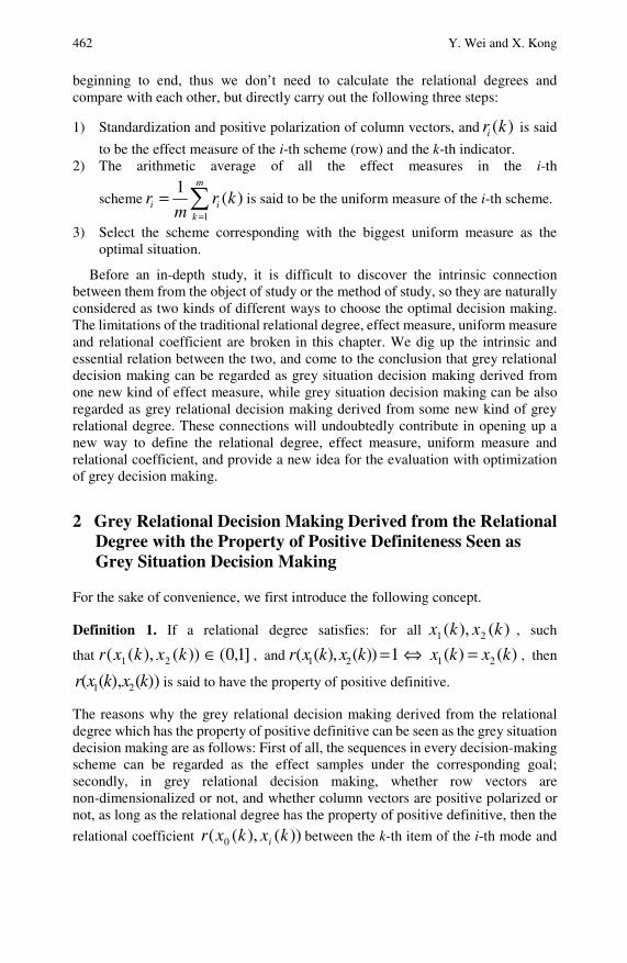
462 Y. Wei and X. Kong
beginning to end, thus we don’t need to calculate the relational degrees and compare with each other, but directly carry out the following three steps:
1) Standardization and positive polarization of column vectors, and ( )ir k is said
to be the effect measure of the i-th scheme (row) and the k-th indicator. 2) The arithmetic average of all the effect measures in the i-th
scheme1
1( )
m
i ik
r r km =
= ∑ is said to be the uniform measure of the i-th scheme.
3) Select the scheme corresponding with the biggest uniform measure as the optimal situation.
Before an in-depth study, it is difficult to discover the intrinsic connection between them from the object of study or the method of study, so they are naturally considered as two kinds of different ways to choose the optimal decision making. The limitations of the traditional relational degree, effect measure, uniform measure and relational coefficient are broken in this chapter. We dig up the intrinsic and essential relation between the two, and come to the conclusion that grey relational decision making can be regarded as grey situation decision making derived from one new kind of effect measure, while grey situation decision making can be also regarded as grey relational decision making derived from some new kind of grey relational degree. These connections will undoubtedly contribute in opening up a new way to define the relational degree, effect measure, uniform measure and relational coefficient, and provide a new idea for the evaluation with optimization of grey decision making.
2 Grey Relational Decision Making Derived from the Relational Degree with the Property of Positive Definiteness Seen as Grey Situation Decision Making
For the sake of convenience, we first introduce the following concept.
Definition 1. If a relational degree satisfies: for all )(),( 21 kxkx , such
that ))(),(( 21 kxkxr ]1,0(∈ , and 1 2( ( ), ( )) 1r x k x k = ⇔ )()( 21 kxkx = , then
))(),(( 21 kxkxr is said to have the property of positive definitive.
The reasons why the grey relational decision making derived from the relational degree which has the property of positive definitive can be seen as the grey situation decision making are as follows: First of all, the sequences in every decision-making scheme can be regarded as the effect samples under the corresponding goal; secondly, in grey relational decision making, whether row vectors are non-dimensionalized or not, and whether column vectors are positive polarized or not, as long as the relational degree has the property of positive definitive, then the
relational coefficient ))(),(( 0 kxkxr i between the k-th item of the i-th mode and

The Relation between Grey Relational Decision Making 463
the k-th item of the ideal mode can be always regarded as the effect
measure ( )ir k of the k-th item, which is regulated having the property of positive
polarity and standardization in the i-th scheme, thus the relational degree between the i-th mode and the ideal mode
0 01
1( , ) ( ( ), ( ))
m
i ik
r X X r x k x km =
= ∑
can be seen as regulating a special uniform measure ir for the i-th scheme
1
1( ) ( )
m
eff i ik
M X r km =
= ∑ .
Selecting the mode corresponding with the biggest relational degree as the satisfactory mode, it can be also seen that selecting the one corresponding with the biggest uniform measure as the optimal situation.
Note 1: It is necessary to satisfy the property of positive definitive for grey
relational degree, otherwise the regulated 1
1( ) ( )
m
eff i ik
M X r km =
= ∑ doesn’t
necessarily satisfy the requirement of measure. Therefore, Xiao suggested that using the related coefficient in probability theory as grey relational degree in (Xiao, 1997), and the correlation relational degree defined in (Wei, 2006) can’t also taken as the responsibility.
By means of the relational degree which doesn’t reflect the property of closeness, even if it is non-negative, we can’t also obtain grey situation decision making. For example, although grey slope relational degree is non-negative, from the proposition 4.5.3 of literature (Liu et al., 2004), we know that the grey slope relational coefficient is only related to the geometrical shape of original data, and has nothing to do with their relative position of space. So it is unable to reflect the property of closeness.
While making the grey relational decision making, we shouldn’t do any data transformation for the mode vectors (row vectors), such as doing the unitization of initial values for the mode vectors (row vectors) (namely, the
transformation)1(
)()(
i
ii x
kxky = ). It is inadvisable to analyze iy , because it will
deny the substance differences between different modes, and then result in the loss of the reasonableness of evaluation. For example, two modes (1,1, ,1) and (0.2,0.2, ,0.2) . Every item of the mode (1,1, ,1) reaches
the perfect standard, and every item of the mode (1,1, ,1) never reaches the
qualified standard, but through unitizing for the initial values, the two are transformed into the same mode (1,1, ,1) .
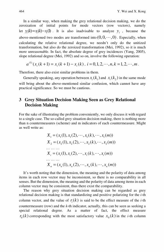
464 Y. Wei and X. Kong
In a similar way, when making the grey relational decision making, we do the zeroization of initial points for mode vectors (row vectors), namely
let )1()()( iii xkxky −= . It is also inadvisable to analyze iy , because the
above-mentioned two modes are transformed into (0,0, ,0) . Especially, when
calculating the relative relational degree, we needn’t only do the unitized transformation, but also do the zeroized transformation (Mei, 1992), so it is much more unreasonable. In fact, the absolute degree of grey incidences (Yang, 2005), slope relational degree (Mei, 1992) and so on, involve the following operation:
)()1()1(()1( kxkxkxa iii −+=+ , 0,1, 2, , , 1, 2, ,i n k m= = .
Therefore, there also exist similar problems in them.
Generally speaking, any operation between 1( )ix k and 2( )ix k in the same mode
will bring about the above-mentioned similar confusion, which cannot have any practical significance. So we must be cautious.
3 Grey Situation Decision Making Seen as Grey Relational Decision Making
For the sake of illustrating the problem conveniently, we only discuss it with regard to a single case. The so-called grey situation decision making, there is nothing more than n countermeasures (scheme) and m indicators of each countermeasure. Might as well write as:
1 1 1 1 1( (1), (2), , ( ), , ( ))X x x x k x m=
2 2 2 2 2( (1), (2), , ( ), , ( ))X x x x k x m=
… … …
( (1), (2), , ( ), , ( ))i i i i iX x x x k x m=
… … …
( (1), (2), , ( ), , ( ))n n n n nX x x x k x m=
It’s worth noting that the dimension, the meaning and the polarity of data among items in each row vector may be inconsistent, so there is no comparability in all senses. But the dimension, the meaning and the polarity of data among items in each column vector may be consistent, thus there exist the comparability.
The reason why grey situation decision making can be regarded as grey relational decision making is that standardizing and positive polarizing for the i-th
column vector, and the value of ( )ir k is said to be the effect measure of the i-th
countermeasure (row) and the k-th indicator, actually, this can be seen as seeking a special relational degree. As a matter of fact, the effect measure
0 ( )r k corresponding with the most satisfactory value )(0 kx in the i-th column
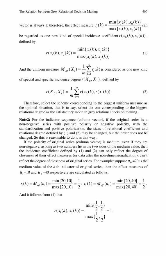
The Relation between Grey Relational Decision Making 465
vector is always 1; therefore, the effect measure 0
0
min{ ( ), ( )}( )
max{ ( ), ( )}i
ii
x k x kr k
x k x k= can
be regarded as one new kind of special incidence coefficient ))(),(( 0 kxkxr i ,
defined by
min{ ( ), ( )}( ( ), ( ))
max{ ( ), ( )}i j
i ji j
x k x kr x k x k
x k x k= (1)
And the uniform measure 1
1( ) ( )
m
eff i ik
M X r km =
= ∑ is considered as one new kind
of special and specific incidence degree ),( 0 iXXr , defined by
),( 0 iXXr ∑=
=m
ki kxrkxr
m 10 ))((),((
1 (2)
Therefore, select the scheme corresponding to the biggest uniform measure as the optimal situation, that is to say, select the one corresponding to the biggest relational degree as the satisfactory mode in grey relational decision making.
Note2: For the indicator sequence (column vector), if the original series is a non-negative series with positive polarity or negative polarity, with the standardization and positive polarization, the sizes of relational coefficient and relational degree defined by (1) and (2) may be changed, but the order does not be changed. So this is reasonable to do it in this way.
If the polarity of original series (column vector) is medium, even if they are non-negative, as long as two numbers lie in the two sides of the medium value, then the incidence coefficient defined by (1) and (2) can only reflect the degree of closeness of their effect measures (or data after the non-dimensionalization), can’t
reflect the degree of closeness of original series. For example: suppose 0u =20 is the
medium value of the k-th indicator of original series, then the effect measures of
1u =10 and 2u =40 respectively are calculated as follows:
1 1
min{20,10} 1( ) ( )
max{20,10} 2effr k M u= = = , 2 2
min{20,40} 1( ) ( )
max{20, 40} 2effr k M u= = = .
And it follows from (1) that
1 2
1 1min{ , }
2 2( ( ), ( )) 11 1
max{ , }2 2
r x k x k = = .

466 Y. Wei and X. Kong
That is to say, the closeness degree of effect measure between 10 and 40 reaches 100%. In fact, the distance between 10 and 40 is farther than that between 10 and 20, but also closer than that between 10 and 20, thus it is obviously unreasonable.
This is the essential cause that some articles complain about why some relational degrees have the ordinal effect after the treatment of non-dimensionalization or positive polarization (Xiao, 1997; Yi et al., 2006; Tang, 1994; Zhang and Zhang, 1996). In fact, any kind of relational degree cannot guarantee that the order of the size of relational degree still maintain unchanged after the data of medium polarity are transformed into the data of positive polarity. This is completely normal phenomenon.
4 Conclusion
Due to the diversity of existing grey relational coefficients and relational degrees, such as the absolute relational degree, the relative relational degree, the slope relational degree, the point relational degree, the improved absolute relational degree, the B-mode degree of grey incidence too, the T-mode relational degree and so on (Liu et al., 2004), it decides on the diversity of effect measures and uniform measures for one indicator through the method provided in this chapter. In particular, it's worth noting that it is likely for the effect measure defined by the relational coefficient in this chapter to break the mode that the effect measure is decided by only single target, and it may emerge the case that we need to use all the data of each indicator to obtain the effect measure, such as the effect measure defined by the traditional relational coefficient (Deng, 1995). Therefore, with regard to the concept of effect measure, its connotation is greatly enriched and its extension is expanded.
References
Deng, J.L.: Grey Prediction and Grey Decision, pp. 100–190. Press of Huazhong University of Science & Technology, Wuhan (2002a)
Deng, J.L.: Grey Elementary Theory, pp. 142–143. Press of Huazhong University of Science & Technology, Wuhan (2002b)
Lin, Y., Chen, M.Y., Liu, S.F.: Theory of grey systems: capturing uncertainties of grey information. Kybernetes: The International Journal of Systems and Cybernetics 33(2), 196–218 (2004)
Lin, Y., Liu, S.F.: Solving problems with incomplete information: A grey systems approach. In: Advances in Imaging and Electron Physics, vol. 141, pp. 77–174 (2006)
Liu, S.F., Dang, Y.G., Fang, Z.G.: Grey System Theory and Its Application, pp. 55–99. Science Press, Beijing (2004)
Lv, H.L., Du, P.F.: An application of grey systems method in the ecological regionalization at county level. Urban Environment & Urban Ecology 18(3), 41–43 (2005)
Liu, S.F., Lin, Y.: Grey Information: Theory and Practical Applications. Springer, London (2006)
Mei, Z.G.: The concept and computation method of grey absolute correlation degree. Systems Engineering 10(5), 43–44 (1992)

The Relation between Grey Relational Decision Making 467 Tang, W.X.: Some shortcomings of grey absolute correlation degree. Systems
Engineering 12(5), 59–62 (1994) Wei, Y.: Differences between the correlation degree of indicator and the closing degree of
mode. Grey System and Its Application, pp. 116–123. Chinese Center for Advanced Science and Technology, Beijing (2006)
Xiao, X.P.: Theoretical study and reviews on the computation method of grey interconnect degree. Systems Engineering Theory and Practice 17(8), 76–81 (1997)
Yang, Y.: The analysis of the generalized gray relatedness in PE application. Journal of Hengyang Normal University 26(3), 129–132 (2005)
Yi, H.Z., Liu, B., Zhang, H., Zhang, R.: A new computation model of incidence degree met four axioms of grey incidence. Henan Science 24(2), 162–165 (2006)
Zhang, Z.L., Zhang, G.L.: Comparisons between computation models of grey interconnect degree and analysis on their shortages. Systems Engineering 14(3), 45–49 (1996)

Use of Grey System for Assessment of Drinking Water Quality: A Case Study of Jiaozuo City, China*
Liangming Hu, Changhui Zhang, Caihong Hu, and Guiqin Jiang
In this chapter, the water standard is interval rather than point, so a new analysis method which proposed from the grey system theory—Grey Relational Analysis (GRA) based on the distance of a point to the interval is used for assessment of drinking water quality in Jiaozuo city China; This method is simple with good operability, and the physics significance was clear. Good results are achieved. The assessment results provide a scientific reference for the integrated planning, management and rational use of drinking water source in Jiaozuo city.
1 Introduction
The water environment quality issue is a subject of ongoing concerned with the development of economy, especially, since the reform and open-up in China. The water resources problems related to environmental degradation have been serious, due to the rapid industrialization and urban sprawl. The China State Environmental Protection Administration investigated the protection status of drinking water sources in major cities in 1989 and 1996 (Han et al., 2000), then evaluated the water quality and management status with the environmental protection planning being carried out in 2006 (China State Environmental Protection, 2006). The China Ministry of Water Resources evaluated the quantity and quality of national city drinking water sources and a national drinking water source protection planning was carried out in 2005 (China Ministry of Water Resources, 2005).
Aquatic ecosystems are subject to a wide variety of pollutants as well as destructive land-use or water-management practices around the world. Drinking water is obtained from two basic sources: surface water and groundwater. All water
Liangming Hu, Changhui Zhang, Caihong Hu, and Guiqin Jiang School of Water Conservancy & Environment Engineering, Zhengzhou University; Zhengzhou 450002, China e-mail: [email protected], [email protected],
[email protected], [email protected] * This work was supported in part by National Science Foundation of The Education
Department of Henan Province in 2009(NO.2009A57009).
470 L. Hu et al.
contains natural contaminants, particularly inorganic contaminants that arise from the geological strata through which the water flows and to a varying extent, anthropogenic pollution by both microorganisms and chemicals (Fung, 2003). The assessment of drinking water quality is a very important content of the assessment of drinking water sources (Wang et al., 2007). Its main task is to analyze the space-time distribution of drinking water quality, and to provide a scientific basic reference for the development and utilization planning of drinking water sources, which is based on the main material components of drinking water and is given water quality standard.
Generally, there are many methods and opinions about the evaluation of the water quality. For example, single index method (Han et al., 2000; Pan et al., 2007), analytic hierarchy process method (AHP) (Ren et al., 2007; Pang et al., 2007), pollution index method (Yu and Wang, 2003; Zhou et al., 2007; Zhang et al., 2009), fuzzy evaluation method (Singh et al., 2008; Zhu and Wu, 2005), matter-element analysis method (Xu and Shang, 1996; Men and Liang, 2003), artificial neural network method (Sun et al., 2004; Ma et al., 2007), set pair analysis method (Li and Chen, 2003; Qiu et al., 2007; Qiu et al., 2008; Li et al., 2004), and Grey evaluation method (Zheng andYu, 1989; Wang et al., 2007; Moran et al., 2006; Wong et al., 2006; Ding, 1995). Besides these, the method using Geographical Information System (GIS) in assessment for water quality is widely used at present (Babiker et al., 2007; Zhou and Zheng, 2008; Xiang et al., 2003). The methods mentioned above have their own scope of application and limitations. Of which single index method is over strict and pessimistic, analytic hierarchy process (AHP) method exits subjectivity when fixing weighting coefficient and leads to flying away from the objectivity of evaluating result. Pollution index method can not reflect the order relation of different water quality categories of different sections although it is easy, and fuzzy evaluation method can avoid the disadvantages, but it is very complicated and not intuitive in concept, while artificial neural network method can equalization the evaluation results when the sample is poor coordination. However, Grey relational analysis method with characteristics of simple in principle and calculation, can make the most of data and do not lose information, whose results can reflect the significant differences of different water quality categories of different sections (Li et al., 2004). Using GIS is a new good method, but it is restricted by the conditions and technical matters.
In this work, given the water quality monitoring data of 13 drinking water sources in Jiaozuo city Henan province China in 2004, grey relational analysis method based on the distance of a point to the interval (Shen and Xie, 1997; Xiao et al., 2005) applied to the drinking water quality assessment has been studied. And the results can provide scientific reference for decision-making by the government.
2 Methodology
A. Grey System theory
Grey incidence analysis is part of grey system theory, which is suitable for solving the complicated interrelationships between multiple factors and variables. A grey
Use of Grey System for Assessment of Drinking Water Quality 471
system is defined as a system containing unknown information presented by grey numbers and grey variables. In Grey theory, black represents a system devoid of information, while white stands for complete information. Thus, the information that is either incomplete or undetermined is called grey. Grey systems theory was initiated by Deng in 1982 (Liu and Lin, 2006; Lin et al., 2004; Lin and Liu, 2006), and has been widely applied in the last decade in China in several research fields (Deng, 1985; Deng, 1999). The system has three approaches such as Grey relational analysis, Grey clustering, Grey decision-making (Song and Deng, 2004; Zhang and Lei, 2005).
Grey relational analysis method has several advantages. The major advantage of Grey theory is that it can handle both incomplete information and unclear problems very precisely. It serves as an analysis tool especially in cases when there is insufficient data. Its concept is intuitive and simple, and no matter what the number of water quality parameters is it can analyze completely; there is no technical problems and it is easy to be promoted (Xu et al., 2006). In the evaluation process, it can make full use of environmental monitoring data, and will not lose information. The results of the evaluation not only reflect the differences between the different levels of water quality samples significantly, but also reflect the differences between different samples of the water environment quality which are at the same level (Li et al., 2004). It has a combined effect which can reflect the various water quality parameters fully (Xu et al., 2006).
It was recognized that the Grey relational analysis in Grey theory had been largely applied to project selection, prediction analysis, performance evaluation, and factor effect evaluation due to Grey relational analysis software development, such as auto control design, water resource development, hydroelectric generation scheduling and environmental management (Fung, 2003; Yeh and Chen, 2004; Liang, 1999; Chang and Lin, 1999). In terms of water quality evaluation, take water environmental monitoring data as reference sequence and water environmental quality standards as comparative sequence. More than one gray relational degree can be obtained according to grade water quality standards, and the grade corresponding with reference sequence which has the largest gray relational degree relative to comparative sequence is the grade of the water sample to be evaluated.
B. Grey Relational Analysis method based on the distance of a point to the interval
According to the differences of calculating method of gray relational coefficient, there are two kinds of method about the application of gray relational analysis for water quality evaluation; calculating the distance based on a point to a point and based on a point to the interval. To the traditional grey relational analysis method, distance based on a point to a point is used to calculate relational coefficient. Thus, typical value must be chosen from the water quality standard, subjectivity must be exited when choosing typical value, and as a result, the objectivity of evaluating result may be deviated. Optimal method which based on the basic application of Monte Carlo stochastic simulation method, relational degree according to the practice requirement is taken as the optimization object was proposed by (Du et al., 2008). Although this method would solve the problem in some degree, its optimization procedure is very complicate. Another gray relational analysis method
472 L. Hu et al.
for water quality in which distance based on a point to a point used to calculate relational coefficient, which is an improvement of traditional method that can fit the characteristic of water quality standard better. A method of calculating gray relational coefficient was defined by (Shen and Xie, 1997), in which the distance of a point to the interval is zero when the point is in the interval. This method leads to the effect is always the same when a point is in the interval and neglects the variations within the interval. Based on the operational method of gray intervals, the distance of a point to the interval is defined from another angle; the traditional gray relational analysis method is broadening (Xiao et al., 2005). This method is scientific and innovative in some degree, when the interval becomes into a point, it is identical with the absolute difference between two points of traditional gray relational analysis method.
(1) Determine the reference sequence and comparative sequence for a Grey system
Suppose the monitoring data 0{ ( )}, ( 1, 2, 3... )x k k n= for assessment of water
quality as the reference sequence, which is the mother sequence; supposes the water quality standards {[ ( ), ( )]} {[ (1), (1)],[ (2), (2)]...}( 1,2,3...; 1,2,3...)i i ii ii
x k x k x x x x i k= = = as
the comparative sequence, which is the sub sequence; (2) Calculating the incidence coefficient (i) Based on operation rule of Grey interval, define the distance of a point to the
interval as (Xiao et al., 2005):
2 20 0 0 0
2( ( ),[ ( ), ( )]) ( ( ) ( )) ( ( ) ( ))
2i ii iiD D x k x k x k x k x k x k x k= = − + −
,
(1)
By (1)-type can be seen that 0 0=| ( ) ( ) |i iD x k x k− is the same as the absolute
distance between two points compute by Grey relational analysis with the
traditional method, when the interval [ ( ), ( )]iix k x k becomes a point ( )ix k .
(ii) Calculating the correlation coefficient The correlation coefficient between the comparative sequence
{[ ( ), ( )]} {[ (1), (1)],[ (2), (2)]...}( 1,2,3...; 1,2,3...)i i ii iix k x k x x x x i k= = = and the reference
sequence 0{ ( )}x k is defined as (Fung, 2003; Yeh and Chen, 2004; Deng, 1989):
min max0
0 max
( ( ),[ ( ), ( )])ii
i
D Dx k x k x k
D D
ργρ
+=+
,
(2)
Wheremax 0max max ( )i
i kD D k=
,
,min 0min min ( )ii k
D D k=,
; ρ is a resolution
coefficient, (0,1)ρ ∈ , usually 0.5ρ = (Deng, 1989).
(3) Calculating the grey relation grade Generally takes mean value, namely 1
=k nω , the grey relation grade is defined
as (Deng, 1989):

Use of Grey System for Assessment of Drinking Water Quality 473
0 01
( , ) ( ( ),[ ( ), ( )])n
iii kk
x x x k x k x kγ ω γ=
=∑ ( 1, 2, 3...)i = (3)
(4) Sort correlation order and determine the water quality categories According to the size of correlation degree which calculated as mentioned above,
we sort correlation order and find out the largest one, and then we can determine the water quality level.
Herein, the grey relation grade represents the degree of correlation between the reference sequence and the sequence for comparison. If a particular sequence for comparison is more important to the reference sequence than other comparative sequences, then the grey relation grade between that comparative sequence and reference sequence exceed the other grey relation grades. If the comparative sequence is consistent with the reference sequence, then the grey relation grade is close to unity. Grey relational analysis measures the absolute differences between sequences, and so can be used to measure the approximate correlation of sequences (Fung, 2003).
3 Case Study
C. Study area
Jiaozuo city is located in the Yellow River Valley, Taihang Mountains, northwestern Henan Province, China (Figure 1), including five city areas, namely Jiefang area, Zhongzhan area, Macun area, Shanyang area, New city area, with two county-level cities, namely Qinyang, Mengzhou, as well as four counties, namely Wen County, Bo'ai County, Xiuwu County and Wuzhi County. It is located between Latitudes 34o48’55”–35o29’59” N and Longitudes 112o33’40” 113o38’42”E, 120 km long from east to west, 77 km wide from north to south, and covers an area of 4071 km2. The climate of the Jiaozou city is subtropics and temperate, and the average annual precipitation and temperature are 650 mm and 14.1oC. More than 70% precipitation occurs particularly between June and October period. It has a total amount of 3,455,000 people, of which 1,155,000 are urban population. There are 13 centralized drinking water sources (excluding self-drilled wells); including 2 reservoir water sources and 11 groundwater sources. Water of good quality is crucial to sustainable social and economic development, and an adequate supply of safe drinking water is one of the main requirements for a healthy life. Therefore, selecting a method for assessment of the water quality scientifically and making a real objective evaluation of the drinking water quality which is in the evaluation regional are particularly important, for protecting, rationally exploiting and utilizing the drinking water sources.
D. Water quality data
In this study, the water quality samples were collected from 13 centralized drinking water sources in 2004. The selected parameters for the estimation of surface water quality characteristics are: Total nitrogen, Potassium permanganate index,
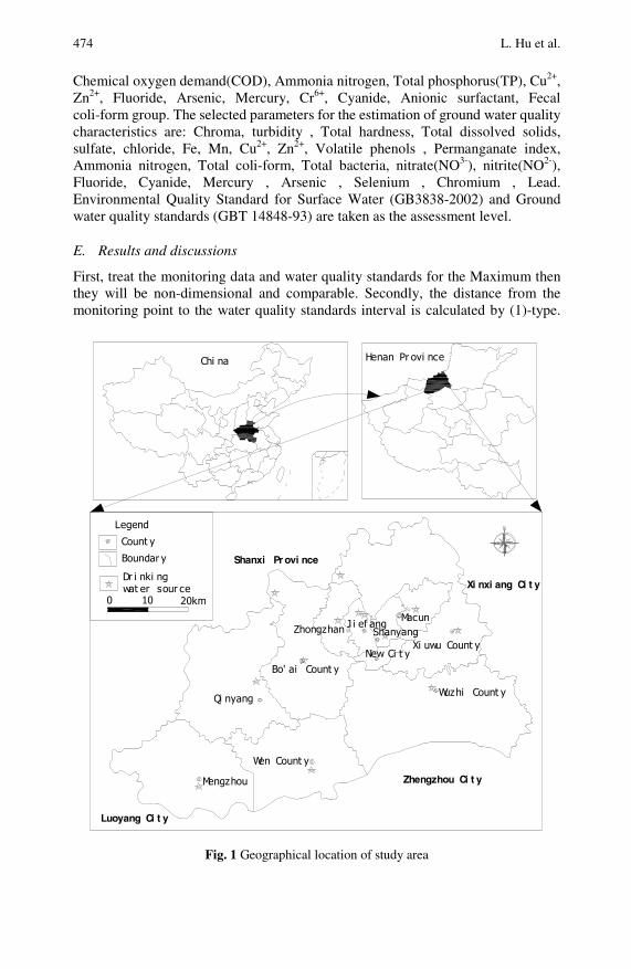
474 L. Hu et al.
Chemical oxygen demand(COD), Ammonia nitrogen, Total phosphorus(TP), Cu2+, Zn2+, Fluoride, Arsenic, Mercury, Cr6+, Cyanide, Anionic surfactant, Fecal coli-form group. The selected parameters for the estimation of ground water quality characteristics are: Chroma, turbidity , Total hardness, Total dissolved solids, sulfate, chloride, Fe, Mn, Cu2+, Zn2+, Volatile phenols , Permanganate index, Ammonia nitrogen, Total coli-form, Total bacteria, nitrate(NO3-), nitrite(NO2-), Fluoride, Cyanide, Mercury , Arsenic , Selenium , Chromium , Lead. Environmental Quality Standard for Surface Water (GB3838-2002) and Ground water quality standards (GBT 14848-93) are taken as the assessment level.
E. Results and discussions
First, treat the monitoring data and water quality standards for the Maximum then they will be non-dimensional and comparable. Secondly, the distance from the monitoring point to the water quality standards interval is calculated by (1)-type.
Henan Pr ovi nceChi na
Wen Count y
Mengzhou
Bo' ai Count y
Wuzhi Count y
Xi uwu Count y
Qi nyang
Zhongzhan J i ef angShanyang
Macun
New Ci t y
Xi nxi ang Ci t y
Zhengzhou Ci t y
Luoyang Ci t y
Shanxi Pr ovi nce
Legend
Count y
Boundar y
Dr i nki ng wat er sour ce
0 10 20km
Fig. 1 Geographical location of study area

Use of Grey System for Assessment of Drinking Water Quality 475
Thirdly, the correlation coefficient was calculated by (2)-type. Finally, the correlation degree was calculated by (3)-type and we can determine the water quality assessment level of different water resource. The water quality evaluation results of surface sources are shown in table I, and that of ground water sources are shown in table II.
Table I The evaluation results of reservoir water quality
Water sources name Flood season Non-flood season Normal water season
Qunying reservoir Ⅰ Ⅰ Ⅰ
Qingtian Rive reservoir Ⅰ Ⅰ Ⅰ
Table II The evaluation results of ground water quality
Urban name
Water sources name Evaluation
result Urban name water sources name
Evaluation result
Taihang sources Ⅱ Bo'ai County Bo'ai waterworks Ⅰ
Fenglin sources Ⅱ Wuzhi County Nanjia sources Ⅱ
Zhongma sources Ⅰ Wen County Wen county waterworks Ⅱ
Zhongzhan sources Ⅱ Qinyang City Qinbei sources Ⅱ
Jiaozuo city zone
New city sources Ⅱ Mengzhou City Mengzhou waterworks Ⅰ
Xiuwu County
Original haizheng waterworks Ⅱ
As shown in table I, the water qualities of the Qunying Reservoir and the Qingtian River Reservoir are all I category no matter when is the flood season and non-flood season or Normal water season. As can be seen from table II, the water qualities of Zhongma sources in Jiaozuo City, Bo’ai waterworks and Mengzhou waterworks are I category, and that of some other sources are II category, such as Taihang sources, Fenglin sources, Zhongzhan sources, New city sources in the Jiaozuo City, Original Haizheng waterworks in Xiuwu County, Nanjia sources in Wuzhi County, Wen County waterworks in Wen County and Qinbei sources in Qinyang City. So the drinking water quality of Jiaozuo city is I or II category, which is good enough to meet the requirement as an origin for drinking water. All the above assessment results provide a scientific theoretical basis for integrated planning of the drinking water resource and the management of water quality in Jiaozuo City.
However, there are still some disadvantages or problems. For example, when
0 ( )hx k is located at the interval endpoint, namely +10 ( )= ( )= ( )i ihx k x k x k ,
which category should it attributed to while evaluating the water quality.
476 L. Hu et al.
4 Conclusions
The water environmental system is a multi-factor, multi-level complex system, in which the information provided by water environmental monitoring data is incomplete and not specific because it is obtained within the scope of the limited time and space, and the circumscription of the evaluation criteria is not absolute, with a certain degree of ambiguity. The gray relational analysis method with characteristics of simple in principle and calculation, and no special requirements about data type and variable distribution, breakthroughs the limit that the precise bound ambiguous can’t be allowed in traditional mathematic. So the gray relational analysis has great value and broad application prospects in water quality evaluation.
In this chapter, given the water quality monitoring data of 13 drinking water sources of Jiaozuo City in 2004, grey correlation evaluation method, which is based on interval arithmetic rules of Grey, is used to do the water quality evaluation. This new method put forward a formula to calculate the distance from a point to the interval, and then calculate the correlation coefficient and correlation degree.
This study shows that this method is well adapted to the characteristics of water quality evaluation. Besides, it had a clear physical meaning and is a useful tool for understanding of complex nature of water quality issues. As any method is not perfect, though there are some disadvantages, it is believed to assist decision makers assessing drinking water quality and determining priorities in pollution prevention efforts.
References
Babiker, I.S., Mohamed, A.A., Hiyama, T.: Assessing groundwater quality using GIS. Water Resources Management 21, 699–715 (2007)
Chang, T.C., Lin, S.J.: Grey relation analysis of carbon dioxide emissions from industrial production. Environ. Manag. 56, 247–257 (1999)
China Ministry of Water Resources. Protection planning of National City Drinking Water Sources (2005) (in Chinese)
China State Environmental Protection. Environmental Protection Planning of National Drinking Water Sources (2006); Fung, C.P.: Manufacturing process optimization for wear property of fiber reinforced poly but line terephthalate composite with grey relation analysis. Wear 254, 298–306 (2003)
Deng, J.L.: Grey System (Society and Economy). Publishing House of National Defense Industry, Wuhan (1985)
Deng, J.L.: Introduction to grey system theory. Journal of Grey System 1(1-24) (1989) Deng, J.L.: Introduction to grey system theory. The Journal of Grey Systems, Sci-Tech
Information Services (1) (1999) Ding, J.B.: A wide-domain grey decision method in water quality evaluation. Environmental
Protection of Chemical Industry 15(1), 40–45 (1995) Du, H.H., Wu, Z.N., Yin, J.: Method of determining the typical value in gray relational
analysis on water quality. Meteorological and Environmental Sciences 31(01), 85–88 (2008)
Use of Grey System for Assessment of Drinking Water Quality 477 Han, M., Zheng, B.H., Li, Z.C., Hao, C.X., Zheng, D.Y.: Drinking water resource quality
evaluation and countermeasures of main cities. Research of environmental sciences 13(05), 31–34 (2000)
Han, Y.M., Wang, M.S., Jin, Y., Li, F.Y., Ding, A.Y.: Assessment and protection of the surface water quality in Caoxian. Journal of Agro-Environment Science 26(B10), 731–733 (2000)
Li, F.X., Chen, W.: The set pair analysis method for seawater eutrophication assessment. Marine Environmental Science 22(2), 72–74 (2003)
Li, Z.Y., Ding, J., Peng, Q.H.: Environmental Quality Assessment Principles and Methods. Chemical industry Press, Beijing (2004)
Liang, R.H.: Application of grey relation analysis to hydroelectric generation scheduling. Electr. Power Energy Syst. 21, 357–364 (1999)
Lin, Y., Chen, M.Y., Liu, S.F.: Theory of grey systems: capturing uncertainties of grey information. Kybernetes: The International Journal of Systems and Cybernetics 33(2), 196–218 (2004)
Lin, Y., Liu, S.F.: Solving problems with incomplete information: A grey systems approach. In: Advances in Imaging and Electron Physics, vol. 141, pp. 77–174. Elsevier, Oxford (2006)
Liu, S.F., Lin, Y.: Grey Information: Theory and Practical Applications. Springer, London (2006)
Ma, X.X., Guo, H.F., Chen, X.: Water quality evaluation model based on ANFIS and its application. Water Resources Protection 23(6), 12–14, 69 (2007)
Men, B.h., Liang, C.: Matter element method for evaluating water quality. Journal of Harbin Institute of Technology 35(3), 358–361 (2003)
Moran, J., Granada, E., Miguez, J.L., Porteiro, J.: Use of grey relational analysis to assess and optimize small biomass boilers. Fuel Processing Technology 87, 123–127 (2006)
Pan, G.Y., Lin, Y., Wang, S.Z.: The study on assessment of groundwater quality in Xinxiang City. Groundwater 29(1), 40–42 (2007)
Pang, Z.L., Chang, H.J., Li, Y.Y., Zhang, N.: Analytical hierarchy process (AHP) evaluation of water quality in Danjiangkou reservoir-source of the middle line project to transfer water from south to north, China. Acta Ecologica Sinica 28(4), 1810–1819 (2007)
Qiu, A., Tang, H.Q., Chen, H.T., Xu, L.: Application of set pair analysis method in the evaluation of groundwater quality. Water Saving Irrigation 1, 13–15 (2007)
Qiu, L., Feng, X.B., Feng, L.Y., Duan, Y.B.: Application of set pair analysis method in eutrophication assessment of lake water. Yangtze River 39(5), 52–54 (2008)
Ren, J., et al.: Comprehensive assessments on standards of drinking water quality. Environmental Monitoring in China 23(6), 20–24 (2007)
Shen, Z.Y., Xie, T.F.: An improved gray association analysis method and its application in water environmental quality assessment. Journal of hydrology 03, 13–15 (1997)
Singh, B., Dahiya, S., Jain, S., Garg, V.K.: Use of fuzzy synthetic evaluation for assessment of groundwater quality for drinking usage: A case study of Southern Haryana, India. Environmental Geology 54, 249–255 (2008)
Song, X.S., Deng, W.: Mathematical Model of the Environment, pp. 264–269. Science Press, Beijing (2004)
Sun, T., Pan, S.B., Li, Y.J.: Application of artificial neural network model to groundwater quality assessment and classification. Hydrogeology and Engineering Geology 31(3), 58–61 (2004)
Wang, H.M., Lu, W.X., Xin, G., Wang, H.X.: Application of grey clustering method for surface water quality evaluation. Water Saving Irrigation 5, 20–22 (2007)

478 L. Hu et al. Wang, L.H., Wang, Q.H., Wang, K.Z.: Research on evaluation indices system for urban well
field protection. Ground water 29(6), 99–102, 121 (2007) Wong, H., Hu, B.Q., Ip, W.C., Xia, J.: Change-point analysis of hydrological time series
using grey relational method. Journal of Hydrology 324, 323–338 (2006) Xiang, S.L., Wu, C.B., Yan, G.Q.: The study on assessment of groundwater quality and
prediction system based on GIS. Hydrogeology and Engineering Geology 34(1), 123–125 (2003)
Xiao, X.P., Song, Z.M., Li, F.: Basic Research and Application of Grey Technology. Science Press, Beijing (2005)
Xu, H.Z., Shang, L.S.: Assessment on the sea water quality using a matter element analysis. Marine Environmental Science 15(3), 10–14 (1996)
Xu, X.M., Li, C.Y., Liu, Y.X., Pen, S.J.: Application of gray correlation analysis method to lake water quality evaluation. Journal of Inner Mongolia Agricultural University (Natural Science Edition) 27(4), 118–121 (2006)
Yeh, Y.L., Chen, T.C.: Application of grey correlation analysis for evaluating the artificial lake site in Pingtung Plain, Taiwan. Can. J. Environ. Eng. 31, 56–64 (2004)
Yu, Z.B., Wang, D.Q.: Evaluation of Lijiang water. Journal of Guilin University of Technology 23(1), 68–71 (2003)
Zhang, H.T., Lei, X.D.: Application of degree of grey incidence analysis on groundwater quality evaluation in Shuguang area of Panjin City. World Geology 24(1), 68–71 (2005)
Zhang, Q., Li, Z.W., Zeng, G.M.: Assessment of surface water quality using multivariate statistical techniques in red soil hilly region: A case study of Xiangjiang watershed, China. Environmental Monitoring and Assessment 152, 123–131 (2009)
Zhang, X.Y., Zhang, Y.J.: The groundwater environmental quality evaluation of the minefield based on gray clustering method. Non—ferrous mining and metallurgy 20(4), 62–64 (2004)
Zheng, Y., Yu, C.X.: The grey cluster method for groundwater quality assessment. Journal of Changchun university of earth sciences 19(3), 347–350 (1989)
Zhou, B.: Application of gray correlation analysis in water quality assessment of Huaihe catchment area. Guangzhou Environmental Sciences, vol 22(3), 39–43 (2007)
Zhou, B.H., Zheng, B.H.: The study on assessment of water quality and nutritional status of Tai lake based on GIS. Hydrogeology and Engineering Geology 10, 34–38 (2008)
Zhou, F., Liu, Y., Guo, H.H.: Application of multivariate statistical methods to water quality assessment of the watercourses in northwestern new territories, Hong Kong. Environmental Monitoring and Assessment 132, 1–13 (2007)
Zhu, L.L., Wu, Z.N.: Use of fuzzy comprehensive evaluation of underground water quality for drinking usage: A case study of Anyang City. South-North Water Diversion and Water Science 3(4), 42–44 (2005)

Part VI Grey Cybernetics and Intelligent
Services

Research on the Support System of Dual-Use Core Technologies Integration Based on Open Innovation*
Jianmin Fan, Guangming Hou, and Xinwen He
Dual-use core technology can be integrated along the entire life cycle of technology because of its value extensibility, while integration of this technology requires a corresponding support system for its success. Owing to problems with China's policy, this support system is a closed type. A support system based on open innovation should be constructed in China in order to deal with the problems of its backward economy and defense, its low efficiency of resource allocation and the rate of success in dual-use core technology integration. This support system should be divided into a software platform subsystem, a hardware platform subsystem, and an organization and coordination subsystem. Sustained efforts countermeasures should be done by the Chinese government in order to build it, such as forming efficient organization and management systems, establishing and improving policies and regulations, building hardware supportive platforms and doing well with matching management measures for the operation of this support system and so on.
1 Introduction
Since Marco Ianisiti (1993, 1997) studied systematically the issue of technology integration, academic research on technology integration has been ascendant. The current technology integration theory is to study how certain technologies can be Jianmin Fan School of Management and Economics, Beijing Institute of Technology, P.R. China, 100081; Tel.:86-10-68914215 e-mail: [email protected]
Guangming Hou and Xinwen He School of Management and Economics, Beijing Institute of Technology, P.R. China, 100081 e-mail: [email protected], [email protected]
* This work was supported in part by the National Natural Science Foundation of China (70873008), the Science and Research Plan on Technology Foundation of the Military Industry of China (C172008C001), and the Fund for Research on Doctoral Programs in Institutions of Higher Learning (20060007034).

482 J. Fan, G. Hou, and X. He
transformed into a product or industry and the release of technology to maximize productivity so as to realize the technology value. The integration of core technologies is the most difficult one in all kinds of technical integrations, but it has a very important practical significance for all countries. Since more than 80% of the key technologies are shared by the military and civilians in the current worldwide high-tech areas, dual-use core technologies integration (to be referred as DCTI hereinafter) can save resources and reduce waste so as to maximize the value of technology. Therefore, the study of the integration law of dual-use core technologies is of greater value. Since it is related to national security, most of China's DCTI is still carried out under the closed status. It is difficult to obtain a large number of dual-use critical technology achievements because it does no help to break the closed state of resources and management, or to absorb more external high-level innovation resources. Therefore, it is necessary for China to build a support system of DCTI based on open innovation. In fact, the United States, Japan, France, Britain and other developed countries have set up DCTI support systems based on open innovation and had successful experiences. To this end, it is an important issue to be settled urgently for home scholars to study how to build an open support system of DCTI by using the theory of open innovation and DCTI and to combine China's actual situation with experiences at home and abroad. At present, since domestic and foreign scholars pay little attention on this research issue, there are almost no research results. In response to this question, this chapter will put forth an open support system model of DCTI and countermeasures to build this support system briefly.
2 Relevant Theoretical Research on Open Innovation and DCTI
A. Research on open innovation
The "open innovation" concept was first proposed in May 2003 by Henry W. Chesbrough, a professor at Harvard Business School. It refers to enterprises in the balanced coordination of internal and external resources that generate innovative ideas and the comprehensive utilization of corporate internal and external marketing channels for the innovation activities of services. Under this innovative model, enterprises should not put a goal on innovating products at the mercy of the traditional operators, but should look for actively external technical licensing, technology partnerships, strategic alliances or risk investments and other suitable business models to make the commercialization of innovative ideas a reality (Chesbrough, 2003). Because it overcomes some defects of the closed-end innovation model, such as a huge money input, a too long research cycle, the large risk of investment, etc., high-tech enterprises can make use of limited resources to acquire the needed technology so as to quickly gain a competitive edge. As a new resource allocation way of innovation, open innovation is not perfect. There are some limitations for it, such as the difficulty to manage and control the innovation process, increasing the uncertainty of successful innovation, creative loss brought by key staff turnover, huge loss caused probably by missing intellectual property for
Research on the Support System of Dual-Use Core Technologies Integration 483
R&D enterprises or institutions, etc. (Chen and Chen, 2008). Since open innovation research is still in a stage of infancy, many issues need be studied in depth. Some areas of the research were almost empty; for example, fields in the defense industry sector are so sensitive to the introduction of open innovation that few scholars have studied them with the theory of open innovation. Zhou Hua, Miao Hong (2007) from China have written an article about open innovation strategy explored in national defense research (Zhou and Miao, 2007), but their paper hardly concerns the issue of open support system of technology integration, similar to other scholars.
B. Research about dual-use core technology Integration
(1) Research on technology integration The earliest scholar to systematically research integration technology is Marco Ianisiti (1993, 1997), a Professor at Harvard Business School. In his view, for industries with rapid development while their technological advances are interrupted, such as those in the semiconductor field, the real competitive advantage does not belong to those who are high-tech but to those who are best at the selection and application of these technologies (Iansiti and West, 1997). By combining the categories of knowledge and multi-categories of technology with the related concept of reasonable business, an effective program of product manufacturing and manufacturing processes forms, so as to achieve volume production (Yan, 2003).
Technology integration is extremely difficult. As the study indicated, 80% of the introduction projects of technology in companies have problems, and most of them considered a basic failure (Rob, 2002). So, this study is necessary. Research on technology integration includes: technology integration for new product development, mass production-oriented technology integration and other broader technology integration (Deng and Lei, 2006). At present, the integration of technology is also still in its infancy, and the research results are very limited. Moreover, research on an open support system of DCTI is difficult to find.
(2) Research on dual-use core technology integration Dual-use technology is a kind of technology with military value, commercial uses and potential for industrial development. Conversion technologies from military to civilian or from civilian to military and technologies for both the military and civilians are in the scope of dual-use technology (Wang and Tong, 2006). Their application areas include aerospace, communications, materials, ship, nuclear, biology, photovoltaic and other industries, and their use is more and more wide.
Core technology is a part of technologies that play a decisive role in the course of enterprise production and operations. It is not only a core component of the essential capabilities, but also a key factor to translate a competitive advantage into core competency (Yu and Fan, 2003). DCTI is the process of convert dual-use core technology into key products or industries, so as to maximize the value of key technologies. As the study in this field is weak at present, it also should be strengthened.
484 J. Fan, G. Hou, and X. He
3 Relation between DCTI and the Open Support System to Integrate Core Technologies
A. The path of DCTI
Due to the notable effect of the dual-use technology bilateral spillovers, which show the scalability of this technical value, we can integrate it at for the entire technology life.
As shown in figure 1, for a single project of DCTI, its integration pathway is very complex and involves many integrations of resources elements, but it also involves the use of lots of the integration strategy. Whether it succeeds or not is decided by not only enterprise power of obtaining dual-use core technology and the ability to integrate its internal resources, but also enterprise capacity access to resources from externally. While the external environment, such as macroscopic systems and mechanisms, policy, the availability of funds, manpower supply, technical supply, access to information channels, competitive situation, etc. have a direct influence on enterprise capacity access to resources from externally. Moreover, it also has an indirect impact on enterprise power for obtaining dual-use core technology. Since the support system of DCTI is a multiple integration of the enterprise external environment, its state of growth has a critical impact on the success or failure of enterprise DCTI.
Within the whole chain of dual-use core technology value includes technology integration process value finding, acquisition of value, cash of value and continuity of value etc. We can integrate them by selecting one or several integration procedures (Fan et al., 2008). This pathway of the whole integration process is shown in figure 1.
B Analysis of the necessity and feasibility of building an open support system for DCTI
(1) Necessity for China to construct an open support system for DCTI
(i) It is determined by a special state situation in China. Table 1 shows us support system states of DCTI in the United State, Japan and China. Accompanied by that of United States and Japan, China's support system of DCTI belongs to a closed type. It is small and short of a defense investment, with many management problems needed to be resolved, so as to lead to a smaller output of DCTI.
Hence, it is necessary for China to construct the support system based on innovation.
(ii) It is practical and required for China to solve the problem of lacking key resources for the development of dual-use technology. Although China's R & D investment has accounted for 1.49 percent of the current GDP and its annual military spending continuously goes up, the contradiction between the supply and demand of doing research has not been resolved (Zhang and Zhang, 2003). This also applies to civilian industries. One of the main reasons is that the support system for China's R & D and technology integration are both closed. Due to the military
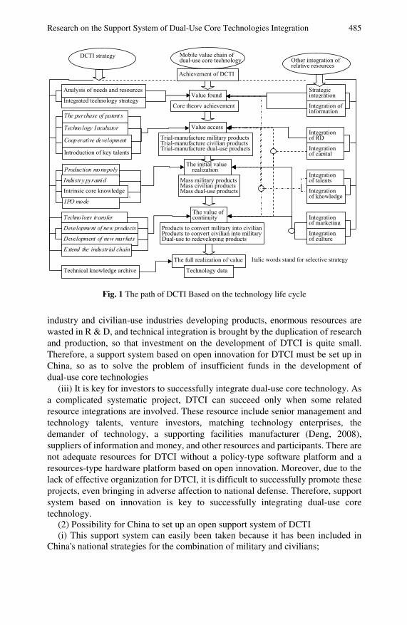
Research on the Support System of Dual-Use Core Technologies Integration 485
Value found
Value access
The initial valuerealization
The value of continuity
The full realization of value
Mobile value chain ofdual-use core technology
DCTI strategy Other integration ofrelative resources
Technology Incubator
Cooperative development
Introduction of key talents
The purchase of patent s
Integrated technology strategy
Analysis of needs and resources
Production monopoly
Industry pyramid
IPO mode
Intrinsic core knowledge
Technology transfer
Development of new products
Development of new markets
Extend the industrial chain
Technical knowledge archive
Strategic integration
Integration ofinformation
Integrationof RD
Integrationof capital
Integrationof talents
Integrationof knowledge
Integrationof marketing
Integrationof culture
Achievement of DCTI
Core theory achievement
Trial-manufacture military productsTrial-manufacture civilian products Trial-manufacture dual-use products
Mass military productsMass civilian products Mass dual-use products
Products to convert military into civilianProducts to convert civilian into militaryDual-use to redeveloping products
Technology data
Italic words stand for selective strategy
Fig. 1 The path of DCTI Based on the technology life cycle
industry and civilian-use industries developing products, enormous resources are wasted in R & D, and technical integration is brought by the duplication of research and production, so that investment on the development of DTCI is quite small. Therefore, a support system based on open innovation for DTCI must be set up in China, so as to solve the problem of insufficient funds in the development of dual-use core technologies
(iii) It is key for investors to successfully integrate dual-use core technology. As a complicated systematic project, DTCI can succeed only when some related resource integrations are involved. These resource include senior management and technology talents, venture investors, matching technology enterprises, the demander of technology, a supporting facilities manufacturer (Deng, 2008), suppliers of information and money, and other resources and participants. There are not adequate resources for DTCI without a policy-type software platform and a resources-type hardware platform based on open innovation. Moreover, due to the lack of effective organization for DTCI, it is difficult to successfully promote these projects, even bringing in adverse affection to national defense. Therefore, support system based on innovation is key to successfully integrating dual-use core technology.
(2) Possibility for China to set up an open support system of DCTI (i) This support system can easily been taken because it has been included in
China's national strategies for the combination of military and civilians;
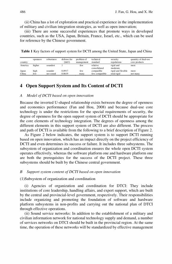
486 J. Fan, G. Hou, and X. He
(ii) China has a lot of exploration and practical experience in the implementation of military and civilian integration strategies, as well as open innovation;
(iii) There are some successful experiences that promote ways in developed countries, such as the USA, Japan, Britain, France, Israel, etc., which can be used for reference by the Chinese government.
Table 1 Key factors of support system for DCTI among the United State, Japan and China
country
openness robustness defense fee (2005)
problem of management
technical standard
security regulations
quantity of dual-use core products
America higher soundest 1 few relative consolidated
rigid and moderate
most
Japan high sounder 0.0917 few compatible rigid and flexible more China low not sound 0.0619 many few compatible total rigid not many
4 Open Support System and Its Content of DCTI
A Model of DCTI based on open innovation
Because the inverted U-shaped relationship exists between the degree of openness and economics performance (Fan and Hou, 2008) and because dual-use core technology is under the restrictions for the special requirements of security, the degree of openness for the open support system of DCTI should be appropriate for the core elements of technology integration. The degrees of openness among the different elements in this support system of DCTI are also different. The process and path of DCTI is available from the following to a brief description of Figure 2.
As Figure 2 below indicates, the support system is to support DCTI running based on open innovation, which has an impact directly on the project efficiency of DCTI and even determines its success or failure. It includes three subsystems. The subsystem of organization and coordination ensures the whole open DCTI system operates effectively, whereas the software platform one and hardware platform one are both the prerequisites for the success of the DCTI project. These three subsystems should be built by the Chinese central government.
B Support system content of DCTI based on open innovation
(1)Subsystem of organization and coordination
(i) Agencies of organization and coordination for DTCI: They include institutions of core leadership, handling affairs, and expert support, which are built by the central and provincial-level government, respectively. Their responsibilities include organizing and promoting the foundation of software and hardware platform subsystems in non-profits and carrying out the national plan of DTCI through effective operations.
(ii) Sound service networks: In addition to the establishment of a military and civilian information network for national technology supply and demand, a number of services networks on DTCI should be built in the provincial region. At the same time, the operation of these networks will be standardized by effective management
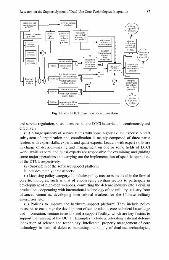
Research on the Support System of Dual-Use Core Technologies Integration 487
foreign investors
mature core technology
achievements
military high-tech products
civilianhigh-tech products
dual-usehigh-techproducts
software supportplatform
licensetype
policies
policies to improve hardware support platform
policies topromote S&T achievements into products
civilianinvestors
entrepreneurs
venture investors
technology transfer intermediaries
R & D achievementsof` core technology
hardware support platform
supporting facilities and equipments
militaryinvestors
professionaltalents
related technology and knowledge
talents
technology
investors
facilities
projects of DCTI for
new products
integrationprojects for mature core technology
investors who take part in DCTI
integrateimmature core
technology into
mature one
integratecivilian core technology into military
products
integrate coretechnology
into dual-use products
integratemilitary core technology into civilian
products
organizers and administrators
of DCTI
Fig. 2 Path of DCTI based on open innovation
and service regulation, so as to ensure that the DTCI is carried out continuously and effectively.
(iii) A large quantity of service teams with some highly skilled experts: A staff subsystem of organization and coordination is mainly composed of three parts: leaders with expert skills, experts, and quasi-experts. Leaders with expert skills are in charge of decision-making and management on one or some fields of DTCI work, while experts and quasi-experts are responsible for examining and guiding some major operations and carrying out the implementation of specific operations of the DTCI, respectively.
(2) Subsystem of the software support platform It includes mainly three aspects: (i) Licensing policy category: It includes policy measures involved in the flow of
core technologies, such as that of encouraging civilian sectors to participate in development of high-tech weapons, converting the defense industry into a civilian production, cooperating with international technology of the military industry from advanced countries, developing international markets for the Chinese military enterprises, etc.
(ii) Policies to improve the hardware support platform: They include policy measures to encourage the development of senior talents, core technical knowledge and information, venture investors and a support facility, which are key factors to support the running of the DCTI . Examples include accelerating national defense innovation of science and technology, intellectual property management of core technology in national defense, increasing the supply of dual-use technologies,

488 J. Fan, G. Hou, and X. He
stinging development of venture investment, dual-use technology intermediary organizations, the pool of entrepreneurs, speeding up high-tech enterprise listings on the stock market, and so on.
(iii) Policies to promote dual-use scientific research achievements into products: They include policies and regulations promoting the technology transfer between military and civilian industries, such as that of opening up information, relatively unified technology standards, and policies to standardize the operation of DCTI projects, such as reasonable governance rules, an income distribution system, innovation culture, security measures and other policy measures to aid the success of the DCTI project.
(3) Subsystem of hardware support platform It includes mainly four aspects , as follows: (i) A national talent net system should be built to optimize entrepreneurs and
professionals allocation for DCTI. Large quantities of senior talents are listed on the net system by the scientific mechanism of selection, use, exchange and elimination to ensure a sufficient supply of outstanding innovative talents in scientific research and management for DCTI projects.
(ii) A large quantity of dual use core technology achievements are provided by some excellent research and development teams, which are not lots of pure theoretical and valueless research results but advanced and practical achievements of dual-use technology.
(iii) Many service institutions of technology transfer intermediary are high-performing, highly reputed and well-functioning, such as military and civilian technology transfer centers, dual-use scientific and technological information networks, operation management agents for DCTI projects, etc.
(iv) Advanced system of venture capital participators: It contains well-developed capital markets, especially securities markets, an adequate supply of experienced venture capitalists, an adequate market supply of start-up money in research and innovation, experimental facilities and experimental equipment that can be shared by others.
5 Countermeasures for China to Establish and Improve the Open Support System of DCTI
A. A highly efficient subsystem of organization and coordination on DTCI should be formed.
(i) The establishment of corresponding organizational institutions: The institution of organization and management of DTCI should be established by the central government. This institution takes charge of strategic planning, policies and regulations, information management, coordinating national DTCI between military and civilian industries, and so on. Correspondingly, this institution should be established by every provincial government, so as to organize and supervise local operations of the DTCI. Meanwhile, several professional service sectors
Research on the Support System of Dual-Use Core Technologies Integration 489
should also be set up by some famous scientific research institutes in support by state but as a non-profit operation, which will bear guiding and set an example for national investors for DTCI project in their respective areas of expertise.
(ii) Accurate positioning functions of this organization and coordination subsystem: Its specific functions at least include: to formulate and release policies and regulations, to long-term and medium-term plan the DTCI, and to supervise their implementation; to organize a demonstration on keeping or removing the confidentiality of national defense core technology projects; to be responsible for the construction and management of DTCI platforms; to set up the anti-risk mechanism of DTCI, and so on.
(iii) Select correctly and make good use of all expert members: On the one hand, every expert should be correctly selected so that they are more with the true operational capacity than the "image ambassador" to represent their sector of interest, and the participation of the experts of the time should be devoted to investment work rather than merely being a "nominal leader". On the other hand, the mechanism of assessment, rewards and punishments of these experts should also be established correspondingly so that staff exert their full capacity and energy into their work concerning DTCI. (Fan and Hou, 2008).
B. Policies and regulations promoting DTCI should be established and improved
(i) In order to relax restrictions on policies and regulations for civilian-use enterprises taking part in DTCI, the permit-type policies and regulations category should be amended and improved by the central government, such as the "confidentiality regulations on defense," "People's Republic of China Interim Regulations on Private Enterprises", technical standards system of national defense, and so on. (Chen and Liu, 2008).
(ii) Some policies and regulations about building the platform of DTCI should be formulated and improved so as to absorb more resources and investors to DTCI projects, such as "Regulations on reasonable flow of senior talents", the "law of entrusting enterprises management to others", the “law on venture investment in China ", regulations on standardizing participants of DTCI, etc.
(iii) In order to speed up national DTCI, policies and regulations about transforming dual-use core technology achievements into products or industry should also be formulated and improved, such as the "law on promoting scientific and technological achievements of national defense", "the Law to promote dual-use technology " and other laws and regulations.
(iv) Policies and regulations on risk prevention should be rigidly drawn. On one hand, a reasonable security threshold should be set, such as to review the contractor's security qualifications level and restrictions on trading with foreign businessmen and treatment of classified information by means of secrecy for items of independent research and development to prevent the risk of technology leaks because of the relaxation threshold. On the other hand, major losses should be avoided by a system of accountability and a heavy crackdown on those who neglect duty.

490 J. Fan, G. Hou, and X. He
C. The hardware support platform of DTCI based on open innovation should be constructed
(i) The establishment of a senior talent pool for the DTCI: In order to afford sufficient talent for DTCI, the senior talent pool of management and technology should follow efficient methods, such as widening the scope of talent selection, scientific and reasonable selection procedure, and so on. Meanwhile, a scientific and effective talent management system should be built for this talent pool, such as establishing an expert agency mechanism to resolve the management of misconduct and the "moral hazard" problem coming from a number of experts, so that the twisted relationship between experts and their working members is readjusted, and the basic system of performance tracking and contact information with various enterprises, with which the effective usage of the personnel is closely followed and unqualified personnel or the dark side of human resources in some units are revealed so as to promote more proper usage of available talents.
(ii) The development of direct participants in the DTCI: In addition to increasing direct supporters concerning the DTCI, such as core technology providers, technical supporters, and material resources available, the technology users, intermediary service organizations, providers of technology information, providers of DTCI services, etc. should be developed so as to promote the development of the DTCI business.
(iii) Supply of adequate funding: The state should take some effective measures to financially support the development of DTCI, such as setting up a special fund, focusing on a financial support or incentives policy for the development projects of DTCI, procuring by the government on home enterprise products of core technologies, introduction of venture investors, etc. Meanwhile, effective venture contract management and the withdrawal mechanism from venture investments should be established by a central government so as to encourage more investors to participate in the DTCI (Ma, 2007).
D. Matching management measures for the operation of this support system should be done well
(i) Deepen reform on resource allocation of the military industry so as to build strategy for military and civilian integration: Firstly, measures that promote and uncover resources for the national defense to advance should be developed, such as the establishing relatively uniform technical standards among military and civilian industries, compressing unnecessary confidentiality restrictions, expanding the scope of civilian-use enterprises to join weapons research and production, establishing unified military and civilian strategy of high-tech R & D and technology integration should be established, etc., so as to break the closed state of resources. Secondly, in order to avoid similar problems of quality, cost and scheduling when weapons are researched and produced, resulting from unreasonable weapon pricing, the state should encourage pricing policies on dual-use core technology products. (Wang, 2008).
(ii) Deal well with the relationship between participants and members of the organization subsystem: The correct positioning of organizing members is that they

Research on the Support System of Dual-Use Core Technologies Integration 491
are makers of policies, regulations and planning, advocates to promote the project operation, coordinators of issues and service of the DTCI work. And they have equal status with participants, correctly guiding participants through the DTCI projects. Moreover, participants and organizers should mutually supervise, so as to prevent corruption of the organizers and participants.
(iii) Correct the twisted relationship between major participants: There are two vexing problems between the major participants of DTCI, one of which is that participants cheat on others; the other is the distortion of the principal-agent relationship coming from a multiple principal-agent way. Due to the lack of effective incentives and restraint mechanisms, it results in the failure of the project commissioned. For the first one, those who break credibility by policy of strict norms and regulations need to be punished; for the second one, comprehensive management measures should be done, such as to reasonably select experts, to streamline the entrustment way, to strengthen incentives and restraint of team members, etc.
6 Conclusions
The DCTI should be laid on as one of first important works for nearly any country in the world. But it is very difficult to do in that, as it involves many aspects for its integration of resources and strategy selection, the external environment having an important impact on it, even directly deciding its success or failure. Due to China's special conditions and restriction of policy, the support system for the DCTI based on innovation has not been built. It is essential and feasible for China to set up this support system. In addition to the management software platform and hardware platform, the organization of administrators is also included in this support system.
In order to build this support system, some countermeasures should be done, such as forming efficient organization and management systems, establishing and improving policies and regulations, building hardware supportive platforms and matching management measures well for the operation of this support system and so on. This initial conclusion still needs to be replenished and bettered further in future.
References
Chen, J.F., Chen, J.: Machanism and Pattern of Open Innovation (Book style). Science and Technology, Beijing (2008)
Chen, X.H., Liu, B.: Study on reregulation issue of entrance to military industry. Military Economic Research, 21–25 (February 2008)
Chen, Y.F., Chen, J.: The influence of openness to innovation performance. Studies in Science of Science, pp. 419–426 (August 2008)
Chesbrough, H.: Open Innovation, the New Imperative for creating and Profiting from Technology (Book style). Harvard Business School, USA (2003)
Deng, Y.: Research on mechanism of enterprises technology integration in China. Ph.D. dissertation, Dept. Economics and Management, Tsinghua, Univ., Peking (2008)
492 J. Fan, G. Hou, and X. He
Deng, Y., Lei, J.S.: Different definitions on technology integration: A review of literatures. Studies in Science of Science 25(supp.2), 205–209 (2006)
Fan, G.M., Hou, G.M.: Research on important decision support system based on integration of knowledge and ability. Studies in Science of Science 27(supp.1), 70–76 (2008)
Fan, G.M., Hou, G.M., Wang, Z.H.: Study on risk governance of core technology integration in high-tech enterprises. In: Proc. International Conf. on Risk and Reliability Management, Beijing, pp. 447–452 (2008)
Iansiti, M., West, J.: Technology Integration: Turning Great Research into Great Product, Harvard Business Review, pp. 69–79 (1997)
Ma, M.J.: Method and enlightenment for USA national defense to set up the technology transfer system. Defense Science & Technology Industry, 64–67 (March 2007)
Rob, B.: Learning from productivity learning curves. Research Technology Management 45, 54–58 (2002)
Wang, K.S., Tong, A.L.: Review and enlightenment of developing dual-use technologies. Dual Use Technologies & Products, 3–5 (Januaray 2006)
Wang, Y.H.: Study on government deregulation and reregulation of the equipment research and manufacture. Ph.D. dissertation, Beijing Institute of Technology, Beijing (July 2008)
Yan, J.S.: Technology integration and its strategy. Tianjin Science & Technology, 51 (April 2003)
Yu, P.L., Fan, Z.P.: Research & development of core technology for enterprise, core competency. Management of Science and Research, 73–76 (May-June 2003)
Zhang, Y.J., Zhang, W.C.: The trend of international safety strategy and the countermeasures of Chinese national defense investment. Military Economic Research, 3–5 (March 2003)
Zhou, H., Miao, H.: Proble and analysis on open innovation R & D strategy in China military industry. National Defense Science & Technology, 65–70 (2007)
Operational Risk Measurement via the Loss Distribution Approach*
Jichuang Feng, Jianming Chen, and Jianping Li**
In the Basel II Accord, banks are encouraged to use the Advanced Measurement Approach (AMA), which is suitable for banks to assess operational risk capital, but banks are required to demonstrate their ability to capture severe tail loss events. In this chapter, based on 860 operational risk loss data of Chinese commercial banks collected from public reports from 1995 to 2006, we found that the sample data set is characterized as having a heavier tail than a normal distribution. Then we use the loss distribution approach (LDA) to measure the operational risk and operational risk capital of Chinese commercial banks after a brief introduction to LDA. At last, we compare the operational risk economic capital of Chinese commercial banks with the operational risk economic capital (EC) of other major banks. We discover that the operational risk of Chinese commercial banks is larger than that of some foreign major commercial banks.
1 Introduction
Operational risk is one of the most important risks of Chinese commercial banks, and it brings huge losses to Chinese commercial banks. In recent years, the fre-quency and severity of operational risk have become increasingly high. We realized Jichuang Feng School of management, University of Science and Technology of China, He Fei, An Hui, China e-mail: [email protected]
Jianming Chen Institute of Policy and Management, Chinese Academy of Sciences, Beijing, China e-mail: [email protected]
Jianping Li Institute of Policy and Management, Chinese Academy of Sciences, Beijing, China Phone: 86-10-6252-7389; Fax: 86-10-6254-2619 e-mail: [email protected]
* The work was supported in part by a grant from the National Science Foundation of China (#70701033, #90718042, and #70531040).
** Corresponding author.
494 J. Feng, J. Chen, and J. Li
that we should use quantitative methods to better understand our operational risk profiles and to estimate the economic capital for operational risk. Operational risk, the BCBS (2004) defines it as “the risk arising from inadequate or failed internal processes, people and systems or from external events” (De Fontnouvelle et al., 2005). This definition, which is based on the underlying causes of operational risk, includes legal risk but excludes business and reputational risk.
Unlike the modeling of market and credit risk, the measurement of operational risk faces the challenge of limited data availability. Furthermore, due to the sensitive nature of operational loss data, banks are not likely to freely share their operational loss data. The Basel II Accord suggests three methods for calculating operational risk capital charges: (i) the basic indicators approach (BIA), (ii) the standardized approach (STA), and (iii) the advanced measurement approach (AMA). As banks become more sophisticated, they are encouraged to move along the spectrum of available approaches. The underlying hypothesis here is that the use of sophisticated approaches to calculate the regulatory capital by a bank that has an appropriate risk management framework should result in a lower operational risk minimum regulatory capital. This means that the prospects of lower regulatory capital induce banks to use sophisticated risk management practices and modeling approaches.
Only for recently years do we have the measurements of operational risk moving towards a data-driven loss distribution approach (LDA). Therefore, many financial institutions have begun collecting operational loss data, as they are trying to move towards an LDA to measure their operational risk. And several researchers have experimented with operational loss data over the past few years (Aue and Kalk-brenner, 2006/2007; De Fontnouvelle et al., 2003; Dutta and Perry, unpublished; Embrechts et al., 2004; Moscadelli, 2004).
One approach for calibrating operational losses is to fit a parametric family of distributions, such as a log-normal, weibull, and exponential. An alternative ap-proach, pioneered in several works by P. Embrechts, uses the extreme value theory (EVT) to fit a generalized pareto distribution (GPD) to extreme losses exceeding a high pre-specified threshold (Embrechts et al., 2003; 2004; 1997; 2005).
In this chapter, we aim to develop a process for Chinese commercial banks to measure their operational risk and enhance their operational risk management. In this chapter, first, 860 pieces of publicly reported operational risk loss data of Chinese commercial banks were collected, which is from 1995 to 2006. We find that the sample data set is characterized as having a heavier tail than a normal dis-tribution. Later, we introduce the framework of the loss distribution approach, which is used in the chapter. Then we use the loss distribution approach to measure the operational risk and operational risk capital of Chinese commercial banks. At last, we compare the operational risk capital of Chinese commercial banks with the operational risk economic capital of other banks. We discover that the operational risk of Chinese commercial banks is larger than that of foreign commercial banks.
The chapter is organized as follows: Section 2 describes the risk measurement framework. In Section 3, we outline the characteristics of the data we collected. In Section 4, we estimate the operational risk of Chinese commercial banks by using
Operational Risk Measurement via the Loss Distribution Approach 495
the traditional LDA, and then we compare the operational risk capital of Chinese commercial banks with the operational risk economic capital of other banks. Fi-nally, Section 5 concludes the chapter and summarizes the findings.
2 Loss Distribution Approach
We describe some basic techniques and concepts used in this chapter in this section, and introduce the framework of the loss distribution approach, which is used in the chapter.
In this chapter, we define the amount of risk as the value at risk (VaR) and the expected shortfall (ES). Unlike VaR, ES satisfies the properties of a coherent risk measurement and enables a better capture of the tail events (Artzner et al., 1999). We assume an operational risk measurement period of one year and choose 99%, 99.9% and 99.98% as confidence intervals. We use the Monte Carlo Simulation to estimate the loss distribution.
LDA combines the loss frequency distribution and the loss severity distribution, where the loss frequency distribution is the probability distribution of the number of times loss occurs during the risk measurement period; meanwhile, the loss severity distribution means the probability distribution of the amount of losses incurred per occurrence. Two assumptions are used in the LDA model: (i) the frequency and severity are independent and (ii) two different losses in the same class are inde-pendently and identically distributed.
The amount of operational risk is estimated by the following process: 1) Estimating the Loss Frequency Distribution The distribution of N, which is the number of losses during the risk measurement
for one year, is estimated. We assume that N follows a Poisson distribution, and the
probability function of the Poisson distribution is ( )!
xef x
x
λ λ− −
= . The expected
value is λ, which is estimated by equating this with the annual average number of loss events.
2) Estimating the Loss Severity Distribution The loss severity distribution means the probability distribution of the amount of
losses incurred per occurrence. Based on the estimation of the loss severity distri-bution, we estimate the amount of losses per occurrence of the operational risk loss events. There are two methods to estimate the severity distribution; one is the pa-rametric method, in which a particular severity distribution is assumed, and the other is the nonparametric method. In this chapter, we use the parametric method.
3) Calculating the Loss Amount We use loss frequency distribution estimated in 1) above, and the number of
annual losses N is derived. Then the severity of losses of N occurrences Xi (i=1, 2, …, N) is derived from the severity distribution estimated in 2) above. The total amount S of operational risk losses of one year equals to:
1
N
ii
S X=
=∑
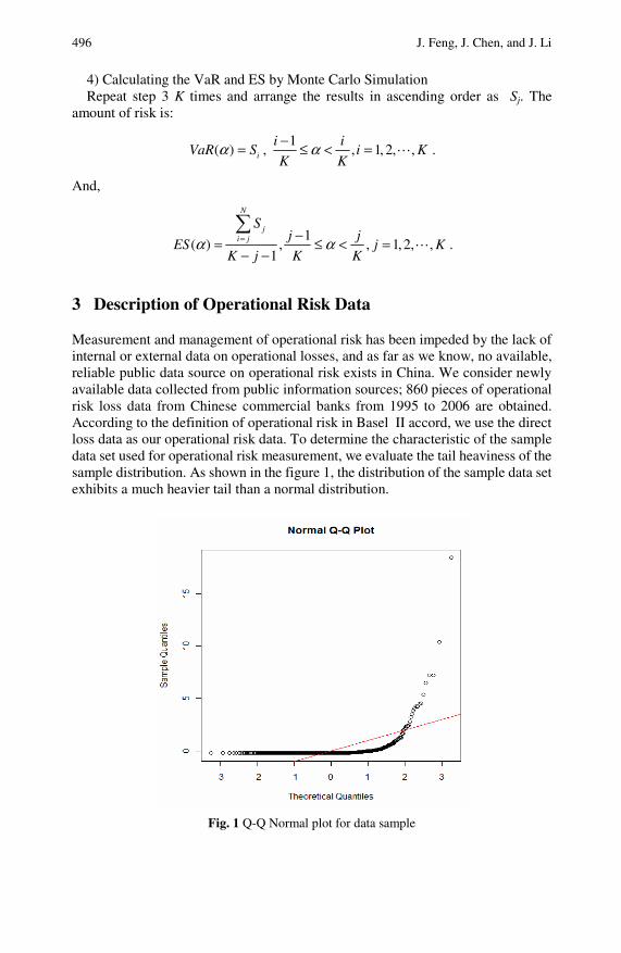
496 J. Feng, J. Chen, and J. Li
4) Calculating the VaR and ES by Monte Carlo Simulation Repeat step 3 K times and arrange the results in ascending order as Sj. The
amount of risk is:
( ) iVaR Sα = , 1
, 1, 2, ,i i
i KK K
α− ≤ < = .
And,
1( ) , , 1,2, ,
1
N
ji j
Sj j
ES j KK j K K
α α= −= ≤ < =− −
∑.
3 Description of Operational Risk Data
Measurement and management of operational risk has been impeded by the lack of internal or external data on operational losses, and as far as we know, no available, reliable public data source on operational risk exists in China. We consider newly available data collected from public information sources; 860 pieces of operational risk loss data from Chinese commercial banks from 1995 to 2006 are obtained. According to the definition of operational risk in Basel II accord, we use the direct loss data as our operational risk data. To determine the characteristic of the sample data set used for operational risk measurement, we evaluate the tail heaviness of the sample distribution. As shown in the figure 1, the distribution of the sample data set exhibits a much heavier tail than a normal distribution.
Fig. 1 Q-Q Normal plot for data sample
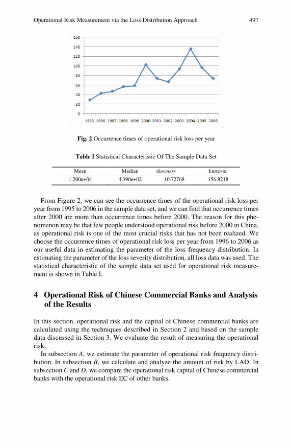
Operational Risk Measurement via the Loss Distribution Approach 497
Fig. 2 Occurrence times of operational risk loss per year
Table I Statistical Characteristic Of The Sample Data Set
Mean Median skewness kurtosis.
1.200e+04 4.390e+02 10.72768 156.8218
From Figure 2, we can see the occurrence times of the operational risk loss per year from 1995 to 2006 in the sample data set, and we can find that occurrence times after 2000 are more than occurrence times before 2000. The reason for this phe-nomenon may be that few people understood operational risk before 2000 in China, as operational risk is one of the most crucial risks that has not been realized. We choose the occurrence times of operational risk loss per year from 1996 to 2006 as our useful data in estimating the parameter of the loss frequency distribution. In estimating the parameter of the loss severity distribution, all loss data was used. The statistical characteristic of the sample data set used for operational risk measure-ment is shown in Table I.
4 Operational Risk of Chinese Commercial Banks and Analysis of the Results
In this section, operational risk and the capital of Chinese commercial banks are calculated using the techniques described in Section 2 and based on the sample data discussed in Section 3. We evaluate the result of measuring the operational risk.
In subsection A, we estimate the parameter of operational risk frequency distri-bution. In subsection B, we calculate and analyze the amount of risk by LAD. In subsection C and D, we compare the operational risk capital of Chinese commercial banks with the operational risk EC of other banks.
498 J. Feng, J. Chen, and J. Li
A. Estimating the Parameter of the Operational Risk Frequency Distribution
If we want to simulate the operational risk, the parameter estimation of the opera-tional risk frequency distribution is needed, so first we estimate the parameter of the operational risk frequency distribution. In Section 2, we have assumed that the occurrence times of the operational risk follow a Poisson distribution. Using oc-currence times of the operational risk loss per year from 2000 to 2006, we adopt the Maximum likelihood Method (MLE). We can get the parameter of operational risk frequency distribution λ=73.
Table II Results of parameter estimation
EXPONENTIAL WEIBULL LOG-NORMAL
Rate Shape Scale Mean-log SD-lo
g MLE
8.331405e-05 3.6503
40e-01
1.87432
4e+03
6.178173
23
2.846
92718
B. Estimating the Parameter of the Operational Risk Severity Distribution
We apply three different severity distributions to all the data and use MLE to quantify the amount of risk. The exponential distribution, the weibull distribution and the log-normal distribution are used. The estimated parameters are shown in Table II.
Before we test the hypothesis, QQ-plots of the empirical distribution with the log-normal, exponential and weibull distribution are shown in Figure 3.
From Figure 3, we could find that the Log-normal distribution fits the data set better than the others.
In Table III, the chi-square test and K-S test for log-normal, weibull and expo-nential distributions fitting the loss data are given.
From Table III, we find that only the Chi-Square test P-value is over 5%, so we can conclude that the data follows a log-normal distribution with a Mean-log=6.17817323, and SD-log=2.84692718 is accepted, as the p-value is greater than the significance level fixed at least in 5%. Meanwhile, we accept the null hypothesis that the data follow a Log-normal distribution, because the K-S p-value is higher enough than the significance levels usually referred to in statistical literature. All in all, we suppose the log-normal distribution fits the operational risk severity distribution well.
C. Results and Results Analysis
Using the method in Section 2, for the distribution we choose and the parameters we estimate, we simulate the situation 1,000,000 times so that we can get the VaR, mean, EC and ES at different confidence intervals. The results are shown in Table IV.

Operational Risk Measurement via the Loss Distribution Approach 499
Fig. 3 QQ-plots of data sample (x denotes sample quantiles and y denotes theoretical quantiles)
a. Log-norm
b. Exponential
c. Weibull
500 J. Feng, J. Chen, and J. Li
Table III P-value of hypothesis test
distribution P-value(chi-square test) P-value (K-S test)
Exponential 0 2.2e-16
Weibull 6.467809e-05 0.001209
Log-normal 0.051 0.2673
Table IV Amount of operational risk
VaR Mean EC ES
99% 170083 19931 150151 422934
99.9% 723061 703130 1527688
99.98% 1679917 1659986 3339510
Unit: million
Table V Detailed data of the different banks
Name of bank Total assets Total regulatory capital: Basel II
approach
Total economic capital
Operational risk economic capi-
tal:Basel II AMA
Operational risk regulatory capital:
Basel II BIA Name of bank
Citigroup $1,484,101 $100,899 $52,200 $8,100 $10,621 $1,484,101
Bank of Amer-ica Corp.
$1,044,660 $92,266 $69300 NA $6,065 $1,044,660
JP Morgan $1,157,248 $96,807 $34,900 $4,500 $4,305 $1,157,248
AIG $1,157,248 $73,317 $40,000 $5,388 $4,875 $1,157,248
Deutsche Bank €€ 1,126,000 NA €€ 11,693 €€ 3,323 NA €€ 1,126,000
Chinese commercial
banks ¥43,949,970 NA NA ¥703,130 NA ¥43,949,970
Unit: million
According to the requirement of Basel II under the 99.9% confidence interval, it is easy to find that the overall operational risk of Chinese commercial banks is 7.23×10¹¹ yuan, the overall operational risk regulatory capital of Chinese com-mercial banks is 7.03×10¹¹ yuan each year, and the ES under the 99.9% confidence interval is 1.53×10¹² yuan. If all commercial banks in China want to get the AA rate, 1.66×10¹² yuan operational risk regulatory capital is needed each year; meanwhile, the ES under the 99.98% confidence interval is 3.34×10¹² yuan.
D. Comparing Results of LDA of Chinese Commercial Banks with Foreign Banks
In subsection C, we measured the operational risk of Chinese national commercial banks. In this subsection, we compare the results with the operational risk of foreign banks. The detail data is shown in Table V.
From Table V, we can see the total assets of China as a nation is larger than foreign banks. Meanwhile, we also find that the operational risk is larger than that of any others. From column 4 and 5, we can discover that the ratio of the operational risk economic capital to the total economic capital is from 12.9% to 28.4%, but we believe that the ratio of Chinese banks is higher than this. The ratio of the
Operational Risk Measurement via the Loss Distribution Approach 501
operational risk regulatory capital to total regulatory capital is from 4.4% to 10.5%. So we get a large operational risk of Chinese commercial banks using the LDA. We suppose that the operational risk of our banks is so large because of two possible reasons: first, the data samples contain a disproportionate number of very large losses. In the present case, the disproportionate number of large losses can lead to an estimate that overstates a bank’s exposure to operational risk. Second, the op-erational risk management in our banks is poor. So our commercial bank should intensify operational risk management to improve our banks’ competitiveness in financial globalization.
5 Conclusion
Despite many headlines having reported operational losses that occurred over the past decade in China, banks have made limited progress in quantifying their opera-tional risk. Instead, qualitative approaches have been emphasized in operational risk management; take enhancing the firm’s control environment and monitoring “key risk” indicators as an example. This qualitative emphasis has been driven by the lack of reliable operational losses. This chapter analyzes recent available publicly dis-closed data, and we implement LDA to measure the commercial banks’ annual operational risk and operational capital. We find that the Chinese commercial banks’ annual operational risk is 7.03×10¹¹ yuan, which is larger than foreign international commercial banks. So our commercial banks should intensify operational risk management to improve our banks competitiveness in financial globalization.
At last, we emphasize that this chapter has to be primarily taken for its meth-odological aspects. Even though our data is real data, it is biased data. Only when banks have completely collected operational data, the full potential of this very promising area of research will find a practical achievement. If more extensive and robust data is available, the results will make sense.
References
Artzner, P., Delbaen, F., Eber, J.M., Heath, D.: Coherent measures of risk. Mathematical Finance 9, 203–228 (1999)
Aue, F., Kalkbrenner, M.: LDA at work, Deutsche Bank’s approach to quantifying opera-tional risk. Journal of Operational Risk 1(4), 49–93 (2006/2007)
BCBS, Basel II: International Convergence of Capital Measurement and Capital Standards: A Revised Framework. Bank for International Settlements, Basel (June 2004)
De Fontnouvelle, P., Rosengren, E., Jordan, J.: Implications of alternative operational risk modelling techniques. Technical Report, Federal Reserve Bank of Boston and Fitch Risk (2005)
De Fontnouvelle, P., Jesus-Rueff, V., Jordan, J., Rosengren, E.: Using Loss Data to Quantify Operational Risk. Federal Reserve of Boston (April 2003)
Development Core Team. A language and environment for statistical computing. Foundation for Statistical Computing, Vienna, Austria (2008), ISBN 3-900051-07-0, http://www.R-project.org

502 J. Feng, J. Chen, and J. Li Dutta, K., Perry, J.: A tale of tails: An empirical analysis of loss distribution models for
estimating operational risk capital. Working Paper 06-13, Federal Reserve Bank of Boston (unpublished)
Embrechts, P., Furrer, H., Kaufmann, R.: Quantifying regulatory capital for operational risk. Derivatives Use, Trading, and Regulation 9(3), 217–233 (2003)
Embrechts, P., Kaufmann, P., Samorodnitsky, G.: Ruin theory revisited: Stochastic models for operational risk. Risk Management for Central Bank Foreign (2004)
Embrechts, P., Klüppelberg, C., Mikosch, T.: Modeling Extremal Events for Insurance and Finance. Springer, Berlin (1997)
Embrechts, P., McNeil, A., Frey, R.: Quantitative Risk Management: Concepts, Techniques and Tools. Princeton Series in Finance (2005)
Guidici, P.: Statistical models for operational risk management. Rontier Science (2003) Moscadelli, M.: The modelling of operational risk: experience with the analysis of the data
collected by the Basel Committee. Temi di discussione (Economic working papers) 517, Bank of Italy, Economic Research Department (2004)
Rosenberg, J.V., Schuermann, T.: A general approach to integrated risk management with skewed, fat-tailed risks. Journal of Financial Economics 79, 569–614 (2006)
Research on Greedy Simulated Annealing Algorithm for Irregular Flight Schedule Recovery Model
Qiang Gao, Xiaowei Tang, and Jinfu Zhu
To release the severe influence caused by irregular flight, this chapter puts forth a new model and its optimization algorithm based on the existing model, the focus of which is to design a Greedy Simulated Annealing Algorithm. The new algorithm, which integrates the characteristics of GRASP and the simulated annealing algorithm, improves the efficiency of neighborhood selection and reduces the probability of falling into a local optimal solution. An example proves that this algorithm is capable of solving large-scale irregular flight schedule recovery, with the time cost suitable to the outcome quality.
1 Introduction
Irregular flights refer to flights that are delayed or cancelled or that land at an al-ternate airport due to bad weather, mechanical failures, traffic control or some other reason. Problems raised by irregular flights cause passengers great inconvenience, as well as tremendous financial losses to airlines. Irregular fight issues have played a core role in operating efficiency and service quality of the air transport system. The recovery of an irregular flight schedule consists of aircraft schedule recovery, crew recovery and passenger flow recovery. Aircraft schedule recovery has the Qiang Gao College of Civil Aviation, Nanjing University of Aeronautics & Astronautics, Nanjing, 210016, China Phone: 816-025-84895388; Fax: 816-025-84891289 e-mail: [email protected]
Xiaowei Tang College of Civil Aviation, Nanjing University of Aeronautics & Astronautics, Nanjing, 210016, China e-mail: [email protected]
Jinfu Zhu College of Civil Aviation, Nanjing University of Aeronautics & Astronautics, Nanjing, 210016, China e-mail: [email protected]
504 Q. Gao, X. Tang, and J. Zhu
greatest influence on revenue management, so it’s the key step. Irregular flight schedule recovery discussed in this chapter refers to aircraft schedule recovery.
To improve market competitiveness and to maximize the utility of aircraft re-sources, airlines carry out much research on flight schedule (including aircraft schedule and crew schedule) optimization. There is virtually not enough slack time (Etschmaier and Mathaisei, 1985) in response to the unexpected changes in the flight schedule. Due to the high backup cost of aircraft resources, airlines are not willing to allow any aircraft to standby, in case of changes to the flight schedule, which is one of the major reasons that the capacity deployment is difficult under irregular circumstances. In addition, the operating environment of the flight schedule is uncertain, e.g. aircraft availability, crew feasibility and maintenance constraints increase the complexity of schedule adjustment, as well as airport runway conditions, flight conditions of plateau regions, air route restrictions, etc.
To exactly describe an irregular flight schedule recovery and search for an op-timization algorithm has always been the central issue in aviation OR research. In order to solve the resource optimization problem that may occur anytime for air-lines, finding a rapid and effective algorithm would result in enormous economic benefits. Studies on aircraft recovery can be traced back to the 1960s. Until the mid-1990s, the study has mainly been focused on the recovery of a single-fleet, small-scale delay (Teodorovic and Guberinic, 1984; Teodorovic, 1988; Teodorovic and Stojkovic, 1995). However, the single-fleet model doesn’t work well for air-lines, because rarely do airlines have a single fleet, and even if it does, aircrafts of the same type are different in airworthiness. In essence, they are multi-type. Since the mid-and-latter-1990s, multi-fleet, multi-type and large-scale delays have gradually been the focus of the study in the field. In model construction, the re-source assignment model and the multi-commodity flow model emerged one after another (Cao and Kanafani, 1997; Yan and Young, 1996; Yan and Tu, 1997; Mi-chael and Jonathan, 1997; Thengvall, 1999). Whether the fleet type is single or multiple, a common problem is algorithm complexity. Irregular flight schedule recovery is a real-time network optimization problem with multiple and compli-cated constraints, the solution space of which increases exponentially with the number of aircrafts and flights, that is, a NP-hard problem with multiple parameters and multiple constraints. At present, GRASP, a time-space network algorithm, etc. have been maturely applied. As a heuristic algorithm, GRASP is most applicable on large-scale problems. However, for large-scale problems, it has poor convergence and more easily falls into a local optimal solution. The time-space network algo-rithm tries to reduce the delayed time by reconstructing new routes, which makes the problem difficult to solve. When the scale reaches more than 20 aircrafts and 80 flights, the computing time required by the time-space network algorithm extends beyond 30 minutes, which is difficult for meeting the real-time control requirement of the airlines.
First, this chapter appropriately improves the irregular flight schedule optimiza-tion model raised in Reference (Michael and Jonathan, 1997), focusing on bringing forward the Greedy Simulated Annealing Algorithm. The new algorithm includes the greedy and random ideas in GRASP and improves the convergence of GRASP by designing an alternative pool with neighborhood solutions in it. Also, it
Research on Greedy Simulated Annealing Algorithm 505
incorporates the characteristics of simulated annealing, reducing the probability of falling into a local optimal solution.
2 Optimization Model of Irregular Flight Schedule Recovery
Existing optimization model (Michael and Jonathan, 1997) could describe irregular flight schedule recovery issues well. However, the required constraints for the recovery haven’t been discussed in detail, including flight connecting constraint, turn-time constraint, airport curfew constraint, etc. In this chapter, the model is properly improved. Variables used in the model are defined as follows:
O : set of aircraft routes in the original flight schedule A : set of implemented aircraft routes C : set of cancelled aircraft routes F : set of flights S : set of overnight airports P : set of airports covered by flights
iO : aircraft route i of the original flight schedule
iA : implemented aircraft route i
iC : cancelled aircraft route i
ij
KF : flight K is No. j on aircraft route i. The last flight in aircraft i is called the
tail flight, denoted as KitailF .
,K
ij departureF : departure airport of flight j on aircraft route i with flight No. K
,K
ij arrivalF : arrival airport of flight j on aircraft route i with flight No. K
Kp : number of passengers in flight K
, ( )Kitail arrivalF s : the arrival airport of tail flight K on aircraft route i is S
sN : number of overnight aircrafts required in airport s
,K
ij ETDF : estimated departure time of flight K, ,
K
ij STDF : scheduled departure time
of flight K, ,K
ij ETAF : estimated arrival time of flight K, ,K
ij STAF : scheduled arrival
time of flight K Kd : delayed time of flight K, determined by the difference between K
ETDF
and K
STDF
CD : delayed cost per passenger if the flight is cancelled. In accordance with international practice, cancellations could be seen as delays, and the delayed time of cancelled passengers is 480 minutes.
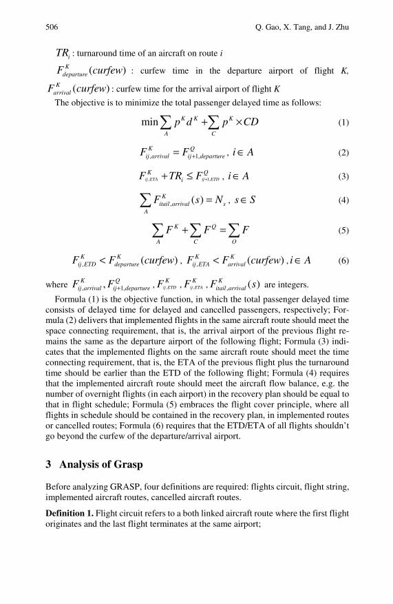
506 Q. Gao, X. Tang, and J. Zhu
iTR : turnaround time of an aircraft on route i
( )KdepartureF curfew : curfew time in the departure airport of flight K,
( )KarrivalF curfew : curfew time for the arrival airport of flight K
The objective is to minimize the total passenger delayed time as follows:
min K K K
A C
p d p CD+ ×∑ ∑ (1)
, 1,K Q
ij arrival ij departureF F += , i A∈ (2)
, 1,ij ETA ij ETD
K QiF TR F ++ ≤ , i A∈ (3)
, ( )Kitail arrival s
A
F s N=∑ , s S∈ (4)
K Q
A C O
F F F+ =∑ ∑ ∑ (5)
, ( )K Kij ETD departureF F curfew< , , ( )K K
ij ETA arrivalF F curfew< , i A∈ (6)
where , 1,,K Qij arrival ij departureF F + , ,ij ETD
KF , ,ij ETA
KF , , ( )Kitail arrivalF s are integers.
Formula (1) is the objective function, in which the total passenger delayed time consists of delayed time for delayed and cancelled passengers, respectively; For-mula (2) delivers that implemented flights in the same aircraft route should meet the space connecting requirement, that is, the arrival airport of the previous flight re-mains the same as the departure airport of the following flight; Formula (3) indi-cates that the implemented flights on the same aircraft route should meet the time connecting requirement, that is, the ETA of the previous flight plus the turnaround time should be earlier than the ETD of the following flight; Formula (4) requires that the implemented aircraft route should meet the aircraft flow balance, e.g. the number of overnight flights (in each airport) in the recovery plan should be equal to that in flight schedule; Formula (5) embraces the flight cover principle, where all flights in schedule should be contained in the recovery plan, in implemented routes or cancelled routes; Formula (6) requires that the ETD/ETA of all flights shouldn’t go beyond the curfew of the departure/arrival airport.
3 Analysis of Grasp
Before analyzing GRASP, four definitions are required: flights circuit, flight string, implemented aircraft routes, cancelled aircraft routes.
Definition 1. Flight circuit refers to a both linked aircraft route where the first flight originates and the last flight terminates at the same airport;

Research on Greedy Simulated Annealing Algorithm 507
Definition 2. Flight string refers to a both linked aircraft route where the first flight originates and the last flight terminates at different airports;
Definition 3. Implemented aircraft routes: aircraft routes that are operated with the aircraft No (four numbers) in the original flight schedule.
Definition 4. Cancelled aircraft routes: aircraft routes that are operated with a vir-tual aircraft No (begin with V). A virtual aircraft that just is assumed for operator is not actually possessed by airlines. Flights in this aircraft route will be cancelled.
Fig. 1 Flight Circuit, Flight String, Implemented Aircraft Route, Cancelled Aircraft Route
GRASP consists of circulating three stages: beginning with initial feasible solu-
tions and constructging neighborhood solutions; then, putting better neighborhood solutions into the RCL; finally, randomly choosing one from the RCL to construct feasible solutions. The specific operations are based on the flight circuit and flight string, including 7 types: the flight circuit prefix, flight circuit infix, flight circuit suffix, flight circuit cancelled, rear connect flight string, swap flight strings with the same departure airport and swap flight strings with the same departure and arrival airport. The deficiencies of GRASP are as follows:
1) Three of the foregoing seven operations could be merged. 2) The length of the RCL list is not easily determined. Even worse, the se-
quencing operation applied to inserting neighborhood solutions into the RCL results have worse time efficiency.
3) GRASP only allows the feasible solutions to iterate on the cost-reduced di-rection, which could cause the algorithm to fall into a local optimal solution.
4 Greedy Simulated Annealing Algorithm
A. Construction of neighborhood solutions in the new algorithm
The model in this chapter is based on aircraft routes, so in essence the optimization process is to construct new routes to replace the ones with the same flight No in previous solutions. To ensure the generation process is not against Formula
508 Q. Gao, X. Tang, and J. Zhu
(2)(4)(5), it should be in accordance with operations raised by GRASP. It was analyzed that the flight circuit prefix, infix and suffix could be combined as the flight circuit insertion. Thus, the seven operations can be simplified as five. The five operations are equivalent to constructing neighborhood solutions to create new aircraft routes. Newly-generated routes can meet the constraint (3) by re-scheduling the ETD and ETA of flights. Re-scheduling methods are as follows:
1) Set the ready time of a certain aircraft as the ETD of its first flight in the im-plemented route if the STD is earlier than the ready time.
2) The ETA of the first flight equals the ETD plus the flight span (STA of the first flight minus STD). STA refers to Scheduled Time of Arrival and STD for Sched-uled Time of departure.
3) The ETD of the following flight equals the ETA of the previous flight plus the turn-time of this aircraft.
4) The ETA of the following flight equals the ETD plus the previous flight span (STA of this flight minus STD)
Choosing any two aircraft routes by the five operations would result in many neighborhood solutions, over ten under normal circumstances. If there are many routes in the flight schedule, the number of generated neighborhood solutions is very large; thus, the construction of the new feasible solutions requires special treatment.
B. Alternative Pool of Neighborhood Solutions
One feasible solution is a flight recovery scenario. Generate neighborhood solutions by choosing two aircraft routes from a recovery scenario and then replace the air-craft routes with the same aircraft No in a current solution, and new feasible solu-tion emerges. However, choosing a pair of routes from the previous solution could generate many neighborhood solutions.
To ensure the feasibility of the algorithm, an evaluation should be made to choose the optimal neighborhood solution from the generated ones. If the total delayed cost of its neighborhood solution is less than the previous two routes, we put it in an alternative pool for cost-reducing solutions; otherwise, it is put into an alternative pool for cost-increasing solution. The two pools are collectively referred to as alternative pools of the neighborhood solutions.
The new algorithm does not store the superior solutions into an RCL list but di-rectly puts the optimal neighborhood solution into the alternative pool, which could better control the scale of the neighborhood solutions, remove the sequencing op-eration and improve time efficiency. But it increases the probability of falling into a local optimal solution. So in the new algorithm, we bring forward a search strategy based on the simulated annealing algorithm to settle it.
C. Construction of a feasible solution in the new algorithm
By combining any two aircraft routes, we could obtain neighborhood solutions and put them into cost-reducing and cost-increasing alternative pools, then randomly choosing only one from the pools to construct a feasible solution from the pools. The details are as follows:
Research on Greedy Simulated Annealing Algorithm 509
1) To ensure Formula (6), aircraft routes that are beyond curfew require assigning a considerable delayed cost. First, check whether there are aircraft routes that vio-late curfew in the incumbent solution. If there are, prioritize choosing the neighborhood solution to replace the ultra-curfew routes. Through this method, infeasible solutions can be turned into feasible ones by finite iterations.
2) If there are no aircraft routes beyond curfew in the current solution and the cost-reducing alternative pool is not empty, choose a neighborhood solution ran-domly from it.
3) If there are no ultra-curfew aircraft routes in the current solution and the cost-reducing alternative pool is empty, it indicates that the current solution doesn’t have a cost-reducing direction. To avoid falling into a local optimal solution, the current solution is allowed to deteriorate temporarily in accordance with the simu-lated annealing algorithm, so choose a neighborhood solution from the cost-increasing alternative pool. Since the cost-increasing direction always exists and the number of neighborhood solutions is large, judge the number of neighborhood solutions that meet Formula (7) and its percentage in the cost-increasing alternative pool. If the percentage is over 5%, randomly choose one; otherwise, the algorithm terminates.
exp( / ) (0,1)tK random−Δ > (7)
Of which: Δ is the increased delayed cost of the neighborhood solution; tK is
current temperature; (0,1)random is a uniform random number between 0 and 1.
After choosing a neighborhood solution, we may improve the current solution to get a new solution for the next iteration. If there is no neighborhood solution that meets all the constraints, the algorithm exits automatically. Irregular flight schedule recovery is of a high level in time efficiency, so the function for controlling time is set in the algorithm. When the operating time reaches the limit, it is forced to exit. The overall flow diagram is as follows (See Figure 2).
5 Example Analysis
One day, an airline’s flight schedule has not yet been operated when some irregu-larities occur, the causes of which are shown in Table 1. The original schedule consists of 149 flights, carried out by 30 aircrafts. Due to limited space, here lists only 5 aircraft routes in table 2. The curfew time of some airports is shown in Table 3. The delayed cost for airline passengers is 1 RMB / (minutes * person).
When the causes of the flight irregularities appear, if the flight operators don’t adopt a positive strategy and implement the flights as scheduled—postponing the flights—it will result in the cancellation of the light GH9538 flown by aircraft 2875 because the departure time is beyond the curfew time. This does not only influence itself but also the implementation of the flight schedule the next day. This method will cause a total delayed cost of 503,730 RMB.
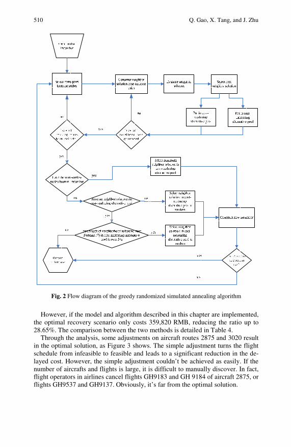
510 Q. Gao, X. Tang, and J. Zhu
Fig. 2 Flow diagram of the greedy randomized simulated annealing algorithm
However, if the model and algorithm described in this chapter are implemented, the optimal recovery scenario only costs 359,820 RMB, reducing the ratio up to 28.65%. The comparison between the two methods is detailed in Table 4.
Through the analysis, some adjustments on aircraft routes 2875 and 3020 result in the optimal solution, as Figure 3 shows. The simple adjustment turns the flight schedule from infeasible to feasible and leads to a significant reduction in the de-layed cost. However, the simple adjustment couldn’t be achieved as easily. If the number of aircrafts and flights is large, it is difficult to manually discover. In fact, flight operators in airlines cancel flights GH9183 and GH 9184 of aircraft 2875, or flights GH9537 and GH9137. Obviously, it’s far from the optimal solution.

Research on Greedy Simulated Annealing Algorithm 511
Table I Reasons for Irregular Flights
Irregular Reason Tail No. Estimated
Ready Time
Scheduled
Ready Time
Airport
Name
Start Time
of Closing
End Time
of Closing
Mechanical Problem 2153 1000 830
Mechanical Problem 2833 1100 700
Mechanical Problem 2875 1030 830
Mechanical Problem 5088 840 740
Mechanical Problem 5142 900 810
Mechanical Problem 5148 1105 805
Weather ZGGG 800 1000
Weather ZSPD 1800 2000
Table II Original Flight Schedule (A)
Tail No.
Seats Ready Time
Turn Around Time
Flight No.
Depart Airport
STD ETD Arrival Airport
STA ETA Pax
2153 171 1000 40 GH9521 ZSSS 830 1000 ZSFZ 940 1100 47
GH9129 ZSFZ 1255 1255 ZBTJ 1500 1500 12
GH9130 ZBTJ 1545 1545 ZSSS 1730 1730 72
GH9115 ZSSS 1935 1935 ZBAA 2155 2155 37
2833 200 1100 40 GH2833 ZSPD 700 1100 ZSSS 720 1120 165
GH9117 ZSSS 845 1200 ZBAA 1055 1410 96
GH9118 ZBAA 1155 1450 ZSSS 1355 1650 15
GH823 ZSSS 1530 1730 RKSS 1720 1920 171
GH824 RKSS 1820 2000 ZSSS 2005 2145 11
GH9379 ZSSS 2110 2225 ZGSZ 2345 2500 102
2875 200 1030 40 GH9466 ZUUU 830 1030 ZSPD 1100 1300 130
GH9183 ZSPD 1205 1340 ZYTX 1400 1535 53
GH9184 ZYTX 1455 1755 ZSPD 1700 2000 149
GH9537 ZSPD 1805 2040 ZJSY 2055 2330 140
GH9538 ZJSY 2155 2410 ZSPD 2445 2700 63
3020 50 800 35 GH9275 ZSPD 800 800 ZSAQ 920 920 34
GH9276 ZSAQ 1000 1000 ZSPD 1120 1120 17
GH9221 ZSPD 1240 1240 ZLYA 1520 1520 28
GH9222 ZLYA 1600 1740 ZSPD 1820 2000 8
…
The running time of applying the algorithm on a P4 2.6G, 512 M memory
desktop for a solution is 57 seconds, far lower than the time required for a manual recovery scenario. This wins time for plan approval, resource preparation and crew arrangement. Through a large number of experiments, it shows that the model and optimized algorithm have the following advantages:
1) The model is of good readability. It gives a detailed description of the space and time connecting constraint and airport curfew constraint.

512 Q. Gao, X. Tang, and J. Zhu
Table III Curfew time of airports covered by flights
Airport Curfew Time
Airport Curfew Time
AirportCurfew Time
AirportCurfewTime
AirportCurfew Time
RJNT 2400 VMMC 2400 ZBTJ 2400 ZGSZ 0 ZPJH 2400
RJTT 2400 VTSP 2400 ZBYN 2400 ZGZJ 2400 ZPPP 2400
RKPK 2400 VVTS 0 ZGDY 2400 ZHHH 2400 ZSAM 2400
RKSI 2400 WADD 2400 ZGGG 2400 ZHYC 2400 ZSAQ 2400
RKSS 2400 ZBAA 2400 ZGKL 2400 ZJSY 2400 ZSFZ 2400
ZYTL 2400 ZYTX 2400 ZYYJ 2400 ZLYA 2400 ZWWW 2400
ZSNJ 2400 ZSPD 0 ZSQD 2400 ZSSS 0 ZSTX 2400
ZWTN 2400 ZUCK 2400 ZUMY 2400 ZUUU 2400
“0” means no curfew.
Table IV Comparison between postponed scenario and optimization scenario
Total
Aircraft
Cancelled
Flights
Delayed
Flights
Delayed
Cost
Delays
In
0.5h
Delays
In
1h
Delays
In
2h
Delays
In
3h
Delays
In
4h
Delays
Over
4h
Postponed 30 0 39 503730 2 6 15 12 3 1
Optimization 30 0 38 359820 2 6 15 10 2 3
Fig. 3 Illustration of the aircraft route changes in the optimal solution
2) It has a high running efficiency. For an irregular case within 50 aircrafts and 200 flights, the general solving time is less than 2 minutes, and it’s capable of meeting the actual requirement. Also, it may significantly reduce the established time for the recovery scenario and win time for organizing work.
Research on Greedy Simulated Annealing Algorithm 513
3) It has a good effect on optimization. For an irregular case with 50 aircrafts and 200 flights, it may reduce the total delayed cost up to 14-19%. For a medium-sized airline, 90 million RMB per year could be saved accordingly.
4) The algorithm has practicality. The recovery scenario obtained through this algorithm has a small disturbance on the original flight schedule, so it is easy for airlines to deploy aircraft supporting resources.
6 Conclusion
This chapter modifies the original irregular flight schedule optimization model and presents a new algorithm based on GRASP and the simulated annealing algorithm. The new algorithm may improve the time efficiency by applying an alternative pool of neighborhood solutions (including cost-reducing and cost-increasing alternative pools) to replace the RCL linked list in GRASP. Moreover, it incorporates the ideas of the simulated annealing algorithm to effectively reduce the probability of falling into a local optimal solution. The major deficiencies of this algorithm are that the objective function doesn’t contain all the costs required for an irregular flight schedule recovery, including the cost of ferrying and fleet substitution. These will direction improvement in the next step.
References
Cao, J., Kanafani, A.: Real-time decision support for integration of airline flight cancella-tions and delays, part I: mathematical formulations. Transportation Planning and Tech-nology 20(3), 183–199 (1997)
Etschmaier, M.M., Mathaisei, D.F.X.: Airline scheduling: An overview. Transportation Science 19(2), 127–138 (1985)
Michael, F.A., Jonathan, F.B.: A grasp for aircraft routing in response to grounding and delays. Journal of Combinatorial Optimization 1(3), 211–228 (1997)
Teodorovic, D.: Airlines Operation Research, pp. 256–300. Gordon and Breach Science Publishers, New York (1988)
Teodorovic, D., Guberinic, S.: Optimal dispatching strategy on an airline network after a schedule perturbation. European Journal of Operational Research 15(2), 178–182 (1984)
Teodorovic, D., Stojkovic, G.: Model to reduce airline schedule disturbances. Journal of Transportation Engineering 121(4), 324–331 (1995)
Thengvall, B. G. : Models and Solution Techniques for the Aircraft Schedule Recovery Problem. Dissertation, Austin, The University of Texas (1999)
Yan, S., Tu, Y.: Multi-fleet routing and multi-stop flight scheduling for schedule perturba-tion. European Journal of Operational Research 103(1), 155–169 (1997)
Yan, S., Young, H.: A decision support framework for multi-fleet routing and multi-stop flight scheduling. Transportation Research 30(A), 379–398 (1996)
Network Externality, Call Externality and Price Policy: A Consumer Development Analysis of China’s 3G Mobile Data Services*
Yonghua Gong and Bangyi Li
The key to 3G data service development in the primary period is to expand the firm’s number of subscribers and market share. However, price strategy is an im-portant weapon for popularizing 3G data services to some extent. This chapter studies the price of 3G data services and market development under network ex-ternalities and call externalities. Consumer “self-selection” is induced in models of bundling tariffs and two-part tariffs. Then the optimal pricing strategies of the two pricing models are analyzed, and then the corresponding market development strategies are dropped from the optimal pricing strategy. The result shows that the optimal consumer development strategy is to draw high-demand consumers to becoming the firm’s subscribers with a precedent in both pricing systems because of the effects of network externalities. Following the increase of the proportion of the firm’s subscribers, the firm’s development of low-demand consumers spreads out. Moreover, call externalities will reduce the firm’s activity to serve low-demand consumers.
1 Introduction
The market structure has changed from a duopoly to a triopoly in China’s 3G mo-bile communication market. The competition for mobile communication service firms is becoming fiercer, where 3G tariffs are becoming one of the most important focuses. Compared to 2G, 3G can provide more new services, such as Network Yonghua Gong College of Economics and Management, Nanjing University of Aeronautics and Astronautics, China Phone: 086-025-84895404 e-mail: [email protected]
Bangyi Li College of Economics and Management, Nanjing University of Aeronautics and Astronautics, China e-mail: [email protected]
* This work was supported by the Scientific and Technical Innovation Project of the Jiangsu Provincial Department of Education under Grant CX08B_040R.

516 Y. Gong and B. Li
Access, Mobile Electronic Business, Location Services (LCS), File Transfering, Conference Bridge and Video on Demand multimedia and Broadband Data Ser-vices et al., besides Mobile Voice and Short Messaging Service (SMS). The variety of 3G services, especially the data services, makes the tariff problem even more complicated. The detailed tariff pattern includes the flat-rate, the number of uses, and usage-based and content-based accounting. However, China’s 3G firms can still adopt the existing tariff strategy-bundling tariff and two-part tariff, according to the operation experiences of foreign 3G firms and Fu Gang’s study (2007). In fact, no matter what tariff policy the firm chooses, attracting more consumers, rapidly opening the market, and improving the market share are the most important things firms need to consider during the early period of 3G services entering the market. However, we know the communication service industry has obvious network ef-fects, and which firm consumers choose will be affected by network externalities, and they will anticipate the net scale and growth prospect. Moreover, interactive services, Point to Point (P2P) and Point to Multi-Point (P2MP) services increase a lot in the 3G age, so under the condition of a one-way charge, the consumers’ choice will also be affected by call externalities. With those two externalities, adding a network increases the surplus of other subscribers who are able to call and be called by the new customer, and therefore affects not only consumers’ demand for the service but also their demand for a subscription.
If we investigate the market development problem for 3G mobile communication services in the market introduction phase from externalities (network and call ex-ternalities) and pricing strategy, then the content that we will study is very clear.
This chapter includes four parts. In the first part, we preview correspondent lit-erature. In the second part, we make some assumptions. In the third part, we first propose a pricing model with network externalities and call externalities. It includes two pricing models-bundling tariffs and two-part tariffs. Then, we solve the pricing models and give the optimal price strategies. Finally, we analyze the relevant market development strategy. In the last part, we draw the conclusions.
2 Literature Review
In this section, we mainly review literature concerning the tariffs model building with network and call externalities. Economists have been quite active in analyzing the effect of network externalities on firms’ pricing policies in telecommunications. The main focus has been on how Ramsey pricing should be adjusted in order to internalize network externalities. Efficient pricing with network externalities typi-cally involves a lower price mark-up for uniform pricing (Willing, 1979) and a lower fixed fee for two-part tariffs (Littlechild, 1975), compared to ordinary mar-kets without network externalities. Einhorn (1993) emphasized the importance of the identity of the marginal customer in determining the welfare-maximizing two-part tariff with network externalities. Blonski (2002) found that there’s a ten-dency for conformity that is established by network externalities that may in some sense be overcome by sufficient differentiation in price structures. Call external-ities, however, have been given little attention in literature, which is somewhat surprising, considering that roughly half of the benefits of using a telephone service
Network Externality, Call Externality and Price Policy 517
is from receiving calls. To our knowledge, Squire (1973) is the first economist who analyzed incorporating call externalities into telecommunication pricing. He de-rived the best two-part tariff with call and network externalities, and the result is that a per-call price is less than the marginal cost, which reflects the effect of call externalities. However, it is not implementable without subsidizing the firm using public funds. Willing (1979) argued that call externalities are hard to deal with if they are not easily related to other variables. Hahn (2003) extended previous work on telecommunication pricing to a more general environment where consumers benefit not only from network externalities but also from call externalities. He related the call externalities to variables like outgoing calls and the subscription rate, and he then gave the consumers’ utility function.
This chapter will adopt Hahn’s dealing method of introducing network exter-nalities and call externalities in a consumer utility function. Since the consumers’ utility function consists of the subscription rate, we can use it to analyze a firm’s consumer development according to the pricing policy, which is important and new for China’s 3G data services during the introduction period. Shuai and Chen (2003) researched China’s mobile communication market competition for 2G/1G and 2.5G; they also used network externalities to analyze consumers’ choice of services. Pan and Chen (2006) built a two-period model with network externalities to analyze the monopolist’s pricing strategy. Xu and Chen (2006) found that network effects can relax the equilibrium condition to engage in price discrimination. Teng and Tang (2008) analyzed the price and social welfare in a duopoly market when the firms both engage in third-degree price discrimination, where the consumers are divided into two types: low-demand and high-demand. The consumer segment is the base for the firm to engage in discrimination. Two-part tariffs and bundling tariffs always divide consumers into different types, depending on the consumption preference. Kolay (2003) builds the two-part tariffs and bundling pricing model just on that consumer segment. So, in our pricing models, we also will focus on two consumer types that differ in their quantity demanded of a product of a fixed quality.
3 Hypothesis and Variables
Consider a monopolistic firm selling a two-way telecommunications service with a marginal cost c. We make the following assumptions for analytical simplicity:
(1) Uniform communicating pattern: Every subscriber equally distributes his/her outgoing communications across all subscribers in the network. (2) Indifference to communication partners: Subscribers gain the same benefit from an outgoing or incoming communication regardless of who the recipient (caller) is.
(3) No charge for incoming calls: The recipient is free from charge. (4) Two types of subscribers: Subscribers differ in their consumption preference
according to taste parameter θ , the low-demand group has taste parameter 1θ and
the high- demand group has taste parameter 2θ , where 2 1θ θ> .
518 Y. Gong and B. Li
(5) The firm’s subscriber number is [0,1]n ∈ , the low- demand group occurs in
the proportion [0,1]λ ∈ , and the high- demand group occurs in the proportion 1-λ.
Network effects make subscribers’ value received from connecting to a network depend on the number of subscribers connecting to the network. Subscribers also can get value from call externalities when receiving calls is free. So the subscriber utility consists two parts, from calling and receiving calls. On the basis of the hy-pothesis mentioned above and the achievement of Hahn (2003), we can define the utility function as ( )( , , , ) ( , )U q q n nu q nqα θθ θ= + . q is the number of calls a
subscriber makes to each of the other subscribers in the network. q is the average
number of incoming calls the customer receives from other subscribers in the network. Here, n reflects the effects of network externalities, and ( )α θ reflects the
effect of call externalities. We assume 0α ≥ , ( ) 0α ′ ⋅ > , ( ) 0α ′′ ⋅ ≥ . When call
externalities do not exist, 0α = . The following restrictions are imposed on ( , , , )U q q nθ :
(a) 2
2
( , , , ) ( , , , )0 0,
U q q n U q q n
q q
θ θ∂ ∂<
∂ ∂>
(b) 2( , , , ) ( , , , )
0, 0U q q n U q q n
q
θ θθ θ
∂ ∂> >
∂ ∂ ∂
With the subscription rate n, the subscriber’s total number of outgoing calls is simply given by nq , and then the utility ( )( , , , ) ( , )U nq q n nu nq nqα θθ θ= + .
We further assume that ( , ) ( , )u nq nu qθ θ= , then 2 ( )( , , , ) ( , )U nq q n n u q nqα θθ θ= + .
4 Consumer Development Strategy in a Two Pricing Policy
1. Bundling Tariff Model
Now suppose the monopolist offers a menu of bundles ((nq1, T1), (nq2, T2)), where nqi denotes the bundled quantity of services and Ti is its price, with (nq1, T1) meant for the low-demand consumer and (nq2, T2) meant for the high-demand consumer. Then the monopolist’s problem is
1 1 2 21 2 1, , , 2
( ) (1 )( )max B
q q T Tn T cnq n T cnqλ λπ − + − −= (1)
Subject to the low-demand consumer purchasing a positive quantity,
1 1 1 12 ( , ) ( ) 0Tn u q nqθ α θ+ − ≥ (2)
And the high-demand consumer choosing the bundle nq2 at price T2 , rather than nq1 at price T1,
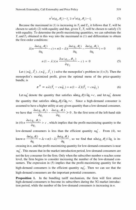
Network Externality, Call Externality and Price Policy 519
2 2 2 1 22 2
1( , ) ( , )T Tn u q n u qθ θ− ≥ − (3)
Because the maximand in (1) is increasing in T1 and T2, it follows that T1 will be chosen to satisfy (2) with equality and that, given T1, T2 will be chosen to satisfy (3) with equality. To determine the profit-maximizing quantities, we can substitute the T1 and T2 obtained in this way into the maximand in (1) and differentiate to obtain the first-order conditions:
1 1 1 1 1 2
1 1 1
( , ) ( , ) ( , )( ) (1 )( ) 0
u q u q u qn c n
q q q
θ θ θλ λ
∂ ∂ ∂− + − − =
∂ ∂ ∂ (4)
2 2
2
( )(1 )( ) 0
,u qn n c
q
θλ
∂− − =
∂ (5)
Let ( 1 1ˆˆ( , )nq T , 2 2
ˆˆ( , )nq T ) solve the monopolist’s problem in (1)-(3). Then the
monopolist’s maximized profit, given the optimal menu of the price-quantity bundle, is
1 1 2 2ˆ ˆˆ ˆ( ) (1 ( ))B n T cnq n T cnqπ λ λ+ −= − − (6)
Let 1cnq denote the quantity that satisfies 1 1 1( , ) /n u q q cθ∂ ∂ = , and let 2
cnq denote
the quantity that satisfies 2 2 2( )/,n u q q cθ∂ ∂ = . Since a high-demand consumer is
assumed to have a higher utility at any given quantity than a low-demand consumer,
we have that 1 2 1 1
1 1
( , ) ( , )0
u q u q
q q
θ θ∂ ∂−
∂ ∂> . So the first term of the left-hand side
in (4) 1 1
1
( , )u qn c
q
θ∂>
∂, which implies that the profit-maximizing quantity to the
low-demand consumers is less than the efficient quantity 1cnq . From (4), we
know 1 1 1 2
1 1
( , ) ( , )(1 )
u q u qn c n
q q
θ θλ λ
∂ ∂⋅ = + −
∂ ∂, so we find that 1 1 1( , ) /n u q qθ∂ ∂ is in-
creasing in n, and the profit-maximizing quantity for low-demand consumers is near
1cnq . This means that in the market introduction period, low-demand consumers are
not the key consumer for the firm. Only when the subscriber number n reaches some level, the firm begins to consider increasing the number of the low-demand con-sumers. The expression in (5) implies that the profit-maximizing quantity for the
high-demand consumers is the efficient quantity 2cnq . Then we can see that the
high-demand consumers are the important potential consumers.
Proposition 1. In the bundling tariff mechanism, the firm will first attract high-demand consumers to become its subscribers during the 3G market introduc-tion period, while the number of the low-demand consumers is increasing in n.
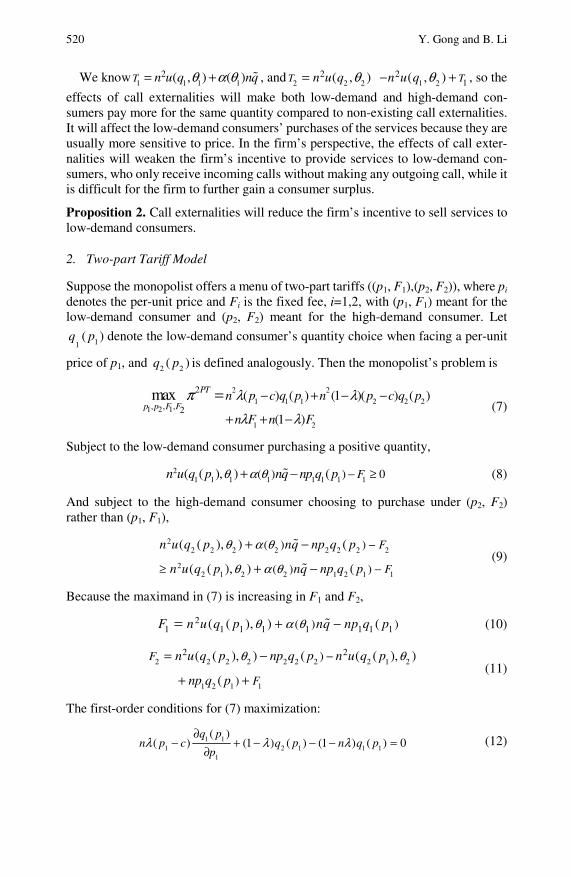
520 Y. Gong and B. Li
We know 1 1 1 12 ( , ) ( )T n u q nqθ α θ= + , and 2 2 2
2 ( , )T n u q θ= 1 22
1( , ) Tn u q θ− + , so the
effects of call externalities will make both low-demand and high-demand con-sumers pay more for the same quantity compared to non-existing call externalities. It will affect the low-demand consumers’ purchases of the services because they are usually more sensitive to price. In the firm’s perspective, the effects of call exter-nalities will weaken the firm’s incentive to provide services to low-demand con-sumers, who only receive incoming calls without making any outgoing call, while it is difficult for the firm to further gain a consumer surplus.
Proposition 2. Call externalities will reduce the firm’s incentive to sell services to low-demand consumers.
2. Two-part Tariff Model
Suppose the monopolist offers a menu of two-part tariffs ((p1, F1),(p2, F2)), where pi
denotes the per-unit price and Fi is the fixed fee, i=1,2, with (p1, F1) meant for the low-demand consumer and (p2, F2) meant for the high-demand consumer. Let
11( )q p denote the low-demand consumer’s quantity choice when facing a per-unit
price of p1, and 2 2( )q p is defined analogously. Then the monopolist’s problem is
2 2
1 1 1 2 2 2
1 2
1 2 1
2
, , , 2
( ) ( ) (1 )( ) ( )
(1 )
max PT
p p F Fn p c q p n p c q p
n F n F
λ λ
λ λ
π − + − −
+ + −
=
(7)
Subject to the low-demand consumer purchasing a positive quantity,
21 1 1 1 1 1 1 1( ) ) 0( ( ), ) ( Fn u q p nq np q pθ α θ − ≥+ − (8)
And subject to the high-demand consumer choosing to purchase under (p2, F2) rather than (p1, F1),
22 2 2 2 2 2 2 2
22 1 2 2 1 2 1 1
( ) )
( ) )
( ( ), ) (
( ( ), ) (
F
F
n u q p nq np q p
n u q p nq np q p
θ α θ
θ α θ
−
≥ −
+ −
+ − (9)
Because the maximand in (7) is increasing in F1 and F2,
21 1 1 1 1 1 1 1( ) )( ( ), ) (F n u q p nq np q pθ α θ+ −= (10)
2 2 2 2 2 2 2 2 1 2
1 2 1 1
2 2)
)
( ( ), ) ( ( ( ), )
(
F
F
n u q p np q p n u q p
np q p
θ θ−= −
+ + (11)
The first-order conditions for (7) maximization:
1 11 2 1 1 1
1
( )( ) (1 ) ( ) (1 ) ( ) 0
q pn p c q p n q p
pλ λ λ
∂− + − − − =
∂ (12)
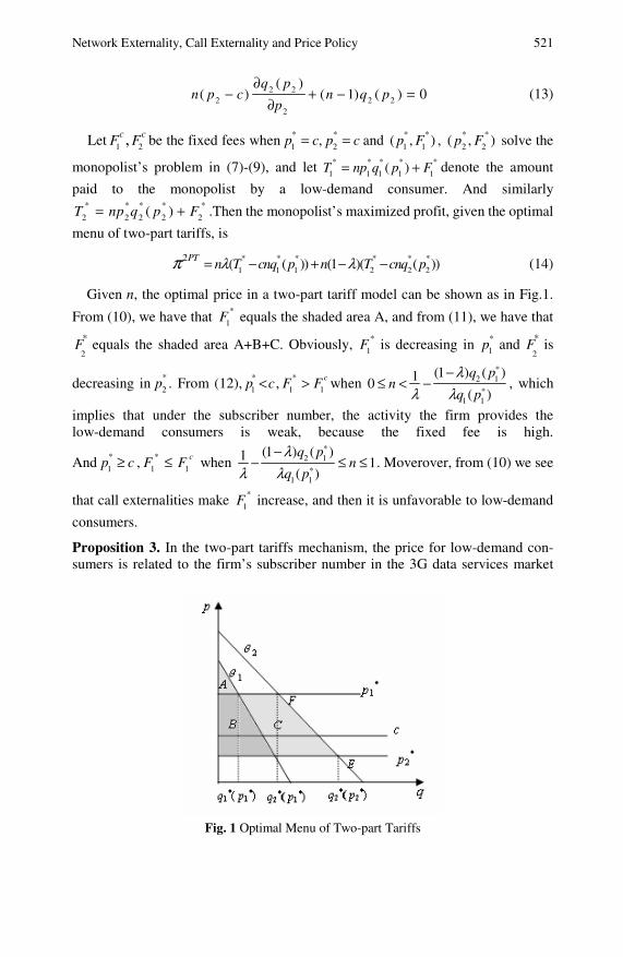
Network Externality, Call Externality and Price Policy 521
2 22 2 2
2
( )( ) ( 1) ( ) 0
q pn p c n q p
p
∂− + − =
∂ (13)
Let 1 2,c cF F be the fixed fees when * *
1 2,p c p c= = and * *
1 1( , )p F , * *
2 2( , )p F solve the
monopolist’s problem in (7)-(9), and let * * * * *
1 1 1 1 1( )T np q p F= + denote the amount
paid to the monopolist by a low-demand consumer. And similarly * * * * *
2 2 2 2 2( )T np q p F= + .Then the monopolist’s maximized profit, given the optimal
menu of two-part tariffs, is
* * * * * *
1 1 1 2 2 2
2 ( ( )) (1 )( ( ))PT n T cnq p n T cnq pλ λπ = − + − − (14)
Given n, the optimal price in a two-part tariff model can be shown as in Fig.1.
From (10), we have that *
1F equals the shaded area A, and from (11), we have that
2
*F equals the shaded area A+B+C. Obviously, *
1F is decreasing in *
1p and 2
*F is
decreasing in *
2p . From (12), *
1p c< , *
1 1
cF F> when *
2 1
*1 1
(1 ) ( )10( )
q pn
q p
λλ λ
−≤ < − , which
implies that under the subscriber number, the activity the firm provides the low-demand consumers is weak, because the fixed fee is high.
And *
1p c≥ , *
1 1
cF F≤ when *
2 1
*1 1
(1 ) ( )1 1( )
q pn
q p
λλ λ
−− ≤ ≤ . Moverover, from (10) we see
that call externalities make *
1F increase, and then it is unfavorable to low-demand
consumers.
Proposition 3. In the two-part tariffs mechanism, the price for low-demand con-sumers is related to the firm’s subscriber number in the 3G data services market
Fig. 1 Optimal Menu of Two-part Tariffs
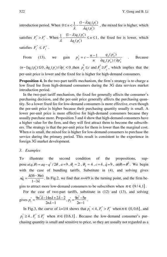
522 Y. Gong and B. Li
introduction period. When *
2 1
*1 1
(1 ) ( )10( )
q pn
q p
λλ λ
−≤ < − , the mixed fee is higher, which
satisfies *
1 1
cF F> . When*
2 1
*1 1
(1 ) ( )1 1( )
q pn
q p
λλ λ
−− ≤ ≤ , the fixed fee is lower, which
satisfies *
1 1
cF F≤ .
From (13), we gain*
2 2*2 * *
2 2 2
( )1( ) /
q pnp cn q p p−= −
∂ ∂⋅ . Because
*2 2( 1) ( ) 0n q p− ≤ , * *
2 2 2( ) / 0q p p∂ ∂ < ,then
2
*p c≤ and2 2
* cF F≥ , which implies that the
per-unit price is lower and the fixed fee is higher for high-demand consumers.
Proposition 4. In the two-part tariffs mechanism, the firm’s strategy is to charge a low fixed fee from high-demand consumers during the 3G data services market introduction period.
In the two-part tariff mechanism, the fixed fee generally affects the consumer’s purchasing decision, and the per-unit price generally affects the purchasing quan-tity. So a lower fixed fee for low-demand consumers is more effective, even though the per-unit price is higher because their purchasing quantity usually is small. A lower per-unit price is more effective for high-demand consumers because they usually purchase more. Proposition 3 and 4 show that high-demand consumers have a higher value for the firm, and they will first attract them to become the subscrib-ers. The strategy is that the per-unit price for them is lower than the marginal cost. When n is small, the mixed fee is higher for low-demand consumers to purchase the service during the primary period. This result is consistent to the experience in foreign 3G market development.
3. Examples
To illustrate the second condition of the propositions, sup-
pose 2( , ) / 2u q aq qθ θ= − , 9a = , 1 2θ = , 2 4θ = , 4c = , 9q = , 2( )α θ θ= . We begin
with the case of bundling tariffs. Substitute in (4), and solving gives
1
(16 36 )ˆ
1 3
nnq
λλ
−=
−. In Fig.2, we find that n=4/9 is the turning point, and the firm be-
gins to attract more low-demand consumers to be subscribers when 9 / 4,1( ]n ∈ .
For the case of two-part tariffs, substitute in (12) and (13), and solving
gives2
*
19 14 2 2
2 1n np
nλ λ λ
λ− + −=
−,
2*
29 52 1n npn−=−
.
In Fig.3, the curve of λ=1/4 shows that *
1 4p < , *
1 1
cF F> when 0, 0.6( ]n ∈ , and *
1 4p ≥ , *
1 1
cF F≤ when 0.6,1( ]n ∈ . Because the low-demand consumer’s pur-
chasing quantity is small and sensitive to price, so they are usually not regarded as a
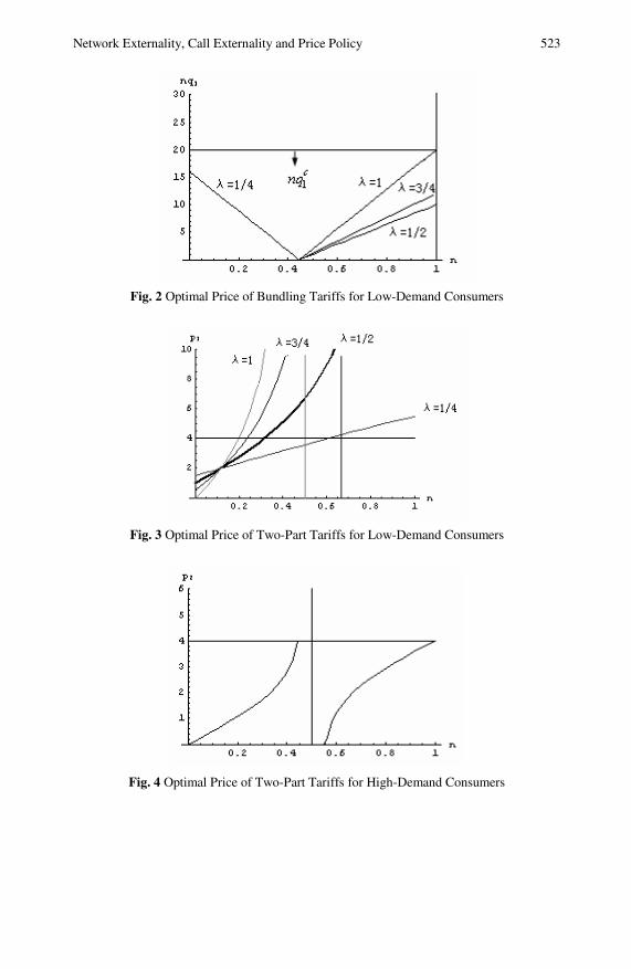
Network Externality, Call Externality and Price Policy 523
Fig. 2 Optimal Price of Bundling Tariffs for Low-Demand Consumers
Fig. 3 Optimal Price of Two-Part Tariffs for Low-Demand Consumers
Fig. 4 Optimal Price of Two-Part Tariffs for High-Demand Consumers
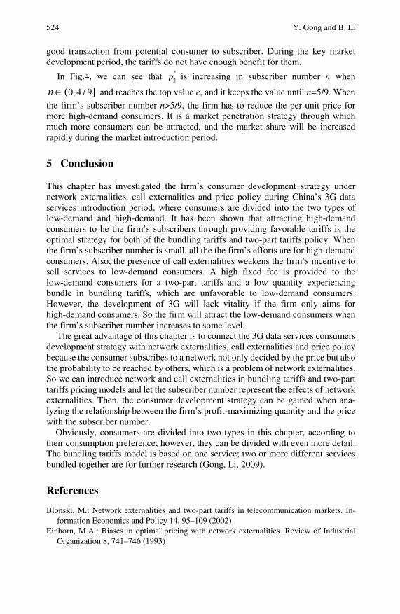
524 Y. Gong and B. Li good transaction from potential consumer to subscriber. During the key market development period, the tariffs do not have enough benefit for them.
In Fig.4, we can see that *
2p is increasing in subscriber number n when
0, 4 / 9( ]n ∈ and reaches the top value c, and it keeps the value until n=5/9. When
the firm’s subscriber number n>5/9, the firm has to reduce the per-unit price for more high-demand consumers. It is a market penetration strategy through which much more consumers can be attracted, and the market share will be increased rapidly during the market introduction period.
5 Conclusion
This chapter has investigated the firm’s consumer development strategy under network externalities, call externalities and price policy during China’s 3G data services introduction period, where consumers are divided into the two types of low-demand and high-demand. It has been shown that attracting high-demand consumers to be the firm’s subscribers through providing favorable tariffs is the optimal strategy for both of the bundling tariffs and two-part tariffs policy. When the firm’s subscriber number is small, all the the firm’s efforts are for high-demand consumers. Also, the presence of call externalities weakens the firm’s incentive to sell services to low-demand consumers. A high fixed fee is provided to the low-demand consumers for a two-part tariffs and a low quantity experiencing bundle in bundling tariffs, which are unfavorable to low-demand consumers. However, the development of 3G will lack vitality if the firm only aims for high-demand consumers. So the firm will attract the low-demand consumers when the firm’s subscriber number increases to some level.
The great advantage of this chapter is to connect the 3G data services consumers development strategy with network externalities, call externalities and price policy because the consumer subscribes to a network not only decided by the price but also the probability to be reached by others, which is a problem of network externalities. So we can introduce network and call externalities in bundling tariffs and two-part tariffs pricing models and let the subscriber number represent the effects of network externalities. Then, the consumer development strategy can be gained when ana-lyzing the relationship between the firm’s profit-maximizing quantity and the price with the subscriber number.
Obviously, consumers are divided into two types in this chapter, according to their consumption preference; however, they can be divided with even more detail. The bundling tariffs model is based on one service; two or more different services bundled together are for further research (Gong, Li, 2009).
References
Blonski, M.: Network externalities and two-part tariffs in telecommunication markets. In-formation Economics and Policy 14, 95–109 (2002)
Einhorn, M.A.: Biases in optimal pricing with network externalities. Review of Industrial Organization 8, 741–746 (1993)

Network Externality, Call Externality and Price Policy 525 Fu, G.: Research on 3G tariffs strategy. Telecommunication World 27, 21–22 (2007) Gong, Y.H., Li, B.Y.: Bundling pricing theory and method of mobile communication ser-
vices. Finance & Trade Economics 4, 114–118 (2009) Hahn, J.H.: Nonlinear pricing of telecommunication with call and network externalities.
International Journal of Industrial Organization 21, 949–967 (2003) Kolay, S.: Bundling and menus of two-part tariffs. Journal of Industrial Economics LI,
383–403 (2003) Li, X., Chen, H.M.: Study on pricing strategy choice of firms with network externality.
Journal of Management Science in China 9, 23–30 (2006) Littlechild, S.G.: Two-part tariffs and consumption externalities. Bell Journal of Economics
and Management Science 6, 661–670 (1975) Pan, X.J., Chen, H.M., Hou, H.Y.: Monopoly pricing strategy with network externality.
Journal of Industrial Engineering and Engineering Management 20, 67–71 (2006) Shuai, X., Chen, H.M.: Network externality and the competition in China’s mobile market.
World Economy 4, 45–52 (2003) Squire, L.: Some aspects of optimal pricing for telecommunication. Bell Journal of Eco-
nomics and Management Science 4, 515–525 (1973) Teng, Y., Tang, X.W.: Third-degree price discrimination with network externality. Control
and Decision 23, 251–257 (2008) Willig, R.D.: The theory of network access pricing. In: Trebing, H. (ed.) Issues in Public
Utility Regulation Public Utilities Papers, pp. 109–152. Michigan State University (1979)

Coordinating an Online Dual-Channel Supply Chain with Asymmetrical Information*
Liu Bin, Zhang Rong, and Bai Hongyuan
Mixed channels are attracting more and more channels firms. This chapter inves-tigates an online dual channels supply chain system, and deals with its coordination with a menu of contract under information asymmetry. First, according to the cen-tralized system, the optimal production and pricing strategies are depicted. Then, for the decentralized system, we consider two kinds of contracts, a single contract and a menu of contracts, to coordinate the channel system, and depict their pro-duction and pricing decisions with principle-agent method under the asymmetrical information on traditional channel. Finally, some interesting insights are found out.
1 Introduction
It is known that there are several channel modes in our present marketing system, and they are traditional channels, direct-selling channels with the Internet (abbre-viated as on-line channels), and dual channels combined with the above two-type channels. In a traditional channel, retailers who confront uncertain settings take on full risk by buying products from suppliers at a wholesale price and selling them to the end customers. In a direct-selling channel, such as the Dell channel, suppliers sell their products to consumers directly through the Internet, and suppliers often Liu Bin Department of Management Science
Zhang Rong Department of Management Science College of Economics and Management, Nanjing University of Aeronautics and Astronautics, Nanjing, P.R. China Phone: 02584892700 e-mail: [email protected]
Bai Hongyuan Department of Information and Computing Science, Henan Agricultural University, Zhengzhou, P.R. China e-mail: [email protected]
* This work is partly supported by the National Nature and Science Fund of China (grant number 70871035), the Nature Science Fund of Henan Education Committee (grant number 2008A630020 and 2009A630022), and the Financial Program for Core Teachers of Henan University.
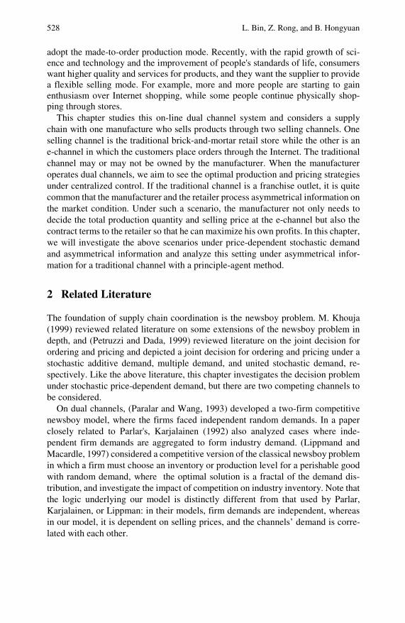
528 L. Bin, Z. Rong, and B. Hongyuan
adopt the made-to-order production mode. Recently, with the rapid growth of sci-ence and technology and the improvement of people's standards of life, consumers want higher quality and services for products, and they want the supplier to provide a flexible selling mode. For example, more and more people are starting to gain enthusiasm over Internet shopping, while some people continue physically shop-ping through stores.
This chapter studies this on-line dual channel system and considers a supply chain with one manufacture who sells products through two selling channels. One selling channel is the traditional brick-and-mortar retail store while the other is an e-channel in which the customers place orders through the Internet. The traditional channel may or may not be owned by the manufacturer. When the manufacturer operates dual channels, we aim to see the optimal production and pricing strategies under centralized control. If the traditional channel is a franchise outlet, it is quite common that the manufacturer and the retailer process asymmetrical information on the market condition. Under such a scenario, the manufacturer not only needs to decide the total production quantity and selling price at the e-channel but also the contract terms to the retailer so that he can maximize his own profits. In this chapter, we will investigate the above scenarios under price-dependent stochastic demand and asymmetrical information and analyze this setting under asymmetrical infor-mation for a traditional channel with a principle-agent method.
2 Related Literature
The foundation of supply chain coordination is the newsboy problem. M. Khouja (1999) reviewed related literature on some extensions of the newsboy problem in depth, and (Petruzzi and Dada, 1999) reviewed literature on the joint decision for ordering and pricing and depicted a joint decision for ordering and pricing under a stochastic additive demand, multiple demand, and united stochastic demand, re-spectively. Like the above literature, this chapter investigates the decision problem under stochastic price-dependent demand, but there are two competing channels to be considered.
On dual channels, (Paralar and Wang, 1993) developed a two-firm competitive newsboy model, where the firms faced independent random demands. In a paper closely related to Parlar's, Karjalainen (1992) also analyzed cases where inde-pendent firm demands are aggregated to form industry demand. (Lippmand and Macardle, 1997) considered a competitive version of the classical newsboy problem in which a firm must choose an inventory or production level for a perishable good with random demand, where the optimal solution is a fractal of the demand dis-tribution, and investigate the impact of competition on industry inventory. Note that the logic underlying our model is distinctly different from that used by Parlar, Karjalainen, or Lippman: in their models, firm demands are independent, whereas in our model, it is dependent on selling prices, and the channels’ demand is corre-lated with each other.
Coordinating an Online Dual-Channel Supply Chain 529
Information is very important for all members of the supply chain, especially for the manufacturers who almost do not directly contact the end customer. Researchers were therefore motivated to explore supply chain models under information asymmetry, such as asymmetry in cost information and asymmetry in demand information. (Corbett, 2001), for instance, compared quantity discount mechanisms with symmetric and asymmetric downstream cost information in a decentralized supply chain consisting of one supplier and multiple buyers who may not share their cost information. (Ha, 2001) considered the asymmetrical cost information problem of determining an optimal coordinated contract in a two-echelon newsboy model. (Lau, 2003) explored two-echelon newsboy models with asymmetrical demand information, in which the retailer has better market information than the manufac-turer, and analyzed the effects of improving the retailer's and the manufacturer's market knowledge of their profits and the system profit. As for the rationality of two-echelon supply chain gaming models, (Chen, 2005) studied Gonik's scheme and compared it with a menu of linear contracts – a solution often used in the agency literature – in a model where the market information possessed by the sales force is important for the firm's production and inventory-planning decisions.
Based on the above literature, this chapter will investigate the joint decision of production and pricing and coordinate the system with asymmetrical information. Other than the above literature, we address a new type of market setting, on-line dual channels with different operation modes, and study how to make a joint deci-sion for the production and pricing of a centralized system and a decentralized system with asymmetrical information, respectively. Further, we will investigate how to measure the information value when making use of private information and which coordination mechanism is optimal for a decentralized system under fran-chise outlet mechanisms.
3 Denotations and Assumptions for Modeling
A. Modeling denotations
In this chapter, c is for the production cost per unit, and
sc is for the salvage value
of unsold products at the end of the selling period. e is additional payment for a shortage.
1s is the selling cost per unit in an e-channel, 2s is the selling cost per
production in a traditional channel operated by the manufacturer, and rs2 is the
selling cost per production in a traditional channel operated by a retailer. For the decision variables,
1p is the selling price of a product sold in the
e-channel, while 2p is the selling price in a traditional channel. Furthermore, Q is
for the ordering/production quantity made before the beginning of the selling period.
For stochastic customer demand, ),,( 211 xppD is the demand function in the
e-channel, and its form is 211 ppbx β+− , while ),,( 212 xppD is the demand func-
tion in a traditional channel, with the form 122 ppbx β+− , where
1b is the
530 L. Bin, Z. Rong, and B. Hongyuan
price-demand elasticity of the e-channel, 2b is the price-demand elasticity of a
traditional channel (especially Hb2 with a higher probability ρ and Lb2 with a
lower probability ρ−1 ), and β is the price elasticity on another channel. The
market scale x is a random variable, its probability distribution function is )(⋅F ,
and the density function is )(⋅f with the mean μ .
Additionally, we denote the expected profit of a centralized and a decentralized
system with ∏ ⋅)(C and ∏ ⋅DC )( , respectively, and use S and M to denote the
mechanism single contract and menu of contracts, respectively. S and M will be denoted in superscript. The superscripts * on some variables are used to denote optimization, such as the optimal selling prices, and the optimal ordering quantity. We use R and M in subscript to denote the retailer and manufacturer of this supply chain.
B. Assumptions
For simplicity, the following assumptions are made according to the marketing setting and its practical operation mode.
1)scce >> , which implies that the emergent production will occur more costs
than the normal one if there is a shortage, and at the same, all unsold products will be sold with the salvage value
sc .
2) β>> 21 bb , which implies that the customers in the e-channel are more sen-
sitive to the selling price than those in the traditional channel because of the rapid transfer of information on the Internet. At the same time, the customers are more sensitive to local selling prices than another’s prices because of the time effect.
3)122 sss r >> , which shows that the selling cost in a traditional channel operated
by the manufacturer is more than that in a traditional channel operated by a retailer and much more than that in an e-channel because there are more selling locations and more salesmen.
4) The production plan must be made and be one-off before the selling period, and all of members of the supply chain are risk-neutered.
5) It is the most important that we assume all customer demand will be met and that the manufacturer can ensure the supply with emergence production or trans-portation from other stores. Interestedly, this assumption is different from that of the newsboy problem, which assumes that these are in shortage during the selling period. Certainly, some scholars have adopted a simliar assumption in their re-search, such as literature (Chen, 2005). Additionally, all of the above parameters are more than zero, and the initial inventory of the whole system is zero.
4 Joint Decision on Production and Pricing for a Centralized System
Under a centralized system, the expected profit is
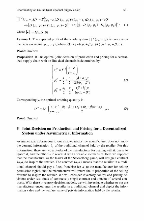
Coordinating an Online Dual-Channel Supply Chain 531
∏ ),,( 21 QppC
{ cQppDspppDspE −−+−= ),()(),()( 2122221111
[ ]+−+− QppDppDe ),(),( 212211 [ ] }+−−+ ),(),( 212211 ppDppDQcs (1)
where [ ] }0,{•=• + Max .
Lemma 1: The expected profit of the whole system ∏ ),,( 21 zppC is concave on
the decision vector ),,( 21 zpp , where )()( 122211 ppbzppbzQ ββ +−++−= .
Proof: Omitted.
Proposition 1: The optimal joint decision of production and pricing for a central-ized supply chain with on-line dual channels is determined by
⎪⎪⎪⎪
⎩
⎪⎪⎪⎪
⎨
⎧
−+++=
−+++=
⎟⎟⎠
⎞⎜⎜⎝
⎛−−= −
)(2
)(
22
)(2)(
22
221
12*
2
221
21*
1
1*
βμβ
βμβ
bb
bcsp
bb
bcsp
ce
ceFz
C
C
s
C
(2)
Correspondingly, the optimal ordering quantity is
μββ −+−++−−⎟⎟⎠
⎞⎜⎜⎝
⎛−−= −
2
))(())((2 22111* scbscb
ce
ceFQ
s
C . (3)
Proof: Omitted.
5 Joint Decision on Production and Pricing for a Decentralized System under Asymmetrical Information
Asymmetrical information in our chapter means the manufacturer does not know the demand information 2b of the traditional channel held by the retailer. For this
information, there are two attitudes of the manufacturer for dealing with it: one is to ignore it, and the other is to reveal it with a feasible mechanism. Here we suppose that the manufacture, as the leader of the Stackelberg game, will design a contract
),( da to inspire the retailer. The contract ),( da means that the retailer in a tradi-
tional channel should pay a fixed franchise fee d to the manufacturer for selling permission rights, and the manufacturer will return the a proportion of the selling revenue to inspire the retailer. We will consider inventory control and pricing de-cisions under two kinds of contracts: a single contract and a menu of several con-tracts. With these inventory decision models, we will investigate whether or not the manufacturer encourages the retailer in a traditional channel and depict the infor-mation value and the welfare value of private information held by the retailer.
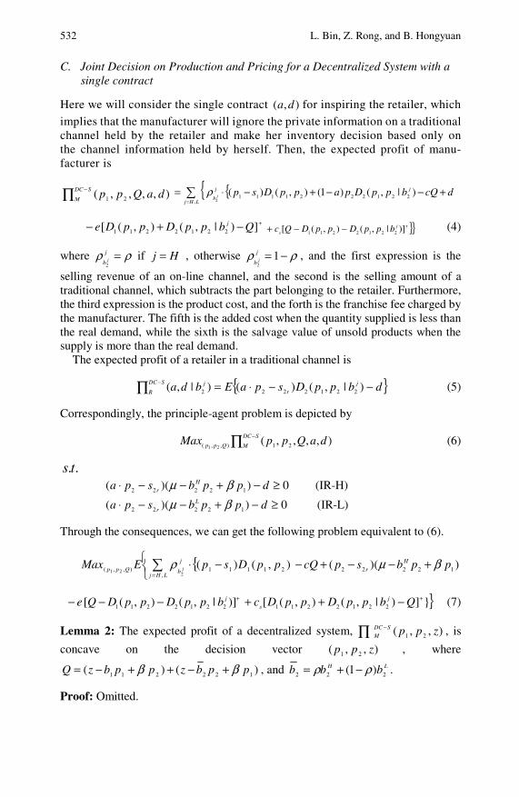
532 L. Bin, Z. Rong, and B. Hongyuan
C. Joint Decision on Production and Pricing for a Decentralized System with a single contract
Here we will consider the single contract ),( da for inspiring the retailer, which
implies that the manufacturer will ignore the private information on a traditional channel held by the retailer and make her inventory decision based only on the channel information held by herself. Then, the expected profit of manu-facturer is
∏ −SDC
MdaQpp ),,,,( 21
{{∑=
+−−+−⋅=LHj
jj
bdcQbppDpappDspj
,2212221111 )|,()1(),()(
2
ρ
+−+− ])|,(),([ 2212211 QbppDppDe j }}+−−+ )]|,(),([ 2212211
j
s bppDppDQc (4)
where ρρ =j
b j2
if Hj = , otherwise ρρ −= 12
j
b j , and the first expression is the
selling revenue of an on-line channel, and the second is the selling amount of a traditional channel, which subtracts the part belonging to the retailer. Furthermore, the third expression is the product cost, and the forth is the franchise fee charged by the manufacturer. The fifth is the added cost when the quantity supplied is less than the real demand, while the sixth is the salvage value of unsold products when the supply is more than the real demand.
The expected profit of a retailer in a traditional channel is
{ }dbppDspaEbda j
r
SDC
R
j −−⋅=∏ − )|,()()|,( 2212222 (5)
Correspondingly, the principle-agent problem is depicted by
∏ −SDC
MQpp daQppMax ),,,,( 21),,( 21 (6)
..ts
0))(( 12222 ≥−+−−⋅ dppbspa H
r βμ (IR-H)
0))(( 12222 ≥−+−−⋅ dppbspa L
r βμ (IR-L)
Through the consequences, we can get the following problem equivalent to (6).
{⎩⎨⎧ −⋅∑
= LHj
j
bQpp ppDspEMax j
,21111),,( ),()(
221
ρ ))(( 12222 ppbspcQ H
r βμ +−−+−
+−−− )]|,(),([ 2212211jbppDppDQe }}])|,(),([ 2212211
+−++ QbppDppDc j
s (7)
Lemma 2: The expected profit of a decentralized system, ∏ − ),,( 21 zppSDC
M , is
concave on the decision vector ),,( 21 zpp , where
)()( 122211 ppbzppbzQ ββ +−++−= , and LH bbb 222 )1( ρρ −+= .
Proof: Omitted.
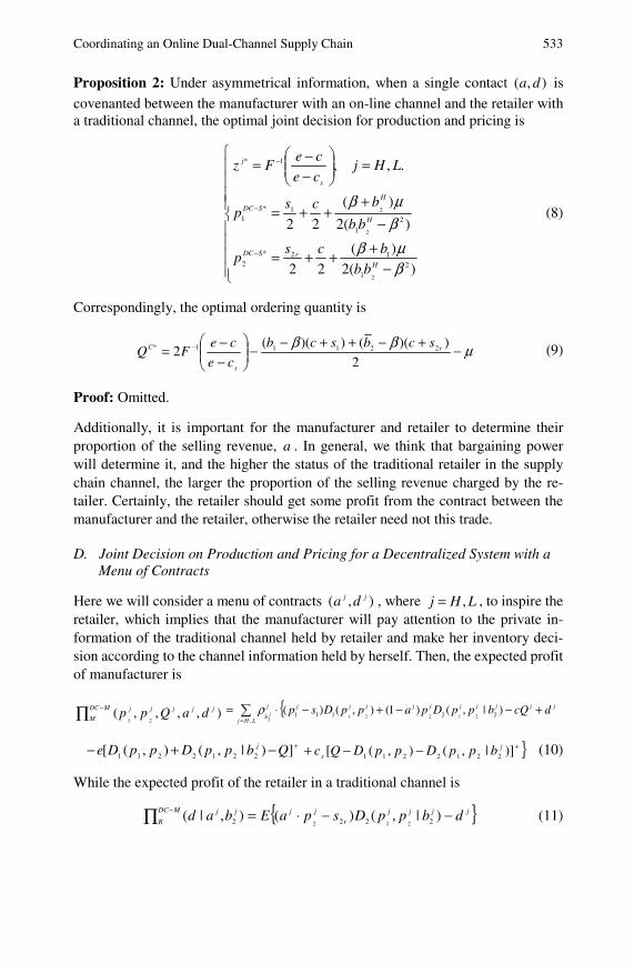
Coordinating an Online Dual-Channel Supply Chain 533
Proposition 2: Under asymmetrical information, when a single contact ),( da is
covenanted between the manufacturer with an on-line channel and the retailer with a traditional channel, the optimal joint decision for production and pricing is
⎪⎪⎪⎪
⎩
⎪⎪⎪⎪
⎨
⎧
−+++=
−+
++=
=⎟⎟⎠
⎞⎜⎜⎝
⎛−−=
−
−
−
)(2)(
22
)(2
)(
22
.,,
21
12*
2
2
1
1*1
1*
2
2
2
βμβ
βμβ
H
rSDC
H
H
SDC
s
j
bb
bcsp
bb
bcsp
LHjce
ceFz
(8)
Correspondingly, the optimal ordering quantity is
μββ −+−++−−⎟⎟⎠
⎞⎜⎜⎝
⎛−−= −
2
))(())((2 22111* r
s
C scbscb
ce
ceFQ (9)
Proof: Omitted.
Additionally, it is important for the manufacturer and retailer to determine their proportion of the selling revenue, a . In general, we think that bargaining power will determine it, and the higher the status of the traditional retailer in the supply chain channel, the larger the proportion of the selling revenue charged by the re-tailer. Certainly, the retailer should get some profit from the contract between the manufacturer and the retailer, otherwise the retailer need not this trade.
D. Joint Decision on Production and Pricing for a Decentralized System with a Menu of Contracts
Here we will consider a menu of contracts ),( jj da , where LHj ,= , to inspire the retailer, which implies that the manufacturer will pay attention to the private in-formation of the traditional channel held by retailer and make her inventory deci-sion according to the channel information held by herself. Then, the expected profit of manufacturer is
∏ −MDC
M
jjjjj daQpp ),,,,(21
{∑=
+−−+−⋅=LHj
jjjjjjjjjjj
bdcQbppDpappDspj
,22111 )|,()1(),()(
212212
ρ
+−+− ])|,(),([ 2212211 QbppDppDe j }+−−+ )]|,(),([ 2212211
j
s bppDppDQc (10)
While the expected profit of the retailer in a traditional channel is
{ }jjjj
r
jjMDC
R
jj dbppDspaEbad −−⋅=∏ − )|,()(),|( 2222 212 (11)
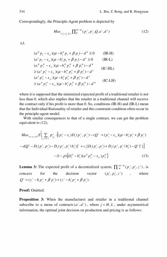
534 L. Bin, Z. Rong, and B. Hongyuan
Correspondingly, the Principle-Agent problem is depicted by
∏ −MDC
M
jjjj
QppdaQppMax jjj ),,,,(
2121
),,( (12)
..ts
0))(( 12222 ≥−+−− HH
r
H dppbspa βμ (IR-H)
0))(( 12222 ≥−+−− LL
r
L dppbspa βμ (IR-L)
LLLH
r
LL
HHHH
r
HH
dppbspa
dppbspa
−+−−≥−+−−
))((
))((
12222
12222
βμβμ
(IC-HL)
HHHL
r
HH
LLLL
r
LL
dppbspa
dppbspa
−+−−≥−+−−
))((
))((
12222
12222
βμβμ
(IC-LH)
where it is supposed that the minimized expected profit of a traditional retailer is not less than 0, which also implies that the retailer in a traditional channel will receive the contract only if his profit is more than 0. So, conditions (IR-H) and (IR-L) mean that the Individual Rationality of retailer and this constraint condition often occur in the principle-agent model.
With similar consequences to that of a single contract, we can get the problem equivalent to (12),
{⎩⎨⎧ −−⋅∑
=
jjjj
LHj
j
bQpp cQppDspEMax j ),()(21
221 111
,),,( ρ ))((
122 22
jjj
r
j ppbsp βμ +−−+
+−−− )]|,(),([ 221 2121
jjjjjj bppDppDQe }}])|,(),([ 221 2121
+−++ jjjjjj
s QbppDppDc
{ }H
r
HHLH pspabb 22222 ))(()1( −−−− ρ (13)
Lemma 3: The expected profit of a decentralized system, ∏ − ),,(21
jjjMDC
M zpp , is
concave for the decision vector ),,( 21jjj zpp , where
)()(1221 21
jjjjjjjj ppbzppbzQ ββ +−++−= .
Proof: Omitted.
Proposition 3: When the manufacturer and retailer in a traditional channel subscribe to a menu of contracts ),( jj da , where LHj ,= , under asymmetrical
information, the optimal joint decision on production and pricing is as follows:

Coordinating an Online Dual-Channel Supply Chain 535
⎪⎪⎪⎪⎪⎪⎪⎪⎪⎪⎪⎪⎪⎪
⎩
⎪⎪⎪⎪⎪⎪⎪⎪⎪⎪⎪⎪⎪⎪
⎨
⎧
−+−⋅+
+
−+−⋅−
+
−+−⋅−+−
=
−+−⋅−++
+
−+−⋅−
−
−+−⋅−+−
+=
−+
++=
−+
++=
=⎟⎟⎠
⎞⎜⎜⎝
⎛−−=
−
−
−
−
−−
−
−
−
−
−
−
−−
−
−
−
)]()[(2
)(
)]()[(2
)(
)]()[(2
])()[(
)]()[(2
])([
)]()[(2
)]([
)]()[(2
])()([(
2
)(2
)(
22
)(2
)(
22
.,,
221
121
1
221
121
21
221
121
2122
12
1*2
221
121
22
1
221
12
1
222
1
221
121
22
1
11*1
21
12*_
2
2
1
1*_1
1*
2
2
2
2
2
2
2
2
2
2
2
2
2
LHHH
LHHH
H
LHHH
r
LHH
HMDC
LHHH
HLHH
LHHH
r
LHH
LHHH
HLHH
HMDC
L
rLMDC
L
L
LMDC
s
j
bbbabb
b
bbbabb
cbb
bbbabb
sbbbbbp
bbbabb
abbb
bbbabb
sbba
bbbabb
cabbbbsp
bb
bcsp
bb
bcsp
LHjce
ceFz
ρρ
ρρ
ρρ
ρρ
ρρ
ρρ
ρρ
ρρ
ρρ
ρρ
βμβ
ββ
ββ
βμβ
ββ
ββ
βμβ
βμβ
(14)
Proof: Omitted.
Interestingly, the proportions of selling revenue ja are critical for channel coor-dination. Certainly, they are the profit balance between the manufacturer and the retailer in the traditional channel, and their bargaining power and channel status determine these proportions. Generally, because the retailer should get the more profit than 0, the feasible region of Ha is
⎥⎦
⎤⎢⎣
⎡
−−++−+−
−1,
)()())((
)(2
2211
12
212
2
2
21
LHH
r
r
H
bbbbbbcs
sbb
ρρμββ
β (15)
and the feasible region of La is
⎥⎦
⎤⎢⎣
⎡++−+
−1,
)())((
)(2
12
212
2
2
21
μβββ
bbbcs
sbbL
r
r
L
(16)
Now we compare the optimal selling prices of a decentralized system with a single contract to that with a menu of contracts, and we get several deductions, as follows.
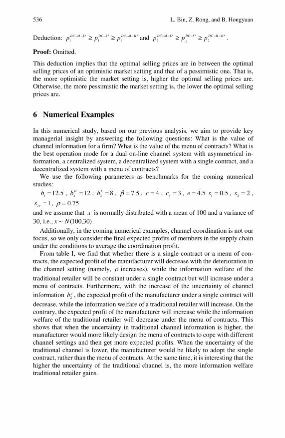
536 L. Bin, Z. Rong, and B. Hongyuan
Deduction: *1
*1
*1
HMDCSDCLMDC ppp −−−−− ≥≥ and *
2
**
2 2
HMDCSDCLMDC ppp −−−−− ≥≥ .
Proof: Omitted.
This deduction implies that the optimal selling prices are in between the optimal selling prices of an optimistic market setting and that of a pessimistic one. That is, the more optimistic the market setting is, higher the optimal selling prices are. Otherwise, the more pessimistic the market setting is, the lower the optimal selling prices are.
6 Numerical Examples
In this numerical study, based on our previous analysis, we aim to provide key managerial insight by answering the following questions: What is the value of channel information for a firm? What is the value of the menu of contracts? What is the best operation mode for a dual on-line channel system with asymmetrical in-formation, a centralized system, a decentralized system with a single contract, and a decentralized system with a menu of contracts?
We use the following parameters as benchmarks for the coming numerical studies:
5.121 =b , 122 =Hb , 82 =Lb , 5.7=β , 4=c , 3=sc , 5.4=e 5.01 =s , 22 =s ,
12 =rs , 75.0=ρ
and we assume that x is normally distributed with a mean of 100 and a variance of 30, i.e., )30,100(~ Nx .
Additionally, in the coming numerical examples, channel coordination is not our focus, so we only consider the final expected profits of members in the supply chain under the conditions to average the coordination profit.
From table I, we find that whether there is a single contract or a menu of con-tracts, the expected profit of the manufacturer will decrease with the deterioration in the channel setting (namely, ρ increases), while the information welfare of the
traditional retailer will be constant under a single contract but will increase under a menu of contracts. Furthermore, with the increase of the uncertainty of channel information jb2 , the expected profit of the manufacturer under a single contract will
decrease, while the information welfare of a traditional retailer will increase. On the contrary, the expected profit of the manufacturer will increase while the information welfare of the traditional retailer will decrease under the menu of contracts. This shows that when the uncertainty in traditional channel information is higher, the manufacturer would more likely design the menu of contracts to cope with different channel settings and then get more expected profits. When the uncertainty of the traditional channel is lower, the manufacturer would be likely to adopt the single contract, rather than the menu of contracts. At the same time, it is interesting that the higher the uncertainty of the traditional channel is, the more information welfare traditional retailer gains.
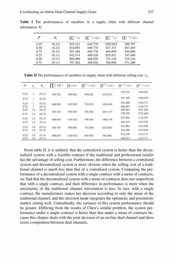
Coordinating an Online Dual-Channel Supply Chain 537 Table I The performances of members in a supply chain with different channel
information jb2
ρ jb2 ∏ − ⋅SDC
M)( ∏ − ⋅SDC
R
Lb )|( 2 ∏ − ⋅MDC
M)( ∏ − ⋅MDC
R
Lb )|( 2
0.25 (8,12) 922.221 640.778 1092.042 209.787 0.50 (8,12) 814.693 640.778 827.315 407.465 0.75 (8,12) 707.166 640.778 664.049 544.080 0.25 (9,11) 942.514 408.920 855.851 197.400 0.50 (9,11) 869.900 408.920 751.139 310.336 0.75 (9,11) 797.284 408.920 704.090 371.280
Table II The performances of members in supply chain with different selling cost rs2
ρrs2 jb2 ∏ ⋅C Hb )|( 2 ∏ ⋅C Lb )|( 2 ∏ − ⋅SDC Hb )|( 2 ∏ − ⋅SDC Lb )|( 2 ∏ − ⋅MDC Hb )|( 2 ∏ − ⋅MDC Lb )|( 2
0.25 1 (8,12) 479.472 1549.876
0.75 1 (8,12)
565.763 1505.001 599.638 1670.527 553.369 1549.876
0.25 1 (9,11) 643.888 1149.777
0.75 1 (9,11) 688.045 1107.652 724.670 1424.049
680.097 1149.777 0.25 1.4 (8,12) 466.465 1531.446
0.75 1.4 (8,12) 565.763 1505.001 585.368 1651.137
538.358 1531.446
0.25 1.4 (9,11) 627.892 1132.387
0.75 1.4 (9,11) 688.045 1107.652 709.360 1406.179
664.319 1132.387
0.25 1.8 (8,12) 453.884 1513.656
0.75 1.8 (8,12) 565.763 1505.001 572.058 1632.067
524.288 1513.656
0.25 1.8 (9,11) 612.425 1115.717
0.75 1.8 (9,11) 688.045 1107.652 694.930 981.068
649.415 1115.717
From table II, it is unlikely that the centralized system is better than the decen-
tralized system with a feasible contract if the traditional and professional retailer has the advantage of selling cost. Furthermore, the difference between a centralized system and decentralized system is more obvious when the selling cost of a tradi-tional channel is much less than that of a centralized system. Comparing the per-formance of a decentralized system with a single contract with a menu of contracts, we find that the decentralized system with a menu of contracts does not outperform that with a single contract, and their difference in performance is more when the uncertainty of the traditional channel information is less. In fact, with a single contract, the manufacturer makes her decision according to only the mean of the traditional channel, and this decision mode integrates the optimistic and pessimistic market setting well. Undoubtedly, the variance of this system performance should be greater. Differing from the results of Chen’s similar problem, the system per-formance under a single contract is better than that under a menu of contracts be-cause this chapter deals with the joint decision of an on-line dual channel and there exists competition between dual channels.
538 L. Bin, Z. Rong, and B. Hongyuan
7 Conclusions
In this chapter, we investigate a supply chain with one manufacturer who sells products through two selling channels. One selling channel is the traditional brick-and-mortar retail store, while the other is an e-channel in which customers place orders through the Internet. The traditional channel may or may not be owned by the manufacturer. According to the centralized system, namely, the market set-ting where the manufacturer operates dual channels, the optimal production and pricing strategies are depicted. According to the decentralized system, we consider two kinds of franchise outlets to coordinate the channel system: one is a single contract and the other is a menu of contracts. We depict their production and pricing decisions with a principle-agent method under asymmetrical information of the traditional channel. Some interesting management insights are found.
1) It is unlikely that the centralized system is better than the decentralized system with a feasible contract if the traditional and professional retailer has an advantage in selling cost.
2) The more optimistic the market setting is, the higher the optimal selling prices are; otherwise, the more pessimistic the market setting is, the lower the optimal selling prices are.
3) When uncertainty in the traditional channel information is higher, the manu-facturer would be more likely to design the menu of contracts to cope with the different channel setting, then getting more expected profits. When the uncertainty of the traditional channel is lower, the manufacturer would be more likely to adopt the single contract rather than the menu of contracts.
4) The higher the uncertainty of the traditional channel, the more the information welfare of the traditional retailer gains.
5) The decentralized system with a menu of contracts does not outperform that with a single contract, which integrates the optimistic and pessimistic market setting well, and their difference in performance is more when the uncertainty of the tra-ditional channel information is less.
In this chapter, we only consider the decision setting where the manufacturer holds the pricing power for a traditional channel and the retailer does not make a pricing decision according to his private channel information. For future research, we will investigate scenarios similar to this chapter, but the retailer will make the pricing decision on the traditional channel.
References
Chen, F.: Sales-force incentives, market information, and production/inventory planning. Management Science 51(1), 60–75 (2005)
Corbett, C.J.: Stochastic inventory systems in a supply chain with asymmetrical information: Cycle stocks, safety stocks, and consignment stock. Operational Research 49(4), 487–500 (2001)
Ha, A.Y.: Supplier-buyer contracting: Asymmetrical cost information and cutoff level policy for buyer participation. Naval Research Logistics 48(1), 41–64 (2001)

Coordinating an Online Dual-Channel Supply Chain 539 Karjalainen, R.: The newsboy game. University of Pennsylvania working paper, Philadelphia
(1992) Khouja, M.: The single-period (news-vendor) problem: Literature review and suggestions for
further research. Omega 27(5), 537–553 (1999) Lau, H.S.: Effects of a demand-curve’s shape on the optimal solutions of a multi-echelon
inventory/pricing model. European Journal of Operational Research 147(3), 530–548 (2003)
Lippmand, S.A., Macardle, K.F.: The competitive newsboy. Operations Research 45(1), 54–65 (1997)
Paralar, M., Wang, D.: Diversification under yield randomness in inventory models. Euro-pean Journal of Operational Research 66(1), 52–64 (1993)
Petruzzi, N.C., Dada, M.: Pricing and the newsvendor problem: A review with extensions. Operations Research 47(2), 183–194 (1999)
The Optimization of Supply Chain Components’ Quality Characteristics Based on the Structural Equation Model
Yuan Liu, Zhigeng Fang, Sifeng Liu, and Baohua Yang*
Aiming to quality character management under the “Main Manufacturer-Supplies” model, the structural equation model and programming model are set up to evaluate and optimize the supply chain components’ quality characteristics. This chapter can be divided into 4 parts: (1) The quality loss function: We design the quality loss functions according to 3 quality types as input for the model; (2) The structural equation model: We establish the two-order factor model to illustrate the production model and evaluate the quality contribution weight for the product’s quality; (3) The programming model: we set up the programming model to optimize the quality per-formance based on the evaluation results; (4) A case study: An automobile production case is researched to show the effectiveness of the method. This chapter provides a new way to evaluate and improve the supply chain components’ quality characters.
1 Introduction
Because of labor division and specification, the “Main Manufacturer–Supplies” (M-S) production model has become the foremost manufacturing pattern around the Yuan Liu College of Economics and Management, Nanjing University of Aeronautics and Astronautics, Nanjing 210016, PR China Tel.: +86-025-84896149, +86-13814162077; Fax: +86-025-84896149 e-mail: [email protected]
Zhigeng Fang College of Economics and Management, Nanjing University of Aeronautics and Astronautics, Nanjing 210016, PR China Tel.: +86-025-84896149, 86-13814093744 e-mail: [email protected]
Sifeng Liu College of Economics and Management, Nanjing University of Aeronautics and Astronautics, Nanjing 210016, PR China Tel.: 86-13851422964 e-mail: [email protected]
Baohua Yang College of Economics and Management, Nanjing University of Aeronautics and Astronautics, Nanjing 210016, PR China
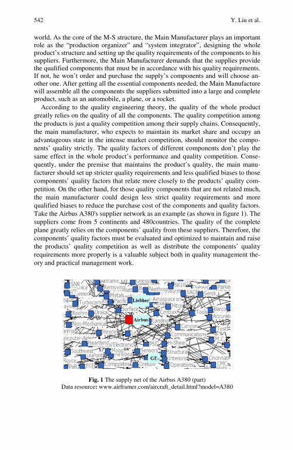
542 Y. Liu et al. world. As the core of the M-S structure, the Main Manufacturer plays an important role as the “production organizer” and “system integrator”, designing the whole product’s structure and setting up the quality requirements of the components to his suppliers. Furthermore, the Main Manufacturer demands that the supplies provide the qualified components that must be in accordance with his quality requirements. If not, he won’t order and purchase the supply’s components and will choose an-other one. After getting all the essential components needed, the Main Manufacture will assemble all the components the suppliers submitted into a large and complete product, such as an automobile, a plane, or a rocket.
According to the quality engineering theory, the quality of the whole product greatly relies on the quality of all the components. The quality competition among the products is just a quality competition among their supply chains. Consequently, the main manufacturer, who expects to maintain its market share and occupy an advantageous state in the intense market competition, should monitor the compo-nents’ quality strictly. The quality factors of different components don’t play the same effect in the whole product’s performance and quality competition. Conse-quently, under the premise that maintains the product’s quality, the main manu-facturer should set up stricter quality requirements and less qualified biases to those components’ quality factors that relate more closely to the products’ quality com-petition. On the other hand, for those quality components that are not related much, the main manufacturer could design less strict quality requirements and more qualified biases to reduce the purchase cost of the components and quality factors. Take the Airbus A380's supplier network as an example (as shown in figure 1). The suppliers come from 5 continents and 480countries. The quality of the complete plane greatly relies on the components’ quality from these suppliers. Therefore, the components’ quality factors must be evaluated and optimized to maintain and raise the products’ quality competition as well as distribute the components’ quality requirements more properly is a valuable subject both in quality management the-ory and practical management work.
Fig. 1 The supply net of the Airbus A380 (part) Data resource: www.airframer.com/aircraft_detail.html?model=A380
The Optimization of Supply Chain Components 543
Looking over the relevant literature of recent years that we could find in this field, some scholars and management practitioners have done a series of related studies and research. Some representative views are as follows:
Nien-Lin Hsueh, Peng-Hua Chu and William Chu discussed a quantitative method for evaluating the quality design patterns, which was planned to calculate the effectiveness of quality improvement in a design pattern where pattern users could determine which design patterns were applicable to satisfy their functional and quality requirements (Hsueh et al., 2008). In (Fynes and De Búrca, 2005), a new path model was set up to incorporate the design quality, conformance quality, ex-ternal quality-in-use, product cost, time-to-market and customer satisfaction that was conformed to data gathered from 351 production companies in the Republic of Ireland. Ful-Chiang Wu presented a measure to optimize the nonlinear multiple dynamic quality characteristics on the base of the double-exponential desirability function (Wu, 2008). E. Ertugrul Karsak designed a fuzzy multiple-objective pro-gramming measure to determine the design requirements under the “Quality Func-tion Deployment” model with imprecise and subjective information (Karsak, 2004). Furthermore, many other researchers made considerable contributions in the quan-tity characteristics designing and management field (Liu and Fang, 2007; Han and Xiong, 2002; Powell and Pyke, 1996).
Throughout related literature of recent years, we can find that research in the quality characteristic designing, evaluating and optimizing fields are mainly limited to one enterprise, which concentrates on the product lever. But in the M-S produc-tion model that widely exists, because of various supply chains, kinds of compo-nents, numerous enterprises and complex relationships among them, the quality management of products and components under the M-S production model is more difficult and worthy of analysis and research. But the research on this subject and field wasn’t mature and didn’t form a scientific theory system. In main manufac-turer enterprises, such as Boeing, Airbus, Toyota, and Volkswagen, a proper and effective management measure to design and evaluate the component quality characteristics in the whole product wasn’t found, nor can it be optimized and improved.
Based on the above considerations, this chapter applies the “Structural Equation Model” theory to the M-S production model to get the evaluation of components’ quality and affective factor loading. A programming model is established to cal-culate the components’ quality performance under a series of constraints to confirm the quality characteristics’ optimal value. The chapter is aimed to set up and es-tablish a new method for product quality management under the M-S production model.
The chapter mainly solves the problems above: (1) Improve Artiles-Leon’s quality loss function (nominal type) and design 2
kinds of quality loss functions towards the larger-the-better type and smaller-the-better type to measure the quality characters’ performance completely and properly .
(2) Set up the high-order factor model to describe the M-S production model and input the quality characters’ performance of components to calculate the affective factor loading from quality characters to the final product’s quality.
544 Y. Liu et al.
(3) Based on the factor loading weight, establish the programming model to calculate and optimize the quality characters’ objective performance in order to design the quality characters’ requirements and allocate the management resources scientifically and probably.
2 The Improved Quality Loss Functions
A. The Quality Loss Function of Product Characteristics
The generalized quality loss of product characteristics was firstly introduced by Taguchi. He argued that a product’s quality fluctuation was a kind of objective reality. If the quality character deviates from the expected value designed, quality loss has happened.
In order to describe the quality loss of product characteristics, people designed the quality loss function to show the distance between a realistic value and an ex-pected value. According to the meanings of an expected quality value, the quality loss function can be divided into the nominal type, the larger-the-better type and the smaller-the-better type.
B. The Nominal Type Quality Loss Function
Nominal type characteristics are called N-type for short and means refers to when the quality is better because the realistic value is closer to the expected value. In the quality engineering theory, when the realistic value is just equal to the expected value, the quality loss is 0, the smallest; when the realistic value reaches the upper or lower limit, the quality loss is 1, the largest. If the realistic value is beyond the upper or lower limit, the product is wasteful and isn’t accepted. Consequently, if the
nominal type characteristics (N-type) ~ ( , , )iY USL LSLμ , under standardized
and dimensionless procedures, its quality loss function can be defined as follows:
2( ) 4( )ii
YL Y
USL LSL
μ−=−
(1)
In formula (1), μ is iY ’s expected value, and ,USL LSL are iY ’s upper and
lower limits.
C. The Larger-the-better Type Quality Loss Function
The larger-the-better type characteristic is called the L-type for short and refers to when the quality is better because the realistic value is higher. Similarly, if lar-
ger-the-better type characteristics (L-type) ~ ( , )j U LY Y Y , its quality loss function
can be defined as follows:
2( ) ( )j Uj
U L
Y YL Y
Y Y
−=
− (2)

The Optimization of Supply Chain Components 545
In formula (2), uY is jY ’s Max-satisfied value, and LY is jY ’s Min-acceptable
value.
D. The Smaller-the-Better Type Quality Loss Function
The smaller-the-better type characteristic is called the S-type for short and refers to when the quality is better because the realistic value is lower. Similarly, if
smaller-the-better type characteristics (S-type) ~ ( , )k U LY Y Y′ ′ , its quality loss
function can be defined as follows:
2( ) ( )k Uk
U L
Y YL Y
Y Y′
′ ′
−=−
(3)
In formula (3), LY ′ is kY ’s Min-satisfied value and UY ′ is kY ’s Max-acceptable
value.
3 The Evaluation of M-S Quality Characteristics Based on the Structural Equation Model
E. The Structural Equation Model of the M-S System
Structural equation model (SEM) is a multivariate statistical analysis model and method that deals with complex data operating and researching. SEM is composed of two parts, the observable indicates (that can be measured or calculated directly and accurately) and the latent indicates (that can’t be describe and shown immedi-ately and exactly). SEM is an effective tool to establish a structure model consisting of the complex relationships between the observable indicates and latent indicates, or between a latent indicate and another.
According to function relations among the product structure and logistic goods flow directions among enterprises, we design the quality characters’ performance (described as quality loss) as observable indicates that can be measured by quality loss functions. The quality lever of the components and whole product are devised as latent indicates connecting to observable indicates (which belong to the com-
ponent) and each other. iδ is character 1’s measuring error. We create the path
diagram of a structural equation model under the M-S production system, as shown in figure 2.
F. Data Collection and Adjustment
The SEM requires a strict demand for the size of sample, which reaches at least 100-200. We should collect 200 samples of each quality character realistic value to satisfy the requirement. For example, there are 12 types of quality characters, and each quality character needs to be measured 200 times. The sample size is 200, the indicator number is 12, and the data points are 12*200, or 2400, in total. SEM needs
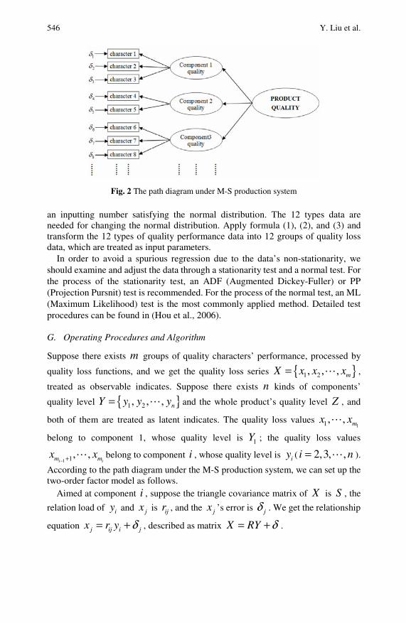
546 Y. Liu et al.
Fig. 2 The path diagram under M-S production system an inputting number satisfying the normal distribution. The 12 types data are needed for changing the normal distribution. Apply formula (1), (2), and (3) and transform the 12 types of quality performance data into 12 groups of quality loss data, which are treated as input parameters.
In order to avoid a spurious regression due to the data’s non-stationarity, we should examine and adjust the data through a stationarity test and a normal test. For the process of the stationarity test, an ADF (Augmented Dickey-Fuller) or PP (Projection Pursnit) test is recommended. For the process of the normal test, an ML (Maximum Likelihood) test is the most commonly applied method. Detailed test procedures can be found in (Hou et al., 2006).
G. Operating Procedures and Algorithm
Suppose there exists m groups of quality characters’ performance, processed by
quality loss functions, and we get the quality loss series { }1 2, , , mX x x x= ,
treated as observable indicates. Suppose there exists n kinds of components’
quality level { }1 2, , , nY y y y= and the whole product’s quality level Z , and
both of them are treated as latent indicates. The quality loss values 11, , mx x
belong to component 1, whose quality level is 1Y ; the quality loss values
1 1, ,i im mx x− + belong to component i , whose quality level is iy ( 2,3, ,i n= ).
According to the path diagram under the M-S production system, we can set up the two-order factor model as follows.
Aimed at component i , suppose the triangle covariance matrix of X is S , the
relation load of iy and jx is ijr , and the jx ’s error is jδ . We get the relationship
equation j ij i jx r y δ= + , described as matrix X RY δ= + .
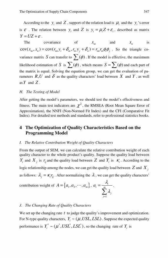
The Optimization of Supply Chain Components 547
According to the iy and Z , support of the relation load is iμ and the iy ’s error
is ε . The relation between iy and Z is i i iy Zμ ε= + , described as matrix
Y UZ ε= + .
The covariance of mx and nx is
cov( , ) cov( , )m n im i m in j n im in i jx x r y r y r rδ δ φ φ= + + = . So the triangle co-
variance matrix S can transfer to ( )φ∑ . If the model is effective, the maximum
likelihood estimation of S is ( )φ∑ , which means ( )S φ=∑ and each part of
the matrix is equal. Solving the equation group, we can get the evaluation of pa-rameters ,R U and δ as the quality characters’ load between X and Y , as well
asY and Z .
H. The Testing of Model
After getting the model’s parameters, we should test the model’s effectiveness and
fitness. The main test indicators are 2χ , the RMSEA (Root Mean Square Error of
Approximation), the NNFI (Non-Normed Fit Index) and the CFI (Comparative Fit Index). For detailed test methods and standards, refer to professional statistics books.
4 The Optimization of Quality Characteristics Based on the Programming Model
I. The Relative Contribution Weight of Quality Characters
From the output of SEM, we can calculate the relative contribution weight of each quality character to the whole product’s quality. Suppose the quality load between
iY and jX is ijr and the quality load between Z and iY is iκ . According to the
logic relationship among the nodes, we can get the quality load between Z and jX
as follows: j i ijrλ κ= . After normalizing the λ , we can get the quality characters’
contribution weight of { }1 2, , , mA a a a= ,
1
ii m
jj
aλ
λ=
=∑
.
J. The Changing Rate of Quality Characters
We set up the changing rate t to judge the quality’s improvement and optimization.
For N-type quality characters, ~ ( , , )iY USL LSLμ . Suppose the expected quality
performance is * * * *~ ( , , )iY USL LSLμ , so the changing rate of iY is
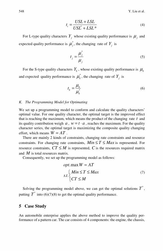
548 Y. Liu et al.
* *i
USL LSLt
USL LSL
+=+
(4)
For L-type quality characters jY whose existing quality performance is jμ and
expected quality performance is *jμ , the changing rate of jY is
*j
jj
tμμ
= (5)
For the S-type quality characters kY , whose existing quality performance is kμ
and expected quality performance is *kμ , the changing rate of jY is
*k
kk
tμμ
= (6)
K. The Programming Model for Optimating
We set up a programming model to conform and calculate the quality characters’ optimal value. For one quality character, the optimal target is the improved effect that is reaching the maximum, which means the product of the changing rate t and its quality contribution weigh a , atw ⋅= , reaches the maximum. For the quality character series, the optimal target is maximizing the composite quality changing effort, which means W AT= .
There are mainly 2 kinds of constraints, changing rate constraints and resource constraints. For changing rate constraints, Min T Max≤ ≤ is represented. For
resource constraints, CT M≤ is represented, C is the resources required matrix and M is total resources matrix.
Consequently, we set up the programming model as follows:
.max
. .
opt W AT
Min T Maxs t
CT M
=≤ ≤⎧
⎨ ≤⎩
(7)
Solving the programming model above, we can get the optimal solutions *T ,
putting *T into (6)(7)(8) to get the optimal quality performance.
5 Case Study
An automobile enterprise applies the above method to improve the quality per-formance of a pattern car. The car consists of 4 components: the engine, the chassis,
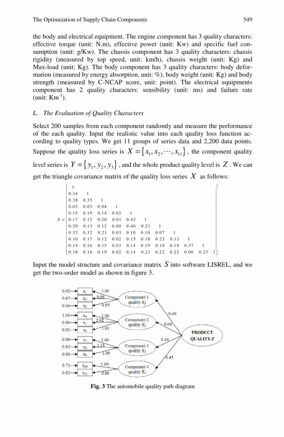
The Optimization of Supply Chain Components 549
the body and electrical equipment. The engine component has 3 quality characters: effective torque (unit: N.m), effective power (unit: Kw) and specific fuel con-sumption (unit: g/Kw). The chassis component has 3 quality characters: chassis rigidity (measured by top speed, unit: km/h), chassis weight (unit: Kg) and Max-load (unit: Kg). The body component has 3 quality characters: body defor-mation (measured by energy absorption, unit: %), body weight (unit: Kg) and body strength (measured by C-NCAP score, unit: point). The electrical equipments component has 2 quality characters: sensibility (unit: ms) and failure rate (unit: Km-1).
L. The Evaluation of Quality Characters
Select 200 samples from each component randomly and measure the performance of the each quality. Input the realistic value into each quality loss function ac-cording to quality types. We get 11 groups of series data and 2,200 data points.
Suppose the quality loss series is { }1 2 11, , ,X x x x= , the component quality
level series is { }1 2 3, ,Y y y y= , and the whole product quality level is Z . We can
get the triangle covariance matrix of the quality loss series X as follows:
1
0 .34 1
0 .38 0 .35 1
0 .02 0 .03 0 .04 1
0 .15 0 .19 0 .14 0 .02 1
0 .17 0 .15 0 .20 0 .01 0 .42 1
0 .20 0 .13 0 .12 0 .00 0 .40 0 .21 1
0 .32 0 .32 0 .21 0 .03 0 .10 0 .10 0 .07 1
0 .10 0 .17 0 .12 0 .02 0 .15 0 .18 0 .23 0 .13 1
0 .14 0 .16 0 .15 0 .03 0 .14 0 .19 0 .18 0 .1 8 0 .37 1
0 .18 0 .16
S =
0 .19 0 .02 0 .14 0 .21 0 .2 2 0 .22 0 .06 0 .23 1
⎡ ⎤⎢ ⎥⎢ ⎥⎢ ⎥⎢ ⎥⎢ ⎥⎢ ⎥⎢ ⎥⎢ ⎥⎢ ⎥⎢ ⎥⎢ ⎥⎢ ⎥⎢ ⎥⎢ ⎥⎢ ⎥⎣ ⎦
Input the model structure and covariance matrix S into software LISREL, and we get the two-order model as shown in figure 3.
Fig. 3 The automobile quality path diagram
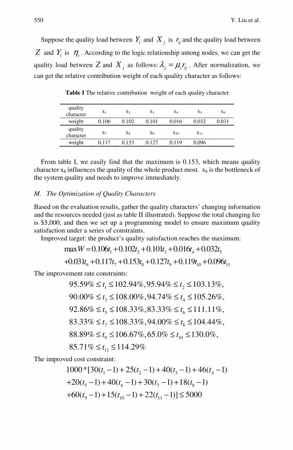
550 Y. Liu et al.
Suppose the quality load between iY and jX is ijr and the quality load between
Z and iY is iη . According to the logic relationship among nodes, we can get the
quality load between Z and jX as follows: j i ijrλ μ= . After normalization, we
can get the relative contribution weight of each quality character as follows:
Table I The relative contribution weight of each quality character
quality character
x1 x2 x3 x4 x5 x6
weight 0.106 0.102 0.101 0.016 0.032 0.031 quality
character x7 x8 x9 x10 x11
weight 0.117 0.153 0.127 0.119 0.096
From table I, we easily find that the maximum is 0.153, which means quality
character x8 influences the quality of the whole product most. x8 is the bottleneck of the system quality and needs to improve immediately.
M. The Optimization of Quality Characters
Based on the evaluation results, gather the quality characters’ changing information and the resources needed (just as table II illustrated). Suppose the total changing fee is $5,000, and then we set up a programming model to ensure maximum quality satisfaction under a series of constraints.
Improved target: the product’s quality satisfaction reaches the maximum:
1 2 3 4 5
6 7 8 9 10 11
max 0.106 0.102 0.101 0.016 0.032
0.031 0.117 0.153 0.127 0.119 0.096
W t t t t t
t t t t t t
= + + + ++ + + + + +
The improvement rate constraints:
1 2
3 4
5 6
7 8
9 10
11
95.59% 102.94%,95.94% 103.13%,
90.00% 108.00%,94.74% 105.26%,
92.86% 108.33%,83.33% 111.11%,
83.33% 108.33%,94.00% 104.44%,
88.89% 106.67%,65.0% 130.0%,
85.71% 114.29%
t t
t t
t t
t t
t t
t
≤ ≤ ≤ ≤≤ ≤ ≤ ≤≤ ≤ ≤ ≤≤ ≤ ≤ ≤≤ ≤ ≤ ≤≤ ≤
The improved cost constraint:
1 2 3 4
5 6 7 8
9 10 11
1000*[30( 1) 25( 1) 40( 1) 46( 1)
20( 1) 40( 1) 30( 1) 18( 1)
60( 1) 15( 1) 22( 1)] 5000
t t t t
t t t t
t t t
− + − + − + −+ − + − + − + −+ − + − + − ≤
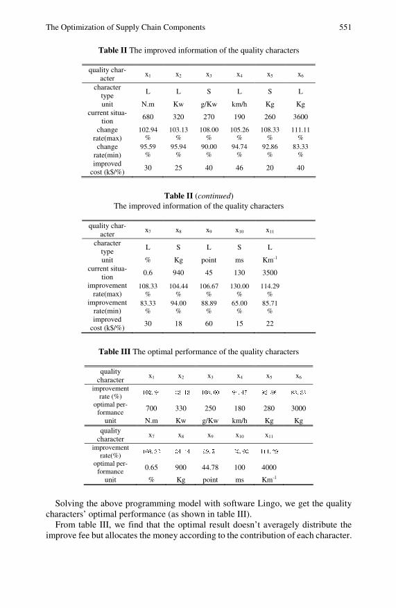
The Optimization of Supply Chain Components 551
Table II The improved information of the quality characters
quality char-acter
x1 x2 x3 x4 x5 x6
character type
L L S L S L
unit N.m Kw g/Kw km/h Kg Kg current situa-
tion 680 320 270 190 260 3600
change rate(max)
102.94%
103.13%
108.00%
105.26%
108.33%
111.11%
change rate(min)
95.59%
95.94%
90.00%
94.74%
92.86%
83.33%
improved cost (k$/%)
30 25 40 46 20 40
Table II (continued)
The improved information of the quality characters
quality char-acter
x7 x8 x9 x10 x11
character type
L S L S L
unit % Kg point ms Km-1 current situa-
tion 0.6 940 45 130 3500
improvement rate(max)
108.33%
104.44%
106.67%
130.00%
114.29%
improvement rate(min)
83.33%
94.00%
88.89%
65.00%
85.71%
improved cost (k$/%)
30 18 60 15 22
Table III The optimal performance of the quality characters
quality
character x1 x2 x3 x4 x5 x6
improvement rate (%)
102.94 103.13 108.00 94.47 92.86 83.33
optimal per-formance 700 330 250 180 280 3000
unit N.m Kw g/Kw km/h Kg Kg quality
character x7 x8 x9 x10 x11
improvement rate(%)
108.33 104.44 99.51 130.00 114.29
optimal per-formance 0.65 900 44.78 100 4000
unit % Kg point ms Km-1
Solving the above programming model with software Lingo, we get the quality
characters’ optimal performance (as shown in table III). From table III, we find that the optimal result doesn’t averagely distribute the
improve fee but allocates the money according to the contribution of each character.

552 Y. Liu et al.
While all the quality characters’ performance is improving, some are weakening,
such as 4 5 6 9, , ,x x x x . Under the optimal schedule, the quality competition of the
product can rise 7.14%, the maximum improvement.
6 Conclusion
Because of various supply chains, kinds of components, numerous enterprises and complex relationships, the quality management for products and components under the M-S production model is more difficult and worthy of analysis and research, but in theory, research and the practical fields, there are few mature and effective methods to handle it. This chapter applies the structural equation model to this field to evaluate the quality characters. The programming model is set up to optimize based on the output of SEM. Lastly, the case study shows the effectiveness of the method, getting a good result.
References
Fynes, B., De Búrca, S.: The effects of design quality on quality performance. International Journal of Production Economics 96, 1–14 (2005)
Han, Z.D., Xiong, D.Q.: Hybrid Petri nets for modeling of manufacturing systems. J. Tsinghua Univ. (Sci. &Tech.) 42, 1429–1432 (2002)
Hou, J.T., Wen, Z.L., Cheng, Z.J.: Structural Equation model and Its Application, pp. 137–145. Educational Science Press, Beijing (2006)
Hsueh, N.L., Chu, P.H., Chu, W.: A quantitative approach for evaluating the quality of design patterns. Journal of Systems and Software 81, 1430–1439 (2008)
Karsak, E.E.: Fuzzy multiple objective programming framework to prioritize design re-quirements in quality function deployment. Computers & Industrial Engineering 47, 149–163 (2004)
Liu, Y., Fang, Z.G.: Study on Production System Performance with Petri Net Analysis Model with Grey Parameters. In: Proceedings of 2007 IEEE International Conference on Grey Systems and Intelligent Services, pp. 1357–1362 (2007)
Powell, S., Pyke, D.F.: Allocation of buffers to serial production lines with bottlenecks. IIE Transactions 28, 18–29 (1996)
Wu, F.C.: Robust design of nonlinear multiple dynamic quality characteristics. Computers & Industrial Engineering 56, 1328–1332 (2008)
The Gap Prediction for the Sci-tech Innovative Talent of Jiangsu Province*
Jianling Wang, Sifeng Liu, and Yun Wang
Sci-tech innovative talent have been the most important source for Jiangsu prov-ince, and prominent achievements of the sci-tech jog have been made. In this chapter, the definition of sci-tech innovative talent is first explored, and the gap between the demand and supply of Jiangsu sci-tech innovative talent is predicted based on GM(1,1). Lastly, some policy suggestions are proposed.
1 Introduction
Sci-tech innovative talent (STIT) are special groups of talent, and their quantity and quality promote scientific and technological progress to a great extent, and they have gradually been attached to great importance by most countries in recent years (Song, 2006). As an eastern coast province, Jiangsu province has an important position in China's development, and great expectations have been taken by the Party Central Committee. While building a well-off society, it has been fully real-ized that sci-tech innovations are based on talented persons, and STIT has been the most important source for Jiangsu province. Technology jobs of Jiangsu having made remarkable achievements, the team of Jiangsu STIT grows gradually, and it has formed a hierarchy of innovative talent, which provides a new impetus and the intellectual support necessary for sustainable development in Jiangsu (Jiangsu Province Science and Technology Agency, 2008). The rules of economic devel-opment also determined that STIT is the primary resource for the development of Jiangsu during the new era, so it’s of great significance to build the STIT team. In addition, it will be a useful implication to other provinces. Jianling Wang Economics and Management College, Nanjing University of Aeronautics and Astronautics, 29 Yudao Street, Nanjing City, Jiangsu Province 210016, China e-mail: [email protected] Sifeng Liu and Yun Wang Economics and Management College, Nanjing University of Aeronautics and Astronautics, 29 Yudao Street, Nanjing City, Jiangsu Province 210016, China * This work was supported in part by the Soft Science of Jiangsu Province under grant
SBR200950.

554 J. Wang, S. Liu, and Y. Wang
At present, there are no commonly accepted concepts of innovative talent and STIT. Generally, it’s agreed that to judge whether a person belongs to the innova-tive talent, the standard does not lie in his career nor in high or low positions and qualifications, but it lies in whether he is innovative in what he is assigned to do, and studious with research and practice, and if he achieved outstanding innovations (Liu, 2008; Wang et al., 2006; Mm , and Tan, 2002). We believe that STIT has a high scientific and technological innovation capacity, as well as a long-term sus-tainability to engage in scientific discovery and research and development activi-ties. Their performance is mainly reflected in certain scientific and technological achievements. They promote scientific and technological progress and social de-velopment.
In China, statistical significant terms for STIT have not yet been made. As for the "[China’s] Statistical Yearbook" and the "Statistical Yearbook of Science & Technology of China," 3 relevant groups correspond to the group of STIT: staff of scientific and technological activities (T&S S), staff of research and experimental development (R&D S), and staff of scientists and engineers (S&E S). T&S S are those who are engaged in or participate in scientific and technological activities directly, as well as scientific and technological management and service providing staff. S&E S are those who graduate from universities with high academic quali-fications or above or are with a senior primary professional title. They are the core of science and technology staff. R&D S are those who are engaged in innovative scientific research. In short, T&S S, R&D S and S&E S are the mainstays of STIT, reflecting the structure and hierarchy of STIT.
In this chapter, the STIT Status Quo of Jiangsu is analyzed thoroughly based on the definition of STIT, and the future status is predicted by GM (1, 1). At last, the conclusion and a suggestion are given.
2 The Status Quo pf Jiangsu STIT
Jiangsu has made remarkable achievements on the cultivation of STIT, with a dramatic increase of both the quantity and quality. According to "The Monitoring Results of Jiangsu Province of Scientific and Technological Progress and Tech-nology Statistics Statistical Bulletin" and the "Jiangsu Statistical Yearbook" (Ji-angsu Province Science and Technology Agency, 2002-2007; Tan and Luo, 2003; Pu and Xi, 2007), it’s found that Jiangsu STIT show the following characteristics:
A. The quantity and quality of Jiangsu STIT rank at the top among ones in China
In recent years, the sci-tech jobs of Jiangsu have achieved remarkable results, and the comprehensive assessment has ranked second nationwide in China. Not only is the STIT quantity of Jiangsu among the most of the provinces, but it also has cul-tivated groups of leading STIT in different areas. At present, there are 3413 thou-sand professional technical personnel and 395 thousand T&S S, which rank in the top two in China. Among those, there are 140 thousand R&D S and 240 thousand S&E S, which rank in the top three in China. While the scale of Jiangsu STIT is gradually growing, the talent reservation is substantial.
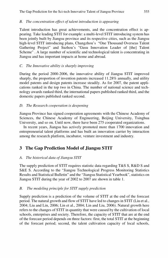
The Gap Prediction for the Sci-tech Innovative Talent of Jiangsu Province 555
B. The concentration effect of talent introduction is appearing
Talent introduction has great achievements, and the concentration effect is ap-pearing. Take leading STIT for example: a multi-level STIT introducing system has been jointly built by Jiangsu province and its respective cities, such as the Jiangsu high-level STIT introducing plans, Changzhou’s “One Thousand Overseas Talent Gathering Project” and Suzhou’s "Gusu Innovation Leader of [the] Talent Scheme" . A large number of scientific and technological talent is concentrating in Jiangsu and has important impacts at home and abroad.
C. The Innovative ability is sharply improving
During the period 2000-2006, the innovative ability of Jiangsu STIT improved sharply, the proportion of invention patents increased 11.28% annually, and utility model patents and design patents increase steadily. As for 2007, the patent appli-cations ranked in the top two in China. The number of national science and tech-nology awards ranked third, the international papers published ranked third, and the domestic papers published ranked second.
D. The Research cooperation is deepening
Jiangsu Province has signed cooperation agreements with the Chinese Academy of Sciences, the Chinese Academy of Engineering, Beijing University, Tsinghua University, and so on. Until now, there have been 275 cooperated organizations.
In recent years, Jiangsu has actively promoted more than 1700 innovation and entrepreneurial talent platforms and has built an innovation carrier by interaction among the research platform, incubator, venture investment and industry.
3 The Gap Prediction Model of Jiangsu STIT
A. The historical data of Jiangsu STIT
The supply prediction of STIT requires statistic data regarding T&S S, R&D S and S&E S. According to the “Jiangsu Technological Progress Monitoring Statistics Results and Statistical Bulletin” and the “Jiangsu Statistical Yearbook”, statistics on Jiangsu STIT during the year of 2002 to 2007 are shown in table 1.
B. The modeling principle for STIT supply prediction
Supply prediction is a prediction of the volume of STIT at the end of the forecast period. The natural growth and flow of STIT have led to changes in STIT (Liu et al., 2004; Liu and Lin, 2006; Lin et al., 2004; Lin and Liu, 2006). Natural growth here refers to the changes of STIT in quantity that were caused by the cultivation of local schools, enterprises and society. Therefore, the capacity of STIT that are at the end of the forecast period depends on three factors: first, the total STIT at the beginning of the forecast period; second, the talent cultivation capacity of local schools,
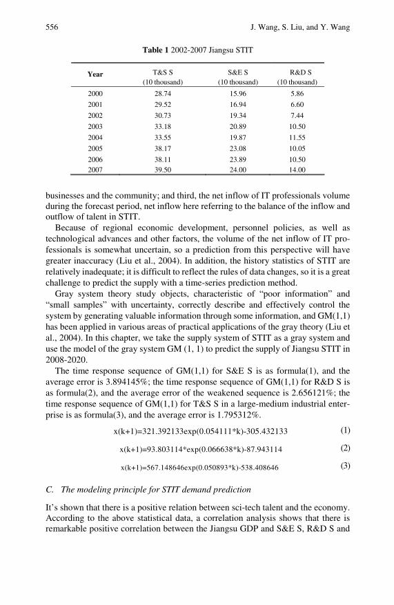
556 J. Wang, S. Liu, and Y. Wang
Table 1 2002-2007 Jiangsu STIT
T&S S S&E S R&D S Year (10 thousand) (10 thousand) (10 thousand)
2000 28.74 15.96 5.86
2001 29.52 16.94 6.60
2002 30.73 19.34 7.44
2003 33.18 20.89 10.50
2004 33.55 19.87 11.55
2005 38.17 23.08 10.05
2006 38.11 23.89 10.50 2007 39.50 24.00 14.00
businesses and the community; and third, the net inflow of IT professionals volume during the forecast period, net inflow here referring to the balance of the inflow and outflow of talent in STIT.
Because of regional economic development, personnel policies, as well as technological advances and other factors, the volume of the net inflow of IT pro-fessionals is somewhat uncertain, so a prediction from this perspective will have greater inaccuracy (Liu et al., 2004). In addition, the history statistics of STIT are relatively inadequate; it is difficult to reflect the rules of data changes, so it is a great challenge to predict the supply with a time-series prediction method.
Gray system theory study objects, characteristic of “poor information” and “small samples” with uncertainty, correctly describe and effectively control the system by generating valuable information through some information, and GM(1,1) has been applied in various areas of practical applications of the gray theory (Liu et al., 2004). In this chapter, we take the supply system of STIT as a gray system and use the model of the gray system GM (1, 1) to predict the supply of Jiangsu STIT in 2008-2020.
The time response sequence of GM(1,1) for S&E S is as formula(1), and the average error is 3.894145%; the time response sequence of GM(1,1) for R&D S is as formula(2), and the average error of the weakened sequence is 2.656121%; the time response sequence of GM(1,1) for T&S S in a large-medium industrial enter-prise is as formula(3), and the average error is 1.795312%.
x(k+1)=321.392133exp(0.054111*k)-305.432133 (1)
x(k+1)=93.803114*exp(0.066638*k)-87.943114 (2)
x(k+1)=567.148646exp(0.050893*k)-538.408646 (3)
C. The modeling principle for STIT demand prediction
It’s shown that there is a positive relation between sci-tech talent and the economy. According to the above statistical data, a correlation analysis shows that there is remarkable positive correlation between the Jiangsu GDP and S&E S, R&D S and
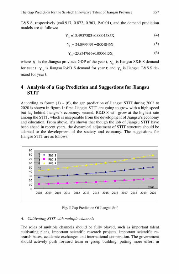
The Gap Prediction for the Sci-tech Innovative Talent of Jiangsu Province 557
T&S S, respectively (r=0.917, 0.872, 0.963, P<0.01), and the demand prediction models are as follows:
1 t tY =13.4937303+0.0004585X (4)
2 t tY =-24.0997099 . 4046X +000 (5)
3 t tY =23.8347616+0.0006615X (6)
where tX is the Jiangsu province GDP of the year t,
1 tY is Jiangsu S&E S demand
for year t; 2 tY is Jiangsu R&D S demand for year t; and
3 tY is Jiangsu T&S S de-
mand for year t.
4 Analysis of a Gap Prediction and Suggestions for Jiangsu STIT
According to forum (1) ~ (6), the gap prediction of Jiangsu STIT during 2008 to 2020 is shown in figure 1: first, Jiangsu STIT are going to grow with a high speed but lag behind Jiangsu’s economy; second, R&D S will grow at the highest rate among the STIT, which is inseparable from the development of Jiangsu’s economy and education. From above, it’s shown that though the job of Jiangsu STIT have been ahead in recent years, the dynamical adjustment of STIT structure should be adapted to the development of the society and economy. The suggestions for Jiangsu STIT are as follows:
0102030405060708090
2008 2009 2010 2011 2012 2013 2014 2015 2016 2017 2018 2019 2020
year
10 t
hous
and
S&E SR&D SS&T S
Fig. I Gap Prediction Of Jiangsu Stif
A. Cultivating STIT with multiple channels
The roles of multiple channels should be fully played, such as important talent cultivating plans, important scientific research projects, important scientific re-search bases, academic exchanges and international cooperation. The government should actively push forward team or group building, putting more effort in
558 J. Wang, S. Liu, and Y. Wang
fostering an academic leader and key technology staff, and perfecting the rules and system of training and selecting high-level innovation talent.
B. Encouraging independent innovation
The whole society is not very confident for producing indigenous local innovative products, so the opportunity is uncertain for them to be chosen in government and enterprise procurement. Under these circumstances, even if some independent innovations are proven to be a technological breakthrough, enterprise profit is still hard. Therefore, the government should enhance supporting independent innovat-ing products, recommend these products to be listed in the export catalog of new high technology products, invest more in introducing technology and equipments, and encourage the exportation of re-innovation enterprises by using economical instruments like taxation and the exchange rate.
C. Perfecting the achievements transformation platform
The incubator, science and technology parks play important roles in STIT con-structing, venture capitalism, the infrastructure and service system to directly promote the job, which cannot be ignored, so the hardware building of STIT should first be strengthen. Accompanied with these strategies, the innovation service quality should be enhanced, and the interaction mechanisms should be explored deeply.
References
Jiangsu Province Science and Technology Agency. Jiangsu Province: Results of Statistical Monitoring Progress of Science and Technology. Science and Technology Statistical Bulletin (2002-2007)
Jiangsu Province Science and Technology Agency. Implementing the Scientific Develop-ment Concept Analysis. Report by Provincial Science and Technology Agency Leaders Team (2008)
Lin, Y., Chen, M.Y., Liu, S.F.: Theory of grey systems: capturing uncertainties of grey information. Kybernetes: The International Journal of Systems and Cybernetics 33(2), 196–218 (2004)
Lin, Y., Liu, S.F.: Solving problems with incomplete information: A grey systems approach. In: Advances in Imaging and Electron Physics, vol. 141, pp. 77–174. Elsevier, Oxford (2006)
Liu, S.F., Dang, Y.G., Fang, Z.G.: Grey System Theory and Its Applications, 3rd edn. Sci-ence Press, Beijing (2004)
Liu, S.F., Lin, Y.: Grey Information: Theory and Practical Applications. Springer, London (2006)
Liu, X.N.: The connotation enterprise technological innovation and quality analysis. Pro-ductivity Research (1), 129–131 (2008)
Mm, L.N., Tan, G.X.: Regarding the management of innovation talent. Discussion about theory (5), 55–56 (2002)

The Gap Prediction for the Sci-tech Innovative Talent of Jiangsu Province 559 Pu, X.L., Xi, Q.: Nantong “Eleventh Five-Year” period, the supply and demand of IT
manpower forecasting and gap analysis. Technology and Industry 7(3), 34–38 (2007) Song, K.Q.: Foreign technological innovation of environmental studies. Economic and
Management Research (2), 29–33 (2006) Tan, T.T., Luo, J.L.: Shanghai science and technology talent shortage prediction. Scientific
Study of Science and Technology Management 24(8), 77–79 (2003) Wang, R.L., Liu, S.F., Gu, J.Q.: Jiangsu Province: The flow of innovative talent cost-benefit
analysis. Industrial Techno-Economics (3), 16–18 (2006)

Community Degree, Clustering Coefficient and Knowledge Propagation Efficiency in Complex Networks*
Wenping Wang, Qiuying Shen, and Yuqing Chen
The impact of complex network structure on knowledge propagation is currently one of the hotspots in complex network research. Based on the SIR epidemic model and mean-field theory of dynamical physics, this chapter conducts the research into the law of how the community degree and clustering coefficient influence the knowledge propagation efficiency in complex networks. The research discovered that when the clustering coefficient is below a certain value, there exists a network community degree threshold; when the network community degree is lower than the threshold, the knowledge propagation efficiency decreases as the community degree increases; when the network community degree is higher than the threshold, the knowledge propagation efficiency increases as the community degree increases, meaning the relationship between the two follows a "U-type" curve; when the clustering coefficient is higher than a certain value, the relationship between them monotonically increases.
1 Introduction
Knowledge and ability are the roots of organizational competitive advantage (Zahra et al., 1999), and knowledge propagation is the premise of organizational knowl-edge integration and ability building. The behavior of economic subjects is em-bedded in concrete and real-time complex networks (Granovetter, 1985), and knowledge is also contained in the network and community (Landry et al., 2002). The network is the structural basis for knowledge propagation among subjects. Therefore, to study the influence relationship between complex networks, structural characteristics and knowledge propagation is of great significance. Knowledge propagation is achieved through the connection among nodes, but then, what is the Wenping Wang School of Economics and Management, Southeast University, Nanjing 210096, China Phone: 0086-025-83426299; Fax: 0086-025-52090702 e-mail: [email protected]
Qiuying Shen and Yuqing Chen School of Economics and Management, Southeast University, Nanjing 210096, China * This work was sponsored by the National Science Fund (70571013, 70973017) and the
New Century Excellent Talent of Education Ministry (NECT-06-0471).
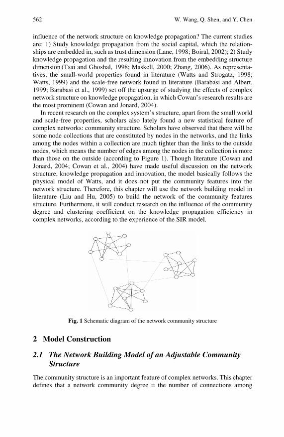
562 W. Wang, Q. Shen, and Y. Chen
influence of the network structure on knowledge propagation? The current studies are: 1) Study knowledge propagation from the social capital, which the relation-ships are embedded in, such as trust dimension (Lane, 1998; Boiral, 2002); 2) Study knowledge propagation and the resulting innovation from the embedding structure dimension (Tsai and Ghoshal, 1998; Maskell, 2000; Zhang, 2006). As representa-tives, the small-world properties found in literature (Watts and Strogatz, 1998; Watts, 1999) and the scale-free network found in literature (Barabasi and Albert, 1999; Barabasi et al., 1999) set off the upsurge of studying the effects of complex network structure on knowledge propagation, in which Cowan’s research results are the most prominent (Cowan and Jonard, 2004).
In recent research on the complex system’s structure, apart from the small world and scale-free properties, scholars also lately found a new statistical feature of complex networks: community structure. Scholars have observed that there will be some node collections that are constituted by nodes in the networks, and the links among the nodes within a collection are much tighter than the links to the outside nodes, which means the number of edges among the nodes in the collection is more than those on the outside (according to Figure 1). Though literature (Cowan and Jonard, 2004; Cowan et al., 2004) have made useful discussion on the network structure, knowledge propagation and innovation, the model basically follows the physical model of Watts, and it does not put the community features into the network structure. Therefore, this chapter will use the network building model in literature (Liu and Hu, 2005) to build the network of the community features structure. Furthermore, it will conduct research on the influence of the community degree and clustering coefficient on the knowledge propagation efficiency in complex networks, according to the experience of the SIR model.
Fig. 1 Schematic diagram of the network community structure
2 Model Construction
2.1 The Network Building Model of an Adjustable Community Structure
The community structure is an important feature of complex networks. This chapter defines that a network community degree = the number of connections among

Community Degree, Clustering Coefficient and Knowledge Propagation Efficiency 563
inter-community nodes / the number of connections among nodes within the community (Liu and Hu, 2005), which is denoted by p . This chapter makes use of
the network building model in literature (Liu and Hu, 2005), which can adjust the size of community identity p dynamically, and the degree distribution function
is 122
22)(
−−
−−
−= p
m
p
m
kp
mkP ( m denotes that the new joining node is connected to m
nodes in the community), so the degree distribution )(kP is controlled
by p ( 0 1p< < ) (Liu and Hu, 2005) and the clustering coefficient of complex
networks is (1 / ) * ii
C N C= ∑ , in which 2 / ( ( 1))i i i iC E k k= − , iE is the
total connection number of node i’s ik neighbor nodes, the clustering coefficient is
the probability that the two nodes connected to the same node are also connected in the network (Liu, 2004). The network building model can adjust the network
structure parameter q at the same time, because iE and q are directly propor-
tional (Liu and Hu, 2005), so qC ~ and the network structure parameter q in-
directly determines the network clustering coefficient C ( 0 1q< < ).
2.2 SIR Model for Knowledge Propagation
This chapter assumes that knowledge of network nodes only propagates through the connection among nodes. It does not take into account the impact of the distance between nodes on knowledge propagation, nor does it take into account the impact of propagation time. We refer to the SIR epidemic model (Anderson and May, 1991), which assumes that for a certain knowledge, each node in the network has
three states ( 1A , 2A , 3A ), in which: state 1A (does not have that kind of knowl-
edge); State 2A (temporarily receives the knowledge through the propagation
path); and State 3A (perpetually owns the knowledge through digestion and ab-
sorption). β is the probability of the node knowledge’s propagation to the con-
nected other. Depending on the encoded degree of knowledge, knowledge can be divided into explicit knowledge and tacit knowledge. The explicit knowledge can be encoded for transmission, while tacit knowledge can not. Because the tacit knowledge is of high embedded nature, the explicit knowledge can be propagated more easily in the network than the tacit knowledge, so the propagation probability of explicit knowledge in the network is greater than the probability of tacit knowledge.
Without the loss of generality, assume that the propagation probability of explicit knowledge in the network β = 0.9, and the propagation probability of tacit knowl-
edge β = 0.5. Suppose that there’s only one node in the network initially owning
certain knowledge. The node will propagate its knowledge to the connected nodes
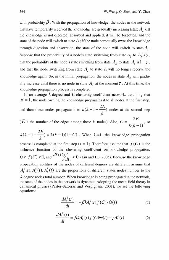
564 W. Wang, Q. Shen, and Y. Chen
with probability β . With the propagation of knowledge, the nodes in the network
that have temporarily received the knowledge are gradually increasing (state 2A ). If
the knowledge is not digested, absorbed and applied, it will be forgotten, and the
state of the node will switch to state 1A ; if the node perpetually owns the knowledge
through digestion and absorption, the state of the node will switch to state 3A .
Suppose that the probability of a node’s state switching from state 2A to 3A isγ ,
that the probability of the node’s state switching from state 2A to state 1A is1 γ− ,
and that the node switching from state 2A to state 1A will no longer receive the
knowledge again. So, in the initial propagation, the nodes in state 2A will gradu-
ally increase until there is no node in state 2A at the momentτ . At this time, the
knowledge propagation process is completed. In an average k degree and C clustering coefficient network, assuming that
1=β , the node owning the knowledge propagates it to k nodes at the first step,
and then these nodes propagate it to )2
1(k
Ekk −− nodes at the second step
( E is the number of the edges among these k nodes). Also, )1(
2
−=
kk
EC , so
)2
1(k
Ekk −− = )1)(1( Ckk −− . When C =1, the knowledge propagation
process is completed at the first step ( 1=t ). Therefore, assume that )(Cf is the
influence function of the clustering coefficient on knowledge propagation,
,1)(0 << Cf and 0)( <dCCdf
(Liu and Hu, 2005). Because the knowledge
propagation abilities of the nodes of different degrees are different, assume that
1 2 3( ), ( ), ( )k k kA t A t A t are the proportions of different states nodes number to the
k degree nodes total number. When knowledge is being propagated in the network, the state of the nodes in the network is dynamic. Adopting the mean-field theory in dynamical physics (Pastor-Satorras and Vespignani, 2001), we set the following equations:
11
( )( ) ( ) ( )
kkdA t
kA t f C tdt
β= − ⋅Θ (1)
21 2
( )( ) ( ) ( ) ( )
Kk kdA t
kA t f C t A tdt
β γ= Θ − (2)
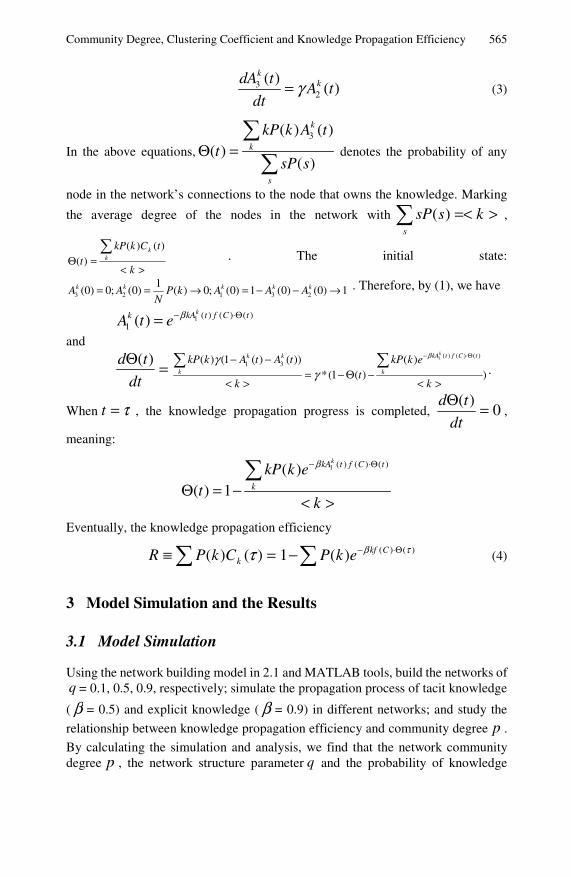
Community Degree, Clustering Coefficient and Knowledge Propagation Efficiency 565
32
( )( )
kkdA t
A tdt
γ= (3)
In the above equations,3( ) ( )
( )( )
k
k
s
kP k A tt
sP sΘ =
∑∑
denotes the probability of any
node in the network’s connections to the node that owns the knowledge. Marking
the average degree of the nodes in the network with ∑ >=<s
kssP )( ,
><=Θ∑
k
tCkkPt k
k )()()( . The initial state:
3 2 1 3 2
1(0) 0; (0) ( ) 0; (0) 1 (0) (0) 1k k k k kA A P k A A A
N= = → = − − → . Therefore, by (1), we have
1 ( ) ( ) ( )1 ( )
kkA t f C tkA t e β− ⋅Θ=
and
=Θdt
td )( 1 ( ) ( ) ( )1 3( ) (1 ( ) ( )) ( )
*(1 ( ) )
kkA t f C tk k
k k
kP k A t A t kP k et
k k
βγγ
− ⋅Θ− −= − Θ −
< > < >
∑ ∑.
When τ=t , the knowledge propagation progress is completed, 0)( =Θ
dt
td,
meaning:
1 ( ) ( ) ( )( )( ) 1
kkA t f C t
k
kP k et
k
β− ⋅Θ
Θ = −< >
∑
Eventually, the knowledge propagation efficiency
=≡∑ )()( τkCkPR ( ) ( )1 ( ) kf CP k e β τ− ⋅Θ−∑ (4)
3 Model Simulation and the Results
3.1 Model Simulation
Using the network building model in 2.1 and MATLAB tools, build the networks of q = 0.1, 0.5, 0.9, respectively; simulate the propagation process of tacit knowledge
( β = 0.5) and explicit knowledge ( β = 0.9) in different networks; and study the
relationship between knowledge propagation efficiency and community degree p .
By calculating the simulation and analysis, we find that the network community degree p , the network structure parameter q and the probability of knowledge
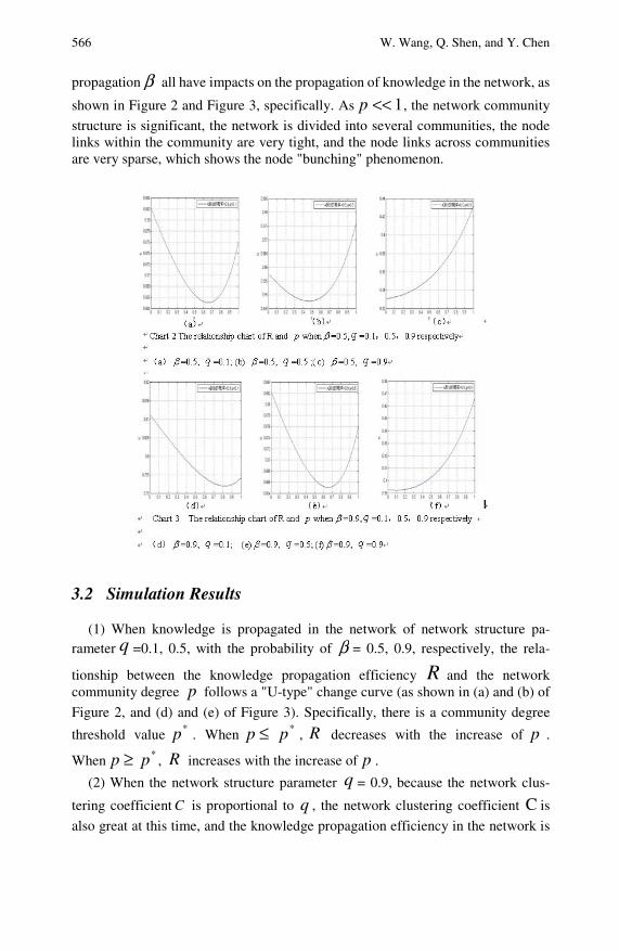
566 W. Wang, Q. Shen, and Y. Chen
propagation β all have impacts on the propagation of knowledge in the network, as
shown in Figure 2 and Figure 3, specifically. As 1<<p , the network community
structure is significant, the network is divided into several communities, the node links within the community are very tight, and the node links across communities are very sparse, which shows the node "bunching" phenomenon.
3.2 Simulation Results
(1) When knowledge is propagated in the network of network structure pa-rameter q =0.1, 0.5, with the probability of β = 0.5, 0.9, respectively, the rela-
tionship between the knowledge propagation efficiency R and the network community degree p follows a "U-type" change curve (as shown in (a) and (b) of
Figure 2, and (d) and (e) of Figure 3). Specifically, there is a community degree
threshold value *p . When p ≤ *p , R decreases with the increase of p .
When p ≥ *p , R increases with the increase of p .
(2) When the network structure parameter q = 0.9, because the network clus-
tering coefficient C is proportional to q , the network clustering coefficient C is
also great at this time, and the knowledge propagation efficiency in the network is
Community Degree, Clustering Coefficient and Knowledge Propagation Efficiency 567
an increasing function of the community degree p (as shown in (c) of Figure 2 and
(f) of Figure 3). (3) When the network structure parameter q is set, the tacit knowledge and ex-
plicit knowledge are propagated in the network with the probability of 0.5 and 0.9, respectively. Compare Figure 2 (a) to Figure 3 (d) and Figure 2 (b) to Figure 3 (e),
and we find that the community degree threshold value *p corresponding to the
lowest point of the knowledge propagation efficiency curve shifts to the right with an increase of the knowledge propagation probability. When knowledge (tacit knowledge or explicit knowledge) is propagated in different networks ( q =0.1 and
q =0.5), compare Figure 2 (a) to (b), or Figure 3 (d) to (e), and we find that with the
increase of q , because the clustering coefficient C is proportional to parame-
ter q , C also increases, and the community degree threshold value *p corre-
sponding to the minimum of knowledge propagation efficiency in the network shifts to the left.
4 Conclusions and Future Research
With the above model and the simulation results, we can obtain the following conclusions:
1) The network clustering coefficient impacts the relationship between knowl-edge propagation efficiency and the network community degree. When the clus-tering coefficient is below a certain value, the relationship follows a "U-type" curve, and there exists a community degree threshold value at this time. As the network community degree is lower than the threshold value, the knowledge propagation efficiency decreases with the increase of the community degree. As the network community degree is higher than the threshold value, the knowledge propagation efficiency increases with the increase of the community degree. When the cluster-ing coefficient is higher than a certain value, the relationship between knowledge propagation efficiency and the network community degree monotonically in-creases, meaning the knowledge propagation efficiency increases monotonically with an increase in the network community degree.
As the network clustering coefficient increases, the probability of the connection of the two nodes that are connected to the same node in the network is high. At this time, as the network community degree increases, the network becomes more akin to the regular network, so the knowledge propagation efficiency in the network becomes higher. For example, in the World Wide Web, which is approximate to the regular network, when a message appears on a website, it is quickly reproduced on other sites as the result of the network structure of the World Wide Web, and it becomes com-mon news. The high propagation efficient makes people "breathtaking."
2) In the knowledge propagation process, the size of the network clustering co-efficient impacts the community degree threshold value in the above conclusions. As the network clustering coefficient increases, the community degree threshold
568 W. Wang, Q. Shen, and Y. Chen
value in the relationship between the knowledge propagation efficiency and the network community degree decreases.
3) The knowledge characteristics of the network (knowledge explicit degree) impact the community degree threshold value in the relationship between the knowledge propagation efficiency and the network community degree. As the knowledge explicit degree increases, the knowledge propagation probability in-creases, and the community degree threshold value in the above conclusions increases.
The above conclusions indicate that the network structure impacts knowledge propagation, and specific network architecture helps to improve the knowledge propagation efficiency. This research can provide the theoretical basis for enter-prises to build and optimize their network structure and thus improve their knowledge propagation efficiency. In addition, this chapter conducts research on the impact of network structure on knowledge propagation on the basis of a static network. In fact, with the interaction of network nodes, the interactive history will make the nodes have different degrees of trust with the other nodes, thus resulting in different effects of different network connections on knowledge propagation, namely, the heterogeneity of network relationships. Researching into laws between the community degree and knowledge propagation efficiency is still an issue for further study. In addition, adjusting and optimizing the network structure to im-prove the knowledge propagation efficiency based on the above findings is also for future research.
References
Anderson, R.M., May, R.M.: Infectious Diseases of Humans: Dynamics and Control. Oxford University Press, Oxford (1991)
Audretsch, D.B., Feldman, M.P.: Knowledge spillovers and the geography of innovation and production. American Economic Review 86(3), 630–640 (1996)
Baptista, R.: Do innovations diffuse faster within geographical clusters. International Journal of Industrial Organization 18(3), 515–535 (2000)
Barabasi, A.L., Albert, R.: Emergence of scaling in random networks. Science 286(5439), 509–512 (1999)
Barabasi, A.L., Albert, R., Jeong, H.: Mean-field theory for scale-free random networks. Phys. A 272(1), 173–187 (1999)
Boiral, O.: Tacit knowledge and environmental management. Long Range Planning 35(3), 291–317 (2002)
Cowan, R., Jonard, N.: Network structure and the diffusion of knowledge. Journal of Eco-nomic Dynamics & Control 28(8), 1557–1575 (2004)
Cowan, R., Jonard, N., Ozman, M.: Knowledge dynamics in a network industry. Techno-logical Forecasting & Social Change 71(5), 469–484 (2004)
Jaffe, A., Trajtenberg, M., Henderson, R.: Geographic localization of knowledge spillovers as evidenced by patent citations. Quarterly Journal of Economics 108(3), 577–598 (1993)
Granovetter, M.: Economic action and social structure: The problem of embeddedness. American Journal of Sociology 91(3), 481–510 (1985)
Lane, L.: Relative absorptive capacity and inter-organizational learning. Strategic Man-agement Journal 19(5), 461–477 (1998)

Community Degree, Clustering Coefficient and Knowledge Propagation Efficiency 569 Landry, R., Amara, N., Lamari, M.: Does social capital determine innovation? To what
extent. Technological Forecasting and Social Change 69(7), 681–701 (2002) Liu, J.: Introduction to Social Network Analysis. Social Science literature Press, Beijing
(2004) Liu, Z.H., Hu, B.B.: Epidemic spreading in community networks. Europhys. Lett. 72(2),
315–321 (2005) Maskell, P.: Social capital, innovation and competitiveness. In: Baron, S., Field, J., Schuller,
T. (eds.) Social capital, Critical Perspectives. Oxford University Press, Oxford (2000) Pastor-Satorras, R., Vespignani, A.: Epidemic spreading in scale-free networks. Phys. Rev.
Lett. 86(14), 3200–3203 (2001) Tsai, W., Ghoshal, S.: Social capital and value creation: The role of intra-firm networks.
Academy of Management Journal 41(4), 464–476 (1998) Watts, D.: Dynamics and the small-world phenomenon. American Journal of Sociol-
ogy 105(2), 493–527 (1999) Watts, D., Strogatz, S.: Collective dynamics of small-world networks. Nature 393(6684),
440–442 (1998) Zahra, S.A., Nielsen, A.P., Bogner, W.C.: Corporate entrepreneurship, knowledge, and
competence development. Entrepreneurship: Theory & Practice 23(3), 169–189 (1999) Zhang, F.H.: Study on the relationship between knowledge-based firm’s social capital and
knowledge acquisition. Studies in Science of Science 24(1), 106–111 (2006)
A Study on E-Government Information Sharing*
Zhijun Yan, Baowen Sun, and Tianmei Wang
Information sharing is of vital importance in cross-organizational collaboration. It can help achieve many important public benefits. From the integrated view of the technology system and trust, this chapter analyzes the influential factors of e-government information sharing. Derived from the DeLone & McLean model and Technology Acceptance Model (TAM), information quality, information use, perceived benefit, trust, perceived usefulness and perceived ease of use are proposed as antecedents of the users’ intention to share information. Then, the research model is given and the research hypotheses are derived.
1 Introduction
Information is one of the most important resources in the public and private sectors. It is asserted that information needs to be well regulated to improve organizational efficiency. For public government agencies, information sharing is a crucial factor to achieving important public benefits: increased productivity, improved policymaking and integrated public services (Dawes, 1996). Fundamentally, sharing information reduces the "paperwork burden" on citizens, streamlines work processes, and enriches the formulation, implementation, and evaluation of policy (Landsbergen, Jr. and Wolken, Jr., 2001). Although there are many obvious advantages for information sharing, the existing barriers significantly impede the information sharing process across organizational boundaries. For example, the perceived risk is recognized as one major barrier that decreases user involvement with information sharing. Many scholars have studied the factors that affect Zhijun Yan School of Management and Economics, Beijing Institute of Technology, Beijing 100081, P.R. China, Phone: 0086-10-68914219; Fax: 0086-10-68914219 e-mail: [email protected]
Baowen Sun and Tianmei Wang School of Information, Central University of Finance and Economics, Beijing 100081, P.R. China e-mail: [email protected], [email protected]
* This work was supported in part by the Humanities & Social Sciences Key Project of the Ministry of Education of China (Grant No. 07JZD0019) and the National Science Foundation of China (Grant No.70872119).
572 Z. Yan, B. Sun, and T. Wang
information sharing from many distinct aspects, such as organizational culture (Drake et al., 2004), employee belief (Kolekofski and Heminger, 2003) and trust scheme (Peng Liu, 2005). Different from previous research, this chapter analyzes the influential factors of information sharing from the integrated view of the technology system and trust, and it proposes the hypothesis research model based on the updated DeLone & McLean information systems success model.
The chapter is organized as follows: Section 2 gives a literature review on information sharing in the e-government. The theory base of our research work is presented in section 3. Then, section 4 introduces the research model, and the research hypotheses are derived. The conclusions and further works are described in section 5.
2 Literature Review
Information sharing is a hot topic in e-government research and receives more attention from many scholars. This section only sheds light on some of such scholars’ literature.
As one of the most cited references, Dawes’s article states that information sharing is often limited by technical, organizational, and political barriers. The attitudes and opinions of state government managers on information sharing were analyzed. The result showed that more than 8 in 10 judge information sharing to be moderately to highly beneficial. Based on the survey results, a theoretical model for understanding how policy, practice, and attitudes interact was proposed. And the model also suggested two policy principles, stewardship and usefulness, to promote the benefits and mitigate the risks of information sharing (Dawes, 1996).
Extending from the research result of Dawes, Landsbergen analyzed the benefits and barriers of interoperability, which means the talking and sharing of information. Differing from Dawes’ model, Landsbergen gave a three-stage theoretical model. The first stage is the theoretical model of individual agency-to-agency information sharing. The second stage concerns the infrastructure to support information sharing. The last stage focuses on the synthesis of legal, managerial and policy approaches to interoperability sharing (Landsbergen, Jr. and Wolken, Jr., 2001).
Seung investigated the influence of cultural factors on information sharing in China. They postulated that social network structures such as guanxi, Confucian dynamism,and collectivism could explain the degree to which information sharing took place between people in China. Then they administrated a survey to 140 high-level managers, general managers, and deputy general mangers in Chinese enterprises. The data analysis results confirmed their research hypothesis, which was that guanxi, Confucian dynamism and collectivism both have a significant influence on information sharing in China (Shin et al., 2007).
Based upon the theory of reasoned action (TRA), Keith proposed a model that defines the influential factors of one’s intent to share information in a governmental organization. The research model was tested by surveying the workers in a unit of a large governmental organization that often fails to reap the benefits. The study suggests that stewardship attitude, instrumentality of sharing information and interpersonal feelings are three key factors that managers should address when
A Study on E-Government Information Sharing 573
striving to encourage wider sharing of organizational information (Kolekofski and Heminger, 2003).
J. Ramon Gil-Garcia proposed that expected benefits are an important reason for starting information sharing among government organizations and that potential impediments will limit the attainment of information-sharing projects’ benefits, jeopardizing the project’s business case and even the project itself. Using data from six public sector information-sharing projects, they revealed how some managerial and cultural impediments limit the perceptions of expected benefits. The three major managerial and cultural impediments are the controlled-oriented management style, lack of agreement on goals and the perception of management impatience (Gil-Garcia et al., 2007).
Theresa reported a comparative examination of knowledge sharing in two separate networks of public sector organizations participating in information technology innovation projects in the state of New York. Using interviews, observations and the document analysis method, the case studies follow knowledge sharing and other interactions in the inter-organizational networks of these two distinct settings. Their results confirm the difficulty of sharing knowledge across agencies and further reveals the influence of several relevant factors—incentives, risks and barriers for sharing, and trust—on the effectiveness of knowledge sharing (Pardo et al., 2006).
Soonhee Kim discussed the impact of organizational context and IT on employees’ perceptions of knowledge-sharing capabilities. He proposed that three dimensions—organizational culture, organizational structure and information technology—are related to employee knowledge-sharing capabilities. Through the survey of 322 employees in five public sector and five private sector organizations in South Korea, the research found that social networks, centralization, performance-based reward systems, employee usage of IT applications, and user-friendly IT systems significantly affect employee knowledge-sharing capabilities in the organizations studied (Soonhee Kim, 2006).
Based on an interview with local government leaders, a literature review in a related field and the innovation diffusion theory, Hu put forth three main factors that influence information sharing among departments of the local government in China, including the resources, drives and cognitions of information sharing. Then, Hu investigated 50 government departments in a medium city in China and validated the effect of these three influential factors of information sharing (Hu et al., 2007).
3 Theoretical Framework
A. DeLone & McLean Information Systems Success Model
The DeLone & McLean information systems success model is a framework and model for measuring the complex-dependent variable in IS research (DeLone and McLean, 1992). DeLone and McLean first conceptualize their model in three hierarchical levels: a technical level, a semantic level, and an effectiveness level. The technical level concerns how well the system transfers the symbols of

574 Z. Yan, B. Sun, and T. Wang
communication, the semantic level concerns the interpretation of meaning by the receiver compared to the intended meaning of the sender, and the effectiveness level relates to how well the meaning conveyed to the receiver affects the actual behavior. In terms of DeLone and McLean’s taxonomy, System Quality belongs to the technical level and Information Quality belongs to the semantic level. IS Use, User Satisfaction, Individual Impact and Organizational Impact belong to the effectiveness-influence level. The hierarchy of levels provide a basis for modeling System Quality and Information Quality as antecedents of IS Use, User Satisfaction, Individual Impact and Organizational Impact.
System Quality measures the processing system itself and is proved by many researchers as one of the key indicators in IS success. Information Quality focuses on the quality of the information that the system produces, including the form of information and its usefulness. A core aspect of the DeLone & McLean model is that IS Use is considered an IS success variable and is labeled as the consumption of an IS output. User Satisfaction describes the user’s response to the use of the information system. Lastly, Individual Impact and Organizational Impact evaluate the effect of the information on the behavior of the recipient and the organizational performance, respectively.
In 2003, DeLone & McLean proposed the updated success model (Fig.1), which includes the new construct “Service Quality” and incorporates the “Individual Impact” and “Organizational Impact” into one construct “Net Benefit” (William and Ephraim, 2003). Service Quality describes the extent an IS employee promptly provides service to users. Net Benefit is a simple and parsimonious indicator that measures the impact an information system engenders in the personal and organizational context.
Fig. 1 Updated DeLone&McLean Model
The System Quality, Information Quality, and Net Benefit are accepted as antecedents of information sharing in the e-government. IS use is the measure of behavior, and User Satisfaction evaluates the usage of information systems from a subjective perception view. All of these two measures highlight the user of the information system. Thus, we combine these two constructs into “Information Use” in our work. Service Quality concerns the information system service, which is not related to information sharing and not included in our model.
User Satisfaction
Net Benefits
System Quality
Service Quality
Information Quality Use
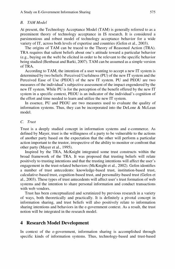
A Study on E-Government Information Sharing 575
B. TAM Model
At present, the Technology Acceptance Model (TAM) is generally referred to as a preeminent theory of technology acceptance in IS research. It is considered a parsimonious and robust model of technology acceptance behavior for a wide variety of IT, across both levels of expertise and countries (Gefen et al., 2003).
The origins of TAM can be traced to the Theory of Reasoned Action (TRA). TRA requires that salient beliefs about one’s attitude toward a particular behavior (e.g., buying on the web) be elicited in order to be relevant to the specific behavior being studied (Benbasat and Barki, 2007). TAM can be assumed as a simple version of TRA.
According to TAM, the intention of a user wanting to accept a new IT system is determined by two beliefs: Perceived Usefulness (PU) of the new IT system and the Perceived Ease of Use (PEOU) of the new IT system. PU and PEOU are two measures of the individual’s subjective assessment of the impact engendered by the new IT system. While PU is for the perception of the benefit offered by the new IT system in a specific context, PEOU is an indicator of the individual’s cognition of the effort and time needed to learn and utilize the new IT system.
In essence, PU and PEOU are two measures used to evaluate the quality of information systems. Thus, they can be incorporated into the DeLone & McLean model.
C. Trust
Trust is a deeply studied concept in information systems and e-commerce. As defined by Mayer, trust is the willingness of a party to be vulnerable to the actions of another party based on the expectation that the other will perform a particular action important to the trustor, irrespective of the ability to monitor or confront that other party (Mayer et al., 1995).
Inspired by the TRA, McKnight integrated some trust constructs within the broad framework of the TRA. It was proposed that trusting beliefs will relate positively to trusting intentions and that the trusting intentions will affect the user’s engagement in the trust-related behaviors (McKnight et al., 2002). Gefen identifies a number of trust antecedents: knowledge-based trust, institution-based trust, calculative-based trust, cognition-based trust, and personality-based trust (Gefen et al., 2003). These types of trust antecedents will affect user’s trust formation of web systems and the intention to share personal information and conduct transactions with web vendors.
Trust has been conceptualized and scrutinized by previous research in a variety of ways, both theoretically and practically. It is definitely a pivotal concept in information sharing, and trust beliefs will also positively relate to information sharing intentions and behaviors in the e-government context. As a result, the trust notion will be integrated in the research model.
4 Research Model Development
In context of the e-government, information sharing is accomplished through specific kinds of information systems. Thus, technology-based and trust-based
576 Z. Yan, B. Sun, and T. Wang
Fig. 2 Research Model
antecedents should work together to influence the decision to share information with other public agencies and employees. This section derives the research hypotheses of information sharing. The research model is depicted in Fig.2.
Information Quality measures the sharing information provided by other agencies and employees. The content of the information quality includes information accuracy, timeliness, usefulness, completeness and customized information presentation. Information quality has a positive influence on the user’s intentions and behaviors of adopting and sharing information (Hsiu-Fen and Gwo-Guang, 2006). People definitely want to adopt accurate and useful information from other parties. Moreover, we argue that information users seem to enter into an implied agreement with the information providers and delegate the task of collecting and organizing information services to the providers. In order to counterbalance the information asymmetry between information providers and users, the information providers should make clearly visible, high-quality, and irreversible investments (Zahedi and Song, 2008). In the case of information sharing, information quality is the most important visible, high-quality, and irreversible investment. Information quality serves as one of the most important antecedents of consumers’ beliefs in information providers’ trustworthiness (Zahedi and Song, 2008). On the other hand, in return for the benefit brought by information sharing, information users like to share high quality information with providers. Thus a stable mutual information sharing relationship will be built based on the accruing benefits. Hence, the information quality will affect the user’s intention to use the information sharing system and share information.
Hypothesis 1a: Sharing information quality is positively associated with trust in other agencies and employees.
Hypothesis 1b: Sharing information quality is positively associated with the users’ intention to share information.
If the user needs to accomplish the organizational goal with the help of information sharing systems, he/she will have a high dependence on information
Perceived Usefulness
Perceived Easy of Use
Information Use
Perceived Benefit
Trust Information Quality
Intention to Share
Information
H1b
H1a
H2
H3aH3b
H4
H5
H3c
H6

A Study on E-Government Information Sharing 577
sharing. Information Use measures the extent of a user’s work dependent on the sharing information from other parties and is the corresponding construct of IS Use and User Satisfaction in the DeLone & McLean model. Information use is actually a behavior and describes the user’s dependence on the information sharing system (Rai et al., 2002). A high information use means the user will adopt the sharing information in a high frequency and use that in management actions. Then, the employee will increase benefits from the information sharing activity. In the adoption process of the sharing information, a user among different government departments will establish the communication channel and share information for gradual mutual benefits. Thus, the higher dependence the user has in the sharing information, the higher the intention the user has to be involved in information sharing activities.
Hypothesis 2: The information use is positively associated with the users’ intention to share information.
The information system is the basic technological infrastructure of information sharing in the public sector. It proffers a fundamental sharing platform for information in different public sector organizations. As such, information sharing intentions should be explained in part by the technology acceptance model, TAM, which contains the two basic constructs PU and PEOU.
The DeLone & McLean model doesn’t include PU and PEOU, which are also important to IS success. Some notions in the DeLone & McLean taxonomy are closely associated to PU and PEOU. Information Quality in the semantic level of the DeLone & McLean model can make users perceive the IT system’s usefulness. PEOU and PU are two salient indicators of System Quality.
Thus, the proposed research model takes the PU and PEOU into account, and we hypothesize that paths predicted by TAM apply also to information sharing. The more useful the information sharing system is for enabling users to accomplish their tasks, the more involved it will be. The easier the information sharing system is to use in enabling the users to accomplish their tasks, the more it will be provided.
Hypothesis 3a: PU is positively associated with the users’ intention to share information.
Hypothesis 3b: PEOU is positively associated with the users’ intention to share information.
Hypothesis 3c: PEOU is positively associated with PU. Perceived benefits are defined as advantages offered by information sharing to
policy makers, agencies, and the public. It is the analog of the net benefits construct in the DeLone & McLean model. Proponents of information sharing can enumerate an extensive list of potential benefits. First of all, information sharing will streamline the data management and contribute to the information infrastructure. From the organizational view, information sharing will support collaborative problem solving and broaden the professional network. At last, information sharing will improve public accountability and foster program and service coordination (Dawes, 1996). It is obvious that the perceived benefit will positively affect the users’ intention to share information across organizational boundaries.
578 Z. Yan, B. Sun, and T. Wang
Hypothesis 4: Perceived benefits are positively associated with the users’ intention to share information.
In context of e-government information sharing, trust also has been scrutinized by previous researchers in a variety of ways. Theresa pointed out that trust building is both a key factor for developing cross-boundary information sharing and, in a much broader sense, is an important element of the social capital needed for any type of successful cooperation or collaboration within and across social networks (Pardo et al., 2006).
Peng stated that the primary reason for hesitation and reluctance of agencies to share sensitive information with one another is that they simply don’t trust each other, and trust-based information sharing schemes can easily lead to effective information sharing among government agencies (Peng Liu, 2005). One of the major reasons for distrust is that conflicts of interest usually exist between agencies. Thus having agency A share some information with agency B may actually compromise the interests of agency A. Another major reason for the lack of trust is that shared information may be improperly processed by an agency.
As shown in previous research, trust is a pivotal element in the cross-organizational collaboration. Trust is a useful assurance to mitigate the perceived risks and social uncertainty. If mutual trust has been built, the trustor will establish the truthful belief on the trustee’s ability, benevolence and integrity. The trustor will believe that the trustee will not misuse the sharing information of the trustor and jeopardize the trustor’s interests. Thus, the trustor will have more incentives to share information.
Hypothesis 5: Trust in other agencies and employees is positively associated with the users’ intention to share information.
Trust should also increase certain aspects of the perceived usefulness of information sharing systems and sharing information. As Gefen stated, the usefulness of an information system depends on both the effectiveness of its relevant technological properties, such as advanced search engines, and on the extent of the human services behind the IT, which make the non-technological aspects of the IT effective (Gefen et al., 2003). One integral part of the human services behind the IT is the information sharing service offered by other agencies and employees. Viewed from this non-technological manner, trust will increase the perceived usefulness of information systems. Once mutual trust is built, information users can believe in the information the system produces and perceive the high quality of information systems. Thus, the benefits of sharing information will be maximized.
Hypothesis 6: Trusting other agencies and employees is positively associated with PU.
5 Conclusions
Information sharing is important in inter-organizational collaboration. Based on the DeLone & McLean model and TAM, this chapter integrates technology-based and trust-based antecedents to depict users’ intentions for information sharing. Having a critical analysis of the previous theory, the corresponding information sharing
A Study on E-Government Information Sharing 579
influential factor research model is proposed and the corresponding hypotheses are derived. Information quality, information use, perceived benefit, trust, perceived usefulness and perceived ease of use are proposed as antecedents of the users’ intention to share information. The research model provides a new research angle for information sharing, based on classic information system critical success factors. For our next research work, we will collect data from government agencies and validate the proposed research model.
References
Benbasat, I., Barki, H.: Quo vadis, TAM? Journal of the Association for Information Systems 8(4), 212–218 (2007)
Dawes, S.: Interagency information sharing: Expected benefits, manageable risks. Journal of Policy Analysis and Management, 377–394 (1996)
DeLone, W.H., McLean, E.R.: Information Systems Success: The Quest for the Dependent Variable. Information Systems Research, 3(1), 60–95 (1992)
Drake, D.B., Steckler, N.A., Koch, M.J.: Information Sharing in and Across Government Agencies: The Role and Influence of Scientist, Politician, and Bureaucrat Subcultures. Social Science Computer Review 22(1), 67–84 (2004)
Gefen, D., Karahanna, E., Straub, D.W.: Trust and TAM in online shopping: an integrated model. MIS Quarterly 27(1), 51–90 (2003)
Gil-Garcia, J.R., Chengalur-Smith, I., Duchessi, P.: Collaborative e-Government: impediments and benefits of information-sharing projects in the public sector. European Journal of Information Systems 16(2), 121–133 (2007)
Hsiu-Fen, L., Gwo-Guang, L.: Determinants of success for online communities: an empirical study. Behaviour & Information Technology 25(6), 479–488 (2006)
Hu, P., Zhang, P.G., Ye, J.: The Empirical Research on Influencing Factors of Information Sharing Among the Departments of Local Government in China. Information Science 25(004), 548–556 (2007)
Kolekofski, K.E., Heminger, A.R.: Beliefs and attitudes affecting intentions to share information in an organizational setting. Information & Management 40(6), 521–532 (2003)
Landsbergen Jr., D., Wolken Jr., G.: Realizing the Promise: Government Information Systems and the Fourth Generation of Information Technology. Public Administration Review 61, 206–220 (2001)
Mayer, R.C., Davis, J.H., Schoorman, F.D.: An integrative model of organizational trust. Academy of Management Review 20(3), 709–734 (1995)
McKnight, D.H., Choudhury, V., Kacmar, C.: Developing and Validating Trust Measures for e-Commerce: An Integrative Typology. Information Systems Research 13(3), 334–359 (2002)
Pardo, T., et al.: Knowledge sharing in cross-boundary information system development in the public sector. Information Technology and Management 7(4), 293–313 (2006)
Pardo, T., Gil-Garcia, J., Burke, G.: Building response capacity through cross-boundary information sharing: The critical role of trust. In: The eChallenges Conference, Barcelona, Spain (2006)

580 Z. Yan, B. Sun, and T. Wang Peng Liu, A.C.: Trust-based secure information sharing between federal government
agencies. Journal of the American Society for Information Science and Technology 56(3), 283–298 (2005)
Rai, A., Lang, S., Welker, R.: Assessing the Validity of IS Success Models: An Empirical Testand Theoretical Analysis. Information Systems Research 13(1), 50–69 (2002)
Shin, S., Ishman, M., Sanders, G.: An empirical investigation of socio-culural factors of information sharing in China. Information & Management 44(2), 165–174 (2007)
Soonhee Kim, H.L.: The Impact of Organizational Context and Information Technology on Employee Knowledge-Sharing Capabilities. Public Administration Review 66(3), 370–385 (2006)
William, H.D., Ephraim, R.M.: The DeLone and McLean Model of Information Systems Success: A Ten-Year Update. Journal of Management Information Systems 19(4), 9–30 (2003)
Zahedi, F.M., Song, J.: Dynamics of Trust Revision: Using Health Infomediaries. Journal of Management Information Systems 24(4), 225–248 (2008)

Research on Situations and Development Trends of Emergency Logistics at Home and Abroad
Xiufeng Zuo, Qian Ran, and Wenzhuo Gu1
This chapter describes the features of emergency logistics and the role it plays in emergency management under the cognition of characteristics of public emergency. It elaborates on the three phases of foreign research and the situation of domestic research. The current emergency logistics research focuses on aspects of the organization, operation and control, the technical support, as well as policies and legislation. Finally, the chapter points out the trends of emergency logistics research.
1 Introduction
In 2008, snowstorms, frost, earthquakes, landslides, air crashes and mine disasters reminded us that human beings are sometimes faced with paroxysmal natural and man-made disaster. The unexpected occurrences disrupt the normal procedures of our daily work and life if we do not prepare for them. Therefore, it is an important research task to understand the principles and features of all kinds of disasters, to set up a system to deal with such incidents, and to optimize a rescue and emergency resources dispatch scheme so that we are active in dealing with emergencies.
With the development of human civilization, high-rise buildings, pipelines, efficient communications and traffic make comfortable living and working conditions for people. But, when we face disasters, the community becomes increasingly fragile. With GDP growth, the effect of emergencies is increasing. It is a strong national need to strengthen public security, and integrated emergency management is the core issue of public security (Fan, 2007).
Based on the principles of disaster and crisis, integrated emergency management covers disaster prevention, monitoring, forecasting, identification, measuring, Xiufeng Zuo Beijing Institute of Technology, School of Management and Economics, Beijing 100081, P.R. China, Phone: 86-010-68912844 email: [email protected]
Qian Ran and Wenzhuo Gu Beijing Institute of Technology, School of Management and Economics, Beijing 100081, P.R. China e-mail: [email protected]

582 X. Zuo, Q. Ran, and W. Gu
rescue control, emergency preplans, rapid reactions, after-action reviews, reconstruction and so on (Cao et al., 2007). It also includes scientific management, dispatching and coordinating personnel and financial, material and informational resources during emergencies (Cao et al., 2007). At present, due to the lack of national-level research on integrated emergency management, it is still difficult to develop the storage of national emergency resources reasonably and build national and local monitoring networks and an emergency resource system to satisfy the demand of emergency handling and reconstruction (Cao et al., 2007).
The occurrence and development of public emergencies are non-reversible and non-experimental, so simulation experiments are an important method for studying the reasoning and principles of various kinds of emergencies and to take emergency management (Cao et al., 2007). Because Integrated Emergency Management is a complicated system, it is necessary to carry out the simulation research based on the rules of the evolution of emergencies. But research in this area both at home and abroad are still inadequate. Therefore, employing modern complex system modeling and simulation technology to study Integrated Emergency Management is a difficult task and has significant meaning.
A sudden, unexpected incident can cause serious damage. Emergency logistics is a special logistic activity that satisfies the demand of materials, personnel, information and finances during various kinds of emergencies. The basic features of emergency logistics are unpredictability, urgency and diversity in demands, as well as emergency mobilization of the army and local participation. The logistics disorder in the relief process of the massive earthquake in Wenchuan has been noted (Xu and Huang, 2008). Comprehensive arrangements for different resources and reducing waste are important elements in emergency management.
Emergency logistics research studies how to make use of technology to quickly identify the disaster’s state and the demands of disaster relief resources (the location and quantity of the needed resources) and how to use an appropriate means of transportation and routes to transport the materials efficiently and accessibly from the resource point to the rescue point, reducing the impact of the disaster and achieving the best disaster relief results.
2 Foreign Research on Emergency Logistics
There are three phases of research on emergency logistics abroad: before the mid-1990s, from mid-1990s to the start of the 21st century, and since the start of the 21st century.
In the first phase, before the mid-1990s, the difference between emergency logistics and general logistics was not much, and a few limiting factors were considered. In 1985, Aikens gave a location model based on linear programming, integer programming and dynamic programming (Aikens, 1985). Ray, in 1987, studied a transportation problem on emergency relief resources with different constraints to minimize transportation costs (Ray, 2003). Haghani and Oh, in 1996, developed a space-time network flow model (Haghani and Oh, 1996). At the same time, Gutierrez provided an optimization network design under uncertainty (Gutierrez et al., 1979).
Research on Situations and Development Trends of Emergency Logistics 583
In the second phase, from the mid-1990s to the start of the 21st century, researchers focused on the reality of emergency management, though the study range was still not wide, and they built more complex models under the consideration of more practical constraints and goals, and they employed the simulation method to study logistic problems. In 1997, Ahmed S. Zakit and Hsing Kenneth Cheng established a simulation analysis and management system of emergency services, which was designated by a mobile unit in a certain region, in order to respond to unexpected incidents occurring in different parts of a megalopolis (Zakit and Cheng, 1997). Wybo Jean Luc, et al. (1998) used the decision-making tools of GIS, simulator, information systems, as well as multimedia systems to build models (Luc et al., 1992). Owen and Daskin (1998) studied the problem of facilities location under uncertainty (Owen and Daskin, 1998). In 1998, Paulm and Needham studied an emergency transport problem using the simulation method and verified the effectiveness of the simulation used in emergency management (Needham, 1998). In 1999, Subramanian, in his doctoral dissertation, studied the transportation, emergency response, risk management and planning and location issues using the methods of the location of the supply center, path selection, resource allocation, etc. (Subramanian, 1999) Taniguchi (1999) used two-level programming to solve the location problem of public logistics transfer stations (Taniguchi, 1999). Holmberg K (1999) considered the location problem of non-linear freight costs. In order to minimize the number of deaths, Fiedrich (2000) studied an optimization model of resource distribution and transportation for the number of scenes after an earthquake under limited time and resources (Fiedrich et al., 2000a). Fiedich (2000) studied the heuristic arithmetic of the optimization of resource distribution after an earthquake, and proposed a dynamic portfolio optimization model to minimum the number of facilities during the rescue (Fiedich et al., 2000b).
In the third phase, since the beginning of this century, the research range of the emergency logistics was widening, using the system method to analyze and integrate a number of models. Especially after “9-11 incident”, researchers laid emphasis on information, emergency response, emergency decision-making theories and the group decision support system. Yoshitaka Kuwata, et al. (2002) discussed a new simulation methodology and an approach assessing, designing and evaluating the emergency decision support system, which can quantitatively evaluate the effectiveness of the decision support system of an emergency response (Kuwata et al., 2002). Michael J. Kevany (2003) described the emergency maps, data center, and operational process, and he analyzed the function of GIS in emergency response through the “9-11 incident” (Kevany, 2003). In 2004, Eytan Pollak and Mark Falash gave an integrated analysis framework of emergency management (Pollak and Falash, 2004). Mei-Po Kwan and Jiyeong Lee (2005) further analyzed the structure of the GIS-based intelligent emergency response system (Kwan and Lee, 2005). Trevor Hale and Christopher R. Moberg (2005) studied the choice of the emergency logistics supply points (Hale and Moberg, 2005). For the number of emergency supply storages on the points, a quantitative model had been established. Groothedde B (2005) studied the coordinative HUB network, which can reduce the logistics costs and keep the level of service
584 X. Zuo, Q. Ran, and W. Gu
(Groothedde et al., 2005). Yufei Yuan (2005) introduced an intelligent mobile emergency response system as well as its structure and functions (Yuan and Detlor, 2005). David Mendonca (2006) assessed a group decision support system of emergency response by game simulation (Mendonca et al., 2006). Yi W, et al. (2007) established a dynamic logistics coordination model for evacuation and rescue-injured personnel by studying FLP and VRP problems in emergency logistics as well as coordination between emergency delivery and people evacuation after disasters (Yi and Zdamar, 2007; Yi and Kumar, 2007). Jiuh-Biing Sheu (2005) thought that the core of the framework of emergency logistics was made of the following aspects: the forecast of the demand of the distributing materials, the emergency logistics network plan and design, the distribution of emergency materials, the rapid response of emergency material distribution, and the international emergency logistics cooperation (Sheu, 2005). Jiuh-Biing Sheu (2007) established a distribution system against the variability of the emergency materials demand. After obtaining the disaster information, the system first classified the grade stricken by the disaster in a different place with the fuzzy classification method, assessed the relational priority of the distribution, and then handled the distribution.
3 Domestic Research on Emergency Logistics
After SARS in 2003, Chinese scholars started to pay attention to the research of emergency logistics. Ou Zhongwen, et al. (2003) proposed to establish a support mechanism against the problems in present emergency logistics (Ou et al., 2004). Zhang Jing, using a utility function with a preference-order, solved the problem of resource allocation when multiple emergencies occurred simultaneously (Zhang et al., 2007). Xie Ruhe and Zong Yan (2005) discussed the establishment of a emergency response logistics system (ERL) by setting up an ERL Center, a public information platform and a distribution system (Xie and Zong, 2005). Li Lefei (2008) discussed the framework of the artificial emergency- logistics- planning system (Li, 2008). Hu Jiaxiang and Zhao Lindu established a framework for the logistics management system based on a multi-agent, including a communication support layer, a data layer, an accident find layer, an emergency operation layer, and a user layer (Hu and Zhao, 2008). Wang Dading and Chen Yuefeng, counting the complexity of equipment and logistics demands at war, provided a multi-agent framework of equipment and logistics systems based on a swarm platform to adapt different states, styles and environments of war. Liao Guangxuan proposed an assistant decision support system for urban emergency response, which integrated many areas of theories and technologies, including expertise, modern technologies and calculation models (Liao et al., 2005). Han Xiaomei and Han Jingti (2007) studied the emergency logistics intelligent decision support system under case-based reasoning technology and the intelligent decision-making method (Han and Han, 2007). Ji Lei, Chi Hong, Chen An, et al. (2006) described the concept of emergency management, essential contents and methods from the macro, middle, and micro aspects. Wang Feng, Jiang Yuhong and Wang Jin (2007) discussed

Research on Situations and Development Trends of Emergency Logistics 585
essential contents of emergency logistics. Yu Jinju (2008) carried out an agent-based simulation research on natural disasters in airdrome management.
Domestic research has just started, but domestic researchers are no less aware of emergency logistics than those abroad. Both domestic and foreign research focus on operational control, technical support, and policies and legislation. The focal points of the study include: (1) research on emergency logistics information systems and technology; (2) research on rescue resource allocation and resource storage; (3) research on multi-supplier, multi-depot location routing problems; (4) research on the emergency logistics decision support system, integrating the above three aspects; (5) Based on the research above, discussion of the organization of emergency logistics, the effectiveness of relevant policies and the rationality of the emergency plan.
4 Trends of Future Research on Emergency Logistics
Emergency logistics are carried out under the interaction of emergency incident occurrence and its evolution and emergency handling. It is a complex process, composed of many departments and uncertainties. To reveal the real rules and mechanisms of the process, multidisciplinary research must be carried out.
Therefore, there are three aspects of future research: multidisciplinary research, the simulation method, and empirical study for different emergencies.
First, emergency logistics involves the disaster from the emergency, personnel reaction to the emergency, damage prediction or evaluation, information technology, decision-making methods, logistics, etc (Fan, 2007; Cao et al., 2007). Only under the ground of recognizing the damage of disasters, such as an earthquake, can we know the reactions of humans and predict injuries. According to the disaster information, it can organize an emergency rescue and material dispatch. Then, according to the disaster process, it can adjust the decision goals and produce a rescue plan of different levels.
Second, due to the emergency’s uncertainty, serious damage and non-experimental research on emergency management are difficult. The effectiveness of emergency decision-making and the rationality of the emergency plan should not be measured by the heavy loss after such incidents. The simulations that have been currently conducted quickly have become an effective tool. Orienting continuous variation, discrete events and multi-agents, various kinds of simulation platforms are emerging. A simulation method is adapted to the variability of dynamic change of emergency logistics, involving multiple participants and complex relationships existing in emergency logistics. It can also integrate the multidisciplinary research results and embed these results in a simulation model. Through the operations of the simulation mode, we can study the process and the rules of emergency logistics. Therefore, the experiment method of simulation is an effective way to study emergency logistics.
Third, different kinds of emergencies have different principles of evolution, so they should be studied separately. This way, results are of pertinence and direction. It also facilitates testing and estimating the results. At the same time, it gives evidence to making an emergency plan and related policies.
586 X. Zuo, Q. Ran, and W. Gu
References
Aikens, C.H.: Facility location models for distribution planning. European Journal of Operational Research 22(3), 263–279 (1985)
Cao, J., Yang, X.G., Wang, S.Y.: The important scientific problems of emergency management research on sudden public events. Journal of Public Administration 4(2) (2007)
Fan, W.C.: The consideration and suggestion of scientific problems on emergency management of national sudden public events. Science Foundation of China (2), 71–76 (2007)
Fiedrich, F., Gehbayer, F., Rickers, U.: Optimized resource allocation for emergency response after earthquake disasters. Safety Science 35(1), 41–57 (2000a)
Fiedich, F., Gehbauer, F., Rickers, U.: Optimized resource allocation for emergency response after earthquake disasters. Safety Science 35, 41–57 (2000b)
Groothedde, B., Ruijgrok, C., Tavasszy, L.: Towards collaborative inter-modal hub networks a case study in the fast moving consumer goods market. Transportation Research Part E 41(6), 567–583 (2005)
Gutierrez, G., Kouvelis, J., Kurawala, J.: A robustness approach to un-capacitated network design problems. European Journal of Operations Research 94, 362–376 (1979)
Haghani, A., Oh, S.: Formulation and solution of a multi-commodity, multi-modal network flow model for disaster relief operations. Transportation Research A 30, 231–250 (1996)
Hale, T., Moberg, C.R.: Improving supply chain disaster preparedness decision process for secure site location. International Journal of Physical Distribution & Logistics Management 5, 195–207 (2005)
Han, X.M., Han, J.T.: Research on intelligent decision support system of emergency support logistics based on CBR theory. Computer Engineering and Applications 43(20), 204–206 (2007)
Holmberg, K.: Exact solution methods for uncapacitated location problem with convex transportation costs. European Journal of Operational Research 114(2), 127–140 (1999)
Hu, J.X., Zhao, L.D.: Research on agent-based modeling for an emergency logistics management system, p. 4. IEEE Computer Society, Los Alamitos (2008)
Ji, L., Chi, H., Chen, A., Chen, J.M., Zhao, H., Wang, Y.H., Li, J.P.: Emergency Management of Sudden Accidents. Higher Education Press, Beijing (2006)
Kevany, M.J.: GIS in the world trade center attack trial by fire. Computers, Environment and Urban Systems 27(6), 571–583 (2003)
Kuwata, Y., Noda, I., Ohta, M., Ito, N., Shinhoda, K., Matsuno, F.: Evaluation of decision support systems for emergency management. In: Proceedings of the 41st SICE Annual Conference, vol. 2(5-7), pp. 860–864 (2002)
Kwan, M.P., Lee, J.Y.: Emergency response after 9/11: The potential of real-time 3D GIS for quick emergency response in micro-spatial environments. Computers, Environment and Urban Systems 29(2), 93–113 (2005)
Li, L.F.: An artificial emergency-logistics-planning system for severe disasters, p. 10. IEEE Computer Society, Los Alamitos (2008)
Liao, G.X., Weng, T., Zhu, J.P., Liu, T.M., Liu, G.Z.: Research on emergency aided decision support system of city major accident. Chinese Engineering Science 7(7) (2005)
Luc, W., Kowalski, J., Madland, K.: Command centers and emergency management support. Safety Science 30(1-2), 131–138 (1992)
Research on Situations and Development Trends of Emergency Logistics 587 Mendonca, D., Beroggi, E.G., van Gent, D., Wallace, W.A.: Designing gaming simulations
for the assessment of group decision support systems in emergency response. Safety Science 44(6), 523–535 (2006)
Needham, P.: The influence of individual cost factors on the use of emergency transshipment. Transportation Research: Logistics and Transportation Review 34(2), 149–160 (1998)
Ou, Z.W., Wang, H.Y., Jiang, D.L.: Emergency logistics. Journal of Chongqing University (National Science Edition) 27(3) (2004)
Owen, S.H., Daskin, M.S.: Strategic facility location: A review. European Journal of Operational Research (11), 423–447 (1998)
Pollak, E., Falash, M.: Automated database and schema-based data interchange for modeling and simulation. In: Proceedings of 2004 Winter Simulation Conference, pp. 191–197 (2004)
Ray, J.: A multi-period linear programming modal for optimally scheduling the distribution of food -aid in west Africa. Dissertation. University of Tennessee, Knoxville (2003)
Sheu, J.B.: Special issue on emergency logistics management. Transportation Research Part E: Logistics and Transportation Review 41, 459–460 (2005)
Sheu, J.B.: An emergency logistics distribution approach for quick response to urgent relief demand in disasters. Transportation Research Part E 43 (2007)
Subramanian, W.: Optimization models and analysis of routing, location, distribution and design problems on networks. Dissertation, Virginia Polytechnic Institute and State University (1999)
Taniguchi, E.: Optimal size and location planning of public logistics terminals. Transportation Research 35, 207–222 (1999)
Wang, D.D., Chen, Y.F.: The logistics simulation model for war-time equipment based on CAS theory. China Logistics and Purchasing 24 (2007)
Wang, F., Jiang, Y.H., Wang, J.: Emergency Logistics. China Material Press, Beijing (2007) Xie, R.H., Zong, Y.: The construction of emergency logistics system. Journal of Guangzhou
University (Social Science Edition) (11), 561–567 (2005) Xu, D., Huang, D.Z.: From earthquake relief to see the construction of emergency logistics.
Special Report (6), 32–34 (2008) Yi, W., Kumar, A.: Ant colony optimization for disaster relief operations. Transportation
Research Part E: Logistics and Transportation Review 43(6), 660–672 (2007) Yi, W., Zdamar, L.: A dynamic logistics coordination model for evacuation and support in
disaster response activities. European Journal of Operational Research 179(3), 1177–1193 (2007)
Yu, J.J.: Research on agent-based emergency management simulation for explosive threat to the airport. Beijing Institute of Technology master’s thesis, Beijing (2008)
Yuan, Y.F., Detlor, B.: Intelligent mobile crisis response systems. Communications of the ACM 48(2), 95–98 (2005)
Zakit, A.S., Cheng, H.K.: A simulation model for the analysis and management of an emergency service system. Socio-Econ. plan. Sci. 31(3), 173–189 (1997)
Zhang, J., Shen, S.F., Yang, R.: The game model for the allocation of emergency resources based on the preferences sequence. Journal of Tsinghua University: National Science Edition 47(12), 2167–2170 (2007)
Author Index
Bin, Liu 527
Cai, Fengjing 361Cao, Jie 13Chang, Hei-Tsz 371Chao, Rih-Chang 121Chen, Guey-Shya 371Chen, Guohong 255Chen, Hongzhuan 407Chen, Jianming 493Chen, Jiaying 297Chen, Kejia 297Chen, Ye 3Chen, Yuqing 561Cui, Lizhi 131
Dang, Luo 437Dang, Yaoguo 341Delcea, Camelia 105Ding, Ye 281Dong, Fenyi 203Duan, Lizhong 215Du, Juan 141
Fang, Zhigeng 3, 229, 541Fan, Jianmin 481Fan, Xingxing 215Feng, Jichuang 493Feng, Xiuqin 305
Gao, Hong 385Gao, Qiang 503Gong, Yonghua 515Gong, Zaiwu 13, 385
Guo, Benhai 229Guo, Huan 177, 305Guo, Ruilin 419Gu, Wenzhuo 581
Hao, Yonghong 153He, Chunhua 327He, Xinwen 481Hongyuan, Bai 527Hou, Guangming 481Hsieh, Tien-Yu 121Hu, Caihong 469Hu, Haiqing 449Hu, Liangming 469Hu, Xinyu 317
Jiang, Guiqin 469Jian, Lirong 245Jin, Zhenxin 407Ji, Peirong 317
Kaczorek, Tadeusz 429Kong, Xinhai 461Kuijper, Hans 23Kuo, Bor-Chen 121
Li, Bangyi 515Li, Bingjun 327Li, Jianping 493Li, Lianshui 13Li, Meijuan 255Ling, Zhou 437Lin, Lihua 47Liu, Bin 203Liu, Hong 95
590 Author Index
Liu, Junjuan 203Liu, Sifen 407Liu, Sifeng 3, 59, 87, 131, 191, 245,
267, 281, 541, 553Liu, Yafei 419Liu, Yuan 541Li, Xuemei 341Luo, Ning 165Luo, Zhifeng 47
Ma, Hongfang 245Ma, Hsiu-Lan 371Masatake, Nagai 121Mei, Shu’e 165
Ran, Qian 581Rong, Zhang 527
Scarlat, Emil 105Sheng, Keqin 267Shen, Qiuying 561Sheu, Tian-Wei 121Song, Dejin 229Song, Zhongmin 37Sun, Baowen 571
Tang, Chi 395Tang, Xiaowei 503Tsai, Ya-Hsun 121
Wang, Jianling 553Wang, Jingshun 419Wang, Qiuping 449Wang, Tianmei 571Wang, Wenping 561Wang, Xuemeng 141, 153Wang, Yinao 361Wang, Yun 553
Wang, Zhanzhong 419Wan, Qin 349Wei, Hengwu 3Wei, Ting 153Wei, Wenchang 47Wei, Yong 349, 461Wu, Der-Bang 371Wu, Lifeng 361Wu, Shunxiang 47
Xiao, Xinping 177, 305Xie, Naiming 59, 385
Yang, Baohua 3, 541Yang, Junjie 47Yang, Xiongqiong 349Yang, Yingjie 73Yan, Xizu 37Yan, Zhijun 571Yao, Tianxiang 13, 385Yeh, Shin-I 121Yin, Boming 395Yuan, Chaoqing 87
Zhang, Changhui 469Zhang, Daohong 449Zhang, Ke 191Zhang, Lixia 153Zhang, Qishan 95, 297Zhang, Ying 215Zhao, Jiejue 341Zhong, Weijun 165Zhuang, Hua 255Zhu, Jianjun 281Zhu, Jinfu 503Zhu, Ningning 281Zou, Hongbo 317Zuo, Xiufeng 581
Index
1-AGO 342 3G data services 515 aberrant data 329, 330 absolute degree of grey incidences 191, 464 accumulating generation operator 318 accuracy 359additional payment 529 ADF testing 299 adjustable community structure 562
advanced measurement approach 494 aggregation approach 282 AGO 374 aircraft routes 505 analysis of variance 395 anthropogenic activities 153 approximate technique 451 ARMA model 298 attribute weights 177 automobile production 541
behavioral data 349, 359 behavioral matrix 193 behavioral sequence 133 B-mode degree of grey incidence 466 boundary 30 boundary points 203 bundling tariff model 518
call externalities 516 centralized system 529 chance-constrained programming 95 Chinese commercial banks 493 Chinese medicine 215, 216 climate change 153 clustering coefficient 563 clustering object 204 coefficient matrix 424 cognition of characteristics 581 collaboration 410
communicating pattern 517 community degree 562 comparative sequence 471 comparison vector 123 complex network 561 complex systems’ modeling 177 composition and extension 31 comprehensive evaluation 177 comprehensive index 356 computer decision-making system 420 concentration effect of talent 555 consistent sub-matrices 15 continuous-time 429 contour lines 351, 352 contribution degree 255 conventional GM (1, 1) model 328, 330 coordination subsystem 481, 489 countermeasure 240, 488 covered set 61 critical path 37 cross-organizational collaboration 578 curfew time 506
data analysis 122 delayed and nonlinear system 305 Delphi method 245 development coefficient 386 development trends 255 difference operator 298 direct model 361 direct modeling method 361 discrete GM(1,1) model 386 discrete-time linear systems 429 distribution center 95 dominant strategy 413 driving-couple 5 dualistic operations 70
Index 592
dual-use core technology 481, 483 dynamic decision-making 407 dynamic prediction model 297 dynamic process 298 dynamic relationship 199 dynamical physics 564
economic capital 493 economic growth 142, 166 economic-financial ratios 105 effect-evaluating vector 49 efficiency of resource allocation 481 e-government 572 emergency logistics 582 emergency management 11, 582 emergency mobilization 582 emergency response logistics system 584 empirical study 166 energy consumption 87, 281 energy efficiency 87 energy intensity 87 energy policy 281, 283 energy-saving effect 87 energy-saving technologies 281 equilibrium point 415 evaluation indicator 255 evaluation object 261 evaluation set 245 extended clusters 191
feasible index 245 financial performance 105 forecasting error 338 forecasting formula 355, 356 forecasting model 359 forest fires 8 fuzzy comprehensive evaluation
method 248 fuzzy equivalent clustering 52 fuzzy logic 106 fuzzy relation 49
game theory 409 gap prediction model 555 Gauss method 363 geometric similarity 197 geometrical structure 381 GERTS Network 5 GM (1, 1) model 143, 154, 318, 343, 556 GM(0,N) 374 gradual tempo 132
GRASP 504 greedy simulated annealing
algorithm 504 grey breeding computer decision-making
system 420 grey category 204 grey classes 49 grey clustering analysis 216 grey clustering coefficient vector 204 grey clustering method 203 grey coefficient 38 grey decision-making 471 grey dynamic clustering algorithm 47 grey dynamic model 143 grey evolutionary game 416 grey incidence model 216, 217 grey incidence 437 grey incidence analysis 110, 121, 131,
166, 177, 421, 470 grey incidence coefficient 124 grey incidence coefficient vectors 51 grey information 95 grey integrated clustering 204 grey math 426 grey mathematics 59 grey model 371, 372 grey multi-attribute 438 grey selection 422 grey situation decision making 461 grey systems theory 37 grey throughput 97 grey Verhulst model 396 grey volume 142 grey wave forecasting model 349, 350 grey programming model 95 gross domestic product 141, 298 group decision-making 281, 438 group deviation 442
high-demand consumers 519 hybrid particle swarm optimization 101 hypothesis testing 395
IAGO 396 identification 27 incidence coefficient 258, 465, 472 incidence degree 141, 216, 259, 461 incidence order 461
Index 593
independent innovation 558 industrial structure 87 influence factors 216 information abstracting 63 information asymmetry 527 information background 61 information of grey numbers 60 information quality 574 information sharing 571 information system 572 information technology 395 initial value 387, 463 innovation capacity 255 innovative ability 555 integrated evaluation method 249 integrated optimization model 437 international cooperation 245 interval forecasting 327, 328 interval grey number 47, 438 interval number 450 interval plan network 37 inverse accumulated generating
operation 396 irregular flight 503 IT personnel 268
Java technique 426 Jiangsu Province 267 joint decision 528 judgment matrices 13
key technology 245 knowledge characteristic 568 knowledge propagation 561 knowledge propagation efficiency 565
least squares method 10, 309, 362 least-squares 7 linear regression model 328, 329 linguistic information 451, 453 local optimal solution 503, 504 location of logistics distribution 101 logistics distribution 96 logistics system 95 loss amount 495 loss distribution approach 494 loss frequency distribution 495
macro-economy 141 management problem 229 MAPE 323, 363
MAPLE 323 market development 522 matrix of symptoms 105 matrix sequence 192 maximal element 203 maximum eigenvalue 125 mean generation 108 mean spacing 331 mean square deviation 332 mean-field theory 564 menu of contracts 530 metabolism GM(1,1) Model 303
MGM 1 N 305
MGM (1, , )N rτ 306
mixed channels 527 model simulation 565 model testing 314 modeling Logistic 362 modeling process 305 modified GM (1, 1) 322 modified relative error 361 module 421 Monte Carlo Simulation 495 Monte Carlo stochastic simulation 471 multi-objective quadratic programming
185multiple attribute decision making 13 multiplicative consistent 14 multiplicative consistent condition 17
negation operator 451 neighborhood selection 503 network community degree threshold 561 network diagram 9 network externalities 516 new industrial development 231 new information priority 341, 342 non-equidistant GM(1,1) 330 nonlinear optimal models 18 non-negative raw data 317 numerical differentiation 363
objective factors 37 online dual channels supply chain
system 527 open innovation 482 open support system 483 operational risk loss 494 optimal menu of two-part tariffs 521 optimization 94
Index 594
optimization algorithm 504 optimization method 178, 342 optimization technique 385 outer measure 177, 180 overnight airports 505
panel data 191 parameter identification 308 particle swarm optimization 309 part-whole relation 28 patent 169 perceived usefulness 575 piecewise analysis 153population forecasting 361 possible value error 281 prediction accuracy 298, 303 prediction value 318 preference relations 14 preference value 449 price strategy 515 principle-agent method 538 prioritized format 121 priority vectors 19 production cost 529 programming model 547 project sources 245 proposition-information 61 public benefits 571 pure exponential sequence 385
quality character management 541 quality loss functions 543 quality performance 546
random fluctuation 157 random samples 323 rate of success 481 recurrence formula 387 recursive formula 415 reference sequence 471 reform and opening up 141 regional characteristics 267, 268 regional distribution 267 regional technological innovation 255 regression analysis 395 reliability coefficient 374 research and development 165
residual sum of squares 342, 343 resources dispatch 581 risk 438 risk capital 497 risk index model 106 risk investment 455 risk measurement 495 rural economy 207
saturation value 402 scalar multiplication 135 scenario deduction 11 schedule recovery 503 science and technology 165 science and technology talent 230 sci-tech innovative talent 553 sensitivity analysis 178 short-term forecast 328 similarity coefficient 47, 48 simulation 414 simulation accuracy 341, 342 simulation value 387 single contract 530 SIR epidemic model 563 SIR model 563 situation decision making 461 small sample 341 software platform 485 sovereignty 23 spring flow 153, 155 standardization 462 structural equation model 541 structures 27 subjective factors 37 subjective opinions 13 subscribers 516 sum of the squares 361 supply chain 542 support system 481 system integrator 542 systemic view 27systems analysis 37 systems science 27
T’s incidence degree 166 technical support 585 technological progress 166 technology acceptance model 575 technology integration 483 technology life cycle 485 technology system 572

Index 595
territory 23 tertiary industry 87, 136 three-point interval number 281, 282 time response sequence 556 time sequence 351 time series 132 total factor productivity 165 transfer model 298 transformation platform 558 triangular fuzzy number 450 true value 61 trust 573
uncertain network optimization 95 uncertainty 42 uncertainty intervals 13 unexpected incident 583 urbanization 136 urgent index 245
value interval 203 van Hiele’s geometric thinking 371
water balance analysis 153 water environment quality 469 water environmental monitoring da 471 wave crest 357 waveform graph 352 weight 444 weight estimation approach 281 weight vector 205, 443 weighted least square method 343, 345 weighting range 376 whitening values 37 whitenization weight function 48 Wu’s geometry test 373
Z-score model 106


![Zggh]hPH>new.groteck.ru/images/catalog/40429/9deec18637ee6ecbb5a6ae0a1… · UCS 6200 Series Fabric Interconnect UCS Manager UCS C240 M3/M4 Series Rack Server UCS Integrated Infrastructure](https://img.pdfslide.us/doc/110x75/5fcc7e22130a463bbb0b3c57/zgghhphnew-ucs-6200-series-fabric-interconnect-ucs-manager-ucs-c240-m3m4.jpg)