Embed Size (px)
Citation preview
1
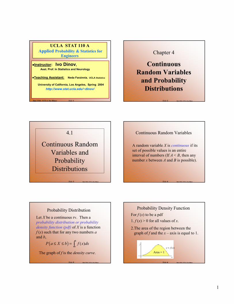
Stat 110A, UCLA, Ivo Dinov Slide 1
UCLA STAT 110 AApplied Probability & Statistics for
Engineers
Instructor: Ivo Dinov, Asst. Prof. In Statistics and Neurology
Teaching Assistant: Neda Farzinnia, UCLA Statistics
University of California, Los Angeles, Spring 2004http://www.stat.ucla.edu/~dinov/
Stat 110A, UCLA, Ivo DinovSlide 2
Chapter 4
Continuous Random Variables
and Probability Distributions
Stat 110A, UCLA, Ivo DinovSlide 3
4.1
Continuous Random Variables and
Probability Distributions
Stat 110A, UCLA, Ivo DinovSlide 4
Continuous Random Variables
A random variable X is continuous if its set of possible values is an entire interval of numbers (If A < B, then any number x between A and B is possible).
Stat 110A, UCLA, Ivo DinovSlide 5
Probability DistributionLet X be a continuous rv. Then a probability distribution or probability density function (pdf) of X is a function f (x) such that for any two numbers aand b,
( ) ( )b
aP a X b f x dx≤ ≤ = ∫
The graph of f is the density curve.
Stat 110A, UCLA, Ivo DinovSlide 6
Probability Density FunctionFor f (x) to be a pdf1. f (x) > 0 for all values of x.
2.The area of the region between the graph of f and the x – axis is equal to 1.
Area = 1( )y f x=

2
Stat 110A, UCLA, Ivo DinovSlide 7
Probability Density Function
is given by the area of the shaded region.
( )y f x=
ba
( )P a X b≤ ≤
Stat 110A, UCLA, Ivo DinovSlide 8
Continuous RV’s
A RV is continuous if it can take on any real value in a non-trivial interval (a ; b).
PDF, probability density function, for a cont. RV, Y, is a non-negative function pY(y), for any real value y, such that for each interval (a; b), the probability that Y takes on a value in (a; b), P(a<Y<b) equals the area under pY(y) over the interval (a: b).
pY(y)
a b
P(a<Y<b)
Stat 110A, UCLA, Ivo DinovSlide 9
Convergence of density histograms to the PDF
For a continuous RV the density histograms converge to the PDF as the size of the bins goes to zero.
AdditionalInstructorAids\BirthdayDistribution_1978_systat.SYD
Stat 110A, UCLA, Ivo DinovSlide 10
Convergence of density histograms to the PDF
For a continuous RV the density histograms converge to the PDF as the size of the bins goes to zero.
Stat 110A, UCLA, Ivo DinovSlide 11
Uniform Distribution
A continuous rv X is said to have a uniform distribution on the interval [A, B] if the pdf of X is
( )1
; ,0 otherwise
A x Bf x A B B A
≤ ≤= −
Stat 110A, UCLA, Ivo DinovSlide 12
Probability for a Continuous rv
If X is a continuous rv, then for any number c, P(x = c) = 0. For any two numbers a and b with a < b,
( ) ( )P a X b P a X b≤ ≤ = < ≤
( )P a X b= ≤ <
( )P a X b= < <

3
Stat 110A, UCLA, Ivo DinovSlide 13
4.2
Cumulative Distribution Functions and Expected
Values
Stat 110A, UCLA, Ivo DinovSlide 14
The Cumulative Distribution Function
The cumulative distribution function, F(x) for a continuous rv X is defined for every number x by
( )( ) ( )x
F x P X x f y dy−∞
= ≤ = ∫For each x, F(x) is the area under the density curve to the left of x.
Stat 110A, UCLA, Ivo DinovSlide 15
Using F(x) to Compute Probabilities
( ) ( ) ( )P a X b F b F a≤ ≤ = −
Let X be a continuous rv with pdf f(x) and cdf F(x). Then for any number a,
and for any numbers a and b with a < b,
( ) 1 ( )P X a F a> = −
Stat 110A, UCLA, Ivo DinovSlide 16
Obtaining f(x) from F(x)
If X is a continuous rv with pdf f(x) and cdf F(x), then at every number xfor which the derivative
( ) ( ).F x f x′ =( ) exists, F x′
Stat 110A, UCLA, Ivo DinovSlide 17
Percentiles
Let p be a number between 0 and 1. The (100p)th percentile of the distribution of a continuous rv X denoted by , is defined by
( )pη
( ) ( )( ) ( )
pp F p f y dy
ηη
−∞= = ∫
Stat 110A, UCLA, Ivo DinovSlide 18
Median
The median of a continuous distribution, denoted by , is the 50th percentile. So satisfies That is, half the area under the density curve is to the left of
µ%
.µ%
µ%0.5 ( ).F µ= %

4
Stat 110A, UCLA, Ivo DinovSlide 19
Expected Value
The expected or mean value of a continuous rv X with pdf f (x) is
( ) ( )X E X x f x dxµ∞
−∞
= = ⋅∫
Stat 110A, UCLA, Ivo DinovSlide 20
Expected Value of h(X)
If X is a continuous rv with pdf f(x) and h(x) is any function of X, then
[ ] ( )( ) ( ) ( )h XE h x h x f x dxµ∞
−∞
= = ⋅∫
Stat 110A, UCLA, Ivo DinovSlide 21
Variance and Standard Deviation
The variance of continuous rv X with pdf f(x) and mean is
2 2( ) ( ) ( )X V x x f x dxσ µ∞
−∞
= = − ⋅∫( )2[ ]E X µ= −
The standard deviation is
µ
( ).X V xσ =
Stat 110A, UCLA, Ivo DinovSlide 22
Short-cut Formula for Variance
( ) [ ]22( ) ( )V X E X E X= −
Stat 110A, UCLA, Ivo DinovSlide 23
4.3
The Normal Distribution
Stat 110A, UCLA, Ivo DinovSlide 24
Normal Distributions
2 2( ) /(2 )1( )2
xf x e xµ σ
σ π− −= − ∞ < < ∞
A continuous rv X is said to have a normal distribution with parameters
and , where and µ σ µ− ∞ < < ∞0 , if the pdf of isXσ<

5
Stat 110A, UCLA, Ivo DinovSlide 25
Standard Normal Distributions
2 / 21( ;0,1)2
zf z eσ π
−=
The normal distribution with parameter values is called a standard normal distribution. The random variable is denoted by Z. The pdf is
0 and 1µ σ= =
The cdf is
z− ∞ < < ∞
( ) ( ) ( ;0,1)z
z P Z z f y dy−∞
Φ = ≤ = ∫Stat 110A, UCLA, Ivo DinovSlide 26
Standard Normal Cumulative Areas
0 z
Standard normal curve
Shaded area = ( )zΦ
Stat 110A, UCLA, Ivo DinovSlide 27
Standard Normal Distribution
a.
Area to the left of 0.85 = 0.8023
b. P(Z > 1.32)
Let Z be the standard normal variable. Find (from table)
( 0.85)P Z ≤
1 ( 1.32) 0.0934P Z− ≤ =
Stat 110A, UCLA, Ivo DinovSlide 28
Find the area to the left of 1.78 then subtract the area to the left of –2.1.
= 0.9625 – 0.0179
= 0.9446
c. ( 2.1 1.78)P Z− ≤ ≤
= ( 1.78) ( 2.1)P Z P Z≤ − ≤ −
Stat 110A, UCLA, Ivo DinovSlide 29
Notationzα
will denote the value on the measurement axis for which the area under the z curve lies to the right of .zα
zα
zα0
Shaded area ( )P Z zα α= ≥ =
Stat 110A, UCLA, Ivo DinovSlide 30
= 2[P(z < Z ) – ½] P(z < Z < –z ) = 2P(0 < Z < z)
z = 1.32
Ex. Let Z be the standard normal variable. Find z if a. P(Z < z) = 0.9278.
Look at the table and find an entry = 0.9278 then read back to find
z = 1.46.
b. P(–z < Z < z) = 0.8132
= 2P(z < Z ) – 1 = 0.8132P(z < Z ) = 0.9066
6
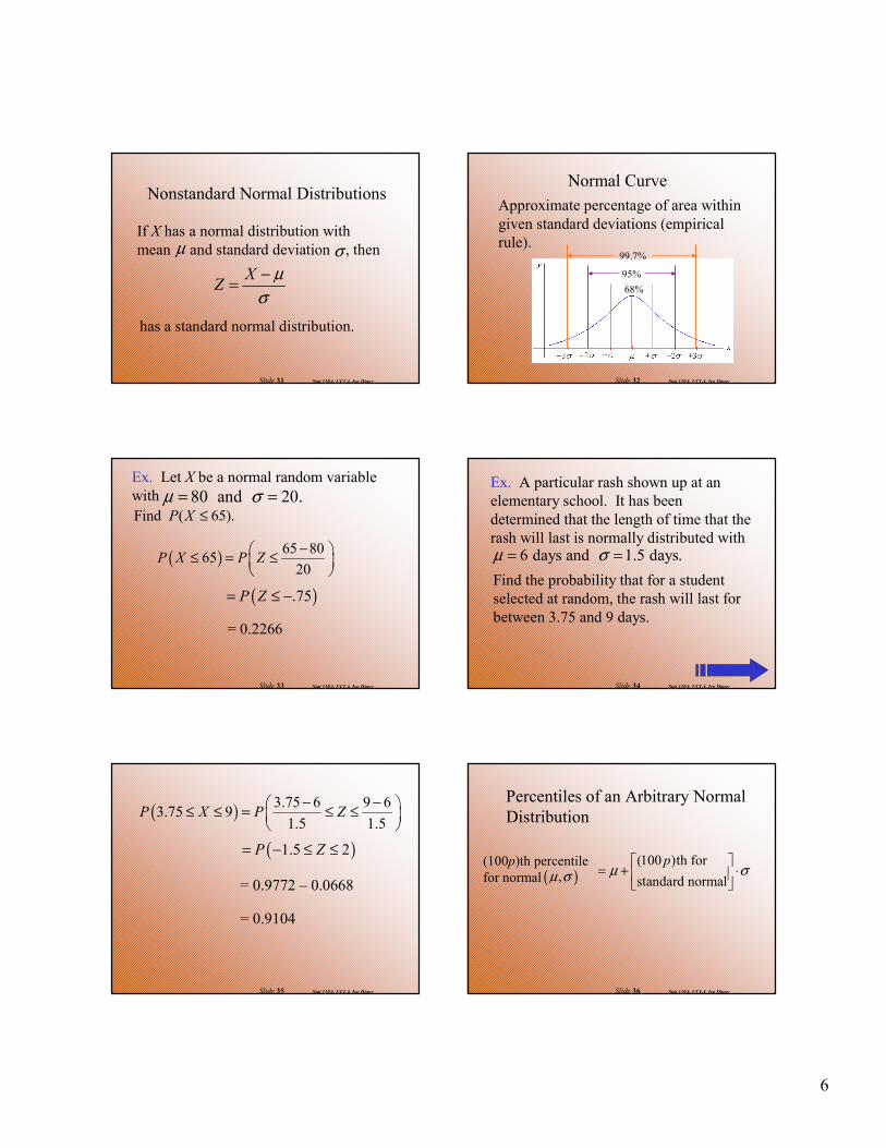
Stat 110A, UCLA, Ivo DinovSlide 31
Nonstandard Normal Distributions
If X has a normal distribution with mean and standard deviation , then µ σ
XZ µσ−=
has a standard normal distribution.
Stat 110A, UCLA, Ivo DinovSlide 32
Normal Curve
68%95%
99.7%
Approximate percentage of area within given standard deviations (empirical rule).
Stat 110A, UCLA, Ivo DinovSlide 33
Ex. Let X be a normal random variable with
= 0.2266
( ) 65 806520
P X P Z − ≤ = ≤
( ).75P Z= ≤ −
Find ( 65).P X ≤80 and 20.µ σ= =
Stat 110A, UCLA, Ivo DinovSlide 34
Ex. A particular rash shown up at an elementary school. It has been determined that the length of time that the rash will last is normally distributed with
6 days and 1.5 days.µ σ= =Find the probability that for a student selected at random, the rash will last for between 3.75 and 9 days.
Stat 110A, UCLA, Ivo DinovSlide 35
( ) 3.75 6 9 63.75 91.5 1.5
P X P Z− − ≤ ≤ = ≤ ≤
( )1.5 2P Z= − ≤ ≤
= 0.9772 – 0.0668
= 0.9104
Stat 110A, UCLA, Ivo DinovSlide 36
Percentiles of an Arbitrary Normal Distribution
(100p)th percentile for normal
(100 )th forstandard normal
pµ σ
= + ⋅ ( ),µ σ

7
Stat 110A, UCLA, Ivo DinovSlide 37
Let X be a binomial rv based on n trials, each with probability of success p. If the binomial probability histogram is not too skewed, X may be approximated by a normal distribution with
and .np npqµ σ= =
Normal Approximation to the Binomial Distribution
0.5( ) x npP X xnpq
+ −≤ ≈ Φ
Stat 110A, UCLA, Ivo DinovSlide 38
Ex. At a particular small college the pass rate of Intermediate Algebra is 72%. If 500 students enroll in a semester determine the probability that at least 375 students pass.
500(.72) 360npµ = = =
500(.72)(.28) 10npqσ = = ≈
375.5 360( 375) (1.55)10
P X − ≤ ≈ Φ = Φ
= 0.9394
Stat 110A, UCLA, Ivo DinovSlide 39
Normal approximation to Binomial
Suppose Y~Binomial(n, p)Then Y=Y1+ Y2+ Y3+…+ Yn, where
Yk~Bernoulli(p) , E(Yk)=p & Var(Yk)=p(1-p)
E(Y)=np & Var(Y)=np(1-p), SD(Y)= (np(1-p))1/2
Standardize Y:Z=(Y-np) / (np(1-p))1/2
By CLT Z ~ N(0, 1). So, Y ~ N [np, (np(1-p))1/2]
Normal Approx to Binomial is reasonable when np >=10 & n(1-p)>10(p & (1-p) are NOT too small relative to n).
Stat 110A, UCLA, Ivo DinovSlide 40
Normal approximation to Binomial – Example
Roulette wheel investigation:Compute P(Y>=58), where Y~Binomial(100, 0.47) –
The proportion of the Binomial(100, 0.47) population having more than 58 reds (successes) out of 100 roulette spins (trials).
Since np=47>=10 & n(1-p)=53>10 Normal approx is justified.
Z=(Y-np)/Sqrt(np(1-p)) = 58 – 100*0.47)/Sqrt(100*0.47*0.53)=2.2P(Y>=58) P(Z>=2.2) = 0.0139True P(Y>=58) = 0.177, using SOCR (demo!)Binomial approx useful when no access to SOCR avail.
Roulette has 38 slots18red 18black 2 neutral
Stat 110A, UCLA, Ivo DinovSlide 41
Normal approximation to Poisson
Let X1~Poisson(λ) & X2~Poisson(µ) X1+ X2~Poisson(λ+µ)
Let X1, X2, X3, …, Xk ~ Poisson(λ), and independent,Yk = X1 + X2 + ··· + Xk ~ Poisson(kλ), E(Yk)=Var(Yk)=kλ.
The random variables in the sum on the right are independent and each has the Poisson distribution with parameter λ.By CLT the distribution of the standardized variable (Yk − kλ) / (kλ)1/2 N(0, 1), as k increases to infinity.
So, for kλ >= 100, Zk = {(Yk − kλ) / (kλ)1/2 } ~ N(0,1).Yk ~ N(kλ, (kλ)1/2).
Stat 110A, UCLA, Ivo DinovSlide 42
Normal approximation to Poisson – example
Let X1~Poisson(λ) & X2~Poisson(µ) X1+ X2~Poisson(λ+µ)
Let X1, X2, X3, …, X200 ~ Poisson(2), and independent,Yk = X1 + X2 + ··· + Xk ~ Poisson(400), E(Yk)=Var(Yk)=400.
By CLT the distribution of the standardized variable (Yk − 400) / (400)1/2 N(0, 1), as k increases to infinity.
Zk = (Yk − 400) / 20 ~ N(0,1) Yk ~ N(400, 400).P(2 < Yk < 400) = (std’z 2 & 400) = P( (2−400)/20 < Zk < (400−400)/20 ) = P( -20< Zk<0) = 0.5

8
Stat 110A, UCLA, Ivo DinovSlide 43
Poisson or Normal approximation to Binomial?
Poisson Approximation (Binomial(n, pn) Poisson(λ) ):
n>=100 & p<=0.01 & λ =n p <=20Normal Approximation
(Binomial(n, p) N ( np, (np(1-p))1/2) )np >=10 & n(1-p)>10
!)1(
yey
ppyn
npn
nyn
n
y
n
λλλ
− →−
→×
∞→− WHY?
Stat 110A, UCLA, Ivo DinovSlide 44
4.4
The Gamma Distribution and Its
Relatives
Stat 110A, UCLA, Ivo DinovSlide 45
The Gamma Function
For 0, α > the gamma function( ) is defined byαΓ
1
0
( ) xx e dxαα∞
− −Γ = ∫
Stat 110A, UCLA, Ivo DinovSlide 46
Gamma Distribution
A continuous rv X has a gamma distribution if the pdf is
1 /1 0( ; , ) ( )
0 otherwise
xx e xf x
α βαα β β α
− − ≥= Γ
where the parameters satisfy 0, 0.α β> >The standard gamma distribution has 1.β =
Stat 110A, UCLA, Ivo DinovSlide 47
Mean and Variance
The mean and variance of a random variable X having the gamma distribution
( ; , ) aref x α β
2 2( ) ( )E X V Xµ αβ σ αβ= = = =
Stat 110A, UCLA, Ivo DinovSlide 48
Probabilities from the Gamma Distribution
Let X have a gamma distribution with parameters
( ) ( ; , ) ;xP X x F x Fα β αβ
≤ = =
Then for any x > 0, the cdf of X is given byand .α β
where1
0
( ; )( )
x yy eF x dyα
αα
− −=
Γ∫

9
Stat 110A, UCLA, Ivo DinovSlide 49
Exponential Distribution
A continuous rv X has an exponential distribution with parameter if the pdf is
0( ; ) 0 otherwise
xe xf xλλλ
− ≥=
λ
Stat 110A, UCLA, Ivo DinovSlide 50
Mean and Variance
The mean and variance of a random variable X having the exponential distribution
2 22
1 1µ αβ σ αβλ λ
= = = =
Stat 110A, UCLA, Ivo DinovSlide 51
Probabilities from the Gamma Distribution
Let X have a exponential distributionThen the cdf of X is given by
0 0( ; )
1 0x
xF x
e xλλ −
<= − ≥
Stat 110A, UCLA, Ivo DinovSlide 52
Applications of the Exponential Distribution
Suppose that the number of events occurring in any time interval of length thas a Poisson distribution with parameter and that the numbers of occurrences in nonoverlapping intervals are independent of one another. Then the distribution of elapsed time between the occurrences of two successive events is exponential with parameter
tα
.λ α=
Stat 110A, UCLA, Ivo DinovSlide 53
The Chi-Squared DistributionLet v be a positive integer. Then a random variable X is said to have a chi-squared distribution with parameter v if the pdf of X is the gamma density with
/ 2 and 2.vα β= = The pdf is( / 2) 1 / 2
/ 21 0
( ; ) 2 ( / 2) 0 0
v xv x e x
f x v vx
− − ≥= Γ <
Stat 110A, UCLA, Ivo DinovSlide 54
The Chi-Squared Distribution
The parameter v is called the number of degrees of freedom (df) of X. The symbol is often used in place of “chi-squared.”
2χ

10
Stat 110A, UCLA, Ivo DinovSlide 55
Identifying Common Distributions – QQ plots
Quantile-Quantile plots indicate how well the model distribution agrees with the data.
q-th quantile, for 0<q<1, is the (data-space) value, Vq, at or below which lies a proportion q of the data.
1 Graph of the CDF, FY(y)=P(Y<=Vq)=q
0
q
Vq
Stat 110A, UCLA, Ivo DinovSlide 56
Constructing QQ plots
Start off with data {y1, y2, y3, …, yn}Order statistics y(1) <= y(2) <= y(3) <=…<= y(n)Compute quantile rank, q(k), for each observation, y(k),
P(Y<= q(k)) = (k-0.375) / (n+0.250),where Y is a RV from the (target) model distribution.Finally, plot the points (y(k), q(k)) in 2D plane, 1<=k<=n.Note: Different statistical packages use slightly different formulas for the computation of q(k). However, the results are quite similar. This is the formulas employed in SAS.Basic idea: Probability that: P((model)Y<=(data)y(1))~ 1/n; P(Y<=y(2)) ~ 2/n; P(Y<=y(3)) ~ 3/n; …
Stat 110A, UCLA, Ivo DinovSlide 57
Example - Constructing QQ plots
Start off with data {y1, y2, y3, …, yn}.
Plot the points (y(k), q(k)) in 2D plane, 1<=k<=n.
-3-2-10123
Exp
ecte
d V
a lue
for
Nor
mal
Dis
trib
utio
n
C:\I
vo.d
ir\U
CLA
_Cla
sses
\Win
ter2
002\
Add
ition
alIn
stru
ctor
Aid
sB
irthd
ayD
istri
butio
n_19
78_s
ysta
t.SY
DSY
STA
T, G
raph
Prob
abili
ty P
lot,
Var
4, N
orm
al D
istri
butio
n
Stat 110A, UCLA, Ivo DinovSlide 58
4.5
Other Continuous Distributions
Stat 110A, UCLA, Ivo DinovSlide 59
The Weibull Distribution
A continuous rv X has a Weibulldistribution if the pdf is
1 ( / ) 0( ; , )
0 0
xx e xf x
x
αα βα
αα β β
− − ≥= <
where the parameters satisfy 0, 0.α β> >
Stat 110A, UCLA, Ivo DinovSlide 60
Mean and Variance
The mean and variance of a random variable X having the Weibulldistribution are
22 21 2 11 1 1µ β σ β
α α α
= Γ + = Γ + − Γ +

11
Stat 110A, UCLA, Ivo DinovSlide 61
Weibull Distribution
The cdf of a Weibull rv having parameters
( / )1 0( ; , ) 0 < 0
xe xF xx
αβα β
− − ≥=
and is α β
Stat 110A, UCLA, Ivo DinovSlide 62
Lognormal Distribution
A nonnegative rv X has a lognormal distribution if the rv Y = ln(X) has a normal distribution the resulting pdf has parameters
2 2[ln( ) ] /(2 )1 0( ; , ) 2
0 0
xe xf x x
x
µ σµ σ πα
− − ≥= <
and and isµ σ
Stat 110A, UCLA, Ivo DinovSlide 63
Mean and Variance
The mean and variance of a variable Xhaving the lognormal distribution are
( )2 2 2/ 2 2( ) ( ) 1E X e V X e eµ σ µ σ σ+ += = −
Stat 110A, UCLA, Ivo DinovSlide 64
Lognormal Distribution
( ; , ) ( ) [ln( ) ln( )]F x P X x P X xµ α = ≤ = ≤
The cdf of the lognormal distribution is given by
ln( ) ln( )x xP Z µ µσ σ
− − = ≤ = Φ
Stat 110A, UCLA, Ivo DinovSlide 65
Beta Distribution
A rv X is said to have a beta distributionwith parameters A, B, 0, and 0α β> >if the pdf of X is( ; , , , )f x A Bα β =
1 11 ( ) 0( ) ( )
0 otherwise
x A B x xB A B A B A
α βα βα β
− − Γ + − − ⋅ ≥ − Γ ⋅Γ − −
Stat 110A, UCLA, Ivo DinovSlide 66
Mean and VarianceThe mean and variance of a variable Xhaving the beta distribution are
( )A B A αµα β
= + − ⋅+
22
2( )
( ) ( 1)B A αβσ
α β α β−=
+ + +

12
Stat 110A, UCLA, Ivo DinovSlide 67
4.6
Probability Plots
Stat 110A, UCLA, Ivo DinovSlide 68
Sample Percentile
Order the n-sample observations from smallest to largest. The ith smallest observation in the list is taken to be the [100(i – 0.5)/n]th sample percentile.
Stat 110A, UCLA, Ivo DinovSlide 69
Probability Plot
[100( .5) / ]th percentile th smallest sampleof the distribution observation
i n i− ,If the sample percentiles are close to the corresponding population distribution percentiles, the first number will roughly equal the second.
Stat 110A, UCLA, Ivo DinovSlide 70
Normal Probability Plot
A plot of the pairs( )[100( .5) / ]th percentile, th smallest observationi n z i−
On a two-dimensional coordinate system is called a normal probability plot. If the drawn from a normal distribution the points should fall close to a line with slope and interceptσ .µ
Stat 110A, UCLA, Ivo DinovSlide 71
Beyond NormalityConsider a family of probability distributions involving two parameters
Let denote the1 2 and .θ θ 1 2( ; , )F x θ θcorresponding cdf’s. The parameters
1 2 and θ θ are said to location and scaleparameters if
11 2
2( ; , ) is a function of .xF x θθ θ
θ−
Stat 110A, UCLA, Ivo DinovSlide 72
Relation among Distributions
Normal (X)2,σµ
Normal (Z)1,0
σµ−= XZ
Lognormal (Y)2,σµ
YX ln= XeY =Chi-square ( )
n
2χ
∑ == n
i iZ1
2χ
Gammaβα ,
2,2/ == βα n
Exponential(X)β
1=α
n=2
Weibullβγ ,
1=γ
Uniform(U)1,0
UX lnβ−=
Uniform(X)βα ,
αβα
−−= XU ααβ +−= UX )(
Betaβα , 1== βα
Cauchy(0,1)
Tdf=n(0,1)
∞→df
1→df