Embed Size (px)
Citation preview
UCGE Reports
Number 20311
Department of Geomatics Engineering
Reliability of Combined GPS/GLONASS Ambiguity
Resolution
(URL: http://www.geomatics.ucalgary.ca/graduatetheses)
by
Richard Ong
July 2010

UNIVERSITY OF CALGARY
Reliability of Combined GPS/GLONASS Ambiguity Resolution
by
Richard Ong
A THESIS
SUBMITTED TO THE FACULTY OF GRADUATE STUDIES
IN PARTIAL FULFILMENT OF THE REQUIREMENTS FOR THE
DEGREE OF MASTER OF SCIENCE
DEPARTMENT OF GEOMTICS ENGINEERING
CALGARY, ALBERTA
July 2010
© Richard Ong (2010)
ii
Abstract
This thesis presents an analysis of the impact of combining GPS and GLONASS on the
reliability of phase ambiguity resolution (fixing). The rate of correct fixes (i.e. the actual
success rate) is investigated, as well as the identification of those fixes as correct or
incorrect. Two reliability indicators – the predicted success rate and the F-test – are
evaluated.
The processing software PLANSoft™ was developed to do GPS/GLONASS ambiguity
resolution. GLONASS is incorporated either by partial fixing (only GPS) or full fixing
(both GPS and GLONASS). Single- and dual-frequency strategies are also investigated.
Static analysis reveals that GLONASS full fixing increases actual success rate, fix
reliability (using the F-test) and solution availability. The L1/L2 strategy similarly
improves success rate and reliability. Widelane is effective for longer baselines due to the
smaller effect of phase errors. Testing under overhead foliage induces cycle slips which
decrease the observability of the ambiguities.

iii
Acknowledgements
I would like to acknowledge the following persons and parties for their invaluable
contributions to this thesis:
1. First and foremost, my family: my parents William and Nancy, my brother Jan,
and my fiancée Leslie. Nothing in this world would be possible or worthwhile
without your endless love, support and encouragement.
2. My supervisor, Professor Gérard Lachapelle. My internship, graduate studies and
various research projects under your guidance and support have opened many
doors, both to wisdom and to opportunity. Thank you for sharing your knowledge
and your advice and your stories, and for giving me countless opportunities to
push myself and develop new skills.
3. My co-supervisor, Professor Mark Petovello. I am grateful to you for both the
volume of knowledge you passed on to me as well as the patience, perseverance
and guiding hand with which you passed on that knowledge.
4. Research associates, past and present, from the PLAN Group with whom I have
collaborated: Dr. Cillian O’Driscoll, Dr. Daniele Borio, Dr. Tom Williams, Dr.
Valerie Renaudin, Mr. Rob Watson, Mr. Saurabh Godha and Mr. John Schleppe.
iv
Many of the skills that I required for this research have been developed in one
way or another through my collaborations with these individuals.
5. Those individuals involved with the STEALTH™ project for Alpine Canada,
General Motors or the Crash Avoidance Metrics Partnership (CAMP): Professor
Gérard Lachapelle, Aiden Morrison, Dr. Gerald Cole, James Perks, Dr. Tom
Williams, Dr. Paul Alves and Dr. Chaminda Basnayake. Much of my theoretical
and practical knowledge of ambiguity resolution has come from my involvement
with these projects and individuals.
6. Those individuals who helped me collect data for this research: Professor Gérard
Lachapelle, Dr. Tom Williams, Jared Bancroft, Billy Chan, Towfique Ahmed and
Michelle Hua. Data collection is more effective and pleasant as a team effort.
7. Professor Kyle O’Keefe and Dr. Glenn MacGougan. Our discussions regarding
RTK implementation details were invaluable to the design of PLANSoft™. I am
also grateful to Professor Mark Petovello, Mr. Junjie Liu and all other developers
of FLYKIN+™, from which much of the structure and implementation of
PLANSoft™ was adapted.
8. The National Sciences and Engineering Research Council of Canada (NSERC),
and the Alberta Informatics Circle of Research Excellence (iCORE) for their
financial support.
v
Table of Contents
Abstract ............................................................................................................................... ii
Acknowledgements ............................................................................................................ iii
Table of Contents .................................................................................................................v
List of Tables .................................................................................................................... vii
List of Figures ......................................................................................................................x
List of Symbols and Abbreviations.................................................................................. xiv
CHAPTER ONE: INTRODUCTION ..................................................................................1
1.1 Background ................................................................................................................1
1.2 Objectives ..................................................................................................................3
1.3 Thesis Outline ............................................................................................................5
CHAPTER TWO: AMBIGUITY ESTIMATION AND RESOLUTION ...........................7
2.1 Principles of Navigation and Ambiguity Estimation .................................................7
2.1.1 Measurements ....................................................................................................7
2.1.2 Ambiguity Estimation .....................................................................................10
2.1.3 Ambiguity Resolution .....................................................................................12
2.2 GLONASS Ambiguity Resolution ..........................................................................14
2.3 Reliability of Ambiguity Resolution ........................................................................17
2.4 Ambiguity Resolution Success Rate ........................................................................20
2.5 Fix Validation and the F Ratio Test .........................................................................24
CHAPTER THREE: TESTING AND ANALYSIS METHODS ......................................30
3.1 Test Scenarios ..........................................................................................................30
3.1.1 Static Baselines ................................................................................................30
3.1.2 Vehicle-to-Vehicle Relative Navigation .........................................................32
3.1.3 Downhill Ski Runs ..........................................................................................35
3.2 Hardware Characteristics .........................................................................................38
3.3 Navigation Methodology: PLANSoft™ ..................................................................41
3.4 Estimation Strategies ...............................................................................................46
vi
3.5 Convergence Time ...................................................................................................50
3.6 Generating Integer Fixes ..........................................................................................51
CHAPTER FOUR: STATIC TESTING RESULTS ..........................................................53
4.1 Positioning Accuracy ...............................................................................................54
4.2 Actual Success Rates ...............................................................................................67
4.3 Float Estimate Errors before Ambiguity Resolution ...............................................71
4.4 Phase Errors .............................................................................................................76
4.5 Success Rates under Simulated Reduced Visibility ................................................80
4.6 Reliability Testing: Predicted Success Rate ............................................................91
4.7 Reliability Testing: F-Test .....................................................................................100
4.8 Combining Reliability Tests ..................................................................................106
4.9 Probability of Cycle Slip Detection .......................................................................108
4.10 Reliability under Simulated Reduced Visibility ..................................................113
CHAPTER FIVE: KINEMATIC TESTING RESULTS .................................................123
5.1 Vehicle-to-Vehicle Relative Navigation ................................................................123
5.1.1 Actual Success Rates and Reliability Testing ...............................................124
5.1.2 Positioning Accuracy .....................................................................................133
5.1.3 Signal Tracking and Cycle Slips under Foliage ............................................138
5.2 Downhill Ski Runs .................................................................................................148
CHAPTER SIX: CONCLUSIONS AND RECOMMENDATIONS ..............................159
6.1 Conclusions ............................................................................................................160
6.2 Recommendations ..................................................................................................163
REFERENCES ................................................................................................................165
vii
List of Tables
Table 1 - Errors in ambiguity resolution reliability testing and fault detection ................ 19
Table 2 - F-test thresholds from central F distribution (significance level 10%) ............. 29
Table 3 - Signal tracking for V2V in all environments .................................................... 34
Table 4 - NovAtel OEMV2-G + NovAtel GPS-702-GG hardware: code multipath under open sky .......................................................................................................... 40
Table 5 - Median position errors from correct fixes - 2 km baseline under 5° mask ....... 57
Table 6 - RMS position errors from correct fixes - 2 km baseline under 5° mask ........... 57
Table 7 - Median position errors from correct fixes - 18 km baseline under 5° mask ..... 60
Table 8 - RMS position errors from correct fixes - 18 km baseline under 5° mask ......... 60
Table 9 - Actual success rate probabilities - static baselines under 5° mask .................... 68
Table 10 - Horizontal float errors before fix - static baselines under 5° mask ................. 72
Table 11 - Total number of fixes - static baselines under 30° mask ................................. 81
Table 12 - Actual success rate probabilities - static baselines under 30° mask ................ 81
Table 13 - Horizontal float errors before fix - static baselines under 30° mask ............... 83
Table 14 - Predicted success rate results - 2 km baseline under 5° mask ......................... 92
Table 15 - Predicted success rate results for undifferenced phase 1σ of 6.5 mm - 2 km baseline under 5° mask ............................................................................................. 97
Table 16 - Predicted success rate results - 18 km baseline under 5° mask ....................... 98
Table 17 - F-test results - 2 km baseline under 5° mask ................................................. 100
Table 18 - F-test power as a function of number of ambiguities .................................... 102
Table 19 - F-test results - 18 km baseline under 5° mask ............................................... 104
Table 20 - Combined reliability testing results - 2 km baseline under 5° mask ............. 107
Table 21 - Combined reliability testing results - 18 km baseline under 5° mask ........... 107
Table 22 - Probability of cycle slip detection results - 2 km baseline under 5° mask .... 112

viii
Table 23 - Probability of cycle slip detection results - 18 km baseline under 5° mask .. 113
Table 24 - Predicted success rate results - 2 km baseline under 30° mask ..................... 114
Table 25 - Predicted success rate results - 18 km baseline under 30° mask ................... 114
Table 26 - F-test results - 2 km baseline under 30° mask ............................................... 118
Table 27 - F-test results - 18 km baseline under 30° mask ............................................. 119
Table 28 - Combined reliability testing results - 2 km baseline under 30° mask ........... 122
Table 29 - Combined reliability testing results - 18 km baseline under 30° mask ......... 122
Table 30 - Total number of fixes - V2V all environments under 5° mask ..................... 124
Table 31 - Actual success rate probabilities - V2V all environments under 5° mask .... 126
Table 32 - Predicted success rate results - V2V open sky under 5° mask ...................... 128
Table 33 - Predicted success rate results - V2V foliage under 5° mask ......................... 129
Table 34 - F-test results - V2V open sky under 5° mask ................................................ 130
Table 35 - F-test results - V2V foliage under 5° mask ................................................... 130
Table 36 - Combined reliability testing results - V2V open sky under 5° mask ............ 132
Table 37 - Combined reliability testing results - V2V foliage under 5° mask ............... 132
Table 38 - Median position errors from correct fixes - V2V open sky under 5° mask .. 136
Table 39 - RMS position errors from correct fixes - V2V open sky under 5° mask ...... 136
Table 40 - Median position errors from correct fixes - V2V foliage under 5° mask ...... 137
Table 41 - RMS position errors from correct fixes - V2V foliage under 5° mask ......... 137
Table 42 - Signal tracking for V2V in all environments ................................................ 139
Table 43 - Signal tracking parameters for correct and incorrect L1 + L2 GG fixed GLO fixes - V2V foliage under 5° mask ................................................................ 142
Table 44 - Total number of fixes - downhill ski runs with all masks ............................. 149
Table 45 - Actual success rate probabilities - downhill ski runs with all masks ............ 152
Table 46 - Predicted success rate results - downhill ski runs with 5° mask ................... 153
Table 47 - Predicted success rate results - downhill ski runs with 30° mask ................. 154

ix
Table 48 - F-test results - downhill ski runs with 5° mask ............................................. 155
Table 49 - F-test results - downhill ski runs with 30° mask ........................................... 156
Table 50 - Combined reliability testing results - downhill ski runs with 5° mask.......... 157
Table 51 - Combined reliability testing results - downhill ski runs with 30° mask........ 158
x
List of Figures
Figure 1 - Static baselines - base station ........................................................................... 31
Figure 2 - Static baselines - rover station.......................................................................... 31
Figure 3 - Vehicle-to-vehicle relative navigation - partly open sky ................................. 33
Figure 4 - Vehicle-to-vehicle relative navigation - under foliage ..................................... 33
Figure 5 - Tracking downhill ski runs............................................................................... 36
Figure 6 - Vertical consistency of ski runs at checkpoints ............................................... 37
Figure 7 - NovAtel OEMV2-G + NovAtel GPS-702-GG hardware: code and phase errors under an open-sky zero-baseline configuration .............................................. 40
Figure 8 - NovAtel OEMV2-G + ANTCOM-GG hardware: code and phase errors from an open-sky kinematic test ............................................................................... 41
Figure 9 - Example of SD to DD transformation .............................................................. 45
Figure 10 - Measurement combinations and fixing strategies .......................................... 49
Figure 11 - Relationship between fix reliability and convergence time ........................... 50
Figure 12 - Data processing method for generating many integer fixes ........................... 52
Figure 13 - 2D view of position errors, all fixes - 2 km baseline under 5° mask ............. 56
Figure 14 - 2D view of position errors, correct fixes - 2 km baseline under 5° mask ...... 56
Figure 15 - 2D view of position errors, all fixes - 18 km baseline under 5° mask ........... 59
Figure 16 - 2D view of position errors, correct fixes - 18 km baseline under 5° mask .... 59
Figure 17 - Horizontal fixed errors vs. ADOP - 2 km baseline under 5° mask ................ 62
Figure 18 - Horizontal fixed errors vs. ADOP - 18 km baseline under 5° mask .............. 63
Figure 19 - Frequency distributions of ADOP - 18 km baseline under 5° mask .............. 63
Figure 20 - L1 DD phase errors - static baselines ............................................................. 64
Figure 21 - Horizontal fixed errors vs. phase error standard deviation - 2 km baseline under 5° mask ........................................................................................................... 66
xi
Figure 22 - Horizontal fixed errors vs. phase error standard deviation - 18 km baseline under 5° mask ........................................................................................................... 67
Figure 23 - GLONASS adjusted ambiguity uncertainties for L1 only GG float GLO solution - 2 km baseline under 5° mask .................................................................... 70
Figure 24 - Actual success rate vs. 3D fixed errors - 18 km baseline under 5° mask ...... 70
Figure 25 - Actual success rate vs. median horizontal float errors - static baselines under 5° mask ........................................................................................................... 73
Figure 26 - Actual success rate vs. horizontal float errors - 2 km baseline under 5° mask .......................................................................................................................... 75
Figure 27 - Actual success rate vs. horizontal float errors - 18 km baseline under 5° mask .......................................................................................................................... 76
Figure 28 - Distribution of phase error standard deviation for L1 only GG fixed GLO solution - 18 km baseline under 5° mask .................................................................. 77
Figure 29 - Actual success rate vs. phase error standard deviation - 2 km baseline under 5° mask ........................................................................................................... 79
Figure 30 - Actual success rate vs. phase error standard deviation - 18 km baseline under 5° mask ........................................................................................................... 79
Figure 31 - Distribution of phase error standard deviation for widelane GG fixed GLO solution - 18 km baseline under 5° mask ......................................................... 80
Figure 32 - Relationship between horizontal float error before fix and HDOP using L1 only GPS only solution - 2 km baseline .............................................................. 83
Figure 33 - Distribution of number of ambiguities for L1 only GPS only solution - 2 km baseline under 5° mask ....................................................................................... 85
Figure 34 - Distribution of number of ambiguities for L1 only GPS only solution - 2 km baseline under 30° mask ..................................................................................... 86
Figure 35 - Distribution of number of ambiguities for L1 only GG float GLO solution - 2 km baseline under 30° mask ................................................................................ 86
Figure 36 - Distribution of number of ambiguities for L1 only GG fixed GLO solution - 2 km baseline under 30° mask ................................................................................ 87
Figure 37 - Actual success rate vs. number of ambiguities - 2 km baseline under 30° mask .......................................................................................................................... 88
Figure 38 - Actual success rate vs. number of ambiguities - 18 km baseline under 30° mask .......................................................................................................................... 89
xii
Figure 39 - Actual success rate vs. ADOP - 2 km baseline under 30° mask .................... 90
Figure 40 - Actual success rate vs. ADOP - 18 km baseline under 30° mask .................. 90
Figure 41 - Distribution of predicted success rate for L1 only GPS only solutions - 2 km baseline under 5° mask .................................................................................... 94
Figure 42 - Predicted success rate as a function of a priori phase uncertainty ................ 95
Figure 43 - Distribution of predicted success rate for widelane GG fixed GLO solution - 18 km baseline under 5° mask .................................................................. 99
Figure 44 - Distribution of F-test result for L1 only GPS only solution - 2 km baseline under 5° mask ......................................................................................................... 103
Figure 45 - F-test correct fix acceptance vs. phase error standard deviation - 2 km baseline under 5° mask ........................................................................................... 104
Figure 46 - F-test correct fix acceptance vs. phase error standard deviation - 18 km baseline under 5° mask ........................................................................................... 105
Figure 47 - Time series of probabilities of cycle slip detection for L1 only GPS only solution - 2 km baseline under 5° mask .................................................................. 110
Figure 48 - Distribution of probabilities of cycle slip detection for L1 only GPS only solution - 2 km baseline under 5° mask .................................................................. 110
Figure 49 - Relationship between probability of cycle slip detection and predicted success rate for L1 only GPS only solution - 2 km baseline under 5° mask .......... 111
Figure 50 - Relationship between probability of cycle slip detection and F-test result for L1 only GPS only solution - 2 km baseline under 5° mask .............................. 111
Figure 51 - Predicted success rate incorrect fix rejection vs. number of ambiguities - 2 km baseline under 30° mask ................................................................................... 116
Figure 52 - Predicted success rate incorrect fix rejection vs. number of ambiguities - 18 km baseline under 30° mask .............................................................................. 116
Figure 53 - F-test correct fix acceptance vs. number of ambiguities - 2 km baseline under 30° mask ....................................................................................................... 119
Figure 54 - F-test correct fix acceptance vs. number of ambiguities - 18 km baseline under 30° mask ....................................................................................................... 120
Figure 55 - F-test correct fix acceptance vs. ADOP - 2 km baseline under 30° mask ... 120
Figure 56 - F-test correct fix acceptance vs. ADOP - 18 km baseline under 30° mask . 121
xiii
Figure 57 - 2D view of position errors, all fixes - V2V open sky under 5° mask .......... 133
Figure 58 - 2D view of position errors, correct fixes - V2V open sky under 5° mask ... 134
Figure 59 - 2D view of position errors, all fixes - V2V foliage under 5° mask ............. 134
Figure 60 - 2D view of position errors, correct fixes - V2V foliage under 5° mask ...... 135
Figure 61 - L1 DD code and phase errors - V2V all environments ................................ 140
Figure 62 - Actual success rate vs. lock time - V2V foliage under 5° mask .................. 143
Figure 63 - Relationship between ADOP and convergence time for L1 only GPS only solution - V2V foliage under 5° mask .................................................................... 144
Figure 64 - Relationship between ADOP and convergence time for L1 only GG fixed GLO solution - V2V foliage under 5° mask ........................................................... 145
Figure 65 - Relationship between ADOP and convergence time for L1 + L2 GPS only solution - V2V foliage under 5° mask .................................................................... 145
Figure 66 - Predicted success rate incorrect fix rejection vs. lock time - V2V foliage under 5° mask ......................................................................................................... 147
Figure 67 - Predicted success rate probability vs. lock time - V2V foliage under 5° mask ........................................................................................................................ 147
Figure 68 - F-test correct fix acceptance vs. lock time - V2V foliage under 5° mask .... 148

xiv
List of Symbols and Abbreviations
Symbol Definition
Single-difference operator for quantity
Double-difference operator for quantity
N Phase ambiguities
Phase in units of distance
Phase in units of cycles
Phase wavelength
Abbreviation Definition
ADOP Ambiguity dilution of precision
DD Double-difference
DOP Dilution of precision
FDMA Frequency division multiple access
GG GPS/GLONASS
GLO GLONASS
HDOP Horizontal dilution of precision
ILS Integer least-squares
LAMBDA Least-squares ambiguity decorrelation adjustment
PDOP Position dilution of precision
xv
RTK Real-time kinematic
SD Single-difference
V2V Vehicle-to-vehicle
WL Widelane
WSSR Weighted sum-of-squared residuals
1
Chapter One: Introduction
Differential carrier phase ambiguity resolution is a common technique for achieving sub-
decimetre positioning accuracy with Global Navigation Satellite Systems (GNSS). If the
ambiguities can be resolved to their correct integer values, the phase measurements can
be used for ranging with millimetre-level precision. However, an incorrectly resolved
ambiguity results in an undetected position bias. The reliability of positioning is thus
directly related to the reliability of ambiguity resolution. This thesis investigates the
impact of integrating the Russian Global Navigation Satellite System (GLONASS) with
the Global Positioning System (GPS) on the reliability of ambiguity resolution.
1.1 Background
GNSS carrier phase measurements are generally very precise. Spatially correlated effects
(such as orbit and atmosphere) and clock effects are removed or reduced by differencing
measurements between receivers. The resulting differential phase precision is at the
millimetre level; however differential ionospheric errors can sometimes exceed the metre
level over long distances (over 100 km) between the two receivers when the ionosphere is
disturbed (Cosentino et al 2006). However, the phase measurements also contain an
unknown number of integer cycles. This ambiguity must be resolved (or fixed; the terms
“ambiguity resolution” and “ambiguity fix” are used interchangeably herein) to the
correct integer value before the phase can be used for high-precision ranging.

2
The importance of resolving the ambiguities correctly must be emphasized. An error of
even one cycle on a single phase measurement can result in a position bias of many
centimetres or decimetres (depending on the geometry). This bias often goes undetected
as the position is generally assumed to be precise if the ambiguity is resolved correctly
(even when that is not actually the case). The ambiguities must be highly observable in
order to get initial real-valued (“float”) estimates that are accurate enough to be
subsequently fixed to the correct integer (“fixed”) values.
The observability of the ambiguities is a fundamental challenge: phase measurements
alone generally cannot observe them. Code and phase measurements together can
observe them but differential code accuracy is at the decimetre level at best (Cosentino et
al 2006). Observability of the ambiguities can be improved by using measurements taken
over multiple epochs. As the position states converge to the true trajectory, the
ambiguities become more observable by both code and phase, and will converge to their
correct integer values as well. Observability can also be improved by using code and
phase measurements from more satellites. This improves the position geometry and
speeds up the convergence of the position and ambiguities. In addition, the accuracy after
the ambiguities are resolved is marginally improved by averaging down noise and
multipath and improving satellite geometry.
Ambiguity resolution is difficult in signal shaded environments like mountainous areas,
and residential and inner city areas where trees and buildings obstruct lines-of-sight to the
satellites. This significantly impacts the observability of both the position and the

3
ambiguities. Consequently, the ambiguities cannot be fixed to their correct integer values
as often. GPS is frequently used alone but might not provide the adequate geometry.
Other GNSS can be used to increase the number of available code and phase
measurements. GLONASS is currently the only GNSS near full operational capability.
Ambiguity resolution using GPS and GLONASS together has been widely investigated
(e.g. van Diggelen 1997, Keong & Lachapelle 2000, Habrich et al 1999, Wang 2000).
The focus of much of the literature is on algorithms for integrating GLONASS phase
measurements (e.g. Wang 2000), or the effect of GLONASS on position accuracy and fix
performance (e.g. van Diggelen 1997). It has generally been found that the addition of
GLONASS improves positioning accuracy.
1.2 Objectives
It is difficult to resolve the phase ambiguities correctly all of the time and in all
environments and field conditions, even when GPS and GLONASS are integrated. The
consequence of resolving the ambiguities incorrectly is undetected position biases, hence
it is critically important not to accept incorrect fixes. In that light, this thesis investigates
the impact of adding GLONASS to GPS on the reliability of the ambiguity resolution
process itself. Reliability in this context refers to the ability to reject incorrect ambiguity
fixes, such that they do not introduce position biases. However the identification and
acceptance of correct fixes is also important to achieve precise positioning. The
objectives of this research are the following:
4
1. Determine how adding GLONASS impacts the rate of correct ambiguity fix. This
is often referred to as the actual success rate. This effect is important to study as
one way to reduce the rate of incorrect fix acceptance is to just reduce the rate of
incorrect fixes.
2. Determine how adding GLONASS impacts the rate of acceptance of correct fixes
and rejection of incorrect fixes. The predicted success rate and F-test reliability
tests are described herein as methods of discriminating the correctness of fixes.
The impact of GLONASS on the performance of these tests is investigated.
3. Characterize the factors that influence success rate and reliability. Different
environments, restricted satellite visibility and the effect of ionosphere over
longer inter-receiver distances are explored.
Much of the previous research in fix reliability has characterized it theoretically or using
simulations (e.g. Teunissen 1998, Teunissen and Verhagen 2004, Teunissen et al 1999,
Verhagen 2004, 2005, O’Keefe et al 2006). The scope of this research is fix reliability in
three real-world scenarios: 1.) static baselines under open sky; 2.) platform-to-platform
relative navigation under open sky and foliage; and 3.) tracking downhill skiers. Inter-
receiver distances range from 10 m to 18 km (at which point ionosphere effects are
studied). Restricted satellite visibility conditions are simulated by imposing circular
elevation masks of up to 30°. Ambiguity resolution is performed repeatedly by fixing and
then resetting the ambiguities. Special processing software (PLANSoft™) was developed

5
to do the GPS/GLONASS ambiguity resolution, as well as generate the predicted success
rate and F-test result. These tests are evaluated by determining how often they correctly
identify correct and incorrect fixes.
The contribution of this research is characterizing the exact impact of GLONASS on fix
reliability. This is evaluated by comparing the performance of GPS alone to that of
GPS/GLONASS (GG). GPS and GLONASS are integrated in two ways: 1.) partial fixing
of only GPS ambiguities; and 2.) full fixing of both GPS and GLONASS ambiguities.
Different subsets of phase measurements – L1 only, L1 and L2 used separately, and L1
and L2 in the widelane combination – are also explored. To accomplish the above,
PLANSoft™ was developed by the author and significant field testing was conducted.
1.3 Thesis Outline
This thesis consists of six chapters. Chapter One introduces the motivation and objectives
of this thesis. The scope and contributions of the research are defined.
Chapter Two presents an overview of ambiguity estimation and resolution. The reliability
of ambiguity resolution is discussed in detail. The predicted success rate and the F-test
are introduced and their role in ambiguity estimation is discussed.
Chapter Three describes the testing, data processing and analysis methods. Three test
scenarios are proposed: 1.) static baselines under open sky; 2.) platform-to-platform

6
navigation in urban environments; and 3.) downhill skiers on an open ski slope. The
GLONASS navigation and ambiguity resolution algorithm (implemented in
PLANSoft™) is described, and various strategies for incorporating measurements into
ambiguity estimation are outlined. The methods and visual displays used to derive and
analyze the ambiguity resolution results are also defined.
The results of the static baseline testing are presented in Chapter Four. This chapter
investigates the impact of GLONASS and dual-frequency measurement combinations on
the success rate, as well as the acceptance of correct fixes and the rejection of incorrect
fixes. The causative and related factors are then investigated in detail, including: float
solution errors; phase errors; number of ambiguity states; ambiguity dilution of precision;
and the probability of cycle slip detection. These are illustrated to visually facilitate
interpretation. An analysis of the fixed-ambiguity positioning accuracy is also provided.
The results of the two kinematic tests are presented in Chapter Five. This chapter gives an
overview of the success rate and reliability of ambiguity resolution in these scenarios.
The impact of foliage, particularly in terms of how signal tracking affects ambiguity
resolution, is further investigated.
Chapter Six concludes this thesis and presents the major findings from the previous
chapters. Recommendations for future research in this area are finally made.
7
Chapter Two: Ambiguity Estimation and Resolution
This chapter presents an overview of phase ambiguity estimation. The role of code and
phase measurements in navigation using ambiguity estimation is described in detail. A
review of ambiguity resolution methods from the literature is then presented, both in
general and specific to the use of GLONASS. The reliability of ambiguity resolution is
also discussed.
2.1 Principles of Navigation and Ambiguity Estimation
2.1.1 Measurements
GNSS provides two types of measurements for ranging and position estimation: code and
phase measurements. These measurements have different properties:
1. Code measurements are derived from the pseudo-random noise (PRN) code
overlaid on the carrier signal. Correlating the incoming PRN code with a locally
generated replica gives an estimate of the signal delay. This delay can be
converted into the satellite-to-user range; however it is affected by satellite and
receiver clock errors. Atmosphere effects and orbit determination errors also
impact the accuracy of the code measurement. The latter effects are spatially
correlated, and are reduced by differencing measurements between two nearby
GNSS receivers (often designated as base and rover receivers or stations). This

8
single-differencing (SD) technique also removes the satellite clock errors. Further
refinement is done by differencing SD measurements between satellite pairs to
remove receiver clock errors. Usually all of the satellite pairs share a common
satellite, designated as the base satellite. The resulting double-differenced (DD)
code measurement is parameterized as
PP R
where “ ” is the double-differencing operator,
P is the DD code measurement,
R is the DD satellite-to-user range, and
P is the DD code error.
The DD code measurement directly observes the DD satellite-to-user range,
which is used to derive the vector between the base and rover receivers. Spatially
correlated effects like the atmosphere are reduced in this manner. However,
measurement noise and multipath do not cancel out; instead, they are additive
when expressed as variances (Lachapelle 2008). The exact level of noise and
multipath is highly dependent on receiver technology, signal strength and
reflector type. However, code chips are generally hundreds of metres long,
ultimately limiting the precision of the derived signal delay. Conley et al (2006)
gives a typical stand-alone error budget of 10 cm and 20 cm for noise and

9
multipath, respectively. For SD or DD processing these budgeted errors must be
multiplied by 2 .
2. Phase measurements are derived from the Doppler frequency of the carrier signal
itself. Correlating the incoming carrier with a locally generated replica gives an
estimate of the carrier’s Doppler frequency. This frequency is a measure of the
satellite-to-user relative velocity. The Doppler frequency induces a change in the
phase of the carrier; integrating these phase changes over time gives the total
change in the satellite-to-user range since the start of integration. Therefore the
phase does not measure the absolute range, but contains an ambiguity that (when
expressed in carrier cycles) is integer in nature.
Like the code, the phase is affected by clock errors, atmospheric effects and
incorrect orbit determination. The double-differenced parameterization (which
removes or reduces these effects) is expressed as
i i base baseR N N
where “ ” is the single-differencing operator,
is the DD phase (expressed in units of distance),
N is the DD phase ambiguity,
baseN is the base satellite’s SD phase ambiguity,
10
i is the wavelength of the signal from the ith satellite
base is the wavelength of the signal from the base satellite, and
is the DD phase error.
The precision of DD phase measurements is much better than that of the code
measurement due to the shorter carrier wavelength. Phase noise is nominally on
the order of 1-2 mm, while the typical phase multipath 1σ level is around 2 cm in
benign environments (Lachapelle 2008).
If velocity estimation is required, it can be achieved either by differentiating positions
over time, or using the un-integrated Doppler frequency of the carrier.
2.1.2 Ambiguity Estimation
To use phase measurements for positioning, it is necessary to estimate the phase
ambiguities. Ideally they are estimated as integers in the process of integer ambiguity
resolution or ambiguity fixing. However they can also be estimated as real or “floating-
point” values in the process of float ambiguity estimation. There are two approaches to
ambiguity estimation (e.g. O’Keefe et al 2009):
11
1. Geometry-based approach. The DD measurements are used to estimate the
position (more correctly, the vector between the base and rover receivers) along
with the ambiguities until the latter can be resolved.
2. Geometry-free approach. Each DD measurement is used to estimate the
corresponding DD satellite-to-user range and ambiguity. Different DD
measurements are treated independently until the ambiguities can be resolved, at
which point the DD phase measurements are used to estimate the positions.
In both approaches, the phase measurements generally cannot be used alone to estimate
the ambiguities since they cannot simultaneously observe the position and ranges. The
code measurements must be used in conjunction, which is a limiting factor in ambiguity
estimation. Even with sub-metre code noise and multipath, a single epoch of code and
phase measurements is generally not enough to do float ambiguity estimation to better
than half a wavelength (e.g. for the L1 band, less than 10 cm; for the L2 band, less than
13 cm). As a rule of thumb, this is the accuracy required to resolve the ambiguities
correctly and reliably. This problem is overcome by taking advantage of the fact that
phase ambiguities remain constant over time if phase lock is maintained, i.e. there are no
cycle slips. Thus the ambiguities can be estimated using measurements over multiple
epochs.
The estimation is more effective if there is also a priori knowledge of the position or the
satellite-to-user ranges. For kinematic applications the position (or range) and

12
ambiguities can both be constrained in a filter (such as a Kalman filter) designed and
tuned for the expected dynamics. Within such a filter, the position (or range) and
ambiguity estimates are said to converge to their true values as the measurement errors
are smoothed out.
2.1.3 Ambiguity Resolution
Ambiguity resolution is an integer estimation problem. Therefore, standard linear
estimators such as parametric least-squares cannot be used to estimate the integer
ambiguities. Solving for the integer ambiguities is conceptually defined as a three-step
process (Teunissen 2003): 1.) estimate the float ambiguities; 2.) map the float ambiguities
to integer values, and validate those integers; and 3.) adjust the float estimate of the
position. If the integer ambiguity estimate is correct, then the phase measurements can
directly observe the satellite-to-user ranges (and consequently the user’s position) with up
to millimetre-level precision.
The most basic ambiguity resolution methods are integer rounding and bootstrapping. In
integer rounding, each real-valued ambiguity is rounded to the nearest integer.
Bootstrapping is a variation of integer rounding: after one ambiguity is rounded to the
nearest integer, the real-valued estimates of the remaining unrounded ambiguities are
corrected according to their correlation with the first ambiguity (Teunissen 2003).
13
More sophisticated ambiguity resolution methods have been listed and classified by Yang
et al (2006). The most common class of ambiguity resolution method is the search
method. Han & Rizos (1996) define searching techniques in three domains: 1.) the
measurement domain; 2.) the position domain; and 3.) the ambiguity domain. In each
case a “search space” of candidate values is defined for the parameter in the search
domain. The candidates in the search space are discriminated (according to some criteria)
and the one corresponding to the “best” estimate of the integer ambiguities is chosen.
The integer least-squares (ILS) method has been demonstrated as the optimal search
method in terms of maximizing the probability of correct fix (Teunissen 2001a, 2003).
Float estimation with a geometry-based model is used to initialize a search space over the
integer ambiguities. ILS then seeks to minimize the weighted sum of squared ambiguity
residuals, or the distances between the (initial) float and (final) integer ambiguity
estimates (Teunissen 2000b). Other search methods include the ambiguity function
method (Counselman & Gourevitch 1981, Mader 1992), the Fast Ambiguity Search Filter
(FASF) (Chen & Lachapelle 1995), and the Fast Ambiguity Resolution Approach
(FARA) (Frei & Butler 1990).
Pre-processing of the ambiguities has also been investigated with positive results in terms
of reducing search spaces. The most important of these is the Least-Squares Ambiguity
Decorrelation Adjustment (LAMBDA), which applies a linear transformation to the
ambiguities to decorrelate them for more efficient searching (Teunissen 1995). Cholesky

14
decomposition of the variance-covariance matrices was also proposed by Landau & Euler
(1992) as a way to reduce the search space.
2.2 GLONASS Ambiguity Resolution
Resolving GLONASS phase ambiguities is difficult due to the frequency division
multiple access (FDMA) structure of the GLONASS signal. The DD phase
parameterization is reiterated here:
i i base baseR N N .
For GPS measurements, the term i base is zero since each satellite transmits on the
same frequency. The term N is the only ambiguity that needs to be estimated. This is
the DD phase ambiguity and is integer in nature. For GLONASS this is not the case since
each satellite transmits its signals on a different frequency. The maximum wavelength
difference between signals from different satellites is 0.9 mm (in the L1 band) and 1.1
mm (in the L2 band). Therefore, there are two ambiguity terms to consider: N , the
DD phase ambiguity; and baseN , the SD phase ambiguity of the GLONASS base
satellite. Both ambiguities are integer in nature. However, if the frequency division of the
signals is ignored, then the base satellite SD ambiguity is effectively absorbed by the DD
ambiguity and the resulting quantity ( i i base baseN N ) is not integer in nature.
15
Several methods to overcome this problem have been presented in the literature. Some of
the major results and innovations include:
Keong & Lachapelle (2000) investigated GPS/GLONASS real-time kinematic
(RTK) processing for short-baseline attitude determination. The primary
innovation was the use of a common oscillator to drive both GNSS receivers. This
made double-differencing unnecessary as the clock errors between the two
receivers were only separated by a constant offset. Once the offset was calibrated
(using the residuals), SD measurements were used estimate and resolve the SD
phase ambiguities.
Wang (2000) attempted to estimate the SD ambiguity of the GLONASS base
satellite using code-minus-carrier. This rough estimate was refined by doing a
search over the adjacent integers, using test statistics to choose the integer.
Habrich et al (1999) used SD measurements to do float ambiguity estimation in a
geometry-based approach – i.e. the position and ambiguities were estimated
together with the latter estimated as real values. This produced an estimate of the
SD ambiguity of the GLONASS base satellite. DD ambiguities were then derived
by a linear transformation of the SD ambiguities.
van Diggelen (1997) compared two RTK approaches: dual-frequency GPS-only
and single-frequency GPS/GLONASS. It was found that the GPS/GLONASS

16
approach resulted in faster ambiguity resolution for baselines less than 1 km in
length, while the dual-frequency approach was faster for longer baselines.
Takac (2009) noted that the sensitivity to errors in the estimate of the GLONASS
base satellite SD ambiguity is low. For the GLONASS L1 band, the worst-case
error in the DD ambiguity is 4.6 mm per metre of error in the base satellite SD
ambiguity. It follows that at least 40 m of error in the base satellite ambiguity can
be tolerated before inducing a half-cycle error in the DD ambiguity.
Other methods that have been proposed include scaling the GLONASS phase
measurements to the GPS wavelength (Kozlov & Tkachenko 1998), scaling the
measurements to “common” wavelengths on the order of µm (Rossbach 2000),
and introducing a constant “system bias” for single-differenced phase
measurements (Leick et al 1998). Leick (1998) gives an overview of some of
these workarounds.
Another side effect of GLONASS FDMA is that all GNSS measurements contain
frequency-dependent biases related to the hardware or receiver architecture (Takac 2009,
Boriskin & Zyryanov 2008, Kozlov et al 2000). These are often calibrated and minimized
by receiver manufacturers. Any residual biases will cause problems in double-
differencing as the biases will not cancel out, leaving inter-frequency biases. This
becomes a concern when using receiver types of different brands, as the biases can have a
17
larger effect than noise and multipath (Kozlov et al 2000) and can exceed one half-cycle
in some cases (Takac 2009).
Pre-mission calibration of receiver pairs over a zero baseline has been proposed by Takac
(2009); however this does not address residual biases caused by inconsistency between
units. Kozlov et al (2000) suggests partial fixing of the ambiguities known to be
unbiased, which implies fixing only GPS ambiguities. Inter-frequency biases have a
minimal impact in this thesis as only one family of receivers is used; however the idea of
partial fixing will be investigated in great detail.
2.3 Reliability of Ambiguity Resolution
The correctness of the integer ambiguity estimates is a paramount factor in ambiguity
resolution. However, the reliability of the ambiguities is also an important consideration.
Ambiguity resolution can be evaluated by various reliability tests that indicate (to a
certain level of confidence) how likely it is that a correct integer estimate could be found,
or whether or not an actual estimate is thought to be correct. Two of these reliability tests
are described in subsequent sections.
Evaluating the reliability of ambiguity resolution can be thought of as a hypothesis test
(although not all reliability tests are statistical tests). The null hypothesis is that the
correct integer estimate cannot be determined. That is, no candidate integer set is
sufficiently more likely to be correct than any other candidate integer set. The alternative
18
hypothesis is the logical negation of this null hypothesis. This gives rise to two types of
errors that reliability testing might not detect:
1. A Type I error occurs when a true null hypothesis is rejected. For reliability
testing, this occurs when a correct integer estimate really cannot be determined
(the true null hypothesis) but the reliability test indicates that a correct estimate
can be found (the rejection of the hypothesis). As a result, the user will proceed to
find a “correct” estimate, which is overwhelmingly likely to be actually incorrect
(only one integer set out of the many candidates can be correct). The user has
false confidence in the incorrect ambiguities and accepts an undetected bias in the
position.
2. A Type II error occurs when a false null hypothesis is accepted. For reliability
testing, this occurs when a correct integer estimate really can be determined (the
false null hypothesis) but the reliability test indicates that a correct estimate
cannot be found (the acceptance of the hypothesis). As a result, the user will not
try to find an integer estimate at all (even though a correct estimate can be found).
The ambiguities are not used to refine the position estimate, and it remains a
“float” estimate. The user accepts a loss of precision in the position.
The end results of Type I and II errors are described by Verhagen (2004) as “failure” and
“false alarm”, respectively. These are similar to the results of measurement fault
detection: undetected biases from not detecting a present fault, or loss of precision from

19
detecting an absent fault. Table 1 shows the relationship between the errors that can be
made in reliability testing for ambiguity resolution and fault detection for navigation.
Table 1 - Errors in ambiguity resolution reliability testing and fault detection
Fix reliability testing Fault detection
Error: Undetected
biases (“failure”)
A correct integer estimate really cannot be determined
… But reliability test indicates a correct estimate can be found
… As a result, (incorrect) integer estimate is identified and used
There is actually a measurement fault present
… But fault detection test does not
detect the fault …
As a result, faulty measurement is used
Error: Loss of
precision (“false alarm”)
A correct integer estimate really can be determined
… But reliability test indicates a
correct estimate cannot be found …
As a result, correct integer estimate is not identified and used
There is no measurement fault present
… But fault detection detects a fault
anyway …
As a result, measurement with detected fault is rejected
It is impossible to minimize both undetected biases and loss of precision. From a
navigation reliability point of view, an undetected bias is highly detrimental because the
estimated accuracy of the position is often much higher than the actual accuracy. For
ambiguity resolution this is compounded by two factors: 1.) incorrect fixes can be
common especially in more challenging signal environments; 2.) applications that use
ambiguity resolution often require centimetre-level accuracy, so there is very little
tolerance for biases.
20
The reliability tests used in this thesis – predicted success rate and the F-test – can be
tuned to reject more incorrect fixes, i.e. detect and reject more biases. However, this
comes at the expense of rejecting more correct fixes, i.e. more loss of precision. This may
lengthen the time to successful ambiguity resolution, which is a fairly important
consideration especially for kinematic applications. Although only a single successful fix
is required in the absence of cycle slips, in some environments cycle slips can happen
frequently. In this thesis, both correct fix acceptance and incorrect fix rejection will be
considered when evaluating reliability testing.
2.4 Ambiguity Resolution Success Rate
Success rate is another term for the rate of correct ambiguity resolution. In the context of
navigation reliability, it would be ideal to know how often the ambiguities are correctly
fixed. This implies knowledge of the actual success rate. However, since it is impossible
to detect all instances of incorrect fix (without an external truth solution with sub-
decimetre accuracy), the actual success rate for any field test is unknown.
However, whenever the ambiguities are about to be resolved, the success rate of that
instance of ambiguity resolution can be predicted. Conceptually, this quantity – the
predicted success rate – comes from integrating over the probability density function
(PDF) of the ambiguities (Teunissen 2000a). The predicted success rate is often
expressed as a probability value (i.e. ranging from zero to one) and depends on the
following three factors (Teunissen et al 1999):

21
1. The measurement model. The type of model (geometry-based or geometry-free)
affects the success rate. For the former, the satellite geometry affects the precision
of the estimated positions and ambiguities and impacts the predicted success rate.
2. The stochastic model. The predicted success rate is based on the PDF of the
ambiguities. This is often represented by the precision of the ambiguities, which
can be estimated from the precision of the code and phase measurements.
3. The integer estimation method. The success rate is affected by the “pull-in region”
of the ambiguities (Verhagen 2005) which is the range over which different float
ambiguity estimates will converge to the same integer estimate (Teunissen
2001a). Different integer estimation methods have different pull-in regions and
therefore different success rates. Another technique is LAMBDA, which is
applied to the ambiguities to de-correlate the ambiguities and reshape their PDF.
Teunissen (1998) has defined an exact formula for predicting the success rate of the
bootstrapping method, which has been shown to work nearly optimally when LAMBDA
is applied beforehand. Verhagen (2005) uses this as a lower bound for the optimal
estimation method (integer least-squares) and shows that it follows the actual success rate
to within a probability level of 0.07 over a range of ionospheric standard deviations and
different numbers of satellites. This lower bound is defined as
22
1 |
12 1
2
n
Li i I
P
where LP is the predicted success rate lower bound,
|i I is the standard deviation of the ith ambiguity after the previous i – 1
ambiguities have been fixed, and
x is the integral of the standard normal distribution from –∞ to x.
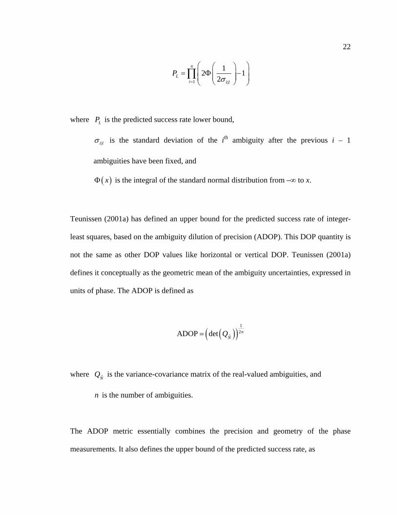
Teunissen (2001a) has defined an upper bound for the predicted success rate of integer-
least squares, based on the ambiguity dilution of precision (ADOP). This DOP quantity is
not the same as other DOP values like horizontal or vertical DOP. Teunissen (2001a)
defines it conceptually as the geometric mean of the ambiguity uncertainties, expressed in
units of phase. The ADOP is defined as
1
2ˆADOP det n
NQ
where N
Q is the variance-covariance matrix of the real-valued ambiguities, and
n is the number of ambiguities.
The ADOP metric essentially combines the precision and geometry of the phase
measurements. It also defines the upper bound of the predicted success rate, as

23
2
2
2 2
n
U
n n
PADOP
where UP is the predicted success rate upper bound, and
x is the gamma function at x .
Other approximations of the predicted success rate can be found in Teunissen (1998),
Teunissen et al (1999) and Verhagen (2005). Because the predicted success rate is an a
priori metric, it can be an optimistic measure. Hence this thesis implements the predicted
success rate lower bound LP and investigates whether this approximation of the predicted
success rate helps to indentify which fixes are likely correct, and which are likely
incorrect. There are several considerations that must be taken into account when using the
predicted success rate:
The predicted success rate is an a priori metric as it only depends on the float
ambiguity uncertainties. Therefore the predicted success rate can only be used as
a measure of confidence in the ability to validate integer ambiguity estimates (as
demonstrated in the next section). It cannot actually be used to validate the integer
estimate itself.

24
The float ambiguity uncertainties are partly a function of differential code
accuracy, consisting of noise, multipath and residual atmospheric effects. The
non-stochastic, non-Gaussian nature of multipath is not taken into account, which
will affect how closely the predicted success rate follows the actual success rate.
The predicted success rate lower bound is based on the estimated uncertainties of
the ambiguities, which should be on the order of fractional cycles when doing
integer estimation. If there is an bias in the estimated value of the ambiguities, this
will not be reflected in the predicted success rate. For example, the predicted
success rate can be very high (even close to one) but the actual success rate with a
one-cycle bias is essentially zero. Therefore the predicted success rate does not
capture the negative effect of phase biases (Teunissen 2001b).
The rate of incorrect fix will occasionally be referred to as failure rate for the sake of
brevity. For other studies involving predicted success rate with GPS and GLONASS and
Galileo, refer to O’Keefe et al (2006, 2009).
2.5 Fix Validation and the F Ratio Test
Fix validation – determining whether the “most likely” integer estimate of the
ambiguities is actually correct – is a crucial step in ambiguity resolution. For the ILS
estimation method, statistical hypothesis testing of the measurement or ambiguity
residuals has been widely used for fix validation. This is valid under the assumption of
25
measurement data with normally distributed errors which, when passed through a linear
estimator results in normally distributed parameter errors. However, this is not the case
for integer estimation as the integer parameters are not normally distributed (Verhagen
2005). As well, GNSS measurement errors are generally not normally distributed due to
multipath and atmospheric effects.
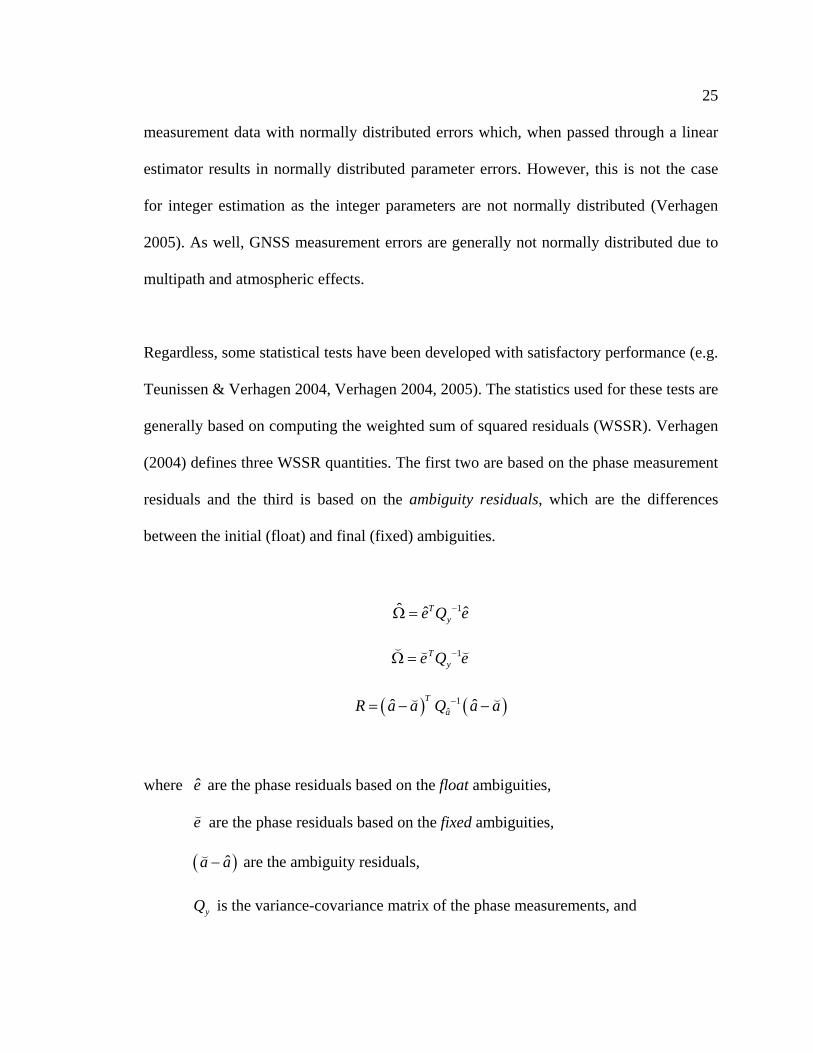
Regardless, some statistical tests have been developed with satisfactory performance (e.g.
Teunissen & Verhagen 2004, Verhagen 2004, 2005). The statistics used for these tests are
generally based on computing the weighted sum of squared residuals (WSSR). Verhagen
(2004) defines three WSSR quantities. The first two are based on the phase measurement
residuals and the third is based on the ambiguity residuals, which are the differences
between the initial (float) and final (fixed) ambiguities.
1ˆ ˆ ˆTye Q e
1Tye Q e
1ˆˆ ˆ
T
aR a a Q a a
where e are the phase residuals based on the float ambiguities,
e
are the phase residuals based on the fixed ambiguities,
ˆa a are the ambiguity residuals,
yQ is the variance-covariance matrix of the phase measurements, and

26
aQ is the variance-covariance matrix of the float ambiguities.
The process of choosing which integer estimates are “likely” to be correct is called
identification. An example of an identification test based on WSSR quantities is given
below (Verhagen 2004). Conceptually, the WSSR quantities of an integer estimate
represent the errors associated with that estimate. Therefore an identification test statistic
based on WSSR can be thought of as a measure of an integer estimate’s likelihood, with
more likely estimates having smaller test statistics. The “most likely” integer estimate
should both pass the following identification test and have the smallest test statistic:
ˆ
Rn
K
m n p
where m is the number of measurements,
n is the number of ambiguities,
p is the number of position states, and
K is the identification test threshold.
Once the most likely integer estimate is identified, fix validation in the form of
discrimination testing can be done. Because it is possible for multiple integer estimates to
pass the identification test, the most likely estimate must be sufficiently more likely than

27
the “second-most likely” estimate. A comprehensive review of discrimination tests can be
found in Verhagen (2004).
The most common class of discrimination test is the F ratio test (or the F-test for short).
The concept behind the F-test is that WSSR-based test statistics approximately represent
likelihood of correctness. Therefore the ratio between two statistics can be thought of as
the difference in likelihood. The standard form of the ratio test is defined by Verhagen
(2004) as
2
1
K
where 1
is computed from the most likely integer estimate,
2
is computed from the second-most likely integer estimate, and
K is the F-test threshold.
An alternate form of the ratio test is the following (Euler & Schaffrin 1990):
2
1
RK
R
For both forms of the ratio test, the null hypothesis is that a correct integer estimate
cannot be determined. That is, 1
and 2
(or 1R and 1R ) cannot be discriminated from
28
one another. Verhagen (2004) develops a basis for hypothesis testing by assuming that if
the null hypothesis is true, then the ratio statistic is distributed according to a central F
distribution. That is, the weighted phase residuals (for the standard form) or weighted
ambiguity residuals (for the alternative form) for both the most likely and second-most
likely integer estimates are zero-mean. In practice, this assumption is invalid:
Leick (2004) correctly notes that both the numerator and denominator of the ratio statistic
are distributed according to non-central χ2 distributions, so the ratio is distributed
according to the doubly non-central F distribution. However, the assumption of centrality
is often used for simplicity.
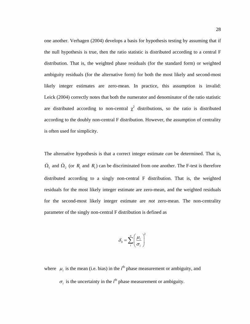
The alternative hypothesis is that a correct integer estimate can be determined. That is,
1
and 2
(or 1R and 1R ) can be discriminated from one another. The F-test is therefore
distributed according to a singly non-central F distribution. That is, the weighted
residuals for the most likely integer estimate are zero-mean, and the weighted residuals
for the second-most likely integer estimate are not zero-mean. The non-centrality
parameter of the singly non-central F distribution is defined as
2
0
ni
i i
where i is the mean (i.e. bias) in the ith phase measurement or ambiguity, and
i is the uncertainty in the ith phase measurement or ambiguity.

29
In this thesis, fix validation will be investigated using the alternate form of the F-test, as it
is commonly implemented and is easy to generate from the by-products of ambiguity
resolution. Verhagen (2004) emphasizes that there are no thresholds with sound
theoretical bases. Under the (invalid) assumption of the centrality of the ratio distribution
under the null hypothesis, the F-test threshold is taken from the central F distribution at
the desired significance level and with degrees of freedom equal to the number of
ambiguities. Alternatively, several constant thresholds have been proposed in the
literature: e.g. 2.0 (Landau & Euler 1992); 3.0 (Leick 2004); and 4.23 (Verhagen 2004).
However, a variable threshold based on the central F distribution is useful as it adapts to
the number of ambiguities. Table 2 shows the threshold for various numbers of
ambiguities using a significance level of 10%. The ability of the F-test to reject incorrect
fixes (or in terms of navigation reliability, reject and detect biases) will be particularly
highlighted as the F-test results are derived from actual measurement data.
Table 2 - F-test thresholds from central F distribution (significance level 10%)
Number of ambiguities
F-test threshold
Number of ambiguities
F-test threshold
5 3.45 9 2.44
6 3.05 10 2.32
7 2.78 11 2.23
8 2.59 12 2.15
30
Chapter Three: Testing and Analysis Methods
This chapter describes the testing, data processing and analysis methods used in this
thesis. A description of the field testing is given, including the test scenarios that were
investigated and the hardware that was used. The processing and analysis methodologies
are then explained in detail.
3.1 Test Scenarios
Fix reliability was investigated using real GNSS measurement data collected in the city
of Calgary and the surrounding areas. These tests are categorized under the following
three scenarios.
3.1.1 Static Baselines
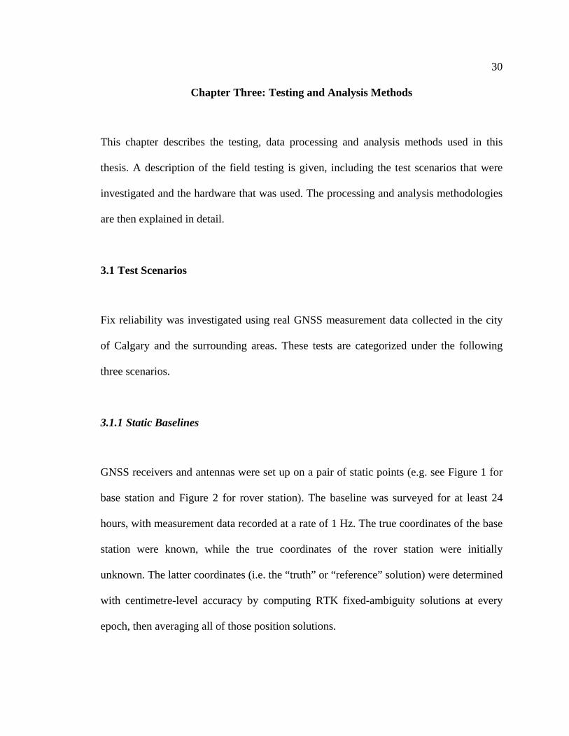
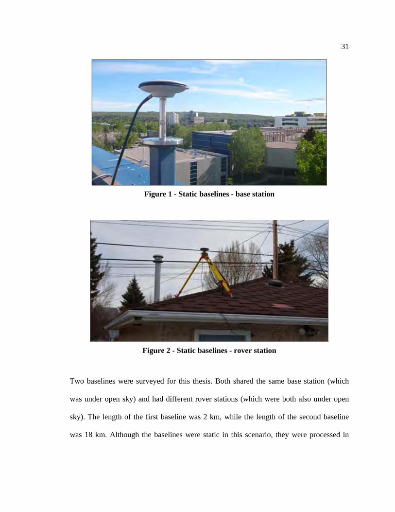
GNSS receivers and antennas were set up on a pair of static points (e.g. see Figure 1 for
base station and Figure 2 for rover station). The baseline was surveyed for at least 24
hours, with measurement data recorded at a rate of 1 Hz. The true coordinates of the base
station were known, while the true coordinates of the rover station were initially
unknown. The latter coordinates (i.e. the “truth” or “reference” solution) were determined
with centimetre-level accuracy by computing RTK fixed-ambiguity solutions at every
epoch, then averaging all of those position solutions.
31
Figure 1 - Static baselines - base station
Figure 2 - Static baselines - rover station
Two baselines were surveyed for this thesis. Both shared the same base station (which
was under open sky) and had different rover stations (which were both also under open
sky). The length of the first baseline was 2 km, while the length of the second baseline
was 18 km. Although the baselines were static in this scenario, they were processed in

32
kinematic mode – that is, epoch-to-epoch processing with the position allowed to move in
order to provide a more refined accuracy analysis.
3.1.2 Vehicle-to-Vehicle Relative Navigation
A two-vehicle road test was conducted in the Mount Royal residential area in Calgary.
GNSS receivers and antennas were mounted on each vehicle. The application tested here
was relative navigation; instead of generating a fixed-ambiguity solution for each vehicle
using separate static stations, the inter-vehicle vector and velocity were directly estimated
in a moving baseline approach. The vehicles were separated by a maximum of 300 m.
The road test lasted 97 minutes, with measurement data collected at a rate of 2 Hz. There
were two major environment sky coverage types encountered in this test:
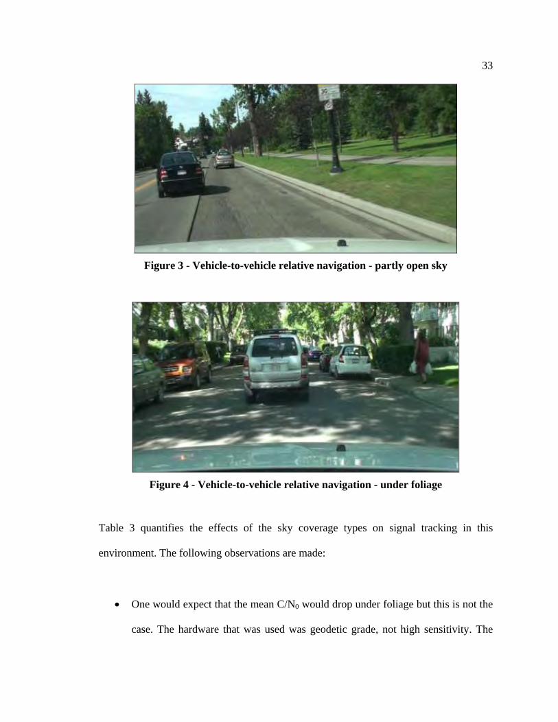
1. Approximately half of the test (49 minutes) was conducted under open sky
conditions. This environment is illustrated by Figure 3. There was some
occasional tree coverage that was unavoidable; for example, in Figure 3 there are
trees by the side of the road.
2. The other half of the test (49 minutes) was conducted mainly under foliage. This
environment is illustrated by Figure 4. Canopies extend above the road,
sometimes resulting in near-total coverage.
33
Figure 3 - Vehicle-to-vehicle relative navigation - partly open sky
Figure 4 - Vehicle-to-vehicle relative navigation - under foliage
Table 3 quantifies the effects of the sky coverage types on signal tracking in this
environment. The following observations are made:
One would expect that the mean C/N0 would drop under foliage but this is not the
case. The hardware that was used was geodetic grade, not high sensitivity. The
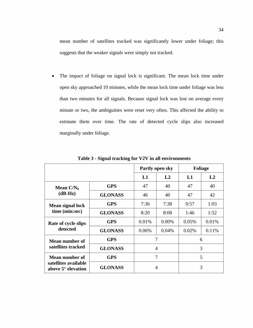
34
mean number of satellites tracked was significantly lower under foliage; this
suggests that the weaker signals were simply not tracked.
The impact of foliage on signal lock is significant. The mean lock time under
open sky approached 10 minutes, while the mean lock time under foliage was less
than two minutes for all signals. Because signal lock was lost on average every
minute or two, the ambiguities were reset very often. This affected the ability to
estimate them over time. The rate of detected cycle slips also increased
marginally under foliage.
Table 3 - Signal tracking for V2V in all environments
Partly open sky Foliage
L1 L2 L1 L2
Mean C/N0 (dB-Hz)
GPS 47 40 47 40
GLONASS 46 40 47 42
Mean signal lock time (min:sec)
GPS 7:36 7:38 0:57 1:03
GLONASS 8:20 8:08 1:46 1:52
Rate of cycle slips detected
GPS 0.01% 0.00% 0.05% 0.01%
GLONASS 0.06% 0.04% 0.02% 0.11%
Mean number of satellites tracked
GPS 7 6
GLONASS 4 3
Mean number of satellites available above 5° elevation
GPS 7 5
GLONASS 4 3

35
The reference or truth trajectory (i.e. the true inter-relative vehicle vectors at every
epoch) was obtained using a GPS/INS solution. A NovAtel SPAN-CPT integrated
GPS/INS (OEMV3 receiver with 20°/hr gyros) was mounted on the lead vehicle; on the
trailing vehicle, a Honeywell HG1700 tactical grade inertial sensor integrated with a
NovAtel OEM4 receiver was used. Position solutions for both vehicles were generated
with the Waypoint Inertial Explorer™ post-processing software using forward-backward
smoothing. The individual vehicle solutions were then differenced to form the relative
solutions. The availability of solutions with estimated 1σ horizontal accuracies at the sub-
decimetre level is 98% under open sky and 72% under foliage.
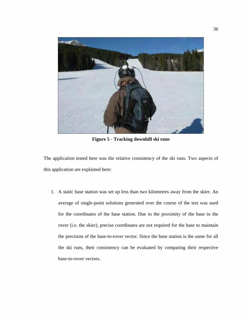
3.1.3 Downhill Ski Runs
A ski test consisting of a series of seven downhill runs was conducted at the Nakiska ski
resort in February 2010. The ski slope used was situated under open sky with mask
angles of up to 20° from the slope itself. The skier, shown in Figure 5, wore a backpack
with the antenna mounted on his helmet. Each downhill run lasted four to eight minutes,
with measurement data collected at a rate of 2 Hz.
36
Figure 5 - Tracking downhill ski runs
The application tested here was the relative consistency of the ski runs. Two aspects of
this application are explained here:
1. A static base station was set up less than two kilometres away from the skier. An
average of single-point solutions generated over the course of the test was used
for the coordinates of the base station. Due to the proximity of the base to the
rover (i.e. the skier), precise coordinates are not required for the base to maintain
the precision of the base-to-rover vector. Since the base station is the same for all
the ski runs, their consistency can be evaluated by comparing their respective
base-to-rover vectors.
37
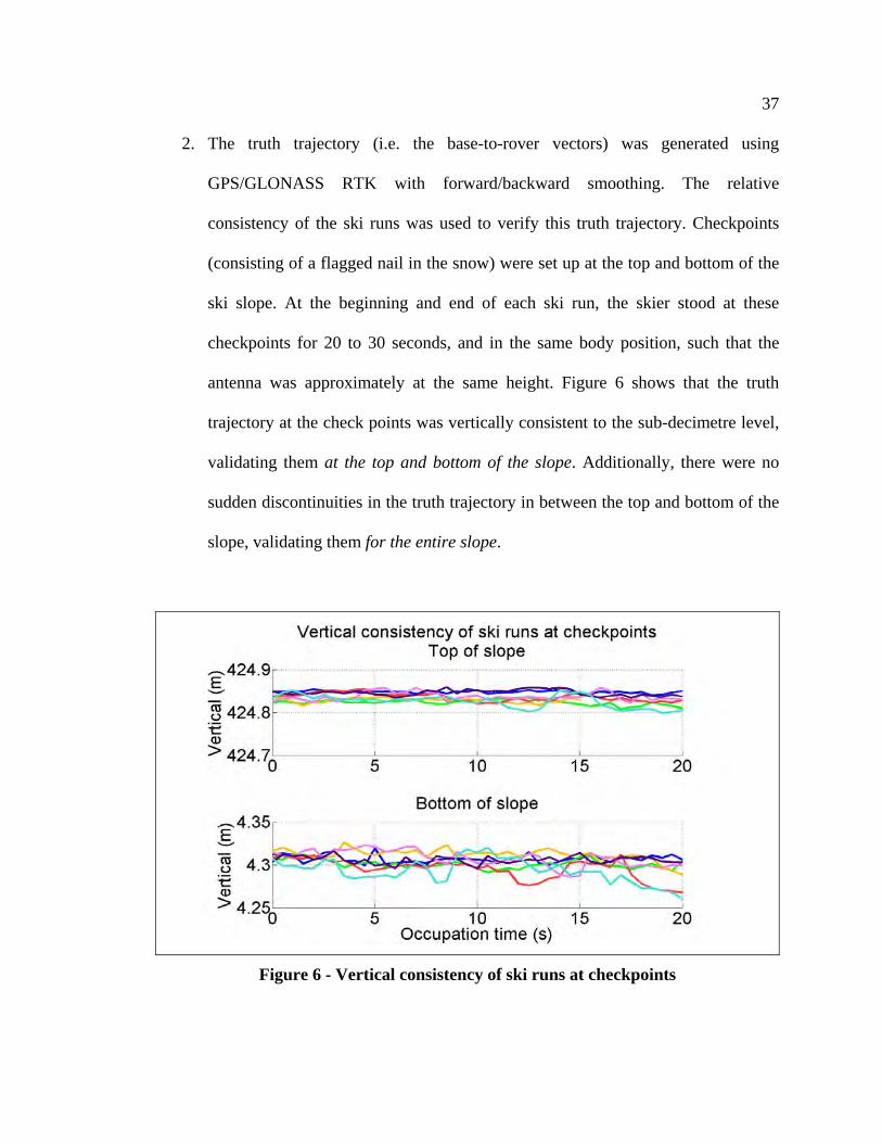
2. The truth trajectory (i.e. the base-to-rover vectors) was generated using
GPS/GLONASS RTK with forward/backward smoothing. The relative
consistency of the ski runs was used to verify this truth trajectory. Checkpoints
(consisting of a flagged nail in the snow) were set up at the top and bottom of the
ski slope. At the beginning and end of each ski run, the skier stood at these
checkpoints for 20 to 30 seconds, and in the same body position, such that the
antenna was approximately at the same height. Figure 6 shows that the truth
trajectory at the check points was vertically consistent to the sub-decimetre level,
validating them at the top and bottom of the slope. Additionally, there were no
sudden discontinuities in the truth trajectory in between the top and bottom of the
slope, validating them for the entire slope.
Figure 6 - Vertical consistency of ski runs at checkpoints
38
3.2 Hardware Characteristics
Field tests were conducted using identical receiver pairs, with base and rover stations
both equipped with NovAtel OEMV2-G receivers. These are geodetic-grade GNSS
receivers, capable of tracking GPS and GLONASS signals in their respective L1 and L2
bands. The Vision Correlator technology (Fenton & Jones 2005) is implemented to
reduce code multipath. Two types of antennas were used with this receiver: 1.) the
NovAtel GPS-702-GG antenna, in the static and vehicle navigation test scenarios; and 2.)
the ANTCOM-GG antenna, in the downhill ski run test scenario. One of these receivers
was housed in a STEALTH™ unit (Lachapelle et al 2009).
The quality of the OEMV2-G + GPS-702-GG receiver-antenna combination was assessed
by testing them under open sky in a zero-baseline configuration. The distributions of the
double-differenced (DD) code and phase residuals (i.e. errors) are shown in Figure 7. The
code multipath was determined using single-point code-minus-carrier, and the RMS
values for GPS L1 C/A and GLONASS L1 CA code are shown in Table 4. The following
inferences regarding the hardware quality were made:
The zero-baseline code and phase errors from Figure 7 are mainly determined by
the receiver noise level, with the exception of GLONASS phase (addressed
below). The code noise is on the centimetre-level while the phase noise is on the
millimetre-level, for both GPS and GLONASS. This is indicative of the receiver
quality, and suggests that GPS and GLONASS measurements from these
39
receivers can be easily integrated. The reason for the high quality code accuracy
is likely carrier phase smoothing in the receiver firmware.
Code accuracy is a limiting factor in ambiguity resolution. In turn, multipath is a
limiting factor in (differential) code accuracy. Code multipath RMS levels were
found to be at the sub-metre level for both GPS and GLONASS in the
environment tested. The code from both systems is thus accurate to around a few
multiples of their respective L1 phase wavelengths, and can provide reasonable
initial position estimate with proper measurement weighting and filter tuning.
However, it must be noted that these specific values only apply to this
environment, which had open sky coverage with relatively few nearby reflectors.
GLONASS inter-frequency phase biases manifest themselves as multiple peaks in
the phase error distribution. Three distinct peaks can be identified in Figure 7;
however these peaks are only separated by millimetres. These biases are not
expected to significantly affect ambiguity resolution in the scenarios tested herein.
However it is important to consider inter-frequency biases when using receivers
from different manufacturers.

40
Figure 7 - NovAtel OEMV2-G + NovAtel GPS-702-GG hardware: code and phase errors under an open-sky zero-baseline configuration
Table 4 - NovAtel OEMV2-G + NovAtel GPS-702-GG hardware: code multipath under open sky
Code multipath RMS (cm)
GPS L1 C/A code 49
GLONASS L1 CA code 61
The quality of the OEMV2-G + ANTCOM-GG receiver-antenna combination was
assessed separately in an open sky kinematic test. The station in Figure 1 was used as the
base station, and then the OEMV2-G + ANTCOM-GG receiver-antenna pair was carried
by a pedestrian walking under open sky. The measurement errors were derived by
computing fixed-ambiguity solutions and extracting the DD residuals. Their distributions
are shown in Figure 8, and they contain both noise and multipath. Figure 8 suggests that
the ANTCOM-GG antenna provides lower code and phase quality than the NovAtel
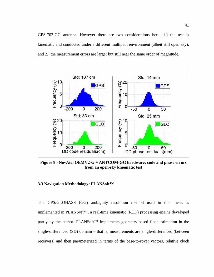
41
GPS-702-GG antenna. However there are two considerations here: 1.) the test is
kinematic and conducted under a different multipath environment (albeit still open sky);
and 2.) the measurement errors are larger but still near the same order of magnitude.
Figure 8 - NovAtel OEMV2-G + ANTCOM-GG hardware: code and phase errors from an open-sky kinematic test
3.3 Navigation Methodology: PLANSoft™
The GPS/GLONASS (GG) ambiguity resolution method used in this thesis is
implemented in PLANSoft™, a real-time kinematic (RTK) processing engine developed
partly by the author. PLANSoft™ implements geometry-based float estimation in the
single-differenced (SD) domain – that is, measurements are single-differenced (between
receivers) and then parameterized in terms of the base-to-rover vectors, relative clock
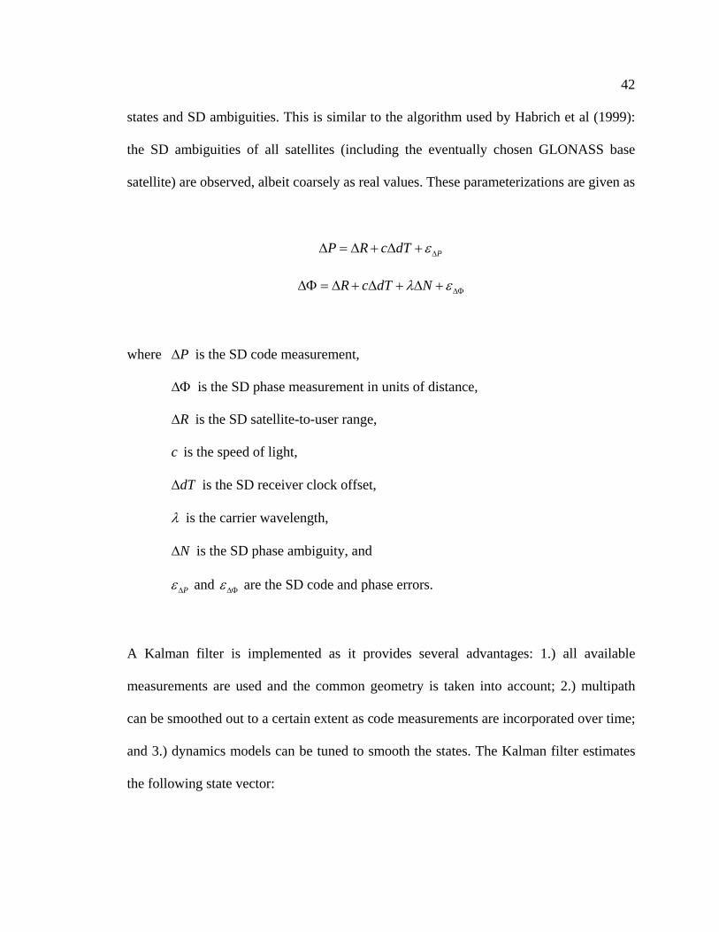
42
states and SD ambiguities. This is similar to the algorithm used by Habrich et al (1999):
the SD ambiguities of all satellites (including the eventually chosen GLONASS base
satellite) are observed, albeit coarsely as real values. These parameterizations are given as
PP R c dT
R c dT N
where P is the SD code measurement,
is the SD phase measurement in units of distance,
R is the SD satellite-to-user range,
c is the speed of light,
dT is the SD receiver clock offset,
is the carrier wavelength,
N is the SD phase ambiguity, and
P and are the SD code and phase errors.
A Kalman filter is implemented as it provides several advantages: 1.) all available
measurements are used and the common geometry is taken into account; 2.) multipath
can be smoothed out to a certain extent as code measurements are incorporated over time;
and 3.) dynamics models can be tuned to smooth the states. The Kalman filter estimates
the following state vector:
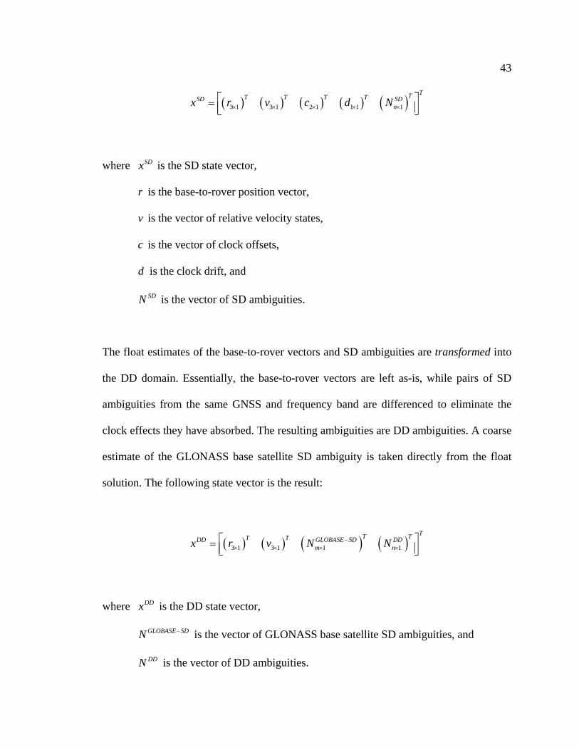
43
3 1 3 1 2 1 1 1 1
TTT T T TSD SDnx r v c d N
where SDx is the SD state vector,
r is the base-to-rover position vector,
v is the vector of relative velocity states,
c is the vector of clock offsets,
d is the clock drift, and
SDN is the vector of SD ambiguities.
The float estimates of the base-to-rover vectors and SD ambiguities are transformed into
the DD domain. Essentially, the base-to-rover vectors are left as-is, while pairs of SD
ambiguities from the same GNSS and frequency band are differenced to eliminate the
clock effects they have absorbed. The resulting ambiguities are DD ambiguities. A coarse
estimate of the GLONASS base satellite SD ambiguity is taken directly from the float
solution. The following state vector is the result:
3 1 3 1 1 1
TT TT TDD GLOBASE SD DDm nx r v N N
where DDx is the DD state vector,
GLOBASE SDN is the vector of GLONASS base satellite SD ambiguities, and
DDN is the vector of DD ambiguities.
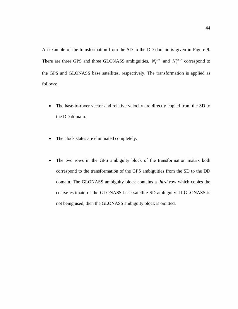
44
An example of the transformation from the SD to the DD domain is given in Figure 9.
There are three GPS and three GLONASS ambiguities. 1GPSN and 1
GLON correspond to
the GPS and GLONASS base satellites, respectively. The transformation is applied as
follows:
The base-to-rover vector and relative velocity are directly copied from the SD to
the DD domain.
The clock states are eliminated completely.
The two rows in the GPS ambiguity block of the transformation matrix both
correspond to the transformation of the GPS ambiguities from the SD to the DD
domain. The GLONASS ambiguity block contains a third row which copies the
coarse estimate of the GLONASS base satellite SD ambiguity. If GLONASS is
not being used, then the GLONASS ambiguity block is omitted.

45
2 1
3 1
2 1
3 1
1
0 0 0 0 0 0 0 0 0
0 0 0 0 0 0 0 0 0
0 0 0 0 1 1 0 0 0 0
0 0 0 0 1 0 1 0 0 0
0 0 0 0 0 0 0 1 1 0
0 0 0 0 0 0 0 1 0 1
0 0 0 0 0 0 0 1 0 0
Transformation matrix
GPS
GPS
GLO
GLO
GLO
DD
r I
v I
N
N
N
N
N
x
1
2
3
1
2
3
GPS
GPS
GPS
GLO
GLO
GLO
SD
r
v
c
d
N
N
N
N
N
N
x
Figure 9 - Example of SD to DD transformation
Processing in PLANSoft™ was done in post-mission, but with all algorithms
implementable in real-time – that is, epoch-by-epoch processing with no rewinding or
forward/backward smoothing. GLONASS inter-frequency phase biases are not corrected,
as they were demonstrated earlier to be very small for the receiver pairs used. Unless
otherwise stated, the following processing parameters were used for both GPS and
GLONASS:
Elevation-based measurement uncertainty model: sin
zenith
elevation
.
Code uncertainty (at zenith) of 50 cm.

46
Phase uncertainty (at zenith) of 4 mm.
Random walk model with velocity spectral densities of 1.0 (m/s)2/s in each
direction. This spectral density is sufficient for the kinematic scenarios
investigated herein. Although lower (or zero) spectral density values can be used
for the static baselines, the same values are used for consistency.
Fault detection at 0.1% significance level.
Phase rate cycle slip detection with 4-cycle threshold.
LAMBDA decorrelation and integer least-squares for ambiguity resolution.
3.4 Estimation Strategies
Section 3.3 defined a framework for navigation estimation and ambiguity resolution
within PLANSoft™. Within that framework, there are several ways to change how the
positions and ambiguities are estimated. This thesis investigates the impact of these
estimation strategies on the success rate and reliability of ambiguity resolution.
The inputs to navigation estimation are the code and phase measurements. Different
combinations of these measurements can be used. The choice of combination is
motivated by two factors: 1.) if L2 measurements are used, then dual-frequency hardware
47
is required, and the cost of that hardware is currently affected by the Y-code encryption
of the GPS L2 P signal; and 2.) different dual-frequency combinations have different
characteristics in terms of measurement noise and performance over varying baseline
lengths. Three measurement combinations were investigated:
1. L1 only. The code measurements used are GPS L1 C/A and GLONASS L1 CA.
The phase measurements used are GPS and GLONASS L1. These are used to
estimate the base-to-rover vector and the L1 ambiguities.
2. L1 + L2. The code measurements used are GPS L1 C/A and GLONASS L1 CA.
Code from L2 is not used. The phase measurements used are GPS and GLONASS
L1 and L2. The L1 and L2 phase are not combined, but used separately. These are
used to estimate the base-to-rover vector and the L1 and L2 ambiguities
3. Widelane. The code measurements used are GPS L1 C/A and GLONASS L1 CA.
Code from L2 is not used. The phase measurements used are GPS and GLONASS
L1 and L2. The L1 and L2 phase are combined by forming the quantity
WL L2 L1 for each satellite. WL is referred to as widelane (WL) phase and is
treated as a phase measurement with a wavelength of L1 L2/ c f f . For GPS this
wavelength is 86 cm and for GLONASS it is approximately 84 cm for all
satellites with differences between satellites of up to 3.9 mm. The L1 and L2
ambiguities are also combined in the manner above to form widelane ambiguities.
48
The L1 code and widelane phase are used to estimate the base-to-rover vector and
the widelane ambiguities.
Once the measurement combination was chosen, there were several ways of generating
the fixed ambiguity solutions. Three of these fixing strategies were investigated:
1. GPS only: only GPS measurements are used to estimate the float solution prior to
ambiguity resolution. The chosen measurement combination determines which
code and phase measurements are used. The float solution contains only GPS
ambiguities. All GPS ambiguities are fixed to integers when possible.
2. GG – float GLO: both GPS and GLONASS measurements are used to estimate
the float solution prior to ambiguity resolution. The chosen measurement
combination determines which code and phase measurements are used. The float
solution contains both GPS and GLONASS ambiguities. All GPS ambiguities are
fixed to integers, but all GLONASS ambiguities remain as real-valued (float)
estimates. The motivation for this approach is discussed in more detail below.
3. GG – fixed GLO: both GPS and GLONASS measurements are used to estimate
the float solution prior to ambiguity resolution. The chosen measurement
combination determines which code and phase measurements are used. The float
solution contains both GPS and GLONASS ambiguities. All GPS and GLONASS
ambiguities are fixed to integers.

49
The choice of using GLONASS in a fixing strategy is motivated by hardware
requirements: most legacy receivers and many of the current receivers track only GPS. It
is also important to investigate the effect of fixing the GLONASS ambiguities, because
doing so is more difficult than for GPS. Estimating the GLONASS ambiguities as float
values also removes the risk of fixing the ambiguities incorrectly due to GLONASS inter-
frequency biases. Some commercial RTK software such as Waypoint’s GrafNav™
provide the option to use GLONASS measurements without fixing the ambiguities.
Therefore it must be determined whether it is worth fixing the GLONASS ambiguities, or
if using the measurements in the float solution is sufficient.
Figure 10 shows the different the estimation strategies and solutions that were generated.
Figure 10 - Measurement combinations and fixing strategies
L1 only L1 + L2 Widelane
Fix GPS ambiguities
Fix only GPS ambiguities
Fix GPS and GLONASS ambiguities
Use GPS in floatsolution
Use GPS and GLONASS (GG) in float solution
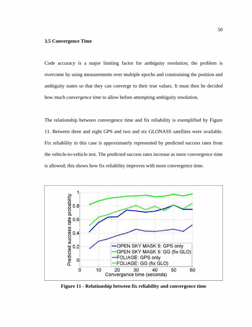
50
3.5 Convergence Time
Code accuracy is a major limiting factor for ambiguity resolution; the problem is
overcome by using measurements over multiple epochs and constraining the position and
ambiguity states so that they can converge to their true values. It must then be decided
how much convergence time to allow before attempting ambiguity resolution.
The relationship between convergence time and fix reliability is exemplified by Figure
11. Between three and eight GPS and two and six GLONASS satellites were available.
Fix reliability in this case is approximately represented by predicted success rates from
the vehicle-to-vehicle test. The predicted success rates increase as more convergence time
is allowed; this shows how fix reliability improves with more convergence time.
Figure 11 - Relationship between fix reliability and convergence time
51
For actual field work, convergence time should generally be increased, within reason, to
maximize fix reliability. This is often done through a static initialization period when
practical. However, the analysis herein requires some fixes to be incorrect so that the
reliability tests can be evaluated. In the results presented in this thesis, there was
generally no static initialization (unless the test itself was static) and convergence times
were chosen through trial and error, such that there were a sufficient proportion of correct
and incorrect fixes to analyze.
3.6 Generating Integer Fixes
Navigation methods that implement ambiguity resolution take advantage of the fact that
phase ambiguities are constant unless there are cycle slips. The ambiguities are resolved
to integers if reliability tests such as the predicted success rate and F-test pass. Once
successfully resolved, the integer values of the ambiguities are stored in memory and re-
used at every epoch thereafter. Ambiguity resolution is not attempted again unless cycle
slips are detected or residual analysis indicates that the original integer fix is incorrect.
However, this approach is not suitable for the analysis in this thesis. A single instance of
ambiguity resolution will not yield statistically meaningful results; the process must be
conducted many times in order to generate many integer fixes, predicted success rates
and F-test results under a wide range of visibility conditions. As well, the performance of
the predicted success rate and F-test are being investigated, so they cannot at the same
time be used to decide whether or not to resolve the ambiguities.
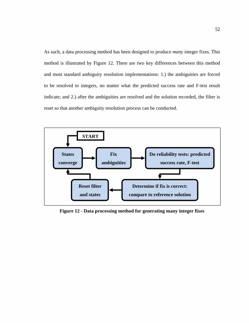
52
As such, a data processing method has been designed to produce many integer fixes. This
method is illustrated by Figure 12. There are two key differences between this method
and most standard ambiguity resolution implementations: 1.) the ambiguities are forced
to be resolved to integers, no matter what the predicted success rate and F-test result
indicate; and 2.) after the ambiguities are resolved and the solution recorded, the filter is
reset so that another ambiguity resolution process can be conducted.
Figure 12 - Data processing method for generating many integer fixes
Fix
ambiguities
States
converge
Do reliability tests: predicted
success rate, F-test
Reset filter
and states
START
Determine if fix is correct:
compare to reference solution
53
Chapter Four: Static Testing Results
This chapter presents the analysis and discussion of the reliability of ambiguity resolution
for static testing. Two static surveys were conducted under open sky conditions, over
baselines of 2 km and 18 km respectively. The 2 km baseline was surveyed on March 5-
6, 2010, in the city of Calgary. Observations taken on those days from the Meanook
Geomagnetic Observatory (450 km north of Calgary) indicate that the geomagnetic K
index did not exceed 2.0 (Space Weather Canada 2009). This level of K index does not
suggest a significant ionospheric disturbance (USNOAA 2005). Between seven and 12
GPS and four and eight GLONASS satellites were available. This baseline was surveyed
for 39 hours, and a total of 6975 ambiguity fixes were generated (with a convergence
time of 20 seconds).
The 18 km baseline was surveyed on August 9-10, 2009, also in the city of Calgary. The
K index did not exceed 1.0 (Space Weather Canada 2009), indicating no significant
ionospheric disturbance. Regardless, the length of the baseline is expected to be a factor
due to larger residual atmospheric effects. Between six and eleven GPS and three and
seven GLONASS satellites were available. This baseline was surveyed for 26 hours, and
a total of 4751 ambiguity fixes were generated (with a convergence time of 20 seconds).
For both baselines, nine types of solutions are investigated. The L1 only, L1 + L2 and
widelane (WL) measurement combinations are each combined with the GPS only, GG
float GLO and GG fixed GLO fixing strategies. Circular elevation mask angles of 5°

54
and 30° are also applied and investigated. The latter simulates reduced visibility
conditions, which are discussed in greater detail in Sections 4.5 and 4.10.
4.1 Positioning Accuracy
An analysis of the solutions in the position domain is first presented. Position accuracies
are determined by a comparison to a truth or reference solution. For both baselines, the
reference solution is obtained by computing fixed-ambiguity positions at every epoch,
and then taking the average of all of those positions. The 3D precision of the reference
solution is better than 2 cm (1σ) for both baselines.
Figure 13 is a 2D representation of the position errors from the 2 km baseline, for both
the correct and incorrect fixes. It is clear that incorrect fixes can lead to very large
position errors. The characteristics of the positions derived from correct fixes are much
more interesting. These are graphically represented in Figure 14 and further summarized
in Table 5 (the median errors) and Table 6 (the RMS errors). The actual success rates
(fully investigated in Section 4.2) are given to show the availability of these fixed-
ambiguity positions, with the actual numbers of correct fixes highlighted in blue. The
following trends are observed:
There appears to be little difference in the position errors whether GPS is used
alone, or GPS and GLONASS are combined. However, when the GLONASS
55
ambiguities are fixed (i.e. when the GG fixed GLO strategy is used), the cluster
of position errors do appear to be visually tighter.
The position errors do not appear to be affected whether L1 only or L1 + L2 is
used. However the spread of errors is much larger when widelane is used
(highlighted in red in Table 5 and Table 6). This is expected because the
differential atmospheric effects over a distance of 2 km are generally negligible.
Also, the widelane solution noise is always higher than in an L1 only solution
due to the linear combination of observables.
The spread of position errors is larger vertically than horizontally, and larger
north-south than east-west. This is expected: the measurement geometry is
weakest in the vertical direction, and then weaker north-south than east-west as
the receiver gets farther from the equator (e.g. at Calgary’s 51° N latitude).

56
Figure 13 - 2D view of position errors, all fixes - 2 km baseline under 5° mask
Figure 14 - 2D view of position errors, correct fixes - 2 km baseline under 5° mask
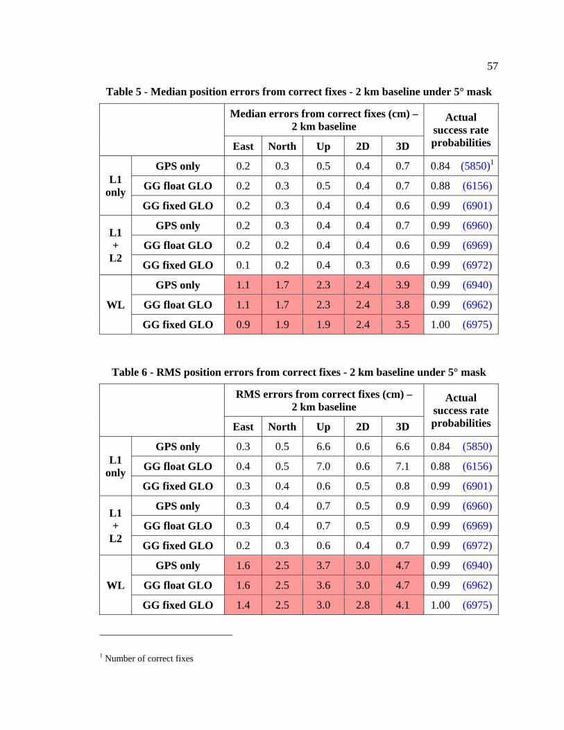
57
Table 5 - Median position errors from correct fixes - 2 km baseline under 5° mask
Median errors from correct fixes (cm) – 2 km baseline
Actual success rate probabilities East North Up 2D 3D
L1 only
GPS only 0.2 0.3 0.5 0.4 0.7 0.84 (5850)1
GG float GLO 0.2 0.3 0.5 0.4 0.7 0.88 (6156)
GG fixed GLO 0.2 0.3 0.4 0.4 0.6 0.99 (6901)
L1 +
L2
GPS only 0.2 0.3 0.4 0.4 0.7 0.99 (6960)
GG float GLO 0.2 0.2 0.4 0.4 0.6 0.99 (6969)
GG fixed GLO 0.1 0.2 0.4 0.3 0.6 0.99 (6972)
WL
GPS only 1.1 1.7 2.3 2.4 3.9 0.99 (6940)
GG float GLO 1.1 1.7 2.3 2.4 3.8 0.99 (6962)
GG fixed GLO 0.9 1.9 1.9 2.4 3.5 1.00 (6975)
Table 6 - RMS position errors from correct fixes - 2 km baseline under 5° mask
RMS errors from correct fixes (cm) – 2 km baseline
Actual success rate probabilities East North Up 2D 3D
L1 only
GPS only 0.3 0.5 6.6 0.6 6.6 0.84 (5850)
GG float GLO 0.4 0.5 7.0 0.6 7.1 0.88 (6156)
GG fixed GLO 0.3 0.4 0.6 0.5 0.8 0.99 (6901)
L1 +
L2
GPS only 0.3 0.4 0.7 0.5 0.9 0.99 (6960)
GG float GLO 0.3 0.4 0.7 0.5 0.9 0.99 (6969)
GG fixed GLO 0.2 0.3 0.6 0.4 0.7 0.99 (6972)
WL
GPS only 1.6 2.5 3.7 3.0 4.7 0.99 (6940)
GG float GLO 1.6 2.5 3.6 3.0 4.7 0.99 (6962)
GG fixed GLO 1.4 2.5 3.0 2.8 4.1 1.00 (6975)
1 Number of correct fixes
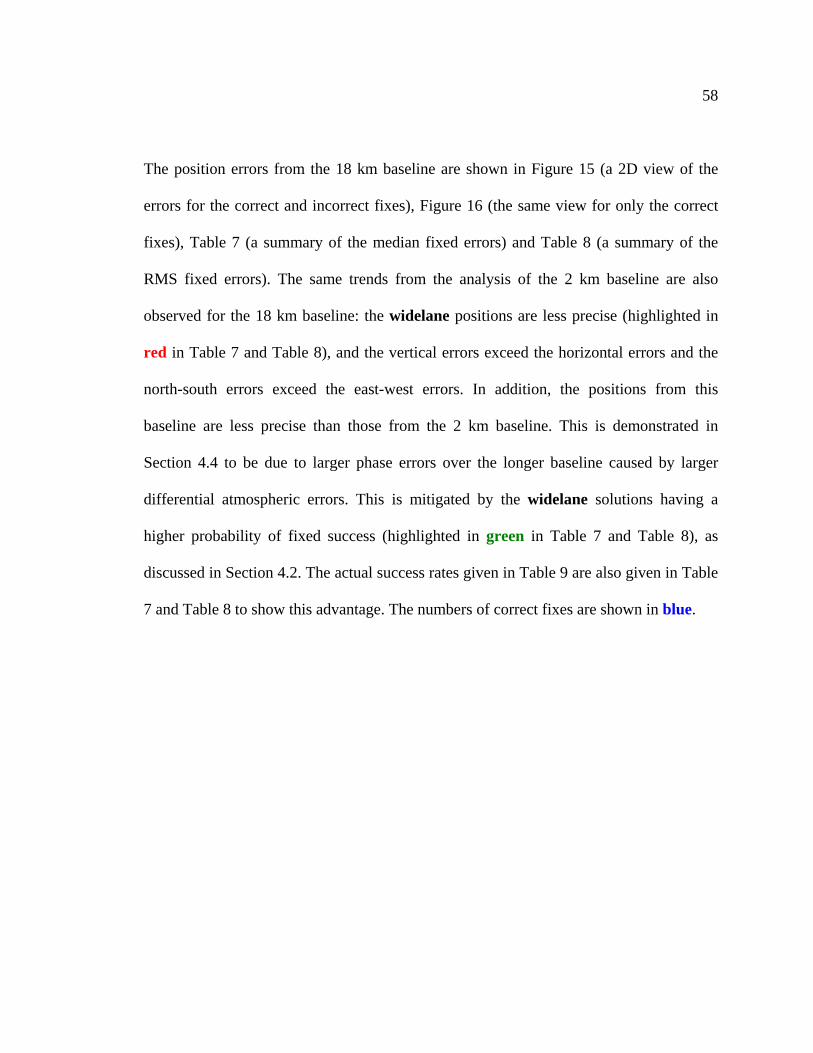
58
The position errors from the 18 km baseline are shown in Figure 15 (a 2D view of the
errors for the correct and incorrect fixes), Figure 16 (the same view for only the correct
fixes), Table 7 (a summary of the median fixed errors) and Table 8 (a summary of the
RMS fixed errors). The same trends from the analysis of the 2 km baseline are also
observed for the 18 km baseline: the widelane positions are less precise (highlighted in
red in Table 7 and Table 8), and the vertical errors exceed the horizontal errors and the
north-south errors exceed the east-west errors. In addition, the positions from this
baseline are less precise than those from the 2 km baseline. This is demonstrated in
Section 4.4 to be due to larger phase errors over the longer baseline caused by larger
differential atmospheric errors. This is mitigated by the widelane solutions having a
higher probability of fixed success (highlighted in green in Table 7 and Table 8), as
discussed in Section 4.2. The actual success rates given in Table 9 are also given in Table
7 and Table 8 to show this advantage. The numbers of correct fixes are shown in blue.
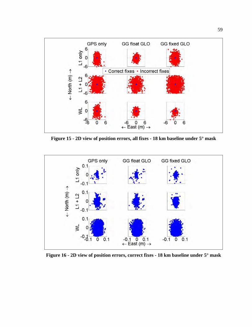
59
Figure 15 - 2D view of position errors, all fixes - 18 km baseline under 5° mask
Figure 16 - 2D view of position errors, correct fixes - 18 km baseline under 5° mask
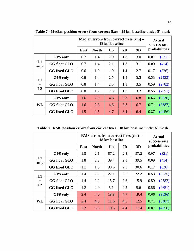
60
Table 7 - Median position errors from correct fixes - 18 km baseline under 5° mask
Median errors from correct fixes (cm) – 18 km baseline
Actual success rate probabilities East North Up 2D 3D
L1 only
GPS only 0.7 1.4 2.0 1.8 3.0 0.07 (321)
GG float GLO 0.7 1.4 2.1 1.8 3.1 0.09 (414)
GG fixed GLO 0.6 1.0 1.9 1.4 2.7 0.17 (826)
L1 +
L2
GPS only 0.8 1.4 2.5 1.8 3.5 0.53 (2535)
GG float GLO 0.8 1.4 2.5 1.8 3.5 0.59 (2782)
GG fixed GLO 0.8 1.2 2.3 1.7 3.2 0.56 (2651)
WL
GPS only 1.6 2.9 4.8 3.8 6.8 0.66 (3136)
GG float GLO 1.6 2.8 4.6 3.8 6.7 0.71 (3387)
GG fixed GLO 1.5 2.5 4.7 3.4 6.4 0.87 (4156)
Table 8 - RMS position errors from correct fixes - 18 km baseline under 5° mask
RMS errors from correct fixes (cm) – 18 km baseline
Actual success rate probabilities East North Up 2D 3D
L1 only
GPS only 1.8 2.1 57.2 2.8 57.2 0.07 (321)
GG float GLO 1.8 2.2 39.4 2.8 39.5 0.09 (414)
GG fixed GLO 1.1 1.8 30.6 2.1 30.6 0.17 (826)
L1 +
L2
GPS only 1.4 2.2 22.1 2.6 22.2 0.53 (2535)
GG float GLO 1.4 2.2 15.7 2.6 15.9 0.59 (2782)
GG fixed GLO 1.2 2.0 5.1 2.3 5.6 0.56 (2651)
WL
GPS only 2.4 4.0 18.8 4.7 19.4 0.66 (3136)
GG float GLO 2.4 4.0 11.6 4.6 12.5 0.71 (3387)
GG fixed GLO 2.2 3.8 10.5 4.4 11.4 0.87 (4156)
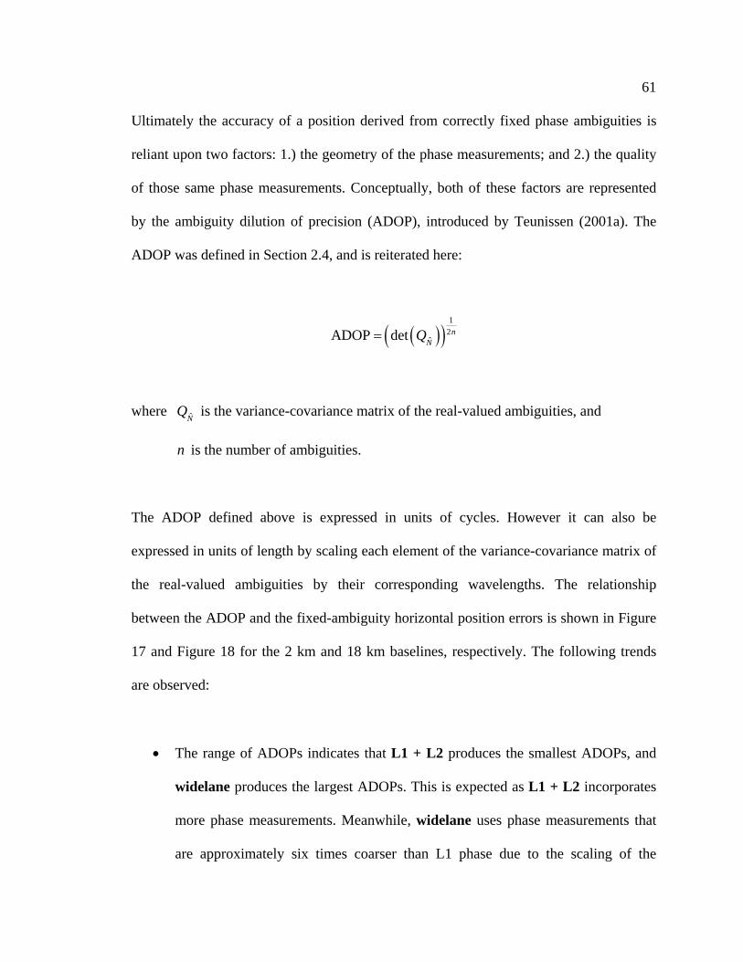
61
Ultimately the accuracy of a position derived from correctly fixed phase ambiguities is
reliant upon two factors: 1.) the geometry of the phase measurements; and 2.) the quality
of those same phase measurements. Conceptually, both of these factors are represented
by the ambiguity dilution of precision (ADOP), introduced by Teunissen (2001a). The
ADOP was defined in Section 2.4, and is reiterated here:
1
2ˆADOP det n
NQ
where N
Q is the variance-covariance matrix of the real-valued ambiguities, and
n is the number of ambiguities.
The ADOP defined above is expressed in units of cycles. However it can also be
expressed in units of length by scaling each element of the variance-covariance matrix of
the real-valued ambiguities by their corresponding wavelengths. The relationship
between the ADOP and the fixed-ambiguity horizontal position errors is shown in Figure
17 and Figure 18 for the 2 km and 18 km baselines, respectively. The following trends
are observed:
The range of ADOPs indicates that L1 + L2 produces the smallest ADOPs, and
widelane produces the largest ADOPs. This is expected as L1 + L2 incorporates
more phase measurements. Meanwhile, widelane uses phase measurements that
are approximately six times coarser than L1 phase due to the scaling of the
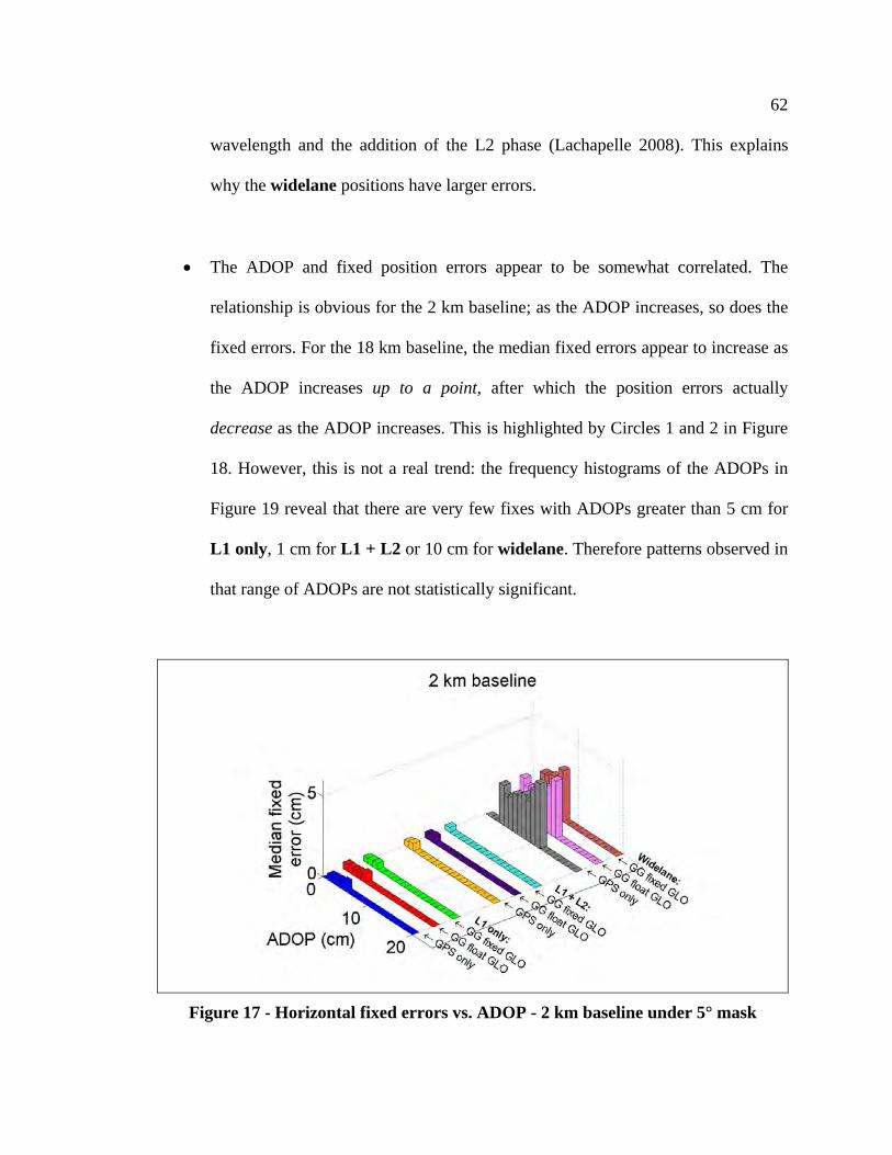
62
wavelength and the addition of the L2 phase (Lachapelle 2008). This explains
why the widelane positions have larger errors.
The ADOP and fixed position errors appear to be somewhat correlated. The
relationship is obvious for the 2 km baseline; as the ADOP increases, so does the
fixed errors. For the 18 km baseline, the median fixed errors appear to increase as
the ADOP increases up to a point, after which the position errors actually
decrease as the ADOP increases. This is highlighted by Circles 1 and 2 in Figure
18. However, this is not a real trend: the frequency histograms of the ADOPs in
Figure 19 reveal that there are very few fixes with ADOPs greater than 5 cm for
L1 only, 1 cm for L1 + L2 or 10 cm for widelane. Therefore patterns observed in
that range of ADOPs are not statistically significant.
Figure 17 - Horizontal fixed errors vs. ADOP - 2 km baseline under 5° mask
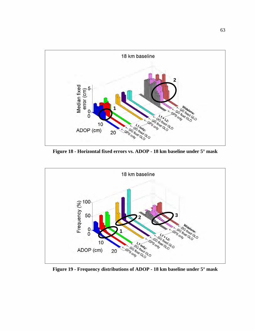
63
Figure 18 - Horizontal fixed errors vs. ADOP - 18 km baseline under 5° mask
Figure 19 - Frequency distributions of ADOP - 18 km baseline under 5° mask
1
2
1
32
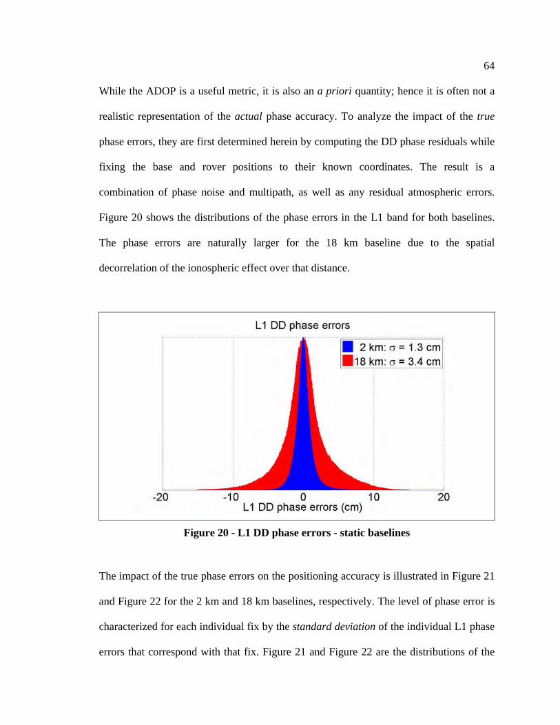
64
While the ADOP is a useful metric, it is also an a priori quantity; hence it is often not a
realistic representation of the actual phase accuracy. To analyze the impact of the true
phase errors, they are first determined herein by computing the DD phase residuals while
fixing the base and rover positions to their known coordinates. The result is a
combination of phase noise and multipath, as well as any residual atmospheric errors.
Figure 20 shows the distributions of the phase errors in the L1 band for both baselines.
The phase errors are naturally larger for the 18 km baseline due to the spatial
decorrelation of the ionospheric effect over that distance.
Figure 20 - L1 DD phase errors - static baselines
The impact of the true phase errors on the positioning accuracy is illustrated in Figure 21
and Figure 22 for the 2 km and 18 km baselines, respectively. The level of phase error is
characterized for each individual fix by the standard deviation of the individual L1 phase
errors that correspond with that fix. Figure 21 and Figure 22 are the distributions of the

65
median horizontal fixed position errors for different phase error standard deviations.
There is a trend for the L1 only and L1 + L2 combinations: larger phase errors generally
lead to larger position errors. This effect is anticipated since the purpose of ambiguity
resolution is to use the phase for positioning. This is also the underlying cause behind the
loss of precision in the solutions generated for the 18 km baseline, relative to the 2 km
baseline.
The more interesting result is the trend for widelane. The dependency of the position
errors on the phase errors is actually relatively flat for the widelane solutions. This
implies that higher levels of phase errors can be tolerated, which can be useful for longer
baselines. There are two things to consider about this result:
1. The differential atmospheric effects are very small for the 2 km baseline, and for
the 18 km baseline the 1σ value of the phase error distribution is still less than a
quarter of an L1 cycle. It is possible that widelane would not tolerate phase errors
larger than the ones analyzed here, especially since the effect of the ionosphere is
multiplied by 1.28 when using widelane over L1 (Lachapelle 2008). However, the
widelane wavelength is also more than four times wider than L1, suggesting that
the final effect of the ionosphere when using widelane is less than half the effect
when using L1.
2. There is a problem when specifically considering positioning accuracy: even
though the relationship between position and phase errors is nearly flat, the

66
position errors are larger to begin with and little benefit is gained. However this
property of widelane – to tolerate larger phase errors – manifests itself in other
aspects of ambiguity resolution. This is demonstrated later in this chapter
(Sections 4.4 and 4.7).
Figure 21 - Horizontal fixed errors vs. phase error standard deviation - 2 km baseline under 5° mask
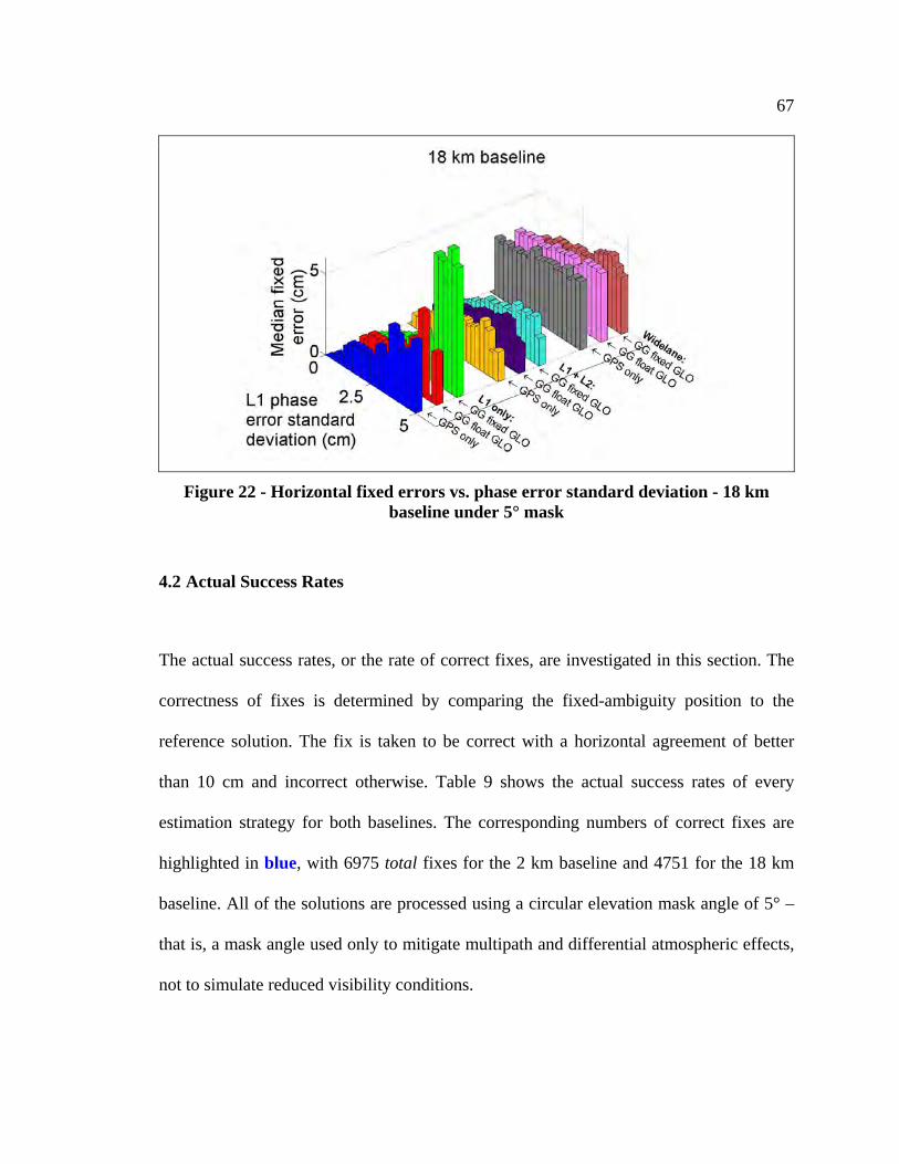
67
Figure 22 - Horizontal fixed errors vs. phase error standard deviation - 18 km baseline under 5° mask
4.2 Actual Success Rates
The actual success rates, or the rate of correct fixes, are investigated in this section. The
correctness of fixes is determined by comparing the fixed-ambiguity position to the
reference solution. The fix is taken to be correct with a horizontal agreement of better
than 10 cm and incorrect otherwise. Table 9 shows the actual success rates of every
estimation strategy for both baselines. The corresponding numbers of correct fixes are
highlighted in blue, with 6975 total fixes for the 2 km baseline and 4751 for the 18 km
baseline. All of the solutions are processed using a circular elevation mask angle of 5° –
that is, a mask angle used only to mitigate multipath and differential atmospheric effects,
not to simulate reduced visibility conditions.
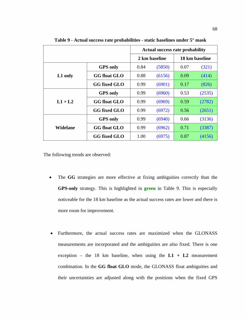
68
Table 9 - Actual success rate probabilities - static baselines under 5° mask
Actual success rate probability
2 km baseline 18 km baseline
L1 only
GPS only 0.84 (5850) 0.07 (321)
GG float GLO 0.88 (6156) 0.09 (414)
GG fixed GLO 0.99 (6901) 0.17 (826)
L1 + L2
GPS only 0.99 (6960) 0.53 (2535)
GG float GLO 0.99 (6969) 0.59 (2782)
GG fixed GLO 0.99 (6972) 0.56 (2651)
Widelane
GPS only 0.99 (6940) 0.66 (3136)
GG float GLO 0.99 (6962) 0.71 (3387)
GG fixed GLO 1.00 (6975) 0.87 (4156)
The following trends are observed:
The GG strategies are more effective at fixing ambiguities correctly than the
GPS-only strategy. This is highlighted in green in Table 9. This is especially
noticeable for the 18 km baseline as the actual success rates are lower and there is
more room for improvement.
Furthermore, the actual success rates are maximized when the GLONASS
measurements are incorporated and the ambiguities are also fixed. There is one
exception – the 18 km baseline, when using the L1 + L2 measurement
combination. In the GG float GLO mode, the GLONASS float ambiguities and
their uncertainties are adjusted along with the positions when the fixed GPS
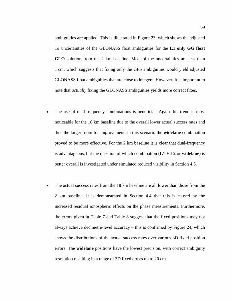
69
ambiguities are applied. This is illustrated in Figure 23, which shows the adjusted
1σ uncertainties of the GLONASS float ambiguities for the L1 only GG float
GLO solution from the 2 km baseline. Most of the uncertainties are less than
1 cm, which suggests that fixing only the GPS ambiguities would yield adjusted
GLONASS float ambiguities that are close to integers. However, it is important to
note that actually fixing the GLONASS ambiguities yields more correct fixes.
The use of dual-frequency combinations is beneficial. Again this trend is most
noticeable for the 18 km baseline due to the overall lower actual success rates and
thus the larger room for improvement; in this scenario the widelane combination
proved to be more effective. For the 2 km baseline it is clear that dual-frequency
is advantageous, but the question of which combination (L1 + L2 or widelane) is
better overall is investigated under simulated reduced visibility in Section 4.5.
The actual success rates from the 18 km baseline are all lower than those from the
2 km baseline. It is demonstrated in Section 4.4 that this is caused by the
increased residual ionospheric effects on the phase measurements. Furthermore,
the errors given in Table 7 and Table 8 suggest that the fixed positions may not
always achieve decimetre-level accuracy – this is confirmed by Figure 24, which
shows the distributions of the actual success rates over various 3D fixed position
errors. The widelane positions have the lowest precision, with correct ambiguity
resolution resulting in a range of 3D fixed errors up to 20 cm.
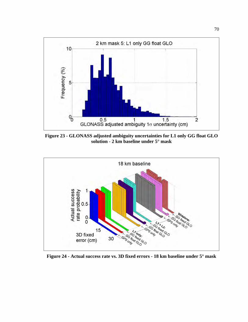
70
Figure 23 - GLONASS adjusted ambiguity uncertainties for L1 only GG float GLO solution - 2 km baseline under 5° mask
Figure 24 - Actual success rate vs. 3D fixed errors - 18 km baseline under 5° mask

71
4.3 Float Estimate Errors before Ambiguity Resolution
The trends in the actual success rate are ultimately driven by a number of underlying
factors. The first of these is the error in the float estimate of the position (referred to as
“float errors” herein), just prior to ambiguity resolution. Recall the parameterization of
the double-differenced (DD) phase measurement:
i i base baseR N N
An error in the float estimate of the position will affect the range term R , which in
turn affects the float estimates of the ambiguities N and baseN . The effect of the
float errors on the ambiguity resolution process is investigated here. Table 10 shows the
median horizontal float errors for all of the integer fixes together, and also the correct and
incorrect fixes separately.

72
Table 10 - Horizontal float errors before fix - static baselines under 5° mask
Median horizontal float errors before fix (cm)
2 km baseline 18 km baseline
All fixes
Correct fixes
Incorrect fixes
All fixes
Correct fixes
Incorrect fixes
L1 only
GPS only 49 46 67 87 62 89
GG float GLO 40 39 56 69 48 72
GG fixed GLO 40 40 61 69 57 73
L1 +
L2
GPS only 48 48 68 86 82 92
GG float GLO 40 40 28 69 65 75
GG fixed GLO 40 40 42 69 66 72
WL
GPS only 50 50 119 88 73 130
GG float GLO 41 41 86 71 62 106
GG fixed GLO 41 41 – 71 68 109
There is a slight correlation between the median float errors before ambiguity resolution,
and the actual success rate probability of ambiguity resolution (see Table 9). Figure 25
illustrates this for both baselines. The actual success rate goes up as the median float
errors decrease. This trend is different between the baselines, and confined to solutions
that use the same measurement combination. For instance the actual success rates are
much higher for the L1 + L2 and widelane combinations than for the L1 only
combination, despite similar median float errors.
An interesting observation is that the float errors do not change significantly between
different measurement combinations. The combinations use different subsets of phase
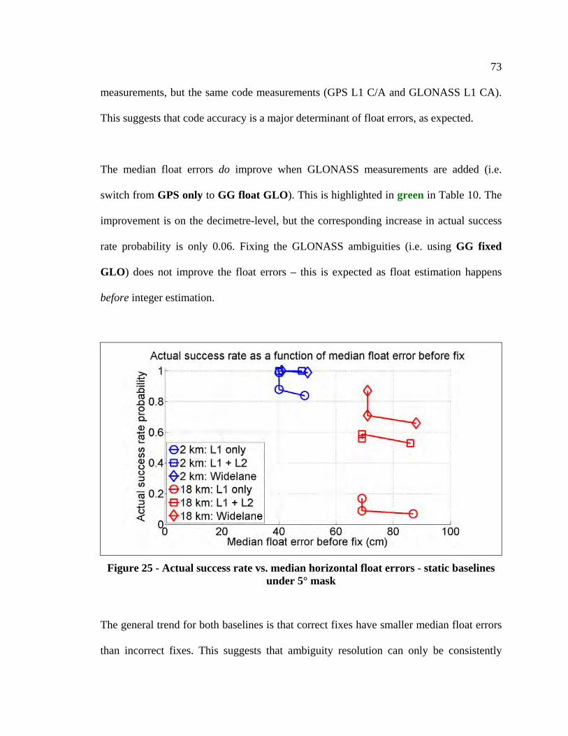
73
measurements, but the same code measurements (GPS L1 C/A and GLONASS L1 CA).
This suggests that code accuracy is a major determinant of float errors, as expected.
The median float errors do improve when GLONASS measurements are added (i.e.
switch from GPS only to GG float GLO). This is highlighted in green in Table 10. The
improvement is on the decimetre-level, but the corresponding increase in actual success
rate probability is only 0.06. Fixing the GLONASS ambiguities (i.e. using GG fixed
GLO) does not improve the float errors – this is expected as float estimation happens
before integer estimation.
Figure 25 - Actual success rate vs. median horizontal float errors - static baselines under 5° mask
The general trend for both baselines is that correct fixes have smaller median float errors
than incorrect fixes. This suggests that ambiguity resolution can only be consistently

74
successful with a precise initial float estimate. The dependence on the float estimate
accuracy is further illustrated by Figure 26 and Figure 27 for the 2 km and 18 km
baselines, respectively. These are the distributions of the actual success rate probability
for various levels of float errors before fix.
The actual success rate does not significantly change whether GPS is used alone or
combined with GLONASS. Hence, the role of the GLONASS measurements appears to
be to provide more accurate float estimates in the first place, rather than to change the
distribution of the actual success rate. From these distributions, it is also clear why the
GG float GLO strategy does not have a big impact on the actual success rate in this case:
decimetre-level improvements in float errors do not improve the actual success rate
probability by more than 0.10.
However, the actual success rates tend to be higher when the GLONASS ambiguities are
fixed. This implies that estimating the GLONASS ambiguities improves the overall
ambiguity resolution process, beyond just decreasing the float errors by virtue of having
more measurements in float estimation. This is explored in greater detail in Section 4.5.
As well, the actual success rates (for the same levels of float error) are much higher when
dual-frequency measurement combinations are used. Widelane has the highest actual
success rate distributions – this is expected as its ambiguity has a longer wavelength than
either L1 or L2 and is thus inherently more observable with the coarser code
measurements. For L1 + L2 there are other factors that are investigated in Section 4.5.
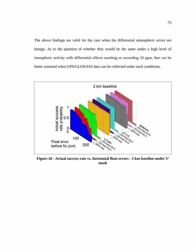
75
The above findings are valid for the case when the differential atmospheric errors are
benign. As to the question of whether they would be the same under a high level of
ionospheric activity with differential effects reaching or exceeding 10 ppm, that can be
better assessed when GPS/GLONASS data can be collected under such conditions.
Figure 26 - Actual success rate vs. horizontal float errors - 2 km baseline under 5° mask
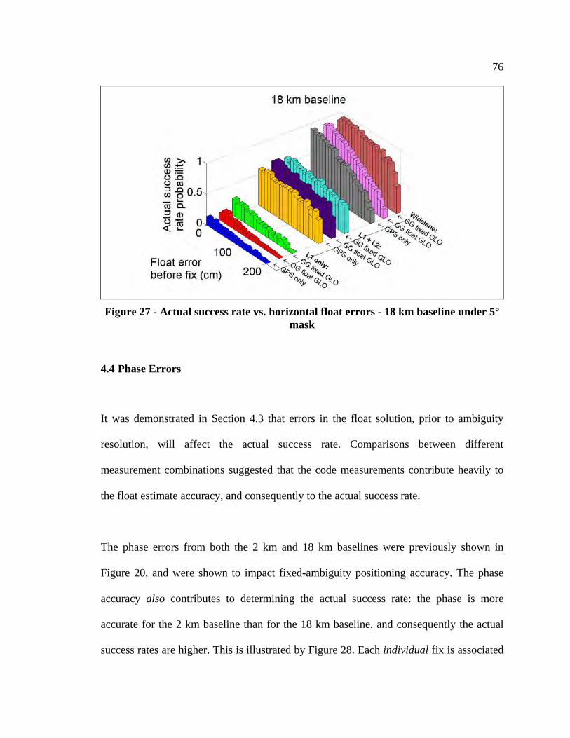
76
Figure 27 - Actual success rate vs. horizontal float errors - 18 km baseline under 5° mask
4.4 Phase Errors
It was demonstrated in Section 4.3 that errors in the float solution, prior to ambiguity
resolution, will affect the actual success rate. Comparisons between different
measurement combinations suggested that the code measurements contribute heavily to
the float estimate accuracy, and consequently to the actual success rate.
The phase errors from both the 2 km and 18 km baselines were previously shown in
Figure 20, and were shown to impact fixed-ambiguity positioning accuracy. The phase
accuracy also contributes to determining the actual success rate: the phase is more
accurate for the 2 km baseline than for the 18 km baseline, and consequently the actual
success rates are higher. This is illustrated by Figure 28. Each individual fix is associated

77
with a set of phase residuals, characterized by their standard deviation. Figure 28 is the
distribution of the phase error standard deviations for every L1 only GG fixed GLO
integer fix for the 18 km baseline. Note that this solution is only chosen for illustrative
purposes – results for all of the solutions are presented afterwards.
For this particular solution, the phase error standard deviations are clearly larger for the
incorrect fixes than the correct fixes. The median phase error standard deviation is 1.7 cm
for the correct fixes and 2.8 cm for the incorrect fixes. Additionally, there are many
incorrect fixes with phase error standard deviations in the range of 3 to 5 cm, which
indicates that there are individual phase errors with larger magnitudes. This suggests that
the level of phase errors has an effect on ambiguity resolution.
Figure 28 - Distribution of phase error standard deviation for L1 only GG fixed GLO solution - 18 km baseline under 5° mask
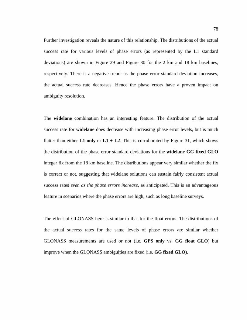
78
Further investigation reveals the nature of this relationship. The distributions of the actual
success rate for various levels of phase errors (as represented by the L1 standard
deviations) are shown in Figure 29 and Figure 30 for the 2 km and 18 km baselines,
respectively. There is a negative trend: as the phase error standard deviation increases,
the actual success rate decreases. Hence the phase errors have a proven impact on
ambiguity resolution.
The widelane combination has an interesting feature. The distribution of the actual
success rate for widelane does decrease with increasing phase error levels, but is much
flatter than either L1 only or L1 + L2. This is corroborated by Figure 31, which shows
the distribution of the phase error standard deviations for the widelane GG fixed GLO
integer fix from the 18 km baseline. The distributions appear very similar whether the fix
is correct or not, suggesting that widelane solutions can sustain fairly consistent actual
success rates even as the phase errors increase, as anticipated. This is an advantageous
feature in scenarios where the phase errors are high, such as long baseline surveys.
The effect of GLONASS here is similar to that for the float errors. The distributions of
the actual success rates for the same levels of phase errors are similar whether
GLONASS measurements are used or not (i.e. GPS only vs. GG float GLO) but
improve when the GLONASS ambiguities are fixed (i.e. GG fixed GLO).
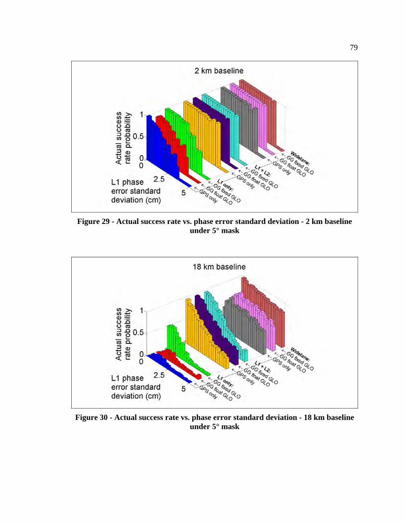
79
Figure 29 - Actual success rate vs. phase error standard deviation - 2 km baseline under 5° mask
Figure 30 - Actual success rate vs. phase error standard deviation - 18 km baseline under 5° mask
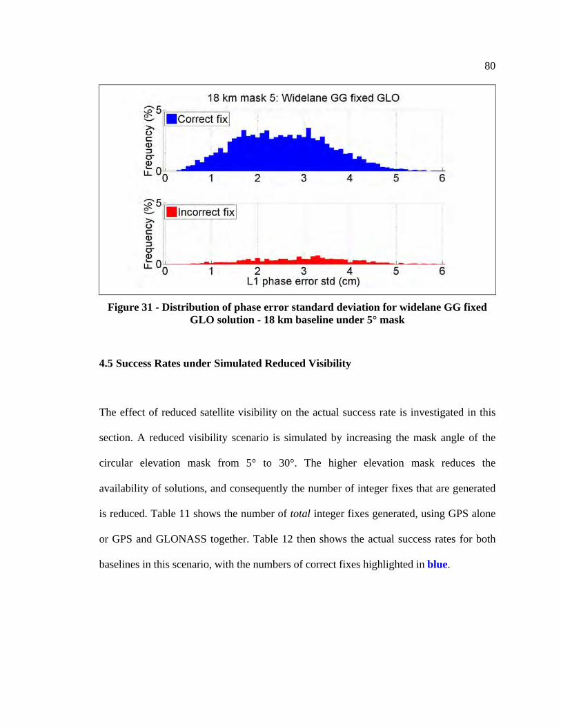
80
Figure 31 - Distribution of phase error standard deviation for widelane GG fixed GLO solution - 18 km baseline under 5° mask
4.5 Success Rates under Simulated Reduced Visibility
The effect of reduced satellite visibility on the actual success rate is investigated in this
section. A reduced visibility scenario is simulated by increasing the mask angle of the
circular elevation mask from 5° to 30°. The higher elevation mask reduces the
availability of solutions, and consequently the number of integer fixes that are generated
is reduced. Table 11 shows the number of total integer fixes generated, using GPS alone
or GPS and GLONASS together. Table 12 then shows the actual success rates for both
baselines in this scenario, with the numbers of correct fixes highlighted in blue.
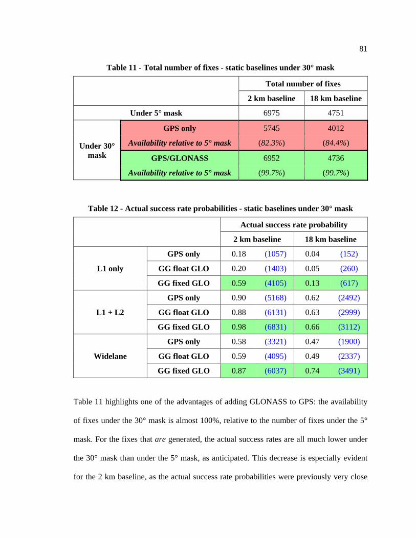
81
Table 11 - Total number of fixes - static baselines under 30° mask
Total number of fixes
2 km baseline 18 km baseline
Under 5° mask 6975 4751
Under 30° mask
GPS only 5745 4012
Availability relative to 5° mask (82.3%) (84.4%)
GPS/GLONASS 6952 4736
Availability relative to 5° mask (99.7%) (99.7%)
Table 12 - Actual success rate probabilities - static baselines under 30° mask
Actual success rate probability
2 km baseline 18 km baseline
L1 only
GPS only 0.18 (1057) 0.04 (152)
GG float GLO 0.20 (1403) 0.05 (260)
GG fixed GLO 0.59 (4105) 0.13 (617)
L1 + L2
GPS only 0.90 (5168) 0.62 (2492)
GG float GLO 0.88 (6131) 0.63 (2999)
GG fixed GLO 0.98 (6831) 0.66 (3112)
Widelane
GPS only 0.58 (3321) 0.47 (1900)
GG float GLO 0.59 (4095) 0.49 (2337)
GG fixed GLO 0.87 (6037) 0.74 (3491)
Table 11 highlights one of the advantages of adding GLONASS to GPS: the availability
of fixes under the 30° mask is almost 100%, relative to the number of fixes under the 5°
mask. For the fixes that are generated, the actual success rates are all much lower under
the 30° mask than under the 5° mask, as anticipated. This decrease is especially evident
for the 2 km baseline, as the actual success rate probabilities were previously very close

82
to one. One of the reasons is that the errors in the float estimate, just prior to ambiguity
resolution, are higher under a 30° mask than a 5° mask. Table 13 shows the median
horizontal float errors for all of the fixes together as well as the correct and incorrect
fixes. The float errors are larger due to the poorer satellite geometry, as illustrated in
Figure 32 using the L1 only GPS only solution from the 2 km baseline.
Under the normal 5° mask, there was a correlation observed between the median float
errors and the actual success rate. Under this reduced-visibility 30° mask, this
relationship is very weak. Table 13 shows that adding GLONASS measurements (i.e.
going from GPS only to GG float GLO) does decrease the float errors. However, Table
12 indicates that adding those same GLONASS measurements barely affects the success
rate – the maximum increase in actual success rate probability is 0.02. What does
improve the actual success rate significantly is when the GLONASS ambiguities are
fixed (as highlighted in green).
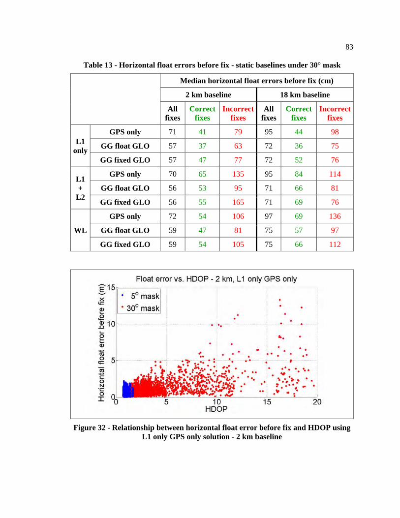
83
Table 13 - Horizontal float errors before fix - static baselines under 30° mask
Median horizontal float errors before fix (cm)
2 km baseline 18 km baseline
All fixes
Correct fixes
Incorrect fixes
All fixes
Correct fixes
Incorrect fixes
L1 only
GPS only 71 41 79 95 44 98
GG float GLO 57 37 63 72 36 75
GG fixed GLO 57 47 77 72 52 76
L1 +
L2
GPS only 70 65 135 95 84 114
GG float GLO 56 53 95 71 66 81
GG fixed GLO 56 55 165 71 69 76
WL
GPS only 72 54 106 97 69 136
GG float GLO 59 47 81 75 57 97
GG fixed GLO 59 54 105 75 66 112
Figure 32 - Relationship between horizontal float error before fix and HDOP using L1 only GPS only solution - 2 km baseline
84
The independence of the success rate from the float errors and the difference between the
GG float GLO and GG fixed GLO strategies both point to an underlying factor related
to the integer ambiguity estimation that is impacting the success rate. This underlying
factor is the number of ambiguities estimated as integers within the ambiguity resolution
process: the actual success rate is higher with more ambiguities in the ambiguity
resolution process (not the float estimation process). To illustrate this relationship, the
distributions of the number of ambiguities are analyzed for a series of solutions from the
2 km baseline. The results are shown as follows:
Figure 33: Under the 5° mask, the L1 only GPS only fixes have between six and
eleven ambiguities. With the abundance of ambiguities, most of the fixes are
correct.
Figure 34: When the 30° mask is applied for the same L1 only GPS only
solution, the number of ambiguities decreases to between three and seven. Most
of the fixes are now incorrect.
Figure 35: Under the same 30° mask, the number of ambiguities stays the same
when the estimation strategy is switched to L1 only GG float GLO. Because
there are still so few ambiguities, most of the fixes are still incorrect.
Figure 36: Finally, under the same 30° mask, the number of ambiguities increases
substantially when the estimation strategy is switched to L1 only GG fixed GLO.
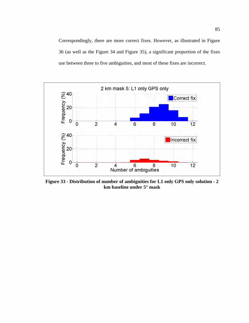
85
Correspondingly, there are more correct fixes. However, as illustrated in Figure
36 (as well as the Figure 34 and Figure 35), a significant proportion of the fixes
use between three to five ambiguities, and most of these fixes are incorrect.
Figure 33 - Distribution of number of ambiguities for L1 only GPS only solution - 2 km baseline under 5° mask

86
Figure 34 - Distribution of number of ambiguities for L1 only GPS only solution - 2 km baseline under 30° mask
Figure 35 - Distribution of number of ambiguities for L1 only GG float GLO solution - 2 km baseline under 30° mask
81%
79%
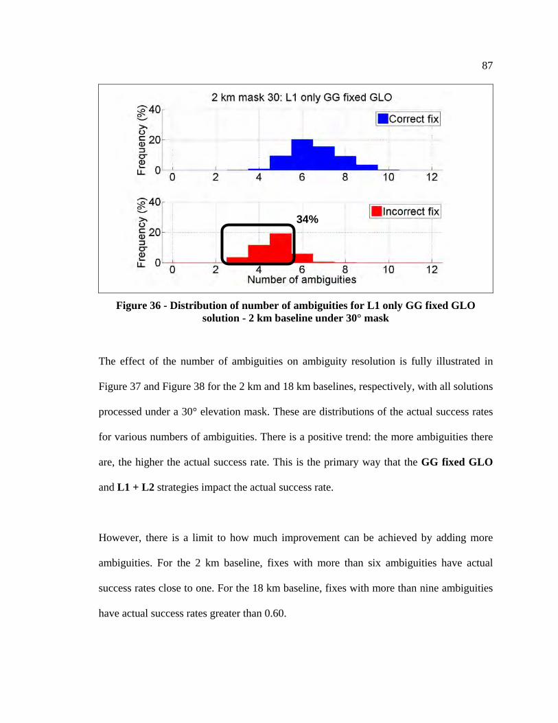
87
Figure 36 - Distribution of number of ambiguities for L1 only GG fixed GLO solution - 2 km baseline under 30° mask
The effect of the number of ambiguities on ambiguity resolution is fully illustrated in
Figure 37 and Figure 38 for the 2 km and 18 km baselines, respectively, with all solutions
processed under a 30° elevation mask. These are distributions of the actual success rates
for various numbers of ambiguities. There is a positive trend: the more ambiguities there
are, the higher the actual success rate. This is the primary way that the GG fixed GLO
and L1 + L2 strategies impact the actual success rate.
However, there is a limit to how much improvement can be achieved by adding more
ambiguities. For the 2 km baseline, fixes with more than six ambiguities have actual
success rates close to one. For the 18 km baseline, fixes with more than nine ambiguities
have actual success rates greater than 0.60.
34%
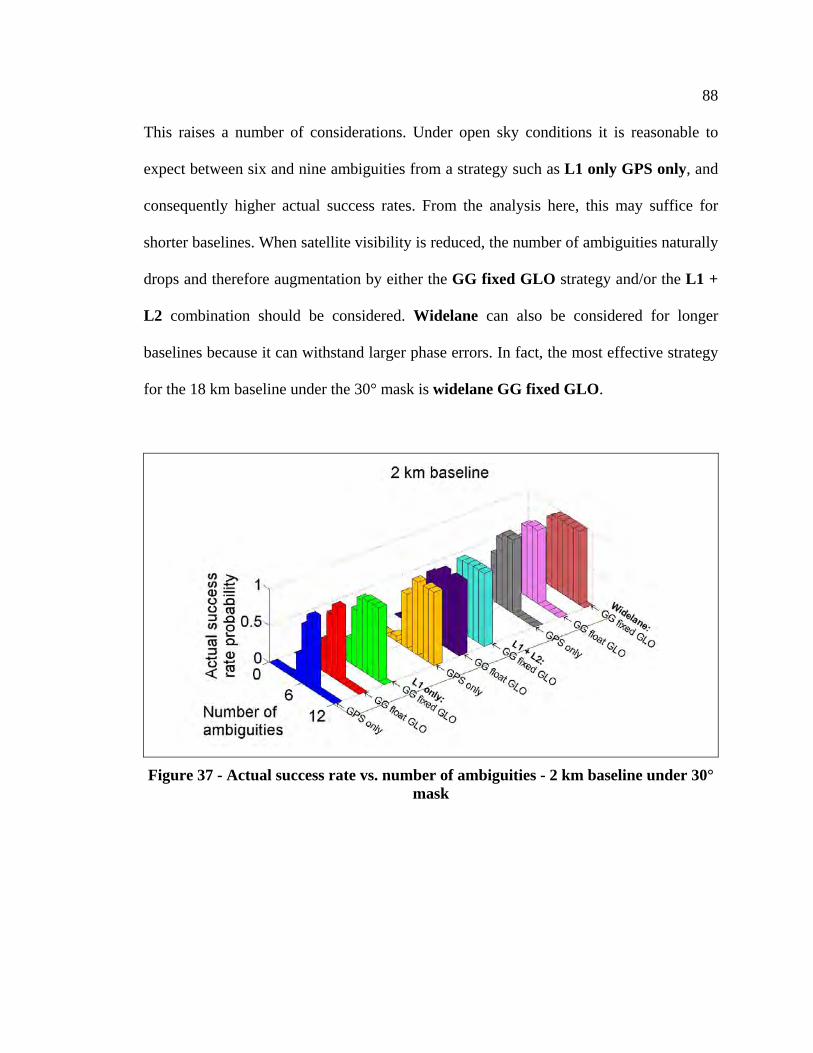
88
This raises a number of considerations. Under open sky conditions it is reasonable to
expect between six and nine ambiguities from a strategy such as L1 only GPS only, and
consequently higher actual success rates. From the analysis here, this may suffice for
shorter baselines. When satellite visibility is reduced, the number of ambiguities naturally
drops and therefore augmentation by either the GG fixed GLO strategy and/or the L1 +
L2 combination should be considered. Widelane can also be considered for longer
baselines because it can withstand larger phase errors. In fact, the most effective strategy
for the 18 km baseline under the 30° mask is widelane GG fixed GLO.
Figure 37 - Actual success rate vs. number of ambiguities - 2 km baseline under 30° mask
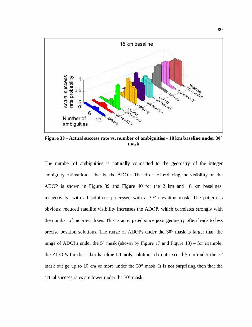
89
Figure 38 - Actual success rate vs. number of ambiguities - 18 km baseline under 30° mask
The number of ambiguities is naturally connected to the geometry of the integer
ambiguity estimation – that is, the ADOP. The effect of reducing the visibility on the
ADOP is shown in Figure 39 and Figure 40 for the 2 km and 18 km baselines,
respectively, with all solutions processed with a 30° elevation mask. The pattern is
obvious: reduced satellite visibility increases the ADOP, which correlates strongly with
the number of incorrect fixes. This is anticipated since poor geometry often leads to less
precise position solutions. The range of ADOPs under the 30° mask is larger than the
range of ADOPs under the 5° mask (shown by Figure 17 and Figure 18) – for example,
the ADOPs for the 2 km baseline L1 only solutions do not exceed 5 cm under the 5°
mask but go up to 10 cm or more under the 30° mask. It is not surprising then that the
actual success rates are lower under the 30° mask.
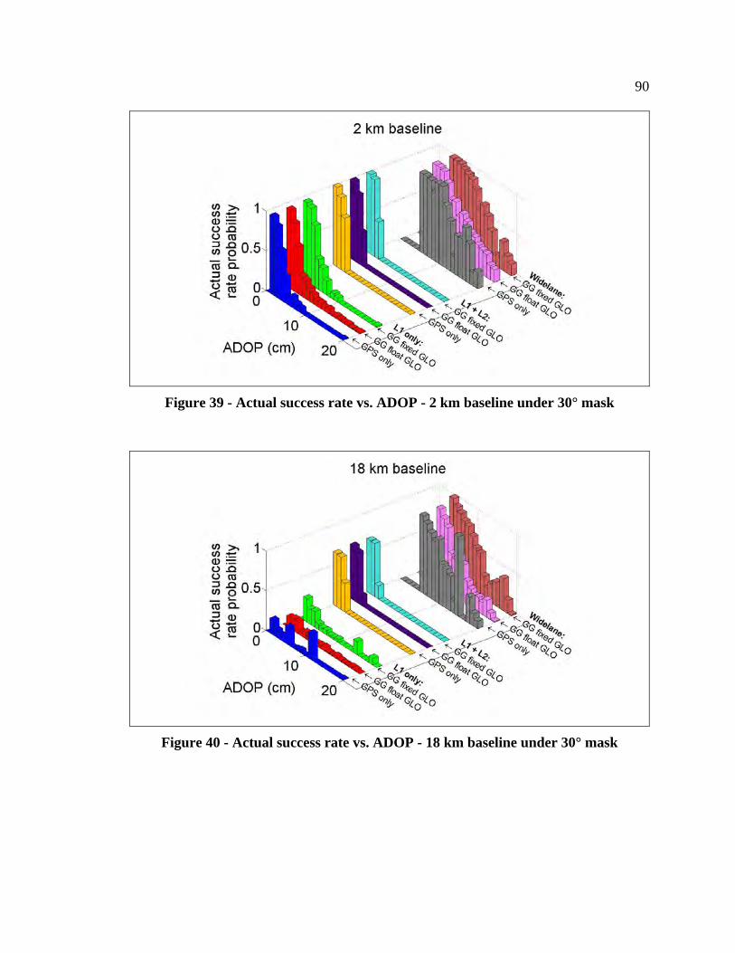
90
Figure 39 - Actual success rate vs. ADOP - 2 km baseline under 30° mask
Figure 40 - Actual success rate vs. ADOP - 18 km baseline under 30° mask
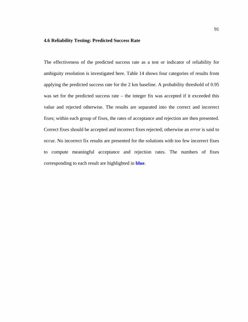
91
4.6 Reliability Testing: Predicted Success Rate
The effectiveness of the predicted success rate as a test or indicator of reliability for
ambiguity resolution is investigated here. Table 14 shows four categories of results from
applying the predicted success rate for the 2 km baseline. A probability threshold of 0.95
was set for the predicted success rate – the integer fix was accepted if it exceeded this
value and rejected otherwise. The results are separated into the correct and incorrect
fixes; within each group of fixes, the rates of acceptance and rejection are then presented.
Correct fixes should be accepted and incorrect fixes rejected; otherwise an error is said to
occur. No incorrect fix results are presented for the solutions with too few incorrect fixes
to compute meaningful acceptance and rejection rates. The numbers of fixes
corresponding to each result are highlighted in blue.
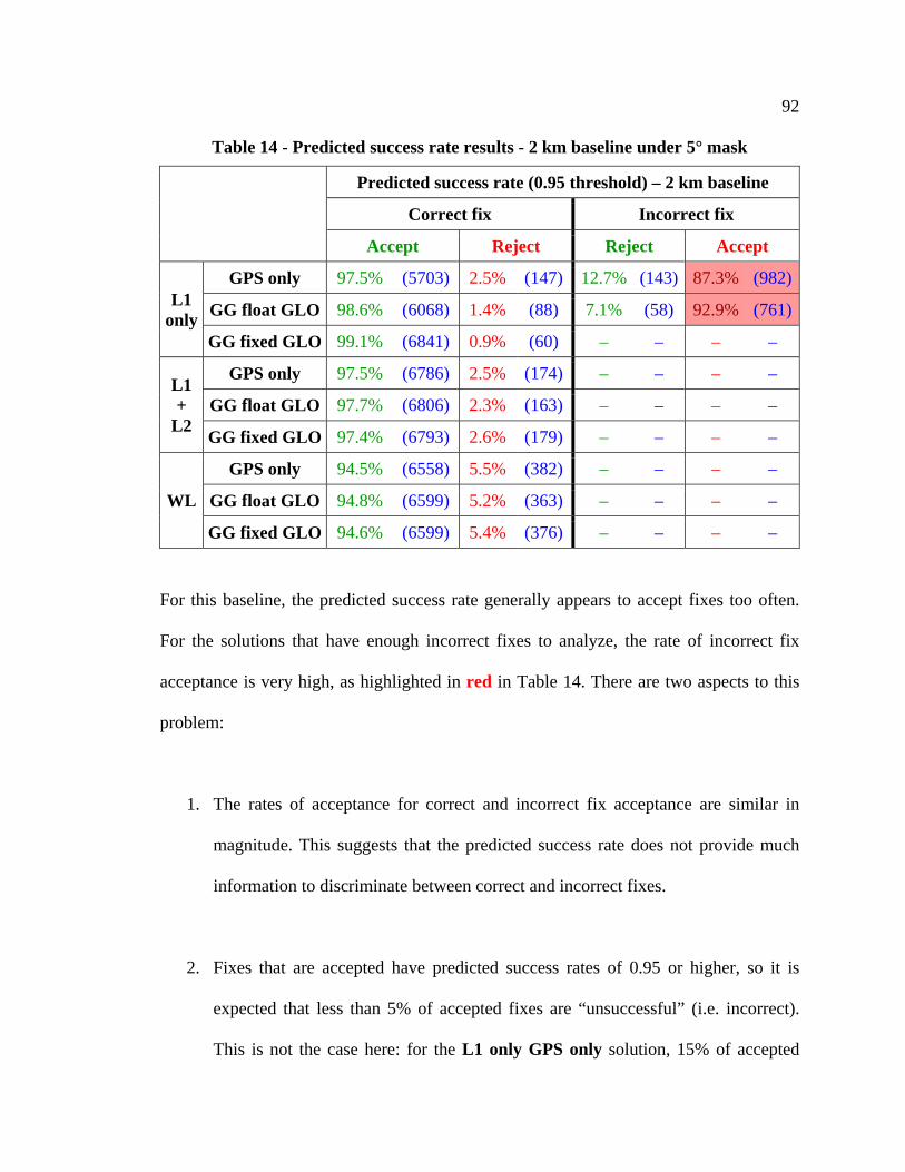
92
Table 14 - Predicted success rate results - 2 km baseline under 5° mask
Predicted success rate (0.95 threshold) – 2 km baseline
Correct fix Incorrect fix
Accept Reject Reject Accept
L1 only
GPS only 97.5% (5703) 2.5% (147) 12.7% (143) 87.3% (982)
GG float GLO 98.6% (6068) 1.4% (88) 7.1% (58) 92.9% (761)
GG fixed GLO 99.1% (6841) 0.9% (60) – – – –
L1 +
L2
GPS only 97.5% (6786) 2.5% (174) – – – –
GG float GLO 97.7% (6806) 2.3% (163) – – – –
GG fixed GLO 97.4% (6793) 2.6% (179) – – – –
WL
GPS only 94.5% (6558) 5.5% (382) – – – –
GG float GLO 94.8% (6599) 5.2% (363) – – – –
GG fixed GLO 94.6% (6599) 5.4% (376) – – – –
For this baseline, the predicted success rate generally appears to accept fixes too often.
For the solutions that have enough incorrect fixes to analyze, the rate of incorrect fix
acceptance is very high, as highlighted in red in Table 14. There are two aspects to this
problem:
1. The rates of acceptance for correct and incorrect fix acceptance are similar in
magnitude. This suggests that the predicted success rate does not provide much
information to discriminate between correct and incorrect fixes.
2. Fixes that are accepted have predicted success rates of 0.95 or higher, so it is
expected that less than 5% of accepted fixes are “unsuccessful” (i.e. incorrect).
This is not the case here: for the L1 only GPS only solution, 15% of accepted
93
fixes are incorrect (i.e. 982 / [982 + 5703]). For the L1 only GG float GLO
solution, 11% of accepted fixes are incorrect (i.e. 761 / [761 + 6068]).
Accepting incorrect fixes leads to undetected position biases, a major problem for fixed-
ambiguity applications where the expectation is to have position accuracies better than
10 cm. This is further illustrated in Figure 41, which shows the distribution of predicted
success rates for the L1 only GPS only solutions. The predicted success rate probabilities
for nearly every fix are greater than 0.98, despite the fact that the aggregate actual
success rate probability (from Table 9) is only 0.84.
Conversely, correct fixes do not appear to be rejected very often for this baseline.
Rejecting a correct fix induces a loss of precision in the position. This is again a function
of the predicted success rate being so optimistic; fixes in general are not rejected very
often.
There is an important consideration regarding the solutions with few incorrect fixes.
These solutions either use GLONASS measurements and fix the ambiguities, or use dual-
frequency measurement combinations. The actual success rates are so high that there are
few incorrect fixes that could actually be accepted. Hence, the use of GLONASS or dual-
frequency measurements can be partly viewed as a positive contributor to fix reliability,
in that they drive the actual success rate higher and remove incorrect fixes that can be
potentially accepted.
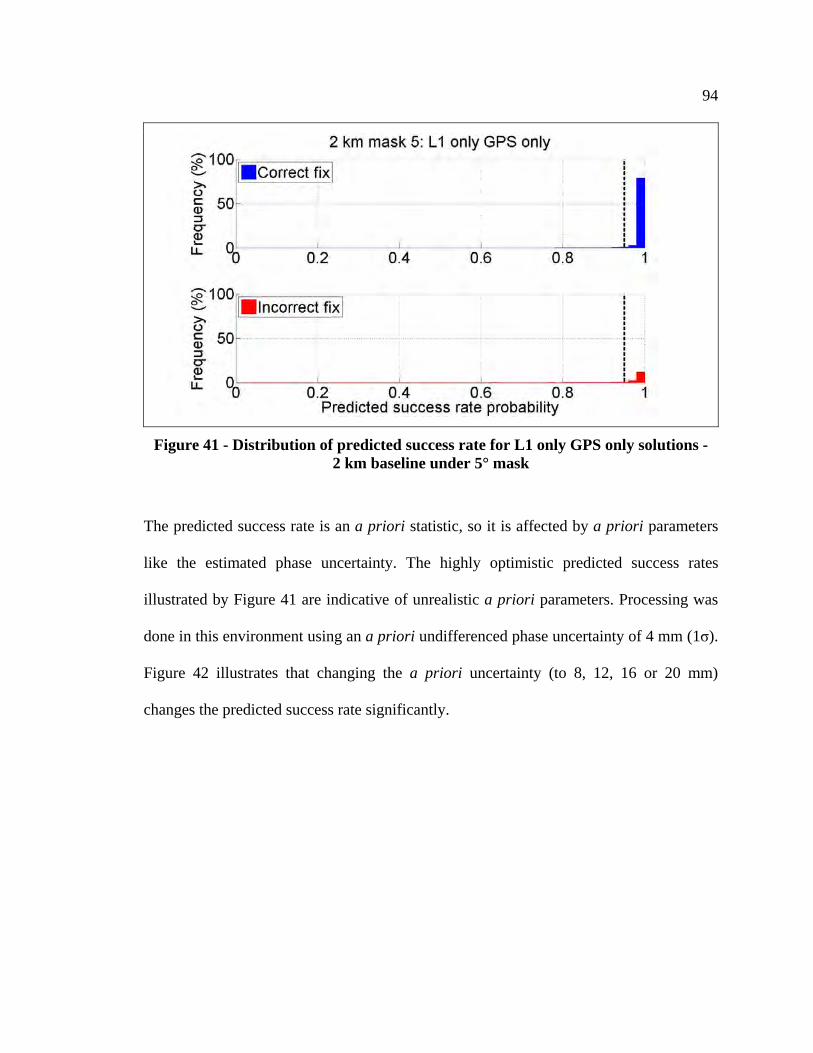
94
Figure 41 - Distribution of predicted success rate for L1 only GPS only solutions - 2 km baseline under 5° mask
The predicted success rate is an a priori statistic, so it is affected by a priori parameters
like the estimated phase uncertainty. The highly optimistic predicted success rates
illustrated by Figure 41 are indicative of unrealistic a priori parameters. Processing was
done in this environment using an a priori undifferenced phase uncertainty of 4 mm (1σ).
Figure 42 illustrates that changing the a priori uncertainty (to 8, 12, 16 or 20 mm)
changes the predicted success rate significantly.
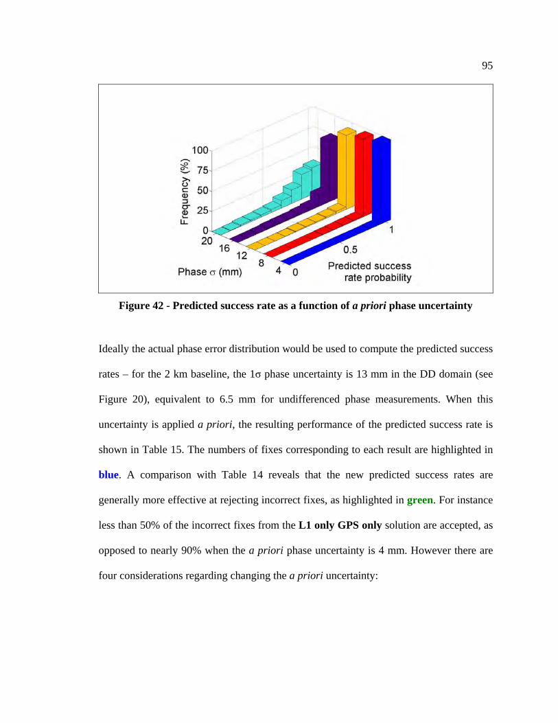
95
Figure 42 - Predicted success rate as a function of a priori phase uncertainty
Ideally the actual phase error distribution would be used to compute the predicted success
rates – for the 2 km baseline, the 1σ phase uncertainty is 13 mm in the DD domain (see
Figure 20), equivalent to 6.5 mm for undifferenced phase measurements. When this
uncertainty is applied a priori, the resulting performance of the predicted success rate is
shown in Table 15. The numbers of fixes corresponding to each result are highlighted in
blue. A comparison with Table 14 reveals that the new predicted success rates are
generally more effective at rejecting incorrect fixes, as highlighted in green. For instance
less than 50% of the incorrect fixes from the L1 only GPS only solution are accepted, as
opposed to nearly 90% when the a priori phase uncertainty is 4 mm. However there are
four considerations regarding changing the a priori uncertainty:
96
1. The reduction in incorrect fix acceptance is not overwhelming – a rate of 50% is
still potentially harmful, especially when operating in environments where
incorrect fixes are more common.
2. The reduction in incorrect fix acceptance comes at the expense of higher correct
fixes rejection. This is expected since the predicted success rates decrease (as
illustrated by Figure 42) but it means that the ambiguities are resolved less often.
3. The true phase errors are generally not known before a survey is undertaken.
Determining them requires precise knowledge of the rover station coordinates,
which is often the objective of ambiguity resolution in the first place.
4. Phase error growth is strongly correlated to the level of ionospheric activity. The
latter could be automatically assessed in software if dual-frequency measurements
are available and adapted accordingly. An investigation of adaptability would
require data over different inter-receiver distances and under different ionospheric
conditions.
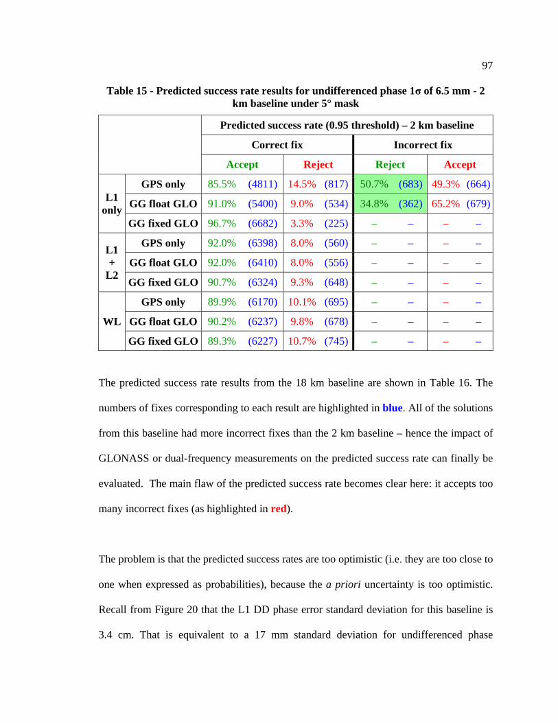
97
Table 15 - Predicted success rate results for undifferenced phase 1σ of 6.5 mm - 2 km baseline under 5° mask
Predicted success rate (0.95 threshold) – 2 km baseline
Correct fix Incorrect fix
Accept Reject Reject Accept
L1 only
GPS only 85.5% (4811) 14.5% (817) 50.7% (683) 49.3% (664)
GG float GLO 91.0% (5400) 9.0% (534) 34.8% (362) 65.2% (679)
GG fixed GLO 96.7% (6682) 3.3% (225) – – – –
L1 +
L2
GPS only 92.0% (6398) 8.0% (560) – – – –
GG float GLO 92.0% (6410) 8.0% (556) – – – –
GG fixed GLO 90.7% (6324) 9.3% (648) – – – –
WL
GPS only 89.9% (6170) 10.1% (695) – – – –
GG float GLO 90.2% (6237) 9.8% (678) – – – –
GG fixed GLO 89.3% (6227) 10.7% (745) – – – –
The predicted success rate results from the 18 km baseline are shown in Table 16. The
numbers of fixes corresponding to each result are highlighted in blue. All of the solutions
from this baseline had more incorrect fixes than the 2 km baseline – hence the impact of
GLONASS or dual-frequency measurements on the predicted success rate can finally be
evaluated. The main flaw of the predicted success rate becomes clear here: it accepts too
many incorrect fixes (as highlighted in red).
The problem is that the predicted success rates are too optimistic (i.e. they are too close to
one when expressed as probabilities), because the a priori uncertainty is too optimistic.
Recall from Figure 20 that the L1 DD phase error standard deviation for this baseline is
3.4 cm. That is equivalent to a 17 mm standard deviation for undifferenced phase
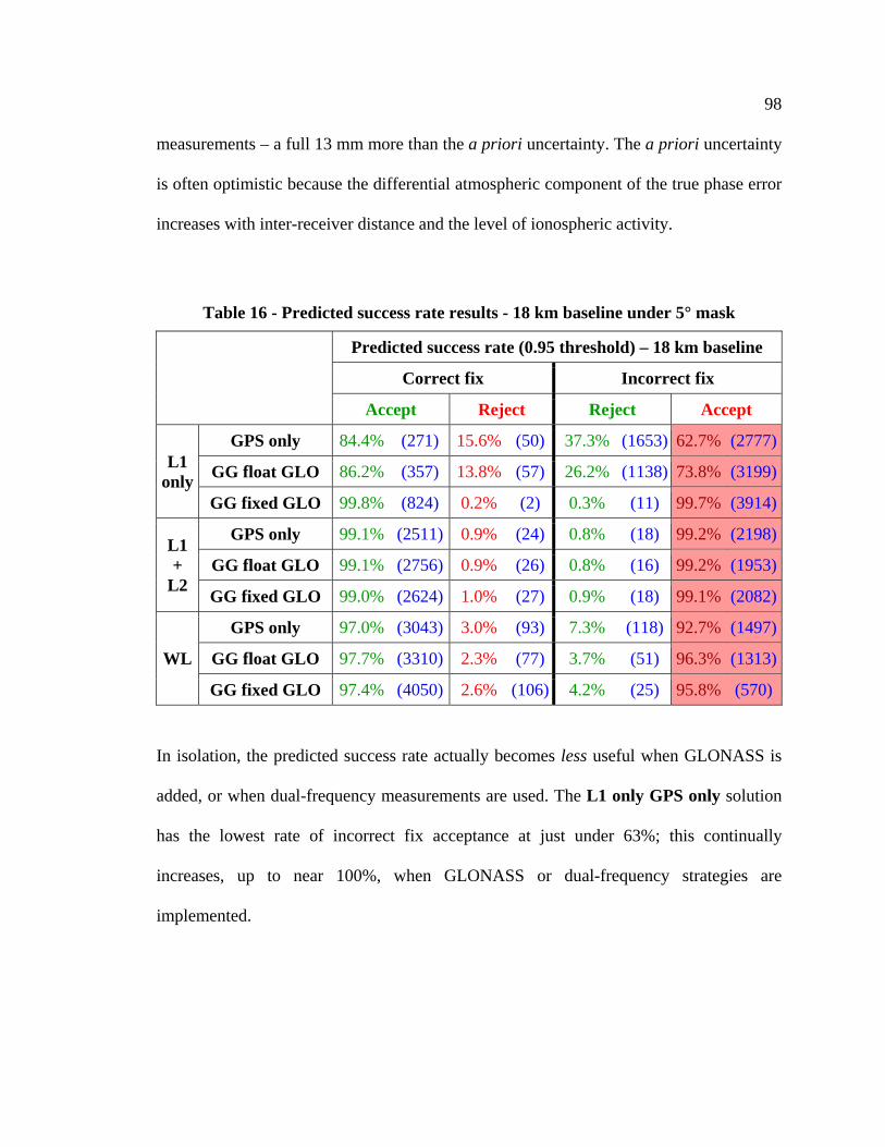
98
measurements – a full 13 mm more than the a priori uncertainty. The a priori uncertainty
is often optimistic because the differential atmospheric component of the true phase error
increases with inter-receiver distance and the level of ionospheric activity.
Table 16 - Predicted success rate results - 18 km baseline under 5° mask
Predicted success rate (0.95 threshold) – 18 km baseline
Correct fix Incorrect fix
Accept Reject Reject Accept
L1 only
GPS only 84.4% (271) 15.6% (50) 37.3% (1653) 62.7% (2777)
GG float GLO 86.2% (357) 13.8% (57) 26.2% (1138) 73.8% (3199)
GG fixed GLO 99.8% (824) 0.2% (2) 0.3% (11) 99.7% (3914)
L1 +
L2
GPS only 99.1% (2511) 0.9% (24) 0.8% (18) 99.2% (2198)
GG float GLO 99.1% (2756) 0.9% (26) 0.8% (16) 99.2% (1953)
GG fixed GLO 99.0% (2624) 1.0% (27) 0.9% (18) 99.1% (2082)
WL
GPS only 97.0% (3043) 3.0% (93) 7.3% (118) 92.7% (1497)
GG float GLO 97.7% (3310) 2.3% (77) 3.7% (51) 96.3% (1313)
GG fixed GLO 97.4% (4050) 2.6% (106) 4.2% (25) 95.8% (570)
In isolation, the predicted success rate actually becomes less useful when GLONASS is
added, or when dual-frequency measurements are used. The L1 only GPS only solution
has the lowest rate of incorrect fix acceptance at just under 63%; this continually
increases, up to near 100%, when GLONASS or dual-frequency strategies are
implemented.
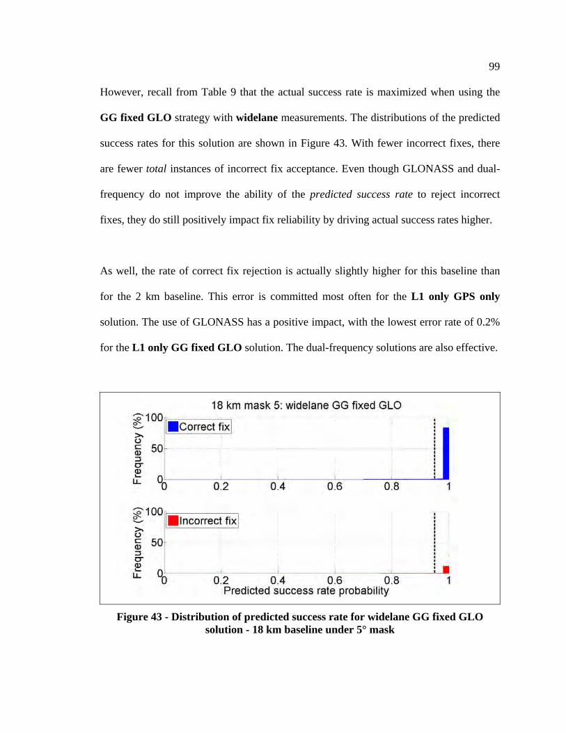
99
However, recall from Table 9 that the actual success rate is maximized when using the
GG fixed GLO strategy with widelane measurements. The distributions of the predicted
success rates for this solution are shown in Figure 43. With fewer incorrect fixes, there
are fewer total instances of incorrect fix acceptance. Even though GLONASS and dual-
frequency do not improve the ability of the predicted success rate to reject incorrect
fixes, they do still positively impact fix reliability by driving actual success rates higher.
As well, the rate of correct fix rejection is actually slightly higher for this baseline than
for the 2 km baseline. This error is committed most often for the L1 only GPS only
solution. The use of GLONASS has a positive impact, with the lowest error rate of 0.2%
for the L1 only GG fixed GLO solution. The dual-frequency solutions are also effective.
Figure 43 - Distribution of predicted success rate for widelane GG fixed GLO solution - 18 km baseline under 5° mask
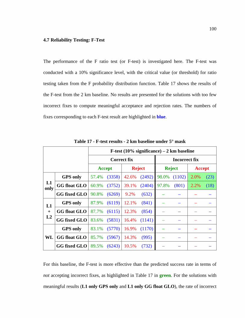
100
4.7 Reliability Testing: F-Test
The performance of the F ratio test (or F-test) is investigated here. The F-test was
conducted with a 10% significance level, with the critical value (or threshold) for ratio
testing taken from the F probability distribution function. Table 17 shows the results of
the F-test from the 2 km baseline. No results are presented for the solutions with too few
incorrect fixes to compute meaningful acceptance and rejection rates. The numbers of
fixes corresponding to each F-test result are highlighted in blue.
Table 17 - F-test results - 2 km baseline under 5° mask
F-test (10% significance) – 2 km baseline
Correct fix Incorrect fix
Accept Reject Reject Accept
L1 only
GPS only 57.4% (3358) 42.6% (2492) 98.0% (1102) 2.0% (23)
GG float GLO 60.9% (3752) 39.1% (2404) 97.8% (801) 2.2% (18)
GG fixed GLO 90.8% (6269) 9.2% (632) – – – –
L1 +
L2
GPS only 87.9% (6119) 12.1% (841) – – – –
GG float GLO 87.7% (6115) 12.3% (854) – – – –
GG fixed GLO 83.6% (5831) 16.4% (1141) – – – –
WL
GPS only 83.1% (5770) 16.9% (1170) – – – –
GG float GLO 85.7% (5967) 14.3% (995) – – – –
GG fixed GLO 89.5% (6243) 10.5% (732) – – – –
For this baseline, the F-test is more effective than the predicted success rate in terms of
not accepting incorrect fixes, as highlighted in Table 17 in green. For the solutions with
meaningful results (L1 only GPS only and L1 only GG float GLO), the rate of incorrect
101
fix acceptance is less than 3%. This appears to come at a cost: the F-test rejects correct
fixes much more often than the predicted success rate, leading to a loss of precision in the
position. This is expected due to the nature of the F-test, which is described below:
The null and alternative hypotheses for the F-test are described in Section 2.5.
The probability of a Type II error is defined by the power of the F-test. For a 10%
significance level, Table 18 shows the test powers and corresponding probabilities
of Type II error for different numbers of ambiguities. The non-centrality
parameter is computed based on the assumption that only one ambiguity is
incorrect (and thus biased) – test powers for different biases and uncertainties are
also shown in Table 18. The test power varies significantly based on the
magnitudes of the ambiguity bias and uncertainty. In some cases, Type II errors
occur at probabilities of more than 60%.
For the two solutions from the 2 km baseline with incorrect fixes to analyze, the
occurrence of Type II error (i.e. rejection of correct fix) is 69% for the L1 only
GPS only solution (i.e. 2492 / [2492 + 1102]) and 75% for the L1 only GG float
GLO solution (i.e. 2404 / [2404 + 801]). These are slightly larger than the
theoretical probabilities from Table 18. However much larger probabilities of
Type II error can be derived from larger ambiguity biases, smaller ambiguity
uncertainties, or multiple incorrect ambiguities.

102
Table 18 - F-test power as a function of number of ambiguities
Number of ambiguities
Ambiguity bias
(cycles)
Ambiguity uncertainty
(cycles)
Test power (%)
Probability of Type II error
(%)
5
1 1 86.5% 13.5%
1 0.5 75.3% 24.7%
2 0.5 36.0% 64.0%
8
1 1 87.0% 13.0%
1 0.5 77.3% 22.7%
2 0.5 38.5% 61.5%
12
1 1 87.5% 12.5%
1 0.5 79.1% 20.9%
2 0.5 42.4% 57.6%
Rejecting correct fixes is problematic for applications that require ambiguity resolution,
although it is generally better to lose precision than to have an undetected bias. The
behaviour of the F-test is illustrated by Figure 44, which shows the distribution of the
F-test results (pass or fail) for the L1 only GPS only solution.
The problem of the F-test rejecting more correct fixes is mitigated by the addition of
GLONASS. The lowest rate of correct fix rejection is achieved by the L1 only GG fixed
GLO solution. The dual-frequency measurement combinations also help in this regard as
rejection rates are less than 20%. Since ambiguity resolution can be repeated if not
successful the first time, these rejection rates are acceptable. Overall the F-test performs
well as a reliability test, for this particular baseline and environment.
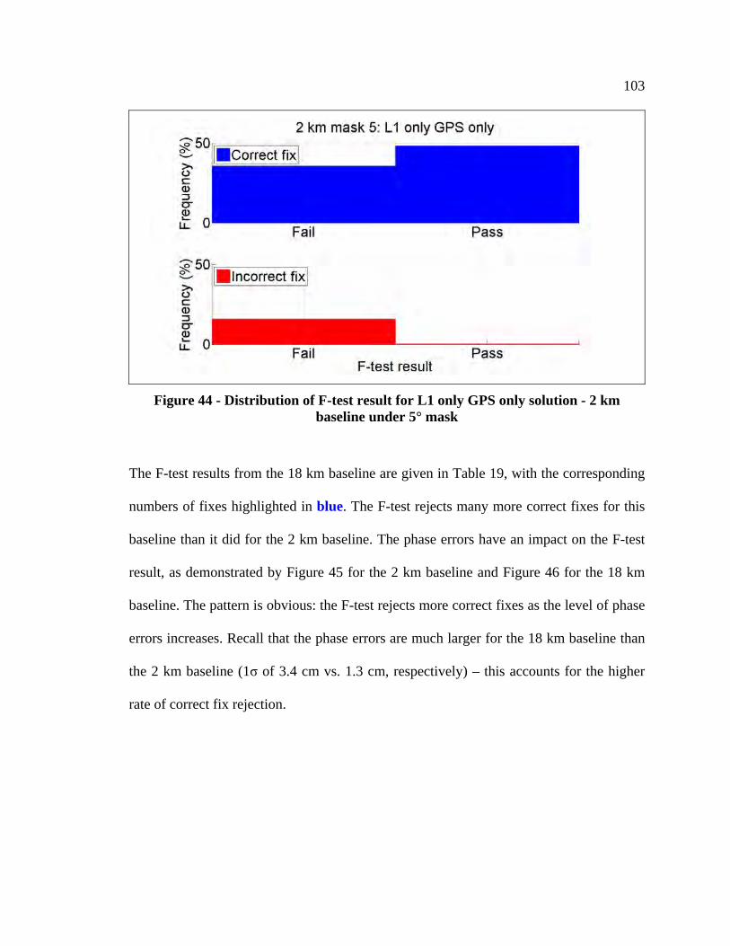
103
Figure 44 - Distribution of F-test result for L1 only GPS only solution - 2 km baseline under 5° mask
The F-test results from the 18 km baseline are given in Table 19, with the corresponding
numbers of fixes highlighted in blue. The F-test rejects many more correct fixes for this
baseline than it did for the 2 km baseline. The phase errors have an impact on the F-test
result, as demonstrated by Figure 45 for the 2 km baseline and Figure 46 for the 18 km
baseline. The pattern is obvious: the F-test rejects more correct fixes as the level of phase
errors increases. Recall that the phase errors are much larger for the 18 km baseline than
the 2 km baseline (1σ of 3.4 cm vs. 1.3 cm, respectively) – this accounts for the higher
rate of correct fix rejection.
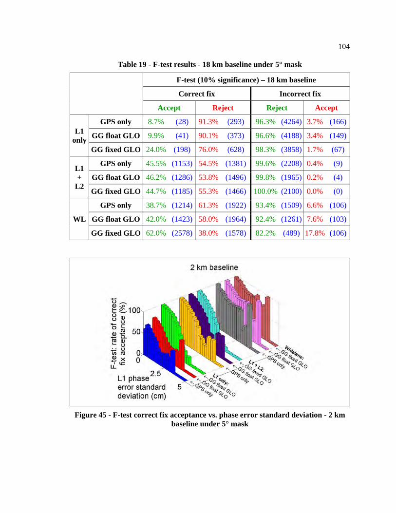
104
Table 19 - F-test results - 18 km baseline under 5° mask
F-test (10% significance) – 18 km baseline
Correct fix Incorrect fix
Accept Reject Reject Accept
L1 only
GPS only 8.7% (28) 91.3% (293) 96.3% (4264) 3.7% (166)
GG float GLO 9.9% (41) 90.1% (373) 96.6% (4188) 3.4% (149)
GG fixed GLO 24.0% (198) 76.0% (628) 98.3% (3858) 1.7% (67)
L1 +
L2
GPS only 45.5% (1153) 54.5% (1381) 99.6% (2208) 0.4% (9)
GG float GLO 46.2% (1286) 53.8% (1496) 99.8% (1965) 0.2% (4)
GG fixed GLO 44.7% (1185) 55.3% (1466) 100.0% (2100) 0.0% (0)
WL
GPS only 38.7% (1214) 61.3% (1922) 93.4% (1509) 6.6% (106)
GG float GLO 42.0% (1423) 58.0% (1964) 92.4% (1261) 7.6% (103)
GG fixed GLO 62.0% (2578) 38.0% (1578) 82.2% (489) 17.8% (106)
Figure 45 - F-test correct fix acceptance vs. phase error standard deviation - 2 km baseline under 5° mask
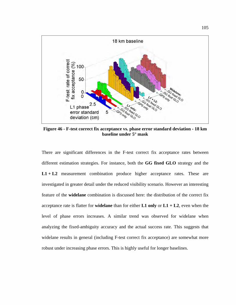
105
Figure 46 - F-test correct fix acceptance vs. phase error standard deviation - 18 km baseline under 5° mask
There are significant differences in the F-test correct fix acceptance rates between
different estimation strategies. For instance, both the GG fixed GLO strategy and the
L1 + L2 measurement combination produce higher acceptance rates. These are
investigated in greater detail under the reduced visibility scenario. However an interesting
feature of the widelane combination is discussed here: the distribution of the correct fix
acceptance rate is flatter for widelane than for either L1 only or L1 + L2, even when the
level of phase errors increases. A similar trend was observed for widelane when
analyzing the fixed-ambiguity accuracy and the actual success rate. This suggests that
widelane results in general (including F-test correct fix acceptance) are somewhat more
robust under increasing phase errors. This is highly useful for longer baselines.
106
4.8 Combining Reliability Tests
Up to now the predicted success rate and F-test have been analyzed individually;
however in practice they can be combined to give the best chance of detecting and
rejecting incorrect fixes. If one of the reliability tests would reject a fix, then the fix is
rejected. Conversely, the fix is only accepted if all of the reliability tests would accept it.
The results of combining the predicted success rate and F-test are shown in Table 20 and
Table 21 for the 2 km and 18 km baselines, respectively. The numbers of fixes
corresponding to each result are highlighted in blue. The combined testing results are
almost the same as the F-test results. This is expected as the F-test rejects many more
fixes than the predicted success rate.
Since the combined reliability test and the F-test are nearly identical, it is useful to
interpret the combined test as “adding” information from the predicted success rate to the
F-test. Doing this very slightly improves (that is, decreases) the rate of incorrect fix
acceptance, compared to using the F-test alone. The maximum improvement is 0.4% for
the 2 km baseline and 1.5% for the 18 km baseline (both highlighted in green). This
suggests that the F-test captures most of the information that the predicted success rate
provides. Adding the predicted success rate is not costly – the maximum loss incurred in
correct fix acceptance is only 0.2% for both baselines.
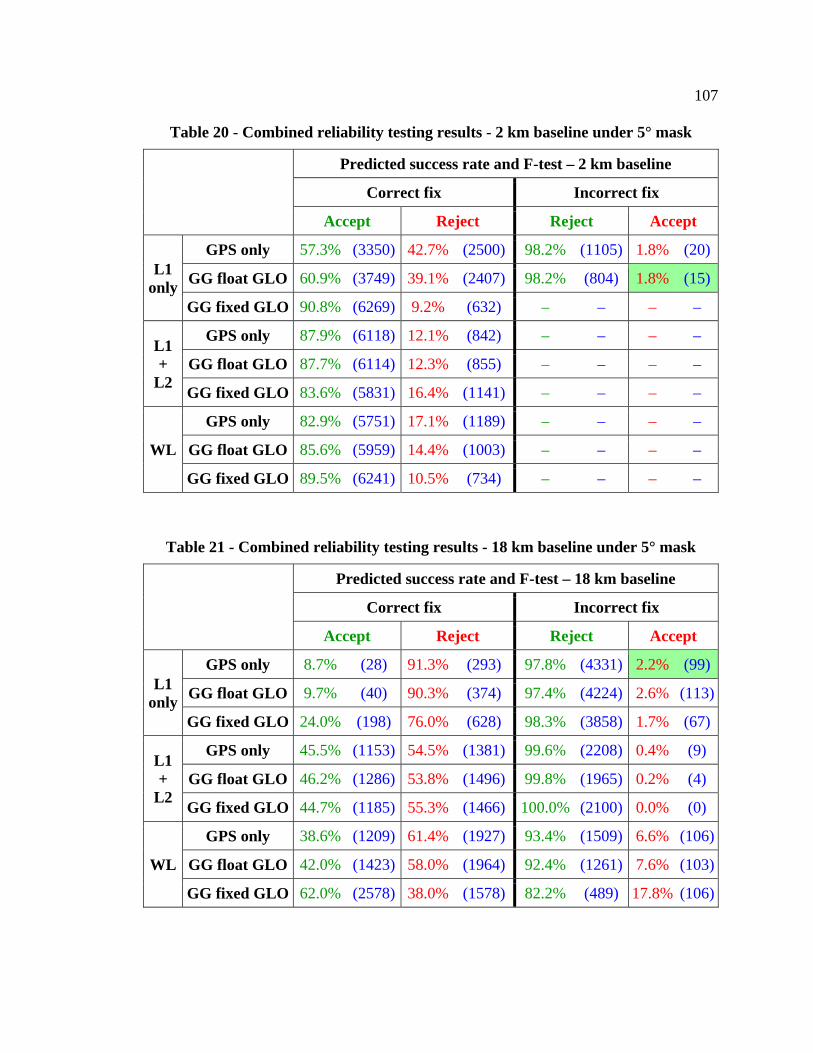
107
Table 20 - Combined reliability testing results - 2 km baseline under 5° mask
Predicted success rate and F-test – 2 km baseline
Correct fix Incorrect fix
Accept Reject Reject Accept
L1 only
GPS only 57.3% (3350) 42.7% (2500) 98.2% (1105) 1.8% (20)
GG float GLO 60.9% (3749) 39.1% (2407) 98.2% (804) 1.8% (15)
GG fixed GLO 90.8% (6269) 9.2% (632) – – – –
L1 +
L2
GPS only 87.9% (6118) 12.1% (842) – – – –
GG float GLO 87.7% (6114) 12.3% (855) – – – –
GG fixed GLO 83.6% (5831) 16.4% (1141) – – – –
WL
GPS only 82.9% (5751) 17.1% (1189) – – – –
GG float GLO 85.6% (5959) 14.4% (1003) – – – –
GG fixed GLO 89.5% (6241) 10.5% (734) – – – –
Table 21 - Combined reliability testing results - 18 km baseline under 5° mask
Predicted success rate and F-test – 18 km baseline
Correct fix Incorrect fix
Accept Reject Reject Accept
L1 only
GPS only 8.7% (28) 91.3% (293) 97.8% (4331) 2.2% (99)
GG float GLO 9.7% (40) 90.3% (374) 97.4% (4224) 2.6% (113)
GG fixed GLO 24.0% (198) 76.0% (628) 98.3% (3858) 1.7% (67)
L1 +
L2
GPS only 45.5% (1153) 54.5% (1381) 99.6% (2208) 0.4% (9)
GG float GLO 46.2% (1286) 53.8% (1496) 99.8% (1965) 0.2% (4)
GG fixed GLO 44.7% (1185) 55.3% (1466) 100.0% (2100) 0.0% (0)
WL
GPS only 38.6% (1209) 61.4% (1927) 93.4% (1509) 6.6% (106)
GG float GLO 42.0% (1423) 58.0% (1964) 92.4% (1261) 7.6% (103)
GG fixed GLO 62.0% (2578) 38.0% (1578) 82.2% (489) 17.8% (106)
108
4.9 Probability of Cycle Slip Detection
It was discussed in Section 2.3 that fix reliability and navigation reliability are analogous,
as errors will result in either loss of precision or undetected biases in the position. The
concept of the marginally detectable blunder (MDB) is discussed in Lachapelle (2008).
This concept has been extended in Petovello (2003): an MDB of one cycle yields a test
power for fault detection that is essentially the probability of detecting that one-cycle
blunder. In other words, it is the probability of detecting a cycle slip. This is critical for
ambiguity resolution since a cycle slip induces a change in the integer value of the
ambiguity; any previously resolved and stored integers will actually induce measurement
biases. It is also important in the float estimation of the position and ambiguities.
Measurements from multiple epochs is often incorporated to estimate the float
ambiguities; if there is a cycle slip, phase measurements before the cycle slip cannot be
combined with phase measurements after the cycle slip.
The properties of the probability of cycle slip detection are illustrated by the time series
in Figure 47 and the frequency distributions in Figure 48, for the L1 only GPS only
solution from the 2 km baseline. Results from the other solutions are presented later. The
probabilities appear to be heavily skewed towards one. However, there are many fixes for
which the probability of cycle slip detection is much lower; for instance, 14% of the
epochs in Figure 47 have a probability of cycle slip detection of less than 0.50. At these
epochs, the user cannot have more than 50% confidence that the position solution is not
affected by a one-cycle phase measurement bias. This gives rise to a reliability problem,
109
even if the user chooses to use a float solution to avoid potentially unreliable integer
fixes. The time series in Figure 47 also indicates that the probability of cycle slip
detection is time-correlated, which is expected since they are ultimately dependent on the
slowly-changing satellite geometry. The probability of cycle slip detection tends to
converge to a maximum value; in this case, the maximum is one. The same trend is
observed in Petovello (2003).
Both the probability of cycle slip detection and the predicted success rate tend to be very
close to one for many fixes (see Figure 41). The relationship between these two
parameters is further illustrated in Figure 49, also for the L1 only GPS only solution
from the 2 km baseline. The pattern is not strong: both parameters are close to one for
many fixes, but there are many more fixes with probability of cycle slip detection
significantly less than one. Hence, the probability of cycle slip detection is less optimistic
than the predicted success rate. There is no correlation observed between the probability
of cycle slip detection and the F-test result, as demonstrated in Figure 50.
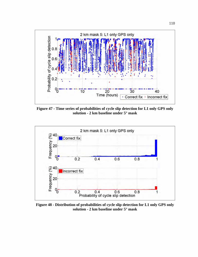
110
Figure 47 - Time series of probabilities of cycle slip detection for L1 only GPS only solution - 2 km baseline under 5° mask
Figure 48 - Distribution of probabilities of cycle slip detection for L1 only GPS only solution - 2 km baseline under 5° mask
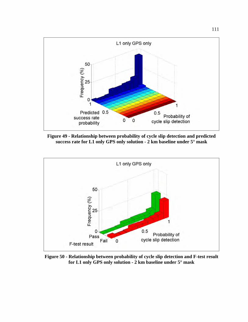
111
Figure 49 - Relationship between probability of cycle slip detection and predicted success rate for L1 only GPS only solution - 2 km baseline under 5° mask
Figure 50 - Relationship between probability of cycle slip detection and F-test result for L1 only GPS only solution - 2 km baseline under 5° mask
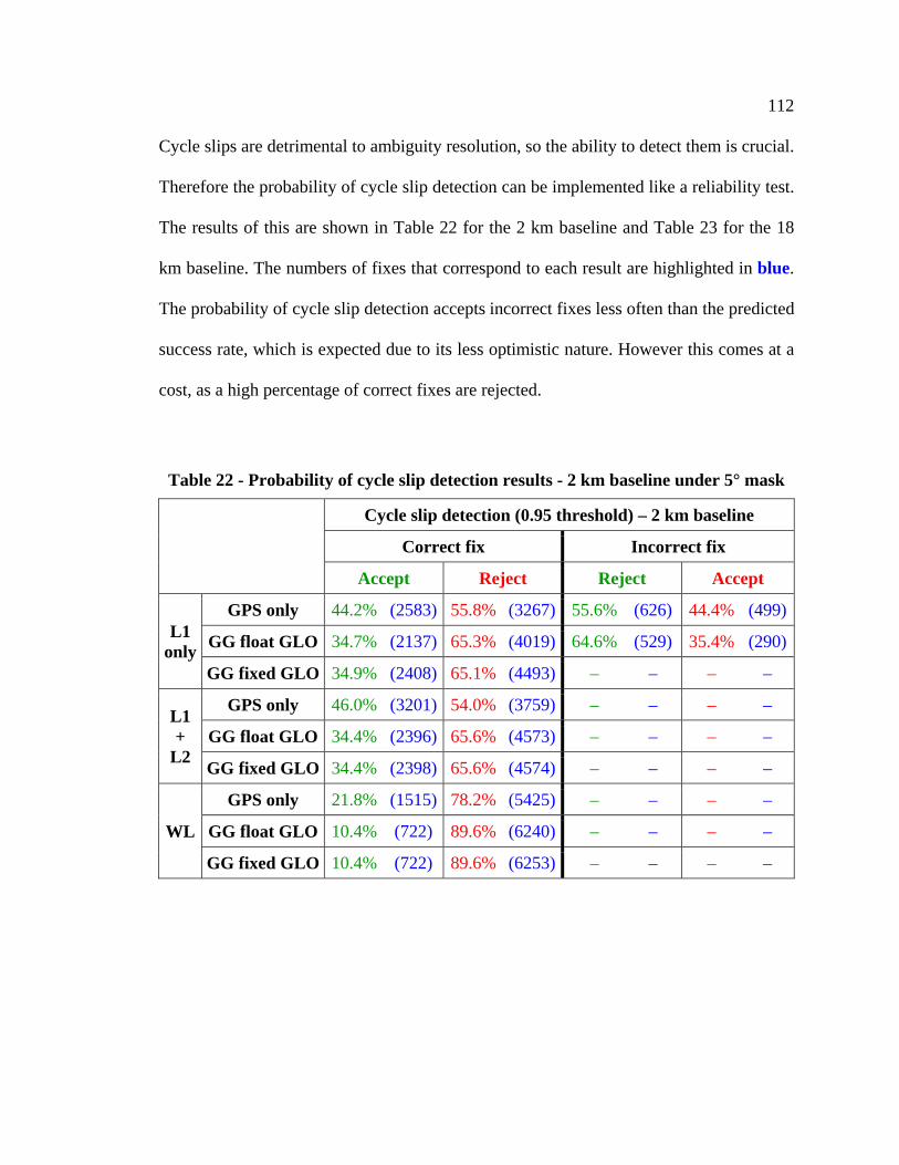
112
Cycle slips are detrimental to ambiguity resolution, so the ability to detect them is crucial.
Therefore the probability of cycle slip detection can be implemented like a reliability test.
The results of this are shown in Table 22 for the 2 km baseline and Table 23 for the 18
km baseline. The numbers of fixes that correspond to each result are highlighted in blue.
The probability of cycle slip detection accepts incorrect fixes less often than the predicted
success rate, which is expected due to its less optimistic nature. However this comes at a
cost, as a high percentage of correct fixes are rejected.
Table 22 - Probability of cycle slip detection results - 2 km baseline under 5° mask
Cycle slip detection (0.95 threshold) – 2 km baseline
Correct fix Incorrect fix
Accept Reject Reject Accept
L1 only
GPS only 44.2% (2583) 55.8% (3267) 55.6% (626) 44.4% (499)
GG float GLO 34.7% (2137) 65.3% (4019) 64.6% (529) 35.4% (290)
GG fixed GLO 34.9% (2408) 65.1% (4493) – – – –
L1 +
L2
GPS only 46.0% (3201) 54.0% (3759) – – – –
GG float GLO 34.4% (2396) 65.6% (4573) – – – –
GG fixed GLO 34.4% (2398) 65.6% (4574) – – – –
WL
GPS only 21.8% (1515) 78.2% (5425) – – – –
GG float GLO 10.4% (722) 89.6% (6240) – – – –
GG fixed GLO 10.4% (722) 89.6% (6253) – – – –

113
Table 23 - Probability of cycle slip detection results - 18 km baseline under 5° mask
Cycle slip detection (0.95 threshold) – 18 km baseline
Correct fix Incorrect fix
Accept Reject Reject Accept
L1 only
GPS only 76.6% (246) 23.4% (75) 29.7% (1314) 70.3% (3116)
GG float GLO 78.0% (323) 22.0% (91) 25.5% (1107) 74.5% (3230)
GG fixed GLO 71.9% (594) 28.1% (232) 24.6% (966) 75.4% (2959)
L1 +
L2
GPS only 74.4% (1886) 25.6% (649) 26.4% (586) 73.6% (1630)
GG float GLO 67.9% (1888) 32.1% (894) 31.8% (627) 68.2% (1342)
GG fixed GLO 65.6% (1740) 34.4% (911) 29.0% (610) 71.0% (1490)
WL
GPS only 47.3% (1482) 52.7% (1654) 73.0% (1179) 27.0% (436)
GG float GLO 47.2% (1600) 52.8% (1787) 58.7% (800) 41.3% (564)
GG fixed GLO 46.8% (1944) 53.2% (2212) 63.0% (375) 37.0% (220)
4.10 Reliability under Simulated Reduced Visibility
The effect of reduced satellite visibility on reliability testing is investigated here. This is
the same reduced visibility scenario used to analyze the actual success rates earlier – the
circular elevation mask is increased from 5° to 30°. The results of using the predicted
success rate as an indicator of reliability are shown in Table 24 and Table 25 for the 2 km
and 18 km baselines, respectively. The numbers of fixes corresponding to each result are
highlighted in blue.
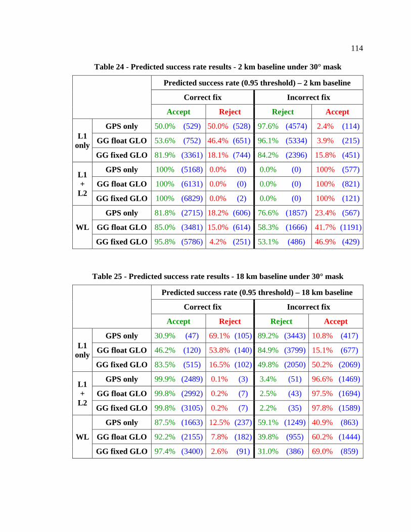
114
Table 24 - Predicted success rate results - 2 km baseline under 30° mask
Predicted success rate (0.95 threshold) – 2 km baseline
Correct fix Incorrect fix
Accept Reject Reject Accept
L1 only
GPS only 50.0% (529) 50.0% (528) 97.6% (4574) 2.4% (114)
GG float GLO 53.6% (752) 46.4% (651) 96.1% (5334) 3.9% (215)
GG fixed GLO 81.9% (3361) 18.1% (744) 84.2% (2396) 15.8% (451)
L1 +
L2
GPS only 100% (5168) 0.0% (0) 0.0% (0) 100% (577)
GG float GLO 100% (6131) 0.0% (0) 0.0% (0) 100% (821)
GG fixed GLO 100% (6829) 0.0% (2) 0.0% (0) 100% (121)
WL
GPS only 81.8% (2715) 18.2% (606) 76.6% (1857) 23.4% (567)
GG float GLO 85.0% (3481) 15.0% (614) 58.3% (1666) 41.7% (1191)
GG fixed GLO 95.8% (5786) 4.2% (251) 53.1% (486) 46.9% (429)
Table 25 - Predicted success rate results - 18 km baseline under 30° mask
Predicted success rate (0.95 threshold) – 18 km baseline
Correct fix Incorrect fix
Accept Reject Reject Accept
L1 only
GPS only 30.9% (47) 69.1% (105) 89.2% (3443) 10.8% (417)
GG float GLO 46.2% (120) 53.8% (140) 84.9% (3799) 15.1% (677)
GG fixed GLO 83.5% (515) 16.5% (102) 49.8% (2050) 50.2% (2069)
L1 +
L2
GPS only 99.9% (2489) 0.1% (3) 3.4% (51) 96.6% (1469)
GG float GLO 99.8% (2992) 0.2% (7) 2.5% (43) 97.5% (1694)
GG fixed GLO 99.8% (3105) 0.2% (7) 2.2% (35) 97.8% (1589)
WL
GPS only 87.5% (1663) 12.5% (237) 59.1% (1249) 40.9% (863)
GG float GLO 92.2% (2155) 7.8% (182) 39.8% (955) 60.2% (1444)
GG fixed GLO 97.4% (3400) 2.6% (91) 31.0% (386) 69.0% (859)
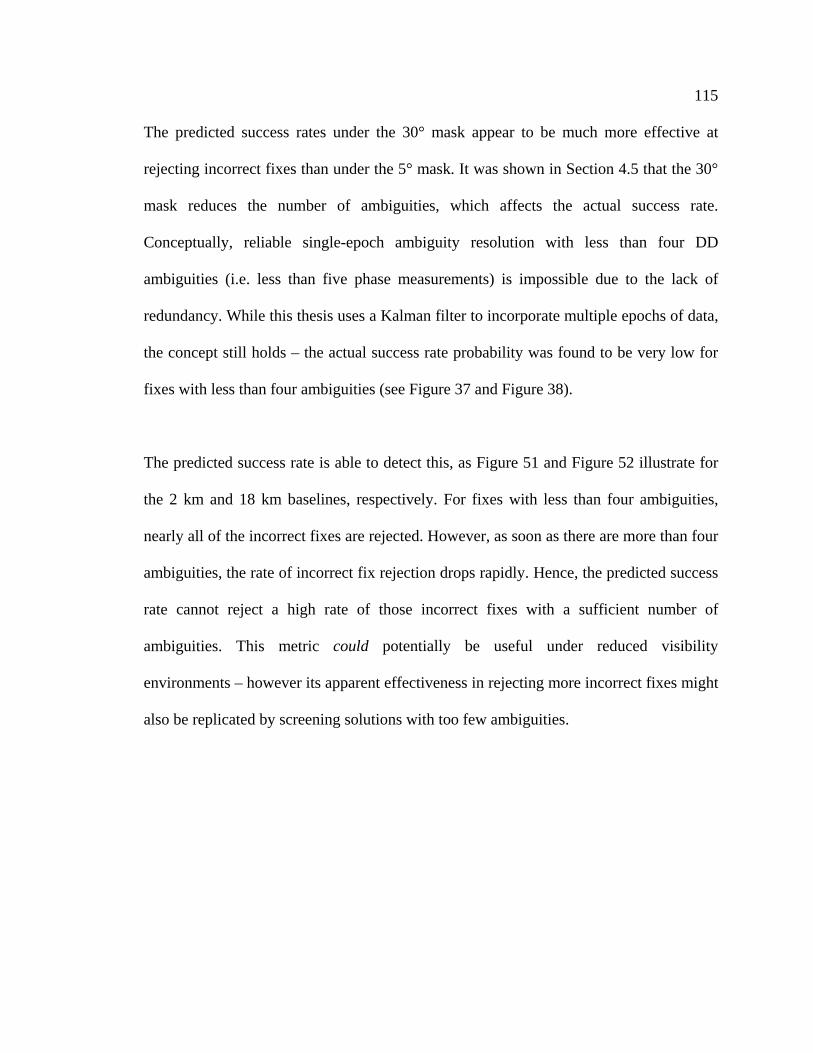
115
The predicted success rates under the 30° mask appear to be much more effective at
rejecting incorrect fixes than under the 5° mask. It was shown in Section 4.5 that the 30°
mask reduces the number of ambiguities, which affects the actual success rate.
Conceptually, reliable single-epoch ambiguity resolution with less than four DD
ambiguities (i.e. less than five phase measurements) is impossible due to the lack of
redundancy. While this thesis uses a Kalman filter to incorporate multiple epochs of data,
the concept still holds – the actual success rate probability was found to be very low for
fixes with less than four ambiguities (see Figure 37 and Figure 38).
The predicted success rate is able to detect this, as Figure 51 and Figure 52 illustrate for
the 2 km and 18 km baselines, respectively. For fixes with less than four ambiguities,
nearly all of the incorrect fixes are rejected. However, as soon as there are more than four
ambiguities, the rate of incorrect fix rejection drops rapidly. Hence, the predicted success
rate cannot reject a high rate of those incorrect fixes with a sufficient number of
ambiguities. This metric could potentially be useful under reduced visibility
environments – however its apparent effectiveness in rejecting more incorrect fixes might
also be replicated by screening solutions with too few ambiguities.
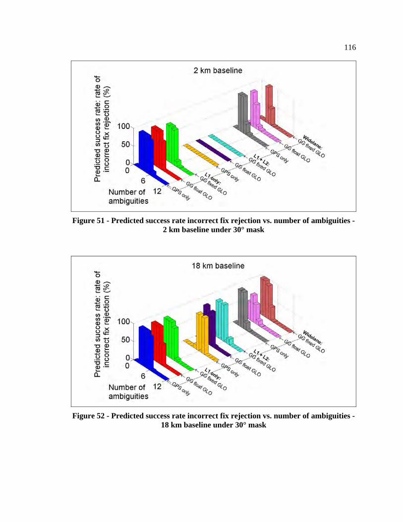
116
Figure 51 - Predicted success rate incorrect fix rejection vs. number of ambiguities - 2 km baseline under 30° mask
Figure 52 - Predicted success rate incorrect fix rejection vs. number of ambiguities - 18 km baseline under 30° mask

117
The F-test results under the 30° mask are shown in Table 26 and Table 27 for the 2 km
and 18 km baselines, respectively, with the numbers of fixes corresponding with each
result highlighted in blue. The F-test is once again more effective than the predicted
success rate at rejecting incorrect fixes – that is, avoiding undetected biases in the
position. However, compared to its performance under the 5° mask, the F-test rejects
many more correct fixes – that is, loss of position precision and availability.
The number of ambiguities again plays a role, as Figure 53 and Figure 54 demonstrate for
the 2 km and 18 km baselines, respectively, with all solutions processed under a 30°
mask. These are distributions of the F-test rate of correct fix acceptance for various
numbers of ambiguities. The more ambiguities there are, the more effective the F-test is
at accepting correct fixes. Since there are fewer ambiguities in the reduced visibility
scenario, the F-test will obviously be less effective.
However, Table 26 and Table 27 show a strategy (in green) that stands out for its ability
to detect more correct fixes with the F-test: the L1 + L2 GG fixed GLO strategy. These
two strategies add ambiguities, and thus improve the F-test performance. This is one of
the primary ways that either GLONASS or dual-frequency impact fix reliability.
The dependence of the F-test performance on the geometry of integer estimation is
further illustrated in Figure 55 and Figure 56 for the 2 km and 18 km baselines,
respectively, with all solutions processed under a 30° mask. These are distributions of the
F-test rate of correct fix acceptance for various levels of ADOP. The trend from the
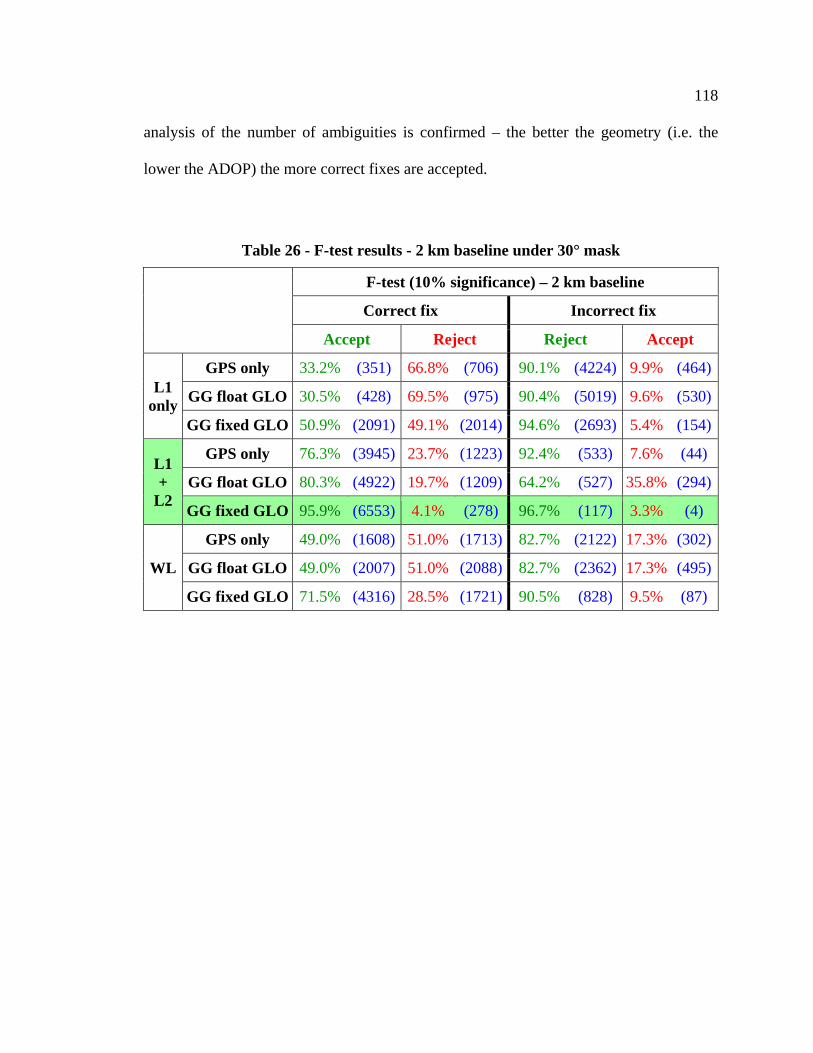
118
analysis of the number of ambiguities is confirmed – the better the geometry (i.e. the
lower the ADOP) the more correct fixes are accepted.
Table 26 - F-test results - 2 km baseline under 30° mask
F-test (10% significance) – 2 km baseline
Correct fix Incorrect fix
Accept Reject Reject Accept
L1 only
GPS only 33.2% (351) 66.8% (706) 90.1% (4224) 9.9% (464)
GG float GLO 30.5% (428) 69.5% (975) 90.4% (5019) 9.6% (530)
GG fixed GLO 50.9% (2091) 49.1% (2014) 94.6% (2693) 5.4% (154)
L1 +
L2
GPS only 76.3% (3945) 23.7% (1223) 92.4% (533) 7.6% (44)
GG float GLO 80.3% (4922) 19.7% (1209) 64.2% (527) 35.8% (294)
GG fixed GLO 95.9% (6553) 4.1% (278) 96.7% (117) 3.3% (4)
WL
GPS only 49.0% (1608) 51.0% (1713) 82.7% (2122) 17.3% (302)
GG float GLO 49.0% (2007) 51.0% (2088) 82.7% (2362) 17.3% (495)
GG fixed GLO 71.5% (4316) 28.5% (1721) 90.5% (828) 9.5% (87)

119
Table 27 - F-test results - 18 km baseline under 30° mask
F-test (10% significance) – 18 km baseline
Correct fix Incorrect fix
Accept Reject Reject Accept
L1 only
GPS only 10.5% (16) 89.5% (136) 92.2% (3557) 7.8% (303)
GG float GLO 8.1% (21) 91.9% (239) 92.1% (4123) 7.9% (353)
GG fixed GLO 16.0% (99) 84.0% (518) 96.5% (3974) 3.5% (145)
L1 +
L2
GPS only 51.2% (1277) 48.8% (1216) 96.2% (1461) 3.8% (58)
GG float GLO 54.8% (1642) 45.2% (1357) 90.0% (1563) 10.0% (174)
GG fixed GLO 66.5% (2071) 33.5% (1041) 99.1% (1609) 0.9% (15)
WL
GPS only 31.7% (602) 68.3% (1298) 89.5% (1891) 10.5% (221)
GG float GLO 35.2% (823) 64.8% (1514) 86.8% (2083) 13.2% (316)
GG fixed GLO 52.0% (1814) 48.0% (1677) 92.2% (1148) 7.8% (97)
Figure 53 - F-test correct fix acceptance vs. number of ambiguities - 2 km baseline under 30° mask

120
Figure 54 - F-test correct fix acceptance vs. number of ambiguities - 18 km baseline under 30° mask
Figure 55 - F-test correct fix acceptance vs. ADOP - 2 km baseline under 30° mask
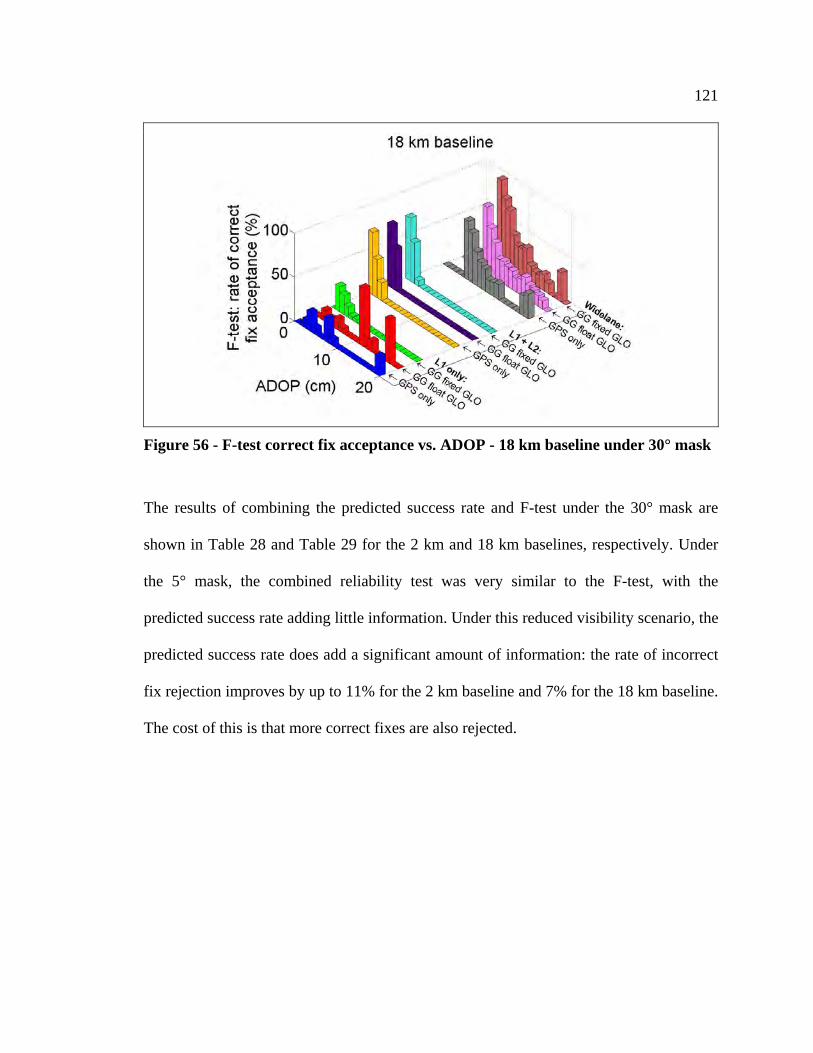
121
Figure 56 - F-test correct fix acceptance vs. ADOP - 18 km baseline under 30° mask
The results of combining the predicted success rate and F-test under the 30° mask are
shown in Table 28 and Table 29 for the 2 km and 18 km baselines, respectively. Under
the 5° mask, the combined reliability test was very similar to the F-test, with the
predicted success rate adding little information. Under this reduced visibility scenario, the
predicted success rate does add a significant amount of information: the rate of incorrect
fix rejection improves by up to 11% for the 2 km baseline and 7% for the 18 km baseline.
The cost of this is that more correct fixes are also rejected.
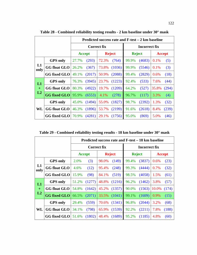
122
Table 28 - Combined reliability testing results - 2 km baseline under 30° mask
Predicted success rate and F-test – 2 km baseline
Correct fix Incorrect fix
Accept Reject Reject Accept
L1 only
GPS only 27.7% (293) 72.3% (764) 99.9% (4683) 0.1% (5)
GG float GLO 26.2% (367) 73.8% (1036) 99.9% (5546) 0.1% (3)
GG fixed GLO 49.1% (2017) 50.9% (2088) 99.4% (2829) 0.6% (18)
L1 +
L2
GPS only 76.3% (3945) 23.7% (1223) 92.4% (533) 7.6% (44)
GG float GLO 80.3% (4922) 19.7% (1209) 64.2% (527) 35.8% (294)
GG fixed GLO 95.9% (6553) 4.1% (278) 96.7% (117) 3.3% (4)
WL
GPS only 45.0% (1494) 55.0% (1827) 98.7% (2392) 1.3% (32)
GG float GLO 46.3% (1896) 53.7% (2199) 91.6% (2618) 8.4% (239)
GG fixed GLO 70.9% (4281) 29.1% (1756) 95.0% (869) 5.0% (46)
Table 29 - Combined reliability testing results - 18 km baseline under 30° mask
Predicted success rate and F-test – 18 km baseline
Correct fix Incorrect fix
Accept Reject Reject Accept
L1 only
GPS only 2.0% (3) 98.0% (149) 99.4% (3837) 0.6% (23)
GG float GLO 4.6% (12) 95.4% (248) 99.3% (4444) 0.7% (32)
GG fixed GLO 15.9% (98) 84.1% (519) 98.5% (4058) 1.5% (61)
L1 +
L2
GPS only 51.2% (1277) 48.8% (1216) 96.2% (1462) 3.8% (57)
GG float GLO 54.8% (1642) 45.2% (1357) 90.0% (1563) 10.0% (174)
GG fixed GLO 66.5% (2071) 33.5% (1041) 99.1% (1609) 0.9% (15)
WL
GPS only 29.4% (559) 70.6% (1341) 96.8% (2044) 3.2% (68)
GG float GLO 34.1% (798) 65.9% (1539) 92.2% (2211) 7.8% (188)
GG fixed GLO 51.6% (1802) 48.4% (1689) 95.2% (1185) 4.8% (60)
123
Chapter Five: Kinematic Testing Results
This chapter presents the analysis and discussion of the reliability of ambiguity resolution
for kinematic testing. Two kinematic scenarios are investigated for this thesis: 1.) vehicle-
to-vehicle relative navigation conducted under both open sky and foliage; and 2.)
downhill ski runs.
5.1 Vehicle-to-Vehicle Relative Navigation
Vehicle-to-vehicle (V2V) relative navigation was conducted for 97 minutes under two
types of sky coverage: 1.) open sky (49 minutes); and overhead foliage (49 minutes). The
open sky environment was not perfect as there were occasionally trees in view. The
overhead foliage environment sometimes resulted in near-total obstruction of the sky.
The inter-vehicle distances did not exceed 300 metres, so residual atmospheric effects
were not significant. Regardless, the K index on the day of the test (August 17, 2009) did
not exceed 1.0, based on observations from the Meanook Geomagnetic Observatory
(Space Weather Canada 2009). Therefore there were no significant ionospheric
disturbances. Under open sky, between four and eight GPS and three and six GLONASS
satellites were available. Under foliage, between three and seven GPS and two and four
GLONASS satellites were available. A convergence time of 20 seconds was chosen to
generate fixes. Table 30 shows the total number of fixes according to the solution type.
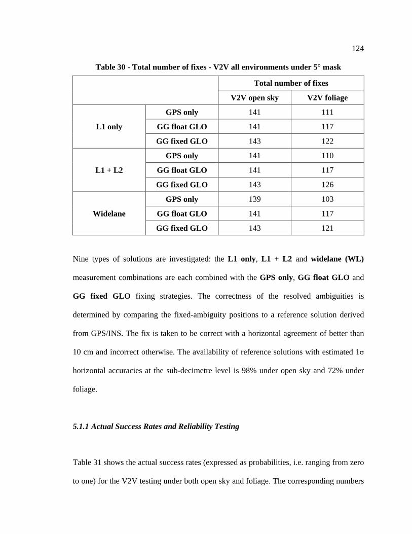
124
Table 30 - Total number of fixes - V2V all environments under 5° mask
Total number of fixes
V2V open sky V2V foliage
L1 only
GPS only 141 111
GG float GLO 141 117
GG fixed GLO 143 122
L1 + L2
GPS only 141 110
GG float GLO 141 117
GG fixed GLO 143 126
Widelane
GPS only 139 103
GG float GLO 141 117
GG fixed GLO 143 121
Nine types of solutions are investigated: the L1 only, L1 + L2 and widelane (WL)
measurement combinations are each combined with the GPS only, GG float GLO and
GG fixed GLO fixing strategies. The correctness of the resolved ambiguities is
determined by comparing the fixed-ambiguity positions to a reference solution derived
from GPS/INS. The fix is taken to be correct with a horizontal agreement of better than
10 cm and incorrect otherwise. The availability of reference solutions with estimated 1σ
horizontal accuracies at the sub-decimetre level is 98% under open sky and 72% under
foliage.
5.1.1 Actual Success Rates and Reliability Testing
Table 31 shows the actual success rates (expressed as probabilities, i.e. ranging from zero
to one) for the V2V testing under both open sky and foliage. The corresponding numbers
125
of correct fixes are highlighted in blue. All of the solutions are processed using a circular
elevation mask of 5°. The following trends are observed:
The impact of GLONASS on the actual success rate in this scenario is the same as
the static baseline. Just adding the GLONASS measurements (i.e. switching from
GPS only to GG float GLO) does have a small effect, but actually resolving the
GLONASS ambiguities (i.e. switching from GG float GLO to GG fixed GLO)
greatly improves the actual success rate. This is highlighted in green in Table 31.
The impact of dual-frequency on the actual success rate in this scenario is the
same as the static baseline. Both L1 + L2 and widelane improve the actual
success rate over L1 only. Since the inter-vehicle distances are short, L1 + L2 is
more effective than widelane. The combination of both dual-frequency and
GPS/GLONASS gives the best results, as highlighted in green in Table 31.
The actual success rates achieved under foliage are all much lower than those
achieved under open sky. It is demonstrated in Section 5.1.2 that this is likely
caused by the increased frequency of cycle slips under foliage.
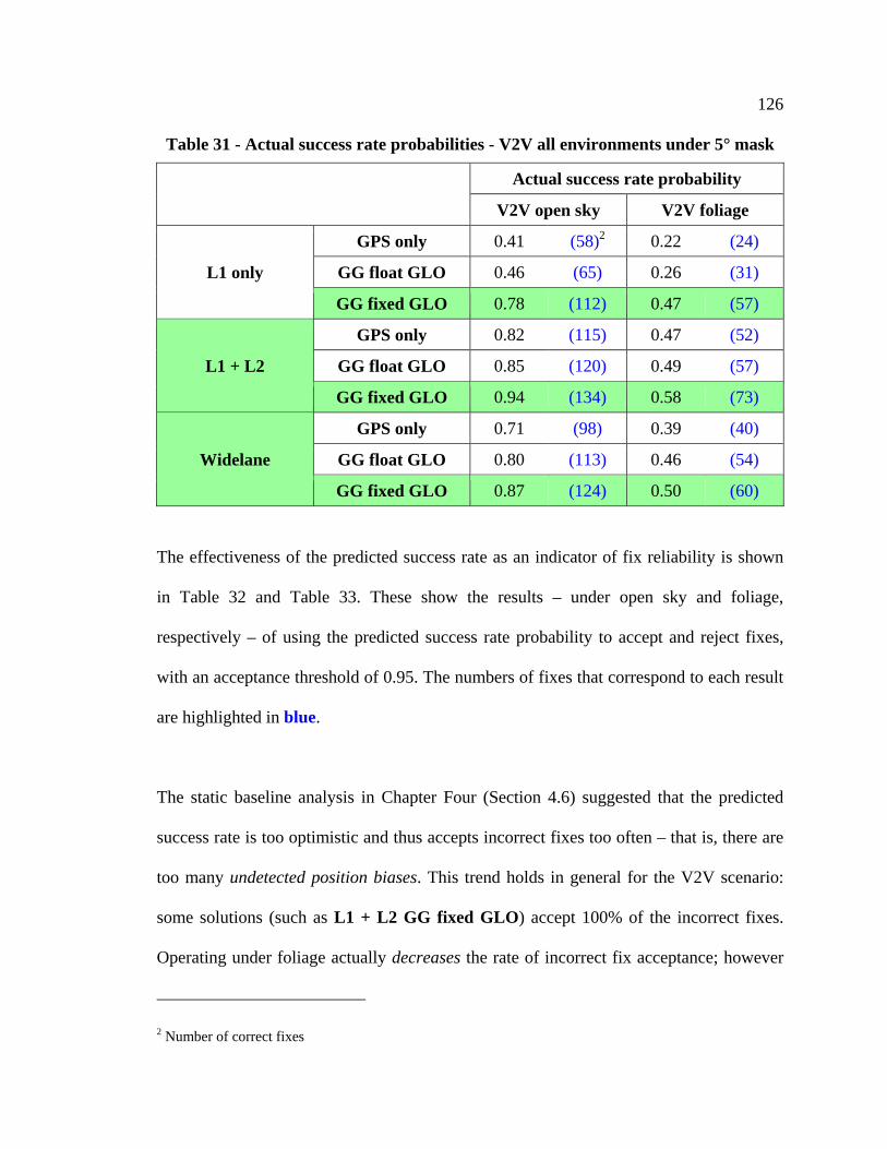
126
Table 31 - Actual success rate probabilities - V2V all environments under 5° mask
Actual success rate probability
V2V open sky V2V foliage
L1 only
GPS only 0.41 (58)2 0.22 (24)
GG float GLO 0.46 (65) 0.26 (31)
GG fixed GLO 0.78 (112) 0.47 (57)
L1 + L2
GPS only 0.82 (115) 0.47 (52)
GG float GLO 0.85 (120) 0.49 (57)
GG fixed GLO 0.94 (134) 0.58 (73)
Widelane
GPS only 0.71 (98) 0.39 (40)
GG float GLO 0.80 (113) 0.46 (54)
GG fixed GLO 0.87 (124) 0.50 (60)
The effectiveness of the predicted success rate as an indicator of fix reliability is shown
in Table 32 and Table 33. These show the results – under open sky and foliage,
respectively – of using the predicted success rate probability to accept and reject fixes,
with an acceptance threshold of 0.95. The numbers of fixes that correspond to each result
are highlighted in blue.
The static baseline analysis in Chapter Four (Section 4.6) suggested that the predicted
success rate is too optimistic and thus accepts incorrect fixes too often – that is, there are
too many undetected position biases. This trend holds in general for the V2V scenario:
some solutions (such as L1 + L2 GG fixed GLO) accept 100% of the incorrect fixes.
Operating under foliage actually decreases the rate of incorrect fix acceptance; however
2 Number of correct fixes
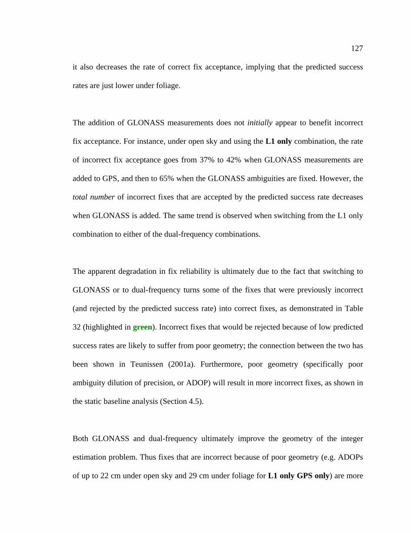
127
it also decreases the rate of correct fix acceptance, implying that the predicted success
rates are just lower under foliage.
The addition of GLONASS measurements does not initially appear to benefit incorrect
fix acceptance. For instance, under open sky and using the L1 only combination, the rate
of incorrect fix acceptance goes from 37% to 42% when GLONASS measurements are
added to GPS, and then to 65% when the GLONASS ambiguities are fixed. However, the
total number of incorrect fixes that are accepted by the predicted success rate decreases
when GLONASS is added. The same trend is observed when switching from the L1 only
combination to either of the dual-frequency combinations.
The apparent degradation in fix reliability is ultimately due to the fact that switching to
GLONASS or to dual-frequency turns some of the fixes that were previously incorrect
(and rejected by the predicted success rate) into correct fixes, as demonstrated in Table
32 (highlighted in green). Incorrect fixes that would be rejected because of low predicted
success rates are likely to suffer from poor geometry; the connection between the two has
been shown in Teunissen (2001a). Furthermore, poor geometry (specifically poor
ambiguity dilution of precision, or ADOP) will result in more incorrect fixes, as shown in
the static baseline analysis (Section 4.5).
Both GLONASS and dual-frequency ultimately improve the geometry of the integer
estimation problem. Thus fixes that are incorrect because of poor geometry (e.g. ADOPs
of up to 22 cm under open sky and 29 cm under foliage for L1 only GPS only) are more
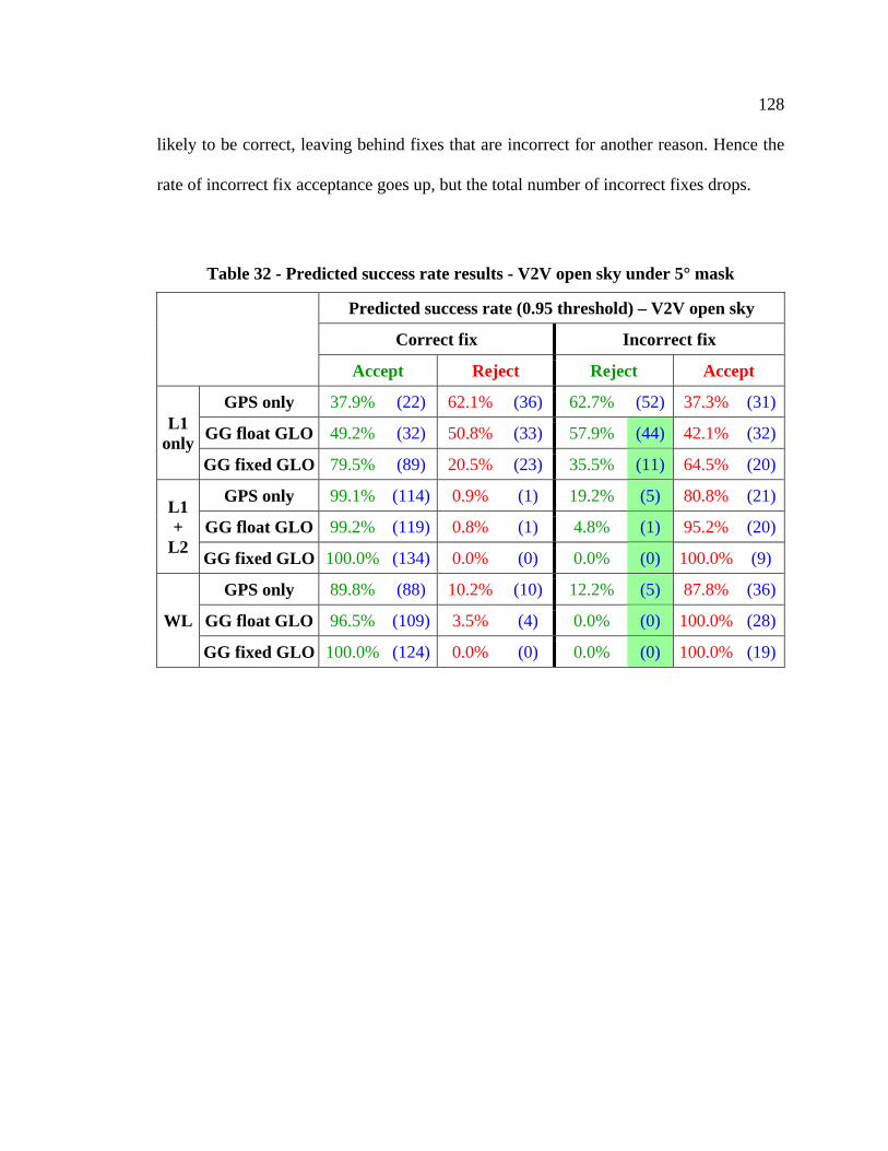
128
likely to be correct, leaving behind fixes that are incorrect for another reason. Hence the
rate of incorrect fix acceptance goes up, but the total number of incorrect fixes drops.
Table 32 - Predicted success rate results - V2V open sky under 5° mask
Predicted success rate (0.95 threshold) – V2V open sky
Correct fix Incorrect fix
Accept Reject Reject Accept
L1 only
GPS only 37.9% (22) 62.1% (36) 62.7% (52) 37.3% (31)
GG float GLO 49.2% (32) 50.8% (33) 57.9% (44) 42.1% (32)
GG fixed GLO 79.5% (89) 20.5% (23) 35.5% (11) 64.5% (20)
L1 +
L2
GPS only 99.1% (114) 0.9% (1) 19.2% (5) 80.8% (21)
GG float GLO 99.2% (119) 0.8% (1) 4.8% (1) 95.2% (20)
GG fixed GLO 100.0% (134) 0.0% (0) 0.0% (0) 100.0% (9)
WL
GPS only 89.8% (88) 10.2% (10) 12.2% (5) 87.8% (36)
GG float GLO 96.5% (109) 3.5% (4) 0.0% (0) 100.0% (28)
GG fixed GLO 100.0% (124) 0.0% (0) 0.0% (0) 100.0% (19)

129
Table 33 - Predicted success rate results - V2V foliage under 5° mask
Predicted success rate (0.95 threshold) – V2V foliage
Correct fix Incorrect fix
Accept Reject Reject Accept
L1 only
GPS only 4.2% (1) 95.8% (23) 97.7% (85) 2.3% (2)
GG float GLO 9.7% (3) 90.3% (28) 94.2% (81) 5.8% (5)
GG fixed GLO 63.2% (36) 36.8% (21) 80.0% (52) 20.0% (13)
L1 +
L2
GPS only 98.1% (51) 1.9% (1) 15.5% (9) 84.5% (49)
GG float GLO 98.2% (56) 1.8% (1) 16.7% (10) 83.3% (50)
GG fixed GLO 95.9% (70) 4.1% (3) 34.0% (18) 66.0% (35)
WL
GPS only 75.0% (30) 25.0% (10) 44.4% (28) 55.6% (35)
GG float GLO 94.4% (51) 5.6% (3) 25.4% (16) 74.6% (47)
GG fixed GLO 96.7% (58) 3.3% (2) 26.2% (16) 73.8% (45)
The F-test results are shown in Table 34 and Table 35 for the open sky and foliage
environments, respectively. A significance level of 10% is used to compute the ratio
testing critical value (or threshold) from the F distribution. As with the static baseline
analysis, the F-test is more effective than the predicted success rate at rejecting incorrect
fixes, but at the cost of rejecting more correct fixes (i.e. accepting loss of precision).
Foliage affects the F-test negatively: more correct fixes end up being rejected than under
open sky. However, GLONASS helps the F-test accept more correct fixes, especially
when the ambiguities are fixed (i.e. when the GG fixed GLO strategy is used). Dual-
frequency also helps; the most effective solution in terms of accepting correct fixes is
widelane GG fixed GLO (highlighted in green in both Table 34 and Table 35).

130
Table 34 - F-test results - V2V open sky under 5° mask
F-test (10% significance) – V2V open sky
Correct fix Incorrect fix
Accept Reject Reject Accept
L1 only
GPS only 62.1% (36) 37.9% (22) 85.5% (71) 14.5% (12)
GG float GLO 47.7% (31) 52.3% (34) 86.8% (66) 13.2% (10)
GG fixed GLO 62.5% (70) 37.5% (42) 87.1% (27) 12.9% (4)
L1 +
L2
GPS only 88.7% (102) 11.3% (13) 50.0% (13) 50.0% (13)
GG float GLO 90.8% (109) 9.2% (11) 47.6% (10) 52.4% (11)
GG fixed GLO 88.8% (119) 11.2% (15) 33.3% (3) 66.7% (6)
WL
GPS only 76.5% (75) 23.5% (23) 36.6% (15) 63.4% (26)
GG float GLO 81.4% (92) 18.6% (21) 25.0% (7) 75.0% (21)
GG fixed GLO 96.0% (119) 4.0% (5) 31.6% (6) 68.4% (13)
Table 35 - F-test results - V2V foliage under 5° mask
F-test (10% significance) – V2V foliage
Correct fix Incorrect fix
Accept Reject Reject Accept
L1 only
GPS only 33.3% (8) 66.7% (16) 81.6% (71) 18.4% (16)
GG float GLO 25.8% (8) 74.2% (23) 81.4% (70) 18.6% (16)
GG fixed GLO 59.6% (34) 40.4% (23) 87.7% (57) 12.3% (8)
L1 +
L2
GPS only 88.5% (46) 11.5% (6) 48.3% (28) 51.7% (30)
GG float GLO 87.7% (50) 12.3% (7) 46.7% (28) 53.3% (32)
GG fixed GLO 89.0% (65) 11.0% (8) 62.3% (33) 37.7% (20)
WL
GPS only 82.5% (33) 17.5% (7) 46.0% (29) 54.0% (34)
GG float GLO 83.3% (45) 16.7% (9) 54.0% (34) 46.0% (29)
GG fixed GLO 93.3% (56) 6.7% (4) 50.8% (31) 49.2% (30)
131
The predicted success rate and F-test are combined into one reliability test, the results of
which are shown in Table 36 and Table 37 for open sky and foliage, respectively. The
combined reliability test is set up such that a fix is only accepted if both of the individual
tests would accept it; conversely a fix is rejected if either test would reject it. The
numbers of fixes corresponding to each combined test result are highlighted in Table 36
and Table 37 in blue.
In the static baseline analysis (Section 4.8), the combined reliability test was
demonstrated to be very similar to the F-test, with marginal information added to it by the
predicted success rate. For both V2V scenarios, the predicted success rate adds an
enormous amount of information when only single-frequency data is used (i.e. the L1
only combination). This is highlighted in green in both Table 36 and Table 37.For
instance, under open sky the rate of incorrect fix acceptance drops by up to 11%, and
under foliage it drops by up to 18%.
The improvements gained by adding the predicted success rate when using L1 only come
at a major cost: correct fix acceptance. Combining the tests severely decreases the
number of correct fixes that are accepted; this is most noticeable in the L1 only GPS
only solution under foliage (highlighted in red in Table 37), for which no correct fixes
are accepted. While it is important to detect and reject incorrect fixes, not being able to
get an integer fix at all may be too detrimental for some applications.
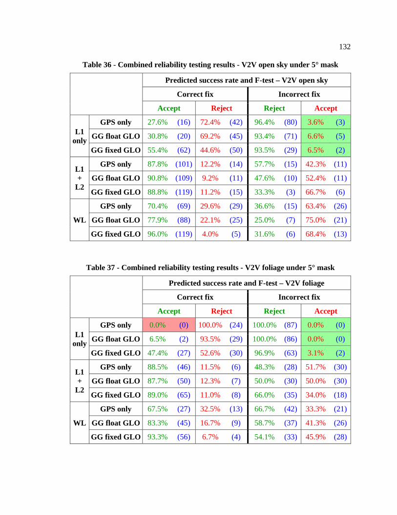
132
Table 36 - Combined reliability testing results - V2V open sky under 5° mask
Predicted success rate and F-test – V2V open sky
Correct fix Incorrect fix
Accept Reject Reject Accept
L1 only
GPS only 27.6% (16) 72.4% (42) 96.4% (80) 3.6% (3)
GG float GLO 30.8% (20) 69.2% (45) 93.4% (71) 6.6% (5)
GG fixed GLO 55.4% (62) 44.6% (50) 93.5% (29) 6.5% (2)
L1 +
L2
GPS only 87.8% (101) 12.2% (14) 57.7% (15) 42.3% (11)
GG float GLO 90.8% (109) 9.2% (11) 47.6% (10) 52.4% (11)
GG fixed GLO 88.8% (119) 11.2% (15) 33.3% (3) 66.7% (6)
WL
GPS only 70.4% (69) 29.6% (29) 36.6% (15) 63.4% (26)
GG float GLO 77.9% (88) 22.1% (25) 25.0% (7) 75.0% (21)
GG fixed GLO 96.0% (119) 4.0% (5) 31.6% (6) 68.4% (13)
Table 37 - Combined reliability testing results - V2V foliage under 5° mask
Predicted success rate and F-test – V2V foliage
Correct fix Incorrect fix
Accept Reject Reject Accept
L1 only
GPS only 0.0% (0) 100.0% (24) 100.0% (87) 0.0% (0)
GG float GLO 6.5% (2) 93.5% (29) 100.0% (86) 0.0% (0)
GG fixed GLO 47.4% (27) 52.6% (30) 96.9% (63) 3.1% (2)
L1 +
L2
GPS only 88.5% (46) 11.5% (6) 48.3% (28) 51.7% (30)
GG float GLO 87.7% (50) 12.3% (7) 50.0% (30) 50.0% (30)
GG fixed GLO 89.0% (65) 11.0% (8) 66.0% (35) 34.0% (18)
WL
GPS only 67.5% (27) 32.5% (13) 66.7% (42) 33.3% (21)
GG float GLO 83.3% (45) 16.7% (9) 58.7% (37) 41.3% (26)
GG fixed GLO 93.3% (56) 6.7% (4) 54.1% (33) 45.9% (28)
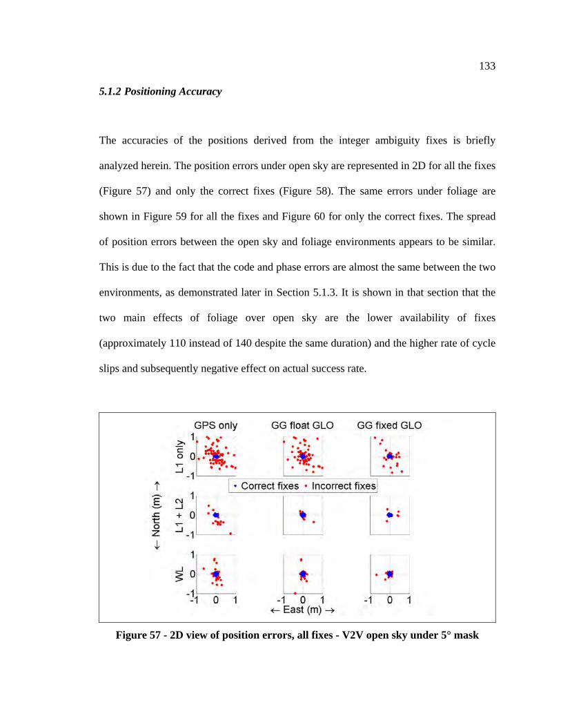
133
5.1.2 Positioning Accuracy
The accuracies of the positions derived from the integer ambiguity fixes is briefly
analyzed herein. The position errors under open sky are represented in 2D for all the fixes
(Figure 57) and only the correct fixes (Figure 58). The same errors under foliage are
shown in Figure 59 for all the fixes and Figure 60 for only the correct fixes. The spread
of position errors between the open sky and foliage environments appears to be similar.
This is due to the fact that the code and phase errors are almost the same between the two
environments, as demonstrated later in Section 5.1.3. It is shown in that section that the
two main effects of foliage over open sky are the lower availability of fixes
(approximately 110 instead of 140 despite the same duration) and the higher rate of cycle
slips and subsequently negative effect on actual success rate.
Figure 57 - 2D view of position errors, all fixes - V2V open sky under 5° mask

134
Figure 58 - 2D view of position errors, correct fixes - V2V open sky under 5° mask
Figure 59 - 2D view of position errors, all fixes - V2V foliage under 5° mask

135
Figure 60 - 2D view of position errors, correct fixes - V2V foliage under 5° mask
The position errors from the correct fixes are summarized in Table 38 and Table 39
(median and RMS errors under open sky) and Table 40 and Table 41 (median and RMS
errors under foliage). The corresponding actual success rates and numbers of correct fixes
are also given, with the latter highlighted in blue.
The impact on the fixed-ambiguity positioning accuracy of using GLONASS or dual-
frequency over the standard single-frequency GPS solution (i.e. L1 only GPS only) is
minimal. The use of GLONASS does reduce the RMS vertical errors under foliage, but
since the median vertical error remains approximately the same, this only indicates the
removal of a few larger vertical errors. What GLONASS (or dual-frequency) does do is
increase the actual success rate, and thus the availability of fixed-accuracy solutions.
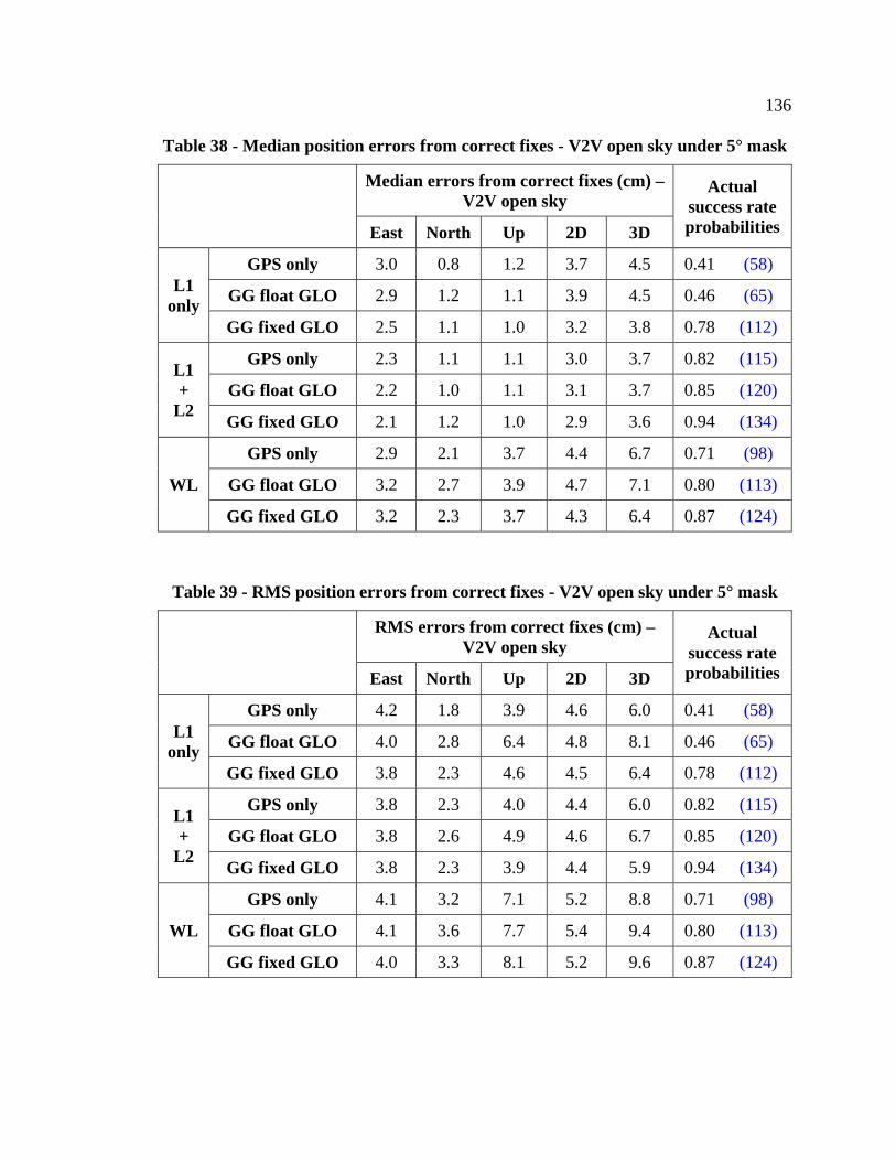
136
Table 38 - Median position errors from correct fixes - V2V open sky under 5° mask
Median errors from correct fixes (cm) – V2V open sky
Actual success rate probabilities East North Up 2D 3D
L1 only
GPS only 3.0 0.8 1.2 3.7 4.5 0.41 (58)
GG float GLO 2.9 1.2 1.1 3.9 4.5 0.46 (65)
GG fixed GLO 2.5 1.1 1.0 3.2 3.8 0.78 (112)
L1 +
L2
GPS only 2.3 1.1 1.1 3.0 3.7 0.82 (115)
GG float GLO 2.2 1.0 1.1 3.1 3.7 0.85 (120)
GG fixed GLO 2.1 1.2 1.0 2.9 3.6 0.94 (134)
WL
GPS only 2.9 2.1 3.7 4.4 6.7 0.71 (98)
GG float GLO 3.2 2.7 3.9 4.7 7.1 0.80 (113)
GG fixed GLO 3.2 2.3 3.7 4.3 6.4 0.87 (124)
Table 39 - RMS position errors from correct fixes - V2V open sky under 5° mask
RMS errors from correct fixes (cm) – V2V open sky
Actual success rate probabilities East North Up 2D 3D
L1 only
GPS only 4.2 1.8 3.9 4.6 6.0 0.41 (58)
GG float GLO 4.0 2.8 6.4 4.8 8.1 0.46 (65)
GG fixed GLO 3.8 2.3 4.6 4.5 6.4 0.78 (112)
L1 +
L2
GPS only 3.8 2.3 4.0 4.4 6.0 0.82 (115)
GG float GLO 3.8 2.6 4.9 4.6 6.7 0.85 (120)
GG fixed GLO 3.8 2.3 3.9 4.4 5.9 0.94 (134)
WL
GPS only 4.1 3.2 7.1 5.2 8.8 0.71 (98)
GG float GLO 4.1 3.6 7.7 5.4 9.4 0.80 (113)
GG fixed GLO 4.0 3.3 8.1 5.2 9.6 0.87 (124)
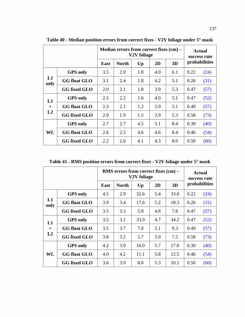
137
Table 40 - Median position errors from correct fixes - V2V foliage under 5° mask
Median errors from correct fixes (cm) – V2V foliage
Actual success rate probabilities East North Up 2D 3D
L1 only
GPS only 3.5 2.0 1.8 4.0 6.1 0.22 (24)
GG float GLO 3.1 2.4 1.8 4.2 5.1 0.26 (31)
GG fixed GLO 2.0 2.1 1.8 3.9 5.3 0.47 (57)
L1 +
L2
GPS only 2.5 2.2 1.6 4.0 5.1 0.47 (52)
GG float GLO 2.3 2.1 1.2 3.9 5.1 0.49 (57)
GG fixed GLO 2.0 1.9 1.5 3.9 5.3 0.58 (73)
WL
GPS only 2.7 2.7 4.5 5.1 8.4 0.39 (40)
GG float GLO 2.6 2.5 4.6 4.6 8.4 0.46 (54)
GG fixed GLO 2.2 2.6 4.1 4.3 8.0 0.50 (60)
Table 41 - RMS position errors from correct fixes - V2V foliage under 5° mask
RMS errors from correct fixes (cm) – V2V foliage
Actual success rate probabilities East North Up 2D 3D
L1 only
GPS only 4.5 2.9 32.6 5.4 33.0 0.22 (24)
GG float GLO 3.9 3.4 17.6 5.2 18.3 0.26 (31)
GG fixed GLO 3.5 3.3 5.8 4.8 7.6 0.47 (57)
L1 +
L2
GPS only 3.5 3.1 33.9 4.7 34.2 0.47 (52)
GG float GLO 3.5 3.7 7.8 5.1 9.3 0.49 (57)
GG fixed GLO 3.8 3.2 5.7 5.0 7.5 0.58 (73)
WL
GPS only 4.2 3.9 16.0 5.7 17.0 0.39 (40)
GG float GLO 4.0 4.2 11.1 5.8 12.5 0.46 (54)
GG fixed GLO 3.6 3.9 8.6 5.3 10.1 0.50 (60)
138
5.1.3 Signal Tracking and Cycle Slips under Foliage
The foliage environment affects the ambiguity resolution process negatively: ambiguities
are correctly fixed less often, and identifying fixes as correct or incorrect is harder. In
fact, foliage does impact signal tracking significantly – this was first demonstrated in
Chapter Three (Section 3.1.2) and is reiterated in Table 42. The quality of the phase
measurements was also discussed in Chapter Three where it was shown that the phase
noise under open sky is at the millimetre level. The foliage does not impact the C/N0 of
the signals that are tracked. One would expect that the C/N0 would be lower under
foliage; however the hardware used in this thesis is geodetic grade, not high-sensitivity.
The average number of satellites under foliage is lower, suggesting that the weaker
signals were simply not tracked.
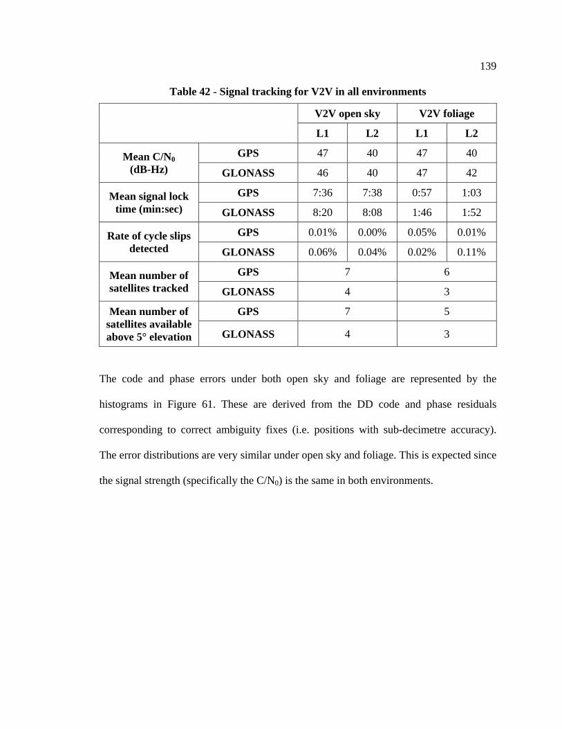
139
Table 42 - Signal tracking for V2V in all environments
V2V open sky V2V foliage
L1 L2 L1 L2
Mean C/N0 (dB-Hz)
GPS 47 40 47 40
GLONASS 46 40 47 42
Mean signal lock time (min:sec)
GPS 7:36 7:38 0:57 1:03
GLONASS 8:20 8:08 1:46 1:52
Rate of cycle slips detected
GPS 0.01% 0.00% 0.05% 0.01%
GLONASS 0.06% 0.04% 0.02% 0.11%
Mean number of satellites tracked
GPS 7 6
GLONASS 4 3
Mean number of satellites available above 5° elevation
GPS 7 5
GLONASS 4 3
The code and phase errors under both open sky and foliage are represented by the
histograms in Figure 61. These are derived from the DD code and phase residuals
corresponding to correct ambiguity fixes (i.e. positions with sub-decimetre accuracy).
The error distributions are very similar under open sky and foliage. This is expected since
the signal strength (specifically the C/N0) is the same in both environments.
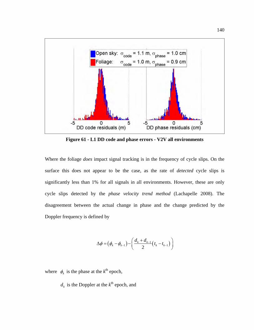
140
Figure 61 - L1 DD code and phase errors - V2V all environments
Where the foliage does impact signal tracking is in the frequency of cycle slips. On the
surface this does not appear to be the case, as the rate of detected cycle slips is
significantly less than 1% for all signals in all environments. However, these are only
cycle slips detected by the phase velocity trend method (Lachapelle 2008). The
disagreement between the actual change in phase and the change predicted by the
Doppler frequency is defined by
11 12
k kk k k k
d dt t
where k is the phase at the kth epoch,
kd is the Doppler at the kth epoch, and
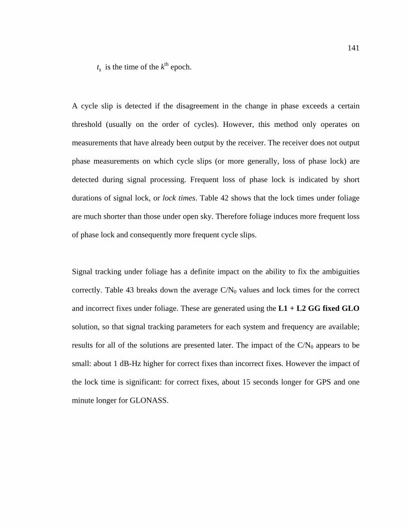
141
kt is the time of the kth epoch.
A cycle slip is detected if the disagreement in the change in phase exceeds a certain
threshold (usually on the order of cycles). However, this method only operates on
measurements that have already been output by the receiver. The receiver does not output
phase measurements on which cycle slips (or more generally, loss of phase lock) are
detected during signal processing. Frequent loss of phase lock is indicated by short
durations of signal lock, or lock times. Table 42 shows that the lock times under foliage
are much shorter than those under open sky. Therefore foliage induces more frequent loss
of phase lock and consequently more frequent cycle slips.
Signal tracking under foliage has a definite impact on the ability to fix the ambiguities
correctly. Table 43 breaks down the average C/N0 values and lock times for the correct
and incorrect fixes under foliage. These are generated using the L1 + L2 GG fixed GLO
solution, so that signal tracking parameters for each system and frequency are available;
results for all of the solutions are presented later. The impact of the C/N0 appears to be
small: about 1 dB-Hz higher for correct fixes than incorrect fixes. However the impact of
the lock time is significant: for correct fixes, about 15 seconds longer for GPS and one
minute longer for GLONASS.
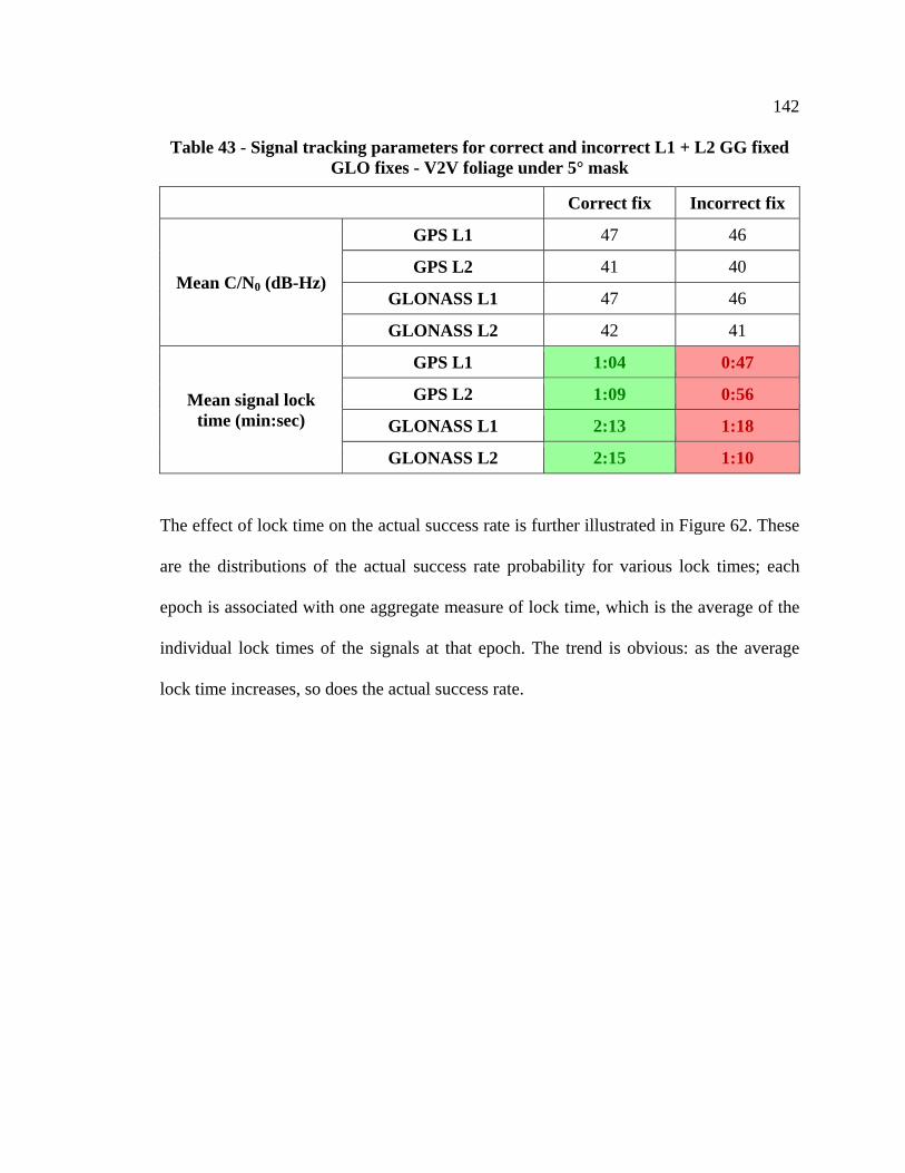
142
Table 43 - Signal tracking parameters for correct and incorrect L1 + L2 GG fixed GLO fixes - V2V foliage under 5° mask
Correct fix Incorrect fix
Mean C/N0 (dB-Hz)
GPS L1 47 46
GPS L2 41 40
GLONASS L1 47 46
GLONASS L2 42 41
Mean signal lock time (min:sec)
GPS L1 1:04 0:47
GPS L2 1:09 0:56
GLONASS L1 2:13 1:18
GLONASS L2 2:15 1:10
The effect of lock time on the actual success rate is further illustrated in Figure 62. These
are the distributions of the actual success rate probability for various lock times; each
epoch is associated with one aggregate measure of lock time, which is the average of the
individual lock times of the signals at that epoch. The trend is obvious: as the average
lock time increases, so does the actual success rate.
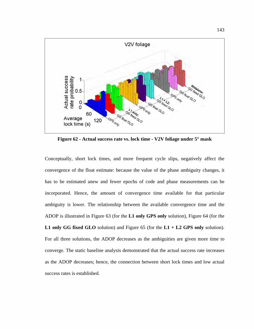
143
Figure 62 - Actual success rate vs. lock time - V2V foliage under 5° mask
Conceptually, short lock times, and more frequent cycle slips, negatively affect the
convergence of the float estimate: because the value of the phase ambiguity changes, it
has to be estimated anew and fewer epochs of code and phase measurements can be
incorporated. Hence, the amount of convergence time available for that particular
ambiguity is lower. The relationship between the available convergence time and the
ADOP is illustrated in Figure 63 (for the L1 only GPS only solution), Figure 64 (for the
L1 only GG fixed GLO solution) and Figure 65 (for the L1 + L2 GPS only solution).
For all three solutions, the ADOP decreases as the ambiguities are given more time to
converge. The static baseline analysis demonstrated that the actual success rate increases
as the ADOP decreases; hence, the connection between short lock times and low actual
success rates is established.
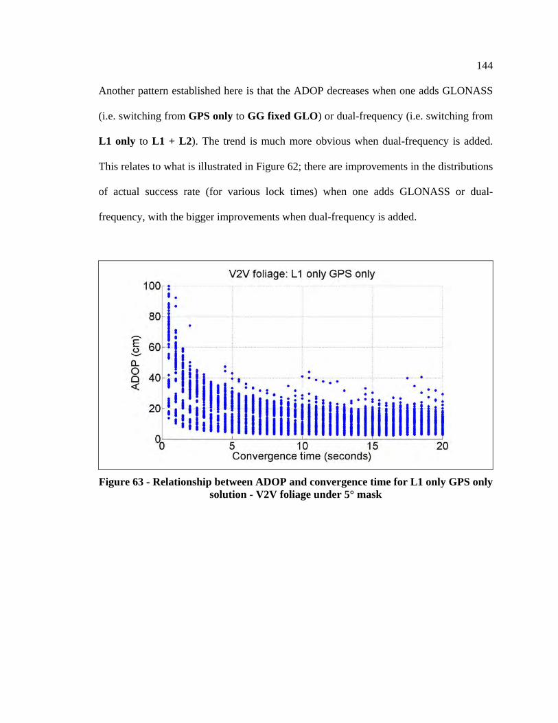
144
Another pattern established here is that the ADOP decreases when one adds GLONASS
(i.e. switching from GPS only to GG fixed GLO) or dual-frequency (i.e. switching from
L1 only to L1 + L2). The trend is much more obvious when dual-frequency is added.
This relates to what is illustrated in Figure 62; there are improvements in the distributions
of actual success rate (for various lock times) when one adds GLONASS or dual-
frequency, with the bigger improvements when dual-frequency is added.
Figure 63 - Relationship between ADOP and convergence time for L1 only GPS only solution - V2V foliage under 5° mask
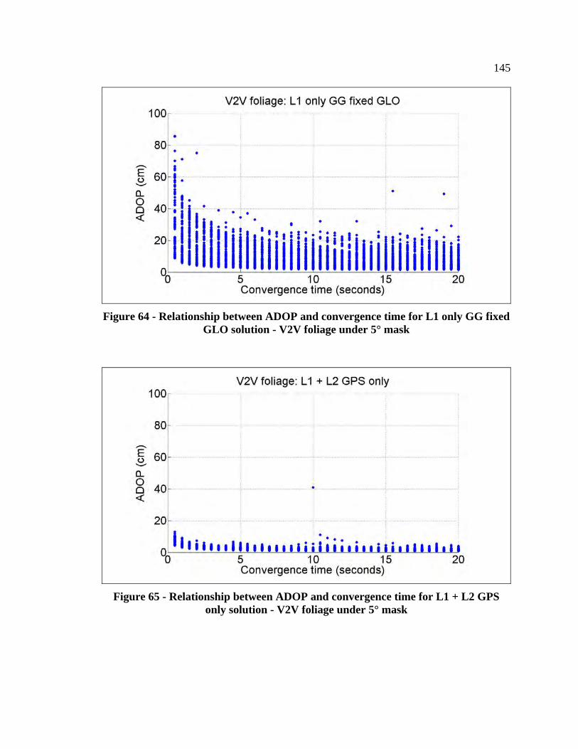
145
Figure 64 - Relationship between ADOP and convergence time for L1 only GG fixed GLO solution - V2V foliage under 5° mask
Figure 65 - Relationship between ADOP and convergence time for L1 + L2 GPS only solution - V2V foliage under 5° mask
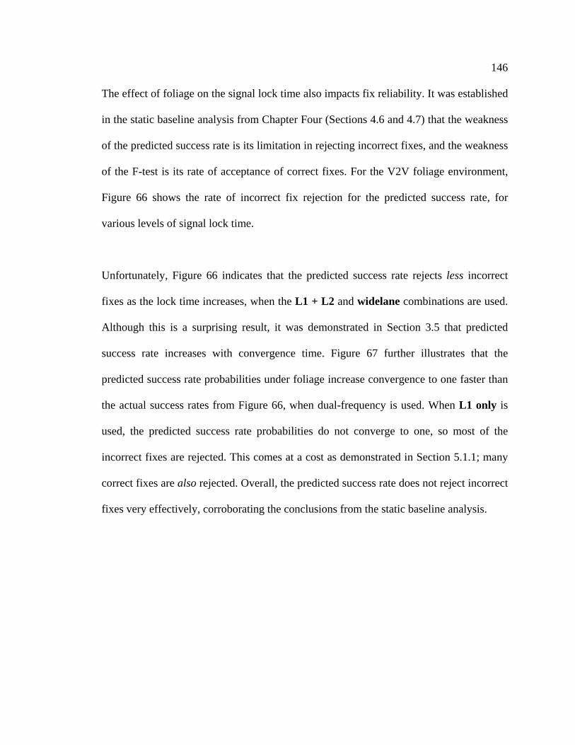
146
The effect of foliage on the signal lock time also impacts fix reliability. It was established
in the static baseline analysis from Chapter Four (Sections 4.6 and 4.7) that the weakness
of the predicted success rate is its limitation in rejecting incorrect fixes, and the weakness
of the F-test is its rate of acceptance of correct fixes. For the V2V foliage environment,
Figure 66 shows the rate of incorrect fix rejection for the predicted success rate, for
various levels of signal lock time.
Unfortunately, Figure 66 indicates that the predicted success rate rejects less incorrect
fixes as the lock time increases, when the L1 + L2 and widelane combinations are used.
Although this is a surprising result, it was demonstrated in Section 3.5 that predicted
success rate increases with convergence time. Figure 67 further illustrates that the
predicted success rate probabilities under foliage increase convergence to one faster than
the actual success rates from Figure 66, when dual-frequency is used. When L1 only is
used, the predicted success rate probabilities do not converge to one, so most of the
incorrect fixes are rejected. This comes at a cost as demonstrated in Section 5.1.1; many
correct fixes are also rejected. Overall, the predicted success rate does not reject incorrect
fixes very effectively, corroborating the conclusions from the static baseline analysis.
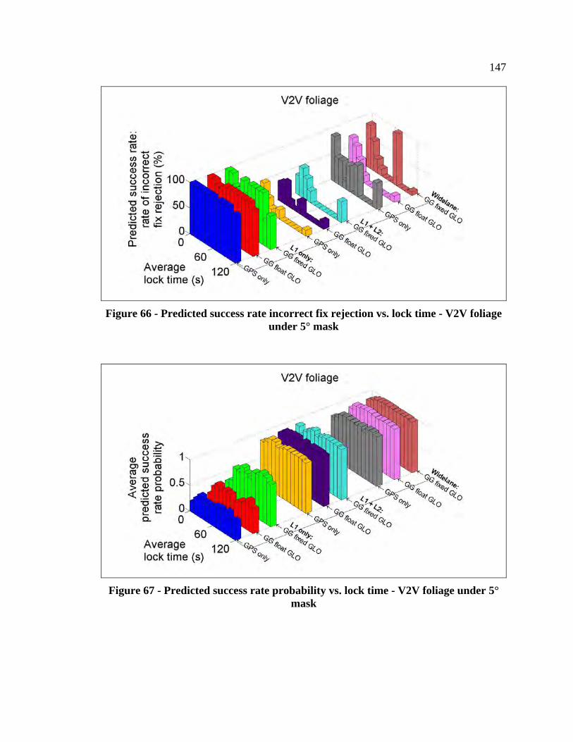
147
Figure 66 - Predicted success rate incorrect fix rejection vs. lock time - V2V foliage under 5° mask
Figure 67 - Predicted success rate probability vs. lock time - V2V foliage under 5° mask
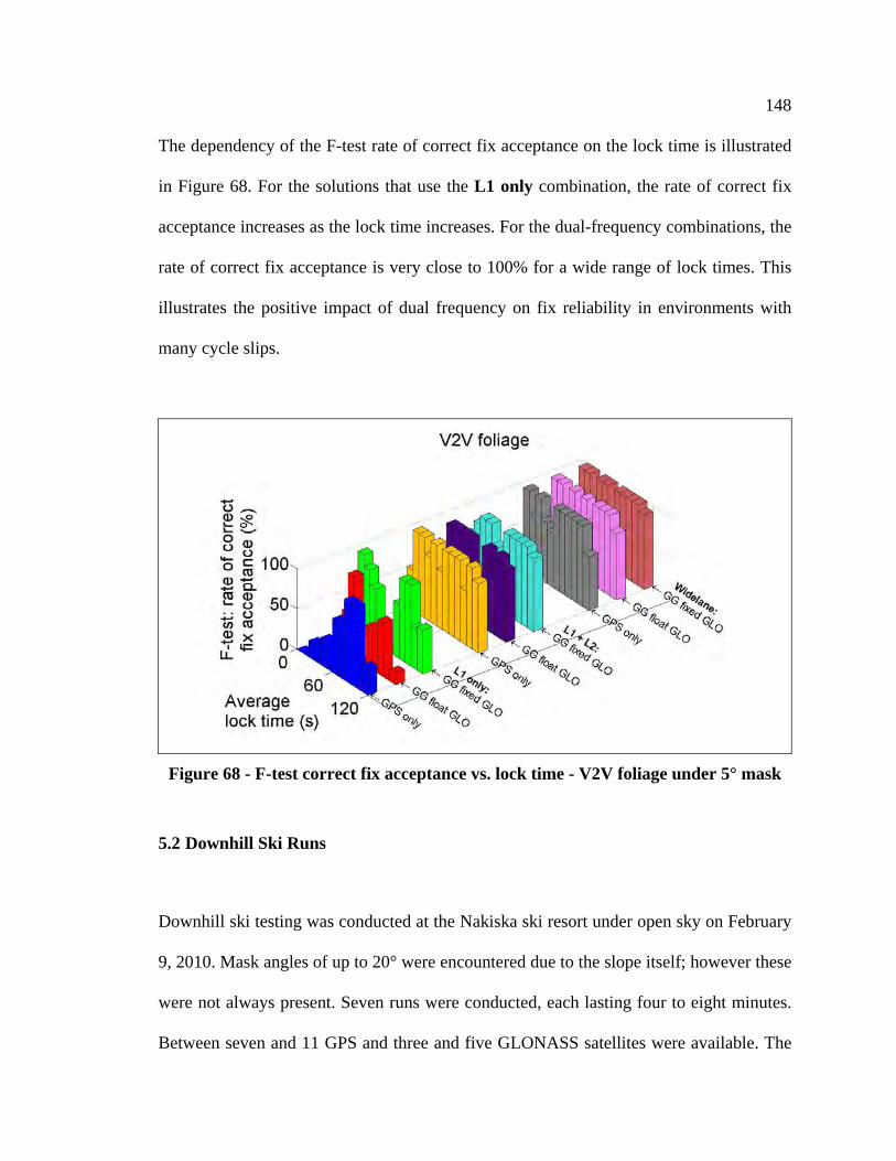
148
The dependency of the F-test rate of correct fix acceptance on the lock time is illustrated
in Figure 68. For the solutions that use the L1 only combination, the rate of correct fix
acceptance increases as the lock time increases. For the dual-frequency combinations, the
rate of correct fix acceptance is very close to 100% for a wide range of lock times. This
illustrates the positive impact of dual frequency on fix reliability in environments with
many cycle slips.
Figure 68 - F-test correct fix acceptance vs. lock time - V2V foliage under 5° mask
5.2 Downhill Ski Runs
Downhill ski testing was conducted at the Nakiska ski resort under open sky on February
9, 2010. Mask angles of up to 20° were encountered due to the slope itself; however these
were not always present. Seven runs were conducted, each lasting four to eight minutes.
Between seven and 11 GPS and three and five GLONASS satellites were available. The
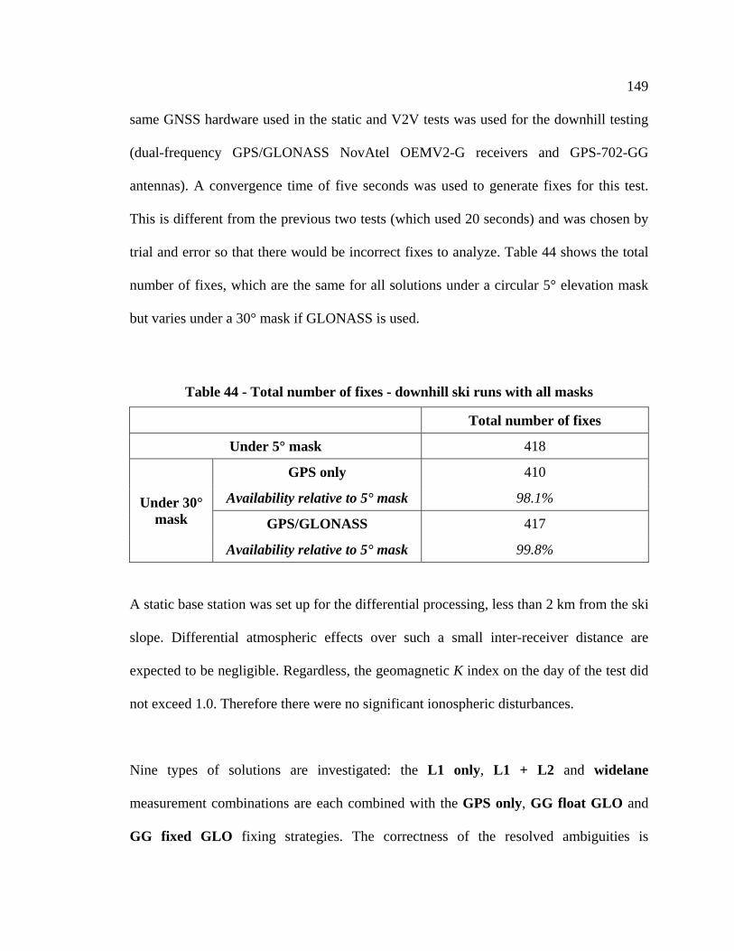
149
same GNSS hardware used in the static and V2V tests was used for the downhill testing
(dual-frequency GPS/GLONASS NovAtel OEMV2-G receivers and GPS-702-GG
antennas). A convergence time of five seconds was used to generate fixes for this test.
This is different from the previous two tests (which used 20 seconds) and was chosen by
trial and error so that there would be incorrect fixes to analyze. Table 44 shows the total
number of fixes, which are the same for all solutions under a circular 5° elevation mask
but varies under a 30° mask if GLONASS is used.
Table 44 - Total number of fixes - downhill ski runs with all masks
Total number of fixes
Under 5° mask 418
Under 30° mask
GPS only 410
Availability relative to 5° mask 98.1%
GPS/GLONASS 417
Availability relative to 5° mask 99.8%
A static base station was set up for the differential processing, less than 2 km from the ski
slope. Differential atmospheric effects over such a small inter-receiver distance are
expected to be negligible. Regardless, the geomagnetic K index on the day of the test did
not exceed 1.0. Therefore there were no significant ionospheric disturbances.
Nine types of solutions are investigated: the L1 only, L1 + L2 and widelane
measurement combinations are each combined with the GPS only, GG float GLO and
GG fixed GLO fixing strategies. The correctness of the resolved ambiguities is
150
determined by comparing the fixed-ambiguity positions to a reference solution derived
from GPS/GLONASS RTK with forward-backward smoothing applied. The fix is taken
to be correct with a horizontal agreement of better than 10 cm and incorrect otherwise.
The precision of the reference solution was evaluated by the vertical consistency at
physical checkpoints that the skier occupied at the beginning and end of each run. The
vertical range of the reference solution at these checkpoints (i.e. maximum minus
minimum height) did not exceed 5 cm either at the top or bottom of the hill.
Table 45 shows the actual success rate probabilities for downhill skiing. The numbers of
correct fixes that correspond to the success rates are highlighted in blue. Two scenarios
are investigated, namely the use of a standard circular elevation mask angle of 5°, and
then a circular mask angle of 30°. The latter approximately simulates downhill skiing on
a steeper hill where the mask angles from the slopes themselves are more severe. Such
mask angles could realistically be encountered in all directions (i.e. like a circular mask)
when skiing in mountainous valleys with steep slopes and trees along ski runs. The
following trends are observed:
For both downhill scenarios, the impact of GLONASS on the actual success rate
is the same as for the static and V2V analyses. The actual success rate effectively
does not change when the GLONASS measurements are simply added to float
estimation. However, significant improvement is observed when fixing the
GLONASS ambiguities.

151
Because of the short inter-receiver distances (and consequently the smaller phase
errors), switching from L1 only to L1 + L2 improves the actual success rate more
than switching to widelane, as highlighted in green in Table 45. As with the
analyses of previous scenarios, either dual-frequency combination benefits the
actual success rate over L1 alone.
The higher elevation mask has a negative impact on the actual success rate, which
is completely expected. However it is noteworthy that when GLONASS is fully
incorporated (even with L1 only), the ambiguities are more likely than not to be
fixed correctly. For the specific application of tracking skiers, single-frequency
ambiguity resolution can be useful even under high elevation masks, if
GLONASS is also used. In fact this has already been demonstrated for Olympic
alpine skiing (Lachapelle et al 2009).

152
Table 45 - Actual success rate probabilities - downhill ski runs with all masks
Actual success rate probability
Downhill 5° Downhill 30°
L1 only
GPS only 0.83 (347)3 0.22 (91)
GG float GLO 0.82 (344) 0.21 (87)
GG fixed GLO 0.94 (395) 0.51 (214)
L1 + L2
GPS only 0.99 (415) 0.92 (378)
GG float GLO 0.99 (415) 0.91 (380)
GG fixed GLO 1.00 (417) 0.98 (408)
Widelane
GPS only 0.87 (363) 0.51 (211)
GG float GLO 0.89 (374) 0.55 (229)
GG fixed GLO 0.94 (393) 0.71 (298)
The results of using the predicted success rate as an indicator of fix reliability are shown
in Table 46 and Table 47, for the 5° and 30° mask scenarios, respectively. Fixes are
accepted if they exceed the threshold of 0.95, and are otherwise rejected. No incorrect fix
results are presented for the solutions with actual success rates of 0.98 and above, as there
are too few incorrect fixes to compute meaningful acceptance and rejection rates.
For the 5° mask scenario, the predicted success rate is very optimistic, as it accepts
almost all of the fixes whether they are correct or incorrect. This implies that the
predicted success rate provides almost no information about the fix reliability. For the
30° mask scenario, the predicted success rates are less optimistic.
3 Number of correct fixes
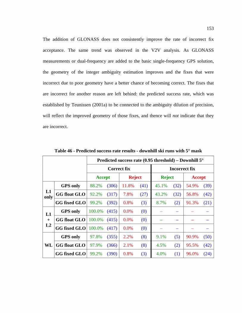
153
The addition of GLONASS does not consistently improve the rate of incorrect fix
acceptance. The same trend was observed in the V2V analysis. As GLONASS
measurements or dual-frequency are added to the basic single-frequency GPS solution,
the geometry of the integer ambiguity estimation improves and the fixes that were
incorrect due to poor geometry have a better chance of becoming correct. The fixes that
are incorrect for another reason are left behind: the predicted success rate, which was
established by Teunissen (2001a) to be connected to the ambiguity dilution of precision,
will reflect the improved geometry of those fixes, and thence will not indicate that they
are incorrect.
Table 46 - Predicted success rate results - downhill ski runs with 5° mask
Predicted success rate (0.95 threshold) – Downhill 5°
Correct fix Incorrect fix
Accept Reject Reject Accept
L1 only
GPS only 88.2% (306) 11.8% (41) 45.1% (32) 54.9% (39)
GG float GLO 92.2% (317) 7.8% (27) 43.2% (32) 56.8% (42)
GG fixed GLO 99.2% (392) 0.8% (3) 8.7% (2) 91.3% (21)
L1 +
L2
GPS only 100.0% (415) 0.0% (0) – – – –
GG float GLO 100.0% (415) 0.0% (0) – – – –
GG fixed GLO 100.0% (417) 0.0% (0) – – – –
WL
GPS only 97.8% (355) 2.2% (8) 9.1% (5) 90.9% (50)
GG float GLO 97.9% (366) 2.1% (8) 4.5% (2) 95.5% (42)
GG fixed GLO 99.2% (390) 0.8% (3) 4.0% (1) 96.0% (24)
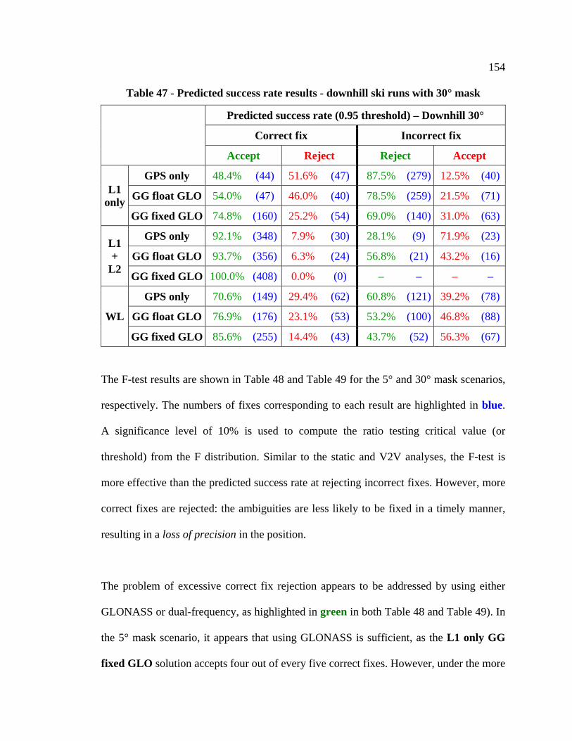
154
Table 47 - Predicted success rate results - downhill ski runs with 30° mask
Predicted success rate (0.95 threshold) – Downhill 30°
Correct fix Incorrect fix
Accept Reject Reject Accept
L1 only
GPS only 48.4% (44) 51.6% (47) 87.5% (279) 12.5% (40)
GG float GLO 54.0% (47) 46.0% (40) 78.5% (259) 21.5% (71)
GG fixed GLO 74.8% (160) 25.2% (54) 69.0% (140) 31.0% (63)
L1 +
L2
GPS only 92.1% (348) 7.9% (30) 28.1% (9) 71.9% (23)
GG float GLO 93.7% (356) 6.3% (24) 56.8% (21) 43.2% (16)
GG fixed GLO 100.0% (408) 0.0% (0) – – – –
WL
GPS only 70.6% (149) 29.4% (62) 60.8% (121) 39.2% (78)
GG float GLO 76.9% (176) 23.1% (53) 53.2% (100) 46.8% (88)
GG fixed GLO 85.6% (255) 14.4% (43) 43.7% (52) 56.3% (67)
The F-test results are shown in Table 48 and Table 49 for the 5° and 30° mask scenarios,
respectively. The numbers of fixes corresponding to each result are highlighted in blue.
A significance level of 10% is used to compute the ratio testing critical value (or
threshold) from the F distribution. Similar to the static and V2V analyses, the F-test is
more effective than the predicted success rate at rejecting incorrect fixes. However, more
correct fixes are rejected: the ambiguities are less likely to be fixed in a timely manner,
resulting in a loss of precision in the position.
The problem of excessive correct fix rejection appears to be addressed by using either
GLONASS or dual-frequency, as highlighted in green in both Table 48 and Table 49). In
the 5° mask scenario, it appears that using GLONASS is sufficient, as the L1 only GG
fixed GLO solution accepts four out of every five correct fixes. However, under the more
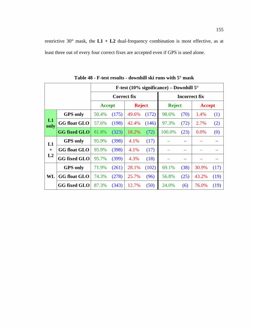
155
restrictive 30° mask, the L1 + L2 dual-frequency combination is most effective, as at
least three out of every four correct fixes are accepted even if GPS is used alone.
Table 48 - F-test results - downhill ski runs with 5° mask
F-test (10% significance) – Downhill 5°
Correct fix Incorrect fix
Accept Reject Reject Accept
L1 only
GPS only 50.4% (175) 49.6% (172) 98.6% (70) 1.4% (1)
GG float GLO 57.6% (198) 42.4% (146) 97.3% (72) 2.7% (2)
GG fixed GLO 81.8% (323) 18.2% (72) 100.0% (23) 0.0% (0)
L1 +
L2
GPS only 95.9% (398) 4.1% (17) – – – –
GG float GLO 95.9% (398) 4.1% (17) – – – –
GG fixed GLO 95.7% (399) 4.3% (18) – – – –
WL
GPS only 71.9% (261) 28.1% (102) 69.1% (38) 30.9% (17)
GG float GLO 74.3% (278) 25.7% (96) 56.8% (25) 43.2% (19)
GG fixed GLO 87.3% (343) 12.7% (50) 24.0% (6) 76.0% (19)
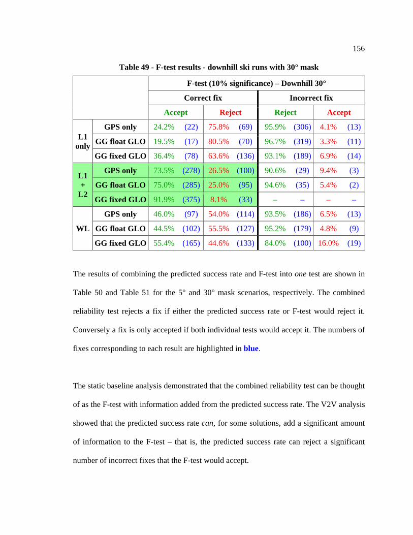
156
Table 49 - F-test results - downhill ski runs with 30° mask
F-test (10% significance) – Downhill 30°
Correct fix Incorrect fix
Accept Reject Reject Accept
L1 only
GPS only 24.2% (22) 75.8% (69) 95.9% (306) 4.1% (13)
GG float GLO 19.5% (17) 80.5% (70) 96.7% (319) 3.3% (11)
GG fixed GLO 36.4% (78) 63.6% (136) 93.1% (189) 6.9% (14)
L1 +
L2
GPS only 73.5% (278) 26.5% (100) 90.6% (29) 9.4% (3)
GG float GLO 75.0% (285) 25.0% (95) 94.6% (35) 5.4% (2)
GG fixed GLO 91.9% (375) 8.1% (33) – – – –
WL
GPS only 46.0% (97) 54.0% (114) 93.5% (186) 6.5% (13)
GG float GLO 44.5% (102) 55.5% (127) 95.2% (179) 4.8% (9)
GG fixed GLO 55.4% (165) 44.6% (133) 84.0% (100) 16.0% (19)
The results of combining the predicted success rate and F-test into one test are shown in
Table 50 and Table 51 for the 5° and 30° mask scenarios, respectively. The combined
reliability test rejects a fix if either the predicted success rate or F-test would reject it.
Conversely a fix is only accepted if both individual tests would accept it. The numbers of
fixes corresponding to each result are highlighted in blue.
The static baseline analysis demonstrated that the combined reliability test can be thought
of as the F-test with information added from the predicted success rate. The V2V analysis
showed that the predicted success rate can, for some solutions, add a significant amount
of information to the F-test – that is, the predicted success rate can reject a significant
number of incorrect fixes that the F-test would accept.
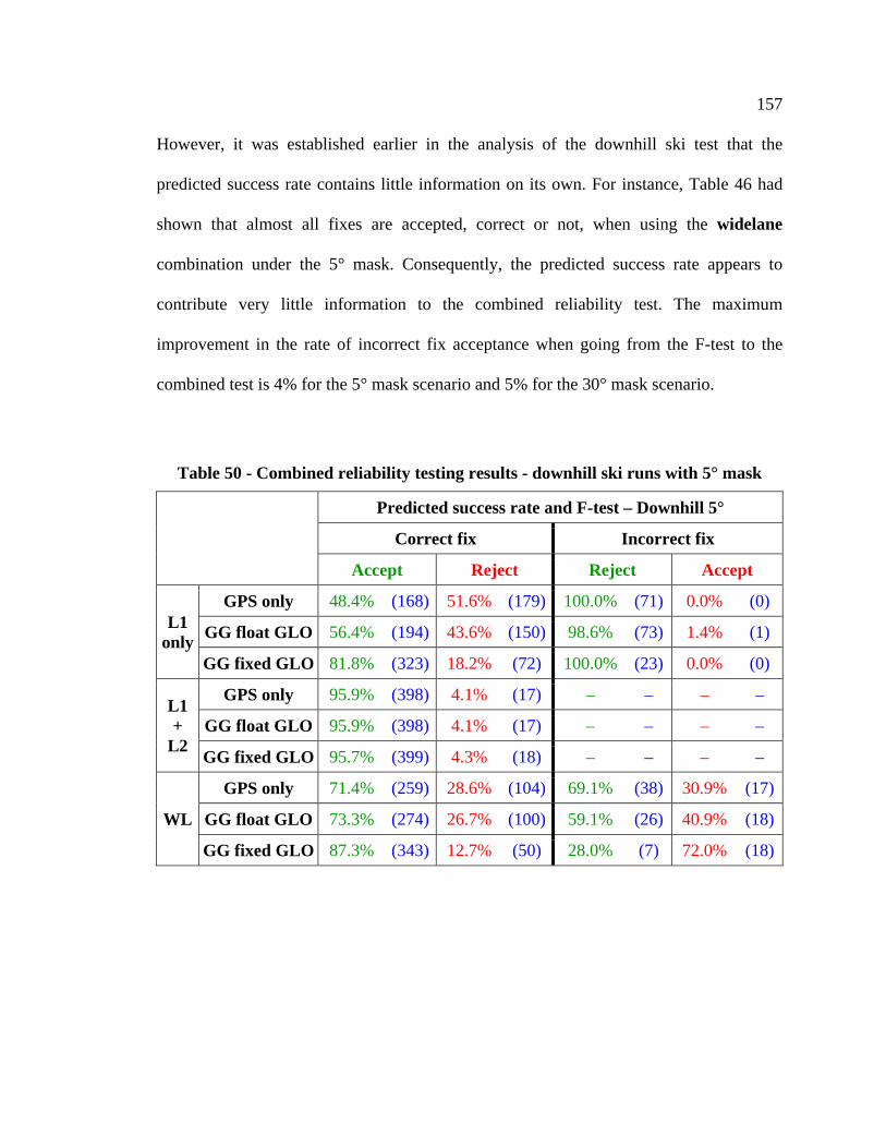
157
However, it was established earlier in the analysis of the downhill ski test that the
predicted success rate contains little information on its own. For instance, Table 46 had
shown that almost all fixes are accepted, correct or not, when using the widelane
combination under the 5° mask. Consequently, the predicted success rate appears to
contribute very little information to the combined reliability test. The maximum
improvement in the rate of incorrect fix acceptance when going from the F-test to the
combined test is 4% for the 5° mask scenario and 5% for the 30° mask scenario.
Table 50 - Combined reliability testing results - downhill ski runs with 5° mask
Predicted success rate and F-test – Downhill 5°
Correct fix Incorrect fix
Accept Reject Reject Accept
L1 only
GPS only 48.4% (168) 51.6% (179) 100.0% (71) 0.0% (0)
GG float GLO 56.4% (194) 43.6% (150) 98.6% (73) 1.4% (1)
GG fixed GLO 81.8% (323) 18.2% (72) 100.0% (23) 0.0% (0)
L1 +
L2
GPS only 95.9% (398) 4.1% (17) – – – –
GG float GLO 95.9% (398) 4.1% (17) – – – –
GG fixed GLO 95.7% (399) 4.3% (18) – – – –
WL
GPS only 71.4% (259) 28.6% (104) 69.1% (38) 30.9% (17)
GG float GLO 73.3% (274) 26.7% (100) 59.1% (26) 40.9% (18)
GG fixed GLO 87.3% (343) 12.7% (50) 28.0% (7) 72.0% (18)
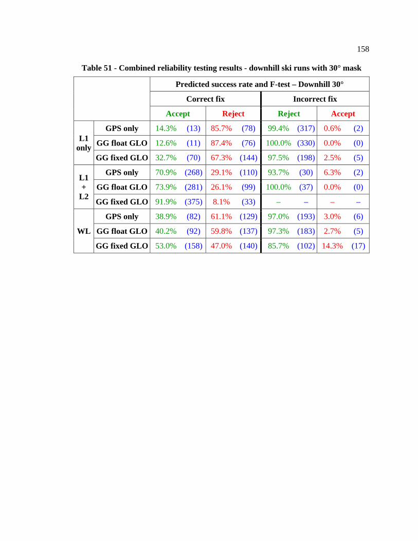
158
Table 51 - Combined reliability testing results - downhill ski runs with 30° mask
Predicted success rate and F-test – Downhill 30°
Correct fix Incorrect fix
Accept Reject Reject Accept
L1 only
GPS only 14.3% (13) 85.7% (78) 99.4% (317) 0.6% (2)
GG float GLO 12.6% (11) 87.4% (76) 100.0% (330) 0.0% (0)
GG fixed GLO 32.7% (70) 67.3% (144) 97.5% (198) 2.5% (5)
L1 +
L2
GPS only 70.9% (268) 29.1% (110) 93.7% (30) 6.3% (2)
GG float GLO 73.9% (281) 26.1% (99) 100.0% (37) 0.0% (0)
GG fixed GLO 91.9% (375) 8.1% (33) – – – –
WL
GPS only 38.9% (82) 61.1% (129) 97.0% (193) 3.0% (6)
GG float GLO 40.2% (92) 59.8% (137) 97.3% (183) 2.7% (5)
GG fixed GLO 53.0% (158) 47.0% (140) 85.7% (102) 14.3% (17)
159
Chapter Six: Conclusions and Recommendations
This thesis has examined the impact of combining GPS and GLONASS on the reliability
of carrier phase ambiguity resolution, or ambiguity fixing. Reliability in this context
refers to the ability to identify and reject incorrectly fixed ambiguities, as these lead to
undetected position biases. The ability to generate more correct fixes (and subsequently
identify and accept them) was also investigated, as the objective of ambiguity resolution
is to obtain sub-decimetre level position accuracy. Three key concepts related to fix
reliability were investigated herein: the actual success rate (i.e. the rate of correct fix); the
predicted success rate (i.e. an a priori indicator of the likelihood of a fix being correct);
and the F ratio test or F-test (i.e. a discriminator of correct and incorrect fixes).
The PLANSoft™ real-time kinematic (RTK) processing software was developed by the
author to perform GPS/GLONASS ambiguity resolution. The impact of GLONASS was
examined in two contexts: partial fixing (i.e. only the GPS ambiguities are resolved) and
full fixing (i.e. both GPS and GLONASS ambiguities are resolved). Single- and dual-
frequency measurement combinations were also investigated.
Three tests were conducted to investigate ambiguity resolution. Static baselines were
analyzed over distances of 2 km and 18 km, with the static surveys exceeding 24 hours to
provide statistically significant data. Vehicle-to-vehicle (V2V) relative navigation was
conducted over inter-receiver distances of up to a few hundred metres. A series of
downhill ski runs was tracked using a base station less than 2 km away from the ski slope.
160
Geodetic-grade GPS/GLONASS dual-frequency hardware (NovAtel OEMV2-G
receivers and GPS-702-GG antennas) were used to collect the data. No significant
ionospheric disturbances were encountered during these data collections.
6.1 Conclusions
The following conclusions are based on the data used in the thesis and should be
interpreted in this context. The use of additional data sets under different atmospheric
conditions could impact these conclusions, as noted in the next section on
recommendations.
Impact of GLONASS: The main effect of adding the GLONASS measurements is that
the accuracy of the float estimate of the position improves. This is expected since adding
GLONASS measurements improves the geometry of the float position estimation.
However, the float position error just prior to ambiguity resolution is only weakly
correlated with the correctness of the resulting fixed ambiguities. Hence GLONASS with
partial fixing does not significantly improve the actual success rate.
GLONASS with full fixing improves the actual success rate significantly. The additional
ambiguities from GLONASS improve the geometry of the integer ambiguity estimation
(represented by the ambiguity dilution of precision, or ADOP). Both the number of
ambiguities and the ADOP are strongly correlated with actual success rate.
161
GLONASS has a small effect on the fixed position accuracies that correspond with
correct fixes. However since GLONASS (with full fixing) provides many more correct
fixes, the availability of precise (sub-decimetre) positioning accuracy is higher in general.
One of the other major benefits of GLONASS is increased solution availability under
certain scenarios where the satellite visibility is reduced. Tests under elevation mask
angles of 30° have shown that a GPS/GLONASS solution maintains nearly 100%
solution availability, while GPS-only availability was as low as 80% for some tests. The
effect of GLONASS in other reduced-visibility scenarios (such as urban canyons) has not
been explored and may not produce results that are as successful.
GLONASS with full fixing also improves the reliability of ambiguity resolution, as it
generally maximizes both incorrect fix rejection and correct fix acceptance (over GPS
alone or GLONASS with partial fixing) when the predicted success rate and F-test are
both used to identify correct and incorrect fixes. The performance of the F-test has a
strong correlation with the integer estimation geometry (i.e. both the number of
ambiguities and the ADOP) which GLONASS with full fixing improves substantially.
Impact of dual-frequency: Incorporating L1 and L2 phase measurements (as separate
measurements) is a similar strategy to adding GLONASS with full fixing. The main
effect of L1 and L2 is the improvement in the geometry of the integer estimation (but not
the geometry of the satellites), which comes about from the additional L2 ambiguities.
The better geometry results in higher success rates and better fix reliability when the F-
test is applied.
162
Combining the L1 and L2 phase measurements into widelane measurements widens the
wavelength of the phase ambiguities from approximately 19 cm to 86 cm. The benefits of
using widelane are two-fold. The widelane ambiguities are easier to fix than L1 due to the
wider wavelength. As well, the effect of phase errors on a single widelane cycle is less
than half the effect on an L1 cycle. The actual success rate and fix reliability are both
negatively affected by the magnitude of the phase errors. Hence, widelane could
potentially be useful for longer inter-receiver distances where the phase errors are larger.
However this conclusion can only be made for static baselines under open sky. No
significant ionospheric disturbances were encountered, so widelane could not be
evaluated with phase errors exceeding half a cycle. Using widelane comes at a cost:
positions derived from correct widelane fixes tend to be much less precise than when L1
or L2 are used.
Cycle slips: A higher frequency of cycle slips was found to negatively impact the actual
success rate. This is expected because a cycle slip resets the corresponding ambiguity to a
new value and shortens the available convergence time for that ambiguity. The geometry
of the integer estimation problem is affected: a negative relationship was demonstrated
between convergence time and ADOP. This result only applies for the foliage portion of
the vehicle-to-vehicle test conducted herein. However this is also expected to be true
under more severe signal environments.
163
The probability of cycle slip detection was also investigated. When used as an a priori
indicator of reliability, it is similar to the predicted success rate but accepts less fixes in
general (and consequently accepts less incorrect fixes).
6.2 Recommendations
In order to expand upon the results and conclusions derived from this thesis, the
following recommendations are made:
1. The hardware used in this thesis is geodetic-grade and is calibrated to minimize
GLONASS inter-frequency biases. The effect of those inter-frequency biases can
exceed one half-cycle and should be investigated with lower-quality receivers.
2. The testing scenarios can be expanded. Reduced satellite visibility was
investigated using a 30° circular elevation mask, and overhead foliage was used to
investigate cycle slips. An environment that induces multipath and lower signal
strength could be investigated.
3. The analysis of the effect of phase errors in this thesis can be expanded. Single-
and dual-frequency solutions can be analyzed over a number of inter-receiver
distances and under different ionospheric conditions to validate and/or update the
findings described in this thesis. Ionospheric effects can potentially be
investigated during the next two years as the sunspot number increases.

164
4. An analysis of the effect of convergence time should be done. In this thesis
convergence times were chosen such that there would be enough incorrect fixes to
analyze. Convergence times can be added as a variable in the analysis of (for
instance) the rate of incorrect fix acceptance for the predicted success rate and the
F-test.

165
References
Boriskin, A. and G. Zyryanov (2008). “Algorithms to Calibrate and Compensate for
GLONASS Biases in GNSS RTK Receivers Working with 3rd Party Networks”,
in Proceedings of ION GNSS 2008, September 16-19, Savannah, GA, pp. 376-
384.
Chen, D., and G. Lachapelle (1995). “A Comparison of the FASF and Least-Squares
Search Algorithms for Ambiguity Resolution On The Fly”, in Navigation, vol. 42,
no. 2, pp. 371-390.
Conley, R., R. Cosentino, C. J. Hegarty, E. D. Kaplan, J. L. Leva, M. U. de Haag and K.
Van Dyke (2006). “Performance of Stand-Alone GPS”, chapter 7 in
Understanding GPS Principles and Applications, 2nd edition, Kaplan, E. D. and
Hegarty, C. J., ed. Artech House, Norwood MA.
Cosentino, R. J., D. W. Diggle, M. U. de Haag, C. J. Hegarty, D. Milbert and J. Nagle
(2006). “Differential GPS”, chapter 8 in Understanding GPS Principles and
Applications, 2nd edition, Kaplan, E. D. and Hegarty, C. J., ed. Artech House,
Norwood MA.
Counselman, C. C. and S. A. Gourevitch (1981). “Miniature Interferometer Terminals for
Earth Surveying: Ambiguity and Multipath with Global Positioning System”, in
IEEE Transactions on Geoscience and Remote Sensing, vol. GE-19, no. 4, pp.
244-252.
Euler H. J. and B. Schaffrin (1990) “On a Measure of the Discernibility between
Different Ambiguity Solutions in the Static-Kinematic GPS-Mode”, in IAG
166
Symposium No. 107, Kinematic Systems in Geodesy, Surveying, and Remote
Sensing, September 10-13, Banff, AB, pp 285-295.
Fenton, P. and J. Jones (2005). “The Theory and Performance of NovAtel Inc.’s Vision
Correlator” in Proceedings of ION GNSS 2005, September 13-16, Long Beach,
CA, Institute of Navigation, pp. 2178-2186.
Frei, E. and G. Beutler (1990). “Rapid Static Positioning Based on the Fast Ambiguity
Resolution Approach ‘FARA’: Theory and First Results”, in Manuscripta
Geodaetica, vol. 15, pp. 325-356.
Habrich, H., Beutler, G., Gurtner, W. and Rothacher, M. (1999). “Double Difference
Ambiguity Resolution for GLONASS/GPS Carrier Phase”, in Proceedings of ION
GPS 1999, September 14-17, Nashville, TN, Institute of Navigation, pp. 1609-
1618.
Han, S. and C. Rizos (1996). “Integrated Method for Instantaneous Ambiguity Resolution
Using New Generation GPS Receivers”, in IEEE Position, Location and
Navigation Symposium (PLANS) 1996, April 22-26, Atlanta, GA, pp. 254-261.
Keong, J. H. and G. Lachapelle (2000). “Heading and Pitch Determination Using
GPS/GLONASS”, in GPS Solutions, vol. 3, no. 3, pp. 26-36.
Kozlov, D. and M. Tkachenko (1998). “Centimeter-Level Real-Time Kinematic
Positioning with GPS + GLONASS C/A Receivers”, in Navigation, vol. 45, no. 2,
pp. 137-147.
Kozlov, D., M. Tkachenko and A. Tochilin (2000). “Statistical Characterization of
Hardware Biases in GPS+GLONASS Receivers”, in Proceedings of ION GPS
2000, September 19-22, Salt Lake City, UT, pp. 817-826.
167
Lachapelle, G. (2008). Advanced GNSS Theory and Applications. ENGO 625 lecture
notes, Department of Geomatics Engineering, University of Calgary.
Lachapelle, G., A. Morrison and R. Ong (2009). “Ultra-Precise Sport Positioning for
Sport Applications”, in Proceedings of the 13th International Association of
Institutes of Navigation, October 27-30, Stockholm, Sweden, 11 pages.
Landau, H. and H. J. Euler (1992). “On-the-Fly Ambiguity Resolution for Precise
Differential Positioning”, in Proceedings of ION GPS 1992, September 16-18,
Albuquerque, NM, pp. 607-613.
Leick, A. (2004). GPS Satellite Surveying. 3rd edition, John Wiley and Sons,
Hoboken, NJ.
Leick, A. (1998). “GLONASS Satellite Surveying”, in Journal of Surveying Engineering,
vol. 124, no. 2, pp. 91-99.
Leick, A., J. Beser, P. Rosenboom and B. Wiley (1998). “Assessing GLONASS
Observation”, in Proceedings of ION GPS 1998, September 15-18, Nashville, TN,
pp. 1605-1612.
Mader, G. L. (1992). “Rapid Static and Kinematic Global Positioning System Solutions
Using the Ambiguity Function Technique”, in Journal of Geophysical Research,
vol. 97, no. B3, pp. 3271-3283.
O’Keefe, K., M. G. Petovello, W. Cao, G. Lachapelle and E. Guyader (2009).
“Comparing of Multi-Carrier Ambiguity Resolution Methods for Geometry-
Based GPS and Galileo Low Earth Orbiting Satellite Attitude Determination”, in
International Journal of Navigation and Observation, volume 2009, article ID
592073, 15 pages.
168
O'Keefe, K., M. G. Petovello, G. Lachapelle and M. E. Cannon (2006). “Assessing
Probability of Correct Ambiguity Resolution in the Presence of Time Correlated
Errors”, in Navigation, vol. 53, no. 4, pp. 269-282.
Petovello, M. G. (2003). “Real-Time Integration of a Tactical-Grade IMU and GPS for
High-Accuracy Positioning and Navigation”. PhD thesis, Report 20173,
Department of Geomatics Engineering, University of Calgary, Calgary, Canada.
Rossbach, U. (2000). “GLONASS Double Difference Ambiguity Resolution in Real-
Time” in Proceedings of ION GPS 2000, September 19-22, Salt Lake City, UT,
pp. 163-171.
Space Weather Canada (2009). “Indices”, retrieved on May 26, 2010 from
http://www.spaceweather.gc.ca/si-eng.php.
Takac, F. (2009). “GLONASS inter-frequency biases and ambiguity resolution”, in Inside
GNSS, vol. 2, no. 4, March/April 2009, pp. 24-28.
Teunissen, P. J. G. (2003). “Towards a Unified Theory of GNSS Ambiguity Resolution”,
in Journal of Global Positioning Systems, vol. 2, no. 1, pp. 1-12.
Teunissen, P. J. G. (2001a). “Statistical GNSS Carrier Phase Ambiguity Resolution: A
Review”, in Proceedings of the 11th IEEE Signal Processing Workshop on
Statistical Signal Processing (2001), August 6-8, Singapore, Japan, pp. 4-12.
Teunissen, P. J. G. (2001b). “Integer Estimation in the Presence of Biases”, in Journal of
Geodesy, vol. 75, nos. 7-8, pp. 399-407.
Teunissen, P. J. G. (2000a). “The success rate and precision of GPS ambiguities”, in
Journal of Geodesy, vol. 74, nos. 3-4, pp. 321-326.
169
Teunissen, P. J. G. (2000b). “The GPS Integer Least-Squares Statistics” in Physics and
Chemistry of the Earth, Part A: Solid Earth and Geodesy, vol. 25, nos. 9-11, pp.
673-677.
Teunissen, P. J. G. (1998). “Success probability of integer GPS ambiguity rounding and
bootstrapping”, in Journal of Geodesy, vol. 72, no. 10, pp. 606-612.
Teunissen, P. J. G. (1995). “The Least-Squares Ambiguity Decorrelation Adjustment: A
Method for Fast GPS Integer Ambiguity Estimation”, in Journal of Geodesy, vol.
70, nos. 1-2, pp. 65-82.
Teunissen, P. J. G. and S. Verhagen (2004). “On the Foundation of the Popular Ratio
Test for GNSS Ambiguity Resolution”, in Proceedings of ION GNSS 2004,
September 21-24, Long Beach, CA, pp. 2529-2540.
Teunissen, P. J. G., P. Joosten and D. Odijk (1999). “The Reliability of GPS Ambiguity
Resolution”, in GPS Solutions, vol. 2, no. 3, pp. 63-69.
USNOAA – United States National Oceanic and Atmospheric Administration (2005).
“NOAA Space Weather Scales”, retrieved on May 26, 2010 from
http://www.swpc.noaa.gov/NOAAscales/index.html.
Van Diggelen, F. (1997). “GPS and GPS+GLONASS RTK”, in Proceedings of ION GPS
1997, September 16-19, Kansas City, MO, pp. 139-144.
Verhagen, S. (2005). “On the Reliability of Ambiguity Resolution”, in Navigation, vol.
52, no. 2, pp. 99-110.
Verhagen, S. (2004). “Integer Ambiguity Validation: An Open Problem?”, in GPS
Solutions, vol. 8, no. 1, pp. 36-43.
170
Wang, J. (2000). “An Approach to GLONASS ambiguity resolution”, in Journal of
Geodesy, vol. 74, no. 5, July 2000, pp. 421-430.
Yang, Y., R. T. Sharpe and R. R. Hatch (2006). “A Fast Ambiguity Resolution Technique
for RTK Embedded Within a GPS Receiver”. NavCom Technology white paper,
October 2006, retrieved on April 25, 2010 from
http://www.navcomtech.com/Support/DownloadCenter.cfm?category=
whitepapers.