Embed Size (px)
Citation preview
UC BerkeleyLecture Notes for ME233
Advanced Control Systems II
Xu Chen and Masayoshi Tomizuka
Spring 2014

Copyright: Xu Chen and Masayoshi Tomizuka 2013~. Limited copying or use for educationalpurposes allowed, but please make proper acknowledgement, e.g.,
“Xu Chen and Masayoshi Tomizuka, Lecture Notes for UC Berkeley Advanced Control SystemsII (ME233), Available at http://www.me.berkeley.edu/ME233/sp14, May 2014.”
or if you use LATEX:
@Miscxchen14,key = controls,systems,lecture notes,author = Xu Chen and Masayoshi Tomizuka,title = Lecture Notes for UC Berkeley Advanced Control Systems II (ME233),howpublished = Available at \urlhttp://www.me.berkeley.edu/ME233/sp14,month = may,year = 2014
ContentsA1 Syllabus, Spring 20140 Introduction1 Dynamic Programming3 Probability Theory4 Least squares (LS) estimation5 Stochastic state estimation (Kalman Filter)6 Linear Quadratic Gaussian (LQG) Control7 Principles of Feedback Design8 Discretization and Implementation of Continuous-time Design9 LQG/Loop Transfer Recovery (LTR)10 LQ with Frequency Shaped Cost Function (FSLQ)11 Feedforward Control: Zero Phase Error Tracking12 Preview Control13 Internal Model Principle and Repetitive Control14 Disturbance Observer15 System Identification and Recursive16 Stability of Parameter Adaptation Algorithms17 PAA with Parallel Predictors18 Parameter Convergence in PAAs19 Adaptive Control based on Pole Assignment

University of California at Berkeley
Department of Mechanical Engineering
ME 233: Advanced Control Systems II Spring 2014
ME233 discusses advanced control methodologies and their applications to engineering systems.
Methodologies include but are not limited to: Linear Quadratic Optimal Control, Kalman Filter,
Discretization, Linear Quadratic Gaussian Problem, Loop Transfer Recovery, System Identification, Adaptive
Control and Model Reference Adaptive Systems, Self Tuning Regulators, Repetitive Control, and Disturbance
Observers.
Instructor: Xu Chen, [email protected]
Office: 5112 Etcheverry Hall
Office Hour: Tu, Th 1:00pm – 2:30pm in 5112 Etcheverry Hall
Teaching Assistant: Changliu Liu, [email protected]
Office Hour: M, W 10:00am – 11:00am in 136 Hesse Hall
Lectures: Tu, Th 8:00 am - 9:30 pm in Rm. 3113 Etcheverry Hall
Discussion: Fri. 10am-11am in Rm 1165 Etcheverry Hall
Prerequisites: ME C 232 (syllabus on course website) or its equivalence
Course website: http://www.me.berkeley.edu/ME233/sp14/ and bCourses.berkeley.edu
Remark: lecture videos are webcasted to Youtube and iTunes-U (links on the course website)
Grading: Two Midterm Exams (open one-page summary sheet for each exam) 2*20 %
Final Examination (open notes) 40 %
Homework (see policy on course website) 20 %
Class Notes: ME233 Class Notes by M. Tomizuka (Parts I and II)
They can be purchased at Copy Central, 48 Shattuck Square, Berkeley
Tentative Schedule (Subject to change):
Week Days Topics
1 1/21, 1/23 Dynamic Programming, Discrete Time LQ problem, Review of Probability Theory:
Sample Space, Random Variable, Probability Distribution and Density Functions.
2 1/28, 1/30 Review of Probability Theory: Random Process, Correlation Function, Spectral
Density
3 2/4, 2/6 Principle of Least Squares estimation; Stochastic State Estimation (Kalman Filter).
4 2/11, 2/13 Stochastic Estimation (continuation)
5 2/18, 2/20 Linear Stochastic Control (Linear Quadratic Gaussian (LQG) Problem); Singular
values; Introduction to linear multivariable control.
6 2/25, 2/27 Linear multivariable control; Loop Transfer Recovery
7 3/4, 3/6 Frequency-shaped LQ; in-class Midterm I on 3/4/2014
8 3/11, 3/13 Feedforward and preview control; Internal Model Principle and Repetitive Control.
9 3/18, 3/20 Disturbance Observer
3/25, 3/27 SPRING RECESS
10 4/1, 4/3 System Identification and Adaptive Control
11 4/8, 4/10 Parameter Estimation Algorithms
12 4/15, 4/17 Stability analysis of adaptive systems; in-class Midterm II on 4/15/2014
13 4/22, 4/24 Parallel Adaptation Algorithms; Parameter Convergence
14 4/29, 5/1 Direct and Indirect Adaptive Control; Adaptive Prediction
Final Examination: May 15 (Th) 2014, 7-10 pm
Please notify the instructor in writing by the second week of the semester, if you have any potential
conflict(s) about the class schedule, or if you need special accommodations such as: disability-related
accommodations, emergency medical information you wish to discuss with the instructor, or special
arrangements in case the building must be evacuated.

ME 233, UC Berkeley, Spring 2014 Xu Chen
Introduction
Big pictureSyllabus
Requirements
Big pictureME 233 talks about advanced and practical control theories, including but notlimited to:
I dynamic programmingI optimal estimation (Kalman Filter) and stochastic controlI SISO and MIMO feedback design principlesI digital control: implementation and designI feedforward design techniques: preview control, zero phase error
tracking, etcI feedback design techniques: LQG/LTR, internal model principle,
repetitive control, disturbance observerI system identificationI adaptive controlI ...
Introduction ME233 0-1

Teaching staff and class notes
I instructor:I Xu Chen, 2013 UC Berkeley Ph.D., [email protected] office hour: Tu Thur 1pm-2:30pm at 5112 Etcheverry Hall
I teaching assistant:I Changliu Liu, [email protected] office hour: M, W 10:00am – 11:00am in 136 Hesse Hall
I class notes:I ME233 Class Notes by M. Tomizuka (Parts I and II); Both canbe purchased at Copy Central, 48 Shattuck Square, Berkeley
Introduction ME233 0-2
Requirements and evaluations
I website (case sensitive):I www.me.berkeley.edu/ME233/sp14I bcourses.berkeley.edu
I prerequisites: ME C 232 or its equivalenceI lectures: Tu Thur 8-9:30am, 3113 Etcheverry HallI discussions: Fri. 10-11am, 1165 Etcheverry HallI homework (20%)I two in-class midterms (20% each): Mar. 4, 2014 and Apr. 15,
2014; one-page handwritten summary sheets allowedI one final exam (40%): May 15 2014 (Th), 7 pm -10 pm; open
notes
Introduction ME233 0-3

Prerequisites (ME 232 table of contents)
I Laplace and Z transformationsI Models and Modeling of linear dynamical systems: transfer
functions, state space modelsI Solutions of linear state equations
I Stability: poles, eigenvalues, Lyapunov stabilityI Controllability and observabilityI State and output feedbacks, pole assignment via state feedbackI State estimation and observer, observer state feedback controlI Linear Quadratic (LQ) Optimal Control, LQR properties, Riccati
equation
Introduction ME233 0-4
Remark
ME233 will be webcasted:I Berkeley’s YouTube channel
(http://www.youtube.com/ucberkeley)I iTunes U (http://itunes.berkeley.edu/)I webcast.berkeley (http://webcast.berkeley.edu)
links will be posted on course website when available
Introduction ME233 0-5

References (also on course website)
I ProbabilityI Bertsekas, Introduction to Probability, Athena ScientificI Yates and Goodman, Probability and Stochastic Processes, second edition, Willey
I Linear Quadratic Optimal ControlI Anderson and Moore, Optimal Control: Linear Quadratic Methods, Dover Books on Engineering (paperback),
2007. A PDF can be downloaded from: http://users.rsise.anu.edu.au/%7Ejohn/papers/index.htmlI Lewis and Syrmos, Vassilis L., Optimal Control, Wiley-IEEE, 1995I Bryson and Ho, Applied Optimal Control: Optimization, Estimation, and Control, Wiley
I Stochastic Control Theory and Optimal FilteringI Brown and Hwang, Introduction to Random Signals and Applied Kalman Filtering, Third Edition, WilleyI Lewis and Xie and Popa, Optimal and Robust Estimation, Second Edition CRCI Grewal and Andrews, Kalman Filter, Theory and Practice, Prentice HallI Anderson, and Moore, Optimal Filtering, Dover Books on Engineering (paperback), New York, 2005. A PDF
can be downloaded from: http://users.rsise.anu.edu.au/%7Ejohn/papers/index.htmlI Astrom, Introduction to Stochastic Control Theory, Dover Books on Engineering (paperback), New York, 2006
I Adaptive ControlI Astrom and Wittenmark, Adaptive Control, Addison Wesley, 2nd Ed., 1995I Goodwin and Sin, Adaptive Filtering Prediction and Control, Prentice Hall, 1984
I Krstic, Kanellakopoulos, and Kokotovic, Nonlinear and Adaptive Control Design, Willey
Introduction ME233 0-6

ME 233, UC Berkeley, Spring 2014 Xu Chen
Lecture 1: Dynamic Programming
General problemMultivariable derivative
Discrete-time LQ
Dynamic programming (DP)introduction:
I history: developed in the 1950’s by Richard BellmanI “programming”: ~“planning” (has nothing to do with
computers)
I a useful concept with lots of applications
I IEEE Global History Network: “A breakthrough which set thestage for the application of functional equation techniques in awide spectrum of fields. . . ”
Lecture 1: Dynamic Programming ME233 1-1
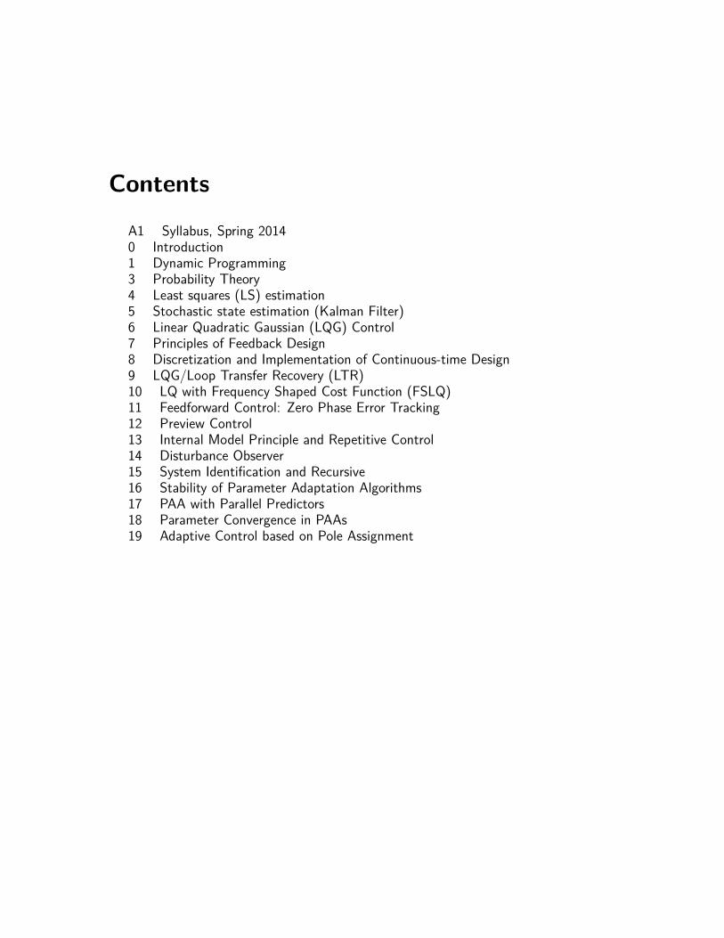
Essentials of dynamic programmingI key idea: solve a complex and difficult problem via solving a
collection of sub problems
Example (Path planning)goal: obtain minimum cost path from S to E
S
A
C D
B
E
1
6
32 1
2
4 1
I observation: if node C is on the optimal path, the then pathfrom node C to node E must be optimal as well
Lecture 1: Dynamic Programming ME233 1-2
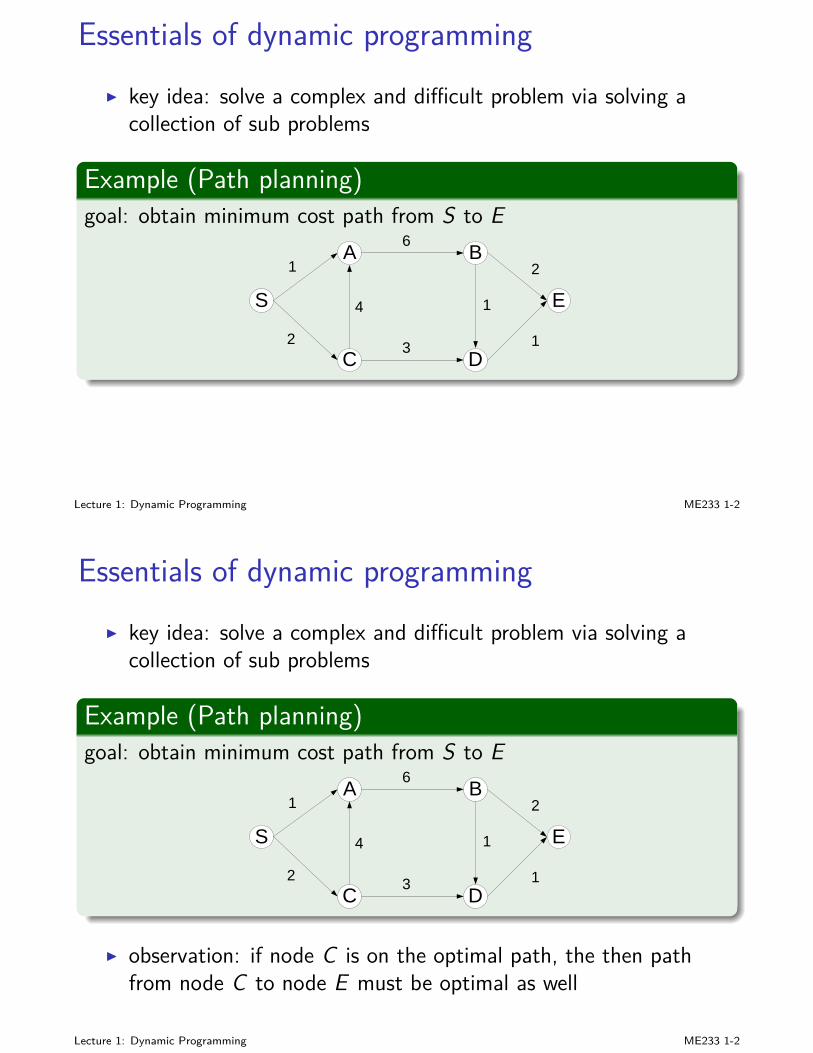
Essentials of dynamic programming
S
A
C D
B
E
1
6
32 1
2
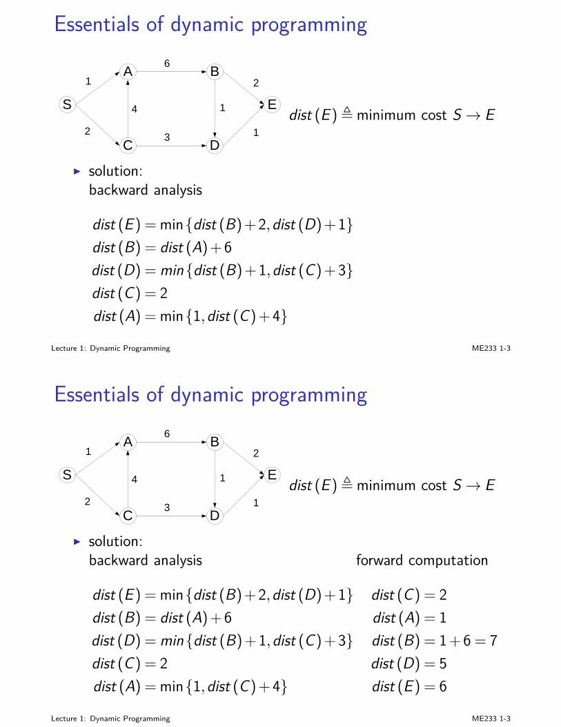
4 1 dist (E ),minimum cost S → E
I solution:backward analysis
dist (E ) =mindist (B)+2,dist (D)+1dist (B) = dist (A)+6dist (D) = mindist (B)+1,dist (C)+3dist (C) = 2dist (A) =min1,dist (C)+4
forward computation
dist (C) = 2dist (A) = 1dist (B) = 1+6= 7dist (D) = 5dist (E ) = 6
Lecture 1: Dynamic Programming ME233 1-3
Essentials of dynamic programming
S
A
C D
B
E
1
6
32 1
2
4 1
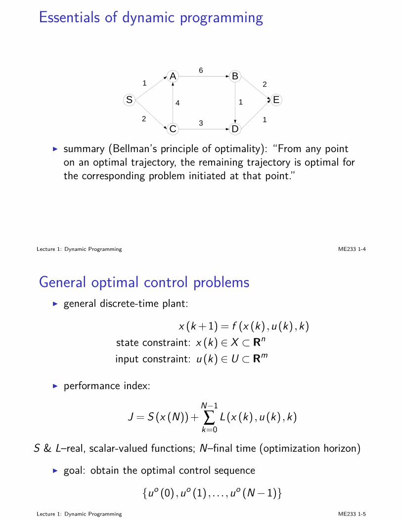
I summary (Bellman’s principle of optimality): “From any pointon an optimal trajectory, the remaining trajectory is optimal forthe corresponding problem initiated at that point.”
Lecture 1: Dynamic Programming ME233 1-4
General optimal control problemsI general discrete-time plant:
x (k +1) = f (x (k) ,u (k) ,k)state constraint: x (k) ∈ X ⊂ Rn
input constraint: u (k) ∈ U ⊂ Rm
I performance index:
J = S (x (N))+N−1∑k=0
L(x (k) ,u (k) ,k)
S & L–real, scalar-valued functions; N–final time (optimization horizon)
I goal: obtain the optimal control sequence
uo (0) ,uo (1) , . . . ,uo (N−1)Lecture 1: Dynamic Programming ME233 1-5
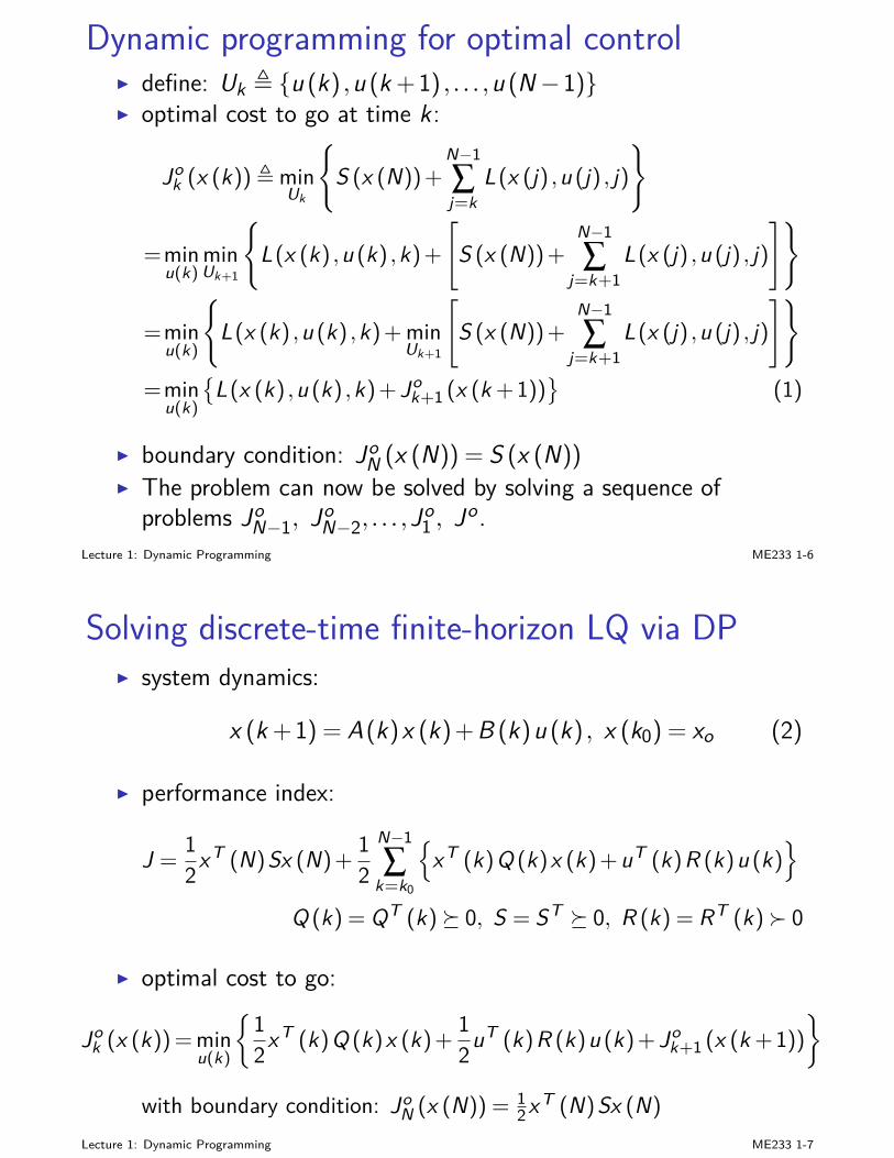
Dynamic programming for optimal controlI define: Uk , u (k) ,u (k +1) , . . . ,u (N−1)I optimal cost to go at time k :
Jok (x (k)),min
Uk
S (x (N))+
N−1∑j=k
L(x (j) ,u (j) , j)
=minu(k)
minUk+1
L(x (k) ,u (k) ,k)+
[S (x (N))+
N−1∑
j=k+1L(x (j) ,u (j) , j)
]
=minu(k)
L(x (k) ,u (k) ,k)+min
Uk+1
[S (x (N))+
N−1∑
j=k+1L(x (j) ,u (j) , j)
]
=minu(k)
L(x (k) ,u (k) ,k)+Jo
k+1 (x (k +1))
(1)
I boundary condition: JoN (x (N)) = S (x (N))
I The problem can now be solved by solving a sequence ofproblems Jo
N−1, JoN−2, . . . ,Jo
1 , Jo.Lecture 1: Dynamic Programming ME233 1-6
Solving discrete-time finite-horizon LQ via DPI system dynamics:
x (k +1) = A(k)x (k)+B (k)u (k) , x (k0) = xo (2)
I performance index:
J =12xT (N)Sx (N)+
12
N−1∑
k=k0
xT (k)Q (k)x (k)+uT (k)R (k)u (k)
Q (k) = QT (k) 0, S = ST 0, R (k) = RT (k) 0
I optimal cost to go:
Jok (x (k))=min
u(k)
12xT (k)Q (k)x (k)+ 1
2uT (k)R (k)u (k)+Jok+1 (x (k +1))
with boundary condition: JoN (x (N)) = 1
2xT (N)Sx (N)
Lecture 1: Dynamic Programming ME233 1-7
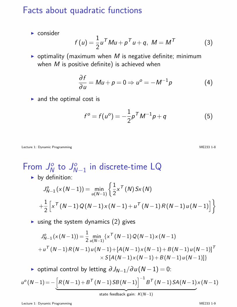
Facts about quadratic functions
I considerf (u) = 1
2uT Mu+pT u+q, M = MT (3)
I optimality (maximum when M is negative definite; minimumwhen M is positive definite) is achieved when
∂ f∂u = Mu+p = 0⇒ uo =−M−1p (4)
I and the optimal cost is
f o = f (uo) =−12pT M−1p+q (5)
Lecture 1: Dynamic Programming ME233 1-8
From JoN to Jo
N−1 in discrete-time LQI by definition:
JoN−1 (x (N−1)) = min
u(N−1)
12xT (N)Sx (N)
+12[xT (N−1)Q (N−1)x (N−1)+uT (N−1)R (N−1)u (N−1)
]
I using the system dynamics (2) gives
JoN−1 (x (N−1)) = 1
2 minu(N−1)
xT (N−1)Q (N−1)x (N−1)
+uT (N−1)R (N−1)u (N−1)+[A(N−1)x (N−1)+B (N−1)u (N−1)]T
×S [A(N−1)x (N−1)+B (N−1)u (N−1)]
I optimal control by letting ∂JN−1/∂u (N−1) = 0:
uo (N−1)=−[R (N−1)+BT (N−1)SB (N−1)
]−1BT (N−1)SA(N−1)
︸ ︷︷ ︸state feedback gain: K(N−1)
x (N−1)
Lecture 1: Dynamic Programming ME233 1-9
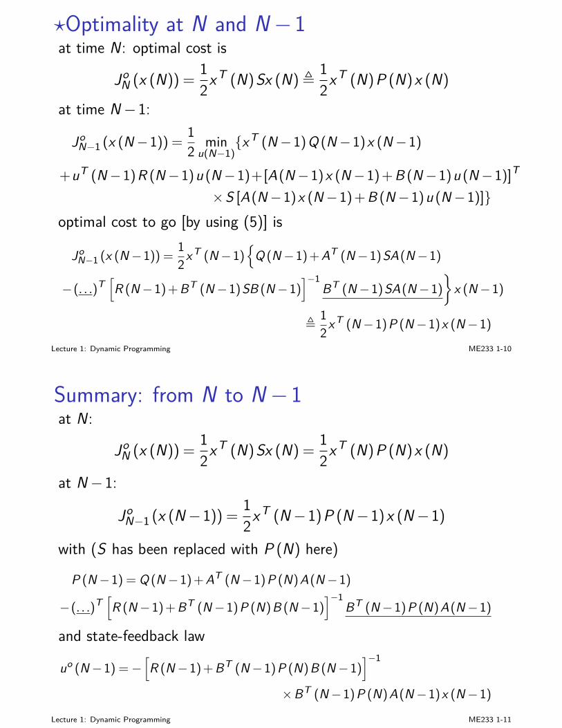
?Optimality at N and N−1at time N : optimal cost is
JoN (x (N)) =
12xT (N)Sx (N), 1
2xT (N)P (N)x (N)
at time N−1:
JoN−1 (x (N−1)) = 1
2 minu(N−1)
xT (N−1)Q (N−1)x (N−1)
+uT (N−1)R (N−1)u (N−1)+[A(N−1)x (N−1)+B (N−1)u (N−1)]T
×S [A(N−1)x (N−1)+B (N−1)u (N−1)]optimal cost to go [by using (5)] is
JoN−1 (x (N−1)) = 1
2xT (N−1)
Q (N−1)+AT (N−1)SA(N−1)
−(. . .)T[R (N−1)+BT (N−1)SB (N−1)
]−1BT (N−1)SA(N−1)
x (N−1)
, 12xT (N−1)P (N−1)x (N−1)
Lecture 1: Dynamic Programming ME233 1-10
Summary: from N to N−1at N :
JoN (x (N)) =
12xT (N)Sx (N) =
12xT (N)P (N)x (N)
at N−1:
JoN−1 (x (N−1)) = 1
2xT (N−1)P (N−1)x (N−1)
with (S has been replaced with P (N) here)
P (N−1) = Q (N−1)+AT (N−1)P (N)A(N−1)
−(. . .)T[R (N−1)+BT (N−1)P (N)B (N−1)
]−1BT (N−1)P (N)A(N−1)
and state-feedback law
uo (N−1) =−[R (N−1)+BT (N−1)P (N)B (N−1)
]−1
×BT (N−1)P (N)A(N−1)x (N−1)Lecture 1: Dynamic Programming ME233 1-11
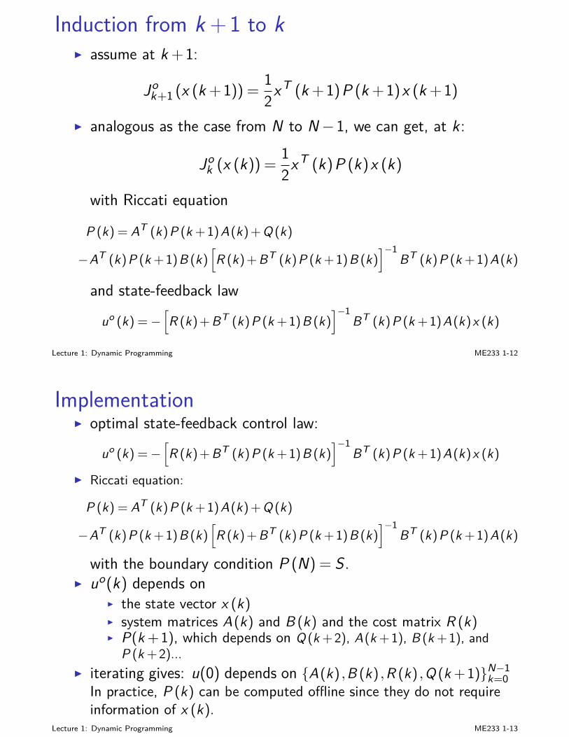
Induction from k +1 to kI assume at k +1:
Jok+1 (x (k +1)) = 1
2xT (k +1)P (k +1)x (k +1)
I analogous as the case from N to N−1, we can get, at k :
Jok (x (k)) =
12xT (k)P (k)x (k)
with Riccati equation
P (k) = AT (k)P (k +1)A(k)+Q (k)
−AT (k)P (k +1)B (k)[R (k)+BT (k)P (k +1)B (k)
]−1BT (k)P (k +1)A(k)
and state-feedback law
uo (k) =−[R (k)+BT (k)P (k +1)B (k)
]−1BT (k)P (k +1)A(k)x (k)
Lecture 1: Dynamic Programming ME233 1-12
ImplementationI optimal state-feedback control law:
uo (k) =−[R (k)+BT (k)P (k +1)B (k)
]−1BT (k)P (k +1)A(k)x (k)
I Riccati equation:
P (k) = AT (k)P (k +1)A(k)+Q (k)
−AT (k)P (k +1)B (k)[R (k)+BT (k)P (k +1)B (k)
]−1BT (k)P (k +1)A(k)
with the boundary condition P (N) = S.I uo(k) depends on
I the state vector x (k)I system matrices A(k) and B (k) and the cost matrix R (k)I P(k +1), which depends on Q (k +2), A(k +1), B (k +1), and
P (k +2)...I iterating gives: u(0) depends on A(k) ,B (k) ,R (k) ,Q (k +1)N−1
k=0In practice, P (k) can be computed offline since they do not requireinformation of x (k).
Lecture 1: Dynamic Programming ME233 1-13
ME 233, UC Berkeley, Spring 2014 Xu Chen
Lecture 3: Review of Probability Theory
Connection with control systemsRandom variable, distributionMultiple random variables
Random process, filtering a random process
Big picturewhy are we learning this:
We have been very familiar with deterministic systems:
x (k +1) = Ax (k) + Bu (k)
In practice, we commonly have:
x (k +1) = Ax (k) + Bu (k) + Bww (k)
where w (k) is the noise term that we have been neglecting. Withthe introduction of w (k), we need to equip ourselves with someadditional tool sets to understand and analyze the problem.
Lecture 3: Review of Probability Theory ME233 3-1
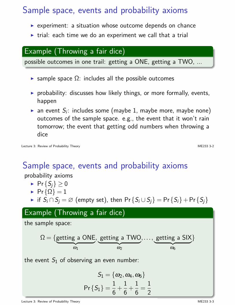
Sample space, events and probability axiomsI experiment: a situation whose outcome depends on chanceI trial: each time we do an experiment we call that a trial
Example (Throwing a fair dice)possible outcomes in one trail: getting a ONE, getting a TWO, ...
I sample space Ω: includes all the possible outcomes
I probability: discusses how likely things, or more formally, events,happen
I an event Si : includes some (maybe 1, maybe more, maybe none)outcomes of the sample space. e.g., the event that it won’t raintomorrow; the event that getting odd numbers when throwing adice
Lecture 3: Review of Probability Theory ME233 3-2
Sample space, events and probability axiomsprobability axioms
I PrSj ≥ 0I PrΩ= 1I if Si ∩Sj = ∅ (empty set), then PrSi ∪Sj= PrSi+PrSj
Example (Throwing a fair dice)the sample space:
Ω = getting a ONE︸ ︷︷ ︸ω1
, getting a TWO︸ ︷︷ ︸ω2
, . . . , getting a SIX︸ ︷︷ ︸ω6
the event S1 of observing an even number:
S1 = ω2,ω4,ω6
PrS1=16 +
16 +
16 =
12
Lecture 3: Review of Probability Theory ME233 3-3
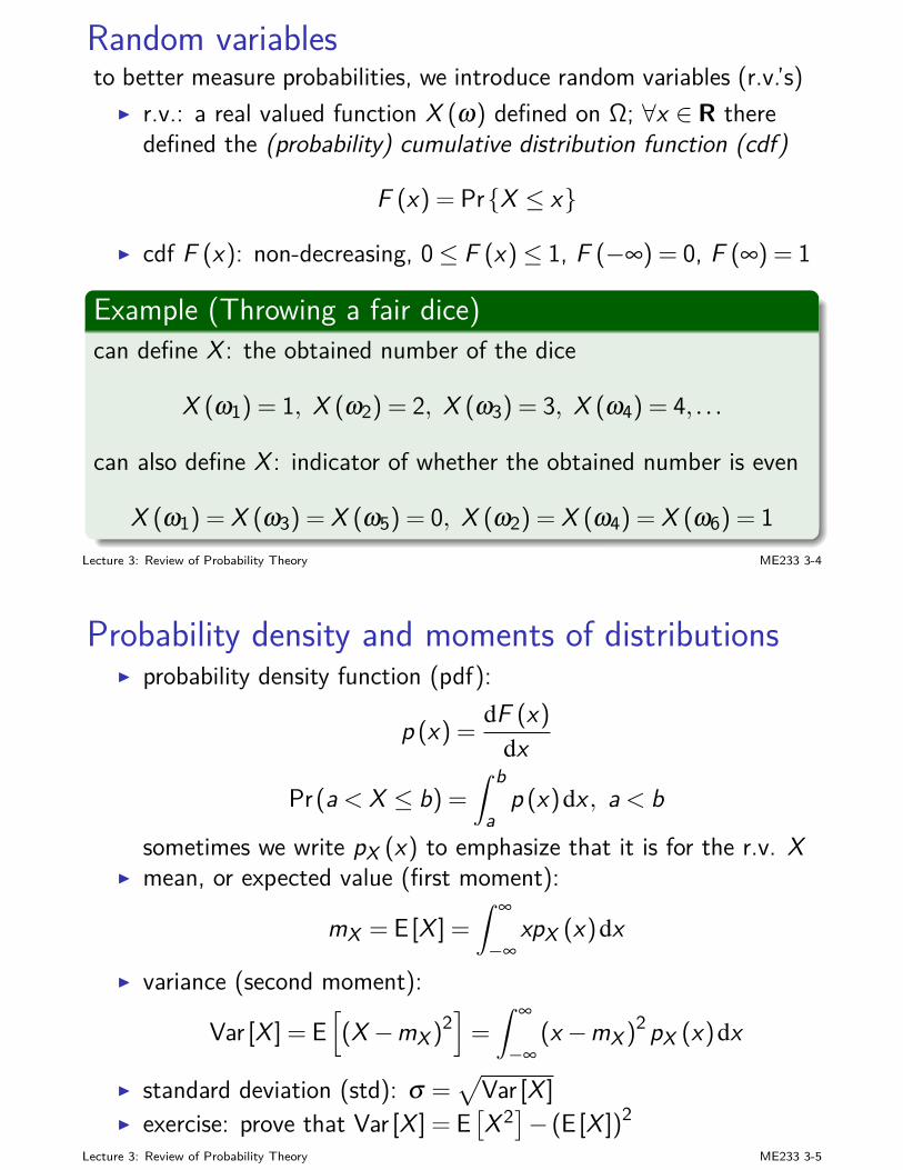
Random variablesto better measure probabilities, we introduce random variables (r.v.’s)
I r.v.: a real valued function X (ω) defined on Ω; ∀x ∈ R theredefined the (probability) cumulative distribution function (cdf)
F (x) = PrX ≤ x
I cdf F (x): non-decreasing, 0≤ F (x)≤ 1, F (−∞) = 0, F (∞) = 1
Example (Throwing a fair dice)can define X : the obtained number of the dice
X (ω1) = 1, X (ω2) = 2, X (ω3) = 3, X (ω4) = 4, . . .
can also define X : indicator of whether the obtained number is even
X (ω1) = X (ω3) = X (ω5) = 0, X (ω2) = X (ω4) = X (ω6) = 1Lecture 3: Review of Probability Theory ME233 3-4
Probability density and moments of distributionsI probability density function (pdf):
p (x) =dF (x)
dx
Pr(a < X ≤ b) =∫ b
ap (x)dx , a < b
sometimes we write pX (x) to emphasize that it is for the r.v. XI mean, or expected value (first moment):
mX = E [X ] =∫ ∞
−∞xpX (x)dx
I variance (second moment):
Var [X ] = E[
(X −mX )2]
=∫ ∞
−∞(x −mX )2 pX (x)dx
I standard deviation (std): σ =√
Var [X ]I exercise: prove that Var [X ] = E
[X 2]− (E [X ])2
Lecture 3: Review of Probability Theory ME233 3-5
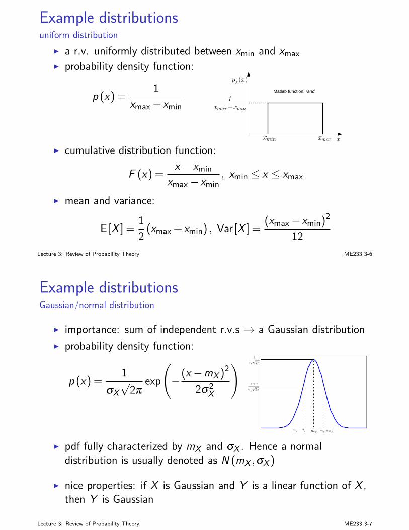
Example distributionsuniform distribution
I a r.v. uniformly distributed between xmin and xmaxI probability density function:
p (x) =1
xmax− xmin
pX(x)
1xmax¡xmin
xxmaxxmin
Matlab function: rand
I cumulative distribution function:
F (x) =x − xmin
xmax− xmin, xmin ≤ x ≤ xmax
I mean and variance:
E [X ] =12 (xmax + xmin) , Var [X ] =
(xmax− xmin)2
12Lecture 3: Review of Probability Theory ME233 3-6
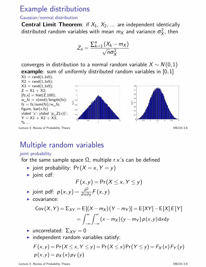
Example distributionsGaussian/normal distribution
I importance: sum of independent r.v.s → a Gaussian distributionI probability density function:
p (x) =1
σX√2π
exp(−(x −mX )2
2σ2X
) 1
σX
√
2π
0.607
σX
√
2π
mX− σ
X mX+ σ
XmX
I pdf fully characterized by mX and σX . Hence a normaldistribution is usually denoted as N (mX ,σX )
I nice properties: if X is Gaussian and Y is a linear function of X ,then Y is Gaussian
Lecture 3: Review of Probability Theory ME233 3-7
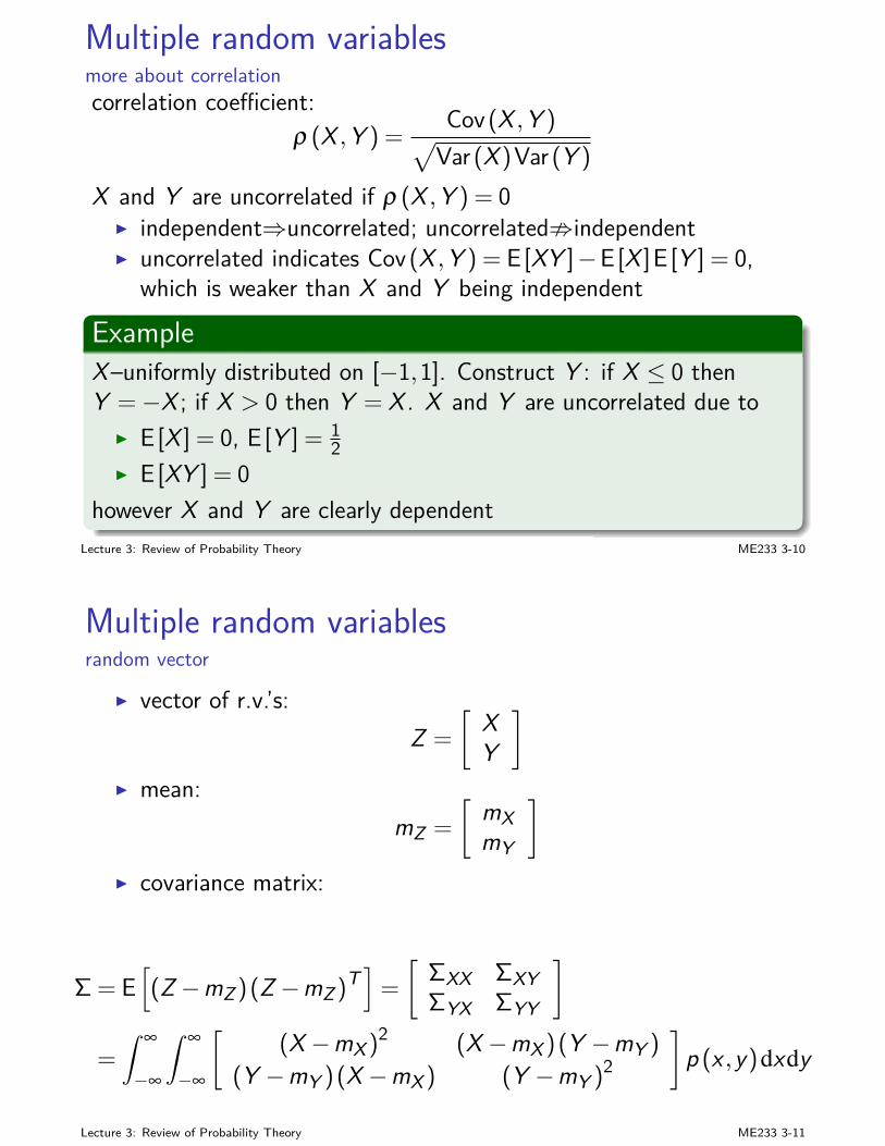
Example distributionsGaussian/normal distributionCentral Limit Theorem: if X1, X2, ... are independent identicallydistributed random variables with mean mX and variance σ2
X , then
Zn =∑n
k=1 (Xk −mX )√nσ2X
converges in distribution to a normal random variable X ∼ N (0,1)example: sum of uniformly distributed random variables in [0,1]X1 = rand(1,1e5);X2 = rand(1,1e5);X3 = rand(1,1e5);Z = X1 + X2;[fz,x] = hist(Z,100);w_fz = x(end)/length(fz);fz = fz/sum(fz)/w_fz;figure, bar(x,fz)xlabel ’x’; ylabel ’p_Z(x))’;Y = X1 + X2 + X3;% ...
Lecture 3: Review of Probability Theory ME233 3-8
Multiple random variablesjoint probabilityfor the same sample space Ω, multiple r.v.’s can be defined
I joint probability: Pr(X = x ,Y = y)I joint cdf:
F (x ,y) = Pr(X ≤ x ,Y ≤ y)
I joint pdf: p (x ,y) = ∂ 2∂x∂y F (x ,y)
I covariance:Cov (X ,Y ) = ΣXY = E [(X −mX )(Y −mY )] = E [XY ]−E [X ]E [Y ]
=∫ ∞
−∞
∫ ∞
−∞(x −mX )(y −mY )p (x ,y)dxdy
I uncorrelated: ΣXY = 0I independent random variables satisfy:
F (x ,y) = Pr(X ≤ x ,Y ≤ y) = Pr(X ≤ x)Pr(Y ≤ y) = FX (x)FY (y)
p (x ,y) = pX (x)pY (y)
Lecture 3: Review of Probability Theory ME233 3-9
Multiple random variablesmore about correlationcorrelation coefficient:
ρ (X ,Y ) =Cov (X ,Y )√Var (X )Var (Y )
X and Y are uncorrelated if ρ (X ,Y ) = 0I independent⇒uncorrelated; uncorrelated;independentI uncorrelated indicates Cov (X ,Y ) = E [XY ]−E [X ]E [Y ] = 0,
which is weaker than X and Y being independent
ExampleX–uniformly distributed on [−1,1]. Construct Y : if X ≤ 0 thenY =−X ; if X > 0 then Y = X . X and Y are uncorrelated due to
I E [X ] = 0, E [Y ] = 12
I E [XY ] = 0however X and Y are clearly dependent
Lecture 3: Review of Probability Theory ME233 3-10
Multiple random variablesrandom vector
I vector of r.v.’s:Z =
[XY
]
I mean:mZ =
[mXmY
]
I covariance matrix:
Σ = E[
(Z −mZ )(Z −mZ )T]
=
[ΣXX ΣXYΣYX ΣYY
]
=∫ ∞
−∞
∫ ∞
−∞
[(X −mX )2 (X −mX )(Y −mY )
(Y −mY )(X −mX ) (Y −mY )2
]p (x ,y)dxdy
Lecture 3: Review of Probability Theory ME233 3-11
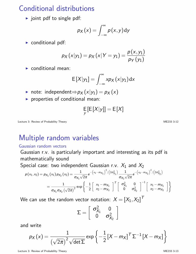
Conditional distributionsI joint pdf to single pdf:
pX (x) =∫ ∞
−∞p (x ,y)dy
I conditional pdf:
pX (x |y1) = pX (x |Y = y1) =p (x ,y1)
pY (y1)
I conditional mean:
E [X |y1] =∫ ∞
−∞xpX (x |y1)dx
I note: independent⇒pX (x |y1) = pX (x)I properties of conditional mean:
Ey
[E [X |y ]] = E [X ]
Lecture 3: Review of Probability Theory ME233 3-12
Multiple random variablesGaussian random vectorsGaussian r.v. is particularly important and interesting as its pdf ismathematically soundSpecial case: two independent Gaussian r.v. X1 and X2
p (x1,x2) = pX1 (x1)pX2 (x2) =1
σX1
√2π
e−(
x1−mX1
)2/(2σ2
X1
)1
σX2
√2π
e−(
x2−mX2
)2/(2σ2
X2
)
=1
σX1σX2(√
2π)2 exp
−12
[x1−mX1x2−mX2
]T [ σ2X1
00 σ2
X2
]−1 [ x1−mX1x2−mX2
]
We can use the random vector notation: X = [X1,X2]T
Σ =
[σ2
X10
0 σ2X2
]
and write
pX (x) =1
(√2π)2√detΣ
exp−12 [X −mX ]T Σ−1 [X −mX ]
Lecture 3: Review of Probability Theory ME233 3-13
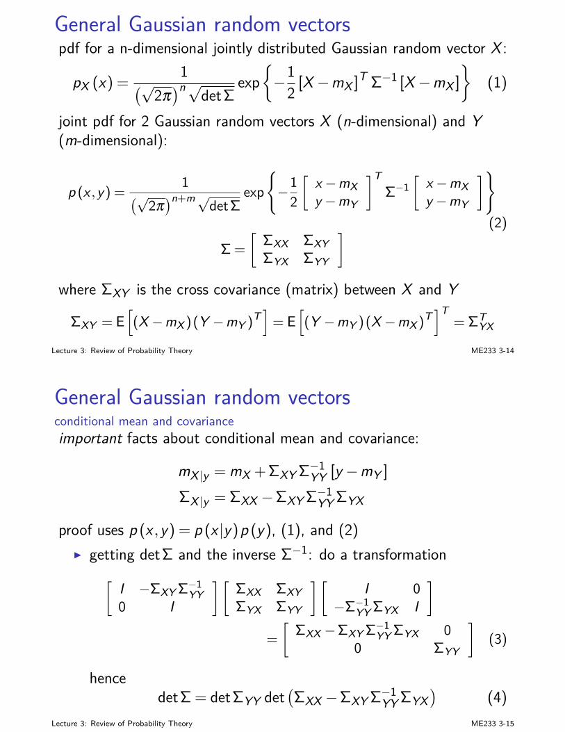
General Gaussian random vectorspdf for a n-dimensional jointly distributed Gaussian random vector X :
pX (x) =1(√
2π)n√detΣ
exp−12 [X −mX ]T Σ−1 [X −mX ]
(1)
joint pdf for 2 Gaussian random vectors X (n-dimensional) and Y(m-dimensional):
p (x ,y) =1
(√2π)n+m√detΣ
exp−12
[x −mXy −mY
]TΣ−1
[x −mXy −mY
]
(2)
Σ =
[ΣXX ΣXYΣYX ΣYY
]
where ΣXY is the cross covariance (matrix) between X and Y
ΣXY = E[(X −mX )(Y −mY )T
]= E
[(Y −mY )(X −mX )T
]T= ΣT
YX
Lecture 3: Review of Probability Theory ME233 3-14
General Gaussian random vectorsconditional mean and covarianceimportant facts about conditional mean and covariance:
mX |y = mX + ΣXY Σ−1YY [y −mY ]
ΣX |y = ΣXX −ΣXY Σ−1YY ΣYX
proof uses p (x ,y) = p (x |y)p (y), (1), and (2)I getting detΣ and the inverse Σ−1: do a transformation
[I −ΣXY Σ−1YY0 I
][ΣXX ΣXYΣYX ΣYY
][I 0
−Σ−1YY ΣYX I
]
=
[ΣXX −ΣXY Σ−1YY ΣYX 0
0 ΣYY
](3)
hencedetΣ = detΣYY det
(ΣXX −ΣXY Σ−1
YY ΣYX)
(4)Lecture 3: Review of Probability Theory ME233 3-15
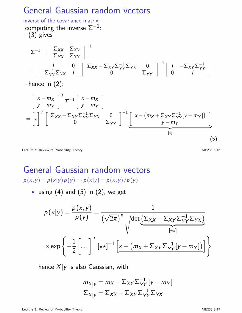
General Gaussian random vectorsinverse of the covariance matrixcomputing the inverse Σ−1:–(3) gives
Σ−1 =
[ΣXX ΣXYΣYX ΣYY
]−1
=
[I 0
−Σ−1YY ΣYX I
][ΣXX −ΣXY Σ−1YY ΣYX 0
0 ΣYY
]−1 [ I −ΣXY Σ−1YY0 I
]
–hence in (2):[
x −mXy −mY
]TΣ−1
[x −mXy −mY
]
=
[?
]T [ΣXX −ΣXY Σ−1YY ΣYX 0
0 ΣYY
]−1 [ x −(mX + ΣXY Σ−1YY [y −mY ]
)
y −mY
]
︸ ︷︷ ︸[?]
(5)
Lecture 3: Review of Probability Theory ME233 3-16
General Gaussian random vectorsp (x ,y) = p (x |y)p (y)⇒ p (x |y) = p (x ,y)/p (y)
I using (4) and (5) in (2), we get
p (x |y) =p (x ,y)
p (y)=
1(√
2π)n√det
(ΣXX −ΣXY Σ−1
YY ΣYX)
︸ ︷︷ ︸[??]
× exp−12
[. . .
]T[??]−1
[x −
(mX + ΣXY Σ−1
YY [y −mY ])]
hence X |y is also Gaussian, with
mX |y = mX + ΣXY Σ−1YY [y −mY ]
ΣX |y = ΣXX −ΣXY Σ−1YY ΣYX
Lecture 3: Review of Probability Theory ME233 3-17
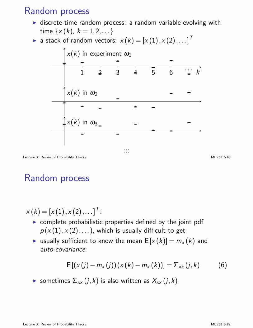
Random processI discrete-time random process: a random variable evolving with
time x (k), k = 1,2, . . .I a stack of random vectors: x (k) = [x (1) ,x (2) , . . . ]T
1 2 3 4 5 6 . . . k
x(k) in experiment ω1
x(k) in ω2
x(k) in ω3
.........Lecture 3: Review of Probability Theory ME233 3-18
Random process
x (k) = [x (1) ,x (2) , . . . ]T :I complete probabilistic properties defined by the joint pdf
p (x (1) ,x (2) , . . .), which is usually difficult to getI usually sufficient to know the mean E [x (k)] = mx (k) and
auto-covariance:
E [(x (j)−mx (j))(x (k)−mx (k))] = Σxx (j ,k) (6)
I sometimes Σxx (j ,k) is also written as Xxx (j ,k)
Lecture 3: Review of Probability Theory ME233 3-19
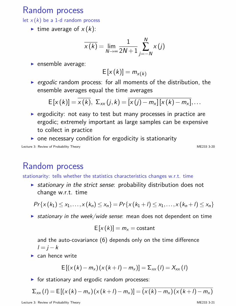
Random processlet x (k) be a 1-d random process
I time average of x (k):
x (k) = limN→∞
12N +1
N∑
j=−Nx (j)
I ensemble average:E [x (k)] = mx(k)
I ergodic random process: for all moments of the distribution, theensemble averages equal the time averages
E [x (k)] = x (k), Σxx (j ,k) = [x (j)−mx ] [x (k)−mx ], . . .
I ergodicity: not easy to test but many processes in practice areergodic; extremely important as large samples can be expensiveto collect in practice
I one necessary condition for ergodicity is stationarityLecture 3: Review of Probability Theory ME233 3-20
Random processstationarity: tells whether the statistics characteristics changes w.r.t. time
I stationary in the strict sense: probability distribution does notchange w.r.t. time
Prx (k1)≤ x1, . . . ,x (kn)≤ xn= Prx (k1 + l)≤ x1, . . . ,x (kn + l)≤ xnI stationary in the week/wide sense: mean does not dependent on time
E [x (k)] = mx = costant
and the auto-covariance (6) depends only on the time differencel = j−k
I can hence write
E [(x (k)−mx )(x (k + l)−mx )] = Σxx (l) = Xxx (l)
I for stationary and ergodic random processes:
Σxx (l) = E [(x (k)−mx )(x (k + l)−mx )] = (x (k)−mx )(x (k + l)−mx )
Lecture 3: Review of Probability Theory ME233 3-21
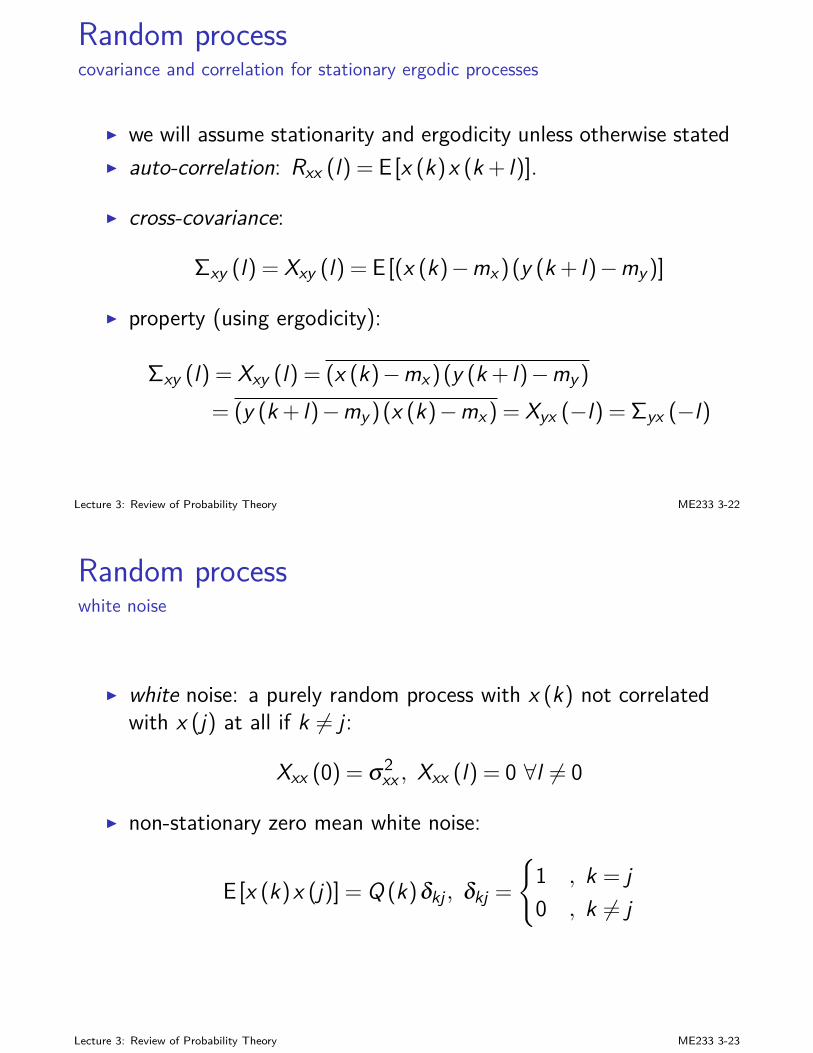
Random processcovariance and correlation for stationary ergodic processes
I we will assume stationarity and ergodicity unless otherwise statedI auto-correlation: Rxx (l) = E [x (k)x (k + l)].
I cross-covariance:
Σxy (l) = Xxy (l) = E [(x (k)−mx )(y (k + l)−my )]
I property (using ergodicity):
Σxy (l) = Xxy (l) = (x (k)−mx )(y (k + l)−my )
= (y (k + l)−my )(x (k)−mx ) = Xyx (−l) = Σyx (−l)
Lecture 3: Review of Probability Theory ME233 3-22
Random processwhite noise
I white noise: a purely random process with x (k) not correlatedwith x (j) at all if k 6= j :
Xxx (0) = σ2xx , Xxx (l) = 0 ∀l 6= 0
I non-stationary zero mean white noise:
E [x (k)x (j)] = Q (k)δkj , δkj =
1 , k = j0 , k 6= j
Lecture 3: Review of Probability Theory ME233 3-23
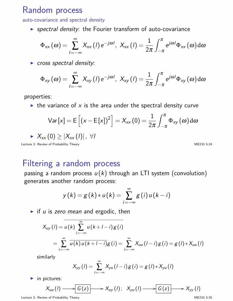
Random processauto-covariance and spectral density
I spectral density: the Fourier transform of auto-covariance
Φxx (ω) =∞
∑l=−∞
Xxx (l)e−jω l , Xxx (l) =12π
∫ π
−πejω l Φxx (ω)dω
I cross spectral density:
Φxy (ω) =∞
∑l=−∞
Xxy (l)e−jω l , Xxy (l) =12π
∫ π
−πejω l Φxy (ω)dω
properties:I the variance of x is the area under the spectral density curve
Var [x ] = E[
(x −E [x ])2]
= Xxx (0) =12π
∫ π
−πΦxy (ω)dω
I Xxx (0)≥ |Xxx (l)| , ∀lLecture 3: Review of Probability Theory ME233 3-24
Filtering a random processpassing a random process u (k) through an LTI system (convolution)generates another random process:
y (k) = g (k)∗u (k) =∞
∑i=−∞
g (i)u (k− i)
I if u is zero mean and ergodic, then
Xuy (l) = u (k)∞
∑i=−∞
u (k + l− i)g (i)
=∞
∑i=−∞
u (k)u (k + l− i)g (i) =∞
∑i=−∞
Xuu (l− i)g (i) = g (l)∗Xuu (l)
similarlyXyy (l) =
∞
∑i=−∞
Xyu (l− i)g (i) = g (l)∗Xyu (l)
I in pictures:
Xuu (l) // G (z) // Xuy (l) ; Xyu (l) // G (z) // Xyy (l)Lecture 3: Review of Probability Theory ME233 3-25
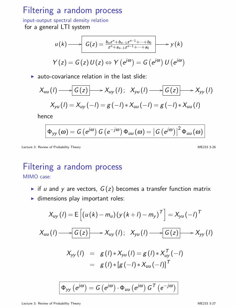
Filtering a random processinput-output spectral density relationfor a general LTI system
u (k) // G(z) = bnzn+bn−1zn−1+···+b0zn+an−1zn−1+···+a0
// y (k)
Y (z) = G (z)U (z)⇔ Y(ejω)= G
(ejω)U
(ejω)
I auto-covariance relation in the last slide:
Xuu (l) // G (z) // Xuy (l) ; Xyu (l) // G (z) // Xyy (l)
Xyu (l) = Xuy (−l) = g (−l)∗Xuu (−l) = g (−l)∗Xuu (l)hence
Φyy (ω) = G(ejω)G
(e−jω)Φuu (ω) =
∣∣G(ejω)∣∣2 Φuu (ω)
Lecture 3: Review of Probability Theory ME233 3-26
Filtering a random processMIMO case:
I if u and y are vectors, G (z) becomes a transfer function matrixI dimensions play important roles:
Xuy (l) = E[
(u (k)−mu)(y (k + l)−my )T]
= Xyu (−l)T
Xuu (l) // G (z) // Xuy (l) ; Xyu (l) // G (z) // Xyy (l)
Xyy (l) = g (l)∗Xyu (l) = g (l)∗XTuy (−l)
= g (l)∗ [g (−l)∗Xuu (−l)]T
Φyy(ejω)= G
(ejω) ·Φuu
(ejω)GT (e−jω)
Lecture 3: Review of Probability Theory ME233 3-27
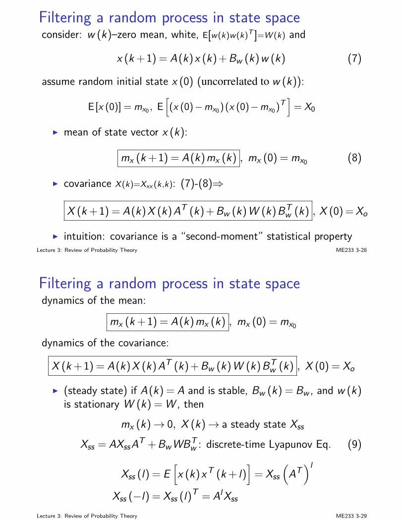
Filtering a random process in state spaceconsider: w (k)–zero mean, white, E[w(k)w(k)T ]=W (k) and
x (k +1) = A(k)x (k) + Bw (k)w (k) (7)
assume random initial state x (0) (uncorrelated to w (k)):
E [x (0)] = mx0 , E[(x (0)−mx0)(x (0)−mx0)T
]= X0
I mean of state vector x (k):
mx (k +1) = A(k)mx (k) , mx (0) = mx0 (8)
I covariance X(k)=Xxx (k,k): (7)-(8)⇒
X (k +1) = A(k)X (k)AT (k) + Bw (k)W (k)BTw (k) , X (0) = Xo
I intuition: covariance is a “second-moment” statistical propertyLecture 3: Review of Probability Theory ME233 3-28
Filtering a random process in state spacedynamics of the mean:
mx (k +1) = A(k)mx (k) , mx (0) = mx0
dynamics of the covariance:
X (k +1) = A(k)X (k)AT (k) + Bw (k)W (k)BTw (k) , X (0) = Xo
I (steady state) if A(k) = A and is stable, Bw (k) = Bw , and w (k)is stationary W (k) = W , then
mx (k)→ 0, X (k)→ a steady state Xss
Xss = AXssAT + BwWBTw : discrete-time Lyapunov Eq. (9)
Xss (l) = E[x (k)xT (k + l)
]= Xss
(AT)l
Xss (−l) = Xss (l)T = AlXss
Lecture 3: Review of Probability Theory ME233 3-29
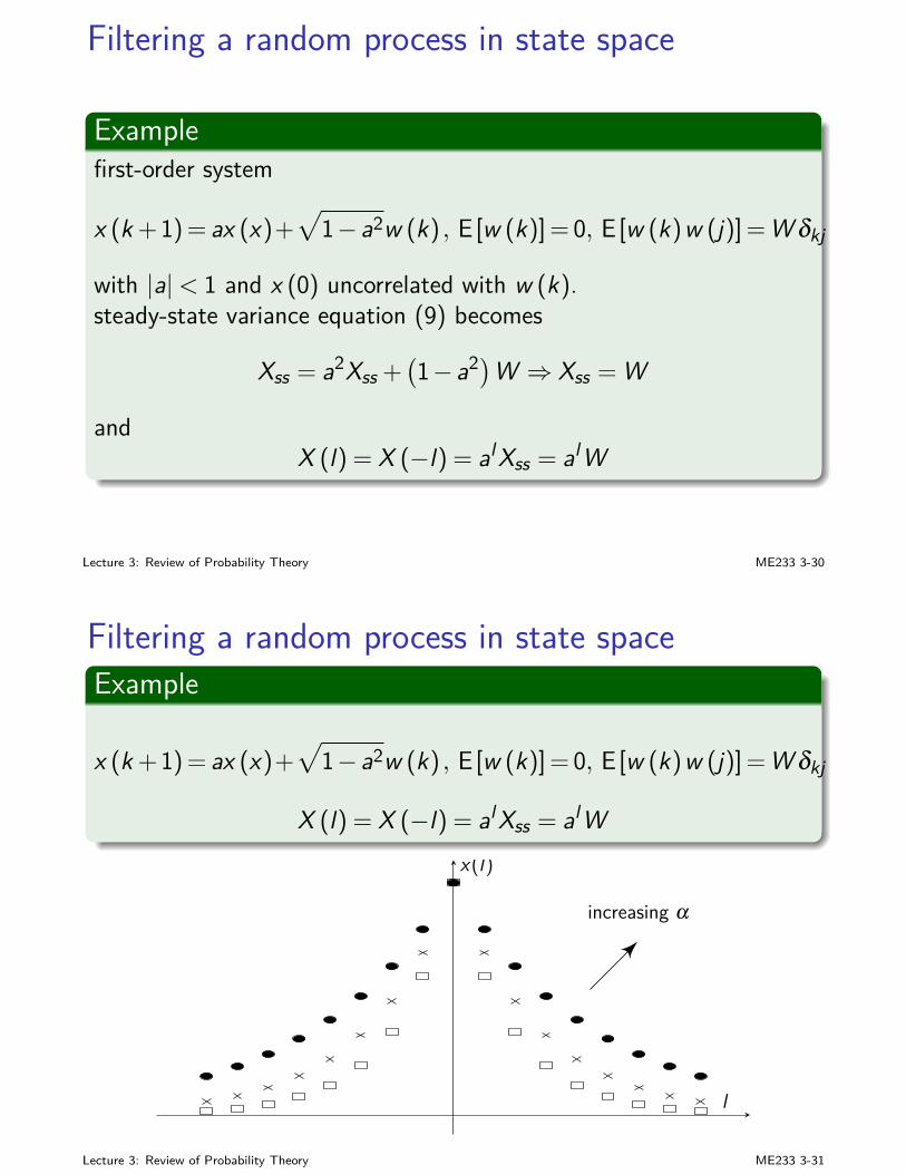
Filtering a random process in state space
Examplefirst-order system
x (k +1) = ax (x)+√
1−a2w (k) , E [w (k)] = 0, E [w (k)w (j)] = W δkj
with |a|< 1 and x (0) uncorrelated with w (k).steady-state variance equation (9) becomes
Xss = a2Xss +(1−a2)W ⇒ Xss = W
andX (l) = X (−l) = alXss = alW
Lecture 3: Review of Probability Theory ME233 3-30
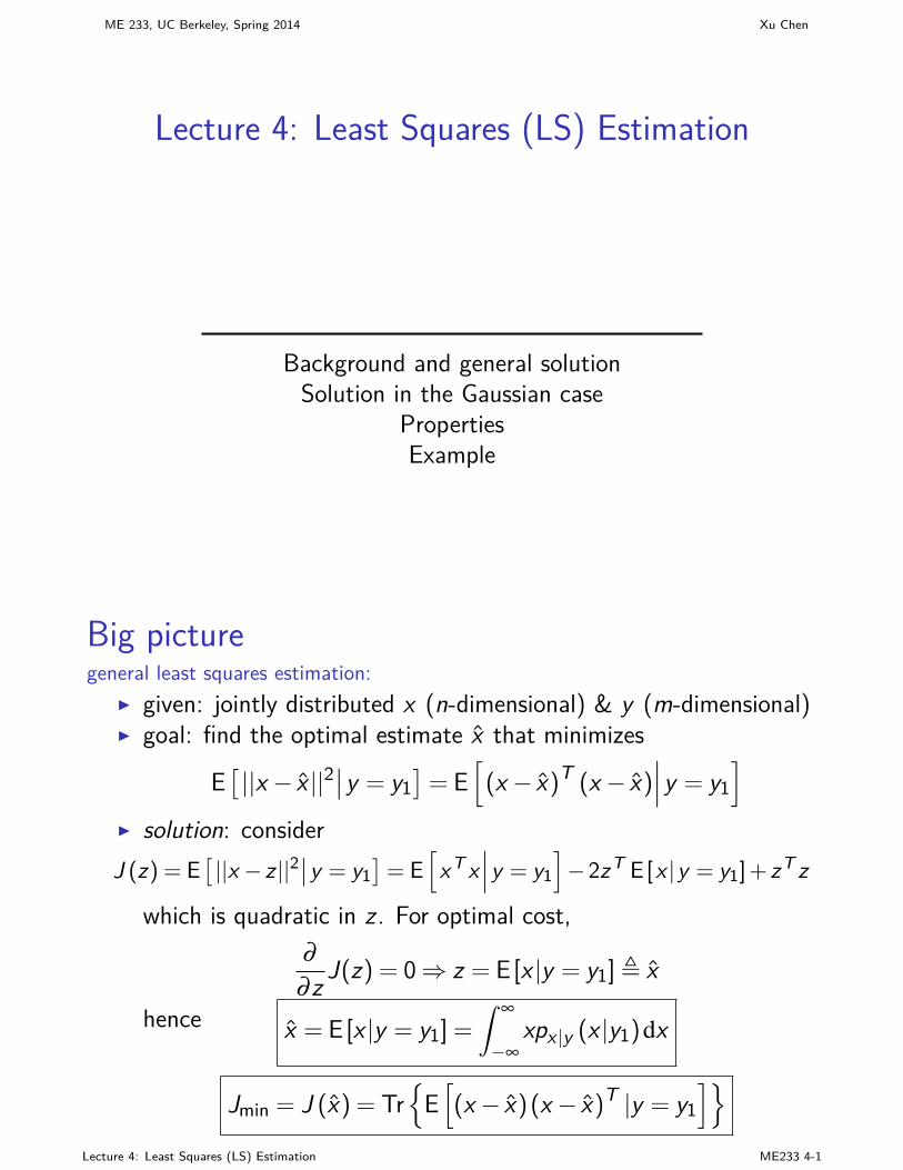
Filtering a random process in state spaceExample
x (k +1) = ax (x)+√
1−a2w (k) , E [w (k)] = 0, E [w (k)w (j)] = W δkj
X (l) = X (−l) = alXss = alWx(l)
l
increasing α
Lecture 3: Review of Probability Theory ME233 3-31

Filtering a random processcontinuous-time casesimilar results hold in the continuous-time case:
u (t) // G(s) // y (t)
I spectral density (SISO case):Φyy (jω) = G (jω)G (−jω)Φuu (jω) = |G (jω)|2 Φuu (jω)
I mean and covariance dynamics:dx (t)
dt = Ax (t) + Bw w (t) , E [w (t)] = 0, Cov [w (t)] = Wdmx (t)
dt = Amx (t) , mx (0) = mx0
dX (t)
dt = AX + XAT + Bw WBTw
I steady state: Xss (τ) = XsseAT τ ; Xss (−τ) = eAτXss whereAXss + XssAT =−Bw WBT
w : continuout-time Lyapunov Eq.Lecture 3: Review of Probability Theory ME233 3-32
Appendix: Lyapunov equationsI discrete-time case:
AT PA−P =−Qhas the following unique solution iff λi (A)λj (A) 6= 1 for alli , j = 1, . . . ,n:
P =∞
∑k=0
(AT)k
QAk
I continuous-time case:
AT P + PA =−Q
has the following unique solution iff λi (A) + λj (A) 6= 0 for alli , j = 1, . . . ,n:
P =∫ ∞
0eAT tQeAtdt
Lecture 3: Review of Probability Theory ME233 3-33

Summary
1. Big picture
2. Basic concepts: sample space, events, probability axioms, randomvariable, pdf, cdf, probability distributions
3. Multiple random variablesrandom vector, joint probability and distribution, conditionalprobabilityGaussian case
4. Random process
Lecture 3: Review of Probability Theory ME233 3-34
ME 233, UC Berkeley, Spring 2014 Xu Chen
Lecture 4: Least Squares (LS) Estimation
Background and general solutionSolution in the Gaussian case
PropertiesExample
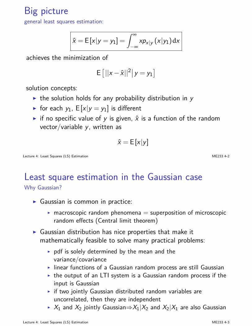
Big picturegeneral least squares estimation:
I given: jointly distributed x (n-dimensional) & y (m-dimensional)I goal: find the optimal estimate x that minimizes
E[||x − x ||2
∣∣y = y1]= E
[(x − x)T (x − x)
∣∣∣y = y1]
I solution: considerJ (z) = E
[||x − z ||2
∣∣y = y1]= E
[xT x
∣∣∣y = y1]−2zT E [x |y = y1]+ zT z
which is quadratic in z . For optimal cost,∂
∂z J(z) = 0⇒ z = E [x |y = y1], x
hence x = E [x |y = y1] =∫ ∞
−∞xpx |y (x |y1)dx
Jmin = J (x) = TrE[(x − x)(x − x)T |y = y1
]
Lecture 4: Least Squares (LS) Estimation ME233 4-1
Big picturegeneral least squares estimation:
x = E [x |y = y1] =∫ ∞
−∞xpx |y (x |y1)dx
achieves the minimization of
E[||x − x ||2
∣∣y = y1]
solution concepts:I the solution holds for any probability distribution in yI for each y1, E [x |y = y1] is differentI if no specific value of y is given, x is a function of the random
vector/variable y , written as
x = E [x |y ]Lecture 4: Least Squares (LS) Estimation ME233 4-2
Least square estimation in the Gaussian caseWhy Gaussian?
I Gaussian is common in practice:I macroscopic random phenomena = superposition of microscopicrandom effects (Central limit theorem)
I Gaussian distribution has nice properties that make itmathematically feasible to solve many practical problems:
I pdf is solely determined by the mean and thevariance/covariance
I linear functions of a Gaussian random process are still GaussianI the output of an LTI system is a Gaussian random process if theinput is Gaussian
I if two jointly Gaussian distributed random variables areuncorrelated, then they are independent
I X1 and X2 jointly Gaussian⇒X1|X2 and X2|X1 are also Gaussian
Lecture 4: Least Squares (LS) Estimation ME233 4-3
Least square estimation in the Gaussian caseWhy Gaussian?
Gaussian and white:I they are different conceptsI there can be Gaussian white noise, Poisson white noise, etcI Gaussian white noise is used a lot since it is a good
approximation to many practical noises
Lecture 4: Least Squares (LS) Estimation ME233 4-4
Least square estimation in the Gaussian casethe solutionproblem (re-stated): x , y–Gaussian distributed
minimize E[||x − x ||2
∣∣y]
solution: x = E [x |y ] = E [x ]+XxyX−1yy (y −E [y ])properties:
I the estimation is unbiased: E [x ] = E [x ]I y is Gaussian⇒x is Gaussian; and x − x is also GaussianI covariance of x :E[(x −E [x ]) (x −E [x ])T
]=E
(y −E [y ])
[Xxy X−1
yy (y −E [y ])]T
=Xxy X−1yy Xyx
I estimation error x , x − x : zero mean and
Cov [x ] = E[(x −E [x |y ]) (x −E [x |y ])T
]
︸ ︷︷ ︸conditional covariance
= Xxx −Xxy X−1yy Xyx
Lecture 4: Least Squares (LS) Estimation ME233 4-5
Least square estimation in the Gaussian case
x = E [x |y ] = E [x ]+XxyX−1yy (y −E [y ])
E [x |y ] is a better estimate than E [x ]:I the estimation is unbiased: E [x ] = E [x ]I estimation error x , x − x : zero mean and
Cov [x − x ] = Xxx −XxyX−1yy Xyx Cov [x −E [X ]]
Lecture 4: Least Squares (LS) Estimation ME233 4-6
Properties of least square estimate (Gaussian case)two random vectors x and y
Property 1:(i) the estimation error x = x − x is uncorrelated with y(ii) x and x are orthogonal:
E[(x − x)T x
]= 0
proof of (i):
E[x (y −my )
T]= E
[(x −E [x ]−XxyX−1yy (y −my )
)(y −my )
T]
= Xxy −XxyX−1yy Xyy = 0
Lecture 4: Least Squares (LS) Estimation ME233 4-7
Properties of least square estimate (Gaussian case)two random vectors x and y
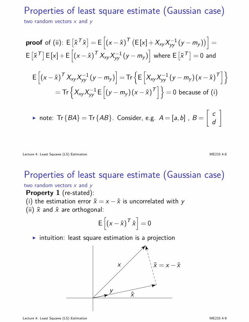
proof of (ii): E[xT x
]= E
[(x − x)T
(E [x ]+XxyX−1yy (y −my )
)]=
E[xT ]E [x ]+E
[(x − x)T XxyX−1yy (y −my )
]where E
[xT ]= 0 and
E[(x − x)T XxyX−1yy (y −my )
]=Tr
E[XxyX−1yy (y −my )(x − x)T
]
= Tr
XxyX−1yy E[(y −my )(x − x)T
]= 0 because of (i)
I note: TrBA= TrAB. Consider, e.g. A = [a,b] , B =
[cd
]
Lecture 4: Least Squares (LS) Estimation ME233 4-8
Properties of least square estimate (Gaussian case)two random vectors x and yProperty 1 (re-stated):(i) the estimation error x = x − x is uncorrelated with y(ii) x and x are orthogonal:
E[(x − x)T x
]= 0
I intuition: least square estimation is a projection
x = x − xx
xy
Lecture 4: Least Squares (LS) Estimation ME233 4-9

Properties of least square estimate (Gaussian case)three random vectors x y and z , where y and z are uncorrelatedProperty 2: let y and z be Gaussian and uncorrelated, then(i) the optimal estimate of x is
E [x |y ,z ] = E [x ]+first improvement︷ ︸︸ ︷(E [x |y ]−E [x ])+
second improvement︷ ︸︸ ︷(E [x |z ]−E [x ])
= E [x |y ]+ (E [x |z ]−E [x ])
Alternatively, let x|y , E [x |y ] , x|y , x −E [x |y ] = x − x|y , then
E [x |y ,z ] = E [x |y ]+E[x|y |z
]
(ii) the estimation error covariance isXxx −Xxy X−1
yy Xyx −XxzX−1zz Xzx = Xx x −XxzX−1
zz Xzx = Xx x −XxzX−1zz Xzx
where Xx x = E[x|y xT
|y
]and Xx z = E
[x|y (z−mz)
T]
Lecture 4: Least Squares (LS) Estimation ME233 4-10
Properties of least square estimate (Gaussian case)three random vectors x y and z , where y and z are uncorrelated
proof of (i): let w = [y ,z ]T
E [x |w ] = E [x ]+[
Xxy Xxz][ Xyy Xyz
Xzy Xzz
]−1[ y −E [y ]z−E [z ]
]
Using Xyz = 0 yields
E [x |w ] = E [x ]+XxyX−1yy (y −E [y ])︸ ︷︷ ︸E[x |y ]−E[x ]
+XxzX−1zz (z−E [z ])︸ ︷︷ ︸E[x |z]−E[x ]
= E [x |y ]+E[(
x|y + x|y)|z]−E [x ]
= E [x |y ]+E[x|y |z
]
where E[x|y |z
]= E [E [x |y ] |z ] = E [x ] as y and z are independent
Lecture 4: Least Squares (LS) Estimation ME233 4-11
Properties of least square estimate (Gaussian case)three random vectors x y and z , where y and z are uncorrelated
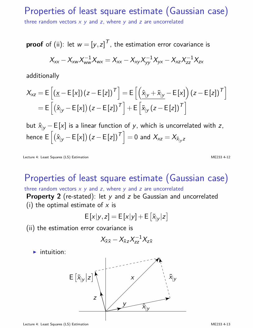
proof of (ii): let w = [y ,z ]T , the estimation error covariance is
Xxx −XxwX−1wwXwx = Xxx −XxyX−1yy Xyx −XxzX−1zz Xzx
additionally
Xxz = E[(x −E [x ]) (z−E [z ])T
]= E
[(x|y + x|y −E [x ]
)(z−E [z ])T
]
= E[(
x|y −E [x ])(z−E [z ])T
]+E
[x|y (z−E [z ])T
]
but x|y −E [x ] is a linear function of y , which is uncorrelated with z ,hence E
[(x|y −E [x ]
)(z−E [z ])T
]= 0 and Xxz = Xx|y z
Lecture 4: Least Squares (LS) Estimation ME233 4-12
Properties of least square estimate (Gaussian case)three random vectors x y and z , where y and z are uncorrelatedProperty 2 (re-stated): let y and z be Gaussian and uncorrelated(i) the optimal estimate of x is
E [x |y ,z ] = E [x |y ]+E[x|y |z
]
(ii) the estimation error covariance isXx x −Xx zX−1zz Xzx
I intuition:
z
xE[x|y∣∣z] x|y
x|yy
Lecture 4: Least Squares (LS) Estimation ME233 4-13
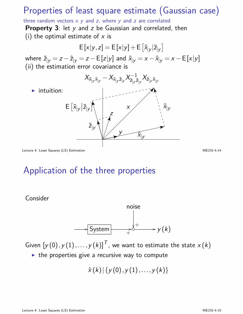
Properties of least square estimate (Gaussian case)three random vectors x y and z , where y and z are correlatedProperty 3: let y and z be Gaussian and correlated, then(i) the optimal estimate of x is
E [x |y ,z ] = E [x |y ]+E[x|y |z|y
]
where z|y = z− z|y = z−E [z |y ] and x|y = x − x|y = x −E [x |y ](ii) the estimation error covariance is
Xx|y x|y −Xx|y z|y X−1z|y z|y Xz|y x|y
I intuition:
z|y
E[x|y∣∣z|y]
zx x|y
x|yy
Lecture 4: Least Squares (LS) Estimation ME233 4-14
Application of the three properties
Considernoise
+// System+// // y (k)
Given [y (0) ,y (1) , . . . ,y (k)]T , we want to estimate the state x (k)I the properties give a recursive way to compute
x (k) |y (0) ,y (1) , . . . ,y (k)
Lecture 4: Least Squares (LS) Estimation ME233 4-15
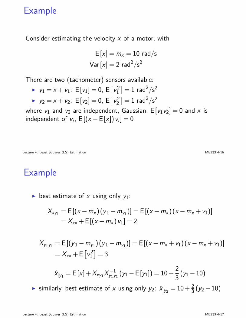
Example
Consider estimating the velocity x of a motor, with
E [x ] = mx = 10 rad/sVar [x ] = 2 rad2/s2
There are two (tachometer) sensors available:I y1 = x + v1: E [v1] = 0, E
[v21]= 1 rad2/s2
I y2 = x + v2: E [v2] = 0, E[v22]= 1 rad2/s2
where v1 and v2 are independent, Gaussian, E [v1v2] = 0 and x isindependent of vi , E [(x −E [x ])vi ] = 0
Lecture 4: Least Squares (LS) Estimation ME233 4-16
Example
I best estimate of x using only y1:
Xxy1 = E [(x −mx )(y1−my1)] = E [(x −mx )(x −mx + v1)]= Xxx +E [(x −mx )v1] = 2
Xy1y1 = E [(y1−my1)(y1−my1)] = E [(x −mx + v1)(x −mx + v1)]= Xxx +E
[v21]= 3
x|y1 = E [x ]+Xxy1X−1y1y1 (y1−E [y1]) = 10+ 23 (y1−10)
I similarly, best estimate of x using only y2: x|y2 = 10+ 23 (y2−10)
Lecture 4: Least Squares (LS) Estimation ME233 4-17
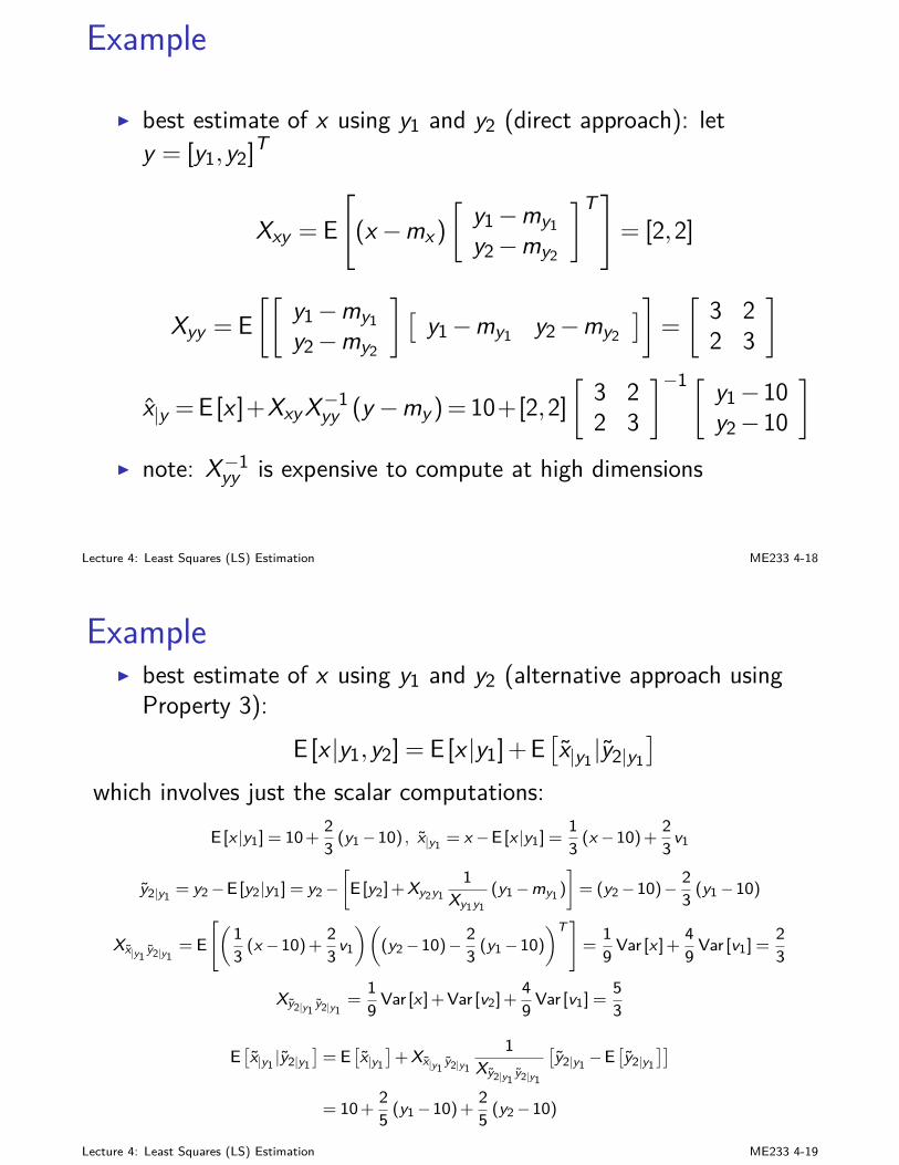
Example
I best estimate of x using y1 and y2 (direct approach): lety = [y1,y2]T
Xxy = E[(x −mx )
[y1−my1y2−my2
]T]= [2,2]
Xyy = E[[
y1−my1y2−my2
][y1−my1 y2−my2
]]=
[3 22 3
]
x|y =E [x ]+XxyX−1yy (y −my )= 10+[2,2][3 22 3
]−1[ y1−10y2−10
]
I note: X−1yy is expensive to compute at high dimensions
Lecture 4: Least Squares (LS) Estimation ME233 4-18
ExampleI best estimate of x using y1 and y2 (alternative approach using
Property 3):E [x |y1,y2] = E [x |y1]+E
[x|y1 |y2|y1
]
which involves just the scalar computations:E [x |y1] = 10+ 2
3 (y1−10) , x|y1 = x −E [x |y1] =13 (x −10)+ 2
3 v1
y2|y1 = y2−E [y2|y1] = y2−[E [y2]+Xy2y1
1Xy1y1
(y1−my1 )
]= (y2−10)− 2
3 (y1−10)
Xx|y1 y2|y1= E
[(13 (x −10)+ 2
3 v1
)((y2−10)− 2
3 (y1−10))T]
=19 Var [x ]+ 4
9 Var [v1] =23
Xy2|y1 y2|y1=
19 Var [x ]+Var [v2]+
49 Var [v1] =
53
E[x|y1 |y2|y1
]= E
[x|y1
]+Xx|y1 y2|y1
1Xy2|y1 y2|y1
[y2|y1 −E
[y2|y1
]]
= 10+ 25 (y1−10)+ 2
5 (y2−10)
Lecture 4: Least Squares (LS) Estimation ME233 4-19
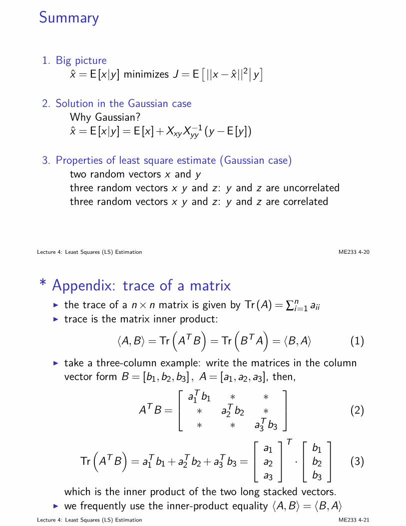
Summary
1. Big picturex = E [x |y ] minimizes J = E
[||x − x ||2
∣∣y]
2. Solution in the Gaussian caseWhy Gaussian?x = E [x |y ] = E [x ]+XxyX−1yy (y −E [y ])
3. Properties of least square estimate (Gaussian case)two random vectors x and ythree random vectors x y and z : y and z are uncorrelatedthree random vectors x y and z : y and z are correlated
Lecture 4: Least Squares (LS) Estimation ME233 4-20
* Appendix: trace of a matrixI the trace of a n×n matrix is given by Tr (A) = ∑n
i=1 aiiI trace is the matrix inner product:
〈A,B〉= Tr(
AT B)= Tr
(BT A
)= 〈B,A〉 (1)
I take a three-column example: write the matrices in the columnvector form B = [b1,b2,b3] , A = [a1,a2,a3], then,
AT B =
aT1 b1 ∗ ∗∗ aT
2 b2 ∗∗ ∗ aT
3 b3
(2)
Tr(
AT B)= aT
1 b1+aT2 b2+aT
3 b3 =
a1a2a3
T
·
b1b2b3
(3)
which is the inner product of the two long stacked vectors.I we frequently use the inner-product equality 〈A,B〉= 〈B,A〉
Lecture 4: Least Squares (LS) Estimation ME233 4-21
ME 233, UC Berkeley, Spring 2014 Xu Chen
Lecture 5: Stochastic State Estimation(Kalman Filter)
Big pictureProblem statement
Discrete-time Kalman FilterProperties
Continuous-time Kalman FilterPropertiesExample
Big picturewhy are we learning this?
I state estimation in deterministic case:
Plant: x (k +1) = Ax (k)+Bu (k) , y (k) = Cx (k)Observer: x (k +1) = Ax (k)+Bu (k)+L(y (k)−Cx (k))
I L designed based on the error (e (k) = x (k)− x (k)) dynamics:
e (k +1) = (A−LC)e (k) (1)
to reach fast convergence of limk→∞ e (k) = 0I L is not optimal when there is noise in the plant; actually
limk→∞ e (k) = 0 isn’t even a valid goal when there is noiseI Kalman Filter provides optimal state estimation under input and
output noisesLecture 5: Stochastic State Estimation (Kalman Filter) ME233 5-1
Problem statement
plant: x (k +1) = A(k)x (k)+B (k)u (k)+Bw (k)w (k)y (k) = C (k)x (k)+ v (k)
I w (k)–s-dimensional input noise; v (k)–r -dimensionalmeasurement noise; x (0)–unknown initial state
I assumptions: x (0), w (k), and v (k) are independent andGaussian distributed; w (k) and v (k) are white:
E [x (0)] = xo, E[(x (0)−xo)(x (0)−xo)T
]= X0
E [w (k)] = 0, E [v (k)] = 0, E[w (k)vT (j)
]= 0 ∀k, j
E[w (k)wT (j)
]= W (k)δkj , E
[v (k)vT (j)
]= V (k)δkj
Lecture 5: Stochastic State Estimation (Kalman Filter) ME233 5-2
Problem statement
I goal:
minimize E[||x (k)− x (k) ||2
∣∣Yj
], Yj = y (0) ,y (1) , . . . ,y (j)
I solution:x (k) = E [x (k) |Yj ]
I three classes of problems:I k > j : prediction problemI k = j : filtering problemI k < j : smoothing problem
Lecture 5: Stochastic State Estimation (Kalman Filter) ME233 5-3
History
Rudolf Kalman:I obtained B.S. in 1953 and M.S. in 1954 from MIT, and Ph.D. in
1957 from Columbia University, all in Electrical EngineeringI developed and implemented Kalman Filter in 1960, during the
Apollo program, and furthermore in various famous programsincluding the NASA Space Shuttle, Navy submarines, etc.
I was awarded the National Medal of Science on Oct. 7, 2009from U.S. president Barack Obama
Lecture 5: Stochastic State Estimation (Kalman Filter) ME233 5-4
Useful factsassume x is Gaussian distributed
I if y = Ax +B then
Xxy = E[(x −E [x ]) (y −E [y ])T
]= XxxAT
Xyy = E[(y −E [y ]) (y −E [y ])T
]= AXxxAT (2)
I if y = Ax +B and y ′ = A′x +B ′ then
Xyy ′ = AXxx(
A′)T
, Xy ′y = A′XxxAT (3)I if y = Ax +Bv ; v is Gaussian and independent of x , then
Xyy = AXxxAT +BXvvBT (4)I if y = Ax +Bv , y ′ = A′x +B ′v ; v is Gaussian and dependent of
x , thenXyy ′ = AXxx
(A′)T
+ AXxv(
B ′)T
+ BXvx(
A′)T
+ BXvv(
B ′)T
(5)
Lecture 5: Stochastic State Estimation (Kalman Filter) ME233 5-5
Derivation of Kalman FilterI goal:
minimize E[||x (k)− x (k) ||2
∣∣Yk
], Yk = y (0) ,y (1) , . . . ,y (k)
I the best estimate is the conditional expectation
E [x (k) |Yk ] = E [x (k)|Yk−1,y (k)]= E [x (k) |Yk−1]+E
[x (k) |Yk−1
∣∣ y (k) |Yk−1
]
I introduce some notations:a priori estimation x (k|k−1) = E [x (k) |Yk−1] = x (k) |y(0),...y(k−1)
a posteriori estimation x (k|k) = E [x (k) |Yk ] = x (k) |y(0),...y(k)a priori covariance M (k) = E
[x (k) |Yk−1 xT (k) |Yk−1
]
a posteriori covariance Z (k) = E[x (k) |Yk xT (k) |Yk
]
Lecture 5: Stochastic State Estimation (Kalman Filter) ME233 5-6
Derivation of Kalman FilterKF gain updateto get E
[x (k) |Yk−1
∣∣ y (k) |Yk−1
]in
E [x (k) |Yk ] = E [x (k) |Yk−1]+E[x (k) |Yk−1
∣∣ y (k) |Yk−1
]
we need Xx(k)|Yk−1 y(k)|Yk−1and X−1
y(k)|Yk−1 y(k)|Yk−1
y (k) = C (k)x (k)+ v (k) gives
y (k) |Yk−1 = C (k) x (k|k−1)+ v (k) |Yk−1 = C (k) x (k|k−1)⇒ y (k) |Yk−1 = C (k) x (k|k−1)+ v (k)
hence
Xx(k)|Yk−1 y(k)|Yk−1= M (k)CT (k) (6)
Xy(k)|Yk−1 y(k)|Yk−1= C (k)M (k)CT (k)+V (k) (7)
Lecture 5: Stochastic State Estimation (Kalman Filter) ME233 5-7
Derivation of Kalman FilterKF gain update
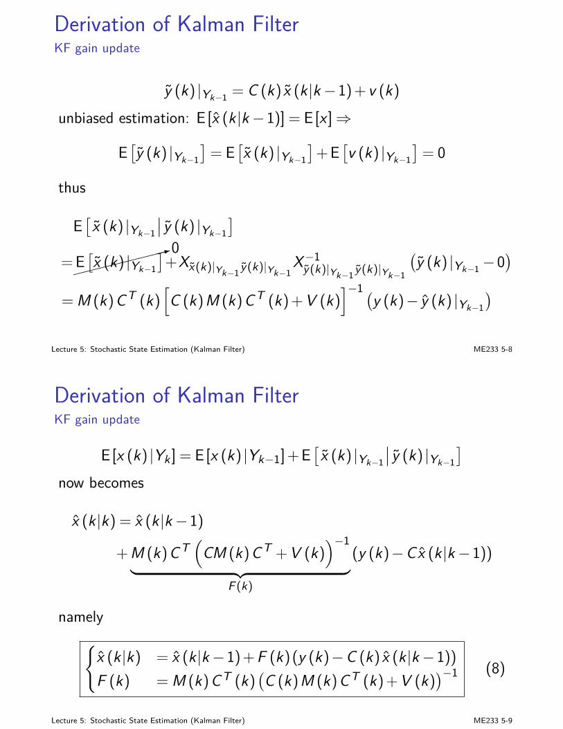
y (k) |Yk−1 = C (k) x (k|k−1)+ v (k)unbiased estimation: E [x (k|k−1)] = E [x ]⇒
E[y (k) |Yk−1
]= E
[x (k) |Yk−1
]+E
[v (k) |Yk−1
]= 0
thus
E[x (k) |Yk−1
∣∣ y (k) |Yk−1
]
=
:0
E[x (k) |Yk−1
]+Xx(k)|Yk−1 y(k)|Yk−1
X−1y(k)|Yk−1 y(k)|Yk−1
(y (k) |Yk−1−0
)
= M (k)CT (k)[C (k)M (k)CT (k)+V (k)
]−1 (y (k)− y (k) |Yk−1
)
Lecture 5: Stochastic State Estimation (Kalman Filter) ME233 5-8
Derivation of Kalman FilterKF gain update
E [x (k) |Yk ] = E [x (k) |Yk−1]+E[x (k) |Yk−1
∣∣ y (k) |Yk−1
]
now becomes
x (k|k) = x (k|k−1)
+M (k)CT(
CM (k)CT +V (k))−1
︸ ︷︷ ︸F (k)
(y (k)−Cx (k|k−1))
namely
x (k|k) = x (k|k−1)+F (k)(y (k)−C (k) x (k|k−1))F (k) = M (k)CT (k)
(C (k)M (k)CT (k)+V (k)
)−1 (8)
Lecture 5: Stochastic State Estimation (Kalman Filter) ME233 5-9
Derivation of Kalman FilterKF covariance update
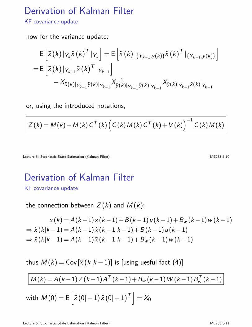
now for the variance update:
E[x (k) |Yk x (k)T |Yk
]= E
[x (k) |Yk−1,y(k)x (k)
T |Yk−1,y(k)]
=E[x (k) |Yk−1 x (k)T |Yk−1
]
−Xx(k)|Yk−1 y(k)|Yk−1X−1
y(k)|Yk−1 y(k)|Yk−1Xy(k)|Yk−1 x(k)|Yk−1
or, using the introduced notations,
Z (k) = M (k)−M (k)CT (k)(
C (k)M (k)CT (k) + V (k))−1
C (k)M (k)
Lecture 5: Stochastic State Estimation (Kalman Filter) ME233 5-10
Derivation of Kalman FilterKF covariance update
the connection between Z (k) and M (k):
x (k) = A(k−1)x (k−1) + B (k−1)u (k−1) + Bw (k−1)w (k−1)
⇒ x (k|k−1) = A(k−1) x (k−1|k−1) + B (k−1)u (k−1)
⇒ x (k|k−1) = A(k−1) x (k−1|k−1) + Bw (k−1)w (k−1)
thus M (k) = Cov [x (k|k−1)] is [using uesful fact (4)]
M (k) = A(k−1)Z (k−1)AT (k−1) + Bw (k−1)W (k−1)BTw (k−1)
with M (0) = E[x (0|−1) x (0|−1)T
]= X0
Lecture 5: Stochastic State Estimation (Kalman Filter) ME233 5-11
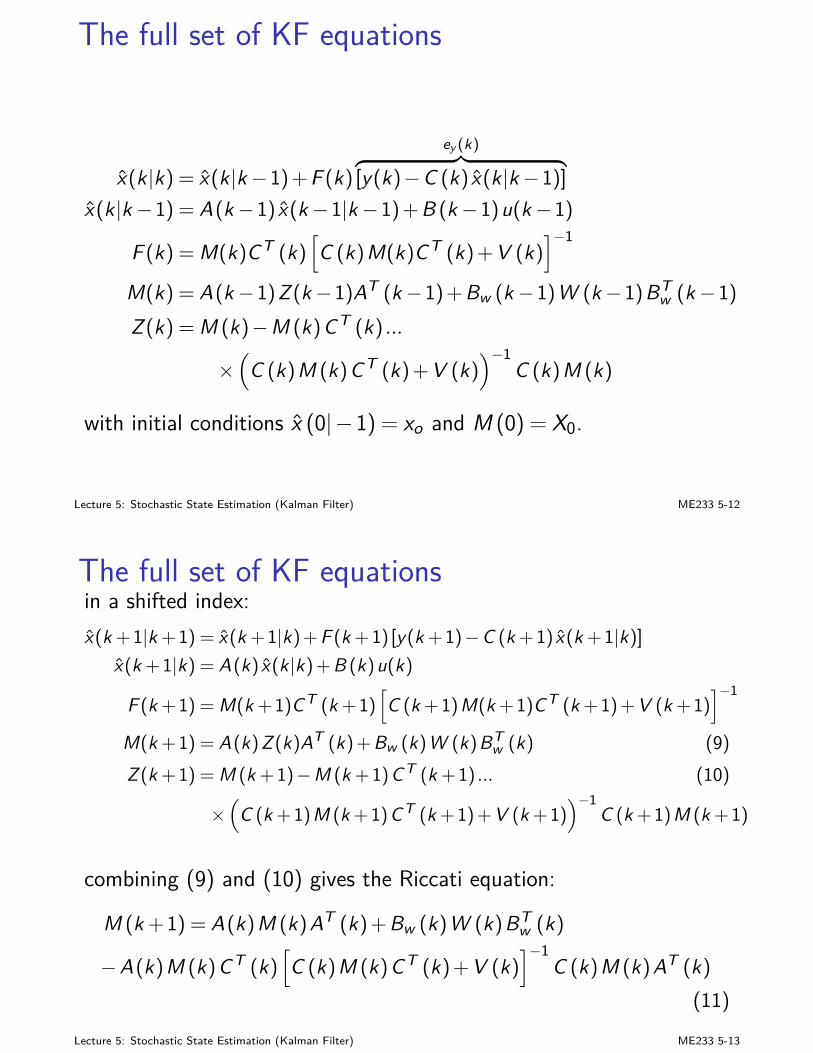
The full set of KF equations
x(k|k) = x(k|k−1) + F (k)
ey (k)︷ ︸︸ ︷[y(k)−C (k) x(k|k−1)]
x(k|k−1) = A(k−1) x(k−1|k−1) + B (k−1)u(k−1)
F (k) = M(k)CT (k)[C (k)M(k)CT (k) + V (k)
]−1
M(k) = A(k−1)Z (k−1)AT (k−1) + Bw (k−1)W (k−1)BTw (k−1)
Z (k) = M (k)−M (k)CT (k) ...
×(
C (k)M (k)CT (k) + V (k))−1
C (k)M (k)
with initial conditions x (0|−1) = xo and M (0) = X0.
Lecture 5: Stochastic State Estimation (Kalman Filter) ME233 5-12
The full set of KF equationsin a shifted index:x(k +1|k +1) = x(k +1|k) + F (k +1) [y(k +1)−C (k +1) x(k +1|k)]
x(k +1|k) = A(k) x(k|k) + B (k)u(k)
F (k +1) = M(k +1)CT (k +1)[C (k +1)M(k +1)CT (k +1) + V (k +1)
]−1
M(k +1) = A(k)Z (k)AT (k) + Bw (k)W (k)BTw (k) (9)
Z (k +1) = M (k +1)−M (k +1)CT (k +1) ... (10)
×(
C (k +1)M (k +1)CT (k +1) + V (k +1))−1
C (k +1)M (k +1)
combining (9) and (10) gives the Riccati equation:
M (k +1) = A(k)M (k)AT (k) + Bw (k)W (k)BTw (k)
−A(k)M (k)CT (k)[C (k)M (k)CT (k) + V (k)
]−1C (k)M (k)AT (k)
(11)Lecture 5: Stochastic State Estimation (Kalman Filter) ME233 5-13
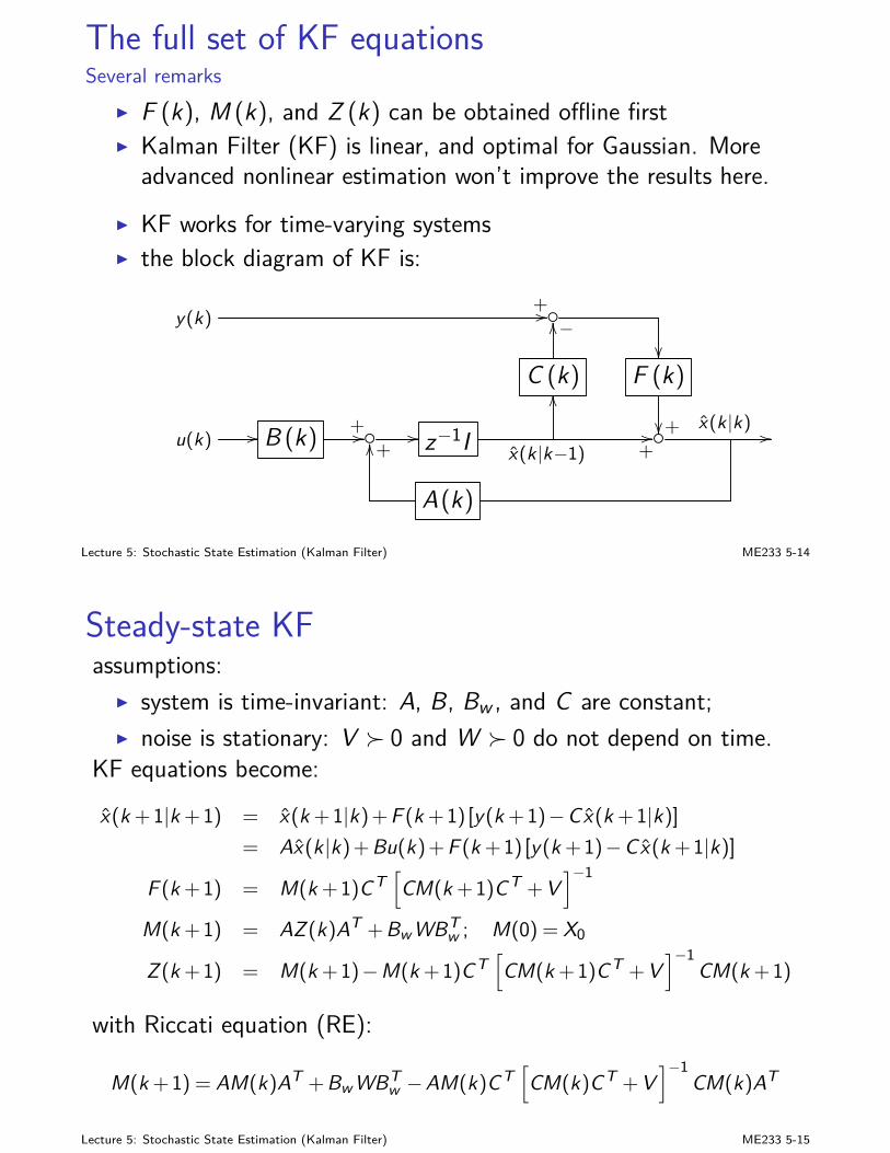
The full set of KF equationsSeveral remarks
I F (k), M (k), and Z (k) can be obtained offline firstI Kalman Filter (KF) is linear, and optimal for Gaussian. More
advanced nonlinear estimation won’t improve the results here.
I KF works for time-varying systemsI the block diagram of KF is:
y(k)+//
C (k)
−OO
F (k)
+u(k) // B (k) +// // z−1I x(k|k−1)
OO
+// x(k|k) //
+OO
A(k)
Lecture 5: Stochastic State Estimation (Kalman Filter) ME233 5-14
Steady-state KFassumptions:
I system is time-invariant: A, B, Bw , and C are constant;I noise is stationary: V 0 and W 0 do not depend on time.
KF equations become:
x(k +1|k +1) = x(k +1|k) + F (k +1) [y(k +1)−Cx(k +1|k)]
= Ax(k|k) + Bu(k) + F (k +1) [y(k +1)−Cx(k +1|k)]
F (k +1) = M(k +1)CT[CM(k +1)CT + V
]−1
M(k +1) = AZ (k)AT + Bw WBTw ; M(0) = X0
Z (k +1) = M(k +1)−M(k +1)CT[CM(k +1)CT + V
]−1CM(k +1)
with Riccati equation (RE):
M(k +1) = AM(k)AT + Bw WBTw −AM(k)CT
[CM(k)CT + V
]−1CM(k)AT
Lecture 5: Stochastic State Estimation (Kalman Filter) ME233 5-15
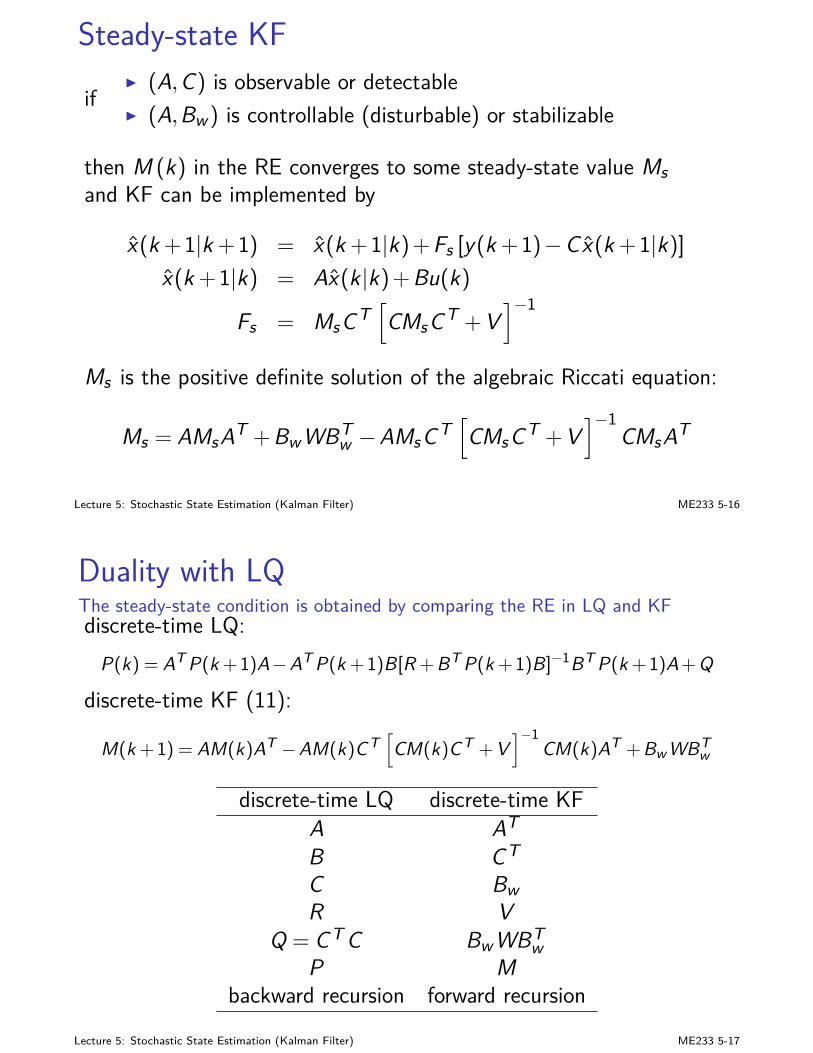
Steady-state KF
ifI (A,C) is observable or detectableI (A,Bw ) is controllable (disturbable) or stabilizable
then M (k) in the RE converges to some steady-state value Msand KF can be implemented by
x(k +1|k +1) = x(k +1|k)+Fs [y(k +1)−Cx(k +1|k)]x(k +1|k) = Ax(k|k)+Bu(k)
Fs = MsCT[CMsCT +V
]−1
Ms is the positive definite solution of the algebraic Riccati equation:
Ms = AMsAT +BwWBTw −AMsCT
[CMsCT +V
]−1CMsAT
Lecture 5: Stochastic State Estimation (Kalman Filter) ME233 5-16
Duality with LQThe steady-state condition is obtained by comparing the RE in LQ and KFdiscrete-time LQ:
P(k) = AT P(k +1)A−AT P(k +1)B[R + BT P(k +1)B]−1BT P(k +1)A + Q
discrete-time KF (11):
M(k +1) = AM(k)AT −AM(k)CT[CM(k)CT + V
]−1CM(k)AT + Bw WBT
w
discrete-time LQ discrete-time KFA AT
B CT
C BwR V
Q = CT C BwWBTw
P Mbackward recursion forward recursion
Lecture 5: Stochastic State Estimation (Kalman Filter) ME233 5-17
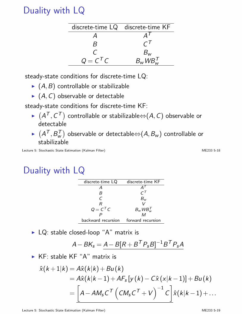
Duality with LQdiscrete-time LQ discrete-time KF
A AT
B CT
C BwQ = CT C BwWBT
w
steady-state conditions for discrete-time LQ:I (A,B) controllable or stabilizableI (A,C) observable or detectable
steady-state conditions for discrete-time KF:I(AT ,CT ) controllable or stabilizable⇔(A,C) observable ordetectable
I(AT ,BT
w)observable or detectable⇔(A,Bw ) controllable or
stabilizableLecture 5: Stochastic State Estimation (Kalman Filter) ME233 5-18
Duality with LQdiscrete-time LQ discrete-time KF
A AT
B CT
C BwR V
Q = CT C Bw WBTw
P Mbackward recursion forward recursion
I LQ: stable closed-loop “A” matrix isA−BKs = A−B[R +BT PsB]−1BT PsA
I KF: stable KF “A” matrix isx(k +1|k) = Ax(k|k)+Bu (k)
= Ax(k|k−1)+AFs [y (k)−Cx (x |k−1)]+Bu (k)
=
[A−AMsCT
(CMsCT +V
)−1C]x(k|k−1)+ . . .
Lecture 5: Stochastic State Estimation (Kalman Filter) ME233 5-19
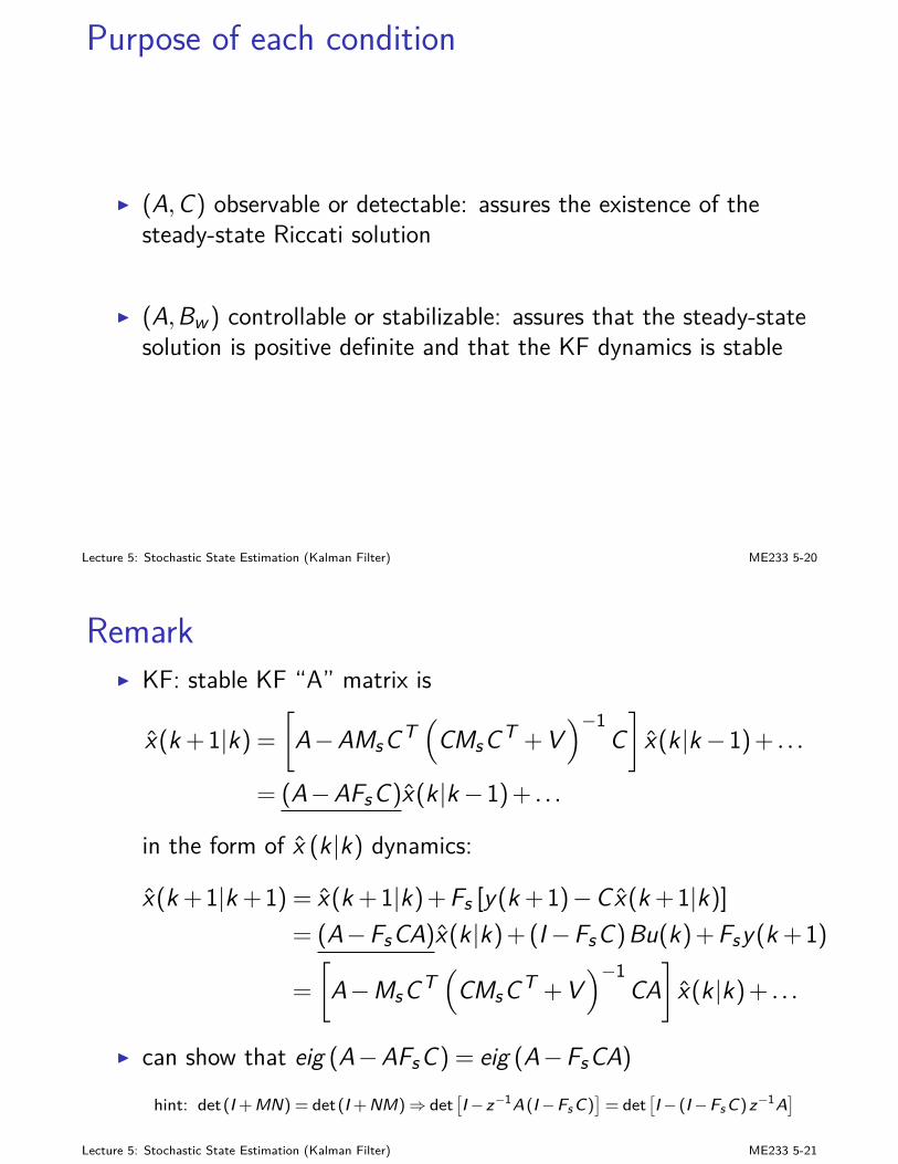
Purpose of each condition
I (A,C) observable or detectable: assures the existence of thesteady-state Riccati solution
I (A,Bw ) controllable or stabilizable: assures that the steady-statesolution is positive definite and that the KF dynamics is stable
Lecture 5: Stochastic State Estimation (Kalman Filter) ME233 5-20
RemarkI KF: stable KF “A” matrix is
x(k +1|k) =[A−AMsCT
(CMsCT +V
)−1C]
x(k|k−1)+ . . .
= (A−AFsC)x(k|k−1)+ . . .
in the form of x (k|k) dynamics:
x(k +1|k +1) = x(k +1|k)+Fs [y(k +1)−Cx(k +1|k)]= (A−FsCA)x(k|k)+(I−FsC)Bu(k)+Fsy(k +1)
=
[A−MsCT
(CMsCT +V
)−1CA]
x(k|k)+ . . .
I can show that eig (A−AFsC) = eig (A−FsCA)hint: det(I +MN) = det(I +NM)⇒ det
[I−z−1A(I−FsC)
]= det
[I− (I−FsC)z−1A
]
Lecture 5: Stochastic State Estimation (Kalman Filter) ME233 5-21
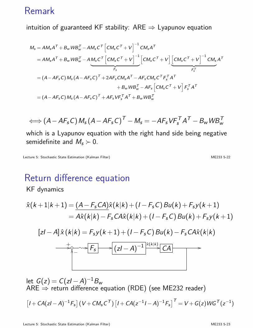
Remarkintuition of guaranteed KF stability: ARE ⇒ Lyapunov equation
Ms = AMsAT +Bw WBTw −AMsCT
[CMsCT +V
]−1CMsAT
= AMsAT +Bw WBTw −AMsCT
[CMsCT +V
]−1
︸ ︷︷ ︸Fs
[CMsCT +V
][CMsCT +V
]−1CMs
︸ ︷︷ ︸F Ts
AT
= (A−AFsC)Ms (A−AFsC)T +2AFsCMsAT −AFsCMsCT F Ts AT
+Bw WBTw −AFs
[CMsCT +V
]F T
s AT
= (A−AFsC)Ms (A−AFsC)T +AFsVF Ts AT +Bw WBT
w
⇐⇒ (A−AFsC)Ms (A−AFsC)T −Ms =−AFsVF Ts AT −BwWBT
w
which is a Lyapunov equation with the right hand side being negativesemidefinite and Ms 0.
Lecture 5: Stochastic State Estimation (Kalman Filter) ME233 5-22
Return difference equationKF dynamics
x(k +1|k +1) = (A−FsCA)x(k|k)+(I−FsC)Bu(k)+Fsy(k +1)= Ax(k|k)−FsCAx(k|k)+(I−FsC)Bu(k)+Fsy(k +1)
[zI−A] x (k|k) = Fsy(k +1)+(I−FsC)Bu(k)−FsCAx(k|k)+// ∼ // Fs // (zI−A)−1 x(k|k) // CA //−OO
let G(z) = C(zI−A)−1BwARE ⇒ return difference equation (RDE) (see ME232 reader)[I + CA(zI−A)−1Fs
](V +CMsCT )
[I + CA(z−1I−A)−1Fs
]T= V +G(z)WGT (z−1)
Lecture 5: Stochastic State Estimation (Kalman Filter) ME233 5-23
Symmetric root locus for KFI KF eigenvalues:
det[I +CA(zI−A)−1Fs
]= det
[I +(zI−A)−1FsCA
]
=det(zI−A+FsCA)
det(zI−A) , β (z)φ (z)
I taking determinants in RDE gives
β (z)β (z−1) = φ(z)φ(z−1)det(V +G(z)WGT (z−1)
)
det(V +CMCT )
I single-output case: KF poles come from β (z)β (z−1) = 0, i.e.
det(
V +G(z)WGT (z−1))= V
(1+G(z)W
V GT (z−1)
)= 0
I W /V → 0: KF poles → stable poles of G (z)GT (z−1)
I W /V → ∞: KF poles → stable zeros of G (z)GT (z−1)
Lecture 5: Stochastic State Estimation (Kalman Filter) ME233 5-24
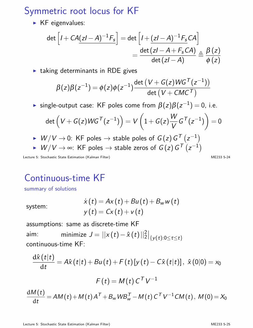
Continuous-time KFsummary of solutions
system: x (t) = Ax (t)+Bu (t)+Bww (t)y (t) = Cx (t)+ v (t)
assumptions: same as discrete-time KFaim: minimize J = ||x (t)− x (t) ||22
∣∣y(τ):0≤τ≤t
continuous-time KF:
dx (t|t)dt = Ax (t|t)+Bu (t)+F (t) [y (t)−Cx (t|t)] , x (0|0) = x0
F (t) = M (t)CT V−1
dM (t)
dt = AM (t)+M (t)AT +Bw WBTw −M (t)CT V−1CM (t) , M (0) = X0
Lecture 5: Stochastic State Estimation (Kalman Filter) ME233 5-25
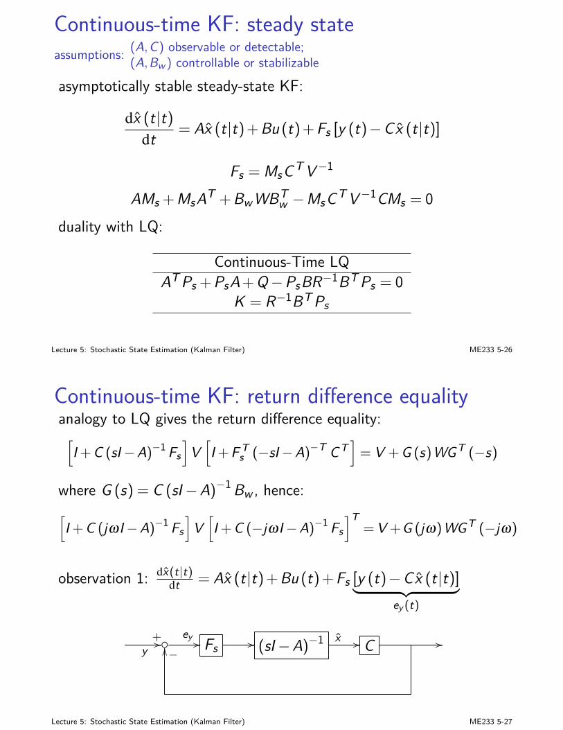
Continuous-time KF: steady stateassumptions: (A,C) observable or detectable;
(A,Bw ) controllable or stabilizable
asymptotically stable steady-state KF:
dx (t|t)dt = Ax (t|t)+Bu (t)+Fs [y (t)−Cx (t|t)]
Fs = MsCT V−1
AMs +MsAT +BwWBTw −MsCT V−1CMs = 0
duality with LQ:
Continuous-Time LQAT Ps +PsA+Q−PsBR−1BT Ps = 0
K = R−1BT Ps
Lecture 5: Stochastic State Estimation (Kalman Filter) ME233 5-26
Continuous-time KF: return difference equalityanalogy to LQ gives the return difference equality:[I + C (sI−A)−1 Fs
]V[I + F T
s (−sI−A)−T CT]
= V + G (s)WGT (−s)
where G (s) = C (sI−A)−1 Bw , hence:[I + C (jωI−A)−1 Fs
]V[I + C (−jωI−A)−1 Fs
]T= V +G (jω)WGT (−jω)
observation 1: dx(t|t)dt = Ax (t|t)+Bu (t)+Fs [y (t)−Cx (t|t)]︸ ︷︷ ︸
ey (t)
y+// ey // Fs // (sI−A)−1 x // C //−OO
Lecture 5: Stochastic State Estimation (Kalman Filter) ME233 5-27
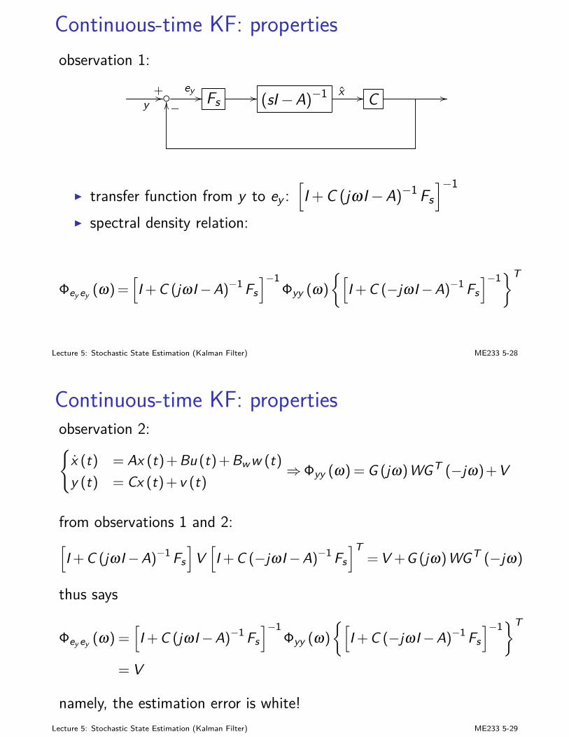
Continuous-time KF: propertiesobservation 1:
y+// ey // Fs // (sI−A)−1 x // C //−OO
I transfer function from y to ey :[I +C (jω I−A)−1 Fs
]−1
I spectral density relation:
Φey ey (ω) =[I + C (jωI−A)−1 Fs
]−1Φyy (ω)
[I + C (−jωI−A)−1 Fs
]−1T
Lecture 5: Stochastic State Estimation (Kalman Filter) ME233 5-28
Continuous-time KF: propertiesobservation 2:
x (t) = Ax (t) + Bu (t) + Bw w (t)
y (t) = Cx (t) + v (t)⇒Φyy (ω) = G (jω)WGT (−jω)+V
from observations 1 and 2:[I + C (jωI−A)−1 Fs
]V[I + C (−jωI−A)−1 Fs
]T= V +G (jω)WGT (−jω)
thus says
Φey ey (ω) =[I + C (jωI−A)−1 Fs
]−1Φyy (ω)
[I + C (−jωI−A)−1 Fs
]−1T
= V
namely, the estimation error is white!Lecture 5: Stochastic State Estimation (Kalman Filter) ME233 5-29
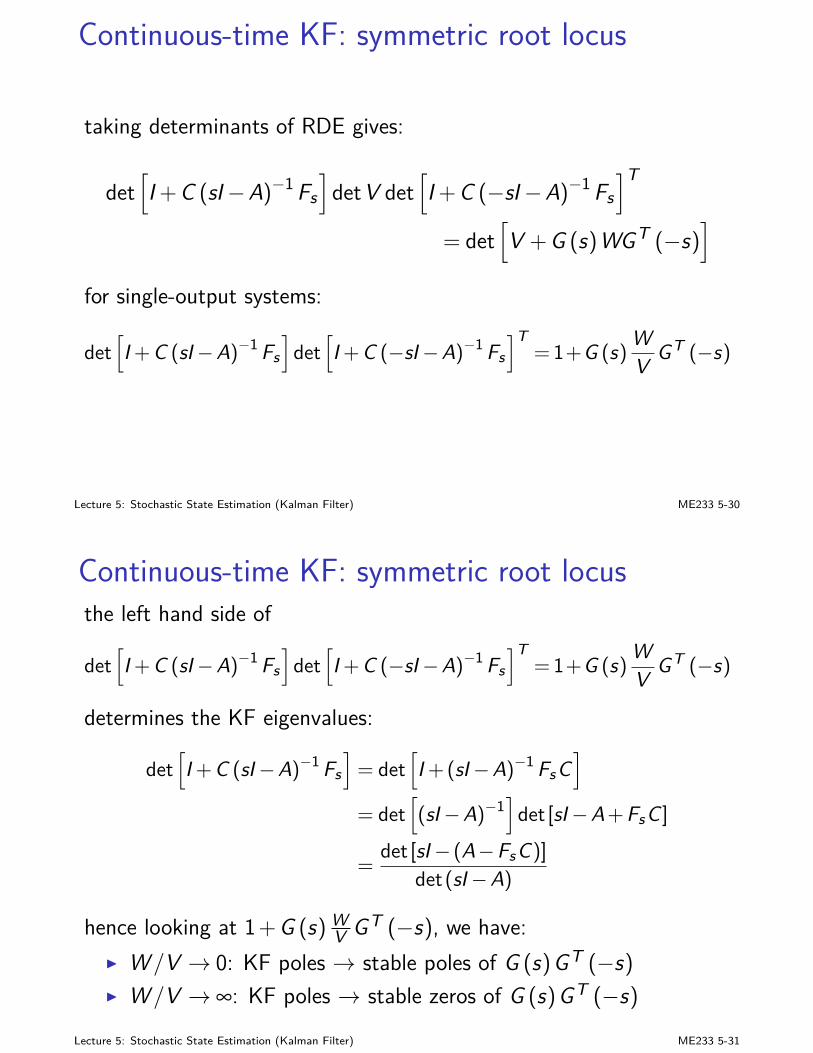
Continuous-time KF: symmetric root locus
taking determinants of RDE gives:
det[I +C (sI−A)−1 Fs
]detV det
[I +C (−sI−A)−1 Fs
]T
= det[V +G (s)WGT (−s)
]
for single-output systems:
det[I + C (sI−A)−1 Fs
]det[I + C (−sI−A)−1 Fs
]T= 1+G (s)
WV GT (−s)
Lecture 5: Stochastic State Estimation (Kalman Filter) ME233 5-30
Continuous-time KF: symmetric root locusthe left hand side of
det[I + C (sI−A)−1 Fs
]det[I + C (−sI−A)−1 Fs
]T= 1+G (s)
WV GT (−s)
determines the KF eigenvalues:
det[I + C (sI−A)−1 Fs
]= det
[I + (sI−A)−1 FsC
]
= det[(sI−A)−1
]det [sI−A + FsC ]
=det [sI− (A−FsC)]
det(sI−A)
hence looking at 1+G (s) WV GT (−s), we have:
I W /V → 0: KF poles → stable poles of G (s)GT (−s)I W /V → ∞: KF poles → stable zeros of G (s)GT (−s)
Lecture 5: Stochastic State Estimation (Kalman Filter) ME233 5-31

Summary1. Big picture
2. Problem statement
3. Discrete-time KFGain updateCovariance updateSteady-state KFDuality with LQ
4. Continuous-time KFSolutionSteady-state solution and conditionsProperties: return difference equality, symmetric root locus...
Lecture 5: Stochastic State Estimation (Kalman Filter) ME233 5-32
ME 233, UC Berkeley, Spring 2014 Xu Chen
Lecture 6: Linear Quadratic Gaussian (LQG)Control
Big pictureLQ when there is Gaussian noise
LQGSteady-state LQG
Big picturein deterministic control design:
I state feedback: arbitrary pole placement for controllable systemsI observer provides (when system is observable) state estimation
when not all states are availableI separation principle for observer state feedback control
we have now learned:I LQ: optimal state feedback which minimizes a quadratic cost
about the statesI KF: provides optimal state estimation
in stochastic control:I the above two give the linear quadratic Gaussian (LQG)
controller
Lecture 6: Linear Quadratic Gaussian (LQG) Control ME233 6-1
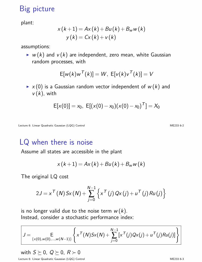
Big pictureplant:
x (k +1) = Ax (k)+Bu (k)+Bww (k)y (k) = Cx (k)+ v (k)
assumptions:I w (k) and v (k) are independent, zero mean, white Gaussian
random processes, with
E[w(k)wT (k)] = W , E[v(k)vT (k)] = V
I x (0) is a Gaussian random vector independent of w (k) andv (k), with
E[x(0)] = x0, E[(x(0)− x0)(x(0)− x0)T ] = X0
Lecture 6: Linear Quadratic Gaussian (LQG) Control ME233 6-2
LQ when there is noiseAssume all states are accessible in the plant
x (k +1) = Ax (k)+Bu (k)+Bww (k)
The original LQ cost
2J = xT (N)Sx (N)+N−1∑j=0
xT (j)Qx (j)+uT (j)Ru (j)
is no longer valid due to the noise term w (k).Instead, consider a stochastic performance index:
J = Ex(0),w(0),...,w(N−1)
xT (N)Sx(N)+
N−1∑j=0
[xT (j)Qx(j)+uT (j)Ru(j)]
with S 0, Q 0, R 0Lecture 6: Linear Quadratic Gaussian (LQG) Control ME233 6-3
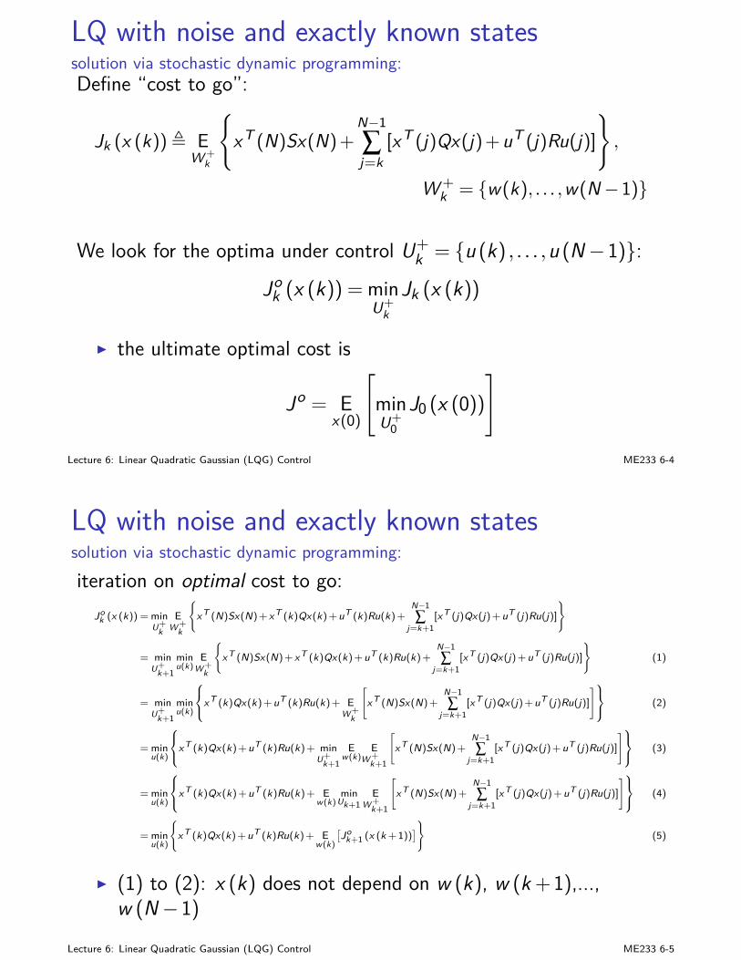
LQ with noise and exactly known statessolution via stochastic dynamic programming:Define “cost to go”:
Jk (x (k)), EW+
k
xT (N)Sx(N)+
N−1∑j=k
[xT (j)Qx(j)+uT (j)Ru(j)],
W+k = w(k), . . . ,w(N−1)
We look for the optima under control U+k = u (k) , . . . ,u (N−1):
Jok (x (k)) =min
U+k
Jk (x (k))
I the ultimate optimal cost is
Jo = Ex(0)
[minU+
0
J0 (x (0))]
Lecture 6: Linear Quadratic Gaussian (LQG) Control ME233 6-4
LQ with noise and exactly known statessolution via stochastic dynamic programming:iteration on optimal cost to go:
Jok (x (k)) = min
U+k
EW+
k
xT (N)Sx(N)+xT (k)Qx(k)+uT (k)Ru(k)+
N−1∑
j=k+1[xT (j)Qx(j)+uT (j)Ru(j)]
= minU+
k+1minu(k)
EW+
k
xT (N)Sx(N)+xT (k)Qx(k)+uT (k)Ru(k)+
N−1∑
j=k+1[xT (j)Qx(j)+uT (j)Ru(j)]
(1)
= minU+
k+1minu(k)
xT (k)Qx(k)+uT (k)Ru(k)+ E
W+k
[xT (N)Sx(N)+
N−1∑
j=k+1[xT (j)Qx(j)+uT (j)Ru(j)]
] (2)
= minu(k)
xT (k)Qx(k)+uT (k)Ru(k)+ min
U+k+1
Ew(k)
EW+
k+1
[xT (N)Sx(N)+
N−1∑
j=k+1[xT (j)Qx(j)+uT (j)Ru(j)]
] (3)
= minu(k)
xT (k)Qx(k)+uT (k)Ru(k)+ E
w(k)min
Uk+1E
W+k+1
[xT (N)Sx(N)+
N−1∑
j=k+1[xT (j)Qx(j)+uT (j)Ru(j)]
] (4)
= minu(k)
xT (k)Qx(k)+uT (k)Ru(k)+ E
w(k)
[Jo
k+1 (x (k +1))]
(5)
I (1) to (2): x (k) does not depend on w (k), w (k +1),...,w (N−1)
Lecture 6: Linear Quadratic Gaussian (LQG) Control ME233 6-5
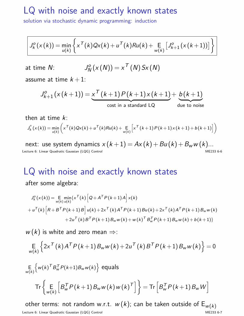
LQ with noise and exactly known statessolution via stochastic dynamic programming: induction
Jok (x (k)) = min
u(k)
xT (k)Qx(k)+uT (k)Ru(k)+ E
w(k)
[Jo
k+1 (x (k +1))]
at time N : JoN (x (N)) = xT (N)Sx (N)
assume at time k +1:
Jok+1 (x (k +1)) = xT (k +1)P (k +1)x (k +1)︸ ︷︷ ︸
cost in a standard LQ
+ b (k +1)︸ ︷︷ ︸due to noise
then at time k :Jo
k (x (k)) = minu(k)
(xT (k)Qx(k)+uT (k)Ru(k)+ E
w(k)
[xT (k +1)P (k +1)x (k +1)+b (k +1)
])
next: use system dynamics x (k +1) = Ax (k)+Bu (k)+Bww (k)...Lecture 6: Linear Quadratic Gaussian (LQG) Control ME233 6-6
LQ with noise and exactly known statesafter some algebra:
Jok (x (k)) = E
w(k)minu(k)xT (k)
[Q+AT P (k +1)A
]x(k)
+uT (k)[R +BT P (k +1)B
]u(k)+2xT (k)AT P (k +1)Bu (k)+2xT (k)AT P (k +1)Bw w (k)
+2uT (k)BT P (k +1)Bw w (k)+w (k)T BTw P (k +1)Bw w (k)+b (k +1)
w (k) is white and zero mean ⇒:
Ew(k)
2xT (k)AT P (k +1)Bw w (k)+2uT (k)BT P (k +1)Bw w (k)
= 0
Ew(k)
w(k)T BT
w P(k+1)Bw w(k)equals
Tr
Ew(k)
[BT
w P (k +1)Bw w (k)w (k)T]
= Tr[BT
w P (k +1)Bw W]
other terms: not random w.r.t. w (k); can be taken outside of Ew(k)Lecture 6: Linear Quadratic Gaussian (LQG) Control ME233 6-7
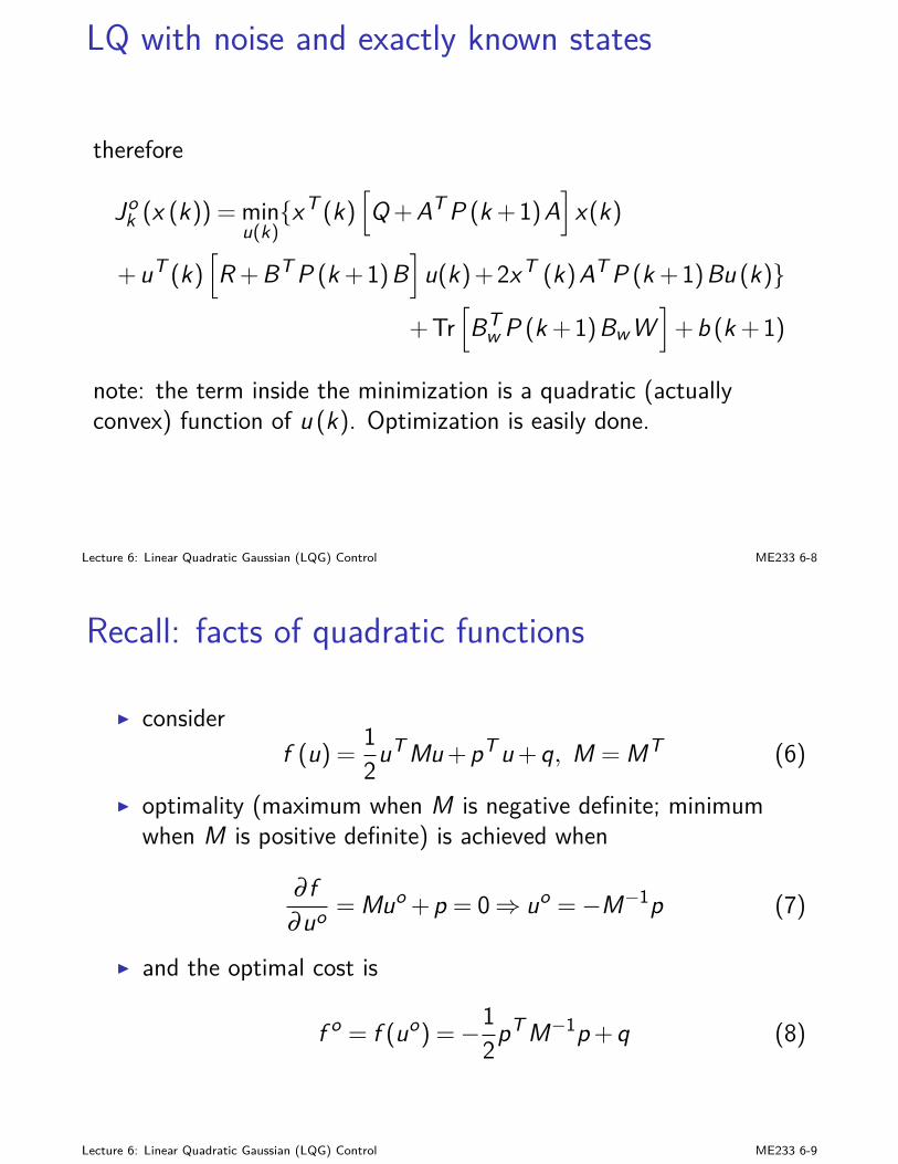
LQ with noise and exactly known states
therefore
Jok (x (k)) =min
u(k)xT (k)
[Q+AT P (k +1)A
]x(k)
+uT (k)[R +BT P (k +1)B
]u(k)+2xT (k)AT P (k +1)Bu (k)
+Tr[BT
w P (k +1)BwW]+b (k +1)
note: the term inside the minimization is a quadratic (actuallyconvex) function of u (k). Optimization is easily done.
Lecture 6: Linear Quadratic Gaussian (LQG) Control ME233 6-8
Recall: facts of quadratic functions
I considerf (u) = 1
2uT Mu+pT u+q, M = MT (6)
I optimality (maximum when M is negative definite; minimumwhen M is positive definite) is achieved when
∂ f∂uo = Muo +p = 0⇒ uo =−M−1p (7)
I and the optimal cost is
f o = f (uo) =−12pT M−1p+q (8)
Lecture 6: Linear Quadratic Gaussian (LQG) Control ME233 6-9
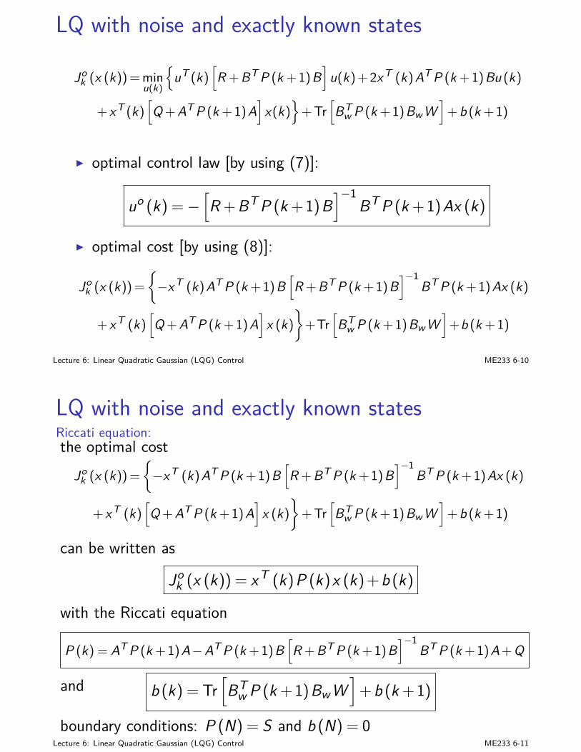
LQ with noise and exactly known states
Jok (x (k))=min
u(k)
uT (k)
[R +BT P (k +1)B
]u(k)+2xT (k)AT P (k +1)Bu (k)
+ xT (k)[Q+AT P (k +1)A
]x(k)
+Tr
[BT
w P (k +1)Bw W]+b (k +1)
I optimal control law [by using (7)]:
uo (k) =−[R +BT P (k +1)B
]−1BT P (k +1)Ax (k)
I optimal cost [by using (8)]:
Jok (x (k))=
−xT (k)AT P (k +1)B
[R +BT P (k +1)B
]−1BT P (k +1)Ax (k)
+ xT (k)[Q+AT P (k +1)A
]x (k)
+Tr
[BT
w P (k +1)Bw W]+b (k +1)
Lecture 6: Linear Quadratic Gaussian (LQG) Control ME233 6-10
LQ with noise and exactly known statesRiccati equation:the optimal cost
Jok (x (k))=
−xT (k)AT P (k +1)B
[R +BT P (k +1)B
]−1BT P (k +1)Ax (k)
+ xT (k)[Q+AT P (k +1)A
]x (k)
+Tr
[BT
w P (k +1)Bw W]+b (k +1)
can be written as
Jok (x (k)) = xT (k)P (k)x (k)+b (k)
with the Riccati equation
P (k) = AT P (k +1)A−AT P (k +1)B[R +BT P (k +1)B
]−1BT P (k +1)A+Q
and b (k) = Tr[BT
w P (k +1)BwW]+b (k +1)
boundary conditions: P (N) = S and b (N) = 0Lecture 6: Linear Quadratic Gaussian (LQG) Control ME233 6-11
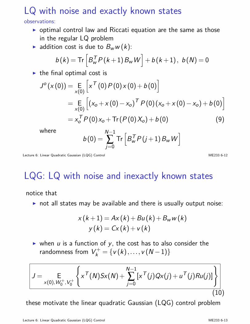
LQ with noise and exactly known statesobservations:
I optimal control law and Riccati equation are the same as thosein the regular LQ problem
I addition cost is due to Bww (k):
b (k) = Tr[BT
w P (k +1)BwW]+b (k +1) , b (N) = 0
I the final optimal cost is
Jo (x (0)) = Ex(0)
[xT (0)P (0)x (0)+b (0)
]
= Ex(0)
[(xo + x (0)− xo)
T P (0)(xo + x (0)− xo)+b (0)]
= xTo P (0)xo +Tr (P (0)Xo)+b (0) (9)
whereb (0) =
N−1∑j=0
Tr[BT
w P (j +1)BwW]
Lecture 6: Linear Quadratic Gaussian (LQG) Control ME233 6-12
LQG: LQ with noise and inexactly known statesnotice that
I not all states may be available and there is usually output noise:
x (k +1) = Ax (k)+Bu (k)+Bww (k)y (k) = Cx (k)+ v (k)
I when u is a function of y , the cost has to also consider therandomness from V+
k = v (k) , . . . ,v (N−1)
J = Ex(0),W+
0 ,V+0
xT (N)Sx(N)+
N−1∑j=0
[xT (j)Qx(j)+uT (j)Ru(j)]
(10)these motivate the linear quadratic Gaussian (LQG) control problem
Lecture 6: Linear Quadratic Gaussian (LQG) Control ME233 6-13
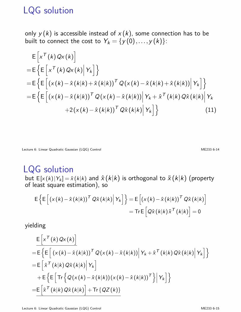
LQG solution
only y (k) is accessible instead of x (k), some connection has to bebuilt to connect the cost to Yk = y (0) , . . . ,y (k):
E[xT (k)Qx (k)
]
=E
E[
xT (k)Qx (k)∣∣∣Yk
]
=E
E[(x (k)− x (k|k)+ x (k|k))T Q (x (k)− x (k|k)+ x (k|k))
∣∣∣Yk]
=E
E[(x (k)− x (k|k))T Q (x (k)− x (k|k))
∣∣∣Yk + xT (k|k)Qx (k|k)∣∣∣Yk
+2(x (k)− x (k|k))T Qx (k|k)∣∣∣Yk
](11)
Lecture 6: Linear Quadratic Gaussian (LQG) Control ME233 6-14
LQG solutionbut E [x (k) |Yk ] = x (k|k) and x (k|k) is orthogonal to x (k|k) (propertyof least square estimation), so
E
E[(x (k)− x (k|k))T Qx (k|k)
∣∣∣Yk]
= E[(x (k)− x (k|k))T Qx (k|k)
]
= TrE[Qx (k|k) xT (k|k)
]= 0
yielding
E[xT (k)Qx (k)
]
=E
E[(x (k)− x (k|k))T Q (x (k)− x (k|k))
∣∣∣Yk + xT (k|k)Qx (k|k)∣∣∣Yk
]
=E[
xT (k|k)Qx (k|k)∣∣∣Yk
]
+E
E[
Tr
Q (x (k)− x (k|k))(x (k)− x (k|k))T∣∣∣Yk
]
=E[xT (k|k)Qx (k|k)
]+TrQZ (k)
Lecture 6: Linear Quadratic Gaussian (LQG) Control ME233 6-15
LQG solution
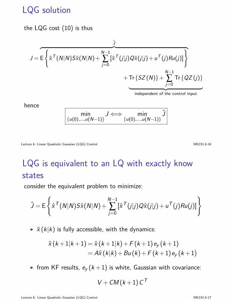
the LQG cost (10) is thus
J =
J︷ ︸︸ ︷
E
xT (N|N)Sx(N|N)+N−1∑j=0
[xT (j |j)Qx(j |j)+uT (j)Ru(j)]
+TrSZ (N)+N−1∑j=0
TrQZ (j)︸ ︷︷ ︸
independent of the control input
hencemin
u(0),...,u(N−1)J ⇐⇒ min
u(0),...,u(N−1)J
Lecture 6: Linear Quadratic Gaussian (LQG) Control ME233 6-16
LQG is equivalent to an LQ with exactly knowstatesconsider the equivalent problem to minimize:
J = E
xT (N|N)Sx(N|N)+N−1∑j=0
[xT (j |j)Qx(j |j)+uT (j)Ru(j)]
I x (k|k) is fully accessible, with the dynamics:
x (k +1|k +1) = x (k +1|k)+F (k +1)ey (k +1)= Ax (k|k)+Bu (k)+F (k +1)ey (k +1)
I from KF results, ey (k +1) is white, Gaussian with covariance:
V +CM (k +1)CT
Lecture 6: Linear Quadratic Gaussian (LQG) Control ME233 6-17
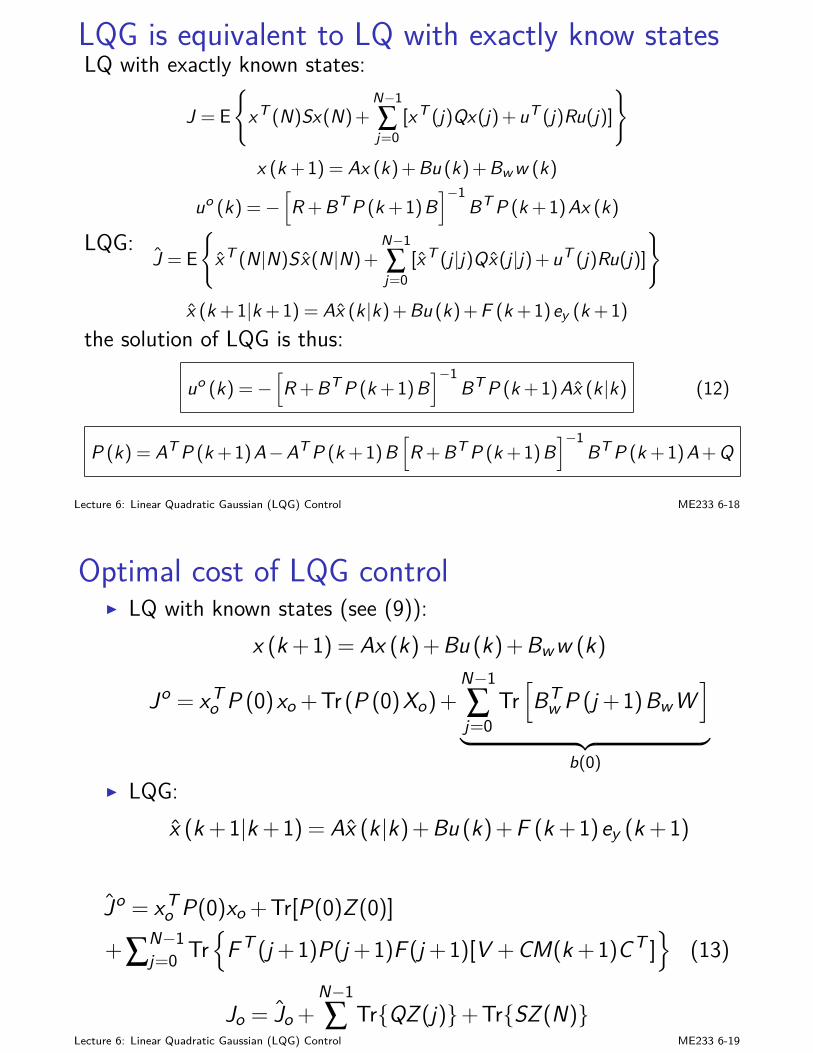
LQG is equivalent to LQ with exactly know statesLQ with exactly known states:
J = E
xT (N)Sx(N)+N−1∑j=0
[xT (j)Qx(j)+uT (j)Ru(j)]
x (k +1) = Ax (k)+Bu (k)+Bw w (k)
uo (k) =−[R +BT P (k +1)B
]−1BT P (k +1)Ax (k)
LQG:J = E
xT (N|N)Sx(N|N)+
N−1∑j=0
[xT (j |j)Qx(j |j)+uT (j)Ru(j)]
x (k +1|k +1) = Ax (k|k)+Bu (k)+F (k +1)ey (k +1)the solution of LQG is thus:
uo (k) =−[R +BT P (k +1)B
]−1BT P (k +1)Ax (k|k) (12)
P (k) = AT P (k +1)A−AT P (k +1)B[R +BT P (k +1)B
]−1BT P (k +1)A+Q
Lecture 6: Linear Quadratic Gaussian (LQG) Control ME233 6-18
Optimal cost of LQG controlI LQ with known states (see (9)):
x (k +1) = Ax (k)+Bu (k)+Bww (k)
Jo = xTo P (0)xo +Tr (P (0)Xo)+
N−1∑j=0
Tr[BT
w P (j +1)BwW]
︸ ︷︷ ︸b(0)
I LQG:x (k +1|k +1) = Ax (k|k)+Bu (k)+F (k +1)ey (k +1)
Jo = xTo P(0)xo +Tr[P(0)Z (0)]
+∑N−1j=0 Tr
F T (j +1)P(j +1)F (j +1)[V +CM(k +1)CT ]
(13)
Jo = Jo +N−1∑j=0
TrQZ (j)+TrSZ (N)Lecture 6: Linear Quadratic Gaussian (LQG) Control ME233 6-19
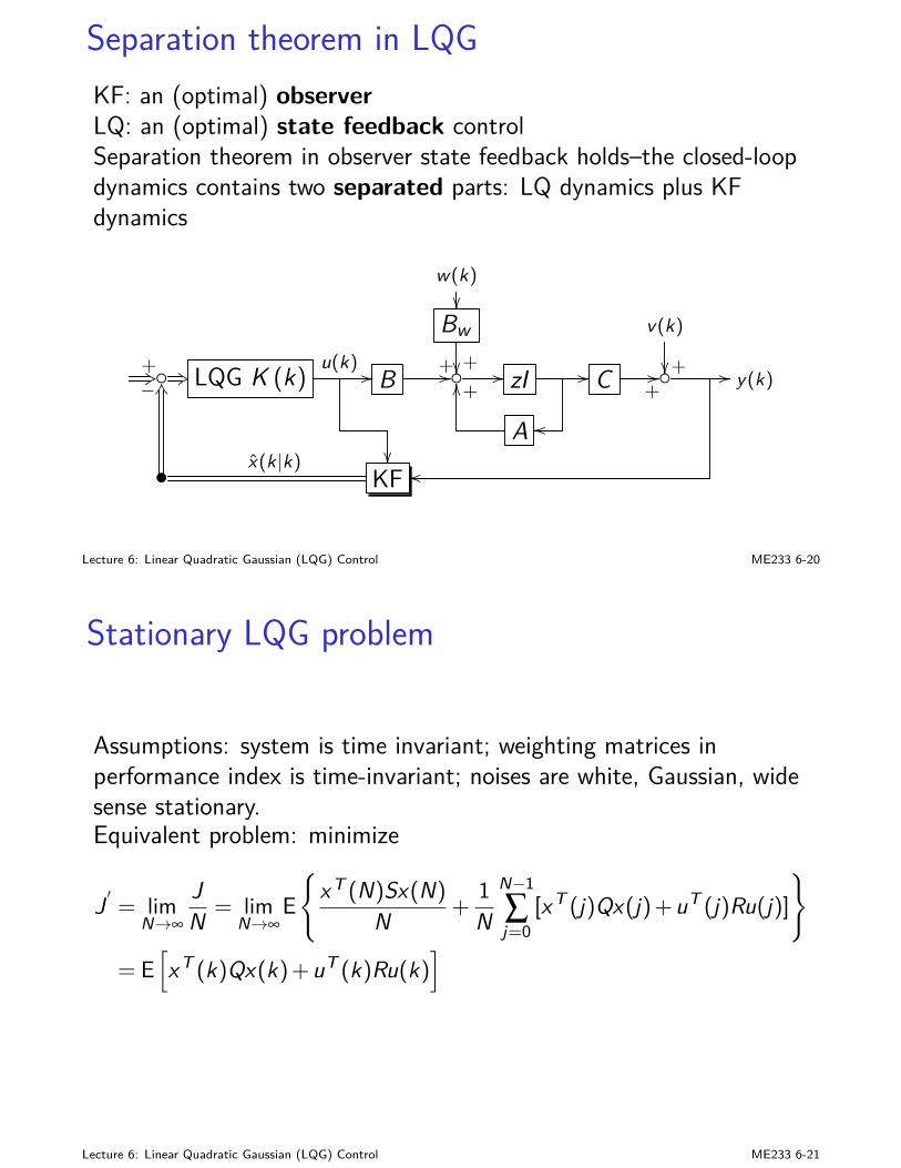
Separation theorem in LQGKF: an (optimal) observerLQ: an (optimal) state feedback controlSeparation theorem in observer state feedback holds–the closed-loopdynamics contains two separated parts: LQ dynamics plus KFdynamics
w(k)
Bw+
v(k)
+++3 +3 LQG K (k) u(k) // B +// // zI // C +// // y(k)
+OO
A oo
•
− KS
KFx(k|k) oo
Lecture 6: Linear Quadratic Gaussian (LQG) Control ME233 6-20
Stationary LQG problem
Assumptions: system is time invariant; weighting matrices inperformance index is time-invariant; noises are white, Gaussian, widesense stationary.Equivalent problem: minimize
J ′ = limN→∞
JN = lim
N→∞E
xT (N)Sx(N)
N +1N
N−1∑j=0
[xT (j)Qx(j)+uT (j)Ru(j)]
= E[xT (k)Qx(k)+uT (k)Ru(k)
]
Lecture 6: Linear Quadratic Gaussian (LQG) Control ME233 6-21
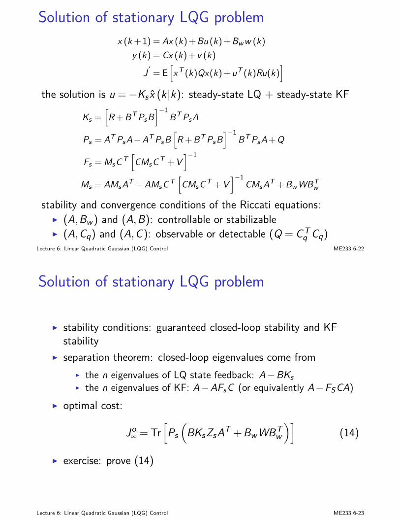
Solution of stationary LQG problemx (k +1) = Ax (k)+Bu (k)+Bw w (k)
y (k) = Cx (k)+ v (k)
J ′ = E[xT (k)Qx(k)+uT (k)Ru(k)
]
the solution is u =−Ks x (k|k): steady-state LQ + steady-state KF
Ks =[R +BT PsB
]−1BT PsA
Ps = AT PsA−AT PsB[R +BT PsB
]−1BT PsA+Q
Fs = MsCT[CMsCT +V
]−1
Ms = AMsAT −AMsCT[CMsCT +V
]−1CMsAT +Bw WBT
w
stability and convergence conditions of the Riccati equations:I (A,Bw ) and (A,B): controllable or stabilizableI (A,Cq) and (A,C): observable or detectable (Q = CT
q Cq)Lecture 6: Linear Quadratic Gaussian (LQG) Control ME233 6-22
Solution of stationary LQG problem
I stability conditions: guaranteed closed-loop stability and KFstability
I separation theorem: closed-loop eigenvalues come fromI the n eigenvalues of LQ state feedback: A−BKsI the n eigenvalues of KF: A−AFsC (or equivalently A−FSCA)
I optimal cost:
Jo∞ = Tr
[Ps(
BKsZsAT +BwWBTw)]
(14)
I exercise: prove (14)
Lecture 6: Linear Quadratic Gaussian (LQG) Control ME233 6-23
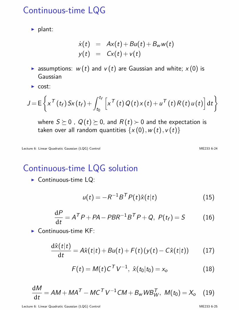
Continuous-time LQGI plant:
x(t) = Ax(t)+Bu(t)+Bww(t)y(t) = Cx(t)+ v(t)
I assumptions: w (t) and v (t) are Gaussian and white; x (0) isGaussian
I cost:
J =E
xT (tf )Sx (tf )+∫ tf
t0
[xT (t)Q (t)x (t)+uT (t)R (t)u (t)
]dt
where S 0 , Q (t) 0, and R (t) 0 and the expectation istaken over all random quantities x (0) ,w (t) ,v (t)
Lecture 6: Linear Quadratic Gaussian (LQG) Control ME233 6-24
Continuous-time LQG solutionI Continuous-time LQ:
u(t) =−R−1BT P(t)x(t|t) (15)
dPdt = AT P +PA−PBR−1BT P +Q, P(tf ) = S (16)
I Continuous-time KF:
dx(t|t)dt = Ax(t|t)+Bu(t)+F (t)(y(t)−Cx(t|t)) (17)
F (t) = M(t)CT V−1, x(t0|t0) = xo (18)
dMdt = AM +MAT −MCT V−1CM +BwWBT
W , M(t0) = Xo (19)
Lecture 6: Linear Quadratic Gaussian (LQG) Control ME233 6-25

Summary
1. Big picture
2. Stochastic control with exactly known state
3. Stochastic control with inexactly known state
4. Steady-state LQG
5. Continuous-time LQG problem
Lecture 6: Linear Quadratic Gaussian (LQG) Control ME233 6-26

ME 233, UC Berkeley, Spring 2014 Xu Chen
Lecture 7: Principles of Feedback Design
MIMO closed-loop analysisRobust stability
MIMO feedback design
Big picture
I we are pretty familiar with SISO feedback system design andanalysis
I state-space designs (LQ, KF, LQG,...): time-domain; goodmathematical formulation and solutions based on rigorous linearalgebra
I frequency-domain and transfer-function analysis: buildsintuition; good for properties such as stability robustness
Lecture 7: Principles of Feedback Design ME233 7-1
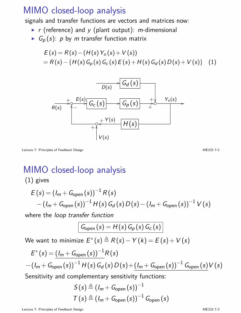
MIMO closed-loop analysissignals and transfer functions are vectors and matrices now:
I r (reference) and y (plant output): m-dimensionalI Gp (s): p by m transfer function matrix
E (s) = R (s)− (H (s)Yo (s)+V (s))= R (s)−H (s)Gp (s)Gc (s)E (s)+H (s)Gd (s)D (s)+V (s) (1)
D(s)// Gd (s)
+ R(s)
+// E(s) // Gc (s) // Gp (s)+// Yo(s) //
−OO
H (s)+Y (s)oo
+
V (s)
OO
Lecture 7: Principles of Feedback Design ME233 7-2
MIMO closed-loop analysis(1) gives
E (s) = (Im + Gopen (s))−1 R (s)
− (Im + Gopen (s))−1 H (s)Gd (s)D (s)− (Im + Gopen (s))−1 V (s)
where the loop transfer functionGopen (s) = H (s)Gp (s)Gc (s)
We want to minimize E ∗ (s) , R (s)−Y (k) = E (s) + V (s)
E ∗ (s) = (Im + Gopen (s))−1R (s)
−(Im + Gopen (s))−1 H (s)Gd (s)D (s)+(Im + Gopen (s))−1 Gopen (s)V (s)
Sensitivity and complementary sensitivity functions:S (s) , (Im + Gopen (s))−1
T (s) , (Im + Gopen (s))−1 Gopen (s)
Lecture 7: Principles of Feedback Design ME233 7-3
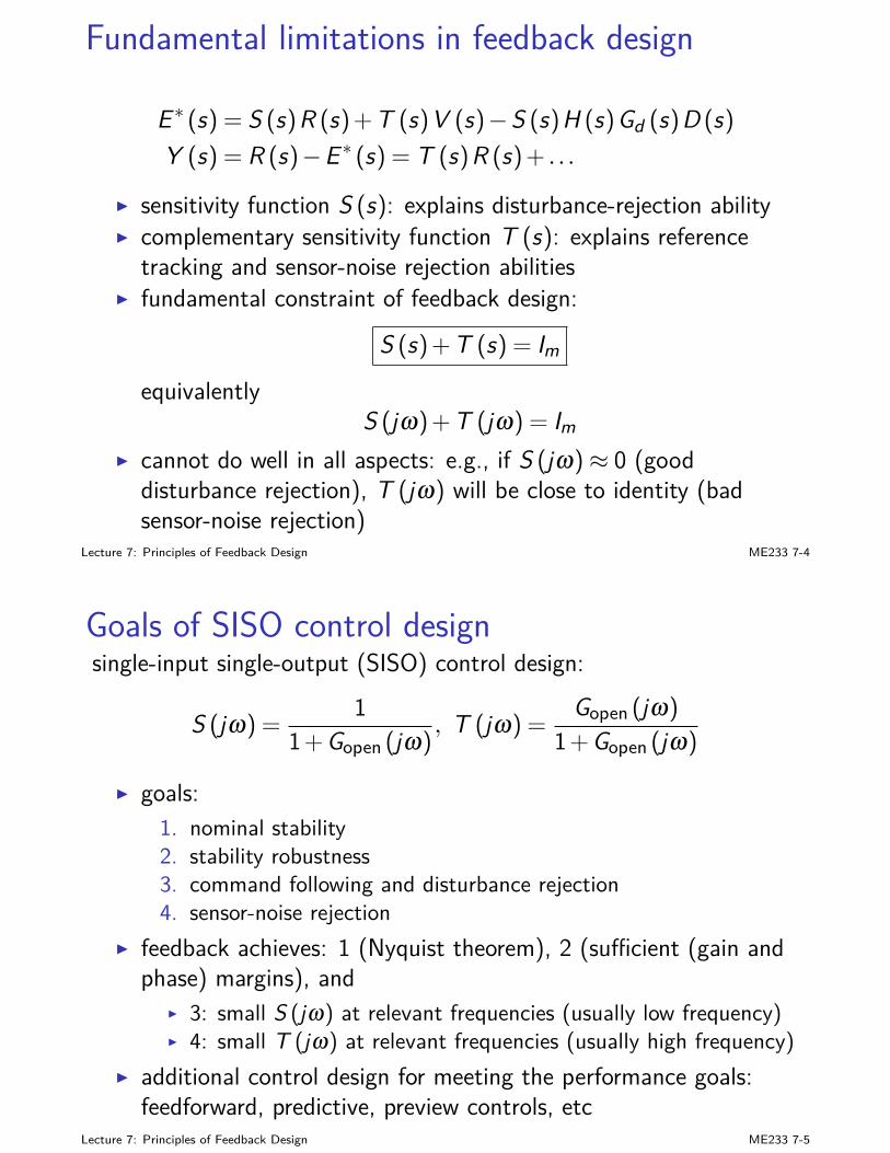
Fundamental limitations in feedback design
E ∗ (s) = S (s)R (s) + T (s)V (s)−S (s)H (s)Gd (s)D (s)
Y (s) = R (s)−E ∗ (s) = T (s)R (s) + . . .
I sensitivity function S (s): explains disturbance-rejection abilityI complementary sensitivity function T (s): explains reference
tracking and sensor-noise rejection abilitiesI fundamental constraint of feedback design:
S (s) + T (s) = Imequivalently
S (jω) + T (jω) = ImI cannot do well in all aspects: e.g., if S (jω)≈ 0 (good
disturbance rejection), T (jω) will be close to identity (badsensor-noise rejection)
Lecture 7: Principles of Feedback Design ME233 7-4
Goals of SISO control designsingle-input single-output (SISO) control design:
S (jω) =1
1+ Gopen (jω), T (jω) =
Gopen (jω)
1+ Gopen (jω)
I goals:1. nominal stability2. stability robustness3. command following and disturbance rejection4. sensor-noise rejection
I feedback achieves: 1 (Nyquist theorem), 2 (sufficient (gain andphase) margins), and
I 3: small S (jω) at relevant frequencies (usually low frequency)I 4: small T (jω) at relevant frequencies (usually high frequency)
I additional control design for meeting the performance goals:feedforward, predictive, preview controls, etc
Lecture 7: Principles of Feedback Design ME233 7-5
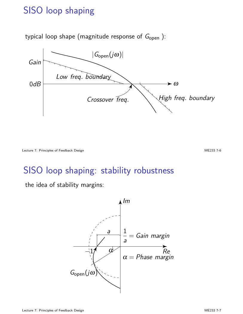
SISO loop shaping
typical loop shape (magnitude response of Gopen ):
ω
Gain
0dB
|Gopen(jω)|
Low freq. boundary
Crossover freq. High freq. boundary
Lecture 7: Principles of Feedback Design ME233 7-6
SISO loop shaping: stability robustnessthe idea of stability margins:
Re
Im
−1 α
a 1a = Gain margin
α = Phase margin
Gopen(jω)
Lecture 7: Principles of Feedback Design ME233 7-7
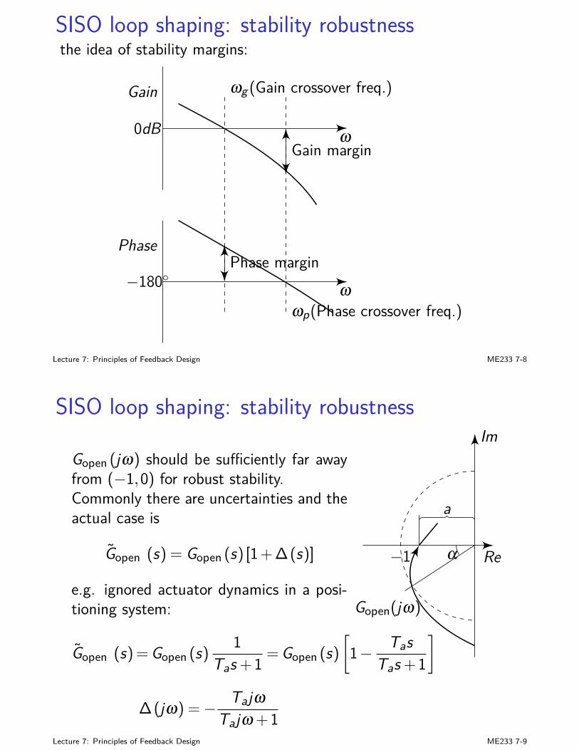
SISO loop shaping: stability robustnessthe idea of stability margins:
ω
Phase
ω
Gain
0dB
−180
ωg (Gain crossover freq.)
ωp(Phase crossover freq.)
Gain margin
Phase margin
Lecture 7: Principles of Feedback Design ME233 7-8
SISO loop shaping: stability robustness
Gopen (jω) should be sufficiently far awayfrom (−1,0) for robust stability.Commonly there are uncertainties and theactual case is
Gopen (s) = Gopen (s) [1+ ∆(s)]
e.g. ignored actuator dynamics in a posi-tioning system:
Gopen (s) = Gopen (s)1
Tas +1 = Gopen (s)
[1− Tas
Tas +1
]
∆(jω) =− TajωTajω +1
Re
Im
−1 α
a
Gopen(jω)
Lecture 7: Principles of Feedback Design ME233 7-9
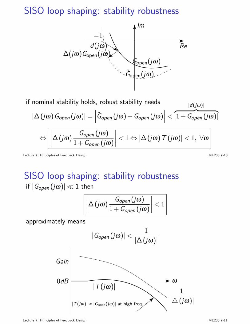
SISO loop shaping: stability robustness
Re
Im−1
Gopen(jω)
Gopen(jω)
d(jω)∆(jω)Gopen(jω)
if nominal stability holds, robust stability needs
|∆(jω)Gopen (jω)|=∣∣∣Gopen (jω)−Gopen (jω)
∣∣∣<|d(jω)|︷ ︸︸ ︷
|1+ Gopen (jω)|
⇔∣∣∣∣∆(jω)
Gopen (jω)
1+ Gopen (jω)
∣∣∣∣< 1⇔ |∆(jω)T (jω)|< 1, ∀ω
Lecture 7: Principles of Feedback Design ME233 7-10
SISO loop shaping: stability robustnessif |Gopen (jω)| 1 then
∣∣∣∣∆(jω)Gopen (jω)
1+ Gopen (jω)
∣∣∣∣< 1
approximately means
|Gopen (jω)|< 1|∆(jω)|
ω
Gain
0dB |T (jω)| 1|4 (jω)||T (jω)| ≈ |Gopen(jω)| at high freq.
Lecture 7: Principles of Feedback Design ME233 7-11
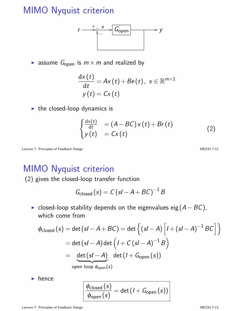
MIMO Nyquist criterion
r +// e // Gopen // y−OO
I assume Gopen is m×m and realized by
dx (t)
dt = Ax (t) + Be (t) , x ∈ Rm×1
y (t) = Cx (t)
I the closed-loop dynamics is
dx(t)dt = (A−BC)x (t) + Br (t)
y (t) = Cx (t)(2)
Lecture 7: Principles of Feedback Design ME233 7-12
MIMO Nyquist criterion(2) gives the closed-loop transfer function
Gclosed (s) = C (sI−A + BC)−1 B
I closed-loop stability depends on the eigenvalues eig (A−BC),which come from
φclosed (s) = det(sI−A + BC) = det
(sI−A)[I + (sI−A)−1 BC
]
= det(sI−A)det(
I + C (sI−A)−1 B)
= det(sI−A)︸ ︷︷ ︸open loop φopen(s)
det(I + Gopen (s))
I henceφclosed (s)
φopen (s)= det(I + Gopen (s))
Lecture 7: Principles of Feedback Design ME233 7-13
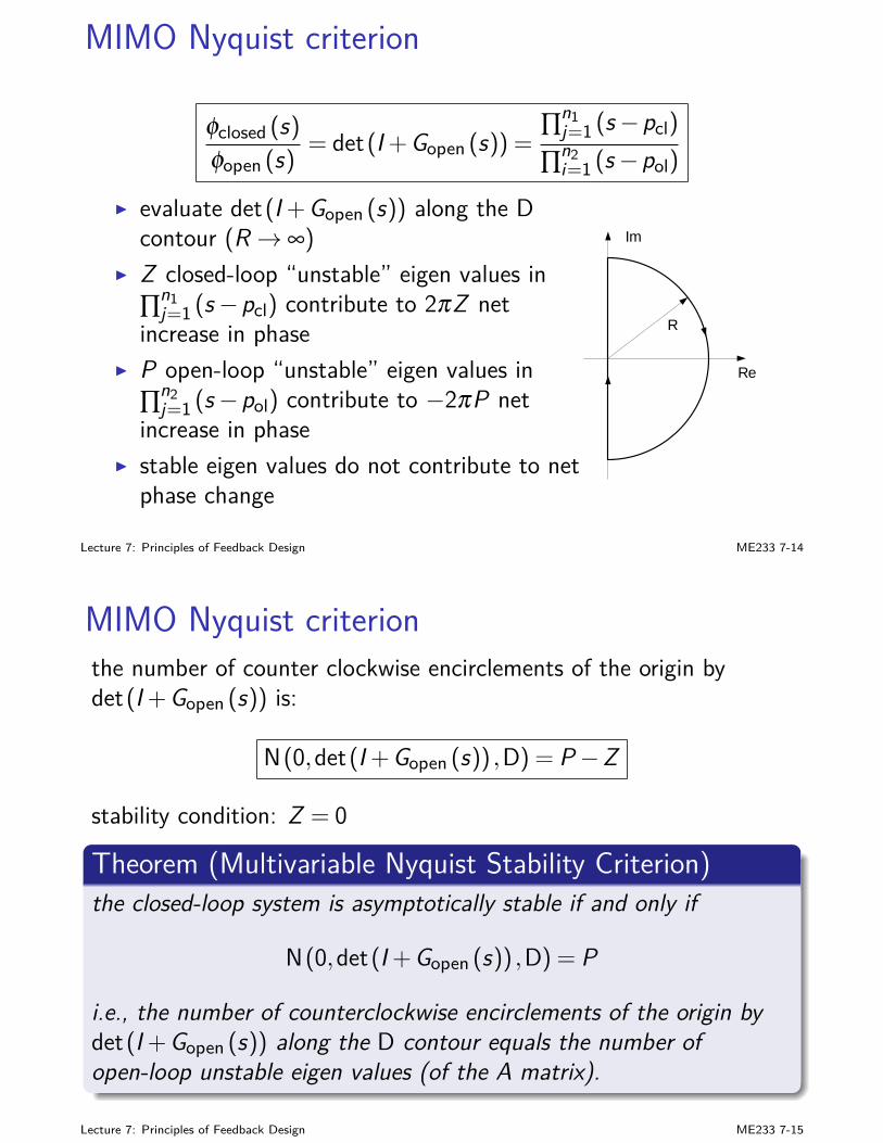
MIMO Nyquist criterion
φclosed (s)
φopen (s)= det(I + Gopen (s)) =
∏n1j=1 (s−pcl)
∏n2i=1 (s−pol)
I evaluate det(I + Gopen (s)) along the Dcontour (R → ∞)
I Z closed-loop “unstable” eigen values in∏n1
j=1 (s−pcl) contribute to 2πZ netincrease in phase
I P open-loop “unstable” eigen values in∏n2
j=1 (s−pol) contribute to −2πP netincrease in phase
I stable eigen values do not contribute to netphase change
R
Re
Im
Lecture 7: Principles of Feedback Design ME233 7-14
MIMO Nyquist criterionthe number of counter clockwise encirclements of the origin bydet(I + Gopen (s)) is:
N(0,det(I + Gopen (s)) ,D) = P−Z
stability condition: Z = 0
Theorem (Multivariable Nyquist Stability Criterion)the closed-loop system is asymptotically stable if and only if
N(0,det(I + Gopen (s)) ,D) = P
i.e., the number of counterclockwise encirclements of the origin bydet(I + Gopen (s)) along the D contour equals the number ofopen-loop unstable eigen values (of the A matrix).
Lecture 7: Principles of Feedback Design ME233 7-15
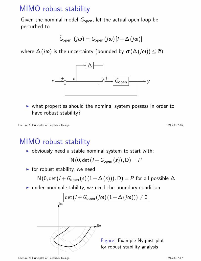
MIMO robust stabilityGiven the nominal model Gopen, let the actual open loop beperturbed to
Gopen (jω) = Gopen (jω) [I + ∆(jω)]
where ∆(jω) is the uncertainty (bounded by σ (∆(jω))≤ σ )
// ∆
+r +// e +
// Gopen // y−OO
I what properties should the nominal system possess in order tohave robust stability?
Lecture 7: Principles of Feedback Design ME233 7-16
MIMO robust stabilityI obviously need a stable nominal system to start with:
N(0,det(I + Gopen (s)) ,D) = PI for robust stability, we need
N(0,det(I + Gopen (s)(1+ ∆(s))) ,D) = P for all possible ∆
I under nominal stability, we need the boundary conditiondet(I + Gopen (jω)(1+ ∆(jω))) 6= 0
Re
Im
Figure: Example Nyquist plotfor robust stability analysis
Lecture 7: Principles of Feedback Design ME233 7-17
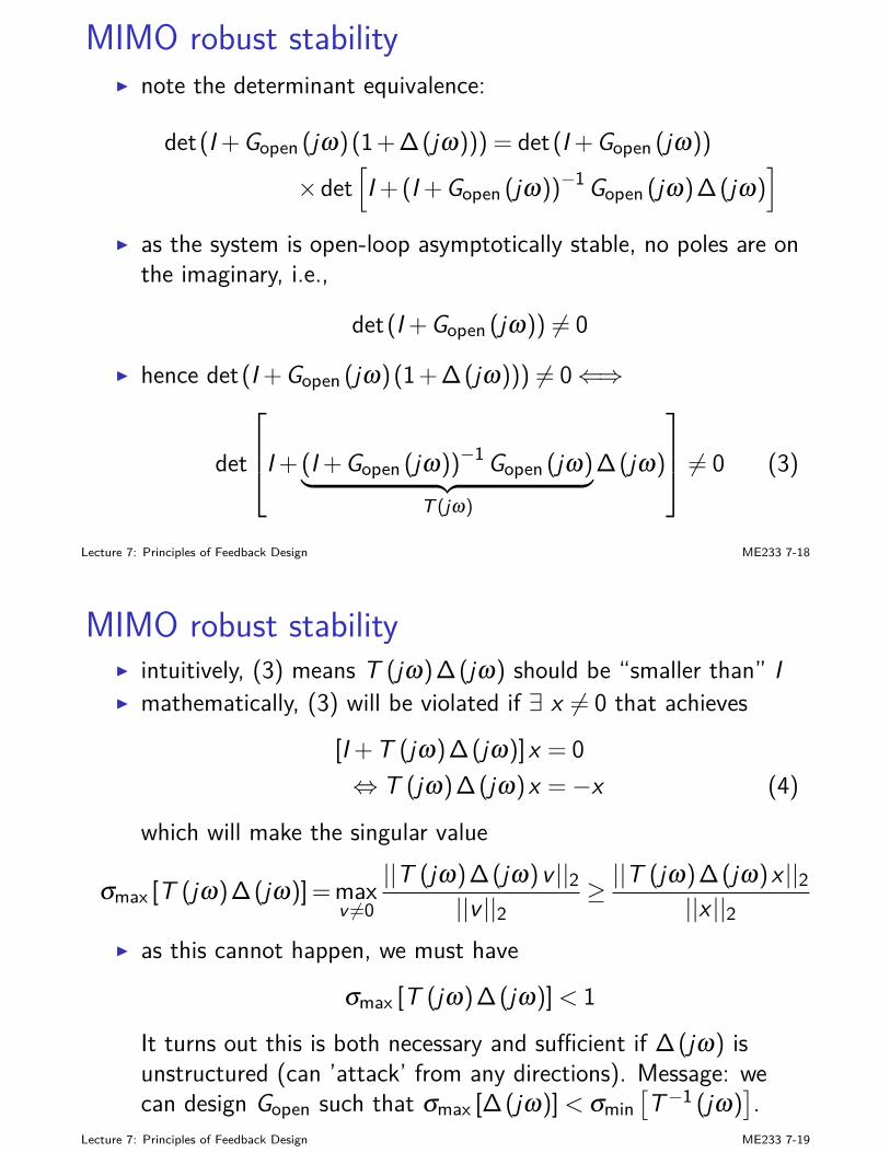
MIMO robust stabilityI note the determinant equivalence:
det(I + Gopen (jω)(1+ ∆(jω))) = det(I + Gopen (jω))
×det[I + (I + Gopen (jω))−1 Gopen (jω)∆(jω)
]
I as the system is open-loop asymptotically stable, no poles are onthe imaginary, i.e.,
det(I + Gopen (jω)) 6= 0
I hence det(I + Gopen (jω)(1+ ∆(jω))) 6= 0⇐⇒
det
I + (I + Gopen (jω))−1 Gopen (jω)︸ ︷︷ ︸
T (jω)
∆(jω)
6= 0 (3)
Lecture 7: Principles of Feedback Design ME233 7-18
MIMO robust stabilityI intuitively, (3) means T (jω)∆(jω) should be “smaller than” II mathematically, (3) will be violated if ∃ x 6= 0 that achieves
[I + T (jω)∆(jω)]x = 0⇔ T (jω)∆(jω)x =−x (4)
which will make the singular value
σmax [T (jω)∆(jω)] =maxv 6=0||T (jω)∆(jω)v ||2
||v ||2≥ ||T (jω)∆(jω)x ||2
||x ||2I as this cannot happen, we must have
σmax [T (jω)∆(jω)] < 1
It turns out this is both necessary and sufficient if ∆(jω) isunstructured (can ’attack’ from any directions). Message: wecan design Gopen such that σmax [∆(jω)] < σmin
[T−1 (jω)
].
Lecture 7: Principles of Feedback Design ME233 7-19

Summary
1. Big picture
2. MIMO closed-loop analysis
3. Loop shapingSISO case
4. MIMO stability and robust stabilityMIMO Nyquist criterionMIMO robust stability
Lecture 7: Principles of Feedback Design ME233 7-20

ME 233, UC Berkeley, Spring 2014 Xu Chen
Lecture 8: Discretization and Implementationof Continuous-time Design
Big pictureDiscrete-time frequency response
Discretization of continuous-time designAliasing and anti-aliasing
Big picturewhy are we learning this:
I nowadays controllers are implemented in discrete-time domainI implementation media: digital signal processor,
field-programmable gate array (FPGA), etcI either: controller is designed in continuous-time domain and
implemented digitallyI or: controller is designed directly in discrete-time domain
Lecture 8: Discretization and Implementation of Continuous-time Design ME233 8-1
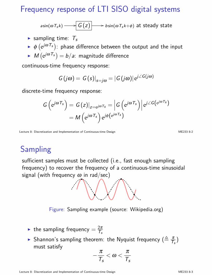
Frequency response of LTI SISO digital systemsa sin(ωTsk) // G (z) // b sin(ωTsk+φ) at steady state
I sampling time: TsI φ
(ejωTs
): phase difference between the output and the input
I M(ejωTs
)= b/a: magnitude difference
continuous-time frequency response:
G (jω) = G (s)|s=jω = |G (jω)|ej∠G(jω)
discrete-time frequency response:
G(
ejωTs)= G (z)|z=ejωTs =
∣∣∣G(
ejωTs)∣∣∣ej∠G(ejωTs )
= M(
ejωTs)
ejφ(ejωTs )
Lecture 8: Discretization and Implementation of Continuous-time Design ME233 8-2
Samplingsufficient samples must be collected (i.e., fast enough samplingfrequency) to recover the frequency of a continuous-time sinusoidalsignal (with frequency ω in rad/sec)
Figure: Sampling example (source: Wikipedia.org)
I the sampling frequency = 2πTs
I Shannon’s sampling theorem: the Nyquist frequency (, πTs)
must satisfy− π
Ts< ω <
πTs
Lecture 8: Discretization and Implementation of Continuous-time Design ME233 8-3
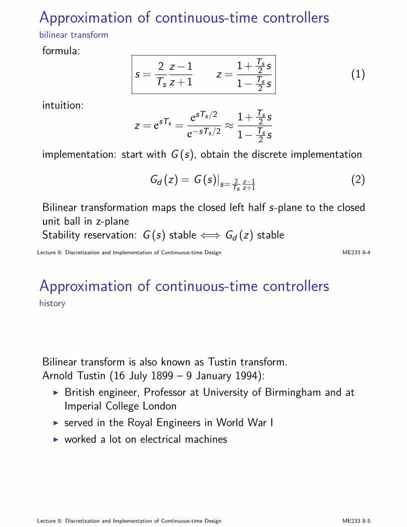
Approximation of continuous-time controllersbilinear transformformula:
s = 2Ts
z−1z +1 z =
1+ Ts2 s
1− Ts2 s
(1)
intuition:z = esTs =
esTs/2
e−sTs/2 ≈1+ Ts
2 s1− Ts
2 simplementation: start with G (s), obtain the discrete implementation
Gd (z) = G (s)|s= 2Ts
z−1z+1
(2)
Bilinear transformation maps the closed left half s-plane to the closedunit ball in z-planeStability reservation: G (s) stable ⇐⇒ Gd (z) stable
Lecture 8: Discretization and Implementation of Continuous-time Design ME233 8-4
Approximation of continuous-time controllershistory
Bilinear transform is also known as Tustin transform.Arnold Tustin (16 July 1899 – 9 January 1994):
I British engineer, Professor at University of Birmingham and atImperial College London
I served in the Royal Engineers in World War II worked a lot on electrical machines
Lecture 8: Discretization and Implementation of Continuous-time Design ME233 8-5
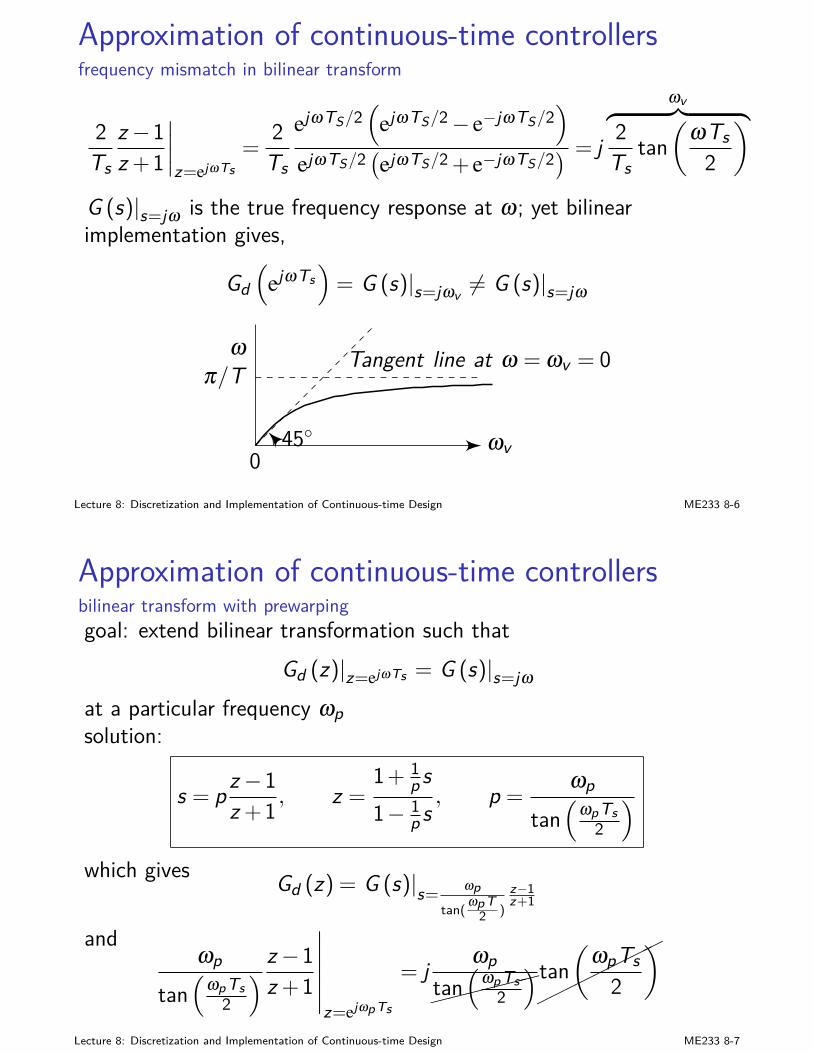
Approximation of continuous-time controllersfrequency mismatch in bilinear transform
2Ts
z−1z +1
∣∣∣∣z=ejωTs
=2
Ts
ejωTS/2(
ejωTS/2− e−jωTS/2)
ejωTS/2 (ejωTS/2 + e−jωTS/2) = j
ωv︷ ︸︸ ︷2
Tstan(
ωTs2
)
G (s)|s=jω is the true frequency response at ω ; yet bilinearimplementation gives,
Gd(
ejωTs)= G (s)|s=jωv 6= G (s)|s=jω
ωv
ω
0
π/T Tangent line at ω = ωv = 0
45
Lecture 8: Discretization and Implementation of Continuous-time Design ME233 8-6
Approximation of continuous-time controllersbilinear transform with prewarpinggoal: extend bilinear transformation such that
Gd (z)|z=ejωTs = G (s)|s=jω
at a particular frequency ωpsolution:
s = p z−1z +1 , z =
1+ 1p s
1− 1p s
, p =ωp
tan(
ωpTs2
)
which gives Gd (z) = G (s)|s= ωptan(ωpT
2 )
z−1z+1
andωp
tan(
ωpTs2
) z−1z +1
∣∣∣∣∣∣z=ejωpTs
= j ωp
tan(
ωpTs2
)tan(
ωpTs2
)
Lecture 8: Discretization and Implementation of Continuous-time Design ME233 8-7
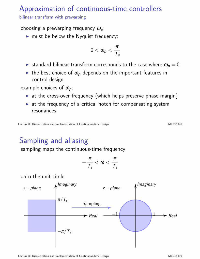
Approximation of continuous-time controllersbilinear transform with prewarping
choosing a prewarping frequency ωp:I must be below the Nyquist frequency:
0< ωp <πTs
I standard bilinear transform corresponds to the case where ωp = 0I the best choice of ωp depends on the important features in
control designexample choices of ωp:
I at the cross-over frequency (which helps preserve phase margin)I at the frequency of a critical notch for compensating system
resonances
Lecture 8: Discretization and Implementation of Continuous-time Design ME233 8-8
Sampling and aliasingsampling maps the continuous-time frequency
− πTs
< ω <πTs
onto the unit circle
Real
Imaginary
π/Ts
−π/Ts
s−plane
Real
Imaginaryz−plane
−1 1
Sampling
Lecture 8: Discretization and Implementation of Continuous-time Design ME233 8-9
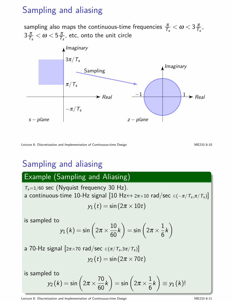
Sampling and aliasingsampling also maps the continuous-time frequencies π
Ts< ω < 3 π
Ts,
3 πTs
< ω < 5 πTs, etc, onto the unit circle
Real
Imaginary
π/Ts
3π/Ts
−π/Ts
s−plane
Real
Imaginary
z−plane
−1 1
Sampling
Lecture 8: Discretization and Implementation of Continuous-time Design ME233 8-10
Sampling and aliasingExample (Sampling and Aliasing)Ts=1/60 sec (Nyquist frequency 30 Hz).a continuous-time 10-Hz signal [10 Hz↔ 2π×10 rad/sec ∈(−π/Ts ,π/Ts)]
y1 (t) = sin(2π×10t)
is sampled toy1 (k) = sin
(2π× 10
60k)= sin
(2π× 1
6k)
a 70-Hz signal [2π×70 rad/sec ∈(π/Ts ,3π/Ts)]y2 (t) = sin(2π×70t)
is sampled toy2 (k) = sin
(2π× 70
60k)= sin
(2π× 1
6k)≡ y1 (k)!
Lecture 8: Discretization and Implementation of Continuous-time Design ME233 8-11
Anti-aliasing
need to avoid the negative influence of aliasing beyond the Nyquistfrequencies
I sample faster: make π/Ts large; the sampling frequency shouldbe high enough for good control design
I anti-aliasing: perform a low-pass filter to filter out the signals|ω|> π/Ts
Lecture 8: Discretization and Implementation of Continuous-time Design ME233 8-12
Summary
1. Big picture
2. Discrete-time frequency response
3. Approximation of continuous-time controllers
4. Sampling and aliasing
Lecture 8: Discretization and Implementation of Continuous-time Design ME233 8-13
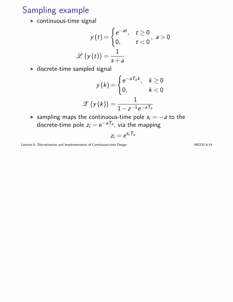
Sampling exampleI continuous-time signal
y (t) =
e−at , t ≥ 00, t < 0
, a > 0
L y (t)= 1s +a
I discrete-time sampled signal
y (k) =
e−aTsk , k ≥ 00, k < 0
Z y (k)= 11− z−1e−aTs
I sampling maps the continuous-time pole si =−a to thediscrete-time pole zi = e−aTs , via the mapping
zi = esi Ts
Lecture 8: Discretization and Implementation of Continuous-time Design ME233 8-14
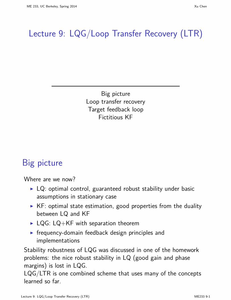
ME 233, UC Berkeley, Spring 2014 Xu Chen
Lecture 9: LQG/Loop Transfer Recovery (LTR)
Big pictureLoop transfer recoveryTarget feedback loop
Fictitious KF
Big pictureWhere are we now?
I LQ: optimal control, guaranteed robust stability under basicassumptions in stationary case
I KF: optimal state estimation, good properties from the dualitybetween LQ and KF
I LQG: LQ+KF with separation theoremI frequency-domain feedback design principles and
implementationsStability robustness of LQG was discussed in one of the homeworkproblems: the nice robust stability in LQ (good gain and phasemargins) is lost in LQG.LQG/LTR is one combined scheme that uses many of the conceptslearned so far.
Lecture 9: LQG/Loop Transfer Recovery (LTR) ME233 9-1
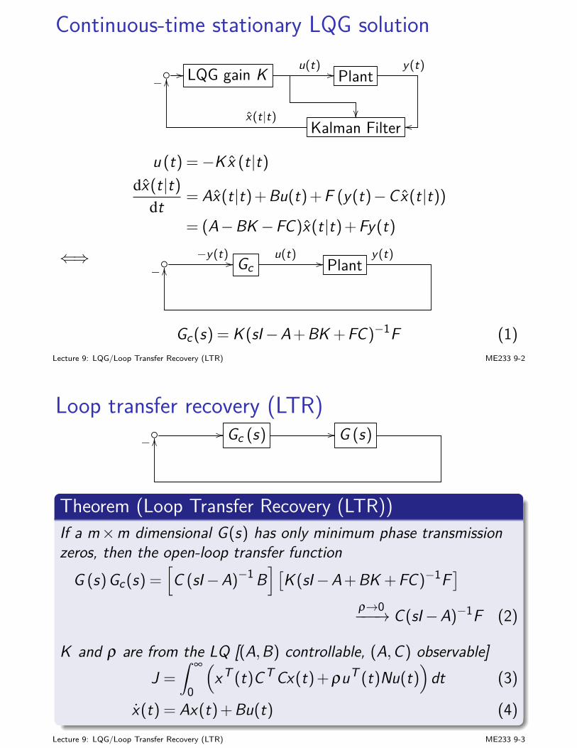
Continuous-time stationary LQG solution
// LQG gain K u(t) // Planty(t)
− OO
Kalman Filterx(t|t) oo
u (t) =−Kx (t|t)
dx(t|t)
dt = Ax(t|t) +Bu(t) +F (y(t)−Cx(t|t))
= (A−BK −FC)x(t|t) +Fy(t)
⇐⇒ −y(t) // Gcu(t) // Plant
y(t)− OO
Gc(s) = K (sI−A+BK +FC)−1F (1)Lecture 9: LQG/Loop Transfer Recovery (LTR) ME233 9-2
Loop transfer recovery (LTR) // Gc (s) // G (s)− OO
Theorem (Loop Transfer Recovery (LTR))If a m×m dimensional G(s) has only minimum phase transmissionzeros, then the open-loop transfer functionG (s)Gc(s) =
[C (sI−A)−1B
][K (sI−A+BK +FC)−1F
]
ρ→0−−−→ C(sI−A)−1F (2)
K and ρ are from the LQ [(A,B) controllable, (A,C) observable]J =
∫ ∞
0
(xT (t)CTCx(t) + ρuT (t)Nu(t)
)dt (3)
x(t) = Ax(t) +Bu(t) (4)Lecture 9: LQG/Loop Transfer Recovery (LTR) ME233 9-3
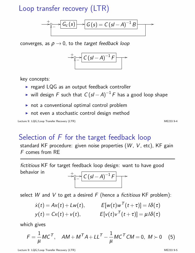
Loop transfer recovery (LTR)+// // Gc (s) // G (s) = C (sI−A)−1B //−OO
converges, as ρ → 0, to the target feedback loop
+// // C (sI−A)−1F //−OO
key concepts:I regard LQG as an output feedback controllerI will design F such that C (sI−A)−1F has a good loop shapeI not a conventional optimal control problemI not even a stochastic control design method
Lecture 9: LQG/Loop Transfer Recovery (LTR) ME233 9-4
Selection of F for the target feedback loopstandard KF procedure: given noise properties (W , V , etc), KF gainF comes from RE
fictitious KF for target feedback loop design: want to have goodbehavior in +// // C (sI−A)−1F //
−OO
select W and V to get a desired F (hence a fictitious KF problem):
x(t) = Ax(t) +Lw(t), E [w(t)wT (t + τ)] = Iδ (τ)
y(t) = Cx(t) + v(t), E [v(t)vT (t + τ)] = µ Iδ (τ)
which gives
F =1µMCT , AM +MTA+LLT − 1
µMCTCM = 0, M 0 (5)
Lecture 9: LQG/Loop Transfer Recovery (LTR) ME233 9-5
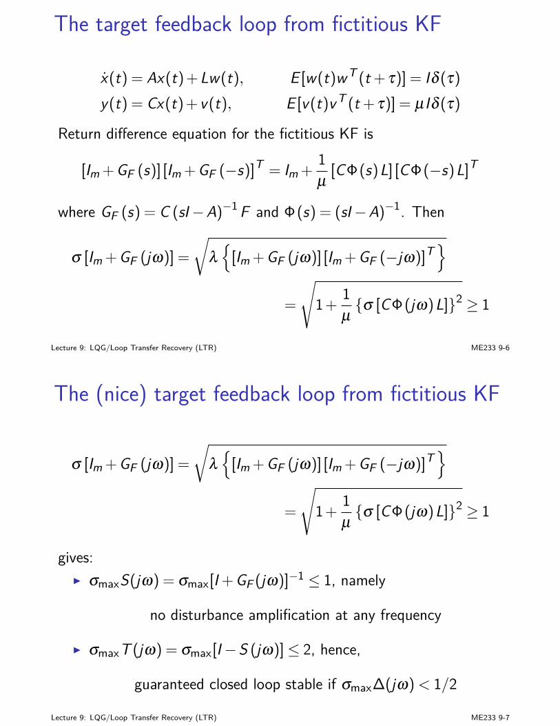
The target feedback loop from fictitious KF
x(t) = Ax(t) +Lw(t), E [w(t)wT (t + τ)] = Iδ (τ)
y(t) = Cx(t) + v(t), E [v(t)vT (t + τ)] = µ Iδ (τ)
Return difference equation for the fictitious KF is
[Im +GF (s)] [Im +GF (−s)]T = Im +1µ
[CΦ(s)L] [CΦ(−s)L]T
where GF (s) = C (sI−A)−1F and Φ(s) = (sI−A)−1. Then
σ [Im +GF (jω)] =
√λ
[Im +GF (jω)] [Im +GF (−jω)]T
=
√1+
1µσ [CΦ(jω)L]2 ≥ 1
Lecture 9: LQG/Loop Transfer Recovery (LTR) ME233 9-6
The (nice) target feedback loop from fictitious KF
σ [Im +GF (jω)] =
√λ
[Im +GF (jω)] [Im +GF (−jω)]T
=
√1+
1µσ [CΦ(jω)L]2 ≥ 1
gives:I σmaxS(jω) = σmax[I +GF (jω)]−1 ≤ 1, namely
no disturbance amplification at any frequency
I σmaxT (jω) = σmax[I−S (jω)]≤ 2, hence,
guaranteed closed loop stable if σmax∆(jω) < 1/2
Lecture 9: LQG/Loop Transfer Recovery (LTR) ME233 9-7
ME 233, UC Berkeley, Spring 2014 Xu Chen
Lecture 10: LQ with Frequency Shaped CostFunction (FSLQ)
BackgroundParseval’s Theorem
Frequency-shaped LQ cost functionTransformation to a standard LQ
Big picturewhy are we learning this:
I in standard LQ, Q and R are constant matrices in the costfunction
J =∫ ∞
0
(xT (t)Qx(t)+ρuT (t)Ru(t)
)dt (1)
I how can we introduce more design freedom for Q and R?
Lecture 10: LQ with Frequency Shaped Cost Function (FSLQ) ME233 10-1
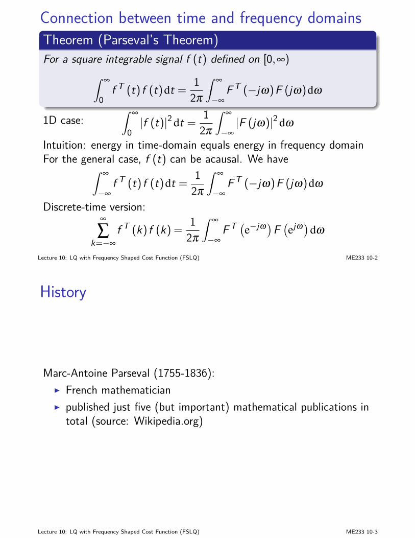
Connection between time and frequency domainsTheorem (Parseval’s Theorem)For a square integrable signal f (t) defined on [0,∞)
∫ ∞
0f T (t) f (t)dt = 1
2π
∫ ∞
−∞FT (−jω)F (jω)dω
1D case:∫ ∞
0|f (t)|2 dt = 1
2π
∫ ∞
−∞|F (jω)|2 dω
Intuition: energy in time-domain equals energy in frequency domainFor the general case, f (t) can be acausal. We have
∫ ∞
−∞f T (t) f (t)dt = 1
2π
∫ ∞
−∞FT (−jω)F (jω)dω
Discrete-time version:∞
∑k=−∞
f T (k) f (k) = 12π
∫ ∞
−∞FT (e−jω)F
(ejω)dω
Lecture 10: LQ with Frequency Shaped Cost Function (FSLQ) ME233 10-2
History
Marc-Antoine Parseval (1755-1836):I French mathematicianI published just five (but important) mathematical publications in
total (source: Wikipedia.org)
Lecture 10: LQ with Frequency Shaped Cost Function (FSLQ) ME233 10-3
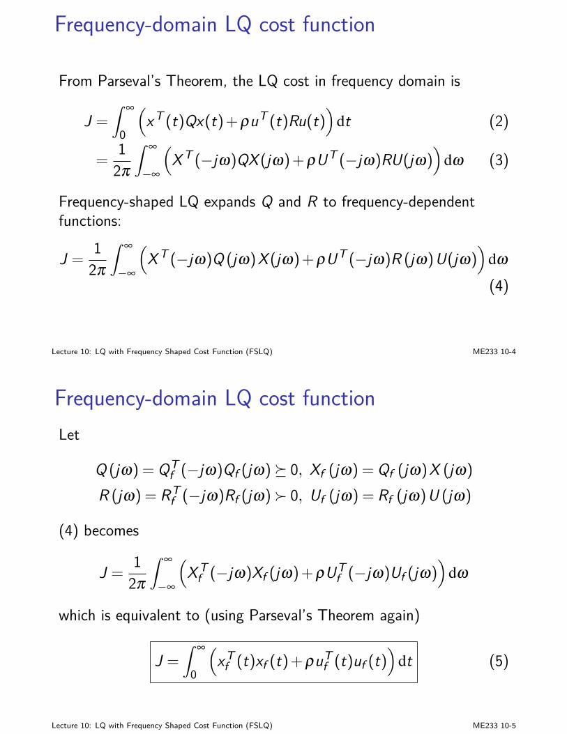
Frequency-domain LQ cost function
From Parseval’s Theorem, the LQ cost in frequency domain is
J =∫ ∞
0
(xT (t)Qx(t)+ρuT (t)Ru(t)
)dt (2)
=12π
∫ ∞
−∞
(XT (−jω)QX (jω)+ρUT (−jω)RU(jω)
)dω (3)
Frequency-shaped LQ expands Q and R to frequency-dependentfunctions:
J =12π
∫ ∞
−∞
(XT (−jω)Q (jω)X (jω)+ρUT (−jω)R (jω)U(jω)
)dω
(4)
Lecture 10: LQ with Frequency Shaped Cost Function (FSLQ) ME233 10-4
Frequency-domain LQ cost functionLet
Q (jω) = QTf (−jω)Qf (jω) 0, Xf (jω) = Qf (jω)X (jω)
R (jω) = RTf (−jω)Rf (jω) 0, Uf (jω) = Rf (jω)U (jω)
(4) becomes
J =12π
∫ ∞
−∞
(XT
f (−jω)Xf (jω)+ρUTf (−jω)Uf (jω)
)dω
which is equivalent to (using Parseval’s Theorem again)
J =∫ ∞
0
(xT
f (t)xf (t)+ρuTf (t)uf (t)
)dt (5)
Lecture 10: LQ with Frequency Shaped Cost Function (FSLQ) ME233 10-5
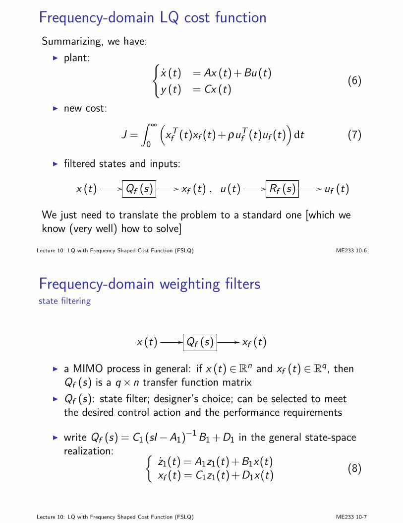
Frequency-domain LQ cost functionSummarizing, we have:
I plant: x (t) = Ax (t)+Bu (t)y (t) = Cx (t)
(6)
I new cost:
J =∫ ∞
0
(xT
f (t)xf (t)+ρuTf (t)uf (t)
)dt (7)
I filtered states and inputs:
x (t) // Qf (s) // xf (t) , u (t) // Rf (s) // uf (t)
We just need to translate the problem to a standard one [which weknow (very well) how to solve]
Lecture 10: LQ with Frequency Shaped Cost Function (FSLQ) ME233 10-6
Frequency-domain weighting filtersstate filtering
x (t) // Qf (s) // xf (t)
I a MIMO process in general: if x (t) ∈ Rn and xf (t) ∈ Rq, thenQf (s) is a q×n transfer function matrix
I Qf (s): state filter; designer’s choice; can be selected to meetthe desired control action and the performance requirements
I write Qf (s) = C1 (sI−A1)−1B1 +D1 in the general state-space
realization: z1(t) = A1z1(t)+B1x(t)xf (t) = C1z1(t)+D1x(t)
(8)
Lecture 10: LQ with Frequency Shaped Cost Function (FSLQ) ME233 10-7
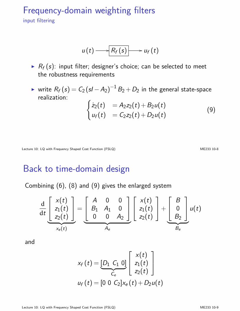
Frequency-domain weighting filtersinput filtering
u (t) // Rf (s) // uf (t)
I Rf (s): input filter; designer’s choice; can be selected to meetthe robustness requirements
I write Rf (s) = C2 (sI−A2)−1B2 +D2 in the general state-space
realization: z2(t) = A2z2(t)+B2u(t)uf (t) = C2z2(t)+D2u(t)
(9)
Lecture 10: LQ with Frequency Shaped Cost Function (FSLQ) ME233 10-8
Back to time-domain designCombining (6), (8) and (9) gives the enlarged system
ddt
x(t)z1(t)z2(t)
︸ ︷︷ ︸xe(t)
=
A 0 0B1 A1 00 0 A2
︸ ︷︷ ︸Ae
x(t)z1(t)z2(t)
+
B0B2
︸ ︷︷ ︸Be
u(t)
and
xf (t) = [D1 C1 0]︸ ︷︷ ︸Ce
x(t)z1(t)z2(t)
uf (t) = [0 0 C2]xe (t)+D2u(t)
Lecture 10: LQ with Frequency Shaped Cost Function (FSLQ) ME233 10-9
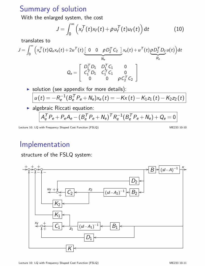
Summary of solutionWith the enlarged system, the cost
J =∫ ∞
0
(xT
f (t)xf (t)+ρuTf (t)uf (t)
)dt (10)
translates toJ =
∫ ∞
0
(xT
e (t)Qexe(t)+2uT (t)[0 0 ρDT
2 C2]
︸ ︷︷ ︸Ne
xe(t)+uT (t)ρDT2 D2︸ ︷︷ ︸Re
u(t))
dt
Qe =
DT1 D1 DT
1 C1 0CT
1 D1 CT1 C1 0
0 0 ρCT2 C2
I solution (see appendix for more details):u (t) =−R−1
e (BTe Pe +Ne)xe (t) =−Kx (t)−K1z1 (t)−K2z2 (t)
I algebraic Riccati equation:AT
e Pe +PeAe− (BTe Pe +Ne)
TR−1e (BT
e Pe +Ne)+Qe = 0Lecture 10: LQ with Frequency Shaped Cost Function (FSLQ) ME233 10-10
Implementationstructure of the FSLQ system:
+//+//+// // B // (sI−A)−1 x //−OO
+
D2 oo
ufoo C2+oo oo (sI−A2)
−1z2 B2oo oo
−OO
K2 oo
−OO
K1 oo
xfoo +oo C1 oo (sI−A1)−1
z1B1oo oo
+OO
D1 oo
K oo
Lecture 10: LQ with Frequency Shaped Cost Function (FSLQ) ME233 10-11
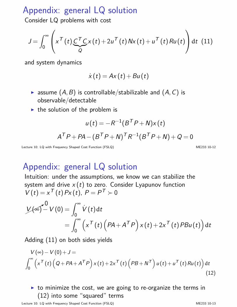
Appendix: general LQ solutionConsider LQ problems with cost
J =∫ ∞
0
xT (t)CTC︸ ︷︷ ︸
Qx (t)+2uT (t)Nx (t)+uT (t)Ru (t)
dt (11)
and system dynamics
x (t) = Ax (t)+Bu (t)
I assume (A,B) is controllable/stabilizable and (A,C) isobservable/detectable
I the solution of the problem is
u (t) =−R−1(BTP+N)x (t)
ATP+PA− (BTP+N)TR−1(BTP+N)+Q = 0Lecture 10: LQ with Frequency Shaped Cost Function (FSLQ) ME233 10-12
Appendix: general LQ solutionIntuition: under the assumptions, we know we can stabilize thesystem and drive x (t) to zero. Consider Lyapunov functionV (t) = xT (t)Px (t), P = PT 0
*0
V (∞)−V (0) =∫ ∞
0V (t)dt
=∫ ∞
0
(xT (t)
(PA+ATP
)x (t)+2xT (t)PBu (t)
)dt
Adding (11) on both sides yieldsV (∞)−V (0)+J =
∫ ∞
0
(xT (t)
(Q+PA+AT P
)x (t)+2xT (t)
(PB +NT
)u (t)+uT (t)Ru (t)
)dt(12)
I to minimize the cost, we are going to re-organize the terms in(12) into some “squared” terms
Lecture 10: LQ with Frequency Shaped Cost Function (FSLQ) ME233 10-13
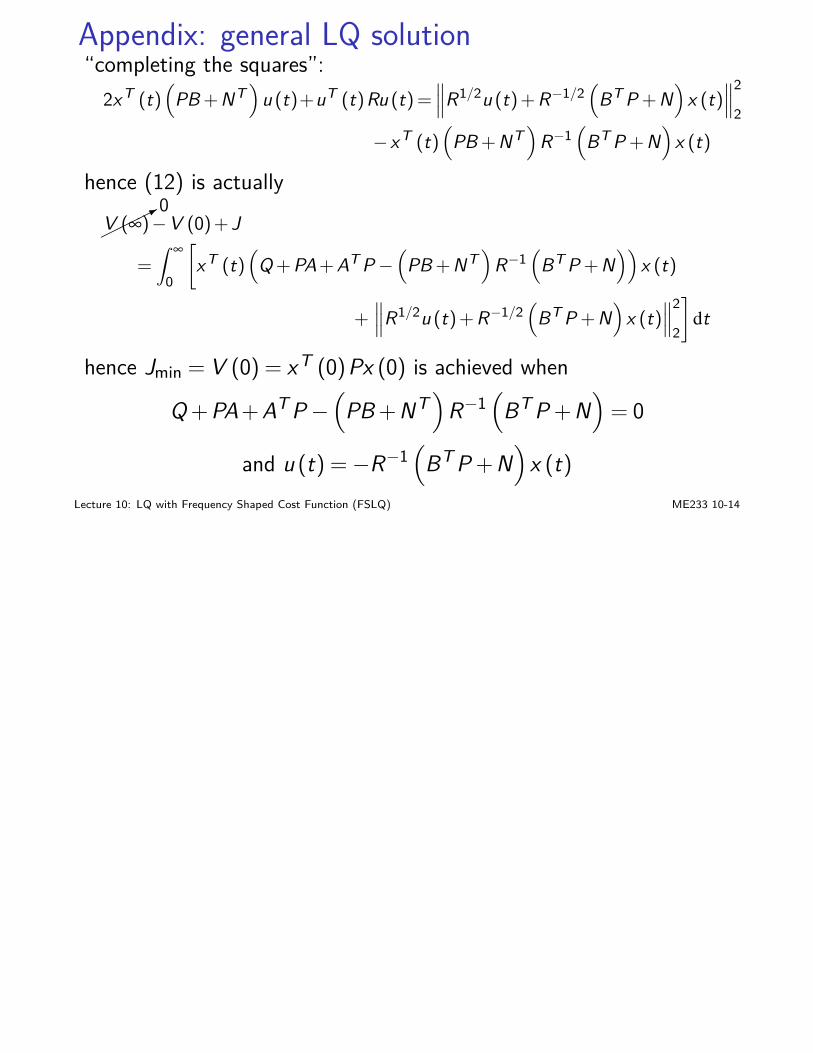
Appendix: general LQ solution“completing the squares”:
2xT (t)(
PB +NT)
u (t)+uT (t)Ru (t)=∥∥∥R1/2u (t)+R−1/2
(BT P +N
)x (t)
∥∥∥2
2
−xT (t)(
PB +NT)
R−1(
BT P +N)
x (t)
hence (12) is actually
*0
V (∞)−V (0)+J
=∫ ∞
0
[xT (t)
(Q+PA+AT P−
(PB +NT
)R−1
(BT P +N
))x (t)
+∥∥∥R1/2u (t)+R−1/2
(BT P +N
)x (t)
∥∥∥2
2
]dt
hence Jmin = V (0) = xT (0)Px (0) is achieved when
Q+PA+ATP−(PB+NT
)R−1
(BTP+N
)= 0
and u (t) =−R−1(BTP+N
)x (t)
Lecture 10: LQ with Frequency Shaped Cost Function (FSLQ) ME233 10-14
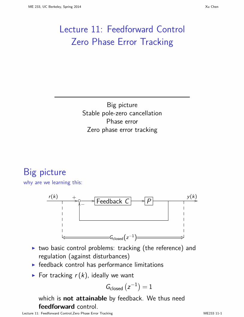
ME 233, UC Berkeley, Spring 2014 Xu Chen
Lecture 11: Feedforward ControlZero Phase Error Tracking
Big pictureStable pole-zero cancellation
Phase errorZero phase error tracking
Big picturewhy are we learning this:
r(k) + //− // Feedback C // Py(k) //OO
ks Gclosed(z−1) +3
I two basic control problems: tracking (the reference) andregulation (against disturbances)
I feedback control has performance limitationsI For tracking r (k), ideally we want
Gclosed(z−1)= 1
which is not attainable by feedback. We thus needfeedforward control.
Lecture 11: Feedforward Control,Zero Phase Error Tracking ME233 11-1
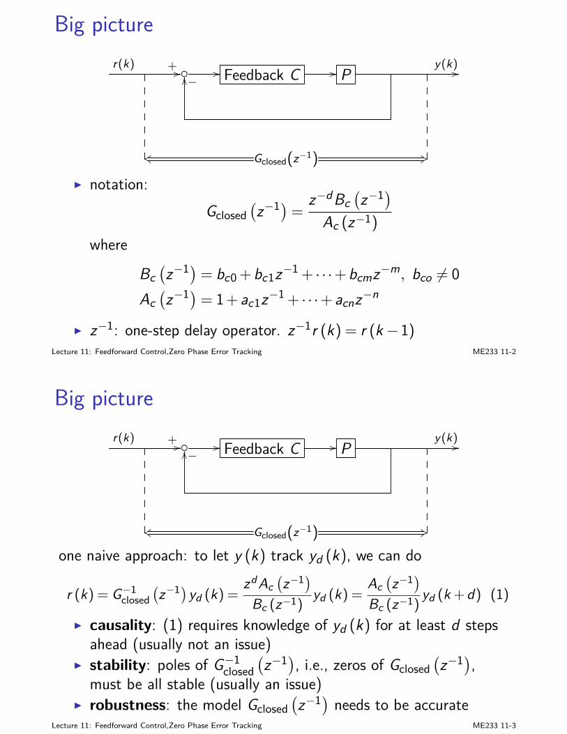
Big picturer(k) + //− // Feedback C // P
y(k) //OO
ks Gclosed(z−1) +3
I notation:Gclosed
(z−1)= z−dBc
(z−1)
Ac (z−1)
where
Bc(z−1)= bc0 +bc1z−1 + · · ·+bcmz−m, bco 6= 0
Ac(z−1)= 1+ac1z−1 + · · ·+acnz−n
I z−1: one-step delay operator. z−1r (k) = r (k−1)Lecture 11: Feedforward Control,Zero Phase Error Tracking ME233 11-2
Big picturer(k) + //− // Feedback C // P
y(k) //OO
ks Gclosed(z−1) +3
one naive approach: to let y (k) track yd (k), we can do
r (k) = G−1closed
(z−1)yd (k) =
zdAc(z−1)
Bc (z−1)yd (k) =
Ac(z−1)
Bc (z−1)yd (k +d) (1)
I causality: (1) requires knowledge of yd (k) for at least d stepsahead (usually not an issue)
I stability: poles of G−1closed
(z−1), i.e., zeros of Gclosed
(z−1),
must be all stable (usually an issue)I robustness: the model Gclosed
(z−1) needs to be accurate
Lecture 11: Feedforward Control,Zero Phase Error Tracking ME233 11-3
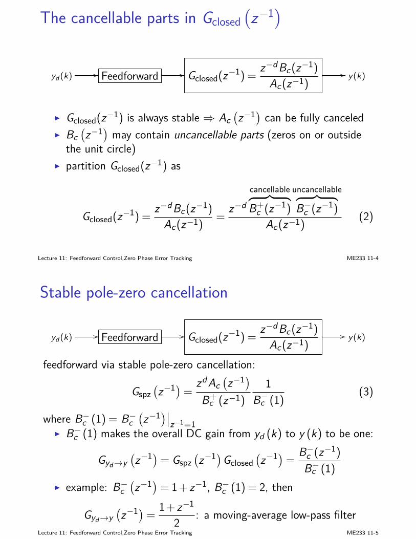
The cancellable parts in Gclosed(z−1)
yd (k) // Feedforward // Gclosed(z−1) =z−dBc(z−1)
Ac(z−1)// y(k)
I Gclosed(z−1) is always stable ⇒ Ac(z−1) can be fully canceled
I Bc(z−1) may contain uncancellable parts (zeros on or outside
the unit circle)I partition Gclosed(z−1) as
Gclosed(z−1) =z−dBc(z−1)
Ac(z−1)=
z−dcancellable︷ ︸︸ ︷B+
c (z−1)
uncancellable︷ ︸︸ ︷B−c (z−1)
Ac(z−1)(2)
Lecture 11: Feedforward Control,Zero Phase Error Tracking ME233 11-4
Stable pole-zero cancellation
yd (k) // Feedforward // Gclosed(z−1) =z−dBc(z−1)
Ac(z−1)// y(k)
feedforward via stable pole-zero cancellation:
Gspz(z−1)= zdAc
(z−1)
B+c (z−1)
1B−c (1)
(3)
where B−c (1) = B−c(z−1)∣∣
z−1=1I B−c (1) makes the overall DC gain from yd (k) to y (k) to be one:
Gyd→y(z−1)= Gspz
(z−1)Gclosed
(z−1)= B−c (z−1)
B−c (1)I example: B−c
(z−1)= 1+ z−1, B−c (1) = 2, then
Gyd→y(z−1)= 1+ z−1
2 : a moving-average low-pass filterLecture 11: Feedforward Control,Zero Phase Error Tracking ME233 11-5
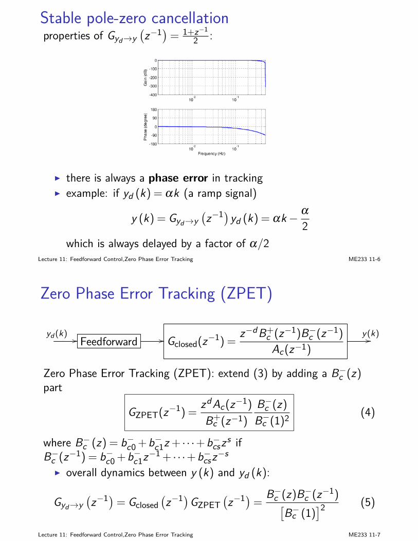
Stable pole-zero cancellationproperties of Gyd→y
(z−1)= 1+z−1
2 :
I there is always a phase error in trackingI example: if yd (k) = αk (a ramp signal)
y (k) = Gyd→y(z−1)yd (k) = αk− α
2which is always delayed by a factor of α/2
Lecture 11: Feedforward Control,Zero Phase Error Tracking ME233 11-6
Zero Phase Error Tracking (ZPET)
yd (k) // Feedforward // Gclosed(z−1) =z−dB+
c (z−1)B−c (z−1)Ac(z−1)
y(k)//
Zero Phase Error Tracking (ZPET): extend (3) by adding a B−c (z)part
GZPET(z−1) =zdAc(z−1)
B+c (z−1)
B−c (z)B−c (1)2
(4)
where B−c (z) = b−c0 +b−c1z + · · ·+b−cszs ifB−c (z−1) = b−c0 +b−c1z−1 + · · ·+b−csz−s
I overall dynamics between y (k) and yd (k):
Gyd→y(z−1)= Gclosed
(z−1)GZPET
(z−1)= B−c (z)B−c (z−1)
[B−c (1)
]2 (5)
Lecture 11: Feedforward Control,Zero Phase Error Tracking ME233 11-7
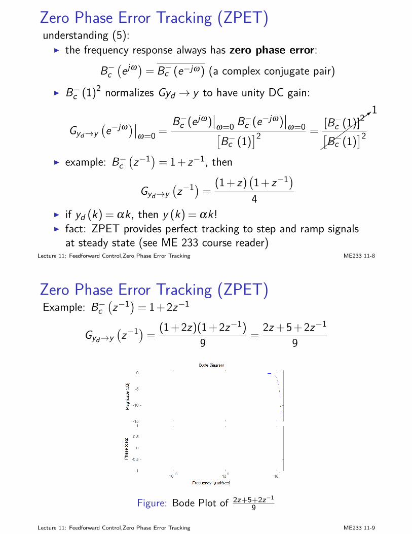
Zero Phase Error Tracking (ZPET)understanding (5):
I the frequency response always has zero phase error:B−c(ejω)= B−c (e−jω) (a complex conjugate pair)
I B−c (1)2 normalizes Gyd → y to have unity DC gain:
Gyd→y(e−jω)∣∣
ω=0 =B−c (ejω)
∣∣ω=0 B−c (e−jω)
∣∣ω=0[
B−c (1)]2 =
>
1[B−c (1)]2[B−c (1)
]2
I example: B−c(z−1)= 1+ z−1, then
Gyd→y(z−1)= (1+ z)
(1+ z−1)
4I if yd (k) = αk , then y (k) = αk!I fact: ZPET provides perfect tracking to step and ramp signals
at steady state (see ME 233 course reader)Lecture 11: Feedforward Control,Zero Phase Error Tracking ME233 11-8
Zero Phase Error Tracking (ZPET)Example: B−c
(z−1)= 1+2z−1
Gyd→y(z−1)= (1+2z)(1+2z−1)
9 =2z +5+2z−1
9
Figure: Bode Plot of 2z+5+2z−19
Lecture 11: Feedforward Control,Zero Phase Error Tracking ME233 11-9
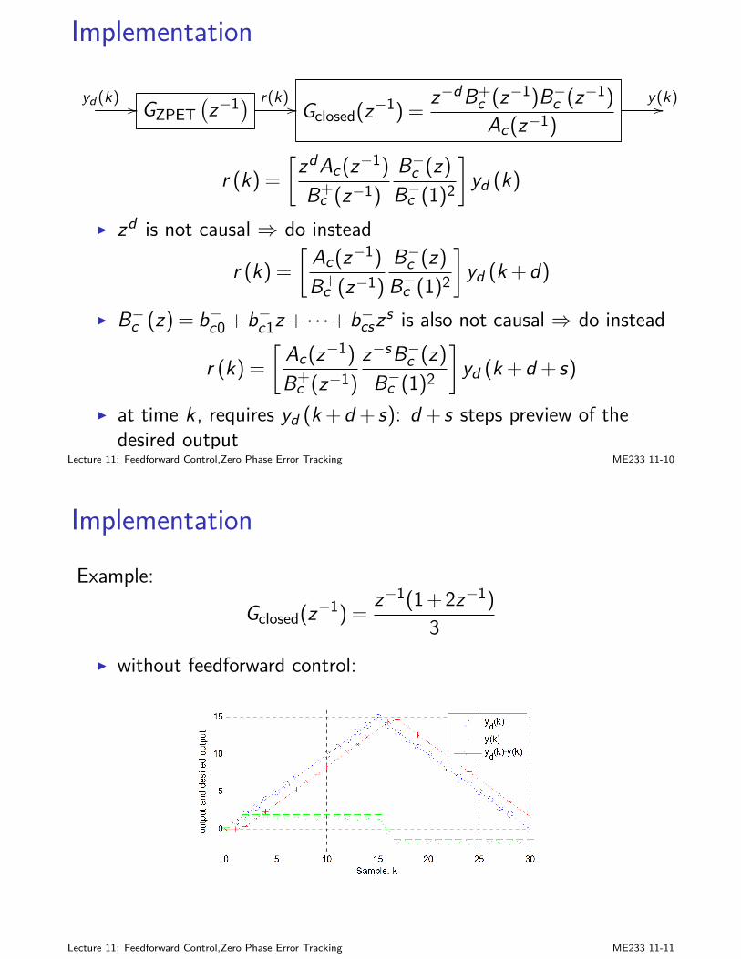
Implementation
yd (k) // GZPET(z−1) r(k) // Gclosed(z−1) =
z−dB+c (z−1)B−c (z−1)Ac(z−1)
y(k)//
r (k) =[
zdAc(z−1)
B+c (z−1)
B−c (z)B−c (1)2
]yd (k)
I zd is not causal ⇒ do instead
r (k) =[
Ac(z−1)
B+c (z−1)
B−c (z)B−c (1)2
]yd (k +d)
I B−c (z) = b−c0+b−c1z + · · ·+b−cszs is also not causal ⇒ do instead
r (k) =[
Ac(z−1)
B+c (z−1)
z−sB−c (z)B−c (1)2
]yd (k +d + s)
I at time k , requires yd (k +d + s): d + s steps preview of thedesired output
Lecture 11: Feedforward Control,Zero Phase Error Tracking ME233 11-10
ImplementationExample:
Gclosed(z−1) =z−1(1+2z−1)
3I without feedforward control:
Lecture 11: Feedforward Control,Zero Phase Error Tracking ME233 11-11

ImplementationExample:
Gclosed(z−1) =z−1(1+2z−1)
3I with ZPET feedforward:
Lecture 11: Feedforward Control,Zero Phase Error Tracking ME233 11-12
ImplementationZPET extensions:
I standard form:
GZPET(z−1) =zdAc(z−1)
B+c (z−1)
B−c (z)B−c (1)2
I extended bandwidth (ref: B. Haack and M. Tomizuka, “Theeffect of adding zeros to feedforward controllers,” ASME J. Dyn.Syst. Meas. Control, vol. 113, pp. 6-10, 1991):
GZPET(z−1) =zdAc(z−1)
B+c (z−1)
B−c (z)B−c (1)2
(z−1−b
)(z−b)
(1−b)2, 0< b < 1
I remark:(z−1−b
)(z−b)/(1−b)2 , 0< b < 1 is a high-pass
filter with unity DC gain
Lecture 11: Feedforward Control,Zero Phase Error Tracking ME233 11-13
ME 233, UC Berkeley, Spring 2014 Xu Chen
Lecture 12: Preview Control
Big pictureProblem formulationRelationship to LQ
Solution
Review: optimal trackingWe consider controlling the system
x (k +1) = Ax (k)+Bu (k) (1)y (k) = Cx (k)
wherex ∈ Rn, u ∈ Rm, y ∈ Rr
Optimal tracking with full reference information (homework 1):
minU0
J :=12 [yd (N)−y(N)]T S [yd (N)−y(N)]
+12
N−1∑k=0
([yd (k)−y(k)]T Qy [yd (k)−y(k)] + u(k)T Ru(k)
)(2)
uo(k) = −[R + BT P(k + 1)B
]−1BT[P(k + 1)Ax(k) + bT (k + 1)
](3)
Jok (x(k)) =
12xT (k)P(k)x(k) + b(k)x(k) + c(k) (4)
Lecture 12: Preview Control ME233 12-1
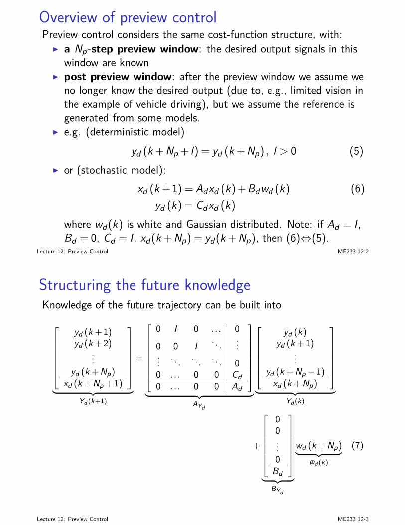
Overview of preview controlPreview control considers the same cost-function structure, with:
I a Np-step preview window: the desired output signals in thiswindow are known
I post preview window: after the preview window we assume weno longer know the desired output (due to, e.g., limited vision inthe example of vehicle driving), but we assume the reference isgenerated from some models.
I e.g. (deterministic model)yd (k +Np + l) = yd (k +Np) , l > 0 (5)
I or (stochastic model):xd (k +1) = Adxd (k)+Bdwd (k) (6)
yd (k) = Cdxd (k)where wd(k) is white and Gaussian distributed. Note: if Ad = I ,Bd = 0, Cd = I , xd(k +Np) = yd(k +Np), then (6)⇔(5).
Lecture 12: Preview Control ME233 12-2
Structuring the future knowledgeKnowledge of the future trajectory can be built into
yd (k + 1)yd (k + 2)
...yd (k + Np)
xd (k + Np + 1)
︸ ︷︷ ︸Yd (k+1)
=
0 I 0 . . . 0
0 0 I . . . ...... . . . . . . . . . 00 . . . 0 0 Cd0 . . . 0 0 Ad
︸ ︷︷ ︸AYd
yd (k)yd (k + 1)
...yd (k + Np−1)
xd (k + Np)
︸ ︷︷ ︸Yd (k)
+
00...0
Bd
︸ ︷︷ ︸BYd
wd (k + Np)︸ ︷︷ ︸wd (k)
(7)
Lecture 12: Preview Control ME233 12-3
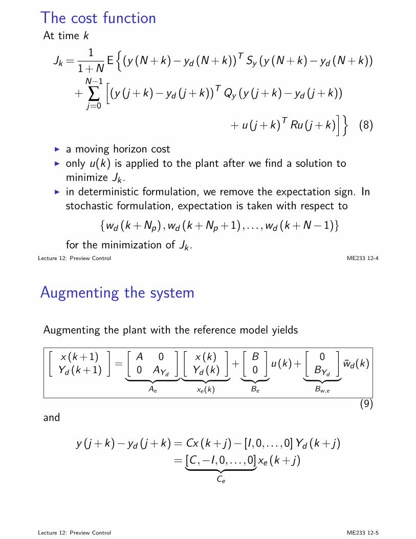
The cost functionAt time k
Jk =1
1+N E(y (N +k)− yd (N +k))T Sy (y (N +k)− yd (N +k))
+N−1∑j=0
[(y (j +k)− yd (j +k))T Qy (y (j +k)− yd (j +k))
+ u (j +k)T Ru (j +k)]
(8)
I a moving horizon costI only u(k) is applied to the plant after we find a solution to
minimize Jk .I in deterministic formulation, we remove the expectation sign. In
stochastic formulation, expectation is taken with respect towd (k +Np) ,wd (k +Np +1) , . . . ,wd (k +N−1)
for the minimization of Jk .Lecture 12: Preview Control ME233 12-4
Augmenting the system
Augmenting the plant with the reference model yields[
x (k + 1)Yd (k + 1)
]=
[A 00 AYd
]
︸ ︷︷ ︸Ae
[x (k)
Yd (k)
]
︸ ︷︷ ︸xe(k)
+
[B0
]
︸ ︷︷ ︸Be
u (k) +
[0
BYd
]
︸ ︷︷ ︸Bw ,e
wd (k)
(9)and
y (j +k)− yd (j +k) = Cx (k + j)− [I ,0, . . . ,0]Yd (k + j)= [C ,−I ,0, . . . ,0]︸ ︷︷ ︸
Ce
xe (k + j)
Lecture 12: Preview Control ME233 12-5
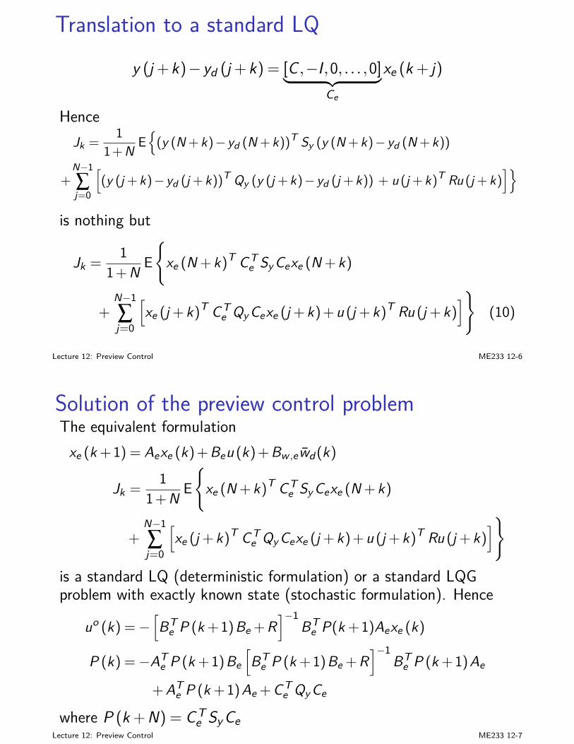
Translation to a standard LQy (j +k)− yd (j +k) = [C ,−I ,0, . . . ,0]︸ ︷︷ ︸
Ce
xe (k + j)
HenceJk =
11 + N E
(y (N + k)−yd (N + k))T Sy (y (N + k)−yd (N + k))
+N−1∑j=0
[(y (j + k)−yd (j + k))T Qy (y (j + k)−yd (j + k)) + u (j + k)T Ru (j + k)
]
is nothing but
Jk =1
1 + N E
xe (N + k)T CTe Sy Cexe (N + k)
+N−1∑j=0
[xe (j + k)T CT
e Qy Cexe (j + k) + u (j + k)T Ru (j + k)]
(10)
Lecture 12: Preview Control ME233 12-6
Solution of the preview control problemThe equivalent formulation
xe (k + 1) = Aexe (k) + Beu (k) + Bw ,ewd (k)
Jk =1
1 + N E
xe (N + k)T CTe Sy Cexe (N + k)
+N−1∑j=0
[xe (j + k)T CT
e Qy Cexe (j + k) + u (j + k)T Ru (j + k)]
is a standard LQ (deterministic formulation) or a standard LQGproblem with exactly known state (stochastic formulation). Hence
uo (k) =−[BT
e P (k + 1)Be + R]−1
BTe P(k + 1)Aexe (k)
P (k) =−ATe P (k + 1)Be
[BT
e P (k + 1)Be + R]−1
BTe P (k + 1)Ae
+ ATe P (k + 1)Ae + CT
e Qy Ce
where P (k +N) = CTe SyCe
Lecture 12: Preview Control ME233 12-7
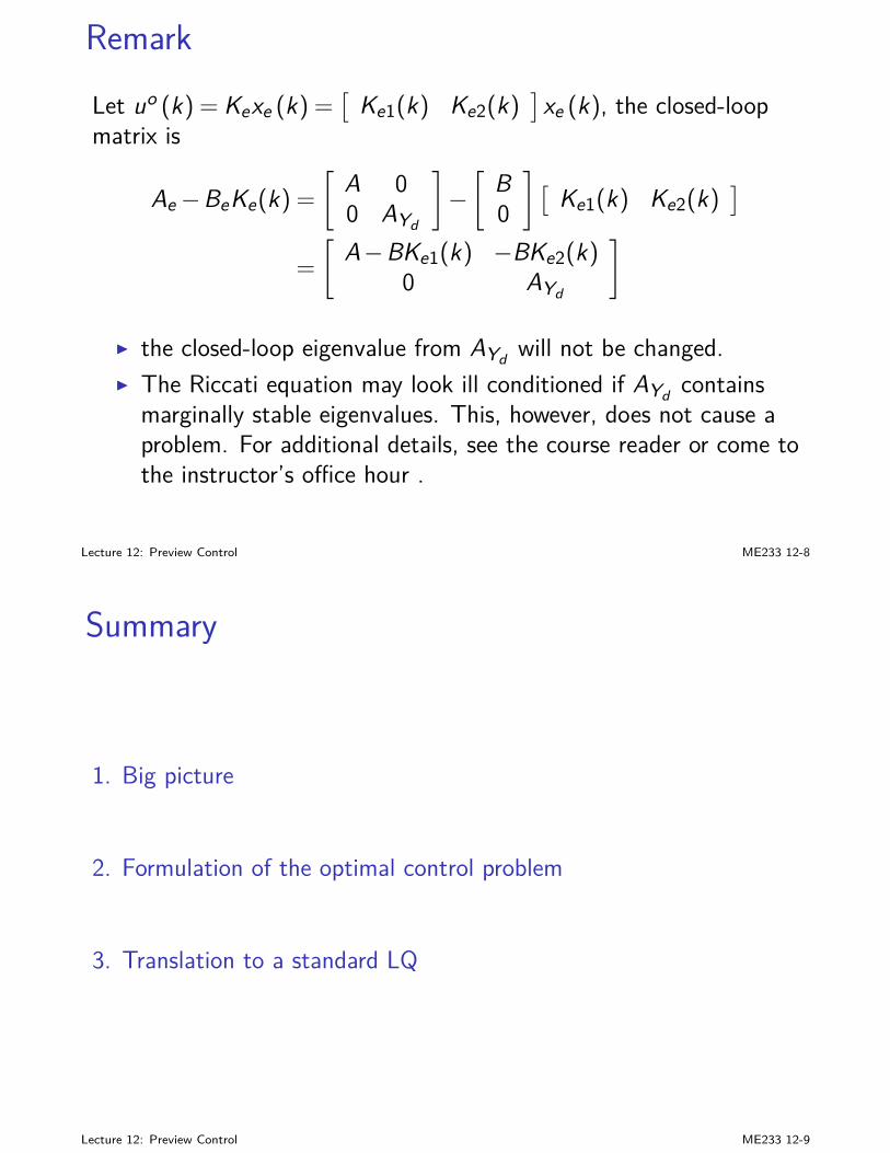
RemarkLet uo (k) = Kexe (k) =
[Ke1(k) Ke2(k)
]xe (k), the closed-loop
matrix is
Ae−BeKe(k) =[
A 00 AYd
]−[
B0
][Ke1(k) Ke2(k)
]
=
[A−BKe1(k) −BKe2(k)
0 AYd
]
I the closed-loop eigenvalue from AYd will not be changed.I The Riccati equation may look ill conditioned if AYd contains
marginally stable eigenvalues. This, however, does not cause aproblem. For additional details, see the course reader or come tothe instructor’s office hour .
Lecture 12: Preview Control ME233 12-8
Summary
1. Big picture
2. Formulation of the optimal control problem
3. Translation to a standard LQ
Lecture 12: Preview Control ME233 12-9
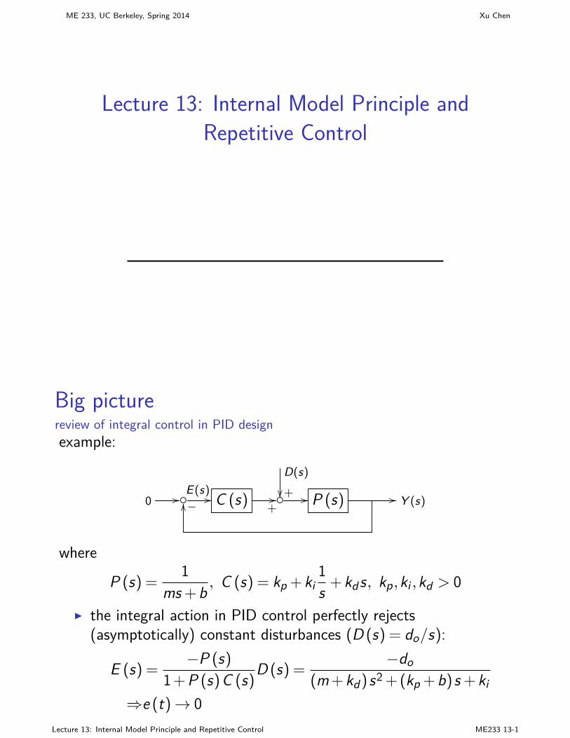
ME 233, UC Berkeley, Spring 2014 Xu Chen
Lecture 13: Internal Model Principle andRepetitive Control
Big picturereview of integral control in PID designexample:
+
D(s)0 //E(s) // C (s)
+// // P (s) // Y (s)−OO
where
P (s) =1
ms +b , C (s) = kp +ki1s +kds, kp,ki ,kd > 0
I the integral action in PID control perfectly rejects(asymptotically) constant disturbances (D (s) = do/s):
E (s) =−P (s)
1+P (s)C (s)D (s) =
−do(m+kd )s2 + (kp +b)s +ki
⇒e (t)→ 0Lecture 13: Internal Model Principle and Repetitive Control ME233 13-1
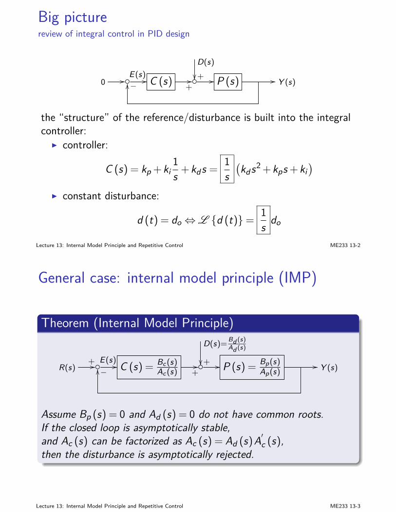
Big picturereview of integral control in PID design
+
D(s)0 //E(s) // C (s)
+// // P (s) // Y (s)−OO
the “structure” of the reference/disturbance is built into the integralcontroller:
I controller:
C (s) = kp +ki1s +kds =
1s(kds2 +kps +ki
)
I constant disturbance:
d (t) = do ⇔L d (t)=1s do
Lecture 13: Internal Model Principle and Repetitive Control ME233 13-2
General case: internal model principle (IMP)
Theorem (Internal Model Principle)
+
D(s)=Bd (s)Ad (s)
R(s)+ //E(s) // C (s) = Bc(s)
Ac(s) +// // P (s) =
Bp(s)Ap(s)
// Y (s)−OO
Assume Bp (s) = 0 and Ad (s) = 0 do not have common roots.If the closed loop is asymptotically stable,and Ac (s) can be factorized as Ac (s) = Ad (s)A′c (s),then the disturbance is asymptotically rejected.
Lecture 13: Internal Model Principle and Repetitive Control ME233 13-3
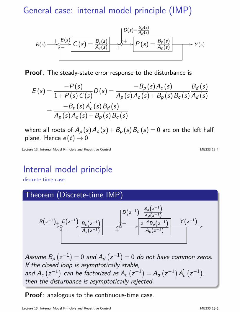
General case: internal model principle (IMP)
+
D(s)=Bd (s)Ad (s)
R(s)+ //E(s) // C (s) = Bc(s)
Ac(s) +// // P (s) =
Bp(s)Ap(s)
// Y (s)−OO
Proof: The steady-state error response to the disturbance is
E (s) =−P (s)
1+P (s)C (s)D (s) =
−Bp (s)Ac (s)
Ap (s)Ac (s) +Bp (s)Bc (s)
Bd (s)
Ad (s)
=−Bp (s)A′c (s)Bd (s)
Ap (s)Ac (s) +Bp (s)Bc (s)
where all roots of Ap (s)Ac (s) +Bp (s)Bc (s) = 0 are on the left halfplane. Hence e (t)→ 0
Lecture 13: Internal Model Principle and Repetitive Control ME233 13-4
Internal model principlediscrete-time case:
Theorem (Discrete-time IMP)
+
D(z−1)=Bd(z−1)Ad (z−1)
R(z−1)+ //E(z−1)
// Bc(z−1)Ac(z−1) +
// // z−d Bp(z−1)Ap(z−1)
Y (z−1)//
−OO
Assume Bp(z−1)= 0 and Ad
(z−1)= 0 do not have common zeros.
If the closed loop is asymptotically stable,and Ac
(z−1) can be factorized as Ac
(z−1)= Ad
(z−1)A′c
(z−1),
then the disturbance is asymptotically rejected.
Proof: analogous to the continuous-time case.
Lecture 13: Internal Model Principle and Repetitive Control ME233 13-5
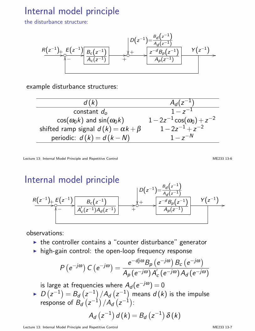
Internal model principlethe disturbance structure:
+
D(z−1)=Bd(z−1)Ad (z−1)
R(z−1)+ //E(z−1)
// Bc(z−1)Ac(z−1) +
// // z−d Bp(z−1)Ap(z−1)
Y (z−1)//
−OO
example disturbance structures:
d (k) Ad (z−1)constant do 1− z−1
cos(ω0k) and sin(ω0k) 1−2z−1 cos(ω0) + z−2
shifted ramp signal d (k) = αk + β 1−2z−1 + z−2
periodic: d (k) = d (k−N) 1− z−N
Lecture 13: Internal Model Principle and Repetitive Control ME233 13-6
Internal model principle
+
D(z−1)=Bd(z−1)Ad (z−1)
R(z−1)+ //E(z−1)
// Bc(z−1)A′c(z−1)Ad (z−1) +
// // z−d Bp(z−1)Ap(z−1)
Y (z−1)//
−OO
observations:I the controller contains a “counter disturbance” generatorI high-gain control: the open-loop frequency response
P(e−jω)C
(e−jω)=
e−djωBp(e−jω)Bc
(e−jω)
Ap (e−jω)A′c (e−jω)Ad (e−jω)
is large at frequencies where Ad (e−jω) = 0I D
(z−1)= Bd
(z−1)/Ad
(z−1) means d (k) is the impulse
response of Bd(z−1)/Ad
(z−1):
Ad(z−1)d (k) = Bd
(z−1)δ (k)
Lecture 13: Internal Model Principle and Repetitive Control ME233 13-7
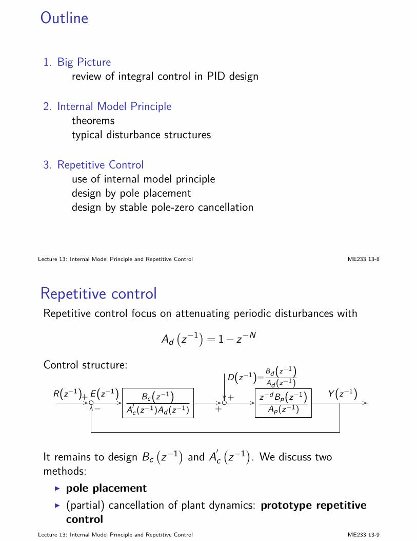
Outline
1. Big Picturereview of integral control in PID design
2. Internal Model Principletheoremstypical disturbance structures
3. Repetitive Controluse of internal model principledesign by pole placementdesign by stable pole-zero cancellation
Lecture 13: Internal Model Principle and Repetitive Control ME233 13-8
Repetitive controlRepetitive control focus on attenuating periodic disturbances with
Ad(z−1)= 1− z−N
Control structure:
+
D(z−1)=Bd(z−1)Ad (z−1)
R(z−1)+ //E(z−1)
// Bc(z−1)A′c(z−1)Ad (z−1) +
// // z−d Bp(z−1)Ap(z−1)
Y (z−1)//
−OO
It remains to design Bc(z−1) and A′c
(z−1). We discuss two
methods:I pole placementI (partial) cancellation of plant dynamics: prototype repetitive
controlLecture 13: Internal Model Principle and Repetitive Control ME233 13-9
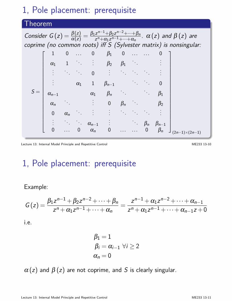
1, Pole placement: prerequisiteTheoremConsider G (z) = β (z)
α(z) = β1zn−1+β2zn−2+···+βnzn+α1zn−1+···+αn
. α (z) and β (z) arecoprime (no common roots) iff S (Sylvester matrix) is nonsingular:
S =
1 0 . . . 0 β1 0 . . . . . . 0
α1 1 . . . ... β2 β1. . . ...
... . . . . . . 0... . . . . . . . . . ...
... α1 1 βn−1. . . . . . 0
αn−1 α1 βn. . . . . . β1
αn. . . ... 0 βn
. . . β2
0 αn. . . ...
... . . . . . . . . . ...... . . . . . . αn−1
... . . . βn βn−10 . . . 0 αn 0 . . . . . . 0 βn
(2n−1)×(2n−1)
Lecture 13: Internal Model Principle and Repetitive Control ME233 13-10
1, Pole placement: prerequisite
Example:
G (z) =β1zn−1 + β2zn−2 + · · ·+ βnzn + α1zn−1 + · · ·+ αn
=zn−1 + α1zn−2 + · · ·+ αn−1
zn + α1zn−1 + · · ·+ αn−1z +0
i.e.
β1 = 1βi = αi−1 ∀i ≥ 2αn = 0
α (z) and β (z) are not coprime, and S is clearly singular.
Lecture 13: Internal Model Principle and Repetitive Control ME233 13-11
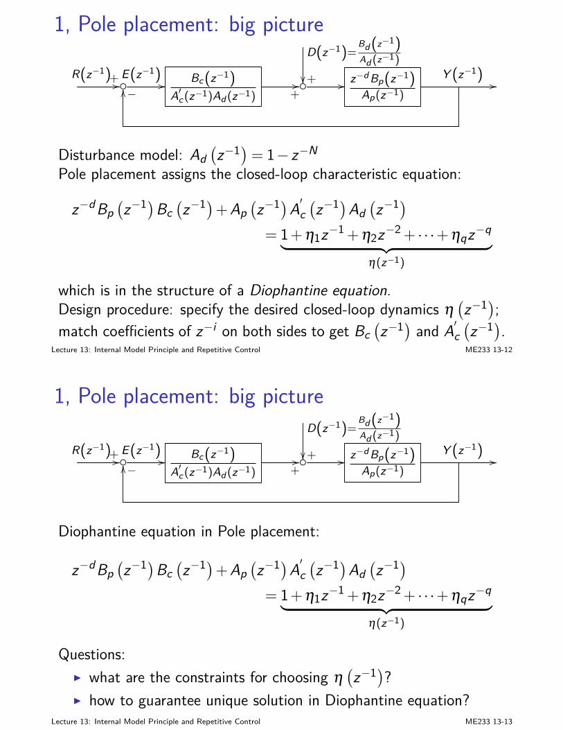
1, Pole placement: big picture
+
D(z−1)=Bd(z−1)Ad (z−1)
R(z−1)+ //E(z−1)
// Bc(z−1)A′c(z−1)Ad (z−1) +
// // z−d Bp(z−1)Ap(z−1)
Y (z−1)//
−OO
Disturbance model: Ad(z−1)= 1− z−N
Pole placement assigns the closed-loop characteristic equation:
z−dBp(z−1)Bc
(z−1)+Ap
(z−1)A′c
(z−1)Ad
(z−1)
= 1+ η1z−1 + η2z−2 + · · ·+ ηqz−q︸ ︷︷ ︸
η(z−1)
which is in the structure of a Diophantine equation.Design procedure: specify the desired closed-loop dynamics η
(z−1);
match coefficients of z−i on both sides to get Bc(z−1) and A′c
(z−1).
Lecture 13: Internal Model Principle and Repetitive Control ME233 13-12
1, Pole placement: big picture
+
D(z−1)=Bd(z−1)Ad (z−1)
R(z−1)+ //E(z−1)
// Bc(z−1)A′c(z−1)Ad (z−1) +
// // z−d Bp(z−1)Ap(z−1)
Y (z−1)//
−OO
Diophantine equation in Pole placement:
z−dBp(z−1)Bc
(z−1)+Ap
(z−1)A′c
(z−1)Ad
(z−1)
= 1+ η1z−1 + η2z−2 + · · ·+ ηqz−q︸ ︷︷ ︸
η(z−1)
Questions:I what are the constraints for choosing η
(z−1)?
I how to guarantee unique solution in Diophantine equation?Lecture 13: Internal Model Principle and Repetitive Control ME233 13-13
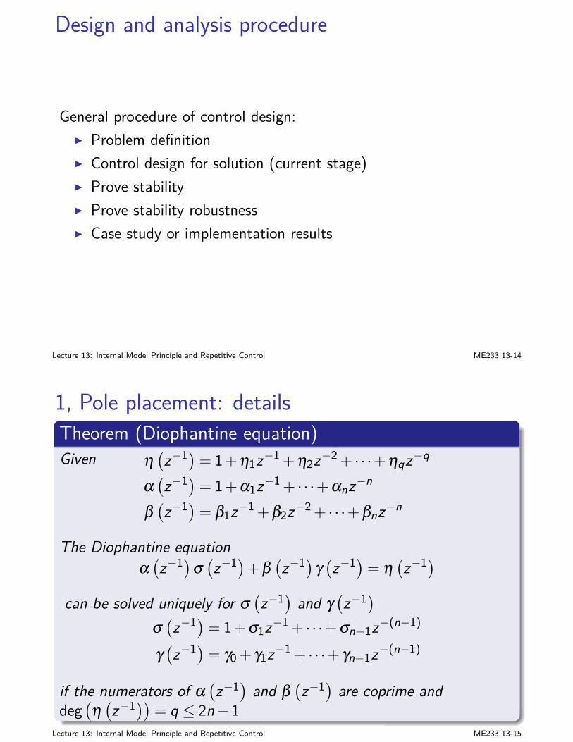
Design and analysis procedure
General procedure of control design:I Problem definitionI Control design for solution (current stage)I Prove stabilityI Prove stability robustnessI Case study or implementation results
Lecture 13: Internal Model Principle and Repetitive Control ME233 13-14
1, Pole placement: detailsTheorem (Diophantine equation)Given η
(z−1)= 1+ η1z−1 + η2z−2 + · · ·+ ηqz−q
α(z−1)= 1+ α1z−1 + · · ·+ αnz−n
β(z−1)= β1z−1 + β2z−2 + · · ·+ βnz−n
The Diophantine equationα(z−1)σ
(z−1)+ β
(z−1)γ
(z−1)= η
(z−1)
can be solved uniquely for σ(z−1) and γ
(z−1)
σ(z−1)= 1+ σ1z−1 + · · ·+ σn−1z−(n−1)
γ(z−1)= γ0 + γ1z−1 + · · ·+ γn−1z−(n−1)
if the numerators of α(z−1) and β
(z−1) are coprime and
deg(η(z−1))= q ≤ 2n−1
Lecture 13: Internal Model Principle and Repetitive Control ME233 13-15
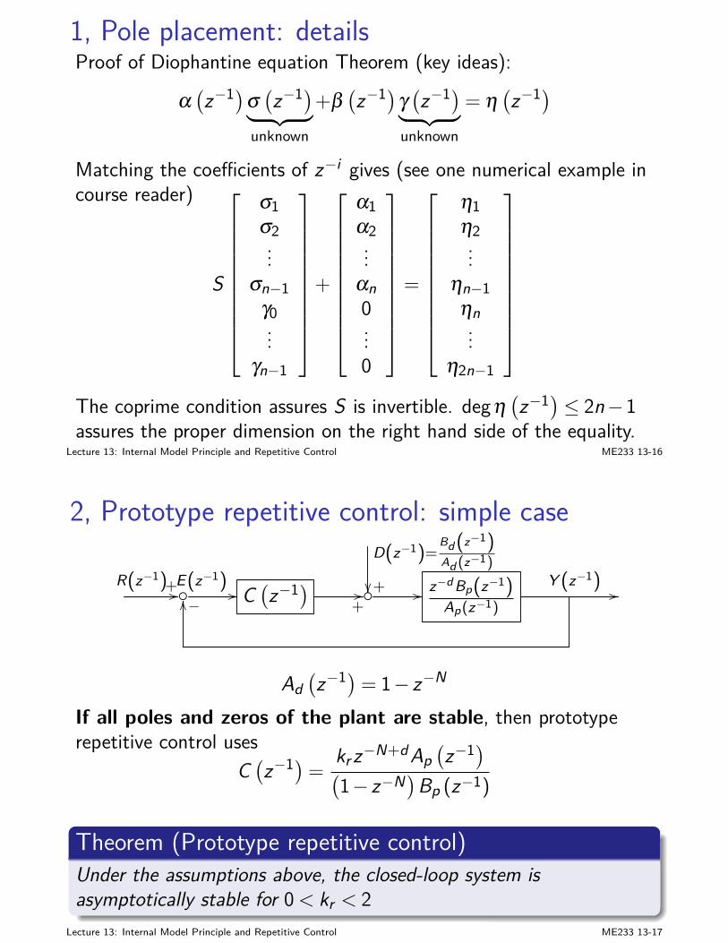
1, Pole placement: detailsProof of Diophantine equation Theorem (key ideas):
α(z−1)σ
(z−1)
︸ ︷︷ ︸unknown
+β(z−1)γ
(z−1)
︸ ︷︷ ︸unknown
= η(z−1)
Matching the coefficients of z−i gives (see one numerical example incourse reader)
S
σ1σ2...
σn−1γ0...
γn−1
+
α1α2...
αn0...0
=
η1η2...
ηn−1ηn...
η2n−1
The coprime condition assures S is invertible. degη(z−1)≤ 2n−1
assures the proper dimension on the right hand side of the equality.Lecture 13: Internal Model Principle and Repetitive Control ME233 13-16
2, Prototype repetitive control: simple case
+
D(z−1)=Bd(z−1)Ad (z−1)
R(z−1)+ //E(z−1)
// C(z−1)
+// // z
−d Bp(z−1)Ap(z−1)
Y (z−1)//
−OO
Ad(z−1)= 1− z−N
If all poles and zeros of the plant are stable, then prototyperepetitive control uses
C(z−1)=
krz−N+dAp(z−1)
(1− z−N)Bp (z−1)
Theorem (Prototype repetitive control)Under the assumptions above, the closed-loop system isasymptotically stable for 0< kr < 2
Lecture 13: Internal Model Principle and Repetitive Control ME233 13-17
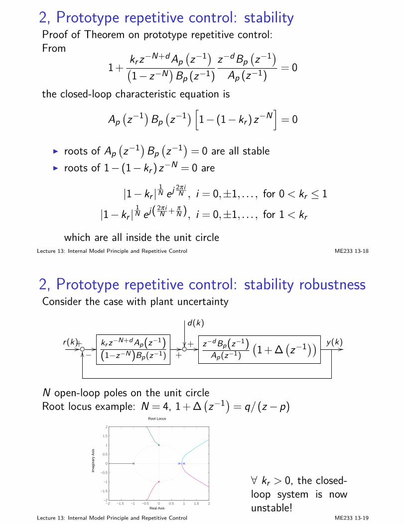
2, Prototype repetitive control: stabilityProof of Theorem on prototype repetitive control:From
1+krz−N+dAp
(z−1)
(1− z−N)Bp (z−1)
z−dBp(z−1)
Ap (z−1)= 0
the closed-loop characteristic equation is
Ap(z−1)Bp
(z−1)[1− (1−kr )z−N
]= 0
I roots of Ap(z−1)Bp
(z−1)= 0 are all stable
I roots of 1− (1−kr )z−N = 0 are
|1−kr |1N ej 2π i
N , i = 0,±1, . . . , for 0< kr ≤ 1|1−kr |
1N ej( 2π i
N + πN ), i = 0,±1, . . . , for 1< kr
which are all inside the unit circleLecture 13: Internal Model Principle and Repetitive Control ME233 13-18
2, Prototype repetitive control: stability robustnessConsider the case with plant uncertainty
+
d(k)
r(k)+// // kr z−N+d Ap(z−1)(1−z−N)Bp(z−1) +
// // z−d Bp(z−1)Ap(z−1)
(1+ ∆
(z−1)) y(k) //
−OO
N open-loop poles on the unit circleRoot locus example: N = 4, 1+ ∆
(z−1)= q/(z−p)
−2 −1.5 −1 −0.5 0 0.5 1 1.5 2−2
−1.5
−1
−0.5
0
0.5
1
1.5
2
Root Locus
Real Axis
Imag
inar
y A
xis
∀ kr > 0, the closed-loop system is nowunstable!
Lecture 13: Internal Model Principle and Repetitive Control ME233 13-19
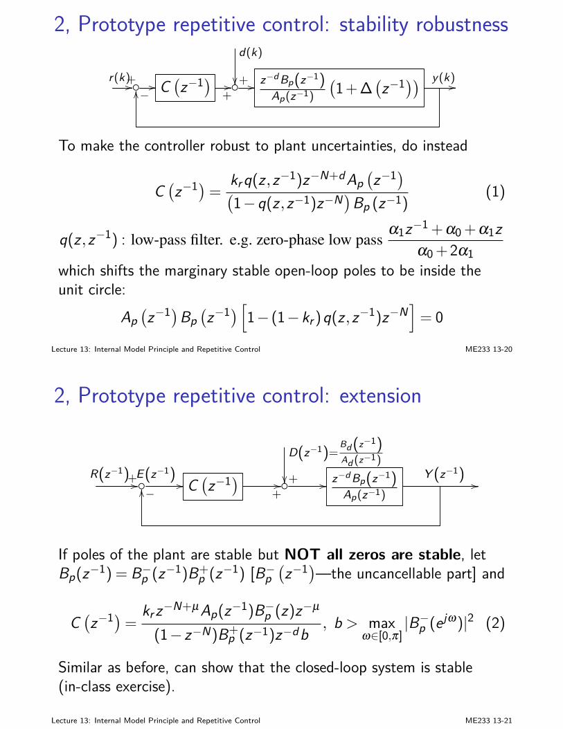
2, Prototype repetitive control: stability robustness
+
d(k)
r(k)+// // C(z−1)
+// // z
−d Bp(z−1)Ap(z−1)
(1+ ∆
(z−1)) y(k) //
−OO
To make the controller robust to plant uncertainties, do instead
C(z−1)=
krq(z ,z−1)z−N+dAp(z−1)
(1−q(z ,z−1)z−N)Bp (z−1)
(1)
q(z ,z−1) : low-pass filter. e.g. zero-phase low passα1z−1 + α0 + α1z
α0 +2α1which shifts the marginary stable open-loop poles to be inside theunit circle:
Ap(z−1)Bp
(z−1)[1− (1−kr )q(z ,z−1)z−N
]= 0
Lecture 13: Internal Model Principle and Repetitive Control ME233 13-20
2, Prototype repetitive control: extension
+
D(z−1)=Bd(z−1)Ad (z−1)
R(z−1)+ //E(z−1)
// C(z−1)
+// // z
−d Bp(z−1)Ap(z−1)
Y (z−1)//
−OO
If poles of the plant are stable but NOT all zeros are stable, letBp(z−1) = B−p (z−1)B+
p (z−1) [B−p(z−1)—the uncancellable part] and
C(z−1)=
krz−N+µAp(z−1)B−p (z)z−µ
(1− z−N)B+p (z−1)z−db
, b > maxω∈[0,π]
|B−p (ejω)|2 (2)
Similar as before, can show that the closed-loop system is stable(in-class exercise).
Lecture 13: Internal Model Principle and Repetitive Control ME233 13-21
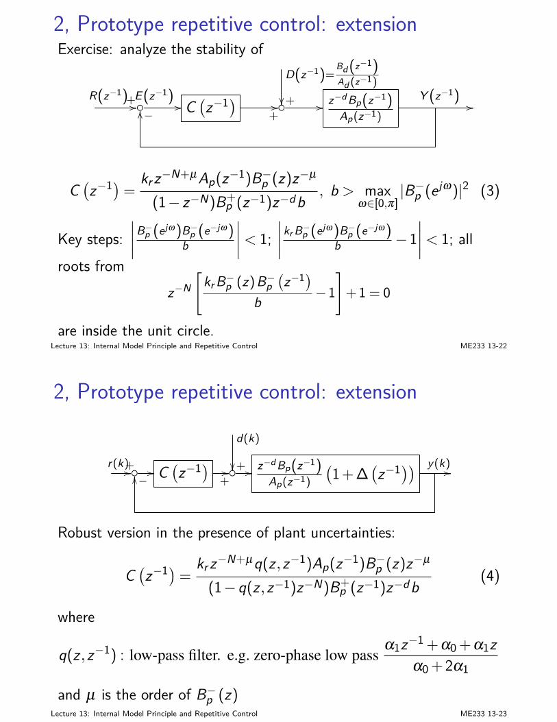
2, Prototype repetitive control: extensionExercise: analyze the stability of
+
D(z−1)=Bd(z−1)Ad (z−1)
R(z−1)+ //E(z−1)
// C(z−1)
+// // z
−d Bp(z−1)Ap(z−1)
Y (z−1)//
−OO
C(z−1)=
krz−N+µAp(z−1)B−p (z)z−µ
(1− z−N)B+p (z−1)z−db
, b > maxω∈[0,π]
|B−p (ejω)|2 (3)
Key steps:∣∣∣∣
B−p (ejω)B−p (e−jω)b
∣∣∣∣< 1;∣∣∣∣
kr B−p (ejω)B−p (e−jω)b −1
∣∣∣∣< 1; allroots from
z−N[
kr B−p (z)B−p(z−1)
b −1]+1 = 0
are inside the unit circle.Lecture 13: Internal Model Principle and Repetitive Control ME233 13-22
2, Prototype repetitive control: extension
+
d(k)
r(k)+// // C(z−1)
+// // z
−d Bp(z−1)Ap(z−1)
(1+ ∆
(z−1)) y(k) //
−OO
Robust version in the presence of plant uncertainties:
C(z−1)=
krz−N+µq(z ,z−1)Ap(z−1)B−p (z)z−µ
(1−q(z ,z−1)z−N)B+p (z−1)z−db
(4)
where
q(z ,z−1) : low-pass filter. e.g. zero-phase low passα1z−1 + α0 + α1z
α0 +2α1
and µ is the order of B−p (z)Lecture 13: Internal Model Principle and Repetitive Control ME233 13-23
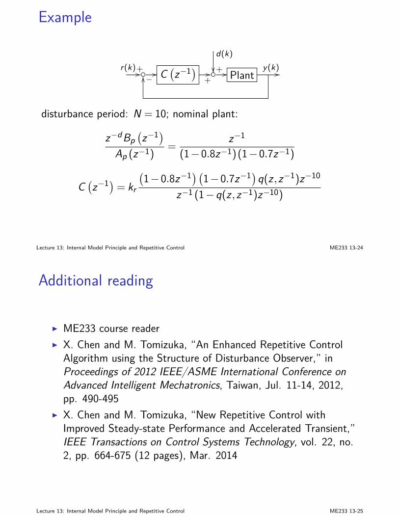
Example
+
d(k)
r(k)+// // C(z−1)
+// // Plant
y(k) //−OO
disturbance period: N = 10; nominal plant:
z−dBp(z−1)
Ap (z−1)=
z−1
(1−0.8z−1)(1−0.7z−1)
C(z−1)= kr
(1−0.8z−1)(1−0.7z−1)q(z ,z−1)z−10
z−1 (1−q(z ,z−1)z−10)
Lecture 13: Internal Model Principle and Repetitive Control ME233 13-24
Additional reading
I ME233 course readerI X. Chen and M. Tomizuka, “An Enhanced Repetitive Control
Algorithm using the Structure of Disturbance Observer,” inProceedings of 2012 IEEE/ASME International Conference onAdvanced Intelligent Mechatronics, Taiwan, Jul. 11-14, 2012,pp. 490-495
I X. Chen and M. Tomizuka, “New Repetitive Control withImproved Steady-state Performance and Accelerated Transient,”IEEE Transactions on Control Systems Technology, vol. 22, no.2, pp. 664-675 (12 pages), Mar. 2014
Lecture 13: Internal Model Principle and Repetitive Control ME233 13-25
Summary
1. Big Picturereview of integral control in PID design
2. Internal Model Principletheoremstypical disturbance structures
3. Repetitive Controluse of internal model principledesign by pole placementdesign by stable pole-zero cancellation
Lecture 13: Internal Model Principle and Repetitive Control ME233 13-26

ME 233, UC Berkeley, Spring 2014 Xu Chen
Lecture 14: Disturbance Observer
Big picture
Disturbance and uncertainties in mechanical systems:I system models are important in design: e.g., in ZPET, observer,
and preview controlsI inevitable to have uncertainty in actual mechanical systemsI system is also subjected to disturbances
Related control design:I robust controlI adaptive control
Disturbance observer is one example of robust control.
Lecture 14: Disturbance Observer ME233 14-1
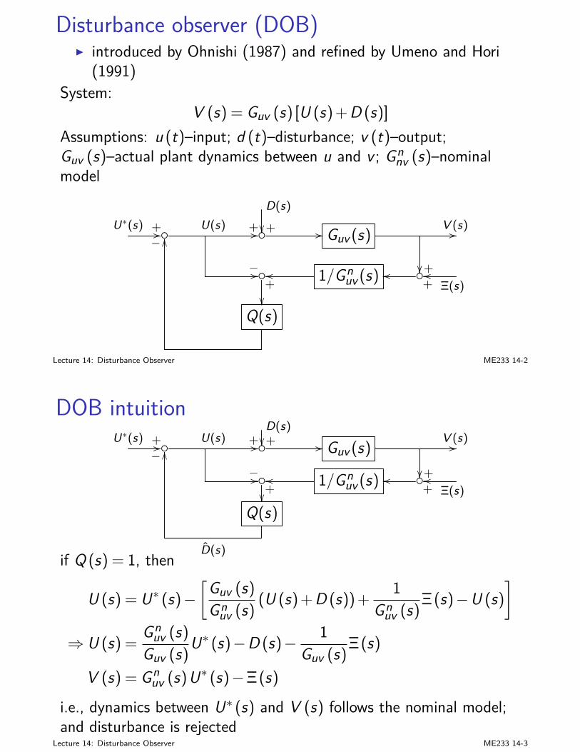
Disturbance observer (DOB)I introduced by Ohnishi (1987) and refined by Umeno and Hori
(1991)System:
V (s) = Guv (s) [U (s) + D (s)]
Assumptions: u (t)–input; d (t)–disturbance; v (t)–output;Guv (s)–actual plant dynamics between u and v ; Gn
nv (s)–nominalmodel
D(s)
+U∗(s) +// U(s) +// // Guv (s)V (s)//
+−//
1/Gnuv (s)
+oo oo
Ξ(s)+oo
Q(s)
− OO
D(s)Lecture 14: Disturbance Observer ME233 14-2
DOB intuitionD(s)+U∗(s) +// U(s) +// // Guv (s)
V (s)//
+−//
1/Gnuv (s)
+oo oo
Ξ(s)+oo
Q(s)
− OO
D(s)if Q (s) = 1, then
U (s) = U∗ (s)−[
Guv (s)
Gnuv (s)(U (s) + D (s)) +
1Gnuv (s)
Ξ(s)−U (s)
]
⇒ U (s) =Gn
uv (s)
Guv (s)U∗ (s)−D (s)− 1
Guv (s)Ξ(s)
V (s) = Gnuv (s)U∗ (s)−Ξ(s)
i.e., dynamics between U∗ (s) and V (s) follows the nominal model;and disturbance is rejected
Lecture 14: Disturbance Observer ME233 14-3
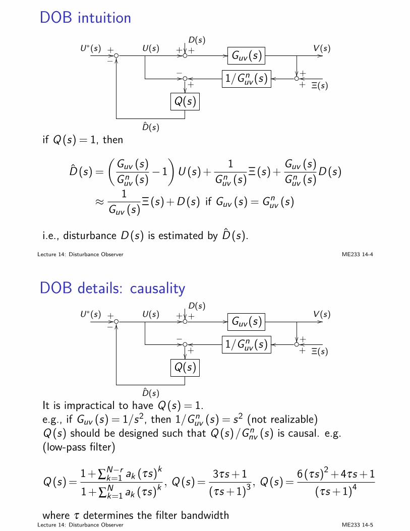
DOB intuitionD(s)+U∗(s) +// U(s) +// // Guv (s)
V (s)//
+−//
1/Gnuv (s)
+oo oo
Ξ(s)+oo
Q(s)
− OO
D(s)
if Q (s) = 1, then
D (s) =
(Guv (s)
Gnuv (s)−1)
U (s) +1
Gnuv (s)Ξ(s) +
Guv (s)
Gnuv (s)D (s)
≈ 1Guv (s)
Ξ(s) + D (s) if Guv (s) = Gnuv (s)
i.e., disturbance D (s) is estimated by D (s).Lecture 14: Disturbance Observer ME233 14-4
DOB details: causalityD(s)+U∗(s) +// U(s) +// // Guv (s)
V (s)//
+−//
1/Gnuv (s)
+oo oo
Ξ(s)+oo
Q(s)
− OO
D(s)
It is impractical to have Q (s) = 1.e.g., if Guv (s) = 1/s2, then 1/Gn
uv (s) = s2 (not realizable)Q (s) should be designed such that Q (s)/Gn
nv (s) is causal. e.g.(low-pass filter)
Q (s) =1+ ∑N−r
k=1 ak (τs)k
1+ ∑Nk=1 ak (τs)k , Q (s) =
3τs +1(τs +1)3 , Q (s) =
6(τs)2 +4τs +1(τs +1)4
where τ determines the filter bandwidthLecture 14: Disturbance Observer ME233 14-5
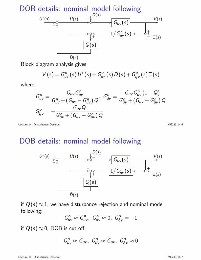
DOB details: nominal model followingD(s)+U∗(s) +// U(s) +// // Guv (s)
V (s)//
+−//
1/Gnuv (s)
+oo oo
Ξ(s)+oo
Q(s)
− OO
D(s)
Block diagram analysis givesV (s) = Go
uv (s)U∗ (s) + Godv (s)D (s) + Go
ξv (s)Ξ(s)
where
Gouv =
GuvGnuv
Gnuv + (Guv −Gnuv )Q , Godv =
GuvGnuv (1−Q)
Gnuv + (Guv −Gnuv )Q
Goξv =− GuvQ
Gnuv + (Guv −Gnuv )QLecture 14: Disturbance Observer ME233 14-6
DOB details: nominal model followingD(s)+U∗(s) +// U(s) +// // Guv (s)
V (s)//
+−//
1/Gnuv (s)
+oo oo
Ξ(s)+oo
Q(s)
− OO
D(s)
if Q (s)≈ 1, we have disturbance rejection and nominal modelfollowing:
Gouv ≈ Gn
uv , Godv ≈ 0, Go
ξv =−1if Q (s)≈ 0, DOB is cut off:
Gouv ≈ Guv , Go
dv ≈ Guv , Goξv ≈ 0
Lecture 14: Disturbance Observer ME233 14-7
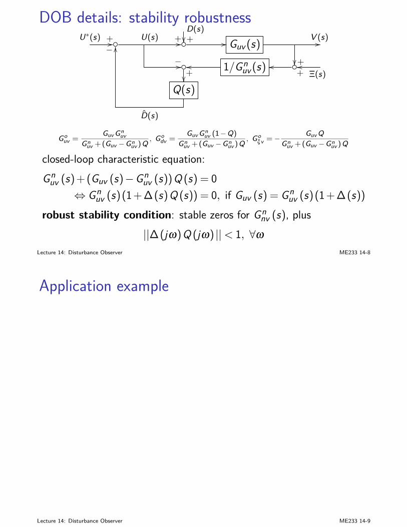
DOB details: stability robustnessD(s)+U∗(s) +// U(s) +// // Guv (s)
V (s)//
+−//
1/Gnuv (s)
+oo oo
Ξ(s)+oo
Q(s)
− OO
D(s)
Gouv =
Guv Gnuv
Gnuv +(Guv −Gnuv )Q , Godv =
Guv Gnuv (1−Q)
Gnuv +(Guv −Gnuv )Q , Goξv =− Guv Q
Gnuv +(Guv −Gnuv )Q
closed-loop characteristic equation:Gn
uv (s) + (Guv (s)−Gnuv (s))Q (s) = 0
⇔ Gnuv (s)(1+ ∆(s)Q (s)) = 0, if Guv (s) = Gn
uv (s)(1+ ∆(s))
robust stability condition: stable zeros for Gnnv (s), plus
||∆(jω)Q (jω) ||< 1, ∀ωLecture 14: Disturbance Observer ME233 14-8
Application example
Lecture 14: Disturbance Observer ME233 14-9
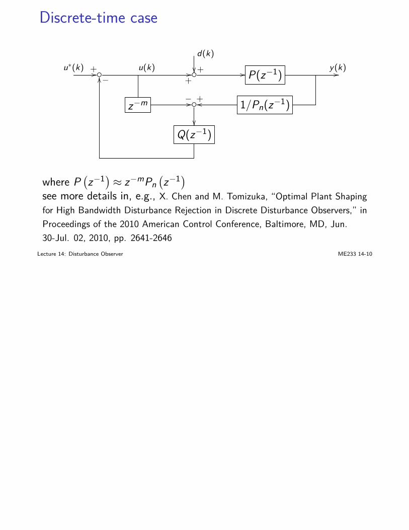
Discrete-time case
d(k)
+u∗(k) +// u(k)
+// // P(z−1)
y(k)//
z−m −//
1/Pn(z−1)+oo
Q(z−1)
−OO
where P(z−1)≈ z−mPn
(z−1)
see more details in, e.g., X. Chen and M. Tomizuka, “Optimal Plant Shapingfor High Bandwidth Disturbance Rejection in Discrete Disturbance Observers,” inProceedings of the 2010 American Control Conference, Baltimore, MD, Jun.30-Jul. 02, 2010, pp. 2641-2646
Lecture 14: Disturbance Observer ME233 14-10

ME 233, UC Berkeley, Spring 2014 Xu Chen
Lecture 15: System Identification and RecursiveLeast Squares
Big picture
We have been assuming knwoledge of the plant in controller design.In practice, plant models come from:
I modeling by physics: Newton’s law, conservation of energy, etcI (input-output) data-based system identification
The need for system identification and adaptive control come fromI unknown plantsI time-varying plantsI known disturbance structure but unknown disturbance
parameters
Lecture 15: System Identification and Recursive Least Squares ME233 15-1
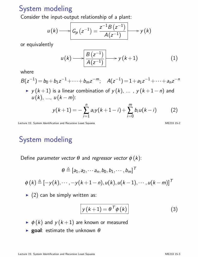
System modelingConsider the input-output relationship of a plant:
u (k) // Gp(z−1)= z−1B
(z−1)
A(z−1)// y (k)
or equivalently
u (k) // B(z−1)
A(z−1)// y (k +1) (1)
whereB(z−1)= b0+b1z−1+· · ·+bmz−m; A(z−1)= 1+a1z−1+· · ·+anz−n
I y (k +1) is a linear combination of y (k), ... , y (k +1−n) andu (k), ..., u (k−m):
y(k +1) =−n∑i=1
aiy(k +1− i)+m∑i=0
biu(k− i) (2)
Lecture 15: System Identification and Recursive Least Squares ME233 15-2
System modeling
Define parameter vector θ and regressor vector φ (k):
θ , [a1,a2, · · ·an,b0,b1, · · · ,bm]T
φ (k), [−y(k), · · · ,−y(k +1−n),u(k),u(k−1), · · · ,u(k−m)]T
I (2) can be simply written as:
y (k +1) = θT φ (k) (3)
I φ (k) and y (k +1) are known or measuredI goal: estimate the unknown θ
Lecture 15: System Identification and Recursive Least Squares ME233 15-3
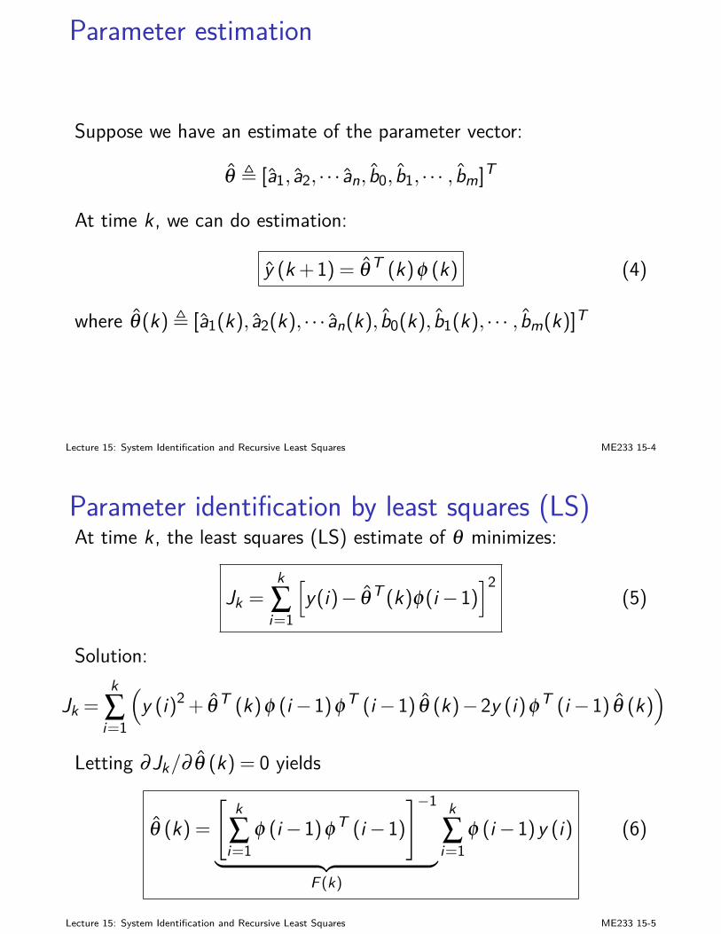
Parameter estimation
Suppose we have an estimate of the parameter vector:
θ , [a1, a2, · · · an, b0, b1, · · · , bm]T
At time k , we can do estimation:
y (k +1) = θ T (k)φ (k) (4)
where θ (k), [a1(k), a2(k), · · · an(k), b0(k), b1(k), · · · , bm(k)]T
Lecture 15: System Identification and Recursive Least Squares ME233 15-4
Parameter identification by least squares (LS)At time k , the least squares (LS) estimate of θ minimizes:
Jk =k∑i=1
[y(i)− θ T (k)φ(i−1)
]2(5)
Solution:
Jk =k∑i=1
(y (i)2 + θT (k)φ (i−1)φT (i−1) θ (k)−2y (i)φT (i−1) θ (k)
)
Letting ∂Jk/∂ θ (k) = 0 yields
θ (k) =[
k∑i=1
φ (i−1)φT (i−1)]−1
︸ ︷︷ ︸F (k)
k∑i=1
φ (i−1)y (i) (6)
Lecture 15: System Identification and Recursive Least Squares ME233 15-5
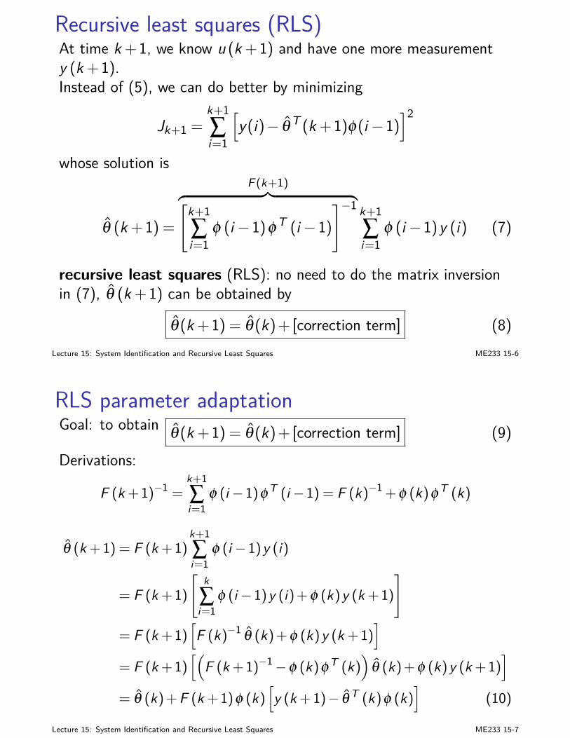
Recursive least squares (RLS)At time k +1, we know u (k +1) and have one more measurementy (k +1).Instead of (5), we can do better by minimizing
Jk+1 =k+1∑i=1
[y(i)− θT (k +1)φ(i−1)
]2
whose solution is
θ (k +1) =
F (k+1)︷ ︸︸ ︷[k+1∑i=1
φ (i−1)φT (i−1)]−1 k+1
∑i=1
φ (i−1)y (i) (7)
recursive least squares (RLS): no need to do the matrix inversionin (7), θ (k +1) can be obtained by
θ (k +1) = θ (k)+ [correction term] (8)Lecture 15: System Identification and Recursive Least Squares ME233 15-6
RLS parameter adaptationGoal: to obtain θ (k +1) = θ (k)+ [correction term] (9)Derivations:
F (k +1)−1 =k+1∑i=1
φ (i−1)φT (i−1) = F (k)−1+φ (k)φT (k)
θ (k +1) = F (k +1)k+1∑i=1
φ (i−1)y (i)
= F (k +1)[
k∑i=1
φ (i−1)y (i)+φ (k)y (k +1)]
= F (k +1)[F (k)−1 θ (k)+φ (k)y (k +1)
]
= F (k +1)[(
F (k +1)−1−φ (k)φT (k))
θ (k)+φ (k)y (k +1)]
= θ (k)+F (k +1)φ (k)[y (k +1)− θ T (k)φ (k)
](10)
Lecture 15: System Identification and Recursive Least Squares ME233 15-7
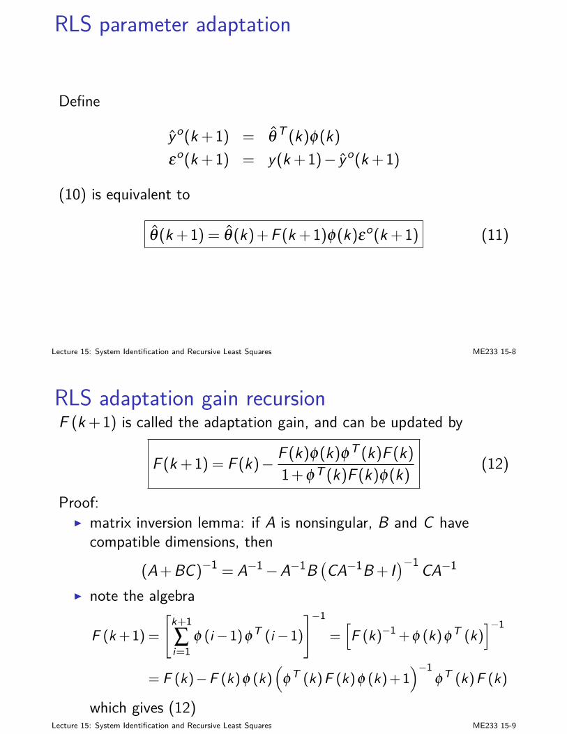
RLS parameter adaptation
Define
yo(k +1) = θT (k)φ(k)εo(k +1) = y(k +1)− yo(k +1)
(10) is equivalent to
θ (k +1) = θ (k)+F (k +1)φ(k)εo(k +1) (11)
Lecture 15: System Identification and Recursive Least Squares ME233 15-8
RLS adaptation gain recursionF (k +1) is called the adaptation gain, and can be updated by
F (k +1) = F (k)− F (k)φ(k)φT (k)F (k)1+φT (k)F (k)φ(k) (12)
Proof:I matrix inversion lemma: if A is nonsingular, B and C have
compatible dimensions, then(A+BC)−1 = A−1−A−1B
(CA−1B + I
)−1 CA−1
I note the algebra
F (k +1) =[
k+1∑i=1
φ (i−1)φT (i−1)]−1
=[F (k)−1+φ (k)φT (k)
]−1
= F (k)−F (k)φ (k)(
φT (k)F (k)φ (k)+1)−1
φT (k)F (k)
which gives (12)Lecture 15: System Identification and Recursive Least Squares ME233 15-9
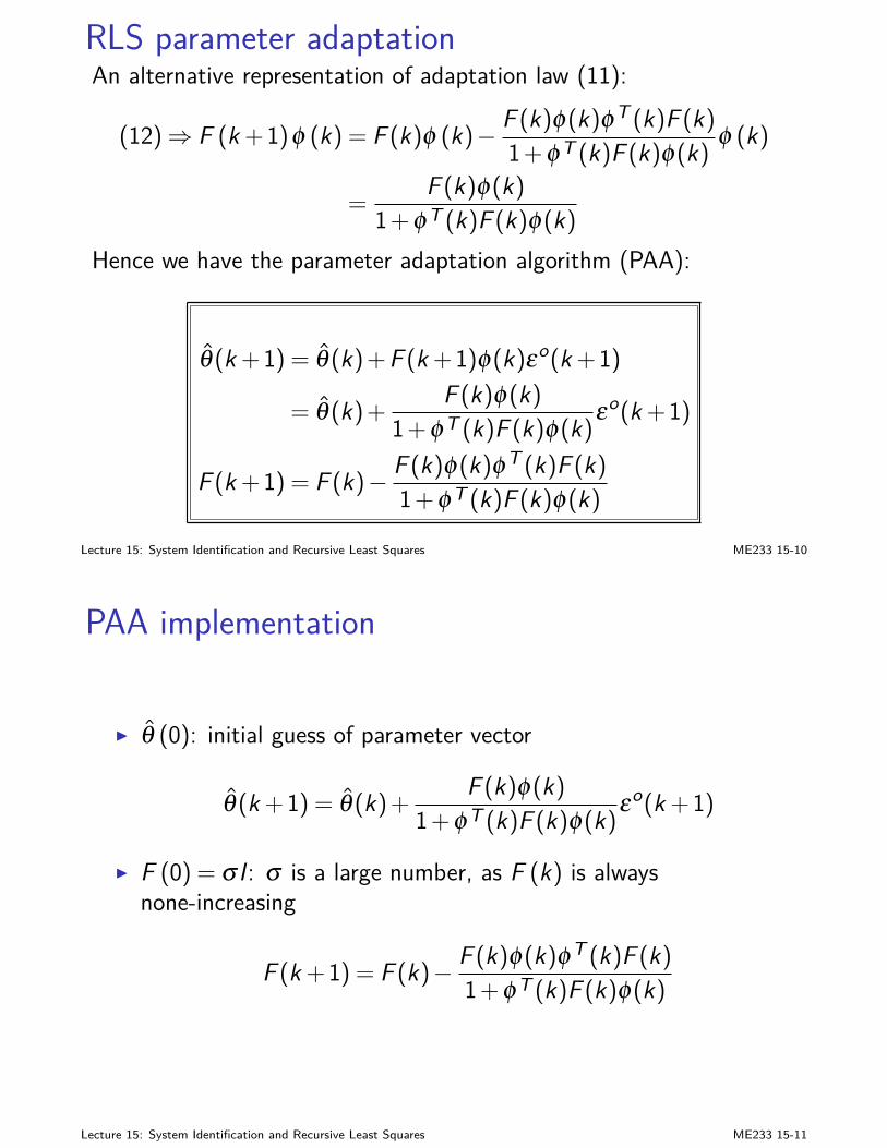
RLS parameter adaptationAn alternative representation of adaptation law (11):
(12)⇒ F (k +1)φ (k) = F (k)φ (k)− F (k)φ(k)φT (k)F (k)1+φT (k)F (k)φ(k) φ (k)
=F (k)φ(k)
1+φT (k)F (k)φ(k)Hence we have the parameter adaptation algorithm (PAA):
θ (k +1) = θ (k)+F (k +1)φ(k)εo(k +1)
= θ (k)+ F (k)φ(k)1+φT (k)F (k)φ(k)εo(k +1)
F (k +1) = F (k)− F (k)φ(k)φT (k)F (k)1+φT (k)F (k)φ(k)
Lecture 15: System Identification and Recursive Least Squares ME233 15-10
PAA implementation
I θ (0): initial guess of parameter vector
θ (k +1) = θ (k)+ F (k)φ(k)1+φT (k)F (k)φ(k)εo(k +1)
I F (0) = σ I : σ is a large number, as F (k) is alwaysnone-increasing
F (k +1) = F (k)− F (k)φ(k)φT (k)F (k)1+φT (k)F (k)φ(k)
Lecture 15: System Identification and Recursive Least Squares ME233 15-11
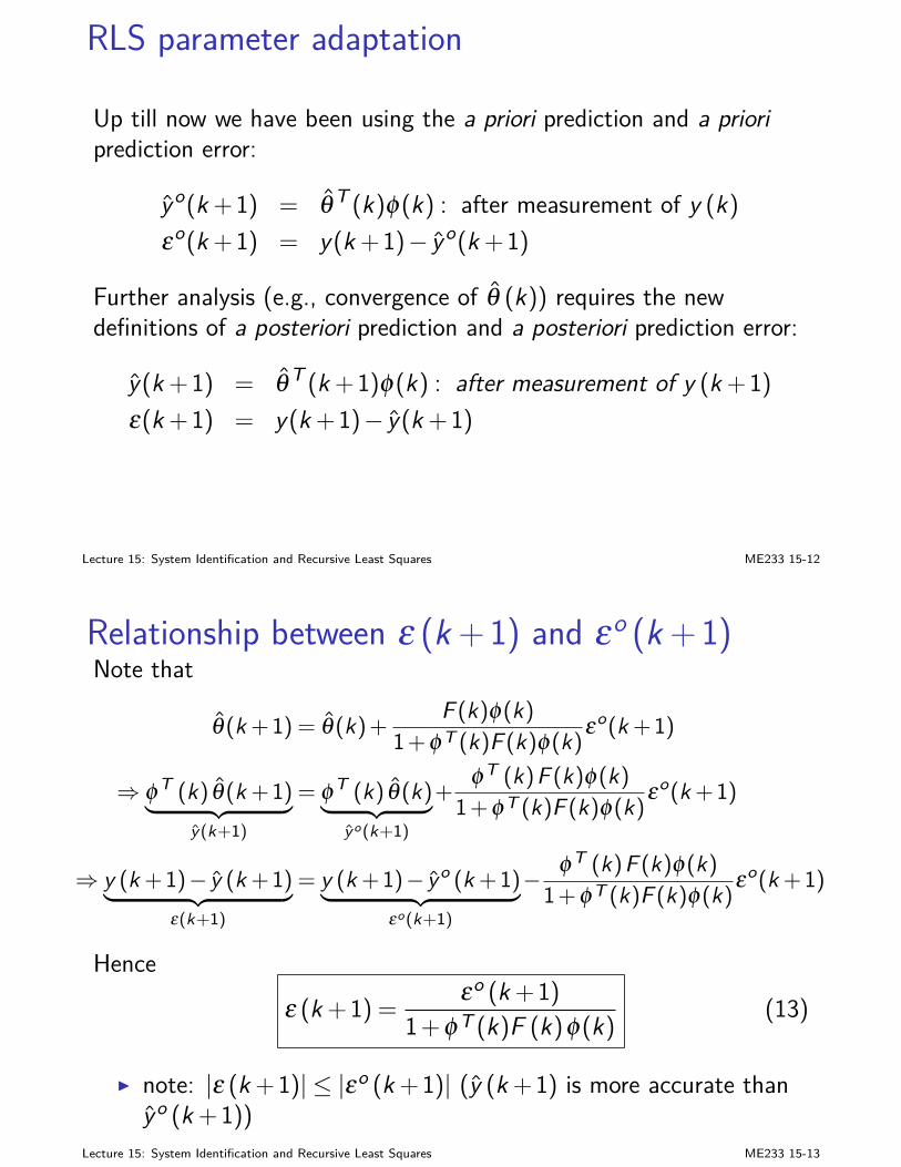
RLS parameter adaptation
Up till now we have been using the a priori prediction and a prioriprediction error:
yo(k +1) = θT (k)φ(k) : after measurement of y (k)εo(k +1) = y(k +1)− yo(k +1)
Further analysis (e.g., convergence of θ (k)) requires the newdefinitions of a posteriori prediction and a posteriori prediction error:
y(k +1) = θ T (k +1)φ(k) : after measurement of y (k +1)ε(k +1) = y(k +1)− y(k +1)
Lecture 15: System Identification and Recursive Least Squares ME233 15-12
Relationship between ε (k +1) and εo (k +1)Note that
θ(k +1) = θ(k)+ F (k)φ(k)1+φT (k)F (k)φ(k)εo(k +1)
⇒ φT (k) θ(k +1)︸ ︷︷ ︸y(k+1)
= φT (k) θ(k)︸ ︷︷ ︸yo(k+1)
+φT (k)F (k)φ(k)
1+φT (k)F (k)φ(k)εo(k +1)
⇒ y (k +1)− y (k +1)︸ ︷︷ ︸ε(k+1)
= y (k +1)− yo (k +1)︸ ︷︷ ︸εo(k+1)
− φT (k)F (k)φ(k)1+φT (k)F (k)φ(k)εo(k +1)
Henceε (k +1) = εo (k +1)
1+φT (k)F (k)φ(k) (13)
I note: |ε (k +1)| ≤ |εo (k +1)| (y (k +1) is more accurate thanyo (k +1))
Lecture 15: System Identification and Recursive Least Squares ME233 15-13
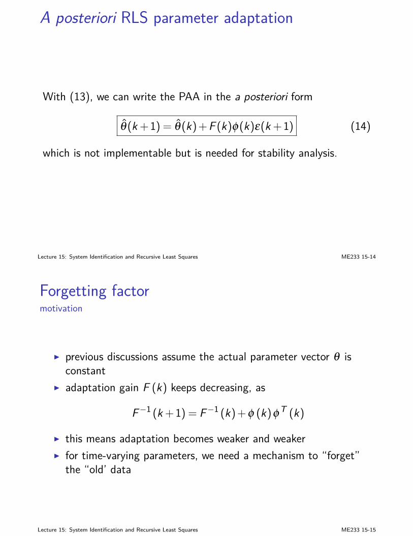
A posteriori RLS parameter adaptation
With (13), we can write the PAA in the a posteriori form
θ (k +1) = θ (k)+F (k)φ(k)ε(k +1) (14)
which is not implementable but is needed for stability analysis.
Lecture 15: System Identification and Recursive Least Squares ME233 15-14
Forgetting factormotivation
I previous discussions assume the actual parameter vector θ isconstant
I adaptation gain F (k) keeps decreasing, as
F−1 (k +1) = F−1 (k)+φ (k)φT (k)
I this means adaptation becomes weaker and weakerI for time-varying parameters, we need a mechanism to “forget”
the “old’ data
Lecture 15: System Identification and Recursive Least Squares ME233 15-15
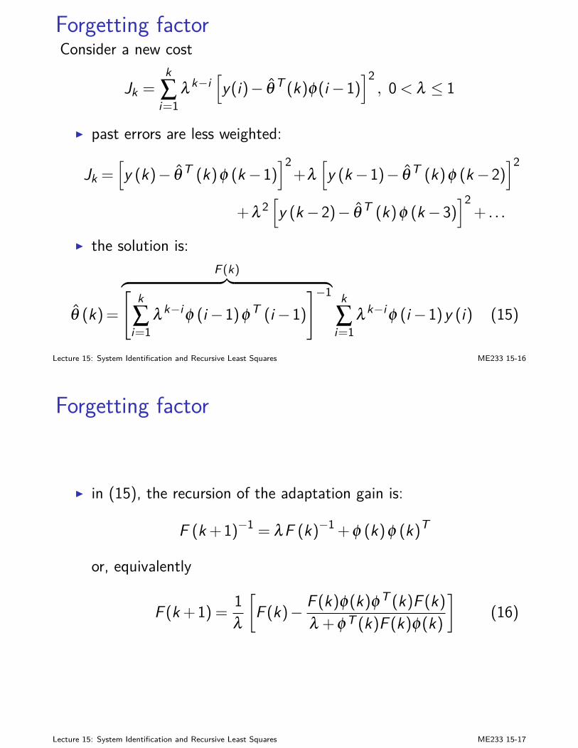
Forgetting factorConsider a new cost
Jk =k∑i=1
λ k−i[y(i)− θ T (k)φ(i−1)
]2, 0< λ ≤ 1
I past errors are less weighted:
Jk =[y (k)− θ T (k)φ (k−1)
]2+λ
[y (k−1)− θ T (k)φ (k−2)
]2
+λ 2[y (k−2)− θ T (k)φ (k−3)
]2+ . . .
I the solution is:
θ (k) =
F (k)︷ ︸︸ ︷[k∑i=1
λ k−iφ (i−1)φT (i−1)]−1 k
∑i=1
λ k−iφ (i−1)y (i) (15)
Lecture 15: System Identification and Recursive Least Squares ME233 15-16
Forgetting factor
I in (15), the recursion of the adaptation gain is:
F (k +1)−1 = λF (k)−1 +φ (k)φ (k)T
or, equivalently
F (k +1) = 1λ
[F (k)− F (k)φ(k)φT (k)F (k)
λ +φT (k)F (k)φ(k)
](16)
Lecture 15: System Identification and Recursive Least Squares ME233 15-17
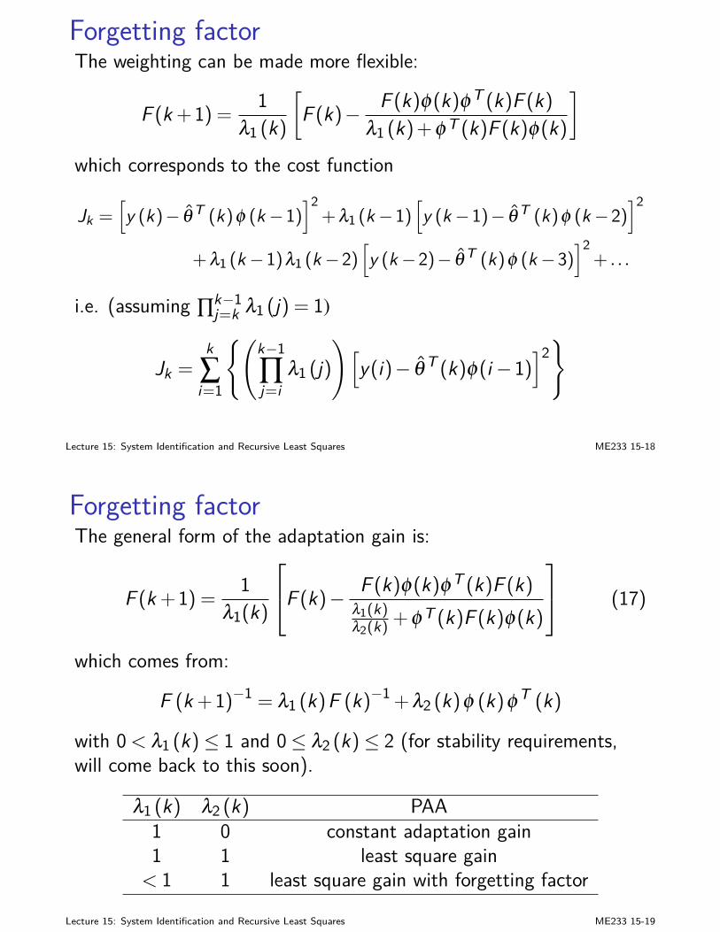
Forgetting factorThe weighting can be made more flexible:
F (k +1) = 1λ1 (k)
[F (k)− F (k)φ(k)φT (k)F (k)
λ1 (k)+φT (k)F (k)φ(k)
]
which corresponds to the cost function
Jk =[y (k)− θ T (k)φ (k−1)
]2+λ1 (k−1)
[y (k−1)− θ T (k)φ (k−2)
]2
+λ1 (k−1)λ1 (k−2)[y (k−2)− θ T (k)φ (k−3)
]2+ . . .
i.e. (assuming ∏k−1j=k λ1 (j) = 1)
Jk =k∑i=1
(k−1∏j=i
λ1 (j))[
y(i)− θ T (k)φ(i−1)]2
Lecture 15: System Identification and Recursive Least Squares ME233 15-18
Forgetting factorThe general form of the adaptation gain is:
F (k +1) = 1λ1(k)
F (k)− F (k)φ(k)φT (k)F (k)
λ1(k)λ2(k) +φT (k)F (k)φ(k)
(17)
which comes from:
F (k +1)−1 = λ1 (k)F (k)−1 +λ2 (k)φ (k)φT (k)
with 0< λ1 (k)≤ 1 and 0≤ λ2 (k)≤ 2 (for stability requirements,will come back to this soon).
λ1 (k) λ2 (k) PAA1 0 constant adaptation gain1 1 least square gain< 1 1 least square gain with forgetting factor
Lecture 15: System Identification and Recursive Least Squares ME233 15-19
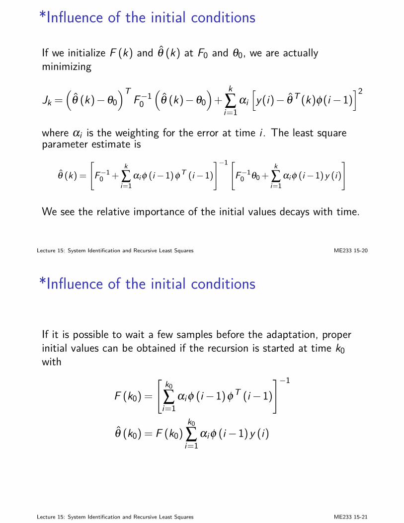
*Influence of the initial conditions
If we initialize F (k) and θ (k) at F0 and θ0, we are actuallyminimizing
Jk =(
θ (k)−θ0)T
F−10
(θ (k)−θ0
)+
k∑i=1
αi[y(i)− θT (k)φ(i−1)
]2
where αi is the weighting for the error at time i . The least squareparameter estimate is
θ (k) =[
F−10 +k∑i=1
αi φ (i−1)φT (i−1)]−1[
F−10 θ0+k∑i=1
αi φ (i−1)y (i)]
We see the relative importance of the initial values decays with time.
Lecture 15: System Identification and Recursive Least Squares ME233 15-20
*Influence of the initial conditions
If it is possible to wait a few samples before the adaptation, properinitial values can be obtained if the recursion is started at time k0with
F (k0) =
[k0∑i=1
αiφ (i−1)φT (i−1)]−1
θ (k0) = F (k0)k0∑i=1
αiφ (i−1)y (i)
Lecture 15: System Identification and Recursive Least Squares ME233 15-21

ME 233, UC Berkeley, Spring 2014 Xu Chen
Lecture 16: Stability of Parameter AdaptationAlgorithms
Big picture
I Forθ (k+1) = θ (k)+ [correction term]
we haven’t talked about whether θ (k) will converge to the truevalue θ if k → ∞. We haven’t even talked about whether θ (k)will stay bounded or not!
I Tools of stability evaluation: Lyapunov-based analysis, orhyperstability theory (topic of this lecture)
Lecture 16: Stability of Parameter Adaptation Algorithms ME233 16-1

Outline
1. Big picture
2. Hyperstability theoryPassivityMain resultsPositive real and strictly positive realUnderstanding the hyperstability theorem
3. Procedure of PAA stability analysis by hyperstability theory
4. AppendixStrictly positive real implies strict passivity
Lecture 16: Stability of Parameter Adaptation Algorithms ME233 16-2
Hyperstability theoryhistory
Vasile M. Popov:I born in 1928, Romania
I retired from University of Florida in 1993I developed hyperstability theory independently from Lyapnov
theory
Lecture 16: Stability of Parameter Adaptation Algorithms ME233 16-3
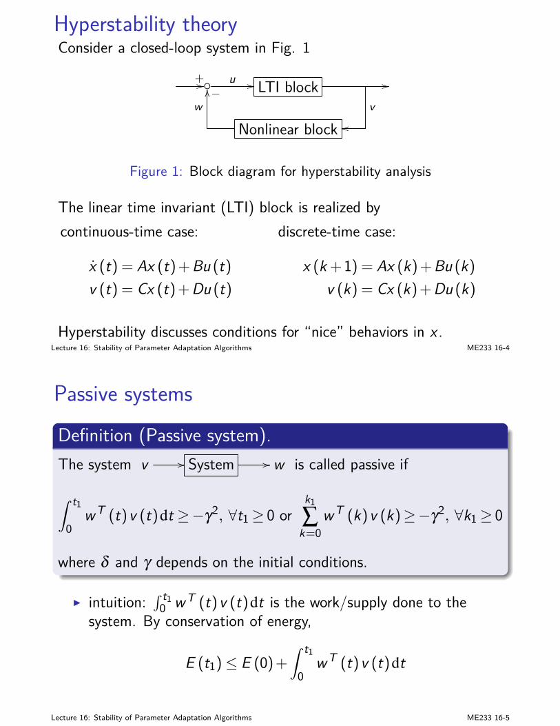
Hyperstability theoryConsider a closed-loop system in Fig. 1
+// u // LTI block //
vw−OO
Nonlinear block oo
Figure 1: Block diagram for hyperstability analysis
The linear time invariant (LTI) block is realized bycontinuous-time case:
x (t) = Ax (t)+Bu (t)v (t) = Cx (t)+Du (t)
discrete-time case:
x (k+1) = Ax (k)+Bu (k)v (k) = Cx (k)+Du (k)
Hyperstability discusses conditions for “nice” behaviors in x .Lecture 16: Stability of Parameter Adaptation Algorithms ME233 16-4
Passive systemsDefinition (Passive system).The system v // System // w is called passive if
∫ t1
0wT (t)v (t)dt ≥−γ2, ∀t1≥ 0 or
k1
∑k=0
wT (k)v (k)≥−γ2, ∀k1≥ 0
where δ and γ depends on the initial conditions.
I intuition:∫ t1
0 wT (t)v (t)dt is the work/supply done to thesystem. By conservation of energy,
E (t1)≤ E (0)+∫ t1
0wT (t)v (t)dt
Lecture 16: Stability of Parameter Adaptation Algorithms ME233 16-5
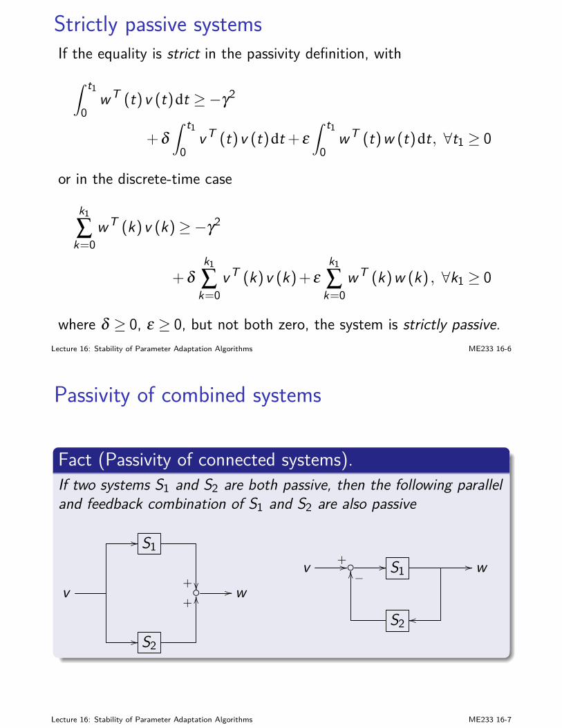
Strictly passive systemsIf the equality is strict in the passivity definition, with∫ t1
0wT (t)v (t)dt ≥−γ2
+δ∫ t1
0vT (t)v (t)dt+ ε
∫ t1
0wT (t)w (t)dt, ∀t1 ≥ 0
or in the discrete-time case
k1
∑k=0
wT (k)v (k)≥−γ2
+δk1
∑k=0
vT (k)v (k)+ εk1
∑k=0
wT (k)w (k) , ∀k1 ≥ 0
where δ ≥ 0, ε ≥ 0, but not both zero, the system is strictly passive.Lecture 16: Stability of Parameter Adaptation Algorithms ME233 16-6
Passivity of combined systems
Fact (Passivity of connected systems).If two systems S1 and S2 are both passive, then the following paralleland feedback combination of S1 and S2 are also passive
// S1
+ v // w
// S2
+OO
v + // // S1 // w−OO
S2 oo
Lecture 16: Stability of Parameter Adaptation Algorithms ME233 16-7
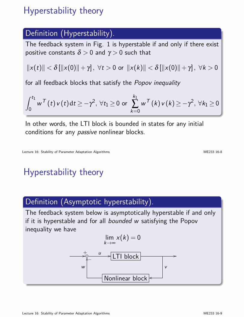
Hyperstability theory
Definition (Hyperstability).The feedback system in Fig. 1 is hyperstable if and only if there existpositive constants δ > 0 and γ > 0 such that
‖x(t)‖< δ [‖x(0)‖+ γ] , ∀t > 0 or ‖x(k)‖< δ [‖x(0)‖+ γ] , ∀k > 0
for all feedback blocks that satisfy the Popov inequality∫ t1
0wT (t)v (t)dt ≥−γ2, ∀t1≥ 0 or
k1
∑k=0
wT (k)v (k)≥−γ2, ∀k1≥ 0
In other words, the LTI block is bounded in states for any initialconditions for any passive nonlinear blocks.
Lecture 16: Stability of Parameter Adaptation Algorithms ME233 16-8
Hyperstability theory
Definition (Asymptotic hyperstability).The feedback system below is asymptotically hyperstable if and onlyif it is hyperstable and for all bounded w satisfying the Popovinequality we have
limk→∞
x(k) = 0
+//−u // LTI block //
vw
OO
Nonlinear block oo
Lecture 16: Stability of Parameter Adaptation Algorithms ME233 16-9
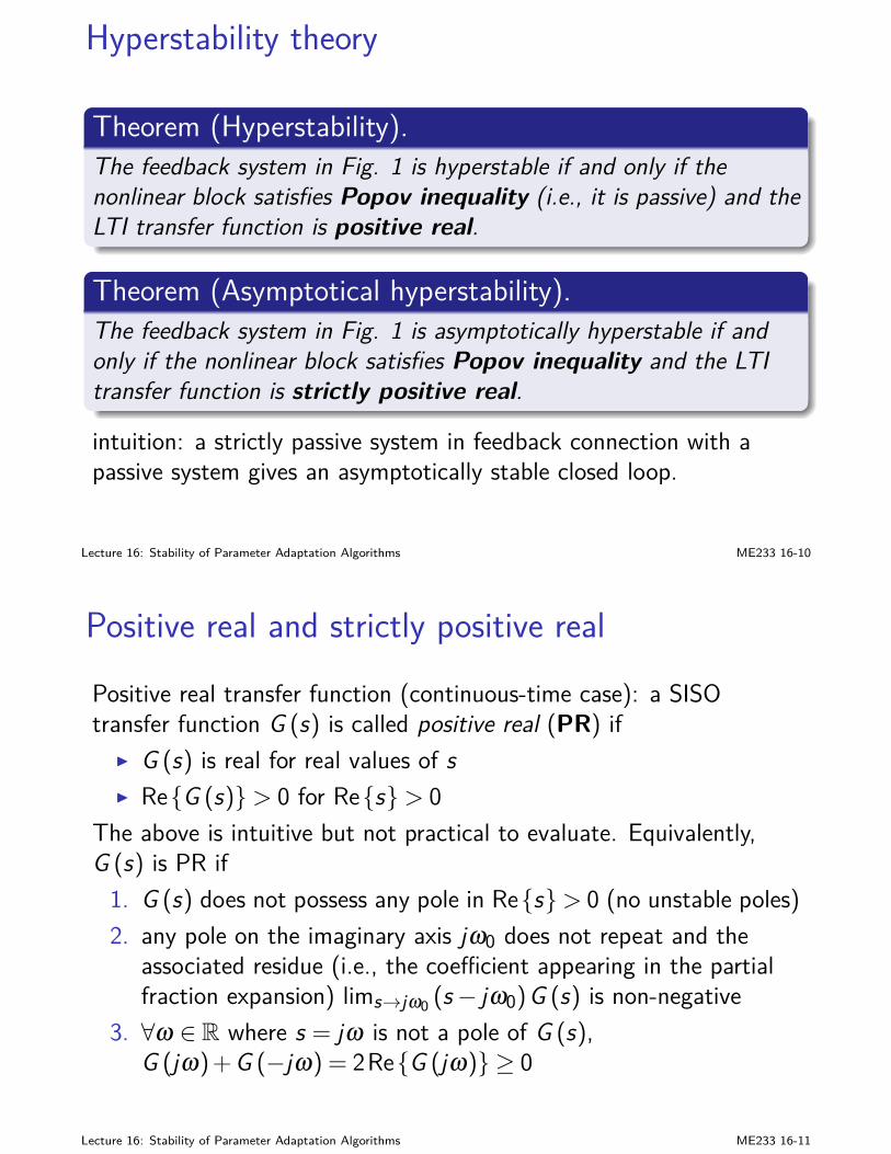
Hyperstability theory
Theorem (Hyperstability).The feedback system in Fig. 1 is hyperstable if and only if thenonlinear block satisfies Popov inequality (i.e., it is passive) and theLTI transfer function is positive real.
Theorem (Asymptotical hyperstability).The feedback system in Fig. 1 is asymptotically hyperstable if andonly if the nonlinear block satisfies Popov inequality and the LTItransfer function is strictly positive real.
intuition: a strictly passive system in feedback connection with apassive system gives an asymptotically stable closed loop.
Lecture 16: Stability of Parameter Adaptation Algorithms ME233 16-10
Positive real and strictly positive realPositive real transfer function (continuous-time case): a SISOtransfer function G (s) is called positive real (PR) if
I G (s) is real for real values of sI ReG (s)> 0 for Res> 0
The above is intuitive but not practical to evaluate. Equivalently,G (s) is PR if1. G (s) does not possess any pole in Res> 0 (no unstable poles)2. any pole on the imaginary axis jω0 does not repeat and the
associated residue (i.e., the coefficient appearing in the partialfraction expansion) lims→jω0 (s− jω0)G (s) is non-negative
3. ∀ω ∈ R where s = jω is not a pole of G (s),G (jω)+G (−jω) = 2ReG (jω) ≥ 0
Lecture 16: Stability of Parameter Adaptation Algorithms ME233 16-11
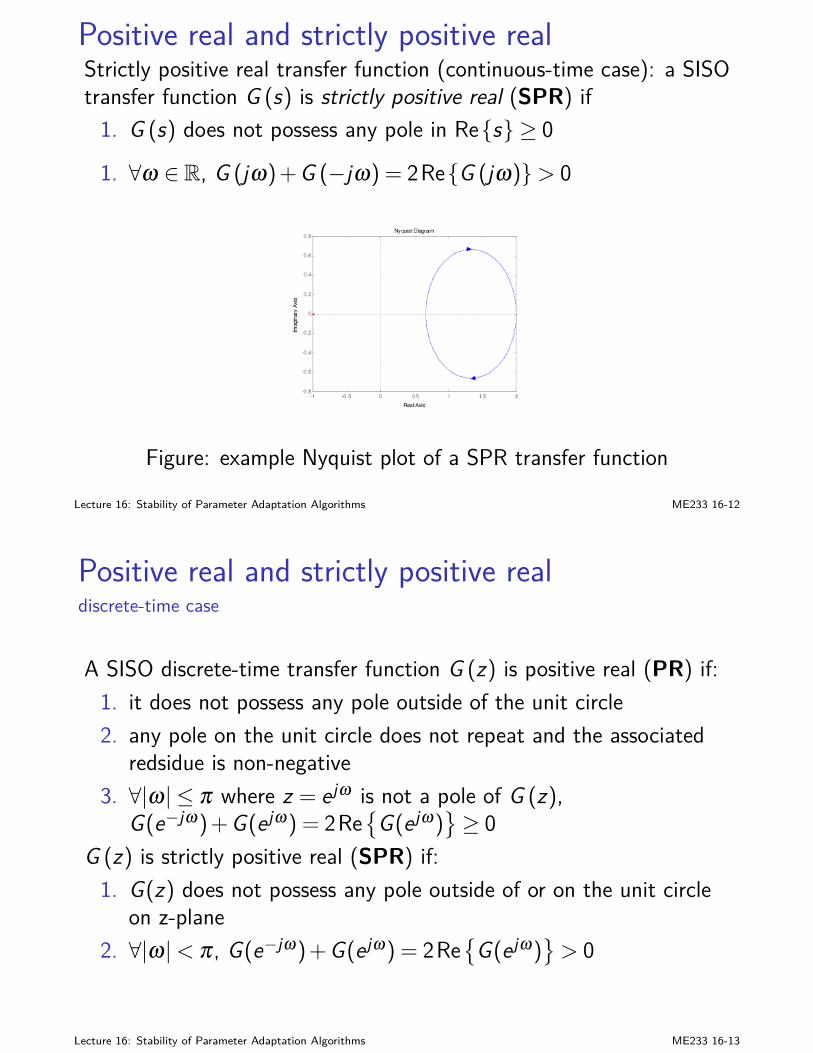
Positive real and strictly positive realStrictly positive real transfer function (continuous-time case): a SISOtransfer function G (s) is strictly positive real (SPR) if1. G (s) does not possess any pole in Res ≥ 0
1. ∀ω ∈ R, G (jω)+G (−jω) = 2ReG (jω)> 0
Figure: example Nyquist plot of a SPR transfer function
Lecture 16: Stability of Parameter Adaptation Algorithms ME233 16-12
Positive real and strictly positive realdiscrete-time case
A SISO discrete-time transfer function G (z) is positive real (PR) if:1. it does not possess any pole outside of the unit circle2. any pole on the unit circle does not repeat and the associated
redsidue is non-negative3. ∀|ω| ≤ π where z = ejω is not a pole of G (z),
G(e−jω)+G(ejω) = 2ReG(ejω)
≥ 0
G (z) is strictly positive real (SPR) if:1. G(z) does not possess any pole outside of or on the unit circle
on z-plane2. ∀|ω|< π, G(e−jω)+G(ejω) = 2Re
G(ejω)
> 0
Lecture 16: Stability of Parameter Adaptation Algorithms ME233 16-13
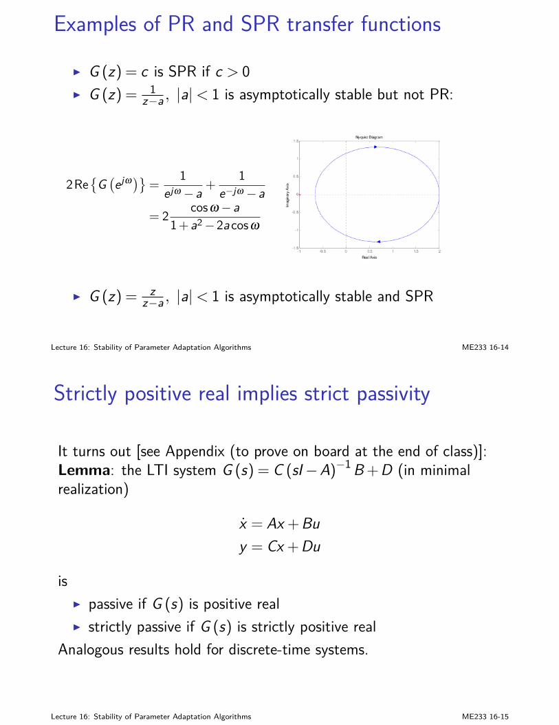
Examples of PR and SPR transfer functions
I G (z) = c is SPR if c > 0I G (z) = 1
z−a , |a|< 1 is asymptotically stable but not PR:
2Re
G(ejω)= 1
ejω −a +1
e−jω −a= 2 cosω−a
1+a2−2acosω
I G (z) = zz−a , |a|< 1 is asymptotically stable and SPR
Lecture 16: Stability of Parameter Adaptation Algorithms ME233 16-14
Strictly positive real implies strict passivity
It turns out [see Appendix (to prove on board at the end of class)]:Lemma: the LTI system G (s) = C (sI−A)−1B+D (in minimalrealization)
x = Ax +Buy = Cx +Du
isI passive if G (s) is positive realI strictly passive if G (s) is strictly positive real
Analogous results hold for discrete-time systems.
Lecture 16: Stability of Parameter Adaptation Algorithms ME233 16-15
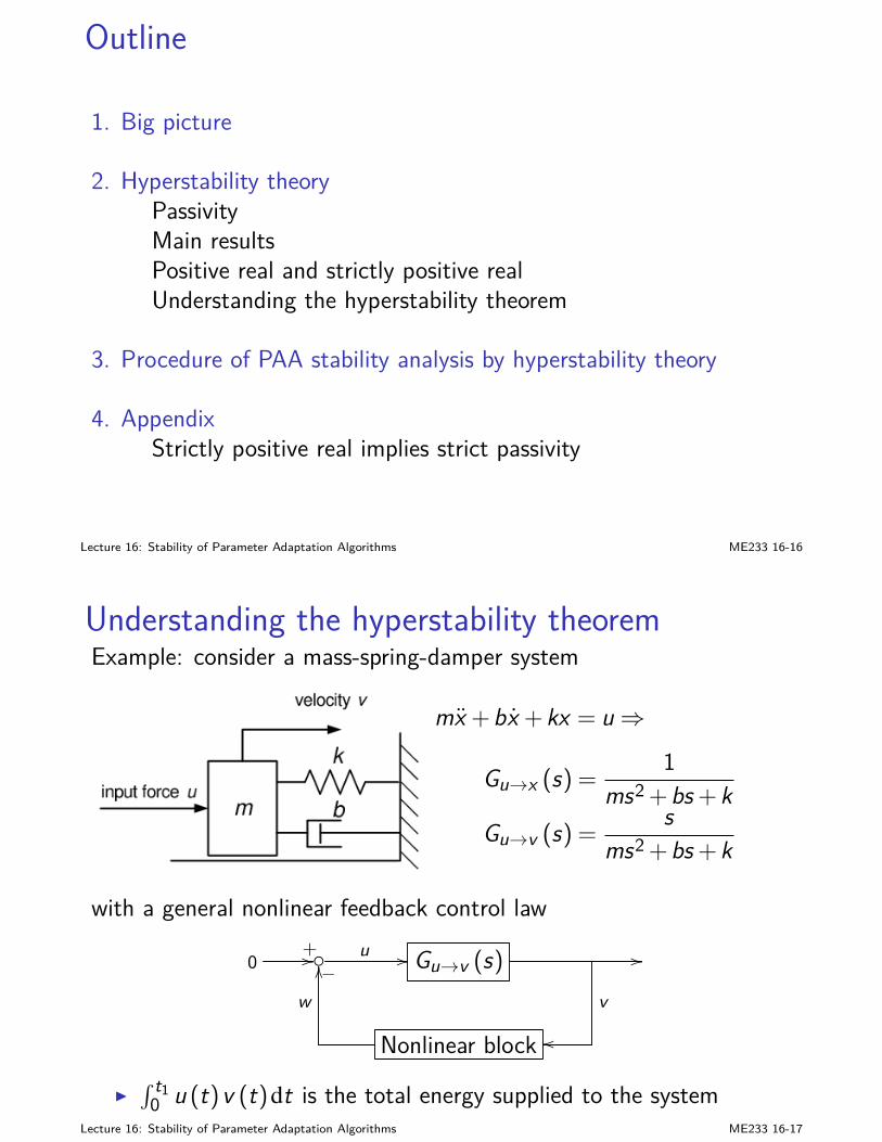
Outline
1. Big picture
2. Hyperstability theoryPassivityMain resultsPositive real and strictly positive realUnderstanding the hyperstability theorem
3. Procedure of PAA stability analysis by hyperstability theory
4. AppendixStrictly positive real implies strict passivity
Lecture 16: Stability of Parameter Adaptation Algorithms ME233 16-16
Understanding the hyperstability theoremExample: consider a mass-spring-damper system
mx +bx +kx = u⇒
Gu→x (s) =1
ms2 +bs+kGu→v (s) =
sms2 +bs+k
with a general nonlinear feedback control law
0+//−
u // Gu→v (s) //
vw
OO
Nonlinear block oo
I∫ t1
0 u (t)v (t)dt is the total energy supplied to the systemLecture 16: Stability of Parameter Adaptation Algorithms ME233 16-17
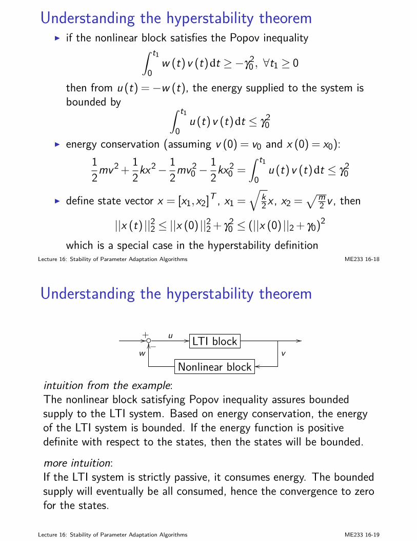
Understanding the hyperstability theoremI if the nonlinear block satisfies the Popov inequality
∫ t1
0w (t)v (t)dt ≥−γ2
0 , ∀t1 ≥ 0
then from u (t) =−w (t), the energy supplied to the system isbounded by ∫ t1
0u (t)v (t)dt ≤ γ2
0
I energy conservation (assuming v (0) = v0 and x (0) = x0):12mv2 +
12kx
2− 12mv2
0 −12kx
20 =
∫ t1
0u (t)v (t)dt ≤ γ2
0
I define state vector x = [x1,x2]T , x1 =
√k2x , x2 =
√m2 v , then
||x (t) ||22 ≤ ||x (0) ||22 + γ20 ≤ (||x (0) ||2 + γ0)
2
which is a special case in the hyperstability definitionLecture 16: Stability of Parameter Adaptation Algorithms ME233 16-18
Understanding the hyperstability theorem
+//−u // LTI block //
vwOO
Nonlinear block oo
intuition from the example:The nonlinear block satisfying Popov inequality assures boundedsupply to the LTI system. Based on energy conservation, the energyof the LTI system is bounded. If the energy function is positivedefinite with respect to the states, then the states will be bounded.more intuition:If the LTI system is strictly passive, it consumes energy. The boundedsupply will eventually be all consumed, hence the convergence to zerofor the states.
Lecture 16: Stability of Parameter Adaptation Algorithms ME233 16-19
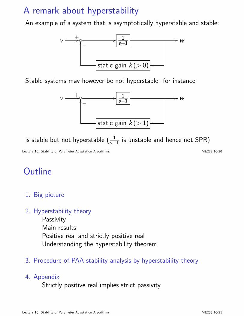
A remark about hyperstabilityAn example of a system that is asymptotically hyperstable and stable:
v + // // 1s+1
// w−OO
static gain k (> 0) oo
Stable systems may however be not hyperstable: for instance
v + // // 1s−1
// w−OO
static gain k (> 1) oo
is stable but not hyperstable ( 1s−1 is unstable and hence not SPR)
Lecture 16: Stability of Parameter Adaptation Algorithms ME233 16-20
Outline
1. Big picture
2. Hyperstability theoryPassivityMain resultsPositive real and strictly positive realUnderstanding the hyperstability theorem
3. Procedure of PAA stability analysis by hyperstability theory
4. AppendixStrictly positive real implies strict passivity
Lecture 16: Stability of Parameter Adaptation Algorithms ME233 16-21
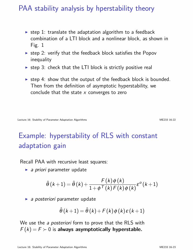
PAA stability analysis by hperstability theory
I step 1: translate the adaptation algorithm to a feedbackcombination of a LTI block and a nonlinear block, as shown inFig. 1
I step 2: verify that the feedback block satisfies the Popovinequality
I step 3: check that the LTI block is strictly positive real
I step 4: show that the output of the feedback block is bounded.Then from the definition of asymptotic hyperstability, weconclude that the state x converges to zero
Lecture 16: Stability of Parameter Adaptation Algorithms ME233 16-22
Example: hyperstability of RLS with constantadaptation gain
Recall PAA with recursive least squares:I a priori parameter update
θ (k+1) = θ (k)+ F (k)φ (k)1+φT (k)F (k)φ (k)εo (k+1)
I a posteriori parameter update
θ (k+1) = θ (k)+F (k)φ (k)ε (k+1)
We use the a posteriori form to prove that the RLS withF (k) = F 0 is always asymptotically hyperstable.
Lecture 16: Stability of Parameter Adaptation Algorithms ME233 16-23
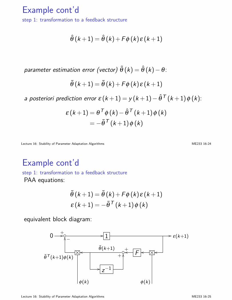
Example cont’dstep 1: transformation to a feedback structure
θ (k+1) = θ (k)+Fφ (k)ε (k+1)
parameter estimation error (vector) θ (k) = θ (k)−θ :
θ (k+1) = θ (k)+Fφ (k)ε (k+1)
a posteriori prediction error ε (k+1) = y (k+1)− θT (k+1)φ (k):
ε (k+1) = θ T φ (k)− θ T (k+1)φ (k)=−θ T (k+1)φ (k)
Lecture 16: Stability of Parameter Adaptation Algorithms ME233 16-24
Example cont’dstep 1: transformation to a feedback structurePAA equations:
θ (k+1) = θ (k)+Fφ (k)ε (k+1)ε (k+1) =−θ T (k+1)φ (k)
equivalent block diagram:
0 +// // 1 // ε(k+1)−OO
×θT (k+1)φ(k)
oo θ(k+1)F+oo ×oo oo
// z−1
+OO
φ(k) φ(k)
Lecture 16: Stability of Parameter Adaptation Algorithms ME233 16-25
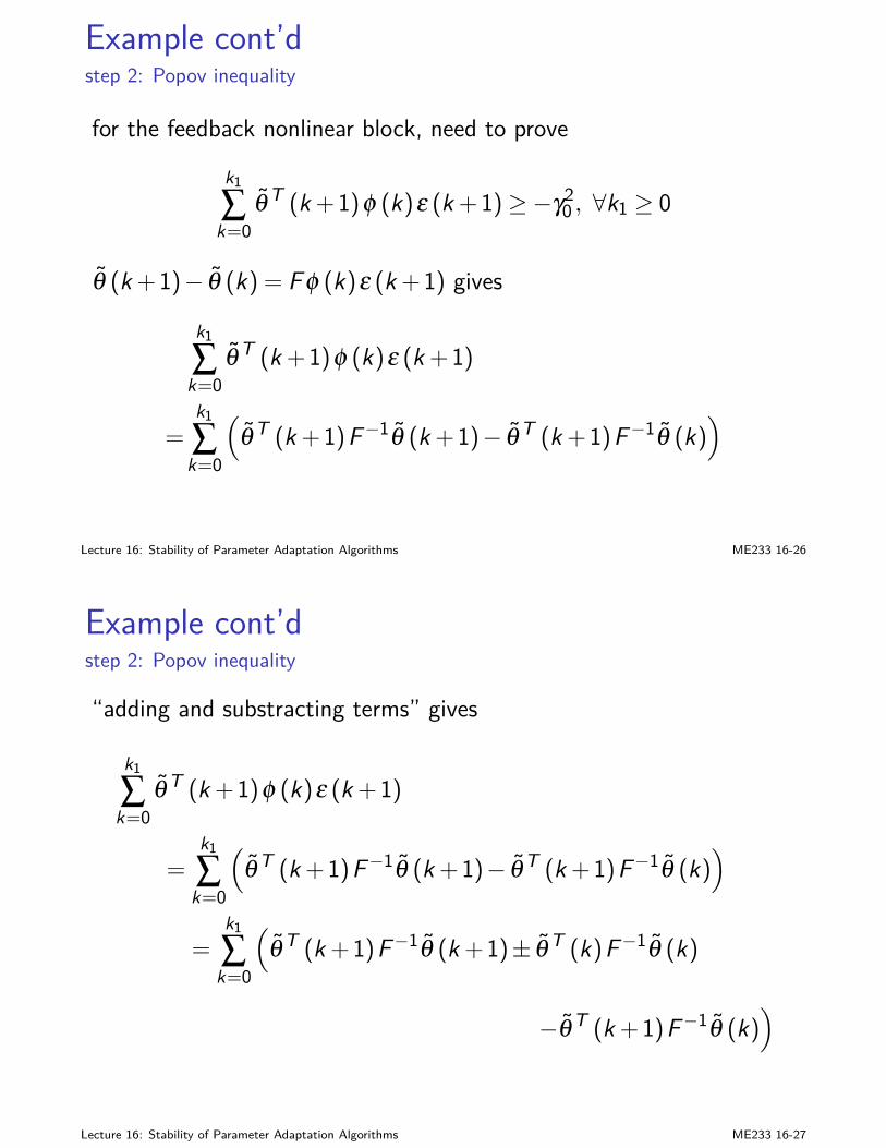
Example cont’dstep 2: Popov inequality
for the feedback nonlinear block, need to prove
k1
∑k=0
θT (k+1)φ (k)ε (k+1)≥−γ20 , ∀k1 ≥ 0
θ (k+1)− θ (k) = Fφ (k)ε (k+1) gives
k1
∑k=0
θT (k+1)φ (k)ε (k+1)
=k1
∑k=0
(θT (k+1)F−1θ (k+1)− θT (k+1)F−1θ (k)
)
Lecture 16: Stability of Parameter Adaptation Algorithms ME233 16-26
Example cont’dstep 2: Popov inequality
“adding and substracting terms” gives
k1
∑k=0
θT (k+1)φ (k)ε (k+1)
=k1
∑k=0
(θ T (k+1)F−1θ (k+1)− θ T (k+1)F−1θ (k)
)
=k1
∑k=0
(θ T (k+1)F−1θ (k+1)± θT (k)F−1θ (k)
−θT (k+1)F−1θ (k))
Lecture 16: Stability of Parameter Adaptation Algorithms ME233 16-27
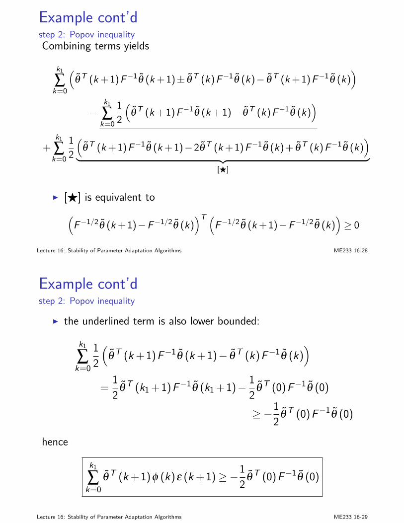
Example cont’dstep 2: Popov inequalityCombining terms yields
k1
∑k=0
(θ T (k +1)F−1θ (k +1)± θ T (k)F−1θ (k)− θ T (k +1)F−1θ (k)
)
=k1
∑k=0
12(
θ T (k +1)F−1θ (k +1)− θ T (k)F−1θ (k))
+k1
∑k=0
12(
θ T (k +1)F−1θ (k +1)−2θ T (k +1)F−1θ (k)+ θ T (k)F−1θ (k))
︸ ︷︷ ︸[F]
I [F] is equivalent to(
F−1/2θ (k +1)−F−1/2θ (k))T (
F−1/2θ (k +1)−F−1/2θ (k))≥ 0
Lecture 16: Stability of Parameter Adaptation Algorithms ME233 16-28
Example cont’dstep 2: Popov inequality
I the underlined term is also lower bounded:
k1
∑k=0
12(
θT (k+1)F−1θ (k+1)− θT (k)F−1θ (k))
=12 θT (k1 +1)F−1θ (k1 +1)− 1
2 θT (0)F−1θ (0)
≥−12 θT (0)F−1θ (0)
hence
k1
∑k=0
θ T (k+1)φ (k)ε (k+1)≥−12 θT (0)F−1θ (0)
Lecture 16: Stability of Parameter Adaptation Algorithms ME233 16-29
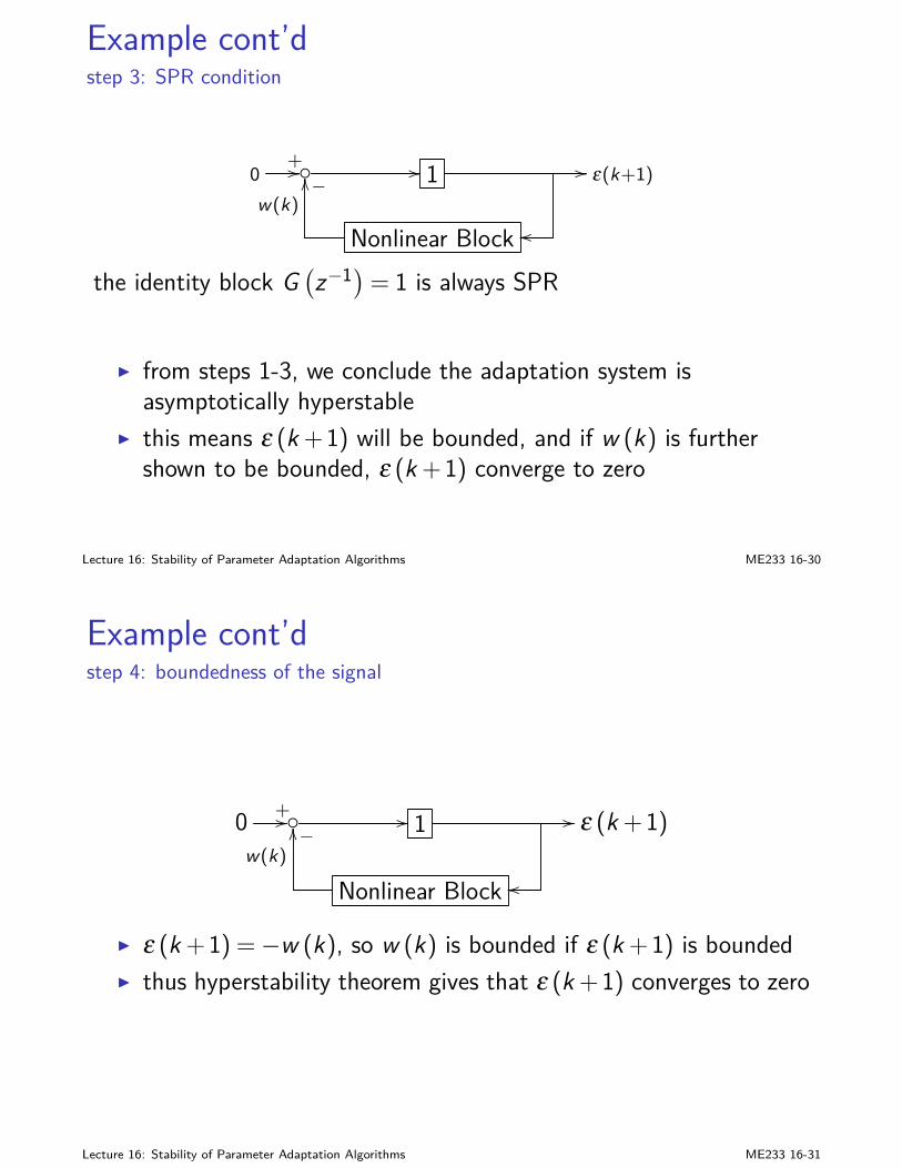
Example cont’dstep 3: SPR condition
0+// // 1 // ε(k+1)−
w(k)OO
Nonlinear Block oo
the identity block G(z−1)= 1 is always SPR
I from steps 1-3, we conclude the adaptation system isasymptotically hyperstable
I this means ε (k+1) will be bounded, and if w (k) is furthershown to be bounded, ε (k+1) converge to zero
Lecture 16: Stability of Parameter Adaptation Algorithms ME233 16-30
Example cont’dstep 4: boundedness of the signal
0 +// // 1 // ε (k+1)−w(k)
OO
Nonlinear Block oo
I ε (k+1) =−w (k), so w (k) is bounded if ε (k+1) is boundedI thus hyperstability theorem gives that ε (k+1) converges to zero
Lecture 16: Stability of Parameter Adaptation Algorithms ME233 16-31
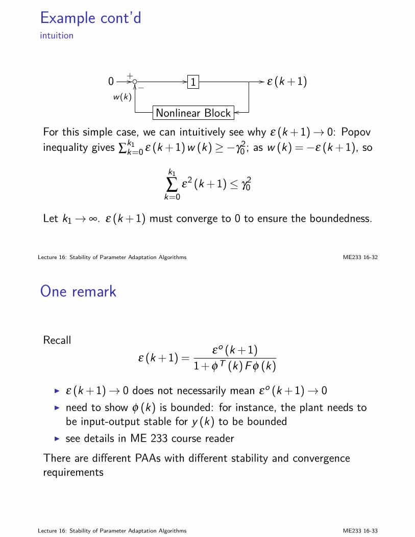
Example cont’dintuition
0 +// // 1 // ε (k+1)−w(k)
OO
Nonlinear Block oo
For this simple case, we can intuitively see why ε (k+1)→ 0: Popovinequality gives ∑k1
k=0 ε (k+1)w (k)≥−γ20 ; as w (k) =−ε (k+1), so
k1
∑k=0
ε2 (k+1)≤ γ20
Let k1→ ∞. ε (k+1) must converge to 0 to ensure the boundedness.
Lecture 16: Stability of Parameter Adaptation Algorithms ME233 16-32
One remark
Recallε (k+1) = εo (k+1)
1+φT (k)Fφ (k)
I ε (k+1)→ 0 does not necessarily mean εo (k+1)→ 0I need to show φ (k) is bounded: for instance, the plant needs to
be input-output stable for y (k) to be boundedI see details in ME 233 course reader
There are different PAAs with different stability and convergencerequirements
Lecture 16: Stability of Parameter Adaptation Algorithms ME233 16-33
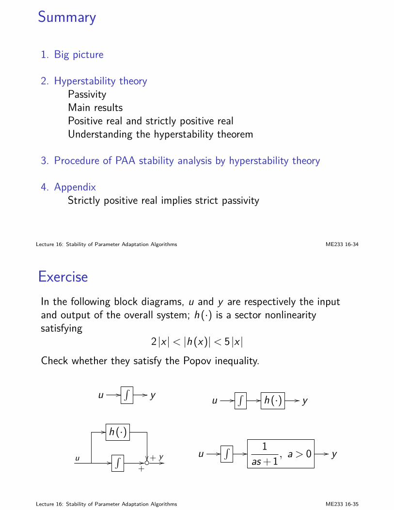
Summary
1. Big picture
2. Hyperstability theoryPassivityMain resultsPositive real and strictly positive realUnderstanding the hyperstability theorem
3. Procedure of PAA stability analysis by hyperstability theory
4. AppendixStrictly positive real implies strict passivity
Lecture 16: Stability of Parameter Adaptation Algorithms ME233 16-34
ExerciseIn the following block diagrams, u and y are respectively the inputand output of the overall system; h (·) is a sector nonlinearitysatisfying
2 |x |< |h (x)|< 5 |x |Check whether they satisfy the Popov inequality.
u //∫
// y u //∫
// h (·) // y
// h (·)
+u //∫
+// y //
u //∫
// 1as+1 , a > 0 // y
Lecture 16: Stability of Parameter Adaptation Algorithms ME233 16-35
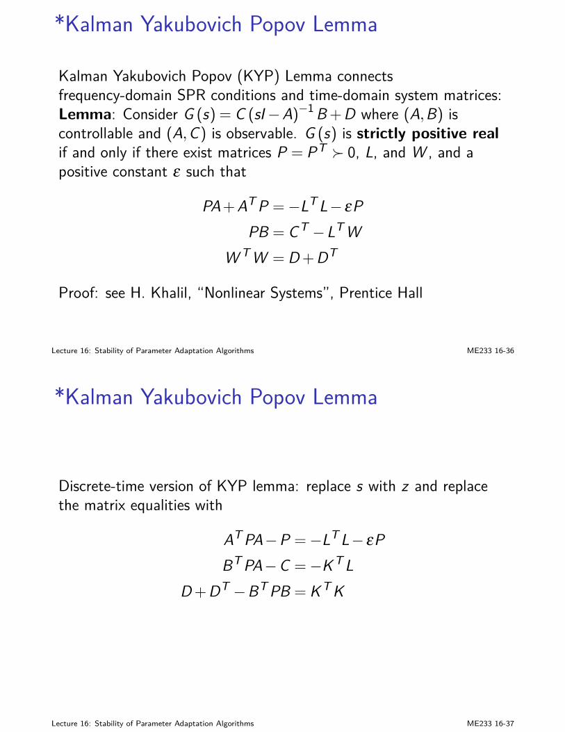
*Kalman Yakubovich Popov Lemma
Kalman Yakubovich Popov (KYP) Lemma connectsfrequency-domain SPR conditions and time-domain system matrices:Lemma: Consider G (s) = C (sI−A)−1B+D where (A,B) iscontrollable and (A,C) is observable. G (s) is strictly positive realif and only if there exist matrices P = PT 0, L, and W , and apositive constant ε such that
PA+ATP =−LTL− εPPB = CT −LTW
W TW = D+DT
Proof: see H. Khalil, “Nonlinear Systems”, Prentice Hall
Lecture 16: Stability of Parameter Adaptation Algorithms ME233 16-36
*Kalman Yakubovich Popov Lemma
Discrete-time version of KYP lemma: replace s with z and replacethe matrix equalities with
ATPA−P =−LTL− εPBTPA−C =−KTL
D+DT −BTPB = KTK
Lecture 16: Stability of Parameter Adaptation Algorithms ME233 16-37
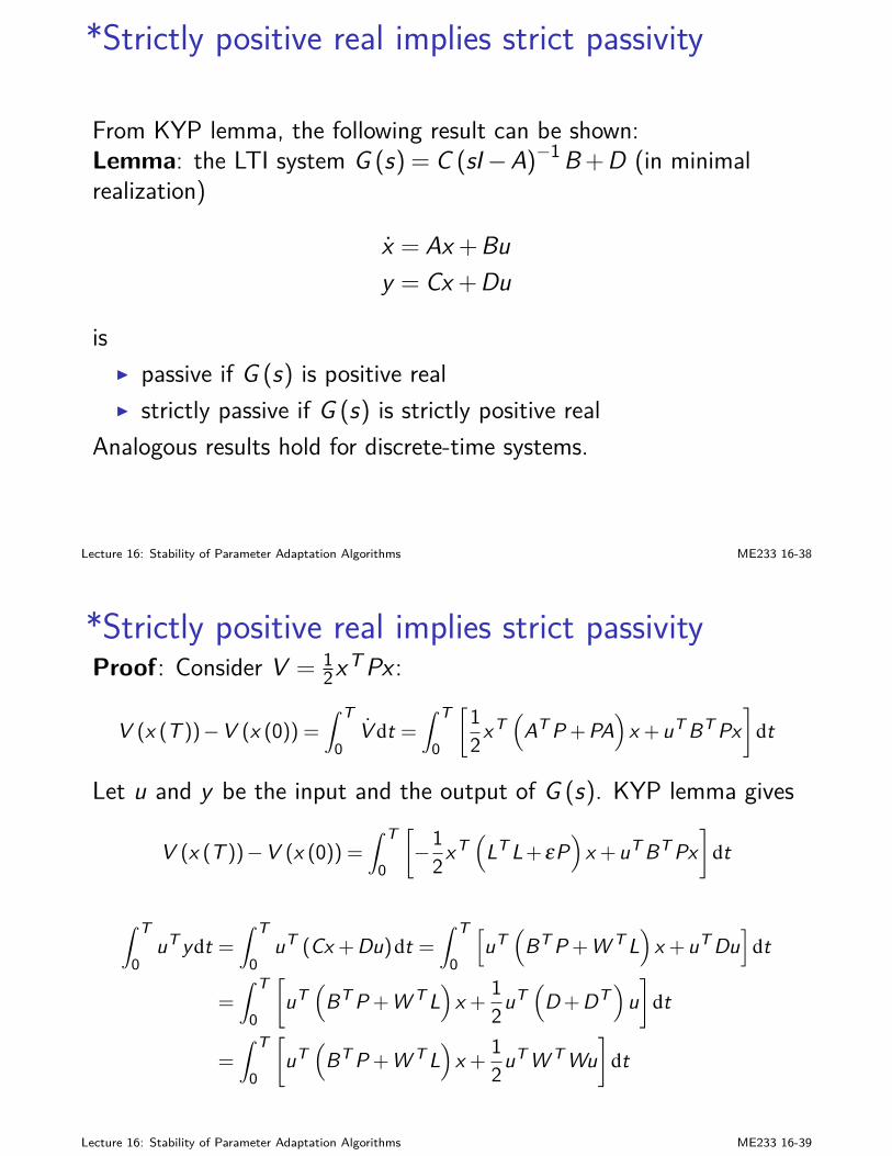
*Strictly positive real implies strict passivity
From KYP lemma, the following result can be shown:Lemma: the LTI system G (s) = C (sI−A)−1B+D (in minimalrealization)
x = Ax +Buy = Cx +Du
isI passive if G (s) is positive realI strictly passive if G (s) is strictly positive real
Analogous results hold for discrete-time systems.
Lecture 16: Stability of Parameter Adaptation Algorithms ME233 16-38
*Strictly positive real implies strict passivityProof: Consider V = 1
2xTPx :
V (x (T ))−V (x (0)) =∫ T
0V dt =
∫ T
0
[12xT
(AT P +PA
)x +uT BT Px
]dt
Let u and y be the input and the output of G (s). KYP lemma gives
V (x (T ))−V (x (0)) =∫ T
0
[−1
2xT(
LT L+ εP)
x +uT BT Px]
dt
∫ T
0uT ydt =
∫ T
0uT (Cx +Du)dt =
∫ T
0
[uT(
BT P +W T L)
x +uT Du]
dt
=∫ T
0
[uT(
BT P +W T L)
x +12uT
(D+DT
)u]
dt
=∫ T
0
[uT(
BT P +W T L)
x +12uT W T Wu
]dt
Lecture 16: Stability of Parameter Adaptation Algorithms ME233 16-39
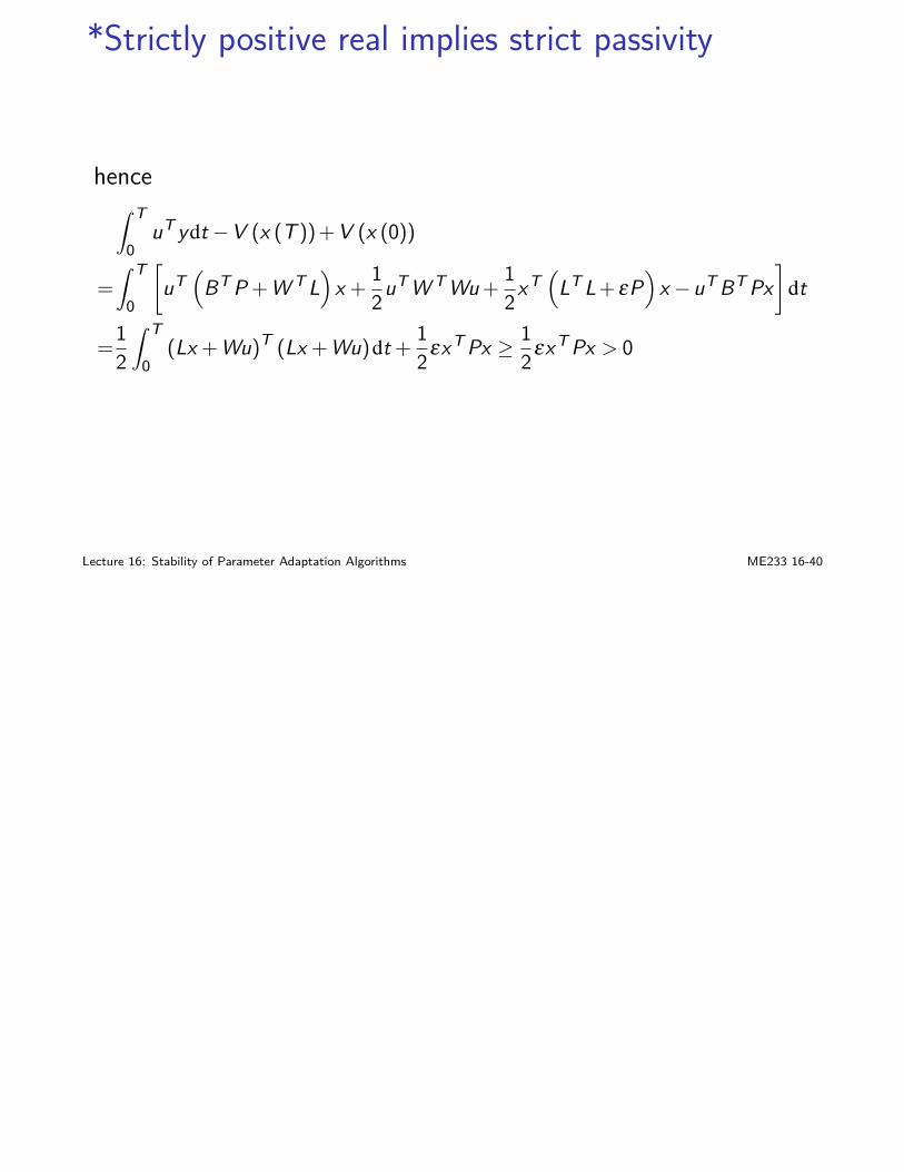
*Strictly positive real implies strict passivity
hence∫ T
0uT ydt−V (x (T ))+V (x (0))
=∫ T
0
[uT(
BT P +W T L)
x +12uT W T Wu+
12xT
(LT L+ εP
)x −uT BT Px
]dt
=12
∫ T
0(Lx +Wu)T (Lx +Wu)dt + 1
2εxT Px ≥ 12εxT Px > 0
Lecture 16: Stability of Parameter Adaptation Algorithms ME233 16-40
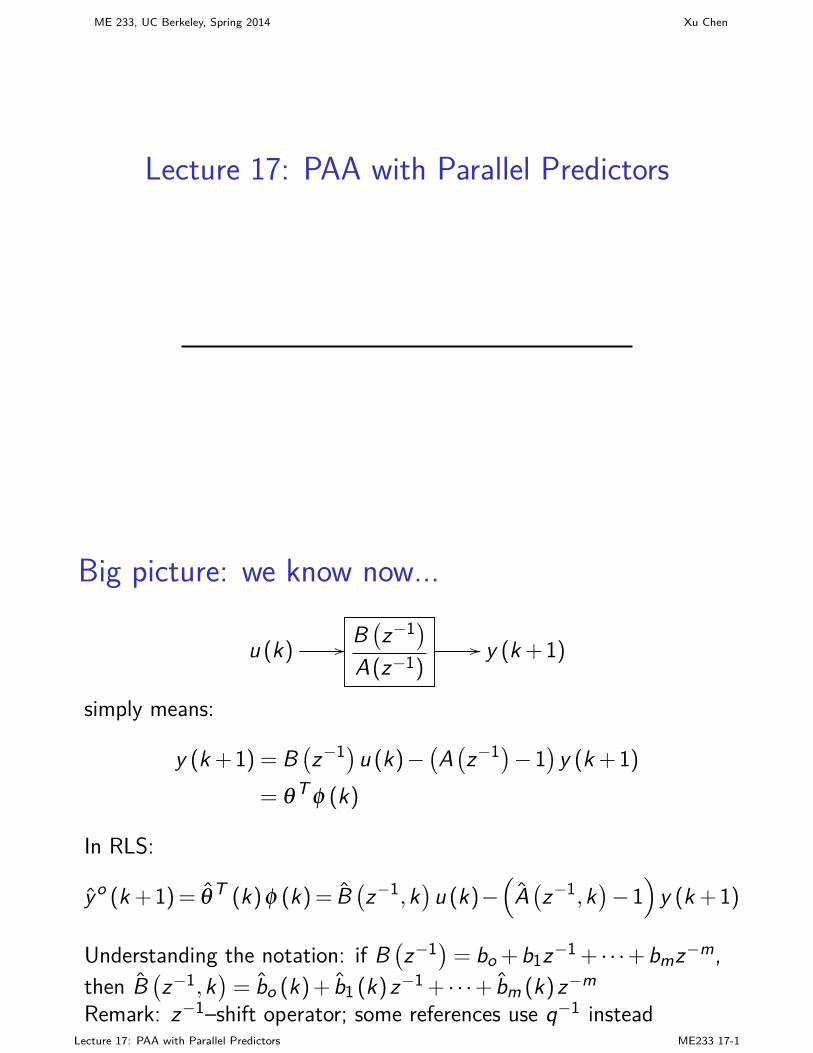
ME 233, UC Berkeley, Spring 2014 Xu Chen
Lecture 17: PAA with Parallel Predictors
Big picture: we know now...
u (k) // B(z−1)
A(z−1)// y (k +1)
simply means:
y (k +1) = B(z−1)u (k)−
(A(z−1)−1
)y (k +1)
= θT φ (k)
In RLS:
yo (k +1)= θT (k)φ (k)= B(z−1,k
)u (k)−
(A(z−1,k
)−1)
y (k +1)
Understanding the notation: if B(z−1)= bo +b1z−1 + · · ·+bmz−m,
then B(z−1,k
)= bo (k)+ b1 (k)z−1 + · · ·+ bm (k)z−m
Remark: z−1–shift operator; some references use q−1 insteadLecture 17: PAA with Parallel Predictors ME233 17-1
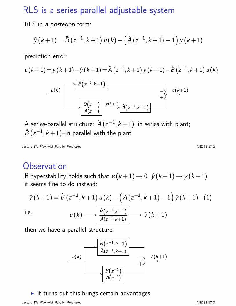
RLS is a series-parallel adjustable systemRLS in a posteriori form:
y (k +1) = B(z−1,k +1
)u (k)−
(A(z−1,k +1
)−1)
y (k +1)
prediction error:
ε (k +1)= y (k +1)− y (k +1)= A(z−1,k +1
)y (k +1)−B
(z−1,k +1
)u (k)
// B(z−1,k+1)− u(k) ε(k+1)//
// B(z−1)A(z−1)
y(k+1) // A(z−1,k+1)
+OO
A series-parallel structure: A(z−1,k +1
)–in series with plant;
B(z−1,k +1
)–in parallel with the plant
Lecture 17: PAA with Parallel Predictors ME233 17-2
ObservationIf hyperstability holds such that ε (k +1)→ 0, y (k +1)→ y (k +1),it seems fine to do instead:
y (k +1) = B(z−1,k +1
)u (k)−
(A(z−1,k +1
)−1)
y (k +1) (1)
i.e. u (k) // B(z−1,k+1)
A(z−1,k+1)// y (k +1)
then we have a parallel structure
// B(z−1,k+1)
A(z−1,k+1)− u(k) ε(k+1)//
// B(z−1)A(z−1)
+OO
I it turns out this brings certain advantagesLecture 17: PAA with Parallel Predictors ME233 17-3
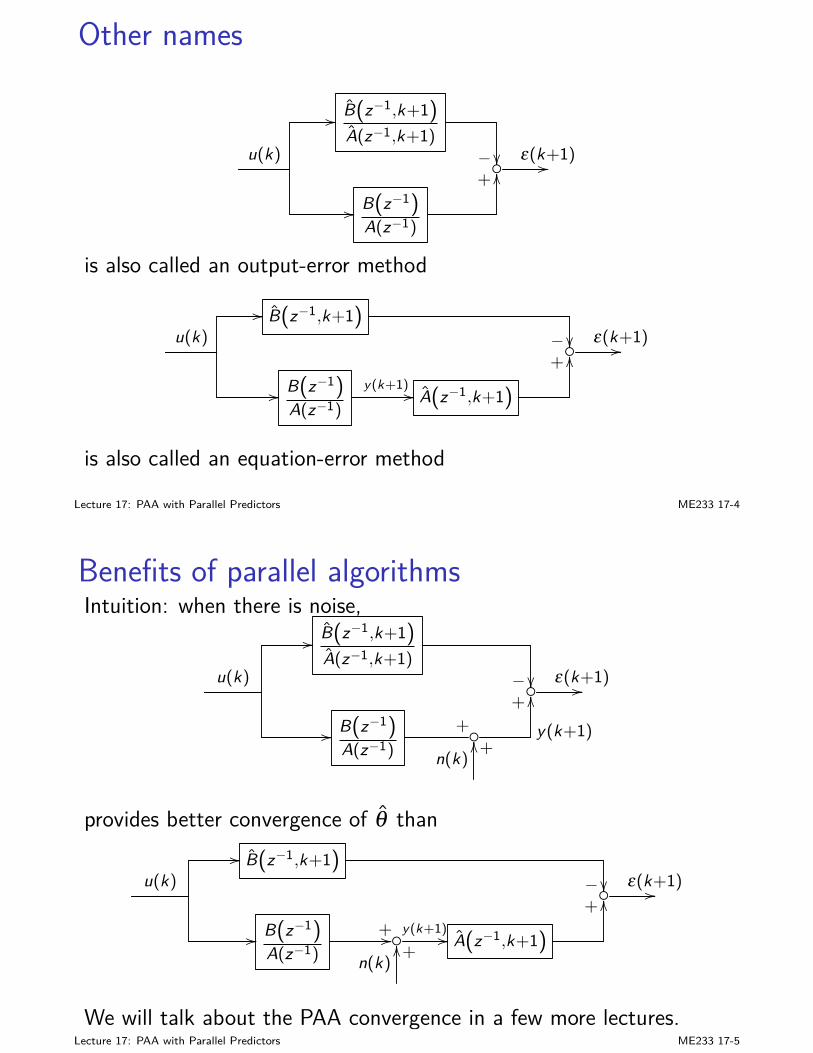
Other names
// B(z−1,k+1)
A(z−1,k+1)− u(k) ε(k+1)//
// B(z−1)A(z−1)
+OO
is also called an output-error method
// B(z−1,k+1)− u(k) ε(k+1)//
// B(z−1)A(z−1)
y(k+1) // A(z−1,k+1)
+OO
is also called an equation-error method
Lecture 17: PAA with Parallel Predictors ME233 17-4
Benefits of parallel algorithmsIntuition: when there is noise,
// B(z−1,k+1)
A(z−1,k+1)− u(k) ε(k+1)//
// B(z−1)A(z−1)
++
y(k+1)
OO
n(k) +OO
provides better convergence of θ than// B(z−1,k+1)
− u(k) ε(k+1)//
// B(z−1)A(z−1)
+//y(k+1) // A(z−1,k+1)
+OO
n(k) +OO
We will talk about the PAA convergence in a few more lectures.Lecture 17: PAA with Parallel Predictors ME233 17-5
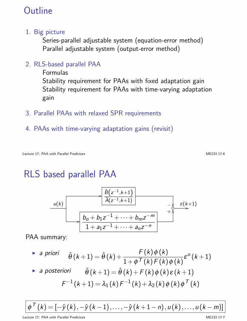
Outline
1. Big pictureSeries-parallel adjustable system (equation-error method)Parallel adjustable system (output-error method)
2. RLS-based parallel PAAFormulasStability requirement for PAAs with fixed adaptation gainStability requirement for PAAs with time-varying adaptationgain
3. Parallel PAAs with relaxed SPR requirements
4. PAAs with time-varying adaptation gains (revisit)
Lecture 17: PAA with Parallel Predictors ME233 17-6
RLS based parallel PAA
// B(z−1,k+1)
A(z−1,k+1)− u(k) ε(k+1)//
// bo +b1z−1 + · · ·+bmz−m
1+a1z−1 + · · ·+anz−n
+OO
PAA summary:
I a priori θ (k +1) = θ (k)+ F (k)φ (k)1+φT (k)F (k)φ (k)εo (k +1)
I a posteriori θ (k +1) = θ (k)+F (k)φ (k)ε (k +1)F−1 (k +1) = λ1 (k)F−1 (k)+λ2 (k)φ (k)φT (k)
φT (k) = [−y (k) ,−y (k−1) , . . . ,−y (k +1−n) ,u (k) , . . . ,u (k−m)]
Lecture 17: PAA with Parallel Predictors ME233 17-7
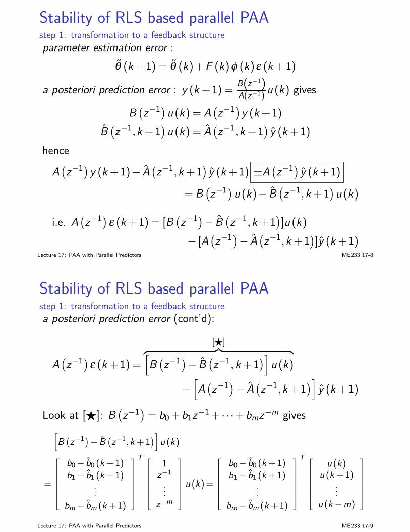
Stability of RLS based parallel PAAstep 1: transformation to a feedback structureparameter estimation error :
θ (k +1) = θ (k)+F (k)φ (k)ε (k +1)
a posteriori prediction error : y (k +1) = B(z−1)A(z−1) u (k) gives
B(z−1)u (k) = A
(z−1)y (k +1)
B(z−1,k +1
)u (k) = A
(z−1,k +1
)y (k +1)
hence
A(z−1)y (k +1)− A
(z−1,k +1
)y (k +1) ±A
(z−1) y (k +1)
= B(z−1)u (k)− B
(z−1,k +1
)u (k)
i.e. A(z−1)ε (k +1) = [B
(z−1)− B
(z−1,k +1
)]u (k)
− [A(z−1)− A
(z−1,k +1
)]y (k +1)
Lecture 17: PAA with Parallel Predictors ME233 17-8
Stability of RLS based parallel PAAstep 1: transformation to a feedback structurea posteriori prediction error (cont’d):
A(z−1)ε (k +1) =
[F]︷ ︸︸ ︷[B(z−1)− B
(z−1,k +1
)]u (k)
−[A(z−1)− A
(z−1,k +1
)]y (k +1)
Look at [F]: B(z−1)= b0 +b1z−1 + · · ·+bmz−m gives
[B(z−1)− B
(z−1,k +1
)]u (k)
=
b0− b0 (k +1)b1− b1 (k +1)
...bm− bm (k +1)
T
1z−1
...z−m
u (k)=
b0− b0 (k +1)b1− b1 (k +1)
...bm− bm (k +1)
T
u (k)u (k−1)
...u (k−m)
Lecture 17: PAA with Parallel Predictors ME233 17-9
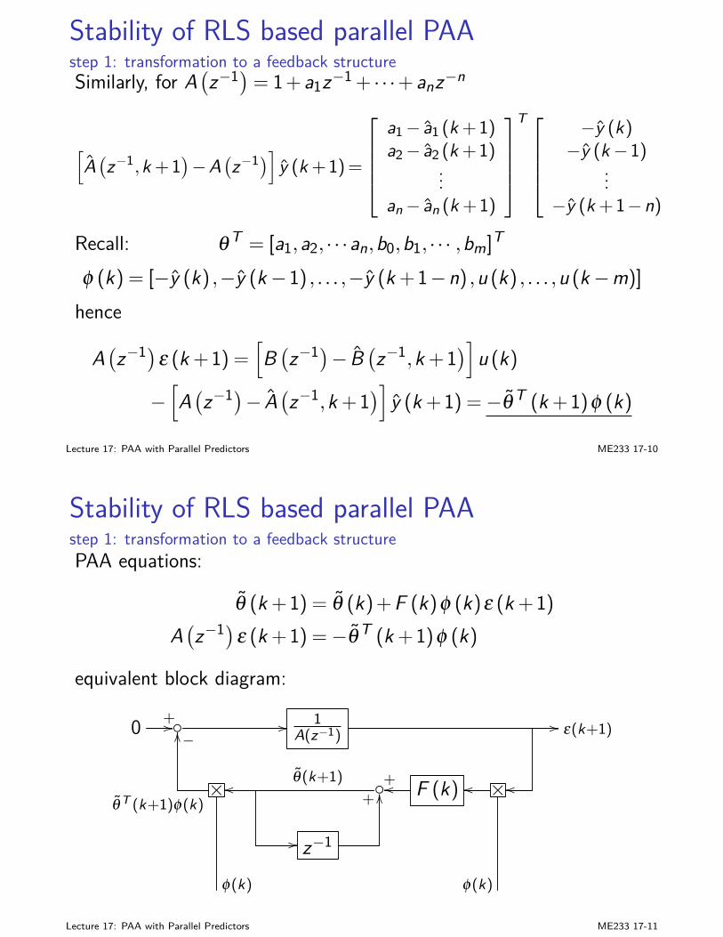
Stability of RLS based parallel PAAstep 1: transformation to a feedback structureSimilarly, for A
(z−1)= 1+a1z−1 + · · ·+anz−n
[A(z−1,k +1
)−A
(z−1)] y (k +1)=
a1− a1 (k +1)a2− a2 (k +1)
...an− an (k +1)
T
−y (k)−y (k−1)
...−y (k +1−n)
Recall: θT = [a1,a2, · · ·an,b0,b1, · · · ,bm]T
φ (k) = [−y (k) ,−y (k−1) , . . . ,−y (k +1−n) ,u (k) , . . . ,u (k−m)]
hence
A(z−1)ε (k +1) =
[B(z−1)− B
(z−1,k +1
)]u (k)
−[A(z−1)− A
(z−1,k +1
)]y (k +1) =−θT (k +1)φ (k)
Lecture 17: PAA with Parallel Predictors ME233 17-10
Stability of RLS based parallel PAAstep 1: transformation to a feedback structurePAA equations:
θ (k +1) = θ (k)+F (k)φ (k)ε (k +1)A(z−1)ε (k +1) =−θT (k +1)φ (k)
equivalent block diagram:
0 +// // 1A(z−1)
// ε(k+1)−OO
×θT (k+1)φ(k)
oo θ(k+1) F (k)+oo ×oo oo
// z−1
+OO
φ(k) φ(k)
Lecture 17: PAA with Parallel Predictors ME233 17-11
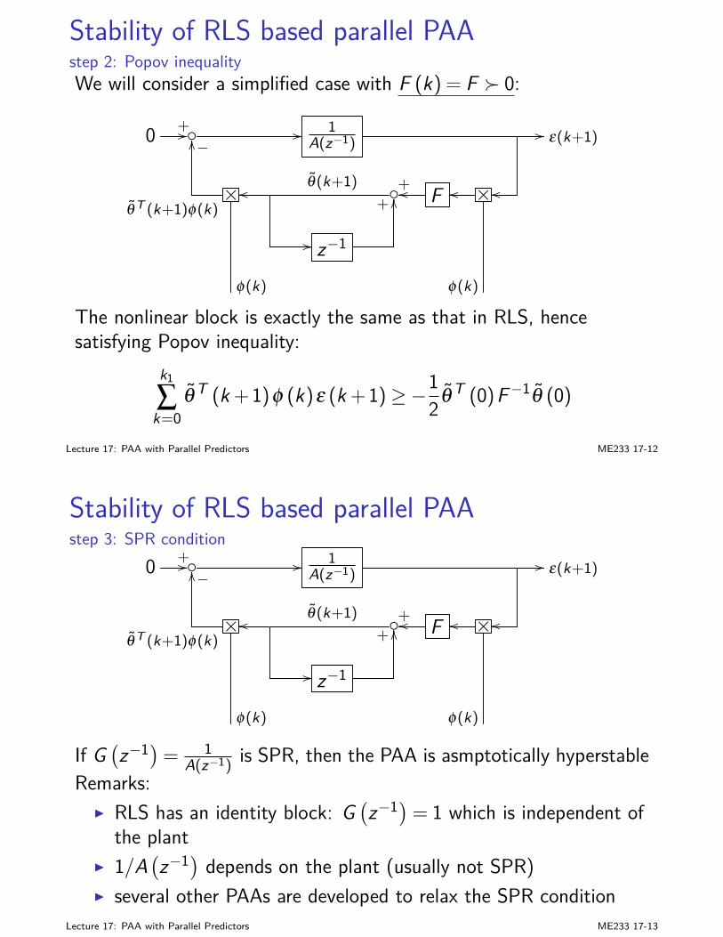
Stability of RLS based parallel PAAstep 2: Popov inequalityWe will consider a simplified case with F (k) = F 0:
0 +// // 1A(z−1)
// ε(k+1)−OO
×θT (k+1)φ(k)
oo θ(k+1)F+oo ×oo oo
// z−1
+OO
φ(k) φ(k)
The nonlinear block is exactly the same as that in RLS, hencesatisfying Popov inequality:
k1
∑k=0
θ T (k +1)φ (k)ε (k +1)≥−12 θT (0)F−1θ (0)
Lecture 17: PAA with Parallel Predictors ME233 17-12
Stability of RLS based parallel PAAstep 3: SPR condition
0 +// // 1A(z−1)
// ε(k+1)−OO
×θT (k+1)φ(k)
oo θ(k+1)F+oo ×oo oo
// z−1
+OO
φ(k) φ(k)
If G(z−1)= 1
A(z−1) is SPR, then the PAA is asmptotically hyperstableRemarks:
I RLS has an identity block: G(z−1)= 1 which is independent of
the plantI 1/A
(z−1) depends on the plant (usually not SPR)
I several other PAAs are developed to relax the SPR conditionLecture 17: PAA with Parallel Predictors ME233 17-13
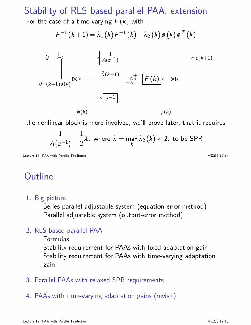
Stability of RLS based parallel PAA: extensionFor the case of a time-varying F (k) with
F−1 (k +1) = λ1 (k)F−1 (k)+λ2 (k)φ (k)φT (k)
0 +// // 1A(z−1)
// ε(k+1)−OO
×θT (k+1)φ(k)
oo θ(k+1) F (k)+oo ×oo oo
// z−1
+OO
φ(k) φ(k)
the nonlinear block is more involved; we’ll prove later, that it requires1
A(z−1)− 1
2λ , where λ =maxk
λ2 (k)< 2, to be SPR
Lecture 17: PAA with Parallel Predictors ME233 17-14
Outline
1. Big pictureSeries-parallel adjustable system (equation-error method)Parallel adjustable system (output-error method)
2. RLS-based parallel PAAFormulasStability requirement for PAAs with fixed adaptation gainStability requirement for PAAs with time-varying adaptationgain
3. Parallel PAAs with relaxed SPR requirements
4. PAAs with time-varying adaptation gains (revisit)
Lecture 17: PAA with Parallel Predictors ME233 17-15
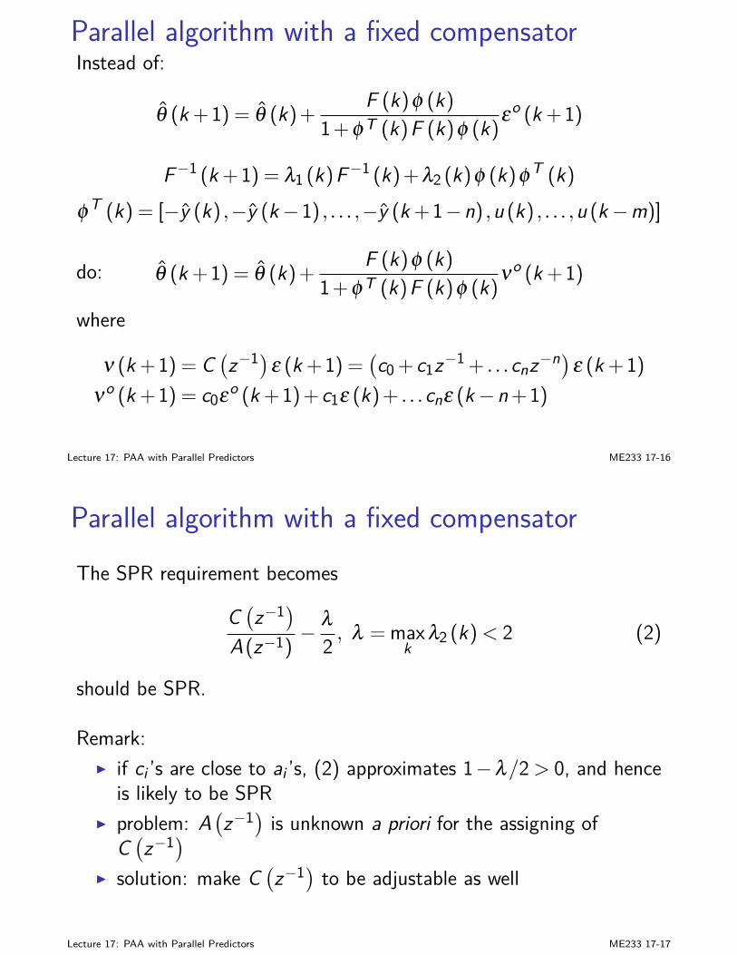
Parallel algorithm with a fixed compensatorInstead of:
θ (k +1) = θ (k)+ F (k)φ (k)1+φT (k)F (k)φ (k)εo (k +1)
F−1 (k +1) = λ1 (k)F−1 (k)+λ2 (k)φ (k)φT (k)φT (k) = [−y (k) ,−y (k−1) , . . . ,−y (k +1−n) ,u (k) , . . . ,u (k−m)]
do: θ (k +1) = θ (k)+ F (k)φ (k)1+φT (k)F (k)φ (k)νo (k +1)
where
ν (k +1) = C(z−1)ε (k +1) =
(c0 + c1z−1 + . . .cnz−n)ε (k +1)
νo (k +1) = c0εo (k +1)+ c1ε (k)+ . . .cnε (k−n+1)
Lecture 17: PAA with Parallel Predictors ME233 17-16
Parallel algorithm with a fixed compensatorThe SPR requirement becomes
C(z−1)
A(z−1)− λ
2 , λ =maxk
λ2 (k)< 2 (2)
should be SPR.
Remark:I if ci ’s are close to ai ’s, (2) approximates 1−λ/2> 0, and hence
is likely to be SPRI problem: A
(z−1) is unknown a priori for the assigning of
C(z−1)
I solution: make C(z−1) to be adjustable as well
Lecture 17: PAA with Parallel Predictors ME233 17-17

Parallel algorithm with an adjustable compensatorIf A
(z−1)= 1+a1z−1 + · · ·+anz−n, let C
(z−1)= 1+ c1z−1 + · · ·+ cnz−n and
ν (k +1) = C(z−1,k +1
)ε (k +1)
νo (k +1) = εo (k +1)+n∑i=1
ci (k)ε (k +1− i)
do θe (k +1) = θe (k)+Fe (k)φe (k)
1+φTe (k)Fe (k)φe (k)νo (k +1)
θ Te (k) =
[θT (k) , c1 (k) , . . . , cn (k)
]
φTe (k) =
[φT (k) ,−ε (k) , . . . ,−ε (k +1−n)
]
F−1e (k +1) = λ1 (k)F−1
e (k)+λ2 (k)φe (k)φTe (k)
which has guaranteed asymptotical stablility.
Lecture 17: PAA with Parallel Predictors ME233 17-18
General PAA block diagram
0 +// // H(z−1) //
−OO
×oo θ(k+1) or θe(k+1) F (k)+oo ×oo oo
// z−1
+OO
φ(k) or φe(k) φ(k) or φe(k)
H(z−1) PAA1 RLS/parallel predictor with adjustable compensator
1/A(z−1) parallel predictorC(z−1)/A(z−1) parallel predictor with fixed compensator
Lecture 17: PAA with Parallel Predictors ME233 17-19
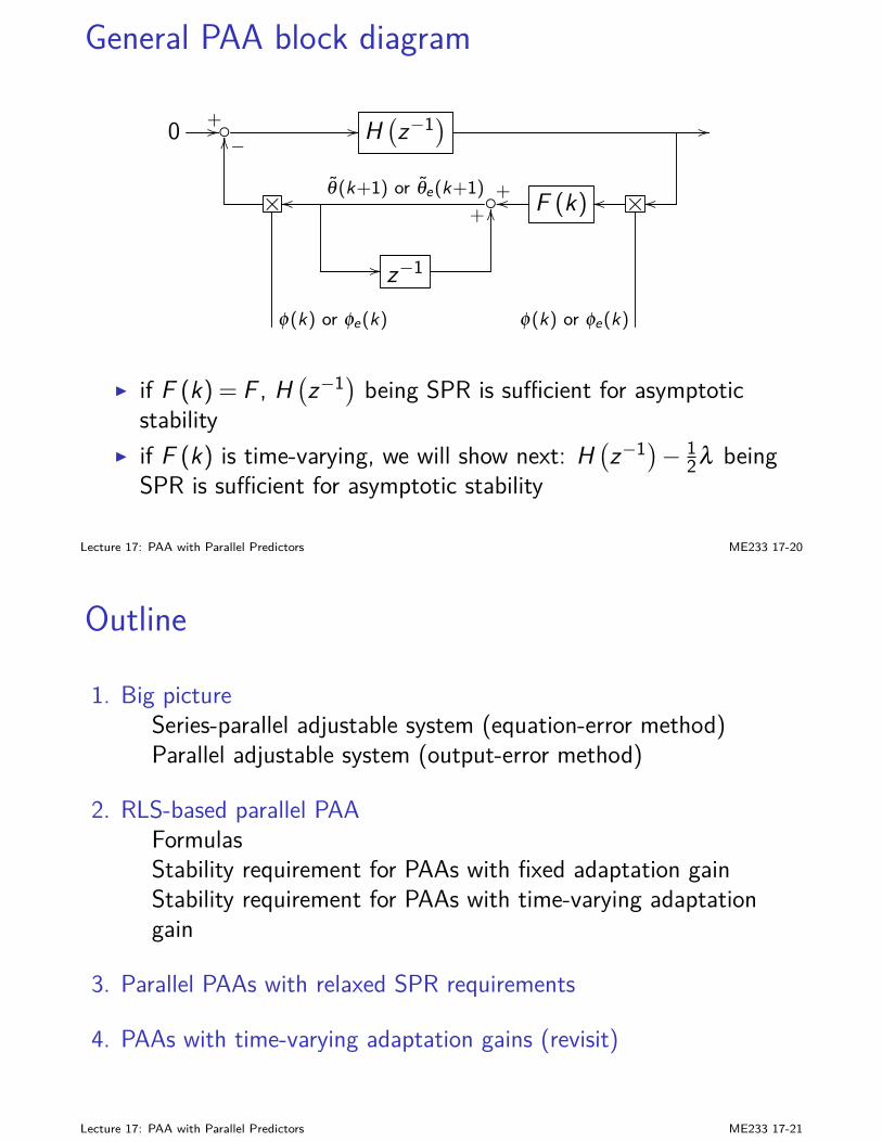
General PAA block diagram
0 +// // H(z−1) //
−OO
×oo θ(k+1) or θe(k+1) F (k)+oo ×oo oo
// z−1
+OO
φ(k) or φe(k) φ(k) or φe(k)
I if F (k) = F , H(z−1) being SPR is sufficient for asymptotic
stabilityI if F (k) is time-varying, we will show next: H
(z−1)− 1
2λ beingSPR is sufficient for asymptotic stability
Lecture 17: PAA with Parallel Predictors ME233 17-20
Outline
1. Big pictureSeries-parallel adjustable system (equation-error method)Parallel adjustable system (output-error method)
2. RLS-based parallel PAAFormulasStability requirement for PAAs with fixed adaptation gainStability requirement for PAAs with time-varying adaptationgain
3. Parallel PAAs with relaxed SPR requirements
4. PAAs with time-varying adaptation gains (revisit)
Lecture 17: PAA with Parallel Predictors ME233 17-21
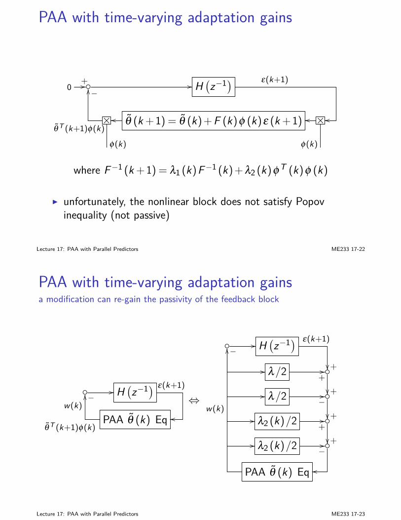
PAA with time-varying adaptation gains
0+// // H
(z−1) ε(k+1)
−OO
×θT (k+1)φ(k)
θ (k +1) = θ (k)+F (k)φ (k)ε (k +1)oo ×oo oo
φ(k) φ(k)
where F−1 (k +1) = λ1 (k)F−1 (k)+λ2 (k)φT (k)φ (k)
I unfortunately, the nonlinear block does not satisfy Popovinequality (not passive)
Lecture 17: PAA with Parallel Predictors ME233 17-22
PAA with time-varying adaptation gainsa modification can re-gain the passivity of the feedback block
// H(z−1) ε(k+1)
−w(k)
OO
PAA θ (k) EqθT (k+1)φ(k)
oo
⇔
// H(z−1) ε(k+1)
+//
OO
λ/2+//+// λ/2 −//+// λ2 (k)/2 +//+// λ2 (k)/2 −//
−
w(k)
PAA θ (k) Eq oo
Lecture 17: PAA with Parallel Predictors ME233 17-23
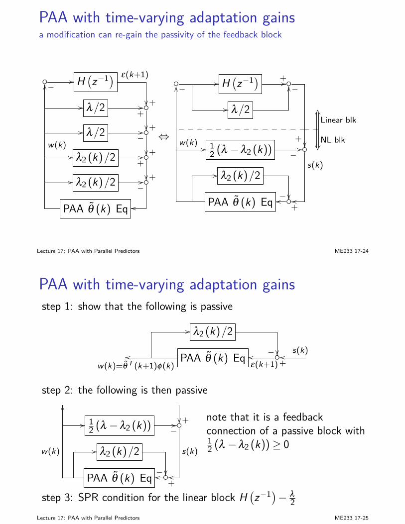
PAA with time-varying adaptation gainsa modification can re-gain the passivity of the feedback block
// H(z−1) ε(k+1)
+//
OO
λ/2+//+// λ/2 −//+// λ2 (k)/2 +//+// λ2 (k)/2 −//
−
w(k)
PAA θ (k) Eq oo
⇔
// H(z−1) +//
// λ/2
−OO
+ NL blk
Linear blkKS
// 12 (λ −λ2 (k)) −
//s(k)
// λ2 (k)/2−
−
w(k)
OO
PAA θ (k) Eq oo+oo
Lecture 17: PAA with Parallel Predictors ME233 17-24
PAA with time-varying adaptation gainsstep 1: show that the following is passive
// λ2 (k)/2−
w(k)=θT (k+1)φ(k)oo PAA θ (k) Eq
ε(k+1)oo
+
s(k)oo
step 2: the following is then passive
+//
OO
12 (λ −λ2 (k)) −
//
s(k)// λ2 (k)/2−
w(k)
PAA θ (k) Eq oo+oo
note that it is a feedbackconnection of a passive block with12 (λ −λ2 (k))≥ 0
step 3: SPR condition for the linear block H(z−1)− λ
2Lecture 17: PAA with Parallel Predictors ME233 17-25
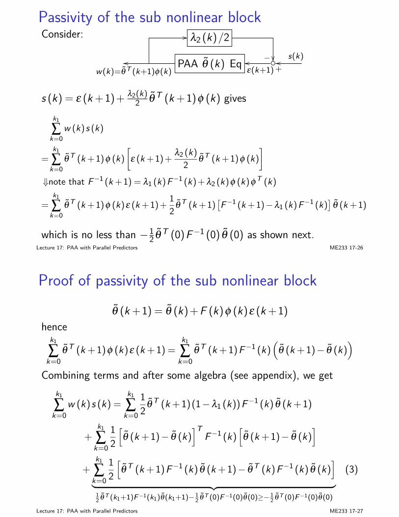
Passivity of the sub nonlinear blockConsider: // λ2 (k)/2
− w(k)=θT (k+1)φ(k)
oo PAA θ (k) Eq ε(k+1)oo
+
s(k)oo
s (k) = ε (k +1)+ λ2(k)2 θT (k +1)φ (k) gives
k1
∑k=0
w (k)s (k)
=k1
∑k=0
θ T (k +1)φ (k)[
ε (k +1)+ λ2 (k)2 θ T (k +1)φ (k)
]
⇓note that F−1 (k +1) = λ1 (k)F−1 (k)+λ2 (k)φ (k)φT (k)
=k1
∑k=0
θ T (k +1)φ (k)ε (k +1)+ 12 θ T (k +1)
[F−1 (k +1)−λ1 (k)F−1 (k)
]θ (k +1)
which is no less than −12 θT (0)F−1 (0) θ (0) as shown next.
Lecture 17: PAA with Parallel Predictors ME233 17-26
Proof of passivity of the sub nonlinear blockθ (k +1) = θ (k)+F (k)φ (k)ε (k +1)
hencek1
∑k=0
θ T (k +1)φ (k)ε (k +1) =k1
∑k=0
θ T (k +1)F−1 (k)(
θ (k +1)− θ (k))
Combining terms and after some algebra (see appendix), we getk1
∑k=0
w (k)s (k) =k1
∑k=0
12 θ T (k +1)(1−λ1 (k))F−1 (k) θ (k +1)
+k1
∑k=0
12[θ (k +1)− θ (k)
]TF−1 (k)
[θ (k +1)− θ (k)
]
+k1
∑k=0
12[θ T (k +1)F−1 (k) θ (k +1)− θ T (k)F−1 (k) θ (k)
]
︸ ︷︷ ︸12 θ T (k1+1)F−1(k1)θ(k1+1)− 1
2 θ T (0)F−1(0)θ(0)≥− 12 θ T (0)F−1(0)θ(0)
(3)
Lecture 17: PAA with Parallel Predictors ME233 17-27
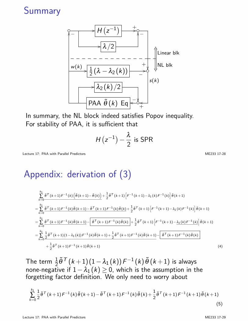
Summary
// H(z−1) +//
// λ/2
−OO
+ NL blk
Linear blkKS
// 12 (λ −λ2 (k)) −
//s(k)
// λ2 (k)/2−
−
w(k)
OO
PAA θ (k) Eq oo+oo
In summary, the NL block indeed satisfies Popov inequality.For stability of PAA, it is sufficient that
H(z−1)− λ
2 is SPR
Lecture 17: PAA with Parallel Predictors ME233 17-28
Appendix: derivation of (3)k1∑
k=0θT (k +1)F−1 (k)
(θ (k +1)− θ (k)
)+
12 θT (k +1)
[F−1 (k +1)−λ1 (k)F−1 (k)
]θ (k +1)
=k1∑
k=0θT (k +1)F−1 (k) θ (k +1)− θT (k +1)F−1 (k) θ (k)+ 1
2 θT (k +1)[F−1 (k +1)−λ1 (k)F−1 (k)
]θ (k +1)
=k1∑
k=0θT (k +1)F−1 (k) θ (k +1)− θT (k +1)F−1 (k) θ (k) +
12 θT (k +1)
[F−1 (k +1)−λ1 (k)F−1 (k)
]θ (k +1)
=k1∑
k=0
12 θT (k +1)(1−λ1 (k))F−1 (k) θ (k +1)+ 1
2 θT (k +1)F−1 (k) θ (k +1)− θT (k +1)F−1 (k) θ (k)
+12 θT (k +1)F−1 (k +1) θ (k +1) (4)
The term 12 θT (k +1)(1−λ1 (k))F−1 (k) θ (k +1) is always
none-negative if 1−λ1 (k)≥ 0, which is the assumption in theforgetting factor definition. We only need to worry about
k1
∑k=0
12 θ T (k +1)F−1 (k) θ (k +1)− θ T (k +1)F−1 (k) θ (k)+ 1
2 θ T (k +1)F−1 (k +1) θ (k +1)
(5)
Lecture 17: PAA with Parallel Predictors ME233 17-29
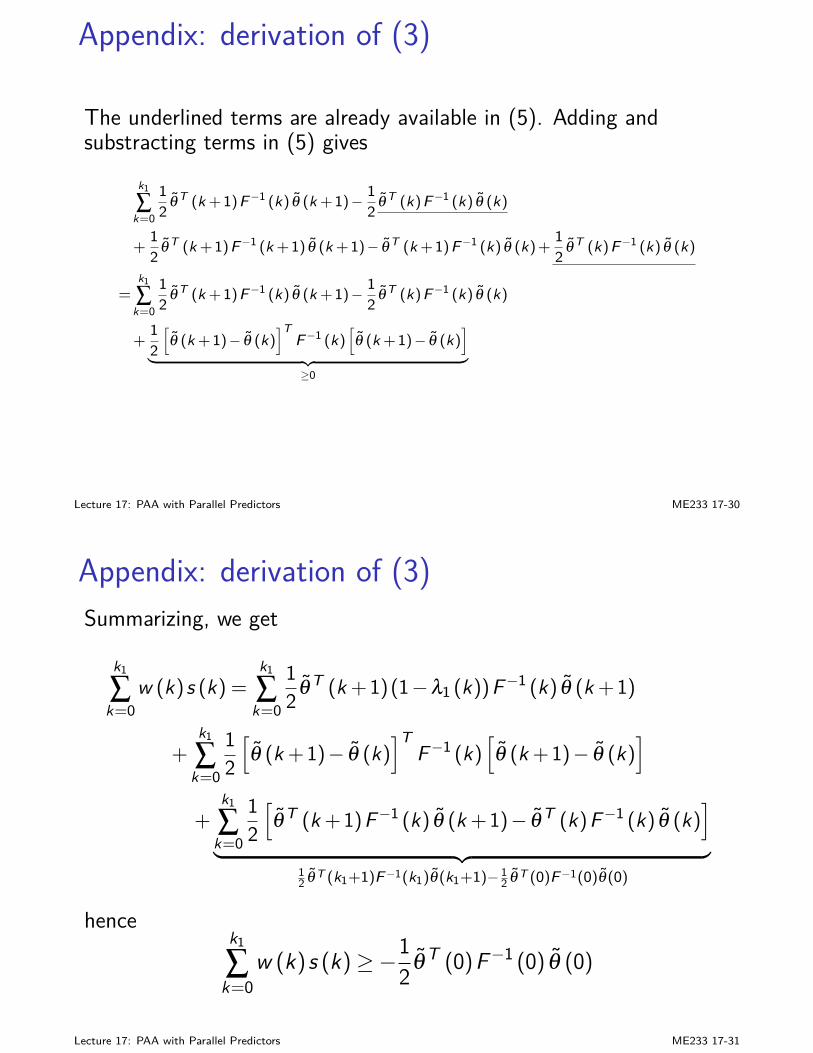
Appendix: derivation of (3)
The underlined terms are already available in (5). Adding andsubstracting terms in (5) gives
k1
∑k=0
12 θ T (k +1)F−1 (k) θ (k +1)− 1
2 θ T (k)F−1 (k) θ (k)
+12 θ T (k +1)F−1 (k +1) θ (k +1)− θ T (k +1)F−1 (k) θ (k)+ 1
2 θ T (k)F−1 (k) θ (k)
=k1
∑k=0
12 θ T (k +1)F−1 (k) θ (k +1)− 1
2 θ T (k)F−1 (k) θ (k)
+12[θ (k +1)− θ (k)
]TF−1 (k)
[θ (k +1)− θ (k)
]
︸ ︷︷ ︸≥0
Lecture 17: PAA with Parallel Predictors ME233 17-30
Appendix: derivation of (3)Summarizing, we get
k1
∑k=0
w (k)s (k) =k1
∑k=0
12 θ T (k +1)(1−λ1 (k))F−1 (k) θ (k +1)
+k1
∑k=0
12[θ (k +1)− θ (k)
]TF−1 (k)
[θ (k +1)− θ (k)
]
+k1
∑k=0
12[θ T (k +1)F−1 (k) θ (k +1)− θ T (k)F−1 (k) θ (k)
]
︸ ︷︷ ︸12 θ T (k1+1)F−1(k1)θ(k1+1)− 1
2 θ T (0)F−1(0)θ(0)
hencek1
∑k=0
w (k)s (k)≥−12 θ T (0)F−1 (0) θ (0)
Lecture 17: PAA with Parallel Predictors ME233 17-31
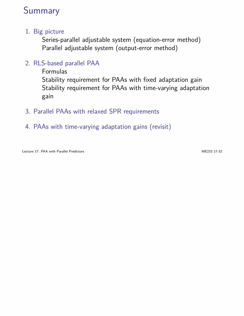
Summary
1. Big pictureSeries-parallel adjustable system (equation-error method)Parallel adjustable system (output-error method)
2. RLS-based parallel PAAFormulasStability requirement for PAAs with fixed adaptation gainStability requirement for PAAs with time-varying adaptationgain
3. Parallel PAAs with relaxed SPR requirements
4. PAAs with time-varying adaptation gains (revisit)
Lecture 17: PAA with Parallel Predictors ME233 17-32
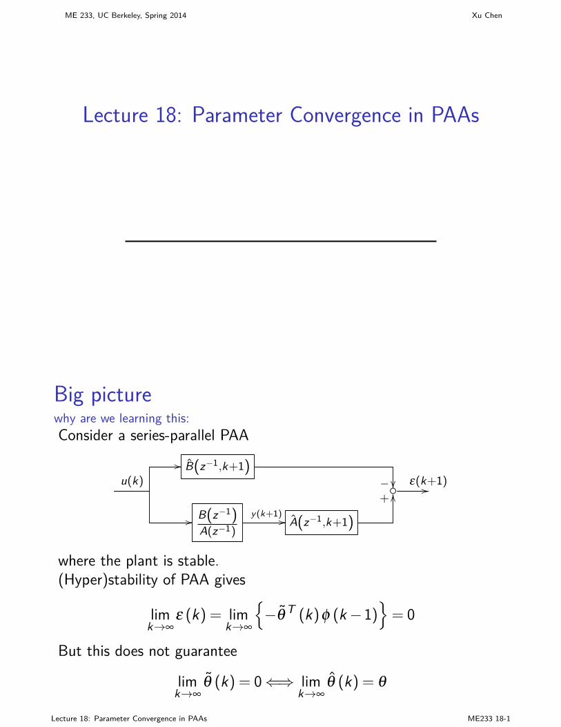
ME 233, UC Berkeley, Spring 2014 Xu Chen
Lecture 18: Parameter Convergence in PAAs
Big picturewhy are we learning this:Consider a series-parallel PAA
// B(z−1,k+1)− u(k) ε(k+1)//
// B(z−1)A(z−1)
y(k+1) // A(z−1,k+1)
+OO
where the plant is stable.(Hyper)stability of PAA gives
limk→∞
ε (k) = limk→∞
−θT (k)φ (k−1)
= 0
But this does not guarantee
limk→∞
θ (k) = 0⇐⇒ limk→∞
θ (k) = θ
Lecture 18: Parameter Convergence in PAAs ME233 18-1
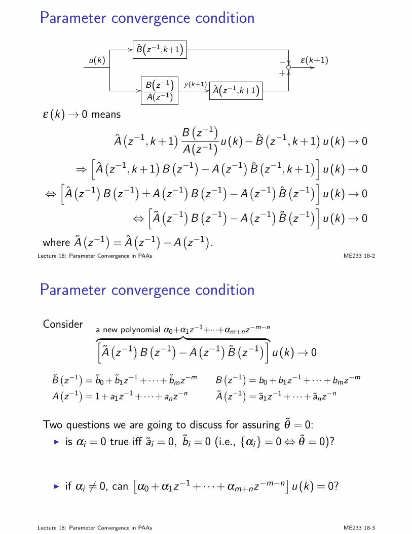
Parameter convergence condition// B(z−1,k+1)
− u(k) ε(k+1)//
// B(z−1)A(z−1)
y(k+1) // A(z−1,k+1)
+OO
ε (k)→ 0 means
A(z−1,k+1
) B(z−1)
A(z−1)u (k)− B
(z−1,k+1
)u (k)→ 0
⇒[A(z−1,k+1
)B(z−1)−A
(z−1) B
(z−1,k+1
)]u (k)→ 0
⇔[A(z−1)B
(z−1)±A
(z−1)B
(z−1)−A
(z−1) B
(z−1)]u (k)→ 0
⇔[A(z−1)B
(z−1)−A
(z−1) B
(z−1)]u (k)→ 0
where A(z−1)= A
(z−1)−A
(z−1).
Lecture 18: Parameter Convergence in PAAs ME233 18-2
Parameter convergence condition
Consider a new polynomial α0+α1z−1+···+αm+nz−m−n︷ ︸︸ ︷[A(z−1)B
(z−1)−A
(z−1) B
(z−1)]u (k)→ 0
B(z−1)= b0 + b1z−1 + · · ·+ bmz−m
A(z−1)= 1+a1z−1 + · · ·+anz−n
B(z−1)= b0 +b1z−1 + · · ·+bmz−m
A(z−1)= a1z−1 + · · ·+ anz−n
Two questions we are going to discuss for assuring θ = 0:I is αi = 0 true iff ai = 0, bi = 0 (i.e., αi= 0⇔ θ = 0)?
I if αi 6= 0, can[α0 +α1z−1 + · · ·+αm+nz−m−n]u (k) = 0?
Lecture 18: Parameter Convergence in PAAs ME233 18-3
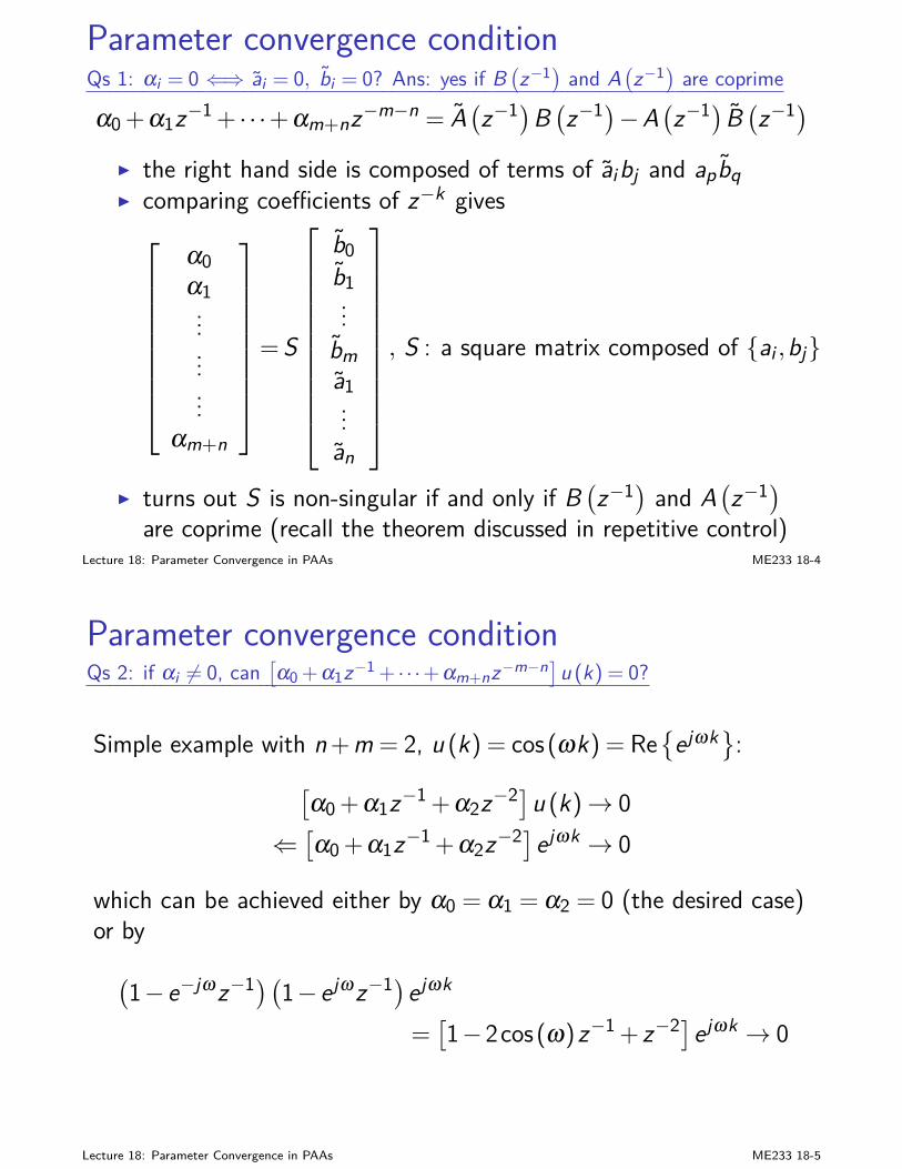
Parameter convergence conditionQs 1: αi = 0 ⇐⇒ ai = 0, bi = 0? Ans: yes if B
(z−1) and A
(z−1) are coprime
α0 +α1z−1 + · · ·+αm+nz−m−n = A(z−1)B
(z−1)−A
(z−1) B
(z−1)
I the right hand side is composed of terms of aibj and ap bqI comparing coefficients of z−k gives
α0α1.........
αm+n
= S
b0b1...bma1...an
, S : a square matrix composed of ai ,bj
I turns out S is non-singular if and only if B(z−1) and A
(z−1)
are coprime (recall the theorem discussed in repetitive control)Lecture 18: Parameter Convergence in PAAs ME233 18-4
Parameter convergence conditionQs 2: if αi 6= 0, can
[α0 +α1z−1 + · · ·+αm+nz−m−n]u (k) = 0?
Simple example with n+m = 2, u (k) = cos (ωk) = Reejωk:
[α0 +α1z−1 +α2z−2]u (k)→ 0
⇐[α0 +α1z−1 +α2z−2]ejωk → 0
which can be achieved either by α0 = α1 = α2 = 0 (the desired case)or by(1− e−jωz−1)(1− ejωz−1)ejωk
=[1−2cos (ω)z−1 + z−2]ejωk → 0
Lecture 18: Parameter Convergence in PAAs ME233 18-5
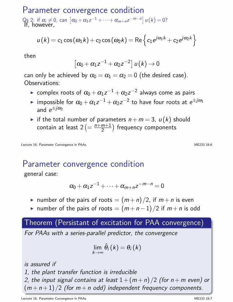
Parameter convergence conditionQs 2: if αi 6= 0, can
[α0 +α1z−1 + · · ·+αm+nz−m−n]u (k) = 0?
If, however,
u (k) = c1 cos (ω1k)+ c2 cos (ω2k) = Rec1ejω1k + c2ejω2k
then [α0 +α1z−1 +α2z−2]u (k)→ 0
can only be achieved by α0 = α1 = α2 = 0 (the desired case).Observations:
I complex roots of α0 +α1z−1 +α2z−2 always come as pairsI impossible for α0 +α1z−1 +α2z−2 to have four roots at e±jω1
and e±jω2
I if the total number of parameters n+m = 3, u (k) shouldcontain at least 2
(= n+m+1
2)frequency components
Lecture 18: Parameter Convergence in PAAs ME233 18-6
Parameter convergence conditiongeneral case:
α0 +α1z−1 + · · ·+αm+nz−m−n = 0
I number of the pairs of roots = (m+n)/2, if m+n is evenI number of the pairs of roots = (m+n−1)/2 if m+n is odd
Theorem (Persistant of excitation for PAA convergence)For PAAs with a series-parallel predictor, the convergence
limk→∞
θi (k) = θi (k)
is assured if1, the plant transfer function is irreducible2, the input signal contains at least 1+(m+n)/2 (for n+m even) or(m+n+1)/2 (for m+n odd) independent frequency components.
Lecture 18: Parameter Convergence in PAAs ME233 18-7
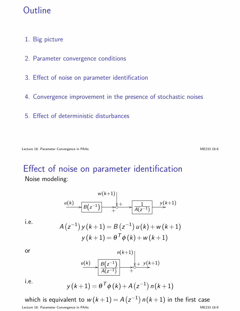
Outline
1. Big picture
2. Parameter convergence conditions
3. Effect of noise on parameter identification
4. Convergence improvement in the presence of stochastic noises
5. Effect of deterministic disturbances
Lecture 18: Parameter Convergence in PAAs ME233 18-8
Effect of noise on parameter identificationNoise modeling:
+
w(k+1)
u(k) // B(z−1)+// // 1
A(z−1)y(k+1)//
i.e. A(z−1)y (k+1) = B
(z−1)u (k)+w (k+1)
y (k+1) = θT φ (k)+w (k+1)
or
+
n(k+1)
u(k) // B(z−1)A(z−1) +
// y(k+1)//
i.e. y (k+1) = θ T φ (k)+A(z−1)n (k+1)
which is equivalent to w (k+1) = A(z−1)n (k+1) in the first case
Lecture 18: Parameter Convergence in PAAs ME233 18-9
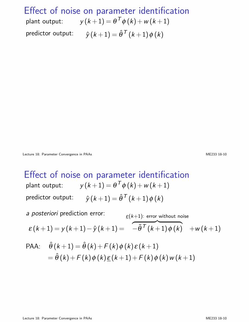
Effect of noise on parameter identificationplant output: y (k+1) = θ T φ (k)+w (k+1)predictor output: y (k+1) = θT (k+1)φ (k)
a posteriori prediction error:
ε (k+1) = y (k+1)− y (k+1) =
ε(k+1): error without noise︷ ︸︸ ︷−θ T (k+1)φ (k) +w (k+1)
PAA: θ (k+1) = θ (k)+F (k)φ (k)ε (k+1)= θ (k)+F (k)φ (k)ε (k+1)+F (k)φ (k)w (k+1)
I F (k)φ (k)w (k+1) is integrated by PAAI need: E [φ (k)w (k+1)] = 0
and a vanishing adaptation gain F (k):F−1 (k+1) = λ1 (k)F−1 (k)+λ2 (k)φ (k)φT (k), λ1 (k) k→∞−→ 1 and0< λ2 (k)< 2
Lecture 18: Parameter Convergence in PAAs ME233 18-10
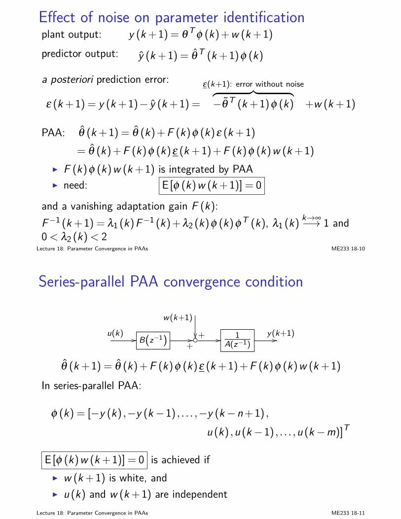
Series-parallel PAA convergence condition
+
w(k+1)
u(k) // B(z−1)+// // 1
A(z−1)y(k+1)//
θ (k+1) = θ (k)+F (k)φ (k)ε (k+1)+F (k)φ (k)w (k+1)In series-parallel PAA:
φ (k) = [−y (k) ,−y (k−1) , . . . ,−y (k−n+1) ,u (k) ,u (k−1) , . . . ,u (k−m)]T
E [φ (k)w (k+1)] = 0 is achieved ifI w (k+1) is white, andI u (k) and w (k+1) are independent
Lecture 18: Parameter Convergence in PAAs ME233 18-11
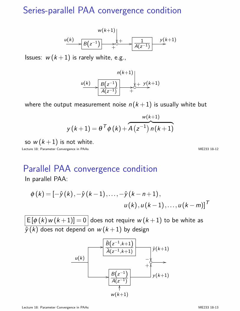
Series-parallel PAA convergence condition
+
w(k+1)
u(k) // B(z−1)+// // 1
A(z−1)y(k+1)//
Issues: w (k+1) is rarely white, e.g.,
+
n(k+1)
u(k) // B(z−1)A(z−1) +
// y(k+1)//
where the output measurement noise n (k+1) is usually white but
y (k+1) = θ T φ (k)+w(k+1)︷ ︸︸ ︷
A(z−1)n (k+1)
so w (k+1) is not white.Lecture 18: Parameter Convergence in PAAs ME233 18-12
Parallel PAA convergence conditionIn parallel PAA:
φ (k) = [−y (k) ,−y (k−1) , . . . ,−y (k−n+1) ,u (k) ,u (k−1) , . . . ,u (k−m)]T
E [φ (k)w (k+1)] = 0 does not require w (k+1) to be white asy (k) does not depend on w (k+1) by design
// B(z−1,k+1)
A(z−1,k+1)−
y(k+1)
u(k) //
// B(z−1)A(z−1)
+
y(k+1)
OO
w(k+1)
OO
Lecture 18: Parameter Convergence in PAAs ME233 18-13
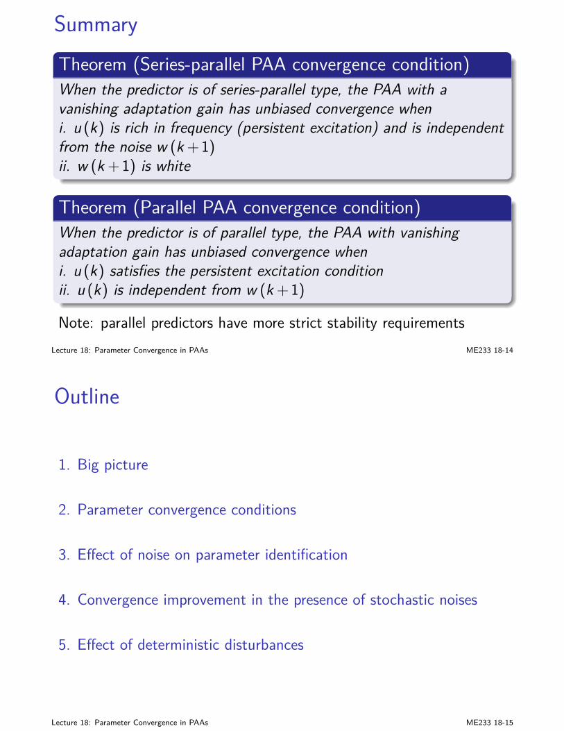
SummaryTheorem (Series-parallel PAA convergence condition)When the predictor is of series-parallel type, the PAA with avanishing adaptation gain has unbiased convergence wheni. u (k) is rich in frequency (persistent excitation) and is independentfrom the noise w (k+1)ii. w (k+1) is white
Theorem (Parallel PAA convergence condition)When the predictor is of parallel type, the PAA with vanishingadaptation gain has unbiased convergence wheni. u (k) satisfies the persistent excitation conditionii. u (k) is independent from w (k+1)
Note: parallel predictors have more strict stability requirementsLecture 18: Parameter Convergence in PAAs ME233 18-14
Outline
1. Big picture
2. Parameter convergence conditions
3. Effect of noise on parameter identification
4. Convergence improvement in the presence of stochastic noises
5. Effect of deterministic disturbances
Lecture 18: Parameter Convergence in PAAs ME233 18-15
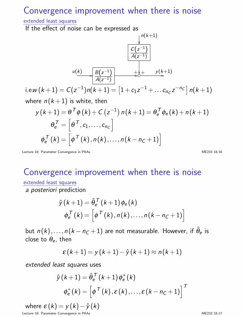
Convergence improvement when there is noiseextended least squaresIf the effect of noise can be expressed as
n(k+1)
C(z−1)A(z−1)
+u(k) // B(z−1)A(z−1)
+// y(k+1)//
i.e.w (k+1) = C(z−1)n(k+1) =[1+ c1z−1 + . . .cnC z−nC
]n(k+1)
where n (k+1) is white, theny (k+1) = θT φ (k)+C
(z−1)n (k+1) = θT
e φe (k)+n (k+1)
θ Te =
[θT ,c1, . . . ,cnC
]
φTe (k) =
[φT (k) ,n (k) , . . . ,n (k−nC +1)
]
Lecture 18: Parameter Convergence in PAAs ME233 18-16
Convergence improvement when there is noiseextended least squaresa posteriori prediction
y (k+1) = θTe (k+1)φe (k)
φTe (k) =
[φT (k) ,n (k) , . . . ,n (k−nC +1)
]
but n (k) , . . . ,n (k−nC +1) are not measurable. However, if θe isclose to θe , then
ε (k+1) = y (k+1)− y (k+1)≈ n (k+1)
extended least squares uses
y (k+1) = θTe (k+1)φ∗e (k)
φ∗e (k) =[φT (k) ,ε (k) , . . . ,ε (k−nC +1)
]T
where ε (k) = y (k)− y (k)Lecture 18: Parameter Convergence in PAAs ME233 18-17
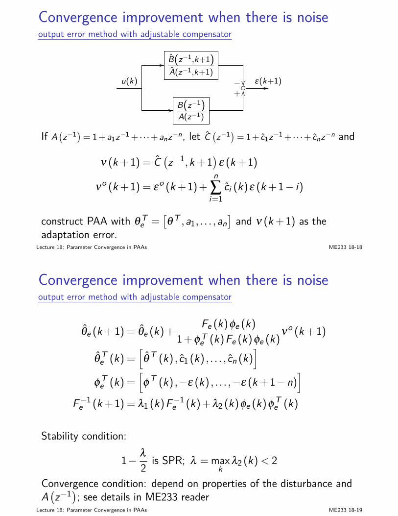
Convergence improvement when there is noiseoutput error method with adjustable compensator
// B(z−1,k+1)
A(z−1,k+1)− u(k) ε(k+1)//
// B(z−1)A(z−1)
+OO
If A(z−1)= 1+a1z−1 + · · ·+anz−n, let C
(z−1)= 1+ c1z−1 + · · ·+ cnz−n and
ν (k+1) = C(z−1,k+1
)ε (k+1)
νo (k+1) = εo (k+1)+n∑i=1
ci (k)ε (k+1− i)
construct PAA with θTe =
[θ T ,a1, . . . ,an
]and ν (k+1) as the
adaptation error.Lecture 18: Parameter Convergence in PAAs ME233 18-18
Convergence improvement when there is noiseoutput error method with adjustable compensator
θe (k+1) = θe (k)+Fe (k)φe (k)
1+φTe (k)Fe (k)φe (k)νo (k+1)
θ Te (k) =
[θT (k) , c1 (k) , . . . , cn (k)
]
φTe (k) =
[φT (k) ,−ε (k) , . . . ,−ε (k+1−n)
]
F−1e (k+1) = λ1 (k)F−1
e (k)+λ2 (k)φe (k)φTe (k)
Stability condition:
1− λ2 is SPR; λ =max
kλ2 (k)< 2
Convergence condition: depend on properties of the disturbance andA(z−1); see details in ME233 reader
Lecture 18: Parameter Convergence in PAAs ME233 18-19
Different recursive identification algorithms
I there are more PAAs for improved convergence
I each algorithm suits for a certain model of plant + disturbance
Lecture 18: Parameter Convergence in PAAs ME233 18-20
Outline
1. Big picture
2. Parameter convergence conditions
3. Effect of noise on parameter identification
4. Convergence improvement in the presence of stochastic noises
5. Effect of deterministic disturbances
Lecture 18: Parameter Convergence in PAAs ME233 18-21
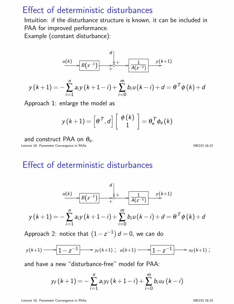
Effect of deterministic disturbancesIntuition: if the disturbance structure is known, it can be included inPAA for improved performance.Example (constant disturbance):
+
d
u(k) // B(z−1)+// // 1
A(z−1)y(k+1)//
y (k+1) =−n∑i=1
aiy (k+1− i)+m∑i=0
biu (k− i)+d = θT φ (k)+d
Approach 1: enlarge the model as
y (k+1) =[θT ,d
][ φ (k)1
]= θT
e φe (k)
and construct PAA on θe .Lecture 18: Parameter Convergence in PAAs ME233 18-22
Effect of deterministic disturbances
+
d
u(k) // B(z−1)+// // 1
A(z−1)y(k+1)//
y (k+1) =−n∑i=1
aiy (k+1− i)+m∑i=0
biu (k− i)+d = θT φ (k)+d
Approach 2: notice that(1− z−1)d = 0, we can do
y(k+1) // 1− z−1 // yf (k+1) ; u(k+1) // 1− z−1 // uf (k+1) ;
and have a new “disturbance-free” model for PAA:
yf (k+1) =−n∑i=1
aiyf (k+1− i)+m∑i=0
biuf (k− i)
Lecture 18: Parameter Convergence in PAAs ME233 18-23
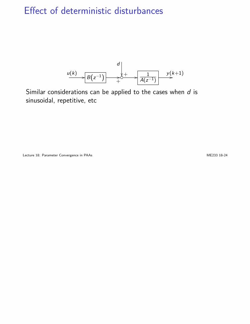
Effect of deterministic disturbances
+
d
u(k) // B(z−1)+// // 1
A(z−1)y(k+1)//
Similar considerations can be applied to the cases when d issinusoidal, repetitive, etc
Lecture 18: Parameter Convergence in PAAs ME233 18-24

ME 233, UC Berkeley, Spring 2014 Xu Chen
Lecture 19: Adaptive Control based on PoleAssignment
Big picture
reasons for adaptive control:I unknown or time-varying plantsI unknown or time-varying disturbance (with known structure but
unknown coefficients)two main steps:
I decide the controller structureI design PAA to adjust the controller parameters
two ways of adaptation process:I indirect adaptive control: adapt the plant parameters and use
them in the updated controllerI direct adaptive control: directly adapt the controller parameters
Lecture 19: Adaptive Control based on Pole Assignment ME233 19-1
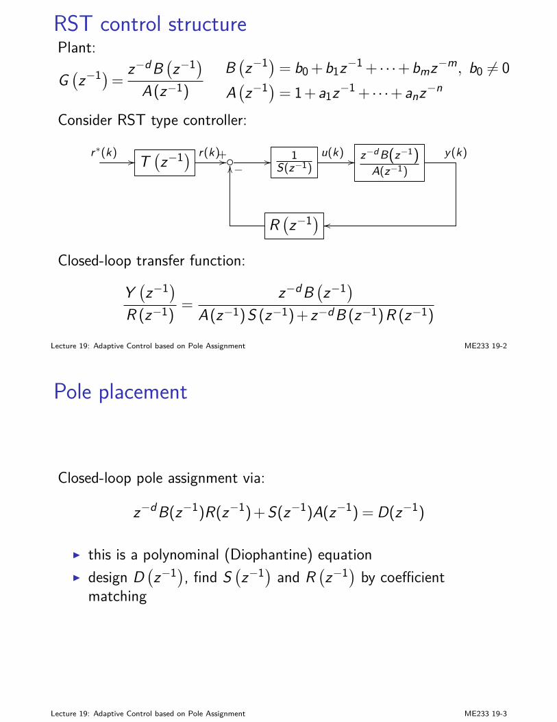
RST control structurePlant:
G(z−1)= z−dB
(z−1)
A(z−1)
B(z−1)= b0 +b1z−1 + · · ·+bmz−m, b0 6= 0
A(z−1)= 1+a1z−1 + · · ·+anz−n
Consider RST type controller:
r∗(k) // T(z−1) r(k)+// // 1
S(z−1)u(k) // z−d B(z−1)
A(z−1)
y(k)−OO
R(z−1) oo
Closed-loop transfer function:
Y(z−1)
R (z−1)=
z−dB(z−1)
A(z−1)S (z−1)+ z−dB (z−1)R (z−1)
Lecture 19: Adaptive Control based on Pole Assignment ME233 19-2
Pole placement
Closed-loop pole assignment via:
z−dB(z−1)R(z−1)+S(z−1)A(z−1) = D(z−1)
I this is a polynominal (Diophantine) equationI design D
(z−1), find S
(z−1) and R
(z−1) by coefficient
matching
Lecture 19: Adaptive Control based on Pole Assignment ME233 19-3
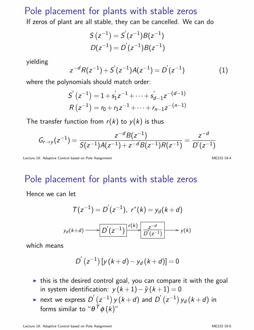
Pole placement for plants with stable zerosIf zeros of plant are all stable, they can be cancelled. We can do
S(z−1)= S ′(z−1)B(z−1)
D(z−1) = D ′(z−1)B(z−1)
yieldingz−dR(z−1)+S ′(z−1)A(z−1) = D ′(z−1) (1)
where the polynomials should match order:
S ′(z−1)= 1+ s ′1z−1 + · · ·+ s ′d−1z−(d−1)
R(z−1)= r0 + r1z−1 + · · ·+ rn−1z−(n−1)
The transfer function from r(k) to y(k) is thus
Gr→y (z−1) =z−dB(z−1)
S(z−1)A(z−1)+ z−dB(z−1)R(z−1)=
z−d
D ′(z−1)
Lecture 19: Adaptive Control based on Pole Assignment ME233 19-4
Pole placement for plants with stable zerosHence we can let
T (z−1) = D ′(z−1), r∗(k) = yd(k +d)
yd (k+d) // D ′(z−1)r(k) // z−d
D′(z−1)// y(k)
which means
D ′(z−1) [y (k +d)− yd (k +d)] = 0
I this is the desired control goal, you can compare it with the goalin system identification: y (k +1)− y (k +1) = 0
I next we express D ′(z−1)y (k +d) and D ′
(z−1)yd (k +d) in
forms similar to “θT φ (k)”
Lecture 19: Adaptive Control based on Pole Assignment ME233 19-5
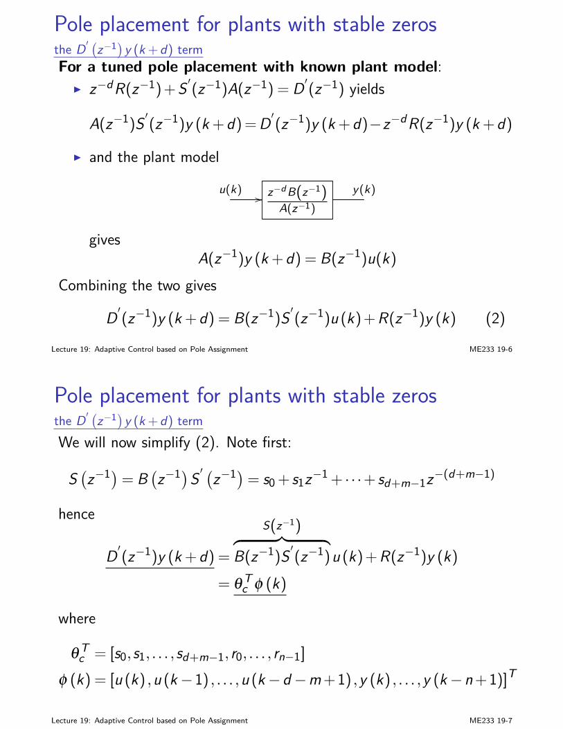
Pole placement for plants with stable zerosthe D ′
(z−1)y (k +d) term
For a tuned pole placement with known plant model:I z−dR(z−1)+S ′(z−1)A(z−1) = D ′(z−1) yields
A(z−1)S ′(z−1)y (k +d)=D ′(z−1)y (k +d)−z−dR(z−1)y (k +d)
I and the plant model
u(k) // z−d B(z−1)A(z−1)
y(k)
givesA(z−1)y (k +d) = B(z−1)u(k)
Combining the two gives
D ′(z−1)y (k +d) = B(z−1)S ′(z−1)u (k)+R(z−1)y (k) (2)Lecture 19: Adaptive Control based on Pole Assignment ME233 19-6
Pole placement for plants with stable zerosthe D ′
(z−1)y (k +d) term
We will now simplify (2). Note first:
S(z−1)= B
(z−1)S ′
(z−1)= s0 + s1z−1 + · · ·+ sd+m−1z−(d+m−1)
hence
D ′(z−1)y (k +d) =
S(z−1)︷ ︸︸ ︷B(z−1)S ′(z−1)u (k)+R(z−1)y (k)
= θTc φ (k)
where
θ Tc = [s0,s1, . . . ,sd+m−1, r0, . . . , rn−1]
φ (k) = [u (k) ,u (k−1) , . . . ,u (k−d −m+1) ,y (k) , . . . ,y (k−n+1)]T
Lecture 19: Adaptive Control based on Pole Assignment ME233 19-7
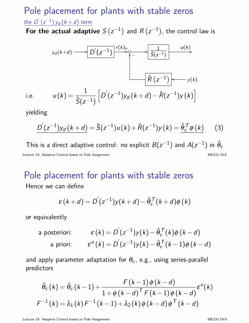
Pole placement for plants with stable zerosthe D ′
(z−1)yd (k +d) term
For the actual adaptive S(z−1) and R
(z−1), the control law is
yd (k+d) // D ′(z−1)r(k)+// // 1
S(z−1)u(k) //
−OO
R(z−1) y(k)oo
i.e. u (k) = 1S(z−1)
[D ′(z−1)yd (k +d)− R(z−1)y (k)
]
yielding
D ′(z−1)yd (k +d) = S(z−1)u (k)+ R(z−1)y (k) = θ Tc φ (k) (3)
This is a direct adaptive control: no explicit B(z−1) and A(z−1) in θcLecture 19: Adaptive Control based on Pole Assignment ME233 19-8
Pole placement for plants with stable zerosHence we can define
ε (k +d) = D ′(z−1)y(k +d)− θTc (k +d)φ (k)
or equivalently
a posteriori: ε (k) = D ′(z−1)y(k)− θTc (k)φ (k−d)
a priori: εo (k) = D ′(z−1)y(k)− θTc (k−1)φ (k−d)
and apply parameter adaptation for θc , e.g., using series-parallelpredictors
θc (k) = θc (k−1)+ F (k−1)φ (k−d)1+φ (k−d)T F (k−1)φ (k−d)
εo(k)
F−1 (k) = λ1 (k)F−1 (k−1)+λ2 (k)φ (k−d)φT (k−d)
Lecture 19: Adaptive Control based on Pole Assignment ME233 19-9
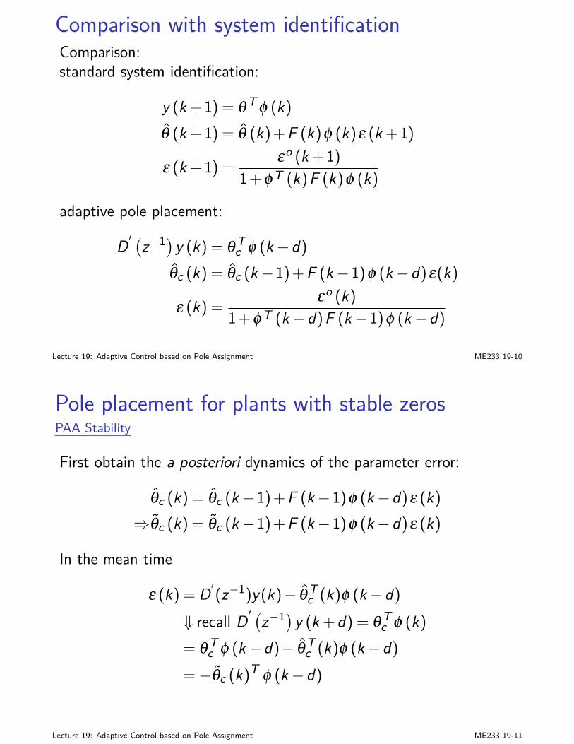
Comparison with system identificationComparison:standard system identification:
y (k +1) = θ T φ (k)θ (k +1) = θ (k)+F (k)φ (k)ε (k +1)
ε (k +1) = εo (k +1)1+φT (k)F (k)φ (k)
adaptive pole placement:
D ′(z−1)y (k) = θT
c φ (k−d)θc (k) = θc (k−1)+F (k−1)φ (k−d)ε(k)
ε (k) = εo (k)1+φT (k−d)F (k−1)φ (k−d)
Lecture 19: Adaptive Control based on Pole Assignment ME233 19-10
Pole placement for plants with stable zerosPAA Stability
First obtain the a posteriori dynamics of the parameter error:
θc (k) = θc (k−1)+F (k−1)φ (k−d)ε (k)⇒θc (k) = θc (k−1)+F (k−1)φ (k−d)ε (k)
In the mean time
ε (k) = D ′(z−1)y(k)− θTc (k)φ (k−d)
⇓ recall D ′(z−1)y (k +d) = θT
c φ (k)= θ T
c φ (k−d)− θTc (k)φ (k−d)
=−θc (k)T φ (k−d)
Lecture 19: Adaptive Control based on Pole Assignment ME233 19-11
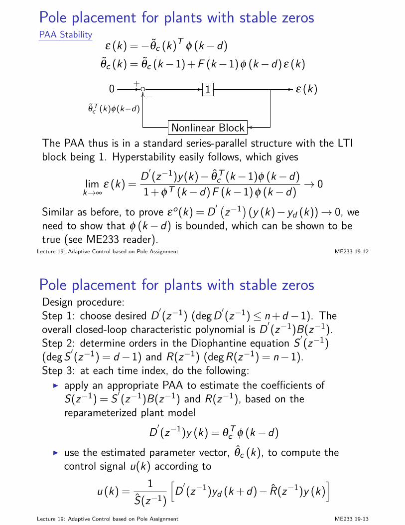
Pole placement for plants with stable zerosPAA Stability
ε (k) =−θc (k)T φ (k−d)θc (k) = θc (k−1)+F (k−1)φ (k−d)ε (k)
0 +// // 1 // ε (k)−
θTc (k)φ(k−d)
OO
Nonlinear Block ooThe PAA thus is in a standard series-parallel structure with the LTIblock being 1. Hyperstability easily follows, which gives
limk→∞
ε (k) = D ′(z−1)y(k)− θTc (k−1)φ (k−d)
1+φT (k−d)F (k−1)φ (k−d) → 0
Similar as before, to prove εo(k) = D ′(z−1)(y (k)− yd (k))→ 0, we
need to show that φ (k−d) is bounded, which can be shown to betrue (see ME233 reader).
Lecture 19: Adaptive Control based on Pole Assignment ME233 19-12
Pole placement for plants with stable zerosDesign procedure:Step 1: choose desired D ′(z−1) (degD ′(z−1)≤ n+d −1). Theoverall closed-loop characteristic polynomial is D ′(z−1)B(z−1).Step 2: determine orders in the Diophantine equation S ′(z−1)(degS ′(z−1) = d −1) and R(z−1) (degR(z−1) = n−1).Step 3: at each time index, do the following:
I apply an appropriate PAA to estimate the coefficients ofS(z−1) = S ′(z−1)B(z−1) and R(z−1), based on thereparameterized plant model
D ′(z−1)y (k) = θTc φ (k−d)
I use the estimated parameter vector, θc (k), to compute thecontrol signal u(k) according to
u (k) = 1S(z−1)
[D ′(z−1)yd (k +d)− R(z−1)y (k)
]
Lecture 19: Adaptive Control based on Pole Assignment ME233 19-13
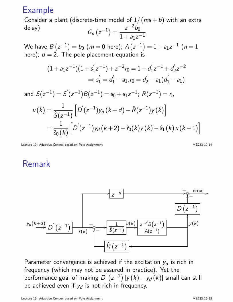
ExampleConsider a plant (discrete-time model of 1/(ms +b) with an extradelay) Gp
(z−1)= z−2b0
1+a1z−1
We have B(z−1)= b0 (m = 0 here); A
(z−1)= 1+a1z−1 (n = 1
here); d = 2. The pole placement equation is
(1+a1z−1)(1+ s ′1z−1)+ z−2r0 = 1+d ′1z−1 +d ′2z−2
⇒ s ′1 = d ′1−a1,r0 = d ′2−a1(d′1−a1)
and S(z−1) = S ′(z−1)B(z−1) = s0 + s1z−1; R(z−1) = ro
u (k) = 1S(z−1)
[D ′(z−1)yd (k +d)− R(z−1)y (k)
]
=1
s0 (k)[D ′(z−1)yd (k +2)− r0(k)y (k)− s1 (k)u (k−1)
]
Lecture 19: Adaptive Control based on Pole Assignment ME233 19-14
Remark
// z−d +// error //
D(z−1)−OO
yd (k+d) // D ′(z−1)
r(k)+// // 1
S(z−1)u(k) // z−d B(z−1)
A(z−1)
y(k)
OO
−OO
R(z−1) oo
Parameter convergence is achieved if the excitation yd is rich infrequency (which may not be assured in practice). Yet theperformance goal of making D ′
(z−1) [y (k)− yd (k)] small can still
be achieved even if yd is not rich in frequency.
Lecture 19: Adaptive Control based on Pole Assignment ME233 19-15
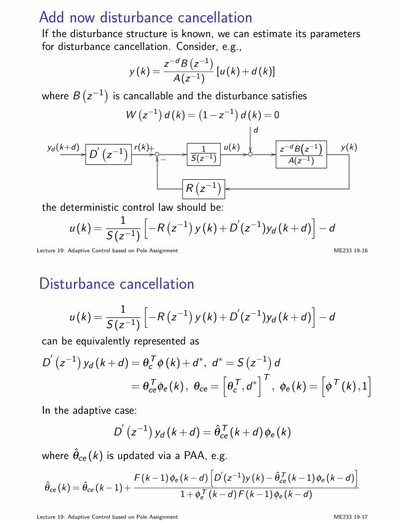
Add now disturbance cancellationIf the disturbance structure is known, we can estimate its parametersfor disturbance cancellation. Consider, e.g.,
y (k) =z−dB
(z−1)
A(z−1)[u (k)+d (k)]
where B(z−1) is cancallable and the disturbance satisfies
W(z−1)d (k) =
(1− z−1)d (k) = 0
d
yd (k+d) // D ′(z−1) r(k)+// // 1
S(z−1)u(k) // // z−d B(z−1)
A(z−1)
y(k)−OO
R(z−1) oo
the deterministic control law should be:
u (k) = 1S (z−1)
[−R
(z−1)y (k)+D ′(z−1)yd (k +d)
]−d
Lecture 19: Adaptive Control based on Pole Assignment ME233 19-16
Disturbance cancellation
u (k) = 1S (z−1)
[−R
(z−1)y (k)+D ′(z−1)yd (k +d)
]−d
can be equivalently represented as
D ′(z−1)yd (k +d) = θ T
c φ (k)+d∗, d∗ = S(z−1)d
= θ Tceφe (k) , θce =
[θT
c ,d∗]T
, φe (k) =[φT (k) ,1
]T
In the adaptive case:
D ′(z−1)yd (k +d) = θT
ce (k +d)φe (k)
where θce (k) is updated via a PAA, e.g.
θce (k) = θce (k−1)+F (k−1)φe (k−d)
[D ′(z−1)y (k)− θ T
ce (k−1)φe (k−d)]
1+φTe (k−d)F (k−1)φe (k−d)
Lecture 19: Adaptive Control based on Pole Assignment ME233 19-17
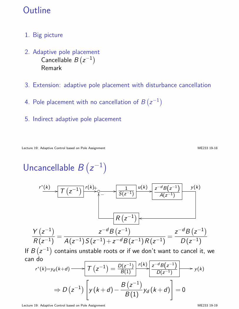
Outline
1. Big picture
2. Adaptive pole placementCancellable B
(z−1)
Remark
3. Extension: adaptive pole placement with disturbance cancellation
4. Pole placement with no cancellation of B(z−1)
5. Indirect adaptive pole placement
Lecture 19: Adaptive Control based on Pole Assignment ME233 19-18
Uncancellable B(z−1)
r∗(k) // T(z−1) r(k)+// // 1
S(z−1)u(k) // z−d B(z−1)
A(z−1)
y(k)−OO
R(z−1) oo
Y(z−1)
R (z−1)=
z−dB(z−1)
A(z−1)S (z−1)+ z−dB (z−1)R (z−1)=
z−dB(z−1)
D (z−1)
If B(z−1) contains unstable roots or if we don’t want to cancel it, we
can dor∗(k)=yd (k+d) // T
(z−1)= D(z−1)
B(1)r(k) // z−d B(z−1)
D(z−1)// y(k)
⇒ D(z−1)
[y (k +d)− B
(z−1)
B (1) yd (k +d)]= 0
Lecture 19: Adaptive Control based on Pole Assignment ME233 19-19
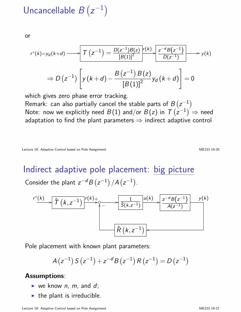
Uncancellable B(z−1)
or
r∗(k)=yd (k+d) // T(z−1)= D(z−1)B(z)
[B(1)]2r(k) // z−d B(z−1)
D(z−1)// y(k)
⇒ D(z−1)
[y (k +d)− B
(z−1)B (z)[B (1)]2
yd (k +d)]= 0
which gives zero phase error tracking.Remark: can also partially cancel the stable parts of B
(z−1)
Note: now we explicitly need B (1) and/or B (z) in T(z−1) ⇒ need
adaptation to find the plant parameters ⇒ indirect adaptive control
Lecture 19: Adaptive Control based on Pole Assignment ME233 19-20
Indirect adaptive pole placement: big pictureConsider the plant z−dB
(z−1)/A
(z−1).
r∗(k) // T(k,z−1) r(k)+// // 1
S(k,z−1)u(k) // z−d B(z−1)
A(z−1)
y(k)−OO
R(k,z−1) oo
Pole placement with known plant parameters:
A(z−1)S
(z−1)+ z−dB
(z−1)R
(z−1)= D
(z−1)
Assumptions:I we know n, m, and d ;I the plant is irreducible.
Lecture 19: Adaptive Control based on Pole Assignment ME233 19-21
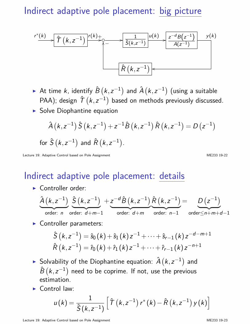
Indirect adaptive pole placement: big picture
r∗(k) // T(k,z−1) r(k)+// // 1
S(k,z−1)u(k) // z−d B(z−1)
A(z−1)
y(k)−OO
R(k,z−1) oo
I At time k , identify B(k,z−1) and A
(k,z−1) (using a suitable
PAA); design T(k,z−1) based on methods previously discussed.
I Solve Diophantine equation
A(k,z−1) S
(k,z−1)+ z−1B
(k,z−1) R
(k,z−1)= D
(z−1)
for S(k,z−1) and R
(k,z−1).
Lecture 19: Adaptive Control based on Pole Assignment ME233 19-22
Indirect adaptive pole placement: detailsI Controller order:
A(k,z−1)
︸ ︷︷ ︸order: n
S(k,z−1)
︸ ︷︷ ︸order: d+m−1
+z−d B(k,z−1)
︸ ︷︷ ︸order: d+m
R(k,z−1)
︸ ︷︷ ︸order: n−1
= D(z−1)
︸ ︷︷ ︸order≤n+m+d−1
I Controller parameters:S(k,z−1)= s0 (k)+ s1 (k)z−1 + · · ·+ sr−1 (k)z−d−m+1
R(k,z−1)= r0 (k)+ r1 (k)z−1 + · · ·+ rr−1 (k)z−n+1
I Solvability of the Diophantine equation: A(k,z−1) and
B(k,z−1) need to be coprime. If not, use the previous
estimation.I Control law:
u (k) = 1S (k,z−1)
[T(k,z−1) r∗ (k)− R
(k,z−1)y (k)
]
Lecture 19: Adaptive Control based on Pole Assignment ME233 19-23
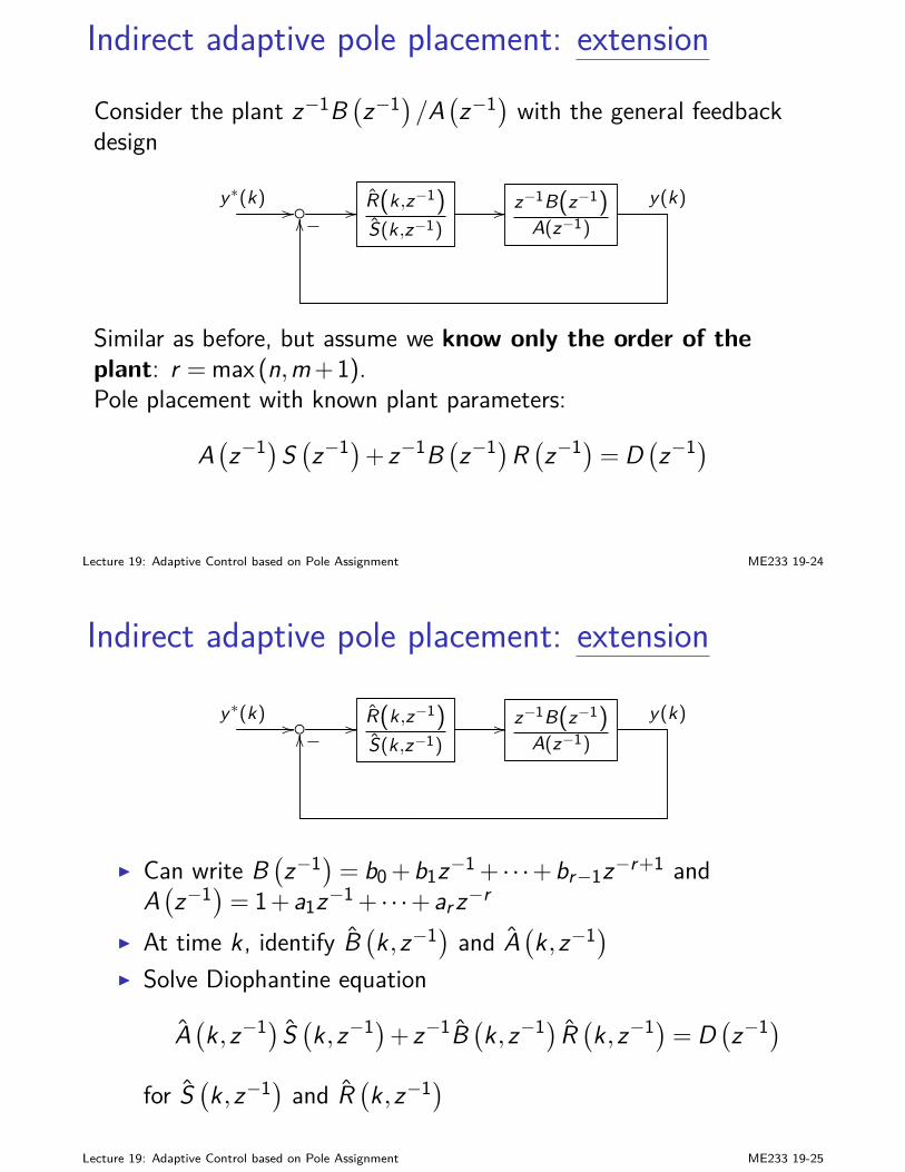
Indirect adaptive pole placement: extension
Consider the plant z−1B(z−1)/A
(z−1) with the general feedback
design
y∗(k) // // R(k,z−1)
S(k,z−1)// z−1B(z−1)
A(z−1)
y(k)−OO
Similar as before, but assume we know only the order of theplant: r =max (n,m+1).Pole placement with known plant parameters:
A(z−1)S
(z−1)+ z−1B
(z−1)R
(z−1)= D
(z−1)
Lecture 19: Adaptive Control based on Pole Assignment ME233 19-24
Indirect adaptive pole placement: extension
y∗(k) // // R(k,z−1)
S(k,z−1)// z−1B(z−1)
A(z−1)
y(k)−OO
I Can write B(z−1)= b0 +b1z−1 + · · ·+br−1z−r+1 and
A(z−1)= 1+a1z−1 + · · ·+ar z−r
I At time k , identify B(k,z−1) and A
(k,z−1)
I Solve Diophantine equation
A(k,z−1) S
(k,z−1)+ z−1B
(k,z−1) R
(k,z−1)= D
(z−1)
for S(k,z−1) and R
(k,z−1)
Lecture 19: Adaptive Control based on Pole Assignment ME233 19-25
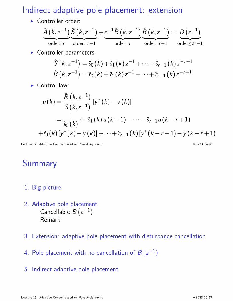
Indirect adaptive pole placement: extensionI Controller order:
A(k,z−1)
︸ ︷︷ ︸order: r
S(k,z−1)
︸ ︷︷ ︸order: r−1
+z−1B(k,z−1)
︸ ︷︷ ︸order: r
R(k,z−1)
︸ ︷︷ ︸order: r−1
= D(z−1)
︸ ︷︷ ︸order≤2r−1
I Controller parameters:S(k,z−1)= s0 (k)+ s1 (k)z−1 + · · ·+ sr−1 (k)z−r+1
R(k,z−1)= r0 (k)+ r1 (k)z−1 + · · ·+ rr−1 (k)z−r+1
I Control law:
u (k) =R(k,z−1)
S (k,z−1)[y∗ (k)− y (k)]
=1
s0 (k)−s1 (k)u (k−1)−·· ·− sr−1u (k− r +1)
+r0 (k) [y∗ (k)− y (k)]+ · · ·+ rr−1 (k) [y∗ (k− r +1)− y (k− r +1)]Lecture 19: Adaptive Control based on Pole Assignment ME233 19-26
Summary
1. Big picture
2. Adaptive pole placementCancellable B
(z−1)
Remark
3. Extension: adaptive pole placement with disturbance cancellation
4. Pole placement with no cancellation of B(z−1)
5. Indirect adaptive pole placement
Lecture 19: Adaptive Control based on Pole Assignment ME233 19-27
References
Goodwin and Sin, “Adaptive Filtering, Prediction and Control,”Prentice Hall.
Lecture 19: Adaptive Control based on Pole Assignment ME233 19-28
Exercises
I We mentioned that direct adaptive control requires noidentification of the plant. In direct adaptive pole placement, theclosed loop characteristic polynomial is
D(z−1)= D ′
(z−1)B
(z−1)
which depends on B(z−1). So the closed-loop design directly
depends on the plant zeros. Why is it still direct adaptivecontrol?
Lecture 19: Adaptive Control based on Pole Assignment ME233 19-29