Embed Size (px)
Citation preview
U l t I fl ti d E i P liUnemployment, Inflation, and Economic Policy
Topic 7Topic 7
1 Macroeconomics 302 - Lecture 7
Goals of Topic 7
Definition of Short-Run and Long-Run Equilibrium.g q
An analysis of demand and supply shocks.
Unemployment and Inflation Dynamics: Phillips Curve.
Fed’s Objectives and Behavior.Fed s Objectives and Behavior.
Macroeconomics 302 - Lecture 72
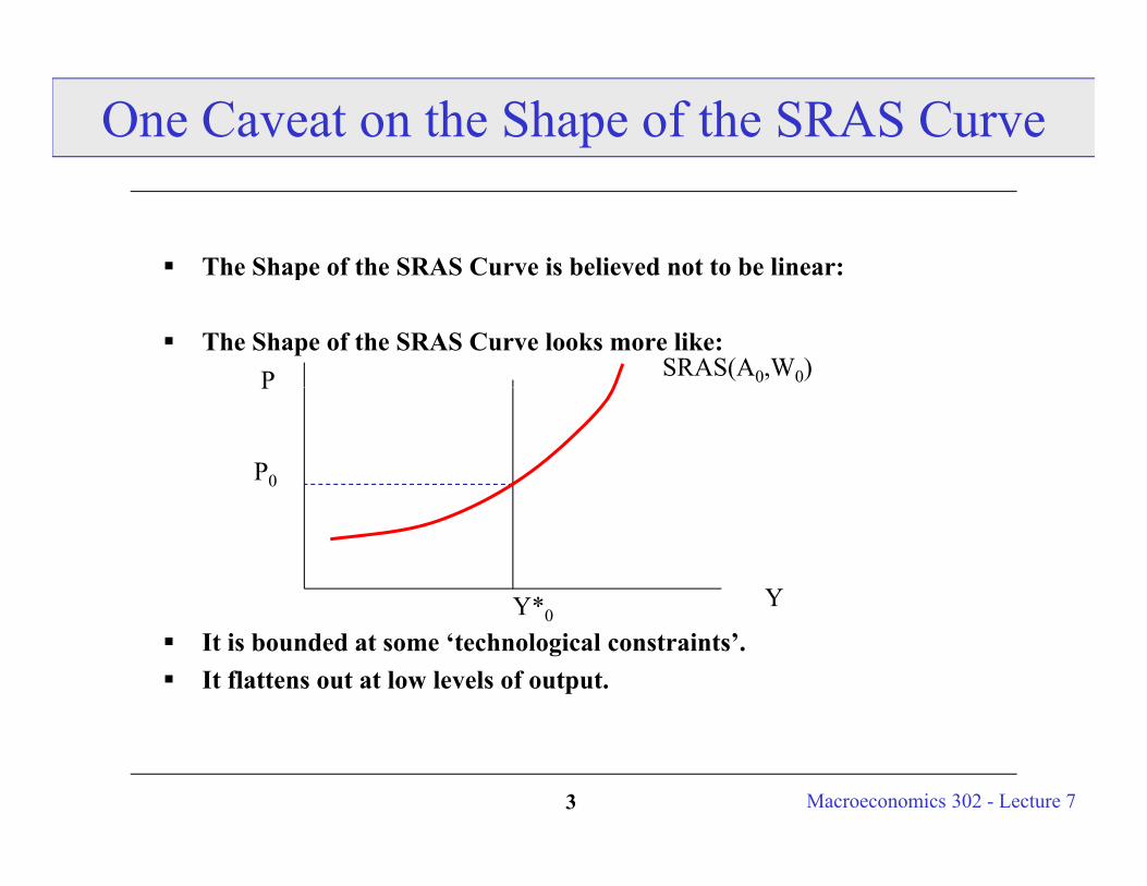
One Caveat on the Shape of the SRAS Curve
The Shape of the SRAS Curve is believed not to be linear:p
The Shape of the SRAS Curve looks more like:SRAS(A0,W0)P
P0
P
Y*0Y
It is bounded at some ‘technological constraints’. It flattens out at low levels of output.
Y 0
Macroeconomics 302 - Lecture 73
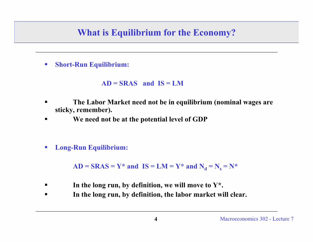
What is Equilibrium for the Economy?
Short-Run Equilibrium:
AD = SRAS and IS = LM
The Labor Market need not be in equilibrium (nominal wages are q gsticky, remember).
We need not be at the potential level of GDP
Long-Run Equilibrium:
AD = SRAS = Y* and IS = LM = Y* and N = N = N*AD = SRAS = Y and IS = LM = Y and Nd = Ns = N
In the long run, by definition, we will move to Y*. In the long run, by definition, the labor market will clear.
Macroeconomics 302 - Lecture 74
g , y ,
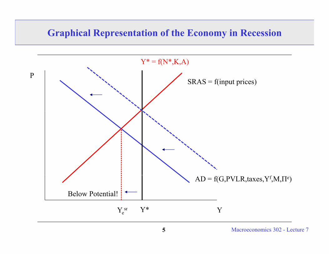
Graphical Representation of the Economy in Recession
PS AS f(i i )
Y* = f(N*,K,A)
SRAS = f(input prices)
AD = f(G,PVLR,taxes,Yf,M,Πe)
Y*
Below Potential!
Macroeconomics 302 - Lecture 75
YY*Yesr
More on Equilibrium Equilibrium is a point of attraction for the economy:
Most macroeconomists believe that, in the absence of shocks, theMost macroeconomists believe that, in the absence of shocks, the economy would reach equilibrium after perhaps 5 years. Thus the economy is in equilibrium in the “long run” (after 5 years).
Is the economy ever in long run equilibrium? Is the economy ever in long-run equilibrium?
Given that shocks are always hitting, the economy is not likely to be in long-run equilibrium at any point in time. Yet the force of attraction of equilibrium keeps the economy hovering around the equilibrium.
Why is the long-run equilibrium point attractive?
Because there the labor market clears. Away from Y* workers are not on their labor supply curve (and firms may be off their labor demand curve). Maximizing behavior by workers and firms push the economy t d l ilib i Sh k h th
Macroeconomics 302 - Lecture 76
towards long-run equilibrium. Shocks push the economy away temporarily.
How do we represent recessions? Unofficial Definition - 2 consecutive quarters of negative real GDP growth Our Model: Y < Y* We define the o tp t gap as Y* Y sr We define the output gap as Y* - Ye
sr
Remember: Y* trends upward overtime (even though in our model - we have it constant - population growth, K grows (we abstract from these trends p p g , g (in our model), TFP is growing every period). It makes things easier to keep Y* constant initially.
Our Model removes the trends in N and K due to population growth and K Our Model removes the trends in N and K due to population growth and K (by assumption).
Questions for the rest of class: Questions for the rest of class: What causes recessions? Why would the fed be concerned about inflation when Ye
sr >Y*? How do we get out of recessions once we are in them?
Macroeconomics 302 - Lecture 77
g Can the economy correct itself?
Where Do Recessions Come From?
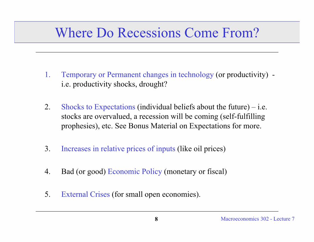
1 Temporary or Permanent changes in technology (or productivity) -1. Temporary or Permanent changes in technology (or productivity) -i.e. productivity shocks, drought?
2 Shocks to Expectations (individual beliefs about the future) i e2. Shocks to Expectations (individual beliefs about the future) – i.e. stocks are overvalued, a recession will be coming (self-fulfilling prophesies), etc. See Bonus Material on Expectations for more.
3. Increases in relative prices of inputs (like oil prices)
4. Bad (or good) Economic Policy (monetary or fiscal)
5. External Crises (for small open economies).
Macroeconomics 302 - Lecture 78
( p )
Analysis of the Business Cycle: Examples
We now start analyzing shocks to the economy that move it away We now start analyzing shocks to the economy that move it away from full-employment output.
In the examples that follows such shocks are permanent You can In the examples that follows such shocks are permanent. You can also study their temporary counterparts.
C i h i i i l “ h k d i bl ” ( G Convention: the initial “shocked variable” (say, G, Ms, consumer confidence,etc.) has a 1 subscript (example if I tell you we are increasing G then we move from G0 to G1 > G0).
Macroeconomics 302 - Lecture 79
Some Examples
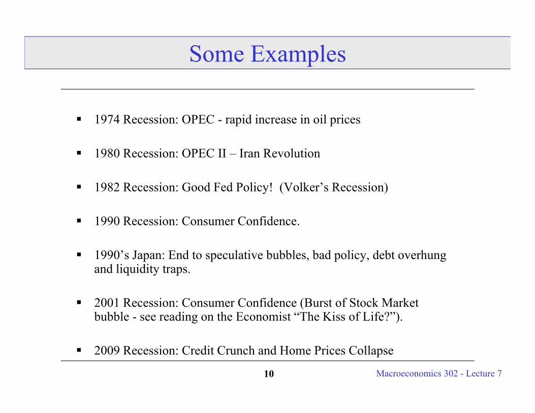
1974 Recession: OPEC - rapid increase in oil prices
1980 Recession: OPEC II – Iran Revolution
1982 Recession: Good Fed Policy! (Volker’s Recession)
1990 Recession: Consumer Confidence.
1990’s Japan: End to speculative bubbles, bad policy, debt overhung and liquidity traps.
2001 Recession: Consumer Confidence (Burst of Stock Market bubble - see reading on the Economist “The Kiss of Life?”).
Macroeconomics 302 - Lecture 710
2009 Recession: Credit Crunch and Home Prices Collapse
Example 1: Changes in Consumer Confidence
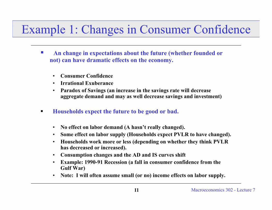
An change in expectations about the future (whether founded or not) can have dramatic effects on the economy.
• Consumer Confidence• Irrational Exuberance• Paradox of Savings (an increase in the savings rate will decreaseParadox of Savings (an increase in the savings rate will decrease
aggregate demand and may as well decrease savings and investment)
Households expect the future to be good or bad.
• No effect on labor demand (A hasn’t really changed).• Some effect on labor supply (Households expect PVLR to have changed).• Households work more or less (depending on whether they think PVLR
has decreased or increased). • Consumption changes and the AD and IS curves shift• Example: 1990-91 Recession (a fall in consumer confidence from the
Gulf War)
Macroeconomics 302 - Lecture 711
• Note: I will often assume small (or no) income effects on labor supply.
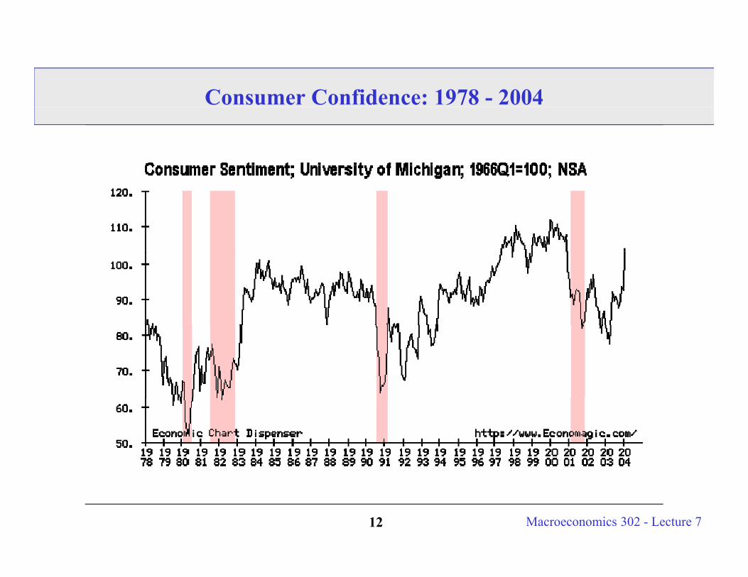
Consumer Confidence: 1978 - 2004
Macroeconomics 302 - Lecture 712
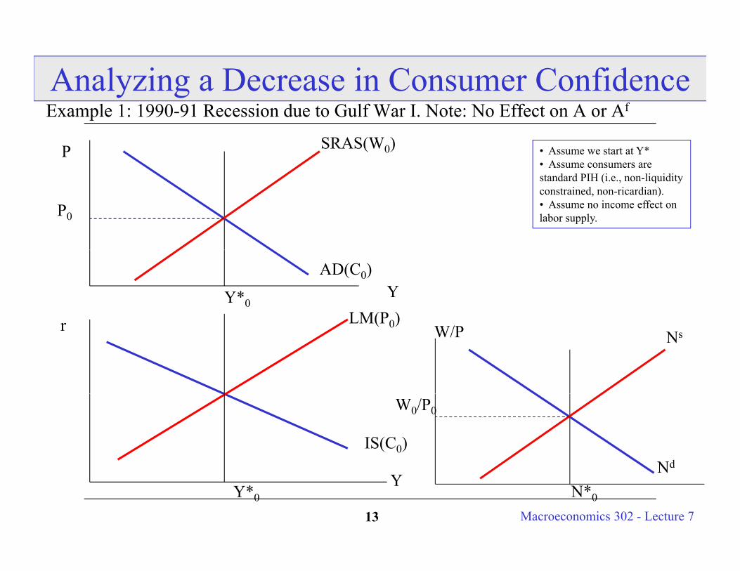
Analyzing a Decrease in Consumer ConfidenceE l 1 1990 91 R i d t G lf W I N t N Eff t A AfExample 1: 1990-91 Recession due to Gulf War I. Note: No Effect on A or Af
SRAS(W0)P • Assume we start at Y*• Assume consumers are standard PIH (i e non liquidity
P0
standard PIH (i.e., non-liquidityconstrained, non-ricardian).• Assume no income effect onlabor supply.
LM(P0)
AD(C0)
Y*0Y
LM(P0)rNsW/P
IS(C0)
W0/P0
Nd
Macroeconomics 302 - Lecture 713
Y*0Y
N*0
Nd
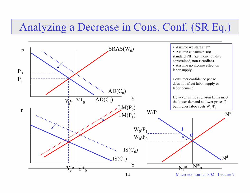
Analyzing a Decrease in Cons. Conf. (SR Eq.)
SRAS(W0)P• Assume we start at Y*• Assume consumers are standard PIH (i.e., non-liquidity
t i d i di )
P1
constrained, non-ricardian).• Assume no income effect onlabor supply.
Consumer confidence per se does not affect labor supply or
P0
LM(P0)
AD(C0)
Y*0Y
does not affect labor supply or labor demand.
However in the short-run firms meet the lower demand at lower prices P1but higher labor costs W0 /P1
AD(C1)Yesr
LM(P0)rLM(P1) NsW/P
0W0/P1 1
IS(C0)IS(C )
W0/P0
Nd
0
Macroeconomics 302 - Lecture 714Y*0
YIS(C1)
Yesr N*0
Nd
Nesr
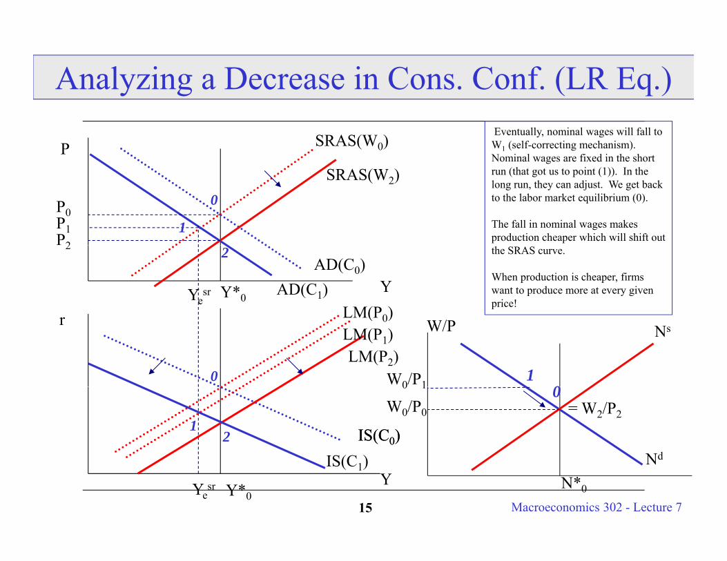
Analyzing a Decrease in Cons. Conf. (LR Eq.)
SRAS(W0)PEventually, nominal wages will fall to W1 (self-correcting mechanism). Nominal wages are fixed in the short run (that got us to point (1)). In theSRAS(W )
P0
run (that got us to point (1)). In the long run, they can adjust. We get back to the labor market equilibrium (0).
The fall in nominal wages makes production cheaper which will shift out
SRAS(W2)
P1P2
0
1
LM(P0)
AD(C0)
Y*0Y
the SRAS curve.
When production is cheaper, firms want to produce more at every given price!
AD(C1)Yesr
2 2
LM(P0)r
LM(P2)LM(P1)
0
NsW/P
0W0/P1
1
IS(C0)IS(C )
IS(C0)1
2
W0/P0
Nd
= W2/P2
00 1
Macroeconomics 302 - Lecture 715Y*0
YIS(C1)
Yesr N*0
Nd
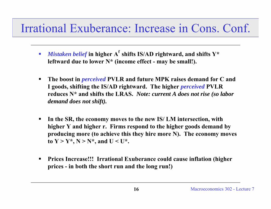
Irrational Exuberance: Increase in Cons. Conf.
Mistaken belief in higher Af shifts IS/AD rightward, and shifts Y* leftward due to lower N* (income effect - may be small!).
The boost in perceived PVLR and future MPK raises demand for C and I goods, shifting the IS/AD rightward. The higher perceived PVLR reduces N* and shifts the LRAS. Note: current A does not rise (so labor demand does not shift).
I th SR th t th IS/ LM i t ti ith In the SR, the economy moves to the new IS/ LM intersection, with higher Y and higher r. Firms respond to the higher goods demand by producing more (to achieve this they hire more N). The economy moves to Y > Y*, N > N*, and U < U*., ,
Prices Increase!!! Irrational Exuberance could cause inflation (higher prices - in both the short run and the long run!)
Macroeconomics 302 - Lecture 716
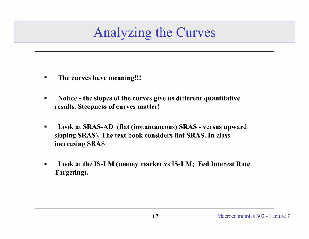
Analyzing the Curves
The curves have meaning!!!
Notice - the slopes of the curves give us different quantitative lt St f tt !results. Steepness of curves matter!
Look at SRAS-AD (flat (instantaneous) SRAS - versus upward sloping SRAS) The text book considers flat SRAS In classsloping SRAS). The text book considers flat SRAS. In class increasing SRAS
Look at the IS-LM (money market vs IS-LM; Fed Interest RateLook at the IS-LM (money market vs IS-LM; Fed Interest Rate Targeting).
Macroeconomics 302 - Lecture 717

Example 2: Supply Side of the Economy - Oil
R ibl ( ti ll ) f th 1975 d 1979 1980 E i Responsible (partially) for the 1975 and 1979-1980 Economic Recessions (OPEC I and OPEC II)
Also important for today’s economy! Stellar oil prices. so po ta t o today s eco o y! Ste a o p ces.
Supply shocks cause unemployment and prices to move in the same direction (VERY DIFFERNET FROM DEMAND SHOCKS).
Supply Shocks - oil and technology! When an input is more expensive, I need to employ less of it and produce less.
Demand Shocks: M, G, T and consumer confidence. As we will see soon - supply shocks could have demand effects!
Macroeconomics 302 - Lecture 718
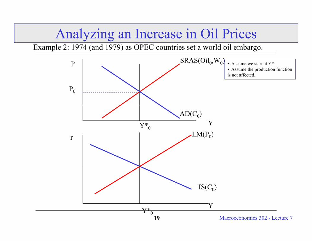
Analyzing an Increase in Oil PricesE l 2 1974 ( d 1979) OPEC i ld il b
SRAS(Oil0,W0)P • Assume we start at Y*• Assume the production functionis not affected
Example 2: 1974 (and 1979) as OPEC countries set a world oil embargo.
P0
is not affected.
LM(P0)
AD(C0)
Y*0Y
LM(P0)r
IS(C0)
Macroeconomics 302 - Lecture 719Y*0
Y
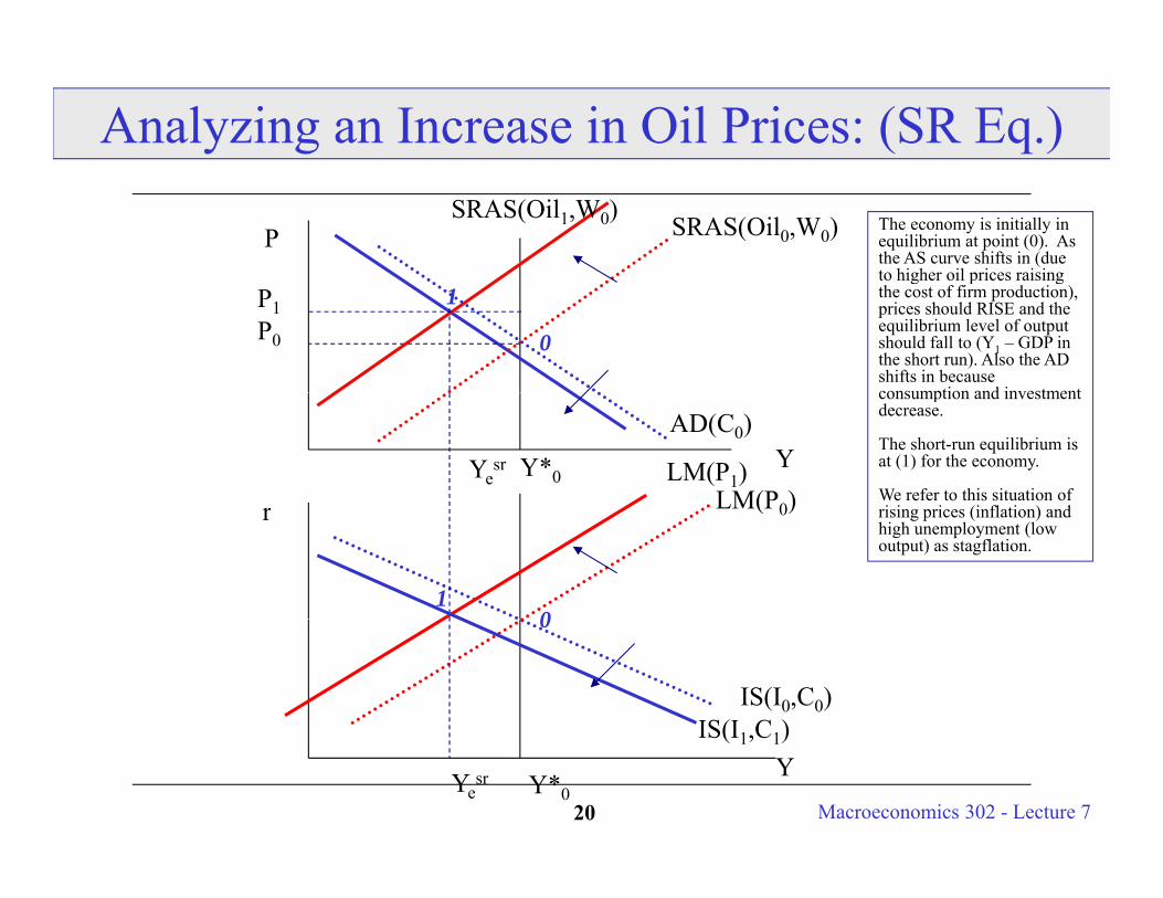
Analyzing an Increase in Oil Prices: (SR Eq.)
SRAS(Oil0,W0)PSRAS(Oil1,W0) The economy is initially in
equilibrium at point (0). As the AS curve shifts in (due to higher oil prices raising
P0
P1
to higher oil prices raising the cost of firm production), prices should RISE and the equilibrium level of output should fall to (Y1 – GDP in the short run). Also the AD shifts in because consumption and investment
0
1
LM(P0)
AD(C0)
Y*0YLM(P1)
consumption and investment decrease.
The short-run equilibrium is at (1) for the economy.
We refer to this situation of i i i (i fl i ) d
Yesr
LM(P0)r rising prices (inflation) and high unemployment (low output) as stagflation.
01
IS(I0,C0)
0
IS(I1 C1)
Macroeconomics 302 - Lecture 720Y*0
YYesr
IS(I1,C1)
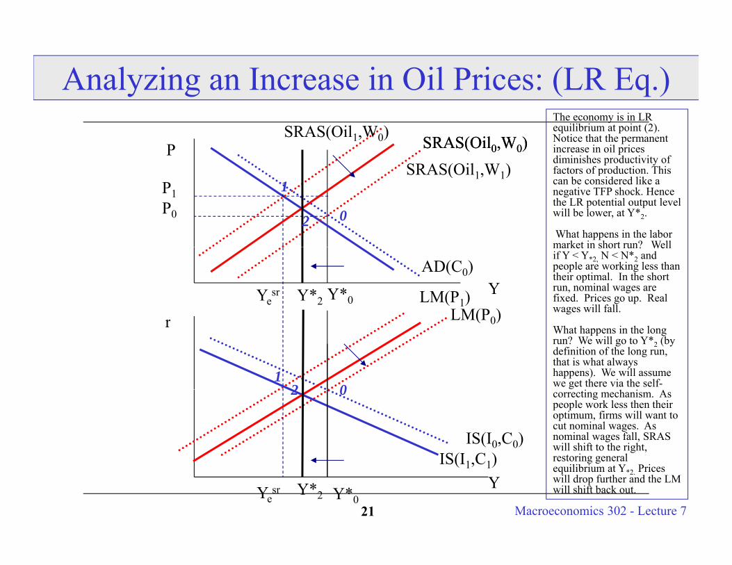
Analyzing an Increase in Oil Prices: (LR Eq.)
SRAS(Oil0,W0)SRAS(Oil1,W1)
SRAS(Oil0,W0)PSRAS(Oil1,W0)
The economy is in LR equilibrium at point (2).Notice that the permanent increase in oil prices diminishes productivity of factors of production. This ( 1, 1)
P0
P1
0
1
2
pcan be considered like a negative TFP shock. Hence the LR potential output level will be lower, at Y*2.
What happens in the labor market in short run? Well
LM(P0)
AD(C0)
Y*0YLM(P1)Ye
sr Y*2
market in short run? Well if Y < Y*2, N < N*2 and people are working less than their optimal. In the short run, nominal wages are fixed. Prices go up. Real wages will fall.LM(P0)r
021
What happens in the long run? We will go to Y*2 (by definition of the long run, that is what always happens). We will assume we get there via the self-
IS(I0,C0)
02
IS(I1 C1)
correcting mechanism. As people work less then their optimum, firms will want to cut nominal wages. As nominal wages fall, SRAS will shift to the right, restoring general
Macroeconomics 302 - Lecture 721Y*0
YYesr
IS(I1,C1)
Y*2
restoring general equilibrium at Y*2. Prices will drop further and the LM will shift back out.

Example 3: 1990s and increase in A Increase Y* (shift out labor demand and shift in labor supply - regardless
if N increases or decreases, Y* will likely increase - the TFP effect will usually dominate).y )
SRAS will shift out (Cost of Production Falls) AD and IS will shift out (C and I will increase, PVLR and MPK will
i )increase)
How far will AD and SRAS shift out? Depends - many cases.
Summary, Y will increase in both short and long run. The effect on Prices is ambiguous: they could rise, fall or stay the same, interest rates will likely rise (although, it is not guaranteed if there is a sufficiently l d i h i l l) C ill i i h d l I illlarge drop in the price level), C will rise in short and long run, I will likely rise in short run and may rise in long run, Tax Revenues will increase, Public saving will rise, Private Saving is uncertain - may stay the same, may rise or may fall - depending on the timing of the
h l h d h i d h ld l h (i
Macroeconomics 302 - Lecture 722
technology changes and the instruments used to hold wealth (ie, pensions).

Analyzing an Increase in TFP - Labor Market
/
An increase in A will increase Nd directly. An increase in technology
N’s
NsW/P
2 LR
gy(like an Internet revolution) will increase the marginal product of labor which will make labor more productive ( d h th1 SR
W0/P0 0
(and hence worth more to the firm).
And because of change in PVLR as real wages increase Ns will fallN’
1 SR
N
increase, N will fall.
If the substitution effect dominates, Y* will increase (both A and N rise). If the income
N’d
N0
Nd
N2
effect dominates, it is uncertain whether Y* increases (A increases Y and lower N causes Y to fall). N1
Macroeconomics 302 - Lecture 723
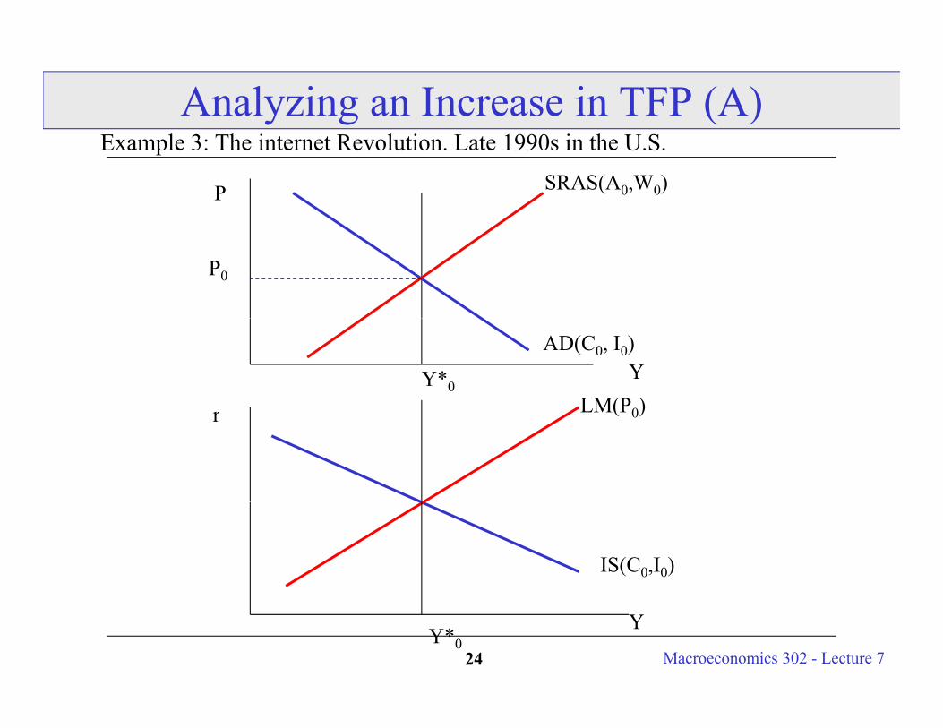
Analyzing an Increase in TFP (A)E l 3 Th i R l i L 1990 i h U S
SRAS(A0,W0)P
Example 3: The internet Revolution. Late 1990s in the U.S.
P0
LM(P0)
AD(C0, I0)
Y*0Y
LM(P0)r
IS(C0,I0)
Macroeconomics 302 - Lecture 724Y*0
Y
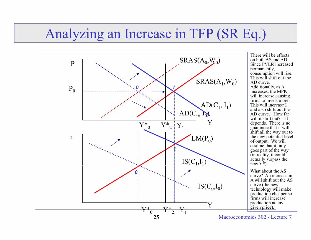
Analyzing an Increase in TFP (SR Eq.)
PThere will be effects on both AS and AD. Since PVLR increased permanently, consumption will rise.
SRAS(A0,W0)
P0
AD(C I )
consumption will rise. This will shift out the AD curve. Additionally, as A increases, the MPK will increase causing firms to invest more. This will increase I
0 1SRAS(A1,W0)
AD(C0, I0)
Y*0Y
AD(C1, I1)
Y*2
This will increase I and also shift out the AD curve. How far will it shift out? – It depends. There is no guarantee that it will shift all the way out to h i l l l
Y1
LM(P0)r the new potential level of output. We will assume that it only goes part of the way (in reality, it could actually surpass the new Y*). IS(C1,I1)
1
IS(C0,I0)
)What about the AS curve? An increase in A will shift out the AS curve (the new technology will make production cheaper so
0
Macroeconomics 302 - Lecture 725Y*0
YY*2
p pfirms will increase production at any given price).Y1
Analyzing an Increase in TFP (SR Eq.)
This representation of the economy is the one that the Fed thought that wewere in during Spring 2000 (read FOMC statements at the time):
1) Technology had improved.
2) C ti h d i d 2) Consumption had increased
3) Investment had been rising.
4) Unemployment was lower than the estimated natural rate ofunemployment.
5) Prices had been relatively stable DESPITE the rapid GDP growth.
6) Fed thought the labor market was ‘tight’ – another word for wagespossibly rising in the future
Macroeconomics 302 - Lecture 726
possibly rising in the future.
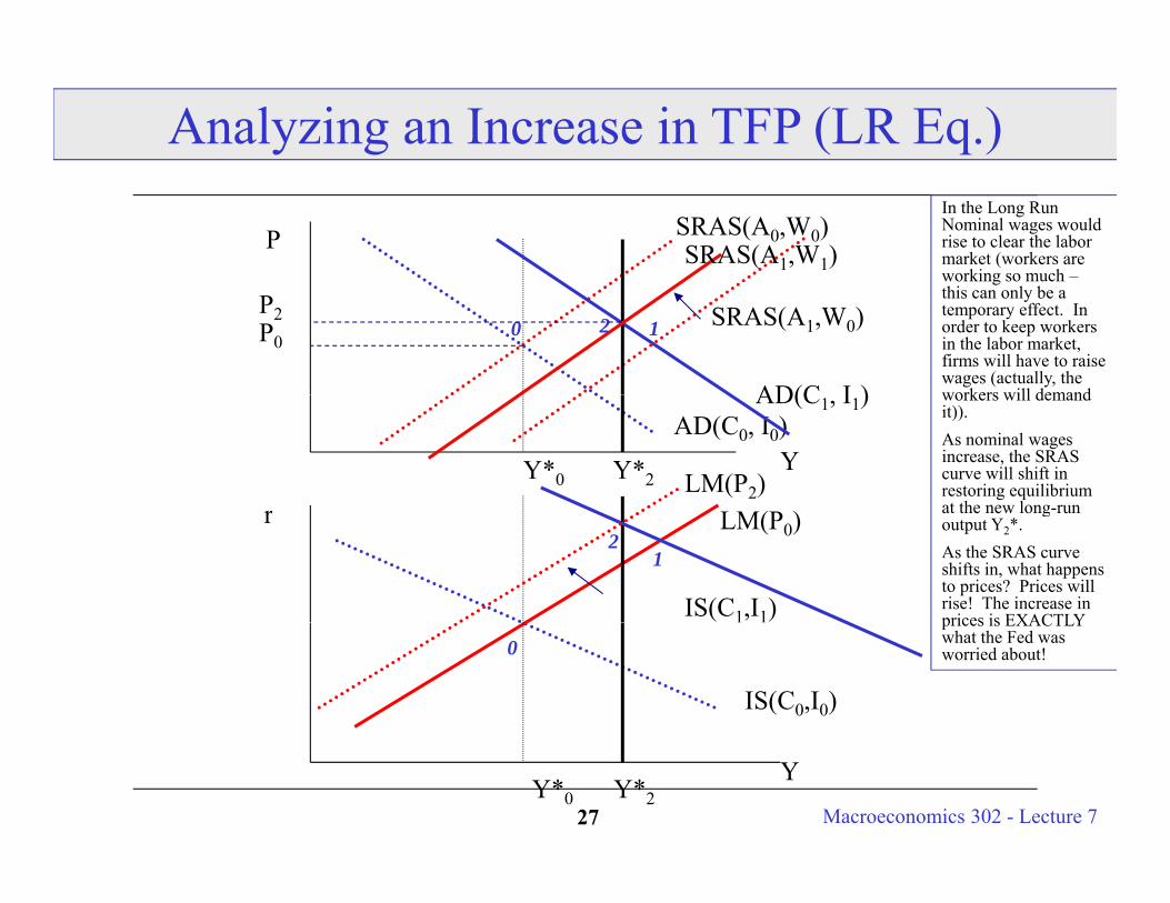
Analyzing an Increase in TFP (LR Eq.)
PIn the Long Run Nominal wages would rise to clear the labor market (workers are working so much –
SRAS(A0,W0)SRAS(A1,W1)
P0
AD(C I )
working so much this can only be a temporary effect. In order to keep workers in the labor market, firms will have to raise wages (actually, the workers will demand
0 12 SRAS(A1,W0)P2
AD(C0, I0)
Y*0Y
AD(C1, I1)
Y*2
workers will demand it)). As nominal wages increase, the SRAS curve will shift in restoring equilibrium at the new long-run
LM(P2)LM(P0)r at the new long-run
output Y2*. As the SRAS curve shifts in, what happens to prices? Prices will rise! The increase in prices is EXACTLYIS(C1,I1)
12
IS(C0,I0)
prices is EXACTLY what the Fed was worried about! 0
Macroeconomics 302 - Lecture 727Y*0
YY*2
Reviewing The Data:
From First Class: We saw that some falls in GDP were associated with no increase in prices.
We also so that some falls in GDP were associated with large increase in prices.
Do our theories reconcile these facts?
• YES! Demand shocks result in recessions without a corresponding rise in prices.
• YES! Supply shocks (like changes in oil prices) result in recessions with a large corresponding positive change in prices.
• You should really understand the difference between demand shocks (things that primarily affect AD) and supply shocks (things that primarily affect AS) on the economy - their implications are
Macroeconomics 302 - Lecture 728
much different from each other.

Economic Policy
Monetary and Fiscal Policy: May they help in stabilizing the economy from demand and supply shocks?
NOT AN EXACT SCIENCE - How much stimulus is necessary to move the economy to Y*economy to Y .
Policy Creates uncertainty as economic agents try to anticipate Fed/Government rules.
Some argue avoid using no stabilization policy (just a simple Quantity Theory representation) or suggest using very simple rules.
Policy often entails long and variable lags!
Some research says that every sustained period of large inflation is due to
Macroeconomics 302 - Lecture 729
Some research says that every sustained period of large inflation is due to the Fed!
Fiscal Policy in Action: Stabilizing Output
Another stabilization mechanism is to shock AD through a change in g gG (fiscal policy).
Not necessarily the best approach (we know that an increase in G y pp (crowds out private investment by decreasing savings and increasing r – i.e. investment moves up along the Id curve in the goods market).
It suffers from even longer lags than monetary policy due to the budgeting process.
I b i fl i It may be inflationary.
Graphical Analysis of an increase in G follows.
Macroeconomics 302 - Lecture 730
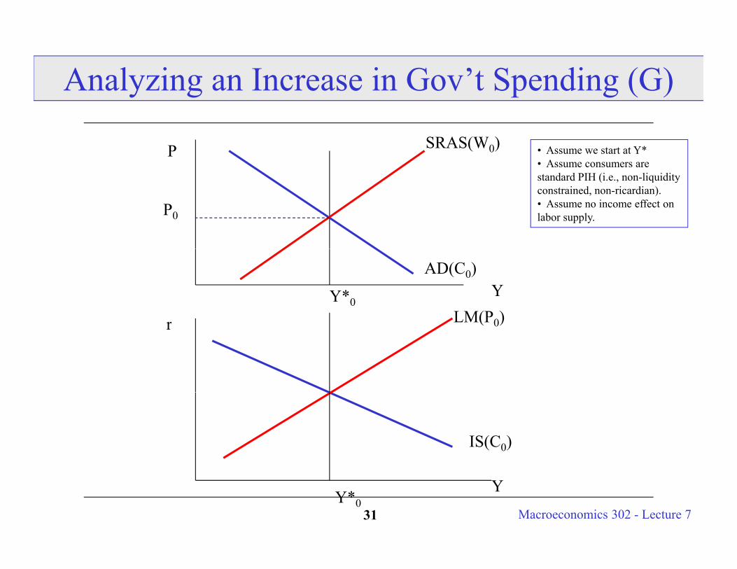
Analyzing an Increase in Gov’t Spending (G)
SRAS(W0)P • Assume we start at Y*• Assume consumers are standard PIH (i e non liquidity
P0
standard PIH (i.e., non-liquidityconstrained, non-ricardian).• Assume no income effect onlabor supply.
LM(P0)
AD(C0)
Y*0Y
LM(P0)r
IS(C0)
Macroeconomics 302 - Lecture 731Y*0
Y
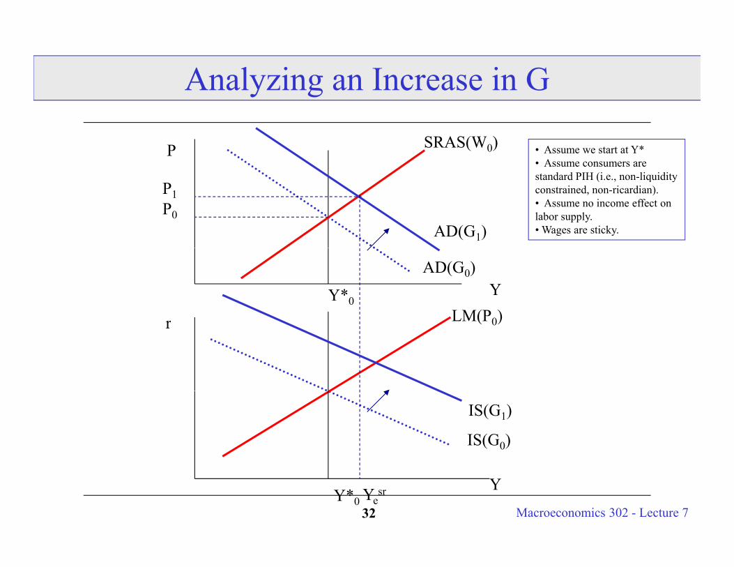
Analyzing an Increase in G
SRAS(W0)P • Assume we start at Y*• Assume consumers are standard PIH (i e non liquidity
P0
standard PIH (i.e., non-liquidityconstrained, non-ricardian).• Assume no income effect onlabor supply.• Wages are sticky.AD(G1)
P1
LM(P0)
AD(G0)
Y*0Y
LM(P0)r
IS(G0)
IS(G1)
Macroeconomics 302 - Lecture 732Y*0
YYesr
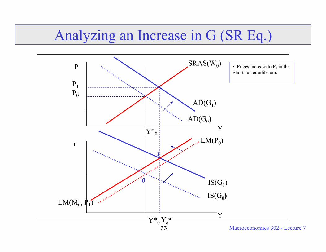
Analyzing an Increase in G (SR Eq.)
SRAS(W0)P • Prices increase to P1 in the Short-run equilibrium.
P0AD(G1)
P0
P1
LM(P0)
AD(G0)
Y*0Y
LM(P0)LM(P0)r LM(P0)
1
IS(C0)IS(G0)
IS(G1)
LM(M0, P1)
0
Macroeconomics 302 - Lecture 733Y*0
YYesr
( 0, 1)
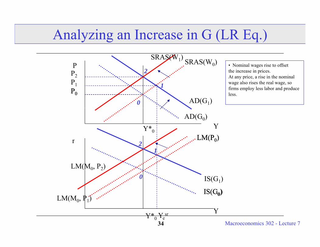
Analyzing an Increase in G (LR Eq.)
SRAS(W0)P • Nominal wages rise to offsetthe increase in prices.At any price a rise in the nominal
SRAS(W1)
P22
P0
At any price, a rise in the nominalwage also rises the real wage, so firms employ less labor and produce less.
AD(G1)P0
P1
2
0
1
LM(P0)
AD(G0)
Y*0Y
LM(P0)LM(P0)r
LM(M0, P2)
LM(P0)
12
IS(C0)IS(G0)
IS(G1)
LM(M0, P1)
0
Macroeconomics 302 - Lecture 734Y*0
YYesr
( 0, 1)
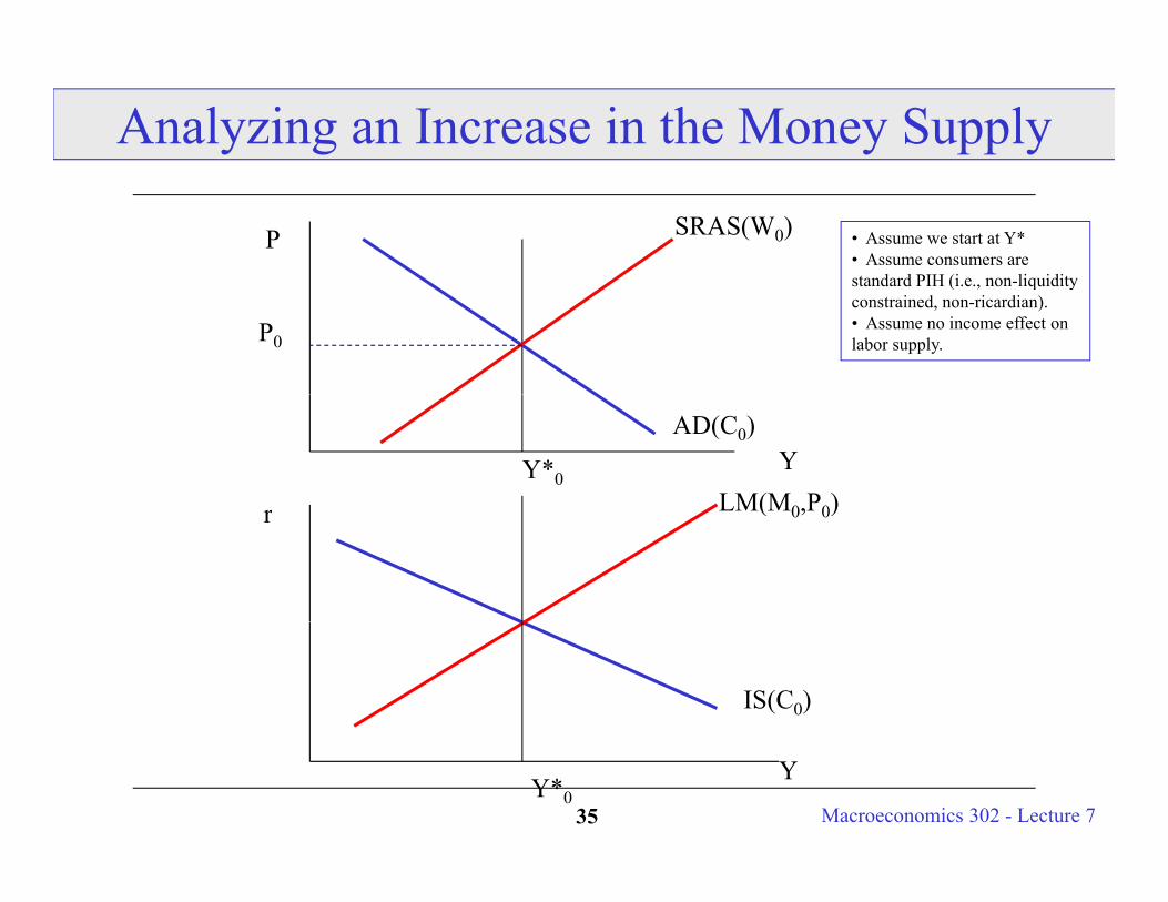
Analyzing an Increase in the Money Supply
SRAS(W0)P • Assume we start at Y*• Assume consumers are standard PIH (i e non liquidity
P0
standard PIH (i.e., non-liquidityconstrained, non-ricardian).• Assume no income effect onlabor supply.
AD(C0)
Y*0Y
LM(M0,P0)r LM(M0,P0)
IS(C0)
Macroeconomics 302 - Lecture 735Y*0
Y
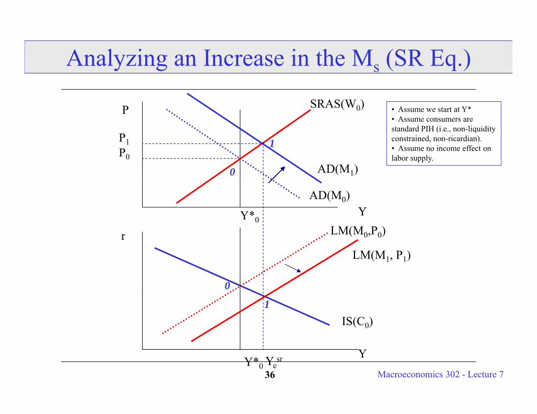
Analyzing an Increase in the Ms (SR Eq.)
SRAS(W0)P • Assume we start at Y*• Assume consumers are standard PIH (i e non liquidity
P0
standard PIH (i.e., non-liquidityconstrained, non-ricardian).• Assume no income effect onlabor supply.
AD(M1)
P1
0
1
LM(M0,P0)
AD(M0)
Y*0Y
LM(M0,P0)rLM(M1, P1)
0
IS(C0)
0
1
Macroeconomics 302 - Lecture 736Y*0
YYesr
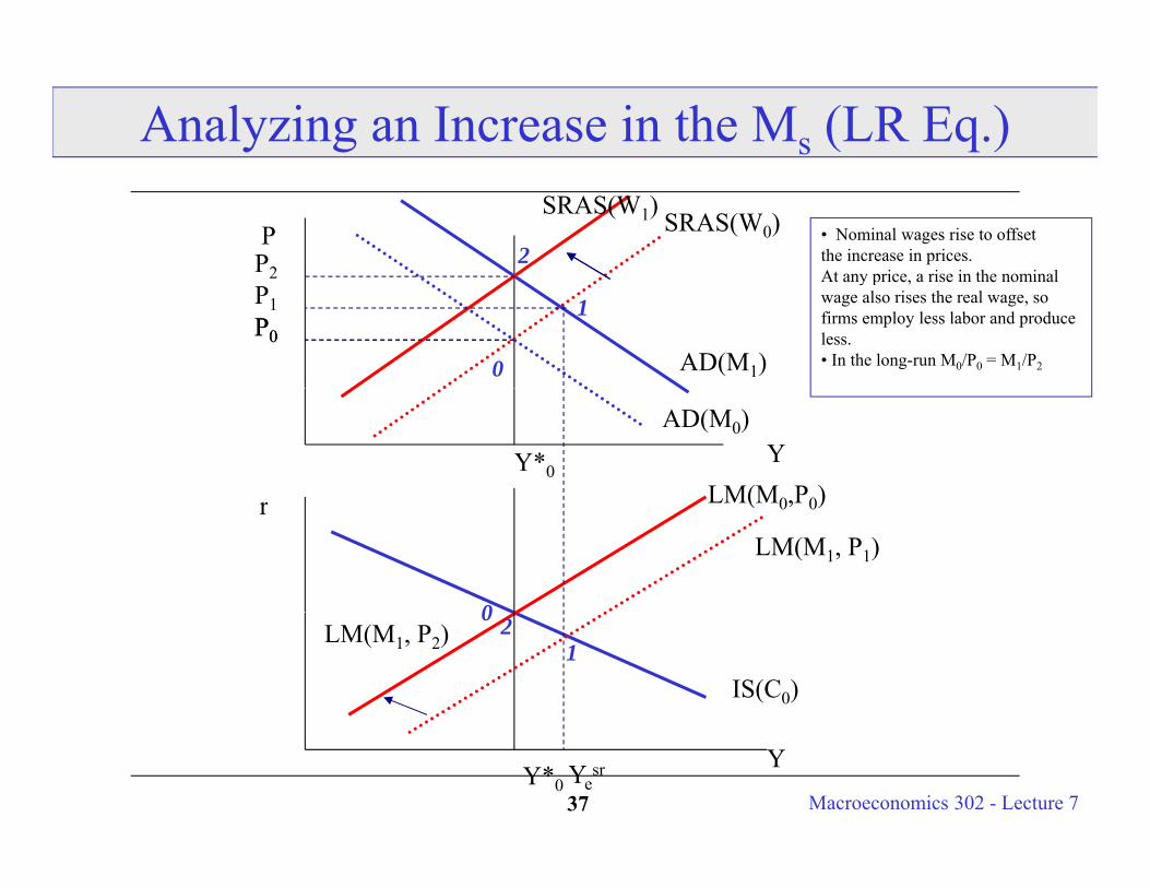
Analyzing an Increase in the Ms (LR Eq.)
SRAS(W0)P • Nominal wages rise to offsetthe increase in prices.At any price a rise in the nominal
SRAS(W1)
P22
P0
At any price, a rise in the nominalwage also rises the real wage, so firms employ less labor and produce less.• In the long-run M0/P0 = M1/P2AD(M1)
P0
P1
2
0
1
AD(M0)
Y*0Y
LM(M0,P0)rLM(M1, P1)
0
LM(M0,P0)
IS(C0)
LM(M1, P2)0
12
Macroeconomics 302 - Lecture 737Y*0
YYesr
Some Thoughts on Money Let us look at the Fed increasing the nominal money supply
We are going to look at money supply setting (as opposed to interest rate We are going to look at money supply setting (as opposed to interest rate setting – the Fed can only set either one or the other – Ld matters!).
Assume we start at Y*.
Fed increases Ms and LM shifts right, r falls and I increases.
A hif i ( *) d i l AD shifts out - Y increases (Y > Y*). Puts upward pressure on nominal wages (notice the key role of nominal wages as an indicator of future inflation).
As nominal wages rise - SRAS shifts in (up).
Prices rise and we return to Y* (basically - this is what is predicted by h i h f !!!!)
Macroeconomics 302 - Lecture 738
the quantity theory of money!!!!)
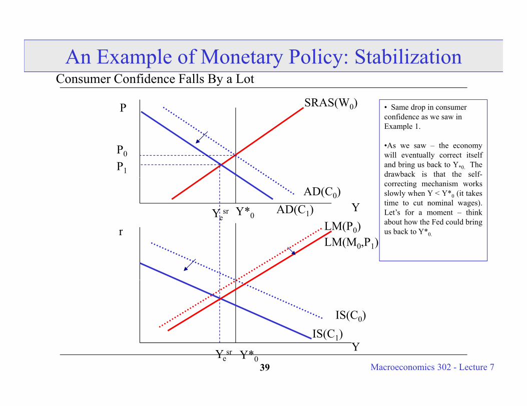
An Example of Monetary Policy: StabilizationC C fid F ll B L tConsumer Confidence Falls By a Lot
SRAS(W0)P • Same drop in consumer confidence as we saw in Example 1
P1
Example 1.
•As we saw – the economywill eventually correct itselfand bring us back to Y*0. Thedrawback is that the self-
P0
LM(P0)
AD(C0)
Y*0Y
correcting mechanism worksslowly when Y < Y*0 (it takestime to cut nominal wages).Let’s for a moment – thinkabout how the Fed could bring
b k *
AD(C1)Yesr
LM(P0)r us back to Y*0.
LM(M0,P1)
IS(C0)IS(C )
Macroeconomics 302 - Lecture 739Y*0
YIS(C1)
Yesr
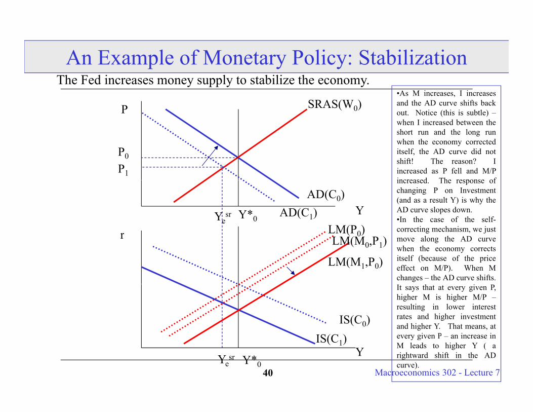
An Example of Monetary Policy: StabilizationTh F d i l t t bili thThe Fed increases money supply to stabilize the economy.
SRAS(W0)P•As M increases, I increasesand the AD curve shifts backout. Notice (this is subtle) –when I increased between the
P1
short run and the long runwhen the economy correcteditself, the AD curve did notshift! The reason? Iincreased as P fell and M/Pincreased The response of
P0
LM(P0)
AD(C0)
Y*0Y
increased. The response ofchanging P on Investment(and as a result Y) is why theAD curve slopes down.•In the case of the self-correcting mechanism, we just
AD(C1)Yesr
LM(P0)r g , jmove along the AD curvewhen the economy correctsitself (because of the priceeffect on M/P). When Mchanges – the AD curve shifts.
LM(M1,P0)
LM(M0,P1)
IS(C0)
It says that at every given P,higher M is higher M/P –resulting in lower interestrates and higher investmentand higher Y. That means, atevery given P an increase inIS(C )
Macroeconomics 302 - Lecture 740Y*0
Yevery given P – an increase inM leads to higher Y ( arightward shift in the ADcurve).
IS(C1)
Yesr
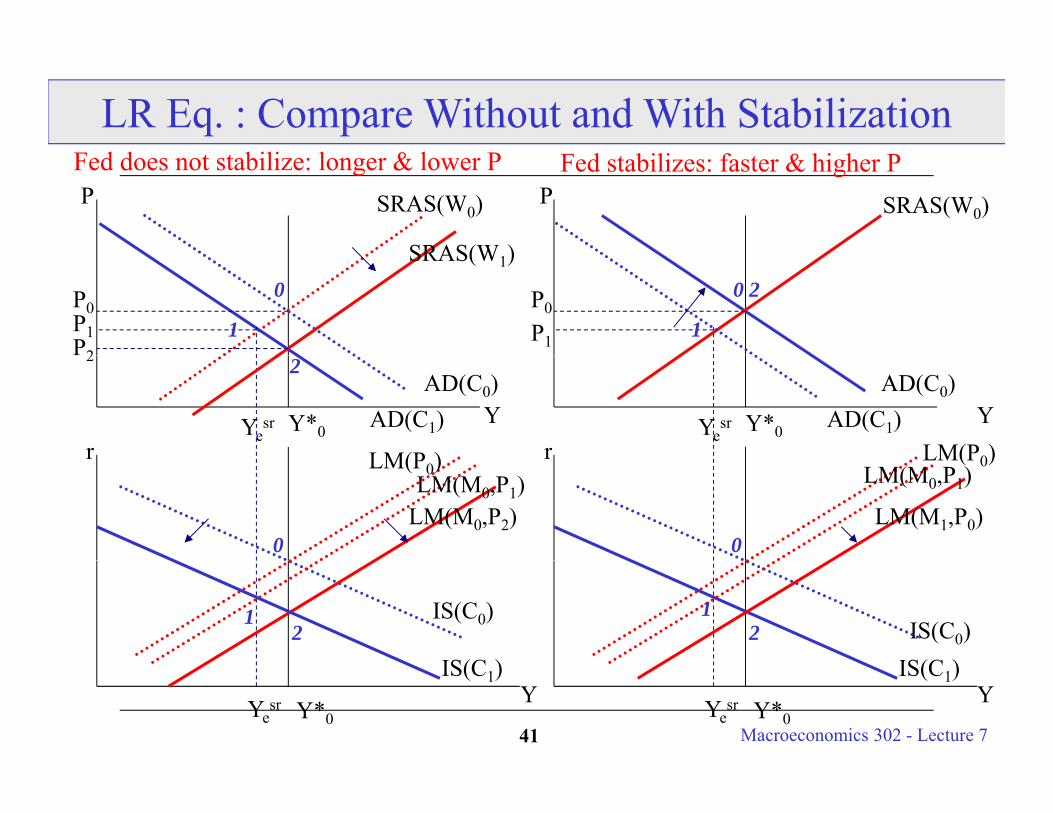
LR Eq. : Compare Without and With Stabilization
SRAS(W0)PSRAS(W0)P
SRAS(W )
Fed does not stabilize: longer & lower P Fed stabilizes: faster & higher P
P1
P0P0
SRAS(W1)
P1P2
0
1
0 2
1
LM(P0)
AD(C0)
Y*0r
YAD(C1)Yesr
LM(P )
AD(C0)
Y*0r
YAD(C1)Yesr
2 2
LM(P0)r
LM(M1,P0)
LM(M0,P1)LM(P0)r
LM(M0,P2)LM(M0,P1)
0 0
IS(C0)IS(C )
IS(C0)
IS(C )
12
12
Macroeconomics 302 - Lecture 741Y*0
YIS(C1)
YesrY*0
YIS(C1)
Yesr
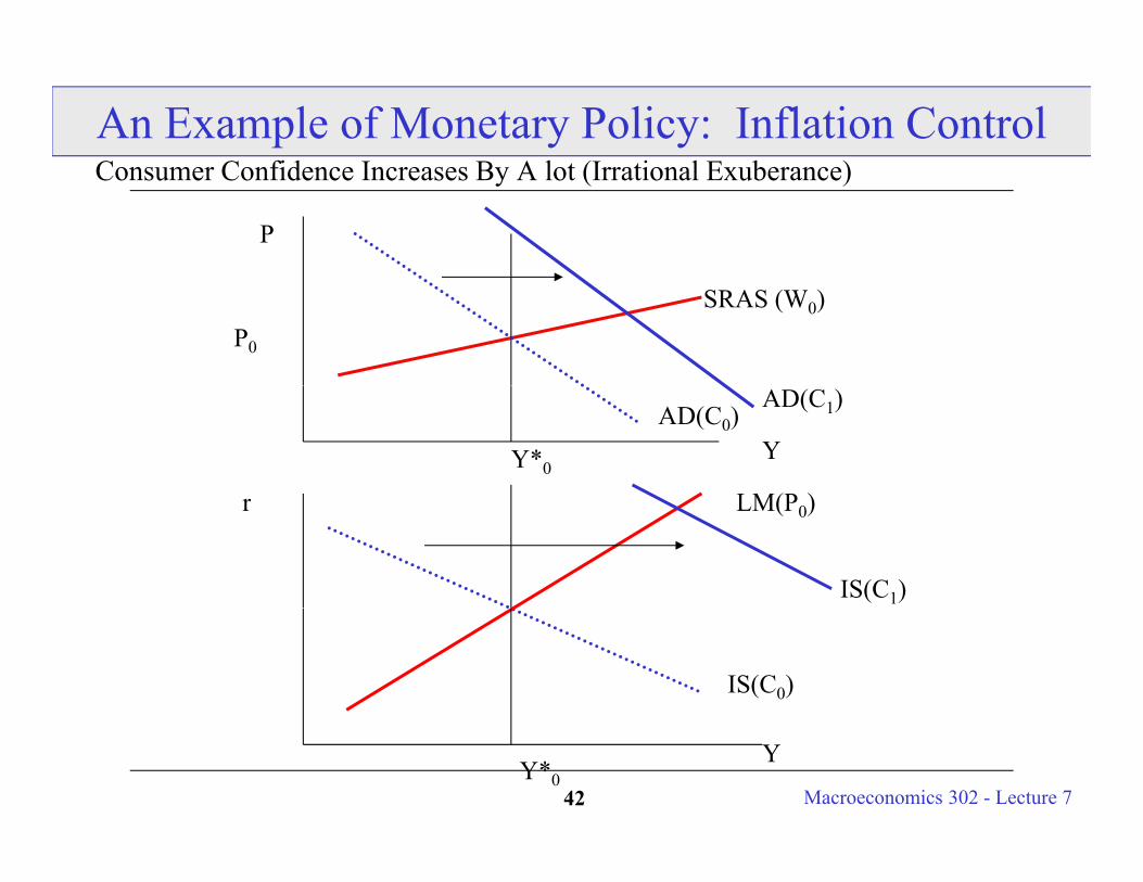
An Example of Monetary Policy: Inflation ControlC C fid I B A l t (I ti l E b )Consumer Confidence Increases By A lot (Irrational Exuberance)
P
SRAS (W0)P0
LM(P )
AD(C0)
Y*0Y
AD(C1)
LM(P0)r
IS(C1)
IS(C0)
Macroeconomics 302 - Lecture 742Y*0
Y

Goals of the Fed
Fed’s primary goals are to foster economic growth and job creation and restrain inflationary pressure.y p
The Fed wants to set r so that
• r = r*, Y = Y*, U = U*, N = N* ( these are equivalent).
• = * (0-2% inflation).
The Fed wants to raise r when
• r < r*, Y > Y*, U < U*, N > N*
• > *
Macroeconomics 302 - Lecture 743
The Fed wants to lower r when the opposite conditions hold.
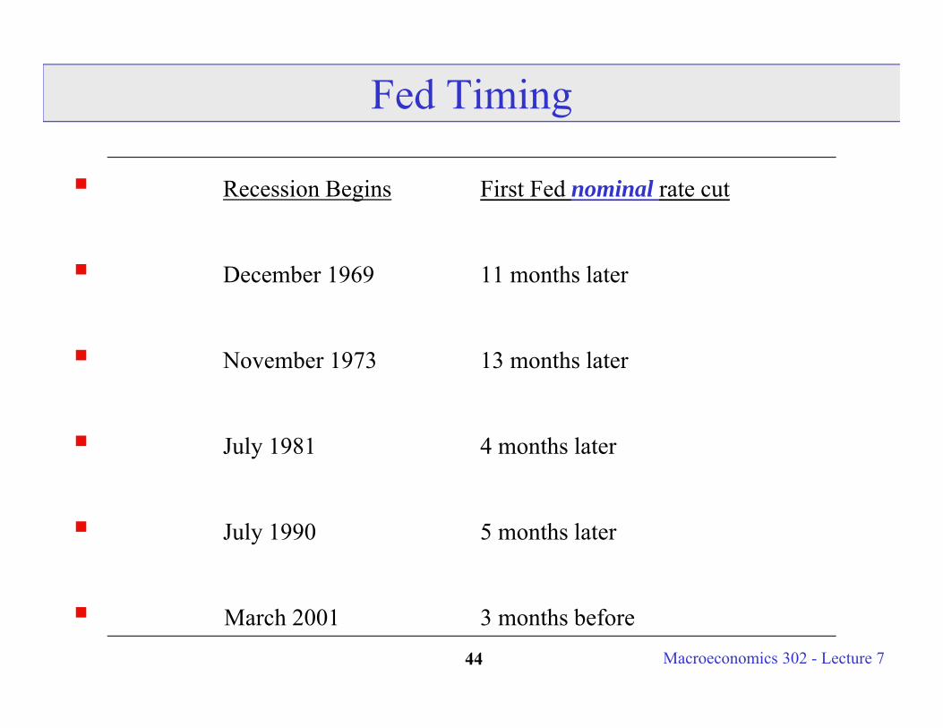
Fed Timing
Recession Begins First Fed nominal rate cut
December 1969 11 months later
November 1973 13 months later
July 1981 4 months later
July 1990 5 months later
Macroeconomics 302 - Lecture 744
March 2001 3 months before
Rules vs. Discretion
Should a central bank have a specific policy rule:
Rules are explicit and may be mandated by law
• Money should grow at 4% per year (Friedman preferred rule).y g p y ( p )• Explicit inflation target: UK has an inflation target of 2% (+/- 1%)
See main web page http://www.bankofengland.co.uk/
Rules may be implicit and known by all economic agents
• The Fed will target the inflation rate at 2-4% per year.
Macroeconomics 302 - Lecture 745
Benefits of Rules
Commits Central Bank to Some Policy
Removes Inflation Temptation
Creates a more stable economic situation: Individuals and Firms can anticipate the central bank actions. No surprises!
Prevents central bank from thinking too much - the economy is so complex that Fed policy can have delayed impact and is usually initiated too late! Central Bank actions can often be ‘destabilizing’. (F id L B h f i l l )(Freidman, Lucas: Both prefer simple rules).
Macroeconomics 302 - Lecture 746
Benefits of Discretion Central Bank uses all information possible to make the best decision
at the time.
The Fed uses a discretionary rule. The members of the bank vote on a monetary policy eat each FOMC meeting. The policy is not dictated by some explicit ruledictated by some explicit rule.
Benefits of Discretion:• Allows Central Bank to choose from competing policyAllows Central Bank to choose from competing policy
goals. (Sometimes inflation targeting is not best for the economy)
• The Fundamentals of the Economy may change/or evolveThe Fundamentals of the Economy may change/or evolve over time - the rule becomes outdated.
• How do we know where the economy is relative to Y* and target inflation rate? Information flows slowly and is
Macroeconomics 302 - Lecture 747
and target inflation rate? Information flows slowly and is complex to analyze.
Hawks and Doves
How does the Fed balance price stability ( = *) and full employment (U = U*) when they conflict?
[For example, when > * and U > U* at the same time.]
Hawks put more weight on * (and have lower values for it).p g ( )• U.K., Canada, New Zealand.• Bundesbank before; European Central Bank now?
Doves put more weight on staying near U* (and have higher *).
k d h i h h Bernanke tends to puts the same “weight” on each.
My current research relates to communication of those weights to the
Macroeconomics 302 - Lecture 748
market.
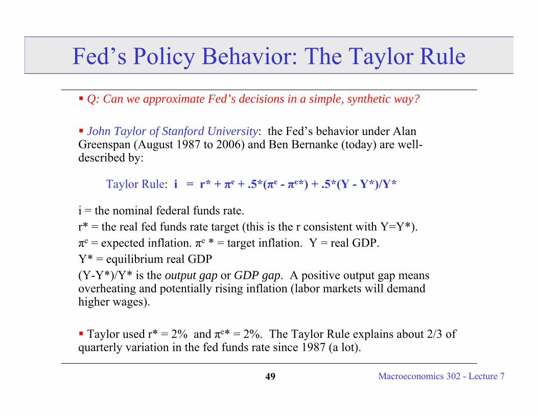
Fed’s Policy Behavior: The Taylor Rule Q: Can we approximate Fed’s decisions in a simple, synthetic way?
J h T l f St f d U i it : the Fed’s beha ior nder Alan John Taylor of Stanford University: the Fed’s behavior under Alan Greenspan (August 1987 to 2006) and Ben Bernanke (today) are well-described by:
T l R l i * + e + 5*( e e*) + 5*(Y Y*)/Y*Taylor Rule: i = r* + πe + .5*(πe - πe*) + .5*(Y - Y*)/Y*
i = the nominal federal funds rate. r* = the real fed funds rate target (this is the r consistent with Y=Y*).πe = expected inflation. πe * = target inflation. Y = real GDP.Y* = equilibrium real GDP (Y-Y*)/Y* is the output gap or GDP gap. A positive output gap means overheating and potentially rising inflation (labor markets will demandoverheating and potentially rising inflation (labor markets will demand higher wages).
Taylor used r* = 2% and πe* = 2%. The Taylor Rule explains about 2/3 of
Macroeconomics 302 - Lecture 749
y y pquarterly variation in the fed funds rate since 1987 (a lot).
Notes on the Taylor Rule
Fed economists find an even better fit with 1 on the GDP gap term.Fed economists find an even better fit with 1 on the GDP gap term.
This does NOT mean that Bernanke uses this ‘rule’, it is just that Fed behavior looks very similar to this rule.
Furthermore, the Fed tends to smooth interest rates relative to the Rule:
This quarter’s actual i = .6*(Last quarter’s actual i) + .4*(Taylor Rule’s i)
Studies have found that other G7 Central Banks (e.g., the Bundesbank, ECB) have also followed versions of a smoothed Taylor RuleECB) have also followed versions of a smoothed Taylor Rule.
Read the speeches by Bernanke, Greenspan and Gramlich to see the Fed’s take on such subject.
Macroeconomics 302 - Lecture 750
A Look At Liquidity Traps
Recall Krugman’s “Babysitting the Economy” (From Topic 1)
Nominal Interest Rates Are Bounded At Zero!
People Believe that there will be deflation in the future!
Real Interest Rates are Large and Positive.
Fed Would like to cut rates (to stimulate Y (shift out AD) which will putFed Would like to cut rates (to stimulate Y (shift out AD) which will put upward pressure on prices), but nominal rates cannot go below zero!
The Fed is helpless. How do they stimulate investment and consumption h h i l i ?when they cannot cut nominal interest rates?
This describes the situation in Japan during the late 1990s. Japan has experienced deflation AND nominal rates are close to zero. Central Bank of
Macroeconomics 302 - Lecture 751
experienced deflation AND nominal rates are close to zero. Central Bank of Japan is helpless.
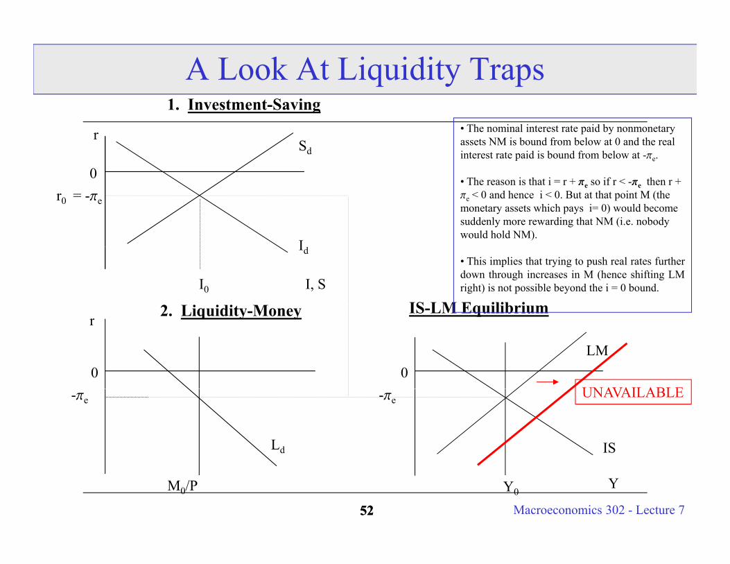
A Look At Liquidity Traps1 Investment Saving1. Investment-Saving
Sdr • The nominal interest rate paid by nonmonetary
assets NM is bound from below at 0 and the real interest rate paid is bound from below at -pe.
0r0
I
= -pe
• The reason is that i = r + pe so if r < -pe then r + pe < 0 and hence i < 0. But at that point M (the monetary assets which pays i= 0) would become suddenly more rewarding that NM (i.e. nobody would hold NM).
0
IS-LM Equilibrium2. Liquidity-MoneyI0 I, S
Id• This implies that trying to push real rates furtherdown through increases in M (hence shifting LMright) is not possible beyond the i = 0 bound.
q y y
LM
UNAVAILABLE
r
0 0
Ld IS
UNAVAILABLE-pe -pe
Macroeconomics 302 - Lecture 75252
M0/P Y0Y

Demand Side Effects of Deflation Deflation can make borrowers - either consumers or firms, worse off.
As we saw early in the course unexpected inflation makes borrowers better As we saw early in the course, unexpected inflation makes borrowers better off. They expected to pay a certain real rate and when inflation is higher and the nominal rate is fixed, the real rate they pay is lower (in terms of lost purchasing power).
If the economy experiences unexpected deflation, the opposite happens: borrowers are paying more in terms of lost real purchasing power when there is unexpected deflation. Borrowers, both consumers and firms, will essentially be poorer. (Even though, there is another side of the market -somebody’s got to lend to them, this could still have large effects on consumption and investment). This demand side effect of deflation is called ‘debt overhang’ or ‘debt deflation’. <<Note, even the government is paying higher than expected real rates on their debt>>.
Even if the deflation is expected, large transfers can occur from borrowers to lenders because nominal interest rates are bounded by zero (shuts down
Macroeconomics 302 - Lecture 753
lenders because nominal interest rates are bounded by zero (shuts down lending channels).
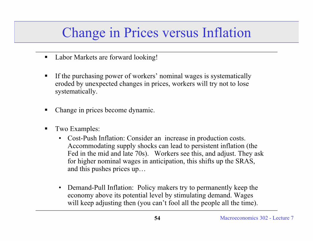
Change in Prices versus Inflation Labor Markets are forward looking!
If the p rchasing po er of orkers’ nominal ages is s stematicall If the purchasing power of workers’ nominal wages is systematically eroded by unexpected changes in prices, workers will try not to lose systematically.
Change in prices become dynamic.
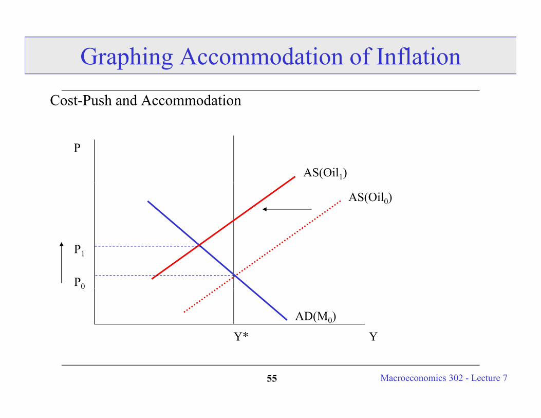
Two Examples: C P h I fl i C id i i d i• Cost-Push Inflation: Consider an increase in production costs. Accommodating supply shocks can lead to persistent inflation (the Fed in the mid and late 70s). Workers see this, and adjust. They ask for higher nominal wages in anticipation, this shifts up the SRAS,
d hi h iand this pushes prices up…
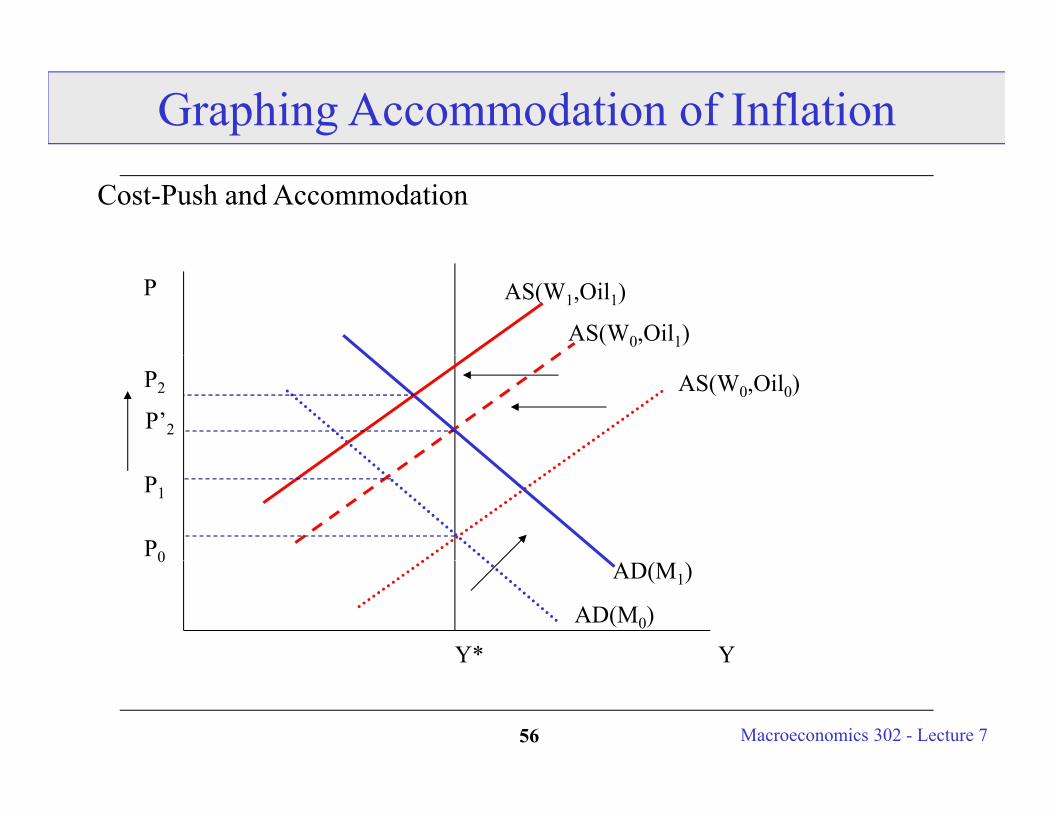
• Demand-Pull Inflation: Policy makers try to permanently keep the economy above its potential level by stimulating demand Wages
Macroeconomics 302 - Lecture 754
economy above its potential level by stimulating demand. Wages will keep adjusting then (you can’t fool all the people all the time).
Graphing Accommodation of Inflation
Cost-Push and Accommodation
P
AS(Oil1)
AS(Oil0)
P1
P0
Y
AD(M0)
Y*
0
Macroeconomics 302 - Lecture 755
Graphing Accommodation of Inflation
Cost-Push and Accommodation
P
AS(W0,Oil1)
AS(W1,Oil1)
AS(W0,Oil0)P’2
P2
P1
P0
Y
AD(M0)
Y*
AD(M1)0
Macroeconomics 302 - Lecture 756

How do we get out of Cost-Push Inflation?
Fed Can Break the Inflation! Reset, expected inflation rates., p
The 1982 - Volker Recession (Paul Volker, an extremely underrated Fed Chair).
Through a cold-turkey cut of money supply and with a substantial effort to modify the market’s perception of the Fed he managed to cut inflation from double digits to 4%.
It did cost the economy a short but deep recession though.
Macroeconomics 302 - Lecture 757

Graphing Demand-Pull InflationG h f i d li k Y b Y*Graph of a sustained policy to keep Y above Y*.
P
SRAS(W0)
P1
P0
Y
AD(M0)
Y*
0AD(M1)
Macroeconomics 302 - Lecture 758
Graphing Demand-Pull InflationG h f i d li k Y b Y* M i d d i l i PGraph of a sustained policy to keep Y above Y*. May induce an upward spiral in P.
P SRAS(W1)
P2
SRAS(W0)
P1
P0AD(M2)
Y
AD(M0)
Y*
0AD(M1)
Macroeconomics 302 - Lecture 759
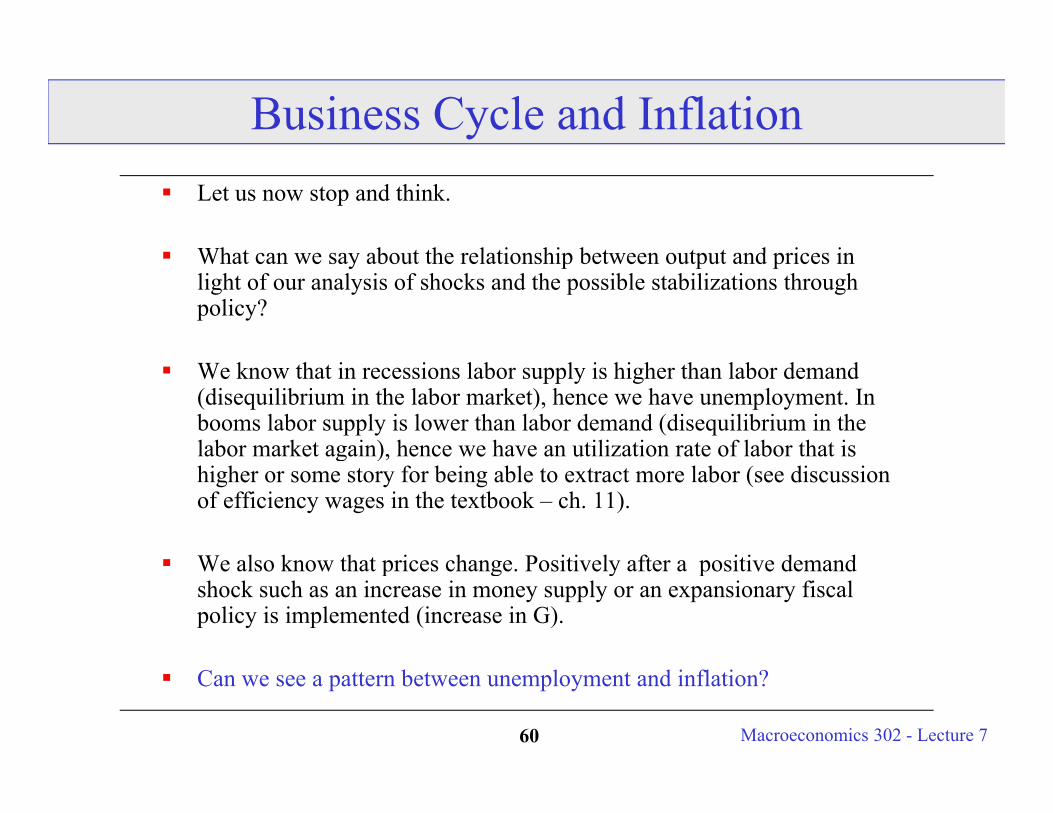
Business Cycle and Inflation Let us now stop and think.
What can e sa abo t the relationship bet een o tp t and prices in What can we say about the relationship between output and prices in light of our analysis of shocks and the possible stabilizations through policy?
We know that in recessions labor supply is higher than labor demand (disequilibrium in the labor market), hence we have unemployment. In booms labor supply is lower than labor demand (disequilibrium in the labor market again), hence we have an utilization rate of labor that is g ),higher or some story for being able to extract more labor (see discussion of efficiency wages in the textbook – ch. 11).
We also know that prices change Positively after a positive demand We also know that prices change. Positively after a positive demand shock such as an increase in money supply or an expansionary fiscal policy is implemented (increase in G).
Macroeconomics 302 - Lecture 760
Can we see a pattern between unemployment and inflation?

The Phillips Curve
Discoverer: British economist A.W. Phillips.
Discovery: A negative correlation between the unemployment rate and the inflation rate across years within a country in the 1950s. Corr(π, u ) < 0
The correlation was also negative in the U.S. and other countries through the 1960s.
Old Keynesians in the 1960s: We have found a stable, exploitable tradeoff between the rate of inflation and the rate of unemployment. We can permanently lower the rate of unemployment at the cost of a permanently higher inflation rate.
No. The negative relation is only between unexpected inflation and cyclical unemployment. Expectations-augmented Phillips Curve (Friedman-Phelps)
Phillips Curve: π = πe - h*(u - u)
Macroeconomics 302 - Lecture 761
u is the natural unemployment rate (structural and frictional unemployment only).
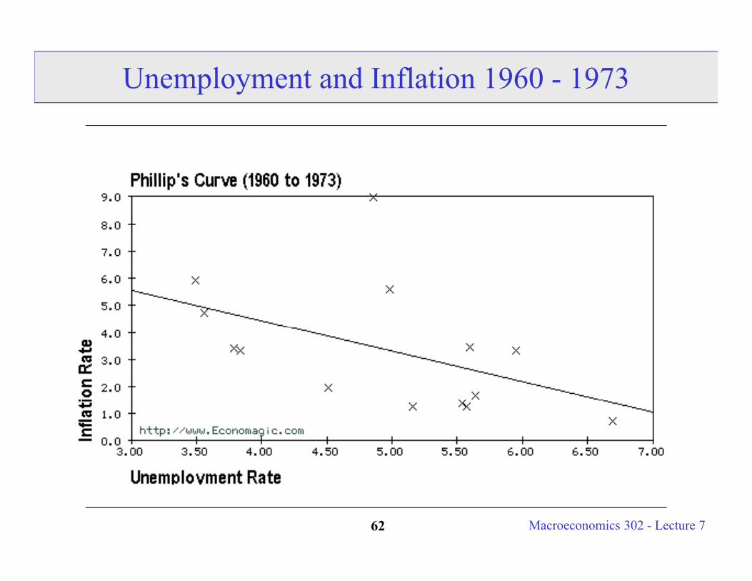
Unemployment and Inflation 1960 - 1973
Macroeconomics 302 - Lecture 762
Friedman and Phelps: Expectations Matter
You cannot exploit the trade off between inflation and unemployment unless you constantly surprise people. That is, if workers and firms are rational they will incorporate the economic policy that exploits the trade off in their decisions and will not allow the government to fool them systematically by increasing Ms or G.
Milton Friedman in 1968: Theory predicts that the only AD shocks that are going to y p y g gThe LR Phillips Curve is vertical.
Vindicating evidence:
• The Phillips Curve broke down after 1970’s.
• Over time in the U.S., higher money growth just leads to more inflation d hi h l GDPand no higher real GDP.
• Across countries, higher money growth just leads to more inflation and no higher real GDP. Real GDP actually appears to be hindered by high levels
Macroeconomics 302 - Lecture 763
of inflation.
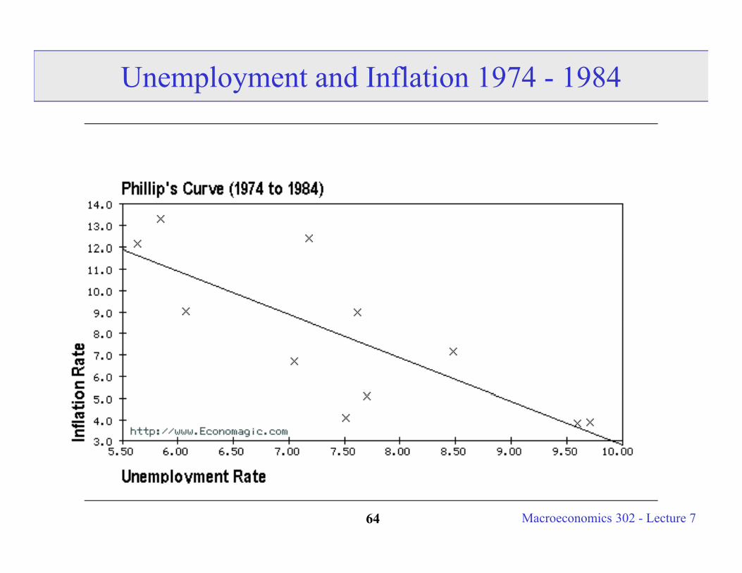
Unemployment and Inflation 1974 - 1984
Macroeconomics 302 - Lecture 764
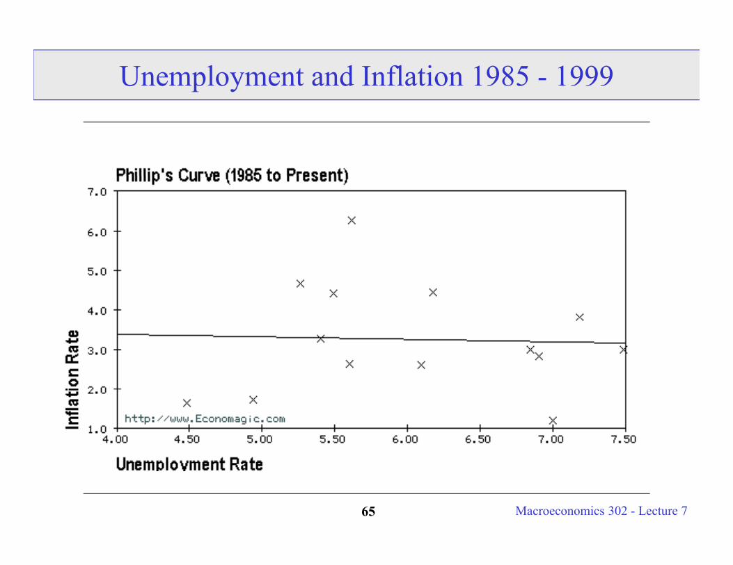
Unemployment and Inflation 1985 - 1999
Macroeconomics 302 - Lecture 765
To help protect your privacy, PowerPoint prevented this external picture from being automatically downloaded. To download and display this picture, click Options in the Message Bar, and then click Enable external content.
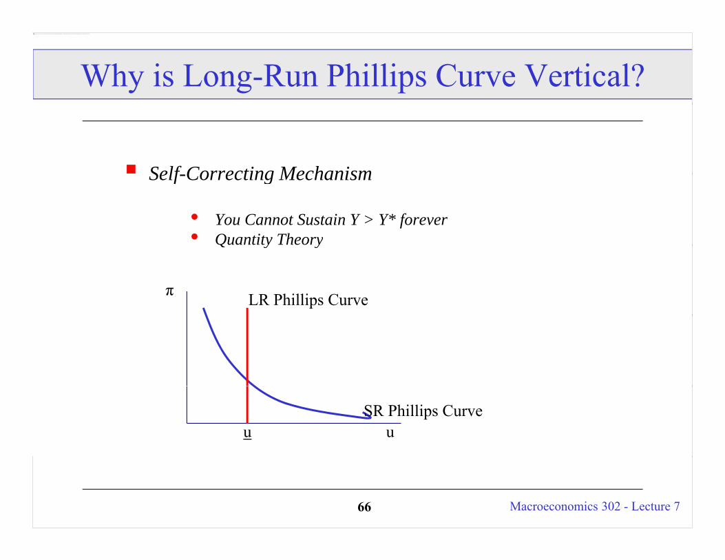
Why is Long-Run Phillips Curve Vertical?
Self Correcting MechanismSelf-Correcting Mechanism
• You Cannot Sustain Y > Y* forever• Quantity TheoryQ y y
π LR Phillips Curve
uuSR Phillips Curve
Macroeconomics 302 - Lecture 766
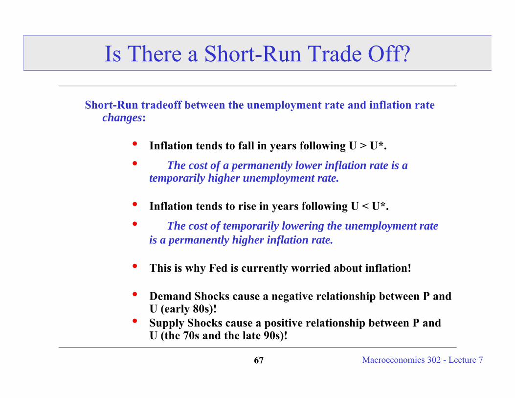
Is There a Short-Run Trade Off?
Short-Run tradeoff between the unemployment rate and inflation rate changes:
• Inflation tends to fall in years following U > U*.
• The cost of a permanently lower inflation rate is a il hi h ltemporarily higher unemployment rate.
• Inflation tends to rise in years following U < U*.
• The cost of temporarily lowering the unemployment rate• The cost of temporarily lowering the unemployment rateis a permanently higher inflation rate.
• This is why Fed is currently worried about inflation!
• Demand Shocks cause a negative relationship between P and U (early 80s)!
• Supply Shocks cause a positive relationship between P and
Macroeconomics 302 - Lecture 767
Supply Shocks cause a positive relationship between P and U (the 70s and the late 90s)!
Conclusions
We have experimented with different types of shock to our aggregate economy. Supply and demand shocks.
We can describe in a simple, intuitive way most past booms and recessions. Also our simple graphical analysis is helpful for describing possible future scenariospossible future scenarios.
We now have a way of modeling Output Stabilization Policies and Inflation Control Policies.
The Fed’s Objectives and the Taylor Rule.
Defined the Phillips Curve and the Expectations augmented Phillips curve.
Macroeconomics 302 - Lecture 768


![all - sci.skru.ac.th fileall . n '" in .J ti/fl UfI . 08612555 . 1'U~ 23 'Wt]fl'~fllO'U 'Vi-fl'. 2555 . I~t:l.:l 'U tJfid1lJtJ'4 lm . l~tf'l.h ~'l5l-fflJ'W'U.fil . f1H rns . i~[Jl-!](https://img.pdfslide.us/doc/110x75/5cd6027188c993f06f8d5e7d/all-sciskruacth-n-in-j-tifl-ufi-08612555-1u-23-wtflfllou.jpg)