TYPE THEORIES IN CATEGORY THEORY

TESLA ZHANG

July 26, 2021

ABSTRACT. We introduce basic notions in category theory to type theorists, in-cluding comprehension categories, categories with attributes, contextual categories,type categories, and categories with families along with additional discussionsthat are not very closely related to type theories by listing definitions, lemmata,and remarks. By doing so, this introduction becomes more friendly as a referentialmaterial to be read in random order (instead of from the beginning to the end). Inthe end, we list some mistakes made in the early versions of this introduction.

The interpretation of common type formers in dependent type theories are dis-cussed based on existing categorical constructions instead of mechanically derivedfrom their type theoretical definition. Non-dependent type formers include unit,products (as fiber products), and functions (as fiber exponents), and dependent onesinclude extensional equalities (as equalizers), dependent products, and the uni-verse of (all) propositions (as the subobject classifier).

CONTENTS

1. Preface 22. Background and motivation 22.1. Pullbacks and products 42.2. Duality and coproducts 52.3. The category of contexts 63. Basic category theory 73.1. Grothendieck fibrations 93.2. Towards a comprehension category 103.3. Slightly higher categories 123.4. Preparation for a category with attributes 133.5. Cartmell’s artifacts 144. Categorical semantics 154.1. Star at the top: the unit type 174.2. Like a semiring: the (co)product type 184.3. Internal homs and the evaluation map 204.4. Locally cartesian closed contextual categories and fiber exponents 214.5. Simple type theory: the function type 225. Alternative constructions 235.1. Type categories 245.2. Categories with families 266. Dependent type theory 276.1. Equalizers: the extensional equality type 286.2. Locally cartesian closed categories: the dependent product type 30

1

2 TESLA ZHANG

6.3. Subobject classifiers: the universe of all propositions 316.4. Internalized constructions 337. More category theory 347.1. Common mistakes and counterexamples 36Acknowledgement 37References 37

1. PREFACE

Warning 1.1 (Prerequisites). We assume the familiarity of the following concepts:(1) Set theory: sets, subsets, elements, functions, image, fiber, injectivity, and

cartesian products.(2) Type theory: dependent types, lambda calculus, (telescopic) contexts, typ-

ing judgments, and substitutions.(3) Category theory: categories, objects, morphisms, isomorphisms, commu-

tative diagrams, functors, and natural transformations.Typing judgments and substitutions are slightly discussed (in §2), but not in anintroductory way. A

Notation 1.2. We introduce some notational conventions in category theory.• We write A ∈ C to say that “A is an object in the category C”, and f ∈C(A, B) to say that “ f is a morphism in the category C from A towards B”.In the literature, the former is also written as A ∈ Ob(C) and the latter isalso written as f ∈ HomC(A, B).• We write Ob(C) for the set of objects in C.• We write idA ∈ C(A, A) for the identity morphism, dom( f ) and cod( f ) for

the domain projection and the codomain projection of morphisms. We alsosay a morphism f is a morphism from dom( f ) and towards cod( f ).• We write f g ∈ C(dom(g), cod( f )) for composition of morphisms.

Terminology 1.3 (NatIncl). For two sets B ⊆ A, the “identity” function ι : B → Ais called a natural inclusion.

Convention 1.4 (Sterling [Ste20]). In the typing rules, some judgments might beentailed by another. We write the entailed judgment(s) out explicitly in gray if theyworth it.

Convention 1.5 (Cockx [CA18]). We use boxes to distinguish type theory or cat-egory theory notations from natural language text, e.g. “we combine a term awith a term b to get a term a b ”.

2. BACKGROUND AND MOTIVATION

Remark 2.1. The notion of substitution in type theory is the process of replacinga variable with a term. We sometimes refer to the action of replacement with theverb apply, like “apply this substitution to that term”. We generalize this notion tolists, so that one substitution deals with multiple replacements.

TYPE THEORIES IN CATEGORY THEORY 3

Definition 2.2 (SubstObj). The data carried by a substitution is called a substitutionobject – a list of mapping from variables to terms. Substitution objects can be appliedon terms.

Demonstration 2.3. Consider a lambda calculus term (λx.λy.u) a b, we denote itsreduced form as u[a/x, b/y] (a notation similar to the one used by Curry [CFC59]).The [a/x, b/y] part is an example of a substitution object (definition 2.2).

Remark 2.4 (Nameless). Contexts, types, terms, and substitution objects are con-sidered up to α-renaming throughout this introduction. That is to say, there are no“names” in these structures – α-equivalent terms are considered the same. We canimagine that we are using a nameless representation of binding structures, such asde Bruijn indices [de 72].

Notation 2.5. We introduce some notational conventions in type theory.We use Γ, ∆ to denote contexts, σ, γ (recall convention 1.5) for substitution ob-

jects (definition 2.2), lowercase letters for terms (preferably u, v), and uppercaseletters for types (preferably A, B).

We write uσ for “applying the substitution object σ to term u”.

Remark 2.6. In a simple type theory, terms are typed in a context and types arecanonical mathematical objects. However, since we are dealing with a dependenttype theory, types will be formed in a context too.

We will have two basic judgments: context formation Γ ` (the types in Γ are well-typed) and type formation Γ ` A type (A is a well-typed type in Γ). Based on thesejudgments, we define the judgment for terms (using convention 1.4):

Γ ` Γ ` A typeΓ ` u : A

Γ ` Γ ` A type Γ ` u : A Γ ` v : AΓ ` u = v : A

It reads “term u has type A in context Γ, presupposing Γ ` A type ”. We also havethe judgment for substitution objects:

Γ ` ∆ `Γ ` σ : ∆

It reads “in the context Γ, the i-th term in σ have the i-th type in ∆, presupposingΓ `, ∆ `”. It is assumed that σ and ∆ have the same length.

Remark 2.7 (Substitutions). Although we are going to treat substitution infor-mally, we would like to emphasize some important insights about substitutions.

• Consider a substitution object Γ ` σ : ∆ (a judgment already describedin remark 2.6): it is a fact that “terms in σ can refer to bindings in Γ”, andwe say “σ instantiates the context ∆”.• Consider a term ∆ ` u : A, both u and A can refer to bindings in ∆.

We can turn u into another term, typed in the context Γ by applying the substitu-tion σ since the open references to ∆ can be replaced by the terms in σ, which canrefer to bindings in Γ. This process can be described by the following deduction:

Γ ` ∆ `Γ ` σ : ∆

∆ ` A type∆ ` u : A

Γ ` Aσ type and Γ ` uσ : Aσ

4 TESLA ZHANG

Similarly, for contexts Γ, Γ′, Γ′′ and substitutions objects σ, γ, there is:

Γ ` Γ′ `Γ ` σ : Γ′

Γ′ ` Γ′′ `Γ′ ` γ : Γ′′

Γ ` γσ : Γ′′

The above deduction tree induces the definition of a category (definition 2.25).

2.1. Pullbacks and products.

Notation 2.8. We refer to the category of small sets1 as Set.

Definition 2.9 (TermObj). For a category C, an object 1 ∈ C is called terminal if forevery A ∈ C there is a unique morphism 1A ∈ C(A, 1). The visualization is trivial:

• • •

• 1 •

Lemma 2.10 (Uniqueness). If a category C has several terminal objects, they are (uniquely)isomorphic to each other.

Proof. By definition 2.9, consider two terminal objects X, Y ∈ C, there are uniquemorphisms XY ∈ C(Y, X) and YX ∈ C(X, Y) whose compositions cannot be anymorphism other than the identity morphism. Thus an isomorphism.

Definition 2.11 (Product). For a category C and A, B ∈ C, the product object ofA and B, denoted (A × B) ∈ C, is an object in C equipped with two morphismsπ1 ∈ C(A × B, A) and π2 ∈ C(A × B, B) such that for every object D ∈ C withtwo morphisms f1 ∈ C(D, A) and f2 ∈ C(D, B), there is a unique morphism inC(D, A× B) (called the product morphism of f1 and f2) that commutes the followingdiagram:

D

A A× B Bπ1 π2

f1 f2

Lemma 2.12 (Uniqueness). In a category C and A, B ∈ C, the product object is uniqueup to unique isomorphism.

Proof. By the definition of product objects, they have unique morphisms towardseach other, and these two morphisms are inverse to each other by their uniqueness.

Exercise 2.13. Prove that in Set the cartesian product of sets A, B ∈ Set is theproduct object.

Exercise 2.14. For readers who are familiar with the notion of groups and directproduct of groups, prove that in the category of groups and group homomorphismsthe direct product of groups is the product object.

1If you do not know what are small sets, think of them as sets.

TYPE THEORIES IN CATEGORY THEORY 5

Exercise 2.15. For readers who are familiar with the notion of topological spacesand product space, prove that in the category of topological spaces and continuousfunctions the product space of topological spaces is the product object.

Definition 2.16 (Pullback). For a category C, objects A, B, C ∈ C, and morphismsf ∈ C(A, C), g ∈ C(B, C), the pullback of f and g is an object D ∈ C equippedwith two morphisms a ∈ C(D, A) and b ∈ C(D, B) where f a = g b ∈ C(D, C),such that every object E ∈ C with a′ ∈ C(E, A) and b′ ∈ C(E, B) where f a′ =g b′ ∈ C(E, C), there is a unique morphism in C(E, D) commuting the followingdiagram:

E D B

A Cf

ga′

b′

aby

If in a category C, for all objects A, B, C ∈ C and pairs of morphisms f ∈ C(A, C),g ∈ C(B, C) the pullback of f and g exists, we say that C has all pullbacks.

Remark 2.17. Note how similar the diagrams in definitions 2.11 and 2.16 are. Wesometimes denote the pullback D in definition 2.16 as A×C B and refer to D as thefiber product of A and B.

Notation 2.18. In definition 2.16, the objects A, B, C, D ∈ C constitute a commuta-tive square. If a commutative square characterizes a pullback, we mark it with a yand refer to the square as a pullback square:

A×C B B

A Cf

gy

Lemma 2.19. In a category C with all pullbacks (definition 2.16) and a terminal object(definition 2.9) 1 ∈ C, for every A, B ∈ C we have A×1 B = A× B.

Proof. We prove by constructing both commutative squares:

A×1 B B A× B B

A 1 A1

1y

The fact that the right-bottom vertex of the pullback square is 1 makes the squarealways commutative, so being a pullback means being terminal in all such squares,which is a product object. The other side of the implication holds in a similarway.

2.2. Duality and coproducts.

Definition 2.20 (Opposite). For a category C, the opposite category Cop of C is C butthe domain and codomain of every morphism are swapped.

6 TESLA ZHANG

Definition 2.21 (InitObj). For a category C, an object 0 ∈ C is called initial if it isthe terminal object (definition 2.9) in Cop (definition 2.20), visualized below:

• • •

• 0 •

Demonstration 2.22 (Parker). The empty set ∅ is the initial object of Set since themaps from ∅ are all trivial.

Definition 2.23 (Coproduct). For a category C and A, B ∈ C we say take the prod-uct object (A× B) ∈ Cop to be the coproduct object (A t B) ∈ C, visualized alongwith the product object (A× B) ∈ C below:

A A t B B •

• A A× B B

Note that flipping the arrows in one of the diagrams results in the other.

Convention 2.24 (Duality). If one construction in a category C is another con-struction in the category Cop, we say that these two constructions are dual to eachother. For example, product objects (definition 2.11) are dual to coproduct objects(definition 2.23), terminal objects (definition 2.9) are dual to initial objects (defini-tion 2.21).

2.3. The category of contexts.

Definition 2.25 (ContextCat). A category of contexts C is a category whose objectsare (telescopic) contexts and morphisms are substitutions objects. For instance,if there are objects Γ, ∆ ∈ C that correspond to some contexts in type theory, themorphism σ ∈ C(Γ, ∆) corresponds to a substitution object that is typed in Γ andinstantiates (remark 2.7) ∆.

For an object Γ ∈ C, we define idΓ to be the identity substitution and σ γ as“applying the substitution γ on the terms in σ”.

The category of contexts of a type theory T is also known as the syntactical cate-gory [Sco, definition 2] of T.

Definition 2.26 (ClCat). The classifying category Cl(T) of a type theory T is the mostgeneral interpretation of T. The name is due to Pitts [Pit01, §4.2]. In most cases, notonly all constructions in T are interpreted in Cl(T), but also all the constructionsin Cl(T) are interpreted in T. This property is also known as completeness.

Demonstration 2.27. The syntactical category (definition 2.25) of a type theory isa classifying category (definition 2.26).

Notation 2.28. We write JΓK for the semantical interpretation of a type theoreticalconstruct Γ in a category. This notation will be overloaded for contexts and sub-stitution objects. Later, in §4, the same notation will be used on types and terms,too.

Demonstration 2.29. Recall the last deduction in remark 2.7. It corresponds tothe composition of substitution objects in the category of contexts C: for JγK ∈

TYPE THEORIES IN CATEGORY THEORY 7

C(JΓ′K, JΓ′′K) and JσK ∈ C(JΓK, JΓ′K), there is JγσK = JγK JσK ∈ C(JΓK, JΓ′′K). Visu-alization omitting the brackets:

Γ′

Γ Γ′′σ γ

γσ

Remark 2.30. Recall the second last deduction in remark 2.7. Consider an opera-tion πA for a dependent type A (we did not say that A belong to any category, butwe can still talk about functions acting on types) that gives the context where A isformed within, the following diagram commutes in a syntactical category (all ofthe vertices are from the second last judgment in remark 2.7):

Aσ A

Γ ∆

σ

πAσ

σ

πAy

Exercise 2.31. Prove the universal property of the pullback (definition 2.16) squarein remark 2.30. A referential proof is in [Sco, lemma 6].

Remark 2.32 (STLC). The category of contexts (definition 2.25) already providessemantics for simple type theories. Types are just contexts of length one, whileterms are just substitution objects of length one. This is because in a simple typetheory, types are formed without a context:

A type B type(A× B) type

A type B type(A→ B) type

A type(List A) type

A type(Maybe A) type

Int type Bool type > type ⊥ type

The formation of types is interpreted as objects in a category of contexts, and thetyping judgments Γ ` u : A, Γ ` σ : ∆ are interpreted as morphisms in a categoryof contexts.

Remark 2.33. It is possible to describe a dependent type in a category of contexts Cby interpreting the judgment Γ ` A type as Γ, A ` so that it corresponds to anobject in C. However, by constructing a categorical model directly from the clas-sifying category, we will learn nothing about the relationship between categorytheory and type theory.

To find a better interpretation, we construct a category theoretical constructiondirectly in category theory and interpret type theoretical constructions with it.

3. BASIC CATEGORY THEORY

Definition 3.1 (Presheaf). For a category C, functor T : Cop → Set is called apresheaf. Sometimes we also say that functor T′ : Cop → V to be a V-valuedpresheaf.

Convention 3.2 (Presheaves). Not all categories V are suitable as the codomain ofpresheaves (definition 3.1). We normally use those whose objects are some kind of

8 TESLA ZHANG

“containers” (like sets, categories, etc.) so that for each object and morphism in C,we obtain information about them from the presheaves over C.

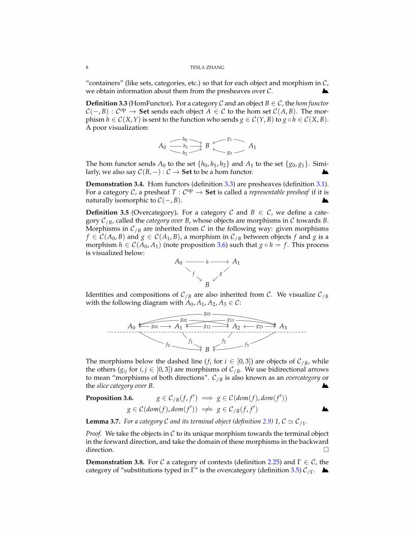
Definition 3.3 (HomFunctor). For a category C and an object B ∈ C, the hom functorC(−, B) : Cop → Set sends each object A ∈ C to the hom set C(A, B). The mor-phism h ∈ C(X, Y) is sent to the function who sends g ∈ C(Y, B) to g h ∈ C(X, B).A poor visualization:

A0 B A1h1

h0

h2 g0

g1

The hom functor sends A0 to the set h0, h1, h2 and A1 to the set g0, g1. Simi-larly, we also say C(B,−) : C → Set to be a hom functor.

Demonstration 3.4. Hom functors (definition 3.3) are presheaves (definition 3.1).For a category C, a presheaf T : Cop → Set is called a representable presheaf if it isnaturally isomorphic to C(−, B).

Definition 3.5 (Overcategory). For a category C and B ∈ C, we define a cate-gory C/B, called the category over B, whose objects are morphisms in C towards B.Morphisms in C/B are inherited from C in the following way: given morphismsf ∈ C(A0, B) and g ∈ C(A1, B), a morphism in C/B between objects f and g is amorphism h ∈ C(A0, A1) (note proposition 3.6) such that g h = f . This processis visualized below:

A0 A1

B

f

h

g

Identities and compositions of C/B are also inherited from C. We visualize C/Bwith the following diagram with A0, A1, A2, A3 ∈ C:

A0 A1 A2 A3

Bf1 f2f0 f3

g23g12

g13g01

g02

g03

The morphisms below the dashed line ( fi for i ∈ [0, 3]) are objects of C/B, whilethe others (gij for i, j ∈ [0, 3]) are morphisms of C/B. We use bidirectional arrowsto mean “morphisms of both directions”. C/B is also known as an overcategory orthe slice category over B.

Proposition 3.6. g ∈ C/B( f , f ′) =⇒ g ∈ C(dom( f ), dom( f ′))

g ∈ C(dom( f ), dom( f ′)) 6=⇒ g ∈ C/B( f , f ′)

Lemma 3.7. For a category C and its terminal object (definition 2.9) 1, C ' C/1.

Proof. We take the objects in C to its unique morphism towards the terminal objectin the forward direction, and take the domain of these morphisms in the backwarddirection.

Demonstration 3.8. For C a category of contexts (definition 2.25) and Γ ∈ C, thecategory of “substitutions typed in Γ” is the overcategory (definition 3.5) C/Γ.

TYPE THEORIES IN CATEGORY THEORY 9

Definition 3.9 (ArrowCat). For an arbitrary category C, the arrow category C→ (orArr(C)) is the category whose objects are morphisms in C. The morphisms inC→ are commutative diagrams in C. For example, for f0, f1 ∈ C→, the hom setC→( f0, f1) are pairs of morphisms (g0, h0) in C such that the following square com-mutes:

• •

• •f0

g0

f1h0

Composition in C is the composition of commutative diagrams. For example, thecomposition of (g0, h0) ∈ C→( f0, f1) and (g1, h1) ∈ C→( f1, f2) can be visualized inthis way:

• • •

• • •f0

g0

f1h0

g1

h1

f2

Lemma 3.10 (CodProj). The codomain projection cod : C→ → C and the domain projec-tion dom : C→ → C (notation 1.2) are functors from the arrow category (definition 3.9)of C to C.

Proof. The functorality follows directly from morphism composition in C.

3.1. Grothendieck fibrations.

Definition 3.11 (Cartesianness). For arbitrary categories E , C, a functor p : E → C,and objects Γ ∈ C and D, E ∈ E , a morphism f ∈ E(D, E) is called Grothendieckcartesian if for all D′ ∈ E and f ′ ∈ E(D′, E) such that p( f ) = p( f ′) ∈ C(Γ, p(E))(this implies p(D) = p(D′) = Γ ∈ C), there is a unique g ∈ E(D′, D) such thatp(g) = idΓ and f ′ = f g. We visualize the Grothendieck cartesianness of f as:

E p(E)

D′ D Γ

p( f )

g

f ′ f

The diagram shows why f is sometimes known as a terminal lifting. This definitionis due to Jacobs [Jac93, definition 2.1 (i)] and Grothendieck [Gro71].

History 3.12. The definition 3.11 is called cartesianness in [Jac93], but we pre-fix it with “Grothendieck” because there is another (newer) definition of carte-sianness of morphisms in category theory, which is discussed in definition 7.8.Grothendieck cartesianness is also known as weak cartesianness, where definition 7.8is also known as strong cartesianness.

Definition 3.13 (Fibration). For arbitrary categories E , C, objects Γ ∈ C and D ∈E , a functor p : E → C is called a Grothendieck fibration or a fibered category ifcomposition in E preserves Grothendieck cartesianness and for every E ∈ E andσ ∈ C(Γ, p(E)), there exists a Grothendieck cartesian morphism f ∈ E(D, E) such

10 TESLA ZHANG

that p( f ) = σ. We visualize the definition as:

E p(E)

D Γ

σfp

This definition is due to Jacobs [Jac93, definition 2.1 (iii)] and Grothendieck [Gro71].

Remark 3.14. A Grothendieck fibration (definition 3.13) is a functor p : E → Csuch that given a morphism f in C, we can determine some morphisms in E thatare sent to f by p.

Convention 3.15. We will refer to “Grothendieck fibrations” as “fibrations” in therest of this introduction since we do not discuss other kinds of fibrations.

Demonstration 3.16. The codomain projection functor cod : C→ → C (lemma 3.10)is a fibration (definition 3.13) if C has all pullbacks (definition 2.16). For a, b ∈ C→such that cod(a) = A ∈ C and cod(b) = B ∈ C, we visualize the fact that thecartesianness of f ∈ C(B, A) is equivalent to the existence of a pullback:

• B B

• A A

ff

a

b

y

There is a square and a line in the above visualization. The square is a morphismin C→ (from a towards b), and the line is a morphism in C.

Demonstration 3.17. The domain projection functor dom : C→ → C (lemma 3.10)is a fibration (definition 3.13). For a, b ∈ C→ such that dom(a) = A ∈ C anddom(b) = B ∈ C, we visualize the fact that f ∈ C(B, A) is cartesian:

B B •

A A •

f

a

g

b

f

Unlike in demonstration 3.16, C does not need to have pullbacks because the carte-sianness of f only requires the commutativity of the square.

3.2. Towards a comprehension category.

Definition 3.18 (Jacobs’ CompCat). A comprehension category is a structure consist-ing of a category (definition 2.25) C, a functorF : E → C→ preserving Grothendieckcartesianness of morphisms, and p := cod F : E → C a fibration (definition 3.13).We denote F0 = dom F due to Jacobs [Jac93, notation 4.2]. The definition of a

TYPE THEORIES IN CATEGORY THEORY 11

comprehension category commutes the following diagram:

• Γ

• • ∆ Γ

• • ∆ C

C→y

E

F0

p

F

We refer to the functor F as the (context) comprehension. The intuition of this nameis elaborated in definition 3.20.

Remark 3.19. Although p := cod F is a fibration in definition 3.18, cod is not nec-essarily a fibration because C may not have all pullbacks (see demonstration 3.16).We require the functor F to preserve Grothendieck cartesianness so that only theimage of F are Grothendieck cartesian morphisms.

Definition 3.20 (CtxExt). For a comprehension (definition 3.18) F : E → C→ andmorphism σ ∈ C(Γ, ∆) such that σ can be uniquely lifted (definition 3.11) to bothE and C→ since F preserves Grothendieck cartesianness. In case σ is lifted to amorphism in E(A, B), we denote F (A) as πA so that πA ∈ C/Γ and refer to themas display maps.

For all such object A ∈ E , we can uniquely determine an object πA ∈ C/Γ withF , whose domain is another object in C. We refer to this uniquely determinedobject dom(πA) as the context extended from Γ with A, denoted (Γ, A) ∈ C.

A visualization of (Γ, A) in the (sub)diagram in definition 3.18, recall that F0 :=dom F as mentioned in definition 3.18:

A Γ, A Γ

B ∆, B ∆

σ

πA

C→y

πB

Note that the right-half of the diagram is similar to a rotated version of the diagramin remark 2.30.

Remark 3.21 (Spoiler I). The definition 3.18 of a comprehension category gives usa basic sketch of a (dependent) type theory:

(1) Recall remark 2.32, we already interpreted contexts and substitutions in C.(2) Objects in E should be considered “dependent types”. It is in E that type

formation happens.(3) Introduction and elimination happen in C.(4) p(A) ∈ C is the context where the type A is formed within. So, A is a type

formed in the context p(A).(5) F allows us to add new types to a context, see definition 3.20.

We complete the interpretation formally in §4.

Definition 3.22 (CartLift). In the diagram in definition 3.13, we define D as σ∗(E)since it can be uniquely characterized by σ and E. We refer to f as the cartesianlifting of σ to E, denoted σ(E) : E(σ∗(E), E). The diagram can be redrawn in this

12 TESLA ZHANG

way, using much fewer variables:

E p(E)

σ∗(E) Γ

σσ(E)p

This entire diagram is uniquely determined by only two variables: σ and E.

3.3. Slightly higher categories.

Definition 3.23 (2-Cat). A strict 2-category C is a category such that for objectsA, B ∈ C, the hom sets f , g ∈ C(A, B) are also categories (called hom-categories),and the morphisms in all these categories compose if their domain and codomainmatch (this includes a lot of cases).

The objects of C are called 0-cells, the morphisms of C are called 1-cells or 1-morphisms, and the morphisms in C(A, B) are called 2-cells or 2-morphisms. Tovisualize a strict 2-category, we draw a random commutative square in a strict2-category, where for i ∈ [0, 3], Fi is a 1-cell and ti is a 2-cell:

• • • •

• • • •F0 F1

F3 F2

t3 t1

t2

t0

Remark 3.24. A formal definition of strict 2-categories is actually much more com-plex than definition 3.23, where we omit the preservation of identities and the de-tailed definition of compositions. By that, we capture the essential features of strict2-categories and get rid of the bureaucracy of dealing with associators.

Remark 3.25 (Enrichment). A strict 2-category (definition 3.23) is a special caseof an enriched category. We will define the notion of enrichment in §7, demonstra-tion 7.10.

Demonstration 3.26 (Cat). The category of small categories2, Cat, is a strict 2-category (definition 3.23), whose objects are small categories, 1-morphisms arefunctors, and 2-morphisms are natural transformations.

Definition 3.27 (Pseudofunctor). For strict 2-categories (definition 3.23) C, D andx, y, z ∈ C, a pseudofunctor F : C → D maps Ob(C) to Ob(D) and C(x, y) toD(F (x),F (y)). In particular, identities in C are mapped to some morphisms in Dthat are 2-isomorphic to identities, and the natural transformation t in the follow-ing diagram must be a natural isomorphism:

y z F (y) F (z) F (z)

x F (x) F (x)

g

fg f

F (g)

F ( f )

F (g)F ( f ) F (g f )t

2If you do not know what are small categories, think of them as categories.

TYPE THEORIES IN CATEGORY THEORY 13

Definition 3.28. The “functorality” condition of a pseudofunctor (definition 3.27)is not up to strict equality, but up to natural isomorphism. We refer to this notionas pseudofunctorality.

Warning 3.29. A Cat-valued (demonstration 3.26) pseudofunctor may not be apresheaf (definition 3.1) since presheaves must be functors (definition 3.27). Maybewe can call it a pseudopresheaf, but this terminology is unpopular (yet). A

3.4. Preparation for a category with attributes.

Definition 3.30 (Subcategory). For a category C, a subcategory H of C is a categorysuch that Ob(H) ⊂ Ob(C) and for A, B ∈ H, H(A, B) ⊂ C(A, B). The identitiesmust exist in the hom sets of H, and the hom sets of H must close under composi-tion.

Definition 3.31 (FullSub). For a category C, a full subcategory H of C is a subcate-gory (definition 3.30) of C such that the natural inclusion (terminology 1.3) functorι : H → C is fully faithful.

Definition 3.32 (FullSub). This is an alternative to definition 3.31. For a categoryC, a full subcategory H of C is a subcategory of C such that for every A, B ∈ H andevery f ∈ C(A, B), f ∈ H(A, B).

Definition 3.33 (Fiber). For categories E , C and a functor F : E → C, the fiber of Fover an object Γ ∈ C (denoted as EΓ) is a full subcategory (definitions 3.31 and 3.32)of E whose objects are mapped to Γ by F and morphisms are mapped to idΓ byF .

Terminology 3.34. In [Jac93, definition 2.2], Jacobs said that EΓ (definition 3.33)has objects above C, and it has vertical morphisms. The intuition of these termi-nologies is visualized in a rotated version of the diagram in definition 3.11, wherethe (E, D, D′)-triangle is “above” the (Γ, p(E))-line.

Definition 3.35 (Reindex). For a fibration p : E → C, morphisms σ ∈ C(Γ, ∆), andf ∈ E∆(D, E) (definition 3.33) (so that p(D) = p(E) = ∆ ∈ C and p( f ) = id∆),we can take the cartesian lifting (definition 3.22) of σ to both D and E – the objectsσ∗(D), σ∗(E) ∈ EΓ, to characterize the morphism σ∗( f ) in the following pullbacksquare:

σ∗(D) σ∗(E) Γ

D E ∆

σ

f

σ(D) σ(E)

σ∗( f )

y

We can observe that the cartesian lifting of σ ∈ C(Γ, ∆) to objects in E∆ are objectsin EΓ, and the morphisms in E∆ can also be lifted. Therefore we obtain a functorσ∗ : E∆ → EΓ for every σ ∈ C(Γ, ∆), called the reindexing functor.

Exercise 3.36. Define and prove the universal property of the pullback squarein definition 3.35.

Remark 3.37 (Spoiler II). In definition 3.35, the morphism σ ∈ C(Γ, ∆) induces thefunctor σ∗ : E∆ → EΓ. The second last deduction in remark 2.7 and the diagramin remark 2.30 show that given a substitution Γ ` σ : ∆, it can bring the type A in∆ to Γ. Recall the previous spoiler remark 3.21, We can think of σ∗ as the “actionto apply the substitution σ on a type”.

14 TESLA ZHANG

Definition 3.38 (Cleavage). For a fibration p : E → C, a particular choice of σ∗ andσ (definition 3.22) for every σ ∈ C(Γ, ∆) is called a cleavage of p. In other words, acleavage of p is a mapping from σ to the pair (σ∗, σ).

A cleavage of p is equivalent to a subcategory (definition 3.30) of E .

Remark 3.39. In definition 3.13, a fibration p : E → C is equipped with an oper-ation that takes a morphism σ and returns p−1(σ) a Grothendieck cartesian mor-phism. To some extent, p is an “invertible” functor: for a morphism f ′ in E , wecan send it to C by p and take it back to a cleavage (definition 3.38) f in E . Therelationship between f ′ and f is similar to the morphisms of the same name in def-inition 3.11.

Lemma 3.40 (Faker). For a fibration p : E → C, we have a pseudofunctor (defini-tion 3.27) Ψ : Cop → Cat by Ψ(Γ) := EΓ and for σ ∈ C(Γ, ∆), Ψ(σ) := σ∗.

Proof. We verify the pseudofunctorality of Ψ:• For Γ ∈ C, Ψ(idΓ) = id∗Γ ' idEΓ a natural isomorphism.• For σ ∈ C(Γ′, Γ′′) and γ ∈ C(Γ, Γ′) (so that σ γ ∈ C(Γ, Γ′′)), we know

Ψ(σ γ) = (σ γ)∗ and σ∗ γ∗ = Ψ(σ) Ψ(γ), and there is (σ γ)∗ 'σ∗ γ∗ a natural isomorphism.

Definition 3.41 (Split). We say a fibration p : E → C is split or cloven if the pseud-ofunctor Ψ (lemma 3.40) defined on it satisfies functorality instead of pseudofunc-torality. This requires the following strict equalities:

• For Γ ∈ C, id∗Γ = idEΓ .• For σ ∈ C(Γ′, Γ′′) and γ ∈ C(Γ, Γ′), (σ γ)∗ = σ∗ γ∗.

Demonstration 3.42. Ψ in a split fibration (definition 3.41) is a Cat-valued presheaf(definition 3.1).

Remark 3.43 (Coherence). If our comprehension category is not split, we willhave substitutions up to isomorphism instead of strict equality as discussed byCurien [Cur90].

Terminology 3.44. We say a comprehension category (definition 3.18) to be full ifthe comprehension F is fully faithful, and split if the underlying fibration p is split(definition 3.41).

3.5. Cartmell’s artifacts.

Definition 3.45 (Cartmell’s CwA). A category with attributes (CwA) is a full split(terminology 3.44) comprehension category. Note that the codomain C of the com-prehension has a terminal object.

We refer to the domain E of the comprehension as the attributes.

History 3.46. CwA was already well-established when comprehension categorywas discussed. The original definition of CwA is more similar to type categories(definition 5.6) where the dependent types indexed by an object in C forms a setinstead of a fiber in another category E . In this case, it is not (but similar to) a fullsplit comprehension category. We discuss the difference in remark 5.16.

Treating a CwA as a full split comprehension category is accepted in recentyears, though.

TYPE THEORIES IN CATEGORY THEORY 15

Definition 3.47 (Contextuality). A CwA (definition 3.45) F : E → C→ is contextualif there exists a length function ` : C →N such that:

(1) `(1) = 0, and for every Γ ∈ C, `(Γ) = 0 ⇐⇒ Γ = 1 holds. The terminalobject 1 must be unique.

(2) For every Γ ∈ C and A ∈ EΓ, `(Γ, A) = `(Γ) + 1 holds.(3) For every ∆ ∈ C where `(∆) > 0, there exists uniquely Γ ∈ C and A ∈ EΓ

such that ∆ = (Γ, A).In other words, the objects in C are generated from the terminal object and contextextension (definition 3.20), and we can do induction on it.

A similar definition can be found in [CCD19, definition 2].

Definition 3.48 (Cartmell’s CxlCat). A CwA satisfying contextuality (definition 3.47)is called a contextual category. This is essentially the definition in [Car86, §14],where objects are described as a tree.

Remark 3.49. In [Sco, definition 7], the length function (definition 3.47) is de-scribed as a grading of objects in C, where the objects are indexed by a naturalnumber. It is denoted Ob(C) := än:N Obn(C).

Definition 3.50 (Democracy). A CwA (definition 3.45) F : E → C→ is democraticif for every Γ ∈ C there is an object A ∈ E1 such that Γ ' (1, A). This definition isdue to [CCD19, definition 3].

4. CATEGORICAL SEMANTICS

Definition 4.1 (TT). A type theory consists of the following constructions, definedby typing judgments:

(1) Contexts, whose well-formedness is denoted Γ `. There is a well-formedempty context 1.

(2) Types formed in contexts, denoted Γ ` A type , and type equality, de-

noted Γ ` A = B type .

(3) Context extension. Given Γ ` A type , we can add A to the end of Γ toform a new context. We denote this process using the following rule:

Γ ` Γ ` A typeΓ, A `

(4) Substitution objects, whose well-formedness is denoted Γ ` σ : ∆. There isa well-formed empty substitution Γ ` [] : 1.

(5) Typing of terms. Given A formed in Γ, “term u is of type A” and “terms uand v are equal instances of type A” are described as:

Γ ` Γ ` A typeΓ ` u : A

Γ ` Γ ` A type Γ ` u : A Γ ` v : AΓ ` u = v : A

(6) Substitution extension. This is similar to context extension:

Γ ` ∆ ` ∆ ` A type Γ ` σ : ∆ Γ ` a : Aσ

Γ ` (σ, a) : (∆, A)

16 TESLA ZHANG

Remark 4.2. The type theory defined in definition 4.1 can be extended in manyways. We only discuss the essential parts here: the formation of contexts, depen-dent types, terms, and substitutions.

In definition 4.16 we extend the type theory with the Cartesian product type,and more constructions in the literature of type theory will be added in §6.

Warning 4.3 (Universe). We do not have any type that represents the universe typethat usually appear in a type theory, such as the intuitionistic type theory due toMartin-Löf [Mar75], the calculus of constructions due to Coquand [Coq85], and theextended calculus of constructions due to Luo [Luo90; Luo94].

We cannot have a type ` U type for all types (including ` U : U ) due to theparadox construction by Girard [Gir72] (and later simplified by Hurkens [Hur95]).

A

Definition 4.4. We interpret contexts and substitutions in a CwA (definition 3.45).(1) A context Γ is interpreted as an object in C, denoted JΓK ∈ C. In particular,

J1K := 1, the terminal object in C which is said to exists in definition 2.25.(2) A substitution Γ ` σ : ∆ is interpreted as a morphism in C, denoted JσK :C(JΓK, J∆K). The empty substitution is the morphism from an object to theterminal object 1, which always exists by the universal property of terminalobjects.

Definition 4.5. We interpret types and terms with their equalities in a CwA (defi-nition 3.45). For a context Γ in type theory and its interpretation JΓK ∈ C,

(1) The judgment Γ ` A type is interpreted as an object JAK ∈ EJΓK.(2) Two types A, B formed in context Γ are said to be equal (the judgment

Γ ` A = B type ) if their interpretations are uniquely isomorphic objectsin the fiber (definition 3.33) EJΓK.

(3) Context extension JΓ, AK is defined as (JΓK, JAK) ∈ C using the constructionin definition 3.20.

(4) We interpret judgments Γ ` a : A as Γ ` σ : (Γ, A) for some σ. We requireσ to satisfy that πJAK JσK = idJΓK (note that JσK ∈ C(JΓK, JΓ, AK)).

(5) Two terms u, v of the same type A are said to be equal (the judgment Γ `u = v : A) if their interpretations are uniquely isomorphic objects in theovercategory C/JΓK,JAK (note that their domains are both JΓK).

Remark 4.6. The interpretation of term/type equality in definition 4.5 is slightlydifferent from the one in [Pit01, §6.4], where they require sameness instead of uniqueisomorphism.

Terminology 4.7. In definition 4.5, the substitutions σ ∈ C(Γ, (Γ, A)) such thatπA σ = idΓ are called the global sections of A.

Exercise 4.8. Interpret substitution extension in a CwA.

Exercise 4.9 (Weakening). Interpret in a CwA the context weakening rule:

Γ ` Γ ` A type Γ ` u : A Γ ` B typeΓ, B ` u : A

TYPE THEORIES IN CATEGORY THEORY 17

Remark 4.10 (Strictness). The substitution operation is interpreted as morphismsin C. So, if two contexts are equivalent up to substitution, their cartesian lifting(definition 3.22) will be the same (instead of being naturally isomorphic categories)thanks to the strictness condition in definition 3.41.

4.1. Star at the top: the unit type.

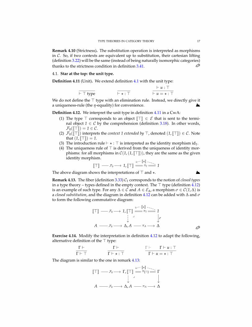
Definition 4.11 (Unit). We extend definition 4.1 with the unit type:

` > type ` ? : >` u : >` u = ? : >

We do not define the > type with an elimination rule. Instead, we directly give ita uniqueness-rule (the η-equality) for convenience.

Definition 4.12. We interpret the unit type in definition 4.11 in a CwA:(1) The type > corresponds to an object J>K ∈ E that is sent to the termi-

nal object 1 ∈ C by the comprehension (definition 3.18). In other words,F0(J>K) = 1 ∈ C.

(2) F0(J>K) interprets the context 1 extended by >, denoted (1, J>K) ∈ C. Notethat (1, J>K) = 1.

(3) The introduction rule ` ? : > is interpreted as the identity morphism id1.(4) The uniqueness rule of > is derived from the uniqueness of identity mor-

phisms: for all morphisms in C(1, (1, J>K)), they are the same as the givenidentity morphism.

J>K 1, J>K 1π1F0

J?K

The above diagram shows the interpretations of > and ?.

Remark 4.13. The fiber (definition 3.33) C1 corresponds to the notion of closed typesin a type theory – types defined in the empty context. The > type (definition 4.12)is an example of such type. For any ∆ ∈ C and A ∈ E∆, a morphism σ ∈ C(1, ∆) isa closed substitution, and the diagram in definition 4.12 can be added with ∆ and σto form the following commutative diagram:

J>K 1, J>K 1

A ∆, A ∆

σ

πA

π1F0

F0

J?K

y

Exercise 4.14. Modify the interpretation in definition 4.12 to adapt the following,alternative definition of the > type:

Γ `Γ ` >

Γ `Γ ` ? : >

Γ ` Γ ` u : >Γ ` u = ? : >

The diagram is similar to the one in remark 4.13:

J>K Γ, J>K Γ

A ∆, A ∆πA

πJ>KF0

F0

J?K

y

18 TESLA ZHANG

This version of > is similar to a combination of definition 4.12 and exercise 4.9.

Remark 4.15. In definition 4.12, we interpret the formation, introduction, andelimination rules for a type theoretical construction. Then, we prove the unique-ness rule. If there are other equalities that we can prove in the categorical modelbut cannot be derived from the type theory, we may add these equalities to makethe type theory more convenient to work with. This is a benefit we can gain fromcategorical models of type theory.

Unfortunately, the > type is too simple. In §4.2, we are going to see such anequality in theorema 4.18.

4.2. Like a semiring: the (co)product type.

Definition 4.16 (Product). We extend definition 4.1 with the (non-dependent) prod-uct type, using the same notation as product objects (definition 2.11):

Γ ` Γ ` A type Γ ` B typeΓ ` (A× B) type

Γ ` A type Γ ` B type Γ ` (A× B) type Γ ` u : A× BΓ ` u.1 : A and Γ ` u.2 : B

Γ ` A type Γ ` B type Γ ` u : A Γ ` v : BΓ ` 〈u, v〉 : A× B

Γ ` A type Γ ` B type Γ ` u : A Γ ` v : BΓ ` 〈u, v〉.1 = u : A and Γ ` 〈u, v〉.2 = v : B

Definition 4.17. The context Γ extended by the product type (definition 4.16) A× B,(Γ, A× B), is interpreted as the pullback (definition 2.16) (JΓK, JAK)×Γ (JΓK, JBK) ∈C, denoted (JΓK, JA× BK) ∈ C in a contextual category (definition 3.48).

Note that we are not talking about the product type itself, but instead, we definecontexts extended by a product type. By contextuality (definition 3.47), there is anobject JA× BK ∈ E that corresponds to this extended context.

The interpretation of the formation rule is visualized below:

JΓK, JA× BK JΓK, JBK

JΓK, JAK JΓK

πJA×BKπJBK

πJAK

y

In the introduction rule, the inputs are JuK, a global section (terminology 4.7) ofJAK, and JvK, a global section of JBK.

JΓK, JA× BK JΓK, JAK

JΓK, JBK JΓKJvK

yJuK

TYPE THEORIES IN CATEGORY THEORY 19

The introduction rule itself corresponds to the product morphism of JuK and JvK.The elimination rules are directly derived from the property of the product object.

JΓK, JA× BK JΓK, JAK

JΓK, JBK JΓK

elim2

elim1

JvK

JuKJ〈u,v〉Ky

Theorema 4.18 (Uniqueness). The interpretation in definition 4.17 satisfies the η-rulefor the product type:

Γ ` (A× B) type Γ ` t : A× BΓ ` t = 〈t.1, t.2〉 : A× B

Proof. By doing some replacements of terms in the last diagram in definition 4.17:

JΓK, JA× BK JΓK, JAK

JΓK, JBK JΓK

elim2

elim1

Jt.2K

Jt.1KJtKy

Definition 4.19 (Coproduct). We extend definition 4.1 with the coproduct type:

Γ ` Γ ` A type Γ ` B typeΓ ` (A t B) type

Γ ` (A t B) type Γ ` A type Γ ` u : AΓ ` inl(u) : A t B

Γ ` (A t B) type Γ ` B type Γ ` u : BΓ ` inr(u) : A t B

Γ ` (A t B) type Γ ` A type Γ ` B typeΓ ` C type Γ, A ` u : C Γ, B ` v : C Γ ` t : A t B

Γ ` match(t, u, v) : C

Γ ` A type Γ ` B type Γ ` C typeΓ, A ` u : C Γ, B ` v : C Γ ` t : A

Γ ` match(inl(t), u, v) = ut : C

Γ ` A type Γ ` B type Γ ` C typeΓ, A ` u : C Γ, B ` v : C Γ ` t : B

Γ ` match(inr(t), u, v) = vt : C

Note that in the two rules, ut and vt denote the operation of “applying thesingleton substitution object t” to the term u and v, respectively.

Remark 4.20. Type theoretically, the coproduct type is dual to the product type.Since product types are interpreted as pullbacks (see definition 4.17) which are

20 TESLA ZHANG

“products in the overcategory”, the coproduct types should look like “coproductsin the overcategory”.

Exercise 4.21. Interpret the coproduct type (definition 4.19) in a contextual cate-gory (definition 3.48). Beware of warning 7.14.

4.3. Internal homs and the evaluation map.

Definition 4.22 (StrMonCat). A category C is strictly monoidal if there is an oper-ation (called the tensor product) ⊗ such that for A, B ∈ C, A⊗ B ∈ C. Apart fromthat, the following additional properties must hold:

(1) For A, B, C, D ∈ C, f ∈ C(A, C), and g ∈ C(B, D), there is a morphismf ⊗ g ∈ C(A⊗ B, C⊗ D).

(2) There is an object 1 ∈ C, called the tensor unit, satisfying that for everyA ∈ C, A⊗ 1 = 1⊗ A = A.

(3) The tensor product of objects and morphisms are strictly associative.

Definition 4.23 (Bifunctor). For (small) categories C1, C2,D ∈ Cat, we take theproduct object (definition 2.11) C1 × C2 and refer to a functor F as a bifunctor if itof form F : C1 × C2 → D. We say that F is a bifunctor from C1, C2 to D.

Definition 4.24 (MonCat). The definition 4.22 can be loosen into the general no-tion of monoidal categories in order to allow tensor products that are not strictlycommutative (but up to isomorphism). We define⊗ as a bifunctor (definition 4.23)C ⊗ C → C, also called the tensor product, with the following additional structures:

(1) The tensor unit object 1 ∈ C.(2) For x, y, z ∈ C, an isomorphism αx,y,z ∈ C((x⊗ y)⊗ z, x⊗ (y⊗ z)).(3) For x ∈ C, two isomorphisms ρx ∈ C(x⊗ 1, x) and λx ∈ C(1⊗ x, x).

These structures commute the following diagrams:

(x⊗ 1)⊗ y x⊗ (1⊗ y)

((w⊗ x)⊗ y)⊗ z x⊗ y w⊗ (x⊗ (y⊗ z))

(w⊗ x)⊗ (y⊗ z)

(w⊗ (x⊗ y))⊗ z w⊗ ((x⊗ y)⊗ z)

αw⊗x,y,z αw,x,y⊗z

αw,x,y⊗idz

αw,x⊗y,z

αx,1,y

ρx⊗idy idx⊗λy

idw⊗αx,y,z

Definition 4.25 (CartMonCat). We say a monoidal category (definition 4.24) to becartesian if its tensor products are the product objects (definition 2.11) and its tensorunit is the terminal object (definition 2.9).

Definition 4.26 (SymMonCat). We say a monoidal category (definition 4.24) to besymmetric if its tensor product is commutative up to isomorphism. This definitionis slightly weaker than the conventional one, but it is simpler.

TYPE THEORIES IN CATEGORY THEORY 21

Definition 4.27 (ClosedSMCat). We say a symmetric monoidal category C (defini-tion 4.26) to be closed if for objects a, b, c ∈ C, there is an object [b, c] ∈ C (called aninternal hom) such that following three pairs of hom presheaves (definition 3.3) arenaturally isomorphic:

C(−⊗ b, c) ' C(−, [b, c])

C(a⊗−, c) ' C(a, [−, c])

C(a⊗ b,−) ' C(a, [b,−])

This is just an unnecessarily complicated way of saying that there is an equivalenceC(a⊗ b, c) ' C(a, [b, c]).

Definition 4.28 (EvalMap). In a symmetric monoidal closed category (definition 4.27)C, its objects a, b, c ∈ C, and a morphism f ∈ C(a⊗ b, c), by the equivalences in def-inition 4.27 we can obtain the unique morphism λ. f ∈ C(a, [b, c]) commuting thefollowing diagram:

a⊗ b

[b, c]⊗ b c

λ. f⊗idb

eval

f

The morphism eval is therefore a unique isomorphism. We refer to this morphismas the evaluation map for the internal hom [b, c].

Lemma 4.29 (Internalization). In a symmetric monoidal closed category (definition 4.27)C, its tensor unit (definition 4.24) 1 ∈ C, and objects b, c ∈ C, there is an isomorphismC(b, c) ' C(1, [b, c]).

Proof. By specializing the object a in the equivalence in definition 4.27 to 1:

C(1, [b, c]) ' C(1⊗ b, c) ' C(b, c)

Lemma 4.30. The tersor unit used in lemma 4.29 can be replaced with any object a ∈ Csuch that a⊗ b ' b.

4.4. Locally cartesian closed contextual categories and fiber exponents.

Definition 4.31 (CCC). We say a symmetric closed monoidal category (defini-tion 4.27) to be cartesian if it is also cartesian monoidal (definition 4.25). In thiscase, the category is called a cartesian closed category, or CCC. The internal homsof a CCC are also known as exponential objects and we denote [b, c] as cb.

Demonstration 4.32 (FunctionSet). Since functions are sets too and they satisfythe natural isomorphisms in definition 4.27, Set is a CCC (definition 4.31). Theevaluation map (definition 4.28) in Set is just function application: for A, B ∈ Set,the internal hom (definition 4.27) A→ B has the evaluation map eval ∈ Set((A→B)× A, B).

Lemma 4.33. In a CwA (definition 3.45) F : E → C→ where C has pullbacks (in thesense of product types as in definition 4.17), for Γ ∈ C and A ∈ EΓ, Γ×Γ (Γ, A) ' Γ, A.

Proof. By the second projection of the pullback in the forward direction and πA×ΓidΓ,A in the backward direction.

22 TESLA ZHANG

Definition 4.34 (LCCC). We say a category C to be a locally cartesian closed categoryor an LCCC if the overcategory C/Γ for every Γ ∈ C is cartesian closed. The relationbetween LCCC and type theories has been explored by Seely and Hofmann [See84;Hof94].

Lemma 4.35. An LCCC (definition 4.34) is a CCC (definition 4.31) if it has a terminalobject.

Proof. Consider an LCCC C with a terminal object 1, we know that C/1 is a CCC.By lemma 3.7, C is a CCC.

Lemma 4.36. In an LCCC (definition 4.34) C and Γ, A, B ∈ C, the cartesian product inCΓ is given by the pullback A×Γ B ∈ C.

Definition 4.37 (FiberExp). In an LCCC (definition 4.34) C, for Γ, A, B ∈ C, a ∈C(A, Γ), and b ∈ C(B, Γ) (so that a, b ∈ C/Γ), the fiber exponent A →Γ B is thedomain of the exponential object ba ∈ C/Γ. The name is inspired from the alias“fiber product” of pullbacks (definition 2.16) and “fiber coproduct” of pushouts(definition 7.1). Visualization:

B A

A→Γ B Γ

ab

ba

Note that by lemma 4.29, there is an isomorphism C/Γ(a, b) ' C/Γ(1C/Γ, ba).

4.5. Simple type theory: the function type.

Definition 4.38 (Function). We extend definition 4.1 with the function type, de-fined by the following rules:

Γ ` Γ ` A type Γ ` B typeΓ ` (A→ B) type

Γ ` (A→ B) type Γ ` A type Γ ` B type Γ, A ` u : BΓ ` λ.u : A→ B

Γ ` (A→ B) typeΓ ` A type Γ ` B type Γ ` u : A→ B Γ ` v : A

Γ ` ap(u, v) : B

Γ, A ` Γ ` B type Γ, A ` u : B Γ ` v : AΓ ` ap(λ.u, v) = uv : B

Definition 4.39. In a contextual category (definition 3.48) F : E → C→ where C isan LCCC, we can interpret definition 4.38.

Consider types Γ ` A type, Γ ` B type, Γ ` C type . The formation of context Γextended by the function type A→ B is the fiber exponent (definition 4.37) (JΓK, JAK)→JΓK

TYPE THEORIES IN CATEGORY THEORY 23

(JΓK, JBK), denoted (JΓK, JA → BK) ∈ C, whose display map (definition 3.20) isgiven by the exponential object πJA→BK = π

πJAKJBK ∈ C/JΓK.

JΓK, JBK JΓK, JAK

JΓK, JA→ BK JΓK

πJAKπJBK

πJA→BK

The introduction rule takes a morphism JuK ∈ C((JΓK, JAK), (JΓK, JBK)) such thatπJBK JuK = πJAK to the morphism Jλ.uK ∈ C(JΓK, (JΓK, JA → BK)) by the isomor-phism in definition 4.37:

JΓK, JBK JΓK, JAK

JΓK, JA→ BK JΓK

πJAKπJBK

Jλ.uK

JuK

The rest of the rules involve the fiber product (JΓK, JA → BK)×JΓK (JΓK, JAK) ∈ C.For simplicity, we denote it as “data”, and we denote idJΓK,JA→BK×JΓK ( f πJA→BK)

as data( f ) for morphism f ∈ C(JΓK, (JΓK, JAK)).The elimination rule is interpreted by morphism composition and the evalua-

tion map (definition 4.28), visualized as the following diagram which commuteseverywhere:

data JΓK, JBK JΓK, JAK

JΓK, JA→ BK JΓKJuK

JvKy eval

data(JvK) Jap(u,v)K

The fact that the evaluation map (definition 4.28) is a unique isomorphism showsthat the β-equality of this interpretation holds:

data JΓK, JBK JΓK, JAK

JΓK, JA→ BK JΓKJλ.uK

JvKy eval

data(JvK) JuKJvK

JuK

5. ALTERNATIVE CONSTRUCTIONS

Definition 5.1 (DiscreteCat). We say a category C to be discrete if it has no mor-phism other than identity morphisms.

Proposition 5.2. C is discrete ⇐⇒ C ' Ob(C).

Definition 5.3 (Discreteness). We say a fibration p : E → C to be discrete if eachfiber (definition 3.33) is discrete (definition 5.1).

Remark 5.4. In the literature, we sometimes ask the fibration p of a CwA (defini-tion 3.45) to be a discrete fibration (definition 5.3). This is what Pitts [Pit01, §6] hasdone implicitly (without mentioning the notion of fibrations (definition 3.13) andcomprehension categories (definition 3.18)).

24 TESLA ZHANG

Definition 5.5 (Fam). The category of indexed families of sets, Fam, consists ofthe following:

(1) Objects (Ux)x∈X , where X is a set and for each x ∈ X, Ux is a set.(2) Morphisms ( f , (gx)x∈X) ∈ Fam((Ux)x∈X , (Vy)y∈Y), where f : X → Y is a

function (called the reindexing function, similar to definition 3.35) and foreach x ∈ X, gx : Ux → Vf (x) is a function.

5.1. Type categories.

Definition 5.6 (Pitts’ TypeCat). A type category consists of:(1) A category C, in analog to the category of contexts (definition 2.25).(2) A presheaf (definition 3.1) Ty : Cop → Set. We refer to Ty(Γ) as the set of

dependent types indexed by Γ.(3) A context extension operation, constructing (Γ, A) ∈ C from A ∈ Ty(Γ).(4) A projection morphism πA ∈ C((Γ, A), Γ), the inverse of context extension.

We also require the object (∆, σ∗A) ∈ C (where σ∗A ∈ Ty(∆) is called the pullbackof A along ∆) and the morphism σA : C((∆, σ∗A), (Γ, A)) to exist (assuming Γ ∈C, ∆ ∈ C, A ∈ Ty(Γ)) by the following pullback square:

∆, σ∗A Γ, A

∆ Γ

πσ∗A

σA

πA

σ

y

The following strictness condition must hold in the pullback square:

id∗Γ A = A idAΓ = idΓ,A

γ∗(σ∗A) = (σ γ)∗A σA γσ∗A = (σ γ)A

This definition is due to [Pit01, definition 6.3.3].

Remark 5.7. The “projection morphism” in definition 5.6 is similar to the “displaymaps” in definition 3.20, and the pullback square in definition 5.6 is similar to thepullback square in remark 2.30.

Lemma 5.8. For Γ ∈ C, the set Ty(Γ) has an embedding in the objects in the overcategory(definition 3.5) C/Γ.

Proof. By mapping A ∈ Ty(Γ) to πA ∈ C((Γ, A), Γ).

Remark 5.9. By lemma 5.8, we may add morphisms between the elements of Ty(Γ)to form a category in order to put more categorical structures into it. This willmake Ty into a functor Ty : Cop → Cat, similar to the functor Ψ : Cop → Cat(lemma 3.40) in a split (definition 3.41 and terminology 3.44) comprehension cate-gory (since we have the strictness conditions in definition 5.6).

Notation 5.10. We define two syntactical shorthands for type categories (defini-tion 5.6) for convenience.

• For A ∈ Ty(1), we write A ∈ C for (1, A) ∈ C.• TyΓ(A, B) for the hom set Ty(Γ)(A, B).

Definition 5.11 (TyMor). The hom set TyΓ(A, B) is defined as the hom set C/Γ(πA, πB).Identities and compositions are inherited from C. This realizes remark 5.9.

TYPE THEORIES IN CATEGORY THEORY 25

Lemma 5.12. Ty(Γ) is a full subcategory (definitions 3.31 and 3.32) of C/Γ if for everyA 6= B ∈ Ty(Γ), (Γ, A) 6= (Γ, B) ∈ C.

Proof. By definition 5.11.

Theorema 5.13. A discrete (definition 5.3) CwA (definition 3.45) is equivalent to a typecategory (definition 5.6).

Proof. We try to equate a CwA with a type category by identifying:

(1) The category interpreting contexts C. Both of them have such categories.(2) The category of Γ-indexed dependent types for Γ ∈ C. This is called Ψ(Γ)

in a CwA and Ty(Γ) in a type category. Ty(Γ) is a set, while Ψ(Γ) is also aset (since being discrete).

(3) The context comprehension operation. We have this operation in the defi-nition of a type category, and we have constructed the same operation in aCwA in definition 3.20.

(4) See lemma 5.14.

Lemma 5.14. The context comprehension in a CwA satisfies the pullback square in defi-nition 5.6.

Proof. We define the following category ΣΨ (recall lemma 3.40) on a CwA (defini-tion 3.45), which is a construction due to Pitts [Pit01, example 6.3.9] and Grothendieck:

• Objects are pairs (Γ, A) for Γ ∈ C and A ∈ Ψ(Γ) a category.• Morphisms are pairs (σ, f ) ∈ ΣΨ((Γ, A), (∆, B)) for σ ∈ C(Γ, ∆) and f :

A → Ψ(σ)(B) (note Ψ(σ)(B) = σ∗(B)) a functor whose domain andcodomain are both in Ψ(Γ).

We construct the following pullback square:

(Γ, A) (∆, B)

Γ ∆

(σ, f )

πA

σ

πBy

The (fully faithful) functorality (definition 3.41) of Ψ says that f is an equivalenceand the composition of substitution objects σ is therefore strictly associative. Thissatisfies the strictness conditions required by the square in definition 5.6.

Exercise 5.15. Define the composition and identities of ΣΨ in lemma 5.14.

Remark 5.16. The original definition of a CwA is discrete (and is almost the sameas a type category), which means that the morphisms in the fibers in E are allidentity morphisms. In definition 3.45, on the other hand, we allow arbitrary mor-phisms in E as long as F preserves cartesianness and p is a full split fibration.

The benefit of defining a CwA based on a comprehension category is that com-prehension categories are appreciated by mathematicians since they have theirown well-established fibrations. Curious readers may refer to [Jac93, example4.10].

26 TESLA ZHANG

5.2. Categories with families.

Definition 5.17 (Dybjer’s CwF). A category with families (CwF) [CCD19; Dyb96;Hof97] is a structure consisting of:

(1) A category interpreting contexts (definition 2.25) C.(2) A Fam-valued presheaf T : Cop → Fam (definitions 3.1 and 5.5).(3) A context comprehension operation defined in definition 5.21. It is similar

to definitions 3.20 and 5.6.

Remark 5.18. We can also have a contextual (definition 3.47) CwF by requiring an` operation on its C category, or a democratic (definition 3.50) CwF by requiringsuch types to exists.

Notation 5.19. We have the following syntactical shorthands:(1) Ty(Γ) = X for Γ ∈ C if T(Γ) = (Ux)x∈X . In fact, Ty is a presheaf.(2) Tm(Γ, A) = UA for A ∈ Ty(Γ) if T(Γ) = (Ux)x∈X .(3) For a substitution object σ ∈ C(Γ, ∆), there exist the following function:

T(σ) : (Tm(∆, A))A∈Ty(∆) → (Tm(Γ, B))B∈Ty(Γ).

Definition 5.20 (Substitution). The morphism T(σ) in notation 5.19 consists of twomaps:

(1) A reindexing map σ∗ : Ty(∆) → Ty(Γ) called the substitution on types,similar to definition 3.35.

(2) A map σ∗ : Tm(∆, A)→ Tm(Γ, σ∗(A)) called the substitution on terms.Note that the names of these two maps are overloaded. These maps constitute thefollowing commutative square:

Γ Ty(Γ) Tm(Γ, σ∗(A))

∆ Ty(∆) Tm(∆, A)

σ σ∗ σ∗

Beware of the directions of the arrows. A substitution σ ∈ C(Γ, ∆) brings typesformed in ∆ to Γ, as discussed in remark 3.37.

Definition 5.21 (Comprehension). For Γ ∈ C and A ∈ Ty(Γ), the context comprehen-sion of a CwF consists of an assigned context Γ · A and two functions pΓ,A : Γ · A→Γ (which is also a substitution (definition 5.20)) and qΓ,A ∈ Tm(Γ · A, (pΓ,A)

∗(A)),such that the following property holds:

For every σ ∈ C(Γ, ∆), A ∈ Ty(∆), and a ∈ Tm(Γ, σ∗(A)), a substitution ob-ject σ · a ∈ C(Γ, ∆ · A) is uniquely identified such that p∆,A (σ · a) = σ and(σ · a)∗q∆,A = a. The characterization is visualized in the following commutativeparallelogram:

∆ · A ∆

σ∗(A) Γ

σ·aσ

p∆,A

q∆,A

a

Theorema 5.22. A CwF is equivalent to a type category.

Proof. We try to equate a CwF with a type category by identifying:

TYPE THEORIES IN CATEGORY THEORY 27

(1) The category interpreting contexts C. Both of them have such categories.(2) The (discrete) category of Γ-indexed dependent types for Γ ∈ C. They are

called Ty(Γ) in both categories, both are sets.(3) The set of terms of type A in a CwF is Tm(Γ, A), while in a type category

it is just the set of global sections (terminology 4.7) of A ∈ C.

Exercise 5.23. Prove that the context comprehension operation in a CwF (defini-tion 5.21) and a type category (definition 5.6) are equivalent.

Corollary 5.24. A CwF is equivalent to a CwA.

Proof. By theoremata 5.13 and 5.22.

Remark 5.25. We consider a CwF (definition 5.17) as a CwA (definition 3.45) or atype category (definition 5.6) with additional but unnecessary structures.

Remark 5.26. The structure of a CwF is very close to the syntax of type theory– both the formation of contexts and types and the typing of substitutions andterms have a direct correspondence to a “belong to” relation in a CwF. In [CCD19],Castellan even used the notation of substitution from type theory directly (_[γ]instead of γ∗), but we avoid their notation for consistency with the rest of thisintroduction.

Terminology 5.27. The model of type theory based on a CwF (definition 5.17) isknown as the presheaf model since the notion of “dependent types defined in acontext” is interpreted as a presheaf.

6. DEPENDENT TYPE THEORY

Definition 6.1 (Monic). We say a morphism f ∈ C(A, B) to be a monomorphism, amono, or monic if for every C ∈ C and g1, g2 ∈ C(C, A) such that:

f g1 = f g2 =⇒ g1 = g2

Holds. A monomorphism is also known as a left-cancallative morphism. The aboveequality is visualized below:

C A Bg1g2

f

Demonstration 6.2 (Injection). In Set, a morphism is monic (definition 6.1) if andonly if it is an injective function.

Definition 6.3 (Monic). This is an alternative to definition 6.1. In a category C,if for every C ∈ C the hom functor (definition 3.3) C(C,−) takes f ∈ C(A, B) toinjective functions C(C, f ) : C(C, A)→ C(C, B), we say f to be monic.

Lemma 6.4 (MonoIso). If for a mono (definitions 6.1 and 6.3) f , there exist a morphismg such that f g = idcod( f ), then f is an isomorphism.

Proof. f g f = idcod( f ) f = f = f iddom( f ) and by the definition of mono andthe associativity of composition g f = iddom( f ). Thus f an isomorphism.

Remark 6.5. There is an intuitive justification of lemma 6.4: in Set, invertible andinjective (see demonstration 6.2) functions are isomorphisms.

28 TESLA ZHANG

Lemma 6.6 (IsoMono). If for an isomorphism f , there exist morphisms g1, g2 such thatg1 f = g2 f , then g1 = g2.

Proof. g1 = g1 f f−1 = g2 f f−1 = g2.

6.1. Equalizers: the extensional equality type.

Remark 6.7 (McBride). We begin this section with a quotation by Conor McBridefrom his suspended Twitter account3:

Never trust a type theorist who has not changed their mind aboutequality.

Definition 6.8 (Id). We extend definition 4.1 with the following type:

Γ ` Γ ` A type Γ ` a : A Γ ` b : AΓ ` (IdA a b) type

Γ ` A type Γ ` a : AΓ ` refla : IdA a a

Γ ` A type Γ ` a : A Γ ` b : A Γ ` p : IdA a bΓ ` a = b : A

This type is known as the extensional equality type, in contrast to the intensionalequality type. We will only talk about the extensional one for convenience.

Terminology 6.9. The introduction rule in definition 6.8 is known as the rule forreflexivity, and the elimination rule is known as equality reflection.

Definition 6.10 (Equalizer). In a category C and for f , g ∈ C(X, Y) (we refer topairs of morphisms like this as parallel morphisms), there might be some objectsE ∈ C together with morphisms of form e ∈ C(E, X) commuting the followingdiagram (so that f e = g e ∈ C(E, Y)):

E X Yfge

We take the terminal object of the full subcategory (definitions 3.31 and 3.32) ofC/X commuting the above diagram which consists of morphisms like e, and referto the object E (denoted Eq( f , g)) and the morphism e (denoted eq( f , g)) as theequalizer of f and g. We bring these notations into the diagram above:

Eq( f , g) X Yfgeq( f ,g)

In case each parallel morphisms in C has an equalizer, we say that C has all equaliz-ers. The definition of equalizers is from [EH63].

Lemma 6.11. A category C has all equalizers (definition 6.10) if it has a terminal objectand all pullbacks (definition 2.16).

3https://twitter.com/pigworker

TYPE THEORIES IN CATEGORY THEORY 29

Proof. By lemma 2.19 we know C has products. We construct the equalizer forarbitrary parallel morphisms f , g ∈ C(X, Y):

Eq( f , g) X

Y Y×Y(idY ,idY)

eq( f ,g)

( f ,g)y

Lemma 6.12 ([EH63, Proposition 1.3]). For a category C and f , g ∈ C(X, Y), eq( f , g)is monic (definition 6.1).

Lemma 6.13. In a category C and a morphism f ∈ C(X, Y), the equalizer of f and f isidX .

Definition 6.14. We interpret the extensional identity type in a contextual cate-gory (definition 3.48) as an equalizer (definition 6.10). The formation of the con-text Γ extended by IdA a b (denoted (JΓK, JIdA a bK) ∈ C) is by taking the equal-izer Eq(JaK, JbK), where the display map (definition 3.20) is given by the equalizer:πJIdA a bK = eq(JaK, JbK):

JΓK, JAK JΓK JΓK, JIdA a bKJaKJbK

eq(JaK,JbK)

By lemma 6.13, eq(JaK, JaK) = idJΓK. So, we define JreflaK = idJΓK:

JΓK, JAK JΓK JΓK, JIdA a aKJaK JreflaK

In case we have a morphism f corresponding to an instance of the identity type, itis an inverse to the equalizer (eq(JaK, JbK) f = idJΓK,JIdA a bK), and by lemma 6.4 fis an isomorphism. Then, by lemma 6.6 JaK = JbK holds, and that makes sense ofthe elimination rule:

JΓK, JAK JΓK JΓK, JIdA a bKJaK

JbK f

eq(JaK,JbK)πJAK

Lemma 6.15 (UIP). The interpretation in definition 6.14 gives rise to the following“uniqueness of the identity proof” rule:

Γ ` A type Γ ` a : A Γ ` p : IdA a aΓ ` p = refla : IdA a a

Proof. By lemma 6.13 and the uniqueness of the identity morphism. For visualiza-tion, see the second diagram in definition 6.14.

Theorema 6.16 (Uniqueness). The interpretation in definition 6.14 gives rise to thefollowing “uniqueness rule” of the identity type:

Γ ` A type Γ ` a : A Γ ` b : AΓ ` p : IdA a b Γ ` q : IdA a b

Γ ` p = q : IdA a b

Proof. (Type theory perspective) By equality reflection, the existence of p and qimplies a = b, so p and q are also instances of IdA a a, and by lemma 6.15 they areboth equal to refla.

30 TESLA ZHANG

Proof. (Categorical perspective) JpK eq(JaK, JbK) = JqK eq(JaK, JbK), and thenJpK = JqK since eq(JaK, JbK) is monic.

6.2. Locally cartesian closed categories: the dependent product type.

Definition 6.17 (Pi). We extend definition 4.1 with the dependent product type,defined by the following typing rules:

Γ ` Γ ` A type Γ, A ` B typeΓ ` (ΠAB) type

Γ ` (ΠAB) type Γ, A ` B type Γ, A ` u : BΓ ` Λ.u : ΠAB

Γ ` (ΠAB) type Γ ` A type Γ, A ` B type Γ ` u : ΠAB Γ ` v : AΓ ` ap(u, v) : Bv

Γ ` (ΠAB) type Γ ` A type Γ, A ` B type Γ, A ` u : B Γ ` v : AΓ ` ap(Λ.u, v) = uv : Bv

Definition 6.18 (DepProd). Consider an LCCC (definition 4.34) C, Γ, A, B ∈ C,a ∈ C(A, Γ), bC(B, A). Observe that b a ∈ C(B, Γ).

Then, since C is an LCCC, C/Γ is a CCC (definition 4.31), so we can take theexponential object of a and b a, denoted (b a)a ∈ C/Γ. We denote the fiberexponent (definition 4.37) as ΠAB = dom((b a)a) ∈ C, and for every Q ∈ C, q ∈C(Q, Γ), we have C/Γ(q× a, b a) ' C/Γ(q, (b a)a).

By the definition of overcategories (definition 3.5), the above isomorphism isalso an isomorphism in C, written as C(Q × A, B) ' C(Q, ΠAB). Diagrammati-cally, the morphisms “left” and “right” below are in isomorphic hom sets:

Q× A Q

B A Γ ΠABa (ba)a

qq×aleft right

b

We refer to ΠAB as a dependent product.

Notation 6.19. In case we are working in a contextual category (definition 3.48)and A, B, Q corresponds to the extended contexts (Γ, A′), (Γ, B′), (Γ, Q′) ∈ C anda, b, q corresponds to the display maps (definition 3.20) πA′ , πB′ , πQ′ , we writeΠA′B′ for ΠAB and refer to (πB′ πA′)

πA′ as πΠA′B′

Lemma 6.20. In a CwA (definition 3.45) F : E → C→ where C is an LCCC (defini-tion 4.34), for Γ ∈ C, A ∈ EΓ, and B ∈ EΓ,A, there is an isomorphism C((Γ, A), (Γ, A, B)) 'C(Γ, (Γ, ΠAB)).

TYPE THEORIES IN CATEGORY THEORY 31

Proof. By specializing the object Q to Γ, the morphisms a, b, q to πA, πB, πQ in thediagram in definition 6.18:

Γ× (Γ, A) Γ

Γ, A, B Γ, A Γ Γ, ΠABπA (πBπA)πA

right

πB

left

Now, we have an isomorphism C(Γ× (Γ, A), (Γ, A, B)) ' C(Γ, (Γ, ΠAB)). By lemma 4.33,we can replace Γ× (Γ, A) with (Γ, A).

Notation 6.21. In an LCCC C, by the equivalence in lemma 6.20, for a morphismf ∈ C((Γ, A), (Γ, A, B)) we can uniquely obtain a morphism Λ. f ∈ C(Γ, (Γ, ΠAB)).The diagram in the proof of lemma 6.20 can be simplified as:

Γ, A Γ

Γ, A, B Γ, ΠAB

f Λ. f

Lemma 6.22 (EvalMap). In an LCCC C and for Q, A, B ∈ C, f ∈ C(Q× A, B), thereis a unique isomorphism ΠAB× A ' B.

Proof. The following diagram is uniquely determined by the choice of f (using no-tation 6.21):

Q× A ΠAB× A

B

(Λ. f )×idA

f eval

Definition 6.23. We interpret the dependent product type (definition 6.17) in acontextual category F : E → C→ where C is an LCCC (definition 4.34). The in-troduction and elimination rules are just morphism compositions in the followingdiagram, omitting the semantic brackets since we are not distinguishing the inter-pretations and their type theoretical counterparts:

Γ, A, B Γ, A×ΠAB Γ, ΠAB

Γ, A Γa

Λ.uu

evaly

a×(Λ.u)

The input of the introduction rule is u, and we take it to Λ.u ∈ C(Γ, (Γ, ΠAB)). Inthe elimination rule, the input is the product a× (Λ.u), and the commutativity ofthe diagram justifies the β-equality of the dependent product type.

6.3. Subobject classifiers: the universe of all propositions.

Definition 6.24 (Prop). We extend definition 4.1 with a type Prop, defined by thefollowing typing rules:

32 TESLA ZHANG

` Prop typeΓ ` p : Prop

Γ ` El(p) typeΓ ` p : Prop Γ ` u : El(p) Γ ` v : El(p)

Γ ` u = v : El(p)

Γ ` A type Γ ` p : Πx:AΠy:AIdA x yΓ ` R(A, p) : Prop

We can think of R as an injective function that maps the unique instance (whenexists) of a type into an instance of Prop.

Demonstration 6.25 (Truth). The unit type (definition 4.11), >, has a correspond-ing proposition (definition 6.24) R(>, Λ.Λ.refl?) : Prop.

Terminology 6.26. When talking about the instances of a type, we say that the typeis inhabited if it has at least one instance, and these instances are called inhabitants.

If the type has no instance, we say it is uninhabited.

Remark 6.27. The definition 6.24 is an imitation of the Prop universe in the (ex-tended) calculus of constructions [Coq85; Luo90; Luo94], which can be regarded asthe type of all types (called propositions) that “have either one single inhabitant (ter-minology 6.26) or have no instance at all”. The second last rule in definition 6.24captures such uniquely inhabited property of propositions.

By having a universe for some types (propositions), we partially addresses warn-ing 4.3.

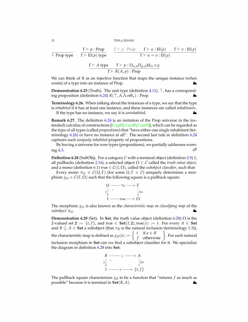
Definition 6.28 (SubObj). For a category C with a terminal object (definition 2.9) 1,all pullbacks (definition 2.16), a selected object Ω ∈ C called the truth value object,and a mono (definition 6.1) true ∈ C(1, Ω), called the subobject classifier, such that:

Every mono πU ∈ C(U, Γ) (for some U, Γ ∈ C) uniquely determines a mor-phism χU ∈ C(Γ, Ω) such that the following square is a pullback square:

U Γ

1 Ω

1

true

πU

χUy

The morphism χU is also known as the characteristic map or classifying map of thesubobject πU .

Demonstration 6.29 (Set). In Set, the truth value object (definition 6.28) Ω is the2-valued set 2 := t, f , and true ∈ Set(1, 2), true(x) := t. For every A ∈ Setand B ⊆ A ∈ Set a subobject (that πB is the natural inclusion (terminology 1.3)),

the characteristic map is defined as χB(a) :=

t if a ∈ Bf otherwise

. For each natural

inclusion morphism in Set can we find a subobject classifier for it. We specializethe diagram in definition 6.28 into Set:

B A

1 t, f 1

t

⊆

χBy

The pullback square characterizes χB to be a function that “returns f as much aspossible” because it is terminal in Set(B, A).

TYPE THEORIES IN CATEGORY THEORY 33

Definition 6.30. We interpret the universe of propositions (definition 6.24) in acontextual category (definition 3.48) with a subobject classifier (definition 6.28)defined as demonstration 6.25.

Consider a type Γ ` A type , it is a proposition when uniquely inhabited (ter-minology 6.26) by Γ ` u : A or uninhabited. In the following diagram, the contextΓ extended by the proposition A is the pullback (JΓK, JAK) ∈ C, and the interpretationof the Prop universe is the truth object:

JΓK, JAK JΓK

1 JPropK

πJAK

JR(A,p)K

JR(>,Λ.Λ.?)K

y

(1) Since πJAK is mono, its inverse JuK ∈ C(JΓK, (JΓK, JAK)) (if exists) must beunique. This uniqueness justifies the uniqueness rule of propositions andis guaranteed by the proof p.

(2) For every proposition A, we define a (unique) term R(A, p) ∈ Prop thatcorresponds to A. The uniqueness justifies the extensionality (see theo-rema 6.31) of Prop and the existence justifies the completeness.

(3) The El(−) operation takes a morphism A ∈ C(JΓK, JPropK) (which is aninstance of Prop) on the left of the above diagram and returns the pullback.To some extent, El(−) and R(−, p) are inverse to each other.

Theorema 6.31 (Extensionality). The extensionality of propositions holds in the inter-pretation in definition 6.30:

Γ ` A type Γ ` p : Πx:AΠy:AIdA x yΓ ` B type Γ ` q : Πx:BΠy:BIdB x y

Γ ` R(A, p) = R(B, q) : Prop

Theorema 6.32. For any type A and its instances x : A, y : A, IdA x y is a proposition.In other words, the following type is inhabited:

Πx:AΠy:AΠi:IdA x yΠj:IdA x yIdIdA x y i j

Proof. By theorema 6.16 we can prove it by reflexivity: uip := Λx.Λ.Λ.Λ.reflreflx(alternatively we can write uip := Λ.Λy.Λ.Λ.reflrefly ).

6.4. Internalized constructions.

Definition 6.33 (Bool). We define a type Bool in the type theory in definition 4.1with the extensions (definitions 4.11 and 4.19) as:

(1) Bool := >t>.(2) true := inl(?).(3) false := inr(?).(4) 〈t ? u : v〉 := match(t, u, v).

From the above definition, we can derive the following typing rules for Bool:

34 TESLA ZHANG

Γ `Γ ` Bool type

Γ `Γ ` true : Bool and Γ ` false : Bool

Γ ` A type Γ ` u : A Γ ` v : A Γ ` t : BoolΓ ` 〈t ? u : v〉 : A

Γ ` A type Γ ` u : A Γ ` v : A Γ ` t : BoolΓ ` 〈true ? u : v〉 = u : A and Γ ` 〈false ? u : v〉 = u : A

Definition 6.34 (PropTrunc). For every well-formed type Γ ` A type , we define

a type Γ ` ||A|| type , called the propositional truncation of A:

(1) ||A|| := ∏P:Prop(A→ El(P))→ El(P) (using definitions 4.38, 6.17 and 6.24).(2) For Γ ` u : A, Γ ` |u| : ||A|| (unfolds to Γ ` |u| : ∏P:Prop(A → El(P)) →

El(P)), defined as |u| := ΛP.λ f .ap( f , u).(3) The elimination, that for Γ ` u : ||A||we can eliminate it to another propo-

sition Γ ` P : Prop with the map Γ ` f : A→ El(P) by ap(ap(u, P), f ).From the above definition, we can derive the following typing rules for || − ||:

Γ ` Γ ` A typeΓ ` ||A|| type

Γ ` A type Γ ` u : AΓ ` |u| : ||A||

Γ ` A type Γ ` ||A|| typeΓ ` P : Prop Γ ` f : A→ El(P) Γ ` u : ||A||

Γ ` ||_||-elim(u, P, f ) : El(P)

Definition 6.35. We construct an alternative definition of Id that lives in Prop(see theorema 6.32) by Id′A a b := R(IdA a b, ap(ap(uip, a), b)). We derive thefollowing judgment:

Γ ` Γ ` A type Γ ` a : A Γ ` b : AΓ ` Id′A a b : Prop

Definition 6.36 (Void). We define the empty type ⊥ := ∏P:Prop P using defini-tions 6.17 and 6.24.

7. MORE CATEGORY THEORY

Definition 7.1 (Pushout). The notion dual to pullback (definition 2.16) is pushout(or pushforward), characterizing objects by taking pullbacks in the opposite cate-gory (definition 2.20), denoted and diagramed below:

C B

A A tC B

y

The pushout (A tC B) ∈ C is also known as the fiber coproduct of A and B.

TYPE THEORIES IN CATEGORY THEORY 35

Definition 7.2 (Undercategory). For a category C and X ∈ C, the undercategory /XC(also known as the coslice category under X) is the overcategory Cop

/X . The objectsof an undercategory are certain morphisms from X in C commuting the (reversedversion of the) diagrams in definition 3.5.

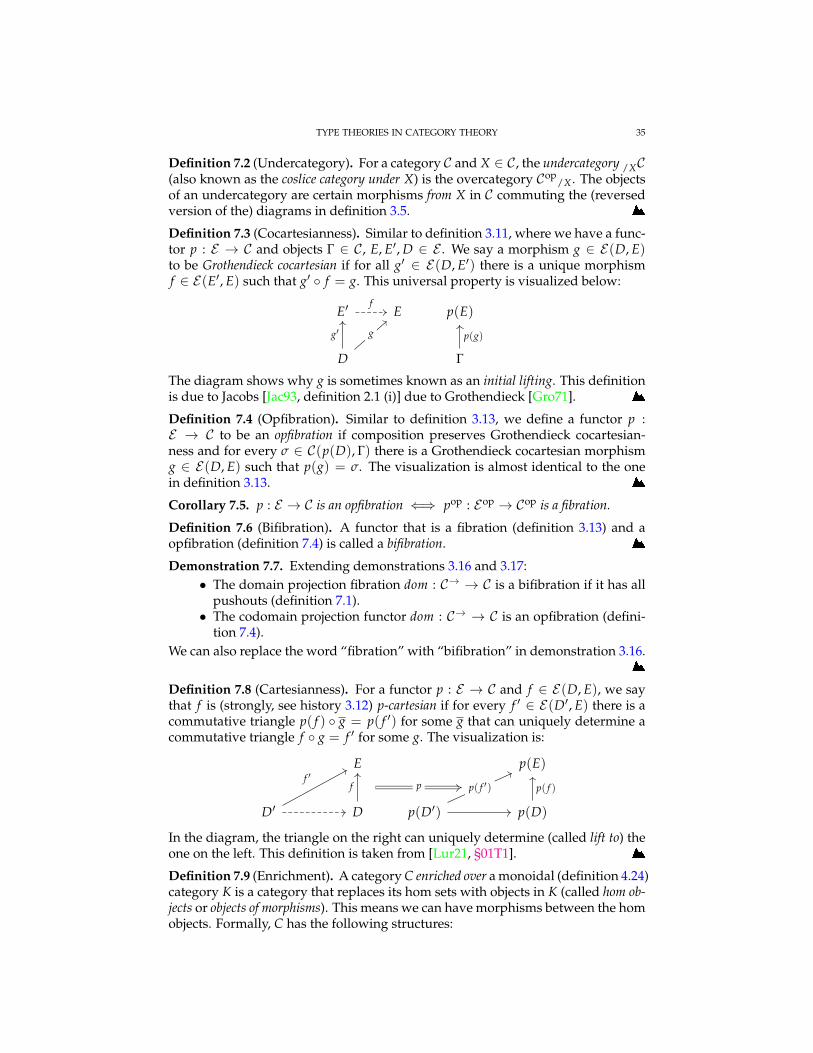
Definition 7.3 (Cocartesianness). Similar to definition 3.11, where we have a func-tor p : E → C and objects Γ ∈ C, E, E′, D ∈ E . We say a morphism g ∈ E(D, E)to be Grothendieck cocartesian if for all g′ ∈ E(D, E′) there is a unique morphismf ∈ E(E′, E) such that g′ f = g. This universal property is visualized below:

E′ E p(E)

D Γ

p(g)g′

f

g

The diagram shows why g is sometimes known as an initial lifting. This definitionis due to Jacobs [Jac93, definition 2.1 (i)] due to Grothendieck [Gro71].

Definition 7.4 (Opfibration). Similar to definition 3.13, we define a functor p :E → C to be an opfibration if composition preserves Grothendieck cocartesian-ness and for every σ ∈ C(p(D), Γ) there is a Grothendieck cocartesian morphismg ∈ E(D, E) such that p(g) = σ. The visualization is almost identical to the onein definition 3.13.

Corollary 7.5. p : E → C is an opfibration ⇐⇒ pop : Eop → Cop is a fibration.

Definition 7.6 (Bifibration). A functor that is a fibration (definition 3.13) and aopfibration (definition 7.4) is called a bifibration.

Demonstration 7.7. Extending demonstrations 3.16 and 3.17:• The domain projection fibration dom : C→ → C is a bifibration if it has all

pushouts (definition 7.1).• The codomain projection functor dom : C→ → C is an opfibration (defini-

tion 7.4).We can also replace the word “fibration” with “bifibration” in demonstration 3.16.

Definition 7.8 (Cartesianness). For a functor p : E → C and f ∈ E(D, E), we saythat f is (strongly, see history 3.12) p-cartesian if for every f ′ ∈ E(D′, E) there is acommutative triangle p( f ) g = p( f ′) for some g that can uniquely determine acommutative triangle f g = f ′ for some g. The visualization is:

E p(E)

D′ D p(D′) p(D)

p( f ′)f ′

f p( f )p

In the diagram, the triangle on the right can uniquely determine (called lift to) theone on the left. This definition is taken from [Lur21, §01T1].

Definition 7.9 (Enrichment). A category C enriched over a monoidal (definition 4.24)category K is a category that replaces its hom sets with objects in K (called hom ob-jects or objects of morphisms). This means we can have morphisms between the homobjects. Formally, C has the following structures:

36 TESLA ZHANG

(1) Objects and morphisms, just like other categories. Morphisms are objectsin K, so we will denote objects in K as C(a, b) for a, b ∈ C.

(2) For a, b, c ∈ C, there is a morphism a,b,c ∈ K(C(a, b) ⊗ C(b, c), C(a, c)),called the composition morphism.

(3) For the tensor unit 1 ∈ K and a ∈ C, there is an identity morphism 1a ∈K(1, C(a, a)).

Such that the following diagrams commute:

C(b, b)⊗ C(a, b) C(a, b) C(a, b)⊗ C(a, a)

1⊗ C(a, b) C(a, d) C(a, b)⊗ 1

C(b, d)⊗ C(a, b) C(c, d)⊗ C(a, c)

(C(c, d)⊗ C(b, c))⊗ C(a, b) C(c, d)⊗ (C(b, c)⊗ C(a, b))

a,b,b a,a,b

1a⊗idC(a,b) idC(a,b)⊗1aλC(a,b) ρC(a,b)

a,b,d a,c,d

αC(c,d),C(b,c),C(a,b)

b,c,d⊗idC(a,b) idC(c,d)⊗a,b,c

Demonstration 7.10. A category enriched in Cat is a strict 2-category (defini-tion 3.23). This is a realization of remark 3.25.

7.1. Common mistakes and counterexamples.

Warning 7.11. For a category C and objects A, B ∈ C, we take the full subcategory(definitions 3.31 and 3.32) of C by selecting objects X ∈ C such that both C(X, A)and C(X, B) are nonempty.

The terminal object in such full subcategory is not the product object A× B ∈C. The reason is that the terminal object in such subcategory does not commute(although the morphisms exist) the diagram in definition 2.11. A

Demonstration 7.12. In Set, for sufficiently large sets (say, size larger than 2)A, B ∈ Set, the full subcategory of Set like in warning 7.11 is equivalent to Set,whose terminal object is the trivial set ∅. This is definitely not the productA× B.

Remark 7.13. Similar to warning 7.11, pullbacks cannot be characterized as a ter-minal object in a subcategory either.

Warning 7.14. Coproduct types are not interpreted as pushouts (definition 7.1)which are coproducts in the undercategory (definition 7.2). Instead, they corre-spond to coproduct objects in the overcategory (definition 3.5). A

Warning 7.15. We cannot turn isomorphisms of hom sets in the overcategory intothe original category. In other words, given a category C, objects A, B, C, D, X ∈ C,and the following morphisms:

B D

A X Ca

b d

c

REFERENCES 37

There is C/X(a, b) ' C/X(c, d) 6=⇒ C(A, B) ' C(C, D) because C(A, B) may con-tain more morphisms than C/X(a, b), and similarly for C(C, D) and C/X(c, d). A

Demonstration 7.16. In definition 4.37, even C/Γ(a, b) ' C/Γ(1C/Γ, ba), we cannot

conclude C(B, A) ' C(A→Γ B, Γ).

Warning 7.17. Speaking of internalized definitions, we cannot yet define types bylarge elimination because there is not a type for all types (warning 4.3) (althoughwe have a type for all propositions). A

Warning 7.18. For a category C, its terminal object 1 ∈ C, an arbitrary object A ∈ C,and a morphism f ∈ C(1, A), f is not the terminal object in the overcategory C/X .

Terminal objects in overcategories are identity morphisms. A

ACKNOWLEDGEMENT

We are grateful to Yuchen Wu, Niels van der Weide, Ende Jin, Anqur Lu, JonathanSterling, Parker Liu, and GitHub users @dramforever, @AliceLogos, and @Guest0x0for their useful suggestions on improving this introduction. We thank @AliceLogosfor carefully checking the definitions in the draft version of this introduction andValery Isaev for sharing ideas on categorical semantics of dependent type theories.

The development of this introduction is based on the following artifacts:

• The LATEX system, its TEXLive distribution4, the BIBTEX tool, and the math-pazo5 font.• The “quiver” tool6, an interactive commutative-diagramming tool.• “Detexify”7, a tool that suggests LATEX commands from a drawing.• “BIBTEX Tidy”8, a smart formatter for BIBTEX entries.• The Emacs operating system and the AUCTEX9 major-mode of it.• The “ncatlab” website10, the “kerodon” website [Lur21], the TEX Q&A

website11 and the Wikipedia.• Several social networks connecting researchers together.

REFERENCES

[Ste20] Jonathan Sterling. An OK Version of Type Theory. 2020. URL: https://www.jonmsterling.com/pdfs/ok-type-theory.pdf.

[CA18] Jesper Cockx and Andreas Abel. “Elaborating Dependent (Co)PatternMatching”. In: Proc. ACM Program. Lang. 2.ICFP (July 2018). DOI: 10.1145/3236770.

[CFC59] Haskell B. Curry, Robert Feys, and William Craig. “Combinatory Logic,Volume I”. In: Philosophical Review 68.4 (1959), pp. 548–550. DOI: 10.2307/2182503.

4https://www.tug.org/texlive5https://www.ctan.org/pkg/mathpazo6https://q.uiver.app7https://detexify.kirelabs.org/classify.html8https://flamingtempura.github.io/bibtex-tidy9https://www.gnu.org/software/auctex10https://ncatlab.org/nlab/show/HomePage11https://tex.stackexchange.com

38 REFERENCES

[de 72] N.G de Bruijn. “Lambda calculus notation with nameless dummies, atool for automatic formula manipulation, with application to the Church-Rosser theorem”. In: Indagationes Mathematicae (Proceedings) 75.5 (1972),pp. 381–392. ISSN: 1385-7258. DOI: 10.1016/1385-7258(72)90034-0.URL: https : / / www . sciencedirect . com / science / article / pii /1385725872900340.

[Sco] Luis Scoccola. Models of Intensional Dependent Type Theory. URL: http://luisscoccola.github.io/Luis%20Scoccola_files/dttmodels.pdf.

[Pit01] Andrew M. Pitts. “Categorical Logic”. In: Handbook of Logic in ComputerScience: Volume 5: Logic and Algebraic Methods. USA: Oxford UniversityPress, Inc., 2001, pp. 39–123. ISBN: 0198537816.

[Jac93] Bart Jacobs. “Comprehension categories and the semantics of type de-pendency”. In: Theoretical Computer Science 107.2 (1993), pp. 169–207.ISSN: 0304-3975. DOI: 10.1016/0304-3975(93)90169-T. URL: https://www.sciencedirect.com/science/article/pii/030439759390169T.

[Gro71] Alexander Grothendieck. “Categories Fibrees et Descente”. In: Revête-ments Etales et Groupe Fondamental. Berlin, Heidelberg: Springer BerlinHeidelberg, 1971, pp. 145–194. ISBN: 978-3-540-36910-3.

[Cur90] P.-L. Curien. “Substitution up to isomorphism”. en. In: Diagrammes 23(1990), pp. 43–66. URL: http://www.numdam.org/item/DIA_1990__23__43_0/.

[CCD19] Simon Castellan, Pierre Clairambault, and Peter Dybjer. “Categorieswith Families: Unityped, Simply Typed, and Dependently Typed”. In:CoRR abs/1904.00827 (2019). arXiv: 1904.00827.

[Car86] John Cartmell. “Generalised algebraic theories and contextual categories”.In: Annals of Pure and Applied Logic 32 (1986), pp. 209–243. ISSN: 0168-0072. DOI: 10.1016/0168- 0072(86)90053- 9. URL: https://www.sciencedirect.com/science/article/pii/0168007286900539.

[Mar75] Per Martin-Löf. “An intuitionistic theory of types: predicative part”. In:Logic Colloquium ’73, Proceedings of the Logic Colloquium. Ed. by H.E. Roseand J.C. Shepherdson. Vol. 80. Studies in Logic and the Foundations ofMathematics. North-Holland, 1975, pp. 73–118.

[Coq85] Thierry Coquand. “Une théorie des constructions”. PhD thesis. L’universiteParis VII, 1985.

[Luo90] Zhaohui Luo. “An Extended Calculus of Constructions”. PhD thesis.University of Edinburgh, 1990.

[Luo94] Zhaohui Luo. Computation and Reasoning: A Type Theory for ComputerScience. USA: Oxford University Press, Inc., 1994. ISBN: 0198538359.

[Gir72] Jean-Yves Girard. “Interpretation fonctionelle et elimination des coupuredans l’arithmetic d’ordre superieur”. PhD thesis. L’universite Paris VII,1972.

[Hur95] Antonius J. C. Hurkens. “A simplification of Girard’s paradox”. In:Typed Lambda Calculi and Applications. Ed. by Mariangiola Dezani-Ciancagliniand Gordon Plotkin. Berlin, Heidelberg: Springer Berlin Heidelberg,1995, pp. 266–278. ISBN: 978-3-540-49178-1.

[See84] Robert AG Seely. “Locally cartesian closed categories and type theory”.In: Mathematical proceedings of the Cambridge philosophical society. Vol. 95.1. Cambridge University Press. 1984, pp. 33–48.

REFERENCES 39

[Hof94] Martin Hofmann. “On the Interpretation of Type Theory in LocallyCartesian Closed Categories”. In: Selected Papers from the 8th Interna-tional Workshop on Computer Science Logic. CSL ’94. Berlin, Heidelberg:Springer-Verlag, 1994, pp. 427–441. ISBN: 3540600175. DOI: 10.5555/647844.736579.

[Dyb96] Peter Dybjer. “Internal type theory”. In: Types for Proofs and Programs.Ed. by Stefano Berardi and Mario Coppo. Berlin, Heidelberg: SpringerBerlin Heidelberg, 1996, pp. 120–134. ISBN: 978-3-540-70722-6.

[Hof97] Martin Hofmann. “Syntax and semantics of dependent types”. In: Ex-tensional Constructs in Intensional Type Theory. London: Springer Lon-don, 1997, pp. 13–54. ISBN: 978-1-4471-0963-1. DOI: 10.1007/978-1-4471-0963-1_2.

[EH63] Beno Eckmann and P.J. Hilton. “Group-like structures in general cat-egories II equalizers, limits, lengths”. In: Mathematische Annalen 151.2(1963), pp. 150–186. ISSN: 1432-1807. DOI: 10.1007/BF01344176.

[Lur21] Jacob Lurie. Kerodon. https://kerodon.net. 2021.

THE PENNSYLVANIA STATE UNIVERSITY

Email address: yqz5714@psu.eduURL: https://personal.psu.edu/yqz5714