University of Arkansas, FayettevilleScholarWorks@UARK

Theses and Dissertations

8-2013

Two Studies on Childhood Obesity: Effect ofObesity on Academic Achievement and Effect ofFood Store Access on Diet QualityGaogao YuUniversity of Arkansas, Fayetteville

Follow this and additional works at: http://scholarworks.uark.edu/etd

Part of the Food Security Commons

This Thesis is brought to you for free and open access by ScholarWorks@UARK. It has been accepted for inclusion in Theses and Dissertations by anauthorized administrator of ScholarWorks@UARK. For more information, please contact scholar@uark.edu, ccmiddle@uark.edu.

Recommended CitationYu, Gaogao, "Two Studies on Childhood Obesity: Effect of Obesity on Academic Achievement and Effect of Food Store Access onDiet Quality" (2013). Theses and Dissertations. 804.http://scholarworks.uark.edu/etd/804

TWO STUDIES ON CHILDHOOD OBESITY: EFFECT OF OBESITY ON ACADEMIC

ACHIEVEMENT AND EFFECT OF FOOD STORE ACCESS ON DIET QUALITY

TWO STUDIES ON CHILDHOOD OBESITY: EFFECT OF OBESITY ON ACADEMIC ACHIEVEMENT AND EFFECT OF FOOD STORE ACCESS ON DIET QUALITY

A thesis submitted in partial fulfillment of the requirements for the degree of

Master of Science in Agricultural Economics

By

Gaogao Yu University of Missouri

Master of Art in Economics, 2010

August 2013 University of Arkansas

ABSTRACT

This thesis includes two studies on childhood obesity. This first study investigates

whether childhood obesity rates affect their academic achievement scores by using a school-level

panel data set on Arkansas 4th and 6th grades. The main results indicate that childhood obesity

rates do not significantly affect academic achievement scores. Controls for education inputs such

as library volume, educational expenditures per student and teacher salary show consistently

significant positive relationship to students’ test scores in both whole sample and in subsample

analyses by socio-economic and minority status. The second study examines the effect of a

neighborhood food environment feature, specifically food retailer access on diet quality of young

children. Binary and index diet quality measures are developed and proximity and density of

food store access measures are computed at the census block level. In general, both proximity

and density measures do not have any significant marginal effects on children’s diet quality in

the baseline model. When using instrumental variable (IV) approach, the food store proximity

measure has a strong impact on consumption of fruit and density measure has significant

marginal effects on likelihood of having risk of consuming both fruit and vegetables. Parents’

mental health indicator of depression has a consistent negative impact on index diet quality

measure in the baseline model but not in the IV model.

This thesis is approved for recommendation to the Graduate Council.

Thesis Director:

Dr. Michael Thomsen

Thesis Committee:

Dr. Rodolfo M. Nayga, Jr.

Dr. Daniel Rainey

THESIS DUPLICATION RELEASE I hereby authorize the University of Arkansas Libraries to duplicate this thesis when needed for research and/or scholarship.

Agreed

Gaogao Yu

Refused Gaogao Yu

ACKNOWLEDGEMENTS

Special thanks to my advisors Dr. Michael Thomsen and Dr. Rodolfo Nayga who spent

time discussing and revising every part of the thesis with me. Plenty of thanks go to Dr. Daniel

Rainey for his valuable comments and suggestion. I also would like to thank Diana Danforth,

Leanne Whiteside-Mansell, and Taren Swindle who helped with gathering and preparing data.

Finally I appreciate the financial support for these two research studies provided by Agriculture

and Food Research Initiative Competitive Grant no. 2011-68001-30014 from the USDA National

Institute of Food and Agriculture.

TABLE OF CONTENTS

I. INTRODUCTION 1 II. EFFECT OF CHILDHOOD OBESITY ON ACADEMIC ACHIEVEMENT 4 A. Literature Review 4

B. Data and Summary Statistics 6 1. Reverse Causation 7 2. Descriptive Statistics 8

C. Model Specification 9 D. Results 10

III. EFFECT OF FOOD STORE ACCESS ON EARLY CHILDHOOD DIET QUALITY 21 A. Literature Review 21 B. Data and Descriptive Statistics 24

1. Diet Quality Measure 25 2. Food Store Access Measure 29 3. Control Variables 30

C. Statistical Method 31 D. Results 34

IV. DISCUSSION AND CONCLUSION 57 A. Childhood Obesity and Academic Achievement 57 B. Food Store Access and Childhood Diet Quality 58 V. REFERENCES 62

1 I. INTRODUCTION

During the past 20 years, there has been a dramatic increase in the obesity rate in the

United States. According to the National Health and Nutrition Examination Survey1, more than

one-third of U.S. adults are obese and approximately 17% (or 12.5 million) children and

adolescents aged 2-19 years are obese. In 2011, no state had a prevalence of obesity less than

20%. In addition, thirty-six states had a prevalence of 25% or more and 12 of these states had a

prevalence of 30% or more. Arkansas, the focus of my study, is in one of these 12 states.

The increase in proportion of obese children has received considerable attention due to

the associated health risks such as coronary heart disease, type2 diabetes, and respiratory

problems. Also being obese can potentially affect academic accomplishment and quality of life

as children become adults in the long run (Currie 2009). Freedman et al. (2005) showed that

children who became obese as early as age 2 were more likely to be obese as adults. Health

conditions play an important role on childhood learning and academic performance. Poor health

can negatively impact students’ educational performance (Ding et al. 2009). Obesity may affect

students’ education performance in different ways. For example, students who have obesity

related illnesses and medical problems may result in more school day absences than average.

Obese students may also experience prejudice and discrimination from teachers and peers in the

school, resulting in stigmatization that lowers self-esteem and increases mental stress and

depression. These negative mental health issues could make it more difficult for children to

concentrate or be attentive in class or simply result in the child being less willing to attend

school. In 2001, the United States government passed the No Child Left Behind Act (NCLB),

which aims to improve individual outcomes in education. Under NCLB, schools have to meet

1 See http://www.cdc.gov/obesity/data/trends.html#National

2

their established adequate yearly progress (AYP) goals or show adequate growth in all standard

subject tests for all subgroups. AYP is a federally approved, state-specific standard that requires

public schools to continuously and substantially improve student achievement in math and

reading. The goal is to ensure that students meet or exceed their state’s standard for proficiency

in math and reading by 2014. The issue of whether childhood health, specifically obesity, really

affects academic performance is an important and interesting topic for those who care about

educational outcomes. Consequently, the first study in this thesis is to investigate whether there

is an association between academic achievement and obesity rates among young children in

Arkansas public schools. The reason we choose Arkansas is because Arkansas is an interesting

case to study. First, Arkansas is one of the poorest and least healthy states and has one of the

highest childhood obesity rates in the United States2. Furthermore, Arkansas is among the states that have the lowest student achievement test scores3.

Uncovering and better understanding the causes of childhood obesity is also essentially

important to the public and policy makers. Bad food choices and dietary intake have been

documented to relate to many diseases and health problems, such as cardiovascular disease, and

obesity (Gibson 1996; Johnson et.al. 2007). People’s dietary habit and food choice could be

closely related to the local food environment. People living in an area with limited access to

supermarkets or large grocery stores are facing significant higher costs to purchase food items in

terms of time, price of food, and travel cost. Instead, convenience stores that tend to sell high

2 Based on National Conference of State Legislation, Arkansas had rates of overweight and obese children higher than 35.1% in 2007. See http://www.ncsl.org/issues-research/health/childhood-obesity-trends-state rates.aspx#2005_Map 3 According to 2011 survey and assessment results from the National Assessment Education Progress (NAEP), reading and math scores earned by Arkansas fourth graders on the 2011 national exam were stagnant and below the national average.

3

calorie food items become the alternative food sources for those people (Alviola, Nayga and

Thomsen 2013). Understanding the relation between local food environment, food choices and

diet intake is important and beneficial to the efforts on the prevention of childhood obesity.

Therefore, the second study in this thesis examines the effect of food store accessibility on

children’s diet quality.

The rest of this thesis is laid out as follows. Chapter 2 covers the study of the

consequences of childhood obesity rates on educational outcomes targeting on grade 4 and 6

students from Arkansas public schools. In chapter 3 we switch the focus to the factors that

contribute to childhood obesity, and mainly focus on investigating how accessibility of food

retailers impact children’s dietary intake quality. Chapter 2 and 3 each represent self-contained

studies and include a review of existing literature, data description, statistical model specification

and results. The last chapter gives conclusions and some discussion on the limitations of the two

studies.

4

II. EFFECT OF CHILDHOOD OBESITY ON ACADEMIC ACHIEVEMENT

The aim in this study is to examine the issue of the effect of obesity rates on children’s

academic achievement scores. We utilize a grade level panel data set from 2005 to 2009 which

contains school, school district and community level information. Different statistical regression

models (pooled OLS, fixed effects and random effects) and subsamples are employed to access

the relationship between childhood obesity prevalence and academic achievement.

A. Literature Review

Educational economists have carried out many studies analyzing the factors that affect

students’ educational performance and assessing different ways to improve students’ academic

achievement scores from the perspective of an education production function. On the one hand, a

large body of research focused on the influence of inputs such as parental school involvement,

family socioeconomic background, and household resources on children’s cognitive, social and

emotional development (Hill and Neill 1994; Muller 1995; Blau 1999; Okpala, Okpala and

Smith 2001; Israel, Beaulieu and Hartless 2001; Hill and Taylor 2004; Yan and Lin 2005; Sirin

2005).They agree on the importance of parent child interaction and believe that parents’

socioeconomic status plays a significant role in shaping children’s educational performance. On

the other hand, a multitude of studies have also been conducted on the impact of school inputs

(e.g., school resources and facilities, financial budgets and expenditures, class and school size,

and teacher characteristics) on students’ educational outcomes. For instance, early work by

Hanushek (1986, 1989), found out that there is no strong evidence to support the notion that

teacher-student ratios, teacher education and teacher experience positively affect student

achievement. However, more recent studies by Hedges, Laine and Greenwald (1994), Wayne

5

and Youngs (2003), Rivkin, Hanushek and Kain (2005), Clotfelter, Ladd and Vigdor (2006) and

Aaronson, Barrow and Sander (2007) not only agree that schools and teachers matter, but they

also assert that these factors make significant contributions to students’ educational outcomes. In

addition, many other factors such as school learning environment and culture, students’ peer

impacts, and learning programs and approaches have been shown to be related to students’

academic outcomes.

There are also studies that address the relationship between academic performance and

student health and wellbeing along dimensions such as hunger, malnutrition, sleep, physical and

emotional abuse, and chronic illness (Austin et al. 1998; Glewwe, Jacoby and King 2001; Taras

2005a, 2005b; Puskar and Bernardo 2007; Carlson et al 2008; Belot and James 2011). Recently,

there are an increasing number of studies focusing on examining and verifying the link between

childhood body weight and educational outcomes. The results are inconsistent. Many of them

found a negative association between overweight and school performance (Crosnoe and Muller

2004; Datar, Sturm and Magnabosco 2004; Taras and Potts-Datema 2005; Datar and Sturm

2006; Sabia 2007; Gurley-Calvez and Higginbotham 2010; Averret and Stifel 2010). For

instance, Datar, Sturm and Magnabosco (2004) used data from the Early Childhood Longitudinal

Study-Kindergarten Class (ECLS-K) to investigate the association between childhood

overweight and academic performance. They found out that overweight kindergartners scored

significantly lower than their non-overweight peers on standardized tests but acknowledged that

these effects could be attributed to potential confounding variables. Thus, they concluded that

obesity is a marker as opposed to a causal factor when it comes to low academic performance.

Gurly-Calvez and Higginbotham (2010) used West Virginia fifth grade school district level panel

6

data to examine the relationship between childhood obesity and performance in schools based on

different family income levels. Their results suggest that obesity has a negative effect on

academic achievement in lower income school districts and that these effects for low-income

children can be offset by additional educational spending. Sabia (2007) studied sample drawing

from the National Longitude Survey of Adolescent Health and concluded that there is a negative

relationship between body weight and academic performance among white females. Similarly,

using individual children’s data with mother’s historic BMI as instrumental variable, study by

Averret and Stifel (2010) found that overweight white boys have both math and reading scores

about one standard deviation below that of their peers and obese black boys and girls have

significantly lower reading scores but not math scores. However, some other papers found no

relationship between body weight and achievement test scores. For example, in MacAcann and

Roberts’ study (2013), they found that obese students obtain equivalent test scores to nonobese

students and they asserted that the differences in grades obtained between obese and nonobese

students are due to the peer and teacher prejudice and discrimination. Again, Kaestner and

Grossman (2009), and Schoolder et al. (2010) both claimed that there is no significant

association between weight status and academic achievement in their paper.

B. Data and Summary Statistics

The data come from four different sources. The students’ BMI measurements are

provided by the Arkansas Center for Health Improvement (ACHI), which has been given a

mandate by the state to conduct annual BMI assessment of Arkansas public school students. The

BMI measurements were taken by trained personnel for children in even numbered grades from

7

kindergarten through grade 10. An advantage of the ACHI data is that the BMI outcomes are

based on physical measurements and are considered more accurate and reliable than either

parent-reported or self-reported height and weight data that appear in many of the earlier studies.

In this study, we use student BMI measurement equal to or above 85th percentile. The data are

aggregated to the school level for each grade from 2005 to 2009. The students’ standardized test

scores and school-level measures are obtained from the Arkansas Department of Education

(ADE). The standardized test used to measure students’ math and literacy knowledge is the

Arkansas Augmented Benchmark Exams 4 . National Office for Research, Measurement and

Evaluation Systems (NORMES) provided additional school-level characteristics that matched

with students’ test scores dataset. The last source of our data is the 2000 Census, which includes

information on a broad range of socio-demographic and economic characteristics of the school

districts and the communities. We first merged our BMI data with the academic achievement

scores data and NORMES dataset with matched school-level information5. Then we merged

those with the 2000 census data by school district code and name6. Reverse causation

4 The augmented benchmark exams include criterion-referenced tests (CRT) component, which focuses on measuring student performance on items specifically developed by Arkansas teachers, and norm-referenced tests (NRT) component, which focuses on rank-ordering student performance based on national norms and contains items in the subsections of reading comprehension, math problem solving, and language skills. 5 The matched school-level information including enrollment, poverty statistics, language spoken at home, school average math or literacy test scores. The match of schools across all data sources was not perfect, but the number of non-matching schools was only 25-45 out of approximately 1,100 schools in all years. 6 The 2000 Census data contain census block-level information and each block has a census school district unified code.

8

As emphasized by Gurley-Calvez and Higginbatham (2010), reverse causation can be

problematic because poor academic performance might cause stress or depression and thereby

contribute to weight gain. However, they argue that reverse causality is less problematic for

young children compared to adolescents and adults because young children’s diets and routines

are mainly controlled by parents and schools. Hence, considering the possibility of reverse

causality when analyzing older children, we limited our analysis only to children in the 4th and 6th grades in our sample. These are the youngest grades for which we have both standardized test

scores and measures of obesity prevalence.

Descriptive Statistics

Table 1 gives the means and standard deviations of all the variables used in our analysis

by grade. All variables are measured in percentages except for the students’ test scores, the

school library volume, district-average teacher salary, district expenditure per student, and

district per capita income. The average percent of obesity children in grade 4 and 6 are 40.94%

and 43.2% respectively with 2.08 percent difference. The students’ test scores by year in both

grade 4 and 6 are normalized7. Since free and reduced lunch participation depends on income eligibility, this variable can be viewed as an indicator of family income status. On average, about

63 percent of both 4th and 6th graders were eligible for participation in free and reduced price

lunches. The two largest minority groups are comprised of African American and Hispanic

students, which combined average to about 30 percent of school enrollment.

7 Same grade exam in different years could be different in format, contents, score weight in different sections and many other factors. Normalized test scores are more comparable cross years than non-normalized ones.

9

C. Model Specification A panel data model of the form

is specified, where represents the average math or literacy test scores of grade i, in school j

during year t; indicates the average obesity rates in grade i, in school j during year t; is

the average enrollment percentage for grade i in school j; is a vector of school level

characteristics; is a vector of school district and community level characteristics; and is the spherical error term. The coefficient is the parameter of main interest. It represents the

expected marginal effect of students’ obesity rates on their educational achievement scores. We

first use pooled ordinary least squares and cluster the standard errors at the school district and

community level to account for the possibility of having intra school correlation within the same

school district. This clustering approach is robust to heteroskedasticity in the school level errors

over time.

We also consider a fixed effects model to control for time invariant unobserved school specific

effects that could potentially bias the estimates. The fixed effects equation is specified as:

where represents unobserved and unmeasured time variant school characteristics specific to the grade in question. The other regressors are the same as those in equation (1). The fixed

effects model uses deviations from averages over time to remove the influence of unobserved

heterogeneity. For example, although we cannot measure the effectiveness of each school’s

administration, school level fixed effects can absorb this effect and also implicitly control for

10

unobservable characteristics that may vary across schools. They also implicitly control for other

unobservable and unmeasured student, teacher and school characteristics that may vary across

schools.

However, the fixed effects model has some limitations. The estimates generated by the

fixed effects model are derived from within-school difference over time, which discards the

information about differences across schools. So we would not be able to identify the effect of

other interesting time-invariant variables after the equations are differenced. Consequently, we

also estimate a random effects model. This allows estimation of coefficients for time-invariant

variables but requires an additional strong assumption that the time invariant unobservables are

not correlated with any of the observable covariates in the model. Given the advantages and

disadvantages of these two estimation procedures, we present and compare both estimates in the

discussion of our empirical results.

D. Results

The main objective of this study is to investigate whether childhood obesity has an

influence on academic achievement scores. Tables 2(a) and 2(b) present the pooled OLS results

for grades 4 and 6, respectively. In Table 2(a), the estimated effect of obesity on math test scores

is -0.037, which means that an increase of one percent in average obesity rate will decrease the

average math test score by 0.037 standard deviation. Although it is the expected sign if obesity

rates lower students’ school performance, the estimate is small in magnitude and is not

statistically significant. Aside from the average obesity rate variable, all the other control

11

variables have a statistically significant effect on students’ average math test scores except for

the percentage of females, the proportion of Asian students, and the proportion of students with

Spanish as the language spoken at home. It is worth pointing out that the estimate for percentage

of eligibility for free or reduced lunch, a proxy for home income level, has a negative sign at the

1% significance level, which is consistent with most common findings in education research that

children’s socioeconomic status and school performance are linked. From the second two

columns of this table, we note that the effect of obesity rates on students’ literacy test scores is

also not statistically significant. The effects of other variables on literacy test scores appear to be

similar to those on math test scores with few differences on their statistical significance. The

estimates for grade 6 are presented in Table 2(b). The estimated effects of obesity rates on both

math and literacy are positive, at 0.105 and 0.036 respectively, but are not statistically

significant. Fewer control variables are statistically significant for grade 6. Although the

magnitude are very small, parameter estimates for library volume, student expenditure and

teacher salary are statistically significant for both grades 4 and 6.

As mentioned before, a limitation of these OLS results is that there may be omitted

variables that are correlated with the obesity measure and test scores which can bias our

estimates. Hence, we used fixed effects estimation to address this limitation by accounting for

school specific fixed effects. We also consider the alternative random effects approach that

assumes that the distribution for follows a normal distribution with mean 0 and variance, N (0, ). We present estimates of both methods and obtain quantitatively similar results.

The fixed effects and random effects results for grade 4 students are displayed in Table

3(a). The effect of proportion of obese students on math scores is negative in both the fixed

12

effects model and the random effects model, while the effect on literacy is positive. None of

these effects, however, are statistically significant. It is worth mentioning that in the fixed effects

model, although quite small in magnitude, only the three educational input variables library

volume, students’ expenditure, and teacher salaries have significantly positive effects at the 1%

level. As expected this suggests that children perform better if they are in higher-input school

districts. Previous studies have found abundant teacher sorting across schools and districts.18, 40-43

School districts with higher teacher salaries are more likely to attract more experienced and

qualified teachers. In the fixed effects model, all other control variables are not statistically

significant. In comparison, there are more variables showing statistical significance in the

random effects model and they appear to be of the same significance as those reported in the

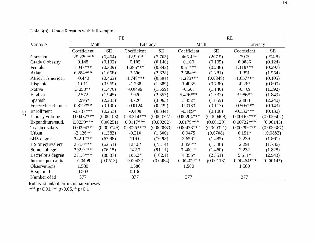
OLS model. Moving to Table 3 (b), we find no statistical evidence of a significant relationship

between obesity rates and 6th grade students’ achievement scores in both math and literacy. Again, library volume, student expenditure, and teacher salaries have significant and positive

effects on students’ achievement scores in both the fixed and random effects models.

Finally, to further investigate the effect of childhood obesity on educational outcomes, we

also separate our sample into different subsamples. As mentioned before, eligibility for free or

price reduced lunch is based on family income and so we use eligibility as a proxy for

socioeconomic status (SES). We divide the full sample into low SES and high SES subsamples

based on the percentage of students with free or price reduced lunch. We choose 60% as a cutoff

as this is near the statewide mean reported earlier in Table 1. Schools that have free or reduced

lunch eligibility greater than 60% on average across all years are classified as low SES schools

with the rest being classified as high SES schools. Similarly, based on minority status, we also

13

break the full sample into high minority and low minority subsamples by using the sum of the

percentage of African American and Hispanic students. If this sum is greater than or equal to

30%, the school is classified as a high minority school. Otherwise, the school is classified as a

low minority school. Figure 1 presents the average obesity rates of grade 4 and 6 students with

different subsamples. In general, grade 6 students have relatively higher obesity rates compared

to grade 4 students (i.e., 40.5% vs 38% in the high SES subsamples, 45.2% vs. 43.4% in the low

SES subsamples, 41.3% vs. 39.5% in the low minority subsamples, and 44.5% vs. 41.8% in the

high minority subsamples, respectively). Also, the average obesity rates of students from

subsample with lower income and higher percent of minority families is higher than that of

students from subsample with high SES and low percent of minority families.

Table 4 presents the estimates of obesity prevalence by subsample and by grade from

both the fixed effects and random effects models. Interestingly, in the low SES grade 4

subsamples, both fixed effects and random effects estimates show a statistically significant

positive effect deviation of obesity on literacy test scores but no significant effect on math test

scores. In contrast, in the high SES grade 4 subsamples, the estimates from both the fixed effects

and random effects models show a negative effect on math test scores at the 5% significance

level but no effect on literacy. The estimates across the low and high minority sub-samples

generally show no effect on the test scores for grade 4 or grade 6. Although not reported, all the

educational input variables are positive and statistically significant at the 1% level in these

subsample analyses for both grades.

14

Aver

age

obes

ity r

ates

Av

erag

e ob

esity

rat

es

Aver

age

obes

ity r

ates

Av

erag

e ob

esity

rat

es

Figure1. Grade 4 and 6 student average obesity prevalence with different subsamples

Grade 4 student obesity prevalence with SES subsample

Grade 6 student obesity prevalence with SES subsample

50 45

40 38.0 35 30 25 20 15 10

5 0

43.4

50 45 40.5 40 35 30 25 20 15 10 5 0

45.2

High% SES Low% SES High% SES Low% SES

Grade 4 student obesity prevalence with minority

subsample 50

Grade 6 student obesity prevalence with minority subsample

45 39.5

40 35 30 25 20 15 10 5 0

41.8 50 45 41.3 40 35 30 25 20 15 10 5 0

44.5

Low% minority High% minority Low% minority High% minority

15

Table1. Descriptive Statistics, Arkansas, 2005-2009

Grade 4 Grade6

Variable Mean SD Mean SD Percent of obese students 40.94 6.36 43.02 6.36 Standardized average math score -0.04 0.92 -0.04 0.92 Standardized average literacy score -0.04 0.94 -0.05 0.93 Enrollment proportion 18.43 7.92 23.95 13.01 Percent female students Percent eligibility for free or reduced price lunch

48.61

62.62

2.57 20.10

48.56

62.94

4.14

17.96 Percent black students 24.09 30.51 20.99 28.89 Percent white students 66.20 30.91 71.58 29.38 Percent Hispanic students 7.71 12.23 5.73 9.48 Percent Asian students 1.36 2.45 1.04 2.04 Percent native American students 0.63 0.99 0.65 1.10 Percent English as home language 93.04 13.06 95.06 10.24 Percent Spanish as home language 6.00 11.72 4.27 9.12 Library volume 8724.20 3464.75 8218.99 3443.69 Average teacher salary ($) 43835.92 5313.08 41956.09 4681.41 Expenditure per student ($) 8123.63 1031.99 7956.38 906.22 Per capita income ($) 16720.86 2887.52 15764.00 2529.22 Percent urban 46.68 37.12 34.65 35.93 Percent of less than high school degree 25.29 7.59 27.69 7.15 Percent of high school degree or equivalent 34.58 5.68 36.30 5.08 Percent of some college or associates degree 24.19 4.53 22.84 4.53 Percent of Bachelor's degree 10.55 5.05 8.78 4.12 N 506 377

1. School level variables. The proportion of students within the school. 2. School-district level variables. The proportion of population or households within the school

district.

16

Table 2(a). Ordinary least square results for grade 4 (N=2,311).

Variable Math Literacy Coefficient SE Coefficient SE Constant -279.0 (262.4) -579.4 (374.9) Grade 4 obesity -0.0371 (0.108) 0.0913 (0.166) Female 0.0259 (0.293) 0.675 (0.481) Asian 1.783 (1.738) 3.741 (2.500) African American -1.059*** (0.0904) -1.684*** (0.132) Hispanic 1.485** (0.752) 1.801* (1.087) Native -2.865*** (1.007) -5.223*** (1.375) English as home language 3.552* (2.036) 5.520* (2.924) Spanish as home language 1.286 (2.244) 2.299 (3.282) Free or price reduced lunch -0.426*** (0.134) -1.168*** (0.221) Grade 4 enrollment 0.345** (0.140) 0.277* (0.163) Library volume 0.000766** (0.000359) 1.56e-06 (0.000514) Expenditure per student 0.0108*** (0.00165) 0.0139*** (0.00236) Teacher salary 0.00274*** (0.000578) 0.00284*** (0.000693) Urban 0.166** (0.0746) 0.299*** (0.0977) Less than high school degree 4.092** (1.658) 6.034*** (2.223) High school degree or equivalent

4.081***

(1.494)

4.895**

(2.011)

Some college and associate degree

3.833**

(1.654)

5.266**

(2.266)

Bachelor's degree 6.263** (2.469) 9.694*** (3.159) Income per capita

- 0.00368***

(0.00134)

-0.00595***

(0.00179)

R-squared 0.446 0.525 Robust standard errors in parentheses *** p<0.01, ** p<0.05, * p<0.1

17

Table 2(b). Ordinary least square results for grade 6 (N=1,580).

Variable Math Literacy Coefficient SE Coefficient SE Constant -111.2 (264.4) 226.5 (311.2) Grade 6 obesity 0.105 (0.131) 0.0361 (0.156) Female 0.228 (0.218) 0.958*** (0.238) Asian 1.977 (1.640) 0.427 (1.953) African American -1.041*** (0.0998) -1.480*** (0.127) Hispanic 1.868** (0.753) 1.089 (1.046) Native -0.957 (1.131) -0.266 (1.487) English as home language 5.004** (2.143) 2.898 (2.631) Spanish as home language 2.491 (2.335) 0.342 (2.986) Free or price reduced lunch -0.274 (0.168) -0.659** (0.257) Grade 6 enrollment -0.207* (0.124) -0.410** (0.183) Library volume 0.00105** (0.000464) 0.00104* (0.000592) Expenditure per student 0.00928*** (0.00199) 0.000887 (0.00262) Teacher salary 0.00337*** (0.000569) 0.00262*** (0.000691) Urban 0.0663 (0.0932) 0.152 (0.131) Less than high school degree 1.432 (1.663) 1.444 (1.720) High school degree or equivalent 1.212 (1.635) 0.890 (1.628) Some college and associate degree

1.783

(1.708)

1.072

(1.841)

Bachelor's degree 2.114 (2.556) 4.214 (2.775) Income per capita -0.00345** (0.00165) -0.00442** (0.00189) R-squared 0.374 0.499

Robust standard errors in parentheses *** p<0.01, ** p<0.05, * p<0.1

18

Coefficient SE Coefficient SE Coefficient SE Coefficient SE Constant -425.7 (7,039) 4,035 (7,638) -444.9*** (151.5) -767.8*** (228.2) Grade 4 obesity -0.0931 (0.0889) 0.0571 (0.134) -0.0694 (0.0864) 0.0496 (0.126) Female 0.117 (0.397) 0.168 (0.463) 0.00498 (0.260) 0.401 (0.384) Asian 1.801 (1.647) 1.973 (2.416) 1.275 (1.045) 2.719* (1.552) African American 0.0675 (0.397) -0.876 (0.569) -1.212*** (0.0653) -1.936*** (0.0993) Hispanic 1.295 (0.864) 0.855 (0.932) 1.320*** (0.444) 1.190* (0.656) Native 1.329 (1.481) 0.589 (1.895) -1.968** (0.957) -3.651** (1.433) English -0.607 (1.641) 1.155 (2.228) 2.794** (1.178) 4.495** (1.748) Spanish -0.923 (1.600) 1.087 (2.234) 0.550 (1.302) 1.754 (1.928) Free/reduced lunch 0.157 (0.197) -0.142 (0.300) -0.213*** (0.0788) -0.822*** (0.119) Enrollment 0.204 (0.263) 0.196 (0.282) 0.464*** (0.122) 0.428** (0.185) Library volume 0.00345*** (0.000889) 0.00297*** (0.00107) 0.00140*** (0.000305) 0.000762* (0.000462) Expenditure/stud. 0.0202*** (0.00209) 0.0264*** (0.00260) 0.0167*** (0.000914) 0.0217*** (0.00135) Teacher salary 0.00437*** -0.000815 0.00402*** (0.000840) 0.00401*** (0.000252) 0.00417*** (0.000374) Urban -0.995 (1.646) -1.795 (2.741) 0.123** (0.0544) 0.261*** (0.0836) ≤ HS degree 3.676 (69.18) -51.23 (71.72) 5.132*** (1.057) 7.285*** (1.627) HS or equivalent 9.220 (63.49) -28.75 (69.91) 5.861*** (0.978) 7.162*** (1.504) Some college -21.09 (74.00) -75.02 (75.66) 5.074*** (1.014) 6.902*** (1.560) Bachelor's degree -6.848 (73.56) -28.97 (80.26) 7.970*** (1.735) 12.07*** (2.669) Income per capita 0.0526 (0.0741) 0.0318 (0.0967) -0.00430*** (0.000885) -0.00670*** (0.00136) Observations 2,311 2,311 2,311 2,311 R-squared 0.448 0.291 Number of id 506 506 506 506

26

Table 3(a). Grade 4 results with full sample

FE RE Variable Math Literacy Math Literacy

Robust standard errors in parentheses *** p<0.01, ** p<0.05, * p<0.1

19

Coefficient SE Coefficient SE Coefficient SE Coefficient SE Constant -25,229*** (6,464) -12,991* (7,763) -466.4** (207.5) -79.29 (254.8) Grade 6 obesity 0.148 (0.102) 0.105 (0.146) 0.160 (0.105) 0.0886 (0.124) Female 1.047*** (0.309) 1.285*** (0.345) 0.514** (0.246) 1.119*** (0.297) Asian 6.284*** (1.668) 2.596 (2.628) 2.584** (1.281) 1.351 (1.554) African American -0.440 (0.463) -1.748*** (0.594) -1.283*** (0.0848) -1.657*** (0.105) Hispanic 1.011 (0.969) -1.788 (1.389) 1.403* (0.738) -0.285 (0.890) Native 3.258** (1.476) -0.0499 (1.559) -0.667 (1.146) -0.409 (1.392) English 2.572 (1.945) 3.020 (2.357) 5.476*** (1.532) 3.986** (1.849) Spanish 3.995* (2.203) 4.726 (3.063) 3.352* (1.859) 2.888 (2.240) Free/reduced lunch 0.819*** (0.190) -0.0124 (0.229) 0.0133 (0.117) -0.505*** (0.143) Enrollment -0.737*** (0.253) -0.400 (0.344) -0.189* (0.106) -0.336*** (0.130) Library volume 0.00432*** (0.00103) 0.00314*** (0.000727) 0.00204*** (0.000408) 0.00165*** (0.000502) Expenditure/stud. 0.0239*** (0.00251) 0.0117*** (0.00202) 0.0179*** (0.00120) 0.00732*** (0.00145) Teacher salary 0.00394*** (0.000749) 0.00253*** (0.000830) 0.00438*** (0.000321) 0.00299*** (0.000387) Urban -3.126** (1.383) -0.210 (1.300) 0.0475 (0.0708) 0.151* (0.0883) ≤HS degree 242.1*** (63.98) 119.0 (76.98) 2.656* (1.485) 2.239 (1.861) HS or equivalent 255.0*** (62.51) 134.6* (75.14) 3.356** (1.386) 2.291 (1.736) Some college 292.0*** (76.15) 142.7 (91.11) 3.400** (1.460) 2.232 (1.828) Bachelor's degree 371.8*** (88.87) 183.2* (102.1) 4.356* (2.351) 5.611* (2.943) Income per capita -0.0409 (0.0513) 0.00432 (0.0484) -0.00402*** (0.00118) -0.00464*** (0.00147) Observations 1,580 1,580 1,580 1,580 R-squared 0.503 0.136 Number of id 377 377 377 377

27

Table 3(b). Grade 6 results with full sample

FE RE Variable Math Literacy Math Literacy

Robust standard errors in parentheses *** p<0.01, ** p<0.05, * p<0.1

20

28

Table4. Estimates for different subsamples for grade 4 and 6

Grade 4 Grade 6 Subsample Model Subject Coefficient SE Obs. # of Schools Coefficient SE Obs. # of schools

Low SES

FE Math 0.0445 (0.120) Literacy 0.336* (0.171)

1229 275

0.205 (0.144) 0.355* (0.193)

812 204

RE Math 0.0839 (0.117) 0.279* (0.144) Literacy 0.351** (0.175) 0.376** (0.176)

High SES

FE Math -0.222* (0.126) Literacy -0.267 (0.198)

1082 231

0.0869 (0.148) -0.192 (0.213)

768 173

RE Math -0.227* (0.127) 0.0419 (0.152) Literacy -0.273 (0.180) -0.178 (0.173)

Low

Minority FE Math -0.0707 (0.135)

Literacy 0.103 (0.208)

879 192

0.248 (0.154) 0.165 (0.218)

719 173

RE Math -0.0213 (0.130) 0.285** (0.141) Literacy 0.135 (0.197) 0.164 (0.174)

Math -0.0577 (0.120) FE

0.0704 (0.142) High Literacy 0.0869 (0.185) 0.0806 (0.208)

Minority RE

Math -0.0787 (0.114)

1432 314 0.0423 (0.151)

861 204

Literacy 0.0370 (0.164) 0.0293 (0.177) Robust standard errors in parentheses *** p<0.01, ** p<0.05, * p<0.1

29

III. EFFECT OF FOOD STORE ACCESS ON EARLY CHILDHOOD DIET QUALITY.

The objective of this study is to examine the extent to which accessibility of food stores

around young children’s home neighborhood impacts their dietary intake by using cross-section

data on Head Starts (HS) children in Arkansas. We use proximity and density measures to

represent food store access. Simple probit and OLS baseline models and instrumental variable

approaches are utilized to examine the relationship between the children’s neighborhood food

environment features and their dietary consumption quality.

A. Literature Review

The increase of obesity prevalence in the past decades has led to increasing interest on

analyzing the effect of food environment on obesity outcomes. The food environment includes

not only food service establishments such as full-service restaurants and fast food outlets, but

also retail food stores like supermarkets, grocery stores, drugstores and convenience stores.

Typically, large grocery stores and full-service restaurants offer healthier foods than convenience

stores and fast food outlets. Fast food has been blamed as one of the reasons for the prevalence

of childhood obesity as some studies have documented evidence that access to fast food is

associated with a higher BMI among children (Davis and Carpenter 2009; Currie et al. 2010;

Alviola et al. 2011). For example, focusing on 9th grade children, Currie et al. (2010) find a significant effect of proximity to fast food restaurant on the risk of obesity. Especially they find

that the presence of a fast food restaurant within a tenth of a mile of school is associated with at

least a 5.2 percent higher obesity rate compared to a fast food restaurant present within 0.25

miles of the school. Similarly, using a sample of Arkansas public school children with a broad

29

30

range of grades from kindergarten through 10th grade, Alviola et al. (2013) ascertain that the

number of fast food restaurants within a mile of school is significantly positively related to

childhood obesity rates.

In addition to fast food restaurants, food retailers make up another important component

of the food environment. Large grocery retailers have been found to offer a wide variety of foods

often at relatively lower prices. Compared to households in higher income neighborhoods,

households in low income neighborhood often face fewer large grocery stores and more small

food stores like dollar stores and convenience stores (Morland et al. 2002; Powell et al. 2006;

Blanchard and Lyson 2007; Wang et al. 2007). Due to limited access to healthier and cheaper

food choices, these families may potentially consume more energy dense foods, which can lead

to weight gain. Many studies that examined the effect of food deserts8 on childhood obesity suggest that increasing the availability of supermarkets in the local area is associated with a

lower incidence of childhood obesity while the presence of convenience stores is linked to higher

incidences of childhood obesity (Liu et al. 2007; Powell et al. 2007; Galvez et al. 2009; Leung et

al. 2011).

While more attention has been focused on the effect of food environment on health

outcomes like BMI in the literature, less attention has been given directly to the linkage between

food environment features and diet. BMI is a result of many factors, but people’s dietary intake

might be more closely influenced by the neighborhood environment. Kyureghian and Nayga

(2013) examine whether access to food retailer outlets is a significant predictor of the probability

8 Food deserts are defined as areas where people do not have easy access to an affordable and healthy diet (Cummins and Macintyre 2002).

30

31

of shopping at those outlets to purchase healthy food like fruits and vegetables. Their results,

suggest that availability of different types of food stores does not have a significant effect on the

likelihood of patronizing any specific type of food stores when purchasing fruits and vegetables.

Furthermore, Pearson et al. (2005) and Laska et al. (2010) do not find any statistically significant

association between the accessibility of food stores and vegetable and fruit purchases and

consumption. In contrast, some other studies found different results. Drawing a sample from

different states in the nation, result findings by Morland, Wing, and Roux (2002) suggest that

there are some associations between the local food environment and residents’ diets. They find

that people living in areas with supermarkets have healthier diets in terms of fruits and

vegetables, total fat and saturated fat. Hanson et al. (2004) draws a similar conclusion that

increasing household availability of healthy food choices can enhance the consumption of fruit,

vegetables and dairy foods.

One limitation of these prior studies is that they largely focused on each individual

dietary components intake (e.g. fruit and vegetables intake). Foods are usually not consumed in

isolation, however. Due to the potential of synergy among foods, using alternative measurement

like diet indices to measure the quality of diet could potentially provide additional insight

(Moore et al. 2008). For instance, employing the Alternative Healthy Eating Index (AHEI)

measure, Moore et al. (2008) found that people living in areas with poor food environments were

much less likely to have a healthy diet than those around rich food environments. Another

limitation of many of previous work that try to find a causal relationship between food

environment features and diet intake or health outcomes is that they do not take into

consideration the potential endogeneity issues of accessibility of food stores on the grounds that

31

32

people tend to select where they live partially based on neighborhood characteristics (e.g. the

proximity between their homes and certain stores and services) and their food purchase and

consumption is a function of price of food, which is partially determined by the availability and

travel costs to acquire the food.

In order to closely examine the relationship between the accessibility of food stores and

children’s diet quality, we analyze both individual dietary components intake and a diet quality

index called Family Map Healthy Eating Index (FMHEI) in this study. In addition, we utilize

both proximity and density measures to assess the accessibility to the food stores. In contrast to

Moore et al (2008) who use adults aged 45 to 84 from 3 big metropolitan areas, our study

particularly focuses on low income family children from small cities in relatively rural areas in

Arkansas. Arkansas is an interesting case to study since it has one of the highest childhood

obesity rates in the United States. In addition, we are more cautious about the potential

endogeneity issues and apply an instrumental variable approach in the model to analyze the

relationship between the food store access and diet quality.

B. Data and descriptive statistics

The main dataset we use in this study is based on Arkansas Family Map (FM) data in

school year 2006-2007. FM is a structured interview assessment that targets head start (HS)

children aged from 3 to 5. There are 161 HS children in our study sample, majority of HS

children are from five major towns and they are Russellville, Clarksville, Dardanelle, Morrilton,

32

33

and Plumerville, Arkansas9. We select these places as our study areas because these are the only

areas where FM data can provide the geo-code of centroid of census block where each HS

student’s home locates. Since the objective of FM is to assess multiple aspects of the family to

identify concerns in the home that could potentially lead to poor child development, a series of

critical home and family information of children is elicited and collected by HS teachers during

the home visit interviews. The interview questionnaire has 12 sections in total covering different

aspects of the family information including demographics, routines, school readiness,

monitoring, environment safety, discipline, health, basic need, home and car safety, social

integration, and an end of visit observation. In this study, the main focus is on the parents’

reported dietary intake information of the children.

Food retailer geo-locations data are from Dun and Bradstreet (D&B), a commercial data

source that provides related business and commercial information. This data provide a broad

variety of types of food establishments. In this study, we only cover three major types of food

establishments and they are convenience stores, drug stores, and large grocery stores. The large

grocery stores in our study are defined as containing full line of grocery items, including a full

fresh produce department with annual sales more than $500,000.

We also use zoning map of the five major towns to construct instrumental variables.

Zoning maps are obtained from the each town’s government office. A Geographic Information

9The number of children from the major five towns comprises over 90 percent. 25 of them are from Dardanelle, 29 of them are from Morrilton, 41 of them are from Clarksville, 51 of them are from Russellville, and 5 of them are from Plumerville. The rest of students are from other surrounding small towns.

33

34

System (ArcGIS) is used to geo-process those zoning maps and create the desired data for

regression analysis.

Diet quality measure

Dichotomous measure

The dietary intake information contains questions about how frequently the child

consumes healthful foods as well as less healthy food. There are 10 questions and each question

pertains to certain group of food. The food groups are dairy products (like milk, cheese, yogurt,

etc.); meat (like beef, chicken, fish, eggs, etc.); beans (like dried beans/peas, peanut butter,

veggie burger, bean soup, baked/canned beans, etc); bread (or grain substitutes like rice, pasta,

cereals, tortilla breads etc.); vegetable (Dark green or orange/yellow vegetables like greens,

carrots, broccoli, squash, sweet potatoes); fruit (like apples, oranges, bananas, grapes, peaches,

applesauce); 100% fruit juice; sweets (like cakes, cookies, candy, etc.); sugar drinks (like cola,

Kool-aid, Yohoo, and fruit flavored drinks etc.); and sports drinks (like Gatorade, Power Aid,

etc.).

Parents give answers on how frequent the child eats the foods from each different group

(excluding food eaten at HS) by choosing answers from multiple choices. There are five choices

and they are none, once per week, 2-6 times a week, once per day, and more than once per day.

Grey shaded areas and non-shaded areas on the survey instrument separate the answers so that

the interviewer can easily identify and assess whether a child is at risk in terms of eating a

balanced diet. The parents being interviewed do not see the shaded area on the survey

instrument. With healthy groups of food, grey shaded areas indicate inadequate consumption.

34

35

For dairy, vegetables, and fruits groups, less than once a day answers (e.g. none, once per week,

2-6 times a week) fall within the grey shaded area. If a child’s parents choose those answers, the

child is considered at risking having sufficient consumption. Therefore improvement on

consuming more these groups of food should be considered as a family goal in the future. For

beans, meat and bread, the grey area cutoff answer is 2-6 times a week. If a child’s parents

choose answers none or once a week, the answers fall into the grey area. With less healthy

groups of food, grey areas indicate excessive consumption. For juice, sweets, sports drinks and

sugar drinks, taking more than once a day is considered at risk excessively consuming these

groups of food for children.

Table 1 gives the proportion of children who are at risk of consuming each group of food

(insufficient consumption of healthy food and excessive consumption of less healthy food) with

different sample size. The first column represents the whole sample. It is notable that for the

healthy groups of food such as vegetables and fruit, there are about 57.1% of HS children who

are having trouble consuming adequate dark green or orange/yellow vegetables (less than once a

day) and 28.6% of them at risk of consuming adequate fruits. Also, there are about 15.8% of

answers falling into the grey shaded area for the question on frequency of consumption of

sweets, which indicates that those children are at risk of overeating sweets (more than once per

day). Moving to the next column, we limit our sample to the HS children who have risk on

consuming enough either fruit or vegetables. Interestingly, compared to the full sample, the risk

rate on sweet and sugar drink consumption falls to 15% and 13% respectively, although not

much. No children have a problem with sport drinks either. We also separate the full sample by

gender. Columns 3 and 4 report the percentage of risk on different group of food consumption

35

36

for boys and girls respectively. Boys have less risk rate on taking enough vegetables and fruits

than girls. For example, for fruit group, the difference of the risk rate between girls and boys is

11.4% with 34.2% for girls and 22.8% for boys. On the other hand, however, boys have a higher

risk rate on consuming less healthy foods than girls.

Index measure

The Health Eating Index (HEI) is a scoring measure system that is developed and used by

the U.S. government to assess diet quality and compliance with dietary guidelines for Americans

(Kennedy et al. 1995; Guenther et al. 2007). The Youth Healthy Eating Index (YHEI) is a

modified scoring system developed to address dietary issues of children and adolescents

explicitly (Feskanich et al. 2004). Following the YHEI, a simplified and modified eating index

called Family Map Healthy Eating Index (FMHEI) specific for the family map HS children is

constructed in this study. Besides using intake frequency information of each group of food, two

additional questions pertaining eating habit and environment under routines section are also

used. The two questions are asking how many days the family ate dinner at a regular time and

how many days the family stick to regular morning routines. Consequently, the FMHEI is an

absolute score that is the sum all the scores contributed by the answer of all the included

questions. FMHEI consist of 14 components and the total scale ranges from 0 to 100. The higher

scores the index, the better the diet quality is implied. Table 2 lists the scoring criteria for each

component.

Dairy, bread, vegetable, fruit, and sweets can score up to 10 points for each group. The

less frequent the child eats the healthy group of food the lower score contributes to the index,

36

37

while it is the opposite for less healthy group of food. For example, for vegetables, 0 points is

scored when the frequency answer is none while 10 points is given when frequency answer is

more than once a day. For sweets, it is the opposite way, 0 point is awarded for an answer of

more than once a day and 10 points are scored for an answer of none. The three choices in

between these values are equally spread out into 2.5, 5 and 7.5 points.

Since meat and beans are substitutes for sources of protein, each is assigned a maximum

of 5 points with a total of 10 points for these two groups together (total protein servings).

Similarly, up to 5 points is assigned to answers on sports drinks and sugar drinks with a total of

10 points for these two groups together because they are both sugary beverages. For the juice

group, none and more than once a day choices are both assigned 0 points10. and the scores are

spread among the rest three choices with maximum 5 points for choice once per day. However,

the FM data do not collect any information about salty snacks like potato chips, corn chips,

popcorn, pretzels, and crackers, which is a major source for sodium intake. We arbitrarily assign

3.75 points to every child in the sample with a maximum 5 points for this category, which is an

assumption that children consume salty snacks at least once a week.

To take into consideration of the effect of eating habit and environment on children’s

diet, up to 5 points are assigned to components that ask how many times do a family eats dinner

at regular time and follows morning routines in a week. Few days are given lower scores11.

10 A child will get too much sugars or carbohydrates from it if he or she overdrinks juice. Study shows that excess fruit juice consumption can contribute to obesity (Dennison, Rockwell and Baker 1999). 11 There are 8 answer choices for these two questions: none, 1 day, 2 days, 3 days, 4 days, 5 days, 6 days, and 7 days. 0 point is assigned to those who choose answer 1 and 2, 1.67 points are

37

38

Compared to YHEI, the FM data do not contain information about how often the children take

multivitamins, have margarine and butter, and consume fried foods outside the home and

consume animal visible fat12. Therefore, we put all this missing information into one category

called “other” and assign a total of 5 points for everybody.

Based on above scoring criteria, the mean of the FMHEI score in our sample is 67.19

with a minimum of 42.9 and maximum of 85.0. Figure 2 presents the histogram of FMHEI.

Using midpoint method plotting, the most frequent scores are between 60 and 72, with 53 out of

161 scoring around 72 points.

Food store access measure

Distance is one of the important factors that people consider where to shop foods because

travel cost to food stores can be regarded as an implicit cost of the food. The shorter the distance

from home to food retailers, the less time and cost people use. In our study, we use proximity

which is the radius distance in miles from each HS child’s residence to the nearest different types

of food store to measure food store access. However, the distance to the closest food retail stores

can vary substantially among households living in rural and urban areas. Alternatively, we also

consider density measure that is the constructed by accounting for the number of the certain

assigned if the choice is either answer 3 or 4, 3.67 points are assigned if the choice is either 5 or 6, and finally, maximum of 5 points are assigned to those who choose either answer 7 or 8. 12 Multivitamins with minerals provide calcium and iron, which are essential during growth and sexual maturity. Margarine is a major contributor toward trans-fatty acids in diet and butter is a source of saturate fat. Fried foods contribute to a high energy intake and fried foods outside of home is likely be high in trans-fatty acids. Visible fat on meat contributes toward saturated fat in the diet and total fat (Feskanich et al. 2004).

38

39

types of food stores within 0.5 mile radius buffer13. Table 3 contains summary statistics of food

store access measures for the three types of food retailers in this study. The average distance of a

HS child’s family to large grocery store is 1.56 miles with minimum 0.1 miles and maximum

8.23 miles which points an uneven access to large grocery stores across sample size due to

different household locations between urban and rural areas. The average distance to nearest

drug store and convenience store are 1.55 miles and 0.88 miles respectively. For density

measure, the minimum counts within 0.5 mile buffer is 0 for all three types of store and the

maximum accounts are 2 for large grocery stores and drug stores, and 3 for convenience stores.

Since there are only a few different counts, figure 1 shows a histogram of the frequency of each

density count for three different types of food stores. It is easy to see that the majority of the HS

families do not have any type of store within the 0.5 mile buffer of their census block of

residence. For HS families that have 2 large grocery stores, 3 convenience stores, and 2 drug

stores within 0.5 radius buffer, the numbers of frequency are only 6, 2 and 11 respectively.

Control variables

We also include some related variables in predicting the children’s diet quality as control

variables in the model. Table 4 presents the summary statistics of control variables14. There are

40.4% of white children and 12.7% of African American children. The rest are considered as one

group called other races that includes Asian, Hispanic, biracial/multiracial and etc. Boys and

13 0.5 mile is the most reasonable distance to create a radius buffer for each HS household due to the relatively small size of the towns in my sample. 14 In order to keep enough degree of freedom in our analysis, we decide only include a few control variables and do not include other possible control variables such as caregivers’ education level, marital status, and work status.

39

40

girls are almost equally represented. In additional to gender and race, another important control

variable included in the model is the caregiver’s mental health condition. This variable is derived

from the 2 questions: (1) during past 2 weeks, how often do you have been bothered by feeling

down, depressed, or hopeless; (2) how often do you have been bothered by having little interest

or pleasure in doing things. We create a variable called depression and define it as a binary

variable. It equals to 1 if parents choose any of the following choices (several days, more than ½

the days and nearly every day) in either question (1) or (2) and equals to 0 otherwise. The reason

we include this variable in our model is that we believe that mental health play an important role

on parenting. Caregivers who are suffering mental health problem are also less likely to create a

pleasant home environment for their children, which may indirectly affect the child’s diet.

C. Statistical Method

Baseline probit and OLS models are used to measure the association between diet quality

and food store access for each individual child. The general structure is represented as:

(1)

where represents the diet quality measure for each individual child i; is the food store

access measure (proximity or density) for individual i; is a vector of control variables that

includes children’s gender, race, and caregivers’ mental health condition; is the error term;

and and are the coefficient estimates. When is defined as a dichotomous measure, the

probit model is used to estimate the effect of accessibility of food stores on the likelihood of a

40

41

child having an unbalanced diet based on the frequency of consumption of each individual group

of food. takes a value of 1 if a child is at risk for consuming a certain group of food and 0

otherwise. To gain additional insight, we also replace the dichotomous measure with a

continuous measure named FMHEI in the baseline model to analyze the effect of food store

access on children’s diet quality. When FMHEI is utilized, the baseline model is regarded as a

simple OLS model.

In the baseline model, the coefficient estimates are unbiased based on the assumption that

the error term is not correlated with the regressors in the equation. This assumption, however, is

likely to be violated due to omitted unobserved variables. For example, people may select where

they live based on some subset of neighborhood characteristics and individual preferences. These

factors may be correlated with people’s neighborhood environment features such as accessibility

to food retailers, which, in turn, may be correlated with people’s food purchase and consumption

behavior that is partially determined by the cost of travel (Chen, Florax and Snyder 2009). Also

young children’s food choices and preference are mostly controlled and determined by parental

grocery purchase decision. Thus, there is possible endogeneity that when parents are making

decision on their children’s diet based on what they purchase from available stores in their

neighborhood. Consequently, the above directly produced regression estimates are likely to be

biased. Given these concerns, we introduce an instrumental variable strategy in our analysis.

Chen, Florax and Snyder (2009) use city zoning maps to determine the amount of land available

for fast food restaurants to locate within a half mile radius of a person’s residence as an

instrument to evaluate the effect of the number of fast food restaurants on adults’ obesity rates.

41

42

Following their approach, the first stage relation involving the instrumentation of the availability

of food stores can be specified as:

(2)

where is the instrumental variable representing the percentage of land within 0.5 mile radius of

a child’s family zoned for commercial use, is defined as before, and is an error term.

Consequently, a two-stage estimation technique can be employed in the case of a reduced-form

structural model. The first stage predicts the food store access measure as a function of the

instrument and covariates and the second stage predicts the outcome based on the first stages’

predicted variable and the covariates.

When is a binary variable that indicates whether the child has risk on consuming each

group of food, an ivprobit model is utilized. It is based on the assumption that the error terms in

the reduced-form probit equation for the endogenous regressor is bivariate normally distributed.

When is represented by the continuous variable FMHEI, a two-stage limited information

maximum likelihood (LIML) estimation is used15.

As mentioned above, this analysis considers measures of food store accessibility

(proximity and density). When using proximity as an indicator for food store accessibility, we

directly use the distance to the nearest to food stores for each type. However, when using a

density measure, we change the variable to a binary variable and use it in the model. The

measure equals 1 if there are any stores within a 0.5 mile radius buffer and 0 if there are none.

15 LIML has superior small sample performance than 2-stage least square (2sls) with weak instruments.

42

43

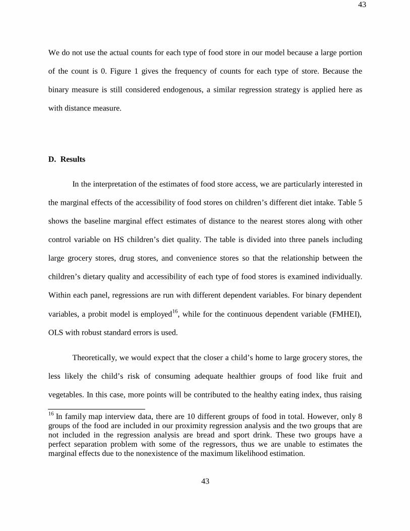
We do not use the actual counts for each type of food store in our model because a large portion

of the count is 0. Figure 1 gives the frequency of counts for each type of store. Because the

binary measure is still considered endogenous, a similar regression strategy is applied here as

with distance measure.

D. Results

In the interpretation of the estimates of food store access, we are particularly interested in

the marginal effects of the accessibility of food stores on children’s different diet intake. Table 5

shows the baseline marginal effect estimates of distance to the nearest stores along with other

control variable on HS children’s diet quality. The table is divided into three panels including

large grocery stores, drug stores, and convenience stores so that the relationship between the

children’s dietary quality and accessibility of each type of food stores is examined individually.

Within each panel, regressions are run with different dependent variables. For binary dependent

variables, a probit model is employed16, while for the continuous dependent variable (FMHEI), OLS with robust standard errors is used.

Theoretically, we would expect that the closer a child’s home to large grocery stores, the

less likely the child’s risk of consuming adequate healthier groups of food like fruit and

vegetables. In this case, more points will be contributed to the healthy eating index, thus raising

16 In family map interview data, there are 10 different groups of food in total. However, only 8 groups of the food are included in our proximity regression analysis and the two groups that are not included in the regression analysis are bread and sport drink. These two groups have a perfect separation problem with some of the regressors, thus we are unable to estimates the marginal effects due to the nonexistence of the maximum likelihood estimation.

43

44

higher FMHEI score. On the other hand, we would expect that the closer children live to drug

stores or convenience stores, the more likely the risk for over-consuming unhealthy food like

sweets and sugar drinks because drug stores and convenience stores usually tend to sell a large

amount of high energy dense foods and sell few fruit or vegetables. In this case, FMHEI scores

will be lower. When examining the marginal effect of proximity on both binary and index dietary

measures, however, we notice that none of the estimates are statistically significant. Increasing

the distance from a child’s house to any type of food stores by one mile influences neither the

probability of having risk on consuming any group of food regardless of healthy food

(consuming too less) and unhealthy food (consuming too much) nor the healthy eating index.

An interesting finding from this table is that the mental health condition of a child’s

parents has a significant negative impact on the integrated dietary measure FMHEI but not on

each individual binary dietary measure across all groups of food. It appears that if a caregiver is

suffering mental depression or stress, it is expected to affect the child’s healthy eating index by

about -3.5 points at a 5 percent significance level. This result is consistent with our expectation

that parents who are bothered by depression, feelings of hopeless, lack of interest or pleasure

doing things are less likely to provide high quality childcare or parenting, which may indirectly

affect a child’s diet quality. Depression does not have a significant effect on the risk of the binary

dietary measure but only on the eating index. A likely explanation is that the eating index is

comprised of more components such as eating environment and habit than just food intake

information. When parents are mentally stressed or depressed, it is very less likely that they

would create a pleasant family eating environment for their children or follow a regular eating

habit or routine, which can contribute to a lower score on the FMHEI. It is also worth pointing

44

45

out that our individual group of food intake information is only a binary diet measure that only

indicates whether or not the child is at risk of consuming certain group of food, while the FMHEI

is a continuous diet measure capturing more information on the child’s diet information.

Therefore, the results imply that parents’ mental health conditions result in no change in the

probability of having risk of consuming each group of food but change in child’s eating index as

an integrated measure.

Demographic variables such as gender and race show some significant effects in a few

regressions. For example, under the large grocery stores panel, girls have 7% less probability of

having risk in consuming insufficient meat than boys. Although very small in magnitude, the

result is statistically significantly at 5 percent level. Compared to other races, African American

children have 25 percent greater probability of having risk on consuming inadequate beans and

28 percent higher probability of having risk on over-consuming juice. Also, under the juice

column, being white shows a negative significant influence on the probability of having risk of

consuming excessive juice. Like the proximity and depression variables, however, demographic

variables do not show any significant effect on consumption of any other interesting groups of

food like fruit, vegetables, sweets and sugar drinks. These results are consistent across three

different types of food store.

In an attempt to limit the bias from endogeneity, we employ an instrumental variable

approach targeting at each child’s family location decision and food store location decision. A

valid instrumental variable should only impact a child’s dietary quality through its effect on food

store locations and will only correlate with the food store access but not child’s dietary quality

45

46

measure. The instrumental variable we use to identify our model is the percentage of land that

was zoned as commercial within a 0.5 mile radius buffer of each child’s residence. The logic is

that food store establishments not only first locate to the commercial zoning area, but they also

tend to choose to locate to places where neighborhood residences can easily access to their

establishments and where business can capture sales. Figure 3 provides the maps of the food

stores, indicating the available land for food stores to locate within a 0.5 mile buffer of a child’s

residence for all five major towns. A visual inspection of the map for each town in figure 3

confirms the correlation between of the food store location and the instrument17. Unfortunately, the two weak identification diagnostic F test statistics18 are quite small, which indicate that we

fail to reject the null hypothesis that our equation is weakly identified. To compare to the

marginal effects in baseline model, we present the second stage results of the IV model, however.

Table 6 provides the marginal effects of food store access on children’s dietary quality

with IV approach for large grocery stores, drug stores and convenience stores. It is surprising

that many of the marginal effects of proximity become strongly statistically significant. For

example, increasing one mile of distance to the nearest large grocery store will increase the

chance of having trouble on consuming beans and meat by 19 percent and 18 percent

respectively. The probability of a child having trouble consuming fruits and vegetables will both

increase approximately 20 percent if the family must travel one more mile of distance to shop at

the large grocery stores from their home. Moving to drug stores, the effect of the proximity has

17 Plumerville is a very small city in Conway county in state Arkansas. The population is only 854. The fact is that people who live at Plumerville shop at Morrilton where the stores concentrate. 18 Cragg-Donald Wald F statistic is 0.13 and Kleibergen-Paap Wald rk F Statistic is 0.17.

46

47

the opposite effect on the risk of bean and fruit consumption. The further the child’s home to the

drug stores, the less likely the child will have risk on fruit consumption, and this magnitude is

16.5 percent, at 1 percent level of statistical significance. This implies that the further the drug

stores to the child’s home, the more likely they will consume healthier foods. We would also

expect that the further the drug stores, the more likely the children will have risk on over-

consuming sweets and sugar drink. However, those estimates are not statistically significant,

although the signs are as expected. Turning to the convenience store panel, the negative effect of

distance to nearest convenience stores on risk of fruit consumption is twice as large as the effect

of drug stores proximity on risk of fruit consumption, and this is the only effect of convenience

stores proximity on any risk of food intake.

However, distance to the closest drug store and convenience store does not show any

impact on vegetable consumption like large grocery stores. Moreover, no impacts of distance to

the closest drug store and convenience store appear on the consumption of unhealthy foods like

sweets and sugar drinks. Demographic variables show some interesting impacts on risk for

consumption of some groups of food. For instance, in panel two, compared to other races, white

children are less likely to have problem with consuming beans, vegetables and fruit while

African American children are more likely to have trouble taking adequate those foods. In panel

three, girls show about 15 percent greater risk on consuming fruit than boys. Again, like the

marginal effects in Table 5, depression doesn’t show any significant influence on any of the

binary measures. When using FMHEI as a diet quality measure, the significant effect by

depression observed in Table 5 disappears when IV strategy is adopted here.

47

48

In Table 7 and Table 8, we switched the food store access measure to density and present

marginal effects of variables 19 in the baseline model and instrumental variable model as

presented in Table 5 and Table 6. As we mentioned before, we alter the density to binary

variable with the case that the majority of the count is zero. Results in these two tables are

similar to the proximity model results. The food store access density measure does not have any

association with the integrated diet quality measure FMHEI in either baseline or IV model.

However, the density measure presents a different influence on the binary diet measures between

the baseline and IV models. For instance, compared to HS children who live at the location that

does not have any large grocery stores within a 0.5 mile buffer, children who live in the

neighborhood that can reach large grocery stores within 0.5 mile are 53 percent less likely to

have trouble consuming vegetable and 71 percent less likely to have risk of consuming fruits. On

the other hand, the difference between the impact of having a convenience store within 0.5 mile

neighborhood and not having one on children’s probability of having problem consuming fruit

and vegetables is about 51 percent. Again, having one or more drug stores within 0.5 mile tends

to increase the risk of children consuming sweets and sugar drink by 50 percent chance. Finally,

similarly as before, the significance of the effect of depression on FMHEI disappears when

included in the IV model.

19 For the binary dependent variable, we only include 7 groups of food in the density model. The excluded group is the meat group. The existence of the perfect separation problem with some of the regressors does not allow us to estimate the marginal effects due the nonexistence of the maximum likelihood estimation.

48

49

Den

sity

coun

t D

ensi

ty co

unt

Den

sity

coun

t

Figure1. The frequency of density measure for each types of food store

Frequency of density counts of large grocery stores within 0.5 mile buffer

2 6

1 30

0 125

0 50 100 150 Frequency

Frequency of density counts of drug stores within 0.5 mile buffer

3 2

2 13

1 50

0 96

0 50 100 150 Frequency

Frequency of density counts of convenience stores within 0.5 mile buffer

2 11

1 30

0 120

0 50 100 150

Frequency

49

50

Figure2. Frequency for FMHEI

50

51

Figure 3(a)

Food stores in Clarksville, Arkansas

51

52

Figure 3(b)

Food stores in Morrilton, Arkansas

52

53

Figure 3(c)

Food stores in Russellville and Dardanelle, Arkansas

53

54

Figure 3(d)

Food stores in Plumerville, Arkansas

54

55

Table1. Proportion of risk on HS children consuming each group of food with different sample size

Group Full sample Risk on F or V Male Female Dairy 11.18% 15.84% 13.92% 8.54% Meat 4.38% 3.96% 7.69% 1.22% Beans 23.90% 29.00% 26.92% 20.99% Bread 1.88% 1.98% 1.28% 2.44% Vegetables 57.14% 91.09% 53.16% 60.98% Fruits 28.57% 45.54% 22.78% 34.15% Juice 22.15% 23.23% 21.05% 23.17% Sweets 15.82% 15.00% 19.23% 12.50% Sugar drink 13.38% 13.00% 14.67% 12.20% Sport drink 1.89% 0.00% 2.53% 1.25% Sample size 161 101 79 82

55

56

FMHEI total (0-100) FMHEI Scoring Criteria FMHEI components Requirements for max score of 10 Requirements for min score of 0

Frequency 1 Dairy ≥1 time/day 0 2 Bread ≥1 time/day 0 3 Vegetables ≥1 time/day 0 4 Fruits ≥1 time /day 0 5 Sweet snacks 0 ≥1/day

Requirements for max score of 5 Requirements for min score of 0

6 Beans 7 Meat 8 Sugar drink 9 Sports drink 10 Juice

Frequency ≥1 time/day 0 ≥1 time/day 0

0 ≥1 time/day 0 ≥1 time/day

2-6 times/week 0 or ≥1 time/day Family eating dinner at regular

11 time ≥6 times/week ≤1 time/week 12 Follow morning routines ≥6 times/week ≤1 time/week

13 Salt snack1 3.75

14 Others2 5

1. Salt snacks include potato chips corn chips, nachos, popcorn, pretzels, and crackers 2. Others include multivitamin use, margarine and butter, fried foods outside home and visible animal fat

56

Table2. Family Map Healthy Eating Index (FMHEI) scoring criteria

57

Table3. Descriptive statistics for food store access measure

Food store access measure Mean SD Min Max

Distance to the nearest large grocery store

1.56

1.55

0.10

8.23 Distance to the nearest convenience store 0.88 0.80 0.04 4.66 Distance to the nearest drug store 1.55 1.86 0.07 11.10 Density of large grocery stores within 0.5 mile radial distance 0.26 0.52 0.00 2.00 Density of convenience stores within 0.5 mile radial distance 0.51 0.70 0.00 3.00 Density of drug stores within 0.5 mile radial distance 0.32 0.60 0.00 2.00

Table4. Characteristics of control variables

Variables Proportion Race White 40.35% African American 12.66% Other 46.99% Target Child Gender Female 49.36% Male 50.64% Depression 32.92%

57

58

Large Grocery Stores Variables Dairy Beans Meat Vegetable Fruit Juice Sweets Sugar Drink FMHEI Proximity -0.0267 0.00499 0.00672 0.00757 0.00544 0.0118 0.00991 -0.0142 0.0306

(0.0215) (0.0217) (0.00946) (0.0255) (0.0230) (0.0192) (0.0180) (0.0191) (0.488) Female -0.0400 -0.0245 -0.0703** 0.0216 0.103 0.0623 -0.0698 -0.00173 -1.195

(0.0471) (0.0671) (0.0330) (0.0778) (0.0710) (0.0636) (0.0566) (0.0531) (1.377) Black 0.0944 0.246* -0.0404 0.0633 0.113 0.277* 0.0545 0.0774 -3.611

(0.0888) (0.134) (0.0366) (0.125) (0.126) (0.150) (0.104) (0.118) (2.353) White 0.0824 -0.0947 0.0234 -0.0589 0.00387 -0.267*** 0.0200 -0.0877 -0.263

(0.0692) (0.0913) (0.0487) (0.108) (0.0994) (0.0804) (0.0815) (0.0722) (1.845) Depression 0.0834 -0.0636 -0.0199 -0.133 -0.00628 0.0906 -0.00377 -0.0168 -3.508**

(0.0790) (0.0867) (0.0381) (0.107) (0.0972) (0.0938) (0.0777) (0.0695) (1.633) Drug Stores

Proximity -0.0151 -0.00719 0.00435 0.00414 0.00153 0.00194 0.00905 -0.00777 0.0479 (0.0174) (0.0188) (0.00803) (0.0215) (0.0194) (0.0165) (0.0151) (0.0159) (0.381)

Female -0.0405 -0.0262 -0.0707** 0.0214 0.103 0.0612 -0.0698 -0.00139 -1.192 (0.0473) (0.0671) (0.0330) (0.0778) (0.0711) (0.0637) (0.0565) (0.0532) (1.374)

Black 0.0915 0.255* -0.0401 0.0640 0.115 0.284* 0.0519 0.0758 -3.634 (0.0890) (0.134) (0.0369) (0.126) (0.127) (0.149) (0.104) (0.118) (2.377)

White 0.0841 -0.106 0.0235 -0.0597 0.00143 -0.272*** 0.0240 -0.0867 -0.229 (0.0709) (0.0907) (0.0496) (0.109) (0.100) (0.0796) (0.0830) (0.0730) (1.894)

Depression 0.0821 -0.0599 -0.0201 -0.132 -0.00522 0.0945 -0.00477 -0.0173 -3.518** (0.0793) (0.0873) (0.0381) (0.108) (0.0975) (0.0941) (0.0775) (0.0696) (1.634)

58

Table5. Marginal effects of baseline proximity model

59

Convenience Stores Variables Dairy Beans Meat Vegetable Fruit Juice Sweets Sugar Drink FMHEI Proximity 0.00551 -0.00822 0.0191 0.00550 -0.0722 -0.0297 0.0152 -0.0215 -0.0972

(0.0311) (0.0449) (0.0186) (0.0500) (0.0513) (0.0417) (0.0354) (0.0377) (0.664) Female -0.0386 -0.0232 -0.0748** 0.0196 0.122* 0.0678 -0.0735 0.00368 -1.176

(0.0475) (0.0680) (0.0336) (0.0786) (0.0716) (0.0642) (0.0569) (0.0537) (1.403) Black 0.0757 0.248* -0.0397 0.0669 0.125 0.290** 0.0611 0.0714 -3.585

(0.0846) (0.133) (0.0362) (0.125) (0.125) (0.147) (0.104) (0.117) (2.350) White 0.105 -0.0993 0.0219 -0.0631 -0.0194 -0.279*** 0.0169 -0.0858 -0.314

(0.0725) (0.0896) (0.0474) (0.107) (0.0962) (0.0773) (0.0807) (0.0728) (1.855) Depression 0.0723 -0.0603 -0.0200 -0.131 0.00671 0.102 -0.00408 -0.0164 -3.488**

(0.0782) (0.0876) (0.0379) (0.107) (0.0972) (0.0945) (0.0780) (0.0697) (1.609)

59

Table5. Marginal effects of baseline proximity model (cont.)

60

Large Grocery Stores Variables Dairy Beans Meat Vegetable Fruit Juice Sweets Sugar Drink FMHEI Proximity -0.213*** 0.1903*** 0.182*** 0.198*** 0.195*** 0.164 -0.201 -0.208*** -3.735

(0.0395) (0.045) (0.072) (0.037) (0.024) (0.373) (0.042) (0.015) (17.08) Female -0.041 0.0115 -0.023 0.024 0.032 0.042 -0.045 -0.018 -1.459

(0.085) (0.051) (0.112) (0.053) (0.0601) (0.3005) (0.092) (0.052) (2.270) Black 0.159 -0.057 -0.114 -0.091 -0.091 0.085 0.132 0.137 -4.402

(0.149) (0.164) (0.066) (0.105) (0.0902) (1.436) (0.097) (0.105) (4.141) White -0.106 0.125 0.146** 0.134 0.1502** -0.071 -0.148 -0.189 -3.064

(0.213) (0.114) (0.075) (0.106) (0.068) (1.795) (0.086) (0.1) (13.00) Depression 0.093 -0.0603 0.055 -0.083 -0.049 -0.01 0.051 0.045 -0.207

(0.137) (0.066) (0.059) (0.1104) (0.063) (0.545) (0.073) (0.074) (3.841) Drug Stores

Proximity 0.089 -0.151** -0.136 -0.512 -0.165*** -0.087 0.108 0.013 1.267 (0.125) (0.064) (0.098) (0.805) (0.029) (0.155) (0.096) (0.085) (5.008) Female -0.023 -0.036 -0.129 -0.00998 0.023 0.042 -0.0.39 0.105 -1.084

(0.066) (0.0596) (0.083) (0.270) (0.071) (0.078) (0.072) (0.051) (1.360) Black -0.015 0.262** 0.066 0.613 0.184** 0.305*** -0.048 -0.048 -3.104

(1.161) (0.119) (1.623) (0.802) (0.088) (0.122) (0.128) (0.126) (2.685) White 0.1996 -0.234*** -0.148 -0.789 -0.197*** -0.340*** 0.143 0.077 1.326

(0.104) (0.081) (1.50) (1.038) (0.080) (0.119) (0.130) (0.166) (6.769) Depression 0.026 0.016 0.019 -0.138 0.062 0.117 -0.039 -0.053 -1.504

(0.117) (0.101) (0.105) (0.457) (0.077) (0.089) (0.072) (0.065) (2.635)

60

Table6. Marginal effects of IV proximity model

61

61

Table6. Marginal effects of IV proximity model (cont.)

Convenience Stores

Variables Dairy Beans Meat Vegetable Fruit Juice Sweets Sugar Drink FMHEI Proximity 0.012 -0.247 -0.186 -0.202 -0.336*** -0.112 0.166 0.178 1.324

(0.218) (0.166) (0.200) (0.194) (0.010) (0.238) (0.195) (0.179) (5.230) Female -0.065 0.035 -0.078 0.063 0.149** 0.084 -0.102* -0.040 -1.482

(0.067) (0.077) (0.071) (0.078) (0.062) (0.077) (0.060) (0.066) (2.016) Black 0.063 0.221* -0.036 0.075 0.115 0.284** 0.040 0.047 -3.324

(0.089) (0.124) (0.094) (0.110) (0.104) (0.144) (0.1002) (0.109) (2.159) White 0.138 -0.149 -0.044 -0.112 -0.095 -0.295*** 0.059 -0.031 0.180

(0.086) (0.086) (0.097) (0.100) (0.086) (0.089) (0.094) (0.106) (2.636) Depression 0.055 -0.023 -0.012 -0.083 0.043 0.110 -0.020 -0.036 -0.942

(0.085) (0.096) (0.083) (0.118) (0.086) (0.095) (0.075) (0.069) -1.455

62

Large Grocery Stores Variables Dairy Beans Vegetable Fruit Juice Sweets Sugar Drink FMHEI Density -0.0332 -0.00142 -0.0252 -0.107 0.0239 -0.0211 -0.0612 1.508

(0.0530) (0.0809) (0.0941) (0.0785) (0.0784) (0.0652) (0.0560) (1.600) Female -0.0399 -0.0251 0.0193 0.0953 0.0619 -0.0712 -0.00441 -1.110

(0.0474) (0.0672) (0.0779) (0.0710) (0.0637) (0.0566) (0.0532) (1.387) Black 0.0739 0.248* 0.0665 0.107 0.286* 0.0623 0.0717 -3.522

(0.0840) (0.133) (0.125) (0.125) (0.147) (0.104) (0.116) (2.332) White 0.105 -0.0980 -0.0636 0.00494 -0.274*** 0.0121 -0.0781 -0.347

(0.0714) (0.0897) (0.106) (0.0972) (0.0781) (0.0798) (0.0728) (1.844) Depression 0.0687 -0.0624 -0.133 -0.0158 0.0982 -0.00239 -0.0276 -3.369**

(0.0771) (0.0871) (0.108) (0.0960) (0.0945) (0.0779) (0.0668) (1.591) Drug Stores

Density 0.0330 0.143* -0.0428 -0.0627 -0.0326 0.0263 -0.0378 0.776 (0.0571) (0.0836) (0.0911) (0.0784) (0.0724) (0.0674) (0.0581) (1.484)

Female -0.0388 -0.0323 0.0223 0.104 0.0611 -0.0724 0.00192 -1.226 (0.0474) (0.0664) (0.0777) (0.0709) (0.0636) (0.0566) (0.0533) (1.385)

Black 0.0803 0.275** 0.0623 0.108 0.284* 0.0660 0.0674 -3.496 (0.0854) (0.133) (0.125) (0.126) (0.148) (0.105) (0.115) (2.347)

White 0.0974 -0.126 -0.0558 0.0118 -0.270*** 0.00861 -0.0744 -0.443 (0.0708) (0.0866) (0.108) (0.0993) (0.0794) (0.0797) (0.0737) (1.890)

Depression 0.0763 -0.0578 -0.131 -0.00764 0.0947 3.70e-05 -0.0229 -3.488** (0.0778) (0.0860) (0.107) (0.0970) (0.0939) (0.0783) (0.0680) (1.598)

62

Table7. Marginal effects of baseline density model

63

63

Table7. Marginal effects of baseline density model (cont.)

Convenience Stores

Variables Dairy Beans Vegetable Fruit Juice Sweets Sugar Drink FMHEI Density -0.0754 -0.0407 -0.0522 -0.0285 0.0260 -0.0178 -0.0605 1.490

(0.0508) (0.0698) (0.0803) (0.0738) (0.0656) (0.0585) (0.0569) (1.461) Female -0.0440 -0.0315 0.0115 0.0972 0.0651 -0.0733 -0.00688 -0.938

(0.0472) (0.0679) (0.0790) (0.0722) (0.0645) (0.0571) (0.0533) (1.426) Black 0.0687 0.248* 0.0669 0.115 0.285* 0.0620 0.0612 -3.562

(0.0820) (0.134) (0.124) (0.126) (0.147) (0.104) (0.112) (2.369) White 0.117 -0.0955 -0.0590 0.00312 -0.275*** 0.0148 -0.0669 -0.460

(0.0726) (0.0902) (0.106) (0.0980) (0.0779) (0.0802) (0.0735) (1.865) Depression 0.0651 -0.0660 -0.132 -0.00523 0.0976 -0.000862 -0.0262 -3.466**

(0.0765) (0.0867) (0.107) (0.0971) (0.0940) (0.0781) (0.0674) (1.581)

64

Large Grocery Stores Variables Dairy Beans Vegetable Fruit Juice Sweets Sugar Drink FMHEI Density 0.378 -0.629** -0.527* -0.714*** -0.375 0.441 0.458* 5.885

(0.418) (0.248) (0.295) (0.0715) (0.705) (0.288) (0.259) (23.71) Female -0.0100 -0.0519 -0.0178 0.000891 0.0309 -0.0216 0.0275 -0.886

(0.0740) (0.0578) (0.0652) (0.0686) (0.0919) (0.0806) (0.0496) (1.575) Black 0.0816 0.105 0.0170 0.0139 0.220 0.0645 0.0720 -3.592*

(0.0916) (0.162) (0.109) (0.0992) (0.223) (0.0890) (0.0962) (1.842) White 0.0668 -0.0371 -0.0194 0.0267 -0.250** -0.0102 -0.0735 -0.459

(0.123) (0.102) (0.0940) (0.0732) (0.128) (0.0687) (0.0784) (1.885) Depression 0.0941 -0.0927 -0.128 -0.0636 0.0473 0.0405 0.0263 -1.109

(0.0759) (0.0791) (0.0956) (0.0740) (0.136) (0.0747) (0.0781) (1.526) Drug Stores

Density 0.438 -0.615*** -0.564*** -0.667*** -0.501 0.490** 0.499** 6.058 (0.320) (0.155) (0.202) (0.0321) (0.730) (0.241) (0.229) (24.69) Female -0.0406 0.0112 0.0302 0.0526 0.0661 -0.0552 -0.0172 -1.365

(0.0486) (0.0568) (0.0517) (0.0622) (0.0643) (0.0613) (0.0454) (1.729) Black 0.109 0.0157 -0.0392 -0.0510 0.153 0.0985 0.105 -4.040

(0.0805) (0.173) (0.113) (0.0942) (0.340) (0.0814) (0.0892) (2.585) White -0.0248 0.0792 0.0811 0.129** -0.160 -0.0872 -0.136** -1.404

(0.163) (0.115) (0.102) (0.0627) (0.364) (0.0763) (0.0594) (4.833) Depression 0.0532 -0.0341 -0.0693 -0.0108 0.0651 0.00835 -0.00389 -0.596

(0.0867) (0.0798) (0.111) (0.0665) (0.120) (0.0607) (0.0643) (2.105)

64

Table8. Marginal effects of IV density model

65

65

Table8. Marginal effects of IV density model (cont.)

Convenience Stores Variables Dairy Beans Vegetable Fruit Juice Sweets Sugar Drink FMHEI Density -0.546*** 0.514*** 0.523*** 0.519*** 0.507*** -0.536*** -0.534*** -7.543

(0.0806) (0.0502) (0.0160) (0.0241) (0.114) (0.0444) (0.0515) (31.90) Female -0.102 0.0848* 0.0917** 0.0943** 0.100 -0.103 -0.0903** -2.301

(0.0763) (0.0438) (0.0425) (0.0473) (0.0702) (0.0837) (0.0403) (5.191) Black 0.00614 0.0345 0.0202 0.0189 0.0785 -0.00119 -0.00244 -2.799

(0.116) (0.135) (0.0828) (0.0764) (0.360) (0.0871) (0.0815) (3.978) White 0.0894 -0.0692 -0.0682 -0.0597 -0.136 0.0637 0.0496 0.757

(0.165) (0.0706) (0.0691) (0.0531) (0.385) (0.0585) (0.0767) (4.804) Depression 0.00451 0.00481 -0.00431 0.0119 0.0346 -0.0121 -0.0159 0.523

(0.105) (0.0656) (0.102) (0.0545) (0.130) (0.0570) (0.0591) (6.537)

66

IV. DISCUSSION AND CONCLUSION A. Childhood obesity and academic achievement

The objective of this study is to investigate whether there is an association between

academic achievement and obesity rates among young children in Arkansas public schools.

Using grade level panel data, our results suggest that there is no evidence showing that obesity

rates in grades 4 and 6 are associated with math and literacy achievement scores. This finding is

robust across our pooled OLS, fixed effects, and random effects models. These results are also

consistent with the findings of some of the previous studies (MacCann and Roberts, 2013;

Kaestern and Grossman, 2009; Scholder et al., 2010). Admittedly, our finding of no significant

relationship between childhood obesity and academic achievement scores does not imply that

obesity has no causal impact at all on educational outcomes. While we controlled for time

invariant unobservables, our analysis does not mitigate time varying unobservables that may

affect both academic performance and obesity prevalence. We were not able to take this issue

into account due to lack of potential instruments in our data. While it is indeed a challenge to

find valid instrumental variables, future studies should attempt to replicate our analysis using not

only fixed effects models but also instrumental variable models.

We found additional interesting results when we separated our sample between low and

high SES schools and between low and high minority schools. For example, our results indicate

that obesity prevalence has a positive effect on grade 4 students’ literacy test scores in the low

SES subsample but a negative effect on math test scores in the high SES subsample. The behind

mechanism for the positive effect on grade 4 literacy scores of students in the low SES category

is not clear. More research is needed to more definitively examine the linkage between obesity

prevalence and academic performance. What is consistently clear in our results is that although

66

67

the magnitude are small, educational input measures have a positive relationship to students’

achievement scores and this finding is robust across the different models and subsamples.

B. Food store access and childhood diet quality

This study explores the effect of food store access on 3-5 year old HS children’s dietary

quality by using cross sectional sample of 2006-2007 Arkansas family map interview data. One

of the key strengths of this paper is that in addition to investigating the effect of food store access

on risk of each individual group of food consumption, we create the FMHEI, an integrated

measure that contains not only information about consumption of each group of food but also

information about children’s eating environment and habit, to gain a more comprehensive view

on the linkage between food store access and children’s dietary quality. Another advantage of

this paper is that while exploring the relationship between the food store access and children’s

diet quality, we are more cautious about the existence of potential endogenous issue that most of

the prior papers did not take into account. We use an instrumental variable strategy in the model

to tackle the problem by using zoning regulations to calculate the percentage of land for

commercial use within the 0.5 mile buffer of each child residence with ArcGIS software. In

addition, we evaluate the effect of food store access on dietary quality with both proximity and

density measures

In general, food store accessibility measures (proximity and density) do not show any

significant effect on either the binary diet measures or diet quality index measure in the baseline

models. However, both proximity and density measures have very significantly strong impacts

on the risk of some of individual group of food consumption when instrumental variable strategy

67

68

is applied to a probit model. A one mile increase of distance to the closest large grocery store is

expected to raise the probability of risk of consuming both fruit and vegetable for HS children by

20 percent and reduce the chance of risk on consuming sugar drinks by 20 percent. The longer

the distance from the children’s homes to drug stores and convenience stores, the less likely the

children will have risk on fruit consumption. The difference between the effect of having any

type of food stores within a 0.5 mile neighborhood and not having them on the risk of consuming

any group of food is strong as well. Available large grocery stores within a 0.5 mile buffer from

the home tend to reduce the likelihood of having trouble consuming vegetables by 53 percent

and reduce the likelihood of having trouble having fruits by 71 percent. On the opposite, the

existence of convenience stores within a 0.5 mile buffer will increase the risk of having

vegetables and fruits by both 52 percent. An interesting finding is that the variable depression,

the indicator for parents’ mental health, has a closely association with the diet quality of the HS

children in baseline model and its significance disappears when the instrumental variable

approach is applied.

One limitation in this study is that the distance is the direct measure between two

locations from the map, not the actual travel routes based on the networking analysis in ArcGIS.

The real distance based on actual networking could be much longer than the way we calculate for

the HS family to travel to the nearest food stores. The density measure could potentially change

correspondingly based on the networking buffer instead of the direct radius buffer. A second

limitation of this study is that the sample size is fairly small. When the instrument variable we

use is weak, the estimates generated by the IV approach with small sample size are biased and

theoretically the results are no better than simple OLS. In our study, we tried to improve the

performance of the estimates by using LIML while executing the IV estimation with the

68

69

continuous variable FMHEI. For the instrumental variable approach with binary dependent

measure, to our knowledge, there is not an available technology for us to improve the small

sample estimation properties. Another problem with small simple size for our study is that we are

unable to break our sample to further explore the effect of food store access on different group of

children’s diet quality. Finally, the data we use is only cross sectional data, and we lack of panel

data that would allow us to control for more factors over time. Future studies should replicate

this study by improving upon the aforementioned limitations.

69

70

References Aaronson, D, L Barrow, W Sander. 2007. “Teachers and Student Achievement in the Chicago Public High Schools.” Journal of Labor Economics, 25 (1): 95-135.

Alviola, P, RM Nayga, Jr., M Thomsen, D Danforth, J Smartt. 2013. “The Effect of Fast-Food Restaurants on School-Level Obesity.” Economics and Human Biology, forthcoming.

Alviola, P, RM Nayga, Jr., M Thomsen. 2013. “Food Deserts and Childhood Obesity.” Applied Economic Perspectives and Policy, 35 (1): 106-124.

Averett, SL, DC Stifel. 2010. Race and Gender Differences In the Cognitive Effects of Childhood Overweight. Applied Economics Letters, 17: 1673-1679.

Austin, JK, TJ Huberty, GA Huster, DW Dunn. 1998. “Academic Achievement in Children with Epilepsy or Asthma.” Developmental Medicine and Child Neurology, 40(4): 248-255.

Bacolod, M. 2007. “Who Teaches and Where They Choose to Teach: College Graduates of the 1990s” Educational Evaluation and Policy Analysis, 29 (3): 155-168.

Belot, M, J James. 2011. “Healthy School Meals and Educational Outcomes.” Journal of health Economics, 30 (3): 489-504.

Blau, DM. 1999. “The Effect of Income on Child Development.” The Review of Economics and Statistics, 81 (2): 261-276.

Blandchard T, T Matthews. 2007. “Retail Concentration, Food Deserts and Food Disadvantaged Dommunities in Rural America.” Remaking the North American Food system, 201-215. Lincoln: University of Nebraska Press.

Bonesronning, H, T Falch, B Strom. 2005 “Teacher Sorting, Teacher Quality, and Student Composition.” European Economic Review, 49 (2): 457-483.

Carlson, SA, JE Fulton, SM Lee, MM, DR Brown, HW Kohl III, WH Dietz. 2008. “Physical Education and Academic Achievement in Elementary School: data from the Early Childhood Longitudinal Study.” American Journal of Public Health, 98 (4): 721-727.

Chen S.E., RJGM Florax, SD Snyder. 2009 “Obesity in Urban Food Markets: Evidence from Georeferenced Micro Data” Research report, Dept. Agricultural Economics, Purdue University, Lafayette.

Chen S., Florax R.J.G.M., and Miller C.C. 2010. “Obesity and Access to Chain Grocers”. Economic Geography, 86(4): 431-452.

Clotfelter, Charles T., Helen F. Ladd and Jacob L. Vigdor. 2006. “Teacher-Student Matching and the Assessment of Teacher Effectiveness.” The Journal of Human Resources, 41 (4): 778-820.

70

71

Crosnoe, R, C Muller. 2004. “Body Mass Index, Academic Achievement, and School Context: Examining the Educational Experiences of Adolescents at Risk of Obesity,” Journal of Health and Social Behavior, 45: 393-407.

Cummins, SS. Macintyre. 2002. “Food Deserts-Evidence and Assumption in Health Policy Making.” British Medical Journal, 235: 436-438

Currie, J. 2009. “Health, Wealthy, and Wise: Socioeconomic Status, Poor Health in Childhood, and Human Capital Development.” Journal of Economic Literature, 47(1): 87-122 (36).

Currie, J, S DellaVigna, E Moretti, S Pathania. 2010. “The Effect of Fast-Food Restaurants on Obesity and Weight Gain.” American Economic Journal: Economic Policy, 2(3), 32-63.

Datar, A, R Sturm, JL Magnabosco. 2004. “Childhood Overweight and Academic Performance: National Study of Kindergartners and First-Graders.” Obesity Research, 12 (1): 58-68

Datar, A, R Sturm. 2006. “Childhood Overweight and Elementary School Outcomes.” International Journal of Obesity, 30: 1449-1460.

Davis, B., Carpenter, C. 2009. “Proximity of Fast-Food Restaurants on Schools and Adolescent Obesity.” American Journal of Public Health, 99 (3): 505-510

DeCuri-Gunby, JT, JD Taliaferro, D Greenfield. 2010. “Educators’ Perspectives on Culturally Relevant Programs for Academic Success: The American Excellence Association.” Education and Urban Society, 42 (2): 182-204.

Dennison, BA, RL. Helen, SL Baker. 1997. “Excess Fruit Juice Consumption by Preschool-aged Children is Associated with Short Stature and Obesity.” American Academy of Pediatrics, 99 (1): 15-22.

Ding, WL, SF Lehrer, JN Rosenquist, J Audrain-McGovern. 2009. “The Impact of Poor Health on Academic Performance Using Genetic Markers”. J of Health Economics, 28; 578 – 597.

Feskanich, D, RH Helaine, RD Graham, A Colditz. 2004. “Modifying the Healthy Eating Index to Assess Diet Quality In Children and Adolescents.” Journal of the American Dietetic Association, 104(9): 1375-1383.

Freedman, DS., LK Khan, MK Serdula, WH Dietz, SR Srinivasan, GS Berenson. 2005. “The Relation of Childhood BMI to Adult Adiposity: The Bogalusa Heart Study.” Pediatrics, 115: 22- 27.

Gibson, SA. 1996. “Are High-fat, High-sugar Foods and Diets Conducive to Obesity?” International Journal of Food Sciences and Nutrition, 47: 405-415.

71

72

Glewwe, PH, G Jacoby EM King. 2001. “Early Childhood Nutrition and Academic Achievement: A Longitudinal Analysis.” Journal of Public Economics, 81: 345-368.

Guenther, PM, J Reedy, SM Krebs-Smith, BB Reeve, PP Basiotis. 2007 “Development and Evaluation of Healthy Eating Index-2005: Technical Report. Center for Nutrition Policy and Promotions, U.S. Department of Agriculture.

Gurley-Calvez, T, A Higginbotham. 2010. “Childhood Obesity, Academic Achievement, and School Expenditures.” Public Finance Review, 38 (5): 619-646.

Galvezm, MP, L Hong, E Choi, L Liao, J Godbold, B Brenner. 2009. “Childhood obesity and neighborhood food-store availability in an inner-city community.” Academic Pediatrics, 9:339- 343.

Hanson, NI, D Neumark-Sztainer, ME Eisenberg, M Story, M Wall. 2004. “Association between Parental Report of the Home Food Environment and Adolescent Intakes of Fruits, Vegetables and Dairy Foods”. Public Health Nutrition, 8(1): 77-85.

Hanushek, EA. 1986. “The Economics of Schooling: Production and Efficiency in the Public Schools.” Journal of Economic Literature, 49 (3): 1141-1177.

Hanushek, EA. 1989. “The Impact of Differential Expenditures on School Performance.” Educational Researcher, 18 (4): 45-62.

Hanushek, EA, JF Kain, JM Markman, SG Rivkin. 2003. “Does Peer Ability Affect Student Achievement?” Journal of Applied Econometrics 18:527-547.

Hedges, LV, RD Laine, R Greenwald. 1994. “Does Money Matter? A Meta-Analysis of Studies of the Effects of Differential School Inputs on Student Outcomes.” American Educational Research Researcher, 23 (3): 5-14.

Hill, AM, J O’Neill. 1994. “Family Endowments and the Achievement of Young Children with Special Reference to the Underclass.” Journal of Human Resources, 29 (4): 1065-1100.

Hill, NE, LC Taylor. 2004. “Parental School Involvement and Children’s Academic Achievement: Pragmatics and Issues.” Current Direction in Psychological Science, 13 (4): 161- 164.

Israel, GD, LJ Beaulieu, G Hartless. 2001. “The Influence of Family and Community Social Capital on Educational Achievement.” Rural Sociology, 66(1): 43-68

Jackson, KC. 2009. “Student Demographics, Teacher Sorting, and Teacher Quality: Evidence from the End of School Desegregation.” Journal of Labor Economics, 27 (2): 213-256.

72

73

Johnson, RJ, MS Segal, Y Sautin, T Nakagawa, DI Feig, DH Kang et al. 2007. “Potential Role of Sugar (Fructose) in the Epidemic of Hypertension, Obesity and the Metabolic Syndrome, Diabetes, Kidney Disease, and Cardiovascular Disease.” The American Journal of Clinical Nutrition, 86: 899-906.

Kaestner, R, M Grossman. 2009. “Effects of Weight on Children’s Educational Achievement.” Economics of Education Review, 28(6): 651-661.

Kennedy ET, J Ohls, S Carlson, K Fleming. 1995. “The Healthy Eating Index: design and applications.” Journal of American Diet Association, 95: 1103-1108.

Kyureghain, G, RM Nayga Jr., 2013. “Food Store Access, Availability, and Choice When Purchasing Fruit and Vegetables.” American Journal of Agricultural Economics, in press.

Lankford, H, S Loeb, J Wyckoff. 2002. “Teacher Sorting and the Plight of Urban Schools: A Descriptive Analysis.” Education Evaluation and Policy Analysis, 24 (1): 37-62.

Laska, MN, MO Hearst, A Forsyth, AF Pasch, KE Pasch, L Lytle. 2010. “Neighborhood Food Environments: Are They Associated with Adolescent Dietary Intake, Food Purchases and Weight Status?” Public Health Nutrition, 13(11): 1757-1763.

Lavy, VM, D Paserman, A Schlosser. 2008. “Inside the Black of Box of Ability Peer Effects: Evidence from Variation in the Proportion of Low Achievers in the Classroom.” National Bureau of Economic Research, Inc, Working papers: 14415.

Leung, CW, BA Laraia, M Kelly, D Nickleach, NE Adler, LH Kushi et al. 2011. “The Influence of Neighborhood Food Stores on Change in Young Grils’ Body Mass Index.” American Journal of Preventive Medicine, 41 (1): 43-51.

Liu, GC, JS Wilson, R Qi, J Ying. 2007. “Green Neighborhoods, Food Retail and Childhood Overweight: Differences by Population Density.” American Journal of Health Promotion, 21 (4): 317-325.

MacCann C, RD Roberts. 2013. “Just as Smart But Not as Successful: Obese Students Obtain Lower School Grades But Equivalent Test Scores to Nonobese Students.” International Journal of Obesity, 37: 40-46.

Moore LV, AD Roux, V JA, Nettleton, DR Jocobs, Jr. 2008 “Association of the Local Food Environment with Diet Quality- A Comparison of Assessments based on Surveys and Geographic Information Systems.” American Journal of Epidemiology, 167(8): 917-924

Morland K., S Wing, AD Roux, C Poole. 2002. “Neighborhood Characteristics Associated with the Location of Food Stores and Food Service Places.” American Journal Prevention Medicine, 22(1): 23-29

73

74

Morland K., S Wing, AD Roux 2002. “The Contextual Effect of the Local Food Environment on Residents’ Diets: The Atherosclerosis Risk in Communities Study.” American Journal of Public Health, 92(11): 1761-1767.

Muller, C. 1995. “Maternal Employment, Parent Involvement, and Mathematics Achievement among Adolescents.” Journal of Marriage and Family, 57 (1): 85-100.

Okpala CO, AO Okpala, FE Smith. 2001. “Parental Involvement, Instructional Expenditures, Family Socioeconomic Attributes, and Student Achievement.” The Journal of Educational Research, 95 (2): 110-115.

Pearson, T, J Russell, M Campbell, M Barker. 2005. Do Food Deserts Influence Fruit and Vegetable Consumption? A Cross-Sectional Study.” Appetite, 45: 195-197.

Powell, L.M., MC Auld, FJ Chaloupka, PM O’Malley, LD Johnston 2008 “Association Between Access to Food Stores and Adolescent Body Mass Index.” American Journal of Preventive Medicine, 33(4S): S301-307.

Powell, LM, S Slater, D Mirtcheva, Y Bao, FJ Chaloupka. 2007. “Food Stores Availability and Neighborhood Characteristics in the United States.” Preventive Medicine, 44: 189-195.

Puskar, KR, LM Bernardo. 2007. “Mental Health and Academic Achievement: Role of School Nurses.” Journal of Specialists in Pediatric Nursing, 12(4): 215-223.

Rivkin, SG, EA Hanushek, JF Kain. 2005. “Teachers, Schools and Academic Achievement.” Econometrica, 73 (2): 417-458

Sabia, JJ. 2007. “The effect of Body Weight on Adolescent Academic Performance.” Southern Economic Journal, 73 (4): 871-900.

Scholder, S, von HK, GD. Smith, DA Lawlor. 2010. “Genetic Markers as Instrumental Variables: An Application to Child Fat Mass and Academic Achievement.” Health Econometrics and Data Group, Working paper.

Sirin, SR. 2005. “A Meta-Analytic Review of Research.” Review of Educational Research 75 (3): 417-453.

Slavin, RE, C Lake. 2008. “Effective Programs in Elementary Mathematics: A Best-Evidence Synthesis.” Review of Educational Research 78 (3): 427-515.

Taras, H. 2005a. “Nutrition and Student Performance at School.” Journal of School Health, 75 (6): 199-213.

Taras, H. 2005b. “Physical Activity and Student Performance at School.” Journal of School Health, 75 (6): 214-218.

74

75

Taras, H, W Potts-Datema. 2005. “Obesity and Student Performance at School.” Journal of School Health, 75 (8): 291-5.

Wayne, AJ, P Youngs. 2003. “Teacher Characteristics and Student Achievement Gains: A Review.” Review of Education Research, 73 (1):89-122.

Wang, MC, S Kim, AA Gonzalez, KE MacLeod, MA Winkleby 2007. “Socio-economic and Food-Related Physical Characteristics of the Neighborhood Environment Are Associated with Body Mass Index.” Journal Epidemiol Community Health, 61(6): 491-498.

Yan, W and Q Lin. 2005. “Parental Involvement and Mathematics Achievement: Contrast across Racial and Ethnic Groups.” The Journal of Educational Research, 99 (2):116-127.

75