Two-stream theory of light propagation in amplifying media

Two-stream theory of light propagationin amplifying mediaVADIM A. MARKEL

Department of Radiology, University of Pennsylvania, Philadelphia, Pennsylvania 19104, USA ([email protected])

Received 6 November 2017; revised 7 January 2018; accepted 8 January 2018; posted 9 January 2018 (Doc. ID 312781);published 8 February 2018

The two-stream approximation to the radiative transport equation (RTE) is a convenient exactly solvable modelthat allows one to analyze propagation of light in amplifying media. In spite of neglecting the phase and theinterference effects, this model describes the same phenomena as Maxwell’s equation: electromagnetic resonances,onset of lasing, and onset of instabilities. An important added bonus of the RTE description is that it provides fora simple and unambiguous test of physicality of stationary solutions. In the case of Maxwell’s equations, it is notalways obvious or easy to determine whether certain stationary (in particular, monochromatic) solutions arephysical. In the case of RTE, the specific intensity of unphysical stationary solutions becomes negative for somesubset of its arguments. In the paper, stationary and time-dependent solutions to the two-stream model are an-alyzed. It is shown that the conditions for stationary lasing and for emergence of instabilities depend only on thegeometry of the sample and the strength of amplification but not on the intensity of incident light. © 2018

Optical Society of America

OCIS codes: (110.6960) Tomography; (290.5855) Scattering, polarization; (110.5405) Polarimetric imaging.

https://doi.org/10.1364/JOSAB.35.000533

1. INTRODUCTION

Recently, propagation of light in amplifying media has attractedconsiderable interest [1–10], and even some controversy[11–14]. The problem has, in fact, a long history [15,16],and a comprehensive exposition of the subject has been givenin [17]. The difficulty seems to be rooted in the attempts todescribe amplifying media phenomenologically by a linear per-mittivity ϵ with a negative imaginary part. This description issometimes valid and sometimes not, but it is easy to make amistake by assuming the existence of certain stationary (in par-ticular, monochromatic) solutions to Maxwell’s equations thatare not physically realizable. That is, these solutions—eventhough they appear to be perfectly valid—can never be reachedif one starts from a physically reasonable initial condition. Inaddition, amplifying media are known to possess instabilities.This means that solutions can depend dramatically on smallvariations in the initial conditions or the form of externalradiation.

In the case of Maxwell’s equations, determining which sta-tionary solutions are physical and which are not is not alwaysstraightforward. However, if we describe the light propagationin the medium by the radiative transport equation (RTE), thedetermination becomes much simpler. The reason for this sim-plification is that the specific intensity I, which is the physicalquantity described by the RTE [18], is point-wise nonnegativeby definition. We will see that the stationary solutions

purportedly yielding I can be, in fact, negative, at least for somesubsets of the arguments of I , if these solutions are unphysicalin the above sense. This is a red flag; such solutions are math-ematical artifacts of an imprecise or incomplete model; they donot correspond to the physical reality and should not be used.A related point is that, for the corresponding parameters ofthe medium, stationary solutions do not exist, and one mustconsider time dependence.

A similar consideration cannot be applied to the electricfield, which is a vector and can have a projection of arbitrarysign on any given axis. However, we will show that many im-portant features of light propagation in amplifying slabs asdescribed by Maxwell’s equations [17] are also present in thetransport theory. This is counterintuitive, because the RTEdisregards the phase of light and, correspondingly, it disregardsthe interference effects. Nevertheless, the transport theory pre-dicts that a sample of amplifying medium has resonances andcan support stable lasing or exponentially growing runawaysolutions, just as is the case for Maxwell’s equations.

Thus, the main goal of this paper is to provide an alternativeand a somewhat simpler (albeit an approximate) theoreticalframework in which propagation through amplifying mediacan be considered. It will be shown that, although the math-ematical model employed below does not involve the phase, itcaptures, at least qualitatively, certain physical phenomena suchas resonances and the onset of lasing that are generally believed

Research Article Vol. 35, No. 3 / March 2018 / Journal of the Optical Society of America B 533

0740-3224/18/030533-12 Journal © 2018 Optical Society of America

https://orcid.org/0000-0002-9748-6865

https://orcid.org/0000-0002-9748-6865

https://orcid.org/0000-0002-9748-6865

mailto:[email protected]



https://doi.org/10.1364/JOSAB.35.000533

https://crossmark.crossref.org/dialog/?doi=10.1364/JOSAB.35.000533&domain=pdf&date_stamp=2018-02-06

to be closely related to phase and interference. The advantage ofusing the formalism of this paper is simplicity and transparency.It will become clear, for example, that, in the recent controversybetween Baranov et al. and Wang et al. [13,14], the former areright: the onset of lasing is a condition that involves the size ofthe sample and the magnitude of the imaginary part of the per-mittivity but not the field strength.

To avoid unnecessary complications, we will consider a sim-ple exactly solvable model that involves two oppositely directedstreams of radiation. The corresponding two-stream approxima-tion was originally introduced by Kubelka and Munk in 1931[19], well before the modern radiative transport theory wasdeveloped. The goal of the original paper by Kubelka andMunk was to compute the reflectance of a layer of paint.However, the model with just two streams, although never pre-cise, is surprisingly rich and describes radiation transfer in manyphysical systems qualitatively. For example, the two-streamapproximation can be used to explain the varying colors ofclouds. Also, the two-stream theories are applicable to allone-dimensional systems in which forward and backwardpropagation is possible, such as waveguides and transmissionlines. More broadly, the theory of this paper can be applicableto random lasing in micro- or nanopowders wherein thedescription in terms of Maxwell’s equations is too complexand detailed to be practical and the approximate descriptionbased on the RTE must be used instead.

The point of departure for this paper is the RTE written inthe form�

1

c∂∂t

� s · ∇� μt

�I�r; s; t� � μs

ZA�s; s 0�I�r; s 0; t�d2s 0:

(1)

Here I�r; s; t� is the specific intensity at the position r in thedirection of the unit vector s and at the time t, c is the averagespeed of light in the medium, μt � μa � μs is the total attenu-ation coefficient of the medium, with μa and μs being theabsorption and the scattering coefficients, and, finally,A�s; s 0� is the single-scattering phase function. We assume thatexternal radiation enters the medium through its boundary,which can be described mathematically by inhomogeneousboundary conditions (stated below).

The two-stream approximation grows from the minimalisticassumption that only forward and backward scattering is pos-sible. In this case, single scattering in the medium is governedby the delta-Eddington phase function:

A�s; s 0� � pδ2�s; s 0� � qδ2�s; −s 0�; (2)

where p and q are the probabilities of forward and backwardscattering (p� q � 1). The scattering asymmetry parameterof the medium is g � p − q � 1 − 2q � 2p − 1. The transportmean free path l� is given for this medium by

l� � 1

μa � �1 − g�μs� 1

μa � 2qμs: (3)

Note that δ2�s; s 0� in Eq. (2) is the two-dimensional angulardelta function with the property

Rδ2�s; s 0�f �s 0�d2s 0 � f �s�

[20]. Upon substitution of Eq. (2) into Eq. (1), the RTEbecomes

�1

c∂∂t

� s · ∇� μa � qμs

�I�r; s; t� � qμsI�r; −s; t�: (4)

In what follows, we will consider the case when the vector s isperpendicular to an infinite slab of a material. In this case,propagation is described by a one-dimensional set of equations.

2. STATIONARY TWO-STREAM EQUATIONS

Consider the case when a sufficiently wide front of parallel raysof stationary intensity I 0 (incoming energy per unit surface perunit time) is normally incident onto a layer contained betweenthe planes z � 0 and z � L. The slab is characterized by spa-tially uniform coefficients μs and μa and by the scattering prob-abilities p and q. Under certain conditions, which are exploredin detail below (and certainly in the case μa > 0), the specificintensity is also stationary and can be written in the form

I�r; s; t� � I 0�i1�z�δ2�s; z� � i2�z�δ2�s; −z��; (5)

where the two dimensionless streams, i1�z� and i2�z�, satisfy thepair of ordinary differential equations

��d∕dz � μa � qμs�i1�z� � qμs i2�z�; (6a)

�−d∕dz � μa � qμs�i2�z� � qμsi1�z�; (6b)

and the boundary condition

i1�0� � 1; i2�L� � 0: (7)

Note that the above boundary condition does not account forFresnel reflections of the streams at the slab interfaces (i.e., dueto an index mismatch). A more general case of nonnegligibleFresnel reflections is considered in Section 7 below. We thus seethat the parameter 1∕qμs sets the characteristic length scale ofthe problem. All possible solutions can be expressed in terms ofthree dimensionless variables: qμsz, qμsL, and μa∕qμs. Withoutloss of generality, we can assume that qμs is fixed, while μa andL and z can vary. This point of view is adopted everywherebelow except in Section 7, where, in one of the figures, weassume that μa is fixed while qμs and L can vary.

Note that the stationary two-stream equations (6) are equiv-alent to a one-dimensional stationary diffusion equation for theenergy density u�z� (this equivalence does not hold in the time-dependent case; see below). Indeed, let us define the densityand current of energy as u�z� � �I 0∕c��i1�z� � i2�z�� andJ�z� � I 0�i1�z� − i2�z��. The two functions satisfy

dJ∕dz � αu�z� � 0; Ddu∕dz � J � 0; (8)

where D � cl� and α � cμa are the diffusion coefficient andthe rate of absorption. Thus, Fick’s law (second equation above)holds in the two-stream model exactly. We can further trans-form Eq. (8) into a second-order diffusion equation for u, viz.,

�−Dd 2∕dz2 � α�u � 0: (9)The boundary condition for the diffusion equation followsfrom Eq. (7) and is of the form

u�0� − l�u 0�0� � 2I0; u�L� � l�u 0�L� � 0: (10)This is a special case of the more general boundary condition�u� ln · ∇u�jr∈∂Ω, where n is the outward unit normal to theboundary ∂Ω of the domain Ω occupied by the medium, andthe parameter l is known as the extrapolation distance [21].Generally, the value of l depends on the medium parameters

534 Vol. 35, No. 3 / March 2018 / Journal of the Optical Society of America B Research Article

and, in three dimensions, the typical value of l is l ∼ 0.71l�

[22] (in the absence of Fresnel reflections at the interfaces). Theabove result l � l�, as well as the expression D � cl� for thediffusion coefficient, are exact only in the one-dimensionaltwo-stream model.

Note that it is possible to establish an exact equivalencebetween the one-dimensional diffusion equation (9) withthe boundary condition (10) and the two-stream equations (6)with the boundary condition (7). However, there is no suchcorrespondence between the one-dimensional diffusion equa-tion and a more general one-dimensional RTE. If the phasefunction is not of the delta-Eddington form (2), then the dif-fusion equation (9) is only an approximation to the RTE and,moreover, one should use in this case different values for theparameters D and l.

For our purposes, it is more convenient to work directlywith the streams i1 and i2, since both functions are physicallyrequired to be nonnegative. The solution to Eqs. (7), (6) is

i1�z� �a−eλ�z−L� − a�eλ�L−z�

a−e−λL − a�eλL; (11a)

i2�z� � qμseλ�z−L� − eλ�L−z�

a−e−λL − a�eλL; (11b)

where

a � μa � qμs λ; (12a)

λ �ffiffiffiffiffiffiffiffiffiffiffiffiffiffiffiffiffiffiffiffiffiffiffiffiffiffiffiμa�μa � 2qμs�

p�

ffiffiffiffiffiffiffiffiffiffiffiffiμa∕l�p

: (12b)

As one could expect, the expressions for i1�z�, i2�z� are invari-ant with respect to the substitution λ → −λ. Although nothingdepends on the choice of the square root branch in Eq. (12b),we will, for the sake of clarity, fix the branch by applying thecondition 0 ≤ arg�λ� < π. Then we can distinguish thefollowing cases:

(i) If μa > 0, then λ > 0.(ii) If μa � 0, then λ � 0.(iii) If −2qμs < μa < 0, then λ � ijλj � i

ffiffiffiffiffiffiffiffiffiffiffiffiffiffiffiffiffiffiffiffiffiffiffiffiffiffiffiffiffiffiffijμaj�2qμs − jμaj�p

.In this case, maxμa jλj � qμs is achieved at μa � −qμs.

(iv) If μa � −2qμs, then λ � 0.(v) If μa < −2qμs, then λ � ffiffiffiffiffiffiffiffiffiffiffiffiffiffiffiffiffiffiffiffiffiffiffiffiffiffiffiffiffiffiffijμaj�jμaj − 2qμs�

p> 0.

To summarize, λ is either purely real and positive, or purelyimaginary with a positive imaginary part, or zero.

3. STATIONARY TRANSMISSION ANDREFLECTION BY A SLAB

We can define the transmission and reflection coefficients ofthe slab as T � i1�L� and R � i2�0�. The reflection coefficientR is called the albedo; it would yield, for example, the reflec-tivity of a plane-parallel atmosphere. From the result (11),we can find that

T � λ

�μa � qμs� sinh�λL� � λ cosh�λL� ; (13a)

R � qμs sinh�λL��μa � qμs� sinh�λL� � λ cosh�λL� : (13b)

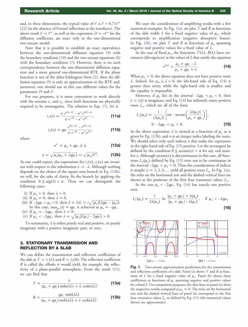
We start the consideration of amplifying media with a fewnumerical examples. In Fig. 1(a), we plot T and R as functionsof the slab width L for a fixed negative value of μa, whichcorresponds to amplification (negative absorptive losses).In Fig. 1(b), we plot T and R as functions of μa spanningnegative and positive values for a fixed value of L.

In the case of fixed μa, the functions T �L�, R�L� have res-onances (divergences) at the values of L that satisfy the equation

e2λL � μa � qμs − λμa � qμs � λ

: (14)

When μa > 0, the above equation does not have positive rootsL. Indeed, for μa; L; λ > 0, the left-hand side of Eq. (14) isgreater than unity, while the right-hand side is smaller, andthe equality is impossible.

However, if μa lies in the interval −2qμs < μa < 0, thenλ � ijλj is imaginary, and Eq. (14) has infinitely many positiveroots Ln, which are all of the form

Ln�μa� �1

jλ�μa�j

�nπ − arctan

� jλ�μa�jμa � qμs

��;

if − 2qμs < μa < 0: (15)

In the above expression, λ is viewed as a function of μa as isgiven by Eq. (12b), and n is an integer index labeling the roots.We should select only such indices n that make the expressionin the right-hand side of Eq. (15) positive. Let the arctangent bedefined by the condition 0 ≤ arctan�z� < π for any real num-ber z. Although arctan�z� is discontinuous in this case, all func-tions Ln�μa� defined by Eq. (15) turn out to be continuous inthe interval −2qμs < μa < 0. Then the consideration of indicesis simple: n � 1; 2; 3;… yield all positive roots Ln. In Fig. 1(a),the ticks on the horizontal axis and the dashed vertical lines areshown at the positions of the first four resonance values Ln.

In the case μa < −2qμs, Eq. (14) has exactly one positiveroot:

L1�μa� �1

2λ�μa�ln

jμa � qμsj � λ�μa�jμa � qμsj − λ�μa�

; if μa < −2qμs :

(16)

(a) (b)

Fig. 1. Two-stream approximation predictions for the transmissionand reflection coefficients of a slab. Panel (a) shows T and R as func-tions of L for a fixed negative value of μa. Panel (b) shows thesecoefficients as functions of μa spanning negative and positive valuesfor a fixed L. For comparison purposes, the thin lines in panel (a) showthe respective results computed at μa � 0. The ticks on the horizontalaxis and the dashed vertical lines of panel (a) correspond to the firstfour resonance values Ln as defined by Eq. (15) (the numerical valuesshown are approximate).


Note that the expression under the logarithm and the functionλ�μa� are positive under the conditions of applicabilityof Eq. (16).

The function L1�μa� can be defined using Eq. (15) andEq. (16) and is positive and continuous in the whole openinterval μa < 0, while the functions Ln�μa� with n > 1 aredefined only in the interval −2qμs < μa < 0 [23]. The firstseveral functions Ln�μa� are plotted in Fig. 2.

For a fixed value of L, we can similarly find the resonancevalues of μa as the roots μan�L� of Eq. (14). The two obviousroots μa � 0 and μa � −2qμs should be considered separately.These values of μa satisfy Eq. (14) irrespectively of L. However,the root μa � 0 does not correspond to a resonance and shouldalways be excluded from consideration. In fact, the transmis-sion and reflection coefficients at μa � 0 are always finiteand positive. The root μa � −2qμs corresponds to a resonanceonly if, in addition, L � 1∕qμs. For a general L, the transmis-sion and reflection coefficients at μa � −2qμs are given byT � 1∕�1 − qμsL� and R � qμs∕�1 − qμsL�. Obviously, theseresults are physical and correct if qμsL < 1 and unphysical andincorrect otherwise; the divergence occurs at L � 1∕qμs.

The number of real-valued roots μan�L� is finite and almostalways odd, except for a discrete set of values of L. At least oneresonance value of the absorption coefficient exists for anyL > 0. For example, only one such resonance exists for theparameters of Fig. 1(b); the divergence of T and R at this singleresonance value of μa is clearly visible in the figure.

The resonance values of μa cannot be expressed in terms ofelementary functions. However, it is easy to find these rootsnumerically or visualize graphically. Indeed, let us plot allthe functions Ln�μa� defined in Eqs. (15) and (16), as is donein Fig. 2. The roots μan�L� can be visualized as the intersectionsof a horizontal line L � const with all the curves shown in thefigure. It can indeed be seen that the number of roots is oddexcept when the horizontal line touches the minimum of one ofthese curves [24].

Let us now fix some μa < 0, and let L1�μa� be the first (thesmallest) resonance value of L for this particular μa. Then thecoefficients T and R are positive for any L in the interval0 < L < L1�μa�. This is illustrated in Fig. 1(a). In fact, not

only the transmission and reflection coefficients, but thespecific intensity is also positive for these values of L. Thisis illustrated in Fig. 3(a), where the functions i1�z� andi2�z� are plotted for μa � −0.2qμs [same value as in Fig. 1(a)]and qμsL � 3.5. This value of L satisfies the inequality0 < L < L1�μa�. Indeed, we have qμsL1�−0.2qμs� ≈ 4.15.

We can generalize that, for any μa < 0, the two-streamapproximation yields physically meaningful solutions as longas L < L1�μa�, that is, in sufficiently thin slabs, up to the firstresonance value of L. Similarly, for any fixed value of L, thesolutions are physical for μa > μa1�L�, where μa1�L� is thefirst (negative) resonance value of μa for the given L. The two-dimensional region in the plane �μa; L� where physicallymeaningful solutions exist is illustrated in Fig. 2.

It may seem that, in some cases, physically meaningful sta-tionary solutions can exist even beyond the first resonance, thatis, above and to the left of the curve L1�μa� in Fig. 2. For ex-ample, both coefficients T and R are positive for μa � −0.2qμsand qμsL � 12.5, as can be seen in Fig. 1(a). This point �μa; L�is above the curve L1�μa�. However, the individual streams in-side the medium change sign and are unphysical at these valuesof parameters; this is illustrated in Fig. 3(b). Generally, the sta-tionary solutions are always unphysical for L > L1�μa� orμa < μa1�L�. Exactly at the resonances, stationary solutionssimply do not exist. Past the first resonance and betweenhigher-order resonances, solutions exist, but the specific inten-sity becomes negative at least for some positions and directions.

4. STATIONARY LASING

We have defined the resonances of the two-stream model as theset of parameters μa and L, for which the stationary two-streamequations (6) with the inhomogeneous boundary condition (7)has no solutions. This set is defined by all possible solutions toEq. (14). All real resonance values of the above two parameterslie on the curves shown in Fig. 2.

We can as well say that the two-stream equations (6) withthe homogeneous boundary condition i1�0� � i2�L� � 0 havenontrivial solutions if and only if the parameters μa and L takethe resonance values. Let us look in more detail at these non-trivial stationary solutions, which are obtained in the absenceof any external sources. Equations (6) with the above homo-geneous boundary condition are satisfied by the functions

Fig. 2. Loci of the resonances of the two-stream model in the real�μa; L� plane. A point on any of the curves corresponds to a root ofEq. (14). The lowest resonance curve L1�μa� is emphasized by colorand linewidth. All points to the right and below the curve L1�μa� cor-respond to physically meaningful unique solutions to the stationarytwo-stream equations (6). Any point above and to the left ofL1�μa�, but not on any of the other curves, Ln�μa� corresponds toa unique but unphysical solution. Finally, for any point on any ofthe curves Ln�μa�, solutions, even unphysical ones, do not exist forthe inhomogeneous boundary condition (7).

(a) (b)

Fig. 3. Two streams i1�z� and i2�z� for μa � −0.2qμs and L �3.5∕qμs (a), L � 12.5∕qμs (b). The streams are shown as functionsof the dimensionless variable z∕L. At L � 12.5∕qμs , both the trans-mission and reflection coefficients are positive (see Fig. 1), but bothfunctions i1�z� and i2�z� change sign; such solutions are unphysical.


i1�z� � A�eλz − e−λz�; (17a)

i2�z� �Aqμs

��μa � qμs � λ�eλz − �μa � qμs − λ�e−λz �; (17b)

provided that Eq. (14) holds. Otherwise, the problem has onlythe trivial solution. Here A is an arbitrary constant, and weshould exclude the root μa � 0 (which satisfies Eq. (14) foran arbitrary L) from consideration. As was explained inSection 3, μa � 0 is not a resonance of the system.

As for the resonance at the point μa � −2qμs, L � 1∕qμs, itshould be considered separately. The right-hand sides in theequations (17) turn to zero in this case. However, there existsa nontrivial linear solution at this resonance point; it is of theform i1�z� � Az, i2�z� � A�1 − z∕L�. This solution can be,in fact, obtained from Eq. (17) if we make the substitu-tion A → A∕2λ.

An important consideration is symmetry. Since, in theabsence of any incoming external radiation, the two possibledirections of propagation are physically equivalent, we expectthe expressions for the two streams to satisfy i1;2�z� �i2;1�L − z�. The possibility of the minus sign in the abovesymmetry relation is somewhat counterintuitive. However,Eqs. (17) allow for both possibilities. The physical requirementthat each stream transforms into itself after we apply the oper-ation of coordinate inversion twice holds in both cases.Moreover, the solution (17) satisfies the symmetry relation withthe plus sign if the point �μa; L� lies on one of the curves Ln�μa�with an odd index n and with the minus sign if the index is even.Indeed, let L � Ln�μa�. We can use Eq. (17a) to write

i1�Ln − z� � A�eλ�Ln−z� − e−λ�Ln−z��: (18)

We now use Eqs. (15) and (16), which define the functionsLn�μa� for all possible indices and values of the argument, tofind that

eλLn � �−1�n μa � qμs λ

qμs: (19)

To derive Eq. (19), one should be careful to use the correctbranch of the arctangent in Eq. (15) (recall that the arctangentin this formula is defined so that 0 ≤ arctan�z� < π for any realnumber z). Note that, if we square Eq. (19), we would obtainthe resonance condition (14). This result follows immediately ifwe account for the identity

�μa � qμs − λ��μa � qμs � λ� � �qμs�2: (20)

Finally, we substitute Eq. (19) into Eq. (18), compare theresult to Eq. (17b), and find that the solution (17) satisfiesi1�Ln − z� � �−1�n�1i2�z�.

We can now see that the solution (17) is unphysical for alleven n. Indeed, the two streams cannot be simultaneously pos-itive in this case. In fact, an even stronger condition holds: thesolution is unphysical for all n > 1. Indeed, for n > 1, λ isimaginary, and we have i1�z� � 2iA sin�jλjz�. We can selectA � A 0∕2i, where A 0 > 0. Then the overall coefficient is pos-itive. However, we also have jλjLn > π for n > 1. Therefore,the function sin�jλjz� necessarily changes sign in this case,and the solution cannot be physically valid.

We can conclude that the stationary solution given byEq. (17) is physical only if the point �μa; L� lies on the curve

L1�μa�. In this case, we can write i1�z� � A sin�jλjz� if−2qμs < μa < 0 and i1�z� � A sinh�λz� if μa < −2qμs.Here A is an arbitrary positive constant, and the total powergenerated by the system, e.g., i1�L� � i2�0�, is also arbitrary.

The stationary solution described above can be understoodas the state of continuous-wave lasing. This interpretation mayseem counterintuitive because lasers, generally, require a reso-nator. In the two-stream model discussed so far, there appearsto be no resonator. Moreover, there is no electromagnetic phaseand no constructive interference. However, as we have seen,there are resonances. The backward reflections and mutualconversion of the two streams work so as to create a semblanceof a resonator. We will consider the role of the resonator andthe more general condition of stationary lasing with reflectionof the streams at the slab interfaces in Section 7 below.

5. TIME EVOLUTION IN AN AMPLIFYINGMEDIUM

So far, we have considered only stationary solutions. We haveseen that such solutions can be physical or unphysical.Apparently, the unphysical stationary solutions cannot beachieved by considering any transient process in which the ini-tial state of both streams is zero. Questions arise about how aphysical state of stable lasing can be excited, or what wouldhappen if we apply external radiation to a medium with param-eters �μa; L� for which stationary solutions do not exist or areunphysical. We are therefore motivated to look at the time evo-lution in the two-stream model. We note that time-dependentsolutions to a general RTE with any physically reasonablesource and initial conditions are unique and nonnegative, evenfor arbitrary negative μa [22]. This mathematical result appliesto the two-stream theory of this paper.

The time-dependent two-stream equations are of the form�1

c∂∂t

� ∂∂z

� μa � qμs

�i1�z; t� � qμsi2�z; t�; (21a)

�1

c∂∂t

−∂∂z

� μa � qμs

�i2�z; t� � qμs i1�z; t�: (21b)

We also assume that the streams satisfy the time-dependentboundary conditions

i1�0; t� � S�t�; i2�L; t� � 0; (22)

and the initial conditions ik�z; t� � S�t� � 0 for t → −∞.Thus, the intensity of the external radiation incident ontothe z � 0 face of the slab is described by the function S�t�,which tends to zero in the sufficiently distant past.

Unlike the stationary equations, the set [Eq. (21)] cannot bereduced to a one-dimensional diffusion equation. Rather, it isequivalent to the telegraph equation, which contains bothfirst and second time derivatives [25].

It is tempting to try to solve Eq. (21) by temporal Fouriertransform. This approach works fine if the medium is absorb-ing (i.e., μa > 0), and even under some less restrictiveconditions. However, for sufficiently negative values of μa orfor sufficiently large width L for a given μa < 0, the streamsik�z; t� can increase exponentially in time and, in this case, theirtemporal Fourier transforms do not exist, even in the sense of


generalized functions. One can still apply the Fourier transformtechnique formally to Eq. (21), but the result would be incor-rect and, in particular, it will violate causality [1]. The math-ematical difficulty here is subtle and may not be obvious whenthe actual calculations are done; it is the a priori assumptionthat certain Fourier transforms exist when, in fact, they mightnot, that is causing the trouble. We will therefore use theFourier–Laplace transform instead, as was done previously inthe case of Maxwell’s equations [1,7,17].

Let us search for solutions to Eq. (21) in the form

i1;2�z; t� � e−cμat f 1;2�z; t�: (23)

The effect of this substitution is to eliminate μa from thedifferential equations. Indeed, the functions f 1;2 satisfy�

1

c∂∂t

� ∂∂z

� qμs

�f 1�z; t� � qμsf 2�z; t�; (24a)

�1

c∂∂t

−∂∂z

� qμs

�f 2�z; t� � qμsf 1�z; t�: (24b)

However, μa is now present in the boundary conditions

f 1�0; t� � ecμatS�t�; f 2�L; t� � 0: (25)

It can be seen that the functions f 1;2 are solutions to the origi-nal two-stream equations (21) in a medium with μa � 0 andwith the modified source S 0�t� � ecμat S�t�. Let us assume thatthis modified source injects a finite energy into the medium sothat

RS 0�t�dt < ∞. If μa � 0, this energy is neither absorbed

nor amplified and will eventually be radiated into free spacethrough the slab surfaces without net loss or gain. In this case(and accounting for the positivity of f 1;2 ) we haveR jf 1;2�z; t�jdt < ∞. Consequently, the functions can beFourier-transformed with respect to t. Keep in mind, however,that, if S�t� contains generalized functions, the same can beexpected of f 1;2�z; t�.

We can now write the boundary condition in Fourierrepresentation as

f 1�0;ω� � F�ω� ≡Z

∞

−∞S�t�e�cμa�iω�tdt; f 2�L;ω� � 0:

(26)

Here we have used the Fourier transform convention,

x�ω� �Z

∞

−∞x�t�eiωtdt; x�t� �

Z∞

−∞x�ω�e−iωt dω

2π; (27)

for all time-dependent functions. We can now solve Eq. (24) byFourier transform. The result is

f 1;2�z; t� �Z

∞

−∞g1;2�z;ω�F �ω�e−iωt

dω

2π; (28)

where g1;2�z;ω� are the linear transfer functions. At every valueof the Fourier variable ω, the problem of computing the trans-fer functions is formally equivalent to the stationary problemconsidered in Section 3, with the only difference being that μashould now be replaced by −iω∕c. Therefore, we obtain thefollowing expressions:

g1�z;ω� �a−�ω�eλ�ω��z−L� − a��ω�eλ�ω��L−z�

a−�ω�e−λ�ω�L − a��ω�eλ�ω�L ; (29a)

g2�z;ω� � qμseλ�ω��z−L� − eλ�ω��L−z�

a−�ω�e−λ�ω�L − a��ω�eλ�ω�L ; (29b)

where

λ�ω� �ffiffiffiffiffiffiffiffiffiffiffiffiffiffiffiffiffiffiffiffiffiffiffiffiffiffiffiffiffiffiffiffiffiffiffiffiffiffiffiffiffiffiffiffiffi−i�ω∕c��−iω∕c � 2qμs�

p; (30a)

a�ω� � −iω∕c � qμs λ�ω�: (30b)

Let us further assume that the source is a delta-function pulseof the form S�t� � δ�t − t0� and, correspondingly, F �ω� �e�cμa�iω�t0 . Solutions to Eq. (21) with this delta source arethe Green’s functions of the time-dependent two-stream equa-tions, which we denote by G1;2�z; t − t0�. In terms of theresponse functions, we have

G1;2�z; τ� � e−cμaτZ

∞

−∞g1;2�z;ω�e−iωτ

dω

2π: (31)

Solutions for more general sources can be found bysuperposition, viz.,

i1;2�z; t� �Z

G1;2�z; τ�S�t − τ�dτ: (32)

Note the following properties of the transfer functions:

g1�z; 0� � 1 −qμsz

1� qμsL; g2�z; 0� �

qμs�L − z�1� qμsL

: (33)

From this, we conclude that 0 ≤RG1;2�z; τ�ecμaτdτ < 1. The

first inequality can be expected on physical grounds, since thestreams are nonnegative by definition. The second inequalityplaces a bound on how fast the solutions can grow with timein amplifying media. Note that g1�L; 0� � g2�0; 0� � 1. Thisequality means that all energy injected into a medium withμa � 0 leaves eventually through the surfaces. This can beexpected, since Eqs. (24) do not contain the absorption oramplification; the latter are accounted for by the exponentialfactor e−cμaτ in Eq. (31).

It is also useful to write out the first few terms in the ballisticexpansion of the Green’s functions. This expansion is of theform

G1;2�z; τ� � e−c�μa�qμs�τX∞k�0

�qμs�kK �k�1;2�z; τ�; (34)

and it can be derived by starting with the initial guess i1 �i2 � 0 in the right-hand side of Eq. (24) and iterating theresulting equations. The first two terms in this expansionare easy to compute, and they are given by the expressions

K �0�1 �z; τ� � δ�τ − z∕c�; (35a)

K �1�2 �z; τ� � c

2θ�τ − z∕c�; (35b)

K �2�1 �z; τ� � c

2zθ�τ − z∕c�; (35c)

K �2k�1�1 �z; τ� � K �2k�

2 �z; τ� � 0; k � 0; 1; 2…; (35d)

where θ�x� is the unit step function. The term K �0�1 describes

the propagation of the nonscattered light (the precursor). Wewill refer to this term as to the ballistic component of the spe-cific intensity. Note that K �0�

1 �z; τ� turns to zero identicallywhen τ > L∕c. In the case of a more general excitation, the


ballistic component of the forward stream can be found fromEqs. (32) and (35a):

i�0�1 �z; t� � e−�μa�qμs�zS�t − z∕c�: (36)

The second-order term K �2�1 �z; τ� does not contain a singularity

but is discontinuous at τ � z∕c. All higher-order termsK �2k�

1 �z; τ� are continuous. For this reason, Eq. (35c) yieldsthe exact result for the jump of the Green’s function G1�z; τ�at τ � z∕c: the jump is equal to 1

2 c�qμs�2ze−�μa�qμs�z .The Green’s function G2�z; τ� and the reverse stream

i2�z; t� do not have ballistic components and, correspondingly,K �0�

2 �z; τ� � 0. This is, of course, due to the assumption thatthe exciting pulse enters the medium only through the surfacez � 0. However, G2�z; τ� still has a discontinuity at τ � z∕c.Again, Eq. (35b) predicts the jump correctly, since all higher-order terms are continuous.

We could easily derive several higher-order terms in Eq. (34);all these terms are causal; that is, they turn identically to zero forτ < z∕c. The ballistic expansion is useful at small times with thecharacteristic time scale being 1∕qμsc. We therefore have shownthat, at small times, the response of the system is causal. We arehowever more interested in the long-time behavior. To this end,it is instructive to evaluate the Fourier transform (31) by contourintegration. Although the poles of the transfer functions cannotbe computed analytically, the resulting semianalytical formulaswill provide an important insight.

The first thing to note is that g1;2�z;ω� are single-valuedfunctions of ω in spite of the presence of square roots inthe definitions (29) and (30). This is similar to the case oftransmission and reflection coefficients of homogeneous slabscomputed from Maxwell’s equations [1,2]. In particular, whenω → ∞ (on the real axis), we have

g1�z;ω�⏤→ω→∞

e�iωc−qμs�z : (37)

Therefore, G1�z;ω� contains a singularity, which must be ex-tracted before computing the Fourier transform (31). This sin-gularity is exactly equal to the ballistic term given in Eq. (35a).Let us adopt the following notations:

g1�z;ω� � g �0�1 �z;ω� � g �d �1 �z;ω�; (38a)

g �0�1 �z;ω� � e�iωc−qμs�z : (38b)

The corresponding ballistic and diffuse parts of the Green’sfunction G�0�

1 and G�d �1 are obtained by computing the

Fourier transforms of g �0�1 and g �d �1 according to Eq. (31).Referring to expansion (35), we can identify

G�d �1 �z; τ� � G1�z; τ� − e−c�μa�qμs�τδ�τ − z∕c�: (39)

Viewed as functions of ω, g�d �1 �z;ω� and g2�z;ω� are casuallinear transfer functions. Both have Fourier transforms and nosingularities on or above the real axis. In the lower open half-plane, the functions are analytic everywhere except for a count-able infinite set (same for both functions) of simple polesωn�L�, which accumulate at infinity. The poles can be foundby solving Eq. (14) for a fixed value of L treating μa as theunknown. The equation has infinitely many solutionsμan�L� but only a finite number of them are real-valued. Thesereal roots have been discussed in Sections 3 and 4. Now we

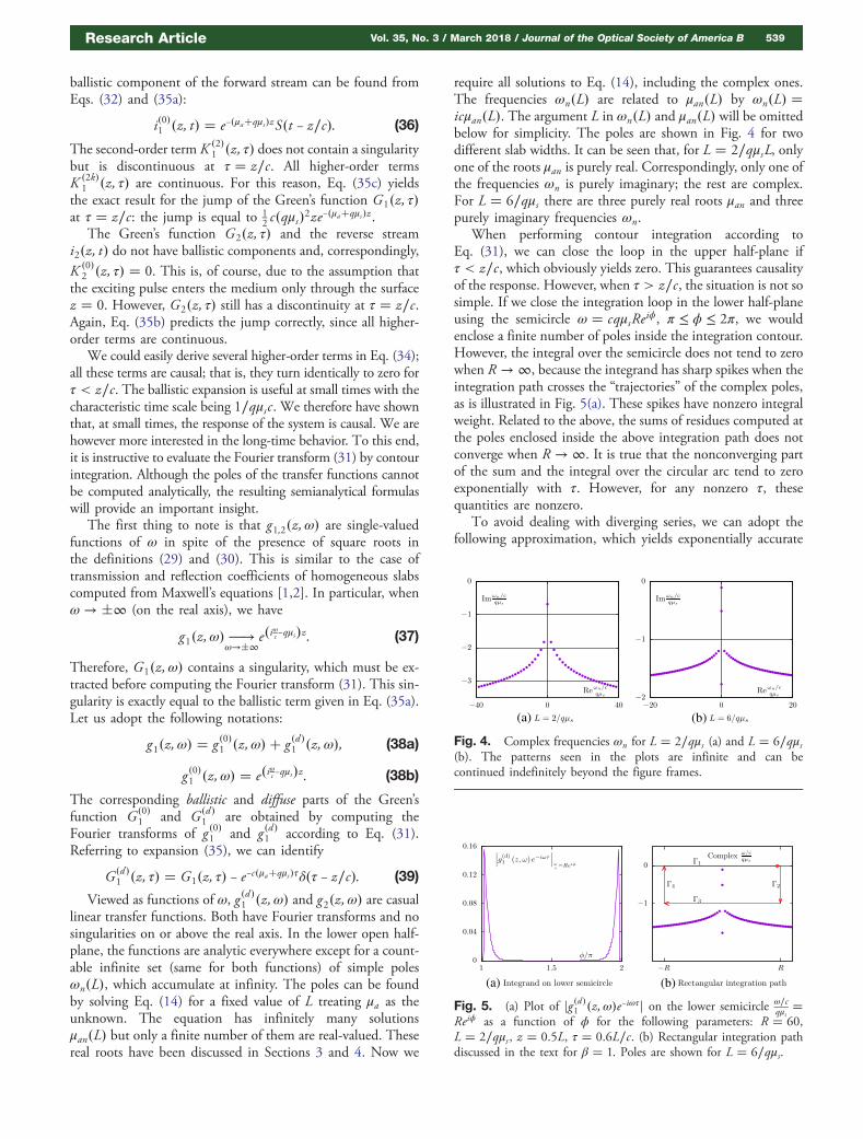
require all solutions to Eq. (14), including the complex ones.The frequencies ωn�L� are related to μan�L� by ωn�L� �icμan�L�. The argument L in ωn�L� and μan�L� will be omittedbelow for simplicity. The poles are shown in Fig. 4 for twodifferent slab widths. It can be seen that, for L � 2∕qμsL, onlyone of the roots μan is purely real. Correspondingly, only one ofthe frequencies ωn is purely imaginary; the rest are complex.For L � 6∕qμs there are three purely real roots μan and threepurely imaginary frequencies ωn.

When performing contour integration according toEq. (31), we can close the loop in the upper half-plane ifτ < z∕c, which obviously yields zero. This guarantees causalityof the response. However, when τ > z∕c, the situation is not sosimple. If we close the integration loop in the lower half-planeusing the semicircle ω � cqμsReiϕ, π ≤ ϕ ≤ 2π, we wouldenclose a finite number of poles inside the integration contour.However, the integral over the semicircle does not tend to zerowhen R → ∞, because the integrand has sharp spikes when theintegration path crosses the “trajectories” of the complex poles,as is illustrated in Fig. 5(a). These spikes have nonzero integralweight. Related to the above, the sums of residues computed atthe poles enclosed inside the above integration path does notconverge when R → ∞. It is true that the nonconverging partof the sum and the integral over the circular arc tend to zeroexponentially with τ. However, for any nonzero τ, thesequantities are nonzero.

To avoid dealing with diverging series, we can adopt thefollowing approximation, which yields exponentially accurate

(a) (b)

Fig. 4. Complex frequencies ωn for L � 2∕qμs (a) and L � 6∕qμs(b). The patterns seen in the plots are infinite and can becontinued indefinitely beyond the figure frames.

(a) (b)

Fig. 5. (a) Plot of jg �d�1 �z;ω�e−iωτj on the lower semicircle ω∕cqμs

�Reiϕ as a function of ϕ for the following parameters: R � 60,L � 2∕qμs , z � 0.5L, τ � 0.6L∕c. (b) Rectangular integration pathdiscussed in the text for β � 1. Poles are shown for L � 6∕qμs.


results when τ → ∞. Let τ > z∕c. We then close the integra-tion contour, as is shown in Fig. 5(b). The integration path isthe rectangle with the vertices at �−R; 0� to �R; 0�, �R; −β�,�−R; −β� in the complex ω∕c

qμsplane. It can be seen that the

segment Γ3 passes clear of any poles. This is different fromthe case of a semicircle, which necessarily crosses the regionswhere the poles are located very close to each other and forman almost continuous “trajectory.” As a result, the integral overΓ3 is not zero but small and can definitely be neglected whenτ → ∞ (integrals over Γ2 and Γ4 tend to zero when R → ∞and can always be neglected). The optimal choice of the param-eter β depends on L. In relatively thin slabs, one might need totake β ≥ 2 so that at least one pole is inside the rectangle. ForL > 2∕qμs, one can safely use β � 1, as is shown in the figure.This choice yields an especially simple integral over the segmentΓ2. For our purposes, computing this integral is unimportant;we just assume that it is negligible at large times.

We finally need to compute the residues of g �d �1 �z;ω�, whichis a cumbersome but straightforward task. The result is

limω→ωn

�ω − ωn�g �d �1 �z;ω� � cλn2i

eλnz − e−λnz

1� �qμs � μan�L: (40)

We do not need to compute the residues of g2�z;ω�, as theycan easily be found by applying Eq. (24a) to Eq. (40). Puttingeverything together, we obtain the following result:

G�d �1 �z; τ� ≈ c

2θ�τ −

zc

�e−cμaτ

×Xn

θ

�μanqμs

� β

�ecμanτ

λn�e−λnz − eλnz�1� �qμs � μan�L

;

(41a)

G2�z; τ� ≈c2θ�τ −

zc

�e−cμaτ

×Xn

θ

�μanqμs

� β

�ecμanτ

λn�a−ne−λnz − a�n eλnz�qμs �1� �qμs � μan�L�

:

(41b)

Thus, the nature of the approximation is quite simple: truncatethe summation over the infinite set of poles so that the cutoff isdrawn in the widest gap separating one group of poles fromanother. The line Γ3 in Fig. 5 is such a cutoff. It separatesthe poles with relatively small imaginary parts, which dominatethe large-time behavior from the rest of the poles.

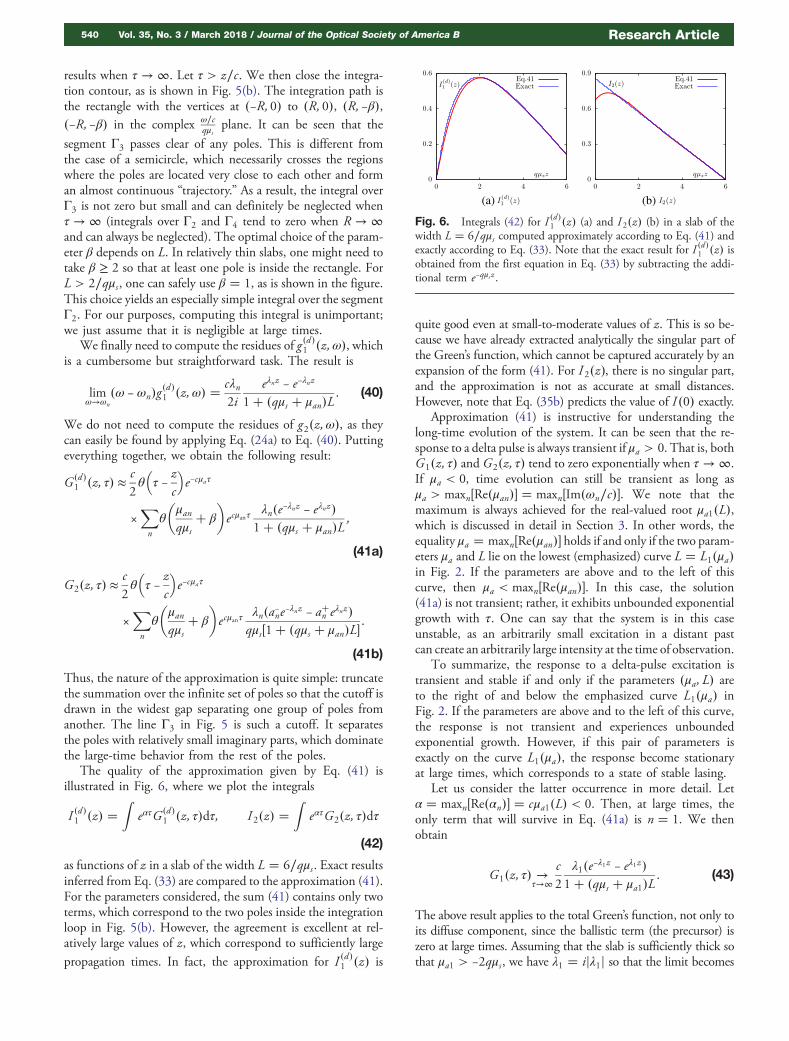
The quality of the approximation given by Eq. (41) isillustrated in Fig. 6, where we plot the integrals

I �d �1 �z� �Z

eατG�d �1 �z; τ�dτ; I 2�z� �

ZeατG2�z; τ�dτ

(42)

as functions of z in a slab of the width L � 6∕qμs. Exact resultsinferred from Eq. (33) are compared to the approximation (41).For the parameters considered, the sum (41) contains only twoterms, which correspond to the two poles inside the integrationloop in Fig. 5(b). However, the agreement is excellent at rel-atively large values of z, which correspond to sufficiently largepropagation times. In fact, the approximation for I �d �1 �z� is

quite good even at small-to-moderate values of z. This is so be-cause we have already extracted analytically the singular part ofthe Green’s function, which cannot be captured accurately by anexpansion of the form (41). For I2�z�, there is no singular part,and the approximation is not as accurate at small distances.However, note that Eq. (35b) predicts the value of I�0� exactly.

Approximation (41) is instructive for understanding thelong-time evolution of the system. It can be seen that the re-sponse to a delta pulse is always transient if μa > 0. That is, bothG1�z; τ� and G2�z; τ� tend to zero exponentially when τ → ∞.If μa < 0, time evolution can still be transient as long asμa > maxn�Re�μan�� maxn�Im�ωn∕c��. We note that themaximum is always achieved for the real-valued root μa1�L�,which is discussed in detail in Section 3. In other words, theequality μa � maxn�Re�μan�� holds if and only if the two param-eters μa and L lie on the lowest (emphasized) curve L � L1�μa�in Fig. 2. If the parameters are above and to the left of thiscurve, then μa < maxn�Re�μan��. In this case, the solution(41a) is not transient; rather, it exhibits unbounded exponentialgrowth with τ. One can say that the system is in this caseunstable, as an arbitrarily small excitation in a distant pastcan create an arbitrarily large intensity at the time of observation.

To summarize, the response to a delta-pulse excitation istransient and stable if and only if the parameters �μa; L� areto the right of and below the emphasized curve L1�μa� inFig. 2. If the parameters are above and to the left of this curve,the response is not transient and experiences unboundedexponential growth. However, if this pair of parameters isexactly on the curve L1�μa�, the response become stationaryat large times, which corresponds to a state of stable lasing.

Let us consider the latter occurrence in more detail. Letα � maxn�Re�αn�� cμa1�L� < 0. Then, at large times, theonly term that will survive in Eq. (41a) is n � 1. We thenobtain

G1�z; τ� →τ→∞

c2

λ1�e−λ1z − eλ1z�1� �qμs � μa1�L

: (43)

The above result applies to the total Green’s function, not only toits diffuse component, since the ballistic term (the precursor) iszero at large times. Assuming that the slab is sufficiently thick sothat μa1 > −2qμs, we have λ1 � ijλ1j so that the limit becomes

(a) (b)

Fig. 6. Integrals (42) for I �d �1 �z� (a) and I 2�z� (b) in a slab of thewidth L � 6∕qμs computed approximately according to Eq. (41) andexactly according to Eq. (33). Note that the exact result for I �d �1 �z� isobtained from the first equation in Eq. (33) by subtracting the addi-tional term e−qμs z .


G1�z; τ� →τ→∞

cjλ1j sin�jλ1jz�1� �qμs � μa1�L

: (44)

The denominator in this expression is positive. This is the sinus-oidal solution corresponding to stable lasing that was foundpreviously in Section 4. The positive z-independent coefficientin Eq. (44) quantifies the achieved lasing power due to a unitpower injected into the system in the distant past. Also, as wasdiscussed in Section 4, the sine in Eq. (44) does not change sign,so that the solution is positive for all z, as expected.

Finally, if the slab is sufficiently thin so that μ1a < −2qμs,the exponent λ1 is real and positive so that the hyperbolicstationary lasing solution of the form G1 ∝ sinh�λ1z�, whichwas also discussed in Section 4, is obtained.

6. NUMERICAL EXAMPLES

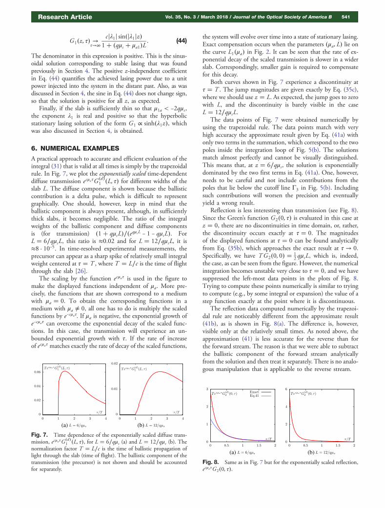
A practical approach to accurate and efficient evaluation of theintegral (31) that is valid at all times is simply by the trapezoidalrule. In Fig. 7, we plot the exponentially scaled time-dependentdiffuse transmission ecμaτG�d �

1 �L; τ� for different widths of theslab L. The diffuse component is shown because the ballisticcontribution is a delta pulse, which is difficult to representgraphically. One should, however, keep in mind that theballistic component is always present, although, in sufficientlythick slabs, it becomes negligible. The ratio of the integralweights of the ballistic component and diffuse componentsis (for transmission) �1� qμsL�∕�eqμsL − 1 − qμsL�. ForL � 6∕qμsL, this ratio is ≈0.02 and for L � 12∕qμsL, it is≈8 · 10−5. In time-resolved experimental measurements, theprecursor can appear as a sharp spike of relatively small integralweight centered at τ � T , where T � L∕c is the time of flightthrough the slab [26].

The scaling by the function ecμaτ is used in the figure tomake the displayed functions independent of μa. More pre-cisely, the functions that are shown correspond to a mediumwith μa � 0. To obtain the corresponding functions in amedium with μa ≠ 0, all one has to do is multiply the scaledfunctions by e−cμaτ. If μa is negative, the exponential growth ofe−cμaτ can overcome the exponential decay of the scaled func-tions. In this case, the transmission will experience an un-bounded exponential growth with τ. If the rate of increaseof ecμaτ matches exactly the rate of decay of the scaled functions,

the system will evolve over time into a state of stationary lasing.Exact compensation occurs when the parameters �μa; L� lie onthe curve L1�μa� in Fig. 2. It can be seen that the rate of ex-ponential decay of the scaled transmission is slower in a widerslab. Correspondingly, smaller gain is required to compensatefor this decay.

Both curves shown in Fig. 7 experience a discontinuity atτ � T . The jump magnitudes are given exactly by Eq. (35c),where we should use z � L. As expected, the jump goes to zerowith L, and the discontinuity is barely visible in the caseL � 12∕qμsL.

The data points of Fig. 7 were obtained numerically byusing the trapezoidal rule. The data points match with veryhigh accuracy the approximate result given by Eq. (41a) withonly two terms in the summation, which correspond to the twopoles inside the integration loop of Fig. 5(b). The solutionsmatch almost perfectly and cannot be visually distinguished.This means that, at z � 6∕qμs, the solution is exponentiallydominated by the two first terms in Eq. (41a). One, however,needs to be careful and not include contributions from thepoles that lie below the cutoff line Γ3 in Fig. 5(b). Includingsuch contributions will worsen the precision and eventuallyyield a wrong result.

Reflection is less interesting than transmission (see Fig. 8).Since the Green’s function G2�0; τ� is evaluated in this case atz � 0, there are no discontinuities in time domain, or, rather,the discontinuity occurs exactly at τ � 0. The magnitudesof the displayed functions at τ � 0 can be found analyticallyfrom Eq. (35b), which approaches the exact result at τ → 0.Specifically, we have TG2�0; 0� � 1

2 qμsL, which is, indeed,the case, as can be seen from the figure. However, the numericalintegration becomes unstable very close to τ � 0, and we havesuppressed the left-most data points in the plots of Fig. 8.Trying to compute these points numerically is similar to tryingto compute (e.g., by some integral or expansion) the value of astep function exactly at the point where it is discontinuous.

The reflection data computed numerically by the trapezoi-dal rule are noticeably different from the approximate result(41b), as is shown in Fig. 8(a). The difference is, however,visible only at the relatively small times. As noted above, theapproximation (41) is less accurate for the reverse than forthe forward stream. The reason is that we were able to subtractthe ballistic component of the forward stream analyticallyfrom the solution and then treat it separately. There is no analo-gous manipulation that is applicable to the reverse stream.

(a) (b)

Fig. 7. Time dependence of the exponentially scaled diffuse trans-mission, ecμaτG�d �

1 �L; τ�, for L � 6∕qμs (a) and L � 12∕qμs (b). Thenormalization factor T � L∕c is the time of ballistic propagation oflight through the slab (time of flight). The ballistic component of thetransmission (the precursor) is not shown and should be accountedfor separately.

(a) (b)

Fig. 8. Same as in Fig. 7 but for the exponentially scaled reflection,ecμaτG2�0; τ�.


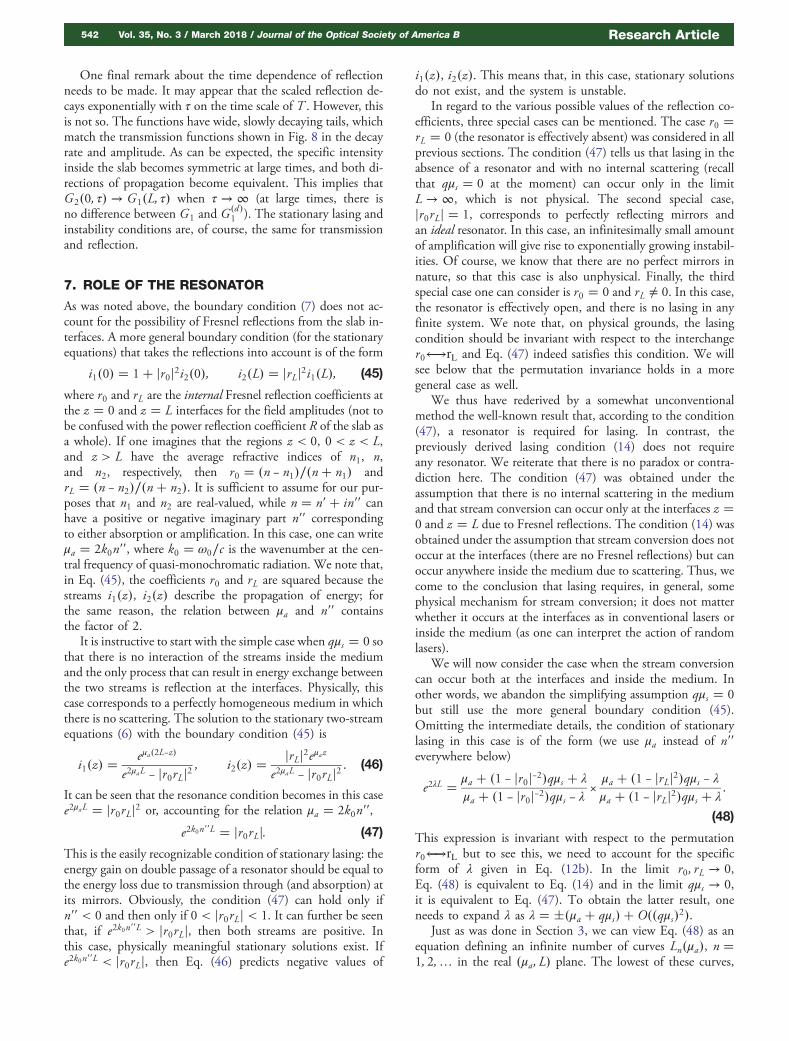
One final remark about the time dependence of reflectionneeds to be made. It may appear that the scaled reflection de-cays exponentially with τ on the time scale of T . However, thisis not so. The functions have wide, slowly decaying tails, whichmatch the transmission functions shown in Fig. 8 in the decayrate and amplitude. As can be expected, the specific intensityinside the slab becomes symmetric at large times, and both di-rections of propagation become equivalent. This implies thatG2�0; τ� → G1�L; τ� when τ → ∞ (at large times, there isno difference between G1 and G�d �

1 ). The stationary lasing andinstability conditions are, of course, the same for transmissionand reflection.

7. ROLE OF THE RESONATOR

As was noted above, the boundary condition (7) does not ac-count for the possibility of Fresnel reflections from the slab in-terfaces. A more general boundary condition (for the stationaryequations) that takes the reflections into account is of the form

i1�0� � 1� jr0j2i2�0�; i2�L� � jrLj2i1�L�; (45)

where r0 and rL are the internal Fresnel reflection coefficients atthe z � 0 and z � L interfaces for the field amplitudes (not tobe confused with the power reflection coefficient R of the slab asa whole). If one imagines that the regions z < 0, 0 < z < L,and z > L have the average refractive indices of n1, n,and n2, respectively, then r0 � �n − n1�∕�n� n1� andrL � �n − n2�∕�n� n2�. It is sufficient to assume for our pur-poses that n1 and n2 are real-valued, while n � n 0 � in 0 0 canhave a positive or negative imaginary part n 0 0 correspondingto either absorption or amplification. In this case, one can writeμa � 2k0n 0 0, where k0 � ω0∕c is the wavenumber at the cen-tral frequency of quasi-monochromatic radiation. We note that,in Eq. (45), the coefficients r0 and rL are squared because thestreams i1�z�, i2�z� describe the propagation of energy; forthe same reason, the relation between μa and n 0 0 containsthe factor of 2.

It is instructive to start with the simple case when qμs � 0 sothat there is no interaction of the streams inside the mediumand the only process that can result in energy exchange betweenthe two streams is reflection at the interfaces. Physically, thiscase corresponds to a perfectly homogeneous medium in whichthere is no scattering. The solution to the stationary two-streamequations (6) with the boundary condition (45) is

i1�z� �eμa�2L−z�

e2μaL − jr0rLj2; i2�z� �

jrLj2eμaze2μaL − jr0rLj2

: (46)

It can be seen that the resonance condition becomes in this casee2μaL � jr0rLj2 or, accounting for the relation μa � 2k0n 0 0,

e2k0n 0 0L � jr0rLj: (47)

This is the easily recognizable condition of stationary lasing: theenergy gain on double passage of a resonator should be equal tothe energy loss due to transmission through (and absorption) atits mirrors. Obviously, the condition (47) can hold only ifn 0 0 < 0 and then only if 0 < jr0rLj < 1. It can further be seenthat, if e2k0n 0 0L > jr0rLj, then both streams are positive. Inthis case, physically meaningful stationary solutions exist. Ife2k0n 0 0L < jr0rLj, then Eq. (46) predicts negative values of

i1�z�, i2�z�. This means that, in this case, stationary solutionsdo not exist, and the system is unstable.

In regard to the various possible values of the reflection co-efficients, three special cases can be mentioned. The case r0 �rL � 0 (the resonator is effectively absent) was considered in allprevious sections. The condition (47) tells us that lasing in theabsence of a resonator and with no internal scattering (recallthat qμs � 0 at the moment) can occur only in the limitL → ∞, which is not physical. The second special case,jr0rLj � 1, corresponds to perfectly reflecting mirrors andan ideal resonator. In this case, an infinitesimally small amountof amplification will give rise to exponentially growing instabil-ities. Of course, we know that there are no perfect mirrors innature, so that this case is also unphysical. Finally, the thirdspecial case one can consider is r0 � 0 and rL ≠ 0. In this case,the resonator is effectively open, and there is no lasing in anyfinite system. We note that, on physical grounds, the lasingcondition should be invariant with respect to the interchanger0←⏤→rL and Eq. (47) indeed satisfies this condition. We willsee below that the permutation invariance holds in a moregeneral case as well.

We thus have rederived by a somewhat unconventionalmethod the well-known result that, according to the condition(47), a resonator is required for lasing. In contrast, thepreviously derived lasing condition (14) does not requireany resonator. We reiterate that there is no paradox or contra-diction here. The condition (47) was obtained under theassumption that there is no internal scattering in the mediumand that stream conversion can occur only at the interfaces z �0 and z � L due to Fresnel reflections. The condition (14) wasobtained under the assumption that stream conversion does notoccur at the interfaces (there are no Fresnel reflections) but canoccur anywhere inside the medium due to scattering. Thus, wecome to the conclusion that lasing requires, in general, somephysical mechanism for stream conversion; it does not matterwhether it occurs at the interfaces as in conventional lasers orinside the medium (as one can interpret the action of randomlasers).

We will now consider the case when the stream conversioncan occur both at the interfaces and inside the medium. Inother words, we abandon the simplifying assumption qμs � 0but still use the more general boundary condition (45).Omitting the intermediate details, the condition of stationarylasing in this case is of the form (we use μa instead of n 0 0

everywhere below)

e2λL � μa � �1 − jr0j−2�qμs � λ

μa � �1 − jr0j−2�qμs − λ×μa � �1 − jrLj2�qμs − λμa � �1 − jrLj2�qμs � λ

:

(48)

This expression is invariant with respect to the permutationr0←⏤→rL but to see this, we need to account for the specificform of λ given in Eq. (12b). In the limit r0; rL → 0,Eq. (48) is equivalent to Eq. (14) and in the limit qμs → 0,it is equivalent to Eq. (47). To obtain the latter result, oneneeds to expand λ as λ � �μa � qμs� � O��qμs�2�.

Just as was done in Section 3, we can view Eq. (48) as anequation defining an infinite number of curves Ln�μa�, n �1; 2;… in the real �μa; L� plane. The lowest of these curves,


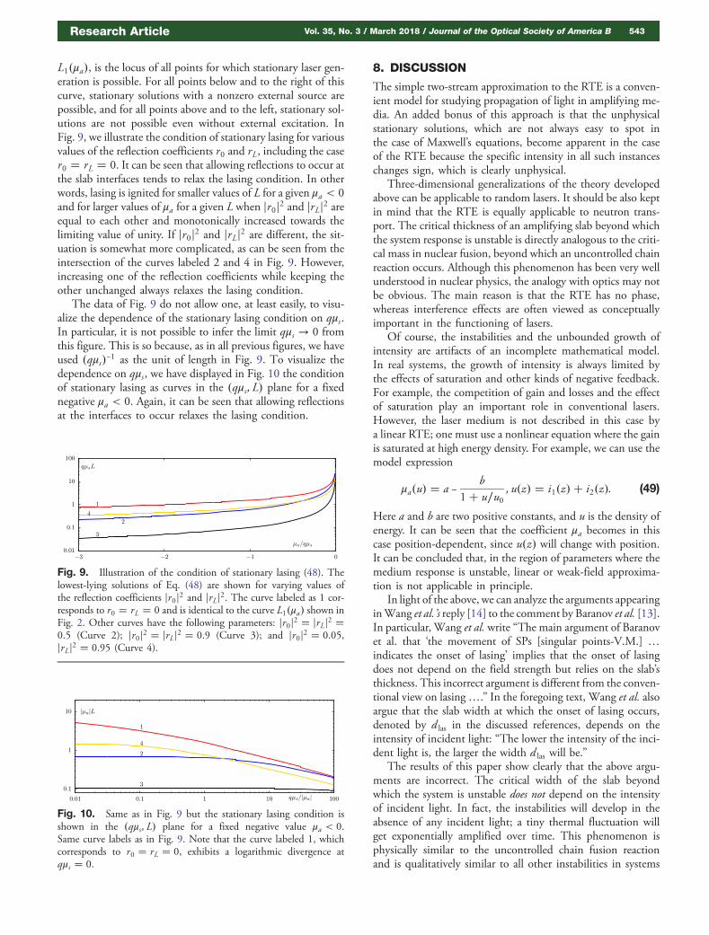
L1�μa�, is the locus of all points for which stationary laser gen-eration is possible. For all points below and to the right of thiscurve, stationary solutions with a nonzero external source arepossible, and for all points above and to the left, stationary sol-utions are not possible even without external excitation. InFig. 9, we illustrate the condition of stationary lasing for variousvalues of the reflection coefficients r0 and rL, including the caser0 � rL � 0. It can be seen that allowing reflections to occur atthe slab interfaces tends to relax the lasing condition. In otherwords, lasing is ignited for smaller values of L for a given μa < 0and for larger values of μa for a given L when jr0j2 and jrLj2 areequal to each other and monotonically increased towards thelimiting value of unity. If jr0j2 and jrLj2 are different, the sit-uation is somewhat more complicated, as can be seen from theintersection of the curves labeled 2 and 4 in Fig. 9. However,increasing one of the reflection coefficients while keeping theother unchanged always relaxes the lasing condition.

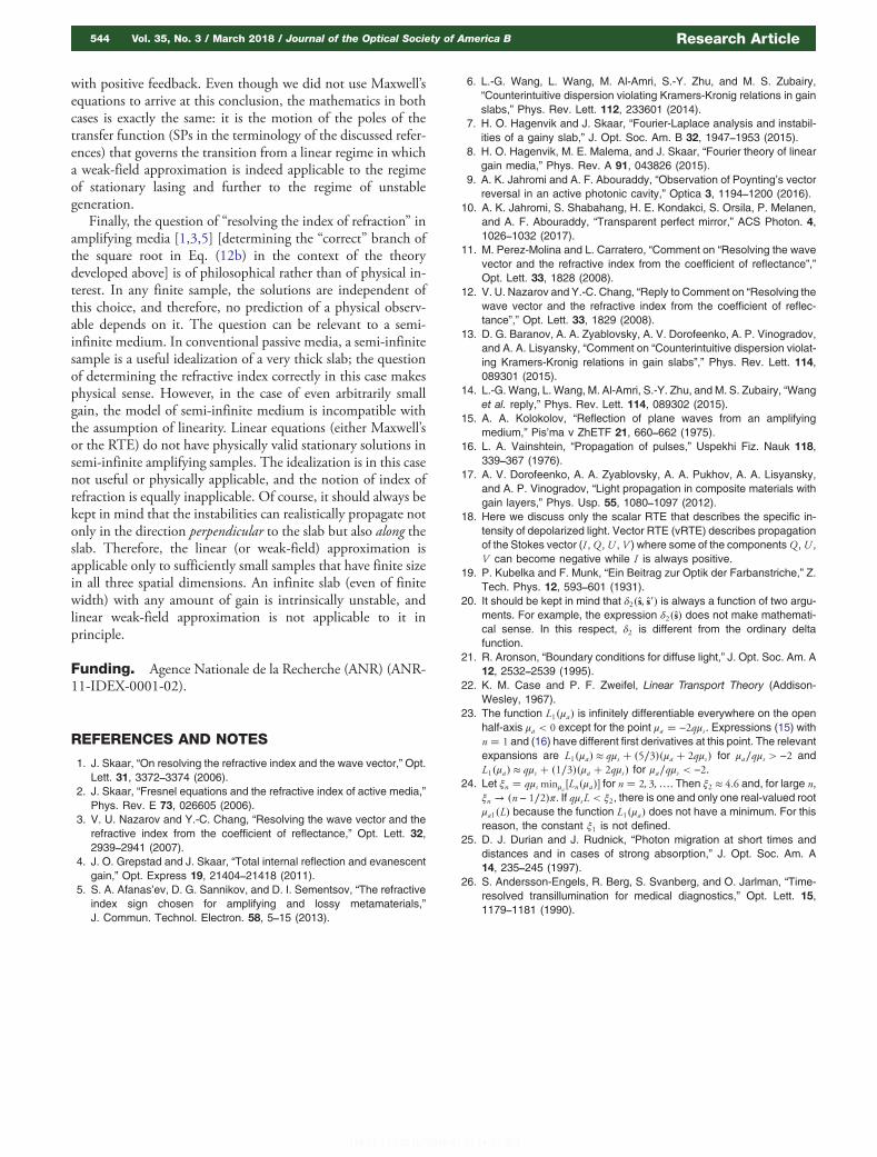
The data of Fig. 9 do not allow one, at least easily, to visu-alize the dependence of the stationary lasing condition on qμs.In particular, it is not possible to infer the limit qμs → 0 fromthis figure. This is so because, as in all previous figures, we haveused �qμs�−1 as the unit of length in Fig. 9. To visualize thedependence on qμs, we have displayed in Fig. 10 the conditionof stationary lasing as curves in the �qμs ; L� plane for a fixednegative μa < 0. Again, it can be seen that allowing reflectionsat the interfaces to occur relaxes the lasing condition.

8. DISCUSSION

The simple two-stream approximation to the RTE is a conven-ient model for studying propagation of light in amplifying me-dia. An added bonus of this approach is that the unphysicalstationary solutions, which are not always easy to spot inthe case of Maxwell’s equations, become apparent in the caseof the RTE because the specific intensity in all such instanceschanges sign, which is clearly unphysical.

Three-dimensional generalizations of the theory developedabove can be applicable to random lasers. It should be also keptin mind that the RTE is equally applicable to neutron trans-port. The critical thickness of an amplifying slab beyond whichthe system response is unstable is directly analogous to the criti-cal mass in nuclear fusion, beyond which an uncontrolled chainreaction occurs. Although this phenomenon has been very wellunderstood in nuclear physics, the analogy with optics may notbe obvious. The main reason is that the RTE has no phase,whereas interference effects are often viewed as conceptuallyimportant in the functioning of lasers.

Of course, the instabilities and the unbounded growth ofintensity are artifacts of an incomplete mathematical model.In real systems, the growth of intensity is always limited bythe effects of saturation and other kinds of negative feedback.For example, the competition of gain and losses and the effectof saturation play an important role in conventional lasers.However, the laser medium is not described in this case bya linear RTE; one must use a nonlinear equation where the gainis saturated at high energy density. For example, we can use themodel expression

μa�u� � a −b

1� u∕u0; u�z� � i1�z� � i2�z�: (49)

Here a and b are two positive constants, and u is the density ofenergy. It can be seen that the coefficient μa becomes in thiscase position-dependent, since u�z� will change with position.It can be concluded that, in the region of parameters where themedium response is unstable, linear or weak-field approxima-tion is not applicable in principle.

In light of the above, we can analyze the arguments appearinginWang et al.’s reply [14] to the comment by Baranov et al. [13].In particular, Wang et al. write “The main argument of Baranovet al. that ‘the movement of SPs [singular points-V.M.] …indicates the onset of lasing’ implies that the onset of lasingdoes not depend on the field strength but relies on the slab’sthickness. This incorrect argument is different from the conven-tional view on lasing….” In the foregoing text, Wang et al. alsoargue that the slab width at which the onset of lasing occurs,denoted by d las in the discussed references, depends on theintensity of incident light: “The lower the intensity of the inci-dent light is, the larger the width d las will be.”

The results of this paper show clearly that the above argu-ments are incorrect. The critical width of the slab beyondwhich the system is unstable does not depend on the intensityof incident light. In fact, the instabilities will develop in theabsence of any incident light; a tiny thermal fluctuation willget exponentially amplified over time. This phenomenon isphysically similar to the uncontrolled chain fusion reactionand is qualitatively similar to all other instabilities in systems

Fig. 9. Illustration of the condition of stationary lasing (48). Thelowest-lying solutions of Eq. (48) are shown for varying values ofthe reflection coefficients jr0j2 and jrLj2. The curve labeled as 1 cor-responds to r0 � rL � 0 and is identical to the curve L1�μa� shown inFig. 2. Other curves have the following parameters: jr0j2 � jrLj2 �0.5 (Curve 2); jr0j2 � jrLj2 � 0.9 (Curve 3); and jr0j2 � 0.05,jrLj2 � 0.95 (Curve 4).

Fig. 10. Same as in Fig. 9 but the stationary lasing condition isshown in the �qμs ; L� plane for a fixed negative value μa < 0.Same curve labels as in Fig. 9. Note that the curve labeled 1, whichcorresponds to r0 � rL � 0, exhibits a logarithmic divergence atqμs � 0.


with positive feedback. Even though we did not use Maxwell’sequations to arrive at this conclusion, the mathematics in bothcases is exactly the same: it is the motion of the poles of thetransfer function (SPs in the terminology of the discussed refer-ences) that governs the transition from a linear regime in whicha weak-field approximation is indeed applicable to the regimeof stationary lasing and further to the regime of unstablegeneration.

Finally, the question of “resolving the index of refraction” inamplifying media [1,3,5] [determining the “correct” branch ofthe square root in Eq. (12b) in the context of the theorydeveloped above] is of philosophical rather than of physical in-terest. In any finite sample, the solutions are independent ofthis choice, and therefore, no prediction of a physical observ-able depends on it. The question can be relevant to a semi-infinite medium. In conventional passive media, a semi-infinitesample is a useful idealization of a very thick slab; the questionof determining the refractive index correctly in this case makesphysical sense. However, in the case of even arbitrarily smallgain, the model of semi-infinite medium is incompatible withthe assumption of linearity. Linear equations (either Maxwell’sor the RTE) do not have physically valid stationary solutions insemi-infinite amplifying samples. The idealization is in this casenot useful or physically applicable, and the notion of index ofrefraction is equally inapplicable. Of course, it should always bekept in mind that the instabilities can realistically propagate notonly in the direction perpendicular to the slab but also along theslab. Therefore, the linear (or weak-field) approximation isapplicable only to sufficiently small samples that have finite sizein all three spatial dimensions. An infinite slab (even of finitewidth) with any amount of gain is intrinsically unstable, andlinear weak-field approximation is not applicable to it inprinciple.

Funding. Agence Nationale de la Recherche (ANR) (ANR-11-IDEX-0001-02).

REFERENCES AND NOTES

1. J. Skaar, “On resolving the refractive index and the wave vector,” Opt.Lett. 31, 3372–3374 (2006).

2. J. Skaar, “Fresnel equations and the refractive index of active media,”Phys. Rev. E 73, 026605 (2006).

3. V. U. Nazarov and Y.-C. Chang, “Resolving the wave vector and therefractive index from the coefficient of reflectance,” Opt. Lett. 32,2939–2941 (2007).

4. J. O. Grepstad and J. Skaar, “Total internal reflection and evanescentgain,” Opt. Express 19, 21404–21418 (2011).

5. S. A. Afanas’ev, D. G. Sannikov, and D. I. Sementsov, “The refractiveindex sign chosen for amplifying and lossy metamaterials,”J. Commun. Technol. Electron. 58, 5–15 (2013).

6. L.-G. Wang, L. Wang, M. Al-Amri, S.-Y. Zhu, and M. S. Zubairy,“Counterintuitive dispersion violating Kramers-Kronig relations in gainslabs,” Phys. Rev. Lett. 112, 233601 (2014).

7. H. O. Hagenvik and J. Skaar, “Fourier-Laplace analysis and instabil-ities of a gainy slab,” J. Opt. Soc. Am. B 32, 1947–1953 (2015).

8. H. O. Hagenvik, M. E. Malema, and J. Skaar, “Fourier theory of lineargain media,” Phys. Rev. A 91, 043826 (2015).

9. A. K. Jahromi and A. F. Abouraddy, “Observation of Poynting’s vectorreversal in an active photonic cavity,” Optica 3, 1194–1200 (2016).

10. A. K. Jahromi, S. Shabahang, H. E. Kondakci, S. Orsila, P. Melanen,and A. F. Abouraddy, “Transparent perfect mirror,” ACS Photon. 4,1026–1032 (2017).

11. M. Perez-Molina and L. Carratero, “Comment on “Resolving the wavevector and the refractive index from the coefficient of reflectance”,”Opt. Lett. 33, 1828 (2008).

12. V. U. Nazarov and Y.-C. Chang, “Reply to Comment on “Resolving thewave vector and the refractive index from the coefficient of reflec-tance”,” Opt. Lett. 33, 1829 (2008).

13. D. G. Baranov, A. A. Zyablovsky, A. V. Dorofeenko, A. P. Vinogradov,and A. A. Lisyansky, “Comment on “Counterintuitive dispersion violat-ing Kramers-Kronig relations in gain slabs”,” Phys. Rev. Lett. 114,089301 (2015).

14. L.-G. Wang, L. Wang, M. Al-Amri, S.-Y. Zhu, and M. S. Zubairy, “Wanget al. reply,” Phys. Rev. Lett. 114, 089302 (2015).

15. A. A. Kolokolov, “Reflection of plane waves from an amplifyingmedium,” Pis’ma v ZhETF 21, 660–662 (1975).

16. L. A. Vainshtein, “Propagation of pulses,” Uspekhi Fiz. Nauk 118,339–367 (1976).

17. A. V. Dorofeenko, A. A. Zyablovsky, A. A. Pukhov, A. A. Lisyansky,and A. P. Vinogradov, “Light propagation in composite materials withgain layers,” Phys. Usp. 55, 1080–1097 (2012).

18. Here we discuss only the scalar RTE that describes the specific in-tensity of depolarized light. Vector RTE (vRTE) describes propagationof the Stokes vector (I ,Q ,U , V ) where some of the componentsQ,U ,V can become negative while I is always positive.

19. P. Kubelka and F. Munk, “Ein Beitrag zur Optik der Farbanstriche,” Z.Tech. Phys. 12, 593–601 (1931).

20. It should be kept in mind that δ2�s; s 0� is always a function of two argu-ments. For example, the expression δ2�s� does not make mathemati-cal sense. In this respect, δ2 is different from the ordinary deltafunction.

21. R. Aronson, “Boundary conditions for diffuse light,” J. Opt. Soc. Am. A12, 2532–2539 (1995).

22. K. M. Case and P. F. Zweifel, Linear Transport Theory (Addison-Wesley, 1967).

23. The function L1�μa� is infinitely differentiable everywhere on the openhalf-axis μa < 0 except for the point μa � −2qμs . Expressions (15) withn � 1 and (16) have different first derivatives at this point. The relevantexpansions are L1�μa� ≈ qμs � �5∕3��μa � 2qμs� for μa∕qμs > −2 andL1�μa� ≈ qμs � �1∕3��μa � 2qμs� for μa∕qμs < −2.

24. Let ξn � qμs minμa �Ln�μa�� for n � 2; 3;…. Then ξ2 ≈ 4.6 and, for large n,ξn → �n − 1∕2�π. If qμsL < ξ2, there is one and only one real-valued rootμa1�L� because the function L1�μa� does not have a minimum. For thisreason, the constant ξ1 is not defined.

25. D. J. Durian and J. Rudnick, “Photon migration at short times anddistances and in cases of strong absorption,” J. Opt. Soc. Am. A14, 235–245 (1997).

26. S. Andersson-Engels, R. Berg, S. Svanberg, and O. Jarlman, “Time-resolved transillumination for medical diagnostics,” Opt. Lett. 15,1179–1181 (1990).


Documents

Two-stream theory of light propagation in amplifying media