Chapter 3

Two species models

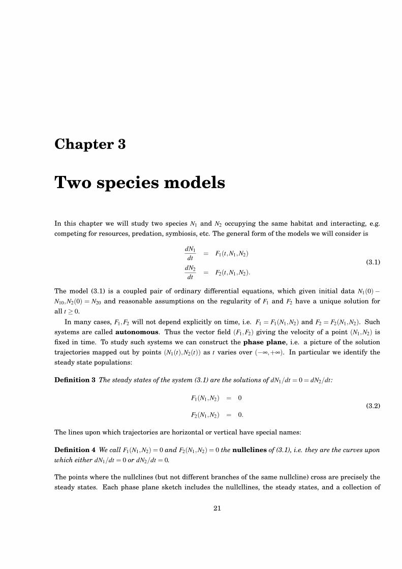
In this chapter we will study two species N1 and N2 occupying the same habitat and interacting, e.g.competing for resources, predation, symbiosis, etc. The general form of the models we will consider is

dN1

dt= F1(t,N1,N2)

dN2

dt= F2(t,N1,N2).

(3.1)

The model (3.1) is a coupled pair of ordinary differential equations, which given initial data N1(0)!N10,N2(0) = N20 and reasonable assumptions on the regularity of F1 and F2 have a unique solution forall t " 0.

In many cases, F1,F2 will not depend explicitly on time, i.e. F1 = F1(N1,N2) and F2 = F2(N1,N2). Suchsystems are called autonomous. Thus the vector field (F1,F2) giving the velocity of a point (N1,N2) isfixed in time. To study such systems we can construct the phase plane, i.e. a picture of the solutiontrajectories mapped out by points (N1(t),N2(t)) as t varies over (!!,+!). In particular we identify thesteady state populations:

Definition 3 The steady states of the system (3.1) are the solutions of dN1/dt = 0 = dN2/dt:

F1(N1,N2) = 0

F2(N1,N2) = 0.(3.2)

The lines upon which trajectories are horizontal or vertical have special names:

Definition 4 We call F1(N1,N2) = 0 and F2(N1,N2) = 0 the nullclines of (3.1), i.e. they are the curves uponwhich either dN1/dt = 0 or dN2/dt = 0.

The points where the nullclines (but not different branches of the same nullcline) cross are precisely thesteady states. Each phase plane sketch includes the nullcllines, the steady states, and a collection of

21

CHAPTER 3. TWO SPECIES MODELS

trajectories that start in varies parts of the plane. The individual trajectories are solutions of

dN1

dN2=

F1(N1,N2)F2(N1,N2)

, N1(0) = N10,N2(0) = N20. (3.3)

In some cases the complete picture of the solutions of (3.1) can be established just by considering thenullclines, steady states and how the sign of dN1/dN2 changes as we go between regions demarked bynullclines. In some cases, however, this level of detail is insufficient, and we must study more carefullyhow (3.1) behaves near a steady state by considering its linearised form about that steady state.

1 Rules aiding construction of the phase plane

We list the following set of rules that help with the construction of the phase plane of the system (3.1):

1. trajectories cross vertically the nullcline

F1(N1,N2) = 0

since here dN1/dt = 0;

2. trajectories cross horizontally the nullcline

F2(N1,N2) = 0

since here dN2/dt = 0;

3. in regions enclosed by nullclines dN1/dN2 has constant sign, i.e. trajectories are either rising orfalling;

4. trajectories can only go flat or vertical across nullclines;

5. steady states are where any branches of nullclines F1(N1,N2) = 0 and F2(N1,N2) = 0 cross.

In some cases further analysis (linear stability analysis of (3.1)) is required to further characterise thedetailed behaviour near a steady state, such as, for example, to distinguish between simple non-oscillatorybehaviour (e.g. tending directly to a steady state) or oscillatory behaviour (spiralling in to the steadystate).

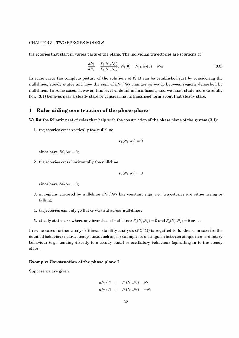
Example: Construction of the phase plane I

Suppose we are given

dN1/dt = F1(N1,N2) = N2

dN2/dt = F2(N1,N2) =!N1.

22

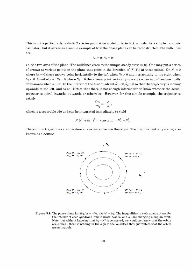
This is not a particularly realistic 2 species population model (it is, in fact, a model for a simple harmonicoscillator), but it serves as a simple example of how the phase plane can be reconstructed. The nullclinesare

N2 = 0, N1 = 0,

i.e. the two axes of the plane. The nullclines cross at the unique steady state (0,0). One may put a seriesof arrows at various points in the plane that point in the direction of (F1,F2) at those points. On N1 = 0where N2 = 0 these arrows point horizontally to the left when N2 > 0 and horizontally to the right whenN2 < 0. Similarly on N2 = 0 where N1 = 0 the arrows point vertically upwards when N1 > 0 and verticallydownwards when N1 < 0. In the interior of the first quadrant N1 < 0, N2 > 0 so that the trajectory is movingupwards to the left, and so on. Notice that there is not enough information to know whether the actualtrajectories spiral inwards, outwards or otherwise. However, for this simple example, the trajectoriessatisfy

dN1

dN2=!N2

N1,

which is a separable ode and can be integrated immediately to yield

N1(t)2 +N2(t)2 = constant = N210 +N2

20.

The solution trajectories are therefore all circles centred on the origin. The origin is neutrally stable, alsoknown as a centre.

Figure 3.1: The phase plane for dN1/dt =!N2, dN2/dt = N1. The inequalities in each quadrant are forthe interior of each quadrant, and indicate how N1 and N2 are changing along an orbit.Note that without knowing that N2

1 + N22 is conserved, we would not know that the orbits

are circles - there is nothing in the sign of the velocities that guarantees that the orbitsare not spirals.

23

CHAPTER 3. TWO SPECIES MODELS

2 Behaviour on the boundary of the first quadrant

The kind of ode population models considered in this course are part of a larger class of systems calledKolmogorov systems. Such systems take the form xi = xi fi(x1, . . . ,xn) for i = 1, . . . ,n where n is the numberof species and the smooth functions fi describe the per capita growth rate for the ith species. One of thekey properties of such systems is that if at some time t# we have xi(t#) = 0 for i $ J (where J % {1,2, . . . ,n}is some nonempty set) then xi(t) = 0 for all t and i $ J. In our planar models this means that trajectoriesstarting on the axes stay on the axes, and interior trajectories cannot reach the axes in finite time. Henceto find what happens to a trajectory starting at x1 = 0 we simply solve

x2 = x2 f2(0,x2), x2(0) given,

which is a ode in one variable, as for the single species models of the first 2 chapters. Hence drawing thetrajectories on each axes in the phase plane is a relatively simple task for planar Kolmogorov systems.

Example: The Lotka-Volterra competition equations

Recall the Logistic equation for a single speces:

dNdt

= "N!

1! NK

".

Here " is the linear birth rate, and K the carrying capacity. For two species N1,N2 living in the samehabitat, but not interacting, we simply have

dN1

dt= "1N1

!1! N1

K1

"

dN2

dt= "2N2

!1! N2

K2

".

The competition in these equations intraspecific (i.e. between the same species). When the species com-pete with each other (for nesting sites, food, etc.), the interspecific competition is detrimental to bothspecie’s per capita growth rates. The simplest model is to say that the per capital growth rates decreaselinearly with the density of the other species. The competition equations then become

dN1

dt= "1N1

!1! N1

K1! c1

"1N2

"

dN2

dt= "2N2

!1! N2

K2! c2

"2N1

",

(3.4)

where c1,c2 > 0 measure the strength of the interspecific competition. To ease calculations, we first setui = Ni/Ki for i = 1,2 and a12 = c1K2/"1, a21 = c2K1/"2. We also introduce a dimensionless time # = "1t and

24

set " = "2/"1. This gives the simpler set of equations (fewer parameters)

du1

d#= u1 (1!u1!a12u2)

du2

d#= "u2 (1!u2!a21u1) .

(3.5)

Our first step is to locate the nullclines: These are

u1 = 0 and 1!u1!a12u2 = 0 (3.6)

u2 = 0 and 1!u2!a21u1 = 0. (3.7)

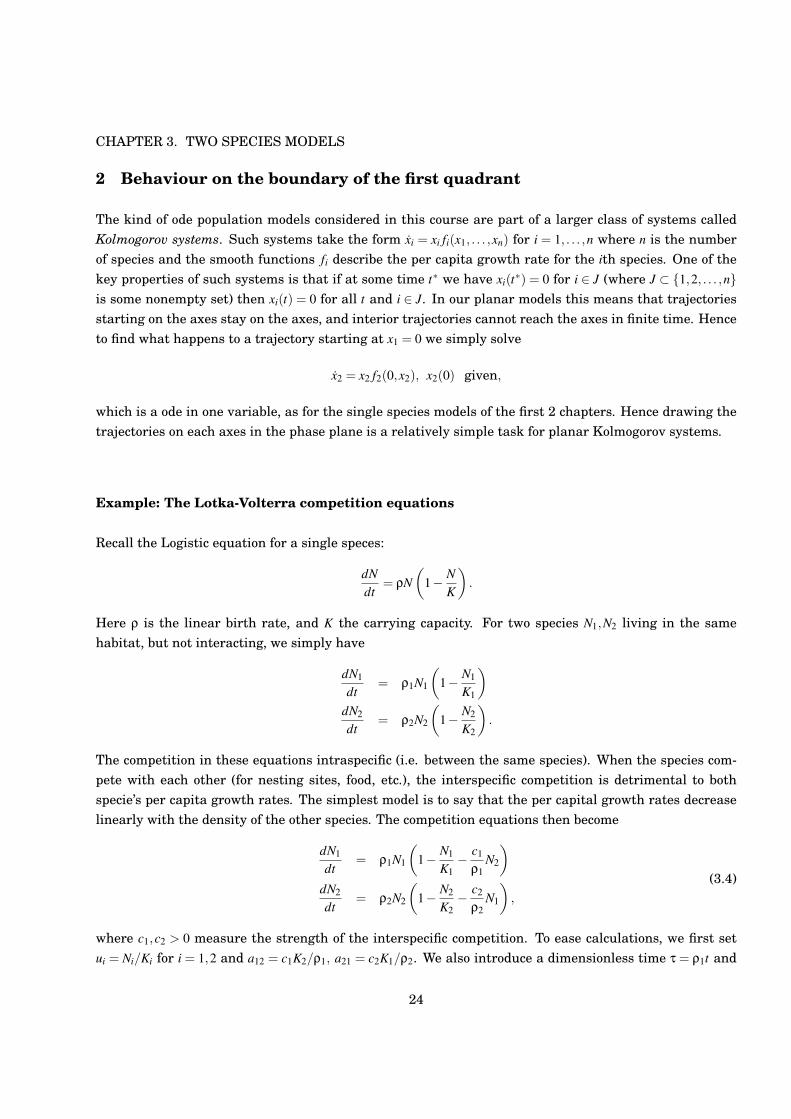
Hence steady states occur at points

(u#1,u#2) = (0,0), (1,0), (0,1),P =

!1!a12

1!a12a21,

1!a21

1!a12a21

".

This last steady state is only feasible (non-negative populations!) when either1

1. a12 > 1 and a21 > 1, since then also 1!a12a21 < 0; OR

2. a12 < 1 and a21 < 1, since then also 1!a12a21 > 0;

Hence we have either 3 or 4 steady states. As we indicate in Figure 3.2 there are 4 cases to consider:

Case I a12 < 1 and a21 < 1;

Case II a12 > 1 and a21 > 1;

Case III a12 < 1 and a21 > 1;

Case IV a12 > 1 and a21 < 1.

Now let us determine what happens on the axes. Suppose first that initially u2 = 0, so that the evolutionis on the u1 axis. We find u1(t) by solving the first equaton in (3.5) with u2 = 0:

u1 = u1(1!u1).

This is just the Logistic equation with " = 1,K = 1. Provided u1(0) > 0 we have u1(t)& 1 as t&!. Similarlywe find when u1(0) = 0 then u2 = "u2(1!u2) and hence u2(t)& 1 as t & ! if u2(0) > 0 (see Figure 3.3).

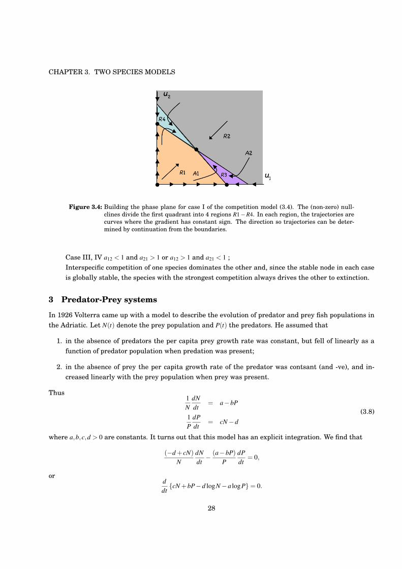
Let us consider the case I in detail (see figure 3.4). We have already dealt with the boundary behaviour.Consider an interior trajectory A1. It starts (as drawn, at least) in region R1 that lies below both nullclines1!u1!a12u2 = 0 and 1!u2!a21u1 = 0 so that here u1 > 0, u2 > 0 and the trajectory therefore advances inthe direction shown. This trajectory has positive gradient provided that it does not cross a nullcline. Infact, all trajectories in R1 have positive gradient. Following A1 we see that it cannot turn back on itself,and so must cross the nullcline where u1 = 0, whereby its gradient becomes negative since then, in R3 we

1For simplicity here we do not consider the cases where a12 = 1 and/or a21 = 1.

25

CHAPTER 3. TWO SPECIES MODELS

1

N1

N2

P=(u1*, u

2*)

steady state

N1

N2

P=(N1*, N

2*)

N1

N2

N1

N2

case I case II

case III case IV

1/a21

1

1/a12

1

1/a12

1/a21 1

1/a12

1 1/a12

1

1/a21

1/a211 1

Figure 3.2: The possible nullcline crossings for the Lokta-Volterra model (3.4)

have u1 < 0, u2 > 0. The trajectory thus goes vertical across u1 = 0 and continues upwards to the left. Itcannot leave R3, since to re-enter R1 is needs to cross it vertically and thus must go horizontal first, andit cannot enter R2 since trajectories cross the boundary between R2 and R3 downwards. Hence A1 ends atthe interior steady state. A similar argument works for A2. In R3 the trajectories are above the nullclines1! u1! a12u2 = 0 and 1! u2! a21u1 = 0 so that here u1 < 0, u2 < 0. A2 enters from R2 into R3 where it isthen trapped and must end at the interior steady state. After some practice, it is possible to draw thetrajectory directions by noting their directions on the nearby boundary. We can thus construct sketchesfor the phase planes in each of these 4 cases:

Case I a12 < 1 and a21 < 1;The steady state P attracts all interior trajectories. The remaining 3 steady states are unstable.

Case II a12 > 1 and a21 > 1;The steady state P is unstable. The steady state (0,0) is unstable, and both (1,0) and (0,1) are stable.A separatrix splits the phase plane into two regions; above the seperatrix interior trajectories go tothe steady state (1,0) and below they go to the steady state (0,1)

26

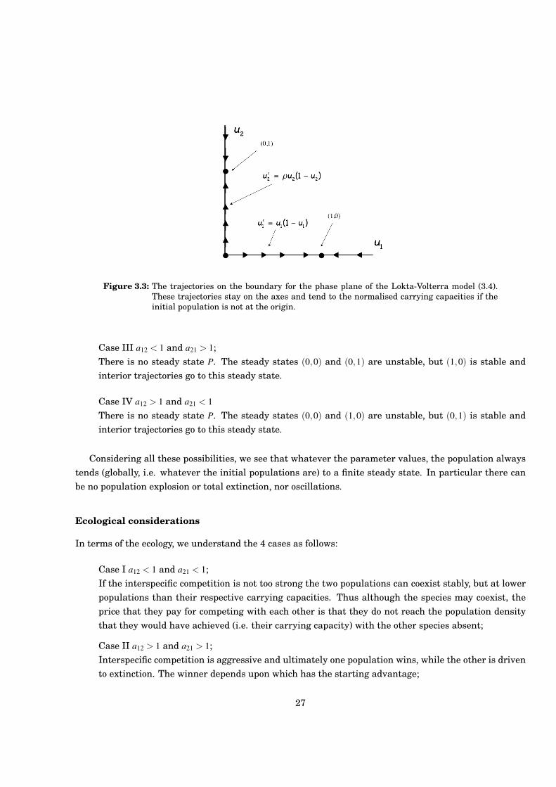
Figure 3.3: The trajectories on the boundary for the phase plane of the Lokta-Volterra model (3.4).These trajectories stay on the axes and tend to the normalised carrying capacities if theinitial population is not at the origin.

Case III a12 < 1 and a21 > 1;There is no steady state P. The steady states (0,0) and (0,1) are unstable, but (1,0) is stable andinterior trajectories go to this steady state.

Case IV a12 > 1 and a21 < 1There is no steady state P. The steady states (0,0) and (1,0) are unstable, but (0,1) is stable andinterior trajectories go to this steady state.

Considering all these possibilities, we see that whatever the parameter values, the population alwaystends (globally, i.e. whatever the initial populations are) to a finite steady state. In particular there canbe no population explosion or total extinction, nor oscillations.

Ecological considerations

In terms of the ecology, we understand the 4 cases as follows:

Case I a12 < 1 and a21 < 1;If the interspecific competition is not too strong the two populations can coexist stably, but at lowerpopulations than their respective carrying capacities. Thus although the species may coexist, theprice that they pay for competing with each other is that they do not reach the population densitythat they would have achieved (i.e. their carrying capacity) with the other species absent;

Case II a12 > 1 and a21 > 1;Interspecific competition is aggressive and ultimately one population wins, while the other is drivento extinction. The winner depends upon which has the starting advantage;

27

CHAPTER 3. TWO SPECIES MODELS

Figure 3.4: Building the phase plane for case I of the competition model (3.4). The (non-zero) null-clines divide the first quadrant into 4 regions R1!R4. In each region, the trajectories arecurves where the gradient has constant sign. The direction so trajectories can be deter-mined by continuation from the boundaries.

Case III, IV a12 < 1 and a21 > 1 or a12 > 1 and a21 < 1 ;Interspecific competition of one species dominates the other and, since the stable node in each caseis globally stable, the species with the strongest competition always drives the other to extinction.

3 Predator-Prey systems

In 1926 Volterra came up with a model to describe the evolution of predator and prey fish populations inthe Adriatic. Let N(t) denote the prey population and P(t) the predators. He assumed that

1. in the absence of predators the per capita prey growth rate was constant, but fell of linearly as afunction of predator population when predation was present;

2. in the absence of prey the per capita growth rate of the predator was contsant (and -ve), and in-creased linearly with the prey population when prey was present.

Thus1N

dNdt

= a!bP

1P

dPdt

= cN!d(3.8)

where a,b,c,d > 0 are constants. It turns out that this model has an explicit integration. We find that

(!d + cN)N

dNdt! (a!bP)

PdPdt

= 0,

orddt

{cN +bP!d logN!a logP} = 0.

28

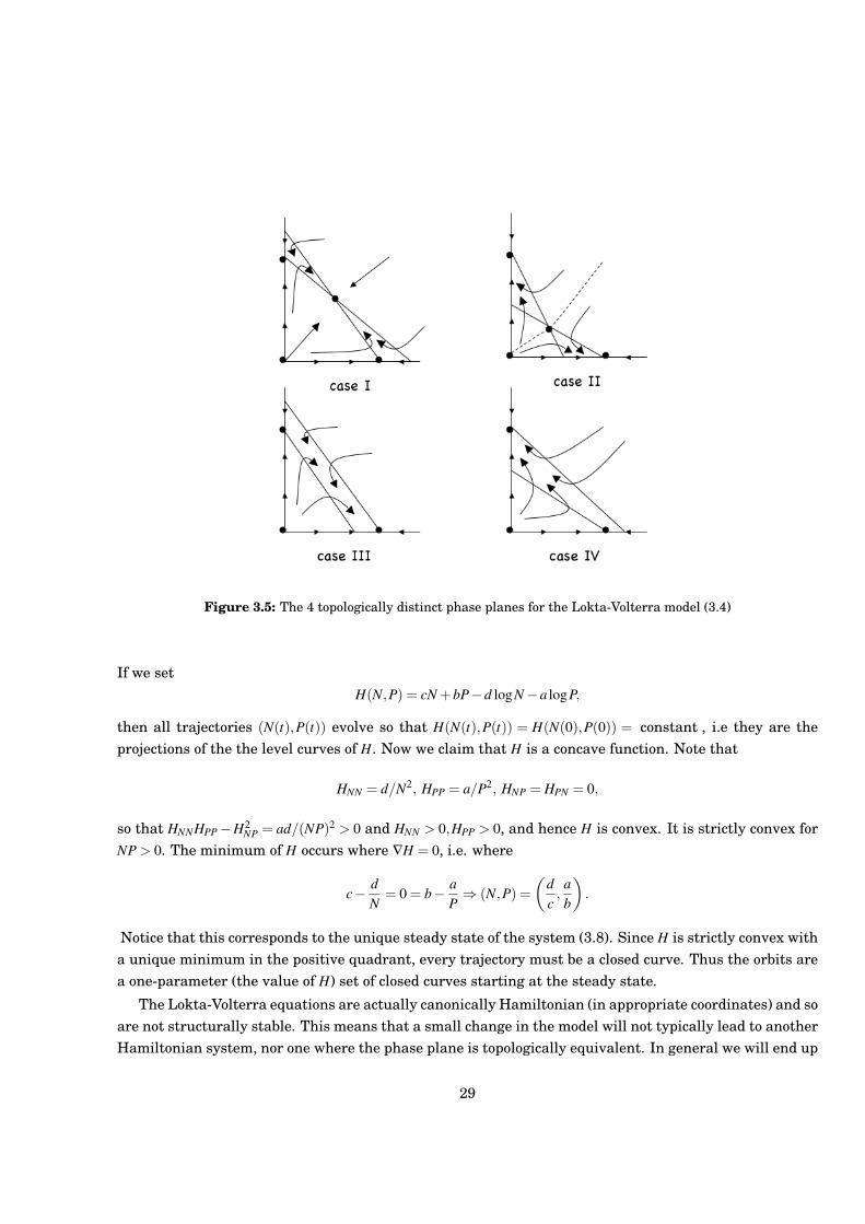
Figure 3.5: The 4 topologically distinct phase planes for the Lokta-Volterra model (3.4)

If we setH(N,P) = cN +bP!d logN!a logP,

then all trajectories (N(t),P(t)) evolve so that H(N(t),P(t)) = H(N(0),P(0)) = constant , i.e they are theprojections of the the level curves of H. Now we claim that H is a concave function. Note that

HNN = d/N2, HPP = a/P2, HNP = HPN = 0,

so that HNNHPP!H2NP = ad/(NP)2 > 0 and HNN > 0,HPP > 0, and hence H is convex. It is strictly convex for

NP > 0. The minimum of H occurs where $H = 0, i.e. where

c! dN

= 0 = b! aP' (N,P) =

!dc,

ab

".

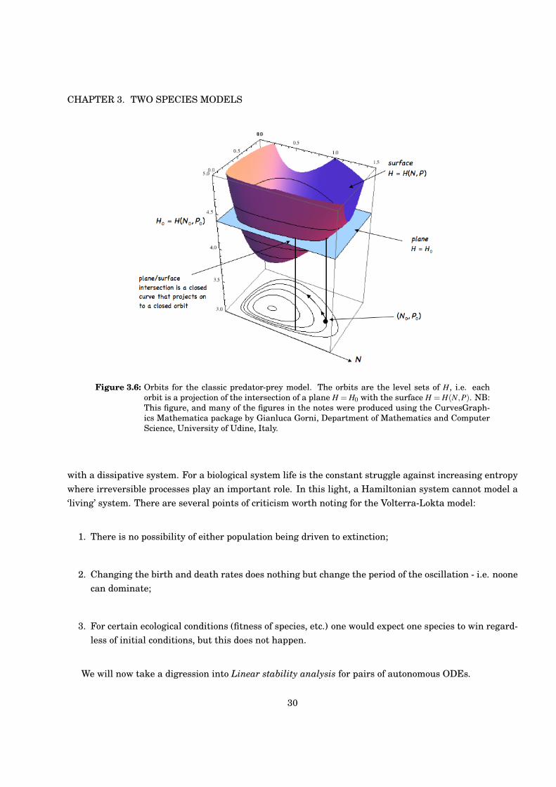
Notice that this corresponds to the unique steady state of the system (3.8). Since H is strictly convex witha unique minimum in the positive quadrant, every trajectory must be a closed curve. Thus the orbits area one-parameter (the value of H) set of closed curves starting at the steady state.

The Lokta-Volterra equations are actually canonically Hamiltonian (in appropriate coordinates) and soare not structurally stable. This means that a small change in the model will not typically lead to anotherHamiltonian system, nor one where the phase plane is topologically equivalent. In general we will end up

29

CHAPTER 3. TWO SPECIES MODELS

Figure 3.6: Orbits for the classic predator-prey model. The orbits are the level sets of H, i.e. eachorbit is a projection of the intersection of a plane H = H0 with the surface H = H(N,P). NB:This figure, and many of the figures in the notes were produced using the CurvesGraph-ics Mathematica package by Gianluca Gorni, Department of Mathematics and ComputerScience, University of Udine, Italy.

with a dissipative system. For a biological system life is the constant struggle against increasing entropywhere irreversible processes play an important role. In this light, a Hamiltonian system cannot model a‘living’ system. There are several points of criticism worth noting for the Volterra-Lokta model:

1. There is no possibility of either population being driven to extinction;

2. Changing the birth and death rates does nothing but change the period of the oscillation - i.e. noonecan dominate;

3. For certain ecological conditions (fitness of species, etc.) one would expect one species to win regard-less of initial conditions, but this does not happen.

We will now take a digression into Linear stability analysis for pairs of autonomous ODEs.

30

3.1. DIGRESSION: LINEAR STABILITY ANALYSIS OF PLANAR ODES

0 1 2 3 4

0

1

2

3

4

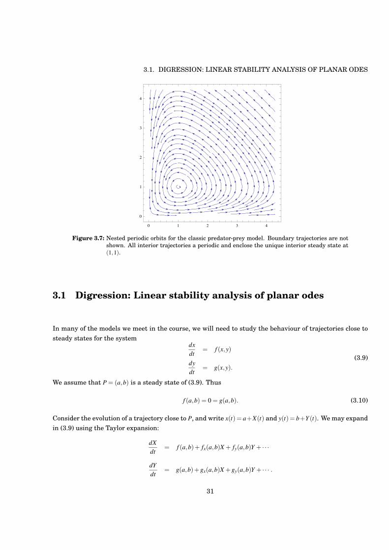
Figure 3.7: Nested periodic orbits for the classic predator-prey model. Boundary trajectories are notshown. All interior trajectories a periodic and enclose the unique interior steady state at(1,1).

3.1 Digression: Linear stability analysis of planar odes

In many of the models we meet in the course, we will need to study the behaviour of trajectories close tosteady states for the system

dxdt

= f (x,y)

dydt

= g(x,y).(3.9)

We assume that P = (a,b) is a steady state of (3.9). Thus

f (a,b) = 0 = g(a,b). (3.10)

Consider the evolution of a trajectory close to P, and write x(t) = a+X(t) and y(t) = b+Y (t). We may expandin (3.9) using the Taylor expansion:

dXdt

= f (a,b)+ fx(a,b)X + fy(a,b)Y + · · ·

dYdt

= g(a,b)+gx(a,b)X +gy(a,b)Y + · · · .

31

CHAPTER 3. TWO SPECIES MODELS

Using (3.10), this becomes

dXdt

= fx(a,b)X + fy(a,b)Y + · · ·

dYdt

= gx(a,b)X +gy(a,b)Y + · · · .

Close to P, |X(t)|, |Y (t)|( 1 this system is well-approximated by the linearised version obtained by neglect-ing second order terms in X ,Y :

dXdt

= fx(a,b)X + fy(a,b)Y

dYdt

= gx(a,b)X +gy(a,b)Y.

(3.11)

Notice that since we are neglecting higher order than linear terms, the linear approximation will onlypotentially give a good indication of the full nonlinear system while X(t),Y (t) remain small.

Now let X(t) = (X(t),Y (t))T and

M =

#fx(a,b) fy(a,b)gx(a,b) gy(a,b)

$.

Then (6.12) can be rewritten in matrix form:

dX(t)dt

= MX(t). (3.12)

This has steady state (0,0) (which corresponds to (x,y) = (a,b)). For a trajectory of the linearised system(3.12) starting at X(0) = X0,

X(t) = exp(Mt)X0.

If M has two distinct eigenvalues %1,%2 with corresponding eigenvectors v1,v2 then

X(t) = &e%1tv1 +'e%2tv2, (3.13)

where &,' are defined by the decomposition X0 = &v1 +'v2 (using linear independence of v1,v2). When thetwo eigenvalues are equal (and therefore real) we have

X(t) = e%t(X0 + ctv) (3.14)

for some real c (which may be zero).To find the (local) stability of the steady state (a,b) we examine the dynamics of (3.12) which has

solution (3.13). If (a,b) is stable then for small X0, the solution X(t) will eventually decay to the origin(0,0) and this happens, according to (3.13), when both eigenvalues have negative real parts.

Let us list the various possibilities for behaviour near a steady state

1. %1 )= %2 $ R

(a) %1 < %2 < 0 - stable node.

32

3.1. DIGRESSION: LINEAR STABILITY ANALYSIS OF PLANAR ODES

0

0

0

0

0

0

0

0

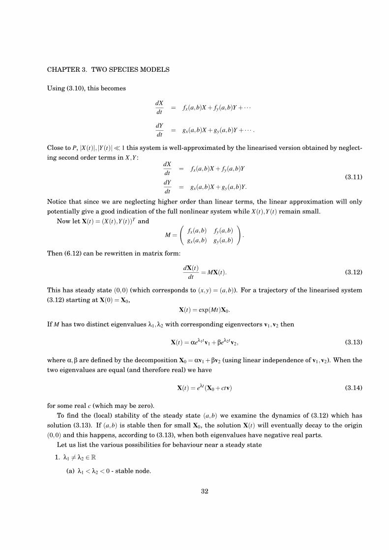
Figure 3.8: Linear stability for real eigenvalues: (i) %1,%2 < 0 (stable node) and (ii) %1%2 < 0 (saddle).The thick (red) lines are in the direction of the eigenvectors.

(b) %1 > %2 > 0 - unstable node.

(c) %1%2 < 0 - saddle (unstable)

(The reader may wish to ask themselves what happens when %1%2 = 0)

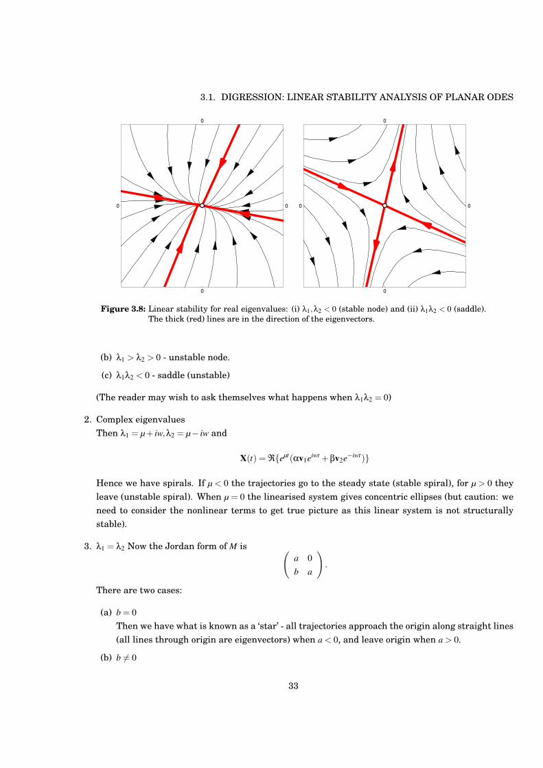
2. Complex eigenvaluesThen %1 = µ+ iw,%2 = µ! iw and

X(t) = ({eµt(&v1eiwt +'v2e!iwt)}

Hence we have spirals. If µ < 0 the trajectories go to the steady state (stable spiral), for µ > 0 theyleave (unstable spiral). When µ = 0 the linearised system gives concentric ellipses (but caution: weneed to consider the nonlinear terms to get true picture as this linear system is not structurallystable).

3. %1 = %2 Now the Jordan form of M is #a 0b a

$.

There are two cases:

(a) b = 0Then we have what is known as a ‘star’ - all trajectories approach the origin along straight lines(all lines through origin are eigenvectors) when a < 0, and leave origin when a > 0.

(b) b )= 0

33

CHAPTER 3. TWO SPECIES MODELS

0

0

0

0

0

0

0

0

Figure 3.9: Linear stability for complex eigenvalues: (i) % = µ± iw,µ > 0 (unstable spiral) and (ii) % =±iw (centre).

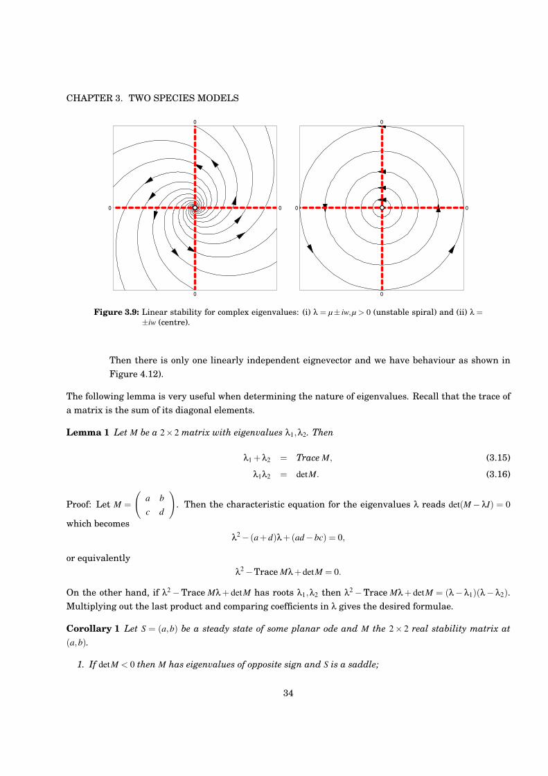
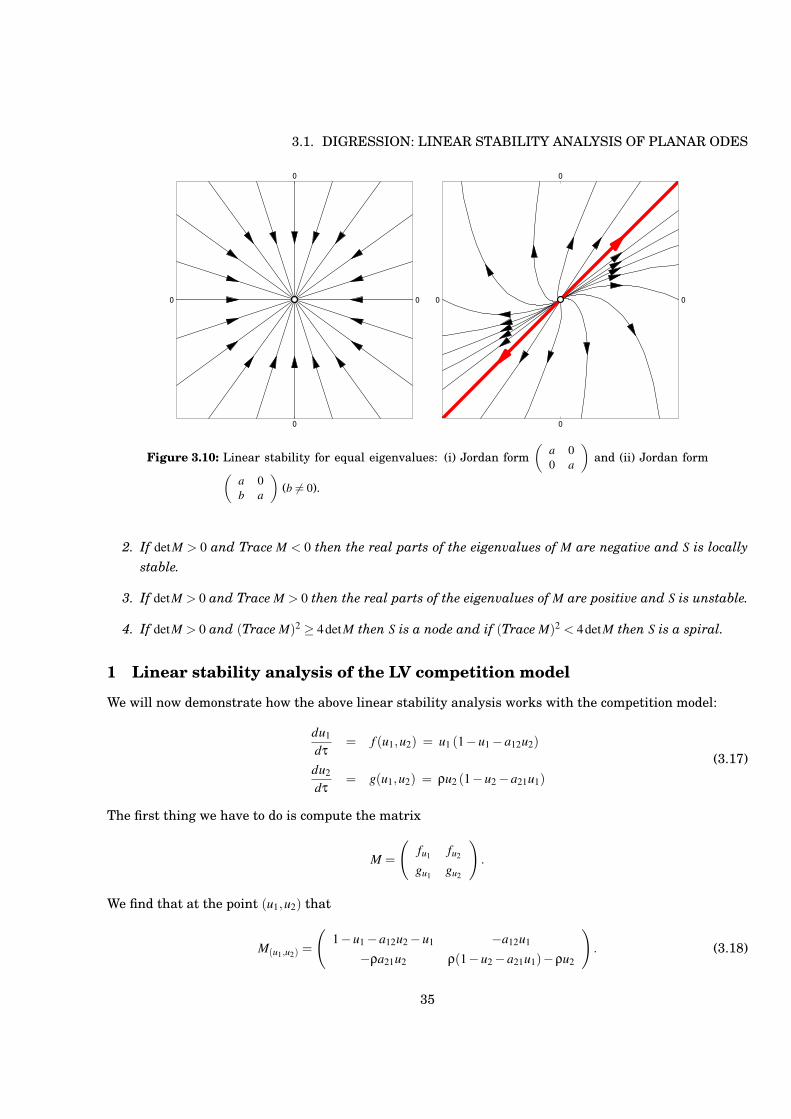
Then there is only one linearly independent eignevector and we have behaviour as shown inFigure 4.12).

The following lemma is very useful when determining the nature of eigenvalues. Recall that the trace ofa matrix is the sum of its diagonal elements.

Lemma 1 Let M be a 2*2 matrix with eigenvalues %1,%2. Then

%1 +%2 = Trace M, (3.15)

%1%2 = detM. (3.16)

Proof: Let M =

#a bc d

$. Then the characteristic equation for the eigenvalues % reads det(M! %I) = 0

which becomes%2! (a+d)%+(ad!bc) = 0,

or equivalently%2!Trace M%+detM = 0.

On the other hand, if %2!Trace M% + detM has roots %1,%2 then %2!Trace M% + detM = (%! %1)(%! %2).Multiplying out the last product and comparing coefficients in % gives the desired formulae.

Corollary 1 Let S = (a,b) be a steady state of some planar ode and M the 2* 2 real stability matrix at(a,b).

1. If detM < 0 then M has eigenvalues of opposite sign and S is a saddle;

34

3.1. DIGRESSION: LINEAR STABILITY ANALYSIS OF PLANAR ODES

0

0

0

0

0

0

0

0

Figure 3.10: Linear stability for equal eigenvalues: (i) Jordan form!

a 00 a

"and (ii) Jordan form

!a 0b a

"(b )= 0).

2. If detM > 0 and Trace M < 0 then the real parts of the eigenvalues of M are negative and S is locallystable.

3. If detM > 0 and Trace M > 0 then the real parts of the eigenvalues of M are positive and S is unstable.

4. If detM > 0 and (Trace M)2 " 4detM then S is a node and if (Trace M)2 < 4detM then S is a spiral.

1 Linear stability analysis of the LV competition model

We will now demonstrate how the above linear stability analysis works with the competition model:

du1

d#= f (u1,u2) = u1 (1!u1!a12u2)

du2

d#= g(u1,u2) = "u2 (1!u2!a21u1)

(3.17)

The first thing we have to do is compute the matrix

M =

#fu1 fu2

gu1 gu2

$.

We find that at the point (u1,u2) that

M(u1,u2) =

#1!u1!a12u2!u1 !a12u1

!"a21u2 "(1!u2!a21u1)!"u2

$. (3.18)

35

CHAPTER 3. TWO SPECIES MODELS

There are always the 3 steady states (0,0), (1,0) and (0,1). There may be a fourth and interior steadystate.

1. (u1,u2) = (0,0). Here

M(0,0) =

#1 00 "

$.

Since the eigenvalues of a triangular matrix are its diagonal elements, we see that the eigenvaluesof the linear stability matrix at the origin are 1,". Since these are both positive we conclude that(0,0) is an unstable node.

2. (u1,u2) = (1,0). Here

M(1,0) =

#!1 !a12

0 "(1!a21)

$.

Thus the eigenvalues are !1,"(1! a21) and hence (1,0) is a stable node if a21 > 1 and a saddle ifa21 < 1.

3. (u1,u2) = (0,1). Here

M(0,1) =

#1!a12 0!"a21 !"

$.

Thus the eigenvalues are 1!a21,!" and hence (0,1) is a stable node if a12 > 1 and a saddle if a12 < 1.

Finally, when the interior steady state (u#1,u#2) exists, so that a12,a21 > 1 or a12,a21 < 1, we obtain

M(u#1,u#2) =

#(1!u#1!a12u#2)!u#1 !a12u#1

!"a21u#2 "(1!u#2!a21u#1)!"u#2

$.

Now since (u#1,u#2) is an interior steady state 1! u#1! a12u#2 = 0 = 1! u#2! a21u#1 and hence the bracketed

expressions in the last matrix vanish and we have

M(u#1,u#2) =

#!u#1 !a12u#1

!"a21u#2 !"u#2

$. (3.19)

Notice that we left M in the form (3.18) in order to obtain the simple form of the stability matrix at thethe interior steady state in (3.19). In order to determine the nature of the eigenvalues of M(u#1,u#2) we useCorollary 1. We see that Trace M =!u#1!"u#2 < 0 and detM = "u#1u#2(1!a12a21). Hence if a12 < 1,a21 < 1 thenS is locally stable (we do not bother to distinguish between a focus and a spiral), and if a12 > 1,a21 > 1 thenS is a saddle.

These calculations can be checked by referring back to the phase plane plots in Figure 3.5.

36

3.1. DIGRESSION: LINEAR STABILITY ANALYSIS OF PLANAR ODES

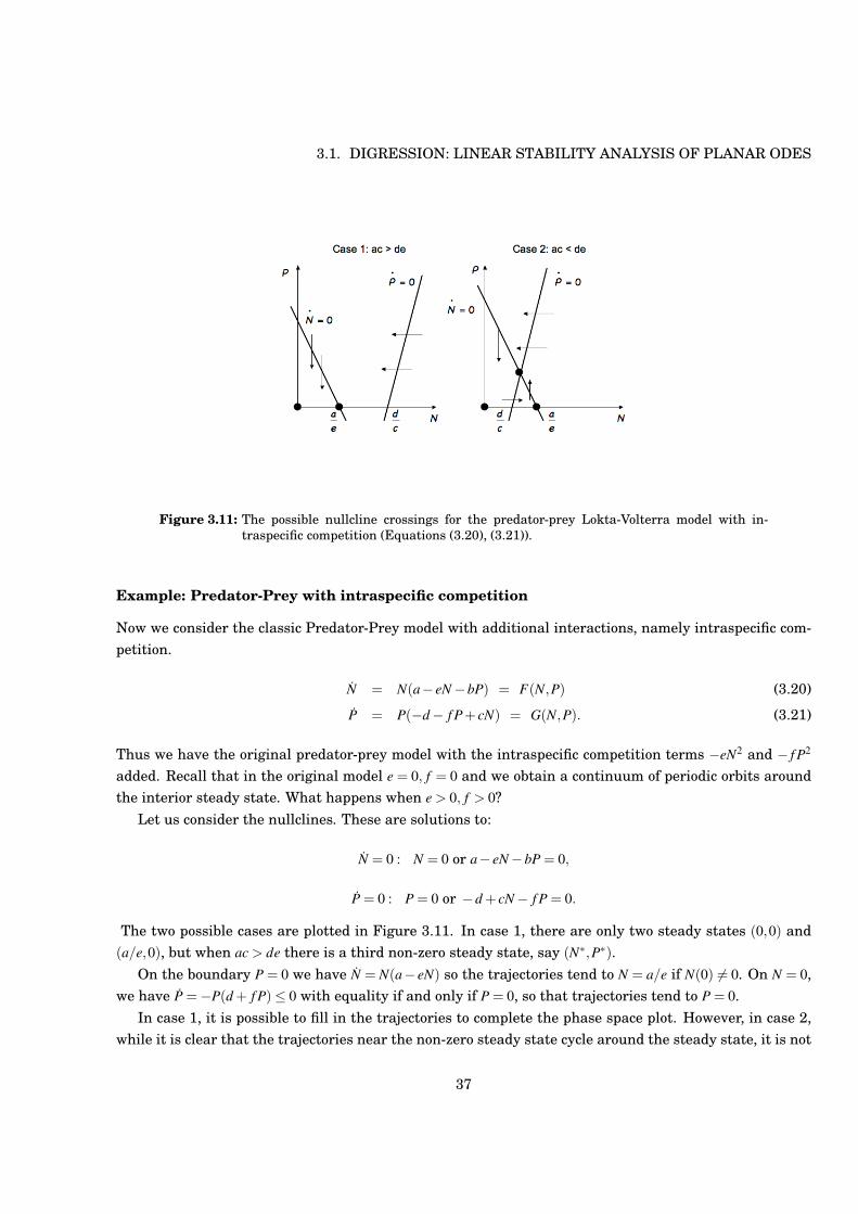
Figure 3.11: The possible nullcline crossings for the predator-prey Lokta-Volterra model with in-traspecific competition (Equations (3.20), (3.21)).

Example: Predator-Prey with intraspecific competition

Now we consider the classic Predator-Prey model with additional interactions, namely intraspecific com-petition.

N = N(a! eN!bP) = F(N,P) (3.20)

P = P(!d! f P+ cN) = G(N,P). (3.21)

Thus we have the original predator-prey model with the intraspecific competition terms !eN2 and ! f P2

added. Recall that in the original model e = 0, f = 0 and we obtain a continuum of periodic orbits aroundthe interior steady state. What happens when e > 0, f > 0?

Let us consider the nullclines. These are solutions to:

N = 0 : N = 0 or a! eN!bP = 0,

P = 0 : P = 0 or !d + cN! f P = 0.

The two possible cases are plotted in Figure 3.11. In case 1, there are only two steady states (0,0) and(a/e,0), but when ac > de there is a third non-zero steady state, say (N#,P#).

On the boundary P = 0 we have N = N(a! eN) so the trajectories tend to N = a/e if N(0) )= 0. On N = 0,we have P =!P(d + f P)+ 0 with equality if and only if P = 0, so that trajectories tend to P = 0.

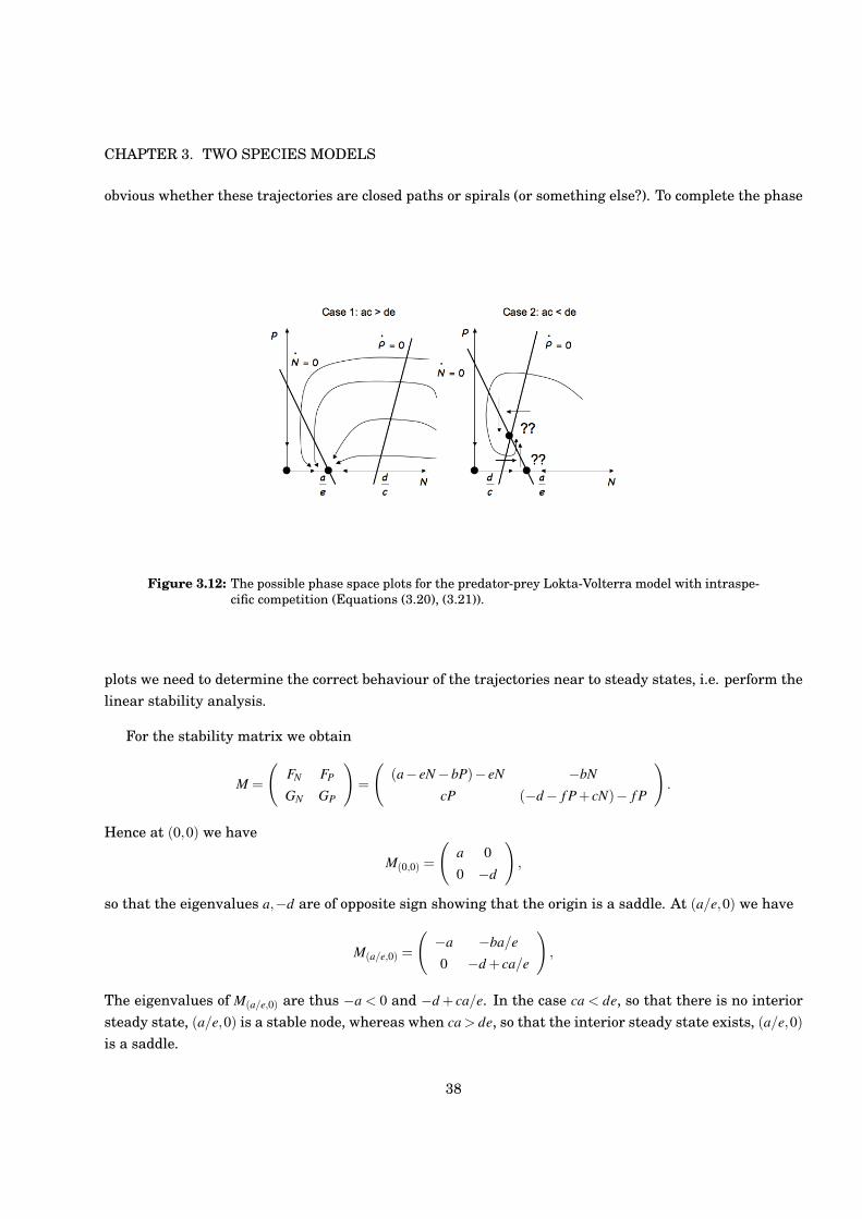
In case 1, it is possible to fill in the trajectories to complete the phase space plot. However, in case 2,while it is clear that the trajectories near the non-zero steady state cycle around the steady state, it is not

37

CHAPTER 3. TWO SPECIES MODELS

obvious whether these trajectories are closed paths or spirals (or something else?). To complete the phase

Figure 3.12: The possible phase space plots for the predator-prey Lokta-Volterra model with intraspe-cific competition (Equations (3.20), (3.21)).

plots we need to determine the correct behaviour of the trajectories near to steady states, i.e. perform thelinear stability analysis.

For the stability matrix we obtain

M =

#FN FP

GN GP

$=

#(a! eN!bP)! eN !bN

cP (!d! f P+ cN)! f P

$.

Hence at (0,0) we have

M(0,0) =

#a 00 !d

$,

so that the eigenvalues a,!d are of opposite sign showing that the origin is a saddle. At (a/e,0) we have

M(a/e,0) =

#!a !ba/e0 !d + ca/e

$,

The eigenvalues of M(a/e,0) are thus !a < 0 and !d + ca/e. In the case ca < de, so that there is no interiorsteady state, (a/e,0) is a stable node, whereas when ca > de, so that the interior steady state exists, (a/e,0)is a saddle.

38

3.1. DIGRESSION: LINEAR STABILITY ANALYSIS OF PLANAR ODES

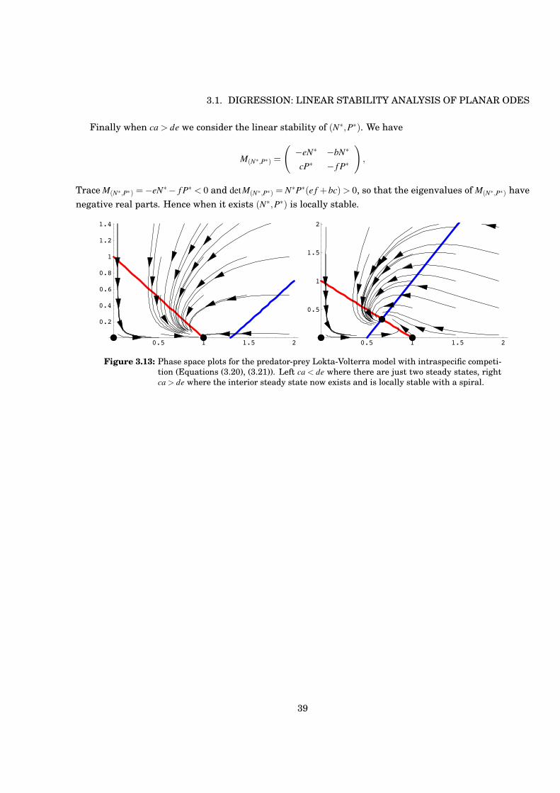
Finally when ca > de we consider the linear stability of (N#,P#). We have

M(N#,P#) =

#!eN# !bN#

cP# ! f P#

$,

Trace M(N#,P#) =!eN# ! f P# < 0 and detM(N#,P#) = N#P#(e f +bc) > 0, so that the eigenvalues of M(N#,P#) havenegative real parts. Hence when it exists (N#,P#) is locally stable.

0.5 1 1.5 2

0.2

0.4

0.6

0.8

1

1.2

1.4

0.5 1 1.5 2

0.5

1

1.5

2

Figure 3.13: Phase space plots for the predator-prey Lokta-Volterra model with intraspecific competi-tion (Equations (3.20), (3.21)). Left ca < de where there are just two steady states, rightca > de where the interior steady state now exists and is locally stable with a spiral.

39