Embed Size (px)
Citation preview

Two Sides of the Same Rupee?Comparing Demand for Microcredit and Microsaving in a Framed
Field Experiment in Rural Pakistan*
Uzma Afzal†, Giovanna d’Adda‡, Marcel Fafchamps§,Simon Quinn¶ and Farah Said||
March 18, 2017
Abstract
We use a field experiment to test whether saving and borrowing satisfy demand for lump-sum accumulationfrom regular deposits. Inspired by ROSCAs, we offer different credit and savings contracts to subjects. Wefind that individuals often accept both credit and saving contract across experimental waves. This behaviourcan be rationalised by assuming that individuals seek lump-sum payments and struggle to hold savings.Structural estimation of this model accounts for the behaviour of 75% of participants. Of these, two-thirdshave high demand for lump-sum accumulation but savings difficulties. These results imply that the distinctionbetween microlending and microsaving is largely illusory.
*This project was funded by the UK Department for International Development (DFID) as part of the programmefor Improving Institutions for Pro-Poor Growth (iiG). The project would not have been possible without the support ofDr Rashid Bajwa and Tahir Waqar at the National Rural Support Programme, and Dr Naved Hamid at the Centre forResearch in Economics and Business at the Lahore School of Eonomics. We received outstanding assistance in Sargodhafrom Rachel Cassidy, Sharafat Hussain, Tazeem Khan, Pavel Luengas-Sierra, Saad Qureshi and Ghulam Rasool. Wethank audiences at the Berlin Social Science Center, the University of Houston, the University of Maryland, NEUDC,Stanford University, the South Asia Microfinance Network Regional Conference and the University of Oxford. We alsothank Joshua Blumenstock, Justin Sandefur and Amma Serwaah-Panin for their useful comments. Our pre-analysis planis registered at the Registry for International Development Impact Evaluations (RIDIE-STUDY-ID-528385f5d3034).
†Lahore School of Economics‡Milan Politecnico§Stanford University¶corresponding author: Department of Economics, University of Oxford, Manor Road Building, OX1 3UQ, United
Kingdom, [email protected]||Lahore School of Economics
1
Two Sides of the Same Rupee?
1 Introduction
1.1 Saving and borrowing: An illusory distinction?
Saving and borrowing are often considered to be diametrically different behaviours: the former is a
means to defer consumption; the latter, a means to expedite it. However, this distinction collapses
under two important conditions that are common in developing countries. First, many in poor com-
munities struggle to hold savings over time, e.g., because of external sharing norms (Anderson and
Baland, 2002; Platteau, 2000) or internal lack of self-control (Ashraf et al., 2006; Gugerty, 2007;
Bernheim et al., 2015; Kaur et al., 2015; John, 2015). Second, the poor sometimes wish to incur
lumpy expenditures — for instance, to purchase an ‘indivisible durable consumption good’ (Besley
et al., 1993) or take advantage of a ‘high-return but lumpy and illiquid investment opportunity’
(Field et al., 2013).
If these two conditions hold — as they clearly do in many poor communities — then the same
individual may prefer to take up a saving product than to refuse it and, simultaneously, prefer to
accept a loan product than to refuse it. This demand has nothing to do with deferring or expediting
consumption. Rather, both products provide a valuable mechanism for accumulating a lump-sum
at some point in time. In doing so, each product meets the same demand for a regular schedule of
deposits and a lump-sum withdrawal. No longer do saving products and borrowing products stand
in stark juxtaposition to each other; they are, rather, two sides of the same coin. Several authors
have suggested this kind of motivation for the adoption of microlending contracts in developing
countries. Rutherford (2000) contrasts ‘saving up’ (setting aside funds to receive a lump sum) and
‘saving down’ (receiving a lump sum that is repaid in regular instalments); the latter behaviour
is termed by Morduch (2010) as ‘borrowing to save’ (see also Collins et al. (2009)). Bauer et al.
(2012) support this ‘alternative view of microcredit’, showing ‘a robust positive correlation between
having present-biased preferences and selecting microcredit as the vehicle for borrowing’.
In this paper, we run a framed field experiment in rural Pakistan to test directly whether microlend-
2 Afzal, d’Adda, Fafchamps, Quinn & Said
Two Sides of the Same Rupee?
ing serves a microsaving objective. We take a simple repayment structure — loosely modelled on
the idea of a ROSCA — and offer it as an individual microfinance product. We offer the product
three times to each subject, randomly varying the time of repayment and the repayment amount.
Namely, the product can take the form of a microcredit or of a microcredit contract, and the repay-
ment amount can either be equal, 10% smaller or 10% larger than their total contribution. Together,
these two sources of variation allow us to test between a ‘traditional’ benchmark model of micro-
finance in which participants prefer either to borrow or to save, and an alternative model in which
participants welcome both borrowing and savings contracts as opportunities for lump-sum pay-
ments.
We find that the same pool of respondents simultaneously have a demand both for microcredit and
for microsaving. Indeed, over the course of the three experiment waves, 277 of the 709 respon-
dents were offered both a credit contract and a savings contract; of these, 148 (53%) accepted both
forms of contract. Demand for our microfinance product is generally high, with approximately 65%
take-up. Sensitivity to interest rate and day of payment is statistically significant but not large in
magnitude.
We extend this analysis using a structural estimation to quantify the heterogeneity in clients’ deep
preferences. Specifically, we build competing structural models of demand for microfinance prod-
ucts, and we use a Non-Parametric Maximum Likelihood method to estimate the proportion of
respondents adhering to each model. Our structural framework rationalises the behaviour of 75% of
the participants. Of these rationalised participants, two-thirds behave as if they have high demand
for lump-sum accumulation coupled with savings difficulties. Together, the results imply that the
distinction between microlending and microsaving is largely illusory. Rather, many people wel-
come microcredit and microsavings products for the same reason: that each provides a mechanism
for regular deposits and a lump-sum payment.
3 Afzal, d’Adda, Fafchamps, Quinn & Said
Two Sides of the Same Rupee?
1.2 Daily deposits and the context of the experiment
We implement our experiment using a fixed schedule of daily deposits. The focus on daily deposits
is motivated by the nature of the study population, which is composed of urban and peri-urban
households who are not, as a rule, in permanent employment. As we document in the data section,
a large share of subject households have a daily income flow — typically from casual wage labour,
self-employment in a small business (e.g., retail shop, personal services, rickshaw driver), or the sale
of dairy farm products. Even among the 28% of households where the household head or spouse
has a permanent wage job, we observe other more frequent sources of cash inflow. By opting for a
frequency of deposits that matches the periodicity of income, we seek to maximise the commitment
value of the microfinance product we offer.1
Daily deposit schedules are a relatively common feature of microfinance products in many countries
— particularly those targeted at clients who are self-employed. In particular, they are the defining
feature of ‘daily collectors’ — informal mobile bankers who allow daily deposits and withdrawals
in many countries, particularly in West Africa.2 These mobile bankers provide a critically important
financial service for many poor households. For example, in a sample drawn from the outskirts of
Cotonou, Somville (2011) finds that approximately one third of positive income-earners make such
payments (see also Aryeetey and Steel (1995) and Aryeetey and Udry (1997)). Similarly, Ananth
et al. (2007) describe a small survey of vegetable vendors in Chennai. They find that approximately
50% of respondents had engaged in very short-term borrowing for at least a decade, including the
use of daily repayment products to support working capital; this can even involve taking a loan in
the morning to purchase vegetables from a wholesaler, then repaying the loan on the same afternoon
from daily sales.3
1 The ‘hand-to-mouth’ phenomenon need not be restricted to poor households with a daily income: for example, Kaplanet al. (2014) argue that a substantial proportion of households in developed economies are ‘wealthy hand-to-mouth’,in the sense of holding “little or no liquid wealth, whether in cash or in checking or savings accounts, despite owningsizable amounts of illiquid assets”.
2 Such collectors are also known as ‘tontinier’ in Benin, ‘susu’ in Ghana, ‘esusu’ in Nigeria and ‘deposit collectors’ inparts of India (Somville, 2011).
3 See also Rutherford (2000), who discusses the same practice in Andhra Pradesh.
4 Afzal, d’Adda, Fafchamps, Quinn & Said

Two Sides of the Same Rupee?
Formal organisations sometimes play a similar role. Most prominently, the NGO SafeSave provides
‘passbook savings’ accounts, in which clients may make deposits and withdrawals at their house
when a collector calls each day (Armendáriz de Aghion and Morduch, 2005; Dehejia et al., 2012;
Islam et al., 2013; Laureti, 2015).4 Similarly, Ashraf et al. (2003) document Jigsaw Development’s
‘Gold Savings’ account, in which daily instalments were used to repay purchases of gold; the au-
thors also describe the ‘Daily Deposit Plan’, the most popular account of Vivekananda Sevakendra
O Sishu Uddyon, an NGO operating in West Bengal.5
Daily deposit schedules are also facilitated by many ROSCAs. For example, Rutherford (1997)
studied 95 loteri samities in the slums of Dhaka, finding that approximately two-thirds collected
payments daily.6 Work in other contexts finds the proportion to be much smaller, but certainly
not negligible. For example, Adams and Canavesi de Sahonero (1989) find that 15% of sampled
pasankus in Bolivia used daily repayments (particularly those used by self-employed women), Al-
iber (2001) reports that 10% of stockvels in Northern Province used daily payments (again, particu-
larly those used by the self-employed), Tanaka and Nguyen (2010) report a figure of 8.8% of huis
in South Vietnam, and Kedir and Ibrahim (2011) report 2.8% for Ethiopian equbs.7
Approximately 80% of respondents are familiar with the concept of a ROSCA (known in Pakistan
as a ‘savings committee’). Of these, about two-thirds have ever participated in one. This is im-
portant for ensuring that our repayment structure resonates with a well-understood local financial
product. Of the respondents who had ever participated in a committee, 90% report that the commit-
tee required payments on a monthly basis; only 4% of respondents reported a committee with daily4 See also http://www.safesave.org/products.5 Of course, even banks without formal daily payment products may still facilitate daily deposits. For example, Steel
et al. (1997) describe a savings and loan company in Ghana that would encourage self-employed women to depositproceeds each evening and then withdraw as necessary the following morning.
6 Rutherford’s impression from those loteri samities matches closely the key hypothesis that we test in this paper. Ruther-ford writes (page 367): “The most common answer to the question ‘why did you join this samity?’ was ‘to save, becauseit is almost impossible to save at home’. Follow-up questions showed that the intermediation of those savings into ausefully large lump sum is also important. But it is not true that most members want to take that lump sum as a loan.. . . There is little doubt in my mind that the respondents understand these samities as being, primarily, about savingsrather than about loans.”
7 See also Handa and Kirton (1999), who report that 6% of Jamaican ROSCAs — known as ‘partners’ — meet morefrequently than once per week.
5 Afzal, d’Adda, Fafchamps, Quinn & Said

Two Sides of the Same Rupee?
deposits. Anecdotal evidence suggests that daily instalment structures are nonetheless quite com-
mon in Pakistan Punjab through informal providers, including in the locations of the study. Often,
this involves ‘commission agents’ (arthis), who can offer short-term loans to retailers to enable the
purchase of stock. For small shopkeepers and street vendors, this can involve a daily loan to be paid
back at the close of business (sometimes as a percentage of daily sales).8
In sum, commitment products with daily repayments are common in many developing countries. In
Pakistan, such products are hardly ever offered as ROSCAs, and appear to have fallen beneath the
radar of microfinance institutions. Nonetheless, the demand for daily borrowing through informal
providers indicates that there are many Pakistanis with extremely short-term cash flow management
needs. In this paper, we offer an original solution to these problems that offers an ideal way to test
the value of having regular deposits towards an achievable goal.
We deliberately run the experiment using clients of a microcredit programme, that is, using a subject
population with a demonstrated demand for credit. If this population displays as much interest in
a commitment saving contract as in borrowing, this will suggest that their demand for credit may
partly reflect a demand for commitment saving. Finally, to make the demonstration even more
salient, we choose a short credit and saving duration — i.e., one week — in order to reduce the
attractiveness of credit as an intertemporal smoothing device: if borrowing only serves to accelerate
consumption or investment, we expect few takers for credit contracts with a one week maturation
period and a high interest rate.
1.3 Recent research on microfinance
Our key empirical result — that, for a high proportion of microfinance clients, credit and savings can
act as substitutes — is useful for understanding recent research on microfinance. Growing empiri-
cal evidence suggests that savings products can be valuable for generating income and for reducing
poverty (Burgess and Pande, 2005; Dupas and Robinson, 2013; Brune et al., 2014). Standard micro-8 See Haq et al. (2013), who describe the role of arthis in longer-term lending for agricultural commodity markets.
6 Afzal, d’Adda, Fafchamps, Quinn & Said
Two Sides of the Same Rupee?
credit products — with high interest rates and immediate repayments — increasingly seem unable
to generate enterprise growth (Karlan and Zinman, 2011; Banerjee et al., 2015). In contrast, recent
evidence shows that an initial repayment grace period increases long-run profits of microfinance
clients by facilitating lumpy investments (Field et al., 2013). Indeed, a growing literature suggests
that part of the attraction of microcredit is as a mechanism to save — whether to meet short-term
liquidity needs (Kast and Pomeranz, 2014), to resist social or familial pressure (Baland et al., 2011),
or as a commitment device against self-control problems (Collins et al., 2009; Bauer et al., 2012).9
We make several contributions to this literature. First, we introduce a new experimental design
which, to our knowledge, is the first to allow a direct test between demand for microsaving and
demand for microcredit. Second, our design generates new empirical results showing that the same
respondent population has high demand for both microcredit and microsaving (see also Gross and
Souleles (2002), Collins et al. (2009), Morduch (2010), Kast and Pomeranz (2014) and Laureti
(2015)). Indeed, the same individuals often take up either contracts within the span of a couple
weeks. Third, we make a methodological contribution through our structural framework. Specifi-
cally, we parameterise a Besley et al. (1993) model to test the demand for (latent) lumpy purchases.
We show how to nest this model in a discrete finite mixture framework to allow for maximal het-
erogeneity in individual preferences.
The paper proceeds as follows. In section 2, we provide a conceptual framework. This motivates
the experimental design, which we describe in section 3. We report regression results in section
4. Section 5 parameterises the conceptual framework for structural analysis and presents the Non-
Parametric Maximum Likelihood estimator. We discuss identification and show structural results.
Section 6 concludes.9 Mullainathan and Shafir (2009) discuss the role of lottery tickets as commitment savings devices – analogously to
random ROSCAs. See also Basu (2008), who provides a theoretical model in which sophisticated time-inconsistentagents find it welfare-enhancing both to borrow and to save simultaneously.
7 Afzal, d’Adda, Fafchamps, Quinn & Said
Two Sides of the Same Rupee?
2 Conceptual framework
This section develops a simplified theoretical framework; this framework motivates the experiment,
and serves as a foundation for the structural analysis. We use a dynamic model in which we intro-
duce a preference for infrequent lump-sum payments. We begin with a benchmark model in which
individuals either demand a savings product or a loan product, but not both. We then show how
this prediction changes when we impose that people cannot hold cash balances, e.g., because of
self-commitment problems due to time inconsistency.
We start by noting that the simple credit and savings products used by the poor can be nested into
a generalised ROSCA contract. The contract spans periods t ∈ {1, . . . , T} and has a single payout
period, p ∈ {1, . . . , T}. In periods t 6= p, the participant pays an instalment of s; in period t = p,
the participant receives a lump sum equal to (T − 1) · s · (1+ r). Parameter r represents the interest
rate of the contract, which can be positive or negative. In a standard ROSCA contract, r = 0 and
p is determined through random selection. In a typical (micro)credit contract with no grace period,
r < 0, the lump sum is paid in period p = 1, and instalments s are made in periods 2 to T . A typical
commitment savings contract (e.g., retirement contribution) is when r > 0, the lump-sum is paid in
the last period (p = T ), and instalments s are made from period 1 to period (T − 1).
We first consider a benchmark utility maximising framework. We begin by assuming (i) that there
is no particular demand for lumpy consumption, and (ii) that individuals can hold positive cash
balances between time periods. To illustrate the predictions that this model makes about the de-
mand for generalised ROSCA contracts, consider a short-term T -period model with cash balances
mt ≥ 0. Each individual is offered a contract with an instalment level s, a payment date p, and
an interest rate r. The contract is therefore completely characterised by the triple (s, p, r). The
individual chooses whether or not to take up the contract, which is then binding.
8 Afzal, d’Adda, Fafchamps, Quinn & Said

Two Sides of the Same Rupee?
Let y be the individual’s cash flow from period 1 to T .10 The value from refusing a contract (s, p, r)
is:
Vr = max{mt≥0}
T∑t=1
βt · ut(yt +mt−1 −mt),
where ut(.) is an instantaneous concave utility function (which may be time-varying), β ≤ 1 is the
discount factor, and m0 ≥ 0 represents initial cash balances. Given the short time interval in the
experiment, β is approximately 1. Hence if ut(.) = u(.), the optimal plan is approximately to spend
the same on consumption in every period. In this case, demand for credit or saving only serves to
smooth out fluctuations in income.
The more interesting case is when the individual wishes to finance a lumpy expenditure (for exam-
ple, to bulk-purchase food products, buy a consumer durable, pay rent, or invest for a business). We
treat the purchase of a lumpy good as a binary decision taken in each period (Lt ∈ {0, 1}), and we
use α to denote the cost of the lumpy good. We consider a lumpy expenditure roughly commensu-
rate to the lump-sum payment: α ≈ (T − 1) · s · (1 + r). Following Besley et al. (1993), we model
the utility from lumpy consumption L = 1 and continuous consumption c as u(c, 1) > u(c, 0).
Without the generalised ROSCA contract, the decision problem becomes:
Vr = max{mt≥0,Lt={0,1}}
T∑t=1
βt · u(yt +mt−1 −mt − α · Lt, Lt). (1)
With the ROSCA contract, the value from taking the contract (s, p, r) is:
Vc = max{mt≥0,Lt={0,1}}
∑t6=p
[βt · u (yt − s+mt−1 −mt, Lt)
]+ βp · u [yp + (T − 1) · s · (1 + r) +mp−1 −mp − α,Lp]
}. (2)
If α is not too large relative to the individual’s cash flow yt, it is individually optimal to accumulate
cash balances to incur the lumpy expenditure, typically in the last period T . Otherwise, the indi-10 We could make yt variable over time, but doing so adds nothing to the discussion that is not already well known. Hence
we ignore it here.
9 Afzal, d’Adda, Fafchamps, Quinn & Said

Two Sides of the Same Rupee?
vidual gets discouraged and the lumpy expenditure is either not made, or delayed to a time after T .
Taking up the contract increases utility if it enables consumers to finance the lumpy expenditure α.
For individuals who would have saved on their own to finance α, a savings contract with r > 0 may
facilitate savings by reducing the time needed to accumulate α.11 Hence we expect some take-up of
savings contracts with a positive return.
A credit contract allows incurring the lumpy expenditure right away and saving later. Hence, for a
credit contract with a positive interest charge to be attractive, the timing of Lt = 1 must be crucial
for the decision maker. Otherwise the individual is better off avoiding the interest charge by saving
in cash and delaying expenditure L by a few days. This is the reason that — as discussed earlier —
we do not expect such an individual to be willing to take up both a credit and a savings contract at
the same time: either the timing of Lt = 1 is crucial or it is not.
In addition to the above observations, the presence of cash balances also generates standard arbitrage
results. The predictions from this benchmark model can be summarised as follows:
(i) Individuals always refuse savings contracts (p = T ) with r < 0 (i.e., a negative return). This is
because accepting the contract reduces consumption by T ·s·r. Irrespective of their smoothing
needs, individuals can achieve a higher consumption by saving through cash balances.
(ii) Individuals always accept credit contracts (p = 1) with r > 0 (i.e., a negative interest charge).
This is because, irrespective of their smoothing needs, they can hold onto T · s to repay the
loan in instalments, and consume T · s · r > 0.
(iii) Individuals refuse credit contracts (p = 1) with a large enough cost of credit r < 0. This
follows from the concavity of u(.): there is a cost of borrowing so high that individuals prefer
not to incur expenditure L.
(iv) Individuals accept savings contracts (p = T ) with a high enough return r ≥ 0. This too
follows from the concavity of u(.).
11 Offering a positive return on savings may even induce saving by individuals who otherwise find it optimal not to save:McKinnon (1973).
10 Afzal, d’Adda, Fafchamps, Quinn & Said

Two Sides of the Same Rupee?
(v) The same individual will not demand both a savings contract (with a positive return r > 0)
and a credit contract (with a non-negative interest cost r ≤ 0).
Things are different when people use credit or ROSCAs as a commitment device to save. Within
our framework this is most easily captured by assuming that people cannot hold cash balances (that
is, mt = 0). It is of course possible to construct a more complete model in which mt = 0 is not an
assumption but an equilibrium outcome.12 This would make the model more complicated without
adding any new insight. The key idea is that when individuals cannot accumulate cash balances on
their own, for whatever the reason, then the only way for them to make the lumpy purchase is to
take the (s, p, r) contract. This creates a wedge between Vr and Vc that increases the likelihood of
take-up: the contract enables the individual to incur the lumpy expenditure, something they could
not do on their own. If the utility gain from buying the lumpy good is high, individuals are predicted
to accept even contracts that would always be refused by someone who can hold cash balances —
such as savings contracts with a negative return or credit contracts with a high interest charge.
Take-up predictions under the alternative model can thus be summarised as follows:
(i) Time of payment (p) is irrelevant: if an individual accepts a credit contract with s and r , (s)he
also accepts a savings contract with the same s and r.
(ii) Individuals may accept savings contracts (p = T ) with r < 0 (i.e., a negative return); the
arbitrage argument no longer applies. Individuals refuse savings contracts (p = T ) with a low
enough return r. This again follows from the concavity of u(.): the only difference is that now
the threshold interest rate r may be negative.
(iii) Individuals do not always accept credit contracts (p = 1) with r > 0 (i.e., a negative interest
charge). This is because they cannot hold onto (T − 1) · s to repay the loan in instalments.
Individuals refuse credit contracts (p = 1) with a large enough cost of credit r < 0. This
prediction still holds since it follows from the concavity of u(.).
12 Example of micro-foundations include quasi-hyperbolic preferences as in Ambec and Treich (2007); pressure from thespouse as in Anderson and Baland (2002) and Somville (2014); pressure from non-household members as in Goldberg(2011).
11 Afzal, d’Adda, Fafchamps, Quinn & Said

Two Sides of the Same Rupee?
3 Experiment
3.1 Experimental design
We implement a stylised version of this theoretical model as a field experiment. At the beginning of
each week, on day 0, each participant is offered one of 12 different generalised ROSCA contracts,
where the type of contract offered is determined by the random draw of cards.13 The 12 contracts
differ by (i) timing of lump-sum payment p and (ii) interest rate r but all share the same instalment
size s. All disbursements start the next day, on day 1.14 Lump-sum payments are either made on
Day 1, Day 3, Day 4 or Day 6. On any day that the lump sum is not paid, the participant is re-
quired to pay s = 200 Pakistani rupees (PKR). The base lump-sum payment is either 900 PKR (that
is, r = −10%), 1000 PKR (r = 0) or 1100 PKR (r = +10%). At the time of the experiment,
200 Pakistani rupees was worth approximately US$1.90; 1000 rupees was therefore approximately
US$9.50.15
The following Table illustrates the payment schedule for a contract with lump-sum payment on day
p = 3 and interest rate r = +10%:
DAY 0 DAY 1 DAY 2 DAY 3 DAY 4 DAY 5 DAY 6
Participant pays take up 200 200 200 200 200
Bank pays decision 1100
Since there are three possible interest rate values and four possible days for the lump-sum payment,
12 different contracts are used in the experiment to represent each combination of p and r. At the
beginning of the week on day 0 each participant receives a take-it-or-leave-it offer of one of these
contracts, and must decide on the spot whether to accept it or not. We test (i) whether there is
demand for this generalised ROSCA contract, and (ii) if so, how demand varies with the terms of
the contract.13 From the point of view of the participant, the payment structure of this contract is equivalent to a one-off random
ROSCA (Kovsted and Lyk-Jensen, 1999), but it is implemented on an individual basis.14 This short delay serves to mitigate against distortions in take-up arising from differences in the credibility of lump-sum
payment between contracts (Coller and Williams, 1999; Dohmen et al., 2013).15 As we explain in more detail shortly, the median household income in the study area is approximately 600 PKR per
day.
12 Afzal, d’Adda, Fafchamps, Quinn & Said

Two Sides of the Same Rupee?
3.2 Experimental implementation
We ran this experiment over September and October 2013 in Sargodha, Pakistan Punjab. Our sam-
ple comprises female clients of the National Rural Support Programme (NRSP). At the time of
running the experiment, all participants were active NRSP borrowers.16 The experiment was con-
ducted through four NRSP offices in the Sargodha district. Female members of these four branches
were invited to attend meetings set in locations near their residences. Members who stayed for the
first meeting were individually offered a generalised ROSCA contract randomly selected from the
12 possible contracts described above. Participants were free to take up or reject the contract offered
in that week. Even if they refused the contract offered to them in that week, participants were still
required to participate in the meeting held the following week, when they were again offered a con-
tract randomly selected from the list of 12. In total, there were three weekly meetings. Those who
attended all three meetings (whether choosing to accept or reject the product for that week) received
a show-up fee of 1100 PKR at the end of the trial. Once a subject had accepted a contract, they were
expected to abide by the terms of that contract. Failure to do so resulted in exclusion from the rest
of the experiment – and from receiving the show-up fee. NRSP ensured that subjects did not benefit
or suffer financially from dropping out (apart from losing the show-up fee). In practice, this meant
reimbursing subjects for partial contributions, and recouping amount received but not fully repaid.
We implemented the experiment in NRSP branches located within a 30 km radius around the city of
Sargodha. 32 microfinance groups participated to the experiment. In each group, the product was
explained by an experienced NRSP staff member.17 In three of these groups, there were breaches
of experiment protocol.18 We drop these three groups from the analysis, a decision taken before we16 Depending on the client, NRSP loans were classified either as ‘livestock’, ‘enterprise’ or ‘agricultural’ loans — though
the distinction is largely in name. The loan size for all three types of loan is 20,000 PKR for first-time borrowers, withincrements of 5,000 per repeat loan. The duration of enterprise and livestock loans is usually 12 months; the durationof an agriculture loan varies by crop but cannot exceed eight months.
17 These staff members received precise instructions on how to present the experimental design. In the Online Appendix,we analyse take-up patterns by staff member and by location. If the results were driven by different enumerators havingexplained the product differently — for example, by some enumerators having confused participants about the show-up fee — then we would expect substantial clustering of take-up behaviour by staff member or by location. As theOnline Appendix shows, there is substantial heterogeneity in take-up patterns, both within location and for participantsinstructed by the same staff member.
18 These breaches were through no fault of the research team or the implementing partner, NRSP. This is discussed inmore detail in the appendix.
13 Afzal, d’Adda, Fafchamps, Quinn & Said

Two Sides of the Same Rupee?
began any of the analysis. This means that we have a total of 29 microfinance groups/clusters in the
following analysis.19
In these 29 groups, we collected baseline data from 955 respondents. Of these, 889 decided to par-
ticipate in the experiment, and made a decision on the first offered contract. Of the 66 women who
left before the experiment began, 41 stated that they did not have time to attend each day; six said
that they did not understand the product. Our sample ranges in age from 18 to 70, with a median
age of 38. 90% of the participants are married, and only 30% have completed one or more years of
schooling. By design, the respondents live close to the meeting place (the median is four minutes’
walking time). This is important for ensuring that take-up decisions are based primarily on the fi-
nancial costs and benefits of the products offered, rather than on the time and effort of commuting
to the place of payment. Detailed summary statistics are presented in the Online Appendix.
Table 1 describes the main variables used in the analysis. We place particular focus on variables
proxying for frequency with which participating households receive an income, such as occupa-
tion.20 As the table shows, the overwhelming majority of the subjects (88%) have at least one
source of income from employment other than permanent wage employment – that is, from casual
labor (i.e., paid a daily wage), self-employment in a business, or sales of dairy farm products.21 (As
a convenient shorthand, we refer to such income as ‘non-salaried income’. We refer to income from19 Our results are robust to the use of Moulton-corrected standard errors. This is not surprising given that most of our
results of interest are highly significant.20 Unfortunately, we were unable to collect baseline data on frequency of monetary inflows into the household. Prompted
by an anonymous referee, we returned to Sargodha in mid-2016 to resurvey a sample of 100 of the original participantsto the experiment and asked them about the frequency with which they receive an income. When we asked respondentsdirectly about daily income, 58% report that either they or another household member earn income each day (95%confidence interval: 48% to 67%). A substantial number of respondents also have an occupation yielding an incomeor business cash flow that varies daily but does not necessarily provide them with a guaranteed daily income. Theseinclude farmers, non-farm self-employed and casual labourers. When we combine these occupations, the proportion ofhouseholds with income that varies daily is 86% of the sample (95% confidence interval: 78% to 92%). (Further, of our100 resurveyed respondents, 65 agree with the statement ‘My household needs an income each day to make it to thenext day’.) The resurvey confirms that there is a strong positive correlation between having daily income and havingemployment either as a farmer, non-farm self-employed, or casual labourer: of the 78 respondents having a familymember in one of these three occupational categories, 50 report having daily income (i.e. 64%); of the 22 respondentsnot having a family member in one of those occupations, only eight report receiving a daily income (i.e. 36%).
21 Since subjects were not asked whether they derive income from the sale of dairy products, this is inferred from livestockownership (cow or bullock). Given the widespread use of livestock as source of dairy income, this is a relativelyinnocuous assumption – and is the best we can do with the data at hand.
14 Afzal, d’Adda, Fafchamps, Quinn & Said

Two Sides of the Same Rupee?
permanent wage employment as ‘salaried income’.) In the population at large, 42% of households
have a member in permanent wage employment (PSLM, 2010-11). This proportion is smaller (28%)
among the experimental subjects, who are selected among clients of a microfinance organization
that, in part, targets self-employed individuals. Most households with permanent wage employment
also have some source of daily income; 19% of all participating households have both.22
< Table 1 here. >
Table 1 also reports p-values for randomisation balance across each variable; this is calculated by re-
gressing each baseline variable on the experimentally assigned interest rate and payment day, using
a saturated specification. We find two of the 11 variables to be unbalanced at the 90% confidence
level. We provide a more extensive set of balance tests in the Online Appendix, from which we
conclude that the randomisation is correctly balanced.23
Attrition from the experiment has two sources: 80 subjects defaulted on a contract, and another 98
simply stopped attending.24 The large majority of defaults and exits occur within or at the end of
the first round. Most exiting subjects answered an exit questionnaire, stating the reason for leaving.
Defaulting subjects list shocks (e.g., illness, travel), inability to pay, and unwillingness to come to
daily meetings as their main reasons for leaving. Non-defaulting leavers list unwillingness to come
to daily meetings as main reason. There is a small but significant effect of contract terms on the
probability of default: women offered p = 1 were about 2.7 percentage points less likely to default
than women drawing p = 3, p = 4 or p = 6. In Section 4.3 and the Online Appendix, we show that
attrition does not affect the other results.
It is worth noting that subjects who attrite forfeit the show-up fee of 1100 PKR. Participants should
therefore refuse a contract that they do not expect to fulfil: by defaulting they lose a show-up fee of22 Some 3% of participating households do not report an occupation that can be a source of earned income – they must
have a source of income that enables them to pay daily instalments, but we do not know what it is.23 The analysis in appendix shows that two of the 22 variables are mismatched at the 90% confidence level: the number
of years as an NRSP client; and a dummy variable for whether the respondent makes the final decision on house-hold spending (either individually or jointly with her husband or others). As a robustness check, we re-run the mainestimations with these two variables as additional controls, but results are unaffected.
24 Four subjects are recorded as having defaulted in one of the rounds but have participated in the remaining rounds.
15 Afzal, d’Adda, Fafchamps, Quinn & Said

Two Sides of the Same Rupee?
1100 PKR compared with a maximum material gain of 100 PKR on a contract. If they had refused
the contract instead of defaulting, they would have avoided a loss ≥ 1000 PKR. Individuals who
default can thus be seen as misjudging their future ability to fulfil a commitment contract. This
behaviour is akin to the type of ‘naive sophisticates’ studied by John (2015), namely, individuals
with a mistaken anticipation about their future ability to comply with an incentivised commitment
contract.25
Of the 709 respondents participating in all three experiment rounds, 92% said afterwards that they
understood the product, 96% said that they were glad to have participated, and 87% said that they
would recommend the product to a friend.26 82% said that the product helped them to commit to
saving, and 64% said that the product helped them to resist pressure to share money with friends
and family. At baseline, we asked respondents to imagine that NRSP were to loan them 1000 PKR
and asked them an open-ended question about how they would use the money. Approximately half
gave a non-committal response (e.g., domestic needs or something similar). Of those who gave a
specific answer, a majority listed a lumpy expenditure, that is, an expenditure not easily made in
small increments. Of the lumpy expenditures described, the most common are sewing equipment,
chickens or goats, and school materials (particularly school uniforms). Based on responses given to
this question, we create a dummy variable equal to one if the respondent would invest or save the
funds, as opposed to spending them on divisible consumption.
4 Reduced-form results
We begin by reporting reduced-form results. The purpose of this approach is to reassure the reader
that our main findings are immediately apparent in the data, and are not an artefact of the structural25 A standard example of naive sophisticates concerns individuals who take a membership to a gym as a commitment to
exercise, but fail to use it: DellaVigna and Malmendier (2006).26 Prompted by a referee’s comment, we conducted a small follow-up survey in mid-2016 with 100 of the original re-
spondents. To test respondent understanding, we described a hypothetical rotating savings committee, then askedrespondents to answer specific right-or-wrong questions. Of the 100 respondents who answered the question aboutthe pot size, 80 answered correctly without assistance. We asked about the duration of the hypothetical product; 86correctly answered without assistance. Finally, we asked about the lottery concept as applied to the committee; 72correctly answered without assistance. On the whole, 61 answered all three questions correctly without any assistance,and 86 were able to answer all three questions correctly with minimal prompting.
16 Afzal, d’Adda, Fafchamps, Quinn & Said

Two Sides of the Same Rupee?
estimation.
4.1 Stylised facts about take-up
Table 2 shows average take-up across the 12 different types of contract offered. The Table brings to
light the first two important stylised facts. First, overall take-up is very high (approximately 65%
on average). Second, take-up varies with contractual terms – respondents are more likely to take a
contract when p = 1 than when p = 6. But the variation is not large, and certainly not nearly as
stark as the variation predicted by the benchmark model with mt ≥ 0.
< Table 2 here. >
Table 3 shows an important third stylised fact: there appears to be important heterogeneity across
individuals. Of the 709 individuals completing all three experiment waves, 319 (45%) accepted all
three contracts offered, and 121 (17%) accepted none of the contracts offered. This was despite the
vast majority of respondents having been offered three different contracts.
< Table 3 here. >
The implication of this is clear, and is a fourth stylised fact: many individuals accepted both a
credit contract and a savings contract, even over the very short duration of the experiment. As Table
4 shows, of the 709 respondents completing all waves, 277 were offered both a savings contract
(p = 6) and a credit contract (p = 1). Of these, 148 accepted at least one savings contract and at
least one credit contract.
< Table 4 here. >
This fact already challenges the benchmark model. Recall Prediction 5 of that model: the same
individual will not demand both a savings contract with r > 0 and a credit contract with r ≤ 0.
Table 5 considers those respondents who were both offered a savings contract with r > 0 and a
credit contract with r ≤ 0. There were 87 such respondents; of these, 44 (51%) accepted both a
savings contract with r > 0 and a credit contract with r ≤ 0.
17 Afzal, d’Adda, Fafchamps, Quinn & Said

Two Sides of the Same Rupee?
< Table 5 here. >
Similarly, the benchmark model predicts that individuals always refuse savings contracts (p = T )
with r < 0, and always accept credit contracts (p = 1) with r > 0. In the experiment, 184 re-
spondents were offered at least one savings contract with r < 0; of these 86 accepted at least one
(47%).27 230 respondents were offered at least one credit contract with r > 0; of these, 29 rejected
at least one (13%).
Together, these stylised facts suggest that many of the microfinance clients view saving and bor-
rowing contracts as substitutes. Indeed, as Table 6 summarises, the experiment provided 439 of our
709 respondents an opportunity to violate at least one of the specific predictions of the benchmark
model: 155 of them did so.
< Table 6 here. >
4.2 Product take-up, income frequency, and commitment needs
We use regression analysis to summarise in a compact way how the take-up response of experi-
mental subjects varies with contract terms. We begin by documenting the sensitivity of take-up to
the interest rate and the timing of the lump-sum payment. Formally, let yiw be a dummy variable
for whether individual i agreed to the offered contract in experiment wave w ∈ {1, 2, 3}. Define
rnegiw as a dummy for riw = −0.1 and rposiw as a dummy for riw = 0.1 (with zero interest as the
omitted category). Further let p1iw and p6iw be dummy variables for time of payment (leaving days
3 and 4 as the joint omitted category). We test sensitivity to contract terms by estimating a linear
probability model of the form:
yiw = β0 + β1 · rnegiw + β2 · rposiw + β3 · p1iw + β4 · p6iw + µiw, (3)
27 Of these 86, 84 accepted all such contracts that they were offered: 163 respondents were offered one such contract, ofwhom 72 accepted it; 19 were offered two such contracts, of whom 11 accepted both; and two were offered three suchcontracts, of whom one accepted all three.
18 Afzal, d’Adda, Fafchamps, Quinn & Said

Two Sides of the Same Rupee?
Standard errors are clustered by microfinance group.28
We estimate this regression for the entire sample. We then examine variation in take-up associated
with differences in the frequency of income flows and in the commitment needs of the household.
We start by investigating whether take-up varies with various proxies for the commitment needs
of the household. The results are presented in Table 7. We find that take-up is higher among
households that face many financial requests from family members and among households that
find it easier to save. The latter result seems at first glance to contradict our model, but given the
context of the experiment, participants who state it is difficult for them to save may include many
who are too poor to save. We also find that respondents who stated that they would save or invest
a hypothetical loan have a significantly and substantially larger intercept term than those who did
not, and are significantly less responsive to contractual terms (in particular, less responsive to being
offered a positive interest rate and to having payment on day 1). Similarly, respondents who report
pressure from family and friends are significantly less responsive to contractual terms — again, less
responsive to being offered a positive interest rate and to having payment on day 1. We interpret
these results as consistent with the idea that these respondents value the product — whether offered
in the credit or the savings domain — as a means to accumulate a lump-sum.29
< Table 7 here. >
Next, we consider variation in income frequency.30 As discussed in the conceptual section, we ex-
pect demand for a financial product with daily deposits to be highest among households that have
daily income flows. It is also possible that households in permanent wage employment have less
demand for a lump sum because they can finance lumpy expenditures from salaries paid at regular28 In the Online Appendix, we present a battery of alternative regression models — including a saturated model —
specified in the Pre-Analysis Plan. All our conclusions are robust to using these alternative specifications instead of thesimpler specification presented here.
29 We cannot entirely rule out that some respondents took up the product purely as commitment device to work hardereach day. This could apply, for instance, to the New York taxi drivers of Camerer et al. (1997), who ‘set a loose dailyincome target and quit working once they reach that target’, or to alcoholic rickshaw drivers as in Schilbach (2015).Given that all our respondents are women and not all of them work, we find it unlikely in this context that the productis serving to commit respondents to worker harder.
30 The Online Appendix discusses subgroup variation in further detail, and shows regression results for all subgroups,including all subgroups that were listed in the pre-analysis plan.
19 Afzal, d’Adda, Fafchamps, Quinn & Said

Two Sides of the Same Rupee?
weekly or monthly intervals. If this is true, such households should be primarily interested in con-
tracts that generate a positive return (i.e., r = 0.1). To investigate these issues, we split households
into four categories according to whether or not they have salaried income, and whether or not they
have non-salaried income. As discussed earlier, in the study area non-salaried income implies high-
frequency — e.g., daily — inflows of income. We estimate equation 3 separately for each group.
Results are presented in Table 8.
< Table 8 here. >
We see that households with non-salaried income have a higher intercept and thus higher take-up in
general, in agreement with predictions. Households without non-salaried income seem to be more
sensitive to r > 0 and to p = 1, suggesting that their take-up is more motivated by standard motives
(e.g., profitability and impatience) than by demand for commitment saving. Take-up is highest
among households with both salaried and non-salaried forms of income. One possible explanation
is that these households are richer and more financially secure, and thus have higher demand for
credit and savings instruments, which they can finance from high-frequency non-salaried income.
4.3 Extensions and robustness
We now investigate the robustness of our results. First, we test for the effect of lagged take-up
(which we instrument using the lagged contractual offer). We find that lagged take-up has a large
and highly significant effect: accepting the contract offer in period t causes a respondent to be about
30 percentage points more likely to accept in period t + 1. This speaks to a possible ‘familiarity’
or ‘reassurance’ effect, whereby trying the product improves respondents’ future perceptions of the
offer. The Online Appendix also reports a test of parameter stability across experiment waves. We
find a large and significant decline in willingness to adopt in the third experimental round. In addi-
tion, we observe a significant increase in the sensitivity to a positive interest rate, and to a negative
interest rate when p = 1. This could be due to a variety of causes, including respondent fatigue.
The Online Appendix reports a reduced form regression of take-up on past contractual terms. We
20 Afzal, d’Adda, Fafchamps, Quinn & Said

Two Sides of the Same Rupee?
find that a negative interest in the previous round decreases take-up in the current period. This result
disappears in the saturated model. These findings do not affect the main results of interest.
We run several other robustness checks. The Online Appendix reports a battery of estimations on
attrition. We find that respondents are more likely to attrite after having been offered a contract
with payment on day 6 (regardless of whether the interest rate was positive, negative or zero). We
find no other significant effect of contractual terms on attrition. A separate estimation (omitted
for brevity) tests attrition on a large number of baseline characteristics; none of the characteristics
significantly predicts attrition. Further, the Online Appendix compares estimation results with only
those respondents who remained in the experiment for all three rounds. We find that this has no
significant effect on the parameter estimates (p-value= 0.334).31 We also test for parameter stability
when attrition is taken to be an indication of refusal of the product. In the Online Appendix we show
that parameter estimates are not significantly affected when attrition is taken to imply refusal.
5 Structural analysis
Regression results shown so far indicate (i) a high take-up in general, (ii) a small but statistically
significant sensitivity to the terms of the contract, and (iii) some treatment heterogeneity on income
frequency and on baseline observable characteristics — particularly on whether respondents would
save/invest a hypothetical loan, and whether respondents report pressure from friends or family to
share cash on hand.
These regression results document the general pattern of take-up, but they do not identify the kind
of model heterogeneity that can account for this pattern. Put differently, the regressions identify Av-
erage Treatment Effects — but they do not identify the underlying distribution of behavioural types
among participants. Yet this underlying distribution is a critical object of interest for the study:31 We have also confirmed that the results are not driven by a ‘day of week’ effect. We have further re-run the estimations
including the two covariates for which the randomisation was unbalanced (namely, years as a microfinance client, andwhether the respondent makes the final decision on spending). Our conclusions are robust to the inclusion of theseadditional controls.
21 Afzal, d’Adda, Fafchamps, Quinn & Said

Two Sides of the Same Rupee?
we want to know what proportion of participants behave as the benchmark model predicts, what
proportion follow the alternative model presented in the conceptual section, and what proportion
follow neither of the two.
To recover that underlying distribution, we use a discrete finite mixture model. This model exploits
the panel dimension of the data to estimate the distribution of underlying behavioural types in the
sample. To endow those behavioural types with economic meaning, we use a structural framework.
In this section, we parameterise the model developed in section 2 and use numerical methods to
obtain predictions about the take-up behaviour of different types of decision-makers. The results
show that approximately 75% of participants can have their decisions rationalised by at least one of
the scenarios considered by the model; of these scenarios, the largest share comprises respondents
who value lump-sum payments and who struggle to hold cash over time.32
5.1 A structural model
We begin by parameterising the conceptual framework of Section 2. First, we model respondents as
having log utility in consumption c, and receiving an additively separable utility gain from consum-
ing the lumpy good: u(c, L; γ) = ln c + γ · L, where L ∈ {0, 1}. The parameter γ is at the heart
of the structural estimation. If γ = 0, respondents behave as if they have no preference for lumpy
consumption; as γ increases, the importance of lumpy consumption increases relative to continuous
consumption c – and demand for lump-sum accumulation goes up.33
To give a meaningful interpretation to the magnitudes of c and γ, we need a normalisation for in-
come as anchor. We use yiw = 599 PKR. This is the median daily household income across the32 In the original Pre-Analysis Plan, we had specified a simpler structural model that we intended to estimate. We have
abandoned that model in favour of the current model. Results from that model add nothing of substance to the currentstructural results.
33 The assumption of log utility could readily be changed — for example, by using a CRRA utility. However, thecurvature of that function (i.e. reflecting the intertemporal elasticity of substitution) is not separately identified sincethere is nothing in the experimental design to shed light on individuals’ intertemporal substitution preferences. Wetherefore use log utility for convenience. We could vary this assumption, but doing so would not change any of thepredictions of the model, and would therefore not change any of the conclusions from the structural estimation. Itwould, of course, require a reparameterisation of the critical values of γ in Table 9 — but these values serve simply asan expositional device to capture demand for lump-sum accumulation.
22 Afzal, d’Adda, Fafchamps, Quinn & Said

Two Sides of the Same Rupee?
district of Sargodha from the 2010-11 PSLM survey (corrected for CPI inflation since 2011). We set
α = (T − 1) · s · (1− 0.1) = 900, as a description of the kind of lumpy expenditure made possible
by the contracts we offered. For simplicity — and given the short time-frame of the experiment —
we assume that the discount factor β = 1.34
We solve the problem numerically by a series of nested optimisations.35 Table 9 shows the take-up
predictions coming out of the model for different parameter values. There is a close congruence
with theoretical predictions made in section 2. This is hardly surprising given that the structural
specification is a parameterised version of the models presented in that Section. In particular, Types
A, B and C reflect the benchmark model. Thus, for example, as predicted in section 2, these types
always accept credit contracts (p = 1) with r > 0, and never demand both a savings contract with
r > 0 and a credit contract with r ≤ 0; indeed, in the structural implementation, the benchmark
model predicts take-up only for r > 0. Types D, E, F and G reflect the alternative model. As in
earlier predictions, time of payment is irrelevant, and the behaviour of these types differ only in their
sensitivity to r; this heterogeneity is driven by variation in the demand for lump-sum accumulation.
To better illustrate the magnitude of the estimates of γ, we present a stylised measure of equivalent
variation, γev. This is defined through a simple thought experiment. Imagine, in a static setting, a
respondent holding a daily income y. Imagine her facing a cost of lumpy consumption α, and allow
her to spend y either on purchasing the lumpy consumption good L or on divisible consumption c.
We define γev as the additional money transfer required to persuade her not to consume the lumpy
good — that is, ln(y) + γ ≡ ln(y + α+ γev).
< Table 9 here. >34 This assumption, too, could be changed by setting another value for β. Since the experiment is not designed to identify
intertemporal preferences, it is convenient to set β = 1 given that the time horizon of the experiment is very short (i.e.,6 days) and that present bias is deliberately mitigated by separating take-up decisions taken on day 0 from any of thepayments that take place on days 1 to 6.
35 The algorithm is discussed in detail in the Online Appendix.
23 Afzal, d’Adda, Fafchamps, Quinn & Said

Two Sides of the Same Rupee?
The structural model is necessarily stylised. 36 We therefore do not ask the reader to interpret Table
9 literally. Rather, the purpose of the Table is to identify stylised predictions about the different pat-
terns of adoption that we might expect to observe, each of which is grounded in explicit behavioural
assumptions. We interpret the results of the mixture model in light of their structural underpinning.
But they remain informative about take-up patterns even if we dismiss their structural interpretation.
5.2 A discrete finite mixture estimator
We want to estimate the structural model with maximal heterogeneity, i.e., we want to allow differ-
ent respondents to have different values of γ, and to differ in whether they are constrained tomt = 0
or not. To do this, we use a discrete finite mixture model. This follows a body of recent literature
— led by Glenn Harrison, Elisabet Rutström and co-authors — showing how laboratory behaviour
can be analysed empirically by allowing for a mixture of different behaviour types in a population:
Andersen et al. (2008, 2014); ?); ?); ?); ?. Our specific approach is similar in spirit to Stahl and
Wilson (1995): the model identifies a number of different types of respondents, and we estimate the
proportion of each type in the population.37 Mixture models for experimental analysis often require
the estimation of both mixing proportions and other parameters — e.g., parameters characterising
the shape of participants’ utility functions. In our context, Table 9 makes joint discrete predictions.
Hence, in contrast to previous papers, we develop a simple Non-Parametric Maximum Likelihood
estimator to recover the mixture distribution.
We take the predictions in Table 9 as the foundation for estimation. We define this model over com-
binations of the contracts offered in the first, second, and third waves. We index all contract offer36 For instance, it implies that respondents demand credit under r = −0.1 only if they are unable to hold cash balances
between periods (i.e., if they are Type F or G). Take up of such a credit contract could also arise because the respondenthas access to an investment opportunity that yields a return in excess of 10% over a 6 day period. While we cannot ruleout that such cases exist, we deem them highly unlikely in the context of the study. Conversely, a respondent in thebenchmark model may decline a contract with p = 1, r = 0.1 if transaction cost of paying the daily instalments is largeenough. Although we cannot rule out this possibility entirely, we suspect that, since participation to the experiment isvoluntary, such individuals are not in the study.
37 Von Gaudecker et al. (2011) use an alternative approach with a continuous distribution of the parameters of interest,on the basis that ‘finite mixture models have difficulty handling a large number of potential values for the parametersand a small set of values seems insufficient to explain the very heterogeneous choice behaviour illustrated. . . ’ (page677). The finite mixture model is appropriate for our case, however, given that the model only predicts a relativelysmall number of distinct forms of behaviour (namely, the behaviour shown in the rows of Table 9).
24 Afzal, d’Adda, Fafchamps, Quinn & Said

Two Sides of the Same Rupee?
combinations by k ∈ {1, . . . ,K}, where K is the total number of contract combinations possible.38
For each contract combination, a respondent can make eight possible choices for (yi1, yi2, yi3). We
index these eight possible choices by c ∈ {1, . . . , C}.
Table 9 shows that the model implies seven distinct types; we index these types as t ∈ {1, . . . , T}.
Define a matrixX of dimensions (KC)× T , such that elementXC·(k−1)+c,t records the probabil-
ity that type t will make choice c when faced with contract combination k. To illustrate, consider
‘Type A’ from Table 9. Suppose that someone of this type is offered the following three contracts:
(r, p) = (0.1, 1), then (r, p) = (0, 3), then (r, p) = (−0.1, 4). Table 9 shows that this person should
accept the first of these, but not the second or third; thus, with probability 1, someone of Type A
should respond to this contract combination by choosing (1, 0, 0).
Define a (KC)-dimensional vector y, such that element yC·(k−1)+c is the sample probability of a
respondent choosing choice combination c, conditional on having been offered contract combination
k. Define β as a T -dimensional vector for the proportions of each type in the population (such that∑t βt = 1). Then, straightforwardly, y = Xβ. β is the key structural parameter of interest. By
standard properties of the Moore-Penrose pseudoinverse, β is identified if and only if rank(X) = T .
(In the current application, rank(X) = T = 7; β is therefore identified.) Given that β is identified,
we can estimate efficiently by Non-Parametric Maximum Likelihood. Let the sample size be N ,
and let the number facing contract combination k be nk. Then the log-likelihood for the sample is:
`(β) =
K∑k=1
nk ·C∑c=1
y[C·(k−1)+c] · ln
(T∑t=1
βt · x[C·(k−1)+c],t
). (4)
5.3 Structural results
The structural estimates are reported in Table 10. The Table includes 95% confidence intervals
calculated using a bootstrap with 1000 replications. The results are stark: we estimate that about
65% of respondents find it difficult to hold onto cash from day to day (Types D, E, F and G). For38 There are 123 = 1728 possible contract combinations that could have been offered; in practice, only 554 of these
possible combinations were actually offered.
25 Afzal, d’Adda, Fafchamps, Quinn & Said

Two Sides of the Same Rupee?
about 55% of respondents (i.e. Types G and H), this is coupled with a large value of lump-sum
accumulation (in the sense of γev > 1950 PKR). These proportions dwarf those of respondents who
adhere to the benchmark model in which mt ≥ 0 (Types A, B and C): the combined proportion of
these respondents in the study sample is only about 10%.
< Table 10 here. >
In Table 11, we estimate the mixture model separately for different subsets. Mirroring Table 7, we
disaggregate by: (i) whether the respondent faces pressure from family members to share available
funds; (ii) whether the respondent reports difficulty in saving; (iii) whether the respondent describes
a lumpy purchase at baseline; and (iv) whether the respondent indicates a desire to save/invest a
hypothetical loan of 1000 PKR. The last panel of the Table reports Likelihood Ratio tests to compare
estimates between columns.39
< Table 11 here. >
We find few differences between samples. For none of the comparisons in the table do we find a
significant difference between those adhering to the benchmark model and those adhering to the
alternative model. The differences that we do find are in the implied magnitudes of γ, rather than
in the constraint mt = 0. The contrast is strongest between participants who report they would
invest or save a 1000 PKR lump sum, and those who do not. Among those who would save or
invest, we find a substantially lower preference for lumpy purchases among those with mt ≥ 0, and
a substantially higher preference for lumpy purchases among those constrained to mt = 0. We also
find significantly different proportion of types between participants who report receiving requests
for money from family members, and those who do not. But these differences are hard to rationalise
— for example, more Type B and fewer Type E are among those who receive requests. In the other
two cases, we cannot reject the null that the proportions of types are equal across subsamples.40
39 We report three tests: (i) an omnibus test of whether the proportions in each type differ, conditional on being ratio-nalised; (ii) a test of whether the combined proportion in types A, B and C differs, conditional on being rationalised;and (iii) a test of whether the proportion rationalised is equal.
40 We also find a significantly higher proportion of non-rationalised behaviour among those whose family membersrequest money (compared to those who do not) and among those who report difficulty saving (compared to thosewho do not).
26 Afzal, d’Adda, Fafchamps, Quinn & Said

Two Sides of the Same Rupee?
In Table 12, we mirror the reduced form disaggregation presented in Table 8. Only a small propor-
tion of participants can be classified as adhering to the benchmark model. These findings are in line
with those reported in Table 8, but confirm that reduced-form differences imply different models of
behaviour. We report p-values from various hypothesis tests at the bottom of the Table. We find that
the mix of types does not vary substantially by the frequency of income flows. The tests show some
significant heterogeneity between columns 2 and 3: those without salaried income are significantly
more likely to adhere to the predictions of the benchmark model, but the overall proportion adhering
to that model remains small.
< Table 12 here. >
Taken together, the results confirm that the breakdown of study participants into different be-
havioural types is quite stable irrespective of their circumstances. This also implies that, in general,
answers to survey questions are not good predictors of the type of motivation people have when
saving. This motivation is better captured in the structural analysis. The only exceptions relate to
(i) individuals who earn both daily and monthly income and (ii) individuals who report wanting
to save or invest. Both categories exhibit a higher demand for lump-sum accumulation — perhaps
because they have a higher income. These are also the households who, according to theory, are
most interested in the commitment saving aspect of our product.
5.4 Structural results: Robustness
We run three robustness checks on the structural model. First, we consider the possibility that,
in anticipation of receiving the 1100 PKR show-up fee, respondents may deviate from their usual
strategy and refuse offers in the third period. To test this, we add additional types as follows: for
each of the types in Table 9, we introduce a new ‘star’ type to capture respondents who refuse all
contracts offered in the final round. For example, Type A accepts in rounds 1, 2 and 3 if and only
if r = 0.1 and p = 1 while Type A? does the same in rounds 1 and 2 and always rejects in round 3.41
41 The model remains identified under this extension: rank(X) = T = 13.
27 Afzal, d’Adda, Fafchamps, Quinn & Said

Two Sides of the Same Rupee?
Table 13 shows the results. The key conclusions do not change: if anything, allowing for ‘star’
types only strengthens our earlier conclusions. We now find that about 75% of respondents act as if
they are constrained in holding cash between periods (that is, types D, D? and onwards), and over
60% of respondents also have a preference for lump-sum accumulation (that is, types E, E? and
onwards).
< Table 13 here. >
Second, we split the mixture model to run it separately for (i) a pooled sample across waves 1 and
2 and (ii) a pooled sample across waves 2 and 3. We use a naive Bayes classifier, assigning each
respondent her most likely type, given the estimates of the mixture model (Frühwirth-Schnatter,
2006, p.27). Of the 575 respondents whose behaviour can be rationalised in both estimated models,
450 (i.e. almost 80%) received the same classification in both. We interpret this as reassurance that
it is reasonable to pool all three waves in the same structural estimation.42 The cross-tabulation is
presented in the Online Appendix.
Third, we consider the possibility that some respondents are playing randomly — as if tossing a
coin to decide whether to accept or not, rather than behaving according to any the types that we
have modelled. To test this, we allow an additional type, whose respondents accept every offer
with 50% probability.43 Table 14 shows the results. By allowing for this additional type, we can
now rationalise all observed play. Previously, we were unable to rationalise the behaviour of 24%
of respondents. We now estimate that 40% of respondents are playing randomly. This is an inter-
esting result in its own right. One possibility is that some of these participants do not have stable
preferences across rounds — for instance because their desire for lump-sum accumulation varies
over time. In the absence of exogenous time-varying variation in the determinants of preference
for lump-sum accumulation (and other preference shifters), we unfortunately have no way of in-
vestigating this formally. Another possibility is that some participants regard the experiment as a42 It would be erroneous to conclude from this evidence that the remaining 125 individuals switch types between waves;
the naive Bayes classifier is crude in that it assigns the single most likely type to each individual, rather than allowingfor a probabilistic distribution across types. For this reason, it is possible for an individual of a fixed type to be classifiedin two different ways in two different samples.
43 The model remains identified under this extension, too: rank(X) = T = 8.
28 Afzal, d’Adda, Fafchamps, Quinn & Said

Two Sides of the Same Rupee?
form of entertainment, and make decisions that are not determined by deep preferences. While we
cannot rule out this possibility entirely, it is unlikely to play a big role here: non only are partic-
ipants sufficiently poor to care about the monetary amounts at stake in the experiment, the study
takes place over several weeks and is run by NRSP, an organization from which they receive regular
loans. From this we suspect that the contextual frame of the experiment reduces the likelihood of
careless play. One remaining possibility is that random play is due to poor understanding of the
type of financial product we offered. As discussed earlier, this is not what participants reported at
the end of the experiment. Nonetheless, as discussed in section 3.2, we conducted a survey in mid-
2016 to check understanding of the product among our original respondents, and found widespread
familiarity with such contract; this is is unsurprising given that they mimic the well-known local
‘committee’ institution. Other results do not change substantively: almost 50% of respondents act
as if they are constrained in holding cash (Types D, E, F and G), and that about 45% of respondents
also have a preference for lump-sum accumulation (types E, F and G).
< Table 14 here. >
6 Conclusions
In this paper, we have introduced a new framed field experiment to distinguish between demand
for microcredit and demand for microsaving. Traditional models often predict that people should
either demand to save or demand to borrow. This, however, is emphatically not what the results
show. Rather, we find a high demand both for saving and for credit — even among the same re-
spondents at one or two weeks interval. We hypothesise that saving and borrowing are substitutes
for many microfinance clients, satisfying the same underlying demand for lump-sum accumulation
via regular deposits. We test this hypothesis using a new structural methodology with maximal het-
erogeneity; the results confirm that a clear majority of respondents have high demand for lump-sum
accumulation while also struggling to hold cash over time. This result has potential implications for
future academic research and for the design of more effective microfinance products.
29 Afzal, d’Adda, Fafchamps, Quinn & Said

Two Sides of the Same Rupee?
Although we do find sizeable demand for our product from households deriving all their income
from salaries paid at regular intervals, take-up was nonetheless lower among them. We indeed ex-
pect less interest in daily instalments among salaried workers because they can use their monthly or
bi-weekly pay to finance lump-sum expenditures of the magnitude covered by the experiment. But
these households may nonetheless have pent up demand for commitment saving instruments with a
longer horizon – e.g., to save for retirement or set up a college fund for their children. Such financial
instruments are indeed offered in many developed economies, either by commercial banks (e.g.,
saving set-aside), by life insurance institutions, or as part of government- or employer-sponsored
programs.
Regarding the external validity of the results, we can offer some evidence from subsequent work we
conducted in Pakistan. We conducted an experiment with a similar subject population in the same
region of Pakistan. The design of the microfinance product offered is identical, but instalments are
due weekly instead of daily. With weekly instalments, take-up falls by more than half compared to
the experiment presented in this paper. Further, the large fall in take-up occurred even though we set
the weekly deposit amount at 500 PKR only, compared to 200 PKR daily deposit in this experiment
(i.e., less than half the amount of savings mobilization per week). Even more striking: we investi-
gated the possibility of offering a similar microfinance product with a monthly instalment. When
we floated the idea to the subject population, we were told that the maximum monthly deposit that
would generate any enthusiasm in the product would be of the order of 1000 PKR. In other words,
less than a quarter the savings per month than could be mobilised through daily instalments. While
this final evidence is only impressionistic, it is consistent with the idea that the study population has
pent up demand for savings and credit products with daily instalments, something that is perfectly
consistent with (i) having frequent cash inflows and (ii) finding it difficult to save at home. This also
explains why participants take up a daily instalment product even though they also receive medium-
term loans with monthly instalments from the MFI. The reason is that our product serves a different
purpose, namely, to accumulate small lump-sums from cash inflows that vary day to day. For that
purpose, credit and savings are largely equivalent in the eyes of the study population.
30 Afzal, d’Adda, Fafchamps, Quinn & Said

Two Sides of the Same Rupee?
Tabl
e1:
Des
crip
tion
ofm
ain
vari
able
s
Mean
Balance
(p)
Dum
my:
Res
pond
ento
rhus
band
earn
sfr
omca
sual
wor
k0.
460.
037
Dum
my:
Res
pond
ento
rhou
seho
ldow
nsa
busi
ness
0.34
0.85
2
Dum
my:
Res
pond
ento
rfam
ilyow
nsliv
esto
ck0.
490.
025
Dum
my:
Res
pond
ento
rhus
band
earn
ssa
lari
edin
com
e0.
280.
170
Dum
my:
Res
pond
ento
rhus
band
earn
sno
n-sa
lari
edin
com
e(c
asua
lwor
k,se
lf-e
mpl
oym
ento
rliv
esto
ck)
0.88
0.63
7
Dum
my:
Res
pond
ento
rhus
band
earn
sno
n-sa
lari
edan
dsa
lari
edin
com
e0.
190.
112
Dum
my:
Res
pond
ento
rhus
band
earn
neith
ersa
lari
edno
rnon
-sal
arie
din
com
e0.
030.
891
Dum
my:
‘Whe
neve
rIha
vem
oney
onha
nd,m
ysp
ouse
orot
herf
amily
mem
bers
alw
ays
end
upre
ques
ting
som
eof
it’0.
690.
443
Dum
my:
‘Ifin
dit
hard
tosa
vem
oney
fort
hefu
ture
’0.
430.
420
Dum
my:
Res
pond
entw
ould
use
PKR
1000
loan
fora
lum
pypu
rcha
se0.
270.
357
Dum
my:
Res
pond
entw
ould
use
PKR
1000
loan
tosa
ve/in
vest
0.27
0.49
0
This
tabl
epr
ovid
esba
sic
sum
mar
yst
atis
tics
for
the
mai
nva
riab
les
used
inth
ean
alys
is.
We
have
889
base
line
obse
rvat
ions
for
each
vari
able
(exc
ludi
ngth
efin
alva
riab
le,
for
whi
chw
eha
ve88
8).F
orea
chva
riab
le,‘
Bal
ance
’rep
orts
ap
-val
uefr
oma
join
ttes
toft
henu
llhy
poth
esis
that
the
vari
ance
isba
lanc
edac
ross
the
trea
tmen
ts.
31 Afzal, d’Adda, Fafchamps, Quinn & Said

Two Sides of the Same Rupee?
Table 2: Product take-up by contract type
INTEREST RATE
PAYMENT DAY r = −0.1 r = 0 r = 0.1
p = 1 60.0% of 215 offers 78.2% of 239 offers 86.6% of 262 offersp = 3 51.9% of 131 offers 64.6% of 127 offers 68.4% of 133 offersp = 4 52.6% of 116 offers 61.9% of 113 offers 72.7% of 154 offersp = 6 47.8% of 207 offers 57.2% of 187 offers 64.2% of 243 offers
This table shows average take-up across the 12 different types of contract offered.
32 Afzal, d’Adda, Fafchamps, Quinn & Said

Two Sides of the Same Rupee?
Table 3: Individual heterogeneity
ACCEPTANCES UNIQUE CONTRACTS OFFERED TOTAL3 2 1
0 94 26 1 121 (17%)1 88 17 1 106 (15%)2 135 24 4 163 (23%)3 241 73 5 319 (45%)
558 140 11 709 (100%)
This table shows the total number of contract acceptances by individual respondents, against the total numberof different types of contract offered to those individuals. It highlights that almost half the respondentsaccepted all contracts offered.
33 Afzal, d’Adda, Fafchamps, Quinn & Said
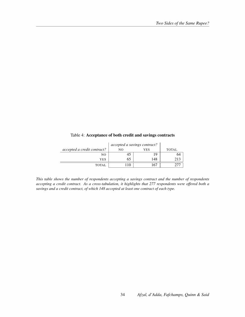
Two Sides of the Same Rupee?
Table 4: Acceptance of both credit and savings contracts
accepted a savings contract?accepted a credit contract? NO YES TOTAL
NO 45 19 64YES 65 148 213
TOTAL 110 167 277
This table shows the number of respondents accepting a savings contract and the number of respondentsaccepting a credit contract. As a cross-tabulation, it highlights that 277 respondents were offered both asavings and a credit contract, of which 148 accepted at least one contract of each type.
34 Afzal, d’Adda, Fafchamps, Quinn & Said

Two Sides of the Same Rupee?
Table 5: Acceptance of savings contracts with r ≥ 0 and credit contracts with r ≤ 0
accepted a savings contract with r > 0?accepted a credit contract with r ≤ 0? NO YES TOTAL
NO 15 11 26YES 17 44 61
TOTAL 32 55 87
This table is motivated by Prediction 5 of the benchmark model. It shows that 87 respondents were offered asavings contract with r > 0 and a credit contract with r ≤ 0; of these 44, accepted at least one contract ofeach type.
35 Afzal, d’Adda, Fafchamps, Quinn & Said

Two Sides of the Same Rupee?
Tabl
e6:
Vio
latio
nsof
the
benc
hmar
km
odel
PR
ED
ICT
ION
OP
PO
RT
UN
ITY
TO
VIO
LA
TE
PR
ED
ICT
ION
PR
ED
ICT
ION
VIO
LA
TE
D
will
nota
ccep
tsav
ings
with
r>
0an
dcr
edit
with
r≤
087
44(5
1%)
alw
ays
refu
sesa
ving
sw
ithr<
018
486
(47%
)al
way
sac
cept
cred
itw
ithr>
023
029
(13%
)an
ypr
edic
tion
439
155
(35%
)
This
tabl
esu
mm
aris
esth
epr
edic
tions
ofth
ebe
nchm
ark
mod
el;
itsh
ows
the
num
ber
ofre
spon
dent
svi
olat
ing
such
pred
ictio
ns,c
ompa
red
toth
enu
mbe
rbe
ing
offe
red
the
oppo
rtun
ityto
doso
.
36 Afzal, d’Adda, Fafchamps, Quinn & Said

Two Sides of the Same Rupee?
Tabl
e7:
Det
erm
inan
tsof
take
-up:
Het
erog
enei
tyby
mea
sure
sofs
avin
gspr
essu
re
(1)
(2)
(3)
(4)
(5)
(6)
(7)
(8)
(9)
(10)
(11)
(12)
FAM
ILY
ME
MB
ER
Seq
ualit
yD
IFFI
CU
LTY
equa
lity
LU
MP
Yeq
ualit
yW
OU
LD
equa
lity
RE
QU
ES
TM
ON
EY
?(p
-val
ues)
SA
VIN
G?
(p-v
alue
s)P
UR
CH
AS
E?
(p-v
alue
s)S
AV
E/I
NV
ES
T?
(p-v
alue
s)Y
ES
NO
YE
SN
OY
ES
NO
YE
SN
O
Dum
my:
r=−0.1
-0.1
15-0
.136
0.70
7-0
.134
-0.1
080.
609
-0.1
68-0
.102
0.19
6-0
.179
-0.1
010.
260
(0.0
36)∗
∗∗(0
.046
)∗∗∗
(0.0
45)∗
∗∗(0
.032
)∗∗∗
(0.0
45)∗
∗∗(0
.032
)∗∗∗
(0.0
60)∗
∗∗(0
.032
)∗∗∗
Dum
my:
r=
+0.1
0.04
10.
119
0.11
90.
029
0.09
50.
164
0.04
40.
074
0.45
90.
018
0.08
60.
133
(0.0
30)
(0.0
37)∗
∗∗(0
.041
)(0
.026
)∗∗∗
(0.0
34)
(0.0
27)∗
∗(0
.040
)(0
.026
)∗∗∗
Dum
my:
p=
10.
106
0.16
50.
247
0.14
70.
108
0.46
20.
136
0.12
20.
773
0.12
30.
123
0.99
5(0
.037
)∗∗∗
(0.0
38)∗
∗∗(0
.037
)∗∗∗
(0.0
42)∗
∗(0
.043
)∗∗∗
(0.0
36)∗
∗∗(0
.043
)∗∗∗
(0.0
34)∗
∗∗
Dum
my:
p=
6-0
.079
-0.0
050.
138
-0.0
57-0
.046
0.87
0-0
.026
-0.0
660.
490
0.03
5-0
.096
0.00
4∗∗∗
(0.0
33)∗
∗(0
.036
)(0
.046
)(0
.036
)(0
.051
)(0
.031
)∗∗
(0.0
36)
(0.0
33)∗
∗∗
Con
stan
t0.
666
0.59
20.
407
0.61
10.
661
0.53
00.
684
0.62
50.
367
0.73
60.
608
0.07
9∗
(0.0
50)∗
∗∗(0
.085
)∗∗∗
(0.0
60)∗
∗∗(0
.065
)∗∗∗
(0.0
51)∗
∗∗(0
.058
)∗∗∗
(0.0
46)∗
∗∗(0
.061
)∗∗∗
join
ttes
t:0.
066∗
join
ttes
t:0.
286
join
ttes
t:0.
553
join
ttes
t:0.
003∗
∗∗
Obs
.16
2971
810
1513
3265
716
9063
117
15R
20.
045
0.07
30.
051
0.05
20.
062
0.04
80.
055
0.05
7Th
ista
ble
repo
rts
LPM
estim
ates
for
take
-up
asa
func
tion
ofco
ntra
ctte
rms.
Pare
nthe
ses
show
stan
dard
erro
rs,w
hich
allo
wfo
rcl
uste
ring
bym
icro
finan
cegr
oup.
‘Equ
ality
test
s’re
fer
topa
irw
ise
coef
ficie
nteq
ualit
yte
sts.
Sign
ifica
nce:∗⇔
p<
0.1
,∗∗⇔
p<
0.05
,∗∗∗⇔
p<
0.01
.
37 Afzal, d’Adda, Fafchamps, Quinn & Said

Two Sides of the Same Rupee?
Tabl
e8:
Det
erm
inan
tsof
take
-up:
Het
erog
enei
tyby
base
line
inco
me
flow
(1)
(2)
(3)
(4)
(5)
(6)
SA
LA
RIE
DIN
CO
ME
?(W
HO
LE
SA
MP
LE
)N
OY
ES
NO
YE
Seq
ualit
yte
sts
NO
N-S
AL
AR
IED
INC
OM
E?
(WH
OL
ES
AM
PL
E)
NO
NO
YE
SY
ES
(p-v
alue
s)
Dum
my:r=−0.1
-0.1
20-0
.017
-0.1
23-0
.112
-0.1
800.
657
(0.0
29)∗
∗∗(0
.131
)(0
.086
)(0
.030
)∗∗∗
(0.0
52)∗
∗∗
Dum
my:r=
+0.1
0.06
60.
133
0.13
60.
068
0.02
20.
480
(0.0
23)∗
∗∗(0
.124
)(0
.077
)∗(0
.028
)∗∗
(0.0
51)
Dum
my:p=
10.
125
0.25
80.
283
0.10
50.
096
0.15
5(0
.031
)∗∗∗
(0.1
26)∗
∗(0
.083
)∗∗∗
(0.0
28)∗
∗∗(0
.051
)∗
Dum
my:p=
6-0
.055
0.03
8-0
.090
-0.0
54-0
.060
0.88
1(0
.027
)∗(0
.129
)(0
.075
)(0
.029
)∗(0
.052
)
Con
stan
t0.
641
0.54
80.
559
0.63
00.
744
0.09
8∗
(0.0
49)∗
∗∗(0
.112
)∗∗∗
(0.0
73)∗
∗∗(0
.026
)∗∗∗
(0.0
49)∗
∗∗
join
ttes
tofa
llpa
ram
eter
s:0.
000∗
∗∗
Obs
erva
tions
2347
7720
316
1645
1R
20.
051
0.08
10.
127
0.04
20.
065
This
tabl
ere
port
sLP
Mes
timat
esfo
rta
ke-u
pas
afu
nctio
nof
cont
ract
term
s.Pa
rent
hese
ssh
owst
anda
rder
rors
,whi
chal
low
for
clus
teri
ngby
mic
rofin
ance
grou
p.‘E
qual
ityte
sts’
refe
rto
coef
ficie
nteq
ualit
yac
ross
colu
mns
(2),
(3),
(4)a
nd(5
).Si
gnifi
canc
e:∗⇔p<
0.1
,∗∗⇔p<
0.05
,∗∗∗⇔p<
0.01
.
38 Afzal, d’Adda, Fafchamps, Quinn & Said

Two Sides of the Same Rupee?
Tabl
e9:
Defi
nitio
nof
poss
ible
resp
onde
ntty
pes
CO
NT
RA
CT
OFF
ER
ED
r-0
.10
0.1
p1
34
61
34
61
34
6
TY
PE
DE
FIN
ITIO
ND
EC
ISIO
N(1
=A
CC
EP
T)
‘BE
NC
HM
AR
KM
OD
EL
’‘A
’m
t≥
0an
dγev∈[−
900,132
0)0
00
00
00
01
00
0‘B
’m
t≥
0an
dγev∈[
1320,141
0)0
00
00
00
01
10
0‘C
’m
t≥
0an
dγev≥
1410
00
00
00
00
11
10
‘ALT
ER
NA
TIV
EM
OD
EL
’‘D
’m
t=
0an
dγev∈[−
900,195
0)0
00
00
00
00
00
0‘E
’m
t=
0an
dγev∈[
1950,243
0)0
00
00
00
01
11
1‘F
’m
t=
0an
dγev∈[
2430,311
0)0
00
01
11
11
11
1‘G
’m
t=
0an
dγev≥
3110
11
11
11
11
11
11
This
tabl
ere
cord
sth
epr
edic
tions
ofth
est
ruct
ural
mod
elfo
rdi
ffere
ntty
pes
ofco
ntra
ctof
fere
d.A
sa
benc
hmar
k,w
eno
rmal
ise
daily
inco
me
to59
9P
KR
:th
em
edia
nda
ily
hous
ehol
din
com
efo
rth
edi
stri
ctof
Sarg
odha
from
the
PSL
M20
10-1
1su
rvey
(cor
rect
edfo
rC
PIi
nflat
ion)
.
39 Afzal, d’Adda, Fafchamps, Quinn & Said
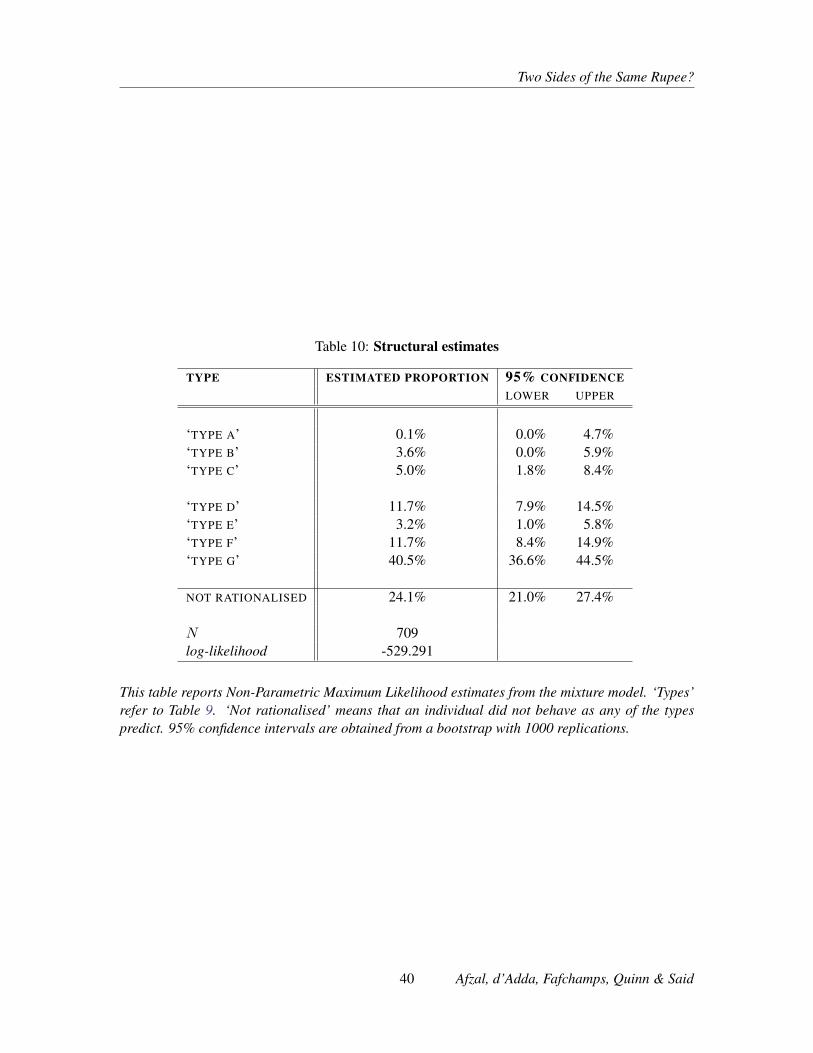
Two Sides of the Same Rupee?
Table 10: Structural estimates
TYPE ESTIMATED PROPORTION 95% CONFIDENCELOWER UPPER
‘TYPE A’ 0.1% 0.0% 4.7%‘TYPE B’ 3.6% 0.0% 5.9%‘TYPE C’ 5.0% 1.8% 8.4%
‘TYPE D’ 11.7% 7.9% 14.5%‘TYPE E’ 3.2% 1.0% 5.8%‘TYPE F’ 11.7% 8.4% 14.9%‘TYPE G’ 40.5% 36.6% 44.5%
NOT RATIONALISED 24.1% 21.0% 27.4%
N 709log-likelihood -529.291
This table reports Non-Parametric Maximum Likelihood estimates from the mixture model. ‘Types’refer to Table 9. ‘Not rationalised’ means that an individual did not behave as any of the typespredict. 95% confidence intervals are obtained from a bootstrap with 1000 replications.
40 Afzal, d’Adda, Fafchamps, Quinn & Said

Two Sides of the Same Rupee?
Tabl
e11
:Str
uctu
rale
stim
ates
:Dis
aggr
egat
ing
byba
selin
ech
arac
teri
stic
s
EST
IMA
TE
DP
RO
PO
RT
ION
S
FAM
ILY
ME
MB
ER
SD
IFFI
CU
LTY
LU
MP
YW
OU
LD
RE
QU
ES
TM
ON
EY
?S
AV
ING
?P
UR
CH
AS
E?
SA
VE
/IN
VE
ST
?Y
ES
NO
YE
SN
OY
ES
NO
YE
SN
O
‘TY
PE
A’
0.0%
5.1%
0.0%
0.2%
3.9%
0.0%
1.4%
0.8%
‘TY
PE
B’
4.2%
0.0%
3.8%
3.6%
0.0%
4.2%
5.4%
2.1%
‘TY
PE
C’
4.9%
5.5%
3.4%
5.8%
6.0%
4.7%
4.3%
5.8%
‘TY
PE
D’
11.4
%9.
4%15
.6%
9.0%
8.7%
12.6
%2.
8%14
.5%
‘TY
PE
E’
1.0%
8.5%
3.7%
3.2%
0.0%
3.9%
0.0%
4.1%
‘TY
PE
F’11
.4%
12.7
%8.
7%13
.6%
14.3
%10
.9%
13.5
%11
.1%
‘TY
PE
G’
40.9
%39
.3%
36.5
%43
.6%
42.8
%39
.5%
47.0
%38
.1%
NO
TR
AT
ION
AL
ISE
D26
.1%
19.5
%28
.3%
20.9
%24
.2%
24.1
%25
.7%
23.6
%
N49
421
530
740
219
851
118
952
2lo
g-lik
elih
ood
-351
.3-1
72.4
-213
.2-3
12.0
-136
.8-3
89.6
-112
.9-4
06.6
HY
PO
TH
ES
IST
ES
TS
OF
EQ
UA
LIT
YB
ET
WE
EN
CO
LU
MN
S(p
-VA
LU
ES):
AL
LPA
RA
ME
TE
RS:
0.08
0∗0.
230
0.44
20.
003∗∗∗
PR
OP
OR
TIO
NIN
A,B
OR
C:
0.74
20.
550
0.76
90.
551
PR
OP
OR
TIO
NR
AT
ION
AL
ISE
D:
0.05
6∗0.
022∗∗
0.96
20.
565
This
tabl
ere
port
sN
on-P
aram
etri
cM
axim
umLi
kelih
ood
estim
ates
from
the
mix
ture
mod
el,
disa
ggre
gate
dby
bina
ryba
selin
eco
vari
ates
.‘T
ypes
’re
fer
toTa
ble
9.‘N
otra
tiona
lised
’m
eans
that
anin
divi
dual
did
notb
ehav
eas
any
ofth
ety
pes
pred
ict.
The
last
pane
loft
heTa
ble
repo
rts
Like
lihoo
dR
atio
test
sto
com
pare
estim
ates
betw
een
colu
mns
.‘A
llpa
ram
eter
s’re
fers
tote
sts
ofw
heth
erth
epr
opor
tion
ofea
chty
pear
eco
mm
onbe
twee
nco
lum
ns(d.f.=
6).
‘Pro
port
ion
inA
,Bor
C’
test
sw
heth
erth
epr
opor
tion
adhe
ring
toth
ebe
nchm
ark
mod
elis
equa
lac
ross
colu
mns
(d.f.=
1).
Not
eth
atth
isis
equi
vale
ntto
test
ing
whe
ther
the
prop
ortio
nin
D,E
,Fan
dG
iseq
ual.
‘Pro
port
ion
ratio
nalis
ed’
uses
Like
lihoo
dR
atio
sfr
omth
eB
erno
ulli
dist
ribu
tion
tote
stw
heth
eran
equa
lsha
reis
ratio
nalis
edac
ross
colu
mns
(d.f.=
1).
Not
eth
atth
isis
equi
vale
ntto
test
ing
whe
ther
the
prop
ortio
nno
trat
iona
lised
iseq
ual.
41 Afzal, d’Adda, Fafchamps, Quinn & Said

Two Sides of the Same Rupee?
Table 12: Structural estimates: Disaggregating by baseline income flow
ESTIMATED PROPORTIONS(1) (2) (3)
SALARIED INCOME? NO NO YES
NON-SALARIED INCOME? NO YES YES
‘TYPE A’ 0.0% 5.0% 0.0%‘TYPE B’ 4.4% 1.6% 4.7%‘TYPE C’ 4.6% 6.5% 0.2%
‘TYPE D’ 14.2% 4.6% 18.0%‘TYPE E’ 0.0% 2.7% 5.8%‘TYPE F’ 16.0% 13.0% 8.8%‘TYPE G’ 36.7% 40.3% 41.7%
NOT RATIONALISED 24.1% 26.3% 20.9%
N 83 377 249log-likelihood -62.145 -261.008 -196.646HYPOTHESIS TESTS: ALL PROPORTION IN PROPORTION
PARAMETERS A, B OR C RATIONALISED
H0: column (1) = column (2) (p): 0.561 0.504 0.682H0: column (1) = column (3) (p): 0.618 0.395 0.542H0: column (2) = column (3) (p): 0.013∗∗ 0.054∗ 0.122H0: all columns equal (p): 0.089∗ 0.152 0.302
This table reports Non-Parametric Maximum Likelihood estimates from the mixture model, disag-gregated by binary baseline covariates. ‘Types’ refer to Table 9. ‘Not rationalised’ means that anindividual did not behave as any of the types predict. The last panel of the Table reports LikelihoodRatio tests to compare estimates between columns. ‘All parameters’ refers to tests of whether theproportion of each type are common between columns (d.f. = 6 for the first three tests; d.f. = 12for the final test). ‘Proportion in A, B or C’ tests whether the proportion adhering to the benchmarkmodel is equal across columns (d.f. = 1 for the first three tests; d.f. = 2 for the final teste). Notethat this is equivalent to testing whether the proportion in D, E, F and G is equal. ‘Proportionrationalised’ uses Likelihood Ratios from the Bernoulli distribution to test whether an equal shareis rationalised across columns (d.f. = 1 for the first three tests; d.f. = 2 for the final teste). Notethat this is equivalent to testing whether the proportion not rationalised is equal.
42 Afzal, d’Adda, Fafchamps, Quinn & Said

Two Sides of the Same Rupee?
Table 13: Structural estimates: Allowing automatic refusal in wave 3
TYPE ESTIMATED PROPORTION 95% CONFIDENCELOWER UPPER
‘TYPE A’ 0.0% 0.0% 3.3%‘TYPE A?’ 1.2% 0.0% 5.7%‘TYPE B’ 3.4% 0.0% 5.9%‘TYPE B?’ 0.0% 0.0% 3.6%‘TYPE C’ 2.6% 0.0% 5.7%‘TYPE C?’ 1.1% 0.0% 4.9%
‘TYPE D/D?’ 10.4% 6.1% 13.8%‘TYPE E’ 2.5% 0.6% 4.8%‘TYPE E?’ 0.9% 0.0% 2.6%‘TYPE F’ 8.7% 5.7% 12.0%‘TYPE F?’ 4.6% 2.2% 7.0%‘TYPE G’ 41.5% 37.7% 45.4%‘TYPE G?’ 9.0% 6.6% 11.5%
NOT RATIONALISED 14.1% 11.4% 16.9%
N 709log-likelihood -749.576
This table reports Non-Parametric Maximum Likelihood estimates from the mixture model. Thisaugments the estimates in Table 10 by allowing some respondents to behave according to the struc-tural model in waves 1 and 2, then refuse automatically in wave 3; this is denoted by the addition of‘?’. ‘Types’ refer to Table 9. ‘Not rationalised’ means that an individual did not behave as any ofthe types predict. 95% confidence intervals are obtained from a bootstrap with 1000 replications.
43 Afzal, d’Adda, Fafchamps, Quinn & Said

Two Sides of the Same Rupee?
Table 14: Structural estimates: Allowing a type with random play
TYPE ESTIMATED PROPORTION 95% CONFIDENCELOWER UPPER
‘TYPE A’ 0.9% 0.0% 5.7%‘TYPE B’ 0.8% 0.0% 4.1%‘TYPE C’ 4.5% 0.1% 7.5%
‘TYPE D’ 8.3% 3.8% 11.7%‘TYPE E’ 0.0% 0.0% 3.3%‘TYPE F’ 8.5% 4.9% 11.9%‘TYPE G’ 36.6% 32.5% 41.0%
RANDOM PLAY 40.5% 35.0% 45.6%
NOT RATIONALISED 0.0% 0.0% 0.0%
N 709log-likelihood -1183.7
This table reports Non-Parametric Maximum Likelihood estimates from the mixture model. Thisaugments the estimates in Table 10 by introducing a type that decides to accept or reject by tossinga fair coin in each wave. ‘Types’ refer to Table 9. ‘Not rationalised’ means that an individual didnot behave as any of the types predict. 95% confidence intervals are obtained from a bootstrap with1000 replications.
44 Afzal, d’Adda, Fafchamps, Quinn & Said

Two Sides of the Same Rupee?
ReferencesAdams, D. and Canavesi de Sahonero, M. (1989). ‘Rotating Savings and Credit Associations in Bolivia’,
Savings and Development, vol. 13(3), pp. 219–236.
Aliber, M. (2001). ‘Rotating Savings and Credit Associations and the Pursuit of Self-Discipline: A CaseStudy in South Africa’, African Review of Money, Finance and Banking, pp. 51–73.
Ambec, S. and Treich, N. (2007). ‘Roscas as Financial Agreements to Cope with Self-Control Problems’,Journal of Development Economics, vol. 82(1), pp. 120–137.
Ananth, B., Karlan, D. and Mullainathan, S. (2007). ‘Microentrepreneurs and Their Money: Three Anoma-lies’, Working paper (Financial Access Initiative and Innovations for Poverty Action).
Andersen, S., Harrison, G.W., Lau, M.I. and Rutström, E.E. (2008). ‘Eliciting Risk and Time Preferences’,Econometrica, vol. 76(3), pp. 583–618.
Andersen, S., Harrison, G.W., Lau, M.I. and Rutström, E.E. (2014). ‘Discounting Behavior: A Reconsidera-tion’, European Economic Review, vol. 71, pp. 15–33.
Anderson, S. and Baland, J.M. (2002). ‘The Economics of ROSCAs and Intrahousehold Resource Alloca-tion’, Quarterly Journal of Economics, pp. 963–995.
Armendáriz de Aghion, B. and Morduch, J. (2005). The Economics of Microfinance, The MIT Press.
Aryeetey, E. and Steel, W. (1995). ‘Savings Collectors and Financial Intermediation in Ghana’, Savings andDevelopment, vol. 19(2), pp. 189–199.
Aryeetey, E. and Udry, C. (1997). ‘The Characteristics of Informal Financial Markets in Sub-Saharan Africa’,Journal of African Economies, vol. 6(1), pp. 161–203.
Ashraf, N., Gons, N., Karlan, D. and Yin, W. (2003). ‘A Review of Commitment Savings Products in Devel-oping Countries’, ERD Working Paper Series, No. 45.
Ashraf, N., Karlan, D. and Yin, W. (2006). ‘Tying Odysseus to the Mast: Evidence from a CommitmentSavings Product in the Philippines’, The Quarterly Journal of Economics, vol. 121(2), pp. 635–672.
Baland, J.M., Guirkinger, C. and Mali, C. (2011). ‘Pretending to be Poor: Borrowing to Escape ForcedSolidarity in Cameroon’, Economic Development and Cultural Change, vol. 60(1), pp. 1–16.
Banerjee, A., Duflo, E., Glennerster, R. and Kinnan, C. (2015). ‘The Miracle of Microfinance? Evidencefrom a Randomized Evaluation’, American Economic Journal: Applied Economics, vol. 7(1), pp. 22–53.
Basu, K. (2008). ‘A Behavioral Model of Simultaneous Borrowing and Saving’, Working Paper.
Bauer, M., Chytilová, J. and Morduch, J. (2012). ‘Behavioral Foundations of Microcredit: Experimental andSurvey Evidence from Rural India’, The American Economic Review, vol. 102(2), pp. 1118–1139.
Bernheim, B.D., Ray, D. and Yeltekin, S. (2015). ‘Poverty and self-control’, Econometrica, vol. 83(5), pp.1877–1911.
Besley, T.J., Coate, S. and Loury, G.C. (1993). ‘The Economics of Rotating Savings and Credit Associations’,American Economic Review, vol. 83(4), pp. 792–810.
Brune, L., Giné, X., Goldberg, J. and Yang, D. (2014). ‘Facilitating Savings for Agriculture: Field Experi-mental Evidence from Malawi’, Working paper.
45 Afzal, d’Adda, Fafchamps, Quinn & Said

Two Sides of the Same Rupee?
Burgess, R. and Pande, R. (2005). ‘Do Rural Banks Matter? Evidence from the Indian Social BankingExperiment’, American Economic Review, pp. 780–795.
Camerer, C., Babcock, L., Loewenstein, G. and Thaler, R. (1997). ‘Labor Supply of New York City Cab-drivers: One Day at a Time’, The Quarterly Journal of Economics, pp. 407–441.
Coller, M. and Williams, M.B. (1999). ‘Eliciting Individual Discount Rates’, Experimental Economics,vol. 2(2), pp. 107–127.
Collins, D., Morduch, J., Rutherford, S. and Ruthven, O. (2009). Portfolios of the Poor: How the World’sPoor Live on $2 a Day, Princeton University Press.
Dehejia, R., Montgomery, H. and Morduch, J. (2012). ‘Do Interest Rates Matter? Credit Demand in theDhaka Slums’, Journal of Development Economics, vol. 97.
DellaVigna, S. and Malmendier, U. (2006). ‘Paying Not to go to the Gym’, The American Economic Review,pp. 694–719.
Dohmen, T., Falk, A., Huffman, D. and Sunde, U. (2013). ‘Interpreting Time Horizon Effects in Inter-Temporal Choice’, Working paper.
Dupas, P. and Robinson, J. (2013). ‘Why Don’t the Poor Save More? Evidence from Health Savings Experi-ments’, American Economic Review, vol. 103(4), pp. 1138–71.
Field, E., Pande, R., Papp, J. and Rigol, N. (2013). ‘Does the Classic Microfinance Model Discourage En-trepreneurship Among the Poor? Experimental Evidence from India’, The American Economic Review,vol. 103(6), pp. 2196–2226.
Frühwirth-Schnatter, S. (2006). Finite mixture and Markov switching models, Springer Science & BusinessMedia.
Goldberg, J. (2011). ‘The Lesser of Two Evils: The Roles of Social Pressure and Impatience in ConsumptionDecisions’, University of Maryland (mimeograph).
Gross, D.B. and Souleles, N.S. (2002). ‘Do liquidity constraints and interest rates matter for consumer be-havior? evidence from credit card data’, Quarterly Journal of Economics, pp. 149–185.
Gugerty, M.K. (2007). ‘You Can’t Save Alone: Commitment in Rotating Savings and Credit Associations inKenya’, Economic Development and Cultural Change, vol. 55(2), pp. 251–282.
Handa, S. and Kirton, C. (1999). ‘The Economics of Rotating Savings and Credit Associations: Evidencefrom the Jamaian ‘Partner’’, Journal of Development Economics, vol. 60, pp. 173–194.
Haq, A., Aslam, A., Chaudhry, A.A., Naseer, A., Muhammad, K., Mushtaq, K. and Saleem, M.F. (2013).‘Who is the ‘Arthi’: Understanding the Commission Agent’s Role in the Agriculture Supply Chain’, IGCWorking Paper.
Islam, M.T., Takanashi, C. and Natori, T. (2013). ‘Big Challenges by a Small Microfinance Institution: ACase Study of SafeSave Bangladesh from the Customer Satisfaction and ICT Introduction Perspective’,International Journal of Business and Management, vol. 8(14).
John, A. (2015). ‘When Commitment Fails – Evidence from a Regular Saver Product in the Philippines’,Working paper (ENSAE, Paris).
Kaplan, G., Violante, G. and Weidner, J. (2014). ‘The Wealthy Hand-to-Mouth’, Brookings Papers on Eco-nomic Activity.
46 Afzal, d’Adda, Fafchamps, Quinn & Said

Two Sides of the Same Rupee?
Karlan, D. and Zinman, J. (2011). ‘Microcredit in Theory and Practice: Using Randomized Credit Scoringfor Impact Evaluation’, Science, vol. 332(6035), pp. 1278–1284.
Kast, F. and Pomeranz, D. (2014). ‘Saving More to Borrow Less: Experimental Evidence from Access toFormal Savings Accounts in Chile’, Harvard Business School Working Paper, No. 14-001.
Kaur, S., Kremer, M. and Mullainathan, S. (2015). ‘Self control at work’, Journal of Political Economy, vol.123(6), pp. 1227 – 1277.
Kedir, A. and Ibrahim, G. (2011). ‘ROSCAs in Urban Ethiopia: Are the Characteristics of the InstitutionsMore Important Than Those of Members?’, Journal of Development Studies, vol. 47(7), pp. 998–1016.
Kovsted, J. and Lyk-Jensen, P. (1999). ‘Rotating Savings and Credit Associations: The Choice BetweenRandom and Bidding Allocation of Funds’, Journal of Development Economics, vol. 60(1), pp. 143–172.
Laureti, C. (2015). ‘The Debt Puzzle in Dhaka’s Slums: Do Poor People Co-hold for Liquidity Needs?’,Centre Emile Bernheim Working Paper 15/021.
McKinnon, R.I. (1973). Money and Capital in Economic Development, Brookings Institution.
Morduch, J. (2010). ‘Borrowing to Save’, Journal of Globalization and Development, vol. 1(2).
Mullainathan, S. and Shafir, E. (2009). ‘Savings Policy and Decision-Making in Low-Income Households’, in(M. Barr and R. Blank, eds.), Insufficient Funds: Savings, Assets, Credit and Banking Among Low-IncomeHouseholds, .
Platteau, J.P. (2000). Institutions, Social Norms, and Economic Development, vol. 1, Psychology Press.
Rutherford, S. (1997). ‘Informal Financial Services in Dhaka’s Slums’, in (Wood, Geoffrey and Sharif, Iffath,ed.), Who Needs Credit? Poverty and Finance in Bangladesh, Dhaka University Press.
Rutherford, S. (2000). The Poor and Their Money, Oxford University Press.
Schilbach, F. (2015). ‘Alcohol and Self-Control: A Field Experiment in India’, Working Paper.
Somville, V. (2011). ‘Daily Collectors, Public Good Provision and Private Consumption: Theory and Evi-dence from Urban Benin’, Univerity of Namur Department of Economics Working Paper 1106.
Somville, V. (2014). ‘Informal Savings and Intra-household Strategies: Theory and Evidence from UrbanBenin’, Namur University (mimeograph).
Stahl, D.O. and Wilson, P.W. (1995). ‘On PlayersâAš Models of Other Players: Theory and ExperimentalEvidence’, Games and Economic Behavior, vol. 10(1), pp. 218–254.
Steel, W., Aryeetey, E., Hettige, H. and Nissanke, M. (1997). ‘Informal Financial Markets Under Liberaliza-tion in Four African Countries’, World Development, vol. 25(5), pp. 817–830.
Tanaka, T. and Nguyen, Q. (2010). ‘ROSCA as a Saving Commitment Device for Sophisticated HyperbolicDiscounters: Field Experiment from Vietnam’, Working Paper.
Von Gaudecker, H.M., Van Soest, A. and Wengström, E. (2011). ‘Heterogeneity in Risky Choice Behavior ina Broad Population’, The American Economic Review, pp. 664–694.
47 Afzal, d’Adda, Fafchamps, Quinn & Said