Two Sample t Tests

Karl L. Wuensch

Department of Psychology

East Carolina University

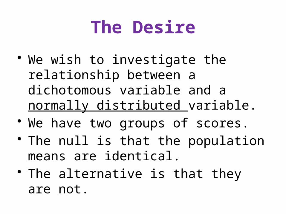
The Desire

• We wish to investigate the relationship between a dichotomous variable and a normally distributed variable.

• We have two groups of scores.• The null is that the population means are

identical.• The alternative is that they are not.

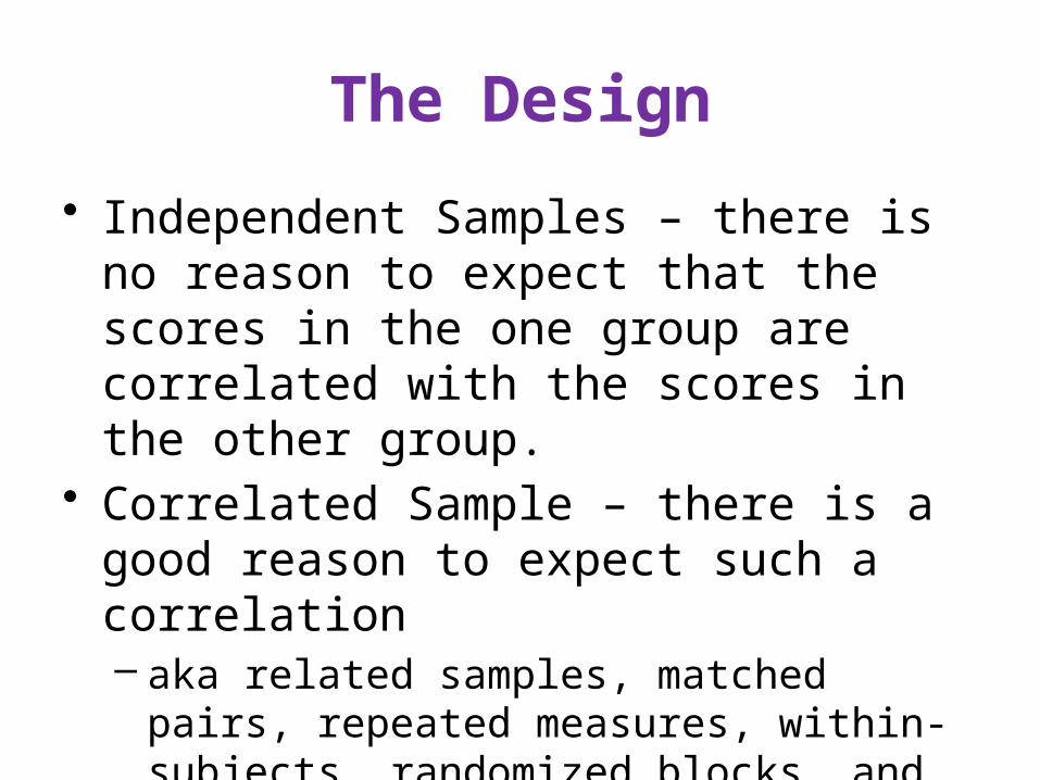
The Design

• Independent Samples – there is no reason to expect that the scores in the one group are correlated with the scores in the other group.

• Correlated Sample – there is a good reason to expect such a correlation– aka related samples, matched pairs, repeated

measures, within-subjects, randomized blocks, and split plot.

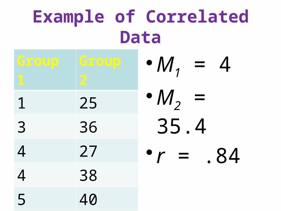
Example of Correlated Data

Group 1 Group 2

1 253 364 274 385 407 46

•M1 = 4

•M2 = 35.4

• r = .84

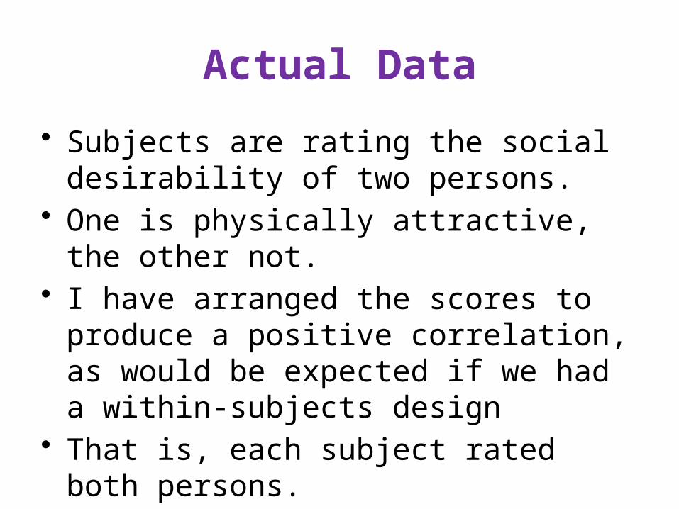
Actual Data

• Subjects are rating the social desirability of two persons.

• One is physically attractive, the other not.• I have arranged the scores to produce a

positive correlation, as would be expected if we had a within-subjects design

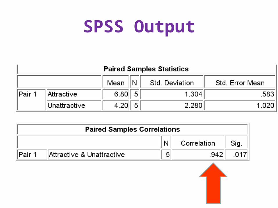
• That is, each subject rated both persons.• The observed correlation is r = .92

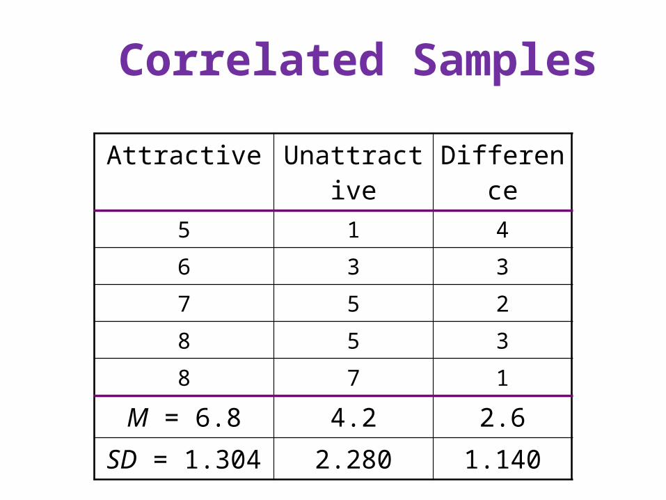
Attractive Unattractive Difference

5 1 4

6 3 3

7 5 2

8 5 3

8 7 1

M = 6.8 4.2 2.6

SD = 1.304 2.280 1.140

Correlated Samples

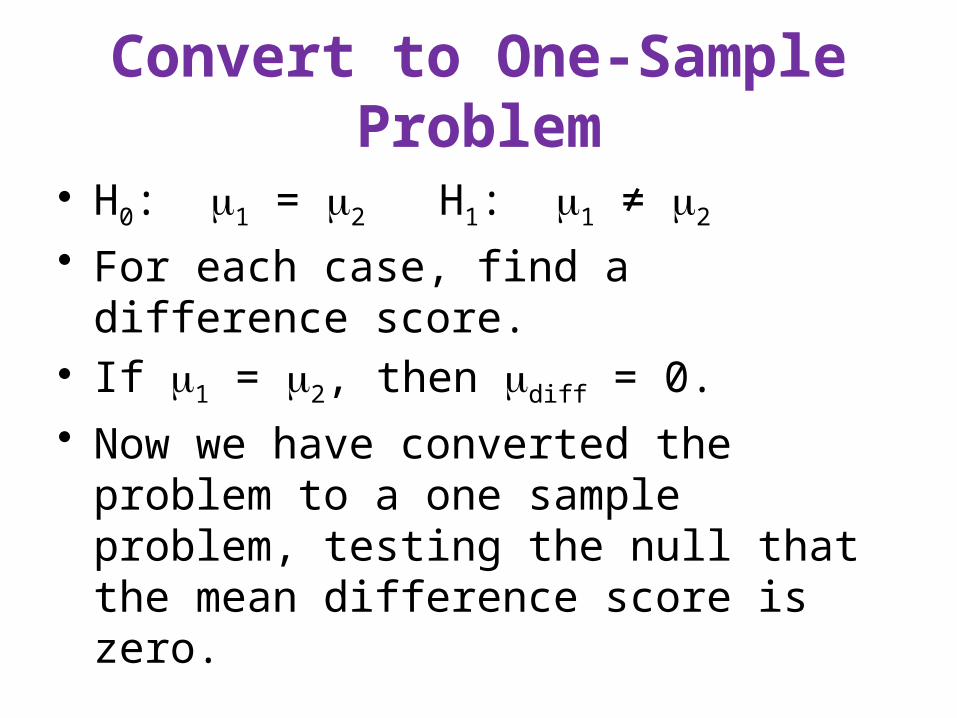
Convert to One-Sample Problem

• H0: 1 = 2 H1: 1 ≠ 2

• For each case, find a difference score.• If 1 = 2, then diff = 0.

• Now we have converted the problem to a one sample problem, testing the null that the mean difference score is zero.

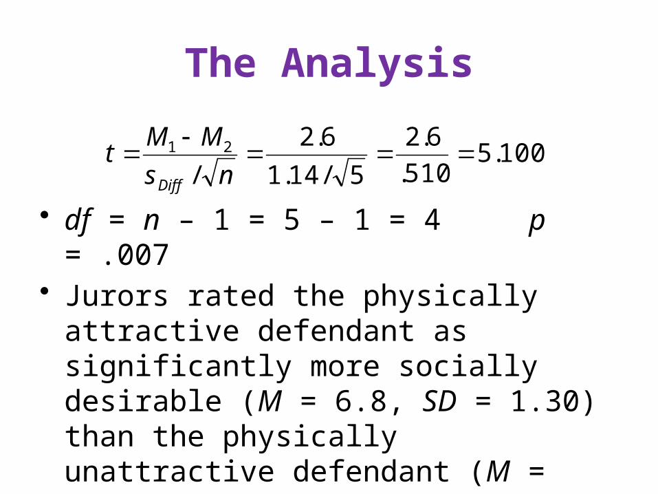
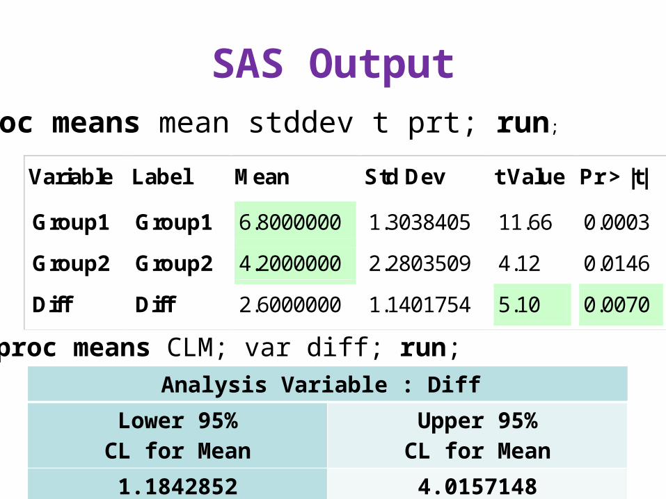
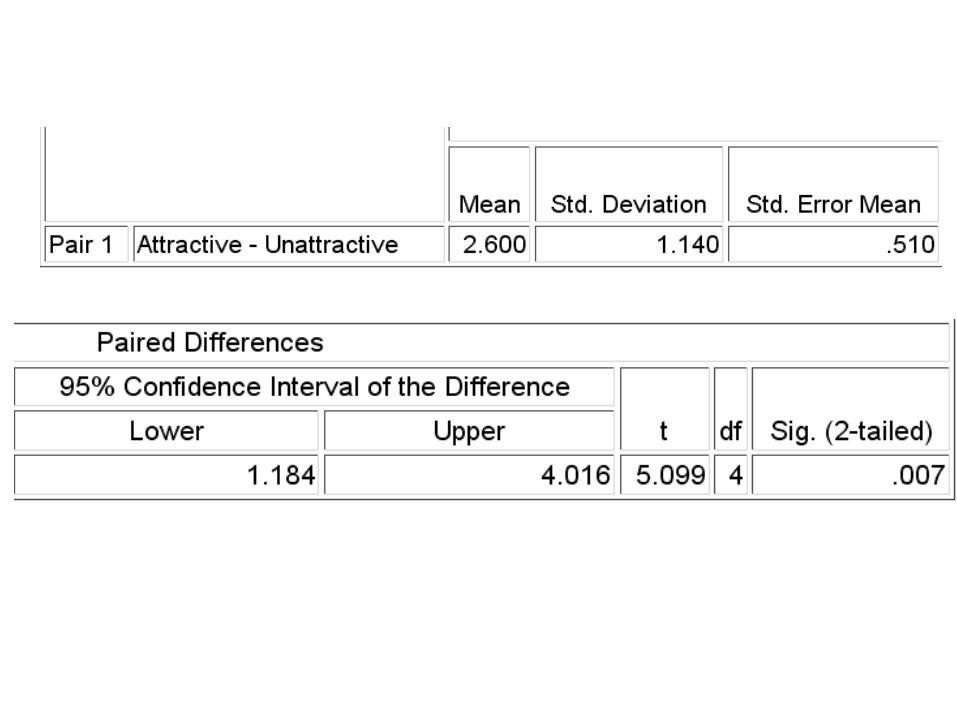
The Analysis

• df = n – 1 = 5 – 1 = 4 p = .007• Jurors rated the physically attractive

defendant as significantly more socially desirable (M = 6.8, SD = 1.30) than the physically unattractive defendant (M = 4.2, SD = 2.28), t(4) = 5.10, p = .007.

100.5510.

6.2

5/14.1

6.2

/21

ns

MMt

Diff

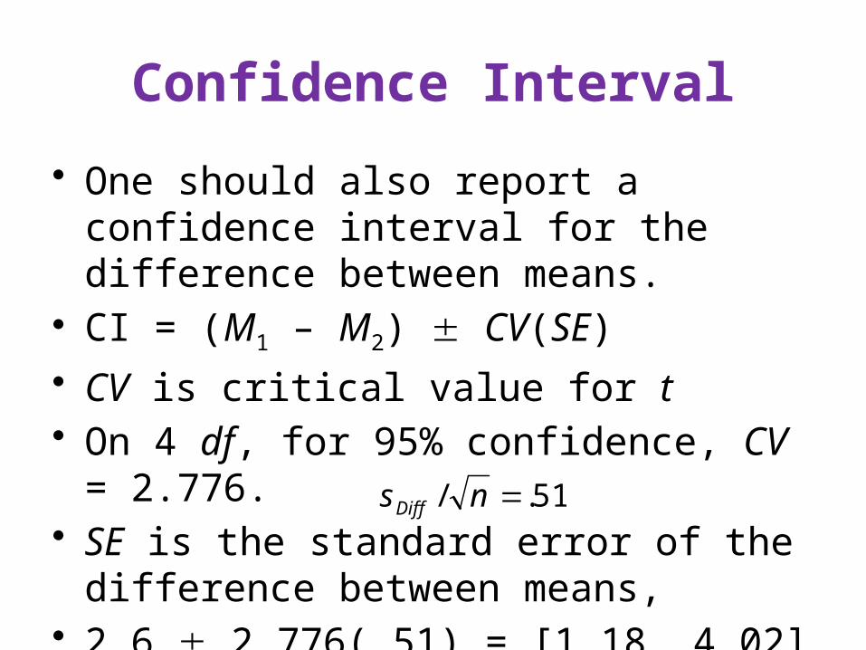
Confidence Interval

• One should also report a confidence interval for the difference between means.

• CI = (M1 – M2) CV(SE)

• CV is critical value for t• On 4 df, for 95% confidence, CV = 2.776.• SE is the standard error of the difference

between means, • 2.6 2.776(.51) = [1.18, 4.02]

51./ nsDiff

SAS Output

Variable Label Mean Std Dev t Value Pr > |t|

Group1

Group2

Diff

Group1

Group2

Diff

6.8000000

4.2000000

2.6000000

1.3038405

2.2803509

1.1401754

11.66

4.12

5.10

0.0003

0.0146

0.0070

Analysis Variable : Diff Lower 95%CL for Mean

Upper 95%CL for Mean

1.1842852 4.0157148

proc means CLM; var diff; run;

proc means mean stddev t prt; run;

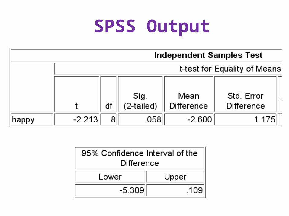
SPSS Output

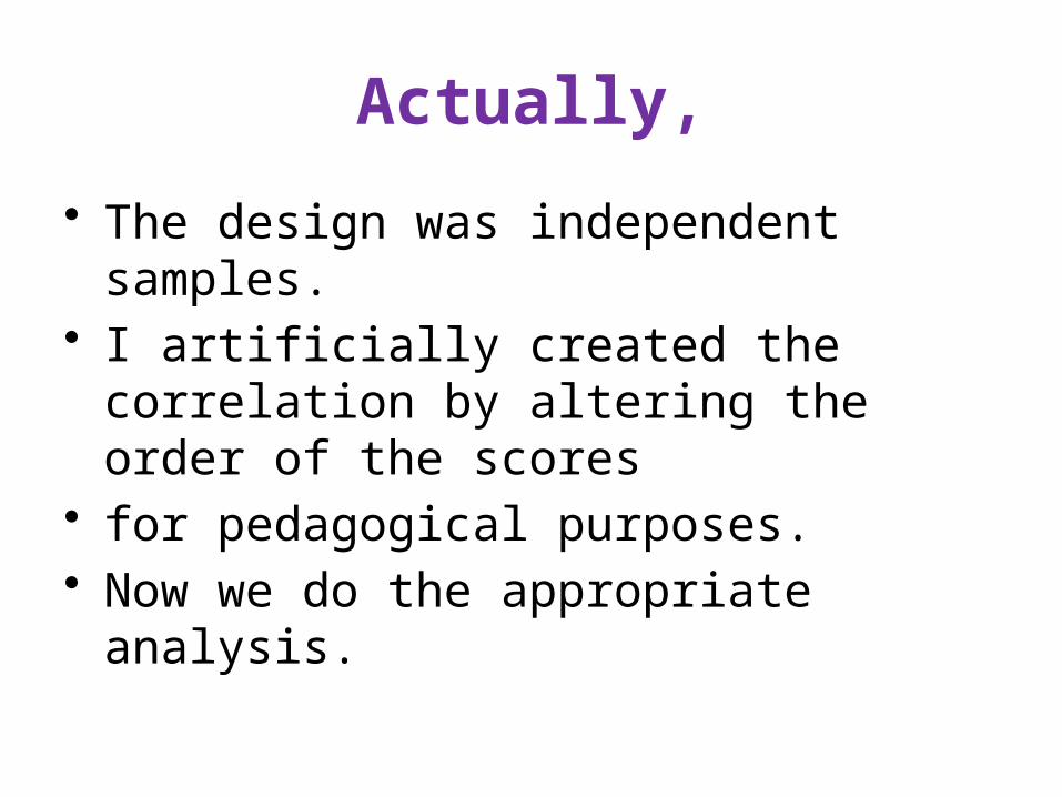
Actually,

• The design was independent samples.• I artificially created the correlation by

altering the order of the scores• for pedagogical purposes.• Now we do the appropriate analysis.

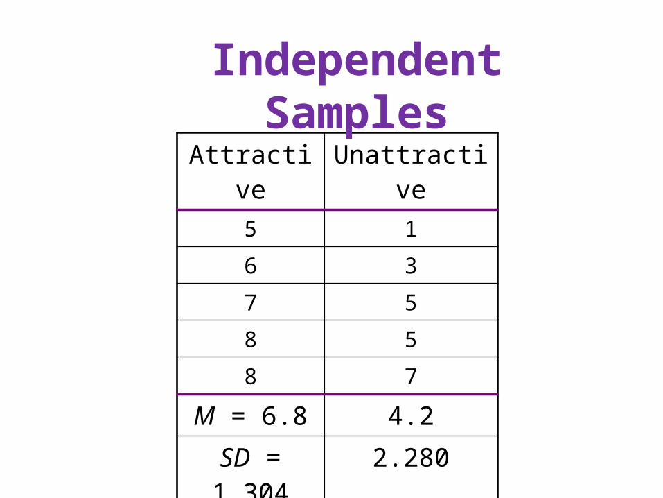
Attractive Unattractive

5 1

6 3

7 5

8 5

8 7

M = 6.8 4.2

SD = 1.304 2.280

Independent Samples

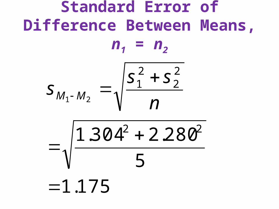
Standard Error of Difference Between Means, n1 = n2

175.15

280.2304.1 22

22

21

21

n

sss MM

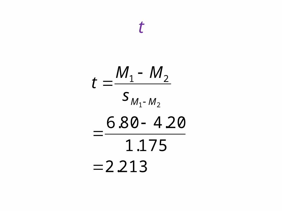
t

213.2175.1

20.480.621

21

MMs

MMt

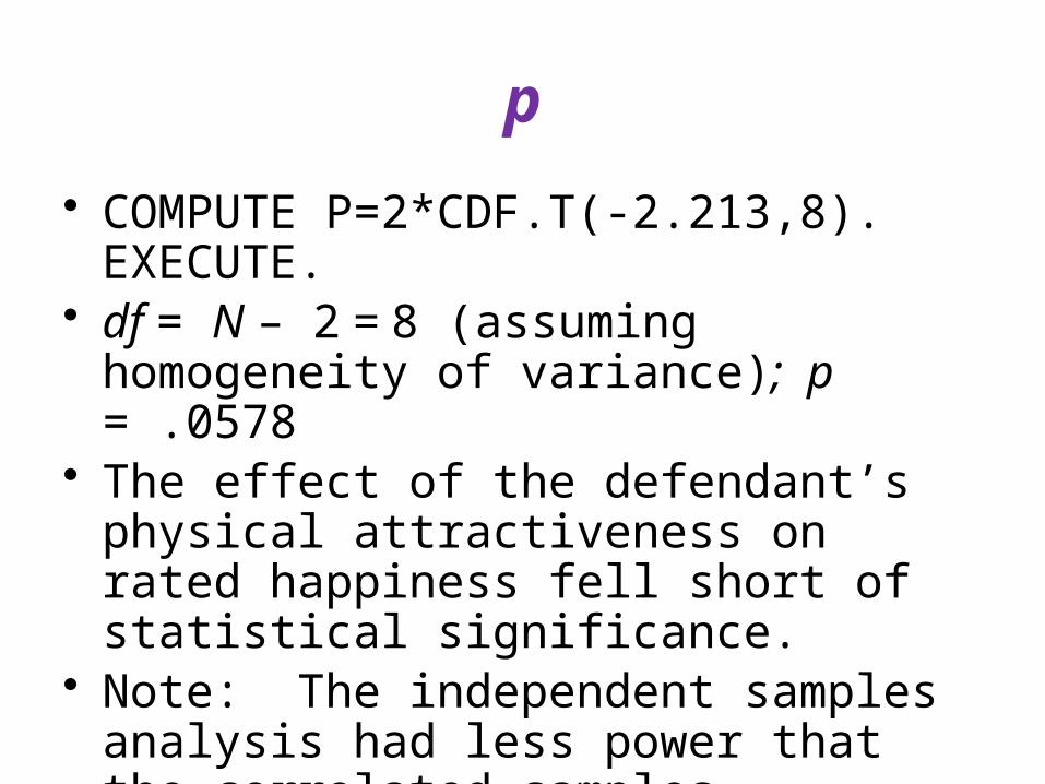
p

• COMPUTE P=2*CDF.T(-2.213,8).EXECUTE.

• df = N – 2 = 8 (assuming homogeneity of variance); p = .0578

• The effect of the defendant’s physical attractiveness on rated happiness fell short of statistical significance.

• Note: The independent samples analysis had less power that the correlated samples analysis.

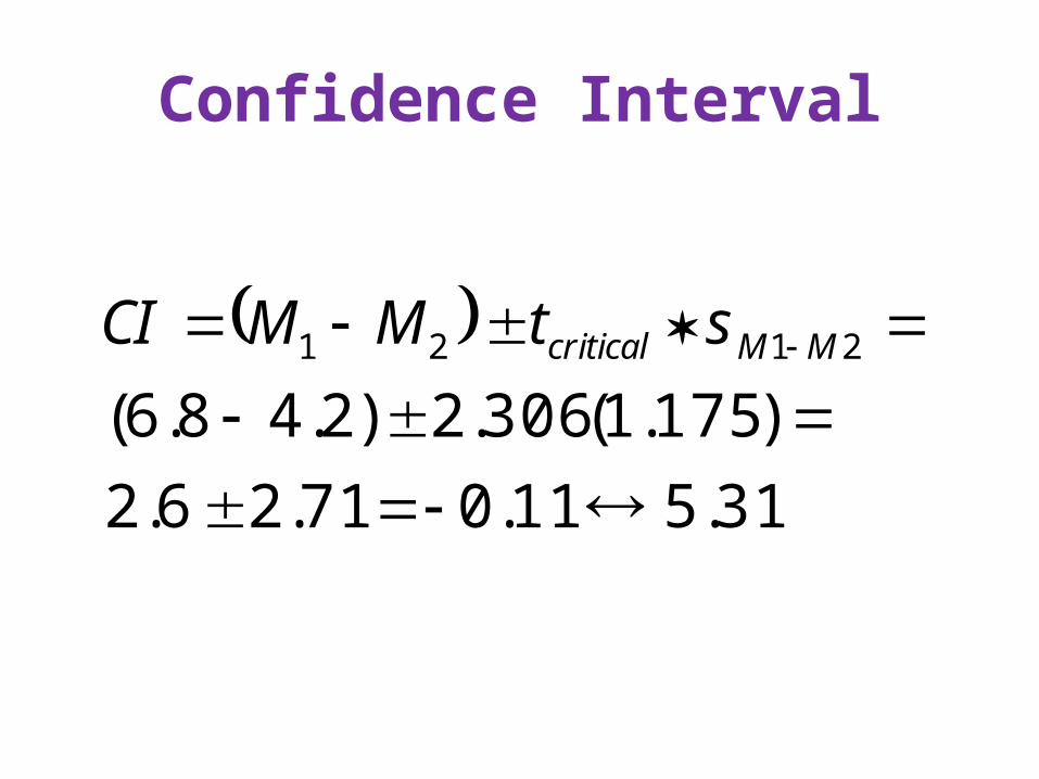
Confidence Interval

31.511.071.26.2

)175.1(306.2)2.48.6(2121

MMcritical stMMCI

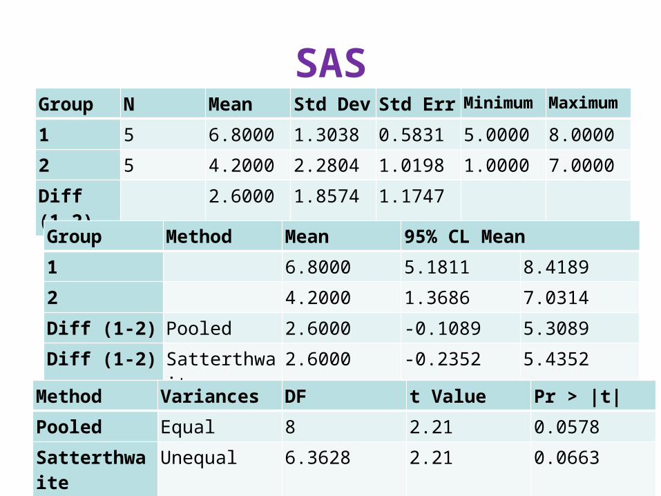
SASGroup N Mean Std Dev Std Err Minimum Maximum

1 5 6.8000 1.3038 0.5831 5.0000 8.0000

2 5 4.2000 2.2804 1.0198 1.0000 7.0000

Diff (1-2)   2.6000 1.8574 1.1747  

Group Method Mean 95% CL Mean

1   6.8000 5.1811 8.4189

2   4.2000 1.3686 7.0314

Diff (1-2) Pooled 2.6000 -0.1089 5.3089

Diff (1-2) Satterthwaite 2.6000 -0.2352 5.4352

Method Variances DF t Value Pr > |t|

Pooled Equal 8 2.21 0.0578

Satterthwaite Unequal 6.3628 2.21 0.0663

SPSS Output

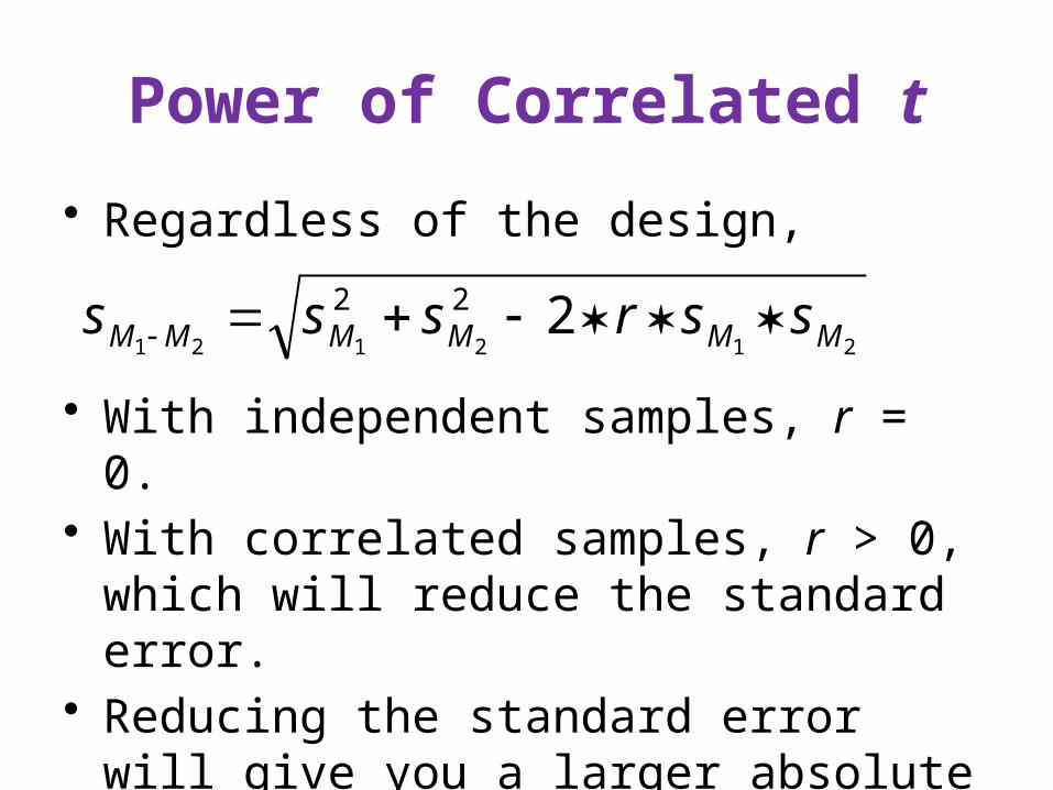
Power of Correlated t

• Regardless of the design,

• With independent samples, r = 0.• With correlated samples, r > 0, which will

reduce the standard error.• Reducing the standard error will give you a

larger absolute value of t.

2121212 22

MMMMMM ssrsss

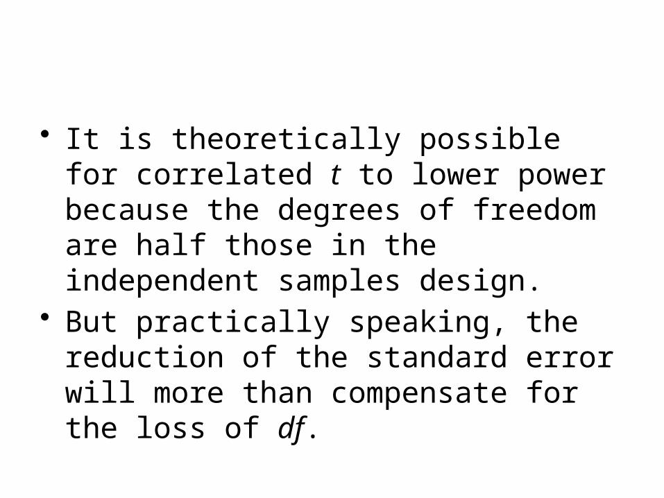
• It is theoretically possible for correlated t to lower power because the degrees of freedom are half those in the independent samples design.

• But practically speaking, the reduction of the standard error will more than compensate for the loss of df.

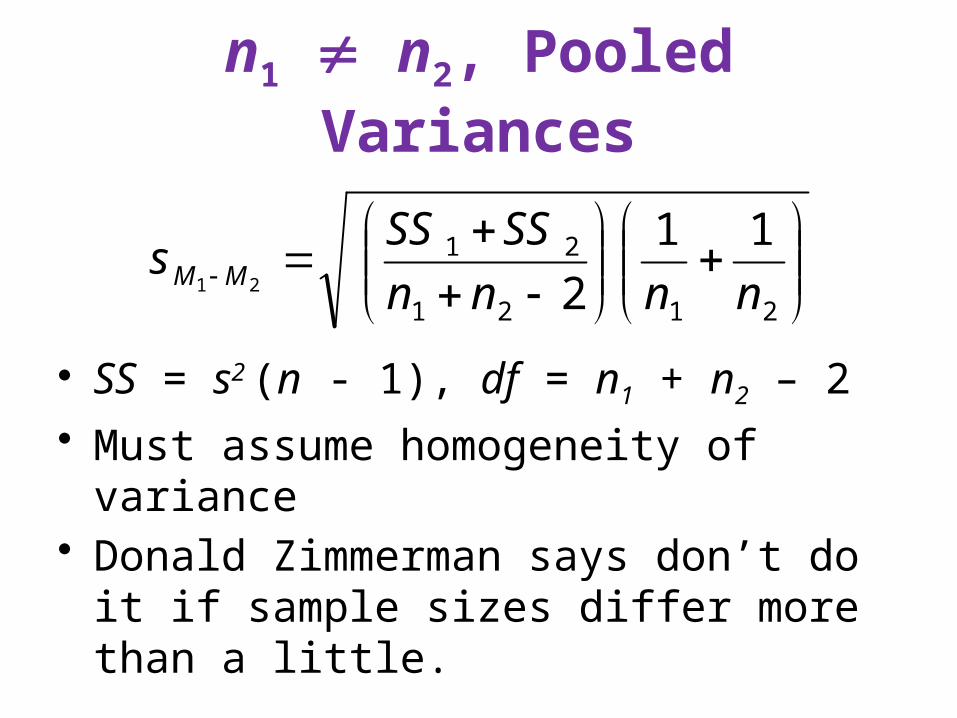
n1 n2, Pooled Variances

• SS = s2 (n - 1), df = n1 + n2 – 2

• Must assume homogeneity of variance• Donald Zimmerman says don’t do it if

sample sizes differ more than a little.

2121

21 11

2

21 nnnn

SSSSs MM

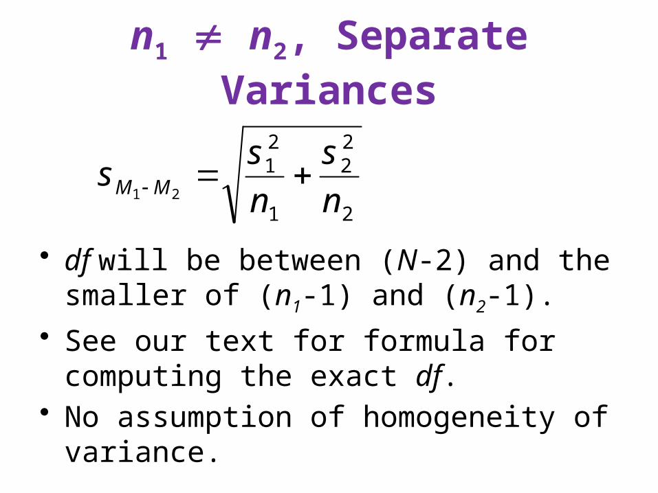
n1 n2, Separate Variances

• df will be between (N-2) and the smaller of (n1-1) and (n2-1).

• See our text for formula for computing the exact df.

• No assumption of homogeneity of variance.

2

22

1

21

21 n

s

n

ss MM

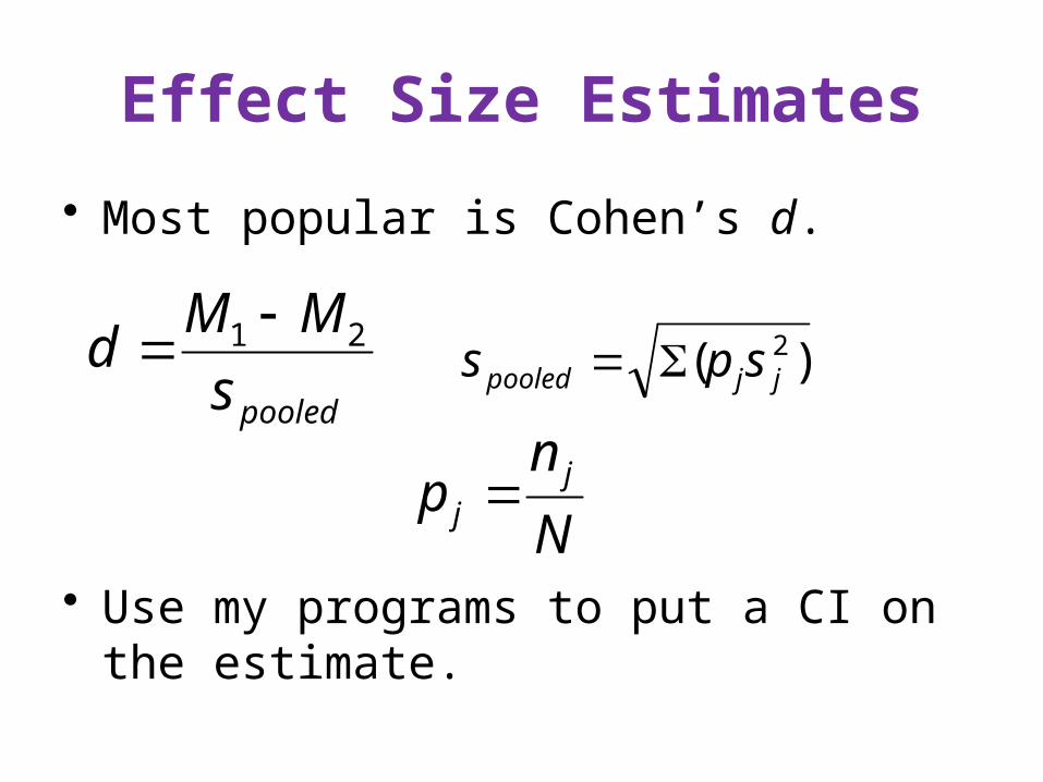
Effect Size Estimates

• Most popular is Cohen’s d.

• Use my programs to put a CI on the estimate.

pooleds

MMd 21

)( 2jjpooled sps

N

np j

j

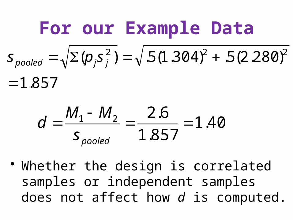
For our Example Data

• Whether the design is correlated samples or independent samples does not affect how d is computed.

857.1

)280.2(5.)304.1(5.)( 222

jjpooled sps

40.1857.1

6.221

pooleds

MMd

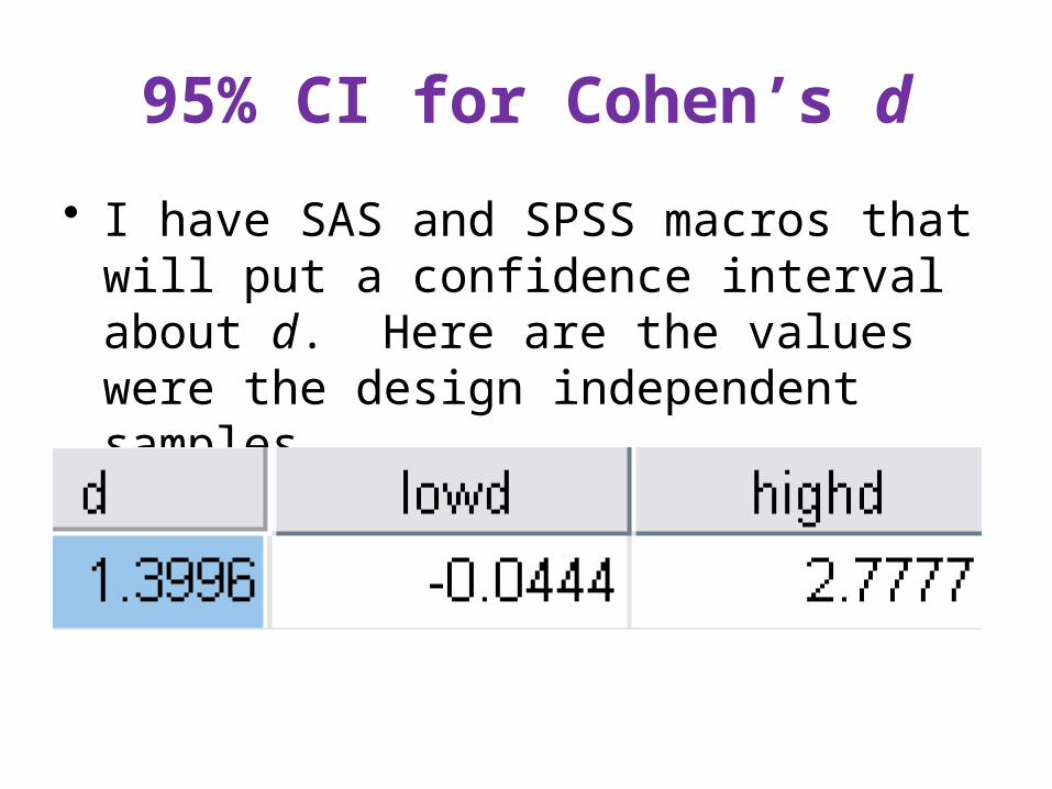
95% CI for Cohen’s d

• I have SAS and SPSS macros that will put a confidence interval about d. Here are the values were the design independent samples.

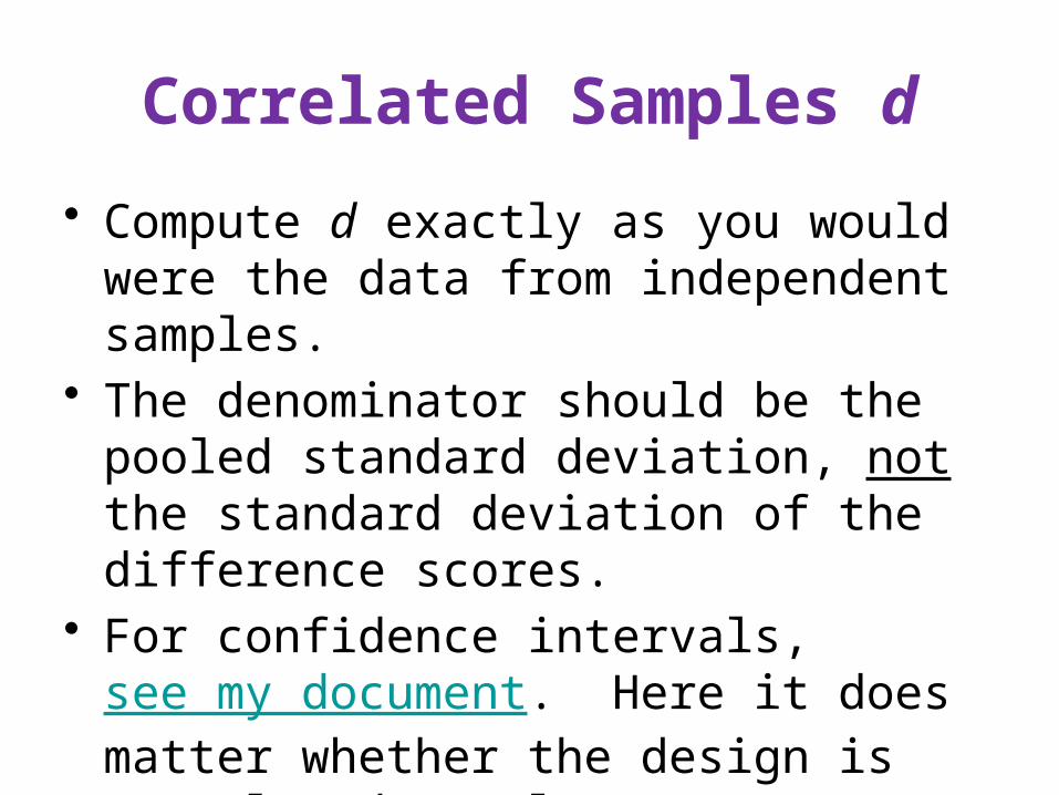
Correlated Samples d

• Compute d exactly as you would were the data from independent samples.

• The denominator should be the pooled standard deviation, not the standard deviation of the difference scores.

• For confidence intervals, see my document. Here it does matter whether the design is correlated samples or independent samples.

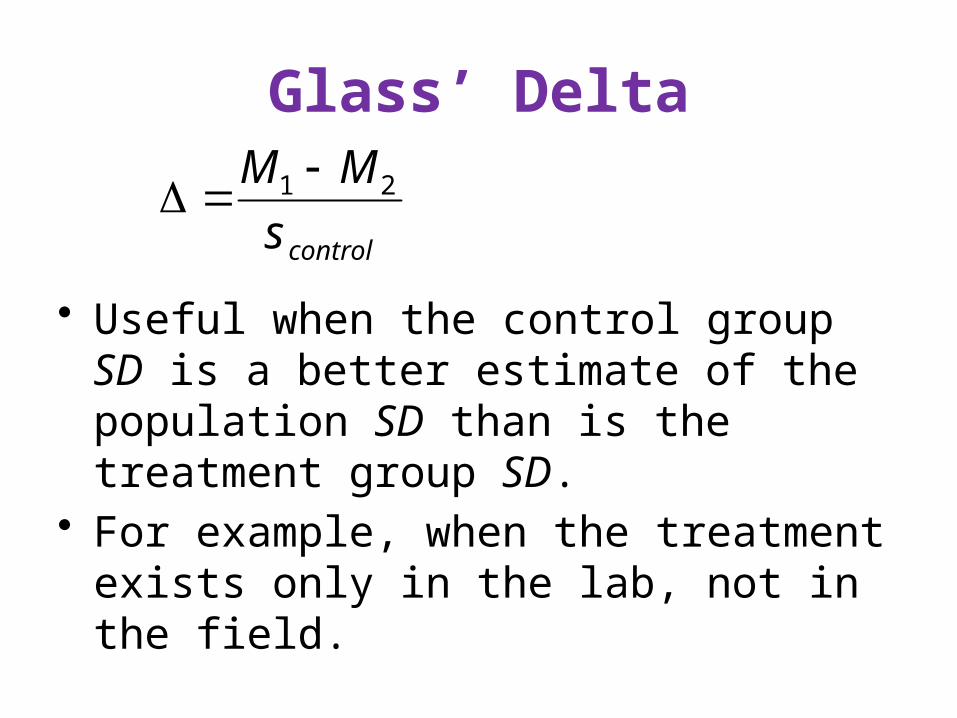
Glass’ Delta

• Useful when the control group SD is a better estimate of the population SD than is the treatment group SD.

• For example, when the treatment exists only in the lab, not in the field.

controls

MM 21

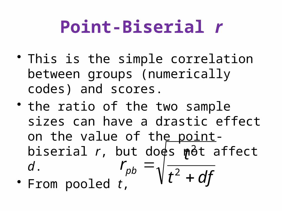
Point-Biserial r

• This is the simple correlation between groups (numerically codes) and scores.

• the ratio of the two sample sizes can have a drastic effect on the value of the point-biserial r, but does not affect d.

• From pooled t,

dft

trpb

2

2

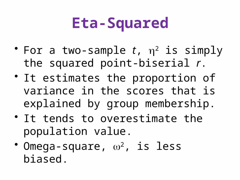
Eta-Squared

• For a two-sample t, 2 is simply the squared point-biserial r.

• It estimates the proportion of variance in the scores that is explained by group membership.

• It tends to overestimate the population value.

• Omega-square, 2, is less biased.

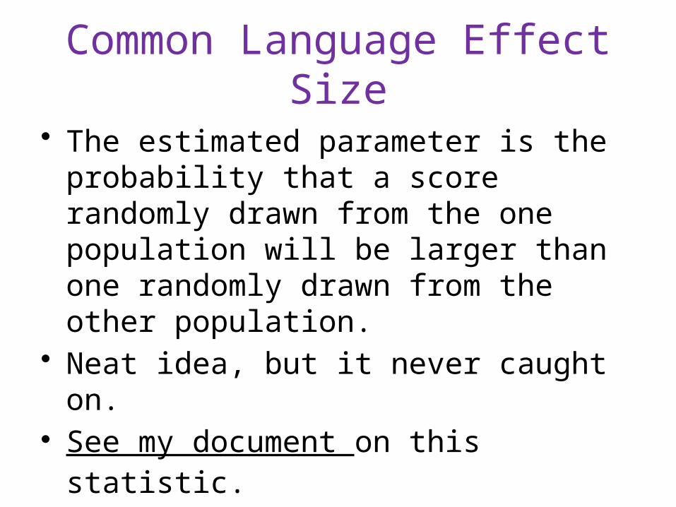
Common Language Effect Size

• The estimated parameter is the probability that a score randomly drawn from the one population will be larger than one randomly drawn from the other population.

• Neat idea, but it never caught on.• See my document on this statistic.

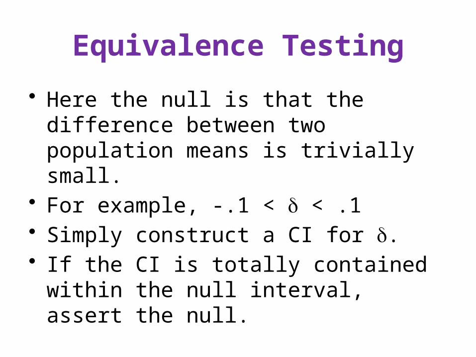
Equivalence Testing

• Here the null is that the difference between two population means is trivially small.

• For example, -.1 < < .1• Simply construct a CI for .• If the CI is totally contained within the null

interval, assert the null.

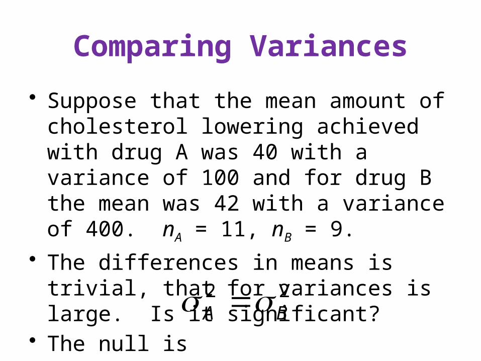
Comparing Variances

• Suppose that the mean amount of cholesterol lowering achieved with drug A was 40 with a variance of 100 and for drug B the mean was 42 with a variance of 400. nA = 11, nB = 9.

• The differences in means is trivial, that for variances is large. Is it significant?

• The null is 22BA

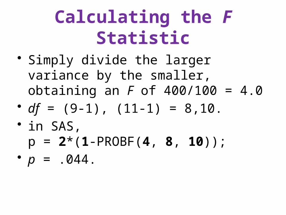
Calculating the F Statistic

• Simply divide the larger variance by the smaller, obtaining an F of 400/100 = 4.0

• df = (9-1), (11-1) = 8,10.• in SAS,

p = 2*(1-PROBF(4, 8, 10));• p = .044.

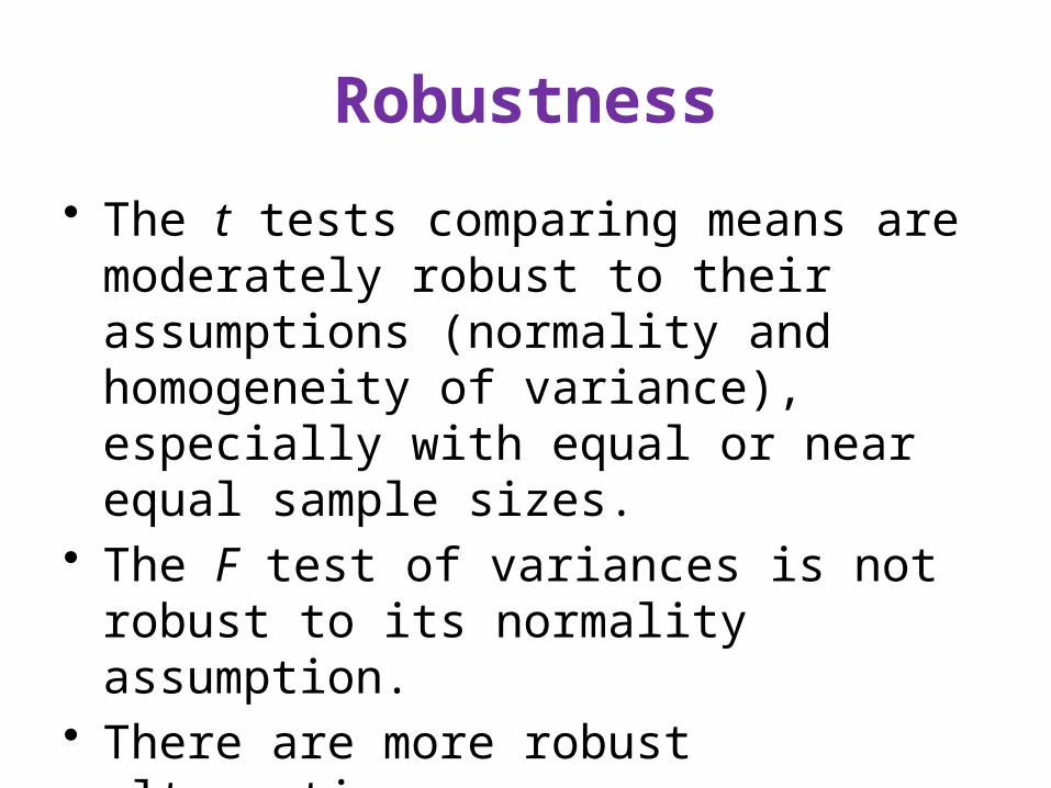
Robustness

• The t tests comparing means are moderately robust to their assumptions (normality and homogeneity of variance), especially with equal or near equal sample sizes.

• The F test of variances is not robust to its normality assumption.

• There are more robust alternatives.

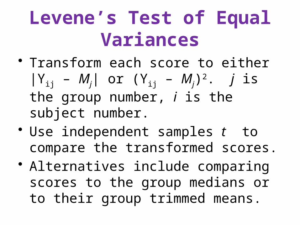
Levene’s Test of Equal Variances

• Transform each score to either |Yij – Mj| or (Yij – Mj)2. j is the group number, i is the subject number.

• Use independent samples t to compare the transformed scores.

• Alternatives include comparing scores to the group medians or to their group trimmed means.

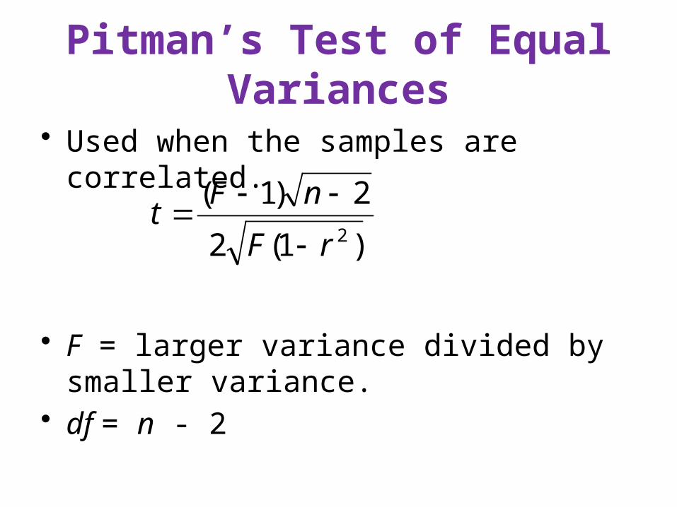
Pitman’s Test of Equal Variances

• Used when the samples are correlated.

• F = larger variance divided by smaller variance.

• df = n - 2

)1(2

2)1(2rF

nFt

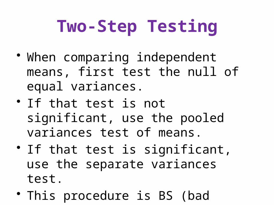
Two-Step Testing

• When comparing independent means, first test the null of equal variances.

• If that test is not significant, use the pooled variances test of means.

• If that test is significant, use the separate variances test.

• This procedure is BS (bad statistics)

Why is it BS?

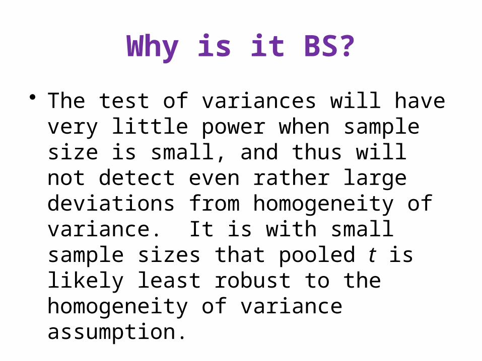
• The test of variances will have very little power when sample size is small, and thus will not detect even rather large deviations from homogeneity of variance. It is with small sample sizes that pooled t is likely least robust to the homogeneity of variance assumption.

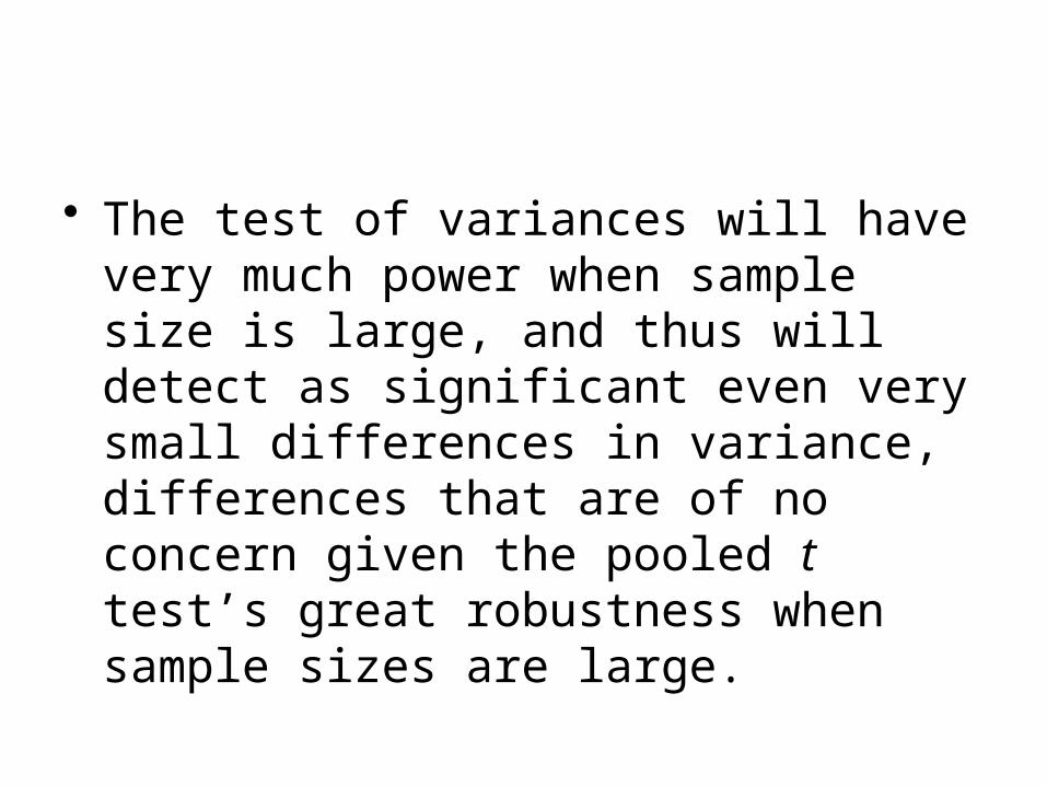
• The test of variances will have very much power when sample size is large, and thus will detect as significant even very small differences in variance, differences that are of no concern given the pooled t test’s great robustness when sample sizes are large.

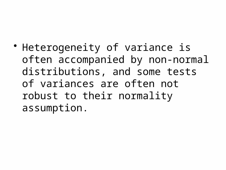
• Heterogeneity of variance is often accompanied by non-normal distributions, and some tests of variances are often not robust to their normality assumption.

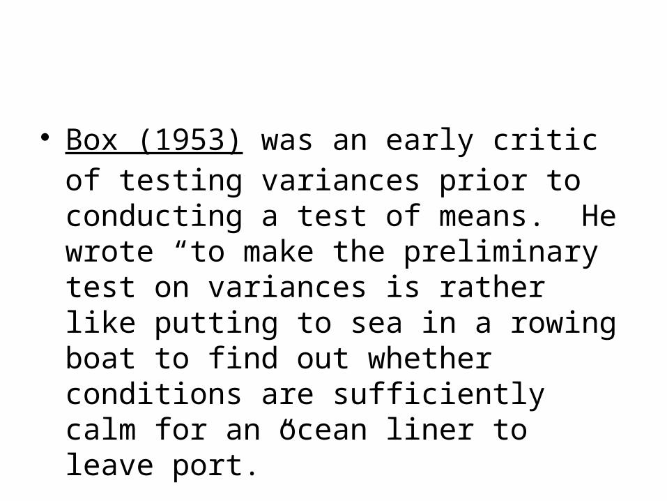
• Box (1953) was an early critic of testing variances prior to conducting a test of means. He wrote “to make the preliminary test on variances is rather like putting to sea in a rowing boat to find out whether conditions are sufficiently calm for an ocean liner to leave port.”

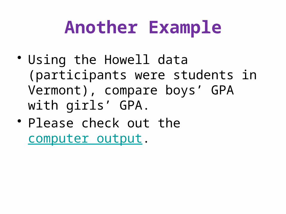
Another Example

• Using the Howell data (participants were students in Vermont), compare boys’ GPA with girls’ GPA.

• Please check out the computer output.

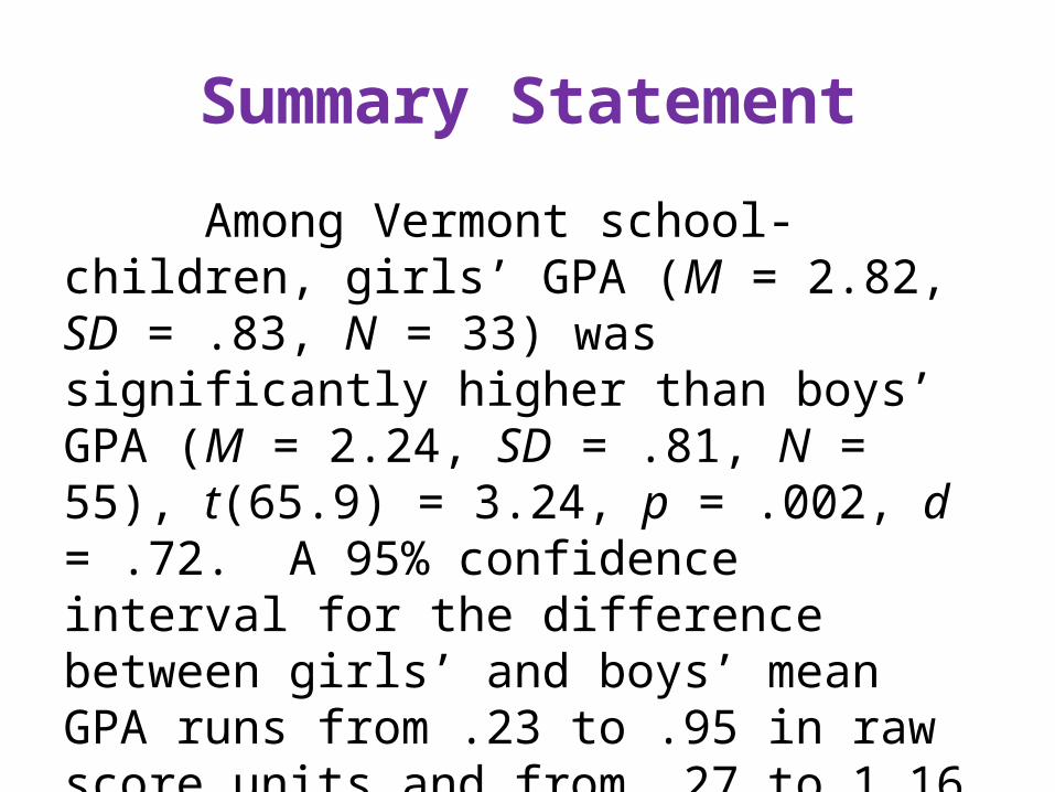
Summary Statement

Among Vermont school-children, girls’ GPA (M = 2.82, SD = .83, N = 33) was significantly higher than boys’ GPA (M = 2.24, SD = .81, N = 55), t(65.9) = 3.24, p = .002, d = .72. A 95% confidence interval for the difference between girls’ and boys’ mean GPA runs from .23 to .95 in raw score units and from .27 to 1.16 in standardized units.

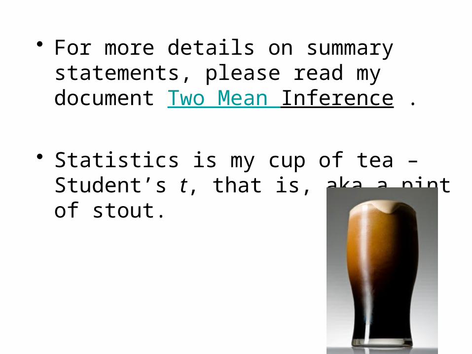
• For more details on summary statements, please read my document Two Mean Inference .

• Statistics is my cup of tea – Student’s t, that is, aka a pint of stout.