Louisiana State UniversityLSU Digital Commons

LSU Master's Theses Graduate School

5-24-2018

TWO-PHASE FLOW REGIME MAP FORLARGE DIAMETER PIPES AND HIGH-VELOCITY FLOWSMatheus Sigaki CapovillaLouisiana State University and Agricultural and Mechanical College, msigak1@lsu.edu

Follow this and additional works at: https://digitalcommons.lsu.edu/gradschool_theses

Part of the Other Mechanical Engineering Commons

This Thesis is brought to you for free and open access by the Graduate School at LSU Digital Commons. It has been accepted for inclusion in LSUMaster's Theses by an authorized graduate school editor of LSU Digital Commons. For more information, please contact gradetd@lsu.edu.

Recommended CitationSigaki Capovilla, Matheus, "TWO-PHASE FLOW REGIME MAP FOR LARGE DIAMETER PIPES AND HIGH-VELOCITYFLOWS" (2018). LSU Master's Theses. 4726.https://digitalcommons.lsu.edu/gradschool_theses/4726

TWO-PHASE FLOW REGIME MAP FOR LARGE DIAMETER PIPES ANDHIGH-VELOCITY FLOWS

A Thesis

Submitted to the Graduate Faculty of theLouisiana State University and

Agricultural and Mechanical Collegein partial fulfillment of the

requirements for the degree ofMaster of Science

in

Craft & Hawkins Petroleum Engineering Department

byMatheus Sigaki Capovilla

B.Sc., Federal University of Santa Catarina, 2015 Mechanical EngineerAugust 2018

Acknowledgments

I would like to thank my advisor, Dr. Paulo Waltrich for the opportunity given to me

to be part of this program and this project. I also want to thank him for all discussions

and help building knowledge to complete this thesis. I want to extend this acknowledgment

to my committee members, Dr. Crag Griffith, Dr. Mauricio Almeida, and Dr. Julius

Langlinais, who generously accepted a short notice invitation to be part of it. You honor

me by sharing your knowledge and experience with me.

I am very grateful for my family, for the unconditional love given to me. My parents

Ivete and Marcos, for being the most loving and supportive people in the world. My fiancée

Larissa, for always being there for me, for putting me up everytime I went down, and for

sharing the best moments of my life. My daughter Beatriz, for giving me a reason to go

forward. I also thank my siblings, Mariana and Alyson, for being part of my life.

Finally, I want to thank my friends. New friends that I made here in Baton Rouge and

old friends that I carry with me for a long time. You have made my path more enjoyable.

Special thanks for my best friend, Thiago, for helping me to keep me on my way.

Thank y’all.

ii

Table of Contents

ACKNOWLEDGMENTS . . . . . . . . . . . . . . . . . . . . . . . . . . . . . . . . . . . . . . . . . . . . . . . . . . . . . . . . . ii

LIST OF TABLES . . . . . . . . . . . . . . . . . . . . . . . . . . . . . . . . . . . . . . . . . . . . . . . . . . . . . . . . . . . . . . . iv

LIST OF FIGURES . . . . . . . . . . . . . . . . . . . . . . . . . . . . . . . . . . . . . . . . . . . . . . . . . . . . . . . . . . . . . . v

ABSTRACT . . . . . . . . . . . . . . . . . . . . . . . . . . . . . . . . . . . . . . . . . . . . . . . . . . . . . . . . . . . . . . . . . . . . . . viii

CHAPTER1 INTRODUCTION . . . . . . . . . . . . . . . . . . . . . . . . . . . . . . . . . . . . . . . . . . . . . . . . . . . . . . . . . 1

1.1 WCD rate calculation . . . . . . . . . . . . . . . . . . . . . . . . . . . . . . . . . . . . . . . . . . . . . . . . 11.2 Two-phase flow regimes in vertical pipes. . . . . . . . . . . . . . . . . . . . . . . . . . . . . . . 31.3 Influence of pipe diameter on two-phase flow regimes . . . . . . . . . . . . . . . . . . 61.4 Statement of the problem and objectives . . . . . . . . . . . . . . . . . . . . . . . . . . . . . . 9

2 LITERATURE REVIEW . . . . . . . . . . . . . . . . . . . . . . . . . . . . . . . . . . . . . . . . . . . . . . . . . . 132.1 Important parameters for two-phase flow in pipes . . . . . . . . . . . . . . . . . . . . . 132.2 Teles and Waltrich model [33] (or modified Pagan et al. [34]) . . . . . . . . . . 142.3 Pagan et al. [34] model . . . . . . . . . . . . . . . . . . . . . . . . . . . . . . . . . . . . . . . . . . . . . . . 152.4 Duns and Ros [11] model . . . . . . . . . . . . . . . . . . . . . . . . . . . . . . . . . . . . . . . . . . . . . 192.5 Flow regime maps . . . . . . . . . . . . . . . . . . . . . . . . . . . . . . . . . . . . . . . . . . . . . . . . . . . . 262.6 Critical flow transition . . . . . . . . . . . . . . . . . . . . . . . . . . . . . . . . . . . . . . . . . . . . . . . . 41

3 EXPERIMENTAL DATA . . . . . . . . . . . . . . . . . . . . . . . . . . . . . . . . . . . . . . . . . . . . . . . . . . 453.1 Experimental data from literature . . . . . . . . . . . . . . . . . . . . . . . . . . . . . . . . . . . . . 453.2 LSU experiments from Waltrich et al. [9] . . . . . . . . . . . . . . . . . . . . . . . . . . . . . . 48

4 RESULTS AND DISCUSSIONS . . . . . . . . . . . . . . . . . . . . . . . . . . . . . . . . . . . . . . . . . . . 524.1 Evaluation of current flow regime maps . . . . . . . . . . . . . . . . . . . . . . . . . . . . . . . 524.2 Computational Fluid Dynamic (CFD) observations . . . . . . . . . . . . . . . . . . . . 574.3 Flow regime map validation . . . . . . . . . . . . . . . . . . . . . . . . . . . . . . . . . . . . . . . . . . . 614.4 Water and air – Data from Waltrich et al. [9] . . . . . . . . . . . . . . . . . . . . . . . . . 654.5 Oil and gas – Data from Asheim [65] . . . . . . . . . . . . . . . . . . . . . . . . . . . . . . . . . . 704.6 Critical flow . . . . . . . . . . . . . . . . . . . . . . . . . . . . . . . . . . . . . . . . . . . . . . . . . . . . . . . . . . 71

5 CONCLUSIONS AND FUTURE WORKS . . . . . . . . . . . . . . . . . . . . . . . . . . . . . . . . . 805.1 Summary and conclusions . . . . . . . . . . . . . . . . . . . . . . . . . . . . . . . . . . . . . . . . . . . . 805.2 Recommendations for future work . . . . . . . . . . . . . . . . . . . . . . . . . . . . . . . . . . . . . 82

REFERENCES . . . . . . . . . . . . . . . . . . . . . . . . . . . . . . . . . . . . . . . . . . . . . . . . . . . . . . . . . . . . . . . . . . . . 84

APPENDIX: DATA FROM LSU EXPERIMENTS . . . . . . . . . . . . . . . . . . . . . . . . . . . . . . . . . 90

VITA . . . . . . . . . . . . . . . . . . . . . . . . . . . . . . . . . . . . . . . . . . . . . . . . . . . . . . . . . . . . . . . . . . . . . . . . . . . . . 94

iii

List of Tables

2.1 Summary of pros and cons of the flow regime maps consideredin this study. . . . . . . . . . . . . . . . . . . . . . . . . . . . . . . . . . . . . . . . . . . . . . . . . . . . . . . . . . . . . . . . . 32

3.1 Literature review on flow regime characterization of verticalupward two-phase flows in large diameter pipes. . . . . . . . . . . . . . . . . . . . . . . . . . . . . . . 46

3.2 Field data that provide information of pressure gradient. . . . . . . . . . . . . . . . . . . . . . 48

4.1 Analysis of conforming and non-conforming experimental datapoints for different transition boundaries of different flow regime maps. . . . . . . . 55

4.2 Experimental data considered for calculation of pressure gradientwith CFD on Waltrich et al. [9]. . . . . . . . . . . . . . . . . . . . . . . . . . . . . . . . . . . . . . . . . . . . . . 57

4.3 Comparative of calculated absolute error with the model proposedin this work and the model by Teles and Waltrich for groups ofdata points with different diameters and similar conditions. . . . . . . . . . . . . . . . . . . 67

4.4 Natural gas composition considered for the calculation of thecritical mixture velocity. . . . . . . . . . . . . . . . . . . . . . . . . . . . . . . . . . . . . . . . . . . . . . . . . . . . . . 71

A.1 Experimental data generated at LSU. . . . . . . . . . . . . . . . . . . . . . . . . . . . . . . . . . . . . . . . . 90

iv

List of Figures

1.1 Elements required for the prediction of production rates . . . . . . . . . . . . . . . . . . . . . . 2

1.2 Simplified diagram for WCD rate calculation. . . . . . . . . . . . . . . . . . . . . . . . . . . . . . . . . 4

1.3 Visual representation of the four central flow regimes duringupward flow in a vertical pipe . . . . . . . . . . . . . . . . . . . . . . . . . . . . . . . . . . . . . . . . . . . . . . . 5

1.4 Flow regime maps: (a) Aziz et al. [17] empirical map, and (b)Taitel et al. [18]. . . . . . . . . . . . . . . . . . . . . . . . . . . . . . . . . . . . . . . . . . . . . . . . . . . . . . . . . . . . . 6

1.5 Force balance sustained in a Taylor bubble. . . . . . . . . . . . . . . . . . . . . . . . . . . . . . . . . . . 7

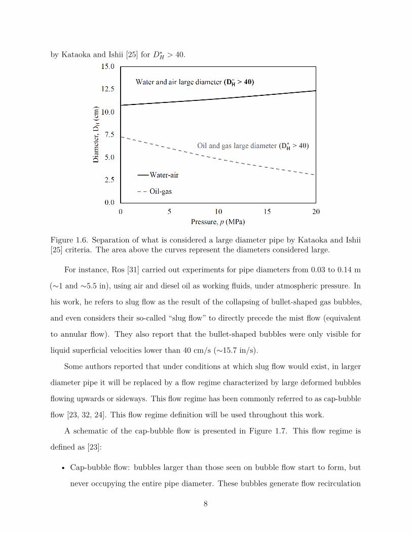
1.6 Separation of what is considered a large diameter pipe by Kataokaand Ishii [25] criteria. The area above the curves represent thediameters considered large. . . . . . . . . . . . . . . . . . . . . . . . . . . . . . . . . . . . . . . . . . . . . . . . . . . 8

1.7 Cap-bubble flow, adapted from Ohnuki and Akimoto [23]. . . . . . . . . . . . . . . . . . . . . 9

1.8 Flow regime progression with increasing height along the wellboreand estimated pressure profiles considering different flow regimesalong the flow. . . . . . . . . . . . . . . . . . . . . . . . . . . . . . . . . . . . . . . . . . . . . . . . . . . . . . . . . . . . . . . 11

2.1 Teles and Waltrich model workflow [33]. . . . . . . . . . . . . . . . . . . . . . . . . . . . . . . . . . . . . . 15

2.2 Average Absolute Error of pressure gradient in % for varioustwo-phase flow pressure gradient models . . . . . . . . . . . . . . . . . . . . . . . . . . . . . . . . . . . . . 16

2.3 Force balance for a pipe segment for churn and annular flow regimes . . . . . . . . . . 16

2.4 Empirical flow regime map by Duns and Ros [11] . . . . . . . . . . . . . . . . . . . . . . . . . . . . 20

2.5 L1 and L2 factors versus dimensionless diameter number (𝑁𝑑) [11]. . . . . . . . . . . . 22

2.6 F-factor numbers for Region I, based on the dimensionless vis-cosity number 𝑁𝑙 [11]. . . . . . . . . . . . . . . . . . . . . . . . . . . . . . . . . . . . . . . . . . . . . . . . . . . . . . . . 24

2.7 F-factor numbers for Region II, based on the dimensionlessviscosity number 𝑁𝑙 [11]. . . . . . . . . . . . . . . . . . . . . . . . . . . . . . . . . . . . . . . . . . . . . . . . . . . . . 24

2.8 Dimensionless f1 factor as a function of Re and relative roughness𝜀/D [11]. . . . . . . . . . . . . . . . . . . . . . . . . . . . . . . . . . . . . . . . . . . . . . . . . . . . . . . . . . . . . . . . . . . . . 25

2.9 Dimensionless 𝑓2 factor as a function of the group 𝑓1𝑅𝑁2/3𝑑 [11]. . . . . . . . . . . . . . . 26

2.10 Correlation for the film-thickness 𝜀 under mist-flow conditions [11]. . . . . . . . . . . . 27

v

2.11 Representation of Wu et al. [16] method to evaluate accuracy offlow regime map. . . . . . . . . . . . . . . . . . . . . . . . . . . . . . . . . . . . . . . . . . . . . . . . . . . . . . . . . . . . . 28

2.12 Comparative between different flow regime transitions modelsand experimental observations for pipe diameters between 12.3and 67 mm [16]. . . . . . . . . . . . . . . . . . . . . . . . . . . . . . . . . . . . . . . . . . . . . . . . . . . . . . . . . . . . . . 29

2.13 Experimental results reported by Beck et al. [61] for experimentaltwo-phase flow in a pipe with a 0.12 m diameter and Wallis [41]calculated for their experimental conditions. . . . . . . . . . . . . . . . . . . . . . . . . . . . . . . . . . 44

3.1 Different flow regimes for vertical upward two-phase flows inlarge diameter pipes of the experimental data considered in this study.. . . . . . . . 47

3.2 Literature review on works with characterized flow regimes forvertical upward two-phase flows in large diameter pipes. . . . . . . . . . . . . . . . . . . . . . . 48

3.3 Schematic diagram of the experimental apparatus and picturesof the test sections . . . . . . . . . . . . . . . . . . . . . . . . . . . . . . . . . . . . . . . . . . . . . . . . . . . . . . . . . . 49

3.4 LSU data points with the final visual observation of flow regimes. . . . . . . . . . . . . 50

3.5 Superficial fluid velocity ranges for the data considered in thiswork, including data produced at LSU. . . . . . . . . . . . . . . . . . . . . . . . . . . . . . . . . . . . . . . 51

4.1 Flow regimes of 695 experimental data points plotted againsttransition curves of flow regime maps by Duns and Ros [11], Azizet al. [17], Mishima and Ishii [19], and Schlegel et al. [32]. . . . . . . . . . . . . . . . . . . . . 53

4.2 Slug flow development depending on pipe diameter. . . . . . . . . . . . . . . . . . . . . . . . . . . 56

4.3 Data points evaluated with CFD on Waltrich et al. [9] workplotted on newly proposed flow regime map. . . . . . . . . . . . . . . . . . . . . . . . . . . . . . . . . . 58

4.4 CFD visualization of experimental data points reported by Aliand Yeung [24] presented in Table 4.2. . . . . . . . . . . . . . . . . . . . . . . . . . . . . . . . . . . . . . . . 59

4.5 CFD visualization of experimental data points reported by Wal-trich et al. [9] presented in Table 4.2. . . . . . . . . . . . . . . . . . . . . . . . . . . . . . . . . . . . . . . . . 59

4.6 Flow regime observation for Test 1 from Waltrich et al. [9] conditions. . . . . . . . . 60

4.7 Modified diagram proposed by this work for the model developedby Teles and Waltrich. . . . . . . . . . . . . . . . . . . . . . . . . . . . . . . . . . . . . . . . . . . . . . . . . . . . . . . 62

vi

4.8 Proposed flow regime maps with all experimental data pointsproduced at LSU, classified into the four flow regimes consideredin this work, plus the data points without identified flow regimes . . . . . . . . . . . . . 66

4.9 Comparison of errors in dp/dz calculation for the experimentaldata predicted to be in cap-bubble flow, simulated with different models. . . . . . 67

4.10 Comparison of errors in dp/dz calculation for the experimentaldata predicted to be in be cap-bubble flow, simulated withdifferent models. Only data without identified flow regimes fromLSU were considered. . . . . . . . . . . . . . . . . . . . . . . . . . . . . . . . . . . . . . . . . . . . . . . . . . . . . . . . . 69

4.11 Comparison of pressure gradient prediction accuracy betweendifferent models for conditions predicted as cap-bubble flow inthe newly proposed flow regime map . . . . . . . . . . . . . . . . . . . . . . . . . . . . . . . . . . . . . . . . . 69

4.12 Comparison of errors in pressure gradient calculation for the datereported by Asheim [65], simulated with the model by Teles andWaltrich and with the modification proposed in this work. . . . . . . . . . . . . . . . . . . . . 70

4.13 Comparative of the effect of pressure on the critical mixturevelocity for mixtures of (a) black oil and natural gas, and (b)water and air. . . . . . . . . . . . . . . . . . . . . . . . . . . . . . . . . . . . . . . . . . . . . . . . . . . . . . . . . . . . . . . . 72

4.14 Example calculation of an equivalent property for a two-phasemixture being assumed as a homogeneous fluid. . . . . . . . . . . . . . . . . . . . . . . . . . . . . . . 73

4.15 Mixture critical velocity and void fraction relation for black oiland natural gas, and water and air mixtures. The consideredconditions are a 9.62 MPa pressure and 15 ∘C temperature. . . . . . . . . . . . . . . . . . . 75

4.16 Representative model well in the Gulf of Mexico region during ablowout and the critical flow transition boundary considering asurface and sub-sea release. . . . . . . . . . . . . . . . . . . . . . . . . . . . . . . . . . . . . . . . . . . . . . . . . . . 76

4.17 Surface release data points by Zulqarnain [3] plotted with Wallis[41] critical flow transition criteria and its modification by Becket al. [61] . . . . . . . . . . . . . . . . . . . . . . . . . . . . . . . . . . . . . . . . . . . . . . . . . . . . . . . . . . . . . . . . . . . 77

4.18 Proposed hybrid flow regime map with critical flow transition boundary. . . . . . . 78

4.19 Flow regime maps by (a) Mishima and Ishii [19]; and (b) Schelegelet al. [32]. . . . . . . . . . . . . . . . . . . . . . . . . . . . . . . . . . . . . . . . . . . . . . . . . . . . . . . . . . . . . . . . . . . . 79

vii

Abstract

Worst-case-discharge (WCD) calculations are a pre-requisite for any new well to be

drilled in the Gulf of Mexico (GoM). Models that were mostly developed for production

rates prediction are currently used to calculate the WCD rate. These models were mostly

developed for pipe diameters and flow velocities much smaller than those expected during

WCD events. Therefore, these models may be miscalculating WCD rates.

This study aims at analyzing one of possible sources of errors in these models: the flow

regime maps. The influence of diameter change on flow regimes is discussed. A thorough

literature review is carried out for different flow regime maps. These maps are tested against

experimental data to define the best flow transition models. A new map with the best

transition models is presented. A new flow regime is added to the map, replacing the

slug flow: cap-bubble flow. This map is tested with numerical simulation to reproduce

experimental and field conditions. In order to do this, a modification to a numerical model

is proposed, coupling the new map to the model and the calculation of the pressure gradient

when in cap-bubble flow. The results show improvement over the standard map.

Critical flow regime models and its existence during WCD are discussed. It is observed

that it will be unlikely for the flow to be in critical conditions during a sub-sea release of

deepwater wells, but it is possible that it happens during surface releases.

A series of future works is recommended.

viii

Chapter 1Introduction

Vertical gas-liquid two-phase upward flow can be found in a wide range of pipe diameters

in many industrial applications such as in offshore risers in the petroleum industry, cooling

towers in the nuclear industry, and in gas-liquid pipelines in petrochemical plants. A typical

example of a problem that requires the knowledge about vertical two-phase upward flow

in pipes is in worst-case-discharge (WCD) calculations. The Bureau of Ocean Energy

Management (BOEM) defined the WCD rate as the maximum uncontrollable daily flow

rate of hydrocarbons through an unobstructed wellbore [1]. In other words, WCD rate is

the maximum expected flow rate during a blowout, considering the absence of an in-hole

drillstring and a wellhead.

Recent new regulations require from any operator company planning to drill new wells

in the Gulf of Mexico the submission of an Oil Spill Response Plan (OSRP), which should

include a contingency plan to be followed in case of a blowout [2]. An estimative of WCD

rate is required in this type of report. Two primary characteristics are expected during WCD

events: high flow rates and large-diameter long-vertical pipes. Later OSRP reports present

WCD flow rates in the Gulf of Mexico ranging from 0.63 to 75,678 m3/day (4 to 476,000

bbl/day), averaging for the Central Gulf of Mexico about 9,540 m3/day (60,000 bbl/day),

and for the Western Gulf of Mexico about 2,225 m3/day (14,000 bbl/day) [2]. Furthermore,

Zulqarnain [3] described a representative well configuration based on statistical analysis

about the current wells in the Gulf of Mexico, in which the predominant pipe diameter is

about 0.25 m (∼10 in).

1.1 WCD rate calculation

In 2015, SPE released a technical report proposing a methodology for the calculation

of WCD rates [1], based on a technique known as nodal analysis (see Figure 1.1), used

in production rates estimation. The nodal analysis approach is dependent on reservoir

characteristics and the pressure drop along the flowing wellbore. Figure 1.1.a shows a

1

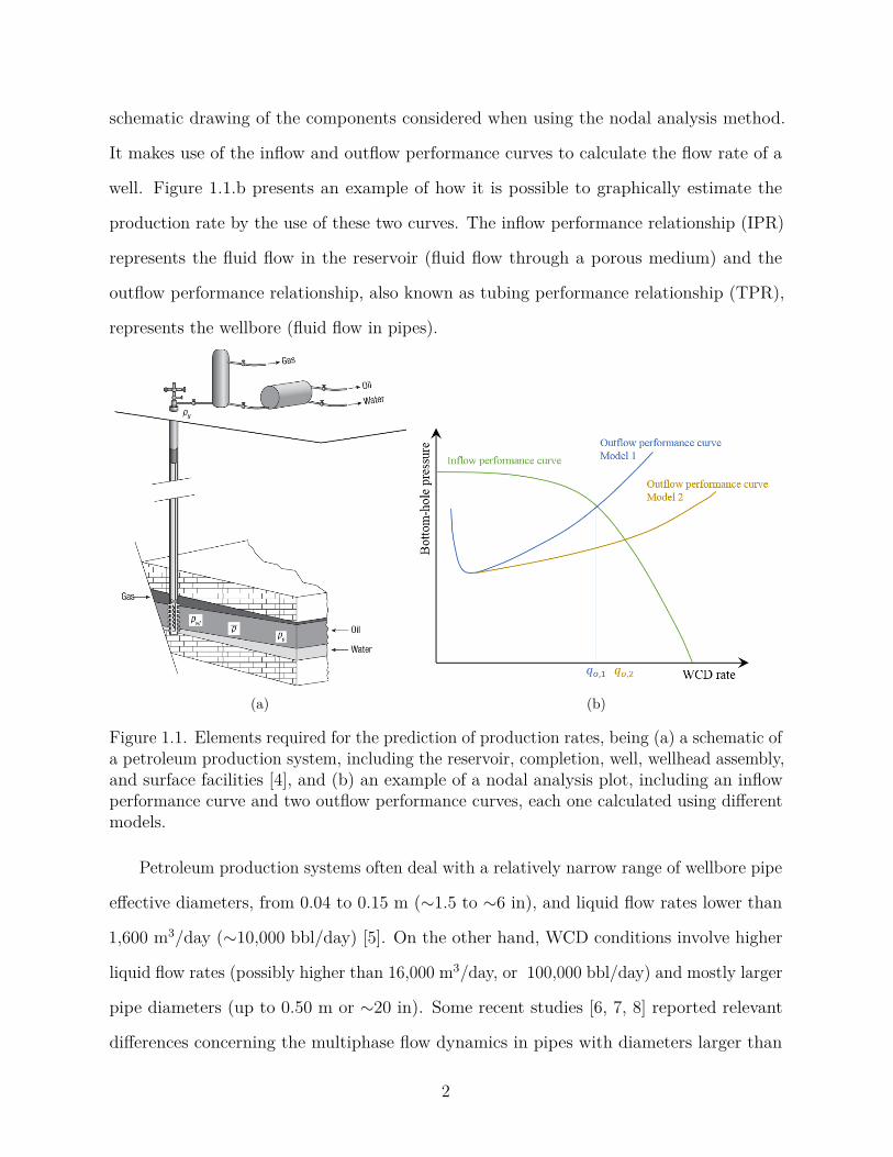
schematic drawing of the components considered when using the nodal analysis method.

It makes use of the inflow and outflow performance curves to calculate the flow rate of a

well. Figure 1.1.b presents an example of how it is possible to graphically estimate the

production rate by the use of these two curves. The inflow performance relationship (IPR)

represents the fluid flow in the reservoir (fluid flow through a porous medium) and the

outflow performance relationship, also known as tubing performance relationship (TPR),

represents the wellbore (fluid flow in pipes).

(a) (b)

Figure 1.1. Elements required for the prediction of production rates, being (a) a schematic ofa petroleum production system, including the reservoir, completion, well, wellhead assembly,and surface facilities [4], and (b) an example of a nodal analysis plot, including an inflowperformance curve and two outflow performance curves, each one calculated using differentmodels.

Petroleum production systems often deal with a relatively narrow range of wellbore pipe

effective diameters, from 0.04 to 0.15 m (∼1.5 to ∼6 in), and liquid flow rates lower than

1,600 m3/day (∼10,000 bbl/day) [5]. On the other hand, WCD conditions involve higher

liquid flow rates (possibly higher than 16,000 m3/day, or 100,000 bbl/day) and mostly larger

pipe diameters (up to 0.50 m or ∼20 in). Some recent studies [6, 7, 8] reported relevant

differences concerning the multiphase flow dynamics in pipes with diameters larger than

2

0.10 m (∼4 in). When not considered, flow behavior for larger diameters can be translated

into erroneous predictions of pressure drops for the wellbore. These errors will appear as

differences in the flow rate calculations, as shown in Figure 1.1.b. Thus, as the wellbore

models (i.e., TPRs) used for WCD rate calculations were developed to calculate the outflow

performance curves based on production conditions (being tested and verified only for lower

rates and smaller diameters) the reliability of these models is still questionable [1].

Waltrich et al. [9] tested several different models used in WCD calculations against

experimental pressure gradient data for vertical upward two-phase flow in large diameter

pipes. Most models showed errors higher than 50% for the pressure gradient predictions.

Thus, tracking the elements that could be driving those models to this high levels of errors

is essential.

The present work will focus on one of the elements of wellbore flow modeling that may

be causing the errors reported by Waltrich et al. [9]. One of the sources of the errors is

possibly related to the flow regime prediction. Figure 1.2 presents a simplified diagram for

the calculation of WCD rates. As shown in the figure, flow regime predictions can have a

direct impact on WCD rate estimation.

1.2 Two-phase flow regimes in vertical pipes

The definition of flow regimes (sometimes called flow patterns) is an essential part

of two-phase flow analysis [10]. Many multiphase flow models are flow regime dependent

[11, 12, 13, 14]. Two-phase flow regime is described by Shoham [10] as a group of similar

geometrical distribution of the gas and liquid phases in a pipe during a two-phase flow.

Although it is possible to find several different vertical upward two-phase flow regimes

characterizations throughout the literature (depending on the author), four flow regimes

are most commonly defined, as shown in Figure 1.3.

These flow regimes can be described as [4, 15, 10]:

• Bubble flow: continuous liquid-phase upward stream, with dispersed gas phase flowing

upward in the form of discrete bubbles.

3

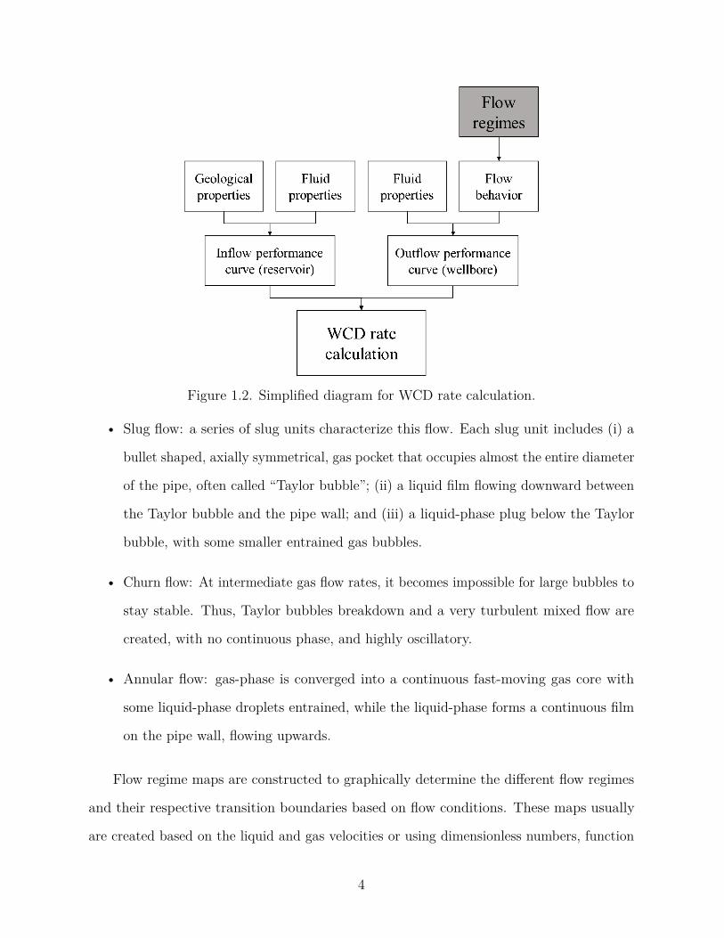
Figure 1.2. Simplified diagram for WCD rate calculation.

• Slug flow: a series of slug units characterize this flow. Each slug unit includes (i) a

bullet shaped, axially symmetrical, gas pocket that occupies almost the entire diameter

of the pipe, often called “Taylor bubble”; (ii) a liquid film flowing downward between

the Taylor bubble and the pipe wall; and (iii) a liquid-phase plug below the Taylor

bubble, with some smaller entrained gas bubbles.

• Churn flow: At intermediate gas flow rates, it becomes impossible for large bubbles to

stay stable. Thus, Taylor bubbles breakdown and a very turbulent mixed flow are

created, with no continuous phase, and highly oscillatory.

• Annular flow: gas-phase is converged into a continuous fast-moving gas core with

some liquid-phase droplets entrained, while the liquid-phase forms a continuous film

on the pipe wall, flowing upwards.

Flow regime maps are constructed to graphically determine the different flow regimes

and their respective transition boundaries based on flow conditions. These maps usually

are created based on the liquid and gas velocities or using dimensionless numbers, function

4

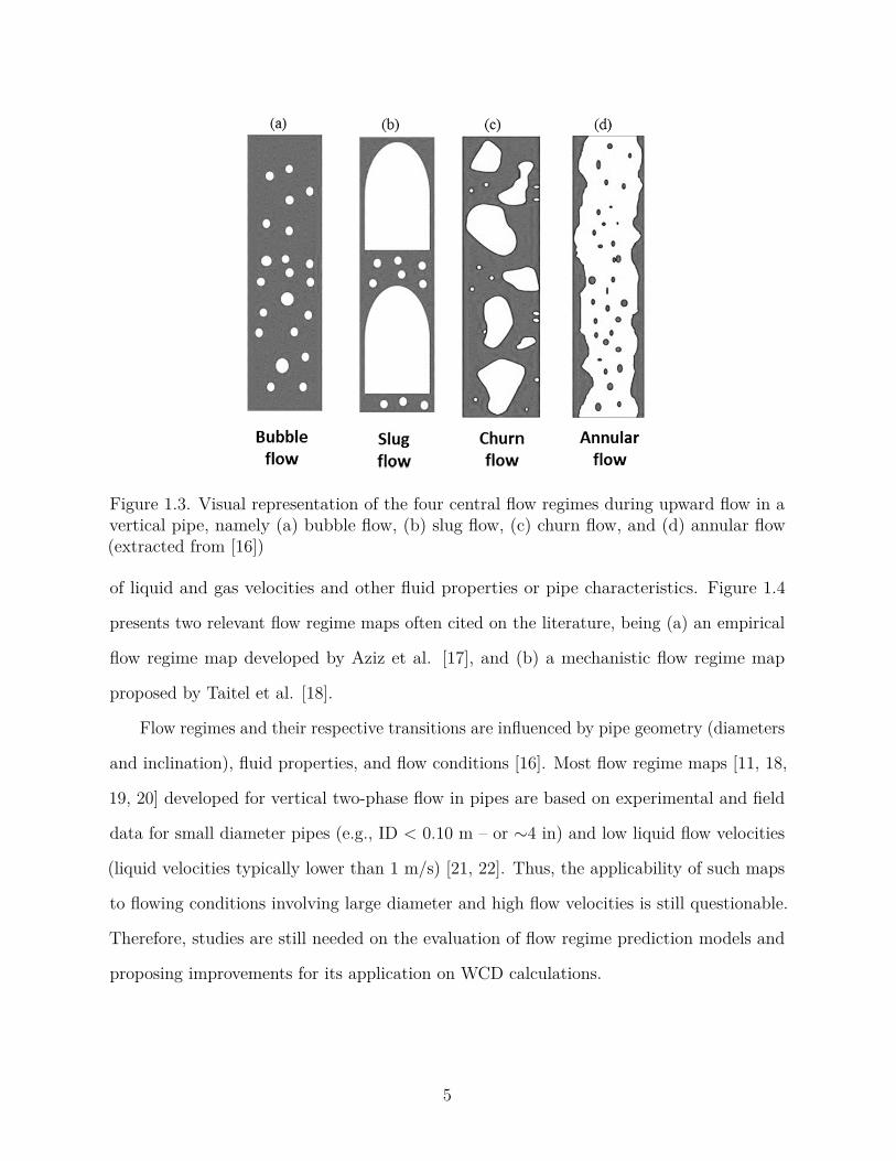
Figure 1.3. Visual representation of the four central flow regimes during upward flow in avertical pipe, namely (a) bubble flow, (b) slug flow, (c) churn flow, and (d) annular flow(extracted from [16])

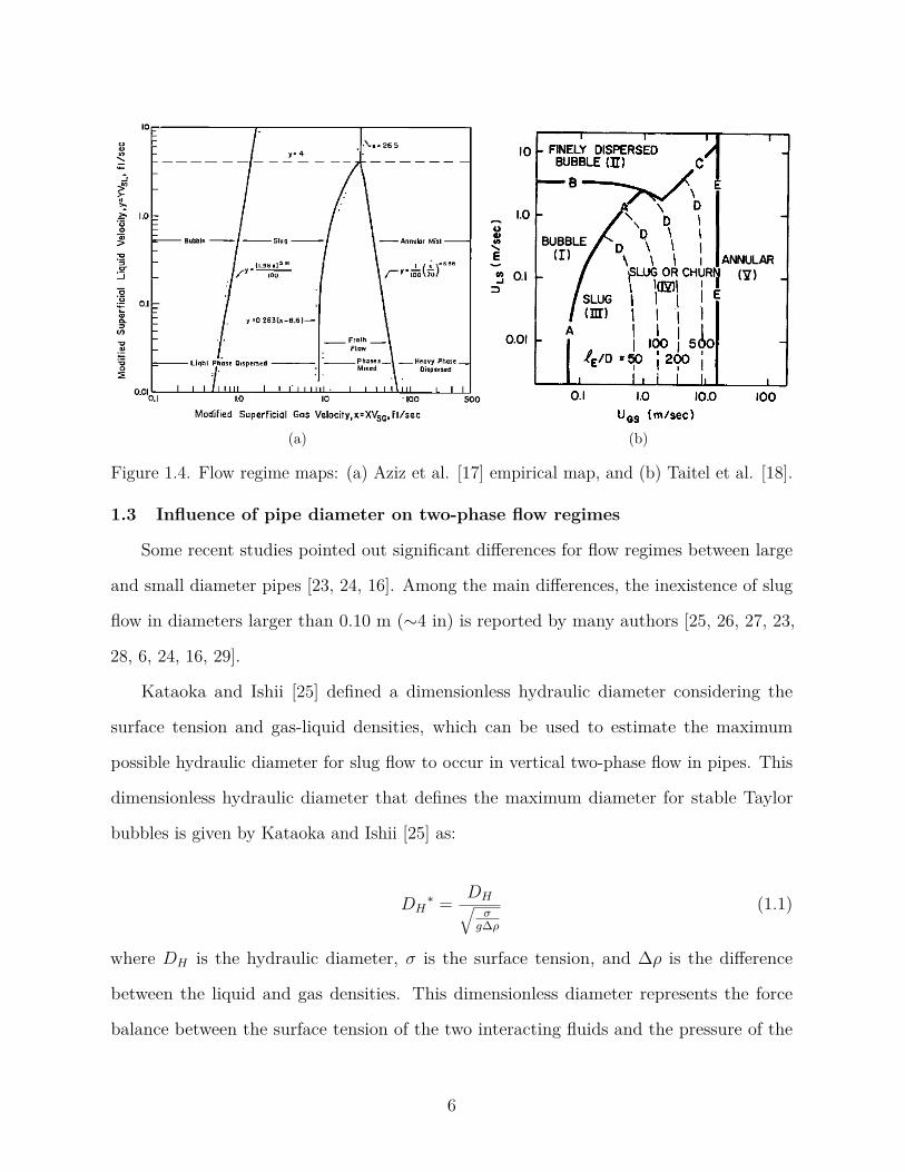
of liquid and gas velocities and other fluid properties or pipe characteristics. Figure 1.4

presents two relevant flow regime maps often cited on the literature, being (a) an empirical

flow regime map developed by Aziz et al. [17], and (b) a mechanistic flow regime map

proposed by Taitel et al. [18].

Flow regimes and their respective transitions are influenced by pipe geometry (diameters

and inclination), fluid properties, and flow conditions [16]. Most flow regime maps [11, 18,

19, 20] developed for vertical two-phase flow in pipes are based on experimental and field

data for small diameter pipes (e.g., ID < 0.10 m – or ∼4 in) and low liquid flow velocities

(liquid velocities typically lower than 1 m/s) [21, 22]. Thus, the applicability of such maps

to flowing conditions involving large diameter and high flow velocities is still questionable.

Therefore, studies are still needed on the evaluation of flow regime prediction models and

proposing improvements for its application on WCD calculations.

5

(a) (b)

Figure 1.4. Flow regime maps: (a) Aziz et al. [17] empirical map, and (b) Taitel et al. [18].

1.3 Influence of pipe diameter on two-phase flow regimes

Some recent studies pointed out significant differences for flow regimes between large

and small diameter pipes [23, 24, 16]. Among the main differences, the inexistence of slug

flow in diameters larger than 0.10 m (∼4 in) is reported by many authors [25, 26, 27, 23,

28, 6, 24, 16, 29].

Kataoka and Ishii [25] defined a dimensionless hydraulic diameter considering the

surface tension and gas-liquid densities, which can be used to estimate the maximum

possible hydraulic diameter for slug flow to occur in vertical two-phase flow in pipes. This

dimensionless hydraulic diameter that defines the maximum diameter for stable Taylor

bubbles is given by Kataoka and Ishii [25] as:

𝐷𝐻* = 𝐷𝐻√︁

𝜎𝑔Δ𝜌

(1.1)

where 𝐷𝐻 is the hydraulic diameter, 𝜎 is the surface tension, and Δ𝜌 is the difference

between the liquid and gas densities. This dimensionless diameter represents the force

balance between the surface tension of the two interacting fluids and the pressure of the

6

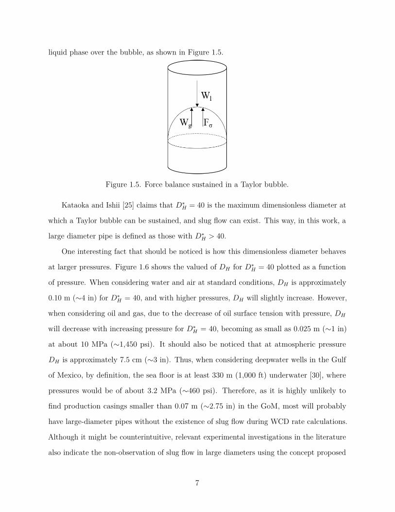
liquid phase over the bubble, as shown in Figure 1.5.

Figure 1.5. Force balance sustained in a Taylor bubble.

Kataoka and Ishii [25] claims that 𝐷*𝐻 = 40 is the maximum dimensionless diameter at

which a Taylor bubble can be sustained, and slug flow can exist. This way, in this work, a

large diameter pipe is defined as those with 𝐷*𝐻 > 40.

One interesting fact that should be noticed is how this dimensionless diameter behaves

at larger pressures. Figure 1.6 shows the valued of 𝐷𝐻 for 𝐷*𝐻 = 40 plotted as a function

of pressure. When considering water and air at standard conditions, 𝐷𝐻 is approximately

0.10 m (∼4 in) for 𝐷*𝐻 = 40, and with higher pressures, 𝐷𝐻 will slightly increase. However,

when considering oil and gas, due to the decrease of oil surface tension with pressure, 𝐷𝐻

will decrease with increasing pressure for 𝐷*𝐻 = 40, becoming as small as 0.025 m (∼1 in)

at about 10 MPa (∼1,450 psi). It should also be noticed that at atmospheric pressure

𝐷𝐻 is approximately 7.5 cm (∼3 in). Thus, when considering deepwater wells in the Gulf

of Mexico, by definition, the sea floor is at least 330 m (1,000 ft) underwater [30], where

pressures would be of about 3.2 MPa (∼460 psi). Therefore, as it is highly unlikely to

find production casings smaller than 0.07 m (∼2.75 in) in the GoM, most will probably

have large-diameter pipes without the existence of slug flow during WCD rate calculations.

Although it might be counterintuitive, relevant experimental investigations in the literature

also indicate the non-observation of slug flow in large diameters using the concept proposed

7

by Kataoka and Ishii [25] for 𝐷*𝐻 > 40.

Figure 1.6. Separation of what is considered a large diameter pipe by Kataoka and Ishii[25] criteria. The area above the curves represent the diameters considered large.

For instance, Ros [31] carried out experiments for pipe diameters from 0.03 to 0.14 m

(∼1 and ∼5.5 in), using air and diesel oil as working fluids, under atmospheric pressure. In

his work, he refers to slug flow as the result of the collapsing of bullet-shaped gas bubbles,

and even considers their so-called “slug flow” to directly precede the mist flow (equivalent

to annular flow). They also report that the bullet-shaped bubbles were only visible for

liquid superficial velocities lower than 40 cm/s (∼15.7 in/s).

Some authors reported that under conditions at which slug flow would exist, in larger

diameter pipe it will be replaced by a flow regime characterized by large deformed bubbles

flowing upwards or sideways. This flow regime has been commonly referred to as cap-bubble

flow [23, 32, 24]. This flow regime definition will be used throughout this work.

A schematic of the cap-bubble flow is presented in Figure 1.7. This flow regime is

defined as [23]:

• Cap-bubble flow: bubbles larger than those seen on bubble flow start to form, but

never occupying the entire pipe diameter. These bubbles generate flow recirculation

8

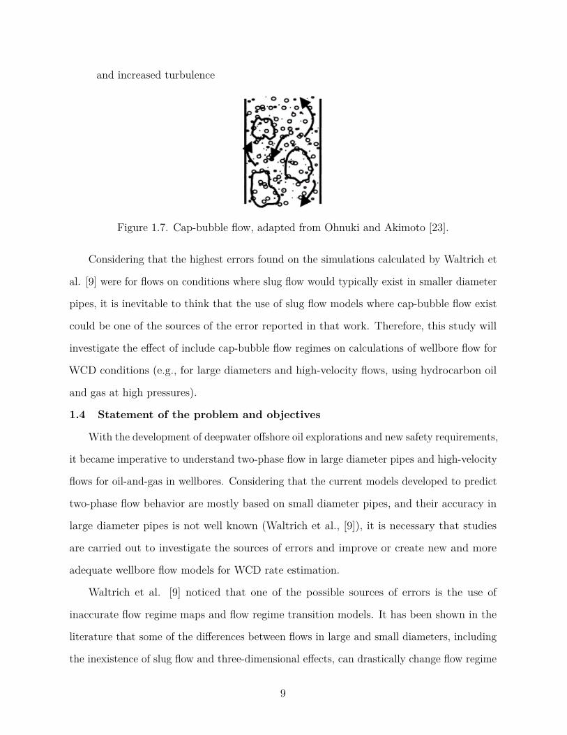
and increased turbulence

Figure 1.7. Cap-bubble flow, adapted from Ohnuki and Akimoto [23].

Considering that the highest errors found on the simulations calculated by Waltrich et

al. [9] were for flows on conditions where slug flow would typically exist in smaller diameter

pipes, it is inevitable to think that the use of slug flow models where cap-bubble flow exist

could be one of the sources of the error reported in that work. Therefore, this study will

investigate the effect of include cap-bubble flow regimes on calculations of wellbore flow for

WCD conditions (e.g., for large diameters and high-velocity flows, using hydrocarbon oil

and gas at high pressures).

1.4 Statement of the problem and objectives

With the development of deepwater offshore oil explorations and new safety requirements,

it became imperative to understand two-phase flow in large diameter pipes and high-velocity

flows for oil-and-gas in wellbores. Considering that the current models developed to predict

two-phase flow behavior are mostly based on small diameter pipes, and their accuracy in

large diameter pipes is not well known (Waltrich et al., [9]), it is necessary that studies

are carried out to investigate the sources of errors and improve or create new and more

adequate wellbore flow models for WCD rate estimation.

Waltrich et al. [9] noticed that one of the possible sources of errors is the use of

inaccurate flow regime maps and flow regime transition models. It has been shown in the

literature that some of the differences between flows in large and small diameters, including

the inexistence of slug flow and three-dimensional effects, can drastically change flow regime

9

determination [25, 23, 14, 8, 29].

As mentioned before, flow regimes are dependent on fluid properties and have an essential

dependence on the gas-liquid volume fraction in the flowing mixture. The gas-liquid-ratio

will strongly influence the pressure drop of the flow. Consequently, flow-regime dependent

models will calculate the pressure gradient in different ways for different flow regimes. For

example, a flow regime with low gas-liquid-ratio will have a higher density than a flow

regime with high gas-liquid-ratio and therefore, will cause a higher pressure drop due to

gravitational forces. On the other hand, in flow regimes with high gas-liquid-ratio, the

tendency is that the flow is at a higher velocity (due to the gas expansion tendency with

reducing pressure), and will present a higher pressure drop due to friction. This way, a right

prediction of flow regime is essential when calculating the pressure gradient for vertical

upward two-phase flow.

Figure 1.8 shows a schematic of two-phase flow in a vertical pipe, including the expected

pressure profiles considering different flow regimes. As fluid mixture flow upwards, the

gas expands and increases its gas velocity (as a consequence of mass and momentum

conservation). This increase in gas velocity will make the bubbles coalesce and cause flow

regime transitions. If a model is considering erroneous flow regimes transition, there is

a chance that the final calculated pressure drop is also wrong. As shown in Figure 1.8,

changing the condition to which a flow regime will change, or the expected pressure drop for

different flow regimes, as for flow regime maps 1 and 2, the final calculated pressure (in this

case, the bottom-hole pressure) will be different. Hence, the more precisely you can predict

the flow regime, the more accurate will be the final pressure calculation. It is interesting to

notice that if using the criteria of large diameter by Kataoka and Ishi [25], it is possible to

have a transition to from cap-bubble to slug in the same wellbore due to pressure drops

with the upwards flows, even without changing the pipe diameter (see Figure 1.6). In other

words, if the pressure drops enough, and the flow is in the right conditions, the pipe might

“become” small enough for the existence of slug flow.

10

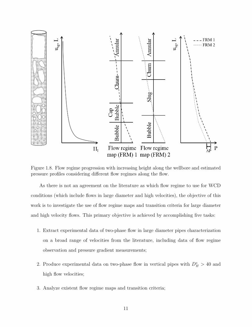
Figure 1.8. Flow regime progression with increasing height along the wellbore and estimatedpressure profiles considering different flow regimes along the flow.

As there is not an agreement on the literature as which flow regime to use for WCD

conditions (which include flows in large diameter and high velocities), the objective of this

work is to investigate the use of flow regime maps and transition criteria for large diameter

and high velocity flows. This primary objective is achieved by accomplishing five tasks:

1. Extract experimental data of two-phase flow in large diameter pipes characterization

on a broad range of velocities from the literature, including data of flow regime

observation and pressure gradient measurements;

2. Produce experimental data on two-phase flow in vertical pipes with 𝐷*𝐻 > 40 and

high flow velocities;

3. Analyze existent flow regime maps and transition criteria;

11

4. Compare existent flow regime maps against experimental data flow in large diameter

pipes and high flow-velocities;

5. Propose or develop an adequate flow regime map for large diameter pipes, and high

velocity flows and test it in a model to evaluate if it improves or not the pressure drop

estimation.

12

Chapter 2Literature Review

2.1 Important parameters for two-phase flow in pipes

Some relevant parameters are unique in the analysis of two-phase flow phenomena.

These parameters are defined below and will be used throughout this work [10]:

• Liquid holdup (𝐻𝑙): can be defined in steady-state flows as the time-averaged volu-

metric fraction of liquid-phase in a pipe segment.

• Void fraction (𝛼) or gas holdup (𝐻 − 𝑔): such as the liquid holdup, can be defined

in steady-state flows as the time-averaged volumetric fraction of gas-phase in a pipe

segment. The liquid holdup and void fraction can be correlated as:

𝛼 + 𝐻𝑙 = 1

• Pressure gradient (𝑑𝑝/𝑑𝑧): pressure variation along the axial direction in a pipe.

• Superficial velocity (𝑢𝑠𝑙 for liquids and 𝑢𝑠𝑔 for gases): geometrical parameter correlation

the injected volumetric flow rate and the pipe cross-section. Can be calculated as

𝑢𝑠𝑛 = 𝑄𝑛

𝐴

where the subscripts s represents that the velocity u is superficial, and n refers to the

considered fluid (replaced by l for liquids and g for gases), Q is the volumetric flow

rate and A is the cross-section of the pipe.

• Mixture velocity (𝑢𝑚): the sum of liquid and gas superficial velocities.

• Slip ratio (𝑢𝑠𝑔/𝑢𝑠𝑙): the ratio between gas and liquid superficial velocities.

13

2.2 Teles and Waltrich model [33] (or modified Pagan et al. [34])

A new wellbore two-phase flow model to estimate pressure gradient for the four classical

flow regimes (bubble, slug, churn, and annular flow) in large diameter pipes has been

developed at LSU and recently proposed in an interim report by LSU and submitted to

BOEM [33].

The model herein called Teles and Waltrich [33] is a modification to the model proposed

by Pagan et al. [34] for churn and annular flow, coupled with Duns and Ros [11] empirical

correlations to calculate bubble and slug flow. Furthermore, this new model makes use of

Eq. 1.1 to evaluate whether the pipe will be considered as large or not and, consequently, if

it will present slug flow. The model also adds a criteria that for any flow with a slip ratio

lower than 1, Duns and Ros [11] should be automatically selected, not mattering at which

flow regime the flow is. The model is also adequate to calculate the pressure gradient in

small diameter pipes, making use of Duns and Ros [11] model in such cases.

The flowchart shown in Figure 2.1 illustrates how the algorithm of this model works

for the calculation of pressure in each section of the well, being deployed for each length

increment from a known pressure. The initial conditions and input parameters are an initial

conditions (wellhead pressure, fluids flow rates, temperatures), fluid properties (gas-liquid

ratio, fluid densities), well parameters (inclination, diameter, vertical length), and the

desired number of finite length increments.

This model was tested against other relevant models [11, 35, 36, 12, 13, 37] with good

results, showing average absolute errors on the pressure gradient estimation comparable to

all these other relevant models. A comparative between the error from the calculation of

the pressure gradient by Teles and Waltrich model and others is presented in Figure 2.2.

The data used for these simulations can be found in the Appendix, in Table A.1. A full

review of these results and more is reported in the Interim report from LSU to BOEM [33].

14

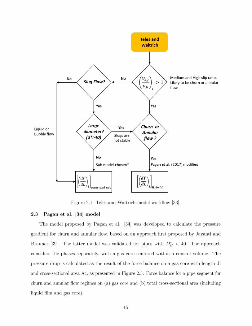
Figure 2.1. Teles and Waltrich model workflow [33].

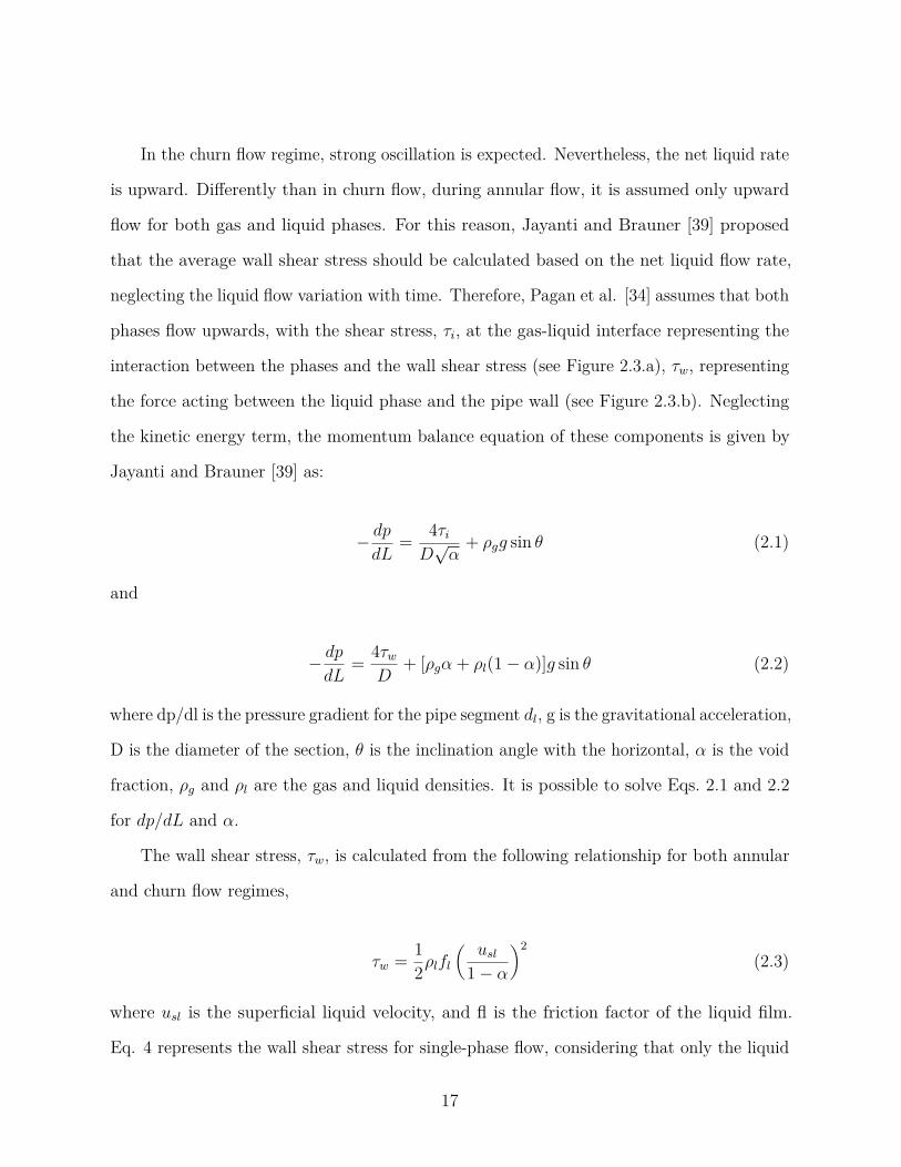
2.3 Pagan et al. [34] model

The model proposed by Pagan et al. [34] was developed to calculate the pressure

gradient for churn and annular flow, based on an approach first proposed by Jayanti and

Brauner [39]. The latter model was validated for pipes with 𝐷*𝐻 < 40. The approach

considers the phases separately, with a gas core centered within a control volume. The

pressure drop is calculated as the result of the force balance on a gas core with length dl

and cross-sectional area Ac, as presented in Figure 2.3: Force balance for a pipe segment for

churn and annular flow regimes on (a) gas core and (b) total cross-sectional area (including

liquid film and gas core).

15

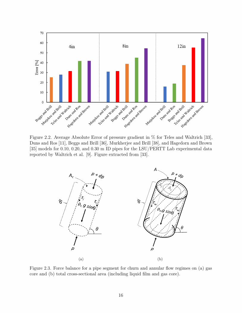
Figure 2.2. Average Absolute Error of pressure gradient in % for Teles and Waltrich [33],Duns and Ros [11], Beggs and Brill [36], Murkherjee and Brill [38], and Hagedorn and Brown[35] models for 0.10, 0.20, and 0.30 m ID pipes for the LSU/PERTT Lab experimental datareported by Waltrich et al. [9]. Figure extracted from [33].

(a) (b)

Figure 2.3. Force balance for a pipe segment for churn and annular flow regimes on (a) gascore and (b) total cross-sectional area (including liquid film and gas core).

16

In the churn flow regime, strong oscillation is expected. Nevertheless, the net liquid rate

is upward. Differently than in churn flow, during annular flow, it is assumed only upward

flow for both gas and liquid phases. For this reason, Jayanti and Brauner [39] proposed

that the average wall shear stress should be calculated based on the net liquid flow rate,

neglecting the liquid flow variation with time. Therefore, Pagan et al. [34] assumes that both

phases flow upwards, with the shear stress, 𝜏𝑖, at the gas-liquid interface representing the

interaction between the phases and the wall shear stress (see Figure 2.3.a), 𝜏𝑤, representing

the force acting between the liquid phase and the pipe wall (see Figure 2.3.b). Neglecting

the kinetic energy term, the momentum balance equation of these components is given by

Jayanti and Brauner [39] as:

− 𝑑𝑝

𝑑𝐿= 4𝜏𝑖

𝐷√

𝛼+ 𝜌𝑔𝑔 sin 𝜃 (2.1)

and

− 𝑑𝑝

𝑑𝐿= 4𝜏𝑤

𝐷+ [𝜌𝑔𝛼 + 𝜌𝑙(1 − 𝛼)]𝑔 sin 𝜃 (2.2)

where dp/dl is the pressure gradient for the pipe segment 𝑑𝑙, g is the gravitational acceleration,

D is the diameter of the section, 𝜃 is the inclination angle with the horizontal, 𝛼 is the void

fraction, 𝜌𝑔 and 𝜌𝑙 are the gas and liquid densities. It is possible to solve Eqs. 2.1 and 2.2

for 𝑑𝑝/𝑑𝐿 and 𝛼.

The wall shear stress, 𝜏𝑤, is calculated from the following relationship for both annular

and churn flow regimes,

𝜏𝑤 = 12𝜌𝑙𝑓𝑙

(︂𝑢𝑠𝑙

1 − 𝛼

)︂2(2.3)

where 𝑢𝑠𝑙 is the superficial liquid velocity, and fl is the friction factor of the liquid film.

Eq. 4 represents the wall shear stress for single-phase flow, considering that only the liquid

17

phase is in contact with the pipe wall.

The liquid film friction factor can be considered as Fanning friction factor, 𝑓 , which

can be calculated by a Blasius-type equation, as

𝑓 = 𝐶Relf−𝑛 (2.4)

where Re𝑙𝑓 is the Reynolds number of the liquid film, and n and C are constants dependent

on flow conditions, i.e., if it is turbulent or laminar. The flow will be considered laminar if

the Reynolds number is smaller than 2,100, and turbulent if it is greater than 2,100. This

way, n = 1 and C = 16 for laminar flow, and n = 0.2 and C = 0.046 for turbulent flow.

The Reynolds number for the liquid film can be calculated as:

𝑅𝑒𝑙𝑓 = 𝜌𝑙𝑢𝑙𝑓𝐷

𝜇𝑙

(2.5)

where D is the pipe diameter, 𝜇𝑙 is the liquid viscosity, and 𝑢𝑙𝑓 is the liquid film velocity

given by:

𝑢𝑙𝑓 = 𝑢𝑠𝑙

1 − 𝛼(2.6)

The interfacial shear stress between the gas core and the liquid film shown in Figure 2.3.a

is calculated as:

𝜏𝑖 = 12𝜌𝑔𝑓𝑖

(︂𝑢𝑠𝑔

𝛼

)︂2(2.7)

where 𝑢𝑠𝑔 is the superficial gas velocity. Eq. 2.7 neglects the liquid superficial velocity

component for considering that the superficial gas velocity is much higher during churn or

annular flows. This way 𝜏𝑖 is calculated considering a single-phase gas flow.

Pagan et al. [34] calculate the interfacial friction factor as proposed by Jayanti and

Brauner [39] as:

18

𝑓𝑖 = 12(𝑓𝑖,𝑊 + 𝑓𝑖,𝐵) (2.8)

A correlation suggested by Alves [40] is used to calculate 𝑓𝑖,𝐵, given by:

𝑓𝑖,𝐵 = 0.005 + 10(︁

−0.56+ 9.07𝐷*

𝐻

)︁ [︃𝐷*

𝐻(1 − 𝛼)4

]︃(︁1.63+ 4.74𝐷*

𝐻

)︁(2.9)

where 𝐷*𝐻 is the dimensionless diameter calculated by Eq. 1.1. Pagan et al. [34] suggest

the calculation of 𝑓𝑖,𝑊 using the general equation for interfacial friction factor introduced

by Wallis [41] as:

𝑓𝑖,𝑊 = 0.005(︃

1 + 300 𝛿

𝐷

)︃(2.10)

where 𝛿/𝐷 is the dimensionless liquid film thickness. The latter term on the RHS can

be represented in terms of 𝛼, as it can be calculated as the ratio between the cross-sectional

area of the gas core, 𝐴𝑐, and the cross-sectional area of the pipe A. Thus, this study proposes

Wallis [41] modified interfacial friction factor without assumption of thin liquid film in pipes

for churn flow regime, given by:

𝑓𝑖,𝑊 = 0.005 + 0.75(1 −√

𝛼) (2.11)

Wallis [41] modified interfacial friction factor equation with the assumption of the thin

liquid film is used only for annular flow regime, and is given by:

𝑓𝑖,𝑊 = 0.005 + 0.375(1 − 𝛼) (2.12)

2.4 Duns and Ros [11] model

Duns and Ros [11] developed an empirical model, based on a proprietary flow regime

map. Duns and Ros [11] empirical map separate flow regimes into three regions (see

Figure 2.4), sometimes englobing more than one flow regime at a time. These regions are

19

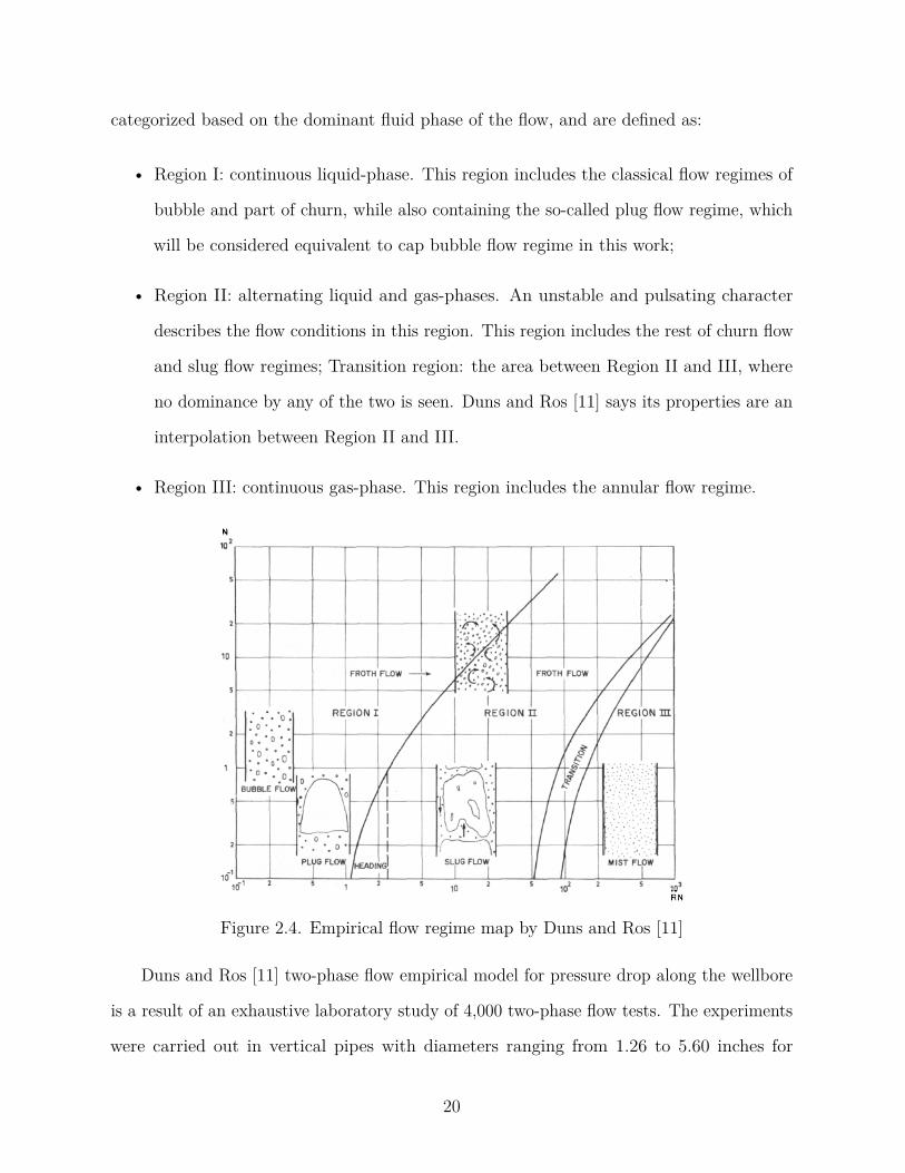
categorized based on the dominant fluid phase of the flow, and are defined as:

• Region I: continuous liquid-phase. This region includes the classical flow regimes of

bubble and part of churn, while also containing the so-called plug flow regime, which

will be considered equivalent to cap bubble flow regime in this work;

• Region II: alternating liquid and gas-phases. An unstable and pulsating character

describes the flow conditions in this region. This region includes the rest of churn flow

and slug flow regimes; Transition region: the area between Region II and III, where

no dominance by any of the two is seen. Duns and Ros [11] says its properties are an

interpolation between Region II and III.

• Region III: continuous gas-phase. This region includes the annular flow regime.

Figure 2.4. Empirical flow regime map by Duns and Ros [11]

Duns and Ros [11] two-phase flow empirical model for pressure drop along the wellbore

is a result of an exhaustive laboratory study of 4,000 two-phase flow tests. The experiments

were carried out in vertical pipes with diameters ranging from 1.26 to 5.60 inches for

20

gas-water flow [15], and gas-diesel oil flows. The modified Pagan et al. [34] model, herein

called Teles and Waltrich model makes use of Duns and Ros [11] correlations for bubble

and slug flow due to its good accuracy on predicting pressure drop in these flow regimes for

air-water and gas-oil fluids, for a wide range of pipe diameters.

To account for fluid and flow conditions, Duns and Ros [11] make use of dimensionless

numbers to place the flow into the flow regime map. The dimensionless liquid and gas

velocity numbers are respectively defined as:

𝑅𝑁 = 𝑢𝑠𝑔

√︁𝜌𝑙/(𝑔𝜎) (2.13)

𝑁 = 𝑢𝑠𝑙

√︁𝜌𝑙/(𝑔𝜎) (2.14)

where 𝜌𝑙 is the liquid density.

The map is then built plotting RN as the x-axis and N as the y-axis, and the transition

boundaries are empirically placed.

The Region I to Region II transition describes the change from a continuous liquid flow

to intermittent flow. The boundary between these two regions can be calculated as:

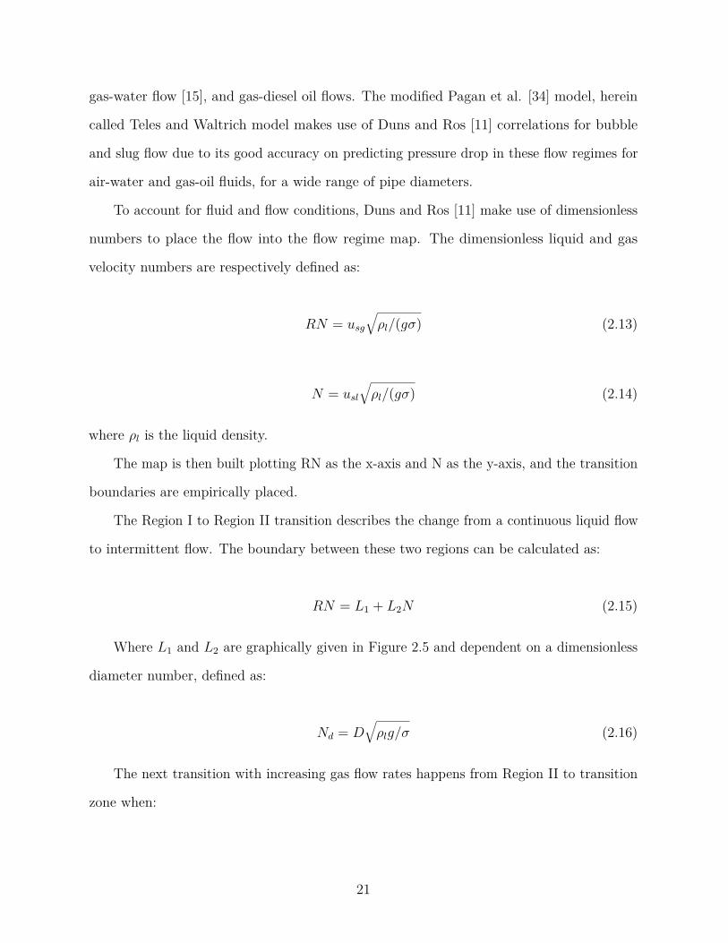
𝑅𝑁 = 𝐿1 + 𝐿2𝑁 (2.15)

Where 𝐿1 and 𝐿2 are graphically given in Figure 2.5 and dependent on a dimensionless

diameter number, defined as:

𝑁𝑑 = 𝐷√︁

𝜌𝑙𝑔/𝜎 (2.16)

The next transition with increasing gas flow rates happens from Region II to transition

zone when:

21

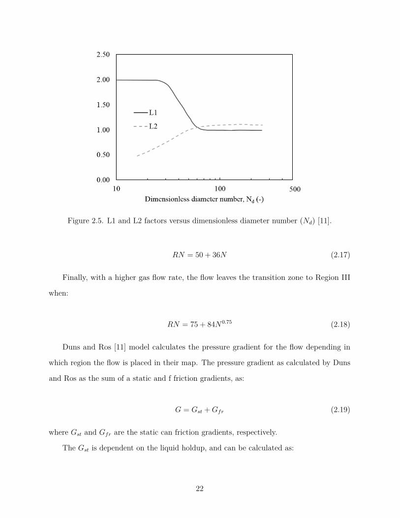
Figure 2.5. L1 and L2 factors versus dimensionless diameter number (𝑁𝑑) [11].

𝑅𝑁 = 50 + 36𝑁 (2.17)

Finally, with a higher gas flow rate, the flow leaves the transition zone to Region III

when:

𝑅𝑁 = 75 + 84𝑁0.75 (2.18)

Duns and Ros [11] model calculates the pressure gradient for the flow depending in

which region the flow is placed in their map. The pressure gradient as calculated by Duns

and Ros as the sum of a static and f friction gradients, as:

𝐺 = 𝐺𝑠𝑡 + 𝐺𝑓𝑟 (2.19)

where 𝐺𝑠𝑡 and 𝐺𝑓𝑟 are the static can friction gradients, respectively.

The 𝐺𝑠𝑡 is dependent on the liquid holdup, and can be calculated as:

22

𝐺𝑠𝑡 = 1𝜌𝑙𝑔

(︃𝑑𝑝

𝑑𝑧

)︃𝑠𝑡

= 𝐻𝑙 + (1 − 𝐻𝑙)𝜌𝑔

𝜌𝑙

(2.20)

The liquid holdup is proportional to the slip velocity, us, defined as the difference

between the actual gas and liquid velocities, defined as:

𝑢𝑠 = 𝑢𝑠𝑔

1 − 𝐻𝑙

− 𝑢𝑠𝑙

𝐻𝑙

(2.21)

This slip velocity can be non-dimensionalized, as the other groups as:

𝑆 = 𝑢𝑠

√︁𝜌𝑙/(𝑔𝜎) (2.22)

Therefore, by defining S it is possible to calculate 𝐻𝑙 and, consequently, 𝐺𝑠𝑡.

Duns and Ros [11] propose an empirical formula to calculate S according to the different

Regions in their map.

The empirical formula for Region I is:

𝑆 = 𝐹1 + 𝐹2𝑁 + 𝐹 ′3

(︂𝑅𝑁

1 + 𝑁

)︂2(2.23)

This formula correlates the empirical F-factors with the dimensionless liquid and gas

velocities N and RN, respectively. The F-factors for this region can be obtained from

Figure 2.6 using the dimensionless liquid viscosity number defined as 𝑁𝑙 = 𝜇𝑙

√︁𝜌𝑙/(𝑔𝜎3). It

is important to notice that 𝐹3 is given in the plot, but 𝐹 ′3 can be calculated as:

𝐹 ′3 = 𝐹3 − 𝐹4

𝑁𝑑

(2.24)

For Region II, the empirical correlation for the dimensionless slip velocity number can

be had as:

𝑆 = (1 + 𝐹5)(𝑅𝑁)0.982 + 𝐹 ′

6(1 + 𝐹7𝑁)2 (2.25)

23

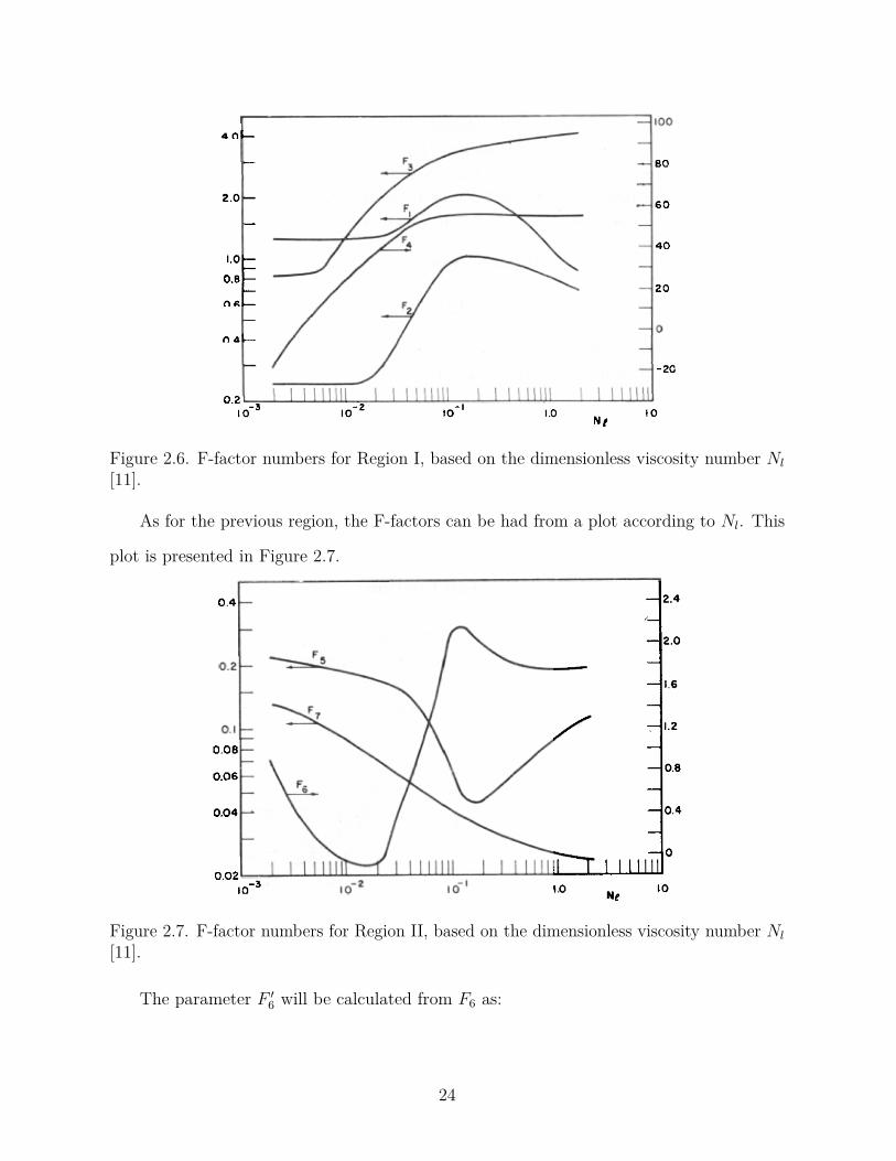
Figure 2.6. F-factor numbers for Region I, based on the dimensionless viscosity number 𝑁𝑙

[11].

As for the previous region, the F-factors can be had from a plot according to 𝑁𝑙. This

plot is presented in Figure 2.7.

Figure 2.7. F-factor numbers for Region II, based on the dimensionless viscosity number 𝑁𝑙

[11].

The parameter 𝐹 ′6 will be calculated from 𝐹6 as:

24

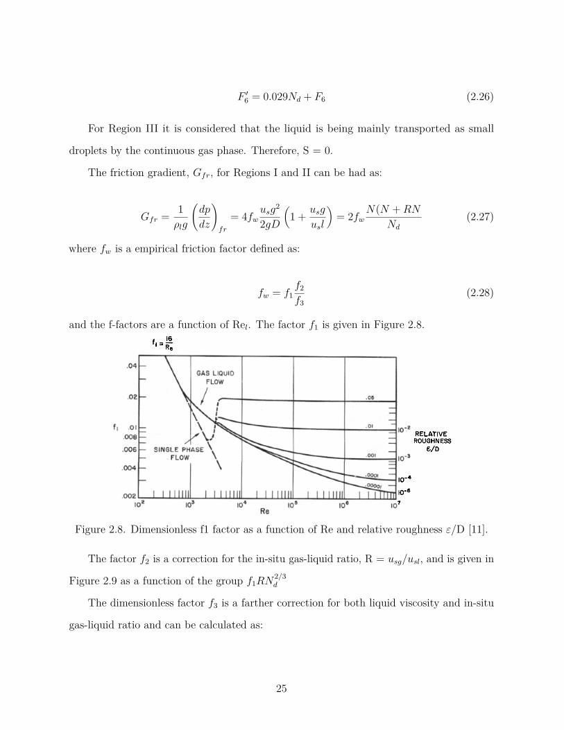
𝐹 ′6 = 0.029𝑁𝑑 + 𝐹6 (2.26)

For Region III it is considered that the liquid is being mainly transported as small

droplets by the continuous gas phase. Therefore, S = 0.

The friction gradient, 𝐺𝑓𝑟, for Regions I and II can be had as:

𝐺𝑓𝑟 = 1𝜌𝑙𝑔

(︃𝑑𝑝

𝑑𝑧

)︃𝑓𝑟

= 4𝑓𝑤𝑢𝑠𝑔

2

2𝑔𝐷

(︂1 + 𝑢𝑠𝑔

𝑢𝑠𝑙

)︂= 2𝑓𝑤

𝑁(𝑁 + 𝑅𝑁

𝑁𝑑

(2.27)

where 𝑓𝑤 is a empirical friction factor defined as:

𝑓𝑤 = 𝑓1𝑓2

𝑓3(2.28)

and the f-factors are a function of Re𝑙. The factor 𝑓1 is given in Figure 2.8.

Figure 2.8. Dimensionless f1 factor as a function of Re and relative roughness 𝜀/D [11].

The factor 𝑓2 is a correction for the in-situ gas-liquid ratio, R = 𝑢𝑠𝑔/𝑢𝑠𝑙, and is given in

Figure 2.9 as a function of the group 𝑓1𝑅𝑁2/3𝑑

The dimensionless factor 𝑓3 is a farther correction for both liquid viscosity and in-situ

gas-liquid ratio and can be calculated as:

25

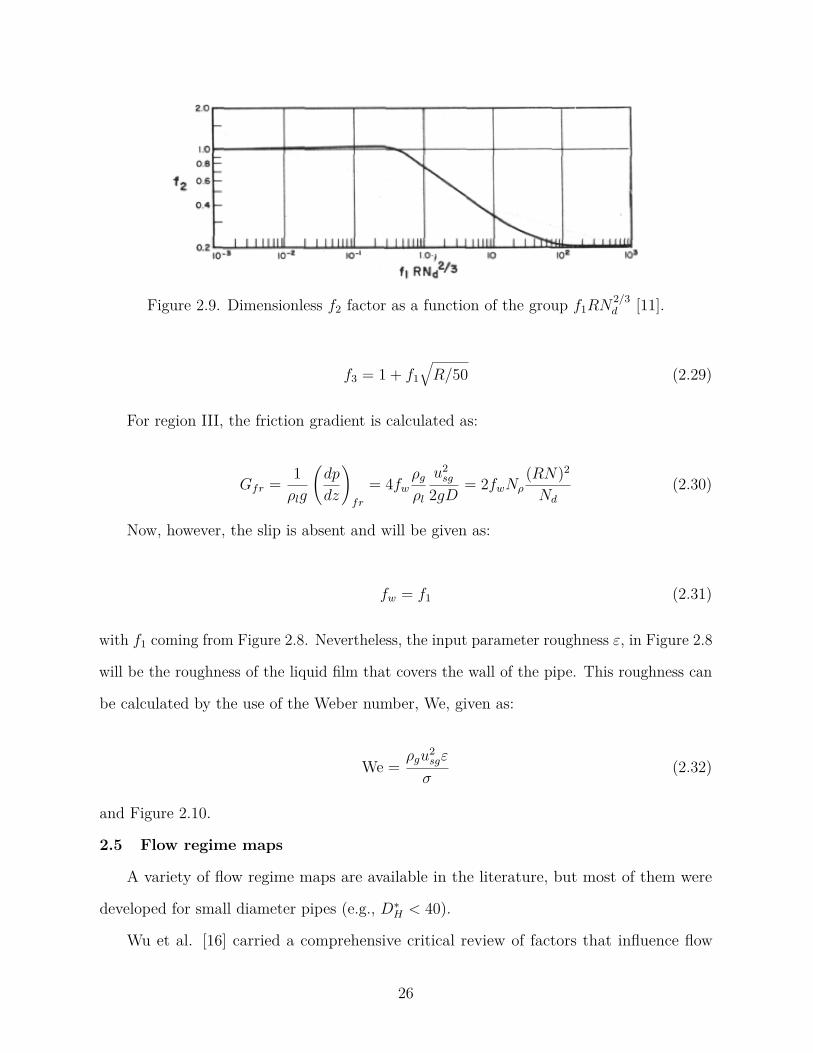
Figure 2.9. Dimensionless 𝑓2 factor as a function of the group 𝑓1𝑅𝑁2/3𝑑 [11].

𝑓3 = 1 + 𝑓1

√︁𝑅/50 (2.29)

For region III, the friction gradient is calculated as:

𝐺𝑓𝑟 = 1𝜌𝑙𝑔

(︃𝑑𝑝

𝑑𝑧

)︃𝑓𝑟

= 4𝑓𝑤𝜌𝑔

𝜌𝑙

𝑢2𝑠𝑔

2𝑔𝐷= 2𝑓𝑤𝑁𝜌

(𝑅𝑁)2

𝑁𝑑

(2.30)

Now, however, the slip is absent and will be given as:

𝑓𝑤 = 𝑓1 (2.31)

with 𝑓1 coming from Figure 2.8. Nevertheless, the input parameter roughness 𝜀, in Figure 2.8

will be the roughness of the liquid film that covers the wall of the pipe. This roughness can

be calculated by the use of the Weber number, We, given as:

We =𝜌𝑔𝑢2

𝑠𝑔𝜀

𝜎(2.32)

and Figure 2.10.

2.5 Flow regime maps

A variety of flow regime maps are available in the literature, but most of them were

developed for small diameter pipes (e.g., 𝐷*𝐻 < 40).

Wu et al. [16] carried a comprehensive critical review of factors that influence flow

26

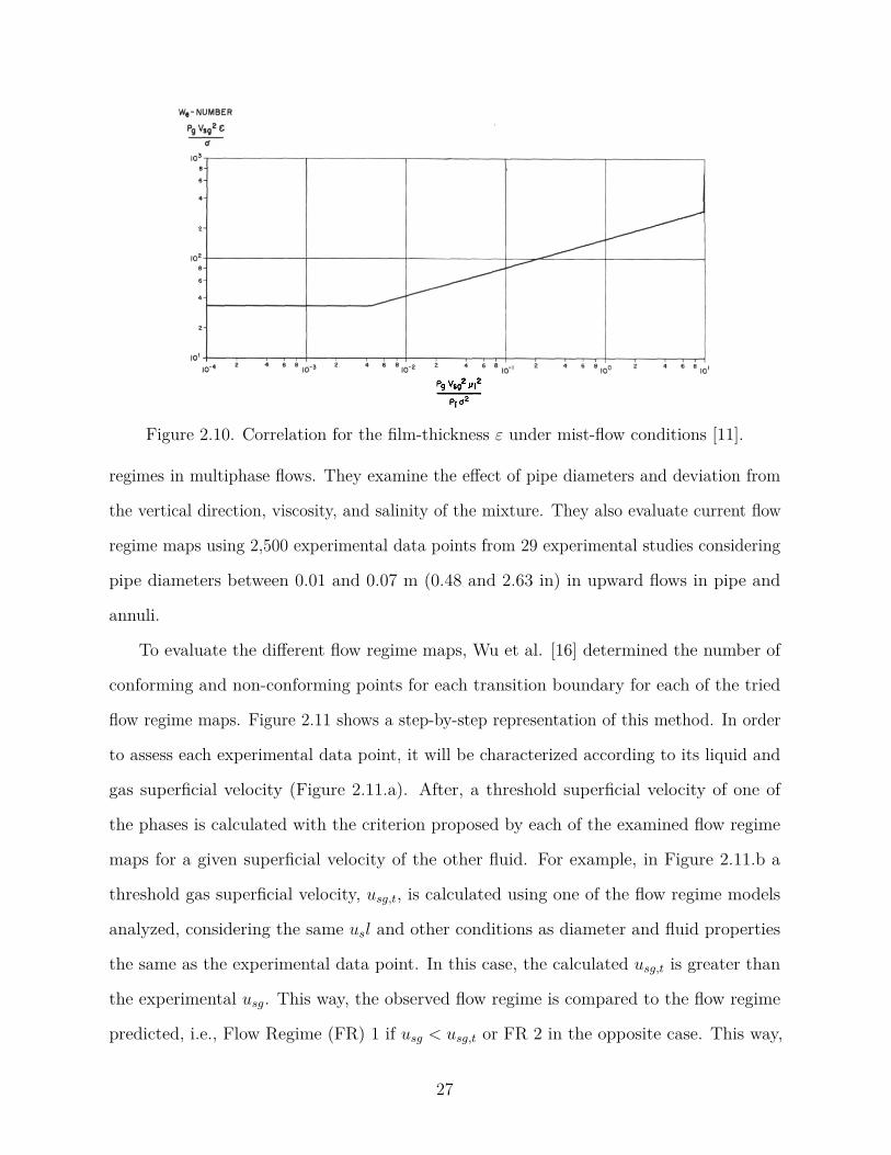
Figure 2.10. Correlation for the film-thickness 𝜀 under mist-flow conditions [11].

regimes in multiphase flows. They examine the effect of pipe diameters and deviation from

the vertical direction, viscosity, and salinity of the mixture. They also evaluate current flow

regime maps using 2,500 experimental data points from 29 experimental studies considering

pipe diameters between 0.01 and 0.07 m (0.48 and 2.63 in) in upward flows in pipe and

annuli.

To evaluate the different flow regime maps, Wu et al. [16] determined the number of

conforming and non-conforming points for each transition boundary for each of the tried

flow regime maps. Figure 2.11 shows a step-by-step representation of this method. In order

to assess each experimental data point, it will be characterized according to its liquid and

gas superficial velocity (Figure 2.11.a). After, a threshold superficial velocity of one of

the phases is calculated with the criterion proposed by each of the examined flow regime

maps for a given superficial velocity of the other fluid. For example, in Figure 2.11.b a

threshold gas superficial velocity, 𝑢𝑠𝑔,𝑡, is calculated using one of the flow regime models

analyzed, considering the same 𝑢𝑠𝑙 and other conditions as diameter and fluid properties

the same as the experimental data point. In this case, the calculated 𝑢𝑠𝑔,𝑡 is greater than

the experimental 𝑢𝑠𝑔. This way, the observed flow regime is compared to the flow regime

predicted, i.e., Flow Regime (FR) 1 if 𝑢𝑠𝑔 < 𝑢𝑠𝑔,𝑡 or FR 2 in the opposite case. This way,

27

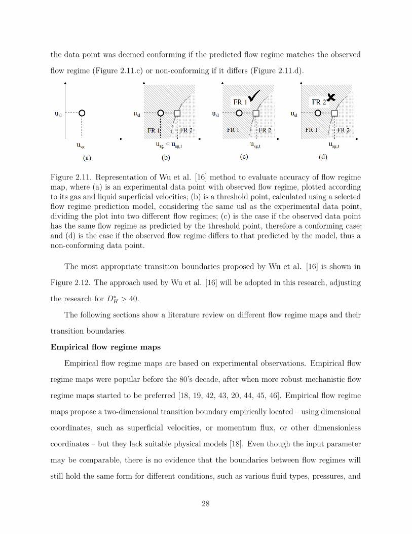
the data point was deemed conforming if the predicted flow regime matches the observed

flow regime (Figure 2.11.c) or non-conforming if it differs (Figure 2.11.d).

Figure 2.11. Representation of Wu et al. [16] method to evaluate accuracy of flow regimemap, where (a) is an experimental data point with observed flow regime, plotted accordingto its gas and liquid superficial velocities; (b) is a threshold point, calculated using a selectedflow regime prediction model, considering the same usl as the experimental data point,dividing the plot into two different flow regimes; (c) is the case if the observed data pointhas the same flow regime as predicted by the threshold point, therefore a conforming case;and (d) is the case if the observed flow regime differs to that predicted by the model, thus anon-conforming data point.

The most appropriate transition boundaries proposed by Wu et al. [16] is shown in

Figure 2.12. The approach used by Wu et al. [16] will be adopted in this research, adjusting

the research for 𝐷*𝐻 > 40.

The following sections show a literature review on different flow regime maps and their

transition boundaries.

Empirical flow regime maps

Empirical flow regime maps are based on experimental observations. Empirical flow

regime maps were popular before the 80’s decade, after when more robust mechanistic flow

regime maps started to be preferred [18, 19, 42, 43, 20, 44, 45, 46]. Empirical flow regime

maps propose a two-dimensional transition boundary empirically located – using dimensional

coordinates, such as superficial velocities, or momentum flux, or other dimensionless

coordinates – but they lack suitable physical models [18]. Even though the input parameter

may be comparable, there is no evidence that the boundaries between flow regimes will

still hold the same form for different conditions, such as various fluid types, pressures, and

28

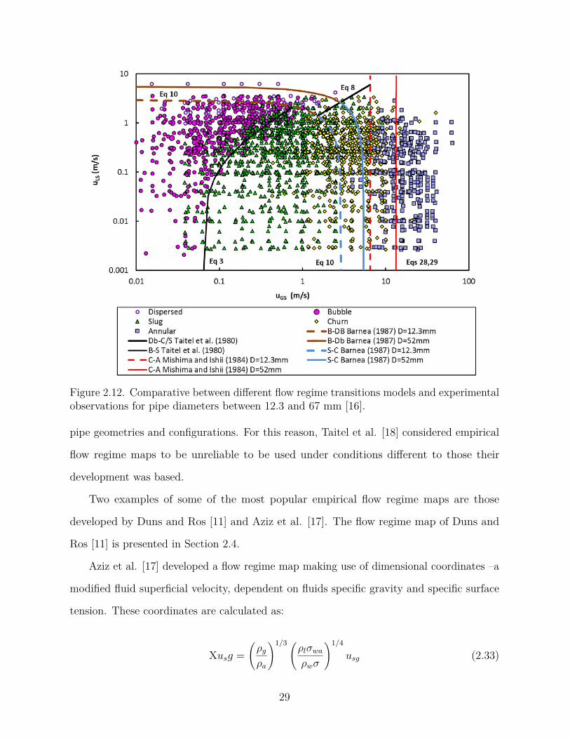
Figure 2.12. Comparative between different flow regime transitions models and experimentalobservations for pipe diameters between 12.3 and 67 mm [16].

pipe geometries and configurations. For this reason, Taitel et al. [18] considered empirical

flow regime maps to be unreliable to be used under conditions different to those their

development was based.

Two examples of some of the most popular empirical flow regime maps are those

developed by Duns and Ros [11] and Aziz et al. [17]. The flow regime map of Duns and

Ros [11] is presented in Section 2.4.

Aziz et al. [17] developed a flow regime map making use of dimensional coordinates –a

modified fluid superficial velocity, dependent on fluids specific gravity and specific surface

tension. These coordinates are calculated as:

X𝑢𝑠𝑔 =(︃

𝜌𝑔

𝜌𝑎

)︃1/3 (︃𝜌𝑙𝜎𝑤𝑎

𝜌𝑤𝜎

)︃1/4

𝑢𝑠𝑔 (2.33)

29

Y𝑢𝑠𝑙 =(︃

𝜌𝑙𝜎𝑤𝑎

𝜌𝑤𝜎

)︃1/4

𝑢𝑠𝑙 (2.34)

where the subscripts a and w represent air and water, respectively.

The flow regimes defined by Aziz et al. [17] are a bubble, slug, froth, and annular mist

flow. The transition boundaries are calculated as:

• Bubble to slug transition:

Y𝑢𝑠𝑙 = 0.01(1.96𝑋𝑢𝑠𝑔)5.81 (2.35)

• Slug to froth transition

Y𝑢𝑠𝑙 = 0.263(X𝑢𝑠𝑔 − 8.61) for Y𝑢𝑠𝑙 ≤ 4 (2.36)

for Y𝑢𝑠𝑙 > 4, X𝑢𝑠𝑔 = 26.5

• Froth to annular mist transition

Y𝑢𝑠𝑙 = 1100

(︃X𝑢𝑠𝑔

70

)︃−6.18

(2.37)

The experiments to develop this map were carried out for oil and gas producing wells

with diameters of ∼0.06 m (2.4 in).

Mechanistic flow regime maps

Mechanistic flow regime maps describe transition boundaries based on conservation

principles, force balances, and drift-flux approach. The authors of these flow regime maps

develop equations that will represent the transition criteria between flow regimes. For

example, traditional principles for the transition of bubble flow to slug/cap-bubble flow is

the maximum bubble size before its coalescence. Therefore, a geometrical parameter will be

30

correlated to a given property, in this case, the void fraction, so it is possible to model the

transition.

Table 1 shows the main advantages and limitations of relevant mechanistic flow-regime

transition models. The next section will briefly describe each of these relevant mechanistic

flow-regime transition models.

∙ Taitel et al. flow regime map

Taitel et al. [18] state that no empirical flow regime map produced before their study

could be extrapolated to conditions outside of those that they were developed for, due to

insufficient physical basis. The authors also point out that these maps differ among them

in absolute value and trend for the transition boundaries.

To address this limitation in the literature, Taitel et al. [18] developed a mechanistic flow

regime map, defining mechanistic transition boundaries dependent on fluid properties, the

velocity of the phases, and pipe geometry. Besides the flow regimes previously identified in

this thesis, the authors proposed the so-called dispersed bubble flow, which is characterized

by small-diameter spherical gas bubbles dispersed in the liquid phase.

Taitel et al. [18] claim that the transition from bubble to slug flow requires a process of

agglomeration or coalescence. Both of these processes can be achieved with increasing gas

flow rate, which increases the bubble density and thus shortens the space between bubbles,

increasing the coalescence rate. On the other hand, the increase of liquid flow rate increase

the turbulent fluctuations, which can break larger diameter bubbles (sustaining smaller

bubbles in the flow) and make impossible the recoalescence of the bubbles. Therefore, the

transition from bubble flow needs to be separated into two different conditions: where

dispersion forces are dominant – i.e., high liquid flow rates – and where they are not.

Under the condition at which the liquid rate is not high enough to not cause this

disturbance, the increase of gas flow rate reaches a point at which the bubble density is

high enough so that the bubbles are very tightly packed. This proximity results in many

collisions and the small bubbles will agglomerate into larger bubbles, which is when the

31

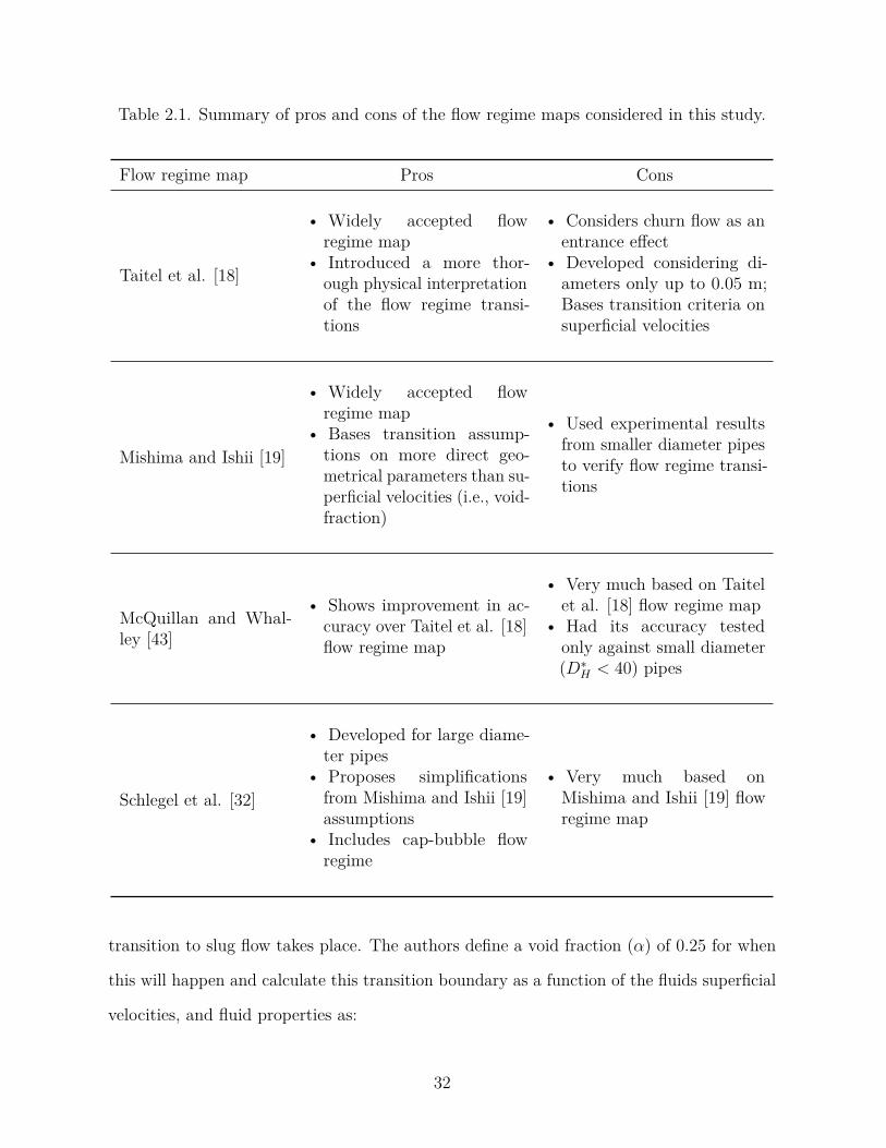
Table 2.1. Summary of pros and cons of the flow regime maps considered in this study.

Flow regime map Pros Cons

Taitel et al. [18]

• Widely accepted flowregime map

• Introduced a more thor-ough physical interpretationof the flow regime transi-tions

• Considers churn flow as anentrance effect

• Developed considering di-ameters only up to 0.05 m;Bases transition criteria onsuperficial velocities

Mishima and Ishii [19]

• Widely accepted flowregime map

• Bases transition assump-tions on more direct geo-metrical parameters than su-perficial velocities (i.e., void-fraction)

• Used experimental resultsfrom smaller diameter pipesto verify flow regime transi-tions

McQuillan and Whal-ley [43]

• Shows improvement in ac-curacy over Taitel et al. [18]flow regime map

• Very much based on Taitelet al. [18] flow regime map

• Had its accuracy testedonly against small diameter(𝐷*

𝐻 < 40) pipes

Schlegel et al. [32]

• Developed for large diame-ter pipes

• Proposes simplificationsfrom Mishima and Ishii [19]assumptions

• Includes cap-bubble flowregime

• Very much based onMishima and Ishii [19] flowregime map

transition to slug flow takes place. The authors define a void fraction (𝛼) of 0.25 for when

this will happen and calculate this transition boundary as a function of the fluids superficial

velocities, and fluid properties as:

32

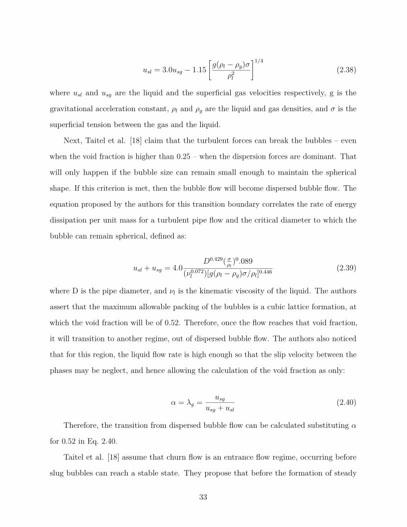
𝑢𝑠𝑙 = 3.0𝑢𝑠𝑔 − 1.15[︃

𝑔(𝜌𝑙 − 𝜌𝑔)𝜎𝜌2

𝑙

]︃1/4

(2.38)

where 𝑢𝑠𝑙 and 𝑢𝑠𝑔 are the liquid and the superficial gas velocities respectively, g is the

gravitational acceleration constant, 𝜌𝑙 and 𝜌𝑔 are the liquid and gas densities, and 𝜎 is the

superficial tension between the gas and the liquid.

Next, Taitel et al. [18] claim that the turbulent forces can break the bubbles – even

when the void fraction is higher than 0.25 – when the dispersion forces are dominant. That

will only happen if the bubble size can remain small enough to maintain the spherical

shape. If this criterion is met, then the bubble flow will become dispersed bubble flow. The

equation proposed by the authors for this transition boundary correlates the rate of energy

dissipation per unit mass for a turbulent pipe flow and the critical diameter to which the

bubble can remain spherical, defined as:

𝑢𝑠𝑙 + 𝑢𝑠𝑔 = 4.0𝐷0.429( 𝜎

𝜌𝑙)0.089

(𝜈0.072𝑙 )[𝑔(𝜌𝑙 − 𝜌𝑔)𝜎/𝜌𝑙]0.446 (2.39)

where D is the pipe diameter, and 𝜈𝑙 is the kinematic viscosity of the liquid. The authors

assert that the maximum allowable packing of the bubbles is a cubic lattice formation, at

which the void fraction will be of 0.52. Therefore, once the flow reaches that void fraction,

it will transition to another regime, out of dispersed bubble flow. The authors also noticed

that for this region, the liquid flow rate is high enough so that the slip velocity between the

phases may be neglect, and hence allowing the calculation of the void fraction as only:

𝛼 = 𝜆𝑔 = 𝑢𝑠𝑔

𝑢𝑠𝑔 + 𝑢𝑠𝑙

(2.40)

Therefore, the transition from dispersed bubble flow can be calculated substituting 𝛼

for 0.52 in Eq. 2.40.

Taitel et al. [18] assume that churn flow is an entrance flow regime, occurring before

slug bubbles can reach a stable state. They propose that before the formation of steady

33

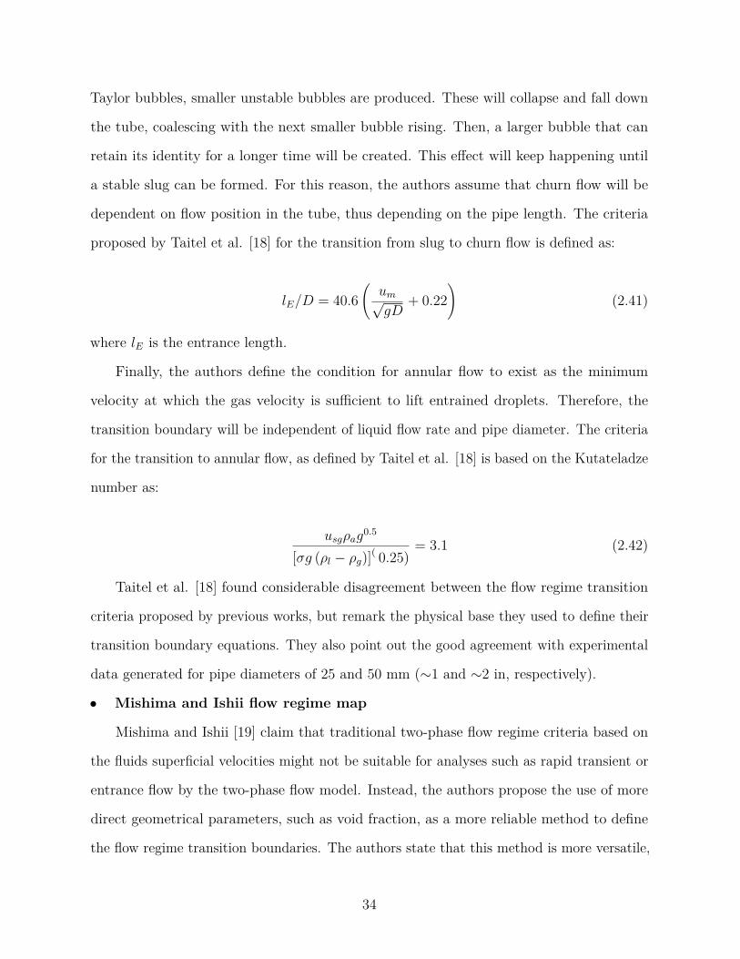
Taylor bubbles, smaller unstable bubbles are produced. These will collapse and fall down

the tube, coalescing with the next smaller bubble rising. Then, a larger bubble that can

retain its identity for a longer time will be created. This effect will keep happening until

a stable slug can be formed. For this reason, the authors assume that churn flow will be

dependent on flow position in the tube, thus depending on the pipe length. The criteria

proposed by Taitel et al. [18] for the transition from slug to churn flow is defined as:

𝑙𝐸/𝐷 = 40.6(︃

𝑢𝑚√𝑔𝐷

+ 0.22)︃

(2.41)

where 𝑙𝐸 is the entrance length.

Finally, the authors define the condition for annular flow to exist as the minimum

velocity at which the gas velocity is sufficient to lift entrained droplets. Therefore, the

transition boundary will be independent of liquid flow rate and pipe diameter. The criteria

for the transition to annular flow, as defined by Taitel et al. [18] is based on the Kutateladze

number as:

𝑢𝑠𝑔𝜌𝑎𝑔0.5

[𝜎𝑔 (𝜌𝑙 − 𝜌𝑔)]( 0.25)= 3.1 (2.42)

Taitel et al. [18] found considerable disagreement between the flow regime transition

criteria proposed by previous works, but remark the physical base they used to define their

transition boundary equations. They also point out the good agreement with experimental

data generated for pipe diameters of 25 and 50 mm (∼1 and ∼2 in, respectively).

∙ Mishima and Ishii flow regime map

Mishima and Ishii [19] claim that traditional two-phase flow regime criteria based on

the fluids superficial velocities might not be suitable for analyses such as rapid transient or

entrance flow by the two-phase flow model. Instead, the authors propose the use of more

direct geometrical parameters, such as void fraction, as a more reliable method to define

the flow regime transition boundaries. The authors state that this method is more versatile,

34

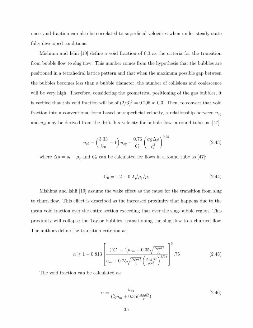
once void fraction can also be correlated to superficial velocities when under steady-state

fully developed conditions.

Mishima and Ishii [19] define a void fraction of 0.3 as the criteria for the transition

from bubble flow to slug flow. This number comes from the hypothesis that the bubbles are

positioned in a tetrahedral lattice pattern and that when the maximum possible gap between

the bubbles becomes less than a bubble diameter, the number of collisions and coalescence

will be very high. Therefore, considering the geometrical positioning of the gas bubbles, it

is verified that this void fraction will be of (2/3)2 = 0.296 ≈ 0.3. Then, to convert that void

fraction into a conventional form based on superficial velocity, a relationship between 𝑢𝑠𝑔

and 𝑢𝑠𝑙 may be derived from the drift-flux velocity for bubble flow in round tubes as [47]:

𝑢𝑠𝑙 =(︂3.33

𝐶0− 1

)︂𝑢𝑠𝑔 − 0.76

𝐶0

(︃𝜎𝑔Δ𝜌

𝜌2𝑙

)︃0.25

(2.43)

where Δ𝜌 = 𝜌𝑙 − 𝜌𝑔 and 𝐶0 can be calculated for flows in a round tube as [47]:

𝐶0 = 1.2 − 0.2√︁

𝜌𝑔/𝜌𝑙 (2.44)

Mishima and Ishii [19] assume the wake effect as the cause for the transition from slug

to churn flow. This effect is described as the increased proximity that happens due to the

mean void fraction over the entire section exceeding that over the slug-bubble region. This

proximity will collapse the Taylor bubbles, transitioning the slug flow to a churned flow.

The authors define the transition criterion as:

𝛼 ≥ 1 − 0.813

⎡⎢⎢⎢⎣ ((𝐶0 − 1)𝑢𝑚 + 0.35√︁

Δ𝜌𝑔𝐷𝜌𝑙

𝑢𝑚 + 0.75√︁

Δ𝜌𝑔𝐷𝜌𝑙

(︂Δ𝜌𝑔𝐷3

𝜌𝑙𝜈2𝑙

)︂1/18

⎤⎥⎥⎥⎦0

.75 (2.45)

The void fraction can be calculated as:

𝛼 = 𝑢𝑠𝑔

𝐶0𝑢𝑚 + 0.35(Δ𝜌𝑔𝐷𝜌𝑙

)(2.46)

35

For the transitions from churn to annular flow, the authors defined two mechanisms

that could lead the flow to change from churn to annular, namely (i) flow reversal in the

liquid film around large bubbles, and (ii) destruction of the liquid slug or large wave that

can be sustained as small droplets in a gas core. As for large diameter pipes that fit the

inequality

𝐷 >

√︁𝜎/(𝑔Δ𝜌)𝑁−0.4

𝜇𝑙

[(1 − 0.11 * 𝐶0)/𝐶0]2(2.47)

where 𝑁𝜇𝑙 is a dimensionless viscous number, defined as

𝑁𝜇𝑙 = 𝜇𝑙(︂𝜌𝑙𝜎

√︁𝜎

𝑔Δ𝜌

)︂1/2 (2.48)

For water and air at standard conditions, this diameter is of 0.06 m ( 2-3/8 in). Therefore,

for all the pipes considered in this work, the transition to annular flow can be modelled

according to Mishima and Ishii [19] as:

𝑢𝑠𝑔 > 𝑁−0.2𝜇𝑙

𝜎𝑔Δ𝜌

𝜌𝑔

1/4(2.49)

The authors compared their flow regime map with other empirical maps and claimed

that despite apparent differences in trend and values, considering the subjectivity of visual

characterization of flow regimes and transition zones instead of evident transition curves,

the agreement is good. They also compared their flow regime map with the one developed

by Taitel et al. [18] and found good agreement.

∙ McQuillan and Whalley flow regime map

McQuillan and Whalley [43] developed a hybrid flow regime map, making use of

mechanistic and semi-empirical equations defined by other authors, and developed a new

equation to explain the transition from slug to churn flow. The authors assumed Taitel et

al. [18] equation for the transition from bubble to slug flow.

36

For the boundary between non-dispersed to dispersed bubble flow, they adopted the

correlation defined by Weisman et al. [48], calculated as:

𝑢𝑠𝑙 ≥ 6.8𝜌0.444

𝑙

(𝑔𝐷Δ𝜌)0.278(︃

𝐷

𝜇𝑙

)︃0.112

(2.50)

This correlation was empirically adapted (for a broader range of diameters) from Taitel

and Dukler [49] relationship for horizontal tubes. To apply it for vertical tube flows, they

assumed that the liquid velocities under consideration were high enough so that the effect

of slip between the two phases are negligible and that the turbulence is caused by the bulk

flow alone, without the influence of the tube inclination. The correlation developed by

Weisman et al. [48] differs from the one produced by Taitel et al. [18] by having a smaller

tube diameter effect than the latter.

For the transition from dispersed bubble to churn or annular flow, the authors consider

that this flow regime limit is set when the bubbles are in a close-packed lattice formation –

opposed to the cubic lattice formation assumed by Taitel et al. [18]. In this formation, the

void fraction is 𝛼 = 0.74. It is important to notice that at the flow velocity considered for

dispersed bubble flow, the is no slip between the phases. Therefore, the void fraction can

be calculated by Eq. 2.40. The following equation gives the transition boundary:

𝑢𝑠𝑔 = 0.74(𝑢𝑠𝑔 + 𝑢𝑠𝑙) (2.51)

and will begin at the end of the transition curve from bubble to slug flow.

McQuillan and Whalley [43] claimed that the requirement of knowledge of the length

of the tube to calculate the transition from slug to churn flow proposed by Taitel et al.

[18] are rare to be given in experimental reports. They also questioned the assumption by

Mishima and Ishii [19] that the length of the gas plug is the distance between the top of

the Taylor bubble and the point at which the film thickness is equal to the Nusselt film

thickness. The authors also point out the Mishima and Ishii [19] used Bernoulli’s equation

37

for their modeling, even though the flow is unsteady, which could lead to errors. Thus,

McQuillan and Whalley [43] propose a new method to predict the transition boundary from

slug to churn flow: the flooding of the falling liquid film surrounding the Taylor bubble.

To calculate the transition boundary, they propose the use of a semi-empirical equation

to predict the flooding gas and liquid flowrates developed by Wallis [41], substituting the

superficial gas and liquid velocities in the equation by the plug and liquid film velocities,

which yields:

𝑢*𝑠𝑔 + 𝑢*

𝑠𝑙 = 𝐶 (2.52)

where C is a constant and 𝑢*𝑃 and 𝑢*

𝑓 are the dimensionless plug and liquid film velocities,

defined as:

𝑢*𝑠𝑔 = 𝑢𝑃 𝜌1/2

𝑔 [𝑔𝐷(𝜌𝑙 − 𝜌𝑔)]−1/2 (2.53)

𝑢*𝑠𝑔 = 𝑢𝑓𝜌

1/2𝑙 [𝑔𝐷(𝜌𝑙 − 𝜌𝑔)]−1/2 (2.54)

The superficial plug flow (𝑢𝑃 ) and superficial liquid film velocities (𝑢𝑓 ) can be calculated

by iteratively solving the equations

𝑢𝑃 =(︃

1 − 4𝛿

𝐷

)︃⎡⎣1.2𝑢𝑚 + 0.35(︃

𝑔𝐷Δ𝜌

𝜌𝑙

)︃1/2⎤⎦ (2.55)

𝛿 =(︃

3𝐷𝜇𝑙𝑢𝑓

4𝑔𝜌𝑙

)︃1/3

(2.56)

𝑄𝑃 = 𝑄𝑓 + (𝑄𝑔 + 𝑄𝑙) ⇐⇒ 𝑢𝑃 = 𝑢𝑓 + 𝑢𝑚 (2.57)

Lastly, the boundary to the transition to annular flow is correlated to a modified Froude

38

number as

𝑢𝑠𝑔

√︃𝜌𝑔

𝑔𝐷(𝜌𝑙 − 𝜌𝑔) ≥ 1 (2.58)

The authors use Hewitt and Wallis [50] and Bennett et al. [51] work to corroborate

that when this modified Froude number is bigger than 1, the inertia forces of the flow will

overcome the gravitational effects, and so the flow will become annular.

The flow regime map developed by the authors present a good agreement with exper-

imental observations – 70.1 % of the 1399 evaluated points were in agreement with the

experimentally observed flow regimes, and 84.1 % were in accordance with the intermittent

vs. continuous nature of the flow. Thus they conclude that their flow regime map is a more

robust option when compared to empirical flow regime maps. The authors also suggest

farther studies in flow pattern observations in tubes larger than 0.05 m.

∙ Schlegel et al. flow regime map for large diameter pipes

Schlegel et al. [32] developed a flow regime map for large diameter pipes based on

Mishima and Ishii [19] transition criteria, calculating the boundaries by the use of drift-flux

models developed for large diameter pipes [25, 14]. The one-dimensional drift-flux model,

making use of dimensionless numbers is calculated as:

𝑢𝑠𝑔

𝛼= ⟨⟨𝑢+

𝑔 ⟩⟩ = 𝐶0𝑢+𝑚 + 𝑉 +

𝑔𝑗 (2.59)

where ⟨⟨ ⟩⟩ represent the void-fraction weighted mean quantity; 𝑉 +𝑔𝑗 is the dimensionless

void-fraction-weighted mean drift velocity, defined according to flow conditions; and 𝑢+𝑔 and

𝑢+𝑚 are the gas and mixture velocity non-dimensionalized by a factor of (𝜎𝑔Δ𝜌/𝜌2

𝑙 )1/4, i.e.

𝑢+𝑔 = 𝑢𝑔

(𝜎𝑔Δ𝜌/𝜌2𝑙 )1/4 (2.60)

𝑢+𝑚 = 𝑢𝑚

(𝜎𝑔Δ𝜌/𝜌2𝑙 )1/4 (2.61)

39

Schlegel et al. [32] assumed that Mishima and Ishii [19] criteria for the bubble-to-slug

transition is applicable as the transition from bubble to cap bubble flow in large diameter

pipe. Thus, the change will happen once the maximum packing void fraction happens

(𝛼 = 0.3). Based on experimental observations, the author claims that the shift to cap-

bubble flow starts when the void fraction is equal to 0.2 and ends when 𝛼 = 0.3. Thus, they

assume the beginning of the change at 𝛼 = 0.2 (the flow is still in an entirely bubbly flow

regime) and the end at 𝛼 = 0.3 (completely cap-bubbly flow). They use Hibiki and Ishii

[14] drift-flux model to calculate the transition boundary for bubbly flow and the Kataoka

and Ishii [25] drift-flux model to estimate the boundary when the flow is cap-bubbly. The

boundary transition can be calculated as:

𝑢+𝑠𝑔 = 0.3(𝐶0𝑢

+𝑚 + 𝑉 +

𝑔𝑗 ) (2.62)

where 𝑢+𝑠𝑔 is the superficial gas velocity non-dimensionalized by a factor of (𝜎𝑔Δ𝜌/𝜌2

𝑙 )1/4

(analogously to Eqs. 2.60 and 2.61), and 𝐶0 can be calculate as [14]:

𝐶0 = exp⎡⎣0.475 *

(︃𝑢+

𝑠𝑔

𝑢+𝑚

)︃1.69⎤⎦(︃1 −

√︃𝜌𝑔

𝜌𝑙

)︃+

⎯⎸⎸⎷𝑢+𝑠𝑔

𝑢+𝑚

, for 0 ≤𝑢+

𝑠𝑔

𝑢+𝑚

≤ 0.9 (2.63)

and if > 0.9, 𝐶0 can be calculated by Eq. 2.44. 𝑉 +𝑔𝑗 can be calculated by [25]:

⎧⎪⎪⎪⎪⎪⎪⎪⎪⎪⎪⎪⎪⎪⎪⎪⎪⎪⎪⎪⎪⎨⎪⎪⎪⎪⎪⎪⎪⎪⎪⎪⎪⎪⎪⎪⎪⎪⎪⎪⎪⎪⎩

Low viscous case: 𝑁𝜇𝑙 ≤ 2.25 × 10−3

𝑉 +𝑔𝑗 = 0.0019𝐷*

𝐻0.809

(︃𝜌𝑔

𝜌𝑙

)︃−0.157

𝑁−0.562𝜇𝑙 , for 𝐷*

𝐻 ≤ 30

𝑉 +𝑔𝑗 = 0.030

(︃𝜌𝑔

𝜌𝑙

)︃−0.157

𝑁−0.562𝜇𝑙 , for 𝐷*

𝐻 > 30

High viscous case: 𝑁𝜇𝑙 > 2.25 × 10−3

𝑉 +𝑔𝑗 = 0.92

(︃𝜌𝑔

𝜌𝑙

)︃−0.157

, for 𝐷*𝐻 > 30

(2.64)

40

where 𝑁𝜇𝑙 can be calculated with Eq. 2.48 and 𝑉 +𝑔𝑗 is the dimensionless drift velocity, given

by:

𝑉 +𝑔𝑗 = ⟨⟨𝑉𝑔𝑗⟩⟩(︂

𝜎𝑔Δ𝜌𝜌2

𝑙

)︂1/4 (2.65)

The transition from cap-bubbly to turbulent-churn is described by Schlegel et al. [32]

similarly to the transition from slug to churn-flow by Mishima and Ishii [19], i.e., the shift

occurring when the void fraction on the liquid phase is equal to the void fraction in the cap

bubbles. That void fraction is 0.51, which is considered the criteria for the transition from

cap-bubbly to turbulent flow. In this case, Kataoka and Ishii [25] model can be used to

calculate the transition boundary in the usg x usl coordinate, i.e., Eqs. 2.59 and 2.64.

Finally, the transition to annular flow is modeled assuming the entrainment of the liquid

into the gas flow, as reported by Mishima and Ishii [19].

The authors report good agreement with experimental data produced by them in a

pipe with a diameter of 0.15 m, for air and water superficial velocities ranging from 0.1

to 5.1 m/s and 0.01 to 2.0 m/s, respectively. They also reported good agreement with

experimental data from the experiments in a 0.2 m diameter pipe carried out by Ohnuki

and Akimoto [23] and the flow regime transition boundaries reported by Smith [52]. The

authors recommend that additional experiments should be carried out to investigate more

thoroughly flow regimes in large diameter pipes, especially for conditions of liquid velocity

higher than 1 m/s. It is also important to notice that for large diameter pipes (𝐷*𝐻 ≥ 30),

Schlegel et al. [32] flow regime map is independent of the diameter size.

2.6 Critical flow transition

Single-phase critical flow is defined as the condition when the downstream flow rate is

independent of the upstream conditions. It happens when molecular relaxation phenomena

are sufficiently rapid for the gas to be considered under thermodynamic equilibrium. This

equilibrium is usually achieved when Mach number is equal to 1 at the most constricted

41

cross-section (i.e., when the flow reaches sonic velocity). In two-phase critical-flow, however,

the analysis becomes more complex, with the critical flow being dependent on the whole

“critical region” of rapid property change. Some mathematical methods were defined to

predict conditions for criticality at one location, but in two-phase flows, this analysis cannot

be constrained to one specific location [53].

Most critical flow models were developed for small orifices [54, 55, 56, 57, 58] more

focused on valves and orifices plates. Nevertheless, Beck et al. [59] tested for pipes with

diameters ranging from 0.02 to 0.05 m (0.92 and 1.94 in) the correlations by Wallis [41] and

Fortunati [60]. Their results presented a good agreement for engineering purposes for the

flows in these pipe diameters. Later, Beck et al. [61] tested Wallis [41] correlation for a 0.12

m (4.9 in) diameter pipe. The larger diameter introduced high errors to the calculation.

Beck et al. [61] proposed an empirical modification of the Wallis [41] model to fit their data,

reaching an acceptable error for engineering calculations.

Beck et al. [59] noticed that both Wallis [41] and Fortunati [60] equations predict a

minimum critical velocity for flows with void fraction around to 0.5 and give approximately

the same critical flow velocity. Therefore, due to ease of use and to having available a

comparison against experimental data for a 0.12 m diameter pipe, only the model by Wallis

[41] will be considered from now on.

Wallis [41] model is a Homogeneous Equilibrium Model (HEM) for critical two-phase

flow prediction. It approaches the critical flow problem by assuming the two-phase mixture

as a pseudo-fluid, described by the same equations as a single-phase flow. Therefore, this

approach is based on the ideal case of complete interphase equilibrium, neglecting effects

such as nucleation, interphase heat exchange, mass and momentum transfer, and multi-

dimensional effects and developing two-phase flow patterns [53]. This type of approach

is adequate for long pipes, with sufficient length to achieve equilibrium and flow patterns

favorable for interphase forces repressing relative motion. Therefore, it is deemed adequate

for the application on black-oil wells. The critical two-phase flow velocity described by

42

Wallis [41] correlates the no-slip liquid holdup of the phases and their respective sonic

velocities as:

𝑢𝑚,𝑐 =[︃(𝜆𝑔𝜌𝑔 + 𝜆𝑙𝜌𝑙)

(︃𝜆𝑔

𝜌𝑔𝑢2𝑔,𝑐

+ 𝜆𝑙

𝜌𝑙𝑢2𝑙,𝑐

)︃]︃−0.5

(2.66)

where 𝜆𝑔 and 𝜆𝑙 are the no-slip liquid and gas holdups (see Eq. 2.40) and 𝑢𝑙,𝑐, and 𝑢𝑔,𝑐 are

the critical velocity in the liquid and gas phases, respectively:

𝑢𝑙,𝑐 =√︃

1𝜌𝑙𝐶𝑙

(2.67)

𝑢𝑙,𝑔 =√

𝑘𝑍𝑅𝑇 = 16.94

⎯⎸⎸⎷𝑘𝑍𝑇

𝛾𝑔

(2.68)

where 𝐶𝑙 is the liquid compressibility, k is the adiabatic compression/expansion factor (ratio

of specific heats (𝑘 = 𝑐𝑝/𝑐𝑣), and R is the individual gas constant.

Beck et al. [61] reported that Wallis [41] model tends to under-predict the critical

conditions. To fix this issue, they proposed an empirical modification to the calculation of

the critical flow rate by the addition of a multiplicative factor of 3.017𝐷0.29. The authors

reported that the addition of this parameter improved the model accuracy when predicting

the critical flow rate in the 0.12 m diameter pipe, while not affecting the prediction in the

0.05 and 0.02 m diameter pipes. Figure 2.13 shows the experimental data by Beck et al. [61]

for the 0.12 m pipe and the critical flow criteria curves by Wallis [41] and its modification

proposed by Beck et al. [61], calculated for the experimental conditions. The dotted region

is everything that is considered to be in critical condition according to Wallis [41] criteria;

the hachured area is considered to be in critical condition according to the modified criteria

with the diameter dependent multiplier.

43

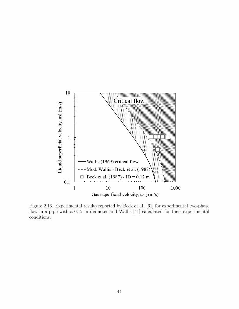
Figure 2.13. Experimental results reported by Beck et al. [61] for experimental two-phaseflow in a pipe with a 0.12 m diameter and Wallis [41] calculated for their experimentalconditions.

44

Chapter 3Experimental Data

To evaluate flow regime maps, relevant data on the conditions of interest is necessary. In

the case of this work, data covering large diameters and a wide range of flow velocities will

be used. Flow data from both field and lab were collected from the literature. Experimental

data was also collected at LSU, covering a gap left in the literature involving larger diameter

pipes (up to 0.30 m) and high flow velocities.

3.1 Experimental data from literature

Eight studies on two-phase flow in large diameter vertical pipes that provide flow regime

characterization are summarized in Table 3.1. This table presents information about the

working fluids, pipe diameters, superficial liquid and gas velocities, and relevant measured

parameters (pressure gradient, liquid holdup, and flow regime) of each respective study. This

table is used as the starting point for the comprehensive literature review to gather data

and empirical observations on vertical two-phase flows in large diameter pipes for a wide

range of gas-liquid velocities. Most flow regime maps were evaluated with experimental data

with water and air. The exception is Oddie et al. [62] data, who used nitrogen and water as

working fluids. In this case, to simplify the analysis, the properties of air were considered

instead of the properties of Nitrogen, as air is composed of more than 70% of Nitrogen and

the experimental conditions do not include high pressures or temperatures. The ideal gas

law is also considered, and the specific gravity of nitrogen and air are approximately the

same.

Most of the flow regime characterizations in Table 3.1 were obtained based on visual

observations. The exception is the research carried out by Smith et al. [22]. They made use

of a neural network classification system, coupled with an electrical impedance void-meter.

Ali [7] also characterized the flow regimes visually but assisted their definition with the

use of the statistical analysis of void fraction data calculated with the use of the pressure

drop method. All of the authors unanimously claim the absence of slug flow in its classical

45

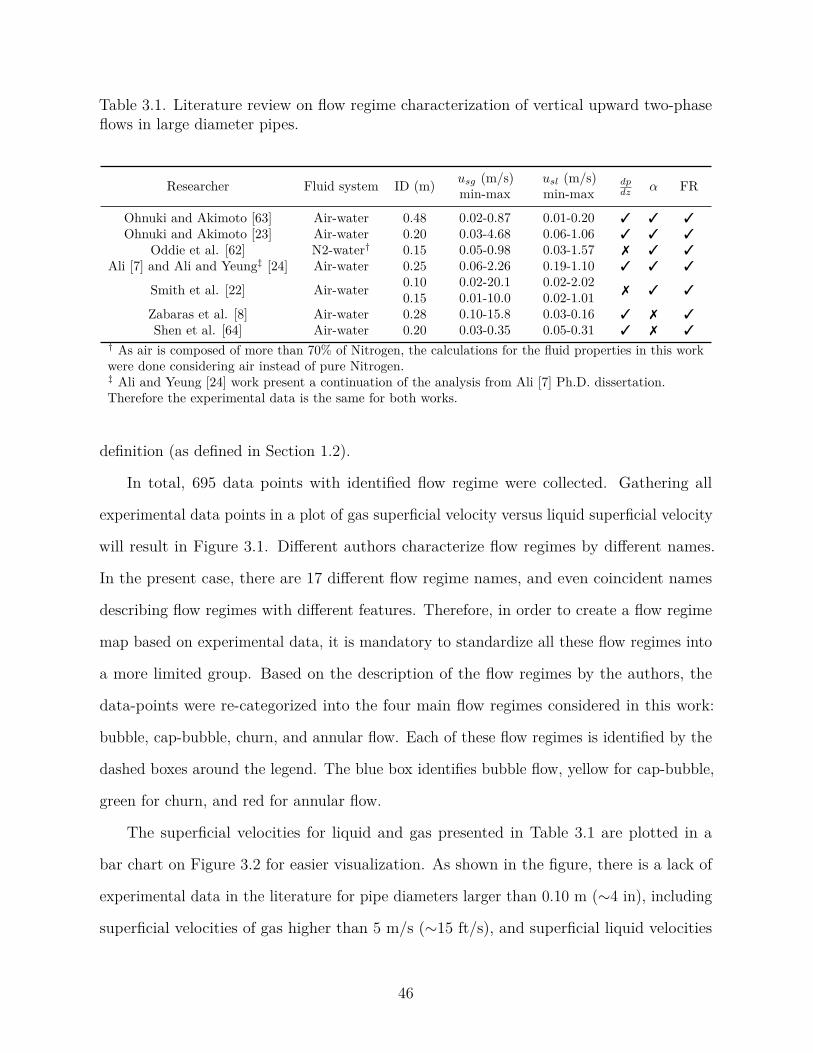
Table 3.1. Literature review on flow regime characterization of vertical upward two-phaseflows in large diameter pipes.

Researcher Fluid system ID (m) 𝑢𝑠𝑔 (m/s)min-max

𝑢𝑠𝑙 (m/s)min-max

𝑑𝑝𝑑𝑧 𝛼 FR

Ohnuki and Akimoto [63] Air-water 0.48 0.02-0.87 0.01-0.20 3 3 3

Ohnuki and Akimoto [23] Air-water 0.20 0.03-4.68 0.06-1.06 3 3 3

Oddie et al. [62] N2-water† 0.15 0.05-0.98 0.03-1.57 7 3 3

Ali [7] and Ali and Yeung‡ [24] Air-water 0.25 0.06-2.26 0.19-1.10 3 3 3

Smith et al. [22] Air-water 0.10 0.02-20.1 0.02-2.027 3 30.15 0.01-10.0 0.02-1.01

Zabaras et al. [8] Air-water 0.28 0.10-15.8 0.03-0.16 3 7 3

Shen et al. [64] Air-water 0.20 0.03-0.35 0.05-0.31 3 7 3† As air is composed of more than 70% of Nitrogen, the calculations for the fluid properties in this workwere done considering air instead of pure Nitrogen.‡ Ali and Yeung [24] work present a continuation of the analysis from Ali [7] Ph.D. dissertation.Therefore the experimental data is the same for both works.

definition (as defined in Section 1.2).

In total, 695 data points with identified flow regime were collected. Gathering all

experimental data points in a plot of gas superficial velocity versus liquid superficial velocity

will result in Figure 3.1. Different authors characterize flow regimes by different names.

In the present case, there are 17 different flow regime names, and even coincident names

describing flow regimes with different features. Therefore, in order to create a flow regime

map based on experimental data, it is mandatory to standardize all these flow regimes into

a more limited group. Based on the description of the flow regimes by the authors, the

data-points were re-categorized into the four main flow regimes considered in this work:

bubble, cap-bubble, churn, and annular flow. Each of these flow regimes is identified by the

dashed boxes around the legend. The blue box identifies bubble flow, yellow for cap-bubble,

green for churn, and red for annular flow.

The superficial velocities for liquid and gas presented in Table 3.1 are plotted in a

bar chart on Figure 3.2 for easier visualization. As shown in the figure, there is a lack of

experimental data in the literature for pipe diameters larger than 0.10 m (∼4 in), including

superficial velocities of gas higher than 5 m/s (∼15 ft/s), and superficial liquid velocities

46

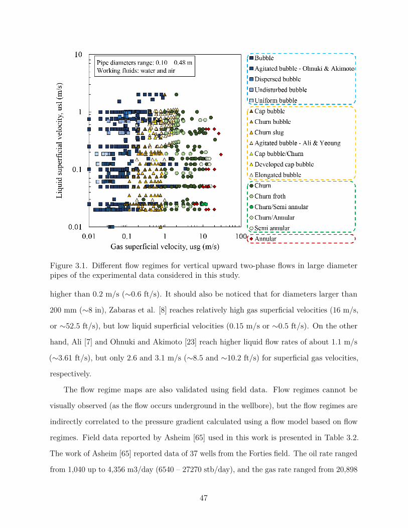
Figure 3.1. Different flow regimes for vertical upward two-phase flows in large diameterpipes of the experimental data considered in this study.

higher than 0.2 m/s (∼0.6 ft/s). It should also be noticed that for diameters larger than

200 mm (∼8 in), Zabaras et al. [8] reaches relatively high gas superficial velocities (16 m/s,

or ∼52.5 ft/s), but low liquid superficial velocities (0.15 m/s or ∼0.5 ft/s). On the other

hand, Ali [7] and Ohnuki and Akimoto [23] reach higher liquid flow rates of about 1.1 m/s

(∼3.61 ft/s), but only 2.6 and 3.1 m/s (∼8.5 and ∼10.2 ft/s) for superficial gas velocities,

respectively.

The flow regime maps are also validated using field data. Flow regimes cannot be

visually observed (as the flow occurs underground in the wellbore), but the flow regimes are

indirectly correlated to the pressure gradient calculated using a flow model based on flow

regimes. Field data reported by Asheim [65] used in this work is presented in Table 3.2.

The work of Asheim [65] reported data of 37 wells from the Forties field. The oil rate ranged

from 1,040 up to 4,356 m3/day (6540 – 27270 stb/day), and the gas rate ranged from 20,898

47

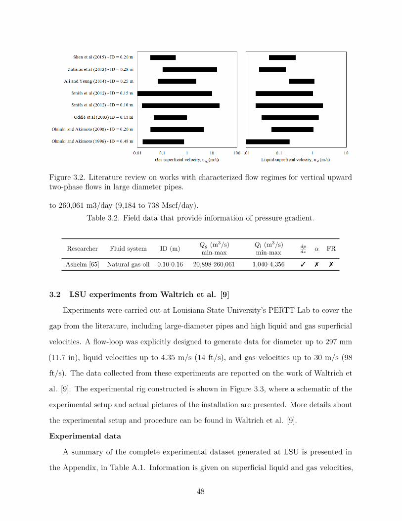
Figure 3.2. Literature review on works with characterized flow regimes for vertical upwardtwo-phase flows in large diameter pipes.

to 260,061 m3/day (9,184 to 738 Mscf/day).Table 3.2. Field data that provide information of pressure gradient.

Researcher Fluid system ID (m) 𝑄𝑔 (m3/s)min-max

𝑄𝑙 (m3/s)min-max

𝑑𝑝𝑑𝑧 𝛼 FR

Asheim [65] Natural gas-oil 0.10-0.16 20,898-260,061 1,040-4,356 3 7 7

3.2 LSU experiments from Waltrich et al. [9]

Experiments were carried out at Louisiana State University’s PERTT Lab to cover the

gap from the literature, including large-diameter pipes and high liquid and gas superficial

velocities. A flow-loop was explicitly designed to generate data for diameter up to 297 mm

(11.7 in), liquid velocities up to 4.35 m/s (14 ft/s), and gas velocities up to 30 m/s (98

ft/s). The data collected from these experiments are reported on the work of Waltrich et

al. [9]. The experimental rig constructed is shown in Figure 3.3, where a schematic of the

experimental setup and actual pictures of the installation are presented. More details about

the experimental setup and procedure can be found in Waltrich et al. [9].

Experimental data

A summary of the complete experimental dataset generated at LSU is presented in

the Appendix, in Table A.1. Information is given on superficial liquid and gas velocities,

48

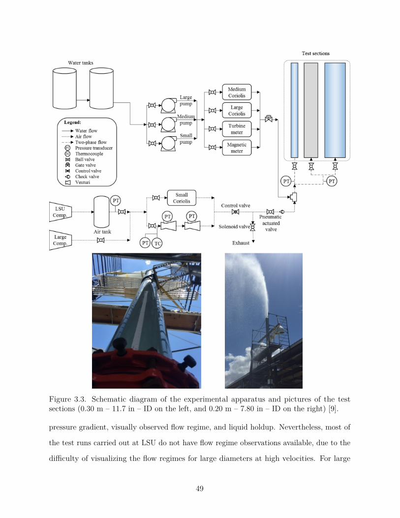
Figure 3.3. Schematic diagram of the experimental apparatus and pictures of the testsections (0.30 m – 11.7 in – ID on the left, and 0.20 m – 7.80 in – ID on the right) [9].

pressure gradient, visually observed flow regime, and liquid holdup. Nevertheless, most of

the test runs carried out at LSU do not have flow regime observations available, due to the

difficulty of visualizing the flow regimes for large diameters at high velocities. For large

49

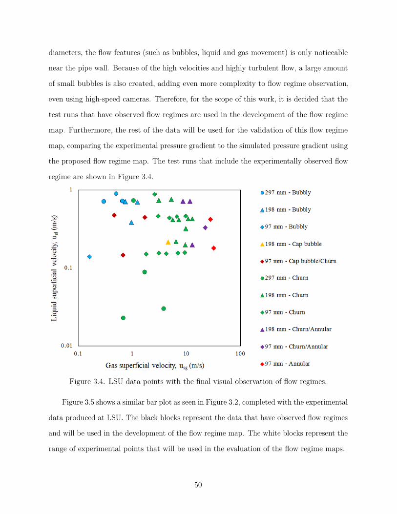
diameters, the flow features (such as bubbles, liquid and gas movement) is only noticeable

near the pipe wall. Because of the high velocities and highly turbulent flow, a large amount

of small bubbles is also created, adding even more complexity to flow regime observation,

even using high-speed cameras. Therefore, for the scope of this work, it is decided that the

test runs that have observed flow regimes are used in the development of the flow regime

map. Furthermore, the rest of the data will be used for the validation of this flow regime

map, comparing the experimental pressure gradient to the simulated pressure gradient using

the proposed flow regime map. The test runs that include the experimentally observed flow

regime are shown in Figure 3.4.

Figure 3.4. LSU data points with the final visual observation of flow regimes.

Figure 3.5 shows a similar bar plot as seen in Figure 3.2, completed with the experimental

data produced at LSU. The black blocks represent the data that have observed flow regimes

and will be used in the development of the flow regime map. The white blocks represent the

range of experimental points that will be used in the evaluation of the flow regime maps.

50

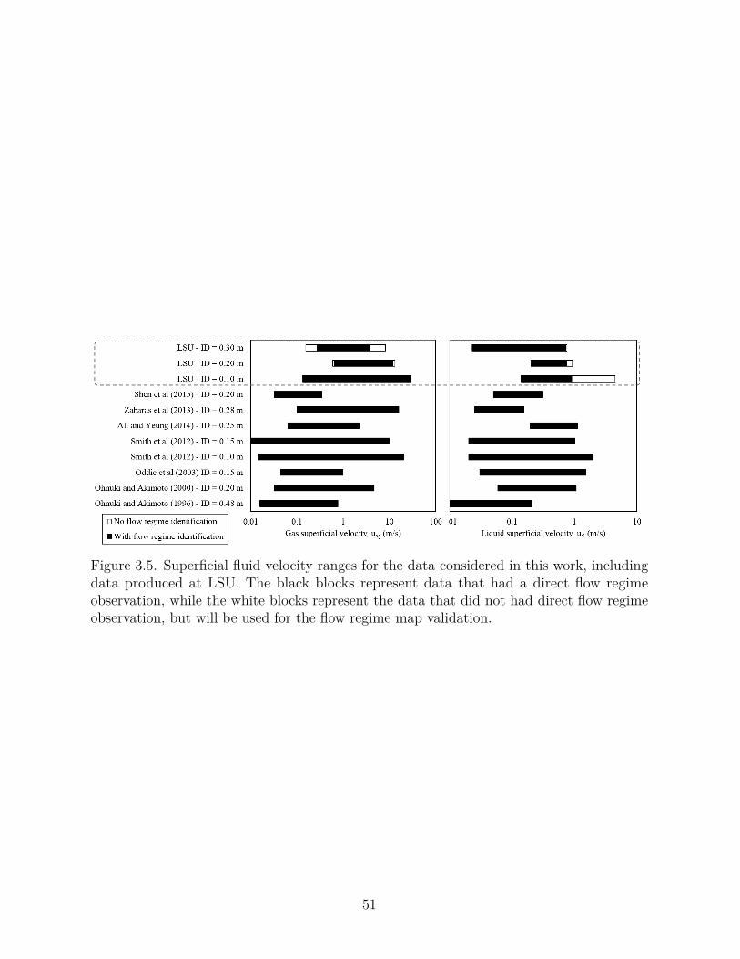
Figure 3.5. Superficial fluid velocity ranges for the data considered in this work, includingdata produced at LSU. The black blocks represent data that had a direct flow regimeobservation, while the white blocks represent the data that did not had direct flow regimeobservation, but will be used for the flow regime map validation.

51

Chapter 4Results and Discussions

4.1 Evaluation of current flow regime maps

A critical remark from the observed flow regimes is the absence of slug flow noted in all

the experimental works on pipes with 𝐷*𝐻 > 40 considered in this work. Thus, considering

this absence and that most of the flow regime maps evaluated in this work predict slug flow,

this flow regime is replaced by cap-bubble flow in these analysis.

The flow regimes are re-categorized into only four flow regimes to evaluate the flow

regime maps, based on the description provided in each work. The selected flow regimes are

bubble, cap-bubble, churn, and annular. The characteristics of each of these flow regimes

are as described in Chapter 1.

The observed flow regimes data points were tested based on its flow and fluid properties

against four different flow regime maps: Duns and Ros [11] and Aziz et al. [17] empirical

flow regime maps, and Mishima and Ishii [19] and Schlegel et al. [32] mechanistic flow

regime maps. Figure 4.1 shows all the 695 experimental observations of flow regimes already

re-categorized into the four flow regimes. The legends of the transition boundaries are

included by the name of the author who described them, followed by the transition which it

represents. The transitions are abbreviated as:

• B-S: Bubble to Slug flow

• S-C: Slug to Churn flow

• C-A: Churn to Annular flow

• B-CB: Bubble to Cap bubble flow

• CB-C: Cap bubble to Churn flow

• -A: Transition to Annular flow

• I-II: Transition from Region I to Region II, by Duns and Ros [11]

52

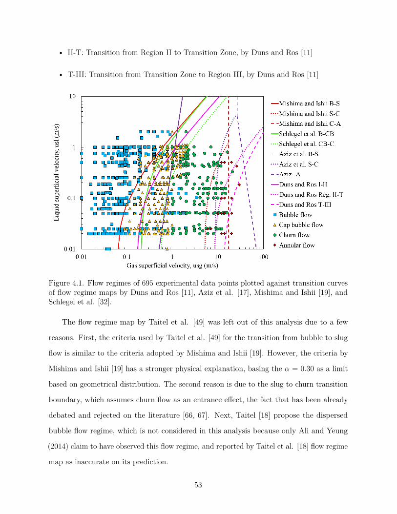
• II-T: Transition from Region II to Transition Zone, by Duns and Ros [11]

• T-III: Transition from Transition Zone to Region III, by Duns and Ros [11]

Figure 4.1. Flow regimes of 695 experimental data points plotted against transition curvesof flow regime maps by Duns and Ros [11], Aziz et al. [17], Mishima and Ishii [19], andSchlegel et al. [32].

The flow regime map by Taitel et al. [49] was left out of this analysis due to a few

reasons. First, the criteria used by Taitel et al. [49] for the transition from bubble to slug

flow is similar to the criteria adopted by Mishima and Ishii [19]. However, the criteria by

Mishima and Ishii [19] has a stronger physical explanation, basing the 𝛼 = 0.30 as a limit

based on geometrical distribution. The second reason is due to the slug to churn transition

boundary, which assumes churn flow as an entrance effect, the fact that has been already

debated and rejected on the literature [66, 67]. Next, Taitel [18] propose the dispersed

bubble flow regime, which is not considered in this analysis because only Ali and Yeung

(2014) claim to have observed this flow regime, and reported by Taitel et al. [18] flow regime

map as inaccurate on its prediction.

53

McQuillan and Whalley [43] flow regime map were also not included in this analysis.

The authors base their flow regime map on Taitel et al. [18], adopting the same transition

criteria for bubble to slug, and churn to annular. The novelty they bring to Taitel et al.

[18] approach is the suggestion to calculate the transition from bubble to dispersed bubble

flow, which will not be considered in this work, and propose a new method to calculate the

transition from slug to churn flow. This criterion is based on the flooding of the liquid film

around the Taylor bubble during the slug flow. However, as noted before, no slug flow was

observed in the studies considered in this work, and slug flow is no expected for 𝐷*𝐻 > 40.

Wu et al. [16] evaluate the flow regimes boundaries by the amount of conforming

and non-conforming points to each transition boundary. The authors consider pairs of

flow regimes at a time and assess if the observed data point will match the predicted flow

regime or not (stay on the other side of the boundary). Then, they evaluate the amount

of incorrectly predicted points by the boundary and the number of points that match the

anticipated flow regime.

The analysis conducted in this study is similar to that carried out by Wu et al. [16].

The results of the evaluation of the different flow regime maps against the experimental

data for pipe with 𝐷*𝐻 > 40 is plotted in Table 4.1.

The results for the transition boundary from bubble to cap-bubble presented in Table 4.1

give a better index for the Schlegel et al. [32] criteria than for Mishima and Ishii [19] criteria.

However, the difference between both is very small. Through visual inspection, it is possible

to see that Mishima and Ishii [19] transition criteria does a better job predicting cap-bubble

flow (less yellow markers outside of the delimited cap-bubble region). Therefore, considering

that negligible difference between both transition boundaries from bubble to cap-bubble

and the visually better performance on predicting cap-bubble flow, Mishima and Ishii [19]

transition criteria for the transition from bubble to cap-bubble flow will be adopted for the

flow regime map in this work.

Hence, the most appropriate transition boundaries are:

54

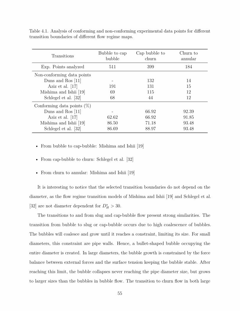
Table 4.1. Analysis of conforming and non-conforming experimental data points for differenttransition boundaries of different flow regime maps.

Transitions Bubble to capbubble

Cap bubble tochurn

Churn toannular

Exp. Points analyzed 511 399 184Non-conforming data points

Duns and Ros [11] - 132 14Aziz et al. [17] 191 131 15

Mishima and Ishii [19] 69 115 12Schlegel et al. [32] 68 44 12

Conforming data points (%)Duns and Ros [11] - 66.92 92.39

Aziz et al. [17] 62.62 66.92 91.85Mishima and Ishii [19] 86.50 71.18 93.48

Schlegel et al. [32] 86.69 88.97 93.48

• From bubble to cap-bubble: Mishima and Ishii [19]

• From cap-bubble to churn: Schlegel et al. [32]

• From churn to annular: Mishima and Ishii [19]

It is interesting to notice that the selected transition boundaries do not depend on the

diameter, as the flow regime transition models of Mishima and Ishii [19] and Schlegel et al.

[32] are not diameter dependent for 𝐷*𝐻 > 30.

The transitions to and from slug and cap-bubble flow present strong similarities. The

transition from bubble to slug or cap-bubble occurs due to high coalescence of bubbles.

The bubbles will coalesce and grow until it reaches a constraint, limiting its size. For small

diameters, this constraint are pipe walls. Hence, a bullet-shaped bubble occupying the

entire diameter is created. In large diameters, the bubble growth is constrained by the force

balance between external forces and the surface tension keeping the bubble stable. After

reaching this limit, the bubble collapses never reaching the pipe diameter size, but grows

to larger sizes than the bubbles in bubble flow. The transition to churn flow in both large

55

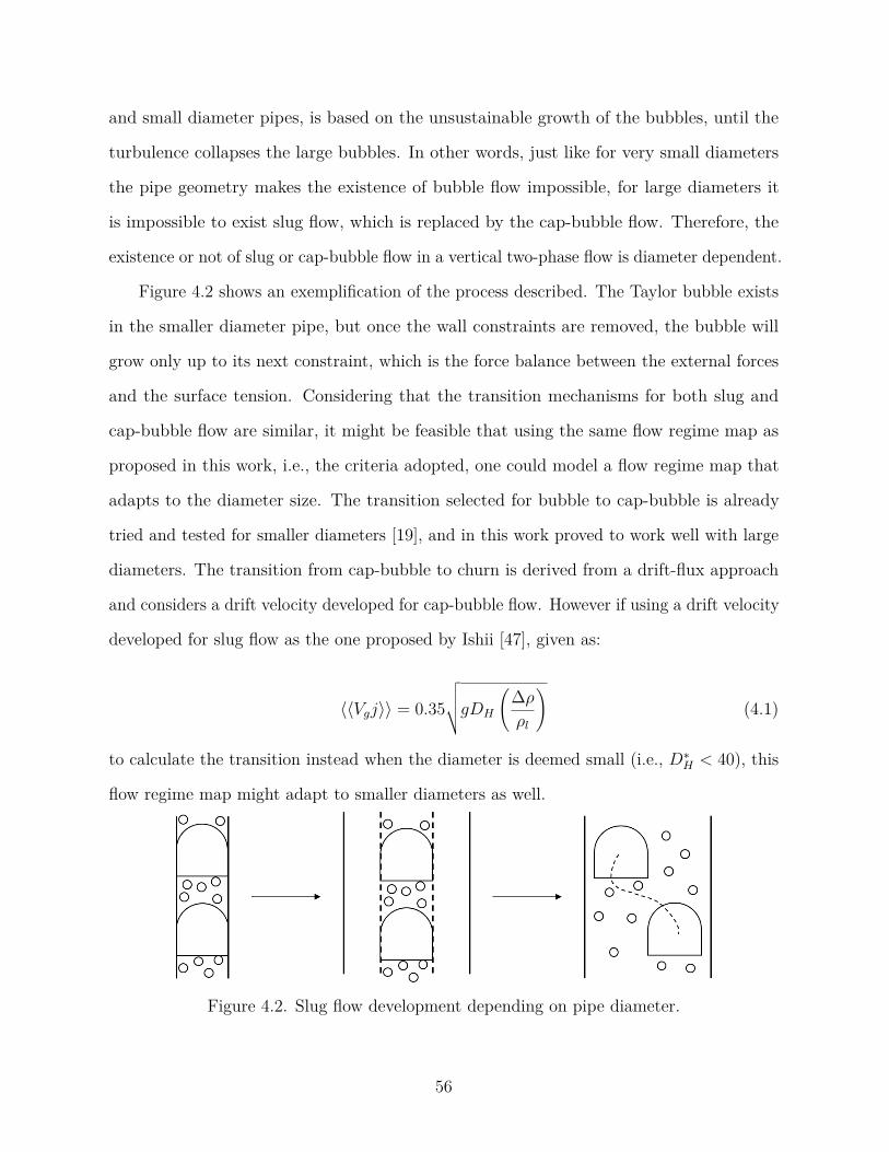
and small diameter pipes, is based on the unsustainable growth of the bubbles, until the

turbulence collapses the large bubbles. In other words, just like for very small diameters

the pipe geometry makes the existence of bubble flow impossible, for large diameters it

is impossible to exist slug flow, which is replaced by the cap-bubble flow. Therefore, the

existence or not of slug or cap-bubble flow in a vertical two-phase flow is diameter dependent.

Figure 4.2 shows an exemplification of the process described. The Taylor bubble exists

in the smaller diameter pipe, but once the wall constraints are removed, the bubble will

grow only up to its next constraint, which is the force balance between the external forces

and the surface tension. Considering that the transition mechanisms for both slug and

cap-bubble flow are similar, it might be feasible that using the same flow regime map as

proposed in this work, i.e., the criteria adopted, one could model a flow regime map that

adapts to the diameter size. The transition selected for bubble to cap-bubble is already

tried and tested for smaller diameters [19], and in this work proved to work well with large

diameters. The transition from cap-bubble to churn is derived from a drift-flux approach

and considers a drift velocity developed for cap-bubble flow. However if using a drift velocity

developed for slug flow as the one proposed by Ishii [47], given as:

⟨⟨𝑉𝑔𝑗⟩⟩ = 0.35

⎯⎸⎸⎷𝑔𝐷𝐻

(︃Δ𝜌

𝜌𝑙

)︃(4.1)

to calculate the transition instead when the diameter is deemed small (i.e., 𝐷*𝐻 < 40), this

flow regime map might adapt to smaller diameters as well.

Figure 4.2. Slug flow development depending on pipe diameter.

56

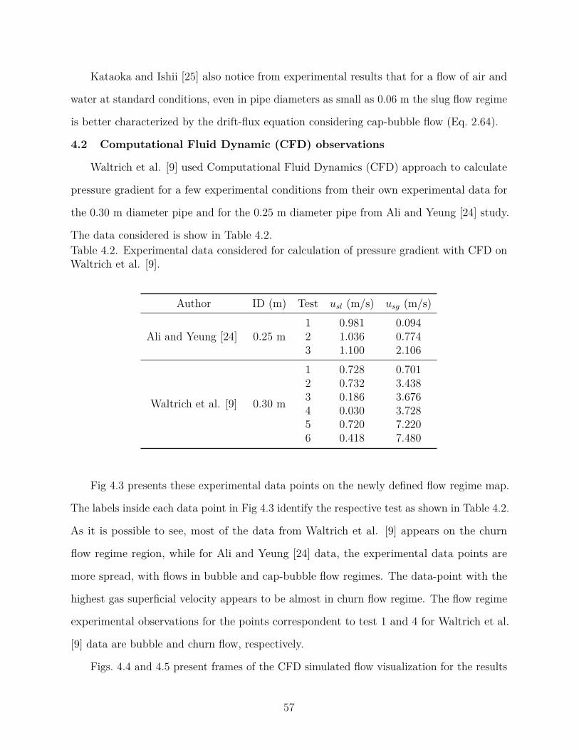
Kataoka and Ishii [25] also notice from experimental results that for a flow of air and

water at standard conditions, even in pipe diameters as small as 0.06 m the slug flow regime

is better characterized by the drift-flux equation considering cap-bubble flow (Eq. 2.64).

4.2 Computational Fluid Dynamic (CFD) observations

Waltrich et al. [9] used Computational Fluid Dynamics (CFD) approach to calculate

pressure gradient for a few experimental conditions from their own experimental data for

the 0.30 m diameter pipe and for the 0.25 m diameter pipe from Ali and Yeung [24] study.

The data considered is show in Table 4.2.Table 4.2. Experimental data considered for calculation of pressure gradient with CFD onWaltrich et al. [9].

Author ID (m) Test 𝑢𝑠𝑙 (m/s) 𝑢𝑠𝑔 (m/s)

Ali and Yeung [24] 0.25 m1 0.981 0.0942 1.036 0.7743 1.100 2.106

Waltrich et al. [9] 0.30 m

1 0.728 0.7012 0.732 3.4383 0.186 3.6764 0.030 3.7285 0.720 7.2206 0.418 7.480

Fig 4.3 presents these experimental data points on the newly defined flow regime map.

The labels inside each data point in Fig 4.3 identify the respective test as shown in Table 4.2.

As it is possible to see, most of the data from Waltrich et al. [9] appears on the churn

flow regime region, while for Ali and Yeung [24] data, the experimental data points are

more spread, with flows in bubble and cap-bubble flow regimes. The data-point with the

highest gas superficial velocity appears to be almost in churn flow regime. The flow regime

experimental observations for the points correspondent to test 1 and 4 for Waltrich et al.

[9] data are bubble and churn flow, respectively.

Figs. 4.4 and 4.5 present frames of the CFD simulated flow visualization for the results

57

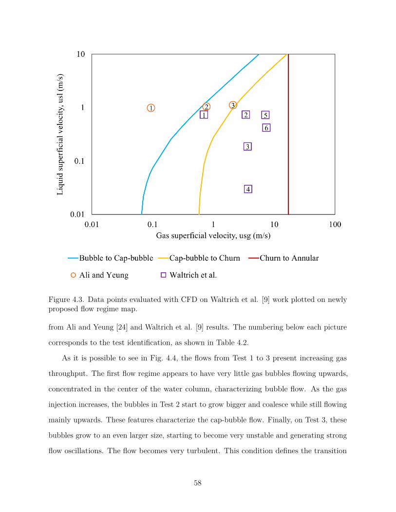
Figure 4.3. Data points evaluated with CFD on Waltrich et al. [9] work plotted on newlyproposed flow regime map.

from Ali and Yeung [24] and Waltrich et al. [9] results. The numbering below each picture

corresponds to the test identification, as shown in Table 4.2.

As it is possible to see in Fig. 4.4, the flows from Test 1 to 3 present increasing gas

throughput. The first flow regime appears to have very little gas bubbles flowing upwards,

concentrated in the center of the water column, characterizing bubble flow. As the gas

injection increases, the bubbles in Test 2 start to grow bigger and coalesce while still flowing

mainly upwards. These features characterize the cap-bubble flow. Finally, on Test 3, these

bubbles grow to an even larger size, starting to become very unstable and generating strong

flow oscillations. The flow becomes very turbulent. This condition defines the transition

58

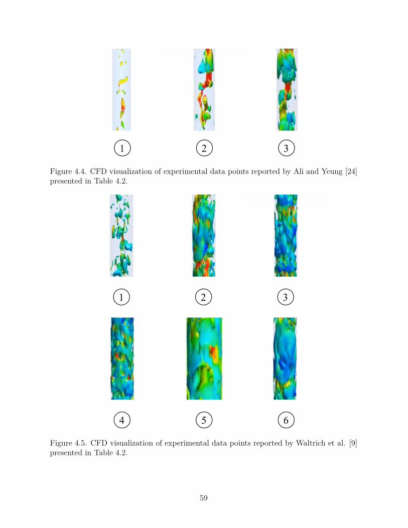
Figure 4.4. CFD visualization of experimental data points reported by Ali and Yeung [24]presented in Table 4.2.

Figure 4.5. CFD visualization of experimental data points reported by Waltrich et al. [9]presented in Table 4.2.

59

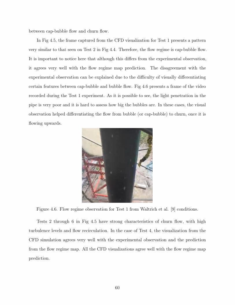
between cap-bubble flow and churn flow.

In Fig 4.5, the frame captured from the CFD visualization for Test 1 presents a pattern

very similar to that seen on Test 2 in Fig 4.4. Therefore, the flow regime is cap-bubble flow.

It is important to notice here that although this differs from the experimental observation,

it agrees very well with the flow regime map prediction. The disagreement with the

experimental observation can be explained due to the difficulty of visually differentiating

certain features between cap-bubble and bubble flow. Fig 4.6 presents a frame of the video

recorded during the Test 1 experiment. As it is possible to see, the light penetration in the

pipe is very poor and it is hard to assess how big the bubbles are. In these cases, the visual

observation helped differentiating the flow from bubble (or cap-bubble) to churn, once it is

flowing upwards.

Figure 4.6. Flow regime observation for Test 1 from Waltrich et al. [9] conditions.

Tests 2 through 6 in Fig 4.5 have strong characteristics of churn flow, with high

turbulence levels and flow recirculation. In the case of Test 4, the visualization from the

CFD simulation agrees very well with the experimental observation and the prediction

from the flow regime map. All the CFD visualizations agree well with the flow regime map

prediction.

60

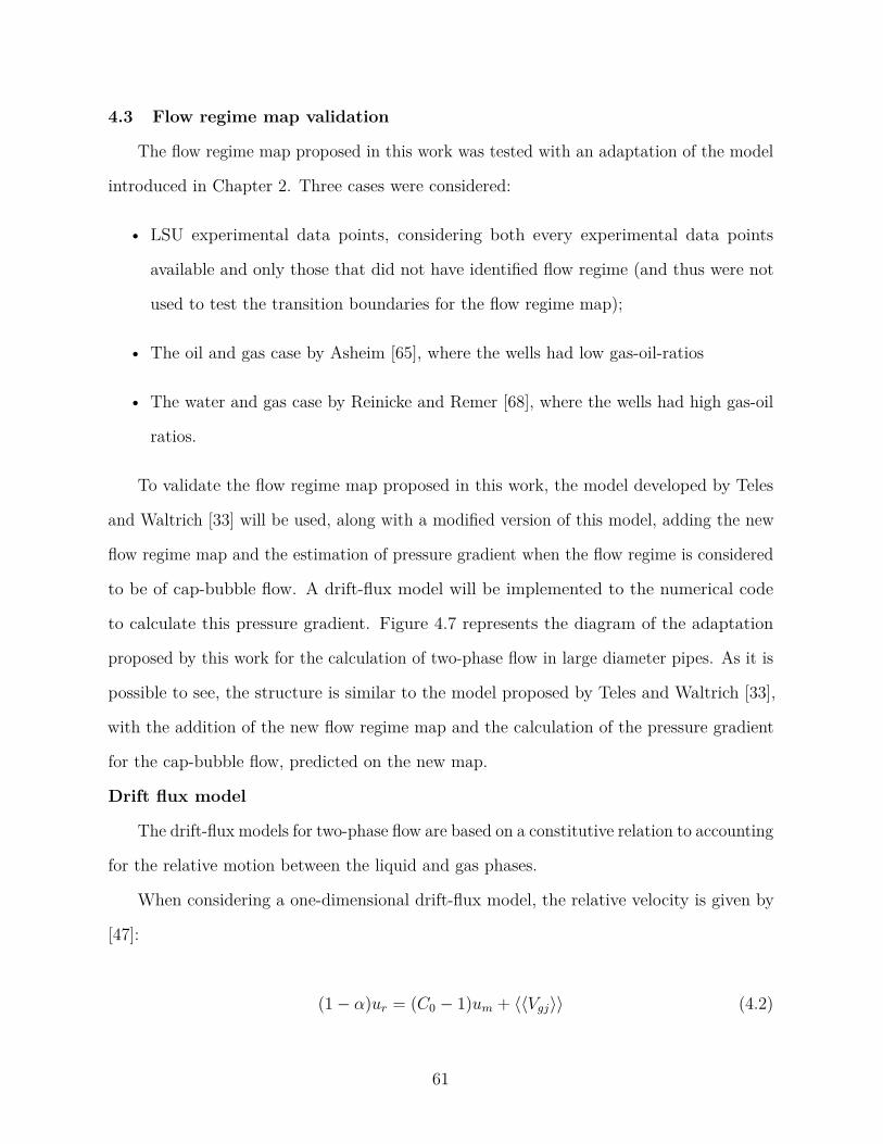
4.3 Flow regime map validation

The flow regime map proposed in this work was tested with an adaptation of the model

introduced in Chapter 2. Three cases were considered:

• LSU experimental data points, considering both every experimental data points

available and only those that did not have identified flow regime (and thus were not

used to test the transition boundaries for the flow regime map);

• The oil and gas case by Asheim [65], where the wells had low gas-oil-ratios

• The water and gas case by Reinicke and Remer [68], where the wells had high gas-oil

ratios.

To validate the flow regime map proposed in this work, the model developed by Teles

and Waltrich [33] will be used, along with a modified version of this model, adding the new

flow regime map and the estimation of pressure gradient when the flow regime is considered

to be of cap-bubble flow. A drift-flux model will be implemented to the numerical code

to calculate this pressure gradient. Figure 4.7 represents the diagram of the adaptation

proposed by this work for the calculation of two-phase flow in large diameter pipes. As it is

possible to see, the structure is similar to the model proposed by Teles and Waltrich [33],

with the addition of the new flow regime map and the calculation of the pressure gradient

for the cap-bubble flow, predicted on the new map.

Drift flux model

The drift-flux models for two-phase flow are based on a constitutive relation to accounting

for the relative motion between the liquid and gas phases.

When considering a one-dimensional drift-flux model, the relative velocity is given by

[47]:

(1 − 𝛼)𝑢𝑟 = (𝐶0 − 1)𝑢𝑚 + ⟨⟨𝑉𝑔𝑗⟩⟩ (4.2)

61

Figure 4.7. Modified diagram proposed by this work for the model developed by Teles andWaltrich.

where 𝑢𝑟 is the relative velocity, 𝐶0 is the distribution parameter, and ⟨⟨𝑉𝑔𝑗⟩⟩ is the

void-fraction weighted area average of the local drift velocity. The relative velocity, 𝑢𝑟 can

be calculated as:

𝑢𝑟 = 𝑢𝑔 − 𝑢𝑙 (4.3)

The average gas and liquid velocities can be correlated to the void-fraction as:

𝑢𝑔 = 𝑢𝑠𝑔

𝛼(4.4)

and

62

𝑢𝑙 = 𝑢𝑠𝑙

1 − 𝛼(4.5)

The void fraction can be calculated as:

𝛼 = 𝑢𝑠𝑔

𝐶0𝑢𝑚 + ⟨⟨𝑉𝑔𝑗⟩⟩(4.6)

Hibiki and Ishii [14] recommended the use of Kataoka and Ishii [25] drift-flux correlation

for cap-bubble flow regime. According to Kataoka and Ishii [25], the drift velocity in

large-diameter pipes is dependent on the diameter, pressure, gas flux, and fluid physical

properties, and can be calculated by Eq. 2.64. The distribution factor 𝐶0, can be calculated

with Eq. 2.44.

Once the void-fraction is calculated, it is possible to estimate the pressure drop. The

pressure gradient equation for multiphase flow can be used by considering the fluids as a

homogeneous mixture as (Shoham, 2006):

𝑑𝑝

𝑑𝐿=(︃

𝑑𝑝

𝑑𝐿

)︃𝑔𝑟𝑎𝑣𝑖𝑡𝑎𝑡𝑖𝑜𝑛𝑎𝑙

+(︃

𝑑𝑝

𝑑𝐿

)︃𝑓𝑟𝑖𝑐𝑡𝑖𝑜𝑛𝑎𝑙

+(︃

𝑑𝑝

𝑑𝐿

)︃𝑎𝑐𝑐𝑒𝑙𝑒𝑟𝑎𝑡𝑖𝑜𝑛𝑎𝑙

(4.7)

In general, the gravitational pressure gradient is based on the in-situ mixture density,

𝜌𝑚, as

(︃𝑑𝑝

𝑑𝐿

)︃𝑔𝑟𝑎𝑣𝑖𝑡𝑎𝑡𝑖𝑜𝑛𝑎𝑙

= 𝜌𝑚𝑔 sin 𝜃 (4.8)

The frictional pressure drop can be calculated based on the Fanning friction factor, f,

as:

(︃𝑑𝑝

𝑑𝐿

)︃𝑓𝑟𝑖𝑐𝑡𝑖𝑜𝑛𝑎𝑙

= 2𝑓𝜌𝑚𝑢2𝑚

𝐷(4.9)

The Reynolds number for a two-phase flow mixture can be calculated as:

63

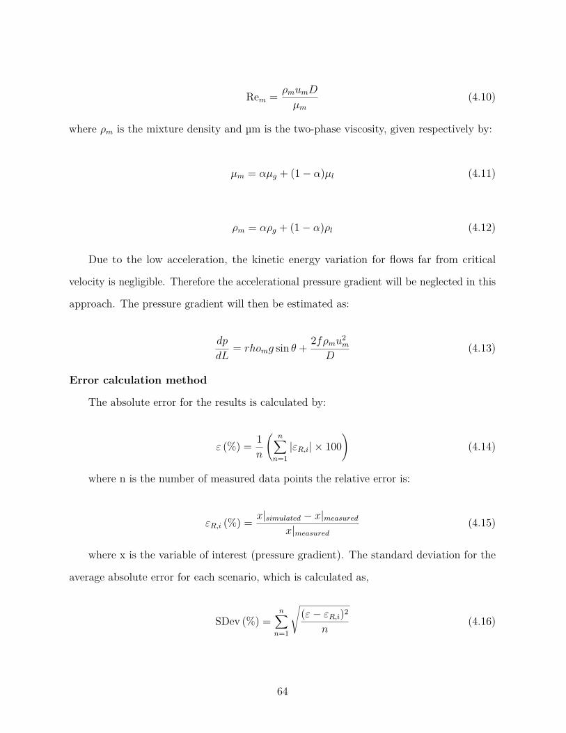
Re𝑚 = 𝜌𝑚𝑢𝑚𝐷

𝜇𝑚

(4.10)

where 𝜌𝑚 is the mixture density and µm is the two-phase viscosity, given respectively by:

𝜇𝑚 = 𝛼𝜇𝑔 + (1 − 𝛼)𝜇𝑙 (4.11)

𝜌𝑚 = 𝛼𝜌𝑔 + (1 − 𝛼)𝜌𝑙 (4.12)

Due to the low acceleration, the kinetic energy variation for flows far from critical

velocity is negligible. Therefore the accelerational pressure gradient will be neglected in this

approach. The pressure gradient will then be estimated as:

𝑑𝑝

𝑑𝐿= 𝑟ℎ𝑜𝑚𝑔 sin 𝜃 + 2𝑓𝜌𝑚𝑢2

𝑚

𝐷(4.13)

Error calculation method

The absolute error for the results is calculated by:

𝜀 (%) = 1𝑛

(︃𝑛∑︁

𝑛=1|𝜀𝑅,𝑖| × 100

)︃(4.14)

where n is the number of measured data points the relative error is:

𝜀𝑅,𝑖 (%) = 𝑥|𝑠𝑖𝑚𝑢𝑙𝑎𝑡𝑒𝑑 − 𝑥|𝑚𝑒𝑎𝑠𝑢𝑟𝑒𝑑

𝑥|𝑚𝑒𝑎𝑠𝑢𝑟𝑒𝑑

(4.15)

where x is the variable of interest (pressure gradient). The standard deviation for the

average absolute error for each scenario, which is calculated as,

SDev (%) =𝑛∑︁

𝑛=1

√︃(𝜀 − 𝜀𝑅,𝑖)2

𝑛(4.16)

64

4.4 Water and air – Data from Waltrich et al. [9]

Figure 4.8 shows the experimental data extracted from Waltrich et al. [9] points plotted

over the newly proposed flow regime map. As it is possible to see, the map matches well

with the churn and annular flow observations. However, it only achieves 50 % of conforming

cap-bubble and only about 43 % bubble flow prediction. This may be due to the difficulties

of visually identifying flow regimes in large diameter pipes. As it is possible to see, for

the 0.10 m pipe the predicted flow regime matches very well with the observed, while the

highest errors are for the 0.20 m diameter pipe, which have metal walls and do not allow

the direct visualization of the flow.

Figure 4.9 shows the absolute averaged error for the pressure gradients using the model

presented in Figure 4.7 and the model by Teles and Waltrich [33]. The standard deviation

of the absoulte error is also plotted in the figure as the deviation bars. The results were

compared only for the data points that are estimated as cap-bubble flow by the flow regime

map proposed in this work. Conditions to which more than 10% of the total flow length

was of a different flow regime were not considered in this comparison.

It is possible to see a considerable drop in the error for the cases where the new map

considered cap-bubble – and that the pressure drop was calculated as such. It is also

possible to notice that the error difference appears to be reduced with the increasing pipe

diameter. One conceivable explanation is that due to the broader space that the flow has

on the larger diameter, the cap-bubbles are not as relevant to the pressure drop and, once

they grow to a size which has enough influence, the turbulence is already high enough so

that the flow is already almost configured as churn flow. This conclusion might be biased

once it is considered factors such as the different flow velocities of the data considered for

each pipe diameter, or even the amount of data-points.

In order to reduce the bias of the previous analysis, it is important to compare the error

for similar conditions. This way, a few data-points for each diameter under similar liquid

and gas superficial velocities were selected. Two groups with data for the three different

65

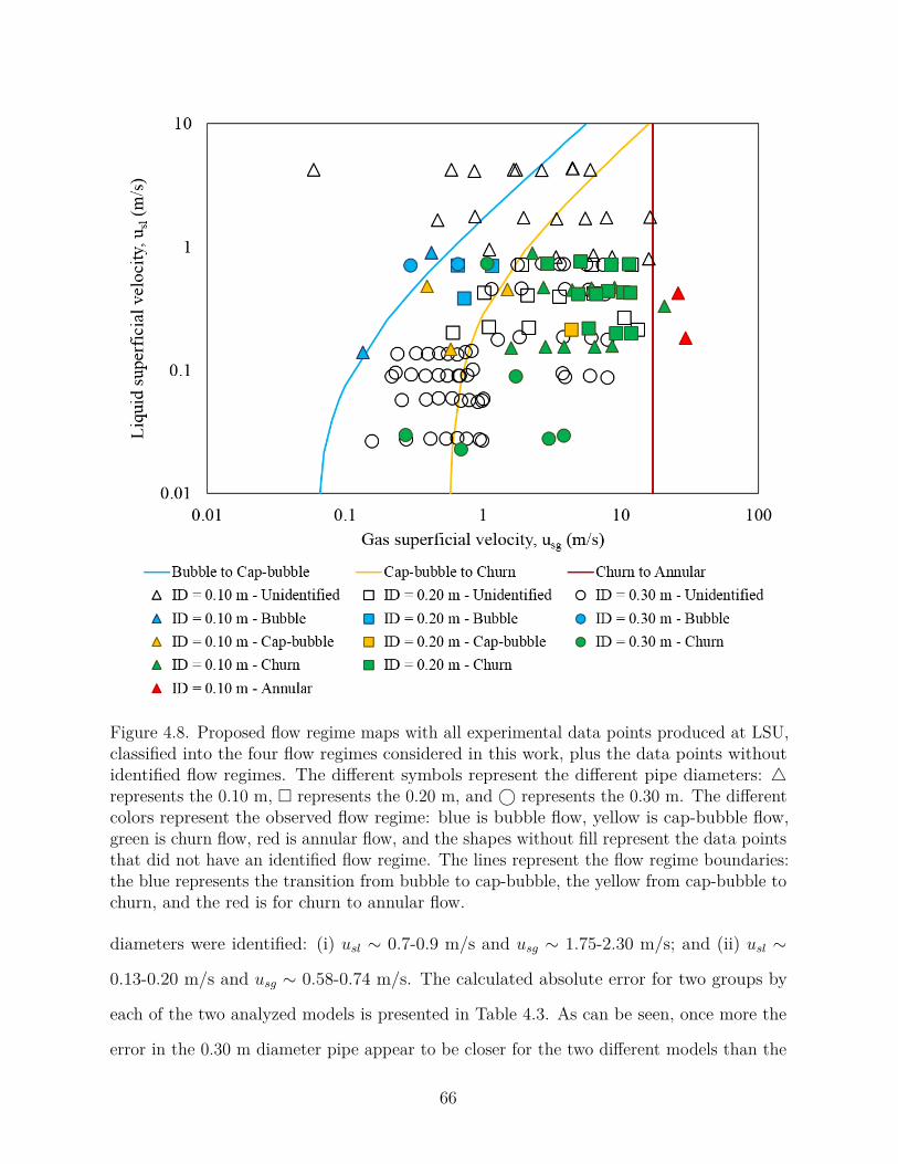
Figure 4.8. Proposed flow regime maps with all experimental data points produced at LSU,classified into the four flow regimes considered in this work, plus the data points withoutidentified flow regimes. The different symbols represent the different pipe diameters: △represents the 0.10 m, � represents the 0.20 m, and ○ represents the 0.30 m. The differentcolors represent the observed flow regime: blue is bubble flow, yellow is cap-bubble flow,green is churn flow, red is annular flow, and the shapes without fill represent the data pointsthat did not have an identified flow regime. The lines represent the flow regime boundaries:the blue represents the transition from bubble to cap-bubble, the yellow from cap-bubble tochurn, and the red is for churn to annular flow.

diameters were identified: (i) 𝑢𝑠𝑙 ∼ 0.7-0.9 m/s and 𝑢𝑠𝑔 ∼ 1.75-2.30 m/s; and (ii) 𝑢𝑠𝑙 ∼

0.13-0.20 m/s and 𝑢𝑠𝑔 ∼ 0.58-0.74 m/s. The calculated absolute error for two groups by

each of the two analyzed models is presented in Table 4.3. As can be seen, once more the

error in the 0.30 m diameter pipe appear to be closer for the two different models than the

66

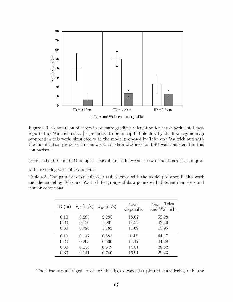
Figure 4.9. Comparison of errors in pressure gradient calculation for the experimental datareported by Waltrich et al. [9] predicted to be in cap-bubble flow by the flow regime mapproposed in this work, simulated with the model proposed by Teles and Waltrich and withthe modification proposed in this work. All data produced at LSU was considered in thiscomparison.

error in the 0.10 and 0.20 m pipes. The difference between the two models error also appear

to be reducing with pipe diameter.Table 4.3. Comparative of calculated absolute error with the model proposed in this workand the model by Teles and Waltrich for groups of data points with different diameters andsimilar conditions.

ID (m) 𝑢𝑠𝑙 (m/s) 𝑢𝑠𝑔 (m/s) 𝜀𝑎𝑏𝑠 -Capovilla

𝜀𝑎𝑏𝑠 – Telesand Waltrich

0.10 0.885 2.285 18.07 52.280.20 0.720 1.907 14.22 43.500.30 0.724 1.782 11.69 15.950.10 0.147 0.582 1.47 44.170.20 0.203 0.600 11.17 44.280.30 0.134 0.649 14.81 28.520.30 0.141 0.740 16.91 29.23

The absolute averaged error for the dp/dz was also plotted considering only the

67

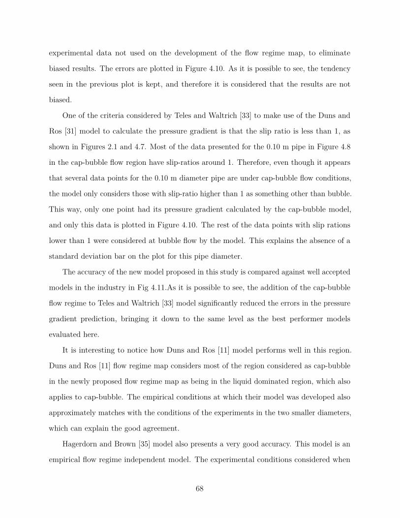
experimental data not used on the development of the flow regime map, to eliminate

biased results. The errors are plotted in Figure 4.10. As it is possible to see, the tendency

seen in the previous plot is kept, and therefore it is considered that the results are not

biased.

One of the criteria considered by Teles and Waltrich [33] to make use of the Duns and

Ros [31] model to calculate the pressure gradient is that the slip ratio is less than 1, as

shown in Figures 2.1 and 4.7. Most of the data presented for the 0.10 m pipe in Figure 4.8

in the cap-bubble flow region have slip-ratios around 1. Therefore, even though it appears

that several data points for the 0.10 m diameter pipe are under cap-bubble flow conditions,

the model only considers those with slip-ratio higher than 1 as something other than bubble.

This way, only one point had its pressure gradient calculated by the cap-bubble model,

and only this data is plotted in Figure 4.10. The rest of the data points with slip rations

lower than 1 were considered at bubble flow by the model. This explains the absence of a

standard deviation bar on the plot for this pipe diameter.

The accuracy of the new model proposed in this study is compared against well accepted

models in the industry in Fig 4.11.As it is possible to see, the addition of the cap-bubble

flow regime to Teles and Waltrich [33] model significantly reduced the errors in the pressure

gradient prediction, bringing it down to the same level as the best performer models

evaluated here.

It is interesting to notice how Duns and Ros [11] model performs well in this region.

Duns and Ros [11] flow regime map considers most of the region considered as cap-bubble

in the newly proposed flow regime map as being in the liquid dominated region, which also

applies to cap-bubble. The empirical conditions at which their model was developed also

approximately matches with the conditions of the experiments in the two smaller diameters,

which can explain the good agreement.

Hagerdorn and Brown [35] model also presents a very good accuracy. This model is an

empirical flow regime independent model. The experimental conditions considered when

68

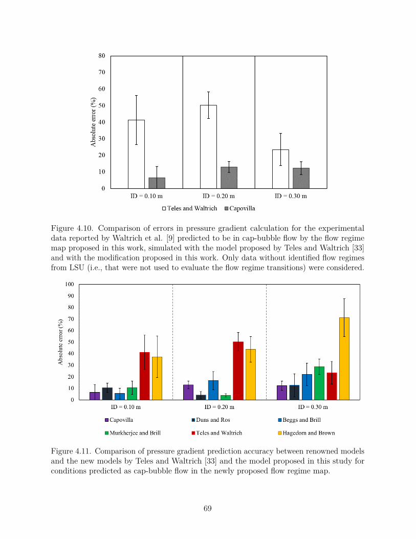
Figure 4.10. Comparison of errors in pressure gradient calculation for the experimentaldata reported by Waltrich et al. [9] predicted to be in cap-bubble flow by the flow regimemap proposed in this work, simulated with the model proposed by Teles and Waltrich [33]and with the modification proposed in this work. Only data without identified flow regimesfrom LSU (i.e., that were not used to evaluate the flow regime transitions) were considered.

Figure 4.11. Comparison of pressure gradient prediction accuracy between renowned modelsand the new models by Teles and Waltrich [33] and the model proposed in this study forconditions predicted as cap-bubble flow in the newly proposed flow regime map.

69

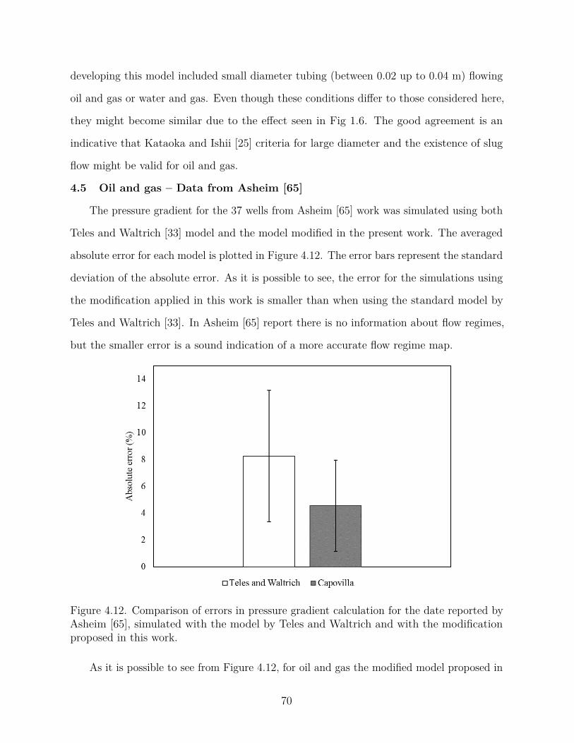
developing this model included small diameter tubing (between 0.02 up to 0.04 m) flowing

oil and gas or water and gas. Even though these conditions differ to those considered here,

they might become similar due to the effect seen in Fig 1.6. The good agreement is an

indicative that Kataoka and Ishii [25] criteria for large diameter and the existence of slug

flow might be valid for oil and gas.

4.5 Oil and gas – Data from Asheim [65]

The pressure gradient for the 37 wells from Asheim [65] work was simulated using both

Teles and Waltrich [33] model and the model modified in the present work. The averaged

absolute error for each model is plotted in Figure 4.12. The error bars represent the standard

deviation of the absolute error. As it is possible to see, the error for the simulations using

the modification applied in this work is smaller than when using the standard model by

Teles and Waltrich [33]. In Asheim [65] report there is no information about flow regimes,

but the smaller error is a sound indication of a more accurate flow regime map.

Figure 4.12. Comparison of errors in pressure gradient calculation for the date reported byAsheim [65], simulated with the model by Teles and Waltrich and with the modificationproposed in this work.

As it is possible to see from Figure 4.12, for oil and gas the modified model proposed in

70

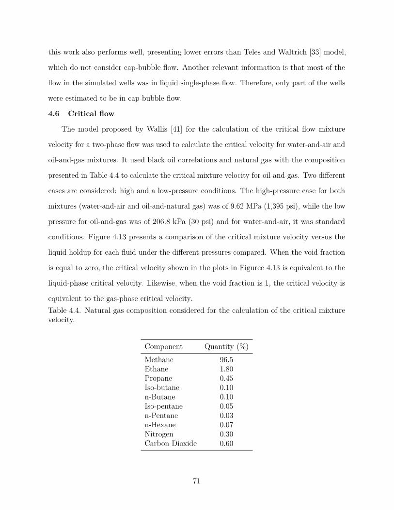
this work also performs well, presenting lower errors than Teles and Waltrich [33] model,

which do not consider cap-bubble flow. Another relevant information is that most of the

flow in the simulated wells was in liquid single-phase flow. Therefore, only part of the wells

were estimated to be in cap-bubble flow.

4.6 Critical flow

The model proposed by Wallis [41] for the calculation of the critical flow mixture

velocity for a two-phase flow was used to calculate the critical velocity for water-and-air and

oil-and-gas mixtures. It used black oil correlations and natural gas with the composition

presented in Table 4.4 to calculate the critical mixture velocity for oil-and-gas. Two different

cases are considered: high and a low-pressure conditions. The high-pressure case for both

mixtures (water-and-air and oil-and-natural gas) was of 9.62 MPa (1,395 psi), while the low

pressure for oil-and-gas was of 206.8 kPa (30 psi) and for water-and-air, it was standard

conditions. Figure 4.13 presents a comparison of the critical mixture velocity versus the

liquid holdup for each fluid under the different pressures compared. When the void fraction

is equal to zero, the critical velocity shown in the plots in Figuree 4.13 is equivalent to the

liquid-phase critical velocity. Likewise, when the void fraction is 1, the critical velocity is

equivalent to the gas-phase critical velocity.Table 4.4. Natural gas composition considered for the calculation of the critical mixturevelocity.

Component Quantity (%)Methane 96.5Ethane 1.80Propane 0.45Iso-butane 0.10n-Butane 0.10Iso-pentane 0.05n-Pentane 0.03n-Hexane 0.07Nitrogen 0.30Carbon Dioxide 0.60

71

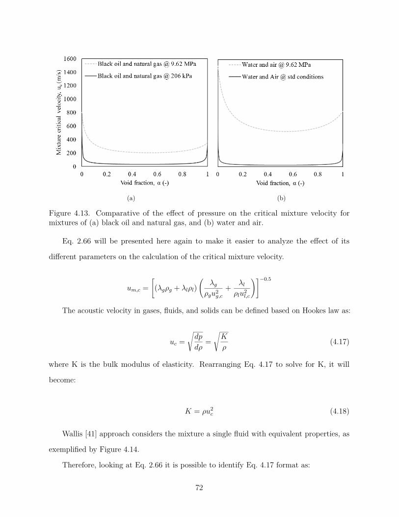
(a) (b)

Figure 4.13. Comparative of the effect of pressure on the critical mixture velocity formixtures of (a) black oil and natural gas, and (b) water and air.

Eq. 2.66 will be presented here again to make it easier to analyze the effect of its

different parameters on the calculation of the critical mixture velocity.

𝑢𝑚,𝑐 =[︃(𝜆𝑔𝜌𝑔 + 𝜆𝑙𝜌𝑙)

(︃𝜆𝑔

𝜌𝑔𝑢2𝑔,𝑐

+ 𝜆𝑙

𝜌𝑙𝑢2𝑙,𝑐

)︃]︃−0.5

The acoustic velocity in gases, fluids, and solids can be defined based on Hookes law as:

𝑢𝑐 =√︃

𝑑𝑝

𝑑𝜌=√︃

𝐾

𝜌(4.17)

where K is the bulk modulus of elasticity. Rearranging Eq. 4.17 to solve for K, it will

become:

𝐾 = 𝜌𝑢2𝑐 (4.18)

Wallis [41] approach considers the mixture a single fluid with equivalent properties, as

exemplified by Figure 4.14.

Therefore, looking at Eq. 2.66 it is possible to identify Eq. 4.17 format as:

72

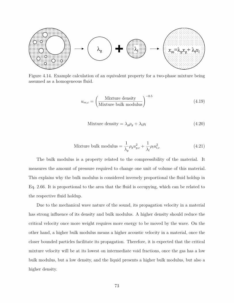
Figure 4.14. Example calculation of an equivalent property for a two-phase mixture beingassumed as a homogeneous fluid.

𝑢𝑚,𝑐 =(︃

Mixture densityMixture bulk modulus

)︃−0.5

(4.19)

Mixture density = 𝜆𝑔𝜌𝑔 + 𝜆𝑙𝜌𝑙 (4.20)

Mixture bulk modulus = 1𝜆𝑔

𝜌𝑔𝑢2𝑔,𝑐 + 1

𝜆𝑙

𝜌𝑙𝑢2𝑙,𝑐 (4.21)

The bulk modulus is a property related to the compressibility of the material. It

measures the amount of pressure required to change one unit of volume of this material.

This explains why the bulk modulus is considered inversely proportional the fluid holdup in

Eq. 2.66. It is proportional to the area that the fluid is occupying, which can be related to

the respective fluid holdup.

Due to the mechanical wave nature of the sound, its propagation velocity in a material

has strong influence of its density and bulk modulus. A higher density should reduce the

critical velocity once more weight requires more energy to be moved by the wave. On the

other hand, a higher bulk modulus means a higher acoustic velocity in a material, once the

closer bounded particles facilitate its propagation. Therefore, it is expected that the critical

mixture velocity will be at its lowest on intermediate void fractions, once the gas has a low

bulk modulus, but a low density, and the liquid presents a higher bulk modulus, but also a

higher density.

73

With pressure variations, the property that will be the most influenced in Eq. 2.66 is the

gas density, due to its high compressibility (and consequent low bulk modulus). With the

gas density increase, it would be expected a drop on the mixture critical velocity. However,

the increase of the gas density will have a bigger impact on the mixture bulk modulus,

strongly increasing it. As it is expected, the more compressed a fluid is the more difficult

it will be to farther compress it. Hence, a higher bulk modulus is expected under higher

pressures. WCD events and sub-sea releases will occur at high pressures. Therefore, the

effect of pressure becomes very important, once the deeper the release, the higher the 𝑢𝑚,𝑐.

In other words, the deeper the discharge is, the more difficult it will be that the discharge

is under critical flow conditions.

The effect of the difference on bulk modulus and fluids density can also be seen in

Figure 4.15, where the critical mixture velocity as a function of the void fraction is compared

to two different mixtures under the same high pressure (9.62 MPa). Because of the difference

between natural gas and air densities, the water-air mixture have a higher critical mixture

velocity than the oil-gas mixture. While the natural gas density for such conditions is of

82.7 kg/m3 (5.16 lbm/ft3), the air density is of 116 kg/m3 (7.26 lbm/ft3). Other factors

such as the difference between the gas and liquid critical velocities (lower for both oil vs.

water and natural gas vs. air comparisons), and oil density (also lower than water density)

have influence on the difference seen in Figure 4.15 as well.

The work of Zulqarnain [3] presented a statistical study of a representative well for the

Gulf of Mexico during a blowout. Figure 4.16.a provides the information of the statistically

representative black oil well in the GoM from Zulqarnain [3] work. The figure also shows

information on the flow velocities and exit pressure for a sub-sea and surface releases,

represented by the subscripts SS and SR, respectively. A sub-sea release is a condition when

the oil spill happens at the bottom of the sea, under high pressure exerted by the water

hydrostatic, while a surface release is an event when the oil spill occurs at the surface (for

instance, at the rig floor), under atmospheric pressure. Figure 4.16.b shows those velocities

74

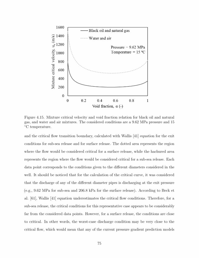
Figure 4.15. Mixture critical velocity and void fraction relation for black oil and naturalgas, and water and air mixtures. The considered conditions are a 9.62 MPa pressure and 15∘C temperature.

and the critical flow transition boundary, calculated with Wallis [41] equation for the exit

conditions for sub-sea release and for surface release. The dotted area represents the region

where the flow would be considered critical for a surface release, while the hachured area

represents the region where the flow would be considered critical for a sub-sea release. Each

data point corresponds to the conditions given to the different diameters considered in the

well. It should be noticed that for the calculation of the critical curve, it was considered

that the discharge of any of the different diameter pipes is discharging at the exit pressure

(e.g., 9.62 MPa for sub-sea and 206.8 kPa for the surface release). According to Beck et

al. [61], Wallis [41] equation underestimates the critical flow conditions. Therefore, for a

sub-sea release, the critical conditions for this representative case appears to be considerably

far from the considered data points. However, for a surface release, the conditions are close

to critical. In other words, the worst-case discharge condition may be very close to the

critical flow, which would mean that any of the current pressure gradient prediction models

75

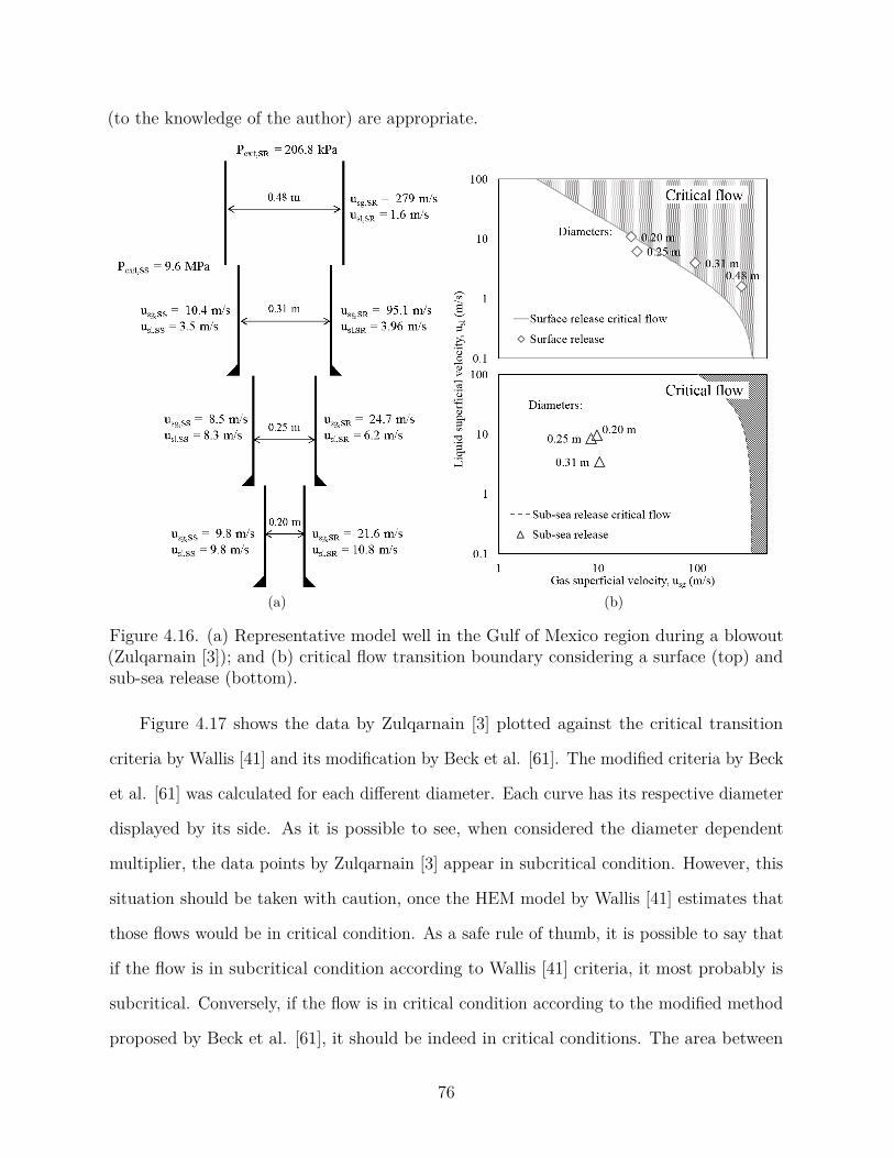
(to the knowledge of the author) are appropriate.

(a) (b)

Figure 4.16. (a) Representative model well in the Gulf of Mexico region during a blowout(Zulqarnain [3]); and (b) critical flow transition boundary considering a surface (top) andsub-sea release (bottom).

Figure 4.17 shows the data by Zulqarnain [3] plotted against the critical transition

criteria by Wallis [41] and its modification by Beck et al. [61]. The modified criteria by Beck

et al. [61] was calculated for each different diameter. Each curve has its respective diameter

displayed by its side. As it is possible to see, when considered the diameter dependent

multiplier, the data points by Zulqarnain [3] appear in subcritical condition. However, this

situation should be taken with caution, once the HEM model by Wallis [41] estimates that

those flows would be in critical condition. As a safe rule of thumb, it is possible to say that

if the flow is in subcritical condition according to Wallis [41] criteria, it most probably is

subcritical. Conversely, if the flow is in critical condition according to the modified method

proposed by Beck et al. [61], it should be indeed in critical conditions. The area between

76

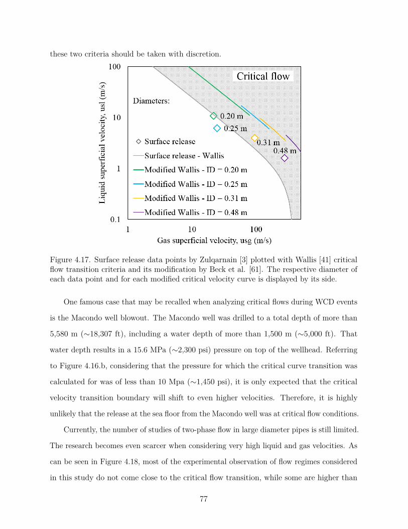
these two criteria should be taken with discretion.

Figure 4.17. Surface release data points by Zulqarnain [3] plotted with Wallis [41] criticalflow transition criteria and its modification by Beck et al. [61]. The respective diameter ofeach data point and for each modified critical velocity curve is displayed by its side.

One famous case that may be recalled when analyzing critical flows during WCD events

is the Macondo well blowout. The Macondo well was drilled to a total depth of more than

5,580 m (∼18,307 ft), including a water depth of more than 1,500 m (∼5,000 ft). That

water depth results in a 15.6 MPa (∼2,300 psi) pressure on top of the wellhead. Referring

to Figure 4.16.b, considering that the pressure for which the critical curve transition was

calculated for was of less than 10 Mpa (∼1,450 psi), it is only expected that the critical

velocity transition boundary will shift to even higher velocities. Therefore, it is highly

unlikely that the release at the sea floor from the Macondo well was at critical flow conditions.

Currently, the number of studies of two-phase flow in large diameter pipes is still limited.

The research becomes even scarcer when considering very high liquid and gas velocities. As

can be seen in Figure 4.18, most of the experimental observation of flow regimes considered

in this study do not come close to the critical flow transition, while some are higher than

77

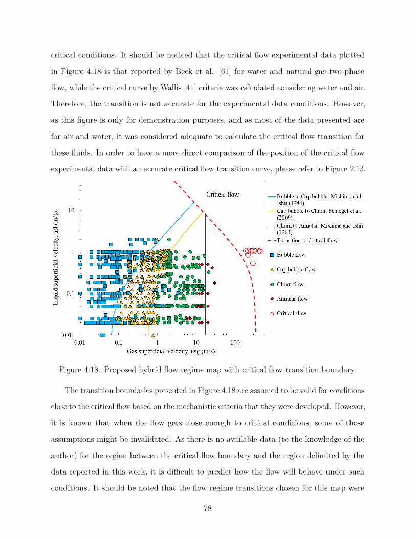
critical conditions. It should be noticed that the critical flow experimental data plotted

in Figure 4.18 is that reported by Beck et al. [61] for water and natural gas two-phase

flow, while the critical curve by Wallis [41] criteria was calculated considering water and air.

Therefore, the transition is not accurate for the experimental data conditions. However,

as this figure is only for demonstration purposes, and as most of the data presented are

for air and water, it was considered adequate to calculate the critical flow transition for

these fluids. In order to have a more direct comparison of the position of the critical flow

experimental data with an accurate critical flow transition curve, please refer to Figure 2.13.

Figure 4.18. Proposed hybrid flow regime map with critical flow transition boundary.

The transition boundaries presented in Figure 4.18 are assumed to be valid for conditions

close to the critical flow based on the mechanistic criteria that they were developed. However,

it is known that when the flow gets close enough to critical conditions, some of those

assumptions might be invalidated. As there is no available data (to the knowledge of the

author) for the region between the critical flow boundary and the region delimited by the

data reported in this work, it is difficult to predict how the flow will behave under such

conditions. It should be noted that the flow regime transitions chosen for this map were

78

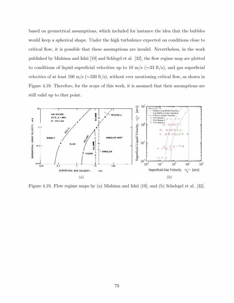
based on geometrical assumptions, which included for instance the idea that the bubbles

would keep a spherical shape. Under the high turbulence expected on conditions close to

critical flow, it is possible that these assumptions are invalid. Nevertheless, in the work

published by Mishima and Ishii [19] and Schlegel et al. [32], the flow regime map are plotted

to conditions of liquid superficial velocities up to 10 m/s (∼33 ft/s), and gas superficial

velocities of at least 100 m/s (∼330 ft/s), without ever mentioning critical flow, as shown in

Figure 4.19. Therefore, for the scope of this work, it is assumed that their assumptions are

still valid up to that point.

(a) (b)

Figure 4.19. Flow regime maps by (a) Mishima and Ishii [19]; and (b) Schelegel et al. [32].

79

Chapter 5Conclusions and Future Works

5.1 Summary and conclusions

1. Some recent studies pointed out significant differences for flow regimes between large

and small diameter pipes. Among the main differences, the inexistence of slug flow

in diameters larger than 0.10 m (∼4 in) is reported by many authors. Thus, one of

the sources of the errors is possibly related to the flow regime prediction, once most

models were developed based on small diameter pipes. A criteria by Kataoka and Ishii

[25] correlating the surface tension of the mixture and the pressure of the liquid phase

over the bubble was used to define the largest diameter in which a Taylor bubble can

be stable (i.e., slug flow is existent). It is considered that diameters larger than that

should be considered large. It was noticed that while this diameter would increase

with pressure for water-and-air mixtures, it would decrease for oil-and-gas mixtures.

2. Cap-bubble flow regime is proposed here under conditions at which slug flow would

exist for 𝐷*𝐻 > 40. Cap-bubble flow regime is characterized by bubbles larger than the

classical bubble flow, but these large bubbles never occupy the entire pipe diameter.

These bubbles generate flow recirculation and increased turbulence.

3. A thorough literature review was carried out on six different flow regime maps – four

mechanistic, and two empirical. Four flow regime maps were selected to be tested

on predicting the flow regime for flows in large diameter pipes and relatively high

fluid flow velocities: Duns and Ros [11], Aziz et al. [17], Mishima and Ishii [19], and

Schlegel et al. [32].

4. A literature review was carried out on experiments for two-phase flow regime character-

ization of air and water flows in large diameter pipes. 695 data points of experimental

flow regime observation were collected and used on the flow regime maps evaluation.

Data from an experimental study carried out at LSU were presented in completeness

80

for the first time.

5. A new flow regime map was proposed after evaluating the different flow regime

transition using Wu et al. [16] approach. It was proposed the existence of cap-bubble

flow in large diameter pipe for conditions where slug flow would exist in smaller

diameter pipes. The existence of this flow regime was considered an effect of the

increasing pipe diameter size, with the former Taylor bubbles not being able to grow

to the size of the pipe diameter, but reaching sizes larger than common bubbles in a

classical bubble flow and being deformed because of instabilities due to turbulence.

6. A recent model proposed by Teles and Waltrich [33] was modified to adapt the use of

the newly introduced flow regime map and the calculation of the pressure gradient

under cap-bubble flow. The results from the simulations for the pressure gradient

of the water and air experimental data and natural gas and oil field data presented

improvements over the standard model. It was noticed for the calculation of pressure

gradient of the air-and-water experimental data that the error difference between

the standard and the modified model proposed in this work was tending to reduce

with increasing diameter. This may be due to the diameter effect on the formation of

bubbles, making their size less influent for lower gas throughput, and approaching its

behavior more to churn flow with higher gas velocities.

7. Critical flow regime transition in large diameter was evaluated. A Homogeneous

Equilibrium Model (HEM) by Wallis [41] was tested against data of a representative

well in the GoM. An empirical model adapting the Wallis [41] for larger diameters was

also evaluated. It was noticed that with increasing pressure, the parameter that affects

the most on the critical flow velocities is the gas density. Under high pressures, the

gas density will increase substantially, increasing the critical flow velocities. Because

of this increase in critical velocities with pressure, it is unlikely that WCD on the

sea floor will be in critical condition. However, when the discharge happens at lower

81

pressures, such as at atmospheric pressures at the rig floor, the flow might be in

critical conditions. Therefore, it is recommended the addition of the critical flow

transition in the new flow regime map.

8. Little is known about the effects of increasing velocity in the region between the end

of the experimental data and the critical flow transition. It is estimated that the

flow regime transition boundaries will be kept in such conditions because of their

mechanistic nature. However, it is uncertain to affirm that they will indeed keep their

form.

5.2 Recommendations for future work

For both experimental and numerical future work, the following recommendations are

made.

1. In order to better understand the physics behind each flow regime and its particular

characteristics, it is mandatory a better method to observe them. The visual charac-

terization of flow regime is a limited method, and appears to be insufficient. Some

authors correlate the void-fraction probabilistic density function (pdf) of a flow with

different flow regimes, by the use of electrical impedance void-meters and artificial

intelligence neural network. However, this method still do not give a good description

of the physical phenomena happening during each flow regime. Other methods such

as capturing the sound signature of flow regimes or works using wire mesh sensors are

highly recommended.

2. The literature lacks experimental observations of flow regimes for oil and gas mixture

flows under high pressure. Because of this, it is hard to prove the validity of Kataoka

and Ishii [25] large diameter criteria for these fluids. This way, new experiments of

two-phase flow with different diameter sizes, ranging from 0.02 to 0.08 m and high

pressures are highly encouraged to evaluate the possible absence of slug flow by the

classical definition under those conditions

82

3. Another important experimental investigation is on the effect of pipe inclination on

flow regimes in large diameter pipes. By definition, slug flow in inclined pipes do

not occupy its entire diameter. Therefore, it is possible that this flow is present in

deviated wells and might highly influence the calculation of pressure gradients.

4. Due to the uncertainty about the flow behavior in conditions close to critical flow,

it is recommended that new experimental studies are carried out for two-phase flow

mixtures in velocities nearly around the predicted critical flow transition, ideally

overlapping it. The flow regime identification and the flow behavior understanding

under this conditions might be very important to predict surface release WCD.

5. It is recommended the evaluation of new critical flow transition models experimentally

for diameters larger than 0.12 m to complement Beck et al. [61] work and develop

better prediction methods for critical flow transition.

83

References

[1] SPE, “Calculation of worst-case discharge (wcd),” tech. rep., Society of PetroleumEngineers, 2015.

[2] K. Buchholz, A. Krieger, J. Rowe, D. S. Etkin, D. F. McCay, M. S. Gearon, M. Grennan,and J. Turner, “Oil spill response plan (osrp) equipment capabilities review - task1: Worst case discharge analysis (volume i),” Tech. Rep. BPA No. E14PB00072, U.S.Department of the Interior Bureau of Safety and Environmental Enforcement (BSEE),02 2016.

[3] M. Zulqarnain, Deepwater Gulf of Mexico oil pill scenarios development and theirassociated risk assessment. PhD thesis, Louisiana State University, Craft & HawkingPetroleum Engineering Department, 2015.

[4] M. J. Economides, A. D. Hill, C. Ehlig-Economides, and D. Zhu, Petroleum ProductionSystems. Prentice Hall, 2nd ed. ed., Oct. 2012.

[5] G. Takacs, “Considerations on the selection of an optimum vertical multiphase pressuredrop prediction model for oil wells,” in SPE Production and Operations Symposiumheld in Oklahoma City, Oklahoma, 24–27 March 2001, no. SPE-68361-MS, 2001.

[6] N. Omebere-Iyari, B. Azzopardi, and Y. Ladam, “Two-phase flow patterns in largediameter vertical pipes at high pressures,” AIChE J., vol. 53, pp. 2493–2504, 10 2007.

[7] S. F. Ali, Two phase flow in large diameter vertical riser. PhD thesis, CranfieldUniversity, School of Engineering, Department of Process and System Engineering,2009.

[8] G. Zabaras, R. Menon, W. Schoppa, and M. W. III, “Large diameter riser laboratory gas-lift tests,” in Offshore Technology Conference held in Houston, Texas, USA, no. OTC23968, 2013.

[9] P. Waltrich, M. S. Capovilla, W. Lee, P. C. de Souza, M. Zulqarnain, R. Hughes,M. Tyagi, W. Williams, S. Kam, A. Archer, J. Singh, H. Nguyen, J. Duhon, and C. Grif-fith, “Experimental evaluation of wellbore flow models applied to worst-case-dischargecalculations,” in SPE Health, Safety, Security, Environment & Social ResponsibilityConference-North America, no. SPE184444-MS, 04 2017.

[10] O. Shoham, Mechanistic modeling of gas-liquid two-phase flow in pipes. Society ofPetroleum Engineers, 2006.

[11] H. J. Duns and N. Ros, “Vertical flow of gas and liquid mixtures in wells,” in 6th WorldPetroleum Congress, no. WPC-10132, World Petroleum Congress, 06 1963.

[12] H. Gray, Vertical Flow Correlation in Gas Wells. Appendix B, user’s manual for api

84

148 subsurface controlled safety valve sizing computer program ed., 1974.

[13] A. Ansari, N. Sylvester, O. Shoham, J. Brill, et al., “A comprehensive mechanisticmodel for upward two-phase flow in wellbores,” in SPE Annual Technical Conferenceand Exhibition, Society of Petroleum Engineers, 1990.

[14] T. Hibiki and M. Ishii, “One-dimensional drift–flux model for two-phase flow in alarge diameter pipe,” International Journal of Heat and Mass Transfer, vol. 46, no. 10,pp. 1773–1790, 2003.

[15] J. Brill and H. Mukherjee, Multiphase Flow in Wells, No. 17. Society of Petroleum,1999.

[16] B. Wu, M. Firouzi, T. Mitchell, T. E. Rufford, C. Leonardi, and B. Towler, “Acritical review of flow maps for gas-liquid flows in vertical pipes and annuli,” ChemicalEngineering Journal, vol. 326, pp. 350–377, Oct. 2017.

[17] K. Aziz, G. W. Govier, and M. Fogarasi, “Pressure drop in wells producing oil andgas,” Journal of Canadian Petroleum Technology, vol. 11, no. 03, 1972.

[18] Y. Taitel, D. Bornea, and A. Dukler, “Modelling flow pattern transitions for steadyupward gas-liquid flow in vertical tubes,” AIChE J., vol. 26, pp. 345–354, 05 1980.

[19] K. Mishima and M. Ishii, “Flow regime transition criteria for upward two-phase flow invertical tubes,” International Journal of Heat and Mass Transfer, vol. 27, pp. 723–737,May 1984.

[20] D. Barnea, “A unified model for predicting flow-pattern transitions for the whole rangeof pipe inclinations,” Int. J. Multiphase Flow, vol. 13, no. 1, pp. 1–12, 1987.

[21] N. Omebere-Iyari, B. Azzopardi, D. Lucas, M. Beyer, and H.-M. Prasser, “The charac-teristics of gas/liquid flow in large risers at high pressures,” Int. J. Multiphase Flow,vol. 34, pp. 461–476, 2008.

[22] T. Smith, J. Schlegel, T. Hibiki, and M. Ishii, “Two-phase flow structure in largediameter pipes,” Int. J. Heat Fluid Flow, vol. 33, pp. 156–167, 2012.

[23] A. Ohnuki and H. Akimoto, “Experimental study on transition of flow pattern andphase distribution in upward air-water two-phase flow along a large vertical pipe,” Int.J. Multiphase Flow, vol. 26, pp. 367–386, 2000.

[24] S. F. Ali and H. Yeung, “Two-phase flow patterns in large diameter vertical pipes,”Asia-Pacific Journal of Chemical Engineering, vol. 9, pp. 105–116, June 2014.

[25] I. Kataoka and M. Ishii, “Drift flux model for large diameter pipe and new correlationfor pool void fraction,” Int. J. Heat Mass Transfer, vol. 30, no. 9, pp. 1927–1939, 1987.

85

[26] H. Cheng, J. H. Hills, and B. J. Azzopardi, “A study of the bubble-to-slug transitionin vertical gas-liquid flow in columns of different diameters,” Int. J. Multiphase Flow,vol. 24, no. 3, pp. 431–452, 1998.

[27] T. Hibiki and M. Ishii, “Experimental study on hot-leg u-bend two-phase naturalcirculation in a loop with a large diameter pipe,” Nuclear Engineering and Design,vol. 195, pp. 69–84, 2000.

[28] M. Shoukri, I. Hassan, and I. Gerges, “Two-phase bubbly flow structure in large-diameter vertical pipes,” The Canadian Journal of Chemical Engineering, 2003.

[29] M. S. Capovilla, P. C. de Sousa, and P. J. Waltrich, “Experimental investigation ofvertical high-velocity two-phase flows in large-diameter pipes,” in 18𝑡ℎ InternationalConference on Multiphase Production Technology 2017, Cannes, France, 2017.

[30] Minerals Management Service, “Gulf of mexico deepwater operations and activities,”Environmental Assessment OCS EIS/EA MMS 2000-001, U.S. Department of theInterior - Minerals Management Service, New Orleans, May 2000.

[31] N. Ros et al., “Simultaneous flow of gas and liquid as encountered in well tubing,”Journal of Petroleum Technology, vol. 13, no. 10, pp. 1–037, 1961.

[32] J. Schlegel, P. Sawant, S. Paranjape, B. Ozar, T. Hibiki, and M. Ishii, “Void fractionand flow regime in adiabatic upward two-phase flow in large diameter vertical pipes,”Nuclear Engineering and Design, vol. 239, pp. 2864–2874, 2009.

[33] F. B. X. Teles, P. J. Waltrich, M. S. Capovilla, I. Gupta, and R. Highes, “Developmentand improvement of flow models applied to multiphase flows in large-diameter pipes andhigh-velocity flows,” Internal interim report prepared under BOEM Award M17PX00030by Louisiana State University, US Department of the Interior - Bureau of Ocean EnergyManagement, 2018.

[34] E. Pagan, W. Williams, S. Kam, and P. Waltrich, “A simplified model for churn andannular flow regimes in small-and large-diameter pipes,” Chemical Engineering Science,vol. 162, pp. 309–321, 2017.

[35] A. Hagedorn and K. Brown, “The effect of liquid viscosity in two-phase vertical flow,”Journal of Petroleum Technology, vol. 16-02, pp. 203 – 210, 02 1964.

[36] D. Beggs and J. Brill, “A study of two-phase flow in inclined pipes,” Journal ofPetroleum Technology, vol. 25-05, 05 1973.

[37] Schlumberger, “Olga dynamic multiphase flow simulator,” 2000.

[38] H. Mukherjee and J. Brill, “Pressure drop correlations for inclined two-phase flow,”Journal of energy resources technology, vol. 107, no. 4, pp. 549–554, 1985.

86

[39] S. Jayanti and N. Brauner, “Churn flow,” Multiphase Science and Technology, vol. 8,no. 1-4, 1994.

[40] M. V. C. Alves, Modelagem Numerica do Escoamento Transient Churn-Annular emTubulacoes Verticais e sua Aplicacao na Simulacao de Carga de Liquido em Pocosde Gas. PhD thesis, Universidade Federal de Santa Catarina, Florianopolis, SantaCatarina, 2014.

[41] G. B. Wallis, One Dimensional Two-Phase Flow. Ney York: McGraw-Hill, 1969.

[42] N. Brauner and D. Barnea, “Slug/churn transition in upward gas-liquid flow,” Chemicalengineering science, vol. 41, no. 1, pp. 159–163, 1986.

[43] K. McQuillan and P. Whalley, “Flow patterns in vertical two-phase flow,” InternationalJournal of Multiphase Flow, vol. 11, pp. 161–175, mar 1985.

[44] A. Hasan and C. Kabir, “Two-phase flow in vertical and inclined annuli,” InternationalJournal of Multiphase Flow, vol. 18, no. 2, pp. 279–293, 1992.

[45] S. Jayanti and G. Hewitt, “Prediction of the slug-to-churn flow transition in verticaltwo-phase flow,” International Journal of Multiphase Flow, vol. 18, no. 6, pp. 847–860,1992.

[46] J. Tengesdal, A. Kaya, C. Sarica, et al., “Flow-pattern transition and hydrodynamicmodeling of churn flow,” SPE Journal, vol. 4, no. 04, pp. 342–348, 1999.

[47] M. Ishii, “One-dimensional drift-flux model and constitutive equations for relativemotion between phases in various two-phase flow regimes,” Tech. Rep. ANL-77-47,Argonne National Laboratory, 9700 South Class Avenue; Argonne, Illinois 60439, 101977.

[48] J. Weisman, D. Duncan, J. Gibson, and T. Crawford, “Effects of fluid properties andpipe diameter on two-phase flow patterns in horizontal lines,” International Journal ofMultiphase Flow, vol. 5, no. 6, pp. 437–462, 1979.

[49] Y. Taitel and A. Dukler, “A model for predicting flow regime transitions in horizontaland near horizontal gas-liquid flow,” AIChE Journal, vol. 22, no. 1, pp. 47–55, 1976.

[50] G. F. Hewitt and G. B. Wallis, “Flooding and associated phenomena in falling filmflow in a tube,” tech. rep., United Kingdom Atomic Energy Authority. Research Group.Atomic Energy Research Establishment, Harwell Berks, England, 1963.

[51] A. Bennett, “Flow visualisation studies of boiling at high pressure,” Proc. Inst. Mech.Eng., vol. 180, pp. 1–11, 1965.

[52] T. Smith, “Two-phase flow regime identification in large diameter pipes,” MSNE Thesis,Purdue University, USA, 1999.

87

[53] G. B. Wallis, “Critical two-phase flow,” International Journal of Multiphase Flow,vol. 6, no. 1-2, pp. 97–112, 1980.

[54] W. Gilbert et al., “Flowing and gas-lift well performance,” in Drilling and productionpractice, American Petroleum Institute, 1954.

[55] F. Ashford et al., “An evaluation of critical multiphase flow performance throughwellhead chokes,” Journal of Petroleum Technology, vol. 26, no. 08, pp. 843–850, 1974.

[56] F. Ashford, P. Pierce, et al., “Determining multiphase pressure drops and flow capacitiesin down-hole safety valves,” Journal of Petroleum Technology, vol. 27, no. 09, pp. 1–145,1975.

[57] R. Sachdeva, Z. Schmidt, J. Brill, R. Blais, et al., “Two-phase flow through chokes,”in SPE Annual Technical Conference and Exhibition, Society of Petroleum Engineers,1986.

[58] S. Selmer-Olsen, H. Holm, K. Haugen, P. J. Nilsen, and R. Sandberg, “Subsea chokesas multiphase flowmeters.,” in International Confonference on Multiphase Production,Cannes, France., 1995.

[59] F. Beck, J. Langlinais, A. Bourgoyne Jr, et al., “Experimental and theoretical consider-ations for diverter evaluation and design,” in SPE California Regional Meeting, Societyof Petroleum Engineers, 1986.

[60] F. Fortunati, “Two-phase flow through wellhead chokes,” in SPE European SpringMeeting, Society of Petroleum Engineers, 1972.

[61] F. Beck, J. Langlinais, A. Bourgoyne Jr, et al., “An analysis of the design loadsplaced on a well by a diverter system,” in SPE/IADC Drilling Conference, Society ofPetroleum Engineers, 1987.

[62] G. Oddie, H. Shi, L. Durlofsky, K. Aziz, B. Pfeffer, and J. Holmes, “Experimentalstudy of two and three phase flows in large diameter inclined pipes,” InternationalJournal of Multiphase Flow, vol. 29, no. 4, pp. 527–558, 2003.

[63] A. Ohnuki and H. Akimoto, “An experimental study on developing air-water two-phaseflow along a large verticalpipe: effect of air injection method,” Int. J. Multiphase Flow,vol. 22, no. 6, pp. 1143–1154, 1996.

[64] X. Shen, J. P. Schlegel, S. Chen, S. Rassame, M. J. Griffiths, T. Hibiki, and M. Ishii,Frontiers and Progress in Multiphase Flow I, ch. Chapter 2 - Flow Characteristics andVoid Fraction Prediction in Large Diameter Pipes, pp. 55–103. Springer, 2014.

[65] H. Asheim et al., “Mona, an accurate two-phase well flow model based on phaseslippage,” SPE Production Engineering, vol. 1, no. 03, pp. 221–230, 1986.

88

[66] P. J. Waltrich, G. Falcone, and J. R. Barbosa, “Axial development of annular, churnand slug flows in a long vertical tube,” Int. J. Multiphase Flow, vol. 57, pp. 38–48,2013.

[67] G. Hewitt and S. Jayanti, “To churn or not to churn,” International Journal ofMultiphase Flow, vol. 19, no. 3, pp. 527–529, 1993.

[68] K. Reinicke, R. Remer, and G. Hueni, “Comparison of measured and predicted pressuredrops in tubing for high-water-cut gas wells,” in 1987 SPE Annual Technical Conferenceand Exhibition held in Houston, Spet 16-19, no. SPE13279, 1987.

89

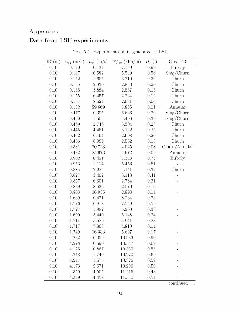
Appendix:Data from LSU experiments

Table A.1. Experimental data generated at LSU.

ID (m) 𝑢𝑠𝑔 (m/s) 𝑢𝑠𝑙 (m/s) 𝑑𝑝/𝑑𝑧 (kPa/m) 𝐻𝑙 (-) Obs. FR0.10 0.140 0.134 7.759 0.99 Bubbly0.10 0.147 0.582 5.540 0.56 Slug/Churn0.10 0.152 1.605 3.710 0.36 Churn0.10 0.155 2.830 2.833 0.20 Churn0.10 0.155 3.884 2.557 0.13 Churn0.10 0.155 6.457 2.264 0.12 Churn0.10 0.157 8.624 2.031 0.06 Churn0.10 0.182 29.669 1.855 0.11 Annular0.10 0.477 0.395 6.626 0.70 Slug/Churn0.10 0.450 1.503 4.496 0.39 Slug/Churn0.10 0.469 2.746 3.504 0.28 Churn0.10 0.445 4.461 3.122 0.25 Churn0.10 0.462 6.164 2.608 0.20 Churn0.10 0.466 8.989 2.562 0.18 Churn0.10 0.331 20.723 2.045 0.08 Churn/Annular0.10 0.422 25.973 1.972 0.09 Annular0.10 0.902 0.421 7.343 0.73 Bubbly0.10 0.953 1.114 5.456 0.51 -0.10 0.885 2.285 4.141 0.32 Churn0.10 0.827 3.402 3.118 0.41 -0.10 0.857 6.301 2.734 0.21 -0.10 0.829 8.636 2.570 0.16 -0.10 0.803 16.035 2.998 0.14 -0.10 1.639 0.471 8.284 0.73 -0.10 1.776 0.878 7.559 0.59 -0.10 1.727 1.982 5.960 0.33 -0.10 1.690 3.440 5.148 0.24 -0.10 1.714 5.529 4.941 0.23 -0.10 1.717 7.863 4.810 0.14 -0.10 1.749 16.333 5.627 0.17 -0.10 4.232 0.059 10.983 0.90 -0.10 4.228 0.590 10.587 0.69 -0.10 4.125 0.867 10.339 0.55 -0.10 4.248 1.740 10.270 0.69 -0.10 4.247 1.675 10.326 0.59 -0.10 4.173 2.671 10.206 0.50 -0.10 4.350 4.505 11.416 0.43 -0.10 4.349 4.458 11.380 0.54 -

continued . . .

90

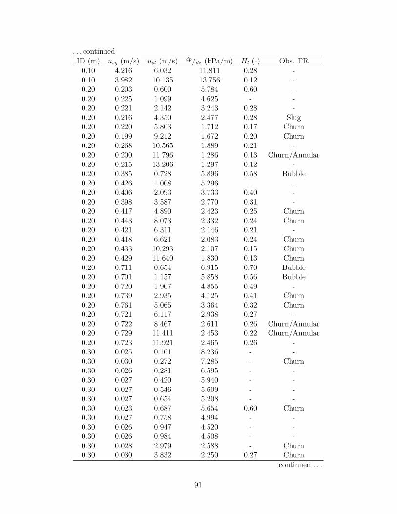
. . . continuedID (m) 𝑢𝑠𝑔 (m/s) 𝑢𝑠𝑙 (m/s) 𝑑𝑝/𝑑𝑧 (kPa/m) 𝐻𝑙 (-) Obs. FR

0.10 4.216 6.032 11.811 0.28 -0.10 3.982 10.135 13.756 0.12 -0.20 0.203 0.600 5.784 0.60 -0.20 0.225 1.099 4.625 - -0.20 0.221 2.142 3.243 0.28 -0.20 0.216 4.350 2.477 0.28 Slug0.20 0.220 5.803 1.712 0.17 Churn0.20 0.199 9.212 1.672 0.20 Churn0.20 0.268 10.565 1.889 0.21 -0.20 0.200 11.796 1.286 0.13 Churn/Annular0.20 0.215 13.206 1.297 0.12 -0.20 0.385 0.728 5.896 0.58 Bubble0.20 0.426 1.008 5.296 - -0.20 0.406 2.093 3.733 0.40 -0.20 0.398 3.587 2.770 0.31 -0.20 0.417 4.890 2.423 0.25 Churn0.20 0.443 8.073 2.332 0.24 Churn0.20 0.421 6.311 2.146 0.21 -0.20 0.418 6.621 2.083 0.24 Churn0.20 0.433 10.293 2.107 0.15 Churn0.20 0.429 11.640 1.830 0.13 Churn0.20 0.711 0.654 6.915 0.70 Bubble0.20 0.701 1.157 5.858 0.56 Bubble0.20 0.720 1.907 4.855 0.49 -0.20 0.739 2.935 4.125 0.41 Churn0.20 0.761 5.065 3.364 0.32 Churn0.20 0.721 6.117 2.938 0.27 -0.20 0.722 8.467 2.611 0.26 Churn/Annular0.20 0.729 11.411 2.453 0.22 Churn/Annular0.20 0.723 11.921 2.465 0.26 -0.30 0.025 0.161 8.236 - -0.30 0.030 0.272 7.285 - Churn0.30 0.026 0.281 6.595 - -0.30 0.027 0.420 5.940 - -0.30 0.027 0.546 5.609 - -0.30 0.027 0.654 5.208 - -0.30 0.023 0.687 5.654 0.60 Churn0.30 0.027 0.758 4.994 - -0.30 0.026 0.947 4.520 - -0.30 0.026 0.984 4.508 - -0.30 0.028 2.979 2.588 - Churn0.30 0.030 3.832 2.250 0.27 Churn

continued . . .

91

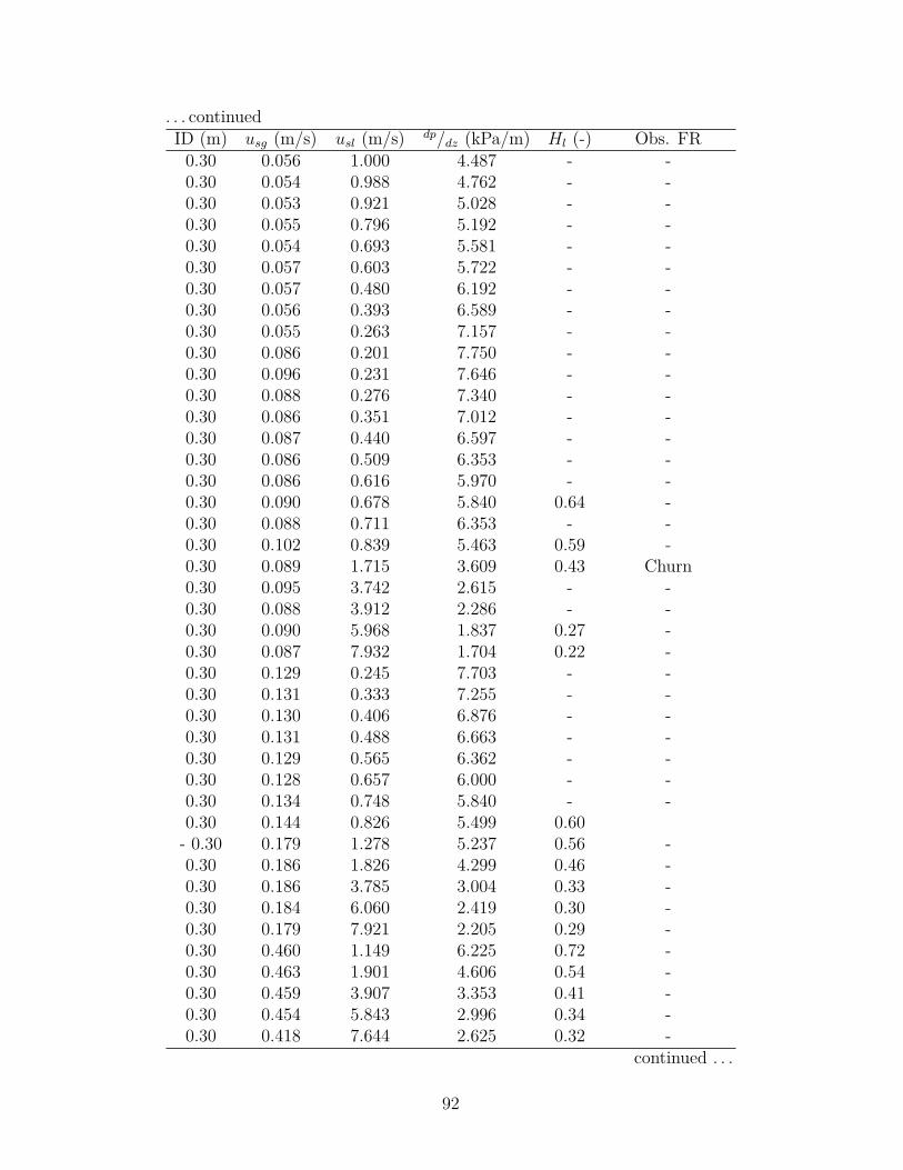
. . . continuedID (m) 𝑢𝑠𝑔 (m/s) 𝑢𝑠𝑙 (m/s) 𝑑𝑝/𝑑𝑧 (kPa/m) 𝐻𝑙 (-) Obs. FR

0.30 0.056 1.000 4.487 - -0.30 0.054 0.988 4.762 - -0.30 0.053 0.921 5.028 - -0.30 0.055 0.796 5.192 - -0.30 0.054 0.693 5.581 - -0.30 0.057 0.603 5.722 - -0.30 0.057 0.480 6.192 - -0.30 0.056 0.393 6.589 - -0.30 0.055 0.263 7.157 - -0.30 0.086 0.201 7.750 - -0.30 0.096 0.231 7.646 - -0.30 0.088 0.276 7.340 - -0.30 0.086 0.351 7.012 - -0.30 0.087 0.440 6.597 - -0.30 0.086 0.509 6.353 - -0.30 0.086 0.616 5.970 - -0.30 0.090 0.678 5.840 0.64 -0.30 0.088 0.711 6.353 - -0.30 0.102 0.839 5.463 0.59 -0.30 0.089 1.715 3.609 0.43 Churn0.30 0.095 3.742 2.615 - -0.30 0.088 3.912 2.286 - -0.30 0.090 5.968 1.837 0.27 -0.30 0.087 7.932 1.704 0.22 -0.30 0.129 0.245 7.703 - -0.30 0.131 0.333 7.255 - -0.30 0.130 0.406 6.876 - -0.30 0.131 0.488 6.663 - -0.30 0.129 0.565 6.362 - -0.30 0.128 0.657 6.000 - -0.30 0.134 0.748 5.840 - -0.30 0.144 0.826 5.499 0.60

- 0.30 0.179 1.278 5.237 0.56 -0.30 0.186 1.826 4.299 0.46 -0.30 0.186 3.785 3.004 0.33 -0.30 0.184 6.060 2.419 0.30 -0.30 0.179 7.921 2.205 0.29 -0.30 0.460 1.149 6.225 0.72 -0.30 0.463 1.901 4.606 0.54 -0.30 0.459 3.907 3.353 0.41 -0.30 0.454 5.843 2.996 0.34 -0.30 0.418 7.644 2.625 0.32 -

continued . . .

92

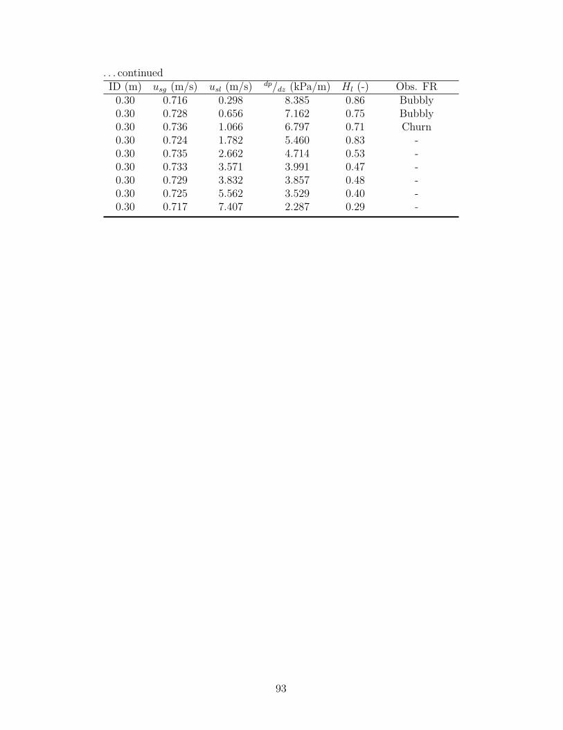
. . . continuedID (m) 𝑢𝑠𝑔 (m/s) 𝑢𝑠𝑙 (m/s) 𝑑𝑝/𝑑𝑧 (kPa/m) 𝐻𝑙 (-) Obs. FR

0.30 0.716 0.298 8.385 0.86 Bubbly0.30 0.728 0.656 7.162 0.75 Bubbly0.30 0.736 1.066 6.797 0.71 Churn0.30 0.724 1.782 5.460 0.83 -0.30 0.735 2.662 4.714 0.53 -0.30 0.733 3.571 3.991 0.47 -0.30 0.729 3.832 3.857 0.48 -0.30 0.725 5.562 3.529 0.40 -0.30 0.717 7.407 2.287 0.29 -

93

Vita

Matheus Sigaki Capovilla was born in Maringá, Paraná, Brazil, on January 12, 1992.

He is son of Ivete Naomi Sigaki and Marcos Aurelio Borges Capovilla.

Matheus started his academic carreer at the Federal university of Santa Catarina in Au-

gust, 2010. During his Mechanical Engineering undergraduate course, he joined an emerging

technologies research team at Polo Research Laboratories for Emerging Technologies in

Cooling and Thermophysics. He helped developing the first operating magnetic refrigeration

prototype in the Southern Hemisphere.

After graduating in September of 2015, he was accepted to enter the Graduate Program

at Louisiana State University in Petroleum Engineering with full assistantship. He started

his program in January of 2016.

94