Embed Size (px)
Citation preview
TWO PHASE FLOW PHENOMENA IN FUEL CELL MICROCHANNELS
A DISSERTATION
SUBMITTED TO THE DEPARTMENT OF MECHANICAL ENGINEERING
AND THE COMMITTEE ON GRADUATE STUDIES
OF STANFORD UNIVERSITY
IN PARTIAL FULFILLMENT OF THE REQUIREMENTS
FOR THE DEGREE OF
DOCTOR OF PHILOSOPHY
Julie Elizabeth Steinbrenner
March 2011

http://creativecommons.org/licenses/by-nc/3.0/us/
This dissertation is online at: http://purl.stanford.edu/gz938pg6790
© 2011 by Julie Elizabeth Steinbrenner. All Rights Reserved.
Re-distributed by Stanford University under license with the author.
This work is licensed under a Creative Commons Attribution-Noncommercial 3.0 United States License.
ii

I certify that I have read this dissertation and that, in my opinion, it is fully adequatein scope and quality as a dissertation for the degree of Doctor of Philosophy.
Kenneth Goodson, Primary Adviser
I certify that I have read this dissertation and that, in my opinion, it is fully adequatein scope and quality as a dissertation for the degree of Doctor of Philosophy.
John Eaton
I certify that I have read this dissertation and that, in my opinion, it is fully adequatein scope and quality as a dissertation for the degree of Doctor of Philosophy.
Carlos Hidrovo
Approved for the Stanford University Committee on Graduate Studies.
Patricia J. Gumport, Vice Provost Graduate Education
This signature page was generated electronically upon submission of this dissertation in electronic format. An original signed hard copy of the signature page is on file inUniversity Archives.
iii

iv
v
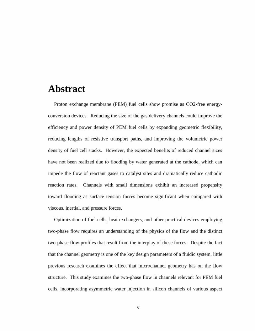
Abstract
Proton exchange membrane (PEM) fuel cells show promise as CO2-free energy-
conversion devices. Reducing the size of the gas delivery channels could improve the
efficiency and power density of PEM fuel cells by expanding geometric flexibility,
reducing lengths of resistive transport paths, and improving the volumetric power
density of fuel cell stacks. However, the expected benefits of reduced channel sizes
have not been realized due to flooding by water generated at the cathode, which can
impede the flow of reactant gases to catalyst sites and dramatically reduce cathodic
reaction rates. Channels with small dimensions exhibit an increased propensity
toward flooding as surface tension forces become significant when compared with
viscous, inertial, and pressure forces.
Optimization of fuel cells, heat exchangers, and other practical devices employing
two-phase flow requires an understanding of the physics of the flow and the distinct
two-phase flow profiles that result from the interplay of these forces. Despite the fact
that the channel geometry is one of the key design parameters of a fluidic system, little
previous research examines the effect that microchannel geometry has on the flow
structure. This study examines the two-phase flow in channels relevant for PEM fuel
cells, incorporating asymmetric water injection in silicon channels of various aspect
vi
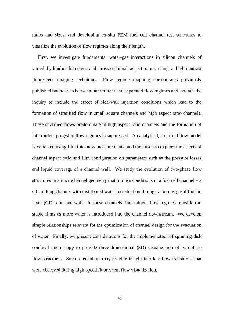
ratios and sizes, and developing ex-situ PEM fuel cell channel test structures to
visualize the evolution of flow regimes along their length.
First, we investigate fundamental water-gas interactions in silicon channels of
varied hydraulic diameters and cross-sectional aspect ratios using a high-contrast
fluorescent imaging technique. Flow regime mapping corroborates previously
published boundaries between intermittent and separated flow regimes and extends the
inquiry to include the effect of side-wall injection conditions which lead to the
formation of stratified flow in small square channels and high aspect ratio channels.
These stratified flows predominate in high aspect ratio channels and the formation of
intermittent plug/slug flow regimes is suppressed. An analytical, stratified flow model
is validated using film thickness measurements, and then used to explore the effects of
channel aspect ratio and film configuration on parameters such as the pressure losses
and liquid coverage of a channel wall. We study the evolution of two-phase flow
structures in a microchannel geometry that mimics conditions in a fuel cell channel – a
60-cm long channel with distributed water introduction through a porous gas diffusion
layer (GDL) on one wall. In these channels, intermittent flow regimes transition to
stable films as more water is introduced into the channel downstream. We develop
simple relationships relevant for the optimization of channel design for the evacuation
of water. Finally, we present considerations for the implementation of spinning-disk
confocal microscopy to provide three-dimensional (3D) visualization of two-phase
flow structures. Such a technique may provide insight into key flow transitions that
were observed during high-speed fluorescent flow visualization.
vii
By characterizing and modeling two-phase flow in various microchannel
geometries under a large range of flow conditions, these studies provide insight that
enables the improved design of microchannels for two-phase flow in fuel cells.
viii
Acknowledgements
In addition to the incredible resources and facilities available at Stanford
University, the true asset of this place is the exceptional people who populate it. First
and foremost, I thank my advisor, Professor Ken Goodson for his support and
encouragement throughout my thesis program. I know that he often takes extra stress
on himself in order to allow his students to explore the questions that interest them; it
is a gift and a privilege for his students. His advice too, is a gift, and often contains
wisdom that becomes only more and more apparent with time.
I thank my reading committee for their time and contributions to my thesis work.
Professor Carlos Hidrovo is a mentor and a friend, who gave me great advice and
encouragement throughout the past years. Professor John Eaton is a talented
researcher and teacher whose insight and ideas were always very helpful.
Much of my work would not have been possible without the collaboration of the
other students of the fuel cell project. I thank Fumin Wang for the countless hours he
spent fabricating samples, to Sebastien Vigneron for many insightful conversations
about life and math, and to Eon Soo Lee who collaborated with me in the lab.
The other members of the Microheat laboratory have been an integral part of my
learning and growing during graduate school. I started to name names and tell stories,
ix
but I just couldn‟t find a good place to stop, so I won‟t even start here. You are
inspiring to me in your enthusiasm for life and heat transfer. I do owe special thanks
to Joe, Milnes, Roger, Saniya, and Anita – I value your insights, aids, ideas, and
friendship.
I would not be here if it were not for the advice, support, and encouragement of
two of my undergraduate professors from Valparaiso University, Dr. Michael Barrett
and Prof. Robert Palumbo. They each inspired in me a desire to learn energy systems,
taught me the fundamental techniques and motivations for research, and challenged
me to live a life and a career that has a positive influence. I cannot understate the
impact that working with them has had on my professional and personal development
and I would not be where I am today if it were not for them.
To my friends, thank you for being there for me through the years. I cherish the
laughs we‟ve had, the meals we‟ve shared, the issues we‟ve debated, the mountains
we‟ve climbed, the bubble teas we‟ve sipped, the roads we‟ve run and biked, the
places we‟ve camped, the trails we‟ve hiked, the ravines we‟ve canyoneer-ed, the
oceans we‟ve explored, the bells we‟ve rung, the slopes we‟ve skied, and the
memories we‟ve made. My life would not be as rich without you.
Finally, to my family, I repeat the phrase that I‟ve used before -- I did it because
you believed that I could. Your unfailing love, support, and confidence have lifted me
up throughout this journey. To my mom and dad especially, I want to thank you for
the sacrifices you‟ve made, for the wisdom you‟ve shared, and for the example you‟ve
been throughout my life.
x
I am grateful to have been awarded the Charles H. Kruger Stanford Graduate
Fellowship at the beginning of my graduate studies. I thankfully acknowledge the
financial support for my work which was provided by Honda Research and
Development, Inc., by a DURIP grant from the Office of Naval Research, and by
access to the Stanford Nanofabrication Facility, an NSF supported-laboratory. I
acknowledge the support of the Chateaubriand Fellowship which provided me the
engaging opportunity to work at the Commissariat à l‟Energie Atomique in Grenoble,
France during a leave of absence from my thesis work in 2007.
xi
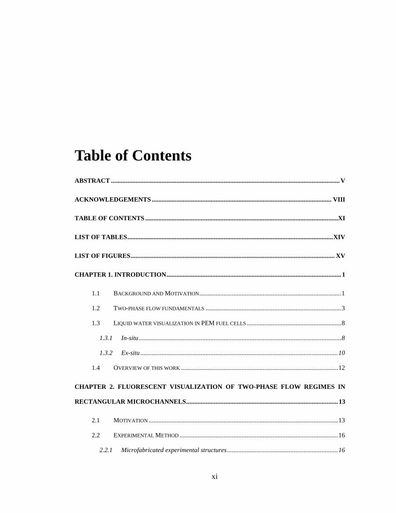
Table of Contents
ABSTRACT ............................................................................................................................................ V
ACKNOWLEDGEMENTS .............................................................................................................. VIII
TABLE OF CONTENTS ......................................................................................................................XI
LIST OF TABLES .............................................................................................................................. XIV
LIST OF FIGURES ............................................................................................................................. XV
CHAPTER 1. INTRODUCTION ........................................................................................................... 1
1.1 BACKGROUND AND MOTIVATION ....................................................................................... 1
1.2 TWO-PHASE FLOW FUNDAMENTALS ................................................................................... 3
1.3 LIQUID WATER VISUALIZATION IN PEM FUEL CELLS .......................................................... 8
1.3.1 In-situ ............................................................................................................................ 8
1.3.2 Ex-situ ......................................................................................................................... 10
1.4 OVERVIEW OF THIS WORK ................................................................................................ 12
CHAPTER 2. FLUORESCENT VISUALIZATION OF TWO-PHASE FLOW REGIMES IN
RECTANGULAR MICROCHANNELS ............................................................................................. 13
2.1 MOTIVATION .................................................................................................................... 13
2.2 EXPERIMENTAL METHOD ................................................................................................. 16
2.2.1 Microfabricated experimental structures .................................................................... 16
xii
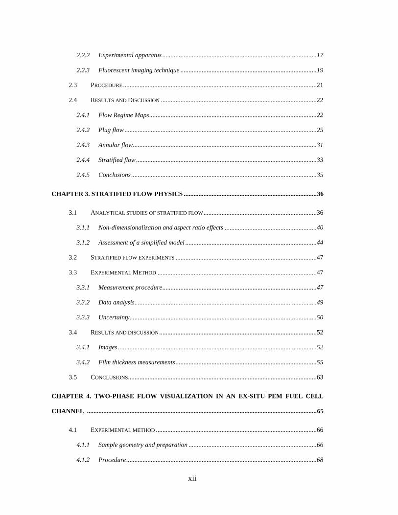
2.2.2 Experimental apparatus ..............................................................................................17
2.2.3 Fluorescent imaging technique ...................................................................................19
2.3 PROCEDURE ......................................................................................................................21
2.4 RESULTS AND DISCUSSION ...............................................................................................22
2.4.1 Flow Regime Maps ......................................................................................................22
2.4.2 Plug flow .....................................................................................................................25
2.4.3 Annular flow ................................................................................................................31
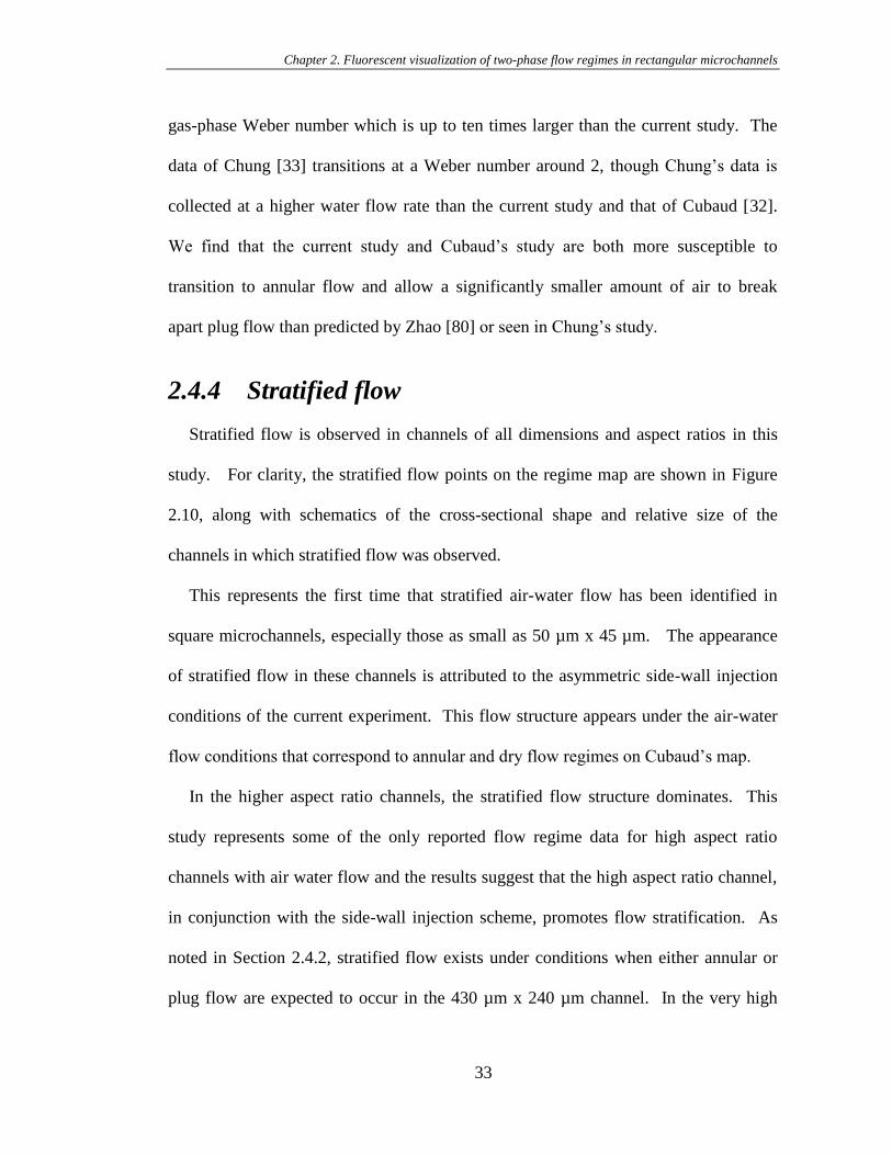
2.4.4 Stratified flow ..............................................................................................................33
2.4.5 Conclusions .................................................................................................................35
CHAPTER 3. STRATIFIED FLOW PHYSICS ................................................................................. 36
3.1 ANALYTICAL STUDIES OF STRATIFIED FLOW .....................................................................36
3.1.1 Non-dimensionalization and aspect ratio effects ........................................................40
3.1.2 Assessment of a simplified model ................................................................................44
3.2 STRATIFIED FLOW EXPERIMENTS ......................................................................................47
3.3 EXPERIMENTAL METHOD .................................................................................................47
3.3.1 Measurement procedure ..............................................................................................47
3.3.2 Data analysis ...............................................................................................................49
3.3.3 Uncertainty ..................................................................................................................50
3.4 RESULTS AND DISCUSSION ................................................................................................52
3.4.1 Images .........................................................................................................................52
3.4.2 Film thickness measurements ......................................................................................55
3.5 CONCLUSIONS...................................................................................................................63
CHAPTER 4. TWO-PHASE FLOW VISUALIZATION IN AN EX-SITU PEM FUEL CELL
CHANNEL ............................................................................................................................................ 65
4.1 EXPERIMENTAL METHOD ..................................................................................................66
4.1.1 Sample geometry and preparation ..............................................................................66
4.1.2 Procedure ....................................................................................................................68
xiii
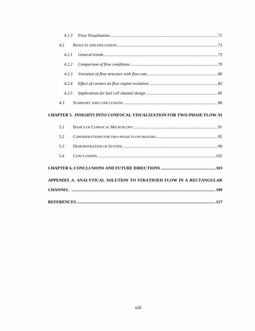
4.1.3 Flow Visualization ...................................................................................................... 71
4.2 RESULTS AND DISCUSSION................................................................................................ 73
4.2.1 General trends ............................................................................................................ 73
4.2.2 Comparison of flow conditions ................................................................................... 79
4.2.3 Variation of flow structure with flow rate ................................................................... 80
4.2.4 Effect of corners on flow regime evolution ................................................................. 82
4.2.5 Implications for fuel cell channel design .................................................................... 85
4.3 SUMMARY AND CONCLUSIONS ......................................................................................... 88
CHAPTER 5. INSIGHTS INTO CONFOCAL VISUALIZATION FOR TWO-PHASE FLOW. 91
5.1 BASICS OF CONFOCAL MICROSCOPY ................................................................................ 91
5.2 CONSIDERATIONS FOR TWO-PHASE FLOW IMAGING .......................................................... 95
5.3 DEMONSTRATION OF SYSTEM .......................................................................................... 99
5.4 CONCLUSIONS ................................................................................................................ 102
CHAPTER 6. CONCLUSIONS AND FUTURE DIRECTIONS .................................................... 103
APPENDIX A. ANALYTICAL SOLUTION TO STRATIFIED FLOW IN A RECTANGULAR
CHANNEL ......................................................................................................................................... 109
REFERENCES .................................................................................................................................... 117
xiv
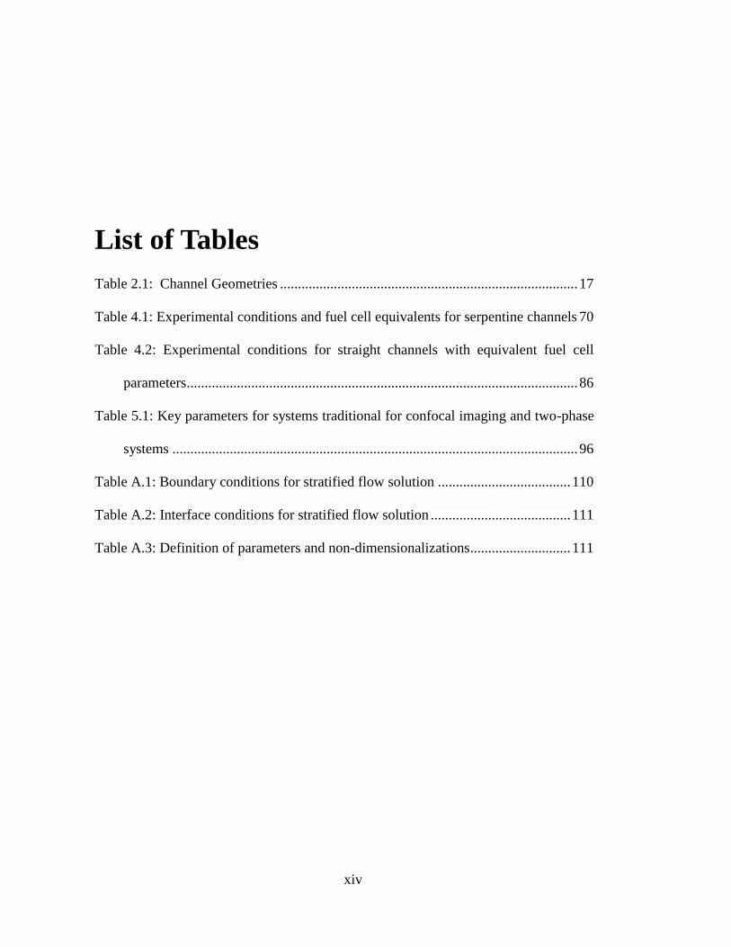
List of Tables
Table 2.1: Channel Geometries ................................................................................... 17
Table 4.1: Experimental conditions and fuel cell equivalents for serpentine channels 70
Table 4.2: Experimental conditions for straight channels with equivalent fuel cell
parameters ............................................................................................................. 86
Table 5.1: Key parameters for systems traditional for confocal imaging and two-phase
systems ................................................................................................................. 96
Table A.1: Boundary conditions for stratified flow solution ..................................... 110
Table A.2: Interface conditions for stratified flow solution ....................................... 111
Table A.3: Definition of parameters and non-dimensionalizations ............................ 111
xv
List of Figures
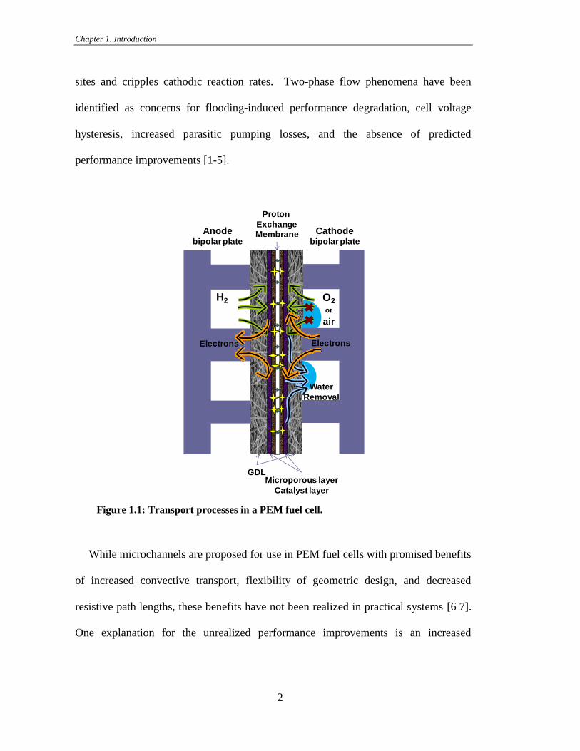
Figure 1.1: Transport processes in a PEM fuel cell. ....................................................... 2
Figure 2.1: Flow regime maps from previous visualization studies in square cross-
section microchannels .......................................................................................... 15
Figure 2.2: Layout of channel structures. ..................................................................... 16
Figure 2.3: Schematic of experimental setup. .............................................................. 18
Figure 2.4: Schematic of fluorescent imaging principle .............................................. 20
Figure 2.5: Flow regime map for five types of channels of various dimensions and
aspect ratios. ......................................................................................................... 24
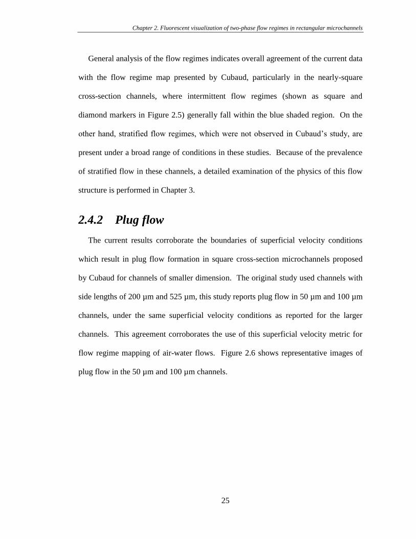
Figure 2.6: Representative images of plug flow in 50 and 100 µm square channels ... 26
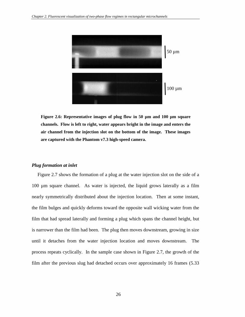
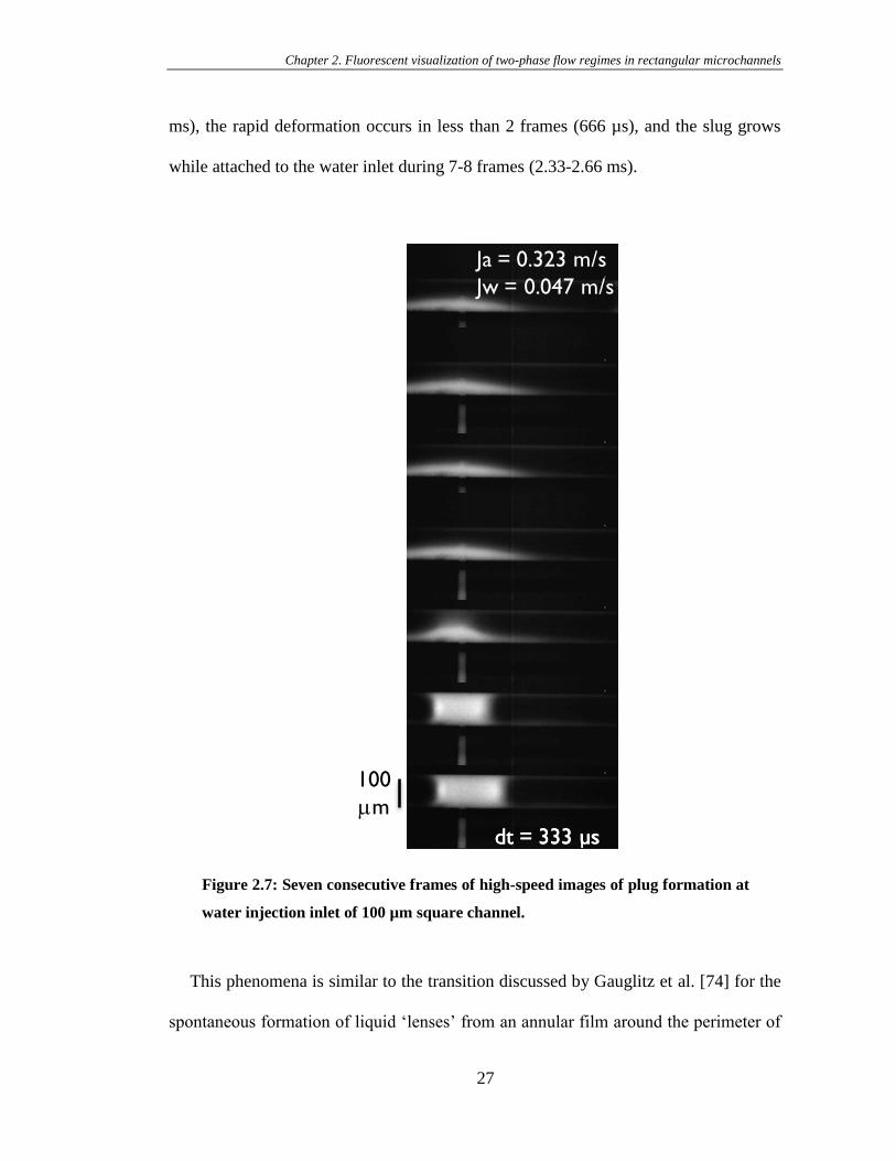
Figure 2.7: Seven consecutive frames of high-speed images of plug formation at water
injection inlet of 100 µm square channel ............................................................. 27
Figure 2.8: Formation of a plug .................................................................................... 30
Figure 2.9: Image of the formation of annular flow at the water inlet in a 50 µm x 50
µm square channel. ............................................................................................... 31
Figure 2.10: Prevalence of stratified flow on the regime map and schematics of
channel cross-sections in which it is observed. .................................................... 34
Figure 3.1: Schematic of geometry for analytical solution .......................................... 37
xvi
Figure 3.2: Velocity profile in liquid phase calculated from analytical solution to
stratified two-phase flow in 500 x 45 µm rectangular microchannel ................... 38
Figure 3.3: Geometry for aspect ratio and GDL coverage area analysis. ..................... 42
Figure 3.4: Decrease of channel coverage ratio with increasing channel aspect ratio. 43
Figure 3.5: Increase in pressure requirement for increasing channel aspect ratio over a
range of stoichiometric ratios. .............................................................................. 44
Figure 3.6: Deviation factor of gas-phase area model of stratified flow compared with
a 2D analytical solution. ....................................................................................... 46
Figure 3.7: Process of image thresholding with an example image of stratified flow at
the water injection location .................................................................................. 49
Figure 3.8: Example images of stratified flow from 500 µm x 45 µm channels. ......... 53
Figure 3.9: Example images of stratified flow in 500 µm x 400 µm channels. ........ 54
Figure 3.10: Variation of film thickness with inlet air superficial velocity in 500 µm x
45 µm channel ...................................................................................................... 56
Figure 3.11: Variation of film thickness with superficial air velocity in 500 µm x 45
µm channels for a variety of water injection rates ............................................... 57
Figure 3.12: Presentation of film thickness variation results from 500 µm x 50 µm
channels according to non-dimensional parameters, film thickness fraction and
ratio of volumetric flow rates. .............................................................................. 58
Figure 3.13: Variation in film thickness with volumetric flow rate ratio in a 430 µm x
240 µm channel compared with the analytical solution ....................................... 60
Figure 3.14: Variation of film thickness fraction with volumetric flow rate ratio in 500
µm x 400 µm U-shaped channel........................................................................... 63
xvii
Figure 4.1: Channel assembly. ..................................................................................... 67
Figure 4.2: Schematic of experimental setup. .............................................................. 69
Figure 4.3: Image decomposition ................................................................................ 71
Figure 4.4: Representative images of two-phase flow structures ................................ 72
Figure 4.5: Viscous losses in straight and serpentine channels ................................... 73
Figure 4.6: Observed flow structures and general evolution of flow regimes. ........... 75
Figure 4.7: Images of flow transitions from stratified flow on two walls to one wall.
.............................................................................................................................. 77
Figure 4.8: Flow regimes in serpentine channels mapped against superficial air and
water velocities ..................................................................................................... 81
Figure 4.9: Flow regime map for straight channels with equivalent flow rates to
serpentine channel conditions of Figure 4.8. ........................................................ 84
Figure 5.1: Illustration of confocal imaging principle for (a) laser scanning
microscopy and (b) spinning-disk microscopy ..................................................... 93
Figure 5.2: Schematic of spinning disk implementation using Nikon TE2000-U
inverted microscope and Hyphenated Systems confocal unit .............................. 94
Figure 5.3: Comparison of optical path for reflected and fluorescent imaging of
specularly-reflecting air-water interfaces. ............................................................ 97
Figure 5.4: Illustration of the effect of improper dye concentration in two-phase flow
imaging using a confocal microscope. ................................................................. 99
Figure 5.5: Processing of fluorescent droplet images. Vertical slice of (a) raw data (b)
3 point 3D median filtered data (c) 5-point 3D median filtered data. ................ 100
xviii
Figure 5.6: Results of reconstruction of droplet profile from confocal images of
planes, or “slices” within the droplet. ................................................................. 101
Figure A.1: Geometry for analytical solution to stratified flow in rectangular channel
(a) liquid film on one wall (b) liquid film on two opposite walls ...................... 109
1
Chapter 1. Introduction
1.1 Background and Motivation
Proton exchange membrane (PEM) fuel cells are a promising technology in the
search for portable CO2-free energy conversion alternatives. In these devices,
electricity is produced when hydrogen, encountering a catalyst, is separated into its
ions at the anode. While protons pass through a semi-permeable membrane, electrons
are forced to pass through an external circuit, producing electricity. At the cathode,
the ions combine with oxygen to produce water which is typically evacuated through
the gas delivery channels on the cathode side. While there are some variations in the
construction and materials, a single fuel cell consists of the polymer electrolyte
membrane, flanked on either side by catalyst layers and porous carbon paper gas
diffusion layers (GDLs), and sandwiched between the anode and cathode bipolar
plates which contain the gas delivery channels. Figure 1.1 shows the geometry of the
fuel cell.
Water management is a performance-limiting concern for the operation and
optimization of the PEM fuel cells. While the performance of the membrane depends
on ample humidification, liquid water in the microporous layer, gas diffusion layer
(GDL), and/or gas delivery channels impedes the flow of reactant gases to catalyst
Chapter 1. Introduction
2
sites and cripples cathodic reaction rates. Two-phase flow phenomena have been
identified as concerns for flooding-induced performance degradation, cell voltage
hysteresis, increased parasitic pumping losses, and the absence of predicted
performance improvements [1-5].
Figure 1.1: Transport processes in a PEM fuel cell.
While microchannels are proposed for use in PEM fuel cells with promised benefits
of increased convective transport, flexibility of geometric design, and decreased
resistive path lengths, these benefits have not been realized in practical systems [6 7].
One explanation for the unrealized performance improvements is an increased
Electrons
Water
Removal
Protons
Electrons
H2 O2
or
air
Anodebipolar plate
Cathodebipolar plate
Proton
ExchangeMembrane
GDLMicroporous layer
Catalyst layer
Chapter 1. Introduction
3
propensity toward flooding in smaller channels where surface tension force becomes
significant compared with viscous, inertial, and pressure forces [8].
The issue of flooding in the gas delivery channels of PEM fuel cells has been
addressed in various ways, from in-situ and ex-situ imaging techniques (Section 1.3)
to the development of novel designs and materials which provide wicking or pumping
of liquid water from the electrode areas [9-11]. Yet the optimal design of fuel cell
channels requires clear understanding of the interactions of air and water in small
diameter channels. While many studies have considered the flow in small diameter
tubes (Section 1.2), there remains a need for studies that consider two-phase flow in
microchannel geometries that mimic conditions in fuel cell channels, where
rectangular cross-sections, long channel lengths, distributed water introduction, and
porous walls are defining characteristics. The present work uses experimental
methods to study the physics of two-phase flow in geometries common to practical
fuel cells which is critical to their performance.
1.2 Two-phase flow fundamentals
Fluids moving through confined spaces such as microchannels experience a variety
of forces, with body forces becoming less important relative to surface forces as the
dimensions of the channels become small. In two-phase flow, surface tension at the
air-water interface becomes an important parameter in the behavior of the fluid phases.
The interplay of forces and geometry determine the structure and behavior of the air-
Chapter 1. Introduction
4
water interface, which can have a very important effect on the operation of a fluidic
device.
The Navier-Stokes equations describe the momentum balance in each phase. For
simplicity, the momentum balance is often expressed for two-phase flow in terms of
the Integral Momentum Equation, which accounts for the viscous forces in the gas
phase, the liquid phase, and at the interface.
inertialA
S
A
S
A
S
x
P
i
ii
L
LL
G
GG
(1)
where SG and SL are the wetted perimeters of the wall with the gas and liquid phases
respectively, Si is the perimeter of the gas-liquid interface in the cross-section, AG and
AL are the cross-sectional areas of the gas and liquid phases, Ai is a cross-sectional
area defined according to the particular formulation of τ, where τG, τL, τi are shear
stress coefficients.
Yet this simple expression masks the complexity of definition of the appropriate
shear stress coefficient, τ, which must account for the configuration of the phases
within the flow. Analytical predictions of these coefficients are not available, but
some empirically and theoretically derived expressions have been presented in the
literature [12]. A few studies have attempted to derive phenomenological expressions
for the pressure drop in the channels based on flow regime physics [13 14], but these
models have not been widely adopted as they require more detailed knowledge of the
flow structure.
Surface tension forces can be important at the interface between the gas and liquid
phases. In momentum and energy equations, surface tension forces are accounted for
Chapter 1. Introduction
5
at the boundary between the forces, where the curvature of the interface induces a
pressure difference between the phases according to the Young-Laplace Equation,
01 PPC (2)
where C is curvature of the interface, P1 and P0 are the bulk pressure on either side of
the interface. At the contact line between the interface and the solid surface, a balance
of forces dictates the equilibrium contact angle between the surface and the interface
according to the surface energies of each interface, which is expressed as
SLSOE cos (3)
where subscript S refers to the solid phase, O refers to the gas phase, and L refers to
the liquid phase.
Common flow structures in two-phase microchannels include intermittent regimes
and separated flow regimes. In intermittent regimes, the air and water pass through
the channel periodically and the liquid exists as discrete structures with a continuous
or discontinuous gas phase around them; in this study, we refer to these regimes as
„slug flow‟ and „plug flow‟, respectively. In separated flow regimes, the air flows
through one region of the channel while water flows continuously through another
region. A distinction is made based on to what extent the water covers the channel
walls, with „annular flow‟ corresponding to all walls covered, „stratified flow‟
including one or two walls, and „dry‟ meaning that water only flows in the corners of
the channels.
Flow structure changes due to surface energy differences can occur stochastically,
as the interface configuration spontaneously adjusts from one state to an energetically
favorable state [15]. Surfaces that are not perfectly clean on a molecular level may
Chapter 1. Introduction
6
support a range of stable contact angles, bounded by advancing and receding contact
angles, which are a function of surface characteristics and the fluid [16]. The effect of
contact angle hysteresis has been shown to be significant in describing the motion of
liquid plugs and slugs in gas flows in circular tubes and rectangular microchannels,
and for droplets on flat surfaces [17-19]. Contact angle hysteresis has also been used
to predict the departure of a droplet from a fuel cell gas diffusion layer [20].
Flow regimes are typically recorded on flow regime maps where superficial
velocities of each phase are the key parameters, corresponding to the axes on the map.
Many studies have examined two-phase flow in circular channels with diameters
smaller than 1 mm, though the boundaries between the flow regimes do not all agree
[21-30]. Some discrepancy is expected because the channel materials, geometries, and
injection configurations are not consistent between experimental setups. These studies
do not replicate the distributed liquid water introduction, long channel lengths, and
porous boundary conditions of a PEM fuel cell. Additionally, the liquid flow rates of
interest for these applications are much higher than those relevant to fuel cell
operation. Pehlivan [31] provides a review of the two-phase flow regimes observed in
mini channels as small as 800 µm. His universal flow regime map based on
experimental results from the literature does not extend to low water flow rates
relevant for fuel cell channels. Nevertheless, air flow rate is the dominant parameter
influencing flow regime transitions at the lowest reported water flow rates, a result
which may be relevant for the lower water flow rates applicable to fuel cells.
In contrast with the number of studies in circular channels, very few studies have
examined flow regime boundaries in rectangular channels, which are important for
Chapter 1. Introduction
7
practical devices. Only two studies present flow regime maps for rectangular cross-
section channels with dimensions smaller than 1 mm [32 33 ]; these studies are
discussed in more detail in Section 2.1. Chung et al. [33] performed similar
experiments on channels with square and circular cross-sections of approximately 100
µm; they found a small shift in the flow regime boundaries between the two
geometries. In vertically-oriented mini-channels of critical diameter less than 2.9 mm,
Bi and Zhao [34] found that the flow through the corners of a rectangular channel
caused different flow behavior than flow in circular channels where corner flow does
not exists because of buoyancy effects. However, Garimella‟s models of slug flow in
circular and square microchannels show a small difference in pressure gradient [35].
Perhaps the most important effect of the presence of corners in the cross-section is the
potential establishment of capillary flow in the corner of the channel [36 37], which
may have a significant effect on the fluid interactions depending on flow conditions.
These effects are still not well understood.
The effects of surface properties on the flow have also not been systematically
studied. In mini channels, two studies indicate that the wettability of the surface has a
small effect on the observed flow regimes for moderately non-wetting materials,
however for highly non-wetting surfaces, the effect becomes important [38 39]. In 1
mm square channels exhibiting annular flow, the effect of changing the surface tension
of the liquid on the pressure drop was not significant [40], however this result may not
apply to intermittent flow regimes where the triple point is expected to play a more
significant role in the fluid-surface interactions.
Chapter 1. Introduction
8
1.3 Liquid water visualization in PEM fuel cells
Because water in the cathode channels of a PEM fuel cell can significantly impact
is operation and two-phase flow is generally not well characterized in geometries
relevant to fuel cells, various authors have developed techniques to visualize two-
phase flow in actual and replicated fuel cells [41 42].
1.3.1 In-situ
Some two-phase flow characterization tools have been developed for in-situ fuel
cell applications. In fuel cell components lacking optical access, neutron imaging,
magnetic resonance imaging, and x-ray tomography allow for identification of liquid
water through opaque surfaces. Neutron imaging is a promising technique for imaging
of liquid water in an operating fuel cell [43-45]. Neutron radiography is basically a
two-dimensional technique, requiring detailed analysis to distinguish between the
anode and cathode. Boillat et al. have developed a system optimized for fuel cell
imaging which has a resolution of 20 µm in-plane and 200 µm axially with an
exposure time of 10 seconds by mounting the cell at a steep angle [46]. Studies by
Pekula et al. and Li et al. show the accumulation of water at the corners of serpentine
channels [47 48]. Owejan et al. and Zhang et al. have used neutron radiography to
show the effect of GDL materials on the accumulation of water in operating fuel cells
[49 50]. Neutron tomography allows for differentiation between cells within a stack,
however it is a very time-consuming technique, requiring hours to collect a set of
images [51 52]. The study of a fuel cell stack revealed less water accumulation in
internal cells, likely due to thermal effects. X-ray imaging has captured the formation
Chapter 1. Introduction
9
of droplets and air-water interfaces with high resolution in single cells [53 54]. X-ray
tomography and magnetic resonance imaging have been used to create three
dimensional maps of the water concentration in the membrane and GDL layers with
limited resolution [55 56].
Opaque bipolar plates, layers of porous materials with various surface properties,
and non-uniformity of water production rate and location complicate the imaging and
analysis of flow regimes in fuel cell channels. Yet fuel cells with modified geometries
allow optical access into the gas distribution channels [57 58]. These cells have been
used to correlate the appearance of liquid water with increases in gas pressure in the
channels and voltage drops in the fuel cell [59-61]. Air flow rate is found to be a
critical parameter affecting or preventing flooding [62 63]. In contrast to reported
results of neutron imaging, Ous [64] observed water accumulation in the center of the
channels, away from the corners. Kimball et al. [62] monitored the emergence of
droplets in the channel and their subsequent coalescence and slug formation leading to
flooding; the larger channels in their study exhibited gravity-dependent behavior.
Spernjak‟s [65] results indicated that the materials, such as the microporous layer,
have a significant effect on water appearance in the channels. In general, optical
setups may interfere with typical reaction distribution because the electrical pathways
are distorted when conductive bipolar plates are replaced with non-conductive glass
plates for optical access. While much insight can be drawn from these studies in the
correlation between liquid water and fuel cell performance, the precise flow conditions
at any particular location in the cell are difficult to quantify due to non-uniformities in
reaction distribution and subsequent uncertainties in local flow rates. The
Chapter 1. Introduction
10
discrepancies between these studies highlight the complexity of the interactions of the
electrochemical and fluidic processes in fuel cell devices.
1.3.2 Ex-situ
Ex-situ experiments are proposed as a means of decoupling the electrochemistry
from the fluidic system, allowing the physics of the two-phase flow to be examined
with materials relevant to fuel cell systems without the added complexity of the
operating system. However, the ex-situ experiments provide their own challenges for
implementation and interpretation.
Comparison of in-situ and ex-situ experimental results is complicated by the
definitions commonly prescribed in the literature for given operating conditions. A
single stoichiometric ratio is often reported, but in reality the air flow rate is held at a
fixed value and the current density or cell load is swept through a range of operating
conditions. Therefore, the reported stoichiometric ratio is valid at only a particular
representative current density. This procedure allows for similar fluidic conditions in
each case however, the electrochemical activity and species concentration profile
along the channel varies as more or fewer reactants are consumed. Despite these
difficulties, ex-situ experiments offer the advantage of greater control of experimental
conditions. Absent the electrochemistry of an operating fuel cell, these setups allow
observation of the two-phase flow characteristics in fuel cell geometries while
quantifying the local flow rates of both phases.
Various geometric configurations have been employed which simulate the
conditions of a fuel cell in an ex-situ visualization experiment. Lu et al. [66] and
Chapter 1. Introduction
11
Zhang et al. [67] constructed parallel-flow systems with gas and liquid injection
relevant to fuel cell conditions. Su et al. [68] studied flow in 5 mm square cathode
channels by injecting water into the channels through a carbon paper layer from a
single liquid reservoir, resulting in a lot of flow field flooding and water in the GDL
and channels. Others have examined droplet departure from a GDL into a gas channel
using short channel segments [69 70]. Gao et al. [71] used confocal microscopy to
observe the emergence and coalescence of droplets as they emerge from a GDL
surface.
Few experimental studies have considered fuel cell flow conditions in
microchannels, which is significant as two-phase flow transitions are commonly
considered to be functions of the superficial velocity of the phases. While flow rates
in fuel cell channels are fixed by the current density and stoichiometry, flow velocities
are then determined by channel dimensions. Many relevant non-dimensional
parameters, such as Weber and capillary numbers, corresponding to the ratio of inertia
and viscosity to surface tension, respectively, are often expressed in terms of
superficial velocities. For fuel cell systems, where volumetric flow rates are fixed by
operating conditions, the dimensions of the channel have a significant effect on these
forces. Lee [72] constructed a GDL-integrated microchannel structure in which plug
flow, annular and stratified flows are observed, depending on the Weber and capillary
numbers of the two-phase flow.
Chapter 1. Introduction
12
1.4 Overview of this work
This study examines two-phase flow in microchannels with rectangular cross-
sections in order to gain insight into the physics of the interaction of air and water
phases in rectangular microchannels applicable to practical devices, especially PEM
fuel cells. In Chapter 2, fundamental aspects of two phase flow in microchannels of
various aspect ratios are examined; flow structures are characterized on flow regime
maps and compared with previous results. In Chapter 3, stratified flow, a commonly
observed flow regime during the current study, is examined in more depth.
Measurements of the film thickness of the stratified flow are compared with an
analytically-based model of the flow. Chapter 4 describes the evolution of flow
structure along the length of an ex-situ PEM fuel cell channel with distributed
introduction of water into the channel through a porous GDL paper wall. Finally,
Chapter 5 provides new insight into the use of confocal imaging techniques for the
visualization of two-phase interfaces.
13
Chapter 2. Fluorescent visualization of
two-phase flow regimes in rectangular
microchannels
2.1 Motivation
Despite the importance of predicting the flow structure in microchannels of various
geometries in order to optimize the performance of practical devices, previous
visualization studies of two-phase flow in microchannels are restricted to channels of
circular, square, or triangular cross-section with asymmetric pre-mixed injection
conditions. This study examines flow regimes in channels with rectangular cross-
sections of various aspect ratios and sizes with asymmetric water injection into the
channel from one side wall injection location.
Microfabricated silicon microchannels replicate those found in PEMFC gas
delivery systems, while water injected into the channels simulates liquid entering the
cathode channel due to chemical reaction and electro-osmotic drag. This approach
allows for a controlled water “production” without the unsteady, non-uniform
behavior of actual fuel cell reactions. This is of particular importance to decouple the
problem of water entrainment into the microchannels.
Chapter 2. Fluorescent visualization of two-phase flow regimes in rectangular microchannels
14
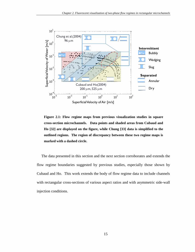
Two previously published visualization studies on two-phase flow in
microchannels with square cross-sections present flow regime maps as shown in
Figure 2.1 [32 33]. Both of these studies were performed on channels with axi-
symmetric injection conditions, where the air and water are mixed upstream of the test
section. The flow regime data are summarized on a flow regime map where the axes
represent the flow rates of air and water expressed as superficial velocities and the
symbols correspond to the flow structure which was identified at these flow conditions.
Generally, both sets of data show intermittent flow regimes (bubbly, wedging, and
slug) occurring for low air flow rates, with separated flow regimes (annular and dry)
prevailing at higher air flow rates. Despite this general agreement, discrepancies
between the two flow regime maps exist at the boundary between the intermittent and
stratified flow. In the smaller, shorter channels of Chung‟s paper, slug flow persists at
higher air flow rates for a given superficial water velocity.
Chapter 2. Fluorescent visualization of two-phase flow regimes in rectangular microchannels
15
Figure 2.1: Flow regime maps from previous visualization studies in square
cross-section microchannels. Data points and shaded areas from Cubaud and
Ho [32] are displayed on the figure, while Chung [33] data is simplified to the
outlined regions. The region of discrepancy between these two regime maps is
marked with a dashed circle.
The data presented in this section and the next section corroborates and extends the
flow regime boundaries suggested by previous studies, especially those shown by
Cubaud and Ho. This work extends the body of flow regime data to include channels
with rectangular cross-sections of various aspect ratios and with asymmetric side-wall
injection conditions.
10-3
10-2
10-1
100
101
102
10-4
10-3
10-2
10-1
100
101
Ua (m/s)
Uw (
m/s
)
Cubaud and Ho(2004)
200 mm, 525 mm
Superficial Velocity of Air [m/s]
Superf
icia
l Velo
city o
f Wat
er
[m/s
]
Chung et al.(2004)
96 mm
Intermittent
Separated
Bubbly
Wedging
Slug
Annular
Dry
Chapter 2. Fluorescent visualization of two-phase flow regimes in rectangular microchannels
16
2.2 Experimental Method
2.2.1 Microfabricated experimental structures
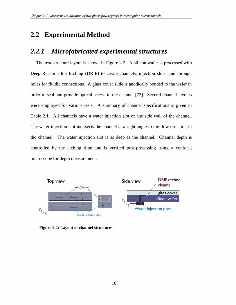
The test structure layout is shown in Figure 2.2. A silicon wafer is processed with
Deep Reaction Ion Etching (DRIE) to create channels, injection slots, and through
holes for fluidic connections. A glass cover slide is anodically bonded to the wafer in
order to seal and provide optical access to the channel [73]. Several channel layouts
were employed for various tests. A summary of channel specifications is given in
Table 2.1. All channels have a water injection slot on the side wall of the channel.
The water injection slot intersects the channel at a right angle to the flow direction in
the channel. The water injection slot is as deep as the channel. Channel depth is
controlled by the etching time and is verified post-processing using a confocal
microscope for depth measurement.
Figure 2.2: Layout of channel structures.
Water Injection Slots
Air Channel
Channel Structure
Top view Side view
silicon wafer
glass cover
DRIE etched
channel
yz
xy Water injection port
Chapter 2. Fluorescent visualization of two-phase flow regimes in rectangular microchannels
17
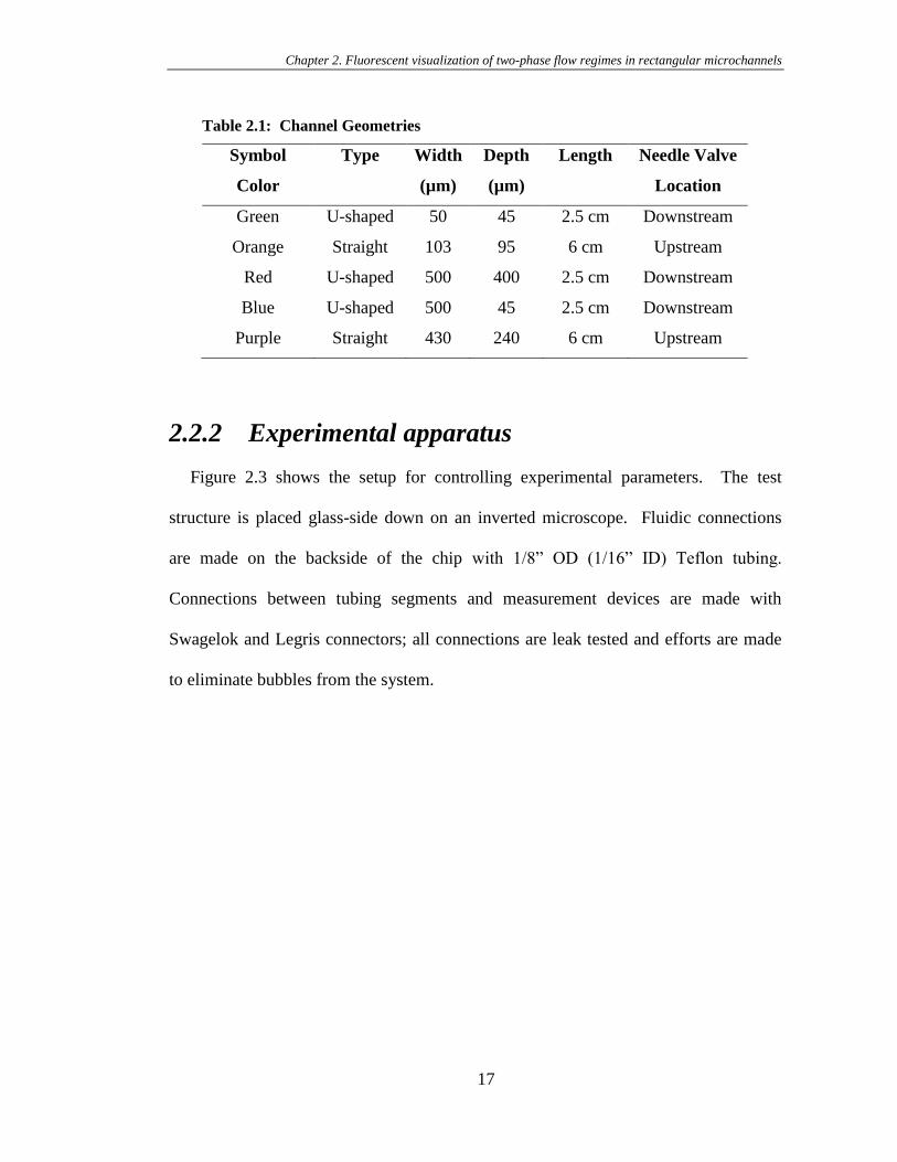
Table 2.1: Channel Geometries
Symbol
Color
Type Width
(µm)
Depth
(µm)
Length Needle Valve
Location
Green U-shaped 50 45 2.5 cm Downstream
Orange Straight 103 95 6 cm Upstream
Red U-shaped 500 400 2.5 cm Downstream
Blue U-shaped 500 45 2.5 cm Downstream
Purple Straight 430 240 6 cm Upstream
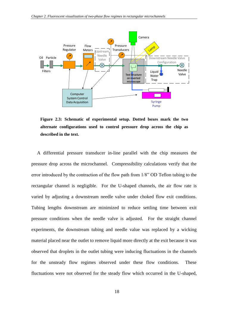
2.2.2 Experimental apparatus
Figure 2.3 shows the setup for controlling experimental parameters. The test
structure is placed glass-side down on an inverted microscope. Fluidic connections
are made on the backside of the chip with 1/8” OD (1/16” ID) Teflon tubing.
Connections between tubing segments and measurement devices are made with
Swagelok and Legris connectors; all connections are leak tested and efforts are made
to eliminate bubbles from the system.
Chapter 2. Fluorescent visualization of two-phase flow regimes in rectangular microchannels
18
Figure 2.3: Schematic of experimental setup. Dotted boxes mark the two
alternate configurations used to control pressure drop across the chip as
described in the text.
A differential pressure transducer in-line parallel with the chip measures the
pressure drop across the microchannel. Compressibility calculations verify that the
error introduced by the contraction of the flow path from 1/8” OD Teflon tubing to the
rectangular channel is negligible. For the U-shaped channels, the air flow rate is
varied by adjusting a downstream needle valve under choked flow exit conditions.
Tubing lengths downstream are minimized to reduce settling time between exit
pressure conditions when the needle valve is adjusted. For the straight channel
experiments, the downstream tubing and needle value was replaced by a wicking
material placed near the outlet to remove liquid more directly at the exit because it was
observed that droplets in the outlet tubing were inducing fluctuations in the channels
for the unsteady flow regimes observed under these flow conditions. These
fluctuations were not observed for the steady flow which occurred in the U-shaped,
PressureRegulator
Filters
Oil Particle
Flow Meters
NeedleValve
SyringePump
Camera
Liquid WaterTrap
PressureTransducers
ComputerSystem ControlData Acquisition
Test Structure on inverted microscope
UpstreamNeedleValve Downstream Needle Valve
Configuration
Chapter 2. Fluorescent visualization of two-phase flow regimes in rectangular microchannels
19
high aspect ratio channels. The air flow rate is measured using either a thermal mass
flow meter (Sensirion EM1) or a laminar flow meter (Omega FMA 1601A, 0-10 ccm,
0-1 LPM, or 0-2 LPM), depending on the range of flow rates.
Images of the flow are captured with a CCD camera through the magnifying
objective on the inverted Nikon microscope.
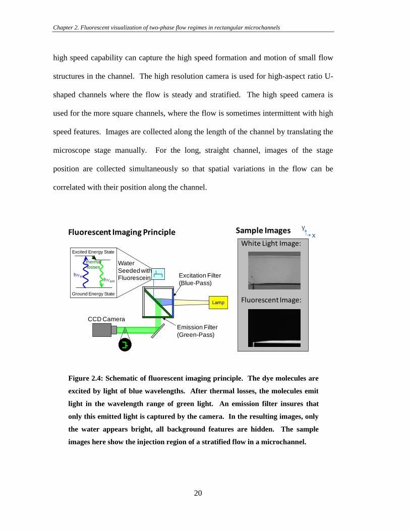
2.2.3 Fluorescent imaging technique
Fluorescent imaging provides detailed information about the flow regime and water
film extent within the channel. Water injected into the channels is seeded with a 0.5
mMol concentration of Fluorescein dye to enable fluorescent visualization of the flow.
Fluorescent excitation is achieved with a broadband metal halide lamp combined with
an FITC filter cube on an inverted microscope as depicted in Figure 2.3. As shown,
fluorescence imaging makes the air/water interfaces more clearly distinguishable and
easily post-processed than with white light imaging. Figure 2.4 is a comparison of
white light and fluorescence imaging of the injection region for a stratified flow in a
microchannel.
Images are recorded using one of two CCD cameras. The CoolSNAP ES camera,
with 1392 x 1040 pixels measuring 6.45 µm each, allows for high resolution imaging.
A 10x objective lens allows a 500 µm channel width to be captured in a single image,
with each square pixel corresponding to a 0.645 µm by 0.645 µm region, for 800 pixel
resolution across the channel width. The Phantom v7.3 camera is a high speed camera,
which is capable of capturing 6688 full 800 x 600 pixel frames per second. With a
pixel size of 22 µm, the resolution of this camera is significantly lower; however the
Chapter 2. Fluorescent visualization of two-phase flow regimes in rectangular microchannels
20
high speed capability can capture the high speed formation and motion of small flow
structures in the channel. The high resolution camera is used for high-aspect ratio U-
shaped channels where the flow is steady and stratified. The high speed camera is
used for the more square channels, where the flow is sometimes intermittent with high
speed features. Images are collected along the length of the channel by translating the
microscope stage manually. For the long, straight channel, images of the stage
position are collected simultaneously so that spatial variations in the flow can be
correlated with their position along the channel.
Figure 2.4: Schematic of fluorescent imaging principle. The dye molecules are
excited by light of blue wavelengths. After thermal losses, the molecules emit
light in the wavelength range of green light. An emission filter insures that
only this emitted light is captured by the camera. In the resulting images, only
the water appears bright, all background features are hidden. The sample
images here show the injection region of a stratified flow in a microchannel.
White Light Image:
Fluorescent Image:Lamp
hnexhnem
thermallosses
Ground Energy State
Excited Energy State
Excitation Filter
(Blue-Pass)
Water
SeededwithFluorescein
CCD Camera
Emission Filter
(Green-Pass)
Fluorescent Imaging Principle Sample Imagesx
y
Chapter 2. Fluorescent visualization of two-phase flow regimes in rectangular microchannels
21
2.3 Procedure
Air flow conditions are established by setting the inlet pressure and/or adjusting the
outlet needle valve. Water is introduced into the channel by starting the syringe pump,
which has been carefully evacuated of air pockets and bubbles in the tubing. The flow
structure is imaged once a steady condition has been achieved, as determined when air
flow rate and pressure readings are not changing. The system was configured to
reduce compressibility and steady conditions were established quickly. Measurements
were typically recorded 30 – 60 seconds after the conditions were set. Water flow was
stopped until the channel and tubing were cleared of residual liquid, then the next test
conditions were established.
Measurements of pressure and flow rates were averaged off-line over the duration
of the experiment. The uncertainty in the velocity measurement is derived from the
quoted accuracy of the mass flow meters and channel geometries. The thermal mass
flow meter has a quoted accuracy of ± 3% measured value. Velocities calculated from
the thermal mass flow meter readings are reported with an accuracy of ± 6% MV,
including uncertainties in the channel depth and air density from the pressure
measurement. The uncertainty in the liquid velocity is due to the compressibility of
the system and uncertainty in the volume flow rate of the syringe pump and the
channel dimensions. The uncertainty is approximated as ± 2%, dominated by the
measurement of channel dimension. The images and videos were examined after the
experiments in order to categorize the observed flow structures.
As previously noted, the channels are etched in silicon using DRIE. This technique
produces several effects which may impact the surface energy and topology of the
Chapter 2. Fluorescent visualization of two-phase flow regimes in rectangular microchannels
22
silicon. The etched walls can be scalloped, though efforts are made to reduce this
effect according to the recipe used. There can also be residual coatings left on the
surface of the channel which may impact the contact angles in the channels. This
coating is persistent and difficult to remove, so it is assumed that all channels used for
these experiments have similar surface properties.
2.4 Results and Discussion
2.4.1 Flow Regime Maps
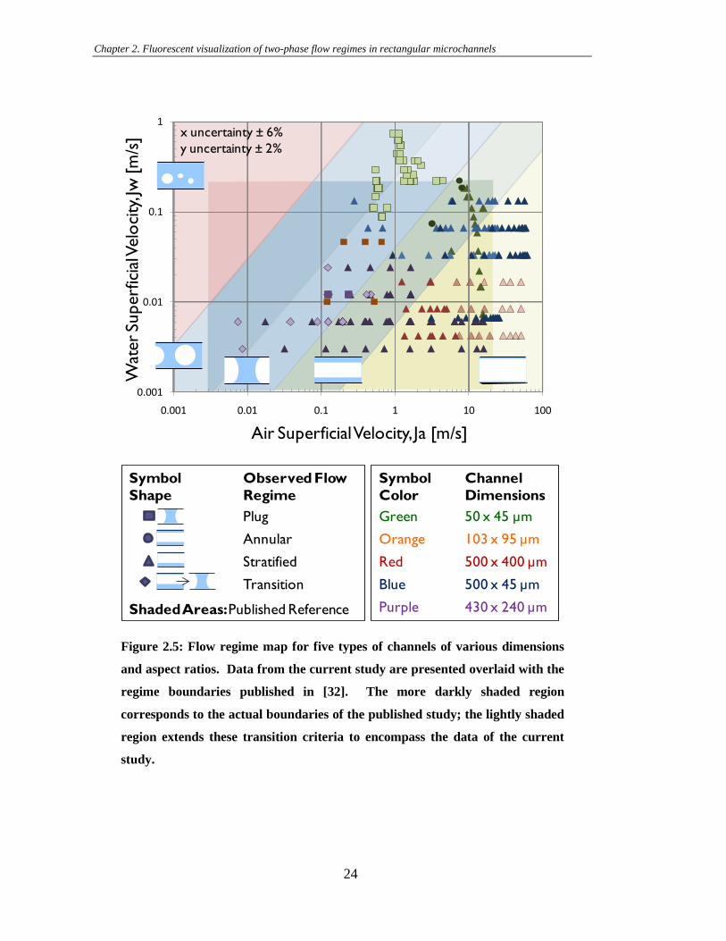
Flow structure data from the five types of channels examined in this study are
summarized in Figure 2.5. This chapter provides more details about the specifics of
the flow regimes summarized on this regime map. The data from the current study is
overlaid with shaded regions which correspond to the boundaries of the study
presented by Cubaud and Ho [32], with the darkly shaded region corresponding to the
limits of that study and the lightly shaded area extending the power law transition
criterion to higher air and water superficial velocities.
In Cubaud and Ho‟s study, flow regimes in square cross-section channels are
reported for two different channel sizes. The flow structure regions are divided by
power law relationships of superficial air and water velocities, shown as parallel lines
on log-log axes of superficial velocities. As the ratio of air to water velocity increases,
the flow regimes progress through the following sequence:
Chapter 2. Fluorescent visualization of two-phase flow regimes in rectangular microchannels
23
bubbly flow – small air bubbles exist in a primarily liquid flow
wedging and slug flow – large air bubbles spatially intermittently fill
the channel. Cubaud makes a distinction between these two regimes,
citing the presence of a thin liquid film around the air bubble in
wedging flow; the absence of which yield slug flow. In this study,
we group these flow regimes together into a single category of
intermittent flow, named plug flow.
annular flow – a gas core is surrounded by liquid film on the walls
dry flow – liquid flows only in the corners of the channel and the
walls of the channel are dry.
Four distinct flow regimes were observed in the channels under the range of
conditions tested. In most cases, a single flow regime is observed along the length of
the channel. Plug, annular, and stratified flows are marked with square, circular, and
triangular symbols, respectively. Under certain flow conditions, instability in the film
causes transition from stratified flow to plug flow downstream of the water injection.
This transitional regime is also noted on the flow regime map in as diamond shaped
symbols.
Chapter 2. Fluorescent visualization of two-phase flow regimes in rectangular microchannels
24
Figure 2.5: Flow regime map for five types of channels of various dimensions
and aspect ratios. Data from the current study are presented overlaid with the
regime boundaries published in [32]. The more darkly shaded region
corresponds to the actual boundaries of the published study; the lightly shaded
region extends these transition criteria to encompass the data of the current
study.
0.001
0.01
0.1
1
0.001 0.01 0.1 1 10 100
Air Superficial Velocity, Ja [m/s]
Wat
er
Superf
icia
l Velo
city
, Jw
[m/s
]
Symbol
Shape
Observed Flow
Regime
Plug
Annular
Stratified
Transition
Symbol
Color
Green
Orange
Red
Blue
Purple
Channel
Dimensions
50 x 45 µm
103 x 95 µm
500 x 400 µm
500 x 45 µm
430 x 240 µmShaded Areas: Published Reference
x uncertainty ± 6%
y uncertainty ± 2%
Chapter 2. Fluorescent visualization of two-phase flow regimes in rectangular microchannels
25
General analysis of the flow regimes indicates overall agreement of the current data
with the flow regime map presented by Cubaud, particularly in the nearly-square
cross-section channels, where intermittent flow regimes (shown as square and
diamond markers in Figure 2.5) generally fall within the blue shaded region. On the
other hand, stratified flow regimes, which were not observed in Cubaud‟s study, are
present under a broad range of conditions in these studies. Because of the prevalence
of stratified flow in these channels, a detailed examination of the physics of this flow
structure is performed in Chapter 3.
2.4.2 Plug flow
The current results corroborate the boundaries of superficial velocity conditions
which result in plug flow formation in square cross-section microchannels proposed
by Cubaud for channels of smaller dimension. The original study used channels with
side lengths of 200 µm and 525 µm, this study reports plug flow in 50 µm and 100 µm
channels, under the same superficial velocity conditions as reported for the larger
channels. This agreement corroborates the use of this superficial velocity metric for
flow regime mapping of air-water flows. Figure 2.6 shows representative images of
plug flow in the 50 µm and 100 µm channels.
Chapter 2. Fluorescent visualization of two-phase flow regimes in rectangular microchannels
26
Figure 2.6: Representative images of plug flow in 50 µm and 100 µm square
channels. Flow is left to right, water appears bright in the image and enters the
air channel from the injection slot on the bottom of the image. These images
are captured with the Phantom v7.3 high-speed camera.
Plug formation at inlet
Figure 2.7 shows the formation of a plug at the water injection slot on the side of a
100 µm square channel. As water is injected, the liquid grows laterally as a film
nearly symmetrically distributed about the injection location. Then at some instant,
the film bulges and quickly deforms toward the opposite wall wicking water from the
film that had spread laterally and forming a plug which spans the channel height, but
is narrower than the film had been. The plug then moves downstream, growing in size
until it detaches from the water injection location and moves downstream. The
process repeats cyclically. In the sample case shown in Figure 2.7, the growth of the
film after the previous slug had detached occurs over approximately 16 frames (5.33
50 µm
100 µm
Chapter 2. Fluorescent visualization of two-phase flow regimes in rectangular microchannels
27
ms), the rapid deformation occurs in less than 2 frames (666 µs), and the slug grows
while attached to the water inlet during 7-8 frames (2.33-2.66 ms).
Figure 2.7: Seven consecutive frames of high-speed images of plug formation at
water injection inlet of 100 µm square channel.
This phenomena is similar to the transition discussed by Gauglitz et al. [74] for the
spontaneous formation of liquid „lenses‟ from an annular film around the perimeter of
C2_101
dt = 333 us
dt = 333 usdt = 333 µs
100
mm
Ja = 0.323 m/s
Jw = 0.047 m/s
Chapter 2. Fluorescent visualization of two-phase flow regimes in rectangular microchannels
28
a circular microchannel. Gauglitz identifies a thickness based transition criterion
which corresponds to the geometry where it is energetically favorable for the liquid to
exist as a “lens” or “plug” rather than an elongated disk. At this point, the liquid
becomes unstable and may spontaneously transition to a stable geometry. Gauglitz
predicts a critical thickness at which an annular film in a circular microchannel
becomes unstable at 12% of the channel radius; reported empirical results give a
critical film thickness of 9%. A similar measurement is carried out for several cases
of plug formation in the current geometry, which differs significantly from the
previous studies because of the following properties:
The channel cross-section is rectangular
Water is injected from the side wall and significant shear forces exist at
the air water interface
The film is discontinuous film at the water injection location after the
previous plug moves downstream
The film thickness just before transition to plug is measured as 33% of the channel
height. There exists a need for further investigation into the conditions for the
formation of plug flow at a side wall injection, including considerations of the effect
of air shear and inertial forces on the plug formation, the critical film spreading length
for formation of a plug, as the water in this spreading air provides the necessary
volume of liquid required to create and sustain a plug across the channel, and lift
Chapter 2. Fluorescent visualization of two-phase flow regimes in rectangular microchannels
29
forces due to the acceleration of the gas phase through the constriction caused by the
liquid slug.
Plug formation from film instability
A similar yet distinct means of plug formation was observed in a transition from a
stratified film. This phenomenon is marked in Figure 2.5 as diamonds. This regime
occurs in the conditions on the flow regime map where Cubaud observed plug flow,
but in the current experiments in the 430 µm x 240 µm channels, we have observed
either stratified flow or this transitional flow regime between stratified and plug flow.
More discussion of this result is presented in the following section.
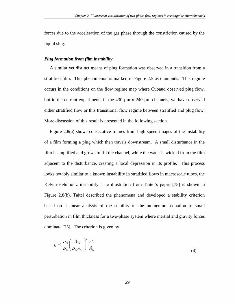
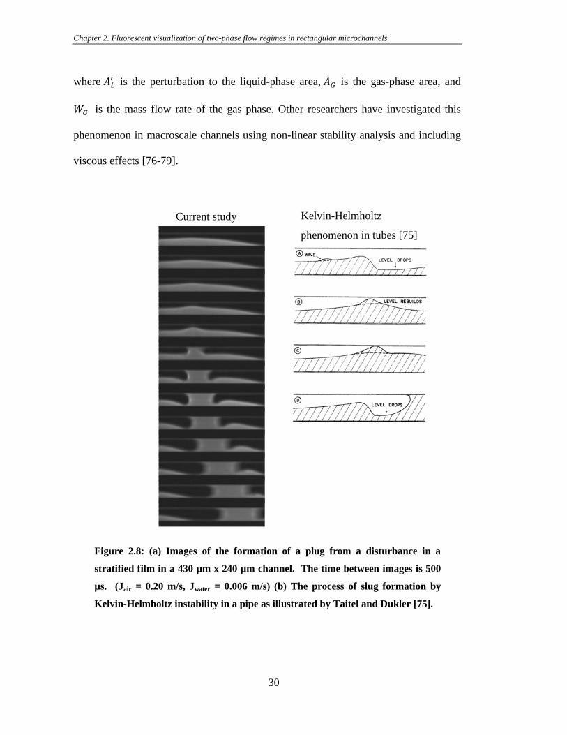
Figure 2.8(a) shows consecutive frames from high-speed images of the instability
of a film forming a plug which then travels downstream. A small disturbance in the
film is amplified and grows to fill the channel, while the water is wicked from the film
adjacent to the disturbance, creating a local depression in its profile. This process
looks notably similar to a known instability in stratified flows in macroscale tubes, the
Kelvin-Helmholtz instability. The illustration from Taitel‟s paper [75] is shown in
Figure 2.8(b). Taitel described the phenomena and developed a stability criterion
based on a linear analysis of the stability of the momentum equation to small
perturbation in film thickness for a two-phase system where inertial and gravity forces
dominate [75]. The criterion is given by
(4) G
L
GG
G
L
G
A
A
A
Wg
2
Chapter 2. Fluorescent visualization of two-phase flow regimes in rectangular microchannels
30
where is the perturbation to the liquid-phase area, is the gas-phase area, and
is the mass flow rate of the gas phase. Other researchers have investigated this
phenomenon in macroscale channels using non-linear stability analysis and including
viscous effects [76-79].
Figure 2.8: (a) Images of the formation of a plug from a disturbance in a
stratified film in a 430 µm x 240 µm channel. The time between images is 500
µs. (Jair = 0.20 m/s, Jwater = 0.006 m/s) (b) The process of slug formation by
Kelvin-Helmholtz instability in a pipe as illustrated by Taitel and Dukler [75].
Kelvin-Helmholtz
phenomenon in tubes [75]
Current study
Chapter 2. Fluorescent visualization of two-phase flow regimes in rectangular microchannels
31
Previous workers have not reported stratified flow in gas-liquid microchannel flow,
therefore the stability of these flows and the formation of plugs from these films have
not been studied. In microchannel flows, the effect of surface tension must also be
considered with viscous and inertial forces creating lift around the disturbance. When
surface tension is significant, a minimum radius of curvature is a likely criterion, while
lift forces suggest a criterion related to the film thickness deviation, and viscous
dissipation may dictate a minimum film thickness. More research is needed to
complete a full stability analysis on this system.
2.4.3 Annular flow
An annular flow regime is observed only under a few conditions tested in the 50
µm x 50 µm channels. These points are marked in Figure 2.5 as circles and fall within
the region where Cubaud also observed annular flow. The conditions where annular
flow is observed in the current study are clustered close to the boundary with the plug
flow regime. At higher air flow rates -- moving to the right on the regime map – the
current geometry favors stratified flow over annular flow.
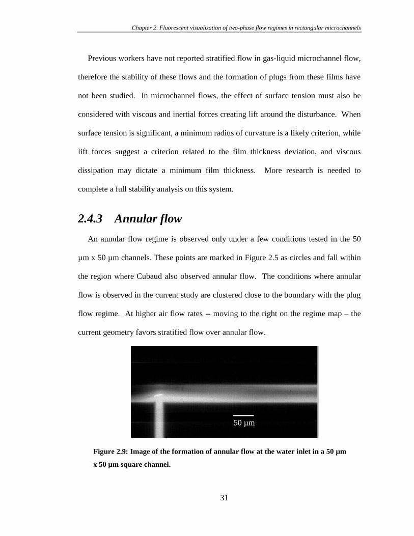
Figure 2.9: Image of the formation of annular flow at the water inlet in a 50 µm
x 50 µm square channel.
50 µm
Chapter 2. Fluorescent visualization of two-phase flow regimes in rectangular microchannels
32
The process of formation of annular flow can be seen at the water injection location.
Under the conditions where annular flow exists, water can be seen entering the
channel from the injection location and starting to protrude into the channel, feigning
formation of a plug. Rather than forming a cohesive plug, however the surface tension
of the water is not strong enough to overcome the inertial force of the air. The liquid
plug is broken and water is forced to the walls and corners of the channel. Gas flows
through the core, creating an annular flow.
The non-dimensional parameter which characterizes the relative magnitude of
internal forces to surface tension forces is the Weber number. The gas phase Weber
number formulation is given in Equation (5). The 1st order dependence on channel
diameter comes from the derivation of the Weber number, where the inertia of the gas
phase acts over the channel area, while surface tension is a line force which acts along
the interface.
(5)
Previous studies on two-phase flow in small tubes in microgravity have
experimentally determined that a gas-phase Weber number between 4 and 8 describes
the minimum gas flow which causes a transition from plug flow to annular flow [80].
In these 50 µm x 45 µm channels, the critical Weber number, measured
experimentally, is in the range of 0.01 to 0.05. This small value denotes that a much
lower flow rate of air is required to overcome the surface tension of the liquid phase in
these rectangular microchannels. The data of Cubaud also demonstrates transition at a
05.001.0
842
DUWe GG
G
tubes in microgravity [80]
current data in 50 µm x 45 µm
rectangular channels
Chapter 2. Fluorescent visualization of two-phase flow regimes in rectangular microchannels
33
gas-phase Weber number which is up to ten times larger than the current study. The
data of Chung [33] transitions at a Weber number around 2, though Chung‟s data is
collected at a higher water flow rate than the current study and that of Cubaud [32].
We find that the current study and Cubaud‟s study are both more susceptible to
transition to annular flow and allow a significantly smaller amount of air to break
apart plug flow than predicted by Zhao [80] or seen in Chung‟s study.
2.4.4 Stratified flow
Stratified flow is observed in channels of all dimensions and aspect ratios in this
study. For clarity, the stratified flow points on the regime map are shown in Figure
2.10, along with schematics of the cross-sectional shape and relative size of the
channels in which stratified flow was observed.
This represents the first time that stratified air-water flow has been identified in
square microchannels, especially those as small as 50 µm x 45 µm. The appearance
of stratified flow in these channels is attributed to the asymmetric side-wall injection
conditions of the current experiment. This flow structure appears under the air-water
flow conditions that correspond to annular and dry flow regimes on Cubaud‟s map.
In the higher aspect ratio channels, the stratified flow structure dominates. This
study represents some of the only reported flow regime data for high aspect ratio
channels with air water flow and the results suggest that the high aspect ratio channel,
in conjunction with the side-wall injection scheme, promotes flow stratification. As
noted in Section 2.4.2, stratified flow exists under conditions when either annular or
plug flow are expected to occur in the 430 µm x 240 µm channel. In the very high
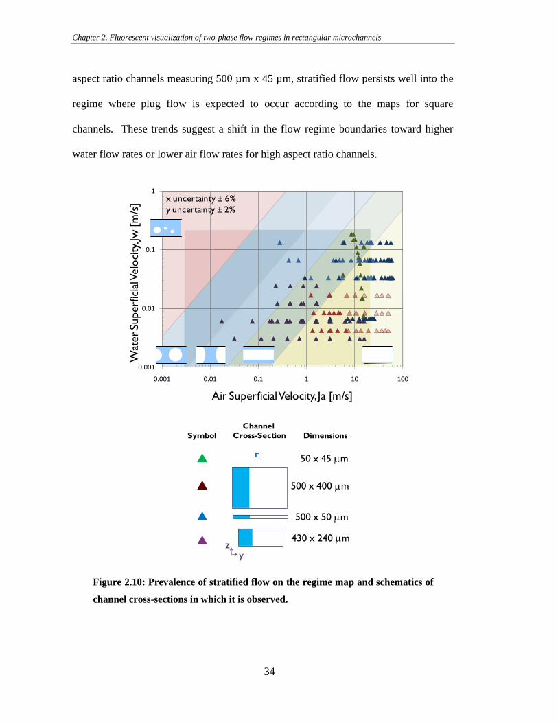
Chapter 2. Fluorescent visualization of two-phase flow regimes in rectangular microchannels
34
aspect ratio channels measuring 500 µm x 45 µm, stratified flow persists well into the
regime where plug flow is expected to occur according to the maps for square
channels. These trends suggest a shift in the flow regime boundaries toward higher
water flow rates or lower air flow rates for high aspect ratio channels.
Figure 2.10: Prevalence of stratified flow on the regime map and schematics of
channel cross-sections in which it is observed.
0.001
0.01
0.1
1
0.001 0.01 0.1 1 10 100
Air Superficial Velocity, Ja [m/s]
Wat
er
Superf
icia
l Velo
city
, Jw
[m/s
]
x uncertainty ± 6%
y uncertainty ± 2%
Channel
Cross-SectionSymbol Dimensions
50 x 45 mm
500 x 400 mm
500 x 50 mm
430 x 240 mm
yz
Chapter 2. Fluorescent visualization of two-phase flow regimes in rectangular microchannels
35
2.4.5 Conclusions
Flow structure mapping for a variety of channel sizes and aspect ratios corroborates
and extends flow regime maps presented in the literature for square cross-section
channels. Plug, annular, stratified, and transitional flow regimes are identified, with
stratified flow being both prevalent in high aspect ratio channels and previously
unseen in square-cross section channels. Direction for further analysis of these results
was presented.
36
Chapter 3. Stratified flow physics
As described in the previous chapter, stratified flow was commonly observed in the
rectangular channels with side-wall water injection used for the fundamental study of
liquid-gas interactions in hydrophilic channels with side-wall water injection. This
section develops a detailed study of the physics of stratified flow including
presentation of a analytical model of flow supported by measurements of the structure
of the stratified film for a variety of air and water conditions in channels of three
different dimensions and aspect ratios. The measurement technique and some results
have been published previously [81].
3.1 Analytical studies of stratified flow
An analytical solution to the velocity distribution in two-phase stratified flow in a
rectangular duct is useful for gaining insight into the interaction of the air and liquid
phases in the experiments. A solution was published in dimensional form by Tang and
Himmelblau [82 ]. We build on this analysis to extract insight into the scaling
arguments, ascertain validity limits for simplified models, and examine the effect of
channel size and aspect ratio. Using an analytical solution, we can also examine
Chapter 3. Stratified flow physics
37
trade-offs relevant to fuel cell operation and predict preferable geometries and
operating conditions.
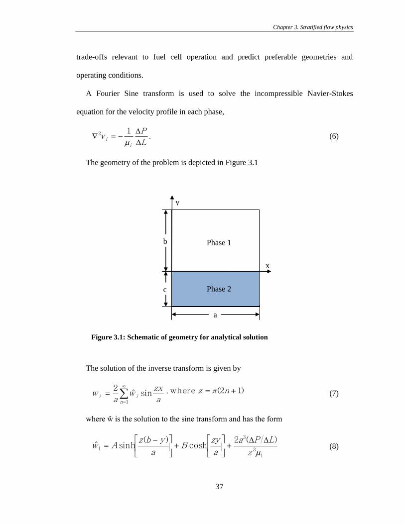
A Fourier Sine transform is used to solve the incompressible Navier-Stokes
equation for the velocity profile in each phase,
L
Pv
i
i
m
12. (6)
The geometry of the problem is depicted in Figure 3.1
Figure 3.1: Schematic of geometry for analytical solution
The solution of the inverse transform is given by
a
zxw
aw
nii sinˆ
2
1
)12( where , nz (7)
where ŵ is the solution to the sine transform and has the form
13
3
1
)(2cosh
)(sinhˆ
mz
LPa
a
zyB
a
ybzAw
(8)
a
b
c Phase 2
Phase 1
x
y
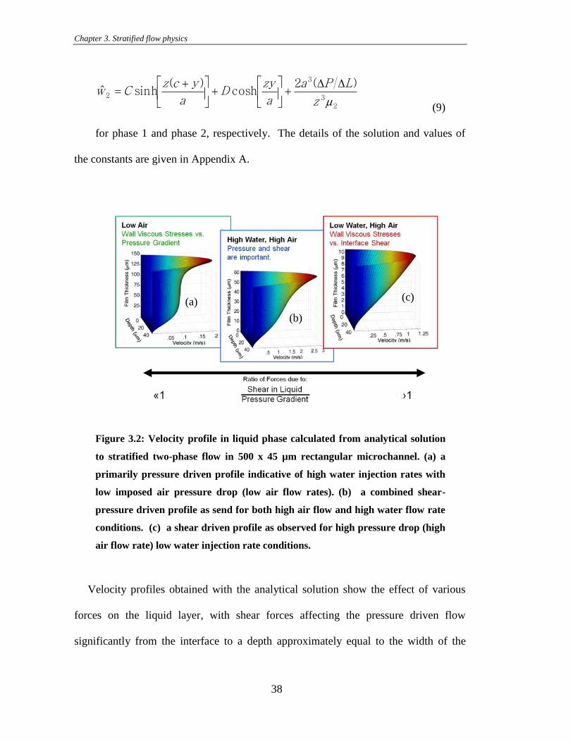
Chapter 3. Stratified flow physics
38
23
3
2
)(2cosh
)(sinhˆ
mz
LPa
a
zyD
a
yczCw
(9)
for phase 1 and phase 2, respectively. The details of the solution and values of
the constants are given in Appendix A.
Figure 3.2: Velocity profile in liquid phase calculated from analytical solution
to stratified two-phase flow in 500 x 45 µm rectangular microchannel. (a) a
primarily pressure driven profile indicative of high water injection rates with
low imposed air pressure drop (low air flow rates). (b) a combined shear-
pressure driven profile as send for both high air flow and high water flow rate
conditions. (c) a shear driven profile as observed for high pressure drop (high
air flow rate) low water injection rate conditions.
Velocity profiles obtained with the analytical solution show the effect of various
forces on the liquid layer, with shear forces affecting the pressure driven flow
significantly from the interface to a depth approximately equal to the width of the
(a) (c)
(b)
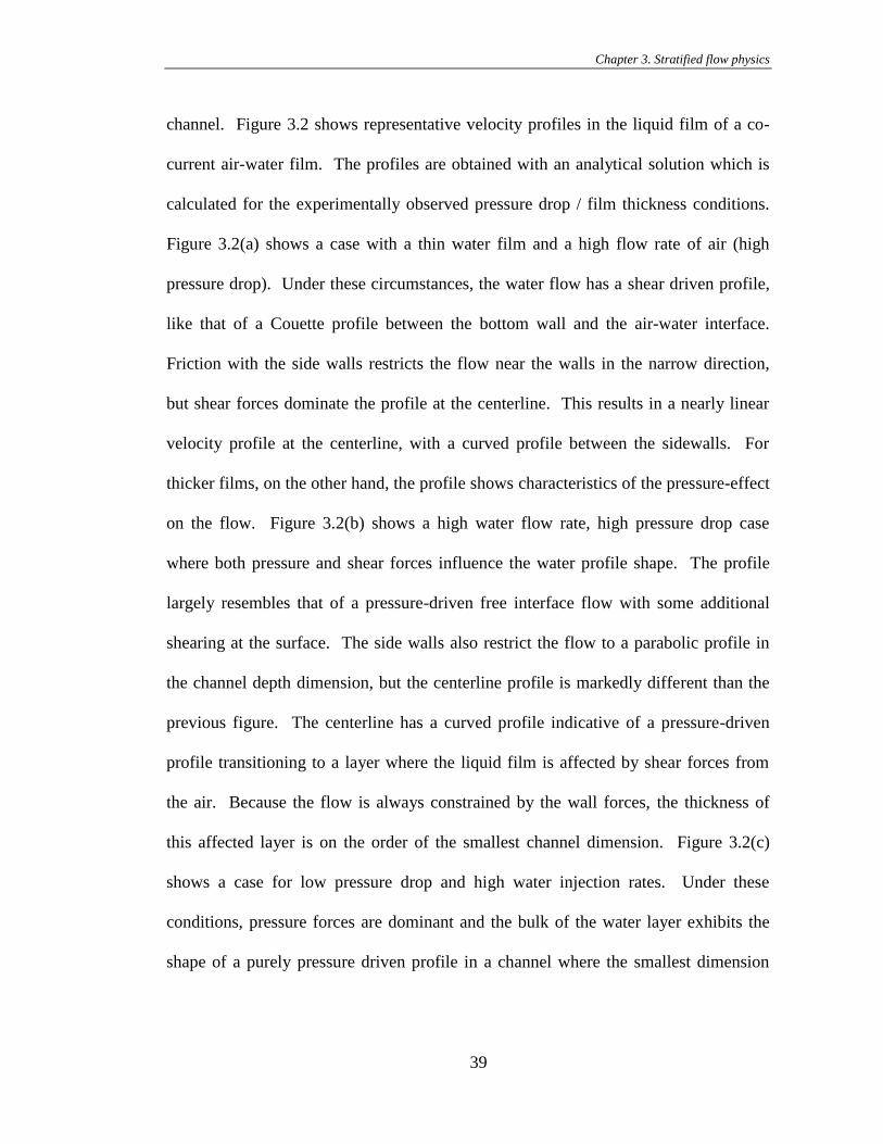
Chapter 3. Stratified flow physics
39
channel. Figure 3.2 shows representative velocity profiles in the liquid film of a co-
current air-water film. The profiles are obtained with an analytical solution which is
calculated for the experimentally observed pressure drop / film thickness conditions.
Figure 3.2(a) shows a case with a thin water film and a high flow rate of air (high
pressure drop). Under these circumstances, the water flow has a shear driven profile,
like that of a Couette profile between the bottom wall and the air-water interface.
Friction with the side walls restricts the flow near the walls in the narrow direction,
but shear forces dominate the profile at the centerline. This results in a nearly linear
velocity profile at the centerline, with a curved profile between the sidewalls. For
thicker films, on the other hand, the profile shows characteristics of the pressure-effect
on the flow. Figure 3.2(b) shows a high water flow rate, high pressure drop case
where both pressure and shear forces influence the water profile shape. The profile
largely resembles that of a pressure-driven free interface flow with some additional
shearing at the surface. The side walls also restrict the flow to a parabolic profile in
the channel depth dimension, but the centerline profile is markedly different than the
previous figure. The centerline has a curved profile indicative of a pressure-driven
profile transitioning to a layer where the liquid film is affected by shear forces from
the air. Because the flow is always constrained by the wall forces, the thickness of
this affected layer is on the order of the smallest channel dimension. Figure 3.2(c)
shows a case for low pressure drop and high water injection rates. Under these
conditions, pressure forces are dominant and the bulk of the water layer exhibits the
shape of a purely pressure driven profile in a channel where the smallest dimension
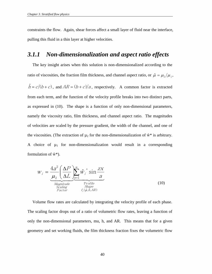
Chapter 3. Stratified flow physics
40
constraints the flow. Again, shear forces affect a small layer of fluid near the interface,
pulling this fluid in a thin layer at higher velocities.
3.1.1 Non-dimensionalization and aspect ratio effects
The key insight arises when this solution is non-dimensionalized according to the
ratio of viscosities, the fraction film thickness, and channel aspect ratio, or 12ˆ mmm ,
)(ˆ cbch , and acbAR )( , respectively. A common factor is extracted
from each term, and the function of the velocity profile breaks into two distinct parts,
as expressed in (10). The shape is a function of only non-dimensional parameters,
namely the viscosity ratio, film thickness, and channel aspect ratio. The magnitudes
of velocities are scaled by the pressure gradient, the width of the channel, and one of
the viscosities. (The extraction of µ2 for the non-dimensionalization of ŵ* is arbitrary.
A choice of µ1 for non-dimensionalization would result in a corresponding
formulation of ŵ*).
(10)
Volume flow rates are calculated by integrating the velocity profile of each phase.
The scaling factor drops out of a ratio of volumetric flow rates, leaving a function of
only the non-dimensional parameters, mu, h, and AR. This means that for a given
geometry and set working fluids, the film thickness fraction fixes the volumetric flow
),ˆ,ˆ(
Pr
1
*
2
2
sinˆ4
ARhfShape
ofile
ni
FactorScaling
Magnitude
i
i
a
zxw
L
Paw
m
m
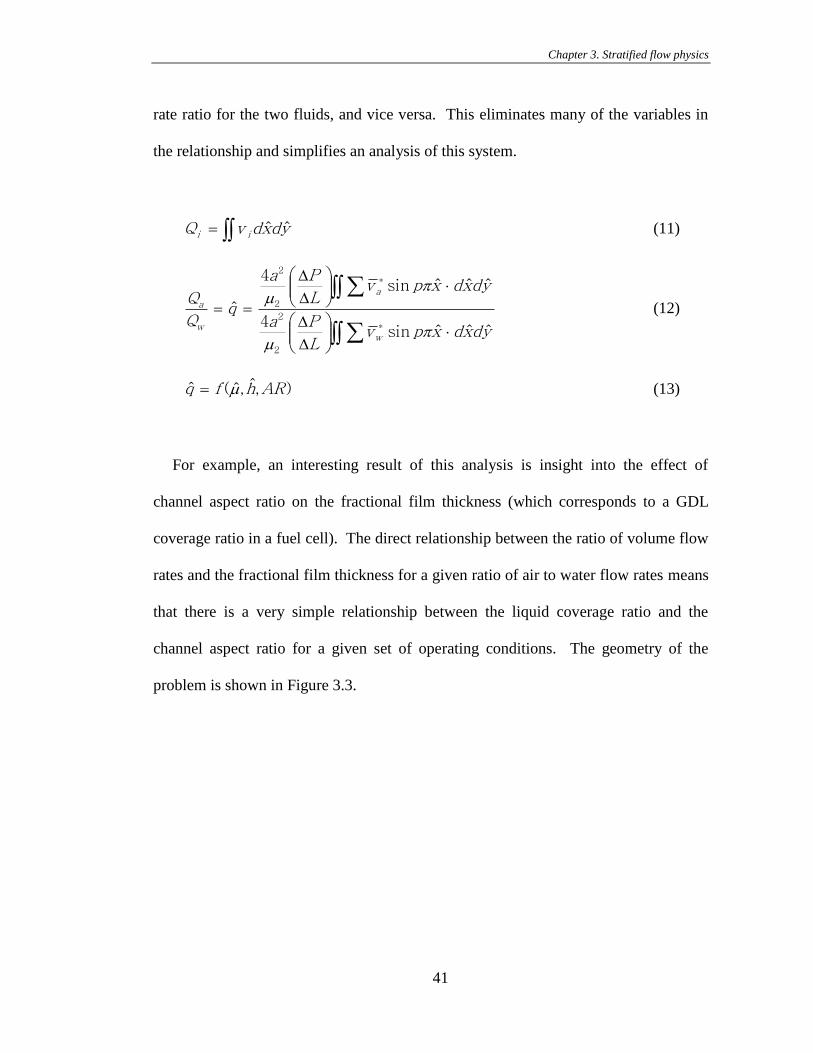
Chapter 3. Stratified flow physics
41
rate ratio for the two fluids, and vice versa. This eliminates many of the variables in
the relationship and simplifies an analysis of this system.
ydxdvQ ii ˆˆ (11)
ydxdxpvL
Pa
ydxdxpvL
Pa
Q
w
a
w
a
ˆˆˆsin4
ˆˆˆsin4
ˆ*
2
2
*
2
2
m
m
(12)
),̂,ˆ(ˆ ARhfq m (13)
For example, an interesting result of this analysis is insight into the effect of
channel aspect ratio on the fractional film thickness (which corresponds to a GDL
coverage ratio in a fuel cell). The direct relationship between the ratio of volume flow
rates and the fractional film thickness for a given ratio of air to water flow rates means
that there is a very simple relationship between the liquid coverage ratio and the
channel aspect ratio for a given set of operating conditions. The geometry of the
problem is shown in Figure 3.3.
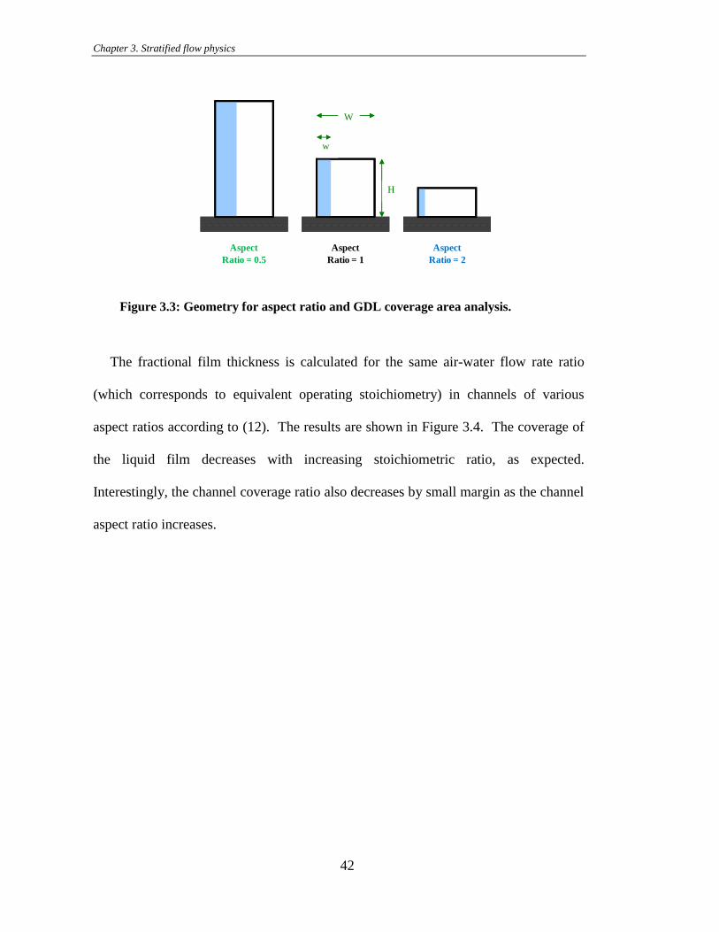
Chapter 3. Stratified flow physics
42
Figure 3.3: Geometry for aspect ratio and GDL coverage area analysis.
The fractional film thickness is calculated for the same air-water flow rate ratio
(which corresponds to equivalent operating stoichiometry) in channels of various
aspect ratios according to (12). The results are shown in Figure 3.4. The coverage of
the liquid film decreases with increasing stoichiometric ratio, as expected.
Interestingly, the channel coverage ratio also decreases by small margin as the channel
aspect ratio increases.
H
w
W
H
w
W
Aspect
Ratio = 0.5
Aspect
Ratio = 1
Aspect
Ratio = 2
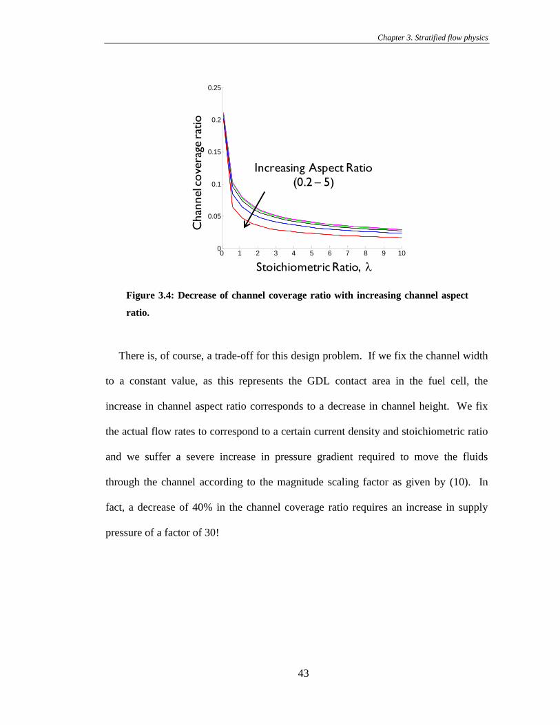
Chapter 3. Stratified flow physics
43
Figure 3.4: Decrease of channel coverage ratio with increasing channel aspect
ratio.
There is, of course, a trade-off for this design problem. If we fix the channel width
to a constant value, as this represents the GDL contact area in the fuel cell, the
increase in channel aspect ratio corresponds to a decrease in channel height. We fix
the actual flow rates to correspond to a certain current density and stoichiometric ratio
and we suffer a severe increase in pressure gradient required to move the fluids
through the channel according to the magnitude scaling factor as given by (10). In
fact, a decrease of 40% in the channel coverage ratio requires an increase in supply
pressure of a factor of 30!
0 1 2 3 4 5 6 7 8 9 100
0.05
0.1
0.15
0.2
0.25
Stoichiometric Ratio,
Channel C
overa
ge R
atio
Increasing Aspect Ratio
(0.2 – 5)
Chan
nel c
ove
rage
rat
io
Stoichiometric Ratio,
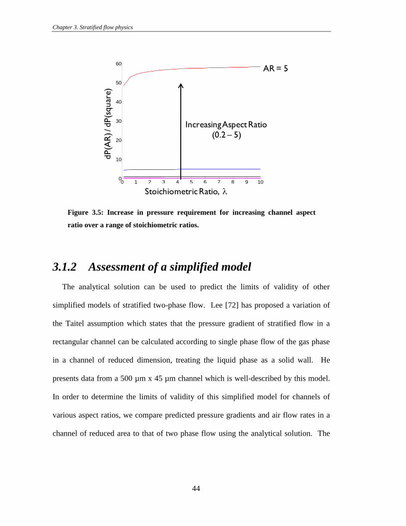
Chapter 3. Stratified flow physics
44
Figure 3.5: Increase in pressure requirement for increasing channel aspect
ratio over a range of stoichiometric ratios.
3.1.2 Assessment of a simplified model
The analytical solution can be used to predict the limits of validity of other
simplified models of stratified two-phase flow. Lee [72] has proposed a variation of
the Taitel assumption which states that the pressure gradient of stratified flow in a
rectangular channel can be calculated according to single phase flow of the gas phase
in a channel of reduced dimension, treating the liquid phase as a solid wall. He
presents data from a 500 µm x 45 µm channel which is well-described by this model.
In order to determine the limits of validity of this simplified model for channels of
various aspect ratios, we compare predicted pressure gradients and air flow rates in a
channel of reduced area to that of two phase flow using the analytical solution. The
0 1 2 3 4 5 6 7 8 9 100
10
20
30
40
50
60
Stoichiometric Ratio,
dP
* AR
/ d
P* A
R=
1dP(A
R) / dP(s
quar
e)
StoichiometricRatio,
AR = 5
Increasing Aspect Ratio
(0.2 – 5)
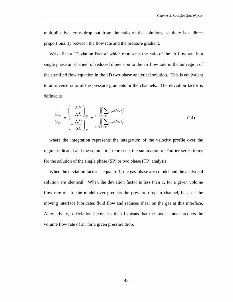
Chapter 3. Stratified flow physics
45
multiplicative terms drop out from the ratio of the solutions, so there is a direct
proportionality between the flow rate and the pressure gradient.
We define a „Deviation Factor‟ which represents the ratio of the air flow rate in a
single phase air channel of reduced dimension to the air flow rate in the air region of
the stratified flow equation in the 2D two-phase analytical solution. This is equivalent
to an inverse ratio of the pressure gradients in the channels. The deviation factor is
defined as
ˆˆ
ˆˆ
ˆ
ˆ
),(
),(
SP
TP
WhH
TP
WhH
SP
TP
SP
ydxd
ydxd
L
P
L
P
Q
Q (14)
where the integration represents the integration of the velocity profile over the
region indicated and the summation represents the summation of Fourier series terms
for the solution of the single phase (SP) or two phase (TP) analysis.
When the deviation factor is equal to 1, the gas-phase area model and the analytical
solution are identical. When the deviation factor is less than 1, for a given volume
flow rate of air, the model over predicts the pressure drop in channel, because the
moving interface lubricates fluid flow and reduces shear on the gas at this interface.
Alternatively, a deviation factor less than 1 means that the model under predicts the
volume flow rate of air for a given pressure drop.
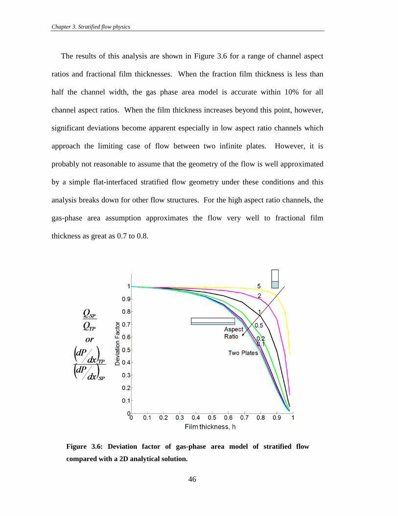
Chapter 3. Stratified flow physics
46
The results of this analysis are shown in Figure 3.6 for a range of channel aspect
ratios and fractional film thicknesses. When the fraction film thickness is less than
half the channel width, the gas phase area model is accurate within 10% for all
channel aspect ratios. When the film thickness increases beyond this point, however,
significant deviations become apparent especially in low aspect ratio channels which
approach the limiting case of flow between two infinite plates. However, it is
probably not reasonable to assume that the geometry of the flow is well approximated
by a simple flat-interfaced stratified flow geometry under these conditions and this
analysis breaks down for other flow structures. For the high aspect ratio channels, the
gas-phase area assumption approximates the flow very well to fractional film
thickness as great as 0.7 to 0.8.
Figure 3.6: Deviation factor of gas-phase area model of stratified flow
compared with a 2D analytical solution.
Chapter 3. Stratified flow physics
47
3.2 Stratified flow experiments
A fluorescence technique is developed to measure the liquid film thickness
variation of stratified flows. The water, seeded with Fluorescein dye, is imaged
through a microscope onto a CCD camera. Liquid film thickness is determined by
counting pixels with intensities above a threshold which was determined by examining
the intensity profile. Uncertainties due to setting the threshold intensity are considered.
Film thickness data is shown as a function of air and water flow rates and compared
with the predictions of a separated two-phase flow model. Significant trends in the
data which characterize the flow regime are discussed.
These data are critical for improving models for two-phase transport in PEM gas
delivery microchannels. The technique developed here provides important
information about the interactions between the gas and liquid phases in the
microchannels, a major driving force behind heat and mass transport management
within the fuel cell.
3.3 Experimental Method
3.3.1 Measurement procedure
Fluorescent images are captured at multiple water flow rates for fixed inlet air
pressures and varying exit pressures. In the U-shaped channels, the inlet pressure was
set at 15 psig and at 30 psig. The pressure drop was controlled with the outlet needle
valve configuration. For an inlet pressure of 15 psig, average inlet air velocities
Chapter 3. Stratified flow physics
48
ranging from less than 1 m/s to greater than 25 m/s were achieved. For an inlet
pressure of 30 psig, maximum air velocities approach 60 m/s. Dry, filtered air is used
for the experiments. At each exit pressure, images of the flow are captured once the
system achieves a steady condition. Between settings, the channel is evacuated of
water by opening the exit valve to the atmosphere and allowing dry air to clear the
water film. This prevents any surface tension induced hysteresis from the previous
flow configuration.
Under some stable flow conditions, fluorescent images are taken at a single
location approximately halfway between the water injection slot and the downstream
bend of the channel. At low air velocities, when large fluctuations in the film
thickness along the length of the channel were observed, multiple locations along the
length of the channel are imaged. Under high air flow rates, a downstream instability
develops in the film, causing the appearance of wisps of liquid departing from the film
into the air stream. In these cases, the film thickness is measured closer to the water
injection point where a stable film adheres to the wall.
Absolute and differential pressure and mass flow rate measurements are also
recorded at each flow condition. Pressure measurements were collected and averaged
in sets of 100 readings. Mass flow rates were measured at 12.5 Hz and averaged over
at least 30 seconds.
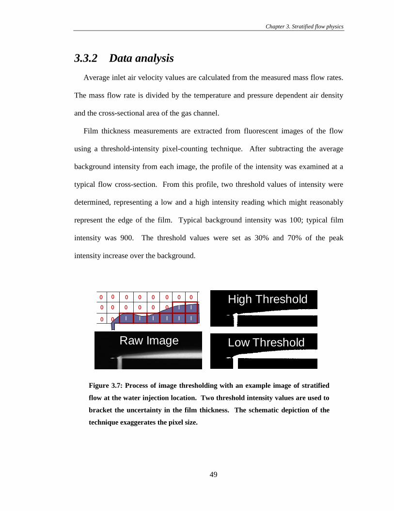
Chapter 3. Stratified flow physics
49
3.3.2 Data analysis
Average inlet air velocity values are calculated from the measured mass flow rates.
The mass flow rate is divided by the temperature and pressure dependent air density
and the cross-sectional area of the gas channel.
Film thickness measurements are extracted from fluorescent images of the flow
using a threshold-intensity pixel-counting technique. After subtracting the average
background intensity from each image, the profile of the intensity was examined at a
typical flow cross-section. From this profile, two threshold values of intensity were
determined, representing a low and a high intensity reading which might reasonably
represent the edge of the film. Typical background intensity was 100; typical film
intensity was 900. The threshold values were set as 30% and 70% of the peak
intensity increase over the background.
Figure 3.7: Process of image thresholding with an example image of stratified
flow at the water injection location. Two threshold intensity values are used to
bracket the uncertainty in the film thickness. The schematic depiction of the
technique exaggerates the pixel size.
0 0 0 0 0 0 0 0
0
0
0
0
0 0 0 0
1 1 1 1 1 1
1 1
Raw Image
High Threshold
Low Threshold
Raw Image
High Threshold
Low Threshold
Chapter 3. Stratified flow physics
50
For each threshold value, images are processed such that each pixel with intensity
greater than the threshold is assigned a binary value of 1, otherwise the pixel is
assigned a value of 0. Figure 3.7 illustrates the transformation of a raw image into
high and low threshold binary images. In this manner, the film thickness at each
cross-section of the channel is easily calculated by summing a column of pixels. The
schematic exaggerates the pixel size relative to the film thickness; in these studies,
images were collected with cross channel resolutions of 100 to 775 pixels, depending
on the camera and magnification of the objective. The particular resolution is noted
with the results for each channel configuration. The recorded film thickness averaged
over the cross section along the length of the channels.
3.3.3 Uncertainty
Velocity
The uncertainty in the velocity measurement is derived from the quoted accuracy of
the mass flow meters and channel geometries. Two mass flow meter readings were
compared: a thermal mass flow meter with a quoted accuracy of ± 3% measured value,
and a laminar pressure drop flow meter with an accuracy of ± 0.015 SLPM. Velocities
calculated from the thermal mass flow meter readings are reported with an accuracy of
± 5% MV, including uncertainties in the channel depth and air density. There is a
constant velocity offset of 1.2 m/s between the two flow meter readings.
Film Thickness
There are several sources of uncertainty in this optical measurement technique.
Less significant sources include the two-dimensional nature of the measurement which
Chapter 3. Stratified flow physics
51
yields depth-averaged fluorescence intensities that are a function of the depth of field
of the microscope objective as well as limitations of resolution due to finite pixel
dimensions. In some cases, optical effects cause unphysical variations in fluorescent
intensity near the edge of the film likely due to internal reflection by incident,
scattered, and emitted light. These fluctuations may be an obstacle when extracting
quantitative information from fluorescent intensity, but they do not significantly affect
this thresholding technique.
Uncertainty due to threshold value setting for the film becomes significant at high
air flow rate, low water flow rate cases as shown in Fig. 4. Under these conditions
there is a grey region of nearly 10 µm between the film thickness measured by high
and low threshold values. This interesting phenomenon may be due to the presence of
a meniscus or 3-dimensional shape of the fluid film, which causes regions of lower
fluorescent intensity at the top and bottom of the channel and blurs the appearance of
the interface in the two-dimensional imaging technique, which is focused near the
vertical center of the channel. Other means of capturing this flow phenomenon and
reducing this uncertainty are being investigated. The results presented in this paper
use the average of the thicknesses calculated from the two threshold values. The error
bars for this uncertainty are shown at high air velocities.
Error bars on low air velocity, large film thicknesses represent the conditions of
high water flow rate and low air flow rates creating stationery waves in the film along
the length of the channel. The magnitude of these waves varies with flow conditions.
A transition occurs for high air flow rates and stationery waves are not observed for
these thinner films.
Chapter 3. Stratified flow physics
52
3.4 Results and discussion
3.4.1 Images
Figures 3.8 and 3.9 show sample images from two of the channels where stratified
conditions are observed. Figure 3.8 shows stratified flow in 500 µm x 45 µm channels.
The imaging location is between the water injection location and the curve of the U-
shaped channel. The variation in the structure of the flow is evident from these
images, where the two images in the top row exhibit large fluctuation in the film
thickness. These images are taken in conditions where the gas flow rate is low. The
gas-phase Weber number of the top images are 3·10-4
and 0.05, while the Reynolds
numbers are 3 and 35, respectively. The low Weber numbers indicated that surface
tension is a dominant force, which is evident in the behavior of these interface. The
interfacial structures are stationary and stable over minutes of constant flow conditions.
When the water flow is stopped and restarted, the exact location of the interface
changes, but the presence of stationary waves is consistent when the flow is restarted.
The particular configuration of the initial impingement of liquid into the dry channel
appears to establish a specific interface profile. Once this interface has been
established, it seems pinned to that configuration as long as water remains in the
channel. When the air flow rate is increased beyond a certain value, the interface can
be moved and reconfigured, however the film is remarkably stable except to large
increases in gas flow, indicating that the contact line pinning is important.
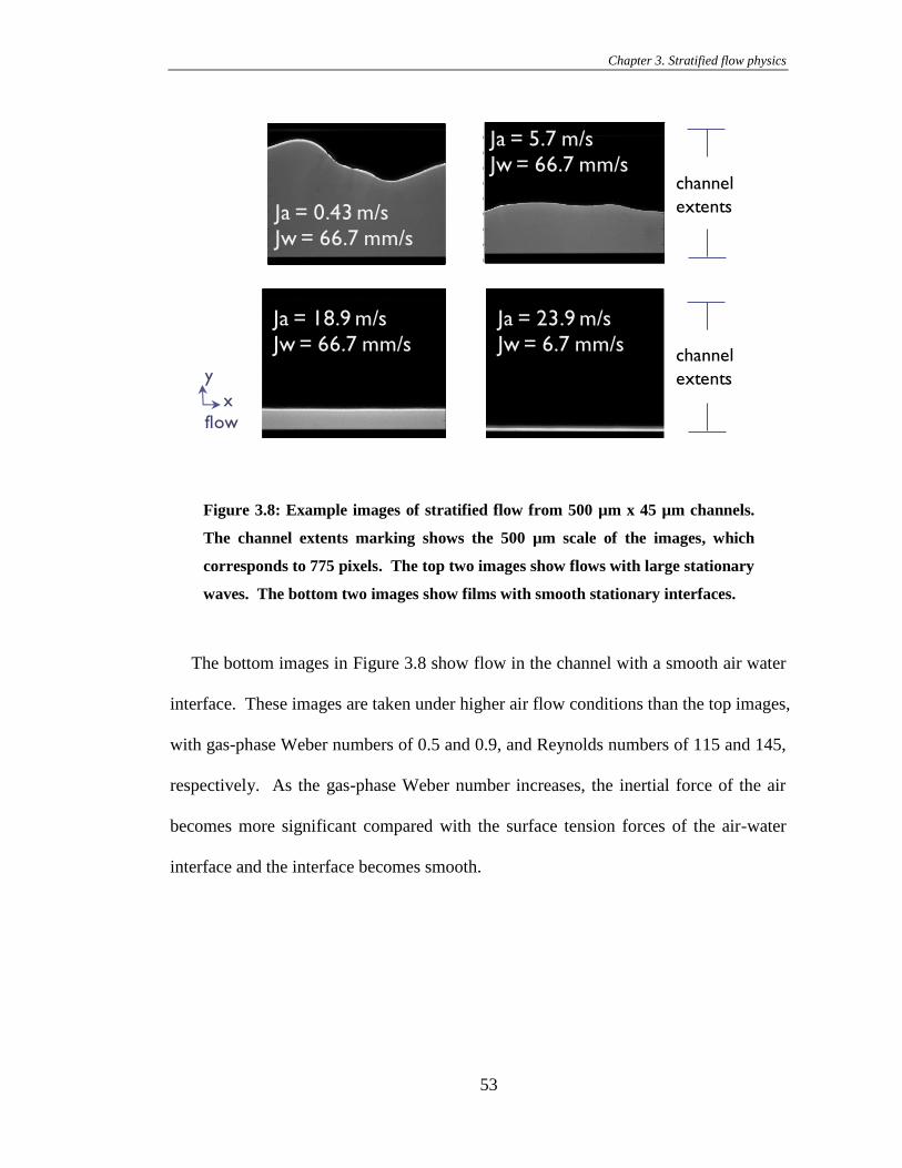
Chapter 3. Stratified flow physics
53
Figure 3.8: Example images of stratified flow from 500 µm x 45 µm channels.
The channel extents marking shows the 500 µm scale of the images, which
corresponds to 775 pixels. The top two images show flows with large stationary
waves. The bottom two images show films with smooth stationary interfaces.
The bottom images in Figure 3.8 show flow in the channel with a smooth air water
interface. These images are taken under higher air flow conditions than the top images,
with gas-phase Weber numbers of 0.5 and 0.9, and Reynolds numbers of 115 and 145,
respectively. As the gas-phase Weber number increases, the inertial force of the air
becomes more significant compared with the surface tension forces of the air-water
interface and the interface becomes smooth.
x
y
flow
channel
extents
200 400 600 800 1000 1200
100
200
300
400
500
600
700
800
900
1000
500
1000
1500
2000
2500
Ja = 0.43 m/s
Jw = 66.7 mm/s
200 400 600 800 1000 1200
100
200
300
400
500
600
700
800
900
1000
500
1000
1500
2000
2500
Ja = 5.7 m/s
Jw = 66.7 mm/s
200 400 600 800 1000 1200
100
200
300
400
500
600
700
800
900
1000
200
400
600
800
1000
1200
200 400 600 800 1000 1200
100
200
300
400
500
600
700
800
900
1000200
400
600
800
1000
1200
1400
1600
1800
Ja = 18.9 m/s
Jw = 66.7 mm/s
Ja = 23.9 m/s
Jw = 6.7 mm/schannel
extents
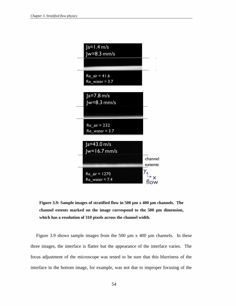
Chapter 3. Stratified flow physics
54
Figure 3.9: Sample images of stratified flow in 500 µm x 400 µm channels. The
channel extents marked on the image correspond to the 500 µm dimension,
which has a resolution of 310 pixels across the channel width.
Figure 3.9 shows sample images from the 500 µm x 400 µm channels. In these
three images, the interface is flatter but the appearance of the interface varies. The
focus adjustment of the microscope was tested to be sure that this blurriness of the
interface in the bottom image, for example, was not due to improper focusing of the
xy
flow
Ja=43.0 m/s
Re_air = 1270
Re_water = 7.4
Jw=16.7 mm/s
Ja=7.8 m/s
Re_air = 232
Re_water = 3.7
Jw=8.3 mm/s
Ja=1.4 m/s
Re_air = 41.6
Re_water = 3.7
Jw=8.3 mm/s
channel
extents
xy
flow
Ja=43.0 m/s
Re_air = 1270
Re_water = 7.4
Jw=16.7 mm/s
Ja=7.8 m/s
Re_air = 232
Re_water = 3.7
Jw=8.3 mm/s
Ja=1.4 m/s
Re_air = 41.6
Re_water = 3.7
Jw=8.3 mm/s
channel
extents
xy
flow
Ja=43.0 m/s
Re_air = 1270
Re_water = 7.4
Jw=16.7 mm/s
Ja=7.8 m/s
Re_air = 232
Re_water = 3.7
Jw=8.3 mm/s
Ja=1.4 m/s
Re_air = 41.6
Re_water = 3.7
Jw=8.3 mm/s
channel
extents
Chapter 3. Stratified flow physics
55
microscope. Instead, the variation in appearance of the interface may represent a
difference in the actual structure of the interface. The bottom image represents the
highest air flow rate tested, corresponding to a Reynolds number of 1270 for the gas
phase, so this is not expected to be an effect of turbulence of the air phase. More
detailed imaging of this interface would be helpful to understand this effect. The
Weber numbers of the flow in the 500 µm x 400 µm channels range from 0.01 to 20,
with transition to the blurry interface like that of the bottom image in Figure 19
occurring for Weber numbers greater than 2. The liquid phase Reynolds numbers of
the blurry interface conditions based on the superficial velocity and hydraulic diameter
of the channel are less than 10.
3.4.2 Film thickness measurements
The horizontal extent of the liquid film is measured according to the threshold-
intensity pixel counting technique described in Section 3.3.2. Under all experimental
conditions tested, the trend is consistent that the measured film thickness decreases
with increasing air velocity, or correspondingly, increasing pressure drop along the
channel. The variation of film thickness in a 500 µm by 45 µm channel with a
constant superficial water velocity of 67 mm/s and inlet air velocities up to 25 m/s is
shown in Figure 3.10. Two types of uncertainty bars are reported on this figure.
Those below an inlet air velocity of 11 m/s correspond to the actual peak-to-peak
variation in the film thickness measured from images taken along the channel. Those
for higher air velocities indicate the range of uncertainty associated with setting the
threshold intensity value for the film.
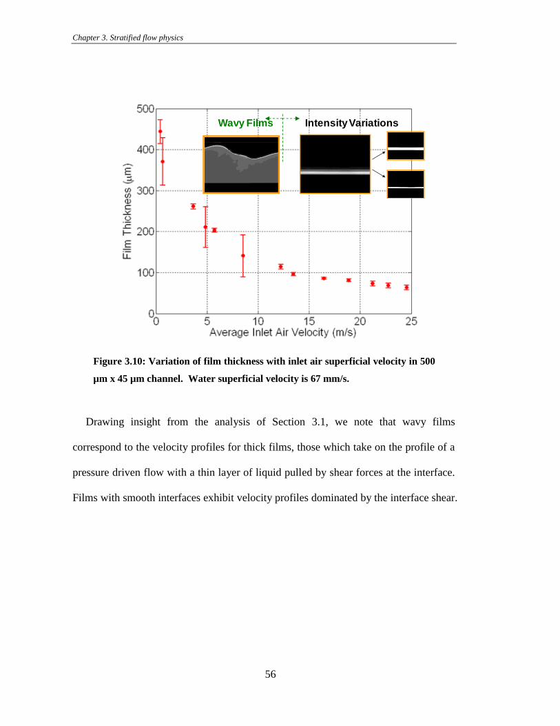
Chapter 3. Stratified flow physics
56
Figure 3.10: Variation of film thickness with inlet air superficial velocity in 500
µm x 45 µm channel. Water superficial velocity is 67 mm/s.
Drawing insight from the analysis of Section 3.1, we note that wavy films
correspond to the velocity profiles for thick films, those which take on the profile of a
pressure driven flow with a thin layer of liquid pulled by shear forces at the interface.
Films with smooth interfaces exhibit velocity profiles dominated by the interface shear.
Wavy Films Intensity Variations
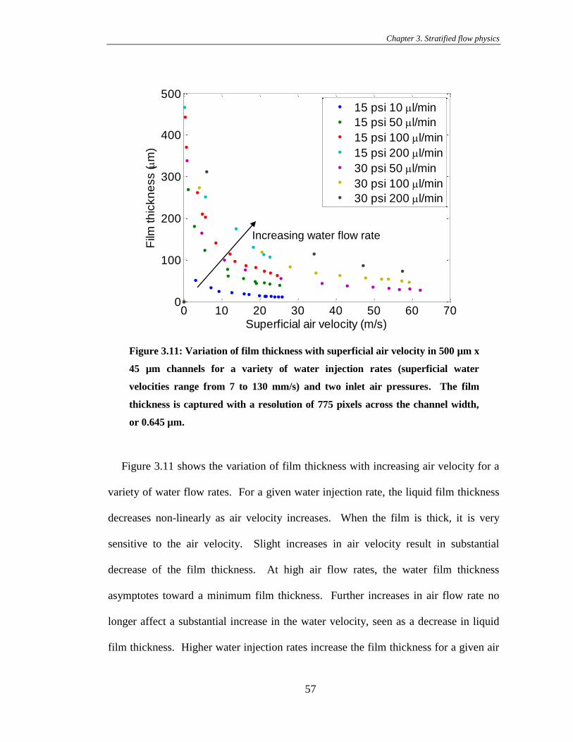
Chapter 3. Stratified flow physics
57
Figure 3.11: Variation of film thickness with superficial air velocity in 500 µm x
45 µm channels for a variety of water injection rates (superficial water
velocities range from 7 to 130 mm/s) and two inlet air pressures. The film
thickness is captured with a resolution of 775 pixels across the channel width,
or 0.645 µm.
Figure 3.11 shows the variation of film thickness with increasing air velocity for a
variety of water flow rates. For a given water injection rate, the liquid film thickness
decreases non-linearly as air velocity increases. When the film is thick, it is very
sensitive to the air velocity. Slight increases in air velocity result in substantial
decrease of the film thickness. At high air flow rates, the water film thickness
asymptotes toward a minimum film thickness. Further increases in air flow rate no
longer affect a substantial increase in the water velocity, seen as a decrease in liquid
film thickness. Higher water injection rates increase the film thickness for a given air
0 10 20 30 40 50 60 700
100
200
300
400
500
Superficial air velocity (m/s)
Film
th
ickn
ess (m
m)
15 psi 10 ml/min
15 psi 50 ml/min
15 psi 100 ml/min
15 psi 200 ml/min
30 psi 50 ml/min
30 psi 100 ml/min
30 psi 200 ml/min
Increasing water flow rate
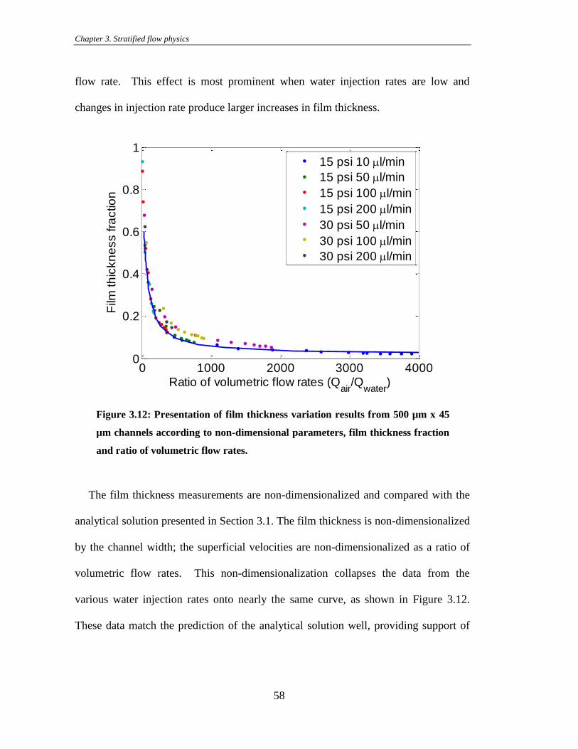
Chapter 3. Stratified flow physics
58
flow rate. This effect is most prominent when water injection rates are low and
changes in injection rate produce larger increases in film thickness.
Figure 3.12: Presentation of film thickness variation results from 500 µm x 45
µm channels according to non-dimensional parameters, film thickness fraction
and ratio of volumetric flow rates.
The film thickness measurements are non-dimensionalized and compared with the
analytical solution presented in Section 3.1. The film thickness is non-dimensionalized
by the channel width; the superficial velocities are non-dimensionalized as a ratio of
volumetric flow rates. This non-dimensionalization collapses the data from the
various water injection rates onto nearly the same curve, as shown in Figure 3.12.
These data match the prediction of the analytical solution well, providing support of
0 1000 2000 3000 40000
0.2
0.4
0.6
0.8
1
Ratio of volumetric flow rates (Qair
/Qwater
)
Film
th
ickn
ess fra
ctio
n
15 psi 10 ml/min
15 psi 50 ml/min
15 psi 100 ml/min
15 psi 200 ml/min
30 psi 50 ml/min
30 psi 100 ml/min
30 psi 200 ml/min
Chapter 3. Stratified flow physics
59
the assumptions of the analytical solution to describe stratified air-water flow in these
high-aspect ratio channels.
The non-dimensional film thickness data are shown in Figure 3.13 and Figure 3.14
for stratified flow in the more square channels, the 430 µm x 240 µm channel and the
500 µm x 400 µm channel. These data are plotted on log-linear axes for clarity. Here,
the two types of uncertainty that have been discussed previously are plotted for each
data point. The lighter lines represent the actual thickness variation measured in the
images recorded along the length of the channel. The dark blue lines correspond to
the variations in setting the threshold intensity for the thickness.
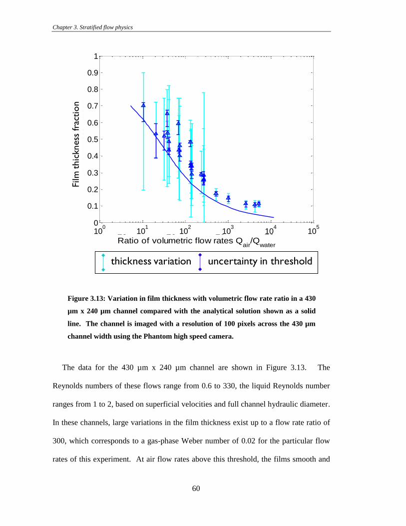
Chapter 3. Stratified flow physics
60
Figure 3.13: Variation in film thickness with volumetric flow rate ratio in a 430
µm x 240 µm channel compared with the analytical solution shown as a solid
line. The channel is imaged with a resolution of 100 pixels across the 430 µm
channel width using the Phantom high speed camera.
The data for the 430 µm x 240 µm channel are shown in Figure 3.13. The
Reynolds numbers of these flows range from 0.6 to 330, the liquid Reynolds number
ranges from 1 to 2, based on superficial velocities and full channel hydraulic diameter.
In these channels, large variations in the film thickness exist up to a flow rate ratio of
300, which corresponds to a gas-phase Weber number of 0.02 for the particular flow
rates of this experiment. At air flow rates above this threshold, the films smooth and
100
101
102
103
104
105
0
0.1
0.2
0.3
0.4
0.5
0.6
0.7
0.8
0.9
1430 x 240 channels
Ratio of volumetric flow rates Qair
/Qwater
Film
thic
kness fra
ction
thickness variation uncertainty in threshold
100
101
102
103
104
105
0
0.1
0.2
0.3
0.4
0.5
0.6
0.7
0.8
0.9
1430 x 240 channels
Ratio of volumetric flow rates Qair
/Qwater
Film
thic
kness
fra
ctio
n
Film
thic
kness
fra
ctio
n
Chapter 3. Stratified flow physics
61
the variation in the actual film thickness is comparable to the uncertainty due to the
intensity threshold. The data nearly collapse to a single curve, though there is more
scatter among the data at lower flow rate ratios which corresponds to the conditions
where the film thickness changes most rapidly with changes in air flow rate.
The data follow the trend predicted by the analytical solution as shown by the solid
line on Figure 3.13, yet the solution slightly under predicts the measured film
thicknesses. This effect is likely due to curvature of the interface which increases the
apparent film thickness due to the presence of a meniscus of water on the glass and
channel surfaces. The analysis and integration of the velocity profiles assume that the
interface between the phases is flat. This imposes both a minimum surface for
interaction of the air and water phases, it also maximizes the liquid volume for a given
film thickness at the wall (assuming this is the point of largest film thickness). If the
effect of the meniscus is not captured in the interface, the measurements will
overestimate the actual film thickness when interfacial curvature is considered.
Figure 3.14 shows the data for the largest channels in this study, which are nearly
square, measuring 500 µm wide x 400 µm deep. Stratified flow appears in these
channels under all conditions tested. Note that the scale on this figure is expanded in
the vertical direction compared with the previous channels. Because a flow rate ratio
lower than 60 was not achieved in these channels, the films never grow thicker than 30%
of the channel width. The large variations in film thickness that characterized the flow
for low flow rate ratios in high aspect ratio channels were not observed in these
channels under the tested conditions. This may be due to a lack of data at lower flow
rate ratios. One noted change in the structure of the liquid film was a blurring of the
Chapter 3. Stratified flow physics
62
film at flow rate ratios greater than 4000. At this point, the film appearance changes
from similar to that of the middle image in Figure 3.9 to similar to the bottom image in
the same figure. At this point, the measured film thickness increases, an artifact of the
extent of the blurred image of the film. This blurring did not improve with an
adjustment of the microscope focus; rather it seems to be an indication of some change
in the structure or imageability of the film due to interference of the channel walls, for
example.
With the exception of the points taken from measurements of the blurred interfaces,
the data in the 500 µm x 400 µm channels follows the general trend of the analytical
solution, with more scatter in the data than seen in the 500 µm x 45 µm case. The data
appears slightly bifurcated, with some data following the analytical solution closely,
but another set of data points from each water injection condition having larger film
thicknesses than predicted by the analytical solution. Following the argument
presented for the 430 µm x 240 µm case, this could be an artifact of the curvature of
the interface, which may lead to a overestimate of the film thickness compared to a
model based on a flat interface. This brings into question the validity of the
assumption of the flat interface model for the analysis of two-phase flow in nearly
square microchannels. Nevertheless, the trend is similar and the results match
reasonably well for the conditions tested, confirming that the analytical solution
presented is a reasonable approximation of these flows.
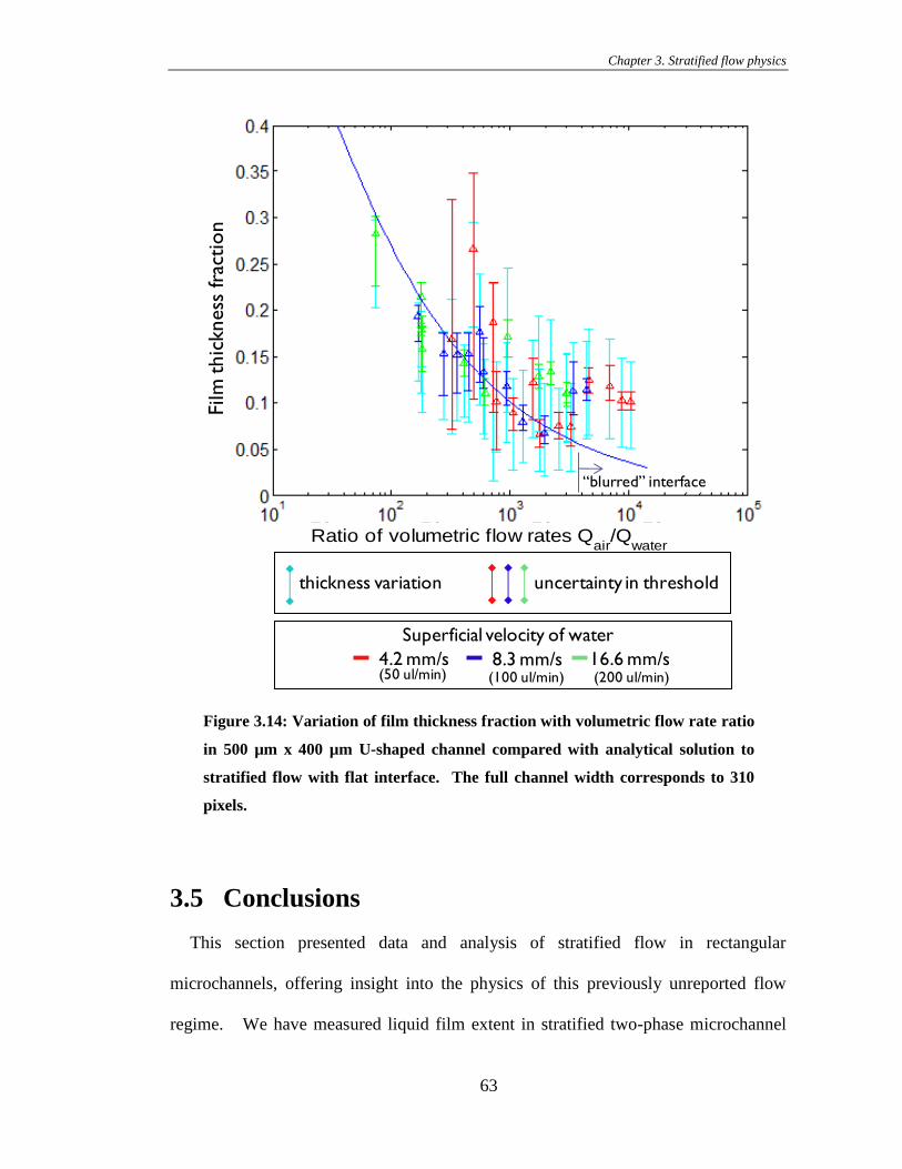
Chapter 3. Stratified flow physics
63
Figure 3.14: Variation of film thickness fraction with volumetric flow rate ratio
in 500 µm x 400 µm U-shaped channel compared with analytical solution to
stratified flow with flat interface. The full channel width corresponds to 310
pixels.
3.5 Conclusions
This section presented data and analysis of stratified flow in rectangular
microchannels, offering insight into the physics of this previously unreported flow
regime. We have measured liquid film extent in stratified two-phase microchannel
thickness variation uncertainty in threshold
Superficial velocity of water
4.2 mm/s 8.3 mm/s 16.6 mm/s(50 ul/min) (100 ul/min) (200 ul/min)
100
101
102
103
104
105
0
0.1
0.2
0.3
0.4
0.5
0.6
0.7
0.8
0.9
1430 x 240 channels
Ratio of volumetric flow rates Qair
/Qwater
Film
thic
kness
fra
ctio
n
Film
thic
kness
fra
ctio
n
“blurred” interface
Chapter 3. Stratified flow physics
64
flows for the purpose of characterizing flow regime parameters and transitions. Film
thickness data vary strongly with air velocity and are consistent with a stratified flow
model which was also presented. This information was used to verify model
predictions of the two-phase flow and validate the limits of applicability of this
simplified model.
65
Chapter 4. Two-phase flow visualization
in an ex-situ PEM fuel cell channel
In order to examine two-phase flow in a microchannel more closely replicating the
geometry and materials of a fuel cell, an ex-situ setup was constructed for the
visualization of the evolution of flow regimes along a long, serpentine microchannel
with distributed water injection through a carbon paper wall [83 84]. The present
work bridges the gap between in-situ experiments on operating fuel cells and two-
phase flow experiments in different geometries. Liquid water is introduced into the
channel through the porous carbon paper gas diffusion layer which flanks one channel
wall, thereby allowing for the characterization of flow regime transitions with known
flow rates. Unlike visualization of operating fuel cells, this setup allows for precise
control of both liquid and gas flow rates and injection conditions. Compared with
other ex-situ experiments, this study incorporates channels with smaller cross-
sectional dimensions than many previous fuel cell related studies. Compared with
fundamental two-phase flow studies in microchannels, this study better replicates the
characteristics of fuel cell channels, including longer channel lengths and distributed
water introduction. The channel dimensions of 500 µm x 500 µm square channels
Chapter 4. Two-phase flow visualization in an ex-situ PEM fuel cell channel
66
were chosen as a trade-off between the projected performance improvements of
microchannels and expected issues with flooding and clogging in small channels.
Understanding the flow regimes in these channels, which are smaller in dimension and
cross-sectional area than standard fuel cell channels, provides insight into the possible
use of microchannels for fuel cell applications. The smaller separation between
channel walls means that a larger percentage of the droplets entering the channel will
come in contact with a channel wall, potentially leading to more favorable flow
regimes at the expense of larger viscous losses. This study provides insight to key
two-phase flow structure transitions of importance for performance-critical water
management in PEM fuel cell channels.
4.1 Experimental method
4.1.1 Sample geometry and preparation
A single serpentine channel replicates flow conditions associated with fuel cell gas
delivery channels as shown in Figure 4.1. A channel with a 500 µm x 500 µm square
cross-section is machined in acrylic. The channel follows a 60-cm long serpentine
layout incorporating five long segments and four short turns. The fourth wall of the
channel is comprised of a 2 mm wide, 190 µm thick ribbon of porous carbon paper
GDL which follows the channel geometry and fits into a latex gasket which is
carefully patterned using a CO2 laser ablator. The GDL paper is pressed against the
channel structure with an acrylic slab using 44 evenly spaced bolts for even
distribution of pressure. Water is injected into the channel at eight locations using a
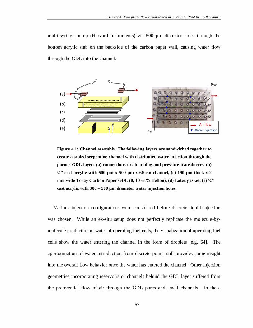
Chapter 4. Two-phase flow visualization in an ex-situ PEM fuel cell channel
67
multi-syringe pump (Harvard Instruments) via 500 µm diameter holes through the
bottom acrylic slab on the backside of the carbon paper wall, causing water flow
through the GDL into the channel.
Figure 4.1: Channel assembly. The following layers are sandwiched together to
create a sealed serpentine channel with distributed water injection through the
porous GDL layer: (a) connections to air tubing and pressure transducers, (b)
¼” cast acrylic with 500 µm x 500 µm x 60 cm channel, (c) 190 µm thick x 2
mm wide Toray Carbon Paper GDL (0, 10 wt% Teflon), (d) Latex gasket, (e) ¼”
cast acrylic with 300 – 500 µm diameter water injection holes.
Various injection configurations were considered before discrete liquid injection
was chosen. While an ex-situ setup does not perfectly replicate the molecule-by-
molecule production of water of operating fuel cells, the visualization of operating fuel
cells show the water entering the channel in the form of droplets [e.g. 64]. The
approximation of water introduction from discrete points still provides some insight
into the overall flow behavior once the water has entered the channel. Other injection
geometries incorporating reservoirs or channels behind the GDL layer suffered from
the preferential flow of air through the GDL pores and small channels. In these
(a)
(b)
(c)
(d)
Pout
Pin
Air flow
Water Injection(e)
Chapter 4. Two-phase flow visualization in an ex-situ PEM fuel cell channel
68
geometries, liquid water cannot be made to completely fill injection reservoirs when a
pressure gradient is applied across the device; air is unavoidably entrained into these
cavities and flows through the channels and the injection reservoirs in parallel.
Consequently, liquid injection was very unevenly distributed and local conditions
were difficult to characterize. Compared with reservoir or channel injection, the
discrete injection scheme provides control of the local water flow rate and facilitates
observation of changes in the flow structure as more water is introduced as the two-
phase flow progresses downstream. The channels were carefully polished with plastic
polishing compound (Novus). In order to examine the influence of corners on the
flow regime transitions, samples with 11 cm long straight channels are also
constructed. These channels are similarly milled in acrylic, with eight water injection
locations evenly spaced along the length.
Toray GDL papers (TGPH-090) with and without impregnation with a 10 wt%
Teflon solution are used in order to examine the effect of GDL hydrophobicity on the
flow observed in the channels. Toray GDL paper is a commercially available material
commonly used in fuel cell manufacture. The specific formula for hydrophobic
coatings is proprietary and varies significantly from manufacturer to manufacturer.
The use of this teflonated GDL is intended to provide qualitative evidence of the
influence of hydrophobicity of the porous material on the flow in the channels.
4.1.2 Procedure
Figure 4.2 shows the experimental setup delivering air and water to the channel
structure. Air and water flow rates are chosen according to the operating conditions of
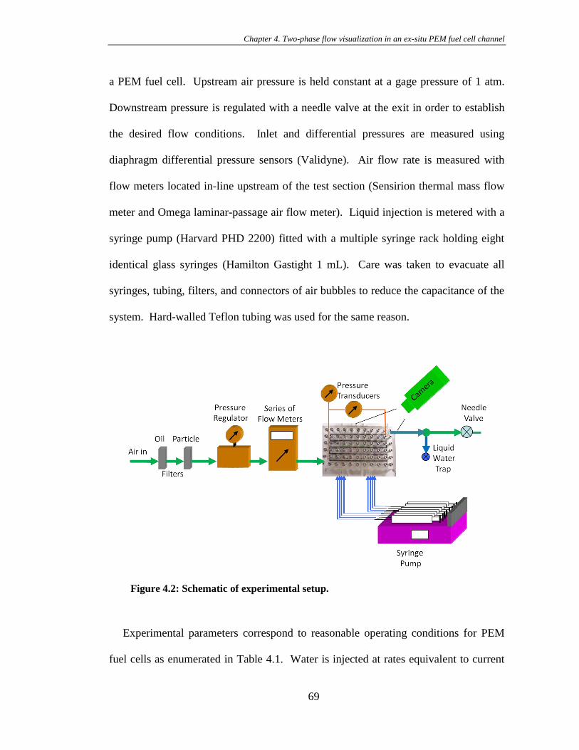
Chapter 4. Two-phase flow visualization in an ex-situ PEM fuel cell channel
69
a PEM fuel cell. Upstream air pressure is held constant at a gage pressure of 1 atm.
Downstream pressure is regulated with a needle valve at the exit in order to establish
the desired flow conditions. Inlet and differential pressures are measured using
diaphragm differential pressure sensors (Validyne). Air flow rate is measured with
flow meters located in-line upstream of the test section (Sensirion thermal mass flow
meter and Omega laminar-passage air flow meter). Liquid injection is metered with a
syringe pump (Harvard PHD 2200) fitted with a multiple syringe rack holding eight
identical glass syringes (Hamilton Gastight 1 mL). Care was taken to evacuate all
syringes, tubing, filters, and connectors of air bubbles to reduce the capacitance of the
system. Hard-walled Teflon tubing was used for the same reason.
Figure 4.2: Schematic of experimental setup.
Experimental parameters correspond to reasonable operating conditions for PEM
fuel cells as enumerated in Table 4.1. Water is injected at rates equivalent to current
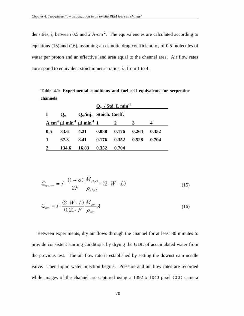
Chapter 4. Two-phase flow visualization in an ex-situ PEM fuel cell channel
70
densities, i, between 0.5 and 2 A-cm-2
. The equivalencies are calculated according to
equations (15) and (16), assuming an osmotic drag coefficient, , of 0.5 molecules of
water per proton and an effective land area equal to the channel area. Air flow rates
correspond to equivalent stoichiometric ratios, , from 1 to 4.
Table 4.1: Experimental conditions and fuel cell equivalents for serpentine
channels
Qa / Std. L min-1
I Qw Qw/inj. Stoich. Coeff.
A cm-2
ml min-1
ml min-1
1 2 3 4
0.5 33.6 4.21 0.088 0.176 0.264 0.352
1 67.3 8.41 0.176 0.352 0.528 0.704
2 134.6 16.83 0.352 0.704
)2(2
)1(
2
2 LWM
FiQ
OH
OH
water
(15)
air
airair
M
F
LWiQ
21.0
)2( (16)
Between experiments, dry air flows through the channel for at least 30 minutes to
provide consistent starting conditions by drying the GDL of accumulated water from
the previous test. The air flow rate is established by setting the downstream needle
valve. Then liquid water injection begins. Pressure and air flow rates are recorded
while images of the channel are captured using a 1392 x 1040 pixel CCD camera
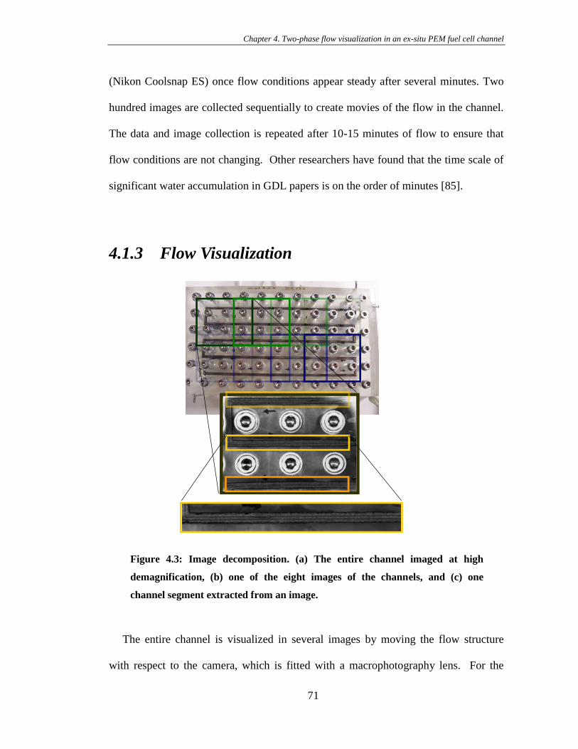
Chapter 4. Two-phase flow visualization in an ex-situ PEM fuel cell channel
71
(Nikon Coolsnap ES) once flow conditions appear steady after several minutes. Two
hundred images are collected sequentially to create movies of the flow in the channel.
The data and image collection is repeated after 10-15 minutes of flow to ensure that
flow conditions are not changing. Other researchers have found that the time scale of
significant water accumulation in GDL papers is on the order of minutes [85].
4.1.3 Flow Visualization
Figure 4.3: Image decomposition. (a) The entire channel imaged at high
demagnification, (b) one of the eight images of the channels, and (c) one
channel segment extracted from an image.
The entire channel is visualized in several images by moving the flow structure
with respect to the camera, which is fitted with a macrophotography lens. For the
Chapter 4. Two-phase flow visualization in an ex-situ PEM fuel cell channel
72
serpentine channels, eight separate sets of images are collected. Images are
decomposed into channel segments, as illustrated in Figure 4.3, in order to examine
the flow as it progresses along the length of the channel.
For analysis of the flow regimes, the flow structure in each channel segment was
examined and categorized. Figure 4.4 shows representative images of the flow
structures that were observed in the channels. Stratified flow is steady and the
position of the interface does not vary with time for given operating conditions, while
plug and slug flow show transient variation of the air-liquid-solid interfaces. Wavy
flow has a constant liquid-solid interface at the channel wall, but a varying liquid-gas
interface. For fluidic analysis, local air and water flow rates are calculated along the
channel based on the inlet air flow rate and the total quantity of water injected
upstream of the imaging location, such that at one test condition, there is a single air
flow rate but eight local water flow rates due to the eight water injection locations.
Figure 4.4: Representative images of two-phase flow structures: slug, plug,
stratified.
Slug
Plug
Stratified
GDL
Channel
Slug
Plug
Stratified
GDL
Channel
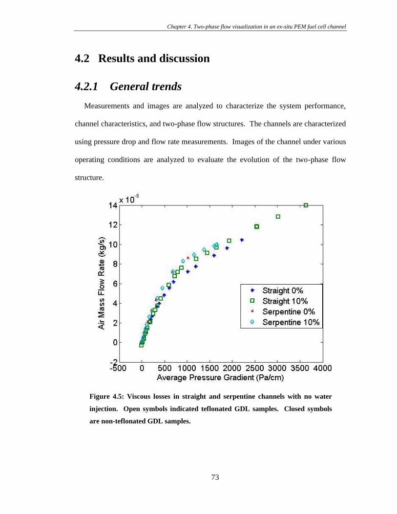
Chapter 4. Two-phase flow visualization in an ex-situ PEM fuel cell channel
73
4.2 Results and discussion
4.2.1 General trends
Measurements and images are analyzed to characterize the system performance,
channel characteristics, and two-phase flow structures. The channels are characterized
using pressure drop and flow rate measurements. Images of the channel under various
operating conditions are analyzed to evaluate the evolution of the two-phase flow
structure.
Figure 4.5: Viscous losses in straight and serpentine channels with no water
injection. Open symbols indicated teflonated GDL samples. Closed symbols
are non-teflonated GDL samples.
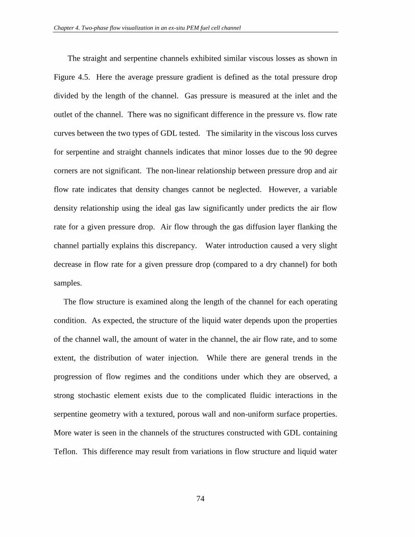
Chapter 4. Two-phase flow visualization in an ex-situ PEM fuel cell channel
74
The straight and serpentine channels exhibited similar viscous losses as shown in
Figure 4.5. Here the average pressure gradient is defined as the total pressure drop
divided by the length of the channel. Gas pressure is measured at the inlet and the
outlet of the channel. There was no significant difference in the pressure vs. flow rate
curves between the two types of GDL tested. The similarity in the viscous loss curves
for serpentine and straight channels indicates that minor losses due to the 90 degree
corners are not significant. The non-linear relationship between pressure drop and air
flow rate indicates that density changes cannot be neglected. However, a variable
density relationship using the ideal gas law significantly under predicts the air flow
rate for a given pressure drop. Air flow through the gas diffusion layer flanking the
channel partially explains this discrepancy. Water introduction caused a very slight
decrease in flow rate for a given pressure drop (compared to a dry channel) for both
samples.
The flow structure is examined along the length of the channel for each operating
condition. As expected, the structure of the liquid water depends upon the properties
of the channel wall, the amount of water in the channel, the air flow rate, and to some
extent, the distribution of water injection. While there are general trends in the
progression of flow regimes and the conditions under which they are observed, a
strong stochastic element exists due to the complicated fluidic interactions in the
serpentine geometry with a textured, porous wall and non-uniform surface properties.
More water is seen in the channels of the structures constructed with GDL containing
Teflon. This difference may result from variations in flow structure and liquid water
Chapter 4. Two-phase flow visualization in an ex-situ PEM fuel cell channel
75
velocity in the channels or may indicate that more liquid water flows through the
hydrophilic GDL so that less water is forced into the channels.
Figure 4.6: Observed flow structures and general evolution of flow regimes.
Figure 4.6 provides a qualitative overview of flow structure observations according
to air and liquid flow conditions. The horizontal axis corresponds to a progression
along the channel and a corresponding increase in local water flow rate as additional
liquid injection locations are encountered. The upper and lower branches represent
flow structures occurring under relatively higher and lower air flow conditions. Black
arrows between images represent common transitions between flow regimes as more
liquid is encountered in the channel. The dry channel transitions to intermittent flow,
a regime where water moves through the channel in discrete packets droplets, slugs, or
Chapter 4. Two-phase flow visualization in an ex-situ PEM fuel cell channel
76
plugs. Intermittent flow becomes wavy flow when the water travels down the channel
as an abrupt thickening of a liquid film on the side walls of the channel. Finally, a
stratified flow ensues when the sidewall film becomes steady and no significant
oscillations are observed at the interface. Stratified flow exists most commonly at the
furthest downstream locations, while slug/plug flow is rarely observed downstream of
the first several injection locations.
These trends suggest that stratified flow is hydrodynamically preferred to
intermittent flow regimes, provided there is enough liquid flowing in the channel to
maintain such a film. When a slug or plug travels, the three-phase interface moves so
surface tension forces must be overcome. Once the liquid forms a film along a
channel wall, this force is eliminated in the flow direction and the gas-liquid surface
area is minimized. The water is propelled by the pressure gradient in the channel and
shear forces from the air. A liquid film provides the most efficient means of water
evacuation from the channels.
One of the most common transitions is a change in structure of stratified flow from
occurrence on two channel walls to occurrence on a single wall. Several conditions
facilitate this transition, including the presence of liquid resting on the GDL surface, a
water injection point which also wets the GDL, or a corner. These liquid bridges may
form where local variations in the surface properties of the GDL favor the
accumulation of water. Figure 4.7 shows two such transition points, in a straight
channel at an injection point and at a corner.
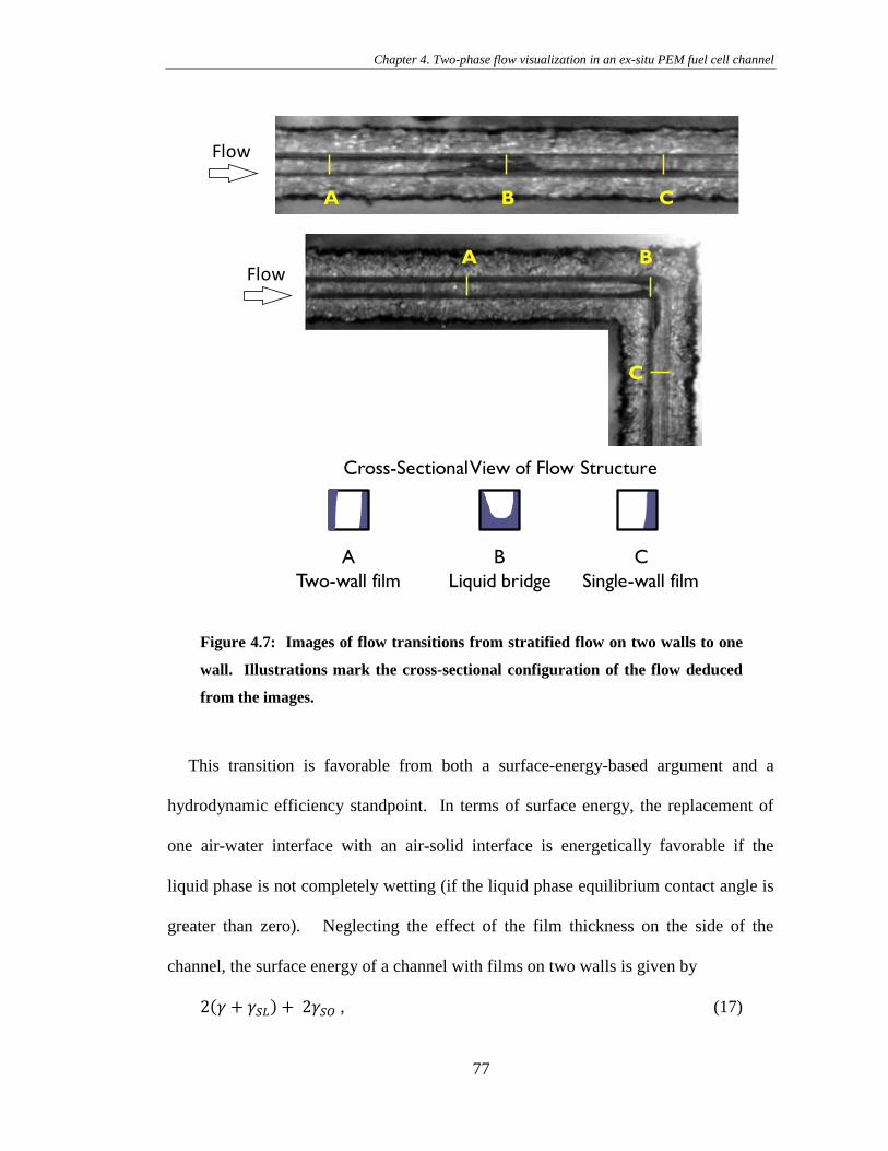
Chapter 4. Two-phase flow visualization in an ex-situ PEM fuel cell channel
77
Figure 4.7: Images of flow transitions from stratified flow on two walls to one
wall. Illustrations mark the cross-sectional configuration of the flow deduced
from the images.
This transition is favorable from both a surface-energy-based argument and a
hydrodynamic efficiency standpoint. In terms of surface energy, the replacement of
one air-water interface with an air-solid interface is energetically favorable if the
liquid phase is not completely wetting (if the liquid phase equilibrium contact angle is
greater than zero). Neglecting the effect of the film thickness on the side of the
channel, the surface energy of a channel with films on two walls is given by
, (17)
Flow
Flow
A
Two-wall film
B
Liquid bridge
C
Single-wall film
Cross-Sectional View of Flow Structure
A B C
A B
C
Chapter 4. Two-phase flow visualization in an ex-situ PEM fuel cell channel
78
while the surface energy of a channel with a film on one wall is given by
. (18)
Comparing these expressions, we find that the surface energy of a two wall stratified
flow is great than that of stratified flow in a one wall stratified flow if
(19)
or, using the definition of the equilibrium contact angle,
(20)
a condition which is satisfied for any partially non-wetting surface.
Analytical solutions to the momentum equations for simplified stratified flow in a
rectangular channel reveal there is also a hydrodynamic advantage of single-wall
stratified flow over two-walled stratified flow. The pressure gradient within a channel
of a particular dimension is determined by the ratio of flow rates of air and liquid
phases (which is proportional to the stoichiometric ratio) and scales with the absolute
magnitude of the flow rate (proportional to current density). After non-
dimensionalization, the ratio of pressure gradient to volume flow rate of air is a
function of the ratio of water to air volume flow rate (equivalent to fuel cell
stochiometry) and aspect ratio of the channel. The pressure gradient necessary to
sustain equivalent flow rates of both gas and liquid in identical square channels is
between 4 and 15% lower for stratified flow on a single-wall compared with stratified
flow on two walls.
Chapter 4. Two-phase flow visualization in an ex-situ PEM fuel cell channel
79
4.2.2 Comparison of flow conditions
There are several ways to compare the data between test conditions. A comparison
of equivalent fuel cell operating conditions is interesting for direct application to fuel
cell systems. The stoichiometric ratio fixes the ratio of air and water flow rates; an
increase in current density for a fixed value of lambda increases both the air and water
flow rates proportionally. A constant stoichiometric coefficient corresponds to a line
with unity slope on a standard flow regime map with superficial velocities of gas and
liquid on the x- and y- axes, respectively.
For channels with teflonated GDL, for a given current density, as the stoichiometric
ratio (or air flow rate) increases, the transition from intermittent flow to films occurs
later in the channel. As current density increases for equivalent stoichiometric ratios,
the transition point occurs further upstream. Alternatively, insight can be gained by
comparing equivalent fluidic conditions, where the air flow rate in the channel is held
constant, but the water flow rate varies. This simulates the common situation where
air flow rate is fixed, but local current density varies in response to the load applied to
the cell. As current density increases for equivalent air flow rates, the transition point
similarly occurs further upstream.
For non-teflonated channels, the trends are less consistent. For i = 0.5 A cm-2
and
low air flow rates, water rests in the channel as thin films and as liquid droplets/plugs
sitting on the GDL. When the air flow rate increases, slugs are observed and the
transition to a film occurs halfway through the channel. For higher water flow rates,
slugs are observed for the lower air flow rates and films are observed at high air flow
rates. Films occur at highest water flow rates. For equivalent stoichiometric ratios,
Chapter 4. Two-phase flow visualization in an ex-situ PEM fuel cell channel
80
the trend is progression from thin films with stationary plugs on the GDL, to moving
slugs, to films.
4.2.3 Variation of flow structure with flow rate
Most two-phase flow studies organize the flow regimes onto regime maps
according to the superficial gas and liquid velocities. In this study, the distributed
water introduction along the length of the channel requires that the flow regime map
consider the local flow rate of liquid after each injection location. Consequently, each
experimental condition provides information at eight aligned locations in flow rate
space. Furthermore, in this complicated geometry, flow structures often change
spatially between injection points, such that a single experimental condition may result
in multiple flow regimes for a particular air and local water flow rate, depicted as
overlapping points on the regime map. Figure 4.8 shows observed flow regimes
plotted against local air and water flow rates. The local water flow rate at a given
position is the product of the number of liquid injection points upstream from the
imaging location and the rate of water introduction per injection point. The
volumetric air flow rate is determined from the inlet mass flow rate and pressure.
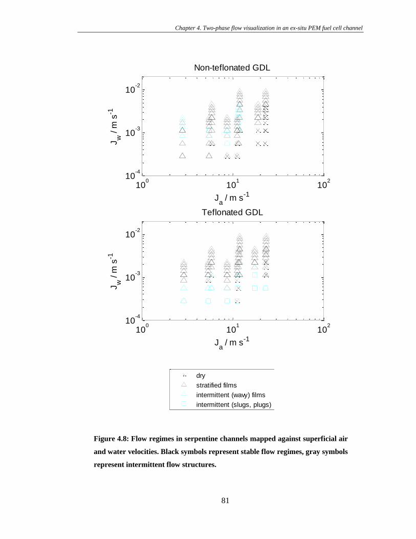
Chapter 4. Two-phase flow visualization in an ex-situ PEM fuel cell channel
81
Figure 4.8: Flow regimes in serpentine channels mapped against superficial air
and water velocities. Black symbols represent stable flow regimes, gray symbols
represent intermittent flow structures.
100
101
102
10-4
10-3
10-2
Ja / m s
-1
Jw
/ m
s-1
Non-teflonated GDL
100
101
102
10-4
10-3
10-2
Ja / m s
-1
Jw
/ m
s-1
Teflonated GDL
0 0.2 0.4 0.6 0.8 1 1.2 1.4 1.6 1.8 20
0.5
1
1.5
2
2.5
3
dry
stratified films
intermittent (wavy) films
intermittent (slugs, plugs)
Chapter 4. Two-phase flow visualization in an ex-situ PEM fuel cell channel
82
In the samples containing Teflon, intermittent (slug and plug) flow regimes occur
for low water injection rates. This corresponds to the first several injection points
along a channel. Plug flow occurs at low air flow rates, but slugs exist at the same
flow parameters because these plugs are quickly broken into slugs as they travel down
the channel. At higher air flow rates, low liquid flow rates yield slug flow. For all air
flow rates, stratified flow is the dominant flow regime at high water flow rates.
The samples without Teflon also exhibit stratified flow at the highest liquid flow
rates as well as at the highest air flow rates. Intermittent flows are observed at
moderate liquid flow rates; plug flow occurs at only under the lowest air flow and
slugs occur at moderate air flow. Comparing the regime maps for the serpentine
samples, the intermittent regimes occur for higher water flow rates in the hydrophilic
GDL case than in the hydrophobic GDL condition. This similarity supports the
observation that more liquid water appears in the channels with Teflon coating.
Liquid water preferentially flowing through the GDL in the hydrophilic case
effectively lowers the water flow rate occurring in the channel.
4.2.4 Effect of corners on flow regime evolution
Flow rates for the straight channels were chosen with two equivalencies to the
serpentine channels: equivalent fuel cell operating parameters where flow rates are
adjusted in proportion to the reduced area of the straight channel, and equivalent
hydrodynamics where the flow rates of each phase are identical to the serpentine
channel conditions. Matching fluidic conditions in the channels provides a control to
examine the effect of the corners on the flow, while matching fuel cell conditions
Chapter 4. Two-phase flow visualization in an ex-situ PEM fuel cell channel
83
provides a better comparison for a fuel cell channel design which would include
multiple shorter channels in parallel. This section describes the results of matching
fluidic conditions. Section 4.2.5 describes the flow regimes which result from the
same current density and stoichiometry in each channel.
For matching fluidic conditions, air and water are introduced into the straight
channel at the same flow rates as for the serpentine channel, as given in Table 4.1.
(This condition corresponds to much higher current densities which would not be
practical. This particular analysis therefore relates only to the hydrodynamic effects of
the corners on the flow regimes.) The pressure drop in the channel is proportionally
smaller than that in a serpentine channel, so the average pressure gradient is
comparable for these two channels and pressure forces exerted on droplets and films in
the channels are equivalent.
Figure 4.9 is a flow regime map for the straight channel experiments. In these
channels, intermittent flow regimes were observed more often than stratified films. In
fact, stratified flow was not observed in the straight channel with teflonated GDL
under any flow conditions.
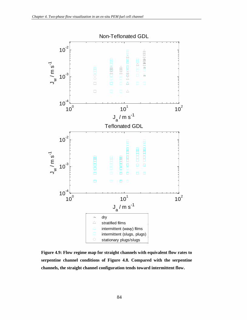
Chapter 4. Two-phase flow visualization in an ex-situ PEM fuel cell channel
84
Figure 4.9: Flow regime map for straight channels with equivalent flow rates to
serpentine channel conditions of Figure 4.8. Compared with the serpentine
channels, the straight channel configuration tends toward intermittent flow.
100
101
102
10-4
10-3
10-2
Non-Teflonated GDL
Ja / m s
-1
Jw
/ m
s-1
100
101
102
10-4
10-3
10-2
Teflonated GDL
Ja / m s
-1
Jw
/ m
s-1
0 0.2 0.4 0.6 0.8 1 1.2 1.4 1.6 1.8 20
0.5
1
1.5
2
2.5
3
3.5
4
dry
stratified films
intermittent (wavy) films
intermittent (slugs, plugs)
stationary plugs/slugs
Chapter 4. Two-phase flow visualization in an ex-situ PEM fuel cell channel
85
Interestingly, flow regime transitions do not occur at the corner in the serpentine
channel samples; however, the flow more frequently transitions to films when corners
are present. The effect of the corner, therefore, is to facilitate the formation of films.
Possible means for this effect are the build-up of water in the corners, which then
facilitates the formation of films when there would otherwise not be enough liquid to
sustain a film. When transitions occur at water injection locations, where they most
often do, there could be a build-up of water in the GDL or corners of the channel near
the injection point that creates conditions favorable to film formation. The corners
reduce the water-repellent effect of the teflonated GDL sample by creating locations
where water can accumulate and remain in the samples.
This effect is consistent, but less marked in the non-teflonated channels, where the
conditions are inherently more favorable for water retention than in the teflonated
samples. Unlike the teflonated samples, films and stationary water plugs are observed
in the more hydrophilic non-teflonated samples. Films with plugs on the GDL occur
at low air flow rates; moving slugs occur when air flow rates are increased. Finally,
films occur at the highest air flow rates. These trends are similar to those observed in
the serpentine channels, except that slugs are observed over a wider range of operating
conditions, specifically for higher air flow rates.
4.2.5 Implications for fuel cell channel design
Matching fuel cell operating conditions in a short straight channel gives insight in
the effect of length and design of multiple channels for fuel cell gas delivery channels.
In these 11 cm samples, the flow rates in the straight channels are 82% lower than
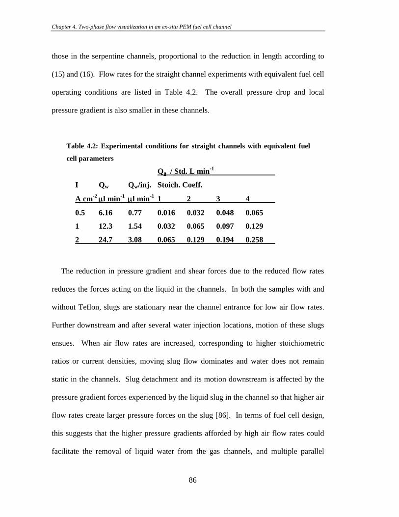
Chapter 4. Two-phase flow visualization in an ex-situ PEM fuel cell channel
86
those in the serpentine channels, proportional to the reduction in length according to
(15) and (16). Flow rates for the straight channel experiments with equivalent fuel cell
operating conditions are listed in Table 4.2. The overall pressure drop and local
pressure gradient is also smaller in these channels.
Table 4.2: Experimental conditions for straight channels with equivalent fuel
cell parameters
Qa / Std. L min-1
I Qw Qw/inj. Stoich. Coeff.
A cm-2
ml min-1
ml min-1
1 2 3 4
0.5 6.16 0.77 0.016 0.032 0.048 0.065
1 12.3 1.54 0.032 0.065 0.097 0.129
2 24.7 3.08 0.065 0.129 0.194 0.258
The reduction in pressure gradient and shear forces due to the reduced flow rates
reduces the forces acting on the liquid in the channels. In both the samples with and
without Teflon, slugs are stationary near the channel entrance for low air flow rates.
Further downstream and after several water injection locations, motion of these slugs
ensues. When air flow rates are increased, corresponding to higher stoichiometric
ratios or current densities, moving slug flow dominates and water does not remain
static in the channels. Slug detachment and its motion downstream is affected by the
pressure gradient forces experienced by the liquid slug in the channel so that higher air
flow rates create larger pressure forces on the slug [86]. In terms of fuel cell design,
this suggests that the higher pressure gradients afforded by high air flow rates could
facilitate the removal of liquid water from the gas channels, and multiple parallel
Chapter 4. Two-phase flow visualization in an ex-situ PEM fuel cell channel
87
segments which would reduce the local volumetric flow rates and overall system
pressure drop might adversely impact water removal from the channels.
Most fuel cell system designs include multiple parallel straight or serpentine gas
delivery channels. While these designs decrease the overall pressure drop for a given
flow rate of air for a specific plate area, the parallel channels are more prone to
flooding as the presence of liquid water in one channel increases flow resistance in
that channel, thereby diverting flow into other channels with relatively lower
resistances. This is similar to the instabilities documented in parallel two-phase
cooling channels, but without the effect of gas expansion during boiling.
In typical single serpentine channel designs, there is cross-talk between channels
through the continuous GDL layer [ 87 88 ]. This cross-talk reduces the overall
pressure drop in the channel and in the entire flow field. Cross-talk also creates zones
at channel corners where water is easily trapped or accumulated as flow preferentially
shortcuts the corner.
It is interesting to note that flooding of the channel is not observed under any flow
conditions during the current studies, likely due to the single channel and sealed GDL
configuration chosen for these tests. Where parallel channels provide alternative flow
paths for the fluids, this single channel configuration and its larger pressure gradients
and air velocities prevent blockage of the channels.
Chapter 4. Two-phase flow visualization in an ex-situ PEM fuel cell channel
88
4.3 Summary and conclusions
As one component of the larger water management problem in PEM fuel cells, the
design of gas delivery channels is in itself a complicated problem involving many
competing phenomena.
In this study, an experimental system was developed to study two-phase flow in
microchannels by ex-situ visualization under known liquid and gas flow rates relevant
to fuel cells in order to understand the flow conditions which favor particular flow
structures in the channel. Images of the channels were collected along the length of
the channel as the two-phase flow structure evolved. Flow structure labeling and
mapping summarizes the observed flow regimes and the conditions under which they
transition from one to another.
The geometric configuration of the channels has a significant effect on the local
flow conditions. The gas flow rates are proportional to the entire length of the channel,
while the liquid flow is “local”, introduced along the length of the channel. This
results in very different local ratios of liquid to gas flow rates depending on channel
configuration and number of parallel flow channels.
In particular, the choice of the number of parallel flow channels covering the cell
area has a marked effect on the flow conditions in those channels. The water flow in
the channel depends on length of channel and reactions occurring under the upstream
channels. The air flow rate for the cell is set based on the stoichiometry and the total
reaction which will occur in the entire flow field. Along a channel, the ratio of water
to air flow rate will vary from zero to the chosen stoichiometry along the length of the
Chapter 4. Two-phase flow visualization in an ex-situ PEM fuel cell channel
89
channel. This ratio changes more quickly in the case of multiple parallel channels
because the channel lengths are shorter.
Multiple parallel channels reduce the overall pressure drop in the system for a
given flow rate (stoichiometric ratio) or, in the case of a given pressure drop, allow
more air flow through the channels. But the flow in multiple channels suffers from
maldistribution, both inherent variations due to small geometric anomalies and
induced redistribution due to the introduction of liquid water droplets [89 90]. These
induced flow redistributions can create instabilities for the operation of the fuel cell
microchannels. Gas flow is preferentially directed to channels which are not blocked
by liquid water slugs, which can further aggravate the flow maldistribution.
Fewer parallel channels mean longer channel lengths. This allows for higher gas
velocities in the channel, improving mass transport and enabling removal of water
from the channels, but sustaining larger overall pressure drop and gas expansion in a
given channel. However, fewer channels in parallel usually necessitate more corners
as the channels serpentine to cover the reaction area. As the current study shows,
corners trap liquid water and lead to liquid accumulation and film formation in the
channels. The choice of channel configuration has a significant effect on the flow
structures which occur in the channels.
The results of the current ex-situ experiments provide insight into the effect of
channel geometry and corners on the evolution of flow structures in long
microchannels relevant to PEM fuel cell operation. It is observed that corners reduce
the water-evacuation capability of the channels and facilitate the formation of liquid
films on the walls of the channel. At the same time, water is more efficiently removed
Chapter 4. Two-phase flow visualization in an ex-situ PEM fuel cell channel
90
from the channels with the larger pressure gradient afforded by high air flow rates
through long channels, rather than shorter parallel channels which can result in
conditions prone to flooding. These results provide insight for gas delivery channels
designed to optimize the performance of PEM fuel cells.
91
Chapter 5. Insights into confocal
visualization for two-phase flow
In order to draw conclusions about the meaning of the data in the previous sections,
the analysis has had to make assumptions about the shape of the interface in the third
dimension perpendicular to the imaging plane. A three-dimensional imaging
technique has been proposed in order to visualize the shape of the interface and fully
understand the interaction of the two-phases. In this chapter, we outline the
development of a confocal imaging system for two-phase flow systems. We discuss
the possibilities and limitations of the use of this technique for the imaging of
interfaces.
5.1 Basics of Confocal Microscopy
Confocal microscopy is a technique that allows for three-dimensional imaging. It
is most often used for biological applications [91], but has also been implemented for
high-resolution particle image velocimetry (PIV) techniques in single phase
microfluidic systems and droplets [ 92 - 95 ]. Fluidic, diffusive, and thermal
Chapter 5. Insights into confocal visualization for two-phase flow
92
interactions at the interface of stratified liquid-liquid flows have been examined using
confocal techniques for two-phases with similar indices of refraction [96-99].
The principle of confocal microscopy relies on the ability of a pinhole aperture in
the illumination and detection path of an imaging setup to isolate light originating
from a single point in space, or in reality a small region called a voxel. Light
originating from any other location is rejected because it is not focused through the
pinhole. In the most basic formulation, the sample is scanned through space and a
three-dimensional image is reconstructed from the intensity of each of the voxels.
This concept was developed by Marvin Minsky in 1955 [100]. The technique is
relatively slow and time consuming because a single focal point must be scanned
through three-dimensional space with time at each location to capture enough light. A
faster variation was developed which allows one focal plane to be imaged at a time,
requiring scanning only in the axial dimension. In this implementation, the rejection
of out of plane light is achieved by an array of pinholes on a spinning disk. Figure 5.1
illustrates the principle of confocal microscopy for a scanning configuration and for a
spinning disk configuration.
There are a few disadvantages to the use of a spinning disk confocal microscopy
setup compared with a laser scanning confocal microscope [101] though some post-
processing techniques have been suggested to correct the images [102]. There is some
loss of resolution and potential for aberrations in the image due to cross-talk between
pinholes. By far, however, the biggest challenge is the rejection of light by the
pinhole disk. While the scanning system is able to focus light from the source into an
area as small as the pinhole, the illumination source for the spinning disk system must
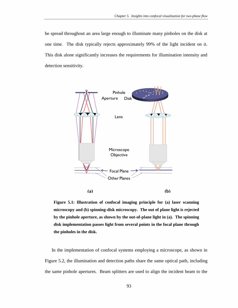
Chapter 5. Insights into confocal visualization for two-phase flow
93
be spread throughout an area large enough to illuminate many pinholes on the disk at
one time. The disk typically rejects approximately 99% of the light incident on it.
This disk alone significantly increases the requirements for illumination intensity and
detection sensitivity.
Figure 5.1: Illustration of confocal imaging principle for (a) laser scanning
microscopy and (b) spinning-disk microscopy. The out of plane light is rejected
by the pinhole aperture, as shown by the out-of-plane light in (a). The spinning
disk implementation passes light from several points in the focal plane through
the pinholes in the disk.
In the implementation of confocal systems employing a microscope, as shown in
Figure 5.2, the illumination and detection paths share the same optical path, including
the same pinhole apertures. Beam splitters are used to align the incident beam to the
Pinhole
Lens
Microscope
Objective
Focal Plane
Other Planes
Aperture Disk
(b) (a)
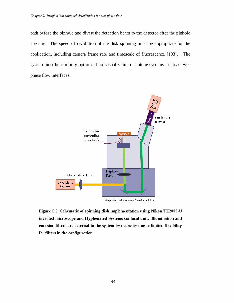
Chapter 5. Insights into confocal visualization for two-phase flow
94
path before the pinhole and divert the detection beam to the detector after the pinhole
aperture. The speed of revolution of the disk spinning must be appropriate for the
application, including camera frame rate and timescale of fluorescence [103]. The
system must be carefully optimized for visualization of unique systems, such as two-
phase flow interfaces.
Figure 5.2: Schematic of spinning disk implementation using Nikon TE2000-U
inverted microscope and Hyphenated Systems confocal unit. Illumination and
emission filters are external to the system by necessity due to limited flexibility
for filters in the configuration.
Hyphenated Systems Confocal Unit
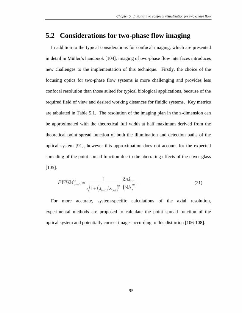
Chapter 5. Insights into confocal visualization for two-phase flow
95
5.2 Considerations for two-phase flow imaging
In addition to the typical considerations for confocal imaging, which are presented
in detail in Müller‟s handbook [104], imaging of two-phase flow interfaces introduces
new challenges to the implementation of this technique. Firstly, the choice of the
focusing optics for two-phase flow systems is more challenging and provides less
confocal resolution than those suited for typical biological applications, because of the
required field of view and desired working distances for fluidic systems. Key metrics
are tabulated in Table 5.1. The resolution of the imaging plan in the z-dimension can
be approximated with the theoretical full width at half maximum derived from the
theoretical point spread function of both the illumination and detection paths of the
optical system [91], however this approximation does not account for the expected
spreading of the point spread function due to the aberrating effects of the cover glass
[105].
22
detNA
2
1
1 exc
exc
zconf
nFWHM
. (21)
For more accurate, system-specific calculations of the axial resolution,
experimental methods are proposed to calculate the point spread function of the
optical system and potentially correct images according to this distortion [106-108].
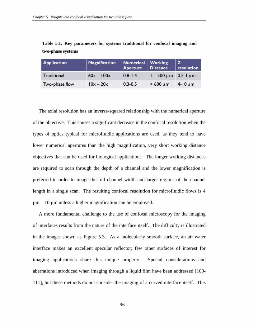
Chapter 5. Insights into confocal visualization for two-phase flow
96
Table 5.1: Key parameters for systems traditional for confocal imaging and
two-phase systems
The axial resolution has an inverse-squared relationship with the numerical aperture
of the objective. This causes a significant decrease in the confocal resolution when the
types of optics typical for microfluidic applications are used, as they tend to have
lower numerical apertures than the high magnification, very short working distance
objectives that can be used for biological applications. The longer working distances
are required to scan through the depth of a channel and the lower magnification is
preferred in order to image the full channel width and larger regions of the channel
length in a single scan. The resulting confocal resolution for microfluidic flows is 4
µm – 10 µm unless a higher magnification can be employed.
A more fundamental challenge to the use of confocal microscopy for the imaging
of interfaces results from the nature of the interface itself. The difficulty is illustrated
in the images shown as Figure 5.3. As a molecularly smooth surface, an air-water
interface makes an excellent specular reflector; few other surfaces of interest for
imaging applications share this unique property. Special considerations and
aberrations introduced when imaging through a liquid film have been addressed [109-
111], but these methods do not consider the imaging of a curved interface itself. This
Application Magnification Numerical
Aperture
Working
Distance
Z
resolution
Traditional 60x – 100x 0.8-1.4 1 – 500 mm 0.5-1 mm
Two-phase flow 10x – 20x 0.3-0.5 > 600 mm 4-10 mm
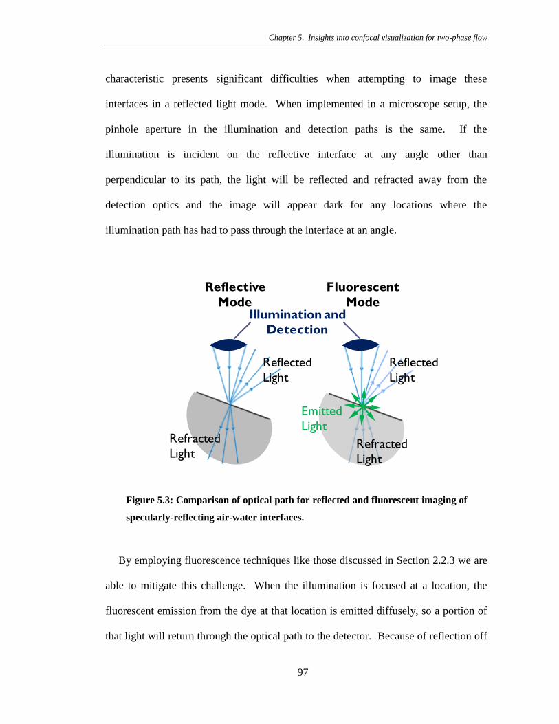
Chapter 5. Insights into confocal visualization for two-phase flow
97
characteristic presents significant difficulties when attempting to image these
interfaces in a reflected light mode. When implemented in a microscope setup, the
pinhole aperture in the illumination and detection paths is the same. If the
illumination is incident on the reflective interface at any angle other than
perpendicular to its path, the light will be reflected and refracted away from the
detection optics and the image will appear dark for any locations where the
illumination path has had to pass through the interface at an angle.
Figure 5.3: Comparison of optical path for reflected and fluorescent imaging of
specularly-reflecting air-water interfaces.
By employing fluorescence techniques like those discussed in Section 2.2.3 we are
able to mitigate this challenge. When the illumination is focused at a location, the
fluorescent emission from the dye at that location is emitted diffusely, so a portion of
that light will return through the optical path to the detector. Because of reflection off
Illumination and
Detection
Reflective
Mode
Fluorescent
Mode
Reflected
Light
Reflected
Light
Refracted
LightRefracted
Light
Emitted
Light
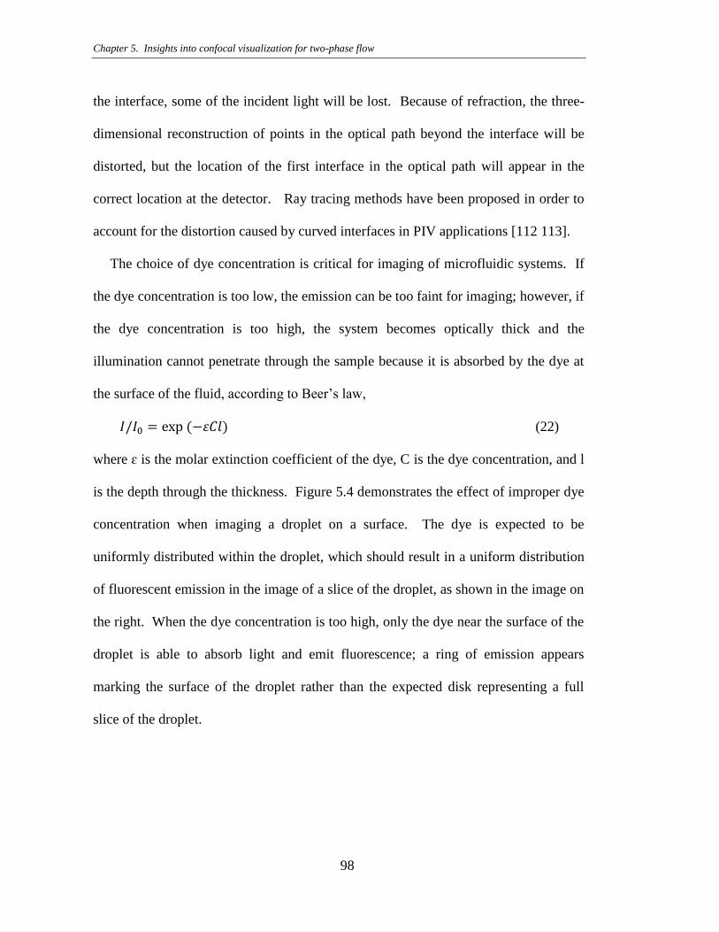
Chapter 5. Insights into confocal visualization for two-phase flow
98
the interface, some of the incident light will be lost. Because of refraction, the three-
dimensional reconstruction of points in the optical path beyond the interface will be
distorted, but the location of the first interface in the optical path will appear in the
correct location at the detector. Ray tracing methods have been proposed in order to
account for the distortion caused by curved interfaces in PIV applications [112 113].
The choice of dye concentration is critical for imaging of microfluidic systems. If
the dye concentration is too low, the emission can be too faint for imaging; however, if
the dye concentration is too high, the system becomes optically thick and the
illumination cannot penetrate through the sample because it is absorbed by the dye at
the surface of the fluid, according to Beer‟s law,
(22)
where ɛ is the molar extinction coefficient of the dye, C is the dye concentration, and l
is the depth through the thickness. Figure 5.4 demonstrates the effect of improper dye
concentration when imaging a droplet on a surface. The dye is expected to be
uniformly distributed within the droplet, which should result in a uniform distribution
of fluorescent emission in the image of a slice of the droplet, as shown in the image on
the right. When the dye concentration is too high, only the dye near the surface of the
droplet is able to absorb light and emit fluorescence; a ring of emission appears
marking the surface of the droplet rather than the expected disk representing a full
slice of the droplet.
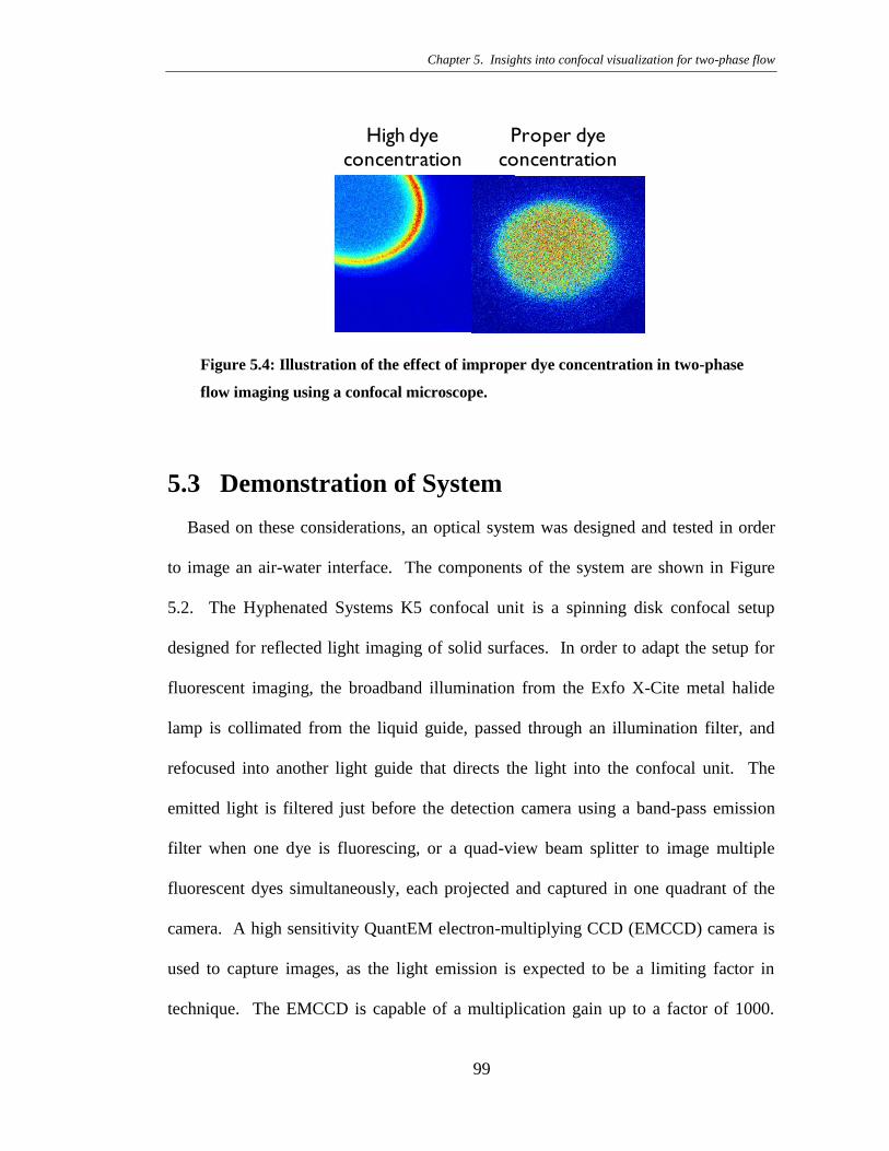
Chapter 5. Insights into confocal visualization for two-phase flow
99
Figure 5.4: Illustration of the effect of improper dye concentration in two-phase
flow imaging using a confocal microscope.
5.3 Demonstration of System
Based on these considerations, an optical system was designed and tested in order
to image an air-water interface. The components of the system are shown in Figure
5.2. The Hyphenated Systems K5 confocal unit is a spinning disk confocal setup
designed for reflected light imaging of solid surfaces. In order to adapt the setup for
fluorescent imaging, the broadband illumination from the Exfo X-Cite metal halide
lamp is collimated from the liquid guide, passed through an illumination filter, and
refocused into another light guide that directs the light into the confocal unit. The
emitted light is filtered just before the detection camera using a band-pass emission
filter when one dye is fluorescing, or a quad-view beam splitter to image multiple
fluorescent dyes simultaneously, each projected and captured in one quadrant of the
camera. A high sensitivity QuantEM electron-multiplying CCD (EMCCD) camera is
used to capture images, as the light emission is expected to be a limiting factor in
technique. The EMCCD is capable of a multiplication gain up to a factor of 1000.
High dye
concentration
Proper dye
concentration
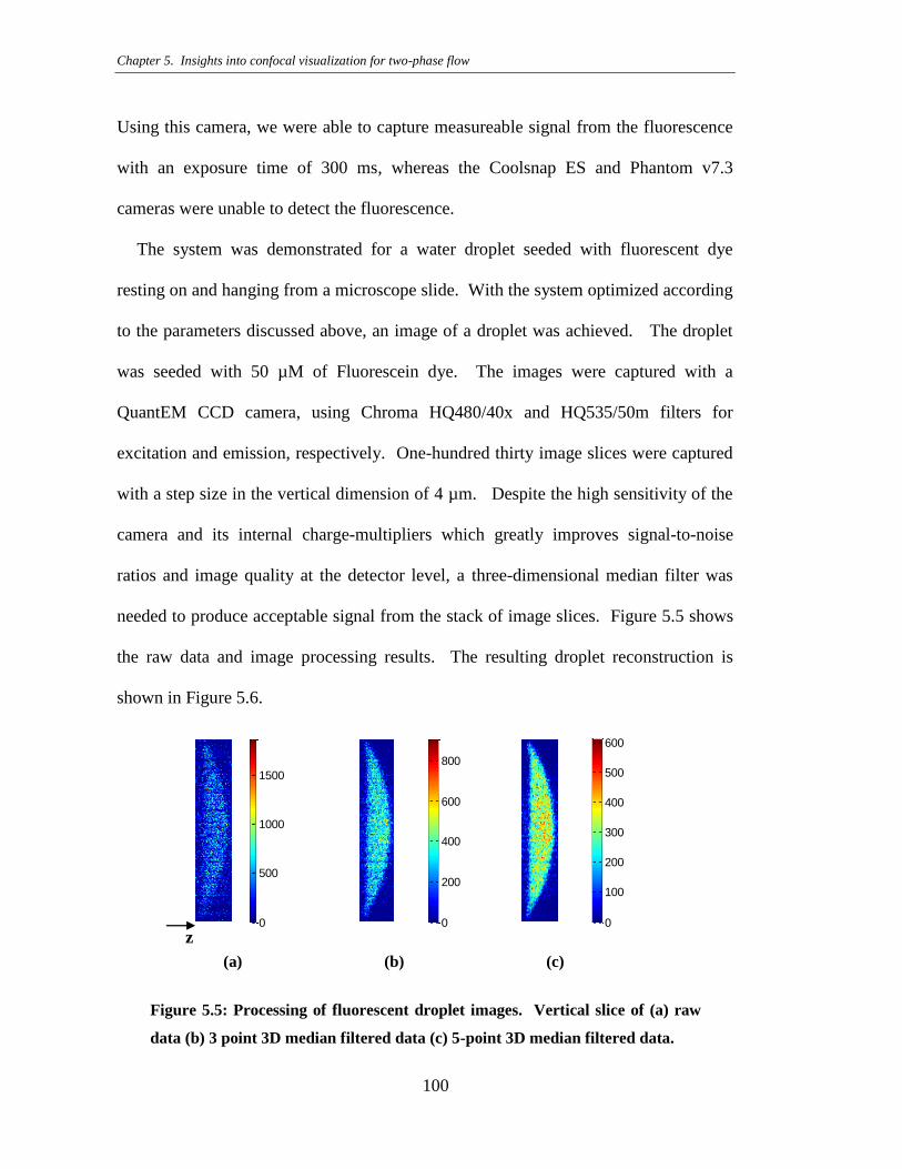
Chapter 5. Insights into confocal visualization for two-phase flow
100
Using this camera, we were able to capture measureable signal from the fluorescence
with an exposure time of 300 ms, whereas the Coolsnap ES and Phantom v7.3
cameras were unable to detect the fluorescence.
The system was demonstrated for a water droplet seeded with fluorescent dye
resting on and hanging from a microscope slide. With the system optimized according
to the parameters discussed above, an image of a droplet was achieved. The droplet
was seeded with 50 µM of Fluorescein dye. The images were captured with a
QuantEM CCD camera, using Chroma HQ480/40x and HQ535/50m filters for
excitation and emission, respectively. One-hundred thirty image slices were captured
with a step size in the vertical dimension of 4 µm. Despite the high sensitivity of the
camera and its internal charge-multipliers which greatly improves signal-to-noise
ratios and image quality at the detector level, a three-dimensional median filter was
needed to produce acceptable signal from the stack of image slices. Figure 5.5 shows
the raw data and image processing results. The resulting droplet reconstruction is
shown in Figure 5.6.
(a) (b) (c)
Figure 5.5: Processing of fluorescent droplet images. Vertical slice of (a) raw
data (b) 3 point 3D median filtered data (c) 5-point 3D median filtered data.
0
500
1000
1500
0
200
400
600
800
0
100
200
300
400
500
600
0
200
400
600
800
0
100
200
300
400
500
50
100
150
200
250
300
350
400
z
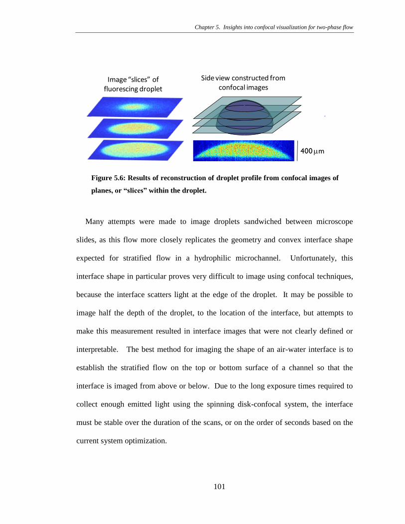
Chapter 5. Insights into confocal visualization for two-phase flow
101
Figure 5.6: Results of reconstruction of droplet profile from confocal images of
planes, or “slices” within the droplet.
Many attempts were made to image droplets sandwiched between microscope
slides, as this flow more closely replicates the geometry and convex interface shape
expected for stratified flow in a hydrophilic microchannel. Unfortunately, this
interface shape in particular proves very difficult to image using confocal techniques,
because the interface scatters light at the edge of the droplet. It may be possible to
image half the depth of the droplet, to the location of the interface, but attempts to
make this measurement resulted in interface images that were not clearly defined or
interpretable. The best method for imaging the shape of an air-water interface is to
establish the stratified flow on the top or bottom surface of a channel so that the
interface is imaged from above or below. Due to the long exposure times required to
collect enough emitted light using the spinning disk-confocal system, the interface
must be stable over the duration of the scans, or on the order of seconds based on the
current system optimization.
400 mm
Image “slices” of fluorescing droplet
Side view constructed fromconfocal images
400 mm
Image “slices” of fluorescing droplet
Side view constructed fromconfocal images
Chapter 5. Insights into confocal visualization for two-phase flow
102
5.4 Conclusions
The use of spinning-disk confocal systems for the fluorescent imaging of air-water
interfaces faces many challenges. In addition to the considerations faced by any
confocal imaging technique in choice of optics and system configuration, two-phase
interface imaging requires the use of fluorescent imaging techniques because of the
reflectivity of the interface; fluorescence dramatically reduces the percentage of
illumination light which can be detected by the sensor. In addition, the reflectivity of
the air-water interface renders some sample configurations unable to be imaged and
distorts others such that post-processing image deconvolution techniques must be
employed to reconstruct the image shape. Some success has been achieved with the
use of a high sensitivity electron multiplying CCD camera. Future development of
this technique could include the development of test structures whose geometry
facilitates the formation of stable films parallel to the imaging plane, as these
interfaces are shown to be more accessible with these imaging techniques.
Deconvolution techniques could improve the output from reconstructed images,
however the fundamental difficulties associated with reflection and refraction at the
interfaces will continue to limit the widespread implementation of confocal imaging
for air-water interface applications.
103
Chapter 6. Conclusions and future
directions
In this work, we have developed visualization and analysis techniques to probe the
interaction of air and water in microchannels applicable to transport phenomena in
fuel cells. In silicon microchannels, we examined fundamental two-phase flow
phenomena with water introduction from side wall injection slots, simulating the
asymmetric water injection in PEM fuel cell channels. We also develop ex-situ fuel
cell channels with distributed water injection along a long, serpentine channel through
an integrated GDL-wall. Various visualization techniques are used to observe the
structure of the flow in order to develop an understanding of the behavior of the two
fluids in fuel cell channels.
6.1 Fluorescent visualization of two-phase flow
regimes in rectangular microchannels
Using fluorescent visualization techniques to observe two-phase flow in
microchannels etched in silicon, we have corroborated and expanded boundaries of
Chapter 6. Conclusions and future directions
104
flow regime maps in rectangular channels to high-aspect ratio channels with
asymmetric injection conditions. In small square channels, our data corroborates the
transition criterion proposed by Cubaud [32] between intermittent and separated flow
regimes. However, the asymmetric injection conditions of the current study favor
flow stratification; we observed stratified flow in high aspect ratio channels under low
air flow conditions where intermittent flow regimes would be expected in square
channels. Even in the small square channels, the injection conditions allow formation
of stratified flow where annular or dry flow has been observed. Two distinct means of
slug formation have been imaged using a high-speed camera which allows for
discernment of the interface during the process of flow transition, providing insight
into the mechanisms of flow structure formation in these channels. This study
represents first-of-kind visualization of two phase flow regimes in channels of various
aspect ratios with asymmetric injection, providing key data for the design and
optimization of flow channels in practical devices where channel aspect ratio is
expected to be an important design parameter.
6.2 Stratified flow physics
High aspect ratio rectangular channels with asymmetric water injection show a
propensity toward stratified flow. Several identifiable regimes of stratified flow are
observed, depending on the flow conditions, with stationary wavy flow occurring for
low air flow rates when surface tension dominates compared with the inertia of the air.
As the air flow rates increase, the films smooth. At the highest air flow rates, the
Chapter 6. Conclusions and future directions
105
interfaces become blurred. The film thickness was measured using an intensity-
thresholding technique. Uncertainty analysis due to variations in the film thickness
and in the sharpness of the interface provides insight into the structure of the film and
highlights the flow conditions under which transition between stratified regimes
occurs. Good agreement between the measured film thicknesses and an analytical
solution to the Navier-Stokes equation for the velocity profile of stratified flow in a
rectangular channel with a flat air-water interface indicates that this solution is a
reasonable approximation to the actual flow in the channels. A key characteristic of
the analytical solution is that both the shape of the velocity profile and the fractional
thickness of the film are functions only of non-dimensional parameters, including the
aspect ratio of the channel and the ratio of the flow rates. This insight allows
simplifications in the analysis of channel designs for the optimization of devices in
which stratified flow is expected or desired.
6.3 Two-phase flow visualization in an ex-situ PEM
fuel cell channel
We have designed an ex-situ fuel cell channel setup to examine the progression of
flow structures in long channels with distributed water injection. GDL-integrated
samples demonstrate the complexity of interactions in two-phase flow systems with
materials exhibiting non-homogeneous surface properties. Flow structures evolve as
they move through the channel, encountering water at downstream injection locations.
Over a range of conditions chosen to reflect the operating conditions of an operating
Chapter 6. Conclusions and future directions
106
fuel cell, the flow consistently transitions from intermittent flow regimes to stable
stratified flows downstream, where more water exists in the channels. Under high air
flow rate conditions, the water droplets remain attached to one wall, while low air
flow rate conditions show droplets spanning the channel width. When the GDL wall
is less hydrophobic, less water is observed in the channel, as it is more likely to remain
in or flow through the GDL. Experiments were also performed in shorter, straight
channels with similar flow rates as the serpentine channels and with similar equivalent
fuel cell operating conditions in order to examine the effects of the channel bends to
the flow structure. In the straight channels, stratified flow is never observed – the flow
remains intermittent along the length of the channel. No flooding conditions are
observed in these channels, a result which is explained by the lack of alternative flow
paths to the single serpentine channel with no cross-talk between channel segments
through the GDL. Implications of the results of these experiments to fuel cell channel
design are proposed.
6.4 Insights into confocal visualization for two-phase
flow
A confocal fluorescent technique was explored for three-dimensional imaging of
the interface shape in two-phase flow systems. While the technique is frequently
employed for biological applications and has recently been adapted to fluidic systems,
this study reveals that extending its use to two-phase flow systems presents unique
challenges and considerations. In particular, the reflective properties of the air-water
Chapter 6. Conclusions and future directions
107
interface render reflective imaging unsuitable for these systems, requiring the use of
fluorescent techniques to observe the interface, which necessitates higher illumination
intensity and a high sensitivity detection camera. The technique is demonstrated for a
droplet on a microscope slide seeded with fluorescein dye, and the importance of
median filtering to extract information from low signal to noise data is demonstrated.
Further development of this technique for other systems is needed, according to the
insight gain in this study.
6.5 Recommendations for future directions
Several interesting phenomena have been observed and identified for future
research on fundamental phenomena in two-phase microchannel flow. This work
presented flow structures and visualization techniques in which asymmetric injection
conditions led to the observation of unique flow structures including stratified flow in
very small channels and flow transitions leading to the formation of plugs in the
channels. High speed visualization provides insight into plug formation, however
further development of stability analysis is needed to determine the transition criteria
for the formation of plugs both at the water injection t-junction and from the instability
of a stratified film where surface tension, viscous forces, and inertial forces may be
important.
While the data of this study corroborated the regime transitions of the literature for
square channels and suggested the regime boundary trends for channels of higher
aspect ratios, a more detailed study is needed to map out this boundary and its
Chapter 6. Conclusions and future directions
108
dependence on aspect ratio. A modification of the Weber number for flow transition
which accounts for channel geometry may be possible and would provide very
valuable insight for the design of practical two-phase flow systems.
Finally, the development of confocal microscopy for two-phase interface detection
has not been achieved in the geometries used in this study. Based on the analysis and
insights gained during the development of this system, the technique may successfully
visualize the shape of an interface of a stable stratified flow if the film were located in
the visualization plane. Further exploration of the limitations and capabilities of
confocal microscopy in two-phase flow systems may reveal other systems of interest
that can be observed using this system.
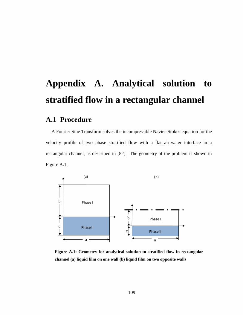
109
Appendix A. Analytical solution to
stratified flow in a rectangular channel
A.1 Procedure
A Fourier Sine Transform solves the incompressible Navier-Stokes equation for the
velocity profile of two phase stratified flow with a flat air-water interface in a
rectangular channel, as described in [82]. The geometry of the problem is shown in
Figure A.1.
Figure A.1: Geometry for analytical solution to stratified flow in rectangular
channel (a) liquid film on one wall (b) liquid film on two opposite walls
a
b
c
a
b
c
Phase I
Phase II
Phase I
Phase II
(a) (b)
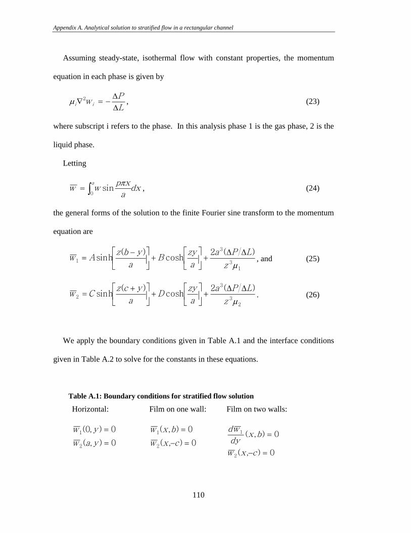
Appendix A. Analytical solution to stratified flow in a rectangular channel
110
Assuming steady-state, isothermal flow with constant properties, the momentum
equation in each phase is given by
L
Pw ii
2m , (23)
where subscript i refers to the phase. In this analysis phase 1 is the gas phase, 2 is the
liquid phase.
Letting
dxa
xpww
a
0
sin
, (24)
the general forms of the solution to the finite Fourier sine transform to the momentum
equation are
13
3
1
)(2cosh
)(sinh
mz
LPa
a
zyB
a
ybzAw
, and (25)
23
3
2
)(2cosh
)(sinh
mz
LPa
a
zyD
a
yczCw
. (26)
We apply the boundary conditions given in Table A.1 and the interface conditions
given in Table A.2 to solve for the constants in these equations.
Table A.1: Boundary conditions for stratified flow solution
Horizontal: Film on one wall: Film on two walls:
0),(
0),0(
2
1
yaw
yw
0),(
0),(
2
1
cxw
bxw
0),(
0),(
2
1
cxw
bxdy
wd
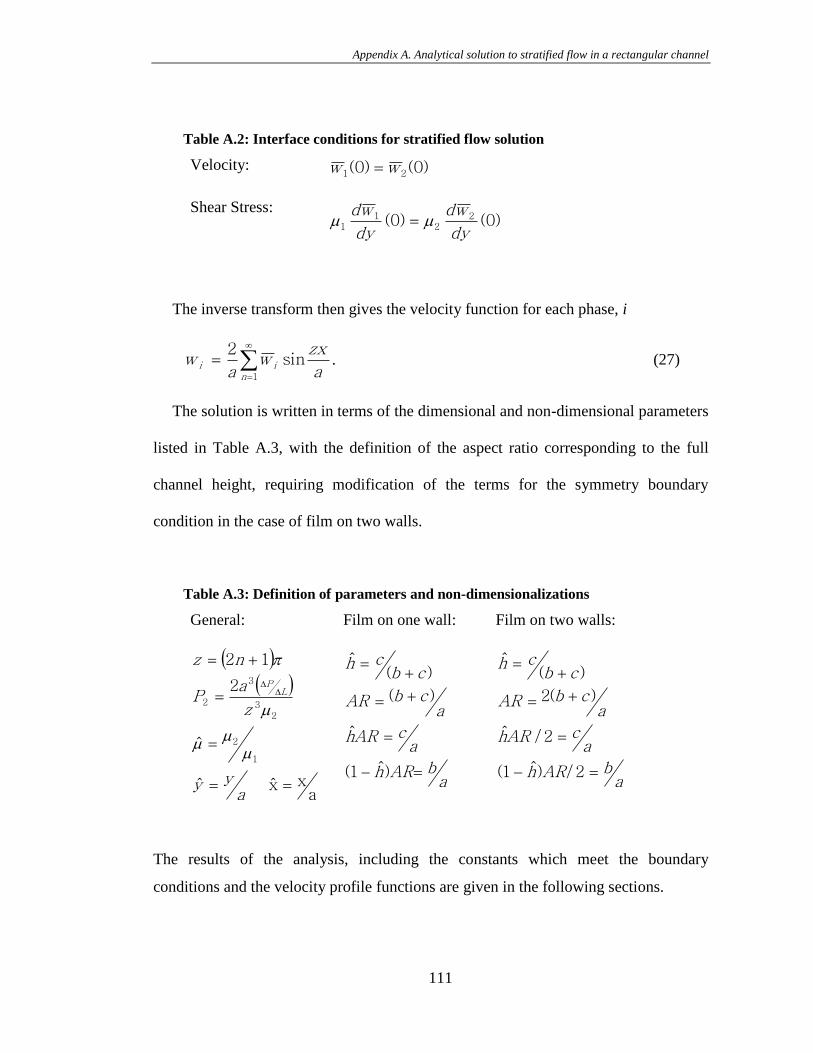
Appendix A. Analytical solution to stratified flow in a rectangular channel
111
Table A.2: Interface conditions for stratified flow solution
Velocity: )0()0( 21 ww
Shear Stress: )0()0( 2
21
1dy
wd
dy
wdmm
The inverse transform then gives the velocity function for each phase, i
a
zxw
aw
nii sin
2
1
. (27)
The solution is written in terms of the dimensional and non-dimensional parameters
listed in Table A.3, with the definition of the aspect ratio corresponding to the full
channel height, requiring modification of the terms for the symmetry boundary
condition in the case of film on two walls.
Table A.3: Definition of parameters and non-dimensionalizations
General: Film on one wall: Film on two walls:
axx̂ ˆ
ˆ
2
12
1
2
23
3
2
ayy
z
aP
nz
LP
mm
m
m
abARh
acARh
acbAR
cbch
)ˆ1(
ˆ
)(
)(ˆ
abARh
acARh
acbAR
cbch
2/)ˆ1(
2/ˆ
)(2
)(ˆ
The results of the analysis, including the constants which meet the boundary
conditions and the velocity profile functions are given in the following sections.
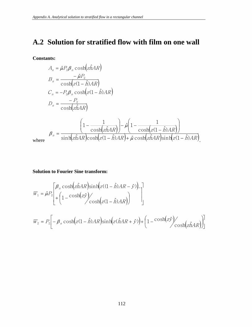
Appendix A. Analytical solution to stratified flow in a rectangular channel
112
A.2 Solution for stratified flow with film on one wall
Constants:
ARhz
PD
ARhzPC
ARhz
PB
ARhzPA
n
nn
n
nn
ˆcosh
)ˆ1(cosh
)ˆ1(cosh
ˆ
ˆcoshˆ
2
2
2
2
m
m
where
ARhzARhzARhzARhz
ARhzARhzn
)ˆ1(sinhˆcoshˆ)ˆ1(coshˆsinh
)ˆ1(cosh
11ˆ
ˆcosh
11
m
m
.
Solution to Fourier Sine transform:
ARhzyzyARhzARhzPw
ARhzyz
yARhzARhz
Pw
n
n
ˆcoshˆcosh1)ˆˆ(sinh)ˆ1(cosh
)ˆ1(coshˆcosh1
...)ˆ)ˆ1((sinhˆcosh
ˆ
22
21
m
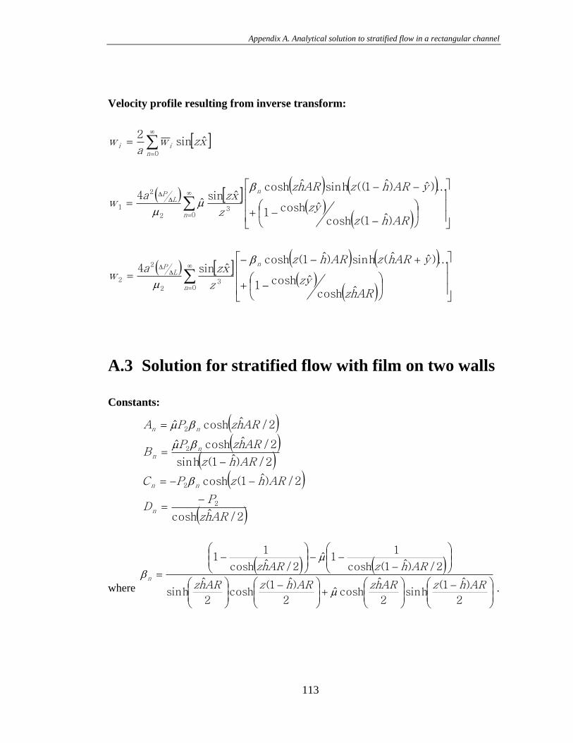
Appendix A. Analytical solution to stratified flow in a rectangular channel
113
Velocity profile resulting from inverse transform:
03
2
2
2
03
2
2
1
0
ˆcoshˆcosh1
...)ˆˆ(sinh)ˆ1(coshˆsin4
)ˆ1(coshˆcosh1
...)ˆ)ˆ1((sinhˆcoshˆsin
ˆ4
ˆsin2
n
nL
P
n
nL
P
nii
ARhzyz
yARhzARhz
z
xzaw
ARhzyz
yARhzARhz
z
xzaw
xzwa
w
m
mm
A.3 Solution for stratified flow with film on two walls
Constants:
2/ˆcosh
2/)ˆ1(cosh
2/)ˆ1(sinh
2/ˆcoshˆ
2/ˆcoshˆ
2
2
2
2
ARhz
PD
ARhzPC
ARhz
ARhzPB
ARhzPA
n
nn
nn
nn
m
m
where
2
)ˆ1(sinh
2
ˆcoshˆ
2
)ˆ1(cosh
2
ˆsinh
2/)ˆ1(cosh
11ˆ
2/ˆcosh
11
ARhzARhzARhzARhz
ARhzARhzn
m
m
.
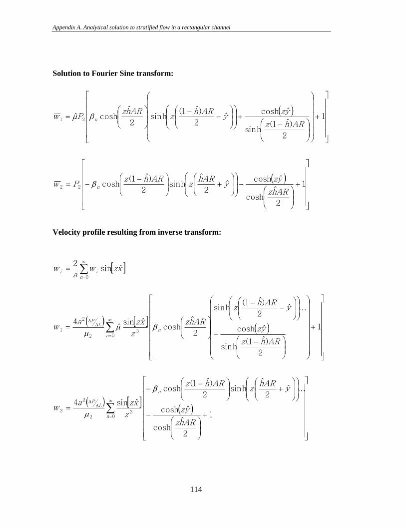
Appendix A. Analytical solution to stratified flow in a rectangular channel
114
Solution to Fourier Sine transform:
1
2
ˆcosh
ˆcoshˆ
2
ˆsinh
2
)ˆ1(cosh
1
2
)ˆ1(sinh
ˆcoshˆ
2
)ˆ1(sinh
2
ˆcoshˆ
22
21
ARhz
yzy
ARhz
ARhzPw
ARhz
yzy
ARhz
ARhzPw
n
n
m
Velocity profile resulting from inverse transform:
03
2
2
2
03
2
2
1
0
1
2
ˆcosh
ˆcosh
...ˆ2
ˆsinh
2
)ˆ1(cosh
ˆsin4
1
2
)ˆ1(sinh
ˆcosh
...ˆ2
)ˆ1(sinh
2
ˆcosh
ˆsinˆ
4
ˆsin2
n
n
LP
nn
LP
nii
ARhz
yz
yARh
zARhz
z
xzaw
ARhz
yz
yARh
z
ARhz
z
xzaw
xzwa
w
m
mm
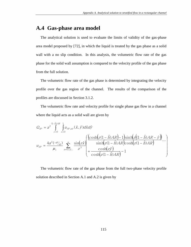
Appendix A. Analytical solution to stratified flow in a rectangular channel
115
A.4 Gas-phase area model
The analytical solution is used to evaluate the limits of validity of the gas-phase
area model proposed by [72], in which the liquid is treated by the gas phase as a solid
wall with a no slip condition. In this analysis, the volumetric flow rate of the gas
phase for the solid wall assumption is compared to the velocity profile of the gas phase
from the full solution.
The volumetric flow rate of the gas phase is determined by integrating the velocity
profile over the gas region of the channel. The results of the comparison of the
profiles are discussed in Section 3.1.2.
The volumetric flow rate and velocity profile for single phase gas flow in a channel
where the liquid acts as a solid wall are given by
1)ˆ1(cosh
ˆcosh
...)ˆ1(cosh)ˆ1(sinh
ˆ)ˆ1(sinh1)ˆ1(cosh
ˆsin)(4
ˆˆ)ˆ,ˆ(
...2,1,03
1
2
)ˆ1(
0
1
0
,2
ARhz
yz
ARhzARhz
yARhzARhz
z
xzau
ydxdyxuaQ
n
dLdP
SP
ARh
y x
airSPSP
m
The volumetric flow rate of the gas phase from the full two-phase velocity profile
solution described in Section A.1 and A.2 is given by
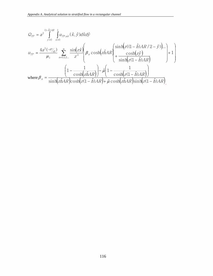
Appendix A. Analytical solution to stratified flow in a rectangular channel
116
1
)ˆ1(sinh
ˆcosh
...)ˆ2/)ˆ1((sinhˆcosh
ˆsin
)(4
ˆˆ)ˆ,ˆ(
...2,1,03
1
2
)ˆ1(
0
1
0
,2
ARhz
yz
yARhz
ARhzz
xzau
ydxdyxuaQ
nn
dLdP
TP
ARh
y x
airTPTP
m
where
ARhzARhzARhzARhz
ARhzARhzn
)ˆ1(sinhˆcoshˆ)ˆ1(coshˆsinh
)ˆ1(cosh
11ˆ
ˆcosh
11
m
m
.
117
References
1 H. Li, Y. Tang, Z. Wang, Z. Shi, S. Wu, D. Song, J. Zhang, K. Fatih, J. Zhang, H.
Wang, Z. Liu, R. Abouatallah, A. Mazza, A review of water flooding issues in
the proton exchange membrane fuel cell, J. Power Sources 178 (2008) 103–117.
2 F. Barbir, H. Gorgun, X. Wang, Relationship between pressure drop and cell
resistance as a diagnostic tool for PEM fuel cells, J. Power Sources 141 (2005)
96–101.
3 T.V. Nguyen, M.W. Knobbe, A liquid water management strategy for PEM fuel
cell stacks, J. Power Sources 114 (2003) 70-79.
4 J.P.Owejan, T.A. Trabold, J.J. Gagliardo, D.L. Jacobson, R.N. Carter, D.S.
Hussey, M. Arif, Voltage instability in a simulated fuel cell stack correlated to
cathode water accumulation, J. Power Sources 171 (2007) 626-633.
5 W. He, G. Lin, T. Van Nguyen, Diagnostic tool to detect electrode flooding in
proton-exchange-membrane fuel cells, AIChE Journal 49 (2003) 3221-3228.
6 M. Müller, C. Müller, F. Gromball, M. Wölfle, W. Menz, Micro-structure flow
field for small fuel cells, Microsystem Tech. 9 (2003) 159-162.
References
118
7 S.W. Cha, R. O‟Hayre, F.B. Prinz, The influence of size scale on the
performance of fuel cells, Solid State Ionics 175 (2004) 789–795.
8 S.W. Cha, R. O‟Hayre, S.J. Lee, Y. Saito, F.B. Prinz, Geometric scale effect of
flow channels on performance of fuel cells, J. Electrochemical Society (2004)
A1856-A1864.
9 S.E. Litster, C.R. Buie, T. Fabian, J.K. Eaton, J.G. Santiago, Active Water
Management for PEM fuel cells, J. Electrochem. Society 154 (2007) B1049-
B1058 .
10 S.E. Litster, C.R. Buie, J.G. Santiago, Engineering model for coupling wicks and
electroosmotic pumps with proton exchange membrane fuel cells for active
water management, Electrochimica Acta 54 ( 2009) 6223-6233.
11 D.G. Strickland, J.G. Santiago, In situ polymerized wicks for passive water
management in proton exchange membrane fuel cells, J. Power Sources 195
(2010) 1667-1675.
12 R.S. Stanley, R.F. Barron, T.A. Ameel, Two-phase flow in microchannels,
ASME Microelectromechanical Systems DSC-62 (2007) 143-152.
13 J. Moreno Quibén, J.R. Thome, Flow pattern based two-phase frictional pressure
drop model for horizontal tubes, Part II: new phenomenological model, Int. J.
Heat Fluid Flow 28 (2007) 1060-1072.
14 D.R. Kim, J.-M. Koo, C. Fang, J.E. Steinbrenner, E.S. Lee, F.-M. Wang, C.H.
Hidrovo, J.K. Eaton, K.E. Goodson, Compact model of slug flow in
microchannels, Proc. of ICNMM (18-20 June 2007) Puebla, Mexico.
References
119
15 P.-G. de Gennes, F. Brochard-Wyart, D. Quéré, Capillarity and Wetting
Phenomena: Drops, Bubbles, Pearls, Waves (2004) Springer-Verlag, New York,
Inc., USA.
16 T. Cubaud, M. Fermigier, Advancing contact lines on chemically heterogeneous
surfaces, J. Colloid and Interface Sci. 269 (2004) 171-177.
17 M.A. Tenan, S. Hackwood, G. Beni, Friction in capillary systems, J. Appl. Phys.
53 (1982) 6687-6692.
18 C. Fang, C.H. Hidrovo, F.-M. Wang, J.K. Eaton, K.E. Goodson, 3-D numerical
simulation of contact angle hysteresis for microscale two phase flow, Int. J.
Multiphase Flow 34 (2008) 690-705.
19 T. Cubaud, U. Ulmanella, C.-M. Ho, Two-phase flow in microchannels with
surface modifications, Plenary Paper, ICMF (30 May – 4 June 2004) Yokahama,
Japan.
20 K.S. Chen, M.A. Hickner, D.R. Noble, Simplified models for predicting the
onset of liquid water droplet instability at the gas diffusion layer/gas flow
channel interface, Int. J. Energy Research 29 (2005) 1113-1132.
21 A. Serizawa, Z. Feng, Z. Kawara, Two-phase flow in microchannels, Exp.
Thermal Fluid Sci. 26 (2002) 703-714.
22 A. Kawahara, P.M.-Y. Chung, M. Kawaji, Investigation of two-phase flow
pattern, void fraction and pressure drop in a microchannel, Int. J. Multiphase
Flow 28 (2002) 1411-1435.
23 M.K. Akbar, D.A. Plummer, S.M. Ghiaasiaan, On gas-liquid two-phase flow
regimes in microchannels, Int. J. Multiphase Flow 29 (2003) 855-865.
References
120
24 S. Saisorn, S. Wongwises, Flow pattern, void fraction and pressure drop of two-
phase air-water flow in a horizontal circular micro-channel, Exp. Thermal and
Fluid Sci. 32 (2008) 748-760.
25 S. Saisorn, S. Wongwises, The effects of channel diameter on flow pattern, void
fraction and pressure drop of two-phase air-water flow in circular micro-
channels, Exp. Thermal and Fluid Sci. 34 (2010) 454-462.
26 M. Kawaji and P. M.-Y. Chung, Adiabatic gas-liquid flow in microchannels,
Microscale Thermophysical Engineering 8 (2004) 239-257.
27 I. Hassan, M. Vaillancourt, K. Pehlivan, Two-phase flow regime transitions in
microchannels: A comparative experimental study, Microscale Thermophysical
Engineering 9 (2005) 165-182.
28 R. Dreyfus, P. Tabeling, H. Willaime, Ordered and disordered patterns in two-
phase flow in microchannels, Physical Review Letters 90 (1993) 144505-(1-4).
29 K.A. Triplett, S.M. Ghiaasiaan, S.I. Abdel-Khalik, D.L. Sadowski, Gas-liquid
two-phase flow in microchannels Part I: two-phase flow patterns, Int. J.
Multiphase Flow 25 (1999) 377-394.
30 J.L. Xu, P. Cheng, T.S. Zhao, Gas-liquid two-phase flow regimes in rectangular
channels with mini/micro gaps, Int. J. Multiphase Flow 25 (1999) 411-432.
31 K. Pehlivan, I. Hassan, M. Vaillancourt, Experimental study on two-phase flow
and pressure drop in millimeter-size channels, Applied Thermal Engineering 26
(2006) 1506-1514.
32 T. Cubaud, C.-M. Ho, Transport of bubbles in square microchannels. Physics of
Fluids 16 (2004) 4575-4584.
References
121
33 P. M.-Y. Chung, M. Kawaji, A. Kawahara, Y. Shibati, Two-phase flow through
square and circular microchannels – effects of channel geometry, J. Fluids
Engineering 126 (2004) 546-552.
34 Q.C. Bi, T.S. Zhao, Taylor bubbles in miniaturized circular and noncircular
channels, Int. J. Multiphase Flow 27 (2001) 561-570.
35 S. Garimella, J.D. Killion, J.W. Coleman, An experimentally validated model for
two-phase pressure drop in the intermittent flow regime for noncircular
microchannels, J. Fluids Eng. 125 (2003) 887-894.
36 T.C. Ransohoff, C.J. Radke, Laminar flow of a wetting liquid along the corners
of a predominantly gas-occupied noncircular pore, J. Colloid Int. Sci. 121 (1988)
392-401.
37 H. Wong, C.J. Radke, S. Morris, The motion of long bubbles in polygonal
capillaries. Part 2. Drag, fluid pressure, and fluid flow, J. Fluid. Mech. 292 (1995)
95-110.
38 A.M. Barajas, R.L. Panton, The effects of contact angle on two-phase flow in
capillary tubes, Int. J. Multiphase Flow 19 (1993) 337-346.
39 C.Y. Lee, S.Y. Lee, Influence of surface wettability on transition of two-phase
flow pattern in round mini-channels, Int. J. Multiphase Flow 34 (2008) 706-711.
40 N.J. English, S.G. Kandlikar, An experimental investigation into the effect of
surfactants on air-water two-phase flow in minichannels, Proc. of ICMM (13-15
June 2005) Toronto, Canada.
41 A. Bazylak, Liquid water visualization in PEM fuel cells: A review, Int. J.
Hydrogen Energy 34 (2009) 3845-3857.
References
122
42 R. Anderson, L. Zhang, Y. Ding, M. Blanco, X. Bi, D.P. Wilkinson, A critical
review of two-phase flow in gas flow channels of proton exchange membrane
fuel cells, J. Power Sources 195 (2010) 4531–4553.
43 D. Kramer, J. Zhang, R. Shimoi, E. Lehmann, A. Wokaun, K. Shinohara, G.G.
Scherer, In situ diagnostic of two-phase flow phenomena in polymer electrolyte
cells by neutron imaging – Part A. Experimental, data treatment, and
quantification, Electrochem. Acta 50 (2005) 2603–2614.
44 D.S. Hussey, D.L. Jacobson, M. Arif, J.P. Owejan, J.J. Gagliardo, T.A. Trabold,
Neutron images of the through plane water distribution of an operating PEM fuel
cell, J. Power Sources 172 (2007) 225–228.
45 T.A. Trabold, J.P. Owejan, D.L. Jacobson, M. Arif, P.R. Huffman, In situ
investigation of water transport in an operating PEM fuel cell using neutron
radiography: Part 1 – Experimental method and serpentine flow field results, Int.
J. Heat Mass Transfer 49 (2006) 4712–4720.
46 P. Boillat, G. Frei, E. H. Lehmann, G.G. Scherer, A. Wokaun, Neutron imaging
resolution improvements optimized for fuel cell applications, Electrochem. and
Solid State Letters 13 (2010) B25-B27.
47 N. Pekula, K. Heller, P.A. Chuang, A. Turhan, M.M. Mench, J.S. Brenizer, K.
Unlu, Study of water distribution and transport in a polymer electrolyte fuel cell
using neutron radiography, Nucl. Instrum. Meth. Phys. Res. A 21 (2005) 134.
48 X. Li, I. Sabir, J. Park, A flow channel design procedure for PEM fuel cells with
effective water removal, J. Power Sources 163 (2007) 933-942.
References
123
49 J.P. Owejan, T.A. Trabold, D.L. Jacobson, M. Arif, S.G. Kandlikar, Effects of
flow field and diffusion layer properties on water accumulation in a PEM fuel
cell, Int. J. Hydrogen Energy 32 (2007) 4489-4502.
50 J. Zhang, D. Kramer, R. Shimoi, Y. Ono, E. Lehmann, A. Wokaun, K. Shinohara,
G.G. Scherer, In situ diagnostic of two-phase flow phenomena in polymer
electrolyte fuel cells by neutron imaging Part B. Material variations,
Electrochimica Acta 51 (2006) 2715–2727
51 R. Satija, D.L. Jacobson, M. Arif, S.A. Werner, In-situ neutron imaging
technique for evaluation of water management systems in operating PEM fuel
cells, J. Power Sources 129 (2004) 238–245.
52 I. Manke, Ch. Hartnig, M. Grünerbel, J. Kaczerowski, W. Lehnert, N. Kardjilov,
A. Hilger, J. Banhart, W. Treimer, M. Strobl, Quasi-in situ neutron tomography
on polymer electrolyte membrane fuel cell stacks, Applied Physics Letters 90
(2007) 184101.
53 I. Manke, Ch. Hartnig, M. Grünerbel, W. Lehnert, N. Kardjilov, A. Heibel, A.
Hilger, J. Banhart, H. Riesemeier, Investigation of water evolution and transport
in fuel cells with high resolution synchrotron x-ray radiography, Applied Physics
Letters 90 (2007) 174105.
54 S.J. Lee, N.-Y. Lim, S. Kim, G.-G. Park, C.-S. Kim, X-ray imaging of water
distribution in a polymer electrolyte fuel cell, J. Power Sources 185 (2008) 867-
870.
55 S. Tsushima, K. Teranishi, S. Hirai, Magnetic resonance imaging of the water
distribution within a polymer electrolyte membrane in fuel cells, Electrochem.
Solid- State Lett. 7 (2004) A269-A272.
References
124
56 P.K. Sinha, P. Halleck, C.-Y. Wang, Quantification of liquid water saturation in
a PEM fuel cell diffusion medium using X-ray microtomography, Electrochem.
Solid State Lett. 9 (2006) A344-A348.
57 K. Tuber, D. Pocza, C. Hebling, Visualization of water buildup in the cathode of
a transparent PEM fuel cell, J. Power Sources 124 (2003) 403–414.
58 D. Spernjak, S.G. Advani, A.K. Prasad, Simultaneous neutron and optical
imaging in PEM fuel cells, J. Electrochemical Society 156 (2009) B109-B117.
59 X.G. Yang, F.Y. Zhang, A.L. Lubawy, C.Y.Wang, Visualization of liquid water
transport in a PEFC. Electrochem. Solid State Lett. 7 (11) (2004) 408–411.
60 X. Liu, H. Guo, F. Ye, C.F. Ma, Water flooding and pressure drop characteristics
in flow channels of proton exchange membrane fuel cells, Electrochimica Acta
52 (2007) 3607–3614.
61 A. Hakenjos, H. Muenter, U. Wittstadt, C. Hebling, A PEM fuel cell for
combined measurement of current and temperature distribution, and flow field
flooding, J. Power Sources 131 (2004) 213–216.
62 E. Kimball, T. Whitaker, Y.G. Kevrekidis, J.B. Benziger, Drops, slugs, and
flooding in polymer electrolyte membrane fuel cells, AIChE Journal 54 (2008)
1313-1332.
63 F.B. Weng, A. Su, C.Y. Hsu, The study of the effect of gas stoichiometric flow
rate on the channel flooding and performance in a transparent fuel cell, Int. J. of
Hydrogen Energy 32 (2007) 666-676.
64 T. Ous, C. Arcoumanis, Visualisation of water droplets during the operation of
PEM fuel cells, J. Power Sources 173 (2007) 137–148.
References
125
65 D. Spernjak, A.K. Prasad, S.G. Advani, Experimental investigation of liquid
water formation and transport in a transparent single-serpentine PEM fuel cell, J.
Power Sources 170 (2007) 334–344.
66 Z. Lu, S.G. Kandlikar, C. Rath, M. Grimm, W. Domigan, A.D. White, M.
Hardbarger, J.P. Owejan, T.A. Trabold, Water management studies in PEM fuel
cells, Part II: Ex situ investigation of flow maldistribution, pressure drop and
two-phase flow pattern in gas channels, Int. J. of Hydrogen Energy 34 (2009)
3445-3456.
67 L. Zhang, H.T. Bi, D.P. Wilkinson, J. Stumper, H. Wang, Gas-liquid two-phase
flow patterns in parallel channels for fuel cells, J. Power Sources 183 (2008)
643-650.
68 A. Su, F.B. Weng, C.Y. Hsu, Y.M. Chen, Studies on flooding in PEM fuel cell
cathode channels, Int. J. of Hydrogen Energy 31 (2006) 1031-1039.
69 J. Benziger, J. Nehlsen, D. Blackwell, T. Brennan, J. Itescu, Water flow in the
gas diffusion layer of PEM fuel cells, J. Membr. Sci. 261 (2005) 98–106.
70 J. Stumper, C. Stone, Recent advances in fuel cell technology at Ballard, J.
Power Sources 176 (2008) 468– 476.
71 B. Gao, T.S. Steenhuis, Y. Zevi, J.-Y. Parlange, R.N. Carter, T.A. Trabold,
Visualization of unstable water flow in a fuel cell gas diffusion layer, J. Power
Sources 190 (2009) 493-498.
72 E.S. Lee, Water transport in two-phase fuel cell microchannels, PhD Thesis
(2007) Stanford University.
73 F.M. Wang, J.E. Steinbrenner, C.H. Hidrovo, T.A. Kramer, E.S. Lee, S.
Vigneron, J.K. Eaton, K.E. Goodson, Microfabricated experimental structures
References
126
for the investigation of two-phase transport phenomena in microchannels, Heat
SET (5-7 April 2005) Grenoble, France. Applied Thermal Engineering 27 (2007)
1728-1733.
74 P.A. Gauglitz, C.J. Radke, An extended evolution equation for liquid film
breakup in cylindrical capillaries, Chemical Engineering Science 43 (1988)
1457-1465.
75 Y. Taitel, A.E. Dukler, A model for slug frequency during gas-liquid flow in
horizontal and near horizontal pipes, Int. J. Multiphase Flow 3 (1977) 585-596.
76 D. Barnea, Y. Taitel, Interfacial and structural stability of separated flow, Int. J.
Multiphase Flow 20 (1994) 387-414.
77 Y. Taitel, A.E. Dukler, A model for predicting flow regime transitions in
horizontal and near horizontal gas-liquid flow, AIChE Journal 22 (1976) 47-55.
78 J. Biswas, P.F. Greenfield, Two phase flow through vertical capillaries –
existence of a stratified flow pattern, Int. J. Multiphase Flow 11 (1985) 553-563.
79 D. Barnea, Y. Luninski, Y. Taitel, Flow pattern in horizontal and vertical two
phase flow in small diameter pipes, Canadian J. Chem. Engineering 61 (1983)
617- 620.
80 J.F. Zhao, W.R. Hu, Slug to annular flow transition of microgravity two-phase
flow, Int. J. Multiphase Flow 26 (2000) 1295-1304.
81 J.E. Steinbrenner, C.H. Hidrovo, F.-M. Wang, S. Vigneron, E.S. Lee, T.A.
Kramer, C.-H. Cheng, J.K. Eaton, K.E. Goodson, Measurements and modeling
of liquid film thickness evolution in stratified two-phase microchannel flows,
Proc. of HeatSET (April 5-7, 2005) Grenoble, France. Applied Thermal
Engineering 27 (2007) 1722-1727.
References
127
82 Y.P. Tang, D.M. Himmelblau, Velocity distribution for isothermal two-phase co-
current flow in a horizontal rectangular duct, Chemical Engineering Science 18
(1963) 143-148.
83 J.E. Steinbrenner, E.S. Lee, F.M Wang, C. Fang, C.H. Hidrovo, K.E. Goodson,
Flow regime evolution in long, serpentine microchannels with a porous carbon
paper wall, Proc. of IMECE (November 2-6, 2008) Boston, Massachusetts, USA.
84 J.E. Steinbrenner, E.S. Lee, C.H. Hidrovo, J.K. Eaton, K.E. Goodson, Impact of
channel geometry on two-phase flow in fuel cell microchannels, J. Power
Sources (2011), in press.
85 J.J. Kowal, A. Turhan, K. Heller, J. Brenizer, M.M. Mench, Liquid water storage,
distribution, and removal from diffusion media in PEFCS, J. Electrochem. Soc.
153 (2006) A1971-A1978.
86 C.H. Hidrovo, F.-M. Wang, J.E. Steinbrenner, E.S. Lee, S. Vigneron, C.-H.
Cheng, J.K Eaton, K.E. Goodson, Water slug detachment in two-phase
hydrophobic microchannel flows, Proc. of ICMM (June 13-15, 2005) Toronto,
Canada.
87 J.P. Feser, A.K. Prasad, S.G. Advani, Particle image velocimetry measurements
in a model proton exchange membrane fuel cell, J. Fuel Cell Sci. Tech. 4 (2007)
328-335.
88 J. Martin, P. Oshkai, N. Djilali, Flow structures in a U-shaped fuel cell flow
channel: Quantitative visualization using particle image velocimetry, J. Fuel Cell
Sci. Tech. 2 (2005) 70-80.
References
128
89 A. Lozano, F. Barreras, L. Valino, C. Marin, Imaging of gas flow through a
porous medium from a fuel cell bipolar plate by laser-induced fluorescence, Exp.
Fluids 42 (2007) 301-310.
90 F. Barreras, A. Lozano, L. Valino, C. Marin, A. Pascau, Flow distribution in a
bipolar plate of a proton exchange membrane fuel cell: experiments and
numerical simulation studies, J. Power Sources 144 (2005) 54-66.
91 S. Paddock, ed. Methods in Molecular Biology, vol. 122: Confocal Microscopy
Methods and Protocols (1998) Humana Press Inc, Totowa, NJ.
92 J.S. Park, K.D. Kihm, Use of confocal laser scanning microscopy (CLSM) for
depthwise resoved microscale-particle image velocimetry (µ-PIV), Optics and
Lasers in Engineering 44 (2006) 208-223.
93 L.E. Rodd, S.T. Huntington, K. Lyytikainen, D.V. Boger, J.J. Cooper-White,
The effect of surface character on flows in microchannels, Proc. of SPIE 5275
(2004) 114-122.
94 H. Kinoshita, S. Kaneda, T. Fujii, M. Oshima, Three-dimensional measurement
and visualization of internal flow of a moving droplet using confocal micro-PIV,
Lab on a Chip 7 (2007) 338-346.
95 R. Lima, S. Wada, M. Takeda, K. Tsubota, T. Yamaguchi, In vitro confocal
micro-PIV measurements of blood flow in a square microchannel: The effect of
the haematocrit on instantaneous velocity profiles, J. Biomechanics 40 (2007)
2752-2757.
96 Y. Yamaguchi, F. Takagi, T. Watari, K. Yamashita, H. Nakamura, H. Shimizu,
H. Maeda, Interface configuration of the two layered laminar flow in a curved
microchannel, Chemical Engineering Journal 101 (2004) 367-372.
References
129
97 R.F. Ismagilov, A.D. Stroock, P.J.A. Kenis, G. Whitesides, H.A. Stone,
Experimental and theoretical scaling laws for transverse diffusive broadening in
two-phase laminar flows in microchannels, Applied Physics Letters 76 (2000)
2376- 2378.
98 D.G.A.L. Aarts, M. Schmidt, H.N.W. Lekkerkerker, Direct visual observation of
thermal capillary waves, Science 304 (2004) 847-850.
99 M. Ichiyanagi, Y. Sato, K. Hishida, Optically sliced measurement of velocity
and pH distribution in microchannel, Exp. Fluids 43 (2007) 425 – 435.
100 M. Minsky, Memoir on Inventing the Confocal Scanning Microscope, Scanning
10 (1988) 128-138.
101 D.T. Fewer, S.J. Hewlett, E.M.McCabe, Laser sources in direct-view-scanning,
tandem-scanning, or Nipkow-disk-scanning confocal microscopy, Applied
Optics 37 (1998) 380-385.
102 S. Inoué, T. Inoué, Digital unsharp masking reveals fine detail in images
obtained with new spinning-disk confocal microscope, Biol. Bull. 191 (1996)
269-270.
103 F.K. Chong, C.G. Coates, D.J. Denvir, N. McHale, K. Thornbury, M. Hollywood,
Optimization of spinning disk confocal microscopy: Syncronozation with the
ultra-sensitive EMCCD, Three-Dimensional and Multidimensional Microscopy,
Image Acquisition and Processing XI, Proc. of SPIE 5324 (2004) 65-76.
104 M. Müller, Introduction to Confocal Fluorescence Microscopy (2006) SPIE
Press, Bellingham, Washington.
References
130
105 O. Haeberlé, Focusing of liquid through a stratified medium: a practical
approach for computing microscope point spread functions – Part II: confocal
and multiphoton microscopy, Optics Communication 235 (2004) 1-10.
106 M. Schrader, U.G. Hofmann, S.W. Hell, Ultrathin fluorescent layers for
monitoring the axial resolution in confocal and two-photon fluorescence
microscopy, J. Microscopy 191 (1998) 135-140.
107 M.A. Model, J.L. Blank, Concentrated dyes as a source of two-dimensional
fluorescent field for characterization of a confocal microscope, J. Microscopy
229 (2008) 12-16.
108 J.M. Zwier, L. Oomen, L. Brocks, K. Jalink, G.J. Brakenhoff, Quantitative
image correction and calibration for confocal fluorescence microscopy using thin
reference layers and SIP chart-based calibration procedures, J. Microscopy 231
(2008) 59-69.
109 C.J.R. Sheppard, M. Gu, Axial imaging through an aberrating layer of water in
confocal microscopy, Optics Communications 88 (1992) 180-190.
110 C.J.R. Sheppard, T.J. Connolly, J. Lee, C.J. Cogswell, Confocal imaging of a
stratified medium, Applied Optics 33 (1994) 631-640.
111 C.J.R. Sheppard, T.J. Connolly, Confocal imaging of thin films, Three-
Dimensional Microscopy, SPIE 2184 (1994) 104-110.
112 K.H. Kang, S.J. Lee, C.M. Lee, I.S. Kang, Quantitative visualization of flw
inside an evaporating droplet using the ray tracing method, Meas. Sci. Technol.
15 (2004) 1104-1112.
References
131
113 G. Minor, P. Oshkai, N. Djilali, Optical distortion correction for liquid droplet
visualization using the ray tracing method: further considerations, Meas. Sci.
Technol. 18 (2007) L23-L28.