Two-Pass Cross-Sectional Regression of Factor Pricing Models:Minimum Distance Approach

Seung C. AhnArizona State University

Christopher GadarowskiArizona State University

This Version: March 1999

Abstract

The two-pass cross-sectional regression method has been widely used to evaluate linear factorpricing models. One drawback of the studies based on this method is that statistical inferences areoften made ignoring potential conditional heteroskedasticity or/and autocorrelation in asset returnsand factors. Based on an econometric framework called minimum distance (MD), this paper derivesthe asymptotic variance matrices of two-pass estimator under general assumptions. The MD methodwe consider is as simple as the traditional two-pass method. However, it has several desirableproperties. First, we find an MD estimator whose asymptotic distribution is robust to conditionalheteroskedasticity or/and autocorrelation in asset returns. Despite this robustness, the MD estimatorhas smaller asymptotic standard errors than other two-pass estimators popularly used in the literature.Second, we obtain a simple � -statistic for model misspecification test, which has a simple form2

similar to the usual generalized method of moments tests. We also discuss the link between the MDmethod and the other methods such as generalized least squares and maximum likelihood. A limitedempirical exercise is conducted to demonstrate the empirical relevance of the MD method.

Acknowledgment

The first author gratefully acknowledges the financial support of the College of Business and Dean'sCouncil of 100 at Arizona State University, the Economic Club of Phoenix, and the alumni of theCollege of Business. We gratefully acknowledge seminar participants at Sogang University andArizona State University, especially Hank Bessembinder, John Griffin, Mike Lemmon and Byung-Sam Yoo. We also thank Zhenyu Wang for comments on the earlier version of the paper, and Guofu Zhou for generously providing us detailed notes on a topic related with this paper. Allremaining errors are of course our own. The first version of this paper was completed while the firstauthor was visiting the Korea Economic Research Institute and University College London.Corresponding author: Seung C. Ahn; Department of Economics, Arizona State University, Tempe,AZ 85287; email: miniahn@asu.edu.

Two-Pass Cross-Sectional Regression of Factor Pricing Models:Minimum Distance Approach

Abstract

The two-pass cross-sectional regression method has been widely used to evaluate linear factorpricing models. One drawback of the studies based on this method is that statistical inferences areoften made ignoring potential conditional heteroskedasticity or/and autocorrelation in asset returnsand factors. Based on an econometric framework called minimum distance (MD), this paper derivesthe asymptotic variance matrices of two-pass estimator under general assumptions. The MD methodwe consider is as simple as the traditional two-pass method. However, it has several desirableproperties. First, we find an MD estimator whose asymptotic distribution is robust to conditionalheteroskedasticity or/and autocorrelation in asset returns. Despite this robustness, the MD estimatorhas smaller asymptotic standard errors than other two-pass estimators popularly used in the literature.Second, we obtain a simple � -statistic for model misspecification test, which has a simple form2

similar to the usual generalized method of moments tests. We also discuss the link between the MDmethod and the other methods such as generalized least squares and maximum likelihood. A limitedempirical exercise is conducted to demonstrate the empirical relevance of the MD method.

Sharpe (1964), Lintner (1965a,b) and Mossin (1966) pioneered CAPM while Ross1

(1976) developed the original theory behind APT. See Copeland and Weston (1992) andCampbell, Lo and MacKinlay (1997) for a summary of the major models and research in this areasince then.

1

1. Introduction

The two-pass cross-sectional regression method, first used by Black, Jensen and Scholes (1972)

and Fama and MacBeth (1973), has been widely used to evaluate linear factor pricing models,

including the capital asset pricing model (CAPM), arbitrage pricing theory (APT) and their

variants. The primary appeal of this method is its simplicity. First, each asset’s betas are1

estimated by time-series linear regression of the asset’s return on a set of common factors. Then,

factor risk prices are estimated by ordinary (OLS) or generalized least squares (GLS) cross-

sectional regressions of mean returns on betas. Because linear regressions are relatively easy to

program, or available in most statistical software packages, the two-pass procedure can be easily

implemented in practice.

Two-pass estimation also provides several convenient ways to test for a given asset pricing

model. Frequently, a factor model is evaluated using the significance of an asset (firm)-specific

regressor in the second-stage regression of factor betas on returns. This method was first used by

Fama and MacBeth (1973). More recently, Jagannathan and Wang (1996) use this approach to

test their Premium-Labor model against the firm-size effects suggested by Berk (1995).

Alternately, Shanken (1985) provides a test based on the residuals from a GLS two-pass

regression that have several advantages over the test of a firm-specific regressor. First, it does

not require a specific alternative model, including other factor models. Second, it does not

require estimation of the auxiliary models augmented with asset-specific variables. As such, the

GLS-residual test has the potential to detect misspecification of an asset pricing model directly

from the estimation results of the model.

Despite its simplicity and intuitive appeal, one problem with the two-pass method is in using

estimated instead of true betas in the second-stage cross-section regression. Using estimated

betas causes a well-known errors-in-variable (EIV) problem. With EIV, the second-stage

regression estimates no longer have the usual OLS or GLS properties. While the estimated factor

prices are consistent, the OLS or GLS standard errors are biased and inconsistent. To address

this problem, Fama and MacBeth (1973) proposed an alternative estimator for the variance

Kim (1995) also considers a case of conditional heteroskedasticity, but it is only a2

particular structure. See equation (18) of his paper.

2

matrix of the two-pass estimator. First, a time series of factor risk prices are estimated by

regressing asset returns on the estimated betas for each time period. Then, the variance matrix of

the two-pass estimator is estimated by the sample variances and covariances of the estimated risk

prices. Because this estimator is simple to compute, it also has been widely used by subsequent

studies. Shanken (1992), however, shows that the Fama-MacBeth variance matrix overstates the

significance of estimated risk prices. Shanken (1985, 1992) also provides an EIV-corrected

formula for consistent standard errors. Unfortunately, Shanken’s EIV-corrected standard errors

are consistent only under the restrictive assumptions of no conditional heteroskedasticity and no

autocorrelation in asset returns. These assumptions are often disputed in empirical studies. 2

Accordingly, Shanken’s EIV adjustments may also produce biased statistical inferences. Most

recently, Jagannathan and Wang (1998a) provide a general form for the correct asymptotic

variance matrix of the two-pass estimator, allowing for both conditional heteroskedasticity as

well as autocorrelation in asset returns. While Jagannathan and Wang show that Fama and

MacBeth’s estimator may not be biased under these more robust conditions, they do not detail the

estimation procedure for the variance matrix, nor provide empirical evidence for the importance

of controlling conditional heteroskedasticity or/and autocorrelation in the two-pass regression.

The main motivation of this paper is to consider alternative estimation and model tests which

are robust to conditional-heteroskedasticity and/or autocorrelation in returns. On this purpose,

we reexamine the asymptotic properties of two-pass estimators and generalize the estimation and

model test methods developed by Shanken (1985, 1992). A novelty of this paper is that we use

the method of minimum distance (MD) which has been developed by Ferguson (1958), Amemiya

(1977), Chamberlain (1982, 1984) and Newey (1987). Based on this method, this paper makes

three contributions to the literature of linear factor pricing models. First, the MD method

provides a systematic method to derive EIV-corrected standard errors of the traditional OLS or

GLS two-pass estimators, under both general and special distributional assumptions on asset

returns. We also show that the MD approach is general enough to subsume the methods

proposed by previous studies.

Second, we derive an optimal MD estimator in the sense that it is asymptotically efficient

3

(minimum-variance) among a class of two-pass regression estimators. This estimator is robust to

conditional heteroskedasticity and/or autocorrelation. Despite this robustness, the optimal

estimator is computationally simple. Furthermore, this estimator is also asymptotically efficient

under the strong conditions justifying maximum likelihood estimation (MLE). Shanken (1992)

shows that a GLS two-pass estimator is asymptotically equivalent to MLE, if the asset returns are

Gaussian, serially uncorrelated, and homoskedastic conditional on realized factors. We show

that under the same conditions, the optimal MD (OMD) estimator becomes asymptotically

equivalent to the GLS estimator. However, if there exists conditional heteroskedasticity or

autocorrelation, our optimal MD estimator is strictly more (asymptotically) efficient than the

GLS estimator. Use of more efficient estimation is desirable in practice because the power of a

test statistic usually increases with the efficiency of the estimator used to compute the statistic.

Third, using the optimal MD estimator, we construct a simple � -statistic for testing a given2

factor pricing model, which has properties similar to the generalized method of moments test

(Hansen, 1982). This statistic can be viewed as a heteroskedasticity-and/or-autocorrelation-

robust version of Shanken’s (1985) GLS residual test. This is so because, despite its robustness,

the statistic is asymptotically equivalent to the GLS residual test under the conditions justifying

GLS.

To demonstrate the empirical relevance of the MD method, we conduct a limited empirical

study. Using the same data as Jagannathan and Wang (1996), we reexamine the basic (single-

beta) CAPM, the three-factor model of Fama and French (1993), and the Premium-Labor model

of Jagannathan and Wang (1996). We find that inference can depend upon whether estimation is

robust to conditional heteroskedasticity and/or autocorrelation and whether an optimal or non-

optimal estimator is used. We also find preliminary evidence that the heteroskedasticity-and/or-

autocorrelation robust two-pass (or MD) estimates and tests may have poor finite-sample

properties when too many assets are analyzed. In addition, the approach used in the paper leads

to some empirical findings that have not been available from previous studies.

The remainder of this paper is organized as follows. In section 2, we discuss the basic asset

pricing model of our interest and assumptions. In section 3, we present the minimum-distance

(MD) approach to estimate and test for the model. Section 4 provides our empirical results.

Finally, section 5 summarizes our findings and suggests directions for future research.

N

Rit � �i ���

iFt � �it ,

Rt � � � �Ft � �t � �Zt � �t ,

T

If a risk-free asset yielding return R is available, R may denote excess return (R -R ).3ft it it ft

For the conditions for -consistency of two-pass estimators, see Shanken (1992).4

Here and throughout our discussion, E(•) means expectation defined over time.5

4

(1)

(2)

2. Basic Model and Assumptions

In this section, we introduce the basic asset pricing model of our interest and assumptions. As

with most work in this area, we assume returns are linearly generated by some common factors.

Specifically, we assume that asset returns are generated by a linear factor specification:

where R is the gross return of asset i (= 1,2,...,N) at time t (= 1,...,T), F = [F , ... , F ]� is theit t 1t kt

vector of k factors at time t, � is the asset-specific intercept term, � is the vector of k betas ofi i

asset i corresponding to F , and � is the idiosyncratic error for asset i at time t. We can write (1)t it3

for all of N assets as:

where R = [R ,...,R ]�, � = [� ,...,� ]�, � = [� ,...,� ]�, � = [�,�], Z = [1,F�]�, and � =t 1t Nt 1 N 1 N t t t

[� ,...,� ]�. We assume that T is large and N is relatively small, so that asymptotics apply as T1t Nt

approaches infinity. That is, this paper considers only the -consistency of two-pass

estimators. 4

With this basic model, some assumptions allow convenient results. Specifically, the

following set of conditions are sufficient to obtain the main results of this paper.

Assumption 1 (i) The data R and F are covariance stationary, ergodic, and have finitet t

moments up to fourth order. (ii) E(�Z �) = 0 for all t: That is, the errors are uncorrelatedt t N×(k+1)

with the contemporaneous factors. (iii) � = [�,�] is of full column: That is, all the columns in5

� are linearly independent.

Several comments on Assumption 1 are worth noting. First, Assumption 1 is general enough to

subsume most of the assumptions frequently adopted in the literature. Under both Assumptions

� � E[(Rt�E(Rt))(Ft�E(Ft))�][Var(Ft)]�1,

� � (� ,�) � �RZ��1ZZ,

T �1�Tt�1ZtZ

�

t T �1�Tt�1RtZ

�

t

�

That is, there is no redundant factor in F .6t

5

(3)

(4)

1(i) and (ii),

where Var(F ) = E[(F -E(F ))(F -E(F ))�] is the variance matrix of F . Thus, the parameter matrixt t t t t t

� reserves the usual beta interpretation. If the data are not stationary (e.g., a factor follows a

unit-root process), the variance matrix of the factor vector, Var(F ), explodes. For this case, thet

beta matrix � is not defined. Assumption 1(ii) also guarantees the consistency of OLS

estimation of �. Note that Assumption 1(ii) is much weaker than the assumption of stochastic

independence between the factor F and the error � . Furthermore, Assumption 1(ii) does not rulet t

out conditional heteroskedasticity in the errors, � , and allows the factors, F , returns, R , andt t t

errors to be serially correlated.

Finally, Assumption 1(iii) implies that in (3), Var(F ) is nonsingular and all the columns int6

E[(R -E(R ))(R -E(R ))�] are linearly independent. This assumption rules out the case in whicht t t t

some columns of E[(R -E(R ))(F -E(F ))�] equal zero vectors. That is, under Assumption 1(iii),t t t t

returns, R , and each factor in F should be contemporaneously correlated. It also implies thatt t

there is no factor in F that is ‘useless’ in the sense of Kan and Zhang (1997); that is, all of thet

factors in F can explain R . Assumption 1(iii), which is also adopted by Jagannathan and Wangt t

(1998a), is essential for the identification of parameters in the restricted models which we discuss

below. In practice, relevance of Assumption (iii) can be checked by some statistical tests. One

example of such tests is discussed below.

The OLS estimator of � = [�,�] is given by

where � = and � = . The asymptotic distribution of the OLSZZ RZ

estimator plays an important role in finding the correct asymptotic distribution of two-pass

estimators. Thus, we here briefly review the distribution of the OLS estimator under several

different sets of assumptions.

We begin with Assumption 1. Substituting (2) into (4) and using some algebra, we can show

(Zt��t)�t

Tvec(���) � (��1ZZ�IN)

1

T�

Tt�1(Zt��t) ,

Tvec(���) � N(0,(��1ZZ�IN)(��1

ZZ�IN)) ,

� limT��Var1

T�

Tt�1(Zt��t) .

vec(�) � N(vec(�) ,T�1(��1ZZ�IN)(��1

ZZ�IN)) .

��1ZZ�IN

��1ZZ

�

1

This matrix estimate is a weighted sum of autocovariance matrices of . In7

practice, OLS residuals, say , can be used to compute this matrix.

6

(5)

(6)

(7)

(8)

where vec(•) is a matrix operator stacking all the columns in a matrix into a column vector, I is aN

N×N identity matrix, and is the Kronecker product of the two matrices obtained by

multiplying each entry of by I . Then, usual asymptotic theories (White, 1984, Chapters 3N

and 4) imply that under Assumption 1, the OLS estimator is consistent and asymptotically

normal:

where “ ” means “converges in distribution,” and

This result implies that for large T,

Note that with Assumption 1(ii), we allow autocorrelation in the errors, � . Under these relativelyt

general conditions, we can consistently estimate by using a nonparametric method developed

by Newey and West (1987), Andrews (1991) or Andrews and Monahan (1993). Hereafter, we

denote this nonparametric estimate of by . Alternately, Assumption 2 as follows simplifies7

estimation of the parameter matrix � in (2) while retaining the possibility of conditional

heteroskedasticity and serially correlated factors.

Assumption 2 (i) In addition to Assumption 1, E(� �F ,...,F ) = 0 , for all t: The factors aret 1 T N×1

strictly exogenous with respect to the errors � . (ii) E(� � ��F ,..,F ) = 0 , for all t � s: Thet t s 1 T N×N

errors are serially uncorrelated given the factors.

Assumption 2(i), which we call the assumption of strictly exogenous factors, has been implicitly

� limT��T�1�

Tt�1Var(Zt��t) � Var(Zt��t) � E(ZtZ

�

t ��t��

t) .

2 � T�1�Tt�1(ZtZ

�

t ��t��

t) ,

E[(Zt��t)(Zs��s)�]

(Zt��t)

Var(Zt��t) � Var(Zs��s)

�t �t � Rt � �Zt

1 2

2 2

2

(Zt��t)

7

(9)

adopted by many empirical studies of unconditional capital asset pricing models, which treat � ast

the modeling error of r and � + �F as a conditional mean of R given the entire history of thet t t

factors, F . Note that Assumption 2(i) is still weaker than the assumption of stochastict

independence between the errors and factors. For example, Assumption 2(i) does allow

conditional heteroskedasticity in the errors, i.e. Var(� �F ) � Var(� �F ), for s � t. Assumptiont t s s

2(ii) does not allow the errors to be serially uncorrelated. However, it allows the factors, F , to bet

serially correlated. Thus, under Assumptions 2, the return vector, R , can be (unconditionally)t

serially correlated because it is a function of the factors.

Estimation of can be quite simplified when Assumption 2 holds. Using the law of iterative

expectation, we can show that under Assumptions 2, = 0, for any t � s. Thus,

the vector is serially uncorrelated. Furthermore, Assumption 1(i) implies that

for any t and s. Using these results, we can show that

.

Accordingly, the variance matrix can be consistently estimated by

where the are OLS residuals, i.e., .

In terms of asymptotics, there really is no need to distinguish between and , because

both of them are consistent estimators of . However, as a practical matter, it may be useful to

consider the simpler estimate . We can conjecture that would have better finite sample

properties if Assumption 2 holds. This is so because is computed explicitly utilizing the

information that the vector is serially uncorrelated under Assumption 2.

Estimation of can be further simplified under the following assumption:

Assumption 3 In addition to Assumption 2, Var(� �F ,...,F ) = � , for any t, where � is thet 1 T

unconditional variance matrix of � , Var(� ).t t

Because Assumption 3 implies that the variance matrix of � does not depend on time or realizedt

factors, we call it the assumption of no conditional heteroskedasticity (NCH). This assumption

3 � �ZZ� ,

vec(�) � N(vec(�) ,T�1(��1ZZ�)) .

Ho: E(Rt) � �0eN � ��1,

E(Rt) � �0eN � ��1 � S�2 � X� ,

� T �1�Tt�1�t�

�

t

Jagannathan and Wang (1998b) provide a correction to the asymptotic results of8

Jagannathan and Wang (1996).

Note that Assumption 2 allows returns and factors to be jointly t-distributed.9

See Copeland and Weston (1992) for a summary discussion of earlier works and10

Campbell, Lo and MacKinlay (1997) for more recent studies.

8

(10)

(11)

(12)

(13)

has been adopted by Shanken (1992), and Jagannathan and Wang (1996). Note that if returns8

and factors are jointly normal and i.i.d. over time, returns are warranted to be homoskedastic

conditional on factors. Under Assumption 3, an alternative simple consistent estimator of is

where . Also, under Assumption 3, we obtain

Assumption 3 is quite restrictive. For example, when returns and factors are jointly t-distributed,

returns should be conditionally heteroskedastic (MacKinlay and Richardson, 1991). While9

Assumption 3 is not essential for this paper, it is often assumed in empirical studies.

Accordingly, we will consider this assumption whenever we wish to compare our estimation

procedures with other methods.

The usual restriction imposed on (2) by linear asset pricing models is given by

where e is the N×1 vectors of ones, � is a unknown constant (e.g., zero-beta return), � is theN 0 1

k×1 vector of factor risk prices. However, tests of asset pricing models using asset-specific

regressors have arisen with mounting evidence inconsistent with the basic factor-structure (12). 10

The two-pass regression approach often uses a generalized model by which the hypothesis H cano

be tested. Specifically, many previous studies consider the following auxiliary model

where S is a N×q matrix of asset-specific variables, � is a q×1 vector of unknown parameters, X2

= [e ,�,S], and � = [� ,� �,� �]�. The restriction � = 0 on (13) implies H in (12). Thus, theN o 1 2 2 q×1 o

�TP � (�0,TP,��1,TP,��2,TP)�� (X �AX)�1X

�AR,

R � T �1�Tt�1Rt

X � (eN,� ,S)

�TP

�1

�

�

�

For any number g, we hereafter use I to denote an g×g identity matrix.11g

Kandel and Stambaugh (1995) also provide some economic reasons for the advantage of12

using GLS over OLS. For details, see their paper.

9

(14)

test of H against (13) can be conducted based on a two-pass regression method applied to (13). o

The traditional two-pass (TP) approach estimates the vector � by regressing on

with an arbitrary positive-definite (and asymptotically nonstochastic) weighting

matrix A:

for any positive definite matrix A. If we choose A = I , then the two-pass estimator T11

becomes an OLS estimator. In contrast, with the choice of A = , it becomes a GLS estimator

(Shanken, 1992; and Kandel and Stambaugh, 1995). A problem of the TP estimator (14) is that

it uses the estimate beta, , because the true beta, �, is not observed. It generates the well-

known EIV problem. Shanken (1992) shows that despite this problem, the TP estimator is

consistent and asymptotically normal. Further, under Assumption 3, he provides the correct

asymptotic variance matrix of the TP estimator explicitly incorporating estimation errors

generated by the use of the estimated beta. A more general variance matrix can be found in

Jagannathan and Wang (1998a).

If Assumption 3 holds and the true value of � (instead of ) is used to compute (14), the

GLS estimator must be more efficient than the OLS estimator, unless is proportional to I . N12

One surprising finding by Shanken (1992) is that even if the estimated beta, , is used, the GLS

estimator is asymptotically equivalent to fully efficient maximum likelihood estimator, if, in

addition to Assumption 3, the errors, � , and the factors, F , are normal: That is, the GLSt t

estimator is the most efficient (minimum variance) estimator under given conditions. However,

Assumption 3 is essential for this result. When Assumption 3 is violated (e.g., conditional

heteroskedasticity exists), there is no guarantee that the GLS estimator is more efficient than

other two-pass estimators such as OLS.

A technical point is also worth mentioning here. The model (13) and the form of the TP

estimator (14) reveal the importance of Assumption 1(iii) in the two-pass regression. To see this,

suppose that the first factor in F is ‘useless’ in the sense of Kan and Zhang (1997); that is, thet

H �

o : � � �0eN � ��1,

X �AX

��

1[Var(�1)]�1�1 �1

��

2,TP[Var(�2,TP)]�1�2,TP

�2,TP

10

(15)

first column of the matrix �, say � , is a zero vector. Let � be the risk price corresponding to1 11

� . Then, since � = 0 , the expected return vector E(R ) does not change, whatever value we1 1 N×1 t

assign for � . That is, when � = 0 , there exists no unique true value for � . This implies11 1 N×1 11

that we cannot identify the parameter � . This problem becomes much clearer if we consider the11

form of the TP estimator. If � = 0 , the probability limit of the matrix is singular and1 N×1

noninvertible. Thus, the TP estimator (14) does not exist asymptotically. In order to avoid this

problem, researchers need to routinely test for the presence of useless factors. For example,

when a researcher wishes to test for the usefulness of the first factor in F , she can use a Waldt

statistic of the form , where is the OLS estimator of � . This statistic is1

asymptotically � -distributed with degrees of freedom equal to N.2

Once the TP estimator (14) is computed, the asset-pricing restriction (12) can be examined by

testing the restriction � = 0 by a Wald test statistic, . This statistic is2 q×1

� -distributed with degrees of freedom equal to q. Alternately, one can use individual t-statistics2

corresponding to each of the elements in . Jagannathan and Wang (1996) use this approach

to test their Premium-Labor model. In particular, they test their model against the residual size

effects suggested by Berk (1995). In their study, the matrix S includes only the logarithm of

firm’s market value. Alternately, the matrix S could include asset-specific variables which

capture the so-called anomalies effects, such as those attributed to proxy variables for past

winners and losers (Jegadeesh and Titman, 1993).

An alternative method often used in the literature to avoid the EIV problem existing in the TP

estimation is maximum likelihood estimation. Work in this area includes Gibbons (1982),

Kandel (1984), Shanken (1986), Gibbons, Ross and Shanken (1989), and Zhou (1998). This

method assumes asset returns are normally distributed and homoskedastic conditional on given

factors. Under these assumptions, asset betas and factor risk premiums are jointly estimated. In

particular, the maximum likelihood estimation (MLE) approach focuses on an alternative null

hypothesis,

where � is the vector of individual intercept terms in the first-pass model (2), and � is a1

unknown k×1 vector. In fact, this hypothesis is equivalent to H in (12). To see this, note thato

under Assumption 1 and (2), we have E(R ) = � + �E(F ). Let � = � and � + E(F ) = � . Then,t t 0 0 1 t 1

� � �0eN � ��1 � S�2 � X� ,

�TP � [�0,TP,��1,TP,��2,TP]�� (X �AX)�1X

�A� .

�0,TP

�1,TP

�2,TP

� (X �AX)�1X �A(�� �F) � �TP � JF �

�0,TP

�1,TP� F

�2,TP

,

H �

o

F T�1�Tt�1Ft

H �

o

H �

o

�

R � X

�TP �TP R � � � �F

F

�1,TP

11

(16)

(17)

(18)

(15) implies E(R ) = � e +�� + �E(F ) = � e + �� (Campbell, Lo and MacKinlay, 1997, p.t 0 N 1 t 0 N 1

227). Note that given the specification (15), the vector of risk prices, � , is decomposed into the1

population mean of the factor vector, E(F ), and the lambda component, � = � - E(F ). Thist 1 1 t

lambda component can be interpreted as the vector of factor-mean adjusted risk prices (Zhou,

1998).

The MLE approach estimates �, � and � jointly, and test the hypothesis by a standard0 1

likelihood ratio (LR) test. Then, the vector of risk prices, � , is estimated by the sum of the1

estimated � and the sample mean of the factor vector, = . This MLE procedure is1

efficient under both Assumption 3 and the joint normality of the factors and returns.

Although the MLE approach focuses on the LR test for the hypothesis , we can think of

an alternative test procedure. As we have extended (12) to (13), we can extend the restriction

(15) into the model

where � = [� ,� �,� �]�, � = � , � = � - E(F ), and � = � . Thus, we can test the null hypothesis0 1 2 0 0 1 1 t 2 2

by testing the restriction � = 0 . A way to estimate � = [� ,� �,� �]�, which has not been2 q×1 0 1 2

considered in the literature, is to apply the two-pass method to (16) with the OLS estimator

replacing in (14) . That is, we estimate � by regressing on :

To see the relationship of and , we substitute the equality (Campbell, Lo

and MacKinlay, 1997, p. 223) into (17). Then, we have

for J = [0 ,I ,0 ]�and any choice of the weighting matrix A. This result implies that the vectork×1 k k×q

of risk prices, � , always can be estimated by the sum of the mean factor vector, , and the two-1

pass estimator .

min�

QMD(� ;A) � T(�� X�)�A(�� X�) ,

ur ur

g( ur, r)�Wg( ur, r)

F

�TP

�TP

12

(19)

3. Minimum Distance Approach

This section introduces a minimum distance (MD) approach to estimation and tests of the

restrictions (13) or (16). Using this approach, we derive the asymptotic distributions of the two-

pass estimator under general assumptions, identify the asymptotically most efficient two-pass

estimator, and obtain a simple specification test statistic.

3.1. Basic Results

Economic or financial econometric models often imply parametric restrictions on a vector of so-

called unrestricted parameters, say . The restrictions are usually of the functional formur

g( , ) = 0 , where p is the number of the restrictions imposed on , and denotes a vectorur r p×1 ur r

of so-called restricted parameters: For example, in (16), � and � are unrestricted parameter

vectors, � is the restricted parameter vector, and g = � - � e - �� - S� . The basic idea of theo N 1 2

minimum distance (MD) method is to estimate and sequentially: First, get an initialur r

consistent estimator of , say , and then estimate � by making the distance of f( , ) fromur r r

the zero vector 0 as small as possible. Specifically, we estimate by minimizing a quadraticp×1 r

function, T× , where W is an arbitrary positive-definite and (asymptotically)

nonstochastic weighting matrix. The resulting MD estimator of is consistent andr

asymptotically normal under quite general assumptions. Chamberlain (1984) provides general

properties of MD estimators.

We now consider the MD estimation of the lambda-component vector of factor risk prices

(the vector of factor-mean adjusted risk prices, � , in (16)). We do so because we always can1

estimate the vector of risk prices, � , by adding the sample mean of the factor vector, , and the1

estimate of � . By definition, a MD estimator of � = (� ,� �,� )� solves the following1 0 1 2

minimization problem:

where A is an arbitrary positive definite and asymptotically nonstochastic weighting matrix.

However, a straightforward algebra shows that the two-pass estimator coincides with the

solution of the problem (19). Thus, is a MD estimator. Amemiya (1978) and Newey (1987)

examine a class of the MD estimators solving the problems similar to (19). Their studies guide

T(�TP��) � N(0,plimT�� (X �AX)�1X�A�AX(X �AX)�1) ,

Var(�TP) � T�1[ X �AX]�1X �A�AX[X �AX]�1.

�1 � (�����1ZZ�IN)1(�

�1ZZ���IN) ,

�2 � (���,TP�

�1ZZ�IN)2(�

�1ZZ��,TP�IN) .

�3 � (�����1ZZ��)� � (1� c)� ,

(�����1ZZ�IN)(��1

ZZ���IN) T(�� X�)

T(�����1ZZ�IN)vec(���) �

��� (1,���1)

� �1

1

c � ��

1�1F �1 �1 � F � �1 F � T�1�

Tt�1(Ft� F)(Ft� F)�

�1

�1

�2 �3

�2 Var(�TP)

�t

13

(20)

(21)

(22)

(23)

(24)

us to obtain the following results.

Theorem 1 (i) Under Assumption 1 and (16) ,

where � = is the asymptotic variance matrix of =

and � = [1,-� �] �. Thus, if we let denote a consistent estimator of* 1

�, for large T,

It follows that � can be consistently estimated by

where , and is any consistent estimator of the factor-mean adjusted risk price

vector, and can be obtained by using a nonparametric estimation method. (ii) Under

Assumption 2 and (16), � can alternately be consistently estimated by

(iii) If Assumption 3 (NCH) also holds, � can be consistently estimated by

where , , and .

All proofs are given in the appendix. Theorem 1 suggests some tractable estimation

procedures when we allow some structure in the errors as provided in Assumptions 2 or 3. The

estimated variance matrix is consistent for � under quite general assumptions. Even if we

impose stronger assumptions about the error structure, such as Assumptions 2 or 3, remains

consistent, although, under Assumptions 2 or 3, or would be better estimates in finite

samples. Note that using for , we can still control for potential conditional

heteroskedasticity in the error, . Further, Assumption 2 allows autocorrelation in returns (if the

factor vector F is autocorrelated). However, as long as the errors � , t = 1,...,T, are seriallyt t

�TP

[((Ft� F)��t)� , (Rt�E(Rt))

�]�

� limT��Var1

T�

Tt�1�t .

T(�TP��) � N(0,plimT�� MM�) ,

Var( TP) �

1T

MM�,

�TP

[�0,TP,��1,TP,��2,TP]�

�TP � [�0,TP,��1,TP,��2,TP]�

c

�1,TP

�1,TP F

�1,TP �TP

�t � [(Zt��t)� , (Ft�E(Ft))

�] �

�TP � �TP � JF M � [( X �AX)�1X �A(�����1ZZ�IN) ,J]

Aside from the notational differences between our approach and that of Jagannathan and13

Wang, readers may find that our asymptotic variance of the two-pass estimator is quitedifferent from that of Jagannathan and Wang. This difference, however, is due to the fact thattheir asymptotics apply to , while our asymptotics apply to

14

(25)

(26)

(27)

uncorrelated, the autocorrelation in returns do not affect the asymptotic distribution of =

.

Although Theorem 1(iii) is not of our direct interest, it is useful to compare our results with

those in Shanken (1992). He shows that under Assumption 3, the traditional TP estimator

given in (14) has the asymptotic variance matrix which contains the

term (24). Shanken interprets the component in (24) as the error component of the TP

estimator caused by the residual errors, � ; and the component as an adjustment for the EIVt

problem caused by the use of estimated beta in the two-pass regression.

In order to see whether factors are priced or not, researchers need to estimate the vector of

risk prices, � . The traditional two-pass estimator, , of � can be simply computed by the1 1

sum of and . Unfortunately, however, as Jagannathan and Wang (1998a) have shown, the

asymptotic variance matrix of (and the variance matrix of ) is somewhat complicated

under Assumption 1. We here state essentially the same asymptotic result as Theorem 1 of

Jagannathan and Wang, but in a different representation:

Theorem 2 Define and

Under Assumption 1 and (16),

where , J = (0 ,I ,0 )�, and . That is, fork×1 k k×q

large T,

where is a consistent estimator of .13

[(Zt��t)� , (Ft�E(Ft))

�]�

(Zt��t) (Ft� F)

� �

1 0

0 F

,

�t

Var(�TP)

T �1/2�Tt�1(Zt��t) T �1/2�

Tt�1(Ft� F)

T �1/2�Tt�1(Zt��t)

T �1/2�Tt�1(Ft� F)

F F limVar[ T(F�E(Ft))] limVar[T �1/2�Tt�1(Ft� F)]

F F

F

. Nonetheless, the variance matrix given (27) is asymptotically equivalentto that given in Theorem 1 of Jagannathan and Wang. A supplemental note on this equivalenceis available from the authors on request.

Note that Assumption 1(ii) rules out non-zero correlation between � and F . But it does14t t

not rule out non-zero correlation between the errors, � , and squared factors. Thus, in principle,t

and could be correlated under Assumption 1.

15

(28)

Although this theorem may be merely a rehearse of Jagannathan and Wang (1998a), it

provides some additional insights into the traditional two-pass estimation. First, estimation of �

requires the nonparametric methods of Newey and West (1987), or Andrews (1991). The reason

for this complexity is that Assumption 1 does not rule out the possibility that the model errors, � ,t

and the factors, F , are autocorrelated. Then, � becomes the sum of all of autocovariancet

matrices of the time series .

Some stronger assumptions can simplify the estimation of . Many studies of asset

pricing models assume that factors are independently and identically distributed (i.i.d.) over time

and stochastically independent of the errors � . This assumption can simplify the structure of �t

considerably. However, in fact, Assumption 2(i), the assumption of strictly exogenous factors, is

sufficient to obtain similar results. Under Assumption 2(i), we can easily show that

and are uncorrelated (by the law of iterative expectation).

This is so because under the assumption, the model errors, � , cannot be correlated with anyt

function of the factors. Thus, under this assumption, the variance matrix � is a diagonal matrix14

whose diagonal blocks are equal to the variance matrices of and

, respectively. Thus, a consistent estimator of � can be obtained by

where is a consistent estimator of = = .

If the factor vectors are serially uncorrelated, then we can choose = . Otherwise, we need

to use nonparametric methods to estimate (Shanken, 1992). Note that the diagonal form (28)

does not require Assumption 2(ii), the assumption of no autocorrelation.

Substituting (28) into (27) immediately gives us the following result.

JFJ� F

Var(�TP) � Var(�TP) � JF J �/T,

�F/T F

�1,TP �1,TP

F

�TP 1 3

F

�

��1

The matrix is equivalent to the “bordered version” of in Shanken (1992).15

Strictly speaking, Corollary 1 is equivalent to Theorem 1 of Shanken (1992) applied to16

the case in which portfolio factors are absent. For this case, our result (29) coincides with thenotation (1+c)� in Theorem 1 of Shanken (1992).

16

(29)

Corollary 1 Suppose that Assumption 2(i) and (16) hold. Then, for large T,

where is the variance matrix of . 15

Corollary 1 implies that under Assumption 2(i) (the assumption of strictly exogenous factors),

the variance matrix of can be estimated simply by the sum of the variance matrices of

and . Note that Assumption 2(i) still allows conditional heteroskedasticity in the error, � , andt

autocorrelation in the factors, F . The formula (29) is relevant even for the case in which F andt t

R are jointly t-distributed (MacKinlay and Richardson, 1991).t

Under Assumption 3, Shanken (1992) derives the asymptotic variance matrix of the TP

estimator, . In fact, if we replace in (28) by , we immediately obtain Theorem 1 of

Shanken (1992). Thus, Corollary 1 can be regarded as a generalization of his result to the case16

in which the asset returns are heteroskedastic or autocorrelated conditional on the realized

factors.

Since market returns or other macroeconomic factors are likely to be autocorrelated in

practice, the variance matrix may have to be estimated nonparametrically. Nonetheless, the

next section shows that the test of model specification (13) or (16) requires only the estimation of

the lambda component (�) of the factor price vector. As long as Assumption 1 holds, the

potential autocorrelation in the factor vector, F , is irrelevant for model specification tests.t

3.2. Optimal Minimum-Distance Estimation and Specification Tests

Because the choice of A is not restricted for (16), there are many possible MD (TP) estimators.

Amemiya (1978), however, shows that the optimal choice of A is the inverse of . That is, the

MD estimator with A = has the smallest asymptotic variance matrix among the MD

estimators with different choices of A. With this choice, we can easily show that the optimal

�OMD � [�0,OMD,��1,OMD,��2,OMD]� � [X ���1X]�1X �

��1� ,

Var(�OMD) � T�1[X ���11 X]�1,

QMD � QMD(�OMD;��1) � T(�� X�OMD)���1(�� X�OMD) � �2(N�1�k�q) ,

[X ���1X]�1

�2 �1

�1,OMD F

��1

[X ��1X]�1X �

�1�

�1

�2

�1 �2 �3

��13

�3

�1

�2

� �1 � �2

�3

17

(30)

(31)

(32)

MD estimator is of a generalized least squares (GLS) form,

and is asymptotically normal with N(�, T ). Thus, under Assumption 1,-1

if the sample size T is large, while under Assumption 2, we have an identical form as (31) but

with replacing . Using the OMD estimator of � , we can also estimate the risk price1

vector, � , simply by adding and . The variance matrix of this estimate of � can be1 2

estimated by (27) with A = , or by (29) if Assumption 2(i) holds.

An interesting result arises if Assumption 3 holds. Substituting (24) into (30), we can show

that the OMD estimator of � exactly equals the GLS estimator applied to (16),

. Shanken (1992, Theorems 3 and 4) shows that this GLS estimator is

asymptotically equivalent to maximum likelihood under Assumption 3 and the joint normality of

asset returns and factors. His result implies that the OMD estimator of � computed with or

are also asymptotically equivalent to maximum likelihood under the same assumptions,

because all of the estimates , and are consistent estimates of �. However, it is

important to note that when Assumption 3 is violated, the GLS estimator is no longer efficient,

although it is still consistent. When Assumption 3 is violated, the weighting matrix (which

results in the GLS estimator) is suboptimal. This is so because is no longer a consistent

estimator of �. For this case, more (asymptotically) efficient MD estimator is obtained using

or .

Putting aside the asymptotic efficiency, one advantage of using the OMD estimator is that it

provides a convenient specification test statistic for testing the restrictions (15) or (16). Stated

formally:

Theorem 3 Under (16),

where = under Assumption 1. If Assumptions 2 or 3 hold, can be replaced by or

, respectively.

QS �(R� X�GLS)

��1(R� X�GLS)

1� ��1,GLS�1F �1,GLS

,

QMD(� : ��1)

�OMD

�� X�

�GLS

[�0,GLS,��1,GLS,��2,GLS]� (X �

�1X)�1X �

�1R

�3

�GLS (X ��1X)�1X �

�1�

�3 �1,GLS

F

�GLS �GLS JF �� X�GLS � R� X�GLS

�1 �2

A general link between OMD and GMM is discussed in Ahn and Schmidt (1995).17

If we could replace the estimated � in the denominator by the true value of � , the181 1

statistic would become exactly F-distributed. Shanken suggests that the statistic (33) becompared to the critical values from the F(N-1-k,T-N+1) distribution.

18

(33)

Observing the form of the OMD minimand , we can see that the OMD estimator

is akin to an optimal generalized method of moments (GMM) estimator based on the set of

(asymptotic) moment conditions, plim ( ) = 0 . Accordingly, we can interpret theT�� N×117

statistic Q as an analog of Hansen’s (1982) GMM overidentifying restriction test.MD

Although the MD test may appear new, it is in fact related with a test considered by Shanken

(1985). To see this, consider the restriction (16). Define a GLS two-pass estimator of � by

= � . Then, Shanken’s GLS residual test statistic has

the form Q � [(T-N+1)/(N-1-k-q)]Q , where C S

and, as above, � is the risk price vector. Shanken shows that under Assumption 3 and the1

normality assumption, this statistic is asymptotically F(N-1-k-q,T-N+1)-distributed. A � -18 2

version of this statistic can be obtained by TQ . We now suppose that Assumption 3 holds, soS

we use for the OMD estimator and the MD statistic. Then, as mentioned before, the OMD

estimator of � = [� ,� �,� �]� becomes the GLS estimator = . If we0 1 2

substitute and this GLS estimator into (32), and if we use the GLS estimator and the

factor mean vector to estimate the risk factor price, we can obtain Q = TQ , using the factMD S

that = + and . Thus, the Q test is simply a � -version ofMD2

the Q test under Assumption 3. Accordingly, the Q statistic computed with or can beC MD

viewed as a heteroskedasticity-and/or-autocorrelation-robust version of the Q statistic.C

An important advantage of using the Q test instead of its � -version, TQ , is that it canC S2

control for the potential size distortions in TQ which may occur when the number of assets (N)S

is large relative to the number of time series observations (T). It is possible that the TQ statisticS

is severely upward biased when N is too large (Shanken, 1992). In contrast, the Q statisticC

penalizes itself through the coefficient (T-N+1) whenever N is too large. Thus, we can

QMD� �T�N

TQMD � (T�N)QS .

H �

o

19

(34)

conjecture that the Q test would have better finite sample-properties than the test based on TQ . C S

Indeed, Amsler and Schmidt (1985) confirm this conjecture through Monte Carlo simulations,

although their simulations are confined to the cases in which Assumption 3 and the normality

assumption hold. This discussion motivates a modified version of the MD statistic. Specifically,

we define

Similarly to the Q test, this modified MD test is designed to control for potential upward biasesC

in the MD test conducted with a large number of assets. In our empirical study, we use both the

Q and Q statistics.MD MD*

The Q (or Q ) statistic computed without asset-specific variables can serve as a test forMD MD*

the asset-pricing restriction (15). One advantage of this test (as well as the Q test) is that it doesC

not require any particular alternative hypothesis. That is, the MD test without asset-specific

variables can test the restriction (15) against a broader range of possible deviations from (15).

Putting aside the usefulness of the model (16) as a tool to test for the asset-pricing

hypothesis given in (15), estimation of the model augmented with asset-specific variables

would be of interest in some cases. A motivation Shanken (1992) provides for testing the

restriction (16) is to determine whether the asset-specific variables included in S can explain

misspecification sources completely in cases in which the specification (15) is rejected (p. 340).

Even as a tool to test for the asset-pricing hypothesis (15), it may be important to test the

specification (16) prior to testing significance of asset-specific variables in S. Jagannathan and

Wang (1998a) show that asset-specific variables tend to be statistically significant, if a

misspecified model (by omitting important factors and/or including irrelevant factors) is

estimated by the two-pass method. However, Jagannathan and Wang obtain this result under

some restricted assumptions. For example, they assume that risk prices of factors in a

misspecified model are exactly identical to risk prices of factors in the true model. It means that

misspecified factors and correctly specified factors are equally priced, which is very unlikely.

Thus, it is not clear how the result of Jagannathan and Wang can be extended to more general

cases. Clearly, significance of asset-specific variables in the two-pass regression is evidence

against a given asset pricing model. However, except the special case which Jagannathan and

Wang assume, there is no firm theoretical foundation for the notion that asset-specific variables

�OMD �OMD �OMD� JF

�

min�,b QMCS(�,b) � Tvec(���(� ,b))�[Var(vec(�))]�1vec(���(� ,b))

� T��eN�0���1�S�2

b�b

�

(�xx��1)

��eN�0���1�S�2

b�b.

�OMD

� [� ,�]

��

MCS,b �

MCS

We here concern only with the efficiency of , not of = .19

It can also include any nonlinear estimator of � as long as the estimator utilizes .20

20

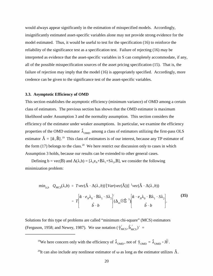
(35)

would always appear significantly in the estimation of misspecified models. Accordingly,

insignificantly estimated asset-specific variables alone may not provide strong evidence for the

model estimated. Thus, it would be useful to test for the specification (16) to reinforce the

reliability of the significance test as a specification test. Failure of rejecting (16) may be

interpreted as evidence that the asset-specific variables in S can completely accommodate, if any,

all of the possible misspecification sources of the asset pricing specification (15). That is, the

failure of rejection may imply that the model (16) is appropriately specified. Accordingly, more

credence can be given to the significance test of the asset-specific variables.

3.3. Asymptotic Efficiency of OMD

This section establishes the asymptotic efficiency (minimum variance) of OMD among a certain

class of estimators. The previous section has shown that the OMD estimator is maximum

likelihood under Assumption 3 and the normality assumption. This section considers the

efficiency of the estimator under weaker assumptions. In particular, we examine the efficiency

properties of the OMD estimator among a class of estimators utilizing the first-pass OLS

estimator = . This class of estimators is of our interest, because any TP estimator of19

the form (17) belongs to the class. We here restrict our discussion only to cases in which20

Assumption 3 holds, because our results can be extended to other general cases.

Defining b = vec(�) and �(�,b) = [� e +�� +S� ,�], we consider the followingo N 1 2

minimization problem:

Solutions for this type of problems are called “minimum chi-square” (MCS) estimators

(Ferguson, 1958; and Newey, 1987). We use notation ( )� =

QMCS � QMCS(�MCS,bMCS) � �2(N�1�k�q) .

Var(�MCS) �

(1�c)T

(X ��1X)�1,

�0,MCS,��1,MCS,��2,MCS,b �

MCS

�

� ,�

c � (�1� F)��1F (�1� F)

�

�1,TP �1,TP� F X Var(�MCS) T �1(1� c)(X ��1X)�1

�1 �3 �OMD �MCS

�OMD �MCS

�OMD

� �

��

MCS,b �

MCS

�0,MCS,��1,MCS,��2,MCS,b �

MCS �MCS

21

(36)

(37)

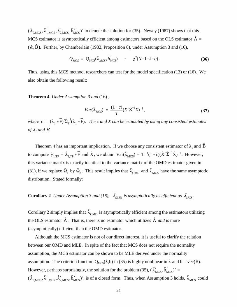
( )� to denote the solution for (35). Newey (1987) shows that this

MCS estimator is asymptotically efficient among estimators based on the OLS estimator =

( ). Further, by Chamberlain (1982, Proposition 8), under Assumption 3 and (16),

Thus, using this MCS method, researchers can test for the model specification (13) or (16). We

also obtain the following result:

Theorem 4 Under Assumption 3 and (16) ,

where . The c and X can be estimated by using any consistent estimates

of � and �.1

Theorem 4 has an important implication. If we choose any consistent estimator of � and 1

to compute = and , we obtain = . However,

this variance matrix is exactly identical to the variance matrix of the OMD estimator given in

(31), if we replace by . This result implies that and have the same asymptotic

distribution. Stated formally:

Corollary 2 Under Assumption 3 and (16), is asymptotically as efficient as .

Corollary 2 simply implies that is asymptotically efficient among the estimators utilizing

the OLS estimator . That is, there is no estimator which utilizes and is more

(asymptotically) efficient than the OMD estimator.

Although the MCS estimator is not of our direct interest, it is useful to clarify the relation

between our OMD and MLE. In spite of the fact that MCS does not require the normality

assumption, the MCS estimator can be shown to be MLE derived under the normality

assumption. The criterion function Q (�,b) in (35) is highly nonlinear in � and b = vec(�). MCS

However, perhaps surprisingly, the solution for the problem (35), ( )� =

( )�, is of a closed form. Thus, when Assumption 3 holds, could

�OMD

��,MCS � (1 ,� ��1,MCS)

� �s

�ZZ��[ ��1

� ��1Se(S

�

e��1Se)

�1S�

e��1] � �

�,MCS

�s

[ �0,MCS,��

2,MCS]� (S�

e��1Se)

�1S�

e��1��

�,MCS T�s

�MCS

�OMD �MCS

�OMD

�OMD

(�ZZ��1)

[(��1ZZ�IN)1(�

�1ZZ�IN)]�1

[(��1ZZ�IN)2(�

�1ZZ�IN)]�1

T�s

T ln(1� �s)

Zhou (1998) derives the variance matrix of the maximum likelihood estimator of �. See21

his equations (21)-(24). Although his MLE variance matrix is not exactly of the form (37), wecan show that Zhou’s formula coincides with (37). A note on this result is available from theauthors upon request.

22

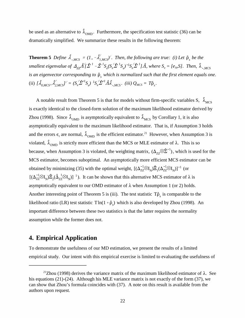
be used as an alternative to . Furthermore, the specification test statistic (36) can be

dramatically simplified. We summarize these results in the following theorem:

Theorem 5 Define . Then, the following are true: (i) Let be the

smallest eigenvalue of , where S = [e ,S]. Then, e N

is an eigenvector corresponding to which is normalized such that the first element equals one.

(ii) = . (iii) Q = .MCS

A notable result from Theorem 5 is that for models without firm-specific variables S,

is exactly identical to the closed-form solution of the maximum likelihood estimator derived by

Zhou (1998). Since is asymptotically equivalent to by Corollary 1, it is also

asymptotically equivalent to the maximum likelihood estimator. That is, if Assumption 3 holds

and the errors � are normal, is the efficient estimator. However, when Assumption 3 ist21

violated, is strictly more efficient than the MCS or MLE estimator of �. This is so

because, when Assumption 3 is violated, the weighting matrix, , which is used for the

MCS estimator, becomes suboptimal. An asymptotically more efficient MCS estimator can be

obtained by minimizing (35) with the optimal weight, (or

). It can be shown that this alternative MCS estimator of � is

asymptotically equivalent to our OMD estimator of � when Assumption 1 (or 2) holds.

Another interesting point of Theorem 5 is (iii). The test statistic is comparable to the

likelihood ratio (LR) test statistic which is also developed by Zhou (1998). An

important difference between these two statistics is that the latter requires the normality

assumption while the former does not.

4. Empirical Application

To demonstrate the usefulness of our MD estimation, we present the results of a limited

empirical study. Our intent with this empirical exercise is limited to evaluating the usefulness of

We also examined excess returns, but the results are not materially different from those22

shown here.

We obtained this data set through the FTP server at the University of Minnesota. We23

gratefully thank Jagannathan and Wang for access to their data.

23

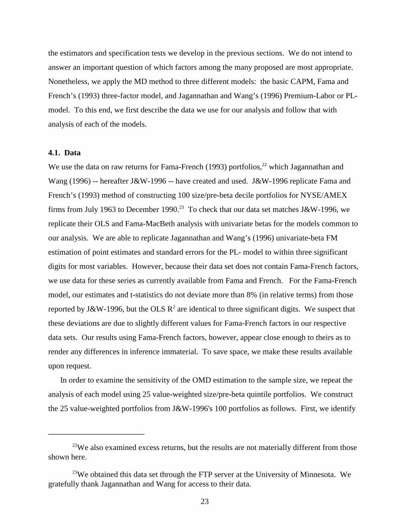
the estimators and specification tests we develop in the previous sections. We do not intend to

answer an important question of which factors among the many proposed are most appropriate.

Nonetheless, we apply the MD method to three different models: the basic CAPM, Fama and

French’s (1993) three-factor model, and Jagannathan and Wang’s (1996) Premium-Labor or PL-

model. To this end, we first describe the data we use for our analysis and follow that with

analysis of each of the models.

4.1. Data

We use the data on raw returns for Fama-French (1993) portfolios, which Jagannathan and22

Wang (1996) -- hereafter J&W-1996 -- have created and used. J&W-1996 replicate Fama and

French’s (1993) method of constructing 100 size/pre-beta decile portfolios for NYSE/AMEX

firms from July 1963 to December 1990. To check that our data set matches J&W-1996, we23

replicate their OLS and Fama-MacBeth analysis with univariate betas for the models common to

our analysis. We are able to replicate Jagannathan and Wang’s (1996) univariate-beta FM

estimation of point estimates and standard errors for the PL- model to within three significant

digits for most variables. However, because their data set does not contain Fama-French factors,

we use data for these series as currently available from Fama and French. For the Fama-French

model, our estimates and t-statistics do not deviate more than 8% (in relative terms) from those

reported by J&W-1996, but the OLS R are identical to three significant digits. We suspect that2

these deviations are due to slightly different values for Fama-French factors in our respective

data sets. Our results using Fama-French factors, however, appear close enough to theirs as to

render any differences in inference immaterial. To save space, we make these results available

upon request.

In order to examine the sensitivity of the OMD estimation to the sample size, we repeat the

analysis of each model using 25 value-weighted size/pre-beta quintile portfolios. We construct

the 25 value-weighted portfolios from J&W-1996's 100 portfolios as follows. First, we identify

We do so using neighboring size and pre-beta portfolios. Because Fama and French24

first sort firms by size, combining neighboring size-decile portfolios into size-decile portfoliosshould exactly replicate true size quintile sorting. In contrast, because sub-sorting by pre-beta isperformed over firms in each size quintile, combining neighboring pre-beta deciles that wereconstructed in different size deciles may result in a different grouping of firms across pre-betaversus true pre-beta quintile sub-sorting. However, because the average pre-betas in neighboringsize deciles in J&W-1996's original 100 portfolio are similar, it is not likely that this difference inpre-beta sub-sorting results in materially different portfolios.

24

groups of 4 original portfolios to form 25 portfolios that roughly relate to the 5-by-5 size/pre-beta

quintiles used by Fama and French (1993). Second, while the 100 portfolios constructed by24

Jagannathan and Wang are reported to be based on equally-weighted returns, it is common

practice to evaluate 25 portfolios using value-weighted returns to avoid creating portfolios that

are not representative of what an actual investor can realistically construct (see Fama and French,

1993). To achieve value-weighting, we use the average firm size values reported for each 100

portfolio. Because we use log size as a portfolio-specific variable in the second (cross-sectional)

regression step, we also construct value-weighted log-size values for each of the 25 value-

weighted portfolio.

4.2. Analysis of the Basic CAPM and the Fama-French model

To date, many studies have strongly rejected the basic CAPM. In contrast, the debate over the

Fama-French model is still ensuing. A drawback of the previous empirical studies is that their

statistical inferences are obtained based on non-robust estimates. We here examine the robust

MD (or TP) estimation results for the basic CAPM and the Fama-French model. The results for

the PL-model are discussed in the next subsection.

[INSERT TABLE 1 HERE]

As a roadmap to our results, note the organization of Panel A in Table 1. In the first and

second rows of each panel, we report the coefficient estimates and p-values obtained using the

method of Fama and MacBeth (1973) -- hereafter, FM. As is well known, these coefficient

estimates are equivalent to those using OLS regression of the mean returns against the

multivariate factor betas and any firm specific variables included in the model. For

Note that by Theorem 1, the EIV correction by MD under Assumption 3 is equivalent to25

that of Shanken (1992).

We also used Andrews (1991) and obtained similar results for most analyses.26

25

comparability with previous studies, we report R and adjusted-R on these OLS results. The2 2

four rows below that show the p-values computed by three different EIV-correction methods:

Shanken (1992) -- hereafter, SH -- and the MD methods based as discussed in Section 3.1. MD-

A2 and MD-A1 indicate the EIV-corrected results under Assumptions 2 and 1, respectively. 25

These results using non-optimal estimation are followed by OMD coefficients and their p-values

as developed in Section 3.2. The OMD estimates and test results are robust under Assumptions

3, 2, and 1, respectively. To compute the heteroskedasticity-and-autocorrelation-robust --

hereafter, HA-robust -- variance matrices where required, we use Newey and West (1987).26

We report the specification test results in the last three columns of each panel. We first

report Shanken’s (1985) Q , and then, Q for OMD-A3 through OMD-A1. As we haveC MD

discussed in Section 3, the Q test computed with OMD-A3 is a � -version of the Q test. MD C2

Further, since the Q test computed with OMD-A3 is designed to share the similar propertiesMD*

with the Q test, we can expect that these two tests would produce quite compatible test results. C

However, the Q test computed with OMD-A2 and OMD-A1 could perform quite differentlyMD*

form the Q test if returns are conditionally heteroskedastic and/or autocorrelated. The Q testC MD*

results with three different OMD estimators are reported in the last column.

Panel A reports the estimation results for the basic CAPM obtained from the analysis of 100

portfolios. As reported in J&W-1996, the estimated coefficient (� ) on the market factor isVW

unexpectedly negative, although it is statistically insignificant. The same result is obtained

whatever estimation method is used. In addition, the traditional OLS analysis of mean returns

yields extremely low R and adjusted R . These results provide strong evidence against the basic2 2

model. In contrast, the specification tests reported in the last three columns do not lead to

decisive conclusions. The Q tests appear highly significant regardless of what OMD method isMD

used, while the basic CAPM is not rejected by Q (p-value, 43.72%). The Q test fails to rejectC MD*

the model with OMD-A3 and OMD-A2, although the same test rejects the model with OMD-A1.

Given this critical difference in the MD test results, it appears important to test for which of

Assumptions 1-3 is appropriate for the analysis of the basicCAPM. We address this issue in

26

detail later.

Panel B reports the results for the size-augmented CAPM with 100 portfolios. Similarly to

J&W-1996, non-optimal MD estimation methods reveal significant size effects (� ). The p-SIZE

value for the coefficient of firm size (� ) remains eventually unaltered however the varianceVW

matrix of the OLS estimator is estimated. Augmenting firm size produces much higher R and2

adjusted R (57,6% and 56.7%, respectively). These results obtained from non-optimal2

estimation are sufficient to reject the basic CAPM. The optimal MD estimation is not favorable

to the CAPM, either. When we use OMD, firm size appears even more significant. Similarly to

Panel A, the Q tests strongly reject the size-augmented model. The Q test is favorable to theMD C

model. However, the Q test rejects the model with OMD-A1, while it dos not with OMD-A2MD*

and OMD-A3.

The Q and Q test results reported in Panels A and B are generally contradictive to eachMD MD*

other. These results are largely due to the fact that the number of assets in the sample we use is

large (100) relative to the number of time-series observations (330). The substantial discrepancy

between the two tests also raises a concern about potential finite-sample biases in the estimates.

In order to examine the sensitivity of estimation results to the number of assets, Panels C and D

report the results from the analysis of 25 portfolios. The basic CAPM again performs poorly.

Many of the results reported in the two panels are qualitatively similar to those reported in Panels

A and B. However, a notable exception is that the Q tests no longer decisively reject the basicMD

CAPM. The fact that most of statistical inferences other than the Q test results remainMD

unchanged regardless of the number of assets used seems to suggest that the Q test tends to beMD

biased toward model rejections when a large number of assets are used for estimation. This

result also indicates that it would be useful to use both Q and Q to test for a given modelMD MD*

specification.

A down side of the specification tests, Q , Q and Q , we observe from Panel C is thatC MD MD*

they fail to strongly reject the basic CAPM. This result is not consistent with both the strong

model rejection by the significance test for firm size and the large increase in R by augmenting2

firm size to the basic CAPM (Panel D). These contradictive results indicate that the specification

tests may have low power to detect model specification. However, Panels C and D are not

without any supportive evidence for the usefulness of the Q and Q tests. First, the two testsMD MD*

mildly reject the basic CAPM with OMD-A1. As we discuss later, we find that Assumption 1 is

Altonji and Segal (1996) provide some Monte Carlo evidence that optimal MD27

estimates could be more biased than the non-optimal MD estimates. However, their results donot directly apply to the optimal MS estimation discussed in this paper. Altonji and Segalconsider only the cases in which restricted parameters are linear functions of unrestrictedparameters and the functions are known to researchers. However, in the factor pricing models ofour interest, the restricted parameters (e.g., risk prices, �) are nonlinear functions of theunrestricted parameters (e.g., � and �).

27

more consistent than Assumptions 2 and 3 for the analysis of the basic CAPM. Thus, it appears

that the MD tests, when they are computed with an appropriate robust OMD estimator, have

some limited power to detect model specifications. Second, observe that the p-values for QMD

and Q are much higher for the size-augmented CAPM than for the basic CAPM: The p-MD*

values reported in Panel D are almost two times as large as those reported in Panel C. Given that

the size-augmented model explains the cross-sectional variations of returns much better than the

basic CAPM, the p-values of the specification tests appear to be positively related with a model’s

explanatory power.

We now turn to the estimation results for the Fama-French model. The estimation results

with 100 portfolios are reported in Panels E and F. Our non-optimal MD results are virtually

similar to those reported in J&W-1996: When 100 portfolios are analyzed, the model has the

relatively high OLS goodness-of-fit found in J&W-1996 (R , 55.1%), a negative but insignificant2

coefficient on the market factor, and positive but insignificant coefficients on both the

SMB(� ) and HML (� ) factors (Panel E). In addition, the non-optimal MD estimation of theSMB HML

size-augmented model produces significantly estimated coefficients on firm size, rejecting the

Fama-French model (Panel F). Our optimal MD estimation rejects the model even more

strongly. However, some caution seems to be required to interpret the statistical significance of

firm size properly. Since the large number of assets are used in this analysis, we cannot rule out

the possibility of finite-sample biases in both the non-optimal and optimal estimation results. It

has been well documented in the literature that Wald tests (such as t-tests of significance) based

on GMM estimators are likely to be biased when too many moment conditions are imposed in

GMM (see, for example, Hansen, Heaton and Yaron, 1996; Andersen and Sørensen, 1996). By

the same token, the optimal and non-optimal MD estimation methods may produce biased t-test

results. 27

An interesting sidelight of Panel E is that it supports Jagannathan and Wang’s (1998b)

28

prediction that coefficient p-values using (non-optimal) HA-robust estimation could be lower

than those using Fama-MacBeth (1973), although the p-values computed following Shanken

(1992) should be higher. For example, note that while the SMB factor’s p-value is larger using

SH (16.05%) than using FM (13.28%), it is nearly identical to that using MD-A1 (13.23%).

Panels G and H report the estimation results for the Fama-French model with 25 portfolios.

Differently from the analysis of 100 assets, there is no longer strong statistical evidence against

the Fama-French model. In Panel H, the non-optimally estimated coefficients on firm size are

insignificant. In addition, the increases in R and adjusted-R by augmenting firm size to the2 2

model are not very substantial compared to the case of the basic CAPM. Turning to optimal

estimation, we see that firm size becomes even more insignificant. Furthermore, none of the Q ,C

Q and Q specification tests reported in Panel G reject the Fama-French model. AugmentingMD MD*

firm size to the model alters the p-values of the tests only marginally.

Despite these favorable results from the specification tests and the significance test for firm

size, there is also some evidence against the Fama-French model. Observe that non-optimal

estimation methods produce insignificantly estimated coefficients on the SMB factor (Panel G).

Even the estimated coefficients on the HML factor are only marginally significant. The optimal

MD estimation also fails to support the Fama-French model. Furthermore, note that the p-values

for the HML factor increase as we move from non-optimal to optimal estimation. OMD-A1

produces a marginally significant coefficient for the HML factor. However, as we discuss below,

Assumption 2 appears more consistent with the analysis of the Fama-French model.

Table 1 shows that non-optimal and optimal estimation may produce different results

depending on the generality of the adopted assumption (from Assumptions 1 to 3). For the basic

CAPM and the Fama-French model, both the coefficient and specification tests based on OMD

appear sensitive to the assumption used for estimation. Thus, it is important to test which

assumption is consistent with data. Presence of ‘useless’ factors (Kan and Zhang, 1997) and

nonstationarity of factors are also our concern, because either of these can lead to a violation of

the regularity conditions that lead to the consistency and asymptotic normality of the MD

estimators. For completeness, we perform all of these tests for each factor model.

[INSERT TABLE 2 HERE]

The variance of the rejection number equals N�(1-�).28

29

As shown in Panel A of Table 2, estimation for both the basic CAPM and the Fama-French

model should ideally be robust to conditional heteroskedasticity, but not necessarily with respect

to autocorrelation. Using White’s (1980) test for heteroskedasticity, we found that both factor

models result in a large percentage of assets having heteroskedastic errors. For the basic CAPM,

24 of 25 assets failed this test at both the 5% and 10% level, while 21 of 25 did so at these levels

for the Fama-French model. A smaller portion of assets failed the Breusch-Godfrey

Largrangean-Multiplier (LM) test for autocorrelation for both models, but the number of

rejections appears higher for the basic CAPM (11 and 8 at the 10% and 5% levels, respectively)

than for the Fama-French model (7 and 3, similarly).

Of course, the non-zero number of rejections, alone, would not be a sufficient indication of

heteroskedasticity or autocorrelation. Even if no return is conditionally heteroskedastic, we can

expect � × 100 percent of rejections by the White test when it is performed at the � level. In

order to check whether or not the frequency of the White (or Breusch-Pagan) tests rejected is

statistically significantly different from the number of rejections expected from a chosen � level,

we conduct a proportion test based on a normal approximation of the binomial distribution. To

motivate our test, suppose that in the basic CAPM model, there is no conditional

heteroskedasticity in any portfolio return. Then, the heteroskedasticity could be falsely rejected

with the probability equal to �. Thus, the number of rejections would follow a binomial

distribution. If the number of trial (in our case, the number of portfolios, N) is large enough, then

the binomial distribution can be approximated by normal distribution. Using this information,28

we can test for statistical significance of the number of rejections. Significance by this test may

be an indicative of the presence of heteroskedasticity in the given model. Not surprisingly, the

number of rejections by the White tests appears statistically significant for each of the basic

CAPM and the Fama-French model.

While the test of proportions strongly suggests that autocorrelation matter in the basic

CAPM, the test result is less strong for the Fama-French model. Admittedly, the proportion test

we use is asymptotically valid only if the Breusch-Pagan LM test results are independently

distributed across different assets. This assumption is likely to be violated in practice because

the residuals from time-series regressions could be correlated across assets through unspecified

30

common factors. Nevertheless, it would be fair to say that the Basic CAPM is more likely to

require autocorrelation-robust estimation than the Fama-French model. The White and Breusch-

Pagan LM test results reveal that Assumption 2 is appropriate for the analysis of the Fama-

French model while Assumption 1 is more appropriate for the analysis of the Fama-French

model.

As discussed by Kan and Zhang (1997), the presence of ‘useless’ factors -- factors where the

true beta for all assets is expected to be zero -- could bias the t-statistics of coefficients. To test

for useless factors, we perform a Wald test for each factor of each model for whether the vector

of betas across assets equals zero. As shown in Panel B of Table 2, all of the tests indicate that

we can reject the null hypothesis of zero-beta vectors. Given the strength of these rejections (all

p-values less than 0.005%), we conclude that neither of the basic CAPM and Fama-French

models.

Lastly, Panel C of Table 2 reports the unit-root test results for the factors used in the basic

CAPM and the Fama-French model. If a factor has a unit root, the MD estimators are not

necessarily asymptotically normal. Realistically, it is not likely that the factors in the basic

CAPM or Fama-French �� all of which are portfolio return series and unlikely to substantially

drift over time in any particular direction �� have unit roots. However, for completeness, we

document this feature as a benchmark for the analysis of other models. In addition, because these

tests are specific to the factors and not the models, results for a factor apply to any model it is

used in. To test for unit roots, we use both Dickey-Fuller (1979) and Phillips-Perron (1988)

tests. As shown by the results in Panel C of Table 2, these tests strongly reject the notion that

VW, SMB nor HML have unit roots.

4.2. Analysis of the PL-model

In addition to testing the basic CAPM and Fama-French model, we also examine the PL-model

introduced by J&W-1996. It is reported in J&W-1996 that the PL-model performs well relative

to both the basic CAPM and the Fama-French model. However, their results partly rely on

estimation which is not HA-robust. We here report more robust results.

[INSERT TABLE 3 HERE]

The previous version of this paper reports that firm size is significant if 25 equally-29

weighted portfolios are used to estimate a size-augmented PL-model. However, the currentversion instead reports the results from the analysis of 25 value-weighted portfolios. We decidedto do so, because the value-weighted portfolios are more representative of what investors arelikely to be able to repeatedly construct. The results with 25 equally-weighted portfolios areavailable from the authors upon request.

31

As shown in Panel A of Table 3, the PL-model generally performs well in non-optimal

estimation with 100 assets (Panel A). The PREM coefficient (� ) is significant (or nearly so)PREM

with all estimators. The LABOR coefficient (� ) is also significant with most estimators. InLABOR

addition, Panel B shows that the firm-size coefficient (� ) is insignificant at the 10% level withSIZE

any non-optimal estimator (FM through MD-A1 in Panel B). These results are consistent with

those reported in J&W-1996. However, perhaps surprisingly, our optimal MD estimation

strongly rejects the model: Firm size is significant at 1% level whatever estimation method is

used (Panel B). The Q test rejects the model with OMD-A2 and OMD A-1, while the QMD MD*

test does only with OMD-A1. Of course, as discussed before, these negative results may be due

to finite-sample biases in the optimal MD estimation caused by the use of too many assets (100)

relative to the time series observations (330). Nonetheless, it is interesting to see that non-

optimal and optimal estimation could generate quite different statistical inferences.

Panels C and D report the estimation results with 25 assets. Similarly to the case of the

Fama-French model, the Q and Q tests no longer reject the PL-model (Panel C). MD MD*

Furthermore, the coefficient on firm size is insignificant regardless of what estimation method is

used (Panel D). Notably, firm size becomes even more insignificant as we move from non-

optimal to optimal estimation. Observe also that the p-values for the Q test for all optimal29MD

estimators (OMD-A3 through A-1) are very high (in excess of 99%) for the PL-model for these

25 assets compared to those for the Fama-French model (from about 17% to 34%). With the

difference in goodness-of-fit across these two models for 25 assets (R for Fama-French model,2

77.0%; for PL-model, 86.8%), the differences in p-values across models seem to suggest that the

PL-model has a better power to explain returns than the Fama-French model. These results are

supportive of the findings of J&W-1996 favoring the PL model over the Fama-French model.

Some of the results reported in Panel C, however, do not support the PL-model. Notably, the

coefficient on the LABOR factor is insignificant whatever estimation method is used. In fact,

even with 100 assets, HA-robust non-optimal estimation (MD-A1) results in an (mildly)

32

insignificant p-value (MD-A1, p-value: 11.20%), although other estimation methods produce at

least marginally significant p-values. These findings against the PL-model are not available from

J&W-1996. They focus only on the results from 100 assets and MD-A1 was not yet available to

them.

[INSERT TABLE 4 HERE]

Our diagnostic tests raise another concern about the PL-model. As shown in Panel A of

Table 4, the returns appear highly heteroskedastic given realized PREM and LABOR factors.

Almost all of the 25 portfolios failed the White test for conditional homoskedasticity at the 5%

level while all do at the 10% level. Many returns also appear autocorrelated given the realized

factors. Specifically, 11 (6) out of the 25 portfolios failed the LM test for autocorrelation at the

10% (5%) level. These results are roughly equivalent to those found for basic CAPM. Given

theses results, Assumption 1 seems to be more consistent with the estimation of the PL-model.

Panel B of Table 4 suggests potential presence of a ‘useless’ factor. The PREM factor

appears to be ‘useful.’ For the case with 100 assets, the Wald test also rejects the hypothesis of

zero-beta vector for the LABOR factor. In contrast, the same test with 25 assets rejects the zero-

beta hypothesis. This result is obtained with estimation that is robust to just conditional

heteroskedasticity (Assumption 2) or also autocorrelation (Assumption 1). While this appears

consistent with LABOR being ‘useless’ with the 25 portfolios, the insignificance of LABOR

contradicts Kan and Zhang’s (1997) prediction that t-statistics for the useless factors tend to

appear falsely significant. Thus, LABOR is unlikely to be a ‘useless’ factor. Nonetheless, the

test result raises a concern that LABOR may be a noisy factor.

Finally, we report the unit-root test results in Panel C of Table 4. While we can reject a unit

root in the LABOR factor, we unexpectedly cannot do so with PREM using either the Dickey-

Fuller or Phillips-Perron test. Admittedly, the test statistics are close to statistical significance at

the 10% for these tests and it is generally known that these tests have low power to reject the null

hypothesis. Additionally, it seems intuitive that PREM, the difference between the interest rates

on Baa and Aaa corporate bond rates, is likely to be stationary over a long time: That is, the two

rates are likely to be cointegrated. However, because our sample is only finite, it is possible that

the inference of two-step estimation is materially perturbed by the presence of a near-unit root

33

factor in a finite sample. This paper does not intend to answer the question of how the presence

of near-nonstationary factors would influence the finite-sample properties of the two-pass

estimator. However, answering this question would be an important future research agenda.

4.3. Summary

Before closing this empirical section, we make several general comments on the results reported

in Tables 1-4. First, we obtain quite different statistical inferences from the analyses of 100 and

25 portfolios, especially when we use optimal MD estimation. GMM estimators obtained by

imposing too many moment conditions are likely to produce biased statistic inferences.

Likewise, the MD estimation (the robust two-pass estimation) applied to the analysis of too many

assets would generate biased estimates and test results. Thus, the MD analysis with 25 portfolios

is likely to produce more reliable statistic inferences. Second, statistical inferences based on the

optimal (or non-optimal) MD could change depending on the choice of the assumption regarding

the conditional distribution of returns. Thus, it is important to test for conditional

heteroskedasticity and autocorrelation in returns routinely. Third, as we see from Panels C and D

of Table 1, the Q and Q tests may have weak power to detect misspecification in a givenmd MD*

factor model. Thus, the MD test results should be interpreted with some caution. Investigation

of the power properties of the MD tests would be an important agenda of our future studies.

Fourth, our study reveals some findings that are not available from J&W-1996. We find from the

analysis of 25 assets that the LABOR factor is not significantly priced. Furthermore, our

diagnostic tests suggest that the LABOR factor may be a ‘useless’ in the sense of Kan and Zhang

(1997) and the PREM factor may be near-nonstationary, if not non-stationary. In this moment,

we are not able to answer the question of how these test results would be related with the finite-

sample properties of the optimal and non-optimal MD estimators. It would be an important

future research agenda to reexamine the relevance of PREM and LABOR as factors in asset

pricing models.

5. Conclusion

The two-pass cross-sectional regression method is widely used to evaluate numerous linear factor

pricing models. Because simple OLS standard errors and test statistics are biased, many

34

solutions to address this bias have been proposed in the literature. MLE has also been used in

efforts to circumvent the estimation errors induced by estimated betas. However, these proposed

methods are legitimate only under strong assumptions.

In this paper, we provide an alternative to traditional two-pass estimation based on the

minimum distance method. With this method we provide a systematic way to derive correct

standard errors of the traditional OLS or GLS two-pass estimators, under quite general

conditions. Using this method, we can control for conditional heteroskedasticity and

autocorrelation in asset returns. We conduct a limited empirical study to demonstrate the

importance of considering heteroskedasticity and autocorrelation in practice, as well as

diagnostic tests of the general robustness of two-step estimation. Use of the minimum-distance

method and some diagnostic test methods leads us to deeper insights into the popular factor

models such as the basic CAPM, Fama-French and Premium-Labor models.

Future work in the line consistent with the approach we adopt for this paper has four

immediate directions. First, the asset pricing models we examine in this paper are factor models

motivated by APT (Ross, 1976) versus rigorous tests of equilibrium models such as CAPM as

discussed by Shanken (1992). In an earlier version of this paper (Ahn and Gadarowski, 1998),

we develop an extension to testing the Black (1972) version of CAPM but do not include it here

to limit the already extensive scope of this paper. Future work will continue with this analysis.

Second, the asset pricing models we test are parametrically unconditional, e.g. models whose

parameters are not expected to change over time based on conditioning information. Because

conditional models have the potential to explain asset prices more accurately than unconditional

models, this extension appears promising. Third, because our OMD estimators are GLS

estimators, OMD alternatives to OLS R can be developed that are likely to have the same2

benefits as extant GLS versions of R but be robust under more general conditions. Fourth, our2

results rely on asymptotic theory and may not be applicable with finite samples. In a separate

paper, we will examine more fully MD methods that are adjusted for degrees of freedom and

conduct some Monte Carlo experiments to investigate their finite sample properties, including

the potential for factors with nearly useless factor and near-unit roots to bias the inference of two-

step estimation.

T(�TP��) � T[(X �AX)�1X �A���] � (X �AX)�1X �A T(�� X�) .

T(�� X�) � T[(���0eN� ��1�S�2)� (���0eN���1�S�2)]

� T[(���)� (���)�1] � T(���)��

� Tvec[(���)��] � (��

��IN) Tvec(���) ,

T(�� X�) � N(0 ,�) ,

��

���1ZZ�� � [1 ,���1]

1� F ��1F F �F �

�1F

��1F F

�1F

1

��1

� 1� [�1� F]��1F [�1� F] .

T(�TP��) � (X �AX)�1X �A T(�� X�)

� (X �AX)�1X �A(�����1ZZ�IN) 1

T�

Tt�1(Zt��t) ,

�TP

� � (�����1ZZ�IN)(��1

ZZ���IN)

1

2

1 �1 3 � �xx�

35

(A1)

(A2)

(A3)

(A4)

(A5)

Appendix

Proof of Theorem 1:

By the definition of , we can show that

Under (16), � - � e - �� - S� = 0. Using this restriction and standard matrix theories, we can0 N 1 2

show

where � = (1,-��)�. Then, it follows that*

where and is defined in (7). Under Assumption 1, can be

estimated by . Thus, (A1) and (A2) imply (22). The part (ii) results from the fact that under

Assumption 2, , which is defined in (9), is a consistent estimator of . Finally, we obtain (iii)

if we replace in by . The equality in (24) results from the fact that

Proof of Theorem 2:

Note that

where the first equality results from (A1) and the second from (A2) and (5). Using (18), and the

T(�TP��) � T(�TP��) � J T(F�E(Ft))

� (X �AX)�1X�A(��

���1ZZ�IN)

1

T�

Tt�1(Zt��t) � J

1

T�

Tt�1(Ft�E(Ft))

� M1

T�

Tt�1�t ,

T(�� X�OMD) � T(�� X�) � X T(�OMD��) .

T(�� X�OMD) � Q T(�� X�) ,

T(�� X�) � Du,

QMD(�OMD;��1) � u �D �Q ���1QDu.

u �D �Q ���1QDu � u �MXu � �2(N�1�k�q) .

��1

Q � IN� X(X ���1X)�1X �

��1 Q � IN�X(X ���1X)�1X ���1

�OMD,��1

36

(A6)

(A7)

(A8)

(A9)

(A10)

(A11)

equalities � = � , � = � + E(F ), and � = � , we can show thato 0 1 1 t 2 2

which gives us the desired result.

Proof of Theorem 3:

The proof is based on Chamberlain (1982, Proposition 8). Observe that

Choosing for A, substitute (A1) into (A7); then we have

where � . Let D be a N×N positive

definite matrix such that DD� = �. Then, under (16),

where u � N(0,I ). Substituting (A8) and (A9) into Q ( ), we obtainN MD

But, using the fact that D�� D = D�(DD�) D = I and D�� = D�(DD�) = D , we can show-1 -1 -1 -1 -1N

D�Q�� QD = I - X (X �X ) X �, where X = D X. Note that M � I - X (X �X ) X � is an-1 -1 -1 -1N D D D D D X N D D D D

idempotent and symmetric matrix with rank equal to (N-1-k-q). Thus, by Schmidt (1976,

Chapter 1.5),

Proof of Theorem 4:

���eN�0���1�S�2

b�b

�(�0,��1,��2,b �)� �

X ��

1�IN

0Nk×(1�k�q) INk

Var�MCS

bMCS

�

1T

X ��

1�Ik

0k×(1�k�q) INk

�

(�ZZ��1)

X ��

1�Ik

0k×(1�k�q) INk

�1

Var(�MCS) �

1T

[1�(�1� F)�{(�1� F)(�1� F)�� F} �1(�1� F)]�1(X ��1X)�1

�

1T

[1� (�1� F)��1F (�1� F)](X �

�1X)�1�

(1�c)T

(X ��1X)�1.

W(�1) �

1 ���

1

0k×1 Ik

� IN.

QMCS(�,b) � [W(�1)d(�,b)]�[W(�1)(��1ZZ�)W(�1)

�]�1[W(�1)d(�,b)] ,

W(�1)d(�,b) �

�� X�

b�b�

����eN�0�S�2

b�b.

��

MCS,b �

MCS

��X� b�b

37

(A12)

(A13)

(A14)

(A15)

(A16)

(A17)

Note that

Then, Chamberlain (1982, Proposition 7) implies that ( )� is asymptotically normal

and for large T,

where X and � can be replaced by any consistent estimates of X and � . But, using usual1 1

partitioned matrix theories and a little algebra, we can show:

Proof of Theorem 5:

Define:

Note that W(� ) is nonsingular for any � . Thus, we can have1 1

where d(�,b) = [( )�,( )�]�. It is straightforward to show

Note that

��1ZZ �

1 F�

F �FF

�1

�

1� F ��1F F �F �

�1F

��1F F

�1F

,

W(�1)(��1ZZ�)W(�1)

��

1 ���

1

0k×1 Ik

1� F ��1F F � F �

�1F

��1F F

�1F

1 01×k

��1 Ik

�

�

1� (�1� F)��1F (�1� F) � (�1� F)��1

F

��1F (�1� F)

�1F

� .

QMCS(�,b) � QM(�) � Ts(�,b)�[K��1]s(�,b),

QM(�) � T(��

��eN�0�S�2)

��1(��

��eN�0�S�2)

��

���1ZZ��

b � b� [(�����1ZZ��)

�1�1F (�1� F)�IN](��

��eN�0�S�2) ;

�0

�2

� [S�

e�1Se]

�1S�

e�1��

�.

�FF � T �1�Tt�1FtF

�

t

K � F � (�1� F)(�1� F)�

b�b� [(�����1ZZ��)

�1�1F (�1� F)�IN](��

��eN�0�S�2)

b �0 �2

38

(A18)

(A19)

(A20)

(A21)

(A22)

(A23)

where . Using this fact, we can show:

Substitute (A17) and (A19) into (A16) and let . Then, a tedious but

straightforward algebra yields

where s(�,b) = , and

We now consider the minimization solutions for b, � , and � given � , which we denote by0 2 1

, , and , respectively. From the first-order conditions �Q /�b = 0 and �Q /�(� ,� �)� =MCS MCS 0 2

0, we can easily show

and

Substituting (A22) and (A23) into Q (�,b) = Q (� ,� ,� ,b), we can obtain a concentratedMCS MCS 0 1 2

minimand:

QCM(�1) � QMCS(�0,�1,�2,b) � T����[�1

��1Se(S

�

e�1Se)

�1�1S�

e]���

��

���1ZZ��

.

�ZZ��[�1

� �1Se(S

�

e�1Se)

�1S�

e�1]�

��,MCS �xx�

�[�1�

�1Se(S�

e�1Se)

�1S�

e�1]�

�s ��[�1

� �1Se(S

�

e�1Se)

�1S�

e�1]��

�,MCS � �s��1ZZ��,MCS

QMCS(�MCS,bMCS) QCM(�1,MCS) T�s

39

(A24)

Thus, minimizing (A24) with respect to � results in the MCS estimator of � . However,1 1

Johansen (1995, Lemma A.7) implies that the eigenvector corresponding to the smallest

eigenvalue of the matrix is a solution for the minimization

of (A24). Thus, we have proven the result (i). The result (ii) comes from (A23). Finally, since

is an eigenvector of corresponding to the

eigenvalue , we have . Substituting

this result into (A24) yields = = .

40

References

Ahn, Seung C. and Christopher Gadarowski, 1998, Two-pass cross-sectional regression of factor

pricing models: Minimum-distance approach, mimeo (August, 1998), Arizona State

University.

Ahn, Seung C. and Peter Schmidt, 1995, Efficient estimation of a model with dynamic panel

data, Journal of Econometrics 68, 5-27.

Altonji, Joseph G. and Lewis M. Segal, 1996, Small-sample bias in GMM estimation of

covariance structures, Journal of Business and Economic Statistics 14, 353-366.

Amemiya, Takeshi, 1978, The estimation of a simultaneous equation generalized probit model,

Econometrica 46, 1193-1205.

Andersen, T. G. and R. E. Sørensen, 1996, GMM estimation of a stochastic volatility model: A

Monte Carlo Study, Journal of Business & Economic Statistics 14, 328-352.

Amsler, Christine E., and Peter Schmidt, 1985, A Monte Carlo investigation of the accuracy of

multivariate CAPM tests, Journal of Financial Economics 14, 359-375

Andrews, Donald W.K., 1991, Heteroskedasticity and autocorrelation consistent covariance

matrix estimation, Econometrica 59, 817-858.

Andrews, Donald W.K., and J. Christopher Monahan, 1993, An improved heteroskedasticity and

autocorrelation consistent covariance matrix estimator, Econometrica 60, 953-966.

Berk, Jonathan B., 1995, A critique of size-related anomalies, Review of Financial Studies 8,

275-286.

Black, Fisher, 1972, Capital market equilibrium with restricted borrowing, Journal of Business,

45, 444-454.

Black, Fisher, Michael C. Jensen, and Myron S. Scholes, 1972, The Capital asset pricing model:

Some empirical tests, in Michael C. Jensen, ed.: Studies in the Theory of Capital Markets

(Praeger, New York, New York).

Breusch, T., 1978, Testing for autocorrelation in dynamic linear models, Australian Economic

Papers 17, 1978, 334-355.

Campbell, John Y., Andrew W. Lo and A. Craig MacKinlay, 1997, The Econometrics of

Financial Markets (Princeton University Press, Princeton, New Jersey).

Chamberlain, Gary, 1982, Multivariate regression models for panel data, Journal of

41

Econometrics 18, 5-46.

Chamberlain, Gary, 1984, Panel data, in Zvi Griliches, and Michael D. Intriligator, eds.:

Handbook of Econometrics, Volume 2 (North-Holland, New York, New York).

Copeland, Thomas E., and J. Fred Weston, 1992, Financial Theory and Corporate Policy

(Addiston-Wesley Publishing Company, Reading, Massachusetts).

Dickey, D.A., and W.A. Fuller, 1979, Distribution of the Estimators for Autoregressive Time

Series with a Unit Root, Journal of the American Statistical Association 74, 427–431.

Fama, Eugene F., and Kenneth R. French, 1993, Common risk factors in the returns on stocks

and bonds, Journal of Financial Economics 33, 3-56.

Fama, Eugene F., and James D. MacBeth, 1973, Risk, Return, and Equilibrium: empirical tests,

Journal of Political Economy 71, 607-636.

Ferguson, T.S., 1953, A method of generating best asymptotically normal estimates with an

application to the estimation of bacterial densities, Annals of Mathematical Statistics 29,

1046-1062.

Gibbons, Michael R., 1982, Multivariate tests of financial models: a new approach, Journal of

Financial Economics 10, 3-27.

Gibbons, Michael R., Stephen A. Ross, and Jay Shanken, 1989, A test of the efficiency of a given

portfolio, Econometrica 57, 1121-1152.

Godfrey, L., 1978, Testing against general autoregressive and moving average error models

when the regressors include lagged dependent variables, Econometrica 46, 1293-1302.

Hamilton, James D., 1994, Time Series Analysis, (Princeton University Press, Princeton, New

Jersey).

Hansen, Lars P., 1982. Large sample properties of generalized method of moments estimators,

Econometrica 50, 1029-1054.

Hansen, L.P., J. Heaton and A. Yaron, 1996, Finite-sample properties of some alternative GMM

estimators, Journal of Business & Economic Statistics, 14, 262-280.

Jagannathan, Ravi, and Zhenyu Wang, 1996, The conditional CAPM and the Cross-Section of

Expected Return, Journal of Finance 51, 3 - 53.

Jagannathan, Ravi, and Zhenyu Wang, 1998a, An asymptotic theory for estimating beta-pricing

models using cross-sectional regression, Journal of Finance 53, 1285-1309.

Jagannathan, Ravi, and Zhenyu Wang, 1998b, A note on the asymptotic covariance in Fama-

42

MacBeth regressions, Journal of Finance 53, 799-801.

Johansen, Søren, 1995, Likelihood-based inference in cointegrated vector autoregressive models

(Oxford University Press Inc., New York, New York).

Jegadeesh, Narasimhan, and Sheridan Titman, 1993, Returns to buying winners and selling

losers: Implications for stock market efficiency, Journal of Finance 45, 881-898.

Kan, Raymond, and Chu Zhang, 1997, Two-pass tests of asset pricing models with useless

factors, mimeo, Washington University.

Kandel, Samuel, 1984, The likelihood ratio test of mean-variance efficiency without a riskless

asset, Journal of Financial Economics 13, 575-592

Kandel, Samuel, and Robert F. Stambaugh, 1995, Portfolio efficiency and the cross section of

expected returns, Journal of Finance 50, 185-224.

Kim, Dongcheol, 1995, The errors in the variables problem in the cross-section of expected

returns, Journal of Finance 50, 1605-1634.

Lintner, John, 1965a, Security prices, risk and maximal gains from diversification, Journal of

Finance 20, 587-615.

Lintner, John, 1965b, The valuation of risky assets and the selection of risky investments in stock

portfolios and capital budgets, Review of Economics and Statistics 47, 13-47.

MacKinlay, A. Craig, and Matthew P. Richardson, 1991, Using generalized methods of moments

to test mean-variance efficiency, Journal of Finance 46, 511-527.

MacKinnon, J.G., 1991, Critical Values for Cointegration Tests, Chapter 13 in Long-run

Economic Relationships: Readings in Cointegration, Ed. R.F.Engle and C.W.J. Granger,

Oxford University Press.

Mossin, Jan, 1966, Equilibrium in a capital asset market, Econometrica 35, 768-783.

Newey, Whitney K., 1987, Efficient estimation of limited dependent variable models with

endogenous explanatory variables, Journal of Econometrics 36, 231-250.

Newey, Whitney K. and Kenneth D. West, 1987, Hypothesis testing with efficient method of

moments estimation, International Economic Review, 28, 777 - 787.

Phillips, P.C.B., and P. Perron, 1988, Testing for a unit root in time series regression,

Biometrika 75, 335–346.

Ross, Stephen A., 1976, The arbitrage theory of capital asset pricing model, Journal of Economic

Theory 13, 341-360.

43

Schmidt, Peter, 1976, Econometrics, Marcel Dekker, Inc., New York, New York.

Shanken, Jay, 1985, Multivariate tests of the zero-beta CAPM, Journal of Financial Economics 14,

327-348.

Shanken, Jay, 1986, Testing portfolio efficiency when the zero-beta rate is unknown, Journal of

Finance 41, 269-276.

Shanken, Jay, 1992, On the estimation of beta-pricing models, Review of Financial Studies 5, 1-34.

Sharpe, William, F., 1964, Capital asset prices: A theory of market equilibrium under conditions of

risk, Journal of Finance 19, 425-442.

White, Halbert, 1980, A heteroskedasticity-consistent covariance matrix and a direct test for

heteroskedasticity, Econometrica 48, 817–838.

White, Halbert, 1984, Asymptotic Theory for Econometricians (Academic Press, INC, San

Diego, California).

Zhou, Guofu, 1994, Analytical GMM tests: Asset pricing with time-varying risk premiums,

Review of Financial Studies 7, 687-709.

Zhou, Guofu, 1998, On cross-sectional stock returns: Maximum likelihood approach, mimeo,

Washington University.